/


Автор: Bickford J. H.
Теги: engineering mechanics mechanical engineering contruction marcel dekker inc bolted joints design of bolted joints
ISBN: 0-8247-9297-1
Год: 1995


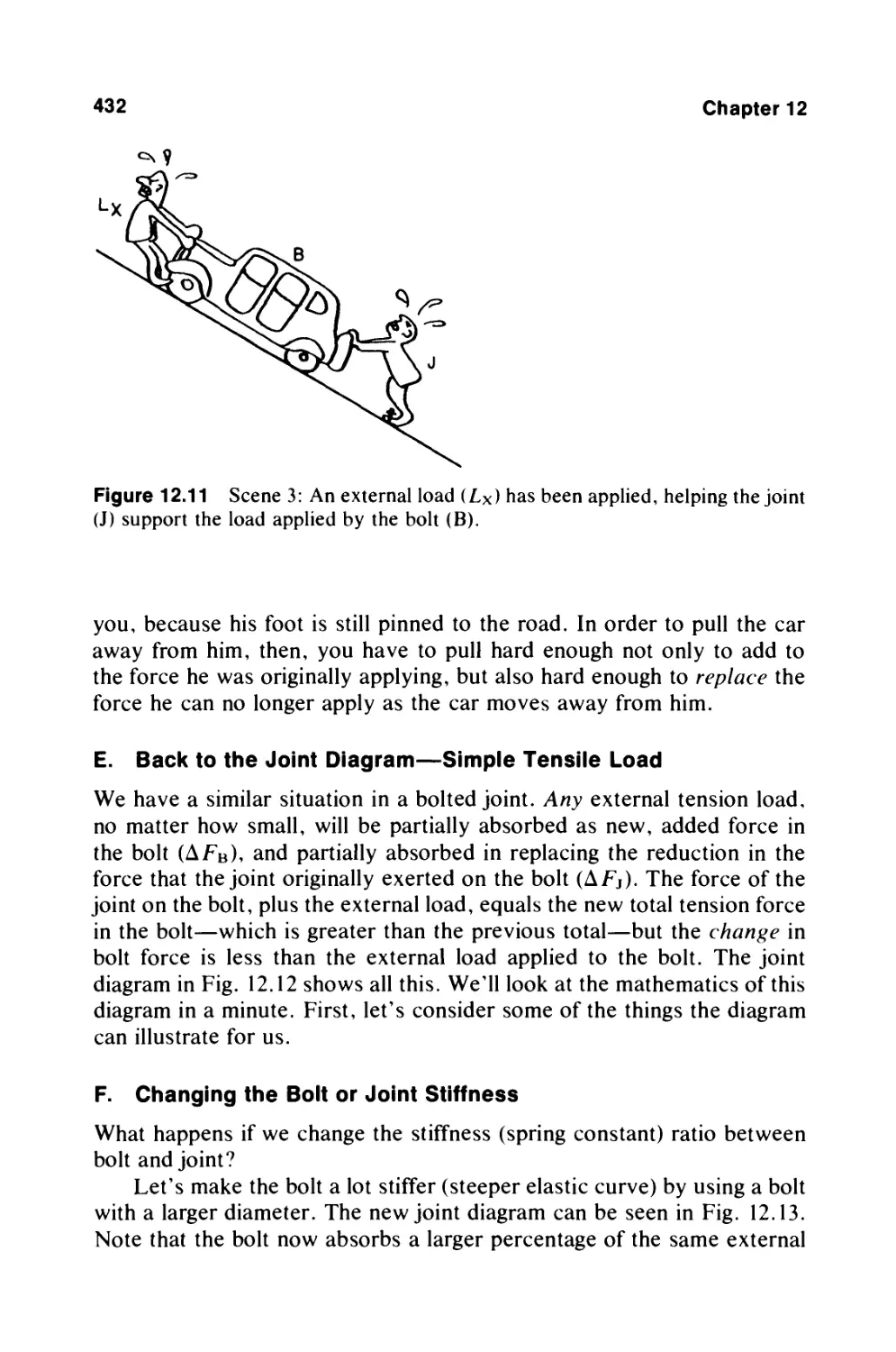
Текст
• A.
1*
f
title
author
publisher
isbnlO I asin
print isbnl3
ebook isbnl3
language
subject
publication date
lcc
ddc
subject
An Introduction to the Design and Behavior of
Bolted JointsMechanical Engineering (Marcel
Dekker, Inc.); 97
Bickford, John H.
0824792971
9780824792978
9780585231815
cover
An Introduction to the Design and Behavior of Bolted Joints
Third Edition, Revised And Expanded
John H. Bickford
Consultant, Bidwell Industrial Group, Inc.
Middletown, Connecticut
Marc x Dekker, Inc. New York ■ Basel
page_i
in
Page ii
Library of Congress Cataloging-in-Publication Data
Bickford, John H.
An introduction to the design and behavior of bolted joints / John
H. Bickford. 3rd ed., rev. and expanded,
p. cm. (Mechanical engineering ; 97)
Includes bibliographical references and index.
ISBN 0-8247-9297-1 (alk. paper)
1. Bolted joints. I. Title. II. Series: Mechanical engineering
(Marcel Dekker, Inc.) ; 97.
TA492.B63B5 1995
621.8'82dc20 95-21233
CIP
The publisher offers discounts on this book when ordered in bulk quantities. For more information,
write to Special Sales/Professional Marketing at the address below.
This book is printed on acid-free paper.
Copyright © 1995 by MARCEL DEKKER, INC. All Rights Reserved.
Neither this book nor any part may be reproduced or transmitted in any form or by any means,
electronic or mechanical, including photocopying, microfilming, and recording, or by any information
storage and retrieval system, without permission in writing from the publisher.
MARCEL DEKKER, INC.
270 Madison Avenue, New York, New York 10016
Current printing (last digit):
109 876
PRINTED IN THE UNITED STATES OF AMERICA
page_ii
Page iii
To my bright and wonderful family, in the order of their arrival:
Anne, David, Peter, Leila, and now Zoe.
page_iii
Page v
PREFACE TO THE THIRD EDITION
Although their exact birth date is unknown, it's certain that threaded fasteners have been around for at
least 500 years. They're still the fastener of choice when we want an easy and relatively low-cost way
to assemble anything from a frying pan to a satellite. They're virtually our only choice if we want to
create a specific clamping force to hold a joint together. The bolt and its cousins are, in fact,
marvelously simple mechanisms for creating and maintaining this force. And, of course, there's no
better fastener if we also need to disassemble and reassemble something for maintenance or other
purposes. Considering its tenacious hold on life and its persistent popularity, it's interesting that we
still don't know all we'd like to about the bolt, or about the bolted joint and the way it behaves in
service. Until a few years ago, moreover, most engineers knew virtually nothing about these things,
and an "introduction" seemed in order. The response to the first and second editions of this text seems
to confirm that premise.
The number of engineers who know the basic concepts of joint behavior, however, has grown
substantially; if my seminar students are any indication. The time has come, therefore, to deal with the
subject in greater depth than in previous editions. As a result, this third edition contains far more
specific information concerning design and behavior; with many new equations and numerical
examples. For example, three new chapters, 2123, are devoted specifically to design, covering joints
loaded in tension, gasketed joints, and joints loaded in shear. In addition, several other chapters have
been expanded to include specific design procedures or recommendations.
page_v
Page vi
A lot of this new materialespecially that dealing with joints loaded in tension-is based on a modified
version of the design procedure defined some years ago by the German engineering society Verein
Deutscher Ingenieure (VDI). I have modified their equations to account for-or at least to make more
visible-such phenomena as elastic interactions, gasket creep, and differential thermal expansion, which
can have a major impact on joint life and behavior. My debt to VDI, however, is substantial. If I have
misinterpreted or misrepresented them, the fault is mine and I apologize.
This edition also contains a detailed discussion of the new gasketed joint design procedure developed
by the Pressure Vessel Research Committee (PVRC) and now being incorporated into the ASME
Boiler and Pressure Vessel Code. This procedure is based on the new gasket factors developed by the
PVRC, and I have included the most recently published list of these factors. I have also shown, in a
numerical example, how to use the new factors, and how the results obtained compare with the results
of calculations based upon the historical Code procedure. Chapter 22, on the design of gasketed joints,
also includes a discussion of alternate design procedures suggested by other people or groups in
Europe.
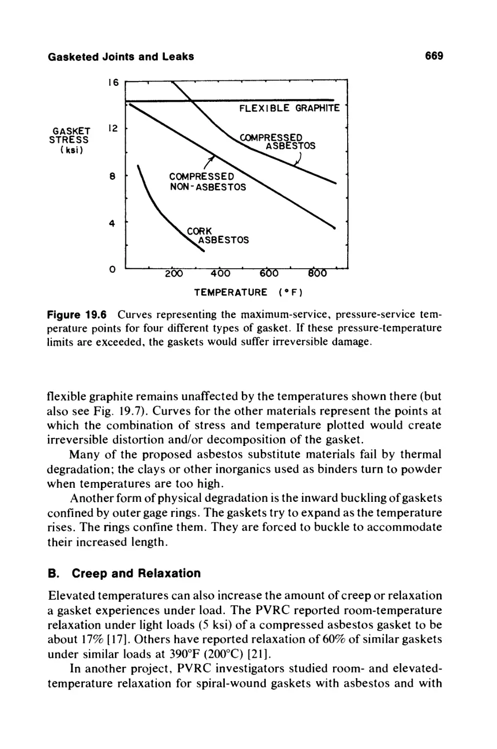
Chapter 19 deals separately with the behavior of gaskets and contains much new material on important
gasket properties such as creep and blowout resistance. Gasket test procedures and the new gasket
rating factors proposed by the PVRC are also discussed at length for the first time.
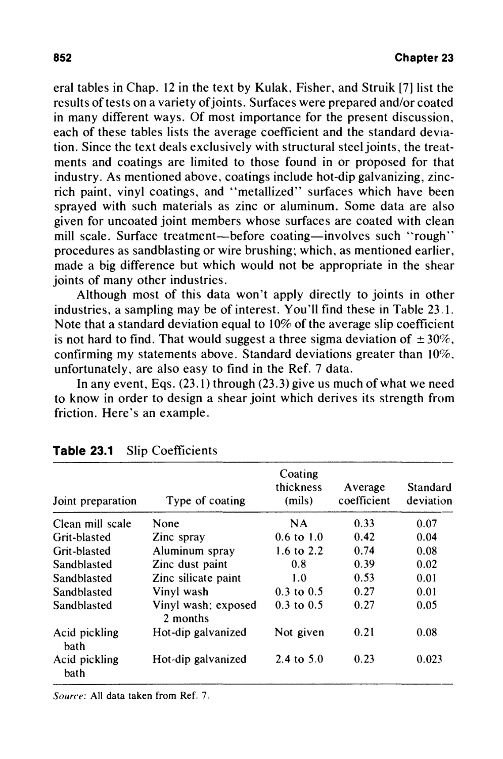
Chapter 23, on the design of shear joints, is based on both VDI techniques and the design
recommendations of the AISC, with the latter being more useful and informative for this type of joint.
As in the other chapters on design, I have included numerical examples, this time for the design of
friction-type, bearing-type and eccentrically loaded joints.
Other new material in this edition includes Chapter 3, on threadsconfigurations, nomenclature,
strength-as well as additional material in Chapters 6, 15, 16, and 17, dealing with joint assembly,
fatigue, self-loosening, and corrosion.
This edition, like the previous ones, is based almost entirely upon the work of others, as shown by the
many references cited at the end of each chapter. Each and every one of those authors deserves my
respect and my thanks. Many of those who contributed the most to my education are listed in the
following Acknowledgments. My current debt is so broad, however, that I'll let the references serve
for this edition.
I do, however, want to add an acknowledgment that I should have included in both the first and the
second editions: my debt to my publisher. I owe a great deal to Graham Garratt, Vice President and
Publisher, who
page_vi
Page vii
first suggested that I write such a textand who later convinced me that a second and now a third edition
were desirable. Writing a book is not a trivial task, and I probably would not have attempted it without
his gentle urging and continued support.
Revising a text, I was surprised to find, is more challenging than writing one. Correcting, updating and
improving a text while adding new material could challenge more nimble minds than mine; and here I
have been blessed with the friendly and helpful guidance of Walter Brownfield, who supervised the
production of both the second and third editions.
So, my thanks to both of these people at Marcel Dekker, Inc., and to the many engineers and scientists
listed in the references.
JOHN H. BICKFORD
page_vii
Page ix
ACKNOWLEDGMENTS
As before, most of the information in this book is not original with me. I am merely passing along to
you the education that I have received from so many other people and sources, including those
mentioned in the Preface to the first edition. For recent years, I am especially indebted to those listed
below.
In the Preface to the second edition, I mentioned the seminar students, who are too numerous to name
but to whom I owe a great deal. My education has been advanced even more, I think, by my
participation in a number of technical societies and groups that are struggling to resolve a variety of
bolting issues. I was involved, for example, with the Subcommittee on Bolted Flange Connections of
the Pressure Vessel Research Committee; I was a member of their Task Group on Gasket Testing and
was the Chairman of the Joint Task group on the Elevated Temperature Behavior of Bolted Flanges. I
have learned a great deal from many of the engineers who have attended these meetings and/or who
serve as consultants to these groups. I am especially indebted to Andre Bazergui of l'Ecole
Polytechnique in Montreal, Jim Payne of J. Payne Associates, George Leon of the Electric Boat
Division of General Dynamics, and J. Ronald Winter of the Tennessee Eastman Company. Dr.
Bazergui was kind enough to review Chap. 18 on gaskets in the second edition. His comments have
influenced the final version of that chapter; any remaining errors are mine.
I was also the Vice-Chairman of The Research Council on Structural Connections and have benefited
significantly from their work and delibera-
page_ix
Page x
tions, which involves special inputs from John Fisher of Lehigh University, Joseph Yura and Karl
Frank of the University of Texas at Austin, Geoffrey Kulak of the University of Alberta, Edmonton,
Thomas Tarpy of Stanley D. Lindsey and Associates of Nashville, Peter Birkemoe of the University of
Toronto, Michael Gilmor of the Canadian Institute of Steel Construction, and Bill Milek, now retired,
formerly with the AISC.
Dr. Kulak revised the valuable and influential text Guide to Design Criteria for Bolted and Riveted
Joints (Wiley, 1987), originally written by John Fisher and John Struik. I cited this text and my debt to
it in the Preface to the first edition.
I also participated in meetings of the Atomic Industrial Forum/Metals Properties Council Task Group
on Bolting and was Chairman of a Working Group on Bolting organized by the ASME Committee on
Operations and Maintenance (Nuclear Codes and Standards). Both of these groups were established to
define and resolve bolting issues which concerned the NRC. Key players to whom I am indebted here
include Ed Merrick, at that time with TVA and now with APTECH in California, Russell Hansen of
GA Technologies and Joe Flynn, Jr., of INPO. I benefited from information on nuclear bolting
problems provided by Ed Jordan, Robert Baer, and William Anderson of the Nuclear Regulatory
Commission. I am also grateful for more recent input from Richard Johnson of the same organization.
The Electric Power Research Institute of California played a significant role in the work of the
AIF/MPC Task Group, funding much of the group's research. They also funded the development at
Raymond Engineering* of a Reference Manual on Good Bolting Practices and three training cassettes
for bolting engineers and mechanics in the nuclear power industry. I was a coauthor of the manual and
participated in the preparation of the cassettes. The material in both was developed with the help of,
and was reviewed by, maintenance and operating engineers in a number of nuclear plants as well as by
members of the ASME Working Group. Many of the tips and suggestions that found their way into the
manual and cassettes have also been included in the second edition.
I am also grateful to the Industrial Fastener Institute of Cleveland. Raymond Engineering was an
invited member of that group for several years, and I have learned much from my contacts with their
members and from technical discussions with Charles Wilson, their Director of Engineering.
Colleagues at Raymond Engineering contributed to my education as
* The Bolting Products Division of Raymond Engineering, Inc., is now the Industrial Tool Division of
Bidwell Industrial Group, Inc.
page_x
Page xi
well. Special mention should go to Jesse Meisterling and to Michael Looram.
Stan Johnson of Johnson Gage deserves mention, too, for his input on thread strength, thread gaging,
and the like.
Bolting products customers of Raymond Engineering have provided much information about bolting
problems in nuclear power, petrochemical, aerospace, automobile, and other industries. Unfortunately
the number of "teachers" here is so great that individual mention is impossible, but my debt to them is
nonetheless considerable.
Last but not least, I would like to acknowledge this latest of many debts to my wife, Anne, who once
again lost a husband to a word processor. Ready or not, Anne, I'm now coming back!
page_xi
Page xiii
PREFACE TO THE SECOND EDITION
When I wrote the first edition of this book, most people, including most engineers, were generally
unaware of the importance of the bolted joint in our "high-tech" world. The few who were experts
were often considered remnants of that previous age when large iron and steel railroads, ships, tractors,
and bridges first evolved.
In recent years, however, a series of newsworthy events, many of them tragic, have made us realize
that the threaded fastener still plays a major role in our lives. Oil drilling platforms have tipped over,
airplane engines have failed, roofs have collapsed, and astronauts have died because of bolted joint
failures. The Nuclear Regulatory Commission has declared "bolting" to be an "unresolved generic
safety issue with number one priority," even though no bolt-related accidents or equipment failures
have occurred in that industry. And, most recently, the realization that substandard or "counterfeit"
bolts are flooding the country, with safety implications for our defense, and our nuclear, aerospace,
auto, and other industries, has led to congressional hearings and has even been reported on network
television.
Even though our general awareness has been raised, the technology of bolted joints is still in its
infancy. We know a lot more than we used to (some of that new knowledge is reflected in this new
edition), but we still have a long way to go. Like weather forecasters, bolting engineers must still deal
with very large numbers of unknowns and variables. As a result, our predictions and attempts to solve
or prevent problems must often be based on past experience, trial and error, overdesign, and so
page_xiii
Page xiv
forth, as in the past, rather than on the hard-and-fast answers so preferred by engineers.
Each of us, however, can benefit from the prior experience, the success and failure of others. Years
ago, I designed a bolted joint seminar based on the material in the first edition. This seminar, which is
still being given, has been sponsored by Raymond Engineering, the University of Wisconsin, and most
recently by the ASME. Students have been drawn from the automobile, aerospace, power, marine,
heavy equipment, and other industries that face bolting problems. The students have included people
who design, build, and use bolted equipment. And I think that, over the years, they have contributed as
much to my education as I have to theirs, offering tips, suggestions, and examples of things that have
worked and have not worked. Their questions and problems have certainly forced me and the other
instructors to dig more deeply than we might have into the literature, and elsewhere, to try to shed light
on some of the problems that still plague us.
Much of that digging is reflected in this new edition, in which I have attempted to include information
that will answer the most commonly asked questions. The first edition, I'm afraid, raised as many
questions as it resolved, and, although neither I nor anyone else at the present time has all the answers
to the questions that face bolting engineers, I have attempted to include far more concrete tips and
suggestions and data than I did in the earlier edition.
The new material in this edition includes:
Specific suggestions for optimizing the results obtained when assembling bolted joints. Tips are
given for assembly procedures based on torque control, torque-turn control, turn of nut, stretch
control, ultrasonic measurement of bolt stress and the like (Chaps. 511).
A variety of suggestions for how to pick preload (or torque) for a given application, starting with
simple methods for relatively unimportant joints and proceeding to more sophisticated methods
(Chap. 21).
A new chapter devoted to the material properties that affect the strength of the fastener and/or the
stability of the preload or clamping force on the joint in service (Chap. 3). Also, more data on
such things as nut factors (Chap. 5), gasket stiffness (Chap. 4), the elevated temperature
properties of bolting materials (Chap. 3), gasket creep (Chap. 18), and the relative costs of
bolting materials (Chap. 3).
A greatly expanded discussion of stress corrosion and other stress cracking phenomena, with data
on the stress corrosion resistance of a variety of bolting alloys (Chap. 19).
page_xiv
Page xv
A tabulation of key bolting equations in calculator (or computer) format (Appendix H).
A discussion of fastener coatings, with their uses, strengths, and weaknesses, including
substitutes for cadmium plating (Chap. 19).
An expanded discussion of fatigue failure, with new data (Chap. 17).
A discussion of a phenomenon I call "elastic interactions," which occurs when we tighten groups
of bolts and which can have a significant influence on the amount of clamping force developed in
a joint (especially a gasketed joint) during assembly. Most people, myself included, were
unaware of this phenomenon when I wrote the first edition. Interactions can cause assembly
preloads to vary by 4: 1 or more, even if tensioners are used to tighten the bolts (Chap. 6).
A simple procedure that will allow you to make a rough estimate of the stiffness of a bolted joint,
a procedure based on experimental data generated by several different groups (Chap. 4).
Although the procedure is only approximate, it is much cheaper than the experiments or finite
element analysis required for a more exact answerand it will be good enough for many
applications.
A nearly complete revision of the discussion of ultrasonic measurement of bolt stress or strain to
reflect the significant advances that have occurred in this technology in recent years (Chap. 11).
Major revisions to and extension of the discussion of gaskets, with a description of recent results
of research sponsored by the Pressure Vessel Research Committee and a discussion of the new
gasket factors now being proposed as replacements for the m and y factors of the ASME Boiler
and Pressure Vessel Code (Chap. 18).
A procedure for estimating the effect of a change in temperature on preload or on the clamping
force on the joint (Chap. 14), plus a discussion of the other ways in which elevated temperature
can affect a gasketed joint (Chap. 18).
A structured procedure for answering bolted joint questions and/or for predicting results when the
joint is assembled and put in service (Chaps. 2021).
I think that you will find that the information listed above, plus that carried over from the first edition,
will help you deal with this complicated thing called a bolted joint.
JOHN H. BICKFORD
page_xv
Page xvii
PREFACE TO THE FIRST EDITION
To "get down to the nuts and bolts" of a topic has always meant to get to the heart of it, and rightfully
so. After all, the joints are the weakest element in most structures. This is where the product leaks,
wears, slips, or tears apart. I have heard that the "improper use of fasteners"in joints, of courseis the
largest single cause of the warranty claims faced by U.S. automobile manufacturers. An Air Force
engineer told me that the cost of a modern military airplane is a linear function of the number of
fasteners involved. These claims may be apocryphal, but the problems are real.
In spite of their importance, bolted joints are not well understood. Mechanical engineering students
may receive a brief introduction to the subject in a design course, but only a small percentage of
themin school or afterwardwill ever get involved enough for a real understanding. The specialists who
design things which must not failairplanes, nuclear reactors, or heavy equipment costing hundreds of
thousands or even millions of dollarsare forced to learn all there is to know about the design and
behavior of bolted joints. The rest of the engineering fraternity, even designers, are guided by
guesswork, experience, or handbooks. And they still have problems.
As a matter of fact, even sophisticated designers have problems at the present state of the art because
the behavior of a bolted joint involves a large number of variables difficult or impossible to predict
and/or control. There are widely used design theories and equations, many of which we shall study in
this book, but these are usually simplifications and approxi-
page_xvii
Page xviii
mations. They have been used, successfully, on all sorts of joints in all sorts of products, but they are
not sufficient for critical joints. Most of them, furthermore, have been around for years, and they have
fallen behind the demands being placed on contemporary designs, e.g., higher operating temperatures
and pressures, new materials, the increased clamor for more safety or environmental protection, and
better strengthto-weight ratios. Even the thorough, widely used, and often-modified ASME Boiler and
Pressure Vessel Code has failed to keep pace with the needs of the designer.
The engineering societies are aware of these problems, of course, and are currently funding extensive
experimental and theoretical studies to advance the science (or is it an art, at present?) of bolted joint
design. It is believed that this work will make accurate joint design possiblebut not until the end of this
decade. That forecast, coming from the most knowledgeable people in this business, gives you an idea
of the magnitude of the problem. None of us, of course, can wait 10 years for solutions to our current
design problems. We have to function at the current state of the art. Even this is a challenge, given the
complexity of the subject, but currently available information can help us minimize joint problems
even if we can't eliminate them. Hence, this book will serve as an introduction to the design and
behavior of bolted joints and a primer for engineers or students who are struggling with the subject in
depth for the first time. It will also help plant engineers, maintenance engineers, production engineers,
and other nondesigners understand the nature of and reasons for their bolted joint problems, and give
them some help in solving or reducing these problems.
The information in this book has come primarily from two sources. My employer, Raymond
Engineering Inc., has manufactured for some years unusual tools and equipment for assembling and
disassembling large bolted joints. In a desire to increase our knowledge of bolted joint technology, we
commissioned, in 1978, a computerized literature search. This search, directed by Stephen Ford of the
Battelle Memorial Institute, uncovered thousands of articles: some unique, some repetitive; some
"correct," some ridiculous; some well-written but some not. File drawers full of articles, including, by
and large, all that was known, or at least all that had been published, about bolted joints at that time.
Since then, we have sponsored a biweekly computerized "update" search of many different
engineering files, including El, DOE, BHRA, NASA, ISMEC, ASM, INSPEC, CPI, CAC, NTIS,
USG, and many others. These updates are made for us by the New England Research Center at the
University of Connecticut.
page_xviii
Page xix
These updates have kept our library currentand our readers busy! This present book is, to a large
extent, an overview of the state of the art as revealed by this literature search, so, as the author, I am
much indebted to Mr. Ford for starting my education, and to UCONN for continuing it.
I'm even more indebted to the many engineers and scientists who wrote the articles: Bob Finkelston,
Gerhard Meyer, and Dieter Strelow of SPS; G. H. Junker of Unbrako-SPS; Nabil Motosh of Asslut
University in Egypt; John Fisher of Lehigh University; Wayne Milestone of the University of
Wisconsin; Ed Rice of Ingersoll-Rand; and Sam Eshghy of Rockwell stand out as key influences, but
there are hundreds of others. Any errors in my book, of course, should not be blamed on them, but
rather on my inability to understand.
But there's more to it than that. We're not scientists or academics. We're engineers and businessmen,
and although we're deeply interested in the theories and explanations, our goal is to understand and
solve, or prevent, field problems. It's nice to know that "the equations don't always work because . . .";
but we still have to tighten those joints, right now, in such a way that they stay put for the life of the
product, or at least until the next maintenance shutdown. And so we kept looking for equations,
information, rules-of-thumb, divine guidance, or anything that would get us there. And this led us in
two directions that have produced results.
First, our search for something better led us to an impressive new instrument called the ultrasonic
extensometerinvented by Donald Erdman of Pasadena and Howard McFaul of Douglas Aircraft
Corporation. This instrument is designed specifically to measure the actual strain in a bolt before,
during, and after tightening. Here, for the first time, we had a way to measure "tightness" in bolts, with
a high degree of accuracy, under any and all field conditions, statically or dynamically, and across the
board. Prior methods were only practical for samplesyou strain-gauged a few bolts, for example, used
load cells under the heads of a few, or made a laboratory experiment. In many cases you modified field
conditions simply by taking the measurements. If nothing else, the results you obtained were
unnaturally "good," because the person using the wrench was more careful with those bolts than before
or after your experiment.
Several types of extensometer are described at length in Chap. 9. I'm indebted to Donald Erdman,
incidentally, for reading and correcting this chapter, as well as for making it possible for us to measure
bolt stretch ultrasonically.
The extensometer makes it possible to check unmodified bolts assembled by unsuspecting people, and
to monitor such elusive things as dy-
page_xix
Page xx
namic loads or long-term relaxation. Engineers have long been able to measure the inputs to the
system, e.g., torque applied to the nut, composition of the lubricant, and angle of turn of the nut. Now
we can see the immediate effects and results, as a function of job conditions and/or time. We felt just
as the electrical engineer must have when someone handed him the first oscilloscope.
We have used this instrument extensively in our laboratory to study bolt problems and to analyze and
check some of the information and theories uncovered by the literature search. But more significantly,
we have used it in the field. We organized a bolting services group which sent technicians to many
parts of the countryand overseas-to help customers tighten or disassemble problem joints. This
hands-on experience provides the second major source of information on which this book is based. I'll
tell you what really happens when you tighten various kinds of joints, under often difficult conditions,
with a variety of tools and procedureseven if no one, at present, can fully explain why they behave this
way. And I'll describe some of the techniques we and our customers have used to solve or minimize
today's problems.
Most of our work has involved very large bolted joints, e.g., pressure vessels, pipe joints, heat
exchangers, engine heads, and helicopter transmissions; but we've also been involved with small
aerospace assemblies, and have had some exposure to the tools and techniques used by automobile and
other mass producers. So, although the case history emphasis in this book will be on large fasteners,
the design and behavior information is applicable to most types of bolted joints.
One warning for those involved in the design and construction of buildings: You will not find much
information here on structural steel joints. Many of the topics covered would be pertinent to such
joints, but I make little or no attempt to relate them to those applications. This is an area in which my
company and I have had very little experienceand it's an area that is very well covered by Fisher and
Struik's excellent Guide to Design Criteria for Bolted and Riveted Joints (Wiley, 1974). That work, on
the other hand, doesn't cover liquid joints, or the problems faced by production engineers.
I am sure that some of you will find the subject of bolted joints as interesting as I doat least by the time
you finish the book. Before we start, let me add one more note of appreciation for my secretary, Tressa
Battista, who faced too many drafts with too little time, but did it all.
We're ready. Let's learn about bolted joints.
JOHN H. BICKFORD
page_xx
CONTENTS
Page
Preface to the Third Edition v
Acknowledgments ix
Preface to the Second Edition xiii
Preface to the First Edition xvii
Part I 1
Introduction to the Bolted Joint
1 3
Basic Concepts
I. Two Types of Bolted Joint 3
II. The Bolt's Job 4
III. The Challenge 7
IV. Failure Modes 10
V. Design 12
VI. The Layout of the Book 13
2 15
Stress and Strength Considerations
I. Types of Strength 15
II. The Bolt in Tension 17
III. The Strength of a Bolt 27
IV. The Strength of the Joint 35
V. Other Types of Load on a Bolt 40
I
INTRODUCTION TO BOLTED
JOINTS
1
Basic Concepts
This book is intended to give you an introduction to the design and
behavior of bolted joints and hopefully will help you become better designers,
assemblers, or users of such joints, or help you analyze and prevent joint
failures. The subject is a complex one, which is why a text of over 700
pages can be considered only an introduction. The material presented
here, however, should be all the information that many or most people
need. Numerous references at the end of each chapter lead the way to
further details for those who need or want to know more.
This first chapter gives an overview of the material to be covered in
the rest of the book; it's an introduction to the introduction, if you will.
You might find it useful to come back to this chapter and reread it, if you
get bogged down in the detail of subsequent chapters and have trouble
seeing how that subject or detail fits the overall picture.
I. TWO TYPES OF BOLTED JOINT
Bolted joints come in two flavors, depending on the direction of the
external loads or forces acting on the joint. If the line of action of the forces
on the joint is more or less parallel to the axes of the bolt, the joint is said
to be loaded in tension and is called a tension or tensile joint. If the line
of action of the load is more or less perpendicular to the axes of the bolt,
the joint is loaded in shear and is called a shear joint. Both types are
illustrated in Fig. 1.1. Some joints support combined tensile and shear
3
4 Chapter 1
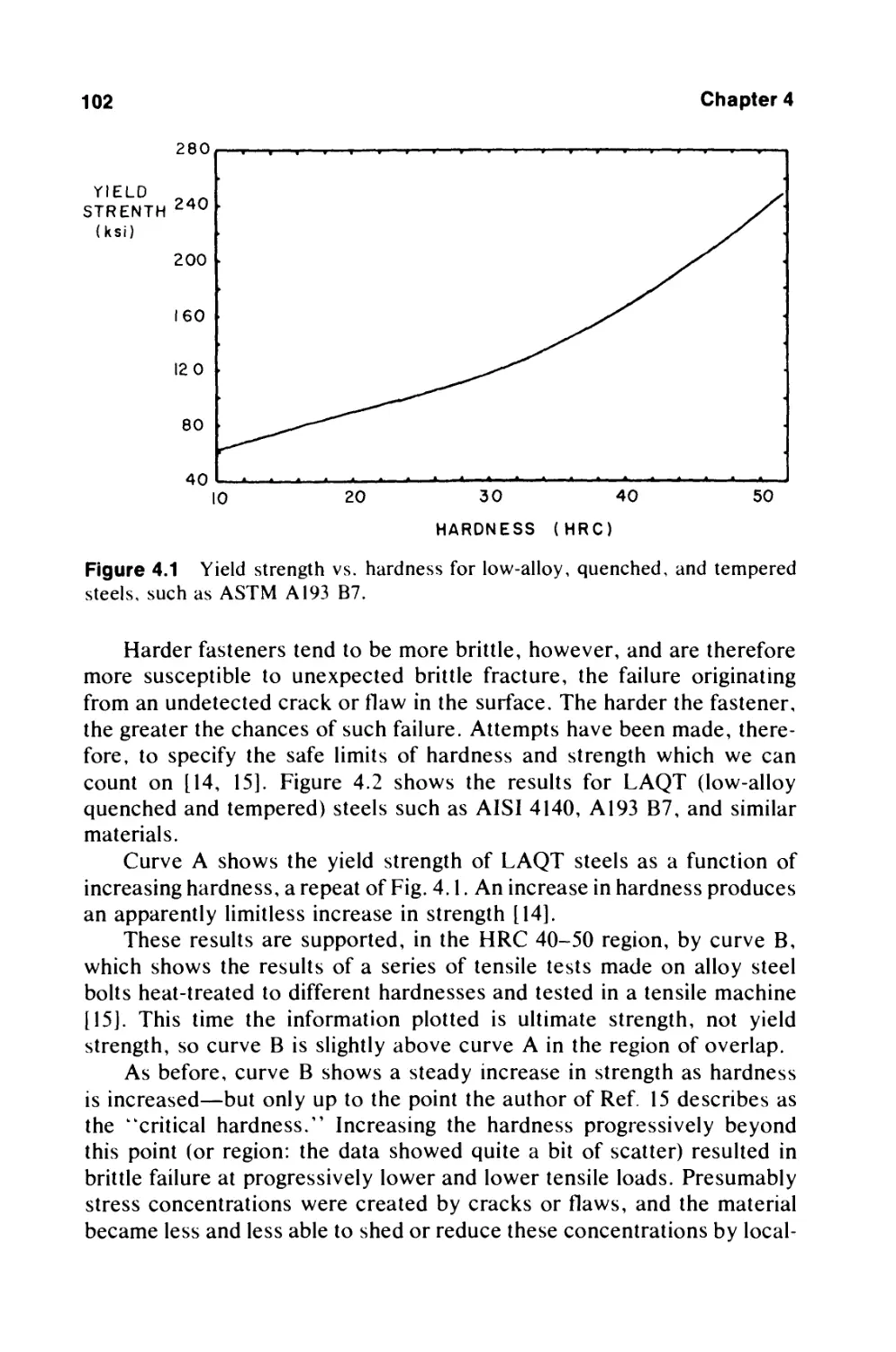
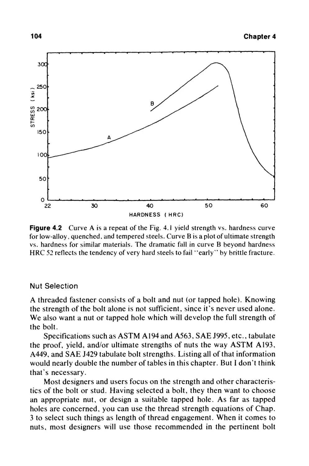
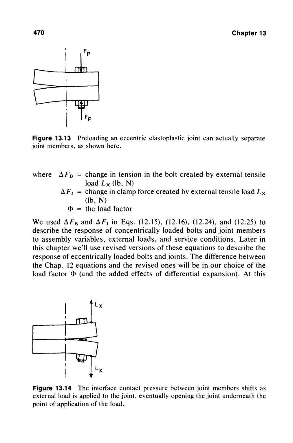
Figure 1.1 Bolted joints are classified by the service loads placed on them. If
those loads—forces—are applied in a direction more or less parallel to the axes
of the bolts, as in the upper sketch here, the joint is called a tensile or tension
joint. If the line of action of the forces is essentially perpendicular to the axes of
the bolts, as in the lower sketch, the joint is called a shear joint.
loads and are named after the larger of the loads placed on them, be it
tensile or shear.
The distinction between tensile and shear joints is important, because
the two types differ in the way they respond to loads, the ways in which
they fail, the ways in which they are assembled, etc. In general, the tensile
joint is the more complex of the two—as far as behavior and failure are
concerned—and it's the more common type of joint. Most of this text,
therefore, is devoted to it. Another reason for this bias: Messers Kulak,
Fisher, and Struik have written an excellent text, Guide to Design Criteria
for Bolted and Riveted Joints, second edition (John Wiley & Sons, New
York, 1987), which is devoted almost entirely to shear joints.
II. THE BOLTS JOB
The purpose of a bolt or group of bolts in all tensile and in most shear
joints is to create a clamping force between two or more things, which
we'll call joint members. In some shear joints the bolts act, instead,
primarily as shear pins, but even here some bolt tension and clamping force
is useful, if for no other reason than to retain the nuts.
Basic Concepts
5
A. Tensile Joints
Specifically, in tensile joints, the bolts should clamp the joint members
together with enough force to prevent them from separating or leaking.
If the joint is also exposed to some shear loads, the bolts must also prevent
the joint members from slipping.
Coincidentally, the tension in the bolt must be great enough to prevent
it from self-loosening when exposed to vibration, shock, or thermal cycles.
High tension in the bolt can also make it less susceptible to fatigue (but
sometimes more susceptible to stress cracking). In general, however, we
usually want the bolt in a joint loaded in tension to exert as much force
on the joint as it and the joint members can stand.
There are two important facts you should keep in mind when dealing
with tension joints. First,
The bolt is a mechanism for creating and maintaining a force, the
clamping force between joint members.
Second,
The behavior and life of the bolted joint depend very much on the
magnitude and stability of that clamping force.
Note that I did not say "magnitude and stability of the preload" or
of the tension in the bolt or of the torque applied to the bolt. Those
parameters are related to the clamping force, often closely related, but the key
issue as far as joint behavior is concerned is the force the two joint
members exert on each other (the clamping force), created, of course, by the
force the bolts are exerting on them.
The key issue as far as bolt life and integrity are concerned is,
however, the tension in it—so we must keep our eye on both interjoint
clamping force and bolt tension to be successful.
The clamping force on the joint is initially created when the joint is
assembled and the bolts are tightened by turning the nut or the head of
the bolt. This act, of course, also creates tension in the bolt; the tension
is usually called preload at this stage.
Although there may be some plastic deformation in some of the
threads when a bolt is tightened normally, most of the bolt and the joint
members respond elastically as the bolt is tightened. The joint members
are compressed a slight amount, and the bolt is stretched by a larger
amount.
In effect, both joint members are bolts behave like stiff springs, one
being compressed and the other stretched as suggested in Fig. 1.2. Like
springs, furthermore, they acquire potential (or stored) energy. If we
released them after tightening them, they would suddenly snap back to their
6
Chapter 1
Figure 1.2 Bolts and joint members deform elastically when the bolts are
tightened. In effect, they act like stiff springs as suggested by this sketch. This fact,
that they act like springs, greatly influences the behavior of the joint.
original dimensions. It is this stored energy which allows bolts to maintain
that all-important clamping force betweenjoint members after we remove
the wrench.
We might even say that the tensile joint, unlike its welded or bonded
joint cousin, is "alive," filled with energy and able to do its job only
because it's filled with energy.
B. Shear Joints
The bolt's main job in a shear joint is to keep the joint from slipping or
from tearing apart in the slip direction. If the joint must also support some
tensile load, the bolt must resist that too.
In some shear joints, as already mentioned, the bolts resist slip by
acting as shear pins, and joint integrity is determined by the shear strength
of the bolts and joint members. There are a number of reasons why we
will often want to tension these bolts, as we'll see, but the exact amount
of tension, or of the energy stored in them, is not a critical factor.
In other shear-loaded joints slip is prevented by friction restraint
betweenjoint members. These friction forces are created by the clamping
load, which in turn is created by heavily tensioned bolts. Here again,
Basic Concepts
7
therefore, the bolt is a mechanism for creating and maintaining a force,
and the magnitude and life of that force depend on the potential energy
stored in the bolts during assembly. Even here, however, we're usually
less concerned about creating an exact amount of tension in the bolts
during assembly than we are when we're dealing with tensile joints,
because service loads don't affect bolt tension and clamping force in shear
joints.
III. THE CHALLENGE
The bolted joint presents users and designers with many problems. In part
this is because it is "alive"—it keeps changing state in response to service
and environmental conditions, as we'll see. A more common source of
problems, however, is the fact that the assembly process and the in-service
behavior are affected by literally hundreds of variables, many of which
are difficult or impossible to control or to predict with accuracy. As a
result, when we deal with bolted joints we must inevitably deal with a lot
of uncertainty. What follows is a quick review of some of the sources of
this uncertainty. We'll take a closer look at most of these things in later
chapters.
A. The Assembly Process
Bolts and joint members in both tension and shear joints respond in the
same way to the act of tightening the bolts. There are differences in the
accuracy with which we must tighten them, but most of the discussion
which follows applies to all joints.
As far as all tension and most shear joints are concerned, the goal of
the assembly process is to establish an initial clamping force between joint
members, to introduce the first energy into bolt and joint springs. And,
in tension joints, we're usually interested not just in tensioning the bolts
but in tensioning them by a desired amount, because the life and behavior
of such joints are so dependent on the "right amount" of clamping force.
We want enough clamping force to prevent a variety of failure modes,
but we must also make sure that the bolt tension and clamping force do
not exceed an upper limit set by the yield strengths of the materials, the
anticipated loads to be placed on the joint in service, and other factors.
Unfortunately, as already mentioned, hundreds of variables affect the
results when we tighten a group of bolts, so predicting or achieving a
given clamping force is extremely difficult.
8
Chapter 1
We attempt to control the buildup of clamping force by controlling
the buildup of tension or preload in the bolt. In most cases, we do that
by controlling the amount of torque applied to the nut or head.
The work we do on the fastener while tightening it is equal to one-half
the applied torque times the angle (measured in radians) through which the
nut turns. Typically, about 10% of this input work ends up as potential
energy stored in the joint and bolt "springs." The rest is lost in a variety
of ways.
Most is lost as heat, thanks to friction restraints between the nut and
joint surface and between male and female threads. Some energy is used
to twist and, often, to bend the bolt a little. Some energy may be lost
simply in pulling heavy or misaligned joint members together or dragging
a bolt through a misaligned or interference fit hole. More is lost by
spreading the bottom of the nut, a process called nut dilation.
A major problem for the designer and assembler is that it is virtually
impossible to predict how much of the input work will be lost due to
factors such as these. The amount lost can and usually will vary a lot
from one bolt to another, even in the same joint.
In spite of these uncertainties and losses, some potential energy is
developed in each bolt as it's tightened, and it starts to create some
clamping force in the joint. But then the bolt relaxes—loses some energy—for
a couple of reasons.
A process called embedment occurs as high spots on thread and joint
contact surfaces creep out from under initial contact pressure and the
parts settle into each other. More drastically, a previously tightened bolt
will relax somewhat when its neighbors in the joint are subsequently
tightened. We call this process elastic interaction, and it can eliminate most
or even all of the tension and energy created in the first bolts tightened
in the joint. We'll examine this phenomenon in detail in a later chapter.
The amount of relaxation a bolt will experience is even more difficult
to predict than the amount of initial tension it acquires when first
tightened, increasing the challenge of the assembly process.
Anything which reduces the amount of energy stored in a bolt reduces
the force it exerts on the joint. Too little torque, too much friction, rough
surface finish, twisting, bending, hole interference, relaxation—all can
result in less stored energy, less preload, less clamping force.
Anything which increases the energy stored will increase the force.
There are a couple of things which can do this during assembly: too much
torque or too little friction, thanks perhaps to a better-than-anticipated
lubricant.
Again, all of these factors are difficult to predict or control, making
it very difficult to achieve a particular amount of preload or clamp force
Basic Concepts
9
at assembly. Because many factors can give us less preload than desired
and only a couple can give us more, we often—perhaps usually—end up
with less than expected at assembly.
Bolts in shear joints are subjected to the same assembly problems and
variables as are bolts in joints loaded in tension. There's a difference,
however.
In tension joints we always care about the amount of preload, tension,
clamping force, and potential energy developed during assembly because
of the way such joints respond to service loads. We're not so concerned
about this when dealing with shear joints. We'll see why when we examine
the in-service behavior of such joints.
B. In-Service Behavior
The in-service behavior of tensile joints differs substantially from that of
shear joints, and this is reflected in the different ways we design and
assemble the two types. Here's a preliminary look at the differences.
Joints Loaded in Tension
We encountered many uncertainties when we assembled a tensile joint.
Further uncertainties are introduced when we put such a joint to
work—when we load it, expose it to vibration or shock, subject it to
change in temperature, anoint it with corrosive fluids, etc. Being alive, it
responds to such things, and as it responds the tension in the bolt and the
clamping force between joint members change.
First, and most important, the tensile load on the joint will almost
always increase the tension in the bolts and simultaneously decrease the
clamping force between joint members. This is undesirable—and
unavoidable. And it is the major reason why we care so much about the exact
amount of bolt tension and clamping force developed at assembly.
If the assembly preloads are too high, the bolts may yield or break
when they encounter the service loads. On the other hand, if assembly
preloads are too small, the clamping force on which the joint depends
may all but disappear when service loads decrease it.
Other service factors can also change bolt tension and clamping force
and will affect our choice of assembly preload. For example, relaxation
processes like embedment—or gasket creep—are increased by loads and
by elevated temperatures. Vibration, shock, or thermal cycles can cause
the bolt to self-loosen. Differential expansion between bolts and joint
members can increase bolt tension and clamping force simultaneously—or
can reduce both. In this case heat energy is being used to increase or
redistribute the energy stored in the parts.
10
Chapter 1
Chemical energy—exhibited as corrosion—can increase clamping
force as corrosion products build up under the face or the nut or head of
the bolt.
These factors present an additional challenge to the designer. They
increase the difficulty of predicting joint behavior, because the designer
can rarely predict the exact service loads or conditions the joints will face.
The joint's response, furthermore, will be influenced by such hard-to-pin-
down factors as the condition of the parts or the exact dimensions and
material properties of the parts. Behavior will also be influenced by the
hard-to-predict amount of preload in the bolts, which the designer must
somehow specify.
Once again, however, the factors which lead to less clamping force
are more common than the ones which can lead to more clamping force.
Since this is also true, as we've seen, of the assembly process, we are
forced to recognize Bickford's little-known First Law of Bolting: Most
bolted joints in this world are providing less clamping force than we think
they are.
Shear Joints
Shear loads do not affect the tension in the bolts or the clamping force
between joint members, at least until such loads become so high that the
joint is about to fail. Predicting behavior and avoiding failure are therefore
easier when we're dealing with shear joints than when we are dealing with
tensile joints. This, in part, explains why people who design airframe,
bridge, or building structures rely so heavily on shear joints and avoid
using tension joints whenever possible.
I don't mean to imply that shear joints won't respond to service loads
and conditions; they will. Bolt tension and clamping force will change if
temperatures change. Vibration or shock can loosen the bolts. Parts can
rust, and corrosion products can build up and alter bolt and joint stresses.
If the loads on the joint are cyclical, the stresses in bolts and joints
members will fluctuate. But the in-service uncertainties the designer faces, and
their consequences, are usually less than those he'll face when dealing
with tensile joints.
IV. FAILURE MODES
The main reason we want to "control" or "predict" the results of the
assembly process and the in-service behavior of the joint is to avoid joint
failure. This can take several forms.
Basic Concepts
11
A joint will obviously have failed if its bolts self-loosen—shake
apart—or break. Self-loosening is a complicated process and is described
in a separate chapter, along with ways to combat it. In general, however,
it's caused by vibratory or other cyclical shear loads which force the joint
members to slip back and forth. A major cause of self-loosening is "too
little preload"—and hence too little clamping force. Both tensile and shear
joints are subject to this common mode of failure.
Bolts in both types of joint can also break because of corrosion, stress
cracking, or fatigue—all of which are also covered in later chapters and
two of which are encouraged by the wrong preload. Stress cracking occurs
when bolts are highly stressed; fatigue is most apt to occur when there's
too little tension in the bolts. Even corrosion can be indirectly linked to
insufficient preload, if a poorly clamped joint leaks fluids which attack
the bolts.
If the bolts fail for the reasons just cited or if they exert too little force
on the joint, perhaps because of the assembly or in-service conditions
discussed earlier, the shear joint may slip or the tension joint may separate
or leak. Each of these things means that the joint has failed.
It's obvious that a leak is a failure, but what's wrong with a little slip
or with separation of a joint that doesn't contain fluid?
Slip can misalign the members of a joint supporting shear
loads—cramping bearings in a machine, for example. Or it can change
the way a structure absorbs load, perhaps overstressing certain members,
causing the structure to collapse. Slip can lead to fretting corrosion or to
fatigue of joint members. As already mentioned, cyclical slip can lead to
self-loosening and perhaps loss of the fasteners. Vibration loosening of
bolts and fatigue failure of shear joint members are of particular concern
to airframe designers.
Separation of the members of a joint supporting tensile loads can
encourage rapid fatigue failure of the bolts. It can also destroy the integrity
of a structure or machine. It can allow corrosants to attack bolts and joint
surfaces. Separation means the total absence of clamping force, which
means, in effect, that the joint is not a joint at all.
A gasketed joint can leak if the initial clamping force between joint
members during assembly is not great enough or if the in-service clamping
force (which will almost always differ from the assembly clamp) is too
low. The joint does not have to separate for leakage to occur.
Note that most joint or bolt failure modes are encouraged by
insufficient bolt tension and/or insufficient clamping force. Self-loosening,
leakage, slip, separation, fatigue—all imply too little clamp.
A few problems can be caused by too much tension or clamping force,
however. Stress corrosion and hydrogen embrittlement cracking of bolts
12
Chapter 1
can occur in both shear and tensile joints and are more likely if bolt stresses
are high. Joint members and gaskets can be damaged by excessive clamp.
Joint members can also be distorted by excessive bolt loads; the
"rotation" of raised face, pressure vessel flanges is a common example. Fatigue
life can sometimes be shortened by high stress, although more commonly
it's caused by insufficient clamping force.
But failures caused by too little clamping force are more common in
either tensile or shear joints than are failures caused by too much clamp.
And, as we've seen, assembly and service conditions are more apt to give
us too little clamp than too much. Welcome to the world of bolting!
V. DESIGN
A. In General
The design of bolted joints, like the design of anything else, involves a
detailed consideration of function, shapes, materials, dimensions, working
loads, service environment, etc. Every industry has characteristic or
"typical" joint configurations and needs, and it would be impossible to detail
each in a single text. We can, however, look at some generalities which
must apply to most joints, whatever their specific application. And we
can review design procedures which have been accepted and used by
many.
Specifically we'll focus on a design procedure developed by Verein
Deutscher Ingenieure (VDI), a German engineering society, but with some
modifications and extensions. We'll also examine in some detail the design
rules for flanged, gasketed joints found in the ASME Boiler and Pressure
Vessel Code, with emphasis on changes which are currently being
introduced to those rules. And we'll take a brief look at the design of structural
steel, shear joints.
B. Specific Goals of the Designer
The joint designer, of course, is faced with all the assembly and in-service
uncertainties detailed earlier. In spite of these uncertainties, he must do
two things when designing a joint which will be loaded all or in part in
tension:
1. He must pick bolt and joint sizes, shapes, and materials which will
guarantee enough clamping force to prevent bolt self-loosening or
fatigue, and to prevent joint slip, separation, or leakage, when
clamping forces are at a minimum (because of the factors we've described)
and those hard-to-predict service loads are at a maximum.
Basic Concepts
13
2. In addition, he wants to select bolts which are able to support a
combination of maximum assembly stress plus the maximum increase in
stress caused by such service conditions as applied load and
differential thermal expansion.
If his joint is loaded only in shear, and will depend for its strength
only on the shear strength of the bolts and joint members, then those
strengths will determine the design. Such joints must not be subjected to
varying or cyclical loads, or self-loosening and fatigue problems might
be encountered. If service conditions permit it, however, such joints are
safe—and greatly simplify the design process.
There are other things which the designer must worry about when
designing tensile joints and some shear joints. He'll consider the bearing
stresses the bolts create on joint surfaces, the amount of change in load
the bolts see (which can affect fatigue life), the accessibility of the bolts
(which can affect assembly results), and the flexibility or stiffness of bolts
and joint members. If he's designing a tension joint he'll be especially
interested in the so-called stiffness ratio of the joint, because this affects
the way in which a given service load changes bolt tension and clamping
force.
In any tension joint and in shear joints where clamping force is
important, the designer will want to do everything he can to improve the energy
storage capacity of his bolts. He'll find that long thin bolts and thick,
metal joint members can store more energy than short stubby boits or
nonmetallic joints; hence our historic problems with sheet metal joints
and our emerging problems when we try to bolt composite materials.
As we'll see, the many assembly and service uncertainties the designer
has faced have traditionally forced him to overdesign—"oversize" might
be better—the bolts and joint members, with resulting penalties in weight
and parts cost. We'll quantify this oversizing and suggest ways it can
sometimes be reduced.
Although most of the book will deal with subjects like assembly
practices, in-service behavior of the joint, and failure modes rather than design
specifics, everything relates to and should affect the design of bolted
joints.
VI. THE LAYOUT OF THE BOOK
We'll start with some background material on the strength of bolts and
of threads, the stiffness of bolts and joint members, and a review of the
properties of the materials usually used for these things. We'll focus on
properties that affect basic strength and which affect the stability of the
14
Chapter 1
parts (several material properties can encourage changes in clamping
force).
Next we'll look in considerable detail at the many options we have
for controlling the assembly process, looking at torque, torque and turn,
strength, direct tension, and ultrasonic control of preload and clamping
force.
Then we'll turn our attention to the joint in service: how it responds
to service loads and conditions, how it fails, how to improve its response
and minimize the chances of failure.
Finally, having learned in detail what we're up against, we'll develop
procedures for estimating results and will close with a detailed discussion
of a modified version of the VDI design procedure.
Appendices in the back will give you a variety of reference data to
aid design activities or analytical calculations.
Enough introduction! Let's begin our serious study of this thing called
a bolted joint.
2
Stress and Strength
Considerations
We learned in the last chapter that the bolt's job is to clamp the joint
together firmly enough to prevent slip, separation, or leakage and that the
bolt must be strong enough to support the maximum preload it receives
at assembly, plus the maximum additional loads it sees in service as a
result of forces applied to the joint, differential thermal expansion, etc.
When designing, evaluating, specifying, or selecting a bolt for a
particular job, therefore, one of our first questions will be: kkIs this bolt strong
enough to clamp this particular joint?" As we're about to see, the question
is much simpler than the answer, because there are many aspects to the
concept of strength when we're dealing with a bolt.
I. TYPES OF STRENGTH
In general, of course, the strength of any machine part is determined by
such things as the size and shape of the part, the material it's made from,
the heat treatment of that material, its operating temperature, and its
condition (has it been abused, is it corroded, etc.?). Engineers also define
strength in a variety of ways. Here are the more important definitions we
use when we're dealing with bolts.
A. Tensile Strength
First, we must worry about the capacity of the bolt to generate and sustain
a sufficient tensile force, since that force will be one of the main factors
15
16
Chapter 2
which determine the clamping force between joint members. (It's not the
only factor, as we'll see in Chap. 6.) In most applications, the room
temperature tensile strength of the bolt under static loads will be one of only
two strength factors we need to be concerned about.
We'll describe this strength in several ways, however, depending on
our needs. We'll use the term ultimate strength, yield strength, or—unique
to threaded fasteners—proof strength. Each of these is defined and
explained in this chapter. Each term defines the amount of tension we can
exert on a bolt before exceeding that definition of its strength. If we apply
more than its ultimate strength, the bolt will break.
B. Thread-Stripping Strength
The amount of tension we can create in a bolt depends not only on the
strength of its body but also on the shear strength of its threads. If we're
designing a nut or deciding how deep to make a tapped hole, we'll want
to be sure that the thread engagement length will be great enough to allow
us to develop the full ultimate strength of the bolt. A broken bolt is easier
to detect than a stripped thread, so we never want the threads to strip.
Thread-stripping strength is the only other strength we'll have to
worry about in most static load applications. In most situations we'll
"consider" it simply by using a standard nut with the bolt we have selected,
more carefully, above. Such nuts have been carefully designed to develop
the full strength of the bolts (as long as nuts of the proper material are
used with a given bolt, see Table 4.3). For tapped holes or special nuts,
however, we'll have to compute thread-stripping strength.
Tensile strength will be considered at length in this chapter, thread-
stripping strength in Chap. 3. Before going on, however, you should be
aware of other strength considerations which will also be treated in later
chapters.
C. Shear Strength
The primary load on most bolts is a tensile load along the axis. In some
situations, however, the bolt also sees a load at right angles to the axis,
usually called a shear load. This is especially common in structural
applications. We'll consider ways to estimate such loads, and their effect on
the bolt, in Chap. 14.
D. Brittle Fracture Strength
In the discussion so far we've been talking about the "normal" strength
of a "normal" bolt under fairly static loads, at room temperature. Things
Stress and Strength Considerations
17
change, sometimes drastically, when one or more of these qualifications
are absent. For example, if the bolt is made of a very hard material it can
theoretically support very high tensile loads. If a tiny crack or flaw exists
in that bolt's surface, however, it might fail suddenly and unexpectedly
under loads well below its theoretical strength. We'll consider brittle
fracture in greater detail in Chap. 4.
E. Strengths at High and Low Temperatures
Another deviation from the norm we must often face is an "extreme"
temperature. Temperatures that are higher or lower than "normal
ambient" (which is usually taken to mean 70°F or 20°C) will alter the tensile
and stripping strength of the bolt, because of basic changes in the tensile
and shear strengths of the material from which the bolt is made. We'll
consider this point in Chap. 4 when we look at some specific bolt materials
and their properties.
F. Fatigue Strength
Tensile and stripping strengths are a measure of the resistance of the bolt
to static or slowly changing loads. Cyclic loads lead to entirely different
types of failure, as we'll see in Chap. 17 when we discuss fatigue. A bolt
which promises to be "better" (stronger) from a static tensile strength
point of view can actually be "weaker" (more likely to fail) under cyclic
loads, a fact which has "burned" many an unsuspecting designer.
G. Stress Corrosion Cracking Strength
Similarly, the resistance of a bolt to stress corrosion cracking (SCC) or
hydrogen embrittlement can be inversely proportional to its conventional
tensile strength. We'll look at SCC in Chap. 18 when we deal with
corrosion failure in general.
So strength is a many-faceted topic which we'll return to again and
again in this text. To get started, let's look at what we usually mean when
we talk about the strength of a bolt, its room temperature tensile strength.
II. THE BOLT IN TENSION
A. Elastic Curves for Bolts in Tension
If we place a relatively ductile fastener (such as an ASTM A325 or an
SAE Grade 5) in a tensile-testing machine and gradually apply a pure
18
Chapter 2
tension load between the head of the bolt and the nut, we'll generate a
tension versus change-in-length curve such as that shown in Fig. 2.1.
The initial, straight-line portion of the elastic curve for a bolt is called
the elastic region. Loading and unloading the bolt repeatedly to some point
on this portion of the curve will never result in a permanent deformation of
the bolt (although it may result in ultimate fatigue failure, as discussed in
Chap. 17).
The upper end of the straight line ends at the proportional limit, where
the line is no longer straight, followed closely by the elastic limit (tension
loads beyond this point will produce some permanent deformation),
followed by the yield strength point. Loading the fastener to this last point
will create a particular amount of permanent deformation—usually
chosen as 0.2 or 0.5% of the initial length. A definition of this sort is necessary
because the point at which an engineering body can be said to have yielded
is not obvious. As we'll see in a minute, some portions of the bolt will
have yielded long before the body as a whole has been loaded to its yield
strength, and other portions of the bolt are not even close to yield when
the bolt has taken a permanent set of 0v5% or the like.
Another point of interest is the ultimate strength (often called tensile
strength) of the bolt. This is the maximum tension which can be created
YIELD STRENGTH
s- ULTIMATE STRENGTH
ELASTIC
REGION
0.15 0.2 0 25 0.3 0.35
CHANGE IN LENGTH (IN.)
Figure 2.1 Points of interest on the elastic curve of a i—16, A325 bolt with a 5-
in. grip length. The proportional limit and elastic limit are located near each other
at the upper end of the elastic region.
Stress and Strength Considerations
19
by a tensile load on the bolt. It is always greater than the yield
strength—sometimes as much as twice yield—but always occurs in the
plastic region of the curve, well beyond the point at which the bolt will
take a permanent set.
A final point of interest on the elastic curve is the rupture point, where
the bolt breaks under the applied load. This and the other points we've
discussed are all shown in Fig. 2.1.
B. Elastic Curves Under Repeated Loading
If we load the bolt well into the plastic region of its curve and then remove
the load, it will behave as suggested in Fig. 2.2. Note that it returns to
the zero-load point along a line that is parallel to the original elastic line,
but offset from the original line by an amount determined by the permanent
deformation created by the earlier tension load on the bolt [11].
If we now reload the bolt but stay below the maximum tensile load
applied earlier, the bolt will follow this new straight line and will again
function elastically. In fact, its behavior will be elastic well past the tensile
load which caused permanent deformation in the first place. The
difference between the original yield strength and the new yield strength is a
,ALp = 0.03'
^—i—i—i—i—i—i—i
0.05 010
ELONGATION (IN)
Figure 2.2 Elastic curve for a §—16 x 4 socket-head cap screw loaded (A) to
point M, well past the yield strength, and then unloaded (B) to reveal a permanent
deformation LP = 0.03 in. If reloaded, it will follow path (C).
20
Chapter 2
function of the work hardening which has been done on the bolt by taking
it past yield on the first cycle, as noted in Fig. 2.2. Loading it past this
new yield point will create additional permanent deformation; but unless
we take it well past the new yield point we won't damage or break the
bolt by yielding it a little—in fact, we'll have made it a little stronger, at
least as far as static loads are concerned.
Many bolt materials can be taken past initial, and new, yield points
a number of times before they will break. The stronger, more brittle
materials, however, can suffer a loss of strength by such treatment, as shown,
for example, by Fisher and Struik [1]. Loss of strength in several ASTM
A490 bolts, because of repeated cycling past yield (under wind and water
loads), has been publicly cited as a contributing factor in the 1979 collapse
of the roof of the Kemper Auditorium in Kansas City, for example [2].
C. Stress Distribution Under Tensile Load
Let's place a bolt in a joint and load it in pure tension (this is possible if
we use a hydraulic tensioner instead of a wrench to tighten the bolt). If
the bolt is perfectly symmetrical, the faces of the head and nut are exactly
perpendicular to the axis of the threads, joint surfaces are flat and parallel,
etc. (most of which we'll never encounter in practice), loading the bolt
and joint this way will produce the stress distribution shown in Fig. 2.3
13,4].
Two points are worth noting:
Even though the bolt has been loaded in pure tension, it is well supplied
with compressive stress, thanks (for example, in the shank) to Pois-
son's reduction and thanks to the fact that the tension built into the
bolt during the tightening process must subsequently be held there by
compressive forces in the nut, bolt head, and joint members.
Complex though the picture is, it's a far cry from the "truth" in most
applications, where it is complicated by imperfect geometry as well
as by the presence of torsional, bending, and shear stresses, as we'll
discuss later. Our picture, furthermore, ignores localized, but often
significant, stress concentrations in the threads.
D. Stress Concentrations
Figure 2.3 gives us a simplified view of the directions of stress in a loaded
bolt and joint. An analysis of stress magnitudes would reveal three danger
points, where stress concentrations create stress levels well beyond the
average. These points are the fillet, where the head joins the body; the
Stress and Strength Considerations
21
Figure 2.3 Lines of principal tension and compression stress in a bolt loaded in
pure tension (and lines of principal compression stress in the joint).
thread run-out point, where the threads meet the body; and the first thread
to engage the nut. As we'll see, these are the points at which the fastener
will usually fall.
E. Magnitude of Tensile Stress
In much of what follows, we'll find it useful to know something about the
magnitude of tensile stress within the fastener. For example, many of our
calculations will be based on the assumption that tensile stress is zero at
the free ends of the bolt and that it rises uniformly through the head to
the level found in the body, as suggested by Fig. 2.4. There's a similar
pattern in the threaded end, but the average stress in the threaded section
is higher than the average in the body because the cross-sectional area is
less in the threads.
A finite element analysis made by General Dynamics-Fort Worth
[4], however, suggests a far more complex pattern. Scientists at General
Dynamics say that the magnitude of tensile stress along the axis of the
bolt does approximate that shown in Fig. 2.4, but that the magnitude of
tension along other lines parallel to the axis of the bolt looks more like
22
Chapter 2
TENSILE
STRESS
Figure 2.4 The magnitude of tensile stress in a bolt—the simplistic view often
assumed in bolt calculations.
that shown in Fig. 2.5, with the peak stresses (at the fillet and nut-bolt
engagement points) being two to four times the average stress in the body.
To complicate things still further, the above is true only for long, thin
bolts, by which is meant bolts that have a grip length-to-diameter ratio
greater than 4:1. In short, stubby bolts, the picture shows a general
variation in tension stress from side to side, as well as end to end, as shown
TENSION
COMPR
Figure 2.5 More accurate view of the tensile stress along four lines parallel to
the axis of the bolt (see also Fig. 2.6).
Stress and Strength Considerations
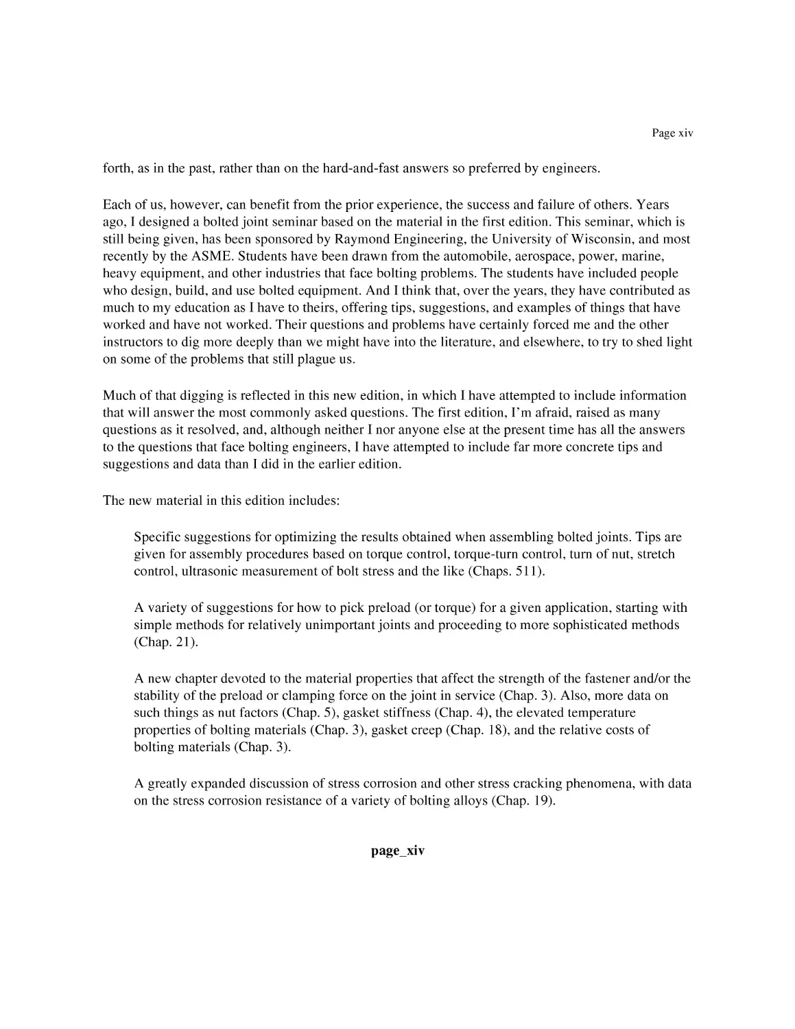
23
in Fig. 2.6. There is now no such thing as "uniform stress level," even
in the body.
If you stop and think for a minute, you'll realize that 4:1 isn't very
short and stubby. A 4-20 bolt having a grip length of 1 in. would be
considered short and stubby by this definition, which means that the
majority of fasteners we're going to deal with are probably short and stubby.
As a result, in the majority of applications, we're dealing with
fasteners in which there is no uniformity of tensile stress. And this has all
sorts of implications when we come to compute such things as stress
level, preload, spring constants, and elongation, as we'll see in subsequent
discussions.
Unfortunately, even the General Dynamics picture is oversimplified,
at least as far as stresses in the threaded portion of the bolt are concerned.
They do not, for example, take into account the stepped difference
between average body stress and average thread stress shown in Fig. 2.4.
They also ignore stress concentrations at thread roots and thread run-out
points. In fact, they assume a threadless fastener with uniform take-out
of load between nut and bolt. This assumption probably doesn't affect
their estimates of stress within the body of the fastener as much as it
affects their estimates of stress levels at the surface of the fastener, but
it's something to keep in mind.
COMPR
Figure 2.6 Magnitude of tensile stress along four separate paths in a bolt having
a length-to-diameter ratio less than 4:1.
24
Chapter 2
Here's a final, and slightly different, look at the tensile stresses in a
bolt. The contour lines in Fig. 2.7 are lines of equal axial tension; they
do not show the direction of tension. They're similar, therefore, to iso-
chromic lines in a photoelastic model.
F. Stress in the Nut
A slightly more accurate plot of the peak stresses in nut or bolt threads
is shown in Fig. 2.8 [3, 6]. The fall-off in stress is not linear, as in the
previous figures, but curved. Note that adding more threads (a longer nut)
doesn't reduce the peak stress by much. The first three threads carry most
of the load in any case.
Obviously, this stress picture is not an attractive one. Since most of
the load is on the first thread or so, most of the nut isn't doing its share
of the work. This situation can be improved in a number of ways—tapering
the threads or altering the pitch on either nut or bolt to force more
uniformity in load distribution, for example. Perhaps the most popular way is to
use a nut that is partially in tension, such as one of those shown in Fig.
2.9 19]
One study [9] of titanium tension nuts, similar to that shown in Fig.
2.9C, with most threads in tension, resulted in the computed stress
distribution shown in Fig. 2.10.
Another analysis, confirmed by experiment [10], shows that if the
pitch of the bolt threads is 0.13% longer than the pitch of the nut
threads—a difference of only 0.000065 in. per pitch in a 4--20 thread, for
Figure 2.7 Lines of equal axial tension in a t&—18 bolt loaded to 100 ksi tension
in the shank [5]. Values given are in ksi.
Stress and Strength Considerations
25
UJ 4
>
UJ
c/> 3
UJ
a:
»-
c/>
1 1
—
—
— 4/
SHANK
1 1
\t\
if
' 1
1
1
t
1
i
i
\
i i i i i i
\5 TEETH
\^\^6 TEETH
7 TEETH —
NUT
1 1 1 I !
—
-
•=
-
32 IOI234567
THREAD NUMBER
Figure 2.8 Peak stresses in three different nuts, having five, six, and seven teeth,
respectively.
Figure 2.9 Nuts which are partially loaded in tension, such as those shown here,
see a more uniform tooth stress distribution than do conventional nuts.
26
Chapter 2
5 -
4 -
3 -
2 "
I -
0 12 3 4 5
THREAO NUMBER
6 7
Figure 2.10 Relative stress level in nut and bolt threads for the tension nut
shown in Fig. 2.9B (curve B) and for a conventional nut (curve A).
example—then the outermost threads of the nut will be stressed more
heavily than the innermost, as shown in Fig. 2.11. This sort of variation
must be common in practice, and it helps explain the difficulties of
predicting how a given fastener or joint will behave.
Stress distribution similar to that shown in Fig. 2.11 can also occur
when the thread engagement is very long. Tapped holes often have more
threads than conventional nuts, which, typically, have five threads. I've
encountered tapped holes with 18 or 20 threads. Large cylindrical nuts,
used for example on large pressure vessel flanges, can have a similar
number of threads. Even if both male and female threads are cut or rolled
to tight, correct tolerances, the threads will usually have slightly different
pitch distances, and this can place the maximum thread contact stress at
the far end of the thread engagement, or in the middle, or "somewhere
else."
Stress and Strength Considerations 27
I _ I 1 ! 1 1 1
.' \a bI *
I
I
I
I
I
I
I
I
! NUT
''''i I I
3 2 1*12 3 4 5 6
i THREAD NUMBER
Figure 2.11 Stress distribution in threads with nominal pitch (A) and when there
is a +0.13% error in the pitch of the bolt threads (B).
III. THE STRENGTH OF A BOLT
A. Proof Strength
It's useful at this point to look at the procedure used to determine and
define such things as the proof strength and yield strength of bolts. We'll
need this information when we study the various means by which we
control the tightening of bolts. Recognize, however, that this is just an
introduction to the important subject of strength (or bolt failure) and that
there are many practical factors which can modify the apparent strength
predicted by the conventional procedures.
In this chapter we want to estimate the static strength of the body
and threads of the fastener, starting with the tensile strength of the
threaded portion of the body (the weakest section). Because the stress
Uj
it
Uj
^j
Uj
It
SHANK
28
Chapter 2
picture is complicated, computing strength would be difficult, so the
engineering societies have devised a way to determine strength experimentally
and to base design and manufacturing specifications on the resulting data.
A large number of fasteners, made with well-defined materials and
standard thread configurations, were subjected to tensile loads to
determine:
The highest tensile force they could withstand without taking any
permanent deformation (called the proof load). See Table 2.1 for a few
examples.
The tensile force which produces 0.2 or 0.5% permanent deformation
(used to define yield strength).
The highest tensile force they could support prior to rupture (used to
define ultimate tensile strength).
The resulting data were then published. You don't have to worry
about stress magnitudes or variations; the tables tell you how many
pounds of force a fastener of a given shape and material can safely stand.
Fastener manufacturers are required to repeat these tests periodically to
make sure that their products meet the original standards.
There was also a need to compute design limits for nonstandard
fasteners. Here the path becomes a little more murky but will still give you
a useful answer unless your need for accuracy and safety is critical.
The people who tested the fasteners found, again by experiment, that
if they divided the experimentally determined load at yield, in pounds, by
a cross-sectional area based on the mean of the pitch and minor diameter of
the threads, the result was a theoretical tensile stress at yield, which
agreed closely with the stress at which a cylindrical test coupon of the
same material would yield, and with similar results for ultimate strength,
proof load, etc. The following data can now be published:
The stress area (As) of a standard thread, based on the mean of pitch and
root diameters
Table 2.1 Proof Loads of a Few Typical Bolts
Bolt
ASTM A307 GR A
SAE J429 GR 8
ASTM A193 B7
H-ll
4-20
2.70
3.82
NA
NA
Bolt
1-8
20
72.7
57.3
117
size (kips)
2-8
91.2
NA
262
537
4-8
364
NA
946
2146
Stress and Strength Considerations
29
The proof strength of a given thread, in pounds per square inch (psi),
computed by dividing the experimentally determined proof strength,
in pounds, by the stress area
The ultimate strength or yield strength, of a given thread, in pounds per
square inch, by dividing the experimentally determined ultimate or
yield load in pounds by the same stress area
B. Tensile Stress Area
Since the mean of pitch and root diameters works for all thread sizes, it's
also possible to write an expression for the stress area (As) of a standard
60° thread, as follows [7]:
/ 0.9743\2
As = 0.785 ID — I (2.1)
where D is the nominal diameter and n is the number of threads per inch.
Appendix F lists the stress areas of all standard unified and metric threads.
As an example, let's compute the stress area of a 4-20 UNC, Class
2A thread.
D = 0.25 in.
n = 20
/ 0 9743 \2
As = 0.785 10.25 - —2q— = 0.0318 in.2
This expression for area is used to compute the tensile or shear strength
of a fastener. For example, to compute the proof load, in pounds, that
your own fasteners should tolerate, it's only necessary to look up (or
compute) the stress area of the threads and then multiply this by the
published values for the proof strength, in pounds per square inch, of that
particular material. And you get the correct answer, for most purposes.
The fallacy, of course, lies in the suggestion that the tensile stress
level within the fastener equals the proof stress at the proof load point,
or the ultimate stress at the ultimate load point. As we've seen in Figs.
2.5 and 2.6, the actual stress levels vary widely within the fastener, and
it's unlikely that much, if any, of the fastener really sees proof stress at
proof load. But the procedure is nicely circular. All of the simplifying
assumptions are neatly counterbalanced by making the same assumptions
in reverse at design time. It works.
A technique similar to that used for bolts is used for specifying the
static strength of nuts. The stress area used to compute average nut stress
30
Chapter 2
levels is, in fact, the cross-sectional area of the male threads, As, just
discussed (showing again how "artificial" these calculations are). The
"strength" of a nut, of course, is simply the stripping strength of its
threads. We get to that in Chap. 3.
C. Other Stress Area Equations
Although Eq. (2.1), or its metric equivalent in Eq. (2.4), is the expression
most often used for the stress area of a thread, there are times when a
more conservative (smaller) area is used for an added factor of safety.
For example, before leaving this topic, we should mention that a slightly
modified equation for stress area is recommended for fastener materials
having an ultimate strength (as determined by coupon tests) in excess of
100,000 psi. This time the stress area is based on the mean of the minimum
pitch diameter (Esmin) permitted by thread tolerances and the nominal
root diameter. This gives a slightly smaller stress area (partially canceling
the load benefits you'd derive from an assumption of higher ultimate
strength). Anyway, the equation is [25]
/£Sm,n 0.16238f
As = it \-z — J (2.2)
To see how this expression for As differs from that given in Eq. (2.1),
let's use it to repeat our calculation of the stress area of another ^-20
UNC Class 2A thread; this one presumably of a stronger material.
£smin = 0.2127 in.
n = 20
-, ,„,™/0-2127 0.16238\2
As = 3.14159 [—2 20—j
As = 0.0301 in.2
So this As is 5% smaller than that we computed earlier.
It's worth noting that an equivalent to Eq. (2.2) was included in the
1974 version of ANSI Bl.l [7] but has been eliminated from the 1984 and
1989 versions of this same standard [19], which, in general, contain a
much shortened discussion of thread strength and the related tensile stress
area than did the earlier version. Presumably Eq. (2.2) is a more accurate
expression for the tensile strength of a high- strength thread than is Eq.
(2.1). All such areas are determined—or at least confirmed—by
experiment, as already mentioned. The authors of Bl.l, however, may have
decided not to confuse the issue by suggesting a variety of stress areas.
Stress and Strength Considerations
31
I leave it for the purists among you to decide which equation to use.
Incidentally, Section 2 of Federal Standard H28, a key document when it
comes to defining the dimensions, tensile stress areas, and recommended
lengths of engagement of threads, currently gives only Eq. (2.1). [24] As
a final comment on all this, and probably to complicate matters further,
ANSI Bl.1-1974 gave the low stress-high stress cutoff point as 180,000
psi, not 100,000 ksi as in Machinery's Handbook [18], and this value
appeared in other references as well (e.g., British Standard BS 3643). All
of this emphasizes the empirical nature of the various equations for As.
They are attempts to define "equivalent cylinders" for bolts, based on
tensile tests of actual bolts.
There's at least one other tensile stress area in common use. The U.S.
military uses a stress area based on maximum pitch diameter for UN and
UNJ threads when dealing with fastener material strengths between 160
and 260 ksi—and when the threads are rolled after heat treatment. The
resulting stress areas are tabulated in military specification NAS 1348.
The areas are larger than the As values computed by Eq. (2:1): about
17% larger for the smallest screws tabulated (0.600-80 threads) to about
4% larger for the largest (1.500-12). Again, these stress areas must reflect
test results which show, in this case, that rolling threads after heat treat
leads to a much stronger bolt than does rolling before heat treat or cutting.
As a final note on tensile stress area, Eq. (2.1) gives reasonable results
for fasteners of diameter 4 in. and larger. The strength of smaller fasteners
will be somewhat less than predicted by Eq. (2.1) [16].
In spite of all these nuances, remember that every time you encounter
"tensile stress area" in the literature or a common standard or the like,
the authors will be referring to Eq. (2.1) "unless otherwise stated." Most
people will never use the alternatives.
There is another, still more conservative stress area that is still widely
used, however. It is based on the root diameter of the threads rather than
on the mean of pitch and root diameter, as for the "true" stress area. It
differs from the areas we've talked about so far in that this one is not
based on experimental data. It is designed to introduce a factor of safety
in thread strength calculations. The designer purposely assumes a stress
area smaller than the "real" [Eq. (2.1)] tensile stress area to be sure the
bolts aren't overstressed in service.
The use of root diameter area rather than tensile stress area is
mandated by the ASME Boiler and Pressure Vessel Code, for example. The
expression for this area is
Ar = 0.7854 (d - -^J (2.3)
where D and n have the same meaning as in Eq. (2.1).
32
Chapter 2
You'll find tensile stress and thread root areas for UN and UNC
threads in Table 2.2 and a complete list of tensile stress areas for all inch
series and metric threads in Appendix F. Figure 2.12 can help you
visualize the differences between the various stress areas we've been discussing.
All of the stress area equations given so far are for American Standard
Unified thread forms with an included angle of 60°. Different equations
must be used for 55° Whitworth, Acme, Buttress, or other thread forms.
D. Stress Areas—Metric Threads
The expressions for the stress areas of metric threads differ from those
used for inch series threads because in metric threads, the pitch of the
Table 2.2 Thread and Bolt Stress Areas [7, 15] (all areas are in
square inches)
Tensile areas Stripping areas
Thread
4-20
£-18
S-16
175-14
7-13
fe-12
5-11
S-io
s-9
1-8
li-8
l3-8
li-8
l*-8
li-8
.1-8
li-8
2-8
2i-8
2^-8
25-8
3-8
34-8
3,-8
3|-8
4-8
/U (stress)
0.0318
0.0524
0.0775
0.1063
0.142
0.182
0.226
0.334
0.462
0.606
0.790
0.969
1.23
1.49
1.78
2.08
2.41
2.50
3.56
4.44
5.43
6.51
7.69
8.96
10.34
12.18
A, (root)
0.0269
0.0454
0.0678
0.0933
0.126
0.162
0.202
0.302
0.419
0.551
0.728
0.890
1.16
1.41
1.68
1.98
2.30
2.30
3.42
4.29
5.26
6.32
7.49
8.75
10.11
11.57
Class 2A thread
0.092
0.147
0.216
0.296
0.390
0.502
0.624
0.908
1.25
1.66
2.13
2.65
3.22
3.86
4.55
5.30
6.09
6.96
8.84
10.95
13.28
15.84
18.62
21.63
24.79
28.28
Class 3A thread
0.096
0.157
0.232
0.321
0.427
0.548
0.681
1.01
1.38
1.82
2.329
2.913
3.55
4.26
5.04
5.03
6.81
7.72
9.83
12.18
14.80
17.67
20.8
24.15
27.79
31.64
Stress and Strength Considerations 33
— nominal diameter (D)
pitch
diameter
root
diameter
Figure 2.12 Relationship between root diameter, pitch diameter, and outside or
nominal diameter in a standard 60° thread. The centerline of the thread is out of
the picture, toward the bottom.
threads, rather than the number of threads per inch, is used to define the
thread. The following metric equation corresponds to Eq. (2.1), defining,
as it does, the common tensile stress area [24]:
As = 0.7854 (D - 0.938/? f (2.4)
where As = tensile stress area (mm)
p = pitch of the threads (mm)
D = nominal diameter of the fastener (mm)
The more conservative expression for higher-strength steels (over 686
MPa—99.5 ksi—this time) is [17]
As = 0.7854(£Sm,n - 0.268867/?)2 (2.5)
And the expression for thread root area is [24]
Ar = 0.7854(D - 1.22687/?f (2.6)
As before, ESmm = minimum pitch diameter (mm); D and /? have the same
meanings as in Eq. (2.4).
E. Strength of the Bolt Under Static Loads
The bolt or nut will fail under static loads if those loads exceed the strength
of the fastener. To understand and avoid static failure, therefore, we must
learn how to calculate the static strength of the parts. We'll concentrate
on tensile loads; we will compute shear strength of the joint in Chap. 14.
In estimating the static strength of a fastener under tensile loads, we
must consider four possibilities:
The body of the bolt will break (usually at one of the three stress
concentration points).
34
Chapter 2
The bolt threads will strip (fail in shear).
The nut threads will strip.
Both threads will strip simultaneously.
To determine the static strength, we must explore each of these four
possible failure modes. The weakest link, of course, will decide the
strength of the chain. We'll consider bolt strength now, and thread
strength in the next chapter.
The static strength of the body is usually computed for that section
which is threaded, i.e., has a reduced cross-sectional area. The tensile
force required to yield or break the bolt (you'll have to decide which of
these definitions of failure you prefer) is, simply,
F = aAs (2.7)
where F = force which will fail the bolt (lb, N)
a = ultimate tensile or yield strength of the bolt material (psi,
MPa)
As = effective "stress area" of the threads (in.2, mm2) [see Eq.
(2.1) or (2.4)]
This equation may be used to compute any kind of tensile
strength—ultimate, proof, yield, etc. As an example, let's compute the room
temperature yield strength of an Inconel 600 bolt with a ^-20 UNC Class 2A
thread. The yield strength of this (and other) bolt materials is given in
Tables 4.1 and 4.4.
a = 37 ksi
As = 0.0318 in.2 [see the example with Eq. (2.1)]
F = 37 x 0.0318 = 1177 1b
What would the strength of this same bolt be at 1200°F (649°C)? With
reference to Table 4.4,
a = 17 ksi
As = 0.0318 in.2
F = 17 x 0.0318 = 541 lb
Remember that part of the strength of the bolt might be absorbed by
torsion stress if we use a wrench to tighten it. This could reduce the
apparent tensile yield or ultimate strength (a) by 10-20%, but only during
tightening. This is why many people say, "If it doesn't break when you
tighten it, it won't ever break." If loads are static only and are less than the
preload developed during tightening, and corrosion or high temperature
doesn't enter the picture, the statement is probably true.
Stress and Strength Considerations
35
The strength of a bolt, of course, determines how much clamping
force it can exert on a joint. Table 2.1 gives a few examples of the forces
bolts can sustain, to give you a general feeling for the capabilities of
individual bolts. The forces tabulated are proof loads or equivalents—about
90% of yield. The forces are given in thousands of pounds (kips). To
convert to metric Newtons, multiply the tabulated figures by 4.448 x 10\
The examples in Table 2.1 show the impressive strength of bolts. They
suggest that a single 4-20 A307 bolt, properly mounted and supported,
could support the weight of a car. Or that one 4-8 H-ll bolt could alone
support the weight of nearly 1000 cars! (The strength of these and other
materials is discussed at length in Chap. 4)
IV. THE STRENGTH OF THE JOINT
Before looking at combinations of loads on the bolt, let's take a quick
look at the joint.
A. Contact Stress Between Fastener and Joint
The contact pressure between the head of the bolt and the joint is not
uniform. Neither is the contact pressure between the nut and the joint.
For either case, the contact pressure might look something like that shown
in Fig. 2.13, as suggested by an experimentally confirmed, finite-element
analysis made in Japan [10].
The contact pressure pattern shown in Fig. 2.13, although
non-uniform, assumes that the contact surfaces of the bolt head and nut will be
perfectly parallel to the surfaces of the joint, at least when loading begins.
Since this will rarely be the case—these surfaces are usually not exactly
perpendicular to the thread or hole axes, for example—the actual pressure
distribution will probably be even more irregular than suggested in the
drawing.
The contact pressure between nut or bolt head and the joint can have
an important influence on the way in which a loaded fastener retains the
potential energy stored in it during assembly (see Chap. 1). Excessive
pressure will allow the head and/or nut to embed itself gradually in the
joint surfaces, allowing the fastener to relax, to shed some of its stored
energy. These contact stresses can be impressive, as suggested by the
data in Table 2.3, which shows the stresses generated when the tabulated
fasteners are tightened to 75% of their tensile proof load. [20] (For those
primarily interested in inch series fasteners, M10, M16, and M22 metric
fasteners are approximately g, g, and g in. in diameter, respectively.) As
36
Chapter 2
RELATIVE
PRESSURE
3 3 ■
2 2
I
-t 1 1 1—
ooN ooH ooH ooN
Figure 2.13 Relative contact pressure between head of bolt, or nut, and the
joint surface. ODn is the outer diameter of the hole. ODn is the outer diameter
of the contact surface of the nut (or bolt head).
can be seen from the data, a flanged head or a washer can significantly
decrease these contact stresses.
The thickness of the washer can also make a difference. Studies made
at Newport News Naval Shipyard confirm the contact stress pattern
shown in Fig. 2.14 and show how this nonuniform head- or nut-to-joint
stress distribution creates high stress gradients in the joint members.
Table 2.3 Contact Stress Between Bolt Head and Joint When the
Bolts Are Tightened to 75% of Proof Load
Contact stress
Fastener
grade
10-9
10-9
10-9
12-9
12-9
Size
M10
M16
M10
M16
M10
M16
M10
M22
M10
M22
Head
Flanged
Plain hex
Hex with washer
Plain hex
Hex with washer
ksi
36.3
39.9
52.2
94.3
27.6
33.4
63.8
131
29
50.8
N/mm
250
275
360
650
190
230
440
900
200
350
Stress and Strength Considerations
37
Figure 2.14 Lines of equal compressive stress in joint members when the bolt
is loaded to 100 kip. Values given are in ksi.
(We'll look at joint stresses in a minute.) The studies further suggest that
standard thickness ANSI washer lack sufficient stiffness to distribute the
bolt loads with acceptable uniformity. Thicker washers are more effective;
they reduce stresses in washer and joint members and, as a result, reduce
joint deformation. The numerical results of these studies have not yet
been published. [21]
What's an acceptable stress? This is considered to be a stress slightly
higher than the compressive yield strength of the joint material [20, 21].
Table 2.4 lists some experimentally derived data for acceptable contact
stresses. The data are taken from the VDI Directive 2230, so the joint
materials are described in terms used in Germany. The designations will
undoubtedly be meaningful to metallurgists in English-speaking countries,
however. [23] Note that VDI suggests that fasteners tightened by hand can
be brought to higher contact stresses than those tightened automatically,
presumably by pneumatic or electric nut runners or the equivalent (see
Chaps. 7 and 8). Why is this? The more sophisticated of such tools can
be more accurate than a hand wrench, so the difference can't be explained
38
Chapter 2
Table 2.4 Acceptable Maximum Head-to-Joint Contact Stress for a
Variety of Joint Materials
How tightened
Automatically By hand
Joint material
St37
St50
C45V
GG-25
GD Mg Al 9
GK Mg Al 9
GK Al Si 6 Cu 4
ksi
29
47.9
87
72.5
11.6
11.6
17.4
N/mm
200
330
600
500
80
80
120
ksi
43.5
72.5
131
109
17.4
17.4
26.1
N/mm
300
500
900
750
120
120
180
by the accuracy tolerance. I suspect that it has to do with the speed with
which the fasteners are tightened.
B. Stresses Within and Between the Joint Members
As a result of all this, the joint is loaded in a nonuniform manner by the
bolt, and these nonuniform stresses are passed down into the joint
members. Figure 2.14 shows the resulting, barrel-shaped, lines of equal
compressive stress within the joint [5]. Notice that the relative magnitude of
stress varies by 8 to 1 between the most highly stressed region and the
outer rim of the barrel-shaped stress pattern.
The fact that the joint members are stressed nonuniformly means that
the clamping pressure exerted by the bolt through the joint members on
the interface between upper and lower joint members is also nonuniform,
a fact that can cause problems in gasketed joints. A number of finite-
element analyses and experimental studies have been made of the contact
interface pressure. The results of one such study [8] are shown in Fig.
2.15. Note that the contact pressures can be zero only two or three bolt
diameters away from the bolt hole. The solution for this problem, of
course, is to place bolts close together in a multibolt joint so that no
portion of the interface is entirely free of contact pressure. It is never
possible, however, to produce exactly uniform pressure at the joint
interface. Too many bolt holes, furthermore, will weaken the flange members
and/or create nut interference and wrenching problems. As a rule of
thumb, therefore, bolt holes are usually placed approximately b diameters
apart.
Stress and Strength Considerations
.0 p^me—i 1—i—i—|—| r
39
2 3
DISTANCE FROM HOLE
(HOLE RADIUS = 1.0)
Figure 2.15 Relative interface pressure between joint members as a function of
the distance from the edge of the hole. R is the ratio between the contact diameter
of the head of the bolt (or nut) and the diameter of the hole.
C. Static Failure of the Joint
Static failure of joint members is even less common than static failure of
the fasteners, except perhaps in structural joints loaded in shear. Failures
here are frequent enough to warrant a brief look. If the designer knows
which cross sections might fail, he can usually avoid failure.
The failures shown here are all of what used to be called bearing-type
joints (see Chap. 14). Friction joints fail statically, too, but they do so by
slipping into bearing and then failing by one of the ways shown below.
Joints in bearing can fail in a number of ways as suggested by Fig.
2.16. The actual failure mode will depend on the relative strength of the
bolts versus the strength of the cross section of the joint members at
various load points. It will also be affected by the distance between the
bolts and the edge of the plates, by the distance between bolts within the
group, etc.
Typical failure modes include [14]:
1. Tear-out or marginal failure, where the bolts are located too close to
the edge of the plate (Fig. 2.16A)
40
Chapter 2
o CD o
Igross
seclion
o
o
o
o
I nel
seel ion
Figure 2.16 Some static failure modes of axial shear joints. (A) Tear-out or
marginal failure. (B) Failure through the "net section/' (C) Zigzag failure.
2. Failure of the "net section" of the plate because the bolts are spaced
too closely, or because the plate is too thin or too soft (Fig. 2.16B)
3. A zigzag failure when there is too short a distance between bolt holes
(Fig. 2.16C)
V. OTHER TYPES OF LOAD ON A BOLT
We have looked, at length, at the stress distribution and strength of a
fastener under pure tensile load, because this is by far the most important
type of loading. A bolt is always put into severe tension when it is properly
tightened. Subsequent external loads won't modify this basic tension load
very much if the joint is designed properly, as we'll see in Chap. 12. On
occasion, however, we do want to estimate the magnitude of other types
of stress which can be imposed on a bolt in use. We'll consider some of
Stress and Strength Considerations
41
these now, one by one, and later suggest a way in which their combined
effects might be estimated, or at least visualized.
A. Shear Loads
Shear loads of the sort shown in Fig. 2.17 are often encountered in
structural steel joints. Note that there can be either one or several shear planes
through the bolt, depending on the nature of the joint and the number of
joint members being clamped together. Note, too, that these shear planes
could pass either through the body of the bolt or through the threads, or
through both.
To compute the shear strength of the bolt we multiply the shear
strength of the material (Su) by the total cross-sectional area of the shear
planes, taking all of them into account. For shear planes through threads,
we use the equivalent thread stress area (As) given earlier in our analysis
of tensile loads. For example, for the conditions of Fig. 2.17D,
F = Su x (2AB + As) (2.8)
where AB is the cross-sectional area of the body (in.2 or mm2). We'll
consider shear loads at greater length in Chap. 14.
B. Torsional Loads
When we tighten a nut, we apply a torsional moment as well as a stretching
force to the bolt, thanks to frictional and geometric restraints between
-f
cm
% ~\
]—F %-£
h-L
\~±
ro
3-1
-£
*-e
(\ V 1 D
'Auik'
Figure 2.17 Possible shear loading conditions on a bolt in a structural joint.
42
Chapter 2
nut and bolt threads. As we'll see in Chap. 7, the torsional moment (7,or)
applied to the bolt is given by the following expression (assuming that
there is no prevailing torque):
where P = thread pitch (in., mm)
|xt = coefficient of friction between threads
r, = effective radius of contact between threads (in., mm)
0 = half-angle of a tooth (30° for UN or ISO threads)
7,or = torsional moment (lb-in., N-mm)
FP = preload (lb, N)
Assuming that we can substitute an equivalent cylinder for the fastener
and that the cylinder has a diameter equal to the nominal diameter (D)
of the fastener and a length equal to the effective length (LE) of the fastener
(see Chap. 5), we can write the following expressions for the angle of
twist (0tVv), the torsional energy (VV,or), and the maximum stress (S,or)
produced in the outermost fiber of the fastener as follows [12]:
32LET,
tor
'tw
vGD'
(2.10)
iT w „ i,~ .-> / 32LE
W.or - iTtor X 6.w = i(7u>r)2 b^l (2-11)
r = _r)3 (2.12)
where 0tw is in radians
5t0r is in psi or N/mm2
G is the shear modulus in psi or N/mm2
D and LE are in in. or mm
C. Bending Loads
If the geometry of the parts forces the bolt to bend as it is tightened, it
will see additional tensile stress along its outer flank and less tensile stress
along the inner flank, as suggested in Fig. 2.18. Assuming once again that
the bolt can be replaced by an equivalent cylinder having an external
diameter equal to the nominal diameter of the fastener (D) and a length
equal to the fastener's effective length (LE), we can compute the bending
moment (Mb), the maximum stress (5b) created by pure bending, and the
bending energy (Wbn) as follows [13]:
Stress and Strength Considerations
43
Figure 2.18 Radius of curvature of a bent bolt.
IE ttED'
Mb = - =
64/?
_ _ MbD _ __
21
ED
2R
Wi
m 2 J0
_jb ,. I £^4^e
£/ 2 64/?2
(2.13)
(2.14)
(2.15)
where LE = effective length of the fastener (in., mm)
E = modulus of elasticity (psi, N/mm2)
/ = moment of inertia (in.4, mm4)
R = radius of curvature (in., mm)
5B = maximum bending stress (psi, N/mm2)
Mb = bending moment (lb-in., N-mm)
D = nominal diameter (in., mm)
VII. COMBINED LOADS ON A BOLT
A. Work-Energy Equation
In most applications a bolt will see a combination of the tension, torsion,
shear, and bending stresses discussed earlier. Exactly which combination
will depend on the geometry of the given set of parts and on the coefficient
of friction. It is never possible in practice to compute the resulting maxi-
44
Chapter 2
mum stresses in a given fastener, because we never have enough
information about the variables involved. I will not attempt, therefore, to describe
how one might combine the possible stresses mathematically into a single
maximum.
Because the bolted joint depends on stored energy to do its job (see
Chap. 1), it's informative to write an equation describing how the input
energy—the work done on the nut by the guy with the wrench—is
absorbed by the bolt and joint members. Although this equation still involves
all of the variables encountered in practice—and we will therefore never
be able to solve it for a particular bolt—it does show us how complex the
act of tightening a bolt can be and forces us to keep this fact in mind when
we deal with some of the simplified design equations we'll encounter in
subsequent chapters.
We'll assume here that there's a linear relationship between input
torque and turn of the nut, so that we can define the work into the system
(Win) as
Wi„ = l(7in X e,n) (2.16)
where 7in is the maximum torque applied to the nut (in.-lb), N-mm) and
0,n is the total turn applied to the nut (rads) after snugging. This is only
an approximation, because it assumes a linear 7in - 6in relationship. We'll
see the real relationship in Chap. 8. But this expression describes most
of the input work, and it will make it unnecessary for us to handle each
term in the energy equation as an integral. We're after a concept here,
not an accurate calculation. In any case, we'll never know enough about
a given fastener to achieve accuracy.
Specifically, when we tighten a nut on a bolt and clamp a joint
together, we do work on the joint in a number of ways. It's possible to write
an expression for each portion of this work and to set their sum equal to
the input work. Since we've assumed a linear relationship between 7in
and 0in, we'll also assume a linear buildup in energy stored in each mode.
We stretch the bolt (tension energy):
Wten = 5(AL x fP) (2.17)
where AL = change in length of the bolt (in., mm)
FP = preload (lb, N)
We twist the bolt (torsional energy):
W,or - 2(Tiov)~ „nn4
(2.12)
Stress and Strength Considerations 45
We do work (Wtf) against the friction forces between nut and bolt
threads (heat energy)—see Chap. 7:
W,f = |r,fxeR = iiig^ (2.18)
where 0R is the relative turn between nut and bolt (rad), and the other
terms have been defined earlier.
We do work (Wn{) against the friction forces between nut and joint
members (heat energy)—Chap. 7 again:
Wnf = kTnt x 6in = ^nFPrnein (2.19)
where 0in = total input turn (rad)
rn = effective contact radius between nut and joint (in., mm)
|xn = coefficient of friction between nut and joint
We bend the bolt (bending energy) {Wbn):
1 TrED4L?
W"« = 2-6iK^ <2-'5)
We compress the joint (compressive energy) (WjC):
Wic = 5(A7j x FP) (2.20)
where A7j = compression of the joint (in., mm)
FP = preload (lb, N)
We compress the nut (compressive energy, Wnc):
Wnc = J(A7N x FP) (2.21)
where A7N = compression of the nut (in., mm)
FP = preload (lb, N)
We can now sum all of these terms together, equate them to the input
work, and combine terms. Here's one possible combination. Note that
2
we can eliminate the 5 from each term.
FP
P + jxtrtV/32L,
2ir cos 3/ \ttD4G
+ FpUl + AT, + ATN + ^j + M-n^rnl (2.22)
(EttD4Lb \ _
+ 64R2 ~ 7in6in ~ °
46
Chapter 2
As we noted earlier, this equation involves a number of factors which will
be difficult or impossible to estimate in a given application—such things
as the coefficients of friction, the radius of curvature of the bolt, the
relative turn between nut and bolt, and the "deflection" of the nut, for
example. The equation also, as we mentioned, assumes a linear buildup
of input torque, which makes it only a rough approximation in any event.
This equation has never been tested, but it would appear to be a more
accurate description of the relationship between applied torque (Tin) and
achieved preload than is the common, long-form torque-preload equation
[Eq. (7.2)], to be discussed at length in Chap. 7. Recently A. R. Srinivas
of the Space Application Center in India has shown, in fact, that Eq. (2.22)
reduces to Eq. (7.2) when one realizes that the F% term can be ignored
(because the product D4G is very large); the A Tj, bending, and A 7N terms
are very small; and 0R is essentially equal to 0jn. It's also necessary to
realize that AL/0in equals P/2ir, where P is the pitch of the threads (the
distance between the crests of two thread teeth) [25].
If nothing else, our energy equation shows that it is not a trivial matter
to predict how much a bolt is going to be preloaded when we apply torque
to the nut. We don't produce "just tension" in the fastener. We create a
lot of other stresses. We produce heat. And it's not at all
obvious—ever—exactly what results we will achieve.
B. Strength Under Combined Loads
We are interested primarily in the tensile strength of bolts, less often in
the shear strength. The tensile strength determines the amount of preload
we can safely put into a bolt on tightening it and the amount of tensile
working load it can see thereafter. It's important to recognize, therefore,
that the tensile strength of a given fastener is reduced if the fastener also
sees torsion or shear loads. In an extreme case, for example, let's assume
that nut and bolt threads have galled near the end of the tightening
operation. This will result in an abnormally high level of torsion in the bolt. If
we now apply tension, we'll find that the bolt will break at a tension level
well below normal—perhaps even below proof load. The torsion stress
has robbed part of the total strength of the bolt. Only if the bolt is loaded,
statically, in pure tension can we count on it to support a proof load
without deformation, or to yield at a particular level of tension.
Note that torsion stress will rob part of the total strength of the bolt
only while the torsion stress is present. As we torque a bolt, for example,
it is subjected to some torsion. Such a bolt will yield at a certain level of
tensile stress. After we remove the torque wrench from the nut, however,
the torsion stress will tend to disappear (thanks to embedment relaxation,
Stress and Strength Considerations
47
bolt loaded in pure tension
bolt loaded by tightening
the nut
100 150 200
ELONGATION
( IN. X I0"3)
Figure 2.19 A fastener tightened with a torque tool, and therefore exposed to
simultaneous torsion and tension, will yield at a slightly lower level of tensile
stress (A) than a fastener subjected to pure tension. This same fastener, however,
will support a higher tensile stress in service before yielding any further (B),
because the torsion stress component will, in general, disappear rather rapidly
after initial tightening in most situations. Data are for a I A325 bolt with a 4| grip
length [1].
as we will learn in Chap. 6). If we now apply an external tensile load to
the fastener, we will discover that it will support a higher level of tension
than that which caused it to yield in the first place, as suggested in Fig.
2.19. A number of different fastening tools and strategies take advantage
of this fact, as we will see later [1].
REFERENCES
1. Fisher, John W., and J. H. A. Struik, Guide to Design Criteria for Bolted
and Riveted Joints, Wiley, New York, 1974.
2. Rocking that fatigued bolts felled arena roof, ENR, McGraw-Hill"s
Construction Weekly, August 16, 1979.
3. Wiegand, H., and K. H. Illgner, Berechnung und Gestaltung von Schraube-
nuerbindungen, Springer-Verlag, Berlin, 1962, p. 48.
4. Fastener preload indicator, Contract no. F33615-76-C-5151, Report prepared
for Air Force Materials Laboratory, Air Force Systems Command, Wright-
Patterson Air Force Base, Ohio, by General Dynamics-Ft. Worth, June 15,
1978.
5. Meyer, G., and D. Strelow, Simple diagrams aid in analyzing forces in bolted
joints, Assembly Eng., January 1972.
6. Seika, M., S. Sasaki, and K. Hosono, Measurement of stress concentrations
in threaded connections, Bull. JSME, vol. 17, no. Ill, September 1974.
48
Chapter 2
7. Unified Inch Screw Threads. ANSI Standard B 1.1-1974, ASME, New York.
1974.
8. Gould, H. H., and B. B. Mikic, Areas of contact and pressure distribution
in bolted joints. Trans. ASME, vol. 94, no. 3, August 1972.
9. Motosh, N., Load distribution on threads of titanium tension nuts and steel
bolts, J. Eng. Ind. ASME, vol. 97, no. 1, pp. 162-166, 1975.
10. Maruyama, K., Stress analysis of a bolt-nut joint by the finite element method
and the copper-electro-plating method. Bull. JSME, vol. 19, no. 130, April
1976.
11. Finkelston, R. J., Preloading for optimum bolt efficiency. Assembly Eng.,
August 1974.
12. Roark, Raymond, and Warren C. Young, Formulas for Stress and Strain.
5th ed., McGraw-Hill, New York, 1975, p. 287.
13. Eshbach, Ovid W.. Handbook of Engineering Fundamentals, 2nd ed.. Wiley.
New York, 1953, pp. 5-28.
14. Fisher, J. W., and J. H. A. Struik, Guide to Design Criteria for Bolted and
Riveted Joints, Wiley, New York, 1974. p. 84 fff.
15. Blake, Alexander, What Every Engineer Should Know about Threaded
Fasteners, Marcel Dekker, New York, 1986.
16. Crispell, Cory, A better way to design small fasteners, Machine Design.
Cleveland, Ohio, Jan. 22, 1987.
17. BS 3643: Part 2: 1966, British Standards Institution, London, 1966.
18. Oberg, Eric, Franklin D. Jones, and Holbrook Horton, Machinery's
Handbook, 20th ed.. Industrial Press, New York, 1975.
19. Unified Inch Screw Threads, ASME BI. 1-1989 (Revision of ANSI Bl.l-
1982), American Society of Mechanical Engineers, New York, 1989.
20. Eccles, William, Bolted Joint Design, Engineering Designer (UK),
November 1984, p. 11.
21. Barron, Joseph, in report to the Bolting Technology Council, at a meeting
in Cleveland, Ohio, April 19, 1993.
22. Junker, G. H., Principle of Calculation of High Duty Bolted Joints;
Interpretation of Directive VDI 2230, published by SPS, Jenkintown. PA (no date
given)
23. VDI 2230: Systematic Calculation of High Duty Bolted Joints, VDI Society
for Design and Development, Committee on Bolted Joints, Issued by the
Verein Deutscher Ingenieure (VDI), VDI Richtlinien (Dusseldorf, October
1977, Translated from the German by Language Services, Knoxville, TN,
published by Oak Ridge National Laboratories as ORNL-tr-5055, Table 14.
24. Screw Thread Standards for Federal Services, Section 2, Unified Inch Screw
Threads—UN and UNR Forms, FED-STD-H28/2B, 20 August 1991,
Defense Industrial Supply Center, Philadelphia. PA, p. 57.
25. Srinivas, A. R., Determination of Torque Values for Metric Fasteners—an
Approach, Space Payload Group, Space Applications Center, Indian Space
Research Organization, Ahmedabad, India, Document 380 053. May 1992.
3
Threads and Their Strength
The threads are obviously an important element of the threaded fastener.
They give this sturdy, industrial product its unique ability to be installed,
removed, and reinstalled as many times as we wish. They also affect
fastener performance in a major way. As we'll see, thread type, thread
class, thread configuration, the way in which the threads are produced,
and the fit between male and female threads can affect not only thread
strength—and, therefore, fastener tensile strength—but also the
resistance of the fastener to such things as self-loosening and fatigue. The
amount of preload achieved for a given torque can be influenced by thread
configuration and by whether the threads have been cut or rolled. All
things considered, it's worthwhile to take a close look at threads.
I. THREAD FORMS
A. Thread Forms in General
Literally hundreds of thread forms have been designed, and many are still
in common use in a wide variety of applications. Fortunately, we only
have to worry about the few that are currently used in threaded fasteners.
To clear the decks, however, let's start by taking a quick look at three
other forms which are often mentioned and which many beginners to
bolting assume that they should know about. These forms are illustrated
49
50
Chapter 3
in Fig. 3.1, along with a currently popular 60° form for comparison.
Anyway, the three we don't have to worry about are [1, 25]:
The ACME thread: this is used for power transmission, for example, to
produce traversing motion on machine tools.
The Buttress thread: used when the thrust on the screw is in one direction
only, for example, airplane propellor hubs and columns for large
presses [26].
The Whitworth thread: this form, which had a 55° included angle instead
of the now universal 60°, was for decades a British standard form but
has now been replaced by an ISO inch series. It was the first screw
thread form to have rounded roots, I believe.
All of the modern fastener thread forms we need to know about—the
metric as well as inch series forms—are based on an arrangement of 60°
angles. As we'll see this basic geometry is modified in several different
ways, but it's the starting point for all contemporary fastener thread
profiles.
B. Inch Series Thread Forms
In the United States our principal inch series thread form standards are
ASME Bl.l 1989 [2] and Federal Standard FED-STD-H 28/2B [3]. Both
UNJ ACME
Figure 3.1 Three well-known thread forms which are not currently used with
threaded fasteners and, for comparison, one which is (the UNJ form). The ACME
is a well-known machine tool thread used for traversing screws. The Whitworth
is a now-obsolete fastener thread form once used in the U.K. It has now been
replaced by a 60-in.-series ISO form.
Threads and Their Strength
51
of these describe the basic Unified Thread Form, identified by the code
letters UN/UNR.
A slightly modified version of the UN/UNR thread is defined in
Military Specification MIL-S-8879 C and is called the UNJ form [4]. An ANSI/
ASME standard for J threads, Bl. 15, is in preparation.
The differences between these three forms, UN, UNR, and UNJ, are
shown in Fig. 3.2. As you can see, the differences are very slight and
consist entirely of the way the sharp roots of the teeth are filled in. These
differences occur only in the external or male thread form. The same
internal thread form is used with each. In any event, the differences are:
The UN form has flat-bottomed or, optionally, slightly rounded roots.
The UNR form must have slightly rounded roots.
The UNJ form has generously rounded roots.
C. Metric Thread Forms
The currently popular metric threads are identified by the code letters M
and MJ. The basic geometry of metric and inch series threads is identical,
UN UNJ or MJ
optional UN UNR or M
Figure 3.2 These are the thread forms most commonly used in the Western
world at the present time. Each is a 60° included angle form. They differ from
each other primarily in the way the roots of the external (male) threads are shaped.
The UN form has flat, or, optionally, slightly rounded roots. The UNJ and metric
MJ forms have generously rounded roots. The UNR and metric M forms have
slightly rounded roots.
52
Chapter 3
but the way we define the metric threads differs from the way we define
the inch series ones, as we'll see.
U.S. standards for metric threads include ANSI/ASME B1.18M-1982
[22] for standard commercial fasteners and ANSI/ASME B1.13M-1983
(Reaffirmed 1989) for fasteners having nonstandard pitch-diameter
combinations and/or special lengths of engagement [5]. Both define M profile
threads. Another standard, ANSI B1.21M-1978, defines MJ threads [6].
The M profile does not include an absolutely flat root option (equivalent
to the UN form) but only a "radiused" option—flat with rounded fillets
blending into the thread flanks—and a "rounded root" option similar to
the UNR profile.
0 125 H
MAJOR
PITCH
DIAM
MINOR
DIAM.
AXIS OF SCREW THREAD
Figure 3.3 The basic profile of the UN, UNR, and metric M thread forms. This
is the starting point for the design of those threads. It is also identical to the so-
called design profile for all UN and most metric internal threads. The design
profiles of external UN or metric threads have slightly altered shapes and
dimensions, as explained in the text.
Threads and Their Strength
53
II. THREAD PROFILES
A. Basic Profile
The design of the male and female threads in a given series starts with
a "basic profile" which has been called the "permanently established
boundary between the provinces of the external and internal threads" [7].
Figure 3.3 shows the basic profile of both external and internal threads
for the UN, UNR, and metric M thread forms. Figure 3.4 shows the few
differences which convert the standard UN or M basic profile to either a
metric J or UNJ profile. Again, only the external J thread's basic profile
is modified; the internal thread profile for J as well as the other threads
is shown in Fig. 3.3.
B. Design Profile
This profile, also called the "design thread form" [7], defines the
maximum material profiles for the internal and external threads of a given
AXIS OF THREAD
I
Figure 3.4 The basic profile for the UNJ and metric MJ threads differs from
the profile shown in Fig. 3.3 only in the dimensions illustrated here. Again, this
basic profile for the J threads is identical to the design profiles for the internal
threads in those classifications but would be modified slightly for the design
profiles of the external threads.
54
Chapter 3
Figure 3.5 The design profiles of the UN/UNR and UNJ (or M and MJ) threads
differ primarily in the way the roots of the teeth are shaped, as suggested by Fig.
3.2. This sketch shows a closeup of the difference for Class 2A UN threads. As
you can see, the difference appears to be slight, but the UNJ and MJ threads have
significant strength and fatigue advantages over the UN/UNR or M threads.
form. Note that if the maximum material profile for both nut and bolt
coincided with the basic profile there would be no clearance between male
and female threads and they couldn't be assembled. Some clearance must
be provided for, and this is generally done by making the design profile
for the male thread slightly smaller in diameter than its basic profile. We'll
take a closer look at how this is done in Sec. IV of this chapter.
The design profile for most female threads is the same as the basic
profile shown in Fig. 3.3 (or Fig. 3.4 for J threads). This is true for all
UN threads and for many or most metric threads. The design profile of
some internal metric threads can deviate from their basic profile as we'll
see.
Design profiles for UN, UNR, and UNJ external threads and their
metric equivalents are shown in Fig. 3.2. Figure 3.5 gives us a closer look
at the differences between the UNR and UNJ (or M and MJ) profiles.
III. THREAD SERIES
Design profiles can be applied to threads of any size, and this leads to what
are called kkthread series." In the Unified Thread system, for example, we
have [2]:
Threads and Their Strength
55
1. Threads called just UN/UNR or UNJ: the "constant-pitch" series.
Each thread in such a series has the same number of teeth per inch.
For example, there's an "8 pitch" series, which means that each
thread in the group has eight threads per inch. The angle the helix of
the thread makes around the fastener varies with the diameter of the
fastener, but the depth of the teeth is constant, regardless of diameter,
because of the rigid 60° geometry on which the form is based.
Altogether there are eight constant-pitch thread series, including
those with 4, 6, 8, 12, 16, 20, 28, and 32 threads per inch, and they're
available in both the basic UN/UNR and the UNJ forms.
2. In addition to the constant-pitch series, there are several groups
classified by "coarseness." This refers not to their quality but to the relative
number of threads per inch produced on a common diameter of
fastener. For example, the codes UNC, UNCR, and UNCJ identify
"coarse-pitch" threads.
3. UNF, UNFR, and UNFJ all designate "fine-pitch" threads.
4. UNEF, UNEFR, and UNEFJ are used for "extra fine" threads.
5. Provision has also been made for a "special" series called UNS,
UNRS, or UNJS having pitch-diameter combinations not found in
any of the standard series above. Most of us will never have to worry
about these.
As I mentioned, the coarseness designations refer to the relative
number of threads per inch. For a fastener of a given diameter a UNC thread
has fewer threads per inch than a UNF, which in turn has fewer than a
UNEF. For example, here is the nomenclature we'd use to define the five
standard threads currently specified for a fastener having a nominal (body)
diameter of j in.
The UNC (coarse) thread for that diameter has 13 threads per inch and
is encoded as a UNC 1 x 13 thread. Our other options here would
be UNRC i x 13 or UNJC 5 x 13.
Next in line we have a UN (constant-pitch) thread which has 16 threads
per inch and is called UN j x 16 or UNR 5 x 16 etc.
Next there's a UNF (fine) thread with 20 threads per inch, called UN 2
x 20.
Then a UNEF (extra fine) thread with 28 threads per inch, or UNEF 5
x 28.
Finally, there's another constant-pitch thread for j-in. fasteners, UN \ x
32. Like all of the others in the group, it can have UNR or UNJ forms
too.
These numbers all change as the diameter of the fastener changes.
For example, the following group of threads has been codified for 2-in.-
56
Chapter 3
diameter fasteners:
UNC 2x4 UN 2 x 12
UN 2 x 6 UN 2 x 16
UN 2 x 8 UN 2 x 20
All the threads in this group are constant-pitch threads except for the first,
coarsest thread. This is true of most "large-diameter" fasteners. In fact,
above a 4 in. diameter there are nothing but constant-pitch threads. And
once again, each of these threads can have a UNR or UNJ form instead
of UN if you wish.
Metric threads generally duplicate the inch series threads, but with
threads considered to be only coarse or fine. Instead of using threads per
inch to classify them, however, we'll use the pitch distance between two
teeth, in millimeters. For example,
M6 x 1
would specify a thread having a nominal diameter of 6 mm and a pitch
distance of 1 mm.
IV. THREAD ALLOWANCE, TOLERANCE, AND CLASS
We still haven't finished classifying threads. The next important
consideration is the way the male and female threads fit together. Is the fit loose
and sloppy, or is it tight? Rough applications require the first, precision
ones the second.
The fit between mating threads is determined by the basic clearance
between them, a clearance determined by the way the threads are
dimensioned and by the tolerances placed on those dimensions. Although the
philosophy is the same for both metric and inch series threads, the
nomenclature used is different [2, 3, 7], so we'll consider the two types
separately.
A. Inch Series Threads
Allowance
The basic clearance is established by a "thread allowance," which
determines the minimum clearance between threads of a given class. Another
way of saying this is that it determines the minimum distance between
male and female threads when both nut and bolt are in their "maximum
material" conditions: the fattest bolt and the thickest nut. The lower
Threads and Their Strength 57
sketch in Fig. 3.6 shows male and female Class 1A or 2A external threads
separated only by the basis allowance.
Tolerance
Manufacturing tolerances are now placed on the allowance. These are
always in the direction of less material; they always make the clearance
Figure 3.6 The lower sketch shows the clearance between male and female Class
2A UN threads when only the basic allowance separates them. The upper sketch
shows how much this clearance increases when the full manufacturing tolerance
is added to the allowance. In effect, the lower sketch shows the maximum material
condition for bolt and nut; the upper sketch the minimum material condition for
both. The bolt thread is reduced in diameter by the allowance and tolerance, and
the roots of the teeth are rounded. The diameter of the nut teeth has been increased
slightly by the manufacturing tolerance, and the roots of the teeth are rounded.
58
Chapter 3
between nut and bolt threads greater than the clearance determined by the
allowance, never less. The upper sketch in Fig. 3.6 shows the clearance
between a pair of external 1A or 2A threads when the full tolerance is
added to the allowance.
In the Unified Thread System the female threads are always
dimensioned to the basic profile; that shown in Figs. 3.3 or 3.4. It's only the
male thread which is reduced a little (made smaller in diameter) by the
allowance. Tolerances, again always in the direction of less material, have
to be placed on both male and female threads, of course.
Class
Three basic fits or ''classes" are defined for Unified threads. These are
given the codes 1A, 2A and 3A for male threads and IB, 2B and 3B for
female threads. The pair 1A and IB define the loosest fit; 3A and 3B
define the tightest.
Class 1A, IB threads are used for rough work, for example, where some
thread damage can be expected or conditions are very dirty. These
are also the easiest threads to assemble.
Class 2A, 2B threads are for "normal" applications. The bolts and nuts
you buy in the hardware store are all of this class.
Class 3A and 3B fasteners are used for applications requiring an extra
degree of precision.
Class 1A and 2A threads are assigned the same allowance in the
Unified system; but more generous tolerances are placed on the l's than on
the 2's, so the average fit is looser.
Class 3 threads are assigned a "zero allowance," so the fit can be
line-to-line. A small tolerance on each thread makes assembly possible.
B. Metric Threads
The clearance between male and female metric threads is also determined
by a basic allowance and by tolerances in the direction of less material.
The number of tolerance and allowance options is greater with metric
threads than with inch series threads, and different names are used to
describe these things [5-7].
Tolerance Position (the Allowance)
The basic clearance between male and female threads, called the
allowance in inch series threads, is called the ''tolerance position" for metric
threads and is identified by a letter symbol:
Threads and Their Strength
59
G or H for internal threads
e, f, g, or h for external threads
G and e define the loosest fits and the greatest clearance (greatest
allowance). H and h define zero allowance, no deviation from the basic profile.
Note that although internal metric threads can be assigned zero allowance
(H) as are internal UN threads, they can optionally be assigned a tangible
allowance (G)—made a little less fat—to accommodate plating or other
coatings or perhaps just to provide a looser fit.
Tolerance Grade (the Tolerance)
What we call the tolerance of inch series threads is called the "Tolerance
grade" for metric threads and is identified by a number symbol. Seven
tolerance grades have been established for external threads and are
identified by the numbers 3 through 9 inclusive. Nine defines the loosest fit
(the most generous tolerance) and 3 defines the tightest. To complicate
our lives further, different groups of options have been established for
external and internal threads, and tolerances have been placed on several
thread dimensions. The possibilities listed in ANSI/ASME 1.13-1983 are
shown in Table 3.1.
Tolerance Class (the Class)
The tolerance grade and tolerance position symbols are now combined
into a "tolerance class" code of alphanumeric symbols. Here are some
examples:
6g is a general-purpose callout for external threads. It defines the tolerance
position and tolerance grade for the major diameter. Used in
conjunction with a 6H nut, the fastener would be a reasonable substitute for
applications previously using a Class 2A/2B pair.
4g6g is also a general-purpose callout for external threads, this time when
a tighter fit is required. It defines the tolerance grade and position for
Table 3.1 Tolerance Grades Assigned to Metric Threads
Dimension controlled Specified tolerance grades
Minor diam., internal threads 4, 5, 6, 7, 8
Pitch diam., internal threads 4, 5, 6, 7, 8
Major diam., external threads 4, 6, 8
Pitch diam., external threads 3, 4, 5, 6, 7, 8, 9
60
Chapter 3
both the pitch diameter (4g) and the major diameter (6g). Note that
in inch series practice these two diameters cannot be toleranced
separately as they can here. Class 4g6g, however, is considered to define
an external thread which is an approximate equivalent to an inch series
Class 3A thread. A nut of tolerance class 6H could be used here.
4H5H defines the tolerance grade and position for a common internal
thread which could also be used with the male threads defined above.
The 4H classifies the pitch diameter and the 5H the minor diameter.
The symbol 5H can also be used alone for applications where a looser
fit is acceptable.
C. Inch Series and Metric Thread Classes, Compared
It's useful to be able to equate inch series and metric allowances and
tolerances. A couple of examples were given above. Table 3.2 [1] defines
some more options. It doesn't define all of the possibilities but only some
of the more common ''approximate equivalents." Pitch diameter
tolerances are not included here for the metric threads, for example. This is
not uncommon, but adding them would presumably identify still more
approximations.
D. Coating Allowances
If fasteners are to be plated or otherwise coated, some clearance must be
provided for the coating. The way this is done is presumably of interest
only to fastener manufacturers, who would be guided by the applicable
standards. Users (buyers) might find the following summary of interest,
however.
Inch series: The allowances specified for Class 2A external threads can
accommodate coatings of reasonable thickness. Special provisions
must be made for other classes of external thread, all internal threads.
Table 3.2 Approximately Equivalent
Classifications: Inch Series and Metric
Threads
Inch series Metric
Bolts Nuts Bolts Nuts
1A IB 8g 7H
2A 2B 6g 6H
3A 3B 4h 5H
Threads and Their Strength
61
and threads to be given heavy coatings. Major and pitch diameter
limits before and after coating must be specified on engineering
drawings, for example [2].
Metric series: External thread tolerance classes 6g and 4g6g provide
allowances which can accommodate normal coatings. For heavy coats, or
if position h or H tolerance positions are involved, one should consult
the standards, e.g., ANSI/ASME B 1.13M, for manufacturing
allowances [5].
Some problems have occurred in recent years with mechanically
galvanized fasteners. The male thread dimensions had been reduced rather
drastically, to accommodate the coating, and that resulted in a significant
loss of tooth strength. This is the kind of problem one sometimes
encounters when using low-cost suppliers.
E. Tolerances for Abnormal Lengths of Engagement
The allowances and tolerances specified in thread standards assume
normal lengths of engagement between male and female threads. The
definition of "normal" is spelled out in the specifications, but, typically, it
means lengths of engagement ranging from one to one and a half times
the nominal diameter of the thread. Lengths for fine-pitch threads are
alternately given in number of pitches, with a range of 5 to 15 being
considered normal [2].
If the length of engagement is to be abnormally short, then it's wise
to reduce the clearance between male and female threads by reducing the
allowance or the tolerance. If the engagement is to be unusually long,
tolerances must be relaxed or pitch mismatch may make it impossible to
assemble the fastener or to run the bolt into a deep, tapped hole.
The standards, again, define the procedures for modifying the
allowance or tolerance. ANSI/ASME B1.13M is especially clear on this point.
It says that for very short lengths of engagement the tolerance on the
pitch diameter of the external thread should be reduced by one number.
For example, instead of 4g6g one might specify 3g6g.
For extra long lengths of engagement B1.13M says that the allowance
on the pitch diameter should be increased. A normal 4g6g would become
5g6g, for example.
V. INSPECTION LEVELS
Several levels of inspection have been defined for threads, depending
upon the nature of the application and the consequences of failure. There
is considerable debate at present about which fasteners should be required
62
Chapter 3
to pass which tests. We'll take a much longer look at this subject, and
the broader subject of thread/fastener strength, later on in the chapter.
Since inspection levels are sometimes tacked onto thread designations,
it's useful to review them briefly at this point [23].
Level 21 is the least rigorous and is designed to guarantee functional
assembly of male onto female threads, plus functional size control of
maximum material limits. This level is used with most fasteners at
present. The inspection can be performed with fixed GO, NO GO
gages.
Level 21A is similar but is used only for metric threads.
Level 22 controls the above and also controls the minimum material size
limits over the full length of engagement of the thread.
Level 23 controls all of the above and also controls, within established
max-min limits, such things as thread flank angles, lead, taper, and
roundness. This kind of inspection can be performed only with
indicating gages or optical comparators or other devices which allow the
inspector to measure all such parameters.
VI. THREAD NOMENCLATURE
We can now put all of the above together to give the complete
alphanumeric code or description of a thread.
A. Inch Series
An example of an inch series external (bolt) thread "code" would be
i-20 UNC 1A (21)
4 = nominal diameter in inches
20 = number of threads per inch
UNC shows that this is a UN thread from the Coarse series.
1A shows that this is a loose fitting, external thread (A) with a finite
allowance and a maximum tolerance on both pitch and major
diameters. (Class 1)
21 shows that the thread is to be inspected with simple GO, NO GO gages.
If that thread were used on a bolt with a l-in.-long body, the code
used to define the fastener would be
5-20 x 1
Coarseness and fit would not usually be added to the fastener code. The
number of threads per inch gives the user coarseness information (a
Threads and Their Strength
63
quarter-inch UNF fastener has 28 threads per inch; a quarter-inch UNEF
one has 32). A fit of 2A and inspection level 21 would presumably be
assumed for such a bolt.
Another example would be
0.2500-32 UNJEF 3A, Safety Critical Thread
Here we see the quarter-inch nominal diameter of the external thread
given in decimal form followed by the number of threads per inch, 32;
the series, UNJ Extra Fine; and the allowance and tolerance level, 3A.
We're also told that this fastener is intended for "safety critical
applications." That statement defines the quality control and gaging procedures
used with it, namely level 23.
B. Metric Thread
An example of a complete code for an external metric thread would be
MJ6 x l-4h6h
M shows that this is a metric thread.
J shows that the teeth have rounded roots with larger than standard radii.
6 = nominal diameter in mm.
1 = distance between successive thread crests (i.e., the pitch) in mm.
4h = the tolerance grade (4) and tolerance position (h) for the pitch
diameter of the thread. (Position h specifies zero allowance; Grade 4 is used
for normal applications.)
6h = the tolerance grade and position for the major diameter. (Again h
signifies zero allowance; Grade 6 is also used for normal applications.)
VII. COARSE VS. FINE VS. CONSTANT-PITCH THREADS
Which is best, coarse-pitch, fine-pitch, or constant-pitch threads? It
depends on your application. Each has advantages over the other [2-4, 8,
9].
A. Coarse-Pitch Threads
Coarse pitch is generally recommended for routine applications. Such
threads will have greater stripping strengths when used with weak nut or
joint materials—or when used on larger-diameter fasteners. Some say
bolts over 1 in. in diameter should always have coarse threads; others put
the crossover point at \j in.
64
Chapter 3
It's easier to tap brittle material if coarse-pitch threads are used. Such
threads are also easier to use in most cases: easier to start, faster rundown,
etc.
B. Fine-Pitch Threads
Fine-pitch threads must be close fitting—made to Class 3 tolerances—to
have acceptable stripping strength, but if this is done the bolts these
threads are used on can have higher tensile strengths because the thread
root and pitch diameters—and therefore the tensile stress area, As—are
greater than they would be for a coarse-pitch thread on the same nominal
diameter. This advantage can be obtained, however, only with a suitably
long length of engagement between male and female threads. We'll study
this subject later on in this chapter.
Fine-pitch threads are stronger in torsion, which means that they can
be loaded to higher preloads before yielding. They also resist
self-loosening under vibration or shock, and resist stress corrosion cracking, better
than do coarse pitch threads.
C. Constant-Pitch Threads
Constant-pitch threads are designed for applications where there will be
repeated assembly and disassembly and/or where it may be necessary to
rethread the part in service. They're used for adjusting collars, for thin
nuts or threaded sleeves on shafts. They're also used in the design of
compact parts [2, 4].
The 8-thread series is used on large-diameter fasteners and was
originally intended for bolts used in gasketed joints containing high pressure.
It's also widely used as a substitute for coarse series fasteners when the
basic fastener diameter exceeds 1 in.
The 12-thread series is used as a continuation of the fine thread series
when bolt diameters exceed U inch. It was also originally intended for
pressure vessels but has now found wider use.
The 16-thread series is also used on large-diameter fasteners, again
for those requiring fine-pitch threads. It's used as well for adjusting collars
and as a continuation of the extra fine pitch series for bolt diameters over
llT; inch.
D. Miscellaneous Factors Affecting Choice
We'll see other thread characteristics which may affect our choice of
thread as we proceed through the book, but a few miscellaneous comments
may be in order here.
Threads and Their Strength
65
A tighter fit, i.e., 3A vs. 2A, gives a 10% increase in thread stripping
strength, because there's more root cross section to be sheared. The
rounded roots of the J profile will increase the strength still further.
The UNJ or MJ threads also have more resistance to fatigue than do
the UN/UNR or M threads [21].
Threads tend to strip before the bolt breaks if the male-female fit is
loose [10].
The number of threads in the grip (between the face of the nut and
the head of the bolt) affects the ductility and stiffness of the fastener.
Since we (usually) want ductility and low stiffness (a more resilient spring
for better energy storage) it would seem that we'd usually want fully
threaded fasteners. We'll be especially interested in ductility if using yield
control to tighten the fasteners. (See Chap. 8.)
Factors like the shear strength of the fastener and its fit with its hole,
however, often argue instead for partial threads and an unthreaded body
of nominal or reduced diameter.
VIII. THE STRENGTH OF THREADS
There's a surprising amount of disagreement on what parameters
determine the strength of a thread and on how best to evaluate the
quality—including the strength—of a threaded fastener before use. Let's take a look
at some conventional wisdom concerning thread strength and then look
at some recent thoughts and concerns about thread strength and quality.
A. Basic Considerations
As we saw in Chap. 1, one of our principal design goals is "a fastener
strong enough to support the maximum preload it might receive during
assembly, plus the maximum additional loads it might see in service, as
a result of forces applied to the joint, differential thermal expansion, etc."
The larger the nominal diameter of a fastener, of course, the stronger it
will be. As far as static loads are concerned, therefore, we'd like the shank
or body of the bolt to be the full, basic, or nominal diameter of the thread,
or at least to be greater than the root diameter of the threads [2].
We must then specify a length of thread engagement capable of
developing the full strength of that body. This is just another way of saying
that we want the body to break before the threads strip, because a broken
bolt is easier to detect than a stripped thread.
When the threads strip they do so by shearing in one of three ways.
If the nut material is stronger than the material from which the bolt is
66
Chapter 3
made, the threads will strip at the roots of the bolt teeth. If the bolt material
is stronger, stripping will occur at the roots of the nut threads. If the
materials have equal strengths, both nut and bolt threads will strip
simultaneously, at their pitch diameters.
Studies made at the National Bureau of Standards many years ago
showed that the tensile/shear strength ratio for common fastener materials
varied from 1.7 to 2.0. As a result, the stripping areas (Ais) defined in
the formulas below (on which the recommended lengths of thread
engagement are based) are set at twice the tensile stress area (As) of the same
thread [5].
If the fastener is to be subjected to fatigue or impact loads, we'd like
it to be more resilient than a fastener subjected to static loads. Some
recommend a shank (body) diameter about 60% of that used for static
loads if the fastener will see impact loads, or a shank diameter of 90% of
the static diameter if it will experience fatigue loads (repeated load cycles)
12].
B. The Static Shear Strength of a Thread
We use a very simple equation to estimate the force required to strip
(shear) the threads of a bolt or nut:
F = SvArs (3.1)
where Su = ultimate shear strength of the nut or bolt materials (psi,
MPa)
v4Ts = cross-sectional area through which the shear occurs (in.2,
mm2) (This is not the cross-sectional area of the body, as
we'll see in a minute.)
As mentioned earlier, thread failure will occur in either the nut or bolt
threads—or in both simultaneously—depending on the relative strengths
of the nut and bolt materials. A different expression must be used to
compute the shear stress area for each type of failure [11].
The following equations were taken for the first edition of this book
from ANSI B 1.1-1974 [11]. Modified versions of the equations for shear
areas, ATs, can be found in the current edition of B1.1 [2] but the equations
for length of engagement, Le, have been removed. All of the equations,
however, can be found in the current FED-STD-H28/2B [3] but with
modified nomenclature.
Simplified formulas for shear areas are also given in H28 and have
been included below.
Those who wish to convert these equations to the present
nomenclature can use Table 3.3.
Threads and Their Strength
Table 3.3 Old vs. New notation Used in
Screw Thread Formulas
Old notation (Used
book)
Ds
Es
Kn
En
u
Ars
in this
New notation
d
d2
D,
D2
LE
ASs for bolts
ASn for nuts
C. Nut Material Stronger than Bolt Material
Failure occurs at the root of bolt threads. The equations for shear area
(Ays) and the length of thread engagement (Le in inches or millimeters)
required to develop full strength of the threads are as follows:
Ays = TrnLcKnr
j- + 0.57735(£"smin ~ Knm,iK)
(3.2)
= 2As
e ~ ™Knmaxl(l/2«) + 0.57735(£smin - Knmax)] °3)
where v4TS = shear area at root of bolt threads (in.2, mm2)
n = number of threads per inch
As = tensile stress area of bolt (in.2, mm2)
A'nmax = maximum inner diameter (ID) of nut (in., mm)
£smin = minimum pitch diameter (PD) of bolt (in., mm)
As mentioned above, FED-STD-H28 gives simplified expressions for
shear areas. Here's the expression used when the nut material is stronger
than the bolt material:
AVs = itEs -y (3.4)
where Es = the basic (or nominal) pitch diameter of the external thread
(in., mm) (see comments below).
Let's do an example to see how much difference we get when using
the simple vs. the more complex expression and to see where to find the
68
Chapter 3
data required to use these equations. Incidentally, most of these
equations—and many of the others found in this text—have been repeated in
calculator/computer format in Appendix H for your convenience in this
electronic age.
We'll take, as our example, a %-12 UN Class 2A thread and compute
A rs for a length of engagement equal to one diameter (the thickness of a
heavy hex nut). We get the necessary data from a recent edition of either
ASME Bl.l or Machinery's Handbook [24]. These tell us that:
Knmax = 0.678 in.
fsmin = 0.6887 in.
£s = 0.6959 in. (see note below)
Note that the basic or nominal pitch diameter of the bolt is equal to
the minimum pitch diameter of the internal (nut) thread, because a zero
allowance is assigned to the internal thread which, therefore, conforms
to the basic profile at the pitch line and elsewhere.
From Eq. (3.2) in calculator format:
A-rs = 3.14159 x 12 x 0.75 x 0.678 x 11/(2 x 12)
+ 0.57735(0.6887 - 0.678)] = 0.917 in.2
From Eq. (3.4)
Ars = 3.14159 x 0.6959 x 5 x 0.75/8 = 1.022 in.2
The difference is 12% in this case, with the simplified expression giving
a slightly less conservative result (it would take more force to shear 1.022
in.2 than 0.917 in.2).
D. Nut Material Weaker than Bolt Material
These are the equations you would use to compute the strength of a tapped
hole in a joint material such as aluminum or cast iron. The use of aluminum
is increasing in automotive and military applications, for example, as
designers struggle to reduce weight. The strengths of various bolt and joint
materials will be found in Chap. 4 in Tables 4.1, 4.2, and 4.14.
Failure occurs at the root of nut threads. The equations are
ATS = TwZ-eA
z- + 0.57735(Dsmin - £nmax)
In
(3.5)
_ 5st(2As)
Le " SmirnDsmin[(V2n) + 0.57735(Dsmin - £nmax)| (3'6)
Threads and Their Strength
69
where Dsmjn = minimum OD of bolt threads (in., mm)
£nmax = maximum PD of nut (in., mm)
Sst = tensile strength of the bolt material (psi, MPa)
n - threads per inch
As = tensile stress area of bolt (in.2, mm2)
Snt = ultimate tensile strength of the nut material
Ars - shear area of root of nut threads (in.2, mm2)
Le = length of thread engagement required to develop full
strength (in., mm)
The simple expression for shear area when the bolt material is stronger
than the nut material, again from FED-STD-H28, is
3Le
v4Ts = -rr£n -j- (3.7)
where En = the basic (minimum) pitch diameter of the nut (in, mm).
E. Nut and Bolt of Equal-Strength Materials
Failure occurs simultaneously in both parts, at the pitch line. The
equations are
ATs = TT£sy (3.8)
44s
it£s
(3.9)
where Es = nominal pitch diameter of the bolt (in., mm)
As = tensile stress area of bolt (in.2, mm2)
Ars = shear area at pitch line of both threads (in.2, mm2)
Le = length of thread engagement required to develop full
strength (in., mm)
F. Things Which Modify the Static Strength of Threads
We saw earlier that there are a number of factors which can modify the
anticipated tensile strength of a bolt—such things as high temperature,
corrosion, torsion, or cyclic loading. These things can also modify the
strength of threads. So can some other factors which aren't quite as
obvious. For example:
Nut dilation [12, 13]. If the walls of the nut are not thick enough, the
wedging action of the threads will dilate the nut, partially extracting
the nut threads from the bolt threads. This reduces thread engagement
70
Chapter 3
and therefore reduces the cross-sectional areas which support the
shear load, reducing shear strength. If the ratio between width across
flats and nominal diameter is only 1.4:1, for example, strength will
be reduced by 25% as shown in Fig. 3.7. (The across flats-to-diameter
ratio of standard nuts is 1.5 or 1.6:1.) Note that the reduction applies
to both nut or bolt threads, the failure occurring in the weaker of the
two.
Relative strength of nut-to-bolt threads [14-16], As we have seen, the
relative strength always determines which members will fail. If there
is too big a difference between the two materials, another factor must
be considered: The weaker of the two threads will deflect under the
relatively stiff action of the other, creating a form of thread
disengagement that again reduces the area supporting shear stress. Note that
it doesn't matter which thread—nut of bolt—is substantially weaker
than the other. The result is shown in Fig. 3.8.
Coefficient of friction. If the coefficient of friction between nut and bolt
threads is too low, then both nut dilation and thread bending become
I .On II I \ I 1 \ \ I 1 I 1 { I [ 11 I 1 I I I | 1 1 1 MM
09
08 —
07
-i i u n 11 m i n 11 n 11111111 m u 1 m u i r
1.4 15 16 17 18
RATIO OF ACROSS FLATS TO NOMINAL DIAMETER
19
Figure 3.7 Strength reduction factor for nut dilation, as a function of the ratio
of the across-t he-flats distance to the nominal diameter of the fastener. (Modified
from Ref. 13.)
Threads and Their Strength 71
'•3 | I l t j I i t | I i I I i i i j i i | | i I i | i i i | l l l | i i t
0.85 ^ t ' i 1 « > t 1 i i i 1 i i t 1 l i i 1 i i i I i i t ( i t t I i i t
0.4 0.6 0.8 1.0 1.2 1.4 1.6 18 20 2.2
STRENGTH RATIO
Figure 3.8 Strength reduction factor for thread bending. The horizontal axis
gives the ratio of nut strength to bolt strength. (Modified from Ref. 14.)
more likely because the threads can pull apart more readily. A
lubricant such as phosphate and oil, for example, is said to reduce
resistance to thread stripping by as much as 10% [14].
Rotary motion [14, 17]. Dynamic friction is usually less than static friction.
As we have seen above, anything which reduces friction between nut
and bolt threads makes it easier for the nut to dilate and/or for the
threads to bend. This means that the threads are a little more likely
to strip during torquing operations when the nut is moving relative to
the bolt than they are under static loads. The reduction in strength is
estimated to be approximately 5%.
To compute the modified potential strength of a nut thread, therefore,
one multiplies the apparent strength in pounds by the appropriate nut
dilation factor from Fig. 3.7 and by the appropriate thread bending factor
(for nuts) from Fig. 3.8. If the threads are lubricated, the computed
strength should be reduced by an additional 10%; if torque is used to
tighten the nuts, a final 5% reduction is required.
Similar calculations are used to estimate the strength of the bolt
threads, the only difference being that the thread bending factor used
(from Fig. 3.8) will be that for bolts rather than for nuts. As an example,
let's compute the strength of the threads for the f-12 UN, 2A bolt whose
thread stripping area we computed a moment ago to be 0.917 in.2 (using
the long expression for ATs)- Let's assume that because of space limita-
72
Chapter 3
tions we're using a nut with a ratio of width across flats to nominal
diameter of 1.45:1, a little less than normal.
We used the thread-stripping area formula for "nut material stronger
than bolt material." Let's now assume that the nut material is 25%
stronger than the bolt material, with a shear strength of 120 ksi. We're
going to use it with an ASTM A490 bolt whose shear strength is 96 ksi
(Table 4.2).
The bolts are to be lubricated with molydisulfide, an even better
thread lube than phosphate and oil (see Table 7.1) and they'll be tightened
with a torque wrench.
We use Eq. (3.1) to compute the theoretical force required to strip
the threads.
F = Sv x ATs
where Su = 96 ksi
ATs = 0.917 in.
F = 88,030 lb
Now we apply the strength reduction factors as follows:
SRI = strength reduction factor for nut dilation for a 1.45:1 ratio = 0.8
(from Fig. 3.7).
SR2 = strength reduction factor when the nut material is 25% stronger
= 1.1 (from Fig. 3.8)
SR3 = coefficient of friction factor. Let's assume 15% loss of strength
(which is probably conservative) because moly is almost 50% more
lubricious than is phos-oil (see Table 7.1). So SR3 = 0.85.
SR4 = rotary motion factor, a loss of 5%; so SR4 = 0.95.
The reduced estimate for the strength of our threads is now:
F' = F x SRI x SR2 x SR3 x SR4
F' = 88,030 x 0.8 x 1.1 x 0.85 x 0.95 = 66,550 lb
A significant difference! Even if we assume a 10% reduction for lubricity
instead of 15%, the reestimated strength is only 66,230 lb. However, the
ultimate tensile strength of a |-12 A490 bolt is only 59,670 lb (found by
multiplying As by the ultimate tensile strength of 170 ksi max from Table
4.1) so the bolt would presumably break before these threads stripped,
which is desirable. Not much margin for safety, however.
Is this analysis valid? The reduction factors we've just used come
from studies made by E. M. Alexander for the SAE [141 and the results,
commonly called the "Alexander model," have been widely accepted and
used. Conclusion: the estimate we've just made is valid. If we needed
Threads and Their Strength
73
more strength than that implied by the results we should increase the
length of engagement between the bolt and our abnormally thin-walled
nut.
G. Which is Usually Stronger—Nut or Bolt?
You will find that the proof strength of a standard nut is generally greater
than the proof strength of the fastener with which it is supposed to be
used. Designers would prefer bolt failure to nut failure because a failure
of the bolt is more obvious. For example, the amount of torque we can
apply to a bolt with a stripped thread is often greater than that we had
applied just before stripping occurred. The increase torque indicates an
increase in tension or preload in the bolt, when, in fact, all preload is lost
when the thread fails. On the other hand, there's no chance of misreading
the situation when the body of a bolt breaks; that's obvious. In an apparent
contradiction, nuts are made of weaker (softer) materials than bolts. This
encourages plastic yielding in nut threads to bring more threads into play
in supporting the load. But the nut as a body will still withstand a higher
tensile force than the mating bolt. For the same reason designers will want
tapped holes to be deep enough to more than support the full strength of
the bolt. Equations (3.3), (3.6), and (3.9) will lead to this result. In fact,
most people will use the equations only to find the length of tapped holes.
They won't design nuts.
Note that standard nuts come in several configurations. As far as hex
nuts are concerned, a regular hex nut has a thread length equal to 0.875
times the nominal diameter of the bolt. Thick and heavy hex nuts have a
length equal to the nominal diameter. All three should be able to develop
the full strength of the bolt with varying factors of safety, but there can
be problems. You'll find a further discussion, and some recommendations
on which nut to use, in Chap. 4, Table 4.3.
H. Table of Tensile Stress and Shear Areas
Equations are nice, but it's often handy to have a table of "answers."
Table 3.4 gives a summary of the various stress areas we've discussed:
tensile stress (As), thread root (Ar), and the stripping areas for external
threads [ATs from Eq. (3.2)]. The stripping areas for internal threads are
1.3 to 1.5 times those shown in the table, so using the tabulated values
gives an added factor of safety. Remember, we want the bolt, not the nut,
to fail.
As mentioned earlier, a more complete table, but of tensile stress
areas only, will be found in Appendix F.
74
Chapter 3
Table 3.4 Thread and Bolt Stress Areas [11, 18] (all areas are in
square inches)
Tensile areas Stripping areas
Thread
5-20
£-18
1-16
£-14
4-13
£-12
1-11
5-10
1-9
1-8
ls-8
I5-8
lt-8
l4-8
l|-8
I5-8
l|-8
2-8
25-8
24-8
25-8
3-8
35-8
3J-8
35-8
4-8
As (stress)
0.0318
0.0524
0.0775
0.1063
0.142
0.182
0.226
0.334
0.462
0.606
0.790
0.969
1.23
1.49
1.78
2.08
2.41
2.50
3.56
4.44
5.43
6.51
7.69
8.96
10.34
11.18
Ar (root)
0.0269
0.0454
0.0678
0.0933
0.126
0.162
0.202
0.302
0.419
0.551
0.728
0.890
1.16
1.41
1.68
1.98
2.30
2.30
3.42
4.29
5.26
6.32
7.49
8.75
10.11
11.57
Class 2A thread
0.092
0.147
0.216
0.296
0.390
0.502
0.624
0.908
1.25
1.66
2.13
2.65
3.22
3.86
4.55
5.30
6.09
6.96
8.84
10.95
13.28
15.84
18.62
21.63
24.79
28.28
Class 3A thread
0.096
0.157
0.232
0.321
0.427
0.548
0.681
1.01
1.38
1.82
2.329
2.913
3.55
4.26
5.04
5.03
6.81
7.72
9.83
12.18
14.80
17.67
20.8
24.15
27.79
31.64
In Table 3.4 the thread-stripping areas are given in square inches for
a length of thread engagement equal to one nominal diameter of the bolt
(the common length for thick or heavy hex nuts).
IX. OTHER FACTORS AFFECTING STRENGTH
So much for the conventional wisdom concerning thread strength. The
formulas we've looked at were all based on the assumption that the threads
would be manufactured within tolerances specified by ANSI/ASME Bl.l
Threads and Their Strength
75
or equivalent. Recent aerospace and other experience has suggested that
this may not be enough, that various thread distortions can be produced
during manufacture—and may have a significant effect on the thread's
strength and performance. The issue is currently being debated, and
several research projects to resolve it are under way or planned at this time
(mid-1995). In any event, here are some of the factors whose importance
is currently being studied.
A. Pitch Diameter
If thread geometry gets too far away from that defined by the ASME B1.1
standard, the equations of this chapter no longer work [19]. And small
differences in thread dimensions, angle, etc. may make a significant
difference in thread strength [20]. The pitch diameter of a 0.625-18 UNF-3A/
3B thread, for example, is a nominal 0.5889 in. ASME Bl.l allows a
tolerance of +0, -0.0035 in. on that pitch diameter. Assuming that this
bolt is used with a nut having a nominal pitch diameter (also 0.5889 in.),
a bolt having the minimum pitch diameter allowed by the specification
would have 16% less thread strength than a bolt with a nominal pitch
diameter.
If the pitch diameter of that bolt is 10 mils less than nominal, it will
have less than half the rated strength; at 20 mils, it will have only a quarter
of its rate strength; all, still, if used with a nut having nominal PD.
A similar loss of strength occurs if the pitch diameter of the nut is
greater than nominal. If both nut and bolt are wrong—the nut being too
large and the bolt too small—the loss of strength can be almost complete.
B. Other Thread Parameters
Pitch diameter is not the only geometrical factor we must be concerned
about. Anything which reduces the amount of contact between male and
female threads will affect their strength. If the bolt or nut is slightly
tapered, for example, the threads will be partially disengaged at one end of
the engagement length. If the threads on either are slightly out of round,
they will not be fully engaged during a portion of each turn. If the pitch
of the male threads differs from that of the female threads, they will be
in engagement only over a portion of the engagement length. If the helix
angle of nut or bolt is irregular, we can get a condition called a "drunken"
thread. If the flank (included) angle of the teeth is too great or too small,
we will get improper engagement. Some of these problems are illustrated
in Figs. 3.9 through 3.11. All of them, again, may cause a significant loss
of strength in the threads: but studies are needed to confirm this.
76
Joint Failure
Chapter 3
TAPERED
OUT-OF-ROUND
DRUNKEN
Figure 3.9 Tapered out-of-round or drunken threads all reduce thread-stripping
strength.
Threads and Their Strength
77
Figure 3.10 If the pitch of the male threads differs significantly from that of the
female threads, they may be in contact for only part of the length of engagement.
These problems, incidentally, have been more common in recent
years, again thanks to manufacturers of low-cost bolts.
Note that simple GO and NO GO thread gages will not catch such
problems as incorrect flank angle or incorrect pitch diameter. They really
only check basic root and nominal diameter, so a bolt can pass such gages
and still have very little thread strength. "Indicating gages" are available,
however, which check all of the necessary geometrical factors.
Figure 3.11 Incorrect tooth angles can also result in improper engagement and
loss of thread strength.
78
Chapter 3
REFERENCES
1. Sharman, J. M., Threaded fastener selection, Engineering (UK), October
1975.
2. Unified Inch Screw Threads UN and UNR Thread Forms, ASME Standard
Bl. 1-1989, ASME, New York, 1989.
3. Screw Thread Standards for Federal Services—Section 2, Unified Inch
Screw Threads—UN and UNR Forms, FED-STD-H28/2B, Federal Supply
Services, General Services Administration, Philadelphia, August 20, 1991.
4. Screw Threads, Controlled Radius Root with Increased Minor Diameter,
General Specification for, MIL-S-8879C, U.S. Government Printing Office,
Washington, DC, July 25, 1991.
5. Metric Screw Threads—M Profile, ANSI/ASMEB1.13M-1983, ASME, New
York, 1983.
6. Metric Screw Threads—MJ Profile, ANSI B1.21M-1978 (Reaffirmed 1991),
ASME, New York, 1991.
7. Nomenclature, Definitions, and Letter Symbols for Screw Threads, ANSI/
ASME B1.7M-1984, Reaffirmed 1992, ASME, New York, 1992.
8. Thread forms and torque systems boost reliability of bolted joints, Product
Engineering, December 1977, p. 37ff.
9. Waltermire, W. G., A fresh look at a basic question: coarse or fine threads?
Machine Design, March 17, 1960.
10. Comments made by Richard T. Barrett of NASA Lewis Research Center at
a bolting conference jointly sponsored by the Industrial Fasteners Institute
and the Federal Highway Commission at the NASA Lewis Research Center,
Cleveland, November 4, 1992.
11. Unified Inch Screw Threads, ANSI Standard B 1.1-1974, ASME, New York.
1974.
12. Ellison, H. W., Effect of Nut Geometry on Nut Strength, General Motors
Corp., Warren, MI, 1970.
13. Formula for calculating the stripping strength of internal threads in steel.
Report to ISO/TCI/WG4 by Sweden-Bultfabrike, AB, 1975.
14. Alexander, E. M., Design and strength of screw threads. Trans, of Conf. on
Metric Mechanical Fasteners co-sponsored by ANSI, ASME, ASTM, and
SAE, Presented at American National Metric Council Conference,
Washington, DC, 1975.
15. Gill, P., The Static Strength of Screw Threads, G. K. N., UK.
16. Parisen, J. D., Length of Thread Engagement in Nodular Iron, General
Motors Corp., Warren, MI, 1969.
17. Wiegand, H., and K. H. Illgner, Boltharkeit von Schraebenuer-bindungen
mit ISO, Gewindeprofil, Konstruktion, 1967.
18. Blake, Alexander, What Every Engineer Should Know About Threaded
Fasteners, Marcel Dekker, New York, 1986.
19. Yura, J. A., K. H. Frank, and D. Polyzois, High strength bolts for bridges,
PMFSEL Report 87-3, University of Texas, Austin, May 1987.
Threads and Their Strength
79
20. From information received from Stanley P. Johnson of the Johnson Gage
Company, Bloomfield, CT, May 1988.
21. McNeill, W., A. Heston, and J. Shuetz, A study of factors entering into the
calculation for connecting rod joints according to VDI 2230 guidelines, VDI
Berichte, No. 766, VDI, Germany, 1989.
22. Metric Screw Threads for Commercial Mechanical Fasteners—Boundary
Profile Defined, ANSI B1.18M-1982 (Reaffirmed 1987), ASME, New York,
1987.
23. Screw Thread Gaging Systems for Dimensional Acceptability—Inch and
Metric Screw Threads (UN, UNR, UNJ, M, and MJ), ANSI/ASME B1.3M-
1986, ASME, New York, 1986.
24. Machinery's Handbook, the 14th or any more recent edition. The Industrial
Press, New York.
25. ACME Screw Threads, ASME/ANSI Bl.5-1988, ASME, New York, 1988.
26. Buttress Inch Screw Threads, ANSI Bl.9-1973 (Reaffirmed 1985). ASME.
New York, 1985.
4
Materials
In the last two chapters we took an initial look at some of the many ways
we could evaluate the strength and integrity of the bolt-nut clamp; and
we learned how to calculate the tensile strength of the bolt and the
stripping strength of the threads, under static tensile loads. In the discussion
it was tacitly assumed that we could always select a bolt material strong
enough to fill our needs. Now we're going to look at a number of specific
bolting materials to see if that's true.
I. PROPERTIES WHICH AFFECT THE CLAMPING FORCE
What properties are we interested in, when we pick a bolting material?
Because the most important purpose of the bolts is to clamp the joint
members together, we're interested in any physical or chemical or other
properties which affect
the magnitude of the clamping force we can create at assembly, and
the stability of that clamping force. How will that force be modified by
use or age or temperature change or some other mechanism?
From an energy standpoint we want to know how much potential
energy we can store in the bolt and how much will be retained by it when
it's put to work. The first consideration is related to the magnitude of the
force, the second to its stability.
80
Materials
81
A. Magnitude of the Clamping Force
From a bolting material point of view, the magnitude of the initial clamping
force will depend primarily on the basic tensile and shear strength of the
material. For a given diameter and thread configuration, a stronger
material means a stronger bolt. And the stronger the bolt, the greater the
clamping force it can produce. We saw how to estimate the strength of a bolt
and its threads in the last two chapters. You'll find tabulations of material
strengths in this chapter. I don't mean to imply that we'll always tighten
bolts to the limit of their strength, but stronger bolts can and usually are
tightened to higher tension than weaker ones. Otherwise, we waste the
extra money we spend on better materials.
Also note that there are a lot of things other than material which affect
the clamping force actually achieved at assembly. We'll look at these
factors in depth in later chapters. At present we're considering only the
clamping capacity of the bolts, the maximum force they could generate
if tightened to their full strength.
B. Stability of the Clamping Force
The stability or reliability of the clamping force is a more complex issue,
because a number of material properties can affect it, often without
affecting the strength of the parts. For example, the clamping force introduced
at assembly can be modified by temperature changes, by corrosion, or
by external loads on the joint, depending in part on the way the bolt
material responds to these things. We'll look at a number of pertinent
properties in this chapter.
Most of the ways in which stability can be affected will be discussed
in later chapters. I've put all of the relevant material properties in the
present chapter, however, because it's easier to pick a material (once you
know the properties you're interested in) if all of the necessary information
is in one place. Comparisons and trade-offs are easier.
So, properties are discussed in this chapter, and how to use them in
subsequent chapters.
As an introduction to the concept of stability, however, here's a brief
summary of some of the ways in which the clamping force can be modified
by environmental factors and by our choice of bolt material.
Thermal Expansion or Contraction
A change in temperature will change the length of the bolts and the
thickness of joint members. Knowing the thermal coefficients of linear
expansion will allow us to estimate how much change each part will experience.
82
Chapter 4
If the parts are made from different materials—or are raised to different
temperatures—the clamping force on the joint and the tension in the bolts
will be modified by differential expansion or contraction. This can increase
or decrease the clamping force. It can also break bolts or totally eliminate
the tension in them. We'll see how to estimate these changes in Chap. 13
but will look at some related material data in this chapter (Table 4.5).
Corrosion
The resistance of the bolt material to corrosion will determine how long
our clamp will survive in the anticipated service environment. The buildup
of corrosion products (e.g., rust) can increase clamping forces; additional
corrosion can eat through the bolts. We'll consider corrosion mechanisms
and stress corrosion cracking in Chap. 18. Some general guidelines will
be found in Table 4.10.
Fatigue Rupture
Many materials have an "endurance limit" which, unfortunately, is only
a fraction of their apparent (static tensile) strength. If cyclic stress levels
are above this endurance limit, the bolt will eventually break and clamping
force will be lost. So, the endurance limit is another property we'll be
interested in. Fatigue will be the topic of Chap. 17; we'll look at the related
material properties here (Table 4.9).
Loss of Strength with Temperature
As already mentioned, a change in temperature can cause a change in
clamp force because of differential expansion between bolts and joint
members. Temperature can create problems even if the bolts and joint
have identical thermal coefficients and identical temperatures, however.
The basic strength of the material can be affected enough by high
temperature to put the joint in jeopardy. You'll find the necessary data in Table
4.4.
Loss of Clamping Force with Temperature
Elevated temperature can also lead to stress relaxation (discussed in Chap.
13), which can reduce or eliminate the clamping force without any visible
or measurable change in the parts. So resistance to stress relaxation is
another material property which can affect the integrity of the clamp.
Figure 4.3 and Tables 4.7 and 4.8 provide stress relaxation data on a
number of fastener materials.
Materials
83
Stress relaxation can and often does take place over an extended
period of time. The lower the temperature, the longer it takes the bolt to
shed stress. Clamping force can also, however, be lost very rapidly if
common bolt materials are subjected to high temperature—during a fire,
for example. Typical results are shown in Fig. 4.4.
Elastic Stiffness of the Parts
The modulus of elasticity is another property we'll often be interested in.
Modulus, in part, determines the stiffness of bolts and joint members, and
stiffness in turn determines how the clamp force introduced at assembly
will change when the joint is put in service. Factors like working loads
(pressure, weight, shock, etc.), gasket creep, embedment of thread
surfaces, elastic interactions between bolts—all to be considered in later
chapters—will work to change those initial clamping forces even at room
temperatures. The amount of change will depend on the relative stiffness
of bolt and joint members (discussed at length in Chap. 5). You'll find
some modulus data in the present chapter, in Table 4.6.
Change in Stiffness with Temperature
The modulus of elasticity is also affected by temperature, so the stiffness
of bolts and joint members will change as the temperature changes. As
one result, a 10% reduction in modulus means a 10% loss of tension in
the bolt because it has become a less stiff spring. Note that a reduction
in modulus occurs with an increase in temperature, and this increase may
cause differential thermal expansion which partially or wholly offsets the
loss in stiffness.
Any change in stiffness may also mean a change in the bolt-to-joint
stiffness ratio; and that means a change in the way the system responds
to external loads. So there are many ways in which a change in
temperature can modify the clamping force, with modulus playing several roles.
Table 4.6 includes extreme as well as room temperature data on the
modulus of elasticity of many materials.
Brittle Fracture
Ductility can be another important consideration, especially if the bolts
are to be tightened past yield (a common practice in structural steel work,
as we'll see in Chap. 8). Very hard materials can be very strong—but
brittle. The brittleness often leads to unexpected failure at loads below
the theoretical strength of the parts. We'll look at some brittle fracture
data in this chapter (Fig. 4.2).
84
Chapter 4
C. Miscellaneous Properties
Although things which determine or threaten the clamping force produced
by the bolt will always be our main concern, there are times when other
material properties must also be considered. Low-weight fasteners, for
example, have always been important in aerospace applications and are
of growing importance in automotive design as well (lower weight means
lower fuel consumption). Some material weights are given in Table 4.13.
The cost of a fastener often influences our choice. Two brief lists of
relative costs are included (Tables 4.14 and 4.15).
The electrical or magnetic properties of the fasteners can also be a
consideration, but so rarely that we won't worry about them here.
The strength of joint members is usually not as big an issue as the
strength of the bolts, but some data are useful and will be found in Table
4.16.
So, there are a number of material properties which will determine
the ability of our bolt to clamp things in service, and other properties
which will influence our material decisions in special situations. How can
we select an appropriate material? The most obvious source of material
information on which to base a decision would be an existing fastener
"standard."
II. FASTENER STANDARDS
It is believed that some 500,000 fasteners have been defined by standards
of some sort. Certainly hundreds of different specifications,
recommendations, etc. are available today. The impact of fastener standards on our
economy as a whole must be enormous—when you consider the
alternative that "everyone designs and builds his own."
Fastener standards are published by several types of organizations,
including the following:
Government organizations—for example, the National Institute of
Standards and Technology (NIST), the Army, the Navy, the Air Force.
Engineering societies—important fastener standards are published by the
Society of Automotive Engineers (SAE), the American Society for
Testing and Materials (ASTM), the American Society of Mechanical
Engineers (ASME), etc.
Trade associations—for example, the American Bureau of Shipping and
the Association of American Railroads publish well-known fastener
standards.
Materials
85
Fastener manufacturers—the principal U.S. source is the Industrial
Fastener Institute, an association of fastener manufacturers (who publish,
among other things, a complete list of other people's standards).
Standards associations—general-purpose groups that publish standards
on all sorts of things. Principal ones at the moment are the American
National Standards Institute (ANSI) and the International Standards
Organization (ISO).
Trade associations, military services, engineering societies, etc. tend, of
course, to publish standards affecting fasteners in which they have a
special interest. Groups such as NIST, ANSI, and IFI publish standards on
all sorts of fasteners.
In general, standards cover such things as fastener materials,
mechanical and physical properties, strengths, configurations, dimensions, usage,
definitions, finishes, test procedures, grade markings, and manufacturing
procedures. This does not mean that every standard covers each of these
things—just that standards exist for all of these topics and for others.
The full names and addresses of the organizations from which you
can buy standards are given in Appendix C.
III. SELECTING AN APPROPRIATE STANDARD
The purpose of a fastener standard is to define a group of materials and/
or fastener configurations which are appropriate for the "typical" needs
of a particular industry or a particular class of applications. The standard
then makes it unnecessary for each engineer to be a metallurgist when
trying to determine what would be appropriate in his application. This
saves a great deal of time and money. Standards also reduce product and
inventory costs, control quality, enhance product and system safety, and
do other important things. For our purposes, we're interested in them as
a source of material information.
If you work for an automobile manufacturer, your first choice of
standards is simple—you try those prepared by the SAE. If you're involved
with pressure vessels, you'll be guided by the ASME, etc.
What do you do if your own industry has not produced a set of bolting
standards? There are two readily available sets that are widely used by
"miscellaneous" industries and designers. I'm sure that the most
commonly used bolting standard, whether users realize they're using it or not,
is SAE's J429, which defines automotive Grades 1 through 8. Bolts of
these materials are made in large quantities and are therefore relatively
inexpensive as specified or standardized bolts go. They're readily avail-
86
Chapter 4
able, and they cover a wide range of strength specifications, with tensile
strengths ranging from 60 ksi (414 MPa) for the cheaper materials to 150
ksi (1034 MPa) for the more expensive Grade 8's. They're available in
sizes ranging from 4 to lj in. in diameter. Therefore, they're widely used
for small and medium-sized bolting jobs.
The second most commonly used bolting standards may be those
published by the ASTM. (They may be the most common.) Some 40 ASTM
standards are available, covering a wide range of threaded fastener
materials, sizes, special applications, etc. You can buy individual standards or
buy a bound volume containing all of them. These standards will be your
first choice if you're working with large equipment or
systems—structures, pressure vessels, power plants, and the like.
In most situations your needs will be covered by fasteners defined by
either the ASTM or the SAE. In every industry, however, including the
automotive, there are special applications where something "better" is
required. And in some industries, such as aerospace, the unusual is usual.
The tables and descriptions which follow are intended to help you identify
available fasteners which are not normally used in your own industry,
whether or not these are common in someone else's industry.
I'll start with an apology. I had hoped to be able to list every property
of interest for every material listed—tensile, yield, and proof strengths;
thermal coefficients of expansion; endurance limits; and all the rest. But
this information is just not available. Different industries face different
problems and specify only those properties of interest to them. If the shear
strength of an A193 B7 bolt isn't of interest to the "normal" user, then
no one is going to specify or report it. In spite of this lack of complete
data, I think you'll usually find what you need—or an approximation of
what you need—in the tabulated material.
Before we get to the data, however, it is useful to discuss what is still
a "hot topic" in some parts of the bolting world (in spite of the antiquity
of the topic!)—the issue of metric fasteners vs. English (U.S. or Unified
or "inch series") fasteners. The tables in this chapter include data on
both kinds, where available. But, generically, should you be interested in
inch series fasteners, or in metric?
Automotive manufacturers in the United States have "gone metric,"
as have some other manufacturers who depend a great deal on exports,
but most manufacturers here are still using English or inch series fasteners.
For those facing a decision, the choice will probably be based on
economic, political, or marketing considerations. From a purely technical
point of view, inch and metric fasteners are available in the same general
strengths, with the same general properties, etc. Currently specified
metric fasteners have, however, been designed and/or specified more recently
Materials
87
than most of their English counterparts. Past experience has revealed
some problems with English materials and geometry; the latest metric
standards have attempted, at least, to overcome these shortcomings. So
metric fasteners may be slightly "better" technically; but the differences
are slight.
Note that the decision to choose metric involves two things: fastener
material and fastener configuration (or at least basic dimensions). We're
primarily interested in materials in this chapter (and in this book). We'll
discuss metric fasteners in Sec. VII of this chapter.
IV. MATERIAL PROPERTY NOMENCLATURE
The "code letters" used to identify different material properties vary a
bit from one bolting standard or trade organization to another. Since this
can confuse the beginner, a brief discussion is in order.
An uppercase S is often used to signify stress. In the ASME Boiler
and Pressure Vessel Code, for example, Sa is used for the allowable bolt
stress at room temperature. But other letters are used elsewhere. For
example, each of the following is used to designate the ultimate tensile
strength (in terms of stress in ksi or MPa) of bolts.
UTS is used, commonly, in bolting literature.
Ftu is used in MIL-Handbook 5.
St is used in the thread standards ASME B1.1 and ANSI/ASME B1.13M.
The use of uppercase F for stress is apparently common, or becoming
common, with the U.S. government; I've encountered it several times
while working on the third edition of this text. Here are some of the other
F's I've run across [63] [64].
Fsu = ultimate shear stress
Fbu = ultimate bearing stress
Fby = yield bearing stress
Fty = tensile yield stress
Fey = compressive yield stress
V. BOLTING MATERIALS
Soon we'll look at some specific properties of materials. But first, a word
of caution: The data which follows is for general reference only. The
properties of an individual batch of bolts can differ from the norm. The
specific heat treatment used by one manufacturer can differ from that
88
Chapter 4
used by another, and this will affect properties. In the tables which follow
you'll sometimes find different values for a given property of a given
material. The ultimate strength, for example, may differ from table to
table. This reflects the fact that the data in the two (or more) tables came
from different sources, and these reported different values.
Differences of this sort are especially common for the more exotic
materials used in aerospace or extreme-temperature applications. The
strength of such materials, as a matter of fact, is often tailored for a specific
application.
The diameter of the fastener can also affect its strength and other
properties, because some bolting materials cannot be through-hardened.
Large diameters don't get fully hardened in the center; smaller diameters
do; so large diameters have lower average tensile strengths (in ksior MPa).
Material near the outer diameter of the fastener will support more load
than material near the center, so the average strength of the larger fastener
is less.
The shape of a fastener can also affect its strength. We're going to
assume "normal" ANSI or equivalent shapes in this text, and so will
ignore the ramifications of special configurations. But you'll usually
recognize an unusual configuration on sight and should be wary of assigning
normal properties to it.
Another factor causing variation in the data is the slow but fairly
continuous evolution of most bolting standards and specifications. The
ASTM and other committees who write these documents meet
periodically and alter them whenever new experience, new conditions, previous
misunderstandings, etc. suggest that a change would be desirable. Some
of the data in the following tables comes from standards published 10 or
more years ago. I've reviewed more recent versions of most of these
documents and, since I have found only minor changes, I've left the earlier
numbers alone. Once again, however, if your designs will affect life or
safety, or if failure will have severe economic consequences, you should
take your design data from the current editions of the pertinent documents
rather than from a text of this sort. Use the tables which follow only as
a "shopping guide."
The data in the tables were taken from the ASTM or other standards
or specifications cited unless otherwise noted by reference numbers. The
latter refer to the References at the end of the chapter.
VI. MATERIAL SETS
To start with, we'll consider several groups of fasteners, each group
characteristically used by a different industry or in a particular set of applica-
Materials
89
tions. These tables will help the beginner fish in the correct pool.
However, they are not intended to define every fastener material used in those
industries or applications, merely representative examples. All of the
materials listed informally here will be described more completely in one or
more of the data tables which follow.
A. General-Purpose/Automotive Group
The most commonly used fasteners which are described by a specification
(unspecified ones are even more common) are probably those defined in
Standard J429 published by the Society of Automotive Engineers (SAE).
Typical examples include:
Yield strength
Spec. Grade ksi MPa
SAE 2 57 393
J429 5 92 634
8 130 896
B. Structural Engineering Group
These fastener materials are used in buildings, bridges, and other
structures. Two of them at least, A325 and A490, are commonly tightened past
yield, on purpose. (See Chaps. 8 and 13 for further information.) The
specifications listed below are all published by the ASTM.
Yield strength
Spec.
A307
A325
A354
A449
A490
ksi
est. 36a
81
99-109
58-92
130
MPa
est. 248
558
683-752
400-635
896
;1 Estimated as 60% of the specified
ultimate strength of 60 ksi.
C. Petrochemical/Power Group
The following materials are commonly used in petrochemical and power
plants, as well as in marine, mining, manufacturing, and other industries
using heavy equipment. The structural steel group of materials is also
90
Chapter 4
commonly found in such applications. Again, the specifications listed
below are published by the ASTM. The wide range of yield strengths
listed here, for a given material, results from the fact that these fasteners
are often made in large sizes—up to several inches in diameter—and the
materials aren't always through-hardened.
Spec.
A193
A540
Grade
B7
B16
B21
B24
Yield
ksi
75-
85-
105-
105-
-105
-105
-150
-150
strength
MPa
515-
585-
720-
720-
-720
-720
-1034
-1034
D. Extreme-Temperature Group
I consider many of the fasteners in this group "exotic"—they're
uncommon and often expensive (see Table 4.4). Note that I've included ASTM
A193 materials in this group as well as in the petrochemical group. An
aircraft engine designer might not consider the A193 temperature limit
of 800°F "high temperature"—but the petrochemical engineer does. See
Tables 4.9 and 4.10 for additional materials, some of which can be used
at temperatures as high as 3000°F (1648°C) and/or can be used at cryogenic
temperatures.
Spec.
ASTM A193
BS4882
A286b
MP35Nb
HI 1
INCONEL, X-750b
WASPALOY
RENE 41
Grade
B7
B8
B16
B80A
Temperature
752
800
800
1400
1200
-320
1000
1000
1500
1600
1600
400
427
427
760
649
-196
538
538
816
871
871
Yield
ksi
76
17
76
73
88
345 UTS
225 UTS
141
44
75
80
strength"
MPa
524
117
524
503
607
2379 UTS
1551 UTS
972
303
517
552
Ref.
1
3
3
2
2
3
3
3
3
a Values given are yield strengths for the cited temperature except for those values marked
UTS, where strength is given as ultimate tensile strength instead of yield.
b Also recommended for cryogenic applications.
Materials
91
E. Corrosion-Resistant Group
As discussed in Chap. 18, no material will resist all types of corrosion. But
ASTM A193, BS4882, A286, and MP35N, listed above, are all considered
"corrosion resistant." Other materials with this reputation include those
listed below. See Table 4.12 for a more complete list.
Spec.
Carpenter Gall-Tough
NITRONIC 50
INCONEL
AISI
TITANIUM
Stainless St.
Grade
430
600
316
416-H
6A1-4V
17-4PH
Yield
ksi
40
70
37
45
95
128
128-
185
strength
MPa
276
483
255
310
655
883
883-1276
Ref.
6
7
3
3
9
F. Metric Group
There are probably as many different specifications for metric fasteners
as there are specifications for English ones. But, as discussed in Section
VI below, most metric standards have adopted a common series of
strength designations. The data below, for example, can be found in either
ASTM A568 or SAE J1199, among other places.
Class
4.6
8.8
10.9
12.9
Yield strength
ksi
35
96
136
160
MPa
240
662
938
1103
So much for fastener groups. Again, these tables are far from
complete. They're merely intended to help you find a standard or group of
standards which might contain the material best suited to your needs.
These and many more materials will be defined in detail in Tables
4.1-4.16. Before getting to those, however, let's take a closer look at
metric fastener specifications.
92
Chapter 4
VII. METRIC FASTENERS
The current effort to get countries now using ''English" units to adopt the
more widespread metric system includes, as it must, a new, international
metric standard for fasteners. Note that, heretofore, there hasn't been
just one metric standard. Engineers could and did write as many different
metric standards as we have English ones. But since most countries have
to accept some change in their own standards to comply with a new
international standard, the current effort is seen as a new—and maybe
last—chance to reduce the vast number of fastener types, sizes, materials,
etc., now currently available. Having standards of any sort was a
start—there was a time when we didn't even have that. But now we have
a chance to simplify things still further. In the long run, such simplification
could more than partially offset the cost of changing drawings, tools,
inventories, manuals, procedures, etc., as we adopt the new fasteners.
The numbers used to define the metric grades (called classes) have
useful meaning. The first number is equal to the minimum tensile strength
of the material, in megapascals (MPa) divided by 100. The second number
represents the approximate ratio between minimum yield and minimum
ultimate strengths for the material. Hence, Class 5.8 has a minimum
ultimate strength of approximately 500 MPa, and its minimum yield strength
is approximately 80% of its minimum ultimate strength.
All this is far more useful than calling out "Grade 5" or "B7" and
letting the uninitiated struggle to find out what that means—as we have
always done in the past.
When we're dealing with metric fasteners, we'll want to use metric
units for such things as torque, stress, force, etc. You'll find conversion
factors (English to metric and vice versa) in Appendix E.
VII. EQUIVALENT MATERIALS
A review of Section V will show that the sets or groups of materials
favored by different industries usually cover approximately the same
range of yield strengths, with the strength of common sets ranging from
something like 30 ksi to 105 ksi or so. As a result, you'll often find that
a material, or at least a room temperature strength rating, in one group
is matched by a similar or equivalent material or strength in one or more
other groups. Substitutions are sometimes possible. In critical
applications, however, you should look at the original specifications for both
materials. In many applications "equivalent strength" isn't the only crite-
Materials
93
rion for selection. Response to a change in temperature or to corrosion
or other factors may differ.
But equivalent materials are available. As one example, all of the
following define basically material of the same strength.
AISI 4140 ASTM A193 B7
ASTM A194—GR 7 ASTM A320—GR L7
Metric 9.9 SAE J429 GR 5 +
BS 970-En 19A BS 1506-621 A
DIN 267—9.9 ASTM SA193—B7
IX. MATERIAL PROPERTIES
Now we'll look at the specific properties of a number of bolting materials.
To get started, here's an index to the tables and graphs which follow. As
mentioned earlier, most of the data in these tables came from the ASTM,
SAE, or other specifications and standards listed in the tables. If other
references were used, or also used, they are cited in the table. Reference
numbers refer to the References at the end of the chapter.
A. Properties Affecting Basic Room Temperature Strength of
Fastener Materials (Initial Clamping Force)
Properties Table or figure
Proof, yield, and ultimate strengths Table 4.1
Hardness Table 4.1
Yield strength vs. hardness Fig. 4.1
Shear strengths Table 4.2
Brittle fracture strength Fig. 4.2
Which nut to use Table 4.3
B. Properties Affecting Life or Stability of the Clamping Force
Properties Table or figure
Yield strengths at elevated temperatures Table 4.4
Thermal coefficients of expansion Table 4.5
Modulus of elasticity vs. temperature Table 4.6
Stress relaxation vs. temperature Fig. 4.3 and
Tables 4.7 and 4.8
Service temperature limits Table 4.9
Cryogenic bolting materials Table 4.10
Fatigure endurance limits Table 4.11
Corrosion resistance Table 4.12
94 Chapter 4
C. Miscellaneous Properties of Fastener Materials
Properties Table or figure
Weight of fastener materials Table 4.13
Relative cost of fastener materials Tables 4.14 and 4.15
D. Properties of Typical Joint Materials
Properties Table or figure
Yield, ultimate, and shear strengths Table 4.16
Strength of Bolting Materials
Now let's look at some data. Table 4.1 gives the basic room temperature
strengths of male fastener materials (bolts, studs, screws) under static,
tensile loads. This strength is expressed in as many as three different
ways—proof, yield, and ultimate tensile—depending on the available
data. The information was taken from the specifications cited in the table
and/or from the references listed in the final column. (See the References
at the end of the chapter for the complete reference.)
Other aspects of the room temperature strength of bolts are covered
later: namely, shear and brittle fracture strengths. A chart giving the
relationship between yield strength and material hardness is also included.
This can help you identify (or estimate the strength) of unmarked or
suspect materials.
Note that only male fastener materials are included here. Nut
materials are covered in Table 4.3.
The strengths in Table 4.1 are given in ksi, even for the metric
materials (to aid comparison). To convert to metric MPa units, multiply the
number of ksi by 6.895. For example, a yield strength of 80 ksi = 80 x
6.895 = 552 MPa.
It is sometimes necessary to determine what material an unmarked
bolt is made from, or to estimate its strength. A metallurgical analysis is
required for a completely accurate answer; but it has been shown that
there's a rough correlation between the hardness of a bolt and its yield
strength (within reason—see the discussion of brittle fracture strength
below). Studies of low-alloy quenched and tempered steels (LAQT steels)
for example, sponsored by the Atomic Industrial Forum/Metals Properties
Council Joint Task Group on Bolting, resulted in the curve shown in Fig.
4.1. Using this curve, plus the hardness data found in Table 4.1, plus,
hopefully, other clues, you may be able to identify an unmarked bolt or
Materials
95
stud. Examples of an LAQT steel would be AISI 4140, ASTM A193 B7,
ASTM A490, SAE J429 GR. 5, etc.
Since most bolts are used as clamps, not as shear pins, most bolting
specifications and standards list only one or more forms of tensile strength
(proof, yield, or ultimate) and not shear strengths. Table 4.2, "Shear
Strengths," lists those few materials for which I've found published or
reported shear strengths.
If the material you're interested in is not included in Table 4.2, it might
help to know that most of the common steels we'll use, with hardness to
40 HRC or so, will have shear strengths in the neighborhood of 60% of
ultimate tensile strength, or, in MIL-Handbook 5 terms, Fsu = 0.6 Ftu
[63]. The stainless steels are an exception to this rule of thumb; they have
shear strengths which are about 55% of their ultimate strengths, or Fsu
= 0.55 Ftu [63].
Note that these are only rules of thumb and that other sources give
other rules. The Unified Inch-Series Thread Standard ASME B 1.1-1989,
for example, says that the shear strength of threads is half the tensile
strength of the material from which the external threaded part is made.
This reflects the fact, I suppose, that nut materials are supposed to be
slightly weaker than the bolt materials they're used with, or there's a
small safety factor introduced here to reduce the chances that the threads
will strip.
A still different rule comes from "the" book on structural steel joints
[49], which suggests that the shear strength of most common (structural
steel) joint materials is 70% of the ultimate strength of those materials.
Another material property we often need when dealing with the shear
strength of the bolts is the bearing yield strength of the joint material. We
want the bearing yield strength of the joint members in a shear-loaded
joint to be less than the shear strength of the bolts. If this is the case, the
walls of the bolt holes in the joint plates will yield before the bolts shear.
This will usually bring more bolts into bearing, reducing the shear loads
on the first bolts to contact the walls of their holes.
As another rule of thumb, the bearing yield strength of common joint
materials is about 1.5 times the material's tensile yield strength, or, in
MIL-Handbook 5 nomenclature, Fby = 1.5 Fty [63].
The strengths in Table 4.2 are given in ksi. To convert to metric MPa,
multiply the value given by 6.895. For example, a shear strength of 132
ksi would be the equivalent of 6.895 x 132 = 910 MPa.
Simplistically, a harder steel is always a stronger steel. A small
fastener can do a big fastener's job—saving weight, reducing joint size,
etc.—if the small one is hard enough. It's appealing!
Table 4.1 Room Temperature Strength of Fastener Materials (ksi)
Strength
Spec.
ASTM
A193
Grade
Size
Hardness
Proof
Yield
Ultimate
Ref.
ASTM
A307
ASTM
A3 20
B5
B6
B7
B7M
B8-C1 l
B8-C1 2
B16
GR A
GR B
L7
L43
L7M
LI
B8CL 1
B8CL 1A
B8CL 2
—
—
<2h
2^-4
>4-7
*24
^
>2\-A
>4-7
*-4
*-4
^
<4
^
<1
—
—
4
>i-ii
94-99 HRB
90 HRB-28 HRC
35 HRC
25-34 HRC
69-100 HRB
69-95 HRB
99 HRB
99 HRB
99 HRB
99 HRB
96 HRB
90 HRB
35 HRC
35 HRC
35 HRC
35 HRC
80
85
105
95
75
80
30-55
50-100
105
95
85
—
—
105
105
80
105
30
30
100
80
65
50
100
110
125
115
100
100
75-100
80-125
125
110
100
60
60-100
125
125
100
125
75
75
125
100
105
100
ASTM
A325
ASTM
A354
ASTM
A437 and
A437M
ASTM
A449
ASTM
A453
ASTM
A490
B8M CL 2
Type
1,2,3
BC
BD
B4B
B4C
B4D
651
660
662
665
1
2
3
>1*-15
4-1
>1-1*
4-24
2|-4
i-24
2|-4
—
^24
24-4
4-7
\-\
i|-i4
1^-3
—
5-1*
5-1
2-1 =
35 HRC
35 HRC
35 HRC
35 HRC
24-35 HRC
19-31 HRC
26-36 HRC
22-33 HRC
33-39 HRC
31-39 HRC
HB331
HB277
HB302
25-34 HRC
19-30 HRC
—
93 HRB-29 HRC
95 HRB-37 HRC
99 HRB-35 HRC
32-41 HRC
33-38 HRC
33-38 HRC
33-38 HRC
—
—
—
—
85
74
105
95
120
105
—
—
—
85
74
55
—
—
—
117-120
117-120
117-120
95
80
65
50
92
81
109
99
130
115
105
85
105
95
85
92
81
58
50-70
85
80-85
120
130
130
130
110
100
95
90
120
105
125
115 4
150
140
145
115
125
110
100
120
105 4
90
95-100
130
125-130
155-170
150-170
150-170 4
150-170
S
0)
2_
5
5T
Table 4.1 Continued
Strength
Spec.
Grade
Size
Hardness
Proof
Yield
Ultimate
Ref.
ASTM
A540
ASTM
A574 and
A574M
ASTM
A687
ASTM
F432
ASTM
F468 and
F468M
B21-B24
CI l
CI 2
CI 3
CI 4
CI 5
B 24V
GR30
GR55
GR75
Copper
Nickel
Aluminum
Titanium
To 8
To 95
To 9^
To9j
To9^
To H
321-444 HB
311-415 HB
293-380 HB
269-363 HB
241-321 HB
293-444 HB
F30-B100
B60-C37
B40-B90
HV140-C36
—
—
—
—
—
—
140
135
150
140
130
120
100
130-150
—
165
155
145
135
115-120
145-165
180
170
105
150
30
55
75
10-55
30-90
31-50
30-125
60
85
100
30-130
70-180
37-76
40-165
ASTM
F593
St. st.
ASTM
F835 and
F835M
ASTM
F837 and
F837M
ASTM
F879
SAE
J429
Stainless steels
1,2,3
4
5
6
7
—
—
AF
CW
GR 1
GR2
GR4
GR5
GR7
GR8
GR8.1
GR8.2
303
410
431
-
1 l-1
4-12
Same
Same
Same
_
_
_
-
4 !2
1 3
4~4
-^4 h
4-12-
i-1
>i-b
4_1 2
4-'2
4-I2-
4-1
-
B65-C36
B65-B95
C20-C45
C25-C48
C28-C38
C36-C44
B70-C43
B65
B96-C33
70-100 HRB
80-100 HRB
70-100 HRB
22-32 HRC
25-34 HRC
19-30 HRC
28-34 HRC
33-39 HRC
—
—
—
—
—
—
—
—
—
—
—
—
—
33
55
33
65
85
74
105
120
120
120
—
—
—
30-90
35
90-120
100-140
105
—
26-120
—
36
57
36
100
92
81
115
130
130
130
40-80
110
140
75-160
70-100
110-190
125-220
135-170
137-150
70-160
86
90
60
74
60 4,
10
115
120
105
133
150
150
150
80-125
170 11
180
S
2L
(O
(O
Table 4.1 Continued
o
o
Spec.
Grade
Size
Hardness
Proof
Strength
Yield
Ultimate
Ref.
High-
performance
materials
Titanium
17-4PH
17-7PH
AM 350
PH15-7MO
A286
Hasteloy-X
H-ll
Inconel 600
Inconel718
Inconel X750
Maraging 300
MP35N
Nimonic 80A
Rene 41
MP 159
Astroloy
Rene 95
K-Monel 500
Ti-6A1-4V
Waspaloy
180
185
162
155
95-119
200
200
200
200
214-260
52
215
37
260
92
260
230
90
157
250
—
—
—
128
115
262
90-300
226
162
—
286
145
206
260
190
230
155
200
185
3, 5,
12,
13
58
58
61
O
apt(
IV
■U
Copper alloys
Fastener grade
aluminum
Metric materials
ISO 898/1
OR
ASTM
F568
OR
SAE
Jl 199
ASTM
A325M
ASTM
A490M
ASTM
F738M
ASTM
F879M
St. St.
Al bronze
Si bronze
Copper
2024-T4
6061-T6
6262-T9
7050-T73
7075-T6
7075-T73
4.6
4.8
5.8
8.8
9.8
10.9
12.9
1,2,3
1,2,3
—
Al-50
Al-70
Al-70
—
—
—
—
—
—
—
—
—
M5-M100
M1.6-M16
M5-M24
M16-M72
M1.6-M16
M5-M100
M1.6-M100
M16-M36
M12-M36
—
—
M3-M14
M16-M20
—
—
—
—
—
—
—
—
—
67-95 HRB
71-95 HRB
82-95 HRB
23-34 HRC
27-36 HRC
33-39 HRC
38-44 HRC
23-34 HRC
33-39 HRC
B81-C48
B88
B96-C33
B83-C30
—
—
—
—
—
—
—
—
—
33
45
55
87
94
120
141
87
120
—
—
—
—
—
—
—
35
49
61
%
104
136
160
96
136
30-138
—
—
93 63
93
93
68 57
45
58
75
83
73
58
61
75
120
131
151
177
120
151
73-174
84
76
64
Sources: ASTM specifications A193. A307, A320. A325. A354, A449, A453, A325M. A490M. F568, A490, A540; SAE J429; plus the references
cited at the end of the chapter; plus ISO 898/1 and SAE J1199.
102
Chapter 4
280 | l l i i l i l i r » » i > l i
YIELD ' '
STRENTH 24° " /
(ksi) yf
200 • yS
160 S^
12 0 ■ ^^^
80 ■ ^
40 I . . . 1 i «—•—■—■ ■—« —>—•—•—«—•—«—i—
10 20 30 40 50
HARDNESS (HRC)
Figure 4.1 Yield strength vs. hardness for low-alloy, quenched, and tempered
steels, such as ASTM A193 B7.
Harder fasteners tend to be more brittle, however, and are therefore
more susceptible to unexpected brittle fracture, the failure originating
from an undetected crack or flaw in the surface. The harder the fastener,
the greater the chances of such failure. Attempts have been made,
therefore, to specify the safe limits of hardness and strength which we can
count on [14, 15]. Figure 4.2 shows the results for LAQT (low-alloy
quenched and tempered) steels such as AISI 4140, A193 B7, and similar
materials.
Curve A shows the yield strength of LAQT steels as a function of
increasing hardness, a repeat of Fig. 4.1. An increase in hardness produces
an apparently limitless increase in strength [14].
These results are supported, in the HRC 40-50 region, by curve B,
which shows the results of a series of tensile tests made on alloy steel
bolts heat-treated to different hardnesses and tested in a tensile machine
[15]. This time the information plotted is ultimate strength, not yield
strength, so curve B is slightly above curve A in the region of overlap.
As before, curve B shows a steady increase in strength as hardness
is increased—but only up to the point the author of Ref. 15 describes as
the "critical hardness." Increasing the hardness progressively beyond
this point (or region: the data showed quite a bit of scatter) resulted in
brittle failure at progressively lower and lower tensile loads. Presumably
stress concentrations were created by cracks or flaws, and the material
became less and less able to shed or reduce these concentrations by local-
Materials
103
Table 4.2 Shear Strength
Material
ASTM A325
ASTM A490
Stainless steel
A286
431
Custom 455
PH12-9MO
PH13-8MO
Cryogenic materials
A286
A286
Unitemp 212
Unitemp 212
Inconel 718
Inconel 718
Miscellaneous materials
H-ll
H-ll
Marage-300
MP35N
Ti6Al-4V
Beryllium
Steel
MP159
Fastener grade aluminum
2024-T4
6061-T6
6262-T9
7050-T73
7075-T6
7075-T73
Ultimate
strength
(ksi)
132
165
232
230
269
280
243
214
291
214
278
226
291
238
269
277
283
200
75
200
68
45
58
75
83
73
Shear
strength
(ksi)
79
96
119
128
151
148
142
116
282
132
166
138
168
135
159
149
162
180
40
240
132
41
30
35
45
48
44
Notes
AT 70°F
AT 423°F
AT 70°F
AT 423°F
AT 70°F
AT 423°F
Ref.
16
16
17
17
17
17
33
18
18
18
18
18
18
33
33
33
33
18
18
18
58
57
Sources: ASTM A325, A490, A286, plus the references cited at the end of the chapter.
ized plastic yielding in the vicinity of the crack. Eventually the bolts would
break. They were truly supporting high stress levels, as an increase in
hardness says they should, but only in a local area. The average stress
across the full bolt, when it broke, was less than the average stress a
softer, more ductile bolt would support.
104 Chapter 4
30C
_250
ksi
£200
UJ
<£
1-
150
100
50
0
A-^^
13/ ^S'
■
.
■
,
\
22
30
40
HARDNESS ( HRC)
50
60
Figure 4.2 Curve A is a repeat of the Fig. 4.1 yield strength vs. hardness curve
for low-alloy, quenched, and tempered steels. Curve B is a plot of ultimate strength
vs. hardness for similar materials. The dramatic fall in curve B beyond hardness
HRC 52 reflects the tendency of very hard steels to fail "early" by brittle fracture.
Nut Selection
A threaded fastener consists of a bolt and nut (or tapped hole). Knowing
the strength of the bolt alone is not sufficient, since it's never used alone.
We also want a nut or tapped hole which will develop the full strength of
the bolt.
Specifications such as ASTM A194 and A563, SAE J995, etc., tabulate
the proof, yield, and/or ultimate strengths of nuts the way ASTM A193,
A449, and SAE J429 tabulate bolt strengths. Listing all of that information
would nearly double the number of tables in this chapter. But I don't think
that's necessary.
Most designers and users focus on the strength and other
characteristics of the bolt or stud. Having selected a bolt, they then want to choose
an appropriate nut, or design a suitable tapped hole. As far as tapped
holes are concerned, you can use the thread strength equations of Chap.
3 to select such things as length of thread engagement. When it comes to
nuts, most designers will use those recommended in the pertinent bolt
Materials
105
specification they're using—or in the nut standard to which the bolt
standard refers.
Table 4.3, "Which Nut to Use," summarizes these bolt-nut
recommendations. If you want to confirm that the recommendations are correct
for your application, you can refer to the standards cited in the table. If
you're bothered by the fact that several grades of nuts are sometimes
listed for a single bolt material—that's the way the nut or bolt standard
does it too. Any of the several nuts listed are acceptable for that bolt.
You can base your choice on availability, cost, your desire to standardize
your own inventories, or on a special requirement for your application.
In some cases you'll be using a bolt which is not included in Table
4.3. Nut recommendations are not made, usually, for the more exotic bolt
materials, for example. In such cases, you'll find the following general
guidelines of use.
1. In general, we want the nut or tapped hole to support more load than
the bolt, because bolt failures are easier to detect than stripped nuts.
One rule of thumb: the nut's proof load should approximately equal
the ultimate tensile strength of the bolt [21].
2. In an apparent contradiction of the above, nuts are usually (but not
always) made of slightly softer (less strong) material than the mating
bolts, so that the nut threads will yield locally and better conform to
the bolt threads when loaded. This better distributes the stresses in
both parts.
Note that the strength of a part depends on dimension, shape, etc.,
as well as choice of material. This is why it is possible to make a
"stronger" nut from a "weaker" material.
3. If you need a nut for a bolt made of a special material such as titanium,
you'd presumably make the nut of the same material. The nut might
be heat-treated differently, however, to satisfy point 2 above. Again,
this is not a universal custom.
4. The strength of a nut depends, in part, on the length of thread
engagement. To increase safety or reduce failure rates, you can consider
increasing the length of engagement. Doubling the length of the nut,
however, won't double its strength; the relationship is more complex
than that, as discussed in Chap. 3.
5. A nut's strength also depends on its width "across flats." Nuts with
thinner walls "dilate" more—partially disengage themselves from the
bolt under load—and so have less strength. This is one of the reasons
why standard nuts are available in several configurations—hex nuts,
thick hex nuts, and heavy hex nuts. These differ in height (thread
length) too. Your choice will be based on economics and on the fact
106
Chapter 4
Table 4.3 Which Nut to Use
Bolt spec.
Grade
Nut spec.
Grade
Ref.
ASTM
A193
ASTM
A307
ASTM
A3 20
ASTM
A325
A354
A449
A453
A490
A540
SAE
J429
Metric
ASTM
A194
Any
Any
2H,4,7, or
8
2HM,4M,7M, 19
8M
B8CL 1
B8CL2
B16
A or B
L7
L43
L7M
LI
B8CL 1
B8 CL 1A
B8CL2
B8M CL 2
1
2
4
5
7
8
4.6
4.8
5.8
8.8
9.8
10.9
12.9
ASTM
A563
ASTM
A194
A194 or A563
A563
A563
A453
A563 or A194
A540
SAE
J995
8
8
4,7, or 8
A,B,C,D,DH,
DH3
4 or 7
4 or 7
7M
4 or 7
8
8
8
8
2 or 2H
C3,D,DH,DH3
C3,D,DH,DH3
C3,D,DH,DH3
DH.DH3
2H
2
2
2,5
5,8
5,8
8
4
4
5 I
8
9
12
12
Materials
Table 4.3 Continued
107
Bolt spec.
Grade
Nut spec.
Grade
Ref.
Special combinations to resist galling
Stainless steel
Low-alloy steel A193
316
Nitronic 60
Cold drawn
316
B7,B16
Stainless steel
Stainless
steel
400 series
Nitronic
50
Cold
drawn
316
300 series
Sources: A194, A563, A453, A540; SAE J995; plus the references cited at the end of the
chapter.
that most bolts (and nuts) aren't loaded anywhere near the limit of
their strengths. As a result, a regular hex nut—or equivalent in a
tapped hole—is sufficient for most applications. Thicked, heavier nuts
would be preferred if the bolts are to be loaded to target preloads
beyond 60-70% of yield perhaps, or if the consequences of failure
suggest that an extra degree of safety would be prudent.
Note a curious fact that is beginning to bother bolting engineers. There
are no standards which define the strength or behavior or properties of a
bolt-and-nut system. Instead, we have separate standards for male and
for female fasteners. And in some situations the dimensional tolerances
on threads are such that the resulting thread engagement can be poor,
sometimes resulting in a bolt-nut system which will be unable to develop
the full load either could support if tested alone. Mechanically galvanized
inch series ASTM A325 bolts and nuts, for example, can cause problems.
See Ref. 16 for a lengthy discussion of the nut-bolt specification problem,
as related to A325 and A490 fasteners and their metric counterparts.
One frequently asked question is "What nut should I use to minimize
galling between nut and bolt?" Table 4.3 ends with a few combinations
I have heard recommended by petrochemical or nuclear power engineers.
They may be worth trying in your application.
Effects of Temperature on Material Properties
Table 4.4 is the first table of data concerning the "stability" of the
clamping force first exerted by the bolt on the joint at the time of assembly. If
the operating temperature of the system is higher than room temperature,
then the strength of the bolt will be less than it was at assembly. As
a result, too high a temperature can cause a bolt—especially a heavily
Table 4.4 Yield Strength (ksi) vs. Temperature
Spec.
ASTM
A193
ASTM
A307
ASTM
A3 20
ASTM
A325
ASTM
A354
ASTM
A453
ASTM
A540
Grade
B6
B7
B8-C1 1
B16
GR B
L7,L43,L7A
Type
1
BC
BD
651
660
B21-B24
CI 1
CI 2
70 (20)
85
75-105
30
85-105
36
105
81
94-109
125
50-70
85
150
140
400
(204)
76
65-92
21
79-98
31
92
70
87-96
110
13-56
82
134
125
600
(316)
72
60-85
18
75-93
27
84
81-89
102
36-51
81
124
116
Temp.
800
(427)
53-74
17
67-83
73
33-46
80
oF (oC)
1000
(538)
1200
(649)
1400
(760)
1600
(871)
1800
(982)
Ref.
1, 8
9
1
1
8
Stainless steels
High-
performance
materials
Titanium
CI 3
CI 4
CI 5
310
420
431
17-4PH
17-7PH
AM 350
PH15-7MO
A286
Hasteloy-X
H-11
Inconel 600
Inconel 718
Inconel X750
Maraging 300
Nimonic 80A
Rene 41
Ti-6A1-4V
Waspaloy
130
120
100-105
40-80
80
140
128-185
185
162
155
95-119
52
215
37
260
92
260
90
157
128
115
116
108
89-94
71
119-168
108
99
83-87
66
115-15<
95
>22
3,9
104
105
88-90
21
141
17
138
>44
73
80
75
Sources: The references cited at the end of the chapter.
110
Chapter 4
preloaded one—to fail. This is certainly a type of "instability" we want
to avoid.
The data in the table are in ksi units. To convert to metric units (MPa)
multiply the number tabulated by 6.895. For example, a yield strength of
85 ksi would be the equivalent of 85 x 6.895 = 586 MPa.
Table 4.5 provides data on one of the most common types of clamping
force instability—thermal expansion. Since few joints operate at a
perfectly constant temperature, thermal expansion or contraction of bolts
and joint members is virtually universal. This is only a problem, however,
when we're dealing with dissimilar materials having different coefficients,
or are dealing with a system in which bolts and joint members reach
different temperatures in operation. Generally speaking, the change in
temperature must be "significant," too, before we run into problems. Normal
changes in ambient temperature don't, in my experience at least, cause
problems.
The coefficients given below are the average coefficients involved in
a temperature change from 70°F to the higher temperature cited. They
are not the coefficients at that higher temperature. You'll find the average
to be more useful than the specific coefficient, as we'll see in Chap. 13.
The data in the table are in inches/inch/°F. To convert to metric units
of mm/mm/°C, multiply the tabulated value by 5/9. For example, a
coefficient of 6.5 in./in./°F would be the equivalent of 6.5 x 5/9 = 3.61 mm/
mm/°C.
Table 4.6 provides data for another common form of clamping force
instability. The modulus of elasticity, in part, determines the stiffness of
bolts and joint members. Stiffness and stiffness ratios affect the degree
to which the clamping forces introduced at assembly will change when
thejoint is subsequently subjected to external loads, temperature changes,
and the like, as we'll see in Chaps. 6, 12, and 13, for example.
The modulus itself also changes as temperature changes; so the
response of the bolt and joint to loads, etc., is different at different
temperatures.
The temperature-induced change in modulus can alone change the
tension in a bolt, all other effects aside, as we'll see in Chap. 13. So,
modulus with and without temperature change affects the stability of the
clamping force in several ways.
The data in Table 4.6 are expressed in x 106 psi. A modulus of 30,
therefore, is 30,000,000 psi. To convert these data to metric units in GPa,
multiply the numbers tabulated by 6.895. A modulus of 30, therefore,
equates to 30 x 6.895 = 207 GPa.
Stress relaxation is a cousin to the more familiar phenomenon called
creep. Creep involves the slow change in dimension (the strain) of a part
subjected to a heavy load (stress). If we threaded one end of a stud into
Materials
111
a ceiling, hung a heavy weight from it, and turned up the temperature in
the room, the stud would slowly stretch and eventually break.
Stress relaxation, on the other hand, involves the slow shredding of
load (stress) by a part under constant deflection (strain). A bolt which has
been tightened into ajoint, for example, is held in a constant, "stretched"
condition by the joint members. The initial tension in the bolt will
gradually disappear if stress relaxation occurs. Again, high temperature
encourages the process. So stress relaxation is another possible source of
"instability" of the clamping force created on the joint when we first tightened
those bolts.
We'll look at stress relaxation in Chap. 13. As we'll see, it's only a
problem at elevated temperatures.
Figure 4.3 and Tables 4.7 and 4.8 give data on stress relaxation for a
number of fastener materials. The data in Table 4.7 are from an ASTM
complilation of stress relaxation data [30]. Data in Table 4.8 are from BS
4882 on petrochemical bolting materials [20].
Figure 4.3 shows the residual stress in a bolt after 1000 hr of exposure
to the temperatures shown. As an example, a carbon steel bolt will lose
approximately 30% (retain 70%) of its initial preload if exposed to 300°C
for 1000 hr. The material references in Fig. 4.3, B7, B8, B8M, and B16,
are from BS 4882:1973, and correspond to equivalent materials in ASTM
A193. B17 is an AISI 660 austenitic alloy. B80A is more commonly known
by its trade name, NIMONIC 80A. Neither of these materials is found in
A193.
Stress values in Tables 4.7 and 4.8 are given in ksi. To convert to
metric MPa units, multiply the value shown by 6.895. For example, a
stress of 30 ksi would be the equivalent of 30 x 6.895 = 207 MPa.
A final word about Table 4.8. This table shows the maximum service
temperatures which BS 4882 and equivalent materials can experience
continuously without losing most of their preload or tension [20]. Comparison
of some of these data with Fig. 4.3 will show that these "upper service
limits" define the final knee in the residual stress-temperature curves for
the materials. Some stress relaxation will occur below these temperatures,
but it won't be as extreme as the relaxation which will occur above them.
See the discussion of Fig. 4.3 for identification of B7, B8, B17, etc.
In spite of stress relaxation there are many exotic aerospace bolting
materials which can be used at very high temperatures and still retain
enough strength and energy storage capacity to be useful. A number of
these are listed in Table 4.9.
We're usually concerned about stress relaxation if our bolted joints
will be exposed, on purpose, to high in-service temperatures for long
periods of time. We use high-temperature materials for such applications
and take their stress relaxation into account when estimating in-service
Table 4.5 Coefficient of Linear Expansion ( x 10 6 in./in./°F)
Spec.
Grade
70 (20)
6.5
5.9
5.6
8.5
5.4
400
(204)
7.0
6.4
6.7
9.2
6.6
600
(316)
7.2
6.5
7.3
9.5
7.2
Temp.
800
(427)
7.3
6.7
7.7
9.8
7.6
oF (oC)
1000 1200
(538) (649)
1400
(760)
1600
(871)
1800
(982)
Ref.
ASTM
A193
ASTM
A307
ASTM
A320
ASTM
A325
ASTM
A354
ASTM
A449
ASTM
A453
B5
B6
B7
B8
B16
L7
L43
L7M
B8CL 1
651
6.4
5.6
6.2
6.2
8.5
6.2
6.2
6.2
9.1
7.1
6.7
7.0
7.0
9.2
7.0
7.0
7.0
9.7
7.4
7.3
7.3
7.3
9.5
7.3
7.7
7.6
7.6
9.8
7.6
7.3 7.6
7.3 7.6
10.0 10.2
22, 23
22, 23
22, 23
22, 23
22, 23
22, 23
22, 23
O
3"
fl)
"O
ter
*>
ASTM
A490
ASTM
A540
Stainless steels
High-
performance
materials
Titanium
B21
B22
B23
B24
310
410
17-4PH
17-7PH
AM 350
PH15-7MO
A286
Hasteloy-X
H-ll
Inconel 600
Inconel 718
Inconel X750
MP35N
Nimonic 80A
Rene 41
Ti-6A1-4V
Waspaloy
Inconel 725
K-Monel 500
6.2
5.4
5.6
6.2
6.2
8.4
5.5
6.0
5.7
6.3
5.0
9.17
7.7
6.1
7.4
7.1
6.96
7.0
6.7
4.8
6.8
7.0
6.6
6.7
7.0
7.0
8.8
6.1
6.6
5.4
9.35
7.82
6.4
7.7
7.5
7.14
7.6
7.2
6.8
5.0
7.1
7.3
7.6
22, 23 S
0)
7.2
7.3
7.3
7.3
9.0
5.6
6.3
6.8
6.8
5.6
9.47
7.9
7.9
7.7
7.46
7.4
7.0
5.1
7.3
7.3
8.4
7.6
7.7
7.6
7.6
9.3
6.5
6.9
5.9
9.64
8.15
6.68
8.1
7.9
7.76
7.6
7.2
5.2
7.6
9.5
6.4
7.2
6.1
9.78
8.39
6.9
8.4
8.0
8.10
8.7
7.7
7.5
5.3
7.8
6.5
9.88
8.56
7.11
8.6
8.4
8.41
7.9
7.8
6.1
8.0
10.32
8.81
8.9
8.9
8.84
8.2
8.2
8.5
9.02
9.1
9.33
8.6
8.7
8.9
9.20
9.3
9.75
9.3
9.8
22,23
24
13, 24
62
62
Table 4.5 Continued
Spec.
Temp. °F (°C)
(760) (871) (982) Ref.
Grade
70 (20)
400
(204)
600
(316)
800 1000 1200 1400 1600 1800
General-joint
materials
Aluminum
Copper
Gray cast iron
Mild steel
Bronze
Concrete
Hard rubber
Brick
18-8 stainless steel
Wood (with grain)
Wood (across
Plain carbon steel
2024 aluminum
Ferritic ductile iron
Pearlitic ductile iron
Austenitic ductile iron
Carbon-silicon steels
High-alloy steels (TYP)
12.8
9.3
5.9
6.7
10
5.6-7.8
44.4
3.4-5.3
9.9
1.4-5.3
18-34
6.41
12.3
5.6
8.5
8.3
7.07
13.3
6.6-7.0
6.5-6.6
2.2-10.5
6.7
9.2
16
8.8
7.42
7.3
9.5
15
7.7i
7.7
9.8
16
25, 26
25, 26
22
22
54
54
54
22
22
5
!
Sources: The references cited at the end of this chapter.
Table 4.6 Modulus of Elasticity at Various Temperatures (x 106 psi)
32.9
31.2
31.6
30.3
31.6
32.3
30.7
31.0
29.7
31.0
30.9
29.2
29.7
28.3
29.7
29.0
27.3
27.9
26.5
27.9
28.0
26.1
26.9
25.3
26.9
26.1
24.7
25.5
24.1
25.5
Temp. °F (°C)
-325 -200 400 600 800 1000 1200 1400 1600 1800
Spec. Grade (-198) (-129) 70(20) (204) (316) (427) (538) (649) (760) (871) (982) Ref.
ASTM B5
A193 B6 31.2 30.7 29.2 27.3 26.1 24.7 23,27
B7
B8-CL 1
B16
ASTM 31.4 30.8 29.5 27.7 26.7 24.2 23, 27
A307
ASTM L7 31.6 31.0 29.7 27.9 26.9 25.5 23,27
A320 L43 31.6 31.0 29.7 27.9 26.9 25.5
B8 30.3 29.7 28.3 26.5 25.3 24.1
ASTM Type 31.4 30.8 29.5 27.7 26.7 24.2 23, 27
A325 1,2,3
ASTM 31.2 30.6 29.3 27.5 26.5 24.0 23, 27
A354
ASTM 31.2 30.6 29.3 27.5 26.5 24.0 23, 27
A449
ASTM 30.3 29.7 28.3 26.5 25.3 24.1 23,27
A453
ASTM 31.2 30.6 29.3 27.5 26.5 24.0 23,27
A490
Table 4.6 Continued
Spec.
ASTM
A540
SAE
J429
High-
performance
materials
Grade
B21,B22
B23,B24
GR 1,2,4
GR 5,7,8
A286
Hasteloy-X
H-11
Inconel 600
Inconel 718
Inconel X750
MP35N
Nimonic 80A
Ti 6A1-4V
Rene 41
Waspaloy
Inconel 725
K-Monel 500
-325
(-198)
31.6
29.6
31.4
31.2
-200
(-129)
31.0
29.1
30.8
30.6
70 (20)
29.7
27.8
29.5
29.3
29.1
28.6
30.6
31.4
29.0
31.0
33.6
31.2
16.5
30.6
30
28
400
(204)
27.9
26.1
27.7
27.5
Temp.
600
(316)
26.9
25.2
26.7
26.5
30.8
oF (oC)
800
(427)
25.5
23.0
24.2
24.0
1000
(538)
23.5
23.0
26.7
1200
(649)
21.1
16.0
25.9
1400
(760)
18.7
1600
(871)
18.9
23.1
22.7
23.6
22.7
1800
(982)
18.5
20.0
Ref.
23, 27
27
13,24
13,24
13,24
13,24
13,24
13,24
13,24
13,24
13,24
13,24
13,24
62
62
I
Metric
SAE J1199
Joint materials
Steels
SAE J158
SAE J434
4.6/4.8/5.8
8.8/9.8/10.9
Low-carbon
Med-carbon
Carbon-moly.
Chrome-moly.
Austenitic
2024 aluminum
Malleable iron
castings
Ductile iron
castings
Cast aluminum
Brass, cold
rolled
Cast iron
Wrought iron
Magnesium
Concrete
Wood (with
grain)
31.4
31.2
31.4
31.2
31.1
31.6
30.3
11.7
30.8
30.6
30.8
30.6
30.5
31.0
29.7
11.4
29.5
29.3
29.5
29.3
29.2
29.7
28.3
10.6
25-26a
22
8-10
13.1
12-14
26-29
6.1
2.0
1.2
27.7
27.5
27.7
27.5
27.4
27.9
26.5
9.2
26.7
26.5
26.7
26.5
26.4
26.9
25.3
24.2
24.0
24.2
24.0
23.9
25.5
24.1
20.4
20.2
20.1
23.9
22.8
27
53
53
53
53
53
53
52
52
52
52
52
52
56
a Modulus of iron can very substantially at room temperature. Remains fairly constant through 800°F. (Ref. 54.)
Sources: The references cited at the end of this chapter.
118
Chapter 4
M CO
V> >P
a: —
300 500 700
TEMPERATURE (°C)
Figure 4.3 Stress relaxation of petrochemical bolting materials as a function of
service temperature. Exposure in each case was for 1000 hr at the temperatures
shown [19],
clamping forces. We face different problems if our products are subjected
to high temperature accidentally, during a fire, for example.
Figure 4.4 shows the response of structural steel bolts when exposed
to high temperatures for only 1 hr. These tests were conducted in Japan,
but I assume that their structural steel bolts would be comparable to our
A325 and A490 materials.
The people who conducted these tests conclude from the data
summarized in Fig. 4.4 that a slip critical structural steel joint (see Chap. 14 for
definition of a slip critical joint) could safely be exposed to a fire
temperature of 350°C (662°F) and still retain structural integrity [59]. Bolts
tightened to a "standard preload" would lose perhaps 10% of this preload in
1 hr. Bolts tightened to only 90% of standard preload would lose as much
as 20%, however.
By further experiments they found that there's a cumulative time and
temperature effect here. A clamping force loss of 20% was encountered
in bolts exposed to any of the following combinations of time and
temperature [60].
250 hr at 250°C (482°F)
Materials
119
20 hr at 300°C (572°F)
0.7 hr at 350°C (662°F)
Other bolted joints showed a 30% loss of clamping force after:
4100 hr at 250°C (482°F)
880 hr at 300°C (572°F)
3.2 hr at 350°C (662°F)
As Fig. 4.4 shows, higher temperatures resulted in greater loss; 1 hr
at 500°C (932°F) reduced tension in bolts to only 10% of their initial
preload, for example. Rapid cooling—e.g., in water—increased the loss,
incidentally. I still think it would be a good idea to let the firemen squirt water
on your burning buildings!
So much for "elevated" temperatures. We're also sometimes
concerned with extreme temperatures in the other direction. Table 4.10 and
Fig. 4.5 provide some data about the strength of certain exotic materials
to very low, cryogenic temperatures [58]. Unfortunately, my source gave
only the room temperature strengths for most of these materials, as you'll
see from Table 4.10. Figure 4.5 suggests that their cryogenic temperature
strengths could be higher than their room temperature strengths, but that
there will be exceptions such as the particular titanium alloy shown in the
chart. You'll have to contact aerospace bolt manufacturers for further
information.
Fatigue Properties
Cyclic loads can cause a bolt to fatigue and break, destroying the clamping
force on the joint. The number of load cycles a bolt will tolerate before
failure is called its fatigue life.
This fatigue life depends on many factors, as we'll see in Chap. 17.
Table 4.11, "Fatigue Data," is included only to give you a rough idea of
the extent to which cyclic loads can degrade the apparent tensile strength
of a threaded fastener. The data would apply directly to your application
only if the environmental and load conditions for your joint were identical
to those seen by the bolt when tested. The bolts would have to be identical
as far as geometry, heat treatment, surface finish, condition, etc., were
concerned—and that will never be the case. Even if conditions were
identical, furthermore, fatigue test data always exhibit a considerable amount
of "scatter." So don't take the data in Table 4.11 as gospel, but the table
is informative.
The data are given in two different ways; as an "endurance limit" or
as a "fatigue strength." The endurance limit is the maximum tensile stress
Table 4.7 Stress Relaxation
Test Residual stress (ksi) Final
temp. Initial
°F stress 100 1000 10,000 Stress Time
Bolt information (°C) (ksi) hr hr hr (ksi) (hr)
ASTM A193 B7 1-in. diam. 850 30.0 13.2 (10.0) 1920
(454)
ASTM A453 GR 651 li-in. diam. 1200 32 5 (2.85) 1012
as rec'd plus 1200°F (650°C)
for 48 hr
(649)
ASTM A453 GR 655: 2-in. diam. 1100 19.9 14.3 15.9 16.0 3769
Type 431 st. steel (AN6C)
1100
(593)
700
(371)
900
(482)
900
(482)
842
(450)
1022
(550)
1200
(649)
19.9
95.8
95.8
63.25
50.6
50.6
70
70
14.3
68
23
20
46.5
34.1
52.9
34
15.9
44.7
22.9
67.8
20
18.8
150
150
150
Austenitic st. steel DIN 17006:
X5CrNiMo 1810 M12 bolt.
Nut: DIN 931 or 934: rolled
threads
A286 bolt: £-in. diam. -MS 1200 70 52.9 100
9035-19 configuration -HiR (649) 70 34 100
thread form per AMS 7478
Nimonic 80A: 3.5-in. diam.
Nimonic 80A: l^-'n. diam.
Bolt: AISI 8740 steel (M12) Nut:
German aircraft spec. LN 1.4944
Vascojet 1000 (modified H-11
steel) 5-20 studs
MP35N: |-28 bolt Nut of same
alloy
Rene 41 bolt: 10-32 threads
Waspaloy nut
Same: 4-threads
Same: 5—20 threads
Same: j-20 threads
Udimet 500 bolt-^-18
threads
Waspaloy nut and bolt MIL-
S-8879 thread form: |-28
threads
1202
(650)
1292
(700)
1499
(815)
1157
(625)
662
(350)
900
(482)
700
(371)
1400
(760)
Same
Same
Same
1100
(593)
1400
(760)
39.5
37.1
29.6
33.1
45
85.2
117
132
99.7
73
73
46.4
50
100
Source: Ref. 30.
30.4
28.5
9.8
28
39
67.5
78
24.2
22.1
24.2
31.5
52.5
17.8
18.6
14.2
15.7
5.7
15.7
21,167
2,900
290
27,200
2
0)
terial
w
13
25.5
32.9
35.1
28.3
36.5
150
50
50
50
50
12
7.7
50
122 Chapter 4
Table 4.8 Stress Relaxation High-
Temperature Service Limit
Temp, limit
Material (from BS 4882)
Carbon steel
Mild steel
B7
B6
B16
B8, B8T, B8C
B8M
B17
B80A
op
572
572
752
932
968
1067
1112
1202
1382
°C
300
300
400
500
520
575
600
650
750
Source: British Standard BS 4882:1973.
the bolt can stand for an infinite number of cycles, infinite life. Fatigue
strength is the maximum stress the bolt will stand for an average life of
the number of load cycles cited in Table 4.11. As an example, an AISI
4340 bolt, heat-treated to a room temperature ultimate tensile strength of
165 ksi, can be expected, on the average, to tolerate 1000 cycles of load
if that load never exceeds 10 ksi. Your bolts might stand more or less
load than this, for 1000 cycles; but your results would probably be similar
to those reported here. You'd be unlikely to get 10 times this much life,
or one-tenth of it.
The data in Table 4.11 are given in ksi. To convert to metric MPa
units, multiply the numbers tabulated by 6.895. For example, a fatigue
strength of 10 ksi would equate to 10 x 6.895 = 69 MPa.
Terms used in the table include:
TRBHT = threads rolled before heat treatment
TRAHT = threads rolled after heat treatment
SMIN, SMAX, SMEAN = minimum, maximum, and mean stress
seen by the bolts during the test (ksi)
Corrosion
Predicting the useful life of a fastener in a corrosive environment is
perhaps even more difficult than predicting its life under cyclic, fatigue loads.
Much depends on the nature of the electrolyte, which can take an almost
infinite number of forms, concentrations, etc. Temperature can play a
Materials
123
Table 4.9 Service Temperature Limits
Material type
Iron-base alloys
Nickle-base alloys
Titanium-base alloys
Haynes alloys
Columbium base
Tantalum base
Name
4340a
PH 13-8 M
Custom 455
Marage 300a
H-lla
A-286
TD-Ni-Cr
MP35N
Inco718
Rene 95
Rene 41
Waspaloy
Astroloy
Ti 1-8-5
Ti 6-6-2
Ti 6-4
HA 188
HA 214
HA 230
Cb752
C 1294
T-222
Ta-lOW
Room temp. UTS
(ksi)
180
220
220
260
260
200
18b
260
180
230
150
150
190
200
180
160
45b
35b
35b
20b
18b
Temperature
limit
op
450
650
650
900
900
1200
700
1200
1200
1400
1400
1600
300
500
500
1800
2000
2000
2500
2500
3000
3000
°C
238
344
344
483
483
649
372
649
649
760
760
871
148
260
260
1093
982
1093
1093
1371
1371
1648
1648
Ref.
58
58
58
58
58
58
a Protective coating required.
b At maximum service temperature, not at room temperature.
large role. So can geometry of the parts, stress levels, stress
concentrations, the properties of mating parts, surface flaws, crevices between
parts, fluid velocity, and many other factors—as we'll see in Chap. 18.
When selecting a fastener material, however, it can be useful to have
a checklist of available materials which are considered "corrosion
resistant" in general. Table 4.12 includes such a list. A list of the relative costs
of corrosion-resistant fastener materials is given in Table 4.15 as well.
124
Chapter 4
RESIDUAL
PRELOAD
(%)
200 400 600
TEMPERATURE (°C)
Figure 4.4 The residual preload in a group of structural steel bolts, as a
percentage of the initial, room temperature preload, after a 1-hr soak at the various
temperatures shown. From this data the investigators concluded that fire temperatures
above 350°C (662°F) and/or "soak" times greater than 1 hr could seriously damage
the integrity of a structure. Note that the diameter of the bolt influences the rate
at which it loses preload. The upper curve is for an M30 bolt, 30 mm (about 1.2
in.) in diameter. The lower curve is for a smaller M16 bolt (59].
Table 4.10 Cryogenic Bolting Materials Used to -423°F (-253°C)
Type
Iron-base alloys
Nickle-base alloys
Titanium-base alloys
Name
A-286
C.R. A-286
PH 13-8 Mo
Custom 455
Rene
Waspaloy
Inco 718
Astroloy
C.R. Inco 718
MP35N
Ti 5Al-2.5Sn
Room temp.
(ksi)
140
200
220
220
150
150
180
190
220
260
110
UTS
Ref.
58
58
58
Materials
l < r
A286"**"^-^ *
Ti -1 AI-8V-5Fe
-423 -320 ROOM
TEMPERATURE (°F)
Figure 4.5 The ultimate strength of three exotic bolting materials at cryogenic
temperatures. As suggested here, the strength of some materials is increased by
a very low temperature, but it would be unwise to assume that this is true for
all materials. The strength of another titanium alloy, Ti-5Al-5Sn-5Zr, increases
between room temperature and -320°C but then decreases a bit if further cooled
to -423°C. Its strength at that temperature is about 210 ksi, still above its room
temperature ultimate of about 160 ksi [58].
Neither list is "complete," but they can help you start a search for a
suitable material.
The ultimate tensile strength (UTS) data given in Table 4.12 are in
ksi. To convert to metric MPa units, multiply the values shown by 6.895.
For example, a UTS of 70 ksi would equal 70 x 6.895 = 483 MPa.
Miscellaneous Considerations
The data in Tables 4.13, 4.14, and 4.15 usually influence the selection of
a fastener material and may dominate the selection in some cases. Weight
is especially important in aerospace applications and is coming to mean
more and more in automotive work. Cost is always of concern to the
responsible designer.
As far as cost is concerned, however, remember that it is influenced
by many factors—the quantities purchased, the popularity of a particular
size or configuration of fastener, economic conditions at the time of
purchase, the competition for a particular market, trade laws and tariffs,
etc. The data in Tables 4.14 and 4.15, therefore, should be used with
considerable caution.
1UU
300
ULTIMATE
STRENGTH
( KSI)
100
Table 4.11 Fatigue Data
Bolt
Metric M16, CL 8.8
Metric M14 x 1.5
SAE J429, GR 8 |
unf. thread
Same
SAE J429, GR 8
SAE J429, GR 8
Metric CL 10.9
M12 x 1.25
Same
AISI 4340 stud
l^-in. diam.
Same
Same
AISI 4340
Ultimate
tensile
strength
(ksi)
126
142-170
150
150
150
150
150
150
128
156
157
159
165
Endurance limit
(ksi)
10.2
7.1-11.4
4500 x D(D =
nom. dia.)
18
8
25.7
Fatigue
strength
(ksi)
9.2
9.2
63
50
67
50
10
103
cycles
5.96
4654.0
35.6
300
22
127
1
S • /
Q
"max
ratio
0.1
0
0
0.59
0.08
0.33
0.1
Test conditions
TRBHT
Rolled threads
Preload = 1420 lb
Preload = 8420 lb
Smean = 100 ksi; TRBHT
Smcan = 100 ksi; TRAHT
Ref.
35
44
39
39
40
37
34
34
38
4
M10, grade 12.9
MIO, grade 12.9
Steel, {-in. diam.
Steel, 5-1'n. diam.
Steel, 3-1'n. diam.
Steel, 3-in. diam.
MP35N
MP35N
MP35N
MP35N
MP35N
Custom 455
PH 13-8 Mo
PH 12-9 Mo
Inconel 718
H-ll
H-ll
Marage 300
180
180
180-200
180-200
180-200
180-200
190
270
260
260
345
220
220
220
220
220
260
260
6.9
10.7
11
8
70
30
82
135
117
135
135
99
99
99
99
99
117
117
65
min.
65
min.
5000
500
2300
500
5000
2000
2000
5000
300
156
0.1
0.1
-1.0
-1.0
-1.0
-1.0
0.1
0.1
0.1
0.1
0.1
0.1
0.1
0.1
Preload = 5.24 lb
Preload = 8.75 lb
Coarse threads, TRBHT
Fine threads, TRBHT
TRAHT
TRAHT
Tested as a shear bolt
Tested as a tension bolt
Tested at room temp.
Tested at 320°F (-196°C)
45
45
36
36
36
36
2
2
33
2
2, 43
33
33
33
33
33
33
33
Source: The references cited at the end of this chapter.
128
Chapter 4
Table 4.12 Corrosion-Resistant Materials
Material
Notes
Steel, coated
Austenitic st. steel
Ferritic st. steel
Martensitic st. steel
Precipitation hardening st.
steel
Nickel-based alloys:
Nickel-copper
Nickel-copper-aluminum
UTS 80-125 ksi
Low-carbon, medium-carbon, and low-alloy steels
can be made more or less resistant to
atmospheric corrosion, or equivalent, by coating
them with paint or by plating them. (See Chap.
19.) Examples of such materials: A193 materials
except the B8 series; A325, A490, SAE J429
materials, metric materials 4.6-12.9, etc.
UTS 75-120 ksi
Most common of the stainless steels and more
corrosion resistant than the three listed below.
Nonmagnetic. Can't be heat-treated but can be
cold-worked. Good high- and low-temperature
properties. 321 can be used up to 1500°F(816°C),
for example. Examples: A193 B8 series, A320
B8 series, any of the 300 or 18-8 series materials,
such as 303, 304, 316, 321, 347, etc. [21].
UTS 70 ksi
Can't be heat-treated or cold-worked. Magnetic.
Examples include 430 and 430F [21 J.
UTS 70-180 ksi
Heat treatable, magnetic. Can experience stress
corrosion if not properly treated. Examples:
410,416, 431 [21].
Typical UTS, 135 ksi
Heat treatable. More ductile than martensitic
stainless steels. Examples: 630, 17-4PH,
Custom 455, PH 13-8 Mo, ASTM A453-B17B, AISI
660 [21,46].
UTS 70-80 ksi
Can be cold-worked, but not heat-treated.
Example: Monel [21].
UTS 130 ksi
Can be both cold-worked and heat-treated. Good
low-temperature material. Example: K-Monel
[21].
Materials
129
Table 4.12 Corrosion-Resistant Materials
Material
Notes
Titanium
Superalloys
Nonferrous materials
Silicon bronze
Aluminum
Nylon
UTS 135-200 ksi
Good corrosion resistance. Low coefficient of
expansion. Has a tendency to gall more readily
than some other corrosion-resistant materials.
Expensive. Example: Ti6Al-4V [21].
UTS 145-286 ksi
High-strength materials with excellent properties
at high and/or low temperatures. Primarily used
in aerospace applications. Expensive. Some,
such as MP35N, are virtually immune to marine
environments and to stress corrosion cracking.
Examples: H-ll, Inconel, MP35N, A286. Ni-
monic 80A, etc. MP35N, Inconel 718, and A286
are especially recommended for cryogenic
applications [33,46].
There are many nonferrous fastener materials
which can provide outstanding corrosion
resistance in applications which would rapidly
destroy more common bolt materials. The main
drawback to these materials is a general lack of
strength; but lack of strength can sometimes be
made up by using fasteners of larger diameter
or by using more fasteners. Here are a few of
the many materials available:
UTS 70-80 ksi;
UTS 13-55 ksi;
UTS 11 ksi.
Source: The references cited at the end of this chapter.
Note that this is confirmed by the tables themselves. They come from
two different sources at two different times. Table 4.15 contains data
compiled by a large "mass producer" in 1980 [42]. The data in Table 4.14
were assembled more recently [28]. The contradictions emphasize the
difficulty of publishing such information. But the tables should serve to
remind you that costs can vary substantially and that a "better" fastener
may not be worth the expense.
130 Chapter 4
Table 4.13 Density of Fastener
Materials (lb/in.3)
Fastener material
Nylon
Berylium
Aluminum (2024-T4)
Titanium 6A1-4V
Steel
H-ll
Waspaloy
A286
Rene 41
Inconel X-750
Inconel 600
Naval brass
K-Monel
Phosphor bronze
Relative weight
0.05
0.066
0.100
0.16
0.28
0.282
0.286
0.286
0.298
0.298
0.301
0.304
0.305
0.320
Source: Ref. 11, 18. 24. 25.
On the other side of the argument, however, remember that the
material cost of a fastener is only part of the job cost. If you use a more
expensive (stronger) material, you may be able to use fewer and/or smaller
fasteners. Joint members can also be scaled down, in many situations.
Assembly costs may be reduced because you don't have to tighten as
many bolts and/or can open preload tolerances. Warranty and liability
Table 4.14 Approximate Relative Costs of Fastener Materials
Generic material
Medium-carbon steel
Stainless steels
Austenitic iron-based
alloys
Nickle-copper alloys
Titanium
Austenitic nickle-based
alloys
Typical examples
ASTM A449, metric 5.8, SAE GR 5,
ASTM A325
304, 316 ASTM A193 B8
A-286
Monel
6A1-4V
Nimonic 80A, Rene 41, Waspaloy,
Inconel X-750
Relative
cost
1
2.5
12
20
75
100
Source: Ref. 42.
Materials 131
Table 4.15 Relative Costs of Corrosion-Resistant Fastener Materials
Material
Nylon
6061 aluminum
2024-T4 aluminum
410 stainless steel
416 stainless steel
18-8 stainless steel
Copper
Silicon bronze
Brass
Naval bronze
316 stainless steel
Carpenter 20
309 stainless steel
Monel 400
Monel K500
Inconel 600
Hastelloy C
Titanium, commercial
Titanium 6A1-4V
Ultimate tensile strength
(ksi)
11
45
60
70-150
85-150
80
45
85
60
70
80
80
80
75
105-150
85
125
65
130-160
Relative cost
2
2
2
2
2
3
4
4
4
5
6
6
6
6
Source: Ref. 28.
claims may be reduced by fewer fastener failures. So "true cost" is a
complex issue. But Tables 4.14 and 4.15 give you some data to start with.
Joint Materials
We've already considered some joint material properties—the coefficient
of linear expansion and the modulus of elasticity, for example (Tables 4.5
and 4.6)—because these things affect the stability of the clamping force.
Now we're going to look at the room temperature strength of some typical
joint materials. I call these "typical" because the choice of joint material
is virtually unlimited. But data in Table 4.16, "Room Temperature
Strength of Typical Joint Materials," can be found in ASME, SAE, or
other standards.
The strength of joint materials is usually not a major factor in bolted
joint analysis or design. If the bolt holes are placed too close to the edge
of joint members, however, they can tear out under shear loads, as we
saw in Chap. 2. More commonly, we'll manage to strip the threads from
a tapped hole, another failure in shear of the joint material.
132
Chapter 4
Table 4.16 Room Temperature Strength of Typical Joint Materials
(ksi)
Strength
Joint material
Yield Tensile Shear Ref.
Structural steels
Low-carbon steels (A36, Fe37)
High-strength steel (A588)
High-strength, low-alloy steel
(A242, A44l, A572. Fe52)
Quenched and tempered carbon steel (A537)
Quenched and tempered alloy steel
(A514, A517)
Automotive materials
Steels
SAE J414
1010 hot rolled
1010 cold drawn
1020 hot rolled
1020 cold drawn
1035 hot rolled
1035 cold drawn
Aluminum die castings
SAE J453
Grade 303. 306, 308, 309
Gray iron castings
SAE J859
G1800
G2500
G3000
etc.
Malleable iron castings
SAE J158
M3210
M4504
M5003
M5503
M7002
M8501
Ductile iron castings
SAE J434
D4018
D4512
D5506
D7003
33-36 58-80 41-56 48
42-50 63-70 44-49 48
40-65 60-80 42-56 48
50-60 70-100 49-70 48
90-100 100-130 70-91 48
26
44
30
51
39.5
67
14-24
47
53
55
61
72
80
46
35
37
41.2
43
54
56
19-29
18
25
30
32
45
50
55
70
85
40
45
55
70
50
65
75
75
90
105
60
65
80
100
31
38
55
Materials
133
Table 4.16 Continued
Joint material
Steel castings
SAE J435
ASTM A27
ASTM A148 low alloys
ASTM A148 high-strength alloys
Pressure vessel and piping flanges
Ferritic steels for high-temperature
service
ASTM A182, GR. Fl, F2, F5,
F7, Fl l, Fl2, etc.
ASTM A182, GR. F6a CI 2
GR. F6a CI 3
GR. F6a CI 4
GR. F6b, F6NM
Yield
30
50-60
85-145
40
55
85
110
90
Strength
Tensile
60-65
80-90
105-175
70
85
110
130
110-135
Shear
49
60
77
91
77-95
Ref.
50
50
50
50
50
Austenitic stainless steels for high-
temperature service
ASTM A182, GR. F304, F310,
F316, F347, F321, etc.
Grades F304N, F316N
Grade FXM-19
Gray iron castings
ASTM A278 CI 20
CI 30
CI 40
CI 50
etc.
Ductile iron castings
ASTM A395
Alloy steel forgings for low-
temperature service
ASTM A522
Austenitic ductile iron castings
for low-temperature service
ASTM A571-71
30
75
40
75
30
60
100
65
50
35
55
80
100
20
30
40
50
50
50
50
50
50
50
50
50
50
Sources: ASTM specifications A36, Fe37, A588, A242, A441. A572, Fe52, A537, A514,
A517; SAE specifications J414, J453, J859, J158, J434, J435; plus Refs. 48, 50, and 55.
134
Chapter 4
Although such failures are reasonably common, you'll find that most
bolted joint failures can be traced to failure of the bolts, or, even more
commonly, to poor assembly practices. Nevertheless, some joint strength
data are useful.
Incidentally, although many of the joint material failures we'll
experience are in shear, information on shear strength is especially difficult to
find. Apparently, shear tests are difficult to make and give scattered
results. In Table 4.16 therefore, I've often resorted to Fisher's comment
that the shear strength of most common steels is usually about 70% of
the tensile strength [49]. He's dealing with structural steels, so I wouldn't
extend that rule of thumb to castings or aerospace materials or other things
which may be common in other industries. But I must confess I haven't
found much data.
The information in Table 4.16 comes from the standards cited and/or
from the references given in the final column.
The values in the table are given in ksi. To convert to metric MPa
units, multiply the number shown by 6.895. For example, a yield strength
of 33 ksi would be equivalent to 33 x 6.895 = 228 MPa.
REFERENCES
Note: In addition to the references listed below, a great deal of information was
taken from the ASTM, SAE, ASME, and other standards cited in the various
tables.
1. ASME Boiler and Pressure Vessel Code, Section III-Div 1, 1983 ed., Table
1-13.3, ASME, New York, 1983.
2. Hood, A. Craig, MP35N—a multiphase alloy for high strength fasteners.
Metal Progress, May 1968.
3. 1984 SAE Handbook, Vol 1, Materials, SAE, Warrendale, PA, 1984, pp.
10.140-10.142.
4. Chung, Y., Threshold preload levels for avoiding stress corrosion cracking
in high strength bolts, Report No. 0284-03EV Rev 1, Bechtel Group, Inc.,
San Francisco, April 1984.
5. Mcllree, A. R., Degradation of high strength austenitic alloys X-750, 718 and
A-286 in nuclear power systems, International Symposium on Environmental
Degradation of Materials in Nuclear Power Systems—Water Reactors,
Electric Power Research Institute, Palo Alto, CA, August 22-24, 1983.
6. Carpenter Gall-Tough Stainless, Brochure of Carpenter Technology Corp..
Reading, PA, 1987.
7. Fighting corrosion with new specialty steels, Product Engineering,
November 1979.
Materials
135
8. ASME Boiler and Pressure Vessel Code, Section III, Div. 1, 1983 ed. Table
1-1.3, ASME, New York, 1983.
9. Winter, J. R., exerpts from Bolt document, privately published, 1974.
10. Grade and material markings, Part VIII, Fastener Technology, pp. 50-58,
December 1986.
11. Hood, A. C, Corrosion in threaded fasteners—causes and cures. Machine
Design, December 1981.
12. Hood, A. C, and R. L. Sproat, Ultrahigh strength steel fasteners. Special
Technical Publication no. 370, ASTM, Philadelphia, 1965.
13. Brochure No. 3275-681-2M, MP35N, SPS Technologies, Jenkintown, PA,
1987.
14. From data presented at a meeting of the Atomic Industrial Forum, Metal
Properties Council Joint Task Group on Bolting, Knoxville, TN, 1983.
15. Gnuchev, V. S., Investigation of the strength of bolts, Problemy Prochnosti,
no. 4, pp. 113-115, April 1977.
16. Yura, J. A., K. H. Frank, and D. Polyzois, High strength bolts for bridges,
PMFSEL Report no. 87-3, University of Texas, Austin. TX, May 1987.
17. Zelus, P., and Peter M. Rush, Survey of fastener technology, Metals
Engineering Quarterly, vol. 10, pp. 1-5, August 1970.
18. Sproat, Robert L., The future of fasteners, Machine Design, vol. 38, no. 30,
pp. 107-122, December 22, 1966.
19. Standard BS 4882:1973, British Standards Institution, London, 1973.
20. Mountford corrosion resistant fasteners, GKN Fasteners Corrosion Lab
Reprint 32, Fred Mountford, Ltd., Warley, UK.
21. Blake, Alexander, What Every Engineer Should Know About Threaded
Fasteners, Marcel Dekker, New York, 1986.
22. ASME Boiler and Pressure Vessel Code, Section III-Div. 1, 1983 ed.. Table
1-5.0, ASME, New York, 1983.
23. Ibid., Table 1-7.3.
24. 1984 SAE Handbook, vol. 1, Materials, SAE Warrendale. PA, pp.
10.137-10.139, 1984.
25. Ibid., p. 10.22.
26. Handbook of Chemistry and Physics, Ed. Charles D. Hodgman, Chemical
Rubber Publishing Co.. Cleveland, OH, 1943.
27. ASME Boiler and Pressure Vessel Code, Section III-Div. 1, 1983 ed.. Table
1-6.0, ASME, New York, 1983.
28. Machinery's Handbook, 20th ed., Industrial Press, New York, 1975, p. 1181.
29. Bickford, J. H., and Michael Looram, Good bolting Practices: a reference
manual for nuclear power plant personnel: vol 1., large bolt manual,
Document no. NP-5067, Electric Power Research Institute, Palo Alto, CA, 1987,
p. 44.
30. Compilation of stress relaxation data for engineering alloys, ASTM, Data
Series, Publication DS 60, Publ. Code #05-060000-30, ASTM, Philadelphia,
1982.
136
Chapter 4
31. Private conversation with Paul Bonenberger, General Motors Corp., Detroit,
MI, 1981.
32. Private conversation with Robert Finkelston, SPS Laboratories, Jenkintown,
PA, 1980.
33. Patel, Sumant, and Edward Taylor, New high strength fastener materials
resist corrosion, Metal Progress, September 1971.
34. Finkelston, R. J., and P. W. Wallace, Advances in high performance
mechanical fastening. Society of Automotive Engineers, no. 800451, Warrendale,
PA, 1980.
35. Yoshimoto, I., K. Maruyama, K. Hongo, and T. Sasaki, On improvement
of fatigue strength of high strength bolts, Bulletin P.M.E., no. 43, Tokyo
Institute of Technology, Tokyo, Japan, March 1979.
36. Crispell, C, New data on fastener fatigue. Machine Design, Penton
Publications, Cleveland, OH, p. 74. April 22, 1982.
37. Thread forms and torque systems boost reliability of bolted joints,
Production Engineering, p. 37, December 1977.
38. Fritz, R. J., Cyclic stresses for bolts and studs, General Electric Co.,
Schenectady, NY.
39. Tensioning of fasteners (studs and bolts). Boiler and Machinery Engineering
Bulletin no. 4.3, American Insurance Association, New York, 1981.
40. Aaronson, Stephen F., Analyzing critical joints. Machine Design, pp.
95-101, January 21, 1982.
41. Crispell, Corey, New data on fastener fatigue, Machine Design, pp. 71-74,
April 22, 1982.
42. From a seminar on threaded fasteners, presented by a FORTUNE 500
manufacturing concern, September 1980.
43. List and description of various aerospace fastening systems used by the
Boeing Commercial Airplane Co., Seattle, WA.
44. Erker. A., Design of screw fastenings subject to repeated stresses, Proc.
of International Conference on Fatigue of Metals, September 10-14, 1956.
Institution of Mechanical Engineers, London, 1956.
45. Chapman, Ian, John Newnham, and Paul Wallace, The tightening of bolts
to yield and their performance under load. Journal of Vibration, Acoustics,
Stress and Reliability in Design, Transactions of the ASME. vol. 108. p.
213, April 1986.
46. Hood, A. Craig, Corrosion in threaded fasteners—causes and cures,
Machine Design, pp. 153-156, December 7, 1961.
47. Snow. A. L.. and B. F. Langer. Low cycle fatigue of large diameter bolts.
Transactions of the ASME. Journal of Engineering for Industry, pp. 53-60.
February 1967.
48. Kulak, Geoffrey L., John W. Fisher, and John H. A. Struik, Guide to Design
Criteria for Bolted and Riveted Joints, 2nd ed., Wiley, New York, 1987, pp.
9-11.
49. Ibid., p. 114.
Materials
137
50. ASME Boiler and Pressure Vessel Code, Section II, Part A, ASME, New
York, 1980.
51. Manual of Steel Construction, 8th ed., AISC, Chicago. 1980. pp. 6-7.
52. Handbook of Chemistry and Physics, 27th ed., Chemical Rubber and
Publishing Co., Cleveland, OH, 1943, p. 1631.
53. ASME Boiler and Pressure Vessel Code, 1983, Section VIII, Part UF, Table
UF-27, ASME. New York, 1983.
54. Elevated temperature properties of cast iron, SAE standard J125, SAE, War-
rendale, PA, 1969.
55. Juvinall, Robert C, Engineering Considerations of Stress, Strain and
Strength, McGraw-Hill, New York, 1967, p. 559.
56. Blake, Alexander, Practical Stress Analysis in Design, Marcel Dekker, New
York, 1982, p. 12.
57. Design factors for threaded aluminum fasteners, Machine Design, June 26,
1980, p. 109.
58. From notes for a bolting seminar prepared by Ray Toosky of McDonnell
Douglas, 1991.
59. Wakiyama, Kozo, and Akio Tatsumi, Residual force in high strength bolts
subjected to heat, Transactions of the A.I.J, No. 313, March 1982, p. 19 ff.
60. Wakiyama. Kozo, and Akio Tatsumi, Residual force in high strength bolts
subjected to cyclic heat, reprinted from Technology Reports of the Osaka
University, vol. 29, no. 1515, 1979, p. 533 ff.
61. Raymond, Louis, Titanium alloys, American Fastener Journal, May/June
1992, p. 8 ff.
62. Faller, Kurt, and William A. Edmonds, The incentives for titanium alloy
fasteners in the Navy/Marine environment, American Fastener Journal,
September/October 1992, p. 44 ff.
63. Barrett, Richard T., Design criteria, Part eight of a ten part series . . .fastener
basics, American Fastener Journal, May/June 1992, p. 56.
64. Conversations with Ray Toosky of McDonnell Douglas, August 1993.
5
Stiffness and Strain
Considerations
As we learned in Chap. 1, both bolt and joint members are, in effect, stiff
springs. They deflect under load. They relax when the load is removed.
They store potential energy and can create an appropriate clamping
force—and therefore function as an effective joint—only as long as they
retain "enough" of that energy.
Because of all this, one of the most important properties of the bolt
and joint members is their stiffness. Less stiff—I'll often call them
"softer"—springs can often store energy more effectively than very stiff ones,
so we'll be interested in how stiff they are. In addition, the "joint stiffness
ratio," which I'll define near the end of this chapter, is an extremely
important design parameter which affects they way the bolts and joint
members absorb external loads, respond to changes in load, respond to
changes in temperature, etc.
Let's look in detail, then, at this concept of stiffness and at the related
deflection of or strain in the bolt and joint members. We'll start with the
bolt, then examine the joint, and then take a brief look at the stiffness
ratio.
I. BOLT DEFLECTION AND STIFFNESS
A. Basic Concepts
Let's apply equal and opposite forces to the ends of a rod of nonuniform
diameter, as shown in Fig. 5.1. If the tension stress created in the rod is
138
Stiffness and Strain Considerations
139
Figure 5.1 Rod of nonuniform diameter, loaded in tension, and equivalent spring
model.
below the proportional limit, we can use Hooke's law and the relationship
between springs in series to compute the change in length of the rod.
The combined change in length of the rod will be equal to the sum of
the changes in each section:
ALC = AL, + AL2 + AL3 (5.1)
Hooke's law tells that the change in one section will be
AL = g (5.2)
where AL = change in length (in., mm)
A = cross-sectional area (in.2, mm2)
L = length of the section (in., mm)
E = modulus of elasticity (psi, GPa)
F = applied tensile force (lb, N)
Since the various sections are connected in series, they each see the same
force, so we can combine the two equations above and write
/ L, L, L3 \
Now, the spring constant of a body is defined as
K = £- (5.4)
140
Chapter 5
where K = spring constant or stiffness (lb/in., N/mm)
AL = change in length of the body under load (in., mm)
F = applied load (lb, N)
The spring constant of a group of bodies, connected in series, is
l l l l
IT = T~ + IT + IT (5-5)
/V'i A. l A. 2 A y
where Kr = combined spring constant of the group (lb/in., N/mm)
tfi, K2,
etc. = spring constants of individual members of the group (lb/
in., N/mm)
Now, the equation for the spring constant of a body can be rewritten
as
M = ^ or M = FhM (5.6)
Comparing our equation for the spring constant for a group of bodies to
the equation for the stretch or change in length of a group of bodies, we
see that
_L _ JiL A±- J±.
KT ~ EAX + EA2 + EAy (5,7)
Note that the stiffness of either a plain or complex body is very much a
function of the ratio between length and cross-sectional area—it's a
function, in other words, of the shape of body just as much as it is a function
of the material from which the body is made. If we take one piece of alloy
steel and make two bolts from it, one a short, stubby bolt and the other
long and thin, and we then place the bolts in tension and plot elastic curves
for them, we will end up with two curves such as shown in Fig. 5.2.
The equations used for a rod having several different diameters are
basically the equations we would use for computing change in length and
stiffness of bolts. If we can compute or predict the lengths, cross-sectional
areas, and modulus of the material, we should be able to compute the
deflection under load. There is some ambiguity, however, about each of
these factors when we're dealing with bolts. Let's take a closer look.
B. Change in Length of the Bolt
Effective Length
Tensile loads are not applied to bolts "from end to end"; they're applied
between the inner face of the nut and the undersurface of the head. The
Stiffness and Strain Considerations 141
(©IE©
Change in Length (ALJ
Figure 5.2 Elastic curves for a short, stubby bolt and a long, thin bolt cut from
the same material.
entire bolt is not loaded, therefore, the way the test rods are. There is
zero tensile stress in the free ends, for example.
There is, however, some stress in portions of both the head and the
threads (see Fig. 2.5). We cannot assume that the bolt is merely a cylinder
equal in length to the grip length. Instead, we have to make some
assumption concerning the stress levels which will allow us to estimate an
"effective length" for the bolt which is somewhere between the true overall
length and the grip length.
We know from Chap. 2 that tensile stress in a bolt is maximum near
the inner faces of the head and nut, and that tensile stress is zero at the
outboard faces of nut and head. Assuming that there is a uniform decrease
in stress from inboard to outboard faces of the head, as suggested by Fig.
2.4, we can make the assumption that the average stress level in the head
of the bolt is one-half the body stress; or we can make a mathematically
equivalent assumption and say that one-half of the head is uniformly
loaded at the body stress level and that the rest of the head sees zero
stress. Similarly, we can say that one-half of the threads engaged by the
nut are loaded at the "exposed thread" stress level. We are now in a
position to say that the effective length (LE) of the fastener is equal to
the length of the body (LB) plus one-half the thickness of the head (TH)
added to the length of the exposed threads (LT) plus one-half the thickness
of the nut (rN), as suggested by Fig. 5.3.
142
Chapter 5
•^ 1
F
A
TH
I—
u
/
*-Ls-
LT
win
|—
-A
—<
v
\
—»>
1 F
F .. 1
B
h* ' F
^
,-
1
■''" «- *"
F
Figure 5.3 Illustration of actual bolt configuration and average tensile stress
levels (A) and the equivalent configuration and stress distribution assumed for
calculation purposes (B).
Compare the "actual" stress levels sketched in Fig. 5.3 with those
shown in Figs. 2.5, 2.6, and 2.7. We have taken the simplest case for
estimating the effective length of our bolt. There's really no simple way
we could deal with the true stress distribution—that would involve a finite-
element analysis or the like and would require more information about
the geometry of a particular bolt and joint than we'll ever have in practice.
We'll find, however, that the assumptions we have made give us
reasonable predictions in many applications, because the bulk of the fastener is
stressed at, or near, the levels we have assumed. It is only the surfaces
of the fastener that exhibit the maximum deviations from these averages.
At least that's true as far as long, thin bolts are concerned. As the
length-to-diameter ratio of the bolt decreases, and the bolt becomes more
and more short and stubby, our assumption of effective length becomes
more and more suspect. More about this in Chaps. 9 and 11.
I have suggested that we use one-half the thickness of the head and
one-half the thickness of the nut to compute the effective length of the
equivalent fastener. I should mention in passing that other sources
recommend slightly different correction factors, such as 0.4 x nominal diameter
for the head, and another 0.4 x D for the nut [1]; or 0.3 x D for each
[2]; or nothing for the head and 0.6 x D for the nut [3]. The thickness of
a standard heavy hex nut, incidentally, is equal to the nominal diameter,
so the correction I have suggested is equal to 0.5 x D for a heavy hex
nut and a little more for a light nut.
Cross-Sectional Areas of the Bolt
We also have to make some assumptions concerning cross-sectional areas
of the bolt when computing change in length. The body area is no mystery;
Stiffness and Strain Considerations
143
it's merely equal to tt x D2 + 4, where D is the nominal diameter of the
fastener.
For the cross-sectional area of the threads, however, we must use the
effective or "stress area" discussed in Chap. 2.
Computing Change in Length of the Bolt
We can now compute the approximate change in length of the bolt under
load:
ALc = FiET» + eaS
(5.8)
where Lhe = the effective length of the body (true body length plus
one-half the thickness of the head of the bolt) (in., mm)
(see Appendix G)
Lse = the effective length of the threads (length of exposed
threads plus one-half the thickness of the nut) (in., mm)
(see Appendix G)
ALC = combined change in length of all portions (in., mm)
As = the effective stress area of the threads (see Chap. 2) (in.2,
mm2) (see Appendix F)
AB = the cross-sectional area of the body (in.2, mm2)
E = the modulus of elasticity (psi, N/mm2) (Table 4.6)
FP = tension in bolt (lb, N)
If the fastener has a more complex shape, as shown in Fig. 5.4, then
additional sections must be computed, but there is otherwise no change
in the procedure. The change in length for the fastener shown in Fig. 5.4,
for example, would be
a / — f i ^' -i- ^2 _l ^3 , ^4 ^5 L(>
zlc - rr\EAi + EAi + £Aa + EAa + EAs + £Afi
(5.9)
Ll L2
znyi
L4 L5 L6
Figure 5.4 Each cross section of a complex fastener must be computed
separately.
144
Chapter 5
C. Bolt Stiffness Calculations
Once we know how to compute the change in length of the fastener, we
can also estimate the spring constant or stiffness, using the relationship
Kb =
Fv
Mc
(5.10)
Before using this equation let me mention that Eq. (5.12) gives us an
alternative—and perhaps more convenient—way to estimate bolt
stiffness. But for now let's continue with Eq. (5.10).
D. Example
Let's compute the stiffness and change in length of a s-16 x 1^ SAE,
Grade 8 hex bolt (shown in Fig. 5.5) in a joint having a 1-in. grip length
(Lg). We can get the nominal dimensions we'll need by measuring a
sample bolt, or, more safely, by referring to the pertinent specifications, or
to the data in Appendixes F and G. These tell us that:
Specification
Dimension
SAE J 104 (nut)
SAE J 105 (bolt)
ANSI Bl. 1-1974 (thread)
Height of nut (TN) = 0.3285 in.
Height of head (TM) = 0.2345 in.
Thread length (L,) = 1.000 in.
Tensile stress area of threads (As)
0.0775 in.
LG
II
Figure 5.5 Bolt whose stiffness and elongation under load are computed in the
text.
Stiffness and Strain Considerations
145
From the description of the bolt we already know, of course, that
Nominal body diameter (D) = 0.375 in.
Nominal shank length (L) = 1.500 in.
We must now compute the nominal cross-sectional area (AB),
ttD2 tt(0.375)2 ,
AB = —r~ = -A = 0.1104 in.-
4 4
the nominal length of the body (LB),
L„ = L - L, = 1.5 - 1.0 = 0.5 in.
and the effective lengths of body and threaded sections, remembering that
we're interested only in the threads that are actively engaged in carrying
load:
Lbe = LB + y = 0.5 + 0.1173 = 0.6173 in.
T
Lse = LG - LB + y = 1.0 - 0.5 + 0.1643 = 0.6643 in.
We're now ready to compute the reciprocal of the spring constant of
this bolt in this joint:
J_ _ _Lbe_ U^ __ 0.6173
Kti ' EAB + EAS ~ 30 x 106 x 0.1104
0 6643
+ 30 x!(f x 0.0775 ° 0.4708 x 10-in./lb
Once we have this, we can compute the change in length for a given
force. What force should we use? A typical tightening specification would
be "60% of yield strength," which, for an SAE Grade 8 bolt, would be
0.6 x 130,000, or 78,000 psi. (You'll find yield strengths in Tables 4.1
and 4.4)
To convert this desired stress level to axial force, we multiply the
stress value by the tensile stress area of the threads:
FP = or x As = 78,000 x 0.0775 = 6045 lb
We can now compute the change in length which this tensile force
would create in this bolt in this joint,
ALC = fAyj = 6045 x 04708 x 10~6 = 0-00285 in.
146
Chapter 5
and, for later reference, we note that
*» = 0.4708 'x I0* = 2l24x l06|b/in-
E. Actual vs. Computed Stretch and Stiffness
The equations we have given are widely used, but the stretch and stiffness
they predict can be quite inaccurate. The exact dimensions of a given bolt
won't be the nominal dimensions in most cases, because of manufacturing
variations. The modulus of elasticity will vary a little. Stress
concentrations of the sort discussed in Chap. 2 can make a large difference in the
actual relationship between applied force and change in length in a given
bolt. Bending can also distort the relationship. These and other factors
will be discussed at length in Chaps. 9 and 11, where we discuss stretch
measurement as a way to control preload.
F. Stiffness of Bolt-Nut-Washer System
So far we have considered only the stiffness of the bolt itself. The joint
is never clamped by "a bolt," however; it's clamped by a bolt-and-nut
k 'system"—or by a bolt-nut-washer system. The stiffness of this
combination of parts is found by
l l l l
IT = IT + T~ + IT (5ll)
A. r Ab A.N A.\v
where KT = total stiffness of the system (lb/in., N/mm)
A'b = stiffness of the bolt (lb/in., N/mm)
/wN = stiffness of the nut (lb/in., N/mm)
A\v = stiffness of washer (lb/in., N/mm)
As we'll see in Chap. 13 when we examine the nonlinear behavior of
a joint, the fact that the joint is clamped by a bolt-nut-washer system,
instead of by the bolt alone, makes a big difference. The stiffness of the
system, for example, is only about half the stiffness of the bolt alone
[6]. Interactions between parts also make the behavior—including the
apparent stiffness—drastically nonlinear, especially at low load levels.
None of this is taken into consideration in classical joint design,
however, which assumes linear, elastic behavior and which assumes that the
stiffness of the clamping element will be that of the bolt alone. We'll know
better by the time we study Chap. 13.
Before leaving the subject of washers we should note that the washer
can have a significant impact on the stiffness of the joint. A large-diameter.
Stiffness and Strain Considerations
147
heavy washer will allow a bolt to apply clamping force to more joint
material than will a light washer—or no washer. The more joint material
involved, the more force it takes to compress the joint by a given amount;
i.e., the joint becomes a stiffer spring. As we'll see in later chapters, this
has many implications for the design and behavior of the bolted joint.
G. Alternative Expression for Bolt Stiffness
Although the procedure we've used to compute bolt stiffness is correct
and emphasizes the all-important deflection or change in length of the
bolt, it's cumbersome. If we're interested in the stiffness of a conventional
bolt we can often use a simpler expression as follows.
We start, again, with Eq. (5.10).
But now we use Hooke's Law to eliminate the F term.
Fn/As
AL/Lf
Hooke's law E =
Rewriting it,
EASAL
Substituting this expression for Fp in Eq. (5.10) gives us
EA
KB = -r-^ (5.12)
where E = modulus of elasticity of the bolt (psi, GPa)
As = tensile stress area of the bolt (in.2, mm2)
Le = effective length of the bolt (in., mm)
This equation assumes that the stiffness of the body of the bolt is the same
as the stiffness of the threaded section—or that the bolt is fully threaded.
If neither is true, Eq. (5.12) is not as accurate as Eq. (5.10). Nevertheless,
it's widely used and gives us a convenient way to approximate KH. When
we computed the stiffness of the bolt shown in Fig. 5.5 we used the
following equation:
KK EAb £As
As you can see, this is an extended version of Eq. (5.12). Like Eq. (5.12),
148
Chapter 5
furthermore, it doesn't require us to compute the change in length of the
bolt. Although a little more complicated than Eq. (5.12), it's still easy to
use and gives us a far more accurate estimate of KK than does the more
common Eq. (5.12).
H. The Energy Stored in the Bolt
Lest we forget!—we're interested in the bolt as an energy storage device.
It can create that all-important clamping force on the joint only as long
as it retains potential energy. Although we'll always be interested in
whether or not our bolts are "good" or k'bad" energy storage devices,
we won't often have to compute the exact amount of that energy. If we
do want to compute it, we use the following expression:
PEB = ALXy (5.13)
where FB = tension in the bolt (lb, N)
AL = deflection in the bolt (in., mm)
And PEB is the potential energy stored in the bolt (in-lb, mm-N). Note
that if we were to plot the tension in the bolt vs. its deflection as we
tightened the nut, we'd generate a curve like that shown in Fig. 5.6: a
PRELOAD
CHANGE IN LENGTH
Figure 5.6 A plot of the tension or preload in a bolt vs. its deflection. The curve
will be a straight line as long as the bolt deforms elastically. When it yields, the
line becomes curved, as shown. The energy stored in the bolt is equal to the area
under the curve.
Stiffness and Strain Considerations
149
straight line as long as the bolt deforms elastically, curving over at the
top if we tighten it so much that it yields (deforms plastically). Equation
(5.13) is good only for the straight-line portion of the curve; it defines the
area under that curve. We'd have to use graphical techniques, calculus,
or a computer to estimate the energy stored in a bolt which had deformed
plastically—but this would still be equal to the area under the FB-AL
curve.
II. THE JOINT
A. Basic Concepts
We can also treat joint members as springs in series when we compute
joint stiffness and deflection. The loads, of course, are compressive rather
than tensile, but the basic equations are the same. For example, if we
apply equal and opposite forces to a pair of blocks as shown in Fig. 5.7,
the change in thickness (ATj) of the system of blocks and the spring
constant (Kj) will be
ATj = AT, + AT2 = F
Tx
T,
EAX EA2
(5.14)
and
K _ JL
Ki ~ AT,
where
(5.15)
1 _ _L _L
K K\ K.2
T2 T2
EAX + EA2
(5.16)
Figure 5.7 Two blocks in compression.
150
Chapter 5
Theoretically, the relationship between applied compressive force and
deflection for our pair of blocks should be linear as long as the force stays
within the elastic limit of the material. In practice, however, we will often
find that the stiffness of a joint is not linear and may not be fully elastic.
Some report the preload-compression relationship shown in Fig. 5.8 [l].
Others report a variety of nonlinear effects. We'll look at some of these
in Chap. 13. Before we consider these complexities, however, it is useful
to review the " 'classical" theories which have been used to evaluate joint
behavior in the past. Although simplified, they are often used as a basis
for more complex theories. They're also "good enough" for many
applications. So let's take a look at them now.
B. Computing Joint Stiffness
We assumed a simplified, equivalent body shape for a bolt, to make
routine calculations of stiffness and deflection less complicated. We have to
do the same sort of thing for the joint.
That portion of the joint which is put in compressive stress by the bolt
can be described as a barrel with a hole through the middle, as suggested in
Fig. 2.3. Some workers, therefore, have substituted an "equivalent
barrel" for the joint [4], but more common substitutions are hollow cylinders
[1] or a pair of frustum cones [5] as in Fig. 5.9.
Compress/on ( T,)
Figure 5.8 The deflection (7j) of joint members can be nonlinear at low load
levels (low FP).
Stiffness and Strain Considerations
151
Figure 5.9 Equivalent shapes substituted for joint members in calculating joint
stiffness and deformation.
Stiffness of Concentric Joints
A discussion of eight proposed ways to estimate the stiffness of a hard
(nongasketed) joint is given by Motosh [4]. The equivalent cylinder
approach is described at length by Meyer and Strelow [1]. Unfortunately,
each of these techniques assumes that:
1. Joint behavior will be linear and fully elastic.
2. There is only one bolt in the joint and it passes through the center of
the members being clamped together (this is called a concentric joint).
3. The external load applied to the joint is a tension load and it is applied
along a line that's concentric with the bolt axis.
Your own experience, I'm sure, will tell you that limitations 2 and 3
are substantial ones and mean that these equations and recommendations
may not apply—at least not very accurately—to many of the joints with
which we will be dealing. They're our only choice at the present state of
the art, however, except as noted below. At least they're our main
theoretical choice. If the approximations they give us aren't good enough, we
have to determine joint stiffness experimentally.
We will use the equivalent cylinder approach, in this book, to estimate
stiffness. This involves the general equation
Ks =
EA,
(5.17)
where K} = stiffness of joint (lb/in., N/mm)
E = modulus of elasticity (psi, MPa)
Ac = cross-sectional area of the equivalent cylinder used to
represent the joint in stiffness calculations (in.2, mm2)
T = total thickness of joint or grip length (in., mm)
Note the similarity of this equation to Eq. (5.12). The big difficulty here
152
Chapter 5
is Ac, the cross-sectional area of the equivalent cylinder. The equations
we'll use for Ac are summarized in Fig. 5.10. Note that there are three
different equations, depending on the diameter of contact (DB) between
the bolt head (or washer) and the joint, and its relationship to the outside
diameter of the joint (Dj) [1,7]. If the joint has a square or rectangular
cross section, its "diameter" is the length of one side (or of the shortest
side of the rectangle). DH is the diameter of the hole.
Stiffness of Eccentric Joints
Most bolts don't run through the centerline of the joint and/or external
tension loads don't align themselves with bolt axes. If bolt and/or load lie
Joint Stiffness,K
EAi
Jc T
T
DB * DJ
(5.19)
then Ac^tDj -DH
if DB <. Dj < 3 DB
and T < 8 D
then
-n 2 2
AC-T(DB ~D'
(5.20)
"H
tt D, Dp T T2
8 DB 5 100
if Dj > 3Dg , and T$8D
then
(5.21)
tt r , t
= -4[(DB + i0
T 2 2
) "DH
Figure 5.10 Equations used to compute the stiffness of concentric joints using
the equivalent cylinder method. We'll call this stiffness /CJC.
Stiffness and Strain Considerations
153
away from the joint centerline, the joint is called eccentric and our choice
of stiffness equations is diminished still further. The German engineering
society, Verein Deutscher Ingenieure (VDI), however, has published
equations that can be used to estimate the stiffness of eccentric joints as
long as the cross-sectional area of that portion of a joint which is loaded
by one bolt is not much larger than the contact area between bolt (or nut
or washer) and joint [7]. With reference to Fig. 5.11, the area we assume
to be loaded by the bolt is Aj. The stiffness equations which follow assume
that
Aj = b x W if W^(DB + Tmin) (5.18a)
A, = b x (DB + Tmin) if W> (DB + rmin) (5.18b)
Figure 5.11 Sketch of an eccentric joint. The shaded area, b x W, can be
considered that portion of the joint interface which is loaded by a single bolt. See text
for the equations used to estimate this area, Aj.
154
Chapter 5
In each case:
b = t if t^(DH + Tmin)
b = (DB + rmin) if / > (DB + Tmin)
where W, t, b, and Tmin are illustrated in Fig. 5.11 (all in in., mm)
DB = diameter of contact between bolt head (or washer) and the
joint (in., mm)
DH = diameter of the bolt hole (in., mm)
If joint dimensions exceed the limits suggested above (for W), the
equations given in Fig. 5.12 don't apply. If the joint satisfies the limitations,
then its stiffness may be estimated from the equations given in Fig. 5.12,
Lx c,
K.-A- (5-22)
where
2
r = — ( I + o L
' KJc RG AJ
B
tj
■ ►"-*T= "?
TC3
wLx
K . - — (5.23)
J rJ
where
„ I s a A p
'j -kT. "+^7!L >
\JC
RG AJ
Figure 5.12 Equations used to compute the stiffness of eccentric joints when
the line of action of the external load (Lx) coincides with the bolt axis (A) and
when it does not (B).
Stiffness and Strain Considerations
155
where
Ci = centerline of joint
Lx = external load (lb, N)
a = distance between external load and joint centerline (in., mm)
s - distance between bolt axis and joint centerline (in., mm)
Ac = cross-sectional area of equivalent concentric cylinder (see Fig.
5.10) (in.2, mm2)
£jC = stiffness of equivalent concentric cylinder (see Fig. 5.10) (lb/
in., N/mm)
Kj = stiffness of eccentric joint (lb/in., N/mm)
r'i = resilience of eccentric joint when load and bolt are coaxial (in./
lb, mm/N)
ri' = resilience of eccentric joint when load and bolt fall along
different axes (in./lb, mm/N)
RG = radius of gyration of joint area AB (in., mm)
As = cross-sectional area of joint (see Fig. 5.11) (in.2, mm2)
For reference, the radius of gyration for a square cross section is [8]
RG = 0.289c/ (5.24)
where d = length of one side
For a rectangular cross section it is
RG = 0.289c/ (5.25)
where d = length of longer side
For a circular cross section it is
Rg = j (5.26)
where d = diameter of circle
Stiffness in Practice
Experience shows that the stiffness of a "typical" joint (whatever that
may be) is about five times the stiffness of the bolt which would be used
in such ajoint. Very thin joints—sheet metal and the like—will be
substantially stiffer, although the stiffness of the bolt will also increase rapidly
as it gets shorter, as suggested in Fig. 5.13. In this figure, incidentally,
156
Chapter 5
2 3 4 5
Grip Length , Lq (in)
40
30
20
10
n
—t 1 1 i i
■ v
1 1 1 1
O 12 3 4 5
Grip Length , Lq (in.)
Figure 5.13 Stiffness of £-16 bolts (A:B) and of the joints (#.,) they must be used
in. Bolt hole to joint edge distance has been assumed constant at 1.25 in. Note
10:1 difference in vertical scale.
Stiffness and Strain Considerations
157
we have used the equivalent cylinder approach to estimate the possible
stiffness of a concentric, hard joint.
A Quick Way to Estimate the Stiffness of Nongasketed Joints
Here's another way to use Motosh and VDI data to estimate the stiffness
of nongasketed joint. Both sources have published charts on which are
plotted the joint-to-bolt stiffness ratio (KjlKH) as a function of the bolt's
"slenderness ratio" LID, where L = the effective length of the bolt and
D = nominal diameter.
Figure 5.14 shows a combined version of the published data for
slenderness ratios varying from 1:1 to 16:1. The straight line represents the
Motosh data; the curved line is from VDI. As you can see, they're in
good agreement above a slenderness ratio of about 4:1.
Figure 5.15 shows a similar plot for thinner joints, with LID ratios of
1.2:1 or less [9]. Projections of the lower end of the VDI and Motosh
curves are also shown in Fig. 5.15, showing that the agreement in the data
STIFFNESS
RATIO
SLENDERNESS
RATIO (L/D)
Figure 5.14 Plots of experimentally determined joint-to-bolt stiffness ratio (Kjl
KB) vs. the length-to-diameter slenderness ratio of the bolt (L/D) for LID ratios
up to 16:1. The straighter line is plotted from data published by Motosh, the
curved line from VDI data.
158
Chapter 5
Stiffness
Ratio
(K,/KB)
3.0, r-
2.5
2.0I
I.5
I.O
0.5
MOTOSH
0.2 0.4 0.6 0.8 I.O I.2 I.4
Slenderness Ratio (L/D)
Figure 5.15 Plot of stiffness ratio vs. slenderness ratio for thin joints. These
data, like those shown in Fig. 5.14, can be used to estimate the stiffness of nongas-
keted joints, as explained in the text. The lower ends of the VDI and Motosh
curves of Fig. 5.14 are repeated here for comparison.
for thin joints is less than perfect. Nevertheless, for any slenderness ratio,
this is the best information I'm aware of.
These curves can be used to estimate joint stiffness as follows:
1. Use Eq. (5.10) or (5.12) or a version thereof to compute the stiffness
of your bolts (A^B).
2. Compute the LID ratio of your bolt, using the effective length (Lbe
+ Lse) for L.
3. Enter Fig. 5.14 or 5.15 with your LID ratio and find the corresponding
KjlKB stiffness ratio.
4. Multiply the A'b computed in step 1 by the KjlKH ratio to estimate
Note that the data in Figs. 5.14 and 5.15 is good only for steel bolts used
in nongasketed steel joints. If your joint is made of something else,
complete the above steps and then modify the estimate of stiffness as follows.
Ki ~ Ks 30 x'lO6
(5.27)
where Kj = stiffness of a steel joint as estimated from the procedure
above (lb/in., N/mm)
Stiffness and Strain Considerations
159
A'j = stiffness of the same joint, but made from an alternate
material (lb/in., N/mm)
Em = modulus of elasticity of the alternate material (psi, MPa)
III. GASKETED JOINTS
A. In General
We've analyzed both the bolt and the joint as groups of springs in series.
In such an arrangement, if the stiffness of one spring is substantially less
than the stiffness of the others, the "soft" one will dominate the behavior
of the group. Minor changes in the stiffness of springs A and C in Fig.
5.16, for example, won't have much influence on the overall deflection
of the train of springs under applied load F. By the same token, changes
in the applied force will create a much larger change in the deflection of
spring B than it will in the deflection of A or C.
Gaskets are relatively soft bodies compared to other joint members;
they have to be in order to do their job of plugging leak paths. As a result,
the stiffness of a gasketed joint is essentially equal to the stiffness of
the gasket. This creates fatigue and other problems, as we'll see in later
chapters. And this is true, incidentally, even if the deformation of the
gasket is basically plastic, rather than elastic, as is often the case.
As we'll soon see, the force-deflection behavior of a gasket is strongly
nonlinear and irreversible (the gasket exhibits hysteresis and creep). Its
"stiffness," therefore, varies as it is loaded and then unloaded. In
estimating joint behavior we'll be interested in the gasket's behavior as it is
unloaded (by pressurizing the vessel, for example, and partially relieving
the joint, as explained in Chaps. 12 and 19). Fortunately, its stiffness is
similar if it is reloaded, by turning off the pressure and/or by pressure
cycles.
Figure 5.16 The overall stiffness and deflection of a group of springs in series
is dominated by one spring (B) if that spring is much less stiff than the others.
160
Chapter 5
Although the earlier statement is usually correct—that the stiffness
of a gasketed joint tends to be dominated by the stiffness of the
gasket—there are times when we wish to confirm this (and times when it's
not true!). The stiffness of a gasketed joint can be estimated as follows.
1. Use the procedure described earlier to estimate the stiffness of a non-
gasketed joint (Kj ofK'j) having the same dimensions as your gasketed
one.
2. Now use the following equation, similar to Eq. (5.11), to estimate the
stiffness of the gasketed joint.
K
TG
J_ _J_
(5.28)
where KTg = stiffness of gasketed joint (lb/in., N/mm)
Kj = stiffness of nongasketed joint (lb/in., N/mm)
Ko = stiffness of the gasket as it is unloaded or reloaded (lb/
in., N/mm)
Note that this discussion, and Eq. (5.28), assumes that the gasket
is located between two concentric cylinder joint members which would
otherwise be in metal-to-metal contact, a joint such as that is shown in
Fig. 5.17A. A joint of the same grip length, using bolts of the same LID
ratio, but having a raised face configuration, such as that shown in Fig.
5.17B, would be less stiff. Fortunately, we now have some data about the
L .
A
< umuimiJiiim t
gasket
Figure 5.17 The text describes a procedure for estimating the stiffness of a
gasketed joint in continuous contact, as in A above. A raised face flange having
the same grip length (B) would presumably be less stiff.
Stiffness and Strain Considerations
161
bolt-to-joint stiffness ratio for raised face flanges. We'll look at that data
in a minute.
To use Eq. (5.28) you need to know the stiffness of the gasket as it
is unloaded and/or reloaded in use by pressure cycles, thermal effects,
external loads, etc. Such data are not readily available and, if an accurate
answer is essential, may require a test. Unfortunately, measuring the
deflection of a gasket under load is not an easy thing to do; so even kka
test" can be a problem. Perhaps the gasket manufacturer can supply the
information.
One of the main reasons that values for gasket stiffness are not
published is that the stress-deflection behavior of gaskets is nonlinear, as
already mentioned. To define stiffness you must know which part of the
behavior curve you're interested in. Figure 5.18 illustrates this problem.
It includes stress-deflection curves for several gaskets, as they are initially
loaded (part A of each curve) and subsequently unloaded and reloaded in
use (part B). Typically the B portion of the curve has a very steep slope
Figure 5.18 Curves of gasket stress (SG) vs. gasket deflection (DG) for four
types of gasket: (1) spiral wound, flexible, graphite filled; (2) spiral wound,
asbestos filled; (3) stainless steel, double jacketed, with flexible graphite envelope; and
(4) compressed asbestos. In each plot the A curve shows the behavior of the
gasket as it is first loaded. Curve B shows the behavior as it is unloaded and
reloaded. As can be seen, the behavior is nonlinear, with gasket stiffness varying
from point to point.
162
Chapter 5
at the upper end (the gasket stiffness is high), but the gasket becomes
progressively less stiff as the stress is reduced. It's not uncommon for
the stiffness to vary by two or three to one, or more, along the part B
curve. Incidentally, the behavior of many compressed fiber, asbestos
substitute gaskets is similar to the behavior of the compressed asbestos gasket
shown in curve 4 of Fig. 5.18.
Like everything else in bolting, furthermore, the behavior of gaskets
is "scattered." The stress-deflection characteristics of one will differ from
those of another, even if they're the same type of gasket and were made
by the same manufacturer at the same time. The same type, but made by
different manufacturers, will vary even more. In addition, the stiffness
will usually increase under repeated load cycles and in some cases will
change as gasket temperature changes. More about this in Chap. 13.
All of this suggests that an author would be unwise or worse to publish
a table of gasket stiffnesses—but here goes!
The data in Table 5.1 has been derived from a long and careful series
of room temperature tests sponsored by the Task Group on Gasket Testing
of the Pressure Vessel Research Committee (PVRC). The gaskets tested
were all designed for pressure vessel use; I don't know of any comparable,
publicly available data for automotive or other types of gasket. But the
materials tested by the PVRC include compressed asbestos, asbestos
substitutes, solid metals, and a number of composites, most of which are also
found in the gaskets used by other industries. I believe, therefore, that
the data tabulated will be of use to most of you who attempt to estimate
the stiffness of a gasketed joint. After all, you'll need a gasket stiffness
estimate of some sort, and no matter how approximate these data may
be for your application, I doubt that you'll be able to find a better number
without making a test of your own.
Note that the stiffnesses in Table 5.1 are expressed in stress (psi) per
inch of deflection rather than in force (lb) per inch of deflection. A gasket
with a large surface area obviously will require more force to compress
than will a smaller gasket. For our purposes, computing the stiffness of
that portion of the gasket which will be compressed by a single bolt, we
must decide how to define an appropriate, single-bolt, joint-interface area.
I suggest the shaded area Aj of Fig. 5.11 would be appropriate, since it
will also be used in estimating the stiffness of the metallic joint members.
An alternate procedure, however, would be to use one of the assumptions
of Fig. 5.9 to define the area of gasket loaded by each bolt.
Once you have an estimate of the area loaded by a bolt, you multiply
that area by a stiffness value from Table 5.1 to get the per bolt stiffness
of the gasket in lb/in. Equation (5.28) is then used to get the combined,
Stiffness and Strain Considerations
Table 5.1 Gasket Stiffness
163
Gasket type
Compressed asbestos
Compressed asbestos
Double-jacketed st.
steel, flex, graphite
envelope
Double-jacketed st.
steel, asbestos filled
Double-jacketed low
carbon St., mica
filled
Spiral wound asbestos
filled
Spiral wound, flex
graphite filled
Spiral wound, chlorite
graphite asbestos
subst.
Sheet PTFE
Metal O-ring (hollow),
silver plated, 321 st.
st. (wall thickness:
0.3 in.)
Nonasbestos auto
head gasket,
laminated on metal
core
Beater added,
compressed aramid
fiber (asbestos
subst.), premium
quality
Compressed aramid
fiber(asbestos
subst.), service
quality
Width,
in. (mm)
0.50
(12.7)
0.9 aver.
(23)
0.50
(12.7)
0.50
(12.7)
0.50
(12.7)
0.689
(17.5)
0.563
(14.3)
0.563
(14.3)
0.938
(23.9)
0.17 ring diam.
(4.3)
—
0.50
(12.7)
0.50
(12.7)
Thickness,
in. (mm)
0.125
(3)
0.062
(1.6)
0.180
(4.57)
0.125
(3)
0.125
(3)
0.180
(4.6)
0.180
(4.6)
0.180
(4.6)
0.100
(2.54)
0.045
(1.13)
0.064
(1.6)
0.064
(1.6)
Stiffness,
psi/in.
x 10s
(MPa/mm)
12-35
(326-952)
22-120
(598-3264)
17-20
(454-549)
33-65
(898-1768)
32-44
(870-1197)
10-66
(272-1795)
7-48
(190-1306)
8-69
(218-1877)
6-26
(163-707)
4-43
(109-1170)
42-97
(1142-2638)
7-19
(190-517)
8-18
(218-490)
Ref.
10
11, 15
10
16
14
17
17
17
12, 17
12, 17
(a)
13
13
164 Chapter 5
Table 5.1 Continued
Stiffness,
psi/in.
Gasket type
Flexible graphite sheet
Flexible graphite sheet
Low carbon steel, flat
Stainless steel, flat
Soft copper, flat flat
flanges
Soft copper, flat 0.064
nubbin, one flange
Soft copper,
corrugated
Low carbon steel.
corrugated
18Cr-8Ni st. steel.
corrugated
Width,
in. (mm)
0.75
(19.1)
0.938
(24)
0.50
(12.7)
0.50
(12.7)
0.375
(9.5)
0.375
0.50
(12.7)
0.50
(12.7)
0.50
(12.7)
Thickness,
in. (mm)
0.061
(1.55)
0.10
(2.5)
0.125
(3.18)
0.125
(3.18)
0.063
(1.60)
0.063
0.020
(0.51)
0.20
(0.51)
0.020
(0.51)
x 105
(MPa/mm)
12.3-18.6
(335-506)
8-22
(218-598)
40-47
(1088-1278)
42-100
(1142-2720)
64-81
(1741-2203)
44-69
43-53
(1170-1442)
43-54
(1170-1469)
33-41
(898-1115)
Ref.
12
17
10, 14
14
10
10
10
10
10
a From private correspondence with a gasket manufacturer.
Source: The references cited at the end of this chapter.
per bolt stiffness of the gasket and joint members. Equation (5.10) or (5.12)
has already been used to estimate the stiffness of a bolt. You're now ready
to compute the various bolt-to-joint stiffness ratios you'll need in Chaps.
12, 13, etc.
B. Stiffness of a Raised Face Flanged Joint
Recently, Dr. Bernard Nau, one of the members of the PVRC's Committee
on Bolted Flanged Connections, performed some calculations to
determine the stiffness of a raised face flange 120]. The calculations were made
for joints containing spiral wound, asbestos-filled and compressed
asbestos gaskets for British Standard BS 1560 flanges of Class 150 to Class
2500 and for nominal pipe diameters ranging from 1 in. (25.4 mm) to 25
in. (635 mm). Other calculations were made for taper hub API 605 flanges
Stiffness and Strain Considerations
165
STIFFNESS
RATIO
(BOLTS TO
GASKET)
4 -
2
0
o
A
a
X
SWA
CLASS I50
CLASS 300
CLASS I500
CLASS 2500
GASKET
0 2 4 6 8 10 12 14 16 18 20 22 24
(A) JOINT SIZE (IN.)
STIFFNESS
RATIO
(BOLTS TO
GASKET)
(B)
O CLASS 300
x CLASS 900
A CLASS I500
a CLASS 2500
CAF GASKET ( 1.5mm )
6 8 10 12 14 16
JOINT SIZE ( IN.)
18 20 22 24
Figure 5.19 (A) The bolt-to-joint stiffness ratio for British Standard BS 1560
raised face flanges containing spiral wound, asbestos-filled gaskets. The stiffness
of the joint is assumed to be equal to (dominated by) the stiffness of the gasket.
(B) The bolt-to-joint stiffness ratio for BS 1560 raised face flanges containing
compressed asbestos gaskets 1.5 mm thick. Again, the gasket stiffness determines
the joint stiffness.
166
02
STIFFNESS
RATIO
( BOLT:GASKET)
O.I
0.05
°25 30 35 40 45 50 55 60
JOINT SIZE ( IN.)
Figure 5.20 The bolt-to-joint stiffness ratio of API 605 raised face flanges
containing compressed asbestos gaskets 1.5 mm thick. As before, the gasket stiffness
determines the joint stiffness.
of 25 to 60 in. (635 to 1524 mm) in diameter. Some of the results are shown
in Figs. 5.19 and 5.20.
Dr. Nau based his calculations on the assumption that the flanges did
not rotate (see Chap. 19) and that the stiffness of the joint was determined
by the stiffness of the gasket. The charts, in other words, show the ratio
of bolt stiffness to gasket stiffness, but we can safely follow his lead and
use this as the bolt-to-joint stiffness ratio. Note that for most of the
conditions analyzed the BS 1560 joints (gaskets) turn out to be about twice as
stiff as the bolts. The bolt stiffness dominates only for the smallest joints.
With the API flanges the gasket stiffness is 5-10 times that of the bolts.
In his referenced paper Dr. Nau also roughed out a considerably more
complex procedure for estimating the stiffness of a raised face flange if it
does rotate. He proposes four simultaneous equations which contain
several ''difficult" (hard to estimate) terms. I've heard that others have used
finite-element analysis to make these estimates.
IV. AN ALTERNATE WAY TO COMPUTE JOINT STIFFNESS
Shoberg and Nassar [19] have recently shown that the stiffness of the
joint and the stiffness ratio can be determined in an experiment which
Chapter 5
-e-e
A API 75
□ API 150
Stiffness and Strain Considerations
167
measures the torque applied to the nut and the angle through which the
nut turns as it is being tightened through the straight line portion of the
torque-turn curve shown in Fig. 5.21, 6.3, or 8.1. The equation they have
derived is:
Ks
where
A77Ae
(KDP \ AT
360 Kb A0
(5.29)
P = pitch of the threads (in., mm)
AT = increase in the torque applied to the nut (lb-in., N-m)
A0 = resulting increase in turn of the nut (degrees)
K = nut factor defining the torque to preload relationship (see
Chap. 7)
D = nominal diameter of the fastener (in., mm)
A'b = stiffness of the bolt (lb/in., N/mm)
A^j = stiffness of the joint (lb/in., N/mm)
I'll give the derivation of this equation in Chap. 8, where we'll take a
close look at the torque-turn behavior of the joint during assembly.
Torque
Figure 5.21 This curve shows the typical relationship between applied torque
and the turn of the nut when a bolt is tightened (see Chap. 8). The middle portion
of the curve is usually an approximately straight line. A change in torque (AT)
along this straight line, and the corresponding change in angle (A0), can be used
to estimate the stiffness of the joint, as explained in the text.
168 Chapter 5
V. THE JOINT STIFFNESS RATIO OR LOAD FACTOR
Now that we know how to compute or estimate the stiffness of the bolts
and of the joint members we're ready to use this data to compute an
important design factor called the "joint stiffness ratio" of the bolted
joint. Note carefully that this is not simply the bolt-to-joint stiffness ratio;
it's more complicated than that. In this book, and in much of the bolting
literature, this ratio is expressed in terms of the stiffness of the joint
elements, or
where 4>k = joint stiffness ratio or load factor (a dimensionless
constant)
KB = stiffness of the bolt (lb/in., N/mm)
Kj = stiffness of the joint material around a bolt (lb/in., N/mm)
In other places, for example, in the German VDI Directive 2230 [18], the
stiffness ratio, called a "load factor," is expressed in terms of the
resilience of the parts. Resilience is the reciprocal of stiffness (i.e., r = l/K),
so
*k = ^ (5.3.1
where 4>k = joint stiffness ratio or load factor (a dimensionless
constant)
rs = resilience of the bolt (in./lb, mm/N)
rj = resilience of the joint (in./lb, mm/N)
We'll see how to use this ratio or load factor in Chap. 12 and in the various
chapters devoted to the design of the joint.
VI. STIFFNESS—SOME DESIGN GOALS
A. The Energy Stored in the Joint Members
Once again we could plot a curve showing the relationship between the
deflection of the joint and the clamping force on it, as in Fig. 5.22; and
once again the energy stored in this "spring" is equal to the area under
the curve. Theoretically that curve will consist of a straight line with a
curve at the upper end if the joint members—or gasket—start to deform
Stiffness and Strain Considerations
169
PRELOAD
(CLAMPING
FORCE )
DECREASE
THICKNESS
Figure 5.22 A plot of the deflection of the joint members as a function of the
clamping force exerted on the joint by the bolts. The plot shown here assumes
that joint deflection is linear as clamping force starts to build up, then becomes
nonlinear when the joint yields and starts to deform plastically. This assumption
is often used for design purposes but doesn't reflect the fact that the true force-
deformation curve of the joint is nonlinear throughout, especially if the joint
contains a gasket.
plastically. As suggested in Fig. 5.8 and as we'll see in more detail in
Chaps. 13 and 18, this picture is a very much simplified illustration of the
actual behavior of the joint spring, especially if this is a gasketed joint;
but Fig. 5.22 can be taken as a first approximation and is used in most
cases to analyze the behavior of a bolted joint. We'll use it, for example,
in Chaps. 12 and 22 when we first look at the response of a bolted joint
to tensile loads, and in Chap. 22 when we learn how to design a nongas-
keted joint.
So now—in Figs. 5.6 and 5.22—we have pictures of the energy stored
in both bolts and joint members. How do we use this information? The
answer: we use it only to remind ourself that stiffness is an important
design consideration—because it affects the amount of energy stored in
the bolt-joint system. The more energy we can store there, the more abuse
the joint will be able to withstand before it fails. And stiffness is the key
170
Chapter 5
to the "amount stored." We won't have to measure or compute the energy
itself; we'll spend our time worrying about, computing, and manipulating
stiffness. Let's take a look.
B. The Relationship Between Stiffness and Stored Energy
Take another look at Fig. 5.6. Let's replace the bolt theoretically
illustrated there with a bolt having a larger diameter. Let's tighten the new
bolt to the same preload as we tightened the old one. Because the larger
bolt is stiffer than the old one, it will deflect less than the old did. Its
preload-deflection curve will be steeper—"more vertical" if you will. This
means that the area under the curve, estimated by Eq. (5.13), will be less.
And this means that the same loss of deflection will mean a greater loss
of preload in the new, fatter bolt than in the original one. The same amount
of thermal change or vibration loosening or relaxation will cause a greater
loss of preload in the bolt which has stored less energy.
Alternately, of course, a bolt of smaller diameter taken to the same
preload would be less sensitive to the changes mentioned above. If we
couldn't take a thinner bolt to this preload we might achieve the same
effect by using two thin bolts in place of the original fat one, or by using
a longer bolt of the original diameter. More length means less stiffness as
suggested by Eq. (5.12).
As an example, consider two §-20 SAE Grade 5 bolts tightened to
proof load (85 ksi). Same applied torque; same preload (7106 lb in these
bolts having a tensile stress area of 0.0836 in.2). But one bolt is \ inch
long, the other % inch—and they're used in joints of those thicknesses.
As we'll see in Table 9.2, these bolts will have been stretched
approximately 0.003 in. per in. of grip length, when taken to proof load (just under
yield). So the short bolt has stretched 0.0015 in., the longer bolt 0.0023
in. If any of the various relaxation effects reduces the deflection of the
shorter bolt by 0.001 in. its preload would drop to 33% of proof load, a
residual clamping force of only 2345 lb. The same 0.001-in. reduction in
the stretch of the longer bolt would drop its preload to 56% of proof; it
retains 3979 lb of clamping force.
The bottom line is this: we almost always want "less stiff bolts if
we have a choice. By this means we hope to avoid the chronic problems
often associated with short, stubby fasteners—such as sheet metal
screws—which loosen so readily in service.
What about the joint? Do we want it to be as resilient as possible?
Probably not. First of all, the bolt, being less stiff, will almost always
store much more energy than the joint. You might think of the bolt as the
active element in the system, with the joint as the passive or resistive
Stiffness and Strain Considerations 171
element. Second, and more important, we also want a "good" stiffness
ratio in our joints.
C. The Stiffness Ratio
We can't go into it at this point, but as we'll see in Chap. 12 and in the
chapters devoted to joint design, we usually want a low stiffness ratio.
The lower this ratio the less the clamping force will be affected by external
loads, by thermal change, by vibration, by fatigue, etc. So we'll often try
to minimize the stiffness ratio. Fortunately, it helps to minimize the bolt
stiffness at the same time; for once we're not trying to achieve conflicting
design goals.
REFERENCES
1. Meyer, G., and D. Strelow, Simple diagrams aid in analyzing forces in bolted
joints, Assembly Eng., January 1972.
2. Fastener Preload Concepts, Contract no. F33615-76-C-5251, for Air Force
Materials Laboratory, Air Force Systems Command, WPAFB, Dayton,
Ohio, by General Dynamics, Fort Worth, June 15, 1978.
3. Sawa, T., and K. Maruyama, On the deformation of the bolt head and nut
in a bolted joint. Bull. JSME, vol. 19, no. 128, February 1976.
4. Motosh, N., Determination of joint stiffness in bolted connections. Trans.
AS ME, August 1976.
5. Osgood, C. C, How elasticity influences bolted joint design. Machine
Design, pp. 92ff, February 24, 1972.
6. Pindera, J. T., and Y. Sze, Influence of the bolt system on the response
of the face-to-face flanged connections, Reprints of the 2nd International
Conference on Structural Mechanics in Reactor Technology, Berlin,
Germany, September 10-14, 1973, vol. Ill, part G-H.
7. Junker, G. H., Principle of the calculation of high duty bolted joints;
interpretation of directive VDI 2230, Unbrako technical thesis, published by SPS,
Jenkintown, PA, p. 7.
8. Oberg, E., F. D. Jones, and H. L. Horton, Machinery's Handbook, 20th
ed.. Industrial Press, New York, 1975, p. 378.
9. Osgood, Carl C, Fatigue Design, Wiley-Interscience, New York, 1970, pp.
196-197.
10. Derenne, Michel, and Andre Bazergui, Results of production tests on
different gasket styles. Preliminary report to the Task Group on Gasket Testing
of the Pressure Vessel Research Committee, October 1985.
11. Bazergui, Andre, and Luc Marchand, PVRC milestone gasket tests, first
results, Welding Research Council Bulletin no. 292, WRC, New York,
February 1984.
172
Chapter 5
12. Bazergui, A., L. Marchand, and H. Raut, Draft of report on the development
of a production test procedure for gaskets, subsequently published as
Welding Research Council Bulletin no. 309, WRC, New York, September 1984.
13. Raut, H. D., Report to Task Group on Gasket Testing, Pressure Vessel
Research Committee, January 26, 1988.
14. Bazergui, Andre, Additional results of production tests of gaskets,
Preliminary report to the Task Group on Gasket Testing of the Pressure Vessel
Research Committee, New York, May 1986.
15. From an expanded plot of Part B test results, gasket stress vs. gasket
deflection, compressed asbestos gasket, provided to the Task Group on Gasket
Testing of the Pressure Vessel Research Committee by Andre Bazergui, New
York, October 1981.
16. Derenne, M., A. Bazergui, and L. Marchand, Draft report on short term
mechanical gasket tests at elevated temperatures, Presented to the Joint Task
Group on the Elevated Temperature Behavior of Bolted Flanges of the
Pressure Vessel Research Committee, New York, October 1986.
17. From enlarged plots of test data produced during the Milestone and
Production Test Series, by A. Bazergui, given to the author in 1985.
18. Junker, G. H., Principle of the calculation of high-duty bolted joints:
Interpretation of VDI Directive 2230, SPS, Jenkintown, PA, date unknown.
19. Shoberg, Ralph S., Engineering Fundamentals of Torque-Turn Tightening,
R. S. Technologies, Ltd., Farmington Hills, MI, 1991 or 1992.
20. Nau, B. S., On the design of gasketed joint, 12th International Conference
on Fluid Sealing, Brighton, UK, May 10-12, 1989.
II
TIGHTENING THE JOINT
Establishing the Clamping
Force
6
Introduction to Assembly
That all-important clamping force which holds the joint together—and
without which there would be no joint—is not created by a good joint
designer, nor by high-quality parts. It is created by the mechanic on the
assembly line or job site, using the tools, procedures, and working
conditions we have provided him with. The force is brought into being as energy
in the mechanic or power tool is converted to potential energy stored in
the joint and bolt members. The correct amount of force cannot be created
if the design is faulty or the parts don't fit together properly or they break;
but getting all this right, while necessary, is not enough. The final,
essential creator of the force is the mechanic, and the time of creation is during
assembly. So it's very important for us to understand the assembly
process.
Because of this, the next six chapters will be devoted to assembly,
starting, in this chapter, with an overview of the process. How do the
bolts and the joint members respond as we tighten the bolts? We'll see
that the behavior of the parts, during assembly, is complex. We'll take a
close look at several unseen, difficult to detect, difficult to quantify factors
which can have a significant impact on the results, on the amount of
clamping force developed in the joint. This in turn will teach us that it
isn't easy to control the build-up of clamping force in the joint and that
those mechanics need all the help we can give them, both as product
designers and as production engineers.
In the following five chapters, we'll look at the many options we have
for control of the bolt-tightening process, starting with relatively simple,
175
176
Chapter 6
crude methods and proceeding on to ever more elaborate and accurate
ones. Our knowledge of the behavior of the bolts and joint during assembly
will help us evaluate the merits of these options.
In still later chapters we'll learn why accurate control of the clamping
force is so necessary, how too much or too little clamp can degrade the
behavior and life of the joint in service. As we learned in Chap. I, if the
bolts and joint members don't contain the correct amount of stored energy
and therefore create the correct amount of clamping force, we'll have
joint problems. In other words, proper assembly is essential.
I. INITIAL VS. RESIDUAL PRELOAD
The clamping force a bolt exerts on the joint is usually called—or equated
to—the so-called preload in the bolt. This term is used in general in most
of the literature on bolting to describe the tension in the bolt at any time,
but this, in my opinion, is a mistake. I like to think of the preload created
in an individual fastener when it is first tightened as initial preload, even
though that term may be redundant. As you'll see, the effects we're about
to discuss will frequently modify this preload as the fastener relaxes and/
or as we tighten other fasteners in the joint. I call the final preload in the
bolts the residual preload.
When the joint is put into service, a variety of things can act to modify
the preload in individual fasteners still further. This could be called in-
service tension in the bolts.
Each of these preloads or tensions is directly proportional to the
amount of potential energy stored in the bolt: as it is first tightened, or
after relaxation occurs, or in service. In most cases these preloads or
tensions will also be directly proportional to the clamping force between
joint members; but there are exceptions, as we'll see.
But—now that we have these definitions under our belt—let's get on
with it. What happens during assembly?
II. STARTING THE ASSEMBLY PROCESS
We're going to assemble a hypothetical joint, using as our example a
round, gasketed, pipe flange joint held together by 16, lg-8, ASTM A193
B7 bolts. (See Fig. 6.1.) The large diameter and the presence of a gasket
make this assembly a little more difficult than most, but therefore allow
us to look at a more complete range of assembly problems than would a
simpler example. Most of the discussion would apply to joints in general.
Introduction to Assembly
177
Figure 6.1 This is a sketch of the large-diameter, pressure vessel joint used as
an example in this chapter. We see what happens when we install and tighten the
bolts.
We're also going to measure the torque we apply to the nuts to control
the build-up of initial preload in these bolts. This is the most common,
and one of the simplest, types of control. It will be the subject of Chap.
7, so we won't go into a lot of detail here about it's pros, cons, etc. We'll
just use it for now.
A. Assembling the Parts
We start by roughly aligning the flanges so that we can insert the bolts
by hand. When we finish pushing and pulling on the flanges their mating
surfaces are not exactly parallel and the holes aren't aligned perfectly, so
we have to tap a few of the bolts with a hammer to get them through their
holes, and some of them stick out a little farther, on the nut end, than do
others. Now we're going to apply a preliminary "snugging torque" to run
the nuts down and pull the flanges together.
B. Tightening the First Bolt
To load the joint (and gasket) evenly we'll apply the snugging torque in
a cross or star pattern, as shown in Fig. 6.2. We'd use a similar pattern
on a square or rectangular joint if the bolts were all around the edge. In
a rectangular, structural joint pattern, with several rows of bolts, we'd
start snugging at the center of the bolt pattern and work our way out to
the free edges.
178 Chapter 6
Figure 6.2 We'll tighten the bolts of our example joint in the "star pattern"
sequence shown here. We'll use three passes, at one-third, two-thirds, and final
torque, following the same sequence on each pass.
We'll use 225 lb-ft of torque for this first, snugging pass. This is about
a third of the final torque we're planning to use, and we'll follow it with
a second pass at two-thirds of final torque, and then a third and final pass
at full torque. In a structural steel joint we would follow the snugging pass
with a second (last) pass at the final torque. Note that in each case we're
following basically a two-step procedure: pull the joint together and then
tighten it. Because this is a learning experiment we'll use ultrasonic
equipment (Chap. 11) to measure the preload in each bolt as we tighten it. We'll
also measure the angle through which the nut turns after it contacts the
surface of the joint, and we'll measure the amount by which the bolt
stretches and the amount by which the joint is compressed.
We now apply the snugging torque to the first bolt and use the resulting
preload, torque, and turn data to plot the curves shown in Fig. 6.3. We're
doing work on this fastener as we tighten it. The amount of work is equal
to the area under the torque turn curve (measured in lb-ft or N-m times
radians). Ideally, all of this work would be converted to potential energy
in the bolt and in those portions of the joint members which surround it.
If that were the case all of the work we do on this fastener would end up
contributing to the clamping force. Unfortunately and unavoidably, most
of our input work is lost.
Typically about 90% of the work we do on a nut is converted to heat,
thanks to the frictional resistance between the face of the nut and the
surface of the joint and between male and female threads. About 50% is
Introduction to Assembly
179
INITIAL
PRELOAD
TORQUE
TORQUE
TURN
Figure 6.3 As we tighten the first bolt in our example joint we plot the buildup
of initial preload vs. applied torque (left-hand diagram) and applied torque vs. the
angle through which the nut turns (right diagram). The area under the torque-turn
curve is equal to the amount of work we're doing on the nut and to the energy
delivered to the fastener-joint system.
lost under the nut, about 40% within the threads, as shown in Fig. 6.4.
Only 10% of the input work typically ends up as potential energy in the
bolt; so only 10% ends up as bolt preload or as clamping force between
joint members.
We'd like to apply a given torque to each bolt and create a given
amount of initial preload—the same amount—in each bolt. But the fact
that most of the work we do on the nuts is converted to heat makes this
virtually impossible, because these frictional losses are extremely difficult
to predict or control. Let's assume, for example, that this first nut we're
tightening is a little drier than average. As a result, let's assume that 52%
of the input work is converted to heat at the nut-joint interface, rather
than the "typical" 50%. A 4% increase in friction—from 50% to 52% of
the input work—is easy to come by.
This 4% increase in friction loss—that extra 2% of the input work
going into heat—means that 2% LESS of the input work will be converted
to the thing we're interested in, the tension in the bolt. We started with
the assumption that an average of only 10% of the input would be going
into preload; now we've lost a fifth of that. This bolt will, therefore, end
up with only 80% as much preload as we expected it to. A 4% swing in
friction has caused a 20% change in assembly preload, a very bad
"leverage" situation. And, as we'll learn in the next chapter, there are a lot of
factors which can cause this kind of variation in friction.
Although in our learning experiment we're measuring both torque and
bolt tension, we won't attempt to compensate for the frictional differences
180
Chapter 6
TORQUE
ored energy
thread friction
oss
TURN
Figure 6.4 This diagram shows the approximate way in which the energy
delivered to the fastener-joint system is absorbed by it. About 50% of the input is lost
as friction-generated heat between the face of the nut and the surface of the joint.
Another 40% is lost as heat between male and female thread surfaces. Only about
10%, on the average, ends up as potential energy stored in the bolt and joint
"springs"; and only that 10%, therefore, ends up as preload in the bolt and
clamping force on the joint.
between bolts; we'll apply the snugging torque of 225 lb-ft to the first bolt
and let the initial preload end up where it may.
We also plot the deflections in the bolt and in the joint material
surrounding the bolt vs. the preload we create in the bolts and the presumably
equal and opposite clamping force on the joint. See Fig. 6.5. We then
combine these force-deflection curves, plotting the preload on a common
axis, as also shown in Fig. 6.5. This creates what the bolting world calls
a "joint diagram." The pure of heart among you may complain that the
preload in the bolt and the clamping force on the joint are equal and
opposite, action and reaction forces, and that both should not be shown
as positive values, but this joint diagram is a great convenience so we'll
draw it as shown.
Since the diagram records the forces developed in bolt and joint and
the deflection of each part, it also gives us a visual indication of the
stiffness of the bolt and the stiffness of the joint. These are proportional to
the slopes of the two straight lines, and, as we saw in Chap. 5, can be
computed as follows:
Introduction to Assembly
181
©
Figure 6.5 As we tighten the first bolt we also plot the buildup of preload (Fp)
in the bolt vs. the increase in length (AL) of the bolt, and the buildup of clamping
force on the joint (FCi.) vs. the compression or change in thickness (AT) of the
joint. At this point we assume that the preload will be equal to the clamping force.
These two plots are shown at the top of this illustration. We then combine those
two plots, as shown at the bottom of this illustration, to start constructing what
we'll call a "joint diagram."
Kn =
AL
(6.i;
K, =
AL
(6.2)
where FP = preload in the bolt and joint (lb, N)
AL = deflection (stretch) of the bolt (in., mm)
AT = deflection (compression) of the joint (in., mm)
KK = stiffness of the bolt (lb/in., N/mm)
Kj = stiffness of the joint material being loaded by this bolt (lb/
in., N/mm)
Note that the areas under the bolt and joint curves also equal the
amount of energy stored in these parts, as shown in Figs. 5.6 and 5.22 in
182
Chapter 6
the last chapter. So this simple diagram contains a lot of useful
information. We'll extend this diagram in Chap. 12 to add the effects of external
loads on the joint. We'll also use joint diagrams when we design joints.
For now, however, we're merely interested in using the joint diagram to
illustrate the preloading of the bolts.
Our boss, who has already read a previous edition of this book, uses
Eq. (7.4) in the next chapter to compute the average preload he expected
us to get in this first bolt when we applied 225 lb-ft of torque to it. He tells
us that we should have created 12,000 lb of tension in the bolt. Because of
the slightly higher than average friction loss described earlier, however,
this bolt has ended up with only 80% of that preload, or 9600 lb.
Has this really created 9600 lb of clamping force between joint
members? Our joint diagram assumes it has, but the correct answer is
"probably not"—at least as far as this first bolt is concerned. Remember that
we had to tap some of those bolts into their holes? This implies that there
was contact between the sides of those bolts and their holes—bolt/hole
interference. Furthermore, the flange surfaces were not pulled into full
contact when we first assembled the parts. They were slightly misaligned,
as we could tell by the fact that some of those bolts stuck out farther on
the threaded end than did others. Before we go on to snug tighten the
remaining 15 bolts in our example joint, let's talk a look at how hole
interference and/or nonparallel flanges might affect the buildup of
clamping force during the assembly process.
III. BOLT PRELOAD VS. CLAMPING FORCE ON THE JOINT
The main purpose of the bolts is to clamp the joint members together. A
common misconception is that there is always an equal and opposite
action-reaction relationship between the tension in the bolts in ajoint and the
thing we're interested in, the clamping force between the joint members. If
there are eight bolts in the joint and an average tension of 10,000 lb in
each of the eight bolts, then, simplistically, the joint is clamped together
with an interface force equal to eight times 10,000, or 80,000 lb. That's
usually true, but there can be some significant exceptions.
A. Effects of Hole Interference
Consider the situation shown in Fig. 6.6. We are tightening this stud by
turning the upper nut. Our goal is to clamp the joint members together.
The hole in the upper joint member is undersized, so the stud is a press
fit in this member.
Introduction to Assembly
183
Figure 6.6 If there is interference between the bolt and the hole, the clamping
force between joint members may be less than the tension in the bolt, changing
the torque-clamping force relationship.
Thanks to frictional and/or embedment constraints between the sides
of the bolt and the walls of the hole, it will take some positive force to
pull the bolt through the hole—and then to stretch it within the hole.
Where does this force come from?
The force is created, obviously, when we turn the nut, creating tension
in the bolt. Thanks to hole interference some of this tension will not end
up as clamping force between joint members. Part of it will be lost as the
bolt fights its way past the walls of the hole.
I'm sure you can envision the extreme case in which the holes are
grossly undersized and the torque normally specified for a bolt of this
diameter is insufficient even to bring the joint members into contact, much
less provide any real clamping force. Note that misalignment between the
holes of upper and lower joint members could create a similar hole-bolt
interface problem.
This is obviously not a "good" situation, but hole misalignment,
undersized holes, press-fit fasteners, etc. are relatively common in the
bolting world.
Hole interference is used on purpose by the airframe industry, for
example, to reduce the possibility of fatigue failure of the shear-loaded
184
Chapter 6
joints used in airframe structures. (Compressive stress built up in the walls
of the bolt holes fights the formation or growth of fatigue cracks.)
The holes are purposely drilled smaller than the diameter of the bolts
to create this interference. There is, of course, a manufacturing tolerance
on the diameters of both holes and bolts, so the amount of interference
varies. The greater the interference, the greater the force required to pull
the bolt through its hole. It also requires more force to pull a bolt through
a thick plate than through a thinner one, for a given amount of interference.
One airframe manufacturer recently measured the amount of force
required to pull bolts of a given nominal diameter through holes drilled
in plates of varying thickness. Some of the results are shown in Figs. 6.7
and 6.8. The bolt and hole diameters used in the experiment varied through
the full range of the manufacturing tolerance. It was found that the force
required to pull some of these bolts through their holes exceeded the
average preload which would be developed, by the specified torque, in a
bolt of that diameter, even if the bolts were used in regular holes with
normal clearance. In other words, the specified torque could not be
INTERFERENCE VS. INSERTION FORCE
FORCE (L B) 2024 AL PLATE, 5/16 WQ FASTENER
6500
INTERFERENCE (INxiO
Figure 6.7 Chart showing the force required to push i7;-in. fasteners through
interference fit holes in aluminum plates varying in thickness from 5 to | in. Bolt
diameters are larger than the hole diameters by the amounts shown on the
horizontal axis. Note the wide scatter in the results, which are summarized in Fig. 6.8.
Introduction to Assembly 185
BOLT TENSION HOLE INTERFERENCE
AT 50% YIELD INSERTION FORCE
Figure 6.8 The three vertical bars on the right side of this chart show the range
of force required to thrust i|-in. fasteners through interference fit holes in
aluminum plates of various thickness, summarizing some of the data shown in Fig. 6.7.
The three bars on the left side of the chart show the nominal preload which would
be generated by i|-in. bolts if tightened to 50% of yield. Three bolt materials are
shown. Note that only the Inconel bolts would have enough preload to overcome
the worst-case interference forces and still provide some interface clamping force
on the joint if 5-in. orVin. plates were involved.
counted on to pull all of the bolts through their holes, much less go on to
develop any clamping force between joint members. In spite of this the
same torque is specified by the airframe manufacturer for all bolts of a
given diameter, without regard to the amount of hole interference seen
by a given bolt—or the thickness of the plates in which the bolt is used.
As a result, torque is not used in this application to pull the bolts
through the holes. A bolt puller does that job, and temporary clamps are
used to hold the joint members together until the bolts have been installed
and tightened. But in somejoints the act of tightening the bolts is supposed
to create some clamping force between upper and lower joint members,
and the amount of this clamp must vary widely.
B. Resistance from Joint Members
Another factor which can rob from the clamping force between joint
members is shown in Fig. 6.9. A heavy cover is being lifted up against a flange
on a pressure vessel. As shown in the figure, the joint members have not
186
Chapter 6
COVER
WEIGHT
Figure 6.9 Heavy and/or misaligned or warped joint members can also affect
the relationship between the torque applied to the fastener, the tension in the
fastener, and the clamping force between joint members.
yet been brought into contact, but we are turning the nut on the stud to
bring them into contact. At the moment shown in the figure, there is
already tension in the stud equal to the weight of the cover. As a result,
it will take torque to advance the cover up against the flange, thanks to
the normal frictional constraints between male and female threads and
between the nut and the cover.
So, at the point shown, there is torque, there is tension, there is
friction loss; there probably will be torsion in the stud—but there is zero
clamping force between joint members.
Eventually the two joint members will be brought into contact. Further
torque, at this point, will be required to create a clamping force between
joint members to load the gasket. That torque should presumably be added
to the torque required to pull the joint members together in the first
place—but it rarely is, in practice.
There aren't many applications in which a heavy weight is raised
against a mating joint member by tightening the bolts, of course (although
we have encountered some such situations). It is, however, common for
large joint members to be misaligned or nonparallel as the assembly
process starts. Getting a pipe flange, for example, to mate with the flange of
Introduction to Assembly
187
a pump or valve often requires a lot of motion in the flange members.
The forces required to align such systems will have the same effect that
the force created by the weight in Fig. 6.9 has on that joint.
I wish I could tell you how much extra torque to add for misalignment
or the like, but I can't. I have never seen anything in the literature on
this subject, either. Yet I'm convinced that this factor can seriously
degrade the relationship between tension in the bolts and clamping force
between joint members, especially in large joints, as one example. Warped
or nonflat (e.g., wavy) joint members, incidentally, could create the same
sort of problem.
I once met a maintenance supervisor in a large petrochemical plant
who took this problem seriously. He insisted that his crews align gasketed
flanges within 12 mils before bolting them together. Bolting nonparallel
flanges, he said, was a waste of time; "they'll always leak."
The Puget Sound Naval Shipyard has also studied this problem [18].
They made theoretical calculations and conducted experiments to
determine the forces, stresses, and moments in pipes and flanges when the
flanges are misaligned. They used an hydraulic tensioner, for example
(see Chap. 10), to measure the force required to pull misaligned flanges
together, as shown in Fig. 6.10. The chart in Fig. 6.11 shows some of the
Hydraulic
Tensioner
Maximum
Gap
misalignment
exaggerated
Gasket
Figure 6.10 Puget Sound Naval Shipyard used a hydraulic tensioner as shown
in this sketch to learn how much force would be required to pull misaligned flanges
together. The data was recorded as a function of the size of the "gap" shown
here.
188
i—i—i—i—i—t—i—i—i—i—i—t—.—i—.—i-
12 3 4 5 6 7 8
Pipe Size (in)
Figure 6.11 A plot of the stress in the pipe adjacent to a misaligned flange vs.
the nominal diameter of the pipe, for misalignment gaps of 0.0I5, 0.020, and 0.025
in.. It is assumed that the nearest rigid support for the pipe is located 100 pipe
diameters away, along the pipe, from the misaligned flange. The moment on the
flange and the force required to pull the two halves into full contact would be
proportional to the pipe stress.
results of their work: the stresses in the pipe adjacent to the flange as a
function of nominal pipe diameter and with flange gaps of 0.015, 0.020,
and 0.025 in. The forces (and torques) required to pull the flanges together
would be proportional to these stresses.
In each case documented in Fig. 6.11 it is assumed that there is a
length of pipe equal to 100 times the nominal pipe diameter between the
flange and the first rigid pipe support (a rod hanger or intersection with
a larger pipe).
As a result of these studies, Puget Sound developed some flange
parallelism criteria, designed, as I understand it, to keep pipe stress below 3
ksi near any flange which is connected to turbines or other rotating
equipment. Pipe stresses beside flanges located 50 or more pipe diameters away
from rotating equipment were allowed to go slightly higher. The resulting
criteria are shown in Table 6.1.
is ■
Adjacent
Pipe Stress
(KSI)
10 •
5 •
n ■
Introduction to Assembly
Table 6.1 Flange Parallelism Criteria3
189
Flanges adjacent to rotating equipment
Line flanges
Pipe size
1 in. or
less
All
h through 8 in.
All sizes
Wall
thickness
Raised face 0.010 in.
Flat face
0.020 in.
SCH 40 or Over 40 through All thicknesses
below SCH 80
0.025 in. 0.020 in. 0.005 in./in. of
contact diameter
0.035 in. 0.030 in. 0.005 in./in. of
contact diameter
a If the pipe diameter is over 10 in. or wall thickness greater than schedule 80. the
specifications say that a special analysis is required.
As a final note, if misalignments and stresses are too high they are
sometimes reduced by the use of bellows-type expansion joints at some
point in the pipeline.
IV. CONTINUING THE SNUGGING PASS
We're now going to continue tightening the 16-bolt gasketed, flange joint
we're taking as an example in this chapter. We apply the snugging torque
of 225 lb-ft to each of those bolts, following the cross-bolting pattern
shown in Fig. 6.2. We measure the preload, turn, and deflection in and
around each bolt as we tighten it and we record these data. We find that,
on average, we've created the anticipated preload in these bolts but that
individual bolt results vary from the average by ±30%. That, our boss
assures us, is a typical result of torque-tightening a group of unlubricated,
as-received, steel bolts and nuts against steel joint surfaces. Everyone's
happy, so we now go out and have lunch.
When we come back from lunch we find our boss's boss on the job
site, reviewing our data. He wants to see how we managed to measure
the tension or preload in these bolts, so we plug in our ultrasonic
instrument and remeasure the preload in bolt number one, the first bolt we
tightened to a preload of 9600 lb. To our embarrassment we find only 900
lb of tension in that bolt. And we find a wide range of residual preloads
in the other 15 bolts. We think that our instrument is misbehaving, but
the boss disagrees. He gives us a lecture on bolt relaxation, which some
people call "torque loss." Here's what he says.
190
Chapter 6
V. SHORT-TERM RELAXATION OF INDIVIDUAL BOLTS
Whether or not there's a one-to-one relationship between bolt tension and
interface clamping force, there will often be some initial loss of tension
in individual bolts after they are initially tightened. Let's call this "short-
term" relaxation, to distinguish it from other effects, to be discussed in
Chap. 13, which will cause further loss of tension over a long period of
time.
In general, short-term relaxation occurs in a bolted joint because
something has been loaded past its yield point and will creep and flow to
get out from under the excessive load. This can be a component, such as
a soft bolt or a gasket; more commonly it's only a portion of a component,
such as the first threads in a nut. Let's look at some examples.
A. Sources of Short-Term Relaxation
Here are some things which can cause relatively short-term relaxation,
starting with the most common of all, embedment.
The surfaces of the threads in the nut, the bolt, and the faying surfaces
of the structural members, washers, etc. are never perfectly flat, even if
such parts are given a high polish—which is rarely the case with industrial
structures and fasteners. Under a microscope they are a series of hills
and valleys.
When such parts are first loaded, they contact each other only through
high spots on the metal surfaces. Even a small bolt, however, is able to
exert extremely high surface pressures on structural members or on its
own threads. Thread dimensions have been selected to support these high
loads, but only if a significant percentage of the total thread surface shares
that load.
Since initial contact areas are relatively small, the metal at the contact
points cannot stand the pressures. Plastic deformation occurs until enough
of the total thread surface has been brought into play to stabilize the
situation and support the load without further deformation.
The same thing happens in the faying surfaces of the structures,
though perhaps to a lesser extent because larger surfaces are involved
and initial contact areas are larger. Embedment is illustrated in Fig. 6.12.
Many of these surface high spots are smoothed away during the
tightening process [1]—at least they will be if the fasteners are torqued.
Hydraulic tensioners don't load the active threads, or even the joint surfaces
underneath the nut or washer, until they let go of the bolt. As a result,
there is often more embedment relaxation after tensioning than there is
after torquing.
Introduction to Assembly
191
Figure 6.12 High spots on thread and other contact surfaces will yield and creep
under initial contact forces. As a result, the surfaces will settle into each other
until enough surface area has been brought into contact to stabilize the joint. The
process is called embedment.
Embedment is worse on new parts than on reused ones. In critical
applications it can be minimized by tightening, loosening, and retightening
the fasteners several times. This is done on camera mounts in space
satellites, for example [2].
Poor Thread Engagement
If the bolt is undersized, or the nut oversized, thread contact areas will
be less than those planned by the designer, and substantial plastic
deformation may occur, as shown in Fig. 6.13 [3].
Figure 6.13 Poor thread engagement may be a major source of plastic
deformation and therefore joint relaxation.
192
Chapter 6
Thread Engagement Too Short
The length of thread engagement for steel fasteners should be at least 0.8
times the nominal diameter of the fastener. If the engagement length is
too short (too few threads support the load), thread contact areas are again
smaller than those intended by the fastener manufacturer and excessive
relaxation can result. One author claims that if thread engagement length is
greater than 1.25 times the nominal diameter, "permanent set is negligibly
small" [l].
Soft Parts
If parts are softer than intended by the designer—perhaps because of
improper heat treat or incorrect material—they may creep and relax
substantially even if the geometry is correct and loads are normal.
Bending
If the fastener is bent as it is tightened, it will see higher stresses along
one side than along the opposite side, as we have seen in previous
chapters. These higher stresses mean more plastic flow and therefore greater-
than-normal embedment or thread relaxation.
Nonperpendicular Nuts or Bolt Heads
The contact faces of nuts and bolt heads are never exactly perpendicular
to the axis of the threads or to the axis of the bolt hole, as suggested in
Fig. 9.1. This means that only a portion of the contact surface of the nut
or bolt head is loaded when we first tighten the fastener. These abnormally
loaded surfaces will creep until enough additional contact area has been
involved to reduce contact pressures and stabilize the joint.
Fillets or Undersized Holes
If the head-to-body fillet contacts the edge of the bolt hole as shown in
Fig. 6.14, the edge of the hole will break down under initial contact
pressures. This may result in a complete loss of preload, since such effects
are usually large compared to the amount by which the bolt was stretched
when it was initially tightened [4].
Oversized Holes
Undersized holes can be a problem; so can oversized holes. Now there
is too little contact between nut and joint surface or between bolt head and
Introduction to Assembly
193
Figure 6.14 Oversized fillets and/or undersized holes may result in total
relaxation of a preloaded fastener.
joint surface. Unless a washer or something is used to distribute contact
pressures and limit contact stresses, the head and/or nut will embed itself
in the joint surfaces, as suggested in Fig. 6.15 [3]. The amount of relaxation
will, of course, depend on the strength of the surface supporting the nut
or washer. The oversized or slotted holes used to aid the assembly of
structural joints, for example, don't increase relaxation appreciably [5].
Conical Makeups
Surface irregularities will exist on conical joint surfaces as well as flat
ones. The effect on axial tension in the fastener, however, is magnified
if the embedment occurs on conical surfaces. A given amount of relaxation
Figure 6.15 Oversized holes may also increase contact stress levels and
therefore increase embedment relaxation.
194
Chapter 6
perpendicular to the surface may mean substantially greater relaxation in
the axial direction, as suggested in Fig. 6.16 and Eq. (6.3).
r = ~^~ (6.3)
sin 0
where e = embedment relaxation perpendicular to the surface of a
conical joint member (in., mm)
r = resulting relaxation parallel to the axis of the fastener (in.,
mm)
0 = half-angle of the cone (deg)
B. Factors Affecting Short-Term Relaxation
Overstressed parts relax. Overstressing may be created in a number of
different ways, as we have seen above. The amount of relaxation which
overstressing causes in a given bolt and joint, however, can depend on a
number of secondary factors. Here are some of them.
Bolt Length
Long, thin bolts will relax by a smaller percentage than short, stubby
ones. The total embedment relaxation or the like will be the same for a
given initial preload, but that embedment will be a different percentage
Figure 6.16 Conical or tapered joints usually relax more than flat ones for
reasons given in the text.
Introduction to Assembly
195
of the total length of the bolt and therefore will mean a different percentage
loss in length. Preload loss will be proportional to the change in length
(see p. 61 in Ref. 5).
Many people take advantage of this fact. They add "bushings" above
and below flange surfaces for example, as shown in Fig. 6.17. This makes
it possible for them to use longer bolts on a given joint.
Belleville Washers
Another common way to reduce the change in clamping force produced
by a given amount of embedment is to use Belleville washers, as also
shown in Fig. 6.17. These springs have a very flat rate, compared to the
stiffness of either bolt or joint members. They will therefore determine
(limit) the preload and clamping force in the system (see Fig. 5.16).
Because of their flat rate, a small deformation in the bolt or joint won't make
an appreciable difference in force levels. For the same reason—and more
commonly—Bellevilles are used to compensate for the effects of
differential temperature expansion. Spring manufacturers have trouble controlling
the stiffness of Bellevilles, however, so this solution to a temperature or
relaxation problem can increase the basic scatter in preload.
Number of Joint Members
Increasing the number of surfaces in a joint may increase relaxation effects
because there are now more high spots to embed and settle in together.
f^^
^
(A)
(B)
Figure 6.17 Since long, thin bolts will relax by a smaller percentage than short,
stubby ones, many people use bushings as shown in (A) to reduce percentage
relaxation in a given joint. Stacks of Belleville washers (B) are also effective.
196
Chapter 6
Doubling the number of contact surfaces, for example, will almost double
relaxation in many cases [6].
Tightening Speed
Creep and flow take time. Fasteners which are tightened very rapidly
won't have time to settle in together during the tightening process and will
relax more after tightening [7]. This is one of the advantages of hesitation
tightening (Fig. 8.18) or torque-recovery tightening (Fig. 8.17). Tighten with
high-speed tools, but pause to give the parts time to relax.
Tightening bolts in a series of passes, rather than applying full torque
on the first pass, allows time for relaxation. This procedure also pulls the
joint together uniformly. For both of these reasons, progressive tightening
is a virtual necessity on large gasketed joints.
Simultaneous Tightening of Many Fasteners
Some experiments [8] have suggested that tightening a group of fasteners
one at a time results in more relaxation in a given fastener than does
tightening several or all of them at once. Presumably a fastener tightened
before its fellow sees higher stress concentrations than it does if it is
tightened simultaneously with the rest and all share the developing load.
Bent Joint Members
If joint members are soft or warped or bent, tightening one fastener can
cause relaxation (or additional stress) in other fasteners. This sort of
"cross-talk" between fasteners is very common, although it is not usually
seen or recognized. More about this in Section IV.
C. Amount of Relaxation to Expect
The factors which cause and contribute to relaxation are many and hard
to predict. Although attempts have been made to write equations for the
amount of relaxation to expect [6,8,9], in most cases the amount must be
determined experimentally. And, as is our common fate when dealing with
bolted joints, it won't be "an" amount, but rather a distribution of values
around some anticipated mean.
In general, fasteners relax rapidly following initial tightening, then
relax at a slower rate, following the pattern shown in Fig. 6.18. The amount
of relaxation varies greatly, depending on the condition of the parts,
finishes, initial and local tension levels, fit of parts, and all of the other
factors discussed earlier. Here are some of the relaxation amounts and
Introduction to Assembly 197
2
O
CO
LU
h-
>-
_J
o
QD
TIME
Figure 6.18 Most short-term relaxation occurs in the first few seconds or
minutes following initial tightening, but continues at a lesser rate for a long period of
time.
times found in the references. Fisher and Struik report that tests of A325
and A354 Grade BD bolts in A7 structural steel showed a loss of 2-1 l%
of preload immediately after tightening, followed by another 3.6% in the
next 21 days, followed by another 2% in the next 11.4 years [5, p. 61].
Bethlehem Steel reports that only 5% of the initial tension will be lost in
structural bolts set by turn-of-nut techniques—5% over the total life of
the structure [10]. Chesson and Munse report a variety of results on a
variety of structural bolts, different types of bolt heads, different nuts,
with and without washers, etc. [11]. As one example, an A325 bolt with
a regular (not heavy) head, a flanged nut, and no washer relaxed 2.6% in
the first minute after tightening (most of this in the first 15-20 sec). It had
relaxed by 6.5% after 5 days. Hardiman reports that most relaxation
occurs in the first few seconds, but that relaxation, usually, never stops [13].
Southwest Research Institute suggests that fasteners lose an average of
5% right after tightening, "because of elastic recovery" [14]. The 2|-8 x
12| Nitronic 50 top guide studs in a BWR relaxed an average of 43% after
tensioning. Grip length was 4.75 in.; studs were hydraulically tensioned
to 160,000 lb; nuts were run down with a measured torque of 500 in.-lb.
This is not all embedment, as we'll see in Sec. VI.
Gasketed joints will relax substantially, whether the bolts are torqued
or tensioned. This is especially true during preliminary passes, when loss
of as much as 80-100% of initial tension is not at all uncommon for reasons
198
Chapter 6
to be discussed soon. Gaskets will eventually stabilize, however, and will
retain the tension introduced in final tightening operations.
D. Torsional Relaxation
We've been looking at preload or tension relaxation. This is of prime
importance to us, because of the general importance of correct preload.
We mustn't forget, however, that torsional stress is also built up in a
fastener as it is tightened, and that this stress is also subject to varying
amounts of relaxation. Many people, in fact, will insist that torsional stress
disappears immediately and completely when the wrench is removed from
the fastener. Others find that it doesn't disappear until a breakaway torque
is applied [15]. Our experience indicates that, like tension relaxation,
torsional relaxation depends on many factors; the amount and rate of
torsional relaxation will vary substantially from bolt to bolt as well as from
application to application.
Figure 6.19 shows the tension and torsion relaxation we measured in
an experiment with a 2^-8 x 12 B16 stud which had been lubricated with
moly. Torsion relaxed 50% when the wrench was removed; tension
actually increased 1-2% during this period. We have subsequently seen this
phenomenon on many other types and sizes of bolt. Our guess is that, as
embedment allows relaxation of both tension and torsion stress to occur,
some of the torsional stress is turned into a little more tension stress.
The twisted bolt screws itself farther into its own nut. The exchange is
encouraged if you lubricate the threads but do not lubricate the face of
the nut.
Sizable relaxation of tension, occurring as the torsional stress
disappears, can, of course, mask this exchange of torsion for tension. Thus
we've observed this exchange only on hard joints. But it's relatively easy
to reproduce, and we think its common. Many bolts in large joints
mysteriously "grow" a little between passes, for example, even when there is
no temperature change or the like to explain the growth, and even when
neighboring bolts remain at constant length. Presumably elastic
interactions (Section VI) play a role here as well.
A torque wrench appears to respond to torsional stress levels in the
bolt as well as to preload levels. The torque required to restart a nut can
be less than that required to tighten it in the first place, even if there has
been no loss in preload in the meantime—// torsional stress has
disappeared or been reduced. Repeated "torque recovery" can, as a result,
gradually increase the tension in a fastener until it is substantially above
initial anticipated levels. In one set of measurements on tank tread end
connector bolts, for example, we first tightened the 5-18 x lj Grade 8
Introduction to Assembly
70
199
60 —
50 -
to
* 40
cr 30
H
to
20 -
-
-
-
"
^/
--r - t
t en si on
stress
. i i
!
torsion
stress
■
-
-
-
*
-
10 -
0 1000 2000 3000
APPLIED TORQUE
( LB-FT )
Figure 6.19 Relaxation of torsional stress in a bolt can be accompanied by an
actual increase in tension. The bolt screws itself into its nut. Data shown were
taken in tests on a 2^-8 x 12 B16 stud.
bolts with a torque of 150 lb-ft. This stretched the bolt 0.0015 in. This
was a tapered joint, so the bolt now relaxed to a stretch of only 0.001 in.
We reapplied 150 lb-ft of torque, and the stretch returned to 0.0014 in.
Incidentally, it took only 100 lb-ft to restart the nut.
The bolt now relaxed again, was tightened again, relaxed some more,
etc., as shown in Fig. 6.20. Final preload (stretch) was 33% greater than
that achieved in the first pass, even though we never applied more than
the initial 150 lb-ft of torque. The final restarting torque was still only 87%
of the rated torque. Many mechanics would conclude from this that
preload was still 13% below the initial value. This possible interaction
between torsional and tension stress further complicates the task of
predicting how much a given fastener will relax, of course. It's another complex
situation.
200
Chapter 6
3 51
FINAL
0.0005
0.001
STRETCH (in.)
0 0015 0.002
Figure 6.20 Torque-stretch-relaxation history of a £-18 x 1^ Grade 5 bolt. A
torque of 150 lb-ft was applied repeatedly to this fastener, with a pause for
relaxation between each pass. Final preload was 339f greater than that achieved on the
first pass.
VI. ELASTIC INTERACTIONS BETWEEN BOLTS
Even if we can avoid the problems cited above, and can count on achieving
a certain amount of preload in the bolts we tighten at assembly one by
one, there are going to be times when that preload will be significantly
modified as we tighten other bolts in the same joint, thanks to "elastic
interactions" between bolts. Let's look at an example.
Let's assume that we're planning to tighten a circular, flanged joint
which contains eight bolts. We're going to use ganged hydraulic wrenches
or hydraulic tensioners to tighten these bolts two at a time. The bolts we
tighten simultaneously, of course, will be opposite each other on the
flange, 180° apart.
To explain the process of elastic interactions, we're going to think of
the joint as a large spring connected by rigid top and bottom plates to
the bolts (smaller springs), which are going to be used to clamp it. This
arrangement is suggested in Fig. 6.21, which shows the first two bolts to
be tightened.
Now, let us assume that we have tightened bolts 1 and 2 in this joint,
and that magically we have achieved exactly the initial preload we wanted
Introduction to Assembly
201
jQl
r^N
*4s^
2
Figure 6.21 A simulated model of a bolted joint, in which the joint members
are represented by a large spring, here "loaded" by the first two bolts to be
tightened.
in each bolt. Let's say that this preload is 10,000 lb of tension in each
bolt.
The 20,000 lb of force which these two bolts are creating on the joint
partially compresses the joint. We now go on to tighten bolts 3 and 4
located 90° away from bolts 1 and 2. Again, our tools work magic for us
and we create exactly 10,000 lb of initial preload in bolts 3 and 4 when
they are tightened (Fig. 6.22).
We now have four small springs (bolts) compressing the joint spring
rather than the two small springs we had a moment ago. If bolts 1 and 2
C^^\ /^V>
(ThfTT)
(unci
v^^
4sr
Figure 6.22 The joint model of Fig. 6.21, but now with four bolts to be tightened.
202
Chapter 6
had retained their full preload, we would now have 40,000 lb of force on
this joint instead of 20,000. Doubling the compressive force on the joint
spring would, of course, double the amount by which it is compressed.
But what happens in bolts 1 and 2 when we tighten 3 and 4? Bolts 1 and
2 are allowed to relax a little as the joint is compressed by bolts 3 and 4.
At this point in the process, therefore, bolts 1 and 2 have a slightly
lower amount of preload in them than bolts 3 and 4—even though each
of the four bolts started with the same initial tension of 10,000 lb. When
we now go on and tighten bolts 5 and 6 in a third step, bolts 3 and 4 will
relax a little, and bolts 1 and 2 will relax further. Tightening bolts 7 and
8 to complete the assembly will create relaxation in each of the six bolts
tightened earlier.
The result is four different levels of residual preload in the eight bolts
when they are tightened two at a time, even though the initial preload in
each one was identical to start with. And this is not just a theoretical
possibility; it's a very common occurrence. Most people are not aware
of this interaction, however, which is visible only if you use ultrasonics
or strain gages or something to monitor the tension in the bolts.
Figures 6.23-6.25 show some actual elastic interaction data. A raised
face gasketed joint with a spiral-wound, asbestos-filled gasket was
tightened in three passes using a cross-bolting pattern and tightening one bolt
STRETCH
( mils)
13 3 II 7 15 2 16 6
ORDER TIGHTENED
12 8 10
Figure 6.23 The elongation or stretch achieved in the 16 bolts of a gasketed
flanged joint as the bolts are initially tightened one by one (x's) and after all have
been tightened (solid line). Numbers on the horizontal axis show the location of
the bolts, and the order in which they were tightened. The second bolt tightened,
#2, is located 180° away from # 1. The third and fourth bolts tightened are halfway
between bolts 1 and 2, etc. The difference between the x's and solid line shows
the loss of initial preload in the bolts as a result of elastic interactions.
Introduction to Assembly 203
12
STRETCH l0
(mils) 8
6
4
2
I 9 5 13 3 II 7 15 2 16 6 14 4 12 8 10
ORDER TIGHTENED
Figure 6.24 Initial and residual preloads in the 16 bolts of the joint shown in
Fig. 6.23 after a second tightening pass at a higher torque.
at a time. Figure 6.23 shows the results after the first pass in which 100
ft-lb of torque was applied to each bolt.
The isolated x's show the initial change in length achieved in each
bolt as it was tightened individually. This change in length, or stretch, is
proportional to the tension in the bolt, as we saw in Chapter 5 (or will
see at greater length in Chapter 9). The sawtooth line shows the pattern
of residual preload (stretch) in all of the bolts in this joint following
completion of the first pass. The numbers on the horizontal axis of the figure
define the sequence in which the bolts were tightened and their relative
position around the joint. For example, bolt 1 was tightened first; bolt 2,
12
STRETCH °
(mils) g
6
4
2
0
I 9 5 13 3 II 7 15 2 16 6 14 4 12 8 10
ORDER TIGHTENED
Figure 6.25 Final tension in the 16 bolts of the joint of Figs. 6.23 and 6.24 after
a final cross-bolting pass at a final (highest) torque.
204
Chapter 6
180° away from bolt 1, was tightened second; bolt 3, halfway between
bolts 1 and 2, was tightened third; etc.
Note that when bolt 1 was originally tightened, approximately 3 mils
of stretch was created in that bolt by the 100 ft-lb of torque. After all the
bolts in the joint had been tightened, however, the tension in bolt 1 was
remeasured, and it was found to have only about 1.5 mils of stretch. Bolt
3 started and ended about the same place. Bolt 6 started with about 2
mils, but lost all but 0.25 mil as the other bolts in the joint were tightened.
In pass 2, 200 ft-lb of torque was now applied to each of the bolts,
again one at a time and in the same cross-bolting pattern used for the first
pass. Figure 6.24 shows the tension created in individual bolts during this
pass (x's) and the final residual tension in each bolt at the end of the pass
(line). Note that the sawtooth curve, which was very regular in Fig. 6.23,
has now started to break up and become more erratic. Note, too, that at
this point in the procedure the scatter between max and min residual
tension in the bolts is nearly 20:1, ranging from less than 1 mil of stretch
in the bolt tightened fourth to nearly 8 mils of stretch in the eleventh bolt
tightened—and this despite the fact that the scatter between max and min
tensions created in individual bolts as they were first tightened is fairly
normal. In pass 1, for example, the scatter between applied torque and
achieved initial preload was roughly ± 30%, as anticipated for as-received
steel-on-steel bolts. But by the end of pass 2, the scatter in residual tension
is 20:1.
Figure 6.25 shows the results after a third and final pass at 275 Ib-ft
of torque. The solid line shows the final residual preload in all bolts. The
max to min range of preload is about 5.5 to 1, a far cry from ±30%.
As mentioned, the joint we have just been examining contained a
spiral-wound, asbestos-filled gasket. The fact that a gasket was involved
certainly contributed to the amount of elastic interaction observed here.
But even hard metal-to-metal joints show this effect to some extent.
The fact that we were using a torque wrench to tighten these bolts
contributes somewhat to the initial bolt-to-bolt scatter in tension, of
course. But the elastic interaction contributes far more to the final scatter,
and has nothing to do with the type of tool used. Figure 10.11, for example,
shows similar results obtained when a large joint was tightened with four
hydraulic tensioners. The range between max and min residual bolt stretch
in this joint was 5 mils to 28 mils, thanks largely to elastic interactions.
This was a foundation joint with no gasket.
Although usually invisible, elastic interactions of the sort shown here
have always been with us. They are one of the reasons why joints have
always had to be grossly overdesigned to function properly. Although
worse in gasketed joints than in metal-to-metal joints, they may be less
Introduction to Assembly
205
significant in the gasketed joint because this joint has a "memory," as
we will see in Chap. 19.
Is there any way to prevent or eliminate elastic interaction?
Attempts have been made to define a torquing procedure which will
minimize the effects of elastic interactions [16,17]. The authors suggest
that if different amounts of torque were applied to each of the groups of
bolts in the example joint illustrated in Fig. 6.22, for example, it would
be possible to end up with the same amount of tension in each bolt after
a single pass. One might, for example, apply 400 ft-lb of torque to bolts
1 and 2; 300 to bolts 3 and 4; 200 to bolts 5 and 6; and 100 to bolts 7 and
8. Bolts 1 and 2 relax three times; bolts 3 and 4 relax twice; bolts 5 and
6 relax once; and all end up with the same amount of tension finally created
in bolts 7 and 8.
Several of us have attempted to do this, but without success. One
problem is that the amount of torque applied to the groups tightened
earliest can be astronomical—unless a large number of bolts are tightened
simultaneously. More important, however, the elastic behavior of the joint
and individual bolts is basically unpredictable. Tightening the same bolts
in the same joint repeatedly usually produces different final patterns of
residual preload.
This is illustrated in Fig. 6.26, which shows the results achieved in
another experiment on the joint described in Figs. 6.23-6.25. The bolts
were tightened in three passes as before, but the final pattern of preload
differs significantly from that shown in Fig. 6.25.
This time, in an experiment to reduce the residual scatter, we made
a fourth pass at the final torque of 275 Ib-ft, but in reverse order. The bolt
tightened last on pass 3 was tightened first on pass 4. The bolt tightened
next to last was tightened second, etc. As you can see, this reduced the
scatter in residual from about 7:1 to about 3:1, which could be helpful in
some situations, but which is probably not worth the effort in others. Note
that even 3:1 is a long way from the "±30%" often claimed for torque
procedures in general.
We've tried other torquing procedures to reduce final scatter. For
example, we've tried making a final pass at 75% of final torque on the
odd-numbered bolts only; tried using a large number of passes (15 or 20)
at the final torque; tried making several passes at the final torque, using
a clockwise pattern, rather than cross-bolting, for these final passes, etc.
Most of the things tried seem to help somewhat, but the main key
seems to be "more passes," regardless of what pattern or format is used.
Scatter is reduced slowly as the number of passes increases. But scatter
cannot be eliminated by any torquing procedure I know of. If ultrasonics
or datum rods or load cells can be used to monitor results, a different
206 Chapter 6
10
STRETCH 8
( in xlO-3)
6
4
2
0
I 9 5 13 3 II 7 15 2 16 6 14 4 12 8 16
ORDER TIGHTENED
Figure 6.26 The dashed line shows the pattern of final, residual tension in the
16 bolts of the joint described in Figs. 6.23-6.25 after that joint has been loosened
and then retightened with the same torques and procedure used earlier. The solid
line shows the change in pattern of residual tensions after a fourth and final pass
in reverse order (the last bolt was tightened first, etc.).
torque can be applied to each bolt and scatter can then be reduced to
± 10% or less, depending on the time you spend on it and the skill of your
mechanics. But this isn't a torque control procedure; it's stretch or strain
control. Pure torque control cannot avoid the type of results described.
The only sure way to eliminate elastic interactions entirely is to tighten
all the bolts in the joint simultaneously. That is actually done on some
reactor pressure vessels and on automotive engine heads, for example.
The closer you can come to simultaneous tightening, the less elastic
interaction effect you will get. For example, if you can tighten half the bolts
in the joint simultaneously, you will see less interaction than if you tighten
them individually or tighten one-quarter of them at a time.
What saves most of us is the fact that it's not necessary to eliminate
or compensate for elastic interactions. The life and behavior of most
joints—including most gasketed, pressurized ones—depends more on the
average tension in the bolts than on the range of tension or minimum
tension. Knowledge of elastic interactions can help you solve a chronic
leak or other joint problem, but in most cases, as we'll see in Chap. 19,
the common solution is an increase in average preload rather than a
decrease in preload scatter, although both are sometimes required.
Introduction to Assembly
207
We can now modify our joint diagram to show the loss in preload
created by embedment and by the average elastic interaction effect, as in
Fig. 6.27. The dashed lines show the situation—bolt and joint forces and
deflections—before relaxation. The solid line shows the residual preload
situation at the end of the assembly operation. It is this solid triangle we'll
build on in later chapters as we add the effects of external loads etc.
As a final note, Dr. George Bibel of the University of North Dakota
has been conducting studies of elastic interactions sponsored by British
Petroleum America and by the Pressure Vessel Research Committee [19,
20]. He has found a way to achieve final bolt tensions, with a scatter of
only ±2% or so, in large-diameter gasketed or ungasketed joints. (His
tests involved flanges with diameters of 16 and 24 in.) Using a cross-
bolting pattern he first tightens the bolts to an arbitrary, experimental
tension, which he monitors with strain gages or ultrasonics. During this
pass he determines the amount of interaction between each bolt and
(primarily) its neighbors. He then loosens the bolts and retightens them in a
single, cross-bolting pass, determining the amount each is to be tightened
by use of a matrix of interaction coefficients derived from the data taken
during the experimental pass. Once again, tension not torque is used to
^^
Figure 6.27 The joint diagram of Fig. 6.5 modified to show the effects of
embedment and elastic interaction on initial preload. The largest triangle reflects the
initial, "just tightened" situation. Embedment reduces the initial preload by an
amount shown as A. The average loss in a group of bolts, caused by elastic
interactions, is shown as loss B. We use the average loss instead of the individual loss
because joint behavior will more likely be determined by average loss than by
worse case. The final, average, residual preload in this group of bolts is represented
by the solid triangle.
208
Chapter 6
determine the initial preload developed in each bolt during this final pass.
He believes that this procedure could, in one possible application, reduce
the radiation exposure of maintenance workers in nuclear power plants.
Dr. Bibel reports that elastic interactions during a conventional three-
pass bolting procedure can result in an average loss of preload of 25-50%.
This is the case, at least, if relatively thick, spiral-wound gaskets are
involved. Thinner gaskets reduce the average loss, as does metal-to-metal
contact—but some loss occurs in each case.
He also reports that the elastic interactions in a given joint appear to
be repeatable and, therefore, predictable, which would suggest that the
interaction coefficients would have to be determined only once for a given
joint. Finally, he reports that the first bolt tightened in a cross pattern can
be overloaded by up to 50% when later bolts are tightened, again, during
a normal bolt-up procedure.
VII. THE ASSEMBLY PROCESS REVIEWED
After learning about elastic interactions, we make one more pass around
our 16-bolt joint, in the reverse order, to reduce the scatter in residual
preload. We remeasure the preloads in each bolt after that pass and find
that each has changed. We accept the final results and then draw the block
diagram shown in Fig. 6.28 to summarize the things we now know can
affect the amount of clamping force created on a multibolt joint when it's
tightened. We include a few things learned in earlier chapters or
elsewhere; for example, the fact that some bolts will be bent slightly if
tightened against nonparallel joint surfaces (as discussed in Chap. 2). We also
include some minor factors not discussed, such as the very small heat
loss in the tools and drive bars we're using. We also include the possibility
of heat loss through "prevailing torque"—when interference of some sort
between male and female threads makes it necessary to use a wrench
simply to run a nut down, before the nut contacts the joint. We'll learn
more about this in Chap. 16.
Because of our interest in stored energy, we also list the many ways
the input work we do on the nuts is absorbed by the bolts and joint
members. The work:
Heats the parts and tools
Enlarges interference fit holes
Bends and twists the bolts
Dilates the nuts (see Chap. 3)
Pulls the joint members together
Introduction to Assembly
209
Apply Input to Bolting Tool
• Force on Wrench Handle
• Hammer Blow
• Air or Hydraulic Pressure
• Etc.. • Creating •
Heat Loss
in Tool
Torque
on Nut
Reaction to
"Prevailing Torque"
Which Results in
'
Unintended'
• Thread
• Interference
• Misalignment
• Galling
Intended
eg. lor
Vibration
Resistance
Heat Loss
in Threads
and NuVJomt
Interlace
Axial Force Will Be "Absorbed" By •
Axial Reaction Force
From Near Side (ol Joint)
Hole/Body Interference
(il Any)
Max Partially
Relax withTime
(Surface Creep)
Tightening Adjacent
Bolts Reduces the
"Elastic Reaction Force"
From Joint Members on
Bolts Tightened Earlier
Initial Clamping
Force on Joint
Interface
Alter Tightening
This is Partially
Dissipated By-
I
Elastic/Plastic
Deformation of
Reaction and Drive
Members
Bending Moment
on Bolt (il
Surfaces Not
Parallel)
Bending
Stress
Cramping
Force on
Joint
Resistance of Joint
Members to Being Pulled
into Contact (it Any)
• Misalignment
■ Weight
• Cramping
■ Interference
Embedment and/or Creep
ol Gaskets, Burrs, Threads
Joint Members Reduces the
"Ptastic Reaction Force*
On All Bolts with Time
Residual Clamping
Force on Joint
Interface
1
Repeat all
Blocks After
"Torque on Nut*
Above
1
Yes/
/ Retighten \^
For Inspection >
or as Part ol
v Assembly /
\. Process /
X ? /
v No
Final Clamping
Force on Joint Interlace
From Assembly Operations
Which may be subsequently modified in service by
Working Loads on the Joint
* Inertia
• Pressure
•Weight
' Axial Eccentric
Prying
In-Service Failure
ol Individual Bolts
• Fatigue
• Corrosion
•SCC
• H, Embrittiemant
Sell Loosening Under
Mechanical Action -
• Vibration
• Joint Flexure
• Joint Slip
Differential Expansion
or Contraction
Further Creep
(Gaskets, etc.)
In Field Maintenance
Operations-
• Skilled
• Unskilled
Sell
Loosening
Buik) Up ol
Corrosion
Products
Boll Failure
Irom Loss ol
Strength
Figure 6.28 Block diagram showing most of the factors which affect the
relationship between the input work done by the tool on the bolt or nut, and the subsequent
in-service clamping force between joint members.
210
Chapter 6
Overcomes prevailing torque
Deforms the parts plastically (embedment and gasket creep)
and—deforms the bolts and joint members elastically. It stretches the
bolts and compresses the joint. Only the work done deforming the parts
elastically ends up as stored energy, creating clamping force, but then
some of this work is lost as the parts embed and relax.
We now realize why accurate control of the assembly process is so
difficult. We would have to predict or control such unpredictable things
as the friction forces between parts, the effort required to pull the joint
together, the amount of hole interference, and the elastic interactions
between bolts to achieve exactly the same amount of residual preload in
each bolt. I think that it's safe to say that we'll never be able to afford
the effort required to predict or control the many variables involved.
VIM. OPTIMIZING ASSEMBLY RESULTS
This doesn't mean, however, that all is lost. A great deal of work has
been and is still being done on assembly tools and techniques. There are
ways to get better results than we achieved with our example joint in this
chapter. In the next five chapters we're going to look at most of these
techniques. This education will allow us to pick the most appropriate
assembly methods for our own applications.
Regardless of the type of control we adopt, furthermore, there are a
number of relatively simple things we can do to improve our chances of
success during assembly operations. In fact, the things listed below can
often make more improvement than the use of elaborate or expensive
preload control equipment. As you can see, most of the items on the
list would tend to make your assembly practices and procedures more
consistent. Although you can't predict or control the many variables
affecting results, you can reduce their variation by being consistent.
1. Be as consistent as possible in your choice and use of tools,
procedures, calibration frequency, etc.
2. Train and supervise the bolting crews. This can help far more than
a "better" lubricant or more expensive tool. Let the people know
how important good results are, and how difficult they are to obtain.
Enlist their help.
3. Make sure the fasteners are in reasonable shape. Wire-brush the
threads if they're dirty and rusted. Use stainless steel bristles on alloy
steel materials. Chase threads with a tap or die if they're damaged.
Introduction to Assembly
211
4. Use hardened washers between the turned element (nut or bolt head)
and joint members.
5. If lubricants are to be used, make sure they're clean and fresh. Apply
them consistently, the same amount to the same surfaces by the
same procedure. Preload scatter will be minimized if lubes are used
on both thread and nut (or head) contact surfaces.
6. Run the nuts down by hand. If you can't, the threads may need to
be cleaned or chased.
7. Hold wrenches perpendicular to the axes of the bolts.
8. Apply torque at a smooth and uniform rate. Avoid a "stick-slip"
situation as you approach the final torque. If necessary, back the
nut off a little so that the specified torque can be reached with the
wrench in motion.
9. If hydraulically powered wrenches are used, be sure that adequate
reaction points are used, and that the tools aren't twisting or
cramping as a result of cocked or yielding reaction surfaces.
10. Snug the joint first, with a modest torque; then tighten it. Try to
align the joint members before tightening the bolts.
11. Tighten from the center of bolt patterns toward the free edges if the
bolt pattern is rectangular (as in a structural steel joint). Work in a
cross-bolting pattern on circular or oval joints.
12. Keep good records of the tools, operators, procedures, torques, and
lubricants used. Bolting is an empirical "art" at present. If you
record details of your "experiment" you'll have the information you
need to make a controlled modification in the procedure the next
time, if the first procedure doesn't give the results you want.
13. If possible, develop your own nut factors, experimentally, rather
than relying on a table. Perform the experiment under actual job
conditions if possible, though a lab test on your joint (or a simulation
of your joint) is better than nothing.
REFERENCES
1. Landt, Richard, Preload Loss and Vibration Loosening, SPS Technologies.
Jenkintown, PA, 1979.
2. Conversation with Carl Osgood, consultant, Cranbury, NJ, 1974.
3. Friesth, E. R., Performance characteristics of bolted joints in design and
assembly, SME Technical Paper AD77-715, 1977.
4. High strength bolted joints, SPS Fastener Facts, SPS Technologies,
Jenkintown, PA, sec. IV-C-4.
212
Chapter 6
5. Fisher, J. W., and J. H. A. Struik, Guide to Design Criteria for Bolted and
Riveted Joints, Wiley, New York, 1974, p. 179.
6. Meyer, G., and D. Strelow, How to calculate preload loss due to permanent
set in bolted joints. Assembly Eng., February and March 1972.
7. Ehrhart, K. F., Preload—the answer to fastener security, Assembly and
Fastener Eng. (London), vol. 9, no. 6, pp. 19-23, June 1971.
8. Prodan, V. D., et al.. More precise load-relief factor for tightened screw
connections, Vest. Mashin., vol. 54, no. 1, pp. 27-28, 1974.
9. Junker, G., Principles of the Calculation of High Duty Bolted
Connections—Interpretation of Guideline VDI 2230, VDI Berichte, no. 220. 1974.
published as an Unbrako technical thesis by SPS, Jenkintown, PA.
10. High Strength Bolting for Structural Joints, Booklet 2867. Bethlehem Steel
Co., Bethlehem, PA, p. 9.
11. Chesson, E., Jr., and W. H. Munse, Studies of the Behavior of High Strength
Bolts and Bolted Joints, University of Illinois College of Engineering,
Engineering Experiment Station Bulletin 469, 1964.
12. Mayer, K. H., Relaxation tests on high temperature screw fastenings. Wire,
vol. 23, pp. 1-5, January-February 1973.
13. Hardiman, R., Vibrational loosening—causes and cures. Presented at the
Using Threaded Fasteners Seminar at the University of
Wisconsin—Extension, Madison, May 8, 1978.
14. Investigation of threaded fastener structural integrity. Report prepared by
Southwest Research Institute, San Antonio, Texas, under contract no.
NAS9-15140, DRL Tii90, CLIN 3, DRD MA 129 TA, SWRI project no. 15-
4665, October 1977.
15. Blake, T. C, and H. J. Kurtz, The uncertainties of measuring fastener
preload. Machine Design, September 30, 1965.
16. Van Campen, D. H., A systematic bolt-tightening procedure for reactor
pressure vessel flanges, ASME First International Conference on Pressure Vessel
Technology, Delft, Netherlands, September 29-October 2, 1969, Part 1, pp.
131-141.
17. Rumyantsev, D. V., V. D. Produn, and A. F. Pershin, A tightening procedure
for fastening bolts applicable to high-pressure apparatus, Khimicheskoe i
Neftyanoe Mashinostroenie, no. 2, pp. 3-5, February 1973.
18. Tripp, Owen S., and Earl D. Stevens, Flange parallelism criteria, presented
to the PVRC Subcommittee on Bolted Flanged Connections, San Francisco.
CA, January 1983.
19. Bibel, G., and R. Ezell, An improved flange bolt-up procedure using
experimentally determined elastic interaction coefficients. Journal of Pressure
Vessel Technology, vol. 114, November, p. 439ff., 1992.
20. Bibel, G., and R. Ezell, Bolted flange assembly: preliminary elastic
interaction data and improved bolt-up procedures, draft of paper submitted to the
Pressure Vessel Research Committee, May 18, 1993.
21. Bibel, G. D., and D. L. Goddard, Preload variation of torqued fasteners, a
comparison of frictional and elastic interaction effects, Fastener Technology-
International, February 17, 1994.
7
Torque Control of Bolt Preload
We have now reviewed the assembly process and have seen why the
control of that all-important clamping force on the joint is so difficult.
During this review we assumed that we were using the torque applied to
the nut to control the tension or preload built up within the bolt. Now
we're going to take a much closer look at torque control itself. We'll learn
how to estimate the initial preload we'll achieve by applying a given torque
to a fastener; we'll take a brief look at torque tools; and we'll look at
"restarting" or "breakaway" torque as a means of evaluating the residual
preload in a bolt.
In later chapters we'll study other means of controlling assembly
preloads. But make no mistake: at this point in time, torque is king. It's by
far the best known, most common, and usually the least expensive way
to control preload. It doesn't do a perfect job, but it produces results
which are good enough for the vast majority of applications requiring
control. So—it certainly deserves our full attention.
I. THE IMPORTANCE OF CORRECT PRELOAD
In earlier chapters we learned that the main purpose of most bolts is to
clamp the joint members together. The clamping force is created when
we tighten the bolts during assembly, when we "preload" the bolts, create
tension in them, by turning the nut or bolt while holding the other.
213
214
Chapter 7
During initial assembly of an individual bolt there's a one-to-one
relationship between the tension in a bolt and its preload. As we saw in the
last chapter, however, the tensile load in a bolt will change as we tighten
other bolts and/or put the joint in service, so the preload is an initial and
short-lived affair. Nevertheless, it's extremely important.
As I mentioned in the last chapter, we're interested in the tension in
a bolt at three different times.
Initial preload: the tension created in a bolt when it is first tightened
Residual preload: the tension remaining in a bolt at the end of the assembly
process, after all bolts have been tightened
The tension in a bolt in service
We're most interested in the last one on this list, the tension in the
bolts while they're in service, but in this and the next four chapters we're
going to focus on the initial preload we get when we first tighten a bolt.
This is the preload over which we have the most direct control, and it
will usually determine and often dominate the residual and in-service
conditions. Unless the joint is very poorly designed, subsequent tightening
of other bolts and/or working loads, thermal loads, vibration loads, etc.
won't modify the initial preloads enough to cause joint problems. In other
words, there'll usually be a direct relationship between this transient,
initial preload and the ultimate behavior of the joint. Correct initial preload
is essential.
A. Problems Created by Incorrect Preload
We'll take a closer look at these points in later chapters, but here's an
introduction to the problems created by incorrect preload.
1. Static failure of the fastener: If you apply too much preload, the body
of the bolt will break or the threads will strip.
2. Static failure of joint members: Excessive preload can also crush or
gall or warp or fracture joint members such as castings and flanges.
3. Vibration loosening of the nut: No amount of preload can fight
extreme transverse vibration, but in most applications, proper preload
can eliminate vibration loosening of the nut.
4. Fatigue failure of the bolt: Most bolts which fail in use do so in fatigue.
Higher preload does increase the mean stress in a fastener, and
therefore threatens to shorten fatigue life. But higher preload also reduces
the load excursions seen by the bolt. The net effect is that higher
preload almost always improves fatigue life.
5. Stress corrosion cracking: Stress corrosion cracking (SCC), like
fatigue, can cause a bolt to break. Stresses in the bolt, created primarily
Torque Control of Bolt Preload
215
by preload, will encourage SCC if they're above a certain threshold
level, as we'll see in Chap. 18.
6. Joint separation: Proper preload prevents joint separation; this means
that it reduces or prevents such things as leaks in a fluid pipeline or
blow-by in an engine. The latter, of course, means that proper preload
allows the engine to produce more horsepower.
7. Joint slip: Many joints are subjected to shear loads at right angles to
the axis of the bolt. Many such joints rely for their strength on the
friction forces developed between joint members, forces created by
the clamping force exerted by the bolt on thejoint. Again, therefore,
it is preload that determines joint integrity. If preload is inadequate,
thejoint will slip, which can mean misalignment, cramping, fretting,
or bolt shear.
8. Excessive weight: If we could always count on correct preload, we
could use fewer and/or smaller fasteners, and often smaller joint
members. This can have a significant effect on the weight of our products.
9. Excessive cost: The cost of many products is proportional to the
number of assembly operations. Correct preload means fewer fasteners
and lower manufacturing costs—as well as lower warranty and
liability costs.
Notice that in all of the above we want "correct" preload, not just
preload. Too much will hurt us—so will too little.
In most situations we also want uniform preload, although this will
usually be less important than a particular preload. Loading a group of
fasteners irregularly can warp or damage joint members or gaskets.
Nonuniform preload will also mean that only a few of the bolts carry the
external loads. If they don't share the burden planned for them by the
designer, thejoint may fail.
B. How Much Preload?
We always want the maximum possible preload, but in choosing this, we
must consider:
The strength of the bolt and of thejoint members under static and dynamic
loads
The accuracy with which we expect to tighten the bolts
The importance of the joint, i.e., the factor of safety required
The operating environment thejoint will experience in use (temperature,
corrosive fluids, seismic shock, etc.)
The operating or working loads which will be placed on the joint in use
216
Chapter 7
Again, we'll consider details of these requirements in later chapters,
and will then reconsider the important question, "How much preload do
I want?" in Chaps. 20 through 23. In the next few chapters, however,
we'll examine the problem of tightening the bolts accurately; we want
enough preload, but we can't stand too much. This implies control of
some sort.
C. Factors Which Affect the Working Loads in the Bolts
We'll start our detailed study of the control problem soon, but first, to
see how control-at-assembly enters the picture, let's quickly summarize
the main factors which will determine the working loads in our bolts.
Important though control at assembly is, we don't want to lose sight of
the fact that it's only one of our many concerns.
All of the following will influence our results.
1. Initial preloads: The preloads we develop in those bolts when we first
tighten them one at a time. Initial preload will be the principal subject
of this and the next four chapters.
2. Sequence/procedure: The procedure with which a group of bolts are
tightened can affect final results substantially. Procedure includes
such things as the sequence with which they're tightened, whether
they're tightened with a single pass at the final torque or in several
passes at steadily increasing torques, etc.
3. Residual preloads: The preloads left in the bolts after embedment and
elastic interactions.
4. External loads: External loads add to or subtract from the tension in
the bolts, and therefore from the clamping force on the joint. Such
loads must be predicted and accounted for when the joint is designed,
and when the "correct" preload is chosen. External loads are created
by such things as pressure in the pipeline or engine, snow on the roof,
inertia, earthquakes, the weight of other portions of the structure,
etc.
5. Service conditions: Severe environments can affect operating
conditions in the joint and bolts. This is especially true of operating
temperatures. These can create differential expansion or contraction which
can significantly alter bolt tensions and clamping force. Corrosion can
cause change as well. Contained pressure will affect clamping forces.
6. Long-term relaxation: There are some long-term relaxation effects
which must also be considered: relaxation caused by corrosion, or
stress relaxation or creep, or vibration. And again, we want correct
bolt loads for the life of the joint, not just for a while.
Torque Control of Bolt Preload
217
7. The quality of parts: We won't get correct preload, or satisfactory
performance from the joint, unless the parts are the right size, are
hardened properly, are in good condition, etc. This factor can't be
handled separately; it gets in the act by affecting the others. If the
bolts are soft, for example, we won't get the expected preload for a
given torque, and relaxation will be worse. If joint members are
warped or misaligned, it may take an abnormal amount of tension in
the bolts (created by an abnormal amount of preload) to create the
necessary clamping force between joint members.
That's only a partial list but it covers the main factors. Obviously,
we've got our work cut out for us if we expect to overcome all of the
possible problems. But we have no choice except to try—or change
professions. The more we know about the possibilities and probabilities,
the better our chances of success. We're going to start by looking at the
most common and popular way to control that all-important initial preload
on which all the other factors depend.
II. TORQUE VS. PRELOAD—THE LONG-FORM EQUATION
Whenever we tighten a bolt we perform two acts. We do the job—we
tighten that bolt; and we control the job—we tighten it to a certain point
and then make a decision to stop. Since the threaded fastener is designed
to be tightened by twisting the nut with respect to the head, or vice versa,
we usually find it convenient to do the job by applying a torque. This does
not mean, however, that we must control the job with torque. We have,
as you will see, many options when it comes to control. Let's look at
some.
When we tighten a bolt:
We apply torque to the nut,
The nut turns,
The bolt stretches,
Creating preload.
As we'll see, we can enter this sequence of events at any point to
control the thing we're interested in—which is always preload. We can
control, in other words, through torque or through turn or through stretch
or through a combination of these things. In a few special situations we
can control through preload directly.
In general, the closer we enter the chain to preload itself, the more
accuracy we can achieve—and the more it will cost us.
218
Chapter 7
We will find it easiest and least expensive to control preload with
torque and/or turn, because these are the inputs to the system. Obviously,
we'd like to be able to predict results; to predict the amount of preload
we get when we tighten a bolt. There are two well-known equations which
give us a shot at doing this, though, as we'll see, with less than perfect
results. The first, which we'll look at now, is called the long-form torque-
preload equation. As Srinivas has shown, this is a simplification of the
more complete, but virtually impossible to use work-energy equation [Eq.
(2.29)] given in Chap. 2. As a matter of fact, even this long-form
simplification presents the user with some problems, but it is, nevertheless, widely
used. Let's take a look at it. Experience and theoretical analysis say that
there is usually a linear relationship between the torque applied to a
fastener and the preload developed in a given fastener, as in Fig. 7.1. In
other words,
Torque = (preload) x (a constant)
7m = FP x C
(7.1)
Torque, T)N ( lb — in. x 10 )
Figure 7.1 Normal relationship between applied torque (Tln) and achieved
preload (FP). Note that the straight line becomes a curve at the top when
something—the bolt or joint—starts to yield. The bolt is an SAE J429, Grade 8, s-16
x 2.
Torque Control of Bolt Preload
219
But what's the constant? A number of equations have been derived
which attempt to define it. Here's one which has been proposed by Motosh
[1]:
where 7in = torque applied to the fastener (in.-lb, mm-N)
FP = preload created in the fastener (lb, N)
P = the pitch of the threads (in., mm)
fit = the coefficient of friction between nut and bolt threads
rt = the effective contact radius of the threads (in., mm)
P = the half-angle of the threads (30° for UN or ISO threads)
fin = the coefficient of friction between the face of the nut and
the upper surface of the joint
rn = the effective radius of contact between the nut and joint
surface (in., mm)
This equation involves a simplification, and so the "answer" it gives us
is in error by a small amount. But I think it is the most revealing of the
so-called long-form equations that have been proposed.
The equation shows that the input torque (left side of the equation)
is resisted by three reaction torques (three components on the right-hand
side). These are as follows:
2tt is produced by the inclined plane action of nut threads on
bolt threads. This could be called the bolt stretch component
of the reaction torque. It also produces the force which
compresses the joint and the nut, and it is part of the torque
which twists the body of the bolt.
F,
^tft
cos p is a reaction torque created by frictional restraint between
nut and bolt threads. It also provides the rest of the torque
which twists the bolt (unless there is some prevailing
torque—discussed later—which would add a third
component to the twist torque).
Fp\±nrn is a reaction torque created by frictional restraint between
the face of the nut and the washer or joint.
If you plug typical fastener dimensions into Eq. (7.2), then assume a
coefficient of friction and input torque, you can compute the magnitude
of each of the three reaction components separately. If you do this, you
220
Chapter 7
will find that the nut friction torque is approximately 50% of the total
reaction; thread friction torque is another 40%, and the so-called bolt
stretch component is only 10%, as shown in Fig. 7.2.
Note that Fig. 7.2 is just another way of illustrating the point made
in Fig. 6.4, where we were primarily concerned with charting the way in
which input work was absorbed by the bolt and joint. Since input work
is equal to torque times turn of nut, there's a linear relationship between
energy and torque. Both Figs. 6.4 and 7.2 give an oversimplified—but
very useful—summary of the real situation, however, by suggesting that
the only energy (or torque) losses are those due to thread or under-nut
friction. In fact, as the energy equation Eq. (2.29) shows, there are other
losses. We're about to discuss some of these. As Srinivas has shown,
however, if the other losses are negligible (and they usually/often are) the
energy equation becomes the long-form torque-preload equation and Figs.
6.4 and 7.2 illustrate the results.
Whether we use the torque equation or the energy equation, however,
we're concerned not with how much of the input goes into preload, but
by the degree of control we can maintain over this process. And here we
run into all sorts of difficulties.
Remember the "leverage" problem we discussed in Chap. 6? Let's
assume that the coefficient of friction between nut and joint surface is
10% greater than average. As we'll see, a 10% variation in friction is
common; it can be caused by all sorts of things. This 10% increase raises
the torque required to overcome nut-joint friction from 50% to 55% of the
input torque. Taken alone, that would be no problem; but where does
that extra torque some from? It can't come from the operator because he
has no way of telling that this set of parts is absorbing more torque between
nut and joint. It won't come from the thread friction component, unless
thread / \
friction / /^
(407) / >^wM inclined plane
/ ><»W^' (10 7.)
f r id ion \ /
(50%) \_ ^y
Figure 7.2 Relative magnitudes (typical) if the three reaction torques which
oppose the input torque applied to a nut.
Torque Control of Bolt Preload
221
the coefficient of friction at that point decreases magically to offset the
other increase. So the only place it can come from is the inclined plane
or bolt stretch component, the preload component—the thing we're after
when we tighten the bolt. But taking an extra 5% of the input torque away
from the stretch component reduces that component from 10% of the input
to 5%. That's a 50% loss in bolt tension, thanks to a 10% increase in
nut friction—a very bad "leverage" situation. And finding things which
increase nut or thread friction is not difficult, as we'll see next.
III. THINGS WHICH AFFECT THE TORQUE-PRELOAD
RELATIONSHIP
Now let's take a closer look at some of the many factors which affect the
amount of initial preload we get when we tighten a fastener. Many of
these factors were included in our discussion in Chap. 6—and in the block
diagram of Fig. 6.28—but we'll consider them at greater length now, and
will add some new ones!
A. Variables Which Affect Friction
The coefficient of friction is very difficult to control and virtually
impossible to predict. There are some 30 or 40 variables that affect the friction
seen in a threaded fastener [30]. These include such things as
The hardness of all parts
Surface finishes
The type of materials
The thickness, condition, and type of plating, if present
The type, amount, condition, method of application, contamination, and
temperature of any lubricants involved
The speed with which the nut is tightened
The fit between threads
Hole clearance
Surface pressures
Presence or absence of washer(s)
Cut vs. rolled threads
A word about the last item, cut vs. rolled threads. J. Ron Winter of
Tennessee Eastman has presented data showing the results he obtained
by tightening separate groups of bolts: one group having cut threads, the
other rolled threads. Some of his results are shown in Fig. 7.3. The bolts
with rolled threads achieved a higher average preload for a given torque,
222
Chapter 7
BOLT
STRETCH
(MILS)
6-
5 ■■
4 ■
3 ■■
2 -
I
23 45 6789
BOLT NUMBER
10
12
Figure 7.3 This shows the pattern of residual preload on two large, pressure
vessel joints after a two-pass bolt-up procedure. Studs with cut threads were used
in one joint, studs with rolled threads in the other. The engineer reported that the
studs with rolled threads ended up with a higher average preload and with less
scatter in preload than did those with cut threads.
and the bolt-to-bolt preloads were less scattered than the bolts with cut
threads. Since a lower average and more scatter are characteristic results
for any effect which increases thread friction, I assume that this item
should be included in the above list.
In any event, you can see that there are many factors which affect
friction, and therefore preload. Some of these factors can be controlled
to some degree—but complete control is impossible.
Together, all of the factors listed above determine what I call
CONTROL ACCURACY, the ability of the variable we've selected for
control—in this case, torque—to create the thing we're after, which is always
preload. As far as torque is concerned, conventional wisdom—and much
experience—suggests that a given torque will create a given preload with
a scatter of ±30% in a large group of as-received bolts.
Torque Control of Bolt Preload
223
B. Geometric Variables
Friction is often cited as the only villain in the torque-preload equation,
but that is not the case. Although we think we know the pitch of the
threads, or the half-angle, or the effective contact radii between parts, in
practice we have surprising variations in all of these things.
The bolt is not a rigid body. It is a highly stressed component with a
very complex shape and severe stress concentrations. The basic
deformation is usually elastic, but there are always portions of the bolt—for
example, in thread roots and the like—which deform plastically, altering
geometric factors rt and pitch.
The face of the nut is seldom exactly perpendicular to the axis of the
threads. Holes are seldom drilled exactly perpendicular to the surface of
the joint, so contact radius rn is usually unknown. Some experiments
indicate that these factors can introduce even more uncertainty than does
friction.
Recently, for example, the Bolting Technology Council sponsored a
research study of the torque-preload relationship [29]. The study was done
at Ecole Polytechnique in Montreal. The purpose of the study was to find
an economically viable way to conduct bolting experiments, the problem
being that very large numbers of variables are often going to affect results.
Eleven variables which were believed to have a significant impact on
the torque-preload relationship were selected for the Ecole Polytechnique
study. Taguchi methods were used to statistically design the experiment.
The variables chosen included "perpendicularity." Some bolts were
tightened against parallel joint surfaces; others were tightened against joints
having a 5° taper. Results of the experiment, which were confirmed by a
second round, showed that perpendicularity affected the amount of
preload achieved for a given torque more than did any other
variable—including whether or not a lubricant had been applied to the threads and nut
face.
C. Strain Energy Losses
All of the above variables are at least visible in the long-term equation.
There are other sources of error, however, to which this torque-balance
equation is blind. When we tighten a nut, we do work on the entire nut-
bolt-joint system, as we saw in Chap. 2. Part of the input work ends up
as bolt stretch or friction loss, as suggested by the long-form equation;
but other portions of the input work end up as bolt twist, a bent shank,
nut deformation, and joint deformation. The "true" relationship between
input torque and bolt preload, therefore, must take these outputs into
account, as we attempted to do in Eq. (2.29). In one extreme case, for
224
Chapter 7
example, if the threads gall and seize, input torque produces just torsional
strain and no preload at all. The long-form equation would suggest that
"all is lost in thread friction torque" for this situation (infinite coefficient
of friction in the threads). This isn't true, but thread friction torque is a
twist component, so the equation doesn't lie. It's just that the result is
strain energy, not heat. In fact, I don't mean to imply that the torque-
balance equation is incorrect. It does, indeed, describe the action and
reaction torques on the system correctly. But you will get into trouble if,
as is common, you then add, "every part of the input energy which is not
converted to preload must end up as friction loss because the equation
shows only preload or friction terms." The torques are only cam action
or friction torques, but what this means from an energy distribution
standpoint is not revealed by the torque equation.
D. Prevailing Torque
Another factor which is not included in the long-form equation is
prevailing torque: the torque required to run down a lock nut which has a plastic
insert in the threads, for example. The insert creates interference between
nut and bolt threads, and thereby helps the fastener resist vibration. The
torque required to overcome this interference doesn't contribute to bolt
stretch. It might be considered an addition to the thread friction
component of torque, but it is a function of the design of the lock nut, and of
the materials used, as well as the geometry, so it's best handled as a
separate term, as suggested below.
T- =F- (£+ ^ii+ *■'■)+ rp ("<
where Tv = prevailing torque (lb-in., N-mm), and all other terms were
defined earlier.
Note that the prevailing torque is not a function of preload, the way
all the other terms are. Note too that prevailing torque may not be a
constant; it may change as the lock nut is run farther down the bolt, or
is reused.
E. Weight Effect
Heavy or misaligned joint members resist being pulled together. This may
not affect the trorque-preload relationship, but it will reduce the amount
of input torque which ends up as clamping force between joint members.
Torque Control of Bolt Preload
225
F. Hole Interference
If the hole is undersize or misaligned it will take some effort merely to
pull the bolt through the hole. This, too, can reduce the amount of torque
available to create bolt preload.
G. Interference Fit Threads
If threads are damaged, or if they're designed to have zero clearance, it
can take some torque to run the nut down on the loose bolt.
H. The Mechanic
Lest we forget, there are people involved here too. The results we get for
a specified torque will depend very much on whether or not the person
using the wrench has been well trained, knows what he's doing, cares
about doing it right, can reach the bolts easily, can see the dial gage on
his wrench, etc. The operator can be a more important factor than all of
the others combined.
I. Tool Accuracy
We must also remember that tools aren't perfect. They will produce a
requested torque with some tolerance or error, depending upon their
construction, the accuracy with which the gage reports their output, how
recently they have been calibrated, etc.
J. Miscellaneous
There are many other factors which have been found to have some effect
on the torque-preload relationship, although generally a smaller effect than
the factors listed above. Some years ago, for example, R. Stewart of the
Wright-Patterson Air Force Base gave me a list of 75 variables which
they had found had a statistically significant impact on the torque-preload
relationship. [30] The list included most—but not all—of the factors listed
above, plus things like type, thickness, and consistency of plating; the
type of bolt head; the treatment of the hole, hole finish, hole concentricity,
hole size, countersunk angle; gaps; burrs; type of wrench used to tighten
the bolts; whether it was torqued from head or nut ends; number of times
the bolt and nut had been used; number, type, and size of the washers
used if any; etc. The list ended with item 76: "Any combination of the
above."
226
Chapter 7
The Ecole Polytechnique study mentioned above also included, as
test variables, such factors as lubricant, grade of bolt, type of wrench
used, whether or not the fastener was covered with rust, whether or not
it was plated, the number of times it was tightened, full vs. partial thread
engagement, and the stiffness of the joint in which the bolts were
tightened. All were found to have some effect on the amount of preload
achieved for a given torque, but most had a relatively—and sometimes
surprisingly—small effect. Corrosion, joint stiffness, and amount of
thread engagement were expected to have a fairly large effect, for
example, but did not.
Since each of the effects listed above is itself affected by many
secondary variables, you can see that literally hundreds of factors can influence
the results when we tighten a single bolt. As we saw in the last chapter,
additional factors—such as elastic interactions—further complicate our
lives when, as usual, we tighten not just one but a group of bolts.
IV. TORQUE VS. PRELOAD—THE SHORT-FORM EQUATION
There's another equation which I feel is more useful than the long-form
equation. It's called the short-form torque-preload equation and it boils
everything down to the "fact" that the initial preload created in a bolt is
equal to the applied torque divided by a constant. Simple—but only if we
know the constant!
A. The Equation
Remember, we are trying to define the constant in the torque-preload
equation. The so-called short-form equation gives us
Tin = FP(KD) (7.4)
where 7;n = input torque (lb-in., not lb-ft; N-mm)
FP = achieved preload (lb, N)
D = nominal diameter (in., mm)
K = "nut factor" (dimensionless)
If a prevailing torque fastener is used, the equation must be written
Tin = FAKD) + TP (7.5)
The discussion which follows assumes no prevailing torque, which is
usually the case.
Torque Control of Bolt Preload
227
Note that the nut factor K is not a coefficient of friction. It is, instead,
a general-purpose, experimental constant—our old friend the bugger
factor—which says that "when we experimentally applied this torque to the
fastener and actually measured the achieved preload, we discovered that
the ratio between them could be defined by the following expression":
FP
(7.4)
The nice thing about K is that it summarizes anything and everything that
has affected the relationship between torque and preload in our
experiment—including friction, torsion, bending, plastic deformation of threads,
and any other factor that we may or may not have anticipated.
The un-nice thing about K, of course, is that it can only be determined
experimentally, and experience shows that we really have to redetermine
it for each new application. Even then it is not a single number. Experience
shows that for accurate prediction we have to make a number of
experiments to determine the mean K, standard deviation, etc. Having done
this, however, we can indeed predict the minimum and maximum preload
we're going to achieve for a given input torque, at a predictable confidence
level. We cannot do this with the long-form equation.
Figure 7.4 will give you some idea of the variations you might expect
to encounter in the K value for as-received steel fasteners. The histogram
in Fig. 7.4 is a compilation of the A"'s reported in the literature obtained
in our monthly computerized search, plus the A"'s reported by our field
service engineers on maintenance and construction sites. The standard
deviation for this K data is 0.05, and the mean is 0.199. Plus or minus three
15 A
> io A
CO
<
GO
O
<r
a.
5 -
T™
0.153 0.178
HMD
mxi n
0.203 0.228 0.253
NUT FACTOR ( K )
Figure 7.4 Histogram of K values reported for as-received steel fasteners from
a large number of sources.
228
Chapter 7
standard deviations, therefore, takes us from a A" of 0.15 to a maximum K
of 0.25.
The data suggest that we can expect a scatter of ± 26% in the preload
achieved at a given input torque. That is very close to the ±30% figure
you will see quoted by many authors; and a 0.199 mean is equal to the
0.2 value usually cited for steel.
It's possible to combine the long-form and short-form equations
mathematically, and so end up with an expression for K in terms of
fastener geometry and the coefficient of friction [2]. There's nothing wrong
with this approach from a mathematical standpoint, but I think it destroys
all that is useful about K. As long as we treat K as an experimental constant
it can help us estimate the relationship between torque and preload—if
we make the right experiments and if we interpret them correctly. These
are big "if s." Finding a mathematical equivalent for AT, however, just
turns the short-form equation into a quicky long-form equation; and since
we can't solve one, we really can't solve the other. Let's free K from any
preconceptions about where it comes from. Emerging ultrasonic
techniques, to be discussed later, make on-site measurement of A" a practical
reality for the first time, and so drastically increase the usefulness of K
and of the short-form equation.
B. Nut Factors
Note that since the nut factor sums up everything which affects the torque-
tension relationship it constitutes an ideal way to report on or analyze the
results of torque control procedures. If we had a handy table of the mean
K, and scatter in A\ associated with various procedures or lubricants or
types of tools or combinations of such things, we'd have everything we
need to pick tools, procedures, lubricants, etc., for our own applications.
As already mentioned, however, an accurate K for a new application must
be derived by experiments which measure torque and tension, and
therefore derive A\ on that application itself, not on similar applications.
Many investigators have found, in fact, that nut factors determined
on a sample or prototype joint, in a laboratory, can often differ
significantly from nut factors determined on the actual joint in the field or on
a production line. This merely reflects the fact that the nut factor does
indeed summarize such things as tool accuracy, operator skill, bolting
procedure, etc., as well as the more obvious factors such as lubricity and
condition of the threads.
If you need further proof that the nut factor is a "soft" number, which
must be used with caution, consider the following case histories:
Torque Control of Bolt Preload
229
1. Brookhaven National Laboratories measured the coefficient of
friction between heavily loaded metal surfaces coated with a number of
thread lubricants. They tested, for example, molydisulfide lubricants
received from four different sources; and tested each one wet and dry
to simulate bolted joint conditions. The coefficients of friction ranged
from 0.026 to 0.273 [3], a variation of over 10:1. Other tests reported
by the NRC [4] on graphite-based lubricants revealed a 3:1 spread in
coefficient: copper-graphite and nickle-graphite lubes had a 2:1 range.
These are coefficient of friction tests, not nut factor tests, but had
the same lubes been tested in bolts the nut factor would presumably
have shown similar—or even greater—dispersion.
2. A diesel engine manufacturer reported privately that the torque
required to achieve a desired preload in engine head bolts increased by
50% with four reassembly operations using the same parts (and relub-
ing them each time). Preloads were measured accurately, with
ultrasonic equipment which will be described in Chap. 11. The nut factor,
in this case, increased 50% with reuse of the fasteners. Field studies
on a large number of 3-in.-diameter fasteners in a nuclear power plant
revealed the same trend: a steady increase in the torque required to
achieve a given, ultrasonically measured preload (meaning a
progressively higher nut factor) when the fasteners were reused.
3. An aerospace manufacturer, however, obtained very different results.
A given g-in. MP35N bolt was tightened, loosened, and retightened
repeatedly to a load of 46,000 lb. The torque required during 20 such
retightenings dropped from 500 lb-ft to less then 200 Ib-ft, as shown
in Fig. 7.5. The nut factor in this case DECREASED with repeated
retightenings.
A completely trustworthy nut factor, therefore, is like the Holy
Grail—something everyone yearns for, but which no one will ever find.
All of this means that we're back in a "box" which is becoming painfully
familiar. We'd like to pick a material property or a gasket stiffness or now
a nut factor from a handy table and then proceed with our design or
maintenance work; but we find every table preceded by warning labels
saying, "For General Use Only: Make Experiments of Your Own to
Determine the True Values for Your Application."
Given the fact that most bolted joints are grossly overdesigned,
however, and/or the fact that an occasional failure would be acceptable and/
or the fact that most people can't afford the time or money required to
make experiments, a table is still welcome. You'll find some nut factors,
therefore, in Table 7.1. These data merely report results obtained by oth-
230
Chapter 7
TORQUE
(LB-FT)
50C-
400.
300-
200
100
PRELOAD =46,000 LBS
10 15
SEQUENCE
20
Figure 7.5 Torque required to produce the same 46,000 lb of tension in a single
bolt, tightened 20 times in the same hole. Note that the bolt, a g-in. MP35N
fastener, became easier to tighten as it was reused.
ers under conditions which will usually differ from the conditions you
face. In most instances not enough information is given on the original
"conditions" to allow much comparison anyway. But the data will give
you an order-of-magnitude feeling for the way various lubes, fastener
materials, rust, etc., affect the torque-tension relationship.
The data in the table are organized by thread "coatings"—lubricants,
rust, platings, or "as-received" surfaces. This reflects the fact that
lubricity has a major influence on the nut factor. A slippery surface will lead
to a lower nut factor than a stickier one. As a result, many people want
to assign a different nut factor to each type of lubricant, and "if other
things are equal," this is possible. I do it in Table 7.1. But we must
remember the earlier discussion of things which affect the initial preloads and/
or the working loads in bolts. Many were lubricity factors, but not all.
Operator errors and tool calibration were also involved, for example. And
we also have the sobering Brookhaven studies, in which they measured
the coefficient of friction between heavily loaded (and undoubtedly
controlled) metal surfaces—test blocks of some sort, not bolts. They found
Torque Control of Bolt Preload
Table 7.1 Nut Factors (K)
231
Reported nut factors
Fastener materials and coatingsaf
Pure aluminum coating on AISI 8740 alloy steel [23]
Electroplated aluminum on AISI 8740 alloy steel [23]
As received, mild or alloy steel on steel
As received, stainless steel on mild or alloy steel
As received, l-in.-diam. A490 [7]
as received
very rustyb
with Johnson 140 stick wax
Black oxided i A325 and A490, slightly rustyc [5]
Black oxide
Cadmium plate (dry)
Vacuum cadmium + chromate [23]
Copper-based antiseize
Cadmium plate (waxed)
Cadmium-plated A286 nuts and bolts [33]
Cadmium plate plus cetyl alcohol on A286 nuts and bolts [33]
Cadmium-plated nuts used with MP35N bolts [33]
Dag (graphite + binder)d [25]
Dicronite (tungsten carbide in lamellar form)de
Emralon (PTFE + resin)d [25]
Everlube 810 (MoS2/graphite in silicone binder)d [24]
Everlube 811 (MoS2/graphite in silicate binder)d [24]
Everlube 6108 (PTFE in phenolic binder)" [24]
Everlube 6109 (PTFE in epoxy binder)d [24]
Everlube 6122
Fel-Pro C54
Fel-Pro C-670
Fel-Pro N 5000 (paste)
Mechanically galvanized A325 bolts [5]
as received
clean and dry
slightly rustyc
Mechanically galvanized A325 bolts; lubed with 1 part water,
1 part Jon Cote 639 wax [5]
Hot-dip galvanized 7/8 A325 [5]
as received
slightly rustyc
clean and dry
Hot-dip galvanized 7/8 A325 lubed with 1 part water, 1 part
Jon Cote 639 wax [5]
Min
0.42
—
0.158
—
—
—
0.15
0.109
0.106
—
0.08
0.17
0.15
0.11
0.18
0.16
0.045
0.10
0.09
0.09
0.105
0.115
0.069
0.08
0.08
0.13
Mean
0.52
0.52
0.2
0.3
0.179
0.389
0.275
—
0.179
0.2
0.21
0.132
0.187
—
—
—
—
—
—
—
—
—
—
0.086
0.132
0.095
0.15
Max
0.62
—
0.267
—
—
—
0.22
0.279
0.328
—
0.23
0.198
0.23
0.16
0.29
0.28
0.075
0.15
0.115
0.115
0.13
0.14
0.103
0.23
0.15
0.27
0.35
0.46
0.49
0.36
0.11
0.14
0.09
0.09
0.10
- 0.39
- 0.26
- 0.31
- 0.17
- 0.37
- 0.16
232
Chapter 7
Table 7.1 Continued
Reported nut factors
Fastener materials and coatings"
Min
Mean
Max
0.4
Gold, on stainless steel or beryllium copper [21]
Graphitic coatings
Lube Lok 1000 (ceramic bonded coating)d e
Lube Lok 2006 (silicone resin bonded M0S2 + graphite)dc
Lube Lok 4253 (high silver and indium content coating)de
Lube Lok 4856 (contains powdered tin + lead)de
Lube Lok 5306de
Machine oil
Microseal 100-1 (graphite plus inorganic binder)d [24]
Molydag(MoS2 + binder)d [25]
Moly paste or grease
Neolube
Never-Seize (paste)
N5000, threads only, not nut [6]
Pepcoat 6122 on nut, threads, and washer [6]
Pepcoate [26]
Phos-Oil
PTFE plus binderd [25]
SermaGard (aluminum particles in ceramic binder)6
#902 or 846; basecoat only
Basecoat + SermaLube 1000
Basecoat + 751 wax
Misc. Sermagard systems with modified
silicone topcoat
SermeTel-W (phosphate-bonded, aluminum-rich coating) [23]
Solid film PTFE
Zinc plate (waxed
Zinc plate (dry)
a All test involve steel bolts in steel joints, unless otherwise noted.
b Exposed outdoors for 2 weeks.
c Dipped in water, air-dried 24 hr twice.
d Use with extra caution. These nut factors were computed from published coefficients of friction (\i)
data, using:
r, u _P_
^Dcos(J + D + 2Dtt
See Eq. (7.2) for terms and units. Threads ranging from 3-20 to 2-4j were assumed in the
calculations.
c From manufacturer's literature.
f See Chap. 18 for list of coating suppliers and their addresses.
0.09
0.275
0.075
0.21
0.21
0.04
0.10
0.09
0.16
0.10
0.14
0.11
0.097
0.080
0.09
0.15
0.10
0.09
0.18
—
0.09
0.071
0.075
—
—
—
—
—
—
0.21
—
—
0.13
0.18
0.17
0.106
0.085
—
0.19
—
0.50
0.15
0.23
0.17
0.30
0.12
0.288
0.295
0.28
0.31
0.25
0.24
0.25
0.18
0.225
0.115
0.40
0.18
0.20
0.21
0.117
0.089
0.11
0.23
0.15
0.40
0.90
—
0.16
0.52
0.53
Torque Control of Bolt Preload
233
a 10:1 variation in lubricity of things called molydisulfide by a variety of
manufacturers. So surface coatings are important, and are used to define
our table, but we should remember that this is only one of the many factors
which determine K.
As a result, the nut factor data in Table 7.1 are "typical" only. They
may not represent your own application. In critical applications you
should always develop your own nut factors by an appropriate experiment.
C. The Coefficient of Friction and the Nut Factor
Lubricant manufacturers and test laboratories are usually interested in
friction in general, not just friction in threaded fasteners. Because of this
they report test results in terms of coefficient of friction (|x) instead of nut
factor. We could use Eq. (7.2) to convert coefficient data to a nut factor,
but it's usually less trouble to use the following approximation:
K is approximately equal to |x plus 0.04
For example, if we're told that a new thread lube provides a steel-on-steel
coefficient of friction of 0.12, we can estimate that a fastener using that
lube would have a nut factor of about 0.16.
Again, this is only an approximation, but many factors in addition to
friction affect the nut factor for a given application, so an approximation
is useful.
V. TORQUE CONTROL IN PRACTICE
A. What Torque Should I Use?
Perhaps the most common question in bolting is "What torque should I
use on this bolt?" The purpose of picking a "good" torque is to end up
with a "good" preload, leading to a "good" clamping force on the joint.
So, in order to answer the torque question we must first decide what
clamping force is required in our application.
We're not ready to do that yet. We must first learn about bolting tools
and the way they affect the results. And, more important, we must learn
about bolt and joint failure modes, and the correlation between bolt
tension, clamping force, and failure. We'll get around to an answer for the
"what torque?" question—but not until Chap. 20.
We have, however, acquired one piece of information which will be
vital to our final choice of assembly torque. We've learned that we can't
count on that torque achieving a single value of tension in all the bolts
234
Chapter 7
we tighten. The resulting tensions will be scattered; we'll end up with a
range of tensions as broad, perhaps, as one of the ranges of nut factor
reported in Table 7.1. To pick a torque to use during assembly we'll
pick an optimum or target preload, selected to avoid or minimize
subsequent joint problems. Then we'll
identify the mean nut factor which best defines the conditions of our
application. We'll
use that nut factor and target preload in the short-form equation [Eq. (7.4)]
to define the torque we'll specify for assembly purposes.
We'll also, if the joint is important, use the reported scatter in possible
nut factor value to estimate the max-min range of preload that torque
might give us. And we'll decide whether those max and min tensions could
lead to joint problems. If so, then we'll have to find a better way to control
the assembly process (to be discussed in the next few chapters)—or we'll
have to redesign the joint to be more tolerant of scatter in clamping force.
The following discussion gives further case histories on nut factor
and preload scatter, using actual data. But first: When discussing preload
scatter we must be careful to distinguish between the initial preload
achieved bolt by bolt as we first tighten them and the residual preloads
in that same or a different group of bolts after all in the group have been
tightened and embedment and elastic interactions have done their work.
Many experimenters report only the first and lull us into a false sense of
security. Residual scatter is always greater—and sometimes much
greater—than the initial scatter.
B. Initial Preload Scatter
Figure 7.6 shows initial preload results for a large number of fasteners
tightened one at a time. Note that the distribution of preload achieved for
a given torque is skewed right in this case, rather than being Gaussian or
normal [15].
If your sample is smaller, there is little you can predict about the
distribution or range of results beyond what you know about the possible
(but not certain) range in K. Since this can vary by ± 26%, the preload
can vary from -21% to -1-35% of the value corresponding to the mean
K. But the distribution can be almost anything, as shown in Fig. 7.7, which
shows the preloads in a group of bolts tightened to two different torques:
400 ft-lb and 800 ft-lb. But there's a hitch here. This time the preloads
plotted are residual preloads measured after all bolts in the joint had been
tightened. The studs were loosened between the two tests. These were
the same studs, on the same joint, tightened by the same operator, using
the same tool, on the same day. Yet the distribution in one case is skewed
Torque Control of Bolt Preload
235
6
>-
t 12
CD
<
CO
o
0.
On.
3300 4500 5700 6900 8100 9300
PRELOAD (lb)
Figure 7.6 Histogram of the initial preload achieved in a large number of i|-24,
SAE Grade 8 fasteners with a 2.3-in. grip length tightened to a uniform torque
level. (Modified from Ref. 15.)
O
O
-z.
O
o
Figure 7.7 Histograms of the residual preload produced in 25, lg-8 x 10, B7
studs coated with solid-film PTFE when torqued to 400 lb-ft (A) or, in a second
test, to 800 lb-ft (B).
236
Chapter 7
right; in the other case, left. Note, too, that the maximum preload obtained
at 400 lb-ft overlaps the minimum obtained at twice that torque.
At first glance it looks as if the nut factors for most of these bolts
changed between the pass at 400 lb-ft and the pass at 800 lb-ft. If the nut
factors had remained the same, and if there were no elastic interactions,
the shape of the histogram would have remained unchanged; only the
mean would have changed. I introduce this case history, however, not to
say that nut factors can change (they can!) but to warn you that the short-
form torque-tension equation, and the nut factor, give less and less useful
results the farther one gets from the tightening of individual bolts. The
joint just discussed can serve as an example.
The short-form equation is useful when we want to describe the
relationship between applied torque and achieved preload as the fastener is
being tightened, or at the instant the tightening process is completed. A
tightening experiment might show the sort of scatter in nut factor
suggested by the data in Table 7.1. If we record the final torque applied
to a fastener, however, and then measure the residual some time after
tightening, and then use the short-form equation to compute K, we'll
usually conclude that the nut factor varies far more than "usual." The scatter
in final tension may be much greater than that shown in Table 7.1.
The reason: postassembly relaxation effects further disperse the
already scattered tensions created in bolts as they were tightened
individually. Embedment relaxation and elastic interactions between bolts in a
group are the main culprits. Both are discussed in the last chapter. As we
saw, the resulting scatter in residual (as opposed to initial) tensions in the
bolts can be 4:1 or 10:1 or worse. The short-form equation can be applied
to such data; you're free to define the terms and conditions for your
experimentally derived nut factors any way you like; but the scatter (and
therefore the uncertainties) in the results becomes so great as to make your
calculations almost useless. It's best to use nut factors only to describe
the initial tightening of individual fasteners—groups of them, sure, but
one at a time.
C. Low Friction for Best Control
Friction affects the efficiency with which input work on the nut is
converted to preload. We're primarily interested, however, in the accuracy
of this process. Does a lubricant on the threads increase or decrease the
preload scatter for a given input torque?
If we use the long-form torque equation to compute the preload
achieved in a given fastener for a given input torque at different
coefficients of friction, we'll get the results shown in Fig. 7.8. At first glance,
Torque Control of Bolt Preload
280
237
0.1
0.2 0.3 0.4 0.5 06 0.7 OB
Coefficient of Friction , ja
Figure 7.8 Theoretical preload achieved for a given input torque as a function
of the coefficient of friction.
Fig. 7.8 suggests that a higher coefficient would provide more accurate
control than a lower coefficient. A ±20% uncertainty in a coefficient of
0.4, for example, would mean a 14-kip scatter in preload; while a ±20%
uncertainty in a coefficient of 0.1 would mean a 28-kip scatter in preload,
although percentage changes in preload would remain about the same.
A similar curve can be drawn for the relationship between K and
preload for a given torque. So, does low friction mean poor control?
No. In practice, lubricants usually reduce scatter in preload.
Histogram A in Fig. 7.9, for example, shows the scatter in torque required to
bring 140, M12 steel bolts to the ultimate tensile point when the bolts were
lubricated with machine oil [8]. Note that the torque required for a given
preload has a normal distribution, at least in this case.
Histogram B in Fig. 7.9 shows the higher torques—and slightly greater
scatter in torque—measured during similar tests on 140, M12 steel bolts
which had been cleaned in gasoline and dried. Since all 280 bolts had been
taken to ultimate strength, the final preload was approximately the same
in each, and "more scatter in torque" means "more variation in fi or A"."
The difference is not great, however, because machine oil isn't a very
good thread lubricant.
238
Chapter 7
A with lube
8 no lube
0.3
0.2
0.1
TORQUE (N-m)
160
Figure 7.9 Histogram of torques required to tension 140 lubricated bolts (A) and
140 unlubricated bolts (B) to ultimate tensile strength. Bolts were Ml2, Steel St.
3. (Modified from Ref. 8.)
Figure 7.10 shows more dramatic results obtained in experiments at
Raymond Engineering [9] on 2|-8 x 12, B16, inner liner studs from a
large steam turbine. The cluster of curves labeled A were obtained in
tests on studs lubricated with molybdenum disulfide grease, a good thread
lubricant; cluster B shows results obtained on cleaned and dried studs.
There's a substantial difference in the torque-preload scatter. The
lubrication obviously helps repeatability here.
Here's some practical advice:
If certainty you need in clamp,
Just make sure those bolts are damp.
D. The Lines Aren't Always Straight
The equations predict, and many experiments confirm, that the
relationship between applied torque and achieved preload is usually linear until
something in the joint yields. There are many times, however, when this
is not true. Sometimes thread lubricants migrate or break down, and/or
minor galling occurs, so that it requires larger and larger increments of
torque to produce the next increment of preload, as shown in Fig. 7.11A
[9, 10, 12, 13]. In other cases [10-12], it becomes easier to produce the
next increment of preload as surfaces smooth, as in Fig. 7.11B [10-12].
There's not much you can do about this, but you should be aware of it.
It usually won't make as big a difference in your results as will other
uncertainties.
Torque Control of Bolt Preload
0.012
0.010
239
'—
TCH
UJ
rr
_i
o
CD
0.008
0.006
0.004
0 002 -
TORQUE (Ib-f t x I0J)
Figure 7.10 Torque-preload tests on lubricated (group A) and unlubricated
(group B) 2*-8 x 12, B16 studs.
E. Other Problems
We can summarize the things we've talked about so far—the things which
affect the torque-preload relationship—with an acronym, FOGTAR, as
follows:
Friction
Operator
Geometry = FOGTAR
Tool Accuracy
Relaxation
Friction includes not only lubricant but surface finish, speed of tightening,
type of materials involved, and many, many more variables. Geometry
includes not only the manufacturing tolerances on parts but that important
perpendicularity between nut face, hole axis, and joint surface. Relaxation
includes embedment and elastic interactions, both of which occur as we
tighten a group of bolts. Operator and tool accuracy are self-explained.
240
Chapter 7
t 1 r
_l
0 1000 3000 5000
Applied Torque ( Ib-ft )
40
30
20
10
n
1
^^
1
1
1
ii i y
B
1 1 1
0 100 200 300 400 500 600
Torq ue ( ft- lb )
Figure 7.11 The relationship between torque and preload is not always a straight
line, as these experimentally derived curves show. Curve A is for a 2|-8 x 12,
B16stud. Curve B is for a 1-in.-diameter ASTM A325 bolt witha2|-in. grip length.
The dashed line in each case is the theoretical line for nut factors of 0.132 and
0.2, respectively.
Torque Control of Bolt Preload
241
FOGTAR! It's probably the Tibetan word for trouble, and it reminds
us that it's not just variation in friction which makes torque control less
than perfect. It's FOGTAR and all that implies.
Remember this and you can't go wrong.
Your tools are weak and the FOGTAR's strong!
And that's not all. We must also worry about poor design, plus
damaged or incorrect parts, if we're the project manager rather than the tool
user. Figure 7.12 shows an example of the problems "other things" can
cause. A study [14] of joint failures during live missions on the Skylab
program showed that only 14% of the failures were caused by what the
author of the final report called "incorrect torque" [14]. "Incorrect
preload" would probably have been a more accurate term, and it would be
the result of most of the factors we've discussed in this chapter.
In any event, 86% of the failures were traced to poor design, bad
parts, or operator problems—and this on a program where the quality
control activity must have been intensive, to say the least.
Our choice of the long-form or short-form equation, our guess for fi
or K, and the accuracy with which we measure torque may have only a
small influence on the number of joint failures we must face. To solve the
total problem we must control Design, FOGTAR, and Parts—DEFOG
TARP? Anyway, as we'll see later, some tools and control systems are
designed to compensate for some, at least, of the FOGTAR
problems—and even for faulty parts. Tool designers have gone well past tool
accuracy in contemporary designs.
ports damaged in
handling (?4 7u)
faulty /\ /<^^v incorrect
parts ^J n. y^vvv\v\\-*--- Prelo°d
(10%) 7^ \ ><^Sv$>^ (14%)
\ 1 -^l^inadeguat e
\ I / design
improper ^<T 1 / (24 *?•)
assembly \. I /
(29 7.) ^^_L—-^
Figure 7.12. A summary of the causes of bolted joint failure on the Skylab
program. All fastners have been torqued. (Modified from Ref. 14.)
242
Chapter 7
F. Case History
I think that it's also useful to look at a detailed case history to see how
the theories relate to the real world of bolting. Here's an example where
torque was used to control the tightening of 120 large bolts in a nuclear
power plant. Although torque was used as the control variable, the results
were monitored with an ultrasonic extensometer. These devices, to be
discussed at length in Chap. 11, measure the change in length of fasteners
as they are tightened. As we saw in Chap. 5, change in length
measurements can be related to fastener preload, using Hooke's law and/or
suitable experiments. Since the extensometer can be used on virtually every
fastener in the field, it gives us, for the first time, an opportunity to
determine the actual results obtained with a variety of tools, lubricants,
procedures, etc., as well as to determine the behavior of joints following
tightening and in use. It certainly reveals the limitations as well as the good
points of conventional bolting tools, procedures, and theories.
Our first case history illustrates our present topic: the accuracy of
torque control in a field situation. Note that this time we're measuring
residual preload in a group of bolts after all have been tightened.
Nuclear Foundation Bolts, 3-8 x 26, B23, 120 Bolts in Two
Concentric Circles
The customer used hydraulic wrenches to tighten these studs. Prior to
erection, the original equipment manufacturer had sponsored a careful
study to determine the amount of preload which would be produced by
the suggested input torque. A few of the studs were strain-gaged for this
purpose; tests were performed in an engineering laboratory. A preload of
680 kip ± 10% was specified.
As a result of these laboratory tests, an input torque of 13,375 lb-ft
was recommended, with a moly lubricant.
In spite of the preliminary tests, the engineers in charge of erection
had some concern about the possible torque-preload relationship. As a
result, an ultrasonic extensometer was used to measure the actual change
in length of each stud as it was tightened, with 0.052 ± 0.005 in.
established as the goal. Calculations confirmed by calibration experiments
related this change in length to the desired preload of 680 kip.
The actual relationship, measured in the field, between applied torque
and achieved stretch is shown in the scatter diagram of Fig. 7.13. Note
that none of the 120 studs reached the desired stretch of 0.052 in. at the
specified input torque. In fact, the mean torque required was 34,611 lb-
ft, with a minimum of 18,000 and a maximum of 42,000 lb-ft. The
distribution is shown by the histogram of Fig. 7.14.
Torque Control of Bolt Preload
0.06
-0.05 -
243
5000
15,000
2p.000
TORQUE
30.000
( Ib-ft )
Figure 7.13 Scatter diagram showing relationship between applied torque and
achieved preload on 120, 3-8 x 26, ASTM A540, Class 1, Grade 23 nuclear
foundation bolts.
It's difficult to explain the large difference between the mean preload
achieved in the field and the mean preload achieved by the laboratory
tests on the same parts, with the same lubricants, etc. A large part of the
scatter, however, is relatively easy to understand; it can be laid to operator
error.
Four hydraulic wrenches, operated in parallel from one pump, were
used to tighten four studs simultaneously. Each wrench was manned by
a crew of four workers. Work was performed around the clock, meaning
three shifts of workers. Each individual and each crew approached the
job a little differently. When it came to lubrication, for example, our
technician reported that some of the workers applied the molycote lubricant
very carefully. Others applied the lubricant only to the near side of the
stud; still others lubricated everything in sight, including wall, ceiling, and
fellow workers!
The four crews were synchronized by a whistle, blown by a foreman.
Because of the nature of the structure being assembled, at least two crews
were out of the foremen's sight at any one time. The whistle
signals—which were sometimes neglected—notified the crews that it was
244
Chapter 7
30
B*
w 25
>-
(-
m 20
03
<
03
O
£ '5
10
5
o -
.
■
20
25
30
35
40
TORQUE ( Ib-ft x \0°)
Figure 7.14 Histogram of the torque required to produce the desired 0.052-in.
± 0.005 in. stretch in the foundation bolts described in Fig. 7.13.
time to move the wrench to the next stud or to reset it for another stroke
on the same stud, or that pressure was about to be applied to the hydraulic
cylinders. (The foreman operated the pump.) Missed strokes were very
common.
But missed strokes don't affect the final torque-preload scatter
because the extensometer revealed these problems and allowed the teams
to compensate for them. Variations in lubricating technique, however,
could not be prevented, although they could also be compensated for by
applying more torque until the desired stretch had been achieved.
Thanks to the use of the ultrasonic equipment, each stud was finally
tightened to the desired preload. Subsequent measurements after a period
of 2 days showed, furthermore, that the studs had retained the final
stretch.
If pure torque control had been used, as originally planned, the results
obtained here would have been drastically different.
Torque Control of Bolt Preload
245
VI. TOOLS FOR TORQUE CONTROL
A. In the Beginning—A Search for Accuracy
Manual Torque Wrenches
Man's quest for more reliable bolted joints probably started with the
manual torque wrench—an attempt to get improved torque accuracy. Today,
after years of development, there are many kinds of torque wrench,
ranging in output from a few ounce-inches to 1000 lb-ft. Output torque
accuracies range from ±2% to ±20% of full scale.
As soon as man had acquired some semblance of torquing accuracy,
he discovered that "accuracy" was not enough. Operator problems—lack
of skill, carelessness, etc.—often wiped out the gains made in accuracy.
Many of the wrenches on the market, therefore, have been designed to
reduce operator problems by providing such things as better gauges,
presets, signal lights, audible outputs (clicks), etc. The latest manual
wrenches are equipped with electronic measuring systems and digital
readout. Figure 7.15 shows some of the many types on the market today.
Shear Loads Created by Torque Wrenches
A manual torque wrench does not just create torque on the nut or bolt
head. It also creates a side load which is equal and opposite to the force
with which the mechanic pulls the handle of the wrench. This reaction
side load is necessary to establish what the professors call "equilibrium."
(We better call it that, too!) The input torque—mechanic's pull times the
length of the wrench—must equal the reaction torque created by thread
and nut friction and by the inclined plane action of the threads, turning
torque into stretch of the bolt. At the same time the sum of forces in the
x, y, and z planes must each equal zero; action forces must be balanced
by reaction forces. Fortunately, we only have to worry about the x plane
if we choose our coordinates properly.
Let's look at an example. The mechanic is pulling on the handle of
the wrench in Fig. 7.16 with a force of 20 lb. The distance between the
center of the bolt and the mechanic's hand is 2 ft. Input torque is clockwise
and is
Tin = 20 x 2 = 40 ft-lb
For equilibrium the input moment—which equals the input torque—must
equal the reaction moment or
Hm = o
246
Chapter 7
Figure 7.15 A few of the many types of torque wrench being manufactured
today. Those shown are made and/or sold by (A, C, F) Snap-On, (B) GSE, and
(D, E) Mountz. See Appendix D for the complete names and addresses of these
and other manufacturers of bolting tools.
The fastener reacts with a 40 ft-lb torque in the counterclockwise
direction.
At the same time the fastener must support the sideways pull of 20
lb. If it didn't, the bolt, mechanic, and wrench would just move sideways.
Looking at the free-body diagram of the nut we see that the act of
tightening it has created a side or shear load of 20 lb between the nut and the
bolt. (This is supported by a 20-lb force between the bolt and its hole.)
Anything which increases the contact pressure between male and
female threads increases the frictional drag as the nut is turned around the
bolt. The axial forces created here, as the bolt is stretched, will be much
greater than this 20-lb side load, but this example illustrates the forces
that are created when any unbalanced torque tool is used to tighten a bolt.
There are some situations, as we'll see later, where these reaction side
loads can become very high.
Torque Control of Bolt Preload
247
2 fi
" 20 lbs
cw momenl
= + 40 ft lbs
ccw M = -40 fl lbs
20 lbs
cwM=+40 fi lbs
20 lbs
4 20 lbs
^ +40 ft lbs
®
20lbs
-40ft lbs
Figure 7.16 A manual torque wrench of any kind produces not only torque on
a nut, but also a reaction side load equal to the force exerted by the mechanic on
the handle of the wrench. The middle drawing here is a free-body diagram of the
wrench. The lower drawing is a free-body diagram of the nut and shows that the
reaction side load must be supported by the bolt (which in turn is supported by
the joint member). Although the 20-lb side load shown in this example is trivial
and would have a negligible effect on the torque-preload relationship, other types
of torque tools can create very large side loads of this sort, as described in the
text.
B. More Torque for Very Large Fasteners
The higher the torque, of course, the more difficult it becomes to produce
it manually. Several tools, therefore, have been designed to help tighten
larger fasteners. Those of us who assemble heavy equipment often need
one or more of the following tools.
248
Chapter 7
Torque Multipliers
Torque multipliers are gearboxes that multiply the torque produced by a
manual torque wrench (see Fig. 7.17). Typical ratios are 4:1 or 10:1,
with a few up to 100:1 or so. Thanks to friction losses in the gear trains,
multipliers tend to decrease the accuracy of a manual wrench somewhat,
but they produce output torques of up to 83,000 lb-ft.
Note that the reaction side loads will tend to increase as the applied
torque increases. Note too that something has to hold the gearbox—the
multiplier—from rotating or moving sideways as it applies torque to the
fastener. Multipliers, therefore, are equipped with a reaction arm which
leans against another bolt in the group (as for example the one shown in
Fig. 7.17C) or against some part of the structure being assembled (Fig.
7.17 B, D, and E). Larger multipliers are equipped with pins in their base
which engage a reaction arm designed for a particular application or
engage holes drilled in the joint member itself. (An example is shown in Fig.
7.17A.)
Geared torque wrenches combine the readout of a torque wrench with
the gearing of a torque multiplier. This time the readout is of output torque
(rather than input to a gear train), and the multiplication ratio is
higher—ranging from 125:1 up to 2400:1 on wrenches producing outputs
of 600 lb-ft up to 20,000 lb-ft. The high gear ratio means that input torques
are very low; the tools can be driven by nut runners. So in fact these are
Figure 7.17 Typical torque multipliers, manufactured by (A, B) B. K. Sweeney.
(C) Mountz, (D) Plarad, (E) X-4 Corp. See Appendix D for more information.
Torque Control of Bolt Preload
249
"nut runner multipliers" rather than "torque wrench multipliers." See
Fig. 7.18.
Like multipliers, geared wrenches must be provided with a reaction
arm of some sort. Those shown in Fig. 7.18A and C have two pins in their
base, equidistant from the output spindle. If provided with a double-sided
reaction arm—and if that reacts against two points in the structure which
are also equidistant from the drive spindle—the tool will produce a pure
torque couple on the fastener. As a result, such tools have been used to
tighten the main spindle nuts of high-speed jet engines and other rotating
equipment, where the concentricity of the final assembly is very important
(to prevent vibration) and it's very useful, therefore, to avoid large side
loads on the fastener and fastened parts during assembly.
Hydraulic Wrenches
Another way to get a lot of torque in a small space is to use a hydraulically
actuated tool in which a piston drives a short, stubby ratchet wrench
through as many cycles as necessary to tighten a bolt. This is probably
the most popular type of production tool when torques in the range 1000
to 5000 lb-ft are required, although the tools are available in torques of
up to 100,000 lb-ft of output. Output torque accuracies of ±29c to 10%
Figure 7.18 Geared torque wrenches made by Raymond Engineering.
250
Chapter 7
of full scale are possible in most cases. This is one of the few power tools
available for extreme torques (Fig. 7.19).
Most of these tools have one-sided reaction arrangements and do,
therefore, exert fairly large side loads on the fasteners being tightened.
C. Toward Higher Speed
None of the tools described so far are very fast, obviously. For
highspeed production applications we must have something else. The most
common "something else" is an air-powered impact wrench or nut runner.
Impact Wrenches
Tiny hammers within impact wrenches give repeated blows on an output
anvil, allowing a relatively small, lightweight, inexpensive tool to produce
surprisingly high output torques—tens of thousands of pound-feet in some
cases—at least on stiff joints. Impact wrenches are notoriously noisy and
Figure 7.19 Hydraulic torque wrenches come in a bewildering variety of sizes
and shapes. Those shown are made and/or sold by (A) Advance Hydraulics, (B.
C) Raymond Engineering, (D) B. K. Sweeney, and (E) Plarad.
Torque Control of Bolt Preload
251
inaccurate, although some improvements have been made in accuracy in
recent years. The amount of torque produced by a given tool on a joint,
however, depends very much on the springiness of that particular joint.
Even changing the length of the drive bit between wrench and socket can
change output substantially—a short bit is a stiffer spring than a long
one. Torque accuracies of ±20% are claimed, but in most situations are
probably less than this [16,17]. A few of the dozens of styles available
are shown in Fig. 7.20.
Nut Runners
Most nut runners contain a small rotary-vane "turbine" whose low torque
and high speed are converted to usable output torque and speed by a
multistage planetary gear train. Nut runners are available with outputs of
up to 650 lb-ft or so. They are quieter than impact wrenches and, even
in their simplest form, more accurate. We'll consider them in more detail
in a moment.
One way to get higher speed, of course, is to tighten several fasteners
simultaneously. Most air-tool manufacturers, therefore, provide multi-
Figure 7.20 All of the impact wrenches shown here are air-powered. A few
electrically actuated tools are also available. Those sketched here are provided
by (A) ARO, (B, C) Chicago Pneumatic, and (D) Torque Systems, Inc.
252
Chapter 7
spindle as well as single-spindle tools. Both single- and multiple-spindle
nut runners are shown in Fig. 7.21.
Multispindle tools react against one nut while turning another. Each
nut being turned, in fact, acts as a reaction point for the other nuts being
turned. This is convenient and makes it possible to tighten groups of
fasteners very rapidly. But the short reaction distances can create substantial
side loads. Consider the situation, for example, in which a two-spindle
nut runner is applying 600 ft-lb of torque to two 1-in.-diameter bolts which
are 3 in. apart.
Torque = 600 ft-lb
Reaction arm = 3 in. = 0.25 ft
Reaction force = tt^z = 2400 lb
If the bolts are only 2 in. apart the reaction force rises to 3600 lb.
Figure 7.21 Single- and multiple-spindle air-powered nut runners available from
(A, B, D) Chicago Pneumatic, (C) Mountz, and (E) Thor. There are many other
sources for such tools. See Appendix D for names and addresses.
Torque Control of Bolt Preload
253
If the tool is tightening a large number of bolts simultaneously—the
tool shown in Fig. 7.2IE, for example—my guess is that each bolt will
see a different amount of reaction force, that these forces will be statically
indeterminate, and that one or a couple of them could be even higher than
would be suggested by considering them in pairs.
Air-Powered Torque Wrenches
Nut runners produce only a limited amount of torque. Large impact
wrenches produce very high torques, but, as mentioned, with relatively
poor accuracy. Several manufacturers, therefore, have combined nut
runners with the geared torque wrenches or multipliers to produce high torque
at moderate speed. Some of these tools are shown in Fig. 7.22. Output
torques of up to 50,000 lb-ft (65,500 N-mm) are available this way.
D. Powered Tools With Improved Control
The early air-powered tools gave people the increase in production speed
they were looking for, but with much less torque control than that avail-
Figure 7.22 Air-powered geared wrenches or multipliers are an attempt to
combine the high torques of the geared tools with the high speed of nut runners.
Those sketched here can be obtained from (A) Raymond Engineering, (B) Kyokuto
Boeki-Kaisha, (C) Norbar, (D) Atlas-Copco, and (E) B. K. Sweeney. See
Appendix D.
254
Chapter 7
able from a good torque wrench. Air-tool designers, therefore, were asked
to improve the control, a process that is still going on [18].
At the present time a number of different levels of control are
available. Stall-torque nut runners, for example, are controlled by input air
supply. When input energy balances output (plus internal loss), the tools
stall. If input air pressure and flow are controlled, the tool will produce
output torque with an accuracy of ± 10% or so, although ± 15% to 20%
is probably more common as the tools wear, etc. [16].
Other nut runners rely on one or more slip clutches in the output
train to prevent overtorquing. Still others have single- or multiple-toothed
clutches which automatically pop open when a preset level of torque has
been reached.
Impact wrenches, in the same way, come with a variety of
mechanisms designed to give varying degrees of control over output torques.
There is so much activity, and so many choices, for both impact wrenches
and nut runners that you'd best consult the manufacturers for accuracy
specifications, but the range is probably ±5-15%.
Note that each type of control has strengths and weaknesses. A
disengaging clutch, for example, may provide maximum accuracy for a
gradually tightened joint, but could have problems with a self-tapping screw or
prevailing torque lock nut (it would disengage prematurely).
E. Add Torque Calibration or Torque Monitoring
Stall-torque or clutched air tools give some degree of output torque
accuracy only as long as they are properly adjusted and within calibration. Air
tools tend to wear rapidly, however, and good control on input air supply
is not always possible. In some cases, operator skill and carelessness can
also make a difference. One of the next steps on the road to better
accuracy, therefore, is torque monitoring [16, 19].
Torque calibration is the simplest way to monitor torque. The user
periodically measures the output torque being produced by the tool, using
a calibration stand of some sort. Several kinds are shown in Fig. 7.23.
The length of time between calibrations depends on such things as
the importance of the joint being tightened, the environment in which the
tools are being used, the stability of the tools, etc. In some cases the
calibration period is specified by a standard-setting body. Structural steel
torque wrenches, for example, must be recalibrated daily, per the
specification on structural joints issued by the Research Council on Structural
Connections of the Engineering Foundation.
The calibrator most frequently used in structural work is shown in
Fig. 7.24. The heart of the device is a short hydraulic cylinder with a hole
through the middle. A bolt is run through the hole, a nut and/or washers
Torque Control of Bolt Preload 255
Figure 7.23 Equipment used to calibrate torque tools comes in many different
sizes and shapes. Traditional calibrators are mechanical devices, but electronics
is rapidly taking over (as in B and D). Equipment shown here is available from
(A and F) Snap-On, (B) Himmelstein, (C) B. K. Sweeney, (D) AKO, and (E and
G) Mountz.
are added, and the bolt is tightened. This raises the pressure in the
cylinder, and a suitably calibrated pressure gauge interprets the increase in
pressure in terms of clamping force. It's a simple, effective, and popular
tool [20]. It's certainly accurate enough for most purposes, but the torque
versus preload relationship is affected somewhat by the stiffness of the
joint in which the fastener is used, as we'll see in later chapters. Since
the stiffness of the hydraulic cylinder is a lot less than the stiffness of
most joints, the accuracy of this calibrator would be a problem in critical
applications.
One problem with calibration is the fact that the torque produced by
some tools can be influenced by the characteristics (e.g., the stiffness) of
the joint. This is especially true of impacting tools, but it can also be true
for other tools. Since the stiffness of the calibrator is never the same as
that of the joint, frequent calibration is not as reliable a means of control
as you might think.
256
Chapter 7
seals
hydraul
fluid
adapter
pr essur e
gaug e
bolt under
test
Figure 7.24 Skidmore-Wilhelm calibrator. A fastener is mounted in the
calibrator (rather than in the actual joint) and is tightened by applying torque to head or
nut. The instrument shows the actual tension achieved in the fastener under these
conditions.
A good way to monitor the torque being delivered to the joint is to
measure the output of the air tool as it actually tightens the fasteners.
Sophisticated torque-monitoring systems are available for this
purpose—electrical or electronic systems give a digital or control signal
readout as the fastener is being tightened. Some systems are used only to
monitor a few bolts once in a while—a sample. Other systems are designed
to monitor all of the bolts tightened at a given production station.
Monitored systems still use ± 10% air tools, but since they are monitored they
Torque Control of Bolt Preload
257
really do produce ± 10% [16]. Figure 7.25 shows some of these monitoring
systems.
Still other systems are intended to monitor the tension in sample joints
as well as the torque applied to the fastener. One such, for example,
interposes a tension load cell between the head of the fastener (or nut)
and the joint. A torque transducer is interposed between the normal
production tool and the drive socket. The readout system—which is
portable—now watches applied torque and achieved tension. The system is
not intended to be used on every assembly. It is used by quality control
inspectors or engineers to evaluate the results achieved on a sample
fastener in a sample joint—perhaps to recalibrate a production tool or to
adjust it in the first place. Figure 7.25D shows such a system.
Here's another way to monitor results: Some tools and systems
automatically mark the parts after a desired torque has been produced, for a
rough visual inspection.
Figure 7.25 Electronic control systems for monitoring and/or controlling the
output of air-powered nut runners. These are made by (A) Ingersoll-Rand, (B)
GSE, (C) Himmelstein, (D) Thor, and (E) Norbar.
258
Chapter 7
F. Add Torque Feedback for Still Better Control
A good torque monitor will usually show that you're not getting consistent
output torque. The next step toward accuracy, therefore, is to provide
some sort of feedback control based on torque. The transducer signal used
for monitor purposes is now massaged, amplified, and used to actually
control the tool—probably through an electrically actuated valve of some
sort. Torque accuracies of ± 1% to ±5% are now possible [16].
A variety of such tools are available with different principles of
operation, response times, control accuracies, etc. Most controls are based on
output torque, but some more recent systems base the control on the
output speed of the tool. Some versions of the control systems shown in
Fig. 7.25 provide air-tool control as well as digital or signal outputs.
VII. FASTENERS WHICH LIMIT THE APPLIED TORQUE
Assembly torque is usually controlled by a torque tool of some sort, but
this is not always the case. The structural steel and airframe industries
favor, instead, special fasteners which limit the amount of torque which
can be applied to them, and, thereby, limit and control the preload
developed in them during assembly. The accuracy with which torque—or, more
important, preload—can be controlled by such fasteners is less than the
accuracy of the best torque tools, but these two industries deal primarily
with joints loaded in shear, and the accuracy requirements are less severe
than they are for critical joints loaded in tension. Some of these special
fasteners are described below. Note that all suffer permanent deformation
in some way as the limiting torque is reached. This prevents the mechanic
from tightening them further. It also allows an inspector to decide, from
visual observation alone, whether or not they have been fully torqued.
And it prevents them from being (easily) loosened. Neither industry needs
to loosen and reinstall the bolts in the joints they're used in, however, so
this is not a problem. This fact does limit their use in other applications,
however.
A. The Twist-off Bolt
The twist-off bolt cannot be held or turned from the head. (You'll note
in the figure that it has an oval head.) Instead, the bolt is held by the
assembly tool from the nut end. An inner spindle on the tool grips a spline
section connected to the main portion of the bolt by a turned-down neck.
An outer spindle on the tool turns the nut and tightens the fastener, with
Torque Control of Bolt Preload
259
the tool reacting against the spline section. When the design torque level
has been reached, the reaction forces on the spline snap it off, as shown
in sketch 3 in Fig. 7.26. The building inspector can determine whether or
not a minimum amount of torque was applied to the fastener by looking
to see whether or not the spline sections have indeed been snapped loose
from the bolts.
If, between calibration and use, the bolts are allowed to become rusty
or in any other way suffer a change of lubricity, then the amount of tension
actually achieved in field assembly can be quite different from that
achieved in the calibration stand, as suggested by some of the data in
Table 7.1.
The fact that this fastener can be calibrated in the as-used condition,
however, and, even more important, the fact that the inspector has a way
to determine whether or not a minimum torque was applied to the fastener
make this a popular item.
B. Frangible Nut
The twist-off bolt is used only in the structural steel industry, as far as I
know. The airframe people use the same principle, but this time applied
to the nut. The outer section of the nut is unthreaded but has a normal
hexagon shape which is driven by the assembly tool. It's fastened by a
reduced cross-section, breakaway collar to a cylindrical inner section
which is threaded. When the limiting torque is reached the hex section
Figure 7.26 A twist-off bolt designed to indicate that a minimum amount of
torque has been applied to the bolt. The tool holds and reacts against spline (A),
while turning the nut (B).
260 Chapter 7
II
Figure 7.27 This type of twist-off fastener is used extensively on airframes. The
cylindrical end of the nut is threaded; the outer, hex section is not. When the
torque applied to the fastener reaches a predetermined value the hex end snaps
off, as shown in the lower sketch, leaving the cylindrical end fully engaged with
the bolt. Only visual inspection is required to prove that a given torque has been
applied to the fastener.
Figure 7.28 This unusual nut must be tightened by a special drive socket which
contains hardened steel balls. When a predetermined torque has been reached the
balls embed their way through the flanks of the nut, leaving the grooves shown
in the sketch to the right. This limits the torque which can be placed on the nut,
and leaves marks which allow an inspector to tell that the desired torque has.
indeed, been applied.
AK
V
p
Torque Control of Bolt Preload 261
breaks away from the cylindrical section, which remains to hold the bolt.
This device is shown in Fig. 7.27.
C. Ball Drive Socket
Figure 7.28 shows a specially heat-treated nut which is driven during
assembly by a drive socket containing hardened balls. When the limiting
torque is reached these balls push their way through the corners of the
hexagonal nut, eliminating further motion of the nut [35].
VIII. IS TORQUE CONTROL NO GOOD?
Does the fact that there are control problems mean that torque control is
no good? No. Torque is still the most versatile and easiest control means.
Design engineers, furthermore, are aware of the limitations of torque
control and have long since learned to overdesign their products to offset the
scatter one will normally get in preload—except in critical joints.
Using torque to control preload is somewhat like driving a car to work.
Statistics prove that every time you get behind the wheel there is some
possibility that you will not arrive at your destination. This doesn't mean
that you should walk instead—or take a commercial airplane (which has a
better per-passenger-mile safety record than the automobile). These other
options are just not practical or economical in most cases—they don't
suit other aspects of your total "get-to-work" problem.
If you know the inherent dangers and limitations of automobile travel,
however, and do things to compensate for them, there's a better chance
that you will arrive at your destination.
Torque control of preload also has obvious limitations and dangers,
but in most cases it will be the only practical or economical choice.
Knowing its limitations will improve your chance of success. And success, in
this case, is not "preload accuracy"; it's "joints which don't fail." There
can be a big difference between those two, and we're doing the person
who pays the bills a big disservice if we ignore that fact. We don't want
"accuracy" simply because it's technically challenging or interesting. We
want it only if we need it.
Besides, there are a lot of things we can do to improve the results we
get when we use torque control. Some of these things are listed at the
end of the last chapter. I've put them there because most of them can be
used to improve assembly results in general, regardless of which type of
tool or control system we use.
262
Chapter 7
IX. BREAKAWAY TORQUE
A. The Breakaway Torque Test
Torque is used mainly to control the buildup of initial preload or tension
in a bolt during assembly. It is also sometimes used to determine whether
or not a fastener has been properly tightened. Clockwise torque is applied
to a previously tightened fastener and is slowly increased until the nut
"breaks away" or "restarts" in the clockwise direction. Sometimes the
operator judges breakaway by noise; the nut will sometimes "snap"
during this process. More commonly the operator decides that breakaway
occurs when the torque reading on his wrench gage stops increasing and
either holds steady or decreases a little.
Note that the inspection torque is always applied in the clockwise or
tightening direction. One reason for this: the torque required to loosen a
freshly tightened fastener is usually less than the torque required to tighten
it, probably because torsional windup in the bolt is now aiding rather
than fighting the torque wrench. One reference reports calculations which
suggest that the torque required to loosen a fastener with UNC threads
will be only 70% of that required to tighten it, the ratio for a fastener with
UNF threads being 89%. [31]
This test is only "fair" on recently tightened fasteners. Bolts which
have been tightened a long time ago can take a lot more torque to
loosen—or to restart—than was originally applied to them, especially if
they have been exposed to heat and/or corrosive fluids. On the other hand,
if they've been exposed to cyclical shear loads from vibration or thermal
changes or the like they can take very little torque to restart or loosen,
as we'll see in Chap. 16.
Assuming that we use breakaway torque only on recently tightened
fasteners, is this a fair test? Does it accurately evaluate the torque used
to tighten the bolt or the tension in it? Thanks to Ralph Shoberg of RS
Technologies in Farmington Hills, Michigan, we now know the answer
to this question [32]. Shoberg used a torque wrench with an electrical
readout attached to a strip-chart recorder, plus a test machine of his own
design which incorporated an ultrasonic instrument to monitor bolt
tension at all points during the test. Here's what he found when he applied
a breakaway torque to a well-lubricated bolt.
B. Well-Lubricated Bolt
With reference to Fig. 7.29, a breakaway torque is slowly built up on a
previously tightened bolt. When the breakaway torque reaches a level
Torque Control of Bolt Preload 263
TIME TIME
Figure 7.29 Curves showing the buildup of torque on and the change in preload
in a previously tightened bolt when it is subjected to a breakaway torque test.
The left-hand curve is for a well-lubricated bolt, the right-hand one for a poorly
lubed bolt. The response of the bolts to this test is described at length in the text.
that would, during assembly, create the tension currently in the bolt, the
friction restraint between the face of the nut and the joint surface is
overcome. No noise occurs at this point and the torque being applied to the
nut does not level off or fall off; instead it continues to climb. The operator
cannot, in fact, detect the nut-joint-friction break point—but that occurs
very close to the installation torque level.
The breakaway torque applied to the bolt is increased further. The
bolt now starts to twist and the tension in the bolt starts to increase, even
though there's no relative motion, yet, between bolt and nut threads.
At some higher, peak torque the friction restraint between male and
female threads breaks. The nut starts to move relative to the bolt and the
torque reading on the wrench gage drops off. This point can be detected
by the operator and he calls this the breakaway torque. It's higher than
installation torque, and the tension in the bolt is now higher than the
installed preload (and the higher tension will remain when the test wrench
is removed). The test is "fair" to the assembler in that it ends up giving
him credit for applying more torque than he actually applied.
Unless—and it's a big unless—embedment and elastic interactions
have reduced the tension in that bolt to something below the actual, initial
preload created when that bolt was first tightened. In this case a blind
breakaway torque test—while accurately evaluating the current tension
264
Chapter 7
in the bolts—will be a very unfair way to judge the performance of the
mechanic.
C. Poorly Lubricated Bolt
Shoberg found that the sequence of events is different if the bolt being
tested is poorly lubed, as also shown in Fig. 7.29. The nut-joint friction
still breaks first, but this time at a point slightly above installation torque
(again assuming no relaxation since installation). The nut will frequently
make a sharp noise at this point. And the torque being applied to the bolt
may drop off. This is a false peak because the threads haven't broken
free from each other yet.
There is no increase in tension this time as higher torque is
applied—until the true peak is reached and the male-female thread friction
breaks.
Again the test tends to give the mechanic a fair shake if the fastener
hasn't relaxed. And it's also a fair judge of the tension in the fastener. So
breakaway torque, a popular way to test assembled joints, passes its own
test with good marks. This is fortunate because breakaway torque is one
of the very few ways we have to inspect or evaluate assembled, bolted
joints.
X. THE INFLUENCE OF TORQUE CONTROL ON JOINT DESIGN
Remember that a bolted joint is a mechanism for creating a force, the
clamping force designed to hold two or more pieces of a structure or
product together. That being the case, anything which affects or helps
determine that clamping force must be of interest to a conscientious
bolted-joint designer. And the type of control we use at assembly is
certainly such a factor.
If we use torque control, with its typical scatter of ±30%, some bolts
in a large group will acquire 30% more initial preload than the target or
average value; other bolts will start their active lives with 30% less; and
most will start with something in between. We could estimate this average,
of course, by using the short-form torque preload equation [Eq. (7.4)].
The thoughtful designer, therefore, cannot assume that the torque he
specifies will achieve average initial preload in every bolt. He must assume
that the initial preload seen by some bolts will be the average preload plus
30%. At the same time he must assume that the initial preloads seen by
other bolts will be average less 30%.
Torque Control of Bolt Preload
265
It's important to understand that, as a result of this, the designer must
select bolts and joint members large and strong enough to support the
stresses encountered at average initial preload plus 30%. At the same time
he must include enough bolts so that there's still sufficient clamping force
to hold the structure together—after embedment and elastic interaction
relaxation occur—even if some of the bolts have as little as average minus
30%.
Theoretically, from a simple, statistical point of view, the average
preload in any group of bolts would be the target preload, with as many
of those bolts above average as below average. The clamping force on
the joint would just be the average preload times the number of bolts—less
embedment and elastic interaction losses, of course. If things were as
simple as that, we really wouldn't have to worry about this ±30%
business.
The trouble comes from the fact that most joints don't contain enough
bolts to guarantee a statistical average preload. And, in a small lot of
bolts, obtained from the same source at the same time, or all subjected
to the same prior service conditions, all may be more, or all less, lubricious
than "average." As a result, and at least in safety-related joints, the safest
course of action is to assume that average initial preloads will be something
less than the short-form equation would lead us to believe. And then to
subtract the further reduction in average preload caused by relaxation
and interactions. What's left will be our estimate of the average residual
preload; and this is all we can count on to generate the clamping force
between joint members as we put that joint to work. All this is illustrated
in Fig. 7.30, an extension of Fig. 6.27.
Should we assume that the average initial preload will be a full 30%
less than the theoretical average? Only an experiment on the actual
product can answer that question with certainty, but 30% would certainly be
a defensible number. Consider it a safety factor, if you will, and increase
or decrease it depending on the consequences of failure, and on your
reading of the care with which you expect this product to be assembled
and used. Before considering a more optimistic average, however, you
should consider the following.
In Section III of this chapter we looked at some of the many factors
which can affect the amount of preload we'll get for a specified applied
torque. Some of these scatter factors can give us either more or less than
average preload; examples include friction, tool accuracy, and the
mechanic. None of the factors can give us only more than average preload.
But—and here's the problem—many of the things listed can only give us
less than average. These include things like joints that are difficult to pull
266
Chapter 7
Average Preload plus 30%
Average Preload as estimated
from T=KDFt
Average Preload
ess 30%
Residual Preload
after embedment and
elastic
interactions of
20%
Figure 7.30 This is an extension of the joint diagram shown in Fig. 6.27. This
one now includes the effect of scatter or uncertainty in the relationship between
applied torque and the initial preload created in the bolt. Conventional wisdom
says that the scatter in preload for a given torque, applied to as-received steel-on-
steel fasteners, will be ±30%, as shown here. Embedment relaxation and elastic
interactions then reduce the initial preloads to some lesser residual value; an
average loss of 20% is suggested above. Bolts and joint members must be sized
to support the maximum force of average plus 30%; yet we must assume a much
lower residual preload when estimating worst-case clamping forces on the joint.
together, nonparallel joint surfaces, nonperpendicular holes, interference
fits, and embedment relaxation. When we consider that the other major
source of scatter in assembly results—elastic interactions—is also a "less
only" factor, we're forced to conclude that it's far safer to assume that
we'll end up with a less than average residual clamping force than with
a greater than average one.
This forces us to "overdesign" the joint. We must include many,
large-diameter bolts and equally large joint members in order to be able
to count on a relatively modest residual clamping force. And the
accuracy—or lack of it—of the assembly control system we have selected
affects the difference between the size of the parts required to support
maximum assembly preloads and the amount of clamping force we can
count on.
Torque Control of Bolt Preload
267
REFERENCES
1. Motosh, N., Development of design charts for bolts preloaded up to the
plastic range, J. Eng. Ind., August 1976.
2. Shigley, J. E., Mechanical Engineering Design, 3rd ed., McGraw-Hill, New
York, 1977.
3. Czajkowski, C. J., Investigations of corrosion and stress corrosion cracking
in bolting materials on light water reactors, Int. J. Pres. Ves Piping, vol. 26,
pp. 87-96, 1986.
4. Anderson, W., and P. Sterner, Degradation of threaded fasteners in reactor
coolant pressure boundary of pressurized water reactor plants, U.S. NRC,
NUREG-1095, May 1985.
5. Yura, Joseph, Karl Frank, and Dimos Polyzois, High strength bolts for
bridges, PMFSEL Report no. 8-3, University of Texas, May 1987.
6. Brenner, Harry S., Results of special evaluation of Pepcoat 6122 and nuclear
grade N5000 anti-seize lubricant systems on torque-tension performance of
ASTM A325 series hex-head bolts submitted by Power and Engineered
Products Company, Inc. (PEPCO), South Plainfield, NJ, Report no. C 16034-1,
Almay Research and Testing Corp, Los Angeles, October 25, 1982.
7. Tests on 1 inch A490 conventional and twist-off high strength bolts and direct
tension indicators conducted in the as-received condition and after
weathering, Report no. 870702, Pittsburgh Testing Laboratory, Pittsburgh, PA, April
10, 1986.
8. Bezborod'ko, M. D., et al., How to secure the reliable tightening of screwed
joints, Vest. Mash., vol. 58, no. 1, 1978.
9. Bickford, J., Study of the tension, torsion and bending stresses in 2^—8 x
12, B16 studs during torquing operations, Raymond Engineering, Inc., in-
house report, April 1976.
10. Brenner, H. S., Development of technology for installation of mechanical
fasteners, Almay Research and Testing Corp., Los Angeles, Report prepared
for NASA under Contract no. NA3-3-20779, 1971.
11. Chesson, E., Jr., N. L. Faustino, and W. H. Munse, High strength bolts
subjected to tension and shear, /. Structural Div., Proc. ASME, October
1965.
12. Breeze, W. D., Tightening torque and clamping force relationship for a range
of threaded fastener sizes, Naval Ship Engineering Center, Hyatsville, MD,
April 1974.
13. Zmieuskii, V. I., et al., Greases for stainless-steel threaded joints, Vest.
Mash., vol. 54, no. 1, 1974.
14. Investigation of threaded fastener structural integrity, Final report. Contract
no. NAS9-15140, DRL-T-1190, CLIN 3, DRD MA 129 TA, Southwest
Research Institute, Project no. 15-4665, October 1977.
15. Eshghy, S., The LRM fastening system, Fastener Technol., July 8, 1978.
16. Rice, E. E., Reliability in threaded fastener tightening, Society of
Manufacturing Engineers, Paper no. AD75-769.
Chapter 7
Ehrhart, K. F., Preload—the answer to fastener security. Assembly and
Fastener Eng., June 1971.
Lesner, R. S., Power tool concepts for precision torque control, Society of
Manufacturing Engineers, Paper no. AD76-638, 1976.
Wakefield, Scott B., Portable electronic joint analysis, Society of
Manufacturing Engineers, Paper no. AD75-769, 1975.
Wilhelm, Jack, Torque-tension testing equipment, Compressed Air Mag.,
vol. 75, no. 8, pp. 20-23, August 1970.
Hung, N., Clamping force for electrically conductive fasteners. Machine
Design, October 1984.
From information received from the E/M Corporation, West Lafayette, IN,
March 1988.
Taylor, Edward, SerMeTel W (TM) aluminum coating for aerospace
fasteners, SPS Laboratory Report no. 5392, SPS Technologies, Inc., Jenkin-
town, PA, October 30, 1980.
Gresham, Robert M., Bonded solid-film lubricants for fastener coatings,
Fastener Technol. Int., April/May 1987.
Emrich, Mary, Corrosion protection for fasteners, Part 1, Assembly Eng.,
October 1982.
Pepcoat, a study in protection and performance, G*Chemical Corp., Wayne,
NJ, undated manufacturer's literature.
Investigation of the torque-tension relationship for Monel, K-Monel and steel
threaded fasteners. Report MPR-920, MPR Associates Inc., prepared for
Attack Submarine Acquisition Program, NAVSEA PMS393TM6,
Washington. DC, June 1986.
Report of torque tests to determine the torque-axial load relationship for
monel and steel bolts lubricated with Neolube and MIL-L-24479B, Report
MPR-1092, MPR Associates, Inc., prepared for Attack Submarine
Acquisition Program, NAVSEA PM393TM6, Washington, DC, October 1988.
Clement, Bernard, and Andre Bazergui, A study of the preload relationship
in bolting technology: experimental design and analysis. Prepared for the
Bolting Technology Council, New York, October 1989.
Stewart, Richard, Torque/tension variables, list prepared at
Wright-Patterson Air force Base, April 16, 1973.
Toosky, Raymond, Threaded Fasteners, Torque and Tension Control, notes
for a seminar given at McDonnell-Douglas, Long Beach, CA, December
1991.
From a presentation made by Ralph Shoberg of R.S. Technologies, Farming-
ton Hills, MI, to the Bolting Technology Council, May 1991.
Crispell, Corey, Torque vs induced load of A-286 and MP35N nuts and bolts
with cadmium, dry film and cetyl alcohol lubricants, Request No. 8-I-7-EH-
07694-AP29-B, NASA Contract No. NAS8-32525, November 14, 1978.
Srinivas, A. R., Determination of torque values for metric fasteners—an
approach, Spacecraft Payload Group, Space Applications Center, Indian
Space Research Organization, Ahmedabad, India, May 1992.
From information provided by the manufacturer, VSI. VOI-SHAN, Redondo
Beach, CA, 1992.
8
Torque and Turn Control
I. BASIC CONCEPTS OF TURN CONTROL
We have tried to use torque as a means of controlling the preload in the
fastener and have found problems. Even perfect input torque can give us
a ±25-30% variation in preload.
But when we apply torque, the nut turns. Can we use turn instead of
torque to control preload? At first glance this looks very promising. After
all, when we turn the nut on a machine-tool lead screw 360°, the screw
advances or retracts with a linear displacement equal to exactly one pitch
of the threads. Won't a bolt stretch by this amount when we rotate the
nut one turn? If so, we could use the "lead screw equation" to relate bolt
stretch to turn of the nut, or
*L = Fm <81)
where AL is bolt stretch (in., mm), P is the pitch of the threads (in., mm),
and 0R is nut rotation (deg) with respect to the bolt. We could then get
bolt preload very easily, assuming that we knew the spring constant or
stiffness of the bolt, from
FP = KB x M = KBPj± (8.2)
where KB is bolt stiffness (lb/in., N/mm) and FP is preload (lb, N).
269
270
Chapter 8
<///##%&««
s/X'/^/sS-t^^ssxX4<2&&^.
Figure 8.1 In a lead screw, one revolution of the nut will produce a linear
displacement of one pitch in the screw or in the nut, depending on which is restrained
and which is free to move.
But life isn't this simple. As illustrated in Fig. 8.1, the lead screw
moves a distance of one pitch when we turn the nut only if the nut is
rigidly restrained and the lead screw is perfectly free. If the nut were free
and the screw restrained, of course, it is the nut which would move, as
it does when we're running a free nut down against a joint. We still have
relative motion, between the bolt and nut, equal to one pitch; but turning
a loose nut obviously produces no preload whatsoever.
After the nut has bottomed, further turning will indeed stretch the
bolt. But during this portion of the tightening process neither nut nor bolt
is rigidly restrained. Rotation of the nut produces, in part, displacement
of the nut downward into the joint, as joint members and nut compress.
It also produces displacement of the bolt upward—elongation of the bolt,
in other words. The relative displacement between nut and bolt is still
one pitch for one input turn (if we ignore bolt twist), but only a portion
of that relative displacement is bolt elongation.
If the spring constant of the body of the bolt equals the combined
spring constant of everything else in the joint (including the nut), then
half of the displacement (or, more accurately, the deformation) will occur
in the bolt and the rest will be distributed in the nut and joint members.
Figure 8.2 shows an analog of this situation. The forces on bolt and joint
are equal and opposite. If the spring constants are equal, then it follows
Torque and Turn Control
271
Figure 8.2 Analog of a bolted joint in which the spring constant of the bolt
equals the spring constant of joint members. The sketch assumes rigid bodies
restrained by equal springs. Displacement of the bolt to the left equals
displacement of the nut to the right. The bulkhead restraining the nut spring (joint) is
shown partially cut away for clarity.
that deformations produced by equal forces must also be equal. Rotating
the nut one turn will only stretch the bolt one-half a pitch.
If the bolt is less stiff than the joint, then it will absorb a larger share
of the overall deformation and the joint will see less. This is the situation
we will find in a heavy joint with a hard makeup. Forces on bolt and joint
are still equal and opposite. Deformations will be in inverse relationship
to bolt and joint stiffness. Rotating the nut one turn will stretch the bolt
more than one-half a pitch, but less than one pitch.
If the joint is relatively soft compared to the bolt—as it sometimes is
if a gasket is involved—then most input turn will be absorbed in
deformation of the joint rather than of the bolt, as suggested in Fig. 8.3. Rotating
the nut one turn stretches the bolt less than half a pitch—usually much
less for large gasketed joints.
Note that we can never generate more force in one spring than we
can in any other spring to which it is connected in series. This is why the
softest member of a joint—whether it's the bolt or a gasket or something
else—will dominate the behavior of the joint, both during tightening and
in use. This is true not only when behavior is elastic, such as above, but
also if the softer member yields, limiting the force it will support. More
of this when we discuss turn-of-nut procedures later in this chapter.
In any event, we now realize that before we can use input turn as a
control means, we must be able to predict the relative stiffness of bolt
and joint members. As we saw in Chap. 5, computing bolt stiffness is a
relatively simple procedure, at least for long thin bolts. Computing joint
272 Chapter 8
Figure 8.3 In a gasketed joint, the spring constant of the bolt is greater than the
combined spring constant of joint members, so turning the nut produces more
deformation in the joint than in the bolt.
stiffness is more difficult; it must be determined experimentally in most
cases. In fact, there will always be some uncertainty, especially if short
bolts, thin joint members, and/or gaskets are involved (see Chap. 9). And
any uncertainties in our estimates of the stiffness ratio lead to similar
uncertainties in our predictions of the relationship between turn and
preload in a given application.
But that's not the crux of the turn control problem. Let's take a closer
look at what happens when we apply turn to a nut.
II. TURN VS. PRELOAD
A. Common Turn-Preload Relationship
Let's assume that we're tightening a hard joint. Here's what happens step
by step as we rotate the nut. We'll assume that turn with respect to the
body of the machine ("ground") equals the turn with respect to the bolt.
The first few turns of the nut produce no preload at all, because the
nut has not yet been run down against joint members and they are
therefore not yet involved. This situation is shown in Fig. 8.4A.
Finally the nut starts to pull joint members together. There may be
frictional restraint between joint members and surrounding structures.
Joint members may not be perfectly flat. There may be a bent washer.
As a result, although we start to produce some tension in the bolt, most
of the input turn is absorbed by the joint and the bolt sees only a small
increase in preload, as suggested by Fig. 8.4B. This process is called
Torque and Turn Control
273
Turn
Turn
Turn
Turn
Figure 8.4 Step-by-step buildup of preload in a joint when the turn of the nut
relative to the bolt equals turn with respect to "ground." (A) Nut run-down
produces no preload. (B) Snugging pulls joint members together, flattens washers,
etc., and produces a little preload. (C) Bolt and joint members all deforming elasti-
cally. (D) Something in the joint—usually the bolt or gasket—yields to limit further
buildup of preload.
snugging the joint, and the amount of turn required varies unpredictably,
even between apparently identical bolts or joints.
After the joint has been snugged, all bolts and joint members start to
deform simultaneously, with individual deformations in inverse
proportion to individual spring constants. Preload now starts to build more
rapidly in the bolt, following a straight line whose slope is equal to
Q1 ^FP (KbKj
s,ope = i^ = krz
P
360
(8.3)
where Kb and K3 are the spring constants of bolt and joint members (lb/
in., N/mm), P is the pitch (in., mm), FP is preload (lb, N), and 0R is the
input turn in degrees. Note that (A"BA"j) -r (Kb + Kj) is the combined
stiffness of the total bolt-joint system, so this equation reduces to a revised
version of the FP-0 equation (8.2).
274
Chapter 8
During this straight-line portion of the process, there is usually a linear
relationship between additional input turn and additional preload, as
shown in Fig. 8.4C. If we could predict the spring constants involved—and
if we could determine where this straight-line portion of the curve
starts—measuring turn would give us good control of preload.
Unfortunately, however, we will find it very difficult to determine where the
straight-line portion of this curve starts. It will vary from bolt to bolt,
from assembly to assembly, and from application to application, adding
to the uncertainties in spring constant.
If we continue to turn the nut, something in the joint will eventually
start to yield. This ends the linear build-up of preload in the joint as
suggested in Fig. 8.4D. More important for control purposes, however, it
ultimately limits the preload created by turning the nut further. This is
really a torque-turn technique, rather than a turn technique, so we'll leave
it for later.
Note that the equation given for the straight-line portion of the turn-
preload curve could also be applied to the upper and lower, curved
portions of this curve if we knew the operating stiffnesses of bolt and joint
at every moment. If a bent washer is being snugged, for example, we'd
have to know the stiffness of the washer, since its spring constant
dominates that of the joint. At the other end, we'd have to know the stiffness
of the bolt when it started to deform plastically. None of this, of course,
is practical, so the equation isn't of any use except in the straight-line
portion. In fact, it even has limitations there, as we'll see in Sec. III.
B. Other Turn-Preload Curves
The S-shaped curve shown in Fig. 8.4 describes the torque-preload
behavior of a conventional, moderately stiff joint. There are, however, other
possibilities.
Sheet Metal Joint
If joint members are very thin, they are also very stiff. This can mean a
nearly vertical rise in the elastic portion of the torque-turn curve, again
creating control problems in high-speed, automatic operations. Figure 8.5,
for example, shows the typical curve for a bolt tightened against sheet
metal [1].
Gasketed Joint
Gasketed joints are often tightened in stages, since irregular loading can
distort and damage a gasket, and it is desirable to pull the joint together
Torque and Turn Control
275
Turn
Figure 8.5 Turn-preload curve for a sheet metal screw. (Modified from Ref. 1.)
simultaneously to the extent possible. A typical procedure is to tighten
all fasteners to 30% of the final desired preload, then go around again and
tighten them all to 60%, and then go around again and tighten them to
100%. Gaskets will usually creep and relax between passes, however, and
gasketed joints will experience the elastic interaction relaxation discussed
in Chap. 6, so if one were to plot the relationship between the turn applied
to a particular fastener and the preload produced in that fastener, he would
usually see a pattern such as that shown in Fig. 8.6.
If all of the bolts in a gasketed joint are tightened simultaneously all
the way, we would expect the turn-preload curve to be relatively
normal—except that the elastic region would have a very low slope, and
there would be relaxation following tightening, as shown in Fig. 8.7.
D /<
A/
h^S C
/
Input Turn
Figure 8.6 The preload in gasketed joints partially relaxes between passes,
because of gasket creep and relaxation. The first pass took the bolt from point A
to point B, the second pass from C to D, etc.
276
Chapter 8
■o
o
o
0)
0.
Turn
Figure 8.7 If all bolts in a gasketed joint are tightened simultaneously, relaxation
occurs only after final tightening—but it still occurs.
III. FRICTION EFFECTS
It is commonly believed that turn control is better than torque control
because the relationship between turn and preload is independent of
friction. All we have to worry about are those spring constants and "where
do we start measuring turn?"
But this is not true. It's a popular misconception based on the fact
that most of the turn control equations you'll find in the literature are
based on the relative turn between nut and bolt (0R). If we could indeed
measure relative turn, we could ignore friction.
I don't know of any way to do that, however, except in a laboratory.
In practice, we always measure turn of nut relative to the frame of the
machine, or the floor, or some fixed reference (0G) other than the body
of the bolt. From our frame of reference, we could give the nut one-half
revolution after snugging and produce no preload at all if the threads had
seized. On the other hand, one-half revolution could stretch the bolt past
yield if someone had used a better-than-normal lubricant on the threads.
In-between coefficients of friction in the threads would give us in-between
results, as far as the relationship between input turn and preload is
concerned.
As a result, we will find that when we measure turn with respect to
the same reference point from which we measure input torque, the floor
on which we are standing, the turn-preload curve becomes a family of
curves like the torque-preload family—a different curve for each
coefficient of friction. And the slope of the center portion of each curve is no
longer just a function of spring constants; it is also affected by the amount
Torque and Turn Control
277
Turn
Figure 8.8 If one measures input turn relative to the machine rather than relative
to the bolt, the preload-turn relationship becomes a family of curves, again
depending on the coefficient of friction in the threads.
of input work that is going into torsional energy or heat loss in the system
(see Fig. 8.8).
As a result of all this, pure turn is no more accurate than pure torque
control. But all is not lost. We apply torque and the nut turns. If we use
both torque and turn to control the process, we do gain some accuracy
over using either torque or turn alone, as we'll see.
Note that the slope of the straight-line portion of these curves is no
longer given by Eq. (8.3), because the angle of turn used in Eq. (8.3) is
the relative angle between nut and bolt, and we're now using turn with
respect to ground. The correct equation for the present curve is far more
complex as we'll see.
IV. TORQUE AND TURN IN THEORY
A. The Equations
If we tighten a fastener and plot the relationship between applied torque
and resulting turn of nut, we will produce an S-shaped curve which looks
very much like the turn-preload curve, as you can see by comparing Fig.
6.4 or 8.11 to Fig. 8.4. If we make a number of such experiments, we will
find that we face all of the uncertainties which plagued us with either
torque or turn control—such things as coefficient of friction, variations
in geometry, difficulties of predicting spring constant or snugging point,
etc.
278
Chapter 8
From a mathematical point of view, we can confirm this by combining
the long-form torque equation with the equation we have used for the
straight-line portion of the S-shaped turn-preload curve [Eq. (8.3)], the
only portion of that curve for which we can predict combined bolt-joint
stiffness with any confidence.
This time, however, we want to express turn of nut in radians, rather
than in degrees, so that we can rewrite the turn-preload equation as
/ KBKj \ P
We can now replace the preload term of the long-form equation with the
above and get the following expression, as you can see by comparison
with Eq. (7.3):
T A / *B*J \ P IP + *'. ^ \ + T ,fi .,
T'»= 0R [kttk;) 2^\2^ + ^t^ + ^]+ 7p (8-5)
Before we get too carried away with all this, however, let's recognize that
we've started with a couple of highly suspect equations and have derived
another of the same. The long-form equation describes the theoretical
torque balance between rigid, perfect parts; the turn-preload equation
describes only a small, theoretically straight-line portion of the complete
turn-preload process. At best, the latest equation will describe only the
straight-line portion of the torque-turn curve; and it will do that only when
we really know the coefficients of friction, the actual geometry for this
set of parts, etc. Note, too, that we must know the relative turn between
nut and bolt, not the turn with respect to ground, since that's what's used
in the turn-preload equation. So the equation isn't of much use in most
situations.
Dr. S. Eshghy of Rockwell International, however, has successfully
utilized this equation (and a number of other bolt-joint relationships) to
produce the interesting logarithmic rate method (LRM) bolt-tightening
system we'll look at in a moment [4].
The above equation attempts to describe the relationship between
turn and torque. In the process of combining our original torque-preload
and turn-preload equations, however, we eliminated, mathematically, the
thing we're most interested in: preload. Can we write an expression for
all three at once? It would seem that we can if we write the turn preload
equation as
2tt ~ 0R { KBK, ) (8-6)
Torque and Turn Control 279
and use the resulting expression to replace the P/2-n term of the long-term
equation, with the following result:
Tin = Ff
FP (KB + Kj\ n„rt
6R I KBKj / cos 0
+ 7p (8.7)
B. Torque, Turn, and Energy
The area under the torque-turn curve defines the amount of energy being
delivered to the fastener during the tightening process, as shown in Fig.
6.3. If we have a computer-generated curve we can use standard softwear
to compute that area—that energy—by integration. Those without this
capability can estimate it by plotting the torque-turn curve, using a planim-
eter or "counting the squares" between the curve and the turn axis to
estimate the area (as we all had to do in the not-so-good old days).
No one estimates the input energy at present, but people who design
and build automated, production torque-turn equipment come closer to
doing this than they realize. We'll take a look at this equipment in Sec.
VII of this chapter.
The fact that torque-turn information defines the input energy is one
reason why torque-turn control is significantly better than torque control.
I think that more specific use will be made of energy information in the
future.
C. Torque-Turn-Preload Cube
Let's pause a moment to recognize the fact that we can never deal with
just torque versus preload or just turn versus preload as we tighten a
fastener. We apply torque, the nut turns, and the bolt stretches, creating
preload. All of this is going on simultaneously. Preload is being developed
in the fastener as a function of both torque and turn simultaneously. We
can plot the resulting "space curve" on the three axes of a cube as shown
in Fig. 8.9. Each face of this cube gives us a different two-dimensional
view of the total preload-versus-torque-and-turn curve, as suggested in
Fig. 8.9. Note that the turn-preload and torque-preload views of the space
curve agree with Fig. 8.4 and with Fig. 7.1 as well.
Anything which affects one view of this space curve will affect the
other views as well. Figure 8.10 shows what a change in friction does to
the torque-turn-preload cube. Note that the torque-versus-turn view of
this process (looking down from the top) is basically S-shaped—like the
turn-preload curve but generally with a different slope, etc.
280 Chapter 8
Figure 8.9 Torque and turn cannot be isolated from each other. Together they
produce preload. View C is an orthographic projection of the cube. View A shows
these projections on the surfaces of the cube, and view B shows the true T-6-fV
curve snaking around inside the cube.
D. The Broader View
Equation (8.7) suggests that we have just involved more variables and
therefore have made things worse by trying to measure torque and turn
at the same time, but that's not true in the real world.
There are, in fact, at least three different ways in which measuring
torque and turn simultaneously can improve our control over preload:
Torque and turn give us sufficient information to tighten safely until
something in the joint yields. The yielding limits, and therefore controls,
preload. One such technique is called turn-of-nut control.
Torque and turn information allows us to spot a large number of serious
practical problems. We haven't considered these yet, because they
don't enter into the "equations," and neither torque nor turn can
reveal them alone. These problems include such things as blind holes,
Torque and Turn Control
T.
281
Figure 8.10 Anything—such as a change in friction—which affects one view of
the torque-turn-preload process must affect the other views as well.
wrong parts, crossed threads, etc. and are of major concern in
automatic production operations. They usually cause less trouble in
manual operations, but only if operators are well trained, properly
motivated, and careful.
Torque and turn information can be fed to microprocessor or computer-
control systems where sophisticated analysis of of the information
can be used in a couple of different ways to give us more accurate
control of preload than would torque or turn information alone.
Let's look at these possibilities in detail.
V. TURN-OF-NUT CONTROL
A. The Theory
The so-called turn-of-nut method is widely used, especially in structural
steel applications. Historically it was the first torque-turn control
technique; it is a manual technique, although computer-control equivalents
are now available, as we'll see.
In the original turn-of-nut procedure, the nut is first snugged with a
torque which is expected to stretch the fastener to a minimum of 75% of
its ultimate strength. The nut is then turned "three flats" (half a turn) or
the like, which stretches the bolt well past its yield point, as shown in
Fig. 8.ll [5].
282
Chapter 8
360 720
TURN (degrees)
Figure 8.11 In turn-of-nut techniques the nut is first tightened with an
approximate torque (A) and then further tightened with a measured turn (B). I x 5j ASTM
A325 bolt.
The preload produced by the snugging torque, of course, varies
because it's affected by all the normal variations in friction, geometry, etc.
Subsequently turning the nut past yield, however, always produces about
as much tension as the bolt can support. Final variation in preload in a
large number of bolts is probably closer to ±5% than to the ±25-30%
which would be the case if we used torque or turn control alone.
Torque instead of turn is used as the control means during the snugging
process because torque is better able to compensate for start-up variables.
If the head of the bolt slips, for example, when we first start to tighten
it, we merely keep turning the nut until we have produced enough torque
to guarantee that everything is truly snugged and we can start measuring
turn.
Turn is used for final control, however, since it is a more accurate
way of determining that we have really stretched the bolt past yield. The
bolt really does behave like a lead screw—an elastic one—during some
portion of its behavior. It has to stretch past yield if we turn the nut 180°
past almost any point on the linear portion of the torque-turn curve.
Note that the final torque required to yield the bolt can vary
drastically, making torque a poor means of determining yield. We could do it
by looking at the rate of change in torque as a function of turn, but this
is an awkward thing to do manually. It is, however, the basis for some
computer-controlled techniques, as we'll see later.
Note that this classical turn-of-nut procedure cannot be used on brittle
bolts. It can be used safely only on ductile bolts having a long plastic
regions, such as the ASTM A325 fasteners used in structural steel work.
Torque and Turn Control
283
Furthermore, it should never be used unless you can predict the
working loads to which the bolt will be subjected in use. Anything which loads
the bolt above the original tension will create additional plastic
deformation in the bolt. If the overloads are high enough, the bolt will break. I
don't mean to suggest that A325 bolts tightened this way will be unable
to support tensile loads. As shown in Fig. 2.21, the bolts will yield under
combined torsional and tensile stress when first tightened. The torsional
stresses will disappear soon after tightening, thanks primarily to
embedment relaxation. This returns some tensile load capacity to the bolt
(perhaps 5-10% of its yield strength). Subsequent tensile loads would have
to exceed this value to cause further yielding or rupture.
B. The Practice
Structural Steel
The turn-of-nut procedure for structural bolts was first proposed in the
mid-1950s by the Association of American Railroads, influenced, perhaps,
by similar techniques being used by the automobile industry [6]. The
technique was later modified by Bethlehem Steel Corporation and
subsequently adopted in that form by the Research Council on Riveted and
Bolted Joints of the Engineering Foundation. In the present form bolts
are first tightened with an impact wrench until the tool starts to impact.
The bolt has now been snugged. The position of the socket, which is
marked at 90° intervals, is now noted and/or marked, and the impact
wrench is used to turn the drive socket another 180-270°, depending on
bolt length and whether or not the surfaces of the joint are perpendicular
to the axis of the bolt threads or are sloped (as is common in structural
steel). Beveled washers are often used to compensate for sloped surfaces.
Table 8.1 shows the amount of turn recommended by the Research
Council [5].
As an alternative, bolts can be snugged by "the full effort of a man
using a spud wrench"; they are then turned the amount shown in Table
8.1 by an impact wrench. This procedure is not considered safe on bolts
less than 4 in. in diameter, however, as a man can tighten small bolts past
the yield point with the spud wrench. Smaller wrenches and/or a different
procedure must then be used [7].
The success with which the turn-of-nut procedure controls bolt
tension can be seen by reference to Fig. 8.12. Note that this is a tension-
elongation curve, not a torque-turn or preload-turn curve, so it is not S-
shaped. It is, instead, the elastic curve for this g-in. A325 bolt, and is
based on tests reported by Fisher and Struik [7]. The histogram under the
graph shows the elongations produced, in a sampling of bolts, by 5 turn
284
Chapter 8
Table 8.1 Nut Rotation from Snug Tight Condition for Turn-of-Nut
Procedureab
Disposition of outer face of bolted parts
Bolt length
(underside of head
to end of bolt)
Up to and including
4 diameters
Over 4 diameters
but not exceeding
8 diam.
Over 8 diameters
but not exceeding
12 diam.
Both faces
normal to
bolt axis
5 turn
4 turn
One face normal to
bolt axis and other
sloped not more
than 1:20 (beveled
washer not used)
4 turn
f turn
Both faces sloped
not more than
1:20 from normal
to the bolt axis
(beveled washer
not used)
5 turn
I turn
3 turn
% turn
turn
•' Nut rotation is relative to bolt regardless of the element (nut or bolt) being turned. For
bolts installed by ? turn and less, the tolerance should be ±30°: for bolts installed by 5 turn
and more, the tolerance should be ±45°.
h Applicable only to connections in which all material within the grip of the bolt is steel.
Source: Ref. 5.
past snug torque. Projecting maximum and minimum elongations up to
the tension-elongation curve shows that there was very little variation in
the preload achieved in this group of bolts, because A325 bolts are made
of a ductile material having a long, flat plastic region.
The Turn-of Nut Procedure in Operations Production
Modifications of the original turn-of-nut procedure are often used in
industry; a torque-then-turn procedure is used, but the bolts aren't stretched
past their yield point. Though not truly "turn of nut," such procedures
can often provide better control than can torque used alone, but because
the fasteners aren't taken past yield, they can't match the high degree of
preload achieved in structural steel work. (Torque-turn provides
manufacturing engineers with other benefits, however, as we'll soon see.)
Figure 8.13 shows the results of an experiment in which a large number
of 1^-24, SAE Grade 8 bolts, with a grip length of 2.3 in., were tightened
with torque-turn air tools against a load washer and a pair of steel blocks
Torque and Turn Control
285
PRELOAD 60
RANGE "1
40
t 1 1 1 1 1 r
A L
RANGE
J I U I L.
40 60 80
AL (in. x I0"3 )
40 60
AL ( in. x 10
-3
80
)
Figure 8.12 Elastic curve for a 1-in. A325 bolt with a 4-in. grip length, and a
histogram of the elongations produced in 28 such bolts by a 5-turn-past-snug
tightening procedure. Note the small variation in preload (tension) in spite of the almost
2.1 scatter in elongation. (Modified from Ref. 5.)
[4]. Here the scatter in preload is about 1.7:1. This is substantially better
than the scatter obtained in a similar group of bolts with torque control,
however, as you can see by reference to Fig. 7.6.
The Turn-of-Nut Procedure in Aerospace Assembly
A number of knowledgeable companies have developed manual torque/
turn procedures which they call "turn of nut," but which do not involve
tightening the fasteners past the yield point. Experience shows that some
of those systems provide additional accuracy over systems using torque
or turn alone. Here's an example from the aerospace industry.
An aircraft engine manufacturer applies a seating torque of 3000 lb-
in. to a large nut located on the central axis of the engine. This is one of
several nuts along the axis; they clamp together the rotating parts of the
turbine engine. The nut is now loosened completely and is then retightened
to 5000 lb-in.
286
Chapter 8
4500 5100 5700
6300 6900 7500 8100
PRELOAD (lb)
Figure 8.13 Histogram of the preload achieved in a group of 76-24 SAE Grade
8 bolts with a 2.3-in. grip length when they were tightened to less than the yield
point by torque-turn procedures. (Modified from Ref. II.)
The nut is loosened a second time and is now retightened to a snug
torque of only 500 lb-in. A turn protractor on the wrench is now set at
0°, and the nut is turned a specified number of degrees and minutes. This
final turn can require as much as 120,000 lb-in. of torque.
The final torque is measured and recorded as a cross-check, to make
sure that nothing has gone wrong, but turn and turn alone is used for the
final control.
There are probably two reasons why preload accuracy is improved
here, even though the fastener is not taken anywhere near yield by this
particular torque-turn procedure. First, the initial cycling of the fastener
will reduce subsequent embedment relaxation. Also, the initial cycling
guarantees that all parts of the assembly have been pulled together before
the official snug torque is applied. This procedure therefore provides a
more stable starting place for the final cycle, reducing some of the major
uncertainties of the torque-turn procedure. Note, however, that the
technique is being used on a high-quality assembly, whose parts are subjected
to far more quality control than are the parts of most bolted joints.
Torque and Turn Control
287
VI. CONTROL OF PRODUCTION PROBLEMS
A. Torque-Turn Control
In most of the foregoing we have treated preload as if it depended only
on the torque or turn accuracy of the tools, and on those physical
properties of a fastener included in the equations—such things as the coefficient
of friction, fastener geometry, the elasticity of various parts, etc. In
practice, however, the engineer—especially the production engineer—faces
many serious problems which have nothing to do with the theoretical
behavior of an ideal fastener. These problems include
Blind holes
Holes not tapped deep enough
Wrong size holes
Wrong size bolts
Dirt in holes
Crossed threads
Partially stripped threads
Soft parts
Gross misalignment of parts
Chips under the head or in the hole
Tool malfunctions
Warped mating parts
Burrs
to which must be added the sometimes gross relaxation of parts which
have been properly preloaded to start with.
Measuring both torque and turn makes it possible to spot problems
of this sort. In one technique, for example, an electronically controlled
air tool will produce first a preset torque, then a preset turn on the fastener.
The control system will examine the final torque required to produce the
final turn. If everything is all right, the torque and turn values will fall
somewhere within an acceptable "window" of values, as suggested by
Fig. 8.14. If there is a blind hole or the threads are galled, however, then
it will take far too much torque to produce the desired turn (and the tool
will shut off when it exceeds the maximum acceptable torque). If the bolt
is too soft, or the hole is grossly oversized, on the other hand, it will
require much less than the rated torque to produce the anticipated turn,
and the tool will again cut off. A typical torque-turn control system is
shown in Fig. 8.15.
288
Chapter 8
Figure 8.14 A typical torque-turn system will first apply a threshold torque (l),
then move the nut a controlled angle of turn (2), and then inspect final (cutoff)
torque and turn to see if final results lie within the ''window" (3) of desired
tolerance. If there's a blind hole, for example, the curve will miss the window,
as shown.
Measuring torque and turn simultaneously also gives a little better
control over preload, simply because you have more information to work
with and "everything can't go wrong at once." But I think the main
advantage of torque-turn is that it sees the gross problems one can't detect
with torque control alone. This is possible, furthermore, even during
highspeed, automatic assembly operations.
Incidentally, torque-turn control can be fooled by certain
combinations of the problems listed above. The combination of a soft bolt with a
high-friction surface, for example, will often be interpreted by the control
system as an acceptable fastener. Bolts which are too hard can't be
detected, either. So, the equipment is very useful, but not infallible. We'll
look at several case histories in a moment.
B. Torque-Time Control
Another, closely related, approach is to monitor the amount of time
required for torque to build up to the desired level. It's easier and cheaper
to measure time than turn, and it does approximately the same thing—it
allows you to spot gross aberrations caused by crossed threads, soft parts,
etc. Unlike torque-turn control, however, torque-time control probably
Torque and Turn Control
289
Figure 8.15 Ten-spindle torque-turn control system.
doesn't give you improved control over preload when everything is
"normal." A typical torque-time curve is shown in Fig. 8.16.
C. Further Refinements
Hesitation Tightening
Neither turn nor time measurement does much about the relaxation
problem. The only cure for this is to "give it time to relax and then retighten it."
Air-tool designers have attempted to cope with this problem by hesitation
tightening of some sort. The tool tightens a fastener part way, and then
hesitates to give the fastener some time to relax before tightening it the
rest of the way. Figure 8.17 shows the torque-time curve for a nut runner
control system in which torque pulses, separated by brief relaxation times,
are applied to the fastener after initial tightening to compensate for
relaxation in the fastener and joint.
PEAK
/ TORQUE
Chapter 8
TIME
Figure 8.16 Torque-time curve of a standard stall-type air motor. A torque-time
control system inspects final results to make sure that they are within the desired
"window" of values specified by the engineers. (Courtesy of Ingersoll-Rand.)
Hesitation or pulsed tightening also gives better control at higher
speeds. By turning the tool off automatically, whether or not it has reached
final torque, you provide your control system with a number of
opportunities to say "no more." Control decisions are always made with the tool
at rest, and there is much less danger of overrunning the set point because
of inertia effects or time delays in the control components.
FINAL
TORQUE
/recovery
TIME
Figure 8.17 Equi-torq motor. Torque pulses are applied to the fastener after
initial tightening, to compensate for relaxation. (Courtesy of Ingersoll-Rand.)
Torque and Turn Control
291
Some tools do all their tightening in a series of pulses, rather then
continuously. The tool shown in Fig. 8.18 also tightens the fasteners to
their yield point, a technique we'll consider in more detail in a minute.
Higher Speeds
Torque-turn, torque-time, and hesitation tightening all reduce assembly
problems by spotting gross aberrations, partially controlling relaxation
in the joint, and/or improving preload control slightly. While all these
developments were going on, however, tool manufacturers were still faced
with the demand for still higher speeds. In part, they responded to such
demands by improving the torque control or response times of basic tools,
as well as by providing the more complex systems we will look at in
a moment. Faster-acting clutches were developed for nut runners, for
example, some of which can now respond to a shut-off signal in as little
as 5 msec. Variable-speed tightening also became available. The nut is
run down at the highest possible speed; then the tool slows to a more
controllable speed for final tightening [8].
The desire to do the job more rapidly also led to multispindle
tightening. You do the job faster if you tighten all of the fasteners at once. Multi-
spindles provide other benefits, too. Tightening several fasteners in a
given joint simultaneously reduces joint relaxation following
tightening—although multispindles are certainly not a complete solution to
relaxation.
Time
Figure 8.18 A simple air-tool control system in which the bolt is tightened in a
series of pulses (Thor).
292
Chapter 8
VII. COMPUTER-CONTROLLED SYSTEMS
A. The Problem
The techniques described above give some control over gross aberrations
and preload, but not enough control of either for really critical joints,
especially when very high speed is a must. People soon found,
furthermore, that attempts to apply electronically controlled tools to a wide range
of production applications were only partially successful. The controls
would work fairly well on a ''normal" joint. This means one with a
relatively ductile bolt, having a conventional shape and a length-to-diameter
ratio that is at least 2:1, used in a joint that contains no gaskets and has
a "reasonable" volume of joint material. These same systems, however,
would not always work when we were dealing with short, stubby bolts,
very high-strength bolts, (low-ductility) sheet metal screws, some types
of prevailing torque, etc. In situations of this sort the basic S-shaped
torque-turn curve becomes distorted, as suggested by Fig. 8.19.
Each of these situations is characterized by a relatively high run-down
torque, followed by a very sharp and sudden rise to final torque. In effect,
the fastener sees enough starting torque to trigger many shut-off systems,
and then slams into a torque wall, putting excessive demands on the
response time of control systems and components [12].
The best way to cope with demanding joints of this sort is to provide
more sophisticated control systems, to be described next. These systems
also provide substantially improved preload accuracy for normal joints as
well.
UJ
O
o
TURN
Figure 8.19 Torque-turn curve for a fastener having a prevailing torque lock
nut. (Modified from Ref. 12.)
Torque and Turn Control
293
B. Tension or Joint Control—Tighten to Yield
Some of the most sophisticated control systems available today are
designed to tighten every fastener to the threshold of yield. Using various
strategies, they watch the torque and turn relationships building up in a
given fastener, recognize and measure the straight-line portion of the
curve, and then shut off when they reach the upper bend in the curve—the
point at which something starts to yield. Note that since the torque-preload
or torque-turn or turn-preload curves all "flatten out" at the yield point,
further input to the fastener does not produce much more preload. This
is why tightening to yield gives more accurate control of preload: ± 3-5%
is often possible. See Fig. 8.20.
Note that tightening a group of fasteners to the yield point does not
mean that each one will be tightened to exactly the same preload. Geomet-
Figure 8.20 (A) A yield-point control system will cut off at point L on the torque-
turn curve if friction is low. It will cut off at H if friction is high. (B) Looking at the
same cutoff points on the torque-preload view of the torque-turn-preload curve, we
can see that yield control does improve preload accuracy substantially. High
friction still results in lower preload at yield because the additional torsion stress robs
some of the bolt's tension capability.
294
Chapter 8
ric and material variations will introduce some scatter. So will variations
in friction, however. As we learned at the end of Chap. 2, torsion stress
will rob some of the strength of a bolt. If the friction is high, therefore,
torsion stress in the bolt will be high at the end of the tightening operation
and the bolt will yield at a lower tensile stress level, i.e., lower preload.
The differences probably won't be great in normal operation, but they
could be substantial if you inadvertently forgot to lubricate normally
lubricated bolts or the like.
The fact that torsion stress absorbs part of the strength of the bolt
during tightening is, in fact, useful in this situation. Remember that the
fastener will recover its full tensile capacity after the torsion stress has
disappeared. And it will disappear shortly after the tightening operation,
thanks to embedment relaxation, at least in most applications. The tensile
stress required to further yield the fastener is higher than that required
to yield it in the first place. This means that the fastener which has been
"tightened to yield" can support additional static and cyclic working loads
without yielding any further—a very important factor in many
applications. It can't support an indefinite increase in load, of course, but it can
support perhaps 10% more than was required to yield it in the first place.
Figure 8.21 shows a multispindle version of the well-known SPS
tighten-to-yield system. The control system shown in Fig. 8.21 monitors
D
Figure 8.21 Multispindle air-tool control system designed to tighten fasteners
to the yield point (SPS).
Torque and Turn Control
295
the rate of change of torque as a function of turn. This derivative peaks
as the tool climbs the straight-line portion of the torque-turn curve; then
it falls suddenly as the yield point is passed [9]. Variations in run-down
torque or snugging angle of turn are ignored, because the computer has
been programmed to look for a change only after it has seen a relatively
high and relatively constant torque-turn ratio. The control curve can be
seen, superimposed on the torque turn curve, in Fig. 8.22.
The system shown in Fig. 8.21 also uses torque-turn windows to spot
gross problems such as crossed threads or soft bolts.
One of the advantages usually cited for yield systems is that they
tighten each fastener to the maximum safe preload available from that
fastener: to the yield point. This means, however, that for a given fastener
they would offer the designer no choice of preload. He could not, for
example, get "60% of yield" to accommodate dynamic loads, temperature
changes, or the like. As a result, currently available yield control systems
have been designed to operate in other torque-turn modes as well (torque-
turn windows, for example).
Note that a ductile fastener tightened to yield still has a substantial
useful life. It hasn't been "damaged": it has just been work-hardened a
little. Thanks to joint relaxation following preload, the designer can often
count on purely elastic behavior from a bolt originally tightened to yield,
as we have seen. One manufacturer has taken this point one step further
UJ
z>
oir
oco
o
2
UJ
O
<
or
o
UJ
r>
o
or
o
TORQUE GRADIENT CURVE
TORQUE CURVE
yield poin t
2
66 ^ % grodi ent
TURN (6G)
Figure 8.22 Torque-turn curve, and the rate of change of torque as a function
of turn. This latter function is used to detect the yield point of the fastener in
torque-turn-to-yield control systems. (From information received from SPS.)
296
Chapter 8
and has patented a control system which tightens just past the yield point
of the fastener, then deliberately loosens the fastener slightly to bring the
average tension back down to some point well within the elastic range,
as suggested by Fig. 8.23 [10]. Since the yield point can be found more
accurately than the snugging point, this torque-to-yield-and-back-again
system improves the accuracy with which the "60% of yield" point, or
the like, can be found.
C. The Logarithmic Rate Method System
One manufacturer currently produces an even more sophisticated torque-
turn control system that allows a fastener to be tightened accurately to
any point on the elastic curve from 50 to 100% of yield, not just to the yield
point [11]. In effect, this system uses a unique mathematical approach to
the torque-turn curve to establish an imaginary threshold torque that is
paradoxically more accurate than the thresholds used in conventional
torque-turn systems. This imaginary threshold is found by projecting the
straight-line portions of the torque-turn curves (a different curve for each
coefficient of friction) downward, as shown in Fig. 8.24. The tool finds
this point by computing the rate of change of the log of net torque on the
fastener versus angle of turn. The "log rate" curve peaks at a turn angle
that coincides with the threshold torque (which is called offset torque).
Like all of the other computer or electronically controlled systems,
this one must be calibrated, experimentally, for each new application.
ELONGATION
Figure 8.23 In one recent variation on torque-to-yield control, the fastener is
tightened (A) to the yield point (B) and then deliberately loosened slightly (C) to
reduce final tension to some percentage of yield. External loads will now work
the fastener elastically rather than plastically. Note that we've illustrated this with
a preload-elongation curve rather than torque-turn.
Torque and Turn Control 297
e0 turn
Figure 8.24 In the LRM system the fastener is first tightened to an imaginary
threshold torque (ros) which is directly under the peak of the log rate curve (L).
The tool then gives the fastener a given turn, starting from 60. This mathematically
sophisticated approach to torque-turn gives excellent control of preload. (Modified
from Ref. 8.)
The behavior of bolts and joints is so complex that it is impossible—not
just difficult—to predict exactly how they're going to behave, even if you
have a computer helping you. The yield point of the fasteners in a given
joint is found experimentally for the SPS or other torque-to-yield systems.
The offset torque must be determined before the logartithmic rate method
(LRM) system can be used.
Note that none of the truly sophisticated control systems base their
decisions on a single parameter or single set of circumstances. The LRM
system uses turn from the peak of the log rate curve for the final decision
only. The computer examines and evaluates dozens of factors and
relationships, working with the torque-turn information. It looks for crossed
threads, blind holes, normal rates of change, windows, etc. Only when
it's satisfied that this is a normal joint does it turn final control of the tool
over to the LRM portion of the program. Systems made by SPS, Ingersoll
Rand, and others do the same thing, ending, however, with different
strategies for the final decision.
Used on "normal" joints, the LRM system can control preload to
within ±2-5%. Figure 8.25 shows one version of the system.
298 Chapter 8
Figure 8.25 LRM console used to control a multispindle air tool of the sort
shown (Rockwell).
The LRM strategy is based on mathematical manipulation of the
classical long-form torque-preload equation (Chap. 7), combined with the turn
of nut with respect to the bolt equation [Eq. (8.2)], as you'll see in the
references. The assumption is made that only the coefficient of friction
will change, from one fastener to another, in a given application. The
system can, therefore, be confused by changes in fastener or joint
dimensions, by nonperpendicular contact between parts, and by changes in
elasticity of fasteners and/or joint members. In many applications, however,
these changes are relatively minor and the system will provide excellent
control of preload. These problems emphasize, however, that all
production control systems of the fastener control systems used in production
today are based on our old friends torque and/or turn, because these are
the only practical control parameters available to the tool designer.
Torque and Turn Control
299
D. Plus—Permanent Records
Once you have a computer, of course, it becomes possible to manipulate
the torque and/or turn and/or preload data in a number of different ways.
Fastener assembly systems can be tied to larger computers used for
production-control purposes, for example. Some systems provide a
continuous statistical analysis of the problems encountered on the assembly line.
This helps quality assurance inspectors spot things like a high percentage
of faulty parts, improper procedures at previous stations on the line, etc.
Hard-copy records of torquing operations can also be kept for warranty
or liability protection purposes, as well as for production-control purposes
(Fig. 8.26).
E. Meanwhile, Out in the Field
Many manufacturers are reluctant to switch to a new production method
of fastener control if they cannot provide the same sort of control to field
service and maintenance people. New controls, for one thing, mean new
software: engineering drawings, specifications, product manuals, etc.
These add to the cost of adopting a new system. If production people are
Figure 8.26 Fully computerized tool control system can be used for production
control, statistical analysis, and the like.
300
Chapter 8
working with one set of specifications and drawings, and service people
in the field are working with a different set, all sorts of confusion and
uncertainty can arise.
Fortunately, the microprocessor makes it possible for companies that
manufacture sophisticated production systems to offer the same "brain
power" in semiportable or hand-held tools, so that field people and
production people can, indeed, use the same tightening strategies (Fig. 8.27).
Such equipment is not inexpensive, of course. For critical joints, however,
where "accuracy" can mean better product life, safety, strength-to-weight
ratios, fewer warranty claims, etc., a switch to the new systems can often
be justified.
Manual turn-of-nut techniques are often used in the field to retighten
fasteners originally tightened to the yield point, if the mechanic does not
have the new microprocessor-controlled tools.
Other types of field equipment are becoming available. SPS has
offered an impact gun with yield control; and they also offer several
microprocessor-controlled hand wrenches which can be used for torque or
torque-angle control (Fig. 8.27).
Figure 8.27 The SENSOR I wrench made by SPS. A microcomputer contained
in the wrench allows it to be used for torque, or torque-angle, or yield control.
The tool can be connected to a recording device such as a strip-chart recorder.
Torque and Turn Control
301
VIM. MONITORING THE RESULTS
The only thing we need to complete the picture is the ability to monitor
the results achieved with the production or field systems. We need some
means that is more accurate than the assembly systems—something which
can be used by quality control or engineering personnel to set up the
systems, calibrate them, recalibrate them, etc. Since the systems
themselves have now become more accurate than manual torque wrenches, a
tension-monitoring device of some sort is almost mandatory.
Tension load cells such as those described in Chap. 10 can sometimes
be used, but these tend to alter the characteristics of the joint enough to
affect the accuracy of their results (when compared against the inherent
accuracy of the best control systems). Nevertheless, this is probably the
most popular way to go at the present time.
In the not-too-distant future I expect that ultrasonic devices will be
used for this monitor function. Ultrasonic extensometers, which measure
the stress or strain in a bolt, are starting to emerge, as discussed in Chap.
II. Such equipment is already being used by a few companies for quality
control evaluation and analysis of joints tightened by the LRM and other
torque-turn systems. Results have been impressive, and we expect that
this technology will play a large part in the future.
The fact that torque-turn systems cannot be monitored on line, in
many situations, has led to the development of laboratory techniques for
adjusting and supporting them. The equipment is used to assemble
samples of the actual joint, in a laboratory where strain gages, ultrasonic
equipment, load cells, and other test equipment can be used to inspect
results. The torque and turn settings revealed by the laboratory tests are
used on the production line. These settings are rechecked in the laboratory
at frequent intervals, sometimes with each new batch of bolts. By this
process the equipment is indirectly monitored.
It is also useful to subject the equipment to many load cycles, to
determine whether or not set points shift, for example. The ideal way to
do this would be to use the equipment to tighten many bolts, since that
would perfectly duplicate the anticipated load patterns it will encounter
in use. This would be very time consuming and expensive, however, so
engineers have sought ways to simulate loads which absorb torque and
require turn.
Tools can be used to drive electrical generators, or to fight partially
engaged clutches or brakes. Even with a small air tool, however, such
tests will generate a significant amount of heat energy which must be
disposed of. And the load devices tend to be short-lived.
302 Chapter 8
Figure 8.28 Diagram of a device used to load a torque-turn tool repeatedly for
life tests. The load is provided by a long shaft and/or by a rubber tube, which are
twisted by the tool as described in the text.
One interesting load device which minimizes these problems is
diagrammed in Fig. 8.28. One end of a shaft, 4-5 ft in length, is connected
to an air brake. A rubber tube, nearly the same length, is held by another
brake. The tool to be tested engages the far end of both shaft and tube.
Depending on which brake is energized, the tool twists the shaft or tube
until the tool stalls or is otherwise turned off. By varying the diameter of
the shaft and the wall thickness or durometer of the rubber tube, operators
can adjust the amount of torque and/or turn required from the tool. The
equipment was developed by the Ford Motor Company, but is now owned
and operated by the Lawrence Technological University in Detroit.
IX. TORQUE-TURN CASE HISTORIES
A. Simple Torque-Turn Experiment
Fasteners: 1-8 x 3$, Grade 8, Cadmium-Plated, 2-in. Grip
In an experiment which was repeated many times, four cadmium-plated
fasteners were tightened on a test block that was lg in. thick. Hard
washers, g in. thick, were used under the nut; 400 ft-lb of torque was applied
to each fastener, after the nuts had been run down "finger tight" with a
hand wrench. The turn required to achieve final torque was measured
from the finger-tight point. All four fasteners were mounted in the same
test block; all fasteners used in the test were obtained at the same time
from the same manufacturer, and appeared to be identical.
Test results are plotted on a torque-turn-preload curve in Fig. 8.29.
The torque-turn and turn-preload curves are not S-shaped because neither
Torque and Turn Control
Figure 8.29 Torque-turn preload plot of tests made with four cadmium-plated,
1-8 x 3i SAE Grade 8 bolts, with a 2-in. grip. Bolt number: (ooooo) 1; (A —
A) 2; ( ) 3; ( ) 4.
the fastener nor the test block was loaded past the yield point, but the
lower curve of the S is visible in most cases. And the torque-preload plots
are approximately straight. In fact, there's nothing particularly
noteworthy about any one of these curve sets, taken one at a time.
Taken together, however, they don't encourage torque, or turn or
torque-turn control, do they? Note, for example, that the torque-turn
behaviors of bolts 1, 3, and 4 are nearly identical. But the torque-elongation
plot shows that bolt 4 stretched (was preloaded) to a value three times
that of bolts 1 and 3. Or note that, while bolts 1, 2, and 3 behaved alike
from a torque-preload point of view, the turn produced by 400 lb-ft on
bolt 2 was less than half that produced on the other two. The behavior
304
Chapter 8
of this group of four bolts is, in fact, even more erratic than usual. It's a
good example of why we often have unexpected problems.
A calculation of the stretch which would be expected in these bolts
when 400 lb-ft of torque is applied suggests that each should have been
stretched approximately 0.0025-0.0061 in. if used in the as-received
cadmium-plated condition. It seems likely, therefore, that bolt 4 had
inadvertently been lubricated (although there was no obvious difference in lube
condition between fasteners).
Same operator, same tool, same test block, apparently identical
fasteners, same torque, yet a three-to-one difference in achieved preload.
Let me warn you, again, that there is a great deal of uncertainty associated
with the tightening of threaded fasteners, and that you must accept this
and take it into account whenever you are designing critical bolted joints;
or you must use something better than torque and/or turn for control.
B. Comparison of Torque, Turn, and Torque-Turn Control
Fasteners: 1-5x4 SAE, Grade 8
A number of fasteners were tightened by a variety of control means. All
were tightened into a Skidmore-Wilhem calibration stand (see Fig. 7.24).
In one series of tests, all of the fasteners were lubricated with molydi-
sulfide paste, and hard washers, also lubricated, were placed between nut
and test fixture.
In a second series of tests, some of the fasteners were lubricated with
moly and some were not, and a variety of washers and gaskets were placed
between nut and test fixture.
The tables on p. 305 show the preload scatter produced by the various
control means.
C. Field Studies: Bolts Tightened by Turn-of-Nut Methods
Several years ago I was the chairman of the Committee on Bolt Load
Determination of the Research Council on Structural Connections. This
Committee was interested in an answer to the question "With what
accuracy are bolts tightened by turn-of-nut procedures under actual field
conditions?" As mentioned earlier, turn-of-nut is capable of controlling preload
within ±5% or so. Careful laboratory tests have demonstrated this, and
were used as the basis for the turn-of-nut procedures currently specified
in Ref. 5. A number of people, however, have questioned whether or not
similar results are obtained under field conditions.
Torque and Turn Control 305
Test Series No. 1: Moly Lube and Washers
Ratio of maximum to
minimum tension measured
Control means during tests
Applied 300 lb-ft of torque 1.25: l
Applied 100° of turn past "finger 2.75:1
tight"
Applied 200 lb-ft of torque to snug 1.5:1
the nut, then 20° of turn
Measured bolt elongation with a 1.03:1
micrometer
Test Series No. 2: Variety of Lube Conditions, from Moly
to Clean and Dry, and a Variety of Washers and Gaskets
Ratio of maximum to
minimum preload measured
Control means during tests
Applied 300 lb-ft of torque 4.6:1
Applied 100° of turn past "finger 7.3:1
tight"
Applied 200 lb-ft of torque to snug 2.8:1
the nut, then 20° of turn
Measured bolt elongation with a 1.25:1
micrometer
In an attempt to answer the question, the Committee sponsored
studies in which bolts previously installed by regular crews under normal
conditions were selectively loosened and retightened by technicians. The
loss of tension in each bolt was measured, ultrasonically, as it was
loosened. Tests were made on several types of structural joint.
The Committee also sought and found results of similar tests
conducted by other organizations. The results were compiled and compared.
The structures involved included several large buildings and a bridge.
Combining these preliminary reports we have data on only 177 bolts,
installed by, at most, four or five crews. About a third of the bolts were
galvanized, the rest coated with black oxide. Bolt sizes ranged from 5 to
1^ in. in diameter. Our sample, therefore, is too diverse and too limited
to be taken as definitive; but I think that the results are interesting.
306
Chapter 8
Only 17 of our 177 bolts were found to have the minimum "snugging"
tension specified in Ref. 5. None had more than the minimum. The
remaining 160 had less than the minimum, in some cases only half the minimum.
All of these measurements were made on joints which had been
assembled anywhere from several weeks to several years prior to the test, so
the low tension values may, in part, reflect short- and long-term relaxation
effects. In at least one case, however, procedural problems must have
contributed. This particular structure was a multistory office building.
Steel erection was nearly complete when it was discovered that the wrong
washers had been used under the nuts. Hardened ^-in.-thick washers
should have been used, since the holes in the joint were oversized. The
requirement for heavy washers had only recently been added to the AISC
specification, however, and the contractor had inadvertently missed it.
Tests showed that the thin washers were probably responsible for the
low levels of tension in these bolts. Nut turn well beyond that called out
in the specification was necessary to bring these bolts to minimum tension,
because the washers "dished" as the bolts were tightened. It was felt,
however, that thin washers alone did not explain the findings, so visits
were made to several other job sites to observe bolting crews in action
[13]. It was discovered that most of the crews were not following the
specified turn-of-nut procedure.
For example, the AISC specification says that bolt-up should start at
the most rigid part of the bolting pattern, then proceed toward the free
edge of the joint. In fact, the crews started at arbitrary points. The
specification also says that the joint should first be snugged, then final-tightened;
but the crews tightened each bolt in a single pass. Match marks on the
joint were not used, so the crews, in effect, were not controlling nut
rotation with any accuracy. Whether or not these practices had been used on
the original "thin washer" job—or on the other jobs reviewed in the
Committee's study—is unknown; but factors such as these would
certainly explain the differences between laboratory studies of the turn-of-
nut method and results under field conditions.
As mentioned, our studies found the typical tension in a bolt to be
less than the minimum specified. We also found the bolt-to-bolt scatter
in preload to exceed ±5% suggested by the laboratory tests. The
coefficient of variation found in the field ranged from a low of ± 3.5% (a three-
sigma scatter of ± 10.5%) to 55%, the worst case being the "thin washer"
job. The average for the "normal" jobs was ±6.6% (a three-sigma
± 19.8%).
Considering the fact that most of the bolts in the sample had probably
not been tightened past yield (because so few were found to have the
specified minimum tension), a three-sigma scatter of only 19.8% is very
Torque and Turn Control
307
good, better than we'd have expected if torque control had been used,
for example.
D. Torque-Turn Control in Engine Production
As mentioned earlier, torque-turn control is widely used in automotive
and off-road equipment production lines. Several manufacturers now use
ultrasonic equipment to set up and calibrate such equipment and to do
production audits. Here are some of the things they report.
A manufacturer of diesel engines used torque-turn window control on
head bolts. He reported that the amount of turn required to create the
desired preload in the bolts varied from about 75° to over 90° and that the
angle setting of the equipment had to be adjusted for each new lot of bolts,
even if they came from the same manufacturer.
An automotive engine manufacturer reported that year-long tests
showed that the torque-turn, window control equipment used on his
production line was able to control initial preload within ± 15% if the engine
head and block were made of cast iron and gaskets and bolts were obtained
from the same suppliers. Scatter could be held within ± 10% on nongas-
keted joints, e.g., bearing caps mounted on the cast iron block.
If the block and head were made of aluminum, however, and the
gaskets and/or bolts came from several sources, initial preloads varied by
±25%. If the block was cast iron and only the head was aluminum, the
scatter was reduced to ±20%.
E. Torque-Turn Assembly of Automotive Transmission
An automotive laboratory used multispindle, torque-turn-controlled air
tools to assemble transmissions. There were about 12 bolts in the
assembly, varying in length but each about 1^ in. long. They joined two complex
aluminum castings which were separated by a stiff metal and rubber-fiber
gasket. Some of the bolts were SAE Grade 2; the rest were Grade 8.
Each spindle of the air tool was adjusted separately, for threshold
torque and final turn, to give the same target tension. It was found that
the settings required for each spindle differed from the settings required
for the others. Threshold torques ranged from 9.7 to 14 lb-ft. Angle settings
ranged from 7° to 17°, the larger angles being used in conjunction with
the smaller threshold torques. Final torques ranged from 12 to 17 lb-ft.
The laboratory personnel also noticed that a significant amount of
relaxation occurred in the tightened assembly. The Grade 8 bolts relaxed
as much as 25% in 5 days, "just sitting there." The Grade 2's relaxed
even more—40% loss in some cases. Relaxation was not uniform, so it
308
Chapter 8
was blamed more on thread and other embedment effects than on gasket
creep. (This was, at least, the preliminary hypothesis.)
X. PROBLEMS REDUCED BY TORQUE-TURN CONTROL
The block diagram Fig. 6.28 illustrates the many factors which affect the
results when we use a torque wrench to tighten a group of bolts. To what
extent does the use of torque-turn control reduce the uncertainties refined
there?
Torque-turn doesn't eliminate any of the factors shown in the diagram,
but it does help us estimate and cope with several of them. For example,
in the third row of boxes, having both torque and turn information will
tell us whether or not we're encountering unintended prevailing torque,
or excessive friction loss, or, sometimes, an abnormal amount of bending.
In the next row, it should help us detect the fact that there's bolt-hole
interference and/or significant resistance to the joint members being pulled
together. All this could be very useful, for each of these five factors can
be a major source of uncertainty during the assembly process.
Torque-turn control does not, on the other hand, eliminate
embedment or elastic interactions (although hesitation tightening will help). It
does not change the effects which such things as working loads, vibration,
thermal changes, etc. have on the clamping force in the joint. That's not
unexpected. It's unfortunate, however, that this better assembly control
technique does not provide us with a more accurate way to compensate,
after initial tightening, for relaxation or in-service effects. We can't go
back to a joint previously tightened by torque-turn and reapply the original
torque-followed-by-turn, to compensate for postassembly changes and
reestablish the desired clamping force on the joint. In this respect, torque-
turn is as "blind" as pure torque. But for initial tightening of individual
bolts at least, it can give us some significant advantages over torque
control.
XI. HOW TO GET THE MOST OUT OF TORQUE-TURN CONTROL
In Chapter 6 we reviewed some of the things we could do to optimize
torque control (see Sec. 6-VII). Many of those steps are also appropriate
for torque-turn control. You should, for example, train and supervise the
crews, keep good records, make sure that bolts and joint members are in
reasonable condition, use properly calibrated tools, etc.
Torque and Turn Control
309
In addition, the following steps can improve the results you get with
torque-turn.
1. Determine the torque and turn you should use on your application by
making one or more calibration tests on the actual joint, or on a model
that simulates the actual joint as closely as possible. Use strain gages
or ultrasonics or micrometer measurements to estimate bolt preloads.
Repeat the tests periodically; for example, if you're about to use a
new lot of bolts (especially if they've come from a new supplier).
2. Be sure that the bolt doesn't rotate while you're applying a measured
turn. The turn values specified by the AISC are based on relative
rotation between nut and bolt. Bolt twist is ignored (and is usually a
small factor). If you define your own turn specifications, they should
be based on the same assumptions.
3. Control the lubricity of your fasteners as well as possible. You may
not need the degree of control you do for pure torque control, but
you want to be sure that your snugging torques develop the desired
minimum preloads, yet don't raise bolt tension so high that subsequent
turn will break the bolts. For example, protect the bolts used on
structural steel jobs so they don't rust before use.
4. Be sure that joint members are properly aligned and in good contact
before applying final snugging torques and final turns. Torque-turn
controls can sense hole interference or joint resistance problems, but
not overcome such problems. Use drift pins to align structural joints,
for example, and snug the joint with a few bolts before inserting the
final bolts. It you can't insert these easily, give more attention to
alignment.
5. Be alert for anything which changes the stiffness of bolts or joint
members. Earlier we learned that thin washers, used on oversized
holes, had resulted in low tension in the bolts. Warped joint members,
or springy joint members which have not been brought into full
contact, can do the same thing.
6. In manual torque-turn operations, such as structural steel work, be
sure to mark the joint surface and the nut before applying the final
turn, to assure that the correct amount of turn has been used.
XII. USING TORQUE-TURN DATA TO ESTIMATE JOINT
STIFFNESS
As I mentioned in Sec. IV of Chap. 5, we can use torque-turn data to
estimate the stiffness of the joint. The procedure was defined by Ralph
310
Chapter 8
Shoberg and Dr. Sayed Nassar. [14] I gave you their final equation [Eq.
(5.30)] in Chap. 5 and promised you the derivation of the equation in this
chapter. Now that we have our torque-turn equations in place, we're ready
to derive Eq. (5.30).
We start with Eqs. (8.3) and (7.4)
^Fp I KBK} , _
' ' (8.3)
A0R \KB + KSJ 360
T = KDFP (7.4)
Therefore:
AT = ATD(AFp)
where K = nut factor (dimensionless)
Kb = bolt stiffness (lb/in., N/mm)
Ki = joint stiffness (lb/in., N/mm)
FP = preload (lb, N)
T = torque (lb-in., N-m)
P = pitch of the threads (in., mm)
0R = angle of turn (degrees)
D = nominal diameter of bolt (in., mm)
We combine these to produce:
AT / KBKj \PKD
A0r \KB + Ki) 360
and rewrite it as
(8.8)
A77A0R
Ks = (KDP/360)KB - (A7/A0R) (8'9) °r (5,30)
We can further substitute Eq. (5.12) if we haven't already computed bolt
stiffness.
Kb =4^ <5I2»
where As = tensile stress area of the bolt (in., mm)
E = modulus of elasticity of the bolt (psi, GPa/mm)
Leff = effective length of the bolt (in., mm)
Torque and Turn Control
311
Since torque-turn information is often more readily available than joint
stiffness test data, this procedure should find wide use.
REFERENCES
1. Ehrhart, K. F., Preload—the answer to fastener security. Assembly and
Fastener, June 1971.
2. Goodman, E., T. Hogland, and J. Miller, Establishment of standardization
data for Monel and K Monel fasteners, Value Engineering Co., Report no.
8-RD-65, Contract no. NObs-90493, AD 643 667, April 27, 1965.
3. Rice, E. E., Reliability in threaded fastener tensioning. Society of
Manufacturing Engineers, Paper no. AD75-795, 1975.
4. Eshghy, S., The LRM fastening system, Society of Manufacturing
Engineers, no. AD77-716, 1977.
5. Specification for Structural Joints Using ASTM A325 or A490 Bolts,
Research Council on Riveted and Bolted Structural Joints of the Engineering
Foundation, November 13, 1985.
6. High Strength Bolting for Structural Joints, Bethlehem Steel Corp.
7. Fisher, J. W., and J. H. A. Struik, Guide to Design Criteria for Bolted and
Riveted Joints, Wiley, New York, 1974, p. 57.
8. High torque nutrunner combines high speed with torque accuracy. Plant
Operating Management, p. 31, May 1973.
9. Boys, J. T., and G. H. Junker, Modern methods for controlling the tightening
of fasteners with power tools, Design Eng., p. 2Iff, January 1975.
10. E. E. Rice, Method for Fastener Tightening, U.S. Patent no. 4,016,938, April
12, 1977.
11. Eshghy, S., The LRM fastening system, Fastener Technoi, pp. 47ff, July
8, 1978.
12. Ehrhart, K. F., Preload—the answer to fastener security, Assembly and
Fastener Eng., June 1976.
13. Notch, J. S., A field problem with preload of large A490 bolts, The Structural
Engineer, vol. 64A, no. 4, pp. 93-99, April 1986.
14. Shoberg, Ralph S., Engineering fundamentals of torque-turn relationship,
R.S. Technologies, Inc., Farmington Heights, MI, 1991 or 1992. (Prepared
as a proposed article for Assembly Engineering magazine.)
9
Stretch Control
We applied torque, the nut turned, stretching the bolt and creating preload.
We have seen that control through torque or turn, or both, did not give
us ideal control of preload. We need something better for critical
applications. How about control through change in length or stretch of the bolt?
I. THE CONCEPT
With torque and/or turn, we're trying to control the tightening process
through the forces applied to, or the motion of, the nut. What we're really
interested in is the bolt, however, since this is the thing which is being
stretched to produce the clamping force on the joint.
As we saw in Chap. 5, we can consider the bolt to be a stiff spring.
The relationship between the change in length of the bolt and the preload
within it can be described by
AL = F„(^) (9.1)
where AL = the change in length of the bolt (in., mm)
Kb = the stiffness of the bolt (lb/in., N/mm)
Fp - preload in the bolt (lb, N)
This equation says that the change in length of a bolt is equal to the preload
312
Stretch Control
313
within it times a constant. We can use Hooke's law to determine the
constant in terms of the bolt properties and dimensions, as we saw in
Chap. 5. For a common hex bolt, with a body, for example,
"* = *(k + k) (92)
where Lbe = effective body length (in., mm) (see Chap. 5)
AB = body cross-sectional area (in.2, mm2)
E = modulus of elasticity (psi, MPa)
Lse = effective thread length (in., mm) (see Chap. 5)
As = effective cross-sectional area of threads (in.2, mm2)
ALc = combined change in length of all sections (in., mm)
Note that we have now apparently eliminated most of the factors
which deal with the relationship between two or more parts in the
system—factors which gave us major control problems when we were dealing
with torque and/or turn. We've eliminated, for example, the friction
between nut and bolt threads and that between nut and workpiece. We've
eliminated the ratio of the spring constant or stiffness of bolt with respect
to the joint. We've eliminated the need to measure the turn of nut with
respect to the bolt or the workpiece. When dealing with stretch control
we are looking, basically, at the bolt alone, and this provides an enormous
simplification—and a subsequent improvement in control accuracy.
Equation (9.2) suggests that if we can measure the change in length of the
bolt accurately, we can determine the preload with the same degree of
accuracy.
One interaction between bolt and joint does remain, however. The
effective length of the threads depend on the grip length of the joint—on
the combined thickness of joint members. The relationship between bolt
stretch and bolt preload will be affected by variations in grip.
Note that all of the variables which remain could be measured and
controlled if we needed the ultimate in preload accuracy. Such unmeasura-
bles as the coefficient of friction or relative turn between nut and bolt
have all been eliminated.
One attractive feature about stretch control is the fact that we can
use it to measure residual preloads long after the fastener has been
tightened. To so this we must keep a permanent log of the original length of
each fastener, which can be a nuisance. But, when necessary, we can
track preload during the life of the bolt merely by comparing its present
length to its initial length. By comparison, we can never return to a
previously tightened bolt and measure residual preload, accurately, with torque
or turn tools.
314
Chapter 9
Another attractive feature of stretch control, for those of us who like
to monitor the energy content of bolts and joint members, is the fact that
stretch measurements, combined with the related preload estimates, give
us our best estimate of the amount of energy stored in the bolt. Take
another look at Fig. 5.6 and Eq. (5.13) to see what I mean. The world at
large doesn't base preload control or maintenance on energy estimates
yet, but those who use various forms of torque-turn control are coming
close to doing this. Those who use stretch control come even closer,
whether they realize it or not. I suspect that future designers of bolted
joints and automated production tooling will pay more attention to energy
content and loss than they do at present.
II. THE PROBLEMS
At first glance it looks as if we have now achieved our goal and have
found a practical way to measure preload. The bolt is, after all, a relatively
simple shape. The modulus of elasticity is a well-known and well-defined
quantity. Bolt dimensions are defined and controlled by a variety of
different specifications. Our problem is solved.
Or is it? Unfortunately—but not surprisingly—we find that we are
still faced with variables and uncertainties. Let's see why.
A. Dimensional Variations
Every dimension on a fastener is, of course, subjected to manufacturing
variation or tolerance, even for something as highly standardized as a
bolt. Table 9.1 lists typical tolerances on things like diameter, thread
length, shank length, head and nut thickness, etc., for a variety of bolts
covered by several different specifications. Note the following:
1. Diameters are controlled fairly closely, varying only a percent or so
in the worst case and a fraction of a percent at best.
2. Tolerances on overall bolt length are reasonable, varying from a
couple of percent for the largest bolts to a maximum of perhaps 10% for
the smallest.
3. Tolerances on body and thread lengths, however, are very wide in
most cases. The body of a «—16 x \{ finished hex bolt can vary by
+ 0 to -46% in length, and the threaded portion of the bolt by + 19
to -0%. These tolerances are perfectly acceptable for normal use,
but could be a problem if you are trying to control the preload in a
bolt by measuring the change of length, because body and threaded
Table 9.1 Dimensional Tolerances: Hex Bolts
References
Bolt
Nut
Threads
Typical percent
tolerance on:
Body diam.
Major diam. of
threads
Bolt length
Thread length
Head height
Nut height
Computed max.
variation in:
Body length
Eff. body length
Eff. thread
length
5-20 x 5
finished hex
bolt
ANSI
B18.2.1-1972
B18.2.2-1972
Bl.1-1974
+ 0, -2%
±1.7%
+ 4%, -6%
+ 4%, -6%
±4%
±3.2%
d
b
b
±6.2%
3-8 x 12
finished hex
bolt
ANSI
B18.2.1-1972
B18.2.2-1972
Bl.1-1974
+ 0, -0.4%
±0.3%
±0.7%
N.A.a
±3%
±2%
e
c
c
c
1-16 x 1±
finished hex bolt
SAE J105
SAE J104
ANSI Bl.1-1974
+ 0, -1.6%
±1.2%
+ 0, -2.6%
+ 19.0%, -0
±3.6%
±3.6%
f
+ 0, -46%
+ 0.7, -37.9%
+ 44.4%, -9.6%
1-8 x 3i
finished hex bolt
SAE J105
SAE J104
ANSI B 1.1-1974
+ 0, -1%
+ 0, -1.5%
+ 0, -2.9%
+ 13.9%, -0
±3.0%
±3.3%
g
+ 0, -33.0%
+ 0.6%, -27.1%
+ 29.0%, -4.4%
M10 x 1.5
35-mm-long
precision hex bolt
British standard
3692-1967
3692-1967
3643-1966
(ISO)
+ 0, -2.2%
+ 0, -1.5%
±1.4%
+ 12%, -0
±2.6%
±2.3%
h
+ 5.6%, -38.9%
+ 4.7%, -28.7%
+ 25.6%, -10.5%
a Tolerance not given in specification.
b Bolt fully threaded, so there's no body.
c Computation not possible because of a.
d The calculations were based on the assumption that the grip length varied from 0.230 to 0.270 in.
e Assuming a grip length variation of 8.625 to 8.875 in.
f Assuming a grip length variation of 0.940 to 1.060 in.
g Assuming a grip length variation of 2.440 to 2.560 in.
h Assuming a grip length variation of 23.5 to 26.5 mm.
316
Chapter 9
regions stretch by significantly different rates. "More threads and less
body" in a bolt means "less preload for a given stretch."
4. We eliminate problem 3, variations in thread and body lengths, in
bolts which have no body—which are fully threaded.
5. In general, there is a smaller percentage tolerance on all dimensions
in larger bolts than there is in smaller ones, making stretch control
of large bolts more accurate than stretch control of small ones (unless
the small ones are fully threaded—no body—which can compensate
for the difference).
6. Tolerances tend to be a little tighter on the new ISO metric bolts
than on those defined by English system specifications such as those
published by ANSI or the SAE. They're also tighter, of course, on
military or aerospace bolts.
B. Effect of Dimensional Tolerances on Preload Scatter
Let's take a number of £-16 x k bolts and tighten each one until it has
been stretched by exactly the same amount. How much variation would
we expect to find in the preload within the bolts for this amount of stretch,
if the dimensions of our sample bolts vary as much as permitted by the
specifications?
One way to determine the theoretical scatter in preload would be to
introduce the maximum and minimum dimensions into the stretch-preload
equation (9.2). The results of such a calculation can be quite startling. As
an example, the preload in a group of s-16 x U SAE J105, Grade 8 bolts
could vary by +6.4 to - 15.8% because of permitted dimensional
tolerances alone. This assumed a nominal grip length of 1.000 in. which varied
by a maximum of ±0.060 in. (the application involved a gasket). The
calculations were made for a "finished" hex bolt. There is no tolerance
on thread length on commercial hex or heavy hex bolts, so the variation
could be even greater there (unless the bolt is fully threaded).
This maximum and minimum dimension approach, however, is very
misleading, and the results are not supported by actual tests. You may
find a full tolerance spread in a given dimension if you test enough bolts,
from enough suppliers, over a long period of time; but the probability of
getting the right combination of maximum and minimum dimensions to
give you a maximum or minimum stretch for a given preload is very low.
The actual situation is better analyzed by statistical methods. The
procedure is beyond the scope of this book, but involves the partial
derivatives of preload as a function of each of the variables in Eq. (9.2), taken one
at a time. These partial derivatives are multiplied by the experimentally
determined variances for each variable; and then all terms are added to
compute the variance for preload as a function of stretch.
Stretch Control
317
Expressed mathematically, this is
^ = ^ [ aK
where o>p = the variance of preload (the standard deviation squared)
<tk = the variance of each parameter taken one at a time (the
parameters are effective lengths, the areas, the modulus,
etc.)
and the remainder of the expression defines the sum of the series of partial
derivatives.
As I said, the procedure is beyond the scope of this text. Full details,
however, can be found in the references [l].
We have measured the actual dimensions in a sample of £-16 x \\
bolts received from a single source and have thereby determined statistical
variances for each dimension separately. We've assumed a
three-standard-deviation value in the modulus of elasticity of ± 1.5% (more about
this variation later) and have used the statistical procedure described
above to compute the possible scatter in preload in all such bolts, for a
given stretch, because of dimensional tolerances. The calculations
indicated that there would be a scatter of only ±2.7%, substantially less than
that predicted by the maximum-minimum dimension approach, and more
in line with our field experiences with many different kinds of fasteners.
A sample received from several sources would presumably show more
scatter, but you'll usually be dealing with single sources on a particular
joint.
Our experience suggests that dimensional variations, while they could
be a problem, are usually not a major source of error when we're using
stretch to control preload.
C. The Effect of a Change in Temperature
The dimensional variations discussed so far dealt with room temperature
variations, i.e., manufacturing tolerances. A change in temperature of the
bolt can create another type of dimensional variation: thermal expansion
or contraction. Such changes can be estimated from the following
equation:
AL = (T2 - T,)p (9.4)
where AL = the change in length of the bolt (in., mm)
T2 = the current temperature of the bolt (°F, °C)
T\ = the temperature at assembly (°F, °C)
o-k
(9.3)
318
Chapter 9
p = the linear coefficient of expansion of the bolt material (in./
in./°F, mm/mm°C) (see Table 4.5)
If you're going to monitor bolt stretch over a period of time, recheck
the stretch after the bolt has been in service. For example, you should
keep a log of the bolt temperature when you assemble the joint, and again
when you make postassembly measurements of length. Any thermally
induced change should be subtracted algebraically from the total change
before estimating bolt tension with Eq. (9.2).
If the bolts and joint members are made from dissimilar materials, or
are at different temperatures, then the problem of relating bolt stretch to
bolt tension becomes more complicated. We'll discuss that situation at
greater length in Chap. 13.
D. Variations in Elastic Modulus
Although the modulus of elasticity of bolting steels is always given as 30
x 106 psi in handbooks and the like, in practice it can be as low as 29 x
106. This can introduce +0, -3% variation in the preload for a given
stretch.
It should be mentioned that the modulus of bolting materials will be
reduced substantially by an increase in temperature, as shown in Table
4.6. The increase itself has to be substantial, however, and you won't be
tightening the bolts at those temperatures unless you're resorting to "hot
bolting" to correct a problem.
E. Gross Plastic Deformation of the Bolt
Our equation assumes elastic behavior of the bolt. If we tighten it past
yield, the modulus of elasticity will be only a fraction of 30 x 106, and if
we're unaware that the bolt has yielded, our estimate of preload will be
grossly inaccurate. This could be the case if the latest batch of bolts have
been improperly heat treated, for example, and are soft. We stretch them
the specified amount, but will produce only a fraction of the anticipated
preload.
F. Variations in Stress Level Within the Fastener
Our equation assumes that the bolt is a pair of cylinders, in series, and
that each cylinder is subjected to uniform stress, that in the body cylinder
being FP/AB, that in the threads being FP/As (see Fig. 5.3, etc.).
In practice, each bolt sees a nearly unique pattern of stress
distribution, with wide variations in stress magnitude, because of large and small
Stretch Control
319
variations in geometry and material and heat treatment. Each microscopic
region of the bolt will yield in proportion to the stress level it
sees—obeying Hooke's law if the stress level is below the elastic limit, deforming
plastically at higher stress levels. All of these localized strains add together
to determine the overall change in length or stretch of the bolt under an
applied load. In order to predict stretch perfectly, we would have to know
what was happening at every point within the bolt. A finite-element
analysis would be better than our "equivalent cylinder" approach, but even
this wouldn't be perfect. To predict the behavior of a particular bolt would
require more information about it than we'll ever have—we'd have to
know such things as the exact radius of each thread root, plus total
information about material or heat treat variations from point to point.
Coarser dimensional differences, such as in the fit between nut and
bolt threads, can have a still larger effect on stress distribution, as
suggested by Fig. 2.H. The length we've assumed for the "equivalent
cylinder" for the threaded section (exposed threads plus half the thickness of
the nut) is too short under these conditions. Even a small change in thread
pitch can have a significant effect on actual results. One of our aerospace
customers used a tensile-testing machine to determine the relationship
between applied tension and bolt elongation in a large number of Inconel
bolts, about « in. in diameter and a couple of inches long. He noticed that
the slope of the force-elongation curve for a given bolt depended on the
number of times that bolt had been loaded. It appeared to be a little less
stiff with each successive run. He also found a variation in behavior from
one bolt to another, on the first run for each, for example. The total scatter
in preload for a given stretch was an alarming 30%.
He traced some of the variation to dimensional tolerances, primarily
in bolt diameter. The major factor, however, turned out to be variations
in the fit between nut and bolt threads. Each time tension was reapplied
to a fastener, the threads yielded a little more, distributing the load over
more threads. Whereas only the first one or two threads carry the load
during the first test, as many as five would share the burden after several
tests, gradually increasing the effective length of the bolt.
He reduced the scatter to an acceptable level (less than 10%) by first
tightening each bolt into a test block with a torque wrench, before
measuring its stiffness in the tensile machine. The torquing operation "wiped in"
the threads, forcing them to conform. This eliminated virtually all of the
drift from test to test.
He reduced the effect of the dimensional variations by measuring the
stiffness of a sample group of fasteners, selected at random from each
shipment received from a supplier. The mean slope of the sample was
then used to establish the stretch to be used as the control value for that
320
Chapter 9
batch of fasteners. Maximum and minimum deviations from the mean now
fell within the tolerance established on preload scatter (±5%).
In another set of experiments, reported in Ref. 2, it was found that
the length of the equivalent body and thread cylinders would have to
include 0.38 of the thickness of the head, and 0.4 of the thickness of the
nut, to make the computed relationship between stretch and preload agree
with actual measurements. Using the conventional assumption of one-half
the thickness of head and nut resulted in a computed stretch that was 16%
greater than actual. The tests were run on an M24 steel bolt, with a grip-
to-diameter ratio of 2:1. So it isn't safe to assume that the errors will
always be toward longer equivalent cylinders.
Uncertainties in stress distribution can therefore introduce a large and
often unacceptable difference between anticipated and actual preload for
a given stretch—a control error that can be as great as those we faced
with torque or turn control, at least in some cases. There's a way around
the problem, however. Before we consider it, let's complete the list of
problems.
G. Bending and Nonperpendicular Surfaces
Because joint and nut surfaces are never exactly perpendicular to thread
axes and/or because of the influence of gaskets, etc., a bolt almost never
stretches uniformly when it is tightened; instead it bends to some degree,
as suggested in Fig. 9.1.
What is the change in length of the fastener under these conditions?
Is it the change along the centerline? We're really interested in preload,
of course, not in change of length per se, so a proper question would be
"What is the relationship between the net clamping force on the joint and
the change in length along the centerline of the fastener, if the fastener
bends as it is tightened?"
Figure 9.1 Few bolts or studs stretch uniformly when tightened, thanks to the
fact that nut, head, and joint surfaces neither start nor end up perpendicular to
thread axes.
Stretch Control
321
I don't have a simple answer for you. We've measured stretch ultra-
sonically for over 10 years, but I'm not aware of any situation in which
bending was severe enough to cause a preload problem. It can, however,
make stretch measurement more difficult, whether micrometers or
ultrasonics or other means are used. Knowing that bending alters the stress
patterns within the bolt and knowing that apparently minor differences in
geometry can result in substantial differences in stress pattern, and hence
in stretch behavior, I expect that we would find that a lot of bending will
make a lot of difference, but, as mentioned, we've never had a serious
problem.
H. Grip Length
A longer bolt will stretch more than a shorter one, given the same general
diameter, shape, and load. As a result, the relationship between computed
preload and measured stretch is a function of the grip length—the
combined thickness of the joint members. There will be manufacturing
tolerance on these dimensions, of course, just as there were on fastener
dimensions.
It's unlikely that this will be a major problem in most applications,
but it might make enough difference to show in a large gasketed flange
joint, if there can be a big difference in the gap between flange members
from one side of the joint to the other. A 0.040-in. difference in gap, for
example, would mean a l% difference in grip length on a flange joint that
had a combined flange thickness of 4 in. And a \% difference in grip would
mean a nearly l% difference in the preload achieved for a given bolt
stretch. If the bolt or stud has a body, furthermore, the effect might be
magnified, since an increase or decrease in gap would change the effective
length of the threaded portion of the fastener, not the effective length of
the body; and the threaded portion stretches more readily than does the
body.
I. Combined Effects
We're talking, still, about the difficulties of predicting the relationship
between bolt stretch and preload. A number of factors can cause
substantial differences between computed and actual results. How do we estimate
the total possible error—add the individual error factors?
We could do this, of course, but the results would be unrealistic. It's
highly unlikely that everything which could increase the preload for a
given stretch will "happen" at the same time. Rather, some factors will
tend to increase it, and others will partially or wholly cancel that tendency.
322
Chapter 9
A more realistic approach, therefore, would be to use the statistical
approach described briefly in Sec. II.B. You would need to know or estimate
the variance for each factor separately, but even guessing these variances
would probably give you a more realistic estimate of the possible error
than would simple addition of all worst-case possibilities.
J. Computed vs. Actual Results in Practice
Does actual field experience reveal the differences between actual and
expected results suggested in the foregoing? Yes.
Thanks to our work with the ultrasonic extensometer, we have
determined the difference between computed and actual stretch or stiffness for
many different studs and bolts. Some of these results are shown in the
scatter diagram of Fig. 9.2. As you can see, computed results can be larger
or smaller than actual results; and the scatter gets worse at smaller grip-
to-diameter ratios.
Differences of ± 5 or ± 10% are common; differences as great as 25%
have been seen on studs with small grip-to-diameter ratios (remember that
x
o
UJ H
£(/>
3
UJ a,
2 o
uj 0
a:
u o
u- z
u. <
<
h- _
O
<
30
20
10
0
10
20
30
""
1
I
1 1 l 1 1
•
• *.:
•
• «
:
•
•
•
liiii
i i i i i
•
•
t
• •
•
i i i i i
i i i i i
-
-
—,
-
• .:
• • -
• —
-
-
-
-
i i i i i
5 10
GRIP-TO-DIAMETER RATIO
15
Figure 9.2 A scatter diagram showing the percentage difference between
computed and measured spring constants (stiffness) for a variety of ASTM A193 B7
and B16 studs, as a function of grip-to-diameter ratio.
Stretch Control
323
the equivalent cylinder model becomes less and less realistic as the bolt
gets shorter). So it looks as if stretch control isn't much better than torque
and/or turn control. This time, however, we can reduce errors in practice.
K. Reducing Errors in Practice
The problems we have examined are those of prediction, not control. We
can't be certain, ahead of time, how a certain group of fasteners will
behave in a given joint (grip length). But we can measure that behavior
in one or a sample. Having done this, we'll find that we can predict, with
a high degree of confidence, how the rest of this group will probably
behave, and can even predict, with somewhat less confidence, how
apparently identical fasteners received at a different time, perhaps even from
a different source, will behave in the same joint. We can't do this sort of
thing with torque or turn control because friction, or snugging turn, is
virtually unpredictable. Measuring these on a sample does not help much
in defining a larger population. The elastic behavior of bolts, by
comparison, is very dependable.
Our field experience indicates, for example, that there is relatively
little scatter in the preload achieved for a given stretch in a small group
of bolts or studs—those found on a given flange joint, for example. Results
of a typical experiment are shown in the histogram of Fig. 9.3. The ±2<r
deviation (95%) is only ±3.8% of the mean.
A similar test was run on 17, l|-8 x 10 ASTM A193 B7 studs which
had been received from two different sources. Applying uniform tension to
the studs resulted in a stretch scatter of only ±5.5% (at the two-standard-
deviation level). And these results are typical.
Note, again, that the factors which could result in preload
scatter—dimensional tolerances and modulus of elasticity—could be measured and
controlled, if we needed that additional degree of confidence (and could
afford it!). The coefficient of friction could never be measured and
controlled, no matter how much we desired it.
In summary, then, although there are several factors which will make
accurate predictions difficult, we can reduce the in-practice uncertainties
by determining the preload-stretch relationship of our fasteners
experimentally—by calibration, if you will. Since the behavior is repetitive, this
"calibration" procedure will give us a degree of control over preload
which is virtually impossible by conventional torque or turn means. (Some
of the more sophisticated, computer-controlled torque-turn systems may
come close, at least on "easy" joints.)
Calibration doesn't solve all of our problems, however. It tells us
what stretch to seek for a given preload. But we now must face certain
324
Chapter 9
7 25
7 75 8 8 25 8.5
ELONGATION ( i n. x IO"3)
Figure 9.3 Histogram of the scatter in stretch required to achieve a given preload
in 18, 1-8 x 33 SAE Grade 8 studs. A small sample of this sort, presumably all
received from the same supplier at the same time, will usually show very little
scatter.
practical difficulties in achieving accurate stretch control, just as we had to
overcome practical problems (remember FOGTAR?) as well as theoretical
problems when dealing with torque control.
L The Wrong Bolt Problem
One practical problem which can destroy the accuracy of stretch
measurement is the "wrong bolt." Remember that we're not interested in
measuring stretch alone. Our goal is to estimate the preload in the bolt, and that
estimate will be based upon a number of assumptions about the bolt. If
the bolt we're measuring is not made from the assumed material, if it's
soft (e.g., hasn't been heat treated properly), or if it's the wrong diameter,
its stretch-to-preload relationship will be much different than we expect
it to be. Stretch measurement is totally blind to differences of this sort.
One way to avoid being misled by wrong bolt problems is to combine
stretch measurement with torque or torque-turn measurements as you
Stretch Control
325
tighten the bolts. Torque-stretch or torque-turn "windows" (see Fig. 8.14)
will make it possible for you catch the bad ones.
That's not our only practical problem, however. We run into other
potential difficulties when we start to measure bolt stretch in the field.
Let's look next at how we do that and at what can go wrong.
III. STRETCH MEASUREMENT TECHNIQUES AND PROBLEMS
There are several traditional ways to measure bolt elongation in practice.
None of them is practical for mass production operations, but they are
used quite frequently for critical joints in heavy equipment, process
systems, construction work, and the like.
A. Micrometer Measurements
The traditional way to measure bolt elongation, of course, is with a
micrometer. If we have access to both ends of the bolt, as suggested in Fig.
9.4, we can use a C-micrometer. There are a number of problems
associated with micrometer measurements, however.
Irregular Measurement Surfaces
As we've seen, most bolts bend slightly as they are tightened, and/or if
the ends of the bolt are not flat and parallel to each other as received.
The bending is always invisible to the operator, but, in effect, it means
Figure 9.4 Using a C-micrometer to measure the change in length of a flange
bolt.
326
Chapter 9
that he must deal with a situation such as that shown (exaggerated) in
Fig. 9.5.
Careful measurements of a number of stretched bolts have shown us
that the distortions can be even more extreme than suggested in Fig.
9.5. A combination of stress concentration effects, nonperpendicularity
between several parts, perhaps nonhomogeneity in the materials, etc.,
can produce end patterns which look more like those shown in Fig. 9.6.
These saddle distortions can be introduced by the tightening process; they
are not necessarily present in the unstressed bolt.
Many as-received bolts have concave ends, of course. Some have
raised grade markings. All of these things greatly complicate the job of
taking accurate measurements with a micrometer.
One way to reduce irregular end uncertainties, at least in experimental
situations, is to embed small bearing balls into the ends of the fastener,
as shown in Fig. 9.7 [3]. Sometimes the balls are driven into place,
sometimes they are cemented into holes drilled in the bolt.
Operator Feel
A certain amount of skill and "feel" is also required for C-micrometer
measurements of conventional bolts or studs. On long bolts the operator
has considerable difficulty in deciding whether or not the anvils of the
micrometer are indeed flat against the ends of the fastener, even if the
ends of the fastener are parallel. The result is that different operators will
get different results. We ran an experiment recently in which five trained
machinists, each well accustomed to making micrometer measurements,
were asked, independently, to measure the change in length of a l§-8 x
10 stud as it was tightened in four stages. The measurements were then
tabulated and plotted, as shown in Fig. 9.8. Interestingly enough, a linear
regression line run through these micrometer measurements coincides
exactly with a regression line run through elongation data taken with the far
more accurate ultrasonic extensometer, "proving" that if you take enough
tt~T77
\±b —
Figure 9.5 Bending, or bolt ends which are not parallel as received, can increase
the difficulty of taking accurate micrometer measurements.
Stretch Control
327
2?
Figure 9.6 Saddlelike distortions are not uncommon in the ends of a stressed
bolt.
Figure 9.7 Mounting small balls in the ends of the fastener improves the
accuracy of micrometer measurements.
012345 6789
STRETCH (IN. XIO'3)
Figure 9.8 Measurements made, independently, by five different machinists on
a l|-8 x 10 B7 stud as it was being tightened. Mechanic: (•) A; (O) B; (□) C;
(A)D;( + )E.
328 Chapter 9
micrometer measurements—and use a number of different people to take
them—you can indeed measure the change in length of a bolt accurately
by this method. It's more common, however, to take single readings,
using a single operator; we feel that such measurements are highly suspect.
Measurement Accuracy Required
A fairly high level of accuracy is required, especially if you are measuring
small bolts (although the smaller the bolt, the more accuracy you can get
with micrometer measurements). Figure 9.9, for example, shows what a
0.001-in. error means as a percent total elongation and as a function of
the grip length of the bolt. If you're trying to control preload within ± 10%,
at 50% of yield (of a Grade 5 or B7 bolt), then ±0.001-in. accuracy is
0 ' i i i t I i i i i I—t—l—l—
0 5 10
GRIP LENGTH ( in.)
Figure 9.9 A measurement error of 0.001 in. leads to a larger percentage error
in predicted preload in a short fastener than it does in a long one. The curve
assumes that all fasteners are loaded to 50% of yield (SAE Grade 5 or ASTM B7
fasteners).
Stretch Control
329
acceptable only for bolts more than 5j in. in effective length. If you want
±2% control of preload in this bolt, then elongation measurements must
be made to the nearest 0.0002 in. If the effective length is only 1 in., then
±2% control would require an accuracy of ±0.00004 in. And in each case
we're assuming that the only errors are measurement errors, which is
highly unlikely.
Depth Micrometers
It isn't common to use C-micrometers to control preload in bolts. It is
common, however, to use depth micrometers to control preload in very
large studs, especially those tightened by heater rods or hydraulic tension-
ers. A loose rod having ground and parallel ends is placed down inside a
hole which has been gun-drilled through the center of the stud, as shown
in Fig. 9.10. The lower end of the hole is capped by a threaded plug; or
the rod has an enlarged end which is threaded, if you can afford or must
have one rod per stud.
The micrometer is now used to measure the distance between the end
of the stud and the rod in the center. As the stud is stretched, this distance
increases because the rod, being loose, is not stretched. The procedure
is simple and the accuracy quite good. The distance measured is small,
even when a large stud is involved, so problems of "feel," etc., are much
less than with a large C-micrometer. The reference anvil of the depth
micrometer should always be oriented in the same clock position to
minimize errors from nonparallel or nonflat surfaces, however.
It is not necessary for the gage rod to run the entire length of the bolt.
If it does not, of course, you will only be measuring stretch in a portion
of the bolt and must take this into account. But that is usually easy to do.
Under these circumstances, it is necessary to control the depth of the
Figure 9.10 Using a depth micrometer and gage rod to measure the change in
length of a stud.
330
Chapter 9
gage hole from bolt to bolt so that you will be measuring the same amount
of bolt each time and don't have to make a separate calculation for each
one. This is especially true if the hole ends in the threaded region of the
bolt, since these portions of the bolt stretch more than does the body.
Except in very long bolts, I think it's better to run the gage rod through
to the other end, as suggested in Fig. 9.10. It can be threaded into the far
end of the bolt or can be retained by a small threaded plug.
Note that the gage rod makes it possible for us to measure the stretch
in one end of the bolt with respect to the other end. This is important if
the bolt or stud is tightened into a blind hole and we have access to only
one end. More important, however, it allows us to measure stretch without
introducing the sort of errors we would encounter if we tried to use any
other surface as a reference point. The bolt as a whole can move toward
the nut as the nut is tightened, flange surfaces deflect, nuts embed
themselves into flange surfaces, etc. The measurement accuracy required here
demands that the other end of the bolt itself must somehow be used as
the reference point.
Note that gage rods provide a built-in "record" of the change in length
of the stud. A depth micrometer can be used at any time after assembly to
determine the residual stretch in the stud. With other stretch measurement
techniques, such as C-micrometers or ultrasonics, it's necessary to keep
a log of the original lengths of the studs, to compare against present
lengths, for postassembly measurements.
B. Dial Gages
Dial gages can be used instead of depth micrometers on
very-large-diameter studs or bolts. They're used to measure the distance between the end
of the stud and the end of an internal gage rod, in the same fashion that
a depth micrometer was used.
Note that a dial gage cannot be set on the flange surface and used to
check the motion of the end of the bolt as it is tightened because, again,
of deflections and general motions in nut, bolt, flange surfaces, etc., and
change in length only. The gage must be set on the bolt.
C. Screw and Washer Gage
Figure 9.11 shows another version of a gage rod bolt. This time the initial
height of the gage rod can be adjusted (it's a screw). The operator sets
the underhead of the gage screw at a desired distance above a cruciform
washer, this distance being equal to the amount of stretch to be developed
in the bolt. The bolt is then tightened until the washer cannot be rotated,
Stretch Control
331
w
CRUCIFORM
WASHER
CRUCIFORM
WASHER
GAUGE
SCREW
INITIAL GAP
FOR CONTROL
LOCKING
NUT
Figure 9.11 Gage screw patented by NASA and available for license. The head
of the gage screw is set at a desired gap above a cruciform washer. The bolt is
then tightened (stretched) until the washer is tight and cannot be moved by hand.
by hand, under the head of the gage screw. To my knowledge this system
is not commercially available. It has been patented by NASA and could
be used under license arrangements with them.
D. Commercially Available Gage Bolts
Figures 9.12 and 9.13 show a couple of commercially available gage rod
bolts with associated measuring devices. The first (Fig. 9.12), available
from SPS, consists of a digital electronic system for measuring the
displacement between gage rod and bolt head. SPS manufactures bolts and
studs and can provide gage pins in any size or type of bolt the customer
is interested in.
Figure 9.13 shows a more elaborate bolt provided by RotaBolt
Limited, in England. A rotating "load indicator" is preset at a prescribed air
332
Chapter 9
DIGITAL READOUT
TRANSDUCER
Figure 9.12 A commercially available gage rod system. The portable transducer
and readout can be provided with a large variety of bolt types and materials (SPS).
gap above the end of the fastener. The fastener is tightened until a control
cap can no longer be turned by hand. The entire measurement system,
load indicator, control cap, etc., remain a part of the fastener and can be
used to recheck for residual stress at any time after assembly.
E. Ultrasonic Measurements
Any sort of micrometer measurement is clumsy and time-consuming and
leaves something to be desired in accuracy. These facts have minimized
the number of applications in which bolt stretch is used to control preload.
A new technology, now emerging, involves the ultrasonic measurement
of the change in length of bolts, and is expected to make stretch control
far more common. Since the technology is new, it should be discussed at
length and will, therefore, be left for Chap. 11. It's enough to say at this
point that ultrasonics overcome many of the practical problems of
micrometer control, without eliminating any of the prediction uncertainties
considered earlier. They also introduce some new problems, of course. But
stretch control promises a new level of preload accuracy, as well as the
ability to monitor residual and working loads in fasteners, so it's well
worth pursuing.
Stretch Control
333
CONTROL CAP
LOAD
INDICATOR
GAGE PIN
Figure 9.13 Another commercially available gage rod bolt. This one retains its
indicator for future inspection. (Rotabolt Ltd., England.)
IV. TORQUE-TURN CONSIDERATIONS
Stretch control doesn't introduce any new variables. The things which
make a difference in the relationship between bolt elongation and achieved
preload also affect the relationship between torque and preload or turn and
preload. As the torque-turn-preload "cube" of Chap. 8 suggests, anything
which affects one of these parameters will have some sort of influence
on the others. For example:
Dimensional changes in bolt diameter would affect the torque required
to produce a given preload. Smaller diameter, less torque; and the
reverse.
334
Chapter 9
Smaller diameters also mean lower bolt stiffness, and this means that more
turn is required to produce a given preload (the bolt has to be stretched
farther because it's a weaker spring).
A decrease in the modulus of elasticity would also increase the turn
required for a given preload, but probably wouldn't affect torque very
much.
Variations in stress distribution within the fastener also affect the stiffness
of the fastener, and hence the turn required.
Bending and nonperpendicular contact (especially between nut and joint
surface) can affect both torque and turn drastically because of high
(if localized) contact pressure, localizing plastic deformation, etc.
Grip length affects stiffness and hence turn.
So the things which cause uncertainty in the stretch-preload relationship
also affect torque or turn controls. The things which cause the biggest
problems with torque or turn, however, friction and snugging turn, for
IOOO 2000 3000 4000
TORQUE (LB-FT )
Figure 9.14 Torque vs. tension stress for a number of 2^-8 x 12 B16 studs
which had been lubricated with a colloidal copper antiseize compound.
Stretch Control
335
example, don't influence stretch at all. Even though some of the things
which affect the accuracy of stretch control—especially variations in
stress pattern—probably affect the stretch-versus-preload relationship
more than they affect the accuracy of torque or turn control, the net gain
is large.
As an example, Fig. 9.14 shows the results of a large number of tests
made on a group of 2j-8 x 12 B16 studs which had been lubricated before
each test run with a colloidal copper antiseize compound. Tension stress
levels were measured with strain gages. As you can see, there is a
"normal" amount of scatter in the torque-preload (stress) behavior of these
studs.
The change in length of these studs was also measured, using a depth
micrometer (these were heater studs) and ultrasonics. The stretch-vs.-
preload behavior of all the studs is plotted in Fig. 9.15. Their stretch
behavior isn't perfect—there is some variation between studs and/or be-
^
to
*:
*—
CO
CO
TRE
CO
tu
_1
CO
2
tu
H
80
76
72
68
64
60
56
52
48
44
40
36 -
32 -
28 -
24 -
20 -
16 -
12 -
8 -
4 -
o L
20
ELONGATION (IN. X I0'3 )
Figure 9.15 The change in length-vs.-preload behavior of the 2^-8 x 12 B16
studs whose torque-preload behavior is plotted in Fig. 9.14.
336
Chapter 9
tween tests. Stretch results are a lot more consistent than the torque-
preload results of Fig. 9.14, however.
V. HOW MUCH STRETCH?
The amount of stretch you want will, of course, be determined by the
amount of preload you want in the fastener. We won't be able to answer
Table 9.2 Typical Elongation Chart for Common Bolting Materials
20% of 40% of 60% of 80% of 100% of
Bolting material yield yield yield yield yield
Monel
40K. psi y.s.
SAE GR 2
55K. psi y.s.
SAE Grade 3; B7 an
over 4 in. diam.
80K psi y.s.
SAE Grade 5; A325;
and B16 up to 4 in
96K. psi y.s.
SAE Grade 8; A490
120K psi y.s.
Inconel 718
180K psi y.s.
4340 steel, RC47
200K psi y.s.
d B16
B7
. diam.
Best available high-strength
bolt material
240K. psi y.s.
Titanium (6A14V)
134K. psi y.s.
E = 17 x 106
0.3
0.4
0.5
0.6
0.8
1.2
1.3
1.6
1.6
0.5
0.7
1.1
1.3
1.6
2.4
2.7
3.2
3.2
0.8
1.1
1.6
1.9
2.4
3.6
4.0
4.8
4.8
1.1
1.5
2.1
2.6
3.2
4.9
5.3
6.4
6.4
1.3
1.8
2.7
3.2
4.0
6.1
6.6
8.0
8.0
Indicated elongation figures (in thousandths of an inch) are for various percentages of yield
strengths (y.s.) of different bolts with a 1-in. grip length. (Modulus of elasticity assumed to
be 30 x 106 unless otherwise noted.) To obtain desired elongation for a particular metal,
read the elongation figure under the appropriate percentage of yield and multiply by the grip
length in inches. For example, to obtain the expected elongation for a SAE Grade 5 bolt
stretched to 80% of yield, with a 5-in. grip length, select the appropriate figure, which in
this case is 2.6, and multiply by 5. The answer is 0.013 in. Note and warning: Many factors
determine the "correct" stretch for a given fastener and application. Use this table with
caution.
Source: Courtesy of Raymond Engineering Inc., Middletown, CT.
Stretch Control
337
the question until after we've considered working loads on the bolt, and
failure modes. Table 9.2, however, shows the amount of stretch you might
see in various bolts, per inch grip length, if they were loaded to 50% of
their yield strength. These are "typical" values, the way that the torque
or nut factor values given in Chap. 7 are typical. It would be advisable
for you to calculate the expected stretch in your application by using
Eq. (9.2) or, better still, be determining the preload-stretch relationship
experimentally, especially if your bolt has a grip-to-diameter ratio below
4:1.
We'll consider the question "How much stretch (preload)?" at greater
length in Chaps. 20 through 23.
VI. PROBLEMS REDUCED BY STRETCH CONTROL
Figure 6.28 lists the factors affecting in-service clamping force. All of
these factors were potential problems when we used torque to control
the tightening operations. Although some of the factors were made less
threatening by torque-turn control, none of them were eliminated. What
about stretch control? Does it help reduce the uncertainties?
It does help. A lot. With stretch control we can estimate the tension
remaining in the bolt after the assembly tools have been removed. This
"feedback" allows us to ignore large groups of variables—or to
compensate for their effects. Prevailing torque, friction loss, bolt-hole
interference, embedment relaxation, elastic interactions—all will still affect the
amount of torque we must apply to the fastener to tighten it, but with
stretch control, we merely apply as much torque as is required to create
the final, residual tension we want in each bolt. We won't have to measure
the applied torque (unless we're concerned about galling or other severe
problems). In practice, if we do keep track, we'll probably find that it
takes a different amount of torque on each fastener to stretch them by
the same amount; but who cares?
If we use gage rods, or keep a log of initial lengths, we can also return
to the fastener after some in-service life, and estimate the effects of such
things as external loads, vibration, thermal effects, etc. So stretch control
is a significant improvement over torque-turn control. At least it is as far
as the measurement of residual preload or in-service tension is concerned.
It's probably NOT an improvement as far as job cost is concerned,
however, especially in production operations. So don't use it unless it's
genuinely necessary.
Note that stretch control is still blind to any factor which affects the
relationship between tension in the bolt and clamping force between joint
members. If the joint members resist attempts to pull them into contact,
338
Chapter 9
stretch control will accurately reflect the effort the bolts are making, but
won't be able to tell us if the tension in the bolts is merely fighting the
joint members or is also, for example, providing pressure on a gasket. In
many situations, of course, other observations or measurements (e.g., of
the gap between flanges) may warn us that we have a problem, but usually
won't tell us how much of a problem.
And before we get too carried away, remember that stretch
measurements do not provide perfect estimates of bolt tension. Variations in such
things as grip length, bolt geometry, the modulus of elasticity, etc., will
still introduce error (scatter) in our preload estimates.
Nevertheless, from an accuracy point of view, stretch is significantly
superior to torque or torque-turn in most situations.
There are, however, some things which torque-turn can do better than
stretch control can do. A stretch control system can't detect a soft bolt,
for example, or a bolt which is the wrong size or made of the wrong
material. Torque-turn systems can usually spot these problems. So, each
has its strengths and weaknesses. In general, however, when preload
accuracy is the main concern, stretch control is usually superior to torque
or torque-turn control.
VII. HOW TO GET THE MOST OUT OF STRETCH CONTROL
To maximize stretch control you should do many of the things suggested
for torque or torque-turn control: keep good records, train and supervise
the crews, be sure that the parts you're using are in good shape, be as
consistent as possible in your bolting techniques and procedures, calibrate
the tools frequently, etc. And there are some items which should be given
special attention.
1. Monitor any and all dimensions which affect the stiffness of the bolt
and, therefore, the relationship between bolt tension and elongation.
Body length, thread length, and grip length can be especially
important.
2. For the same reason, it's useful to monitor the modulus of elasticity
of the bolts. Don't assume that the modulus is 30 million just because
the fasteners are steel. Knowing and/or controlling the modulus is
especially important on long bolts (several feet in length, for example).
3. Be alert to variations in the flatness and/or parallelism on bolt ends.
Dished ends, burrs, damaged surfaces, etc., can introduce errors
when mechanical or ultrasonic techniques are used to measure
stretch.
Stretch Control
339
4. Monitor bolt temperatures if the "before" and "after" measurements
are to be made at different times.
REFERENCES
1. Michalec, George W., Statistical backlash error prediction for gear trains,
Paper no. 302, Presented at the International Symposium of the Japan Society
of Mechanical Engineers, Tokyo, Japan, September 4-8, 1967.
2. Sawa, T., and K. Maruyama, On the deformation of the bolt head and nut in
a bolted joint, Bull. JSME, vol. 19, no. 128, pp. 203-211, February 1976.
3. Cornford, A. S., Bolt preload—how can you be sure it's right?, Machine
Design, vol. 47, no. 5, pp. 78-82, March 6, 1975.
10
Preload Control
We applied torque, the nut turned, and the bolt stretched. We tried to
control the tightening process through torque, turn, and stretch—and
found errors and uncertainties involved with each. Is there any practical
way to control stress or preload directly?
In most applications the answer is "No." But a number of techniques
are emerging which come close to tension control, and which are usually
claimed to be such. For example, there are "tension control" systems
which are based on the measurement of torque and turn, or on the
measurement of strain. We looked at the torque-turn techniques in Chap. 8
and will now look at some of the strain measurement techniques—many
of which are useful in special situations—and then we'll look at some
as-yet-unavailable ways in which actual stress could, theoretically, be
measured. Finally, we'll look at a useful device that is widely, but
erroneously, believed to be a tension-control device: the hydraulic tensioner.
My definition of what constitutes true and direct preload or stress
control, and what does not, will seem overrestrictive to some. For the
purposes of this book, however, I think it's important for you to be able
to tell the difference.
I don't mean to imply that the techniques to be described in this
chapter are not useful, or that they are somehow false. All truly control
tension with some degree of accuracy—but so does a torque wrench. The
fact remains that there is no practical way to measure bolt stress or tension
directly, at the present time, in most situations.
340
Preload Control
341
I. PRESENT MEASUREMENT TECHNIQUES
A. Strain-Gaged Bolts
One way to determine stress, of course, is to use strain (not stress) gages.
The technology here is well advanced, and with the proper procedures
and instruments, you can determine stress with far more precision than
will usually be required. You'll be measuring the strain at a specific point
on the surface of the fastener, however, and so must be careful in locating
your strain gages if what you're interested in is average tensile stress
(preload). You can also determine separately such things as bending stress
or torsion stress by proper positioning of groups of strain gages. Used
properly, strain gages are probably the most accurate way to measure
bolt tension at the present time. Preload accuracies of ± 1-2% are reported
[1,2].
One problem with strain gage techniques, of course, is that they are
expensive and time-consuming. This is perhaps the most accurate way at
present to determine the nominal bolt stress in a specific application, or
to do experimental work, but it's not considered a practical way to
measure stress in each fastener in a production application. One of the things
that contributes to the cost is the fact that disconnecting and reconnecting
the readout instrument to the strain gages can change the resistance
measured by the system substantially (thanks to change in contact resistance
in the connectors). For best accuracy, therefore, the readout instruments
must be connected to the gages at all times—which is obviously
prohibitive. I'm sure there are ways around this problem, but it's the sort of thing
that must be faced when using strain gages to make stress measurements.
Another practical problem is the delicacy of the wires used to connect
the gages to the readout instrument; it's very easy to break these as the
bolt is tightened.
Another problem with strain gages. They must be mounted on a
portion of the bolt that is stressed. You cannot, in other words, mount them
on an easily accessible end of the bolt. You must have access to the shank
of the bolt to take a measurement, and this will be a problem in many
applications. On large-diameter bolts the gages can sometimes be mounted
inside a hollow core. [At least one company (Strainsert, W. Consho-
hocken, PA) sells bolts and studs in which strain gages have been
mounted.]
B. Strain-Gaged Force Washers
Another way to measure preload is to use a force washer—a compressible
ring that has been provided with strain gages. These "preload load cells"
342
Chapter 10
can be used to measure preload continuously while the fastener is being
tightened. An obvious disadvantage is their cost—they have to be left in
place after use to be meaningful. As a result, force washers are useful
only for experimental measurements and/or for very special applications.
Like strain-gaged bolts, however, they are a very accurate way to measure
bolt loads; they also have the same disadvantages as strain-gaged bolts.
C. Direct Tension Indicators
The structural steel industry makes wide use of the turn-of-nut bolting
procedure. In this procedure, as we saw in Chap. 8, the nut is first snugged
with a torque which is intended to create a minimum tension of 75% of
the ultimate strength in the bolt. The nut is then rotated through a
predetermined angle for final tightening, and is normally tightened past yield.
This bolting procedure is appropriate for structural steel work,
because the bolts they use are ductile enough to be taken well past yield,
and because, as we'll see in Chaps. 14 and 23, the integrity of such joints
often depends on the friction forces developed between joint members.
The bolts must provide a minimum clamping force to guarantee a minimum
friction force. Because the bolts used are ductile, there is less concern
about the maximum tension created in the fasteners.
This interest in a guaranteed minimum preload has led the industry
to adopt several new types of fastener which improve the chances that
the fasteners will be preloaded properly and/or make it easier to inspect
previously tightened fasteners for minimum tension. These fasteners are
formally classified as either "alternate design bolts," to be discussed
soon, or fasteners which allow "direct tension indicator tightening."
The most common type of direct tension indicator (DTI) at the present
time is a washer with "bumps" on its upper surface. In one of several
assembly procedures a DTI washer is interposed between the head of the
bolt and the surface of the joint. As the nut is tightened, the bumps on
the DTI washer yield plastically, reducing the gap between the head of
the bolt and the washer. A feeler gage is used to measure this gap. When
the gap has been reduced below a preselected maximum value, the
tightening process is stopped. No subsequent turn-of-nut is required in this
case—this is a substitute procedure for turn-of-nut. In an alternate
procedure, shown in Fig. 10.1, the DTI is used under the nut rather than under
the head of the bolt.
Several studies have been made to evaluate the accuracy with which
the DTI washer controls initial preload in a fastener. In one series of
experiments, the accuracy of the device, when used between parallel joint
surfaces, ranged from +4%, -6% to + 12%, - 10%. When used on non-
Preload Control
343
DIRECT TENSION
INDICATING
WASHER
REGULAR
WASHER
FEELER GAGE
INSERTED HERE
DTI
WASHER
Figure 10.1 Direct tension indicator (DTI). This tension-indicating washer can
be used under the head of a bolt or, as shown here, under the nut. If it is used
under the nut, it is best to interpose a conventional washer between the DTI and
nut. (J. & M. Turner, Inc.)
parallel surfaces (structural steel members are often tapered), the best-
case accuracy was + 15%, - 11% and the worst-case, +23%, - 15%. In
every case, however, the minimum tension required in structural steel
work was achieved [3].
Note that each DTI washer is built to compress the proper distance
at a preselected preload. This means that you must use the right DTI to
get the right preload. There have been situations in which steel erectors
used DTIs built for ASTM A325 bolts in assemblies actually using ASTM
A490 bolts. The results were low preloads—at A325 levels—instead of
the higher preloads which were intended by the building designer.
Another type of crush washer, this one used by the aerospace industry
and called a preload indicating washer (PLI), is shown in Fig. 10.2. The
washer consists of four parts: two conventional washers, plus an inner
ring and an outer ring with radial clearance in between. The inner ring is
slightly thicker than the outer ring. As preload is built up in the bolt, the
inner ring compresses. The operator stops applying torque to the bolt
when the inner washer has been compressed to the thickness of the outer
washer, and the outer washer can no longer be turned around the inner
washer when a small pin is inserted in the capstan hole.
344
Chapter 10
REGULAR WASHER
C~5j SOFT INNER RING
OUTER RING
CAPSTAN HOLE
S* ^X REGULAR
/- & NV«H«
c
£
ASSEMBLED-
READY TO TIGHTEN
Figure 10.2 Preload-indicating (PLI) tension control system used in aerospace
applications.
Again, studies have been made to determine the accuracy with which
PLIs control initial preload. One investigator reports that preload varies
from 65 to 95% of yield [4]. Others report characteristic accuracies of
± 10% of desired preload [5, 6].
Figure 10.3 shows an entirely different type of direct
tension-indicating fastener, a type also intended for the structural steel industry, but
never, I believe, put into production. The bolt in this case has a flanged
head, which is "wavy" when unloaded. The nut is tightened until the
waves in the flange have been flattened against the upper surface of the
joint, as shown in the figure. The amount of tension required to flatten
the waves is known; an inspector can check to see whether or not the
waves have been flattened; so the fastener provides some degree of
tension control and the possibilities of postassembly inspection. Unlike the
DTI washer described earlier, the deformation in this fastener is fully
elastic. If the nut loosens or the bolt loses some tension, the waves will
rise up again above the joint surface, showing that the fastener should be
retightened. The user could detect and compensate for elastic interactions,
for example, which could be a significant advantage.
Preload Control
345
WAVE
FLANGE
ABC
Figure 10.3 Direct tension-indicating bolt. (RB&W Corporation.)
D. Alternate Design Bolts
The AISC specification describes "alternate design bolts" as those which
incorporate a design feature intended to indirectly indicate tension—or
automatically provide it. Figure 10.4 shows what may be the most common
form of this type of bolt at the present time—a "twist-off bolt."
The twist-off bolt cannot be held or turned from the head. (You'll
note in the figure that it has an oval head.) Instead, the bolt is held by
the assembly tool from the nut end. An inner spindle on the tool grips a
spline section connected to the main portion of the bolt by a turned-down
neck. An outer spindle on the tool turns the nut and tightens the fastener,
with the tool reacting against the spline section. When the design torque
level has been reached, the reaction forces on the spline snap it off, as
shown in sketch 3 in Fig. 10.4. The building inspector can determine
whether or not a minimum amount of torque was applied to the fastener
by looking to see whether or not the spline sections have indeed been
snapped loose from the bolts.
Note that this is really a torque control system, not a direct tension
control system. The relationship between torque and tension, therefore,
must be calibrated in a Skidmore-Wilhelm (Fig. 7.24) or equivalent. If,
between calibration and use, the bolts are allowed to become rusty or in
346
Chapter 10
Figure 10.4 A twist-off bolt designed to indicate that a minimum amount of
torque has been applied to the bolt. The tool holds and reacts against spline (A),
while turning the nut (B).
any other way suffer a change of lubricity, then the amount of tension
actually achieved in field assembly can be quite different from that
achieved in the calibration stand, as suggested by some of the data in
Table 7.1.
The fact that this fastener can be calibrated in the as-used condition,
however, and, even more important, the fact that the inspector has a way
to determine whether or not a minimum torque was applied to the fastener
make this a popular item manufactured by a number of bolt suppliers. I
include it here with fasteners which control tension more directly because
the structural steel industry, at least, has accepted it as a bolt which
"automatically provides" tension.
Another type of alternate design bolt, called a lockbolt, is shown in
Fig. 10.5. At first glance it looks similar to a twist-off bolt, but is, in fact,
quite different. In one configuration the nut is replaced by a swaging collar.
The extended end of the bolt, called a pintail, has annular grooves on it
rather than threads. The assembly tool grabs the pintail and pulls on it,
creating a modest amount of tension in the bolt (which is called a "pin"
in this case). The tool then swages the collar against annular grooves in
the end of the bolt, creating substantial further tension. The tool now
breaks the pintail section free from the bolt, once again providing an easy
way for postassembly inspection. Although considered a "bolt" by many,
this fastener could also be defined as a tension-controlled rivet. Another
version, however, is more like a bolt.
Preload Control
347
Figure 10.5 A "lockbolt." The tool applies tension by pulling on the pintail. A
swaged collar, rather than a nut, is used to develop and retain further tension.
The pintail is then broken free. (Huck Manufacturing Co.)
This boltlike lockbolt, which is manufactured by the Huck
Manufacturing Company, has threads instead of annular grooves on the pin. Once
again, a collar is swaged onto the end of the fastener, but this time swaged
into the threads. Also, this time, the swaged collar is hexagonal at its
base, and so can be engaged with a conventional wrench if disassembly
of the joint is necessary.
E. Another Load-Indicating Bolt
A still different type of load-indicating fastener, recently developed, is
shown in Fig. 10.6 [7]. A gage pin run through the center of the bolt
supports a red indicator disk within the head. An envelope of fluid is
interposed between the indicator disk and a transparent window in the
head of the bolt. Before the bolt is tightened, only a thin film of fluid lies
between the window and the disk; so a red spot is visible from the end
of the bolt. When the bolt is tightened (stretched), the gage pin moves
away from the window and additional liquid is interposed between window
and disk. By now the spot visible through the window has changed from
red to black. Since the process is reversible, this DTI, like the bolt with
the wavy flange, would also reveal relaxation or vibration loosening of
the fastener.
In another "calibration gage" version of this fastener, the spot
changes from blue (loose) to green (correct tension) to yellow (over-ten-
348
Chapter 10
TRANSPARENT
WINDOW
INDICATOR FLUID
NDICATOR
DISK
SPOT
CHANGES FROM
RED TO BLACK
Figure 10.6 Indicator bolt. The spot on the end of the bolt changes from red to
black as the bolt is tightened (stretched). (Stress Indicators, Inc.)
sion). The color changes in both types are gradual, not abrupt, but most
of the change occurs near the design tension of 90% of proof load. (The
change is complete at 100% of proof load.) Preloading accuracies of 2%
of minimum tensile strength are claimed by the manufacturer for precision
grades of this fastener.
F. Computerized Tension-Control Systems
Several air-tool companies sell computerized systems that are offered as
"tension-control" systems. They do control tension—with varying
degrees of accuracy—but through sophisticated use of torque and turn
information, not through direct knowledge of bolt stress. Several of them have
been discussed at length in Chap. 8.
G. Ultrasonic Measurement of Stress in a Bolt
Ultrasonic instruments can now be used to estimate the stress or tension
in a bolt. This emerging technology is important enough—and complex
enough—to deserve a separate chapter, Chap. 11.
Preload Control
349
II. THEORETICAL POSSIBILITIES
None of the presently available "tension-measurement" systems really
measures stress, although some of them, like strain gages or computer
control systems, give excellent control of tension. Are there any
theoretical ways to measure stress or tension itself? A number of possibilities
have been explored.
A. Magnetic Measurements
Several of the magnetic properties of a material are directly affected by
changes in the stress level. For example, if you have access to a stressed
portion of the fastener, you can measure the change in magnetic
permeability of the bolt material that occurs when the bolt is loaded. If you place
magnetic pickups in intimate proximity to principal stress trajectories on
the bolt, and connect the pickups to a suitable bridge circuit, you can
measure stress at that point.
The technique has been used for years to measure the torque
transmitted through the propeller shafts of naval vessels [8]. It has been studied
as a possible technique for measuring the tension in mine roof bolts. At
the present time, however, no practical equipment is available for making
such measurements in an average application; and, as with strain gage
measurements, one would still face the necessity of locating the pickups
beside a stressed region of the bolt instead of against an accessible end.
It would also be necessary to control the gap between pickup and bolt
very precisely; a small difference in gap could mask or magnify a large
difference in stress level in the bolt.
Other magnetic properties, such as coercive force, flux density, and
hysteresis, are also affected by stress level [5], but, to my knowledge, no
successful attempt has been made to use these changes to measure bolt
stress.
B. Vibrating-Wire Gauge
In vibrating-wire gauges, one or more pieces of steel wire are fastened,
under tension, to the opposite ends of a short cylinder (a "flat washer")
placed under the head of the bolt. As the bolt is loaded, the tension in
the wires decreases, decreasing their resonant frequency [9].
The technique has been tried experimentally on mine roof bolts. I
suppose that a wire run down the center of a hollow bolt might,
theoretically, be used as well.
350
Chapter 10
C. Acoustic Emission
Most work on acoustic emission has involved large-scale plasticity, or the
detection and analysis of crack initiation and crack propagation. In some
work which was done at MIT, however, it was shown that acoustic
emission can also be used to determine stress level in a body which has not
cracked and which is behaving elastically [9]. The work was not related
to bolts.
D. Miscellaneous Possibilities
In 1977 NASA asked the Southwest Research Institute to look for new
ways to measure bolt stress or preload [5]. A dozen or more possibilities
were explored, including the ultrasonic and magnetic techniques discussed
in this chapter and in Chap. II. Some of the other techniques were
X-ray diffraction
Nuclear magnetic resonance
Exoelectron emission
Eddy currents
Barkhausen noise analysis
Mechanical impact techniques
The experimenters felt, at first, that mechanical impact techniques might
work. Most of the other possibilities—with the exception of ultrasonic
measurements—were rejected after brief studies and/or theoretical
analysis.
The mechanical impact technique consisted of hitting one end of the
tightened bolt with a hammer or a steel ball; an attempt was made to
correlate preload to the acoustic response of the bolt to the blow. "Voice
prints" were recorded and studied.
The experiments were unsuccessful, however, so it was concluded
that only ultrasonics (the methods considered in Chap. II) offers
"something better than torque or turn" at the present time.
III. BOLT TENSIONERS
A. The Hardware
In all of the control strategies we have discussed so far, we have assumed
that we used torque to tighten the fastener even if we used some other
parameter to control the tightening. Because we were not measuring and
controlling the buildup of bolt tension itself, we usually had to face a lot
Preload Control
351
of uncertainty in the relationship between our control parameter—torque,
for example—and the preload or tension we were after. It would be great
if we could apply and control the tension itself. This is the intent of that
family of tools called bolt tensioners. As we'll soon see, these offer some
significant advantages over the techniques we have talked about so far,
but like the others are far from perfect.
Figure 10.7 shows a typical tensioner. Its operation can best be
understood by reference to Fig. 10.8. To start the tensioning process a threaded
section of the tensioner, called a "thread insert" in Fig. 10.7, is run down
by hand over threads on the end of the bolt or stud to be tightened. Note
that these stud threads extend beyond the threads engaged by the stud's
own nut. This first step is diagrammed in Fig. 10.8A.
Hydraulic fluid under pressure is now pumped into the tensioner,
extending its piston and stretching or tensioning the stud, as shown in
Fig. 10.8B. At this point in the process the stud contains a very precisely
controlled amount of tension. Errors in the control of fluid pressure and/
THREAD
INSERT
OIL IN
HERE
BRIDGE
NUT
CAPSTAN
HOLE
Figure 10.7 Cutaway view of an hydraulic tensioner. Oil is introduced under
pressure to apply tension to the bolt. The nut is then run down with a capstan
bar. (Raymond Engineering.)
352
TENSIONER
ENGAGES STUD
STUD PULLED
NUT RUN DOWN
Figure 10.8 Diagram showing the sequence of operations by which a tensioner
preloads a stud. See text for explanation.
or friction between the piston and the rest of the tensioner, etc., will
introduce a little uncertainty, but it will be minor.
If we could walk away from the system at this point, we would indeed
have found a way to preload bolts with almost perfect precision. Instead,
however, we now shift control of that tension from the tensioner itself to
Preload Control
353
something else—in this case the stud's nut. We then rely on the nut to
retain the tension introduced by the tool.
To accomplish this with the system shown in Fig. 10.7, we insert a
steel rod or a capstan bar in a hole in the stud's nut and use the capstan
bar to run the nut down against the top surface of the joint, using as much
torque as we can generate with the capstan bar (which isn't a great deal).
This step is shown in Fig. 10.8C.
We now depressurize the tensioner and remove it from the stud. At
this point only the stud's nut is retaining the tension introduced by the
tool, as suggested in Fig. 10.8D.
Another type of tensioner is shown in Fig. 10.9. This one is very
similar to that shown in Fig. 10.7. Their basic operation is identical. Only
the means of running down the nut are different. In the tensioner shown
hond
crank
puller bar
piston
fluid under
pressur e
socket with
right-angle
gear
joint
surface
Figure 10.9 A typical bolt tensioner. The puller bar engages exposed threads
on the end of the stud or bolt. The hydraulic piston stretches the fastener by
forcing the puller bar upward. The fastener's nut is then run down against the
joint by the hand crank, working through right-angled gearing. (From information
received from Biach Industries, Inc.)
354
Chapter 10
in Fig. 10.7 a capstan bar is used to run the nut down. In Fig. 10.9 a right-
angle gear train has been provided for rundown.
B. Tensioner Accuracy
Elastic Recovery
The accuracy with which we can preload bolts with a hydraulic tensioner
depends primarily on the accuracy with which we can transfer control of
the preload in the stud from the tool to the nut or other device used to
retain the tension. This is the case, at least, if we're relying on the
tensioner both to do the job—to tighten the bolts—and to control the final
preload. Let's see first what happens if we rely entirely on the tensioner
and then look at alternate control means.
A number of factors affect the amount of tension retained in the stud
when we remove the tensioner. First, there's an embedment relaxation
process tensioner manufacturers call "elastic recovery." This process is
illustrated in Fig. 10.8, where I have exaggerated the "embedment" of
the tensioner feet and stud nuts in the joint surfaces. In Fig. 10.8A, nothing
is embedded in the joint surfaces. In Fig. 10.8B, the tensioner is pulling on
the stud. At this point the feet of the tensioner have embedded themselves
slightly into the top surface of the joint. The nut on the far end of the
stud has also been pulled up into the bottom surface of the joint. The
deformations on top and bottom joint surfaces will be primarily elastic.
Figure 10.8B also shows the lines of principal compressive stress
which exist in the joint at this step in the process. The joint is compressed
between the feet of the tensioner and the far nut. If we were to compute
the stiffness of the joint at this point, we would have to include all of the
joint material which was included between the feet of the tensioner and
far nut.
If we were to compute the stiffness of the bolt or stud at this point,
we would have to use an effective length which ran from the midpoint of
the far nut (or tapped hole) to the midpoint of the "thread insert" in Fig.
10.7 or "puller bar" in Fig. 10.9 (the things which are pulling on the top
ends of the studs).
When we run the nut down against the top surface of the joint, as in
Fig. 10.8C, there will be some compressive stress between the upper and
lower nuts. At this point, however, most of the work is still being done
by the tensioner itself; so compressive stress still exists between the feet
of the tensioner and the far nut.
When we remove the tensioner, the upper nut must now pick up the
full compressive load previously supported by the feet of the tensioner.
The only way it can do this is to embed itself elastically in the top surface
of the joint, as shown in Fig. 10.8D. The length of the bolt—and, therefore.
Preload Control
355
the tension in it—is reduced slightly in proportion to the amount which
the upper nut has to sink into the top surface of the joint to pick up the load.
This is the "elastic recovery" referred to by the tensioner manufacturers.
Note that after the tensioner has been removed, the amount of joint
material under compressive stress has been reduced. If we were to
compute the joint stiffness at this point, it would be less than it was when the
tension was still engaged and pulling on the stud.
At the same time the amount of bolt involved has also been reduced,
the effective length now running from the midpoint of the lower nut to
the midpoint of the upper nut. The exposed threads above the upper nut
previously grabbed by the tensioner are now, of course, unloaded. A
shorter effective length for the bolt means that the bolt has become stiffer.
So, the bolt stiffness has increased, the joint stiffness has decreased, and
the bolt-to-joint stiffness ratio has changed. All of this affects the way in
which the bolt and joint distribute the energy put into the system by the
tensioner, as we'll see in greater detail in Chap. 12.
The amount by which the stud or bolt shrinks tends to be a constant
for a given stud diameter, assuming, of course, that both bolts and joint
members are made of steel. In a stud having a short length-to-diameter
ratio, this loss of stretch can be a significant portion of the total stretch
introduced by the tensioner. The loss is a significant percentage of the
original tension. In a long stud the same amount of embedment constitutes
only a small fraction of the initial stretch, so the percentage loss of tension
is small.
The obvious way to compensate for this elastic recovery process is
to introduce additional tension with the tool. Table 10.1 shows the amount
Table 10.1 Overtension Required to Compensate
for Elastic Recovery upon Removal of Tensioner
Length-to-diameter Amount of overtension required
ratio of stud (% of desired residual tension)
2 69
4 38
6 26
8 19
10 15
12 12
14 10.5
16 9
18 7.9
20 6.9
356
Chapter 10
of overtension which one reference [10] says is required as a function of
the length-to-diameter (L/D) ratio of this stud. If the L/D ratio is 8: l, for
example, it is recommended that the tensioner be set to pull on the stud
with a tension that is 19% above the residual tension or preload desired.
The tensioner should never be allowed to pull on the stud with a force
which would exceed the yield strength of the fastener. If 19% of this initial
tension is going to be lost in the example given above, this means that
the maximum residual tension which can be expected in this stud is 81%
of the yield strength of the stud. If the L/D ratio were only 2:1, then the
maximum we could expect would be only 31% of the yield strength of the
stud. In general, therefore, the longer the stud, the more effective the
tensioning process.
Thread Embedment
In addition to elastic recovery, there will also be some thread embedment
when we tighten a stud with a tensioner. Such embedment is probably a
little greater than it is when we use a torque wrench, furthermore, since
as we torque the stud we load the nut and at least partly smooth out the
high spots on the thread surfaces during the tightening process. With a
tensioner we suddenly dump the full load on nut and stud surfaces which
may have been unloaded up to this point (if they are new parts). As
described in Chap. 6, this embedment process will occur over a period of
time, with most of it probably occurring in the first few minutes.
The amount of embedment relaxation will depend, to some extent,
on the hardness of the bolt or stud and its nut. One observer reports that
a five-point difference in Rockwell hardness of these parts can make a
significant difference in the final tension retained by the stud after the
tensioner has been deenergized.
The Effect of Variations in Nut Rundown Torque
There was a time when tensioner manufacturers instructed their
customers to run the stud's nut down "finger-tight" against the upper surface
of the joint. Users were, of course, warned to watch out for thread
imperfections, etc., which might prevent complete rundown. (Obviously, if the
nut is not touching the joint when the tensioner lets go, then little or no
tension will be retained in the stud.) But no emphasis was placed on the
amount of torque applied to the nut on rundown.
Experiments have shown, however, that in some cases the amount
of tension retained can be directly proportional to the amount of torque
used for rundown; doubling the rundown torque doubled the amount of
tension retained in one experiment, for example (Fig. 10.10). Others report
Preload Control 357
40
o 3°-
<
o
_l
Ll) —
Q-- 20-.
_l >>
r> o
o
£~ 10-
0 5 10 15 20 25 30
RUN- DOWN TORQUE
( lb - ft )
Figure 10.10 Residual tension in a 4-IO x 45 hex-head cap screw as a function
of the rundown torque applied to the nut. The screw was stretched hydraulically
to 50% of yield before the nut was run down.
that this is true only up to a certain point, beyond which further rundown
torque does not seem to make much difference.
In any event, it's certainly useful to run the nut down as hard as you
conveniently can against the joint.
Elastic Interactions
Using a tensioner instead of a torque wrench does not eliminate elastic
interactions between bolts in a group as they are tightened one by one or
in subgroups. Figure 10. II, for example, shows some actual data of the
residual tension in a group of 3-8 x 24, B24 foundation bolts tightened
four at a time by hydraulic tensioners. A controlled rundown torque was
used on the nuts. The bolts were tightened in a cross-bolting pattern. The
max-min range in residual tension in these bolts after one pass is roughly
6:1, about what we'd expect to get with a torque wrench. This scatter
can be (and was) reduced by subsequent passes with the tensioner. But
the figure illustrates the fact, I think, that tensioners are not immune to
t 1 1 1 r
i I I I I L
358
Chapter 10
20 25 30
STUD NUMBER
35
40
45
Figure 10.11 Residual tension in 46, 3-8 x 24, B24 foundation bolts when they
were tightened, four at a time, with an hydraulic tensioner. The results reveal a
significant amount of "elastic interaction."
some of the things which affect the accuracy with which preload can be
obtained by other types of tool.
One advantage of tensioners, however, is that they can be
coordinated. If you use several of them, you can power them from the same
hydraulic pump and, as a result, simultaneously apply the same amount
of tension to several bolts in the joint. This can be a big help if you are
pulling together a large-diameter and/or gasketed joint, for example. This
also reduces elastic interactions, and the residual preload scatter caused
by interactions.
Figure 10.12 illustrates this last point. It shows the tension achieved
in the bolts of a 4-in., 2500-lb ANSI flange when half the bolts in the joint
were tightened simultaneously by ganged tensioners [ll]. The first half
were originally tensioned to point A on the solid line. The nuts were run
down and the bolts relaxed, on the average, to tension B. Two more,
identical, passes raised the residual tension to C in this group. The
relaxation to this point was caused by elastic recovery and embedment.
Preload Control
5
359
STRAIN
xlO*
4 •
3 '
2 >
TIME
Figure 10.12 Initial and residual tension pattern in the bolts of a 4-in. ANSI
flange when 50% of the bolts were tightened, simultaneously, in one step, and
the second half were tightened simultaneously in a second step. The results show
elastic recovery (e.g., in the tension drop between point A and point B) and elastic
interaction (in the drop between C and F).
The tensioners were now moved to the remaining half of the bolts,
located between the first half. This time less tension was applied (to point
D in Fig. 10.12). Again, there was elastic recovery and embedment to
contend with, but these bolts were brought to a final tension, represented
by point E. As these studs were being tightened, however, the tension in
the first group of studs relaxed to point F—thanks to elastic interaction
between joint members and the two groups. The second group helped the
first group to compress the joint, allowing the first group to relax.
This is the same process we saw in Chap. 6 when we used torque to
tighten a gasketed joint. The difference this time is that, with tensioners,
the operators were able to predict and compensate for the elastic
interactions (by using less tension on group 2). They used ultrasonics, however,
to measure achieved tensions and so to pick the correct initial tensions
for the two groups. They couldn't eliminate elastic interactions, but they
could adjust their procedure to accommodate them.
If you can afford to mount a separate tensioner on each stud in the
joint, in fact, and tighten them all simultaneously, there will be no elastic
interactions—and that can make a big difference in the max-min scatter
of residual preload left in the joint.
360
Chapter 10
C. Exposed Thread Problems
As described earlier, the studs to be tensioned must be extra long; they
must have exposed threads beyond the stud's nut which the tensioner can
engage when pulling on the stud. This means that you cannot suddenly
decide to switch from a torquing procedure to a tensioning procedure
unless you are also prepared to change to longer studs. This is true, at
least, of the tensioners discussed so far. It is not true of those shown in
Figs. 10.13 and 10.14, which we'll discuss soon.
The exposed threads on the end of the stud can lead to a couple of
problems. In many situations they tend to rust, making removal of the
stud and nut difficult or impossible. To protect against this, most people
lubricate that portion of the stud and then cover the exposed end with a
rubber cap, or with extra nuts.
Another problem: The extra threads can make it impossible to engage
the stud's nut with a conventional socket. The socket isn't deep enough.
As a result, a standard wrench often cannot be used to loosen the nuts
during detensioning.
D. Alternate Control Means
We talked about the accuracy with which we can tighten bolts using a
tensioner alone. As we've seen, there are still substantial possibilities for
error. As a result, many tensioning operations involve some alternate
control means, the most popular being stretch measurement using a gage
OIL
IN HERE
Figure 10.13 Hydraulic nut. This device both tensions a stud and then remains
in place to retain that tension. In operation the nut is run onto the stud (A), and
then pressurized to tension the stud (B). A threaded collar is now run up to retain
that tension (C) and the hydraulic pressure is turned off. (Raymond Engineering.)
Preload Control
361
OIL IN HERE
PISTON
CENTER
LOAD
ROD
NITRILE
SEAL
PROTECTIVE
COVER
NOW A
TIGHT FIT
Figure 10.14 Morgrip bolt. A rod is forced down the center of the bolt to tension
it. The nut on the far end is then run down to retain tension.
rod of some sort, such as that shown in Fig. 9.10. By using a gage rod
and a micrometer, we get the improvement in accuracy and advantages
offered by stretch measurement.
Stretch measurement, in fact, is more frequently used with tensioners
than with torque wrenches, for some reason, with the tensioners getting
credit for the resulting accuracy. That accuracy, however, often comes
from the fact that stretch is used to control the tightening process, or
that ganged tensioners reduce elastic interactions, rather than from any
inherent accuracy of the tensioner itself.
IV. OTHER TYPES OF TENSIONER
Figure 10.13 shows another type of tensioner. This one not only creates
the tension, it remains on the stud to retain it. It's sometimes called an
hydraulic nut.
362
Chapter 10
As shown in the illustration, the nut (tensioner) is first run down onto
the stud (Fig. 10.13A). Hydraulic pressure now extends the body of the
nut, tensioning the stud (Fig. 10.13B). A threaded collar on the lower end
of the tensioning nut is now run up under the body to retain the tension
(Fig. 10.13C). The hydraulic pressure is now turned off.
As with the tensioners we examined earlier, there will be some loss
of tension when control is transferred from the hydraulic piston to the
threaded collar. But the same amount of joint and stud is involved during
and after tensioning; so elastic recovery should be negligible. Elastic
interactions could still occur, but these nuts are generally used on all the studs
in a joint, and they can all be energized simultaneously. This should
virtually eliminate elastic interactions. These nuts, therefore, should be able
to provide higher and more uniform residual preloads than the more
conventional tensioners discussed earlier, unless those too are used
simultaneously on every bolt in the joint.
Figure 10.14 shows an entirely different approach. This time the
tensioner stretches the bolt by pushing a metal rod down into a hole drilled
along the axis of the bolt. The bolt's own nut, on the far end, is now
run up hard against the joint to retain the stretch put in the bolt by the
tensioner.
The tensioner is now removed and a sealing cap is placed over the
end of the bolt to protect it.
One advantage of this bolt is that it can be stretched by the tensioner
before being inserted into the hole in the joint. Thanks to the Poisson
reduction, stretching it will also reduce its diameter. If, when stretched,
it is a running fit in its hole, when the tensioner is removed, it will be a
press fit in the same hole as it expands partially in response to some loss
in stretch. Some additional stretch and reduction in cross section must,
of course, be retained if you wish to retain some tension in the stud. If it
is to be used merely as a shear pin, then an interference fit is sufficient.
V. BOLT HEATERS
A bolt heater accomplishes the same thing as a bolt tensioner, although
the equipment and procedures used are vastly different. A heating rod,
such as that shown in Fig. 10.15, is inserted in a hole drilled down the
axis of the bolt. The bolt expands (increases in both length and diameter)
as it heats up. After it has increased in length by a desired amount, the
nut is placed on the bolt and is run down hard against the top surface of
the joint. The nut is supposed to retain the change in length of the stud.
Preload builds up in the fastener as the bolt cools.
Preload Control
363
Figure 10.15 The bolt heater is inserted in a hole through the center of the bolt.
It raises the temperature of the bolt faster than the temperature of surrounding
parts, and so creates a differential change in length.
This is obviously not as well controlled a process as hydraulic
tensioning. But people who use the technique report that a skilled crew can
usually achieve the desired amount of residual tension in 60% of the studs
in a joint with a first pass. Heater rods are then put back in the remaining
studs in a second attempt to get the desired tension in them. By the third
round, we're told, all studs have been brought to an acceptable tension.
The accuracy of the heater technique depends, of course, on the
amount of stretch introduced into the fastener by the heater in the first
place; then, on the way in which the nut is run down; then, on the way
in which the nut creates and retains tension as the bolt cools. Embedment,
elastic interactions, etc., will all still occur unless all bolts are tightened
simultaneously and by the same amount, which probably never happens.
One big advantage of the bolt heater is that it is very inexpensive.
The larger the stud (in diameter), the greater the cost advantage of the
heater over the wrench or tensioner large enough to do the job. A
disadvantage is that this is a relatively slow procedure, requiring a fair amount
of skill on the part of the operators. Another possible disadvantage is the
fact that decarbonization of thread surfaces can sometimes occur when
the stud is heated. As we'll see in Chaps. 17 and 18, decarbonization can
increase the chances of fatigue failure or stress corrosion cracking.
VI. PROBLEMS REDUCED BY DIRECT TENSION CONTROL
Refer to Fig. 6.28 (p. 209), the block diagram showing factors which affect
the in-service clamping force in a bolted joint if we use torque control
364
Chapter 10
during assembly. Which of these variables are eliminated or made less
troublesome by direct tension control?
The answer depends to some extent, of course, on the type of direct
tension control you're talking about. Let's take them in the order in which
we have discussed them.
A. Direct Tension Indicators
The direct tension-indicating fasteners, shown in Figs. lO.l through 10.3,
would eliminate most of the problems diagrammed in row 3: such things
as bolt twist, heat loss in the threads, and reaction to prevailing torque.
They wouldn't be able to compensate for severe bending of the bolt, but
this is rarely a real problem.
These indicating fasteners cannot, however, distinguish between
tension in the bolt and clamping force on the joint interface, so they do not
eliminate problems which would be caused by axial reaction force from
the near side of the joint, by resistance of the joint members to being
pulled together, etc. Recently, for example, a structural steel erector
reported that the DTIs had flattened before the (misaligned) joint members
had been pulled together. It was suggested that he continue tightening
until the joint was snugged, then remove the bolts one by one, and replace
and retighten them with fresh bolts and fresh DTIs.
The bolt with the wavy flange would show whether or not elastic
interactions, embedment relaxation, vibration loosening, etc., had
occurred because the deformation of its flange is elastic. The DTI washer
would not reveal these problems. It could tell us that the bolt had been
tightened correctly at one time, but would not show whether or not the
bolt had retained that tension. In structural steel situations this is not a
significant problem—but it could be a problem in nonstructural
applications.
B. Alternate Design Bolts
The fastener shown in Fig. 10.4 is really, of course, a torque control
device, not a tension control device. It would, therefore, be subject to all
of the uncertainties shown in Fig. 6.28.
The swaged collar lockbolt of Fig. 10.5, however, would get around
all of the problems of row 3 of Fig. 6.28. Like the direct tension-indicating
fasteners, however, it will be blind to such things as resistance of joint
members to being pulled together, elastic interactions, etc.
Preload Control
365
C. Hydraulic Tensioners
If used alone, without auxiliary control means, hydraulic tensioners again
will only get around the problems shown in row 3 of the diagram. If, as
is common, they're used in conjunction with a stretch control technique
of some sort, they will also be able to compensate for such things as elastic
interactions and/or subsequent vibration loosening. With or without
stretch control they will be unable to detect the difference between bolt
tension and clamping force on the joint interface, however. They will be
blind to axial reaction forces from the joint or resistance of the joint
members to being pulled together. Note that tensioners used without stretch
control cannot detect elastic interactions, but they can eliminate them (if
all studs in the joint are tensioned simultaneously) or reduce them (if
several studs are tightened simultaneously).
D. Bolt Heaters
Bolt heaters reduce most of the problems reduced by hydraulic
tensioners—the factors shown on row 3 of Fig. 6.28. They are also as blind as
tensioners to the differences between bolt tension and clamping force in
the joint interface. Finally, they can probably reduce elastic interactions
if all bolts in the joint are heated simultaneously. Since heaters cannot be
coordinated as accurately as tensioners, however, they probably won't
fully eliminate these interactions.
VII. GETTING THE MOST OUT OF DIRECT PRELOAD CONTROL
As with the other control techniques we have discussed, there are certain
universally useful things which you should do to get the most out of direct
preload control: things like keeping accurate records of your tools,
procedures, results; training and supervising the operators; making sure that
the joint members are properly aligned and pulled together before final
tightening; tightening the joint in several passes rather than in a single
pass; working from the center or most rigid part of the joint outward
toward the free edges; etc. See the end of Chap. 6 for further details.
There are also some special things you can do, depending on the type
of direct tension control you are using.
A. Alternate Design or Direct Tension-Indicating Bolts
Each of the fasteners shown in Figs. 10.1 through 10.5 require different
procedures and precautions. The tools used in some cases are very special
366
Chapter 10
and should, of course, be those provided by the fastener manufacturer.
The correct feeler gage should be used with a DTI washer. In general,
you should obtain and follow the special instructions provided by the
manufacturers of these products.
B. Bolt Tensioners
1. Be sure that the nut turns freely on the stud during rundown, while
the stud is under tension. Remember that only the male threads are
stretched by the tensioner. If close-fitting male and female threads
are being used, stretching the male threads may actually create
interference which can affect the amount of torque required to run the
nut down. It's best, therefore, to use coarse threads and to avoid a
class 3 fit.
2. Run the nuts down with as uniform a torque as possible. Measure
this torque if you can.
3. Tighten as many fasteners as you can afford simultaneously. The
ideal thing would be to tighten them all at once, but this is often
impossible. Nevertheless, the more the merrier, because this reduces
elastic interaction effects.
4. Verify that the specified hydraulic pressure is applied to each
tensioner. Make sure, for example, that all hydraulic connections have
been properly made. Sometimes a press-fit hydraulic connection can
appear to be completed, but not be, so that a tensioner could get no
pressure at all.
5. Use data from the tensioner manufacturer and/or from Table 10.1 to
determine how much overtension you should introduce to
compensate for elastic recovery.
6. Be sure that the base of the tensioner sits squarely on the joint
surfaces, so that the tensioner will pull directly along the axis of the
stud. A distorted base can cause interference with the nut, preventing
smooth nut rundown.
7. For the same reason, be sure that studs are perpendicular to the
joint surface. Tensioning will bend studs if this is not the case, again
binding the nut during rundown and probably reducing the amount
of residual tension created in the studs. Shimming can be used to
compensate for nonperpendicularity.
8. If you are not tightening all studs simultaneously, make a final pass
at the final tensioner pressure to compensate for elastic interactions.
Apply the final rundown torque once more to each nut while its stud
is under tension. If you get a lot of nut motion during this pass, it
is probably wise to have still another pass under the same conditions.
Preload Control
367
9. Use a good thread lubricant on the fasteners to increase the preload
created by a given torque.
10. Use thick, large-diameter washers at both ends of the bolt to increase
the stiffness of the joint.
11. Elastic interactions, elastic recovery, and other relaxation effects
will be reduced if the bolts are less stiff. You can make them less
stiff by turning down the bodies, by gun-drilling them, or by using
longer bolts of the same diameter (placing collars or Belleville springs
under the nuts).
C. Bolt Heaters
1. Use as many heaters as possible simultaneously to minimize elastic
interactions.
2. Go for the final stretch (preload) in a single pass to minimize the
amount of time the heat is applied (and therefore minimize the
possibilities of decarbonizing the studs).
3. Use gage rods, or ultrasonics, or some secondary control means to
measure the residual preloads after the bolts have cooled.
4. Reheat and retighten those which aren't right after the first pass,
second pass, etc.
5. Run the nuts down with a uniform torque, preferably measured.
6. Use less stiff fasteners and/or heavy washers, as with tensioners.
REFERENCES
1. Donald, Eric, Fatigue-indicating fasteners ("bleeding bolts"): a new
dimension in quality control, Fastener Technol., March 4, 1979.
2. Osgood, Carl, How elasticity influences bolted joint design, Machine Design,
March 1978.
3. Struik, John H. A., and John W. Fisher, Bolt tension control with a direct
tension indicator, AISC Eng. J., vol. 10, no. 1, pp. 1-5, first quarter 1973.
4. Brenner, H. S., Development of technology for installation of mechanical
fasteners, Report prepared under Contract no. NAS 3-20779 by Almay
Research and Testing Corp., Los Angeles, for the Research and Technology
Division, Manufacturing Engineering Lab, NAS 8-20779 CR-103179, 1971.
5. Investigation of threaded fastener structural integrity, Report prepared by
Southwest Research Institute, San Antonio, Texas, under Contract no.
NAS9-15140, DRL Tl 190, CLIN 3, DRD MA 129 TA, SWRI Project no. 15-
4665, October 1977.
6. Rodkey, Edwin, Making fastened joints reliable . . . ways to keep 'em tight,
Assembly Eng., pp. 24-27, March 1977.
368
Chapter 10
7. Bolt shows tightness without instruments, Machine Design, p. 62, April 7,
1988.
8. Mechanical Technology, Inc., Latham, NY.
9. Williams, James H., Jr., Stress analysis by acoustic emission, Paper 12-77-
78, Industrial Liaison Program of the Massachusetts Institute of Technology,
Cambridge, MA.
10. Malmstedt, W. D., Tensioning of fasteners (studs and bolts), American
Insurance Association, New York, 1981.
11. Torqueing and tensioning: ignorance still a cause for concern. Nuclear Eng.
Int., UK, pp. 45-47, November 1987.
11
Ultrasonic Measurement of
Bolt Stretch or Tension
In the last several chapters we have discussed a variety of ways in which
we can control the tools used to tighten bolts. In each case our goal has
been to control the amount of tension produced in the bolts during
assembly—or, even more important, to control the amount of clamping force
created between joint members during assembly.
Every method we have considered—torque, torque-turn, stretch, and
tension control—has had drawbacks and limitations. But each of these
methods is good enough for many applications, thanks to the fact that
most bolted joints are overdesigned and/or to the fact that we are usually
not too concerned about the consequences of an occasional failure. In
more and more applications, however, we are becoming concerned and
would like to find a better way to control bolt tension and/or clamping
force. Fortunately, a better way to control bolt tension, at least, is
emerging at the present time; namely, the use of ultrasonic techniques. These
techniques allow us to get past dozens of the variables which affect the
results we achieve with torque and/or turn control. They allow us to see
and compensate for the elastic interactions and other factors which limit
the accuracy with which we can tighten bolts with hydraulic tensioners.
In short, they give us a new, more accurate, and often more convenient
way to get the advantages of stretch control or strain gage control.
369
370
Chapter 11
I. BASIC CONCEPTS
A. Principle of Operation
The basic concepts behind ultrasonic control of bolt stretch or tension
are relatively simple. Although, as we'll see in a moment, several different
types of ultrasonic instruments have been proposed or built, the most
common systems available today are what ultrasonic engineers would call
"pulse-echo" or "transit time" instruments. A small acoustic transducer
of some sort is placed against one end of the bolt being controlled (see Fig.
11.1). An electronic instrument delivers a voltage pulse to the transducer,
which emits a very brief burst of ultrasound (typically two to three cycles).
This burst passes down through the bolt, echoes off the far end, and
returns to the transducer. The electronic instrument measures very
precisely the amount of time required for this burst of sound to make its
round trip in the bolt.
As the bolt is tightened, the amount of time required for the ultrasound
to make its round trip increases for two reasons:
1. The bolt stretches as it is tightened, so the path length increases.
2. The average velocity of sound within the bolt decreases because the
average stress level has increased. Both of these changes are linear
functions of the preload in the fastener, so the total change in transit
time is also a linear function of preload, as shown in Fig. 11.2.
Figure 11.1 An acoustic transducer is held against, or mounted on, one end
(either will do) of the fastener to measure the fastener's change in length as it is
tightened.
Ultrasonic Measurement of Bolt Stretch
371
PRELOAD
Figure 11.2 A transit time ultrasonic instrument responds to a change in bolt
length (curve A) and a change in the velocity of sound through the bolt (curve
B). Both changes increase the transit time linearly, as stress (or preload) in the
bolt increases. Curve C is the total change in transit time as the fastener is loaded.
The instrument has been designed to measure the change in transit
time which occurs during tightening and to interpret and report the results
as either a change in length of the fastener, a change in stress level within
the threaded region of the fastener, or a change in the tension within the
fastener.
The preceding description of "how it works" is obviously simplified.
We'll take a far more detailed look when we discuss currently available
instruments and the accuracy with which we can measure bolt stress or
strain at the present state of the art. In fact, we'll take a much closer look
at how ultrasonic instruments work than we did at torque or tensioning
equipment because ultrasonic techniques are only "emerging" at the
present time, and relatively little information on how they work, and on the
factors which affect their accuracy, is available. A detailed knowledge of
their operating principles and behavior is often required for best results.
First, however, I want to give you a quick overview on how the
instruments are used, and on what kinds of applications.
B. How It's Used
To make this text flow more smoothly, I'm going to call our transit time
ultrasonic instrument a bolt gage, a term used by Raymond Engineering
Inc. to describe its simpler ultrasonic products. Using such an instrument
372
Chapter 11
is simple. A drop of coupling fluid (glycerine, water, oil, grease, resins,
etc., can be used) is placed on one end of the fastener to reduce the
acoustic impedance between transducer and bolt. The transducer is placed
on the puddle of fluid and is held against the bolt, mechanically or
magnetically. The instrument is then zeroed for this particular bolt, because each
one will have a slightly different acoustic length (even if their physical
lengths are the same). If you wish to measure residual preload, or
relaxation, or external loads at some later date, you record the length of the
fastener (at zero load) at this time. Next, the bolt is tightened. If the
transducer can remain in place during tightening, it will show you the
buildup of stretch or tension in the bolt. If it must be removed, it is placed
on the bolt again, after tightening, to show you the results achieved by
the torque, turn, or tension used.
If, at some future time, you wish to measure the present tension in
the bolt, you enter the original length of that bolt in the computer in the
bolt gage, then place the transducer back on the bolt. The instrument will
show you the difference in length or stress between present and zero stress
conditions.
It's also possible to use a bolt gage to measure the residual tension
in bolts whose preload was controlled by something other than ultrasonics.
Let's assume, for example, that the bolts in a bridge were tightened years
ago, with turn-of-nut being used to control preload, and the highway
department now wants to know how much tension is left in the bolts. This
was, in fact, a question which was asked recently—and which was
answered with the help of a bolt gage.
In this case the bolt gage is used in a normal fashion, but the sequence
of measurements is reversed. A transducer is placed on a previously
tightened bolt and its acoustic length is measured. The bolt is now loosened,
completely, and its acoustic length remeasured. The loss in length will be
proportional to the tension which existed in the bolt before it was
loosened. This can be determined by the methods to be described in this
chapter, the most accurate of which would involve a calibration test using
a sample of the actual bolts.
If you wish to measure the residual tension in several bolts in the
same joint you must reinstall and retighten the first one, to its original
tension, before measuring and loosening a second bolt. Elastic interactions
between the bolts will change the residual preloads in others in the group
when you remove the first, as we'll see in a case history near the end of
this chapter (see Fig. II.I3, for example) so we must replace each bolt
before removing the next.
The instrument whose use has just been described is relatively simple.
As we'll see later, more sophisticated equipment is also available
today—equipment which automatically records initial lengths, for example,
Ultrasonic Measurement of Bolt Stretch
373
so that these do not have to be reentered manually by the operator. The
basic steps taken by the instrument, however, are still those described
above.
C. Where It's Used
Measuring or controlling bolt stress or strain ultrasonically is not common
at the present time. The equipment and techniques are relatively new,
and operator training is required. In some applications an oscilloscope
must be used in conjunction with the ultrasonics (at least with the simpler
instruments). In any event, operator involvement is required, so the
equipment cannot be used "automatically" on a production line.
As a result, ultrasonic equipment is used primarily in applications
involving relatively few bolts in critically important joints, or is used for
quality control audits, or to set up and calibrate other types of assembly
equipment (torque, torque-turn, etc.), or to conduct laboratory or field
experiments.
Currently available ultrasonic equipment is ideal for the QC and
laboratory roles because it can monitor bolt tension not only as it is being
developed in a bolt during assembly, but at any time afterward. It can
measure residual preloads after embedment or elastic interactions, it can
observe changes in bolt tension as external loads are applied, it can
monitor the effects of temperature change, etc. It's a low-cost alternative to
strain-gaged bolts in all sorts of studies—"low cost" because such bolts
can cost several hundred dollars each.
Currently available instruments can be used on virtually any kind of
bolt material, including steel, aluminum, titanium, Inconel, MP35N, and
other exotic materials. There are, however, some practical limitations at
the present time.
The instruments cannot be used on bolts whose surface temperatures
exceed 400°F, because higher-temperature transducers are not available.
Both ends of the fastener must have relatively large, flat surfaces on which
to mount the transducer and/or against which to generate an echo. Socket
head screws can be a problem, therefore, unless they are large enough to
mount the transducer down within the socket. The bottom of the socket
hole must be machined flat, furthermore.
Although large, flat bolt surfaces are highly desirable, recent
developments now make it possible to read some bolts which have dished ends,
raised grade markings, and the like. Machining or grinding bolt ends is
still common, but no longer universally necessary.
The instrument can be used in conjunction with any type of assembly
tool, including torque wrenches, slugging wrenches, impact guns,
hydraulic tensioners, right-angle nut runners, etc.
374
Chapter 11
Typical applications at present include such things as the following:
Measuring the residual tension in pressure vessel, reactor, heat
exchanger, and other bolts in petrochemical plants.
Controlling the tightening of nuclear steam generator manway studs.
Calibrating and then monitoring the performance of multispindle, torque-
turn air tools used to assemble automotive engines (e.g., head bolts,
main bearing bolts, connecting rods).
Controlling the tightening of bolted joints in the engines of the Space
Shuttle.
Monitoring the tension in the 40-ft-long tie rods in large die-casting
machines.
Monitoring the tension in the studs that support the vertical cables on
suspension bridges.
Conducting field studies to determine the residual tension in structural
steel bolts tightened by calibrated torque or turn-of-nut procedures.
Controlling the tightening of 6-ft-long studs used to brace the legs of
offshore oil platforms. This work was done at depths of up to 200 ft, in
the North Sea, in February.
Conducting routine qualification tests on fasteners purchased for
automotive production applications (eliminating the need to strain-gage a
sample of the fasteners).
The discussion above describes the present situation.
Note, however, that the use of ultrasonics to monitor or control bolt
stretch or tension is an emerging technology. New capabilities are being
developed at an encouraging pace. New applications are being found all
the time. Check with equipment suppliers or other users before concluding
that ultrasonics is or is not ''practical" for your own applications.
This same "warning" is pertinent for our next topic—currently
available equipment. Here again, designs and concepts are still evolving. Even
if newer equipment has become available, however, knowledge of earlier
products can help you understand the basic techniques, and problems, of
this technology.
II. THE INSTRUMENTS
A. Early Transit Time Instruments
Ultrasonic Thickness Gage
In the beginning we had only conventional, ultrasonic "thickness gages"
to work with. Even though they're no longer used for these applications,
it's instructive to see why these instruments are less than perfect when
Ultrasonic Measurement of Bolt Stretch
375
used with bolts. These instruments operate on either the transit time or
resonant frequency principle (to be discussed later) and they can be used
on bolts. They are not designed, however, to make measurements as the
stress level in the body increases, so they respond to any change in transit
time as if it were a change in dimension—even if part of the change is
caused by the fact that the acoustic velocity of the ultrasound has
decreased.
As a result, a thickness gage will give you a change-in-length readout
that is about three to four times the actual change. Unfortunately, the
exact ratio between readout and actual stretch depends on a number of
factors—including alloy content of the bolt, heat treat, grip-to-diameter
ratio, and stress concentrations—so you can't safely use these
instruments on bolts without first determining the proper ratio for your
application.
You can determine the ratio experimentally, however. You must
measure the actual stretch by some other means and compare it to the
instrument reading to get the correction factor. It's best to test several bolts
rather than one, and use statistics to define the average behavior. You
now have a correction factor which is used as follows.
You measure the length of the first bolt at zero stress. You note this
length. You tighten the bolt and measure its new length. You subtract the
first reading from the second and divide the difference by your correction
ratio. The result will be the actual change in length. If you've chosen your
ratio properly, the results are quite accurate (nearest 0.001 in.).
Since thickness gages are not designed for bolts, you must watch out
for things such as limitations on the range of lengths they'll measure and
temperature response (many are designed only for indoor use). Some of
them get confused between echoes from the far end of the bolt, which
we're interested in, and echoes from nearer threads, because they're
designed to work on castings or pressure vessels having more breadth than
thickness, rather than on long, thin bodies like bolts.
Within their design limits, however, some of these instruments can
be used successfully on bolts.
Computerized Thickness Gage
The arithmetic required when you use a thickness gage on bolts is
obviously undesirable, and a potential source of errors. One response is to
connect the instrument to a computer, and let it do the calculations. A
system of this sort has been proposed by General Dynamics [1].
The General Dynamics system is a very sophisticated one, intended
for mass production applications. A group of high-speed, air-driven tools
will be controlled by a dedicated computer that is fed ultrasonic informa-
376
Chapter 11
tion. The computer is fed a mathematical program involving lengthy
equations which predict the exact relationship between the change in transit
time of an ultrasonic wave in a fastener and the average stress level within
that fastener. By necessity, these equations involve such things as the
second- and third-order elastic constants of the material. Here, for
example, is one of the basic equations ll]:
AT
S x LE
(|x + X)(lO|x + 4X + Am) (X + 21) J_
6[*.K(2v. + X) + 6/C(2(x + X) + E
(11.1)
where AT = change in transit time of the ultrasonic signal as the
fasteners is tightened (sec)
S = average stress within the fastener (psi)
E = Young's modulus (psi)
i'o = velocity of the ultrasonic wave in an unstressed bolt
(cm/sec)
LE = effective length of bolt (in., mm)—equals grip plus
0.6 nominal diameter (see Ref. 1)
K = compressibility in dynes/cm2
(jl, X, /, m = the second- and third-order elastic constants
A dedicated DEC PDP-11 computer was used for the prototype
system, but the designers suggested that a microprocessor would be sufficient
for the production version. A calibration stand is included in the
equipment. It has an interface to the computer, so the user is only required to
place a fastener in the calibrator and activate the system to provide the
computer with all the information it needs about a given fastener to
convert the (incorrect) thickness gage estimates of the bolt stretch into correct
estimates. Readout is in terms of average bolt stress rather than in stretch.
Note that the ultrasonic measurements are combined with the torque-
turn measurements of an air-tool control system. The torque-turn
information is used to spot the gross problems—such as incorrect or soft
bolts—that stretch measurement alone cannot detect.
The U.S. Air Force sponsored the development of this system, so the
resulting design information is available to any interested company. To
date no hardware has been placed on the market.
One interesting feature of the proposed system is that transit time is
measured between the first and second echoes of the ultrasonic burst
rather than between the main bang and the first echo. This eliminated
errors caused by variations in the thickness of the coupling film between
bolt and transducer. It also means the system must work with much
weaker echo signals, which could be a problem.
Ultrasonic Measurement of Bolt Stretch
377
It's very instructive to read the progress reports on this development
(see the references). The designers chose to follow an "intelligent system"
route, in which the controlling computer knows, ahead of time, exactly
how a fastener behaves under stress—the physics involved, if you will.
After receiving calibration information about the idiosyncrasies of a
particular batch of fasteners (to correct for the exact stress pattern of this
fastener), the computer uses its prior knowledge to convert the incorrect
information received from a conventional ultrasonic thickness gage into
an accurate estimate of the average stress in the threaded region of the
fastener. In learning how this system works, you'll learn how truly
complex the stress-strain relationship is in a bolt, and why it's essential to
calibrate any ultrasonic system on your own bolts, before depending on
it for accurate control.
Ultrasonic Stress Analyzer
The Harrisonics Division of the Stavely Corporation markets an
oscilloscope that can be used to measure bolt stress as well as surface and bulk
stress in other types of body. It can determine the principal axes of stress
as well. It is basically a transit time instrument. It measures the transit
time between the first and tenth echo pulses, for improved accuracy, and
is primarily a laboratory instrument [2, 11]. It's shown in Fig. 11.3.
The Erdman-McFaul Extensometer
The Erdman-McFaul Extensometer was the first ultrasonic bolt-control
instrument to reach the marketplace. It was developed jointly by Howard
McFaul of Douglas Aircraft Corporation and Donald Erdman of Erdman
Instruments, Inc., of Pasadena, California, and was designed as a
nondestructive testing or quality control instrument rather than as a mass
production control device. It was a transit time instrument. The primary
readout was in terms of change of length of the fastener, so it was called an
"extensometer." One version of this instrument is shown in Fig. 11.3C.
The designers of this instrument took a simple approach, which can
be loosely explained as follows. The instrument generated a precision
voltage ramp—voltage as a function of time. The slope of this ramp was
adjusted, when the instrument was calibrated for a given bolt material,
to coincide with the slope of the line representing the change in length of
the fastener as a function of transit time. See Fig. 11.4.
A measurement cycle began when the instrument generated a "main
bang"—an abrupt voltage pulse that "rang" an ultrasonic transducer that
had previously been placed against either end of the bolt. The transducer
378
Chapter 11
Figure 11.3 A few of the early ultrasonic instruments used to measure bolt
stress or strain. Those shown were (or are) available from Harrisonics (A), Torque
Systems International (B), and Raymond Engineering (C, D). See Appendix D
for manufacturers' addresses.
AL
TIME
TRANSIT TIME
Figure 11.4 In the Erdman-McFaul extensometer, a voltage ramp was adjusted
to imitate the transit time-vs.-AL curve for the fastener being controlled. The
instrument thus accommodated both velocity and dimensional changes in the bolt.
Ultrasonic Measurement of Bolt Stretch
379
would now oscillate for a few cycles at a frequency that was typically 5
MHz but which could be modified for a particular application.
The burst of ultrasound generated by the ringing of the transducer
traveled down through the bolt to the opposite end. It then reflected off
the end and returned through the bolt to the transducer.
The voltage ramp, meanwhile, had also been started by the main bang.
The returning echo stopped the growth of the ramp. The final ramp voltage
was passed through suitable decoders and was displayed by the instrument
in terms of a change in length of the fastener. The instrument displayed
the change in length of the fastener to the nearest 0.00001 in. [3-5].
The above is a gross simplification of the way the circuits within the
instrument actually functioned, but I think it's a reasonable explanation
of the general philosophy behind the design of the instrument. It required
some considerable sophistication to measure time and to generate an
adjustable voltage ramp with the accuracy required for five-digit AL readout.
But the basic approach was a simple one. Unlike the General Dynamics
system, the instrument didn't know anything about the physics of a
fastener; it just knew how to give you the "correct answer."
B. Current Transit Time Instruments
Change-of-Length Measurement
Figure 11.5 shows some of the most recently introduced transit time
instruments. These are digital electronic systems designed to measure the transit
time of ultrasonic signals with great precision, and then to use those
measurements to compute the change in length of the bolt, the stress in the
threaded region, and/or the tension in the bolt. To do this the instrument
must also be fed certain other information concerning the geometry or
stiffness of the bolt, and the properties of the material from which it is
made. This information is entered manually, by keyboard, or the
instrument is fed a data storage card on which the data have been recorded. The
instrument can also be up- or down-loaded from a PC or other computer.
The basic principle of operation is that described earlier: The
electronics generates brief bursts of ultrasound, which travel through the fastener,
echo off the far end, and return to the sending/receiving transducer (which
can be mounted on either end of the bolt). Transit time is measured either
from main bang to first echo, or between the first and some subsequent
echo (e.g., the fifth). The main bang technique involves larger signals,
which can make life easier for the operator, but bolt ends must often
be premachined to eliminate dishing, nonparallel surfaces, raised grade
markings, and the like. This is still the most common way to measure
380
Figure 11.5 Some currently available, digital ultrasonic instruments from
Raymond Engineering. The nearer one includes a built-in oscilloscope for monitoring
pulse and echo signals, and for displaying digital information. The farther one is
designed specifically for use with high-speed-production air tools.
larger fasteners, however (those over 5 in. in diameter and over 5 in. in
length).
Measuring transit time from first to a later echo requires the
instrument to detect and respond to weaker signals, but allows the equipment
to be used on as-received and/or very short fasteners (including those too
short to strain-gage). It cannot be done on very long bolts (several feet
in length).
Ultrasonic Measurement of Bolt Stretch
381
In any case, a preliminary measurement of transit time is made before
the bolt is tightened. The instrument interprets this as an "initial length"
for that bolt. This information is displayed by the instrument, and is also
stored in its memory. (The instruments can be programmed for any
tightening sequence or strategy of interest to the user.)
The bolt is now tightened, in some cases while the transducer is still
mounted on one end (either the far end or inside the drive socket). In
other cases the transducer is removed, the bolt is tightened, and then the
transducer is replaced. The transit time in the tightened bolt is, typically,
0.3% greater than it was in the untightened bolt.
A microprocessor in the instrument, or a computer connected to it,
now compares the transit time in the unloaded bolt to the final transit
time. It then uses the following algorithm to compute the change in length
of the bolt which occurred as the bolt was tightened:
ALS =
MV y - At (MV y) TF - (MV y
SF (ll.2)
where ALS = the change in length of the bolt which has been created by
the tension in the bolt (i.e., ignoring temperature-induced
change) (in., mm)
MV = the velocity of sound in the unloaded bolt (in./sec, mm/
sec)
T2 = transit time in the tensioned bolt (sec)
T\ = transit time in the unloaded bolt (sees)
At = the change in temperature of the bolt, if any, between
transit time measurements (°F, °C)
TF = a material "temperature factor'' (per °F, per °C)
SF = the "stress factor"
The equation involves three calibration constants which must be
determined beforehand and fed to the instrument, as previously described.
These are MV, SF, and TF. Let's take a closer look at them.
The "material velocity" (MV) is the velocity of sound in the
unstressed bolt, at room temperature. It is typically about 250,000 in./sec.
This velocity is used to calculate the new length of the bolt when under
tension, even though the actual velocity at that point will have decreased
by something like 0.2%. This would introduce a slight error if it weren't
for the fact that MV is always multiplied by the important "stress factor"
(SF), to be discussed soon. SF becomes a catchall calibration constant
which automatically takes any change in actual sonic velocity into
account.
382
Chapter 11
The "temperature factor" (TF) is a "per °F" (or per °C) multiplier
which introduces the two effects which a change in temperature will have
on the transit time of the ultrasonic signals. One change involves the linear
coefficient of expansion; if the temperature increases, the bolt will get
longer. We're only interested in changes in length which have been
accompanied or caused by a change in tension within the bolt, so we want to
factor out changes caused solely by temperature.
An increase in temperature will also cause a decrease in the velocity
of sound within the bolt, as suggested in Fig. 11.6. Like thermal expansion,
this phenomenon will cause an increase in transit time which is unrelated
to a change in tension in the bolt, so it, too, must be factored out. Both
these changes are essentially linear functions of the change in temperature,
and so can be combined into one constant which we determine during a
calibration exercise (to be described later).
We can, and do, usually use a "typical velocity" for MV; and we
will need a temperature factor only if a significant time elapses between
measurement of initial and final transit times; so a "typical" or
"theoretical" TF is often acceptable. But there's no avoiding the final calibration
constant, the "stress factor" (SF).
The stress factor is the ratio between the change in transit time created
by the increase in length of the bolt and the total change in transit time
5960 ■■
5940 ■
5920 •
5900 ■
50 60 70 80
TEMPERATURE CO
Figure 11.6 Velocity of ultrasound in alloy steel as a function of bolt
temperature. (Modified from Ref. 9.)
Ultrasonic Measurement of Bolt Stretch
383
created by the change in stress and the change in length. As illustrated
in Fig. 11.2, therefore, it could be expressed as the slope of line A divided
by the slope of line C.
As already mentioned, the transit time in a typical bolt increases by
something like 0.3% when the bolt is tightened; and about 0.2% of the
change has been contributed by a reduction in ultrasonic velocity which,
in turn, was caused by the increase in stress within the bolt. This means
that the tension-induced increase in length of the bolt has contributed
0.1%, and the stress factor for this bolt is
SF = ££ = 53 = °-33 <"-3>
where SF = stress factor
A7e = change in transit time created by the strain (i.e., change
in length) of the bolt
A7T = total change in transit time (caused by both the velocity
and length changes)
The terms A7e and A7V can be expressed as absolute changes in transit
time, in seconds, or, as I've done above, as percentages of the original
transit time through the unloaded bolt.
Stress factors usually range between 0.25 and 0.35 for most common
bolts.
Theoretically the stress factor is a material constant, whose value
depends on three material properties as follows:
SF = MVMV*T£ ("-4)
where MV = the velocity of sound in the unstressed bolt (in./sec, mm/
sec)
E = the modulus of elasticity of the material (psi, GPa)
At = the (negative) slope of the velocity-stress curve expressed
as a decimal (in./sec per in./sec per psi, mm/sec per mm/
sec per kPa)
The velocity-stress curve is shown in Fig. 11.7. A typical value for
the slope of the curve, for a low-alloy bolting material, might be -8 x
10-3 in./sec per in./sec per psi (-29.5 x 10~3 mm/sec per mm/sec per
kPa).
I called Eq. (11.4) the "theoretical" expression for SF. In practice,
remember, we select SF during a calibration exercise, and we use it, in
part, to compensate for the change in sonic velocity which occurs as the
Chapter 11
MV
VELOCITY
0
STRESS
Figure 11.7 Velocity of the ultrasonic wave through a bolt as a function of the
stress in the bolt. We are primarily interested in the slope of the curve, which is
typically -8 x 10 ^ in./sec for a low-alloy bolting material.
bolt is stretched (because there is no independent way for the bolt gage
to detect or estimate the velocity shift). As a result, the SF we use in
practice could more properly be called a "calibration constant'' and,
although there's some debate on this, it sometimes appears to be a function
of fastener geometry. In any event, and unfortunately, it's clearly affected
by residual manufacturing stresses within the fastener, since these affect
the no-stress sonic velocity (MV).
We'll look at calibration procedures for determining SF in a later
section, and will also take a closer look at the residual stress problem.
Tension or Stress Measurements
We've looked in some detail at the procedure the instruments shown in
Fig. 11.5 use to compute the change in length of the bolt as a function of
the change in transit time. In most cases, depending on the version of the
instrument being used and/or the custom-designed software controlling
its operation, the instrument now goes on to estimate the tension in the
bolt or the stress in the threaded region. There are several basic ways for
it to do this. Let's look at a couple. To simplify things we'll assume,
for the moment, that the fastener is fully threaded. We'll look at more
complicated situations later.
We can program the instrument to read out a stress (or preload) which
approximates the anticipated values. Then, in calibration, we enter typical
MV and TF values, apply a known force to a sample bolt, and adjust the
SF "calibration constant" until the instrument correctly reports this force.
Bolt identification and SF information can now be stored in the instrument
Ultrasonic Measurement of Bolt Stretch
385
for future use. (The appropriate SF will be called up by the instrument
when the bolt identification information is reentered.) In effect, the
algorithm we're using is simply
FP = FE x SFF (11.5)
where FP = actual tension in bolt (lb, N)
FE = preestimated tension (lb, N)
SFF = stress factor used to "correct" the instrument for tension
readout
Stress can then be computed by dividing preload by the tensile stress area
(As) of the fastener (see Chap. 2 for As).
There is significant memory capacity in currently available
instruments, so a large number of bolts can be programmed this way, with
readout in stress or preload.
A second procedure is to base the computation of preload on the
previously computed change in length of the fastener, using Hooke's law
as follows:
(AL)E
oav = —I (11.6)
where <rAv = average tensile stress in the fastener (psi, N/mm)
AL = change in length computed in Eq. (11.2)
Lil = initial, unloaded, effective length of the fastener (in., mm)
E = modulus of elasticity of the material (psi, GPa)
One advantage of this procedure is that no new calibration constants
are allowed; MV, TF, and SF are used to compute AL and that is then
used to compute stress. If we also want preload, we instruct the instrument
to multiply stress by the tensile stress area to display tension in pounds
(or newtons).
Again, we can program the instrument to store the information
required for it to make these computations for many different bolts.
When we get involved with force or stress calibration and readout,
however, we'll find that things are a little less certain than they were when
we were only dealing with bolt stretch. The relationships between the
force on a fastener and its elongation will depend on its elasticity, its
behavior as a spring. We studied this relationship in detail in Chap. 5.
The change in transit time in the fastener will depend on the change
in length and the change in average stress level. A given change in length
will be accompanied by a greater change in stress in a short fastener than
in a long one (assuming the same diameter for each). As we see in Eq.
(11.6), the "initial, unloaded, effective'1'' length of the fastener has entered
386
Chapter 11
the picture. In Chap. 5 we learned that effective length is usually taken
as the grip length plus half the thickness of the nut and bolt head (or two
nuts). This is a reasonable assumption if we're dealing with a fastener
having a length-to-diameter ratio of 4: l or more; but the assumption
becomes more important—and has a larger effect on our calculations—as
the grip length and LID ratio are reduced.
Remember that our instrument can only detect the total change in
transit time in the bolt. Because neither grip nor any other length is
involved when it sorts the stress change from the length change, it can
accurately estimate stretch. But when we try for preload, we must either
tell it, accurately, the effective length of a fully threaded bolt [as in Eq.
(11.6)]; or we must calibrate it for the exact effective length it will have
to deal with on the job. The procedure described in Eq. (II.5), in other
words, works only if SFF is selected for the specific grip length or effective
length to be encountered when the instrument is used.
Since calibrating separately for each grip length can be a real nuisance,
the procedure defined by Eq. (I l .6) is usually preferred. We use an
algorithm which allows the instrument to be calibrated on any convenient grip
length, and then can use the instrument on any other grip or effective
length. We must, in that case, tell the instrument, before use, what the
effective length will be; but at least we've avoided multiple calibrations.
All of this becomes even more complicated if the fastener is not fully
threaded. Now we will no longer be interested in the average stress within
the fastener; we'll want to know the stress in a given region; usually the
threaded region. If the fastener has only two cross sections, body and
threads, we can have the instrument compute the average stress in the
tensile stress cross section (As) by multiplying the stress computed in Eq.
(11.6) by the expression
L1L Ls/As
-j— x i—n -j—t- (11-7)
Ls Lb/As + LSAS
where LiL = initial unloaded length (in., mm)
LB = effective length of body (in., mm)
Ls = effective length of threads within grip (in., mm)
AB = cross-sectional area of body (in.2, mm2)
As = tensile stress area (in.2, mm2)
An instrument using these algorithms can be preprogrammed with all
the dimensional and calibration information required for a given job—or
can be preprogrammed to request bolt length and diameter (and to obtain
As, LB, Ls, etc., from its memory) or preprogrammed to request manual
input of all necessary information, depending on the application. In any
Ultrasonic Measurement of Bolt Stretch
387
event, the three original calibration constant, MV, TF, and SF, are
universally valid for a given bolt material.
The algorithms described about are typical, but many others can be
used. Since most users are more interested in force (preload) readout than
in stress, the following is popular; for example:
FP = ALA X Kb X SF
where ALA = apparent change in length of the bolt (in., mm)
Kb = stiffness of bolt (lb/in., N/mm)
SF = stress factor
FP = preload (lb)
Our other two calibration constants (MV and TF) are involved in ALA,
of course. (Note that ALA x SF equals the true change in length.)
Miscellaneous Features of Current Instruments
In addition to storing calibration information about a variety of bolt
materials and/or bolts, presently available instruments can store and print out
assembly results, using hard-copy printers, tape, or disk recorders. The
instruments can feed information to strip chart recorders for real-time
monitoring of air tools. They can feed PCs or larger computers, to
accumulate assembly data or keep records for statistical studies, warranty
protection, production records, etc. They can prompt operators in assembly
procedures, and/or alert them to assembly problems. They can control
hydraulic wrenches, hydraulic tensioners, or some air tools. They can
also spot and warn the operator of gross cracks in a bolt, although they
aren't true "flaw detectors" and can't see the tiny defects a true flaw
detector can see. In some applications current instruments can accurately
measure the change in length or preload in bolts tightened past yield.
C. Other Types of Instrument
The ROUS System
Dr. Joseph Heyman, at NASA-Langley, has developed the ROUS system.
This is not a transit time system; it is a resonating or continuous wave
(CW) system. The acronym ROUS stands for reflection oscillator
ultrasonic spectrometer. In the original design, one transducer, placed against
either end of the bolt, generates a band of ultrasonic frequencies. A second
transducer, mounted concentrically with the first (or it could be mounted
against the other end of the bolt) looks for that particular frequency which
has resonated within the bolt. This will be that frequency which sees the
388
Chapter 11
length of the bolt as an exact multiple of its wavelength. Actually, the
instrument is designed to measure the change in resonant frequency from
the unstressed to the stressed condition of the bolt, just as the instruments
we considered earlier were designed to measure a change in transit time
rather than transit time itself. In Dr. Heyman's latest design, incidentally,
one time-shared transducer serves as both transmitter and receiver.
Although ROUS does not require as substantial a computer as the
General Dynamics unit, it is still, basically, an equation-solving system.
It works with the following equation [6]:
where Fj = the mechanical resonant frequency in an unstressed bolt
(Hz)
AFj = change in resonant frequency as the bolt is stressed (Hz)
v = the velocity of ultrasound within the bolt (in./sec)
S = average stress within the bolt (psi)
AS = change in stress as the bolt is tightened (psi)
E - Young's modulus (psi)
The resonant frequency is affected by both the change in stress and
the change in length of the fastener, as shown in Fig. H.8. Both changes
are essentially linear functions of the tension in the bolt; and the stress
change creates about two-thirds of the total change in transit time.
Although the hardware and algorithms are different, therefore, this system
has much in common with transit time systems. In fact, one could be
called the inverse of the other; the transit time system measures "time
per cycle"; the ROUS measures "cycles per time."
It is believed that a resonant system would be about 100 times more
accurate than transit time systems. This inherent accuracy may allow
simplification and cost reduction of the instrument, but this level of
accuracy won't be required in most practical applications.
Note that ROUS interprets the change in resonant frequency as a
change in average stress level in the fastener, rather than as stretch or
strain.
Thread Strain Analyzer
An even more elaborate system has been built for the Central Electricity
Generating Board (U.K.). A motor-driven transducer is mounted on the
top of a bolt and is angled to produce echoes from individual threads [8].
Echoes from each thread are received at slightly different times, the time
Ultrasonic Measurement of Bolt Stretch
389
Figure 11.8 Like the transit time instrument, the resonant-frequency ultrasonic
instrument responds linearly to changes in bolt length (D) and to the stress levels
in the bolt (E). Curve F reflects the total change in resonant frequency as the bolt
is loaded.
differences being proportional to thread pitch. As the bolt is loaded, the
pitch increases in proportion to local stress levels. This gives the operator
a very detailed look at the loads on the threads, as in Fig. 11.9.
The transducer is manipulated by three motors, as shown in Fig.
11.10, so that it can be made to sweep the threads, both parallel to the
bolt axis and around it. The space between the transducer and head of
the bolt is filled with a liquid couplant such as ethylene glycol.
Direct Ultrasonic Measurement of Stress
There are several different types of ultrasonic waves. The equipment we
have discussed so far uses only longitudinal waves, which travel in a
direction perpendicular to the surface against which the transducer is
placed. By using a different sort of transducer, however, it is also possible
to generate what are known as shear waves. And, for reasons too complex
to consider here, the difference in velocity between shear and longitudinal
waves is directly proportional to the tensile stress level within the body
[9]. Although this is called a "direct measurement of stress," we're still
looking at measurements, or at least calculations, based on A Ts.
One of the suggested advantages of this ultrasonic system is that it
can be used to estimate stress levels in the plastic region as well as in
390
Chapter 11
o
<
or
i
5 10
THREAD NUMBER
Figure 11.9 Thread pitch measurement on three 4-in.-diameter, BSF mild steel
bolts under load (A) and unloaded (B). The increase in pitch under load can be
used to estimate the magnitude of the load. The nut is engaged with threads 5
through 12. (Modified from Ref. 8.)
tilt
motor
transducer
potentiometer
Figure 11.10 Sectional drawing of the transducer and drive motor assembly of
the instrument used for in situ measurement of thread strain. (Modified from Ref.
8.)
Ultrasonic Measurement of Bolt Stretch
391
the elastic region (at least if you know ahead of time the approximate
relationship between stress and strain for the body in the plastic region).
This longitudinal-shear (or birefringent) technique has not been
reduced to practice. Some laboratory work has been done, but there are
some severe practical problems in building a combination of shear and
longitudinal transducer that can be used on a small-diameter bolt. The
experimental work also suggests that the technique will not work on a
material that exhibits any anisotrophy, indicating that new bolt materials
and/or improved control over present materials would be required.
Experiments also indicate that the technique would not be usable if one wished
to measure preload with an accuracy much better than 10% or 20%. We
can do almost that well with torque! Nevertheless, the technique may be
perfected some day, and is worth knowing about [10].
III. CALIBRATION OF A TRANSIT TIME INSTRUMENT
There is no way at present to predict the exact relationship between a
change in transit time in a fastener and its change in length. Nor, as we
saw in Chap. 9, can we predict the exact relationship between preload or
tension and the change in length. Unless you're content with control errors
approaching those of torque or turn control systems, therefore, you must
determine the behavior of your fastener experimentally and use this
information to calibrate the ultrasonic instrument.
To "determine its behavior" means that you must measure accurately
the change in length of the fastener when it is placed under load. If you
are using an instrument which reads out in terms of change of length, you
must now adjust it to agree with the actual change in length of the fastener.
With other kinds of bolt gage, of course, it is also necessary to measure
the exact amount of load placed on the fastener. You now calibrate the
instrument to give you the correct readout in terms of tension or stress.
The crudest instruments available today measure bolt elongation to
the nearest 0.001 in., the best ones achieve an accuracy of 0.00001 in.
The only way to calibrate an instrument of any sort is to compare it to
something that is more accurate than the bolt gage.
Micrometers are often proposed, but, as we saw in Chap. 9, there are
many practical problems in making accurate micrometer measurements
of a bolt, whether the bolt is in a calibration stand or the actual joint. If
you have no other way to measure the "actual" change in length,
however, and must use a micrometer, then you should make a large number
of micrometer measurements, preferably using a large number of people
392
Chapter 11
to do so, and then use linear regression techniques to estimate the true
change in length as a function of applied load.
A tensile-testing machine can be used if it is equipped with a
mechanical or electronic extensometer. The extensometer on these machines,
however, measures the change in length in the gap between jaws on the
machine—and this does not necessarily equal the change in length of
the fastener under test, especially if there is substantial relaxation in the
threads. Relaxation is often encountered with a fresh thread, furthermore,
so this can be a source of significant error. The tensile machine, however,
is our best bet at the present time for large fasteners.
The clamping force produced by the bolt can also be measured with
strain-gaged or piezoelectric load washers or, more crudely, by the Skid-
more- Wilhelm equipment shown in Fig. 7.24. The bolt gage can now be
adjusted to display the correct readout in terms of tension—or by using
the tensile stress area (As), the correct stress. Or, if stretch readout is
preferred, the change in length of the bolt can be measured, while it
remains on the load cell, with electronic micrometers or displacement
instruments (an LVDT perhaps) or in an instrument such as a shadowgraph.
Bolts calibrated in load cells, incidentally, can be tightened with wrenches;
the torsion introduced by the wrench will not affect the results.
Whenever you are calibrating an instrument for force or stress, you
must also feed it the geometrical or bolt stiffness information used in that
algorithm. When calibrating for stretch no geometrical data are required;
merely adjust the calibration constant SF until the instrument gives the
correct readout at room temperature. The material velocity (MV) will
already have been input, using a "standard" number such as 250,000 in./
sec for alloy steel bolts. As explained earlier, the stress factor adjustments
compensate for any variations in actual velocity.
If this procedure bothers you, and you'd prefer to use the actual
material velocity, the usual practice is to use a fast oscilloscope to display the
first and second echoes of the ultrasonic burst. The scope can be used to
measure the exact elapsed time between these echoes. The physical length
of the bolt is also measured, using the best equipment available (e.g., a
shadowgraph). Length divided by half the transit time (the scope displays
the round trip) gives the average velocity of sound in the unloaded bolt at
room temperature. This velocity is affected by the residual manufacturing
stresses in the bolts, and so will often vary slightly from bolt to bolt in a
batch, and will vary even more between bolts received at different times
and/or from different sources.
Because the response of the bolts will be somewhat scattered, and
because the equipment we use for calibration is not significantly more
Ultrasonic Measurement of Bolt Stretch
393
accurate than the ultrasonic instrument, it's necessary to use statistical
techniques to determine the most accurate calibration factors. Calibrate
against several bolts rather than one, whenever possible. Make several
tests with each bolt. Calibrate the instrument to mean values rather than
to the values obtained from an individual test on a single bolt.
To determine the temperature factor (TF), place an unloaded bolt,
and the ultrasonic transducer, in a temperature chamber. Use the bolt
gage, previously calibrated at room temperature, to measure the initial
length of the bolt. Now raise or lower the temperature of the bolt, letting
it "soak" long enough to stabilize at the new temperature. (It's important
in all this to measure the temperature of the bolt at each step, not the
temperature of the environment.)
Once the temperature of the bolt has stabilized, the new temperature
is input to the bolt gage (via keyboard, usually) and the length of the bolt
is again measured. The length will be found to have changed. A
temperature factor (TF) is now entered (again by keyboard) and is adjusted until
the instrument displays the same bolt length it did when the bolt was first
measured at room temperature. The TF required to correct the length for
the temperature change is now recorded.
The temperature of the bolt is now adjusted to a different value and
the process described above is repeated. Usually three or four different
temperatures are used, including room temperature. The TF values
required for the various tests will vary slightly. Their average is used as the
final calibration constant.
All of this sounds complicated, and it is. The companies which
manufacture the equipment are prepared to perform the calibration tests for
you, but this is not always feasible. The complexity of the procedure is
determined by two unavoidable facts: The instrument we're calibrating is
as accurate as—or more accurate than—the equipment usually available
for its calibration, and the response of the bolts on which we must calibrate
it varies. There's no way around all this at the present time.
Once a bolt gage has been calibrated on a stretched bolt, it can be
used to measure steps in a fixed-gage block. It will see these steps
incorrectly, since there is no change in stress level to accompany the change
in dimension of the block. If its incorrect interpretation of these steps is
recorded, however, the instrument can always be recalibrated—for the
bolt—by adjusting it to give the same "incorrect" reading on the gage
block. This technique is used for recalibration on the production floor or
in the field. Calibrations against an actual bolt, therefore, are required
only once (or once per batch, or supplier, depending on your accuracy
requirements).
394
Chapter 11
IV. ACCURACY OF TRANSIT TIME INSTRUMENTS
A. In General
How accurately can a transit time instrument measure or control the
change in length of a bolt or the tension in it? As we consider the answer
to this question, we'll see that ultrasonic control or measurement, while
often giving us a significant advantage over torque, turn, or some of the
other techniques we have already considered, is far from perfect. Many
variables still affect the accuracy of the result. Fortunately, none of these
variables are subject to as much scatter as, for example, the coefficient
of friction between thread surfaces. But they are scattered. One big
advantage of the ultrasonics, however, is that we can usually use the calibration
exercise to reduce the uncertainties. We can calibrate the instrument using
a small sample of our bolts, then use it with reasonable accuracy on the
rest of the bolts—at least in the same lot. This sort of thing is not possible
with torque control where, by comparison, we'd have to "calibrate" each
individual bolt in many cases.
In general, ultrasonic equipment is capable of measuring the change
in length of a fastener to the nearest ± l% or so. In some situations it can
also measure the tension in a bolt to a similar accuracy. It is not easy or
economical, however, to achieve this level of measurement accuracy in
most applications, and it's even more difficult to control preloads with
this precision. In automotive or aerospace work we will usually settle for
preload control of ±5-10% when using ultrasonics. In field applications
involving large bolts tightened under difficult circumstances we will often
settle for preload (not measurement) accuracies like ±20-30%. This
frequently leads to the charge that "ultrasonic control is no more accurate
than torque." But that's not true. Ultrasonics, even if used in a "quick
and dirty fashion," can give us ±30% of control of residual preload or
tension in the bolts after such things as embedment relaxation, elastic
interactions, thermal effects, and the like. Torque control under ideal
conditions may give us ±30% of initial preload in individual bolts. But, as
we have seen in Chap. 6, the max-to-min scatter in residual tension can
be as great as 4:1 or 10:1, or even worse.
To understand why we settle for ±20-30% control when ultrasonics
is capable of giving us ± 1% measurement accuracy, we must look more
closely at how a typical transit time instrument works and at the factors
which affect the results. Then we must look at the field or usage problems
which usually contribute most of the final variations.
Ultrasonic Measurement of Bolt Stretch
395
B. Basic Principle of Operation
Four basic steps are always involved when we use an ultrasonic
instrument to measure the tension in a bolt.
1. We calibrate the instrument for that particular type of bolt in that
particular application, as discussed in Sec. III.
2. The instrument is now used to measure the time required for a burst
of ultrasound to make a round trip through the unloaded bolt and the
slightly longer time required for a burst of sound to make its round
trip in that same bolt after it has been tightened.
3. A microprocessor within the instrument now uses the difference
between the unloaded and loaded transit times to estimate the change
in length of the fastener as it was tightened. In making this calibration,
the instrument also relies on the "calibration constants" which we
input to the instrument as a result of our calibration exercise.
Thanks to the calibration exercise there is usually a very good
relationship between the measured change in transit time and the
computed change in length. The variables involved here are reliable and
easy to define. We usually have a good deal of confidence in the
change in length displayed by the instrument.
4. The microprocessor or a computer associated with the instrument
now uses the change in length of the bolt to estimate the tension in
it, or the stresses in the threaded region, whichever we are interested
in. To do this it must again use calibration information plus, this time,
information about the geometry of the bolt and the joint. More
variables are involved here than in the estimation of change in length,
and several of these variables are more difficult to pin down than
those we used earlier. As a result, the accuracy with which the
instrument can compute tension is usually less than the accuracy with which
it can compute a change in length.
To understand the accuracy—or the limitations—of ultrasonic
measurements we must (1) look at anything which affects the measurement
of transit time itself, (2) look at anything which affects the use of a change
in transit time to estimate the change in length, and (3) look at anything
which affects the use of the estimated change in length to compute tension.
Such analysis will give us the "theoretical" accuracy of the instrument.
In addition, we must recognize that we're living in a real world and so
must also look at potential operator and equipment problems, things which
could prevent us from realizing the full potential of the instrument.
396
Chapter 11
C. Measurement of Transit Time
Sound travels through an alloy steel bolt at approximately 250,000 in./
sec. If we wish to measure a change in length of that bolt to the nearest
0.0001 in. we'd like to be able to resolve transit time to the equivalent of
the nearest 0.00001 in. From a transit time point of view, we'd like to be
able to resolve
2 x !2^0 ^ = 0.8 x l0-,osec (ll.9)
The "2" is introduced because we're dealing with round-trip transit times.
We're using a digital instrument. To resolve 0.00001 in. in a single
round trip we'd need a system which responded at a 12.5-GHz rate.
0.8x'l0-° = '2'5 X '°9
That's not practical at the present time so, once again, we must resort to
statistical techniques. In one example, the instrument "interrogates" the
bolt 160 times. It measures the length of the bolt "crudely" each time.
Each answer is stored in memory; then 160 answers are averaged to
determine the most likely mean of the population. The central limit theorem
tells us how many measurements are required to achieve a desired level
of accuracy. With a basic clock frequency of 100 MHz and 160
measurements we can estimate the actual transit time with a standard deviation
on the order of 10~8 sec.
At the end of this process the instrument updates the display. It then
makes another 160 measurements and repeats the computation. The
display is updated anywhere from 3 to 400 times a second, depending on the
instrument used, the accuracy required, and the length of the bolt.
The length of the bolt is a factor for two reasons. First, it takes longer
for the ultrasound to make a round trip in a longer bolt, so fewer updates
are possible. Second, longer bolts stretch more. We don't have to measure
stretch with as much precision to achieve a given percentage accuracy.
Incidentally, the other numbers used in this discussion—100 MHz,
160 measurements, etc.—were for example only. The actual values
depend, again, on the instrument used, the bolts involved, and the
application.
D. Transit Time vs. Change in Length
Several factors affect the relationship between transit time—or, more
correctly, a change in transit time—and the estimated change in length of
the bolt. Let's take a look at these factors.
Ultrasonic Measurement of Bolt Stretch
397
Sonic Velocity
Very simplistically, of course, transit time is related to bolt length by the
following relationship:
TT = ~^ (11.10)
where MV = velocity of sound through the unloaded, unstressed
fastener (in./sec, mm/sec)
L = length of the bolt (in., mm)
TT = transit time (sec)
Depending on the material used and its condition, the velocity of
sound in a bolt will range from about 150,000 to over 300,00 in./sec
(3810-7260 m/sec). We are primarily interested in how it varies for our
bolts. Theoretically, the velocity of sound in a rod or bar is [12]
MV = (D (11.11)
where MV = the velocity of sound (in/sec, mm/sec)
p = the density of the rod or bar (slugs/in.\ g/mm3)
E = modulus of elasticity (psi, GPa)
Simplistic handbook data would suggest that E and p will be constants
for a given material. But this is not true. Bolt manufacturers don't control
modulus or density except "by chance." They've had no need to, and
can't even provide data. Some experts in such matters say that the
modulus of as-received bolts will vary from 29 to 30 x 106 psi. Others say that
even wider variations are possible. I assume that density will vary as well.
Certainly, both modulus and density will be functions of bolt temperature.
And the density will be affected by stress, creating the stress-vs.-velocity
effect in Fig. 11.7.
As mentioned earlier, we use the estimated room temperature velocity
of sound in the unloaded bolt in the algorithm used to estimate change in
length or preload. We have to be concerned about variations in as-received
modulus or density, but why worry about the effects of stress at this point?
The problem: Manufacturing operations such as thread cutting, thread
rolling, cold heading, forging, heat treatment, etc., leave a variety of
residual stresses in the bolts. Although the average residual stress level is low,
there can be significant concentrations at thread roots, head-to-body fillet,
etc. The ultrasound will travel more slowly through the concentrations
than in unstressed regions of the bolt. The average velocity, therefore,
398
Chapter 11
tends to vary somewhat from bolt to bolt in a given lot, and will often
vary substantially between bolts made by different vendors.
As a result, several bolts having identical physical lengths will usually
have different "acoustic lengths" if these lengths are measured by a bolt
gage set at a given stress factor and material velocity. Variations in
average velocity, bolt to bolt, will result in apparent variations in length.
As an example, we once compared physical and acoustic lengths in
a group of A193-B7 studs which were nominally 18 in. long. The indicated
acoustic lengths differed from actual lengths by a maximum of about 50
mils. This doesn't sound like a large difference, but a bolt with a 14 in.
grip length tightened to 50% of yield would only be stretched 21 mils or
so. As a result, variations in acoustic length (caused by variations in
physical length and in velocity) become very important. We're forced, in
practice, to measure and store or log the initial acoustic lengths of individual
bolts before tightening them.
There are several procedures for dealing with the variations in room
temperature velocity. In the procedure described at length in Sec. IIB we
feed the bolt gage a single, assumed velocity, e.g., of 250,000 in./sec.
Variations are then accommodated by calibration procedures designed to
determine the mean stress factor calibration constant, and the scatter in
that constant if of interest. But other procedures or algorithms will require
the mean and scatter of the actual sonic velocities in a lot of bolts to be
determined and input to the instrument.
Variations in residual stress, and therefore room temperature sonic
velocity in the unloaded bolt, are one of the most intangible, unavoidable
variables we face when we use ultrasonics on bolts. Field experience in
many industries, however, has shown that the variations between bolts
in a given lot are almost always small enough to make "reasonable"
calibration of the instrument possible. If we're dealing with large bolts, on
pressure vessel flanges, for example, we can even get reasonable results
on bolts of nominally the same material, in spite of the fact that these
have probably been obtained from different sources at different times. In
any case, however, we can only determine the actual material velocity
and/or stress factor by a calibration exercise, and are well advised to use
as large a sample of bolts as practical when performing the tests.
This discussion has focused on "length," not "change in length."
Obviously, however, we get the latter by measuring length twice, before
and after tightening. Variations in sonic velocity, therefore, affect the
change-of-length measurements directly.
Residual stress isn't the only thing which creates uncertainty in
velocity, however. Temperature and preload also affect it.
Ultrasonic Measurement of Bolt Stretch
399
Velocity vs. Temperature
An increase in bolt temperature will lead to a decrease in sonic velocity,
as shown in Fig. 11.6. Again, the effect will vary somewhat from bolt to
bolt and/or between lots of bolts. We cope with the change by determining
an average "temperature factor" on a sample of bolts tested at several
temperatures, as described earlier. This is less of a concern in most
applications than is the residual stress-velocity factor because most bolts are
tightened at a constant temperature. However, even a relatively modest
change in temperature (for example, 1° or 2°) must be reported to the
instrument and used to correct the change-in-length calculations if we
want maximum measurement accuracy. One consideration, therefore, is
the accuracy of the instrument and technique used to determine the
temperature of the bolt.
Normally we have no problem in determining bolt temperature with
acceptable accuracy. A temperature probe, built into the transducer
housing, can do that for us. In some applications, however, temperature can
vary within the bolt. This can be the case in the bolts on a pressure vessel
flange when the system is first started up, or even after it has reached
steady-state operating condition. The middle of the bolts may be exposed
to air, and therefore be cooler than the ends. Bolts on the upper side of
a vertical flange may have different profiles than bolts on the bottom.
Rain can cool exposed portions of some bolts, etc. In all such cases the
temperature of the bolts will vary from point to point, and the velocity
of sound at each point will be a function of the temperature at that point.
Programmable bolt gages can be fed thermal profiles, and can properly
compensate for such variations; but this is an undesirably complicated
thing to do. More commonly the instrument is instructed to base
calculations on a "best guess" of the average temperature within the bolt.
Velocity vs. Stress
Stress affects velocity; that's one of the principal attractions of ultrasonic
measurements. We use shifts in velocity (determined by measuring transit
times) to estimate stress levels. The exact relationship between stress and
velocity, however, is also subject to bolt-to-bolt and lot-to-lot scatter. We
cope with this variation by using the previously described techniques to
determine the mean and scatter of the stress factor calibration constant.
Length Change Not Caused by Tension
If something changes the length of the bolt without changing its stress
level, the bolt gage could interpret the change in transit time incorrectly.
400
Chapter 11
Such changes are not uncommon, but, fortunately, they can be
accommodated.
Let's assume that our transit time instrument has been calibrated to
read, correctly, the change of length in a particular bolt when this bolt is
stretched. One-third of the change in transit time is created by an increase
in path length (AL); the rest of the change is created by the stress-induced
reduction in the velocity of sound.
We measure the length of the bolt with the instrument, with the bolt
unstressed. Then we remove 0.015 in. of material from one end and use
the bolt gage to measure the change in length. The bolt is still unstressed.
Since the instrument has been calibrated to interpret only one-third of
any change in transit time as a change in dimension, it will tell us that the
bolt is now 0.015 -^ 3 or 0.005 in. shorter. This is the sort of "wrong
answer" it gets when it measures steps in gage blocks.
In practice, we can encounter dimensional changes which are
unrelated to stress change when the temperature of the bolt changes.
AL = p(A/)LT (11.12)
where AL = change in length (in., mm)
p = coefficient of linear expansion (in./in./°F, mm/mm/°C)
Ar = change in ambient temperature (°F, °C)
LT = total (not effective) length of the bolt (in., mm)
The length will increase or decrease, of course, as the temperature goes
up or down. The coefficient of linear expansion of steel might be 6.48 x
10~6in./in./°For 11.7 x 10~6mm/mm/°C(thecoefficient varies somewhat
with alloy content, etc.).
We can also encounter a change in length unaccompanied by a change
in stress if there's a long time between initial and final readings and one
end of the bolt has corroded. We can't make good accoustic coupling to
the bolt through rust, so we must remove it with a file or sandpaper. If
we shorten the bolt by 0.006 in. in this process, the instrument will think
it sees a decrease in length of 0.002 in.
The temperature factor calibration constant (TF) allows the
instrument to compensate, automatically, for changes in length caused by
thermal expansion or contraction. Other dimensional changes, caused by
mechanical means, are much less common and must be dealt with
"manually." One trick is to measure the reduction in length of a bolt as
it is loosened; then to take an unloaded reading of its length and compare
this to the length logged before the bolt was first tightened. The log can
now be corrected, and the bolt can be retightened. All of this is rarely
necessary, however.
Ultrasonic Measurement of Bolt Stretch
401
Stress Factor Accuracy
The stress factor calibration constant (SF) has entered the discussion
repeatedly. By now you must realize that it plays a key role in determining
the accuracy of the change-in-length measurements. It defines the basic
ratio between velocity and change-in-length effects in the fastener
material; and it can be, and usually is, used to tidy up such things as variations
in initial velocity caused by residual stress in the bolts. If we don't input
the correct value for SF, the instrument will not be able to report the
actual change in length.
The accuracy of the SF will depend entirely on the accuracy of the
equipment and techniques used to determine the true change in length of
or tension in the sample bolts when we calibrate the bolt gage. As we
learned in Sec. Ill, we probably won't have calibration equipment which
is substantially more accurate than the bolt gage. Statistical techniques
can be used, however, to derive SF with acceptable accuracy.
Manufacturers of the ultrasonic equipment will perform these tests for you, or tell
you how to do them yourself. In any event, however, the instruments used
to calibrate the ultrasonics must, themselves, be properly (and frequently)
calibrated, maintained, and used. If this is done, and the statistical work
is up to par, all other room temperature variations and questions can be
ignored. The ultrasonic equipment can be likened to a "rubber ruler"
which can be adjusted to give any reasonable answer. If we program it with
the right SF, it will give the correct answer, at least for room temperature
measurements. Adding the other important calibration constant, the
temperature factor (TF), will lead to correct answers at all temperatures. It's
certainly useful for you to know the factors which cause uncertainty in
the ultrasonic instrument's estimates of change in length—the factors
discussed in Sees. I-IV—because there may be times when you'll have to
reduce the bolt-to-bolt uncertainties by controlling or measuring velocities
or moduli more carefully. In most cases, however, your measurements
will be accurate enough if you follow Sec. Ill and/or the manufacturer's
instructions and calibrate the instruments properly.
Resulting Accuracy in Change-in-Length Measurements
Results depend on calibration techniques, bolt size, the care taken in using
the instrument, bolt condition and heat treatment, temperature
measurements, and all the other factors we've discussed but, in general, it's
probably safe to say that:
Most present-day transit time instruments are capable of measuring
the change in length of fasteners to the nearest 0.0001 in. Special
402
Chapter 11
instruments are also available which can detect change to the nearest
0.00001 in. These absolute accuracies get less as fastener length
increases, if for no other reason than that the digital circuits and display
can handle only a fixed number of significant digits. The stretch of
threaded rods up to 24 ft in length, however, has been measured with
accuracies which are believed to have approached the nearest 0.001
in.
The equipment accuracies cited above are not always achieved in practice,
especially when the equipment is used under difficult field conditions.
Since there are few ways to confirm or challenge measurements of this
accuracy in the field, data are generally unavailable. My guess is that bolt
stretch can probably be measured to the nearest 5% even under extreme
conditions (although we'll often settle for less accuracy than this).
Production line or laboratory measurements will more likely approach the
accuracy for which the instruments are capable. In any case, the accuracy of
the calibration exercise, and the way the instruments are used, rather than
the capability of the instruments, determine the accuracy of the results.
E. Accuracy of Preload Estimates
We now use the change-in-length algorithms of Eq. (II.6) and (ll.7) (or
equivalent) to estimate bolt preload. The problems in doing this, in relating
change of length to tension, are described in detail in Chap. 5, and involve
uncertainty in the geometry of individual features more than in material
properties. The most significant uncertainty, at least in relatively short
bolts {LID of less than 4:1) concerns the way the male threads engage
the female threads, since this determines the "effective length" of the
fastener, and that, in turn, determines its stiffness. Thread run-out vs.
body length is also significant in short bolts. See Chap. 5 for details.
As mentioned earlier, an accurate stress factor tells us what
percentage of the total change in transit time measured by the instrument was
caused by the stress-related velocity change in the bolt. In fully threaded
bolts this can give us a relatively clear picture of tensile stress and preload.
All we need to know in addition to the change in transit time is the effective
length of the bolt. In a partially threaded bolt we must also know,
separately, the effective length of the threads. Both dimensions are subject to
bolt-to-bolt and lot-to-lot scatter. They can, and often do, change as a
bolt is reused (because of localized plastic deformation and creep in the
threads). The length of time a bolt has been in service can make a
difference, too, because creep is a time-based phenomenon.
What prevents all this from creating serious problems in most
applications is "calibration." In fact, measuring "actual" forces produced by a
Ultrasonic Measurement of Bolt Stretch
403
bolt on a load cell is easier than measuring "actual stretch," partially
offsetting the additional variables. And the bolt-to-bolt scatter in stretch
vs. preload is usually reasonably small, at least within a given lot. As a
result, we feel that the equipment is capable of residual preload
measurements with an accuracy approaching ±5% in most field situations, and
can approach ±2% in laboratory work. There are even well-documented
examples where ±1% was achieved consistently in aerospace
applications; but this was accomplished only by calibrating the instrument several
times a day, by controlling bolt temperatures very carefully, by careful
design and treatment of the bolts (with special attention to end surface
flatness and parallelism), etc. I think it's worth noting that the instruments
are capable of such accuracy, but that economics make this precision
impossible in most applications.
As a final note, the accuracies cited above for stretch and preload
measurements should be considered typical, but not definitive. Detailed
studies have been made of the theoretical precision with which present
instruments can measure stress or strain in bolts [13]. Uncertainties were
estimated using first-order, second-moment methods, lognormal
approximations, and Monte Carlo simulation. Some 11 variables were found to
play key roles in the measurements, and it was found that, in most cases,
one or two of these variables contribute most of the uncertainty in the
final estimates. Different variables, furthermore, dominate different
applications. For example, if the bolts are very long, variations in the modulus
of elasticity can be one of the main problems. In very short bolts
uncertainty in grip and thread lengths can dominate. One value of the study is
that it allows us to identify the one or two variables which, if more
carefully measured or controlled, can produce a significant improvement in
overall accuracy. We needn't control them all. We needn't, in fact
"control" any of them; measuring and knowing them is sufficient is the
instrument is programmed to accept changes in these factors [14].
V. USAGE FACTORS AFFECTING ACCURACY OF
MEASUREMENT AND CONTROL
We've analyzed the accuracy with which current transit instruments are
able to measure bolt stretch or tension. Several times we learned that there
can be a significant difference between the accuracy of the instrument and
the accuracy we actually achieve in the field. We will often settle for
cruder measurements; and we will almost never try to use the instrument
to control preload with instrument precision. Let's look next at some of
the factors that lead us to "settle for less."
404
Chapter 11
A. Transducers
The transducer plays an important role. It consists of a crystal mounted
in a protective housing with a "wear plate" on the business end, to protect
the crystal from mechanical damage or abrasion. Since it's important that
the transducer remain in a fixed position during a measurement, the
protective housing is usually provided with strong magnets to hold the
transducer in place. Transducers used on nonmagnetic bolt materials are held
in place by mechanical means. Sometimes, for example, they're threaded
onto the end of a stud or bolt.
Selection of a Transducer
Transducers come in a variety of diameters, heights, resonant frequencies,
operating temperatures, etc. They range in diameter from about 5 in. to
1 in. In general, one should always use the largest diameter which will fit
on the end of the bolt without extending past the root diameter of the
threads. One reason for selecting a larger diameter: It will pump more
acoustic energy into the bolt than would a smaller diameter. This means
stronger echo signals and usually greater reliability and accuracy. A
transducer whose diameter basically matches that of the bolt, furthermore, is
easy to position or reposition on the bolt (see below).
The resonant frequency of the transducer is another important
consideration. The frequencies used for bolt measurements usually range from
2 to 10 MHz, with 5 MHz being the most popular. A lower frequency
will penetrate the bolt with less loss, but results in a broader "cone''
of transmitted energy—which can mean unwanted echoes from nearby
threads, etc. As a result, higher frequencies usually work more reliably
on longer, thinner bolts.
Most transducers are unable to function at operating temperatures in
excess of 150°F (302°C), but special ones are available which can tolerate
temperatures up to 400°F (752°C).
In the past it was often necessary to try several transducers before
finding one which would work most reliably on a given application, but
advances in the ultrasonic equipment (more "punch power" and ability
to respond to weaker echoes, for example) make trial and error much less
common at the present time.
Placement of the Transducer
The way the transducer is placed on the bolt can affect results. If the
transducer and bolt have the same or similar diameters, placement is sim-
Ultrasonic Measurement of Bolt Stretch
405
pie—the transducer is roughly centered on the end of the bolt, with no
part of the transducer overhanging the edge of the bolt.
On large-diameter studs the transducer can also be placed at the
center. It is then usually moved around slightly while the operator observes
the "initial length" displayed by the instrument. He searches for the
minimum displayed length, and leaves the transducer in that spot. If the
transducer is left in place as the fastener is tightened, no further action is
necessary. If repeat measurements are to be made in the future, with the
transducer removed in between, it is also desirable at this point to mark
the selected location of the transducer with a prick punch, or spot of paint,
or the like, so that it can be replaced in the same location.
This procedure is also required if the transducer is used on a stud
having a heater or gage rod hole gun-drilled along the axis. A
large-diameter transducer can be centered over a small-diameter hole, but more
commonly the transducer will be located to one side of the hole, between the
hole and the outer diameter of the bolt. Again the operator tries several
spots until he finds the minimum initial length. That location is then
marked for future reference, if required.
B. Acoustic Couplant
The Role of the Couplant
The strength of the ultrasonic signal affects the accuracy with which the
instrument can measure the bolt. In general, the stronger the signal, the
more precise and dependable the measurement. A number of things
influence this signal strength.
As one example, the strength of the ultrasonic signal is dependent on
the amount of energy which can be pumped across the gap bridging the
transducer and the fastener. If this is an air gap, the signal will be almost
totally reflected back into the transducer before it reaches the
bolt—because there is a poor acoustic impedance match between the transducer
and air. In practice, therefore, the gap is always filled with an acoustic
coupling material of some sort; glycerine, water, various oils, and greases
have all been used. Each provides a better impedance match between
transducer and fastener than would air alone. The choice of couplant for
a given application depends on such things as roughness of the end of the
fastener, the ambient temperature, fastener location and orientation, etc.
Sometimes contamination or corrosion problems limit our choice (e.g., in
nuclear applications).
406
Chapter 11
Voids in the Couplant
Each spot on the end of the transducer functions as a tiny "antenna" to
propagate an acoustic wave. These small waves all combine to create the
wavefront which travels down the bolt, echoes off the far end, and returns
to the transducer.
If there are voids in the film couplant between transducer and bolt,
then some of these tiny, spot antennas will be unable to contribute much
energy to the combined wavefront. The wavefront becomes distorted. The
shape and/or polarity of various portions of the echo signal is
distorted—and this will affect the measurement of round-trip transit time.
As a result, it's important to make sure that the gap between transducer
and bolt is completely filled with a uniform layer of couplant.
Gap Errors
Transit time instruments will measure the distance between the face of
the transducer element and the far end of the fastener. This distance may
include not only the length of the bolt—which we are interested in—but
the thickness of the gap between the operating face of the transducer and
the bolt. Since we are making very precise measurements of the change
in length of the fastener, it is important that this gap be controlled. We
don't care what it is. We want it to remain the same as the bolt is tightened
or be the same before and after tightening. This means that the transducers
must be held securely against the bolt by magnetic or mechanical means
during the bolt-tightening operation, or must be consistently mounted if
used before and after. Changes in thickness of the acoustic couplant must
be minimized. There is also a wear plate between the working face of
the transducer element and the outer surface of the transducer housing
assembly. We must be sure always to use the same transducer on a given
bolt, or to calibrate out changes in wear plate thickness if we change
transducers on that bolt (and are looking for the ultimate in accuracy).
None of the above is a problem, of course, if the transit time
instrument is designed to measure the time between first and second echoes
rather than between main bang and first echo (or between first and tenth
echoes as with the Harrisonics system). In this case, however, there is
the offsetting difficulty that the extensometer must work correctly with
weaker signals.
C. End Surfaces
Roughness, Grade Markings, Socket Heads
A very rough surface on either end of the bolt can create problems in two
ways. Roughness between the transducer and the input end of the bolt
Ultrasonic Measurement of Bolt Stretch
407
can reduce the amount of ultrasonic energy pumped across the gap,
creating weak, uncertain echoes. Extreme roughness on the far or echo surface
of the fastener can lead to interference effects and can distort the signal
in the same way that near-field interference effects do. This, again, can
lead to improper timing of the echo signal. This is not to say that bolt
ends must be ground and polished in every application. In most cases,
roughness affects accuracy rather than ability to do a job.
Raised grade markings, dished ends, hex sockets, etc., can also cause
coupling problems (but are not a problem, usually, if they're on the echo-
surface end of the bolt). If the transducer can't be placed on a reasonably
flat surface, inside of or beside surface holes or embossings, the bolt
cannot be read ultrasonically.
Grade markings can be removed with a file. The resulting surface is
usable from an ultrasonic point of view, but removing such markings may
not be acceptable to quality control people.
Fasteners with special end treatments can be expensive, forcing many
people to decide against ultrasonic measurements for this reason. A few
people, however, have decided to machine the ends or remove grade
markings on a small sample of the fasteners they use, painting one end red
or something, so that these can be readily identified in the final assembly.
These special fasteners are fed into the assembly operation in a normal
fashion, and conventional assembly tools—torque or turn, or
whatever—use them along with the regular fasteners. Quality control
inspectors then watch for "red bolts" in the final assembly. Each one of these
is measured ultrasonically to monitor the performance of the basic torque-
turn or other control system being used on a production basis. If each of
the special fasteners has approximately the same acoustic length to begin
with (which generally equates to approximately the same physical length),
then this system is a very effective way to monitor the behavior of
assembly tooling and/or to follow subsequent working loads or relaxation
effects.
Nonparallel End Surfaces
If the opposite ends of the fastener are not sufficiently parallel with each
other, the acoustic signal will be weakened or may be lost altogether. This
is not usually a problem with as-received fasteners (although the ends are
never exactly parallel to each other), but it is a frequent problem when
the bolt bends as it is tightened.
Nonparallelism can cause a problem simply because the "length" of
the bolt is not uniform from one point to another. This is no problem if
the diameter of the transducer is nearly as large or as large as the diameter
408
Chapter 11
of the bolt; under these circumstances the ultrasonics will average the
length and/or change in length of the fastener.
If we're using a 2-in.-diameter transducer on a 4-in.-diameter bolt,
however, the instrument will see a different length when it's mounted in
a 12 o'clock position than it would in a 6 o'clock position, or when
mounted on the centerline of the fastener. (Mounting on the centerline is
not always possible because of heater holes and the like.) Under these
conditions the location of the transducer must be marked with dye or a
prick punch when the zero stress reading is taken. It must then be returned
to approximately the same position for the aftertightening reading.
If the nonparallelism is created by or made worse by bending, an
additional problem arises. Remember that the velocity of the ultrasound
is inversely proportional to the stress level within the fastener. The tension
stress down one side of a bent bolt is, of course, higher than the tension
stress down the opposite side. The ultrasound wave front will, therefore,
travel more slowly down one side of the bolt than the other. The bolt acts
as sort of a lens, gradually warping the ultrasonic wavefront, as suggested
in Fig. 11.11.
transducer
wove front
bolt
Figure 11.11 Tensile stress is higher on one side of a bent bolt than on the
opposite side. This will rotate the wavefront of the acoustic signal as shown.
Ultrasonic Measurement of Bolt Stretch
409
If the difference in stress level from one side of the fastener to the
other is too great, the ultrasonic signal can end up echoing off the side of
the bolt rather than the end, and, in effect, will be lost. This is an extreme
case, but it does happen, especially in bolts which have heater holes in
them. (The hole adds an additional level of complication, since the bolt
can no longer act as a waveguide for the signal.)
Nonparallelism, regardless of its sources, can also distort the shape
of an echo signal. Each portion of the echo surface acts as a tiny reflector.
All such reflections are combined to produce the echo signal. If, because
of nonparallelism, these small reflective surfaces are out of phase with
each other, they can partially cancel each other. These interference effects
distort the signal in the same way that the near-field effect distorts it, as
suggested in Fig. 11.12.
D. Controlling Preload
The problems we've discussed above can introduce error in our
measurements, but they still don't explain why we sometimes settle for preload
scatter of 20% or worse when the ultrasonic instruments are capable of
a relatively easy 5%. The reason for the discrepancy: Even though we can
measure preload, during assembly, or after assembly, with an accuracy of
5% or better, we cannot always afford to control it with that precision.
The normal example of this is the large, pressure vessel flange. We tighten
the bolts one or a few at a time, in a cross-bolting pattern. Ultrasonic
measurements are made on a few of the bolts during the early passes—the
first two passes, typically. Only on the final routine pass is the tension
in each bolt measured. Meanwhile, elastic interactions, embedment, and
variations in the torque-preload relationship have led to the results illus-
GOOD DISTORTED
Figure 11.12 Interference patterns produced by nonparallel transmission and
echo surfaces can seriously distort—or even destroy—an echo signal.
410
Chapter 11
trated by Fig. 6.25, a "saw-toothed curve" with residual preloads varying
by 4:1 or more in most cases. And we'll get these results whether or not
the initial preloads achieved in each bolt are monitored ultrasonically as
the bolts are tightened individually. Even perfect ultrasonic measurement
at this point cannot prevent subsequent scatter.
When we first used ultrasonics on such joints, we assumed that it was
only proper to end up with residual preload scatter comparable to the
accuracy of the instrument, ± 1-2% or so. And we found that this was
certainly possible—if one could spend a day or two tightening an
individual joint. But, thank goodness, we also found ourselves forced to give up
when scatter had been reduced from 4:1 to ± 10% or 20%, because every
other part of the plant was ready to go back on line. As a result of being
forced to stop, we learned that ±20% or ±30% or "worse" was a big
improvement over 4:1 and was acceptable on all but the most stubborn
leakers.
On hard joints, or on joints where most or all of the bolts are tightened
simultaneously, scatter in the ±5-10% range is probably the accepted
norm, because interactions are fewer or are nonexistent. Even here,
however, the final variations are determined more by the nature of the joint
and by the tools used to generate bolt loads than by the accuracy of the
ultrasonic measurements.
VI. CASE HISTORIES
The ultrasonic bolt gage is used to control or monitor the tension created
in bolts by torque tools or tensioners. Earlier chapters, therefore, have
included, indirectly, "case histories" of its use, situations in which
ultrasonics was used to reveal the results achieved with a variety of assembly
procedures. The additional examples below will help illustrate the fact
that ultrasonics allows you to see things you cannot see as conveniently
by any other means. In fact, I think it gives the bolt mechanic or engineer
the same sort of insight the electrician gets from an oscilloscope. The
mechanic can make a change in lubricant, tools, fastener material, etc.,
and, thanks to the bolt gage, see immediately the results which that change
has produced—instant feedback in either a static or a dynamic situation.
For the first ime we can go into the field and determine actual results on
actual bolted joints—not just on a few laboratory or field samples specially
prepared with strain gages or the like.
The things you will see will not always be pleasant or understandable.
Bolted joints are a very complex subject, and their behavior is not well
known. They are not very stable, either—they flex and shift and relax
Ultrasonic Measurement of Bolt Stretch
411
under environmental changes and/or variations in external load—as well
as just "all by themselves." When you start to use ultrasonics, therefore,
you should be prepared for a number of unpleasant surprises. I believe
that it was the mathematician Laplace who said, "Getting an education
is like climbing a flagpole; the higher you go the more horizon you can
see." Using ultrasonics on bolted joints gives you such an education.
Here's a typical example.
A. Connecting-Rod Bearing Caps on a Large Diesel Engine
The fasteners were if-10 x 17, 4140 studs. The problem: Fatigue failure
of one stud had created a chain of events which led to the failure of the
entire engine. Ultrasonics was used to answer some of the questions raised
by the analyst.
First question: What would failure of one stud do to the load
distribution in the other seven studs holding down the bearing cap?
To answer this question, eight new studs were used to fasten a bearing
cap onto an actual engine. Ultrasonics was used to control the elongation
in each. One stud—that corresponding to the one which had initiated the
original failure—was now loosened completely. The residual preload in
the remaining studs was measured, with the results shown in Fig. 11.13.
This is a hard joint (no gasket). There is a good fit between mating
parts, joint surfaces are good, parts are massive; yet each stud experiences
/ \
v J
Figure 11.13 Percent growth (more load) or relaxation (less load) in seven studs
in a connecting-rod bearing cap when the eighth stud is loosened completely.
412
Chapter 11
a different change in load when one stud is loosened, and some of the
changes are substantial.
Second question: How much residual preload is there in a typical
bearing cap stud l| years after initial tightening? The engine has been
running for most of this time.
This question was answered by measuring the loss in length in 16
studs (two caps in another engine) when they were removed for routine
maintenance purposes.
As you can see from Fig. 11.14, the mean change in length was 0.0226
in., with a range of 0.0176-0.029 in. (-22% to +28% of the mean).
These results were somewhat surprising, since the maintenance
specifications (and use of the short-form torque-preload equation) would
suggest that initial stretch, U years earlier, was—or should have been—0.016
in. to a maximum of 0.022 in. They probably were overtightened originally;
but they may have tightened somewhat as a result of vibration, a rare,
but not unheard of, possibility.
In any event, use of ultrasonics gave the analyst some joint behavior
and joint condition information which would have been difficult or
impossible to obtain by other means.
B. Ladle Turret Bearing Bolts
A group of 25-12 x 29, 4340 studs were used to preload 14-ft-diameter
bearings which supported a large ladle in a steel mill. The company which
manufactured the bearings told the steel mill that the bearings must be
"properly preloaded" or they would not be covered by the product war-
3 -■
2 -
AL
22 6
RESIDUAL STRETCH ( in. x IO"3)
Figure 11.14 Residual elongation (preload) in 16, I5-IO x 17, 4140 studs after
I3 years of operation.
Ultrasonic Measurement of Bolt Stretch
413
ranties and would probably have a short life. The means for achieving
proper bolt preload, however, was left up to the steel mill.
Hydraulic tensioners were used to tension the studs, and a uniform
run-down torque of 400 lb-ft was applied to each nut. Ultrasonics was
used to measure the amount of tension introduced by the tensioners. The
ultrasonic equipment was also used to measure the amount of residual
tension in each stud, following removal of the tensioners. There turned
out to be a surprisingly wide scatter in residual tension, with many studs
having no residual tension at all.
The first reaction was, "The ultrasonic equipment isn't working."
The tensioners had applied nearly 400,000 lb of force to each stud, and a
high-run-down torque had been used. Relaxation and some elastic
interaction was expected in this nongasketed joint; but we hadn't expected to
loose ALL of the initial preload.
The nuts on the tightened studs were tight, furthermore, even though
the bolt gage said there was no preload. This was considered proof that
the ultrasonics was wrong. Had ultrasonics NOT been used, the job would
have been accepted after the final pass with the tensioners.
The ultrasonic equipment was checked, and found to be working
correctly. Further investigation of the studs and joint uncovered the reasons
for low or zero preload. There were two reasons.
First, close-fitting (Class 3), fine-pitch threads had been specified for
the studs "to do a better job." This was a reaction to the bearing
manufacturer's warning about proper preload. When the studs were tensioned,
however, the pitch of their threads stretched a little, creating, in some
cases, interference between male and female threads. (The nut threads,
of course, did not grow when the studs were pulled by the tensioner.) A
significant part of the 400 lb-ft of run-down torque was used to overcome
this thread interference.
A more serious problem was caused by the fact that the joint surfaces
had been spot-faced under each nut so that opposite sides of the joint
would be flat and parallel to each other, to minimize bending and, again,
"do a better job." The studs were only threaded on the ends, with a solid
body or shank in between. The threaded sections were too short and/or
the spot faces were too deep. It turned out that many nuts had been
tightened down against their own bodies, instead of against the joint
surface, as shown in Fig. 11.15. These were the studs which had ended up
with zero preload.
Once again, therefore, ultrasonics revealed problems which would
not otherwise have been spotted. The circumstances and resulting
problems were admittedly unusual, but the ultrasonics reduced the chances
of early bearing failure and a subsequent, costly, maintenance shutdown.
414 Chapter 11
Figure 11.15 In one application, ultrasonics detected zero preload in large studs
whose nuts had been tightened down against the unthreaded body section of the
studs. The studs were exerting no clamping force on the joint.
C. Automotive Bolting
The automotive industry is the largest user of ultrasonics for bolts at the
present time. The equipment is used in place of strain gages for a variety
of studies and experiments. It's also used to monitor production tooling,
as explained in an earlier chapter. In general, ultrasonics hasn't revealed
unexpected behavior, because this industry has historically paid a great
deal of attention to bolting, and is fully aware of the problems and variables
encountered during assembly operations. In several cases, however, the
relative ease with which ultrasonics can be used (as compared to the
equally accurate strain gage) has made it easier for the manufacturers to
probe and solve suspected problems. A few examples:
Ultrasonics has been used to evaluate quality control procedures for
on-line inspection for residual tension in recently tightened bolts,
procedures based on "breakaway torque." Ultrasonics showed that breakaway
torque was often a poor measure of residual preload, so poor that the
procedure was abandoned in several cases.
Ultrasonics was used to monitor the relaxation of head gaskets,
including that of proposed asbestos substitute gaskets. Tests were on actual
heads, tightened by production tooling. In many cases the relaxation far
exceeded that anticipated.
Aluminum is replacing cast iron and other materials in many parts as
auto makers struggle to reduce fuel consumption by reducing vehicle
Ultrasonic Measurement of Bolt Stretch
415
weight. One manufacturer used ultrasonics extensively to cope with the
extreme relaxation of a tapered aluminum/cast iron joint. Ultrasonic
studies led the way to longer, thinner bolts and the use of Belleville springs
under bolt heads to compensate for embedment relaxation during thermal
cycles.
VII. PROBLEMS REDUCED BY ULTRASONICS
With reference again to Fig. 6.28, ultrasonics allows us to see past many
of the groups of variables which determine the outcome when we tighten
a group of bolts. Like stretch control, ultrasonics is able to focus on the
response of a single part—the bolt—to the assembly tools and procedures.
Gone are the variables introduced by interactions between parts, such as
the friction between nut and bolt, or the relative stiffnesses of bolt and
joint. Because we can read bolts after tightening as well as during, we're
able to see and compensate for elastic interaction and relaxation effects,
another big plus for residual preload accuracy.
But ultrasonics is not perfect. It can't measure the interface clamping
force between joint members, and so can be fooled by hole interference
or joint resistance effects. It sees bending stress as an increase in average
tension. And a variety of material and geometric properties still affect its
accuracy. But it's a big step forward, and its use should become more
and more common in the years ahead.
VIM. GETTING THE MOST OUT OF ULTRASONIC CONTROL
In addition to the many generic things we've discussed several
times—things like training and supervising the operators, keeping good
records, using consistent procedures, etc.—there are a number of special
things you can do to maximize the results you get when you use ultrasonics
to control or monitor bolting operations.
First, recognize that the more precise an instrument is, the more care
and skill are required when you use it. This is true of ultrasonic
measurement of bolt stretch or tension. Using the equipment in a "quick and
dirty way" may give you better preload control than torque and/or turn
procedures, but you must do a lot of things right to get the full accuracy
the instruments are capable of giving you. We've already discussed many
of these points, but here's a summary list of recommendations for use.
416
Chapter 11
A. Manuals
The equipment and the techniques will be in a state of evolution for some
time to come. Study the operating and calibration manuals supplied with
the equipment to make sure you're using it correctly.
B. Calibration
Proper calibration is essential. The equipment can only measure transit
time. You have to tell it how to interpret transit time data for your
application. When calibrating:
1. Calibrate on more than one fastener whenever possible.
2. Make several calibration runs on each fastener, and compute the
mean response—for example, the mean slope of the force-elongation
curve.
3. Compute the theoretical response (stiffness, stretch, etc.) to check
the experimental data. (See Chap. 5 for stiffness equations.) You
won't get perfect agreement, but should be within a percent or so
by the time the instrument is properly caibrated.
4. Record all calibration data, including bolt information, calibration
settings (SF, TF, MV), bolt temperature, instrument and transducer
serial numbers, etc.
5. Load the bolt as heavily as possible during these tests. Higher stress
levels lead to larger changes in transit time which can be interpreted
with greater precision than can small changes.
6. By the same token, use the maximum practical change in
temperature when calibrating for temperature factor (but observe the
temperature limitations of the transducer).
7. Don't rely on the extensometer on the tensile machine for actual
change-in-length data. Thanks to thread embedment the jaws of the
machine can creep a bit under load, with no accompanying change
in bolt tension or elongation.
8. Monitor and record the temperature of the bolt.
9. For maximum accuracy, recalibrate regularly, especially when
starting a new lot of bolts or a new vendor.
10. When calibrating the instrument for an application involving large
bolts received from a variety of sources at different times (e.g.,
petrochemical flanges), it's safe to use generic calibration constants (SF,
TF, MV) provided by the manufacturer of the instrument. If you
want the ultimate accuracy, however, you must calibrate against a
representative sample of your bolts. It may even be necessary to
sort and characterize them by ultrasonic behavior. (I've never en-
Ultrasonic Measurement of Bolt Stretch
417
countered a petrochemical application where this degree of accuracy
was necessary, however.)
11. After calibrating the equipment on bolts, use it to read calibration
bars and record the results. This will make simple recalibration
checks possible.
C. Using the Equipment
1. Make sure that the proper calibration settings have been fed to the
instrument.
2. If the instrument has not been used for some time, or has been
dropped, for example, recheck the calibration against the calibration
bars.
3. Make sure that the ends of the bolts are as flat and parallel as
circumstances permit.
4. On small bolts, center the transducer on one end, and make sure that
it doesn't overhang the root diameter of the threads. If there's any
question, use a smaller-diameter transducer.
5. On large bolts, make preliminary measurements at several locations,
and choose that spot which gives the smallest initial length readings.
Mark that spot with paint, dye, or a prick punch so that the transducer
can be returned to the same location for future measurements.
6. If time allows make several measurements of initial and final bolt
tension or stretch. By this process you'll be able to see past early
relaxation or interaction effects, and will more likely be dealing with
a better coupling film (no voids).
Wipe the end of the bolt before applying new couplant, before each
measurement. Work the transducer down into the couplant before
recording the readout. After a little practice you should be able to
repeat readings within the resolution of the instrument—and without
peeking at the readout!
7. Measure the final tension or stretch in all bolts after tightening the
last one in the joint. This will reveal elastic interaction effects, and
will allow you to compensate for them if desired.
8. Handle the instrument and transducer with care. Store in a clean, dry
place. If using them outdoors, in rain, cover them with a sheet of
plastic or other material whenever possible.
REFERENCES
1. Couchman, J. C, Acoustic-elastic fastener preload indicator. Report
prepared for the Air Force Materials Laboratory, Air Force Systems Command,
418
Chapter 11
Wright-Patterson Air Force Base, under Contract no. F33615-76-C-5151,
Final report, June 15, 1978.
2. Gordon, B. E., Jr., and T. Speidel, Stress measurement by ultrasonic
techniques, Paper presented at the 1973 SESA Fall Meeting, Indianapolis, IN,
October 1973.
3. McFaul, H. J., An ultrasonic device to measure high-strength bolt
preloading, Materials Evaluation, vol. 32, no. 11, pp. 244-248, November 1974.
4. Erdman, D. C, Measuring fastener strain, Paper presented at the Air
Transport Association of America Non-Destructive Testing Meeting, Houston,
September 11-13, 1973.
5. Bickford, J. H., Using ultrasonics to measure bolt tension, a state-of-the-art
report, SME Technical Paper no. AD76-650, 1976.
6. Heyman, J. S., A self-exciting ultrasonic reflection CW instrument, 1976
Ultrasonic Symposium Proceedings, IEEE Cat. no. 76, CHI 120-5 SU.
7. Sakai, T., T. Makino, and H. Toriyama, Bolt clamping force measurement
with ultrasonic waves, Trans. JSME, vol. 43, no. 366, pp. 723-729, February
1977.
8. Mclntyre, P. J., and N. F. Haines, The In-Situ Measurement of Thread
Strain in Mild Steel Bolts, Central Electricity Generating Board, Berkeley
Nuclear Laboratories, Berkeley, Gloucestershire, England, September 1975.
9. Bobrenko, V. M., et al., Ultrasonic method of measuring stresses in parts
of threaded joints, Sov. J. Non-Destructive Testing, vol. 10, no. 1,
January-February 1974 and November 1974.
10. Bickford, John H., Using ultrasonics to measure the residual tension in bolts.
Paper presented at the 1987 SEM Spring Conference on Experimental
Mechanics, Society of Experimental Mechanics, Houston, TX, June 14-19,
1987.
11. Gordon, Bennett, Jr., Measurement of applied and residual stresses using an
ultrasonic instrumentation system, Paper presented at the 24th International
Instrumentation Symposium, Albuquerque, NM, May 1-5, 1978.
12. Sears, Francis Weston, Mechanics Heat and Sound, Addison-Wesley,
Reading, MA, 1950, p. 497.
13. Veneziano, Danielle, Uncertainty in the estimation of bolt stress, Consulting
report to Raymond Engineering, December 15, 1982.
14. Meisterling, Jesse, Accuracy of ultrasonic bolt load determination, Paper
presented at CETIM Symposium on Fluid Sealing Application to Bolted
Flange Connections, Nantes, France, June 18-20, 1986.
Ill
THE JOINT IN SERVICE
Importance and Stability of the
Clamping Force
12
Theoretical Behavior of the
Joint Under Tensile Loads
We've now completed our study of the various ways in which the initial
tension in a bolt—its preload—can be controlled during the tightening
operation. Preload control has probably received more publicity and
attention than any other bolting problem, but it's certainly not the only problem
we face.
We're not just interested in the initial tension, we're interested in
joints that don't fail in service during the expected life of the product.
Correct preload is a critically important factor, but we also need to know
and/or control the service or working loads on the bolt and joint, and need
to understand the many ways in which joint condition and behavior change
with time as a result of relaxation, corrosion, vibration, cyclic loads, etc.
We'll consider these and other aspects of the problem in the next group
of chapters, starting with an analysis of working loads and then looking
at the many ways in which a joint can misbehave or fail—and what we
can do about it.
Note that when we turn our attention from assembly to working loads,
failure modes, and the like, we start to address a new, major topic. Our
first topic, which has occupied most of our attention to date, was
establishing the clamping force on the joint. Where does it come from? How can
we get the clamping force we want? Etc. Now we begin our studies of an
equally important, second topic: How stable will that clamping force be
in service? What can change it? How much will it change? Under what
conditions will it be lost altogether? Will anything increase it to a
dangerous level? We're going to start this study by examining the way the joint
421
422
Chapter 12
responds when exposed to the normal, external loads it has been designed
to support, loads created by external pressure, inertia, weight, etc. As
we learned in Chap. 2, we often categorize joints by the type of loads
they support—calling them "tensile joints" or "shear joints." In this and
the next chapter we're going to look at the first of these—joints in which
the bolts are loaded in tension. We define tension loads as those which
are applied along a line of action more or less parallel to the axes of the
bolts. Then, in Chap. 14, we'll study joints loaded in shear.
There are two key questions we must answer whenever we analyze
the response of a joint to external loads.
What is the maximum force or tension which, in the worst case, the bolts
in the joint will be subjected to?
What will be the minimum clamping force on the joint, again "worst
case"?
We're interested in the answer to the first question because we don't want
the bolts to break. We're interested in the answer to the second question
because we now know, as we learned in Chap. 2, that the life and behavior
of a bolted joint will be very short if there's too little clamping force
between the joint members.
I. THE JOINT DIAGRAM
To understand the working behavior of a bolted joint—for example, its
failure modes—we must first understand in some detail the forces and
deflections in the joint—in other words, its elastic behavior. Figure 12.1,
greatly exaggerated to ilustrate the effects, shows what happens when we
tighten a bolt on a flange or the like. Tightening the bolt sets up stress
and strain in both the bolt and flange members. The bolt is placed in
tension; it gets longer. The joint compresses, at least in the vicinity of the
bolt. It always does this, regardless of how stiff it may appear to be.
A. Elastic Curves for Bolt and Joint Members
In Chap. 6 we constructed a "joint diagram," first for a preloaded bolt
and then for the preloaded bolt after relaxation. We're now going to see
how to extend those diagrams to include the effects of a tensile load on
the joint. It's important for us to know where the diagram comes from,
however, so let's first repeat the development of the diagram for a
preloaded joint.
We start with elastic curves for the bolt and for that portion of the
joint surrounding a single bolt, as in Fig. 12.2. We then push those two
Joint Behavior Under Tensile Loads
423
bolt
stre tche s
CUJ
nut loose nut tightened
Figure 12.1 Tightening a bolt stretches the bolt and compresses the joint.
curves together against a single, central, preload axis, as in Fig. 12.3 to
form the diagram of the preloaded joint. We then reduce the size of this
triangle a little to account for embedment relaxation and for elastic
interactions between bolts during assembly, as in Fig. 6.27.
B. Determining Max and Min Residual, Assembly Preload
The Equations
Now that we know all there is to know about preload scatter (thanks to
Chaps. 6 through 11) we must ask ourselves, "What preload are we talking
about: average preload, maximum preload, or minimum preload?"
Unfortunately, because it means we must construct two joint diagrams (or a
more elaborate and slightly confusing one) we're interested in two things.
First, we're interested in the maximum residual preload in individual bolts,
because that will help us define the maximum loads seen by individual
bolts in service. We don't want any bolts to break under excessive load.
0B AL AT
Figure 12.2 Elastic curves for bolt and joint members.
424
Chapter 12
FP
Figure 12.3 The elastic curves for bolt and joint can be combined to construct
a joint diagram. Ob is the reference point for bolt length at zero stress. Oj is the
reference point for joint thickness at zero stress.
We're also interested in the minimum average preload in the group
of bolts which form this joint, because that will allow us to estimate the
minimum clamping force created on the joint by all of the bolts working
together. In a few cases we might be interested in the worst-case minimum
residual preload in an individual bolt, but almost always that will be of
much less interest than the minimum average because our main concern
is for the total clamping force rather than the minimum, per-bolt clamping
force. In spite of this, however, we start by considering both the maximum
and minimum initial preloads created in individual bolts during assembly.
Let's call average, initial preload at assembly FPa. If the preload
scatter during assembly is called ±s% (with s expressed as a decimal), then
Fpmax = (l + s)FPa (I2.l)
FPmm = d - s)FPa (12.2)
For example, if we're using torque control and expect the initial
preloads achieved for a given torque to vary by ±30%, then
Fpmax = l.30Fpa
Fpmin = 0.70FPa
As we saw in Chap. 6, the initial preloads will be decreased, during
assembly, by embedment relaxation and by elastic interactions. We can
extend Eqs. (12.1) and (12.2) to include these losses, thereby computing
the max and min residual assembly preloads in individual bolts after
relaxation loss. We'll call these Max and Min FPr.
Max FPr = (l + s)FPil - &Fm - AFEi
(12.3)
Joint Behavior Under Tensile Loads
425
Min FPr = (1 - s)FPa - ^Fm - AFE1 (12.4)
When we use these equations we'll have to assume values for the
embedment and elastic interaction losses, and we'll usually find it convenient
to express the losses as fractions of the average preload. To do this we
substitute the following in Eqs. (12.3) and (12.4):
AFm = emFP& (12.5)
AFE1 = ^El^Pa (12.6)
where em = the percentage of average, initial preload lost as a result
of elastic interactions; expressed as a decimal
em = the percentage of average, initial preload lost as a result
of embedment relaxation; expressed as a decimal
An Example
Writing the equations is straightforward enough, but we encounter some
difficulty when we try to apply them to a given case history or example.
The problem comes in deciding what values to assign to the various terms.
The many uncertainties associated with bolted joints force us to make a
number of assumptions, based on prior experience, or on the published
experiences of others.
As we've seen in previous chapters, for example, embedment
relaxation might reduce initial preloads by 10%. Elastic interactions might
reduce them further by an average of 18% for an ungasketed, two-piece
joint; by 30% for a joint containing a sheet gasket; and by 46% for a joint
containing a spiral wound gasket. [6]. Let's assume we're dealing with an
ungasketed joint. Let's also assume that we're going to use torque to
control the buildup of initial preload in these as-received bolts as we
assemble the joint, suggesting an initial preload scatter of ±30%.
Theoretically, the last bolt tightened in a given region of the joint
ends up with 130% of the average preload, less only some embedment
relaxation loss. It wouldn't experience any elastic interaction loss because
it is the last bolt tightened in its region. It's highly unlikely, however, at
least in my opinion, that a given bolt will see both the maximum initial
preload and the minimum elastic interaction loss (none!). If the failure of
an individual bolt in service would compromise a safety-related joint, and
if the combination of initial preload plus working loads suggests that failure
is possible, then we would have to accept 1.30FPa as the maximum residual
preload in an individual bolt. This would mean we'd have to use bolts
and joint members large enough to support 30% more than average bolt
426
Chapter 12
tension; and that could seriously compromise the cost, weight, and size
of the joint.
I'm going to avoid this by using engineering judgment to reduce the
maximum anticipated preload. I'm going to assume that, worst case, an
individual bolt will see the maximum possible initial preload (130% of
average) but will also see average embedment loss of 10% and average
elastic interaction loss of 18%. From Eqs. (12.3), (12.5), and (12.6),
therefore, I estimate maximum residual assembly preload to be
MaxFpr = 1.30FPa - 0.1FPa - 0.18FPa = 1.02FPa
When the time comes I'll enhance the safety of these assumptions by
using no more than 60% of yield as my assembly preload target. Note
that "target preload" and "average assembly preload," FPa, are one and
the same.
Now for the low end. As already mentioned, we're interested here in
averages, not individual minimums. And once again some engineering
judgment will be required to pick values. Theoretically we could
algebraically add the average preload, FPa, to the average embedment loss of 10%
and the average elastic interaction loss of 18%. This would suggest an
average residual preload of (1.0-0.10-0.18) or 0.72FPa but I think that this
is too optimistic. It's extremely important that our joint end up with
enough clamping force, worst case, to survive service loads and
conditions. Furthermore, experience shows that there are far more things which
result in less clamping force than expected rather than in more, as we
saw in Chap. 6. So, I'm going to assume that the average residual will be
based on an average initial preload of 0.70FPa less average embedment
and elastic interaction losses of 10% and 18%, respectively. Equations
(12.4) through (12.6) now give us
MinFpr = 0.70FPa - 0.1FPa - 0.18FPa = 0.42FPa
Incidentally, we obtain FPa by using our old friend the short-form torque-
preload equation.
tpa " KD
where T = torque in in.-lb (N-m)
D = nominal diameter of the fastener (in., m)
K = nut factor (see Table 7.1)
The above gives us the vertical scales for our max and min assembly joint
diagram. Now we need to decide how long to make the baselines of our
triangles.
Joint Behavior Under Tensile Loads
427
We could use the methods of Chap. 4 to actually compute the
deflections of bolt and joint members under the residual preloads, but this is
unnecessary, and we're not much interested in these deflections. It's
sufficient and convenient, therefore, to draw the horizontal lines defining the
deflections of bolt and joint members to any convenient scale. It's only
necessary that they be in the proper proportions to each other. To
determine these proportions we use the methods of Chap. 5 to estimate the
stiffness of bolt, and then obtain the joint-to-bolt stiffness ratio from Fig.
5.14 or by computation. If that stiffness ratio is 5:1, then the joint-to-bolt
deflection ratio will be the inverse of that or 1:5 and the joint's deflection
line will be drawn one-fifth the length of the bolt's deflection line. Let's
assume this 5:1 ratio for the present example, and draw our joint diagram
accordingly.
The resulting "preloaded and relaxed" joint diagrams are shown,
combined, in Fig. 12.4. The tensile force in the bolts at this point is called
the residual assembly preload (Fpr), and it's assumed to be equal and
opposite to the clamping force being exerted by that bolt or those bolts
on the joint. We're ignoring complications like weight effect and hole
interference in this analysis.
Figure 12.4 Joint diagram showing the anticipated maximum load we expect to
see, worst case, in individual bolts (Max Fpr) at the end of the assembly process;
taking preload scatter, embedment relaxation, and elastic interactions into
account; all with reference to a specific example described in the text. The diagram
also shows the worst-case, minimum, average, residual preload (MinFpr) expected
in the same example.
428
Chapter 12
Next we're going to modify this diagram to include an external, tensile
load on the joint. Before we do that, however, note that the energy stored
in the joint and bolt springs, as a result of the assembly process, is equal
to the area enclosed by the joint diagram.
C. Joint Diagram for Simple Tensile Loads
Let's assume that we grab the nut and the head of the bolt with powerful
pliers and pull, producing equal and opposite tension forces on each end
of the bolt, as in Fig. 12.5. This is obviously an unrealistic method of
loading. In fact, we'll never encounter it in practice. But it is the classical
way to approach joint behavior—a useful way to further our
understanding of the joint and the joint diagram. We'll look at more realistic loading
methods later.
Remember, since we tightened the bolt, the joint has been pushing
outward on the bolt, keeping the bolt in tension. The new external tension
load we have just applied with the pliers helps the joint support the tension
in the bolt. In other words, the new external force partially relieves the
joint (Fig. 12.6).
Since strain (deformation) is proportional to stress (applied force), the
partially relieved joint partially returns to its original thickness, moving
back down its elastic curve. Simultaneously, the bolt, under the action
of the combined joint force and external force, gets longer—following its
elastic curve.
Note that the increase in length in the bolt is equal to the increase in
thickness (reduction in compression) in the joint. The joint expands to
Figure 12.5 Let's assume that an external tensile load (Lx) is applied to the nut
and to the head of the bolt as shown.
Joint Behavior Under Tensile Loads
429
Figure 12.6 Forces on the tightened bolt and joint deflection before and after
application of external tension load Lx.
follow the nut as the bolt lengthens. This is an important point; it's a key
to understanding joint behavior. Figure 12.7 summarizes the discussion
so far.
Now remember: The stiffness of the bolt is only one-fifth that of the
joint. This means that, for an equal change in deformation (strain), the
change in load (force) in the bolt must be only one-fifth of the change of
the load in the joint, as noted in Fig. 12.8. The external tension load
(Lx) required to produce this change of force and strain in bolt and joint
members is equal to the increase in force on the bolt (AFB) plus the reduc-
new AT
change-
Figure 12.7 When an external tension load is applied, the bolt gets longer and
joint compression is reduced. The change in deformation in the bolt equals the
change in deformation in the joint.
430 Chapter 12
r
Figure 12.8 Because bolt and joint have different stiffnesses, equal changes in
deformation mean an unequal change in force. AFB is the increase in bolt force;
AFj is the decrease in clamping force in the joint. Lx is the external load.
tion in force in the joint (AFj), or
Lx = AFB + AFj (12.7)
Many people find this point difficult to accept. After all, we have
applied the external load Lx just to the bolt, yet the increase in force seen
by the bolt is only a small portion of this external load; the rest of the
external load is "absorbed" by the joint. We pull the bolt, but it doesn't
feel all the pull. This seems to violate a sacred concept, but it really
doesn't. We're not, in fact, just "pulling on a bolt." We're applying a
tensile load, through the bolt, to a group of springs. The bolt spring
sees—absorbs—some of this load, the other springs, the joint, sees or
absorbs the rest.
It's important to have a clear understanding of all this. The way a
bolted joint absorbs external load is another important key to
understanding joint behavior. So I think it's worthwhile to look at a crude analogy
that may help you see what's happening here.
D. The Parable of the Red Rolls Royce
You're walking up a steep hill in Big City when you see a funny event.
A man has just parked his red Rolls Royce on the hill and has gone around
back to get a briefcase full of municipal bonds out of the trunk. He's
planning to throw them away in an empty lot conveniently provided for
trash disposal. The action starts in Fig. 12.9.
Another citizen, carrying a mace, happens by (on his way to collect
his unemployment check). He hates guys with red cars, so he seizes a
AFC
s' fp
\
t
1
11
\
Joint Behavior Under Tensile Loads
Figure 12.9 Scene 1 of the parable of the red Rolls Royce.
knife that is lying on the street, and, using his mace as a hammer, nails
the first citizen's left foot to the road.
Citizen no. 2 then goes up front and releases the brakes on the car.
He locks the doors and exits, stage left, with the key. Our victim must
now try to keep the car from rolling downhill, rolling over him on its way
(Fig. 12.10).
Being from the country you don't know how to behave in Big City,
so you decide to help this guy (whose name is Mr. Joint). You go to the
front of the car and start to pull on it—you're applying an external tension
force to the car (Fig. 12.11).
But you find that you have a problem. You and Mr. Joint can, indeed,
move the car up the hill, but the farther it moves, the less Joint can help
Figure 12.10 Scene 2: The system has been preloaded.
432 Chapter 12
Figure 12.11 Scene 3: An external load (Lx) has been applied, helping the joint
(J) support the load applied by the bolt (B).
you, because his foot is still pinned to the road. In order to pull the car
away from him, then, you have to pull hard enough not only to add to
the force he was originally applying, but also hard enough to replace the
force he can no longer apply as the car moves away from him.
E. Back to the Joint Diagram—Simple Tensile Load
We have a similar situation in a bolted joint. Any external tension load,
no matter how small, will be partially absorbed as new, added force in
the bolt (AFB), and partially absorbed in replacing the reduction in the
force that the joint originally exerted on the bolt (AFj). The force of the
joint on the bolt, plus the external load, equals the new total tension force
in the bolt—which is greater than the previous total—but the change in
bolt force is less than the external load applied to the bolt. The joint
diagram in Fig. 12.12 shows all this. We'll look at the mathematics of this
diagram in a minute. First, let's consider some of the things the diagram
can illustrate for us.
F. Changing the Bolt or Joint Stiffness
What happens if we change the stiffness (spring constant) ratio between
bolt and joint?
Let's make the bolt a lot stiffer (steeper elastic curve) by using a bolt
with a larger diameter. The new joint diagram can be seen in Fig. 12.13.
Note that the bolt now absorbs a larger percentage of the same external
Joint Behavior Under Tensile Loads
433
Figure 12.12 Summary of the discussion of the joint diagram. Fp = initial
preload; FB = present bolt load; Fj = present joint load; Lx = external tension load
applied to bolt.
load. It's as if the owner of that red Rolls were only a child—you work
harder as you pull the car away from him, because you're tougher than
he is.
If the bolt is made less stiff with respect to the joint, it will see a
smaller percentage of a given external load (Fig. 12.14).
^
AF,
LX
Figure 12.13 Joint diagram when the stiffness of the bolt nearly equals that of
the joint.
434
1
1
\
V
\
\
1
\
Chapte
^FB
I
<rT
"i L
r 12
t
X
V V
Figure 12.14 Joint diagram with softer bolt and stiff joint.
You might get the same effect if the red Rolls Royce had been owned
by a professional football player. You would not have been able to help
him as much as you would an ordinary citizen; he's a lot lkstiffer" than
you are!
The fact that the bolt sees only a part of the external load, and the
amount it sees depends on the stiffness ratio between bolt and joint, has
many implications for joint design, joint failure, measurement of residual
preloads, etc., as we'll see. But we're not done yet.
G. Critical External Load
If we keep adding external load to the original joint, we reach a point
where the joint members are fully unloaded, as in Fig. 12.15. This is called
the critical external load. Note that this critical load is not, in general,
■Xcrit
Figure 12.15 A critical external load (LXcnt) fully unloads the joint (but not the
bolt).
Joint Behavior Under Tensile Loads
435
equal to the original preload in the bolt, although many people think it is.
It's often approximately equal to the preload, however, for several
reasons. For example:
1. In many joints the bolt is relatively soft (low spring rate) compared
to the joint members. Under these conditions there is a very small
difference between the preload in the bolt and the critical external
load required to free the joint members.
2. As we'll see later, joints almost always relax after they have first been
tightened. Relaxation of 10% or 20% of the initial preload is not at all
uncommon. Now, if a bolt has one-fifth the stiffness of the joint (which
is also common), then the critical external load required to free the
joint members is 20% greater than the residual preload in the bolt
when the external load is applied. Under these conditions the
difference between the critical external load and the present preload is just
about equal and opposite to the loss in preload that was caused by
bolt relaxation. Therefore (by coincidence!), the critical external load
equals the original preload before bolt relaxation.
H. Very Large External Loads
Any additional external load we add beyond the critical point will all be
absorbed by the bolt: You're now pulling on the Rolls Royce all by
yourself; Mr. Joint has been left behind (Fig. 12.16). Note that if the external
load gets still larger, the line describing the action of the bolt becomes
nonlinear. We must not forget that all of these joint diagram "triangles"
are just portions of the elastic-plastic curves for the bolt and joint
members.
Although it's usually ignored in joint calculations, there's another
"curve" we should be aware of here. The compressive spring rate of
many joint members is not a constant, as discussed in Chap. 2. A more
accurate joint diagram would show this, as suggested by Fig. 12.17. More
about this in Chap. 13.
Figure 12.16 Lxmax is the maximum external load the bolt can support before
it ruptures (at R).
436
Chapter 12
Figure 12.17 The spring rate of the joint is often nonlinear for small deflections
of the joint.
So much for our first look at a conventional joint diagram. We'll derive
some related mathematics for it later. Before we get into that, however,
I want to introduce you to a different type of joint diagram—one we'll
find useful when we study fatigue failure. [1]
I. Another Form of Joint Diagram
This time we're going to plot the tension in the bolt and the compression
in the joint on different sides of the horizontal axis (which will represent
the external load).
Before we apply any external load we have equal and opposite
preloads in the bolt and in the joint. As we apply external load (see Fig.
12.18), the forces change in both bolt and joint; but the joint, still being
1
LX1
/**
L-X
Figure 12.18 The initial preloads in bolt and joint are ±FP. The bolt load (FB)
increases and the joint load (Fj) decreases when we apply an external load LX\-
Joint Behavior Under Tensile Loads
437
five times stiffer than the bolt, sees more change in force for a given
change in deformation.
If we apply a critical external load to the assembly, the joint finally
becomes completely unloaded. There is no more compressive force in the
joint, and the joint members cannot "grow" in thickness any further to
follow further elongation of the bolt. You would find, if you increased the
external load still further, that there would be an abrupt change in the
slope of the bolt curve beyond this point. In fact, you'd find that you were
now following the elastic curve for the bolt "alone." The bolt is the only
member of the assembly being loaded, now that the joint is fully unloaded
and is no longer able to absorb additional load. All of this is shown in
Fig. 12.19[4].
We'll find both types of joint diagram useful later. They are two
different ways to look at the same phenomenon.
J. Mathematics of the Joint
Let's return now to the first joint diagram—which we'll use more than
the second—and write some equations which will help us analyze and/or
design tensile joints. [2] Figures 12.12 and 12.20 shows a completed
diagram. The central line, labeled FP could be representing either maximum
or minimum residual "relaxed" preload. We'll call it just FP at this point
+ FP
-F,
Figure 12.19 If you increase the external load until it exceeds the critical load,
you'll see a sudden increase in the rate at which the bolt absorbs further external
load.
438
Chapter 12
Or^^^
••
.4
AL
AL' -
J
F
'
i ^y
B Fp
r
»•
\
, ».
L AT
♦
L
X
I . *
\ t
\i
AT'
°J
Figure 12.20 Completed joint diagram.
to avoid two sets of essentially identical equations. So—the diagram
illustrates:
FP = initial preload (lb, N)
Lx = external tension load (lb, N)
AFB = change in load in bolt (lb, N)
AFj = change in load in joint (lb, N)
AL, AL' = elongation of bolt before and after application of the external
load (in., mm)
A 7, A 7' = compression of joint members before and after application
of the external load (in., mm)
Lxcrit = external load required to completely w«load joint (lb, N) (not
shown in the diagram)
The spring constants or stiffness of the bolt and joint can be defined
as follows:
For the bolt:
Kf
AL
(12.8)
For the joint:
Ki ~ A7
(12.9)
By using trigonometry, and by recognizing similar triangles where
they occur, we can now derive the following useful expressions:
Joint Behavior Under Tensile Loads
439
Af- = (sr^)L« (I2I0)
(until joint separation, after which AFB = ALX), and
Lxcrit = Fp(\ + ^) (12.11)
The ratio KB/(KB + Kj) turns out to be so useful that we give it a name
and a symbol of its own. Following VDI practice [6] we'll call it the "load
factor" (3>k)- It defines that portion of the external tensile load which is
seen by the bolt, or:
AFB Kr
$k = -p- = K " (12.12)
and
AFB = <&kLx (12.13)
where Lx = the external, tensile load (lb, N)
KB and Kj are expressed in lb/in. or N/mm
Note that the joint absorbs the rest of the external load, or
AFj = Lx- AFB = (1 - 4>K)Lx (12.14)
We're now in position to write more complete equations for the two
things we're most interested in: the maximum load seen by the bolts and
the minimum clamping force we can expect to see on the joint. To do this
we must once again distinguish between max and min residual preloads
after relaxation. We're going to write the "room temperature" versions
of these equations at this point. In the next chapter we'll extend the
equations to include the thermally induced effects of differential expansion.
Maximum anticipated bolt load in service [with reference to Eq.
(12.3)]
Max FB = Max FPr + AFB
Max FB = Max FPr + <&KLX (12.15)
Max FB = (1 + s)FPa - AFm - AFEI + <*>KLX
Minimum anticipated, per bolt, clamping force in service [with reference
to Eq. (12.4)]
Min Fj = Min FPr - AFj
MinFj = MinFPr - (1 - 4>K)LX (12.16)
Min Fj = (1 - s)FPa - AFm - AFEI - (1 - <DK)LX
440
Chapter 12
As mentioned earlier, we'll usually be more interested in the total clamping
force on the joint than in the clamping force created by an individual bolt.
To get the total, since we're dealing with averages here, we merely
multiply the per bolt force by the number of bolts {N) or:
Total, Min F} = N x per bolt Min F, (12.17)
We'll extend these equations further in Chap. 13 to include the effects of
differential expansion; and further still in Chap. 22 to include the effects
of gasket creep; but Eqs. (12.14) through (12.16) will be all we'll need for
many (perhaps most) applications. Incidentally, the load factor, <J>K< is
sometimes called the "force ratio" or "the joint stiffness ratio." The latter
could be confused with the simpler joint-to-bolt stiffness ratio, so I'll call
<J>K the load factor to avoid confusion.
K. Continuing the Example
In the joint diagram example we started in Sec. IB we computed the
maximum and minimum residual assembly preloads; they were 1.02fVa
and 0.42FPa, respectively, where FPa was the average, initial, assembly
preload. Now let's continue our example by adding the effects of an
external load. Let's assume that the external load (Lx) will equal 0.25FFa.
First, we must compute a load factor. Remember that the joint-to-
bolt stiffness ratio in our example was 5:1. Therefore, from Eq. (12.12c
<$>w = = 0 17
We can now estimate the changes which will occur in bolt tension (FB)
and the clamping force on the joint (Fj) when Lx is applied. From Eq.
(12.13):
AFB = 0.17LX = 0.17(0.25FPa) = 0.043FPa
and, from Eq. (12.14),
AFj = (1 - 0.17)LX = (1 - 0.17)(0.25FPa) = 0.21FPa
Now we can compute the maximum load to be seen by the bolt, as a result
of the assembly process plus the external load (Max FB) and the minimum
clamping force we can expect to achieve on the joint as a result of the
same factors (Min Fj). From Eq. (12.15):
Max FB = Max FPr + &FB
Max FB = 1.02FPa + 0.043FFa = 1.06FPa
Joint Behavior Under Tensile Loads
441
where FPr is the residual preload after embedment and elastic interaction
loss. Next, from Eq. (12.16):
Min Fj = Min FPr - AFj
MinFj = 0.42FPa - 0.21FPa = 0.21FPa
The results are plotted in Fig. 12.21. Note that these results show that
there is an approximately 5:1 ratio between the maximum force which
some of the bolts, worst case, must be able to support; and the minimum
clamping force we can expect, again worst case. These results are based,
of course, on the assumptions I made in Sec. IB and may not be entirely
valid, but those assumptions were reasonable and the results are certainly
not out of line. The results show us why poor control of the assembly
process leads to "overdesign" of the joint. In order to get that minimum
clamping force we must use bolts and joint members that are five times
more massive than would be necessary if we could control residual,
assembly preloads more accurately, perhaps by using something other than
torque control to reduce the scatter in initial preload and/or by using
ultrasonics or equivalent to allow us to compensate for elastic interactions.
Incidentally, the energy contained within an externally loaded joint, in
service, is equal to the area enclosed by the joint diagram of Fig. 12.20.
If you have computed both deflections and forces you can compute the
Figure 12.21 Continuing the example first illustrated in Fig. 12.4, this time to
include the effects of an external tensile load on the joint. The diagram shows the
results of calculations to estimate the maximum, worst-case, load expected in
individual bolts (Max FB) and the worst-case, minimum, average, perbolt clamping
force on the joint (Min Fj). See text for details.
442
Chapter 12
energy stored within the joint from
Ej = 0.5 x A V x F]
and the energy stored in the bolt from
EB = 0.5 x AL' x FB
These equations are of interest only to those having a morbid interest in
bolted joints—like me!—and we won't find much if any use for them. So
I'm not going to give them numbers.
So much for simple joint diagrams. They're very basic, and very
useful, even though they describe the behavior of the joint under a very
//Aicommon type of loading—a tensile load applied between the bolt head
and nut (as with our pliers!) or at least applied to the bolt between the
plane of the upper surface of the joint and the plane of its lower surface.
As we're about to see, our equations must be modified and different
diagrams must be constructed if the loads are applied at some point other
than head-to-nut; but the resulting bolt loads and clamping forces will
often be very similar to those we've just computed. Even though head-
to-nut loading is almost never encountered in practice, the joint diagram
of Fig. 12.12 and its related equations are usually used in design work
because they give a worst-case result for the maximum loads—and load
excursions—to be seen by individual bolts; and they give reasonable
estimates of the minimum clamping force on the joint. They do not, however,
give worst-case estimates for the clamping force. If that is the critical
factor in our application, then we want to refine our equations and joint
diagram to give us a more realistic view of the way tension loads are
actually applied to a joint. We do this by introducing the concept of loading
planes.
II. LOADING PLANES
We have taken a detailed look at the behavior of a bolt in a joint when
tension forces are applied to both ends of the bolt. Now we're going to
look at the behavior of the bolt and joint when tension loads are applied
at other points.
Note that loads are seldom, if ever, applied to a single "point" in a
bolted joint. Loads are created by pressure, weight, shock, inertia, etc.,
and are transferred to the joint by the connected members. An accurate
description of where that load is applied would require a detailed stress
analysis (e.g., a finite-element analysis). The people who developed the
classical joint diagram, however, have found a simpler way to "place"
Joint Behavior Under Tensile Loads
443
the load. They define hypothetical "loading planes," parallel to the joint
interface, and located somewhere between the outer and contact surfaces
of the each joint member. They then assume that the tensile load on the
joint is applied to these loading planes. Joint material between the loading
planes will then be (theoretically) unloaded by a tensile load; joint material
out-board of the planes will be "trapped" between plane of application
of load and the head (or nut) of the fastener.
On our first example (last section), these planes coincided with the
upper and lower surfaces of the flange or joint. For our next example,
loading planes will coincide with the interface between upper and lower
joint members, as suggested in Fig. 12.22.
Note that the loading plane is pure fiction. It's a "bugger factor" used
to correct a joint diagram analysis, to make the analysis agree, for
example, with experimental results (which might show how an external tensile
load actually affects the tension in a preloaded bolt). In any event, the
loading plane is a useful concept. Here's how it works.
A. Tension Applied to Interface of Joint Members
Remember, in our first analysis:
The bolt was treated as a tension spring.
The upper and lower flange members were treated as compression springs.
Tensile loads applied to each end of the bolt stretched (loaded) the bolt
and partially relieved (unloaded) the joint.
All of this was analyzed in a joint diagram which showed how one spring
was loaded and the other unloaded by the external load.
If the same tensile force, however, were applied to the interface
between the upper and lower joint members, then both the bolt tension
Figure 12.22 In this example the external tension load is applied at the joint
interface, as shown here.
444
Chapter 12
spring and the joint compression spring would be loaded by the external
load. What does the joint diagram look like in this situation.
The two flange pieces are originally exerting equal and opposite forces
on each other—forces equal to the preload in the bolt. As we start to
apply a small external load at the interface, we partially replace the forces
that the two joint members are exerting on each other. We're relieving
these flange-on-flange forces rather than adding to them, to start with.
Going back to the parable of the red Rolls Royce, this time you're
trying to help Mr. Joint by picking him up, reducing the force he is exerting
on the road, without changing the amount of force he is exerting on the
car, as shown in Fig. 12.23.
In the joint, of course, this means that the external load reduces the
flange-on-flange force without increasing the total force in either the flange
members or the bolt—yet. The joint diagram for this situation is shown
in Fig. 12.24 12]. Note that I have chosen to draw both elastic curves (bolt
and joint) on the same side of the common vertical axis (the axis that
represents original preload or Ft>). I do this because both springs are
loaded by the external force.
When the external load equals the original preload in the bolt, it will
have replaced all of the force that each joint member was exerting on the
other. In the red Rolls Royce parable, you've just lifted Mr. Joint
completely off the road, but he's still exerting the same amount of force on
the car. Neither bolt deformation nor joint deformation has changed to
this point.
Increasing the external load beyond this point wili now add to the
original deformation of both the bolt and the joint members. The bolt gets
longer and the joint compresses more. The joint diagram merely "gets
larger." (In Fig. 12.25 the dashed lines represent the original joint diagram;
the solid lines represent the new joint diagram.) Note that at all times,
Figure 12.23 We're going to relieve Mr. Joint by picking him up and pushing
through him.
Joint Behavior Under Tensile Loads
445
Figure 12.24 Joint diagram when an external tension load is applied at the joint
interface. AL = elongation of bolt (in., mm), AT = compression of joint (in.,
mm), Fp = original preload (lb, N).
both bolt and joint see the same total load, change in load, etc. In the
Rolls Royce parable, you are now exerting more force on the car than
Mr. Joint was, but you're doing it through Mr. Joint.
As one final comment, the spring rate of the joint members will still
be nonlinear at small deflections, so there would be a curve in the bottom
of that line in a more accurate joint diagram.
B. Mathematics of a Tension Load at the Interface
The mathematics of a tension load at the interface are very simple, and
can be determined by inspection of the joint diagram.
Figure 12.25 The external load applied to the joint interface has exceeded the
critical load by amount A.
446
Chapter 12
The change in bolt force is
AFB = 0
until the external load exceeds the preload (Fp), after which
AFB = Lx - Fp (12.18)
or
further AFB = further ALX
The critical external load required to cause joint separation is
Lxcrit = FP (12.19)
Note that this is true regardless of the spring constants, or spring constant
ratios, of the bolt and joint members.
One of the keys of our first joint diagram (considered in Sec. I) was
that the change in elongation of the bolt under an external load equaled
the change in compression of the joint; but the changes in force in each
were unequal. Note that in the present case, where the tension load is
applied at the interface, the deflections are not equal, but the force in the
bolt is always equal to the force in the flange. So this second example
could be called the inverse of the first.
C. Significance of the Loading Planes
Now that we have examined two cases, we can start to see the significance
of the loading plane. The mathematics above tells us that there will be no
change in the force seen by the bolt when tension loads are applied at the
interface until the external load exceeds the original preload in the bolt.
As we'll see when we look at cyclic loads and fatigue, it would be very
desirable to be able to apply external loads to a joint in such a way.
On the other hand, interface loading gives us a critical external load
(the load required to cause joint separation) that is equal to the preload.
This is less than the load required for separation when the tension loads
are applied at joint surfaces. The load capacity of the interface joint,
therefore, is less than the load capacity of the original joint.
Maximum bolt load, working change in bolt load, and critical external
load are important design factors. They are different for each possible
pair of loading planes, hence the importance of loading planes to our
calculations.
Note that this situation describes a best-case situation for the bolts
and a worst-case situation for the joint. Designers often, therefore, use
this analysis and the analysis of Sec. IJ to analyze a design. The combina-
Joint Behavior Under Tensile Loads
447
tion gives them a look at worst-case assumptions for both bolts and joint.
If their designs can be expected to survive service loads and conditions
under either assumption it's unnecessary for them to agonize over the
"actual" location of the loading planes, which is usually somewhere in
between the two assumptions we've made so far. There are times,
however, when we want a more realistic analysis. To do this we must assume
that the loading planes are located neither at the outer surfaces of the
joint members, nor at their interface, but somewhere within the joint
members. Let's see how we do that.
D. Loading Planes Within the Joint Members
Now let's consider a more complex situation: Let's assume that the
loading planes are at some arbitrary point within the joint members, as
suggested in Fig. 12.26.
Upon reflection we will see that:
The bolt will still stretch when we apply the external load.
The inner portions of each joint member—those portions nearest the
interface—will unload when the external load is applied.
The outer portions of each joint member, however, will be placed under
additional compression load by the external load.
We could diagram this situation by placing the elastic curves for all
the springs that are loaded (by the external load) on the left of the vertical
FP axis, and all of those that are ««loaded on the right. This isn't
particularly helpful, however. It's simpler, and more meaningful, to realize that
the head-to-nut and joint interface diagrams developed earlier represent
limiting conditions. In-between loading planes lead to in-between values
for all factors of interest—bolt loads, joint loads, critical external load,
etc.
Figure 12.26 External loads applied at some point within the joint members.
448
Chapter 12
We can compute values for these things by using a "loading plane
factor" (n) which defines the ratio between the thickness of joint material
being unloaded by the external force and the total thickness, or, with
reference to Fig. 12.27,
T
n = -£■ (12.20)
' i
We can use n to write new equations for the load factor, the change in
tension seen by a bolt, and the change in the per bolt clamping force, as
follows:
3>Kn = n
&F
K,
KB + Ks
KB
KB + K>
AFj = (1 - <J>Kn)^x
n<PK
Lx = <&KnLx
(12.21)
(12.22)
(12.23)
The factor 3>Kn can be substituted for 3>K in Eqs. (12.15) and (12.16), to
include the effects of loading planes. This gives us the following:
1
T
_J
1
\~']>
<A „/L>
T
y
.
2
n.y-
Figure 12.27 The "loading plane factor" discussed in the text is defined as the
ratio between that portion of the joint which is unloaded by an external tensile
load, T2, and the total thickness of the joint, T\.
Joint Behavior Under Tensile Loads
449
Max FB = (1 + s)FPa - AFm - AFE. + <!>KnLx (12.24)
Min Fj = (1 - s)FPa - AFm - AFE1 - (1 - 4>Kn)Lx (12.25)
As before, we can express the embedment and elastic interaction losses
as fractions of the average, initial preload.
AFm = emFPa (12.5)
AFE1 = eE\FPa (12.6)
And, once again, we can estimate the total clamping force on the joint
from:
Total Min Fj = N x per bolt Min F3 (12.17)
where N = the number of bolts in the joint.
These five equations are very basic and very important. We'll use
them—or modifications of them—when we learn how to design bolted
joints. They allow us to estimate the maximum loads to be seen, worst
case, by individual bolts in the joint, and the worst-case minimum
clamping force created by the group of bolts on the joint; all as a function of:
Initial average preload created during assembly (FPa)
The anticipated scatter in preload during assembly {s)
The loss of preload caused by embedment relaxation (em)
The further, average loss in preload caused by elastic interactions (?ei)
The external load (Lx)
The stiffness of bolts and joint members (4>K)
And the way the load is applied to the joint (n)
We'll add other factors later: differential expansion in Chap. 13 and gasket
creep in Chap. 22, for example, but the five equations above are all we'll
need for many—perhaps most is more accurate—applications.
Note that although we've used the original, actual bolt stiffnesses Kj
and KB to compute 3>Kn, the effective stiffness ratio between bolt and
joint seems to have changed. As Fig. 12.28 suggests, not only the loads
on but also the deflections of these two parts have changed. The diagram
tells us that the bolt is deflecting more than it did under our original
assumption of head-to-nut loading; even though the force on the bolt is less
than it was then. Is this reasonable? Yes, it is. The diagram reveals the
fact that the bolt spring, as one of this system of springs, will deflect more
for a given tension load if that load is applied within the joint than it would
if the load were applied between bolt head and nut.
One reason for avoiding calculations based on the true loading plane
location is that this location is difficult to find. Remember that it's not
really a true plane. A finite-element analysis or the like would be required,
450
Chapter 12
|-^-(|-n
)AT
( I -n)Lx
(n-|)Lx
*- -J— nAT
Figure 12.28 The dashed lines reflect the head-to-nut loading condition shown
in Fig. 12.12 or 12.20. The solid lines show how the diagram is modified to
accommodate loading planes within the joint members. The location of these planes is
defined by the loading plane factor, n, explained in Fig. 12.27.
I suspect, to determine what portion of the flange members is unloaded
and what portion sees added load when the external load, is applied.
It's not obvious where the loading planes would be, either, as
suggested by Fig. 12.29 [2]. The location is determined by how much of the
joint is "clamped" and how much is "clamping." Only an experiment
can tell us for sure; though a finite-element analysis might come close.
Those who can't afford either are advised to assume that n = 0.5. In most
applications this will get you closer to the truth than will the assumption
of head-to-nut loading (n = 1.0) or interface loading (n = 0).
Note that an inside-the-joint loading plane makes things easier for the
bolt: it sees less increase in tension for a given external load. But it makes
things worse for the joint: more loss in clamp force. All of which is
supposedly our "most accurate" look at how a joint responds to a tensile load.
But it may not be our safest look, because it's based on so many
assumptions.
In Chap. 22 we'll see that the widely used ASME Boiler and Pressure
Vessel Code takes more conservative point of view than Eq. (12.8); to
introduce a factor of safety it assumes the bolts see 100% of external load
Lx, not an amount reduced by a stiffness ratio. All of this should remind
us that the classical joint diagram, the hypothetical loading plane, and the
Joint Behavior Under Tensile Loads
451
associated equations are simplified and generally conservative tools for
estimating the possible effects of an external load on bolt tension and
interface clamping force. The actual behavior of bolted joints is much
more complex than this. We'll look at a few of the added complexities in
Chap. 13; but a full treatment is beyond the scope of this introductory
text.
Before moving on, a word about stored energy. The energy stored in
the externally loaded joint is still equal to the area enclosed by the joint
diagram, even though that has undergone the changes shown in Fig. 12.28.
In fact, the original and final joint diagrams superimposed in Fig. 12.28
enclose the same amount of area. This must be true because each diagram
is based on the same residual preloads (same amount of energy retained
at the end of the assembly process) increased by applying the same
external loads to the joints (same amount of additional, mechanical energy
added to that stored during assembly). The only difference is in the point
of application of the external loads, and that shouldn't—and
doesn't—affect the resulting contained energy.
E. Modifying Our Example to Include the Effects of Internal
Loading Planes
Before leaving the subject of loading planes, let's see what effect they
have on the results we obtained for our example: Sees. IB and IK. Let's
assume that n = 0.5. The external load, Lx, is still equal to 0.25FPa.
From Eq. (12.21)
**" = °5 {TT~5J = °-08
From Eq. (12.22)
AFB = 0.08(0.25FPa) = 0.02FPa
From Eq. (12.23)
AFj = (1 - 0.08)(0.25FPa) = 0.23FPa
FromEqs. (12.15) and (12.24)
Max FB = Max FPr + AFB = 1.02FPa + 0.02FPa = 1.04FPa
From Eqs. (12.16) and (12.25)
Min Fi = Min FPr - AFj = 0.42FPa - 0.23FPa = 0.19FPa
These figures are very close to the Max FB = 1.06FPa and Min Fj =
0.21FPa we obtained in Sec. IK when we were ignoring the loading plane
452
Figure 12.29 Loading plane factors from Ref. 2. It's not obvious why the factors
are so different for the two pressure vessel joints shown here, nor why the factor
for the engine crankshaft joint is nearly the same as that for the drastically different
pressure vessel having the convex coverplate. This illustrates the difficulty of
trying to guess the location of the loading planes within a new joint. (Figure
continues.)
Joint Behavior Under Tensile Loads
453
n=0.3
Figure 12.29 Continued.
factor; so the differences aren't impressive—and probably aren't
significant—in this example. If this weren't a learning experience we'd have
wasted our time to introduce the loading plane factor. But that won't
always be the case.
The final joint diagram for our example is shown in Fig. 12.30.
Max F,
Min F.
Figure 12.30 Final joint diagram for the example joint previously illustrated in
Figs. 12.4 and 12.21. This time a loading plane factor of 0.5 has been included in
the calculations. As you can see by comparison with Fig. 12.21, this has made
very little difference in the final estimates of maximum individual bolt load (Max
FB) or minimum average, per bolt clamp force on the joint (Min Fj).
454
Chapter 12
III. DYNAMIC LOADS ON TENSION JOINTS
We have seen what happens when we apply an external load to a joint
loaded in tension. The discussion implied that such loads were static.
External loads, however, can also fluctuate. How does this affect the joint
diagram?
First, let's consider a fluctuating load that is applied at the joint surface
(bolt head to nut). The load we apply will have a maximum value a little
less than the critical load. Remember, with a static external load, the bolt
sees a portion of the load and the joint sees the rest—the ratio depending
on the relative stiffness of bolt and joint, at least until the external load
exceeds the critical load. This fluctuating external load will cause the total
tension load in the bolt and the load in the joint to fluctuate also (Fig.
12.31).
Note that, in all of the above, the maximum external load is almost
equal to, but slightly less than, the critical external load required for joint
separation. What happens if the external load exceeds the critical value?
Let's increase the external load by 50%.
A careful layout of this diagram (Fig. 12.32), or suitable calculations,
shows that (for the stiffness ratio we have assumed for this bolt and joint)
the maximum load on the bolt will increase 25% when we raise the external
load approximately 50% above the critical value. However, the magnitude
of the excursion, or change, in bolt tension, (AFB) increases by more
than 250%. This increase in maximum bolt load and—much worse—the
increase in the magnitude of the fluctuation of bolt load greatly increase
the chance of fatigue failure of the bolt.
Notice, too, what happens to the clamping load on the joint under
these circumstances. The joint is fully unloaded about one-third of the
Figure 12.31 Bolt and joint loads when the external load fluctuates.
Joint Behavior Under Tensile Loads
455
Figure 12.32
cal load.
Joint diagram when the fluctuating external load exceeds the criti-
time, and so will be highly susceptable to leaks, slip, fatigue, and fretting
problems.
In the discussion above we assumed that the bolt was loaded between
head and nut. If the tension load is applied, instead, at the joint interface,
the external load will produce no change in bolt tension until the external
load exceeds the critical value required for joint separation. This is an
excellent situation if fatigue is of concern, but zero excursion is difficult
to arrange in practice.
Lkc
I
^>^ F
t
B
-*
\
AT
\ F
FP \
L
J
Figure 12.33 If an hydraulic cylinder is used in a push-pull mode, the joint
between piston and rod will be subjected to alternating tensile and compressive
loads. The tensile loads can be analyzed with the joint diagram of Fig. 12.12,
12.21, or 12.30. The diagram of Fig. 12.34 can be used for the compressive loads.
456
Chapter 12
ROD
PISTON
Figure 12.34 Joint diagram for a joint loaded in axial compression. The
compressive load is Lxc', the resulting bolt tension and joint load are Fb and Fj,
respectively. Bolt and joint deflections are AL and A7\
IV. THE JOINT UNDER A COMPRESSIVE LOAD
Before we leave the subject of joint diagrams let's look briefly at the
response of a joint to a compressive rather than tensile load. Such loads
would appear, at first thought, to be less common than tensile loads, but
I believe we encounter them every time we assemble a multibolt joint.
Tightening bolts 3 and 4 in Fig. 6.22, for example, will apply a compressive
load to the assembly, which previously consisted of bolts 1 and 2 and the
joint members.
The joint between the piston rod and piston in Fig. 12.33 is another
example. This joint will be subjected to an alternating tensile-compressive
load if the hydraulic cylinder is used in a push-pull application [3].
The joint diagram for a compressive load is shown in Fig. 12.34. It
differs only slightly from the diagram of Fig. 12.12. This time the external
load increases the compression of the joint, by A 7, and simultaneously
allows the bolts to relax by the same amount, AL. The new compressive
force on the joint is Fj\ the reduced tension in the bolts is FB, and is less
than the original preload of FF. And all of this has been caused by exerting
a compressive load of LXC on the joint (in a direction along the axis of
the bolts).
V. A WARNING
We now seem to have a good understanding of the behavior of a bolted
joint under tensile loads. The theories we've discussed are widely used
to design and analyze joints. As "experts," though, we should be aware
Joint Behavior Under Tensile Loads
457
of the fact that we've taken a very simplistic approach. We've assumed
that joint behavior is fully elastic and linear. In fact, it is often neither of
these things and, as a result, will not behave as we have predicted. We'll
often have to assume linear behavior to estimate bolt loads or the like
because the true behavior is so complex as to defy current theories, except
in a few special cases. We need a general understanding of the true
behavior, however, and will get that in Chap. 13.
Also note that we've been analyzing "what will we get?" if we apply
an external tensile load to a preload bolted joint. We have not yet
addressed the equally important question, "what results do we want?" in
the way of clamping force and in maximum bolt tension. For example,
what's the least clamping force we can accept? We'll start to get some
answers to these questions when we look at failure modes in Chaps. 15
through 19 and will try to finalize our answers when we deal with joint
design in Chaps. 20 through 23.
REFERENCES
1. Radzinovsky, E. I., Bolt design for repeated loading. Machine Design, pp.
135ff, November 1952.
2. Meyer, G., and D. Strelow, Simple diagrams aid in analyzing force in bolted
joints, Assembly Eng., pp. 28-33, January 1972.
3. Horsch, R., Solve complicated force problems with simple diagrams.
Assembly Eng., pp. 22-24, December 1972.
4. Milestone, Wayne D., Fatigue design considerations in bolted joints, Paper
presented at University of Wisconsin (Madison) Seminar, Using Threaded
Fasteners, April 1979.
5. Webjorn, Jan, The bolted joint, a series of problems, Dissertation No. 130,
Institute of Technology, Department of Mechanical Engineering, Linkoping,
Sweden, 1985.
6. Bibel, G. D., and D. L. Goddard, Preload variation of torqued fasteners: a
comparison of frictional and elastic interaction effects, Fastener Technology
International, February 17, 1994.
7. Junker, G. H., Principle of calculation of high duty bolted
joints—interpretation of VDI 2230 Directive, published by SPS Technologies, Jenkintown, PA
(no date).
13
Behavior of the Joint Loaded
in Tension: A Closer Look
In Chap. 12 we used joint diagrams to estimate the effects which an
external load (Lx) would have on bolt tension (FB) and on the force with which
the joint members are clamped together (Fj). See Fig. 12.20 or the more
complex 12.28 to refresh your memory if necessary.
In that discussion we assumed that the behavior of the nuts, bolts,
and joint members under load would be "linear and fully elastic." In
practice that will rarely, if ever, be true. At the present time, I suspect,
most designers of bolted joints ignore the analytical complexities which
nonlinear behavior introduces. The factors "past experience" and "over-
design"—often expressed as a codified safety factor or as a limit on
"allowable stress"—compensate for any differences between estimated and
actual bolt or joint loads. When optimum joint design is desired, however,
and/or there is considerable concern about the consequences of joint
misbehavior, the designer may want to consider the actual, nonlinear
response of the bolt and joint to external loads. To help people in that
situation we'll begin this chapter by reviewing some of the factors that
lead to nonlinear behavior.
Following that discussion we'll go on to examine two other factors
which can cause bolt loads and clamping forces to differ from those
predicted by the classical joint diagrams of Chap. 12. One of these factors is
a change in temperature of the parts. As we'll see, this can affect the
assembled joint in several ways. The second factor is a phenomenon called
flange rotation, which affects only certain types of joints, but which can
also be troublesome.
458
Loaded in Tension: A Closer Look
459
This doesn't complete the list of factors which can affect bolt loads
and clamp forces in service. Other possibilities include gasket creep, self-
loosening of the bolts, stress relaxation, corrosion, and bolt fatigue. We
will, however, discuss these in later chapters rather than in this one.
One of the reasons why joint behavior is so complex is that the actual
response of a joint to external loads is often elastoplastic and almost
always nonlinear. Joint stiffness and bolt tension, for example, can be a
function of the magnitude of applied loads, and of the point of application
of applied loads, as well as a function of joint dimensions or the modulus
of elasticity. Such behavior is very difficult to define mathematically. In
practice, the actual behavior of most joints has to be determined by
experiment, or by sophisticated finite-element analysis.
As a preliminary example of the complexities of joint behavior, here's
one type of joint nonlinearity which has recently been reported. A finite-
element analysis, partially confirmed by experiments conducted
separately by another investigator, has suggested that the stiffness of a bolted
joint is not merely a function of its geometry, material, etc., but is also
affected by such things as the magnitude of the loads on the joint, the
finish of contact surfaces, and the amount of friction between joint
members [21]. The authors suggest that a change in joint stiffness occurs when
a joint is loaded, a change caused by a reduction in the area of contact
between joint members. The initial, preloaded, area of contact is quite
large. This means that a lot of joint material is involved, and this means
a stiff joint. When a tensile and/or moment load is applied, the joint
members are partially pulled away from each other, reducing the interface
contact area and therefore reducing the stiffness of the joint.
These authors reported a theoretical 50:1 reduction in joint stiffness
as the external load rises from 0 to something approaching initial preload.
This would mean that a simple joint diagram could no longer be used to
estimate bolt loads or the like. The shape of the diagram would keep
changing as loads changed. Interface friction influences the behavior by
inhibiting slip between joint members, making it harder for them to
"rotate" away from each other. Higher friction, therefore, reduces the
amount of change in joint stiffness as loads are applied.
I can neither confirm nor deny any of these theories or hypotheses
or experimental results. There's apparently no question, however, that
actual joint behavior is far more complicated than is suggested by the
classical joint diagram, even if we add the hypothetical loading planes.
Time will tell whether or not a new, general-purpose (and hopefully easy
to use) model of joint behavior will be developed, or whether,
alternatively, each joint configuration will require its own finite-element analysis,
or equivalent.
460
Chapter 13
In any event, we cannot study the full elastic (or elastoplastic)
behavior of joints in an introductory text. The analytical tools I've described
(for example, in Chap. 12) have helped many in the past, and will help
many more in the future. If they lead to overdesign, experiment and
experience will often be used to modify the resulting designs. A designer will
have to concern himself with the true, nonlinear behavior of a joint only
if faced with an especially critical design, or an especially intractable
problem.
There are, however, some other behavioral complexities most of us
cant avoid. These include the phenomenon known as flange rotation, and
the effects of a drastic change in temperature on a bolted joint. We'll look
at these beginning with Sec. IV.
I. THE EFFECT OF PRYING ACTION ON BOLT LOADS
In the simple analysis of the behavior of bolted joints under tension loads,
it is always assumed that the resultant external load is applied at some
point along the axis of the bolt. This is a very useful simplification, since
it leads to linear behavior and therefore allows us to analyze the behavior
of the joint and the bolt with simple mathematics.
Axial loads, however, are rarely, if ever, encountered in practice. It
is far more common for external tensile loads to be applied off to one side
of the bolt. This is called a. prying load; such a load can drastically increase
the amount of tensile and bending stress produced in the bolt by a given
external force.
A. Definition of Prying
To see why, let's bolt a crowbar to a table. If we now apply an external
load (Lx) to the outer end of the bar, the bolt will have to develop a force
larger than Lx (determined by the lever ratio \lf) to hold the bar to the
table, as in Fig. 13.1.
The same sort of thing happens in a structural joint such as that shown
in Fig. 13.2A, if the flange is flexible enough to become a lever. Note that
you don't get much prying action if the flange is very rigid (Fig. 13.2B).
Under these conditions the bolt reacts to an external load just the way it
would if the external load were applied axially. Both upper and lower
flange members must be rigid for this to be the case.
Prying action is often encountered, as suggested by the sketches in
Fig. 13.3.
Loaded in Tension: A Closer Look
'LX
jrn
Figure 13.1 An offset external load exerts a prying action on the bolt, as
suggested by this lever analogy.
♦ Lx
*Lx
rm J
A B
Figure 13.2 Joint members can act as levers to pry the bolt. The action is far
more severe if the joint members are flexible (A) than if they are not (B).
A<-x
HGr
1L
. im / \. rra .
-IB» •Q'"
wrrrr
V
+ I-X
Figure 13.3 Tension loads on the joint are offset from the axis of the bolts in
most joints, such as those shown here.
462
Chapter 13
B. Discussion of Prying
Unfortunately, we can't use a simple lever equation, as we did for the
crowbar, to compute bolt force under prying loads, because we're dealing
with complex, distributed stress and strain in elastic-plastic bodies.
Empirical formulas have been derived to estimate the magnitude of
bolt forces produced in special cases of prying [1-3], and finite-element
analysis has been proposed for more general cases [4]. More usefully, the
German engineering society Verein Deutscher Ingenieure has developed
a set of equations for analyzing the effects of prying loads, and we will
look at those in a moment. First, however, let's discuss the effects in
general terms to better understand what we're trying to analyze.
1. A bolt subjected to a prying load must ultimately resist the full
external load plus the full prying force (see Fig. 13.4), or the joint will
fail.
Fs^Lx + Q (13.1)
2. Note that Eq. (13.1) doesn't include preload, because it defines the
load that the bolt "ultimately" must resist. The bolt won't see the
full external load, plus prying load, at low values of external load,
any more than it would fully see a small axial tension load. In each
Figure 13.4 A bolt subjected to prying must support the external load Lx plus
the reaction force Q (shown schematically).
Loaded in Tension: A Closer Look
463
case it will see only some portion of the external load (or external
load plus prying load), depending on the stiffness ratio between bolt
and joint (KB/Kj)—at least until joint separation. After separation,
it will see all of the applied loads.
We can illustrate prying with a modified joint diagram [5].
Compare Figs. 13.5 and 13.6. Everything that the study of axial loads
has taught us—about load sharing between bolt and flange, about
cyclical external loads, etc.—can be applied to these prying joint
diagrams. That's why it was useful for us to study axial loads, even
if they don't always exist in practise.
Before we leave Fig. 13.6 note that the joint's, curved, unloading
line approaches the line O-S asymptotically as Lx increases. We'll
discuss this, and its effect, later in the chapter.
3. Notice that the equation
FB s> Lx + Q
reduces to
Fb^Lx
when the stiffness of the joint becomes very high (or the bolt-to-joint
stiffness ratio Kb/Kj becomes very small), confirming the sketch in
Fig. 13.2B.
4. We saw when studying axial loading that a small KbIKs ratio was
very desirable. It reduced the percentage of external load seen by
the bolt (at least until joint separation), and it therefore improved
the static load capability and the fatigue life of the joint. Paragraph
3, above, gives us still another reason why a small KB/Kj ratio is
desirable: A stiff flange eliminates the force multiplication caused
by prying action.
Figure 13.5 If the bolt load is axial, the bolt sees only a portion of the applied
Lx until Lx ^ Lxchx-
464
Chapter 13
Figure 13.6 Joint diagram for a prying load. If the flange is flexible enough, the
tension load can't unload it completely. The joint experiences one-sided liftoff,
starting near the point of application of the tensile load. After liftoff the joint
unloading line approaches the line O-S asymptotically.
5. Prying forces can be reduced, with reference to Fig. 13.7 by [1]:
Increasing the distance a from the center of the bolt to the fulcrum
Decreasing the distance b from the bolt center to the point of
application of the external load
Increasing the thickness of joint members
Adding additional outboard fasteners as in Fig. 13.8 doesn't help
much—especially beyond the second row. Almost all of the load is
seen by the first (innermost) row.
Prying always bends the bolt, increasing stress on one side more
than the other.
Experience shows that bolts which fail under prying loads fail in the
threads. Longer bolts (to reduce KB or bending stresses) don't seem
to help much.
If a group of bolts is involved, then, altogether, they must support
(ultimately) the external load and the prying load.
2 ^b ss Lx + Q
All comments made above for a single bolt still apply, but each
bolt in a group of N bolts sees only \/N of the total load.
Loaded in Tension: A Closer Look
*L*
JIIL
Figure 13.7 Prying forces can be reduced by increasing a, tt, or t2 and/or by
decreasing b.
rm
nn
I
rm J
iyj
fi
itf
rst i
/
ow
Figure 13.8 Only the bolts in the first row will see, or have to resist, prying
forces.
466
Chapter 13
10. Prying can also be illustrated by our alternative joint diagram.
First, let's review the axial loading situation. When we first start
to build up external load on an axially loaded bolt, there is little
change in bolt force, since most of the newly applied external load
will be absorbed by the flange. After we have reached the critical
external load, however, the bolt absorbs all additional external load
(Fig. 13.9).
The same thing occurs if we have a prying situation but both
flange members are very thick. If the flanges are flexible enough to
create a prying action, however, the curve is altered. It starts along
the same line it followed when the flange was rigid, but once the
external load becomes large enough to flex the flange, and therefore
to create prying action, the force within the bolt becomes greater
than that which would be produced by the same external load applied
axially. The bolt force stays greater than expected, by an amount
equal to the prying force (Q) until rupture occurs, as shown in Fig.
13.10 [1].
11. Changing the amount of preload in the bolt doesn't affect the ultimate
rupture point. After all, the load in the bolt is well beyond preload
at this point, as would be predicted by the joint diagram. Figure
13.11 shows the response to different preloads.
C. Prying Is Nonlinear
We began this chapter by saying that the behavior of most joints is
nonlinear (even if it's elastic), and that such things as tension in the bolt can be
F„
B
FP
/
/
/
/
yS LXcrit
LX
Figure 13.9 Alternative joint diagram for a bolt subjected to an axial tension
load.
Loaded in Tension: A Closer Look
467
Tension
in
Bolt
initial
preload
bolt
breaks
Q /
I
External
Load
Compression
in Joint
Figure 13.10 Alternative joint diagram when the bolt is subjected to a prying
load. (Modified from Ref. 1.)
a function of the point of application of external load to the joint. Analysis
of prying action gives us insight into one of the reasons for these
statements. Compare Fig. 13.9 to Fig. 13.10, for example. In Fig. 13.9 we
assumed axial loading. The bolt and joint, working together, behave
linearly until joint separation (first leg of the line defining bolt load as a
function of external load). After separation, the bolt follows a second, but still
linear, path on its own. In Fig. 13.10, by contrast, the bolt load is a roughly
S-shaped function of the external load—not because the bolt itself has
Bolt
Tension( Fg)
high Fp
low F
External
Load (Lx)
Figure 13.11 An increase or decrease in initial preload doesn't change the point
at which a bolt breaks.
468
Chapter 13
become a nonlinear spring, but because the mechanism by which the bolt
is loaded in the system is nonlinear. Thanks to the leverlike prying action,
the bolt sees a greater-than-expected increase in bolt tension as the
external load is increased. The loading curve hooks over when the bolt can't
stand any more load; it yields and then breaks.
If the external load were removed before bolt yield, the bolt tension
would return to original preload along the original curve or thereabouts; so
behavior of the system could be both fully elastic and strongly nonlinear.
II. THE MATHEMATICS OF PRYING
A. In General
Joint failure because of prying action was first noticed in structural steel
joints, leading engineers to increase the stiffness of structural steel
members to the point that prying was "eliminated." At least, the problem was
eliminated in structural steel work as long as the designer obeyed the
rules. More recently, however, it has been realized that prying action is
never truly eliminated from any joint which experiences an offset external
load. In fact, some engineers believe prying occurs even if the load on a
single bolt is apparently along the axis, because the face of the nut is
never exactly perpendicular to the axis of the threads. In any event, prying
is very common; it leads to nonlinear behavior of the joint, and it can
cause problems in critical joints. Design calculations based on the
assumption that the joint will behave in a linear manner can lead to conclusions
that are wrong—conclusions concerning such things as the preload
desired in a joint, the fatigue resistance of a joint, and the like.
B. VDI's Analytical Procedure
The German engineering society Verein Deutscher Ingenieure has
published guidelines for the design of nonlinear joints, taking into account
the fact that in practice almost all loads are applied at some point other
than along the axis of the bolts [5-7, 22]. They refer to such loads as
"eccentric," incidentally, and I will do so here. We examined the stiffness
of such joints in Chap. 5 (see Fig. 5.12).
Let's consider the joint shown in Fig. 13.12. The centerline of the
bolt is offset from the centerline or "axis of gyration" of the joint by a
distance s. The external, tensile load is applied along a line of action at
a distance a from the axis of gyration. Experiment and analysis show that
when such a joint is loaded the contact pressure between joint members
Loaded in Tension: A Closer Look 469
CJ
-< v *-
1
rrn
k
L
-• u —
—»-
Figure 13.12 Eccentrically loaded joint and the symbols used by VD1 to identify
the distances from the axis of gyration of the joint (Cj) to the axis of the bolt U),
the line of action of the applied load (a), and the edges of the joint {v and //). The
distance a is always taken as positive. The distance s is considered positive if it's
on the same side of the axis of gyration as a; it's taken as negative if it's on the
opposite side of the axis of gyration.
is not uniform, as was assumed in the Chap. 12 derivation of the equations
for linear elastic analysis of a joint, but is greater on the bolt side of the
joint than on the other. In fact, if the bolt is offset from the centeriine of
the joint by a substantial amount, and the joint has sufficient elasticity,
merely tightening the bolt can separate the joint along the free edge, as
suggested in Fig. 13.13.
As the external tension load is built up on the joint, the interface
contact pressure changes. In general, it is reduced under the point of
application of the external load, and it is increased at the opposite side
of the joint, as suggested by Fig. 13.14.
References 5, 7, and 22 give mathematical expressions which can be
used to compute the tension in the bolt and the clamping force on the
joint when the system is exposed to eccentric loads. These are derived
with the help of two basic equations first encountered in Chap. 12. Let's
see them again now.
AFB = <J>LX (13.2)
AFj = (1 - <D)LX
(13.3)
470
Chapter 13
nrfrn
W
Figure 13.13 Preloading an eccentric elastoplastic joint can actually separate
joint members, as shown here.
where AFB = change in tension in the bolt created by external tensile
load Lx (lb, N)
AFj = change in clamp force created by external tensile load Lx
(lb, N)
<£ = the load factor
We used AFB and ^F] in Eqs. (12.15), (12.16), (12.24), and (12.25) to
describe the response of concentrically loaded bolts and joint members
to assembly variables, external loads, and service conditions. Later in
this chapter we'll use revised versions of these equations to describe the
response of eccentrically loaded bolts and joints. The difference between
the Chap. 12 equations and the revised ones will be in our choice of the
load factor <£ (and the added effects of differential expansion). At this
Figure 13.14 The interface contact pressure between joint members shifts as
external load is applied to the joint, eventually opening the joint underneath the
point of application of the load.
Loaded in Tension: A Closer Look
471
point we're about to define new <£'s for various types of eccentricity. In
Chap. 12 we defined our <£'s in terms of bolt and joint stiffnesses (KB and
Kj). When we write the more complex equations for eccentric joints we'll
find it's easier to use bolt and joint resiliencies.
Resilience is the reciprocal of stiffness; for example,
n = -jT rB = — (13.4)
Aj Ab
where rj = resilience of concentric joint (in./lb, mm/N)
rB = resilience of concentric bolt (in./lb, mm/N)
Kj = stiffness of joint (lb/in., N/mm)
A'b = stiffness of bolt (lb/in., N/mm)
In the same way, the resilience of an eccentric joint (rj or r] from Fig.
13.15) would be the reciprocal of the stiffness of that joint (see Fig. 5.12).
Expressions for the load factor <£ for different situations are given in
Figs. 13.15 and 13.16. The eccentric joints pictured here must meet the
conditions described in Chap. 5 [see Eq. (5.19) and Figs. 5.10 and 5.11].
Here's a summary list of the load factors we have discussed, plus those
we're approaching now.
<I>k = load factor for a simple, concentric joint when the external load
is applied to the bolt head and nut. This is defined in terms of bolt
and joint stiffnesses in Chap. 12 and in terms of resiliencies at the
top of Fig. 13.15.
$Kn = load factor for a simple, concentric joint when the external load
is applied along loading planes within the joint members. This is
described in terms of joint and bolt stiffnesses in Chap. 12 and in
terms of resiliencies at the top of Fig. 13.16.
<I>ek = load factor for a joint in which both the axes of the bolt and the
line of action of the external load are offset from the axis of
gyration—and when the external load is effectively applied to the head
of the bolt and to the nut. This <£ is that given in part B of Fig.
13.15. (The axis of gyration is the centerline of the joint. It is
shown in Fig. 13.15 but identified only in the bottom sketch in
Fig. 13.16.)
<J>en = load factor for a joint in which both the bolt axis and the line of
action of the external load are offset from the axis of
gyration—and the external load is applied along loading planes within
the joint members. This <£ is given at the bottom of Fig. 13.16.
One other situation must be described, that in which the bolt axis coincides
with the axis of gyration (s = 0) but the external load is offset from the
472
Chapter 13
4Lx
2b
=ft
In General
AFBS $LX and r s "k"
For concent r i c joints
'K =
rJ+rB
4<Hl
rt
ffi
B
: af,
For eccentric joints
where
J ^ rB
a 2
r!' -- r. ( I + — X )
J J s
rj - r, ( I + X )
s\2 AC
X =
Figure 13.15 Equations for the load factor cj> for concentric (A) and eccentric
(B) joints when the external load is applied between the head of the bolt and the
nut.
/-j = resilience of a concentric, elastic joint (perhaps determined by the equivalent
cylinder method described in Chap. 5; n = \IK-iC (in./lb, mm/N)
r\ = resilience of an eccentric joint in which the bolt and external load are coaxial
(i.e., a = s) (in./lb, mm/N)
rj = resilience of an eccentric joint when bolt and load are found at different
distances from the centerline of the joint (in./lb, mm/N)
rB = resilience of the bolt (in./lb, mm/N), rB = MKb
Ac = cross-sectional area of an equivalent cylinder (in.2, mm2)—see Fig. 5.10
Aj = cross-sectional area of eccentric joint (in.2, mm2)—see Fig. 5.11
RG = radius of gyration area A} (in., mm)
(See Fig. 5.12 for alternative expressions for the resiliences.)
Loaded in Tension: A Closer Look
In Genera I
.1
ir«-X
ALR = <J)L;
and r =
__' T - For concentric joints
<J>Kn =n -^
[l+ rB
473
I -Hi—
B
:F
...J'
nT
For eccentric joints
ii
rJ
<J>en = n
+ rr
Figure 13.16 Equations for the load factor cj> for concentric (A) and eccentric
(B) joints when the external load is applied between internal loading planes. See
Fig. 13.15 for definitions of most of the terms used. T = grip length (in., mm).
axis of gyration (a ¥=■ 0). In this case <J>en reduces to q>Kn- This situation
is not illustrated.
If a = s, i.e., where bolt and load are coaxial but both are offset from
the axis of gyration, we use the equations for <£ given in Figs. 13.15 and
13.16 and merely enter the same value for a and s. The expression for
the resilience of the joint in this situation is given in Fig. 5.11.
C. Critical Loads and the Preloads Required to Prevent
Joint Separation
We are always interested in the critical external load (LXcrit) required to
reduce the contact pressure between the joint members to zero. In this
case it will become zero only under the point of application of the load.
474
Chapter 13
of course; on the opposite side of the joint, pressure will actually have
increased (because this is a prying load). Nevertheless, we are interested
in determining this critical load.
It turns out that for a nonlinear, eccentrically loaded joint, the critical
load, like the stiffness and the load factor, is not only a function of the
dimensions of joint members, but is also a function of the distance between
the centerline of the joint and the centerline of the bolt, and of the distance
between the centerline of the joint and the centerline of the point of
application of the external load. The bolt location is easy to determine, of
course. But the point of application of the resultant external load on a
joint is often unknown, since the external load is created by distributed
forces (weight, pressure, inertia, etc.) rather than by a point force.
In general, if bolt and load are offset from the axis of gyration, the
relationship between the residual assembly preload required in a joint to
prevent a given external load Lx from causing one sided liftoff near the
point of application of the load is given by the expression:
Fpt = FPmm + AFj (13.5)
where FPr = residual assembly preload (lb, N)
^pmin - clamp force at liftoff (and therefore the minimum clamp
force required to prevent liftoff) (lb, N)
AFj = the change in clamp force created by external load Lx
and, therefore, our old friend (1 - <J>)LX
The clamp force at liftoff can be computed from:
_ (a - s)u
i\ G "+" >J ' U
where FPmin = minimum preload required to prevent separation of an
eccentric joint under the point of application of the load
(lb, N)
Lx = external load (lb, N)
Ra = radius of gyration of the cross-sectional area of the joint
(in., mm)—see Eqs. (5.23)-(5.27)
a, s, and u are defined in Fig. 13.12 or 13.17
If the axis of the bolt coincides with the axis of gyration but the line of
application of the external load is offset (a is positive), the clamp force
required to prevent liftoff is computed from
_ auLx ,,. _.
Kg
Loaded in Tension: A Closer Look
475
OH
Pmin
V
Figure 13.17 FPmin is the minimum preload required to prevent separation of
this eccentrically loaded joint, under the point of application of the load. (Modified
from Ref. 5.)
Note that the eccentric joint we have been discussing has not
necessarily been loaded to the point where something has yielded. The fact that
its behavior is nonlinear does not mean that it is deforming plastically. It
would not necessarily exhibit any of the other effects of plastic
behavior—such as hysteresis—upon being unloaded. As far as load sharing and
apparent joint stiffness are concerned, however, it appears to be behaving
in an elastoplastic manner.
D. Bending Stress in the Bolt Before Liftoff
The following expression can be used to estimate the total stress in the
outer fiber in the root of the first load-bearing thread in an eccentrically
loaded joint, before and up to the point at which one-sided liftoff will
occur [5, 22]. This stress will determine the endurance limit of the bolt,
as we'll see when we discuss fatigue in Chap. 17. It is caused by two
things: the tension in the bolt which has been caused by the external load
and magnified by the prying action, and the bending stresses created in
the bolt as the joint members are pried apart.
476
Chapter 13
1 +
1 s\ LG EB oc-ndm2
&Tn ~ aj IT T} SAjRh
<&enL,
(13.8)
where a, s = dimensions illustrated in Figs. 13.12 and 13.15 (in., mm)
<£en = load factor for an eccentrically loaded joint when the load
is applied at some point within the joint members
A] = effective cross-sectional area of the joint (in.2, mm2) [see
Eq. (5.18) and Fig. 5.11]
RG = radius of gyration of the joint (in., mm) [see Eqs.
(5.23-5.27)]
LG = grip length of the joint (in., mm)
Le = effective length of the bolt (see Chap. 4). (in., mm)
EB = modulus of elasticity of the bolt material (psi, GPa)
Ej = modulus of elasticity of the joint material (psi, GPa)
Lx = the external load on the joint (lb, N)
a = the maximum stress in the outer fiber of the root of the
first, load-bearing thread (psi, Pa)
Note that this stress doesn't enter our basic joint equations [Eq. (12.24)
or (12.25)] but we will use it when we design a joint, in Chap. 21, to
evaluate the bolt recommended by those joint equations.
E. Effects of Very Large External Loads
Most of the discussion so far has dealt with external loads which are less
than or just equal to the amount required to create one-sided liftoff or
separation of joint members near the point of application of the external
load. Rarely—but sometimes—we're interested in the effects of still
higher external loads. I'm neither willing nor able to give you mathematical
formulas for the effect of such a load on bolt tension or clamp force, but
we can approximate the results by reference to Fig. 13.6.
We see there that the joint's unloading line approaches the sloped line
O-S asymptotically. We can construct line O-S by using the following
expression to compute its slope.
Lx (a + v) = FB (s + v)
(13.9)
where Lx = the external load on the joint (lb, N)
FB = the tensile force in the bolt (lb, N)
a, s, and v = dimensions illustrated in Fig. 13.12. Note that we
use the absolute value of v; a is always assumed
to be positive; s is positive if it's on the same side
of the axis of gyration as a, otherwise it's negative.
Loaded in Tension: A Closer Look
477
III. OTHER NONLINEAR FACTORS
A. The Nut-Bolt System
Prying or eccentric action is not the only cause of nonlinear behavior of
a bolted joint. Here's another.
Let's assume that we apply tension to a steel rod of uniform cross
section by pulling on it with our fingers, as shown in Fig. 13.18. As we pull,
we're going to measure the distance between the tips of the fingernails on
our two index fingers; we're also going to measure the change in length
of the rod.
Because of the way in which our fingers are constructed, we would
detect a large and visible change in the distance between our fingernails
even though the balls of our fingertips had only rolled, not slipped, over
the surface of the rod. The simultaneous change in length of the rod itself,
however, would be very small, because we would not be able to exert
much tension this way.
If we plotted the change in length of the rod as a function of the
applied tension, we would find that it would be a straight line. If we plotted
the change in distance between our fingernails as a function of applied
load, however, we would find that it was, in general, not be a straight
line, but depended instead on the load deformation behavior of our flesh
and muscles. I'm not prepared to suggest what the resulting curve would
look like!
A similar situation occurs when we measure the change in spacing
(ALW) between the washers on a bolt, nut, and washer system which is
being subjected to internal pressure load, as in Fig. 13.19.
Figure 13.18 We pull on a steel rod to stretch it, measuring as we do the change
in length of the rod (ALr) and the change in the distance between our fingernails
(ALF).
478
Chapter 13
ML
AL
W
Tff
Figure 13.19 Internal pressure (P) applies a tension load to this bolt, nut, and
washer system. (Modified from Ref. 8.)
If we also measure the change in length of the total bolt (ALB) as a
function of the applied load, we will find that it is a straight line. If we
were to compute the stiffness of the bolt (the slope of the line) using the
equations of Chap. 5, we would find that our calculations would probably
approximate the measured stiffness. The bolt would behave in the
anticipated linear elastic fashion, as long as we did not use too much pressure
to load it.
If we also plot the change in the distance between washers (ALW) in
this situation as a function of applied load, however, we will find that the
behavior is very nonlinear, as suggested in Fig. 13.20 [8, 9].
Figure 13.20 Distance between washers (ALw) of the system shown in Fig.
13.19 as a function of the applied load. Simultaneous change in length of the bolt
alone (ALb) is also shown. (Modified from Ref. 8.)
Loaded in Tension: A Closer Look
479
The thing we are loading—the bolt—behaves in an elastic fashion,
but our method of applying the load—through the nut-and-washer
system—introduces nonlinearities if we measure the result at the wrong
point. The reason for this nonlinear behavior, of course, is that the nuts
and washers have to settle into the threads of the bolt in order to push
on the bolt, some embedment occurs, the washers may flatten out a little,
etc. It is the nature of the loading mechanism rather than the thing being
loaded which determines the apparent behavior.
Who cares? Well, it turns out that the joint designer cares—or should.
After all, the joint neither knows nor cares about the behavior of the bolt
as an isolated body. It is always loaded by a bolt, nut, and washer
assembly. So the force vs. change-in-length behavior which it sees is that
reflected by the distance between the two washers which are being used to
clamp it together. As a result, the distribution of an external load between
bolt and joint, the apparent stiffness of the joint, the apparent stiffness of
the bolt as far as the joint is concerned, etc., are all drastically different
than would be predicted by calculations based on the assumption that
the joint and bolt will both behave as uniformly loaded, linear elastic
members.
Some, at least, of this nonlinear behavior is caused by localized plastic
yielding in the threads, embedment, etc., so the behavior of a joint which
has been preloaded, released, and then reloaded will probably be more
linear than the behavior of a fresh joint.
If sufficient load is applied to the bolt, furthermore, it will be operating
in a region where its behavior is elastic (the upper or right-hand end of
the ALW curve shown in Fig. 13.20). Even here, however, the stiffness
of the bolt, as seen by the displacement between washers, is going to be
only about half the stiffness computed by our equations (which consider
merely the body of the bolt and not the bolt, nut, washer system). This
is because the bolt, the nut, and the washers are each springs; they are
each loaded, in series, and their combined stiffness will be a function of
the stiffness of each one.
1112
At Ab An Aw
where At = stiffness of the entire bolt, nut, washer system (lb/in., N/
mm)
AB = stiffness of the bolt (lb/in., N/mm)
AN = stiffness of the nut (lb/in., N/mm)
Aw = stiffness of the washer (lb/in., N/mm)
Note that in this situation some, at least, of the nonlinear behavior is
determined by plastic yielding, etc., within the system.
480
Chapter 13
We could, therefore, expect to find hysteresis effects, etc., if we made a
close enough examination.
Note, too, that in this case the apparent stiffness of the bolt (as seen
by changes in the distance between the washers) is a function of preload
or tension level as well as of the usual dimensions. The system has a very
low stiffness at low load levels and a stiffness approaching half that of
the bolt alone at high loads. This is similar to the nonlinear behavior of
a block under compressive loads, as we saw in Chap. 5, (Fig. 5.8), and
is really caused by the same phenomenon: initial plastic deformation of
the body under compressive stress.
The situation illustrated in Fig. 13.20 was encountered in some recent
experiments with a Superbolt Torquenut shown in Fig. 13.21. This device
consists of a cylindrical nut (called a Torquenut) which is run down, by
hand, against a heavy, hard washer. A group of "jackbolts" are then
tightened, in a cross-bolting pattern, to tension the large stud or bolt on
which the Torquenut has been placed. Since only a small wrench, and
small amount of torque, is required to tighten the jacking bolts, the
technique allows very large fasteners to be tightened in very inaccessible
places. It also has other applications, of course.
I describe it here because an attempt was made recently to control
the tension built up in the large stud by measuring the change in the gap
between the Torquenut and the washer as the jacking bolts were tightened.
.4^-TORQUENUT
Figure 13.21 A Superbolt Torquenut allows large-diameter fasteners to be
tightened with small, low-torque tools. It also illustrates the behavior shown in Fig.
13.20, as explained in the text.
Loaded in Tension: A Closer Look
481
If there were a one-to-one relationship between the change in this gap
and the stretch of the bolt, gap measurement would provide a ready means
to control the tightening process.
The experiments revealed significant differences between gap change
and bolt stretch, however, with the gap change far exceeding bolt stretch.
The investigators felt that the difference resulted from the fact that the
gap change reflected elastic and plastic deformation of the joint members,
washer, and thread surfaces, as well as elastic stretch of the bolt—all as
suggested in our earlier discussion [19].
IV. FLANGE ROTATION
Another behavioral factor not accounted for by the classical joint diagrams
of Chap. 12 is the phenomenon called flange rotation. It's rarely
encountered outside of the pressure vessel and piping world, but it can be a
problem there.
Rotation can occur when some form of raised face flange is used, with
no contact outside of the bolt circle. As suggested in Fig. 13.22, when the
Figure 13.22 Illustration of "flange rotation." The outer edges of the flange are
pulled toward each other as the bolts are tightened. The inner diameter of the
gasket can be partially unloaded by this process. Thermal expansion and/or
contained pressure can also cause flange rotation.
482
Chapter 13
bolts in such a joint are tightened they tend to pull the unsupported outer
edges of the joint together. Point A in the illustration acts as a fulcrum in
this process. One result is a nonuniform contact pressure between joint
members and/or on a gasket. Contact pressure would be greater at point
A than at point B, for example.
Rotation can be caused, as mentioned, by the act of tightening the
bolts. It can also be caused (or increased) by internal pressure in the
system and/or by thermal expansion. Both effects tend to "inflate" the
vessel or pipe, with thinner sections deforming (deflecting) more than
thicker, again tending to rotate the joints.
When rotation is caused by pressure or temperature, the outer edge
of the gasket can be stressed more heavily than it was during initial
assembly. The inner edge can be partially or wholly relieved. (One result: As
a system comes up to service temperature a leak can open up; or an
existing leak can be shut down. More about this in Chap. 19.)
During this process the tension in the bolts decreases as the outer
edges of the joint move toward each other. So there can be a simultaneous
increase in stress on (a portion of) the gasket and a decrease in bolt tension.
That certainly violates the predictions of a classical joint diagram.
I don't know any simple way to predict the amount a given flange
will rotate in a given application, but analytical programs which do this
are available [10].
METAL
RING
Figure 13.23 A metal ring, inserted between flange surfaces, can reduce or
eliminate objectionable flange rotation.
Loaded in Tension: A Closer Look
483
Petrochemical engineers who must cope with rotation say that it can
greatly increase the difficulties of sealing a joint; some even say that
rotations as small as 0.10° can make a tight seal almost impossible.
One way to prevent excessive flange rotation is to insert a metal ring
between flange surfaces, outboard of the bolts, as shown in Fig. 13.23.
Note that the ring must be correctly dimensioned to work properly,
however. If it's too thin, the flange may still be able to rotate. If it's too thick,
it may prevent the bolts from properly preloading the gasket. If it allows
for gasket deflection but prevents rotation, it will provide an outboard
support or fulcrum for the flanges, and minimize rotation. Again, however,
it won't be easy to dimension a support ring. Designing flanges which are
in contact outside the bolt circle is more difficult than designing what the
ASME Boiler and Pressure Vessel Code calls Part A flanges: those in
contact only inside the bolt circle. [23]. One flange influences the other
and the interactions must be considered. This would presumably be true,
also, if contact outside the bolt circle were provided by an interface ring.
V. THERMAL EFFECTS
Now let's look at what a change in temperature can do to bolt loads and the
interface clamping force. We'll look at five effects: a change in elasticity or
stiffness of bolt and joint members; a loss of strength of the bolt;
modification of bolt loads and clamping force by differential thermal expansion or
contraction; creep relaxation; and stress relaxation. Note that each of
these factors acts to change the clamping force in the joint and/or the
tension in the bolts. We've called changes of this sort "instability in the
clamping force." It's important for us to know how to estimate the amount
of change which will occur, and to learn how to reduce it, or compensate
for it.
A. Change in Elasticity
The modulus of elasticity of bolting materials decreases as the temperature
of the material rises, as we saw in Table 4.6. As a typical example, the
modulus of an A193 B7 bolt drops by about 17% when the temperature
of the bolt is raised from 70°F (20°C) to 800°F (427°C). Unless there are
offsetting differential expansion effects (to be considered soon), the
preload in the bolt will decrease in the same ratio, because the bolt gets "less
stiff." We can estimate the preload in a bolt at elevated temperature by
using the simple expression:
Fn = FPl^ (13.11)
484
Chapter 13
where Fp2 = preload at elevated temperature (lb, N)
FPi = preload at room temperature (lb, N)
E2 = modulus of elasticity at elevated temperature (psi, GPa)
Ei = modulus of elasticity at room temperature (psi, GPa)
Note that temperatures below ambient will increase the preloads
introduced during room temperature assembly. By the same token, preloads
introduced during "hot bolting" procedures at elevated temperatures will
subsequently increase when the system is shut down and the joint cools
(again assuming no differential contraction).
B. Loss of Strength
The tensile strength of most bolts will also decrease as temperature rises,
as shown by Table 4.4. The yield strength of an A193 B8 Class 1 bolt, for
example, drops from 30 ksi at room temperature to only 17 ksi at 800°F;
and B8 is not recommended for use above 800°F. A heavily preloaded
bolt could fail, therefore, if exposed to extreme temperatures—by a fire,
for example.
This problem has received new attention in recent years. It has been
discovered that low-cost suppliers of J429 Grade 8 bolts have often made
the bolts of boron steel instead of medium carbon steel. Boron steel is
permitted for Grade 8.2, but many suppliers have instead marked and sold
boron steel bolts as Grade 8. And this has caused problems at elevated
temperatures.
Boron steel and medium carbon alloy steel have similar properties at
room temperature. But boron steel bolts can lose as much as 75% of their
prestress after 80 hr of exposure to temperatures as low as 700°F (371°C),
compared to a 45% loss for the alloy steel bolts [11]. Attempts are
currently being made to identify the so-called "counterfeit" bolts in the
system, and to prevent further substitutions of this sort.
C. Differential Thermal Expansion
One of the most troublesome thermal effects the bolting engineer must
deal with is differential thermal expansion or contraction between joint
members and bolts. To illustrate the problem, consider the automotive
head joint shown in Fig. 13.24. This is a sketch of an actual joint. Carbon
steel bolts are used to bolt an aluminum head to a cast iron engine block,
loading a steel and asbestos gasket. The relative coefficients of expansion
for these materials might be as follows (all x 10 "6 in./in./°F):
Carbon steel 6-7
Loaded in Tension: A Closer Look
485
STUD
*
ALUMINUM
STEEL
AND ASBESTOS
GASKET
THREADS
CAST
RON
Figure 13.24 Automobile engine head. The variety of materials used here results
in differential expansion between the aluminum head and the carbon steel bolts.
This creates the changes in gasket stress seen in Fig. 13.25.
Cast iron
Aluminum
6
12-13
Figure 13.25 shows the stress on the gasket (or the equivalent tension in
the bolts), as the engine of Fig. 13.24 is assembled and then used. A certain
amount of initial stress is created when the engine is assembled at room
temperature (point A). When the engine is started, gasket stress rises
sharply to point B, thanks to the fact that the aluminum head heats up
more rapidly than the bolts—and because the coefficient of expansion of
the aluminum is approximately double that of the carbon steel bolts. The
aluminum tries to expand but is trapped between the cast iron block and
carbon steel bolts. The differential expansion increases the tension in the
bolts and the clamping force on the gasket.
As the engine continues to run, the temperature of the bolts rises to
more nearly approximate (or equal) that of the aluminum head. As a result
the bolts expand some more, somewhat reducing the clamping force and
stress on the gasket. Because the aluminum still wants to expand more
than the other materials, the steady-state stress on the gasket remains
higher than the initial assembly stress.
When the engine is turned off, and returns to room temperature, the
stress on the gasket returns to the original value. At least it will do this
486
Chapter 13
GASKET
STRESS
Figure 13.25 The automotive gasket of Fig. 13.24 is initially loaded to point A
during assembly at room temperature. As the engine heats up (ahead of the bolts),
the stress rises to point B. It falls to point C when the temperature of the bolts
"catches up" with the temperature of the head, then returns to the original preload
value at point D when the engine is shut down and returns to room temperature.
if the added stress has not caused some irreversible plastic deformation
in the gasket. As we'll see in Chap. 19, thermal cycles can "ratchet" all
of the clamping force out of a gasketed joint, thanks to hysteresis and
creep in the gasket. In the present example, however, the manufacturer
says that the stress merely returns to the original value.
It's often useful to be able to estimate the change (increase or
decrease) in bolt tension, and/or clamping force on the joint, created by
thermal expansion. We can proceed as follows.
The relationship between initial preload in a bolt, and the change of
length of that bolt, can be estimated with Hooke's law.
r A*E A ,
FP = -j— ALB
(13.12)
where
FP
As
E
LE
ALB
= preload (lb, N)
= tensile stress area (in.2,
mm2)
= modulus of elasticity of bolt (psi, N/mms)
= effective length of bolt (in., mm)
= change in length of bolt (in., mm)
The additional tension (or loss of tension) created in the bolt by differential
Loaded in Tension: A Closer Look
487
expansion between joint members and bolt (FT) can be approximated by
Ft = 4^Wj - A^b) (13.13)
where ALj = change in length (thickness) of the joint (in., mm)
ALB = change in length of the bolt (in., mm)
FT = the additional tension or loss of tension created by
differential expansion (lb, N)
Both the tension in the bolt and the clamping force on the joint will be
increased if ALj is greater than ALB- They'll be decreased if the bolt
expands more than the joint. We can compute these changes in length/
thickness as follows.
ALB = piLo(Af) (13.14)
ALj = p2LG(A0 (13.15)
where pi = coefficient of thermal expansion of the bolt material (in./
in./°F, mm/mm/°C)
p2 = coefficient of thermal expansion of the joint material (in./
in./°F, mm/mm/°C)
LG = the grip length of the joint (in., mm)
At = the change in temperature (°F, °C)
It's important to note that the length/thickness changes used in Eqs.
(13.13) through (13.15) are changes which would caused by a change in
temperature if the bolts had not been tightened. For example, if the bolts
and joint members were lying on a bench, and the temperature in the room
raised or lowered, the parts would experience the changes in dimension
calculated by Eqs. (13.14) and (13.15). Note that Eq. (13.13) can also be
written in terms of KB, the stiffness of the bolt, as follows:
Ft = A:B(ALj - ALB) (13.16)
Now, all of the above is "conservative." The increase in tension
estimated by Eq. (13.16) will probably be greater than the actual increase,
because the equation assumes, in effect, that the total thermal load on
the joint will be seen by the bolts. In practice, the stiffness ratio between
bolts and joints, and effects such as flange rotation, will modify the tension
created by the thermal load. For example, Evert Rodabaugh of Battelle,
in the flange design program FLANGE [10], suggests that:
p ALj - ALB
Ft = -: : ; (13.17)
1
KB
+
1
Kji
+
1
^J2
+ . . .
488
Chapter 13
where the various Aj's define the stiffness of individual joint members,
bolts, gasket, joint rotation, etc.
In another, private, reference, an engineer in a large petrochemical
company has used the expression
Ft =
ALj - ALi
Kb Kj
(13.18)
This reduces to
KbKj
Ft =
KB + Ki
(ALj - ALB)
(13.19)
which says that the change in force in the bolt is equal to that portion of
the external load a joint diagram would predict the bolt would see. (See
Fig. 13.26.)
We can rewrite Eq. (13.19) in terms of the load factor (<I>) first defined in
Chap. 12 and further discussed in Sec. IIB of this chapter.
FT = <&Kj(Mj - Mb)
(13.20)
where <£ = any one of the load factors we've defined; 4>K, ^en, etc.
Kj = the joint stiffness associated with that particular load factor
(lb/in., N/mm)
FT = additional tension or loss of tension (lb, N)
Figure 13.26 Differential thermal expansion between bolts and joint members
can simultaneously increase—or simultaneously decrease—the tension in the
bolts and the clamping force on the joint, causing the entire joint diagram to grow
or shrink as shown here.
Loaded in Tension: A Closer Look
489
For example, if the joint is loaded eccentrically, the bolt is offset from
the axis of gyration and the load is applied at some point within the joint
members, we'd use the load factor <J>en as defined in part B of Fig. 13.15.
We'd also, then, have to use the resilience of that sort of joint, r'i (also
defined in Fig. 13.15) to define the joint's stiffness (Kj = l//\j). This force
FT is seen by both the bolt and the joint, because it's created as these
two elements fight each other. The force caused by differential thermal
expansion, in other words, should not be treated like an "external" load.
We can draw a joint diagram to illustrate this, as in Fig. 13.26. I've
included an external load in this diagram because a change in temperature
is usually accompanied or preceded by the application of load. We're
interested in the changes which affect an in-service, working joint. But
it's not the external load which causes the changes shown in Fig. 13.26,
it's the differential expansion. This makes the whole joint diagram—with
the exception of the external load line—grow or shrink, depending upon
whether FT is positive or negative.
Note that two different bolt lengths must be used in these equations
for accuracy. Since we're interested in the forces created by differential
expansion between the joint and bolts, we must look first at the relative
expansion of the joint—and of that portion of the bolt which "traps" the
joint. We consider ALB, in other words, only for the grip length of the
bolt.
Consider what we might conclude if we focused, instead, on the
overall length or on the effective length of the bolt. Assume, for a moment,
that bolts and joint members are made of the same material and experience
the same rise in temperature. If we computed the expansion of bolt and
joint, using different "lengths" for each—grip length for the joint and
effective length for the bolt, for example—we'd conclude that the bolt
would expand more than the joint. After all, expansion is an "inch per
inch" proposition. So we'd predict a drop in bolt tension. But this would
clearly not occur if all parts were of the same material and experienced
the same temperature changes. Thermal expansion of such a system would
change its dimensions, but not the internal stresses or the forces between
subassemblies. The bolt as a free body will expand more than the joint,
it's true, but the expansion within and past the nut doesn't create the
forces we're concerned about. So we focus on the relative expansion of
the joint and of the bolt within the grip length.
When we want to estimate the effect this bolt-joint interference has
on bolt tension or clamping force, however, we must use the correct values
for bolt and joint stiffness. If we assumed at this point that the bolt was
only as long as the grip, we'd conclude that it was stiffer than it really is.
So we must now use the effective length of the bolt (grip length plus half
the height of the head plus half the thickness of the nut) when computing
490
Chapter 13
bolt stiffness KB- The "length" of the joint, of course, remains unchanged
as the grip length. This is illustrated in Fig. 13.27.
D. Stress Relaxation
Two other thermal effects we must be concerned about are the closely
related phenomena of creep and stress relaxation. Creep is the more
familiar of the two, and can be illustrated as follows.
Let's assume that we've fastened one end of a steel bolt to a ceiling.
We now hang a heavy weight from the lower end, and raise the
temperature in the room to 1000°F (538°C). Since this temperature would place
the bolt in its "creep range," it will slowly stretch, necking down as it
does so. Eventually it will get too thin to support the weight, and the bolt
will break. The slow increase in length of a material under a heavy,
constant load is called creep. It can occur in some materials (e.g., lead) at
room temperature, but is more commonly encountered at elevated
temperatures.
Stress relaxation is a similar phenomenon. This time, however, we're
dealing with the steady loss of stress in a heavily loaded part whose
dimensions are fixed. A bolt, for example, is tightened into a joint, which means
it is placed under significant stress. But the bolt doesn't get longer. Its
length is determined by the joint (and the nut). If exposed to 1000°F,
however, the bolt will shed a significant amount of stress—of initial
preload, if you will—as the molecules struggle to relieve themselves of the
imposed load.
Figure 13.27 When computing the effects of differential expansion, one must
use the grip length of the bolt (LG) to estimate the amount of "interference"
between bolt and joint, but use the effective length (LE) of the bolt when computing
the effect this interference will have on bolt length or tension. See text for
discussion.
Loaded in Tension: A Closer Look
491
In Fig. 4.3 we saw an estimate of the percentage of initial tensile stress
various types of bolts would lose in 1000 hr if exposed to temperatures
up to 1472°F (800°C). A carbon steel bolt, for example, would lose about
90% of its initial preload in 1000 hr at 752°F (400°C); while an A193 B8
bolt would lose only 10% or so at that temperature.
These losses, incidentally, would not be repeated. The carbon steel
bolt would not lose 90% of the remaining 10% during the second 1000-hr
period; it would probably have stabilized at the 10% figure, and might
serve indefinitely there, at 400°C, if left in place.
This is because the tendency to relax decreases as the "driving force,"
the tensile stress in the bolt, decreases. This is illustrated in Fig. 13.28,
which shows the relaxation of several A-286 studs in 100 hr at 1200°F
(649°C) [12]. The stud whose behavior is illustrated by curve C in Fig.
13.28 appears to have stabilized, at least. The others may lose a little more
as time goes by; but won't lose the 50% or so they lost in the first 100
hr.
The fact that a material stabilizes after a certain amount of stress
relaxation means that we can compensate for it by overtightening the bolts
during initial assembly. If they're going to lose 50%, we put in an extra
50% to start with, assuming that they and the joint can stand this much
at room temperature. But we must realize that the loss can be substantial,
and can continue for long periods of time. Mayer reports relaxation of
20
4 0 60 80
TIME (HR)
100
Figure 13.28 Stress relaxation of A-286 bolts exposed to 1200°F for 100 hr. Bolt
A was originally stressed to 70 ksi; B and C only to 60 ksi. In the test the bolts
were allowed to creep a small amount, then the loads on them were reduced to
reverse the creep. Bolt B was relieved in coarser steps than bolt A.
492
Chapter 13
50% in CrNiMo fasteners tested at 500°C; with other materials, tested at
425-480°C, still relaxing after periods as long as 104 hr [14]. Markovets
says that El 10 (25Cr2MoV) steel, normalized at 1000°C and tempered at
650°C, will relax 20% in the first 100 hr at 500°C, 56% (and still relaxing)
at 104 hr [13]. Other data are reported in Tables 3.7 and 3.8.
Note that there can be a penalty for using better materials to reduce
stress relaxation. Bolts made from a material such as Nimonic 80A, which
can be used to 1382°F (750°C), can cost five to six times as much as bolts
made of a more common material such as A193 B7 [18].
Stress relaxation is affected by the geometry of the bolt as well as by
the material from which it's made. A test coupon of a given material, for
example, will usually relax much less than a bolt of the same material,
because so much of the relaxation occurs in the threads. There are
exceptions to this rule, but it's generally true [18].
Whether or not threads are rolled or cut can make a difference at the
highest temperatures, but this is said not to matter at temperatures where
relaxation properties are generally good (presumably below the service
limits). Poor-quality threads, however, which we considered in Chap. 3,
will relax much more than good-quality threads [18].
The importance of quality threads is also shown by the fact that Grade
B16 bolts used with high-quality stainless steel nuts (Grade 8) relaxed, in
one series of tests, much less than the same bolts with carbon or low-
alloy nuts [18].
Attempts have been made to use readily available creep data to predict
the amount of stress relaxation one might encounter in a given situation
(because stress relaxation data are much less common). Creep data are
subject to much variation, however, with one investigator reporting data
which differ significantly from data reported by another. As one result,
short-term stress relaxation estimates cannot be based on creep data.
Estimates of long-term loss, however, are more reliable. One can use, for
example, a relationship called Gieske's correlation, which says that "the
residual stress in a bolting material, after 1000 hr at a given temperature
may be taken as equal to the stress required to produce a 0.01% creep in
1000 hr at that same temperature" [12].
E. Creep Rupture
Although bolts are loaded under constant strain (constant length)
conditions, they can fail by a mechanism known as "creep rupture." We tighten
the bolt (i.e., load it heavily) at room temperature, then expose it to
temperatures in the creep range. Stress relaxation will partially relieve it.
Now we return it to room temperature, to perform maintenance on the
system, for example. After completing our work, we retighten it to the
Loaded in Tension: A Closer Look
493
original loads and put it back in service at elevated temperatures. It will
experience a second cycle of stress relaxation.
During each such cycle the bolt experiences some creep damage, even
though its length never exceeds its length when first tensioned. After a
certain number of cycles it will develop a crack, and will eventually break.
The failure is called creep rupture.
It needn't take many cycles to rupture a bolt or stud in
high-temperature service. Seven cycles can do it if initial preloads are high enough.
Lower preloads in the same studs might extend this to 25 cycles. With
only two maintenance cycles a year, however, 25 cycles could equate to
12j years of useful life [15]. Another source recommends a maximum of
six retightening cycles for bolts used in elevated temperature service and
recommends that the accumulated plastic deformation be restricted to a
maximum of 2% [18]. In any event, designers are cautioned to consider
such things when selecting bolting materials and specifying maintenance
procedures [16].
In the discussion so far we've considered only creep or stress
relaxation in the bolts. These phenomena can also occur in joint members and
gaskets, with creep being the more common. The neck of a pipe flange,
in high-temperature service, will creep, as might the flanges themselves
[16, 17]. Gasket creep is also common, and will be discussed in Chap. 19.
F. Compensating for Thermal Effects
The behavior of a bolted joint will ultimately depend to a large extent on
the clamping force on that joint in service, as opposed, for example, to
the clamping force created during assembly. Thermal effects which change
the initial clamping force, therefore, can be a real threat to behavior.
Fortunately, all of the changes we've looked at have limits; they don't
go on forever (at least not rapidly enough to be a problem). Stress
relaxation can be severe in the first few hours or few hundred hours, but stresses
will eventually stabilize. Most gasket creep, as we'll see in Chap. 19,
occurs in the first few minutes. Differential expansion or contraction
ceases when the temperature of the system stabilizes. So we're dealing
with transitions from one stable point to another, rather than with
continuous change. That's a big help!
We're also dealing, still, with a system of springs which will share
loads and changes in load, as suggested by the joint diagram of Fig. 13.26.
That, too, can be a big help, because it means we can often adjust bolt-
to-joint stiffness ratios to reduce the impact of thermal change.
Specifically, therefore, we overtighten bolts at assembly to
compensate for anticipated losses from differential expansion, gasket creep, stress
relaxation, and loss in bolt stiffness. Before overtightening them, of
494
Chapter 13
course, we must determine whether or not the higher preloads will damage
anything during assembly or after temperatures (and therefore loads and
strengths) have changed.
If we're designing the joint, using Eqs. (13.21) through (13.23), we'll
have anticipated the amount of "overdesign" required to compensate for
differential expansion. If we're dealing with a troublesome, existing joint
we could use the same equations to estimate the amount of overtightening
required. We could then use the bolt strength equations of Chap. 2 to
decide if the present bolts will take this much stress. If not, we could
consider using bolts made of a stronger material.
In Chap. 1 we learned that we usually want to use the highest clamping
forces the parts can stand. That's the goal in the process described above.
One common limitation on assembly preload will be the rotation of a
raised face flange. It's not unusual to find yourself trapped between "too
little residual bolt load after differential expansion and/or stress
relaxation" and "flange rotation great enough to open a leak path." The answer
to this dilemma can be more uniform residual tensions in the bolts. Don't
tighten them above a limit determined by rotation, but make sure that
every one is left as tight as that limit allows. More about this in Chap.
22.
If more preload isn't possible, or doesn't solve the problems created
by thermal change, you should consider altering the stiffness ratio between
bolts and joint members. Assuming that the nominal diameter of your
bolts is set by the design of the joint, and that you can't change joint
stiffness, you may want to increase bolt length. This will reduce bolt
stiffness, which will mean less change in bolt tension for a given
expansion-interference forced change in dimension. A less stiff bolt will also
absorb a smaller percentage of a load change than will a stiffer one; as
the joint diagram teaches us.
The normal way to increase bolt length is to stack Belleville washers
under the head and/or nut; or to place elongated collars there. Figure
13.29, for example, shows a very long collar used in a nuclear power
application to solve a difficult, differential expansion problem in a
normally inaccessible joint [20]. Where longer bolts are unacceptable, bolt
stiffness can be reduced by gun-drilling a hole down the bolt axis, and/or
by turning down a portion of the bolt.
Another way to reduce thermal effects, at least those involving
differential expansion, is to use "more similar" materials for bolts and joint
members.
Although you should avoid it if possible, "hot bolting" can also be
used to compensate for thermal changes. Retighten the bolts after they've
relaxed, gaskets have crept, etc. How much torque should you use for
Loaded in Tension: A Closer Look
495
EXPANSION
BOLT
Figure 13.29 The elongated "expansion bolt" on the right replaced the
conventional bolt on the left, to solve a severe differential expansion problem in a nuclear
power application.
this? It's a frequent question and I've never heard a definitive answer. If
the change in temperature didn't affect the lubricity of the parts, then
reapplication of the original torque should reestablish the original
clamping force. If the lubricity has decreased by 10%, torques should probably
be raised a like amount. Perhaps your lubrication supplier can tell you
what changes, if any, to expect. If not, an experiment in an oven, testing
the force required to slip a heavy block over a plate, might give you a
way to estimate the "hot torque." Don't forget, however, that a change
in temperature will also affect a lot of other factors which influence the
torque-preload relationship—things like fits and clearances, the ease with
which operators can reach and tighten the nuts, the calibration of the tools
used in proximity to hot parts, etc. But a lubricant analysis should be a
reasonable way to get a rough estimate.
Beyond that, keep track of the torques used (and the temperatures
involved). Experience will show you whether those torques were "good"
or "bad" for the next shutdown or repair.
496 Chapter 13
VI. JOINT EQUATIONS WHICH INCLUDE THE EFFECTS OF
ECCENTRICITY AND DIFFERENTIAL EXPANSION
A. The Equations
We can now extend the equations of Chap. 12 to include the effects of
differential expansion and joint eccentricity (i.e., prying action).
Remember that we're interested in two things: the maximum tensile load which
must be supported by an individual bolt, and the minimum clamping force
we can expect to find, worst case, in the joint; both of these "in service."
Remember, too, that the sign of the differential expansion force is not
always the same. If the joint expands more than the bolts, it's positive;
if the bolts expand more than the joint, however, there will be a loss of
both clamping force and bolt tension, and the sign will be negative. With
all that in mind, let's rewrite our equations using <J>en as the load factor
and Xlr'i as the joint stiffness (which we'll call K'i).
Maximum bolt load [extending Eq. (12.15)]:
Max FB = (1 + 5)FPa - AFm - AFE1 (13.21)
+ <t>enLx ± <Den/0'(ALj - ALB)
Minimum per-bolt clamping force on the joint [extending Eq. (12.16)]:
Min Fj = (1 - s)FPa - ^Fm - AFE1 (13.22)
- (1 - <J>en)LX ± <I>e„tfj'(ALj - ALB)
Total minimum clamping force on a joint containing N bolts:
Min total F, = N x per bolt Min F} (13.23)
In the three equations above,
FPa = the average or target assembly preload (lb, N)
AFm = the change in preload created by embedment relaxation (lb, N);
Eq. (12.5) showed us that AFm = emFPa
em = percentage of average, initial preload (FPa) lost as a result of
embedment, expressed as a decimal
AFei = the reduction in average, initial, assembly preload caused by
elastic interactions (lb, N); Eq. (12.6) told us that AFEi = eEiFPa
eEi = the percentage of average, initial preload (FPa) lost as a result of
elastic interactions, expressed as a decimal
A LB = the change in length of the grip length portion of a loose bolt
created by a change of A/ (°F, °C) in temperature (in., mm); see
Eq. (13.14)
ALj = the change in thickness of the joint members, before assembly,
if exposed to the same A/ (in., mm); see Eq. (13.15)
Loaded in Tension: A Closer Look
497
s = half the anticipated scatter in preload during assembly, expressed
as a decimal fraction of the average preload; see Eq. (12.1)
Kj = the stiffness of a joint in which both the axes of the bolts and
the line of application of a tensile force are offset from the axis
of gyration of the joint, and in which the tensile load is applied
along loading planes located within the joint members (lb/in.,
N/mm); K'j is the reciprocal of the resilience of such a joint (see
Fig. 13.16)
<J>en = the load factor for the joint whose stiffness is K] (see Fig. 13.16)
N = number of bolts in the joint
Again, these equations can be rewritten using any appropriate
combination of <£ and Kj. This nearly completes our main bolted joint design
equations, but in Chap. 22 we'll add one more factor—gasket
creep—which will be required if we're designing a gasketed joint.
Equations (13.21) through (13.23) will, however, be appropriate for all other
joints.
B. An Example
Now let's run an example to practice using Eqs. (13.21) through (13.23),
extending the example we worked out in the last chapter to include the
effects of eccentricity and differential expansion. We'll assume the
following values. Some of these are the same as those we used in Chap. 12;
others are added to include eccentricity and expansion. This time, for
example, we'll need to enter actual data for such things as bolt and joint
dimensions and material strengths.
Assembly parameters:
s = tool scatter = 0.30
em = 0.1
eEi = 0.18
FPa = target preload = 50% of bolt yield
Service conditions:
Operating temperature = 400°F
External load, Lx = 0.25FPa
n = decimal defining distance between loading planes = 0.5
The joint: dimensions and properties (see Figs. 5.11 and 13.12)
Material: mild steel
E = 27.7 x 10⁶ psi at 400°F (Table 4.6)
a = 0.4 in.
s = 0.2 in.
498
Chapter 13
T = total joint thickness; also = grip length LG = 10 in.
Tmin = thickness of thinner joint member = 0.5 in.
b = distance between bolts = 0.75 in.
Dj = W = 2 x DB = 1.0 in.
Pj = coefficient of expansion = 8.3 x 10~6 in./in./°F (Table 4.5)
N = number of bolts in the joint = 8
Bolt: dimensions and properties:
We'll use a 8-16 x \j Inconel 600 bolt; identical in dimensions to that
used as an example of bolt stiffness in Chap. 5, Section ID (Fig. 5.5)
As = tensile stress area of the threads = 0.0775 in.2 (Appendix F)
E = 30 x 106 psi at 400°F (Table 4.6)
KB = 2.124 x 10⁶ lb/in., as computed in Chap. 5, Section ID
Sy = yield strength at 70°F = 37 x 103 psi (Table 4.4)
DB = width across flats of the head of the bolt = 0.5 in. [24]
DH = 0.4 in.
pB = coefficient of expansion = 9.35 x 10⁻⁶ in./in./°F (Table 4.5)
Now, using the data listed above, we need to compute several factors
required for Eqs. (13.21) through (13.23). First let's compute the "area"
of the joint (Aj) and of the "equivalent cylinder" of the joint (Ac). See
Figs. 5.10 and 5.11 for reference.
Aj = b x W = 0.75 x 1.0 = 0.75 in.2 (see Fig. 5.11)
Ac = ?(DB-D2,)+¥^-^-t-+10()
(5.20)
Ac = 0.11 in.2
Next we must compute the radius of gyration (RG) for the rectangular
area Aj, using Eq. (5.26), where d = the length of the longer side (in this
example d = W).
RG = 0.209*/ = 0.209(1.0) = 0.209 in.
Rh = 0.0437 in.2
Next, we compute the stiffness (#jc) and then the resilience (r}) of the
equivalent cylinder (reference Fig. 5.10).
£AC 27.7 x 10⁶(0.11)
KJC = -~ = j-^p = 3.05 x 10⁶ lb/in.
n = — = 0.328 x 10"6 in./lb
Ajc
Loaded in Tension: A Closer Look
499
Next we need the factor X2 (reference Fig. 13.15)
s2Ac _ 0.22(0.11)
RhAi ~ 0.0437(0.75)
^ = n2 ^ = ^ /n^/» ^ = 0.134
Now we can compute resiliencies rj, rj, rB (reference Fig. 13.15) and joint
stiffness K'j.
r'j = rj(l + X2) = 0.328 x 1Q-6(1 + 0.134) = 0.372 x 10~6 in./lb
fi = n
!a\2
1 +
" s
= 0.328 x 10~6
,0.4 x 0.134
1+1 0.2
r? = 0.416 x 10~6 in./lb
rB = ^ = 2.1241x 106 = 0-471 x lOMn./lb
K'l = - = 2.404 x 10⁶ lb/in.
n
We can now compute load factor <J>en (see Fig. 13.16).
(_A\ n ^ 0416 X 10~6
$en = n T—- = 0.5
/j + rBJ (0.372 + 0.471) x 10~6
<De„ = 0.247
Next we need to compute the changes in length of bolt and joint when
subjected to an increase in temperature of 330°F (from 70°F to 400°F).
ALj = pj(LG)Af = 8.3 x 10⁻⁶(1.0)330 = 0.00274 in.
ALB = Pb(Lg)A/ = 9.35 x 10"6(1.0)330 = 0.00309 in.
Finally, let's select an assembly preload, which becomes our target or
average preload (FPa). We said that we wanted FPa to equal 50% of the
bolt's yield strength. That will be the room temperature yield strength
because assembly is done at room temperature.
FPa = 0.5(5y)As = 0.5(37 x 103)0.0775 = 1.43 x 10³ lb
Now we're finally ready to compute the two things we're most interested
in, the maximum force the bolts must be able to support (Max FB) and
the minimum clamping force on the joint (N x Min per-bolt Fj) using
Eqs. (13.21) through (13.23). And let's compute each term in Eqs. (13.21)
and (13.22) separately before combining them. It's instructive to see how
much change in preload each factor contributes to the final result. Starting
then with Eq. (13.21):
Max assembly preload = (1 + s)FP& = (1 + 0.3) 1.43 x 103 = 1.86 x
103 lb
500
Chapter 13
Embedment loss = emFPa = 0.1(1.43 x 10³) = 0.143 x 10³ lb
Average elastic interaction loss = ^Ei^pa = 0.18(1.43 x 10³) = 0.257 x
103 lb
Increase in bolt tension caused by the external load = <t>enLx =
<&en(FPJ4) = 0.247(1.43 x 10³/4) = 0.0883 x 10³ lb
Decrease in bolt tension caused by differential expansion = Q>enK'l(&Lj
- ALB) = 0.247(2.404 x 10⁶)(0.00274 - 0.00309) = 0.208 x 10³ lb
We can now use Eq. (13.21) to combine these to get the Max FB in service:
MaxFB = 1.34 x 10³ lb
This shows us that, in this application, the maximum tension in the bolts
will occur at room temperature, during assembly, on the most lubricious
bolts (maximum positive tool scatter). This is a desirable situation; it
means that if the bolts don't break during assembly they won't break in
practise.
Now for minimum clamp force [Eq. (13.22)]
Minimum assembly preload = (1 - s)FPa = 0.70(1.43 x 10³) = 1.00 x
103 lb
Embedment and elastic interaction losses are the same as computed
above.
Loss in clamp created by the external load = (1 - <t>en)Lx = (1 - $en)
(FPa/4) = (1 - 0.247)(1.43/4) 103 = 0.269 x 10³ lb
Loss in clamp caused by differential expansion is the same as above.
We use Eq. (13.22) to combine these and get the minimum, per-bolt
clamp force on the joint in service.
MinFj = 0.123 x 10³ lb
The total clamp force on the joint would be N times this, or 8 x 0.123
x 103
Total Min F, = 0.984 x 10³ lb
Note that there's a 15:1 ratio between the maximum tensile force the bolts
must be able to withstand and the minimum force we can count on for
interface clamp.
. _ Max FP _ 1.86 _
Katl° " Min per-bolt Fj ~ 0.123 " 15>1
Once again we see that inability to control assembly preload, elastic
interactions, and embedment, plus the effects of external loads and differential
expansion, have forced a significant "overdesign" of the joint. We could
Loaded in Tension: A Closer Look
501
improve results by using bolt and joint materials having similar coefficients
of expansion and/or by using feedback assembly control to reduce tool
scatter and relaxation losses; but the situation explored in this example
is not uncommon and may be more economical than the "improvements"
just listed.
Note that we've taken a very conservative view in running this
example. Some of the factors we've dealt with—such as the effects of external
load or of differential expansion—are presumably unavoidable. Each and
every joint of this sort, used in the hypothetical service, will be exposed
to those effects. But will each joint see a full ± 30% scatter in the torque-
preload relationship? I very much doubt it. If we had placed this joint in
production we could assume that an occasional joint would see a full
+ 30% or a full -30%; but I would suspect never both. Also, if this joint
Min Per-Bolt Fj '
Figure 13.30 This joint diagram is based on the example given in Sec. VI of
this chapter. The maximum bolt load, in this case, is simply the average assembly
preload, Fpa, plus the maximum anticipated scatter in the relationship between
applied torque and achieved preload. The minimum, per-bolt clamping force is
the average assembly preload less the loss in preload caused by embedment
relaxation (em), elastic interactions (EI), differential expansion (th), and external tensile
load on the joint. The resulting maximum bolt load, which will define the size of
the bolts, is 15 times the minimum per-bolt clamping force we can count on from
those bolts.
502
Chapter 13
was to be used in a safety-related application we might assume both ± 30%
to be sure we had covered all possibilities. But if we were only concerned
about a fewjoints, each containing only a few bolts, we could undoubtedly
use less than ± 30% for the anticipated scatter.
How much less? I'm afraid that I'll have to leave an "accurate"
answer to the statisticians of this world. If the joint is not safety related,
however, I would suggest that ± 10% might be used if our bolts are new
and "as-received" (unlubed) but were all obtained at the same time from
the same source; and perhaps ±5% for new, single-source, lubed bolts.
Higher figures would, of course, be used for old, reused bolts, especially
if they show signs of handling and/or are slightly rusty or something. For
design purposes, however, the full range illustrated in Fig. 13.30 would
apply.
REFERENCES
1. Fisher, J. W., and J. H. A. Struik, Guide to Design Criteria for Bolted and
Riveted Joints, Wiley, New York, 1974, pp. 260ff.
2. Nair, R. S., Peter C. Birkemoe, and W. H. Munse, High strength bolts
subject to tension and prying, J. Structural Div., ASCE, vol. 100, no. ST2,
proc. paper 10373, pp. 351-372, February 1974.
3. Agerskov, H., Analysis of bolted connections subject to prying, J. Structural
Div., ASCE, vol. 103, no. STll, November 1977.
4. Simon, M. W., and J. B. Hengehold, Finite element analysis of prying action
in bolted joints, Paper no. 770545, Society of Automotive Engineers, Earth-
moving Industry Conference, Central Illinois Section, Peoria, IL, April
18-20, 1977.
5. Junker, G., Principles of the Calculation of High Duty Bolted
Connections—Interpretation of the Guideline VDI2230, VDI Berichte no. 220, 1974,
an Unbrako technical thesis, published by SPS, Jenkintown, PA.
6. Finkelston, R. J., and P. W. Wallace, Advances in high performance
fastening; Paper no. 800451, SAE, Warrendale, PA, February 25-29, 1980.
7. Grotewohl, A., Calculation of a Dynamically and Eccentrically Loaded
Bolted Connecting Rod Connection According to VDI 2230, VDI Berichte
no. 220, 1974.
8. Pindera, J. T., and Y. Sze, Response to loads of flat faced flanged
connections and reliability of some design methods, University of Waterloo,
Canada, Trans. CSME, March 1972.
9. Pindera, J. T., and Y. Sze, Influence of the bolt system on the response
of the face-to-face flanged connections, Reprints of the 2nd International
Conference on Structural Mechanics in Reactor Technology, vol. Ill, part
G-H, Berlin, Germany, 10-14 September 1973.
10. Rodabaugh, E. C, FLANGE, a computer program for the analysis of flanged
Loaded in Tension: A Closer Look
503
joints with ring-type gaskets, ORNL-5035, U.S. Department of Commerce,
National Technical Information Services, Springfield, VA, January 1985.
11. False Grade 8 engineering performance marks on bolting and improper
marking of Grade 8 nuts, Research Report of the Industrial Fastener Institute,
Cleveland, OH, April 4, 1986.
12. Halsey, N., J. R. Gieske, and L. Mordfin, Stress relaxation in aeronautical
fasteners, National Bureau of Standards Report no. NBS-9485, February
1967.
13. Markovets, M. P., Graphic analytic method of calculating the time to failure
of bolts under stress relaxation conditions, Teploenergetika, NG, pp. 52-54,
June 1970; English translation, Thermal Eng., vol. 17, no. 6, pp. 77-79, June
1970.
14. Mayer, K. H., Relaxation tests on high temperature screw fastenings, Wire,
vol. 23, pp. 1-5, January-February 1973.
15. Valve studs—tightening, inspection and replacement recommendations
(TIL-891), General Electric Company, Tampa, FL, December 1979.
16. Criteria for design of elevated temperature Class 1 components in Section
III, Division 1, of the ASME Boiler and Pressure Vessel Code, ASME, New
York, May 1976.
17. Kraus, H., and W. Rosenkrans, Creep of bolted flanged connections,
Welding Research Council Bulletin, no. 294, Welding Research Council, New
York, May 1984.
18. Sachs, K., and D. G. Evans, The relaxation of bolts at high temperatures,
Report C364/73 on work done at the GKN Group Technological Center,
Wolverhampton, UK, September 6, 1973.
19. From information received from the manufacturer, Superbolt, Inc.,
Carnegie, PA, 1988.
20. Recommended practices in elevated temperature design: a compendium of
breeder reactor experiences (1970-1987), A. K. Dhalla, Editor, Published
by the Pressure Vessel Research Committee of the Welding Research
Council, New York, in Welding Research Council Bulletin no. 362 (April 1991),
no. 363 (May 1991), no. 365 (July 1991), and no. 366 (August 1991).
21. Grosse, I. R., and L. D. Mitchell, Nonlinear axial stiffness characteristics
of axisymmetric bolted joint, available from the University of Massachusetts,
Amherst, MA, or from the Virginia Polytechnic Institute and State
University, Blacksburg, VA, 1988.
22. VDI 2230, Systematic calculation of high duty bolted joints: issued by Verein
Deutscher Ingenieure (VDI) VDI Richlinien, Dusseldorf, Germany, October
1977; Translation by Language Services, Knoxville, TN, published by the
U.S. Department of Energy as ONRL-tr-5055, p. 44ff.
23. Modern Flange Design, Bulletin 502, Published by Taylor Forge, G&W
Taylor Bonney Division, Southfield, MI (no date).
14
In-Service Behavior of a
Shear Joint
We've studied axial tension loads at length because they're always present
(since we preload—tension—the bolts as we tighten them) and because
they will often dominate the behavior of the joint even when other types
of load are also present. Tension loads in general are also the most difficult
to understand, furthermore, because of the intricate way in which bolt
and joint share them.
Before leaving the subject of working loads, we should examine shear
loading. This is also a common type of load, especially in structural steel
joints; and it demands an entirely different type of joint analysis—and
creates a different joint response—than does a tension load. In fact, as
mentioned in the Preface, it would require a second book to do justice to
the subject of shear joints; I won't attempt to cover them here. Geoffrey
Kulak, John Fisher, and John Struik have produced a well-written and
comprehensive text on the subject, Guide to Design Criteria for Bolted
and Riveted Joints [1, 2], which I recommend.
Although we can't examine them at length, it's pertinent for us to
take a brief look at shear joints—enough to see why they're different,
and enough to know when to read another book!
I. BOLTED JOINTS LOADED IN AXIAL SHEAR
In a shear joint the external loads are applied perpendicular to the axis
of the bolt, as in Fig. 14.1.
504
In-Service Behavior of a Shear Joint
Figure 14.1 Bolted joint loaded in shear.
A. In General
A joint of this sort is called a shear joint because the external load tries
to slide the joint members past each other and/or to shear the bolts. If
the line of action of the external force runs through the centroid of the
group of bolts, it's called an axial shear load, as shown in Fig. 14.2.
The strength of such a joint depends on (1) the friction developed
between the joint surfaces (called faying surfaces) and/or (2) the shearing
strength of the bolts and plates. Until recently, joints loaded in shear were
formally classified as either "friction-type" or "bearing-type" and were
specified and analyzed accordingly. Laboratory studies were used to
confirm design procedures. Now it is recognized, however, that, while it's
possible to construct a pure friction-type or pure bearing-type joint in a
laboratory, no such distinction exists in most field joints.
We'll look at the field situation a little later, and at contemporary shear
joint classifications. First, though, I think that the original definitions are
still a useful place to start learning about the design and behavior of shear
joints. I also think that, although pure friction or bearing joints may be
o o o o
o o o o
Figure 14.2 This is called an axial shear joint because the line of action of the
external load passes through the centerline of the bolt pattern.
506
Chapter 14
difficult or impossible to achieve in structural steel work, they are possible
in nonstructural applications, the main requirement being the ability to
control joint and hole geometry more closely than is possible in structural
steel applications. So, let's start our review by looking at the classical
friction-type and bearing-type joints. Then we'll return to the present
structural steel viewpoint to see why that differs.
B. Friction-Type Joints
The amount of friction between two mechanical parts is, of course,
proportional to the normal force clamping the two parts together, and to the
coefficient of friction at the interface. In a joint the normal force is
produced by the preload (axial tension load) in one or more bolts. The total
friction force developed in the joint is called the slip resistance of the joint
(RS). In Chap. 23 we'll see how to estimate the slip resistance of a joint.
Suffice it to say at this point that it's generally a function of the clamping
force between joint members and the interjoint friction forces which can
be developed as a result.
Bolt Load in Friction-Type Joints
The bolt holes are always -^ in. or so larger than the bolt diameter in
structural steel joints. Until slip occurs, therefore, there are no shearing
forces on the bolt (see Fig. 14.3). Under these conditions the bolt is loaded
by the pure axial tension created when the nuts were tightened. In other
words, we're back to the original joint diagram—with zero external loads
(Fig. 14.4).
The elastic curve for the bolt will be that of a bolt under axial tension
load—for example, the curve shown in Fig. 2.1—even though the external
load on the joint, in the present case, is perpendicular to the axis of the
bolts.
CED
tff
I
Figure 14.3 Any contact between bolts and joint members in a friction-type joint
is accidental, so there is no shear stress on the bolts. The space between bolt and
joint members is free.
In-Service Behavior of a Shear Joint
Figure 14.4 The only load on the bolts in a successful friction-type joint is the
preload (Fp).
The specifications recommend that the bolts in structural joints be set
to a tension at least equal to the proof load of the bolt—i.e., approximately
equal to the yield strength of the bolt. This is the minimum setting
recommended. Through use of turn-of-nut procedures (described in Chap. 8),
or tension-indicating fasteners (Chap. 10), most of the bolts are actually
set well past this point; they are set into the plastic region of the elastic
curve. This means, as we've seen, that every bolt is set to approximately
the same tension. It follows, therefore, that until and unless slip occurs,
all of the bolts in a friction-type joint are essentially loaded equally. This
is not true in a bearing-type joint, as we'll see.
Stresses in Friction-Type Joints
As long as the joint doesn't slip, the tension in one set of plates is
transferred to the others as if the joint were cut from a solid block. Lines of
principal (tension) stress flow from one to the other without interruption
(neglecting for the moment the local stress concentrations caused by the
holes or by the clamping forces produced by individual bolts); see Fig.
14.5.
JTQ ED CO OIL
1 i^i im t^i vyj ^
Figure 14.5 As long as there is no slip between joint members, a shear joint
acts as if it were a solid block, with a smooth transfer of stress from one input
member to the other.
508
Chapter 14
C. Bearing-Type Joints
When the external loads rise high enough to slip a friction-type joint, the
joint plates will move over each other until prevented from further motion
by the bolts (Fig. 14.6). This joint is now considered to be kkin
bearing"—or to be (for purposes of analysis) a bearing-type joint. As
mentioned earlier, some joints are designed to be in bearing from the start.
It's worth noting that the ultimate strength of all shear joints is
determined by their strength in bearing—not by their frictional slip resistance.
Friction-type joints, however, are often considered to have failed if they
slip into bearing. Ultimate strength is rarely a good measure of the design
strength or useful strength of a joint, any more than it is a good measure
of the useful strength of a mechanical part.
Stresses in Bearing-Type Joints
The stress patterns in bearing-type joints are more complex than those in
friction-type joints. The tension in one set of plates is transmitted to the
others in concentrated bundles through the bolts (Fig. 14.7). What's more,
each row of bolts transmits a different amount of load—at least in so-called
long joints (those having many rows of bolts) (Fig. 14.8). The outermost
fasteners always see the largest shear loads (see p. 93 in Ref. 1; p. 12 in
Ref. 3).
We saw a similar phenomenon when studying the stresses in nut and
bolt threads. Remember that the inboard (first engaged) threads saw the
most load. The outboard ones saw the least, because the inboard had
already transferred some of the bolt load to the nut. In the joint case, the
outer rows of bolts transfer some of the load on one set of plates to the
other plates, reducing the loads seen by both plates and bolts toward the
center of the group of bolts.
As a result the outer bolts in a joint see far more than the average
stress level—some say as much as five times the average—while the inner
IT
-4-
V-
il
1
—4
Jj
Figure 14.6 In a bearing-type joint the bolts act as shear pins. The spaces
between bolt and joint members are offset,
In-Service Behavior of a Shear Joint
509
Figure 14.7 In a bearing-type joint the tension in one plate is transmitted to the
other plate through the bolts, making for a more complex stress distribution than
in a friction-type joint (compare with Fig. 14.5).
ones see less than average. The outer bolts, therefore, usually are loaded
plastically rather than elastically. This results in plastic flow, which helps
to distribute the load more uniformly between the various rows of bolts.
Before we leave the subject of the stresses in bearing-type joints, it's
worth noting that since the bolts do bear on the joint, there are shear
stress concentrations in the plates. These can cause local yielding of the
plates (the bolt holes become slots), or the ends of the plate can tear out,
as we'll see in our discussion of joint failures. These failures would not
be seen in a friction-type joint unless it slipped.
I 2 3
A5
d.
l^Jl^t^l^l^JI^JIwJI^JI^J
Shear
Stress
3 4 5 6
8 9
Figure 14.8 Shear stress in individual bolts varies substantially, especially in
long joints. (Modified from Ref. 1.)
510
Chapter 14
II. FACTORS WHICH AFFECT CLAMPING FORCE IN
SHEAR JOINTS
As far as bolt preload and clamping force are concerned, shear joints are
affected by all of the factors which affect those things in tensile joints.
Initial preloads will be scattered as a result of variations in geometry,
lubricity, condition, etc. of the parts involved, as well as variations
in tools, operators, procedures, and all the rest.
The bolts and joint members embed in shear joints, just as they do in
tensile joints.
Elastic interactions occur as a group of bolts are tightened in a shear joint.
Preloads and clamping forces in a shear joint will be altered by differential
expansion if the parts are made of different materials and/or are
subjected to different temperatures.
As a result we can use Eqs. (13.21) through (13.23) to estimate
maximum bolt loads and minimum clamping forces; but with one important
difference. The term <$>enLx should be omitted from Eq. (13.21), and the
term (1 - <$>en)Lx should be omitted from Eq. (13.22), because bolt loads
and clamping forces will not be affected this way by external shear loads.
Bolt-to-joint stiffness ratios have no influence on the way shear joints
absorb loads, although they still affect the way such joints respond to
temperature swings and the resulting differential expansion.
We can draw a joint diagram for such a joint. It would look exactly
like the diagram of Fig. 13.28 but without the external load effect shown
at the bottom of that diagram. The minimum, residual clamping force on
the joint in that diagram, Min per-bolt Fj, will be the clamp left after
differential expansion (shown as kkth" in the diagram).
This is not to say, however, that shear joints don't respond to external
loads. They do, but in ways that differ completely from the way their
tensile cousins respond. Let's take a look.
III. RESPONSE OF SHEAR JOINTS TO EXTERNAL LOADS
Figure 14.9 diagrams the way in which a shear joint responds to ever-
increasing loads. The figure shows the overall deformation and
displacement of joint members as a function of applied shear force. To start with
(part 1 of Fig. 14.9) there is linear, elastic deformation of joint members
under relatively mild loads.
As applied force increases, the friction forces between joint members
are overcome, and the joint slips into bearing (part 2 in Fig. 14.9).
In-Service Behavior of a Shear Joint
511
DEFORMATION
Figure 14.9 This chart illustrates the sequence by which a shear joint fails. See
text for a discussion.
Higher loads create more elastic deformation, this time of both bolts
and joint members, as in part 3 of Fig. 14.9. When these loads rise still
further the parts start to deform plastically (part 4, Fig. 14.9).
Finally—part 5 of Fig. 14.9—something breaks. Either the bolts shear
and the joint members are free to pull past each other or the bolts tear
out through the sides of the joint members.
Clamping forces and bolt stress are changed when shear loads are
applied to the joint. Once the bolts have been brought into bearing shear
stress combines with the original tensile stresses created when we
tightened the bolts to increase total stress in the bolts. Tensile stress doesn't
change; but total stress does. This is true, at least, until the joint nears
failure. Under extreme loads the parts have been much deformed, and
bolts have probably been pulled sideways at an angle. Some of the shear
load may now be seen as an increase in bolt tension. Some experiments
indicate, however, that the bolts shed preload tension when abused this
way. The bolts in shear joints fail, in shear, at about the same shear stress
levels, regardless of how they were originally preloaded [2, p. 49].
None of this, however, can be usefully shown in a joint diagram. The
diagram of Fig. 12.4 still stands as our best representation of a joint loaded
only in shear.
IV. JOINTS LOADED IN BOTH SHEAR AND TENSION
There are joints which must support both shear and tensile loads in
service. Such a joint is subject to all of the variables and potential problems
512
Chapter 14
faced by joints loaded solely in tension, as well as all of the problems
faced by joints loaded only in shear. The full Eqs. (13.21) through (13.23)
can be used to define the effect of the tensile load on bolt tension and
clamp force. The tendency of the joint to slip into bearing can be based
on the resulting Min per-bolt Fj.
The following equation can be used to determine how much shear
stress the bolt can stand if subjected to a given tensile stress, or vice versa
(see p. 69 in Ref. 1; p. 14 in Ref. 3; p. 51 in Ref. 2).
&
+
(14.1)
where 5V = the ratio of shear stress in the shear plane(s) of the bolt to
the ultimate tensile strength of the bolt
7V = the ratio of the tensile stress in the bolt to the ultimate
tensile strength of the bolt
G = the ratio of shear strength and tensile strength of the bolt
(0.5-0.62 typically if computed on the thread stress area)
It is best to compute both ST and TT using the equivalent thread stress
area formulas of Chap. 2 rather than the shank area.
If one plots the equation above for a given bolt, he will obtain an
elliptic curve such as that sketched in Fig. 14.10 (see p. 54 in Ref. 1; p.
Figure 14.10 Elliptic curve used to relate the tensile capacity of a bolt to the
shear stress imposed on a bolt, and vice versa. See Eq. (13.1) for definition of
the terms 7T, St, and G. This curve is for static loads on the thread stress area
of ASTM A325 or A354 BD bolts. (Modified from Ref. 1.)
In-Service Behavior of a Shear Joint
513
51 in Ref. 2), which represents static loads on A325 or A354 BD bolts.
Similar curves can also be drawn for dynamic loads.
Note that Eq. (13.1) does not compute the allowable stress limits for
a given bolt. It merely shows the relationship between tensile and shear
stresses. However, a number of authors have plotted and published
solutions of the equation for stress levels that would constitute failure—either
plastic yield or fracture of the bolts in question. Use such curves with
caution. Note that some are for static loads, some for cyclic loads; some
assume that the shear planes will pass through the shank of the bolt, others
assume that shear planes will pass through the threads, etc.
REFERENCES
1. Fisher, J. W., and J. H. A. Struik, Guide to Design Criteria for Bolted and
Riveted Joints, Wiley, New York, 1974.
2. Kulak, Geoffrey L., John W. Fisher, and John H. A. Struik, Guide to Design
Criteria for Bolted and Riveted Joints, 2nd ed., Wiley, New York, 1987.
3. High Strength Bolting for Structural Joints, Booklet 2867, Bethlehem Steel
Company, Bethlehem, PA.
15
Joint Failure
One of our main goals in studying the design and behavior of bolted joints
is to avoid joint failure by proper design and/or through the use of effective
assembly techniques. Now that we have studied in some detail the
assembly process and the effects of external loads on the joint, we are ready
to turn our attention to the topic of joint failure.
As we learned in Chap. I, the main function of a bolt is to clamp two
or more joint members together. The main function of the assembly
process is to introduce the tension in the bolts which produces the clamping
force.
Joint failure occurs when the bolts fail to perform their clamping
function properly; for example, if they exert too high a force on the joint.
More commonly, as we will see, joint failure will occur if the bolts
provide too little clamping force. In most such situations, the clamping
force will probably be insufficient because of deficiencies in the assembly
process. Remember that most of the factors included in the block diagram
of Fig. 6.28 would result in less than anticipated clamping force rather
than in excessive force.
In other cases, however, insufficient clamping force can result from
some form of instability in bolt tension. In Chap. 4, for example, we looked
at some of the material properties which could lead to instability in service;
and in Chap. 13, we considered changes caused by variations in
temperature. We will be taking a look at other forms of instability in this and in
the next few chapters.
514
Joint Failure
515
We are going to start with an overview of the whole subject of joint
failure; then go on to a closer study of the four principal types of failure:
self-loosening, fatigue, corrosion, and leakage. But first, lets examine
some of the ways in which a joint and/or bolt can fail.
I. MECHANICAL FAILURE OF BOLTS
Obviously, bolts will fail to exert sufficient clamping force on a joint if
they are broken. They can break for a variety of reasons.
Mechanical failure during assembly (the mechanic pulled too hard on the
wrench! or the bolts weren't up to par).
Mechanical failure at elevated temperatures (bolt strength dropped as
temperature rose).
Corrosion ate through the bolt.
Stress corrosion cracking.
Fatigue failure.
We will look at corrosion, stress corrosion cracking, and fatigue in Chaps.
17 and 18. These are relatively common causes of bolt failure. Mechanical
failure during assembly or in service is much less common, but is certainly
not unknown. In recent years, in fact, there has been an increase in the
number of elevated temperature/mechanical failures reported because of
the fact that manufacturers of low-cost bolts have been using boron steel
instead of medium carbon steel for Grade 8 fasteners, and boron steel
loses strength more rapidly than carbon steel does as the temperature is
raised.
There have also been recent reports that heads have snapped off low-
cost bolts when they were tightened because of such things as improper
heat treat (e.g. creating quench cracks), small fillet radii, or poor material.
In a few cases, it was even found that suppliers had welded hexagonal
heads onto threaded rod to manufacture the bolts.
If you use the proper material, maintain bolt quality, and dimension
the bolts to support the intended loads (see Chap. 2), your bolts should
not break because of mechanical failure. They still may break because of
corrosion, stress corrosion, or fatigue, however, as we will see in Chaps.
17 and 18.
II. LOST BOLTS
It's also obvious that bolts won't perform their clamping function properly
if they're missing. Perhaps the most common reason for missing bolts is
516
Chapter 15
a phenomenon called self-loosening, which we will look at in detail in
Chap. 16. Self-loosening is most commonly caused by vibration, but can
also be caused by such things as temperature or pressure cycles. Anything,
in fact, which puts reversing loads on the joint in a direction at right angles
to the axis of the bolts may cause the bolts to loosen.
Self-loosening isn't the only cause of missing bolts, however. In a
surprising number of situations, the bolts are missing because the
mechanic didn't install them. In some cases, involving large, heavy
equipment, some of the bolts were not installed because of hole misalignment
or the like. In other cases, only carelessness was involved. Because most
bolted joints are grossly overdesigned, most of them can get by with a few
missing bolts, but obviously, we don't want to do this in critical situations.
III. LOOSE BOLTS
Bolts which k'aren't tight enough" are probably the most common cause
of joint misbehavior and failure at the present time. Broken and missing
bolts could be considered an extreme form of "loose" as far as failure
analysis is concerned. Any one of these three problems can lead to such
failure modes as:
Joint leakage
Joint slip
Cramping of machine members (for example, bearings can get out of line)
Fatigue failure
Self-loosening
The relationship between loose bolts and self-loosening is a chicken-and-
egg proposition. If the bolts are too loose to start with (were improperly
tightened during assembly, for example), this will encourage
self-loosening. Self-loosening, on the other hand, will progressively loosen the bolts.
It's often difficult to tell, therefore, which was the cause and which the
effect when one is analyzing a joint failure.
The relationship between loose bolts and fatigue requires some
explanation, which you'll find in Chap. 17.
IV. BOLTS TOO TIGHT
It's less obvious and less common, but bolts which are too tight can also
contribute to joint failure. Excessive bolt loads can crush gaskets, for
example, or damage (gall) joint surfaces.
Joint Failure
517
Excessive bolt loads can also encourage stress corrosion cracking, as
we will see in Chap. 18, or can reduce fatigue life, as we will see in Chap.
17.
We learned a minute ago that insufficient preload (loose bolts) can
encourage fatigue failure; now, we learn that "too much" can be a
problem as well. Fatigue is one of those problems which can only be avoided
by just the right amount of tension in the bolts, at least according to some
experts. We will learn more about this in Chap. 17.
V. WHICH FAILURE MODES MUST WE WORRY ABOUT?
Which failure modes must the bolting engineer worry about? The answer
depends on the job being performed by the bolted joints, on the
consequences of failure, on the environment the bolts are working in, and
usually on the industry. The petrochemical industry, for example, is primarily
concerned with leakage from gasketed joints and with corrosion problems.
Fatigue and vibration loosening are usually of little concern.
The automotive industry, on the other hand, would probably name
self-loosening and corrosion as the two main problems, but leakage from
head gaskets is also a significant concern. Fatigue is, again, a relatively
minor issue.
The primary concerns of the structural steel industry are joint slip
and corrosion. Fatigue is sometimes an issue, but usually of joint members
rather than of the bolts. Self-loosening and leakage are never encountered.
The aerospace industry would probably list fatigue first.
VI. THE CONCEPT OF "ESSENTIAL CONDITIONS"
I think it's useful to recognize that each type of failure is set up by a
limited number of "essential conditions," usually three or four in number.
For example, to have a corrosion problem, you must have:
An anode
A cathode
An electrolyte
A metallic connection between anode and cathode
If you can eliminate any one of these essential conditions, you can
completely eliminate the corrosion problem.
There are also essential conditions for the other types of failure we
have discussed, as listed below:
518
Chapter 15
Stress corrosion cracking requires:
A susceptible material
Stress levels above a threshold
An electrolyte
An initial flaw
Hydrogen embrittlement requires:
The same conditions as stress corrosion cracking, but with hydrogen
instead of an electrolyte
Fatigue failure requires:
Cyclic tensile stress
A susceptible material
Stress levels above an endurance limit
An initial flaw
Mechanical failure requires:
Stress levels exceeding the static strength of the bolts or threads
Self-loosening of the fastener requires:
Cyclic loads at right angles to the bolt axis
Relative motion (slip) between nut, bolt, and joint members
The fact that the essential conditions are limited makes it appear that
it would be relatively easy to avoid joint failure. The problem, however,
is that dozens—maybe even hundreds—of secondary conditions can
establish the essential conditions required for a particular type of failure.
We'll look at some of these secondary conditions when we study
corrosion, fatigue, self-loosening, etc., in detail in subsequent chapters. To give
you an example of the diversity of secondary conditions, however, a few
years ago the Nuclear Regulatory Commission (NRC) became concerned
about the growing number of reports they were receiving from nuclear
operators concerning bolt problems on safety-related joints. No joint
failures had been reported, only the failure of individual bolts. These failures
included loose bolts, missing bolts, broken bolts, corroded bolts, etc. [1].
Studies were made to assess the extent of the problems and to reduce
or prevent them. Tabulations were made of the factors which had
contributed to the potential problems which had been reported. These "factors"
are what I have called secondary conditions, above.
Remember that, a few minutes ago, we said that the only essential
condition for mechanical failure was "stress levels exceeding static
strength." A total of 170 safety-related, mechanical failures of bolts were
Joint Failure
519
reported to the NRC over a 3-year period. The following secondary
conditions were reported as possible causes for these failures.
Bolt material not as specified
Poor choice of material by the designer
Improper heat treat (including quench cracks)
Excessive preload
Shear, bending, and torsion stress
Creep damage
Abnormal loads (water hammer, seismic shock, etc.)
Poor fastener dimensions (e.g., poor thread fit)
Elevated temperatures
Construction procedures
It's easy to think of additional things which might cause mechanical
failure of bolts. We've already discussed some of these things. The point
is that the single "essential condition" we've defined for mechanical
failure can be set up by a large number of problems behind the problem. In
many cases, in fact, it is not at all obvious what conditions have led to
the failure of the joint and/or what we could do to prevent a recurrence
of the problem. In many cases, we can't afford to perform the basic
metallurgical, chemical, or analytical work required to reach a correct answer
to the questions "How did it fail, and why?"
In many cases, furthermore, altering the conditions which lead to one
problem can merely create conditions for another. For example, we know
that more preload helps fight vibration or other forms of self-loosening.
Excessive bolt stress, however, can encourage stress corrosion cracking.
If we are concerned about both problems in a given application, then
we're going to be forced to produce exactly the right amount of preload
in those bolts.
VII. THE IMPORTANCE OF CORRECT PRELOAD
This is not the only situation in which correct preload is useful,
incidentally. A study of the essential conditions of the various failure modes
shows that improper preload can be a contributing factor in almost every
situation. Here's a tabulation of the relationship between failure mode
and preload (which includes, in this discussion, its equivalents "bolt
tension" and "clamping force").
520
Chapter 15
Corrosion
Higher stress levels (higher preload) can make a material more anodic,
more active in a corrosive environment.
Insufficient preload can allow electrolytes to leak from pressure vessels
and piping systems, exposing the bolts to corrosion attack.
Stress Corrosion Cracking (SCC)
Excessive preload can raise stress levels above the SCC threshold.
Insufficient preload can again allow leakage of corrosive materials.
Fatigue Failure
Excessive preloads can raise stress levels above endurance limits.
Excessive preloads can mean an unnecessarily high mean stress in the
material.
Insufficient preload can increase the stress excursions seen by the parts.
Mechanical Failure
Excessive preload can add to subsequent service loads, thereby exceeding
the strength of the fastener in service.
Insufficient preload can expose the fastener to the full extent of the
external load (see Chap. 12 on joint diagrams).
Self-Loosening of Fastener
Insufficient preload can allow transverse slip of the bolt and joint
members, an essential condition for self-loosening.
A major weapon against joint failure, therefore, is kkthe correct
clamping force on the joint." This, in turn of course, depends on the correct
preload during assembly and then stability of bolt tension and clamping
force in service.
VIII. LOAD INTENSIFIERS
A large number of factors can contribute to the failure of bolted joints.
In fact, this whole book could be called a discussion of such factors. It's
Joint Failure
521
worthwhile listing some of them here, however, to emphasize their effect
on joint integrity.
Parts fail when subjected to loads which exceed their strength. That
seems straightforward enough. Unfortunately it's often difficult or
impossible to predict or control the loads. All sorts of things can make the actual
loads worse than we thought they'd be. Other factors can increase the
stress levels created by a given load; as far as the fastener is concerned,
the load itself has increased.
In Chap. 13, for example, we saw that bolt loads are increased by
prying action if the bolt and external load are not coaxial; and that the
problem is magnified if joint members aren't "stiff enough." Someone
has discovered all this and opened our eyes to it, which is lucky, because
this particular load intensifier is anything but obvious.
Table 15.1 lists some other things which can increase (intensify) the
stress levels within the loaded bolt, and thereby increase the chance of
failure. After each I've listed the chapter in which you'll find more
information.
The last two items in Table 15.1 require a brief explanation. "Poor
fits" increase stress levels because they reduce the contact areas between
nut and bolt threads, or between nut and joint members (e.g., if the bolt
hole is oversize) and, therefore, increase contact pressures. The resulting
stresses can exceed those anticipated by the designer.
Nonuniform preload in a group of bolts can cause a few of them to
carry more than their share of the total load placed on the system.
Table 15.1 Factors Which Increase the Stress Levels Produced in
Bolts or Joint by a Given External Load
Factor
Prying action
Eccentric loads
Bending
Improper bolt/joint stiffness ratio
Shock or impact
Gaskets
Perpendicularity of threads and hole-to-joint surfaces
Poor fits (e.g., bolt to nut)
Nonuniform preload
Reference
chapters
13
23
2
12, 13, 17
12, 19
2
522
Chapter 15
IX. FAILURE OF JOINT MEMBERS
We've said that a joint fails when the bolts fail to provide a suitable
clamping force, and we've looked at several ways in which this may happen.
What about failure—rupture—of the joint members themselves?
This is uncommon in joints loaded in tension. Sometimes you'll
encounter failure in the neck of a piping flange, but the flanges themselves
rarely crack. Automotive or other castings can crack. But these failures
are seldom, in my limited experience at least, related to the bolting. Failure
of joint members loaded in shear, however, is more common.
We took a brief look at some of the failure modes of joint members
under noncyclic shear loads in Chap. 2; for example, in Fig. 2.18. If the
bolt holes are too closely spaced, the joint can tear through the so-called
kknet section," as in Fig. 15. IB. If there are only a few bolts, and they're
placed too near the edge of a plate, the bolts can pull their way through
the plate, shearing it, as in Fig. 15.1 A.
It won't always be the plates which fail, however. In short joints with
widely spaced holes located well back from the free edge, failure can
Figure 15.1 Some static failure modes of axial shear joints. (A) Tearout or
marginal failure. (B) Failure through the "net section."
Joint Failure
523
Figure 15.2 In long joints the bolts will often fail first, starting with the outermost
ones because these see the greatest loads (see Fig. 14.8).
consist of the simultaneous shearing of all bolts. It will be the bolts which
fail in long joints, too, but in a different way.
Here, many rows of bolts are involved, and there is substantial fric-
tional restraint between joint members, even if the joints are not slip-
critical and the bolts have not been heavily preloaded.
The outermost bolts transfer the largest loads from plate to plate, and
therefore see the largest loads (see Fig. 14.8). As the loads on the joint
increase, relative slip betweenjoint members occurs first at the outer ends
of the members. They're stretching. This act will distort the outer bolt
holes and will eventually shear those bolts. Failure of these bolts can
occur before the innermost bolts have suffered at all. Figure 15.2 shows
such a joint at this point.
Under still higher loads, the remaining frictional restraint between
joint members, in the center of the bolt pattern, will be overcome, and
the rest of the bolts will shear [2].
All of this applies to joints under noncyclical loads. Fatigue loads lead
to other types of failure, as we'll see in Chap. 17.
X. GALLING
A. Discussion
We have now looked briefly at various ways in which a bolted joint can
fail—in most cases because the bolts have failed to clamp the joint
members together properly. Before going on to a detailed look at some of the
more important failure mechanisms, I think we should take a brief look
at another type of bolt "failure" which, while not affecting the
performance of the joint in service, can be a real nuisance and expense. I'm
referring to the galling of some bolts—especially larger ones—as they are
tightened or removed during assembly or maintenance operations.
524
Chapter 15
Galling is a cold welding process which occurs when the surfaces of
male and female threads come in such close contact that an atomic bond
can form between them. Galling is encouraged by such things as lack of
lubrication, lack of oxide film on the metal, high contact pressure, and
heat. Stainless steel bolts are particularly likely to gall.
Minor galling can cause minor damage to thread surfaces, but these
can often be chased with a tap or die; the bolts can be reused. Major
galling, however, can prevent removal of the bolt or nut. If this happens,
the bolts have to be drilled out; the nuts have to be cut apart with a nut
splitter, or, if they're too large for that, burned off with a torch.
There is no foolproof answer to galling. The following techniques,
however, have worked for some people. These tips are listed in no
particular order:
Use coarse threads instead of fine, use a Class 2A fit.
Use a good thread lubricant or antiseize compound. Here are some
popular choices:
Moly disulfide works well if stresses are below 50% of yield and
temperatures are below 750°F (400°C).
FelPro C670 lubricant is popular—again, at temperatures below 750°F
(400°C).
Silver-based lubricants or antiseize compounds are especially effective.
Milk of magnesia has been found to be effective in high-temperature
petrochemical and refinery operations.
Silicon grease works well on stainless steel bolts tightened into
aluminum blocks.
Liquid dish detergent is said to work well if bolts are tightened into
aluminum.
Better material combinations:
Use stainless steel nuts on low-alloy bolts (for example, on A193 B7,
Bl6, etc.).
Cold-drawn 316 stainless steel nuts work well on cold-drawn 316 bolts.
400 series stainless steel nuts work well on 316 series bolts.
Grade 2 ("pure") titanium fasteners work better than the higher-
strength grades of titanium.
ARMCO Nitronic 60 bolts work well with Nitronic 50 nuts—but not
the other way around, for some reason.
Carpenter Gall-tough is a recently introduced austenitic stainless steel
which the manufacturer claims provides good galling protection.
B. Removing Galled Studs
If all else fails and the studs gall and you have to remove them, you might
try some of the following tricks.
Joint Failure
525
If galling is only minor, or if the studs have been exposed to high-
temperature service for a long time, and you are sure that the original
lubricants have dried out and are concerned about galling, you might try
applying a good penetrating oil. These oils are usually slightly acidic. A
product called kkMasteroil" is popular.
Iodine, another mild acid, has worked well for some.
In some piping situations, people have removed the entire flange from
the system and soaked it in a mild acid bath.
Note that, after removing a stud on which you have used these mild
acids, you should clean and relubricate the studs as soon as possible to
prevent unnecessary acid attack.
If the oils don't work, rapid heating and cooling of the flange or
bolt—but not both—will sometimes work. Some people have gun-drilled a
hole through a stud, then filled the hole with weldment to heat it suddenly.
If one of the problems is getting a good enough grip on a stud, apply
penetrating oil and then weld a nut onto the end of the stud. Use the nut
like the head of the bolt to apply more torque.
If the nut or stud has been threaded into a blind hole and you can
reach the bottom of the hole (by drilling through the side of the flange,
or block, or vessel, or whatever), drill such a hole, then tap it for a pipe
fitting. Pump penetrating oil under relatively high pressure—2000 psi has
been suggested—into the blind hole, wait for that oil to start to appear
on the surface of the joint, then remove the bolt or stud.
If all else fails and the bolts must be destroyed, drill them out using
a magnetic hold-down drill. EDM can also be used to k'drill" them out,
but the EDM process leaves a hard-surfaced hole which is more difficult
to retap. After removing the bolts or studs, drill the joint members for a
collar, thread it on both ID and OD (the ID, of course, is tapped for the
DOWEL PIN
' "KEY"
SLEEVE THREADED
ON ID AND OD
Figure 15.3 If galling forces us to drill out a bolt, the hole in the joint can
sometimes be repaired by drilling and tapping a larger hole, then inserting a collar
threaded on the ID to accept a new bolt of the original diameter. Dowel pins can
be used as keys to retain the collar.
526
Chapter 15
original bolts or studs), thread the collar into the drilled-out joint member,
drill a couple of small holes, and insert some pins to retain the collar (as
shown in Fig. 15.3), then replace the bolts [3].
REFERENCES
1. Bickford, J. H., Nuclear bolting issues and programs, Pressure Vessel
Components Design and Analysis—PVP-Vol. 98-2, American Society of Mechanical
Engineers, New York, 1985.
2. Kulak, Geoffrey L., John W. Fisher, and John H. A. Struik, Guide to Design
Criteria for Bolted and Riveted Joints, 2nd ed., Wiley, New York, 1987, pp.
89ff.
3. From a conversation with Richard Potter of Bolting Services, Inc., Houston,
TX, 1985.
16
Self-Loosening
I. THE PROBLEM
When we tighten a fastener, we pump energy into it: tension, torsion, and
bending energy. The fastener is a stiff spring, and we stretch, twist, and
bend it.
After we let go, this energy is held in the fastener by friction
constraints in the threads or between contact faces of the nut and joint. If
something overcomes or destroys these friction forces, the energy stored
in the fastener will be released; the bolt will return to its original length
with the inclined plane of the bolt threads pushing the inclined plane of
the nut threads out of the way.
Subjecting the bolted joint to vibration will do this. Under certain
circumstances, all preload in the fastener will be lost as a result. In fact,
the fastener itself can shake loose and be lost. This can be a severe problem
for any product that is bounced around or handled a lot—anything from
a vehicle to a toy. Losing all preload and/or losing the fastener can, of
course, lead to all sorts of other failures we would rather avoid. So it's
useful to know what causes vibration loosening and some of the things
we can do to minimize or prevent it.
Note that vibration loosening is a common cause of what we have
called "clamping force instability." That force can be significantly
reduced, or lost altogether, as a result of vibration.
It can also be lost by other forms of self-loosening, incidentally.
Vibration may be the most common, but transverse slip, flexing of joint mem-
527
528
Chapter 16
bers, thermal cycles, and other things can also cause a joint to loosen.
The self-loosening mechanism is the same in each case, however. We'll
assume that vibration is the culprit and focus on it for now.
11. HOW DOES A NUT SELF-LOOSEN?
We probably don't know why a fastener will self-loosen under vibration,
shock, thermal cycles, or the like. A number of theories have been
advanced, and their authors believe they know, but the theories vary [1,2,
12, 23-26]. They can't all be right—perhaps none are. A few years ago
an ASME committee attempted to establish a working group to resolve
the question. It was decided that a substantial amount of money would
be required to finance the necessary research; but the attempts to attract
financial support drew a blank. The project was, therefore, abandoned.
We'll examine one of the current theories in detail, and will briefly
review the others. Before we do that, let's take a look at some basic
factors which form a part, at least, of most or all of the existing theories.
Everyone agrees that a threaded fastener will not loosen unless the
friction forces existing between male and female threads are either
reduced or eliminated by some external mechanism acting on the bolt and
joint. The disagreements concern the type of mechanism that does that.
Before looking at these mechanisms, let's examine these all important
friction forces we're trying to preserve.
They are created, of course, by the preload or tension in the bolt,
which creates a ''normal force" between male and female threads. The
nut will turn with respect to the bolt only if some "antifriction force" (or
torque) exceeds the thread-to-thread friction force.
Note that it is not necessary for the antifriction forces to be in the
same direction as the forces which tend to loosen the nut. Let's place a
block on a table as in Fig. 16.1, for example. We want to move the block
from point A to point B by exerting a force on it: force 1. The amount of
force required, of course, is equal to that required to overcome the fric-
tional force between block and table |xW (where (x is the coefficient of
friction and W is the weight of the block) plus the small additional force
required to accelerate the block (to get it moving).
If someone else were to apply a second force to the block in any other
direction—for example, force 2 in Fig. 16.1—and if this second force were
enough to overcome the frictional restraint between block and table, then
we would only have to overcome the inertia of the block in order to move
it from point A to point B.
Self-Loosening
529
Figure 16.1 If force 2 is large enough to overcome any frictional force which
exists between the block and the table, then only a very small force 1 would be
required to move the block from point A to point B. Force 1 would only have to
overcome the inertia of the block.
As an example, it has been pointed out that it is easier to pull the
cork from a wine bottle if one first rotates the cork to break the friction
forces, then pulls the cork out. A straight pull must overcome both the
friction forces and any suction forces, and is more difficult [1].
The point of all this is that vibration forces in direction 2 would allow
some other low-level force to move a relatively heavy block across the
surface of a table—if those direction 2 vibration forces were large enough
to break most or all frictional restraint between block and table.
The fastener, of course, is not a block on a table. It can better be
modeled by the inclined plane and block shown in Fig. 16.2. There is now
a small force which wants to move the block down the plane—a force
equal to W sin 6, where W is the weight of the block and 6 is the angle
of the plane on which the block is resting. This tendency to slide, of
course, can be overcome, or more than overcome, by frictional restraints
(|xW cos 6) between the block and plane. If we were to shake the plane
vigorously in the direction shown by the double arrow, however, the block
would gradually or rapidly walk its way to the bottom of the plane. This
vibration in one direction would destroy the friction forces and allow W
sin 6 to do its job [4].
In the fastener, of course, it is not the weight of the nut, but rather
the tension stored in the bolt, which creates the force which pushes the
inclined plane of the nut out of the way when the vibration forces are
broken. This is suggested in Fig. 16.3.
530
Chapter 16
Wsind
Wcosfl
Figure 16.2 Shaking the inclined plane in the direction shown by the double
arrows would destroy frictional contraints between block and plane and allow
force W sin 6 to move the block to the foot of the plane. (W is the weight of the
block.)
Note that the bolt in Fig. 16.3 must be exerting a force on the nut—or
the block in Fig. 16.2 must be exerting a (gravitational) force on the
inclined plane—if the reduction of friction force is to result in motion. The
theories insist—and experiments appear to confirm—that some "off-
torque" is required to create relative motion between nut and bolt, even
under severe vibration. The source of this off-torque is generally
considered to be the tension in the bolt acting against the inclined plane of the
nut threads [1, 12, 24, 26]. Other theories, however, have been proposed
[2, 23, 25].
BOLT
NUT
Figure 16.3 Schematic of a nut and bolt. Anything which breaks the friction
forces between them (and between the nut and the joint) will allow the tension in
the bolt to push the nut out of the way as the bolt attempts to return to its initial
length.
Self-Loosening
531
One thing that has been agreed upon is that vibration is a far greater
problem in a joint loaded in shear than in a joint loaded only in tension.
Severe vibration parallel to the axis of the bolt, for example, might succeed
in reducing preload by 30% or 40% over a long period of time. But it will
usually not result in total loss of preload or in loss of the fastener. Severe
transverse vibration, perpendicular to the axis of the bolt, can, and often
does, cause complete loss of preload. The theory is that only transverse
vibration destroys those frictional restraints in what are basically
horizontal or transverse surfaces. I found this a little difficult to understand at
first, because instinct tells me that if I tap the inclined plane in Fig. 16.2
with a pencil—in any direction—or bang it up and down, the block will
slip to the foot of the plane just as readily as it would if I shake the
plane back and forth in the direction shown by the arrows. In this case,
therefore, the direction of vibration would be unimportant.
In the bolt, of course, it's easy to see how one could break the
frictional restraints by substantial transverse vibration. If hole clearances,
etc., allow it, I could certainly slip the joint members with respect to the
nut, for example. (Similar slip occurs on a smaller scale between nut and
bolt threads.) It's difficult to envision, however, how even severe axial
vibration would cause slip or separation in these surfaces. Axial vibration
would actually increase the contact forces and strains between parts
during part of each cycle. In fact, at least one reference [3] says that axial
vibration can sometimes tighten a bolt as well as loosen it. Severe axial
vibration, however, can cause periodic dilation of the nut, creating the
relative motion required to break the friction forces [11].
Some fasteners are subjected to neither pure transverse nor pure axial
motion but to a combination, or to arc slip, as shown in Fig. 16.4, where
the vibratory motion is along a circular path rather than a straight one.
Experiments have shown that this type of vibration will sometimes
tighten, sometimes loosen—and sometimes "neither"—the fastener [2].
Figure 16.4 Vibration along the circular path will sometimes tighten, sometimes
loosen, and sometimes "neither" a fastener.
532
Chapter 16
I00
IO IOO
NUMBER OF CYCLES
IOOO
Figure 16.5 Vibration loosening starts with a slow and gradual relaxation of
initial preload. Only when preload has fallen below a certain critical value does
the nut actually start to back off. Loosening is rapid beyond this point. (Modified
fromRef. 1.)
III. LOOSENING SEQUENCE
All agree that a fastener subjected to shock or vibration or thermal cycles
will not lose all preload immediately, but will first undergo a relatively
slow loss of preload. No one knows for sure why this progressive loss
occurs, but it has been well documented [1, 12]. Most seem to think that
cyclic forces applied to the thread surfaces by vibration and the like cause
additional embedment and the slow destruction—the breakdown—of
contact surfaces. Only after sufficient preload has been lost by this process
will the friction forces between thread surfaces be low enough to be
overcome by subsequent load cycles. At this point the nut will loosen rapidly.
Various patterns of loss have been seen, as suggested in Figs. 16.5 and
16.7.
IV. JUNKERS THEORY OF SELF-LOOSENING
I mentioned earlier that several theories of vibration loosening have been
proposed. The best known is probably that of Gerhard Junker [1]. His
Self-Loosening
533
work has been published in many forms, and has apparently been
confirmed by experiments conducted on a "Junker machine," which we'll
discuss later. Further confirmation comes from results obtained with
special vibration-resistant fasteners whose designs have been based on his
theories. His theory is, therefore, a reasonable starting point. Let's look
at it in detail and then review some of the alternatives suggested by others.
A. The Equations
Junker's theories are based, in part, on the so-called "long-form torque
equation" relating the torque applied to a fastener to the frictional and
elastic reactions to that torque. The form of the equation I prefer, because
I find it most descriptive, is a simplified version proposed by Nabil Motosh
[22]:
T- = Fp& + ^+^) (161)
where Tin = torque applied to the nut (in.-lb, N-mm)
FP = preload in bolt (lb, mm)
P = thread pitch (in., mm)
|xt, |xn = coefficient of friction in thread and nut surfaces,
respectively
rt, rn = effective contact radii of thread and nut surfaces (in.,
mm)
P = half-angle of thread tooth (usually 30°)
If a "prevailing torque" fastener is being used, the long-form equation
must be modified to include this torque—a reaction torque (7V) which is
not proportional to preload.
T- =Fp (£+ ^+ *•'■)+ r- (162)
where TP = prevailing torque (in.-lb, N-mm)
B. The Long-Form Equation in Practice
The long-form equation is believed to explain, correctly, the basic
relationship between input and reaction torques in a threaded fastener. In practice,
however, it is virtually useless as a means of predicting the exact
relationship between applied torque and achieved preload in a given fastener,
since we never know what values to assign to the parameters involved.
534
Chapter 16
In spite of these limitations, the long-form equation can be used to
"explain" behavior, even if it's not especially useful for numerical
calculations.
C. The Equation When Applied Torque Is Absent
Junker uses the long-form equation with applied torque, Tm = 0. In other
words, he's only concerned with the torque created by the elastic stretch
of the bolt and the frictional reaction torques. Note that the elastic torque
still wants to rotate the nut in a counterclockwise direction, as it did
while the bolt was being tightened. The friction torque, however, has now
reversed sign because it's opposing the counterclockwise elastic torque
rather than an externally applied clockwise torque. The prevailing torque,
if present, will also change sign. Taking all of this into account, and using
Motosh, we can write for Toff, the net torque tending to loosen the
fastener,
Toff = Fr (£ - ^ - n„rnJ ~ TP (16.3)
How far would the coefficients of friction have to drop before there would
be a net torque to loosen the bolt (assuming nominal geometry and no
prevailing torque)?
As an example, in an ASTM A325 fastener, 1-in. in diameter with
eight threads per inch tightened to proof load (FP = 51,500 lb), the
coefficients of friction would have to drop to about 0.015 before there would
be a net, internal off torque to loosen the bolt. This is one-fifth to one-
tenth what we would expect the coefficients to be under normal
conditions. Some other factor must enter the picture if loosening is to occur.
Junker attempts to explain this other factor. He suggests that (assuming
that no locking or prevailing torque device is present):
1. The elastic stretch in a bolt will create a torque that attempts to loosen
the nut, as suggested by the long-form equation.
2. If vibration is severe enough, transverse slip will occur between male
and female threads and, simultaneously, between the joint surface
and the face of the bolt head.
3. This slip momentarily overcomes all frictional restraint between parts,
frees both ends of the bolt, and allows a portion of the elastic energy
stored in the bolt to escape as the bolt, not the nut, rotates.
4. Whether or not any energy will escape depends on whether or not
external forces on the system are great enough to overpower the fric-
Self-Loosening
535
tion or other forces which resist slip in the threads and between bolt
and joint.
5. How much energy will be lost during each cycle depends on the thread
slip distance involved; the greater the thread clearance, the more
energy will be lost each cycle before slip ends and friction forces are
reestablished.
6. The amount of energy lost during each cycle also depends on the
magnitude of the net "off torque" on the nut during slip. According
to the simplified Motosh equation, this would be, simply:
FPP
Toff = ~^~ (16.4)
since, in effect, (x = 0 momentarily, and there is no TP.
D. Why Slip Occurs
An important part of Junker's theory is the explanation of why transverse
vibration causes thread and nut/joint slip. In the 1969 paper [1] he suggests
the following sequence of events.
1. As a result of the previous cycle, the nut and bolt are in the relative
positions suggested by Fig. 16.6A—where thread clearance has been
magnified for clarity.
2. Now the top joint member starts to move toward the right; the lower
member moves left.
3. At first, the nut and bolt remain in the relative position shown in
Fig. 16.6A, locked in that relationship by thread friction. As joint slip
continues, however, the bolt bends toward the right because of the
relative motion of joint members (Fig. 16.6B).
4. After a while, bending forces overcome the friction forces between
male and female threads. The bolt straightens up and moves toward
the opposite side of the nut. This action alone is not sufficient to cause
loosening since the other end of the bolt is still held by friction forces
(Fig. 16.6C).
5. If conditions are severe enough, however, the head of the bolt also
slips against the adjacent joint surface—after the bolt threads have
started to slip over the nut threads. Under these conditions both ends
of the bolt are momentarily free and it will rotate slightly, losing a
little of the stored potential energy.
6. As joint slip continues, the bolt is now cocked again to the right.
During this period no further preload loss occurs because there is no
further thread clearance in the necessary direction (Fig. 16.6D).
536
Chapter 16
Figure 16.6 Illustration of the process by which fasteners loosen, according to
Gerhardt Junker. See text for discussion.
7. The whole process then reverses, dumping a little more energy on
the return stroke.
The loosening sequence described above has been supported by
experiments made on a "Junker machine," shown in Fig. 16. II and discussed
in Section VI. Careful measurements show the brief instant during which
slip occurs, as well as those portions of the cycle during which the bolt
is clamping the upper and lower joint members. To my knowledge, none
of the other theories for vibration loosening have been demonstrated in
so convincing a fashion.
E. Other Reasons for Slip
Although Junker doesn't mention it, slip can presumably be caused by
factors other than bending of the bolt. The bolts don't necessarily bend
during a MIL-STD-1312 test, for example, but nuts loosen. Inertial forces
presumably cause the slip there. There may be other situations where a
combination of inertia and bending could do it. Anything which causes
simultaneous slip of threads and head will satisfy Junker's theory.
Self-Loosening
537
V. OTHER THEORIES OF SELF-LOOSENING
Now let's take a brief look at some of the alternative explanations which
have been proposed for self-loosening.
A. ESNA Theory
The Elastic Stop Nut Corporation of America (ESNA) agrees with Junker
that a nut will "slide down" the inclined plane of the bolt threads if thread
friction gets too low. But they maintain that this is a "near-terminal
condition" that occurs after most preload has been lost; that most self-loosening
occurs before there is any relative motion between male and female
threads [12, 26].
They report an initial embedment loss of preload amounting to 2-10%
when the fastener is first tightened, depending upon the initial roughness
of the threads. This loss is blamed on embedment plus the loss of the
torsional stress induced in the shank of the bolt by wrenching.
If now exposed to vibration or shock the fastener will lose more
preload, as shown in Fig. 16.7. They believe that vibration or shock loads
|*—Static Load
*- Vibration
Figure 16.7 A bolt will lose some tension after first being tightened, presumably
through embedment and/or loss of the torsional stress introduced when the nut
or bolt was torqued. This initial loss occurs under "static" loading conditions as
suggested here. When subjected to vibration the bolt will lose further tension.
This loss occurs without any relative motion between the nut and the bolt, and,
says ESNA, is caused by further embedment, wear, and "hammering" of the
threads. Only when residual bolt tension drops below a critical value, determined
by the coefficient of friction of contact surfaces, does the nut start to back off
the bolt. The amount of vibration required to reach this point depends in part on
how heavily the bolt was preloaded to start with.
538
Chapter 16
cause the fastener to vibrate at a resonant frequency that is always much
higher than the exciting frequency. Because of the clamping forces
involved, and the massiveness of joint members, such vibration is rapidly
damped, as suggested by Fig. 16.8, but the vibration of the fastener, they
believe, "hammers down" the thread surfaces, causing the progressive
loss of preload.
Their theory is supported by experiments which show that most loss
of preload occurs before the nut starts to back off. Because of this they
claim that prevailing torque (which we'll examine later) can only prevent
loss of the nut; it does not prevent substantial loss of preload. Their
solution is a nut which contains a nylon ring which further damps the resonant
ringing of the fastener, reducing the "hammering" and extending the
fastener's resistance to vibration. We'll take a closer look at this nut in a
minute. They acknowledge that such factors as initial preload and the
bolt's stiffness affect the rate of self-loosening, but suggest that those
factors are predetermined by the design of the joint, and that users facing
vibration problems are best served by increasing the dampening in the
system, which, thanks in part to their nut, is controllable.
B. Kasei and Ishimura
These Japanese research workers believe that as transverse slip occurs
in the joint the nut, at first, sticks to the adjacent joint member and that
this causes the bolt to bend (in agreement with Junker). They suggest,
however, that, as the bolt bends the male threads slide over the female
threads and that this motion, thanks to the helix angle of the threads,
creates a clockwise torsional stress in the shank of the bolt [23]. When
Figure 16.8 Each time a fastener receives a "blow" from the vibrating system
in which it is mounted, it will resonate briefly at its own frequency. Damping
these internal vibrations can reduce the number of load cycles which the fastener
sees, thereby reducing the rate at which it will relax, embed, etc. A well-damped
joint will therefore resist vibration longer than a poorly damped one. (Modified
from Ref. 12.)
Self-Loosening
539
the nut finally looses its grip on the joint the male threads are allowed to
lock onto the female threads. The torsional stress in the shank is relieved
as the bolt turns the nut counterclockwise.
C. Daadbin and Chow
In England, Daadbin and Chow say that the contact between male and
female thread surfaces is damped but elastic. Shock or vibration initially
increases contact forces, but since the parts are elastic, they will then
rebound. If the rebound is great enough the friction forces will be
substantially reduced or even momentarily eliminated—and the nut will "slide
down" the inclined plane of the bolt threads [24]. Their theoretical
equations suggest that a smaller lead angle, longer duration of applied force,
and larger coefficient of friction should all retard loosening; and their
experiments confirm that this is so.
D. Yazawa and Hongo
Yazawa and Hongo believe that shear loads cause the bolt head to slip
over the joint surface, creating friction forces on the underside of the
head, as shown in Fig. 16.9. Because the contact between head and joint
plate is rarely uniform, these forces will be greater on one side of the head
Figure 16.9 According to Yazawa and Hongo, the head of a bolt slips over the
surface of the joint exposed to transverse vibration. The relative motion between
head and plate creates friction forces in the direction of slip, as suggested here.
Since these will not be uniform, a net clockwise or counterclockwise torque will
be created on the bolt, either tightening or loosening it. The authors claim that
this is the source of the torque which results (in some cases) in self-loosening.
540
Chapter 16
than on the other. This creates torques which will either tend to tighten
or to loosen the fastener [25].
E. Sakai
Sakai agrees with Junker and with Kasei and Ishimura that as transverse
slip occurs the bolt inclines in the direction of slip. The male threads slip
over the female threads, with one side slipping "in the ascending direction
of lead angle," the other side in "the descending direction." This creates
loosening torques both as the plate slides forward and as it returns [2].
So much for the theories of self-loosening. We may never know why
it occurs, but everyone agrees on some of the basic things which retard
self-loosening—and all experiments confirm these basics even if
disagreeing on the specifics of the loosening mechanism. All agree that more
preload, more friction, flatter helix angle, and less severe imposed vibration
all retard self-loosening. All agree that transverse forces—and slip—are
required. All agree that prevailing torque helps, but they disagree on "how
much." In a minute we're going to look at some of the many vibration-
resistant fasteners which have been placed on the market, each of which
relies on one or more of the basics just listed. First, though, let's look at
the way in which such fasteners are evaluated.
VI. TESTING FOR VIBRATION RESISTANCE
In a moment we will look at many ways to improve the vibration resistance
of a bolted joint. Since we can't predict vibration loosening
mathematically, the usefulness of such techniques must be determined
experimentally, in a test machine.
Experts warn that it is not sufficient to conduct a laboratory test on
a simulated joint, however. If possible you should always repeat the test
on another system—perhaps the one you are having trouble with—to be
sure that you have really made a difference. Our knowledge of vibration
loosening is entirely empirical, and there are many factors which can make
a difference. Some experiments, in fact, have suggested that complex
interactions between suspected factors, perhaps more than the factors
themselves, determine the rate at which a given system will loosen; and/
or that there probably are other factors which we have not been able to
pin down as yet, which also make a difference [6]. You could easily be
Self-Loosening
541
fooled by some of these unknown interactions and factors if you tested
only a "test joint."
A. ALMA Test
One popular way to test for vibration resistance is shown in Fig. 16.10.
The nut and bolt are tightened onto a small cylinder. This cylinder is
placed in the slot of a test block. The cylinder is longer than the block,
and washers are used at both ends so that the cylinder is free to bang
around in the slot without being able to fall out of it. The block is vibrated
in a vertical direction, causing the fastener and its cylinder to bang back
and forth between the top and bottom of the slot until the nut and bolt
shake apart. Vibration frequency, amplitude, and time are measured to
set a numerical value on the vibration resistance of the fastener system
under test. This is sometimes called the ALMA test [3, 5]. All pertinent
dimensions are defined in the government specification MIL-STD-1312.
It is easy to measure the amplitude and frequency of input vibration
in the ALMA test system. Some people, however, believe that it is more
pertinent to measure the actual magnitude of the force exerted on the joint
under test and/or the actual displacement of joint members. This is not
possible with the ALMA test. You can measure the amplitude of the shake
table, but it is difficult to tell what, if any, displacement has actually
resulted between the fastener and the test cylinder—or to determine the
forces on the fastener—because both of these depend on impact, and
impact is very difficult to predict or control.
Figure 16.10 The ALMA vibration test. The fastener under test is mounted in
a cylinder which is free to bang up and down within the slot in the block as the
block is vibrated vertically.
542
Chapter 16
B. Junker Test
An alternative vibration test machine is shown in Fig. 16.11. This is called
the Junker machine. An eccentric cam generates a controllable amount
of transverse displacement on the joint under test. Force cells measure
the actual transverse forces exerted on the joint. One can now determine
the relationship between residual preload in the fastener under test and
external vibratory forces created by the test machine as a function of time.
Junker machines can be purchased from SPS, whose address is given in
Table 16.1 and Appendix D.
Theoretically, when you test a fastener for vibration resistance, you
would like to subject it to the vibration frequencies and magnitudes you
expect the joint to encounter in your application. Predicting the vibration
environment a given product will see, however, is even more difficult than
predicting external loads. You will rarely be able to find good data in the
literature for your application or product, but will, instead, have to rely
on your own field tests. Vibration frequencies and magnitudes will not be
uniform, furthermore, but can vary from moment to moment as well as
from user to user. Your only recourse is to provide a fastener system that
is immune to the range of frequencies you expect it might encounter in
practice and then to determine by trial and error whether or not you have
been successful.
adjustable
eccentric driver
fixed
base
Figure 16.11 The Junker vibration test machine. The forces exerted on the test
joint and the displacement of the test joint can both be measured with this device.
(Modified from Ref. 17 and from information published by SPS.)
Self-Loosening
Table 16.1 Trade Names and Manufacturers
Cited in Illustrations
Greer/Smyrna
Spiralock
Smyrna, Tennessee
ESNA Division
Amerace Corporation
Union, New Jersey
SPS Technologies
Aerospace and Industrial Products Division
Jenkintown, Pennsylvania
CrestLock
National Twist Drill
Division of Lear Seigler, Inc.
Rochester, Michigan
Disk-Lock International
Los Angeles, California
Stage 8 Fastening Systems
San Rafael, California
Loctite Corporation
Anaerobic adhesives
Newington, Connecticut
Detroit Tool Industries
Spiralock
Madison Heights, Michigan
TrueLock Co.
Herndon, Virginia
MacLean-Fogg Co.
Fasteners and Assemblies Div.
Mundelein, Illinois
VII. TO RESIST VIBRATION
In Chap. 15 we learned that self-loosening will occur only if two essential
conditions are present: cyclic, transverse loads and relative slip between
thread and or joint surfaces. Junker and several others suggest various
ways in which these conditions might cause self-loosening. According to
most theories, we can prevent self-loosening if we can eliminate one or
both of these conditions. It's also obvious that we could prevent at least
544
Chapter 16
complete loss of preload if we could somehow fasten or lock the nut to
the bolt, relying on mechanical or chemical means rather than on friction
to guarantee the integrity of the fastener.
We're now about to examine a few of the many ways which have
been proposed for doing these things. Most of our options will fall into
one of the following categories.
1. Keep the friction forces in thread and joint surfaces from falling below
the forces which are trying to loosen the nut.
2. Mechanically prevent slip between nut and bolt or nut and joint
surfaces.
3. Reduce the helix angle of threads to reduce the back-off torque
component ( W sin 0 in Fig. 16.2).
4. Provide a "prevailing torque" or locking action of some sort which
counters the back-off torque created by the inclined planes of the
threads, and does so even after friction forces in the system have
been overwhelmed by vibration.
Let's look at some of the ways we can accomplish these goals.
A. Maintaining Preload and Friction
Conventional Wisdom
The least expensive and simplest way to fight self-loosening is often by
preventing loss of preload in the fastener. High preload or bolt tension
provides a high "normal force," which, in turn, creates frictional forces
which discourage relative motion between nut and bolt. So we want to
insure proper control of preload during assembly and do whatever is
possible to reduce or eliminate or compensate for the subsequent relaxation
of preload caused by embedment, elastic interactions, and the like.
It is generally agreed that we want to tighten the fasteners to the
threshold of yield if we need maximum vibration resistance 17, 8]—always
recognizing, however, that we may not be able to tighten them this much
if external loads and/or safety factors make this much preload unwise. As
far as vibration resistance alone is concerned, however, the more preload
the better, as shown in Fig. 16.12 17].
We can also do things to modify the coefficient of friction of thread
or other surfaces, avoiding lubricants, for example, and/or plating parts
to increase the coefficient beyond that which we would get with
as-received parts [9J.
Introducing some form of vibration damping can also help maintain
friction, as mentioned earlier, because it reduces the rate at which preload
Self-Loosening
545
UJ
oc
3
_l
<
u.
o
1-
V)
UJ
_l
o
>-
o
1 1 1 1
4k
f\
\\
11
1
/ I
/ \
/ \
/ *
J
y
'
0 50 100
PRELOAD
( % of ultimate
strength )
Figure 16.12 Vibration resistance of a Grade 5 fastener as a function of preload
(expressed as percentage of yield strength).
will relax under vibration. Nylon inserts in the bolt or nut threads are said
to be an effective way to accomplish this 13].
Note that one way to reduce preload loss is to provide a low bolt-to-
joint stiffness ratio. As the joint diagrams in Chap. 12 told us, a relatively
"stiff joint and "soft" bolt will reduce the amount of bolt preload lost
for a given amount of bolt length change; in this case a given amount of
embedment or hammering.
Anything else which reduces the amount and rate of relaxation will
also be helpful. If possible, for example, you should avoid gaskets in a
joint subjected to severe vibration.
Disc-Lock Products
There's an interesting group of products, produced by Disc-Lock
International of Los Angeles, California, that are designed to prevent the loss of
preload in a fastener by mechanical means [27]. The original Disc-Lock
product was a two-piece washer, shown in Fig. 16.13. This consisted of
two mating discs with interposing multitoothed cams, a series of short
ramps. Sharp ridges on the upper and lower outer surfaces of the discs
dig into the nut and joint surfaces. If the nut tries to back off, it must drag
its cam disc along with itself. The cam surfaces on its disc are forced to
climb the cam surfaces on the disc which is gripping the joint. The cam
angle is greater than the lead angle of the threads, so relative motion
between the two cams prevents loosening of the fastener. In fact, if the
nut tries to back off the tension in the bolt can actually increase, at least
546
Chapter 16
r
Figure 16.13 Some of the Disc-Lock International products described in the
text. The washer illustrated by the two sketches at top was the first Disc-Lock
product. The four-piece nut illustrated by the bottom left sketch was introduced
only recently. It can be used on a standard bolt or, as shown at bottom right, can
be provided with a twist-off, torque-controlled bolt.
if initial preload is low, as shown in Fig. 16.14. If initial preload is high,
some of it will be lost, but the loss is minimized by the action of the mating
cams.
More recently the Disc-Lock company has introduced a four-piece
(but preassembled) nut which acts on the same principle as the washer.
The top piece is threaded and has ramped cams on its lower side. The
middle piece is unthreaded and has cam surfaces on its upper side which
engage the cams on the upper piece. A flat washer and a ring which holds
everything together complete the assembly. If the threaded part of the
nut tries to back off it must do so by climbing the ramped cams on the
547
60
1.4
Tension
(KIPS)
0.6
0.2
0
0 15 30 45 60
<B) Time (Sees.)
Figure 16.14 Curves comparing the vibration resistance of Disc-Lock nuts (the
A curves to conventional automotive wheel nuts (B). If heavily preloaded, as in
the top set of curves, the Disc-Lock nut will lose some tension before stabilizing,
when subjected to severe vibration in a Junker's machine. When lightly preloaded,
bottom curve set, the Disc-Lock nut actually increases the tension in the bolt by
a few percent before stabilizing. The conventional nut loses all preload under
either preload condition, and does so in only 1 min.
mating part. Again, the cam angle is greater than the lead angle of the
threads. Hex flange Disc-Lock nuts are available in sizes ranging from
Tt to lg in. and in metric sizes from M8 to M27. The company also
manufactures a twist-off bolt (like that shown in Fig. 10.4) equipped with a Disc-
Lock nut, and a bolt with a multipiece, Disc-Lock head which can be
used in blind holes.
Not long ago I witnessed some very severe and impressive tests of
several Disc-Lock nuts on a Junker machine, and came away a believer.
This product is already widely used as a wheel nut on large military and
commercial vehicles both here and abroad, and it is starting to find other
applications in the automotive world and elsewhere.
Self-Loosening
Boll
Tension
(KIPS)
54
48
40
32
24
16
8
0
(A)
°^-^
15
30
Time (Sees.)
45
-
—
-
- 1 T- \
Z A
"* *B "***
^* ^^
X
X
X
N.
X
x^,
1 1 1 **•
548
Chapter 16
B. Preventing Relative Slip Between Surfaces
Providing and maintaining adequate bolt tension is probably the easiest
and least expensive way to combat moderate vibration. In many cases,
however, it is impossible to provide a large enough fastener to withstand
the vibration present. The preloads required to resist vibration forces
would yield or break the fasteners we have to work with—because of
limitations on joint size, shape, cost, or the like. Under these
circumstances, something else is required.
If you're designing the joint, one way to minimize slip is to orient the
bolts and joints so that bolt axes are parallel to the expected direction of
vibration. Remember that axial vibration is far less of a problem than
transverse vibration.
In many cases a designer can shape the joint so that relative slip
between joint members is prevented or at least minimized. Remember
that there must be actual slip before we break the friction forces that resist
vibration loosening.
Joints such as those shown in Fig. 16.15, therefore, can be very helpful
in fighting vibration 119].
The fastener can sometimes be used as a dowel pin—in a tight
hole—to reduce joint slip. Or an actual dowel pin can be added to the
joint.
Joint members can be tack-welded together. Or adhesives can be used
between joint surfaces to minimize slip.
Experiments have indicated that the nuts of long, thin fasteners won't
slip over joint surfaces under transverse vibration; instead, the fasteners
nn
Figure 16.15 Joints can sometimes be designed to resist transverse slip. This
can be a very effective way to resist vibration loosening. A toothed "shear
washer" has been introduced in joint C.
Self-Loosening
549
bend. If the length-to-diameter ratio is greater than 8:1, "you can't shake
them loose" [10].
C. Reducing Back-Off Torque
One way to reduce back-off torque on the nut would be to reduce preload.
Everyone who has studied the problem, however, says that we always
want the maximum possible preload to reduce vibration loosening. The
loss in friction forces which would result from less preload, in other words,
overwhelms any advantages we would get by reducing the off-torque
created by the inclined planes.
We can, however, reduce the off-torque by decreasing the helix angle.
The only practical way to do this in most situations is to use a fine-pitch
thread instead of a coarse-pitch thread. This can make a useful difference,
as shown in Fig. 16.16.
D. Countering Back-Off Torque
When all else fails—and it often does—the only thing we can do to fight
vibration loosening is to provide another source of torque to counter the
back-off torque produced by the inclined planes of the threads. Now,
even if vibration totally destroys all friction forces, some other mechanism
prevents that nut from being pushed out of the way by the bolt threads.
100 1000
NUMBER OF CYCLES
Figure 16.16 Reducing the helix angle of the threads by using a fine-pitch thread
instead of a coarse-pitch thread can make a useful difference in the vibration
resistance of a fastener. (Modified from Ref. 17.)
550
Chapter 16
Prevailing Torque Fasteners
There are many different types of prevailing torque fasteners, a few of
which are shown in Fig. 16.17. In general they can be classed as (1) all
metal nuts or bolts whose threads have been purposely distorted or
modified to provide some interference with the mating part, (2) nuts or bolts
with a plug or patch or insert of nonmetallic material—often nylon—in
the threads to create interference, and (3) nuts with a collar or ring of
nonmetallic material, again to create interference with the mating bolt
and, in this case, as discussed earlier, to dampen the resonant frequency
vibrations of the fastener.
Since the torque required to run down the nut on a prevailing torque
fastener must be added to the torque required to achieve a desired preload,
it's important to be able to predict the run-down torque. The Industrial
Fasteners Institute in Cleveland, Ohio has developed standards which
specify acceptable run-down torques. They also specify the minimum
torques required to disassemble the fasteners on the first and fifth
removals. These torques, of course, are those which would be acting to prevent
"self-removal," and so are also of interest. Prevailing torque nuts are
covered in IFI Standard 100/107. English and metric series bolts are
covered in IFI 124 and 524, respectively [31].
Figure 16.17 A selection of prevailing torque nuts and bolts. Those shown
include (A) nylon pellet in bolt threads (Greer); (B) interference fit threads (SPS);
(C) nylon locking collar in nut (ESNA); (D) nuts with out-of-round holes.
Self-Loosening
551
Free-Spinning Lock Nuts or Bolts
Free-spinning lock nuts or bolts can be run down with normal (very little)
torque. As they are tightened against the surface of the joint, however,
they dig into it, or distort in some way to create an interference fit with
the mating parts. A few of the many choices are sketched in Fig. 16.18
[11, 13-15, 17]. The serrated head bolt shown in Fig. 16.18B is reported
to be especially effective. So is the Spiralock thread form of Fig. 16.18A.
The bolt threads here are conventional, but the root of the nut threads is
a tiny ramp or inclined plane. As the nut is tightened, the tips of the male
thread are forced into interference fit with the ramps. This eliminates all
clearance between male and female threads. The inventor of this thread
Figure 16.18 Free-spinning lock nuts and bolts which can be run down with
normal torque, but which create an interference of some sort of final tightening.
Those shown include (A) interference thread nut (Spiralock by Greer/Smyrna or
Detroit Tool Industries); (B) serrated head bolt by SPS (serrations dig into joint
surface and resist reverse rotation; serrated face nuts are also available); (C) spring
head nut, which distorts inwardly to pinch bolt; (D) spring arms on top of nut
provide interference fit with bolt threads (called beam-type nut).
552
Chapter 16
form, Harold ("Ace") Holmes of Detroit, is a firm believer in the Junker
theory of vibration loosening. He designed the Spiralock thread form to
eliminate loosening by eliminating slip clearance—and the results seem
to support Junker's theories.
The Spiralock thread form has been tested at MIT [33] and at
Lawrence Livermore Laboratories [34]. In the resulting reports we learn that,
although the nut is free spinning until seated, this thread form requires
20% more torque than a standard thread form to achieve a given preload.
The extra torque, of course, is required to pull the male threads up the
root ramps of the female threads.
Another feature: the Spiralock thread form creates a more uniform
distribution of load and stress than does a standard thread form. For
example, Nayak of MIT says that only 18% of the tensile load in the bolt is
transferred to the first engaged thread; versus 34% in a standard thread
form [33]. He also says that the Spiralock thread requires three times as
much off-torque to start loosening the nut as does a standard form, a
measure of the Spiralock's vibration resistance.
Holmes has also designed another interference fit thread form called
the CrestLock, shown in Fig. 16.19. Again, the bolt threads are
conventional. The innermost threads on the nut are conventional, too, so the nut
is free spinning as it is started on the bolt. The outer nut threads are
undercut, however, to create an interference fit with the tips of the bolt
threads, as shown (exaggerated) in the illustration. Again, the slip
clearance between male and female threads has been eliminated.
When selecting a prevailing torque or locking fastener, you should
consider these points (in consultation with potential suppliers):
Operating temperature limits
Mating thread accommodation
Effect on mating parts (may damage or Brinell them)
Reusability
Type of installation tools required
Effect on the mechanical properties of mating parts (for example, does it
reduce the fatigue life of another part by providing a "softness" in
the joint or by creating stress concentrations'?)
E. Mechanically Locked Fasteners
Sometimes it's impossible to provide enough prevailing torque to prevent
loosening under severe shock or vibration conditions; other times self-
loosening would threaten safety and we want to be absolutely sure the
fasteners won't come loose. In such situations we can consider the use
Self-Loosening
553
Figure 16.19 The CrestLock thread form includes an interference fit between
the outermost threads of the nut and the bolt threads, eliminating clearance for
slip.
of fasteners in which the nut and bolt are mechanically locked together.
We'll find both new and old options in this category.
Lock Wires and Pins
The earliest attempts to prevent self-loosening of a threaded fastener
probably involved lock wires, keys, and cotter pins; and these still find a lot
of use. A couple of examples are shown in Fig. 16.20. These can effectively
prevent total loss of the nut—which may be extremely important—but
they are not very effective in preventing substantial loss of preload within
the fastener. It has been reported, for example, that two degrees of
rotation in the nut can reduce preload in a hard joint by 27%; six degrees can
reduce it 42% [1]. Most lock wires or cotter pins aren't intended to provide
tight control of nut motion. Even if they save the nut, the loss of preload
may lead to fatigue or another type of failure.
Welding
Nuts can be welded to bolts, at least if they're large enough. The normal
procedure is to tack weld the nut to the end of the bolt. Another procedure
is to tack weld both the nut and the head of the bolt to joint surfaces.
Either procedure makes removal of the nut (for maintenance purposes,
for example) very difficult and will probably make it necessary to replace
them with new parts if they are removed. A related procedure, which
554
Chapter 16
Figure 16.20 Lock wires and cotter pins are ancient ways to mechanically fasten
the nut to the bolt. They're both still widely used, but are more awkward to install
than more modern locking fasteners. The cotter pin is often used in conjunction
with a castellated nut, as shown here.
preserves the parts, is to place a "keeper" over the tightened nut and
then weld the keeper to the joint, as shown in Fig. 16.21. This trick has
been used to trap the large nuts used on the foundation studs of nuclear
reactors; nuts which presumably will not be removed until the reactor is
taken out of service.
Stage 8 Fastening System
The Stage 8 fastening system, shown in Fig. 16.22, fights loosening in
still another way. The bolt and nut are conventional except for snap-ring
grooves, as shown. Loosening is resisted by a retaining arm which is
slipped over the nut and/or bolt head. The far end of the arm butts up
against an adjacent nut or other reaction surface to prevent
counterclockwise rotation. The snap-ring prevents loss of the retaining arm. A wide
Self-Loosening
555
keeper welded
to flange
I
1 I ^\ > V V
welded
Figure 16.21 A square plate with a hexagonal hole in it is placed over the nut.
Then the plate is welded to the top surface of the joint to retain the nut.
variety of retaining arms, collars, rings, etc., are available, depending on
the bolt pattern, the reaction surfaces available, etc.
Boydbolt Fastening System
I've never seen one, but as the second edition of this book was being
prepared the locking bolt shown in Fig. 16.23 was being offered for sale
by Rexnord Specialty Fasteners of Torrance, California. A spring-loaded
SPRING CLIP
RETAINER PLATE
'-^GROOVE FOR
SPRING CLIP
BOLT
Figure 16.22 The Stage 8 fastening system provides a reaction or retaining arm
to prevent reverse rotation of the nut or bolt. A variety of reaction arm
configurations are available.
556
Chapter 16
Figure 16.23 The Boydbolt uses steel balls, spring loaded into a detent groove
in the bolt, to resist vibration (Rexnord, Torrance, California).
plunger, running down the axis of the bolt, forces two hardened steel balls
out into detent grooves in the nut, locking the nut to the bolt. The plunger
is depressed, manually, to retract the balls and allow the nut to be
removed, if desired. The device is shown in Fig. 16.23.
Huck Lockbolt
Lest we forget, the so-called lockbolts which are described and illustrated
(Fig. 10.5) in Chap. 10 will also resist severe vibration. Remember that
these bolts are held by collars swaged into annular grooves, or into threads
and a key way instead of by nuts.
TrueLock Bolt
Two new products which provide mechanically locked nuts have recently
been placed on the market. One is the TrueLock Bolt, made by the
Self-Loosening
557
TrueLock Company of Herndon, Virginia [28]. As shown in Fig. 16.24,
a locking pin, parallel to the axis of the bolt, is run into a rounded "key-
way," one-half of which is formed by the nut and one-half by a "lock
crown" which has been connected to the bolt by a fine-pitch threaded
pin run into a hole tapped along the centerline of the bolt. This description
makes it sound more complicated than it really is; see the illustration for
a better understanding. Because the threaded center pin in the lock crown
is elastic, the manufacturer claims that the lock can be achieved at any
nut position. Some other mechanically locked nuts lock in only a limited
number of positions.
Axilok Nut
Another recently introduced product is the Axilok spindle nut shown in
Fig. 16.25, made by the MacLean-Fogg Company of Mundelein, Illinois
[30]. It is intended for use on automotive axles. A locking ring is prevented
Lock
Crowrf
Snap-Lock
Pin
r\^=<7-I—Clamping
Section A-A
Figure 16.24 A TrueLock fastener, recently offered for sale. A Lock Crown,
shown cutaway in section A-A, contains a series of half-round grooves. The
fastener's nut also contains a series of half-round grooves. Since one piece
contains one more groove than the other, only one pair of grooves can be aligned at
any one time. A fine-pitch, threaded pin on the Lock Crown is screwed into a
tapped hole in the end of the bolt, and is tightened until one of its grooves is
aligned with a groove in the previously tightened nut. A snap-lock pin is now run
into the hole formed by the aligned grooves, and is snapped into a retaining ring
on the Lock Crown to complete the assembly.
558
Locking
Figure 16.25 The Axilok automotive spindle nut recently introduced by Mac-
Lean-Fogg. The perforated ring seen at the base of the nut is prevented from
rotating on the end of the axle by a flat or key way, as shown in the smaller
sketches. The nut contains two spring clips which are depressed by a conventional
drive socket as the nut is tightened. Tabs on the lower ends of these spring clips
find holes in the base ring either when the socket is first removed or after the nut
has backed off a degree or two. Further rotation of the nut is impossible, once
the tabs have found their holes; but a conventional socket can once again be used
to depress the clips and remove the nut for maintenance purposes.
from rotating on the axle by virtue of a milled slot or D-shaped key way.
Springy locking clips on the nut engage holes in the locking ring to prevent
the nut from backing off after it has been tightened. These clips are
automatically depressed when a conventional drive socket is placed over the
nut, so installation and removal of the nut can be done with standard
tools.
F. Chemically Bonded Fasteners
Chemically bonded fasteners, while not, perhaps, having the vibration
resistance of mechanically locked ones, are more popular. Part of the
reason for this may be the fact that the chemicals can be used on small
as well as large fasteners. Also contributing to their popularity: the
chemicals cost little and can be used on standard fasteners. In many cases the
chemicals are applied by the user before assembly; in other cases they're
applied by the manufacturer. Several chemicals are used, including
Self-Loosening
559
acrylics, but I believe that microencapsulated anaerobics are the most
popular [32]. Before taking a brief look at them, let's look at another, less
common way to bond nuts to bolts.
Rust
The U.S. Marines have found an interesting way to fight vibration
loosening in tank tread bolts. After they have assembled the tread, they drive
the tank through surf. Saltwater corrosion effectively "welds" the nut
and bolt together and/or welds them to the joint members. Petrochemical
engineers often find rain helpful.
Anaerobic Adhesives
One very good way to resist off-torques is to "cement" the nut and bolt
together. The most common way to do this is with an anaerobic adhesive,
a material which is activated (hardens) when subjected to high pressure
in the presence of metal [16]. It is applied to fastener threads much as a
lubricant would be applied. It "glues" the threads together when they are
tightened; it can, however, be overcome if you subsequently wish to take
the joint apart. The material does no permanent damage to the threads.
A wide variety of anaerobic adhesives are available. Selection would
be based on such things as the size of the gap to be filled, adhesive strength
(off-torque requirements), size of the fastener, method of applications,
etc. It's best to consult the manufacturers for details.
We learned earlier that it is important to know how much torque will
be required to install a prevailing torque fastener, because that torque
must be added to the torque required to achieve a desired preload. The
same is true of fasteners coated with anaerobic adhesives or other
chemicals. We're also interested, of course, in knowing how effective such
coatings are in resisting vibration, which means we'd like to know how
much breakaway torque is required to back off the nut and how much
prevailing torque is involved if we try to loosen it further. The Industrial
Fasteners Institute of Cleveland, Ohio has developed standards listing
acceptable values for each of these torques when the coating is applied
by the manufacturer. Standard IFI-125 covers English series fasteners;
IFI-525 covers metric series fasteners [31, 32].
G. Vibration-Resistant Washers
A wide variety of vibration-resistant or locking washers are also
available—and are very popular. A few of them are shown in Fig. 16.26.
560
Chapter 16
Figure 16.26 Washers used to fight self-loosening. The wave washer is supposed
to provide some spring tension in the bolt after the nut has loosened; but I doubt
if it's of much help. The toothed washer digs into both nut and joint surfaces and
fights relative motion between them. The Belleville washer is usually used in
stacks, on large fasteners in pressure vessel and similar applications. A stack
provides a fairly high spring rate, and also allows us to use longer bolts whose
lower spring rate will be more comparable to that of the Bellevilles. The lower
spring rate also makes the bolt tension less susceptible to fluctuations in external
load, thermal change, and the like, thereby fighting self-loosening by retaining
bolt preload.
Washers Which "Maintain Tension" in the Fastener
The wave and Belleville washers shown in Fig. 16.26 are intended to push
outward on the nut and so maintain some tension in the bolt if the nut
loosens. The wave washer is typically used on small fasteners, the
Belleville on large.
Obviously, all tension will have been lost in the bolt before the wave
washer takes over. Its effectiveness must be questioned, to put it politely.
The Belleville washer, however, has an impressive track record, at least
in the pressure vessel world. They're usually used in stacks, four or more
washers being piled on top of each other. The spring rate of the stack,
while probably less than the spring rate of the bolt, is still high enough
to provide some clamping force on the joint. The stack also allows us to
use a longer bolt, reducing bolt stiffness and making some loss of
deflection less significant; as suggested in Fig. 6.17.
Toothed Washer
The toothed washer shown in Fig. 16.26 is designed, 1 believe, to bite
into both joint member and nut, preventing relative motion. They're
widely used in appliances and in other applications where some
self-loosening is, while annoying, of relatively little concern.
Helical Spring Washer
At first glance the helical spring washer shown in Fig. 16.27 would appear
to be of as little value as the wave washer; unless the cut ends manage
Self-Loosening 561
Figure 16.27 A helical spring lock washer would appear to be a fairly inefficient
way to resist self-loosening; but recent research—described in the text—shows
that this washer twists and rolls when it's fully loaded. Since that requires a
clamping force that can equal 65% of the proof load of the bolt, this washer can,
indeed, provide significant resistance to self-loosening.
to bite into joint and nut and resist relative motion the way the toothed
washer does. Recent research at the Lawrence Technological University
in Southfield, Michigan, however, suggests that this device is more
effective than it appears to be [29]. Dr. Clarence Chambers has shown that,
while this washer is flattened by bolt tension equal to only 5% of its proof
load, increasing bolt preload to 70% of proof will cause the trapezoidal
cross section of the washer to roll and twist down on the outside diameter,
which also grows. This complex action results in a washer spring rate
which can approach 65% of the spring rate of the fastener. That spring
rate will dominate the behavior of the fastener under load, and will reduce
the amount of preload lost under a given applied load. Retaining preload,
of course, is an effective way to resist self-loosening.
Table 16.2 Relative Performance of Various
Types of g—16 Locking Fasteners
Percentage of
initial load
Type of fastener retained
Serrated locking screw 85
Anaerobic adhesive 85
All-metal locking screw 50
Epoxy locking screw 45
Patch-type locking screw 30
Prevailing torque nut 30
562
Chapter 16
Table 16.3 Typical vibration Performance of Various Vibration-Resistant
Nuts (See text concerning the omission from this list of the Disc-Lock nut)
Relative number of
cycles required to
Type of nut shake nut from bolt
Nut with locking ring of nylon 100
Beam-type self-locking nut—aircraft 53
Castellated nut and spring pin 38
Distorted thread nut—aircraft 19
Castellated nut and cotter key 18
Beam-type self-locking nut—commercial 4-17
Distorted thread nut—commercial 1-10
Castellated nut and lock wire 8
Plain nut and spring-type lock washer 5
Plain nut, with or without tooth-type lock washer 1
H. Comparison of Options
As you go through the literature on prevailing torque fasteners, lock
washers, anaerobic adhesives, etc., you will find many claims and
counterclaims about the efficiency and values of various techniques and products.
I am not in a position to pass judgment on these claims—and some of
them may be obsolete by the time you read this. The Disc-Lock nut, for
example, is not included in Table 16.3 and yet I believe might top the list.
Table 16.2 rates a number of different possibilities from the point of view
of one manufacturer (who provides all of the methods tabulated) and may
or may not be pertinent for your own applications [18]. Table 16.3 rates
others from the point of view of a different manufacturer [20]. I suggest
that you talk to many possible suppliers, giving them full information
about your problems, before making a final selection. Even then, it would
be best to test several possibilities in a test mechine such as that described
in Sec. VI before making a final selection.
REFERENCES
1. Junker, G. H., New Criteria for Self-Loosening of Fasteners Under
Vibration, Reprinted October 1973 from Trans. SAE, vol. 78, 1969, by the Society
of Automotive Engineers.
2. Sakai, Tomotsugu, Investigations of bolt loosening mechanism, Bulletin of
theJSME, vol. 21, Paper No. 159-9, September 1978.
Self-Loosening
563
3. Maintaining the Tightness of Threaded Fasteners, ESN A Division, Amerace
Corporation, Union, NJ, 1976.
4. Shigley, J. E., Mechanical Engineering Design, 3rd ed., McGraw-Hill, New
York, 1977, p. 244.
5. Landt, R. C, Vibration loosening—causes and cures, Presented at Using
Threaded Fasteners Seminar, University of Wisconsin-Extension, Madison,
WI, April 24, 1979.
6. Walker, R. A., The factors which influence the vibration loosening of
fasteners, Presented at 1973 Design Engineering Conference, Philadelphia Civic
Center, April 10, 1973.
7. Smith, Stanley K., Fastener tension control—what it's all about, Assembly
Eng., November 1976.
8. Junker, G., Principles of the Calculation of High Duty Bolted
Connections—Interpretation of Guideline VDI 2230, VDI Berichte no. 220, 1974.
An Unbrako technical thesis, SPS, Jenkintown, PA.
9. McKewan, John, The effects of plating on torque-tension relationships and
vibration resistance, Paper no. 800452, Congress and Exposition of the SAE,
Cobo Hall, Detroit, MI, February 19, 1980.
10. Hardiman, Russell, Vibration loosening—causes and cures, Presented at
Using Threaded Fasteners Seminar, University of Wisconsin-Extension,
Madison, WI, May 9, 1978.
11. Aronson, R. B., How locknuts remove the "unknowns" in joint design,
Machine Design, p. 166, October 1978.
12. ESNA Visual Index, ESNA Division, Amerace Corporation, Union, NJ,
1979.
13. There's Nothing Quite Equal to Spiralock® Nuts, Greer/Central, a division
of the Microdot Corp., Troy, MI, 1980.
14. 1979 fastening and joining reference issue, Machine Design, Penton/IPC
Publications, Cleveland, OH, November 15, 1979.
15. Through-hardened DURLOK 180® screws lock tight without gouging,
Advertisement of SPS Technologies, Jenkintown, PC, published in Machine
Design, April 1980.
16. Loctite® Technology, Loctite Corp., Newington, CT, 1979.
17. Ingenious locking concepts abound, Product Eng., p. 39, March 1979.
18. Finkelston, R. F., and P. W. Wallace, Advances in high performance
fastening, Paper no. 800451, Presented at the Congress and Exposition of the SAE,
Cobo Hall, Detroit, MI, February 29, 1980.
19. Bonenberger, P. R., A basic approach to joint design, Presented at Using
Threaded Fasteners Seminar, University of Wisconsin-Extension, Madison,
WI, May 13, 1980.
20. Baubles, R. C, and G. J. McCormick, Loosening of Fasteners by Vibration,
ESNA, Union, NJ, December 1966.
21. Landt, Richard C, Comments made during presentation of a paper,
Vibration loosening—causes and cures, University of Wisconsin-Extension,
Madison, WI, Using Threaded Fasteners Seminar, May 1980.
22. Motosh, N., Development of design charts for bolts preloaded up to the
plastic range, Journal of Engineering for Industry, August 1976.
564
Chapter 16
23. Kasei, Shinji and Mitsutoshi Ishimura, Basic investigation on self-loosening
of threaded joints subjected to repetition of transverse loads, no provenance
or date given in the document; but S. Kasei is a joint author (with A. Yama-
moto) of papers on self-loosening published in the Bull. Japan Soc. ofPrec.
Eng. and so this paper may be a reprint of an article in that journal.
24. Daadbin, A., and Y. M. Chow, A theoretical model to study thread loosening,
Department of Mechanical Engineering, University of Newcastle on Tyne,
NEl 7RU, UK, paper received February 27, 1990.
25. Yazawa, Shimpachi, and Kaoru Hongo, Loosening of a bolt-nut connection
induced by a tangential load applied to a clamped plate. The journal name,
date, etc. are given in Japanese, but I believe this came from the Bull. Jap.
Soc. ofMech. Eng., No. 86-1296 A.
26. Baubles, R. C, G. J. McCormick, andC. C. Faroni, Loosening of fasteners
by vibration, document ER272-2177, Eng. No. 30 published by the Elastic
Stop Nut Corp. of America, Union, NJ, December 1966.
27. From information furnished by Alistair McKinlay of Disc-Lock
International, Los Angeles, CA, June 1994.
28. From information furnished by Dr. Michael Vassalotti of the True Lock
Company, Herndon, VA, June 1994.
29. Chambers, Clarence, Spring rate of helical spring lock washers, Lawrence
Technological University, Southfield, MI, 1991.
30. From information furnished by the MacLean-Fogg Co., Fasteners and
Assemblies Division, Mundelein, IL, 1994.
31. Standards published by the Industrial Fasteners Institute of Cleveland, Ohio,
as listed below:
IFI 100/107, Prevailing-torque type steel hex and hex flange nuts, regular
and light hex series, revised version published on August 15, 1993.
IFI 124, Test procedure for the locking ability performance of nonmetallic
element type prevailing-torque lock screws, 1987.
IFI 125, Test procedure for the locking ability performance of chemical-
coated lock screws, October 1973.
IFI 524, Test procedure for the locking ability performance of metric
nonmetallic locking element type prevailing-torque lock screws, 1982.
IFI 525, Test procedure for the locking ability performance of metric
chemical-coated lock screws, 1982.
32. Petras, Jeff, Designing with locking fasteners. Fastener Technology
International, pp. 48-49, December 1993.
33. Nayak, P. Narayan, Spiralock: vibration resistance and stress distribution,
prepared at MIT for the Chrysler Corporation, published by Spiralock,
Detroit Tool Industries, Madison Heights, MI.
34. Harrel, Alfred, III, Spiralock, finite element analysis, prepared for Lawrence
Livermore Laboratories, published by Spiralock, Detroit Tool Industries,
Madison Heights, MI.
17
Fatigue Failure
A metallic part subjected to cyclic tensile loads can suddenly and
unexpectedly fail—even if those loads are well below the yield strength of the
material. The part has failed in fatigue. Note that the failure occurs under
tensile loads. I've heard that fatigue failure under cyclic compressive loads
is possible—but is rare—so we'll ignore it.
Since failure only occurs under tensile loads, only the bolts (but not
the joint members) in tension joints and only the joint members (but not
the bolts) in shear joints can and do fail in fatigue. We'll devote most of
this chapter to the fatigue failure of bolts; but will also look briefly at
shear joints before we move on.
Fatigue failure of a single bolt means a reduction in clamping force.
This in turn can increase the load excursions seen by the rest of the bolts,
as we'll see later in this chapter, and that can encourage them to fail too.
As a result, fatigue failure often means the complete loss of the joint.
I. THE FATIGUE PROCESS
A. The Sequence of a Fatigue Failure
We learned in Chap. 15 that fatigue will be a potential problem only if
four "essential conditions" are present: cyclic tensile loads, stress levels
above a threshold value (called the endurance limit), a susceptible
material, and an initial flaw in that material. If these conditions are all present,
565
566
Chapter 17
then a natural sequence of events can occur, and can lead to fatigue failure.
These events are called
1. Crack initiation
2. Crack growth
3. Crack propagation
4. Final rupture
This sequence of events is shown in Fig. 17.1. A tiny crack grows slowly,
then more rapidly, until the bolt is destroyed, as shown in Fig. 17.1. Let's
examine this sequence of events one at a time.
Crack Initiation
Many things can produce that first fatal flaw which starts the fatigue
process. A tool mark can do it. So can a scratch produced when the part is
mishandled. Improper heat treatment can leave cracks. Corrosion can
initiate them. Inclusions in the material can do it. It is probably safe to
say, in fact, that no part is entirely free from tiny defects of this sort.
Crack Growth
A tiny crack creates stress concentrations. When the part is subjected
to cyclic tension loads, these stress concentrations yield and/or tear the
material at the root of the crack. Since most of the bolt still remains
undamaged to support the load, initial crack growth is fairly slow.
NUMBER OF CYCLES
Figure 17.1 Fatigue failure occurs when a tiny crack in the bolt grows under
cyclic tension loads until the crack is so large that the next cycle of load breaks
the bolt. The stages of failure are (l) initiation, (2) growth, (3) propagation, and
(4) rupture. (Modified from Ref. I.)
Fatigue Failure
567
Crack Propagation
As the crack grows, stress levels at the end of the crack also increase,
since less and less cross section is left to support the loads. The crack
grows more rapidly as stress levels increase.
Final Rupture
There comes a time when the crack has destroyed the bolt's capability
to withstand additional tension cycles. Failure now occurs very rapidly.
As far as the user is concerned, failure has been sudden and unexpected
because, until this part of the fatigue process is reached, there is often
no visible damage nor change in the behavior of the bolt. Everything
appears to be fine until suddenly, with a loud bang, the bolt breaks.
The number of cycles required to break the bolt this way is called its
fatigue life. Apparently identical bolts in apparently identical applications
can have, of course, substantially different fatigue lives, depending on the
location and seriousness of those initial cracks as well as on apparently
minor, but important, differences in such things as bolt and joint stiffness,
initial preload, alloy content, heat treat, location and magnitude of
external tension loads, etc. As a result, there is a lot of scatter in the fatigue
life of the bolts used in a given application.
B. Types of Fatigue Failure
Fatigue failures are called high-cycle or low-cycle failures, depending on
the number of load cycles required to break the part. High-cycle fatigue
requires hundreds of thousands or even millions of cycles before rupture
occurs. Low-cycle failure occurs in anything from one to a few ten
thousand cycles. You can demonstrate low-cycle fatigue to yourself by bending
a paper clip back and forth until it breaks.
The number of cycles required to break a bolt is determined by the
magnitudes of mean and alternating stresses imposed on the bolt by
external cyclic loads, as we'll see in a minute. Low-cycle failure occurs under
very large loads, high-cycle failure under lesser loads. In many
applications the bolt can see some of each—lots of relatively mild loads
interrupted once in a while by a sudden shock or larger load (perhaps when
the tractor hits a rock). In many cases it's difficult to know whether to
characterize the failure as a low-cycle or a high-cycle failure. In most
well-designed bolted joints, however, fatigue failure, if it occurs at all,
will be high cycle.
568
Chapter 17
C. The Appearance of the Break
Close examination of the broken bolt can often tell you whether or not it
failed in fatigue. That portion of the break surface which failed slowly,
as the crack initiated and grew, will have a relatively smooth and shiny
surface. That portion which failed during crack propagation will have a
rougher surface; that portion which failed during final rupture will have
a very rough surface. If the entire fastener fails suddenly during tightening
or the like, the entire break surface will be rough; so these smooth "beach
marks" seen on a fatigue surface can be used to distinguish fatigue breaks
from breaks which occur under static load. See Fig. 17.2.
You may find more than one crack in a bolt which has failed in fatigue.
The initiation and growth of one crack may drastically increase loads in
another region of the fastener, causing a second crack to grow and
propagate there. Failure can occur in whichever one reduces the strength of
the bolt more rapidly.
The most common places to find fatigue cracks and failures in bolts
are in the regions of highest stress concentration. These are
Where the head joins the shank of the bolt
The thread run-out point
The first thread or two of engagement in the nut
Any place where there is a change in diameter of the body or shank
Figure 17.2 Break surface of a bolt which has failed in fatigue. The surface is
smooth and shiny in those regions which failed during crack initiation and growth
(A). It is rough in those regions which failed rapidly (B).
Fatigue Failure
569
II. WHAT DETERMINES FATIGUE LIFE?
In general, the higher the cyclic loads seen by the bolt, the sooner it will
fail. Whether or not, or how rapidly, a fastener will fail depends on the
mean stress level and the variation in stress level under cyclic loads.
There are techniques for estimating what the life of a given material
and/or body will be. Accurate prediction, however, is possible only
through actual experiments on the body of interest—in our case, on a
bolt. Test results are usually presented in the form of S-N diagrams, where
S stands for stress level and N for number of cycles of applied load. An
examination of these diagrams gives considerable insight into the fatigue
process.
A. S-N Diagrams
Figure 17.3 shows one possible form of the S-N diagram. Alternating
tension and compression loads have been applied to the test specimen.
Maximum compression stress equals maximum tension stress. Maximum
amplitude of either stress is plotted on the vertical axis of the diagram.
CO \
Q. \
c \
CO \
UJ \
Q \
3 \
Q_ ^
<
CO
CO
UJ
<r
H
CO
I04 105 106 107 I08
CYCLES TO FAILURE (N )
Figure 17.3 The mean life ofa group of test coupons subjected to fully alternating
stress cycles. When stresses are "full alternating," maximum tension stress equals
maximum compression stress and the mean stress on the part is zero. (Modified
from Ref. 2.)
570
Chapter 17
The number of cycles required to fail the test coupon is plotted on the
horizontal axis. The curve shows the mean life of the test coupons.
Because the fatigue life of one test coupon may differ drastically from
that of others, it is necessary to test many coupons before plotting the
results shown in Fig. 17.3. The statistical deviations in life can also be
determined by such tests. A more complete picture of the tests, therefore,
would be shown by a diagram such as that given in Fig. 17.4. Note that
many of the test specimens will fail at some number of cycles less than
the mean. The remainder will fail at some number of cycles greater than
the mean. If the lowest line in Fig. 17.4 represents the minus two standard
deviation data, then 95% of the test coupons will survive more cycles
before failure than the number of cycles indicated by this line. Only 5%
will last longer than the number of cycles indicated by the uppermost line.
Note that either Fig. 17.3 or Fig. 17.4 says that cycle life will be very
short when applied alternating stress levels are very high. As alternating
stresses are reduced, cycle life increases. Below some stress level, in fact,
the curve becomes essentially parallel to the horizontal axis, and fatigue
life becomes very large. This stress level is called the endurance limit of
the material, or part, and is defined as the completely reversing stress
level below which fatigue life will be infinite. There is some such limit for
^-^
V)
Q.
c
:=-
V)
'-'
Ml
Q
Z>
»-
_J
Q.
z
<
V)
Vi
Ul
cr
»-
m
\ \
\
\
v
\
\ /~\v
V \
\ \
% \
\ \
*
N
S
1
\
X
V~ _
^
^ — -
1 1 , ,1
I04 I05 lO6 I07 I08
CYCLES TO FAILURE (N)
Figure 17.4 There will be considerable scatter in the life achieved in a group of
test coupons as a result of a particular stress pattern. Rather than show just the
mean life results as in Fig. 17.3, therefore, it is sometimes useful to plot the
statistical deviations as well. (Modified from Ref. 2.)
Fatigue Failure
571
any material and any part. Unfortunately, endurance stress levels are
usually only a small fraction of the static yield strength or static ultimate
strength of a material or body.
Note, however, that only the change in stress must stay below the
endurance limit. The total or mean stress can be considerably higher [5].
Incidentally, not all materials have an endurance limit. Aluminum alloys,
for example, exhibit finite life even at very low cyclic stress levels [18].
We could now test another large number of test specimens, this time
changing the mean tension while leaving the excursion (difference
between maximum and minimum tension) the same as it was in the previous
tests. This would result in a family of curves such as that shown in Fig.
17.5. For clarity, only the mean curves are shown.
Although all the S-N data we have examined are based on tension
(and/or compression) loading along the axis of the fastener, it is worth
noting that if the fastener is subjected to some other form of stress as well
as tension, its fatigue life will be adversely affected.
Shear stress, for example, would rob a portion of the strength of the
fastener, making it more susceptible to tension fatigue. Bending stress,
which is often present, magnifies the tensile stress on one side of the bolt
and can also be a significant problem in a fatigue situation.
s
r\
s
/
^/
TIME
TIME
^/ A
B
N
Figure 17.5 Increasing the mean stress will reduce the number of cycles to
failure produced by a given magnitude of alternating stress. The uppermost curve
here is repeated from Fig. 17.3 for comparison. The mean stress associated with
curve B is higher than that associated with curve A. (Modified from Ref. 2.)
572
Chapter 17
B. Material vs. "the Part"
If we were to test a bunch of coupons made from a different material and/
or subject it to a different heat treatment, we would, in general, generate
a set of curves which would be different from those shown in Figs. 17.3
through 17.5. Fatigue life, in other words, is a function of material and
heat treatment. It is also—and perhaps even more so—a function of the
shape of the part being tested, just as the stress-strain performance of a
body was different from the stress-strain performance of the material from
which it is made (see Chap. 2).
The reason in both cases, of course, is that the shape of the body
determines stress levels. These vary from point to point; the behavior of
the body, therefore, varies from point to point. The gross behavior of the
body is determined by the accumulation of its point-to-point behavior.
A bolt is a very poor shape when it comes to fatigue resistance.
Although the average stress levels in the body may be well below the
endurance limit of the material, stress levels in unavoidable stress concentration
points such as thread roots, head-to-body fillets, etc., can be well over
the endurance limit. As a result, the apparent endurance limit of the
commercial fasteners can be as little as 10% of the endurance limit of the base
material [3]. One source gives the endurance limit of a Grade 8 fastener,
for example, as 18,000 psi [4], well below its proof strength of 120,000
psi.
Another reference says that the fatigue strength of a smooth test bar
of steel is approximately half the ultimate tensile strength (UTS) of the
steel, if the steel has a UTS under 200 ksi (which most bolt materials do)
and if the test is conducted under fully reversing loads (defined as R =
1 as we'll see in Sec. Ill below). The reference goes on to say that the
fatigue limit of the part under test will be less than half the UTS of the
material if any of the following conditions are present:
The part is notched or threaded.
There are residual tensile stresses at the surface of the part.
The part has been electroplated.
The part is corroded.
There has been mechanical damage to the surface.
All of which says "bolt." The reference concludes that if you can't
estimate the influence of these factors, then the only way to determine the
fatigue strength of the part is to conduct S-N tests under service conditions
[18]. We'll look at some actual fatigue strength data for fasteners in a
minute. First, though, let's continue our review of fatigue in general.
Fatigue Failure
573
C. Summary
In summary, the major factors which affect fatigue life are
1. Choice of material
2. Shape of the part
3. Mean stress level
4. Magnitude of stress excursions or variations
5. Condition of the part
Of these, the shape of the part may be the most significant, magnitude
of stress excursions the next most significant, and, within reason, material
choice the least significant.
III. OTHER TYPES OF DIAGRAM
A. Constant Life Diagram
The S-N diagram is only one way to plot the results of a series of fatigue
tests. Another more informative diagram is called a constant life diagram
(Fig. 17.6). Because of the amount of information on this diagram, it takes
a little practice to read it. Let's take an example.
The curved lines marked 103 cycles, 104 cycles, etc., represent
average, "constant," fatigue lives under a variety of conditions.
They intersect the mean stress line at a common point, which is equal
to the ultimate tensile strength (5U) of the material being tested—100 ksi
in the example in Fig. 17.6. The data shown, incidentally, are for a group
of unnotched, polished test specimens of 100-ksi material. Most, if not
all, of the constant life diagrams you'll find are for polished, unnotched
test specimens of this sort rather than for bolts or particular shapes.
Working now with the curved line in Fig. 17.6 which represents 106
cycles, we learn that the average test coupon will have this life when it
sees a maximum tensile stress of 80 ksi (vertical axis of the chart) and
a minimum tensile stress of 30 ksi (horizontal axis). A variety of other
combinations of max and min stress would also result in a coupon life of
106 cycles, but we'll focus on the 80/30 point. This point also represents
a load ratio (R) of 0.375—the ratio between the minimum and maximum
tensile stresses on the part. The mean stress on the part, at this point, is
55 ksi, which we determine merely by adding the max to the min and
dividing by 2.
The total variation in stress on the part is 50 ksi; the difference between
the maximum 80 and the minimum 30 ksi. The "alternating stress" for this
574
Chapter 17
-60 -40 -20 0 «-20 *40 *60 *80 H00 *I20
compression tension
MINIMUM STRESS (ksi)
Figure 17.6 A constant life diagram, the most informative of all fatigue diagrams.
See text for discussion.
situation is half of 50 or 25 ksi, a fact which is perhaps best illustrated by
Fig. 17.7, described next.
B. Center Portion of Constant Life Diagram
Sometimes, only the center portion of the constant life diagram is given,
as in Fig. 17.7, with the alternating stress and mean stress lines now
forming the axes of the diagram. The only information which is missing from
this diagram, maximum and minimum applied stresses, can be computed
from the plotted values for mean and alternating stress. The lines
representing the various load ratios (7?), which I have shown in Fig. 17.7, are
often omitted from this type of diagram.
The concept of load ratios, incidentally, is illustrated in Fig. 17.8. In
part A, the load is static and there would be no fatigue problems. In part B,
the load varies (fluctuates) slightly. The load fluctuations are progressively
more severe in parts C, D, E, and F, with F being the worst situation
from a fatigue point of view. This situation, where the maximum positive
stress equals the maximum negative stress, is called a "completely revers-
Fatigue Failure 575
-1.0 -0.8 -0.6 -0.4 -02 R = 0
♦ 0.2
+ 0.4
+ 0.6
♦0.8
O ' +I.O
0 20 40 60 80 100 120
MEAN STRESS (ksi)
Figure 17.7 A simplified or modified constant life diagram; this one consists of
only the center portion of the diagram shown in Fig. 17.6.
ing load" and represents a load ratio of - 1.0. Note that a load ratio of
- 1.0 is represented by the vertical, alternating stress, axis in the diagram
of Fig. 17.7.
C. Approximate Constant Life Diagram
Note that the constant life lines labeled 103, 104, etc., in Figs. 17.6 and
17.7 are nearly straight lines. This allows us to construct an approximate
but conservative constant life diagram, as illustrated in Fig. 17.9.
To do this, we first make a series of tests in which the mean stress
is always zero. Only the magnitudes of the alternating stresses are varied.
If we plotted the results on an S-N diagram, it would look like the diagram
in the left side of Fig. 17.9. As in all fatigue tests, we would have to test
a number of specimens to get a true mean value—there will be a lot of
scatter in individual results.
Having done this, we can now plot the average alternating stress for
each mean life point of interest on the vertical axis of our modified
constant life diagram, as shown on the right of Fig. 17.9. We next draw straight
lines between these alternating stress points and the point on the
horizontal (mean stress) axis which represents the ultimate tensile strength of the
material (Su). Since these straight lines will always lie below the actual.
CO
to
UJ
cr
t-
CO
o
z
\-
<
z
cr
UJ
t-
576
Chapter 17
STRESS
(S)
R=-»-0.67
0 u
-/- mean
Figure 17.8 Graphical representation of a variety of fatigue loading conditions.
In (A), the loads are static, and there will be no fatigue problem. (B) shows a
slight cyclic fluctuation in load. (C) through (F) show progressively more severe
loads. That in (F) is called a completely reversing load. This is the type of load
used to determine an endurance limit.
slightly curved lines, they are safe and conservative approximations of
the actual lines. We don't have to make any tests at load ratios other than
- 1.0 to construct this diagram.
D. Endurance Limit Diagram
The line representing infinite life in the diagram on the right side of Fig.
17.9 would seem to define, fully, the conditions required for infinite
product life. After all, fully alternating stress is the worst condition from a
Fatigue Failure
577
v
\.
I03 \0H N
^6 STRESS
\-
1
I
ALTERN/
LJ
MEAN STRESS
Figure 17.9 An approximate (conservative) constant life diagram is shown on
the right. It can be constructed from the data used to draw the mean fatigue life
line on an S-N diagram, as shown here.
fatigue standpoint. This line, however, omits one factor; namely, that the
safe static load which can be applied to a part is not its ultimate tensile
strength, but is rather its yield strength. We must take this fact into
account when predicting true "infinite life."
To do this, we construct the diagram shown in Figure 17.10. We start
by repeating the infinite life line, but this time we "lower it" a little to
represent the worst-case condition. Remember from Fig. 17.4 that there
will always be a considerable scatter in the life achieved in a group of test
specimens. For the infinite life diagram, we want to plot the equivalent
of the lower dashed line in Fig. 17.4 rather than the mean line we used
in Fig. 17.9. Let's assume for the discussion that the worst-case line was
20% below the mean line.
There will also be some scatter, of course, in the yield and ultimate
strengths of a material. We'll use the same 20% reduction for these values.
We're now ready to construct our final infinite life diagram.
Instead of the original infinite life line, we now connect a point
representing 80% of the mean infinite life alternating stress to 80% of the
ultimate tensile strength—line A in Fig. 17.10. We now connect points
representing 80% of the yield strength of the material on both horizontal and
vertical axes—line B in Fig. 17.10.
The shaded region in the figure represents the true infinite life of the
part. Any combination of mean and alternating stresses which fall within
this region will never cause a fatigue failure. Note, however, that we're
still dealing with data taken from tests on polished, unnotched test cou-
578
Chapter 17
CO
CO
UJ
cr
t-
CO
o
z
\-
<
z
(T
UJ
»-
0.8 S
0.8 S
I00
MEAN STRESS ( ksi)
Figure 17.10 An infinite life diagram. Line A is a "worst-case" infinite life line,
similar to the one shown on the right side of Fig. 17.9. Line B connects points
representing the worst-case yield strength (Sy) of the material on both axes. Any
combination of mean and alternating stress which falls within the shaded region
would never fail the part.
Stress
Amplitude
(ksi)
jo-
?o.
10-
0-
1 1 . 1 1 r—
. /R = 0
^•"N^/
/^^^
/ ^^^^
/ /
1 /
^
-•—>—■—»—■—1—1—1—1—I—1—1—1—
y
^^ = 0.67
/
^N^,^
ct"—^^>^
^**^^^^.
_1 1 1 1 1 1 1 1 1 1 1 U_^^
50 100 150
Mean Stress (ksi)
200
Figure 17.11 A constant life fatigue diagram for SAE Grade 8 bolts at 10 million
cycles of life. This chart is based on a literature search conducted by the authors
of Ref. 19. Line RT represents fasteners having rolled threads; CT those with cut
threads.
Fatigue Failure
579
pons rather than bolts since all of our data have been based on data
obtained from the diagram of Fig. 17.7. Had we instead conducted the
original tests on actual bolts, then the final diagrams would have represented
the infinite life conditions for the bolt itself.
E. Fatigue Life Data for Fasteners
I have found specific fatigue life or endurance limit data for threaded
fasteners hard to come by. I included what little I had until recently in
Table 4.11 in Chap. 4. Both endurance limits and fatigue strengths
(maximum stress excursions the bolts can stand for a given number of cycles)
are included. Figures 17.11 and 17.12 summarize data which have been
available for some time but are new to me. Figure 17.11 gives fatigue data
for SAE Grade 8 bolts loaded 10 x 106 times [19] and Fig. 17.12 gives
data for ASTM A325 and A354-BD bolts used in structural steel
applications [20]. The tests reported were stopped after 2 x 10⁶ cycles, but the
author says that studies have shown that if heavy structural steel joints
survive that many cycles their life can be considered infinite.
•max
R»-l
50-
40
30
20
10 -
0 L
-40
R»0
R= I
\reversal
^^
1 1 1 -^
1 1 1 1— ' ^0
Bolted^^^ /
joints^***^ /
^^ /
/static
r .i 1 i i —i
-20 0 20
compression tension
Smin
40
60
Figure 17.12 A modified Goodman diagram for structural steel bolts ASTM
A325 and A354-BD subjected to 2 million load cycles. According to Ref. 20, a
heavy structural steel which survives this many load cycles is considered to have
infinite life.
580
Chapter 17
IV. THE INFLUENCE OF PRELOAD AND JOINT STIFFNESS
A. Fatigue in a Linear Joint
As we saw in Chap. 12, the bolt will see a portion of any external tension
load which is imposed on the joint. The magnitude of the mean load on
the bolt depends on the preload in the bolt. The magnitude of the load
excursion (AFB) depends on:
The magnitude of the external tension load
The bolt-to-joint stiffness ratio (KB/Kj)
Whether or not the external tension load exceeds the critical load required
to separate the joint (which is determined by the magnitude of the
initial preload)
The effect of the first two factors is summarized in Fig. 17.13.
We could also use the triangular joint diagram to show the effects of
very large external loads and/or insufficient preload. I think it's more
instructive, however, to use the form of the alternative joint diagram given
in Figs. 12.18 and 12.19, in which we plotted the bolt load as a function
of external load and could readily see what happens to the bolt load when
the external load exceeds the critical level required for joint separation.
small Lx sma'1 afb
large Ly large AF
B
small Kg/Kj
small AFg
W]4
large Kq/Kj
large AFg
Figure 17.13 The load excursions (AFB) in the bolt are increased with an
increase in external load (/.x) and/or an increase in the bolt-to-joint stiffness ratio
(KnlKt). Note that the initial preload is the same in each case.
Fatigue Failure 581
XA LXB
Figure 17.14 The bolt sees a far greater variation intension (AFB) if the external
load exceeds the critical load required for joint separation (as in B) than it does
when external loads are less than the critical value (A). Note that initial preload
and joint stiffness ratio are the same in both cases. (Modified from Ref. 2.)
In Fig. 17.14, for example, we apply external loads to two joints having
the same initial preload and the same stiffness ratios as each other.
Furthermore, the excursion (difference between maximum and minimum) of
the external load is the same in both cases. Only the values of the
maximum and minimum loads have changed. In Fig. 17.14A, the maximum
external load is less than that which would be required for joint separation.
The resulting excursion in bolt load (AFB) is relatively small.
In Fig. 17.14B, however, the maximum external load exceeds the
critical load. The bolt sees 100% of any external load that exceeds the
critical level and so, under these circumstances, the excursion in bolt load
is greatly increased.
The critical load depends on the initial preload. If we lower preload,
we can get into trouble, as shown in Fig. 17.15. Conversely, of course,
raising the preload in the joint can get us out of trouble.
B. Nonlinear Joints
The above analysis was based on the assumption that the joint will behave
in a linear and fully elastic fashion. As we saw in Chap. 13, this is not
always the case—in fact, it may very seldom be the case. If the external
load, for example, is not applied along the axis of the bolt and/or the bolt
is not located in the center of the joint, prying action can increase the
load seen by the bolt. This can make a substantial difference in the load
excursions produced in the bolt by a given cyclic external load, as
suggested in Fig. 17.16.
AFBJ
t
/
/
/
/
/
*- -*
""/l
/ 1
1
1 A
i
i
1
1
LXcrit
-XA LXB
582
Chapter 17
i
Ah.
FP
/
/
/
/
/
/
/
/
/
A
XA
XB
Figure 17.15 The maximum and minimum external loads are the same in both
cases here. The maximum load, however, exceeds the critical load required for
joint separation in B because of insufficient initial preload (FP). Note that the
joint stiffness ratio is the same in both cases.
With reference to Fig. 17.14, we can sometimes reduce the load
excursions seen by the bolt by increasing the preload. This only works,
however, if the new, higher preload raises the critical load required for joint
separation above the maximum external load seen by the joint. If the
maximum external load was already below the critical level, increasing
the preload does not reduce the excursion seen by the bolt but merely
increases the mean stress in the bolt, as shown in Fig. 17.17.
AFB
Figure 17.16 Comparison of the loads seen by a bolt in a linear concentric joint
(A) and an eccentric joint in which the bolt is subjected to prying action (B). Note
that the initial preload, the bolt-joint stiffness ratio, and the maximum-minimum
external loads are the same in both cases. At least the apparent stiffness is the
same. The fact that prying action occurs alters the stiffness of the joint.
Fatigue Failure
583
AF
i
R
t
•
/
/
«• »
ALV
/
A
AF,
\
t
/
/
/
/
/
bLw
^—/
/
/
/
B
Figure 17.17 If the maximum external load (LXb) is already below the external
load required for joint separation, then raising bolt preload will not reduce the
load excursion (AFb) seen by the bolt; it will merely increase the mean load.
Increasing the preload in an eccentric prying joint will also increase
the mean tension seen by the bolt. This time, however, because of the
nonlinear nature of the joint, it's likely that increasing the preload will
also reduce the load excursion seen by the bolt, as suggested in Fig. 17.18.
Under these conditions, increasing the preload can result in a net gain in
fatigue life. The increase in mean stress is detrimental but is more than
offset by the reduction in excursion.
1
HB
t
/
/
^r-
/
/
/
♦__*.
/ /
/
-7
/
A
AU
Figure 17.18 Increasing the preload in an eccentric nonlinear joint subjected to
prying action will increase the mean load seen by the bolt, but will also reduce
the load excursions it sees. Since large excursions are worse than large means,
as far as fatigue life is concerned, this change can result in a net gain in fatigue
life.
584
Chapter 17
C. What is the Optimum Preload?
We're now in position to answer the question "What preload should we
use for maximum fatigue life?"
In general, greater load excursions reduce fatigue life more than higher
mean load—but neither is helpful. As a result, we can conclude that:
1. A higher preload will help if it reduces bolt load excursions
substantially. Higher preload will therefore always help if it raises the critical
load required for joint separation above the maximum external load
which will be seen by the joint. Using a bolt material having a higher
UTS and/or using a bolt with a larger diameter (even though that
means a stiffer bolt) will allow you to increase the initial preload and
so reduce the alternating stresses on the bolts by preventing the partial
opening of the joint under prying action [5, 21]. Higher preload will
also help if it reduces the amount of prying experienced by the joint.
2. A higher preload will reduce fatigue life if it makes no change in the
load excursions seen by the bolt (e.g., Fig. 17.17).
3. A higher preload is probably neither good nor bad if it doesn't reduce
the load excursions by very much. I suspect, in other words, that
there are gray areas where results could go either way.
SPS has published data which suggest that higher preload, up to the yield
point of the fastener, is always desirable in a fatigue situation because
they also believe that prying is (almost) always present as well. Some of
their results are shown in Fig. 17.19 [5, 22], which shows how prying
action can adversely affect the fatigue life of a joint and how an increase
in preload can improve fatigue behavior.
In another project SPS tested automotive connecting rod joints
initially tightened "well past yield." They subjected the joints to 106 load
cycles without failure—even with extreme plastic deformation of the
bolts. In other tests they obtained acceptable fatigue lives from a—16
"industrial bolts" which had been yield tightened as much as three times.
They report that yield tightening did decrease the fatigue life of the bolts
slightly, and that the benefits of rolling the threads after instead of before
heat treatment were reduced somewhat by yield tightening; but that, in
general, yield tightening was beneficial [23].
Anyway, many people—including those at SPS—insist that higher
preload will always improve fatigue behavior. Others, however, argue
that since a higher mean will reduce fatigue life, though not as much as
a higher excursion will, a higher preload can be helpful but may not be
[6] and only a careful analysis will answer the question.
Fatigue Failure
585
70
Endurance
Limit
(KN)
10 20 30 40 50
Preload (KN)
60
Figure 17.19 This chart, based on tests sponsored and/or conducted by SPS,
shows that the endurance limit of a joint is increased if the initial preload applied
to the joints is increased. It also shows that concentric loading results in much
better fatigue performance than eccentric loading. The fasteners used in these
tests were MIO x 65, Grade 12.9 bolts. The length of the concentric joint was
50.8 mm and its contact area was 38 mm2. The contact area of the eccentric joint
was 38 x 38 mm and the distance between the centerline of the bolts and the line
of action of the applied load was 78.9 mm—a substantial eccentricity [22].
D. Fatigue and the VDI Joint Design Equations
We last examined the VDI joint design equations in Chap. 13. Now it's
time to see what they tell us about joint failure. At first glance the answer
is, "not much." Equation (13.21), for example, tells us how to compute
the maximum anticipated tensile stress to be seen by a bolt, as a function
of assembly preloads, relaxation factors, thermal change, and the like.
Most of the factors included in that equation won't fluctuate, and therefore
586
Chapter 17
will only affect the mean preload seen by the bolts. That can influence
fatigue life but we're far more interested in fluctuations in load, if any.
There is one term in Eq. (13.21) which addresses a change in tension
in the bolt caused by external load, namely the AFB term given as 4>en£x
where 4>en is the load factor (sometimes called the joint stiffness ratio) for
a prying joint (with the axes of the bolt and the line of action of the tensile
load both offset from the axis of gyration of the joint) and Lx is the external
load placed on the joint. Other 4>'s also discussed in Chap. 13—for
concentric or nonprying joints etc.—could be multiplied by Lx to compute
AFB for other situations, of course.
Now, the AFB used in Eq. (13.21) was described as the result of a
static Lx exerted on the joint. If, however, the external load fluctuates
between some Lx and zero (R = 0) as illustrated in Fig. 17.14, then 4>LX
can be taken as the stress excursion seen by the bolt. If the external
load fluctuates between an LXmax and an LXmin other than zero, then the
difference between those values must be multiplied by the appropriate 4>
to compute the excursion seen by the bolt.
The "stress amplitude" of this load excursion is now compared to
the endurance limit of the bolt (if infinite life is desired) or to its fatigue
strength for a desired number-of-cycles life. The stress amplitude is the
difference between mean stress and maximum stress, as illustrated in Fig.
17.20, or one-half the fluctuating Lx- In VDI terms we have, if we want
infinite life,
. „ ^Bmax ~~ FBmjn) ^Xa ., _ , _
AFBa = 2 = -y~ (17.1)
and
AFBa < <rAr (17.2)
where Ar = the root diameter area of the threads (in.2,
mm2)
AFBa = stress amplitude seen by the bolt (lb, N)
FBmax and FBmin = max and min tensions in the bolt as a result
of cyclic changes in the external load on the
joint (lb, N)
LXa = the fluctuating portion of the external joint
on the joint (lb, N)
4> = load factor or joint stiffness ratio,
a = the maximum stress in the outer fiber of the
root of the first, load-bearing thread (psi, Pa).
You'll find the worst-case (eccentric prying)
expression for a in Eq. (13.8).
Fatigue Failure
587
Figure 17.20 This joint diagram shows the relationship between the full
excursion of a tensile-tensile (nonreversing) load Lx and the half-excursion LXa called
the "stress amplitude" in the German VDI Directive 2230. Most of the fatigue
data I've seen have been based upon tests conducted under fully reversing loads
(R = - 1). But VDI here used half of a fluctuating tensile load in endurance limit
calculations. Fatigue data are based on many different types of loading conditions
and we're well advised to understand the basis of the data we're using for our
own applications.
Note that in most of this chapter the endurance limit has been based
on tests in which a fully reversing load (R = - 1) was applied to the parts.
With these loading conditions the maximum stress seen by the bolts is
indeed only half the change in stress, since the mean stress is zero. VDI
Directive 2230 suggests that we compare the endurance limit to only half
of a fluctuating stress, as shown Fig. 17.21; even though the mean
stress—thanks to preload—is certainly not zero. Their Directive also
contains a table of endurance limits for DIN steels which may be based on
the same conditions. Certainly most bolts don't see fully reversing stress
cycles. But all of this should alert us to the fact that fatigue test data can
be based on many different kinds of tests and should be applied with
caution to our own applications if conditions differ.
In any event, the VDI 2230 aims at infinite life for every application,
even when prying is present. A commendable goal, but, obviously, it
won't always be economically practical to design for infinite life,
especially under prying conditions. Of course, we'll always want to do it if
practical and always must do it if joint failure would have serious
consequences.
588
Chapter 17
2 3 4 5 6 7 8
NUT ANGULARITY (degrees)
Figure 17.21 If the face of the nut is not exactly parallel to the surface of the
joint, fatigue life can be seriously affected, as shown by this study made by Vigli-
one [10]. Bolts were g-24 MIL-B-7838 with 2-in. grip length.
V. MINIMIZING FATIGUE PROBLEMS
You should realize that each of the things we can do to reduce or eliminate
a fatigue problem is an attempt to overcome one or more of the four
essential conditions without which failure would not occur. Remember
that these conditions were cyclic tensile loads, stresses above an
endurance limit, a susceptible material, and an initial flaw. We can rarely
eliminate any one of these completely; but if we can at least reduce one or
more of these factors we can usually improve the fatigue life of our bolted
joints.
In general, most of the steps we can take are intended to reduce
stress levels (including stress concentrations) and/or to reduce the load
excursions seen by the bolt. Surface flaws and the susceptibility of the
material will usually be the concern of the bolt manufacturer rather than
the user. Let's look at some of our options.
Fatigue Failure
589
A. Minimizing Stress Levels
The following are not listed in order of importance. They merely describe
some of the many things which can be and are done to fasteners to limit
stress concentrations and/or general stress levels. Some of them are
relatively obvious; others are subtle. Many are incorporated in so-called
fatigue-resistant fasteners which are available from some manufacturers. In
any event, here are some of the things which work.
Increased Thread Root Radius
Sharp, internal corners are natural places for fatigue cracks to start, so
using threads with radiused roots can increase fatigue life. For example,
going from a flat root thread to one with a radius equal to 0.268 times
the pitch (a so-called 55% thread) increased the fatigue lives of various
specimens from 80 to as much as 2800% even though the change increased
the tensile strength of the thread by only 1 to 12% [22]. For illustrations
of flat and rounded radius roots see Fig. 3.2.
Rolled Threads
Rolling the threads instead of cutting them provides a smoother thread
finish (fewer initial cracks). Rolling provides an unbroken flow of the grain
of the material in the region of the threads, partially overcoming their
notch effect, and it builds compressive stress into the surface of the bolt.
This compressive "preload" must be overcome by tension force before
the thread roots will be in net tension. A given tension load on the bolt,
therefore, will result in a smaller tension excursion at this critical point
(point to stress concentration).
Threads can be rolled either before or after heat treating. After is
better but is also more difficult. Rolling before heat treating is possible
on larger diameters.
In any event, one authority says that cold-rolled threads have double
the fatigue strength of cut threads, although he doesn't specify whether
the rolling occurs before or after heat treatment [24]. Others report that
the higher the basic strength of the material, the greater the benefit of
rolling after heat treat [25].
Fillets
A generous fillet between head and shank will reduce stress
concentrations at this critical point. The exact shape of the fillet is also important;
an elliptical fillet, for example, is better than a circular one [4].
590
Chapter 17
Increasing the radius of a circular fillet will help. So will prestressing
the fillet (akin to thread rolling) [7].
Perpendicularity
If the face of the nut, the underside of the bolt head, and/or joint surfaces
are not perpendicular to thread axes and bolt holes, the fatigue life of the
bolt can be seriously affected. Fig. 17.21, for example, shows the effect
of a few degrees of nut angularity (lack of perpendicularity) on fatigue
life. A two-degree error reduces fatigue life by 79% [8].
Overlapping Stress Concentrations
Bolts normally see stress concentrations at thread run-out, first threads
to engage the nut, and head-to-shank fillet. Anything which imposes
additional load or concentration of load at these points is particularly
damaging. Some such factors are shown in Fig. 17.22. For best performance,
for example, there should be at least two full bolt threads above and below
the nut. Thread run-out should not coincide with the joint interface (where
shear loads exist), etc.
Thread Run-Out
Thread run-out should be gradual rather than abrupt, as suggested in Fig.
17.23.
Thread Stress Distribution
As we saw in Chap. 2, most of the tension in a conventional bolt is
supported by the first two or three nut threads. Anything which increases
the number of active threads will reduce stress concentrations and
increase fatigue life. Some possibilities are suggested in Figs. 2.9 through
2.11 in Chap. 2. The so-called tension nuts of Fig. 2.9 create nearly uniform
stress in all threads, as shown in Fig. 2.10, for example.
Modifying the nut pitch so that it's slightly different from the pitch
of the bolt threads can also make a substantial improvement in fatigue
life. One authority [1] suggests that a nut with 11.85 threads per inch be
used with a bolt having 12 threads per inch. He points out that this not
only provides more uniform distribution of stress in the threads, but also
reduces the stiffness of the bolt with respect to the joint by making the
effective length of the bolt a little greater. Reducing the stiffness ratio
helps, as we saw in Fig. 17.13.
Fatigue Failure
591
POOR
VjL
GOOD
J
Ly^
POOR
CT~^T
vr
Figure 17.22 Joints should be designed so that maximum loads do not fall on
stress concentration points of the fastener. Several points of good and bad practice
are suggested.
Another way to smooth stress distribution in the threads is to use a
nut that is slightly softer than the bolt. The nut can now conform to the
bolt more readily. Standard nuts are softer than the bolts they're used
with, for this reason; still softer nuts are possible if you can stand the loss
in proof load capability.
A helical thread insert in a tapped hole also "conforms" to the male
threads, because the insert is flexible; but the insert doesn't reduce static
strength the way a soft nut will.
A jam nut improves thread stress distribution too, by preloading the
threads in a direction opposite to that of the final load.
A final way to improve the distribution of stress in the threads is to
taper them slightly, as shown in Fig. 17.24. Tapering the lower threads
592 Chapter 17
Figure 17.23 Thread run-out should be gradual—some people suggest a
maximum of 15°—to maximize stress concentrations at this critical point in the fastener.
of a nut at a 15° angle, until the first thread had been removed, for example,
improved the fatigue life of one fastener by 20% [1]. You must be sure
to put such a nut on in the right direction, however, or it will increase
stress concentrations and reduce fatigue life over that obtained with
conventional nut.
Figure 17.24 Tapering the input threads of the nut can distribute stresses more
uniformly and increase fatigue life. The taper is 15° and is sufficient to just remove
the first thread.
Fatigue Failure
593
Bending
Bending increases the stress levels on one side of the fastener. This is
one of the reasons why nut angularity hurts fatigue life. One way to reduce
bending is to use a spherical washer.
Corrosion
Anything we do to minimize corrosion will reduce the possibilities of crack
initiation and/or crack growth and will therefore extend fatigue life. This
is confirmed by the fact that running bolts in a hard vacuum results in an
order-of-magnitude improvement in fatigue life [1] because it completely
eliminates corrosion. Corrosion, as we'll see in Chap. 18, can be more
rapid at points of high stress concentration. Since this is also the point at
which fatigue failure is most apt to occur, fatigue and corrosion aid each
other, and it is often difficult or impossible to tell which mechanism
initiated and/or resulted in failure.
Flanged Head and Nut
At one time the fastener shown in Fig. 17.25 was being proposed as a
fatigue-resistant, ISO standard configuration. To my knowledge, such a
standard has not yet been published. The proposal is informative,
however, because it shows that details of fastener geometry can have a
significant effect on fatigue life. All of the refinements shown here are intended
to reduce stress concentrations. In addition to the flanges, the design
includes details we previously examined in Figs. 2.9A and 17.24. Dishing
DISHED FACES
Figure 17.25 Flanged, dished, and undercut nut and bolt head improve stress
distribution and therefore fatigue life. (Modified from Ref. 11.)
594
Chapter 17
the flanges slightly, incidentally, creates more uniform distribution of
stress between flange and joint surface.
Surface Condition
Any surface treatment which reduces the number and size of incipient
cracks can improve fatigue life substantially. Polished surfaces, for
example, will make a big difference. Shot peening the surfaces also helps—not
only because it smooths out beginning cracks, but also because it puts
the surfaces in compressive stress (much as thread rolling does).
B. Reducing Load Excursions
Nothing can help extend the fatigue life of a bolt or joint more dramatically
than a reduction in load excursions. We have discussed this at some length
in an earlier section; I repeat it now simply because it is the single most
important thing you can do. Your means of doing it include the following.
Prevent Prying
As we've seen, prying action greatly increases the load excursions seen
by the bolts, and so should be avoided by proper design of the joint if at
all possible. This, however, may mean economically unattractive, massive
joint members.
Proper Selection of Preload
Correctly identify the maximum safe preload that your joint can stand,
estimating fastener strength, joint strength, and external loads, analyzing
them carefully with the help of a suitable joint diagram.
Control of Bolt-to-Joint Stiffness Ratios
Conventional wisdom says that we should try to minimize the bolt-to-
joint stiffness ratio so that most of the excursion and external load will
be seen by the joint and not by the bolt. Use long, thin bolts, for example,
instead of short, stubby ones, even if it means using more bolts in a given
joint. Eliminate gaskets wherever possible and/or use stiffer gaskets. (This
may not, however, be helpful if you have leak problems, as we'll see in
Chap. 19.)
Against all this conventional wisdom, however, we have those who
argue—as we learned earlier—that using stiffer bolts of a larger diameter
will increase not decrease fatigue life because this will allow you to in-
Fatigue Failure
595
crease initial preloads and therefore reduce prying action. Again I think
the stiff bolt vs. soft bolt argument will be won only on a case-by-case
basis.
Achieving the Correct Preload
Poor-quality tools and/or controls will increase the preload scatter and
force you to work to a lower mean preload. Use the best you can afford,
as discussed in Chaps. 7-11.
VI. PREDICTING FATIGUE LIFE OR ENDURANCE LIMIT
Techniques for theoretically predicting endurance limit or fatigue life of
bolts are beyond the scope of this text. You will find some data, however,
to Table 4.11 in Chap. 4. From these data you can see that the endurance
limit of most bolts is significantly less than the endurance limit of the
base materials. We've already learned that one expert [3] says that the
endurance limit of bolts is only about one-tenth the endurance limit of the
base materials. Others say that the cyclic loads imposed on a joint should
be kept below 4% of the ultimate tensile strength of the fasteners if infinite
life is desired [14]. A third source says that we can guesstimate the
endurance limit of a bolt by experimentally determining the endurance limit of
a polished, notch-free specimen of bolt material, then dividing that limit
by a suitable stress concentration factor [15]. As an example, stress
concentration factors for i—13 x 6, SAE J429 Grade 2 fasteners in pure
tension were found to range from 1.57 to 2.11 [16]. So here we have three
experts saying that the endurance limit of a bolt is j^, 25, and \ of the
endurance limit of a test coupon. Take your pick! And accept this
confirmation that fatigue test data are often "scattered."
Here's a more carefully thought-out way to estimate the endurance
limit of a bolt. An automative company estimates the endurance limit
(5n) by multiplying the endurance limit of a standard test specimen by a
series of "correction factors" [17] using the following equation:
S\ = 5n(C, x C2 x C3) (17.3)
where Sn = the endurance limit of a standard test coupon (they say
that this limit is one-half the ultimate tensile strength for
wrought ferrous metals or 0.4 of the ultimate tensile for
stainless steels)
C\ = the loading factor (0.85 for axial loading, 0.58 for torsional
loading)
596
Chapter 17
C2 = the size vs. type of stress effect factor (0.85 for bending or
torsional loads in fasteners 0.5-2 in. in diameter, 1.0 for
axial loads of any diameter)
C3 = the stress concentration factor (0.3 for rolled threads in
quenched and tempered fasteners)
Other correction factors are added if the fastener is to be exposed to a
corrosive environment or if the consequences of failure are great and they
want to add a safety or reliability factor.
To guarantee that 98% of the fasteners will exceed the predicted life,
for example, a reliability factor C4 = 0.8 is included in Eq. (17.3).
The multipliers need not all be less than 1.0, incidentally. If the
fastener has been cold-worked, or surface-hardened and plated, correction
factor C5, greater than 1.0, is also included. The reference, however,
doesn't suggest how MUCH greater. The use of special thread, nut, and
head geometry—as, for example, in Figs. 17.23-17.25—might also allow
use of a C5 greater than one.
I'm sure that Eq. (17.3), and the proposed correction factors C\
through C5, are reasonable and appropriate for the fasteners used by the
auto manufacturer who published this procedure for estimating endurance
limits. The procedure would presumably work for other types of fastener
in other industries as well; but it would be best to base your correction
factors on fatigue tests or experiences of your own, rather than on data
published by others.
VII. THE FATIGUE OF SHEAR JOINT MEMBERS
As I mentioned at the beginning of this chapter, it's the bolts which fail
in joints loaded in tension, but it's the joint members which fail under
shear loads. Such failures—especially of symmetric butt splice joints—are
described at length in the text by Kulak et al. [26] and so I'll only touch
on a few highlights here. All of the following comments are derived from
that text.
In a properly preloaded, slip-resistant shear joint the fatigue failure
will occur through the gross cross section of the joint member. (See Fig.
2.18.) If the joint is a bearing type, or is supposed to be slip resistant but
was improperly preloaded and has slipped into bearing, then failure will
occur through the net cross section which intersects a line or group of
holes. In general, bearing-type joints have less fatigue resistance than
slip-resistant joints of comparable size. In fact, just increasing the slip
resistance in a slip-resistant joint (presumably by increasing the coefficient
Fatigue Failure
597
of friction between faying surfaces and/or by increasing the initial
clamping force) improved the fatigue behavior of the joints.
Kulak et al. summarize the results of fatigue tests conducted by many
different workers. In most of these tests the maximum applied stresses
exceeded the yield strength of the net sections of the test specimens and
often approached or sometimes exceeded the yield strength of the gross
sections. These tests show that stress excursion is the dominant factor in
determining crack growth. In fact, the fatigue strength of these structural
steel members was relatively independent of the grade of steel tested, or
of its strength. The materials tested had yield strengths ranging all the
way from 36 to 120 ksi; but this variation in strength had negligible effect
60
40
Stress 30
range on
gross section
(ksi)
10-
5 ■
3 -
1 1 1—I—1 1 1 11 1 1—1—1—1—1—i—i—
'.
;C==^:::::;^^
^^^^
■
.
1—1—1—1—■ ■ ■ ■ 1 1 1—1—1—■■■'
I05
5 I06 2
Cycles to Failure
3 4 5 7
I01
Figure 17.26 Mean S-N curves summarizing many tests of slip-resistant
structural steel joints. The tests were conducted by many workers under a wide variety
of conditions. Interestingly, they included steels having yield strengths ranging
from 34 to 120 ksi, and show that yield strength has little influence the fatigue
behavior of structural steel joint members. The upper line represents tests
conducted with reversing loads fluctuating between tension and compression (i.e.. R
< 0). The lower line represents the mean S-N data for tests conducted under
tensile loads varying from some maximum value to zero, (i.e., R = 0) Note that
these S-N curves, unlike those we studied earlier, are plotted on log-log scales,
which converts the "curves" we saw earlier to straight lines. This is a very
common way to present S-N data. I used the "curved" versions because I thought
they were more informative for teaching purposes.
598
Chapter 17
on fatigue life. (This is not to say that strength will never affect fatigue
life of a metal part—a bolt, for example. It merely says that strength
variation in the tested range did not affect the lives of structural steel
members.) The joint members tested under reversing loads (R < 0) had
better fatigue lives than those tested under cyclic tensile loads only (R =
0). This was true for both slip-resistant and bearing-type joints. The
authors suggested that this result from the fact that crack growth is inhibited
by compressive loads.
Kulak et al. point out that it is theoretically possible to predict fatigue
life using the techniques of fracture mechanics, but to do so one must
know the shape and size of the initial flaw—and the stress gradient. Since
this is not practical for structural steel design, all of the fatigue data they
report, such as the data shown in Fig. 17.26, must be—and have
been—obtained by laboratory tests. I've been fortunate enough to see
some of the machines used for these tests—at Lehigh University in
Bethlehem, Pennsylvania, at the University of Toronto, and at the University
of Texas at Austin—and they are very large and very impressive. The
failure of a structural steel building is to be avoided at all costs, so a great
deal of work has gone into the design, codification, and testing of this
type of bolted joint. Those interested in this should attend meetings of—or
at least follow the activities of—the Research Council on Bolted Joints,
sometimes called the "Bolting Council." They sponsored the preparation
of the Kulak text, and they have sponsored many of the tests reported
therein as well. Much of their knowledge is summarized in the AISC
document describing the proper use in structural applications of ASTM
A325 and A490 fasteners [27],
VIM. CASE HISTORIES
A. Transmission Towers
A Midwestern power company installed 128, two-pole steel H-shaped
towers to carry two 345-kV circuits in a horizontal configuration. The poles
were fabricated in sections and the sections were connected by flanged,
bolted joints. In some cases the flanges weren't pulled together
completely, but were left open on one side.
The bolts used were U and U in. in diameter, varied in length from
4i to 10i in., and most were made of ASTM A354 (Grade BD) or A325
steel.
Several years after the towers were erected, 15 bolt heads were found
lying on the ground. An investigation showed that wind blowing on the
Fatigue Failure
599
towers had subjected the bolts to dynamic loads which had led to fatigue
failure. The fact that some joints were essentially loose on one side
undoubtedly contributed to the problem; since preload was low and the joint
very "springy," the critical load was low and the bolts had to absorb a
larger share of any external load than intended. It was also felt that the
bolts, being "high strength" (especially the A354), were too brittle to be
acceptable in a fatigue situation.
The joints—there were 688 of them involving 15,000 bolts—were re-
tightened, and many bolts were replaced. The problem was discovered
before failure of any joint [12],
B. Gas Compressor Distance Piece
The studs originally used in this application were ASTM A193 B-7 with
cut threads, used with standard A194, 2H heavy hex nuts, installed with
a nominal torque of 385 lb-ft. Since molydisulfide lubricant was used, this
torque produced bolt tension ranging from 25,000 to 45,000 lb [1]. Studs
were lg-7 x 7 in size.
The operator of this compressor reported daily failure of these studs
when the equipment was first put into operation. An analysis of the failed
bolts showed that they had failed in fatigue, and that bending stresses had
contributed substantially to the problem. The following steps were taken:
1. Stud material was changed from B-7 (basically SAE 4140) to 4340,
heat-treated to 37-43 Rc- This provided a minimum tensile strength
of 160 ksi and a minimum yield of 145 ksi. The cleanliness of the 4340
was controlled.
2. Force washers were installed under one-quarter of the nuts to monitor
installation torque and relaxation on a sample basis.
3. Standcote SC-1 PTFE coating (baked on) was used on all studs, nuts,
and washers to reduce torque-preload scatter.
4. The threads were rolled after heat treating.
5. Nuts with washer faces were used. The faces were carefully machined
perpendicular to thread axes, and seat correction spacers were added.
6. Preload was increased to the range 50,000-55,000 lb.
7. The studs were inspected ultrasonically for fatigue cracks from time
to time.
The results were dramatic. The first stud failure didn't occur until the
studs had been in service for 6 months. The second and third failures
occurred after the seventh and eight months; and the fourth after 18
months. Nine additional bolts were found to be broken (out of 16) after
23 months. (All earlier failures had, of course, been replaced.)
600
Chapter 17
No additional changes were made. All studs were subsequently
replaced after each "first" failure, or after 18 months of service. This is
considered an excellent service life for this very demanding application.
REFERENCES
1. Keith Grigg, Standco Industries, Inc., Houston, Texas, Personal
communication, 1979.
2. Wayne D. Milestone, Fatigue design considerations in bolted joints,
Presented at Using Threaded Fasteners Seminar, University of
Wisconsin-Extension, Madison, WI, April 1979.
3. Robert Finkelston, SPS Laboratories, Jenkintown, PA, Personal
communication, March 1980.
4. Thread forms and torque systems boost reliability of bolted joints. Product
End., December 1977.
5. G. H. Junker, Principle of the Calculation of High-Duty Bolted Joints, Un-
brako-SPS, Jenkintown, PA.
6. G. A. Fazekas, On optimal bolt preload. Trans. ASME. J. Eng. Ind., pp.
779-782. August 1976.
7. R.J. Lingscheid, Environmental Conditions for Advanced Fastener Systems,
Rocketdyne Div., North American Aviation, Inc., Society of Automotive
Engineers, New York, September 1967.
8. High-strength bolted joints, SPS Fastener Facts, Standard Pressed Steel
Co., Jenkintown, PA, Sec. IV-C-4.
9. Carl C. Osgood, Fatigue Design, Wiley, New York, 1970, p. 180.
10. J. Viglione, The effects of nut design on the fatigue life of internal wrenching
bolts, Naval Air Engineering Center, Aeronautical Materials Lab., Report
no. NAEC-AML-1910, AD 446 247, June 17, 1964.
11. Friesth, E. R., Modern metric hardware—simpler and better. Assembly
Eng., pp. 36ff, October 1977.
12. Ficken, L. A., Bolt failures on 345 kV pole type structures. Paper presented
to the Transmission and Distribution Committee of the Edison Electric
Institute, St. Petersburg, FL, January 18, 1980.
13. Bickford, John H., Fatigue failure of threaded fasteners, J. Japan Res. Inst,
for Screw Threads and Fasteners, Vol. 14, No. 10, 1983.
14. Private conversion with Paul Bonenberger, General Motors Corp., Detroit,
MI, 1981.
15. Considerations for the design of bolted joints. Industrial Fastener Institute,
Cleveland, OH, Undated.
16. Walker, R. A., and R. J. Finkelston, Effect of basic thread parameters on
fatigue life. Society of Automotive Engineers, Paper no. 770851, October
1970.
17. Fastener Engineering Handbook, Vol. 3, Ford Motor Co., Detroit, MI, June
1983.
Fatigue Failure
601
18. Krams, Williams E., and Louis Raymond, Ph.D., Installation torque and
fatigue performance of threaded fasteners, part III of a series, American
Fastener Journal, May/June 1991.
19. Krams, William E., and Louis Raymond, Ph.D., Installation torque and
fatigue performance of threaded fasteners, last of a series, American Fastener
Journal, September/October 1991.
20. Osgood, Carl C, Saving weight in bolted joints, Machine Design, pp. 128ff,
October 25, 1979.
21. Junker, G. H., and P. W. Wallace, The bolted joint: economy of design
through improved analysis and assembly methods, Proc. Inst. Mech. Eng.,
vol. 198B, no. 14, 1984.
22. Hood, A. Craig, Factors affecting the fatigue of fasteners. Attachment 7,
Presented at a meeting of the Bolting Technology Council, in Cleveland,
OH, April 19, 1993.
23. McNeill, W., A. Heston, and J. Shuetz, A study of factors entering into the
calculations for connecting rod joints according to VDI 2230 guidelines, VDI
Berichte (Germany), no. 766, 1989.
24. Eccles, Williams, MIED, bolted joint design. Engineering Designer (UK),
pp. lOff, November 1984.
25. Nassar, Sayed, Importance of initial tension on bolt fatigue load capacity,
material passed out at a Bolted Joint Seminar presented by Lawrence
Technological University, Southfield, MI, May 1992.
26. Kulak, Geoffrey L., John W. Fisher, and John H. A. Struik, Guide to Design
Criteria for Bolted and Riveted Joints, 2nd ed., Wiley. New York, 1987.
27. Specification for Structural Joints Using ASTM A325 or A490 Bolts, prepared
by the Research Council on Structural Connections, published by the
American Institute of Steel Construction, Chicago, 1988.
18
Corrosion
One of the most common problems we face when dealing with bolted
joints is corrosion. It can take many forms, and can affect the stability of
the clamping force and the useful life of the bolts or a joint in many ways.
For example, such mechanical failures as thread stripping and fatigue
can be accelerated or made more likely by corrosion. Alternatively, initial
buildup of rust can increase the tension in the bolt and the clamping force
on the joint, because rust IS a buildup, increasing dimensions.
Excessive corrosion, of course, can eventually lead to a reduction in
preload as parts weaken; or to the total loss of clamping force through
corrosion wastage, or, more unexpectedly and suddenly, through the
mechanisms of hydrogen embrittlement or stress corrosion cracking.
Even if corrosion doesn't proceed far enough to affect the clamping
force or life of the joint, it can cause problems. It can spoil the appearance
of a product, or make assembly/disassembly difficult or impossible. So
corrosion, which has been defined as "the deterioration of a material
because of a reaction to its environment" [1], is a problem we can't ignore.
Let's look at some of the factors which cause corrosion, and at some of
the things we can do about it.
602
Corrosion
603
I. THE CORROSION MECHANISM
A. The Galvanic Series
Every metal has a characteristic electrical potential, determined by its
atomic structure and based on the ease with which the material can
produce or absorb electrons. Those materials which will provide electrons
more readily are called anodic; those which absorb electrons more readily
are called cathodic. Anodes and cathodes are called electrodes. If properly
interconnected they create "batteries."
No material is just an anode or just a cathode. Any material can serve
either function, depending on the other materials to which it is connected.
Steel, for example, is anodic in the presence of stainless steel or brass.
It is cathodic in the presence of such materials as zinc or aluminum.
The relative anodic-cathodic potential of metals is defined by a table
called the galvanic series. Materials listed toward the beginning of the
table are anodic compared to those listed nearer the end of the table. The
following list shows the relative anodic-cathodic relationship of many of
the materials we will encounter in bolted joints [10].
Anodic end
(least noble—most likely to corrode)
Magnesium
Zinc
Aluminum 1100
Cadmium
Aluminum 2024-T4
Steel or iron
Cast iron
Chromium iron (active)
Nickel-resist cast iron
Types 304 and 316 stainless steel (active)
Tin
Nickel (active)
Inconel (active
Hastelloy Alloy C (active)
Brasses
Copper
Bronzes
Monel nickel copper alloy
Nickel (passive)
Inconel (passive)
604
Chapter 18
Types 304 and 316 stainless steels (passive)
Hastelloy Alloy C (passive)
Silver
Titanium
Graphite
Gold
Cathodic end
(most noble—least likely to corrode)
Note that some materials appear more than once in the table. Their electric
potential depends on whether or not they are in an "active" or "passive"
condition. Although passivity is not fully understood, it is believed to be
caused by the presence of a very thin oxide layer on the surface of the
material—a layer which, in effect, partially insulates the material and so
reduces the ease with which it can give off electrons.
Although each metal will have a characteristic electric potential, this
potential can vary, depending, as one example, on whether or not the
metal is in an active or passive condition. There are other things which
can alter the electric potential of a particular material. An increase in
stress level, for example, can make a material more anodic. So can high
temperature. Some materials are more anodic at grain boundaries, or in
the vicinity of impurities [2].
Reducing the amount of oxygen in the electrolyte (the solution which
forms the battery) will also make it easier for metals to give up
electrons—it will make them more anodic.
Mechanisms such as these make it possible for a single body to act
as both anode and cathode and so, alone, form its own battery. We'll take
a detailed look in a moment,
B. The Corrosion Cell
We learned in Chap. 15 that the four "essential conditions" for corrosion
were an anode, a cathode, an electrolyte, and a metallic connection. A
body will not corrode until it is immersed in, or wetted by, a solution of
some sort, and provided with an electrical connection to another body
having a different potential which is also immersed in, or wetted by, the
same solution. The two bodies of different potential, electrically
connected together, and in the presence of a liquid, form a miniature battery,
as suggested in Fig. 18.1. The anode in the battery will provide electrons
which flow to the cathode; In this process the anode is gradually
destroyed—in other words, it corrodes. The cathode, on the other hand,
collects material which plates out on its surface. Remember:
Corrosion 605
meta I
connection
Figure 18.1 An electrical battery is formed whenever two metals having different
electrical potentials are connected together by a piece of metal and by a liquid
of some sort. Under these conditions the more anodic of the two materials will
corrode.
Anodes Away
Cathodes Collect
Corrosion ''batteries'' can be formed in many different ways and by
many different combinations of material. Some examples are given below.
Corrosion chemists have distinguished among various classes of corrosion
depending on the basic nature of the battery at work and/or the appearance
of the results. Names given to various types of corrosion include:
General corrosion or uniform attack
Galvanic or two-metal corrosion
Concentration cell corrosion
Stress corrosion cracking
Pitting
And there are others. In every case, however, the basic process is that
described above—a relatively anodic material is connected to a relatively
cathodic material in the presence of a solution, creating a miniature
battery, destroying the anode as it produces electrons.
C. Types of Cells
To minimize corrosion problems we must either prevent the formation of
"batteries" or reduce their size and effectiveness. There are many ways
606
Chapter 18
to do this, as we'll see later. It will be helpful first, however, to look in
detail at how some of these corrosion cells are formed in practice.
Two-Metal Corrosion
The most obvious way to encourage corrosion is to connect two different
metals together, electrically, in the presence of a fluid. The farther apart
the metals are on the galvanic series, the greater the potential difference
between them, and the more apt the anode is to corrode. Using steel bolts
on an aluminum tower that will be exposed to seawater, for example, is
not a good idea, although it has been done (the tower collapsed!) [6].
In a less obvious fashion, dissimilar metals can be coupled through
wet earth, puddles of rainwater, etc. It's surprising, in fact, how often we
can inadvertently design batteries this way, or how often we must live
with them because the design demands dissimilar materials.
Batteries involving two materials are relatively easy to spot and
understand. There are many less obvious ways to create corrosion cells,
however.
Broken Oxide Film
Let's take a piece of steel which has rusted slightly. We will scrape the
rust off one portion of the steel and wet the entire surface with water.
That portion of the surface which is still protected by an oxide film (rust)
will be cathodic with respect to that portion which is not so protected.
There will, therefore, be an electrical potential difference between two
adjacent portions of the surface (connected together inside the body), so
the anode will corrode—forming rust on its surface, as suggested in Fig.
18.2 [2].
Note that the amount of oxide film can also determine the relative
anode-cathode relationship of various portions of the surface of a single
body. As rust builds up on one portion of the body, it becomes less anodic
and will eventually become cathodic with respect to a previously rusted
area. In this way batteries form and re-form across the surface until the
entire body has been destroyed.
Stress Corrosion Cracking
Stress makes a body more anodic. Stress concentrations at the root of a
tiny crack, therefore, will make that portion of the body anodic with
respect to adjacent portions, creating a tiny battery which corrodes and
enlarges the crack (Fig. 18.3). This process often aids the growth of fatigue
cracks—in fact, it's often difficult to tell whether or not a part has failed
Corrosion
607
."A -
drop of liquid
r
metal bar
Figure 18.2 A single body can serve as both anode and cathode if a portion of
it is protected by an oxide film (such as rust) while another portion is not.
Variations in amount of oxide film can also make a difference. As a result, single bodies
can and will rust when exposed to moisture.
in fatigue or in corrosion cracking, or in a combination thereof. Hydrogen
embrittlement may be a form of stress corrosion cracking, according to
some experts [3].
Stress corrosion and hydrogen embrittlement are serious problems
for bolting engineers. They're relatively common in bolts, and they lead
i-
i
C -
Figure 18.3 Stress concentrations make the tip of a crack more anodic than
adjacent regions, leading to stress corrosion cracking.
608
Chapter 18
to sudden and unexpected failure. As a result they deserve special
attention. We'll take a closer look in Sees. II and III.
Crevice Corrosion
We said earlier that reducing the oxygen content of the electrolyte will
make it easier for adjacent metals to produce electrons. Water trapped
under the head of the fastener, for example, as in Fig. 18.4 will be oxygen
starved. Being trapped in a crevice, the oxygen cannot be replenished by
the oxygen in nearby air. The oxygen starved water becomes acidic. As
a result, the crevice becomes more anodic than adjacent regions of the
joint, and corrodes.
Fretting Corrosion
If two oxide-coated bodies are rubbed together, the oxide film can be
mechanically removed from high spots between contacting surfaces, as
shown in Fig. 18.5. These exposed points will now be active (anodic)
compared to nearby portions of the surface which are still protected by
an oxide film (more passive or cathodic). So the exposed regions will rust.
Further relative motion will knock off the next high spots which will rust,
etc.
Over a period of time, this combination of electrochemical corrosion
and mechanical motion will produce a very fine rust powder in the joint,
called the products of fretting corrosion.
There are undoubtedly many other ways in which a corrosion cell can
be formed, but these examples should suffice to convince you that there
are many ways, they are not all obvious, and it can be difficult to eliminate
drop of
wafer
Figure 18.4 The oxygen content of water trapped in a crevice is less than that
of water which is exposed to air. As a result, the crevice is anodic with respect
to surrounding joint material.
Corrosion
609
Figure 18.5 Mechanical action (fretting) removes corrosion products from
surface high spots. Exposed areas will be anodic with respect to other areas which
are still covered with rust or the like.
them all. We'll consider some ways of doing this in Sec. III. First,
however, let's take a closer look at one of the bolting engineer's main corrosion
concerns—stress corrosion.
II. HYDROGEN EMBRITTLEMENT
A. Stress Cracking Failure Modes
The fastener industry—both suppliers and users—face two, major types
of delayed failure by which an apparently good bolt or joint will suddenly
and unexpectedly fail after hours or months or even years of satisfactory
service. The two are fatigue failure, which we discussed in the last chapter,
and stress cracking, which we'll consider now. Of the two, stress cracking
is probably the more troublesome because it's more common. It is caused
by a combination of tensile stress and corrosion, or tensile stress plus
absorbed hydrogen. Unlike fatigue, stress cracking can cause failure even
if the applied loads on the fastener are static, i.e., noncyclic.
Four different mechanisms have been identified which can cause
stress cracking:
Hydrogen embrittlement
Stress embrittlement
Stress corrosion cracking
Hydrogen-assisted stress corrosion
We will discuss each of these but will concentrate on those which cause
bolting engineers the most problems, namely, hydrogen embrittlement and
stress corrosion cracking.
610
Chapter 18
The time required for a bolt to fail under stress corrosion can be
anything from a few hours after tension has been developed in the fastener
to many years. As we'll see later, sophisticated ultrasonic techniques have
been developed for detecting beginning stress corrosion cracks in
in-service bolts, but these techniques are not readily available. Fasteners can
be removed and early cracks may be found with magnetic particle or dye
penetrant inspection, but stud or bolt removal and replacement is not
always possible. As a result, many cracks go undetected until failure,
which is sudden and unexpected.
Since failure is always complete—the bolt breaks—stress corrosion
in its various forms can be a very serious problem.
Let's start by taking a close look at hydrogen embrittlement.
B. The Hydrogen Embrittlement Mechanism of Failure
As far as the number of people affected are concerned, the most
troublesome form of stress cracking is probably hydrogen embrittlement because
it can and often does cause failure of common bolt materials being used
in common applications. It's a frequent problem for the auto industry, for
example, but also concerns the aerospace, structural steel, pressure
vessel, and every other industry where bolt or joint failure has safety
implications.
It can occur any time atomic hydrogen has been absorbed and retained
by the fastener, and there are many ways that this can happen. For
example, atomic hydrogen can be absorbed into the surface of the fastener
during cleaning, descaling, pickling, or electroplating operations. If the
fasteners are not baked properly as part of the plating process, the
hydrogen will remain trapped by the plating.
Although electroplating is the most common source of entrapped
hydrogen, the fastener can acquire it from other sources as well. Since
hydrogen can be created at the cathode of a corrosion cell, embrittlement is
sometimes caused when a sacrificial anode is used to protect a structure
(a procedure described later in this chapter) [31]. Aluminum alloys coupled
to steel will generate hydrogen at the steel electrode [33]. Lubricants can
produce hydrogen if they break down during drilling, machining, or
forming operations. Conversion coating operations such as phosphating or
black oxiding can cause problems. Hydrogen present in the service
environment can also be absorbed by the fastener. And these effects can be
accumulative. Incidentally, highly stressed parts absorb more hydrogen
than lower stressed ones [29].
The fact that properly plated fasteners can still acquire hydrogen and
fail through embrittlement has caused a lot of liability problems for fas-
Corrosion
611
tener suppliers, since most users automatically blame "poor plating
practices" for any embrittlement failure. As the problems often don't become
apparent until the user's product has been assembled and/or put in use, the
liability claims can far exceed the cost of the supposedly faulty fasteners.
Fortunately—at least if they're called upon—there are experts who can
usually determine whether or not the failure was caused by improper
manufacturing procedures or by service conditions [28,31].
The hydrogen absorbed by nonplated fasteners may or may not cause
problems, because it can and often will diffuse out of the parts under
certain conditions. Bolts given a phos-oil treatment, for example, shed
the absorbed hydrogen if left on the shelf for 30 days or more at room
temperature, or if baked for 34 hours at 199°F (93°C). Plated fasteners,
on the other hand will not readily shed absorbed hydrogen if the plating
is more than 0.06 ml (2.5 jxm) in thickness [37]. In summary then—even
unplated fasteners can and do fail, but electroplated ones are most likely
to give us problems.
Failure occurs when the fastener is stressed above a "threshold"
level—by preloading, for example. Curiously enough, the entrapped
hydrogen will tend to migrate to points of stress concentration within the
fastener. The pressure created by the hydrogen creates and/or extends a
crack; which grows until the bolt breaks. That, at least, is one of several
models for hydrogen embrittlement which have been proposed [10]. The
main point for our purposes is that all of the proposed mechanisms start
with the absorption of hydrogen by the base metal—usually during
electroplating operations [3].
Note that although hydrogen embrittlement is usually included in a
discussion of corrosion it is not really a corrosion failure. It usually occurs
in "corrosion-resistant" (i.e., plated) bolts, however, and it's often
difficult to distinguish this type of failure from others we're about to consider
are are corrosion related. So, I'll follow the conventional path and include
it here.
C. Susceptible and Safe Materials
Traditionally, hydrogen embrittlement has been most commonly
encountered in cadmium-plated, "high-hardness" steels. In general, common
experience says that if the hardness of the fastener is less than 35 HRC,
you'll probably have no problems; if it's above 40 HRC, problems are
almost certain; in between you may or may not have a problem [10].
Socket head cap screws made of medium carbon alloy steel and hardened
to over 45 HRC are so apt to fail if plated that plating is considered "risky
business." Plated SAE J429 Grade 8 fasteners, hardened to 39 HRC, are
612
Chapter 18
susceptible, but Grades 5 (34 HRC) or less are said to be immune [37].
There is evidence, however, that lower-hardness, plated steels are not
immune, but simply take longer to fail—years instead of hours—because
crack growth is slowed by a decrease in strength and the toughness of
the steel increases, so that the crack must grow over a larger distance
before the bolt will fail [28].
Although we'll usually encounter hydrogen embrittlement in plated
steels, it can and does occur in other fastener materials such as austenitic
stainless steels [3], aluminum, and titanium [29]. In fact, embrittlement
was a major problem when titanium fasteners were first introduced, but
improved manufacturing procedures have made this type of failure rare.
The alloy Ti-6Al-4V is said to be especially insensitive to embrittlement
[35].
The company Weserchemie GmbH Brueder Mlody in Germany has
recently introduced fasteners hardened to 40 HRC and above which are
coated with a 0.05-mil (2-|xm) layer of copper before being plated with
zinc or nickel. The copper provides a barrier which inhibits the absorption
of hydrogen. The coating process, a combination of mechanical plating
and chemical action, also "polishes" the surface of the fastener and
thereby reduces the "reaction area" for hydrogen [30].
Certain exotic, high-strength materials are also said to be relatively
immune to hydrogen embrittlement. These include Inconel 718 and
MP35N, for example. Unfortunately, their relatively high cost makes them
unacceptable for many of the applications troubled by embrittlement.
D. Testing for Embrittlement
Several documents include test procedures designed to detect hydrogen
embrittlement. Specification ASTM F606-90, Section 7, for example,
describes a procedure for the hydrogen embrittlement testing of commercial
grade, through hardened fasteners having diameters ranging from \ to 1|
in. A sample group of fasteners is taken from a production run. The
fasteners are inserted into a test fixture. A wedge with a 4° to 6° taper is
placed under the head of each fastener, which is then tightened to 75%
of its minimum ultimate tensile strength. The fasteners are left under this
stress for 48 hr, after which a breakaway torque (in the tightening
direction) is applied. If that torque is less than 90% of the initial torque a
fastener is assumed to have relaxed and its test is aborted. Those which
pass the breakaway torque test are examined under 20 power
magnification. If any cracks are found the lot of fasteners is rejected [27].
Corrosion
613
Although the torque test and search for cracks are specified as the
F606-90 inspection criteria, if hydrogen embrittlement is present the heads
of the fasteners will probably break off when the breakaway torque is
applied, or will have popped off during the 48 hours under the high stresses
created by the tapered washer. And failure can be violent: the flying head
can cause serious injury, such as loss of an eye or worse [27, 28]. For
example, if you were testing a f-in.-diameter, 2-in.-long, Grade 8 bolt
loaded to 75% of its UTS or 113 ksi—and it broke—the potential energy
stored in the bolt would be sufficient to project the fastener up onto the
roof of a building six stories high. So—be careful when you conduct these
tests!
Another test for hydrogen embrittlement is described in MIL-STD-
1315-5A. The fasteners tested here are preloaded then left under stress
for 200 hr. Magnetic particle inspection is then used to inspect them for
cracks. If any are found, the sampled lot is rejected [38].
ASTM subcommittee E08.06 has proposed—and may by now have
published—a test procedure in which fasteners hardened to 39 HRC (175
ksi UTS) or higher are left under load for 7 months before being inspected.
Those hardened to less than 39 HRC are to be loaded for 14 months before
inspection; confirming the earlier statement that softer fasteners can fail
but will take longer to do so [31].
And there are still other recommendations. The Industrial Fasteners
Institute recommends a 24-hr test for fasteners in the 32-38 HRC range.
The U.S. Navy requires tests of up to 4 years duration in some cases [31].
In each case visual or other crack detection methods are used at the end
of the test if the fasteners haven't already failed. And failure can occur
quite rapidly. One authority says that if a fastener breaks 1 to 48 hr after
initial preloading the problem is almost certain to be hydrogen
embrittlement. If it breaks during assembly it's almost certain to be something else
[31].
A current incentive to conduct a test of some sort is provided by the
new Public Law 101-592, which requires that all fasteners having a
minimum tensile strength of 150 ksi or more shall be "recertified" after they
are electroplated. Failure to do so can lead to a 5-year jail term and/or a
fine of $25,000 [27].
It would obviously be desirable to find an effective way of testing for
embrittlement in a shorter time than those cited above. A "rising step
load" test has recently been developed by Dr. Louis Raymond. Computer-
controlled equipment is used to monitor the onset of crack growth with
great precision. Dr. Raymond says that with this procedure dependable
hydrogen embrittlement tests can be run in 24 hr [28, 31].
614
Chapter 18
E. Fighting Hydrogen Embrittlement
There are several ways to combat hydrogen embrittlement. The most
common is to try to prevent hydrogen from being absorbed by the fastener.
In most situations this involves the use of correct plating procedures:
baking the fasteners properly, keeping the baths clean, etc. The
preparation and cleaning steps are special problems, with overloaded or
underloaded barrels playing a major role [29]. As far as baking is concerned,
a bake time of at least 3 hr at a temperature of 350-400°F (178-204°C)
within 4 hr of plating used to be recommended for steels of hardness 32
HRC (150 ksi UTS) or higher. If the hardness was 40 HRC or more, a
minimum of 23 hr was recommended; above 50 HRC the recommendation
was "don't electroplate" [38]. It's my understanding that the military, at
least, now specify a minimum of 23.5 hr for hardness of 32 HRC or more.
The requirement that baking start within 4 hr of plating is based on
the fact that if baking is delayed the absorbed hydrogen may already have
concentrated and have started cracks. No amount of baking will eliminate
these cracks. The baking, incidentally, doesn't drive out the hydrogen, it
merely forces it into "traps" where it loses its mobility and therefore
prevents it from concentrating [29].
A second, popular way to avoid entrapped hydrogen is to use fastener
coatings which do not involve electroplating. We'll look at some of these
in a minute, and will see that they include such things as mechanically
plated cadmium or zinc as well as bonded coatings of molybdenum
disulfide or Teflon. Ceramic and aluminum coatings are also finding some
applications. Although these all reduce the chances for embrittlement they
don't always eliminate it, as we've seen—and many of the new coatings
can be expensive.
A third way to avoid hydrogen embrittlement would be to minimize
the stresses placed on the bolts. This would work—but it's not a popular
solution because high clamping force is usually desirable to prevent other
types of bolt or joint failure. We'll see that stress control is the most
popular way to reduce stress corrosion problems—but only because it's
virtually our only option. With hydrogen embrittlement we have other,
more attractive options such as those just cited.
A fourth—and also common—way to minimize embrittlement
problems is to use a less susceptible bolt material. For the budget conscious
this usually means using Grade 5 instead of Grade 8, or Grade 5
equivalents such as ASTM A325 or Metric 8.8. For those with critical
applications, safety concerns, and money to spend, this means such high-class
materials as Inconel 718 or MP35N.
Corrosion
615
III. STRESS CORROSION CRACKING
A. The Mechanism of Failure
We learned earlier that stress tends to make a metal more anodic. The
tip of a crack in a bolt under tension will, therefore, be more anodic than
the materials surrounding it. If an electrolyte is added, we have produced
a small "battery" which will provide the energy needed to eat away the
anode at the tip of the crack. The crack, therefore, will grow again until
the bolt breaks.
Having said all that, I should confess that it is only one of several
theories which attempt to explain the mechanism of stress corrosion
cracking [3]. Although not universally accepted, it certainly illustrates the
apparent process.
There is, I think, no dispute about the essential conditions required
for stress corrosion, whatever the mechanism may be. These conditions
are:
A susceptible material
Tensile stress above a threshold limit
An electrolyte
As far as susceptible material is concerned, all metallic bolting materials
are susceptible to some extent, though some of them much less than
others. As far as the electrolyte is concerned, we do not need to immerse
the part or constantly drip on it, as is usually required for general corrosion
wastage. Only a tiny amount of electrolyte is required for stress corrosion
cracking (SCC). I once heard a "dirty fingerprint" had caused a failure.
The story may have been apocryphal, but the message was valid. Such
normally benign electrolytes as humid air can cause SCC. We'll look at
some other possibilities in Sec. V.
The importance of "stress above a threshold level" is more involved,
and is illustrated in Fig. 18.6. It shows the time to failure of a number of
AISI H-11 bolts subjected to a variety of tensile loads [40]. The higher
the load, the shorter the life of the bolts, at least if the loads exceeded
3500 lb. Bolt life was essentially infinite, however, if the applied load was
3500 lb or less. This load defined the "threshold stress level" for that
material in that environment.
The threshold stress level for a given material can sometimes be
predicted, using the techniques of fracture mechanics and a material property
called A^iscc- Let's take a detailed look at this important concept.
616
Chapter 18
UTS
(ksi)
320
280 -
240 -
200
I60
0 200 400 GOO 800 1000 1200 1400
Time to Failure (Hrs)
Figure 18.6 Rolling fastener threads after heat treatment (TRAHT) gives the
fastener greater resistance to SCC than rolling them before heat treatment
(TRBHT). The data shown here are based on tests of i-28 x 2 AISI H-l l bolts
heat treated to a strength of 260 ksi UTS. (From Ref. 40.)
otpoo o
\ ^Sw
- X ^^^^
mkNw
— ^""■""■'"•i
1 1
1 1 »
TRAHT
' TRBHT
A B
i i i
i
-
-
A
—
A-
1
B. The Concept of ACiscc
Experts in failure analysis and fracture mechanics have given us a linear
elastic fracture mechanics (LEFM) equation with which we can estimate
the amount of stress that can safely be applied to a part which might
otherwise fail through SCC. The equation is [17]:
= Co- x/TTfl
(18.1
Kx
where KiScc = the threshold stress intensity factor for SCC (ksi yjn\.)
C = the shape factor (1.5 has been used for threads) [17]
a = nominal stress (ksi)
a = crack depth (in.)
Note that Eq. (18.1) does not "explain" the mechanism of stress corrosion
cracking. It just provides a means for characterizing the tendency of the
body—in this case a bolt—to crack, given an existing flaw and various
levels of applied stress. The equation tells us that if the product Cct
^Jtui exceeds a certain critical value /Cisco then a crack (the initial flaw,
for example) will grow and the part will break. The initial flaw can be a
tool mark, a corrosion pit, a crack caused by heat treatment, etc.
Even though the equation doesn't give us new knowledge about the
SCC process, it has physical meaning—the all-important threshold stress
Corrosion
617
intensity factor, Kiscc is as much of a material property as yield strength
or coefficient of expansion. It can (and must) be determined
experimentally for a given material, in a given condition (heat treat, etc.) in a given
environment. If we know A^scc for out bolting application, then we can
relate an anticipated flaw size (e.g., crack depth) to an allowable (safe)
stress or preload in the fastener.
Many factors affect K\Scc- We'll look at some of these next. It's
important to realize, however, that the number of variables involved is
so large that experimental results tend to be scattered.
Different investigators get different results because one or more
variables—often unidentified—vary between one set of experiments and
another. Even local variations within a bolt can affect SCC properties [19].
As with vibration and fatigue problems, therefore, we're dealing with
conflicting data, and if avoiding failure is essential, we must set limits on
stress or preload in accordance with the "worst-case" results which have
been reported.
If the calculations are based on the worst-case (i.e., lowest) value of
A^iscc, the results are often very conservative. If an occasional failure is
acceptable and the consequences of failure are of no great concern, then
applied stresses can be higher than suggested by Eq. (18.1) [17].
Unfortunately, there is no common source of information for KiScc
for bolting materials. The literature is scattered, and sometimes
contradictory [10]. In critical applications, you should make your own tests, using
bolts and conditions which closely reflect your own application.
C. Factors Affecting KISCc
Bolt Material
As already mentioned, K\Scc is a material property, like the modulus of
elasticity or the coefficient of thermal expansion. It's sometimes called a
measure of the strength of a material in a corrosive environment [34].
Like most (all?) other material properties, however, it's not a constant,
but is a function of a number of variables.
The Environment
As mentioned earlier, K\Scc is not a single-valued material property, and
therefore there is no single threshold stress level. These things depend
very much on the environment [37]. And, unfortunately, K\Scc data for
many corrosive environments are just plain not available [32].
618 Chapter 18
Thread-Forming Procedure
The way the threads are formed also affects the resistance of the bolt to
SCC. Threads rolled after heat treat have greater resistance than those
rolled before heat treat, as suggested by Fig. 18.6 [40].
Bolt Strength or Hardness
The hardness of the bolt—which relates to its strength—affects the stress
corrosion behavior of the bolt and, therefore, its /usee value. Figure 18.7,
for example, shows KiScc vs. yield strength results (small circles) for a
variety of tests made on a variety of low-alloy quenched and tempered
(LAQT) steels. Examples of such materials would be ASTM A193 B7 or
B16, SAE J 429 Grade 8, AISI 4340, ASTM A490 or A307 or A540, etc.
The environments involved included humid air, seawater, aqueous
solutions of sodium chloride, and distilled water [17].
The solid line on the graph shows the worst-case relationship between
A^1Scc and hardness. If our bolts had a yield strength of 150 ksi, for exam-
120
100
80
KISCC
(ksi/Tn") go
40
20
100 150 200 250 300
YIELD STRENGTH (ksi)
Figure 18.7 Kiscc vs. yield strength for low-alloy quenched and tempered
(LAQT) steel in humid air and chloride-containing aqueous environments. Circles
show results of test made by a variety of investigators under a variety of
conditions. The solid line defines the so-called "lower bound" relationship between
Kiscc and yield strength. Assuming a higher Kiscc for a given yield strength would
introduce some probability of SCC failure.
. , . .
e
■
\ *°
\
\o0
12$
o\
_.
■
. 1 . . .
o
o
o
o
§8
o
g
W
\ o
o \
, 1 ,
o
o
o
fc
o
o
o
Wt
v°
oV2><
. . . i\A
■
-
'
■
_
•
■
o
bosS o
4 O
Corrosion
619
pie, then, using Fig. 18.7, we could safely assume a A^1Scc value of 50
ksi ^/irT or less. From this we could determine an acceptable preload.
Let's take an example.
Let's assume that our bolts are A540, Grade B21's, fa in. in diameter,
with a yield strength of 140 ksi and a K\Scc of 55 ksi^/IrT For the shape
factor (C) we'll use 1.5 [17].
We next have to make some assumptions about the depth of the cracks
or flaws we can expect to find in the bolts before we introduce them to
the SCC environment. This is a tough problem, of course, with no absolute
answers, but we'll assume that the maximum flaw size (a) is 20 mils. Now
we are prepared to answer the question "How much preload can I develop
in this bolt without risking an SCC failure?" We start by solving Eq. (18.1)
for nominal stress.
ex = A'iscc/C^/W
a = 55/1.5^(0.02)
a = 146 ksi
If our bolts have a ^-16 UN thread, then the tensile stress area will be
0.114 in2. We can now compute the safe tension which can be developed
in this bolt when we preload it.
Fp = aAs
Fp + 146(0.114) = 16.6 kips
That calculation is correct, however, only if—and this is a big if—the
environment with which we are involved is similar to those used during
the tests which created the data on which Fig. 18.7 is based. Those tests
were made in "humid air" or salt water environments or equivalent. The
A"iscc value, and safe preload, would be reduced substantially if our
environment included more aggressive electrolytes, such as a strong acid or
hydrogen sulfide, as we'll see later.
If we wish, we could now go on and use the short-form torque-tension
equation t = KDFP to compute the assembly torque.
Note that Fig. 18.7 teaches us that the higher the yield strength of
our bolts, the less the preload we can introduce, safely, at assembly.
This suggests that "stronger" bolts can, in fact, be less dependable than
"weaker" bolts in an SCC situation, at least as far as LAQT steels are
concerned.
Fortunately, not all "strong" bolts are prone to stress corrosion
cracking. Socket head screws, for example, with a hardness of 39-44 HRC,
are resistant to SCC if they are made with a low-alloy steel having suffi-
620
Chapter 18
cient alloying content to gain a high as-quenched hardness and, therefore,
a lower yield-to-ultimate-strength ratio (i.e., good ductility). A generous
chromium content in the steel helps too [10]. We'll look at some other
exceptions in a minute.
Type of Electrolyte
The aggressiveness of the electrolyte has a significant impact on the
probability of an SCC failure. Petrochemical plants manufacturing acids, for
example, have had SCC failures in A193 B7 bolts tempered to values as
low as 22 HRC (80 ksi yield). In a humid air environment, the same bolt
material can be tempered safely to 38 HRC. (See also Fig. 18.13).
As mentioned earlier, even a small amount of electrolyte can cause
problems. In recent years, for example, the nuclear power industry has
been concerned about a number of SCC failures in A193 B7 and other
LAQT steels, where the electrolyte was formed of a combination of humid
air and molydisulfide thread lubricant. The molydisulfide decomposes (hy-
drolyzes) at modestly elevated temperatures to form corrosive hydrogen
sulfide [21].
Moly isn't the only lubricant which can cause such problems. In one
study, sulfur-based, copper-based, and lead-based lubricants also
contributed to the cracking of such materials as 17-4PH, cold-worked 304, and
even annealed 304 stainless steels, as well as Inconel and Inconel-X. Only
graphite-based lubricants led to crack-free behavior [221.
It's interesting to note, I think, that some environments which cause
no corrosion in unstressed parts can cause SCC when tensile stress is
present. Conversely, other electrolytes which lead to rapid general
corrosion may not cause SCC [10]. This, apparently, is one of the mysteries
which tends to refute the "mechanism" discussion I gave in Sec. I.
Temperature
Cracking susceptibility is also a function of temperature. For example,
the resistance of a 132-ksi-yield steel in aqueous hydrogen sulfide solution
was halved when the temperature was raised from room temperature to
300°F (150°C) [19]. The reverse can be true, however, if the bolts are
entirely immersed in the electrolyte. Here, the higher temperatures may
drive off some of the oxygen present in the electrolyte, slowing the rate
at which SCC cracks will develop.
Corrosion 621
Bolt Diameter and Thread Pitch
Apparently there's a relationship between the depth of the threads on a
bolt and its sensitivity to SCC. The presence of a thread makes it difficult
to choose an equivalent crack depth, a. Furthermore, the shape factor,
C, is affected by such things as thread engagement [17]. So, although the
thread itself is not a "crack," it affects SCC sensitivity.
As a result, larger-diameter bolts (deeper threads) of a given material
(given A^iscc) have lower threshold stress (a) levels than smaller bolts,
at least up to a point (see Fig. 18.8). For the same reason (thread depth)
bolts with fine-pitch threads are less sensitive than those with coarse
threads [17, 20].
80
70
THRESHOLD
STRESS
(ksi) 60
50
40
30
20
10
0 12 3 4
BOLT DIAMETER
(inches)
Figure 18.8 Threshold stress as a function of bolt diameter for LAQT steels
with UNC threads. Initial crack depth is assumed to equal the thread depth plus
O.l in. in each case (solid line) or twice thread depth (dotted line).
1 » —T"~-"^-™""■»■"■"^""^"^
622
Chapter 18
D. Combating SCC
To fight SCC, we must try to find a way to eliminate or minimize one of
the three essential conditions: (1) a susceptible material; (2) a stress level
above a threshold limit; or (3) the presence of an electrolyte. Here are
some of the steps commonly taken to accomplish these things.
Susceptibility of the Material
Although every metallic bolting material is susceptible to SCC under
certain conditions, most of them can be made resistant to it if properly heat-
treated, except in the most aggressive of environments. For example,
although carbon steel and LAQT fasteners can have SCC problems at all
strength levels, they are usually safe to use unless hardened to an ultimate
strength in excess of 160 ksi (40 HRC or higher). They should also be
used with some caution in a hardness range 35-39 HRC. Below 35 HRC,
they are generally considered immune to SCC; all of this, again, is for
"normal" environments (humid air, aqueous chloride, etc.). As an
example, steels with yield strengths below 100 ksi are highly resistant to SCC
[19]. ASTM A325 bolts are considered safe from SCC because their
hardness (strength) is not high enough to cause a problem—at least in the sort
of environments they are most likely to encounter in structural steel and
similar applications.
If the environment involves hydrogen sulfide, then such materials
as A193, B7M, and A320 L7M should be considered. They have higher
threshold stress levels than the more common B7 or L7 grades; in fact,
they are intended specifically to resist SCC and have carefully limited
hardnesses.
Austenitic stainless steels (such as A193 B8 and AISI 316) give better
SCC service than martensitic (such as AISI 410, 17-4PH or ASTM A449)
stainless steels because the martensitic materials have a propensity for
pit formation and crevice corrosion which apparently encourage the entry
of hydrogen into the material [19].
As mentioned earlier, socket head screw materials give exceptionally
good service.
Many aerospace materials are essentially immune to stress corrosion
under normal conditions. MP35N, for example, has excellent resistance
to SCC; so do some titanium alloys, although these may be susceptible
to SCC at elevated temperatures unless properly processed [24].
In general, however, SCC failure of aerospace bolts is limited to alloy
steels. These can still be used successfully, but only after being coated
with combinations of cadmium and nickel or other inorganic materials
[26]. More about coating in Sec. IV.
Corrosion
623
Aluminum 7075-T73 (a proprietary Alcoa heat treatment) is fairly
impervious to SCC and is stronger than 2024 T4 aluminum but there is a
significant cost differential as well [24].
NASA's George C. Marshall Space Flight Center has published
extensive lists of resistant and susceptible materials which are to be used or
are proposed for use in space vehicles, other flight hardware, ground
support equipment, and test facilities. This means exposure to seacoast
or mild industrial environments according to their report [37]. The
materials they evaluated include those used in structural or joint applications as
well as for bolting. Their list of alloys having high resistance to SCC
includes: carbon (1000 series) and low-alloy (4130,4340, etc.) steels having
ultimate tensile strengths below 180 ksi and Custom 455 stainless steel in
condition H1000 and above. The list also included the following materials
"in all conditions" (i.e., any hardness): A286 stainless steel, Inconel 718,
Inconel X-750, Rene 41, Unitemp 212, Waspaloy, MP35N, and several
titanium alloys including Ti-6A1-4V.
NASA's list also includes many materials used for joints, structures,
or other purposes as well as for bolting. This includes a number of stainless
steels, wrought and cast aluminum alloys, copper alloys, beryllium, and
magnesium.
Another long list of resistant materials can be found in Ref. 40. In
addition to the materials just cited, they list many titanium alloys including
Ti-7Al-12Zr, Ti-8Al-lMo-lV, and Ti-5Al-5Sn-5Zr. They also list resistant
joint materials such as 7075-T6 aluminum, type 321 stainless steel,
titanium Ti-6A1-4V, and aluminum alloys 2219-287 and 2014-T6.
Materials to avoid include carbon and alloy steels with hardnesses
over 40 HRC and high-strength maraging steels such as Vascomax 250 or
Marage 300. Materials such as these are so sensitive to SCC that a tiny
flaw can be fatal. NASA's list of susceptible materials included carbon,
H-ll, and alloy steels having UTS above 200 ksi and various maraging
steels aged at 900°F.
Eliminating the Electrolyte
One common way to "eliminate" the electrolyte is to coat the bolts to
prevent electrolyte from contacting them. Materials such as aluminum,
ceramics, and graphite, for example, can be very effective against SCC.
You'll find more details in the discussion of fastener coatings. Other than
coating them, it is difficult to isolate the bolts, fully, from environments
which can produce electrolytes sufficiently aggressive to cause SCC. As
mentioned several times, humid air can do it. A dirty fingerprint may
cause a problem. Bolts completely embedded in concrete, and therefore
624
Chapter 18
apparently isolated from corrosive liquids, have failed by SCC because
the concrete leached chlorines which formed the electrolyte [20]. Normal
thread lubricants, as already mentioned, can also lead to SCC problems.
Joint sealants (chemical gaskets) have also been identified as the source
of leachable sulfur, flourine, and chlorine materials which led to cracks
[25]—although there is some debate about these findings. But properly
applied coatings will, in effect, "eliminate the electrolyte."
Although complete elimination of possible electrolytes is very
difficult, without coating protection, reducing the exposure to electrolytes
can extend SCC life. Tightening gasketed joints so that they don't leak
electrolytes onto the bolts is an obvious step for a bolting engineer to
take. This, of course, can also reduce other types of corrosive attack on
the bolts as well as SCC.
Keeping Stress Levels Below a Threshold Limit
Although many of the charts in this chapter imply that only preloads affect
a bolt's resistance to SCC, in fact any source of stress can contribute to
the problem. Preload is usually a major factor, but we mustn't forget
residual manufacturing stresses, bending stress, the stresses created by
hole interference or press fits, etc. In spite of this complexity, probably
the most common way to combat SCC is to keep stress in the fasteners
below a threshold limit defined (or at least computed) by the K\Scc value.
As already discussed, the acceptable stress limit will be a function of
K\scc, the crack shape factor, and the size of the initial flaws which
must be tolerated. With A^sec data in hand, we can compute acceptable
maximum stress levels from a rearrangement of Eq. (18.1).
o- = Kiscc/C sj-na
Figure 18.9 gives the resulting data, as a function of bolt hardness, for
LAQT steels used in aqueous or mildly chlorine environments, assuming
initial crack depths of one and two times the thread depth [17]. Note that
this author reported that these plotted stress limits, suggested by use of
the worst-case (lower bound) stress intensity factor K iscci were "very
conservative." This seems to be confirmed by the theoretical calculations
of acceptable preload stress vs. hardness which resulted in the plot shown
in Fig. 18.10, one of a series of 36 such plots (for a variety of bolting
materials, threads, etc.) reported in Ref. 20. He suggests that a preload
stress as high as 68 ksi would be acceptable for a 4-in.-diameter LAQT
4340 bolt hardened to 42 HRC. Figure 18.9 suggests a maximum preload
stress of 32.5 ksi for a l|-in.-diameter bolt of the same material hardened
to 42 HRC, in spite of the fact that larger-diameter bolts are supposed to
Corrosion
625
—»
(ksi
to
res:
H
to
a
_i
o
i
to
UJ
THR
100
80
60
40
20
\
■
•
/
/*-
■yield
\
a = 2a«
stn
► a
\
t
jngth 1
= a0
i
\
%
\
<
mit
.
■
•
>
»
\
%
x *
X *
22 26 30 34 38
HARDNEoS (HRC)
42
Figure 18.9 Plot of threshold stress limits vs. hardness for U-in.-diameter bolts
of LAQT steel, used in humid air or chloride-containing aqueous environments.
The iViscc values used to compute threshold stresses were taken from the solid
line of Fig. 18.7. Crack depths equal to the thread depth (dashed line above) and
twice that (solid line) were assumed.
be more sensitive to SCC than smaller ones. Both references were using
the same K1Scc data; but the authors of Ref. 20 assumed different crack
depths and crack shape factors than the authors of Ref. 17.
There's another difference here as well. The solid line in Fig. 18.10
is a linear regression line representing the average results of the stress
vs. hardness tests. The line in Fig. 18.9 is based on the lower-bound,
worst-case /CIScc values shown in Fig. 18.7. Although the people who
developed Fig. 18.10 don't say so, they imply that maximum preload (i.e.,
threshold stress) decisions can be based on the average response of the
626
Chapter 18
250
HARDNESS (HRC)
19 32.I 42 52
58.8
200
PRELOAD
(ksi)
150
100
50
I20 180 240
YIELD STRENGTH
(ksi)
300
Figure 18.10 Another plot of acceptable preload (which equates to "threshold
stress") for an LAQT steel with a UNC thread. The differences between the
recommendations of this plot and that of Fig. 18.9 are discussed in the text.
material, rather than on the worst case. So, how we use the data can be
another variable.
Note that this plot shows threshold stress (maximum safe preloads)
as a function of both hardness, as in Fig. 18.9, and yield strength. We'll
use yield strength in the remaining SCC plots. This is a common practice.
We should keep in mind, however, that yield strength alone doesn't
determine SCC behavior. Heat treatment, microstructure, and the composition
of the material also play a role [19].
Figure 18.11 repeats the regression line (called here the "average
response" line) of Fig. 18.10. This time, however, I've also included lower-
bound and upper-bound response lines which fully encompass the
individual test points "spotted" throughout Fig. 18.10. In Fig. 18.11 I've also
replotted the lower-bound threshold stress vs. yield strength line for a 4-
Corrosion
627
0 50 100 150 200 250 300
YIELD STRENGTH
( ksl)
Figure 18.11 A more complete presentation of the data plotted in Fig. 18.10
(from Ref. 20) plus some comparison data from Ref. 17. See the text for details.
in.-diameter bolt, from Ref. 17. As you can see, there's reasonable
agreement between the lower-bound lines of the two references. Our choice of
lower-bound or average data will presumably be based on the
consequences of bolt failure in our own application.
Another aspect of Fig. 18.11 is worth noting. In addition to the lines
derived from KiScc data and calculations, I've plotted a yield line
representing all the points at which the recommended preload (threshold stress)
equals the yield strength of the fasteners. It's important to realize that
Eq. (18.1) will recommend preloads in excess of yield, since the KiScc
628
Chapter 18
values on which it depends are blind to the yield strength of the material.
Your calculations, therefore, must always be checked against yield.
Note, too, that the type of bolting material and the character of the
electrolyte also play roles in the selection of the maximum or threshold
preload for a given situation. Figure 18.12 shows the threshold stress vs.
yield strength for six different bolting materials. (The response of LAQT
steels in general is also shown here, by implication, since it's essentially
identical to that of 4340 steel.) Figure 18.12, like Figure 18.11, is for 4-
in.-diameter bolts in a variety of aqueous and chloride environments.
As you can see from Fig. 18.12, which is taken from various plots in
Ref. 20, different materials exhibit different degrees of sensitivity to SCC
0 50 100 150 200 250 300
YIELD STRENGTH
( ksi)
Figure 18.12 The average response, yield strength vs. threshold stress (max
safe preload), for six different bolting materials. The data are for 4-in.-diameter
bolts in aqueous environments. The response of miscellaneous LAQT steels would
be essentially identical to that of the 4340 steel plotted here.
Corrosion
629
in aqueous environments. I'm a little surprised by the relatively high
standing of maraging steel in this group, since it generally gets low marks in
the literature on SCC. These are all linear regression (average response)
lines, however, which may explain things. The lower-bound line for the
maraging steel, not shown in the figure, is well to the left of the average
4340 line.
Figure 18.13 shows the threshold stress vs. yield strength response of
miscellaneous low-alloy steels to three different environments: aqueous,
including humid air, hydrogen gas, and hydrogen sulfide. As you can see,
the preloads which can be applied safely to a low-alloy steel bolt in humid
PRELOAD
Usi)
ceo
200
175
150
125
100
75
50
25
0
•
«< /
b
>*
•* i
^ 1
A W
/ \ tfl \<t>
I o \»
\ c \
1 (0 1
\ o I
\ c \
1 <p \
\ o \
I ©■ 1
1 © I
1 » 1
\ o
\3
\ <°
\3»
■
-
,
50
100
150
200 250
YIELO STRENGTH
(ksi)
Figure 18.13 The average response, yield strength vs. threshold stress lines,
for LAQT steels in three different environments: aqueous or humid air, hydrogen
gas, and hydrogen sulfide.
630
Chapter 18
air are many times greater than those which can be applied if the bolt is
exposed to hydrogen or H2S. All of which emphasizes that knowing an
experimentally determined Kiscc doesn't eliminate the uncertainties for
our predictions of SCC life, safe preload levels, etc. Reported data are
too scattered, and the assumptions we must make on C and a and the
many other factors which affect SCC are too uncertain to guarantee our
predictions. As in so many aspects of bolting, your own tests and prior
experience should count for more than the data and conclusions published
by others.
If the tests and better data aren't available, try to keep preloads and
working loads in the bolts as low as possible, consistent with any need
to fight leaks or vibration loosening or other problems suggesting high
tension. The Industrial Fastener Institute suggests that you should "be
alert" if bolts are to be tightened to 50% of yield or higher; so you might
try to keep them below that [10].
Another approach is to use very soft bolts—below 22 HRC, for
example—to maximize KlScc, then tighten them to yield. This maximizes the
clamping force available from the most SCC-resistant bolts, and has
worked for petrochemical plants dealing with very aggressive electrolytes.
One final way to reduce stresses in the fastener is to shot-peen or
pressure-roll the fastener in production to build up a compressive stress
on the thread and other surfaces. This reduces the tensile stress when the
fastener is placed under load.
Figure 18.14 gives us a final look at the relationship between SCC
resistance and tensile stress in the fastener. I include these data because
they relate to high-strength H-l 1 steel instead of to the LAQT steels
covered in the previous several figures. The corrosive environment here is
still the same—a sodium chloride solution. Note that even such a high-
strength material as H-l 1 still has a threshold stress level below which it
exhibits long—probably infinite—life in this environment [40].
E. Surface Coatings or Treatment
The KiSCc value for a fastener can be affected by surface coatings or
treatment. Figure 18.15 shows the effect various plating have on low-alloy
steel fasteners, for example [34]. A coat of nickel under conventional
cadmium led to satisfactory SCC resistance in H-l 1 bolts heat treated to
a UTS of 260 ksi and then loaded to 90% of the proportional limit [40].
The same reference says that nickel and nickel-cadmium coatings in
general result in a significant improvement in SCC resistance, as does
electroplated cadmium with a chromate conversion coating. Vapor-deposited
cadmium and a zinc chromate primer give less but some protection. But
Corrosion
631
Applied
Load
(kips)
200 400 600
Time to Failure (Hrs)
800
I000
Figure 18.14 Stress corrosion cracking is similar to fatigue failure in many ways.
For example, SCC won't occur if tensile stress within the bolt is kept below a
threshold value which is a function of the environment. The tests reported here
involved exposure to a 3£% NaCl bath. The fasteners were immersed for 10 min,
then dried for 50 min. This cycle was repeated until failure. The 5-28 x 2 uncoated
AISI HI l bolts, whose threads had been rolled after heat treatment, had infinite
SCC life if subjected to a tensile force of 3500 lb or less in this environment. The
3500 lb load would correspond to an average tensile stress of 96,154 psi or about
37% of the 260 ksi UTS of these bolts. (From Ref. 40.)
plating or surface treatment is not an automatic cure. Gold plating makes
little difference [40]. Nor can you eliminate SCC by chrome plating 440
C stainless steel, for example, or by anodizing 2024-T3 aluminum. And
carburizing a low-strength carbon steel to a surface hardness
corresponding to a UTS of 200 ksi can make that usually-resistant material susceptible
[37].
F. Detecting Early SCC Cracks
As mentioned earlier, SCC cracks can usually be detected by magnetic
particle or dye penetrant techniques if bolts or studs are removed from
the joint for inspection. It would obviously be desirable, however, to
inspect them in place.
632 Chapter 18
200 -i 1 1 1 , H-,
I50 -
KISCC
I00 __
50 -
0 J 1 1 1 . —t-J
100 150 200 250 300
UTS (ksi)
Figure 18.15 KWc vs. tensile strength for low-alloy steel fasteners electroplated
with cadmium, aluminum, or zinc. As the chart shows, some platings are more
beneficial than others in fighting SCC, but none help very much if the bolts are
too hard. (From Ref. 34.)
Conventional ultrasonic flaw detection equipment can be used on
short studs (perhaps up to a foot in length), especially if the cracks are
relatively large and are oriented more or less at right angles to the axis
of the bolts. A crack which has penetrated through one-quarter or one-
half the diameter of the bolt, for example, would be relatively easy to
spot (but might also be propagating so rapidly that it would be detected
too late).
More sophisticated ultrasonic techniques have been developed for
detecting cracks with depths of 50 mils or larger in the threaded regions
of bolts and studs which are up to 112 in. (285 cm) in length [18]. A
cylindrically guided wave technique was used. The investigation was
sponsored by the Electric Power Research Institute of California.
IV. OTHER TYPES OF STRESS CRACKING
Hydrogen embrittlement and stress corrosion cracking are our main
concerns. We should, however, take a brief look at the other two stress
cracking mechanisms before we finish the discussion.
A. Stress Embrittlement
Stress embrittlement is the same as hydrogen embrittlement except that
it starts with a chemical reaction between a noncoated fastener and the
Corrosion
633
atmosphere; for example, a reaction between a high-carbon steel and
hydrogen sulfide. The hydrogen is introduced by the environment rather
than by a plating process.
High-carbon and high-strength steels in general are the most
susceptible to stress embrittlement [10]. High-strength martensitic stainless steels
are also very susceptible, whereas austentitic and ferritic stainless
materials will rarely cause problems [24].
Other bolting materials which are very resistant to stress
embrittlement include ASTM A193/A193M Grade B7M bolts and A1942M nuts.
The bolts, however, should not be hardened above 99 HRB; the nuts
should be 22 HCR or less [10].
B. Hydrogen-Assisted Cracking
Hydrogen-assisted cracking is basically hydrogen embrittlement or stress
embrittlement combined with stress corrosion cracking. A corrosion
cracking process, in other words, is aided by a buildup of hydrogen
pressure, with the hydrogen coming either from a plating process or from a
chemical reaction with the environment.
Hydrogen-assisted cracking, for example, was encountered a few
years ago in some low-carbon martensite bolts tempered to 40 HRC and
higher (metric Class 12.8). Used in automotive rear suspension
applications, the bolts began to fail unexpectedly about 3 years after they were
installed. The failure mechanism was identified as hydrogen-assisted
cracking which had been delayed but not prevented by the fact that the
fasteners also had a decarburized (i.e., softer) surface [23].
V. MINIMIZING CORROSION PROBLEMS
A. In General
To fight corrosion we must find a way to reduce or eliminate one or more
of the four essential conditions: the anode, the cathode, the electrolyte,
or the metallic connection between anode and cathode. Anything we can
do to reduce the efficiency of this corrosion "battery" will be helpful.
Note that we're now talking about reducing corrosion in general.
We've already considered the steps required to combat the special case
of stress corrosion in its various forms.
B. Detailed Techniques
Some of the ways in which we can accomplish our basic goals of
destroying the corrosion battery and/or of minimizing its effectiveness are fairly
634
Chapter 18
obvious. If we can keep a bolted joint dry, for example—perhaps
providing a roof, or drainage holes—we "remove the electrolyte." Simple cures
of this sort, of course, aren't always possible. Some of the other things
we can do are far from obvious. Here are some of the things which are
commonly suggested.
1. When designing fastener, joint, and structure, select materials as
close together as possible in the galvanic series, minimizing electrical
potential differences. The best solution of all, of course, is to use
identical materials (although we would still be faced with differences
in potential created by differences in stress level, temperature, oxide
film, etc.).
2. Since the anode is destroyed, it is desirable to have a large anode
and a small cathode. It now becomes relatively easy for the anode
to supply the electrons demanded by the cathode; only a relatively
small percentage of the anode is destroyed in a given time. By
comparison, it would be very bad to have small aluminum fasteners (small
anode) holding together a large steel structure (large cathode). The
anode would be destroyed very rapidly by the demands of the
cathode. In general, therefore, the fasteners should be the most noble,
most cathodic element in the joint.
3. Break the metallic circuit connecting anode to cathode by electrically
insulating one or the other with paint or other coatings, or with
spacers and the like. If you use coatings, you must keep them in
good repair, however. A small break in the material coating a large
anode will produce a small anode—that portion of the body which
is no longer coated. This can lead to very rapid corrosion at that
point.
Coatings, in general, are such an effective way to fight corrosion
they deserve special treatment. We'll take a detailed look at them
in Sec. VI.
4. Introduce a third electrode—a sacrifical anode—to reverse the flow
of current in the battery. As an example, let's assume that you must
use steel bolts to clamp brass joint members together, and are
troubled by rapid corrosion of the bolts. If blocks of aluminum are placed
near the bolts, they will act as a sacrificial anode. Both steel and
brass now become cathodes, absorbing electrons from the aluminum,
which is rapidly destroyed. The sacrificial aluminum anode is
replaced from time to time to protect the steel bolts. As we'll see,
some types of coating provide "galvanic protection" of this sort,
too.
5. In some critical applications, an actual battery—such as an
automobile battery—is physically connected, in the reverse direction, be-
Corrosion
635
tween the natural anode and cathode. Since the potential of the
battery exceeds that of the corrosion battery, the current is reversed
and that part which would have been an anode is protected.
6. Seal crevices and the like to prevent accumulation of oxygen-starved
moisture. Sealing materials can include paint, putty, nonwicking
plastic washers (such as nylon), and the like.
7. Minimize stresses and/or stress concentrations by providing fillets,
polishing or shot peening surfaces, designing for uniform distribution
of external loads, preloading bolts uniformly, using conical washers
to minimize bending stress, etc.—all the things we have talked about
in previous chapters for minimizing stress variations, fatigue
damage, and the like.
8. If you have some control over the electrolyte, you can sometimes
add inhibitors which reduce its capacity for transporting electrons
(ions). We use such materials to protect the radiators in automobiles,
for example.
9. Use materials which resist the electrolyte. The Industrial Fastener
Institute (IFI) publishes a long table showing how much resistance
such materials as nylon, brass, and stainless steel have to various
chemicals and solutions [4]. Type 304 stainless steel, for example,
has excellent resistance to such materials as turpentine, sulfur, fresh
water, or wine; but it has poor resistance to sulfuric acid or zinc
chloride. Some very general information on corrosion-resistant
materials is given in Table 4.12, but you'll find the very long and detailed
IFI presentation more helpful, I'm sure.
10. If all else fails, or is impractical for your application, you might
consider replacing the bolts periodically, before they fail. This can
be a less expensive solution to a corrosion problem than a more
technical response. No need to decide exactly what type of corrosion
you're facing; no need to search for that perfect bolt material or
coating; just throw them away once in awhile. Fresh anodes! It's a
valid response.
VI. FASTENER COATINGS
A. In General
One of the most common ways to combat corrosion in bolts is to make
the bolts of a corrosion-resistant material, the type of material usually
being a function of the industry you are in. Petrochemical people, for
example, favor various kinds of stainless steel. Aerospace favors Inconel
and titanium. Automotive users favor such things as aluminum and
plastics. Marine users like silicon bronze, Monel, and titanium.
636
Chapter 18
In spite of the popularity of corrosion-resistant base materials, a more
popular way to protect bolts is to coat them with a protective layer of
some sort. One source, for example, says that 90% of all carbon steel
bolts are coated with something or other [10].
Coatings can resist corrosion in one of three ways [15].
They can provide barrier protection, isolating the bolt from the corrosive
environment and/or breaking the metallic circuit which connects the
anode to the cathode.
They can provide "passivation" or "inhibition" slowing down the
corrosion, making the "battery" less effective.
They can provide "galvanic" or sacrificial protection, reversing the
direction of current in the "battery" to protect the more important
electrode (in this case the bolt).
We'll look at coating examples in a minute. Note first, however, that
barrier protection—involving such things as paint, cad plating,
etc.—requires a perfect coating. A small break in the coating can create
a tine anode which will erode more rapidly than would the bolt as a whole.
Sacrificial coatings on the other hand—such as aluminum or zinc—do not
have to be perfect. As long as some of what remains of the coating is near
the material to be protected—and is immersed in the electrolyte—the
coating will provide some protection.
Coatings in general have an enormous impact on fastener
performance. Before we look specifically at their role in the war against
corrosion, it's worth noting that they also provide other important features.
Certain coatings, for example, will have a very desirable effect on the
coefficient of friction, reducing the drag between male and female threads
and/or between nut and workpiece. Perhaps more important, good
coatings also reduce the amount of variation or scatter in friction, improving
the accuracy of the torque-tension relationship. (See Table 7.1.)
A less important, but also popular, use for coatings is to change the
appearance of the fastener—matching colors to hide the fasteners, or
preventing rust for appearance sake rather than for any structural reasons,
or even to make the fasteners stand out as design accents.
Our main concern at the moment, however, is with corrosion
protection.
Coatings are often divided into three groups: organic, metallic, and
composite. Let's look at some examples.
B. Organic Coatings
Organic materials are derived from plant or animal matter and contain
compounds of carbon.
Corrosion
637
They can provide as much as twice the corrosion protection of such
things as cadmium or zinc plating and have the additional advantage that
they can be provided in a wide variety of colors. Like the other types of
coatings we will consider later, organics can be applied by many different
methods—dip/spin, spraying, painting, etc. The resulting layers are not
always uniform in thickness; materials applied by these techniques tend
to build up in the cracks and crevices of a fastener, as shown in Fig. 18.16.
One of the advantages of organic coatings is that they eliminate the
hydrogen embrittlement problems sometimes caused by the electroplating
process. Also, they involve no heavy metals, such as zinc or cadmium,
which are of concern to environmentalists. Organics such as the fluorocar-
bons, furthermore, can provide more resistance to salt spray than can
some of the more popular metallic coatings such as cadmium or zinc.
Typical organic coatings include the following:
Paints
A few years ago, alkyd and phenolic patients were very popular, but
better, more lubricious materials such as the fluorocarbons and other
polymers (to be discussed below) have generally replaced them [9]. Zinc-rich
paint is still popular in structural steel work, but it is generally the entire
joint, including the bolts, which is painted rather than the bolts alone.
Figure 18.16 Organic coatings tend to build up in thread roots and other crevices
as shown here (exaggerated).
638
Chapter 18
Phos-Oil Coatings
Zinc phosphate and manganese phosphate are mild acids. If fasteners are
placed in a solution of one of these materials and then tumbled, their
surfaces will become slightly porous; a "chemical conversion coating"
has been created. Such surfaces provide an excellent base for the retention
of oils, waxes, or other organic lubricants [10]. Such coatings as phosphate
plus oil, phosphate plus paint plus oil, phosphate plus zinc-rich paint, etc.,
have all been very popular [15].
Solid Film Organic Coatings
A bonded, solid-film lubricant provides a coating which might be
described as "a thin layer of slippery paint." The films generally consist of an
air-dried or oven-dried resin binder in which are embedded tiny particles of
one or more lubricating or corrosion-resistant materials. These can include
such things as molybdenum disulfide, graphite, or polytetrafluoroethylene
(PTFE)—at least as far as the organic coatings are concerned [11]. We'll
consider composite solid film coatings later. (A composite coating has
more than one "active" lubricating and/or corrosion-resistant
component.)
Solid-film coatings are available in a wide variety of proprietary
formulations. For example, the fluorocarbons (which are used on carbon
steel, stainless steel, and aluminum fasteners) are sold under such trade
names as Teflon-S, Stalgard, Xylan, Emralon, and Everlube. In general,
the fluorocarbons can be used in applications which involve temperatures
ranging from -450°F (-268°C) to +400°F ( + 204°C).
C. Inorganic or Metallic Coatings
Inorganic materials are any materials not containing plant or animal
matter; hence inanimate. The class can include such things as ceramic
coatings, but we're going to concentrate on the more common metallic
materials.
Metallic coatings can be applied to fasteners by a variety of processes,
including electroplating, hot dipping, vacuum deposition, and so-called
"mechanical plating" techniques.
If electroplating is used, the inorganics tend to build up on the sharp
edges of fastener surfaces rather than in the cracks and crevices, as shown
in Fig. 18.17.
Let's look at some examples.
Corrosion 639
Figure 18.17 Metallic coatings build up on the tips of threads and other sharp
edges and corners.
Electroplated Coatings
Cadmium and zinc are the two most common electrodeposited coatings,
although more expensive materials, such as nickel, chromium, and silver,
can also be applied this way and are used in special applications.
Cadmium protects fasteners more effectively than zinc does in marine
environments; but zinc is a better choice in most industrial environments
(a combination of cadmium and zinc does better than either in both
environments) [13].
A few years ago, cadmium came under attack from the general public
because a cyanide rinse used in the plating process can create a dangerous
effluent [7]. The final coating was not dangerous; but the process was
considered environmentally unsound; and so steps were taken to find
substitute coatings.
This search is still going on. One popular "solution" to the problem
is to use zinc instead of cadmium. One of the attractions of zinc,
incidentally, is that it is a cheaper coating. But zinc is less lubricious than
cadmium, so a given preload requires a higher assembly torque. Zinc also
tends to double the scatter in the torque-tension relationship, which has
created a number of problems in automated assembly operations. Zinc,
furthermore, can provide significantly less corrosion protection than
cadmium in certain environments.
640
Chapter 18
Another disadvantage is that zinc will develop a dull, white corrosion
product called "white rust" unless protected by a clear or colored chro-
mate coating [10]. One advantage of zinc is that it gives galvanic protection
as well as barrier protection. Cadmium provides only barrier protection.
In recent years, techniques have been developed to process
cadmium's cyanide rinse effluent more effectively. Although these increase
the cost of cadmium plating, the lubricity and corrosion problems
encountered when zinc is substituted for cadmium have led to a rebirth of interest
in cadmium. The search for other substitutes was partially successful,
however, so cadmium will probably never regain its previous popularity.
We'll look at some of the coatings selected as cadmium substitutes
in a minute. But first, let's continue our survey of coating types.
Hot Dip Coatings
In general, two materials are applied by hot dip techniques: aluminum
and zinc. Fasteners coated with aluminum are said to be "aluminized."
Zinc-coated fasteners have been "galvanized."
These are both low-cost coatings and are generally used on relatively
inexpensive, high-strength fasteners; ASTM A325 structural steel bolts
are often galvanized, for example.
The hot dip process is difficult to control, so the resulting coatings
tend to vary quite a bit in thickness. Threads are generally undercut or
overcut to provide room for the coating—and then should be recut with
a tap or die after the coating has been applied. Although this process is
relatively common, it can result in a significant reduction in the stripping
strength of the threads, a problem that is generally avoided if the fasteners
are mechanically galvanized (see below) rather than hot dip galvanized.
Hot-dip-galvanized fasteners can have more corrosion resistance than
mechanically galvanized ones, however, because the coating thickness is
greater. On the other hand, because of the difficulties of controlling the hot
dip process, corrosion resistance can vary more for the hot dip products.
Galvanizing in general, incidentally, tends to give greater corrosion
protection than electroplating, again because of the greater thickness.
Mechanical Plating
Fasteners are said to be mechanically plated when a ductile metal such
as cadmium, zinc, or tin is cold-welded onto the metal substrate by
mechanical energy. Glass beads are usually used to do the "welding."
Fasteners which have been mechanically plated with zinc are said to
be mechanically galvanized. As already mentioned, coating thicknesses
Corrosion
641
are much more uniform than they are with the hot dip galvanizing process,
so it is not necessary to chase the coated threads with a die.
One big advantage of mechanical plating, as opposed to electroplating,
is that no baths are involved, eliminating hydrogen embrittlement and
detempering concerns.
In one recently developed process, combinations of aluminum and
zinc can be uniformly deposited on fastener surfaces without buildup in
thread roots, etc. These combinations are said to give the durability of
aluminum coatings plus the galvanic protection of zinc (aluminum alone
does not always give sufficient galvanic protection because it will form
oxide films which partially or wholly isolate it from the electrolyte and
other metals).
The mixed aluminum-zinc coating thickness run about half a mil,
making overlapping unnecessary, and, therefore, preserving thread strength.
The coatings are applied at room temperature so that detemper and
hydrogen embrittlement are not problems. Costs are comparable to those
associated with galvanizing.
A phosphate coating is usually applied on top of the aluminum-zinc
coat for better corrosion resistance and lubricity. The resulting coating is
said to provide better corrosion resistance than galvanizing [13].
Miscellaneous Coating Processes
A large number of other coating processes are available. High-strength
steels and titanium, for example, are sometimes coated with aluminum in
a process called ion vapor deposition (IVD). The resulting coating is said
to have excellent resistance to stress corrosion cracking and to be usable
to temperatures as high as 950°F (510°C) [7].
In another process, a nonporous layer of high-purity nickel is actually
alloyed with the surfaces of carbon or alloy steel fasteners. The process
gives good resistance to severe acids and alkalines and creates no buildup.
Additional coats of cadmium or zinc are sometimes added for additional
corrosion protection and lubricity [8].
D. Composite Coatings
It's not entirely clear to me when a multiple-component coating should
be classed as organic or metallic rather than composite, but, in general,
composite coatings consist of a wide variety of combinations of "active"
organic and/or inorganic materials applied in separate layers and/or in
various mixtures. As one example, using a dip/spin process, one might
apply zinc to a fastener for corrosion protection, cover this with an organic
642
Chapter 18
paint for color, and finish up with a PTFE coating for lubricity [16].
Another available combination is inorganic aluminum coated with phosphate
coated with a chromate. Aluminum with an inorganic ceramic binder is
another offering [15]. In fact, various combinations of aluminum and
inorganic coatings are said to have replaced cadmium across the board in
airframe applications, and are also recommended for electrical
connections. Such coatings are said to give torque-tension characteristics
virtually identical to those of cadmium [14].
Note that stainless steel fasteners are often used in aerospace
applications, which usually involve aluminum structural members. A
combination of stainless steel and aluminum leads to galvanic attack which can
be prevented by coating the stainless steel fasteners with an aluminum/
inorganic coating [14].
The number of composite (and other) coatings which are available is
nearly endless, but the preceding should be sufficient introduction.
Further details on a number of coatings are given in Table 18.1. I don't mean
to "recommend" those listed by including them; nor do I mean NOT to
recommend others by not listing them. The table merely lists typical
offerings that are available, in most cases, from many sources. (Addresses for
the suppliers listed in Table 18.1 are given in Table 18.2.)
The buildup of composites is shown in Fig. 18.18. There's some
buildup in thread roots, but much less than is (sometimes) the case with
organic coatings. There's also some buildup on sharp edges but, unlike
the edge buildup of metallic plating, the composite material accumulated
on edges will break off easily.
E. Rating Corrosion Resistance
One of the columns in Table 18.1 gives the resistance of various coatings
to salt spray. Many different types (concentrations, etc.) of salt spray are
possible; I believe that most, if not all, of the data given in Table 18.1
came from use of the ASTM B 117 procedure. Resistance is given in hours
of successful exposure (before excessive damage has occurred).
Obviously resistance to salt spray doesn't completely define the
corrosion resistance of a coating. You may be primarily interested in resistance
to something else, like a specific acid or fuel or sulfur or wine. Salt spray
is commonly used to rate coatings, however, and so I've used it here.
Suppliers can presumably tell you how well their coatings will stand up
to other types of environment, although the information they'll give you
is often fairly general (good, fair, poor, etc.).
ASTM Standard B-l 17 is not the only possible way to test for
corrosion, of course. Many manufacturers have developed special procedures
Corrosion
643
appropriate for the environments seen by their products. Another
published standard is the German DIN 50018 (called the "Kesternich test").
These tests, which are also specified in the Factory Mutual Standard FM
4470, are conducted in a special cabinet and simulate the effects of acid
rain [45].
Predicting corrosion results is not easy. As is so often the case with
bolted joints, laboratory tests can rarely predict field results. If tests must
be made in a laboratory environment, try to duplicate field conditions as
accurately as possible. Test actual joints, not chunks of metal with bolts
stuck in them. Better yet, find a way to conduct tests in the field, on the
actual job sites, if possible. And remember that past experience, recorded
in maintenance records or the like, may be a more accurate way to
evaluate a corrosion-resistant material or coating than a quick and dirty lab
test.
F. Substitutes for Cadmium Plate
As mentioned earlier, many people have been actively seeking acceptable
substitutes for cadmium plating. Let's take a brief look at some of the
resulting choices.
Ideally, a perfect substitute would equal or exceed cadmium plate in
corrosion resistance, lubricity, and cost. Substitutes which avoided the
hydrogen embrittlement problems sometimes associated with cadmium
plate would be especially attractive. Although none of the substitutes
found so far match all of cadmium's characteristics, they're close enough
to be acceptable.
Here are some of the coatings which have been adopted as substitutes.
(See Table 18.1 for trade names and sources.)
Solid film organics. Fluorocarbons or molybdenum disulfide in resin
binders has been used by some of the automotive companies [8].
Electrodeposited, alloyed coatings of zinc plus tin have been found to
be a good substitute for cadmium when magnesium auto blocks are
involved (e.g., European auto manufacturers) [8].
Aluminum with inorganic binders (e.g., ceramics) provides torque-tension
relationships which are virtually identical to cadmium, and have
replaced cadmium in most airframe applications [14].
Ion vapor deposited (IVD) aluminum is being used in place of cadmium
in many high-performance applications [8].
Tin flash over electroplated zinc. The zinc provides galvanic protection;
the tin prevents galling.
Table 18.1 Fastener Coatings
Type
Aluminum in ceramic binder
Alum, filled, corrosion
inhibitive, organic binder
Alum., inorganic binder and
chromates
Ion vapor deposition alum.
Cadmium, plain
Cadmium plus chromate
Cad-tin (50/50)
Cad-tin-chromate
Cad-zinc(25/75)-chromate
Cad-zinc(50/50)-chromate
Fluorocarbon (PTFE)
Fluorocarbon + resin
binder
PTFE plus binding resin
PTFE in phenolic binder
Fluoropolymers with high-
temp, organic polymers
plus corrosion inhibitors
Graphite plus binder
Graphite plus binder
Molydisulfide + epoxy
binder
Molydis. + silicone binder
Trade namea
SermaGard
Alumazite 'Z*
SermaGard
IVD aluminum
—
—
—
—
—
—
Teflon
Reflon-S
Emralon 305
Everlube 6108
Xylan
Dag
Pepcoat
Ecoalube 642
Everlube WL-135
Manufactured
SermaGard/Teleflex
Tiodize Company
SermaGard/Teleflex
SPS Technologies
3M
3M
3M
3M
3M
3M
DuPont
DuPont
Acheson Colloids Co.
E/M Corporation
Whitford Corporation
Acheson Colloids Co.
G*Chemical Company
E/M Corporation
E/M Corporation
Corrosion
resistance (hr)c
1500
—
Many thousand
1000
50-320d
200-2000d
50-320d
200-2000 + d
2KK)-6700d
5900-6720d
—
1100->3000
500
500
96-2000d
Poor
1200
500
100
Temp, range
(°F)
+ 1200
+ 500
+ 900
+ 925
—
—
—
—
—
—
-450 to +400
- 450 to + 400
+ 500
-100 to +400
—
+ 850
- 350 to + 650
- 365 to + 500
365 to + 1300
Ref.
and
notes
e
8
e
e
8
8
8
8
8
8
7
7, 44
7
11
7
7
e
n
n
Molydis. in bonding resin
MoSj/graphite/phenolic resin
Molydis. plus binder
Surface alloy of nickel
Surf, alloy Ni-Cad-chromate
Surface alloy Ni + zinc
Silver + indium + binder
Zinc, plain
Zinc + clear chromate
Zinc plus yellow chromate
Zn-tin(75/25)-chromate
Zn-tin(50/50)-chromate
Alloyed coatings of electro-
deposited zinc and nickel
Yellow bronze chromate
over zinc plating
Thermosetting epoxy
coating containing
aluminum flake over zinc
plating
Phenoxy topcoat over
organic, zinc-rich film
over zinc phosphated steel
Aqueous coating dispersion
containing chromium,
proprietary organics, and
zinc flake
Lube-Lok 2109
Electrolube E-40
Molydag
Sanbond
Sanbond-Cad
Sanbond-Z
Lube-Loc 4253
—
—
—
—
—
Ni-AUoy
Macrocor 250
Magnigard Silver 17
Electrofilm Inc.
Electrofilm Inc.
Acheson Colloids Co.
AMCA International
AMCA International
AMCA International
Electrofilm Inc.
3M
3M
3M
3M
3M
Deveco Corporation
Nucor Fastener
Magni Industries, Inc.
—
—
—
—
2000
600
—
36-192d
24-192d
100-650d
400-1000d
600-1300d
250
1000-10,000
-459
-459
-459
1 to +450
1 to +450
+ 650
+ 600
+ 600
+ 600
» to +450
+ 500
—
—
—
—
0
—
Magnigard-Black
Dracromet 320
Magni Industries, Inc.
Metal Coatings
International
100-1000
700
41
42
42
43
a Most, if not all, of these trade names are registered.
b Addresses for these manufacturers are given in Table 18.2.
c Usually tested per ASTM Bl 17.
d Depending on the thickness of the coating.
e From the manufacturer's literature.
f Said to have "three times the resistance of zinc chromate coatings."
Table 18.2 Fastener Coating Suppliers
Acheson Colloids Company
Port Huron, Michigan (Dag, Molydag, Emralon)
AMCA International
New Bedford, Massachusetts (Sanbond)
Deveco Corporation
Addison, Illinois
DuPont
Wilmington, Delaware (Teflon)
Elco Industries
Rockford, Illinois
Electrofilm Inc.
Valencia, California (Lub-Lok, Electrolube)
E/M Corporation
West Lafayette, Indiana (Ecoalube, Everlube)
Fel-Pro
Skokie, Illinois (N5000, C5A)
G* Chemical Corporation
Wayne, New Jersey (Pepcoat)
MacDermid Inc.
Waterbury, Connecticut (mechanical Al plus Zn)
Magni Industries, Inc. (Magnigard)
Birminham, Michigan
Metal Coatings International (Dacrotizing, Dacrosealing)
Chardon, Ohio
Never Seez Compound Corp.
Broadview, Illinois (Never-Seez)
Nucor Fastener Corp.
St. Joe, Indiana
Serma Gard
Division of Teleflex Incorporated
Limerick, Pennsylvania (Sermatel, SermaGard)
SPS Technologies
Jenkintown, Pennsylvania (IVD Aluminum)
3M Plating Systems Dept.
Commercial Chemicals Division
St. Paul, Minnesota (mics. plates)
Tiodize Company
Huntington Beach, California (Alumazite)
Whitford Corporation
West Chester, Pennsylvania (Xylan)
646
Corrosion 647
Figure 18.18 Composite coatings build up in crevices and on sharp edges. The
crevice buildup, however, is usually less than that encountered with organic
coatings; and the edge buildup breaks off easily.
Yellow bronze chromate over zinc. This coating has been adopted by the
Defense Industrial Supply Center (DISC) as a substitute for cadmium,
especially on Grade 8 fasteners [41].
REFERENCES
1. Myers, J. R., Fundamentals and Forms of Corrosion, University of
Wisconsin-Extension, Madison, WI, 1980.
2. Neill, W. K., Corrosion prevention—basic theory and practical design
pointers, Presented at the Using Threaded Fasteners seminar, University of
Wisconsin-Extension, Madison, WI, May 9, 1978.
3. Latanision, R., O. H. Gastine, and C. R. Compeau, Stress corrosion cracking
and hydrogen embrittlement—differences and similarities, Paper presented
at Symposium on Environment Sensitive Fracture of Engineering Materials,
October 1965.
4. Fastener Standards, Industrial Fastener Institute, Cleveland, OH, 1988, pp.
B40-B43.
5. Brochure, Standco/Bolt Division of Standco Industries, Inc., Houston, TX.
6. Aimone, M. A., Fundamentals and the forms of corrosion, Presented at
the Using Threaded Fasteners seminar, University of Wisconsin-Extension,
Madison, WI, May 1980.
7. Emrich, Mary, Corrosion protection for fasteners, part 1, Assembly Eng.,
pp. 36-40, October 1982.
648
Chapter 18
8. Emrich, Mary, Corrosion protection for fasteners, part 2, Assembly Eng.,
pp. 17-21, November 1982.
9. 1984 fastening and joining Reference issue. Machine Design, pp. 50, 52-53,
November 15, 1984.
10. Fastener Standards, Industrial Fastener Institute, Cleveland, OH, 1988, pp.
B30-B49.
11. Gresham, Robert M., Bonded solid film lubricants for fastener coatings.
Fastener Technol. Int., April/May 1987.
12. Taylor, Edward, SermeTel W aluminum coating for aerospace fasteners.
SPS Laboratory Report no. 5392, SPS Technologies, Jenkintown, PA, March
24, 1972, Reprinted October 30, 1980.
13. From a speech given by an employee of MacDermid, Inc., Waterbury, CT,
in a meeting of the Research Council on Structural Connections, Miami, Fl,
June 8, 1988.
14. From a speech given by A. E. Simmons, Jr., of the SermaGard Division of
Teleflex, Inc. (USA) at the 1988 Annual Meeting of the Industrial Fastener
Institute, Laguna Niguel, CA, February 22, 1988.
15. From a speech given by T. Dorsett of Metal Coatings International Inc. at
the 1988 Annual Meeting of the Industrial Fastener Institute, Laguna Niguel,
Ca, February 22, 1988.
16. From a speech given by Roger Kelly of the Man-Gill Chemical Company at
the 1988 Annual Meeting of the Industrial Fasteners Institute, Laguna Niguel,
CA, February 22, 1988.
17. Chung, Y., Threshold preload levels for avoiding stress corrosion cracking
in high strength bolts, Tech Report no. 0284-03 EV, Bechtel Group, San
Francisco, April 1984.
18. Light, Glenn M., Harayan R. Joshi, and Soung-Nan Liu, Detection of stress
corrosion cracks in reactor pressure vessel and primary coolant system
anchor studs. Southwest Research Institute, San Antonio, TX, about 1985.
19. Rungta, Ravi, and Bhaskar S. Majumdar, Stress Corrosion cracking of
alternative bolting alloys, Report on research project 2058-12, Battelle Memorial
Institute, Columbus, OH, December 1085.
20. Czajkowski, C. J., Bolting applications, NUREG/CR-3604 BNL-NUREG-
51735, U.S. Nuclear Regulatory Commission, Washington, DC, May 1984.
21. Czajkowski, Carl J., Testing of nuclear grade lubricants and their effect on
A540 B24 and A193 B7 bolting materials, Report NRC FIN A-3011, Brookha-
ven National Laboratories, Upton, NY, March 1984.
22. Rowland, M. C, andT. C. Rose, Tests on thread lubricants for use in nuclear
reactors. Report APED-4422, R63APE 29, General Electric Co., San Jose,
CA, December 1963.
23. Hughel, Thomas J., Delayed fracture of Class 12.8 bolts in automotive rear
suspensions, Fastener Technol., pp. 36-38, April 1982.
24. Blake, Alexander, What Every Engineer Should Know About Threaded
Fasteners, Marcel-Dekker, New York, 1986.
25. Degradation of threaded fasteners in the reactor coolant pressure boundary
Corrosion
649
of PWR plants, IE bulletin no. 82-02, U.S. Nuclear Regulatory Commission,
Office of Inspection and Enforcement, Washington, DC, June 2, 1982.
26. Taylor, Edward, Stress corrosion crack protection from coatings on high
strength H-ll steel aerospace bolts, Special Technical Publication 518.
ASTM, Philadelphia, 1972.
27. Greenslade, Joe, Hydrogen embrittlement testing requirements for bolts per
ASTM F606-90, section 7, American Fastener Journal, pp. 8ff, January/
February 1993.
28. Raymond, Dr. Louis, Hydrogen embrittlement of fasteners: problems and
solutions, American Fastener Journal, pp. 85ff, May/June 1993.
29. Grobin, Allen W., Jr., Hydrogen embrittlement problems, ASTM
Standardization News, March 1990.
30. Mlody, Martina, New method for the prevention of hydrogen embrittlement.
Fastener Technology International, pp. 74ff, February 1994.
31. Raymond, Dr. Louis, Test methods for hydrogen embrittlement of fasteners:
meaning and use, American Fastener Journal, May/June 1994.
32. Raymond, Louis, Ph.D., Titanium alloys, American Fastener Journal, pp.
8ff, May/June 1992.
33. Raymond, Louis, Ph.D., Aluminum alloys, American Fastener Journal, pp.
40ff, January/February 1993.
34. Raymond, Louis, Ph.D., Copper alloys/steels, American Fastener Journal.
pp. 12ff, March/April 1993.
35. Faller, Kurt, and William A. Edmonds, The incentives for titanium alloy
fasteners in the Navy/marine environment, American Fastener Journal, pp.
44ff, September/October 1992.
36. Notes prepared for a bolting seminar by Raymond Tootsky of McDonnell
Douglas Corp., Long Beach, CA, December 1991.
37. Greenslade, Joe, Zinc plating socket head cap screws is a risky business,
American Fastener Journal, pp. 33ff, March/April 1993.
38. Greenslade, Joe, Military hydrogen embrittlement requirements, American
Fastener Journal, pp. 9ff, February/March 1989.
39. Raymond, Louis, Ph.D., Use of a hard plate in hydrogen embrittlement
testing is not everything it's cracked up to be, American Fastener Journal, pp.
49ff, March/April 1994.
40. Hood, A. Craig, Preventing stress-corrosion cracking in threaded fasteners.
Metal Progress, September 1967.
41. Irving, Robert R., DISC gives its approval to new coating, Metalworking
News, pp. 6ff, December 18, 1989.
42. From a brochure published by Magni Industries, Inc., Birmingham, Ml, 1993.
43. From information provided by John Dutton of Metal Coatings International,
Chardon, OH, September 1993.
44. From a brochure provided by Prosper Engineering, Ltd., Irvine, Ayshire,
UK, 1993.
45. Willis, David P. Jr., Engineered coatings for fasteners, Product Finishing,
May 1987.
19
Gasketed Joints and Leaks
Preventing liquid or gas leaks is one of the most important and most
difficult jobs faced by bolted joints. It is important because the contained
fluids are often important from an economic standpoint. Many of these
fluids are also dangerous—toxic or flammable, for example. A leak is
always a nuisance; it will be an expense; it can even lead to a fire,
explosion, or some other disaster.
This is a difficult job for two reasons. The requirement that a joint
be liquid or gas tight means that it must be assembled and tightened with
an extra measure of knowledge—an almost intolerable burden to place
on what is already a very difficult control problem. Liquid or gas joints,
furthermore, usually contain a gasket of some sort, and this always adds
major uncertainties to the behavior of the joint. In spite of their widespread
use, we still don't know as much as we'd like to about how a gasket
behaves or why. Attempts are being made by the engineering societies to
correct this situation, but there are so many variables, and the task is
such a large one, that it may be years before the final uncertainties are
resolved.
Incidentally, there's no such thing as a truly leak-free gaseous joint.
They all leak to some degree; but the best ones leak so slowly that it
doesn't matter and/or may even be extremely difficult to detect. One
current problem facing investigators, in fact, is how to define "leak free."
So we not only face uncertainties when dealing with gasketed joints, we
face a theoretical impossibility, at least as far as gas-containing joints are
concerned (liquid-containing joints can be leak free).
650
Gasketed Joints and Leaks
651
We have to start somewhere, however. We have to go on designing
and using things even if we don't know all of the theoretical answers.
Let's look, therefore, at the mechanical properties of a gasket. We'll
consider first the basic mechanical properties, then look specifically at the
elevated-temperature behavior of the gasket. Next we'll consider the
gasket's leakage behavior and the new gasket factors being developed by the
Pressure Vessel Research Committee (PVRC) to quantify such behavior.
We'll go on to review means of selecting a gasket, selecting the assembly
stress (torques, for example) to be used, and will end with some advice
for and an example from the field.
Most of the material which follows is based on the types of gasket used
in pressure vessels, pipelines, process systems, and similar equipment
because that is where my own experience lies. Obviously, this means
that the joints to be considered (primarily the raised-face pressure vessel
flange) will differ from the types of joint found elsewhere—on an
automotive engine head, for example. The basic behavior of the gasket materials,
however, is the same in all industries and the construction of the gaskets
tends to be similar (though not identical). I believe that the discussion
will be of use to people in most industries using gaskets.
I. WHY DOES A JOINT LEAK?
A joint leaks when the material being contained escapes through pores or
gaps in the gasket, or escapes around the gasket. Persistent leaks through
a gasket can often be reduced by a change in gasket material or type.
Sometimes it helps to coat the gasket with a gasket compound of some
sort. Soaking a gasket in water can reduce nitrogen leaks, for example.
Eliminating leaks around the gasket is a more difficult job. It's not
just a question of eliminating major openings or gaps between gasket and
flange surface—this would be relatively simple to do in most cases.
Instead we must maintain "sufficient" contact pressure—usually called
gasket stress—between the flange and gasket surfaces, and we must maintain
this as bolts or gasket relax, and as the temperature and pressure of the
contained fluid or gas change.
We generate the contact pressure by tightening the bolts or studs
which hold the joint together, tightening them enough to create intimate
(near perfect) contact between gasket and joint surfaces. Nonuniform
tightening can distort the joint members and/or the gasket, opening leak
paths. Rough or damaged flange surfaces will also cause problems. Small
leaks allowed by these conditions will often erode and/or corrode the leak
path, greatly increasing the leak rate.
652
Chapter 19
II. MECHANICAL BEHAVIOR OF A GASKET
Let's start with a review of the mechanical characteristics of gaskets. This
is critically important information for joint designers, because a gasket
dominates the behavior of a joint. Understanding its mechanical behavior
will also help us understand the equally important subject to follow: why
do gasketed joints leak and what can we do about it? So first—mechanical
characteristics.
A. Load-Deflection Behavior
The load-deflection characteristics of a gasket are not reported in terms
of force and deflection, they're reported in terms of compressive stress
on the gasket vs. its deflection under that stress. The symbols we'll use for
these terms are stress, So', deflection, Da- These parameters are usually
measured by loading a small square of gasket material, or by compressing
a small-diameter ring between two hydraulically loaded platens. By these
means a uniform stress can be applied over the entire are of the material
being tested. The actual gasket, in service, does not see uniform stress,
as we'll see in Sec. C.
The gasket can be considered as another spring in series with the bolt,
nut, washer, and flange springs. Since the gasket is part of the joint, we
can combine its spring constant with that of the flange members as before:
l l 1
IF = IT + IT (191>
A.J A.g A.f
where KG = spring constant of the gasket (lb/in., N/m)
Kt = spring constant of the combined flange members (lb/in.,
N/m)
K] = the combined spring constant of the joint (lb/in., N/m)
And we can use the resulting K} to construct a joint diagram and/or make
joint calculations, as in Chap. 12.
The spring constant of the gasket, however, has some very special
and unpleasant characteristics. For example:
1. The spring constant of the gasket in use is often smaller than the
spring constant of the bolt and/or joint members. This "spring,"
therefore, will dominate the elastic behavior of the joint, as suggested in
Fig. 5.16.
2. The spring constant of the gasket is nonlinear, as suggested in Fig.
19.1. Thus we cannot represent its behavior by a single spring constant
but rather must use some function of the compression of the gasket.
Gasketed Joints and Leaks
10
20 30 40
DEFLECTION
( IN. X
50
«o-3)
Figure 19.1. The force-deflection behavior of gaskets is usually nonlinear,
making the spring constant of the gasket a function of applied force. Data shown are
for asbestos-filled, stainless steel, spiral-wound gasket, I2j| in. OD, ll^ in. ID,
and 0.175 in. thick. (Modified from Ref. 3.)
3. The gasket is not a fully elastic spring. It exhibits a great deal of
hysteresis and will take a permanent set. Sometimes some of this
"permanent" deformation will disappear over a period of time, so
that the behavior of a particular type of gasket may be very different
in a dynamic load situation than in a static situation [6]. A typical
hysteresis curve is shown in Fig. 19.2 [7].
4. The temperature coefficient of expansion or contraction of the gasket
is always substantially different from that of the flange members or
bolt, so the behavior is always affected by severe temperature
changes.
5. In some types of joint configuration, for example a raised-face flange,
stiffness of joint members is going to be determined primarily by their
stiffness in rotation rather than their compressive stiffness. There are
computer programs for estimating rotation and rotational stiffness [10]
and the data plotted in Figs. 5.19 and 5.20 give us a new rule of thumb
for estimating overall joint stiffness. Rotation, however, complicates
our efforts to define joint member/gasket stiffness ratios.
If we take a spring of the sort described and introduce it to a joint
diagram, we will see something like that suggested in Fig. 19.3. When the
liquid or gas within the system is pressurized, a working or external load
654
Chapter 19
20 30 40 50 60 70 80
GASKET DEFLECTION ( IN. X I0"3)
Figure 19.2 Load-deformation curve for a spiral-wound gasket, made of 304
stainless steel with asbestos filler, as it is loaded initially and then unloaded in
use. In use the gasket operates as a very rigid, nearly elastic body. Gasket
dimensions: OD = 5.75 in.; ID = 4.75 in.; thickness = 0.177 in. Reloading, in use,
will occur essentially along the "unloading" curve above. (Modified from Ref.
7.)
preloading
BOLT
GASKET
Figure 19.3 Joint diagram for a gasketed joint, showing the effects of nonlinear-
ity and hysteresis of the gasket. The dashed lines show the initial, preloaded state;
the solid lines show the possible working state, after some initial relaxation of the
joint.
Gasketed Joints and Leaks
655
is placed on the joint. The exact influence such a load will have on the
members of the joint, including the gasket, depends on the configuration
of the joint members—which determine the so-called loading plane as we
saw in Chap. 12. In the worse-case situation the loading plane will coincide
with the upper and lower surfaces of the flange members, so we will
assume that the load is placed there.
Under the influence of this load, the bolt increases in length somewhat
and the gasket is partially unloaded. This is the situation we encounter
when trying to make predictions, using such a joint diagram. We must
know the stiffness of the gasket/joint system as it is unloaded and
reloaded—the slope of the "in use" portion of the curve shown in Fig. 19.3.
If a relatively stiff flange is involved, the stiffness of the joint system will
be dominated by the lesser stiffness of the gasket. Until recently that
didn't help much—very little gasket stiffness information was available.
Now, however, data are emerging from studies sponsored by the Pressure
Vessel Research Committee of the Welding Research Council. You'll find
a compilation of the available data in Table 5.1. As just mentioned, the
gasket-driven stiffness of standard raised-face flanges is plotted in Figs.
5.19 and 5.20.
The stress-deflection curves shown in Figs. 19.1 and 19.2 define the
behavior of a spiral-wound gasket; not the behavior of gaskets in general.
Other curves are possible, as shown in Fig. 19.4, with that shown for
flexible graphite (the dotted curve in Fig. 19.4) perhaps being a more
"typical" curve than the others.
B. Creep Relaxation of Gaskets
Another mechanical characteristic of gaskets which has an important
effect on joint behavior is creep relaxation. As bolt preload is being
developed, during assembly of a joint, the gasket is compressed—becomes
thinner—the change in its thickness depending upon its "compressibility"
and upon the amount of bolt load created during assembly. When the
compressive stress is maintained for a long time the gasket slowly but
surely becomes still thinner (and slightly wider), allowing the bolts
clamping the joint to relax. This is reflected in Fig. 19.3. The dashed line shows
the shape of the joint diagram when the gasket is first loaded during
assembly; the solid line shows the shape of the joint diagram after creep
relaxation and internal pressure have taken their toll. The odd shape of the
dashed line in Fig. 19.3 is merely the curve of Fig. 19.2 reversed to
accommodate normal joint diagram usage.
Chapter 19
(INCH)
0.02 0.04 0.06
15
(KSI)
10
5
"0.0 0.5 I.O 1.5
GASKET DEFLECTION (mm)
SWCGA
PTFE
FG
Figure 19.4 Mechanical stress-deflection characteristics of spiral-wound, chlo-
rite-graphite-asbestos-filled (SWCGA), sheet PTFE, and flexible graphite (FG)
sheet gaskets.
Definitions
Gasket creep is measured and described in several different ways in the
literature. Here's a brief glossary of the terms used and their meaning [17,
40,47,48,51].
Pure Creep
Pure creep is the loss of thickness of the gasket under a constant
compressive stress load. This loss can usually be measured only in a test rig,
since the clamping force exerted by the bolts in a conventional flange will
decrease as the gasket creeps. This type of creep is usually reported as
a percentage change in the thickness of the preloaded gasket. That is
usually not equivalent to the loss in stress on the gasket.
656
0.00
100-
80
GASKET
STRESS
(MPa) 60
40 -
20
Gasketed Joints and Leaks
657
Pure Relaxation
Pure relaxation is the loss of compressive stress on a gasket loaded under
constant deflection conditions (e.g., by using it in a flange which has metal-
to-metal contact). It would take very sophisticated equipment to measure
this. Relaxation is reported as the percentage change in the compressive
stress on the gasket versus the initial, preloaded stress [17].
Creep Relaxation
Creep relaxation is a combination of the above. The gasket, for example,
is loaded by tightening bolts. When the gasket creeps, becomes thinner,
the bolts can relax and so there's a simultaneous and corresponding loss
of bolt elongation, bolt tension, clamping force, and, therefore, stress on
the gasket. Since the torque required to restart the bolts is a function of
bolt elongation or tension, there's also a "torque loss" and
creep-relaxation data are often reported in those terms. The ASTM F 38 B and DIN
52913 creep tests are really creep-relaxation tests, but many of the PVRC
tests are not. They're conducted under constant stress or constant
deflection because that's easier to arrange with their automated,
computer-controlled test rigs. But they've also sponsored tests under bolt load.
Here's an example of creep relaxation as measured by the change in
length of the bolts. Let's assume that preloading the bolts created an
average elongation in them of 5 x 10⁻³. The gasket has been compressed
during assembly, but we usually won't know or care by how much. After
a few hours, however, we find that the average elongation of the bolts is
now only 4 x 10~3. The loss of 1 mil represents creep relaxation of 20%.
The same loss of 1 mil has also occurred in the gasket, but will probably be
a smaller percentage of this compressed thickness. Since we're primarily
interested in the change in compressive stress of the gasket, the percentage
change in bolt load is of more interest to us than the percentage change
in gasket thickness. The ASTM Standard F 38B test is reported in terms
of the bolt change, so the C-R creep specifications reported in Table 19.1
reflect the true loss of stress on the gasket during that standard test.
Because creep relaxation occurs under a steadily reduced
compressive load on the gasket it should typically be less than the pure creep of
that same gasket if the preload stress were maintained constant during
the test. As one reported example, a i6-in. compressed asbestos gasket
lost 6% during a pure creep test of 300 hr at 200°F (93°C) but lost only
3% when loaded by bolts under the same conditions [52].
658
Chapter 19
Table 19.1 Gasket Creep-Relaxation Data
Type of gasket
Compr. asbestos
Compr. aramid fiber
Flexible graphite
Cork plus rubber
Cork
Compr. asbestos
Compr. asbestos
Spiral-wound,
asbestos-filled with
outer gage ring
Spiral-wound,
asbestos-filled, no
gage ring
Double-jacketed.
asbestos-filled
Compr. asbestos
Spiral-wound, mica-
graphite-filled, with
outer gage ring
Thickness
(in.)
NA
c
NA
NA
0.062
0.062
0.062
0.062
0.175
0.125
0.125
0.125
0.125
Temp.
(°F)
75
75
750
750
75
75
750
750
75
75
750
750
200
200
200
200
70
70
70
70
800
Type of
test3
C-R
c
C-R
C-R
C-R
C-R
C-R
C
C
Cy-C
R
C
Cy-C
R
C
Cy-C
R
C
Cy-C
R
C
Time
(hr)
24
1000
24
1000
24
1000
24
1000
24
1000
24
1000
18
200
18
200
18
200
300
1.5
Lossb
(%)
21
28
22
35
22
24
80
94
11
12
3
37
82
90
68
82
28
42
6
0.5-8
5-64
14-23
3-19
7-67
17-23
1.2-2.4
2-2.5
6-10
3-8
4-10
5-17
20
Ref.
37
C
37
37
52
52
52
52
17
17
17
17
57
a C = pure creep: Cy-C = cyclic creep: R = relaxation: C-R = creep-relaxation. Creep
and cyclic creep = ADG/initialDG; relaxation = A SG/assy. SG; creep-relaxation = A(ALBV
assy. ALB, where DG = gasket deflection, 5G = gasket stress, LB = effective length of
the bolt.
h Loss of clamping force or one of its equivalents (such as bolt stretch, bolt tension, or
gasket thickness).
c A blank means "same as above."
Gasketed Joints and Leaks
659
Cyclic Creep
The PVRC found that many gaskets will creep more under cyclic loads
than under static loads, so they designed and sometimes report cyclic
tests under pure creep (constant stress) conditions [17].
Some Factors Affecting Creep
Gasket creep is unavoidable because a good gasket material must have
some plasticity to allow it to mate intimately with all the imperfections
of the flange surfaces. The amount of creep will depend on the materials
of which it's made, and its construction. It will also depend on a number
of other factors:
Initial Thickness
Creep relaxation is proportional to the thickness of the gasket. A 4-in.-
thick compressed aramid fiber gasket will relax about four times as much
as a 76"in.-thick gasket made of the same material. This is why gasket
manufacturers tell us to use a gasket which is "as thick as it needs to be
but as thin as possible." The flange condition may force us to use thicker
gaskets than we'd like to. Watch out for the thickness effect: most gasket
manufacturers base published creep data on tests of single thickness;
usually 5^2 in. because that's the default thickness for the ASTM F 38 B test.
You can get into trouble if you apply that data as-is to a thicker gasket.
Time
Most creep relaxation occurs in the first 15-20 minutes after preloading
a gasket, or after 20-25 load cycles [17], but can and probably will continue
at measured rates for several hours, as suggested by Fig. 19.5 [46]. Further
creep will occur after the gasket's temperature is raised, but, again, this
will usually be a short-time affair. Gaskets will continue to creep slowly,
perhaps forever, but the additional change in deflection usually isn't
enough to cause problems. Because they stabilize after a few hours in
service, for all practical purposes, many gasket manufacturers recommend
retightening the bolts after the first 18-24 hr to recover clamping force
lost during this time. The stabilized gasket won't shed the same percentage
of clamping force in the next 18 hr. Retightening, however, often requires
"hot bolting," which is a dangerous practice.
One group of investigators who have studied long-term creep effects
say that creep rates become so slow after 18 hr as to be negligible. As an
example they say that a compressed asbestos gasket which shed 37% of
its bolt load in 18 hr would require 100 years to shed the rest [52].
660
Chapter 19
CREEP
(percent af
thickness)
SWCI-Gr
at I202°l"
(650*0
SWGr at i202°F
'.0,000
100,00
ELAPSED TIME (sees)
Figure 19.5 Creep of chloride-graphite and asbestos-filled spiral-wound gaskets
at room temperature and at 1202°F (650°C). This is a linear-log plot. The asbestos-
filled gasket exhibits less creep at all times and at both temperatures. (Adopted
from Ref. 46.)
Temperature
Temperature is a major factor. High temperature can increase the amount
of creep by a factor of 10 or more, as shown by some of the data in Table
19.3. The creep of an aramid-elastomer gasket increases significantly with
the time of exposure at elevated temperatures; with compressed asbestos,
however, the effect is relatively small [33]. In fact, one of the main
attractions of compressed asbestos is its ability to function at temperatures of
750°F (399°C) or more. We'll take a closer look at elevated-temperature
creep later. But be warned: most of the creep data published by gasket
manufacturers are based on room-temperature tests.
Applied Loads
The amount of initial stress, preload, placed on the gasket affects its creep
rate. Higher loads tend to produce higher amounts of creep; but
sometimes, paradoxically, they can also result in lower percentage losses [17].
Table 19.2 Mechanical Properties of Sheet Gaskets
Type of gasket
Compr. asbestos
Compr. aramid fiber
Compr. carbon fiber
Pure PTFE
PTFE/st. st. core
Rubber and synthetic rubbers
Flexible graphite
Inorganic-filled PTFE
Vegetable fiber sheet
Creep-relax3
(%)
16-30
18-25
14-15
10-55
20
NA
<5-5
30
NA
Tens. str.b
(psi)
2600-5000
2200-2800
1500-1800
1625-2000
5000
1000-2600
900
2000
1000-2000
Reported
Compress.
<%)
7-17
7-17
7-17
6-55
4-9
25-75
40
8-16
25-55
range of properties
Recovery
(%)
40-50
40-50
50
20-40
45-50
NA
20
40
40
P x T
x 1000
350
350
700
50-350
NA
15-20
700
NA
40
Max P
(psi)
1200-3700
900-1200
2000
100
2500
100-150
2000
1200
200
Max T
(°F)
650-1100
700
900
500
500
250-350
932-5432c
500
212-250
a At room temperature.
b Across the grain (i.e., weak direction).
c Highest in a neutral or reducing atmosphere; lowest in an oxidizing atmosphere.
Source: All data taken from manufacturers' catalogs: Refs. 40, 47, 48, 49, and 59.
662
Chapter 19
Bolt Stiffness
The stiffness of a bolt won't affect a gasket's creep-relaxation properties,
but it will affect the relationship between the loss of thickness of the gasket
and the simultaneous loss of clamping force or compressive stress on the
gasket. Long, thin bolts will allow less loss of clamping force, for a given
change in gasket thickness, than will short, stubby bolts. This is one of
the reasons why collars or stacks of Belleville springs are so often found
on bolts in process industry joints.
Creep can be a major problem. It can reduce clamping force to the
point where a leak opens up, or, even worse, reduce clamping force to
the point where the gasket will be blown out of the joint if its tensile
strength alone is not sufficient to resist the contained pressure. For this
reason an asbestos substitute gasket which relaxes twice as much as a
compressed asbestos gasket is considered four times poorer in
performance capability [30]. Gasket leakage is bad news and gasket blowout is
a danger to be avoided! So we want to know by how much a proposed
gasket will creep in our application.
Gasket Creep at Room Temperature
Some years ago the PVRC investigators studied the room-temperature
creep behavior of several types of gasket, because trustworthy data were
lacking, especially for fabricated gaskets such as double-jacketed or spiral-
wound types. In fact, manufacturers only report creep data for sheet
materials such as compressed asbestos, compressed aramid fiber, etc.—the
materials included in Table 19.3. The PVRC was also encouraged to study
creep because engineers often blame it for many of their pressure vessel
and piping problems. The initial PVRC testes involved four types of gasket
[16, 17].
Spiral wound, asbestos filled, with outer compression ring
Spiral wound, asbestos filled, without compression ring
Stainless steel, double jacketed, asbestos filled
Compressed asbestos with rubber binding
Three types of test were made:
Creep under constant gasket stress (maintained by hydraulically loaded
platen)
Creep under cyclic stress
Gasket stress relaxation at constant gasket deflection
None of these tests imitate the true, bolted joint situation, which
would involve simultaneous creep and relaxation with neither constant
Gasketed Joints and Leaks
663
stress nor constant deflection. The tests can be used, however, to estimate
the amount of creep and/or relaxation which might be encountered in
practice. Here are some of the results of these tests [17]. (Incidentally,
these were all room-temperature tests. We'll look at elevated-temperature
creep in Sec. III.)
1. Seventy-five percent of the creep occurred in the first 10-15 min after
stress was applied to the gasket.
2. Relaxation under constant stress continued for a longer period of time,
with perhaps half of it taking place in the first 10-15 min.
3. The cyclic stress tests involved continuous and fairly rapid changes
in stress (100 psi/sec or 0.7 MPa/sec). Under these conditions, most
of the creep occurred within 20-25 cycles.
4. Constant and cyclic stress creep tests were conducted at a variety of
maximum stress levels. The amount of creep which occurred was
found to decrease as initial preloads were increased. For example,
the deflection of the spiral-wound gasket without a gage ring increased
1.85 mils (0.047 mm) in 1 hr under a full-surface-area stress of 20 ksi;
but increased by 3.46 mils (0.088 mm) under a stress of only 5 ksi (35
MPa). The latter stress, incidentally, corresponds to the seating stress
(y factor) recommended for such a gasket by the ASME Boiler and
Pressure Vessel Code, as we'll see in a later section. As a percentage,
deflection increased 2.8% under 20 ksi; 19.1% under 5 ksi.
5. The outer gage ring reduced the amount of creep in a spiral-wound
gasket, the increase in deflection being 0.5% and 9.7% at 20 ksi and
5 ksi, respectively.
6. Relaxation under constant deflection followed a different pattern, with
relaxation increasing as initial stress increased—at least for spiral-
wound and double-jacketed gaskets. Relaxation of the compressed
asbestos gasket was independent of initial stress.
7. Leakage rates tended to decrease with time, i.e., as creep occurred.
Apparently creep helps the gasket mate with flange surfaces.
8. A general conclusion was that it took the gaskets tested about 10 min
to "stabilize." This fact was used to design subsequent leak tests; it
could help people in the field analyze the assembly behavior of their
bolted joints.
Relatively modest amounts of creep were observed during these tests.
Typical losses might correspond to 1-5% of initial preloads, rising to
15-20% for lower stress levels. Bolting engineers in the field, however,
have often encountered much greater "torque loss" than this. Why?
There are three possible explanations. In some cases the relaxation
or loss of initial preload is caused by the elastic interactions discussed in
664
Chapter 19
Chap. 6 rather than by (or in addition to) creep. Remember that
interactions could leave some bolts with only a fraction of their initial preloads.
A second possibility: the gaskets being used may not have been of
the types tested by the PVRC. Gaskets vary drastically in their creep
behavior. One investigators found that creep of a compressed asbestos
gasket resulted in a 28% loss of clamping force in the joint after 1000 hr
at room temperature. The loss with a compressed organic fiber gasket
was 24%; the loss with a flexible graphite gasket was only 12%.
When the same gaskets were tested at 750°F, however, the
compressed asbestos and flexible graphite gaskets each allowed about 35%
relaxation; but the organic fiber gasket allowed 94%—essentially total
loss of clamping force [37]. Which brings us to our third possibility: users
were troubled by creep at elevated, not room, temperatures. More about
elevated-temperature creep in a moment.
Room-temperature creep relaxation data for sheet gaskets have
become more available since the first edition of this book appeared (or at
least I've become more aware of it). Most of the published data are based
on tests made in accordance with ASTM Standard F38. Some typical
numbers are given in Tables 19.1 and 19.2. Creep data for fabricated
gaskets are still not available.
C. Other Mechanical Properties of Gaskets
Tensile Strength and Blowout Resistance
Another mechanical property we're interested in is the tensile strength of
the gasket. A gasket with zero tensile strength could theoretically be held
in the joint if the clamping force on the gasket were high enough, but this
much clamp is rarely possible—or desirable (see the discussion of
crushing strength below). As a result the gasket must count, at least in part,
on its tensile strength to keep it from being torn apart and blown out of
the joint.
Most gaskets have relatively modest tensile strengths, as shown by
the data in Table 19.2. The strength, furthermore, is often different "with
the grain" and ''across the grain," at least in mass-produced, composite
sheet materials such as compressed asbestos or compressed aramid fiber.
The data published by reputable manufacturers are always for the worst
case, across the grain. The tensile strengths of fabricated (spiral wound,
double jacketed, etc.) or solid metal gaskets are presumably considerably
higher than those of the sheet materials reported in Table 19.2 but are not
reported by gasket manufacturers. Because of their strength, soiid metal
gaskets are often preferred when contained, in-service pressures exceed
2500 psi (17.2 MPa).
Gasketed Joints and Leaks
665
Whether or not a gasket will be blown out of the joint depends not
only on its tensile strength and the clamping force exerted on it by the
bolts, but also on service temperatures and pressures. The dependence
on contained pressure is obvious; more pressure will create higher tensile
stress in the gasket. Temperature is a factor because the tensile strength
of a gasket is a function of temperature; higher temperatures mean less
strength. Most of the tensile strength data currently published are based
on the room-temperature ASTM F 152 test; but the AHOTT, EHOTT,
and other PVRC tests described in Sec. V of this chapter will, if adopted
by the ASTM or by gasket manufacturers, change that.
Meanwhile, blowout resistance of a given material is measured by
clamping a test gasket between a pair of flanges and then subjecting it to
elevated pressure and temperature. Typically the gasket and flange are
heated and the contained pressure is then raised until blowout occurs.
After many crush tests a combined "PxT" rating can be assigned to the
gasket. Let's take a quick look at this important rating factor.
The PxT Factor
For every gasket material there's a maximum service temperature above
which it cannot be used, safely. Each also has a limiting service pressure.
For example, a proposed material may have a temperature limit of 300°F
and a contained pressure limit of 1000 psi. It could not be used at 300°F
when the contained pressure is 1000 psi, however; no gasket material can
stand maximum temperature and pressure simultaneously. So the material
will also be assigned a P x T factor: a product of pressure and temperature.
This PxT factor can be used to find any acceptable combination of
maximum temperature and maximum pressure. For example, let's say that the
P x lvalue for the hypothetical material being considered is 250,000. If the
service pressure in a proposed application is 1000 psi, then the maximum
acceptable service temperature for that application will be 250,000 divided
by 1000 or 250°F. If the service temperature will be 350°F, then the
maximum acceptable service pressure will be 250,000/350 or 714 psi. Similar
calculations can be made for any other pressure or temperature.
Crushing Strength
As we'll learn later in this chapter, a gasket will leak less if the clamping
force on the joint is increased—at least up to a point. If the clamp is too
severe, the gasket will be crushed, may actually break up. This strength,
like so many other gasket properties, is a function of temperature and of
gasket thickness—and is not usually reported by gasket manufacturers.
666
Chapter 19
Results of one independent test give the room-temperature crushing
strength of 1.5 mm (60 x 10"3 in.) thick compressed asbestos (CA) as
15,950 psi (110 MPa) and that of 3-mm-thick CA material as only 8700 psi
(60 MPa). The crushing strength of the same gaskets at 508°F (300°C) was
10,440 psi (72 MPa) and 5510 psi (38 MPa), respectively.
The same investigator also tested the crushing strength of compressed
synthetic fiber (polyaramid) gaskets of the same thicknesses and at the
same temperatures. The room-temperature crushing strengths of these
gaskets were comparable to those of the compressed asbestos, but their
crushing strengths at 508°F were only 6,525 psi (45 MPa) for the 1.5-mm
material and 4350 psi (30 MPa) for the 3-mm material [41].
Another reference reports that the crush resistance of some "high
performance" fibrous materials may be as much as 100,000 psi (689 MPa)
or more, but doesn't name the materials [48].
I remember being told that the crushing strength of a spiral-wound
asbestos-filled gasket was "above 35,000 psi (240 MPa)," but you had
better check that with a manufacturer before accepting it. In fact, one
current reference says that the maximum safe seating stress for a spiral-
wound, asbestos-filled gasket is 25,000 psi; that of a PTFE-filled spiral-
wound gasket is only 13,000 psi; and that for a grafoil-filled one is 20,000
psi [49].
Compressibility and Recovery
The last mechanical properties we're going to look at are compressibility
and recovery. Compressibility defines the amount by which a gasket will
change thickness—be compressed—when first preloaded. It tells us
something about the stiffness of a gasket, but is usually not of prime
interest to us. Recovery, however, is more important. It's a measure of
the "spring-back" of a gasket, how much thickness it recovers when the
loads on it are reduced or removed. This is compared to the total
compression of the gasket from the as-received thickness to the end-of-test-after-
creep-relaxation thickness to compute a percentage recovery. This can
be a major factor if we're dealing with cyclic loads. We don't want the
compressive stress on the gasket to fall too far when the contained
pressure is reduced, for example, or when a rainstorm temporarily cools the
flange and reduces the thermal expansion of bolts and joint members.
Manufacturers report both compressibility and recovery of their products,
but—as usual—the data are based on room-temperature tests of a given
thickness of material, often 75 or yg in. Some manufacturer's data are given
in Table 19.2.
Gasketed Joints and Leaks
667
Gasket Stress Not Uniform
The compressive stress seen by the gasket when we assemble the joint
and when we put it in service is not a "mechanical property" of the gasket,
but is certainly a mechanical factor which affects its behavior and is worth
a brief discussion. As we'll see in a minute, the amount a gasket leaks is
a function of the assembly and working stresses on it. Thanks to the work
of the PVRC and others were now able, in many situations, to predict the
amount of leakage, based on a prediction of stress. But we have a problem:
those stresses are not uniform. They vary for a number of reasons, as
follows.
Nonuniform bolt load: Scatter in the torque-preload relationship, elastic
interactions, embedment, and all of the other factors we've discussed
will, of course, create some point-to-point variations in the loads
created in the gasket by individual bolts.
Flange rotation: Raised-face, pressure vessel flanges will, if thin enough,
and if the bolt forces are high enough, pull together slightly along their
outer diameters. This partially unloads the inner diameter of the gasket,
creating a radial variation in stress.
Flange friction: The friction between mating surfaces can affect the
stresses seen by both flanges and gasket, I assume because friction
fights things like thermal expansion and flange rotation [44].
Gasket width: It has been reported recently that the contact pressure on
wide, pressure vessel gaskets is less uniform than that on narrow ones
[34]. Presumably this is because the bolts are farther from the inner
diameter (ID) of the gasket than from the outer diameter (OD).
Gasket stiffness: The same reference reports that thinner gaskets are more
affected by the contained pressure than are thicker gaskets. Thinner
ones will be stiffer than thicker ones, so this makes good joint diagram
sense.
Bending loads on the flange: External bending loads on the flanges affect
both the amount and distribution of stress on the gasket. The PVRC
committees were just starting an attempt to quantify this effect in 1993
[45].
One more gasket stress comment is in order. Because of the possibility
of flange rotation the ASME Boiler and Pressure Vessel Code, which we'll
take a look at a little later, assumes that only the outer half (approximately)
of most gaskets is loaded or stressed during assembly or in service. Their
m and y gasket factors (again to be discussed later) are used with this
assumption in mind. All of the studies made in the last two decades by
668
Chapter 19
the PVRC, CETIM in France, the British Hydromechanics Research
Agency in the UK, and others, however, report the results in terms of
full area contact; so be careful if you try to compare PVRC results to v
factors, for example.
Flange Surface Finish
Here's another mechanical factor which, though not a material property
of the gasket, can and does affect the gasket's leak behavior. "Everyone
knows" that damaged flange surfaces, radial gouges, etc. can cause leaks.
Everyone also seems to have a theory or rule that equates surface
roughness and/or pattern of tool marks with leakage behavior. Some say, for
example, that only circular tools marks are acceptable; others insist that
"phonograph" marks are also acceptable.
Acceptable surface roughness is also a hotly debated issue. Many
years ago the PVRC sponsored roughness tests, checking the leakage of
several type of gasket against surfaces whose roughness varied from 32
to 1000 (xin [60]. The results suggested that, although roughness influenced
leak rate, it was a minor factor compared to such things as gasket type,
gasket stress, and contained pressure. (Solid metal gaskets were an
exception: they were seriously affected by surface finish.) The results were
challenged and so the tests were repeated, with the same results.
Recently, however, the subject has been raised again. There's a
feeling that surface roughness will be important for meeting fugitive emission
standards. So the PVRC Subcommittee on Gasket Testing and Elevated
Temperature Behavior has agreed to sponsor further research [58]. In
the meantime, gasket manufacturers generally publish recommendations
regarding surface finish. Contact your suppliers for advice.
III. MECHANICAL BEHAVIOR AT ELEVATED TEMPERATURES
Elevated temperatures can affect the behavior of gasketed joints in several
ways, most of them unpleasant. Thermal cycles can cause even more
problems for us. Let's look at some of these effects.
A. Physical Degradation of the Gasket
High temperature can degrade a gasket in many ways, changing such
things as tensile strength, resilience, modulus of elasticity, and the ability
to support compressive loads. Figure 19.6 shows a general decrease in
maximum-service stress for a variety of materials, for example [21]. Only
Gasketed Joints and Leaks 669
16
GASKET l2
STRESS
(ksi)
8
4
0 200 400 6015 8015
TEMPERATURE (°F)
Figure 19.6 Curves representing the maximum-service, pressure-service
temperature points for four different types of gasket. If these pressure-temperature
limits are exceeded, the gaskets would suffer irreversible damage.
flexible graphite remains unaffected by the temperatures shown there (but
also see Fig. 19.7). Curves for the other materials represent the points at
which the combination of stress and temperature plotted would create
irreversible distortion and/or decomposition of the gasket.
Many of the proposed asbestos substitute materials fail by thermal
degradation; the clays or other inorganics used as binders turn to powder
when temperatures are too high.
Another form of physical degradation is the inward buckling of gaskets
confined by outer gage rings. The gaskets try to expand as the temperature
rises. The rings confine them. They are forced to buckle to accommodate
their increased length.
B. Creep and Relaxation
Elevated temperatures can also increase the amount of creep or relaxation
a gasket experiences under load. The PVRC reported room-temperature
relaxation under light loads (5 ksi) of a compressed asbestos gasket to be
about 17% [17]. Others have reported relaxation of 60% of similar gaskets
under similar loads at 390°F (200°C) [21].
In another project, PVRC investigators studied room- and elevated-
temperature relaxation for spiral-wound gaskets with asbestos and with
FLEXIBLE GRAPHITE
COMPRESSED
ASBESTOS
670
Chapter 19
a proprietary mica-graphite filler. Behavior was similar when the two
gaskets were tested at room temperature. The asbestos-filled gasket relaxed
much less than the mica-graphite-filled one at 800°F (427°C), however.
Both, incidentally, deflected (crept) under high temperature until the
flange surfaces were in contact with the gasket's outer gage ring. The
gaskets then relaxed, with the gage ring taking more and more of the load
exerted by the flanges. As one result, the flanges used with the mica-
graphite gasket showed a heavy imprint of the ring at the end of the test
[22].
Other PVRC creep results are shown in Table 19.3 [24].
Elevated-temperature creep data are surprisingly rare, considering the
importance of creep to joint behavior, plus the fact that many gasketed
joints must operate at high service temperatures. Some of the original
PVRC test results are given in Table 19.3. Other data are given in Table
19.1 and still other are plotted in Fig. 19.7. The latter shows the results
of many tests on one of the most popular "substitutes for compressed
asbestos," flexible graphite. Although none was used here, most flexible
graphite gaskets include a solid or perforated metal core of steel because
flexible graphite has a lower tensile strength and lower flexural strength
than compressed asbestos, and is, therefore, more difficult to handle if
it's not reinforced with a laminated or solid sheet of some other material.
Flexible graphite's popularity is due in part to its ability to function
at temperatures of 750°F (399°C) or more, just like compressed asbestos.
As Fig. 19.7 shows, however, flexible graphite does creep rather substan-
Table 19.3 Gasket Creep at Room and Elevated Temperatures
Gasket"
DJ, mica filled
DJ, asbestos filled
SW, chlor/graph. filled
SW, asbestos
SW, mica-graphite filled
SW, mica filled
SW, graphite filled
At
Approximate decrease
thickness
room temp.
0.4
0.4
2.0
1.3
3.0
0.1
0.1
in gasket
in 2 hr (%)
At 1200°F
4.0
4.0
2.5
3.5
2.0b
0.2
1.8
a DJ = double jacketed; SW = spiral wound.
h This material "hardens" at elevated temperature.
Gasketed Joints and Leaks
671
500°F
•600°F
'650°F(345°C)
70 0°F
750°F
.01 0.1 I 10 100 1,000 10,000
TIME (hrs)
Figure 19.7 A log-log plot of gasket stress vs. time for gaskets made of flexible
graphite with no appreciable amount of binder subjected to temperatures ranging
from 500°F (260°C) to 850°F (454°C) in an oxidizing atmosphere. On the basis of
these tests it was decided that this material could not be used for continuous
exposure above 650°F (345°C).
tially, at least in an oxidizing atmosphere, after an initial delay, if the
temperature is high enough [42]. PVRC investigators at Ecole Polytech-
nique report that the creep relaxation of flexible graphite increases above
700°F (371°C) because it softens and the oxidation process accelerates
[50]. Tests at Ecole Polytechnique have also suggested, however, that
flexible graphite's creep relaxation at 800°F (427°C), while greater than
that of compressed asbestos, has surprisingly little effect on its sealing
ability [31]. These tests, however, were made in a nonoxidizing
atmosphere and were primarily relaxation tests; gasket deflection was held
constant during most of the test. Many say, in fact, that flexible graphite
gaskets should not be counted on for continuous service above 650°F
(343°C) in an oxidizing atmosphere [37, 42].
C. Thermal Expansion or Contraction
One-shot differential thermal expansion or contraction can increase or
decrease the loads on a gasket, as we saw in Chap. 13. This phenomenon,
then, can raise or lower gasket stress along the unloading-reloading curves
shown in Figs. 19.2 and 19.4. Sealability can be improved or degraded,
depending on whether or not gasket stress is increased or decreased. Such
GASKET
STRESS
(psi)
1,000 -:
i r\r\
672
Chapter 19
changes, however, are relatively easy to estimate, by the techniques
presented in Chap. 13.
D. The Effect of Thermal Cycles
More complex and difficult-to-predict changes occur if repeated thermal
cycles are involved. Two types of behavior have been reported, and are
illustrated in Fig. 19.8 [23]. These observations were made during studies
sponsored by the Task Group on Gasket Testing of the PVRC.
If the load (contact stress) on the gasket was cycled between constant
max-min values, the deflection of the gasket "ratcheted," with the gasket
becoming thinner with each cycle.
If the gasket was cycled between max and min deflections, the stresses
on the gasket progressively decreased, as shown in the lower part of Fig.
19.8.
CONSTANT MAX
LOAD CYCLES
LOAD
DEFORMATION
CONSTANT MAX-MIN
DEFORMATION CYCLES
LOAD
DEFORMATION
Figure 19.8 A gasket subjected to repeated load cycles, between given max and
min values, becomes thinner and thinner, as shown in the upper plot. Repeated
deformation cycles (lower plot) will progressively "ratchet" the contact stress on
the gasket to lower and lower values, eventually opening a leak.
Gasketed Joints and Leaks
673
The gaskets were tested between hydraulically loaded platens in the
tests just described. As a result, stress and deflection could be controlled
independently. In an actual bolted joint the ratcheting which occurs is
expected to be a combination of those shown in Fig. 19.8. A more realistic
representation of the real-world situation might be as shown in Fig. 19.9.
The relative amounts of stress ratcheting and deflection ratcheting will be
determined by the configuration of the joint, the characteristics of the
gasket, the thermal cycle involved, etc.
The ratcheting is caused by a combination of factors, including time-
dependent plasticity (creep), time-independent plasticity (hysteresis), the
general nonlinearity in the stress-stain response of the gasket, and the fact
that these effects (as well as such things as gasket stiffness) change as
the temperature changes. The attempt to analyze or predict ratcheting is
complicated by the fact that most gaskets are not constructed of "a"
material, but are combinations or systems of materials, and by the fact
that present, commonly available analytical codes do not describe
materials having this complex a behavior.
The PVRC has established a Task Group to deal with
elevated-temperature behavior. Analytical tools are being developed but probably won't
be available until the late 1990s.
GASKET DEFLECTION
Figure 19.9 Most gaskets in field applications will experience a combination of
stress ratcheting and deflection ratcheting, as suggested here, rather than one or
the other, as suggested by Fig. 19.8.
GASKET
STRESS
674
Chapter 19
IV. LEAKAGE BEHAVIOR OF A GASKET
A. The Classical View: m and y Factors
The leakage behavior of pressure vessel gaskets is defined, by most
engineers, in terms of two "gasket factors" found in Section VIII of the ASME
Boiler and Pressure Vessel Code. These are called the m or maintenance
factor and the y or seating stress factor. They were and are intended by
Code authors to be used solely for the design of flanged connections; they
are not supposed to be used to predict or explain leakage, nor to define
assembly bolt loads. They are, however, seen by most engineers as at
least a clue to the relationship between assembly or working stress on the
gasket and "leak-free" behavior. If I offer you a new type of gasket,
perhaps a proposed substitute for compressed asbestos (CA), and give
you data on such things as creep rate, tensile strength, P x T factor,
compressibility, recovery, etc., it may help you compare that gasket to
asbestos; but it won't give you a clue as to whether this new material will
require more or less seating stress—more or less torque—than does CA.
You'll get a feeling for that only if I also give you suggested m and y
factors for the new material. So it's inevitable that most users include m
and y in their deliberations when they try to analyze a leakage problem
or pick an assembly torque.
Research in recent years has shown that the classical gasket factors
give a very simplistic view of the relationship between gasket stress and
joint behavior. New gasket factors have been proposed and work is
currently under way to incorporate these in the code. All of this will be
discussed at length in Sec. V. Before looking at the new factors, however,
let's take a closer look at m and y, to see why new factors are necessary.
The y Factor
The y factor is the initial gasket stress or surface pressure required to
preload or seat the gasket to prevent leaks in the joint as the system is
pressurized. Some typical published values are given in Table 19.4.
The m Factor
As already mentioned, when the system is pressurized, the contact
pressure on the gasket is reduced to some residual value, depending on the
elastoplastic behavior of the gasket and its relationship to the elasticity
of the joint. Experiments show that the liquid or gaseous pressure a joint
will contain is proportional to the amount of residual contact pressure
exerted by the joint surfaces on the gasket—and that the contact pressure
Gasketed Joints and Leaks 675
Table 19.4 Typical Gasket Factors from ASME Code
Maintenance Min. seating
Type of gasket factor, m stress, v (psi)
g-in. asbestos with suitable binder for 2.00 1,600
operating conditions
Spiral-wound metal, asbestos filled 2.50-3.0 10,000
Solid, flat, aluminum (soft) 3.25 8,800
Elastomers with cotton fabric insertion 1.25 400
Source: From ASME Boiler and Pressure Vessel Code, Section VIII, Division 1, Appendix
II, Table UA-49.1, p. 317, 1977.
on the gasket must usually be larger than the pressure being contained.
(Some gasket materials will stick to the joint; now contact pressure can
be less than contained pressure and still seal the joint.)
The ratio of contact pressure to contained pressure is called the m
factor, and may be different for different types of gaskets, as suggested
by Table 19.4.
Problems with the m and y Factors
Note that the y and m factors, respectively, define the amount of assembly
stress which must be placed on the gasket and the amount of residual
stress that must be present to prevent a leak after the system has been
pressurized. Those not familiar with gasket behavior might think that only
the second really matters, but decades of experience and experiment have
shown clearly that both of these gasket stresses—initial seating stress and
in-service stress—are equally important. Failure to achieve a given
seating stress, for example, can lead to a leak even if a theoretically correct
maintenance stress is present. This fact has puzzled many people. As
we'll see in Sec. B, however, an explanation is now available.
I have said that the m and y gasket factors are experimentally
determined. Those published in the ASME code, however, were originally
presented as "suggestions" and the experiments from which they were
derived were never published. Many attempts have been made to confirm
or "improve" them with often conflicting results [3]. Here are some of
the claims made about m and y factors.
Most people believe that the y factor for a thick gasket should be
greater than the y factor for a thinner sheet of the same material, yet the
Code y for g-in. compressed asbestos is smaller than the Code y for thinner
CA.
676
Chapter 19
One investigator found that while both m and y should be increased
with an increase of thickness of a synthetic fiber gasket, thickness didn't
affect m and y for compressed asbestos very much [41]. The same
investigator also concluded that m and y depend on whether the contained fluid
will be a liquid or a gas.
There are many other examples of the challenges laid on m and y,
but those will give you an idea. To see why these challenges are valid
we're going to take a look, next, at the early leakage tests run by PVRC
sponsored engineers. Then, in Sect. V, we'll see how the problems are
resolved.
B. Early PVRC Gasket Tests
The following discussion is based on the behavior of a spiral-wound,
asbestos-filled gasket. We'll consider other kinds of gaskets later. As we'll
see, the behavior of many types differs in detail from that of the spiral-
wound gasket, but their basic behavior is the same. If we understand one,
we will understand many, including automotive and other nonpressure
vessel gaskets too, incidentally. We'll also look at some exceptions,
gaskets whose behavior differs from this norm.
In the PVRC tests, data are obtained simultaneously on the
mechanical and leak behavior of the gasket [7, 12]. A typical plot of the mechanical
(force-deformation) behavior, expressed in terms of stress on the gasket
and gasket deflection, is shown in Fig. 19.10.
In the PVRC tests, a gasket of a given type would be loaded and
unloaded progressively. As it was first loaded, for example, the
investigator would apply a partial seating stress to the gasket and would then pause
to make a leak test at that point. He would then apply additional seating
stress and make another leak test, etc.
After loading the gasket to some maximum seating stress, he would
then partially unload the gasket and again check leak rate. The gasket
would be almost fully unloaded and then reloaded to the initial assembly
stress. By the end of a given test series the leak rate might have been
checked at al the points shown by small circles in Fig. 19.10. Contained
pressure was constant during a given test series.
In some tests, the investigator loaded and unloaded the gasket from
several different initial stresses, as suggested in Fig. 19.11. The first
unloading test series was run from initial stress A. After unloading and
reloading cycles the seating stress was raised to point B, followed by further
unloading and reloading tests. The leak test points are still defined by the
small circles.
Gasketed Joints and Leaks
677
GASKET
STRESS,SG
GASKET DEFLECTION , DG
Figure 19.10 Typical stress-deflection curve for a spiral-wound gasket as it is
loaded during assembly, unloaded when the system is pressurized, and reloaded
when the bolts are retightened or the system is depressurized. During PVRC
studies, leak tests were made at each point marked with a small circle. Contained
pressure remained constant during all leak tests.
GASKET
STRESS
(SG)
—i 1 1 r—i
■
" ^
0/
.. 1 1 1 1 1
1 1——1 1 1 1 1 1 1
B
A^--q
11 '■
c /d
. 1 ■ .11111
GASKET DEFLECTION (DG)
Figure 19.11 Similar to Fig. 19.10 but the gasket was first unloaded and reloaded
between points A and C, then taken to stress B, and unloaded/reloaded between
B and D.
678
Chapter 19
As the tests progressed the investigators discovered that the leak rate
of a gasket at any particular point was influenced more by the deflection
of the gasket than by the stress on the gasket at that time. In fact, they
could represent a given leak rate by a nearly vertical line superimposed
on the gasket stress-gasket deflection curve, as suggested in Fig. 19.12.
If the current stress and deflection or the gasket was represented by
any point to the right of the constant 10"3 ml/sec leak rate line shown in
Fig. 19.12, then the actual leak rate at that point would be less than that
represented by the constant leak rate line. Conversely, any combination
of gasket stress and deflection which placed the gasket to the left of the
constant rate line would mean a greater leak rate than represented by the
line.
As the gasket in Fig. 19.12 is first loaded, for example, the leak rate
will drop steadily until it reaches 10"3 ml/sec at an initial stress of 9.9
ksi. If loaded further, to 10.5 ksi, it will leak less than 10"3 ml/sec. As it
is unloaded, the leak rate increases, finally reaching 10~3 ml/sec, again
at a gasket stress of 6.5 ksi.
15
GASKET
STRESS
( ksi)
lO =-
">—r
IO"3 cc/sec
GASKET DEFLECTION
( mils)
Figure 19.12 Same as Fig. 19.10, but with a constant leak rate line superimposed
on the stress-deflection curve. The leak rate would drop to 10~3 ml/sec when
initial seating stress reached 9.9 ksi. If further loaded to 10.5 ksi, it could then be
unloaded to 6.5 ksi before the leak rate would climb to 10~3 ml/sec again. See
text for details.
Gasketed Joints and Leaks
679
Note that more than one constant leak rate line can be defined and
superimposed on our gasket curve, as suggested in Fig. 19.13. Lines
toward the right end of the diagram represent lower leak rates than those
to the left end of the diagram.
The combination of gasket behavior curve and constant leak rate
curve, furthermore, can be used to shed light on the m and y gasket factors
listed in the ASME Code. In Fig. 19.14, for example, let's assume that
we've loaded the gasket to point A, representing an initial seating stress
of 10 ksi. This assembly stress can be compared to the Code-recommended
y factor for this type of gasket. In effect, it becomes "our" y-related factor
for this assembly. The PVRC investigators, incidentally, have always
computed gasket stress based on the full width of the gasket, not on the
approximately half-width used in the ASME Code.
As the gasket is unloaded from this initial assembly point, the stress
on it decreases and the deflection also decreases by a lesser amount. Let
us assume that we can detect a leak—or are otherwise bothered by a
leak—when the unloading curve intersects the 10 ~3 ml/sec constant leak
rate line we have drawn on this figure. The intersection between this line
and the unloading line will define a minimum acceptable in-service gasket
stress and, therefore, can be compared to the minimum or maintenance
stress defined by the code m factor. In Fig. 19.14 the minimum stress is
GASKET
STRESS
(SG)
GASKET DEFLECTION (DG)
Figure 19.13 Same as Fig. 19.11 but with a family of constant leak rate lines
superimposed on the stress-deflection curve. Line 1 represents the smallest leak
rate; line 5 the greatest.
680
Chapter 19
I5
IO 20 30 40 50
GASKET
STRESS
(SG)
(KSI)
GASKET DEFLECTION (DG)
( mils)
Figure 19.14 Curve set showing the relationship between initial seating stress
and the maintenance stress required to keep leak rates below an acceptable
maximum of (in this case) 10 ~3 ml/sec. If initially loaded to point A, this spiral-wound
gasket could be unloaded only to 9 ksi. If loaded to point B, however, it could
be unloaded to 6.5 ksi before the leak rate would reach 10~3 ml/sec.
9 ksi. If we assume that the contained pressure in this test was 1 ksi, then
we have determined that "our" m-related factor (which I'll call mi) is 9
divided by 1, or 9. Note that the Code m for a spiral-wound, asbestos-filled
gasket is 3. Part of the difference here, but only part, can be accounted for
by the fact that the Code m is based on effective rather than full gasket
width.
We can now begin to see why previous gasket leak tests made by
different investigators under different conditions often produced different
results. Figure 19.14, for example, shows what would happen if we loaded
the gasket to a slightly higher assembly or y-related stress of 10.5 ksi
(point B). We could unload the gasket from this point all the way down
to a stress of 6.5 ksi before intersecting the 10 "3 ml/sec constant leak rate
line, giving us an effective m-related factor (m2) of only 6.5. This suggests
that the gasket factors m and y are not unique constants for a given
material, but depend on each other—and on that leak rate we have defined as
"acceptable."
Gasketed Joints and Leaks
681
The tests also have shown repeatedly that a small increase in initial
seating stress can result in a joint which remains tight even under
significantly lower in-service stress. This is illustrated below. Increasing the
initial seating stress on a gasket by about 23% lowered the maintenance
factor (for a given contained pressure and acceptable leak rate) from over
21 to 5.9.
Initial seating stress Corresponding maintenance factor
21.1 ksi 21.2
25.9 5.9
The implications of all this are significant for people who design or
assemble bolted flanged joints: The current Code m and y gasket factors
do not really define the characteristics or behavior of gaskets. As a result,
they do not provide a firm foundation for either design or assembly
decisions.
The PVRC investigators have sought, and appear to have found, an
improved way to define the gasket, to improve the performance of Code-
designed flanges. Their goal has been a design procedure which takes our
new knowledge of gasket behavior into account, yet is similar in
complexity to the present design procedure outlined. Since the actual behavior of
the gasket is far more complex than that implied by m and y factors, this
has been a real challenge.
As of this writing (mid-1994) a new design procedure has been defined
and work is under way to incorporate it in the ASME Code. What follows
is based on preliminary suggestions and findings emerging from the work
of the PVRC investigators. It's "accurate" as far as it goes, but it may
well appear in modified form by the time it enters the Code and becomes
a legal document in most states. It should be used with some caution,
therefore, and checked against more recent publications of the PVRC and/
or ASME before being applied to critical joints.
I am about to describe a new way of defining gasket characteristics
and behavior, based on the concept of gasket "tightness," and on three
new gasket constants, called Gb, a, and Gs, which, unlike m and y, ARE
"constant" for a given type of gasket (at least at a given temperature and
from a given manufacturer!). Let's start by looking at tightness.
C. The Tightness Parameter
The investigators discovered, by testing gaskets under a variety of
conditions and with a variety of contained fluids, that test data could best be
summarized by use of a dimensionless parameter called a "tightness pa-
682
Chapter 19
rameter," defined as follows: [13, 18]
7P _ p*
LrmlJt
(19.2)
where TP = the tightness parameter (dimensionless)
P = the contained pressure (psi or kPa)
P* = reference atmospheric pressure (14.7 psi or 101.3 kPa)
Lrm = mass leak rate (lb/hrin., mg/sec-mm)
Lrm = reference mask leak rate (0.008 lb/hrin., 1 mg/sec-mm)
which is keyed to a normalized reference gasket of 5.9
in. (150 mm) outside diameter.
a = experimentally determined exponent (e.g., 0.5 if the
contained fluid is a gas, 1.0 if it's a liquid)
Dt = gasket OD (in., mm)
A tightness parameter of 100, therefore, would mean that it takes a
contained pressure of 100 atmospheres (1470 psi or 10.1 MPa) to create a
total leak rate of about 1 mg/sec from a gasket having a 6-in. (150-mm)
outer diameter.
Note that the tightness parameter is expressed in terms of mass leak
rate rather than volumetric leak rate. This allows the investigators to lump
together test data representing a variety of test fluids; some gaseous, some
liquid. Since mass leak rates are difficult for the uninitiated to visualize,
Table 19.5 lists some equivalents in terms of volumetric leak rates, and
Table 19.6 gives some bubble equivalents, for gaseous leaks [11].
Figure 19.15 is a log-log plot of gasket stress vs. tightness parameter
for a spiral-wound gasket with flexible graphite filler and stainless steel
windings [12]. A plot of this sort summarizes a large mass of test data
involving a variety of contained pressures, test fluids, gasket stresses,
and leak rates. Note that two different unloading loops are shown in the
figure. The test fluid was helium.
Table 19.5 Volumetric Equivalents for a
Mass Leak Rate of 1 mg/sec (0.008 lb/hr)
Contained fluid
Water
Nitrogen
Helium
Volumetric
ml/sec
1 x 10 3
0.89
6.15
equivalents
pt/hr
0.008
7.1
49
Gasketed Joints and Leaks
Table 19.6 Bubble Equivalents for Volumetric Leak Rates
683
Leak rate (ml/sec)
Volume equivalent
10
10
10
10
Bubble equivalent
1 ml/10 sec
1 ml/100 sec
3 ml/hr
1 ml/3 hr
Steady stream
10/sec
1/sec
1 in 10 sec
D. "Acceptable Tightness"
I've mentioned that there's no such thing as a perfectly tight joint, at least
if the contained fluid is a light gas. Even if the system contains a liquid,
"perfectly tight" can be expensive, requiring heavy flanges, lots of bolts,
accurate preloads, etc. As a result, PVRC investigators felt it necessary
to define "acceptable leak rates" in terms of tightness. Three levels of
tightness were suggested, called economy, standard, and tight, as listed
in Table 19.7. Economy might be used for a low-pressure water line in
I.OE2r
GASKET
STRESS
<S6>
(ksi)
I.OEI
I.OEO
T—I » I HI
r^nrry |
I I i i i iii
....I
I
I.OEI
I.OE2
I.OE3
I.0E4
I.OE5
TIGHTNESS PARAMETER (Tp)
(o»0.5)
Figure 19.15 Gasket stress vs. tightness parameter for a spiral-wound gasket
with flexible graphite filler. The dimensionless tightness parameter allows the
PVRC investigators to summarize the results of leakage tests under different
contained pressures.
684 Chapter 19
Table 19.7 Tightness Criteria for Flange Design
Tightness
classification
Tl—economy
T2—standard
T3—tight
Mass leak rate per unit
diameter (Lrm)
(mg/secmm)
1/5
1/500
1/50,000
(lbm/hrin.)
1/25
1/2480
1/248,000
Constant
C
1/10
1
10
Tightness
parameter
pressure ratio
K ' pmin'*r )
0.18257
1.8257
18.257
the back lot. Standard would presumably be the most common choice.
Tight might often be required to combat fugitive emissions.
At this point I believe that the ASME is planning to include only the
standard tightness in revised flange design rules. They may, however,
provide a new appendix to Section VIII of the Code, describing how the
other levels of tightness can be used as alternates.
The Code committee is also, I've heard, planning to use a simplified
form of the tightness equation. The full expression, Eq. (19.2), is useful
for our purposes because it reveals the definition and meaning of the
tightness parameter. The equation can be simplified, however, by
combining terms and taking advantage of the various constants [46]. This gives
us:
rPmin = 1.82574(Q/\ = 1.83(C)/\ (19.3)
or
7V™ = 0.124(0/* (19.4)
where ^Pmtn = the dimensionless minimum tightness required to keep
leakage equal to or less than a preselected value
C = a constant defining an acceptable leak rate (see Table
19.7)
Pr = the pressure ratio, e.g., P, psi/14.7 psi
P = the service pressure, psi
E. The Effect of Elevated Temperature on Tightness
The elevated-temperature tests of the PVRC have revealed that the basic
sealability of some gasket materials changes as the temperature of the
gasket is increased. The gasket becomes far more sensitive to reductions
in clamping force or compressive stress, as suggested by Fig. 19.16. The
Gasketed Joints and Leaks 685
GASKET DEFLECTION
Figure 19.16 Elevated temperatures can make some gaskets more sensitive to
a subsequent loss of gasket stress, as shown here.
amount by which gasket stress can be reduced (SH in Fig. 19.17) before
the leak rate exceeds an acceptable value has decreased drastically.
A spiral-wound, mica-graphite gasket exhibited this behavior. This
gasket outperformed even a spiral-wound, asbestos-filled gasket at room
temperature and other low temperatures, but the SWCA gasket is better
at high temperatures [both were tested at temperatures of 800°F (427°C),
for example] because its unloading curve is far more stable than that of
the SWMG gasket [46].
Examination following the test revealed that the mica-graphite-filled
gasket had partially buckled inward, reducing the contact area between
gasket and flange at one point, and thereby affecting sealability by
"rotating" the unloading portion of the gasket curve.
A different change in sealability has been noted during tests of aramid-
fiber, asbestos-substitute gaskets. This time the slope of the unloading
curve remained the same (or perhaps steepened a little) but the entire
unloading surve moved to the left (toward reduced tightness, reduced
sealability).
In these same tests, incidentally, elevated temperature created an
initial improvement in sealability as increased gasket creep created a more
perfect mating of gasket and flange surfaces. The subsequent reduction
in sealability may have been caused by degradation of the binder during
prolonged exposure to elevated temperatures. There is, in fact, a very
GASKET
STRESS
686
Chapter 19
definite time factor in all of these tests. A gasket which maintains a given
sealability after several weeks at 650°F, for example, may exhibit that
same sealability after only a few hours at 800°F. The loss of strength, of
integrity, and of sealability takes less time at higher temperatures.
Studies continue on the high-temperature behavior of various gaskets,
especially those which might be used as substitutes for compressed
asbestos. This effort was discussed in Sec. Ill, where we looked at the elevated-
temperature behavior of gaskets, so I won't repeat it here. Remember
that flexible graphite, usually reinforced with a steel core of some sort,
has emerged as the most likely replacement for CA, at least for service
temperatures up to 650°F (343°C).
F. New Gasket Factors
Figure 19.17 is an idealized approximation of the sort of chart shown in
Fig. 19.15, this time with linear regression lines replacing the actual
loading and unloading curves. It is the present intention of the Subcommittee
on Bolted Flanged Connections of the PVRC to summarize and report
years of gasket test data with the aid of such plots, by reporting three
new gasket factors which define such plots.
These factors are:
Gb, the intercept of the upper portion of the loading curve with the gasket
stress axis
a, the slope of that same line
Gs, the intercept of all unloading lines with the gasket stress axis
The PVRC investigators originally labeled these parameters B, d, and
S*\ and they were so reported in the first two editions of this book. The
ASME Code committee requested different terms because B, d, and S
had already been used for other flange design parameters in the existing
Code. Hence the terms listed above.
A word of caution. Since these are log-log plots the gasket stress axis
can be drawn through many different tightness parameter values. In Fig.
19.15, for example, it's located at a tightness parameter of 1.0E1. If you
refer to the PVRC literature, you'll find that both 1.0E1 and 1.0E0 are
frequently used.
The true values of Gb and Gs, however, are determined by the
intercepts of the loading and unloading lines with TP = 1.0E0, as in Fig. 19.17.
The three constants define the leak behavior of a gasket. We'll look
at some specific values in Table 19.8. Note at this point, however, that
the unloading lines all intersect the gasket stress axis in the vicinity of a
common point, defined as Gs and called "the point of ambient tightness."
Gasketed Joints and Leaks
687
I.Utj t 1 1—I I I ■ ■ <l 1 1—I—i i < i i I 1 I—I—r-rrr
GASKET
STRESS
(SG)
(log scale)
I.OEI -
I.OEO
loading lines
unloading
lines
I.OEO
I.OEI I.OE2
TIGHTNESS
PARAMETER
( log scale )
.OE3
(Tp)
Figure 19.17 The "actual" stress vs. tightness parameter curve of Fig. 19.15
can be replaced by the set of linear regression lines shown here. The upper portion
of the initial loading curve is described by a line having intercept Gb and slope a.
Unloading and reloading lines have intercepts near Gs. These three constants,
Gb, a, and Gs, can, therefore, be used to describe the behavior of a given type
of gasket under a wide variety of conditions.
Take some time to study Fig. 19.17. The three new constants which
define this chart—or its mathematical equivalent—are the proposed
replacements for the classical gasket constants m and y. Like m and y,
furthermore, the three new constants are intended primarily for the use
of flange designers. They are idealized constants, the summation of many
688
Chapter 19
Table 19.8 PVRC Gasket Constants Gb, a, and Gs
Gasket description
Gb
(psi/MPa) a
Gs
(psi/MPa)
Beater fiber, premium, j^ in. tk x 5 in. x
5i in. OD, 250 m-in., fl pltns
Compr asbestos, premium, y6 in. tk x 5 in.,
8 in. OD, fl pltns
Compr abestos, premium, g in. tk x 5 in.,
5i in. OD, 250 m-in., fl pltns
Compr fiber, economy, j in. tk x j x 5» in.
OD, 250 m-in., fl pltns
Compr fiber, service, 76 in. tk x 5 in. x 5g
in. OD, 250 m-in., fl pltns
Compr glass fiber, premium, 55 in. tk x
j in. x si in. OD, 250 m-in., fl pltns
Expanded PTFE, flat, . HO in. x g in., 5g
in., 255 m-in., fl pltns
Fit soft aluminum, ■& in. tk x g in., 5g in.
OD, 125 m-in., fl pltns
Fit soft Cu, 17 in. tk x I in.
5g in., 125
ruin., fl pltns
Jktd Cu w/asb millbd, g in., 5g in. x 4g in.,
125 m-in., flat platens
Jktd low C stl w/mica fill, g in. tk, 5g in. x
4g in., 125 m-in., fl pltns
Jktd st stl w/asb millbd, g in. tk, 5g in. x 4g
in., 125 m-in., fl pltns
Jktd low C stl, corr, pipe, w/mica fill, 5 in.
tk, 125 m-in., fl pltns
Lam flex grph w/chem bond to 316SS sheet
(ASTM 6FM F2) 45 in. x 7i in. x jg in.
Lam flex grph w/mech bond to 316SS sheet
(ASTM 6FM Fl) 45 in. x 7« in. x ^ in.
Lam flex grph w/316SS wireless (ASTM
■^ in.
x 5g in., 125
5gin., 125
6FM F2) di in. x 7« in. x
Nbin soft Cu, fl, g in. x j in
m-in., w/one ^ in. nubbin
Nbin L C stl, fl, g in. x 5 in.
m-in., w/one m in- nubbin
SpWnd 6 in. CL600 SS304/Abs fill w/ext
gage rings, 125 m-in. fl pin
SpWnd 4 in. CL600 SS304/mica-graph fill
and ext gage ring
900/6 0.45
2500/17 0.15
400/2.759 0.38
200/1 0.33
1200/8 0.23
285/1 0.45
250/1 0.25
1525/10 0.24
5000/33 0.133
1800/12 0.35
2900/20 0.23
2900/20 0.23
4200/28 0.25
816/5 0.377
450/3 0.45
1700/11 0.26
2400/16 0.2
12000/82 0.11
3400/23 0.3
2600/17 0.23
0.3/0.00207
117/0.8069
15/0.10345
15/0.10345
56/0.38621
117/0.8069
1E-06/6.9E-09
200/1.37931
258/1.7793
15/0.10345
15/0.10345
15/0.10345
200/1.37931
0.066/0.0005
0.009/6.2E-05
15/0.10345
0.250/1.72414
65/0.44828
7/0.04828
15/0.10345
Gasketed Joints and Leaks 689
Table 19.8 Continued
Gasket description
SpWnd 4 in. CL600 SS304/graph fill and ext
gage ring
SpWnd 4 in. CL150 SS304/PTFE fill and
ext gage ring, 125 m-in. fl pin
Corrugated soft Cu, .02 in. x 5 x 5g in.,
125 m-in. fl pltns
Corrugated low C stl, .02 in. x 5 in. x 5«
in., 125 m-in. fl pltns
Corrugated l8Cr-SN8 stl, .02 in. x 5 in. x
5§ in., 125 m-in. fl pltns
Compr glass fiber jg in. thick
SpWnd, st. st. inner gage ring, PTFE filled
Flat metal jacketed with soft copper or
brass insert
Flat metal jacketed with soft steel or iron
insert
Corr metal jacketed with soft steel or iron
insert
Expanded PTFE form in place chord 0.110
Gb
(psi/MPa)
2300/14
4500/31
1500/10
3000/20
4700/32
1150/8
2250/16
1800/12
2900/20
8500/59
800/4
a
0.237
0.14
0.24
0.16
0.15
0.3
0.19
0.35
0.23
0.134
0.25
Gs
(psi/MPa)
13/0.08966
70/0.48276
430/2.96552
115/0.7931
130/0.89655
117/0.8069
67/0.4621
15/0.10345
15/0.10345
230/1.5862
0.005/3.45E5
x g in., g in. thick
Source: Preliminary values prepared by James R. Payne of the PVRC Committee on Bolted
Flanged Connections. From Ref. 46 and 62.
tests and much scatter in test results. They are not specifically intended
for use by people trying to analyze an existing flange or trying to decide
how much torque to apply to the flange bolts, but, like m and y, they are
already being used for such purposes and will continue to be so used until
the gasket world finds some other way to relate assembly preloads and/
or working loads on the gasket to gasket sealability. But at least one
engineer, who has been involved with the PVRC effort from almost the
beginning, says that Gb, a, and Gs can't be used to estimate leak rate
during operation; that we must use actual operating temperatures and
pressures, and an actual tightness graph (such as Fig. 19.15) to do this
[35]. It's still my opinion, however, that since most engineers won't have
access to such graphs, the three new constants will, by default, be used
for such purposes. And, at least, will give more insight than can now be
gained by the use of m and y factors.
690
Chapter 19
V. TESTING AND EVALUATING GASKETS
This book is written for those who use gaskets, not those who make them,
so few of you will ever need to conduct the tests described below. Instead
you will rely on tables of data provided by gasket suppliers, tables giving
the results of tests which they have conducted. It is useful, however, for
the users to have a general awareness of the types of test used to evaluate
a gasket material, because these quantify the properties which the
manufacturers believe will affect the behavior and serviceability of a gasket
when it is put to work. So let's take a quick look at gasket tests.
A. ASTM and DIN Tests
The ASTM, DIN, and other agencies have long published a variety of
standard gasket tests. Some of these test the gasket for its mechanical
properties; such as tensile strength, compressibility under load, ability to
recover its initial shape (primarily thickness) when the load is removed,
and the way it will relax or creep if squeezed by a compressive load
for a long time. Other tests evaluate the gasket's resistance to various
chemicals, and, of course, its ability to seal a joint. The latter, usually
called "leak tests," have normally been conducted with a convenient,
safe, inexpensive, standard test fluid such as water or nitrogen. Here's a
check list of a few of the more important (for our purposes) current test
standards.
ASTM F 36—test for short-term compressibility (not creep) and recovery.
ASTM F 37 B—a room-temperature leakage test, using liquid or gas as
the test fluid.
ASTM F 38 B—measures the loss of gasket thickness caused by creep,
at room temperature, usually using a 32-in. thick gasket. The gasket
is loaded by a bolt, so this is a creep-relaxation test rather than a
"pure" creep test as explained in Sec. Ill B.
ASTM F 146-tests the physical properties of the gasket after immersion
in various fluids.
ASTM F 152-measures tensile strength of most, but not all (e.g., not
rubber), gasket materials.
ASTM F 65586—standard method for leak rate vs. m and y gasket factors.
Room-temperature test.
DIN 3535—a gas permeability test (i.e., leakage through the gasket).
DIN 52913—torque retention test. Gasket loaded by a bolt. The
temperature is raised. Residual gasket compression measured after 16 or 100
hr.
Gasketed Joints and Leaks
691
B. Early PVRC Tests
As already mentioned, several groups have, in recent years, sponsored
or conducted extensive research designed to identify improved methods
of evaluating a gasket's behavior in service. The initial incentive for such
work, at least in the United States, was to define better "gasket factors"
for use by engineers who design pressure vessels, pipe flanges, and related
equipment; and thereby improve our ability to design better flanged joints.
For nearly a decade literally thousands of mechanical and leak tests were
conducted on a variety of gasket materials in a largely successful attempt
to learn why, how, and by how much a given gasket will leak under specific
sets of service conditions. These tests were all conducted at room
temperature in order to simplify a very complex research problem, and because
the sought-for new gasket factors were to be used in the ASME Boiler
and Pressure Vessel Code, whose flange design procedure generally
ignores the effects of temperature on gasket behavior. The Pressure Vessel
Research Committee (PVRC) in the United States was the principal
sponsor for these tests, which were conducted in laboratories in Canada,
France, and England, as well as here.
C. Elevated-Temperature PVRC Tests
Once the basic, room-temperature behavior of a gasket was thoroughly
understood, tests at elevated temperature were initiated. The original
purpose was the same as that of the room-temperature tests: to gain a better
understanding of flange behavior, gasket deformation, and leakage at
elevated temperatures, and thereby improve our ability to design successful
joints. Almost immediately, however, another concern was added to the
original definition of the high-temperature problem. The U.S.
Environmental Protection Agency (EPA) announced, in July 1989, that the
manufacture, importation, and processing of asbestos-containing gaskets would
be prohibited as of August 25, 1993; and the distribution of them would be
further prohibited as of August 25, 1994 [38]. Gaskets exposed to service
temperatures of 750°F (400°C) or above, and those used in corrosive
environments, were exempted from the prohibition. We'll consider some of
the results of this later on in this chapter, but are concerned at this point
only with its impact on gasket tests.
Before leaving the subject of the EPA ban, however, I should
complete the story by saying that the search for suitable asbestos substitutes
was largely unsuccessful; and the use of some of the proposed substitutes
caused problems; including accident and injury. As a result, the EPA ban
was overthrown in October 1991 [40]. It is now legal to make, sell, and
692
Chapter 19
use asbestos gaskets in the United States, as long as certain precautions
are taken (e.g., gaskets must be wetted before and during removal).
Elimination of the ban has not lessened the search for substitutes, however. A
large number of lawsuits involving asbestos in other products make gasket
manufacturers reluctant to continue to supply it. Other countries have or
are planning to ban asbestos gaskets, furthermore. Italy banned them as
of April 1994, for example [36]. So an aggressive search for substitutes is
still going on.
One of the principal characteristics of asbestos is its ability to function
under high temperatures. A truly satisfactory substitute, therefore, had
to do the same; and so the elevated-temperature tests being sponsored
by the PVRC and others became focused—for awhile at least—on tests
of possible substitutes.
Most recently another concern has been raised—government
regulators have announced that "fugitive emissions" must be controlled by the
petrochemical and process industries. In the past leakage from bolted
joints had been a matter for regulation only in the nuclear power industry.
The new law has further increased the interest in better gasket tests. Since
the plants creating the emissions are usually operating at elevated
temperatures, these investigations in many ways dovetail with studies of
elevated-temperature leakage in general, as well as with the search for
asbestos substitutes.
D. The Search for Better Tests
Traditional ASTM and DIN tests can be quite time-consuming, but that's
not a problem when you're using them for routine tests of production
samples, or to test an occasional new material. Most ASTM tests are also
conducted at room temperature. Because of the urgency of some of the
new concerns, however, because large numbers of new materials had to
be tested, and because the search for asbestos substitutes necessitated
elevated-temperature tests—it became obvious to those doing the
research that "better" gasket tests were required and that they must, for
one thing, be faster. Many gasket materials will provide satisfactory
service when first exposed to elevated temperature, for example, but their
behavior worsens upon long exposure. They may crumble, or creep
excessively, or lose tensile strength, or lose their ability to seal a joint. We
need to know if they're going to do these things, but we can't wait months
or years for the results of a test, at least not if a fast test is possible.
Users also face the bewildering task of choosing new gasket materials
for a variety of applications where they've always used asbestos and/or
always accepted a certain amount of leakage. This job would be made
Gasketed Joints and Leaks
693
easier if gasket properties could be defined by standard quality factors of
some sort. So—new ways both to test and to rate or compare gaskets
were sought—and are still being sought. Those most interested in gasketed
joints, in fact, should continue to monitor the work of the various bolted
joint and gasket subcommittees and task groups of the PVRC because the
work is ongoing and will apparently continue for many years in the future.
As of this writing a number of new tests have been designed by PVRC
investigators, and some of these are being codified as ASTM standards.
These measure such things as leakage, relaxation, and tensile strength
after exposure to high temperatures. Each of these has been defined by
an acronym which you may be faced with some day, so here's a check
list of some of them [30, 31].
ARLA—Aged Relaxation Leakage Adhesion test. Measures the weight
loss of the gasket, creep relaxation, leakage, and adhesion to the
flange surfaces under thermal exposure in an air oven. Like the ATRS
test but uses ring gaskets so leakage can be measured.
ATRS—Aged Tensile/Relaxation Screening test. Dumbbell-shaped test
specimens are tested for creep during and tensile strength after up to
42 days of exposure to 750°F (400°C).
EHOT—Emissions HOTT test. A room-temperature leakage test
followed by a 3-day HOTT test, followed by an elevated-temperature
leakage test.
FIRS—Fire Simulation screening test. Specimen subjected to 1200°F
(649°C) for 30 min, then tested for tensile strength and relaxation
properties.
FITT—Simulated Fire Tightness Test. Gasket subjected to 1200°F for 15
min. The leak rate is measured during and after the test.
HATR—High-Temperature Tensile/Relaxation screening test. Conducted
at 1100°F(593°C).
HOTT—Hot Operational Tightness Test. Gasket tested for leak tightness
and blowout resistance under contained pressure, gasket stress, and
temperatures (up to 800°F) (450°C) used in process industries.
ROTT—Room-Temperature Tightness Test.
E. Measuring Gasket Stress and Deflection
Most users won't make the gasket tests described above, but some of us
may want to analyze a flange or gasket problem by measuring the in-
service deflection of a gasket and/or the compressive stress on it. Here's
a quick check list of some of the ways to make such measurements.
Solder plug deflection measurements: Fat plugs of solder are placed in
holes punched through the gasket during assembly of the joint. The
694
Chapter 19
final thickness of the gasket is measured by measuring the thickness of
the solder plugs, when the joint is next disassembled. A time-honored
procedure [52].
Bolt stretch: If the flange has through bolts or studs, their lengths can be
measured before, during, and after the flange is put in service. The
change in elongation of the bolt will equal the change in thickness of
the gasket unless thermal effects also affect bolt and flange
dimensions. The change in elongation of the bolts will also correspond to
a change in compressive stress on the gasket, unless there's metal-
to-metal contact of flange surfaces (and/or a gage ring on the gasket).
The change in elongation can be related to the change in gasket stress
by applying Hooke's law to the bolts, as in Chap. 5, with the same
exceptions.
Flange gap: You can sometimes get a rough idea of gasket deflection by
measuring the gap, and change in gap between flanges, but the gap
is too often affected by rotation and thermal effects to be much use
as a measuring tool. Lines have been scribed on the sides of the flat-
faced "flanges" used in test rigs, however, and used successfully to
measure gasket deflections.
Fuji pre scale film: This pressure-measuring film is placed between flange
surfaces. Its final color intensity is a function of the pressure applied
to it. The film reveals variations in the contact stress between flange
surfaces as well as the magnitude of stress at each point. A
densitometer is used to quantify color intensity [53, 54].
Uniforce sensors: These thin-film sensors contain crossing grids of
metallic conductors separated by an insulator. The greater the pressure
applied to a given point, the greater the conductivity between grid
wires at that point. A computer reads the conductivity at each grid
intersection and produces a colored picture of the contact stress
magnitude and distribution. Standard sensors are available to measure the
contact forces around individual bolts. Custom-made sensors can read
the contact between larger areas. One advantage of this sensor is that
it can monitor dynamic changes in stress in service, as well as static
stress before and after or during service [55, 56].
VI. GASKET QUALITY FACTORS
The results of the PVRC tests have also been used to define a number
of new gasket quality factors which are designed to help users compare
proposed new gaskets to compressed asbestos gaskets [30, 31]. Some of
these are now being considered by the ASTM and others. Here's a
sampling of those which may find use.
Gasketed Joints and Leaks
695
A. Proposed Quality Factors
Ae—the equivalent aged exposure factor. A dimensionless factor which
relates the product of exposure time and exposure temperature to a
standard based on tests of a "typical" compressed asbestos gasket.
Using this factor, the gasket manufacturer can estimate the probable
maximum service temperature of a proposed new gasket after a
relatively short test at high temperature
Ae = K(T - 300) x H02 (19.5)
where T = exposure temperature (°F)
300 = reference temperature below which new materials
tested to date see no damage (°F)
H = exposure time (hr)
K = 0.0502 or 1/19.9054, a constant based on the fact that
Ae typically equals 100 for the substitute materials
tested to date
0.2 = standard exponent based on ATRS tests of elastomer-
bound materials
The anticipated service temperature limit (Ts in °F) of a given length
of exposure, H, can be computed from:
19.9054Ae
7s ~ (H02) + 300 U**bj
Qr—the load-retaining capability factor. A dimensionless factor which
compares the percentage of stud load retained by the new gasket
material to the percentage retained by a "typical" compressed asbestos
gasket.
^ /ATRS percent stud bolt load retained\
G, = ( E 75 ) (19.7)
This factor is squared to emphasize the importance of the retention
of bolt load.
Qx—the tightness quality factor. A dimensionless factor comparing the
sealability of a new material to compressed asbestos.
&-k
log(rpmin) (slope)
1.5 1.5
(19.8)
Slope = 7—pz r r—^ r (19.9)
iog(rpmax) - iog(rpmin)
where Tp = the tightness parameter; see Sees. IVB and IXC.
696
Chapter 19
Qm—the tensile strength factor. The cross-grain tensile strength of the
new material is compared to that of compressed asbestos.
_ ATRS cross-grain posttest tensile strength, psi
Q- 1000 psi (1910)
Qp—the overall quality parameter; the product of Qx and Qr;
acknowledge that stud bolt retention and tensile strength are both extremely
important in evaluating a gasket.
QP = Q* x Qr (19.11)
Ap—equivalent exposure parameter based on the weight loss of the
gasket. I've left this until last because it deserves a little more
discussion than the rest. First, let's look at the present equations for Ap,
based on the temperatures and times used to evaluate the elastomeric
bound gaskets tested to date. These constants may change, so you
should follow the ongoing activities of the PVRC Subcommittee on
Gasket Leakage and Elevated Temperature Behavior if you wish to
make use of Ap [31]. In the following equations, H is the time of
exposure.
Compressed asbestos gaskets
If the exposure temperature, T < 647°F
L _ i
366 T
Ap = 1000 x H06 x (— - -] (19.12)
If T > 647°F
Ap = 17,000 x H0* x (— - j\ (19.13)
Compressed aramid fiber gaskets
If T < 625°F
Ap = 1000 x H°b x (354 - 7) (19.14)
If T > 625°F
Ap = 17,000 x H06 xi—-j\ (19.15)
Now, for a brief discussion of Ap. The PVRC investigators have
discovered that there's a strong correlation between the weight loss of an
elastomeric bound sheet gasket material (such as compressed asbestos or
compressed aramid fiber) and the gasket's mechanical properties, such
Gasketed Joints and Leaks
697
as loss of tensile strength and an increase in creep relaxation. Weight loss
also correlates to an increase in leak rate. This allowed them to develop
the Ap rating factor, which can be used to predict the long-term elevated-
temperature behavior of a proposed gasket material, using relatively short-
term mechanical tests. As a result they believe that Ap will be more useful
than Ae.
The investigators have also found, however, that thermal degradation
of an elastomeric bound gasket depends on such things as the width of
the gasket, the initial seating stress on the gasket, and whether or not an
oxidizing fluid is contained by the gasket. This means that weight loss
tests must take such factors into account.
B. Some Examples of the Use of Quality Factors
Let's see how these quality factors might be used. Remember their
purpose: to help us compare proposed asbestos substitute gaskets to
compressed asbestos itself. Figure 19.18 presents data taken during ATRS
10 |—«—i—«—i—i—i—i—i—i—I—i—i—i—i—i—i—i—i—r
0 10 20 30 40 50 60 70 80 90 100
Figure 19.18 Results of Aged Tensile/Relaxation Screening (ATRS) tests on
elastomer bound gaskets reinforced with asbestos, glass, or aramid fibers. The
glass and aramid results are shown by the solid lines, and are grouped below the
compressed asbestos results. The data are presented as a plot between the overall
quality parameter, Qp, and the equivalent aged exposure parameter, Ac. See the
text for the meanings of these terms. Note that only the compressed asbestos
gasket maintains positive values of Qp past an Ae of 50, and that it ranges between
an Ae of 0.5 and 1.5 at these higher Ae values.
698
Chapter 19
(Aged Tensile/Relaxation Screening) tests on compressed asbestos
gaskets, as well as on elastomer-bound gaskets reinforced with glass or ara-
mid fibers. Quality factors Qx and Qr were determined by test results and
were then combined to compute a Qp value for each test. The exposure
times and temperatures used for each test were used to compute an Ae
value as well. The various pairs of Qp and Ae values were then used to
plot the lines shown in Fig. 19.18.Note how Qp for compressed asbestos
levels off at an Ae of about 50 and stays within a band of about 1 ± 5,
while Qp for the other materials becomes zero at Ae = 50 [30].
Figure 19.19 is another plot of the Qp and Ae data for just one of the
aramid fiber gaskets tested. Test results for this material were, as usual,
scattered. All results leading to a Qp of 1 = |, the stable, long-term Qp
of the compressed asbestos tested, are included in the shaded area. This
range of Qp data corresponds to Ae values ranging from 18 to 37. The
PVRC investigators now used Eq. (19.6) to compute a probable maximum
service temperature (Ts) range for this material, for an anticipated
exposure time was to be 3 years (27,600 hr). An Ae of 18 led to a Ts of 347°F
(175°C). An Ae of 37 suggests a Is of 396°F (202°C) for the same exposure
time [30].
0 10
I I I "I
450° F
18
** 550°F
20 30
—1—1—1—1—1—>—1—«—1—1—1—1—■
37
•
^ acceptable
/ quality
"^"■OOO'F , , .
40 Jp, 60 70 80 90 iC
Figure 19.19 Another graph of some of the data plotted in Fig. 19.18. This time
a "summary" of the aramid fiber data is given, still as a function of the overall
quality parameter, Qp, and the equivalent aged exposure parameter Ac. An
acceptable Qp quality level of 1 ± 5 (based on the performance of compressed asbestos
as plotted in Fig. 19.18) was used to determine the acceptable range of Ae values
for the aramid fiber gaskets tested. The acceptable Ae range of 18 to 37 was
later converted to a range of maximum service temperatures for this material, as
described in the text.
Gasketed Joints and Leaks 699
IOOC
100
Leak Rate
(mg/sec 10
I
0.1
001
0001
0.0001
0 0.1 0.2 0.3 0.4
Fraction of Weight Lost
Figure 19.20 Results of a series of PVRC tests in which the weight lost by
elastomer-bound asbestos and aramid fiber gaskets was correlated against leakage
through the gaskets after various elevated-temperature tests. These were
conducted at a variety of exposure times and temperatures. The close correlation
between these factors leads the PVRC investigators to believe that the elevated-
temperature leakage behavior of elastomer-bound materials can be predicted on
the basis of relatively short-term elevated-temperature studies involving only
weight loss.
Figure 19.20 is the closest I've come to Ap data, which it isn't. But
it does show that the concept of Ap, that a gasket's leakage behavior can
be predicted on the basis of short-term weight loss tests, is valid. It shows
mass leak rate vs. fraction of weight lost for compressed asbestos and
aramid fiber gaskets [31]. As mentioned earlier, this weight loss work is
continuing. It will be reported in a Welding Research Council Bulletin
someday.
VII. SELECTING A GASKET
A. In General
I have said that Gt>, a, Gs, and the concept of tightness fully define the
behavior of a gasket under many different conditions. Can we use this
information, then, to select the optimum gasket for a given application
and/or to distinguish between a "good" gasket and a "bad" one?
M I | I I I I ' | 1 I I I 1 I I I M I I I H ' '' I I I I I I I I 1 I I
asbestos
aramid
fiber
'''I i i ■ i ii iiii I I I i i rIi■■ i ; i i ■ i ■ ■ ■ ■
700
Chapter 19
The new gasket constants can help us select an appropriate gasket,
but they provide only a small part of the information we need for this
task. Selecting a suitable gasket is a complex task involving a great deal
of knowledge about gasket materials, configuration, strength, etc., plus
a great deal of knowledge about the proposed application. Good references
are available from many gasket manufacturers, including those
organizations listed in Table 19.9. In general, these tell us that the selection of a
gasket should be based on [19, 20]:
1. The chemical resistance of the gasket
2. The heat resistance of a gasket
3. Tensile and crush strengths of the gasket
4. The seating stress required by the gasket
5. The cost of the gasket
6. The resilience (stiffness/recovery) of the gasket
7. The pressure of the contained liquid or gas
8. The configuration of the joint to be sealed
9. The nature of the contained fluid (explosive, carcinogenic, benign,
etc.)
10. Permeability of the gasket
Table 19.9 Sources of Information for the Selection of Gaskets
Fel-Pro, Inc. Richard Klinger Inc.
7450 N. McCormick Blvd. 2350 Campbell Rd.
P.O. Box 1103 Sidney, Ohio 45365
Skokie, Illnois 60076-8103 (513) 498-1181
Flexitallic Gasket Co. Lemons Metal Gasket Co.
P.O. Box 760-T P.O. Box 947
Deer Park, Texas 77536 Houston, Texas 77001
(713) 478-3491 (713) 222-0284
Fluid Sealing Association. Inc. Union Carbide Corp.
2017 Walnut St. P.O. Box 94637
Philadelphia, Pennsylvania 19103 Cleveland. Ohio 44101
(215) 569-3650 (216) 529-3900
Garlock Inc.
608 N. 10th St.
Camden, New Jersey 08101
(609) 964-0370
Note: I do not intend to endorse the organizations listed here, or to belittle the many gasket
manufacturers NOT included. These are just the few with which I have some familiarity.
Gasketed Joints and Leaks
701
11. Lubricity of the gasket (for easy release)
12. Creep characteristics of the gasket
13. Thermal conductivity of the gasket
14. The configuration of the gasket
plus a number of lesser factors.
Upon reflection we see that Gb, a, Gs, and TP can only help us with
items 4, 6, 7, and 10 above. At least that's all we can expect from the
room-temperature gasket factors published to date. Work is being done
on the elevated-temperature behavior of gaskets, which will result in high-
temperature values for Gs. (Gb and a remain the same because initial
loading is always at room temperature). Gs can change significantly as
temperatures rise. That information, when available, will help us deal with
item 2 above—one of the factors which dominate gasket selection. The
gasket factors discussed to date, however, can only help with the four
items mentioned earlier.
Nevertheless, they ARE a help there, and so are worth reporting.
You'll find a tabulation of the factors published to date in Table 19.8.
You'll note, I'm sure, that the constants given for one type of gasket
are similar to those for the others in this list. As far as leak rate vs. gasket
stress is concerned, furthermore, the constants are even more similar than
they appear in Table 19.8. This should come as no surprise. The m and
y factors listed in the ASME Code are also similar to each other for most
types of commercially acceptable pressure vessel gasket.
There ARE gasket types whose behavior differs significantly from
those reported in Table 19.8, however. Solid metal gaskets, for example,
tend to have ambient tightness factors (Gs) fairly close to their Gb values.
In other words, they are very sensitive to loss of gasket stress, and will
lose "tightness" quickly when they're unloaded. They also tend to be
difficult to evaluate. They exhibit a lot of scatter in stress vs. leak rate;
they behave differently on reuse than on initial use; etc. As one result,
new gasket constants for these gaskets have not been published as yet.
Note that even though the new gasket factors can help us deal with
some of the parameters which guide our choice of gasket, the new factors
do not fully resolve any of these points all by themselves. Take item 7,
contained pressure, for example. Contained pressure is included in the
calculation of the tightness parameter (TP) and so helps to define leak rate
in relationship to Gb, a, and Gs. The gasket factors help us relate pressure
to our application, therefore. But there are other pressure considerations
which are not addressed by the gasket factors or tightness parameter. A
higher contained pressure, for example, means greater bolt loads—and a
gasket which can resist them. Higher pressure also increases the tendency
702
Chapter 19
of a gasket to blow out—and so influences our consideration of such things
as gasket tensile strength and flange surface finish. So, the gasket factors
tell us only part of what we need to know when introducing "pressure"
to the gasket selection process.
One critically important consideration in the selection of a gasket
is its response to temperature. Tensile strength (and therefore blowout
resistance), creep, recovery, and general sealability are all affected by an
increase in temperature, as we've seen. This has become painfully clear
in recent years as more people than usual are selecting gaskets—to replace
the old standby, compressed asbestos, they've used for many decades.
Even though CA gaskets are once again allowed in the United States, they
are still outlawed in many countries, and the handling or use of asbestos in
any form opens manufacturers and others to the possibilities of lawsuits,
so the search for replacements goes on.
Many of the proposed substitutes consist of a clay or other inorganic
base material to which has been added substitute fibers for strength,
flexibility, and improved processing. Aramid, acrylic, glass, and cellulose
fibers have been used, but, of these, only glass has the heat resistance of
asbestos (but it lacks tensile strength). Some of the proposed substitutes,
incidentally, equal or better asbestos in tightness at room or moderately
elevated temperatures, but fail mechanically when temperatures are
raised.
As already mentioned several times, flexible graphite sandwiched
with a steel core is often chosen as a CA substitute [21] but can't be used
in an oxidizing atmosphere if service temperatures exceed 650°F (343°C).
In an inert or reducing atmosphere it can be used at temperatures up to
5432°F (3000°C) [59].
As suggested earlier, a full treatment of gasket types and the selection
of an optimum gasket is beyond the scope of this text. Those interested
in a full treatment would do well to acquire a copy of Ref. 46. Other help
is available for those who have personal computers.
B. Gasket Selection by Computer
I have complained earlier that information concerning such things as the
crushing strength of a gasket, or the amount of seating stress it requires,
has been difficult to obtain, since it was not published by gasket
manufacturers. That's now starting to change. Several companies can now provide
their customers with floppy discs containing full information about their
products and about the standard flanges they're usually used in. The user
inputs data about his application: flange size and pressure rating, gasket
contact area, bolt lengths, service temperature and pressure, the type of
Gasketed Joints and Leaks
703
fluid to be contained by the gasket, the type of bolts to be used (i.e., the
material), etc. Program outputs include a recommendation for the type of
proprietary gasket which should be used in the application, plus such
things as the recommended seating stress (including assembly torques),
information about the total clamping force those torques will generate on
the flange, the working stress on the gasket, the maximum allowable
gasket stress, sometimes the crushing strength, and other useful information.
In some programs the user can also input special flange dimensions if a
standard flange won't be used.
Such programs have been created by Klinger [32], the Anchor Packing
Division of Robco, Inc. [41], Armstrong World Industries [43], and
perhaps by others.
VIM. SELECTING ASSEMBLY STRESS FOR A GASKET
Perhaps the most common question asked by gasket users, at least in the
pressure vessel world, is, "What torque should I use on this flange?" If
you've plowed through the book from the beginning to this point you'll
know that it's not an easy question to answer. But each user has to answer
it. We're going to look at several possible ways to do so.
Our natural inclination is to turn to our gasket suppliers for advice.
Many product brochures include tables of seating stress vs. torque, for
standard sizes of flange and/or bolts [47, 49]. Such tables appear to be
torque recommendations, but they're not. They simply tell us how much
stress we'll create on a gasket in a given flange if we apply the tabulated
torque to the bolts. But each of the many types and thicknesses of gasket
we might use in our application will presumably require a different amount
of seating stress, not just the "standard" stress made possible by those
bolts. The torque tables are blind to the requirements of the gasket.
Some gasket manufacturers do have application engineers who, if
asked, will provide recommendations for assembly torque, based upon
information provided by the customer; often in a telephone conversation.
Communication between customer and gasket manufacturer can be
imperfect, however, and time constraints can prevent the application engineer
from considering all the factors which should enter into such a
recommendation. The resulting "answers" have not always been the right ones. But
things are changing.
As just mentioned in the last section, some gasket manufacturers can
now provide their customers—or will use in response to a potential
customer's inquiry—sophisticated computer programs whose outputs
include, among other things, recommended seating stresses and/or assembly
704
Chapter 19
torques tailored for your application. The programs require all the inputs
necessary for a more accurate recommendation than is possible with a
brief phone call to an application engineer. I urge you to take advantage
of these programs if you can: the answers they give you will be far better
than those you could get by using the procedures to be described next.
This assistance is only available for those planning to use the products of
the companies who have designed these programs, however, so many
engineers will still have to struggle to answer the "torque question"
themselves. Hence the detailed discussions which follow.
One of the simplest and easiest to apply answers I ever heard goes
like this: "I determine the bolt's yield strength and the crushing strength
of the gasket (in terms of bolt stress). I then use the smaller of those two to
compute assembly torque" [36]. That's fine, as long as things like thermal
expansion, flange rotation, or stress corrosion cracking—to mention only
three—don't concern you.
Most pressure vessel people I've talked to tend to rely on a y factor
obtained from the AS ME Code or from a gasket manufacturer to estimate
a minimum required gasket stress. Others base their torques on a table
of "allowable stress" also found in the Code. We'll examine the Code
and what it says about assembly stress in Sec. A, below. Then, having
shown that the Code tries to ignore the subject of assembly stress, I'll
suggest, in Sec. B, a lengthy procedure in which y factors might be used
to compute an assembly torque, taking a lot of assembly and service
factors we've already discussed into consideration. Finally, in Sec. C and
D, I'll discuss two ways in which the new gasket factors, Gb, a, and Gs,
might be used to pick an assembly stress. Be warned again that m, y, Gb,
a, and Gs aren't supposed to be used for this purpose. You'll probably
have to use them, however, unless you have access to full PVRC or other
test results—or to answers provided by one of the gasket selection
computer programs mentioned earlier. So use them—but cautiously!
A. Assembly Stress and the ASME Code
The design procedure defined by the ASME Code is widely used by
designers and, in general, has been a successful design tool. The m and y
gasket factors published in the Code, however, have often been
challenged. Even though these factors "work" within the framework of the
Code procedure (those many joints and plants are, after all, functioning),
experiments have raised considerable doubt as to the validity of the gasket
factors [5]. A study published in 1973 in Canada, for example, suggested
that the m and y factors should be several times as large as those published
in the 1973 Code [3]. Findings such as these have led to the general recogni-
Gasketed Joints and Leaks
705
tion that Code practice won't guarantee leak-free joints. Does this mean
that the ASME Code is no good? Not at all. It means that its role is
frequently misunderstood.
The Code was never intended to define leak-free behavior of a
gasketed joint. It was intended, instead, to force designers to design pressure
systems which would not "blow up" in service, to eliminate the frequent
boiler explosions which occurred—with often fatal results—before the
Code was written. Leaks were of no real concern to the original authors.
As operating pressures and temperatures have risen, however, we
have become more sensitive to the impact which a leak, or multiple leaks,
can have on the environment and on our safety. As a result there has
been an increasing interest in modifying the Code so that flanges designed
by its procedures would more often operate in a leak-free manner.
To support the statement that the Code is not intended to define leak-
free behavior, note that the gasket factors listed in the Code are
suggestions only. They are not mandatory and—this is less obvious—they are
not intended to define assembly limits on gasket stress.
While we're on the subject of "assembly limits," it should also be
pointed out that the "allowable stresses" listed several places in the Code
are not intended to limit assembly stress in the bolts either. These
allowables are intended to force flange designers to overdesign the joint, to
use more and/or larger bolts and thicker flange members than they might
otherwise be inclined to use. This is one of the many ways in which the
Code introduces significant factors of safety into the design of the
system—again, aiming at elimination of serious accidents.
Only in nonmandatory Appendix S does Section VIII of the Code
deal with assembly stress. And it deals with this topic only in relatively
general terms.
Appendix S, for example, suggests that for assembly purposes you
apply at least one-and-one-half times the allowable stress to the bolts in
order to support the external loads they will see during a hydro test.
Appendix S also goes on to suggest, however, that if one-and-one-half
times allowable isn't enough—if the system still leaks—you should feel
free to go to still higher stress levels.
The closest Appendix S comes to quantifying assembly stresses in
the bolts, as a matter of fact, is in Eq. (19.16), which suggests the amount
of stress you might expect to produce in the bolts at assembly.
45,000
Sa = —lfi- (19.16)
where SA = stress created in the bolts at assembly (psi)
D = nominal diameter of the fasteners (in.)
706
Chapter 19
In short, then, the ASME Code is intended to be a designer's
document, not an assembler's document.
The comments above are based on the provisions of Section VIII of
the Code, the section most commonly used. Things are somewhat different
in Section III, which is used by the nuclear power industry. Assembly
stresses in bolts are dealt with in two different ways. A mandatory
Appendix XII, identical to nonmandatory Appendix S in Section VIII, suggests
that bolts can be tightened as much as necessary to prevent leaks. In this
respect Section III agrees with Section VIII.
In several other places, however, Section III takes a different tack.
Consider subsection NB, for example, which deals with the design and
integrity of Class 1 components whose failure would imperil the primary
pressure boundary of the plant. Paragraphs under NB-3232 describe the
"actual service stresses in bolts, such as those produced by a combination
of preload, pressure and differential thermal expansion." Service stresses
allowed in this section can sometimes reach the yield point of the bolting
materials, and commonly will be two-thirds of yield. A similar discussion
will be found in subsection NE (NE-3230).
Note that these discussions don't recommend loading bolts during
assembly to yield, or to two-thirds yield, or to any other point—they
merely say that service loads of this sort are acceptable. To repeat my
earlier assertion: Nowhere does the Code specify or recommend assembly
preloads.
B. Using y to Pick an Assembly Preload
Now that we know that the y factor is not supposed to be used to pick
an assembly stress or torque, let's see how we might use it to do just that.
I warn you that the procedure I'm about to suggest is rather involved; it
must be to compensate for the shortcomings in the y factor. The process
involves many of the topics we've looked at in previous chapters, too;
forms a sort of summary of how to use the information presented so far
to do a particular job; to pick an assembly torque for a pressure vessel.
Sorry if some of the following seems redundant. I think it's
necessary—and you might find it useful. So, here goes.
The bolts on a gasketed pressure vessel joint must be tightened enough
to mate the gasket surfaces "skintight" with the flange surfaces and
further tightened to compensate for losses in clamping force which occur
during tightening and when the joint is put in service. These losses can
be caused by one or more of the following factors.
Variations in the amount of preload created by a given torque. We call
this "tool scatter."
Gasketed Joints and Leaks
707
Loss in average preload created by elastic interactions between bolts as
they are tightened one by one.
Embedment of thread and joint surfaces.
The loss in preload caused by the hydrostatic end load when the vessel
is pressurized.
The loss in preload caused by creep of the gasket at room or elevated
temperatures.
The change in preload caused by differential thermal expansion between
bolts and joint members as the temperature of the vessel changes.
This change can cause an increase or decrease in preload and clamping
force, depending upon the change in temperature of each part, their
coefficients of expansion, etc.
Let's look at each of these factors and see how to estimate them.
Mating Gasket and Flange Surfaces
The amount of preload required to mate the gasket and flange surfaces
is, at the present time, best defined by the "y factor" in the ASME Boiler
and Pressure Vessel Code. This factor is defined as the minimum seating
stress required for acceptable behavior. It is intended to be used only by
flange designers (who use it to size the flange members and bolts) but it's
usually the only clue a user has for the seating requirements of a given
type of gasket.
Let's take an example. The Code says that a ^-inch-thick compressed
asbestos gasket has a y factor of 3700 psi. This apparently tells us that
the bolts should be tightened to create this much stress on the full seating
surface of the gasket—but that's not the case. The design rules in the
Code tell the designer—and us—that the bolts must be tightened to create
this much seating stress on the "effective area" of the gasket. For our
purpose as users we can take this to be half the actual contact area. Table
UA49.1 in Section VIII of the Code will tell you how to compute this area
more exactly if you wish.
Assuming the half area, proceed as follows:
Multiply it by the y stress to get the total bolt load required (lb or N)
Divide that load by the number of bolts in the joint to get the force required
for each bolt (lb, N). This is the minimum bolt preload required. Now
we must add the additional bolt load required to replace the
anticipated losses.
Preload Scatter
Conventional wisdom says that we'll get a scatter of ± 30% in the preload
we achieve when we tighten a group of as-received bolts with a given
708
Chapter 19
torque. If the bolts and nut faces have been lubricated with a good thread
lubricant the scatter might be half that, or ±15%. With a large group of
bolts, therefore, the average preload should be the middle of these ranges.
Most flanged joints, however, don't have enough bolts in them to achieve
a dependable average. It's probably safer to assume we'll need perhaps
10% more torque than we might think we need, to achieve a desired
average, if we're using as-received bolts; and perhaps 5% more if using
lubricated bolts. Obviously these numbers will vary depending upon the
condition of the bolts, their size (larger ones probably require more
overtorquing), etc. but they're probably a reasonable starting point. So
the minimum preload computed above must be increased 5 or 10% to
accommodate preload scatter.
Embedment
When the bolts are first tightened the thread and joint surfaces contact
each other only on the "high spots" of their always irregular surfaces.
These contact areas will creep; the surfaces will settle into each other,
until enough surface has been brought into contact to stabilize the process.
This embedment can cause a loss of 10% of average preload if the nuts
and bolts are new, perhaps only a third or half as much if they're reused.
This 5 to 10% must be added to our growing bolt tension figure.
Elastic Interaction Loss
When a bolt is tightened in a given location on the flange—let's say the
12 o'clock position—it is stretched a little and it partially compresses the
joint at that point. When neighboring bolts—at the 11 o'clock and 1
o'clock positions—are tightened later in the torquing procedure, they
further compress the joint in the 12 o'clock region. That allows the 12 o'clock
bolt to relax a little; to lose some of its initial preload.
Work done by Dr. George Bibel of the University of North Dakota
suggests that the average loss of preload in a joint containing sheet gasket
will be something like 30%. If a spiral-wound gasket is used, Dr. Bibel
says the average loss will be as much as 48%. So our bolt load target must
be increased another 30-48% for this factor. Note that this loss occurs
during assembly, before we put the joint in service.
Hydrostatic End Load
Now we turn on the vessel. The internal pressure attempts to blow the
flange apart. We call the force created by the pressure the hydrostatic
Gasketed Joints and Leaks
709
end load. It will increase the tension in the bolts and simultaneously
decrease the clamping force on the gasket. The initial, assembly bolt load
must be enough to compensate for this loss. The bolts must also be strong
enough to support the increase in tension caused by the pressure load.
We'll assume that they are (since Code-designed joints have at least a
4:1 safety factor built into the selection of bolt size and material strength).
Let's concentrate on the loss; which we compute as follows:
Determine the area enclosed by the ID of the gasket. (The Code uses a
slightly greater area but this one should suffice for assembly
calculation purposes.)
Multiply that area by the contained pressure. This gives you the total
pressure force being exerted on the joint.
Divide that force by the number of bolts in the joint, and add it to the
previous total.
The number you get by this procedure will be a very conservative one,
and is one used in the ASME Code design rules. In actual fact only about
two-thirds of the hydro load will be seen as a loss in stress on the gasket.
(The other third is seen as increase in bolt tension.)
Gasket Creep Loss
Gaskets must be partially plastic in order to seal a joint. As a result they'll
creep when first preloaded. The amount of creep will vary and will be,
in part, a function of service temperatures (higher temperature means
more creep). Thicker gaskets creep more than thin ones, too. You'll have
to contact your gasket supplier for creep rates of the gaskets you're
planning to use. Be sure to tell him your operating temperatures and the gasket
thicknesses required in your applications. If you're taking the data from
a manufacturer's catalog, be sure to read the fine print concerning
temperature and thickness before accepting a creep rate figure.
Creep amounts can range from 10% or so to almost 80%. Small
amounts can be compensated for by increasing assembly preloads by the
same percentage. Large amounts of creep can only be compensated for
by rebolting (retorquing, for example) after the system has been on line
for awhile. Most creep occurs soon after system start-up; or at least soon
after service temperatures are reached. Retorquing within an hour or two
should compensate for the bulk of the creep. Fortunately, a gasket which
causes a clamping force loss of 50%, because of creep, will not cause a
further loss of 50% if reloaded. It will allow some further loss, but much
less than it caused when first loaded.
710
Chapter 19
Differential Thermal Expansion
To determine the effects of a thermal change on preload you must:
Compute the change in length which would be created in the grip length
of the bolts by the change in temperature, assuming the bolts are not
in the joint.
ALB = Pb(A0£g (19.17)
Compute the change in thickness of the joint members, assuming they're
not clamped by the bolts.
ALj = pj(A/)LG (19.18)
If the bolts and joint members change by a different amount, because
they're at different temperatures and/or are made of different materials,
you must next compute the force created by their differential expansion.
FT = (AsFj(ALj - ALB)/LE (19.19)
where ALB = change in length of a free bolt (in.)
ALj = change in thickness of the joint (in.)
LE = effective length of the bolt (grip length plus one nominal
diameter) (in.)
LG = grip length (distance between face of nut and underface
of head) (in.)
pB = coefficient of thermal expansion of the bolt material (in./
in./°F)
pj = coefficient of expansion of the joint material (in./in./°F)
A/ = change in temperature (°F) (may be different for bolts and
joins members)
This force (FT) must be added to our earlier total. We now have a target
preload for these bolts. It consists of:
The per bolt force required to create a y stress on half the contact surface
of the gasket, plus
5 to 10% more to compensate for tool scatter, plus
5 to 10% more to compensate for embedment, plus
30 to 48% more to compensate for elastic interactions, plus
Whatever is required to compensate for the hydrostatic end load, plus
Whatever is required to compensate for the loss caused by gasket creep,
plus
Whatever is required to compensate for differential expansion, if any.
Gasketed Joints and Leaks
711
Safety Checks
Before using the resulting total to pick a torque or assembly preload, you
should:
Divide the desired force by the "tensile stress area" of the bolt and
compare the result to the yield strength of the bolt at service temperatures.
You'd like your choice of preload to be less than 60% of yield, though
higher percentages are not uncommon.
Discuss the planned seating stress—based on the full, planned preload
not just on the y factor—with your gasket supplier. All gaskets have
crushing strengths which must not be exceeded.
Picking a Torque
If your desired preload passes the safety checks, you're now ready to use
it. If assembly will be controlled ultrasonically, you'll use it "as is." In
this case you can compensate for preload scatter, embedment, and elastic
interactions during assembly, and will need an assembly target which is
much less than you'll need if you're going to use torque control. If torque is
your choice, use your target preload to compute torque with the following
equation:
T = KDFIX2 (19.20)
where T = torque in ft-lb
D = nominal diameter of the bolt (in.)
F = target preload (lb)
K = dimensionless "nut factor"
If you're using:
As-received steel on steel bolts (not stainless steel) K = 0.2
Stainless steel bolts K = 0.3
Lubricated steel bolts K = 0.17
I told you it wouldn't be easy! But that's what you should go through
when using a y factor to pick an assembly torque for a gasketed joint. It's
an involved procedure because y is a design factor; it is not intended to
be used to define an assembly torque and it ignores all of the other stuff
we've just considered. But, used as suggested above, I think that this is
a safe and reasonable procedure. Now let's look at one more way to pick
an assembly stress and torque, this time using the proposed, new gasket
factors Gb, a, and Gs.
712
Chapter 19
C. Using the New Gasket Constants to Select an Assembly
Stress
Before attempting to use Gb, a, Gs, and TP we should take a moment to
think about a fundamental difference between the new and old gasket
constants. The present (old) constants, m and y, provide specific design
recommendations for maintenance and seating stress for a variety of
gaskets. One set of numbers for each type of gasket. Concrete, tangible, easy
to use.
The new constants, Gb, a, and Gs are not "recommendations" at all.
Instead, they help define the behavior of the gasket under all possible
stress conditions. The only design guidance emerging from the PVRC
work is in the concept of "tightness classifications," and even here the
designer may be given, not a set of numbers, but a choice of three possible
tightness levels. Each of those, as we'll see in a minute, can be achieved
by a wide variety of seating and maintenance stress combinations; and
some trial and error and/or past experience is required to pick an
appropriate set. Once the designer has learned how to convert Gb, a, Gs, and a
selected tightness level to specific stress targets, he can presumably design
"better" flanges than he can with the more tangible, present
recommendations. But his job has admittedly been made more complicated.
In one way the new and old constants are the same; neither is intended
to guide the assembler. Since Gb, a, and Gs do genuinely define gasket
behavior, however, I believe that they CAN be useful to the assembler.
In fact, I suggest we start our discussion of use by using them to select
an assembly stress target for a gasket. Then, in Chap. 22, we can go on
to consider their use in design.
Before describing a detailed procedure, let me say that there are many
different ways in which the PVRC information might be used to select an
assembly stress for an existing gasket. I believe that the procedure
suggested below is a reasonable one, and will help me explain to you the
relationships between such factors as leak rate, seating and maintenance
stress on the gasket, assembly bolt loads, anticipated scatter in bolt loads,
etc. Other procedures are possible, however, and may be more efficient
or "safer." Specifically, Jim Payne, of J. Payne Associates, Long Valley,
New Jersey, feels that my procedure might inadvertently lead an engineer
to overstress a flange, in order to obtain a lower leak rate, even though
the engineer is warned against this in step 6 below. I will start, however,
by describing my procedure because it illustrates the relationship of PVRC
data to other assembly factors, as already mentioned, and should be a
safe procedure if my warnings are heeded.
Gasketed Joints and Leaks
713
First we must select an acceptable leak rate, guided by Tables
19.5-19.7. Let's assume that we're dealing with a standard 10-in.
ANSI B16.5 flange. The gasket, therefore, will have an outside
diameter of 12.75 in. We'll also assume that the system contains a noncarcin-
ogenic liquid with a density similar to water. Perhaps a "standard"
(T2) leak rate would be acceptable.
A standard leak rate would be 0.002 mg/secmm (0.0004 lb/hrin.)
or, in easier to visualize volumetric terms, 0.0004 pt of liquid per hour
per inch of gasket diameter (from Table 19.5). For a 12.75-in. gasket
that would be:
LRM = 0.0004 x 12.75 = 0.0051 pt/hr
I should mention that these calculations are only approximate
because they're based on the assumption that mass leak rate is
identical for various fluids. Our starting point is a standard leak rate based
on tests with helium. In fact, conditions allowing a standard mass leak
rate with helium would probably allow a higher leak rate for some
alternate fluids, and a lower rate for still others. To a first
approximation, however, the procedure I'm describing is considered valid. Note
that the leak rate we've computed is so low it is unlikely that we'd
be troubled by slight variations in either direction. It's so low, in fact,
that at this point many designers would be tempted to start over, using
an "economy" leak rate instead of the standard. We'll stick with the
standard for our example, however.
Next we use Eq. (19.2) to convert the maximum acceptable leak rate
to a minimum acceptable tightness parameter. If contained,
(operating) pressure will be 235 psi.
235
Tpn ~ 14.7
0.008
0.0004 x 12.75
0.5
= 20
Note that for LrM we use, not the total volumetric leak rate from
the 10-in. flange, but the selected mass leak rate per inch of diameter
(i.e., a mass leak rate of 0.0004 lb/hrin. rather than 0.005 pt/hr). We
computed the total volumetric leak rate earlier merely to evaluate our
selection of an acceptable level of tightness.
Now we use published Gb, a, and Gs data, plus the rPn calculated
above, to draw the graph shown in Fig. 19.21. Let's assume that we're
trying a new gasket material, and have determined that Gb, a, and Gs
are 7 ksi, 0.33, and 55 psi, respectively. (See Table 19.8 for some
actual gasket factors.)
714
Chapter 19
Since this is a log-log plot, we use a ruler to develop slope a (a
rise of 0.33 in. in 1 in. on the graph, for example).
Next we draw one of many possible unloading lines, such as that
shown in Fig. 19.21. This line must intersect the gasket stress axis at
Gs, and should intersect the loading line (defined by Gb and a) at some
tightness parameter greater than the minimum Tpn computed above.
Trial and error, or past experience, is involved at this point. Note,
however, that the intersection of this unloading line and the TPn line
defines the lowest gasket stress the gasket can tolerate without
exceeding the maximum leak rate we've selected (and defined by rPn).
I've called this intersection Sml in Fig. 19.21.
How do we know if the assembly stress we've arbitrarily selected,
labeled 5Amin in Fig. 19.21, is truly acceptable?
One relatively simple way is to assume that the full hydrostatic
end load created in service is seen as a reduction in stress by the
gasket.
ASG = SH ±
-™G
(19.21)
I.OE2
GASKET
STRESS
(sG,sA)
l.OEO-
1.0E3
TIGHTNESS PARAMETER (Tp )
Figure 19.21 Plot illustrating the use of Gb, a, Gs, and the tightness parameter
to select an assembly stress target (Sat) for, in this case, a double-jacketed, mica-
filled gasket. See text for details.
Gasketed Joints and Leaks
715
where ASg = reduction in gasket stress (psi, MPa)
Sh = contained pressure (psi, MPa)
Av = cross-sectional area of vessel (in.2, mm2)
AG = area of contact between gasket and flange
(in.2, mm2)
In a 12.75-in.-OD gasket the ratio between vessel area and gasket
contact area will probably be about 5:1. The contained pressure is
235 psi. We could expect the reduction in gasket stress, therefore, to
be 5 x 235 or 1175 psi, assuming, again, that the entire external load
is "seen" by the gasket. The joint diagram would tell us that only a
portion of this load will actually be seen by the gasket, so our
assumption is conservative.
Looking at Fig. 19.21 we see that the SAmin we've selected as a
first cut is about 18 ksi. Reducing that by 1175 psi would lower gasket
stress to 16.8 ksi, still comfortably above the level of Smi, which is
6 ksi. So, our choice of SAmin has passed its first test.
6. Next we must decide whether or not our choice of SAmin is too high.
As we saw in the last step, it could presumably be lowered by 10 ksi
or so, but gasket tests show that more stress is better, means less
leakage. Why not leave it at 18 ksi—or even raise it?
To answer these questions we must take a closer look at SAmin.
5Amin is not "the" assembly stress; it is the minimum expected
assembly stress. Somewhere above it will be an average assembly
stress (Sat) and somewhere above that a maximum assembly stress
(5Amax). Our tools and procedures will not be perfect; assembly
stresses will be scattered over a range between 5Amin and 5Amax.
So, when we address the question "Is 5Amin too high?" we must
locate the upper end of the preload scatter band defined by 5Amin,
and ask, instead, whether or not 5Amax will be too high. (5Amax and
min are not equidistant from Sat in Fig. 19.21 because this is a log-
log plot.)
The PVRC studies do not attempt to define upper limits on gasket
stress; their goal was merely to define gasket behavior. So we must
look elsewhere for the things which could limit the assembly stresses
applied to the gasket. A number of factors must be considered.
Too much stress can crush a gasket, but the gasket isn't the only
issue. Gasket stress is created by stress in the bolts and is
accompanied by stress in the flanges as well. We can accept assembly targets
which would raise the stresses in these components past the design
allowables listed in the Code; but we usually don't want to take them
past yield. More about this later.
716
Chapter 19
Excessive bolt loads might also lead to excessive flange rotation, a
situation in which apparently better (higher) gasket stress can actually
make a leak more likely.
Further complicating our lives is the fact that when we analyze
maximum stresses on an operating flange we should, in critical
applications at least, consider not only the stresses (preloads) introduced
at assembly, but possible increases in these stress levels when
pressure loads and/or differential thermal expansion is encountered.
Section VIII Code rules don't include such factors, but they include
several factors-of-safety which lead a designer to a safe design. We, on
the other hand, are trying to estimate a safe, maximum assembly
stress, taking advantage of Appendix S, which implies that we can
stress the bolts as high as we need to, to avoid leaks; but it does not
give us license to use infinite stress. By combining assembly stresses
with subsequent, anticipated, stresses introduced by in-service loads
we can presumably avoid overstressing flanges or bolts.
All of which brings us back to the concerns voiced by Jim Payne of
J. Payne Associates, mentioned earlier. Mr. Payne states, correctly, that
it is imperative that the flanges not be stressed too high by the selection of
an assembly, gasket stress based simply on "less leak rate." The designer
should start by selecting a leak rate. He then proportions the flange to
keep stress levels within Code rules (as discussed in the next section).
The assembler, however, cannot "proportion" his flanges; they already
exist. Maximum stresses, not a preselected leak rate, must dominate his
decisions, So, Mr. Payne suggests that the assembler start with a bolt
preload, plus an assembly tolerance, which will take the flange to near
yield. The assembler can use Code rules, and some trial and error, to do
this.
He then estimates the minimum stress that gasket will see, based on
target preload less an assembly tolerance—and less pressure relief, etc.,
if he wants to carry his analysis this far. He then uses Eq. (19.2) to predict
the leak rate. This will be the best (lowest) leak rate he can achieve,
because it's based on the highest tolerance flange stress.
I don't disagree with all this; far from it. My procedure starts with a
leak rate, ends with flange stress estimates, and recycles if the stresses
are too high. I think the procedure illustrates use of the PVRC data, and
that was my primary goal. But I acknowledge that Mr. Payne's procedure
may be more direct; starting with the highest tolerable stress and then
computing leak rate. No recycling necessary if done properly.
Regardless of just how we use it, the PVRC data can give us significant
insight as we struggle to pick an assembly stress. It is mainly useful in
Gasketed Joints and Leaks
717
picking a target, or minimum stress; other considerations must be used
to set upper limits—and may even force reductions in desired minimums.
A final comment about all this: the procedure I've just outlined is,
I think, a reasonable one, but is incomplete. It ignores several of the
complicating factors included in the previous section,where we used a y
factor to compute an acceptable assembly stress. It does not specifically
address gasket creep or differential expansion effects, for example,
because I didn't want to make you go through all those considerations a
second time. But you should go through them—modify your first answers
to the assembly torque question—if you believe that they'll affect the
behavior of your joint in a significant way.
Understand, too, that the procedure I've suggested is my idea; it is
not something which is emerging from the work of the PVRC and ASME.
The PVRC committees, as already mentioned, are working with ASME
Code committees on modifications of the flange design rules. The PVRC
investigators have included an "assembly efficiency" factor in their
recommendations, but this is included only to force the flange designer to
create heavier flanges if he expects their bolts to be tightened by quick
and dirty means than if he expects them to be tightened by sophisticated
preload control equipment. No attempt is being made to suggest ways in
which appropriate assembly stresses or torques can be computed with the
aid of the new gasket constants. That will come someday, I'm sure, but
not in the foreseeable future.
We're not done yet. Before leaving the topic of how to select an
assembly bolt load or torque for a gasketed, pressure vessel joint I want
to describe one more possibility. If nothing else it should convince you
that all of the procedures we've discussed so far are just "possibilities."
D. An Alternate Procedure, Again Using the New Gasket
Constants
Here, in outline form, is an alternate way to use the new gasket constants
to pick an assembly torque. It is one of several procedures defined by J.
Ronald Winter of Tennessee Eastman, who warns that the procedure used
for a given application will depend on the level of calculation detail
required for that application. Joints containing carcinogens or chemicals
that the EPA says should be monitored will obviously receive more
attention than those of lesser concern [35]. Anyway, here's one of the
procedures he has considered [61].
1. Pick an acceptable, maximum leak rate: economy, standard, or tight.
He believes that standard will be acceptable for most situations, even
718
Chapter 19
those involving fugitive emissions (except, again, for those joints
containing carcinogens etc.).
2. Use Table 19.7 plus your operating pressure (P) and Eq. (19.4) to
compute an acceptable minimum tightness (rpmin).
3. Multiply rpmin by 1.5 for hydrotest purposes. Call this value rpn.
4. Get gasket constants, Gt>, a, and Gs from Table 19.8 and use them,
plus rpn, to compute a possible seating stress.
5. Compute the bolt preload required to create this seating stress. Call
this Fp.
6. Assume that the bolts will also see the full load created by the
contained pressure (i.e., assume that the joint is infinitely stiff and will
absorb none of the pressure load). Call the per-bolt pressure load
U.
7. If Fp >2LX stop! You're done.
8. If not, add a safety factor to Fp.
9. In either case you might also want to add an assembly tool scatter
factor to Fp.
10. Final things to check before using Fp to compute an assembly torque:
(a) Don't load bolts > 50% of yield using this procedure (because
we've ignored things like thermal effects or bending).
(b) The selected Fp should correspond to a bolt stress > 10 ksi.
(He's assuming that ASTM A 193 or equivalent bolts are used;
10 ksi represents too little a percentage of their yield strength.)
(c) Don't pick an Fp which will crush the gaskets.
(d) Don't pick an Fp which will rotate the flanges excessively. (This
could be a tough one to estimate. Past experience may have to
guide you—or trial and error.)
(e) Don't pick an Fp which will encourage stress corrosion
cracking.
That's it. The procedure comes from a man with a great deal of field
experience, as well as long association with the PVRC. It's probably the
best procedure described; but, again, is only one of several Mr. Winter
uses. I think that we've spent enough time on this subject and should
move on. After, however, a final comment.
I've never used any of the computer-program gasket selection routines
mentioned earlier and now provided by several gasket manufacturers
[32, 41, 43]. I'm impressed, however, by the fact that the outputs of these
programs include the gasket manufacturers' recommendations for
assembly bolt loads and torques, and that these recommendations are based
on a lot of application data provided by the user. If the programs are as
good as they appear to be, and if they deal with the kinds of gaskets
Gasketed Joints and Leaks
719
you've going to use, then I would think that they would give more accurate
assembly torque recommendations than would any of the procedures
described in this section of the chapter.
IX. SUGGESTIONS FOR THE FIELD
In spite of the uncertainties, many people use many gaskets and most
joints remain leak free for practical purposes. Here are some suggestions
for reducing the possibility of a leak.
1. Follow Code practice. In spite of the questions now being raised,
the Code defines the best-known way to design liquid or gas joints
at the present time. They have safely and repeatedly "done the job"
even if they don't answer all of the theoretical questions. Used with
the suggestions given below, they should solve your problems as
well—until a well-analyzed and well-tested alternative becomes
available. Now, let's look at some ways to improve the odds.
2. Flange surfaces should be in good condition. Any radial grooves or
erosion should be removed by machining, or the flange should be
replaced. Annular grooves are usually not a problem. Ask the gasket
manufacturer for surface finish recommendations, however.
3. Tighten flange bolts in a cross or star pattern such as that suggested
in Fig. 19.22. Starting at one bolt and working your way around the
flange in sequence 1, 2, 3, etc., can seriously warp the flange and/
or produce a wave in the gasket which will make sealing almost
impossible.
4. Tighten several bolts simultaneously, if you can afford duplicate sets
of tools, extra operators, etc. Hydraulic tensioners can be ganged
and synchronized, for example. So, to a lesser degree of pull-down
accuracy, can hydraulic wrenches. In Fig. 19.22, for example, you
might tighten 1, 11,6, and 16 together; then move on to 2, 12, 7,
and 17. Or do them two or three at a time (e.g., 1,11, and then 6,
16).
5. Use the best bolt control means you can afford, to minimize preload
scatter, Experience indicates that uniform tightening is sometimes
as useful as a particular value of preload. Ultrasonic control, for
example, has been used successfully to control the tightening of
many joints which have been notorious leakers in the past.
6. Uniform preload is important, but it often isn't sufficient. A high
preload is always better than a low preload unless it damages joint
members or the gasket. In fact, the higher the preload you can safely
720
Chapter 19
Figure 19.22 Tighten bolts on a gasketed joint in a star or cross pattern, such
as the 1, 11, 6, 16, 2, 12, etc., sequence shown above. Such a sequence will
minimize the danger of damaging the gasket during assembly.
achieve, the more closely the behavior of a gasketed joint will
approximate the theoretical behavior, in spite of all the uncertainties
and nonlinearities involved. High preload means that a given internal
pressure will result in the least change in contact pressure on the
gasket, for example. It is probably this fact—that "higher is
better"—that has resulted in the degree of success found today.
Mechanics, in desperation, ignore recommended torque values and just
keep tightening those bolts until the leak stops, often taking the flange
bolts past yield. The design theories are now beginning to catch up
with this almost universal practice. Listen to Appendix S of the
Code: if you have leaks, it's probably safe for you to do what most
others do—tighten the bolts some more.
Use a gasket that is in good condition—new, if possible. And don't
damage it as you assemble and tighten the joint.
Follow the engineering literature. Design recommendations and
gasket practices are going to change drastically in the next few years.
Keep records which will allow you to recover critical information
about your tools, procedures, crews, results. As mentioned several
times, the large number of variables we have to deal with makes
bolting an empirical art rather than an exact science at the present
time. You'll learn more from your own experience if you can recover
it accurately.
Gasketed Joints and Leaks
721
10. Be as consistent as possible. Define your procedures, then follow
them. Avoid changes in lubricants, tools, bolts, etc., unless previous
results have been unsatisfactory. Every such change can alter the
set of variables you're dealing with, increasing the scatter in results.
11. Train and supervise your bolting personnel. Welding isn't the only
assembly technology which requires skill and care! Tell the guy with
a wrench what you're trying to accomplish; why you want to
accomplish it; why good results aren't automatically achieved. (Training
videotapes for pressure vessel and piping engineers and mechanics
are available from the Electric Power Research Institute, P.O. Box
217097, Charlotte, NC 28221.)
12. Remember that thin flanges require more care and assembly
accuracy than thick ones; and tailor your training, supervision, selection
of tools, etc. accordingly.
13. If the gasket manufacturer recommends retightening the bolts after
18 or 24 hr to compensate for initial gasket creep, do so. If this
involves hot bolting and/or dangerous fluids take suitable
precautions.
X. A CASE HISTORY
Let's look at an actual example of a joint which has misbehaved. We'll
look at the response of this joint to a change in operating temperature,
and we'll then see what the owners did to eliminate leaks [25, 26, 46].
The joint in question is shown in Fig. 19.23. It is a horizontal heat
exchanger used in 400°F, 600-psig steam service. Although it was designed
some years ago by Code rules, it has an unusual configuration and involves
four different materials. The design is not recommended!
The raised-faced flanges in this joint are made of carbon steel. The
tubesheet is 304 stainless steel. ASTM A193 B7 alloy steel bolts are used.
The gasket is spiral-wound; stainless steel and asbestos.
The coefficients of thermal expansion of the basic materials are shown
below:
Coefficient of expansion
Material (x 10~6 in./in./°F)
Carbon steel 6-7
Alloy steel 6-7
Stainless steel 9-10
722 Chapter 19
CARBON ALLOY STEEL
STEEL BOLTS
Figure 19.23 Simplified, cutaway view of a poorly designed "problem" heat
exchanger discussed in the text.
Figure 19.21 shows the changes in stress and tempearture which
preliminary calculations suggest occur in this joint when it is put in service.
As a first step the bolts are tightened at room temperature, creating
an estimated gasket stress of 20 ksi (Part A, Fig. 19.21). Next, 100-psi
steam is slowly backed into the heater over a 1-hr period. As this process
starts, and the joint responds to the increase in contained pressure, bolt
loads increase slightly and gasket stress decreases—as shown in part B
of Fig. 19.24.
As this process continues, the flange and bolts start to heat up.
Thermal expansion increases gasket and bolt stresses, as shown in part C of
Fig. 19.24. Note that in parts B through E the stress on the OD of the
gasket is greater than that on the ID. The difference is caused by the fact
that this relatively light flange is rotating as it is loaded by pressure and
by thermal effects.
The next step in the start-up process is to allow 600-psi steam to
gradually force the condensate out of the unit, as suggested in parts D
and E of the figure. During the first part (D) of this period the gasket
temperature is approximately 400°F, but the bolts only reach 100°F—as
shown at the top of Fig. 19.24. The gasket is hotter than the bolts during
this half-hour period simply because it is in more intimate contact with
the steam being introduced to the system.
Gasketed Joints and Leaks
UJ
K
I-
<-~
CE U.
UJ e
Q. —
2
UJ
CO
CO
UJ
a.
CO C
CO
I- *
UJ —
CO
<
o
UJ
a.
co to
CO Q_
UJ —
cc
Q-
400
200
100
0
^X^
X
bolt
^ <-"'
600-
400t
200
ABC D E
STEPS IN START-UP SEQUENCE
Figure 19.24 Temperature, pressure, and stress changes experienced by the
exchanger shown in Fig. 19.23 during start-up. The start-up sequence is described
in the text.
During phases C through E the stainless steel tubesheet—which is
also in intimate contact with the steam—expands more rapidly than the B7
bolts, both because it has a greater coefficient of expansion and because it
is heating up sooner than the bolts. This tends to raise the stress on the
gasket.
The joint responds first, however, to the increase in contained
pressure, which reduces the stress on the gasket (part D of Fig. 19.24). This
reduction is partially offset by the differential expansion described above,
but the pressure effect dominates this phase.
724
Chapter 19
As the system continues to heat up, the bolt temperature eventually
reaches approximately 250°F. This expands the bolts so that they partially
catch up with the expansion of the stainless steel tubesheet. That process,
of course, further reduces the clamping force which the bolts are exerting
on the joint, so that the gasket stress drops some more, falling to 8 ksi
on the ID and approximately 17 ksi on the OD in steady-state operation.
In the steady-state condition, therefore, the average stress on the gasket
is not much more than half of what was originally introduced at assembly.
This amount of change is not uncommon, incidentally, and a residual
stress on the gasket equal to half the assembly stress is usually acceptable.
This heat exchanger was a problem for its owner. It never stayed
sealed for more than 3 months of operation and often opened up within
a few days or weeks of plant start-up.
I should mention that the 8-ksi and 17-ksi stresses reported above are
computed, average values. If such stresses had really been present, the
system probably would not have leaked. Factors such as uneven bolt-up,
circumferential temperature gradients, flange surface imperfections (the
flanges had been repaired several times after leakage), the effects of rain
on temperature distribution throughout the flange, etc., were not included
in the analysis. It is suspected that actual gasket stresses were
considerably lower than those reported above, at least in some regions of the
flange.
The solution to this problem, in fact, was improved control of
assembly preloads. The average preload was increased and the bolt-to-bolt
scatter in assembly preload was reduced.
Ultrasonic equipment was used to monitor the change in length of the
bolts in this joint as they were tightened with hydraulic torque tools. At
first the torque and procedure which had "always been used" were used
again, but now with ultrasonic equipment monitoring results. Resulting
assembly tensions in the bolts are shown in line A of Fig. 19.25. Since
these bolts were lubed with Moly, the engineers who had specified the
assembly torque had assumed a nut factor of 0.17 and had, therefore,
believed that the minimum preload created in any of the bolts in this joint
would correspond to a change in length of the bolt of 16 mils, as shown
by the dashed line in the upper part of the figure.
In fact, the actual preloads being achieved turned out to be an average
of 12 mils ranging from as little as 6 to as much as 23 mils in individual
bolts. This was presumably the condition of the joint when it was normally
put into service and normally misbehaved after subsequent thermal cycles,
rain showers, or the like.
With the results of the ultrasonic study in hand, the engineers
increased the assembly torques and, in fact, used the ultrasonic equipment
Gasketed Joints and Leaks
725
BOLT
STRETCH
(mils) (5 ..
20 30 40
BOLT NUMBER
Figure 19.25 Recurring leakage problems with the exchanger shown in Fig.
19.23 were eliminated by improving the pattern of bolt preload, at assembly, from
that shown in line A to that shown in line B. The mean preload was increased,
and the scatter reduced, with the help of ultrasonic measurements of bolt tension.
to control final tensions. Minimum tension was now raised to 16 mils;
maximum was still held at 23 mils. The mean preload now was at a level
corresponding to an average bolt stretch of 18 mils, 50% higher than that
obtained earlier. Final preloads are shown in line B of Fig. 19.25.
The result: No further leaks after 3 years of continuous service. The
residual tensions in these bolts, incidentally, were measured after 1 year
of service during a routine shutdown (and without loosening any of the
bolts). The average bolt had lost approximately 30% of its assembly
preload during this year of operation. But again, that had not opened up a
leak, nor did one open up in the next 2 years of operation. All of this
would appear to confirm the earlier discussion which suggested that an
improvement in the assembly or y stress created in a joint would lead to
a substantial improvement in the maintenance or m stress.
Several years later this flange, which was 5§ in. thick, was replaced
with an 8§-in.-thick one. The thicker flange was much less sensitive to
preload variations, and a return to simple three-pass torque control was
possible [46].
726
Chapter 19
REFERENCES
1. Swick, Robert H., Designing the leak free joint, Machine Design, pp. lOOff,
January 22, 1976.
2. Modern Flange Design, Taylor-Bonney Division of Gulf and Western, South-
field, MI, 1979.
3. Stevens-Guille, P. D., Successful Application of Spiral Wound Gaskets Re-
quies ASME Code Revisions, Atomic Energy of Canada, Ltd., Chalk River
Nuclear Laboratories, Chalk River, Ontario, August 1973.
4. Raut, H. D., and G. F. Leon, Report of gasket factor tests, Welding Res.
Council Bull., no. 233, pp. 1-35, December 1977.
5. Roberts, I., Gaskets and bolted joints, J. Appl. Mech., vol. 17, pp. 169-179,
June 1950.
6. Stahl, I. G., An analysis of gasketed joints, Automotive Des. Eng. (Great
Britain), vol. 12, pp. 75, 77, 79-81, October 1973.
7. Bazergui, A., Luc Marchand, and Gerald Lague, Analysis of exploratory
gasket tests, Interim Report presented to Subcommittee on Bolted Flanged
Connections of the Pressure Vessel Research Committee, May 1980.
8. Payne, J. R., The PVRC's gasket test program II—A Status Report, Reprint
no. 19-80 of a paper presented at the 45th Midyear Refining Meeting of the
American Petroleum Institute Tank Update, Houston, TX, May 14, 1980.
9. Bazergui, Andre, Oral report to Subcommittee on Bolted Flanged
Connections of the Pressure Vessel Research Committee, at United Engineering
Center, New York, May 1980.
10. Rodabaugh, E. C, F. M. O'Hara, Jr., and S. E. Moore, FLANGE—A
computer program for the analysis of a flanged joint with ring type gaskets, Report
ORNL-5035, U.S. Dept. of Commerce, National Technical Information
Services, Washington, DC, January 1976.
11. NUREG/CR-1312 UCRL-51738, Table 1, p. 2, Nuclear Regulatory
Commission, Washington, DC, March 1980.
12. Bazergui, A., L. Marchand, and H. D. Raut, Development of a production
test procedure for gaskets, Bulletin 309, Welding Research Council, New
York, Novermber 1985.
13. Payne, James R., George F. Leon, and Andre Bazergui, Getting new gasket
design constants from gasket tightness data, Experimental Techniques,
Society for Experimental Mechanics, vol. 12, no. 11, pp. 22s-27s, November
1988.
14. Payne, James R., New gasket constants from the PVRC gasket test program,
Report to Subcommittee of Bolted Flanged Connections, PVRC of the WRC,
New York, January 22, 1988.
15. Payne, J. R., Gasket description and typical tightness constants, Data
presented at a meeting of the PVRC's Subcommittee on Bolted Flanged
Connections, New York, May 17, 1988.
16. Kraus, H., and W. Rosenkrans, Creep of bolted flanged connections,
Welding Research Council Bulletin no. 294, WRC, New York, May 1984.
Gasketed Joints and Leaks
727
17. Bazergui, A., Short term creep and relaxation behavior of gaskets, WRC
Bulletin no. 294, WRC, New York, May 1984.
18. Payne, J. R., A. Bazergui, and G. F. Leon, New gasket factors—A proposed
procedure, Proceedings of the 1985 Pressure Vessels and Piping Conference,
PVP, vol. 98-2, pp. 85-93, ASME, New York, 1985.
19. Rhine, John, A. B. Owen, and Richard S. Owen, eds.. Gasket Handbook,
Lamons Metal Gasket Co., Houston, TX, 1980.
20. Technical Handbook, 2nd ed., Metallic Gaskets, Fluid Sealing Association,
Philadelphia, PA, 1979.
21. Petrunich, P. S., Gasket designs and applications using flexible graphite,
SAE Technical Paper no. 830214, SAE, Warendale, MI, 1983.
22. Bazergui, Andre, and Luc Marchand, Development of a tightness test
procedure for gaskets in elevated temperature service, WRC Bulletin 339,
December 1988.
23. Payne, James, J. Payne Associates, Inc., Long Valley, NJ, Private
communication, 1988.
24. Marchand, L., M. Derenne, and A. Bazergui, Short term mechanical tests
at elevated temperatrures, Report to the Joint Task Group of Elevated
Temperature Behavior of Bolted Joints, PVRC, New York, Ocrober 1986.
25. Bickford, J. H., K. Hayashi, A. T. Chang, and J. R. Winter, A preliminary
evaluation of the elevated temperature behavior of a bolted flanged
connection, WRC Bull., 341, February 1989.
26. Winter, J. Ronald, Use of an ultrasonic extensometer to determine variations
in the assembly bolt loads of a problem industrial flange. Experimental
Techniques, Society for Experimental Mechanics, vol. 12, no. 11, pp. 6s—1 Is,
November 1988.
27. Bazargui, A., and G. Louis, Tests with varoius gases in gasketed joints.
Experimental Techniques, Society for Experimental Mechanics, vol. 12, no.
11, pp. 17s-21s, November 1988.
28. Bazergui, A., L. Marchand, and J. R. Payne, Effect of fluid on sealing
behavior of gaskets, Proceedings, 10th International Conference on Fluid Sealing,
Innsbruck, Austria, BHRA, Cranfield, Bedford, England, 1985, pp. 365-385.
29. Bazergui, A., L. Marchand, and H. D. Raut, Further gasket leakage behavior
trends, WRC Bull., 325, pp. 1-10, July 1987.
30. Payne, James R., Andre Bazergui, et al., Summary report on elevated
temperature tests for asbestos free gasket materials, MTI Publication No. 35,
published by the National Association of Corrosion Engineers, 1990.
31. Derenne, Michel, Luc Marchand, Jim Payne, and Andre Bazergui, Elevated
temperature gasket test: Final report, submitted January 1992 to the
Subcommittee on Gasket Testing and Elevated Temperature Behavior of the PVRC,
for publication in WRC Bull.
32. Softwear associated with the Klingerexpert gasket design, application, and
analysis computer program, published by Rich. Klinger GmbH, Idstein,
Switzerland.
33. Marchand, Luc, Andre Bazergui, and Michel Derenne, The influence of ther-
728
Chapter 19
mal degradation on the sealing performance of compressed sheet gasket
materials with elastomer binder, part 1, experimental methods, published by
Ecole Polytechnique de Montreal, 1992.
34. Comments by Yves Birembaut of CETIM, France, contained in the minutes
of a meeting of the Committee on Bolted Flanged Connections of the PVRC,
San Antonio, Texas, February 1, 1994.
35. Comments made in a letter to me from J. Ronald Winter of Tennessee
Eastman Co., March 24, 1993.
36. Comments made by Max Ghirlanda of Guarco, Italy and reported in the
minutes of an Information Meeting on Gasket Testing arranged by the PVRC,
San Antonio, Texas, January 31 and February 1, 1994.
37. Jones, W. F., and B. B. Seth, Evaluation of asbestos free gasket materials,
presented at the Joint ASME/IEEE Power Generation Conference, Boston,
MA, October 21-25, 1990.
38. Cheng, Robert T., and Henry J. McDermott, Exposure to asbestos from
asbestos gaskets, Applied Ocupational and Environmental Hygiene, vol. 6,
no. 7, pp. 588 ff, July 1991.
39. Information distributed to its customers by the Flexitallic Gasket Co.,
Houston, TX, on March 6, 1990.
40. Brochure published by the Durabla Manufacturing Co., Lionville, PA,
received January 1994.
41. Corol, Walter, Get better asbestos free gaskets, Power, pp. 31 ff, December
1990.
42. Jones, William F., and Brij B. Seth, Asbestos free gasket materials for
turbines, ASTM Journal of Testing and Evaluation, pp. 94 ff, January 1993.
43. Moser, Mark A., and Brian C, Lehr, GMX: An expert system that selects the
optimum gasket material for an application, technical paper from Armstrong
World Industries, Inc., Lancaster, PA, received in 1992.
44. Minutes of the meeting of the Flange Parameter Study Task Group of the
PVRC, Penn State University, College Park, PA, May 24, 1993.
45. Draft on request for proposal on bolted flanged joints subjected to externally
applied loads, issued by the PVRC Task Group on Flange Parameter Studies,
June 18, 1993.
46. Winter, J. Ronald, Gasket selection: A flowchart approach, presented at the
1990 ASME Pressure Vessel and Piping Conference, Nashville, TN, June
18-21, 1990.
47. Engineered gasket products, brochure published by the Mechnical Packing
Division of Garlock, Palmyra, NY, 1990.
48. Brochure published by Armstrong World Industries, Inc., Lancaster, PA,
received 1992.
49. Brochures published by the Lamons Gasket Co., Houston, TX, received
1993.
50. Derenne, Michel, and Luc Marchand, Elevated temperature tests on metal
reinforced flexible graphite material: Progress report to the Subcommittee
on Gasket Testing and Elevated Temperature Behavior of the PVRC, May
1993.
Gasketed Joints and Leaks
729
51. Marchand, Luc, Jerome Daoust, and Andre Bazergui, Effect of creep
relaxation on gasket behavior at room temperature, preliminary report to the
Subcommittee on Bolted Flanged Connections of the PVRC, October 1986.
52. Smoley, E. M., F. J. Kessler, R. E. Kottmeyer, and R. G. Tweed, The creep
relaxation properties of a flat faced gasketed joint assembly and their relation
to gasket and flange design, published by the SAE, reprint received from
Armstrong Cork Co., no date given.
53. Fuji Prescale Film: An Instruction Manual, published by the Fuji Photo Film
Co., Tokyo, Japan, no date given.
54. Cavicchioli, James A., Fuji prescale—A picture of pressure, SAE technical
paper 850186, delivered at the SAE International Conference and Exhibition,
Detroit, MI, February 25-March 1, 1985.
55. Czernik, Daniel E., and Frank L. Miszczak, A new technique to measure
real time static and dynamic gasket stresses, SAE paper 910205, delivered
at the SAE International Congress and Exposition, Detroit, MI, February
25-March 1, 1991.
56. Brochure published by Force Imaging Technologies, Chicago, IL, 1994.
57. Bazergui, Andre, and Luc Marchand, Comparison of elevated temperature
tightness test procedures on two spiral wound gaskets, draft of a report to
the Subcommittee on Bolted Flanged Connections of the PVRC, October
1987.
58. Minutes of the meeting of the Subcommittee on Gasket Testing and Elevated
Temperature Behavior of the PVRC, Columbus, OH, May 23, 1994.
59. Brochure published by Marine and Petroleum Manufacturing, Inc., Houston,
TX, received 1994.
60. Payne, James R., Effect of flange surface finish on spiral wound gasket
constants, presented at the 2nd International Symposium on Fluid Sealing of
Static Gasketed Joints, La Baule, France, Sepbember 18-20, 1990.
61. Private correspondence with J. Ronald Winter of Tennessee Eastman Co.,
1992.
62. Payne, James R., Progress report for the PVRC Project: ASTM Standard/
ASME Gasket Factors, under PVRC grants 91-5 and 92-16, presented to the
Committee on Bolted Flanged Connections of the PVRC, October 13, 1992.
IV
USING THE INFORMATION
20
Selecting Preload for an
Existing Joint
We have reviewed all of the main topics which concern the "beginner"
who wants to learn about the design and/or behavior of bolted joints. Even
though this was only an "introduction," it has been a long and sometimes
complex story. It's often difficult for the novice to decide how much of
this is pertinent for a given application. In most situations, he or she can't
afford—or won't need—to address all of the issues we've discussed. We'll
end our studies, therefore, with several chapters which show how to put
it all together; how to focus on the factors of importance for a given
application; how to identify those which can be ignored; and how to
estimate the combined impact of the chosen factors in order to make better
design or assembly decisions.
This first chapter will help you decide how much preload you should
use in an existing joint; or "what torque?" as the question is usually
stated. To answer this question we must briefly review many of the topics
we've covered. Hopefully this summary will help you decide which of
the many factors we've looked at will affect your results. And it will give
you a reasonable way, I think, to make acceptable assembly decisions
without having all the hard and fast data we'd like to have. Such data
cost money—often a lot of money—and are rarely available to those who
must deal with existing joints. In fact, in many (most?) situations you
won't even need most of the procedures to be described in this chapter.
You'll be able to use the "simple ways to select preload" described in
Sec. II. If you've had problems with a joint, however, or have failure or
economic concerns, then you'll need something practical but a little more
733
734
Chapter 20
elaborate; you'll need the procedures which make up the bulk of this
chapter. For safety-related joints you may want to start with these
procedures, but use the information in prior chapters and/or the many references
to go well beyond them. So—here's how we would start our search for
a "better torque" if we had had problems or wanted to do a better job
with an existing joint.
In picking preload or torque for such a joint we should answer two
questions: "How much initial, assembly clamping force do we want in
this joint, considering the service loads and conditions the joint will face?"
and "How much clamping force—and scatter in clamping force—can we
expect from the assembly torques, tools, procedures, etc. we plan to use?"
Let's see how we might answer these questions in an economically
acceptable way.
I. HOW MUCH CLAMPING FORCE DO WE WANT?
A. Factors to Consider
We start by considering the in-service clamping force needs of the joint.
What loads and service conditions must the clamping force between joint
members resist? Note carefully that this is the in-service clamping force
we're talking about; not just that theoretically created by the initial
assembly preloads. That initial clamp must be high enough to compensate for
all of the mechanisms which may reduce the clamping force to the in-
service level, including:
Embedment relaxation
Elastic interactions
Creep of metal parts, gaskets, etc.
External tensile loads
Hole interference
Resistance of joint members to being pulled together
Prevailing torque
Differential thermal expansion
We must start by deciding how much clamp the joint will need in service;
then try to estimate how much each of the above factors will have robbed
from the initial clamp. Only then can we decide how much initial
clamp—and therefore initial, assembly preload—we need. OK—here's a
check list of the main factors which the in-service clamping force might
have to resist.
Selecting Preload for an Existing Joint
735
Joint Slip
This is a key one because slip can cause a lot of problems. It can cause
unfortunate stress concentrations in a slip-distorted structure. It can cause
fretting corrosion or fatigue of joint members. It can cause self-loosening,
or misalign and cramp bearings, etc. It's relatively easy to calculate the
clamping force to reduce slip, however, if we know the magnitude of the
shear loads imposed on the joint.
Let's assume that a shear load of Lx is to be imposed on this joint.
To avoid slip the frictional forces created by the clamping force must
exceed the external load as follows:
F^Lx\i (20.1)
where F = clamping force on the joint (lb, N)
Lx = external load (lb, N)
ix = coefficient of friction (typically 0.15-0.30)
Self-Loosening
We learned in Chap. 16 that self-loosening will occur when transverse
loads cause slip between joint members and thread surfaces. Although it
is often difficult to quantify the vibratory or other forces creating self-
loosening, the joint slip equation above could be used to estimate the point
at which the joint members will slip if the external loads are known.
If external loads cannot be estimated and the application is likely to
involve vibration or other forms of self-loosening, then a good practice
would be to plan for the "maximum clamping force the parts can stand."
The more the better, up to, but probably not exceeding, yield.
Pressure Loads
The influence of pressure loads on bolted joints is explained in some detail
in Chap. 19. One way to quantify the required initial and in-service
clamping forces is to use the equations of the Boiler and Pressure Vessel Code.
These are currently (early 1995) being modified to utilize the new PVRC
gasket factors (see Chaps. 19 and 22) but the equations found in the Code
at present are:
uG2
WMi = —t-P + 2-nGbmP (20.2)
WM2 = irbGy (20.3)
where Wmi = tension in the bolts in service (lb, N)
Wm2 = initial tension in the bolts at assembly (lb, N)
736
Chapter 20
G = diameter of gasket (in., mm)
P = contained pressure (psi, Pa)
b = effective width of the gasket (in., mm)
m = gasket maintenance factor (see Chap. 19)
y = initial gasket stress at assembly (see Chap. 19)
As suggested in Chap. 19, these equations assume that the entire pressure
load will be seen by the bolts (i.e., ignoring the implications of the joint
diagram), but these equations or their equivalent could presumably be
used for an approximate (and conservative) estimate of the clamping force
required in most gasketed joint situations.
Joint Separation
In some applications, a noncritical foundation bolt is an example, gravity
holds the joint in place and it is sufficient for the bolts merely to maintain
alignment. In this situation, clamping force could be as low as 0 without
risk of joint failure. Even here, however, some clamp would be useful
merely to retain the nuts. This little clamp would also be acceptable in
those structural steel joints which are not slip critical. In most tension
joints, however, it's as important to avoid separation as it is to avoid joint
slip—maybe even more important. Separation can lead to such horrors
as gross leakage and low-cycle fatigue of bolts. To avoid separation we
must be sure that the initial preloads are high enough to compensate for
all of the clamp loss factors listed a minute ago and still leave some residual
in-service clamp. A margin of safety, if you will.
Fatigue
Although joint separation can reduce the fatigue life of bolts by a
substantial amount it is not, as some handbooks imply, the only cause of fatigue
failure. "Too little clamping force" or, less commonly, "too high a mean
bolt tension" can also cause problems. This time, however, we have no
simple equation to compute the amount of in-service bolt tension or the
related interface clamping force required. A fairly complex analysis is
required, as described in Chap. 17 and in the references cited at the end
of that chapter.
B. Placing an Upper Limit on the Clamping Force
When determining the amount of clamping force required to combat
separation, self-loosening, slip, or a leak, we are interested in establishing the
essential minimum of force. In each of those situations, additional clamp-
Selecting Preload for an Existing Joint
737
ing force is usually desirable (for added safety) or is at least acceptable.
You might remember that another early theme we addressed was "We
always want the maximum clamping force the parts can stand." There is,
however, always some upper limit on that clamping force. If that weren't
the case, we could simply "tighten them a lot more" to avoid failures.
Instead, we must define an upper limit for our application.
In fact, this is one of two key issues we first addressed in Chaps. 12
and 13. Remember our attempts to identify "the maximum tension which
will be seen by some of the bolts" and "the minimum clamping force we
can expect in some joints"? Well, in Sec. A above we discussed the
minimum clamping force requirements for a joint; now we're about to address
the equally important issue of maximum tension or stress in the bolts
because this will usually—though not always—be the thing which places
an upper limit on the amount of clamp we want. We might like more; but
not if it means broken or threatened bolts. So—here are some bolt factors
which limit clamping force.
The Yield Strength of the Bolt
There is a good deal of debate about this in the bolting world at the present
time, but most people feel that it is unwise to tighten bolts past yield in
most applications. There are many exceptions, with structural steel being
the most obvious. As we saw in Chap. 8, torque-turn equipment which
tightens the fastener past yield, or to yield, is growing in popularity for
automotive and similar applications. In general, however, we usually
won't want to tighten them past yield during initial assembly. Bolt yield,
then, is one easy-to-estimate, "worst-case," upper limit on the in-service
clamp force.
Thread-Stripping Strength
Obviously, we will never want to tighten the fasteners past the point at
which their threads will strip. This then provides another, simplistic,
worst-case upper limit. If we didn't consider this limit when selecting the
bolts, we should do so now (unless one of the limiting factors listed below
will obviously dominate our decision).
Design Allowable Bolt Stress and Assembly Stress Limits
We always want to identify any limits placed on bolt stress by codes,
company policies, standard practices, personal bias, or the like. Both
structural steel and pressure vessel codes, for example, define maximum
design allowable stresses for bolts. It's necessary, however, to distinguish
738
Chapter 20
between a maximum design stress and the maximum stress which may be
allowed in the fastener during assembly. This will differ from the maximum
design allowables if a design safety factor is involved. In the structural
steel world, for example, bolts are frequently tightened well past yield,
even though design allowables are only 35-58% of yield. Pressure vessel
bolts are commonly tightened to twice the design allowable, as explained
in Chap. 19. Aerospace, auto, and other industries may also impose more
stringent limits on design stresses than on actual stresses to force the
designer to use more or larger bolts than he might otherwise select (and,
therefore, to introduce safety factors in the design).
Torsional Stress Factor
If the bolts are to be tightened by turning the nut or the head, then they
will experience some torsional stress as well as tensile stress during
assembly. If tightened to yield, they will yield under a combination of tensile and
torsional stress. If we plan to tighten them to or near yield, it's pertinent to
reduce the maximum tensile stresses allowed at assembly by a "torquing
factor" which makes room for the torsional stress. If as-received steel-
on-steel bolts are used, then a reduction in the allowable tensile stress of
10% is probably reasonable. If the fasteners are to be lubricated, you
might use 5%. The true amount of strength absorbed by torsion will be
determined by all of the variables which affect the torque-preload
relationships, so the torsional effect on the tensile capacity of the bolts may be
much greater than 5 or 10% (and is as difficult to predict as the specific
torque-tension relationship for a given set of parts). Anyway, 5-10% will
probably be acceptable in most applications. Most people don't tighten
bolts to the yield point anyway.
Shear Stress Allowance
If the bolts will also be exposed to shear stress we must take that into
account in defining maximum assembly preloads and the resulting
in-service clamping force, since shear stress will reduce the amount of bolt
strength capacity available for the tensile stress.
The shear reduction is explained and illustrated in Chap. 14 [Eq.
(14.1)].
Stress Cracking
As we learned in Chap. 18, stress cracking is encouraged by excessive
tension in the bolts and we are told to "be alert if service loads exceed
50% of yield," at least for low-alloy quenched and tempered steels. See
Selecting Preload for an Existing Joint
739
the many bolt stress vs. yield strength curves in Chap. 18 for a more
complete definition of this important upper limit.
Combined Loads
As we try to determine the maximum stress the parts can stand, to avoid
damage to the parts, SCC, or other problems, we must evaluate our
estimates in light of the anticipated service loads on the bolts. Most of these
service loads would add to the bolt stresses introduced during assembly
(the preloads) even as they reduce interface clamping force.
The joint diagrams of Chaps. 12 and 13 can be used to add external
loads to preloads. The effects of a temperature change can be estimated
using the procedure described in Chap. 13. The bolts must be able to
withstand worst-case combinations of these pre- and service loads.
All of the limiting factors discussed so far deal with bolt strength,
which, in turn, limits the clamping force available for the joints the bolts
are used in. There are also a few joint factors which can limit clamping
force. Here are some of the most common ones.
Damage to Joint Members
Too much tension in a bolt can cause its head and nut to embed themselves
into the surfaces of the joint; not just by a "normal" amount of a few
mils, but enough to cause visible damage to the joint surfaces. The VDI
Directive 2230, for example, says that the "boundary surface pressure"
(PG) of joint materials is usually slightly greater than the yield strength
of the material, and they recommend that bolt tension not exceed the
value suggested by this equation.
PaAp > 0.9 Max FB (20.4)
where AP = contact area (e.g., between nut face and joint) (in.2, mm2)
FB = tension in the bolt (lb, N)
PG = boundary surface pressure (psi, N/mm2)
The 0.9 is added as a safety factor.
Distortion of Joint Members
Joint members can sometimes be distorted by excessive bolt loads. For
example, the outer ends of raised face flanges can be pulled toward each
other—perhaps bent—by too much preload. This can unload the ID of
the gasket, opening a leak path.
740
Chapter 20
Gasket Crush
Excessive preload can so compress a gasket that it will not be able to
recover when internal pressure or a thermal cycle partially unloads it.
Contact the gasket manufacturer for upper limits. Note that these will be
a function of service temperatures (see Fig. 19.6 for example).
C. Summarizing Clamping Force Limits
Let's try to summarize the range of clamping force we want. Not too
high—that might cause joint problems or, more commonly, bolt problems.
Not too low—that might cause joint slip or separation or leakage.
Figure 20.1 illustrates one possible scenario based on some of the
factors we've just discussed. Each factor is described as a percentage of
the ultimate strength of the bolt, to give us a common, vertical axis. The
figure shows that 100% of ultimate would break the bolts. It suggests that
bolt tension above about 80% of ultimate would take the bolts past yield,
and assumes that we don't want to do that in our application: this region
is considered "unusable."
The chart suggests that we subtract about 5% from the tensile yield
strength of the bolts to account for torsional stress introduced when torque
is applied. It suggests that we might have reduced the maximum allowable
bolt stress still further to accommodate a Code or other specification limit.
And it further reduces the limit by a 5% "safety factor" to acknowledge
that our data are limited and/or that we haven't included such factors as
external loads or differential expansion which can add to bolt tension.
The final result is a suggested upper limit on desired clamp force equal
to 62% of the ultimate strength of the bolts.
The chart also defines an acceptable lower limit on clamping force;
suggesting that we want a clamp equivalent to at least 30% of ultimate to
make sure the nuts don't fall off and that, more seriously, we want a
clamp equivalent to as much as 42% of ultimate to prevent that failure
mode (or modes) we're most concerned about, whether that be
self-loosening, leakage, slip, fatigue, or combination of these. Since the exact
amount of load or vibration to be seen by a joint is often hard to calculate,
and since "more is generally better," we throw in a larger safety factor
on the low end than we did at the high. The result: a lower limit on desired
clamp which is equivalent to 48% of the bolt's ultimate strength (or about
60% of yield if the bolt yields at 80% of ultimate).
All of which is very broad-brush and seat-of-the-pants, but that's the
way most assembly preload or torque decisions are made in the field.
The principal advantage of the procedure is that it forces us to consider
separately, and assign at least gut-feel values to, those factors we think
Selecting Preload for an Existing Joint
741
BOLT TENSION
(% OF ULTIMATE)
100f-
90
80
70
60
50
40
30
20
10
RUPTURE
UNUSABLE
- YIELD IN PURE TENSION
TORSION LOSS
CODE OR OTHER LIMIT?
SAFETY FACTOR?
SAFETY FACTOR?
MIN. CLAMP REQUIRED
FOR VIBRATION OR
FATIGUE OR LEAKS
USUALLY
UNUSABLE
(FOUNDATION
BOLTS?)
JOB RESTRAINTS
Figure 20.1 Chart summarizing the clamp load decisions made for a hypothetical
joint. See the text for a detailed discussion.
might affect our joint. The chart shown in Fig. 20.1, incidentally, can also
be constructed in terms of yield strength or torque, for single bolts or the
whole group.
OK—we have now roughly defined the range of clamping force we'd
like to see in our joint, a range defined in part by limitations in the strength
of the bolts. Now we want to pick a target preload to specify for assembly
purposes. If dealing with a problem joint we'll also want to estimate the
range of clamping force we can expect to achieve during assembly, taking
our choice of preload plus our assembly tools and procedures into account.
It will often be necessary, too, to estimate how much that range might be
742
Chapter 20
increased by postassembly and in-service conditions. With all this
information in hand we can then compare the desired range of clamping force
to the anticipated range. If they agree, we're done. If they don't agree
we'll have to take steps to correct our assembly procedures—perhaps
"pick a better torque"—to make them agree.
Before proceeding, let's acknowledge, once again, that it usually
won't be necessary for us to go through the "full" procedure I'll describe
in a minute. If service conditions are reasonable and we have no safety
concerns, we can choose a preload or torque by some of the very simple
ways described next. We'll want to go beyond these things only if we're
concerned about results, or—more commonly—have had problems with
this joint in the past.
II. SIMPLE WAYS TO SELECT ASSEMBLY PRELOADS
In most situations, as the bulk of prior experience tells us, we can pretend
we never read this book, and can "pick a preload" by one of several
simple, time-proven methods that have worked on most joints in the past.
And we don't want to forget this point because, if we do, we can waste
time and money solving problems which don't exist. So, before
considering a procedure to use when it is necessary to "do it right," let's look
quickly at some of the simpler ways that will often be sufficient.
A. Best Guide: Past Experience
If you've had previous experience assembling this joint, and the results
have been acceptable, don't change your procedures or tools. As we've
seen, bolting involves more variables than we can cope with. We can
never predict results with perfect accuracy; so prior experience, if
satisfactory, is better than all of our theories. Leave it alone! Note that the tools
and procedures you've used have, by default, "selected" a preload range
for you. It worked. It's acceptable.
Note that you won't usually be able to identify a successful preload
per se in situations such as those we're discussing. You'll know what
torque the mechanics have used; or which size of tool; or which
procedure.
Note that even if we know exactly which torque has been used on
this joint we don't know "the" preload created by that torque. A given
torque—any torque—will create a range of preload in a group of bolts.
Variations in friction can scatter the preload by as much as ± 30%. Elastic
Selecting Preload for an Existing Joint
743
interactions can leave residual preloads scattered by max:min ratios of
20:1 or more. Embedment, tool error, operator problems, etc. etc. can
also enter the picture as we have seen. In spite of all this, in spite of the
fact that we haven't measured, or even been aware of, such factors, if the
tools, procedures, torques, etc. we've used in the past have worked—we
should keep using them.
B. Second Best: Ask the Designer
If you've had no prior experience with this joint, or have had some
problems, your best source of information is the man who designed the joint.
As we've seen, many factors must be considered in the design of a
successful joint. It's a rare customer or user or assembler who knows enough
about the materials and configurations of—or loads on—a joint to
duplicate the designer's expectations when it comes to specifying the correct
clamp force. If the selection of preload matters, the designer should know
what the desired range of values should be. Presumably he will have gone
through a design procedure similar to that discussed in Chap. 21.
There will be many cases, however, in which the designer has done
no such thing—but even here he may have been guided by the past
experience of other customers, or by general experience with this type of
product. Even if he hasn't made an analysis, therefore, he may be able to
recommend a preload—again, specified as a torque in most situations.
Note that the designer's recommendations can sometimes be found in the
operating or maintenance manuals which came with the equipment. If
not—give the designer a call!
C. Unimportant Joint: No Prior Experience
In another common situation, you'll have no prior experience with this
joint, and no way to reach the designer (or he can't help) and so must
pick the preload (probably a torque) yourself. If the joint is a "common"
one, and you have no real concern about the consequences of failure,
then the normal procedure is to pick a torque from a suitable table. You
might use that in Appendix F of this book, for example. Picking a torque
(and a tool and a procedure) determines the range of preload you'll achieve
at assembly, even if you won't be able to quantify this range with any
precision. Most joints are overdesigned; most joints will behave
themselves when assembled with a torque selected this way.
Again, picking a torque will, in effect, pick a range of preload, as
suggested in Sec. A above.
744
Chapter 20
D. When More Care is Indicated
If your past experience with the joint could be better and/or you're a little
concerned about the consequences of failure, you might want to compute
an appropriate torque instead of picking one from a table. One way to do
this:
Determine the yield strength (Sy) of the bolt material at the operating
temperature of the joint (data on yield strengths will be found in Chap.
4).
Pick a target "percentage of yield" (P) from Table 20.1.
Determine the tensile stress area of the bolt (As) (see Appendix F or H)
Estimate the lubricity of the fastener by picking a nut factor (K) from
Table 7.1 in Chap. 7.
Now use the following version of the short-form, torque-preload equation
to compute an assembly torque (7) in in.-lb.
T = KDPSyAs (20.5)
(D is the nominal diameter of the bolt in inches.)
Why is a computed torque "better" than a torque taken from a table?
The computation takes specific job constraints into consideration; a table
is based on "normal" assumptions which may or may not be valid for your
application. In the procedure above, for example, we made application-
specific decisions based on:
Percentage of yield strength as a preload (not torque) target
The lubricant we're planning to use
The operating temperature of the joint
In addition, or instead, you could base the desired preload on such things
as the fatigue endurance limit of the bolts or on the limitations suggested
by stress corrosion cracking concerns instead of basing it on a percentage
of yield. But the end result at this level of the preload selection process
is still a torque, with all the subsequent uncertainties of the torque-tension
relationship. Neither this process nor a torque table should be used on
critical joints.
And again—we end up here with a specified torque and with the
unspecified but unavoidable range of preload it will create.
E. If Improvements Are Required
If you've used a torque based on past experience, or picked from a table,
or computed with the short-form equation, and have had nuisance prob-
Selecting Preload for an Existing Joint
745
Table 20.1 Typical Target Preloads as a Percentage of the Yield
Strength of the Bolts
This percentage
of yield Might be appropriate for applications such as these
25 Unimportant nongasketed joints exposed to static loads,
foundation and anchor bolts under static load, also joints
where there have been serious stress corrosion cracking
problems
40 Gasketed joints in routine service, including those covered
by the ASME Code, which have not given problems
50-60 Average nongastketed joint, with "normal" safety or
performance concerns, where past experience does not
suggest higher or lower preloads; a good place to start a
search for the optimum preload when some trial and
error is acceptable
Probably the maximum acceptable preload for gasketed
joints designed to ASME Code rules (although there will
be a few exceptions)
70-75 Upper limit for nongasketed joints with which you've had
"low preload" problems in the past (leaks, self-
loosening, fatigue, etc.) and where torque control will be
used at assembly
85-95 Joints which have had consistent "low preload" problems
in the past; where the need to avoid failure dictates the
use of special techniques such as stretch or ultrasonic
control; and where service loads (or ignorance of service
loads) make it unwise to take the fasteners any closer to
the yield point
100 Structural steel bolts tightened by turn-of-nut procedures;
also high-performance or problem joints facing self-
loosening, fatigue, or other "low preload" problems, but
where service loads can be predicted with sufficient
accuracy to guarantee that the fasteners won't be
"ratcheted" to rupture later on; sometimes used in
gasketed joints in automotive applications, for example;
requires special assembly techniques
746
Chapter 20
lems, and can't get any help from the people who designed the equipment,
you might want to try a different torque. Eureka! Seriously, "trying a
different torque" is valid. Bolting is an empirical art at present;
"experiments" are often the most cost-effective way to make improvements.
They may, in fact, be your only choice. (Again, you shouldn't use this or
any other "simple" preload selection technique if the joint is critically
important and failure would be disastrous.)
What torque should you try? If the problems you've experienced
included a leak, self-loosening, joint slip, joint separation under load or
fatigue, more preload is indicated. Try increasing it (e.g., try increasing
assembly torques) by 10% or so.
If the problem has involved stress corrosion, stripped threads,
crushed gaskets, or excessive flange rotation, try 10% less preload or
torque the next time.
In either case, keep good records so that you can benefit fully from
your "experiments" and ultimately find the optimum preload, torque,
procedure, etc.
Note that "picking a better torque" probably won't reduce the range
of preload created in the bolts; it will merely move the average or mean
preload to a higher or lower level. But that will frequently solve a problem.
F. Selecting Preload for Critical Joints
The procedures described above can be used in most applications.
Obviously they can't be applied—except perhaps as a first step—to critical
or safety-related joints. A good design engineer must then be called upon
to select a preload, and an assembly procedure (to control the range).
Either he—or a well-trained bolting engineer—might be able to use the
more rigorous procedures described in Sec. IV of this chapter; hopefully
with the help of well-founded data on the factors which can affect results
in a given application.
Let's assume that we've used the quick-and-dirty procedures
described above to pick a target preload which we'll use to specify an
assembly torque. We know that this preload will result in a range of residual
preload, and that that range will be further modified by service conditions
to give us a still wider in-service range. We're very interested in estimating
the size and limits of this range, because that range in preload will
determine whether or not we have created at least the minimum clamping force
we decided we needed in Sec. I. Let's see how we might estimate the in-
service range of clamp force.
Selecting Preload for an Existing Joint
747
III. ESTIMATING THE IN-SERVICE CLAMPING FORCE
Placing exact limits on the in-service clamping force will usually be
impossible. There are too many variables, and we'll rarely have good data with
which to define their exact effect on the overall results. We can, however,
often use the procedure I'm about to describe, plus general knowledge of
"typical" values, to give us some idea as to the possible range. The
answers we get will be good enough for most applications.
The procedure we'll follow is this:
We'll list the variables, or groups of variables, which we think will affect
the preload achieved at assembly and/or the stability of that preload
in service. Most, if not all, of the possible assembly problem groups
are listed in Fig. 6.28. It would also be useful to consult the chapter
on the assembly technique (torque or turn, etc.) you're planning to
use. Or you might identify possible variables by looking at the table
of contents or the index to this book. In most situations, incidentally,
you'll be primarily concerned with a half-dozen or so key factors.
You don't have to consider every little thing which could affect the
outcome.
Next we'll estimate the contribution which each key variable, or group,
might make to the preload scatter experienced during assembly, or
might contribute to the subsequent instability. We'll deal with the key
variables one at a time, or one group at a time, as we make these
estimates.
Then we'll use the chart shown in Fig. 20.2 to combine these estimates
and so arrive at final answers to our questions.
The procedure is simple and is easy to use, in part because it's heavily
based on assumptions, estimates, and "typical values." In most situations
this is all we'll have. Accurate data will be rare, and only in the most
critical situations will we be able to afford the time and money to make
the experiments or analyses required to obtain hard data. Nevertheless,
the proposed process will take us well beyond the "usual procedure" for
estimating in-service bolt loads or clamping force on the joint.
What is the "usual procedure"? Most people seem to base their
estimates of assembly accuracy—or in-service preload scatter—entirely on
the process used to tighten individual bolts. If torque control is used at
assembly, for example, it's usually assumed that final assembly preloads
and in-service bolt tensions will be scattered ±30% around a mean or
target value of tension. But the group of variables which create the uncer-
748
Chapter 20
BOLT TENSION SCATTER
NOMINAL PRELOAD
0% 50% 100% 150% 200%
LESS CLAMPING
FORCE ON JOINT
MORE TENSION
IN BOLT
Figure 20.2 Chart used to summarize the results of scatter in the major variables
which affect the amount of bolt tension and interface clamping force expected
during assembly and when the joint is put into service.
tainty in the torque-tension relationship for single bolts is only one of the
many groups of variables which can affect assembly or in-service results.
Elastic interactions, relaxation effects, thermal effects, and many other
things can also play a significant role. The procedure I'm about to describe
allows us to consider all or most of the factors that will make a significant
difference in a given application.
Selecting Preload for an Existing Joint
749
As mentioned, Fig. 20.2 is the worksheet that we'll use to estimate
the combined effect of the factors we think will affect the outcome in a
particular application. Let's work an example to see how it's used.
A. Basic Assumptions
Let's assume that we'll use a torque wrench to tighten the bolts on a
straightforward, nongasketed joint. We'll also assume that we've used the
procedure described in Sec. I to define an acceptable range or preload
(48-62% of the bolt's ultimate tensile strength as in Fig. 20.1). Now, after
reviewing Fig. 6.28 and Chaps. 6 and 7 (on torque-controlled assembly),
let's further assume that we've decided that five factors, each of which
involves a different group of variables, will determine assembly results
and subsequent changes of bolt tension in service. At the end of the
example we'll briefly review some of the other factors we might have
considered.
We've picked the five factors listed below. We could have picked
more—or less. There's nothing magic about five. The following list,
however, includes several different types of problem or variables; some
assembly, some in-service; some introducing plus or minus scatter, others biased
in only one direction; some uncertain, others inescapable; etc. So this is
a good list with which to study the procedure.
Tool accuracy
Operator accuracy
Control accuracy
Short-term relaxation
External loads
B. Combining the Scatter Effects
Now let's use the worksheet to combine these assembly and service
factors. Then we'll be able to compare anticipated results with the desired
results established in Sec. I.
We start with the concept that there is an "ideal" in-service tension
for this joint. If we could always introduce that tension at assembly, and
if subsequent load and environmental factors never altered it, we'd have
achieved perfection. We would have "hit the bull's-eye" 100% of the
time. We represent this ideal tension by a vertical line drawn from the
top of our worksheet to the center of the target at the bottom. As a first
cut, we'll assume that this tension is at the midpoint of the 48-62% range
established earlier—i.e., our target, in-service bolt tension corresponds
750
Chapter 20
to 55% of the ultimate tensile strength of the bolt. This ideal bolt tension,
of course, will create an ideal clamping force between joint members.
Now we introduce our first "factor" of concern—the accuracy of the
tools to be used at assembly. Note that anything which reduces the preload
or service tension in the bolts also reduces the all-important clamping
force on the joint, making it less than our ideal or target value. Anything
which increases the preload or tension means more tensile stress in the
bolt than is "ideal." Let's see what our first variable, tool accuracy, does
to us.
By "tool accuracy" I mean the accuracy with which the tool produces
the thing it's supposed to produce. In this example, the tool produces
"torque" and we'll assume that it does this with an accuracy of ±5%.
(We'll consider the accuracy with which that torque creates preload in a
minute.) We'll assume that this 5% (and the other percentages to follow)
are "3 sigma" values, and represent the worst-case errors we can expect
to encounter in nearly all such assemblies. The worksheet could, instead,
be based on one standard deviation (68% of the population), or on 2 sigma
values (95%), to be less conservative. But we'll assume 3 sigma (99%) for
now.
In the real world, would we really consider tool accuracy to be a key
variable? Sure. It's not uncommon to believe (sometimes correctly) that
a more accurate tool can make a significant difference. For our example,
let's pretend that a torque wrench salesman has heard that we've had
vibration loosening problems, and he says that our problems will be solved
if we use his 5% wrench instead of the 15% multiplier arrangement we've
been using. We can evaluate his claims as we make our analysis; can
decide if a better, more accurate, torque tool would be likely, or unlikely,
to reduce our problems.
We said that we expected the torque accuracy of this tool to be ± 5%.
Since torque is linearly related to preload (see the short-form equation in
Chap. 7), this means that tool inaccuracies, worst case, will introduce as
much as 5% more tension in some of our bolts than we'd like to see; or
create, in other assemblies, as much as 5% less clamping force in the
joints. These are both undesirable results, and therefore are of concern
to us. We don't want to break the bolts (too much tension) and we don't
want the clamping force to be too low (remember that we always want
the maximum clamping force those parts can stand). So, as we plot tool
accuracy on our worksheet, as in Fig. 20.3, we label plus errors as "more
tension in the bolt" and negative errors as "less clamping force on the
joint." The accumulated 3 sigma scatter at this point is, of course, just
±5%.
Selecting Preload for an Existing Joint 751
BOLT TENSION SCATTER
NOMINAL PRELOAD
TOOL ACCURACY
( ± 5%)
-5% /|\ + 5%
0% 50% 100% 150% 200%
LESS CLAMPING I MORE TENSION
FORCE ON JOINT I IN BOLT
Figure 20.3 The first variable, tool accuracy, is assumed to contribute ±5% of
scatter to the bolt tension or clamping force.
Now we introduce the second factor of concern: operator accuracy.
(By "operators" I mean the mechanics or assemblies or others who
"operate" the tools; use the wrenches; tighten the bolts.) This factor defines
the amount of scatter introduced by operator errors, operator
carelessness, poor accessibility (which makes it difficult for the operator to do a
"perfect" or "ideal" job), etc. Let's assume that this factor will
contribute, alone, ± 10% of scatter.
752
Chapter 20
Do operators contribute this much uncertainty to bolted joint results?
They certainly do. Some people claim, in fact, that all in-service problems
result from improper assembly or maintenance practices: the result of
operators who don't care or lack skill. We'll assume that we're dealing
with well-trained mechanics who know that bolting is important. They'll
"contribute" ± 10% to the scatter primarily because accessibility is poor
and working conditions are difficult. Even with a perfectly accurate torque
wrench they won't always be able to apply the "ideal" or target torque
to each nut.
Note that this contribution to the scatter will be especially difficult
to quantify. Our procedure, however, makes our guess more realistic by
isolating it from the other variables we must deal with. Anyway, let's
assume ± 10% for the example.
We don't just add this ± 10% to the tool's ±5%. Probability theory
tells us that it's unlikely that we'll experience a worst-case tool error and
a worst-case operator error in the same assembly. We may see that once
in awhile, but in 99% of the assemblies (3 sigma again) the combined effect
of these two errors will be less. We can compute the probable combined
error by taking the square root of the sum of the squares of the two error
percentages, as follows:
±VT = ±[Vk + V2op]v2 (20.6)
where VT = the total 3 sigma scatter
VTl = the 3 sigma scatter contributed by the tool
Vop = the 3 sigma scatter contributed by the operator
So the combined effect of these two errors is only ±11%, as shown in
Fig. 20.4.
Now we add the third factor, control accuracy. This is the accuracy
with which the selected control variable—torque in this
example—produces the thing we're interested in—which is always bolt tension. Table
20.2, incidentally, lists typical control accuracies for a variety of assembly
tools and procedures. In our example, we'll use the conventional wisdom
and say that the torque-tension scatter will be ± 30%. We could introduce
elastic interactions as an additional variable affecting the bolt tension
achieved at assembly, but won't for this first example. We'll assume a
fairly rigid joint with metal-to-metal contact and insignificant interactions.
We take the square root of the sum of the squares again, taking three
variables into account this time, and now find a cumulative scatter of
±32% (Fig. 20.5).
Our next variable, short-term relaxation, is handled the same way;
but now we have to compute positive and negative errors separately,
Selecting Preload for an Existing Joint 753
BOLT TENSION SCATTER
NOMINAL PRELOAD
TOOL ACCURACY
( ±5%)
OPERATOR
ACCURACY
( ±10%)
-11%
k
+11%
0% 50% 100% 150% 200%
LESS CLAMPING ' MORE TENSION
FORCE ON JOINT I IN BOLT
Figure 20.4 The second variable studied in the example given in the text is
operator accuracy; and is assumed to contribute ± 10% of scatter. The
accumulated scatter at this point is ± 11%. (See text for that calculation.)
since they're different. Let's assume embedment relaxation of - 10%.
Relaxation will never increased bolt tension, so the plus scatter is zero.
Cumulative errors now stand at, worst case, +32% and -34%. This tells
us that, over a long period of time and many assembly operations (i.e.,
a large statistical sample), we could expect to see, worst case, 32% more
tension in some bolts than the "ideal" hoped for; and that, in other cases
(not simultaneously!), we'd see 34% less than the ideal clamping force in
some of the joints (Fig. 20.6).
754
Chapter 20
Table 20.2 Preload Scatter Reported for a Variety of Bolting Tools or
Procedures
Torque control with hand wrench ±30
Stall torque air tool ± 35
Click type torque wrench ±60 to 80
Torque wrench plus multiplier -70 to +150
Turn-of-nut (structural steel) ± 15
Computer-controlled air tool to yield point ±3 to 10
Rockwell International's LRM (torque-angle) system ±3 to 10
Strain gaged load washers ± 15
Strain gaged bolts ± 1
Swaged lockbolts ±5
Air-powered impact wrench - 100 to +150
Hydraulic tensioners with vernier gage readout ± 20
Operator feel ± 35
Bolt stretch (micrometers) ±3 to 15
Ultrasonic control ±1 to 10
All values are in "%" and come from the author's own experiences or from the Standard
Handbook of Machine Design, edited by Joseph R. Shigley and Charles R. Mischke,
McGraw-Hill, New York, 1986, p. 23.23.
This summarizes the situation at the end of assembly. Note that the
±30% torque-tension variable has dominated the results so far (justifying
those who often assume that it's the only variable!). It wouldn't have
dominated results if we had included elastic interactions in our analysis,
or had assigned a large scatter to the operators.
The final variable we've selected involves an in-service condition.
We'll handle it in the same way, however. When we put the joint into
service it sees an external tensile load. This load will both increase the
tension in the bolts and decrease the clamping force on thejoint (remember
thejoint diagrams in Chaps. 12 and 13). If we assume a 5:1 joint-to-bolt
stiffness ratio, and an external tensile load equal to 25% of preload, we
might see a change of +7% in bolt tension and -20% in clamping force
on the joint when the load is applied.
This factor differs from the others we've considered in several ways.
First, it simultaneously affects both bolt tension and clamping force. Most
of the previous variables would affect both, but not in the same assembly.
Second, the external load may be relatively easy to quantify,
compared at least to such factors as operator accuracy or torque-tension
scatter.
Selecting Preload for an Existing Joint
BOLT TENSION SCATTER
755
1.
NOMINAL PRELOAD
TOOL ACCURACY
( ±5%)
OPERATOR
ACCURACY
(±10%)
CONTROL ACCURACY
(±30%)
0% 50% 100% 150% 200%
LESS CLAMPING
FORCE ON JOINT
MORE TENSION
IN BOLT
^ZS.
Figure 20.5 Control accuracy (torque vs. tension) scatter of ±30% raised the
accumulated scatter to ±32%.
Third, this effect will probably be unavoidable. Tools and operators
may perform perfectly, in some assemblies at least, but all assemblies
have been designed to carry an external load. When we combine this
"certain" variation with the earlier "probabilistic" ones, therefore, we're
adding apples to oranges and will undoubtedly distress our neighborhood
expert on probability. But I think the procedure is useful.
We're trying to estimate—roughly, simply, inexpensively—the
combined effect of many variables. Most of the "data" we're using are "soft,"
to say the least. This latest violation of probability mathematics (if that's
what it is) won't, in my opinion, make things much worse.
Adding the first service factor of concern, the effect of tensile loads,
doesn't change the picture much, thanks to the "smoothing" effect of the
square root of the sum of squares equation. The accumulative worst-case
errors now stand at + 34% and -39%, as in Fig. 20.7.
Let's pause at this point and see what those errors suggest. Plus 34%
means that some of our bolts will experience 134% of ideal or optimum
756
Chapter 20
1.
2.
3.
4.
BOLT TENSION SCATTER
NOMINAL PRELOAD
TOOL ACCURACY
( ±5%)
OPERATOR
ACCURACY
( ±10%)
CONTROL ACCURACY
( ±30%)
SHORT TERM
RELAXATION
(-10% +0%)
-34%
\
i
+32%
LESS CLAMPING
FORCE ON JOINT
0% 50% 10b% 150% 200%
MORE TENSION
IN BOLT
Figure 20.6 Short-term relaxation can decrease the clamping force but not
increase bolt tension. The accumulated scatter is now +32% and -34%.
tension because of the combined assembly and service factors considered
so far. Minus 39% tells us that, worst case, we can only count on 61%
(100% - 39%) of the desired clamping force in some of those joints. The
ratio, therefore, between the tension the bolts must be able to support
without breaking and the clamping force we can count on in 99% (3 sigma)
of our assemblies is 134%/61%; in other words, the ratio is greater than
2:1.
Let's assume that past experience has suggested to the designer that
a lg-in.-diameter bolt will probably be required for this joint. This means,
presumably, that a lg-in. bolt can withstand the maximum 134% of ideal
stress experienced by bolts in this application. But we can only count on
61% of the ideal clamping force. We could get that much clamp from a
perfectly tightened 4-in. bolt.
Selecting Preload for an Existing Joint 757
BOLT TENSION SCATTER
NOMINAL PRELOAD
TOOL ACCURACY
( ±5%)
OPERATOR
ACCURACY
( ±10%)
CONTROL ACCURACY
( ±30%)
SHORT TERM
RELAXATION
(-10% +10%)
EXTERNAL LOADS
(-20% +7%)
•39%
I
\
r \
\ \
I I \
J
/ ' \
/ ' \
J I \
I
I
I
i
+34%
0% 50% 100% 150% 200%
LESS CLAMPING I MORE TENSION
FORCE ON JOINT | IN BOLT
Figure 20.7 An external (tensile) load will simultaneously increase bolt tension
by 7% and reduce clamping force by 20% if the bolt/joint stiffness ratio is 5:1 and
the external load is 25% of preload. Note that the accumulated scatter can now
be defined as - 39% to + 34% of the desired or target tension; or it can be defined
as 61-134% of the desired tension.
This demonstrates a phenomenon that we've mentioned several times.
Bolted joints are usually "overdesigned" to compensate for uncertainties
in assembly results and/or in-service conditions. Designers know that they
have to use lots of big bolts to avoid problems. If the assembly and service
variations could be reduced, less overdesign would be required. Smaller
bolts, lighter joint members, smaller tools could do the job now done
by the heavy joints and large bolts. All of this would mean economic
advantages—which would be partially offset by the added costs of better
control at assembly. At present the benefits offset the costs only in
applications where weight, size, efficiency, etc., are also significant factors.
758 Chapter 20
Table 20.3 Joint Overdesign Factor
Ratio between the amount of tension That ratio would require a bolt of the
the bolts must support and the amount diameter shown below (a perfectly
of clamping force we can count on tightened 4-in.-diameter bolt could
(worse case) provide the same clamping force)
2:1 lg in.
5:1 l|in.
10:1 2iin.
16:1 3 in.
Even though we've considered only five variables, the ratio between
the force we can count on and the force the parts must support is over
2:1. Many additional variables will have to be included in some
applications, often increasing the ratio well beyond 2:1. Table 20.3 shows how
the ratio affects the amount of overdesign required in a joint.
In Sec. V we'll try to answer the question, "Which variables should
we include in our analysis?" The answer will have a large impact on the
results we get, and on the estimated ratio between the maximum bolt
tension and the minimum, per-bolt clamping force in the joint. The ratio
between "must support" and "can count on" will often be much greater
than 2:1. Before deciding which variables to include, however, let's see
how we might use the resulting estimate.
IV. RELATING DESIRED TO ANTICIPATED BOLT TENSION
We estimated the range of bolt tension we wanted in Sec. I and the range
we can expect above. Now we will combine our two analyses. To do this
we turn the target of our last worksheet on its side and hold it up against
the "desired tension" summary of Fig. 20.1. The results are shown in
Fig. 20.8. In doing this we have to convert the scatter percentages of Fig.
20.7 to percentages of ultimate strength. The target or ideal preload was
55% of ultimate. On the downside, then, we'd expect a worst-case 61%
of 55%, or 34% of ultimate. On the upper end, we'd expect 134% of 55%,
or 74% of ultimate.
We have said that we want bolt tension to lie between 48% and 62%
of ultimate tensile strength. The assembly/behavior analysis suggests the
actual range will be 34-74%, exceeding both the high and low ends of the
desired range. How can we respond to this?
Selecting Preload for an Existing Joint
759
100
90
80
BOLT
TENSION 70
(% OF
ULTIMATE) 60
50
40
30
20
10
_ RUPTURE
_ UNUSABLE
— YIELD IN PURE TENSION
TORSION LOSS
— SCC CONCERN?
SAFETY FACTOR? ,
SAFETY FACTOR?
— MIN. CLAMP REQD
FOR VIBRATION OR
FATIGUE OR LEAKS
USUALLY
UNUSABLE
(FOUNDATION
— BOLTS?)
J08 RESTRAINTS
100
90
80
60
50
NJ
30
20
10
_ + SCATTER
EFFECT OF L. ON
BOLT TENSION
TARGET PRELOAD
EFFECT OF L x ON
CLAMP FORCE
BOLTING RESULTS
Figure 20.8 Chart combining the estimates of Figs. 20.1 and 20.7. The range in
bolt tension desired is shown on the left; the range expected is summarized on
the right.
Remember that the anticipated range was based on a preselected type
of assembly tool, a torque wrench in our example. Note that we were
using a "better" torque wrench with ±5% scatter instead of ± 15%. This
undoubtedly got us closer to the desired results, but many assemblies will
still lie outside the desired range. Going to a still better torque tool ( ± 2%
is also available) obviously wouldn't provide sufficient improvement.
The scatter in anticipated results could be narrowed considerably by
going to a computerized torque-turn system; and reduced even further by
ultrasonic control of assembly. A second analysis would show whether
or not such refinements would make the anticipated range fall within the
desired range. I'm sure, in this example, that they would. But this much
improvement in assembly accuracy may be economically unattractive for
you. Fortunately, there are other options.
If the consequences of failure aren't too great, you can shrug your
shoulders and accept the fact that some assembled joints will fail; will
require field repair or maintenance, for example. The ranges we've
estimated are 3 sigma ranges—covering the worst case with 99% probability.
Most of the preloads introduced at assembly will be nearer the ideal than
the extremes we've estimated. And, of course, we ARE making estimates,
760
Chapter 20
and not very accurate ones at that. We may luck out! So, let some fail.
Keep good records. Build on your experience to modify your original
selection of the target preload and/or assembly procedures to minimize
failure, even if you can't eliminate it.
Note that your estimates of the bolt tension desired may involve as
much uncertainty as your estimates of expected tension. In our example
we estimated max and min tensions desired—then a couple of safety
factors. Maybe that was unnecessarily conservative. So, all is not lost if
"expected" exceeds "desired."
If the analysis is correct, however, and it matters, another option
would be to use a different fastener. A stronger one would increase
ultimate strength, raising the upper end of the desired range. The target
preload could now be shifted upward as well. The lower end of the desired
range would fall (would become a smaller percentage of the higher ultimate
strength of the new bolt). So a stronger bolt will open up the desired range.
The desired range can also be opened up by other fastener-related
changes. You may have selected a relatively high minimum tension to
fight vibration loosening. Perhaps you can use an anaerobic adhesive or
a prevailing torque fastener to reduce minimum tension requirements.
The maximum desired (acceptable) tension might be increased by
choosing a different fastener material, if stress corrosion cracking is the
concern, etc. There are many other possibilities of this sort which can be
used to make the bolts, and the joint, better able to tolerate a wide
variation in assembly and/or behavioral results. Think "overdesign"!
In some situations you'll find it easy to fit the anticipated range into
the required range. In this case you could ask yourself whether or not
LESS accurate assembly procedures would be acceptable. Presumably
that would reduce assembly costs; and there's no economic sense in
keeping the range of anticipated results under tighter control than required by
the joint. Such results might also indicate excessive overdesign.
All of this will sound too casual to the purists reading this book. But
we're dealing with a "chaotic" number of variables. A rigorously accurate
analysis may be impossible and is often going to be prohibitively
expensive. It will rarely be worth the effort. But the estimating procedure I've
described, even though crude, will take you well beyond the "accuracy"
implied by codes and other documents which merely suggest that you
"tighten them correctly." And in some cases, the accuracy of our rough
estimates can be quite good.
That accuracy, of course, will depend on the accuracy with which
we estimate the scatter of the individual key variables. Sometimes an
experiment can be made to refine our guess for one or a couple of the
variables which contribute the most to the overall scatter. The larger the
Selecting Preload for an Existing Joint
761
number of variables you pin down this way, the more accurate your
estimate, of course. But you'll never—or rarely—be able to pin them all
down.
In any event, I think that you'll find the analysis summarized in Fig.
20.8 to be an efficient and relatively easy way to get an overview of the
many different aspects of bolted joints which we have discussed in this
book.
V. WHICH VARIABLES TO INCLUDE IN THE ANALYSIS?
A. In General
Which variables should we include when making an analysis of this sort
to pick preload or torque for an existing joint? The answer to this question
will obviously have a major impact on the results we get, and the answer
depends upon what it is we are trying to do. Why are we trying to pick
preload or torque or other control variables for this particular joint?
Picking preload or a torque is something the designer should have done—if a
particular value is important. If we're doing it, it can only be because
we think a choice is more important than he did, or his choice wasn't
communicated to us, or because—most commonly—we've been having
troubles with this joint (whether or not the designer specified a preload).
B. Possible Factors to Include
The VDI analysis, which we looked at in Chap. 13 and will return to in
Sec. VII, includes a long list of factors with which to start our own lists
when picking a torque or other type of preload control. In their procedure
they consider:
Magnitude of the external load
Stiffness ratio ("load factor")
Eccentricity, if present
Embedment
Bending stress in the bolts
Tool scatter (e.g., torque-to-preload variations)
The effect of torsional stress on the tensile stress capacity of the bolt
The fatigue endurance limit of the bolts
The bearing stresses between nut or bolt head and joint surface
The clamping loads required to combat self-loosening, fatigue, or leakage
As far as I know, however, the VDI Directive 2230 doesn't include any
of the following effects.
762
Chapter 20
Differential expansion
Gasket creep
Elastic interactions
Hole interference
Resistance of joint members to being pulled together ("weight effect")
Operator errors caused by lack of training, carelessness, or accessibility
problems
Tool calibration errors
Safety factors
C. Which Should We Include?
Almost all of these factors are present and influence results when we
tighten a group of bolts. Only differential expansion, gasket creep, hole
interference, and the weight effect are application specific and may be
absent. And we won't care about the fatigue endurance limit if the applied
loads are noncyclical. But the others, including such major factors as tool
scatter and elastic interactions (and often operator problems) are
essentially always there. If so—why leave any of them out?
One big reason most of these factors have always been left out is that
we have been generally unaware that they exist. Another reason: even if
we know they exist we have had little or no data with which to support
specific values. The VDI Directive is the only publicly available document
I'm aware of which includes things like embedment relaxation and tool
scatter in a formal design procedure, and gives tables of typical values.
Gasket manufacturers publish some gasket creep data, but as we learned
in the last chapter it is usually limited to one thickness of a given material
tested only at room temperature. In this book I've included whatever
further data I could find on other variables, but, considering the number
of variables involved in bolting, the data will often not apply to your
application.
How can we leave them out and still design or assemble most joints
successfully? Easy: we have traditionally overdesigned bolted joints—and
included healthy "safety factors"—to cover our ignorance. The over-
design gives us room to include the factors now, whenever we want a
clearer understanding of why a joint has caused problems and want to
pick a better torque or equivalent. If this is a safety-related joint, however,
in an industry where designers do consider many of these factors, we
should only use the analysis to probe our problems. Only the designer
should pick a better torque.
Even though we'll usually include factors the designer overlooked,
and/or use different assumptions than he did about things like the stiffness
Selecting Preload for an Existing Joint
763
ratio and the magnitude of external loads, it's still useful to make the
analysis described earlier—or the more rigorous one to be described in
Sec. VII. Either analysis is relatively easy to make, so we can repeat
them, using several different sets of factors, and using the "typical" data
found in this book if we have no application-specific data of our own.
Such analyses can often reveal design flaws and/or suggest root causes
for a troublesome problem.
But don't overdo it. Start by including only the three or four factors
you believe will have the most impact on the behavior of your joint, based
on previous experience with that joint whenever possible. Include a safety
factor or "tolerance" to cover uncertainties. Revise your list—or the
values you're using—if the results don't seem reasonable, or don't agree
with prior experience. Add or subtract percentages from some of the
variables to see if results are more realistic. Try adding or subtracting 10%
from the target torque, as suggested earlier in this chapter, and see what
effect that has on your estimated results. Play with this stuff: don't let it
dominate your life. We know too little to lock it in concrete. Remember:
past experience is a better guide than any theory or procedure or equation.
If it ain't broke—don't fix it!
VI. THE BOLTING TECHNOLOGY COUNCIL
I have a final suggestion for those of your who are frustrated by the fact
that bolted joint assembly is still dominated by uncertainty, trial-and-error,
and chance; and by the fact that most standards organizations have
ignored this. Slow, but steady progress has been made on bolting materials,
configurations, and design procedures (finite-element codes, for example)
but very little progress has been made in assembly technology. As a result
a group of us, now representing nearly 100 organizations, have formed the
Bolting Technology Council (BTC), sponsored by the Materials Properties
Council of New York (address in Appendix C). The goal of the BTC is
to sponsor research, provide recommendations, act as a clearinghouse for
information, and, in general, further the technology of bolted joint
assembly and (because it affects assembly) of the behavior of bolted joints in
service. We have sponsored several small research programs, but expect
that it will be years before we can make a significant contribution to this
complex technology. Nevertheless, a start has been made. Anyone
interested in participating in this important effort should contact the Materials
Properties Council for details.
764
Chapter 20
VII. A MORE RIGOROUS PROCEDURE
The procedure we've looked at is very useful for making seat-of-the-pants
decisions about preload and other matters; using our best guess about
which factors might most influence the results—and our guesses about
the possible magnitude of each effect. We use rough statistics to make
the results less intimidating than they might be if we assumed the worst
case for each effect. We ignored many factors we might have included
and assumed typical values for such difficult-to-estimate factors as the
magnitude of the external load or the joint stiffness ratio. In spite of all
this, and although we certainly wouldn't want to use it to make final
decisions on safety-related or critical joints, I think that the procedure is
valid for most situations.
A. Experiments Required for True Accuracy
When truly accurate answers are required, we'd have to make carefully
controlled experiments on the actual joint. Finite-element analysis might
help, but at the present time experiments are the only way to get the
accurate application-specific data we need about such things as elastic
interactions, stiffness ratios, and the response of the joint to service loads.
Just picking a torque or other assembly control parameter isn't enough,
either. We'd also have to impose strict quality standards on such things
as assembly procedures, bolt quality, and lubricity to improve the chances
that results of our experiments accurately and consistently reflect
production assembly results. The auto industry, for one, does all of this now and
has for years.
We could use Eqs. (13.21) through (13.23) to utilize the experimentally
collected data. Those equations are repeated below, with some examples,
for your convenience.
B. The Equations
Whether or not we have experimental data with which to make our
analysis, we will often want a more rigorous way to analyze the possibilities than
the seat-of-the-pants method described earlier. Here's a set of equations
roughly based on those found in the VDI Directive 2230, but including
differential expansion and elastic interactions. The equations can easily
be extended to include more factors, or reduced to include less, to fit your
own applications. The discussion in Sec. V is just as pertinent for this
rigorous analysis as for the simpler one described earlier.
Selecting Preload for an Existing Joint
765
Maximum bolt load [extending Eq. (12.15)]:
Max FB = (1 + s)FPa - AFm - AFm + 4>enLx ±
Qetjr,(ALj - ALB) (13.21)
Minimum per-bolt clamping force on the joint [extending Eq. (12.16)]:
Min Fj = (1 - s)FPa - AFm - AFm - (1 - 4>en)Lx ±
<t>enKUAL, - ALB) (13.22)
Total minimum clamping force on a joint containing N bolts:
Min total Fs = N x per-bolt Min Fs (13.23)
where FPa = the average or target assembly preload (lb,N)
AFm = the change in preload created by embedment relaxation
(lb,N); Eq. (12.5) showed us that AFm = emFPa
em = percentage of average, initial preload (FPa) lost as a
result of embedment, expressed as a decimal
AFei = the reduction in average, initial, assembly preload
caused by elastic interactions (lb,N); Eq. (12.6) told us
that AFei = eEiFPa
eEi = the percentage of average, initial preload (FPa) lost as a
result of elastic interactions, expressed as a decimal
ALB = the change in length of the grip length portion of a loose
bolt created by a change of Af (°F,°C) in temperature
(in.,mm); see Eq. (13.14)
ALj = the change in thickness of the joint members, before
assembly, if exposed to the same Af (in.,mm); see Eq.
(13.15)
s = half the anticipated scatter in preload during assembly,
expressed as a decimal fraction of the average preload;
seeEq. (12.1)
K'j = the stiffness of a joint in which both the axes of the bolts
and the line of application of a tensile force are offset
from the axis of gyration of the joint; and in which the
tensile load is applied along loading planes located within
the joint members (lb/in., N/mm); K'j is the reciprocal of
the resilience of such a joint (see Fig. 13.15)
4>en = the load factor for the joint whose stiffness is K'j\ see
Fig. 13.16
N = number of bolts in the joint
Lx = external tensile load (lb,N)
766
Chapter 20
Again, these equations can be rewritten using any appropriate
combination of 4> and Kj.
C. Minimum Clamping Force—Some Examples
First Example—Using Worst-Case Values
Let's feed these equations some numbers to see how important it is to
use the best available numbers. Let's start with Eq. (13.22) and compute
the anticipated minimum clamping force on the joint. For a first round
we'll assume the parametric values used in the example given in Chap.
13, Sec. VIB. To repeat, these were:
Average assembly preload (FPa) = 1,430 lb.
Tool scatter (s): we assumed a full 30% below target preload, so s = 0.3.
Embedment: assumed a "typical" loss of 10%, sofm = 0.1.
Elastic interactions: assumed an "average" loss of 18% for a two-piece,
metal-on-metal joint, using results obtained in Dr. George Bibel's
experiments, so eEi = 0.18. (Note that Dr. Bibel tells us that the average
loss would be 30% if a sheet gasket were included in the joint; or 46%
if the gasket is a spiral wound type. See Chap. 12, Sec. IB.)
External load effect: the tensile load reduced the per-bolt clamping force
on the joint by 269 lb, based on the assumption that the external load
was equal to 25% of the preload we were trying to compute (talk about
winging it!) and on the "eccentrically and internally loaded" load
factor 4>en computed in Chap. 13. Instead, of course, we could use
any of the other 4>'s listed in Chap. 13, Sec. IIB.
Differential expansion loss: a per-bolt clamping force loss of 208 lb based
on the assumptions that Inconel bolts were being used in a mild steel
joint and that the operating temperature would be 400°F.
These assumptions give us the results shown in Fig. 20.9, a minimum,
per-bolt clamping force on the joint of 123 lb. The ratio between average,
initial preload and residual clamping force is about 12:1. A ratio of 15:1
was calculated in Chap. 13 but was based on maximum, not average,
preload and also included a gasket creep factor which I've omitted here.
Whether the ratio is 12:1 or 15:1, this is not a pretty picture! And it
doesn't include many factors which might have made it worse, such as
the gasket creep, which was included in the Chap. 13 example, or hole
interference or the weight effect, both described in Chap. 8. But how valid
is this calculation?
It purports to define the minimum tension we can expect to see in
some of the bolts. To do that, however, we would have to assume a worst-
case elastic interaction loss of 36% instead of an average 18%. I tried
Selecting Preload for an Existing Joint
1600T
767
R
E
M
A
I
N
I
N
G
P
E
R
B
0
L
T
C
L
A
M
P
1400
1200
1000-
800
600
400-
200-
FPa
Scatter Embed Elast Int Load Diff Exp FPr
FACTORS AFFECTING CLAMPING FORCE
Figure 20.9 Chart showing the large difference expected between the average,
initial, per-bolt clamping force applied to a joint during assembly (Fpa) and the
residual, in-service clamping force (Fpr) when we assume worst-case tool scatter
and embedment losses in bolt tension, plus an average elastic interaction loss,
plus the unavoidable losses in clamping force caused by the external tensile load
and differential expansion between bolts and joints. This is a plot of the
calculations made in Chap. 13, Sec. VI.
that—and computed a residual, minimum, per-bolt clamping force of
minus 135 lb. Since my goal was to teach you how to use Eq. (13.22), not
to define and analyze an actual example, I used 18%. But it means that
the computed 123 lb is an "almost worst case" answer.
Equation (13.23) says that we can compute the minimum anticipated
clamping force on a joint containing N bolts by multiplying 123 by N,
768
Chapter 20
which we did in Chap. 13. But this assumes that every one of the N bolts
in some joints will only contribute an "almost worst case" amount of
clamping force to the joint. I think that that's highly unlikely. I think that
Eq. (13.22) can reasonably predict the worst-case clamp contributed by
an occasional bolt, but not by each bolt in a given joint.
Second Example—Using Statistically Combined Values
In the quick-and-dirty procedure we discussed earlier in this chapter we
used the square root of the sum of the squares of the variances to reduce
the combined effect of tool scatter, embedment, and elastic interactions;
to get a more cheerful—and more realistic—picture. This introduces the
assumption that no one bolt will simultaneously be exposed to the worst-
case minimum assembly preload, maximum embedment, and maximum
interaction loss. The results, shown in Fig. 20.10, are based, therefore,
on the square root of the sum of squares of the following assumptions:
Preload scatter: ± 30%
Embedment: minus 10% max
Elastic interactions: minus 36% max
The load and differential expansion effects remain unchanged at 269 and
208 lb, respectively. Combining the three factors tabulated above suggests
a 3-sigma maximum loss of only 47.9% of average assembly preload (from
which we further subtract the load and differential losses). The resulting
per-bolt clamping force is now 268 lb, more than twice what it was under
our earlier assumptions. The preload-to-residual-clamp ratio is about 5:1;
not something to celebrate, but a definite improvement.
But again, I think it would be very conservative to assume that each
of the N bolts in a given joint ended up with 47.9% less tension than
anticipated by the target preload. What we really need is a series of
experiments, a resulting list of "combined losses" and the mean and scatter for
the combined data. Then we could use Eq. (13.23) with more confidence.
Such data, unfortunately, do not exist.
Third Example—Using Average Values
Could we resolve this by feeding only "average" data into Eq. (13.22)?
That would suggest the following:
Tool scatter: 0% average loss!
Embedment: 5% average
Interaction loss: 18% average
Load and differential expansion losses unchanged
Selecting Preload for an Existing Joint
769
1600
1400-
1200
1000
800
600
400
200
FPa
Scatter Embed Elast Int Load Diff Exp FPr
FACTORS AFFECTING CLAMPING FORCE
Figure 20.10 Chart showing the anticipated difference between initial and
residual clamping force when we assume that worst-case effects will never (or rarely)
occur simultaneously; that the expected deviations in individual factors can be
combined by the square root of squares Eq. (20.6).
These assumptions would result in a big improvement in predicted
clamping force, thanks to the fact that the average of a ± 30% tool scatter factor
is 0%. Although the ± 30% figure appears again and again in the literature,
I think that it's unwise to assume that the plus scatter will equal the minus
scatter on a given joint. We know that more factors lead to less preload
than to more preload. Therefore, although your own experience may well
lead you to use a different value, I'm going to use a minus 10% for the
average, single-joint, per-bolt, tool scatter.
770
Chapter 20
The results are shown in Fig. 20.11, an average worst-case (if there
is such a thing) per-bolt, in-service, clamping force of 495 lb; and a preload-
to-clamp-force ratio of only 2.9:1. I would feel comfortable multiplying
this number by N to estimate the total force on the joint. To repeat,
however, every answer we get depends upon which factors we've
included. Only experiments on the actual joint will give us a truly accurate
answer.
1600
1400
1200
1000
800-
600
400
200
FPa
Scatter Embed Elast Int Load Diff Exp FPr
FACTORS AFFECTING CLAMPING FORCE
Figure 20.11 Chart showing the difference between initial and "average"
residual per-bolt clamping force when we assume an average deviation for the various
loss factors. This is probably a more realistic view of the results than those shown
in Figs. 20.9 and 20.10; especially if our goal is to compute the total clamping
force applied to the joint by N bolts. See the text for a detailed discussion.
Selecting Preload for an Existing Joint
771
Fourth Example—Using Feedback Control Values
If we use strain gage, ultrasonic, or other "feedback" control of final,
assembly preload we can reduce the combined effects of tool scatter,
embedment, and elastic interactions to ± 10%. The results are shown in
Fig. 20.12; a ratio between target preload and final, per-bolt clamping
force of only 1.8 to 1. Since the load effect and differential expansion
losses can be accurately predicted if we know joint materials and geome-
R
E
M
A
I
N
I
N
G
P
E
R
B
O
L
T
C
L
A
M
P
1600T
1400-
1200-
1000-
800-
600-
400-
200-
FPa Assy Res Load Diff Exp FPr
FACTORS AFFECTING CLAMPING FORCE
Figure 20.12 Chart showing the anticipated difference between initial and
residual clamping force when feedback control is used during assembly to correct for
tool scatter and compensate for embedment and elastic interaction loss; giving a
practical, worst-case deviation of assembly preload of only 10% of average
assembly preload.
772
Chapter 20
try—and, the tough part, the magnitude of the loads we will see in
service—this would also eliminate the need for joint experiments. The
feedback gives us the "experimental" data we need as we assemble each joint.
No more need to estimate assembly loss factors or even to decide which
to include in our analysis. But this type of control is expensive and we'll
usually have to settle for estimates. Which we'll use with either the quick-
and-dirty procedures described first in this chapter, or in a more rigorous
analysis such as that described in this section.
D. Maximum Bolt Tension
We have focused this "more rigorous" discussion entirely on the use of
Eqs. (13.22) and (13.23). We should never accept the assembly preloads
suggested by use of these equations without also using Eq. (13.21) to
estimate the worst-case stresses our choice would create in some of the
bolts. These were calculated, correctly for the worst-case example, in
Chap. 13, and so I won't repeat it here. Note that it's perfectly reasonable
to use worst-case deviations when estimating maximum bolt loads,
because we don't want any bolt to break and we don't multiply the results
by N or something. Even here, however, our inputs to the equation can
distort the results and penalize our design. If we're planning to use torque
is it reasonable to assume a worst case 4-30% scatter, for example, or
will that be reduced when we lubricate the bolts?
Regardless of which procedure you use, I think that each of those
we've examined in this chapter has its place and can be useful—can help
you to estimate, however roughly, the assembly and in-service clamping
forces in your joints and thereby can help you to analyze and solve many
bolting problems. They can certainly give you the insight you need to use
good engineeringjudgment when picking a better torque—or when picking
a more appropriate assembly control variable. They've also given us a
chance to review many of the topics we've considered in this book. And
so, with this review under our belts, the time has come to move on to the
subject of the design of bolted joints.
21
Design of Joints Loaded
in Tension
This is the first of three chapters on the design of bolted joints. In this
first chapter we are going to discuss, in general, the design of joints loaded
in tension, first examining a "typical" procedure, then the more rigorous,
VDI procedure. In Chap. 22 we'll consider the design of a specific type
of tension joint, a gasketed pressure vessel or piping joint. Then, in Chap.
23, we'll take a brief look at the design of a joint loaded in shear.
To repeat one of the earliest points we covered, the most common
purpose of the bolted joint is to clamp two or more things together. When
we design a bolted joint, therefore, we are usually designing a clamp and
will be concerned about such things as the strength of the clamp, the
integrity or reliability of the clamp, the stability of the clamp in service,
and the life of the clamp.
The specific factors a given designer must consider will depend, of
course, on the application of his particular joint. Designers of joints for
nuclear power plants or aircraft will obviously have to consider many
more factors and make better decisions than will designers of less critical
joints.
I. A MAJOR GOAL: RELIABLE JOINTS
To the extent that he can afford it, every designer will be interested in
"reliable" joints. This will mean different things in different applications,
of course, and will require joint sizes and configurations appropriate for
773
774
Chapter 21
specific service conditions. In spite of the fact that reliability can mean
many different things, I think that the following checklist will be a useful
place to start our summary of the design process. It tabulates the main
issues which determine reliability. Few applications will involve all of the
points listed here, but each topic is a valid concern somewhere.
When you start a new design, review this list. Check the items as you
read them, to force yourself to focus, if only briefly, on each issue. Double-
check, or make a separate list of, those items which you feel will affect
reliability in your particular application.
Checklist for Reliable Bolted Joints
I recognize that a bolt is a clamp; that an "unreliable joint" is synonymous
with "an inadequate clamp."
I realize that reliability requires the following:
A joint that is strong enough ("rigid" enough) to provide sufficient
structural integrity to prevent slip, separation, vibration, misalignment,
wear, etc., of the interconnected parts of the product or system.
Enough bolts
Adequate bolt diameter
Appropriate material strength
Sturdy joint members
A joint (clamp) which is also stable under service conditions: i.e., won't
degrade or weaken. (Factors such as corrosion, vibration, fatigue,
and elevated temperatures can change the clamp.) Stability requires
the things tabulated below.
Materials which are stable in the service environment.
Won't corrode excessively
Have an acceptable resistance to stress corrosion cracking
Have an acceptable resistance to fatigue
Won't lose too much strength at operating temperatures
Won't relax too much at elevated temperatures (because of stress
relaxation, creep, or reduction in the modulus of elasticity)
Bolt and joint geometry (shape which encourages stability of the clamp.
Properly designed to minimize stress concentrations (e.g., bolt head-
to-shank fillets and thread run-out details which reduce the chances
of fatigue failure; another example—joint shear planes which
coincide with thread run-out encourage failure of the bolt in shear).
Design of Joints Loaded in Tension
775
Bolt-to-joint stiffness ratios which direct external loads and/or loads
created by differential expansion to the components (bolts or joint
members) best able to support them. (Usually means stiff joint
members, flexible bolts.)
An in-service clamping force which is able to enforce stability. (The in-
service clamping force will be determined by the preloads introduced
at assembly, but modified by service loads and/or thermal effects.)
Enough clamp:
The clamping force must be high enough to minimize self-loosening
of the bolts under vibration, thermal cycles, joint flexing, etc.
It must be high enough to minimize load changes in the bolts (thereby
improving fatigue life).
It must be high enough to prevent joint slip (which encourages self-
loosening, wear, unexpected stress concentrations in joint members
and connected parts, etc.).
It must be high enough to prevent leaks, a problem in itself, but which
also lead to corrosion and further degradation of the clamp.
But not too much:
The clamping force must also be low enough to avoid excessive stress
in bolts; this could lead to stress corrosion cracking, for example,
or tensile failure under unexpected loads or thermal effects.
The clamping force must be low enough to avoid damaging or
distorting joint members (e.g., excessive flange rotation).
The clamping force must be low enough to avoid crushing a gasket
(which can also cause leakage).
II. TYPICAL DESIGN STEPS
The checklist above helps us set our sights. Now, how do we proceed?
Most bolted joints in this world probably are, and will continue to be,
designed by gut feel based on past experience with similar joints. This is
perfectly acceptable. A complete design analysis can be very expensive,
thanks to the large number of variables and factors involved. Analysis is
usually justified if one is starting from scratch with no prior experience
in a particular application, and if the consequences of failure are severe; or
if the joint is to be mass-produced and overdesign would be uneconomical.
Even with critical joints, past experience will be involved and
pertinent, of course, again because of the large number of variables and the
inevitable uncertainty in each which will always make the outcome less
than certain.
776
Chapter 21
No matter what the specific application for a bolted joint, certain
common design steps will usually be included in the procedure. The
amount of attention devoted to each step will depend on the importance
of the joint, but the step will be there in some form or other in most
situations. The steps I'm about to describe are summarized in Fig. 21.1.
A. Initial Definitions and Specifications
The obvious first step is to define the purpose of the joint and to rough
out some preliminary specifications concerning the use of the equipment
or system in which the joint is located, defining such things as operating
speed, temperature, desired life, estimated cost targets, etc.
DEFINE
APPROXIMATE
GEOMETRY
ESTIMATE
SERVICE LOADS ON
JOINT AND BOLTS
SELECT BOLTS
ESTIMATE MINIMUM
CLAMP FORCE REQUIRED TO
AVOID SLIP , LEAKS,
SELF LOOSENING, FATIGUE, ETC.
ESTIMATE MAXIMUM
CLAMP FORCE PARTS CAN
STAND CONSIDERING YIELD,
GASKET CRUSH,SCC,FLANGE
ROTATION ETC. - COMPARE
TO COMBINED SERVICE LOADS.
ESTIMATE CHANCES OF
ACHIEVING DESIRED RANGE
OF CLAMP DURING ASSEMBLY
ACCEPT DESIGN
OR REPEAT
ONE OR MORE
OF THE EARLIER STEPS ABOVE
Figure 21.1 Block diagram which summarizes the activities involved in the
design of bolted joints.
Design of Joints Loaded in Tension
777
B. Preliminary Design
Preliminary geometric layouts are usually next. These roughly define the
size and shape of the various parts involved, including the joint members.
C. Load Estimates
Once we know how big this thing is, roughly how much it weighs, and
the intended use, we can start to guesstimate the possible loads on the
bolted joints. Except for obviously critical joints, this is an oft-neglected
step, but for a good reason. It's often very difficult to estimate service
loads. If you're serious about the analytical design of bolted joints,
however, you can't ignore this step.
As far as the joints are concerned, these loads will presumably include
such things as weight, inertial affects, thermal affects (see Chap. 13),
pressure, shock, etc. Both static and dynamic loads must be estimated.
Load intensifiers (prying, eccentricity, etc.) should be acknowledged if
present (see Chaps. 13 and 23).
D. Review Preliminary Layouts; Define the Bolts
The load estimates will, of course, affect the size and shape of parts, and
vice versa. In fact, in most situations, the geometric layout and load-
estimating steps will be performed simultaneously. In any event, with
approximate joint geometry and loads established we can now make a
preliminary selection of bolt size and number. Important parameters to
be defined at this point include nominal diameter, grip length, number of
threads per inch, tensile stress area, the bolt material, and the strength
of the material.
At this point it would also be useful to estimate the stiffness of the
bolt using Eq. (5.10) and then go on to estimate the stiffness of the joint
using the procedure described in Sec. II of Chap. 5. We'll need these
estimates to predict the effects of external loads on the joint, the danger
of fatigue failure, etc.
It's also useful, when selecting the bolts, to estimate their static
strength to set an upper bound on the stress or tension which they can
support. We will rarely design the joint to impose such stresses on the
bolt, but it useful to define this upper limit. At this point, the designer
should also estimate the stripping strength of the threads of bolt unless
an off-the-shelf bolt is to be used with an off-the-shelf and recommended
nut. Stripping strength should always be estimated if the length of thread
engagement is abnormally short or if the bolts are to be tightened into
tapped holes in a soft material such as aluminum.
778
Chapter 21
E. Clamping Force Required
Minimum Clamp
We have now roughed out the joint configuration, picked the bolts, and
estimated the maximum tensile strength (and, therefore, clamping force)
available from these bolts. Our next step (which many designers will place
first!) is to estimate the minimum amount of clamping force the joint must
have to avoid failure in this application. We'll design and assemble for
more than this minimum, to be safe, but start by asking, "What's the least
required here?"
If the joint must only face static or slowly moving tensile loads, then
it will probably be sufficient to design for clamping forces which are
somewhat greater than the maximum anticipated tensile load. If some overde-
sign is acceptable, the designer can ignore such things as the joint diagram
and assume that the bolts will see any external tensile load in its entirety.
The amount by which the assembly and in-service clamping forces
selected by the designer should exceed the external load will depend on
such things as the accuracy with which the bolts are to be tightened, the
accuracy with which service loads can be estimated, the consequences
of failure, etc. As far as assembly accuracy is concerned, the less accurate
the tool, the greater the design clamping force. The larger design value,
of course, means that the joint will have "enough" clamping force even
if grossly "undertorqued" during assembly. This is one of the factors
which cause most joints to be "overdesigned"—heavier than they need
to be to compensate for assembly uncertainties. As an example, many
people want the nominal clamping force to be three to four times the
anticipated service loads.
In critical situations, the designer must carefully estimate the service
loads on the joint and the required resistance to those loads when selecting
a clamping force. The goal, of course, is to eliminate any chance of bolted
joint failure. The analysis, therefore, can be defined in terms of failure
modes, as follows. The designer need only concern himself with one or
a couple of these possibilities in most applications. Few joints are
threatened by all possible modes of failure. The possibilities were listed in the
last chapter and included joint slip or separation, self-loosening, and
fatigue. We'll take a closer look at this in Sec. IV of this chapter.
Maximum Clamp
As mentioned several times in this and previous chapters, it's not enough
to define a minimum clamping force. We must also satisfy ourselves that
the joint—and especially the bolts—are never exposed to too much stress.
Design of Joints Loaded in Tension
779
As we saw in the last chapter, the clamping force is usually limited by a
bolt strength factor; including the bolt's fatigue strength, thread-stripping
strength, or susceptibility to stress corrosion cracking. Sometimes,
however, it's the crushing strength of a gasket or the bearing strength of the
joint member which determines the upper limit. See the last chapter, or
Sec. IV of this chapter, for more specifics.
III. JOINT DESIGN IN THE REAL WORLD
Figure 21.1 implies that joint design is a well-organized, step-by-step
logical procedure. It can be—it has been reduced to this by codified
procedures in several industries. But, in most situations, I suspect it's governed
more by impulse and intuition than logic. The designer starts at this point
in the process which most interests or concerns him, leapfrogs to his next
concern, backs up to repeat an earlier step, balances one concern against
another, circles and cycles until a joint is born.
Design is, after all, a creative process, and too many "rules" can be
counterproductive.
The complex technology of the bolted joint, however, makes "rules,"
"shopping lists," "guidelines," etc., often helpful and sometimes
essential. If the joint is "important" the several topics listed in Fig. 21.1 should
be addressed by the designer, even if he chooses to do so in a different
order. For truly critical joints, where the consequences of failure are
severe, the designer will want to go well past the relatively simplistic
approach described in Sec. II. Perhaps he'll resort to a finite-element
analysis. In other situations he'll want to adhere rigorously to a codified
procedure, many of which are mandated by law. Or, he may want to use
the procedure published some years ago by the German engineering
society VDI. This is the most detailed, publicly available, general-purpose,
joint design procedure I've encountered. We first used a version of it in
Chaps. 12 and 13 when we were studying the behavior of a joint under
tensile loads. We returned to it in the last chapter; using it to define a
more rigorous procedure for selecting preload for an existing joint. Now
we're going to use it for the purpose for which it was intended, to design
a joint.
IV. THE VDI JOINT DESIGN PROCEDURE
I'm basing the following discussion primarily on the G. H. Junker paper
[1] listed in the references at the end of this chapter. Although my copy
780
Chapter 21
isn't dated I know that this paper predates the first edition of this book,
and therefore is probably about 15 years old. The VDI procedure was
first published in 1977 [2] and was modified later. The most recent version
I'm aware of was published in 1986 [3]. I'm sure that the procedure
described by Junker is still valid, however, and we'll follow it step by step,
with only a few modifications to accommodate some personal judgments
and/or new factors such as elastic interactions.
A. Terms and Units
We'll use the following terms and units while following the VDI procedure:
AP = contact area between bolt head, or nut face, and the joint
(in.2,mm2).
Ar = root diameter area of the threads (in.2,mm2); see Table 3.3.
As = tensile stress area of the threads (in.2,mm2); see Appendix F.
FB = tension in bolt, in general (lb,N).
&FB = change in bolt tension caused by external load, Lx (lb,N).
Max FB = maximum estimated bolt tension, e.g., as a result of Max FP
plus the effects of external load, Lx etc. (lb,N); equals the
maximum per-bolt clamping force on the joint under the
present assumptions.
Min FB = minimum estimated bolt tension and per-bolt clamping force
(lb,N).
^Krqd = the minimum preload (or clamping force) required to prevent
separation of an eccentrically loaded joint (lb,N).
FP = preload in general (lb,N).
AFp = loss of preload during or immediately following assembly
because of embedment and elastic interaction effects (lb,N).
Max FP = maximum anticipated per-bolt preload during assembly
(lb,N).
Min FP = minimum anticipated per-bolt preload during assembly (lb,N).
FPii = "target" preload used to compute the torque or other control
parameter to be used at assembly (lb,N).
Fprq<} = minimum preload (or per-bolt clamping force) required to
prevent slip, separation, or leakage of a concentrically loaded
joint (lb,N).
Fj = per-bolt clamping force on the joint, generally assumed to
equal the existing per-bolt preload (lb,N).
A/7) = the change in per-bolt clamping force created by external load,
Lx (lb,N).
Max Fj = maximum bolt preload and clamping force created during
assembly; before the joint is put in service (lb,N).
Design of Joints Loaded in Tension
781
Min Fj = minimum bolt preload and clamping force created during
assembly, before the joint is put in service (lb,N).
Fy = the tensile force required to yield the bolt (lb,N).
K'j = stiffness of a concentric joint loaded at internal loading planes
(lb/in., N/mm).
ALB = increase or decrease in the grip length section of the bolt
because of a temperature change (in., mm).
ALj = increase or decrease in thickness of the joint because of a
temperature change (in., mm).
Ls = external shear load (lb,N).
Lx = external tensile load applied to joint (lb,N); also equals the
maximum external load experienced during a load cycle if the
load varies.
Lxmin = minimum external load experienced during a load cycle if the
load varies (lb,N).
PG = maximum allowable pressure which can be exerted on the
joint by the bolt head or nut without damaging the joint; PG
is usually a little greater than the yield strength of the joint
material (psi, MPa).
RG = radius of gyration of the joint (in., mm).
a, s, u = important dimensions of an eccentrically loaded joint,
illustrated in Fig. 13.12 (in., mm).
s = scatter in preload caused by the assembly tools and
procedures; e.g., if torque is used for control, with a resulting
scatter of ±30%, then s = 0.30. A few values, based on a VDI
table, are given in Table 21.1.
aA = the scatter in preload caused by the assembly tools and
procedures as defined by VDI. aA = Max FP/Min FP. If we use a
±30% torquing procedure, aA = 1.30/0.70 = 1.86. See
Table 21.1 for other VDI values.
$k„ = load factor for a concentric joint, loaded internally at loading
planes. <J>Kn = AFBALx-
|jl = coefficient of friction between joint surfaces.
(ta = the bolt stress at its endurance limit (psi, MPa).
ay = the yield stress of the bolt (psi, MPa).
B. Design Goals
We have two main goals.
1. An in-service clamping force great enough to prevent slip, separation,
or leakage (partial unloading).
782
Chapter 21
Table 21.1 Preload Scatter Factors
Factor used by Factor used in this Type of control used
VDIa aA book ±s during assy
l 0% Yield control6
1.2 10% Elongation control
1.35-1.86 15-30% Torque control
1.5-2.64 20-45% Airstall power wrench
1.67-4.0 25-60% Impact power wrenchesd
" 1 computed these values using the data trabulated in Fig. 7 of Ref. 5 and shown in the
next column. 1 believe that the Ref. 5 numbers are based on Table 17 of Ref. 2 (which is
in German).
b VD1. influenced by Junker and SPS, say that yield control is nearly perfect: that any
scatter will be caused only by variations in the yield points of individual bolts. This view
can. of course, be disputed.
*■' VD1 says that the lower values can be achieved by using an experiment on the actual bolts
to pick the torque. The possible reduction in scatter caused by a good lubricant is not
considered.
d VD1 says that the higher values are for soft connections and/or rough surface finishes.
2. Bolts strong enough to survive and support the maximum assembly
preload plus the maximum service loads, including those caused by
tensile and/or shear forces and thermal effects.
C. General Procedure
We'll assume that we have roughed out the configuration and size of this
joint and its bolts, starting basically as we did in the procedure described
in Sec. II of this chapter. We have also estimated the type and magnitude
of the external loads to be placed on this joint; and have decided how
much clamping force will be required to combat anticipated failure modes
and service conditions. Now we can use the VDI procedure to analyze,
refine, and/or correct our initial decision, as follows.
1. We'll make a preliminary estimate of the assembly preload
requirements, taking things like tool scatter and relaxation effects into
account. We'll assume that preload equals the per-bolt clamping force,
too (i.e., no hole interference or weight effect).
2. Then we'll revise our estimate of the assembly preload requirements
to add the effects of the external loads on the joint. As we take this
step we'll introduce a value for the minimum clamp load required in
service.
Design of Joints Loaded in Tension
783
3. Next we'll add the effects of some other types of load the joint might
see, if we think that they might be present. These include:
Shear loads
Eccentric loads
Bending loads on the bolts and/or on the joint
Load changes caused by differential expansion
Dynamic (i.e., fatigue) loads
Combinations of the above
4. Finally we'll check our results against several limiting conditions to
make sure that neither the bolts nor joint members are overstressed.
We'll do all this to determine:
The maximum tension seen by some bolts
The minimum clamp force seen by some joints
Specifications for the optimum bolt for this joint
D. Estimating Assembly Preloads: Preliminary Estimate of
Minimum and Maximum Assembly Preloads
VDI says that we should use the following expressions for preliminary
estimates of the minimum and maximum preloads to be created during
assembly.
M\nFP = FP + A/> (21.1)
We express this minimum as the sum of an as-yet unidentified preload FP
and the reduction in that preload which will be caused by relaxation effects
during assembly. We do this in order not to overlook the fact that the
assembly preload must be great enough to compensate for the relaxation.
The A/v term gives us our first problem, or rather, our first need for
some engineering judgment. VDI equates &FP to embedment relaxation,
but we now know that elastic interactions will also be present and can
cause far more loss than will embedment. In my opinion, therefore, we
should start by including these interactions. If the results suggest an
unacceptable spread between maximum bolt tension and minimum clamping
force, then we must consider using an assembly procedure that
compensates for relaxation.
The expression we use for a preliminary estimate of the maximum
assembly preload is simply aA times the minimum preload or
Max FP = aA(FP + A/>) (21.2)
It's important to note at this point that VDI assumes that these max and
784
Chapter 21
min assembly preloads are equal to and opposite to the max and min
clamping forces which the bolt will create on the joint. Things like hole
interference and weight effect, in other words, are ignored (as they should
be for most joints).
E. Adding the Effects of the External Load
We have not yet fully defined the max and min preloads we want to create
during assembly, because we haven't taken another important clamp load
loss factor into account. We do so now. The per-bolt clamping force on
the joint will be reduced, by the external load, by an amount equal to
A/^j = (1 - <I>Kn)Lx (21.3)
The external load will also add to the tension in the bolt, as follows:
A/^B = $>KnLX (21.4)
We're going to ignore &FB for the moment and concentrate on A/^j, the
loss in clamp load caused by the external load. We must compensate for
this loss in our selection of assembly preload.
The joint must be able to function, in service, with the minimum
clamping force which remains in the joint after relaxation and external
load effects have done their worst. I'm going to follow the VDI procedure
and call this remaining clamping force the "force that's required" to
prevent the joint from misbehaving or failing, or FPrcid. Junker calls FPriid
"the decisive factor in the design equation." This is the clamping force
which must be able to resist slip, separation, or leakage. I said in an earlier
chapter that the purpose of the bolted joint was to generate a force: this
is that force.
We can now rewrite the expression for the minimum and maximum
preloads we want to create during assembly—taking tool scatter,
relaxation, and load effects into account, as illustrated in Fig. 21.2.
Min Fj = AFj + Fprqc + A/> (21.5)
and
Max Fj = aA[AFj + FPr(id + &FP] (21.6a)
We can rewrite that last expression in terms of the external load or
Max Fj = aA[(l - <PKJLX + FPrqd + AFP] (21.6b)
Now, VDI says that we can use Eq. (21.6) to size the bolts. They do this
by using the relationship
Max Fi < 0.9Fy (21.7)
Why 0.9Fy? VDI assumes that the bolts will be tightened by turning a
Design of Joints Loaded in Tension
- Max Fj =ctAMin Fj
785
Kn'uX
Figure 21.2 This joint diagram illustrates Eqs. (21.5) and (21.6). We start by
applying an assembly preload equal to FP plus AFP to the joint. Elastic interactions
and embedment reduce this to just Fp. This is equal and opposite to the clamping
force on the joint, Fj. When the joint is placed in service the external tensile load
will further reduce the clamping force by a factor equal to (1 - <I>Kn)£x, leaving
a residual clamping force called the "force required to combat joint failu re , t Prqd •
The minimum required assembly preload, Min Fi, is the sum of FPrqd plus the
two loss effects. The maximum assembly preload is aA times that. The target
preload, FPa, to be used to compute an assembly torque lies halfway between the
max and min Fj's.
nut, whether or not torque is selected as the control variable, and that
some of the input energy will be turned into torsional stress, reducing the
bolt's capacity to support tensile stress by 10%.
Note that these equations for max and min joint clamping force, Fj,
are the values we want to or expect to introduce at assembly, before
the external load is actually applied. They are, therefore, still equal and
opposite to the preloads created when we tighten the bolts. The Max Fj
does not define the maximum tension the bolts will see when actually
placed in service. We'll get to that in Eq. (21.9).
F. Is the Required Force "Good Enough"?
At the beginning of this design procedure we defined the failure modes
we fear, and the minimum clamping force we think will be required to
786
Chapter 21
prevent them. We can now enter that clamping force, FPrtiii, in Eq. (21.6).
Is the value we picked appropriate?
In answering this question we are, in effect, repeating the "how much
clamping force do we need?" question raised in Sees. II and IV of the
last chapter. If you skipped those, you might want to review them now.
Or review the various chapters devoted to fatigue, self-loosening, and the
like.
At this point in the procedure, however, VDI gives us the following
suggestions, with which to evaluate our estimate. To combat
Separation: The residual clamping force, FPrc{ii must be greater than zero,
and the "more greater" the better! Limited by the forces/stresses the
parts can stand.
Transverse slip: FPlMii > Fs/\l (21.8)
Leakage: FPr<A(i must be large enough to create the residual gasket stress
currently defined by the ASME Code's "m factor"—or the residual
gasket stress defined by the new PVRC gasket factors. See Chap. 19
for details.
Fatigue: Clamp load FPrqti must be "as large as possible"—presumably
limited by how much force or stress the parts can stand. If this is an
eccentric joint, subjected to cyclic loads, FPrctii will be replaced by
^Krqd as discussed under Eccentric Loading below.
This ends Mr. Junker's list of possible clamp force requirements. We
might want to add other possibilities, again based on the discussion in
Sec. IV of Chap. 20. For example:
Creep relaxation: If this is a gasketed joint we'll certainly want to increase
the assembly preload to compensate for the subsequent loss due to
gasket creep by adding a term covering this loss to those within the
brackets in Eq. (21.6). We might call this term AFcr. We want to do
this—but sometimes may not be able to. Sometimes, as mentioned
in Chap. 19, the loss is so great the initial preload required to
compensate for it would crush the gasket, and we have to compensate by
retightening the bolts after creep has occurred. Nevertheless, it's a
factor we mustn't forget.
Differential thermal expansion: A change in temperature can cause a
simultaneous increase or decrease in bolt tension and clamping force.
If a decrease is indicated we'll want to add a term covering that loss
to Eq. (21.6) as well. The expression for this term would be
AFth = ±(1 - 4>K„)KJ(ALj - A/B)
If an increase is indicated we might be able to subtract the change from
Design of Joints Loaded in Tension
787
the terms within the brackets in Eq. (21.6). We'd certainly want to include
the increase on the left side of Eq. (21.12), below.
G. Further Considerations
VDI adds some further considerations: things to check before we specify
the size and material of the bolts to be used in our newly designed joint.
Static Strength of the Bolt
We don't want the stress in the bolts to exceed their yield strength, so:
Max FB = Max Fj + &FB < Fy (21.9a)
or
Max FB = Max F} + <PKnLx < Fy (21.9b)
These equations define the true, maximum, in-service tension the bolts
will see.
VDI says that another way of expressing this is by the following: [Eq.
(21.7) justifies this alternate way to define the maximum bolt load.]
AFB^0.1(TyAs (21.10)
Fatigue
If the joint is loaded concentrically, and the load cycles between Lx to
zero, we can express the allowable limits on the excursion in load
mathematically by:
AFb/2 = <DKnLx/2 ^ <Wlr (21.11)
We could, of course, substitute a specific fatigue life stress for the
endurance limit stress if something less than infinite life were acceptable for
the application.
If the load cycles between Lx and an LXmin which is greater than zero,
then:
<I>Kn(Lx - LXmin)/2 ^ ^AAr (21.12)
Or, for a "push-pull" load:
<*>Kn(^X tensile ~~ -^X compressive)'2 ^ CTaA,- (21.13)
See Table 4.11 for some endurance limit data if you have none of your
own, or see the discussion in Chap. 17, Sec. VI.
788
Chapter 21
The presence of fatigue loading will usually have a major impact on
the size of the bolt chosen, its material, and/or its design. As a partial
response we might want to use a fatigue-resistant fastener and/or take
some of the other steps described in Chap. 17.
Bearing Stress
VDI says that the bearing stress under the head of the bolt or between
nut and joint should not exceed the "boundary surface pressure" of the
joint material, or
0.9 Max Fj < PGAP (21.14)
where Pc = boundary surface pressure (psi, MPa) and is usually
slightly higher than the yield strength of the joint material
AP = contact area under head or nut (in.2,mm2)
Why Max Fj instead of Max FB here? As we say in Eq. (21.9), Max
FB > Max Fj. The tensile stress in the bolt increases under an external
load, but the clamping force between joint members, and therefore the
contact stress between bolt and joint, decreases because of this same load.
Equation (21.14) acknowledges this by basing the limit on Max F}, the
highest bolt load created during assembly.
Shear Stress
If the bolt will also be loaded in shear its tensile capacity must be reduced
as illustrated in Fig. 14.10. Now we must compare Max FB not to the
yield strength of the bolt, but to remaining tensile capacity of the bolt.
Bending Stress
In critical situations we might want to estimate any bending stresses to
be seen by the bolt; perhaps using the VDI expression given in Eq. (13.8).
Tensile or combined stress limits would then be based upon the loads
seen by the more highly stressed convex side of the bolt rather than on
the average tensile stress.
Eccentric Loading
With eccentric loading and the resulting prying action, things get a little
more complicated. The required force, which we have previously called
Fprqd, is now called FKrqd and is the force required to prevent even partial
separation of the joint. The equation for this force is:
Design of Joints Loaded in Tension
789
(a - s)u
FKnvi " (Rh + su) (2L15)
There are potential problems here. We're told that a can be statically
indeterminate in some joints (e.g., for an automotive conrod) [3] and that
s and Rq are not easy to quantify [1]. See Fig. 13.12 for an illustration
defining a, s, and u.
If the eccentric joint is subjected to cyclical, fatigue loading, then we
must calculate a fatigue strength based upon the maximum fiber stress.
We use Eq. (13.8) to compute the change in fiber stress and use that
change instead of AFb in Eq. (21.11).
H. Revised Bolt Specifications
At the beginning of this design procedure we tentatively selected a bolt
size and material. The analysis which followed was intended to confirm
or refute that choice. VDI tells us that we can now use Eqs. (21.6) through
(21.15) to revise our choice of size and material, if revisions are indicated.
Note that the new selection will be based, not just on gut feel or past
experience, but on an impressive list of design considerations, including:
Yield strengths of the bolt and the joint material
The external loads to be placed on the joint (magnitude, static or dynamic,
tensile or shear, or a combination)
Maximum fiber stress in the bolt
Under head or nut contact stress on joint
Expected relaxation (embedment and elastic interactions)
Tool scatter (which means that we have decided upon the type of tool
and assembly procedure to be used)
The joint stiffness ratio or load factor, with a consideration of how the
joint is going to be loaded (internally or externally; eccentrically or
concentrically)
The amount of bolt strength which will be absorbed by torsional stress
The clamping force required to prevent slip, separation, or leakage
V. AN EXAMPLE
Let's try an example to see how we might use the VDI equations.
A. Inputs
We must first decide whether we want to assign maximum, minimum, or
average values to the various design parameters, in effect facing the same
790
Chapter 21
decisions we dealt with in Chap. 20, Sec. VIIC. My preference at that
time was for average values, and that's what we'll use here. If this were
a safety-related joint we'd also want to run the calculations for worst-
case values. The VDI Directive 2230, incidentally, does not specifically
address this issue, but that document contains several tables of data
defining possible inputs; and I'm sure that these are all average (i.e., "typical")
values. Only tool scatter is treated as a statistical variable by VDI; input
loads may also be treated as variable in fatigue situations, but always with
the implication that the max/min loads are known. In any event—here
are the "average" inputs we're going to use in this example.
Let's assume that we have roughed out the design of our product and
have need for a joint which will be subjected to a concentric, per-bolt
tensile load which will cycle between 3000 and 4000 lb. We'd like the
minimum clamping force to be at least 1000 lb per bolt, to prevent joint
separation. Based on past experience we've decided to use 2-13 UNC
SAE J429 Grade 8 bolts. Joint material will be a low-carbon steel. We've
computed the load factor, using the procedure in Chap. 12, and estimate
it to be 0.2. The equipment will be assembled using manual torque
wrenches, and it will be used at room temperatures only. Here, then, are
our inputs:
As = 0.1419 in.2 (from Appendix F)
AFP = 28% of FP (10% from embedment plus 18% average relaxation
through elastic interaction)
Lx = 4000 lb
Lxm.n = 3000 lb
s = ±30%
*Kn = 0.2
cta = 18 ksi (from Table 4.11)
(Ty of bolts = 130 ksi (from Table 4.1)
(Ty of joint material = 34 ksi (from Table 4.16)
B. Calculations
We start with some preliminary computations.
aA = (1 + s)/(\ - s) = 1.86
Fy = ayAs = 130,000(0.1419) = 18,447 1b
AFP: To compute AFP we must assume or estimate an FP; let's say that
will be
50% of the yield strength of the bolt, or
Fp = o.5 Fy = 0.5(18,447) = 9224 lb
Therefore: AFP = 0.28FP = 2583 lb
AFj = (1 -$Kn)£x = 0.8 (4000) = 3200 lb [from Eq. (21.3)]
Design of Joints Loaded in Tension 791
Max and Min Assembly Preloads
Now we're ready to compute min and max assembly preloads [Eqs. (21.5)
and (21.6)]
MinFj = (AFj + AFPrqd + AFP) = (3200 + 1000 + 2583) = 6783 lb
MaxFj = aA MinFj = 1.86(6783) = 12,616 1b
Static Strength of the Bolts
Are the bolts strong enough? From Eq. (21.7):
0.9Fy = 0.9(18,447) = 16,602 lb
This is greater than Max Fj, so the latter seems OK, but a second test is
required.
From Eqs. (21.3) and (21.6):
AFB = <&KnLx = 0.2(4000) = 800 lb
MaxFj + AFB = 12,616 + 800 = 13,416 1b
That's only 73% of the yield strength (Fy) of the bolt, leaving a 13% safety
factor. Our choice of a 2-in. Grade 8 bolt may not be optimum, but it
certainly appears to be acceptable.
Fatigue Strength
Next we analyze the fatigue situation; using Eq. (21.9).
<*)Kn(^X ~~ ^Xmin)
2 ^CTA
0.2(4000 - 3000)
— = 100 psi
which is well below the endurance limit of 18 ksi, so our choice of bolt
still seems acceptable.
Contact Stress
Finally, we'll check the contact stress between bolt head and joint. We
obtain a sample of the bolt and measure the across-flats distance of its
hex head to be 0.75 in. The bolt, of course, has a nominal diameter of 0.5
in. We use the familiar ir(Z)2/4) to compute the areas described by these
diameters; then we compute the difference between them.
Contact area AP = Anats - Adjam
AP = 0.442 - 0.196 = 0.246 in.2
792
Chapter 21
The yield strength of the joint material is 30 ksi, so we'll call that the
maximum allowable contact pressure, Pc [from Eq. (21.14)]
APPG = 0.246(34,000) = 8364 lb
0.9 Max Fj = 0.9(12,616) = 11,354 1b
APPa is less than 0.9 Max Fj and so the contact stress exceeds the limits
imposed by Eq. (21.14). We could respond by specifying less preload; but
that should be avoided if possible because it would mean a minimum
clamping force of less than 1000 lb per bolt. We could also specify a
stronger joint material, but that sounds expensive. (I'm assuming that our
other joint stress computations say that the material is acceptable.) The
simplest thing to do is to use washers under the bolt head and nut to
reduce contact stress.
A quick calculation shows that a 1-in.-diameter washer would raise
APPG to 20,040 lb, well above the 0.9 Max Fj value of 11,354 lb.
No gasket or temperature change or shear loads or eccentric loads
are involved here, so we're done. As you can see, the procedure is easy
to use. But estimating the values to be used for the input data—loads and
things—can require some effort and some engineering judgment.
VI. OTHER FACTORS TO CONSIDER WHEN DESIGNING
A JOINT
That concludes the discussion of the VDI procedure. There are, however,
many other factors we'll often want to consider when designing a joint.
These include the following, in no particular order.
A. Thread Strength
We want the body of the bolt to break before the threads strip. That will
be the case if we've selected standard bolts and nuts; but we'll want to
use the thread strength equations of Chap. 3 to check length of engagement
etc. if we're planning to use the bolts in tapped holes, especially in soft
materials. For example, one rule of thumb I've heard suggests that the
length of engagement should be at least two times the bolt diameter if a
steel bolt is to be used in a hole tapped in an aluminum joint.
B. Flexible Bolts
Although some say use of stronger bolts with the resulting higher preload
is more important than flexibility, conventional wisdom says that we'll
Design of Joints Loaded in Tension
793
usually prefer flexible bolts. They are much better energy storage devices
and are, therefore, less sensitive to thermal change, vibration, embedment
or other relaxation loss, etc. Although there are no absolutes in bolting,
previous chapters have included statements like this: "If the bolt's length
to diameter ratio is 8:1 or more, it will never self-loosen" or "We always
want the joint-to-bolt stiffness ratio to be 10:1 or greater." In general,
we want to avoid such poor energy storage parts as short, stiff bolts;
composite or soft joint materials; etc.
C. Accessibility
We want a minimum of 60° in which to swing a wrench, and would like
to be able to see the bolts. Remember the guy who wrote that "the preload
in most bolts in this world is directly proportional to their accessibility."
Try to put yourself in the mechanic's shoes when locating those bolts.
D. Shear vs. Tensile Loads
In general, shear joints are subjected to fewer failure modes than are
tensile joints. If you have a choice, therefore, you'd be well advised to
connect your parts with well-designed shear joints rather than with tension
joints. See Chap. 23 for more on shear joint design.
E. Load Magnifiers
We want to avoid things which magnify the loads seen by the bolts. The
most common sources of this problem are prying, as illustrated in Fig.
13.4, and eccentric shear loads, which will be discussed in Chap. 23. (See
Fig. 23.8.)
F. Minimizing Embedment
We can minimize embedment relaxation by chamfering holes, by insisting
on flat and parallel joint surfaces, by specifying that holes should be drilled
perpendicular to joint surfaces, and/or by specifying hard washers.
G. Differential Expansion
Differential expansion can create a significant and simultaneous
increase—or decrease—in both bolt tension and the clamping force of the
joint. We can at least reduce the effects by using bolts and joint members
made of materials having similar coefficients of thermal expansion. It
helps if bolts and joint members are exposed to the same changes in tern-
794
Chapter 21
perature, though this is often difficult to achieve. Using bolts with a
generous length-to-diameter ratio, perhaps with the help of Belleville springs
or cylindrical collars, can be a big help, too.
H. Other Stresses in Joint Members
The general-purpose VDI procedure doesn't cover all of the stresses a
joint might be exposed to, of course, so we must be careful not to overlook
them. Pressure vessel and piping designers, for example, estimate the
stresses in flange fillets. Studies have been made of ways to combat
bending stresses placed on certain types of aerospace joints [4]. And the PVRC
is trying to quantify the effects of bending moments on gasketed, flanged
joints. Excess stress can cause shear joints to tear out, etc. These are
only a few examples, but presumably they'll give you the message, "Don't
base your designs solely on the VDI procedure."
I. Locking Devices
If the joints are to be exposed to extreme shock or vibration, then we
should consider using one of the locking devices or fasteners described
in Chap. 16. It would also help to design the joints so that the axes of the
bolts are more or less parallel to the vibratory or shock loads.
J. Hole Interference
We want to avoid inadvertent interference between the bolts and clearance
holes in joint members, by careful dimensioning of hole locations, sizes,
etc., because hole interference can absorb a substantial portion of
assembly preload. If interference is desired or unavoidable we should specify
that the bolts be forced through the holes by other means before being
tightened.
K. Safety Factors
Many of the values we'll assign to design parameters will be subject to
considerable variation and/or based on an outright guess. The safety and
reliability of our designs, therefore, can be enhanced by the judicial use
of safety factors, applied either to the individual values we use or to final
results. For example, if the analysis suggests that a 2-in.-diameter bolt
will do the job we might well decide to use a s-in. or j-in. one to cover
the uncertainties.
Design of Joints Loaded in Tension
795
L. Selecting a Torque to Be Used at Assembly
VDI doesn't tell us, specifically, how to pick an assembly torque, but
they give us the necessary information to do this. The "target" preload
would be the midpoint between Max Fj and Min Fj as defined in Eqs.
(21.5) and (21.6). Averaging these gives us
FPa = (1 + aA)(MinFj)/2 (21.16)
We'd then use a suitable nut factor (K, from Table 7.1) and the short-
form, torque-preload equation to compute a torque value.
T = KDFPii
where T = torque (in.-lb, mm-N)
K = nut factor (dimensionless); typically 0.2 for as-received
steel
D = nominal diameter of the fastener (in., mm)
^pa = preload to be used at assembly (lb, N)
Continuing the example of Sec. V:
FPa = (1 + 1.86)(6783 )/2 = 9700 lb
T = 0.2(0.5)9700 = 970 in.-lb
And that's it! If we do all of the things described in this section and in
Sec. IV, we'll end up with better designed bolted joints than most of those
which are already out there. Who could ask for anything more?
REFERENCES
1. Junker, G. H., Principle of the calculation of high-duty bolted joints:
interpretation of Directive VDI 2230, published by SPS Technologies, Jenkintown,
PA, no date given (but probably about 1978).
2. VDI 2230: Systematic Calculation of High Duty Bolted Joints, Translated
from the 1977 German text by Language Services, Knoxville, TN, reproduced
by the U.S. Department of Energy, Office of Scientific and Technical
Information, Oak Ridge, TN, no date given.
3. McNeill, W., A. Heston, and J. Schuetz, A study of factors entering into the
calculation for connecting rod joints according to the VDI 2230 guidelines,
VDI Berichte No. 766, 1989.
4. Baumann, Theodore R., Designing safer prestressed joints, Machine Design,
pp. 39ff, April 25, 1991.
5. Eccles, William, Bolted joint design, Engineering Designer (UK), pp. lOff,
November 1984.
796
Chapter 21
BIBLIOGRAPHY ON BOLTED JOINT DESIGN
You might find the following works useful, in addition to the references
cited at the end of this and the next two chapters.
A. General (Includes Auto, Aero, and Miscellaneous Joints)
Blake, Alexander, Design of Mechanical Joints, Marcel Dekker, New York, 1985.
Joint design. Prepared by the Technical Information Staff of the Industrial
Fastener Institute, Machine Design, p. I2ff, September ll, 1969.
Junker, G. H., Principle of the calculation of high-duty bolted joints, SPS, Jenkin-
town, PA.
Osgood, Carl C, How elasticity influences bolted joint design—part l. Machine
Design, p. 92ff, February 24, 1972.
Osgood, Carl C, How elasticity influences bolted joint design—part 2, Machine
Design, p. I04ff, March 9, 1972.
Osgood, Carl C, Fatigue Design, Wiley-Interscience, New York, 1970.
Shigley, Joseph E., Mechanical Engineering Design, McGraw-Hill, New York,
1977.
Shigley, Joseph E., and Charles R. Mischke, eds.. Standard Handbook of
Machine Design, McGraw-Hill, New York, 1986.
Systematische Berechnung hochbeanspruchter Schraubenverbindungen, Verein
Deutscher Ingenieure (VDI), Berlin, West Germany, October 1977.
B. Pressure Vessel and Piping Joints
ASME Boiler and Pressure Vessel Code, ASME, New York, 1983 (e.g.). Section
III—Division l. Subsection NB-Design of Class l components (those
contained in the reactor coolant boundary). See especially sections NB3231 and
Appendix E.
Section III—Division l, Subsection NC—Class 2 components (pressure
retaining). See especially Appendix XI.
Section III—Division l, Subsection NF (component supports). See especially
sections NF 3324.6 and NF 3332.5.
Section VIII—Division l (pressure vessels). See especially Appendix 2 and
Appendix Y.
Section VIII—Division 2 (design of pressure vessels "by analysis" instead
of "by rules"). See especially Appendix 3.
Blach, A. E., A. Bazergui, and R. Baldur, Bolted flanged connections with full
faced gaskets, WRC Bulletin 314, Welding Research Council, New York, May
1986.
Petrie, E. C, The ring joint; its relative merit and application. Heating, Piping
and Air Conditioning, vol. 9, no. 4, April 1937.
Reddy, M. D., and B. S. Nau, Factors affecting the design of large flanged joints
Design of Joints Loaded in Tension
797
and joint seals for chemical plant, British Hydromechanics Research
Association (BHRA), Cranfield, Bedford, England, December 1977.
Rodabaugh, E. C, F. M. O'Hara, Jr., and S. E. Moore, FLANGE, a computer
program for analysis of flanged joints with ring-type gaskets. U.S. Department
of Commerce, National Technical Information Service, Springfield VA,
January 1976.
Rodabaugh, E. C, and S. E. Moore, Evaluation of the bolting and flanges of
ANSI B16.5 flanged joints—ASME Part A Design Rules, ORNL/Sub/2913-
3, NRC-5, PP 115-7h, Oak Ridge National Laboratory, Oak Ridge. TN,
September 30, 1976.
Wesstrom, D. B.. and S. E. Bergh, Effect of internal pressure on stresses and
strains in bolted-flanged connections, ASME Transactions, p. 121 ff, 1951.
Webjorn, Jan, The bolted joint, a series of problems. Dissertation No. 130,
Institute of Technology, Linkoping, Sweden. 1985.
C. Structural Steel Joints
Bibliography on Bolted and Riveted Joints, American Society of Civil Engineers,
New York, 1967.
Frank, K. H., and J. A. Yura, An experimental study of bolted shear connections.
Report FHWA/RD-81-148, U.S. Department of Transportation. Federal
Highway Administration, Published by the National Technical Information
Service, Springfield, VA, December 1981.
Kulak, Geoffrey L., John W. Fisher, and John H. A. Struik, Guide to Design
Criteria for Bolted and Riveted Joints, 2nd ed., Wiley, New York, 1987.
Manual of Steel Construction, 8th ed., American Institute of Steel Construction
(AISC), Chicago, 1980.
Specification for structural steel joints using ASTM A325 or A490 bolts. American
Institute of Steel Construction (AISC), Chicago, November 13, 1985. (Note:
This specification is now available in two versions, one describing allowable
stress design procedures, the other load and resistance factor design
procedures.)
Merritt, Frederick S., ed.. Structural Steel Designers' Handbook, McGraw-Hill,
New York, 1972.
The Design of Gasketed Joints
We've studied, in general, the design of joints loaded in tension. Now
we're going to look at the design of a special class of tension joint; the
gasketed joint. We'll find that adding a gasket tends to complicate things
and that, at least for pressure vessel and piping systems, the engineering
community has responded to the complexity by reducing the design
process to a series of simplified steps. These steps, furthermore, incorporate
a number of safety factors to cover the fact that they ignore many of the
factors which affect the behavior of such joints.
We're going to examine two of these codified procedures: that found
in the current ASME Boiler and Pressure Vessel Code, and the revised
Code procedure recommended by the Pressure Vessel Research
Committee (PVRC). We're also going to look at three other, "unofficial" (at least
in the United States) design procedures proposed by engineers in the UK
and in Germany. We'll start, in fact, with that defined by VDI in Germany,
because we spent much of the last chapter studying this procedure, and
it makes sense to extend it to gasketed joints while it's still fresh in our
minds. It's also a sophisticated procedure which takes far more design
factors into account than do the simplified and/or codified procedures to
be discussed in the rest of this chapter. As a result it gives us a more
accurate look at the gasketed joint than do these other procedures, which
also makes it a good place to start. You should review the discussion in
Sees. IV through VI of Chap. 21 if you skipped them or need a refresher.
798
The Design of Gasketed Joints
799
I. THE VDI PROCEDURE APPLIED TO GASKETED JOINTS
Section 5.6 of VDI 2230 shows how the equations we used in the last
chapter can be applied to a raised face, pressure vessel, flanged joint.
Drawing on another German document, DIN 2505, which I don't have,
the authors introduce values for such things as gasket creep and stiffness
ratios [1]. In the discussion which follows, I'll attempt to show how the
same equations can be used with data published by the PVRC and others,
rather than by DIN.
We would start the design procedure exactly as we would for any
joint, with a preliminary layout probably based on past experience or
custom. We'd estimate the loads to be placed on the joint, and would
probably make preliminary decisions about joint and bolt dimensions and
materials. Then we'd use the VDI equations to evaluate and refine these
initial decisions.
For convenience, let's repeat the VDI equations. We called these
Eqs. (21.5) and (21.6). They are general-purpose equations which can be
used for the design of any type of bolted joint: we've already seen how
to use them to design a joint loaded in tension. They define the minimum
and maximum preloads we want to create in the bolts during assembly;
but they define these bolt loads in terms of the minimum and maximum
clamping forces the bolts will exert on the joint before the joint is placed
in service, and they take into account the anticipated relaxation of the
bolts during assembly, the external loads the joint must support in service,
and the residual clamping force required to avoid failure. So, although
they're "initial assembly preload" equations, they encompass the major
factors which will affect the behavior and life—and therefore the
design—of that joint. Here are those equations.
Min Fj = AFj + FPrqd + AFP (21.5)
Since AFj = (1 - 4>Kn)^x this can also be expressed as
Min Fj = (1 - 4>Kn)Lx + FPrqd + AFP
We also have
Max Fj = aA [(1 - $Kn)Lx + Fw + AFP] (21.6)
where AFP = loss of preload during or soon after assembly (lb, N).
Max Fj = maximum anticipated bolt tension created during
assembly; equals the clamping force that bolt applies to
the joint before the joint is put in service (lb, N).
Min Fj = minimum anticipated bolt tension and clamping force
800
Chapter 22
created during assembly, before the joint is put in
service (lb, N).
Fprqd = minimum preload (and per-bolt clamping force)
required to prevent joint failure (lb, N).
Lx = external tensile load applied to the joint (lb, N).
aA = the scatter in preload caused by the assembly tools
and procedures; aA = Max FP/Min FP.
$Kn = load factor for a concentric joint, loaded internally at
loading planes. 3>Kn = AFBALx where AFB = the
change in tension created in the bolts by the external
load. This is the load factor we used when discussing
tension joints in general. As we saw in previous
chapters—and will see again below—there are other load
factors we might use instead.
Equations (21.5) and (21.6) apply to gasketed joints as well as to any other
kind of joint loaded in tension (or in shear, as we'll see in Chap. 23). To
use them for gasketed joints we must merely define each factor in an
appropriate way. Here's how we do that:
AFP: In a gasketed joint this loss of preload will be caused, in part, by
embedment relaxation and by elastic interactions between bolts
during assembly; as in any joint. Elastic interactions, however, will
usually be greater for a gasketed than for a nongasketed joint. The only
specific data we have on this come from a limited number of tests run
by Dr. George Bibel of the University of North Dakota [2]. He tells
us that the loss will average 30% if the joint contains a sheet gasket,
and as much as 46% if it contains a spiral-wound gasket.
That's not the end of the story for a gasketed joint, however.
Most gaskets creep when first loaded, and often creep more when put
in service and exposed to elevated temperatures. This loss can be
substantial, and must be included when we estimate AFF. VDI 2230
apparently lumps gasket creep with true embedment. In any event,
they call all gasketed joint relaxation embedment and quote data taken
from German Standard DIN 2505.
Gasketed joints often contain dissimilar materials. For example,
we might be faced with aluminum joint members, alloy steel bolts,
and gaskets made of a combination of materials. Each will have a
different coefficient of expansion. Service temperatures can,
therefore, either increase or decrease bolt loads and clamping forces.
Putting all this together for a gasketed joint, therefore:
AFP = AFem + AFE„ + AFCR ± AFTH (22.1)
The Design of Gasketed Joints
801
where em, EI, CR, and TH refer to embedment, elastic interactions,
creep, and thermal effects, respectively.
^prqd'- This term will define the residual stress on the gasket required to
prevent excessive leakage. We might be able to obtain this from the
gasket manufacturer. Or we could use the ASME Code "m" factor
to define it as a multiple of the contained pressure. (The ramifications
of doing this were explained in Chap. 19.) Or, we could do it by using
the new PVRC gasket factors, also discussed in Chap. 19. Or, most
accurate of all, we could base FPrqd on actual PVRC or other leak
test data. We'll be taking another look at the ASME and PVRC
procedures later on in this chapter, so I won't elaborate further at this time.
VDI 2230 again refers to German Standard DIN 2505 for the residual
stress required to prevent leakage. According to the translation I have
[1], the gasket they use in their example is made of high-quality "It-
material," whatever that may be!?
Max Fj, Min Fy. The definitions of these terms remain unchanged for
gasketed joints. It's worth noting, however, that the VDI procedure
is the only one we're going to look at which bases the design upon
assembly preload limits, and which includes significant consideration
of the scatter in assembly preload.
Lx: This is the hydrostatic end load created by the contained pressure.
All the procedures discussed here estimate it the same way; i.e., they
assume that flange rotation partially unloads the gasket, exposing its
inner portions to the contained pressure. This point will be clarified
when we run numerical examples.
aA: the definition of this term is unchanged for a gasketed joint. If we
use torque control at assembly and expect a preload scatter of ± 30%,
thence = 1.3/0.7 = 1.86.
4>Kn: the definition of this term is unchanged, too, but we must recognize
that the gasket will have a major influence on the effective stiffness
of the joint; will dominate it, in fact. VDI 2230 has equations with
which to compute the stiffness of a raised-face flange, and the resulting
load factor for such a joint. I can't repeat those equations here because
my copy of the translation is poor, and some of the terms they use are
apparently not defined. But I prefer experimental data to theoretical
equations when dealing with bolting, and so I suggest that if we're
dealing with a raised-face joint we can use the results of studies made
by Dr. Bernard Nau of the British Hydromechanics Research Agency
to estimate the bolt-to-joint stiffness ratio, as explained in Sec. III-B
of Chap. 5. The table of gasket stiffnesses, derived from PVRC test
data, Table 5.1, can also be useful. In many cases, however, it will
be necessary to conduct an experiment to determine the gasket stiff-
802
Chapter 22
ness. As we learned in Chap. 5, we'll be interested in the stiffness
characteristics revealed by a previously preloaded gasket as it is
unloaded and reloaded. We're not interested in its stiffness during initial
loading.
Is 4>Kn the correct load factor to use for a gasketed joint?
Remember that it is only one of several possibilities, and is supposed to be
used only for joints which are loaded concentrically along internal
loading planes. I think it will be appropriate for the relatively stiff
flanged joint to be used as an example in this chapter, but it might
not be appropriate for other gasketed joints. We have very little
information on stiffness ratios for gasketed joints, however, so this is really
a moot point. We'll rely more on Dr. Nau than on VDI for the actual
values used for this term.
As a final point, only VDI takes stiffness ratios into account. The
other procedures we're going to use ignore them.
Having estimated each of the above factors, we can compute Min Fj
and Max F}. We then use these limits to select bolt size and material; and
we subject our selection to the same cross checks and tests we used in
the last chapter. Again, you should review that discussion if you missed
it.
II. AN EXAMPLE, USING THE VDI PROCEDURE
A. The Inputs
We're going to use several of the procedures described in this chapter to
evaluate the same proposed design, so that we can see how each procedure
works and can compare results. The joint to be designed—more properly
the preliminary design to be evaluated—is shown in Fig. 22.1. Here are
the initial design parameters:
Service pressure (P): 1000 psi
Service temperature (T); 800°F
Bolt material: ASTM A193-B7
Bolt yield strength (ayB): 105 ksi at room temperature (Table 4.1); 64 ksi
at 800°F (Table 4.4)
Bolt size: g—16 x 6
Tensile stress area (As): 0.521 in.2 [7]
Number of bolts: 12
Joint material: low-carbon steel A36
Joint material yield strength (ayJ): 34 ksi (Table 4.16)
The Design of Gasketed Joints
803
12, 7/8-16 x6
A 193 B7 Bolts
Figure 22.1 Tentative design of a blind flange which will be used as an example
in several analyses in this chapter. Further details will be found in the text.
Gasket: double-jacketed; stainless steel, asbestos filled
OD: 10 in.
ID: 8 in.
Width: 1 in.
Thickness: « in.
B. The Calculations
^Prqd: How much residual clamping force do we need here? VDI 2230
gives a value for this, but takes it from DIN 2505 and doesn't tell us
enough about the type of gasket they're using in their example. We
need to use U.S. data of some sort to estimate this factor.
For this example, I'm going to take the common view that the
required residual clamping force is adequately defined by the ASME
Code m factor, which is 3.75 for this type of gasket, even though I
know that the Code's m and y factors are suspect. An m of 3.75 would
suggest an FpTCid capable of creating a residual stress on the gasket of
m x P = 3.15 x 1000 = 3750psion what the Code calls the "effective
area" of the gasket. There are various Code formulas for computing
this area, depending upon flange type and gasket width, but I'm going
to assume that the effective area will be approximately half the
apparent contact area. I know that m is only a rough approximation, so
804
Chapter 22
making an engineering judgment about the contact area seems
reasonable. (See Sec. III-B of this chapter for further information on this
effective area business.) Let's also note in passing that the Code v
factor for a double-jacketed asbestos-filled gasket is 9000 psi, which
I'll also assume is based on about half the contact area of the gasket.
We'll want to compare our Min and Max Fj decisions to this number.
The full contact area of this gasket is:
ri(OD2 - ID2) 3.14159(100 - 64) „0 . ,
= = 28.3 in.-
4 4
So half the area is 14.2 in.2
As a result, I'll assume that the total, residual clamping force on
the joint must be:
3750 x 14.2 = 53,250 lb
or
53,250
12
= 4438 lb per bolt
I emphasize that this is only a ballpark figure, based roughly on Code
data; but it's the kind of information we have been forced to use in
the past. The PVRC tests give us a more accurate look at gasket stress
requirements, and we'll deal with them in Sec. IV.
: VDI says that the gasket is exposed to its midradius, presumably by
flange rotation. They base their calculation of end load, therefore, on
diameter du'-
OD + ID
do = ^
In our example, c/D = 9 in.
Therefore, the hydrostatic end load will be:
P x II x d2D 1000 x 3.14159 x 92
= = 63,617 lb
4 4
or
63,617
12
= 5301 lb per bolt.
4>Kn: As already mentioned, our best information concerning the bolt-to-
joint stiffness ratio of a raised-face, gasketed flange is found in Dr.
Nau's work as reported in Chap. 5 (e.g., in Figs. 5.19 and 5.20). Al-
The Design of Gasketed Joints
805
though that data are not for a double-jacketed gasket, they suggest
that the stiffness ratio is the same for gaskets having quite different
stiffness characteristics; so I'm going to use those numbers as is. They
say that, for a joint this large, joint stiffness Kj is typically twice the
bolt stiffness KB- Therefore:
]_
(1 +2)
$k„ = „ . „, = 0.33
This, incidentally, is much greater than the value computed in the
VDI 2230 example, but, as I've said before, we have no information
concerning the type of gasket they're using.
hFP: This is the tough one. We're going to have to make some engineering
judgments to estimate it. We must estimate each term in Eq. (22.1).
Here goes:
&Fem: Let's assume 5% of the initial preload FP. To estimate it we
need a preliminary, minimum value for FP. As a first guess let's
say that we want the minimum, initial FP to be 50% of the room-
temperature yield strength of the bolt, or:
FP = AsCTyB = (0.521)105,000 = 54,705 lb per bolt.
Half of that would be 27,353 lb per bolt, and
5% of this would be 1368 lb per bolt.
AFEi: We'll use Dr. Bibel's figure of 30% of preload (average loss)
for a sheet gasket. So: &FBl = 0.3 x 27,353 = 8206 lb per
bolt.
&FCr'. VDI says that "embedment" will amount to 5% of the
thickness of the gasket at room temperature and 10% of thickness
at steam temperatures, but, once again, we don't know enough
about the gasket used in their example to compare it to our
double-jacketed, asbestos-filled one. As we learn from Table
19.3, our gasket will lose, through creep, only 0.4% of its initial
thickness at room temperature; but it would lose as much as
4% of its thickness at 1200°F. What can we assume for its loss
at 800°F? Let's assume 800/1200 x 4% or about 3%.
Its initial thickness is gin. (0.125 in.). Three percent of that
is 3.75 mils. What does that mean in terms of preload?
According to Table 9.2 a "typical" ASTM A193, B7 bolt will stretch
about 1.6 mils per inch of grip length if tightened to 50% of
yield. [Alternatively, we could compute the stretch using Eq.
(5.8), but Table 9.2 is accurate enough for these estimates.]
806 Chapter 22
The grip length here is 5 in.; so the bolt will stretch 5 x
1.6 = 8 mils when tightened to a preload of 27,353 lb. The
3.75 mils loss of thickness in the gasket, therefore, will reduce
preload by:
l^YJ x 27,353 = 12,822 lb
AFTh : Even though the operating temperature here will be 800°F, I
think we can ignore any change in preload caused by differential
expansion, since bolts, joint members, and gasket are all made
of steel. There probably would be some change, because these
are different steels, but the effect, I think, would be minor
compared to those we've already considered. See Chap. 13, Sec.
IV-C if you need to estimate this effect.
Putting all of this together we get:
AFP = 1368 + 8206 + 12,822 = 22,396 lb per bolt
AFj: AFj = (1 - 4>Kn)Lx = (1 - 0.33)5301 = 3552 lb per bolt
Min F}: We can now compute Min and Max Fj.
Min Fj = AFj + FPrqd + AFP
Min Fj = 3552 + 4438 + 22,396 = 30,386 lb (56% of yield)
Max Fj = aA Min Fj
MaxFj = 1.86(30,386) = 56,517 lb (103% of yield)
Max FB: Max Fj defines the maximum assembly load the bolt will see,
but not the maximum in-service load. That will be:
Max FB = Max Fj + (4>Kn/>x)
MaxFB = 56,517 + (0.33)(5301) = 58,266 lb (107% of yield)
Looks like we've got some problems. First of all, we said we were
going to tighten the bolts to an initial preload of 50% of yield, but find
that the VDI equations tell us we need at least 56% of yield. Since some
of our calculations were based upon a percentage of preload, it looks like
we should redo the calculations. If we did this, though, we'd get a still
higher Min Fj and theoretically have to repeat the calculations again—and
again.
Remember that the data we're inputting here are all based on typical
or assumed values. The tool scatter of ±30% is worst case and applies
The Design of Gasketed Joints
807
to some bolts but not, probably, to each bolt in a joint. As a result, I think
we can accept 30,386 lb as being essentially equal to the initial guess of
27,353 lb, and move on.
We don't want to tighten any of the bolts past yield, however, and
in fact VDI tells us not to exceed 90% of the yield strength of the bolts,
so I suggest that we use engineering judgment to set Max Fs equal to 90%
of the room-temperature yield strength of the bolts, or 0.9 x 54,705 =
49,235 lb, and use aA to define the Min F} as follows:
Max F. 49 235
Min Fj = = -r^I- = 26,470 lb (48% of yield)
aA 1.86
We now have Max and Min Fj's which are in the ballpark of our first
estimates and are, therefore, reasonable in light of our many assumptions.
The target assembly preload, Fpa, would be halfway between Max and
Min Fj, or
FPa = 49,235 * 26,47° = 37,853 lb (69% of yield)
The maximum in-service bolt load in this case will be:
Max FB = Max F} + (<J>Kn£x)
Max FB = 49,235 + (0.33)(5301) = 50,984 lb
which is only 93% of yield. All of which suggests that our preliminary
choice of a g, B7 bolt appears to be confirmed. If we were nervous about
all these assumptions and readjustments we could do one or more of
several things. We could
Redo the calculations using larger bolts, perhaps 1 in. in diameter.
Insist that the bolts be lubed at assembly, to reduce the ±30% scatter.
Provide instructions that the bolts be retightened after brief service at
800°F to compensate for gasket creep, the largest loss factor.
C. Discussion
How does our proposed range of assembly preload compare to the Code's
suggestion that the joint should be designed so that it is capable of exerting
a seating stress of 9000 psi on the effective area of the gasket? The Code
only suggest this, it doesn't mandate it, but presumably it's a reasonable
suggestion.
At the risk of getting ahead of ourselves: in Sec. IV we'll learn that
the Code calculations suggest that a per-bolt load of 7747 lb is required
to create 9000 psi on the effective area of this particular gasket. The Code
808
Chapter 22
calculations also show us, however, that the joint should be designed for
a seating bolt load of over twice this—of 17,290 lb per bolt—in order to
satisfy the in-service m factor requirements of this gasket.
We've decided to apply an average preload of over twice this, and a
maximum of about three times it! Would that crush the gasket? It might;
we'd certainly want to check that possibility with the gasket manufacturer.
Of more interest to us at the moment, though, is the question, "Has VDI
led us astray here?"
Probably not. The last calculation certainly seems to confirm our bolt
choice. Our bolt can exert five times as much initial clamping force on
the gasket as that suggested by the Code. No need for a bigger bolt if
clamping force is the only consideration. (As we'll see, the Code orders
us to consider other factors as well.) But it looks as if these VDI
calculations are going to suggest a design capable of producing far more preload
than the Code suggests is required by the gasket. Who's right?
First of all, let's acknowledge that I've used a modified version of
the VDI equations. As we saw in the last chapter they equate AFP to
"embedment" only; they don't add the effects of elastic interactions or,
as near as I can tell from the documents in hand, with thermal expansion.
(German Standard Din 2505 or other may well consider thermal effects.)
If we also eliminate interactions from our calculations we get:
Min Fs = 3352 + 4438 + 14,190 = 22,180 lb per bolt (41% of yield)
and
Max Fs = 1.86(22,180) = 41,255 lb per bolt (75% of yield)
FPa = 31,718 lb per bolt (58% of yield)
So, even this change leaves us recommending much higher preloads than
does the present Code, because the Code ignores gasket creep. Does the
fact that the Code ignores creep and that VDI ignores interactions mean
that we can ignore the inevitable and substantial effects of elastic
interactions and gasket creep? The Code at least includes substantial safety
factors to cover their assumptions and omissions. Experience shows us,
however, that the present procedure creates joints that sometimes have to be
retightened to compensate for creep and/or interactions. More massive
joints and bigger bolts could provide enough initial preload to compensate,
but the gaskets may not be able to support such loads. The VDI procedure
assumes that the 90% of the room-temperature yield strength of the bolt
determines the upper limit for Max Fs (unless fatigue or the other
considerations covered in the last chapter further limit the capability of the bolt).
But that's for tension joints in general. The gasket—or flange
rotation—may well define the upper limit for a gasketed joint.
The Design of Gasketed Joints
809
Anyway—we've used a modified VDI procedure to evaluate our
proposed design of a raised-face joint. The design appears to be acceptable,
but our choice of assembly preload looks questionable when compared
to the Code or in light of our concerns about crushing the gasket.
Nevertheless, let's leave it here for now and go on to look at the present Code
procedure, which, incidentally, makes no attempt to define assembly
preloads. It merely suggests how much seating stress and residual stress will
be required to prevent the gasket from leaking excessively; but almost
nothing about how to achieve those stresses, nor how they might vary in
practice.
III. ASME CODE FLANGED JOINT DESIGN RULES
Two design procedures are allowed by the ASME Boiler and Pressure
Vessel Code. That outlined below is the simpler of the two—a
"cookbook" approach in which there are relatively conservative limits on design
configurations, stress levels, etc. This procedure is covered in Section
VIII, Division 1, Appendix II of the Code. The more complex procedure,
described in Section VIII, Division 2, of the Code, allows the designer
greater freedom of choice, but requires a detailed design analysis to prove
the safety of the proposed configuration. In the simpler analysis, the
designer takes the following steps, with reference to Fig. 22.2 [3, 4]
1. The designer selects the general size and type of flange to be used.
2. He selects or determines the following design conditions and
materials:
Operating temperatures
Operating pressures
Flange, bolt, and gasket materials
Allowable stress levels
3. He computes the loads which will be placed on the joint by the internal
pressure. This consists of two components: the hydrostatic end force,
HD, exerted on the closed end of the vessel or pipe system; and the
pressure force, //T, which acts directly on the exposed inner face of
the flange surface (see Fig. 22.2). The end force reaches the flange
through the pipe and the hub.
4. He computes two bolt loads: that required for initial seating of the
gasket, Wm2, and that required to prevent leaks when the system is
pressurized, Wm\. In so doing he relies on the experimentally
determined and published y and m factors discussed above. These calcula-
810
Chapter 22
bolt
hole
gasket
Figure 22.2 Forces involved in the design of a bolted flange joint, and in the
selection of gaskets and bolts. See text for definition of terms.
tions also require the designer to estimate the effective width of the
gasket, b, using rules given in the Code. Because of such things as
flange rotation (discussed later) and nonuniform loading of the gasket,
there can be substantial uncertainty about its effective width. Note
that the loaded gasket exerts a reaction force, Hc, on the flange, and
that this force is in the same direction as the previously calculated
pressure forces, HD and Hr- In any event, the expressions for seating
(Wm2) and maintenance (Wmi) bolt loads are [12]
Wm2 = TxbGy
ttG2
Wmi =
P + litGbmP
(22.2)
(22.3)
where G = diameter of the pressure vessel to the midpoint of
the gasket (in.)
P = contained pressure (psi)
b = effective width of the gasket (usually about half the
actual width) (in.)
m, v = gasket constants discussed earlier
The Design of Gasketed Joints
811
Note that Wm2 is simply the effective contact surface area of the gasket
(TibG) times the recommended seating stress (y, in psi). This defines
the total clamping force the bolts are expected to exert on the joint
upon initial, room-temperature assembly. The bolt load suggested for
in-service Wm2 is the sum of two terms:
a. The force required to resist the tendency for the internal pressure
to pull the flanges apart (irG2/4) x P, plus
b. The additional bolt force required to maintain the suggested,
minimum gasket stress on the full-contact surface of the gasket
IbnGmP, with gasket factor m defining this added force as a
multiple of the contained pressure P.
Note that, to introduce a safety factor, the expression for Wml ignores
the teachings of the joint diagram. It assumes that the bolts will see
the entire external end load created by the contained pressure (item
"a" above) and not merely some fraction of that load as determined
by the bolt-to-joint stiffness ratio.
5. He computes the minimum (total) cross-sectional area of the bolts
required for initial seating of the gaskets, the area required to produce
the initial bolt load of Wm2. Hopefully this amount of bolting will
also be sufficient to provide the residual gasket pressure required to
contain leaks under later internal pressure loads. He doesn't want to
have to retighten the bolts after starting up the system. At this point,
therefore, he also computes the minimum bolt area required to
produce Wmi, the final design choices for actual bolt area, and the flange
design bolt load W.
6. Having computed the four load or reaction forces operating on the
flange, he can compute the bending moments exerted by these forces
on the flange. These moments are taken about the centerline of the
bolt hole. From these moments, the designer can compute the stresses
in the flange. If these are within allowable limits, he's done; if not,
he must go back to the beginning, select different parameters, and
try again. The Code gives all of the necessary equations for these
calculations, plus a large collection of tables and graphs to aid and
guide the designer.
The procedure described above is used for raised-face flanges, the
type shown in Fig. 22.2. Some other types require modified or different
procedures, and some, such as a flat-faced flange having contact outside of
the bolt circle, are very different—and more difficult [4,5]. In my opinion,
therefore, it would be misleading—and possibly dangerous—for me to
describe the Code procedure in greater detail. The failure of a pressurized
joint can be a very serious proposition, and you should design one only
812
Chapter 22
with the full set of conditions, procedures, specifications, and equations
provided by the carefully developed and well-tested Code. This can be
obtained from the ASME, whose address you'll find in Appendix C.
IV. EXAMPLE, USING ASME CODE RULES
Now let's use the present ASME Code rules to analyze the joint illustrated
in Fig. 22.1. This time we'll use the terms and symbols found in the Code,
rather than those I've been using in this book. As before we have roughed
out a design, based on prior habit, and have made preliminary decisions
concerning dimensions, materials, bolt number and size, etc. We have:
A. The Inputs
Design pressure {P): l ,000 psi
Operating temperature (7): 800°F
Bolting material: ASTM A193-B7
From a table of Design Allowable Stresses in the Code we learn that:
Allowable stress at room temperature (Sa): 26 ksi
Allowable stress at 800°F (5b): 19 ksi
Gasket: s-in.-thick, double-jacketed, stainless steel, asbestos filled
OD: 10 in.
ID: 8 in.
Width (N): 1 in.
Gasket factors: m = 3.75: y = 9,000 psi
These are basically the same numbers we started with when using the
VD1 procedure to analyze this same proposed design. The big difference
here, of course, is the "allowable stress" for the bolts. The VDI procedure
allowed stresses up to the 90% of the room-temperature yield point of the
B7 bolts, while the ASME Code imposes a safety factor of 4 on the
maximum stress allowed; reducing it from 105 ksi to 26 ksi. They do this to
force the designer to create pressure vessels which won't burst, that being
one of the main goals of the Code.
B. The Calculations
We now use these inputs to compute the minimum required bolt loads for
assembly and for operating conditions. The Code assumes that flange
rotation will prevent the joint from loading the entire surface of the gasket;
so it has us start by computing a reduced "effective area" based on an
"effective width" (b). Specifically, the procedure is as follows. We
compute a b0 as determined by the flange type (Table 2-5.2 in the 1983 version
The Design of Gasketed Joints
813
of the Code)
N
b0=j (22.4)
and then an effective width, b, using a formula based on the width of the
gasket. Since the width of our gasket exceeds 4 in., we use (from the same
Code table):
b = 0.5(b0U2) (22 5)
b = 0.5(0.5,/2) = 0.354 in.
Gasket diameter (G) at the "gasket load reaction point" (the effective ID
of the gasket)
G = 0D " lh (22.6)
G = 10 - 2(0.354) = 9.292 in.
The effective contact area of the gasket is now estimated as the product
of the circumference of the gasket at reaction diameter G times the
effective width b, or
Area = U x b x G nil\
Area = 3.14(0.354) (9.292) = 10.3 in.2
Note that this is less than the half-area of 14.2 in.2 we assumed when
making the VDI calculations. Anyway, we can now compute the minimum
bolt load required for seating the gasket, to achieve the v stress on the
effective area. The Code calls this bolt load Wm2-
Wm2 = (II bG)y (M g)
Wm2 = 10.3(9000) = 92,700 lb
This, of course, is the total force to be produced by the 12 bolts in the
joint. The Code doesn't bother to compute the per-bolt force, but we'll
want it for comparison with our VDI calculations.
92 700
Per-bolt assembly force = —'—— = 7725 lb
There's not a one-to-one relationship, but the per-bolt Wm2 is roughly
equivalent in concept to the Min F} of our VDI calculations.
We next compute the required bolt load for operating conditions,
called WmX.
Wml = Hp + H (22.9)
814
Chapter 22
where Hp = the force required to produce minimum stress required on
the gasket in service (lb)
H = the hydrostatic end load (lb)
Again, although a direct comparison is not valid, we could express Wml
in VDI terms as follows:
Wml = ^Prqd + ^>X
To continue, the Code teaches us that
(22.10)
//p = IbYlGmP
Hp = 2(0.354) 3.14(9.292) 3.75(1000) =
and
_ &UP
H ~ 4
„ (9.2922) 3.14(1000)
H = . = 67,778 lb
77,465 lb
(22.11)
Note that Eqs. (22.9) through (22.11) introduce several assumptions which
differ from those used in our VDI calculations. First, in the VDI
calculations we used the ID of the gasket to compute the hydrostatic end load.
The ASME Code assumes that flange rotation will expose the inner part
of the gasket to the contained pressure, increasing the estimated end load
from 50,265 lb to 67,778 lb. Second, VDI assumes that the clamping force
on the gasket will be relieved by only part of the hydrostatic end load,
namely (1 - 4>Kn)/>x as determined by the stiffness ratio and load factor,
$Kn. To introduce another safety factor the Code assumes that the
clamping force will be reduced by a full Lx- Anyway, Wmi can now be computed:
Wml = 77,465 + 67,778 = 145,243 lb
or
12,103 lb per bolt.
The Code now has us determine the minimum, total, cross-sectional
area of all the bolts (Am) by dividing the larger of Wmi and Wm2 by the
design allowable bolt stress at the operating temperature. Wm\ is larger
in this example, so:
'Im —
Wml (or Wm2)
Sb (22.12)
_ 145,243 _ ntJL. 2
m ~ 19,000 ~ 6 m-
The Design of Gasketed Joints
815
We must now select a group of bolts which will give us slightly more than
this much cross-sectional area. We have tentatively decided to use 12
bolts in our design, so the cross-sectional area per bolt will be:
-^ = 0.637 in.2
The Code orders us to see this as the root area of the thread, not the
tensile stress area, to introduce still another safety factor. Table 3.3 lists
the root areas of a few threads, but it's best to consult ASMEB1.1 (Unified
Inch Screw Thread Standard) for a larger selection. We would have
several choices, depending on the number of threads per inch we accept. As
one example, p. 84 of the 1989 version of that standard lists root areas
for UNC threads [4]. The l|-7 UNC thread has a root area of 0.693 in.2,
so that's the one we'll use. This is much larger than the g-in. bolt we had
tentatively selected for this joint, and which was apparently confirmed
by the VDI analysis. The difference, of course, has been forced by the 4
to 1 safety factor the Code imposes on allowable bolt stress, plus the fact
that we're required to take the loss of strength created by an elevated
service temperature into account.
Next, still following the Code procedure, we compute the "design
bolt load for seating" (i.e., for assembly). Note that this is based upon
the average of the area we computed, Am, and the combined area of the
nearest, larger, bolts, Ab.
W = 0.5(Am + Ab)5a (22.13)
where Ab = number of bolts x root area „ ..
Ab = 12 x (0.693) = 8.316 in.2 ( }
The Code uses Sa instead of 5b here because the flanges are always seated
(assembled) at room temperature.
W = 0.5(7.644 + 8.316) (26,000) = 207,480 lb
or
207,480/12 = 17,290 lb per bolt.
If we were really designing a flange we'd now use this information,
plus further Code rules, to check the dimensions of the flange, compute
moments on it and stresses in it, etc. See the latest version of the Code
for the full procedure.
816
Chapter 22
C. Discussion
ASME vs. VDI Results
This design bolt load is well below the maximum 41,255 lb per bolt we
computed using the VDI procedure, when we ignored the effects of elastic
interactions—which the Code also ignores. The 17,290 lb represents only
24% of the room-temperature yield strength of these lg-in. bolts, while
the 41,255 lb represented about 75% of yield for the g-in. bolt, so these
results differ significantly from that point of view as well. The VDI
procedure is flexible enough to allow us to include creep and interaction losses,
and when we did so we presumably planned to load some of the bolts
even further; to 90% of the room-temperature yield as approved by that
procedure.
One of the major differences between the VDI and ASME procedures,
of course, is the fact that the ASME introduces safety factors and VDI
does not. Pressure vessel design in Germany, however, is not fully defined
by VDI 2230. We've seen references to DIN 2505, and there are
presumably other pertinent documents as well. I'm sure that German designs are
every bit as safe as ours, however they achieve that goal. The example
given in VDI 2230, however, does not include safety factors—at least I
haven't spotted them.
ASME Seating Load: Design Requirements
Note that we seem to have computed two "seating loads" for this ASME
joint: using Eqs. (22.8) and (22.13). The first, however, defined the
minimum seating stress required by the gasket; the second defines the higher
seating stress required to provide sufficient residual stress on the gasket
in service. Wml dominated our choice of bolt diameter and therefore
dominated the design bolt load for assembly (which in turn will determine flange
stresses and dimensions, etc.). In other situations Wm2 will dominate and
the results of Eqs. (22.8) and (22.13) would be closer even if not identical.
Assembly Preloads per ASME
Neither Wm2 nor W defines the actual stress to be applied to the bolts at
assembly. Unlike VDI, the Code generally avoids this issue, although
nonmandatory Appendix S of Section VIII of the Code discusses assembly
stress. It suggests that at least 1.5 times Sa be applied to accommodate
the hydrotest procedure. This would raise assembly bolt loads to 25,935
lb per bolt in our example. Appendix S also says, however, that it would
expect assembly stresses to be:
The Design of Gasketed Joints
817
S = ^ (22,5,
or, in our example,
S = ~^ = 42,094 psi
This would create a load in our bolts of:
FP = S x AR
where AR = root area of the threads = 0.693 in.2, so
FP = 42,094(0.693) = 29,171 lb
Very close to the Min Fj we computed when using VDI and including
creep and interactions—if that's significant. It probably isn't. Anyway,
Appendix S also says that assembly loads can be increased still further
if that's necessary to prevent leakage. In fact, if the gasket won't be
crushed and the flange members can stand it, the implication is that
assembly preloads could be taken to the room-temperature yield strength of the
lg-inch bolts:
FP = ARdyB = 0.693(105,000) = 72,765 lb per bolt
That's higher than our maximum Max Fs per VDI, because these bolts
are so much larger than those we selected when using the VDI procedure.
As before, I'd wonder what this much load would do to the gasket. Flange
rotation and damage could also be problems.
Nevertheless, all of this seems to suggest that the two procedures,
while very different in detail and in intent, are not incompatible with each
other. Both have excellent track records. Either can be used to design
successful joints. The Code, however, is a legal document in this country
and is, therefore, our preferred choice in the United States.
V. EXAMPLE, USING THE PROPOSED PVRC PROCEDURE
Now we're going to run a third and final analysis of the flange shown in
Fig. 22.1, this time using the proposed PVRC gasket constants. We studied
these in some depth in Chap. 19, and I suggest that you review Sees. IV-
C, D and F and Sees. VIII-C and D of that chapter if you skipped them
or don't recall that discussion.
In Chap. 19 we used the new gasket constants to estimate assembly
preloads. Like the Code's present m and y factors, they're not supposed to
818
Chapter 22
be used that way, but until someone gives us more appropriate information
relating gasket stress requirements to assembly preloads that's one of the
ways in which most people will use them. In this chapter, however, we're
going to use them as intended, to select the bolts for a raised-face flange.
PVRC and ASME committees are currently working to define the
proper use of the PVRC gasket factors. Their goal is to use them to replace
the present m and y factors, but to avoid any other, unnecessary changes
in the current ASME Code rules for flange design. The procedure I'm
about to describe achieves that. The procedure I'm about to describe is
also based on recent, but not final, recommendations of the pertinent
committees. I doubt if it will be altered in any serious way before being
incorporated in the Code, but some alteration is certainly possible. The
discussion which follows, therefore, should be taken as an educational
guide only. You should use the procedure officially described in the Code
when that appears, possibly as early as 1995.
Before proceeding I want to flag one important difference between
the present m and y factors and the new PVRC factors. The m and y
factors are used in conjunction with an "effective area" of the gasket.
The recommended seating stress (y) for our double-jacketed gasket is 9000
psi, applied to only 10.3 in.2 of the apparent contact area, as we saw in
Sec. IV-B of this chapter. The full surface area of this gasket is 28.3 in.2
so a bolt load capable of producing 9000 psi on that area would be able
to produce a stress of only 3276 psi on the full area.
The PVRC gasket factors, by comparison, are based on full contact
area, because most of their many tests were made using hydraulically
loaded test platens rather than rotatable, raised-face, bolted flanges. So
if we use the PVRC factors and decide that we want a seating stress of
9000 psi, we'll have to provide almost three times as much seating bolt
load than we would for a y factor of 9000. To confuse things, however,
the proposed new rules do use an "effective width" of the gasket to
compute an "effective diameter," which is used to compute the hydrostatic
end load. I'll point these things out again as we proceed.
A. Inputs
We start, once again, with the same preliminary design and design
requirements, repeated here for convenience.
Design pressure (P): 1000 psi
Operating temperature (7): 800°F
Bolting material: ASTM A193-B7
The Design of Gasketed Joints
819
Allowable stress at room temperature (5a): 26 ksi
Allowable stress at 800°F (Sb): 19 ksi
Gasket: g-in.-thick, double-jacketed, stainless steel, asbestos filled
OD (G0): 10 in.
ID: 8 in.
Gasket width (N): 1 in.
Gasket constants: This time, instead of the current m and y factors, we
use the new PVRC factors (see Table 22.1 and Fig. 19.17)
Gb = 2,900 psi
a = 0.23
Gs = 15 psi
We also require two new inputs this time.
1. Assembly efficiency (e), defining the type of tools to be used for
assembly. See Table 22.1 for the official choices [6, 8] and see the
end of Sec. C for a discussion of this factor. We're going to assume
almost no torque-preload scatter here, at least to start with; later we'll
see how much difference it would make if we assumed that an impact
wrench would be used.
e = 1.0 for nearly perfect control (± 10% scatter)
2. Tightness factor (c), defining an acceptable, maximum leak rate, as
listed in Table 19.7. The official choices are:
c = 0.1 for "economy" flanges, where a fair amount of leakage is
acceptable
c = 1.0 for "standard tightness" (we'll use this in our first PVRC
example)
c = 10.0 for "tight" flanges, perhaps those containing carcinogens
or explosive fluids
At this writing it appears as if the new Code rules will include only
standard tightness. An appendix to the Code may describe how the
alternates can be used if desired and/or necessary.
B. The Calculations
We start with some preliminary calculations as follows
bQ = effective width of the gasket = Nil = 0.5 in
b = 0.5 (b01/2) = 0.354 in.
G = effective diameter = Go - 2b
G = 10 - 2(0.354) = 9.292 in.
(22.16)
(22.17)
820
Chapter 22
Now we get serious. The terms I use below are those currently proposed.
Stress ratio = tt
b (22.18)
Stress ratio = — = 1.37
A, = pressure load area (i.e., the area used to compute the hydrostatic
end load; based on the effective diameter.)
a = ™i
' 4
(22.19)
3.14(9.2922) 2
A\ = -A = 67.81 in.z
4
Ag = gasket contact area (the full area, as discussed above)
(22.20)
Ag = n(Go - N)N
2
Ag = 3.14(10 - 1) 1 = 28.3 in
Ai 67-81 . ™,
T% ratl° = ^sJ = 23%
Now we compute several tightness factors. See Chap. 19 for the
explanation of tightness, and the derivation of the first equation here.
7pmin = 0.1243 cP (22.21)
7pmin = .1243(1.0)1000 = 124
7pn = *(7pmin) (22.22)
where
X = 1-5 (fjH (22.23)
The 1.5 is included to accommodate hydrotest.
7pn = 1.5(1.37)(124) = 255
I'm following what the PVRC investigators have called the "convenient
method" here. At the moment at least, this is the method favored for the
Code. There's an alternate method which uses iteration to arrive at a
better multiplier than X and which results in an optimum specification for
bolt size. An "optimum specification" is one in which the size of bolt
The Design of Gasketed Joints 821
required for seating equals the size required for sealing the joint in service.
We'll stick with the convenient method, however.
Tightness ratio 7, pn
Log 7pmin (22.24)
T- = Im =ll50
We're also going to need l/7r.
I l
7r 1.150
= 0.870
We can now compute gasket design stresses. The procedure calculates
a "design seating stress," called 5ya, and two other possible design
stresses, 5ml and Sm2.
■Jya — I ) ('pn)
(22.25)
_ /2900\
Sya = l^l (255)° 23 = 10,373 psi
\/Tt
Sm\ — Gs
e ,,,1 x 10,373\°-870 .... .
Sml = 15 ( ^ 1 = 4433 psi
(22.26)
>m2 (l.5SjSb) r\A,
(22.27)
10,373
Sm2 = (1 5 x i 37) " 1Q00(2.396) = 2652 psi
The procedure now selects a "gasket design stress," Smo, as the largest
of three possibilities:
IP = 2000 psi
Smi = 4433 psi
•Sm2 = 2652 psi
Since SmX is the largest, Smo = 4433 psi in this example. Incidentally, the
822
Chapter 22
final Code rules may be written in terms of M0 instead of Smo, where
M0 = ^2 (22.28)
The gasket design stress is now used to compute the design bolt load,
Wmo, which all the bolts together must exert on the gasket. This value
will be used in place of the W of the present Code procedure. Note that
this is the design load and not necessarily—or even likely—the actual
assembly load.
"mo 'Jmov'^g/ ' * v*M/ fyy *)Q\
Wmo = 4433(28.3) + 1000(67.81) = 193,264 1b
If M0 is used instead of Smo the equation will be:
Wmo = P(ASM0 + Ai) (22.30)
There are 12 bolts in our flange, so the individual bolt load, at the design
allowable stress level, is
^=16.105 lb
The allowable stress for B7 material at 800°F is 19,000 psi, so the indicated
thread stress area of an individual bolt would be:
A = (Wmo//!)
R Sb (22.31)
16,105 nntn. ,
R = 1^000 = °'848 m"
Following present Code practice, we must pick a bolt whose thread root
area (not the tensile stress area) exceeds 0.848 in.2 The thread root area
for a l|-8 bolt is 0.929 in.2, and that's the one we'll pick this time [7].
Our proposed design has g-in. bolts which appeared capable of sealing
this joint, according to our VDI analysis, but they don't come close to
satisfying the Code's 4:1 safety factor.
The rest of the new design procedure will be the same as that found
in the current Code, as far as I know, but with Wmo replacing the present
W. Again, however, you should not take my word for this. See the latest
edition of the ASME Code for the official procedure. In any event, the
choice of bolt will determine flange dimensions.
The Design of Gasketed Joints
823
Assembly Preloads
The new Code design rules, like the present ones, won't tell us anything
about the assembly preloads to use on the joint when it's placed in service.
For that we'll still have to rely on Appendix S in Section VIII of the Code.
This would suggest that:
The minimum assembly preload should probably be 1.5 times the per-bolt
design bolt load to accommodate hydrotest. So:
W
Min FP = 1.5
MinFp = 1.5 x 16,105 = 24,158 1b
The maximum assembly preload could be as high as the room-temperature
yield strength of the bolts, if the gasket and flanges can stand that
(which they usually couldn't, I suspect). Anyway, that would give a
maximum of:
Max FP = SyB(AR) (22.32)
Max FP = 105,000(0.929) = 97,545 lb
C. Some Optional Choices
Tight Joint
We picked "standard tightness" for the example above. Here's what we
would get if we chose "tight" tightness instead: a "design leak rate" of
1/100 the standard rate. We'll still assume perfect preload control, so
e = 1.0
c = 10
7pmin = 0.1243(10)1000 = 1243
7pn = 1.5(137)1243 = 2550
TT = 3.407/3.094=1.101
5ya = (2900/1X2550° 23) = 17,616 psi
Sml = 15(1 x 17,616/15)09083 = 9,213 psi
Sm2 = 17,616/(1.5 x 1.37) - 2652 = 5920 psi
Sml dominates this time, so
Smo =9213 psi
Wmo = 9213 (28.3)+ 67,810 = 328,5381b
328,538/12= 27,378 lb per bolt
AR = 27,378/19,000 = 1.441 in2
824
Chapter 22
So this time we'll use a 1^ —8 bolt which has an AR of 1.54 in2 [7]. That
makes sense: we'd expect to need a larger bolt to create a tighter flange.
Note that the flange dimensions would increase to accommodate the larger
bolt while keeping flange stress levels within design allowable limits.
Assembly Preloads
Once again we use Appendix S to estimate possible assembly preloads.
This time:
MinFp = 1.5(27,378) = 41,067 1b
MaxFp = yield of a If* bolt= 105,000(1.54) = 161,7001b
Manual Wrench—Lower Assembly Efficiency
Let's check another option. We've assumed so far that we'd have perfect
preload control at assembly, giving us an assembly efficiency, e, of 1.0.
Now let's see what penalty we'd pay if we decide instead to use a slugging
wrench. We'll return to standard tightness in order to compare this option
to our first example, so
e = 0.75
c = 1.0
5ya = 10,373/0.75 = 13,831 psi
Sml = 15 [0.75(13,831)/15]0870 = 4433 psi
So the higher 5ya has been neatly offset by the lower e and we get the
same SmX as before, but
13 831
Sm2 = t 5 ^ t 37 - 2652 = 4078 psi
The factor Sm2 is now almost double what it was when we assumed ± 10%
control of assembly preload, but it hasn't overtaken Smi, which still
dominates. We'll end up with the same Wmo and the same I5-8 bolt as in our
first example. In other situations the design would be penalized—the
designer will have to provide larger bolts and flange members—if he chooses
an e of 0.75. But it's a little disturbing that he's not forced to do this in
every case.
As a matter of fact, assembly efficiency e has received relatively little
attention from those writing the new Code rules. The present values are
shown in Table 22.1 and (like the present Code m and y factors!) are
"suggested only," with the hope that more definitive values, supported
by experiment, can be found some day [6]. The intent is to include the
effects of both tool scatter and elastic interactions. The expression used
The Design of Gasketed Joints
Table 22.1 Assembly Efficiencies
825
Preload control
method
Typical tools used
Anticipated preload Assembly
scatter efficiency (e)
None
Impact or slug wrench Over ± 50%
Torque Torque or hydraulic From ± 30 to
wrench ± 50%
Tension Multiple stud tensioners From ± 10 to
± 30%
Stress or strain Ultrasonics, strain gages, Max ± 10%
or calipers
0.75
0.85
0.95
1.00
to compute e is
100 - 0.5 (min. initial % scatter)
e =
100
(22.33)
I can't explain the 0.5. Anyway, including an assembly factor is a step in
the right direction. VDI has long since included tool scatter in their design
procedure; it's high time the ASME Code did too. I believe, however,
that "more definitive values" would result in a much larger range for e
than the present 0.75 to 1.0.
D. The PVRC Designed Joint in Service
Although the Code rules won't, I believe, do this, it's informative to see
how the joint we've just analyzed might function when placed in service.
As an example we'll consider the two analyses in which we assumed
±10% control of preload (e = 1.0). In the first analysis we accepted
"standard" tightness; in the second we tried for "tight."
The results of these two analyses are plotted in Fig. 22.3, but with
several additions. In our first analysis we computed a 7pmin of 124 and a
7pn of 255. Vertical lines on the graph illustrate those values, as well as
the Gb, a, and Gs values which define the performance of the double-
jacketed gasket. (Again, see Chap. 19 if you're uncertain about this.)
The graph also shows a suggested assembly seating stress 5yai for
this first set of numbers; the seating stress I have chosen to plot is 10 ksi.
This is less than the 5ya of 10,373 psi which we computed as part of the
proposed PVRC procedure; but you'll recall, I hope, that the Code rules
are not intended to define actual assembly preloads. They're used only
to design the joint. We're free to choose an assembly stress which is less
than—or greater than—the design 5ya. The important thing is to choose
826
Chapter 22
Gasket
Stress
(KSI)
1.0E2c:
Gs= 15 psi
1.0E-2
Tightness Parameter (Tp)
Figure 22.3 The flange shown in Fig. 22.1 was analyzed using a procedure being
developed by the PVRC for inclusion in the ASME Boiler and Pressure Vessel
Code. Some of the results of the analysis are plotted here. A minimum tightness
parameter (7pmin) of 124, combined with Sya\, defines the assembly and in-service
leakage behavior of the joint when designed for "standard" tightness. The 7pmjn
of 1240 and Sya2 define the behavior for "tight" tightness. Again, see the text for
many additional details.
one associated with a tightness greater than 7pn, whose value includes a
consideration of the 1.5 hydrotest multiplier. Any tightness value greater
than 7pn, therefore, also provides for hydrotest.
We now draw a line from 5yai to Gs. This defines the leakage behavior
of the gasket as the stress on it is relaxed by any means: by service
pressure, by gasket creep, by differential expansion, by elastic interactions,
etc. The intersection of this line with the 7pmin line defines the minimum
gasket stress the joint can tolerate without exceeding the "standard" leak
rate. That minimum stress turns out to be about 3 ksi. It would be up to
us, as users, to estimate the losses listed just above to decide if they would
result in a residual stress below 3 ksi. If we decided that they would, we'd
increase Sya and try again. Remember, however, that the stress-tightness
graph we're using defines average behavior of many double-jacketed
gaskets, and won't necessarily define the behavior of the ones we're using.
The data on which the graph is based are intended for design use only.
The Design of Gasketed Joints
827
But, as I've said several times before, it's the only information most of
us will have when trying to pick and assembly preload.
Figure 22.3 also includes a plot of the results of our second analysis,
when we decided that we wanted a "tight" joint. Now 7pmin = 1240 and
7pn = 2550. This time I've suggested an Sya2 of 15 ksi, which is also less
than the calculated design Sya of 17,616 psi. And this time we find that
the leak rate will exceed the selected 7pmin if gasket stress falls below 6
ksi.
There's nothing magic about the Sya's I've used in these examples.
Many other possibilities could be plotted. Again, this is one of the
advantages—or difficulties?—of the new gasket constants. Unlike the old m
and y factors, they don't just define a single outcome.
E. Discussion
Table 22.2 summarizes the results of our several calculations. The various
procedures we've explored have all led to similar results, which is
reassuring and desirable. Although the gasket factors listed in the present Code
are suspect, Code designed flanges have a long and impressive track
record. A modified procedure which resulted in substantial changes in
design requirements would be suspect; and might cause unwarranted
concern about the safety of the many Code-designed flanges now in service.
Although the results should be similar, they should also be "better,"
because they will now be based on a mucJh more accurate understanding of
the leakage behavior of gaskets and, therefore, of the seating and residual
stresses required to minimize leakage. In the example we've run, the new
procedure suggests that a slightly larger bolt will give us better results
than would a bolt whose size was influenced by m and y. In other cases
we'd find that m and y had forced us to overdesign the flange; the new
constants will provide some economic relief.
The bolts we've selected using the present or anticipated Code
procedures are also, of course, larger than the 8-inch bolt our first, VDI analysis
suggested would be capable of sealing this flange. The Code, however,
forces us to base our decision on the "design allowable" bolt stress at
service temperature, which introduces a 4:1 safety factor. Similar
precautions are undoubtedly covered in German regulations, if not specifically
in VDI 2230. The advantage of VDI 2230, for our purposes, is that it gives
us a more accurate look at the actual behavior of a gasketed joint than
do the present or proposed Code rules, which are designed to be used by
flange designers, not by those who wish to analyze behavior.
The present Code procedure does not deal "openly" with such factors
as gasket creep or elastic interactions or tool scatter or thermal expansion,
828
Chapter 22
Table 22.2 Summary of Design Calculations (all tabulated values are in kip
per bolt, i.e., lb/bolt x 1000)
Assumed conditions
Elastic interaction
loss
Assumed tool
scatter ( + /±)
Assy, efficiency
Tightness class
Gasket factors used
Assembly preload
Maximum
Minimum
Max bolt tension
Design bolt load
Design bolt load x 4C
Selected bolt
diameter (inches)
Based on
VDI
equations
Aver. 30%
30%
NA
NA
NA
49.2
26.5
51
49.2
NA
0.875
None
30%
NA
NA
NA
41.3
22.2
43
41.3
NA
0.875
Present
Code
rules
None
NA
NA
NA
m and y
72.8a
25.9b
72.8a
17.3
69.2
1.125
Code rules being proposed t
None
10%
1
Standard
C?b, a, Gs
97.5a
24.2b
97.5a
16.1
64.4
1.25
the PVRC
None
10%
1
Tight
Gb, a, Gs
161.7*
41.1*
161.7*
27.4
109.6
1.5625
Non
5095
0.7!
Stand;
Gb, a,
91.5-
24.2*
97.51
16.1
64.4
1.2:
a From an interpretation of Appendix S (can take bolts to yield if the flanges and gasket can si
this).
b Also from Appendix S (which says apply 1.5 x design bolt load for hydrotest).
c Added to make comparison between VDI and Code results more understandable.
(4 x design allowable = true yield strength at service temperature.)
but these things are provided for by generous safety factors, and by
Appendix S (in Section VIII of the Code), which allows us to tighten the
bolts well beyond the design stress levels. The proposed Code procedure
imitates the present one to some degree but does attempt to include tool
scatter (with scatter factors—"assembly efficiencies"—which I think
require further work).
VI. SOME ALTERNATE PROCEDURES
Gasketed joints are designed by many people in many countries using a
wide variety of procedures. It's useful to take a brief look at these, lest
we become too impressed by those we've looked at so far. Unlike the
ASME Code procedure, these others are not "legal standards" in the
The Design of Gasketed Joints
829
United States, but some of them, at least, have been used enough to prove
their worth. We'll start with one which has a very long and successful
history.
A. The Klinger Procedure
The Procedure
Some years ago the European gasket manufacturer Klinger suggested a
design procedure based on recommended in-service and seating assembly
stresses, and therefore similar to that found in the Code [9]. As I
mentioned in Chap. 19, they have also—more recently—published a
computerized gasket selection procedure which appears to be based on the same
philosophy. Their procedure is based upon experimentally determined m
and y gasket factors; but the Klinger factors have different meanings than
the ASME Code factors, and therefore have different values. For
example, the Code y defines a recommended seating stress which will be equal
to or greater than the pressure effect. The Klinger >\ on the other hand,
is a minimum seating stress to which is added the pressure effect. This
will become clearer as we proceed.
It's unfortunate that Klinger and the ASME both use m and >\ but
define them differently. To distinguish between them I will use m' and y'
for the Klinger factors.
Klinger starts with an experimentally derived curve of in-service
gasket stress vs. contained pressure (curve A in Fig. 22.4). The data shown
are for a compressed asbestos gasket, and the test fluid was nitrogen.
Since there is no such thing as a zero leak rate, when the contained
fluid is a low-molecular-weight gas such as nitrogen, Klinger assumes that
a leakage of 0.25 ml/min (4.2 x 10⁻³ mg/sec) constitutes a technically
tight seal. Any combination of gasket stress and internal pressure located
below the curved line (A) of Fig. 22.4 would result in leakage greater than
0.25 ml/min. Any point above the curved line would result in less than
0.25 ml/min leakage.
Klinger next generates the straight line also shown in Fig. 22.4. They
call the slope of this line m and its intercept y. (I'll call them m' and y'.)
They define the minimum acceptable in-service gasket stress as:
L = y' + m'P (22.34)
where L = minimum gasket service stress (psi)
y' = minimum design seating stress (psi)
m' = maintenance factor
P = internal pressure (psi)
830 Chapter 22
8
6
IN-SERVICE
GASKET
STRESS
(ksi) 4
y'
2
" 0 400 800 1200 1600 2000
INTERNAL PRESSURE
( psi )
Figure 22.4 Curved line A defines the experimentally determined relationship
between in-service gasket stress and contained pressure for a constant leak rate
of 0.25 ml/min, for a compressed asbestos gasket. Straight line B is used to derive
gasket factors m' and y'.
The recommended initial seating stress on the gasket (SG) is simply
the recommended in-service stress (L) plus the reduction in gasket stress
which will result from the hydrostatic end load (//).
Presumably the designer can use joint diagrams or equivalent
techniques to decide how much of the hydrostatic load will actually result in
a reduction in gasket stress. In any event, the seating stress equation
becomes:
SG = y' + m'P + H (22.35)
The Klinger equations seem simpler and more graphic than the ASME
code equations, but they become similar in complexity by the time the
Klinger gasket factors are expressed in terms of bolt load, and the
hydrostatic end load is expressed in terms of gasket contact surface area.
The Klinger design procedure is interesting because it's based on
available experimental data, and because of its interpretation of the m
and y gasket factors. As we saw in Sec. IV, furthermore, the "new"
gasket factors emerging from studies sponsored by the Pressure Vessel
Research Committee bear a strong resemblance to those suggested by
Klinger.
The Design of Gasketed Joints 831
In any event, Klinger gives us an alternate way to select in-service
and seating stresses on the gasket. The rest of the procedure for a flange
joint could, of course, imitate the ASME Code procedure.
Additional "Klinger lines," defining m' and y' factors for several other
types of gasket, can be seen in Fig. 22.5 [9].
The data shown in Fig. 22.5, incidentally, are also based on
"standard" leak rate of 0.25 ml/min, with nitrogen as the contained fluid.
Discussion
One important difference between the Klinger procedure and those found
in or proposed for the ASME Code is the fact that Klinger defines the
amount of stress to be created in the gasket at assembly; not just a design
seating stress, but an actual assembly stress. In this Klinger and VDI
agree.
Like all the others, however, Klinger appears to avoid such factors
as gasket creep or differential expansion effects; at least as far as Ref. 9
I2
IO
IN-SERVICE
GASKET STRESS
(ksi)
6
4
2
0 400 800 I200 I600 2000
INTERNAL PRESSURE
( psi)
Figure 22.5 Gasket factor lines for (A) expanded graphite, (B) compressed non-
asbestos, (C) compressed asbestos (repeated from Fig. 22.4), and (D)
cork-asbestos composition gaskets.
832
Chapter 22
is concerned. They may—I think they must—include these factors in their
computer softwear, but neither creep nor thermal effects are visible as
specific inputs or outputs.
Like the proposed PVRC procedure, Klinger works with the concept
of "acceptable leak rates." These are dealt with in terms of volumetric
leak rates, ml/min of nitrogen, rather than as the PVRC's mass leak rates
(which can theoretically be related to any contained fluid). I've lost Ref.
9 but I don't remember their standard leak rate of 0.25 ml/min being related
to any particular flange or gasket diameter; but it must have been. Their
computer program reports anticipated leak rate in either ml/min or ml/
min x m units; so diameter is taken into account. They also refer to a
"standard gasket ring measuring 90 x 50 mm," and say that a leak rate
of 1 ml/min (measured with nitrogen) is considered "very tight." A leak
rate of 1 ml/min of nitrogen would be about what we'd expect to see in
a 4-in.-diameter flange with a PVRC "standard" leak rate of 1/500 mg/
sec x mm.
B. Procedure Proposed by the BHRA
Dr. Bernard Nau of the British Hydromechanics Research Agency
(BHRA) has proposed a simplified design procedure based upon the
leakage test data published by the PVRC [10]. Dr. Nau has long been a member
of the PVRC committees investigating gasket behavior and has conducted
some of the PVRC leakage tests, so he's intimately acquainted with the
data and with the attempts to use them in a codified design procedure.
He proposes a simpler procedure.
First of all he computes the loss in gasket stress to be caused by the
hydrostatic end load, taking bolt and joint stiffness into account. This is
a significant departure from the present or proposed Code procedures.
(As we'll see in a minute, however, Dr. Nau also suggests an optional
and simpler procedure which ignores these stiffnesses.) In any event, he
defines the hydrostatically created loss as follows. (I'm going to use my
terms for these things, not his, to avoid—I hope—confusing my readers.)
**■ - -(*£*) x fe) (22-36)
where ASg = "gasket stress decrement" (stress loss) (psi)
KG = stiffness of the gasket (lb/in.)
/CB = stiffness of the bolts (lb/in.)
Lx = force created by the contained pressure (lb)
AG = contact area of the gasket (in.2)
The Design of Gasketed Joints
833
This equation is really another version of Eq. (12.14)
AFj = (1 - <D)LX
because
= ASc
and
(1 - $) = 1 *B Ki
Kb + Kj Ks + Kj
He equates the stiffness of the joint (Kj) to the stiffness of the gasket
(Kg) and the change in clamping force or gasket stress is, indeed, negative.
Anyway, he says that the gasket will dominate joint stiffness and has made
studies which confirm this. Some of his results are shown in Figs. 5.19
and 5.20.
He computes Lx from:
Lx = ^ (22.37)
where Dr = diameter of the area affected by the contained pressure (in.)
P = contained pressure (psi)
The affected diameter, in PVRC terms, would be at midwidth of the
gasket. Dr. Nau next relates assembly stress to the residual, gasket working
stress.
Oya
Oya
A SG
\KB + KG)
m
or
where Sm = gasket working stress (psi)
Sya = assembly stress (psi)
We can rewrite this, of course, as
Oya = Sm + Ajg
(22.38)
Dr. Nau then replots the PVRC leak test data in lognormal form, as shown
for example in Fig. 22.6. Note that his expression for "tightness" is
different from that proposed by the PVRC [compare it to Eq. (19.2)] and he
plots it on the vertical axis. This allows him to plot the three factors in
834
Chapter 22
Log
M_ -I.O-
-i.5 i
-4.0
t—r-
2
-i—r
4
m—r
7
i—r
9
10
SG {ksi)
Figure 22.6 Dr. Bernard Nau of the British Hydromechanics Research Agency
(BHRA) has replotted some of the PVRC gasket test data using the conventions
shown here. Tightness is plotted on the vertical scale as a function of mass leak
rate (Lm in Dr. Nau's terms), contained pressure (P), and the PVRC tightness
exponent, a. See Chap. 19, Sec. IV-C for the PVRC expression for tightness.
Gasket stress (S) is plotted against a linear scale on the horizontal. This plot can
be compared to the log-log plot used by the PVRC, which is shown, for example,
in Fig. 22.3. Dr. Nau finds the one shown here more convenient for the flange
design procedure discussed in the text.
Eq. (22.38) in the manner shown in Fig. 22.7. Here he has added a line,
A-B, defining a maximum acceptable leak rate, and has located 5m on
that line, thereby defining the minimum acceptable gasket working stress.
Note that Fig. 22.7 contains a number of possible unloading-reloading
lines, and, unlike those shown in the PVRC-based graph of Fig. 22.5,
these do not all pass through a common point on the vertical axis. Dr.
Nau acknowledges that PVRC data suggest that they should pass through
such a point; but he says that treating them as parallel lines simplifies the
design procedure and experimental scatter obscures any differences.
And that's about it. He suggests that the flange design be based on
Sya. He says that, in practice, tool scatter and flange rotation (including
that induced by thermal expansion) might have to be taken into account.
The Design of Gasketed Joints
835
(linear scale)
Figure 22.7 This graph illustrates the way Dr. Nau of BHRA uses PVRC gasket
leak test data to select assembly stress (Sy) for a proposed flange. The flange
would be sized to create this stress.
In common with the PVRC, his equations ignore such things as gasket
creep, elastic interactions, differential expansion, etc.
He does include the VDI load factor, but then goes on to say that
his studies of bolt-to-joint stiffness ratios show him that "most" of the
hydrostatic end load will be seen as a loss of gasket stress. To simplify
things, therefore, he suggests that the KG/(KB + KG) factor can be
ignored; implying that all of the end load is seen as a reduction in gasket
stress; reducing Eq. (22.38) to:
S = S - —
«-»m «->ya a
(22.39)
He points out that this is a conservative move which would result in
slightly more massive flanges and higher Sya's. It's also the point of view
adopted by the Code, of course.
Dr. Nau's approach is similar in simplicity to the Klinger approach.
Like Klinger's (and the emerging Code procedure) Nau's procedure is
firmly based on actual gasket leakage test data.
836
Chapter 22
C. Flanges in Metal-to-Metal Contact
Dr. Nau's Proposal
The discussion so far has involved only raised-face flanges. These
undoubtedly are in the majority, in process industries at any rate, but other
joint configurations are possible and may be preferred in many
applications. Most of these alternates can be analyzed using the VDI procedure.
Some are also covered by the ASME Code. I'm not going to enumerate
them but, lest we forget they exist, I think that the following is worth
considering.
Dr. Nau of BHRA drafted a paper on what he called controlled
compression bolted gasketed joints [11]. The flanges are in metal-to-metal
contact both within and outside the bolt circle, as shown in Fig. 22.8b.
Any type of "flat" gasket lies in a pocket at the ID of the upper flange.
The arrangement can be compared to the conventional, raised-face flange.
(b) flanges
in metal-to-metal contact
Figure 22.8 Sketch comparing a conventional raised-face flange with the
controlled compression, metal-to-metal-contact flange suggested by Dr. Nau (BHRA).
The conventional flange, in his terms, "floats" upon the spiral-wound or double-
jacketed or compressed asbestos or other gasket. In the proposed design the
compression of the same types of gasket is controlled by contact between the
flanges, contact both within and without the bolt circle.
The Design of Gasketed Joints
837
shown in Fig. 22.8a, where, in Dr. Nau's terms, the flanges "float" on
the gasket. It could also be compared to the relatively common (but not
illustrated) metal-to-metal flange which is sealed by an O-ring gasket
mounted in a midradius pocket. As far as I know, Dr. Nau is the first to
suggest using aflat (spiral-wound, double-jacketed, compressed asbestos,
etc.) gasket in a metal-to-metal joint.
He says that the bolts in such a flange could be tightened to near their
yield point. This won't damage the gasket because its compression is
limited by the depth of the pocket it rides in. Nau suggests that the
clamping force on the gasket would remain constant unless and until the
hydrostatic end load exceeds the preload in the bolts. This would mean no
change in gasket stress or leak rate between assembly and in-service
conditions.
We learned a few minutes ago that, in a raised-face joint, the joint
usually "sees" most of the external load. This means that the clamping
force between flange members would decrease by some amount when the
system was pressurized. Won't that change the stress on the gasket? No.
Surely the stress on that gasket will be determined by its stiffness, not
by the forces exerted by one flange on the other. The interflange force
might change considerably without affecting the force the gasket exerts
on the flanges or vice versa.
As Dr. Nau points out, however, there's a possible problem here.
Gasket creep or differential expansion could alter the gasket stress. How
much will a gasket creep in a constant-deflection application? In some
PVRC tests a gasket was cycled repeatedly between two deflections (Fig.
19.8B) and, in the process, gradually shed stress (i.e., took a permanent
deflection). But Nau is talking about loading it only once. It would lose
some stress because of creep, but not as much as it would if under a
"floating" bolt load where it could get progressively flatter without limit.
A rise in flange temperature would deepen the pocket in which the
gasket sits. This would also reduce stress on the gasket unless it grew by
a similar amount.
To my knowledge Nau's design has been tested only once. Further
tests would be desirable. Perhaps some controlled compression tests
should be made first on spiral-wound or other flat gaskets. If they suggest
that creep or thermal expansion will not cause problems, full flange tests
should be conducted.
Jan Webjorn's Flange Design
Jan Webjorn of Sweden has tried for some years to convince pressure
vessel and piping people on several continents to replace raised-face
838
Chapter 22
flanges with an interesting metal-to-metal contact flange he designed while
an adult student at the Institute of Technology in Linkoping, Sweden [12,
13]. Webjorn's design is shown in Fig. 22.9. Here are some of its features.
This is a "rigid, compact'' flange, significantly smaller in outer
diameter than the raised face flange it would replace.
There is no gasket if an "economy" leak rate is acceptable. A thin
layer of silicone RTV is suggested if a "standard" leak rate is required.
A metallic seal may be required to create a "tight" joint.
The bolts have a minimum length-to-diameter ratio of 6:1. The
combination of thick flange, metal-to-metal contact within and without the bolt
circle, and relatively flexible bolts gives this system a large joint-to-bolt-
stiffness ratio. This results in a small load factor (<J>) and so the hydrostatic
end pressure will create little or no change in bolt tension. Almost all of
the hydrostatic load will be absorbed as a loss of interface contact stress.
This distribution of the hydrostatic load is further guaranteed if the
loading planes of this joint fall at or near the joint interface. That is made
more likely by the fact that the bolt circle is placed as close to the center-
line of the hydrostatic load as possible; and by the fact that there is very
little flange outboard of the bolt circle to create eccentric leverage. As a
result, there is no eccentric magnification of the pressure load. And, of
course, there's no flange rotation.
Because there's little or no gasket flexibility or creep to contend with,
and no danger of crushing a gasket, the bolts can be loaded to a stress
near their yield point. In spite of the fact that all of the hydrostatic end
load will act to reduce contact stress, the assembly preload can be
scattered without having too adverse an effect on performance. (Webjorn
does, however, recommend that properly trained personnel be used to
tighten the bolts, using hydraulic tensioners.)
Figure 22.9 Compact, metal-to-metal-contact flange designed by Jan Webjorn
of Sweden. No gasket is used in this flange if "economy" tightness is sufficient.
"Standard" tightness will require the use of a thin film of silicone RTV. The flange
is produced by SPO in Norway.
The Design of Gasketed Joints
839
Webjorn's design is produced by SPO of Drammen in Norway. These
flanges, incidentally, are stronger than the pipe to which they are attached.
REFERENCES
1. Systematic Calculation of High Duty Bolted Joints, VDI 2230, Society for
Design and Development, Committee on Bolted Joints, Verein Deutscher
Ingenieure, VDI Richtlinien, Dusseldorf, Germany, October 1977;
Translated by Language Services, Knoxville, TN; translation published by the
U.S. Department of Energy as ONRL-tr-5055.
2. Bibel, G. D., and D. L. Goddard, Preload variation of torqued fasteners, a
comparison of frictional and elastic interaction effects, Fastener Technology
International, pp. 31 ff, June/July 1994.
3. Swick, Robert H., Designing the leak free joint, Machine Design, pp. lOOff,
January 22, 1976.
4. Modern Flange Design, Taylor-Bonney Division of Gulf and Western, South-
field, MI, 1979.
5. Rodabaugh, E. C, and S. E. Moore, Flanged Joints with Contact outside
the Bolt Circle—ASME Part B Design Rules, Performed by Battelle,
Columbus, OH, for Oak Ridge National Laboratory, Oak Ridge, TN, May 1976.
6. Payne, Jim, Andre Bazergui, and George Leon, New gasket factors, a
proposed procedure, Paper presented at the ASME Pressure Vessel and Piping
Conference, New Orleans, LA, June 1985.
7. ANSI Bl.1-1989, Unified Inch Screw Thread Standards, Published by the
ASME, New York.
8. Winter, J. Ronald, Gasket selection—a flowchart approach, Paper presented
at the ASME Pressure Vessel and Piping Conference, Nashville, TN, June
18-21, 1990.
9. Sauter, Ernst M., Current and future gasket materials; methods of evaluating
some of their functional properties, Research Laboratories for the
KLINGER group of companies, Switzerland, January 1982, (U.S. branch:
Sidney, OH).
10. Nau, B. S., On the design of bolted gasketed joints. Presented at the 12th
International Conference on Fluid Sealing, Brighton, UK, May 10-12, 1989.
11. Nau, B. S., Controlled compression bolted joints, Draft of a paper written at
the British Hydromechanics Research Agency (BHRA) Cranfield, Bedford,
England, March 1990.
12. Webjorn, Jan, New look at bolted joint design, Machine Design, pp. 81-84,
June 20, 1985.
13. The VERAX Compact Flange System, Brochure of SPO (Steel Products
Offshore), Drammen, Norway.
23
The Design of Joints Loaded
in Shear
I. AN OVERVIEW
Twenty-two chapters ago I described two kinds of bolted joint: those
loaded in tension and those loaded in shear. With the exception of Chap.
14 the discussion since then has been focused on tension joints because
they're more common, their behavior is more complex, and analyzing
them is more difficult. In this last chapter, however, we're going to take
another look at the shear joint. To be specific, we'll study the design of
such joints and will see the ways in which the design process is the same
as that for tension joints, and the many ways in which the two differ.
There are many different types of shear joint, but most can be defined
as either a lap joint or a butt joint, as shown in Fig. 23.1. Historically,
joints of either type were further classified as "friction type" or "bearing
type." The structural steel industry has now abandoned the friction and
bearing classifications, as we'll see, but the distinction is still handy for
a preliminary review of shear joint design, and so I'll continue to use it.
Shear joints are most commonly encountered in "structures," such
as airframes or buildings or bridges. Most of the bolted joints found in
structures, in fact, are shear joints. In part this is because of the way
loads are applied to structures, but I suspect that part of the reason is
that shear joints are more forgiving of assembly errors or preload scatter;
they can operate successfully under a much wider range of clamping force
than can many tension joints. One of the main reasons for this is that
840
Design of Joints Loaded in Shear 841
Figure 23.1 Two basic types of shear joint. The upper is called a lap joint; two
joint members are bolted to each other. The lower is called a butt joint; the joint
members are connected by upper and lower "splice plates."
shear loads don't change bolt tension or clamping force the way tension
loads do.
One new problem we do have to be concerned about, however, when
dealing with shear joints, is the possible mechanical failure of the joint
members themselves. Tension joint failure can usually be blamed on the
bolts; either they have created the wrong clamping force or they have
themselves failed. Improper clamp can cause a shear joint to loosen under
vibration, but most shear joint failures involve the rupture of the joint
members.
We're going to start our study of shear joint design with our old
friends, the VDI equations. We'll see what they have to teach us about
shear joints, and will find that it's useful but not enough. So we'll go on
to look at the way the bolts and joint members see and resist shear loads.
All of this will be pertinent for the design of shear joints in general. As
we go along we'll take an occasional look at some of the codified design
procedures which have been developed by the structural steel industry.
Those procedures are described and explained in detail in the definitive
text by Kulak et al. [7]. Structural steel designers should rely on that text,
and/or on the "bolt specs" written by the Research Council on Structural
Connections and published by the AISC [8, 13], rather than on my text;
so I'm not going to repeat those procedures here. But some comments
are certainly in order.
842
Chapter 23
II. THE VDI PROCEDURE APPLIED TO SHEAR JOINTS
Let's return, for a final time, to the VDI joint design equations first
encountered in Chap. 21 [11]. These raise two important issues we must
address when designing any joint: the minimum clamping force we can
expect to see in the joint; and the maximum tension the bolts will have
to support. Since clamping force is assumed to equal bolt tension, these
equations are expressed in terms of clamp force (Fj) but really define bolt
preload limits. I repeat those equations here, for your convenience.
Min Fs = AFj + FPrqd + AFP (21.5)
Since AFj = (1 - 4>Kn)^x this can also be expressed as
Min Fj = (1 - 4>Kn)£x + FPrqd + AFP
We also have
Max Fj = aA[(l - <J>Kn)Lx + ^Prqd + AFP] (21.6)
where AFP = loss of preload during or soon after assembly (lb, N).
Max Fj = maximum anticipated bolt tension created during
assembly. Equals the clamping force that bolt applies to
the joint before the joint is put in service (lb, N).
Min Fj = minimum anticipated bolt tension and clamping force
created during assembly, before the joint is put in
service (lb, N).
Fj^qd = minimum preload (and per-bolt clamping force)
required to prevent joint failure (lb, N).
Lx = external tensile load applied to the joint (lb, N).
aA = the scatter in preload caused by the assembly tools
and procedures; aA = Max FP/Min FP.
$Kn = load factor for a concentric joint, loaded internally at
loading planes. 4>Kn = AFB/LX where AFB = the
change in tension created in the bolts by the external
load. This is the load factor we used when discussing
tension joints in general.
AFj = the change in clamping force (or bolt tension) created
by an external tensile load on the joint (lb, N).
Let's look at each of these terms and see how they apply to shear joints.
AFj: Since there is no tensile load on a joint loaded only in shear, AFj
= 0.
AFP: When designing a tensile joint we had to consider four ways in
Design of Joints Loaded in Shear
843
which initial preload might be lost during or after assembly, giving us
this expression:
AFP = AFem + AFE1 + AFcr ± AFTH (22.1)
where em = embedment relaxation
EI = elastic interaction loss
CR = creep loss
TH = gain or loss because of thermally induced differential
expansion
Each of these effects can cause a loss of assembly preload in a shear
joint as well as in a tension joint, but the effects are usually smaller;
with the exception of embedment. Let's look at each effect as it
applies to a shear joint.
Embedment: We can expect to see a typical embedment loss;
perhaps 5-10%.
Elastic interactions: Dr. Bibel tells us that the average elastic
interaction loss in an ungasketed, metal on metal joint is 18%, well
below the values for gasketed joints [10]. This figure, however,
is based on limited tests on 24-in.-diameter, raised-face,
pressure vessel joints, where the bolts are unsupported by metal-
to-metal contact. I would expect to see less loss in most shear
joints: but that's just a guess.
Creep: Some structural steel joints are given a thin coat of paint,
to control interface friction and/or to provide some corrosion
protection, and so we might see some creep loss after assembly.
I would expect the loss to be negligible, however; certainly
nothing like the major loss created by a gasket.
Thermal: In most of the (few) structural steel joints I've studied
the bolts and joint members have both been made of steel,
presumably with similar coefficients of expansion. Unlike, say,
a pressure vessel joint, both bolts and joint members would
experience the same change in temperature at the same time.
And the temperature change would be modest; again unlike
pressure vessel applications, where temperatures of 1000°F or
more are not uncommon. All of which suggests that differential
expansion can be ignored in structural steel joints.
Airframe structures, on the other hand, often involve
several materials, including aluminum joint members and bolts of
ferrous metals and/or exotic alloys. Temperature changes, how-
844
Chapter 23
ever, are still modest. Grip lengths, furthermore, tend to be
small in a structure which must be light enough to fly. I'm sure
that airframe designers take thermal change into account; but
I doubt if differential expansion is large enough to be a concern.
All of which suggests that in "most" shear joints, AFP is
probably going to be less than 30% of initial preload; perhaps
much less.
aA: Shear joint bolts will be subject to the same preload scatter as tension
joint bolts. If a torque wrench is used on unlubricated bolts, for
example, scatter might be ±30%. Following VDI's lead, this would create
an aA of (1 + 0.3)/(l - 0.3) or 1.86. There are some factors which
make tool scatter "different" when we're dealing with a shear joint,
however. First of all, preload control is less important in most shear
joints, so scatter doesn't matter as much. Second, in structural steel
work, at least, the bolts are often tightened well past yield, on purpose,
and this reduces scatter to ±5% or so [1] and an aA of only 1.11.
(VDI says that yield control will result in an aA = 1.0, as you'll see
in Table 21.1, but I think that that's overoptimistic.)
Fprqd"- This is the "force required" to guarantee satisfactory operation of
the joint, and it will dominate the selection of the bolts when we design
a shear joint. We'll consider it in some detail in the next section of
this chapter.
Final equations: As a result of all this we end up with the following VDI
equations when we tackle a "typical" shear joint.
MinFj - 1.3/>rMU (23.1)
Max Fs = uA Min F, (23.2)
The 1.3 comes front my conclusion that we need to create an initial
clamping force 30% greater than the in-service force required to accommodate
elastic interactions and embedment. I suspect that that's conservative,
but I'll use it for this example.
Do we now have what we need to design a shear joint? Hardly. The
VDI equations allow us to define the bolts required in a joint. That
information helps us size the joint members and pick joint materials, but it
isn't sufficient to configure a joint. Most configurations will be based on
past experience or custom in a particular application; and shear joints are
no exception to the rule. Most structural steel joints are designed "to
Code," and I'm sure that most airframe joints are equally well defined by
past experience. Both are supported, furthermore, by theoretical studies,
exhaustive tests, and by analysis of past failures. The VDI equations give
us a first cut only at one important input: bolt tensions.
Design of Joints Loaded in Shear
845
As Eqs. (23.1) and (23.2) show us, furthermore, we can't even define
the bolts until we determine FPrqd. Just as the leakage properties of a
gasket determined FPrqd and therefore dominated the design in pressure
vessel applications, so does something other than the bolt dominate the
design of a shear joint. We'll take a close look, therefore, at FPrqd. First,
however, let's look at the way a shear joint resists being torn apart by
applied shear loads.
III. HOW SHEAR JOINTS RESIST SHEAR LOADS
A. In General
Shear joints resist applied loads in two ways. First, the interface clamping
force generated by the bolts creates friction forces which resist joint slip.
Second, the bolts act as shear pins to prevent slip. Because of this,
structural steel joints used to be divided into two categories, "friction type"
and "bearing type," and shear joints in other industries were presumably
seen in the same light. The structural steel industry, however, no longer
considers friction type and bearing type to be valid models for building
or bridge joints. Instead, they now classify shear joints as "slip-critical"
or "not slip-critical." To some extent their concern would apply to shear
joints in other industries as well. Here's what they say.
B. The Concept of Slip-Critical Joints
Why are friction-type and bearing-type joints no longer considered valid
models for structural steel joints, and what has replaced them?
Steel erectors must work with large, cumbersome, relatively crude
components (compared to those found on an assembly line, for example).
Holes in joint members must be oversized or slotted to compensate for
misalignment and to make it possible to insert the bolts. In virtually every
joint, whether it's intended to develop its strength through friction or
bearing, some bolts are "in bearing" from the start. Pure friction-type,
no-hole-bolt-contact joints are almost nonexistent.
Every joint loaded in shear, furthermore, derives some of its initial
strength from friction between the joint members, even if the bolts were
only snugged. Furthermore, every joint under unidirectional axial shear
loads fails by first slipping into bearing. Final failure of such a joint is by
shear of bolts and/or joint members, and the loads required for such failure
always exceed the loads required to overcome any friction forces between
846
Chapter 23
faying surfaces, even if the bolts were tightened past yield. This is
illustrated in Fig. 23.2 [3; p. 89, Ref. 1; p. 94, Ref. 7].
Tests suggest, furthermore, that the shear load at which the joint
finally fails is independent of the initial preload in the bolts and of the
coefficient of friction between faying surfaces [p. 34, Ref. 8].
As a result of all this, structural steel designers currently use the shear
and bearing strengths of bolts and joint members, rather than the friction
forces, to estimate the ultimate strength of all joints. They design for
friction-dependent, no-slip behavior only in applications which the
engineer of record considers to be "slip-critical."
One such situation, for example, could be a joint where the bolt holes
are slots and the shear loads on the joint are parallel to the axis of the
slots. Since the slots would allow significant motion, joint slip could result
in dangerous geometric distortions of the structure, leading to failure even
if the joints themselves did not fail in shear or bearing [p. 38, Ref. 8].
Joints subjected to significant load reversals are also considered slip-
critical, as are some joints under fatigue loading. Again, it's up to the
engineer of record to specify which joints are slip-critical, and should, as
a result, be heavily preloaded. (Structural joints loaded in tension are also
heavily preloaded, to make sure that each bolt carries a share of the load.)
DEFORMATION
Figure 23.2 This graph illustrates the way in which a joint subjected to ever
increasing shear loads will fail. First, section (1) on the curve, joint members,
splice plates, and perhaps bolts will deform elastically; assuming that all are locked
together by interface friction. Second (2), joint members and splice plates slip
past one another until the bolts are brought into bearing. Next (3), there's
additional elastic deformation of the parts. This is followed (4) by plastic yielding of
bolts and/or joint members. Finally (5), something breaks.
Design of Joints Loaded in Shear
847
So, joints whose integrity depends on resistance to slip are still
designed, even though they are no longer referred to as "friction-type"
joints. And, to repeat an earlier suggestion, shear joints in manufactured
products, where close hole tolerances and alignment are economically
feasible, could presumably be designed for friction or bearing strength.
The concept of slip-critical joints was first codified in the November
13, 1985 version of the AISC Specification for Structural Steel Joints Using
A325 and A490 Bolts. This was one of several significant differences
between the 1985 edition of this specification and earlier editions. After
completing the 1985 specification, which defines "allowable stress"
design procedures, the "authors" (The Research Council for Structural
Connections) developed an optional, alternate Load and Resistance Factor
Design Specification—again for A325 and A490 bolts. This so-called
LRFD spec was approved for publication on June 8, 1988. People involved
in structural steel work should obtain and study these two documents.
They are significant departures from previous editions of this important
specification. Slip-critical joints, and other contemporary topics, are also
covered in Ref. 7, an updated version of Ref. 1.
Although the definition of slip-critical comes from the structural steel
industry, the concept is valid for most if not all shear joints. If any amount
of slip will place the structure at risk, the designer must specify enough
bolting to create sufficient friction to prevent slip. If some slip is
acceptable, he can assume and design for strength-through-bearing. There's also
a third option, which combines zero slip with strength-through-bearing.
Airframe designers frequently specify interference fit bolt holes. The bolts
are forced through the holes by an insertion tool of some sort before the
nuts are tightened. Slip is prevented by zero bolt-to-hole clearance. It's
difficult to create a known amount of interface clamping force under these
conditions, however, as illustrated in Figs. 6.6 through 6.8, so the joints
must be designed to resist applied loads in bearing. Interference fit holes
are possible in structural steel, too, using special bolts which have ribs
running parallel to the axis of the bolts, but designers in other industries
are more likely to take advantage of this combination of zero slip and
bearing strength. One of the attractions of using interference fit holes, I'm
told, is that it increases the fatigue resistance of joint members.
When we apply the VDI equations to shear joints we see that FPrqd,
the clamping force required to prevent joint failure, can be a key issue.
In order to quantify Fprqd we need to relate bolt tension to joint strength.
The relationship will depend, obviously, on whether we're designing for
strength-through-friction or strength-through-bearing. We're going to look
at some joint strength details in the next two sections of this chapter and
will see that they do indeed define the Fprqd requirements.
848
Chapter 23
IV. THE STRENGTH OF FRICTION-TYPE JOINTS
A. In General
Frictional resistance to joint slip is created by the normal force which
clamps the joint members together; and that force is created by the bolts.
In the structural steel world that frictional force is called the "slip
resistance" of the joint (Rs) and we'll use the same terminology.
The slip resistance is also a function of the number of slip surfaces
(A/) involved in the joint, Fig. 23.3. Three surfaces produce three times as
much slip resistance as one surface, etc. The equation for slip resistance,
therefore, is (see p. 71 in Ref. 1 or p. 75 in Ref. 7)
Rs = \xsFPNM (23.3)
where Rs = slip resistance of the joint (lb, N)
|xs = slip coefficient of the joint
FP = preload per bolt (lb, N)
N = number of bolts holding the joint together
M = number of slip surfaces (see Fig. 23.3)
This means that FP in Eq. (23.3) is our friend Fprqd. The slip resistance
of the joint, of course, Rs, must be greater than the maximum external
load which the joint will have to resist in service. By definition FPrqd is
the minimum bolt load required for a successful joint; which, in this case
means to prevent slip.
B. The Allowable Stress Procedure
We can use Eqs. (23.1) through (23.3) to design a friction-type shear joint.
We'll look at an example in a minute. But first: I said in the introduction
JH1 CEQ.
T
1
IP *ST
rm rm rm rm
\
*"iyi 14JJ i^jj 14^1 —*
Figure 23.3 Shear joints having one and three slip surfaces.
Design of Joints Loaded in Shear
849
to this chapter that we'd take an occasional look at the codified design
procedures developed by and for the structural steel industry. If we were
designing a shear joint for a bridge or building we wouldn't use Eqs. (23.1)
through (23.3). Instead we'd use equations found in the text by Kulak et
al. [7] or in the AISC bolt specs [8, 13]. One of these specifications presents
what is called the "allowable stress" procedure [8]. Using that document,
we find that the allowable slip load which can be placed on a slip-critical
joint is defined as
Lxmax = FsAbNM (23.4)
where Lxmax = the maximum load which can be placed on the joint (lb,
N)
Ab = nominal body area of a bolt (in.2, mm2)
N = number of bolts on one side of the joint
M = number of slip planes
Fs = allowable slip load per unit of bolt area (psi, MPa)
A table of allowed values of Fs is given in the reference. These values
range from a low of 10 ksi for use with joints having slip coefficients of
0.33 and which contain A325 bolts mounted in long slots which are parallel
to the direction of the applied load, to a maximum of 34 ksi for joints
having slip coefficients of 0.50 and which contain A490 bolts mounted in
standard holes.
This equation does not include any reference to bolt preload, which
might seem to be a strange omission. But it's only one of many provisions
in the bolt spec. In Table 4 of that document we'll find specifications for
the minimum tensions which must be created in bolts of various sizes
during assembly; and elsewhere in the same document we'll even find
instructions concerning the way in which the bolts should be tightened.
Only when we combine these and other Ref. 8 instructions and
specifications with Eq. (23.4) will we see a complete picture and have an
acceptable, allowable stress design.
C. Other Factors to Consider
Equations (23.1) through (23.3) seem to define everything required to
prevent the failure of a general-purpose, friction-type joint. But, as usual,
there some other factors to be considered—including some substantial
uncertainties.
One factor is the strength of the joint member itself. It's certainly
possible to design a joint in which the friction forces will exceed the tensile
strength of the joint. That's also easy to avoid. Cyclic loads on a friction
joint, however, can cause it to suffer a fatigue failure through the gross
cross section as illustrated in Fig. 23.4, and that's much less easy to pre-
850
Chapter 23
i
■ ■- '
o o o d>
i
i
o o o <j>
I
N G
Figure 23.4 A plane passing through a row of bolt holes defines what is called
the "net section" of the joint. A plane passing through an uninterrupted section
of the joint plate defines the "gross section." See also Fig. 15.1. Note that an
external load Lx whose line of action passes through the geometric center of a
symmetrical bolt pattern such as this is called an "axial shear load."
diet. Structural steel and airframe industries spend a lot of time and money
doing joint fatigue tests, and other industries which must deal with cyclic
shear loads will have to do the same. Standard procedures for designing
structural steel joints subject to fatigue loading can be found the references
[7, 8, 13].
As far as uncertainties are concerned, it will often be difficult to
predict the applied load. In critical situations we may have to build,
instrument, and test a prototype or model. Finite-element analysis is also
becoming more popular as a way to do this; but the FEA model should be
confirmed by physical tests whenever possible. As far as structural steel
is concerned, the cited references deal with these uncertainties in a couple
of different ways. More about this in Sec. VII. of this chapter.
In most situations it will also be difficult—perhaps impossible is a
better word—to predict and/or control the coefficient of friction between
joint members. Laboratory tests can give us a clue, but real-world
conditions will affect the friction between joint members as much as they do
between nut and bolt or between nut and joint member. The ± 30% scatter
in preload we expect to see when we tighten a group of as-received bolts
with a given torque will probably be duplicated by a ±30% variation in
the slip resistance in a group of joints clamped together by a given amount
of preload. To my knowledge, only the structural steel industry has
published slip coefficient data. Let's take a quick look at their findings. They
Design of Joints Loaded in Shear
851
won't apply directly to shear joints in other industries, but they will
illustrate the concern and raise issues which must be faced whenever we deal
with shear joints.
D. Slip Coefficients in Structural Steel
The slip resistance of the joint is proportional to the coefficient of friction
in the joint, the so-called slip coefficient, so surface treatment of the joint
members is very important. A number of different treatments have been
studied experimentally. The current practice is to allow the use of any
coating which has been tested by procedures specified in Ref. 8, and which
has been so certified.
Note that the treatment of the faying surfaces and coating, and not just
the type of coating, affects the slip coefficient of the joint. For example, a
hot-dip galvanized coating has a friction coefficient of 0.18 (average). If
that same coating is wire-brushed or grit-blasted, however, the average
coefficient becomes 0.4 [p. 212, Ref. 7].
Note, too, that generic classifications for coatings are not possible.
The actual slip coefficient of an inorganic, zinc-rich paint, for example,
will vary from one paint manufacturer to another, and sometimes even
from lot to lot. Hence the current requirement for coating "certification."
In general, faying surfaces should be clean and dry at assembly. Loose
scale, dirt, etc., should be removed by wire brushing, but clean mill scale
should not be removed unless the joint is going to be grit-blasted, or the
equivalent, to roughen the surfaces (which should never be polished or
buffed or "smoothed").
If a coating is required for corrosion protection, it should be one that
has been thoroughly tested. The four listed below, for example, have at
one time or other been tested by the Research Council. Less expensive
vinyl washes and paints are a recent addition to the list [p. 206, Ref. 7].
1. Metallized aluminum
2. Metallized zinc
3. Hot-dip galvanized
4. Inorganic zinc-rich paint
Miscellaneous paints, platings, etc., are not recommended for friction-
type joints unless previous tests show that they create an adequate slip
coefficient for the joint.
The slip coefficients given above are average figures. In critical
situations it's going to be necessary to use minimum figures or (as is the codified
practice in structural steel, allowable stress procedures) provide enough
safety factor in the bolting requirements to cover such contingencies. Sev-
852
Chapter 23
eral tables in Chap. 12 in the text by Kulak, Fisher, and Struik [7] list the
results of tests on a variety of joints. Surfaces were prepared and/or coated
in many different ways. Of most importance for the present discussion,
each of these tables lists the average coefficient and the standard
deviation. Since the text deals exclusively with structural steel joints, the
treatments and coatings are limited to those found in or proposed for that
industry. As mentioned above, coatings include hot-dip galvanizing, zinc-
rich paint, vinyl coatings, and "metallized" surfaces which have been
sprayed with such materials as zinc or aluminum. Some data are also
given for uncoated joint members whose surfaces are coated with clean
mill scale. Surface treatment—before coating—involves such "rough"
procedures as sandblasting or wire brushing; which, as mentioned earlier,
made a big difference but which would not be appropriate in the shear
joints of many other industries.
Although most of this data won't apply directly to joints in other
industries, a sampling may be of interest. You'll find these in Table 23.1.
Note that a standard deviation equal to 10% of the average slip coefficient
is not hard to find. That would suggest a three sigma deviation of ±30%,
confirming my statements above. Standard deviations greater than 10%,
unfortunately, are also easy to find in the Ref. 7 data.
In any event, Eqs. (23.1) through (23.3) give us much of what we need
to know in order to design a shear joint which derives its strength from
friction. Here's an example.
Table 23.1 Slip Coefficients
Joint preparation
Clean mill scale
Grit-blasted
Grit-blasted
Sandblasted
Sandblasted
Sandblasted
Sandblasted
Acid pickling
bath
Acid pickling
bath
Type of coating
None
Zinc spray
Aluminum spray
Zinc dust paint
Zinc silicate paint
Vinyl wash
Vinyl wash; exposed
2 months
Hot-dip galvanized
Hot-dip galvanized
Coating
thickness
(mils)
NA
0.6 to l.O
1.6 to 2.2
0.8
l.O
0.3 to 0.5
0.3 to 0.5
Not given
2.4 to 5.0
Average
coefficient
0.33
0.42
0.74
0.39
0.53
0.27
0.27
0.21
0.23
Standard
deviation
0.07
0.04
0.08
0.02
0.01
0.01
0.05
0.08
0.023
Source: All data taken from Ref. 7.
Design of Joints Loaded in Shear
853
E. An Example
We'll use the joint shown in Fig. 23.5 as an example. Input data include:
Number of rows of bolts; one on each side of the joint = 1
Number of bolts in each row = N = 2
Bolts are §-20 UN
Bolt material: ASTM A325
Cross-sectional areas of the bolt:
Body = AB = n D2/4 = 0.110 in.2
Tensile stress area of threads = As = 0.0836 in.2 (see Appendix F)
®
®
JZL
<&
®:
J~C
I-!-
V
is
8
1
(A)
I
rrp rrn
a©J ^Qj
Lx =5,000 lbs
(B)
Figure 23.5 The joint shown here is used as a design example in the text. Load
Lx is also an "axial shear load" because its line of action passes through the
centroid of the joint. Note there will be no tendency for the bolt group to rotate
under such a load. The joint and splice plates in this joint are \ in. thick; the bolts
have a nominal diameter of g in. There are two shear planes here. One passes
through the bodies of the bolts, the other through the threads.
854
Chapter 23
Yield strength of bolt material: = ay = 92 ksi (see Table 5.1)
Shear strength of bolt material = as = 79 ksi (see Table 5.2)
Joint material: A36
Number of slip surfaces (or shear planes) = M = 2
Average tensile strength of joint material = atj = 70 ksi (see Table 5.14)
Average shear strength of joint material = asj = 48 ksi (Table 5.14)
Thickness of joint and splice plates: 5 in.
Grip length = LG = 3 x 5 = 5 in.
Other joint dimensions are shown in Fig. 23.5
Load on joint = Lx = 5000 lb
Joint surfaces: clean mill scale
Minimum Preload Required to Prevent Slip
First we'll use Eq. (23.3) to determine the minimum preload required to
prevent slip. Then we'll return to the VDI equations to see what
information they can add. So first, from Eq. 23.3, recognizing that the FP in this
equation is our first cut at the VDI FPrqd:
Rs = VsFprqdNM
The frictional forces must be large enough to resist the 5000-lb load, so
Rs = 5000. The average slip coefficient for clean mill scale is 0.33 (Table
23.1). So we have:
5000 = 0.33(FPrqd)2(2)
FPrqd = 3788 lb
Are the bolts capable of producing this much clamping force? The preload
they could create if tightened to yield would be:
FPy = ASCTy = 0.0836(92,000) = 7691 lb
so everything seems OK so far.
Now, from VDI Eqs. (23.1) and (23.2)
MinFj = 1.3FPrqd = 1.3(3788) = 4924 1b
and
Max Fj = aA (4924)
What value shall we use for aA? If we plan to use torque control at
assembly we'll have to use 1.86, but that would mean a Max Fj greater than
the yield strength of the bolts, and it would be impossible to develop that
much preload in these g-in., A325 bolts. If we accept the VDI equations,
Design of Joints Loaded in Shear
855
therefore, we'd have to redesign the joint to use larger and/or more bolts.
Or we could specify joint surface treatment giving a larger slip coefficient.
There are other ways of looking at this joint, however. Let's see what
happens if we specify that the bolts shall be tightened to or past their yield
point, a common structural steel practice. Now we use the VDI equations
"backward" and set Max Fj equal to bolt tension at yield. The act of
yielding will reduce preload scatter to ±5% [1] so
1.05
aA = 0-^= 1.11.
Now, from Eq. (23.2)
7691 = 1.11 MinFj
Min Fj = 6,929 lb
and, from Eq. (23.1)
6929 = 1.3/^
Fprqd = 5330 lb
This value of FPrqd is greater than the FPrqd determined earlier from Eq.
(23.3). Which is correct? The modified VDI Eqs. (23.1) and (23.2) take
into account such factors as tool scatter and elastic interaction loss, which
are ignored in Eq. (23.3). That equation allows us to compute the minimum
preload required to resist the 5000-lb load, but doesn't tell us how to
achieve that preload. VDI tells us we need more preload than we think
we do to compensate for preload loss and assembly uncertainties.
Another possible concern here would be the fact that we've assumed
an average slip coefficient for clean mill scale. What if the coefficient is,
say, two standard deviations less than average? (See Table 23.1.)
Now
^s = 0.33 - 2(0.07) = 0.19
From Eq. (23.3)
5000 ,.__ ..
Fprqd = 07l9(2)2 = 6579 lb
Plugging this value into Eqs. (23.1) and (23.2) would again suggest a Max
Fj above the tensile capacity of the bolt. One way or another, the cold,
hard, realistic approach of VDI will force us to use larger and/or more
numerous bolts, or higher friction joint surfaces, to guarantee that the
joint won't slip, even if we decide to use yield control.
856
Chapter 23
Alternate Using the Allowable Stress Procedure
Let's repeat the example, using Eq. (23.4) to compute the maximum slip
load which could be placed on this joint per the AISC "bolt spec" [8|.
^Xmax = FsAbNM
Table 3 in the specification says that Fs = 17 ksi if the slip coefficient is
0.33, the bolts are A325's, and holes are "standard" (i.e., neither slotted
nor oversize). So:
Lxmax = 17,000(0.110)2(2) = 7480 1b
Since the anticipated load is only 5000 lb, our design is acceptable. Do
we now use Eq. (23.3) to find the preload required to support this load?
For this example we'd have to. Normally we'd use Table 4 in Ref. 8 to
determine the preload requirements, but that table doesn't include any
bolts less than i in. in diameter.
If we were using larger bolts, however, and were designing a structural
steel or similar joint, we'd be foolish not to use the AISC specifications.
The design equations and allowed stress or load in these documents are
based upon many decades of analysis, test, and experience. Although
such factors as tool scatter and elastic interaction are invisible in the
design equations, they were always present in practice and are covered
by implication in the allowable load figures and/or in the specified
procedures for the handling, installation, and tightening of the bolts. If you are
designing structural steel joints, therefore, you should follow the AISC
design procedures and ignore the complications created by use of the
modified VDI equations. If you're designing any other kind of
slip-resistant shear joint, however, you'd be wise to use Eqs. (23.1) through (23.3)
to get a more detailed look at a proposed design.
In any event, the joint illustrated in Fig. 23.5 would appear to be an
acceptable slip-resistant joint, but only if the bolts are properly tightened
and an acceptable slip coefficient can be guaranteed.
V. THE STRENGTH OF BEARING-TYPE JOINTS
Several factors determine the load-carrying capability of a bearing-type
shear joint. These include:
The shear strength of the bolts
The tensile strength of the joint members (called "plates" in structural
steel)
Design of Joints Loaded in Shear
857
The bearing stress created in the plates by the bolts
The tearout strength of the plates
Let's examine each of these.
A. The Shear Strength of Bolts
The Distribution of Load Among the Bolts
The general shear strength of the bolts in a shear joint can be expressed
as:
RB = AbltMxs (23.5)
where RB = force required to shear all of the bolts on one side of a
joint (lb, N)
Abit = total cross-sectional area of the bolt which must be
sheared (in.2, mm2)
N = number of bolts on one side of the joint
as = shear strength of the bolt material (psi, MPa)
These terms will become clearer when we look at an example in a minute.
But first, some general comments about shear loads on bolts. Equation
(23.5) implies that every bolt will bear an equal share of the load in a shear
joint, and, for simplicity, we'll make this assumption when selecting the
number, size, and type of bolts to be used in our joint. But, in fact, the
bolts will not share the load equally, a fact which was illustrated in Fig.
14.8. Those bolts closest to the leading and trailing edges of the joint
will see far more load than those nearer the center of the bolt pattern.
Unfortunately, not even the bolts in a given row will share the load
absorbed by that row equally. The placement of the bolts in their holes,
minor variations in hole and bolt diameter, and the way the load is applied
to the joint will all affect the loads seen by individual bolts. The situation,
in fact, is statically indeterminate.
The answer to these uncertainties is our old friend the safety factor.
We decide how much shear stress the "average" bolt will see, and then
use a bolt capable of supporting many times that stress. All of this applies
to what we call an "axial shear load," in which the line of action of the
applied load passes through the centroid of the bolt group as it does in
Figs 23.4 and 23.5. The safety factor must be increased still further if the
applied load is "eccentric." Just as prying significantly magnified the
loads seen by some of the bolts in a tension joint, so does eccentricity
magnify them in a shear joint. We'll take a look at that in Sec. VI.
858
Chapter 23
For now, however, we're going to adopt the procedures long used by
the designers of bearing-type joints and assume that each bolt in the joint
sees the same load.
Shear Strength Calculations
Once again we'll use the joint shown in Fig. 23.5 for our example. The
design data given at the beginning of the earlier example, Sec. IV-D, still
apply.
The shear stress within a single bolt will be:
F
<x = T~ (23.6)
•A bit
where a = shear stress (psi, MPa)
F = shearing force applied to that one bolt (lb, N)
Abu = total cross-sectional shear area of that one bolt (in.2, mm2)
If there are N bolts on one side of the joint, then
F = 77 <23-7)
For example, in Fig. 23.5 upper and lower splice plates hold two joint
members together. There are two bolts to the left of the gap between joint
members and two to the right of the gap; so N = 2.
The total shear area of a bolt depends upon how many shear planes
pass through it and whether they pass through the body of the bolt, the
threaded region, or both.
Abit = nbAB + nsAs (23.8)
where nb = number of shear planes which pass through the body
«s = number of shear planes which pass through the threads
AB = cross-sectional area of the body (in.2, mm2)
As = tensile stress area of the threads (in., mm) (see Appendix
F)
In Fig. 23.5 two shear planes pass through each bolt, one plane through
the body and one through the threads, so
Abi. = 1 (AB) + 1 (As)
These are |-20 UN bolts, so AB = 0.110 in.2 and As = 0.0836 in.2
Abu = 0.110 + 0.0836 = 0.194 in.2
We can now compute the stress within the bolt and compare it to an
Design of Joints Loaded in Shear
859
allowable stress. The load on this joint is 5000 lb. From Eqs. (23.6) and
(23.7)
5000 = 12,887 psi (90 MPa)
2(0.194)
The allowable shear stress for Grade A 325 bolts used in structural steel
applications is 21 ksi (145 MPa) [8], so we're probably OK. The allowable
stress in other industries might be higher, closer perhaps to the 79 ksi
shear strength of A325 bolt material (Table 5.2). In fact, as an alternative
we can compute the total shear strength of the bolts in the joint and
compare it to the applied load. From Eq. (23.5)
Rb = AbitMxs
rb = 0.194 (2) 79,000 = 30,652 lb
So the joint shown in Fig. 23.5 should be able to support the 5000-lb load
with a 6:1 safety factor. But we still have several other factors to consider.
B. Tensile Strength of Joint Plates
We compute the tensile strength of the joint with respect to the net section
which includes the most bolts. (All rows may not have the same number
of bolts.) In our example, of course, there are only two bolts per row.
With reference to the dimensions shown in Fig. 23.5, and to the fact that
the joint plates are 0.250 in. thick, the area of the net section is
Aj = 0.250(1.25 + 2 + 1.25) = 1.125 in.2
Since the tensile strength of A36 is 70 ksi, the tensile strength of this joint
will be
Rt = Ajcxu = 1.125(70,000) = 78,750 1b
Obviously not a concern in our example, where the applied load is only
5000 lb.
C. Bearing Stress
The bearing stress the bolts create in the joint plates is found from
where aB = bearing stress (psi, MPa)
Lx = load applied to joint (lb, N)
N = number of bolts on one side of the joint
860
Chapter 23
D = nominal diameter of the bolts (in., mm)
Lg = grip length of the joint (in., mm)
The area in bearing is shown in Fig. 23.6.
In our example:
5000
ctb =
2(0.375)0.750
= 8,889 psi
Is that an acceptable amount? We're concerned here, for example, with
the possibility that the bolt holes will be elongated by the bearing load.
According to Ref. 8, bearing stresses of 1.0 to 1.2 times the ultimate tensile
strength of the plate material are allowed in structural steel if the bolts
are A325 or A490. The exact amount allowed depends upon whether or
not the holes are slotted, on the number of bolts, and on the distance
between the row of bolt holes and the edge of the plate. If we accept 1.0
times the minimum ultimate strength of A36 we can accept a bearing stress
of up to 58,000 psi, well below the amount computed above.
D. Tearout Strength
To compute the tearout strength we must first compute the minimum plate
area which would have to be sheared. This area is illustrated in Fig. 23.7.
Note that there will be two such areas per bolt, or four areas in the present
example. The pieces torn out of the plate are sometimes wedge shaped,
&t
Figure 23.6 We compute the bearing stresses created by the bolt on the joint
plates using the crosshatched area shown here, which is equal to the nominal
diameter of the bolt times the joint's grip length. In the joint shown in Fig. 23.5,
therefore, the bearing area would be 0.375 x 0.750 = 0.281 in2.
Design of Joints Loaded in Shear
861
Figure 23.7 If tearout is to occur each bolt must shear at least twice the amount
of plate area shown crosshatched here. This area is equal to the thickness of the
joint plate times the distance between the centerline of the bolt hole and the edge
of the plate. In the joint shown in Fig. 23.5, therefore, the total area to be sheared
by the two bolts would be would be 4 x 0.25 x 0.75 in.2 = 0.75 in.2 (See also
Fig. 15.1.)
with larger shear areas, but we're only concerned with the minimum force
required. So
Ash = 2NRDLeg (23.10)
where Ash = total area which must be sheared if tearout is to occur
(in.2, mm2)
NR = number of bolts in the row nearest the edge
D = distance to edge of plate (in., mm)
Leg = distance from bolt hole to edge of plate (in., mm)
In our example
Ash = 2(2)0.375(0.750) = 1.125 in.2
And the tearout strength would be
Rto = Ashas (23.11)
where RTO = tearout strength of joint (lb, N)
as = shear strength of plate material (psi, MPa)
In our example:
Rto = 1.125(48,000) = 54,000 1b
Note that computation of tearout strength becomes far more complicated
if there are several rows of bolts on each side of the joint. In this situation
862
Chapter 23
tearout would involve every row—and would be highly unlikely if not
impossible.
E. Summary
We have now decided that the following loads would be required to pull
this joint apart.
By shearing the bolts: 30,652 lb
Through tensile failure of the joint member: 78,750 lb
By tearout of the bolts: 54,000 lb
This means that the shear strength of the bolts determines the strength
of this joint. Since the applied load is only a sixth of the shear strength,
joint failure will not occur.
We also estimated the bearing stress the bolts will create on the joint
and found it to be much less than that we can allow. So the design of our
bearing-type joint is confirmed.
F. Clamping Force Required by a Bearing-Type Joint
OK so far, but remember that one of our goals is to determine how much
^prqd is required to prevent joint failure, so that we could solve VDI Eqs.
(23.1) and (23.2). What do Eqs. (23.5) through (23.11) tell us about FPrqd?
They tell us that no specific FPrqd is required. The bearing-type shear joint
will theoretically resist shear loads even if all the bolts are dead loose. In
practice, we'll tighten them at least enough to retain the nuts—and
therefore to retain the bolts. In fact, we may tighten them more to resist self-
loosening (which, as we saw in Chap. 16, is caused by transverse slip).
Self-loosening requires cyclic loads, however, and they can also cause
fatigue failure of joint members. If we're concerned about self-loosening
we should probably design the joint to resist shear loads through friction
rather than in bearing.
VI. ECCENTRICALLY LOADED SHEAR JOINTS
A. Rotation About an Instant Center
Axial shear load means that the centerline of the external load passes
through the centroid of the group of fasteners holding the shear joint
together, as suggested in Figs. 23.4 and 23.5. In many cases shear joints
are subjected to external loads that don't pass through the centroid of the
fastener group, as in Fig. 23.8. Such joints are called eccentrically loaded
shear joints. The external load is applied to the bolts through some sort
Design of Joints Loaded in Shear
Figure 23.8 A load on a shear joint is said to be eccentric when its resultant
does not pass through the centroid of the bolt pattern.
of leverage determined by the geometry of the joint; so "eccentric load"
is the shear joint equivalent of prying load in a tension joint (see Chap.
13). In both cases leverage makes a big difference in the load seen by
some of the fasteners [1, 5-7].
Under an eccentric load, the entire group of bolts will tend to rotate
about an instant center that is determined by the bolt pattern and by the
direction of the applied load (Fig. 23.9). Computing the exact load on each
bolt under these conditions is time consuming and involves eccentricity
and safety factors that must be determined by experiment. Such factors
are listed in structural design handbooks, which also list precomputed
solutions for a number of standard joints. (See also Refs. 7 and 9.)
For our purposes, it is sufficient to say that those bolts located farthest
from the theoretical center of rotation will carry the greatest load and are
most apt to fail.
B. Rotation About the Centroid of the Bolt Group
Although the joint will actually attempt to rotate about an instant center,
it is easier to estimate the shear loads on the bolts if we assume that it
864
Chapter 23
Figure 23.9 Eccentrically loaded joints want to rotate about an instant center
as shown here, magnifying the shear loads on the bolts.
tries to rotate about the centroid of the bolt group. This historically earlier
and simpler approach results in conservative estimates of shear loads;
i.e., it overestimates them, and so is safe to use. Here's an example of
this procedure.
Find the Centroid of the Bolt Group
We can usually find the centroid of a bolt group by inspection, as in Fig.
23.8. If the bolts are not in neat rows, however, as in Fig. 23.10, we can
use the following equations to locate it [9, 12].
X
2-i A-nXn
2A„
(23.12)
2A„
(23.13)
where A„ = cross sectional area of the body of bolt n (in.2, mm2)
xn = distance of bolt n from an arbitrarily located y axis (in.,
mm)
v„ = distance of bolt n from an arbitrarily located x axis (in.,
mm)
X = distance of the centroid from the v axis (in., mm)
T = distance of the centroid from the x axis (in., mm)
Design of Joints Loaded in Shear
865
2.25
1 t
-\
I 2
*
©> —
LA
•> K
■*- i
-=>-
Figure 23.10 This joint is used as an example in the text, to compute the location
of the centroid (C) of the bolt group. The bolts are 5 in. in diameter. The x and v
axes are arbitrarily located along the left and bottom sides of the plate.
With reference to Fig. 23.10: let's assume that the nominal diameter of
the bolts is 5 in. and that we've arbitrarily located x and v axes along the
bottom and left edge of the splice plate as shown. The distance of bolt 1
from the y axis is x\; its distance from the x axis is yx, etc.
X
n (0.252)
= 0.0491 in.2
A\X\ + A2x2 + A3JC3 + A4X4
A, + A2 + A3 + A4
Since each bolt has the same cross-sectional area in this example:
0.0491(1 + 2 + 3 + 4)
X
4(0.0491)
2.5 in.
866
Chapter 23
Similarly,
- _ 00491(1 +2 + 3 + 3)
2.25 in.
4(0.0491)
The centroid so located is labeled C in Fig. 23.10.
Estimating the Shear Stress on the Most Remote Bolt
Now, with reference to Figs. 23.11 and 23.12 we're going to estimate the
shear load on an eccentrically loaded fastener. Let's assume that the joint
shown is a bearing type. First we compute the primary shear load on each
fastener.
P -^
(23.14)
2 '
® <©>
-*-Z
A
LX = I5,000 lbs
ne of
action
8 —|
Figure 23.11 The joint shown here is used as an example in the text to compute
the effects of an eccentric load on a shear joint. Note that the line of action of
the applied force, Lx, is 8 in. from a parallel line passing through the centroid (C)
of the bolt group.
Design of Joints Loaded in Shear
867
where PP = the primary shear force on each bolt (lb, N)
Lx = the load applied to the joint (lb, N)
N = the number of bolts in the group
In this example
15,000
2500 lb
Next we must compute the secondary shear load on the fastener. To do
this we first compute the distance between the centroid and the most
distant bolt (See Fig. 23.11)
_ 2 _ 2 _
rd — ~ 7co — n -if\-i ~ 2.828 in.
sin 45 0.707
And the reaction moment on the joint
M = LXU (23.15)
where M = reaction moment (in.-lb, mm-N)
Lx = load on the joint (lb, N) = 15,000 lb
U = perpendicular distance between the centroid and the line
of action of Lx (in., mm) = 8 in.
In our example:
M = 15,000(8) = 120,000 in.-lb
Next we estimate the reaction force on the most distant bolt
r< = ^± (23.16)
where P6 = reaction force on most distant bolt (lb, N)
r„ = distance of bolt n from the centroid (in., mm)
From Fig. 23.11 we see that four bolts are each a distance 2.828 in. from
the centroid, and two bolts are 2 in. from it, so:
120,000(2.828)
4(2.8282) + 2(22)
8484 lb
The line of action of the force Pd will be perpendicular to rd, as shown
in Fig. 23.12. Combining the Ps and Pa vectors we get the resultant shear
force (R) exerted on the most distant bolt by the eccentric load Lx. In
our example the resultant is 10,402 lb. This same force would be seen by
868
Chapter 23
8484 I
RM0.402 lbs
Figure 23.12 The shear forces acting on the bolt which is most distant from the
centroid are shown here, along with the resultant force, R. The forces consist of
a primary shear force of 2500 lb and a secondary shear force of 8484 lb created
by the fact that the load is eccentric. The resultant, total force on the bolt is 10,402
lb, well in excess of the 2500 lb the bolt would have to support if the same external
load had a line of action which passed through the centroid of the joint. The same
force would be exerted on each of the bolts in the four corners of the group, but
each force would be in a different direction.
each of the bolts in the four corners of the bolt pattern, but each force
would be in a different direction. We now use Eq. (23.6) to estimate the
shear stress in the most distant bolts.
o"s
R
Abu
If these are £-20 UN, A325 bolts, and there's only one shear plane which
passes through the body of the bolt, then:
n(0.6252)
= 0.307 in.2
Design of Joints Loaded in Shear
869
and
10,402 .
cts = 0 3Q7 = 33,883 psi
This is less than the average shear strength of an A325 bolt, which is 79
ksi, but it exceeds the AISC allowable stress limit of 21 ksi [8]. Note that
the stress would be well under the allowable if the bolt were exposed only
to primary shear force. Eccentricity has magnified the loads seen by the
most distant bolts.
If we were to analyze this joint assuming rotation about an instant
center, we might conclude that the worst-case shear stress in the most
distant bolt was within the allowable limit; but, based on our conservative
rotation-about-the-centroid procedure we have decided that the farthest
bolts will be overstressed. We'd have to go to a g-in. bolt to bring stress
within the allowable limit (or go to a higher-strength bolt material, with
less increase in size).
This would not end the analysis, of course. We must still check the
bearing stress created by the bolts on the joint plates. Tearout and tensile
failure would be unlikely here, but in some designs would have to be
checked. We could also design this joint to be slip resistant by determining
the resultant forces on each bolt, combining these to compute the total
force to be resisted, then choosing bolts and a slip coefficient to provide
sufficient slip resistance. I'll leave that as an exercise for the reader.
VII. ALLOWABLE STRESS VS. LOAD AND RESISTANCE
FACTOR DESIGN
The structural steel examples I've given in this chapter have all been
based upon what that industry calls the "allowable stress design"
procedure [7,8]. Until recently this was the only procedure employed by that
industry.
Any safe design procedure must take into account the fact that
estimates of the strength of a structure are not absolute; that the actual
strength will vary because of inevitable variations in dimensions, material
properties, and the like. Any safe procedure must also take into account
the fact that the exact loads a structure must support are also unknown,
thanks to variations in field or service environments, or design
assumptions or errors which result in unexpected stresses or stress
concentrations. The allowable stress design procedure is based on the worst-case
assumption that a structure will have minimum strength but must support
the maximum possible load. Uncertainties are covered by a variety of
870
Chapter 23
safety factors. The designer, for example, must assume that the strength
of the bolts is less than the minimum strength specified by ASTM.
In the last decade an alternate procedure has been developed by the
industry, led by the Research Council on Structural Connections. This is
called the "load and resistance factor" procedure [7, 13]. Anticipated
loads and anticipated strength (resistance) are modified by factors which
reflect the probabilistic uncertainties in those estimates. The general
expression for relating structural strength to anticipated loads is [7]
$ R = aD + y(L + I) (23.17)
where 4> = resistance factor reflecting the uncertainty in strength
R = the average strength (resistance)
a, 7 = load factors reflecting the probability of an increase in
load
D = the anticipated dead load on the structure
L = the anticipated live load on a structure
/ = the anticipated impact load on a structure
The load and resistance factors would, of course, be a function of the
application, of the type of joint involved. Those used by the structural
steel industry would presumably not be appropriate for the designer of
airframes or autos; so I'm not going to go into more detail here. Those
involved with structural steel design should consult the cited references.
I will add, however, that the two AISC specifications [8, 13] will
lead to similar results. Load and resistance factor design is an alternate
procedure; it is not a mandated replacement for the allowable stress
procedure. Designers are free to use the one they prefer.
REFERENCES
1. Fisher, J. W., and J. H. A. Struik, Guide to Design Criteria for Bolted and
Riveted Joints, Wiley, New York, 1974.
2. Munse, W. H., Final report on riveted and bolted structural joints, Division
of Highways, Federal Highway Administration, NTIS, PB-201297,
1C34022427.
3. Carter, J. W., J. C. McCally, and L. T. Wyly, Comparative Test of a
structural joint connected with high-strength bolts and a structural joint connected
with rivets and high strength bolts, AREA Bull., vol. 56, Proceedings, pp.
217-267.
4. High Strength Bolting for Structural Joints, Booklet 2867, Bethlehem Steel
Company, Bethlehem, PA.
Design of Joints Loaded in Shear
871
5. Fazekas, G. A., On eccentrically loaded fasteners, Trans. AS ME, pp.
776-778, August 1976.
6. Fazekas, G. A., Eccentric limit load on fasteners, Trans. ASME, pp.
773-775, August 1976.
7. Kulak, Geoffrey L., John W. Fisher, and John H. A. Struik, Guide to Design
Criteria for Bolted and Riveted Joints, 2nd ed., Wiley, New York, 1987.
8. Specification for Structural Joints Using A325 and A490 Bolts: Allowable
Stress Design, American Institute of Steel Construction, Chicago, November
13, 1985.
9. Section 23, Bolted and Riveted Joints, Standard Handbook of Machine
Design, Ed. by Joseph E. Shigley and Charles R. Mischke, McGraw-Hill Book
Company, New York, 1986, pp. 23.12-23.16.
10. Bibel, G. D., and D. L. Goddard, Preload variations of torqued fasteners,
a comparison of friction and elastic interaction effect, Fastener Technology
International, pp. 3 Iff, June/July 1994.
11. Systematic Calculation of High Duty Bolted Joints, VDI 223, Society for
Design and Development, Committee on Bolted Joints, Verein Deutscher
Ingenieure, VDI Richtlinien, Dusseldorf, Germany, October 1977; translated
by Language Services, Knoxville, TN; translation published by the U.S.
Department of Energy as ONRL-tr-5055.
12. Shigley, Joseph E., Mechanical Engineering Design, 3rd ed., McGraw-Hill,
New York, 1977, p. 258.
13. Specification for Structural Joints Using A325 and A490 Bolts: Load and
Resistance Factor Design, American Institute of Steel Construction,
Chicago, June 8, 1988.
APPENDICES
Units and Symbol Log
Symbol
A
a
a
a
a
AB
Abit
Ac
AG, Ao
Uses
Area
Slope of the SG-TP line on a log-
log plot: one of three new
PVRC gasket constants
Distance between centerline of an
eccentric joint and the point of
application of an external
tension load (or resultant of
several loads)
Experimentally derived exponent
used to compute T\>
Depth of crack in K\scc
calculations
Cross-sectional area of the body
of a fastener
Total, cross-sectional shear area
of a bolt (sum of the shear
areas through body and through
threads)
Cross-sectional area of the
equivalent cylinder used to
compute joint stiffness
Gasket contact area
English units
in.2
psi
in.
N.
in.
in.2
in.2
in.2
in.2
Metric units
mm2
MPa
mm
one
mm
mm2
mm2
mm2
mm2
875
876
Appendix A
Symbol
Uses
English units Metric units
Ai
A,
AP
Ar
ATs
Atot
Av
b
C
c
Ci-C-s
D
D
d
DH
D}
Area used to compute the
hydrostatic end load on a
gasketed joint
Cross-sectional area of the joint
Contact area between bolt head
or nut face and joint
Cross-sectional area of the
minimum minor diameter of
bolt threads
Effective cross-sectional area of
the threaded section of a
fastener (an assumed area
based on the mean of pitch and
minor diameters)
Area which must be sheared to
"tear out" a shear joint
Cross-sectional area of shear of a
thread
Total loaded cross-sectional area
of a fastener in shear
Cross-sectional area of a pressure
vessel
Effective width of gasket per
ASME Code rules
Shape factor in K\scc calculations
A tightness factor defining an
acceptable, minimum leak rate
Correction factors for fatigue
calculations
Nominal diameter of fastener
The anticipated dead load on a
shear joint
Diameter of hole through or into
fastener
Diameter of bolt head or washer
(diameter of contact with joint
members)
Diameter of bolt hole
Diameter of a cylindrical joint, or
length of one side of a square
joint, or length of short side of
rectangular joint
Minor diameter of male thread
in.~
in.2
in.
in.
lb
in.
in.
in.
in.
in.
mm-
mm-
mm2
mnr
m
Pimm
None
None
None
mm
N
mm
mm
mm
mm
mm
Units and Symbol Log
877
Symbol
Uses
English units Metric units
E
e
£a
**EI
em
mm
nmax
EP
£Smin
F
l±F
f
FB
AFb
Fcl
AFE1
F3
F>
F3
AFj
FKrqd
Root diameter of the threads
Minimum nominal diameter
Young's modulus (modulus of
elasticity)
Assembly efficiency
Average loss of preload because
of elastic interactions
Modulus of elasticity of the bolt
material
Percentage of preload lost
because of elastic interactions,
expressed as a decimal
Percentage of preload lost
because of embedment,
expressed as a decimal
Young's modulus for alternate
joint material
Minimum pitch diameter
Maximum pitch diameter of
internal thread (nut)
Basic (nominal) pitch diameter of
fastener
Minimum pitch diameter of
external thread (bolt)
Force
Change in force
Frequency (A/ = change in
frequency)
Tension force in bolt
Change in bolt tension
Clamping force
Loss of preload caused by elastic
interactions
Per-bolt clamping force on the
joint
Resonant ultrasonic frequency in
a bolt
Compression force in joint
Change in per-bolt clamping force
created by the external load
Minimum preload (or clamping
force) required to prevent
separation of an eccentrically
loaded joint
in.
in.
psi
lb
psi
None
None
None
psi
in.
in.
in.
lb
mm
mm
GPa
N
GPa
GPa
mm
mm
mm
lb
lb
Hz
lb
lb
lb
lb
lb
Hz
lb
lb
N
N
Hz
N
N
N
N
N
Hz
N
N
N
878
Appendix A
Symbol
Uses
English units Metric units
AFn
FP
Fpa
Fs
FT
AFth,
AFTH
Fv
in.
in.
Loss of preload caused by lb
embedment
Preload lb
Average, initial assembly preload; lb
also called the "target" preload
rprqd Minimum preload required to lb
prevent slip, separation, or
leakage of a concentrically
loaded joint
Force required to shear a fastener
Tension created in bolt by
differential thermal expansion
Change in preload caused by a
change in temperature
Force required to create a 0.2%
permanent set in the bolt (i.e.,
to yield it)
fz Amount by which a fastener
embeds
G Diameter of a pressure vessel to
the midpoint of the gasket
G Grip length
G Ratio between shear strength and
tensile strength
G Shear modulus
Gb Intercept of the Sg-Tv line with
the SG axis: one of the three
new PVRC gasket constants
Go Outer diameter of a gasket
Gs Intercept of the gasket's
unloading-reloading line with
the Su axis: one of the three
new PVRC gasket constants
H Height of basic thread triangle (// in.
= 0.86603 - n, if P = 60°)
HD End force exerted by internal lb
pressure (e.g., in a pressure
vessel) on a flange; reaches the
flange through the wall of the
vessel (or pipe) and through the
hub of the flange
HG Reaction force exerted by a lb
gasket on the flange
lb
lb
lb
lb
N
N
N
N
N
mm
in.
psi
psi
in.
psi
None
mm
MPa
MPa
mm
MPa
N
N
Units and Symbol Log
879
Symbol
Uses
English units Metric units
I
K
K
Kb, Kb
KF
KG
Kiscc
kip
K}
K\
Hj Force on a flange created by
pressure exerted by contained
fluid on that portion of the
flange which lies between the
ID of the gasket and the ID of
the pipe or vessel
/ The anticipated impact load on a
shear joint
Moment of inertia
Nut factor
Spring constant or stiffness
Spring constant of bolt
Spring constant of flange
Spring constant of gasket
Threshold stress intensity factor
for SCC
Force in thousands of pounds
Spring constant of joint
Stiffness of a concentric joint
loaded at internal loading
planes
K'i Stiffness of a joint in which both
the axes of the bolts and the
line of application of a tensile
force are offset from the axis of
gyration of the joint, and in
which the tensile load is applied
along loading planes within the
joint members
Kk Spring constant of nut
Knmax Maximum minor diameter of nut
threads
KSI English unit for thousands of
pounds per square inch
Ksmin Minimum minor diameter of bolt
thread
Kj Spring constant of a group of
springs in series
Kj Stiffness of a nut-bolt-washer
system
Kjg Stiffness of a gasketed joint
Ktor "Torsional spring constant,"
defined 3S itor — ^tor X A L
lb
N
lb
N
in. mnrr
None
lb/in. N/mm
lb/in. N/mm
lb/in. N/mm
lb/in. N/mm
psrin.
lb/in.
Pa-mm12
Is an English No
unit equivalent
lb/in. N/mm
lb/in. N/mm
N/mm
lb/in.
in.
Is an English
unit
in.
lb/in.
lb/in.
lb/in.
lb
N/mm
mm
No
equivalent
mm
N/mm
N/mm
N/mm
N
880
Appendix A
Symbol
K\M
L
L
M'
1
Lb
AL,
Uses
Spring constant of washer
Length (AL = change in length)
The anticipated live load on a
shear joint
Bolt stretch after application of
external load
Length
Length of fastener (e.g., body
plus threads)
Bolt stretch (same as ALC)
English units
lb/in.
in.
lb
in.
in.
in.
in.
Metric units
N/mm
mm
N
mm
mm
mm
mm
A LB
Lbe
Lc
ALC
LE
Le
Lc, Lcff
LG
L,
^L}
Ls
Lx
Lxmin
Lrm
Effective length of body of in.
fastener (includes a portion of
the head of the fastener)
Total length of fastener, including in.
head
Combined or total change in in.
length of bolt
Effective length of fastener (total in.
length under load)
Minimum length of thread in.
engagement required to develop
maximum strength
Effective length of the bolt
Distance from bolt hole to tearout
edge of joint plate in a shear
joint
Grip length
Length of joint members involved
in thermal expansion
Increase or decrease in the
thickness of a joint because of
a temperature change
External shear load
External tensile or shear load
applied to joint. Also the
maximum tensile load
experienced during a load cycle
Minimum tensile load experienced lb
during a load cycle
Maximum external load a fastener lb
can support
Mass leak rate lb/hrin.
in.
in.
in.
in.
lb
lb
mm
mm
mm
mm
mm
N
N
mg/secmm
Units and Symbol Log
881
Symbol
^Sm
*^ro
^se
Lj
U
ALW
Lx
Lxc
Lxcrit
M
M
m
Mb
MV
n
N
N
N
n
n
n
Uses
Reference mass leak rate
Length of thread run-out per
ANSI or other fastener
specifications (Lj + LTO — L,)
Effective length of threads of
fastener (exposed threads plus
a portion, e.g., half, of the
threads within the nut)
Minimum thread length per ANSI
or other fastener specifications
Total length of threads on
fastener
Change in distance between the
washers of a bolt as it is loaded
External load on joint
External compression load
Critical external load (load
required to free the joint
completely)
Reaction moment on an
eccentrically loaded shear joint
Number of slip surfaces in a
shear joint
Gasket factor; ratio of residual
(under load) clamping pressure
on a gasket required to prevent
a leak, to the contained
pressure
Bending moment acting on
fastener
Material velocity
Number of bolts in the joint; also
the number of threads per inch
Full width of a gasket
Number of bolts on one side of a
shear joint
Number of cycles; also number of
bolts in a shear joint
Number of tests in a statistical
sample
Number of threads per inch
Fraction of joint thickness which
lies between the loading planes:
also number of bolts in a joint
English units Metric units
lb/hrin.
in.
in.
in.
in.
in.
lb
lb
lb
in.-lb
in.-lb
in. /sec
in.
mg/secmm
mm
mm
mm
mm
mm
N
N
N
mm-N
None
None
N-mm
mm/sec
None
mm
None
None
None
None
None
882
Appendix A
Symbol
Uses
English units Metric units
p
p
p
p. p^p
PEB
Q
R
R
Re
Rb
Rg
Rs
rB
n
r'j
Number of shear planes which
pass through the body of a bolt
Number of bolts in the row
nearest the edge of a shear joint
Number of shear planes which
pass through bolt threads
Percentage, expressed as a
decimal (e.g., 65% = 0.65)
Number of shear planes in a bolt
in a bearing-type shear joint
Pressure
Atmospheric pressure
Pitch of threads
Potential energy stored in the bolt
Maximum allowable pressure
which can be exerted on the
joint by the nut or bolt head
Primary shear load on the
fasteners in an eccentrically
loaded shear joint
Prying force
Radius of curvature of bent bolt
Average strength (resistance) of a
shear joint
Combined shear strength of a
shear joint of all of the bolts in
a shear joint
Total strength (in shear) of
bearing-type shear joint
Radius of gyration of cross-
sectional area of joint
Slip resistance of shear joint
Resilience of bolt (reciprocal of
bolt stiffness KB)
Resilience of concentric joint
(reciprocal of joint stiffness Kj)
Resilience of eccentric joint in
which external load and bolt
are coaxial
Resilience of eccentric joint in
which external load and bolt lie
along different but parallel axes
None
None
None
psi
psi
in.
in.-lb
psi
None
None
Pa
Pa
mm
mm-N
MPa
lb
lb
lb
in.
in./lb
N
lb
in.
lb
N
mm
N
N
N
mm
lb
in./lb
in./lb
in./lb
N
mm/N
mm/N
mm/N
mm/N
Units and Symbol Log
883
Symbol
rn
n
AX
/?TO
rs
S
S
5.;
5,'max
s2;
5,'min
s
s
sa
Sb
sb
sec
SF
Sh
"ml] "m2
"mo
"ns
5S
Uses
Effective radius of contact
between nut and joint or
washer
Effective radius of contact
between nut and bolt threads
Tensile strength of the joint
members in a shear joint
Tearout strength of a shear joint
Resilience of the screw (i.e. bolt)
Sample standard deviation
Stress
Maximum principal tensile stress,
under combined tension and
torsion, at root diameter of bolt
thread
Minimum principal tensile stress,
under combined tension and
torsion, at root diameter of bolt
thread
Scatter in preload caused by
assembly tools and/or
procedures
Distance between centerline of
eccentric joint and centerline of
bolts
Allowable stress at room
temperature (per ASME Code)
Maximum fiber stress created by
pure bending
Allowable stress at service
temperature (per ASME Code)
Stress corrosion cracking
Stress factor
Contained pressure
Design in-service stresses for a
gasketed joint
Gasket design stress: the largest
of three possibilities; IP, Sm\,
or Sm2
Unit shear strength of nut
material
Direct torsional stress for
combined tensile and shear
English units Metric units
in.
in.
lb
lb
in./lb
Any
psi
psi
in.
psi
psi
psi
psi
psi
psi
psi
psi
mm
mm
N
N
mm/N
Any
Pa
Pa
None
mm
MPa
Pa
MPa
None
None
MPa
MPa
MPa
Pa
Pa
884
Appendix A
Symbol
5SS
54
5st
5,
Sv
Sy
S\p
ST
Sv
5ya
T
T
Ti, T2
Uses
Unit shear strength of bolt
material
Maximum shear stress at root
diameter of bolt thread under
combined tension and torsion
Unit tensile strength of bolt
material
Direct tensile stress component of
combined tensile and shear
stresses (shear resulting from
torsion stress)
Ultimate shear strength
Yield strength
Value of tensile stress component
(5t) of total stress when bolt
yields under combined tension
and torsion
Ratio of shear stress in shear
plane of bolt to its ultimate
tensile strength
Ultimate shear strength
Design seating stress for a
gasketed joint
Time (A T = change in time or
transit time)
Thickness of joint
Thickness of joint members 1 and
English units Metric units
psi
psi
psi
psi
psi
psi
psi
psi
psi
sec
in.
in.
Pa
Pa
Pa
Pa
Pa
Pa
Pa
None
GPa
MPa
sec
mm
mm
AT
AT
A/
nT
7"i, Tu
A/
A7t
Compression of joint members
before application of an
external load
Compression of joint members
after application of external
load
Change in temperature
Distance between loading planes
in a joint of thickness T
Wrench torque which gets
converted to frictionally
generated torsion from nut to
bolt
Change in temperature
Change in transit time created by
bolt strain
in.
in.
°F
in.
lb-in.
°F
sec
mm
°C
mm
N-mm
°C
sec
Units and Symbol Log
885
Symbol
TF
7h
Tm
7j
7n
Tos
TP
T?
* pmin
' pn
Tr
Tj
7",f
//
V
V'o
Vt
W
wbn
w,n
WJC
WM.
Wm2
Wnc
Uses
Temperature factor
Height of head of bolt
Torque applied to nut
Thickness of joint
Thickness of nut
Threshold or offset torque used in
LRM tool control
Prevailing torque
Tightness parameter
Minimum acceptable tightness
parameter for a gasketed joint
Minimum acceptable tightness
parameter for a gasketed joint
taking hydrotest pressure and
service temperature into
account
Tightness ratio (Log rpn/Log
* pmin)
Ratio between tensile stress in
bolt and its ultimate tensile
strength
Torque required to overcome
thread friction
Distance from centerline of
eccentric joint to edge nearest
the point of application of an
external load
Velocity of ultrasonic wave in
bolt, in general
Velocity of ultrasonic wave in
unstressed bolt
Velocity of ultrasonic wave in
stressed bolt
Symbol used for bolt tension
ASME Code
Work done in bending bolt
Input work done in tightening nut
Work done in compressing joint
Maintenance bolt load (ASME
Code)
Gasket seating bolt load (ASME
Code)
Work done in compressing nut
English units Metric units
per °F
in.
lb-in.
in.
in.
lb-in.
lb-in.
lb-in.
in.
in. /sec
in. /sec
in. /sec
lb
ft-lb, in.-lb
ft-lb, in.-lb
ft-lb, in.-lb
lb
lb
ft-lb, in.-lb
None
None
None
None
None
per °C
mm
N-mm
mm
mm
N-mm
N-mm
N-mm
mm
cm/sec
cm/sec
cm/sec
N
N-M, N-mm
N-M, N-mm
N-M, N-mm
N
N
N-M, N-mm
886
Appendix A
Symbol
Uses
English units Metric units
Wnf Work done against nut to joint
friction
W,en Work done in stretching bolt
Wtf Work done against thread friction
W,or Work done in twisting bolt
Wmo Design bolt load
y Recommended initial seating
stress on a gasket (ASME
Code)
Zp Polar section modulus of bolt
a Y intercept of linear regression
line
aA Scatter in preload caused by
assembly tools and/or
procedures as defined by VDI
P Slope of linear regression line
P Half-angle of thread root (30° for
UN or ISO metric threads)
A "Change in," e.g., AL is "change
in length"
e Strain
0 Turn of nut
A0 Turn of nut created by a change
in preload (AFP)
0o Starting turn used in LRM tool
control
0o Relative angle of turn between
nut and "ground"
0in Input turn of nut
0R Relative angle of turn between
nut and bolt threads
0,w Angle of twist of bolt under
torsion
fi Coefficient of friction
^n Coefficient of friction between
nut and joint surfaces or
washer
fis Slip coefficient (of friction) of a
shear joint
fi, Coefficient of friction between
male and female thread
surfaces
ft-lb, in.-lb N-M, N-mm
ft-lb
ft-lb, in.
ft-lb, in.
lb
psi
in.3
Any
-lb
-lb
N-M
N-M, N-mm
N-M, N-mm
N
Pa
mm3
Any
None
Any Any
(always a ratio)
deg deg
None
Dimensionless
deg
deg
rad
deg or rad
deg or rad
deg or rad
rad
rad
rad
rad
deg or rad
deg or rad
deg or rad
rad
None
None
None
None
Units and Symbol Log
887
Symbol
Uses
English units Metric units
fi, \, /, Second- and third-order elastic
m constants
tt 3.14159
p Density
p Linear coefficient of expansion
pi Coefficient of thermal expansion
of the bolt material
P2 Coefficient of thermal expansion
of the joint material
a Stress
a Standard deviation of a
population
aA Fatigue endurance limit stress in
the bolt
aav Average stress level in threaded
section of fastener
jb Maximum fiber stress caused by
bending bolt
aB Bearing stress
o> Proof strength of fastener
expressed as stress
as Ultimate shear strength of bolt
asA Change in bolt stress caused by
an external load
asAb Change in the outer fibre of a bolt
caused by bending the bolt
auu Ultimate tensile strength
ay Stress required to yield the bolt
4> Resistance factor reflecting
uncertainty in strength of a
shear joint
4>e, 4>ek Load factor for an eccentrically
loaded tensile joint; loaded at
the joint surfaces
4>en Load factor for an eccentrically
loaded tensile joint: loaded
internally along loading planes
4>k Load factor for concentrically
loaded tensile joint; loaded at
the joint surfaces
4>kn, $n Load factor for concentrically
loaded tensile joint: loaded
internally along loading planes
None
slugs/in.3
in./in./AF
in./in./°F
in./in./°F
lb/in.2
Any
psi
lb/in.2, psi
psi
psi
psi
psi
psi
g/mm3
mm/mm/°C
mm/mm/°C
mm/mm/°C
Pa
Any
MPa
N/mm2
Pa
MPa
Pa
N/mm2
MPa
psi
psi
psi
MPa
MPa
MPa
None
None
None
None
None
B
Glossary of Fastener and
Bolted Joint Terms
Accuracy See Preload accuracy.
AISC The American Institute of Steel Construction.
Allowable stress The maximum stress a designer can assume that the parts will
stand. Is always less than the minimum strength of the material. For example,
the ASME Boiler and Pressure Vessel Code typically specifies an allowable
stress that is one-quarter of the service temperature yield strength of the
material. This introduces a four-to-one safety factor into the design process
and is intended to compensate for uncertainties in estimates of strength,
service loads, etc.
Allowable stress design A design procedure developed for the AISC by the
Research Council on Structural Connections. Purposely underestimates the
strengths of bolts and joint materials to introduce safety factors into the design
of structural steel joints. Is an alternative to the more recently defined load
and resistance factor design procedure.
Angularity The underfaces of the nut and the bolt head should be exactly
perpendicular to the thread or shank axes. If the angle between the face and the
axis is, for example, 86° or 94°, the fastener is said to have an angularity of
4° (sometimes called Perpendicularity).
Anode That electrode in a battery or corrosion cell which produces electrons.
It is the electrode which is destroyed (corrodes).
Area stress or tensile stress See Stress area.
ASME The American Society of Mechanical Engineers.
ASME Code See Boiler and Pressure Vessel Code.
Barrier protection The coating on a fastener is said to provide barrier protection
if it merely isolates the fastener from the environment. Paint, for example,
provides barrier protection.
888
Glossary of Fastener and Bolted Joint Terms
889
Body See Figure B.l.
Boiler and Pressure Vessel Code A large and complex document, maintained and
published by the American Society of Mechanical Engineers (ASME—see
Appendix C for address). The code describes design rules, material
properties, inspection techniques, fabrication techniques, etc., for boilers and
pressure vessels. The recommendations of the Code have been adopted by most
states, and have influenced similar Codes in many countries.
Bolt Officially, a threaded fastener designed to be used with a nut. In this book,
the word is often used interchangeably with Threaded fastener for
convenience.
Bolt gage An ultrasonic instrument, manufactured by Bidwell Industrial Group
(see Appendix D for address) and used to measure the stress or strain in
bolts.
Bolt, parts of See Fig. B.l.
Brittle A bolt is said to be brittle if it will break when stretched only a small
amount past its yield point. (Compare Ductile.)
Cathode That electrode in a battery or corrosion cell which attracts electrons.
Clamping force The equal and opposite forces which exist at the interface
between two joint members. The clamping force is created by tightening the
bolts, but is not always equal to the combined tension in the bolts. Hole
interference problems, for example, can create a difference between clamping
force and bolt loads.
Constant life diagram A plot of experimentally derived fatigue-life data; perhaps
the most complex and complete of the popular charts used to represent such
data. See Fig. 17.6 for an example.
Code The Boiler and Pressure Vessel Code published by the American Society
of Mechanical Engineers (ASME).
Corrosion cell A natural "battery" formed when two metals having different
electrical potentials (an Anode and a Cathode) are connected together in the
presence of a liquid (the Electrolyte).
Creep The slow, plastic deformation of a body under heavy loads.
Time-dependent plasticity.
Dimensions of bolt See Fig. B.2.
HEAD
b)
SHANK
BODY
'^-FILLET
NUT
Figure B.1 Parts of a bolt.
890
Appendix B
LENGTH
GRIP
LENGTH
THICKNESS
OR
HEIGHT
5
Figure B.2 Bolt dimensions.
OF
NUT
DTI Direct tension indicator. A fastener used primarily in the structural steel
industry, designed to indicate that a certain minimum amount of tension has
been developed in the fastener during assembly. See Figs. 10.1 and 10.3 for
examples.
Ductile If a bolt can be stretched well past its yield point before breaking, it is
said to be ductile. (See also Brittle.)
Eccentric load The external load on a fastener or groups of fasteners is said to
be eccentric if the resultant of that load does not pass through the centroid
of the group of fasteners (eccentric shear load) or does not coincide with the
bolt axis (eccentric tensile load).
Effective length of a bolt The grip length plus some portion of the bolt (often
one-half of the thickness of the nuts) which lies within the nut(s) plus some
portion (often one-half the thickness) of the head. Used in stiffness and stretch
calculations. (See Fig. 5.3.)
Effective radius of nut, or bolt head, or threads Distance between the geometric
center of the part and the circle of points through which the resultant contact
forces between mating parts passes. Must be determined by integration.
Elastic interactions When a bolt is tightened it partially compresses the joint
members "in its own neighborhood.'' When nearby bolts are tightened later,
they further compress the joint in this region. This allows the first bolt to
relax a little (lose a little preload). Tightening bolts on the opposite side of
the joint, however, might INCREASE preload in some of the earlier bolts
tightened on the near side. These shifts and changes in the elastic energy
stored in individual bolts, during assembly, are called elastic interactions.
Details can be found in Chap. 6.
Electrode The two metallic bodies in a battery or Corrosion cell which give up
electrons (the Anode) or which attract them (the Cathode).
Electrolyte The liquid with which the Electrodes of a battery or Corrosion cell
are wetted.
Embedment Localized plastic deformation in heavily loaded fasteners allows one
part to sink into, or smooth the surface of, a softer or more heavily loaded
Glossary of Fastener and Bolted Joint Terms
891
second part. Nuts embed themselves in joint surfaces. Bolt threads embed
themselves in nut threads, etc.
Endurance limit That completely reversing stress limit below which a bolt or
joint member will have an essentially infinite life under cyclic fatigue loads.
Note that the mean stress on the bolts here is zero.
Equation, long form An equation which relates the torque applied to a bolt to
the preload created in it, and involves fastener geometry and the coefficient
of friction between mating surfaces. A theoretical equation based on rigid
body mechanics and the assumption that the geometry of the fastener is
perfectly described by blueprint dimensions. [See Eqs. (7.2) and (7.3).]
Equation, short form An empirical equation which relates the torque applied
to the bolt to the preload created in it, and which depends mainly on an
experimentally derived factor called the Nut factor. [See Eq. (7.4).]
Essential conditions Each type of failure to which bolted joints are subject is set
up by three or four conditions. The conditions vary, depending on the mode of
failure, but never number more than four. Eliminating any one of the essential
conditions for a particular type of failure can prevent that type of failure. See
Chap. 15 for specifics.
Extensometer Any instrument which measures the change in length of a part as
the part is loaded.
External load Forces exerted on fastener and/or joint members by such external
factors as weight, wind, inertia, vibration, temperature expansion, pressure,
etc. Does not equal the Working load in the fastener.
Failure of the bolt Term implying that the bolt has broken or the threads have
stripped. There can be many reasons for this.
Failure of the joint Failure of a bolted joint to behave as intended by the designer.
Failure can be caused or accompanied by broken or lost bolts, but can also
mean joint slip or leakage from a gasketed joint even if all bolts still remain
whole and in place. Common reasons for joint failure include vibration
loosening, poor assembly practices, improper design, unexpected service loads or
conditions, etc.
Fastener dimensions See Figure B.2, p. 890.
Fillet Transition region between bolt head and shank, or between other changes
in diameter. (See Figure B.l, p. 889.)
Flange rotation Angular distortion of a flange under the influence of bolt and
reaction forces. Measured with respect to the center of the cross section of
the flange. See Fig. B.3.
Galling An extreme form of adhesive wear, in which large chunks of one part
stick to the mating part (during sliding contact).
Galvanic protection The coating on a fastener is said to provide galvanic
protection if it is more anodic than the fastener and will, therefore, be destroyed
instead of the fastener. Zinc plate (galvanizing) provides galvanic protection
to steel fasteners, for example.
Gasket factors Experimentally derived "constants" used to define the behavior
of a gasket and/or the assembly and in-service conditions required for accept-
892
Appendix B
i_, .... J
\l — '\ I
Figure B.3 Flange rotation.
able behavior. The term "gasket factor'1 comes from the Boiler and Pressure
Vessel Code, which contains a tabulation of m and y factors defining the
recommended Gasket stress in-service and at assembly—for design purposes
only. (Actual assembly and in-service stresses will usually be greater, as
explained in Chap. 19.) New factors, called G/,, a, and Gs, have recently been
proposed for the Code. These factors are not design recommendations, but
instead, define the behavior of the gasket.
Gasket stress The contact stress exerted on the gasket by the joint members.
Grip length Combined thickness of all the things clamped together by the bolt
and nut, including washers, gaskets, and joint members. (See Dimensions of
bolt.)
Head of bolt See Figure B. 1, p. 889.
Height of head or nut See Thickness of head or nut under Dimensions of bolt.
Hydrogen embrittlement A common and troublesome form of Stress cracking.
Several theories have been proposed to explain hydrogen embrittlement, but.
at present, the exact mechanism is still unknown. What is known, however,
is the fact that if hydrogen is trapped in a bolt by poor electroplating practices,
it can encourage stress cracking. Bolts can fail, suddenly and unexpectedly,
under normal loads. See Chap. 18 for a more complete discussion.
Impact wrench An air- or electric-powered wrench in which multiple blows from
tiny hammers are used to produce output torque to tighten fasteners.
Inclusions Small pieces of nonmetallic impurities trapped within the base metal
of, for example, a bolt.
Infinite life diagram A simple plot experimentally derived fatigue-life data,
showing the conditions required for infinite life. See Fig. 17.10 for an example.
Initial preload The tension created in a single bolt as it is tightened. Will usually
be modified by subsequent assembly operations (see Elastic interactions) and/
or by in-service loads and conditions.
Joint diagrams Mathematical diagrams which illustrate the forces on and
deflections of fasteners and joint members. (See Chaps. 12 and 13.)
Glossary of Fastener and Bolted Joint Terms
893
Junker machine A test machine, first proposed by Gerhard Junker, for testing
the vibration resistance of fasteners. See Fig. 16.11.
Length, effective See Effective length of a bolt.
Length of bolt See Figure B.2, p. 890.
Load and resistance factor design A design procedure developed for the A ISC
by the Research Council on Structural Connections. Assigns uncertainties in
the strength of (i.e., resistance of) and in the service loads to be placed on a
shear joint to estimate the probable strength of the joint. Is a recently defined
alternative to the Allowable stress design procedure.
Load factor (<I>) The ratio between an increase in bolt tension and the external
load which has caused the increase (i.e., 4> = AFP/LX).
Load factors (a, 7) Factors reflecting the probability of an increase in load in a
shear joint. Used in load and resistant factor design.
Lockbolt A fastener which bears a superficial resemblance to a bolt, but which
engages a collar (instead of a nut) with annular grooves (instead of threads).
The collar is swaged over the grooves on the male fastener to develop preload.
See Fig. 10.5.
Lock nut A nut which provides extra resistance to vibration loosening (beyond
that produced by proper Preload), either by providing some form of
Prevailing torque, or, in free-spinning lock nuts, by deforming, cramping, and/or
biting into mating parts when fully tightened.
Material velocity The velocity of sound in a body (e.g., a bolt). A term used in
the ultrasonic measurement of bolt stress or strain.
Mean value The average value of a number of data points. Computed by dividing
the sum of all data by the number of data points.
Monitor, torque See Torque monitor.
Nominal diameter The "catalog diameter" of a fastener. Usually roughly equal
to the diameter of the body, or the outer diameter of the threads.
Nonlinear behavior A fastener or joint system is said to exhibit nonlinear
behavior when the relationship between the External load on the joint and
deformation of the parts is nonlinear, or when the relationship between increasing
Preload and deformation is nonlinear. (See Chap. 13.)
Nut factor An experimental constant used to evaluate or describe the ratio
between the torque applied to a fastener and the Preload achieved as a result.
[See Eq. (7.4).]
Perpendicularity See Angularity.
Pitch The nominal distance between two adjacent thread roots or crests. (See
Thread nomenclature.)
Preload The tension created in a threaded fastener when the nut is first tightened.
Often used interchangeably, but incorrectly, with Working load or bolt force
or bolt tension. (See also Clamping force.)
Preload accuracy A measure of the precision with which a given tool or procedure
creates preload in a bolt when the bolt is tightened. A common torque wrench,
for example, is said to produce preload with an accuracy of ± 30%. The mean
preload, however, may not be that which the designer intended, or may not
894
Appendix B
be what he should have intended. Accuracy as used here, in other words, is
synonymous with Scatter.
Preload, initial See Initial Preload.
Preload, residual See Residual preload.
Prevailing torque Torque required to run a nut down against the joint when some
obstruction, such as a plastic insert in the threads, or a noncircular thread,
or other, has been introduced to help the fastener resist vibration loosening.
Prevailing torque, unlike "normal" torque on a nut or bolt, is not proportional
to the Preload in the fastener.
Proof load The maximum, safe, static, tensile load which can be placed on a
fastener without yielding it. Sometimes given as a force (in lb or N) sometimes
as a stress (in psi or MPa).
Prying The magnification of an External load by a pseudolever action when that
load is an Eccentric tensile load.
Radius, effective See Effective radius.
Raised-face flange A flange which contacts its mating joint member only in the
region in which the gasket is located. The flanges do not contact each other
at the bolt circle. Figure B.3 shows a raised-face flange.
Relaxation The loss of tension, and therefore Clamping force, in a bolt and joint
as a result of Embedment, vibration loosening, gasket creep, differential
thermal expansion, etc.
Residual preload The tension which remains in an unloaded bolted joint after
Relaxation.
Resistance factor Probabilistic factor representing the uncertainties in the
designer's estimate of the strength of a shear joint. Used in Load and resistance
factor design.
Rolled thread A thread formed by plastically deforming the surface of the blank
rather than by cutting operations. Increases fatigue life and thread strength,
but is not possible (or perhaps economical) on larger sizes.
Rotation of flange See Flange rotation.
Sacrificial coating See Galvanic protection.
Scatter Data points or calculations are said to be scattered when they are not
all the same. A "lot of scatter in preload" means wide variation in the preloads
found in individual bolts.
Screw Threaded fastener designed to be used in a tapped or untapped (e.g., wood
screw) hole, but not with a nut.
Self-loosening The process by which a supposedly tightened fastener becomes
loose, as a result of vibration, thermal cycles, shock, or anything else which
cause transverse slip between joint members and/or male and female threads.
Vibration loosening is a common, but special, case of self-loosening.
Shank That portion of a bolt which lies under the head. (See Bolts, parts of.)
Shear joint A joint which is subjected primarily to loads acting more or less
perpendicular to the axes of the bolts.
Slug wrench A box wrench with an anvil on the end of the handle. Torque is
produced by striking the anvil with a sledge hammer. Called a flogging wrench
in England.
Glossary of Fastener and Bolted Joint Terms
895
Sonic velocity See Material velocity.
Spherical washer A washer whose upper surface is semispherical. Used with a
nut whose contact face is also semispherical. Reduces bending stress in a
bolt or stud, by allowing some self-alignment and/or some compensation for
nonparallel joint surfaces or Angularity.
Spring constant The ratio between the forces exerted on a spring (or a bolt) and
the deflection thereof. Has the dimensions of force per unit change in length
(e.g., lb/in.). Also called Stiffness.
Standard deviation A statistical term used to quantify the Scatter in a set of data
points. If the standard deviation is small, most of the data points are "nearly
equal." A large deviation means less agreement.
Stiffness See Spring constant.
Strength of bolt An ambiguous term which can mean Ultimate strength or Proof
load or Endurance limit or Yield strength.
Stress area The effective cross-sectional area of the threaded section of a
fastener. Used to compute average stress levels in that section. Based on the
mean of pitch and minor diameters. (See Thread nomenclature.)
Stress corrosion cracking (SCC) A common form of Stress cracking in which an
Electrolyte encourages the growth of a crack in a highly stressed bolt. Only
a tiny quantity of electrolyte need be present, at the tip or face of the crack.
Stress cracking A family of failure modes, each of which involves high stress
and chemical action. The family includes Hydrogen embrittlement, Stress
corrosion cracking, stress embrittlement, and hydrogen-assisted stress
corrosion. See Chap. 18 for details.
Stress factor A calibration constant used in ultrasonic measurement of bolt stress
or strain. It is the ratio between the change in ultrasonic transit time caused
by the change in length of the fastener, under load, to the total change in
transit time (which is also affected by a change in the stress level).
Stress relaxation The slow decrease in stress level within a part (e.g., a bolt)
which is heavily loaded under constant deflection conditions. A "cousin" to
creep, which is a slow change in geometry under constant stress conditions.
Stud A headless threaded fastener, threaded on both ends, with an unthreaded
body in the middle section, or threaded from end to end. Used with two nuts,
or with one nut and a tapped hole.
Temperature factor A calibration constant used in ultrasonic measurement of
bolt stress or strain. Accounts for the effects of thermal expansion and the
temperature-induced change in the velocity of sound.
Tensile strength See Ultimate strength.
Tensile stress area See Stress area.
Tension, bolt Tension (tensile stress) created in the bolt by assembly preloads
and/or such things as thermal expansion, service loads, etc.
Tension joint A joint which is primarily subjected to loads acting more or less
parallel to the axes of the bolts.
Tensioner A hydraulic tool used to tighten a fastener by stretching it rather than
by applying a substantial torque to the nut. After the tensioner has stretched
the bolt or stud, the nut is run down against the joint with a modest torque,
896
Appendix B
and the tensioner is disengaged from the fastener. The nut holds the stretch
produced by the tensioner.
Thickness of nut or of bolt head See Dimensions of bolt (also called Height).
Thread form The cross-sectional shape of the threads, defining thread angle,
root, and crest profiles, etc.
Thread length Length of that portion of the fastener which contains threads cut
or rolled to full depth. (See Figure B.2, p. 890.)
Thread nomenclature See Fig. B.4.
Thread run-out That portion of the threads which are not cut or rolled full depth,
but which provide the transition between full-depth threads and the body or
head. (See Figure B.l, p. 889.) Officially called thread washout or vanish,
although the term run-out is more popular. (Run-out is officially reserved for
rotational eccentricity, as defined by total indicator readings or the like.)
Threaded fastener Studs, bolts, and screws of all sorts, with associated nuts.
One of the most interesting, complex, useful—and frustrating—components
yet devised.
Tightness A measure of the mass leak rate from a gasketed joint.
Tightness, acceptable Wholly leak-free joints are impossible, at least if the
contained fluid is a gas, so it has been proposed that the design of a gasketed
joint should start with the selection of an "acceptable" leak rate. The designer
would dimension bolts and joint members so that the actual leak rate would
never exceed this. Three standard levels of tightness have been proposed as
well. See Chap. 19.
Tightness parameter A dimensionless parameter which defines the mass leakage
of a gasket as a function of contained pressure and a contained fluid constant.
See Eq. (19.2).
Torque The twisting moment, product of force and wrench length, applied to a
nut or bolt (for example).
CREST
ROOT
Figure B.4 Thread nomenclature.
Glossary of Fastener and Bolted Joint Terms
897
Torque monitor A torque tool control system which monitors the amount of
torque being developed by the tool during use, but does not control the tool
or the torque produced.
Torque multiplier A gearbox used to multiply the torque produced by a small
hand wrench (usually a Torque wrench). The output of the multiplier drives
the nut or bolt with a torque that is higher, and a speed that is lower, than
input torque and speed. There is no torque gage or readout on the multiplier.
Torque pack A geared wrench which multiplies input torque and provides a
readout of output torque. In effect, a combination of a Torque wrench and a
Torque multiplier.
Torque wrench A manual wrench which incorporates a gage or measuring
apparatus of some sort to measure and display the amount of torque being delivered
to the nut or bolt. All wrenches produce torque. Only a torque wrench tells
how much torque.
Transducer A device which converts one form of energy into another. An
ultrasonic transducer, for example, converts electrical energy into acoustic energy
(at ultrasonic frequencies) and vice versa.
Turn-of-nut Sometimes used to describe the general rotation of the nut (or bolt
head) as the fastener is tightened. More often used to define a particular
tightening procedure in which a fastener is first tightened with a preselected
torque, and is then tightened further by giving the nut an additional, measured,
turn such as "three flats" (180°).
Ultimate strength The maximum tensile strength a bolt or material can support
prior to rupture. Always found in the plastic region of the stress-strain or
force-elongation curve, and so is not a design strength. Also called Tensile
strength and ultimate tensile strength.
Ultrasonic extensometer An electronic instrument which measures the change in
length of a fastener ultrasonically as, or before and after, the fastener is
tightened. (See also Extensometer.)
Washer, tension indicating See DTI.
Width across flats A principal dimension of nuts, or of bolt heads. (See Fig. B.5.)
m
Figure B.5 Width across flats.
898
Appendix B
Work hardening The slight increase in hardness and strength produced when a
body is loaded past its yield point. Also called strain hardening.
Working load The tension in a bolt in use; tension produced by a combination
of Residual preload and a portion (usually) of any External load. The Joint
diagram is usually used to predict the approximate working load a fastener
will see in service.
Yield strength That stress level which will create a permanent deformation of
0.2% or 0.5% or some other small, preselected, amount in a body.
Approximately equal to the elastic and proportional limits of the material; a little
higher than the proof strength of a bolt. (See Proof load.)
c
Sources of Bolting
Specifications
AISC American Institute of Steel Construction, Inc.
400 North Michigan Avenue
Chicago, Illinois 60611.
AISI American Iron and Steel Institute
1000 16th Street N.W.
Washington, D.C. 20036
AMS Obtain Aeronautical Material Specifications from:
Society of Automotive Engineers
400 Commonwealth Drive
Warrendale, Pennsylvania 15096
ANSI American National Standards Institute
1430 Broadway
New York. New York 10018 (or from the ASME)
ASME American Society of Mechanical Engineers
United Engineering Center
345 East 47th Street
New York, New York 10017
ASTM American Society for Testing and Materials
1916 Race Street
Philadelphia, Pennsylvania 19103
BS British Standards Institution
Sales Branch
Newton House
101/113 Pentonville Rd.
London Nl, England
899
900 Appendix C
BTC Bolting Technology Council
c/o Materials Properties Council
345 East 47th Street
New York, New York 10017
FF Obtain Federal Specifications from:
QQ Commanding Officer
GGG Naval Publications and Forms Center
5801 Tabor Avenue
Philadelphia, Pennsylvania 19120
IFI Industrial Fastener Institute
1505 East Ohio Building
Cleveland, Ohio 44114
ISO American National Standards Institute
1430 Broadway
New York, New York 10018
MIL Obtain Military Specifications from:
Commanding Officer
Naval Publications and Forms Center
5801 Tabor Avenue
Philadelphia, Pennsylvania 19120
NAS National Standards Association
1321 Fourteenth Street N.W.
Washington, D.C. 20005
PVRC Pressure Vessel Research Committee
c/o Welding Research Council
345 East 47th Street
New York, New York 10017
SAE Society of Automotive Engineers
400 Commonwealth Drive
Warrendale, Pennsylvania 15096
WRC Welding Research Council
345 East 47th Street
New York, New York 10017
D
Sources of Bolting Tools
and Equipment
The following is not a complete list, nor is it intended to favor these source
over others.
Company Products
Advance Hydraulics, Inc.
Turnpike Industrial Park
Westfield, Massachusetts 01085
AKO, Inc.
110 Broad Brook Road
Enfield, Connecticut 06082
P.O. Box 998
Hartford, Connecticut 06143
Allen Bradley
624 Alpha Drive
Cleveland, Ohio 44143
Atlas-Copco Tools AB
S-104 60
Stockholm, Sweden
Biach Industries
P.O. Box 337
Cranford, New Jersey 07016
Hydraulic wrenches
Calibration equipment for torque
wrenches, multipliers and other
bolting tools.
Single and multispindle air tools.
Rockwell's LRM fastening systems.
Air-powered tools
Tighten-to-yield systems
Torque and/or turn control
Single or multispindle air tools
Hydraulic tensioners
901
902
Company
Bidwell Industrial Group
Industrial Tool Division
2055 S. Main St.
Middletown, Connecticut 06457
Chicago-Pneumatic
Tool Division
Utica, New York 13503
Flexitallic Gasket Co.
P.O. Box 699
Deer Park, Texas 77536
GSE, Inc.
23640 Research Drive
Farmington Hills, Michigan 48024
Ingersoll-Rand
Automatic Production Systems
Division
23400 Halstead Road
Farmington Hills, Michigan 48024
Mountz, Inc.
1080 North 11th Street
San Jose, California 95112
Norbar Torque Tools, Ltd.
Swan Close
Banbury, Oxfordshire, England
Skidmore-Wilhelm Manufacturing
Co., Inc.
442 South Green Rd.
Cleveland, Ohio 44121
Snap-On Tools Corp.
Kenosha, Wisconsin 53140
SPS Technologies
Highland Avenue
Appendix D
Products
Geared, mechanical wrenches
Hydraulic wrenches
Hydraulic tensioners
Ultrasonic bolt gage
Impact wrenches
Nut runners
Multispindle air tools
Hydraulic wrenches
Hydraulic tensioners
Bolting services
Torque and tension monitors
Electronic readout, manual torque
wrenches
Impact wrenches
Nut runners
Torque controls
Torque-turn controls
Torque-time controls
Fastener-tensioning systems (tighten-
to-yield)
Multispindle air tools
Manual torque tools
Power tools
Torque multipliers
Multipliers
Torque readout systems
Torque wrenches
Air-powered multipliers
Torque wrench calibrators
Manual torque tools
Sockets
Power tools
Torque multipliers
Single or multispindle air tools
Torque wrenches
Sources of Bolting Tools and Equipment
903
Company
Sweeney Division
Sargent Industries
6300 Stapleton South Drive
Denver, Colorado 80216
Thor Power Tool Co.
175 North State St.
Aurora, Illinois 60505
X-4 Corporation
59 Hayward Road
West Acton, Massachusetts 01720
Products
Hydraulic wrenches
Torque multipliers
Nut runners
Torque, control and monitoring
Torque-time controls
Tension monitors
Pulsed tighten to yield
Multispindle air tools
Portable and fixed-station control
systems
Multipliers
English and Metric Conversion
Factors
Conversions
for
Length,
diameter,
etc.
Force
Torque
To
obtain
mm
in.
m
ft
N
kgf
N
lb
kgf
lb
g
lb
oz
g
g-cm
lb-in.
g-cm
oz-in.
N-m
lb-ft
kgf-m
lb-ft
Multiply
number of
in.
mm
ft
m
kgf
N
lb
N
lb
kgf
lb
g
g
oz
lb-in.
g-cm
oz-in.
g-cm
lb-ft
N-m
lb-ft
kgf-m
By
25.4
0.0394
0.305
3.28
9.81
0.102
4.448
0.225
0.454
2.203
454
0.0022
0.0352
28.3
0.000868
1150
0.0139
71.88
1.36
0.738
0.138
7.23
904
English and Metric Conversion Factors
905
Conversions
for
Pressure or
stress
To
obtain
MPa
kgf/mm2
N/mm2
KSI
MPa
KSI
kgf/mm2
MPa
N/m2
KSI
N/mm2
Multiply
number of
kgf/mm2
MPa
MPa
MPa
KSI
kgf/mm2
KSI
psi
Pa
N/mm2
KSI
By
9.804
0.102
1
0.145
6.895
1.42
0.704
6.895 x 10⁻³
1
0.145
6.895
F
Tensile Stress Areas for
English and Metric Threads
with Estimated "Typical"
Preloads and Torques for
As-Received Steel Fasteners
I. GENERAL INSTRUCTIONS
As suggested in Chap. 7, selecting a torque value for a given fastener can
be a complex problem. Tables of recommended torque values, however,
are common and popular. They're safe to use in noncritical applications
and/or such tasks as selecting a tool of the appropriate size. The following
table is based on the assumptions that:
1. The fasteners are commercial grade and made of steel.
2. The nut factor (K) is 0.2; i.e., the fasteners are used in as-received
condition and are neither cleaned nor lubricated.
3. The fasteners will be tightened by applying torque to the nut, not to
the head.
4. The fasteners are tightened to an average stress (in the threaded
section) of 25,000 psi (or its metric equivalent of 172.4 MPa).
II. TORQUES FOR DIFFERENT LUBRICANTS OR STRESS
LEVELS
If you're using a lubricant, and/or want an average stress different than
25 ksi, you can compute the new torque value from the equation
~ K cr
<U X 257)00 X T
906
Tensile Stress Areas
907
where T = corrected torque (in.-lb)
K = nut factor for your application
a = average stress in thread region desired in your application
(psi only; see below for metric)
7V = torque value given in this table (in.-lb)
Example: I want to lubricate a 5-20 screw with moly, and tighten it
to 60 KSI stress in the threads. What torque should I use?
The nut factor, K, for the moly I'm using is, typically, 0.137 (see
Table 7.1, p. 231 ff.). So my new torque T will be
_ 0.137 60,000 _„ ,... ,,
T = ~oTx25Mx 39-75 = 653 mMb
A similar equation is used for metric units:
T ~ U X V72A X Tr
where T = corrected torque (N-m)
K = nut factor (Table 7.1, p. 231 ff.)
cj = average thread stress desired (MPa)
TT = torque from this table (N-m)
III. PRELOADS AND STRESSES FOR DIFFERENT LUBRICANTS
OR TORQUES
In a similar fashion, you can compute the preload achieved with a different
lubricant and/or torque as follows:
hnglish ur metric:
_ 0.2 T
FP — — x — x Fpt
where FP = corrected preload (kip, kN)
K = nut factor for your application
T = torque for your application (in.-lb, N-m)
7V = torque from this table (in.-lb, N-m)
Fpt = preload from this table (in.-lb, N-m)
If you wish to compute the new stress produced by this new preload,
divide the new preload by the tensile stress area given in the table.
908
Appendix F
Example: I want to compute the preload produced in a 4-20 screw
by a torque of 65.3 in.-lb, if I use moly lube. Then I want to compute the
resulting stress level in the fastener.
Fp = (U37 X 39~75 X °795 = 1,9°7 kip
The new stress will be
1-907
CT = 0BT8 = 60 KSI
which agrees with our first example.
IV. TORQUE UNITS
Note that the torques listed in the table are in inch-pounds, not
footpounds because the short-term torque equation,
T = KDF
used to derive the table computes torque in inch-pounds unless the
nominal diameter D is measured in feet. I've seen many errors in the use of
this equation where people dealing with large bolts (and used to working
in foot-pounds) automatically expressed D in inches and then took the
answer as foot-pounds. So, to avoid this I've used inch-pounds in the
table.
If you wish to convert the torque values I've given to foot-pounds, 1
think it's reasonable to divide the value in the table by 10, even though
division by 12 would be theoretically proper. But tables of "recommended
torques" can never do more than approximate the right torque for your
application, so you'll probably get as "good" an answer dividing by 10
as you would be dividing by 12.
In any event, use tables such as this with caution!
English Tensile Stress Areas
Size
0-80
1 - 64
1 - 72
Series
UNF
UNC
UNF
Tensile
stress
area As
(in.2)
0.00180
0.00263
0.00278
Preload
(FP) at
25 KSI
(kip)
0.045
0.0658
0.0695
Torque to
achieve
25 KSI
(in.-lb)
0.54
0.96
1.01
Tensile Stress Areas
909
Size
2-56
2-64
3-48
3-56
4-40
4-48
5-40
5-44
6-32
6-40
8-32
8-36
10 - 24
10 - 32
12 - 24
12 - 28
12 - 32
1/4 - 20
1/4 - 28
1/4 - 32
5/16 - 18
5/16 - 20
5/16 - 24
5/16 - 28
5/16 - 32
3/8 - 16
3/8 - 20
3/8 - 24
Series
UNC
UNF
UNC
UNF
UNC
UNF
UNC
UNF
UNC
UNF
UNC
UNF
UNC
UNF
UNC
UNF
UNEF
UNC
UNF
UNEF
UNC
UN
UNF
UN
UNEF
UNC
UN
UNF
Tensile
stress
area Ag
(in. 2)
0.00370
0.00394
0.00487
0.00523
0.00604
0.00661
0.00796
0.00830
0.00909
0.01015
0.0140
0.01474
0.0175
0.0200
0.0242
0.0258
0.0270
0.0318
0.0364
0.0379
0.0524
0.0547
0.0580
0.0606
0.0625
0.0775
0.0836
0.0878
Preload
(FP) at
25 KSI
(kip)
0.0925
0.0985
0.122
0.131
0.151
0.165
0.199
0.208
0.227
0.254
0.35
0.369
0.438
0.5
0.605
0.645
0.675
0.795
0.91
0.948
1.310
1.367
1.450
1.515
1.563
1.938
2.090
2.195
Torque to
achieve
25 KSI
(in.-lb)
1.59
1.69
2.42
2.59
3.38
3.70
4.98
5.2
6.27
7.01
11.5
12.1
16.6
19.0
26.1
27.9
29.2
39.75
45.5
47.4
82.0
85.6
90.8
94.8
97.8
145.4
156.8
164.6
910
Appendix F
Size
3/8 - 28
3/8 - 32
7/16 - 14
7/16 - 16
7/16 - 20
7/16 - 28
7/16 - 32
1/2 - 13
1/2 - 16
1/2 - 20
1/2 - 28
1/2 - 32
9/16 - 12
9/16 - 16
9/16 - 18
9/16 - 20
9/16 - 24
9/16 - 28
9/16 - 32
5/8- 11
5/8 - 12
5/8 - 16
5/8 - 18
5/8 - 20
5/8 - 24
5/8 - 28
5/8 - 32
13/16 - 12
Series
UN
UNEF
UNC
UN
UNF
UNEF
UN
UNC
UN
UNF
UNEF
UN
UNC
UN
UNF
UN
UNEF
UN
UN
UNC
UN
UN
UNF
UN
UNEF
UN
UN
UN
Tensile
stress
area As
(in.2)
0.0909
0.0932
0.1063
0.1114
0.1187
0.1274
0.1301
0.1419
0.151
0.1599
0.170
0.173
0.182
0.198
0.203
0.207
0.214
0.219
0.222
0.226
0.232
0.250
0.256
0.261
0.268
0.274
0.278
0.289
Preload
(Fp) at
25 KSI
(kip)
2.273
2.330
2.658
2.785
2.968
3.185
3.253
3.548
3.775
3.998
4.250
4.325
4.550
4.950
5.075
5.175
5.350
5.475
5.550
5.650
5.800
6.25
6.400
6.525
6.700
6.850
6.950
7.225
Torque to
achieve
25 KSI
(in.-lb)
170.5
174.8
232.8
244
260
279
285
354.8
378
399.8
425
433
512
557
571
583
602
616
625
706
725
781
800
816
838
856
869
994
Tensile Stress Areas
911
Size
11/16 - 16
11/16 - 20
11/16 - 24
11/16 - 28
11/16 - 32
3/4 - 10
3/4 - 12
3/4 - 16
3/4 - 20
3/4 - 28
3/4 - 32
13/16 - 12
13/16 - 16
13/16 - 20
13/16 - 28
13/16 - 32
7/8 - 9
7/8 - 12
7/8 - 14
7/8 - 16
7/8 - 20
7/8 - 28
7/8 - 32
15/16 - 12
15/16 - 16
15/16 - 20
15/16 - 28
15/16 - 32
Series
UN
UN
UNEF
UN
UN
UNC
UN
UNF
UNEF
UN
UN
UN
UN
UNEF
UN
UN
UNC
UN
UNF
UN
UNEF
UN
UN
UN
UN
UNEF
UN
UN
Tensile
stress
area As
(in.2)
0.308
0.320
0.329
0.335
0.339
0.334
0.351
0.373
0.386
0.402
0.407
0.420
0.444
0.458
0.475
0.480
0.462
0.495
0.509
0.521
0.536
0.554
0.560
0.576
0.604
0.620
0.640
0.646
Preload
(FP) at
25 KSI
(kip)
7.700
8.000
8.225
8.375
8.475
8.350
8.775
9.325
9.650
10.05
10.18
10.50
11.10
11.45
11.88
12.00
11.55
12.38
12.73
13.03
13.40
13.85
14.00
14.40
15.10
15.50
16.00
16.15
Torque to
achieve
25 KSI
(in.-lb)
1,060
1,101
1,132
1,152
1,166
1,253
1,316
1,399
1,448
1,508
1,527
1,707
1,805
1,862
1,932
1,951
2,021
2,167
2,228
2,280
2,345
2,424
2,450
2,701
2,833
2,908
3,002
3,030
oo oo oo oo
tO tO H* H* h-
to •—••—' •—•
O 00 C5 tO
c
z
o
c
z
r.
z
r.
z
c
z
c
z
c
z
c
z
c
z
c
z
c
z
c
z
^
c
z
c
z
o
c
z
c
z
c
z
c
z
c
z
c
z
C
z
c
z
c
z
C
z
G
Z
^
G
Z
o
«c oo
C; to
K-* tO
co i-* co
to k-* co
to to
to to to to
to to to to
co to to co
Co en i-"
en en en en
C: 5
a >t a
P (C »
to ^ w s:
-~i en " 1
£ ^ 2.
-. to £ o
3 (Ji O
tr « <
O
to
>
■o
(D
3
Q.
H
-n
Tensile Stress Areas
913
Size
11/4-8
1 1/4 - 12
1 1/4 - 16
1 1/4- 18
1 1/4 - 20
1 1/4 - 28
1 5/16 - 8
1 5/16 - 12
1 5/16 - 16
1 5/16 - 18
1 5/16 - 20
1 5/16 - 28
13/8-6
13/8-8
1 3/8 - 12
1 3/8 - 16
1 3/8 - 18
1 3/8 - 20
1 3/8 - 28
1 7/16 - 6
1 7/16 - 8
1 7/16 - 12
1 7/16 - 16
1 7/16 - 18
1 7/16 - 20
1 7/16 - 28
11/2-6
Series
UN
UNF
UN
UNEF
UN
UN
UN
UN
UN
UNEF
UN
UN
UNC
UN
UNF
UN
UNEF
UN
UN
UN
UN
UN
UN
UNEF
UN
UN
UNC
Tensile
stress
area As
(in.2)
1.000
1.073
1.111
1.123
1.133
1.160
1.114
1.191
1.230
1.244
1.254
1.282
1.155
1.233
1.315
1.356
1.370
1.382
1.411
1.277
1.360
1.445
1.488
1.503
1.51
1.55
1.405
Preload
(FP) at
25 KSI
(kip)
25.00
26.83
27.78
28.08
28.33
29.00
27.85
29.78
30.75
31.10
31.35
32.05
28.88
30.83
32.88
33.90
34.25
34.55
35.28
31.93
34.00
36.13
37.20
37.58
37.75
38.75
35.13
Torque I
achieve
25 KSI
(in.-lb]
6,250
6,708
6,945
7,020
7,083
7,250
7,311
7,817
8,072
8,164
8,229
8,413
7,942
8,478
9,042
9,323
9,419
9,501
9,702
9,180
9,775
10,387
10,695
10,804
10,853
11,141
10,539
914 Appendix F
Tensile Preload Torque to
stress (Fp) at achieve
area As 25 KSI 25 KSI
Size Series (in.2) (kip) (in.-lb)
1 1/2 -
1 1/2 -
1 1/2 -
1 1/2 -
1 1/2 -
1 1/2 -
1 9/16 -
1 9/16 -
1 9/16 -
1 9/16 -
1 9/16 -
1 9/16 -
1 5/8-
1 5/8 -
1 5/8 -
1 5/8 -
1 5/8 -
1 5/8 -
1 11/16
1 11/16
1 11/16
1 11/16
1 11/16
1 11/16
1 3/4 -
1 3/4 -
8
12
16
18
20
28
- 6
- 8
- 12
- 16
- 18
- 20
6
8
12
16
18
20
- 6
- 8
- 12
- 16
- 18
i - 20
5
6
UN
UNF
UN
UNEF
UN
UN
UN
UN
UN
UN
UNEF
UN
UN
UN
UN
UN
UNEF
UN
UN
UN
UN
UN
UNEF
UN
UNC
UN
1.492
1.581
1.63
1.64
1.65
1.69
1.54
1.63
1.72
1.77
1.79
1.80
1.68
1.78
1.87
1.92
1.94
1.95
1.83
1.93
2.03
2.08
2.10
2.11
1.90
1.98
37.30
39.53
40.75
41.00
41.25
42.25
38.50
40.75
43.00
44.25
44.75
45.00
42.00
44.50
46.75
48.00
48.50
48.75
45.75
48.25
50.75
52.00
52.50
52.75
47.50
49.50
11,190
11,859
12,225
12,300
12,375
12,675
12,031
12,734
13,438
13,828
13,984
14,063
13,650
14,463
15,194
15,600
15,763
15,844
15,441
16,284
17,128
17,550
17,719
17,803
16,625
17,325
Tensile Stress Areas
915
Size
13/4-8
1 3/4 - 12
1 3/4 - 10
1 3/4 - 20
1 13/16 - 6
1 13/16 - 8
1 13/16 - 12
1 13/16 - 16
1 13/16 - 20
17/8-6
17/8-8
1 7/8 - 12
1 7/8 - 16
1 7/8 - 20
1 15/16 - 6
1 15/16 - 8
1 15/16 - 12
1 15/16 - 16
1 15/16 - 20
2-4 1/2
2-6
2-8
2-12
2-16
2-20
2 1/8-6
Series
UN
UN
UN
UN
UN
UN
UN
UN
UN
UN
UN
UN
UN
UN
UN
UN
UN
UN
UN
UNC
UN
UN
UN
UN
UN
UN
Tensile
stress
area As
(in.2)
2.08
2.19
2.24
2.27
2.14
2.25
2.35
2.41
2.44
2.30
2.41
2.53
2.58
2.62
2.47
2.59
2.71
2.77
2.80
2.50
2.65
2.77
2.89
2.95
2.99
3.03
Preload
(Fp) at
25 KSI
(kip)
52.00
54.75
56.00
56.75
53.50
56.25
58.75
60.25
61.00
57.50
60.25
63.25
64.50
65.50
61.75
64.75
67.75
69.25
70.00
62.50
6G.25
69.25
72.25
73.75
74.75
75.75
Torque to
achieve
25 KSI
(in.-lb)
18,200
19,163
19,600
19,863
19,394
20,391
21,297
21,841
22,113
21,563
22,594
23,719
24,188
24,563
23,928
25,091
26,253
26,834
27,125
25,000
26,500
27,700
28,900
29,500
29,900
32,194
CO CO CO CO
en en en en
CO CO CO CO
CO CO CO CO
CO CO CO CO
co co co co
cocococococococo
oo oo oo ao
CO I-* I-*
M °
c c
Z Z
co co co Co
~ 8 » tf
s 2 >i s
• f» « oa
co - oo *~
^ i> m ST
d. W *
co co co
•5' * *"" 5*
~ 2 ft g.
en en en en
J*, o
CO I—
co oo
co co co co
c: co » £
S en O >-<
to "J
J5 w
5= S3 <
a
o
co co co co co
oo oo oo oo
C C
z z
o
co co co co co co to
to (-• »-•
co co co co
co co co co
co co co co
co i-* i-*
C C
z z
Cn CO
I— CO
en en en en
Co oo Co co
oo oo oo oo
I-1 *. H«
o> i-1 iU
o co oo
C: ^ S- ft
O £ ^ 3
• S» <B W
co s^ w **;
~ £ ft g.
~ co g o
1 * 0)" «=
5= S < °
~ ra ft
I
!
CO
918
Appendix F
Size
3 1/4 -
3 1/4 -
3 1/4 -
3 3/8 -
3 3/8 -
3 3/8 -
3 3/8 -
3 3/8 -
3 1/2 -
3 1/2 -
3 1/2 -
3 1/2 -
3 1/2 -
3 5/8 -
3 5/8 -
3 5/8 -
3 5/8 -
3 5/8 -
3 3/4 -
3 3/4 -
3 3/4 -
3 3/4 -
3 3/4-
3 7/8 -
3 7/8-
3 7/8 -
8
12
16
4
6
8
12
16
4
6
8
12
16
4
6
8
12
16
4
6
8
12
16
4
6
8
Series
UN
UN
UN
UN
UN
UN
UN
UN
UNC
UN
UN
UN
UN
UN
UN
UN
UN
UN
UNC
UN
UN
UN
UN
UN
UN
UN
Tensile
stress
area Ag
(in. 2)
7.69
7.89
7.99
7.70
8.11
8.31
8.52
8.63
8.33
8.75
8.96
9.18
9.29
9.00
9.42
9.64
9.86
9.98
9.66
10.11
10.34
10.57
10.69
10.36
10.83
11.06
Preload
(FP) at
25 KSI
(kip)
192.3
197.3
199.8
193
202.8
207.8
213.0
215.8
208.3
218.8
224.0
229.5
232.3
225
235.5
241.0
246.5
249.5
241.5
252.8
258.5
264.3
267.3
259
270.8
276.5
Torque to
achieve
25 KSI
(in.-lb)
124,995
128,245
129,870
130,275
136,890
140,265
143,780
145,665
145,800
153,200
156,800
160,(550
162,610
163,125
170,738
174,725
178,713
180,888
181,125
189,600
193,875
198,225
200,475
200,725
209,870
214,288
•—• i—' i—• •—• co
»^ »^ »^
CO I— >—
\ "v. -v.
<X> tt^- tU-
I I I
^ l_i l_i
c c
z z
C5
G G
Z Z
to
G
Z
*■ oo oo
i i i
^ |_. |_.
C C
z z
c c
z z
o
C7IC7l^»U»^.»^.»^>COCOCOCOCOCOtOtOtOtOtOI-'tOtOI--'l-'l-'l-'l-'
coi-'-atoo>^ts3(Ot^-a(7>coi-'(7>cciootncoooi-'oootno>^co
cd co to oo i-'^.i-'ootnocitssi-'-j^.cocococo o i-* -j oo to o
co co co co
co
*.
oo
co
co
Cn
co
*.
*.
co
*.
I-1
co co co co
co to co
to to —
*- *- oo
S g 1 S
• P <B W
co s^ w —
^
*d 2.
•5" rn ~ °
~ eg R g.
isss
" -r 5" -Q
5= £2 < *
I
!
920
Appendix F
Size
4 1/2 - 16
4 5/8-4
4 5/8-6
4 5/8-8
4 5/8 - 12
4 5/8 - 16
4 3/4-4
4 3/4 6
4 3/4-8
4 3/4 - 12
4 3/4 - 16
4 7/8-4
4 7/8-6
4 7/8-8
4 7/8 - 12
4 7/8 - 16
5-4
5-6
5-8
5-12
5-16
5 1/8-4
5 1/8-6
5 1/8-8
5 1/8 - 12
5 1/8 - 16
Series
UN
UN
UN
UN
UN
UN
UN
UN
UN
UN
UN
UN
UN
UN
UN
UN
UN
UN
UN
UN
UN
UN
UN
UN
UN
UN
Tensile
stress
area Ag
(in. 2)
15.5
15.1
15.6
15.9
16.2
16.4
15.9
16.5
16.8
17.1
17.3
16.8
17.5
17.7
18.0
18.2
17.8
18.4
18.7
19.0
19.2
18.7
19.3
19.7
20.0
20.1
Preload
(FP) at
25 KSI
(kip)
387.5
378
390
398
405
410
397.5
412.5
420
427.5
432.5
420
437.5
443
450
455
445
460
468
475
480
468
482.5
493
500
502.5
Torque to
achieve
25 KSI
(in.-lb)
349,200
349,650
360,750
368,150
374,625
379,250
377,625
391,875
399,000
406,125
410,875
409,500
426,563
431,925
438,750
443,625
445,000
460,000
468,000
475,000
480,000
479,700
494,563
505,325
512,500
515,063
en en en en
en en en en en en
en en en en
co co co co
co co oo oo
»u t-» h*
»U H* H*
en en en en
H» K-* 00 C5
C C C
z z z
G G
z z
G G
z z
to to to to
to to to to
to to to to
CO H* H*
en en en en
CT> CTi C5 C5
3 n» cj a
P» ffi W
CO
<B
w 2 8. g.
5 en o ^
• -. S "O
5= " < a>
I
922
Appendix F
Size
5 7/8-6
5 7/8-8
5 7/8 - 12
5 7/8 - 16
6-4
6-6
6-8
6-12
6-16
Series
UN
UN
UN
UN
UN
UN
UN
UN
UN
Tensile
stress
area As
(in. 2)
25.6
26.0
26.4
26.5
26
26.8
27.1
27.5
27.7
Preload
(FP) at
25 KSI
(kip)
640
650
660
662.5
650
670
678
687.5
692.5
Torque to
achieve
25 KSI
(in.-lb)
752,000
763,750
775,500
778,438
780,000
804,000
813,600
825,600
831,000
Metric Tensile Stress Areas
Size
Series
Tensile
stress
area Ag
(mm2)
1.27
2.07
3.39
5.03
6.78
8.78
14.2
20.1
22.6
36.6
58.0
Preload
Fp at
172.4 MPa
(kN)
0.219
0.357
0.584
0.867
1.169
1.514
2.448
3.465
3.896
6.310
9.999
Torque to
achieve
172.4 MPa
(N-m)
0.070
0.1428
0.292
0.5202
0.8184
1.211
2.448
4.158
4.908
10.1
20.0
Ml.6 x 0.35
M2 x 0.4
M2.5 x 0.45
M3 x 0.5
M3.5 x 0.6
M4 x 0.7
M5 x 0.8
M6 x 1
M6.3 x 1
M8 x 1.25
M10 x 1.5
Tensile Stress Areas
923
Size Series
M12 x 1.75
M14 x 2
M16 x 2
M20 x 2.5
M24 x 3
M30 x 3.5
M36 x 4
M42 x 4.5
M48 x 5
M56 x 5.5
M64 x 6
M72 x 6
M80 x 6
M90 x 6
M100 x 6
Tensile
stress
area As
(mm2)
84.3
115
157
245
353
561
817
1,120
1,470
2,030
2,680
3,460
4,340
5,590
6,990
Preload
Fp at
172.4 MPa
(kN)
14.533
19.826
27.067
42.24
60.96
96.72
140.85
191.71
253.4
349.97
462.03
596.5
748.22
963.72
1,205.08
Torque to
achieve
172.4 MPa
(N-m)
34.9
55.5
86.6
168.96
292.6
580.4
1,014
1,613
2,433
3,920
5,914
8,597
11,968
17,352
24,100
Basic Head, Thread, and
Nut Lengths
Most of the bolts described in these tables are dimensioned as indicated
in Fig. G.l. An additional dimension, thread run-out length (Lro), is given
for some types of bolt (see Fig. G.2). Some portion of the run-out length,
perhaps one-half for the shortest bolts, 90% or so for the longest, should
be added to nominal thread length in stiffness or stretch calculations.
>-
fc±
h
:1
—<
—<
Figure G.1 Bolt dimensions. Note that body length LB equals basic length L
minus thread length Lt.
-If~l"
Figure G.2 Thread run-out length Lr
924
Basic Head, Thread, and Nut Lengths
Type: Square Bolts
Reference: ANSI B18.2.1-1972
Dimensions are in: Inches
Thread length Lt
Nominal
diameter
D
1/4
5/16
3/8
7/16
1/2
5/8
3/4
7/8
1
1 1/8
1 1/4
1 3/8
1 1/2
Head
height
HH
11/64
13/64
1/4
19/64
21/64
27/64
1/2
19/32
21/32
3/4
27/32
29/32
1
Bolts 6 in.
and
shorter
0.750
0.875
1.000
1.125
1.250
1.500
1.750
2.000
2.250
2.500
2.750
3.000
3.250
Bolts over
6 in. in
length
1.000
1.125
1.250
1.375
1.500
1.750
2.000
2.250
2.500
2.750
3.000
3.250
3.500
Type: Hex Bolts
Reference: ANSI B18.2.1-1972
Dimensions are in: Inches
Thread length Lt
Nominal Head Bolts 6 in. Bolts over
diameter height and 6 in. in
D Hh shorter length
1/4 11/64 0.750 1.000
5/16 7/32 0.875 1.125
926
Appendix G
Thread length Lx
Nominal
diameter
D
3/8
7/16
1/2
5/8
3/4
7/8
1
1 1/8
1 1/4
1 3/8
1 1/2
1 3/4
2
2 1/4
2 1/2
2 3/4
3
3 1/4
3 1/2
3 3/4
4
Head
height
HH
1/4
19/64
11/32
27/64
1/2
37/64
43/64
3/4
27/32
29/32
1
1 5/32
1 11/32
1 1/2
1 21/32
1 13/16
2
2 3/16
2 5/16
2 1/2
2 11/16
Bolts 6 in.
and
shorter
1.000
1.125
1.250
1.500
1.750
2.000
2.250
2.500
2.750
3.000
3.250
3.750
4.250
4.750
5.250
5.750
6.250
6.750
7.250
7.750
8.250
Bolts over
6 in. in
length
1.250
1.375
1.500
1.750
2.000
2.250
2.500
2.750
3.000
3.250
3.500
4.000
4.500
5.000
5.500
6.000
6.500
7.000
7.500
8.000
8.500
Basic Head, Thread, and Nut Lengths
Type: Heavy Hex Bolts
Reference: ANSI B18.2.1-1972
Dimensions are in: Inches
Thread length L-j-
Nominal
diameter
D
1/2
5/8
3/4
7/8
1
1 1/8
1 1/4
1 3/8
1 1/2
1 3/4
2
2 1/4
2 1/2
2 3/4
3
Head
he ight
»H
11/32
27/64
1/2
37/64
43/64
3/4
27/32
29/32
1
1 5/32
1 11/32
1 1/2
1 21/32
1 13/16
2
Bolts 6 in.
and
shorter
1.250
1.500
1.750
2.000
2.250
2.500
2.750
3.000
3.250
3.750
4.250
4.750
5.250
5.750
6.250
Bolts over
6 in. in
length
1.500
1.750
2.000
2.250
2.500
2.750
3.000
3.250
3.500
4.000
4.500
5.000
5.500
6.000
6.500
Type: Hex Cap Screws (Finished Hex Bolts)
Reference: ANSI B18.2.1-1972
Dimensions are in: Inches
Thread length Lx
Nominal Head
diameter height Lj for Lx for Lro for Lro for
D HH bolts < 6 in. bolts > 6 in. bolts < 6 in. bolts > 6 in.
1/4 5/32 0.750 1.000 0.400 0.650
5/16 13/64 0.875 1.125 0.417 0.667
(continued)
928
Appendix G
Thread length Lj
Nominal Head —
diameter height Lx for Lx for Lro for Lro for
D Hh bolts < 6 in. bolts > 6 in. bolts < 6 in. bolts > 6 in.
3/8
7/16
1/2
9/16
5/8
3/4
7/8
1
1 1/8
1 1/4
1 3/8
1 1/2
1 3/4
2
2 1/4
2 1/2
2 3/4
3
15/64
9/32
5/16
23/64
25/64
15/32
35/64
39/64
11/16
25/32
27/32
15/16
1 3/32
1 7/32
1 3/8
1 17/32
1 11/16
1 7/8
1.000
1.125
1.250
1.375
1.500
1.750
2.000
2.250
2.500
2.750
3.000
3.250
3.750
4.250
4.750
5.250
5.750
6.250
1.250
1.375
1.500
1.625
1.750
2.000
2.250
2.500
2.750
3.000
3.250
3.500
4.000
4.500
5.000
5.500
6.000
6.500
0.438
0.464
0.481
0.750
0.773
0.800
0.833
0.875
0.929
0.929
1.000
1.000
1.100
1.167
1.167
1.250
1.250
1.250
0.688
0.714
0.731
0.750
0.773
0.800
0.833
0.875
0.929
0.929
1.000
1.000
1.100
1.167
1.167
1.250
1.250
1.250
Type: Heavy Hex Screws
Reference: ANSI B18. 2.1-1972
Dimensions are in: Inches
Thread length Lx
Nominal Head — —
diameter height Lj for Lr for Lro f°r Lro for
D Hh bolts < 6 in. bolts > 6 in. bolts < 6 in. bolts > 6 in.
1/2 5/16 1.250 1.500 0.481 0.731
5/8 25/64 1.500 1.750 0.773 0.773
Basic Head, Thread, and Nut Lengths
929
Nominal
diameter
D
3/4
7/8
1
1 1/8
1 1/4
1 3/8
1 1/2
1 3/4
2
2 1/4
2 1/2
2 3/4
3
Head
height
hh
15/32
35.64
39/64
11/16
25/32
27/32
15/16
1 3/32
1 7/32
1 3/8
1 17/32
1 11/16
1 7/8
Lx for \
bolts < 6 in.
1.750
2.000
2.250
2.500
2.750
3.000
3.250
3.750
4.250
4.750
5.250
5.750
6.250
Thread le
Lt for
bolts > 6 in.
2.000
2.250
2.500
2.750
3.000
3.250
3.500
4.000
4.500
5.000
5.500
6.000
6.500
ngth
Lro for
bolts <. 6 in.
0.800
0.833
0.875
0.929
0.929
1.000
1.000
1.100
1.167
1.167
1.250
1.250
1.250
Lro for
bolts > 6 in.
0.800
0.833
0.875
0.929
0.929
1.000
1.000
1.100
1.167
1.167
1.250
1.250
1.250
Type: Heavy Hex Structural Bolts
Reference: ANSI B18. 2.1-1972
Dimensions are in: Inches
Thread length Lj
Nominal
diameter
D
1/2
5/8
3/4
7/8
1
1 1/8
Head
height
HH
5/16
25/64
15/32
35/64
39/64
11/16
Lx for
any L
Lro for
any L
1.00
1.25
1.38
1.50
1.75
2.00
0.19
0.22
0.25
0.28
0.31
0.34
930
Nominal Head
diameter height
D HH
1 1/4 25/32
1 3/8 27/32
1 1/2 15/16
Nuts
Reference: ANSI Bl8. 2. 2-1972
Dimensions are in: Inches
Nominal
diameter Heavy
D Square square
1/4 7/32 1/4
5/16 17/64 5/16
3/8 21/64 3/8
7/16 3/8 7/16
1/2 7/16 1/2
9/16
5/8 35/64 5/8
3/4 21/32 3/4
7/8 49/64 7/8
1 7/8 1
11/8 1 1 1/8
1 1/4 1 3/32 1 1/4
1 3/8 1 13/64 1 3/8
1 1/2 1 5/16 1 1/2
1 5/8
1 3/4
1 7/8
2
Appendix G
Thread length Lt
Lt for Lro for
any L any L
2.000 0.38
2.25 0.44
2.25 0.44
ight of nut (Hn)
Hex
7/32
17/64
21/64
3/8
7/16
31/64
35/64
41/64
3/4
55/64
31/32
1 1/16
1 11/64
1 9/32
Thick
hex
9/32
21/64
13/32
29/64
9/16
39/64
23/32
13/16
29/32
1
1 5/32
1 1/4
1 3/8
1 1/2
Heavy
hex
15/64
19/64
23/64
27/64
31/64
35/64
39/64
47/64
55/64
63/64
1 7/64
1 7/32
1 11/32
1 15/32
1 19/32
1 23/32
1 27/32
1 31/32
Basic Head, Thread, and Nut Lengths
931
Height of nut (Hn)
Nominal
diameter Heavy
D Square square
Hex
Thick
hex
Heavy
hex
2 1/4
2 1/2
2 3/4
3
3 1/4
3 1/2
3 3/4
4
2 13/64
2 29/64
2 45/64
2 61/64
3 3/16
3 7/16
3 11/16
3 15/16
Bolts
Type: Metric Hex Bolts
Reference: ANSI B18. 2. 3. 5M-1979
Dimensions are in: mm
Nominal
diameter
D
5
6
8
10
12
14
16
20
24
30
Head
height
hh
3.35-3.58
3.55-4.38
5.10-5.68
6.17-6.85
7.24-7.95
8.51-9.25
9.68-10.75
12.12-13.4
14.56-15.9
17.92-19.75
< 125
16
18
22
26
30
34
38
46
54
66
Thread length L-r
> 125
<200
22
24
28
32
36
40
44
52
60
72
>200
35
37
41
45
49
53
57
65
73
85
932
Appendix G
Nominal
diameter
D
36
42
48
56
64
72
80
90
100
Head
height
hh
21.72-23.55
25.03-27.05
28.93-31.07
33.8-36.2
38.68-41.32
43.55-46.45
48.42-51.58
54.26-57.74
60.1-63.9
< 125
78
90
102
Thread length Lj
> 125
< 200
84
96
108
124
140
156
172
192
212
> 200
97
109
121
137
153
169
185
205
225
Type: Metric Hex Cap Screws
Reference: ANSI B18.2.3.1M-1979
Dimensions are in: mm
Nominal
diameter
D
5
6
8
10
12
14
16
20
24
30
height
hh
3.35-3.65
3.85-4.15
5.10-5.50
6.17-6.63
7.24-7.76
8.51-9.09
9.68-10.32
12.12-12.88
14.56-15.44
17.92-19.48
< 125
16
18
22
26
30
34
38
46
54
66
Thread h
> 125
< 200
22
24
28
32
36
40
44
52
60
72
9ngth L-j-
> 200
35
37
41
45
49
53
57
65
73
85
Thread
runout
4.0
5.0
6.2
7.5
8.8
10.0
10.0
12.5
15.0
17.5
Basic Head, Thread, and Nut Lengths 933
Nominal
diameter
D
36
42
48
56
64
72
80
90
100
Head
height
hh
21.62-23.38
25.03-26.97
28.93-31.07
33.80-36.20
38.68-41.32
43.55-46.45
48.42-51.58
54.62-57.74
60.10-63.90
<125
78
90
102
Thread
> 125
< 200
84
96
108
124
140
156
172
192
212
length hj
> 200
97
109
121
137
153
169
185
205
225
Thread
runout
20.0
22.5
25.0
27.5
30.0
30.0
30.0
30.0
30.0
Type: Metric Hex Flange Screws
Reference: ANSI B18.2.3.4M-1979
Dimensions are in: mm
Nominal
diameter
D
5
6
8
10
12
14
16
20
Head
height
HH
5.4
6.6
8.1
9.2
11.5
12.8
14.4
17.1
< 125
16
18
22
26
30
34
38
46
Thread lei
>125
< 200
22
24
28
32
36
40
44
52
ngth Lx
> 200
35
37
41
45
49
53
57
65
Thread
runout
4.0
5.0
6.2
7.5
8.8
10.0
10.0
12.5
934
Appendix G
Type: Metric Heavy Hex Structural Bolts
Reference: ANSI B18.2.3. 7M-1979
Dimensions are in: mm
Nominal
diameter
D
16
20
22
24
27
30
36
Head
height
HH
9.25-10.75
11.60-13.40
13.10-14.90
14.10-15.90
16.10-17.90
17.65-19.75
21.45-23.55
< 100
31
36
38
41
44
49
56
Thread length Lj
> 100
38
43
45
48
51
56
63
Thread
runout
6.0
7.5
7.5
9.0
9.0
10.5
12.0
Type: Metric Heavy Hex Bolts
Reference: ANSI B18. 2.3, 6M-1979
Size Range: M12-M36
Head Heights, Thread Lengths: Same as for Metric Hex Bolts (ANSI
B18.2.3.5M-1979)
Type: Metric Heavy Hex Screws
Reference; ANSI B18. 2. 3. 3M-1979
Size Range: M12-M36
Head Heights, Thread Lengths, Thread Run-Out: Same as for Metric Hex
Cap Screws (ANSI B18. 2. 3.1M-1979)
Type: Metric Formed Hex Screws
Reference: ANSI B18. 2. 3. 2M-1979
Size Range: M5-M24
Head Heights, Thread Lengths, Thread Run-Out: Same as for Metric Hex
Cap Screws (ANSI B18. 2. 3.1M-1979)
Basic Head, Thread, and Nut Lengths
935
Type: Socket Head Cap Screws (Metric Series)
Reference: ANSI B18.3.1-1978
Size Range: M1.6-M48
Table 3 on p. 8 plus Table 3A on p. 9 of the Reference Gives Data from
Which Thread Length Can Be Computed (Many Different, Standard, Grip,
and Body Lengths)
Type: Metric Nuts—Various
Reference: British Standards and ISO R272
Dimensions are in: mm
Nominal ISO Black hex Precision Hi-strength
diameter recommendation (typical) hex hex
D R272 (1968) BS4190-1967 BS3692-1967 BS4395-1969
5
6
8
10
12
14
16
20
24
30
36
42
48
56
64
72
80
90
100
4
5
6.5
8
10
11
13
16
19
24
29
34
38
45
51
58
64
72
80
4
5
6.5
8
10
13
16
19
24
29
34
38
45
51
3.70-4
4.7-5
6.14-6.5
7.64-8
9.64-10
10.57-11
12.57-13
15.57-16
18.48-19
23.48-24
28.48-29
33.38-34
37.38-38
44.38-45
50.26-51
10.45-11.55
14.45-15.55
17.45-18.55
21.35-22.65
25.35-26.65
30.20-31.80
H
Key Equations in Calculator/
Computer Format
I believe that equations in a textbook are easiest to "read" if they are
in old-fashioned algebraic format. I have, therefore, used such a format
throughout this text. I also believe, however, that, in this day and age,
such equations are easiest to USE if they're in a single-line or keyboad
format, for input to a computer or pocket calculator. As a result, I have
included this last appendix. Here you'll find the key equations of the text
repeated in a form appropriate for a BASIC program or a calculator. Terms
and units are the same as those used in the text, of course (and may also
be found in Appendix A).
Note that in the computer/calculator format used here:
* signifies multiplication
** signifies exponentiation
/ signifies division
936
Equation Used to
no. calculate Algebraic form Computer/calculator form
2.1
2.2
2.3
2.4
2.5
2.6
3.2
3.3
3.5
Tensile stress
area
Tensile stress
area (high
strength)
Root area
Tensile stress
Tensile stress
area (metric-
high strength)
Root area
(metric)
Shear area of
bolt threads
(at root)
Thread
engagement
length (nut
material
stronger)
Shear area of
nut threads
(at root)
As =
As =
Ar =
As =
As =
Ar =
ATs
Lc =
ATS
/ 0.9743\2
0.7854 ID - ^^^j
(Dmin 0.16238\2
17 —
\ /
/ 1 3\2
0.7854 ID - -^1
0.7854(D - 0.938/7)2
0.7854(£sm«n - 0.268867p)2
0.7854(D - 1.22687/7)2
= TTnLeKnmax
X
1
^ + 0.57735 x (£Smin - Knmax)
2AS
fT/7/Cnmaxf 1/2/7 + 0.57735(£Smin ~ KnmiiX)]
= TT/?LeDsmjn
X
1
Yn + 0.57735(Dsmin - £nmax)
0.7854*(D - 0.974 3//?)**2 = As
fr*(Dmin/2 - 0.16238//? )**2 = As
0.7854*(D - 1.3//i)**2 = Ar
0.7854*(D - 0.938*/7)**2 = As
0.7854*(£Smin - 0.268867*/7)**2 = As
0.7854*(D - 1.22687*/7)**2 = Ar
TT*/7*Le*tfnmax*(l/(2*/7) + 0.57735*
(£smin "" Lmax)) = AtS
2*AS/(TT*/7*^nmax*(l/(2*/7) + 0.57735*
l^Smin "" ^nmax))) = L'e
TT*/7*Le*Dsmin*(l/(2*/7) + 0.57735"
(Dsmjn ~~ £nmax)) = Ajs
Equation
no.
Used to
calculate
Algebraic form
Computer/calculator form
3.6
3.8
3.9
5.3
5.8
5.9
9.2
5.7
Thread
engagement
length (bolt
material
stronger)
Shear area of
threads (pitch
line)
Thread
engagement
length (nut
and bolt
materials
equal
strength)
Change in
length of a
cylindrical
body under a
tensile load
(several cross
sections)
Compliance of a
group of
springs in
series
U =
SMAs)
5ntTT/jDsmin[ 1/2/7 + 0.57735(DS
Ats — TtEp-j-
u =
4AS
tt£d
ALC = F
EAX
L2 Li
+ EW2+ 'EAl
J±
£A,
L2 ^
+ EA~2 + 'EA'i
(S,t*2Ms)/(S„,*Tr*/I*Dsmi„*(l/(2*/l)
+ 0.57735*(Dsmin - £nmax))) = Le
TT*£p*Le/2 = AjS
4*As/(tt*£p) = Le
F*{Lx/(E*Ai) + L2/(E*A2) + L3/
(£*A3)) = ALC
L,/(£*A,) + L2/(E*A2) + £3/(£*A3) = l/KT
>
■o
o
3
a.
x
z
5.11
4.26
5.17
5.20
5.21
7.2
7.4
Compliance of
bolt-nut-
washer
system
Stiffness of
concentric
joints
Cross-sectional
area of
equivalent
cylinders
1 1 1
^B ^N ^W
Kir —
EA<
= >?
= >
D2H)
Dh)
+ ^ El-i
8 \DB
DbT | T
100
Ac = -7
Dr
T
+ T0
- D
Stiffness of
eccentric joint r*
(axial load)
Stiffness of
eccentric joint
(off axis load)
Torque-preload
relationship
(long form)
Torque-preload
relationship
(short form)
f =
1
1
K}C
1 +
1 +
7in = FP(KD)
R2GA}J
SaAA
RhAj)
, M-tH
cos p
+ H-n^n
\IKB + 1/Kn + 1/KW = \/KT
E*ACIT = A:JC
0.7854*(Dj**2 - DH**2) = Ac
0.7854*(DB**2 - DH**2) + 0.3927*
(Dj/Db - l)*(DB*r/5 + 7**2/100)
0.7854*((DB + 7710)**2 - DH**2) = Ac
(l/KJc)*(l + (5**2*Ac)/(/?g**2*Aj)) = r'
(\/KJc)*(\ + (5*flMc)/(/?G**2Mj)) = r1'
Fp*(P/(2*tt) + (fi,*r,/cos (S) +
(H-n*^)) = Tin
FP*K*D = Tin
O
<<
m
o
3
(0
5"
o
9L
o
= A(
»«
O
O
O
3
to
w
to
Equation Used to
no. calculate Algebraic form Computer/calculator form
8.3
13.16
Slope of pre- f
load-turn o~
KbKj
0r \KB + KiJ 360
curve
Tension created FT = tfB(ALj - ALB)
in bolt by
differential
expansion
(conservative)
13.19 Tension created
in bolt by
differential
expansion
{taking bolt-
joint stiffness
ratio into
account)
Ft =
KB + K}
(ALj - ALB)
(Kb*KAKb + tfj))*P/360 = FP/eR
Kb*(ALj - ALb) = Ft
(KB*K}/(KB + Kj))*(ALj - ALB) = FT
>
■o
o
22.2
22.3
19.2
18.1
Bolt loads for
ASME Code
rules
Tightness
parameter
Threshold stress
intensity
factor for
stress
corrosion
cracking
Wm2 = TT
bGy
ttG2
Wmi = —— P + 2-uGbmP
4
yP _ p*
£rm
/-rm
"
^iscc = Cdyfna
n*b*G*y = Wm2
(tt/4)*G**2*P + 2*-n*G*b*m*P = Wml
(P/P*)*((LtM/LRM)**a) = TP
C*o-*((Tr*a)**0.5) = KiSCc
Note: Lrm and P* are symbols used to express reference mass leak rate and pressure. The asterisks are not operators.