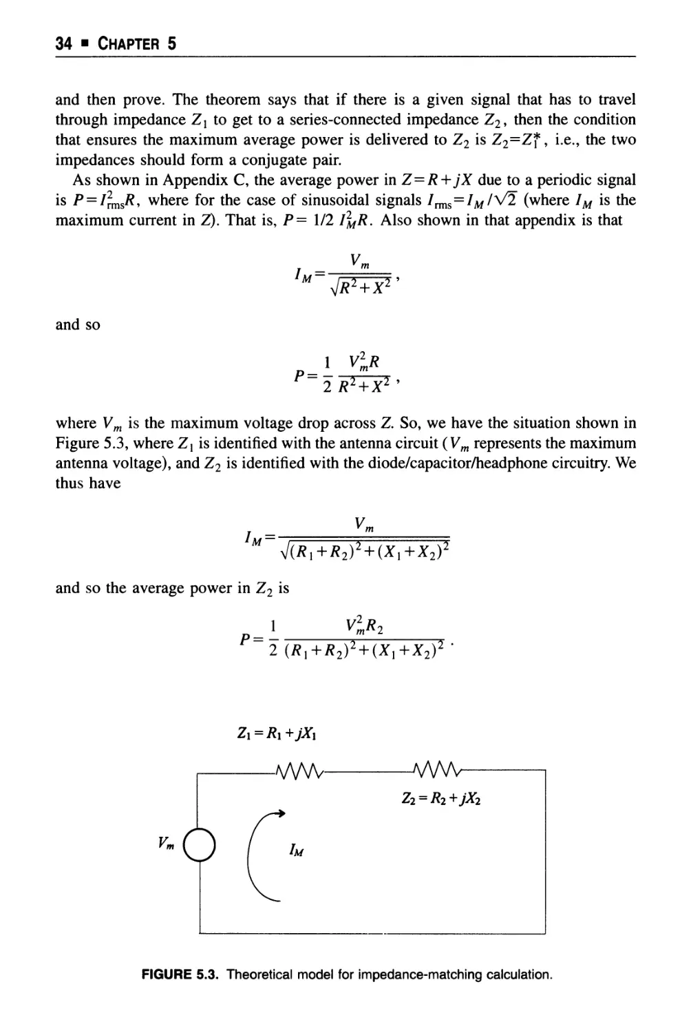
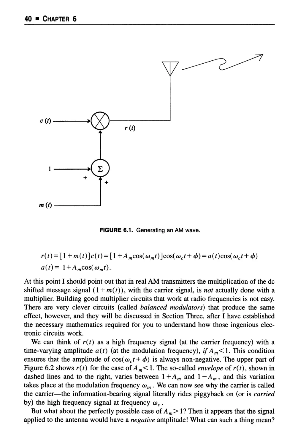
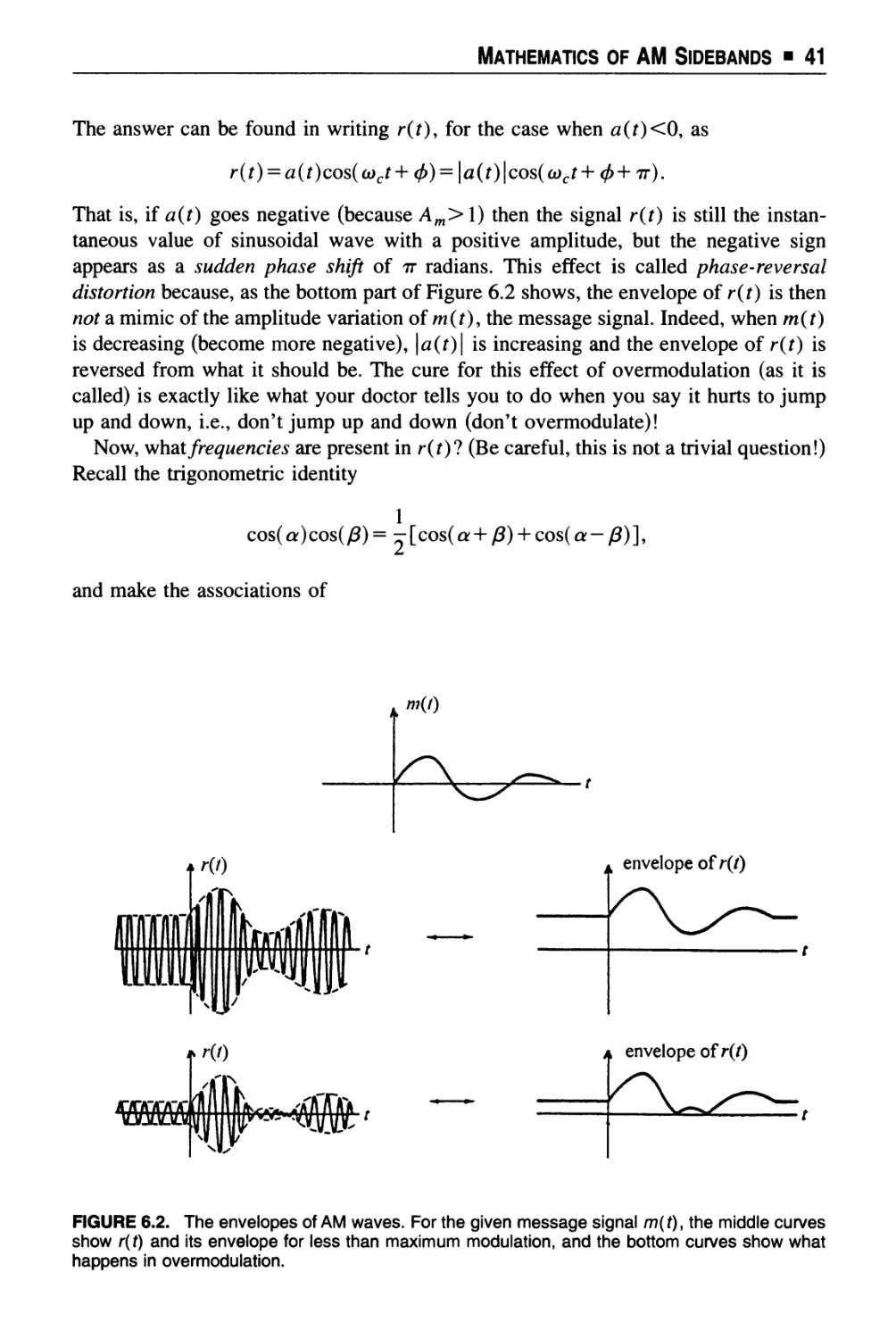
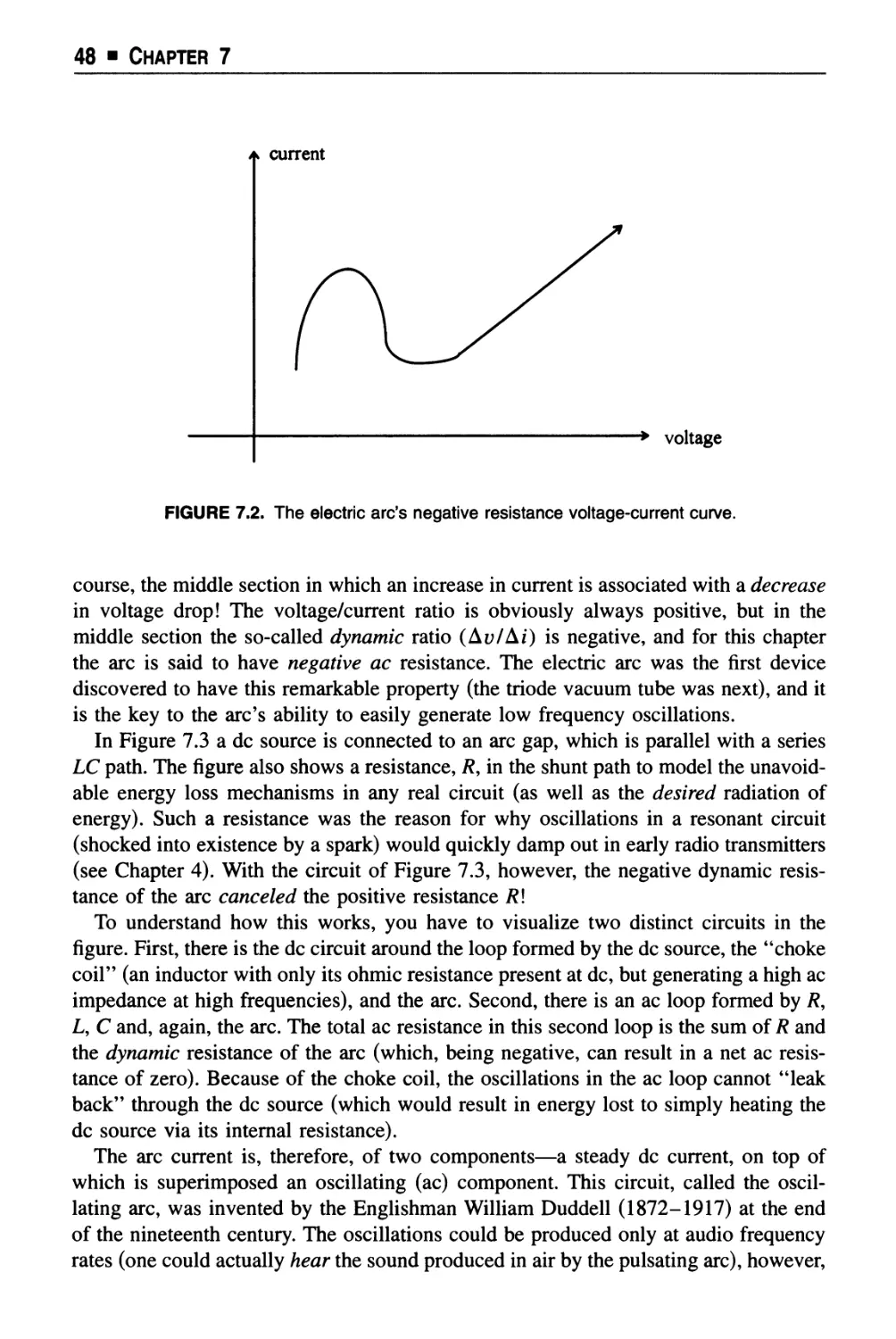
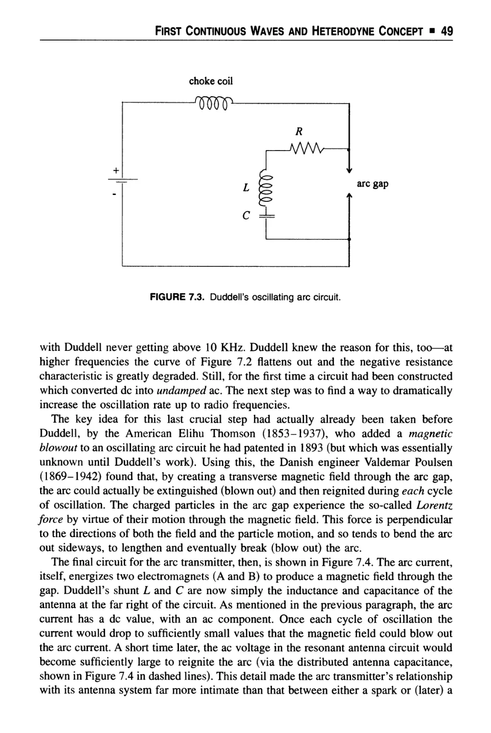
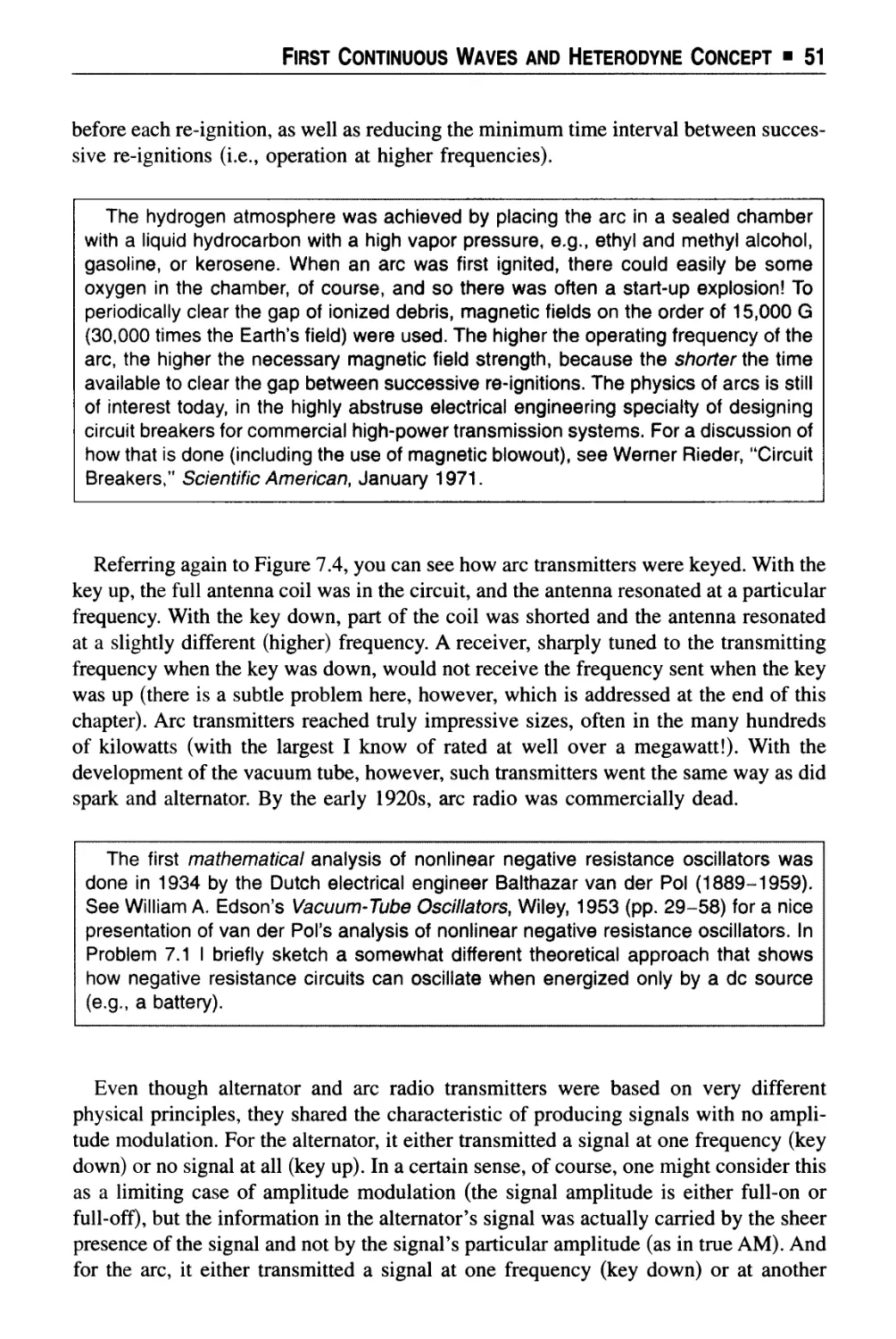
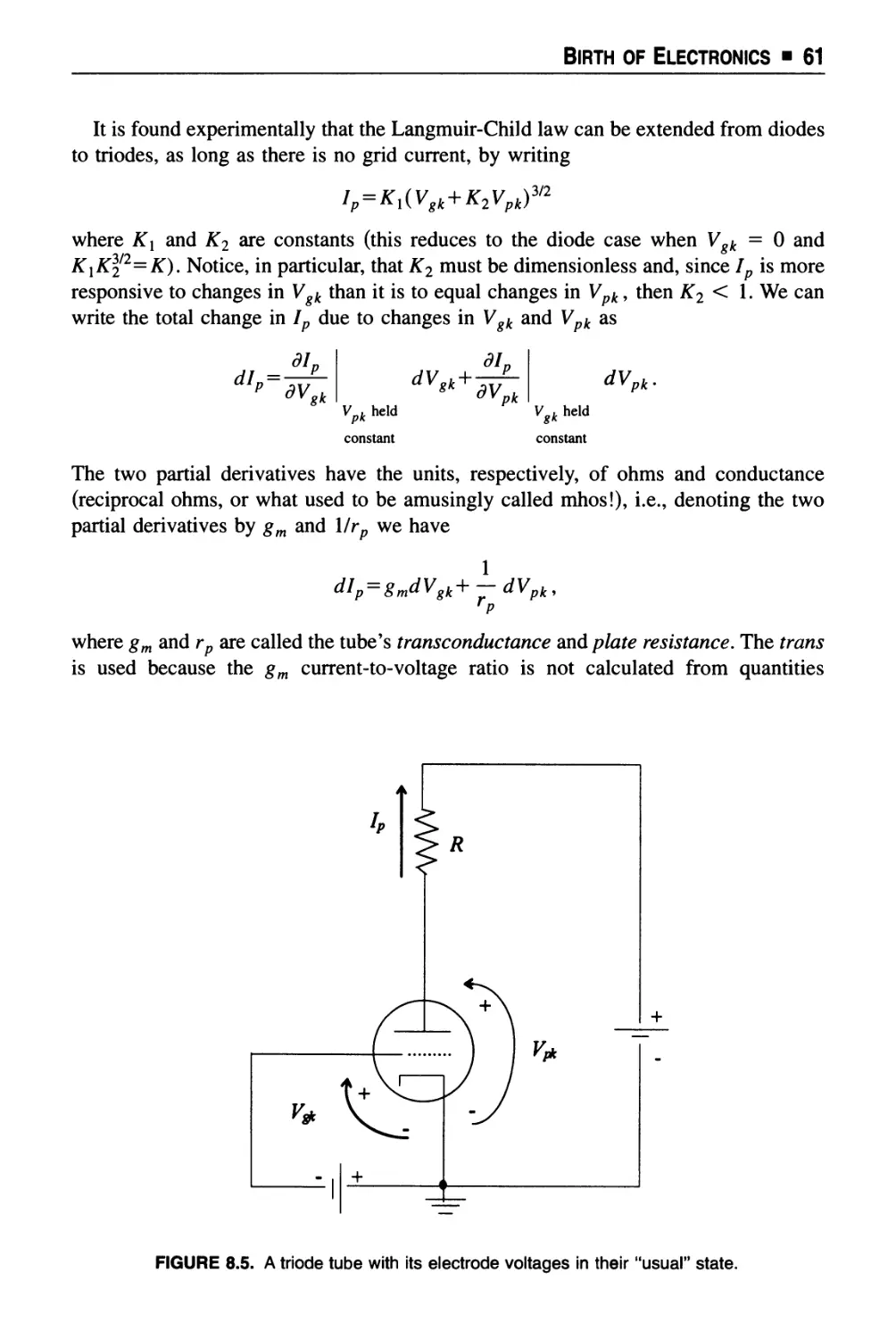
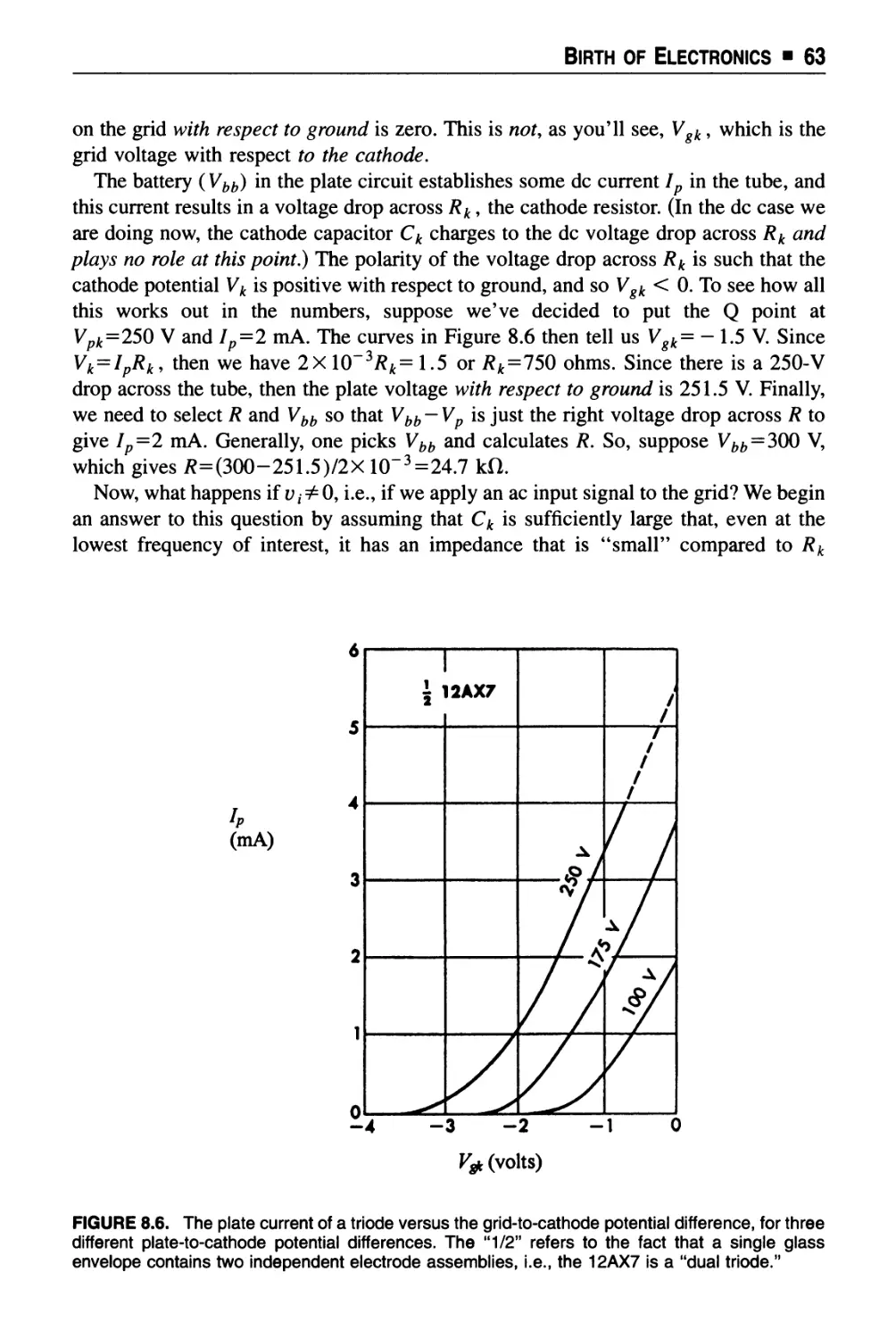
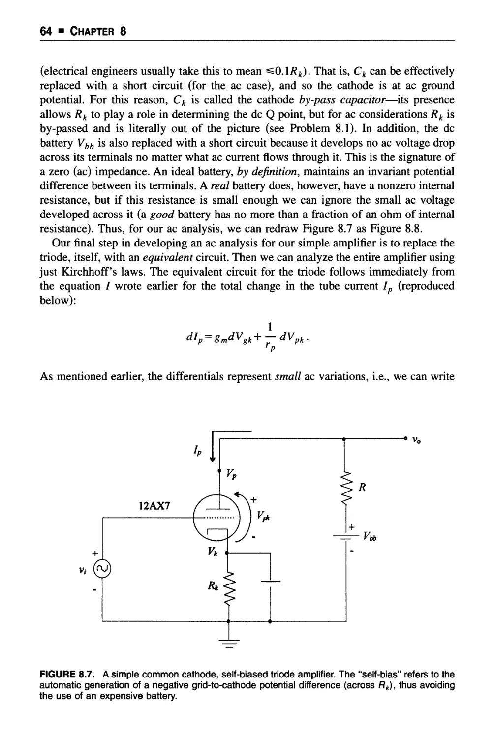
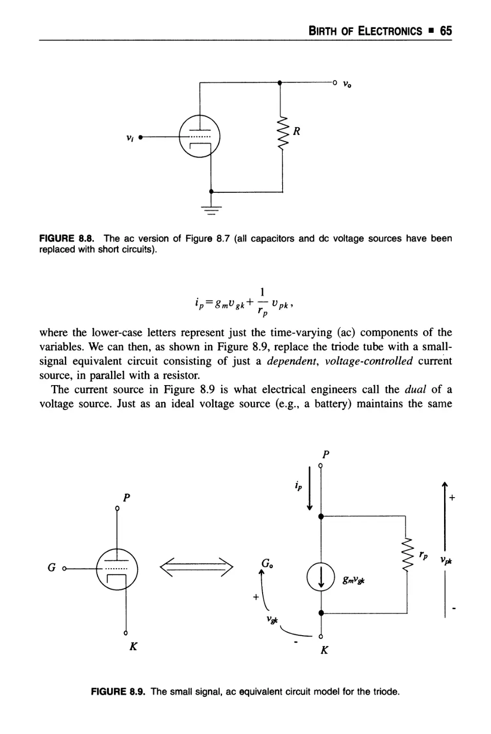
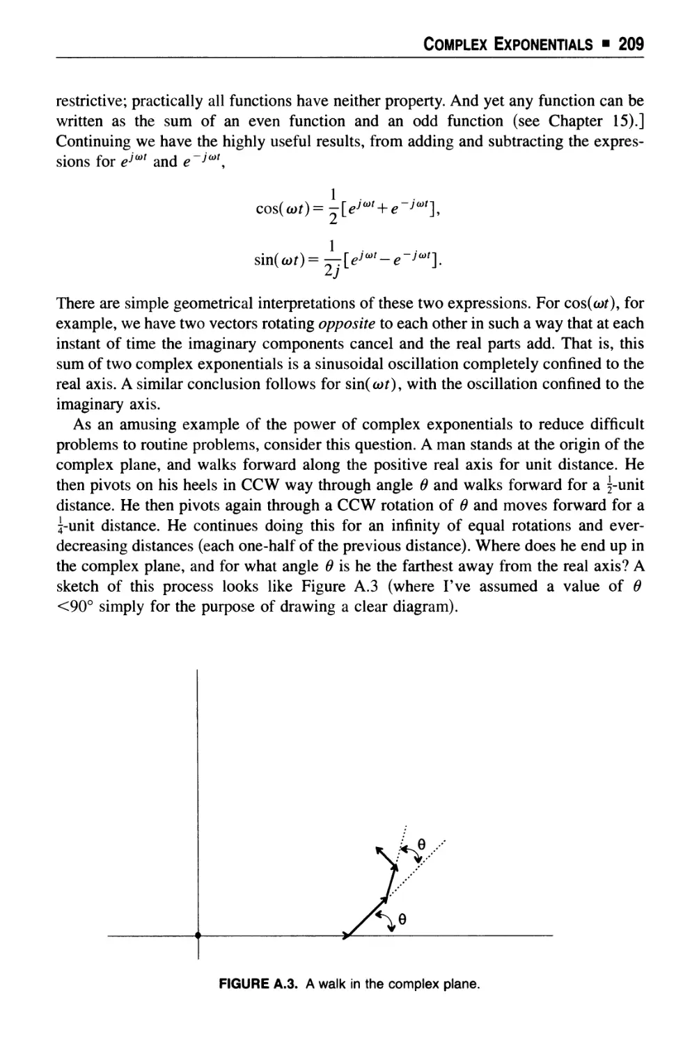
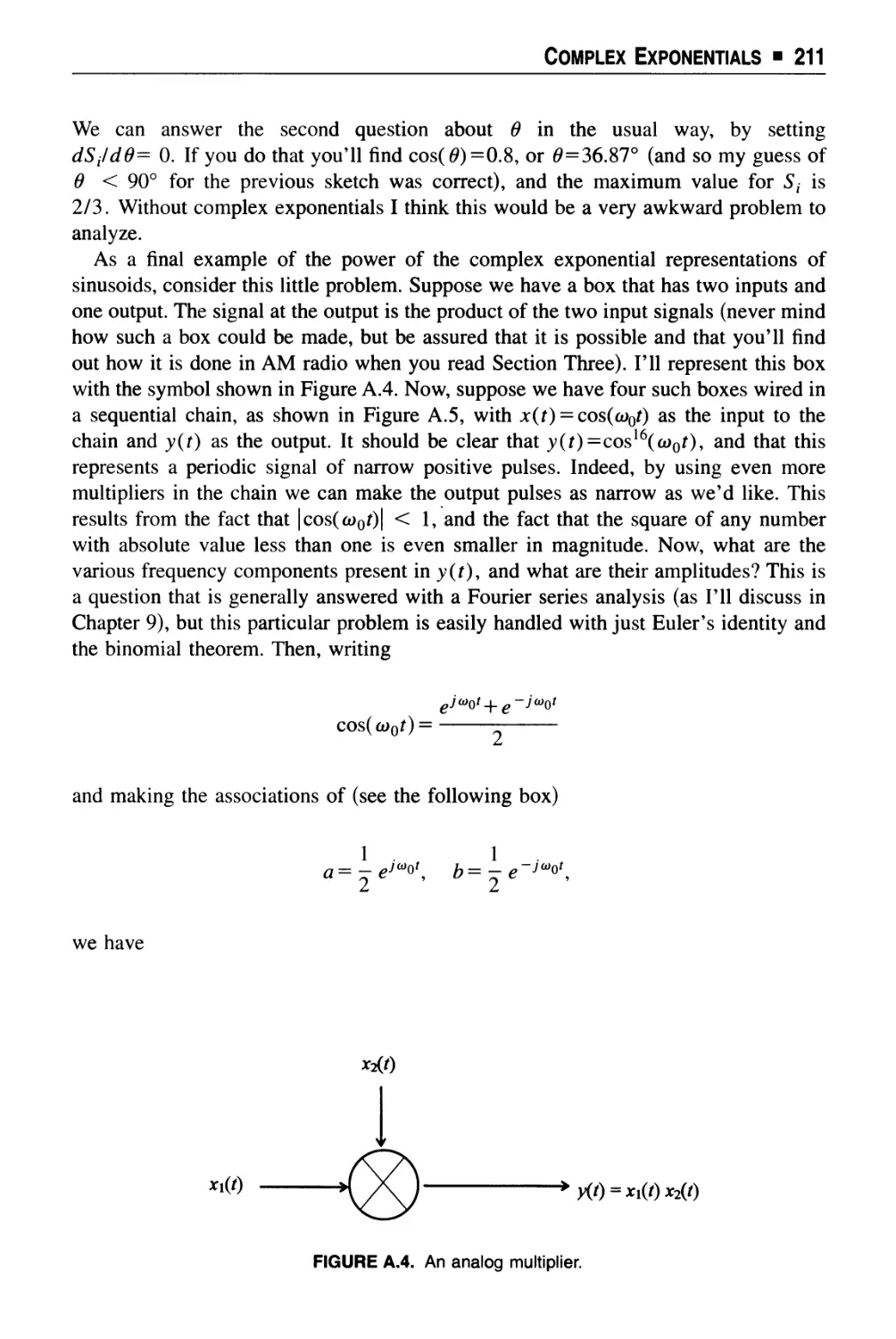
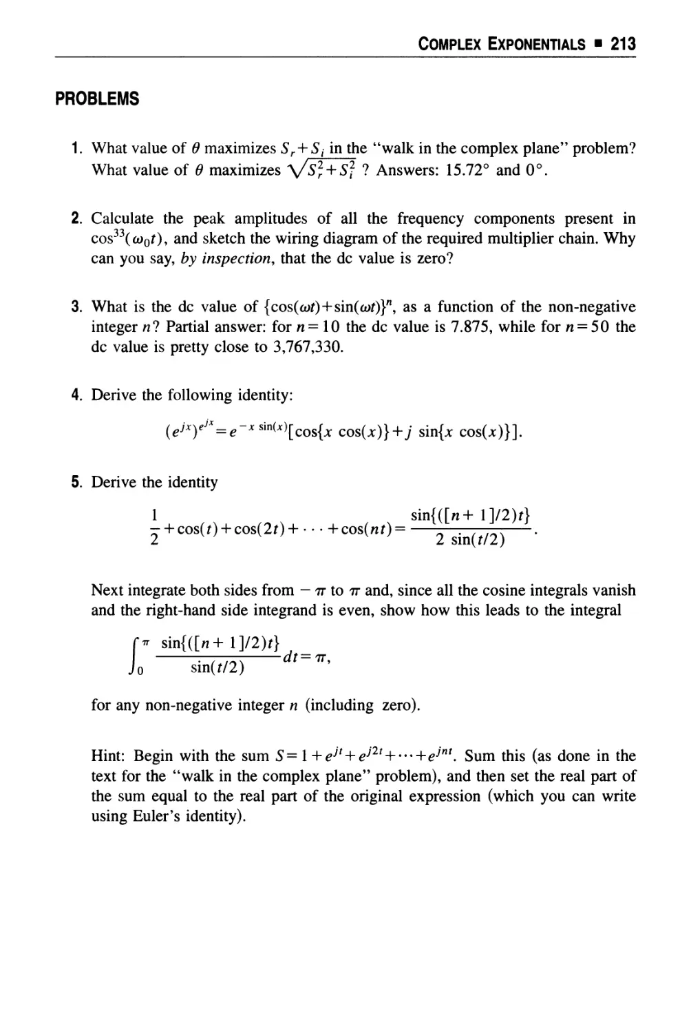
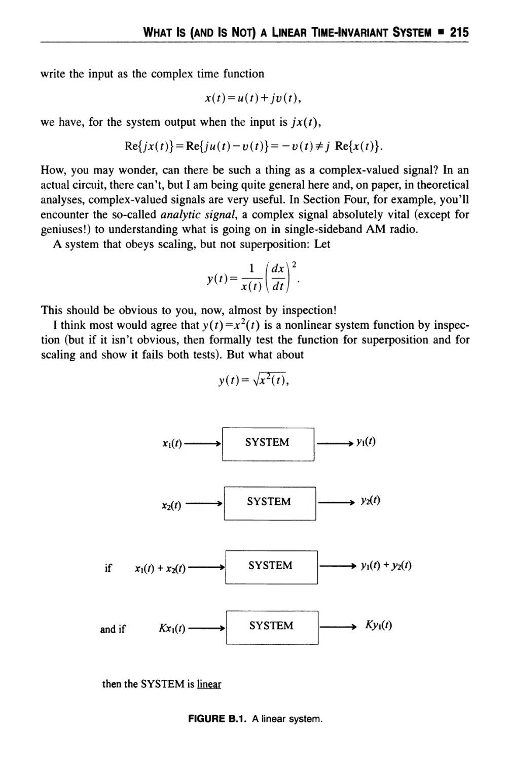
/


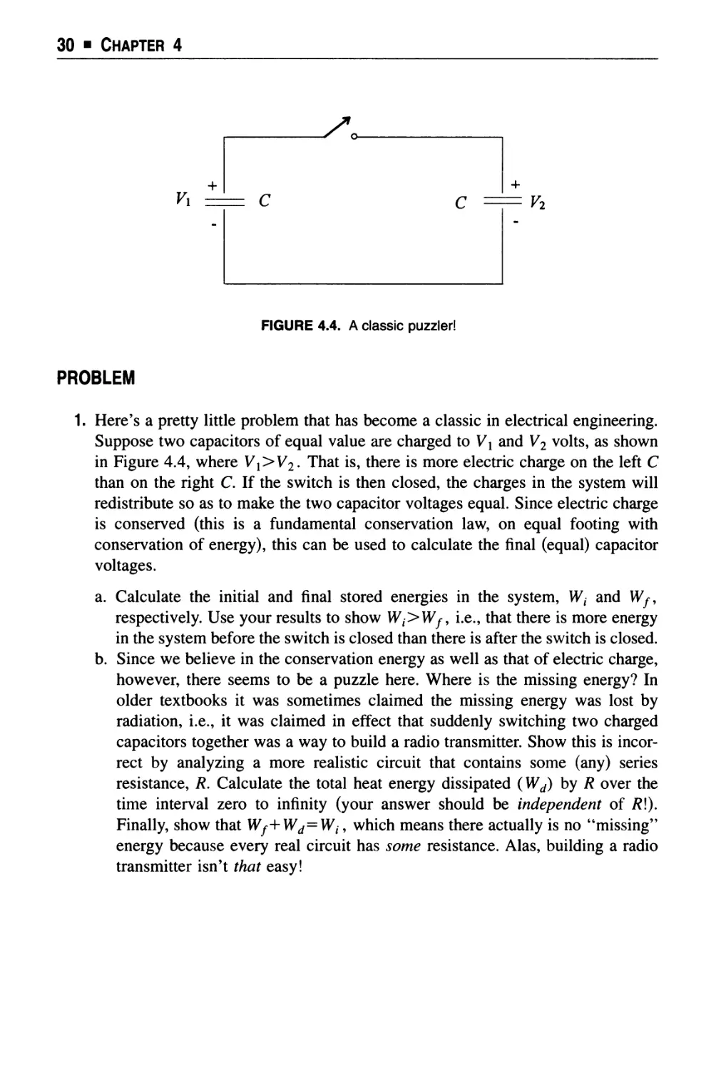
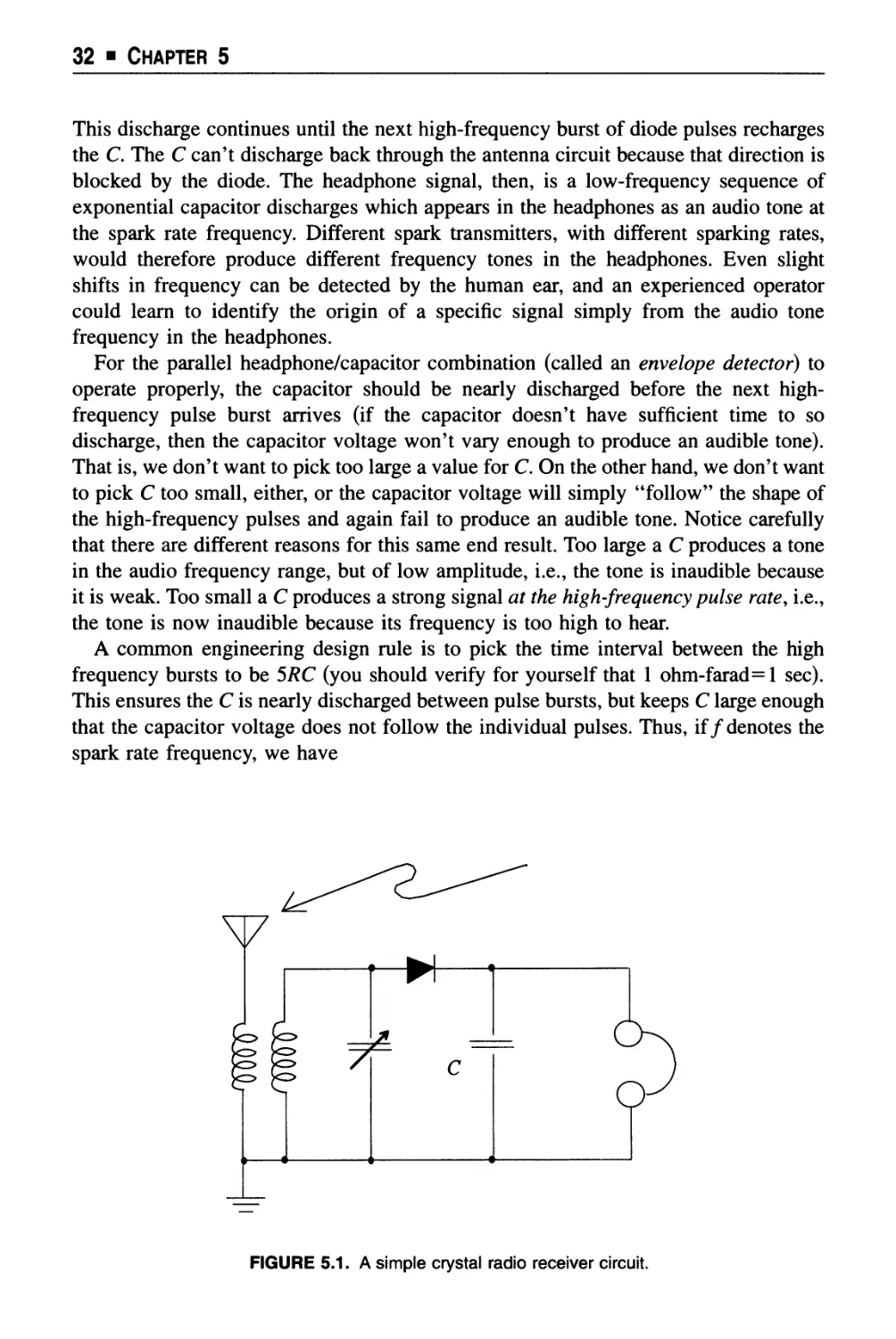


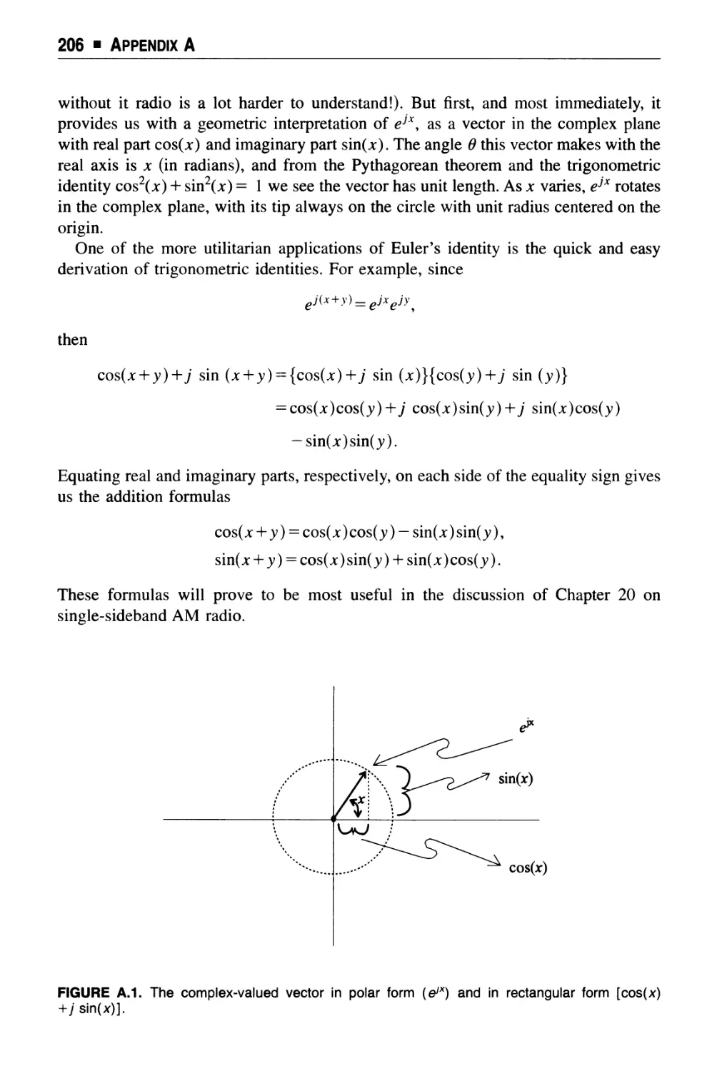


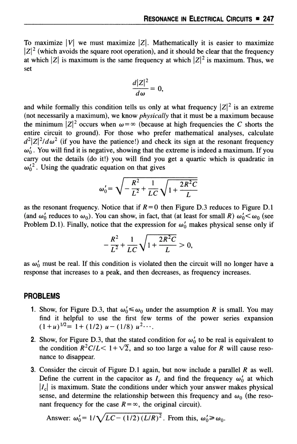


Текст
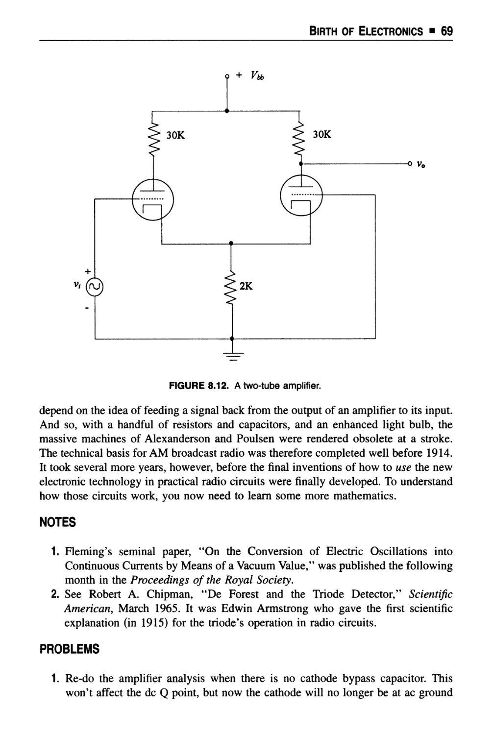
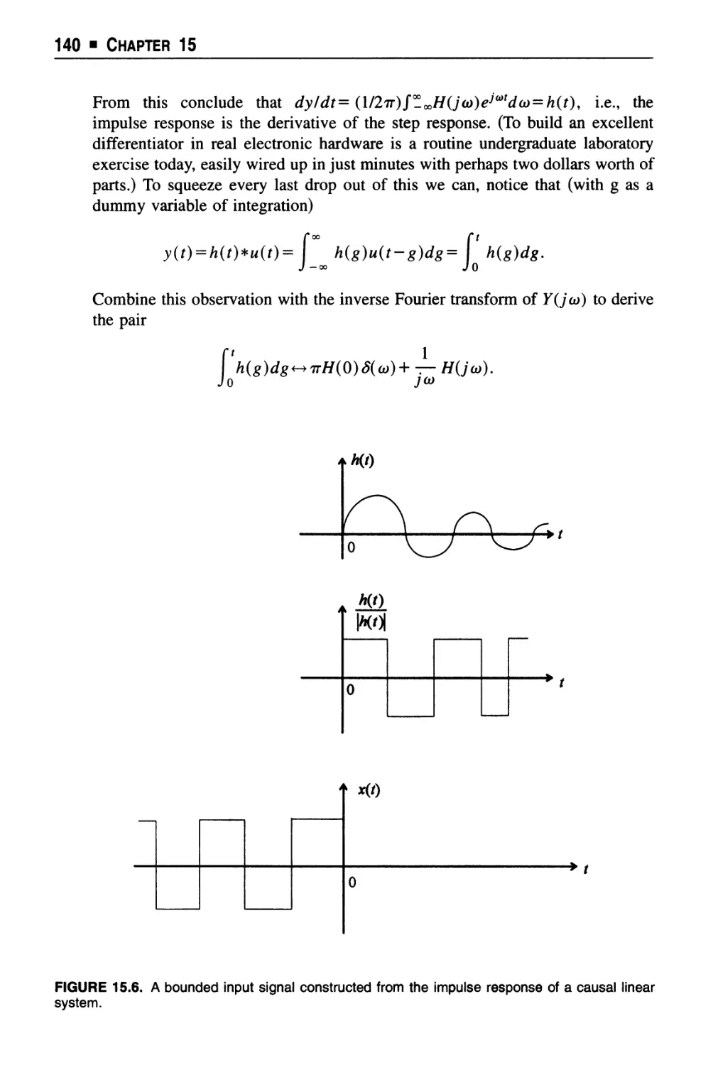
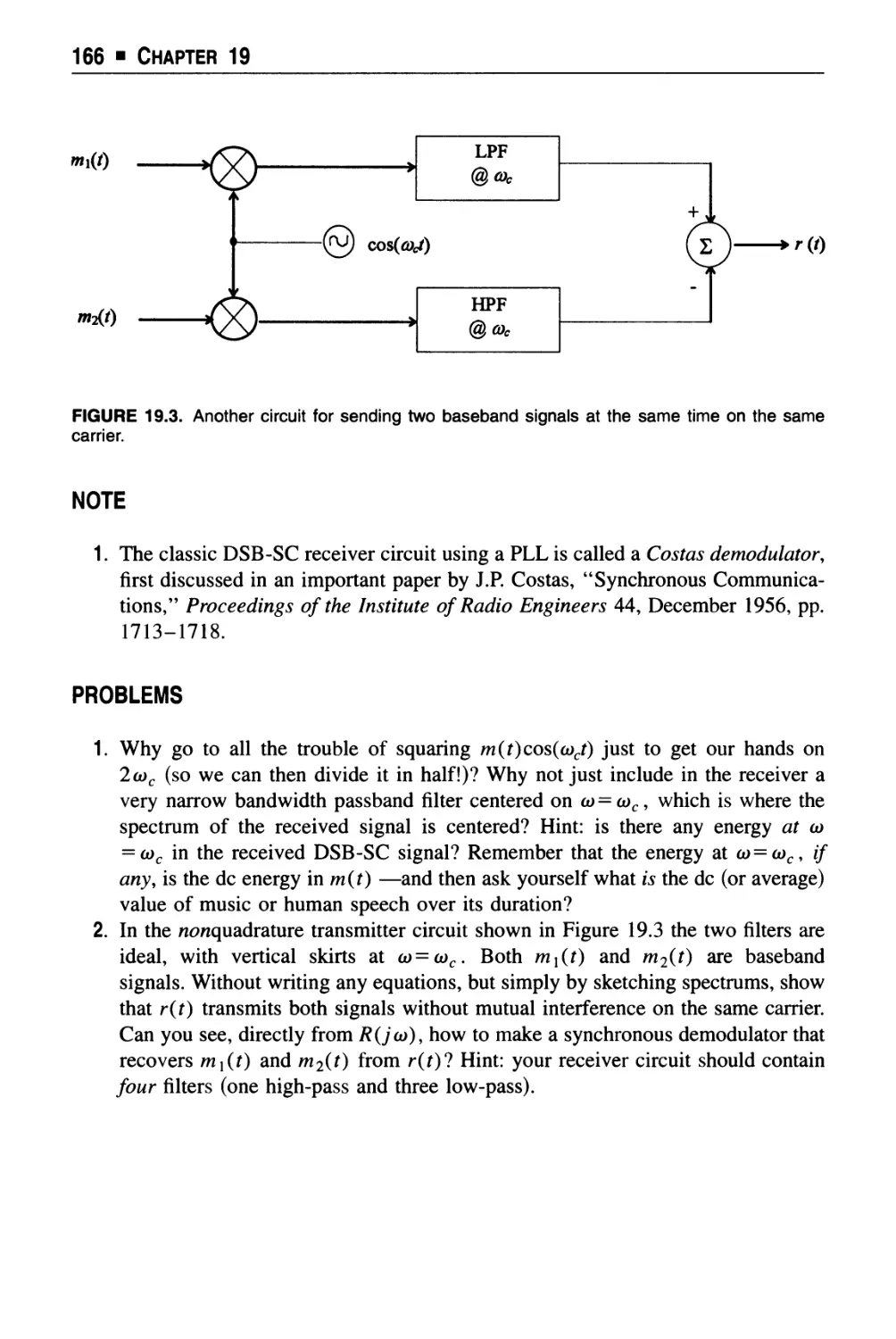
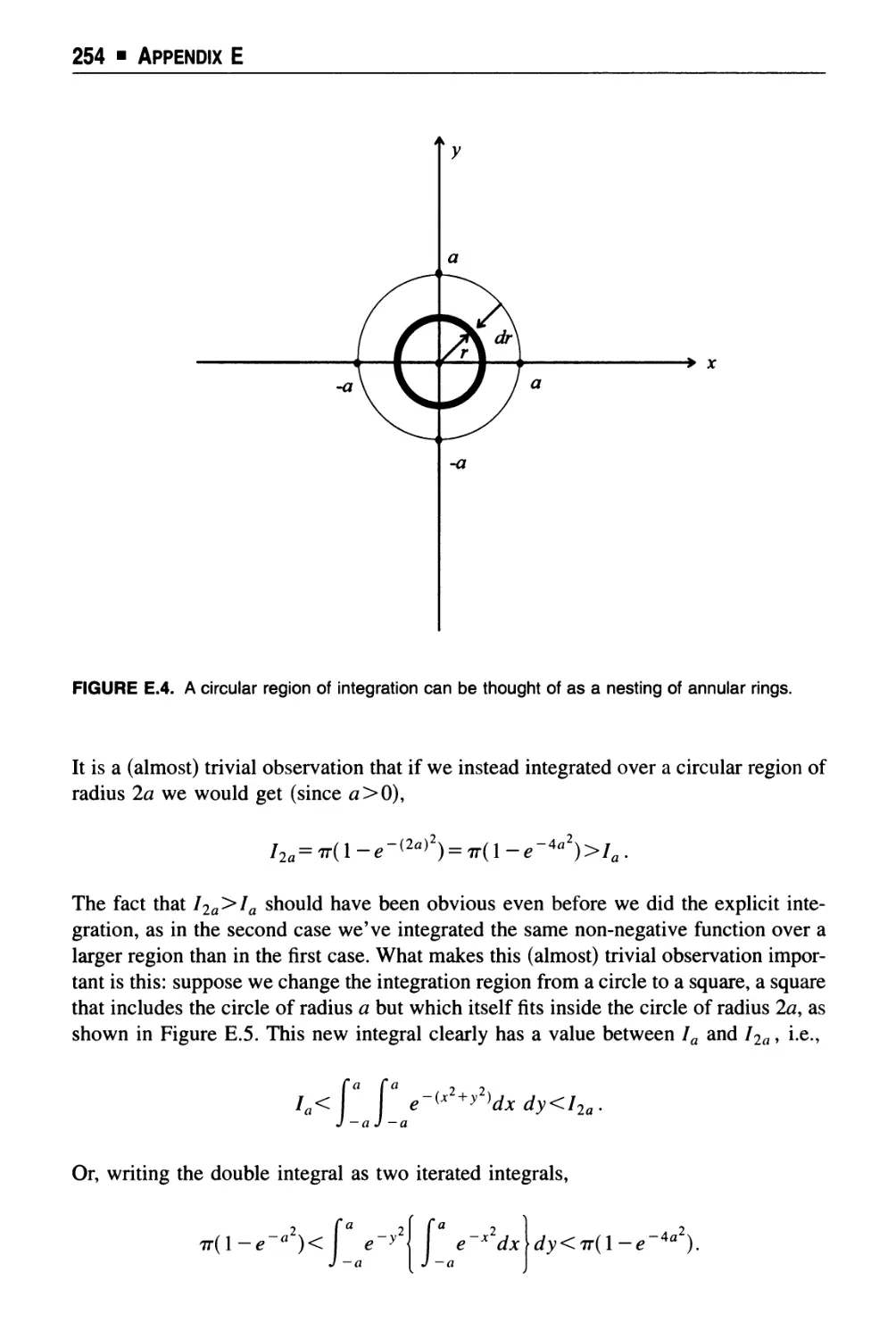
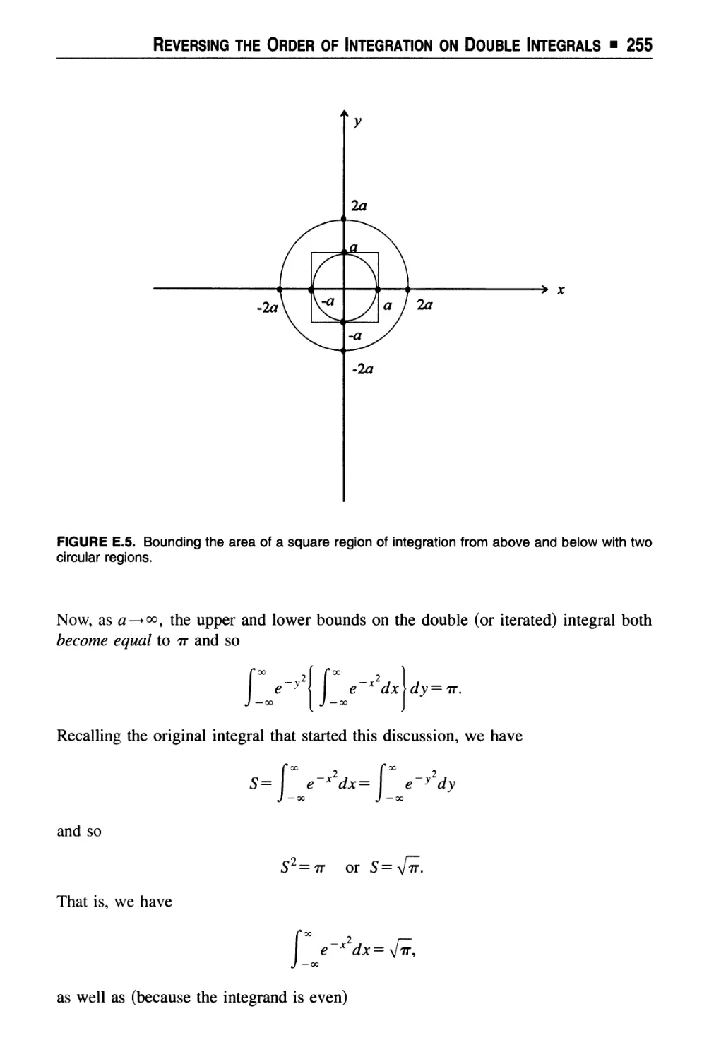
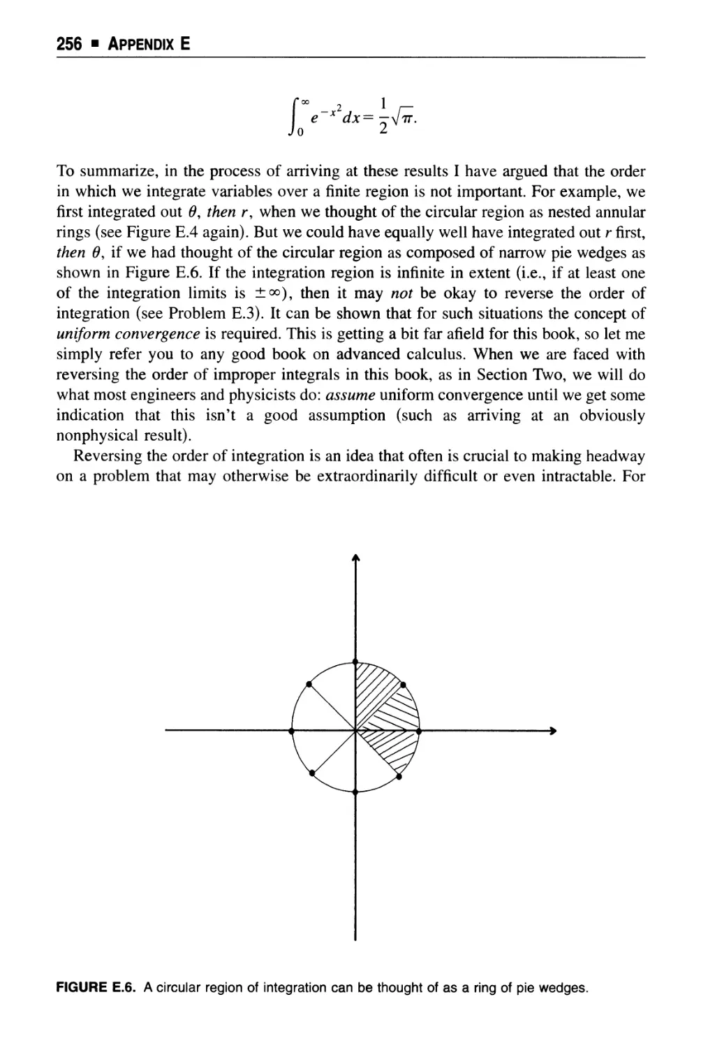
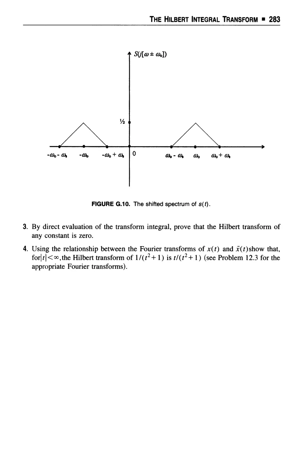
@Q[1K]@B ®P
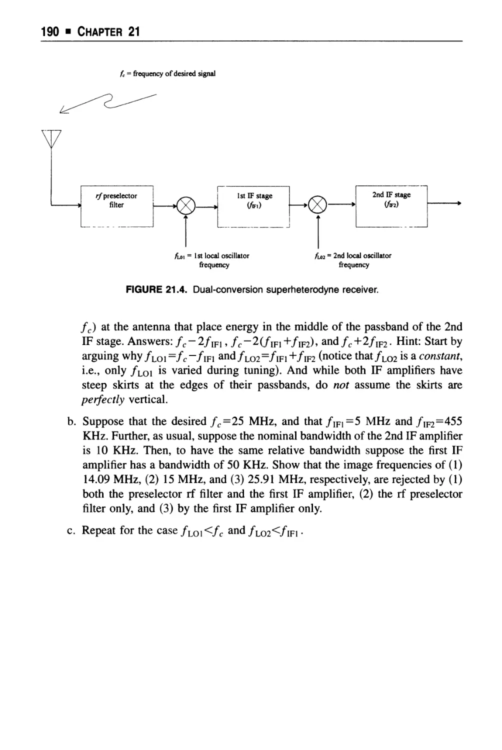
X
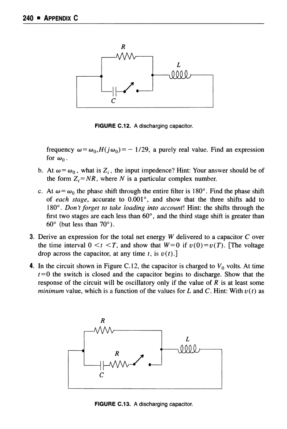
\
A " D
,!
/>
\
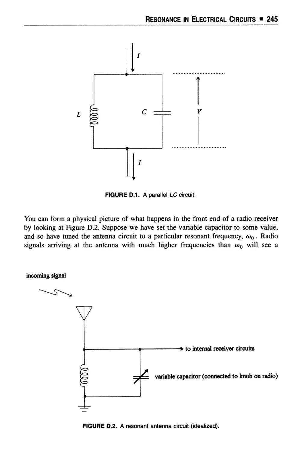
ST
L-' Ll L
C c
Li A L L 1'
"**.
The
Science of Radio
PAUL J. NAHIN
University of New Hampshire
Durham, New Hampshire
AIP
American Institute of Physics Woodbury, New York
In recognition of the importance of preserving what has been written,
it is a policy of the American Institute of Physics to have books
published in the United States printed on acid-free paper.
©1996 by American Institute of Physics
All rights reserved.
Printed in the United States of America.
Reproduction or translation of any part of this work beyond that
permitted by Section 107 or 108 of the 1976 United States Copyright
act without the permission of the copyright owner is unlawful. Requests
for permission or further information should be addressed to the Office
of Rights and Permissions, 500 Sunnyside Boulevard, Woodbury, NY
11797-2999; phone: 516-576-2268; fax: 516-576-2499; e-mail:
rights@aip.org.
AIP Press
American Institute of Physics
500 Sunnyside Boulevard
Woodbury, NY 11797-2999
Library of Congress Cataloging-in-Publication Data
Nahin, Paul J.
The science of radio I Paul J. Nahin.
p. cm.
Includes bibliographical references and index.
ISBN 1-56396-347-7
1. Radio. I. Title.
TK6550.N15 1995 95-25185
621.384-dc20 CIP
10 9876543
Dedicated to
Heaviside and Maxwell,
my two scholarly affectionate felines who insisted on giving their "bottom
line" approval to this book by sitting on each and every page as I wrote it,
and to
my wife Patricia Ann,
who with no complaints (well, maybe just a few) puts up with Heaviside,
Maxwell, and me, which is perhaps more than should be asked of anyone.
A top-down, just-in-time first course in electrical engineering for students who have
had freshman calculus and physics
that answers the questions of,
what's inside a kitchen radio?
how did it all get there?
why does the thing work?,
along with a small collection of theoretical discussions and problems to amuse, perplex,
enrage, challenge, and otherwise entertain the reader.
"E-mail and other tech talk may be the third, fourth or nth wave of the future, but old-
fashioned radio is true hyperdemocracy."
Time, January 23, 1995
Paul J. Nahin is Professor of Electrical Engineering at the University of New Hampshire.
He is the author of Oliver Heaviside (IEEE Press 1988) and of Time Machines: Time
Travel in Physics, Metaphysics, and Science Fiction (AIP Press 1993). He welcomes
comments or suggestions from readers about any of his books; he can be reached on
the Internet at paul.nahin@unh.edu.
"^ *
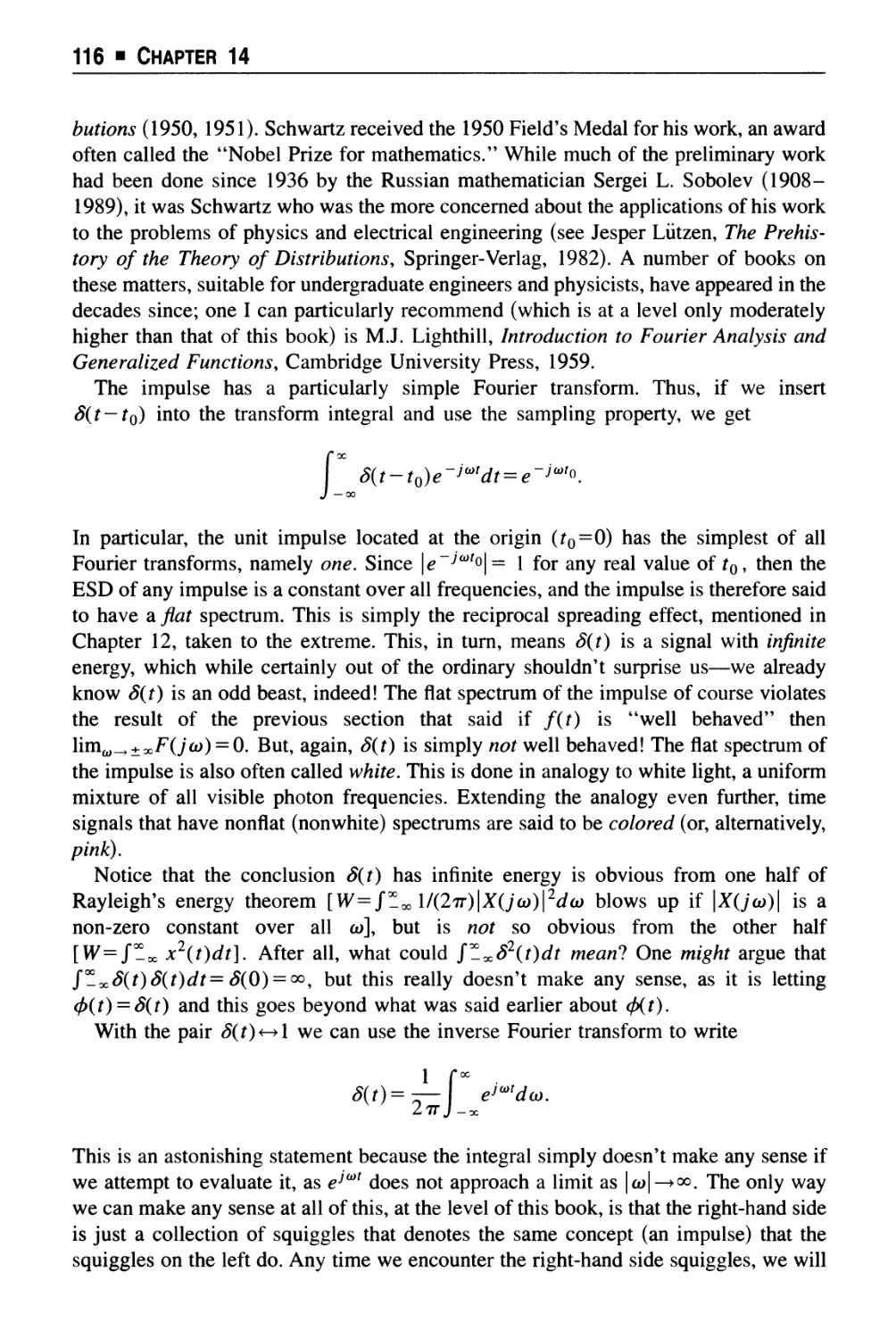
ll' t
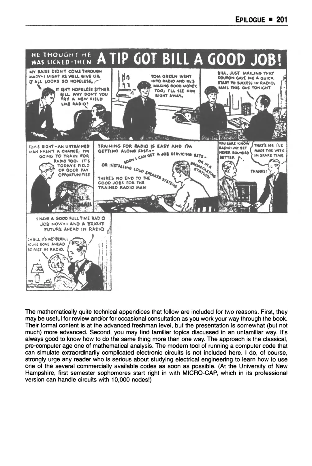
An American family poses proudly in 1947 Southern California. The new Admiral model 7C73
9-tubeAM/FM radio-phonograph console, won in a jingle contest, was more than simply a radio-
it was the family entertainment center and king of the living room furniture. The shy lad at the left
is the author, age seven. Photo courtesy of the author's sister Kaylyn (Nahin) Warner.
Contents
Acknowledgments xi
A Note to Professors xiii
Prologue xxiii
Section 1 ■ Mostly History and a Little Math
Chapter 1 Solution to An Old Problem 3
Chapter 2 Pre-Radio History of Radio Waves 7
Chapter 3 Antennas as Launchers and Interceptors of Electromagnetic
Waves 15
Chapter 4 Early Radio 24
Chapter 5 Receiving Spark Transmitter Signals 31
Chapter 6 Mathematics of AM Sidebands 38
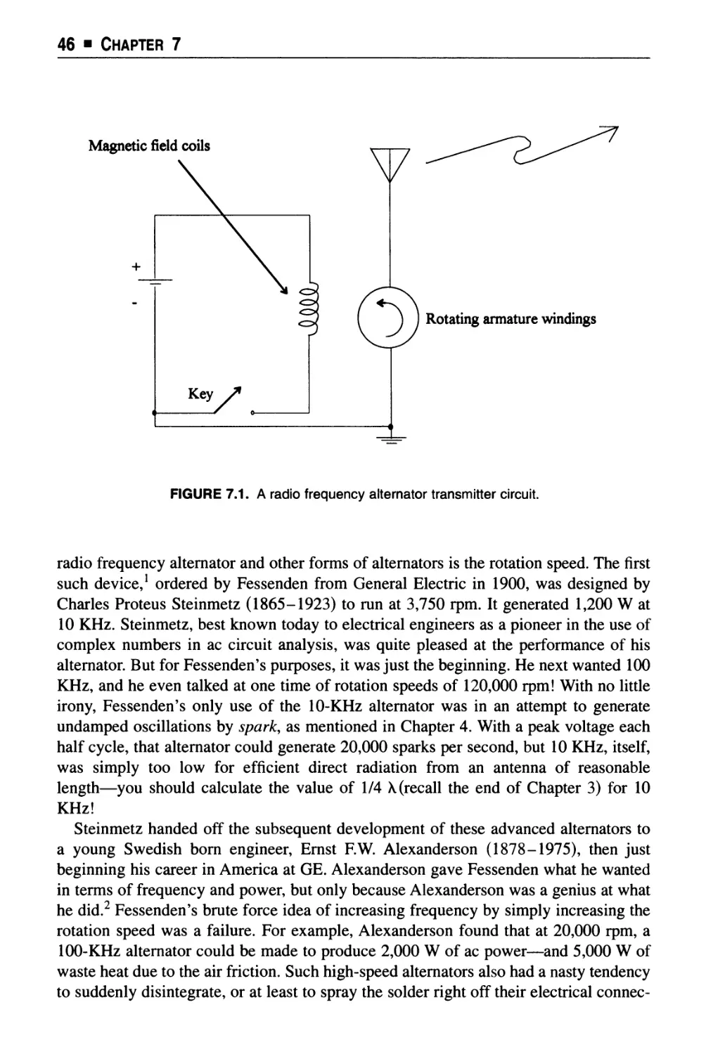
Chapter 7 First Continuous Waves and Heterodyne Concept 44
Chapter 8 Birth of Electronics 56
Section 2 ■ Mostly Math and a Little History
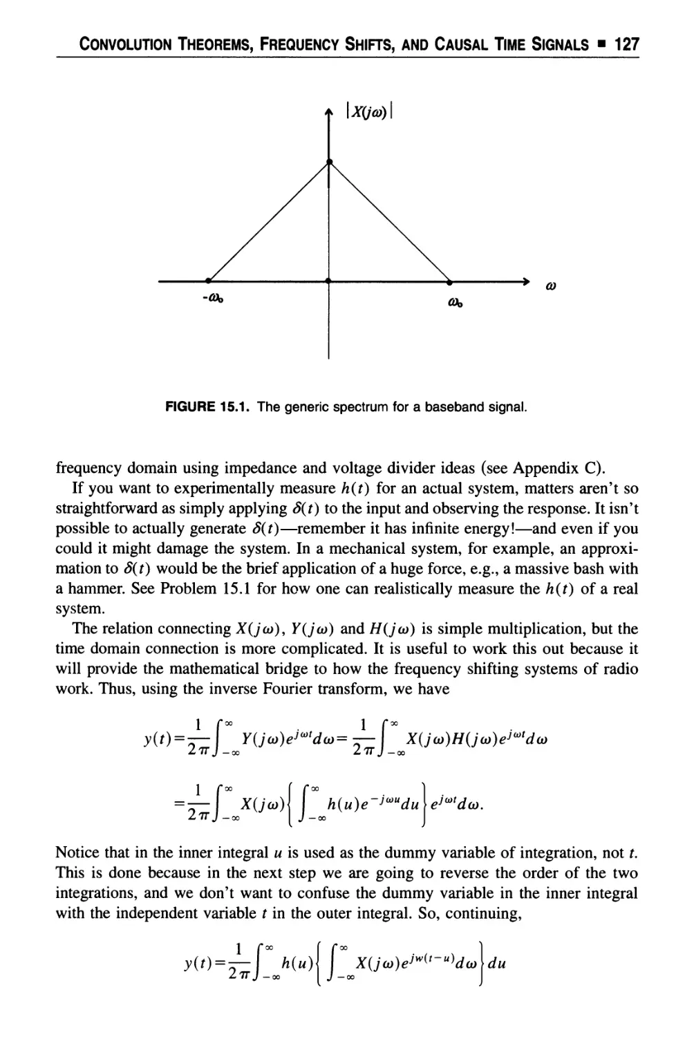
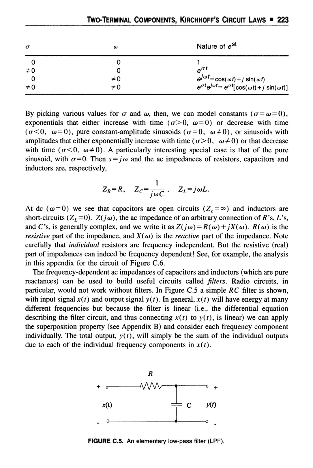
Chapter 9 Fourier Series and Their Physical Meaning 73
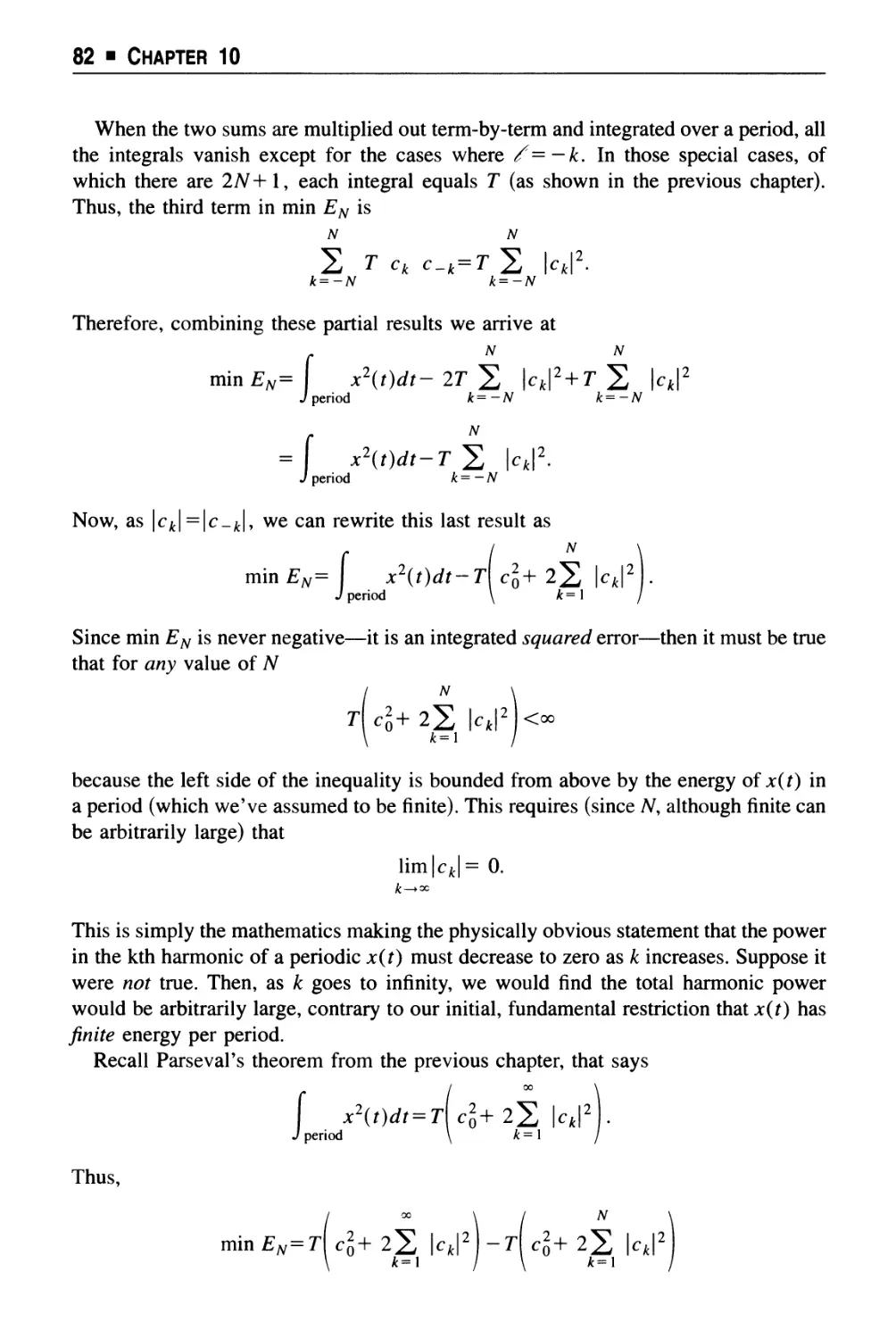
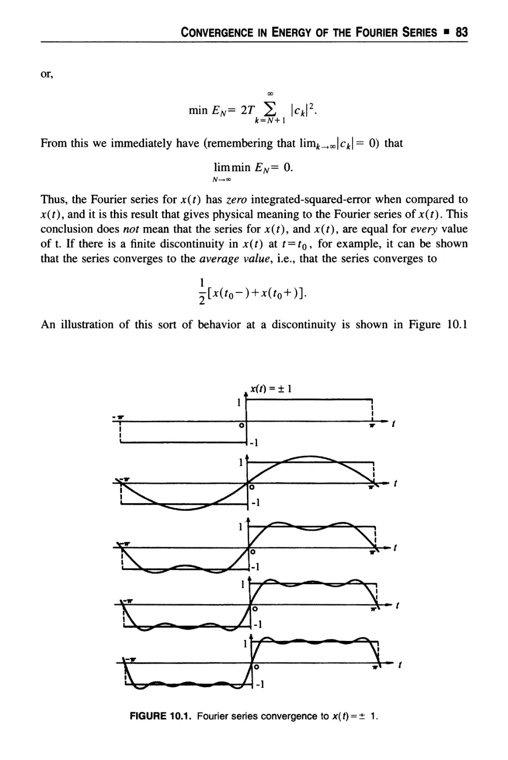
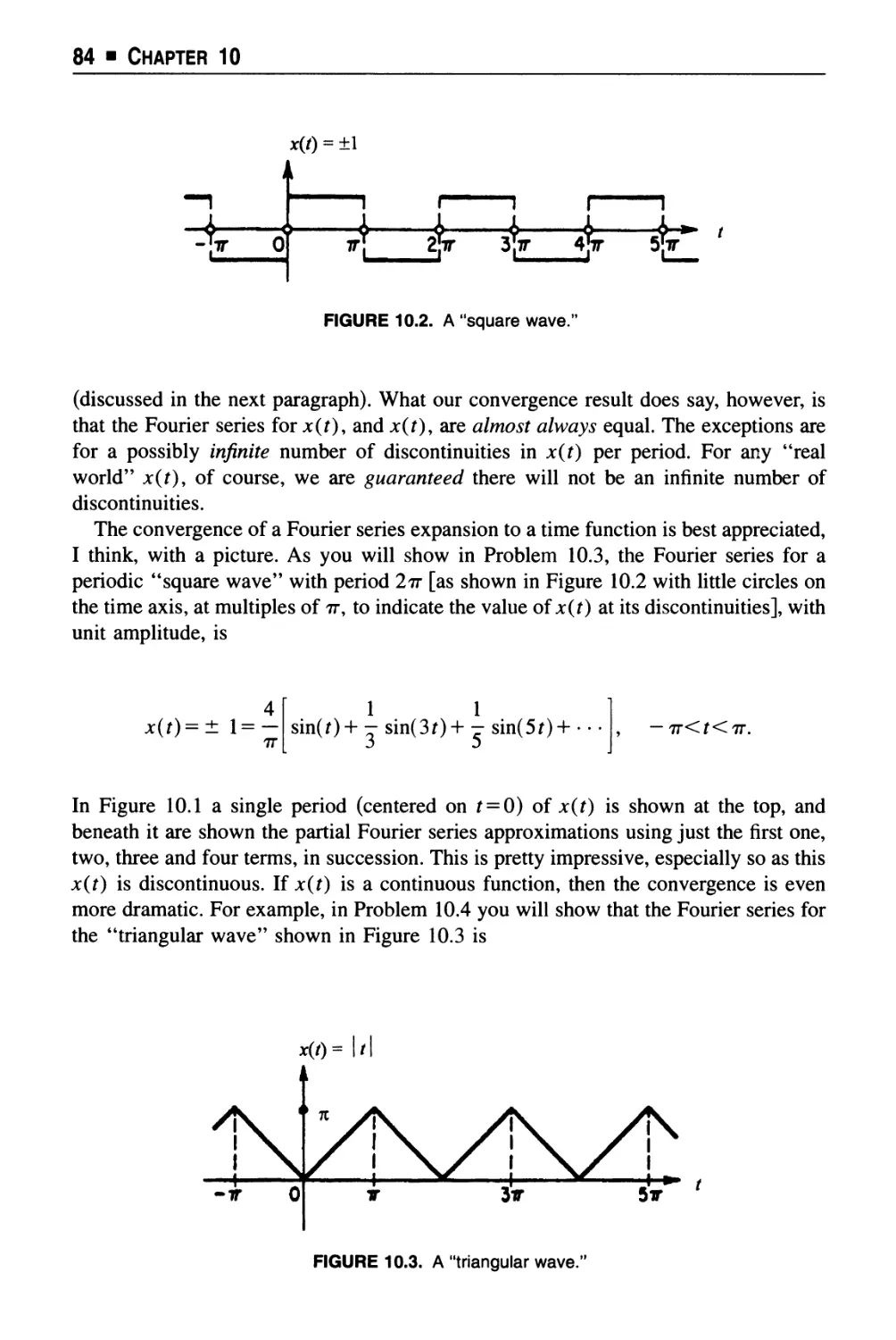
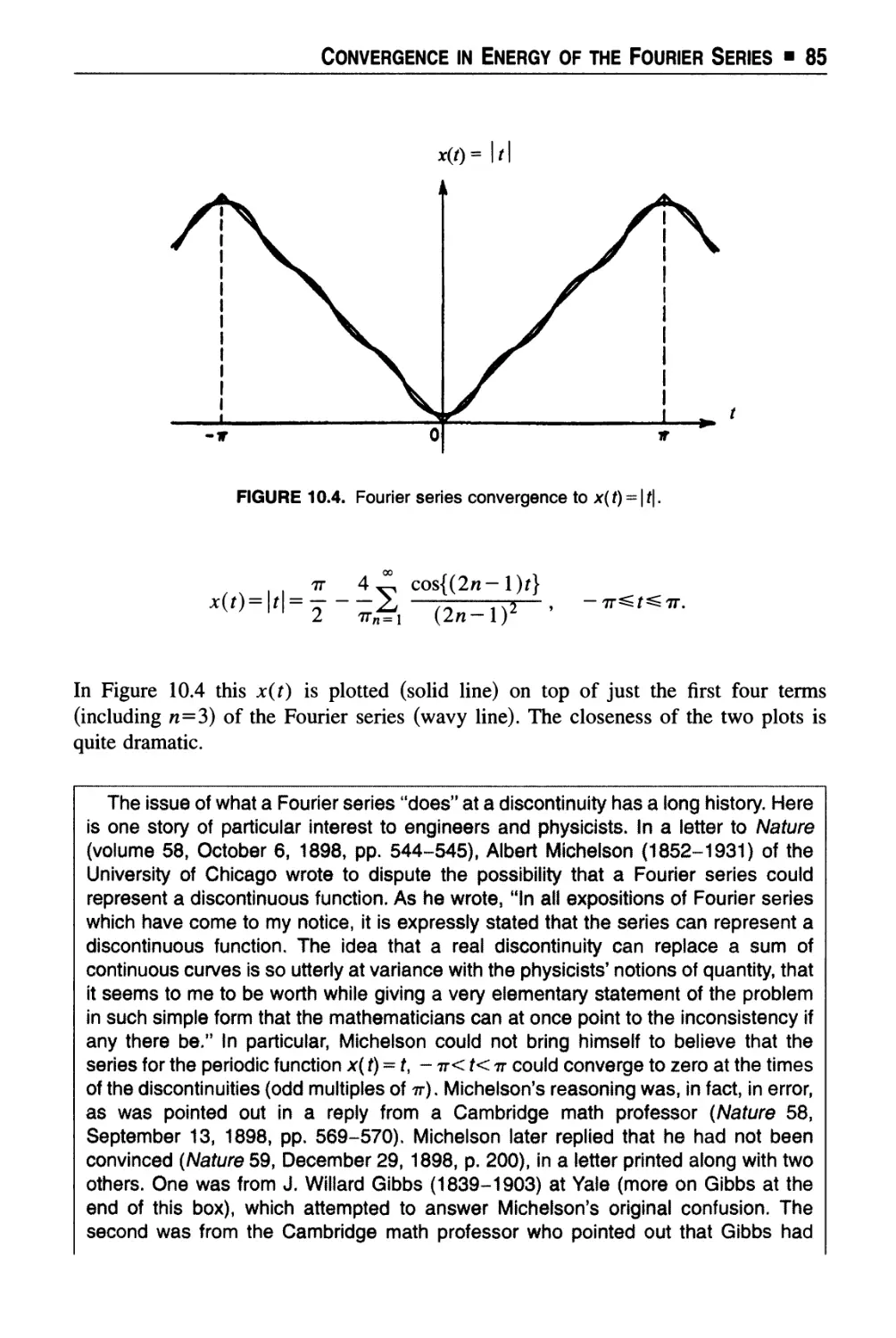
Chapter 10 Convergence in Energy of the Fourier Series 79
Chapter 11 Radio Spectrum of a Spark-Gap Transmitter 91
Chapter 12 Fourier Integral Theorem, and the Continuous Spectrum of
a Non-Periodic Time Signal 97
Chapter 13 Physical Meaning of the Fourier Transform 107
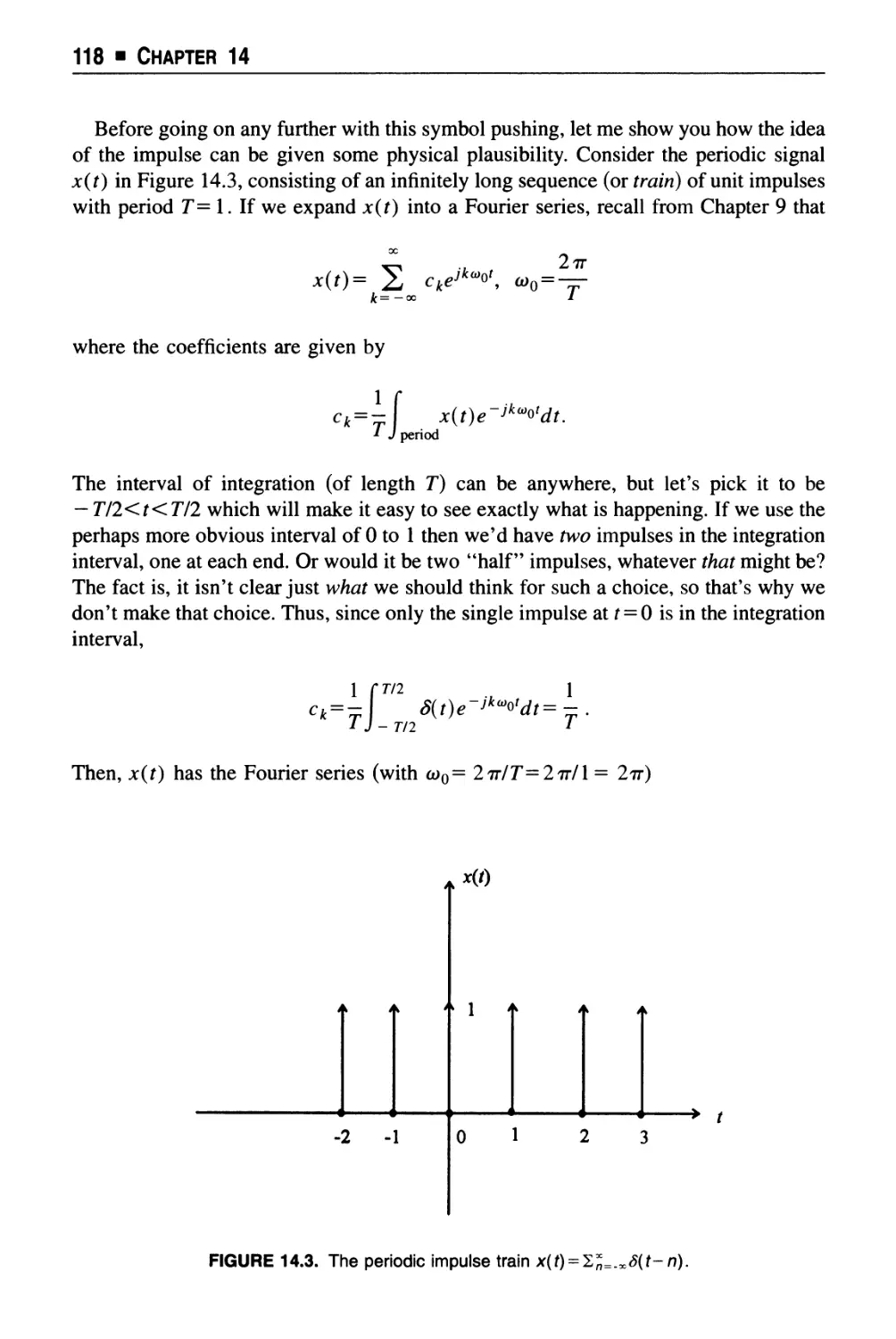
Chapter 14 Impulse "Functions" in Time and Frequency 113
Chapter 15 Convolution Theorems, Frequency Shifts, and Causal Time
Signals 126
Section 3 ■ Nonlinear Circuits for Multiplication
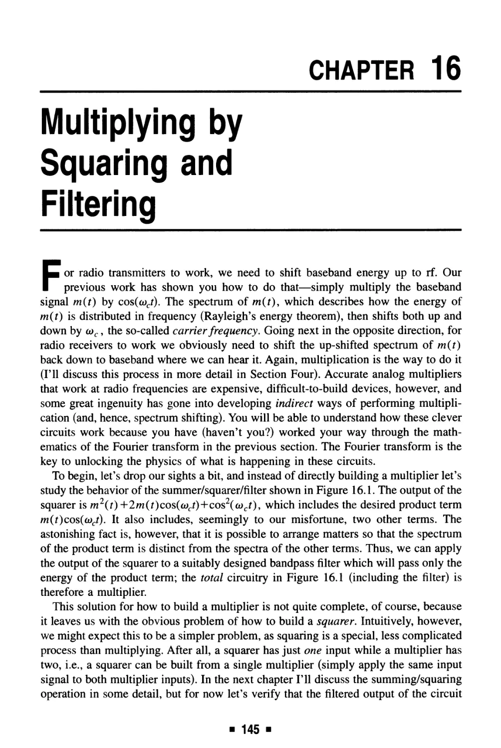
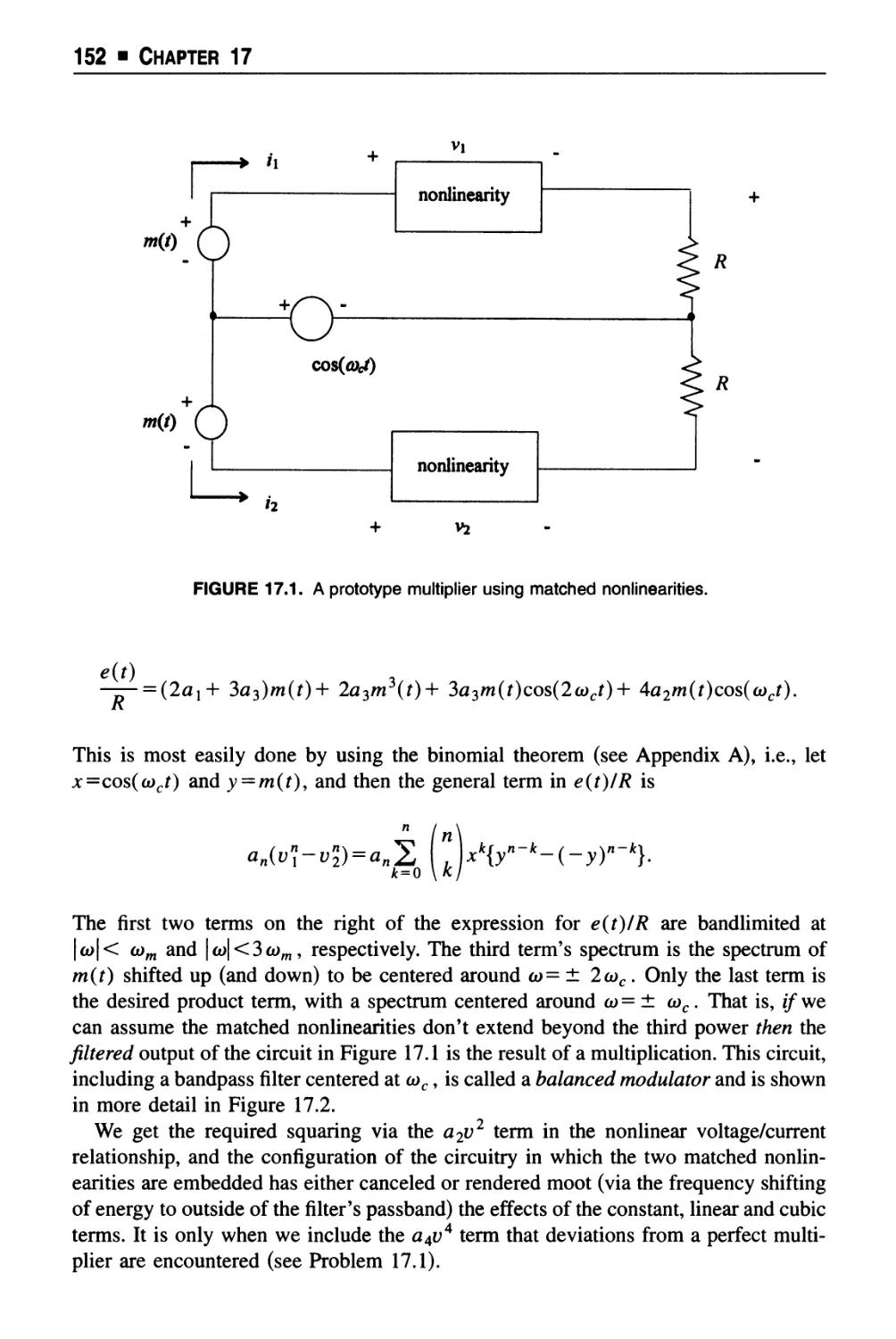
Chapter 16 Multiplying by Squaring and Filtering 145
Chapter 17 Squaring and Multiplying with Matched Nonlinearities .... 151
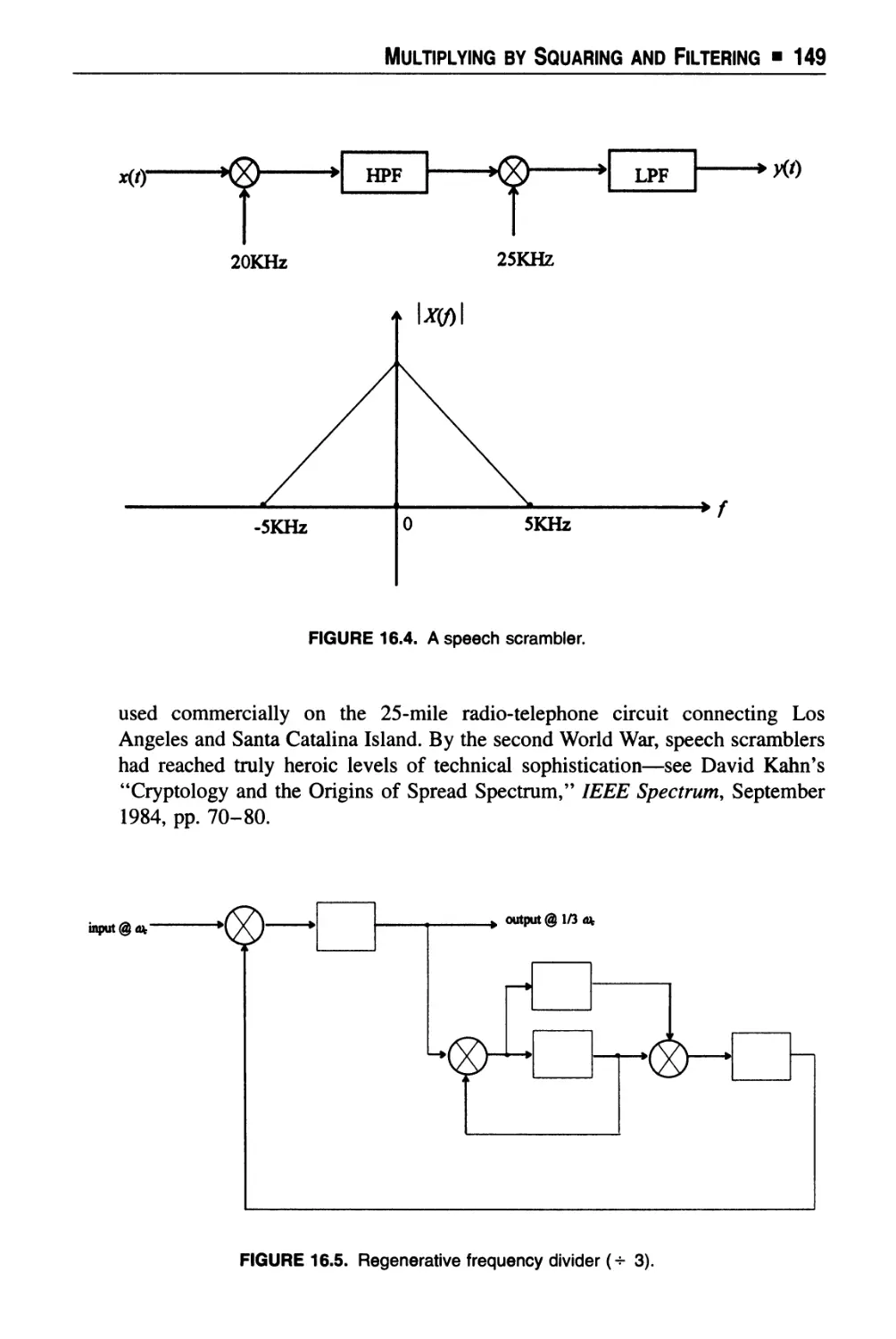
Chapter 18 Multiplying by "Sampling and Filtering" 154
■ ix ■
x ■ Contents
Section 4 ■ The Mathematics of "Unmultiplying"
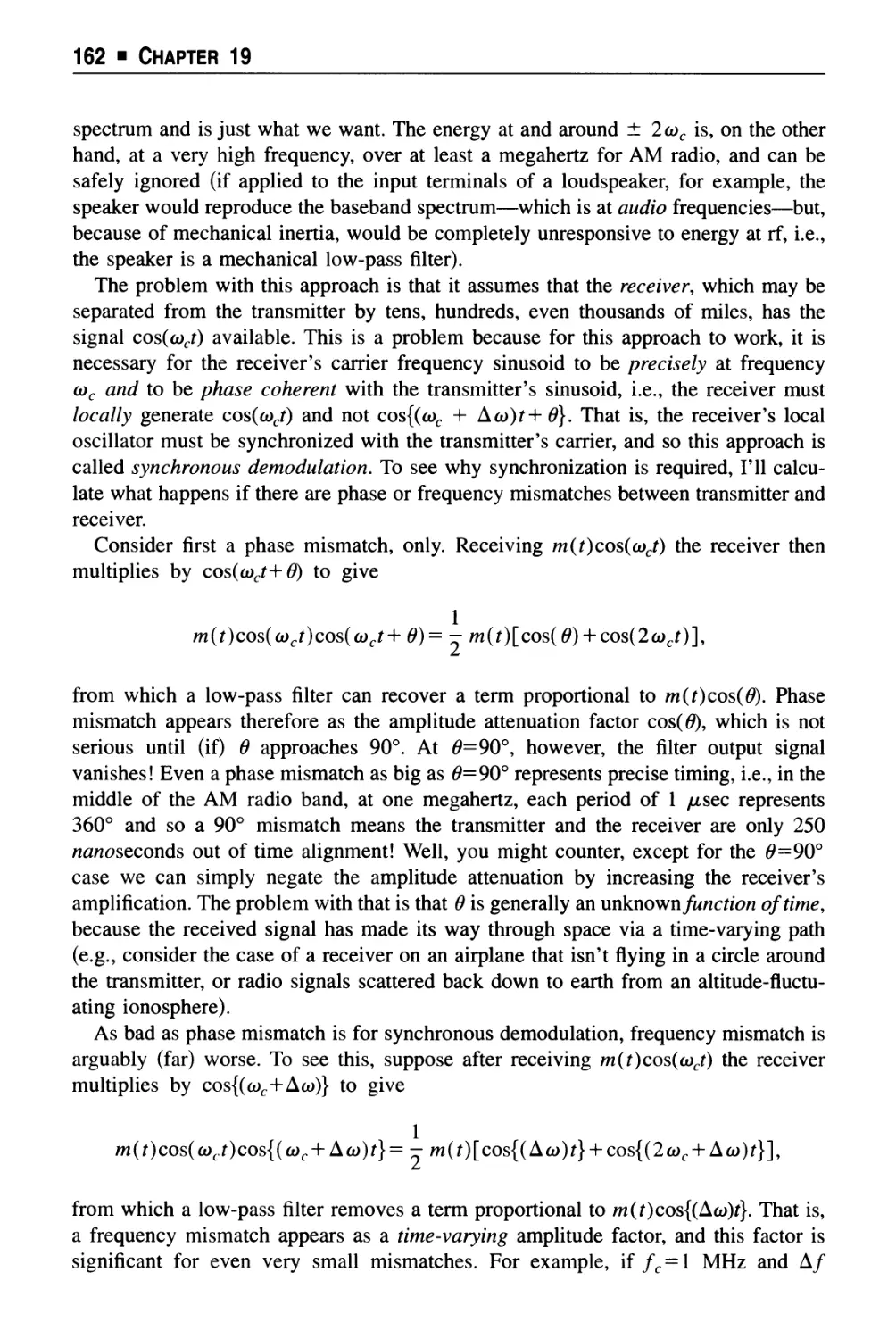
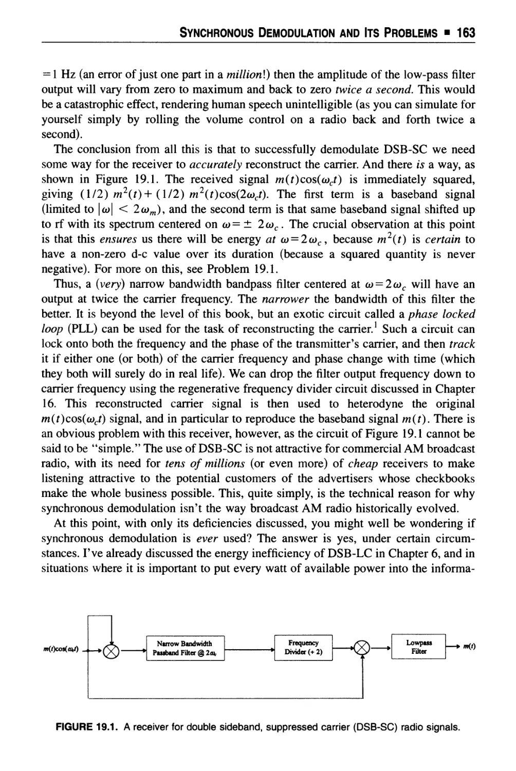
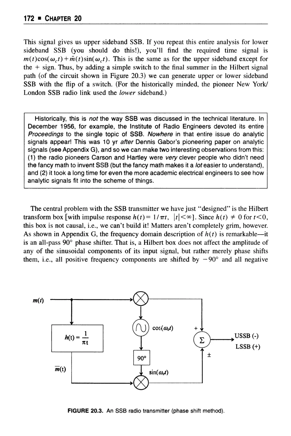
Chapter 19 Synchronous Demodulation and Its Problems 161
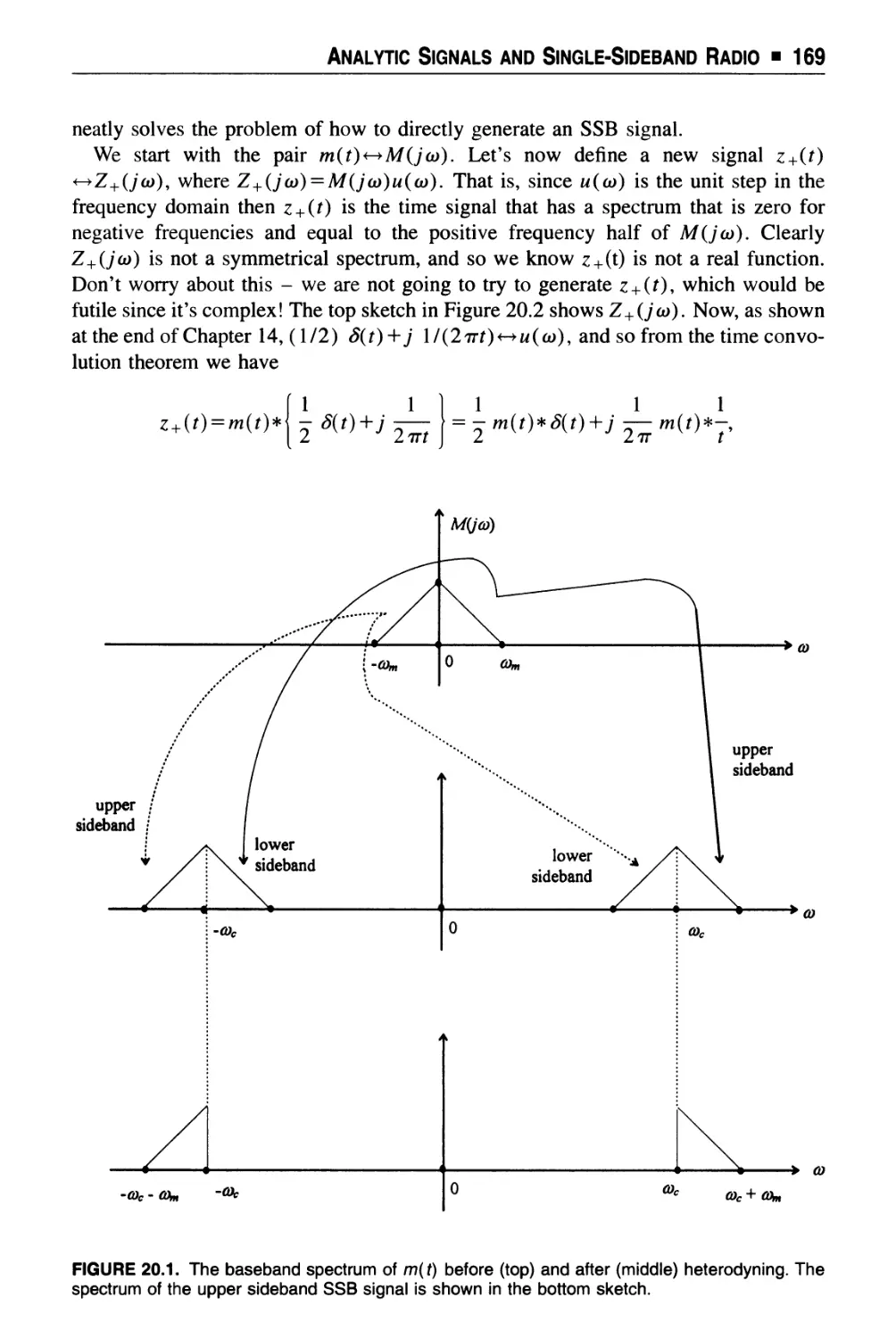
Chapter 20 Analytic Signals and Single-Sideband Radio 167
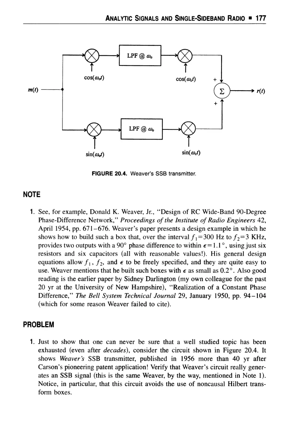
Chapter 21 Denouement 178
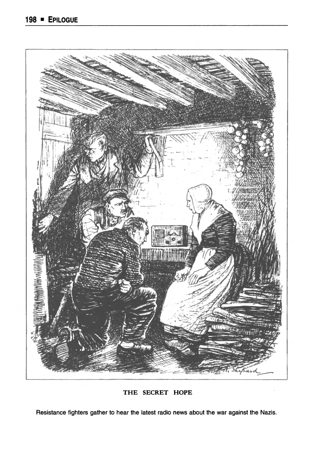
Epilogue 191
■ Technical Appendices
Appendix A Complex Exponentials 205
Appendix B What Is (and Is Not) a Linear Time-Invariant System 214
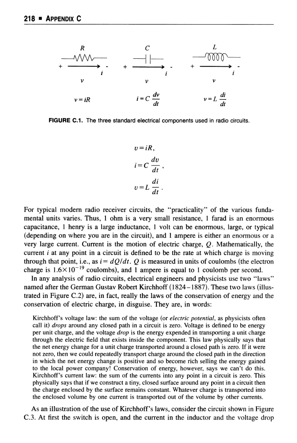
Appendix C Two-Terminal Components, Kirchhoff's Circuit Laws,
Complex Impedances, ac Amplitude and Phase Responses,
Power, Energy, and Initial Conditions 217
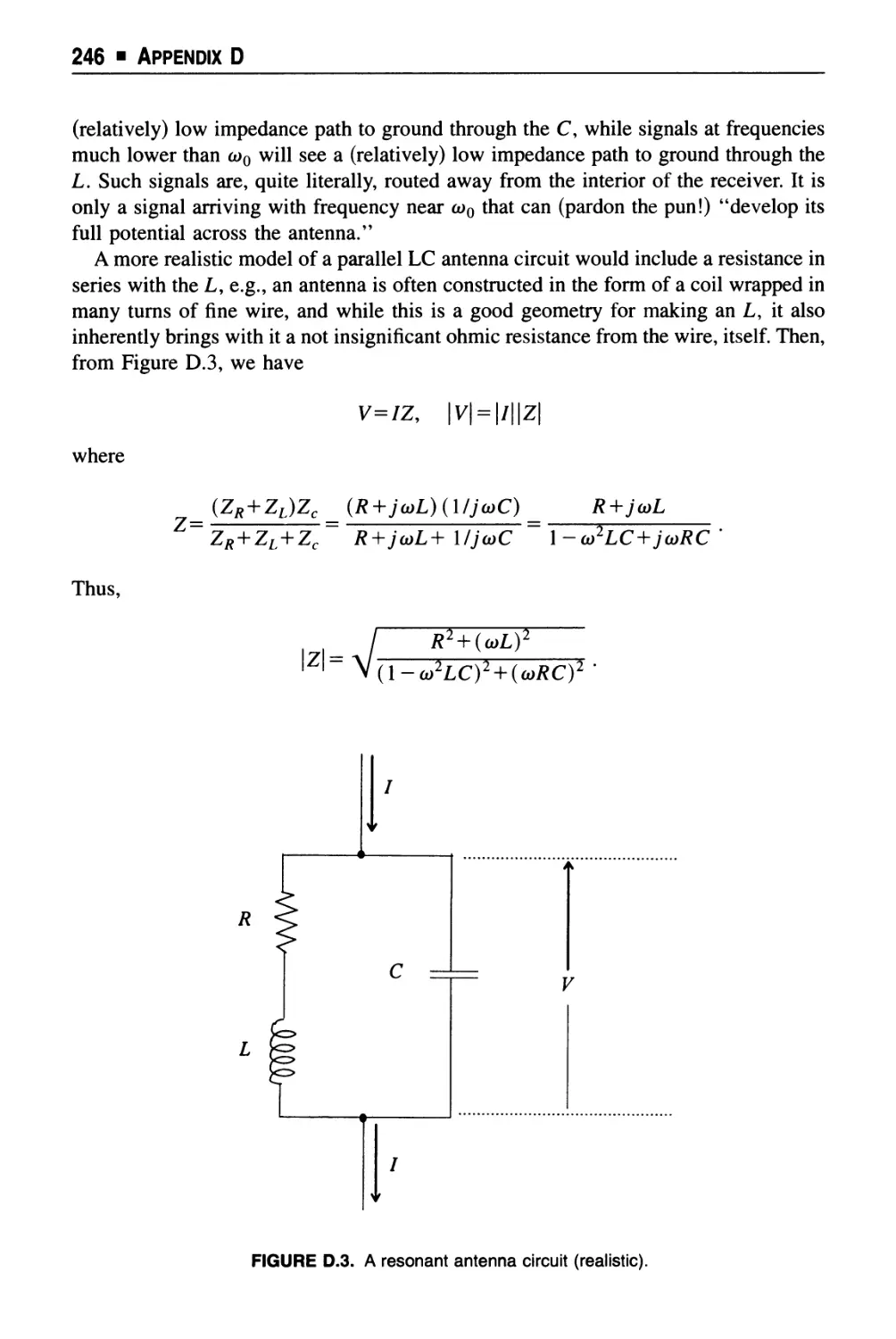
Appendix D Resonance in Electrical Circuits 244
Appendix E Reversing the Order of Integration on Double Integrals,
and Differentiating an Integral 249
Appendix F The Fourier Integral Theorem (How Mathematicians
Do It) 266
Appendix G The Hilbert Integral Transform 272
Appendix H Table of Fourier Transform Pairs and Theorems 284
Last Words 287
Name Index 289
Subject Index 293
Acknowledgments
While the actual writing of this book has been a lone effort, there are some
individuals that I do wish to particularly thank.
At one time, a dear friend of many years, Professor John Molinder at Harvey Mudd
College, and I did talk of doing something like this book together. A separation of
thousands of miles (and different professional pressures) made that not practical. Still,
John's influence over the last quarter century on my thinking about the topics in this
book has been profound. Much of what is in this book came together in my mind when,
during my sabbatical in the Fall of 1991 at Mudd, John and I team-taught E101, the
College's junior year systems engineering course. This is my opportunity to thank him
and our students for being kindred spirits in "all things convolutional".
To all my University of New Hampshire (UNH) electrical engineering students in
the sophomore circuits and electronics, and the junior networks courses (EE541, 548,
and 645), I owe much. Both for patiently (most of the time!) listening to me
occasionally grope my way to understanding what I was talking about, and for providing me
with solutions to a couple of problems I had a hard time doing (and which are now in
this book). To that I want to add a special note of appreciation to the students in my
Honors section of the EE645 networks class in the Fall of 1992, who were my test
subjects for the more advanced parts of this book.
Nan Collins, in the Word Processing Center of the College of Engineering and
Physical Sciences at UNH, has been my cheerful and always patient typist on previous
books, but she rose to new heights of professionalism (and patience) for this one.
Without her skill at transforming my scrawled, handwritten equations in smeared ink
into WordPerfect beauty, I wouldn't have had the strength to finish. All of the line
illustrations were done by my secretary Mrs. Kim Riley, whose skills in image
scanning, bit map manipulation, and keyboard virtuosity in creating WORD graphic files,
are exceeded only by her patience and good humor. My mucho sympatico friend and
UNH colleague, Professor Barbara Lerch, gave me much help by listening and
laughing with me as I read aloud the more outrageous non-technical portions of the
book, by not letting her eyes glaze over too much when I started talking equations, by
reading page proofs and preparing the Name Index, and by simply generously sharing
her time with me over countless cups of coffee.
The late Professor Hugh Aitken of Amherst College greatly influenced this book
through the historical content, and the elegant prose, of his two well-known books on
radio history. I was fortunate to enjoy a correspondence of several years with Hugh, but
I will always regret that I delayed too long in making the short drive from UNH to
■ xi ■
xii ■ Acknowledgments
Amherst. Andrew Goldstein, Curator of the Center for the History of Electrical
Engineering at Rutgers University, was most helpful in providing biographical information
on several of the more obscure personalities that appear in the book.
Three anonymous reviewers provided a number of very helpful comments on how
to make this book better. I adopted very nearly every single one of their suggestions.
I hope they will write to me so that I may thank them in a more personal way.
And finally, it has been my great pleasure to work with AIP Press' Acquisition Editor
Andrew Smith, and with my detail-conscious Production Editor Jennifer VanCura.
Bringing a technical book to completion (particularly one stuffed with mathematics) is
a little bit like bringing a new baby into the world and, like a proud father, I can say
that this book is mine. But, like any father, I am also well aware that I did not do it all
by myself.
A Note To Professors
(Students may read this, too.)
Modern-day electrical engineering academic programs are generally regarded on most
college campuses as among the toughest majors of all, but being tough doesn't mean
being the best. EE programs are tough because there is so much stuff coming at
students all the time—with no let-up for four years—that many of these students are
overwhelmed. In addition to the usual image of trying to drink from a firehose, the
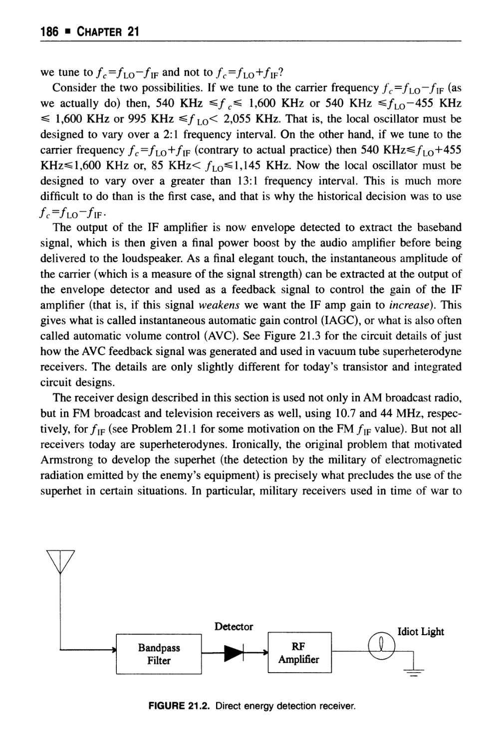
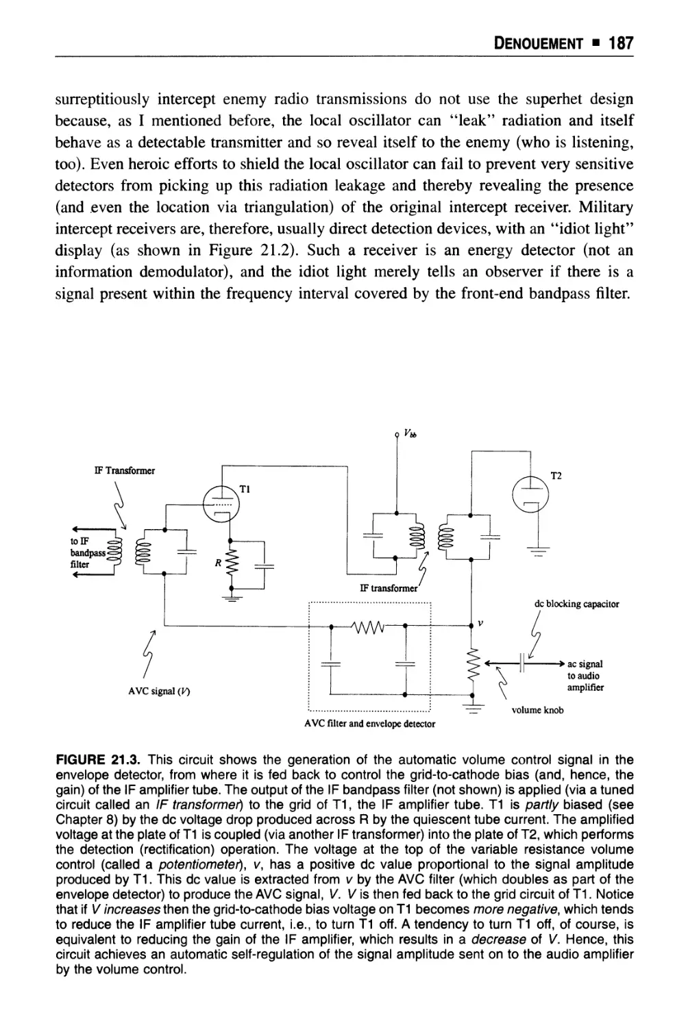
process has been likened to getting on a Los Angeles freeway at age 18, with no speed
limit or off ramps, and being told to drive or die until age 22. A lot of good students
simply run out of gas before they can finish this ordeal.
Most electrical engineering faculty are aware of the crisis in the teaching of their
discipline; indeed, each month engineering education journals in all specialties carry
columns and letters bemoaning the problem. The typical academic response is to
shuffle the curriculum,1 a lengthy and occasionally contentious process that leaves
faculty exhausted and nobody happy. And then, four or five years later, by which time
nearly everyone is really unhappy (again), the whole business is repeated. A more
innovative response, I believe, is to teach more of electrical engineering using the
"top-down," "just-in-time" approaches.
Top-down starts with a global overview of an entire task and evolves into more
detail as the solution is approached. Just-in-time means all mathematical and physical
theory is presented only just before its first use in an application of substance, i.e., not
simply as a means of working that week's turn-the-crank (often unmotivated)
homework problem set. The traditional electrical engineering educational experience is,
however, just the reverse. It starts with a torrent of mind-numbing details (hundreds of
mathematical methods, analog circuit laws, digital circuit theorems, etc., etc., one after
the other), details which faculty expect students to be able to pull out of their heads on
command (i.e., upon the appearance of a quiz sheet). Faculty, who swear by the
fundamental conservation laws of physics in the lab, oddly seem to think they can
violate them in the classroom when it comes to education. They are wrong, of course,
as you simply cannot pour 20 gallons of facts into a 1-gallon head without making a
19-gallon puddle on the floor.
And what is the reward for the agony? Sometime in the third year of this amazing
process the blizzard of isolated facts finally starts to come together with a simple
system analysis or two. In the fourth (and final) year, perhaps a simple design project
will be tackled. It seems to me to really be precious little gain for such an ocean of
■ xiii ■
xiv ■ A Note to Professors
sweat and tears. But faculty appear unmoved by the inefficiency (and the horror) of it
all. As one little jingle that all professors will appreciate (but perhaps not all students)
puts it:
Cram it in, jam it in;
The students' heads are hollow.
Cram it in, jam it in;
There's plenty more to follow.
It is strange that so many engineering professors teach this way. As M.E. Van
Valkenburg, one of the grand old men of American engineering education has
observed2: "engineers seem to learn best by top-down methods." But, except for
isolated, individual teachers going their own way, I know of not a single American
electrical engineering curriculum that is based on the top-down idea, and for a simple
reason. As Professor Van Valkenburg says: "I know of no engineering textbooks that
follow a top-down format."
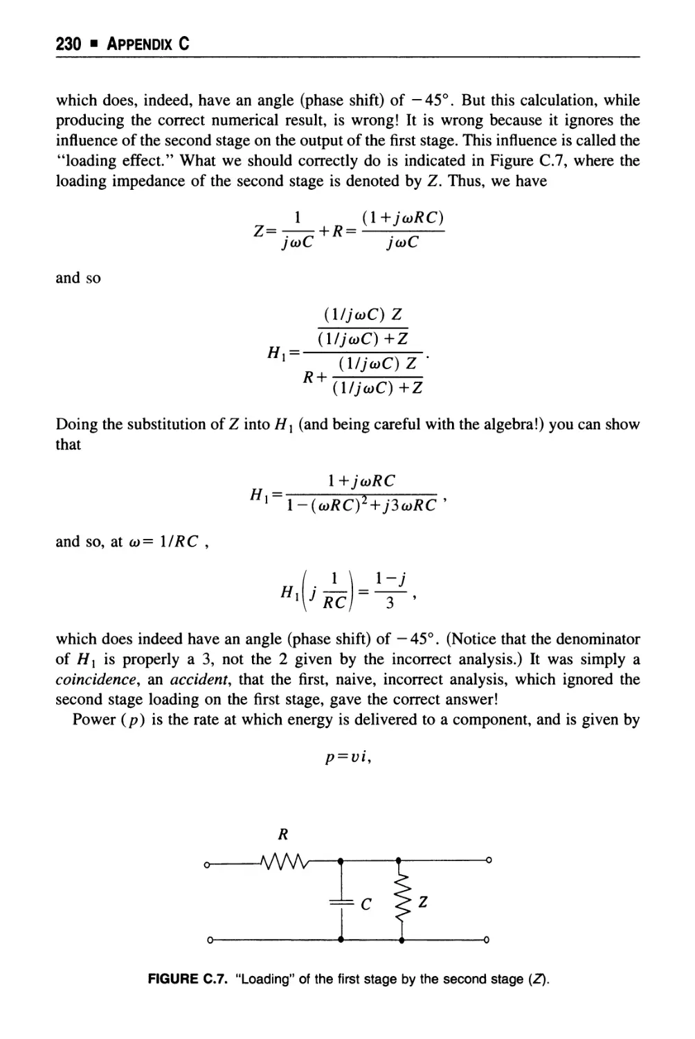
This is truly a Catch-22, chicken-and-egg situation.
There are no top-down books because there are no curricula for them, and there are
no curricula because there are no top-down books. Top-down books, in electrical
engineering, are a huge departure from presently accepted formats, and many potential
authors simply see no financial rewards in writing such books. Instead, we get yet more
books on the same old stuff (e.g., elementary circuit theory), written in the same old
way; how many ways are there, I wonder, of explaining Kirchhoffs laws!? The author
of a modern bestseller was embarrassed enough by this to write in his Preface "the
well-established practice of revising circuit analysis textbooks every three years may
seem odd," and then he went on to blame students' declining abilities for the endless
revisions and the reburying of bones from one graveyard to another. And I had always
thought it had something to do with undermining the used book market. How foolish
of me!
An example of the sort of introductory engineering book I do think worth writing is
John R. Pierce's Almost All About Waves (MIT Press, 1974), in which he ends with
"Commonly, physicists and engineers first encounter waves in various complicated
physical contexts and finally find the simple features that all waves have in common.
Here the reader has considered those simple, common features, and is prepared, I hope,
to see them exemplified [in more advanced books]." Pierce's book then, despite
Professor Van Valkenburg's assessment, was perhaps the first top-down electrical
engineering book, but published before anybody had a name for it! I view my book as a
similar radical departure from ordinary textbooks, an experiment continuing Pierce's
pioneering effort, if you will. My hope is that in years to come faculty will declare the
present state of affairs in the education of electrical engineers as having been quaint,
if not downright bizarre.
This is an attempt at a combination top-down, just-in-time "first course" electrical
engineering book, anchored to the specifics of a technical and mathematical history of
the ordinary superheterodyne AM radio receiver (which, since its invention nearly 80
years ago, has been manufactured in the billions). I have written this book for the
beginning second-year student in any major who has the appropriate math/physics
A Note To Professors ■ xv
background. As I explain in more detail in the Prologue, this means freshman calculus
and physics. To those who complain this is an unreasonable expectation in, say, a
history major, I reply that history faculties really ought to do something about that. To
allow their students to be anointed with the Bachelor of Arts, even while remaining
ignorant of the great discoveries of the 18th and 19th centuries' natural philosophers,
is as great a sin as would be committed, for example, by electrical engineering faculties
allowing their students to graduate without taking several college-level English and
history courses. There are, of course, more advanced books available to those readers
who want more electronic circuit details, but your students will not have to "unlearn"
anything from this book. I offer here what might be called an "advanced primer," with
no simplifications that will fail them in the future.
Your students will see here, for example, not only the Fourier transform but the
Hilbert transform, too, a topic not found in any previous second-year book (see
Appendix G). I have two reasons for doing this. First, and less importantly, the Hilbert
transform occurs in a natural way in expressing the constraints causality places on the
real and imaginary parts of the Fourier transform of a time signal. Second, and more
importantly, the Hilbert transform occurs in a natural way in the theoretical
development of single-sideband radio (which, in turn, is a natural development of radio theory
after AM sidebands and bandwidth conservation are discussed). This book discusses
the Hilbert transform in both applications. The issue of the convergence of the Fourier
series is given more than the usual quick nod and wink. And when I do blow a little
mathematical smoke in front of a mirror—as in the discussion of impulse functions—I
have tried to be explicit about the handwaving. I acknowledge the nontrivialness of
doing such things as reversing the order of integration in double (perhaps improper)
integrals, or of differentiating under the integral sign, two processes my experience has
shown often befuddle even the brightest electrical engineering seniors. Something in
the freshman calculus courses electrical engineers take these days simply isn't taking,
and I have tried to address that failure in this book.
To make the book as self-contained as possible, I've included brief reviews of
complex exponentials (Appendix A), of linear and time invariant systems (Appendix
B), of Kirchhoff's laws and related issues (Appendix C), and of resonance (Appendix
D) for those students who need them. These appendices are written, however, in a
manner that I think will make them interesting reading even for those who perhaps
don't actually need a review, but who nonetheless may learn something new anyway
(as in Appendix F, where even professors may see for the first time how to derive
Dirichlet's discontinuous integral using only freshman calculus).
I have also done my best to emphasize what I consider the intellectual excitement
and beauty of the history and mathematical theory of radio. I frankly admit that the
spiritual influences of greatest impact on the writing of this book were Garrison
Keillor's wonderfully funny novel of early radio, WLT, A Radio Romance (Viking,
1991),3 and Woody Allen's sentimental 1987 movie tribute to World War II radio,
Radio Days. Born in 1940, I was too young to experience first-hand those particular
days, but I was old enough in the late 1940s and early 1950s to catch the tail-end of
radio drama's so-called "Golden Age." I listened, in fascination, to more than my
xvi ■ A Note to Professors
share of "Lights-Out," 'The Lone Ranger," "Little Orphan Annie," "Yours Truly,
Johnny Dollar" (the insurance investigator with the "action-packed expense
account!"), "The Jack Benny Show," "Halls of Ivy," "Boston Blackie," "The
Shadow" and, most wonderful of all, the science fiction thriller "Dimension-X" (later
called "X-Minus One").
And I wasn't alone. As another writer has recalled4 his love of radio as a ten-
year-old in Los Angeles, listening to KHJ in 1945 (just two years before I started to
listen to the same station),
How can sitting in a movie theater or sitting on a couch before my television duplicate the
wonderful times I had when I was tucked safely in bed with the lights out listening to a
small radio present me with drama, fantasy, comedy and variety, all for free, and all of it
dancing beautifully in my imagination, day by month by year? There has never been
anything quite like it and, sadly, I must say there will never be anything like it again.
That's what radio ... and the nineteen forties meant to me.
Three Pedagogical Notes
When the writing of this book reached the point of introducing electronic circuitry
(Chapter 8), I had to make a decision about the technology to discuss. Should it be
vacuum tubes or transistors? Or both? I quickly decided against both, if only to keep
the book from growing like Topsy. The final decision was for vacuum tubes. My
reasons for this choice are both technical and historical. Vacuum tubes are single-
charge carrier devices (electrons), understandable in terms of "intuitive," classical
freshman physics. Transistors are two-charge carrier (electrons and holes) devices,
understandable really only in terms of quantum mechanics. Electrical engineering
professors have, yes, invented lots of smoke and mirror ways of "explaining" holes in
terms of classical physics, but these ways are all, really, seductive frauds. They're
good for their ease in writing equations and in thinking about how circuits work, but
even though they look elementary, I don't like to teach a first course in electrical
engineering with their use. They are really shortcuts for advanced students who have
had quantum mechanics. From a historical point of view, of course, it was the vacuum
tube that made AM broadcast radio commercially possible, and to properly discuss
the work of Fleming and De Forest, the vacuum tube is the only choice. And finally,
students should be told that the small-signal equivalent-circuit model for the junction
field-effect transistor (JFET) is identical to that for the vacuum tube triode! Plus ca
change, plus c'est la meme chose.
A second decision had to be made about the Laplace transform. Studying this
mathematical technique for solving linear constant coefficient differential equations
has traditionally been a "rite of passage" for sophomore electrical engineering
students, but I have decided not to use Laplace in this book. I have the best reason
possible for this important decision—it just isn't necessary! The Laplace transform is
without equal for situations involving transient behavior in linear systems, yes, but the
mathematics of AM radio is essentially steady-state ac theory. For that the Fourier
transform is sufficient. In this book we will never encounter time signals that don't
have a Fourier transform (we do, of course, have to use impulses in the frequency-
domain for steps and undamped sinusoids). Unbounded signals that require the
convergence factor of the Laplace transform do not play a role in this book's telling of
the development of AM radio (but the unbounded signal \t\ does have an impulsive
A Note To Professors ■ xvii
Fourier transform, and I show the reader how to derive it with freshman calculus).
After completing this book, the student will be well prepared for more advanced
studies in engineering and physics that introduce the Laplace transform.
And finally, because this book is written for first-semester sophomores, there is no
discussion that reauires knowledge of probability theory. This means, of course, no
discussion of the impact of noise on the operation of radio circuits.
As an enthusiastic supporter of early radio wrote more than twelve years before I
was born, "nothing could be creepier than human voices stealing through space,
preferably late on a stormy night with a story of the supernatural ... particularly when
you are listening alone." Now those programs are gone forever. One of the characters
in George Lucas's nostalgic tribute to radio, the 1995 film Radioland Murders, says,
"Radio will never die. It would be like killing the imagination." I'm afraid, though,
that the corpse of radio as entertainment has long been cold. As Garrison Keillor wrote
in WLT, "Radio was a dream and now it's a jukebox. It's as if planes stopped flying
and sat on the runway showing travelogues." Today's radio fare, with its rock music,
banal talk, and all-news stations endlessly repeating themselves, is a pale ghost of
those wonderful, long-ago broadcasts. But the technical wonder of radio, itself,
continues.
It was that technical wonder, in fact, that attracted so many youngsters to electrical
engineering from the 1920s through the 1960s. From building primitive radios, to more
advanced electronic kits available through the mail, right up to the early days of the
personal computer (when you could build your own), high schoolers could, before
college, get hands-on experience at what electrical engineers do. I still recall the fun I
had building a Heathkit oscilloscope in 1957, and then using it, when I was a junior in
high school. But as Robert Lucky has noted,6 the development of the totally self-
contained VLSI chip has destroyed the kit market. As he writes,
I hear that freshman enrollment in electrical engineering has been dropping steadily since
those halcyon days of [kit building]. I'm looking at my nondistinctive, keep-your-hands
off [personal computer], and I'm wondering—do you think there is any connection?
I certainly do! As another electrical engineer recently wrote7 of how the wonder of
radio changed his life,
When I was about eight years old, my uncle showed me how to build a radio out of wire
and silver rocks [crystals]. I was astounded. My dad strung a long wire between two trees
in the backyard and I sat in the back on the picnic table listening to the BBC. This is what
shaped my life and my chosen profession. I was truly a lucky child. From the time I was
eight, I knew what I would be when I grew up. I asked my dad, "What kind of guy do you
have to be if you want to work on radios?"
"An electrical engineer," Dad said.
That's what I'm going to be.
In his excellent biography of Richard Feynman, James Gleick catches the spirit of
what radio meant in its early days to inquisitive young minds:8
xviii ■ A Note to Professors
Eventually the art went out of radio tinkering. Children forgot the pleasures of opening the
cabinets and eviscerating their parent's old [radios]. Solid electronic blocks replaced the
radio set's messy innards—so where once you could learn by tugging at soldered wires
and staring into the orange glow of the vacuum tubes, eventually nothing remained but
featureless ready-made chips, the old circuits compressed a thousandfold or more. The
transistor, a microscopic quirk in a sliver of silicon, supplanted the reliably breakable
tube, and so the world lost a well-used path into science.
A couple of pages later, on the fascination of the "simple magic" of a radio set,
Gleick observes:
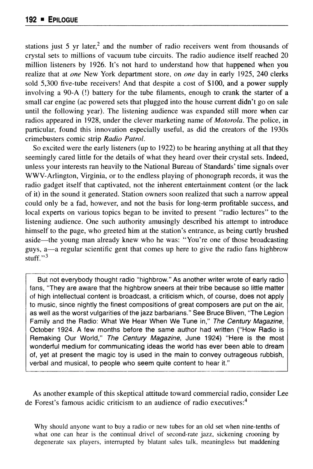
/'look here. nmX
'w*S TRAINED hundred^
\cf MEN LIKE MG TO
\yAKE GOOD MONpV
VI OuESS I'LL GET THAT
v FREE BOOK
^y, >* "•
, THIS IS SWELL FUN.
AND I AM BEGINNING
. ± TO MAKE MONEY
I 6 ON THE SIOE ALREADY
* RADIO SURE IS FULL
OF OPPORTUNITIES
FOR TRAINED MEH
GUCS5 I MAVEUT A
RIGHT TO ASK A GiRL
LIKE MARY TO MARRy
AN ORDINARY MECHANIC
YOU CERTAINLY
KNOW RADIO
MINE NEVER
SOUNDED BETTER
TO"
MM*
'C-'JjM, ITS
■fcCvOERFUL.
'«W VOL'Re
C'J Ttit WAY
»•* c- *" * f* cc
1 - w
,tcr
YES MARY. AND
THERE'S A REAL]
FUTURE FOR
US IN THIS
\RADIO FiCLD.
/'
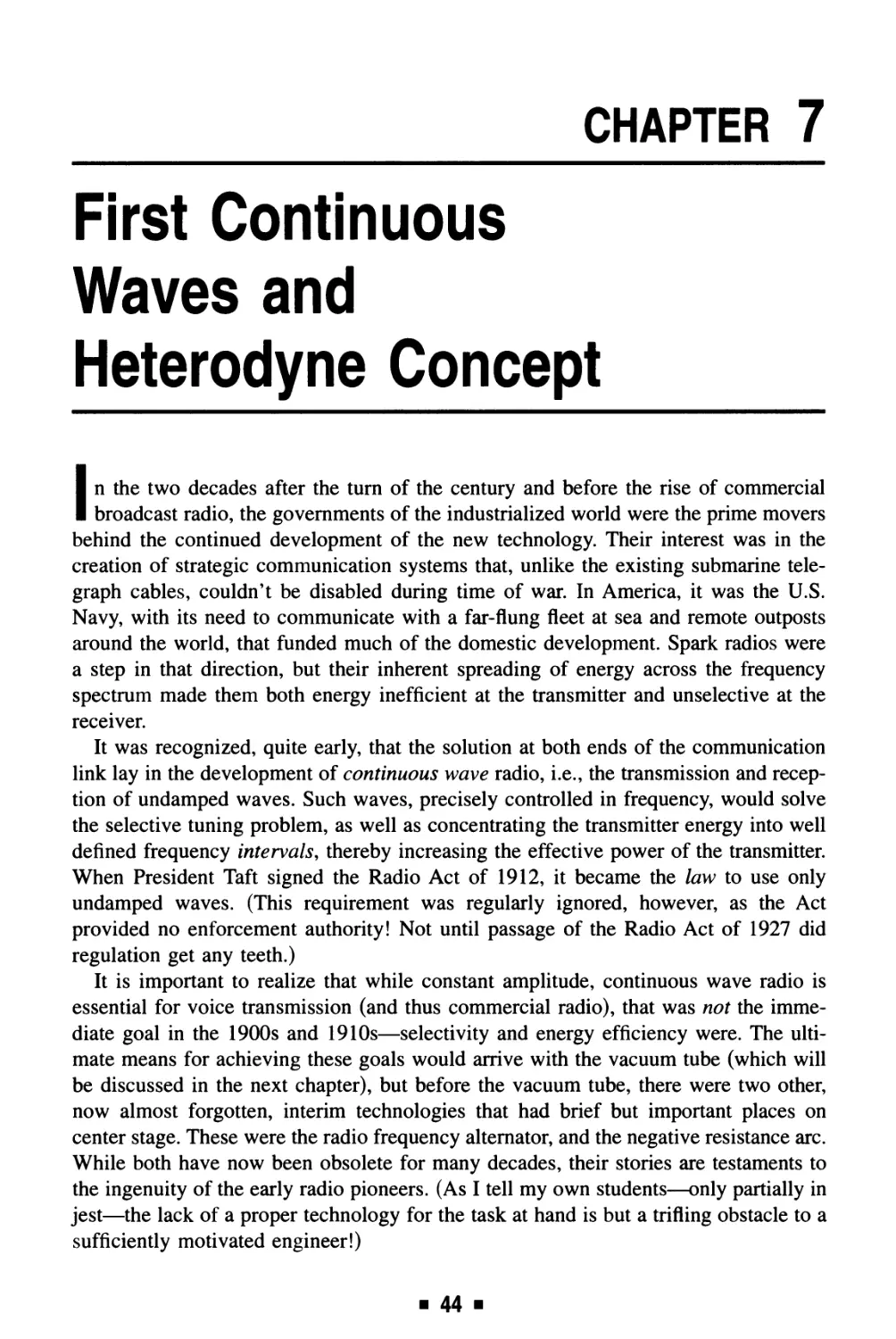
In the early days of broadcast radio, many home correspondence schools used the romantic image
of the new technology to attract students from the ranks of those who felt trapped in depression era,
dead-end jobs. One of the biggest schools was the National Radio Institute, which ran ads in the
pulp fiction magazines most likely to be read by young men. This art was part of such an ad that
appeared in the October 1937 issue of the science fiction pulp Thrilling Wonder Stories. Two other
similar pieces of art from the same time period and magazine appear later in this book, at places
where some encouragement will perhaps help motivate "sticking with it!"
A Note To Professors ■ xix
No wonder so many future physicists started as radio tinkers, and no wonder, before
physicist became a commonplace word, so many grew up thinking they might become
electrical engineers ...
Times have changed, though. In another essay9 Lucky wrote of the time he asked a
college student why she was majoring in materials engineering, rather than electrical
engineering. The student looked at him with incredulity and disdain and replied, "You
can see and touch things here." Then, with a glance (and a shiver) at the nearby
electrical engineering building, she added, "Nothing is real over there." Lucky found
he had to agree with that student's assessment; as he correctly described the state of
electrical engineering today, "Most of our stuff is made of nothing at all. It is made of
software, of math, of conceptual thought. [Electrical engineers now] live mostly in a
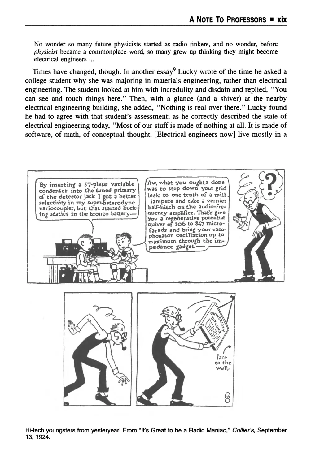
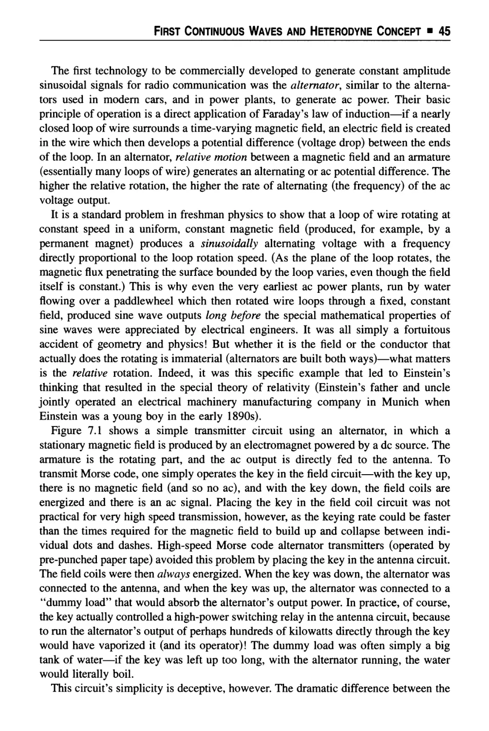
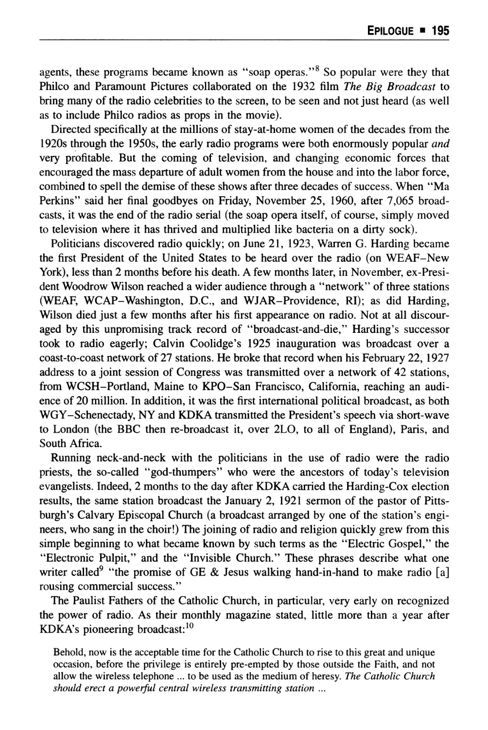
By inserting a 57-plate variable i
condenser into the tuned primary
of the detector jack I got a better
selectivity in my super-heterodyne
variocoupler, but that Started
bucking statics in the bronco battery—
1
r
_ /*
what you oughta done
was to stop down your grid
leak to one tenth of a mill
iampere and take 3 vernier
half-hitch on the audio-fre-
ovency amplifier. That'd give
you a regenerative potential
quiver of 206 to 847
microfarads and hring your caco-
phonator oscillation up to
maximum through the
impedance gadget —-
J d*l
^^ M
8
Hi-tech youngsters from yesteryear! From "It's Great to be a Radio Maniac," Collier's, September
13, 1924.
xx ■ A Note to Professors
virtual world." I have picked the AM radio receiver as the centerpiece for my
experiment in writing an introductory top-down, just-in-time electrical engineering book
because I believe it is the simplest, common household electronic device that seems
mysterious to an intelligent person upon their first encounter with it.
Consider, for example, the case of Leopold Stokowski who, when he died in 1977,
was declared (in his New York Times obituary notice) to have been "possibly the best
known symphonic conductor of all time." In an essay written for The Atlantic Monthly
("New Vistas in Radio," January 1935), Stokowski gloomily asserted "The
fundamental principles of radio are a mystery that we may never fully understand." And an
amusing story from the early days of broadcast radio has a technologically challenged
Supreme Court justice perplexed by radio. When Chief Justice William Howard Taft
was faced with the possibility of hearing arguments about the government regulation
of radio he reportedly wailed "If I am going to write a decision on this thing called
radio, I'll have to get in touch with the occult." If radio doesn't seem mysterious, then
that person simply has no imagination! But nobody can doubt, as they spin the dial,
that radio is very real. There is nothing "virtual" about it! In its own way, then, perhaps
this book (if it falls into the right hands) can spark anew a little bit of the wonder that
has been lost over the years. That, anyway, is my hope.
NOTES
1. See, for example, Robert W. Lucky, "The Curriculum Dilemma," IEEE
Spectrum, November 1989, p. 12. Lucky is an electrical engineer who, after making
impressive technical contributions to the electronic transmission of information,
moved into upper management at the AT&T Bell Laboratories.
2. In his column "Curriculum Trends," Newsletter of the IEEE Education Society,
Fall 1987. Professor Van Valkenburg is former Dean of Engineering at the
University of Illinois at Champaign-Urbana, where he continues as Professor of
Electrical Engineering.
3. The call letters WLT stand for "With Lettuce and Tomatoes," a joke based on the
fictional station being operated out of a sandwich shop! And in real life, too,
station call letters could have equally silly meanings. In Chicago, for example,
the Chicago Tribune began operating WGN—a subtle(?) plug for the "World's
Greatest Newspaper."
4. Ken Greenwald, The Lost Adventures of Sherlock Holmes, Barnes & Noble
Books 1993.
5. Roy S. Durstine, "We're On the Air," Scribners Magazine, May 1928.
6. Robert W. Lucky, "The Electronic Hobbyist," IEEE Spectrum, July 1990, p. 6.
The positive relationship between hobby activity and intellectual stimulation in
young people was recognized very early, e.g., see Howard Vincent O'Brien, "It's
Great to Be a Radio Maniac," Colliers, September 13, 1924, pp. 15-16.
A Note To Professors ■ xxi
7. Joe Mastroianni, "The Future of Ham Radio," QST, October 1992, p. 70.
8. James Glieck, Genius: The Life and Science of Richard Feynman, Pantheon,
1992, p. 17.
9. Robert W. Lucky, "What's Real Anymore?," IEEE Spectrum, November
1991, p. 6.
Prologue
"RADIO SWEEPING COUNTRY—1,000,000 sets in use"
Front-page headline, Variety (March 10, 1922)
"The air is full of wireless messages every hour of the day. In the
evening, particularly, there are treats which no one ought to miss.
Famous people will talk to you, sing for you, amuse you. YOU
DON'T HAVE TO BUY A SINGLE TICKET—You don't have to
reserve seats."
Radio ad in Scientific American (July 1922)
"One ought to be ashamed to make use of the wonders of science
embodied in a radio set, the while appreciating them as little as a
cow appreciates the botanic marvels in the plants she munches."
Albert Einstein, in his remarks opening the
Seventh German Radio Exhibition at Berlin (August 1930)
Radio is almost a miracle.
That's right—the little box by your bedside, or on the refrigerator in the kitchen, or
in the study next to the sofa, or behind the fancy buttons on the dash of your car, is an
invention of near supernatural powers. Now, quickly, before every physicist and
electrical engineer reading these words dismiss this book as the work of an academic
mystic, I wish to point out those two all-important qualifiers almost and near. The
wonder of AM (amplitude modulation) radio, in fact, can be understood through
physics and mathematics, not sorcery or theology—but that is a fact that many of my
students are not so sure about. That's why I have written this book. I want to take the
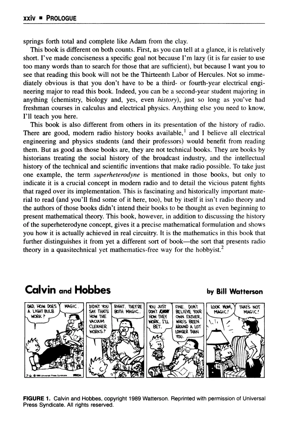
mystery, what some of my students (like Calvin's dad in Figure 1) even think of as the
spookiness, out of radio.
Well, you perhaps say, it's a little late for me to be worrying about that—there are
already plenty of books available on radio theory. That's right, there are, but for my
purposes here they have two characteristics that limit them. First, they are generally
physically big books of several hundred pages, written for advanced students in the
third or fourth year of an electrical engineering major; such books are specifically
published as textbooks. Second, they are essentially 100% theory, with very little
historical development or, even more likely, simply none at all. In those books, radio
■ xxiii ■
xxiv ■ Prologue
springs forth total and complete like Adam from the clay.
This book is different on both counts. First, as you can tell at a glance, it is relatively
short. I've made conciseness a specific goal not because I'm lazy (it is far easier to use
too many words than to search for those that are sufficient), but because I want you to
see that reading this book will not be the Thirteenth Labor of Hercules. Not so
immediately obvious is that you don't have to be a third- or fourth-year electrical
engineering major to read this book. Indeed, you can be a second-year student majoring in
anything (chemistry, biology and, yes, even history), just so long as you've had
freshman courses in calculus and electrical physics. Anything else you need to know,
I'll teach you here.
This book is also different from others in its presentation of the history of radio.
There are good, modern radio history books available,1 and I believe all electrical
engineering and physics students (and their professors) would benefit from reading
them. But as good as those books are, they are not technical books. They are books by
historians treating the social history of the broadcast industry, and the intellectual
history of the technical and scientific inventions that make radio possible. To take just
one example, the term superheterodyne is mentioned in those books, but only to
indicate it is a crucial concept in modern radio and to detail the vicious patent fights
that raged over its implementation. This is fascinating and historically important
material to read (and you'll find some of it here, too), but by itself it isn't radio theory and
the authors of those books didn't intend their books to be thought as even beginning to
present mathematical theory. This book, however, in addition to discussing the history
of the superheterodyne concept, gives it a precise mathematical formulation and shows
you how it is actually achieved in real circuitry. It is the mathematics in this book that
further distinguishes it from yet a different sort of book—the sort that presents radio
theory in a quasitechnical yet mathematics-free way for the hobbyist.
Calvin and HobbeS by Bill Watterson
FIGURE 1. Calvin and Hobbes, copyright 1989 Watterson. Reprinted with permission of Universal
Press Syndicate. All rights reserved.
Prologue ■ xxv
I have become convinced, after 25 yr of college teaching, that most electrical
engineering students spend at least three of their four undergraduate years secretly
wondering just what it is that electrical engineering is about. Their initial course work,
immense in detail but devoid of almost any sense of global direction, tells them little
about where it is all heading. My goal in this book is to develop, quickly, in the second
year of college, a start-to-finish answer-by-example of the sort of system an electrical
engineer deals with, and how it is different from what a mechanical engineer (or, for
that matter, an electrician) is normally concerned about.
I have a quick test to see if you're ready for the next 200 or so pages: Have you
studied calculus to the point of understanding the physical significance of the
derivative of a function, and the area interpretation of an integral? Can you write Kirchhoff 's
equations for electrical circuits (and solve them for "simple" situations)? Do you know
what an electron is? If you can answer yes to these questions, then you are ready for
this book.
This book takes the view that electrical engineers and physicists think with
mathematics, and a quick flip through the following pages will show just how strongly I
hold that belief. The pure historical approach is the prose approach, and while I
encourage you to read what modern historians of technology have written, prose alone
is simply not enough. There are some, however, who actually believe mathematics
somehow detracts from the inherent beauty of nature. Such people might well argue
that radio is more wonderful without mathematics, much as famed essayist Charles
Lamb declared at the so-called "Immortal Dinner." There he toasted a portrait
containing the image of Isaac Newton with words describing Newton as "a fellow who
believed nothing unless it was as clear as the three sides of a triangle, and who had
destroyed all the poetry of the rainbow by reducing it to the prismatic colors."
The "Immortal Dinner" was a party given on December 28, 1817, at the home of
the English painter Benjamin Haydon. In attendance were such luminaries as the
poets Wordsworth and Keats. Lamb was described by Haydon as having been
"delightfully merry" just before he made his toast, which I interpret to mean he was
thoroughly drunk. Certainly, if sober, an intelligent man like Lamb wouldn't have made
such a silly statement.
I don't agree with Lamb; he may have been a great writer but he evidently
understood very little about mathematics and its relationship to physical reality. My
sympathies lie instead with the "master mathematician" in H.G. Wells's powerful story, "The
Star," in which life on earth appears doomed by a cataclysmic collision with an
enormous comet. The mathematician has just calculated the fatal orbit, and gazes up at
the on-rushing mass: "You may kill me, but I can hold you—and all the universe for
that matter—in the grip of this little brain. I would not change. Even now."
Even today many professors probably don't realize that the science-and-math
curriculum of a modern undergraduate electrical engineering program is a relatively
new development. Before the second World War, electrical engineering education was
xxvi ■ Prologue
heavily dominated by nuts-and-bolts technology (e.g., power transmission, and ac
machinery), and tradition (e.g., surveying and drafting). Back in the 1920s and 1930s,
many faculty were convinced that electrical engineers didn't need to know Maxwell's
equations in vector form unless they were going to be PhDs. As a specific example of
what I mean, let me quote from the 1938 book Fundamentals of Radio, by Frederick
E. Terman, then a professor of electrical engineering at Stanford (later Dean of
Engineering, and even later Provost). The chapter on antennas opens with this astonishing
statement: "An understanding of the mechanism by which energy is radiated from a
circuit, and the derivation of equations for expressing this radiation quantitatively,
involve conceptions that are unfamiliar to engineers." No electrical engineering
textbook on radio theory (including this one!) could be published today that made such an
assertion, but in 1938 Terman knew his audience. It was only in graduate school, in
those days, that you could perhaps find an electrical engineer who knew how to solve
Maxwell's equations for the electromagnetic fields inside a waveguide, or how to
calculate the probability density function of the sum of random variables. Today, that
sort of thing is required junior year material. But before the war it wasn't, and when the
war came with its dramatic need for technical people able to apply basic science
principles and high-level mathematics to new problems that didn't have "cookbook"
solutions, most electrical engineers simply came up short. It was found, for example,
that physicists were far better equipped to handle the technical challenges of not only
the atomic bomb, but of microwave radar and the radio proximity fuse, too. Physicists,
of course, have delighted for decades in telling this story. (Electrical engineers can
salvage some pride, however, in knowing that the Director of the Office of Scientific
Research and Development, with oversight of all war research, was the MIT electrical
engineer Vannevar Bush, who reported directly to President Franklin D. Roosevelt.)
That painful, embarrasing lesson wasn't lost on electrical engineering faculties and
after the war, great educational changes were made. One of the personal side benefits
of writing this book, however, is the opportunity it gives me to tell students that radio
was developed almost entirely by electrical engineers [and even one electrical
engineering student—Edwin H. Armstrong (1890-1954) who, in 1912 while an
undergraduate at Columbia University, invented the regenerative feedback amplifier and
oscillator]. These were men who received their formal training in electrical engineering
and who called themselves electrical engineers, not physicists.
One of the early "modern" pioneers of radio was Armstrong's friend Louis A.
Hazeltine (1886-1964), who invented the neutrodyne radio receiver in 1922. Hazeltine
was a professor of electrical engineering at the Stevens Institute of Technology in
Hoboken, New Jersey, until his "retirement" in 1925 (years later Stevens reappointed
him as a professor of mathematical physics). In an interview article that appeared in
Armstrong was also the inventor of the superheterodyne radio receiver, later
became a full professor of electrical engineering at Columbia and, if anyone deserves
the title, was the "Father of Modern Radio." And yet, even though he could read an
equation as well as most electrical engineers, he always retained a cautious
skepticism about too much reliance on mathematics. For Armstrong, physical experiment
Prologue ■ xxvii
was the bottom line. In his later years, after he'd demonstrated frequency modulated
(FM) radio was useful even though some mathematically inclined engineers had
declared it wasn't, Armstrong set the record straight in a paper that must have
surprised a few people: "Mathematical Theory vs. Physical Concept," FM and
Television, August 1944.
the October 1927 issue of Scientific American, the central point was that Hazeltine did
"all his creative work with a notebook, a fountain pen and a slide rule, thus avoiding
trial and error methods." So innovative and striking did the magazine find this
(contrasting greatly with the by then near-mythical Edisonian method of "try
everything until you trip over the answer") that the interview's headline boldly declared, "A
College Professor Solves a Mathematical Problem and Becomes a Wealthy Inventor."
When asked what was the secret of his success, Professor Hazeltine responded, "the
first requisite is a thorough knowledge of fundamental principles."
The late Richard Feynman (who as a boy had a reputation for being a formidable
"fixer of busted radios,"3 and who shared the 1965 Nobel prize in physics) was
agreeing with Hazeltine when he said {The Character of Physical Law, MIT, 1965): "It
is impossible to explain honestly the beauties of the laws of nature [to anyone who
does not have a] deep understanding of mathematics." But keep in mind my promise
that your mathematics, here, doesn't have to be all that deep; just freshman calculus.
(Now and then I do mention such advanced mathematical ideas as contour integration
and vector calculus', but these are never actually used in the book, and are included
strictly for intellectual and historical completeness.)
Still, Lamb's ill-advised praise for technical ignorance dies hard. The Pulitzer Prize-
winning Miami Herald humorist Dave Barry once described how radio works: "by
means of long invisible pieces of electricity (called 'static') shooting through the air
until they strike your speaker and break into individual units of sound ('notes') small
enough to fit inside your ear!" Barry was of course merely trying to be funny, but I
suspect not just a few of his readers either took him at his word, or believe in some
other equally bizarre "explanation."
This book will not correct all the weird misconceptions about radio held by the
"average man on the street," but I hope it will help engineering and science students
who also don't yet quite have it all together. All too often I've had students come to me
and say things like: "Professor, I've just had a course in electromagnetic field theory
and learned how to solve Maxwell's equations inside a waveguide made of a perfect
conductor and filled with an isotropic plasma. I know how Maxwell 'discovered' radio
waves in his mathematics. There are just two things left I'd really like to know: what
is actually happening when a radio antenna radiates energy, and how does a receiver
tune in that energy?"
The plea in those words reminds me of an anonymous bit of doggerel I came across
years ago, while thumbing through the now defunct British humor magazine, Punch.
Titled "A Wireless Problem," it goes like this:4
xxviii ■ Prologue
Music, when soft voices die,
Vibrates in the memory,
But where on earth does music go
When I switch off 2LO?
"2LO" refers to the call letters of the first London radio station (operating at 100 W
from the roof of a department store!), which went on the air in August 1922 at a
frequency of 842 KHz. Just to be sure this notation is clear, "KHz" stands for kilohertz
(and "MHz" denotes megahertz), where hertz is the basic unit of frequency. Just to
show what an old foggy I am, let me loudly state here that the old frequency unit of
cycle per second was perfectly fine! The most logically named radio station I know of,
Radio 1212, used its very frequency as its identification. Radio 1212 was an
American clandestine instrument of psychological warfare against the German
population and regular army troops in the second World War. It operated on a frequency
of 1212 KHz, or 1.212 MHz.
I know what such puzzles feel like, too! I went to a good undergraduate school, with
fine professors, who showed me how to cram my head full of all sorts of neat technical
details; but when I received my first engineering degree I still didn't know, at the
intuitive, gut level, what the devil was really going on inside a kitchen radio. That, like
my thickening girth and thinning hair, came with time.
Today, the ordinary kitchen radio is so common that we take it for granted, and find
it hard to appreciate what an enormous impact it had (and continues to have) on society
and on individuals, too. It is perhaps the single most important electronic invention of
all, surpassing even the computer in its societal impact (the telephone doesn't depend
on electronics for its operation, and television is the natural extension of radio—one
name for it in the 1920s was "radiovision" indeed, television's video and audio signals
are AM and FM radio, respectively). Even if we drop the "electronic" qualifier, even
then only the automobile can compete with radio in terms of its effect on changing the
very structure of society. One of history's greatest intellects took time off from his
physics to comment on this. The last quote that opens this Prologue is from Einstein's
opening address to the 1930 German Radio Exhibition. In that same address he also
stated,5 "The radio broadcast has a unique function to fill in bringing nations together
... Until our day people learned to know each other only through the distorting mirror
of their own daily press. Radio shows them each other in the liveliest form ..."
Because we take radio for granted, many simply don't appreciate how young is
radio. Just think—there was no scheduled radio until the Westinghouse-owned station
KDKA-East Pittsburgh broadcast (with just 100 W) the Harding-Cox presidential
election returns on November 2, 1920! And it wasn't until nearly 2 yr later that
commercial radio (i.e., broadcasts paid for by sponsors running ads) appeared on
WEAF-New York. There are many people still alive today who were teenagers (even
college students perhaps like you) before the very first regular radio programs for
Prologue ■ xxix
entertainment were broadcast. The very first, when movies were still silent and long
before music videos, laser discs, and computer games. Some of these people have
While November 2, 1920 is the traditional date of the "start" of broadcast radio, the
real history is actually a bit more complex. 8MK-Detroit (later WWJ) had been on the
air regularly 2 months before KDKA, and two AT&T experimental stations (2XJ-Deal
Beach, NJ and 2XB-New York) had been transmitting to all who cared to listen since
early 1920. And years before, in 1916, 2ZK-New Rochelle, NY was regularly broad
casting music. And years before that, in 1912, KQW-San Jose, CA could be heard
regularly in earphones. About that same time, Alfred Goldsmith, a professor of
electrical engineering at the City College of New York, who later was chief consulting
engineer to RCA, operated the broadcast station 2XN. What set KDKA apart from all
those earlier efforts (besides being the first station to receive a U.S. Government
license), however, was its owner's intent to provide a freely available commodity
(radio transmissions) that would induce the purchase of a product (radio receivers)
made by that same owner (Westinghouse). Later, this striking concept would be
replaced by an even bolder one. As the price of radio sets dropped (and thus their
profit margins), the sale of receivers as a direct producer of corporate wealth became
inconsequential, i.e., kitchen and bedroom radios today aren't worth fixing and have
literally become throwaway items. What has become profitable to sell is the radio
time, itself, i.e., advertising (in 1922 the rate was just ten dollars a minute). Or so is
the case in America—in England, where radio is a state-controlled monopoly
broadcasting costs are covered by listener-paid fees (an approach considered, but
rejected, in the early days of American radio—see R.H. Coase, British Broadcasting,
Longmans, Green and Co., 1950). For a discussion of the early concerns over
whether American radio should be public or private, see Mary S. Mander, 'The Public
Debate about Broadcasting in the Twenties: An Interpretive History," Journal of
Broadcasting 28, Spring 1984, pp. 167-185.
never forgotten how radio affected them. One of them, R.V. Jones, recalled it this way:6
There has never been anything comparable in any other period of history to the impact of
radio on the ordinary individual in the 1920s. It was the product of some of the most
imaginative developments that have ever occurred in physics, and it was as near magic as
anyone could conceive, in that with a few mainly home-made components simply
connected together one could conjure speech and music out of the air.
One of America's most famous radio sportscasters, Walter ("Red") Barber, who
started his career at the University of Florida's 5,000-W station WRUF while a student
in 1930, put it much the same way (The Broadcasters, Dial, 1970):
Kids today flip on their transistor radios without thinking ... and take it all for granted.
People who weren't around in the twenties when radio exploded can't know what it
meant, this milestone for mankind. Suddenly, with radio, there was instant human
communication. No longer were our homes isolated and lonely and silent. The world
xxx ■ Prologue
came into our homes for the first time. Music came pouring in. Laughter came in. News
came in. The world shrank, with radio.
And John Archibald Wheeler, Feynman's graduate advisor more than half a century
ago (and today an emeritus professor of physics at Princeton University), a few years
ago recalled7 his fascination with radio at age 13 (in 1924):
Living in the steel city of Youngstown, Ohio, I delivered The Youngstown Vindicator to
fifty homes after school. A special weekly section in the paper reported the exciting
developments in the new field of radio, including wiring diagrams for making one's own
receiver. And my paper-delivery dollars made it possible for me to buy a crystal, an
earphone, and the necessary wire. The primitive receiver that I duly assembled picked up
the messages from KDKA ... what joy!
Other listeners like Wheeler just couldn't get enough of radio (radio was such a rage
in the 1920s it even inspired a movie—the 1923 Radio-Mania, in which the hero tunes
in Mars!) The following is typical of the letters8 that poured into early broadcasting
stations:
I am located in the Temegami Forest Reserve, seven miles from the end of steel in
northern Ontario. I have no idea how far I am from [you], but anyway you come in here
swell ... Last week I took the set back into the bush about twenty miles to a new camp ...
Just as I thought—in you came, and the miners' wives tore the head-phones apart trying
to listen in at once. I stepped outside the shack for a while, while they were listening to
you inside. It was a cold, clear, bright night, stars and moon hanging like jewels from the
sky; five feet of snow; forty-two below zero; not a sound but the trees snapping in the
frost; and yet... the air was full of sweet music. I remember the time when to be out here
was to be out of the world—isolation complete, not a soul to hear or see for months on
end; six months of snow and ice, fighting back a frozen death with an ax and stove wood,
in a seemingly never-ending battle. But the long nights are long no longer—you are right
here ... and you come in so plain that the dog used to bark at you ... He does not bark any
more—he knows you.
In its earliest days, radio spoke to the masses who couldn't read, both the millions
of new immigrants and the simply uneducated. But radio had enormous power over all
(see Figure 2), even the educated, multigenerational American. Any who doubt this
need only read the front-page headlines of almost any newspaper in the land for the
morning of October 31, 1938. That was the "morning-after" of Orson Welles's CBS
radio dramatization, on his Mercury Theatre, of H.G. Wells's 1898 novella The War of
the Worlds. As listeners tuned in to the previous evening's Halloween eve, coast-to-
coast broadcast, they heard the horrifying news: Martians had invaded the earth, their
first rockets landing in the little town of Grovers Mill near Princeton, New Jersey!
Hundreds were already dead! Panic and terror literally swept the nation. Radio had
spoken, and people believed.9
The continuing importance of radio, even in the modern age of the ubiquitous
television set, was specifically acknowledged in a recent editorial in The Boston Globe.
Published on August 21, 1991, two days after a powerful hurricane had blown through
Prologue ■ xxxi
i
-jwi'-jh
m
t "'^k, Iff' * ^\
*-. i
C
1,1 *-K I
^Wi^,? l '■ "+x
':*M
«i
I'j i
i ji * . 7' ''""I
' .. %fc- Lea
rllNf/nPll',ll!iJ-
Mi'lll
■fel;.
-111--=¾ , 'III i^ tit
L
VL'/
V**E.
v6> s&...
: '-m~ " ■■----^ "'"''''"'-i"id,,//'Mi
V
)"l
■.w>.
/ /
' Hi
Boawc '
HwrtT ■
V
FIGURE 2. "When Uncle Sam Wants to Talk to All the People." From the May 1922 Issue of Radio
Broadcast.
xxxii ■ Prologue
New England at the same time the second Russian revolution was blowing the Soviet
Union away, "The Power of Radio" declared:
Thousands of New Englanders, darkened by the power blackouts, got much of their news
about the Gorbachev ouster and Hurricane Bob from battery-operated radios. It was a
reminder of the immediacy and power of this medium ... Television pictures are attention
grabbing, but the true communications revolution occurred not when the first TV news
was broadcast but a generation earlier, when radio discovered its voice.
Calvin's dad thought electric lights and vacuum cleaners to be magic, and radio
would surely be supermagic to him. This is really just another form of the famous
"Clarke's Third Law" (after science fiction writer Arthur C. Clarke): "Any sufficiently
advanced technology is indistinguishable from magic." A superheterodyne radio
receiver would have been magic to the greatest of the Victorian scientists, including
James Clerk Maxwell himself, the man who first wrote down the equations that give
life to radio. In the Middle Ages such a gadget would have gotten its owner burned at
the stake—what else, after all, could a "talking box" be but the work of the Devil? I
hope that when you finish this book, however, you'll take Calvin's mom's advice,
forget magic, and agree with me when I say: radio is better than magic!
NOTES
1. I have in mind Susan Douglas's Inventing American Broadcasting, 1899-1922,
Johns Hopkins 1987, the two volumes by Hugh Aitken, Syntony and Spark: The
Origins of Radio, Wiley, 1976 and its sequel The Continuous Wave: Technology
and American Radio, 1900-1932, Princeton, 1985, and George H. Douglas's The
Early Days of Radio Broadcasting, McFarland, 1987. Also recommended is the
biographical treatment by Tom Lewis, Empire of the Air: The Men Who Made
Radio, Harper, Collins, 1991.
2. An excellent example of such a book (which I highly recommend) is Joseph J.
Carr, Old Time Radios! Restoration and Repair, TAB, 1991.
3. See Feynman's funny recounting of how some common sense could go a long
way in fixing a radio in the 1920s and 1930s, in his autobiographical essay "He
Fixes Radios by Thinking!" (in Surely You're Joking, Mr. Feynmanl, W.W.
Norton, 1985).
4. Punch, May 25, 1927, p. 573.
5. Quoted from an article on the front page of The New York Times, August 23,
1930.
6. In his exciting memoir, Most Secret War, Hamish Hamilton, 1978. Jones was a
key player in British Scientific Intelligence during the Second World War. It was
Jones who, in Winston Churchill's words, "broke the bloody [radio] beam" used
by the Germans as an electronic bombing aid during the Battle of Britain.
7. In his book A Journey into Gravity and Spacetime, Scientific American Library,
1990. Norman Rockwell's May 20, 1922 cover on The Saturday Evening Post
also captured the wonder of early radio, showing an elderly couple (who appear
Prologue ■ xxxiii
to have been born about 1850, when Maxwell was still a teenager) listening to a
radio in amazement even as the future Professor Wheeler delivered his papers.
8. Quoted from Bruce Barton, "This Magic Called Radio," The American
Magazine, June 1922.
9. An interesting treatment of this amazing event in radio history (along with a
complete text of the radio play) is in Howard Koch's The Panic Broadcast, Little,
Brown, 1970. Koch, not Orson Welles, was the actual writer of the play, titled
"Invasion from Mars."
Section 1
Mostly History and a Little Math
CHAPTER 1
Solution to
an Old Problem
Speech is one of the central characteristics that distinguishes humans from all the
other creatures on Earth. There are other means of communication, of course, as
anyone who has shared living space with a cat knows, but even the closest human-cat
relationship always ends with the puzzle of 'I wonder what that darn cat is thinkingV
You cannot simply ask the cat; it simply does not know how to answer. You can ask
another human.
Along with this ability to communicate by speech, it seems to be the case that most
humans have a powerful desire to actually do so—and with as many fellow humans as
possible! Before Alexander Graham Bell's invention of the telephone in 1876,
'realtime' speech communication was limited to how loudly you could shout (and how well
the other fellow could hear). Long-distance communication required the written word
or the telegram. And even in the case of the telegraph, which required the use of
intermediaries (telegraph operators and delivery boys), communication wasn't
'realtime.'
With the telephone, however, everything changed. By 1884, with the completion of
one of the earliest long-distance circuits, a husband in Boston could actually talk,
instantly, with his wife in New York! Contrary to what most people today believe,
however, the early telephone was not limited to simple point-to-point, one-on-one
communications. Today we are familiar with such concepts as conference calls,
broadcast advertising, and subscription stereo music (e.g., the innocuous background noise
on telephones when you're put on hold, riding in elevators, and waiting in doctors'
offices), but we all too quickly assume these applications of broadcasting are inherent
to modern radio. That is simply not true. All these concepts quickly achieved reality
with the use of the telephone, all as a means to satisfy an apparently quite basic human
desire: to instantaneously communicate with large numbers of other people for either
entertainment or profit (or both).
A cartoon published in an 1849 issue of Punch indicated that even at that early date
the telegraph, not the telephone, was being used to transmit music over long distances
by unnamed experimenters in America. The text accompanying the illustration stated
"It appears that songs and pieces of music are now sent from Boston to New York by
Electric Telegraph...It must be delightful for a party in Boston to be enabled to call
upon a gentleman in New York for a song." Unfortunately, no specifics were given
■ 3 ■
4 ■ Chapter 1
about who was doing this. Certainly by 1874 the American inventor Elisha Gray had
conducted tests of such telegraphic "electroharmonic" broadcasting.
Later, in 1878, live opera was transmitted over wire lines to groups of listeners in
Switzerland,1 and in 1881 the French engineer Clement Ader (1840-1925) wired the
Paris Opera House with matched carbon microphone transmitters and magneto
telephone receivers to allow stereo listening from more than a mile away. In 1893 wired
broadcasting was a booming commercial business in Budapest, Hungary, with the
operation of the station Telefon-Hirmondo ("Telephonic Newsseller"). With over
6,000 customers, each paying a fee of nearly eight dollars a year, and with an
advertising charge of over two dollars a minute, this was a big operation. The station
employed over 200 people and was 'on the air' with regular news and music
programming 12 hours a day. A similar operation appeared in London in 1895 under the control
of the Electrophone Company. By 1907 it had 600 individual subscribers, as well as 30
theaters and churches as corporate customers, all linked with 250 miles of wired
connections! Such regular wired broadcasting, suggestive of today's cable television,
didn't appear in America until after the turn of the century. Some individual special
events, however, were covered by wired broadcasts in the last decade of the 19th
century; for example, the Chicago Telephone Company broadcast the Congressional
and local election returns of November 1894 by wire, reaching an audience that may
have exceeded 15,000.
Still, while representing a tremendous engineering achievement, wired broadcasting
was simply too cumbersome, inconvenient, and expensive in hardware for commercial
expansion beyond local distances. A way to reach out on a really wide scale, without
having to literally run wires to everyone, was what was needed. As a first step toward
this goal, at least two imaginative American tinkerers looked to space itself as the
means to carry information. These two men, Mahlon Loomis (1826-1886), a
Washington, DC dentist, and Nathan Stubblefield (1859-1928), a Kentucky melon farmer,
both constructed wireless communication systems that used inductive effects. Such a
system uses the energy in a new-propagating field (the so-called induction or 'near'
field); while wireless in a restricted sense, such a system is really not radio. The story
of Loomis' system, which used a kite to loft an antenna over the Blue Ridge Mountains
of Virginia in 1866, is shrouded in some mystery. He did, apparently, achieve a crude
form of wireless telegraphy.3 The story of Stubblefield is better documented and there
is little doubt that he actually did achieve wireless voice transmission as early as 1892.4
Neither man, however, had built a radio which utilized high-frequency electromagnetic
energy radiating through space.
That historic achievement was the success of the Italian Guglielmo Marconi (1874—
1937), who used a pulsating electric spark to generate radio waves and used these
waves to transmit telegraphic Morse code signals. Marconi's system used a true
radiation effect,6 and he could transmit many hundreds of miles; in theory, the transmission
distance is unlimited. One human could at last, in principle, speak to every other
human on earth at the same time. Marconi's work, for which he shared the 1909 Nobel
Prize in physics, was the direct result of the experiments of the tragically fated German
Heinrich Hertz (1857-1894), which were performed in a search for the waves
Solution to an Old Problem ■ 5
predicted by the theory of the equally grim-fated5 Scotsman James Clerk Maxwell
(1831-1879). This theoretical work, among the most brilliant physics in the history of
science, is described in the next section.
The claim sometimes made that the Russian Alexander S. Popov (1859-1905)
invented radio is important to mention here. Popov's work is perhaps less appreciated
than Marconi's because of the excessive zeal of the old Soviet state in claiming
everything was invented by Russians. There is, however, evidence that Popov did in
fact do much independent work that closely paralleled Marconi's, and that Popov was
actually the first to fully appreciate the value of (and to use) an antenna. Oddly
enough, Popov's use of large antennas was based on his incorrectview that wireless
communication had to be line-of-sight. When asked in 1901 about Marconi's claim to
have signaled across the Atlantic, for example, he replied that he had his doubts—
Popov thought such a feat would require fantastically tall antennas to satisfy the
(false) line-of-sight requirement. This, and other observations, are in an essay by the
Russian historian K.A. Loffe, "Popov: Russia's Marconi?" Electronics World and
Wireless World, July 1992. And finally, let me make the personal observation that
Marconi's Nobel prize is one of those very occasional ones that looks increasingly
less deserved with time. Certainly the fundamental theoretical physics that underlies
radio is due to Maxwell, while it was Hertz who did the basic engineering of spark gap
transmitters and receivers. And it was the English scientist Oliver Lodge (1851-1940)
who has priority in developing the fundamental ideas of frequency selective circuits to
implement tuning among multiple signals. By 1909 both Maxwell and Hertz were long
dead, and the prize is never given posthumously. But Lodge was alive—so why did
Marconi get the Nobel prize? The answer may lie buried beneath nearly a century's
weight of paper in the archives of the Nobel committee, but there can be no question
that politics and self-promotion played very big roles. Marconi was certainly a
successful businessman, but that ain't physics! For more on this, see my book Oliver
Heaviside, Sage in Solitude, IEEE Press 1988, pp. 263, 278, and 281.6
I can not resist concluding this chapter with an amusing summary of radio history,
written by two lawyers(!), that has recently appeared.7 Their book is actually quite
interesting, but at one point they say, in a footnote (p. 47), "Once Marconi invented the
wireless telegraph [then] creating radio and television were comparatively simple
engineering tasks." This is simply not so. What it actually required to get from
Marconi's brute force spark gap radio to Armstrong's beautiful superheterodyne radio were
conceptions of pure genius.
NOTES
1. See Elliott Sivowitch's two articles "Musical Broadcasting in the 19th Century,"
Audio, June 1967, pp. 19-23, and "A Technological Survey of Broadcasting's
'Pre-History,' 1876-1920," Journal of Broadcasting 15, Winter 1970-71, pp.
1-20.
2. Such induction communication was well-known in the early 1890s; see, for
6 ■ Chapter 1
example, the letter by E.A. Grissinger in Electrical World 24, November 10,
1894, p. 500.
3. See Otis B. Young, "The Real Beginning of Radio: the neglected story of Mahlon
Loomis," Saturday Review, March 7, 1964, pp. 48-50.
4. See Thomas W. Hoffer, "Nathan B. Stubblefield and His Wireless Telephone,"
Journal of Broadcasting 15, Summer 1971, pp. 317-329. More on Loomis is in
this article, as well.
5. Hertz and Maxwell both died young, in agony; Hertz of blood poisoning after
enduring several operations for terrible jaw, teeth, and head pains, and Maxwell
after long months of suffering from abdominal cancer.
6. For more on Marconi and Lodge, and who did what, when, see Sungook Hong,
"Marconi and the Maxwellians: The Origins of Wireless Telegraphy Revisited,"
Technology and Culture 35, October 1994, pp. 717-749.
7. Thomas G. Krattenmaker and Lucas A. Powe, Jr., Regulating Broadcast
Programming. MIT and AEI Presses 1994.
CHAPTER 2
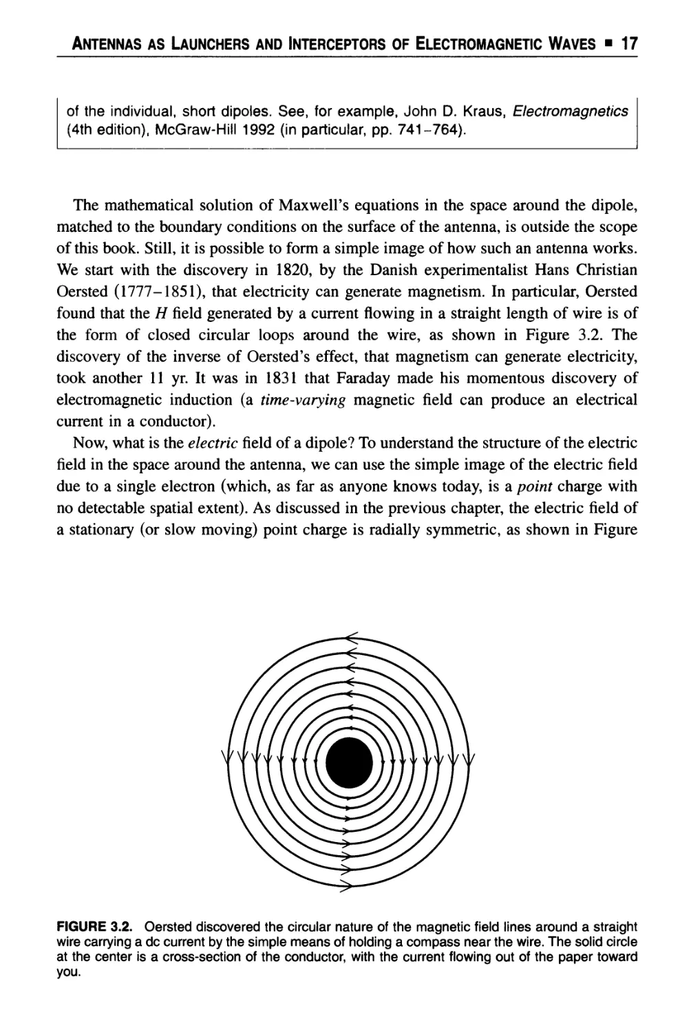
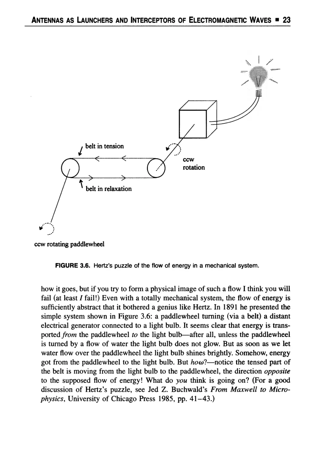
Pre-Radio History
of Radio Waves
As of the middle of the 19th century, scientific knowledge of electricity and
magnetism was mostly a vast collection of experimental observations. There had
been few previous theoretical analyses of electricity, with Germany's Wilhelm Weber's
(1804-1891) incorrect extension of Coulomb's inverse-square force law in the 1840s
(to include velocity and acceleration dependency) indicative of the state-of-the-art. The
greatest electrical experimentalist of the day was Michael Faraday (1791-1867), a man
of intuitive genius who invented the idea of the field; but he was also a man totally
unequipped for the enormous task of translating a tangle of experimental data into a
coherent mathematical theory.
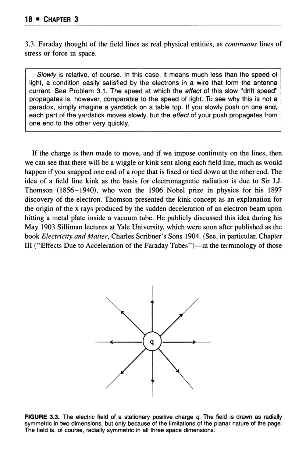
Given a point electric charge, Faraday thought of the space around the charge as
permeated with a spherically symmetric field of radial electric lines of force (pointing
away from a positive charge and pointing towards a negative charge). A positive
(negative) charge in the field of another charge experiences a force in the direction
(opposite to the direction) of the field. Faraday visualized a field of magnetic lines of
force around a magnet, beginning on the North pole and terminating on the South
pole (as beautifully displayed by iron filings on a piece of paper placed over the
magnet). These lines of force were mechanically interpreted by Faraday who thought
of them as stress in the ether, a mysterious substance once thought to fill all space.
As Faraday stood perplexed among a multitude of apparently unconnected facts, two
new players appeared on the scene, each armed with the mathematical skills Faraday
lacked. These two Scotsmen, William Thomson (1824-1907) and his younger friend
James Clerk Maxwell, had both made it their goal to find the unifying theoretical
structure beneath the myriad of individual facts. Thomson, who was the technical
genius behind the first proper mathematical analysis of the Atlantic undersea cables
and who later became the famous Lord Kelvin, eventually fell by the wayside in this
quest after some early, limited successes. Maxwell, however, was successful beyond
what must have been his own secret hopes.
In a series of letters1 in the middle 1850s to Thomson, Maxwell outlined his ideas
on where to start on the path that would lead to a mathematical theory of the ocean of
loosely connected experimental facts that Maxwell called a "whole mass of confu-
■ 7 ■
8 ■ Chapter 2
sion." In particular, Maxwell felt the key was Faraday's intuitive idea on inductive
effects; what Faraday called the electrotonic state. Maxwell's first step toward an
electromagnetic theory started, therefore, with a paper in 1856 on Faraday's vague,
ill-formed concept. He wrote this paper, "On Faraday's Lines of Force," when he was
just 24. In his paper Maxwell borrowed Thomson's 1847 idea of calculating a vector
from another vector using the vector curl operation. This initial paper was followed by
"On Physical Lines of Force," published in four parts during 1861 and 1862. The
electrotonic state was further clarified in terms of a mechanical model of the ether, and
yet more mathematical machinery was introduced; in particular, the famous integral
theorem named after Cambridge mathematician George Stokes (a friend of both
Maxwell and Thomson) that was first published on an exam (taken by Maxwell) given
by Stokes in 1854. And finally, in 1865, came "The Dynamical Theory of the
Electromagnetic Field."
The field concept of Faraday, expressed mathematically by Maxwell, replaced the
older action-at-a-distance idea. Instead of thinking as did Weber of an electric charge
reaching somehow instantaneously across space to directly exert an inverse-square
Coulomb force on another charge, Faraday and Maxwell imagined that a charge
somehow modifies space. This modified space then extends outward with finite speed
and locally interacts with all remotely located charges. Modified space is said to
contain an electric field. Charge A does not directly interact with charge B, but rather
charge A interacts with the field of charge B as that field exists at the location of charge
A, and vice-versa. This may seem like mere word games, and at this point it is, but
Maxwell later showed Faraday's fields actually have physical reality.
Faraday's field concept was one of the great intellectual breakthroughs in human
thought, and all modern physical theories are field theories. A similar process has been
applied, for example, to Newton's direct action-at-a-distance formulation of gravity.
The modern theory of gravity is Einstein's field theory of curved four-dimensional
spacetime, and although requiring more advanced mathematics than does Maxwell's
vector field theory (tensors, of which vectors are a special case), it was Maxwell who
inspired Einstein. As Einstein himself wrote, "Since Maxwell's time, Physical Reality
has been thought of as represented by continuous fields, governed by partial
differential equations." Einstein then went on to declare the field concept to be "the most
profound and the most fruitful that physics has experienced since the time of Newton."
Maxwell's third paper, with the mechanical model of the ether in the second paper
deleted, presents his field theory in its essentially final abstract form. What had started
in Faraday's wonderfully imaginative mind as the electrotonic state had become
Maxwell's electromagnetic momentum. Today we call it the vector potential, a term
first used by Maxwell; the curl of the vector potential is the magnetic field vector. The
third paper (as does the second), however, presents the mathematical theory in a
manner that a modern physicist or electrical engineer, used to vectors and tensors,
wouldn't recognize. Maxwell presented his theory as twenty(!) equations, expressed in
a hodge-podge mix of component and quaternionic (a sort of vector) notation.
The mathematics might look strange, but the physics is all there and the main
conclusion was simply astounding: electromagnetic effects travel through space at the
Pre-Radio History of Radio Waves ■ 9
speed of light. Indeed, light itself is a propagating electromagnetic field. And,
astonishingly, Maxwell could actually calculate the speed of light from the laboratory
measurement of two electrical constants! As Maxwell himself wrote of those
measurements, 'The only use of light in the experiment was to see the instruments." Maxwell
had achieved the second great unification in physics by showing the science of light
and optics is merely a branch of electromagnetism. (The first unification is usually
attributed to Newton's extension of gravity from a mere earthly phenomenon to one
operational throughout the entire universe, i.e., the claim that the mechanics of earth
and of the heavens are one in the same.) It was in this paper, too, that Maxwell stated
that the energy of electromagnetic phenomena resides not just in electrified bodies, but
also in the space surrounding such bodies.
What Maxwell expressed mathematically in his famous set of partial differential
equations is (1) electric lines of force are created either by electric charge or by
time-varying magnetic fields, and (2) magnetic lines of force are created either by
currents (moving electric charge) or by time-varying electric fields. The last half of (2)
is uniquely Maxwell, as it represents his famous displacement current. That a time-
varying electric field in space could produce a magnetic field, just like a conduction
current in a wire, was an audacious statement by Maxwell because at that time there
simply was not the slightest experimental evidence for it. Today, electrical engineering
and physics professors derive the displacement current term by showing that, without
it, the rest of the equations are inconsistent with the conservation of electric
charge3. Maxwell did not reason this way, however, and his hazy physical
arguments4 are now merely of historical interest; but no matter, his intuitive genius
guided him to the correct result anyway.
Maxwell's equations are differential equations for the electric (E) and magnetic (H)
field vectors because these fields, at every point in space, for every instant of time,
can be related to the fields at nearby points in space and time. They are partial
differential equations because there are multiple independent variables, i.e., time,
and at least one space variable.
Any inconsistency with charge conservation is virtually undetectable in a closed
circuit (which is why it had never been observed before, as only closed circuits has
been studied; after all, what sense could an open electrical circuit make?). Without a
closed path for current to flow along, how could anything happen? But with the
displacement current, an open circuit does make sense, and it is the displacement
current that gives life to radio, television, and radar signals, light, and x rays, all of
which are electromagnetic energy, at various frequencies, propagating through space.
A detailed mathematical analysis of Maxwell's equations is required to fully
appreciate how the fields propagate, but even the prose descriptions given in (1) and (2)
provide insight. If one imagines that somehow a time-varying (oscillating) E field has
been generated in space (and in the next chapter I'll tell you how that is done), then (2)
says an oscillating H field will then be created. But then this new H field will in turn,
10 ■ Chapter 2
because of (1), give rise to a new oscillating E field, which then generates an
oscillating H field, etc., etc., etc. This endless spawning of new fields is not perfectly
confined to the same region of space; instead the fields are continually spreading ever
outward. Indeed, the fields spread at the speed of light. An analysis of Maxwell's
equations also tells us that the oscillating E- and //-field vectors are mutually
perpendicular, and that both are in turn perpendicular to their common direction of
propagation. Electromagnetic waves are therefore transverse waves, as opposed to longitudinal
waves (such as sound or pressure waves in matter) in which oscillations occur along
the direction of propagation. The intimate coupling—or "mutual embrace" as Maxwell
often romantically put it5—of the E- and //-field vectors is why we talk not of the
electric and magnetic fields separately, but rather of a unified electromagnetic field.
In 1873 Maxwell brought all his ideas together in book form, in his famous A
Treatise on Electricity and Magnetism. It was clearly his intention to pursue the
implications of his equations (e.g., in his Treatise Maxwell presented the theoretical
prediction of radiation pressure, i.e., electromagnetic radiation carries momentum and
therefore light pushes!) but he had run out of time. In 1879, only 48 years old, he was
dead of the same type of cancer that had killed his mother at the same age. When he
died Maxwell's theory of electricity and magnetism was only one of several, including
Weber's (which Maxwell had called "a mathematical speculation which I do not
believe"). It was only with Heinrich Hertz's experimental discovery in 1887 of
electromagnetic radiation at microwave frequencies (between 50 and 500 MHz), as
predicted by Maxwell, that there could at last be no doubt that Maxwell's theory was
the correct one.
The prediction by Maxwell's theory that light is a wave phenomenon traveling
through air (or even though the vacuum of space, unlike sound waves) quickly
provoked the obvious question—how can such waves at any frequency be generated?
To produce a wave at visible frequencies is, of course, easy; just start a fire, or pass an
electrical current through a wire (such as the filament in a light bulb) so as to make it
hot enough to glow. Such visible electromagnetic waves are very short, however,
because they are of extraordinarily high frequency. Green light, in the middle of the
visible spectrum, for example, has a frequency of 600 million MHz! Even higher
frequencies could be produced in the late 19th century by allowing an accelerated
beam of electrons to strike matter, such as is done in an x ray tube (the first medical
x ray, of a human hand, was made in 1896). How to produce the much lower
frequencies of the radio spectrum was a much more puzzling question, however, one that
attracted the attention of such well-known experimenters as Oliver Lodge in England
and, of course, Hertz in Germany.
The key idea for the first (and eventually successful) approach to generating radio
frequency (rf) waves came from the Irish physicist George Francis FitzGerald (1851-
1901). In what may perhaps be the shortest important scientific paper ever published,
FitzGerald suggested (in 1883) charging a capacitor (e.g., with a static electricity
generator) to a high voltage, and then letting it discharge through an inductive circuit.
The resulting circuit current is oscillatory (as will be shown in Chapter 4), and by
controlling the circuit parameter values, the frequency of oscillation can be
Pre-Radio History of Radio Waves ■ 11
controlled.6 In the next chapter you will see how Hertz used FitzGerald's suggestion to
experimentally demonstrate that Maxwell's theory is correct.
There were those who hadn't had to wait for Hertz, however; these true believers
were members of a small group that has become known as the "Maxwellians." They
included, for example, the Englishman John Poynting (1852-1914) who, in 1883,
diseovered how Maxwell's theory predicts that a propagating electromagnetic field
transports energy through space. This result, in particular, is what makes radio
possible. What Poynting found was that if there are E and H fields at a point in space,
then there is a flow of energy at that point7. The rate at which energy flows is power
and the Poynting vector P gives the power density in units of power per unit area (in
MKS units the Poynting vector has dimensions of joules/second/square meter).
Specifically, P = EXH where the indicated operation is the vector cross product. As
you'll see in the next chapter, radio antennas broadcast energy into space by creating
E and H fields that result in a P vector that always points away from the antenna, i.e.,
there is a unidirectional flow of energy from the antenna into space.
Recall from your math courses that the magnitude of P is the product of the
magnitudes of Eand H, and of the sine of the angle between Eand H. Since Eand
Hare perpendicular for electromagnetic waves, this factor is unity. The direction of P
is given by the so-called right-hand rule; rotate Einto H, with the sense of rotation that
of a right-hand-threaded screw, and then P points in the direction the screw
advances. For example, looking downward at Eand Hin a plane, if Epoints upward
(in the plane) and H points to the right, then the rotation is clockwise and P points into
the plane (away from you). There is also a P vector that alternately points away and
then toward the antenna. This P vector is important only near the antenna, as its
amplitude decays very rapidly with distance (an exact analysis of the Maxwell
equations for an elementary antenna shows that this P vector decays as the inverse fourth
and fifth powers of distance from the antenna). It represents an alternating energy
flow into and out of the antenna, the so-called near- or induction-field (recall the
systems of Stubblefield and Loomis from the previous chapter). This energy always
remains coupled to the antenna. The unidirectional P vector, on the other hand,
decays more slowly with distance and represents the far or radiation field that makes
radio possible (see Problem 2.2). It represents energy that has decoupled from the
antenna, never to return. It is propagating energy.
The technical stage was now clearly set, as * /e can see from the vantage point of the
present, for radio. But it wasn't at all clear at the time, as the following anecdote
illustrates. Even as Hertz was planning his great experiments in Germany, in America
the social commentator Edward Bellamy was penning his Utopian novel Looking
Backward. This is the fantastic story of a young man who goes to sleep one night in the
Boston of 1887, and wakes up in the year 2000! He finds that all of humankind's social
problems have been solved, and that some remarkable technical advances have
occurred over the last 113 yr, as well. In Chapter 11, for example, the hero is shown
a 24-h music distribution system based on the telephone, a system remarkably similar
12 ■ Chapter 2
to the ones described in the previous chapter. In this particular prediction, Bellamy was
five years ahead of his time, but even his active imagination boggled at the idea of
anything better. His hero clearly thought he had seen the last word: "It appears to me
... that if we [the technology of 1887] could have devised an arrangement for providing
everybody with music in their homes, perfect in quality, unlimited in quantity, suited
to every mood, and beginning and ceasing at will, we should have considered the limit
of human felicity already attained, and ceased to strive for further improvements."
What would Bellamy have thought of radio!?—alas, like Maxwell he died young, at
age 48 in 1898, and just missed what even he would have thought of as being simply
magic.
Looking Backward was published in 1888, and in its first year sold a quite
respectable 10,000 copies. The next year, however, its sales soared to over 300,000 copies,
a number not often reached even with today's inexpensive paperbacks. Besides just
selling, Bellamy's book also had enormous impact, worldwide. The great Tolstoy,
himself, for example, arranged for the Russian translation, and when several famous
men of letters (including the editor of the Atlantic Monthly) looked back in 1935 at the
books of the past half-century having the greatest influence on the intellectual thought
of the world, Looking Backward was declared second only to Marx's Das Kapital. It is
still in print. Not everybody could accept Bellamy's timetable for the arrival of his
happy future, however. In a newspaper review of the book, for example, the Boston
Transcript thought the world of 2000 should have more realistically been set 75
centuries into the future!
Since the pioneering work of the Maxwellians, Maxwell's equations have been
studied a century further, and the equations have proven to be one of the most
successful theories in the history of science. For example, when Einstein found that
Newtonian dynamics had to be modified to be compatible with the special theory of
relativity, he also found that Maxwell's equations were already relativistically correct!
This is so because magnetic effects are relativistic effects produced by moving charges,
and so Maxwell had automatically built relativity (before Einstein's birth) into his
equations. And Maxwell's original belief in the fundamental physical significance of
the vector potential, long dismissed by physicists and electrical engineers as simply a
clever mathematical trick, is now gaining acceptance among modern theoreticians.
As an example of just how fast theory developed after Maxwell, Lord Rayleigh
published (in 1897!) a paper that solved the general problem of how electromagnetic
radiation propagates inside perfectly conducting hollow cylinders of arbitrary cross
section. These are what we today call microwave waveguides. Rayleigh treated in
detail the particular cases of rectangular and circular cross section, complete with the
Bessel functions one sees in modern textbooks. (More on Rayleigh is in Chapters 6
and 13.) Just think—waveguide theory was first worked out when Queen Victoria still
sat on the English throne, four decades before waveguides would be used in the
Pre-Radio History of Radio Waves ■ 13
radars that defended England in the second World War! See "On the passage of
electric waves through tubes...," Philosophical Magazine, February 1897, pp.
125-132.
Surely Richard Feynman was correct when he declared, in his famous Lectures on
Physics, "ten thousand years from now—there can be little doubt that the most
significant event of the 19th century will be judged as Maxwell's discovery of the laws of
100%
80%
60%
40%
20%
0%
1900
1910
1920
1930
1940
1950
1960
1970
19S0
FIGURE 2.1. In these graphs we see how five common domestic technologies permeated 20th
century American society. The dips in the curves for the telephone and the automobile are due to
the Great Depression, but even those catastrophic times couldn't stop the inexorable growth of the
electrical and electronic gadgets. Perhaps most astonishing is the market saturation achieved by
radio; as recently as 1980 radio was in more households than even the electric light! Source: U.S.
Bureau of the Census, taken from Claude S. Fischer, America Calling: A Social History of the
Telephone. University of California Press 1992.
14 ■ Chapter 2
electrodynamics. The American Civil War will pale into provincial insignificance in
comparison ..." James Clerk Maxwell had wrought better than he knew (see Figure
2.1).
NOTES
1. See "The Origins of Clerk Maxwell's Electric Ideas as Described in Familiar
Letters to W. Thomson," Proceedings of the Cambridge Philosophical Society 32
(Part 5), 1936, pp. 695-750.
2. See Einstein's essay "Maxwell's Influence on Theoretical Physics," in James
Clerk Maxwell: A Commemoration Volume, Macmillan 1931.
3. For the details of this see my book Oliver Heaviside: Sage in Solitude, IEEE
Press 1988, pp. 90-91.
4. For how Maxwell did reason, see Bruce J. Hunt, The Maxwellians, Cornell
University Press 1991.
5. M. Norton Wise, "The Mutual Embrace of Electricity and Magnetism," Science,
March 30, 1979, pp. 1310-1318.
6. "On the possibility of originating wave disturbances in the ether by means of
electric forces," in The Scientific Writings of the Late George Francis FitzGerald,
Longmans, Green & Co. 1902, p. 92.
7. This comes from a direct mathematical manipulation of Maxwell's equations; see
my previously cited book (Note 3) on Heaviside, pp. 129-132.
PROBLEMS
1. There is an E field in the space between the terminals of a battery. If you hold a
bar magnet near the battery, there is also an H field in that space. Thus, there is
a P vector and so, according to Poynting, there is an energy flow! Where does that
energy come from (and where does it go)? Hint: see Feynman's Lectures on
Physics, vol. 2, Chapter 27, Addison-Wesley 1964.
2. The unidirectional, radiation (or far-field) P vector that represents propagating
energy decays as the inverse square power of distance from the antenna. As
mentioned in the text, however, the induction or near-field P vector decays faster,
at least as fast as the inverse fourth power. Show how these decay rates for the
far- and near-field P vectors explain why (as far as classical, nonquantum physics
is concerned) the near field cannot be detected at "sufficiently great" distances no
matter what the state of technology may some day be, while the far field can, in
principle, be detected at any distance. Hint: consider the energy that can be
intercepted by an antenna subtending a fixed solid angle, and how that energy
depends on distance and field decay rate.
CHAPTER 3
Antennas as Launchers
and Interceptors of
Electromagnetic Waves
Modern atomic theory visualizes matter as made of various kinds of particles, two
of which are the negatively charged electron and the positively charged proton.
Matter, in bulk, is normally electrically neutral because there are usually an equal
number of protons and electrons present. Protons are found inside the nuclei of atoms,
tightly locked into place, while electrons are found in orbits around the nucleus. A
simple image of an atom is that of a miniature solar system, with the nucleus as the
central sun and the electrons as orbiting planets. It is extremely difficult to "get at" the
protons buried inside the nucleus, but the electrons are quite easy to manipulate. The
energies required to influence a proton bound to a nucleus are quite literally of the
magnitude required to split or fission an atom, while the exterior electrons can be
influenced by very much smaller energies. All the reactions we see and experience
countless times each day, from the striking of a match to the digestion of the food we
eat, are chemical reactions that involve only electrons (and even then only the electrons
furthest away from the nucleus, those electrons most weakly bound to the atom in the
outermost valence orbits).
The solar-system model of the atom is usually called the Bohr atom, after the
Danish physicist Niels Bohr (1885-1962), who received the 1922 Nobel prize in
physics for his work with the model. With the development of quantum wave
mechanics in the 1920s, however, Bohr's image of the atom was discarded as a
legitimate representation of reality. Still, as long as one realizes it shouldn't be taken
too literally, the Bohr atom can be a helpful image.
The engineering science of controlling the electrons in matter and space, through the
use of applied electric and magnetic fields, is called electronics. One of the most
elementary examples of such control is the manipulation of the electrons in a wire, i.e.,
in a radio antenna. If electrons in a wire are made to move back and forth along the
■ 15 -
16 ■ Chapter 3
oscillator
FIGURE 3.1. A center-driven dipole antenna, so-called because the upper and lower halves of the
antenna form a dipole (two charges of equal magnitude but opposite sign). The flat plates at the
ends of the dipole provide what is called capacitive loading; by increasing capacitance, increased
energy can be stored in the antenna. As a historical note, Hertz used both spheres and plates, but
they served the same function.
wire, then those electrons are accelerated; and Maxwell's theory predicts accelerated
charges will radiate energy. That is, the antenna will launch electromagnetic waves into
space, which will then travel away from the antenna at the speed of light.
We can accelerate some of the electrons in a wire (the ones most weakly bound to
the atoms of the wire) by connecting the wire, at its center, to a generator of alternating
voltage. This will create an oscillating electric field in the wire, which will drive the
electrons back and forth along the wire. The wire, in total, is always electrically
neutral, with zero net charge, but the generator essentially changes the distribution of
the charge in the wire. The two halves or poles of the wire alternatively change polarity
from plus to minus, as negatively charged electrons surge back and forth along the
wire. There are a vast number of ways to build an antenna, but the one shown in Figure
3.1 is perhaps the simplest. It is called a center-driven dipole. It was just such an
antenna that Hertz used with his transmitter in his pioneering experiments1 that verified
Maxwell's prediction of the existence of electromagnetic waves. In fact, a short,
straight antenna is often called, by physicists and electrical engineers, a Hertzian
dipole.
We measure distance, in radio, in units of wavelength. If \ and /denote wavelength
and frequency, respectively, then \f=c (the speed of light). "Short" means a fraction
of a wavelength, and "long" means at least several wavelengths. Any real antenna
can be considered to be many Hertzian dipoles in series (each with a slightly different
current to model the varying current in a real antenna, as discussed at the end of this
chapter). The total effect of the real antenna is simply the sum of the individual effects
Antennas as Launchers and Interceptors of Electromagnetic Waves ■ 17
of the individual, short dipoles. See, for example, John D. Kraus, Electromagnetics
(4th edition), McGraw-Hill 1992 (in particular, pp. 741-764).
The mathematical solution of Maxwell's equations in the space around the dipole,
matched to the boundary conditions on the surface of the antenna, is outside the scope
of this book. Still, it is possible to form a simple image of how such an antenna works.
We start with the discovery in 1820, by the Danish experimentalist Hans Christian
Oersted (1777-1851), that electricity can generate magnetism. In particular, Oersted
found that the H field generated by a current flowing in a straight length of wire is of
the form of closed circular loops around the wire, as shown in Figure 3.2. The
discovery of the inverse of Oersted's effect, that magnetism can generate electricity,
took another 11 yr. It was in 1831 that Faraday made his momentous discovery of
electromagnetic induction (a time-varying magnetic field can produce an electrical
current in a conductor).
Now, what is the electric field of a dipole? To understand the structure of the electric
field in the space around the antenna, we can use the simple image of the electric field
due to a single electron (which, as far as anyone knows today, is a point charge with
no detectable spatial extent). As discussed in the previous chapter, the electric field of
a stationary (or slow moving) point charge is radially symmetric, as shown in Figure
FIGURE 3.2. Oersted discovered the circular nature of the magnetic field lines around a straight
wire carrying a dc current by the simple means of holding a compass near the wire. The solid circle
at the center is a cross-section of the conductor, with the current flowing out of the paper toward
you.
18 ■ Chapter 3
3.3. Faraday thought of the field lines as real physical entities, as continuous lines of
stress or force in space.
Slowly is relative, of course. In this case, it means much less than the speed of
light, a condition easily satisfied by the electrons in a wire that form the antenna
current. See Problem 3.1. The speed at which the effect of this slow "drift speed"
propagates is, however, comparable to the speed of light. To see why this is not a
paradox, simply imagine a yardstick on a table top. If you slowly push on one end,
each part of the yardstick moves slowly, but the effect of your push propagates from
one end to the other very quickly.
If the charge is then made to move, and if we impose continuity on the lines, then
we can see that there will be a wiggle or kink sent along each field line, much as would
happen if you snapped one end of a rope that is fixed or tied down at the other end. The
idea of a field line kink as the basis for electromagnetic radiation is due to Sir J.J.
Thomson (1856-1940), who won the 1906 Nobel prize in physics for his 1897
discovery of the electron. Thomson presented the kink concept as an explanation for
the origin of the x rays produced by the sudden deceleration of an electron beam upon
hitting a metal plate inside a vacuum tube. He publicly discussed this idea during his
May 1903 Silliman lectures at Yale University, which were soon after published as the
book Electricity and Matter, Charles Scribner's Sons 1904. (See, in particular, Chapter
III ("Effects Due to Acceleration of the Faraday Tubes")—in the terminology of those
FIGURE 3.3. The electric field of a stationary positive charge q. The field is drawn as radially
symmetric in two dimensions, but only because of the limitations of the planar nature of the page.
The field is, of course, radially symmetric in all three space dimensions.
Antennas as Launchers and Interceptors of Electromagnetic Waves ■ 19
times, tubes meant the electric field lines.) The kink idea eventually showed up in the
engineering literature, as in the third edition (1916) of Fleming's The Principles of
Electric Wave Telegraphy.
In Figure 3.4 such a kink in a particular field line of a moved charge is shown. Now,
try to hold in your mind a combination of Figure 3.2 (the //-field lines) and Figure 3.3
(the £-field lines), for the case where the dipole antenna current is upward. Since the
current is upward, then effectively a positive charge q is moving upward (but the actual
moving charges, negative electrons, are moving downward^. Concentrating your
attention on a point in space broadside to the midpoint of the antenna, you should see
that we have a magnetic field vector H pointing into the paper and an electric field
vector E with a component pointing downward in the plane of the paper (parallel to the
antenna). Thus, the Poynting vector P = EXH gives P pointing outward, away from
the antenna (in the plane of the paper). When the current in the antenna reverses
direction, then the direction of H will also reverse. But so, too, will the direction of the
£-field kink, and so the Poynting vector will continue to point outward, away from the
antenna. Besides this component of the Poynting vector that always points outward
(the radiation component), there are also components of the Poynting vector that
alternately point inward and outward (the induction component) and that encircle the
antenna
q at time t = /2 > h
q at time t = t\
FIGURE 3.4. Suddenly moving an electric charge causes a kink in a continuous electric field line
to propagate outward from the charge.
20 ■ Chapter 3
antenna. These two nowadiation components (which are difficult, if not impossible to
"see" with our simple kink imagery) can be studied only by a detailed mathematical
analysis of Maxwell's equations.
The intensity of the radiation from an antenna depends on where we observe it. As
we move further away from the antenna, the intensity will decrease, which is probably
obvious. Slightly more subtle is the observation that even if we stay the same distance
from the antenna, but move off of dead center broadside (the geometry of Figure 3.4),
the intensity will also decrease. As a limiting example of this, consider what you would
observe if you were in-line with the antenna, i.e., sitting at some distance from one end
and on-axis with, the dipole. Then, as electric charges are accelerated back and forth
along the antenna, the £-field lines that pass (through) you will always be straight.
That is, you would observe no kinks, and so the Poynting vector along the axis of the
dipole is zero. There is, as electrical engineers put it, no "end-fire" radiation from a
dipole. The maximum radiation from a dipole is broadside (perpendicular) to the
antenna axis. As a final comment on radiation from an antenna, notice that a kink will
form only if the charge is accelerated (a "snapped rope," if you will), which means an
antenna carrying a steady dc current does not radiate. It is essential that the antenna
current vary with time for radiation to occur.
So, we have now launched a flow of energy through space in the form of an
electromagnetic wave. Another antenna can intercept some of this energy if it is
aligned with the £-field of the passing wave. The incident £-field will accelerate some
of the electrons in the receiving antenna, and thereby create a current that mimics the
amplitude variations of the current in the original transmitting antenna. (What we do
next with this received signal is the topic of the rest of this book!) The direction of the
£-field vector of a radio wave is called the polarization of the wave. Because the
maximum radiation from a dipole is in the broadside direction, commercial AM radio
stations always construct their antennas as vertical structures. This sends the station's
radiated energy mostly out horizontally over the earth (where all the listeners are!) And
because the £-field, broadside, is parallel to the antenna, commercial AM radio signals
are vertically polarized. For maximum signal interception, then, a receiver's antenna
should be vertical, too (and a peek inside an AM radio receiver will reveal either a
vertically mounted planar coil of wire or an elongated coil with its axis horizontal—
both geometries make it difficult to orient the receiver without some part of the antenna
having a vertical component).
The frequency at which an antenna efficiently radiates can be related directly to its
physical length with the aid of Figure 3.5. There we have a vertical antenna of height
h, with a signal source at the base. The inductance and capacitance of the antenna are
distributed parameters, rather than lumped circuit elements; if we think of the
macroscopic antenna as a series connection of Herztian dipoles of differential length, then the
distributed inductance is the inductance of each dipole, and the distributed capacitance
is the capacitance of each dipole to ground (shown in dashed lines). Now, as we follow
the current up the antenna, it continuously decreases as it "shunts off" through the
distributed capacitance to ground (where it then returns to the signal source). This
results, at every instant of time, in maximum current at the base and zero current at the
Antennas as Launchers and Interceptors of Electromagnetic Waves ■ 21
top (if it wasn't zero, where would it go?!). If X is the wavelength of this current
variation (which is, in fact, nearly sinusoidal), then these two electrical boundary
conditions are satisfied if h= 1/4 X. For AM radio, this physical condition results in a
tall antenna (at 1 MHz, X=300 m and a 1/4 X antenna is over 245 ft high). This isn't
the only possibility, of course, only the one that gives the minimum h for a given X.
Can you see that the next possibility (with maximum current at the base and zero at the
top) is A = 3/4 X?
V
Ms
...£•
^-
H
• ••
• ••
J?
•A...
-•A.
-•x
V/
1
•
»
1
•
1
1
•
• • • *
» • %
.....-4-
...>...
.....>
•••••• •» ••••••• *\ •••••••••••»i ••■■•••••••• {% •••••••••• f* ••••
\ \ \ \ \ \ \ \" \
, \ \
v*\
I
<•'•
V2X
i
\\\\\\\\\\\\\ \\\\\\\\\\\\\
FIGURE 3.5. The current distribution along an antenna, with distributed capacitance to ground,
such that the current at the top is always zero. On the left is the case /7= 1/4 X, and on the right is
the case for /7= 3/4 X.
22 ■ Chapter 3
NOTE
1. A detailed, scholarly treatment of Hertz's work can be found in Jed Z. Buchwald,
The Creation of Scientific Effects: Heinrich Hertz and Electric Waves, University
of Chicago Press 1994.
PROBLEMS
1. The individual conduction speeds of electrons in a wire (antenna) are very slow,
much less than the speed of light. You can show this as follows: Suppose the
density of electrons available for the antenna current (the so-called conduction
electrons that come from the weakly bound outer orbit valence electrons of the
atoms of the metal that is the antenna) is n electrons/m . Then, the conduction
charge density in the antenna is p=ne, where e is the charge on an electron (1.6
X 10~19 coulombs). Suppose the antenna is a wire with uniform cross section A
m2. If s denotes the speed of the conduction electrons (in m/sec) when the
antenna current is i (in amperes=coulombs/sec), then dimensionally we see that
i = psA. That is,
s _ 1
i pA
is the electron speed per ampere of antenna current. Calculate the numerical value
of this quantity for an antenna made of #30 copper wire. (#30 wire has a circular
cross section with diameter 0.255 mm, and for copper n=8.43X1028.) Compare
your result with the speed of light (c=3X10⁸ m/sec, in a vacuum) for /=0.1
ampere and /=1,000 amperes. (Don't worry about the "practical" problem of
running a thousand amperes through #30 wire!) Can you see why the conduction
electrons are said to "drift" in a wire even for extremely large currents?
2. In the previous chapter, the statement was made that magnetic effects are rela-
tivistic effects produced by moving charges. But how, you may be wondering, can
that be (if you did the last problem correctly you now know that the conduction
electrons are, even for very large currents, hardly moving at all!)? As you may
recall from freshman physics, special relativity generally introduces a correction
factor of the form \/l — {vie)2 to the answers given by Newtonian physics. For
v<c, this correction factor is essentially equal to 1 — (1/2){vie)2. For i>=30
m/sec, to pick a value that represents an enormous current with hard-to-overlook
magnetic effects, this correction factor is 0.999 999 999 999 995. This seems
awfully close to one (and it is the difference between this number with all the
nines, and one, that gives the magnetic effect), and so how can such a
"correction" factor explain electromagnetic cranes so powerful that, when energized,
they can pick up hunks of iron weighing tons! Hint: don't forget how very large
is the density of conduction electrons!
3. The concept of energy flowing through apparently empty space is really quite an
astonishing claim. We can write equations all day long showing mathematically
Antennas as Launchers and Interceptors of Electromagnetic Waves ■ 23
i /
■■s
/ ■ f
"v
belt in tension
<r
<■
>
>
ccw
rotation
belt in relaxation
ccw rotating paddlewheel
FIGURE 3.6. Hertz's puzzle of the flow of energy in a mechanical system.
how it goes, but if you try to form a physical image of such a flow I think you will
fail (at least I fail!) Even with a totally mechanical system, the flow of energy is
sufficiently abstract that it bothered a genius like Hertz. In 1891 he presented the
simple system shown in Figure 3.6: a paddlewheel turning (via a belt) a distant
electrical generator connected to a light bulb. It seems clear that energy is
transported from the paddlewheel to the light bulb—after all, unless the paddlewheel
is turned by a flow of water the light bulb does not glow. But as soon as we let
water flow over the paddlewheel the light bulb shines brightly. Somehow, energy
got from the paddlewheel to the light bulb. But hoof!—notice the tensed part of
the belt is moving from the light bulb to the paddlewheel, the direction opposite
to the supposed flow of energy! What do you think is going on? (For a good
discussion of Hertz's puzzle, see Jed Z. Buchwald's From Maxwell to Micro-
physics, University of Chicago Press 1985, pp. 41-43.)
CHAPTER 4
Early Radio
To see what G.F. FitzGerald had in mind with his 1883 suggestion to generate
Maxwellian waves by letting a charged capacitor discharge through an inductive
circuit, consider Figure 4.1. The circuit shown there has a charged capacitor in series
with an inductor and a resistor. The total instantaneous energy in the circuit is the
energy stored in the magnetic field of the inductor and in the electric field of the
capacitor. The resistor, of course, stores no energy—a resistor only dissipates energy
by getting hot. Thus, if we use E to denote the total stored energy at any time t, then
with i(t) as the circuit current,
1 2 l 2
E=-Li2+-Cv2c,
where vc is the voltage drop across the capacitor. Differentiating E gives
dE di dvc di i
— = Li — + Cvc-^—=Li -r + Ci>c —
dt dt c dt dt CC
or,
dE di
—r- = iL — + ivr = i
dt dt c
di
= i[vL + vc],
where i>L is the voltage drop across the inductor. But, from Kirchhoff's voltage law,
v c+v l+v r=® (where vR is the voltage drop across the resistor) and so we can write
dE
-^ = i[-vR] = i[-iR]=-i2R^0
as /^0 and R^O for the case where R is a passive circuit element. For the case of
R = 0 the total circuit energy is constant, but if R>0 then the total circuit energy will
steadily decrease with time. That is, the presence of positive circuit resistance is the
mechanism by which this circuit loses energy (the "/ /?" term is called the ohmic
power loss in the resistor and it appears as heat).
The case of R < 0 might seem to be a physically nonsensical situation, perhaps of
interest to mathematicians but not to "practical" electrical engineers. In fact, it is the
R < 0 case that is of primary interest to electrical engineers, and it was first
experimentally observed in the 19th century in the behavior of electric arcs. Later, with the
■ 24 ■
Early Radio ■ 25
+
s<
L
=f= c
R
FIGURE 4.1. A charged capacitor discharging through a series RL circuit.
invention of the triode vacuum tube, it is the R<0 case that allowed the electronic
generation of constant amplitude radio frequency oscillations. We'll take up these
issues in the next several chapters.
I have been able to say something quite specific about the behavior of this circuit
without working out the details of /(f), but now let's look a bit more closely at what
is really happening. If we write Kirchhoff's voltage law out in detail, then (if V0 is the
initial voltage drop across the C at time f = 0)
1 p di
-V0+-\ i(u)du + L— + iR = 0
C Jo dt
or, after differentiation (see Appendix E),
d2i R di 1
y+ +
dr L dt LC
i= 0.
We can solve this second-order differential equation with the trick of assuming /(f) is
of the form Iest, where I and s are some (perhaps complex) constants. The justification
for this trick is that it works! In fact, since this trick works in so many other commonly
encountered differential equations, it is more usually called a method. See Appendix C
for more about this, if necessary. Then, substituting back into the equation and
cancelling the lest factor which appears in each term, we arrive at
Notice that if R = 0 then there are two pure imaginary values for s,
1
1
s=±J
LC
±/*>o> ^o
LC
Thus, the most general solution for /(f), for R = 0, is
26 ■ Chapter 4
l(0 = /l*>0' + /2*~>0r-
Since the circuit current is zero just before we close the switch in Figure 4.1, then the
circuit current is zero just after we close the switch (because the current through the
inductor cannot change instantaneously). Thus, /(0 + ) = 0 = ^ +/2 or Ix = —I2 .
Dropping subscripts, then, we can write
/(0 = /(^^-^^^)= 2/7 sin(<v).
We can determine the value of I by again using the observation that /(0+)=0. This
means there is no voltage drop across R at f=0+, and so at that instant the initial
capacitor voltage must appear across the L. This may seem a silly statement because
we are assuming R=0 and so of course there is no voltage drop across R. However, in
just a few more sentences we will have R>0 and it will be important then to
understand that the voltage drop across R will still be zero at f=0+ [because, as argued,
/(0+)=0]. Thus,
di
L —
dt
= V,
o
t=o+
or,
di
dt
V,
o
r = 0 +
Since
di
— = 2jloj0cos(oj0t),
then substitution for f = 0+ gives
j2(o0I =
V,
o
or,
V,
/=-
o
j2oj0L '
And so, finally, we have for the special case of R = 0,
i(t)= —- sin(aj0t), t^0 where w0 =
Q)0L
y[LC'
Thus, the circuit current oscillates with frequency f0 = a)0/2ir hertz (remember, w0
itself has units of radians/sec). In Figure 4.2 the oscillating magnetic field around the
L is shown coupled, via a second inductance immersed in this field, to an antenna. (The
Early Radio ■ 27
oscillating magnetic field is said to couple the two inductors because the field, created
by an oscillating current in one inductor, induces a new oscillating current in the other
inductor via Faraday's law of electromagnetic induction, mentioned in the previous
chapter. This, then, would seem to be a way to achieve the center-driven dipole
discussed in the previous chapter.) It almost is, but alas, it also has a crucial fault.
If the circuit in Figure 4.2 would, in fact, work, then by definition it would lose
energy (in the form of a radiated signal), and so the lossless energy condition R=0 is
a priori violated! The desired result of radiated energy is not an ohmic, heat loss
mechanism of a physically present resistance, but the net effect is as if a positive R is
in the circuit. So, we must use the condition R>0 for a realistic derivation of i(t) in the
circuit of Figure 4.1. Backing up, then, to just before we set R=0, we return to the
expression for s,
1
S=2
R
L
LC
From this we see that if (R/L)2>4/LC then both values of s are purely real (and
negative), and so there will be no oscillations in i(t). So, we assume instead that the
condition (R/L)2<4/LC is satisfied. Then we can write
1
S=2
= 0-+70/
where cr<0 and o/>0. Then, by repeating the arguments of all the previous steps done
for the R = 0 case, you can show (do it!) that (assuming, don't forget, that
R<2VUC)
V,
0
R
i(t)=——e 21' sin(o/f), t^O where co'=
a) L
R
2L
O)
0
+
R
A/WV
FIGURE 4.2. Magnetically coupling an oscillating circuit to an antenna.
28 ■ Chapter 4
The presence of an R>0, therefore, has two effects. First, i(t) is exponentially
decaying (or amplitude damped) and, second, the oscillation frequency is lower than
that for the R=0 case (this effect is often called frequency damping). If we couple the
oscillations of i(t) to an antenna (see Figure 4.2 again), then R corresponds to the
combined effects of the actual circuit resistance and the effective additional resistance
due to the energy lost by radiation. If we can arrange to periodically inject new energy
into the circuit, then we have a means for radiating a sequence of exponentially
damped electromagnetic waves. And in the early days of radio this is, in fact, precisely
what was done!
An idealized spark transmitter circuit is shown in Figure 4.3. Depressing the
telegraph key produces a sudden spark and discharge current in the primary of a so-called
"oscillation transformer" (see Appendix C for a review of transformers). This
transformer couples the energy of the spark transient into the antenna, which is a series
resonant LC circuit (see Appendix D for a review of resonance). The two horizontal
arms at the bottom of Figure 4.3 terminate in plates that form an "unfolded" C (the
normally open telegraph key
+
K
B
,-1-, primary
spark gap
Induction
Coil
secondary
W^
oscillation transformer
yW"
FIGURE 4.3. A telegraph-keyed spark gap radio transmitter for sending Morse code signals. The
low voltage source B, in series with depressed telegraph key K, provides dc current to the primary
winding of the induction coil through the winding of an electromagnetic relay r in series with a
normally closed contact e. This causes r to break the circuit, thus interrupting the current in the
primary and so inducing a much larger voltage pulse in the secondary winding which appears as a
spark. After the primary current is interrupted then r will close and thus allow e to again complete the
primary circuit. This entire process then repeats at a rate determined by the mechanical parameters
of the relay, e.g., the physical spacing of contacts, the spring constants, and the inertia of each
moving part. It is important to realize that the frequency of this mechanical vibration is not the
radiated signal frequency. The function of the mechanical system is simply to rapidly and
periodically inject energy into the antenna circuit, which then oscillates at its resonant frequency. By
depressing K for long or short intervals of time, the transmitter radiates signals in Morse code
(dashes and dots).
Early Radio ■ 29
arms themselves also serve as the dipole antenna). The intrinsic inductance of the
antenna wires, and the inductance of the oscillation transformer's secondary, form the
L. The effect of the transient spark on the antenna circuit is much like that of hitting
a bell with a hammer—it vibrates (oscillates) at its resonant frequency.
While amplitude damped spark gap radio waves are suitable for transmitting keyed
on-off coded signals, such waves are not suitable for voice (or music) transmission.
The reason for this can be understood once it is realized that for information to be
transmitted it is necessary for something to change. If nothing changes, then the
receiver of the signals can predict with perfect accuracy what the future nature of the
signals will be—exactly what they werel It is unnecessary, actually, to transmit
anything if nothing changes. With a radio wave, there are only a few parameters
available for change—most obvious is the amplitude (frequency is another, but that is
another book). Before you are through with this book, you will see how we can insert
low frequency voice signals onto another higher frequency signal (called the carrier)
by varying the amplitude of the carrier (a process called amplitude modulation) to
mimic the amplitude variations of the voice signal. But an amplitude damped spark gap
signal is inherently amplitude modulated even before we attempt to insert voice signal
amplitude variations, and so the two amplitude modulations become inseparably
mixed. There is no way (or at least no easy way) a receiver could distinguish between
the inherent spark gap amplitude variations, and the voice signal variations.
Acceptable voice transmission by amplitude modulation requires a source of
constant amplitude oscillations, which spark gaps are simply unable to generate. It is
true that in December 1900 the American electrical engineer Reginald Fessenden
(1866-1932) succeeded in sending voice with a spark transmitter, but the quality of the
received signal was far too poor to be acceptable for commercial uses. It was that
failure that caused Fessenden to appreciate the importance of using a constant
amplitude signal for the carrier, and he will appear in the next chapter with his astonishing
concept for mechanically generating such a carrier. Spark gap transmitters continued to
be used as late as the beginning of the 1920s, and were implemented as truly
impressive gadgets that reached power levels as high as 300,000 W. But the future of AM
voice transmission and commercial broadcast radio lay elsewhere. In 1923 spark
transmitters were legally banned, and by the end of the 1920s spark transmitters could be
found only in scrap piles (although even as late as the second World War they were
kept as emergency back-ups on ships at sea).
Fessenden attempted to overcome the damped waves produced by sparks with the
elementary approach of simply increasing the sparking rate to as high as 20,000 sparks
per second (how he did this is mentioned in Chapter 7). There is a certain logic to this
as increasing the spark rate periodically "shocks" the resonate antenna circuit with
fewer intervening cycles of decaying amplitude oscillations. But a simple calculation
shows that even that prodigious sparking rate is far too low. If the antenna circuit
resonates at 500 KHz, there would still be 25 radio frequency cycles between
consecutive sparks and, as will be discussed in Chapter 11, the amplitude of the twenty-fifth
cycle could easily be vanishingly small compared to the amplitude of the first cycle!
30 ■ Chapter 4
+
s<
c
c
v2
FIGURE 4.4. A classic puzzler!
PROBLEM
Here's a pretty little problem that has become a classic in electrical engineering.
Suppose two capacitors of equal value are charged to Vx and V2 volts, as shown
in Figure 4.4, where VX>V2. That is, there is more electric charge on the left C
than on the right C. If the switch is then closed, the charges in the system will
redistribute so as to make the two capacitor voltages equal. Since electric charge
is conserved (this is a fundamental conservation law, on equal footing with
conservation of energy), this can be used to calculate the final (equal) capacitor
voltages.
a. Calculate the initial and final stored energies in the system, Wt and Wf,
respectively. Use your results to show Wi>Wf, i.e., that there is more energy
in the system before the switch is closed than there is after the switch is closed.
b. Since we believe in the conservation energy as well as that of electric charge,
however, there seems to be a puzzle here. Where is the missing energy? In
older textbooks it was sometimes claimed the missing energy was lost by
radiation, i.e., it was claimed in effect that suddenly switching two charged
capacitors together was a way to build a radio transmitter. Show this is
incorrect by analyzing a more realistic circuit that contains some (any) series
resistance, R. Calculate the total heat energy dissipated (Wd) by R over the
time interval zero to infinity (your answer should be independent of /?!).
Finally, show that Wf+Wd=Wt, which means there actually is no "missing"
energy because every real circuit has some resistance. Alas, building a radio
transmitter isn't that easy!
CHAPTER 5
Receiving Spark
Transmitter Signals
A simple receiver circuit capable of detecting the damped sinusoidal Morse code
signals from a spark gap transmitter is shown in Figure 5.1. The only component
in that circuit that needs special explanation is the diode, a device that conducts
electricity in one direction only. A nearly ideal diode is either a low-resistance path
when conducting ("on") or a high-resistance path when not conducting ("off"). The
ratio of the "off" resistance to the "on" resistance for a real diode is typically 10,000
or more. The simplest possible "model" for an ideal diode is that when "on" it is a
short circuit, and that when "off" it is an open circuit. The arrow in the diode symbol
points in the direction of conduction, while the vertical line is a metaphor for "hitting
a wall" in the reverse direction.
The on and off states of the diode are determined only by the voltages at its
terminals: when the arrow end is more positive than the other end (forward bias) the
diode is on, otherwise (reverse bias) it is off. Today we understand the physics of such
a device quite well, either in the form of a vacuum tube or a solid-state junction.1 In
the early days of radio, however, it was only known that certain crystals (e.g., lead
sulphide or galena, and silicon carbide or carborundum) had this peculiar property, but
not why. So, let's ignore the detailed physics for now, and simply accept that such
devices do exist. Then, the rest is easy.
An arriving signal produces a damped, oscillatory current in the antenna, which is
magnetically coupled through a transformer to a tuned (via the variable capacitor)
resonant circuit. Maximum voltage develops across the resonant circuit when it is
tuned to match the frequency of the arriving signal (see Appendix D). Only the positive
half cycles of the oscillations in this tuned circuit are passed by the diode, as shown in
Figure 5.2. Thus, a sequence of closely spaced positive pulses (the result of the diode's
rectification—often called detection—of the damped oscillations in the resonant
circuit) is applied to the capacitor/headphone combination. The pulses occur at a rate
determined by the resonant frequency of the tuned antenna circuit, and this frequency
is typically "high," in the many tens to hundreds of kilohertz. These damped
oscillations are periodically generated in the antenna at the sparking rate of the transmitter,
which is typically in the hundreds of hertz range (say 500 to 1,000 sparks per second).
Each short burst of high-frequency pulses rapidly dumps charge into the C, which
then much more slowly discharges through the headphones (which has resistance R).
■ 31 -
32 ■ Chapter 5
This discharge continues until the next high-frequency burst of diode pulses recharges
the C. The C can't discharge back through the antenna circuit because that direction is
blocked by the diode. The headphone signal, then, is a low-frequency sequence of
exponential capacitor discharges which appears in the headphones as an audio tone at
the spark rate frequency. Different spark transmitters, with different sparking rates,
would therefore produce different frequency tones in the headphones. Even slight
shifts in frequency can be detected by the human ear, and an experienced operator
could learn to identify the origin of a specific signal simply from the audio tone
frequency in the headphones.
For the parallel headphone/capacitor combination (called an envelope detector) to
operate properly, the capacitor should be nearly discharged before the next high-
frequency pulse burst arrives (if the capacitor doesn't have sufficient time to so
discharge, then the capacitor voltage won't vary enough to produce an audible tone).
That is, we don't want to pick too large a value for C. On the other hand, we don't want
to pick C too small, either, or the capacitor voltage will simply "follow" the shape of
the high-frequency pulses and again fail to produce an audible tone. Notice carefully
that there are different reasons for this same end result. Too large a C produces a tone
in the audio frequency range, but of low amplitude, i.e., the tone is inaudible because
it is weak. Too small a C produces a strong signal at the high-frequency pulse rate, i.e.,
the tone is now inaudible because its frequency is too high to hear.
A common engineering design rule is to pick the time interval between the high
frequency bursts to be 5RC (you should verify for yourself that 1 ohm-farad=l sec).
This ensures the C is nearly discharged between pulse bursts, but keeps C large enough
that the capacitor voltage does not follow the individual pulses. Thus, if/denotes the
spark rate frequency, we have
»+
^
FIGURE 5.1. A simple crystal radio receiver circuit.
Receiving Spark Transmitter Signals ■ 33
r5RC
or
C =
5fR'
For a typical spark rate frequency of 500 Hz (i.e., 500 sparks per second at the
transmitter), and a headphone resistance of R=8,000 ohms, this gives a value for C of
0.05 fi¥.
There is no internal energy source in the circuit of Figure 5.1, and so all of the
energy (from each pulse burst) that ends up in the headphones must originate in the
antenna circuit. This generally isn't much energy to start with, and so it is important to
transfer as much as possible (on average) from the antenna to the headphones. The
engineering answer to the question of how to achieve this maximum energy transfer is
based on the so-called "maximum average power transfer theorem," which I now state
r\ T\ rv
FIGURE 5.2. Input and output signals to the diode in a crystal radio. The dashed lines are the
envelopes of the signals.
34 ■ Chapter 5
and then prove. The theorem says that if there is a given signal that has to travel
through impedance Zx to get to a series-connected impedance Z2, then the condition
that ensures the maximum average power is delivered to Z2 is Z2=Z*, i.e., the two
impedances should form a conjugate pair.
As shown in Appendix C, the average power in Z=R+jX due to a periodic signal
is P = I2msR, where for the case of sinusoidal signals /rms=^A//^/2 (where IM is the
maximum current in Z). That is, P= 1/2 I2MR. Also shown in that appendix is that
Im~
V
m
yJR2 + X
I9
and so
1 VZR
p=_ m
2 R2 + X2
where Vm is the maximum voltage drop across Z. So, we have the situation shown in
Figure 5.3, where Zx is identified with the antenna circuit (Vm represents the maximum
antenna voltage), and Z2 is identified with the diode/capacitor/headphone circuitry. We
thus have
Im~
V
m
yl(Ri+R2)2 + (Xi+X2):
and so the average power in Z2 is
1
P=zr
V2mR2
2(R,+R2Y + (Xl+X2)
Z, = .R, +jXi
—VWv-
AA/W
z2=/¾ +jx2
m
0
FIGURE 5.3. Theoretical model for impedance-matching calculation.
Receiving Spark Transmitter Signals ■ 35
It is not uncommon in undergraduate electrical circuits books to see P maximized by
laboriously calculating dPldR2 and dPldX2, and then setting both equal to zero. This
is unnecessary, and P can be maximized in a much more direct way. Simply observe
that, for any given values of R\ and R2, we clearly achieve the largest P by choosing
X2 = ~Xi. With that choice, we then have
1
P=~
v2mR
2(RX+R2y'
This choice is possible because passive X's come in both signs. We cannot use the
same reasoning to argue that for given values of Xx and X2 we achieve the largest P
by choosing R 2= — Rx, because passive /?'s do not come in both signs! Finally, we
select R2 to maximize P (set dP/dR2= 0), which results in R2=R\. Thus, Z2=RX
—jX^Zf, and this proves the maximum average power transfer theorem.
This optimal adjustment of the impedance levels in the receiver (called "impedance
matching") results in half of the total available energy in the antenna circuit being sent
to the output stage (and so under the best of conditions, with perfect matching, a crystal
radio set was only 50% efficient). Figure 5.4 shows a slightly modified Figure 5.1 (now
with two adjusting controls) that allows the receiver to be tuned in frequency, and also
to attempt to impedance-match the antenna circuitry with the diode circuitry. One
simply fiddles with the two knobs until the maximum average power transfer theorem
is experimentally satisfied as nearly as possible (as determined by establishing the
loudest signal possible in the headphones). Problem 5.3 discusses the mathematics of
maximizing the average transferred power when there are constraints on how much we
can adjust Z2.
FIGURE 5.4. A sophisticated, impedance-matched crystal radio receiver circuit.
36 ■ Chapter 5
NOTE
1. For technical details in a readable account, see Desmond Thackeray, "When
tubes beat crystals: early radio detectors," IEEE Spectrum, March 1983. The
definitive early history of detectors is by Vivian J. Phillips, Early Radio Wave
Detectors, Peter Peregrinus 1980.
PROBLEMS
1. Explain what a listener would hear in the headphones if the diode in Figure 5.1
is replaced with a wire, i.e., if the tuned resonant circuit is directly connected to
the parallel capacitor/headphones. What would she hear if the diode is reversed in
direction?
2. In Figure 5.5 the values of V, R{, and R2 are fixed, but R can be varied.
a. Show that maximum power is developed in R when R is equal to the parallel
equivalent of Rx and R2 (i.e., R = R{ \\ R2). Note: Electrical engineering
students will recognize this result as an immediate consequence of Thevenin 's
theorem (not discussed in this book) and the maximum average power transfer
theorem. You, however, should NOT use those theorems to answer this
question. Indeed, your analysis here, based only on Ohm's and Kirchhoff's laws,
will serve as a confirmation of those theorems (for this particular circuit).
b. Suppose R is adjusted to the value of part a. Let PR denote the (maximized)
power in R, and let PB denote the battery power. Derive an expression for E
=PR/PB, and use it to conclude that E< 1/2 for /?2<°°, and that £= 1/2 only
if R2=co. Partial answer: if Rx=30 ohms and if R2=\50 ohms, then your
expression should give E= 5/14 , i.e., if R is adjusted to 30 || 150=25 ohms,
then maximum power will be developed in R but that power will be only
slightly more than one-third of the power delivered to the circuit by the
battery.
The lesson here is that under conditions of maximum power transfer, the
+
Ri
A/WV
Ri
R
FIGURE 5.5. When is the power in R maximum?
Receiving Spark Transmitter Signals ■ 37
maximum possible efficiency is 50% but, depending on the details of the
circuit, can be much less.
3. As shown in the text, if we can adjust R2 and X2 at will then Z2=Zf=Rx
—jXx is the choice that gives the maximum average power in Z2. Suppose now,
however, that there are constraints on how we may adjust Z2 . What then? There
are many different possible situations one can imagine, but here are three in
particular. To understand them, first recall the situation of the unconstrained case.
We have a given Zj, which is a fixed vector in the complex plane, i.e., Zx has a
fixed magnitude \ZX\ and a fixed angle, a. Then, we pick Z2=Z*
= \Z\\L — a. Now,
a. Suppose that |Z2| can be varied at will but the angle of Z2 (call it 6) cannot be
varied at all. Show that the condition that maximizes the average power in
Z2 is \Z2\=\Zi\. Hint: write ZX = \ZX\A a = \Zx\cos(a)+j\Zx\sm(a) and
Z2=|Z2|^ 0=|Z2|cos(0) +j\Z2 sin(0), and note that |Z2| is the only
variable.
b. Suppose that the angle 6 of Z2 can be varied at will but |Z2| cannot be varied
at all. Show that the condition that maximizes the average power in Z2 is
6= —sin
-l
2\ZX\\Z
'2
Notice that in the special case of \ZX\ = \Z2\ this reduces to 6= — a, which is
what we'd expect.
Suppose that neither of R2 and X2 can be varied over all possible values (i.e.,
05¾ R2<°° and — oo<X2<°°), but rather each is confined to a finite interval.
Show that the procedure that maximizes the average power in Z2 is to first
select X2 as close as possible to — Xx, and then to select R2 to be as close as
possible to *\/r\ + {Xx + X2)2. Hint: consider separately the two cases Rx
< ^2min and Rx> R2max, Where /?2min^^2<^2max.
CHAPTER 6
Mathematics
of AM Sidebands
You can understand the theoretical reason behind Fessenden's failed attempt to
send acceptable quality voice by spark-gap transmission once it is understood that
amplitude modulation (AM) spreads energy over an interval of frequencies. If you start
with a constant amplitude sine wave of a given frequency, then you have what is called
a pure tone. But as soon as you begin to vary the amplitude of that pure tone you create
additional tones (sidetones), both higher and lower than the original frequency. This
fact immediately establishes that amplitude modulation is not the result of a linear,
time-invariant system (see Appendix B). In such systems, the output frequencies are
limited to the input frequencies (with amplitudes perhaps modified as a function of
frequency, as discussed in Appendix C).
In AM radio, however, there are frequencies present at the output of the transmitter
that are not present at the input. These new frequencies are created by either a nonlin-
earity, or a time-varying process, inside the transmitter. We can establish this fact very
quickly (and I will before the end of this chapter), but it is astonishing to read the older
technical literature and see how even some of the "big names" in early radio simply
didn't believe it (even after being shown why they were wrong!)
Still interesting reading today is the essay by Sir John Ambrose Fleming, "The
'Wave Band' Theory of Wireless Transmission," Nature, January 18, 1930, pp. 92-93.
Fleming (a Fellow of the Royal Society who had studied at Cambridge under the
direction of the great Maxwell, himself, and was the inventor of the vacuum tube diode
to be discussed in Chapter 8), called the elementary mathematical analysis in this
chapter "a kind of mathematical fiction [that] does not correspond to any reality in
nature." For Fleming to write this in 1930 was astonishing because the observation of
the sidetone phenomenon had occurred long before in 1875. That year, the American
physicist Alfred Mayer (1836-1897) heard them in an acoustical experiment in which
he mechanically interrupted the sound of a vibrating tuning fork. Later, in 1894 when
Lord Rayleigh published the second edition of his enormously influential Theory of
Sound (for more on Rayleigh see Chapter 13), he took notice of Mayer's experiment
and explained it mathematically. In light of this it isn't surprising that Fleming's essay
prompted a flood of replies, all declaring him to be dead wrong. But he remained
unconvinced (see Nature, February 8, pp. 198-199; February 22, pp. 271-273; March
1, pp. 306-307). What really makes Fleming's essay hard to understand however is
■ 38 ■
Mathematics of AM Sidebands ■ 39
that, at the time he wrote it, the first commercial single-sideband (SSB) AM radio link
between New York City and London had been in operation for 3 yr! According to
Fleming's position, such a radio (discussed in great detail in Chapter 20) simply
couldn't work, and the fact that it did work apparently never caused him to reconsider
his position. Old ideas die hard.
As mentioned in the last chapter, the problem with spark gaps is that, even before
you attempt to modulate their transmissions with voice amplitude variations, their
signals are created with AM inherently present because the antenna circuit oscillations
are exponentially damped. The conclusion then (if you accept the premise of the first
paragraph), is that spark-gap radio transmitters are sloppy, literally spilling energy into
frequencies that can be considerably different from the nominal resonant frequency of
the antenna circuit. Later, in Chapter 11, I'll work through the precise mathematical
details of the sloppy radiation behavior so characteristic of spark-gap transmitters,
which was a flaw sufficiently awful as to be a fatal one for their future.
Suppose, then, contrary to the state of technology even as the twentieth century
began, that we have a stable source of constant amplitude, radio frequency oscillations
(at the frequency (oc=27rfc radians/second). The frequency fc (in hertz) is called the
carrier frequency. For commercial AM broadcast radio, fc is in the interval 540-KHz
1,600 KHz. I'll write the carrier as simply
c(t) = cos( (Oct),
with the assumption that the carrier has unit peak amplitude. That is, whatever the
actual peak amplitude of the carrier may be, it will serve as our amplitude reference.
Next, suppose we have a very simple signal we wish to transmit — the sound of a
person whistling at the frequency a)m=2irfm . By experience, we know fm is at most
on the order of a few kilohertz, and so fm<fc. Such signals as a person whistling (or
talking), with frequency content varying from dc (hertz) to some maximum upper
frequency (in the low kilohertz range for human speech) are called baseband signals.
If we denote the amplitude of this "whistle signal" by Am, then the message signal is
m(t)=Amcos(o)mt).
In fact, because c{t) and m(t) are certainly not synchronized, we should actually
toss in an arbitrary phase angle, <f>, to allow for the (almost certain) possibility that
m{t) and c{t) are not simultaneously at their peaks at f = 0. That is, let's more
generally write
c(t) = cos(o)ct+ <f>) and m(t)= A mcos(ajmt).
Now, as shown in Figure 6.1, imagine that we apply the carrier signal to a multiplier,
along with the message signal (added to a dc shift of unity) on the other multiplier
input. Then writing the multiplier's output signal as r(f), i.e., the signal to the radiated,
we have
40 ■ Chapter 6
c(t)
r{t)
m(t)
FIGURE 6.1. Generating an AM wave.
r(t) = [l +m(f)]c(f) = [l +Amcos(a)mt)]cos(a)ct+ <f>) = a(t)cos(coct+ <f>)
a(t) = l+Amcos(a)mt).
At this point I should point out that in real AM transmitters the multiplication of the dc
shifted message signal (1 +m(f)), with the carrier signal, is not actually done with a
multiplier. Building good multiplier circuits that work at radio frequencies is not easy.
There are very clever circuits (called balanced modulators) that produce the same
effect, however, and they will be discussed in Section Three, after I have established
the necessary mathematics required for you to understand how those ingenious
electronic circuits work.
We can think of r(t) as a high frequency signal (at the carrier frequency) with a
time-varying amplitude a{t) (at the modulation frequency), if Am<\. This condition
ensures that the amplitude of cos(a>cf + <f>) is always non-negative. The upper part of
Figure 6.2 shows r(t) for the case of Am< 1. The so-called envelope of r(f), shown in
dashed lines and to the right, varies between 1 +Am and 1 — Am, and this variation
takes place at the modulation frequency a)m . We can now see why the carrier is called
the carrier—the information-bearing signal literally rides piggyback on (or is carried
by) the high frequency signal at frequency a)c.
But what about the perfectly possible case of Am> 1? Then it appears that the signal
applied to the antenna would have a negative amplitude! What can such a thing mean?
Mathematics of AM Sidebands ■ 41
The answer can be found in writing r(t), for the case when a(t)<0, as
r(t) = a(t)cos(a)ct+ (f>) = \a(t)\cos(a)ct+ (/>+ 7r).
That is, if a(t) goes negative (because Am> 1) then the signal r(t) is still the
instantaneous value of sinusoidal wave with a positive amplitude, but the negative sign
appears as a sudden phase shift of tt radians. This effect is called phase-reversal
distortion because, as the bottom part of Figure 6.2 shows, the envelope of r{t) is then
not a mimic of the amplitude variation of m(t), the message signal. Indeed, when m{t)
is decreasing (become more negative), \a{t)\ is increasing and the envelope of r(t) is
reversed from what it should be. The cure for this effect of overmodulation (as it is
called) is exactly like what your doctor tells you to do when you say it hurts to jump
up and down, i.e., don't jump up and down (don't overmodulate)!
Now, what frequencies are present in r(f)? (Be careful, this is not a trivial question!)
Recall the trigonometric identity
1
cos(a)cos(/3)= -[cos(a + /3) + cos(a-/3)],
and make the associations of
* envelope of r{t)
a envelope of r(t)
FIGURE 6.2. The envelopes of AM waves. For the given message signal m(t), the middle curves
show r(t) and its envelope for less than maximum modulation, and the bottom curves show what
happens in overmodulation.
42 ■ Chapter 6
a= <oct + (/>,
P=<omt.
Thus,
1
r(t) = cos((oj)+ - Am{cos([(oc+ com]t+ $) + cos([(oc- (Dm]t+ ¢)}.
That is, the transmitted signal consists of three frequencies. First, there is a carrier
term, which itself contains no message information. Then, there are the so-called
sidetone terms, at the sum (upper sidetone) frequency <oc + a)m, and at the difference
(lower sidetone) frequency coc— ajm. These two sidetones carry the message
information (e.g., the loudness of the whistler) in their peak amplitudes, (1/2) Am .
It is the shift of the tone frequency that is the reason behind why we desire to
implement this seemingly complicated process. The shift solves two fundamental
problems. First, at baseband frequencies the physical size of an antenna would be enormous
(recall Chapter 3). By shifting the message signal up in frequency, we shift the antenna
down in size. Second, the shift allows multiple transmitters to geographically operate
near each other without interference—each has its assigned carrier frequency with
which it shifts the same baseband frequencies by different amounts. This makes it
possible for a receiver to "tune in" a particular signal, and to reject all others.
The Radio Act of 1912 (essentially the legal seizure of the airwaves by the U.S.
government, as a result of the Titanic disaster and the mass confusion caused by
amateur radio chatter about the sinking) assigned ail commercial stations to the same
two carrier frequencies!—832.8 KHz when broadcasting news, lectures and
entertainment, and 618.6 KHz when transmitting government reports (e.g., the weather
forecast). In August 1922 a third frequency was added (749.6 KHz), but this did
nothing to ease the vast mutual interference caused by hundreds of stations. It was
not uncommon for a station, suffering interference, to simply change carrier
frequency on its own initiative, a practice called "wavelength pirating." This bizarre
state of affairs was finally recognized as a problem when the extended band of
frequencies we have today was allocated for commercial AM use; eventually the
1912 Act was replaced with the far more regulatory Radio Act of 1927. For a
contemporary view of the situation in the United States just before passage of that Act, see
H. V. Kaltenborn, "On the Air," Century Magazine, October 1926. For a modern
scholarly assessment, see Marvin R. Bensman, "The Zenith-WJAZ Case and the
chaos of 1926-7," Journal of Broadcasting 14, Fall 1970, pp. 423-440.
Notice that there is no component in r(t) at frequency o)m\ This may seem puzzling
(indeed, I think it should appear puzzling) because the envelope of r(t) is so obviously
varying at frequency (om . This is a good example of how pictures can be misleading
Mathematics of AM Sidebands ■ 43
—what appears to the eye to be a component at frequency (om is really an illusion, the
net result of the two sidetones which are both at considerably higher frequencies than
(om. We create a new signal at frequency (om, of course, using the nonlinear envelope
detector circuit discussed in the previous chapter. But what if the message signal is
more complicated than a single pure tone? If the message signal is a number of distinct
tones, each with its own amplitude, then what is true for the single tone in the previous
analysis is true for each of the individual tones. Since human speech is a diverse
collection of various frequencies, with various amplitudes, the resulting AM sidebands
(a band is an interval of frequency from the lowest sidetone frequency to the highest
sidetone frequency) are equally diverse.
This method of achieving the desirable frequency up-shift doesn't come problem-
free, however. For example, as shown in Appendix C (and used in the previous
chapter), the average power in a sinusoidal waveform with peak value Vm is (1/2) W2m . This
tells us that the total average power in r(t) is
1
2
1 l 2
2 4 m'
The fraction of this total average power that is in the carrier is
1/2 2
(l/2) + (l/4)A?, 2+A2m
This fraction decreases with increasing Am, but even with Am as large as possible
without causing overmodulation distortion (Am = l) there is still two-thirds (!) of the
total average power in the ttomnformation-bearing carrier. The theoretical maximum
efficiency for AM radio (as it is actually implemented) is therefore just 33% (but see
the last sentence of the next paragraph). This is surely wasteful, you surely think, so
why do radio engineers build such an inefficient system? The answer is, as will be
developed as we go along, that the admitted inefficiency at the lone transmitter is
compensated for, many-fold over, by the simplicity of the millions of receivers tuned
to that transmitter. The presence of a strong carrier at the receiver is precisely what
allows the simple, cheap envelope detector to work.
Double-sideband AM transmission without a distinct carrier term is easy to achieve,
yes, but as I'll show you in Section Four, the receiver for such signals is complicated
(i.e., expensive). And single-sideband AM radio, which not only doesn't transmit the
carrier but also suppresses one of the sidebands, is even more energy efficient but also
much more complicated at both the transmitter and the receiver, compared to ordinary
AM radio. When I discuss the nature of the AM sidebands in more mathematical detail
in Section Four, you'll see that the upper and lower sidebands each contain all the
message information. It is redundant to transmit both sidebands, i.e., transmitting just
a single sideband, and no carrier, results in no loss of information. This means that AM
radio (as it is actually implemented) is really only, at most, about 17% efficient!
CHAPTER 7
First Continuous
Waves and
Heterodyne Concept
In the two decades after the turn of the century and before the rise of commercial
broadcast radio, the governments of the industrialized world were the prime movers
behind the continued development of the new technology. Their interest was in the
creation of strategic communication systems that, unlike the existing submarine
telegraph cables, couldn't be disabled during time of war. In America, it was the U.S.
Navy, with its need to communicate with a far-flung fleet at sea and remote outposts
around the world, that funded much of the domestic development. Spark radios were
a step in that direction, but their inherent spreading of energy across the frequency
spectrum made them both energy inefficient at the transmitter and unselective at the
receiver.
It was recognized, quite early, that the solution at both ends of the communication
link lay in the development of continuous wave radio, i.e., the transmission and
reception of undamped waves. Such waves, precisely controlled in frequency, would solve
the selective tuning problem, as well as concentrating the transmitter energy into well
defined frequency intervals, thereby increasing the effective power of the transmitter.
When President Taft signed the Radio Act of 1912, it became the law to use only
undamped waves. (This requirement was regularly ignored, however, as the Act
provided no enforcement authority! Not until passage of the Radio Act of 1927 did
regulation get any teeth.)
It is important to realize that while constant amplitude, continuous wave radio is
essential for voice transmission (and thus commercial radio), that was not the
immediate goal in the 1900s and 1910s—selectivity and energy efficiency were. The
ultimate means for achieving these goals would arrive with the vacuum tube (which will
be discussed in the next chapter), but before the vacuum tube, there were two other,
now almost forgotten, interim technologies that had brief but important places on
center stage. These were the radio frequency alternator, and the negative resistance arc.
While both have now been obsolete for many decades, their stories are testaments to
the ingenuity of the early radio pioneers. (As I tell my own students—only partially in
jest—the lack of a proper technology for the task at hand is but a trifling obstacle to a
sufficiently motivated engineer!)
■ 44 ■
First Continuous Waves and Heterodyne Concept ■ 45
The first technology to be commercially developed to generate constant amplitude
sinusoidal signals for radio communication was the alternator, similar to the
alternators used in modern cars, and in power plants, to generate ac power. Their basic
principle of operation is a direct application of Faraday's law of induction—if a nearly
closed loop of wire surrounds a time-varying magnetic field, an electric field is created
in the wire which then develops a potential difference (voltage drop) between the ends
of the loop. In an alternator, relative motion between a magnetic field and an armature
(essentially many loops of wire) generates an alternating or ac potential difference. The
higher the relative rotation, the higher the rate of alternating (the frequency) of the ac
voltage output.
It is a standard problem in freshman physics to show that a loop of wire rotating at
constant speed in a uniform, constant magnetic field (produced, for example, by a
permanent magnet) produces a sinusoidally alternating voltage with a frequency
directly proportional to the loop rotation speed. (As the plane of the loop rotates, the
magnetic flux penetrating the surface bounded by the loop varies, even though the field
itself is constant.) This is why even the very earliest ac power plants, run by water
flowing over a paddlewheel which then rotated wire loops through a fixed, constant
field, produced sine wave outputs long before the special mathematical properties of
sine waves were appreciated by electrical engineers. It was all simply a fortuitous
accident of geometry and physics! But whether it is the field or the conductor that
actually does the rotating is immaterial (alternators are built both ways)—what matters
is the relative rotation. Indeed, it was this specific example that led to Einstein's
thinking that resulted in the special theory of relativity (Einstein's father and uncle
jointly operated an electrical machinery manufacturing company in Munich when
Einstein was a young boy in the early 1890s).
Figure 7.1 shows a simple transmitter circuit using an alternator, in which a
stationary magnetic field is produced by an electromagnet powered by a dc source. The
armature is the rotating part, and the ac output is directly fed to the antenna. To
transmit Morse code, one simply operates the key in the field circuit—with the key up,
there is no magnetic field (and so no ac), and with the key down, the field coils are
energized and there is an ac signal. Placing the key in the field coil circuit was not
practical for very high speed transmission, however, as the keying rate could be faster
than the times required for the magnetic field to build up and collapse between
individual dots and dashes. High-speed Morse code alternator transmitters (operated by
pre-punched paper tape) avoided this problem by placing the key in the antenna circuit.
The field coils were then always energized. When the key was down, the alternator was
connected to the antenna, and when the key was up, the alternator was connected to a
"dummy load" that would absorb the alternator's output power. In practice, of course,
the key actually controlled a high-power switching relay in the antenna circuit, because
to run the alternator's output of perhaps hundreds of kilowatts directly through the key
would have vaporized it (and its operator)! The dummy load was often simply a big
tank of water—if the key was left up too long, with the alternator running, the water
would literally boil.
This circuit's simplicity is deceptive, however. The dramatic difference between the
46 ■ Chapter 7
Magnetic field coils
Key
/
Rotating armature windings
FIGURE 7.1. A radio frequency alternator transmitter circuit.
radio frequency alternator and other forms of alternators is the rotation speed. The first
such device,1 ordered by Fessenden from General Electric in 1900, was designed by
Charles Proteus Steinmetz (1865-1923) to run at 3,750 rpm. It generated 1,200 W at
10 KHz. Steinmetz, best known today to electrical engineers as a pioneer in the use of
complex numbers in ac circuit analysis, was quite pleased at the performance of his
alternator. But for Fessenden's purposes, it was just the beginning. He next wanted 100
KHz, and he even talked at one time of rotation speeds of 120,000 rpm! With no little
irony, Fessenden's only use of the 10-KHz alternator was in an attempt to generate
undamped oscillations by spark, as mentioned in Chapter 4. With a peak voltage each
half cycle, that alternator could generate 20,000 sparks per second, but 10 KHz, itself,
was simply too low for efficient direct radiation from an antenna of reasonable
length—you should calculate the value of 1/4 \ (recall the end of Chapter 3) for 10
KHz!
Steinmetz handed off the subsequent development of these advanced alternators to
a young Swedish born engineer, Ernst F.W. Alexanderson (1878-1975), then just
beginning his career in America at GE. Alexanderson gave Fessenden what he wanted
in terms of frequency and power, but only because Alexanderson was a genius at what
he did.2 Fessenden's brute force idea of increasing frequency by simply increasing the
rotation speed was a failure. For example, Alexanderson found that at 20,000 rpm, a
100-KHz alternator could be made to produce 2,000 W of ac power—and 5,000 W of
waste heat due to the air friction. Such high-speed alternators also had a nasty tendency
to suddenly disintegrate, or at least to spray the solder right off their electrical connec-
First Continuous Waves and Heterodyne Concept ■ 47
tions and into the face of anybody standing too close. Increasing the rotation speed
from 3,750 to 120,000 rpm increases the centrifugal forces on the rotating parts of the
alternator by the square of the ratio of speeds, i.e., by a factor of 1,024! It was
Alexanderson's engineering skills that eventually overcame these problems.
On Christmas Eve of 1906, after alerting radio operators at sea of his intention,
Fessenden used a 100-KHz alternator (although it probably never got above 50 KHz)
to make what radio historians generally consider to be the first radio voice broadcast.
He played phonograph records, spoke, and played a violin, but mostly he astonished
the operators who heard music and speech in their headphones instead of the dots and
dashes of Morse code. Amplitude modulation was achieved by directly inserting a
water-cooled microphone in the high power antenna circuit (modern radio transmitters
introduce the modulation at the low power front end of the transmitter and then
amplify to produce the high power antenna signal).
Alexanderson's alternators were beautiful, highly precise pieces of machinery, with
clearances of just one-tenth of a millimeter between relatively moving parts. For a
machine weighing 30 tons, as did a typical 200,000-W alternator (delivering over 560
A to the antenna at a frequency of 30 KHz), that was high-tech indeed in 1918. It was
with such an alternator that President Wilson's ultimatum for the Kaiser's abdication
was transmitted directly to Germany in October 1918. But there was really no place for
this technology to go. The radio frequency alternator is a good example of an idea
pursued far beyond its natural limits. It worked, yes, but there was no possibility of
extending it upward to even the lowest carrier frequency of commercial AM radio (540
KHz). Something different was needed, an entirely new approach to continuous wave
radio. That new idea was the negative resistance arc.
Almost from the time of the invention of the electric battery at the beginning of the
nineteenth century, it had been known that continuous low dc voltage (tens of volts)
and high current (hundreds of amperes) produced electrical arcs emitting an
extraordinarily intense light. Arcs are a phenomena totally different from the high-voltage,
low-current discharge of a capacitor to produce a transient spark. If two electrodes
carrying a large current are placed in contact and then slowly pulled apart, the current
will continue to flow across the gap in the form of what can only be described as a
flame. This flame is composed of ionized atmospheric gases and vaporized electrode
material, and can reach temperatures as high as 9,000 °F.
During the 1870s, such arcs were used to light public streets and the interiors of
large buildings, but the sheer brilliance of the light was far too overwhelming for arcs
to be a competitor of the light bulb for use in private homes. Electric arcs were used
in both world wars by all sides as defensive search lights during enemy bombing raids,
and today you still see them at Hollywood events and auto dealerships when the year's
new models come out. And, of course, they are at the heart of electric arc welding. The
electric arc was soon discovered to have an astonishing property, however, that gave it
a future as far removed from the light bulb as rocket flight is from gliding. By the
1890s it was known that the relationship between the voltage drop across the arc gap,
and the gap current, was not the linear Ohm's law, but rather is described by a curve
of the general shape shown in Figure 7.2. The curious feature of this curve is, of
48 ■ Chapter 7
a current
> voltage
FIGURE 7.2. The electric arc's negative resistance voltage-current curve.
course, the middle section in which an increase in current is associated with a decrease
in voltage drop! The voltage/current ratio is obviously always positive, but in the
middle section the so-called dynamic ratio (Av/Ai) is negative, and for this chapter
the arc is said to have negative ac resistance. The electric arc was the first device
discovered to have this remarkable property (the triode vacuum tube was next), and it
is the key to the arc's ability to easily generate low frequency oscillations.
In Figure 7.3 a dc source is connected to an arc gap, which is parallel with a series
LC path. The figure also shows a resistance, R, in the shunt path to model the
unavoidable energy loss mechanisms in any real circuit (as well as the desired radiation of
energy). Such a resistance was the reason for why oscillations in a resonant circuit
(shocked into existence by a spark) would quickly damp out in early radio transmitters
(see Chapter 4). With the circuit of Figure 7.3, however, the negative dynamic
resistance of the arc canceled the positive resistance R\
To understand how this works, you have to visualize two distinct circuits in the
figure. First, there is the dc circuit around the loop formed by the dc source, the "choke
coil" (an inductor with only its ohmic resistance present at dc, but generating a high ac
impedance at high frequencies), and the arc. Second, there is an ac loop formed by R,
L, C and, again, the arc. The total ac resistance in this second loop is the sum of R and
the dynamic resistance of the arc (which, being negative, can result in a net ac
resistance of zero). Because of the choke coil, the oscillations in the ac loop cannot "leak
back" through the dc source (which would result in energy lost to simply heating the
dc source via its internal resistance).
The arc current is, therefore, of two components—a steady dc current, on top of
which is superimposed an oscillating (ac) component. This circuit, called the
oscillating arc, was invented by the Englishman William Duddell (1872-1917) at the end
of the nineteenth century. The oscillations could be produced only at audio frequency
rates (one could actually hear the sound produced in air by the pulsating arc), however,
First Continuous Waves and Heterodyne Concept ■ 49
arc gap
FIGURE 7.3. Duddell's oscillating arc circuit.
with Duddell never getting above 10 KHz. Duddell knew the reason for this, too—at
higher frequencies the curve of Figure 7.2 flattens out and the negative resistance
characteristic is greatly degraded. Still, for the first time a circuit had been constructed
which converted dc into undamped ac. The next step was to find a way to dramatically
increase the oscillation rate up to radio frequencies.
The key idea for this last crucial step had actually already been taken before
Duddell, by the American Elihu Thomson (1853-1937), who added a magnetic
blowout to an oscillating arc circuit he had patented in 1893 (but which was essentially
unknown until Duddell's work). Using this, the Danish engineer Valdemar Poulsen
(1869-1942) found that, by creating a transverse magnetic field through the arc gap,
the arc could actually be extinguished (blown out) and then reignited during each cycle
of oscillation. The charged particles in the arc gap experience the so-called Lorentz
force by virtue of their motion through the magnetic field. This force is perpendicular
to the directions of both the field and the particle motion, and so tends to bend the arc
out sideways, to lengthen and eventually break (blow out) the arc.
The final circuit for the arc transmitter, then, is shown in Figure 7.4. The arc current,
itself, energizes two electromagnets (A and B) to produce a magnetic field through the
gap. Duddell's shunt L and C are now simply the inductance and capacitance of the
antenna at the far right of the circuit. As mentioned in the previous paragraph, the arc
current has a dc value, with an ac component. Once each cycle of oscillation the
current would drop to sufficiently small values that the magnetic field could blow out
the arc current. A short time later, the ac voltage in the resonant antenna circuit would
become sufficiently large to reignite the arc (via the distributed antenna capacitance,
shown in Figure 7.4 in dashed lines). This detail made the arc transmitter's relationship
with its antenna system far more intimate than that between either a spark or (later) a
choke coil
im^
+
R
A/WV
L
C
50 ■ Chapter 7
choke coil
*VA
V
mwmmmw
u
£\
A
]B
key
FIGURE 7.4. The radio frequency arc transmitter, with magnetic blowout for energy injection on
each rf cycle.
vacuum tube transmitter, and their antennas. With those two technologies, oscillations
are generated even if the antenna is a poor one (or even absent). With the arc, however,
there were no oscillations (no periodic re-ignition of the arc) unless the antenna was
very carefully integrated with the arc gap.
Some final comments on the physics of the arc are important to make, because they
get to the reason for why it could generate continuous, undamped high-frequency
waves when spark couldn't. Since the arc was created anew on each rf cycle, it injected
energy into the resonant antenna circuit during each cycle, something even
Fessenden's 20,000 sparks per second alternator couldn't come close to doing. The
ignition/blow out/re-ignition sequence put energy into the antenna circuit literally as
fast as it was lost (via both internal heating and radiation). It was, of course, very
important to make this sequence as stable as possible, with arc re-ignition occurring at
the same relative time within each cycle. Slight variations in the relative re-ignition
time translated into frequency "jitter," i.e., into a somewhat broadened frequency
spectrum for the transmitter (rather than a pure, single frequency). It was found by
early researchers that operating the arc in a hydrogen atmosphere facilitated stable
re-ignition of the arc, because such an atmosphere replaced ionized nitrogen and
oxygen atoms (relatively heavy ions of the major components of air) with the light ions
of hydrogen. These light ions were more quickly removed from the arc gap by the
transverse magnetic field than were the heavier ions, and this so-called "scavaging of
the arc" made it possible to have consistent, reproducible conditions in the gap just
First Continuous Waves and Heterodyne Concept ■ 51
before each re-ignition, as well as reducing the minimum time interval between
successive re-ignitions (i.e., operation at higher frequencies).
The hydrogen atmosphere was achieved by placing the arc in a sealed chamber
with a liquid hydrocarbon with a high vapor pressure, e.g., ethyl and methyl alcohol,
gasoline, or kerosene. When an arc was first ignited, there could easily be some
oxygen in the chamber, of course, and so there was often a start-up explosion! To
periodically clear the gap of ionized debris, magnetic fields on the order of 15,000 G
(30,000 times the Earth's field) were used. The higher the operating frequency of the
arc, the higher the necessary magnetic field strength, because the shorter the time
available to clear the gap between successive re-ignitions. The physics of arcs is still
of interest today, in the highly abstruse electrical engineering specialty of designing
circuit breakers for commercial high-power transmission systems. For a discussion of
how that is done (including the use of magnetic blowout), see Werner Rieder, "Circuit
Breakers," Scientific American, January 1971.
Referring again to Figure 7.4, you can see how arc transmitters were keyed. With the
key up, the full antenna coil was in the circuit, and the antenna resonated at a particular
frequency. With the key down, part of the coil was shorted and the antenna resonated
at a slightly different (higher) frequency. A receiver, sharply tuned to the transmitting
frequency when the key was down, would not receive the frequency sent when the key
was up (there is a subtle problem here, however, which is addressed at the end of this
chapter). Arc transmitters reached truly impressive sizes, often in the many hundreds
of kilowatts (with the largest I know of rated at well over a megawatt!). With the
development of the vacuum tube, however, such transmitters went the same way as did
spark and alternator. By the early 1920s, arc radio was commercially dead.
The first mathematical analysis of nonlinear negative resistance oscillators was
done in 1934 by the Dutch electrical engineer Balthazar van der Pol (1889-1959).
See William A. Edson's Vacuum-Tube Oscillators, Wiley, 1953 (pp. 29-58) for a nice
presentation of van der Pol's analysis of nonlinear negative resistance oscillators. In
Problem 7.1 I briefly sketch a somewhat different theoretical approach that shows
how negative resistance circuits can oscillate when energized only by a dc source
(e.g., a battery).
Even though alternator and arc radio transmitters were based on very different
physical principles, they shared the characteristic of producing signals with no
amplitude modulation. For the alternator, it either transmitted a signal at one frequency (key
down) or no signal at all (key up). In a certain sense, of course, one might consider this
as a limiting case of amplitude modulation (the signal amplitude is either full-on or
full-off), but the information in the alternator's signal was actually carried by the sheer
presence of the signal and not by the signal's particular amplitude (as in true AM). And
for the arc, it either transmitted a signal at one frequency (key down) or at another
52 ■ Chapter 7
frequency (key up). This sort of signal is today called FSK (frequency shift keying)
and it is often used for the transmission of digital data—there is no AM present.
It is not possible to detect such signals using the envelope detection process
described in Chapter 5. The constant amplitude FSK signal of the arc would produce
no output at all from an envelope detector, and the on-off signal of the alternator would
(at best) produce short, pulse-like "clicks" in the headphones of Figure 5.4. The
problem of how to receive alternator and arc signals resulted, in fact, in a solution that
is one of the fundamental concepts of modern radio—the concept of heterodyning
(from the Greek heteros or external, and dynamis or force). Of all his contributions to
early radio, probably Reginald Fessenden's most important (and lasting) is the
heterodyne detector (an example is shown in Figure 7.5, dating from 1907, but the original
patent dates from 1901). The received signal in the antenna is nonlinearly "mixed"
with the output of a local oscillator (i.e., the "external force") via the magnetic
coupling and, as discussed in Chapter 6, new signals will then appear in the
headphones at the sum and difference frequencies. By adjusting the frequency at the local
oscillator, the headphone difference frequency could be placed in the audio range.
Fessenden's circuit was ahead of its time, however, as there simply was no technology
available then with which to build the required local oscillator with the necessary
local (£3)
oscillator
FIGURE 7.5. Fessenden's heterodyne detector circuit, using a local oscillator, for the non-AM
waves produced by alternator and arc transmitters.
First Continuous Waves and Heterodyne Concept ■ 53
frequency stability. The invention of the triode vacuum tube would change that
situation—it was the tube that made AM broadcast radio a commercial possibility.
Power levels for arc transmitters were measured at the input, and since they were
at best only 50% efficient at producing a radiated signal, they got pretty hot! A really
high power arc transmitter would typically be situated next to a cooling pond!
Alternators, by contrast, were rated by power output. Thus, a 200-kW alternator was
approximately equivalent to a 400-kW arc (which produced 200 kW of heat). Both
transmitter types operated in the same general long wavelength frequency range
(30-60 KHz).
NOTES
1. Or perhaps I should say the second, as in the early 1890s the eccentric electrical
genius Nikola Tesla (1856-1943) had built a 15-KHz alternator for ac
experimentation. But he never applied it to radio.
2. The definitive story of Alexanderson's life and work is in James Brittain's Alex-
anderson, Johns Hopkins, 1992. The development of the radio frequency
alternator was really just a small part of this amazing man's creativity. In an
engineering career that spanned nearly three-quarters of a century, he received over
340 patents (the first in 1903, the last in 1968 at age 90).
PROBLEM
1. What follows is far too much for a typical problem, and it is more an outline for
a small project. I leave most of the math details out, but give enough explanation
for you to fill in the missing steps. This you should do! We begin with the arc
circuit of Figure 7.6, where ig and vg are the arc current and voltage drop,
respectively.
Step 1: Write Kirchhoff's laws for the circuit, eliminate the time variable, and
thus show that
L di _V-vg-iR
C dvg i — ig
The variables i (the battery current) and vg are what electrical engineers call state
variables, i.e., their instantaneous values define the instantaneous state of the
circuit. These, we (you) will show, oscillate.
Step 2: Assume the state of the circuit is always confined to the "negative
resistance" region of the arc, which means
54 ■ Chapter 7
where V0 and rg are positive constants (I have linearized this region for
mathematical simplicity). Show then that
di av„ + bii + Ci
dvR vg + b2i + c2
8
where
a= —
r8C
b, = -
raRC
8
C\ =
rgCV
bi = rg, c1=-Vr).
8
Step 3: Change the state variables to y = i — k and x = vg — h, where k and h
are constants, and thus show
dy ax + biy + ah + bik + Ci
dx x + b2y + h + b2k + c2
Observe that it is possible to pick particular values for k and h such that
ah + bik + Ci= 0
h + b2k + c2= 0
and so, for those particular values (which we don't actually need to know for our
purposes here),
R
mw^
'8
\ +
'g
FIGURE 7.6. The oscillating arc circuit for Problem 1.
First Continuous Waves and Heterodyne Concept ■ 55
dy ax + bxy
dx x + b2y
Step 4: Despite initial (horrifying?) appearances, this equation can be exactly
integrated (try the change of variable y = zx and watch the variables separate), but
for our purposes here I'll be far less general. Suppose we adjust R, C, and/or L
such that
r0RC
Then the differential equation takes on the particularly simple form
1
xdy + ydx + rgydy + — xdx = 0.
Since the first two terms are the exact differential d(xy), then we can integrate
directly to
1 2 1 1 2
xy + 2 r*y 7 R constant-
Step 5: We are done! All we need to do is observe that the integrated equation for
the state variables x and y is an ellipse (actually a family of ellipses, as the
constant on the right hand side is still undetermined). That is, the state variables
(which of course are functions of time) are such that the circuit state moves along
a closed loop path, which means the state is periodic. One complete orbit of the
state around the elliptical path is one period. The state variables x and y (or i and
vg) are therefore oscillating, and in fact they both execute undamped sinusoidal
oscillation (undamped because the state orbit is closed rather than an inward
spiral, and sinusoidal because the orbit is elliptical—question: what would the
state orbits be for a circuit generating damped, and then undamped, square wave
oscillations?). These conclusions have been made on the basis of the very special
assumption that rgRC = L, but in fact a more detailed analysis would show they
hold under much more general conditions. The point here was simply to
mathematically demonstrate that undamped sinusoidal oscillations are indeed possible
in negative resistance circuits.
Step 6: You may have noticed that Figure 7.6 doesn't look quite like Figure 7.3,
which was used in describing Duddell's arc circuit. Try repeating this analysis for
Duddell's circuit.
CHAPTER 8
Birth of Electronics
The invention that made modern radio possible was the vacuum electron tube. The
date of the invention of the radio tube, used first as a detector or rectifier of radio
frequency waves, is October 1904, but its genesis can actually be traced back more
than two decades earlier. While experimenting with one of his early light bulbs in an
attempt to discover why their glass envelopes soon became clouded with a dark
deposit, Thomas A. Edison (1847-1931) performed an experiment in February 1880
that was far ahead of its time. Using the circuit of Figure 8.1, he found that if a wire
probe (p) was sealed inside the glass envelope (e) along with the filament (f), then there
was a small current (measured in microamperes) flowing in the evacuated space
between the probe and the filament. That is, there was a current if the current meter (m)
was connected to the positive terminal of the filament. Moving the connection to the
negative terminal resulted in no detected current.
This observation became known as the Edison effect, but because it failed to help
Edison solve his immediate problem with light bulbs, he failed to pursue it. What was
happening is easy to understand today, with more than a century of progress in physics,
but for Edison and his contemporaries it was truly a great mystery. So what is going on
in Figure 8.1? The purpose of the battery is simply to heat the filament to
incandescence (to temperatures between 1800 °F to over 4500 °F), to produce light. Unknown
to Edison, however, was that so great is the thermal agitation in such an intensely hot
filament that electrons are literally 'boiled' out of the filament and into the vacuum of
the bulb. These electrons form a negatively charged electron 'cloud' around the
filament. The size of the cloud depends on the temperature of the filament, but for any
given temperature the space charge cloud quickly self-limits. That is, the negative
charge of the cloud quickly reaches a level where Coulomb repulsion prevents any
further electrons from joining it (like charges repel). When the meter switch in Figure
8.1 was moved to position b (positive terminal of the filament battery), then electrode
p attracted the negative electrons in the filament space charge of Edison's light bulb.
The motion of these electrons is the Edison effect current. Putting the switch in
position a, however (connecting the negative battery terminal to electrode p) did not
attract the space charge electrons.
■ 56 -
Birth of Electronics ■ 57
m
a
FIGURE 8.1. The Edison effect circuit. When the switch is in position "b" there is a current through
the current meter m, but in position "a" there is no current.
The Edison effect wouldn't be understood until after the turn of the century, In large
part because of the work of Sir Owen W. Richardson (1879-1959), who received the
1928 Nobel prize in physics for his theoretical studies of electron emission in vacuum
tubes. The electron itself wasn't discovered until 1897, for which Sir J.J. Thomson
(1856-1940) received the 1906 physics Nobel prize. For more on the Edison effect
experiments (and what was actually causing the dark deposit on Edison's light bulbs)
see J.B. Johnson, "Contributions of Thomas A. Edison to Thermionics," American
Journal of Physics, December 1960.
This simple, two-electrode device (the filament or electron emitter is more
technically called the cathode, and the probe is called the anode, or plate by radio engineers),
which conducts current in only one direction, behaves just like the diode in Chapter 5.
It was the British electrical engineer John Ambrose Fleming (1849-1945) who was the
first to appreciate this in the context of a radio wave detector, and he announced it to
the world at a February 1905 meeting of the Royal Society.1 Fleming used the term
valve rather than tube because the diode's behavior with respect to current struck him
as directly analogous to that of a plumber's valve in controlling the flow of water.
If the circuit of Figure 8.1 is slightly modified by having the filament indirectly heat
the cathode (which can be made from an efficient and copious electron-emitting
material), and also by inserting an adjustable dc voltage source between cathode and anode
(see Figure 8.2), then Figure 8.3 shows how the tube current I varies as a function of
58 ■ Chapter 8
* i
+
electron
flow
to ac power
FIGURE 8.2. A forward biased vacuum diode with indirectly heated cathode.
V (the anode-to-cathode voltage). When V is "low" the current increases rapidly with
increases in V, as more of the available space charge electrons are attracted to the plate
(as I'll call the anode from now on). This current is called the space charge current and
within very weak assumptions it is described by the so-called Langmuir-Child law
space charge limited
current region
T2> Tx
Ti
temperature limited
current region
0
* V
FIGURE 8.3. Voltage/current characteristic curves for a forward biased vacuum diode.
Birth of Electronics ■ 59
/ = KV3/2,
where A' is a constant dependent on the details of the physical geometry of the tube. As
V is increased, however, it eventually becomes sufficiently large that all of the space
charge electrons are attracted to the plate as fast as they are boiled off the cathode, and
so additional increases in V result in no increase in the tube current. The tube current
is then said to be temperature limited. That is, the only way to increase I is to increase
the size of the space charge by increasing the temperature of the cathode. When used
as an rf detector, the vacuum diode can be connected as shown in Figure 8.4.
Indirectly heated cathodes are convenient for a variety of reasons. A practical one
is that the filament (or heater, as it is called by electrical engineers in its electronic,
nonlight bulb application) can be powered by the ac power out of a wall socket
instead of by an expensive battery, and yet, because of the relative massiveness of
the cathode and its thermal inertia, there is no ac frequency "hum" introduced on the
tube current. Another result of indirect heating, that theoreticians like, is that the entire
cathode is at the same potential, while if a cathode-filament is directly powered by a
battery, then different parts of the cathode are at different potentials (because of the
ohmic voltage drop across the cathode structure from one battery terminal to the
other).
In 1906-1907 the American inventor Lee De Forest (1873-1961) inserted a third
electrode between the cathode and the plate. De Forest called his device the "audion,"
f
t)
FIGURE 8.4. The vacuum diode as a radio wave detector (the filament circuit for the indirectly
heated cathode is not shown). When the polarity of the arriving signal is as indicated, the diode
conducts. The circuit is equivalent to that in Figure 5.1.
60 ■ Chapter 8
but it is now called the triode. The triode extended the capability of the vacuum tube
from that of a mere detector of signals to that of an amplifier of them and, perhaps even
more importantly, as the generator of rf signals (even the earliest of commercial
triodes could operate over a frequency interval from fractions of a hertz to several
hundreds of kilohertz). (As discussed in Chapter 21, however, these great circuit
applications of the triode were the work of Edwin Armstrong, not De Forest. Although
he had a PhD from Yale, there is no doubt among modern historians that De Forest had,
at best, only a confused idea of just how and why his three-element vacuum tube
actually worked. ) The triode revolutionized radio, and started an electronics boom that
hasn't stopped since.
The Langmuir-Child equation can be derived from fundamental principles, and has
been known since 1911. See, for a theoretical analysis, any "older" book on
advanced electronics, e.g., Jacob Millman, Vacuum-Tube and Semiconductor
Electronics, McGraw-Hill, 1958, pp. 99-103. ["Older" because most authors of modern
advanced electronics texts seem to have concluded that vacuum tubes are obsolete,
and thus devote themselves exclusively to discussing solid state electronics. For
electronic applications requiring operation at extraordinarily high frequencies
(thousands of megahertz) and high power (hundreds of kilowatts, and even megawatts),
the vacuum tube and its descendants still reign supreme over solid state devices.]
The Langmuir-Child law is very general, holding for a wide variety of cathode/plate
geometries (each with its own particular value for the constant K).
De Forest's third electrode, called the grid because it often takes the form of a
fine-meshed screen, is normally operated at a voltage negative with respect to the
cathode (and so there is normally no current in the grid circuit). That is, in the notation
of Figure 8.5, Vgk<0 and the plate-to-cathode potential difference Vpk > 0. Since the
grid is physically closer to the cathode (and its space charge) than the plate, the tube
current is more responsive to changes in the grid potential than it is to equal changes
in the plate potential. I should mention that a zero grid current is a theoretically nice
assumption that isn't always actually true. It is most closely approximated when triodes
are used as amplifiers, although even then some of the electrons on their way from
cathode to plate can still run into the grid despite its negative, repulsive voltage. The
grid current then, however, is still very small, typically only a fraction of a
microampere. In more sophisticated circuits, beyond what I'll discuss in this book, the grid is
intentionally driven positive (briefly) and this can result (briefly) in substantial grid
currents.
Following tradition, I am using the letter k for cathode, rather than the more obvious
c. Pay close attention to this notation! We could just as well write Vkg > 0 (the
cathode-to-grid potential difference), and Vkp < 0. The order of the subscripts has
meaning. I am using capital letters to denote dc quantities, and will use lower case for
time-varying ones. When we come to differentials (like dlp), we will think of them as
small amplitude ac variations around some particular dc value.
Birth of Electronics ■ 61
It is found experimentally that the Langmuir-Child law can be extended from diodes
to triodes, as long as there is no grid current, by writing
lp = Kx{Vgk + K2Vpk)m
where Kx and K2 are constants (this reduces to the diode case when Vgk = 0 and
KlKln=K). Notice, in particular, that K2 must be dimensionless and, since Ip is more
responsive to changes in Vgk than it is to equal changes in Vpk, then K2 < 1. We can
write the total change in Ip due to changes in Vgk and Vpk as
dl =
dl,
dV
gk
dl,
dVs* + W
Vpk held
constant
Pk
dV
Pk
Vgk held
constant
The two partial derivatives have the units, respectively, of ohms and conductance
(reciprocal ohms, or what used to be amusingly called mhos!), i.e., denoting the two
partial derivatives by gm and \lrp we have
1
dIp = gmdVgk+-dVi
Pk
where gm and rp are called the tube's transconductance and plate resistance. The trans
is used because the gm current-to-voltage ratio is not calculated from quantities
R
FIGURE 8.5. A triode tube with its electrode voltages in their "usual" state.
62 ■ Chapter 8
measured at the same location, but rather one is transferred (in the mathematics) to the
location of the other.
Now, suppose dlp = 0. Then,
dV
Pk
-dV
gk
= rp8
m
That is, if we increase Vpk we tend to increase Ip, and to "undo" that increase we must
decrease (make more negative) Vgk. The ratio of these two voltage changes, equal to
rpgm as I've just shown, is usually written as /x and, as I next show, is a constant. Thus,
from the extended Langmuir-Child law for triodes,
1 dl,
dV
Pk
1/2;
= ^Kl(Vgk + K2Vpk)l,zK
pk<
Vgk held
constant
dl,
8
m
dV
gk
3
2
= ^Kx{Vgk + K2Vpk)m
Vpk held
constant
and so gmrp = jUL= \IK2> 1 (as K2< 1).
More specifically, for the 12AX7 triode operated at a dc plate-to-cathode voltage of
175 volts and a dc grid-to-cathode voltage of —1 volt (these dc operating voltages are
called the bias voltages and they determine what electrical engineers call the quiescent
or Q point of the tube), we find directly from the curves of Figure 8.6 that
AV
pk
A/,
V—'
250- 100
3.3X10"3-0.5X10-3
= 53.5 kfl.
A/,
8 m
AV
gk
Vpk= 175
1X10"3- 3X10⁻³
-1.5-(-0.4)
= 1.8X10 3 Siemens (mhos).
Thus, for the 12AX7 over a wide range of Q points, /ul ^ 97.
The application of an input ac signal to the grid causes the instantaneous state of the
tube to deviate from the Q point, with the result being the generation of an output ac
signal at the plate. If the circuit is designed properly, then the ac output signal can be
much larger than the input. That is, we'll have an amplifier. Figure 8.7 shows a simple
amplifier circuit, called a common cathode amplifier because the cathode is part of both
the input (grid) circuit and the output (plate) circuit. As the grid voltage becomes more
negative, the tube current decreases. This results in a decreased voltage drop across R,
and so the plate voltage increases, i.e., becomes more positive. Since the plate voltage
increases in response to a grid voltage decrease, there is a 180° phase shift in this
circuit from grid to plate. To understand in detail how this circuit works, we start by
doing a dc analysis to determine the Q point. Thus, we take Vj=0 and so the dc voltage
Birth of Electronics ■ 63
on the grid with respect to ground is zero. This is not, as you'll see, Vgk, which is the
grid voltage with respect to the cathode.
The battery (Vbb) in the plate circuit establishes some dc current lp in the tube, and
this current results in a voltage drop across Rk, the cathode resistor. (In the dc case we
are doing now, the cathode capacitor Ck charges to the dc voltage drop across Rk and
plays no role at this point.) The polarity of the voltage drop across Rk is such that the
cathode potential Vk is positive with respect to ground, and so Vgk < 0. To see how all
this works out in the numbers, suppose we've decided to put the Q point at
1^=250 V and Ip=2 mA. The curves in Figure 8.6 then tell us Vgk= - 1.5 V. Since
Vk = IpRk, then we have 2X \0~3Rk= 1.5 or Rk=150 ohms. Since there is a 250-V
drop across the tube, then the plate voltage with respect to ground is 251.5 V. Finally,
we need to select R and Vbb so that Vbb-Vp is just the right voltage drop across R to
give Ip=2 mA. Generally, one picks Vbb and calculates R. So, suppose V^=300 V,
which gives /?=(300-251.5)/2X 10"3=24.7 kft.
Now, what happens if i> £ =£ 0, i.e., if we apply an ac input signal to the grid? We begin
an answer to this question by assuming that Ck is sufficiently large that, even at the
lowest frequency of interest, it has an impedance that is "small" compared to Rk
6
5
(mA)
3
2
1
0
-4 -3 -2 -1 0
V# (volts)
FIGURE 8.6. The plate current of a triode versus the grid-to-cathode potential difference, for three
different plate-to-cathode potential differences. The "1/2" refers to the fact that a single glass
envelope contains two independent electrode assemblies, i.e., the 12AX7 is a "dual triode."
il
I
I2AX7
$ /
V
1 A
/ "^
/
/
/
/
/
/
/
1 I
A J
f x/
V
64 ■ Chapter 8
(electrical engineers usually take this to mean ^0ARk). That is, Ck can be effectively
replaced with a short circuit (for the ac case), and so the cathode is at ac ground
potential. For this reason, Ck is called the cathode by-pass capacitor—its presence
allows Rk to play a role in determining the dc Q point, but for ac considerations Rk is
by-passed and is literally out of the picture (see Problem 8.1). In addition, the dc
battery Vbb is also replaced with a short circuit because it develops no ac voltage drop
across its terminals no matter what ac current flows through it. This is the signature of
a zero (ac) impedance. An ideal battery, by definition, maintains an invariant potential
difference between its terminals. A real battery does, however, have a nonzero internal
resistance, but if this resistance is small enough we can ignore the small ac voltage
developed across it (a good battery has no more than a fraction of an ohm of internal
resistance). Thus, for our ac analysis, we can redraw Figure 8.7 as Figure 8.8.
Our final step in developing an ac analysis for our simple amplifier is to replace the
triode, itself, with an equivalent circuit. Then we can analyze the entire amplifier using
just Kirchhoff's laws. The equivalent circuit for the triode follows immediately from
the equation I wrote earlier for the total change in the tube current Ip (reproduced
below):
1
dIp = gmdVgk+ — dVpk.
As mentioned earlier, the differentials represent small ac variations, i.e., we can write
♦ v„
FIGURE 8.7. A simple common cathode, self-biased triode amplifier. The "self-bias" refers to the
automatic generation of a negative grid-to-cathode potential difference (across Rk), thus avoiding
the use of an expensive battery.
Birth of Electronics ■ 65
V/ •■
■o vfl
R
FIGURE 8.8. The ac version of Figure 8.7 (all capacitors and dc voltage sources have been
replaced with short circuits).
1
ip = 8mVgk+ — vpk,
rp
where the lower-case letters represent just the time-varying (ac) components of the
variables. We can then, as shown in Figure 8.9, replace the triode tube with a small-
signal equivalent circuit consisting of just a dependent, voltage-controlled current
source, in parallel with a resistor.
The current source in Figure 8.9 is what electrical engineers call the dual of a
voltage source. Just as an ideal voltage source (e.g., a battery) maintains the same
G o
«
p
K
gmV&
+
V#*
FIGURE 8.9. The small signal, ac equivalent circuit model for the triode.
66 ■ Chapter 8
voltage drop across its terminals independent of the current through it, an ideal current
source maintains the same current through itself independent of the voltage drop across
its terminals. The current source in the triode equivalent circuit is not an independent
source (like a battery), but is voltage controlled (by vgk). Under extreme situations,
both sources can cause nonphysical happenings (short circuiting an ideal voltage
source results in an infinite current, and open circuiting an ideal current source results
in an infinite potential difference), which simply means more sophisticated models are
needed. We won't need to be that sophisticated in this book.
With the triode circuit model in hand we can then draw Figure 8.10, which is a
completely reduced circuit equivalent of the original electronics in Figure 8.7. Since
vgk ~ vi and vpk = v0, we have
1
iP = 8mVi+ — v0
and
Vn= — in R.
0 *p
Thus, writing A as the voltage gain of the circuit, we have
A V°
A=—=-8m
v0 Rrp
v
R + r,
or, as ii = rpg
m »
G
o
+
-.0
6 P
-o vfl
gn,V&
R
4 K
FIGURE 8.10. The ac equivalent circuit for the amplifier of Figure 8.7.
Birth of Electronics ■ 67
R
A= — LL — .
There are two immediate conclusions that we can draw from this result. First, the
minus sign indicates there is a 180° phase shift from input to output, a result we
already arrived at in a less mathematical way. Second, the voltage gain is less than
/x, reaching /ul only in the limit as /?—►<». For our particular circuit elements, for
example, with /ul=91, rp=53.5 kfl and /?=24.7 kft, we have A =-30.6. Increasing R
increase A comes with a penalty, however. Increasing R requires that the dc plate
supply voltage (Vbb) also be increased, or otherwise the designed Q point value for
Ip will change (decrease). Eventually, Vbb will become unreasonably large.
The invention of electronic amplification was of enormous importance for the
commercial development of radio. Indeed, it was crucial. Before the triode, the only
energy available to the listener at a receiver was the energy intercepted by the antenna.
This is not much energy, and so the need to use headphones. With the availability of
amplification, however, the puny signal out of an antenna wire could be magnified by
truly heroic proportions and applied to a loudspeaker, which could then entertain a
roomful of listeners (none of whom had to be literally tethered to the radio with a set
of headphones!). If the gain of our simple one-tube amplifier is insufficient for the
required amplification, the output can be applied to the input of a second amplifier. If
A is the voltage gain of each amplifier, then n such identical amplifiers in sequence (or
cascade) would have an overall gain of A". For \A\ =30 and n = 3, for example, a gain
of 303=27,000 is easy to achieve, and so even a tiny 10-/>iV antenna signal will emerge
from the third amplifier stage as 0.27 V. Since the input stage is being driven by such
a tiny signal, its grid will always remain negative and so, theoretically, essentially zero
energy would be required from the antenna.
But of course a roomful of people would not be well entertained by amplified Morse
code! To listen to broadcasts of human speech and music required AM radio, and that
in turn requires constant amplitude oscillations. The triode solved that problem, too,
and the lengthy quest for such oscillations by Fessenden and others was at last over.
Triode oscillators had no moving parts (goodbye to the alternator), and no fiery
discharges along with occasional explosions (adios to the electric arc). You could hold
a triode oscillator in your hand, whereas it took a crane to move an alternator or an arc!
Triode oscillators were cheap, too, as a triode is essentially just an enhanced light bulb.
And, best of all, it is easy to get a triode to oscillate. In essence, one simply connects
the output of an amplifier back to its own input terminals.
Figure 8.11 shows in more detail how an "oscillating amplifier" is constructed.
Imagine that a tiny input signal, somehow created, is present at the input terminals to
an amplifier with voltage gain A, with a 180° phase shift through the amplifier. That
is, A<0. The output of the amplifier is fed into a network of passive components that
has a frequency-dependent phase shift. At some frequency, in particular, the network is
designed to have a phase shift of 180°. Thus, at that frequency (call it o>0), tne tota^
phase shift around the loop from amplifier input back to amplifier input is 360°. That
is, at oj0 the output of the network is in-phase with the original, "starting" signal.
68 ■ Chapter 8
/^\^
Amp. ^>
*^ 180° phase
shift
Passive
Network
180° phase
shift
—
FIGURE 8.11. An oscillator is an amplifier with positive feedback.
Now, suppose that at frequency oj0 the network's output amplitude is the input
amplitude attenuated by the factor /3<1. Then, if \A/3\ = \ we see that the signal
originally present at the amplifier input terminals will sustain itself "around the loop."
Indeed, if A/3\> 1 the signal will grow as it circulates round and round the loop. This
is only true at frequency oj0 , however, as at any other frequency the output of the
network will be out-of-phase with the initial signal at the amplifier input and the
circulating signal will destructively interfere with itself. The signal growth will cease
once the signal becomes so large that nonlinear effects limit and finally cut off any
further growth. Thus, the closed loop system of Figure 8.11 oscillates at frequency
A simple resistor/capacitor network that has the appropriate frequency dependent
(O
o
phase shift is given in Problem C2 of Appendix C. If an amplifier has a positive (zero
phase shift) gain, one can still build an oscillator by using a network with a frequency-
dependent phase shift that has zero phase shift, too, at some particular frequency.
The statement that |>4/3|>1 for oscillations to exist is called the Barkhausen
condition, after the German electrical engineer Heinrich Barkhausen (1881-1956). While
intuitive, it is fundamentally flawed (!), which wasn't understood until the late 1920s
(see Chapter 21). Now, a question: where does the initial signal at frequency (o0
come from, the signal we assumed is present at the amplifier input that starts the
oscillations? In fact, in a "perfect" world of no noise, there would be no such signal!
In the real world, however, there are always tiny energy fluctuations present (e.g.,
cosmic rays smashing through the oscillator circuit will result in random voltage
fluctuations). As you will see in the next chapter, such fluctuations invariably have their
energy spread over an enormous interval of frequency, from dc up to many hundreds
of megahertz. Try as you might, you couldn't avoid having some energy at frequency
o>0 present, whatever o>0 might be!
This kind of oscillator, called a phase-shift oscillator, can be easily built to oscillate
over the interval, roughly, from 0.1 Hz to a megahertz or so. To build oscillators that
work at even higher frequencies, more intricate circuits are required but all generally
Birth of Electronics ■ 69
9 + Vtt
30K
30K
"O vfl
* (ru)
2K
FIGURE 8.12. A two-tube amplifier.
depend on the idea of feeding a signal back from the output of an amplifier to its input.
And so, with a handful of resistors and capacitors, and an enhanced light bulb, the
massive machines of Alexanderson and Poulsen were rendered obsolete at a stroke.
The technical basis for AM broadcast radio was therefore completed well before 1914.
It took several more years, however, before the final inventions of how to use the new
electronic technology in practical radio circuits were finally developed. To understand
how those circuits work, you now need to learn some more mathematics.
NOTES
1. Fleming's seminal paper, "On the Conversion of Electric Oscillations into
Continuous Currents by Means of a Vacuum Value," was published the following
month in the Proceedings of the Royal Society,
2. See Robert A. Chipman, "De Forest and the Triode Detector," Scientific
American, March 1965. It was Edwin Armstrong who gave the first scientific
explanation (in 1915) for the triode's operation in radio circuits.
PROBLEMS
1. Re-do the amplifier analysis when there is no cathode bypass capacitor. This
won't affect the dc Q point, but now the cathode will no longer be at ac ground
70 ■ Chapter 8
potential. You should find that the voltage gain decreases from that of the
bypassed case (that's why Ck is usually included!). The cause of this is the ac
signal generated across Rk has a polarity that opposes vt. This is called ac
degeneration, and it is a special case of negative feedback (which has some good
points, which is why Ck is not always included!).
2. In the two-tube amplifier of Figure 8.12, assume the tubes are identical. They
then clearly have the same dc Q points (if v,■ = 0 then the tubes are in identical
situations, with both grids connected to ground). Once, yf-# 0, however, the ac
situations are different since the grid-to-cathode voltages are different). Use the
triode small-signal equivalent circuit model to find the voltage gain as a function
of Jul and rp. Assume that Vbb is whatever it should be so that the small-signal
model is valid (essentially that there is no grid current at any time). (Partial
answer: for /ul= 19 and rp = 10 kft, A = +4.75, i.e., there is zero phase shift from
input to output.)
All of the next Section is mathematical. There are, from time to time, comments directly related to
radio, but not many. Have faith, however! The mathematics is important! Don't slide over it. The
circuitry in Sections Three and Four will simply make no sense without a proper understanding of
Section Two. The math, itself, is beautiful, but it is also most practical as well.
Section 2
Mostly Math and a Little History
CHAPTER 9
Fourier Series
and Their
Physical Meaning
Edwin Armstrong, the inventor of the superheterodyne radio receiver, is one of my
heroes. But that doesn't mean I am blindly uncritical of him. Indeed, one of his
friends remembered1 him saying (in January 1936, at a meeting of the Institute of
Radio Engineers (IRE), after listening to a theoretician's explanation of the theory of
FM radio), "You don't make inventions by fancy mathematics. You make them by
jackassing storage batteries around the laboratory." The President of the IRE,
Armstrong's friend Professor Louis Hazeltine, took exception to that rash assertion
and, of course, so do I. Just look at this book!
During this chapter, and the next, I will be particularly careful in properly
establishing the theoretical underpinnings of the Fourier series. From the series for a
periodic signal comes the Fourier integral for any signal, periodic or otherwise, and from
the integral comes everything in radio. We don't want to build our "House of Radio"
on a loose pile of sand, and so we must be quite careful at the start. We begin.
Suppose x(t) is a periodic, real-valued time signal. That is,
x(t)=x(t+T), -oo<f<oo
where we call the smallest possible T the period of x(t). A little thought should
convince you that there is no such signall This is because for a signal to be periodic
it must have been on forever, and it must be immortal, i.e., it will stay on forever. So,
from a pure engineering view, there is no such signal. Mathematically, of course, we
can at least imagine such signals; and from a practical point of view, if a signal has
been on for a million periods (1 sec for a 1-MHz sine wave) it may as well have been
on forever. Our discussion of periodic functions will assume very little about the
specific nature of x(t), but one restriction we will impose is that x(t) has finite energy
in a period. This is a very weak restriction (such signals are said to be of finite power),
and any "real world" time function will satisfy it.
What is meant by the energy of a signal is quite straightforward. Suppose, to be
specific to electrical engineering, that x(t) is a periodic voltage signal. If x(t) is
applied to a resistor, R, then the instantaneous power is
■ 73 ■
74 ■ Chapter 9
x2(t) 9
p(t)= —r— = xz(t) if R= 1 ohm.
R
The energy per period is, thus,
W= p(t)dt= x2(t)dt
J period J period
which we assume to be finite; that is, 0=^ W<<*>. We then simply define this integral to
be the energy of any periodic signal x(t), whether it is a voltage or not (or if R= 1 ohm
or not). Even the mathematicians do this! Now, assume (for the present) that we can
write
x(t)= 2j ckeJk0)Qt where co0 = —- .
*=-oo T
There is absolutely no reason for you to either understand what motivates writing
this astonishing expression [called the Fourier series expansion of x(t)] or to even
believe it is possible to so express x(t). Just accept it for the present as a possibility,
and by the time the next chapter is over you will see that it is possible to write x{t) this
way, as well as what is the physical meaning of the Fourier series. The use of complex
exponentials is not essential (real-valued sines and cosines can be used), but the
exponential form is mathematically very convenient as you will see when we get to the
Fourier integral.
The energy of x(t) is (note, in particular, that (o0T=27r)
00
J period 1/:=-°0
2
dt.
The ck coefficients are as yet undetermined constants but, in general, because of the
complex-valued exponentials, the ck are complex-valued as well [because x(t) is
real-valued]. Again, because x(t) is real-valued, we also have
oc oc
*(*)= 2 ckejka°' = x*{t)= 2 c* e-jkw°'.
/:=-00 ifc=-oo
Writing out the two sums and matching both sides, term-by-term by frequency, we
conclude that
c-k~ck
Fourier Series and Their Physical Meaning ■ 75
And since c$ —c* then, in particular, c0 is re#/-valued for any real-valued x(t). The
physical significance of this is discussed next.
While some special forms of infinite trigonometric series had been around in
mathematics since before his birth, the name for their theory comes from the Frenchman
Joseph Fourier (1768-1830). It was Fourier who used such series to solve problems
in physics (although the Swiss mathematician Daniel Bernoulli (1700-1782) had
used such a series in 1755 to describe a vibrating string); in particular, in his 1822
treatise The Mathematical Theory of Heat That work generated (appropriately!)
much heat among mathematicians on whether Fourier was right or wrong. Fourier
was mostly right, but from mostly hazy (at best!) reasoning. An excellent popular
discussion on the history of this development is the essay '"Fourier Analysis'" in the
book by Philip J. Davis and Reuben Hersh, The Mathematical Experience,
Birkhauser, 1981.
1/T, with units of sec , is called the fundamental frequency of the periodic signal
x(t). Thus, a Fourier series represents the signal as the sum of a dc term (c0, which
is indeed real-valued, as a dc level better be!) and of sinusoids of various frequencies
which are integer multiples of the fundamental frequency. These frequencies are often
called the harmonics of the fundamental (the fundamental, itself, is called the first
harmonic). Each harmonic has its own real-valued amplitude, which we can calculate
as follows: if, for k^ 1 we combine the c-k and ck terms using Euler's identity, we
obtain
c.k e~jka)^ + ck eik(1)^ = cl(eik(°^ + ck ejk(1)^
= (ck ejk0)^^rck ejk0)^= 2 Re(c* ejk<1>^).
If we then express ck in rectangular form
Ck = ak+jbk, k^ 0
then
2 Rc(ck ejka)ot)= 2[akcos(ka>0t)-bksin(ka>0t)],
which by elementary trigonometry is a sinusoid with frequency k(o0, a phase angle,
and a peak amplitude of
76 ■ Chapter 9
Specifically, akcos(k(o0t)—bksm(k(o0t)=ya^+bl cos{£a>0f+tan \bk/ak)}, and so
the phase of the fcth harmonic is the angle
tan x(bklak).
Now, recalling the energy integral for W, expand the integrand and write
2 oc oc
2 cke'k^'\ = 2 S cmcne!(m+n)a"><
k=—cc
m= — oc n= —oo
and so
OC 00
00 00
w
= f 2 2 cmc„ eA»+»>«o'dr= 2 2 cmcn f ^»+-)«o'rfr.
J period m = -«i «=-<» m = —« n = - oc J period
This integral is particularly easy to evaluate. For any integration interval with a one-
period duration, beginning at the arbitrary time t',
I.
fl + T ej(m + n)u>0t
ej(m + n)a>0tdt=_.
j(m + n)
t' +T eJ(m + n)<D0(t' +T)_ ej(m + n)<x>0t'
1 j(m + n)
ej(m + n)(i)0tr seJ(m + n)<o0T_ j\
j{m + n)
Now, recall that a)0T=27ry and that ej(m+n)27r =1 for all m and n (which are both
integers), and so this integral is almost always equal to zero! But not always, because
for the special cases where m=—n the last expression becomes the indeterminate 0/0.
For those special cases, set m = — n in the energy integral first, and then do the integral:
J period
e°dt=T.
Thus,
00
00
00
W= 2 ckc_kT=T 2 ckcf
£=-oc jfc=-oo
= rl \ck\2=T
Jt=-oo
00
Cn+ 2^ \Ck
0
k=\
Fourier Series and Their Physical Meaning ■ 77
Dividing through by the period we arrive at Parseval's theorem:
1 1 f
- W=- x2(t)dt = cl+2Z, \ck\2.
* * J period k = 1
Marc Antoine Parseval des Chenes (1755-1836) was a French mathematician
who lived on the edges of scientific life* In 1792 he was imprisoned for his Royalist
beliefs, and later had to flee France when Napoleon ordered his arrest for writing
anti-establishment poetry. There are literally dozens of equations in mathematical
physics called "Parseval's equation," and in fact the theorem Parseval presented to
the Paris Academy of Sciences in 1799 bears only the most superficial resemblance
to the theorem stated here.
This statement has an elegant physical interpretation. The integral on the left is the
energy of x(t) per period, or the total average power. On the right, cl is the dc power.
And each 2\ck\2 term represents the average power in the kth harmonic. That is, the
total average power of x(t) is simply the sum of the average powers in the Fourier
series components of x(t). Recall that we showed 2|c*|is the peak amplitude of the kth
harmonic. You should be able to show that the average power of a sinusoid with this
peak value, over a period, is indeed equal to 2|c^|2. (If this presents some difficulty,
review the average power discussion in Appendix C.)
This physical interpretation is encouraging, hinting strongly that we are on to
something interesting. But, to return to the question raised at the beginning of this chapter,
how do we know we really can write a periodic x(t) as
00
jt=-oo
ck\ is related to the power in the kth harmonic, what are the ck, i.e., how
do we calculate them? In the next chapter both of these questions are answered.
Finally, as is shown in Appendix C, if the input to a linear system is x(t) then we can
write the output y(t) by multiplying each complex frequency component by H(jco)
(the system's transfer function), evaluated at the frequency of the component, and
summing the products. In Appendix C I give an example with explicit frequency
components [jc(0 = sin(af)], but with the Fourier series expansion for any periodic
x(t) now available we can immediately write the output for any such input with period
7 as
°° 2
y(t)= 2 ckH(jkoj0)e^o\ a>0~ .
Jfc=-oo 1
78 ■ Chapter 9
NOTE
1. See the remembrances of Harold H. Beverage in IEEE Potentials, February 1992,
pp. 42-44.
PROBLEM
1. Suppose x{t) is any real periodic function with zero average value for which the
Fourier series of x'{t) can be found by differentiating the series for x(t) term-
by-term. Show that
( x/2(t) dt^ ( x2(t) dt
J period J period
if the period is no larger than 2ir. Can you offer a physical interpretation of this
result? Hint: use Parseval's theorem, and imagine how "active" x(t) must be
(i.e., how rapidly it must change during a period) if it is to have an average value
of zero.
CHAPTER 10
Convergence in
Energy of the
Fourier Series
To show you that it is indeed possible to write a periodic x(t) as the infinite-sum
Fourier series of Chapter 9, I'll begin with the truncated sum with a finite number
of terms:
n
(f) = 2 ct «>*"<>'.
k=-N
I'll next define the integrated-squared-error of xN{\) as an approximation to x(t)
EN= [x(t)-xN(t)]2dt =
J period J period
N
k=-N
2
dt.
Notice that the physical significance of EN is that it represents the energy of the
difference signal between x{t) and xN(t), over a period. This definition of EN counts
with equal weight the cases of x(t)>xN(t) and x(t)< xN(t). This avoids the problem
that would occur if we defined EN as, for example, simply the integral of the difference
between x{t) and xN(t); EN could be zero even with wildly different x{t) and
xN{t)\ This cannot happen with a squared integrand. But why a squared integrand?
Why not some other even power of the difference between x(t) and xN(t)l The answer
is a pragmatic one; for the above definition of EN we can actually calculate what
EN is, explicitly, while for other powers we would find this very hard (or even
impossible) to do. And physically, of course, squared voltages lead one to naturally think of
power and energy.
The analysis in this section will now proceed as follows:
(1)1 will find the ck, for a given finite N, that minimize EN. Interestingly, the results
are independent of N.
(2) If we call the minimized EN min EN, then I will show you that
lim^_,oomin EN = 0.
■ 79 ■
80 ■ Chapter 10
That is, the Fourier series expansion of a periodic function has zero integrated-squared-
error (i.e., zero energy in the error signal), and it is this result that justifies the use of
Fourier series to represent periodic signals.
To minimize E^, we must choose the N+ 1 independent c^ (remember, C-k—ck)
coefficients "properly." Let's suppose we've done that for all but one; call that last
independent coefficient to be determined cn, where O^n^N. Then,
Thus,
/
J penod
dE
N
dc
= 0.
n
N
*(*)- 2 ckejk(°^
k=-N
(-e-Jn»o')dt= 0
or,
I x(t)ejna)otdt= 2 cj ej(k-n)<o0tdt
J period k = — N J period
As shown in the previous chapter,
J penod
ej(k-n)a>0tdt =
T for k = n
0 for k±n.
Thus,
J x(t)ejn(°°tdt=Tcn
J period
and so
'" rj.
x(t)e~Jnu,o'dt, -N^n^N.
period
You should notice two characteristics of this expression for cn :
1. cn depends only on x(t) and n, and is independent of all the other ck. Thus, our
expression for cn is valid for any particular value of n, —N^n^N.
2. cn is independent of N. Thus, if we determine cn for some particular value of N,
and then increase Af to A/, we will find the first 2N+ 1 ck for xM{t) are the 2N+ 1
ck for xN{t).
A mathematician would say the ck are robust, i.e., the coefficients ck are insensitive [to
everything but x(t)!]. But now we come to the crux of the matter—do these choices for
the coefficients (the Fourier coefficients) lead to a convergent series, i.e., does
Convergence in Energy of the Fourier Series ■ 81
lim min EN= 0?
W-^oo
I'll now show you that the answer is yes. Inserting our newly found ck, we have
2
X(t) "
min E
J penod
- 2 if x(t)e-jk(0^dt)ejk(0A
k=-N [\* J period / J
dt
x(t)2dt--\ x(t)
J period -* J period
X
2 f jc(o«"j'*w°rAUj,*w°r
= —N \ J period J
dt
f 2 I ^(o«"j'*Wo/aUy*Wof a.
J period k=-N \ •'period / J
l
-1 J period
Since we earlier found that
f x(t)e-jn(°°'dt=Tcn
J period
then we can write the expression for min EN as
min
r 2 r N
EN=\ x\t)dt--\ x{t)2j Tckejka,°'dt
J period ■* J period k= —N
1
N
■* J period [ k= -N
dt.
Now, concentrating on the second term, and canceling the Fs, we see it is
x(t) 2 ck ejka,°'dt= 2 2 cJ jc(r)^^ </,
period k= —N k= —N J period
N
N
= 2^ ck Tc.k= 2T 2
k=-N
k=-N
N
ck ck
= 2T 2 k*|
Similarly, for the third term of min EN (and canceling the T2's),
J period \k=—N J J j
W
W
2 cke
period \k= —N
jk(o0t
2 <y*'/w°'
dt.
82 ■ Chapter 10
When the two sums are multiplied out term-by-term and integrated over a period, all
the integrals vanish except for the cases where /=—k. In those special cases, of
which there are 2N+ 1, each integral equals T (as shown in the previous chapter).
Thus, the third term in min EN is
n n
2 T ck c_k=T 2
k=-N
k=-N
Ck\
Therefore, combining these partial results we arrive at
min EN= \ x2{t)dt- IT 2 k*|2 + T 2 k*|2
J period k= —N k= -N
r N
x2(t)dt-T 2 k*|2.
J period k= —N
Now, as
C-
, we can rewrite this last result as
min
2
EN= x2(t)dt-T\ Cq+ 2^) |c
J period \ k=\
I
Since min EN is never negative—it is an integrated squared error-
that for any value of Af
-then it must be true
T\ c2+ 22 k*|2
k=\
<oo
/
because the left side of the inequality is bounded from above by the energy of x(t) in
a period (which we've assumed to be finite). This requires (since N, although finite can
be arbitrarily large) that
limkfc|= 0.
k—►*>
This is simply the mathematics making the physically obvious statement that the power
in the kth harmonic of a periodic x(t) must decrease to zero as k increases. Suppose it
were not true. Then, as k goes to infinity, we would find the total harmonic power
would be arbitrarily large, contrary to our initial, fundamental restriction that x(t) has
finite energy per period.
Recall Parseval's theorem from the previous chapter, that says
I
00
x2(t)dt=T\ Cq+ 2^ k*|2)-
period \ k=\
Thus,
00
min EN=
T\ Cq+ %2j \ck
-71 cl+ 2^
0
^J \ck\
*=1
Convergence in Energy of the Fourier Series ■ 83
or,
00
min EN= 2T 2j k*|2
k = N+\
From this we immediately have (remembering that lim^oo|c*| = 0) that
limmin EN= 0.
JV—oo
Thus, the Fourier series for x{t) has zero integrated-squared-error when compared to
x{t), and it is this result that gives physical meaning to the Fourier series of x(t). This
conclusion does not mean that the series for x(t), and jc(r), are equal for every value
of t. If there is a finite discontinuity in x(t) at t — t^, for example, it can be shown
that the series converges to the average value, i.e., that the series converges to
1
-|>('o-)+*('o + )]-
An illustration of this sort of behavior at a discontinuity is shown in Figure 10.1
x(t) = ± 1
T~ t
-1
FIGURE 10.1. Fourier series convergence to x(f) = ± 1
84 ■ Chapter 10
x(0 = ±1
-ITT
4 A A A f*
r\ 2br 3!tt 4|t 5^
FIGURE 10.2. A "square wave."
(discussed in the next paragraph). What our convergence result does say, however, is
that the Fourier series for x(t), and x(t), are almost always equal. The exceptions are
for a possibly infinite number of discontinuities in x(t) per period. For any "real
world" jc(r), of course, we are guaranteed there will not be an infinite number of
discontinuities.
The convergence of a Fourier series expansion to a time function is best appreciated,
I think, with a picture. As you will show in Problem 10.3, the Fourier series for a
periodic "square wave" with period 2ir [as shown in Figure 10.2 with little circles on
the time axis, at multiples of 77-, to indicate the value of x(t) at its discontinuities], with
unit amplitude, is
x(t)=± 1=-
77
1 1
sin(f)+ - sin(3f)+ - sin(5f) +
• • •
— 7T<t<7T.
In Figure 10.1 a single period (centered on t = 0) of x(t) is shown at the top, and
beneath it are shown the partial Fourier series approximations using just the first one,
two, three and four terms, in succession. This is pretty impressive, especially so as this
x(t) is discontinuous. If x(t) is a continuous function, then the convergence is even
more dramatic. For example, in Problem 10.4 you will show that the Fourier series for
the "triangular wave" shown in Figure 10.3 is
f-^
FIGURE 10.3. A "triangular wave."
Convergence in Energy of the Fourier Series ■ 85
FIGURE 10.4. Fourier series convergence to x(f) = |f|.
77 4^-, cos{(2n-l)r}
*W = M=2--2< (2n_i)J
— 7T^t^7T.
In Figure 10.4 this x(t) is plotted (solid line) on top of just the first four terms
(including n=3) of the Fourier series (wavy line). The closeness of the two plots is
quite dramatic.
The issue of what a Fourier series "does" at a discontinuity has a long history. Here
is one story of particular interest to engineers and physicists. In a letter to Nature
(volume 58, October 6, 1898, pp. 544-545), Albert Michelson (1852-1931) of the
University of Chicago wrote to dispute the possibility that a Fourier series could
represent a discontinuous function. As he wrote, "In ail expositions of Fourier series
which have come to my notice, it is expressly stated that the series can represent a
discontinuous function. The idea that a real discontinuity can replace a sum of
continuous curves is so utterly at variance with the physicists* notions of quantity, that
it seems to me to be worth while giving a very elementary statement of the problem
in such simple form that the mathematicians can at once point to the inconsistency if
any there be." In particular, Michelson could not bring himself to believe that the
series for the periodic function x( t) = t, - tt< t< tt could converge to zero at the times
of the discontinuities (odd multiples of rr). Michelson's reasoning was, \n fact, in error,
as was pointed out in a reply from a Cambridge math professor (Nature 58,
September 13, 1898, pp. 569-570). Michelson later replied that he had not been
convinced (Nature 59, December 29,1898, p. 200), in a letter printed along with two
others. One was from J. Willard Gibbs (1839-1903) at Yale (more on Gibbs at the
end of this box), which attempted to answer Michelson's original confusion. The
second was from the Cambridge math professor who pointed out that Gibbs had
86 ■ Chapter 10
some misunderstandings in his letter, too! It is important to understand that Michelson
was not being dense (although he was mathematically naive in this particular case).
Indeed, at the time of his writing, it had been 12 yr since he had performed the
famous 1887 experiment (the "Michelson-Morley experiment") that would win him the
1907 Nobel Prize in physics. While Michelson is remembered today only for that and
other optical experiments, he was a gadget builder extraordinaire. In particular, his
interest in Fourier series was experimental, not theoretical. Before his first letter to
Nature he had already reported on his construction of a mechanical device to sum
and plot up to 80 (!) terms of any given Fourier series. For a description of this
fantastic machine, along with some beautiful, automatically generated ink-pen plots
of a large number of exotic series, see Michelson's paper (co-authored with S.W.
Stratton) "A New Harmonic Analyzer," American Journal of Science 5, January 1898,
pp. 1-14. And finally, one last comment on discontinuous functions and their Fourier
series. The depiction in Figure 10.1 of the convergence to a discontinuous function of
the partial sums of a Fourier series shows an interesting effect. Notice that, as the
number of terms in the partial sum is increased, the amplitude of the ripples
decreases everywhere except in the neighborhood of the discontinuity. There the
partial sum overshoots the original function, with a maximum amplitude that does not
decrease with an increasing number of terms. As the number of terms increases, the
duration of the overshoot decreases (which means the total energy in the overshoot
decreases), but not the maximum amplitude. This curious behavior, which is generic
for discontinuities, is called the Gibbs phenomenon, as Gibbs first stated it in a
throwaway line during the exchange of letters mentioned at the beginning of this note
(see Nature 59, April 27, 1899, p. 606).
The physical interpretation of the distribution of the power of a periodic x(t) over
the Fourier harmonics is, of course, of great interest to electrical engineers. Indeed, it
was of paramount importance (and frustration!) to the early radio engineers who ran
head-on into Parseval's theorem with their spark-gap transmitters. The next chapter
shows exactly what these pioneers were up against, as we put all the mathematical
machinery just developed into action.
NOTE
1. See, for example, William Dunham's Journey Through Genius, Penguin 1991,
pp. 212-222.
PROBLEMS
1. A prose description of a periodic signal might simply be "any signal that
endlessly repeats." Is Jt(f)=a constant, periodic? It certainly repeats itself! But,
if it is periodic, what's the period? That is, what is the smallest T such that
x(t)=x{t + T)!
2. Is the sum of two periodic functions necessarily periodic? What, for example, is
the period of jc(0=cos(rV2) + cos(rV3)?
Convergence in Energy of the Fourier Series ■ 87
3. As an example of the power of Fourier series, consider the numerical problem of
summing an infinite series, such as
00
Si = S
1
11 1
and
Such expressions often occur in engineering and theoretical analyses, and their
numerical evaluation is generally no problem—as long as a programmable
calculator is available. For example, summing the first 1000 terms of the two series
above gives (accurate to three decimal places),
5, = 0.749
and
S2= 1.644.
Of course, we wouldn't need a calculator if we could work out the exact values
of such sums, theoretically. In fact, we can do just that for Sj, using only simple
algebra. Thus, write
K
lim 2
1
K
= lim 2
1
K^oon = in -1 K^x n = 2(n+l)(n-l)
K
= lim ^-
n—\ n +1
1
= — lim
2 tf-^oc
K
1
K
-2
i
n = 2n-l n = 2n+l
1
= — lim
1
= — lim
2 tf-^oo
1 1 1
1 +-+-+• • • 4-
2 3 K-\
1 111
-1-+... + + _ +
3 K-1 K K+1
1 1 1
1 +2 ~K ~ K+l
1 3 3
2 2 4
This approach (called telescoping the series because of the internal cancellations)
will obviously not work for S2, however. In fact, even though the two series
superficially look very similar, the second series requires a much more
sophisticated approach. Because S2 stumped so many mathematicians for a very long
time, the problem of summing the reciprocals of the squares of the positive
integers became a famous problem in the history of mathematics. It was first
solved by Euler in 1736, using an extremely clever and deep method (which,
88 ■ Chapter 10
however, is understandable to anyone who has had freshman calculus).1 You,
however, can do it with Fourier analysis (which, while known to Euler, was also
believed by him to apply only in very special circumstances).
a. For the function shown in Figure 10.2 (called a "square wave" for obvious
reasons), verify that its Fourier series is
4
*(')=-
77
1
1
1
sin(f)+-sin (3f)+-sin (5f)+ =■ sin(7f) +
Notice that at t= 77/2 we have x(tt/2)= 1, and so
_ 4
77
77\ 1 /377\ 1 /577'
rin| + sin + sin l + .
or
4
1 =-
77
1 1 1
1-3 + 5-7 + -
or, finally, that
77 111
_= i 1 [-...
4 3 5 7
This is called Leibniz's series [Leibniz discovered it in 1673, by an entirely
different method, but it is known that the Scottish mathematician James
Gregory (1638-1675) knew it earlier, in 1671]. This is not of any use in
finding S2, but we get it along the way—for free, so to speak!
2/,\_
b. Next, observe that x (t)=l for any t. Thus,
16
1?
1 1
sin(f)+ - sin(3f)+ - sin(5f) +
= 1
Expand the right-hand side, integrate term-by-term from 0 to 277, and thereby
show that
111 77'
l+3l + ? + ^+--- = T
When doing the integrals you'll find it helpful to use the so-called
orthogonality property of the sine function, i.e.,
Convergence in Energy of the Fourier Series ■ 89
C2-TT
Jo !
sin(mt)sin(nt)dt='
0, m=£n
77, m = n
where m and n are any integers, positive or negative.
c. The result in part b isn't quite S2, of course, being simply the sum of the
reciprocals of the squares of the odd integers. That is, part b says
00
1 _ 77"
£o(2n+iy 8 •
To complete the calculation of S2, show that
oc
oc
S2=2 l/"2=4/3 2 l/(2n+l)2= tt2/6(= 1.6449... •).
Hint: Use the (almost) trivial observation that all the integers can be separated
into two sets—the evens and the odds. Thus, we can immediately write
00
oc
00
52=2 l/"2=2 1/(2h)2+2 l/(2n+l)2.
Why 7T2 should appear in a problem dealing with only integers is, to me, a
mystery. See Problem E6 for yet another fantastic way to calculate S2 •
4. For an even more direct solution to the previous problem, find the Fourier series
for the periodic function shown in Figure 10.3, where Jt(f) = |f|, — 7r^r^7r.
Then, set t = tt and use the hint at the end of the previous problem to again
evaluate Euler's sum.
it) = i2
FIGURE 10.5. A "parabolic wave."
90 ■ Chapter 10
00
Answer: \t\= tt/2 -(4/77-) 2 cos{(2n- l)t}/(2n- 1)2 , -7r^f^7r.
n=l
5. As another example of the power of Fourier series to calculate sums, find the
Fourier expansion of the function shown in Figure 10.5, where x(t)=t2,
— Tr^t^Tr. Then, set f = 0 in the result and derive the sum 1— 1/22
+ 1/32- l/42+-..= tt2/12 .
00
Answer: t2= tt2/3+ 4^ {(- l)n/n2}cos(nt), -Tr^t^ir.
6. Starting with the periodic function given by x(t)=e~t over the interval
0<r<27r, use Parseval's theorem to derive the formula
00 -- -2tt
2 T
= —00 1
1 \+e
1-77 i _.-2tt
+ kA l-e
Write a simple computer program to numerically check the truth of this result.
CHAPTER 11
Radio Spectrum
of a Spark-Gap
Transmitter
In Chapter 4 I stated (without proof) that the earliest radio transmitters, the spark-gap
transmitters dating from Hertz's original late 1880s experiments, scatter
electromagnetic energy all across the frequency spectrum. Such transmitters are very wasteful of
their available energy, and rather than concentrating it in a narrow band of frequencies,
they literally splatter energy everywhere. You are now in a position to mathematically
study the radio signal generated by these kinds of transmitters, and to substantiate my
earlier statements.
As stated in Chapter 4, a spark-gap transmitter's signal is a periodic, exponentially
damped sinusoid. That is, we can write it, for the particular period 0<t<T and where
N is some constant, as
x(t) = e~atsm(ajct), T=N —.
N is related to the spark-rate frequency (how fast sparks are generated), and ojc is the
resonant frequency of the spark transmitter's antenna circuit (see Figure 4.3 again).
Without loss of very much generality, I have made the following assumptions:
1. The initial signal amplitude factor is unity (this is simply an arbitrary scaling).
2. The signal period is an integer (N) number of complete cycles at frequency a)c.
This is almost certainly not exactly true, but it keeps the math simple and it won't
affect essential nature of the final conclusions.
In the notation of the previous chapters, then, we write
oc
x(t)= E ckejku,°'
where
■ 91 ■
92 ■ Chapter 11
l
co0= 2tt/0= 2tt -
Thus,
(Oc
0)n =
•o N
and
00
x(t)= 2 ckejk~Nf, 0<t<T=
IttN
jfc=-oc (Ot
The Fourier coefficients are given by
(x)c C2ttNIo>c _ *>c
ck = 2^\ e ats™(<»ct)e }k n <dt,
a somewhat formidable looking integral which is actually not too difficult to do. If you
replace sin((oct) with its complex exponential equivalent (recall Chapter 6), and are
careful with the algebra, you will find that
"c2
IttN
1 -e
— a2irN/a)
c
a2 + <(1 - k2/N2)+j2acock/N
While doing the integral you will find it very helpful to remember that both k and JV are
integers; when you find factors of the form e± ;27r ^N± ^ you will of course remember
they are unity for all k and Af.
Now, what is a? It is, of course, the reciprocal of the time constant in the amplitude
exponential decay factor, and thus has the units of frequency. The only specific
frequency parameters we have in the analysis, however, are Af and a)c. It will be
convenient to retain Af as an explicit parameter, and if we write a=rjo)c (where rj is a
dimensionless, non-negative parameter), then all explicit appearances of both a and
a)c disappear and we obtain
1_e-2TrNV x
Ck= 2^N V2 + (l-k2/N2)+j2Vk/N'
?7=0 means no amplitude decay, and tj>0 means decay. ?7<0 would mean amplitude
growth, which implies an energy source mechanism in the spark (which does not
exist). The energy lost in the spark appears in several forms; the most obvious, literally
by definition, is the visible radiation by which you see the spark. Sparks were also very
noisy (the rapid sparking of some transmitters was likened to machine gun fire), and
energy had to be dissipated as well to create sound waves.
Now, notice that C-k = c% , just as we require, since Jt(f) is real-valued. Also, notice
that c0=0 if 7j=0, which is physically correct as rj= 0 means no amplitude damping,
Radio Spectrum of a Spark-Gap Transmitter ■ 93
which in turn means x(t) is a pure, single-frequency, constant-amplitude sinusoid with
zero dc; and c0 is the dc value. Specifically, setting k = 0 for arbitrary 77, we obtain
The energy per period of x{t) is
f f2nN/(oc
x2(t)dt = e-2atsin2(a>ct)dt,
J period J 0
w
period
Using a = rj(oc and again being careful with the algebra, you can evaluate this integral,
and then divide it by the period, to get the average power of x(t):
- W=
877^77(1 + 772) '
However, recall Parseval's theorem from Chapter 9, where it was shown that
-W=c2+2^ \ck\2.
1 k=\
So, using the expressions for c0, and for ck for k>\, we arrive (after some more
algebra) at the following absolutely astonishing conclusion:
x_e-i,NV x v2 ( - (\/TrN)2(l-e-2"Nr>)2 i-e-4«Nv ^
lirN \ + v2) +2 ^1 (V2+ l-k2/N2)2+ Arj2k2IN2 ~ %>nNr)(\ +rj1)^
d-c power average a-c power, by total average
frequency harmonic (by k) power
Be clear in your mind about the frequencies of the harmonics of x{t). They are integer
multiples of (o0= (oc/N , i.e., frequencies that are below ojc (for k<N), as well as
above coc (for k>N), where coc is the resonant frequency of the transmitter's antenna
circuitry.
How do we know this incredible identity is correct? It certainly isn't obvious, at
least not to me! I don't know what a mathematician might do to check this purely
mathematical statement, but to the engineering mind there is a simple approach to
enhance one's confidence that a factor of pi hasn't been lost somewhere (or even
worse). The statement is supposed to be true for any integer N> 1 and any 77X). So,
simply write a computer program that calculates each side and see if the answers agree,
for a wide range of choices of N and rj. It seems quite unlikely that such an agreement
would occur simply by chance. I've done this and (no surprise, since you see it here in
print!) it checks. This isn't a proof, but it is convincing. For example, with N= 1,000
94 ■ Chapter 11
and 77=0.041, the left side calculates (using the first six thousand terms of the sum) as
0.968 756X 10~3, while the right side is equal to 0.968 828X10"3. If we increase rj to
0.41, then the left side is 0.829 95X10"4 and the right side is 0.8308X10"4. For
engineering work, this is pretty good agreement!
These particular values for N and 77 were not picked "at random." Here's how I
arrived at them, in an attempt to realistically model the transmitted signal of a typical
turn-of-the-century spark-gap Morse code transmitter:
a. The radio historian Hugh Aitken has presented convincing evidence that the
spark-rate frequency varied from perhaps 8 sparks per second to up to 20,000
sparks per second. I use 500 sparks per second.1 The value of 500 produced an
audible tone in the headphones of crystal sets receiving Morse code signals (see
Chapter 5 again), while the much higher sparking rates were an attempt (failed)
to approximate continuous waves by generating damped oscillations that had
relatively little time to damp out compared to oscillations created by the lower
sparking rates.
b. The resonant frequencies of the antenna circuits in the early spark transmitters
were in the tens of kilohertz to hundreds of kilohertz range. The lower
frequencies were used by long-range stations that used the radio wave reflection property
of the ionosphere to "bounce" signals back down to the earth, around the
curvature of the planet. Such low frequencies (25 KHz was popular) required
enormous antenna structures, as discussed in Chapter 3. In this analysis, I use 500
KHz, the international maritime distress call frequency.
c. Thus, N=(l/500) seconds/spark X 5X 10⁵cycles/second = 103 cycles/spark
= 1,000 cycles for each period of the damped sinusoid.
d. Professor Aitken says2 the typical damping factor of a spark transmitter was a
factor often after nine cycles. Since the amplitude-damping factor v&e~vatc\ then
for t equal to the duration of nine cycles (at frequency wc), we have
t= 9(2<rr/a)c) and so e~vlS7r= 1/10 or, rj= ln( 10)/18tt= 0.041. Arbitrarily
multiplying by ten is then used to represent even more severe damping (that is,
77=0.41).
We can now complete our study of spark-gap transmitters by returning to the
"incredible identity," and in particular concentrating our attention on the ac harmonics.
If/c=500 KHz and if N= 1,000 (500 sparks per second), then each k represents a
frequency step of 0.5 KHz (e.g., k = N= 1,000 corresponds to 500 KHz). Again using
a computer to perform the odious numerical work, we can calculate how the ac power
of the signal x{t) is distributed over the frequency spectrum. Thus, by first subtracting
off the dc power (which, from Chapter 3, doesn't radiate) from the total power of x(t),
and then calculating the individual ac powers, we can construct a table like the
following one, where, for the two damping factors of 77=0.041 and 77=0.41, the power
distribution is given.
This table immediately shows us why spark-gap transmitters are called "spectrum
polluters." With 77=0.041, for example, only 10% of the total ac power is located
within a 6.5-KHz band of frequencies centered on 500 KHz [50% of the ac power is
below 497 KHz (=994X0.5 KHz), and 60% is below 503.5 KHz (= 1,007X0.5 KHz)].
Radio Spectrum of a Spark-Gap Transmitter ■ 95
Another 10% of the ac power is below 416 KHz (=832X0.5 KHz), and another 5% is
above 583 KHz (=1,166X0.5 KHz). With more severe damping (?7=0.41) the
frequency-spreading of power is even more pronounced. For example, with a high-
power spark of many kilowatts,3 even just 1% of the total ac power could be a
significant signal—and the table shows us that 1% of the ac power, for such a heavily
damped transmitter, is above 1.422 MHz (= 2,845X0.5 KHz), almost three times the
nominal signal frequency of 500 KHz! This analysis does, I must point out, ignore how
much power at each frequency is actually radiated, i.e., how efficient is the coupling,
by the antenna, of the spark-gap energy to space. This coupling is not independent of
frequency, but the broad range of frequencies in the antenna circuitry is quite
suggestive of the range of frequencies over which radiated energy occurs.
% of a-c power at or k
k a>c/N
5
10
20
30
40
50
60
70
80
90
95
99
77=0.041
654
832
928
962
980
994
1007
1022
1044
1092
1166
1509
77=0.41
112
220
417
582
719
838
949
1066
1212
1467
1773
2845
By 1914-1915, the spark-gap radio transmitter was commercially on its way out.
Spark-gap transmitters are outlawed today (since 1923), because no one else could
broadcast and hope to be received without interference if even just one such "dirty"
transmitter turned on anywhere nearby. Indeed, such transmitters are used today by
military organizations as electromagnetic signal jammers\
The low frequencies of the early radio transmitters are still used today by the U.S.
Navy for communication and/or navigation purposes by submerged submarines. One
such transmitter (station NDT in Yosami, Japan), in fact, is a Poulsen arc(!) operating
at 17.4 KHz. The reason for the low frequencies for transmission to subs at great
depths is particularly interesting—as frequency increases, conductive sea water
increasingly shorts out radio waves. The lower the frequency, then, the better. Indeed,
in the late 1960s and early 1970s the U.S. Navy seriously proposed building a
HUGE radio system (Project Seafarer/Sanquine) to operate at 45 Hz (!) and 500
megawatts (!), with a buried 10,000 square mile (!) antenna. See the entire April 1974
96 ■ Chapter 11
issue of the IEEE Transactions on Communications. The month of publication does
seem appropriate.
NOTES
1. See Hugh Aitken, The Continuous Wave: Technology and American Radio, 1900-
1932, Princeton 1985, p. 33 and p. 65.
2. Hugh Aitken, Syntony and Spark: The Origins of Radio, New York: Wiley 1976,
p. 78, note 35.
3. For more on this fantastic radio technology, see George Pickworth, "Marconi's
200 kW Transatlantic Transmitter," Electronics World & Wireless World, January
1994, and the same author's earlier article "The Spark That Gave Radio to the
World," November 1993 (in the same journal).
PROBLEM
1. Write a computer program that calculates the distribution of ac power as a
function of N and rj. As a partial check on your program, what should it calculate
as the ac power distribution table for rj^O, for any integer N> 1?
CHAPTER 12
Fourier Integral
Theorem, and the
Continuous Spectrum
of a Non-Periodic
Time Signal
What can we say about a signal that is not periodic? Recall from Chapter 9 that
I've already argued that, really, no signal is periodic. But I mean something
stronger here. For example, what if v(t) = 1 for 0=^7=^ 1, and is zero at all other times?
Then v(t) is clearly a nonperiodic pulse, and we conclude this without any
philosophical fine points being invoked, as before. Clearly, we can't write a Fourier series
for such a signal, as by definition it doesn't repeat and so there is no period. But, wait
a minute—maybe there is! What if we simply think of such a signal as having an
infinitely long period, and so it is periodic (the signal is still executing, and always will
be, the "present" period). This is, of course, nothing but a devious trick but you'll soon
see that it will lead to something of great interest and value.
Recall from the two previous sections that if T is the period of v(t), then
°° 2
v(t)= 2 cke'k^, a>0 = -r
*=oc 1
1 [T/2
ck = -\ v(t)e-Jk^dt.
* J -T/2
We can use any interval of width T in the integral for ck, but picking it to be
symmetrical about the origin will give us a particularly nice result. I will now "play"
with these two expressions in a rough-and-ready way in what is sometimes derisively
called "engineers' math." I certainly make no claims here for precision, but what is
most important to realize is that it doesn't matterl Once we have the mathematical
result of this chapter, we can literally forget how we got it. We can treat it as a
■ 97 ■
98 ■ Chapter 12
definition, useful because of the physical significance it has (developed in the next
chapter) and, in fact, in books on this topic written by mathematicians the axiomatic
approach is often taken. For engineers and physicists, of course, this should be less
than satisfying. You should demand some motivation, and so here it is.
First, rewrite the second expression as
f 772
Tck= v(t)e-jk(°otdt=V(ka>0),
J - 772
where the V(k(o0) notation simply means that, after the time integration is done, only
k and oj0 (as the product koj0) remain as variables, i.e., the product Tck is some
function of the product koj0. Next, imagine T—► <*> and so w0—>0. Since frequency
"jumps" in steps of w0 in a Fourier series, we will think of the frequency steps
becoming differential increments and so we'll replace w0 with dco. In addition, we'll
replace ka>0 = kda) with oj, a continuous variable (yes, this is sloppy, but remember, it
doesn't matter). Thus, the Tck integral becomes
J -00
V(«)= v(t)e-JU"dt.
J -00
V(co) is called the Fourier transform or spectrum of v(t). You should not yet be
worried about what it means, but rather just accept this as the curious result of some
rather dubious symbol pushing. The ultimate justification comes in the next chapter
where it is shown the Fourier transform has deep physical significance.
Now, looking back at the original series expression for v(t), we can write it as
00 00
v(t)=- 2 Tcke*»«<=^ 2 Tcke*»o<
= JZ 2 Tcke^o'co0.
LIT Jt=-oo
As T—>o° we replace co0 with dco, and Tck with V(co), and imagine the summation
going over into an integral:
v^=^j
oc
V(a))eja)tda).
•00
The last expression is called the inverse Fourier transform of V(oj).
If we change variables from w to/ (from frequency in radians per second, to
frequency in hertz) then we have a) = 2irf and we get the nicely symmetrical form of
the Fourier transform pair,
V(f)
= I " v(t)e-J2"f'dt,
J -oo
Fourier Integral Theorem, and the Continuous Spectrum ■ 99
-\
00
v{t)= V(J)e^f'df.
■00
These two expressions show that v(t)<-> V(/), i.e., the double-headed arrow indicates
that there is a unique, one-to-one correspondence between the time function v(t) and
its spectrum V(/), and that one can be "recovered" from the other. (Our convention
will always be to write a transform pair with the time function at the left-pointing
arrowhead, and the spectrum at the right-pointing arrowhead.) Since integration is a
linear operation, it is immediately obvious that the Fourier transform is linear, i.e., the
transform of a sum is the sum of the transforms.
For those who want to see a less spirited derivation of the Fourier transform pair, see
Appendix F. You should find that completely understandable after reading Chapter 14
on impulses. What we have in this book is the one-dimensional Fourier transform,
because v(t) and V(co) are each functions of a single variable. In more advanced
applications, such as in image transmission theory, the two-dimensional Fourier
transform is used. For AM radio, however, all we need is the one-dimensional version.
The integral frequency representation for a nonperiodic time signal can be compared
to the sum frequency representation for a periodic time signal. In these two cases we
have, respectively,
1 f»
r^J-o
Z 77 J - oo
and
00
k= -oo
where V(w) has been written as V(Joj), i.e., the j is written explicitly to emphasize
that the Fourier transform is generally complex. For the periodic case, x(t) is an
infinite sum of harmonics, where the &th harmonic (at frequency kco0) is the real
quantity
c-ke ~jkti>ot + ckejko)^ = c£ e ~jka>^ + ckejk(°^
= ^^^+(^^ + ,
which has (as shown in Chapter 9) the finite peak amplitude 2\ck\. For the nonperiodic
case, v(t) is an infinite sum of harmonics, too (but now the harmonics have zero
spacing), where the harmonic at frequency oj is the real quantity
1 1 da>
V(-ja))e-Jti,td(o+— V(jaj)eja>td(o=—[V*(ja))e-ja>t+V(ja))eja,t]
2tt 2tt 2tt
do)
[V{ju>)eJ°" + {V(j<o)eJ»'}*l
2 77
100 ■ Chapter 12
which has the differential peak amplitude (2 da)/27r)\V(ja))\ = 2\V(j2irf)\df.
As a simple but important example of a Fourier transform pair, suppose v(t) is
defined as shown in the top half of Figure 12.1, i.e.,
r
v(t) = \ 2
k 0, otherwise.
For the special case of r= 1, this v(t) is often written as ir(t) and called the unit gate
function because, for any function (f>(t), ir(t)(f>(t) is zero except when the gate is
"open" (equal to one). When the gate is open, then the product is (/>(t). Now, in the
general case,
V(Jo>)= I v(t)e-j0)tdt
J -00
T
1
■ja>T/2_eJa>r/2 J 2sinl 2
= r
JO) —JO) I COT
This result is shown in the bottom half of Figure 12.1, and it illustrates the general
property of reciprocal spreading. That is, as the signal becomes narrower in the time
domain (as r —► 0), the spectrum becomes wider (77/7—»o°) in the frequency domain.
Reciprocal spreading is really just a different name for the so-called time/frequency
scaling theorem, which says that if i>(f)<-> V(jco) then v(at)<->(l/\a\)V(j<o/a) for a
any real non-zero constant. This is easily established by simply transforming v(at) and
making the obvious change of variable (do it!), treating the cases a>0 and a<0
separately. To understand how reciprocal spreading comes out of this, suppose v(t) is
a pulse signal existing from 0 to T. Then v(at) is a pulse signal existing from 0 to
Tla . Suppose a> 1. Then v(at) exists over a narrower interval than does v(t). But
the spectrum of v(at) is spread in the frequency domain because the factor a occurs
in the denominator of the argument of V(jo)/a)—the "l/|a|" in front of V(ja)/a) is of
course just an amplitude scaling. Time-scaled signals commonly occur as recorded
signals played back at a speed different from the recording speed. Thus, a > 1
corresponds to fast playback, 0<a< 1 corresponds to slow playback, and a<0 corresponds
to playing a recording backwards (giving a time-reversed signal).
Fourier Integral Theorem, and the Continuous Spectrum ■ 101
-7/2 o
A V{Q>)
FIGURE 12.1. A time signal and its Fourier transform.
The property of reciprocal spreading is sometimes called the uncertainty principle
in Fourier transform theory. See, for example, Athanasious Papoulis, The Fourier
Integral and Its Applications, McGraw-Hill 1962, pp. 62-64. Time scaling was used In
the second World War by German submarines In an attempt to avoid being radio-
located. Messages were prerecorded at normal speed and then transmitted at greatly
increased speed. The sound of a U boat's high-speed radio signal was described as
having a "warbling" time, and it was very brief. One of the many amazing electronic
inventions that came out of that war was the development of high-frequency direction
finding (HF/DF) receivers (commonly called "Huff Duff"). Such receivers could
determine a bearing angle on a U-boat burst signal in just a fraction of a second (see Brian
Johnson, The Secret War, Methuen 1978, pp. 210-212). Huff Duff was one of the
reasons the U boats were so successfully hunted down one-by-one that, by war's
end, they were virtually extinct. For a more recent military application of the time
scaling of recorded messages, see Frederick Forsyth's fictional treatment of the 1991
Gulf War The Fist of God, Bantam 1994. Forsyth uses a value of a=200.
The last example, of the gate function, resulted in V(joj) being real, but as
mentioned before it is generally complex. But it can't be just anything. For example,
if we impose the physically reasonable constraint on v(t) that it is real (as signals in
actual hardware always are!), then we can show that | V(jco)\2 is always even. To prove
this, write
V(jco)
J -00
(t)e~i0"dt
J -00
(t)cos((ot)dt
-jj-.
J -00
(t)sin((ot)dt.
102 ■ Chapter 12
Writing V(joj) = R(oj) +jX( w), then the real and imaginary parts of the spectrum are
[since v(t) is real]
./-.
J -oe
R((o)= v(t)cos(o)t)dt,
--/"■
J -00
X(w)=- y(r)sin(wr)t/r.
Since cos(a>0 and sin(wr) are even and odd, respectively, we immediately have
-0))= v
J -00
R(-oj)= v(t)cos(-a)t)dt = R(a>),
J -00
X(-oj)=- v(t)sm(-(ot)dt=-X((o).
J -00
That is, R((o) is even and X(oj) is odd. Now, since \V(j qj)\2 = R2(a)) + X2(a>), and
since R2 and X2 are each even, then | V(ja>)\2 must be even. It is also easy to show (do
it!) that if v(t) is even (odd) then V(joj) is real (imaginary).
We can also write V(jco) in polar form as V(joj)=A(aj)eje(<1)\ where the real
functions A(a>) and 6((0) are called the amplitude and the phase spectrums of v(t),
respectively. Obviously, |V0'w)| = |A(w)| as |e7(9(ft))| = 1. It is easy to show that
A(oj) is even and that 6(co) is odd [express them in terms of R(co) and X(w) to see
this]. An important property of Fourier transforms is that a time shift appears as a phase
shift in the frequency domain. That is, if v(t)<^V(oj) then v(t — t0)<r^e~j(Ot°V(oj), a
result easily established by transforming v(t — t0) with the obvious change of
variable (you should do this). Notice, in particular, that a time delay (t0>0) is associated
with a negative phase shift.
As an example of transforming a nonsymmetrical time signal, define the so-called
step function u(t) as
u{t) = '
0, f<0
1, f>0
This discontinuous function gets its name from its appearance when graphed. For the
present, I'll leave w(0) undefined. If we attempt to calculate the Fourier transform by
direct evaluation of the integral we run into trouble, i.e.,
oc ^-J<*>t
Too /*oc ^
U(j(o)=\ u(t)e-j0"dt= e-Jo"dt=-
J —oo Jo
JO)
00
= ?
0
— 100
which has no meaning at the upper limit. That is, we can't assign a value to e~J
since the real and imaginary parts of e~ja)t oscillate forever between ±1, and never
approach any particular value as t—►<». So, let's try to be clever and ask, instead,
what is the Fourier transform of v(t) = e~atu(t), where <7>0? We have
Fourier Integral Theorem, and the Continuous Spectrum ■ 103
V(ja>)=\ v(t)e-ju,tdt= e-(<T+ja,)tdt=-—
J-oo Jo -(a-
-((T + jO))t
+Jo>)
1
o J
This works at the upper limit of f = °° because, for any <7>0, the ea"' convergence
factor allows us to say what happens at t = °°. It would seem to be perfectly natural,
then, to conclude that since \im(T_^0v(t) = \im(T_^0e~(Ttu(t) = u(t), then the transform
of u(t) would be \im(T_^QV(j(o)= i/joj . In fact, this is incorrect and the math itself is
telling us that something is wrong because this result is purely imaginary. As stated
before, such a transform is associated with an odd function of time, and u(t) is not odd.
I'll return to this calculation in Chapter 14 and show that l/jco is the correct imaginary
part of U(j(o), but that there is a non-zero real part, too.
The inclusion of a convergence factor in the Fourier integral leads directly to the
Laplace transform. Many time functions that do not have a Fourier transform (unless
we resort to impulses, as will be discussed in Chapter 14), such as u(t), have perfectly
straightforward Laplace transforms.
As an example of some aggressive engineers' math that does happen to work,
consider the integral Jq e~x/Vx dx, which can be shown to be equal to Vtt [change
variables to y = Vx and use a result derived in Appendix E: $$e~y dy= (\/2)Vtt]. If
we make the change of variable x = pt, with p a constant, then we can write
/o e~ptl\Tt dt = Vir/p. If we now pick p=j<o then this becomes
Jo \[t * jo> '
But the integral is the Fourier transform of the time signal u(t)/Vt , i.e., we have the
transform pair
u(t) I it I IT
yjt V JQ) V 2(0
This derivation is really a cheat because in the change of the variable step, I implicitly
assumed that /? is a real positive number (notice how the integration limits
transformed)— but in the very next step I used an imaginary value for p! So, given all
this symbol pushing at its best (worst?), how do we know our transform pair is correct?
One way to answer that concern is to continue with reckless abandon and see if
perhaps we can derive some additional results from our analysis that we are able to say
are correct. So, what we have is the claim that
Jo Vr * jo> '
which as it stands is a purely mathematical statement, independent of our "radio"
interpretation of oj as a frequency variable. It is supposed to be an identity for any
value of a). So, suppose (o= — 1. Then,
104 ■ Chapter 12
C°°ejt \~tt !—-/77-/77
If we change variables to t — y2, then this becomes the claim that
f
Jo
00 . 2 1
ejy dy= —
Using Euler's identity on the integrand, we thus arrive at the conclusions that
roo roo 1/77
J cos(y2)dy= \ sin(y2)dy=-TSJ- .
These two integrals (called Fresnel integrals) are known by other means to be, in fact,
correct (see Problem E7). Thus, our transform pair, of suspicious birth, appears to be
legitimate after all. The major point here is that doing such wild and crazy symbol
pushing is okay—as long as you are always aware of how close to the edge of potential
catastrophe you are walking, and that you keep alert for indications your results may
no longer be making any physical sense.
As a final example, suppose v(t) is the nonperiodic signal shown in Figure 12.2
[two cycles of sin(w0r)], along with the absolute value of its Fourier transform [the
transform, itself, is of course imaginary as v(t) is odd—see Problem 12.5]. While
|VO'w)| is generally non-zero at almost all frequencies, you can see it peaks at a)
= ± (o0. In fact, if instead of two cycles of sin( (o0t) we have v(t) consist of n cycles,
then with a little work you can show that |VO'w)| will still have the same general
behavior (small at all frequencies except for peaks at a) = ± oj0 , with the amplitudes
of the peaks proportional to n). That is, | V(J(o)\ will tend to just two infinite spikes at
o)= ± o)0 as n goes to infinity. I'll return to this example (which has an important role
in AM radio) in Chapter 15.
PROBLEMS
1. Show that the Fourier transform of any odd function of time is zero at a) = 0, i.e.,
shown that ^0^)^=0=^(0)= 0 if v(t) is odd.
2. If v(t)<^> V(joj) is a Fourier transform pair, then show that the transform of
dv/dt is j(oV(joj), and that the transform of tv(t) is j dV/dco. Hint: write
v(t)= (1/27r) f^ocVij^eJ^dco and differentiate with respect to t for the first
case. Using a similar approach with the integral representation for V(joj) gives
the second result. (Read Appendix E for how to differentiate an integral.)
3. Show that the Fourier transforms of l/(f2+l) and t/(t2+l) are
7re~^ and — J7re~^sgn((o), respectively, where
Fourier Integral Theorem, and the Continuous Spectrum ■ 105
-2r/<*0
/k Wm
I* colcoo
FIGURE 12.2. Another time signal and its Fourier transform amplitude.
sgn((o) =
1, w>0;
0, co = 0;
{ -1, oj<0.
The sgn or sign function is discussed in Appendix F.
4. Recall, from the previous section, the damped sinusoidal signal of a spark
transmitter. With u(t) denoting the step function, derive the transform pair
e atsin((oct)u(t)
O).
(a+jaj)2 + aj[
for a>0. Explain why this pair does not make sense for the limiting case a = 0.
Hint: Review the reasoning given in this section for why the result of our first,
naive calculation of the spectrum for u(t) did not make sense.
106 ■ Chapter 12
5. Show that the Fourier transform of the time signal in Figure 12.2 is
¥//. x . 2(o0sin(27T(o/a)0)
V(j<o)=-j J 3
(O — oj0
CHAPTER 13
Physical
Meaning of the
Fourier Transform
F
rom the previous chapter we have the pair of integrals v(t)<^> V(j(o) for the
nonperiodic signal v(t), where
V(ja>)
-/-.
J -00
(t)e-ia"dt,
^=2^/.
oo
V(ja))eja,tda).
■00
Pretty, yes, but what do they meanl To answer this, recall from Chapter 9 that we
defined the energy of the periodic signal x{t) (over a period) as
W= x2(t)dt.
J period
For the case now of a nonperiodic signal (with a "period" we take as infinity), we have
W
-!'•■■
J -00
(t)dt.
Thus,
W
Too Too 1 Too
= v{i)v(t)dt=\ v(t) — V(j(o)eJo"da)
J — 00 J — 00 Z 77 J — 00
dr
or, interchanging the order of integration (see Appendix E),
W
Too i
/-,
J -00
v{t)e)a"dt
du>.
The inner integral is [for real i>(f)] just V*(ya>), and so
■ 107 ■
108 ■ Chapter 13
W=f —V(jw)V*U*»)d<o=f —\V(ja>)\2d
J _oo Z7T J -oo /77
0),
That is, we can calculate the energy of v(t) either in the time domain or in the
frequency domain as
W
= P v2{t)dt= r —\V(ja>)\2da>9
J -oo J -oo Z7T
an important result called Rayleigh's energy theorem (which is Parseval's theorem for
nonperiodic signals).
Lord Rayleigh (John William Strutt) was one of the very big men of English science
in the late 19th century and early 20th century. His genius cut across practically every
aspect of the physics of his time. Rayleigh (1842-1919), a member of the House of
Lords by birthright, received the 1904 Nobel prize in physics for his role in the
discovery of a new element, the inert gas argon. His energy theorem can be found in
his 1889 paper "On the Character of the Complete Radiation at a Given
Temperature," in Scientific Papers of Lord Rayleigh, Vol. 3, Dover, 1964. More on Rayleigh's
contributions to electrical science can be found in my book Oliver Heaviside, Sage in
Solitude, IEEE Press, 1988.
The second integral is interpreted as describing how the energy of v(t) is distributed
V(j(o) has the units of energy per unit frequency and so
l/(2ir)\V(J<»)\2 is called the energy spectral density (ESD), for — oo < co < oo. In
more detail,
energy m the f 2 ! ,t/,. x.2 ,
— \V(j(o)\zd(o.
interval w^o^o^ J<»\L1T
It is this statement that gives physical significance to the Fourier transform, as the
Fourier spectrum tells us where the energy of a time signal is located in frequency.
Knowing the frequency distribution of energy will, in particular, guide us in the next
chapter in understanding how multipliers work at radio frequency.
There are several different-looking versions of the ESD that you will see in other
books (but they are all really equivalent), e.g., as shown in the previous chapter,
I V(j(o)\2 is even if v(t) is real and so
W= I -\V(ja>)\2da>,
J0 TT
Physical Meaning of the Fourier Transform ■ 109
which says the one-sided ESD is (1/tt)\ V(jco)\2, for 0^cd<°°.
As an example of how useful Rayleigh's theorem is right now, even before we see
how it will help us understand radio, recall the v(t)<r+ V(joj) Fourier transform pair
from Chapter 12:
T
, 0, otherwise
sin(wr/2)
V(jq)) = t— — .
(wt/z)
Rayleigh's theorem then tells us that
fT/2 „ CT/2 C°° 1 , n [°° t2 sin2( cot/2)
W=\ v\t)dt=\ dt=\ j-VUco^dco^l —-——j-d(o.
J-r/2 J-r/2 J-oo27T J_oo27T ( CO772)*
Thus,
--f
2ttJ
t2 f00 sin2(wr/2)
(wr/2)2
T= -— — ^—T— d(D.
If you change variables to x=ojt/2, then this immediately becomes
00 sin2(jc)
/:
3 dx=7T
oo JC
or, equivalently, as the integrand is even,
00 sin2(jc) 77
I,
o X I
a definite integral that you will see many more times in advanced engineering and
science (and which is much harder to derive by other means).
In Problem El it is claimed that for any "well behaved" function v(t), its Fourier
transform is such that lim^-H00V(Joj)= 0 (as pointed out there this is a special case
of the so-called Riemann-Lebesque lemma). Rayleigh's theorem then tells us
immediately that the ESD of any well behaved function "rolls-off" to zero as we go ever
higher in frequency. The proof of this is direct and elegant. We have
V(ja>)= T v(t)e-^du
J -00
which, if we change variables to u = t— tt/oj, becomes
V(ja>)= J vlu+-\e-ja)(u+7r/a))du= J ^+-1-^-¾
110 ■ Chapter 13
-r
J -00
0C I tj.
v\ u+-\e"J0)Udu.
0)
Thus,
V(ja>)
l r»
= 2.)-/
(fye'^dt^-
-r
J -oo
00 I ^
CO
If we now change the dummy variable of integration in the second integral back to t,
then we have
V(Jo>)
-kl
oc
■00
v(t)-v\ t +
77
(O
\e
ja)tdt.
Now, since the absolute value of an integral is less than or equal to the integral of the
absolute value of the integrand, and since the absolute value of a product is the product
of the absolute values, and since \e~ja)t\= 1, then we can write
V(ja>
»i- £
77
v(t)-v\ t+ —
dt,
From this we can conclude (assuming we remember the very definition of a derivative,
and also assuming lim ,_^±oc v(t)= 0) that lim^-j-ool V(jco)|= 0, from which
Rayleigh's theorem gives the final conclusion about the ESD of v(t).
Finally, recall from the end of Chapter 9 the expression for y(t), the output of a
linear system with the periodic signal v(t) as the input:
y(t)= 2 ckH{jku>Q)e>k»«\ a>0 = ^ .
In this expression H(joj) is the transfer function of the system. We can convert this to
the case where v(t) is not periodic, using the approach of the previous section. Thus,
1
oc
oc
0)
>(*) = = 2 TckH(jkco0)eJk»°'=^- 2 TckH(jkw0)e^o'
1 k = -oc Z77 k= -oc
1
— 2 TckH(jk(o0)eJk^co0.
Z77 lc= -oo
Now, as T—>oo we have (o0-^d(o, k(o0-^oj and Tck—*V(j<o). Thus, imagining
the summation goes over into an integration,
y(t)
1 f00
277J-0C
V(j(o)H(j(o)eja>tda)
Physical Meaning of the Fourier Transform "111
is the output of a linear system [with transfer function H(jco)] with the nonperiodic
v(t) as its input. But, if Y(j(o) is the Fourier transform of v(0 then
y(t)=,~r YU*>)eJt"'da>9
Z7T J -oc
v(t) =
= {
and so we immediately have the important result Y(joj) = V(j(o)H(j(o). That is, the
spectrum of a linear system's output is simply the product of the system's transfer
function and the input spectrum. You'll see in Chapter 15 how this result has important
implications for radio.
PROBLEMS
1. Starting with the time signal
\ -1, -a<t<0
1, 0<t<a
w 0, otherwise,
use Rayleigh's energy theorem to show that
2 77
dx= — .
4
Note that a much more concise way of writing this v{t) with step functions is
v(t)= — u(t + a) + 2u(t) — u(t-a).
2. Show that the Fourier transform pair derived in the previous section,
e~atu(t)*-> \l((T+j(i)) , satisfies the Rayleigh energy theorem for all a > 0.
3. Show that the ESD at the output of a linear system with transfer function H(j(o)
is |H(jco) |2 times the ESD at the input.
4. A time function of some theoretical importance in electrical engineering is |r|.
This function not only has infinite energy [something we've seen before in such
functions as cos(wf) and the step], but it is also unbounded, i.e., it grows without
limit. It shouldn't be surprising then (perhaps) that this function may present
special difficulties when we try to find its Fourier transform. For now, explain
why \t\ = ft0sgn(x)dx. (Recall Problem 12.3 for the definition of the sgn
function.) Next, combine this expression with the result derived in Appendix F,
(1/77-) f-O0sm((ox)/(Dd(D=sgn(x), and so derive the curious formula
|r|= (I/77-) f-x {1 — cos((ot)}/aj2 dco. (Hint: substitute the first statement into the
second and reverse the order of integration.) Notice that the integrand is well
behaved over the entire interval of integration, including at (o = 0. You should
check this assertion by making a power series expansion of the cosine and
observing what the integrand is like near and at w = 0. The Fourier transform of
If I is discussed in Problem 14.4.
112 ■ Chapter 13
5. Find the Fourier transform of the so-called "Gaussian pulse"
_ 2
v(t) = e at , for |n<°° and a any positive constant. Verify that the resulting
transform pair satisfies Rayleigh's energy theorem. More on this pair can be
found in Problem 14.5. Hint: write V(jco) = f-00e at e J(t)tdt and integrate-by-
parts. Next, notice that differentiating through the transform integral sign gives
_ 2 _ •
dV/do) = fcl00—jte at e J(1)tdt which, when combined with the result of the
integration-by-parts, will allow you to show that V(jco) satisfies the differential
equation dWIdoy— — (co/2a) V. This can then easily be integrated, subject to the
constraint V(0) = f-ooe~at dt = V7r/a, a result you can verify by making the
appropriate change of variable in an integral derived in Appendix E, i.e., in
2 ^_
Jcl00e~x dx = \Zlr.
6. Show that a time delay of one-quarter of a period in the signal cos(wr) is
equivalent to subtracting 90° from the phase of the positive frequency part and adding
90° to the phase of the negative frequency part (recall from Appendix A what
positive and negative frequency mean). This result will be useful later when I
discuss single-sideband radio in Chapter 20.
7. Find the Fourier transform of v(t) = e ''', — oo<f<oo. Use the result, with
Rayleigh's theorem, to show that the energy of v(t) in the frequency interval
|a>|<a>i is
2
Notice that, by letting 0^=00, this result says the total energy of v(t) is 1, which
can be checked by evaluating the energy in the time domain, i.e., by showing that
J"00 v2(t)dt= 1. (Hint: e~M is e~l for t> 0, and el for t< 0.) Determine
/i(= u)\I2tt), accurate to four decimal places, such that 99.9% of the total
energy of v(t) is in the interval |/| < fx. (Answer: 1.1876 Hz.) Repeat for
99.99%.
0)X
-1
1 + al
5+tan l{o)x)
CHAPTER 14
Impulse "Functions"
in Time and Frequency
One of the most important ideas in electrical engineering in general, and certainly
in radio theory, is the concept of an impulse. Impulses occur in analyses
whenever some physical quantity is concentrated in time, space, frequency, etc. To be
simplistic, an impulse denotes something "happening all at once." To get a
mathematical grip on the impulse idea (one I am copying from Dirac), imagine the time
signal in Figure 14.1, a narrow pulse of height 1 lb and width b, centered on t = 0. This
pulse, which I'll call x(t), is zero for all times \t\>b/2 . For any nonzero value of b,
x{t) clearly bounds unit area. It is a perfectly ordinary, well behaved signal.
The impulse is also commonly called the Dirac delta, after the great English
physicist Paul Dirac (1902-1983). First trained as an electrical engineer, Dirac followed his
undergraduate degree in electrical engineering with a PhD in mathematics, and a
share in the 1933 physics Nobel prize for his work in quantum mechanics. Impulses
(also called improper or singular functions) had actually been used for decades
before Dirac, most successfully by the eccentric English electrical engineer and
physicist Oliver Heaviside (1850-1925). Dirac first encountered singular functions via
his reading of Heaviside's books while an undergraduate (one still occasionally finds
the step function called the Heaviside step). For much more on Heaviside, and \n
particular his mathematics, see my book Oliver Heaviside, Sage in Solitude, IEEE
Press, 1988.
Imagine next that we multiply x(t) by some other, arbitrary function cfKt), and then
integrate the product over all time, i.e., let's form the integral
C* Cbll 1 1 Cbll
1= x{t)(f){t)dt= r0(')^r=r 4>(t)dt.
J -oc J - b/2 O O J - b/2
Finally, imagine that b—>0, which physically means the pulse's height becomes very
big and the interval of integration (the pulse's duration) becomes very narrow. If 0(t)
is any function in the real engineering world, then I'll argue that 0(0 cannot change
very much over this narrow interval (if it does, simply make the interval a billion times
■ 113 -
114 ■ Chapter 14
4
<
2
i *VU
Mb
^^
0 b
2
►
FIGURE 14.1. A finite width pulse with unit area.
shorter!). That is, <fj{t) is very nearly equal to (f)(0) over the entire interval of
integration, which is of width b. Thus,
1 Cbll 1
lim/=lim -\ <t>{t)dt = \im -$(0)b = $(0).
I will be quite casual about the nature of <fj(t). Generally, all I will require is that <fj(t)
be differentiable (as many times as needed for the particular problem at hand) and that
it behave "properly" at infinity (which is usually meant to mean \imt^±oc<f>(t) = 0).
Mathematicians often call such functions "good," "moderately good," or "fairly
good." <fj(t) is sometimes called a testing function.
The limit of x(t) as b—►O is shown in Figure 14.2, which tries to indicate the pulse
becomes an infinitely high spike of zero width (which is not an ordinary function at
all!). Since I can't draw an infinitely high spike, the figure simply shows an upward
arrow, with "1" written next to it to indicate it is a so-called unit area or unit strength
impulse. More formally, we write this limit as lim^oJt(0 = ^(0» anc* while it is very
difficult to visualize such an amazing thing as infinite height and zero width with unit
area, we know how S(t) behaves under the integral sign. That is, for any <fj(t) we have
just seen that
oc
S(t)<t>(t)dt=<t>(0).
— oc
Impulse "Functions" in Time and Frequency "115
t 5(0
M 1
> t
0
FIGURE 14.2. When the pulse has zero width.
There is, in fact, nothing particularly special about f = 0 and we can locate the
impulse at any time, say t = t0, simply by writing S(t —10). Then,
00
S{t-t0)<t>(t)dt = <t>(t0),
— 00
an important result called the sampling property of the impulse, one we'll use a lot
from now on. That is, when an impulse occurs inside an integral, the value of the
integral is determined by first determining the location of the impulse (by setting the
argument of the impulse equal to zero) and then evaluating the rest of the integrand at
that location.
All of the preceding is really an "engineer's derivation," and pure mathematicians
will grind their teeth and fight waves of nausea as they read my development of the
impulse. In particular, when I pulled the b outside of the integral (leaving just <£(t)
inside), I was treating b as a constant. But then I let b—>0. Since the operation of
integration, itself, is defined in terms of a limiting operation, what I was really doing
(in the midst of much smoke and fog) was reversing the order of taking two limits.
How do I know that's mathematically valid? Well, I don't!—and often it isn't! Being
engineers and physicists, however, we'll not let this paralyze us into inaction. We'll
simply assume it's okay and go ahead until something awful happens in the math that
tells us we've pushed the symbols too hard. And, after all, physics Nobel laureate Dirac
was professor of mathematics at Cambridge, and if my approach to impulses was good
enough for him I see no reason to apologize!
The mathematics of impulses has, I should say (because you may be thinking my
attitude toward mathematical rigor is just a bit too cavalier) been placed on firm
foundations. This achievement is generally credited to the French mathematician
Laurent Schwartz (born 1915), with the publication of his two books Theory ofDistri-
116 ■ Chapter 14
butions (1950, 1951). Schwartz received the 1950 Field's Medal for his work, an award
often called the "Nobel Prize for mathematics." While much of the preliminary work
had been done since 1936 by the Russian mathematician Sergei L. Sobolev (1908-
1989), it was Schwartz who was the more concerned about the applications of his work
to the problems of physics and electrical engineering (see Jesper Liitzen, The
Prehistory of the Theory of Distributions, Springer-Verlag, 1982). A number of books on
these matters, suitable for undergraduate engineers and physicists, have appeared in the
decades since; one I can particularly recommend (which is at a level only moderately
higher than that of this book) is M.J. Lighthill, Introduction to Fourier Analysis and
Generalized Functions, Cambridge University Press, 1959.
The impulse has a particularly simple Fourier transform. Thus, if we insert
S(t —10) into the transform integral and use the sampling property, we get
f
J -00
S(t-t0)e-ja)tdt = e-ja)t°.
In particular, the unit impulse located at the origin (t0=0) has the simplest of all
Fourier transforms, namely one. Since |e~;6>'°| = 1 for any real value of t0, then the
ESD of any impulse is a constant over all frequencies, and the impulse is therefore said
to have a flat spectrum. This is simply the reciprocal spreading effect, mentioned in
Chapter 12, taken to the extreme. This, in turn, means S(t) is a signal with infinite
energy, which while certainly out of the ordinary shouldn't surprise us—we already
know S(t) is an odd beast, indeed! The flat spectrum of the impulse of course violates
the result of the previous section that said if f(t) is "well behaved" then
\im(x)_±xF(jaj) = 0. But, again, S(t) is simply not well behaved! The flat spectrum of
the impulse is also often called white. This is done in analogy to white light, a uniform
mixture of all visible photon frequencies. Extending the analogy even further, time
signals that have nonflat (nonwhite) spectrums are said to be colored (or, alternatively,
pink).
Notice that the conclusion S(t) has infinite energy is obvious from one half of
Rayleigh's energy theorem [^=/^00 1/(277-)1^(^)12^ blows up if |X(7"w)| is a
non-zero constant over all co], but is not so obvious from the other half
[W=f*Lx x2(t)dt]. After all, what could fyLxS2(t)dt meant One might argue that
fcl0CS(t)S(t)dt= £(0) = o°, but this really doesn't make any sense, as it is letting
(f>(t) = S(t) and this goes beyond what was said earlier about <p{t).
With the pair S(t)<^\ we can use the inverse Fourier transform to write
1 f"
2ttJ -J
S(t)= — \ eJU,tdu).
277 J -oc
This is an astonishing statement because the integral simply doesn't make any sense if
we attempt to evaluate it, as eja)t does not approach a limit as \oj\—► <». The only way
we can make any sense at all of this, at the level of this book, is that the right-hand side
is just a collection of squiggles that denotes the same concept (an impulse) that the
squiggles on the left do. Any time we encounter the right-hand side squiggles, we will
Impulse "Functions" in Time and Frequency "117
simply replace them with S( t). Notice, too, that if we interchange the variables o) and
t on both sides (thus retaining the truth of the statement), we arrive at
2tt)
00
S(co)= — e]0"dt,
■00
an impulse in the frequency domain! (This trick is based on the observation that the
particular squiggles we use in our equations are all historical accidents—the only
constraint is to be consistent.) And finally, if we find the time function associated with
S(co) [call it x(t)] by putting S(co) into the inverse transform integral, we get (using
the sampling property)
If00 1
•*(')= T- S(o))e-Jti,tdaj =
277 J -oo
2tt'
a constant. This makes physical sense, too, because a constant has all its energy at dc,
i.e., at oj=0, which is precisely where S(oj) is located. This gives us the pair 1
<->27r8(oj). As you'll see in the next chapter, these integral representations of time and
frequency impulses are no mere academic observations—such expressions do occur
often in AM radio theory.
The above notational trick can be used to establish a general and most useful
theorem, one I'll use in the next section to solve a problem that would otherwise be
very difficult to do. Suppose we have the pair g(t)<r^G(ja)). Then, from the inverse
transform,
.-Lf
2ttJ.
00
*(/)==- G(jco)eJ°"da>,
■00
or, replacing t with — t on both sides (which leaves the truth of the statement
unaltered),
1 f»
-')=H
277-J-oo
g(-t)=^\ G(J(o)e-^d(o.
Next, using the symbol interchange trick, we have
g(-(o)= — \ G(jt)e-»"dt
/77 J -oo
or,
27rg(-(o)= J G(jt)e-ja,tdt,
J -co
The integral is simply the Fourier transform of the time function G(jt), and so we have
the pair G(jt)<-+27rg( — co). This result is often called the Fourier transform's
property of duality and an application of it appears in the final example of this chapter.
118 ■ Chapter 14
Before going on any further with this symbol pushing, let me show you how the idea
of the impulse can be given some physical plausibility. Consider the periodic signal
x(t) in Figure 14.3, consisting of an infinitely long sequence (or train) of unit impulses
with period 7=1. If we expand x(t) into a Fourier series, recall from Chapter 9 that
x(t)= 2 Ckejkw°', o>0 = -^
where the coefficients are given by
x(t)e-Jk"°'dt.
The interval of integration (of length T) can be anywhere, but let's pick it to be
— T/2<t<T/2 which will make it easy to see exactly what is happening. If we use the
perhaps more obvious interval of 0 to 1 then we'd have two impulses in the integration
interval, one at each end. Or would it be two "half" impulses, whatever that might be?
The fact is, it isn't clear just what we should think for such a choice, so that's why we
don't make that choice. Thus, since only the single impulse at t = 0 is in the integration
interval,
1 fT/2 1
ck = r\ S(t)e-Jk^dt=-.
1 J - 772 *
Then, x(t) has the Fourier series (with w0= 2ttIT=2ttI\ = 2tt)
**(')
*
\ 4
2 -
*
\ *
1
k ~\m/
> 1 <
0
t t
l :
t 4
I
k
^
3
FIGURE 14.3. The periodic impulse train x(t) = 2*=.xS(t-n).
4/
1 J period
Impulse "Functions" in Time and Frequency "119
OC 00
x(t)= X eikl7"= 2 {cos(*2irf)+./sin(*2irt)}.
& = — OC k= — 3C
If you write the sums out term-by-term then you should be able to see that
00
2 sin(£27rf)= 0,
k= -oo
which is satisfying since we would be surprised to see an imaginary part to x{t)!, and
that
00 00
2 COS(£27Tf)= 1+ 2^ COS(£27Tf).
*=-oo k=\
These results follow directly from the oddness and evenness of the sine and cosine,
respectively. Thus the mathematics of impulses is formally telling us that
00 00
x(t)= 2 S(t-n)= 1 + 2^ cos(£27rf).
H = -oo k= 1
Is this true?
The right-hand side of this claim is easy to generate on a computer (try it!), for a
finite number of terms, and Figure 14.4 shows the results when we use the first one,
three, and five terms of the sum. And, by gosh, these plots do look like periodic
impulses are indeed building up, with the harmonically related cosine waves
constructively adding at t = ... ,0,1,2,..., but destructively interfering at all other times. These
plots are very suggestive that, as we add in more and more terms, we will see the
"impulse building" effect become even more pronounced. This isn't a proof, of course,
but it is quite compelling (as well as amazing, I think), and it gives reason to believe
there is a method behind the apparent madness of my symbol pushing.
Consider next the integral of the impulse, i.e., define s(t) = Jt-00S(z)dz,where z is,
of course, just a dummy variable. What is the behavior of s(t)! The impulse is located
at z = 0. Thus, if r<0 the impulse is not inside the interval of integration and so
s(t) = 0. If r>0, however then the impulse is inside the interval and the integral is the
area bounded by the impulse (which is, by the very way we constructed the impulse,
unity). That is, s(t) = l if t>0. We conclude then, that s(t) = u(t), the unit step
function introduced at the end of Chapter 12. Of course, we can position the "start,"
or step, of the step function anywhere we like simply by writing u(t — f0), which is
1 for t>t0 and 0 for t<t0. The integration of the impulse to give the step means that
we can write S(t — t0) = d/dt[u(t — t0)]. Impulses always occur whenever a
discontinuous function is differentiated, and the strength (area bounded) by the impulse is
simply the value of the discontinuous (i.e., step) change.
Continuing with this formal manipulation of symbols, let me next demonstrate two
very important results that we will use in later work.
120 ■ Chapter 14
FIGURE 14.4. The function 1 + 22^,,008(^2^) plotted for A/=1, 3, and 5.
Result One: f £(0=0.
Result Two: S(kt) = (l/\k\)S(t), for k any real non-zero constant.
To understand what these statements mean, remember that impulses really only have
operational meaning when inside an integral (a point particularly emphasized by Dirac
in his uses of impulses in physics). Thus, to say tS(t) =0 means that, inside an integral,
tS(t) and 0 produce the same result. So, for some arbitrary <f>(t), we see first that,
trivially,
f
J -00
0$(t)dt= 0,
Impulse "Functions" in Time and Frequency ■ 121
and then that
Too Too
tS(t)cf>(t)dt= S(t){t$(t)}dt = t(f>(t)\t=0 = 0 0(0)= 0.
J — OC J — 00
This proves Result One. To prove Result Two, simply write $1^8(^) <l>{t)dt, change
variables to u — kt, and treat the cases of k>0 and k<0 separately. You'll see that you
can write both answers as the single expression given in the original claim.
And now, finally, we are at last in a position to return to the calculation that ended
Chapter 12: the determination of the Fourier transform of the unit step function, u(t).
Recall the result of Problem 12.2, where you were asked to show that if v(t)<^> V(j(o)
then dv/dt*->jcoV(j(D). This immediately tells us that if u(t)<^>U(j(o) then
du/dt= S(t)<^jajU(j(o). But since we know the Fourier transform of S(t) is 1, then
we have7(oU(j(o) = 1. From this it seems we again have U(j(o) = l/j(o, the incorrect
result we found before as we let a-+0 in the transform pair e~atu(t)<^>{/(a+jo)).
But, we haven't been quite general enough with this, because j(oU(j(o) =1+0 which
may seem silly to write until you remember Result One, where we found that 0 can
also be written as (08((0).
Result One actually states tS(t)=0, but of course writing (o8(oj)=0 is a trivial
change of variable. This is one of the great strengths of the notation we are using. To
be even more abstract (silly?), we could even write
"pig"5("pig")=0
in the "pig" domain (whatever that is). Thus, most generally, we should write
j(oU(jaj)= l + C(o8((o)where C is some yet to be determined constant. (I have been
able to trace this approach back to Dirac, who discusses it in his famous book The
Principles of Quantum Mechanics, first published in 1930.) So, let's write U(j(o)
= l/j(o —jCS(a))and calculate the value of C.
From the inverse Fourier integral itself we have
1 C OC
u(t)= — \ U(jco)eja>td(o.
2ttJ -oo
Thus,
1 f00 [ 1 1 1 f* da> C C<*
w(0)=— jCS(co) dco=—— J^—\ S((o)d(o.
The first of the last two integrals is zero (because 1/oj is odd), and the second integral
is one (by definition!) Thus, w(0)= —j CUtt or, C=j2iru(0).
So, at last, we can no longer avoid the question of the value of w(0). This might, in
fact, seem to be an ambiguous question. After all, all we have said in defining u(t) is
that it is zero for f<0, and one for f>0. What could force u(t) to be any particular
value right at t = 01 Maybe, in fact, it could be anything we want? But that can't be
right because then we could say w(0) = 0 [and so C = 0, which would give U(j(o)
122 ■ Chapter 14
= l/joj, the incorrect result that keeps coming up]. As I'll now show, u(0) cannot be
just anything and still be consistent with Fourier theory.
Starting with the pair e~atu(t)<r+ l/a+joj, we can use the inverse transform
integral to write
I Too ejt»t
e-°tu(t)= — \ ——da>.
2 77 J -oo (T + JQ)
Writing e~atu(t) is simply a mathematically convenient way of forcing the time
function to be zero for f<0 and e~at for f>0. At t — 0 it is w(0) (independent of
a), which is of course precisely the value we are trying to determine. Setting f = 0, we
get
1 f00 do) 1 C°° (T-joj
u(0)=-— ———=-— —5-—j da).
ZTTJ-00 (T + JO) Z7TJ-00 a + (O
The imaginary part of the integrand is an odd function, and so its contribution to the
integral is zero [which is good, since the mysterious w(0) must at least be real!]. Since
the real part of the integrand is even, then we can write
1 f00
ttJo a-
a
2 , 1 d<»
which is easily evaluated (do it!) to give w(0)= 1/2 .
Thus, C=j27Tu(0)=jir and so we have the pair
1
u(t)<r+ -—!-7r6(a>).
J"
Notice that u(t) is an infinite energy signal. The derivation of U(j(o) in this chapter,
following Dirac's approach, is not the way it is done in most electrical engineering
texts. I like it because it explicitly shows how the answer depends on the value of
w(0). See Appendix G for the usual engineering approach to finding the transform of
a step (in that appendix it is a step in the frequency domain, but that is a trivial
difference). In contrast to S(t), the energy content of u(t) is obvious in the time
domain from W=f°l00u2(t)dt = /0^ = 00.
Finally, we can apply the duality theorem to this pair to derive another pair of an
exotic nature (and with enormous value in single-sideband radio theory). Duality tells
us that 77-5(0+ l/jt<-+2iru(-a)) or, (1/2) S(t)-j l/(27rt)^u(-a)). Then, the
time/frequency scaling theorem from Chapter 12 [i.e., v(at)<r+(l/\a\)V(joj/a)], with
0=-1, says (1/2) S( — t)+j l/(27rt)<r+u(a)) or, as the impulse is even, we have the
pair (1/2) S(t)+j l/(27rt)<r+u((o). Observe carefully that u(co) is not U(jco)\
u(oj), a step in the frequency domain, is the transform of the rather complicated time
signal on the left-hand side of the pair (which you'll see again in Chapter 20), while
U(j(o) is the transform of the step in the time domain.
Impulse "Functions" in Time and Frequency ■ 123
PROBLEMS
1. Show that S(t) is even, i.e., that S(-t) = S(t). Show also that S(t2-a2)
= (l/2\a\)[8(t-a) + 8(t + a)] for a* 0. Hint: write t2-a2=(t- a){t + a) and
use Result Two.
2. If we write S'(t) to denote the derivative if an impulse, then show that tS'(t)
= — S(t). Hint: write floatSr(t)if}(t)dt and integrate by-parts.
3. Recall the sgn or sign function defined in Problem 12.3. Derive the transform pair
sgn(f)<-+2//co. This purely imaginary transform raises no concerns [as did my
naive calculation of U(joj) in Chapter 12, the transform of the step] because
sgn(r) is, indeed, an odd function of time (in the mathematical sense). Hint: write
sgn(f) = 2w(f) — 1 and use the known transforms for the time functions u{t) and
1.
4. Recall the theorem (from Problem 12.2) dv/dt^^jojV(jaj). Using the pair
derived in the previous problem, sgn(t)<-+2/j<o, and the observation sgn(f)
= (d/dt)\t\, derive the pair |f|<-+ — 2/co2. Now, consider the following and ask
yourself if this pair actually makes sense. From the Fourier transform integral we
have, at w = 0, V(0) = f-oov(t)dt=+™ ifv(t) = \t\. The quantity - 21 o)2 does
indeed blow-up at w=0, but the sign is wrong. So, let's try a different approach
to calculating V(jco) for u(f) = |f|. Recall the result from Problem 13.4,
4/.
00
1 — cos(cot)
-5 da),
■00
0)
and substitute it directly into the transform integral. Then,
roo r i roo i-cos(ut) 1
V(j<»)= ~ 2 du\e-Ja)tdt
J -oo 77 J -oo U I
where I've changed the dummy variable in the inner integral from a) to u, to
avoid confusing it with the independent variable oj in the outer integral (I'm
about to reverse the order of integration!). In fact, you do that and write
Too Iff00
J -oo 7TU I J -oo
^0^)= —y {l-cos(ut)}e~j(0tdt\du.
J -oo 7TU I J -oo I
With what you now know from this chapter you should be able to show that the
inner integral is three impulses, i.e.,
/-oo{l _cos{uf)}e~i<i>tdt= 2ir8(a)) — tt${(x) + u) — ir8(a) — u). Inserting this
into the double integral for V(joj) immediately gives
2 f00 du
V(ja>)=--i+2S(u))\ -y.
(O J -oc u
So, it appears that the result —2/(o2 is okay, as long as a)=£0, i.e.,
124 ■ Chapter 14
2
t <-> T , W^ 0.
Right af oj = 0, however, the transform has an impulse with infinite strength (the
integral f-oodu/u2 clearly diverges). Finally, notice that while \t\ has infinite
total energy and is unbounded, there is just a finite amount of energy in any
frequency interval (even of infinite width!) that does not include o>=0. Indeed,
use Rayleigh's energy theorem to show that the energy of |f| in the interval
Ito^toj is 4/(3770^), which is finite no matter how small o>j may be. The
infinite energy of \t\ is packed into the infinitesimally tiny frequency interval
around o>=0 [contrast this to the infinite energy of S(t) which is smeared out
evenly over all frequencies].
_ 2
5. If you did Problem 13.5 then you found the Fourier transform pair e at
^Vir/ae' w /4fl, a>0. Notice, in particular, the reciprocal spreading effect. That
is, as a—>0 the time signal spreads ever wider, approaching a dc value of one for
all t, while the transform collapses into a spike centered on cu = 0 with an ever
increasing amplitude. Now, we know that the transform of a dc time signal is an
impulse in frequency, i.e., recall the pair l<-»27r8(o>) derived in the text. Letting
a—>0 in the Gaussian pulse gives \<^\ima_^0V7r/ae~ w /4a, which implies
S((o) = \ima_0(l/27r)^/7r/ae~ ^ /4a. If this is in fact so, then since
r-^S{a))da) = \ we must have J^lim^o * /(2 ViTa)e~ 0>2'Aad(x)=\. Show that
for any value of a>0 the value of the integral is indeed one. This result gives us
an everywhere continuous approximation to the impulse (an approximation so
smooth that it can be endlessly differentiated everywhere), as opposed to the
discontinuous pulse approximation I used in the text.
6. One of the strangest of the Dirac impulse identities, one that almost always leaves
students with a stunned, glazed stare, is
S( u — x) S(x — v )dx = S(u — v).
When asked to prove it, most of the students I have had over the years reply, in
effect: "Prove it? I don't even know what it is suppose to mean!" Here's how to
do it. Write (f>(u) as a testing function. Then, first evaluate f-x(f)(u)
X{S*L0,8(u — x)8(x — v)dx}du and show it is equal to (fKv). (Hint: reverse the
order of integration.) Then, evaluate f-x<f>(u)S(u — v)du and show that this,
too, is (f)(v). Hence, since they behave the same under an integral sign when
multiplied with a testing function, then we say f™0CS(u—x)S(x — v)dx
= S(u — v). [You could start with <£(u) as the testing function just as well.] Is it
all clear now? If it makes you feel any better, even though I can push the symbols
around and get the formal answer it is still mysterious to me, too. As the historian
of mathematics Jesper Lutzen has put it in a masterful understatement, "All of
this shows Dirac as a skillful manipulator of the £-function." Indeed!
:
Impulse "Functions" in Time and Frequency ■ 125
Let me conclude this somewhat wild, symbol pushing chapter with a little
philosophical preaching. Rigorous mathematicians are, of course, appalled at the sort of
devil-may-care manipulations I have taken you through in this chapter. And, of
course, they are intellectually correct in demanding caution. Mathematicians hate
'hand-waving' arguments, even ones that are 'convincing,' but when asked how to 'do
it right,' they all too often drag out so much mathematical artillery most electrical
engineers and physicists are soon sorry that they asked. My personal position on this
is that electrical engineers and physicists shouldn't be afraid to plunge in ahead of the
rigor. If you make a blunder, you will soon know—perhaps a circuit you've designed
will melt! Much more likely, however, is that you will simply end-up with an obviously
unphysical result. That's just the math telling you that you twisted the rubber-band too
tight, and somewhere in your analysis something 'snapped.' That's the proper time to
go back and be rigorous. For a first attempt at analysis, however, dare to be bold.
CHAPTER 15
Convolution Theorems,
Frequency Shifts,
and Causal Time
Signals
Linear systems are very important in electrical engineering, but radio would simply
not be possible if they were all there is. As discussed in Chapter 6, AM radio
depends on the ability to shift baseband frequencies (dc to several kilohertz for human
speech) up to radio frequencies (i.e., rf) on the order of half a megahertz and more. A
baseband spectrum by definition is zero for all frequencies above some maximum
frequency (and this maximum frequency is certainly far below rf). More generally, a
signal with a transform that is nonzero only over a finite interval or band of frequencies
is said to be bandlimited. A baseband signal x(t), with |X0'o>)|=0 for |w|>w0, as
shown in Figure 15.1, is then a special case of bandlimited signal. Since this is a
generic figure, I have used a triangle as metaphor for spectrum, i.e., the actual shape of
|XO'w)| depends on the details of x(t). However, since x(t) is taken to be real, we at
least know that |XO'w)| is even and that is how I have drawn it.
As shown at the end of Chapter 13, the relationship between the input and the output
spectra of a linear system, X(jco) and Y(jco), respectively, is Y(jaj)=H(jco) X(jco)
where H(j(o) is the transfer function of the system. Therefore, because of the band-
limited nature of X(j(o), the output spectrum must satisfy the same constraint,
I Y(j(o)| =0 for | oj\ > (o0 no matter what H(joj) may be. If we want to shift baseband
energy up to rf, then the conclusion is that a linear system just can't do it.
Linear systems can still be useful to us, however, as a prelude to studying how
certain nonlinear systems can perform the necessary frequency shift. We begin with an
elementary question. We know X(jco) is the transform of the input signal x(t), and that
Y(joj) is the transform of the output signal y(t), but what time signal is H(jco)
associated with? We can write it as /z(f), of course, but what is h(t)l This is actually
quite easy to answer once you recall the pair £(f)<->l. Thus, if x(t) = S(t), then
Y(j(o)=H(jaj) and so y(t) = h(t). That is, h(t) is the system output if the input is an
impulse [and so h(t) is, logically enough, called the impulse response]. This is the time
domain interpretation of the transfer function, a concept originally defined in the
■ 126 -
Convolution Theorems, Frequency Shifts, and Causal Time Signals ■ 127
CO
FIGURE 15.1. The generic spectrum for a baseband signal.
frequency domain using impedance and voltage divider ideas (see Appendix C).
If you want to experimentally measure h(t) for an actual system, matters aren't so
straightforward as simply applying S(t) to the input and observing the response. It isn't
possible to actually generate S(t)—remember it has infinite energy!—and even if you
could it might damage the system. In a mechanical system, for example, an
approximation to S( t) would be the brief application of a huge force, e.g., a massive bash with
a hammer. See Problem 15.1 for how one can realistically measure the h{t) of a real
system.
The relation connecting X(jco), Y(jco) and H(jco) is simple multiplication, but the
time domain connection is more complicated. It is useful to work this out because it
will provide the mathematical bridge to how the frequency shifting systems of radio
work. Thus, using the inverse Fourier transform, we have
y(t)
1 f™
2ttJ-oo
Y(jco)eJa"
d(0=2^j.
00
X(j(o)H(j(o)ej(0td(o
■00
1 f00
2ttJ -oo'
X(jco)
)e-ja,udu
eja,tda).
Notice that in the inner integral u is used as the dummy variable of integration, not t.
This is done because in the next step we are going to reverse the order of the two
integrations, and we don't want to confuse the dummy variable in the inner integral
with the independent variable t in the outer integral. So, continuing,
?(0 = ^J"MA(i<)J ^ X{jco)ejw{t-u)dco
du
128 ■ Chapter 15
= P M«) T-T X(jco)e^'-u)dco
J -oo Z7T J -oo
du
or, recognizing the inner integral as the inverse Fourier transform of x{t — w),
roc
= h(u
J -00
y(t) = h(u)x(t-u)du = =h(t)*x(t).
J -00
That is, the * is defined to be the symbol we'll use to represent the above integral
operation called time convolution. (My other use of * to denote the conjugate of a
complex quantity will always be clear by context.) We thus have the pair h(t)*x(t)
<-+ H(j(o)X(j(o). And since y(t) = h(t) when x(t) = S(t),v/e have the useful relation
h(t)*8(t) = h(t).
We can generalize this for linear systems which also happen to be time invariant
(which means a time shift in the input results in an equal time shift in the output—see
Appendix B). Then, the input S(t—10) must result in the output h(t — t0) or, h(t)*S
(t — t0)=h(t — t0). Direct evaluation of a convolution integral is generally a
complicated business, and the following example is the only direct evaluation I'll do in the
main text of this book (see Appendix G for the only other time it's done in this book!).
It is almost always easier to calculate Y(jco) from H(jco) X(jco) and then to find y(t)
by applying the inverse transform to Y(joj).
For an example of the inner workings of the time convolution integral, recall the unit
gate function mentioned in Chapter 12, i.e.,
f 1 for |r|<l/2
10 otherwise.
I will now calculate the convolution of ir(t) with itself, which we write as
Too
= I 7r(u
J -oo
7r(f)* 7r(f)= ir(u)ir(t — u)du.
J -00
7r( — u) is 7r(w) reflected through (or folded around) the vertical axis, and 7r(t
— u) is then tt( — u) shifted to the left by t. The first two sketches in Figure 15.2 show
these two functions [because of its inherent symmetry tt{ — u) = tt(u), but this
evenness is a peculiarity of the special problem here]. Now, for any particular value of t we
simply multiply the two plots together and compute the area bounded by the result. I
have, to be honest, picked 7r(f)*7r(f) as my example of self-convolution simply
because this process is then easy to do! When t is very negative, there is no overlap of
7r(w) with ir(t— u) and so their product is zero everywhere. As t increases, however,
there comes a time when the two plots do begin to overlap; this occurs when
1/2 +1= — 1/2 (when t= — 1). As t increases from t= — 1 the overlap increases and
the area bounded by the product curve increases linearly until, at f = 0, there is perfect
alignment of tt{u) and tt{ — u). Thus, at t = 0 the integral is maximum and has value
equal to 1. Then, as t increases beyond f = 0, the overlap decreases and so the area
Convolution Theorems, Frequency Shifts, and Causal Time Signals ■ 129
> t
t
i
"2
* n(t
1
t
-u)
1
+ —
2
/<o
f 7C(/) * 7C(/)
* t
FIGURE 15.2. The unit gate function (top), its shifted reflection (middle), and the convolution of the
unit gate with itself (bottom).
130 ■ Chapter 15
bounded by the product curve linearly decreases. The overlap reaches zero when
- 1/2+/= 1/2 (when t= 1). The final result for 7r(f)*7r(f) is thus the triangle in the
bottom sketch of Figure 15.2.
The time convolution integral allows us a very nice way of specifying what is called
the stability of a linear system. A system is said to be stable if, for any bounded input
(the input never becomes infinite), the output is also bounded. This is sometimes called
BIBO stability ("bounded input, bounded output")- Thus, remembering the area
interpretation of the integral, we have
\y(t)\ =
/*oc /*oo /*oc
I h(u)x(t — u)du ^ I \h(u)x(t — u)\du= I \h(u)\\x(t — u)\du,
J — OC J — OC J — 00
Since the input is assumed to be bounded we can write |jt(f)|<A/ for all t, where M
is some finite constant, and so
|v(f)|^Af[ \h{u)\du.
J -oo
Thus, \y(t)\ is also bounded by some finite constant if we have
Too
I \h(u)\du
J -00
<00
That is, if the impulse response of a linear system is absolutely integrable then the
system is BIBO stable. This condition on h(t) is said to be sufficient to ensure stability;
it can also be shown to be necessary because if the absolute integrability condition on
h(t) does not hold then it is possible to demonstrate at least one bounded input that
results in an unbounded output (see Problem 15.3).
To move beyond linear systems, let's take a hint from the result in Chapter 6 that
showed how to shift a low-frequency tone signal up to a higher frequency simply by
multiplying the tone signal by a sinusoid at carrier frequency. It seems likely, then, that
we could learn a lot by applying the Fourier transform to multiplicative systems. For
example, if we have a message signal at baseband, m(t), we can ask what is the
spectrum of m(t)ej(°ctr! The answer is
/*00 /*0O
m{t)e^Ce-J<-"dt= m(/)e"j,""B^/ = M0(«-wf)}.
J — oc J —oc
This is a shift of M(joj) up in frequency by a)c. In an actual system, of course, we
can't simply multiply by just ej(°ct (how do you generate a complex signal?!), but we
can multiply by cos(wcr). From Euler's identity we have the result of this
multiplication as (1/2) m(t)eJ^t + (l/2)m(t)e~ja>^ which has the spectrum (1/2) M{j(<o
— wc)} + (l/2) M{j(d) + (x)c)}. This is the baseband spectrum of m(t) shifted in both
spectral directions, as shown in Figure 15.3. This result is often called the modulation
or heterodyne theorem (recall Fessenden's circuit from Chapter 7). There are two
points to notice about this figure. First, since M(jco) is generally complex, I have
Convolution Theorems, Frequency Shifts, and Causal Time Signals ■ 131
sketched only magnitudes (as in Figure 15.1). Second, I have assumed cjc> a)0, which
prevents overlap of the up-shifted spectrum of m(t) (the M{j((o—(oc)} term) with
the down-shifted spectrum (toward lower frequencies) of m(t). (For AM radio this
condition is easily satisfied, as discussed in Chapter 6. Failure to prevent spectral
overlap leads to what is called spectrum aliasing, an important concern that is of great
interest in more advanced discussions I'll take up later in Chapter 18.)
As a special case of the up-down spectral shift, let's continue with the elementary
message signal consisting of a single tone, which I wrote before as m(t)
=Amcos(ojmt). The spectrum of this m(t) is
M(j(o)
-L
m{t)e-'a'dt
=AA~:
cos(ajmt)e ja)tdt
m
l r*
2)-J
e-j(^-^jtjt+
k\
oc
e-J(«>+o>Jtdt
But, as shown in Chapter 14,
S((o)
l r»
277-J-oc
j0,tdt
and so
■» CO
-(Oc
0
0)c
-Q)c-(Do
-CJc+COo
0)c-OJo
Q)c+COo
FIGURE 15.3. The spectrum of a heterodyned baseband signal.
132 ■ Chapter 15
j e-j(a>-u>jtdt= 27r8{-((o-ajJ},
I e-n»+»m)tdt= 27r8{-((D+(om)}.
J -00
Since the impulse function is even (recall Problem 14.1), we can then write the
transform pair cos(a)mt)<r+7r8(a>+a)m) + 7r8(a>—a>m). That is, the spectrum of
cos((omt) consists of just two impulses, at (o=±(om (recall the related example
worked out in Chapter 12 that approximated these impulses). Thus,
M(j(D)=Am7T[S(Q)+Q)m)+S((D-Q)m)]
and so the shifted spectrum has four impulses:
A /rr A /rr
——[S((0— (x)c+ (Om)+ S((0— (Oc— 0)m)]-\ -—[S((D+ (x)c+ (Om)+ S((D+(Dc—(Dm)].
two impulses at (o=(oc±(om two impulses at (o= — (oc±(om
The multiplication of m{t) by cos(wcr) has accomplished our desired shift of the
baseband spectrum of m(f) up to rf (if a)Q is at rf). So, all we need to do next is
discover how to multiply two time signals together at the transmitter. And at the
receiver we have to discover how to take the intercepted signal at rf and shift its
spectrum back down to baseband so human ears can hear it. As you'll soon see, the
spectral downshift at the receiver is accomplished by another multiplication, and so
learning how to do electronic multiplication is absolutely crucial to AM radio at both
ends of the communication path. And that is what we'll do in the next chapter.
It will be enormously useful to generalize our previous results on multiplying two
time signals together. Instead of multiplying m(t) by cos(wcO as we did before, let's
multiply m(t) by any time function. That is, suppose we have two time signals, m(t)
and g(t) with spectrums M(jco) and G(jco). To find the spectrum of the product
w(0g(0> we evaluate
J m(t)g(t)e-ja,tdt= J m(t)\ —J G(ju)ejutdu\e-ja>tdt,
where g(t) has been replaced with its equivalent inverse transform. Because I am
going to reverse the order of integration in the next step, the dummy variable of
integration in the inner integral has been written as u, not w, to avoid confusion with
the oj in the outer integral which is not the dummy variable there—t is. Thus, doing the
reversal, we continue by writing the spectrum of m(t)g(t) as
^-GU<o)\ m(t)e-j{a)-u)tdt\du= — \ G(ju)M{j(o-u)}du.
J -oo 277 I J-oo J 27TJ-00
Convolution Theorems, Frequency Shifts, and Causal Time Signals ■ 133
Comparing the form of the last integral with that of the time convolution integral, we
see that it is simply a frequency convolution integral, i.e., we have the pair
1
m(t)g(t)~ ^- G(ja))*M(ja>),
Z77
which is nicely symmetric with our earlier time convolution result
m(t)*g(t)~M(j<*)G(ja>).
As an example of the use of time convolution recall the earlier calculation of
7r(r)*7r(r). There we found this is equal to the triangular signal shown in the bottom
sketch of Figure 15.2. Since we have the pair (from Chapter 12) 7r(f)<->II(ja>)
= sin(oV2)/(o>/2), then we immediately have the transform of 7r(f)*7r(f) as
Il2(ja))= sm2(a)/2)/((o/2)2.
The frequency convolution pair contains Rayleigh's energy theorem as a special
case, which is an interesting connection to make as it suggests all of our aggressive
engineers' mathematics may actually be self-consistent! Thus, writing the frequency
convolution pair out in detail,
Too l Too
m(t)g(t)e-Ja,tdt= — G(j((o-u))M(ju)du.
J -oo 277 J -cc
In this statement co is the independent variable, and so the statement is true for any
value of (o. In particular, for w=0 we have
Too 1 Too
m(t)g(t)dt= — \ G(-ju)M(ju)du
J -oo /77 J -oo
or, because G(—ja)) = G*(ja)), then we have (notice that I've changed the dummy
variable in the right integral from u to w, just to match the use of t as the dummy
variable in the left integral)
I m(t)g(t)dt= — I M(jaj)G*(jco)dcD.
J -oo Z77J -oo
Now, suppose m(t)=g(t). Then M(jco) = G(j(o) and so
P m2{t)dt= — T M(ja>)M*(ja>)da>= — r \M(ja>)\2da>,
J -oo Z77J-0O Z77J-oo
which is just Rayleigh's energy theorem.
There is one last topic we should consider, concerning systems in general, about
which Fourier analysis can tell us much. This is the engineering question of the
possibility of constructing the circuits we study, a topic that all electrical engineers and
physicists should find of more than academic interest! What we demand of any system
we wish to construct is that it be causal, that it obey the constraint of cause-and-effect.
134 ■ Chapter 15
Put simply, there must be no output signal before there is any applied input signal. This
may sound so trivially obvious that it seems hardly worth mentioning, but in fact some
circuits that look quite benign on paper are not causal! Try as you might, they are
simply impossible to build according to electrical engineering as it is presently known,
and to save yourself from an endless quest it is good to know how to tell if a theoretical
system design could actually be constructed. To see how this works, let's work through
the details of a specific example. Later, I'll be a little more general.
The requirement that the world always obeys causality has traditionally been
thought of as a "law of physics" as basic as the fundamental conservation laws of
energy and electrical charge. Most electrical engineers and physicists find the
possibility of causality violation to be simply horrifying, and in this book we'll be similarly
shocked at such odd doings. The universe may actually be stranger than many
engineers and scientists think, however, as the recent work by quite serious
physicists on the possibility of time travel hints. Time travel to the past inherently violates
causality, and yet there is nothing in physics as we presently understand it that forbids
time travel! For much more on this, see my book Time Machines, American Institute
of Physics, 1993.
An important circuit in AM radio is the bandpass filter, which allows energy located
in an interval of frequencies to pass through, while stopping energy located outside of
that interval. Such a tuneable filter occurs in the front end of an AM receiver, and its
job is to select out, from all the signals intercepted by the antenna, the one station
signal you want to hear. An idealized plot of the magnitude of the transfer function of
such as filter is shown in Figure 15.4. This plot is said to be idealized because of the
vertical skirts. The term skirt comes from the resemblance the plot of \H(j(o)\ has to
H(jO))
-eotrAo) -q)c
-cOc+Aco
0
tfJc-Atf)
COc
COc+AQ)
+ G)
FIGURE 15.4. Transfer function (magnitude only) of a perfect bandpass filter.
Convolution Theorems, Frequency Shifts, and Causal Time Signals ■ 135
19th century hoop skirts! Actual filters exhibit a less vertical rolloff of the skirts. The
bandwidth of this filter is 2A co, and the frequency interval over which the filter passes
energy is called the passband.
The bandwidth of a system is defined as follows. Let \H(ja>)\ be maximum at a)
= <o0. Then, there are two other frequencies w1<w0<w2 such that \H(ja)i)\
= \H(joj2)\ = (\/V2)\H(joj0)\. The bandwidth is defined to be a>2-a>l. The 1/VI
factor is completely arbitrary in this definition (other than being positive and less than
one). All that really matters is that we all use the same factor!
Knowledge of \H(jco)\ is not enough to completely describe the filter, of course, as
it doesn't include phase information. To determine what we should use for phase we
impose the additional ideal constraint on the filter of zero phase distortion. Phase
distortion is said to occur in a system if energy at different frequencies takes different
times to transit the system from input to output. Physically, zero phase distortion means
the input signal shape will be unaltered (although its amplitude may change) by its
passage through the filter if all the energy of the signal is in the passband (see Problem
15.4).
Consider, then, the particular frequency w, where (o is in the passband of our ideal
filter. Further, suppose all energy propagating through the filter experiences the same
time delay. The input signal eja)t will then produce the output signal
eju>{t-t0) = e-ja>tQeja>t^ But^ by definition of the transfer function (see Appendix C), the
input signal ej0)t will produce the output signal H(j oj) eja)t. Thus, for the ideal
bandpass filter we have H(jco) = e~ja)t° where co is any frequency in the passband
(H(jco) =0, by definition of the ideal bandpass filter, when oj is outside the passband).
That is, an ideal zero phase distorting filter has a negative phase shift that varies
linearly with frequency (as shown in Figure 15.5, where 6(a)) = — a)t0 for coc
-A(d<(d<o)c + Aco). Unfortunately, the ideal bandpass filter described by
1
W
-Ao
w
-(Or
4
• * ' ' « .
* * • *.
-6)C+A0)
K 9(o>)
CDc-Ao)
■"•■•-.J
CDC
Q)c+A(D
FIGURE 15.5. Transfer function (phase only) of a perfect bandpass filter.
136 ■ Chapter 15
Figures 15.4 and 15.5 is impossible to build because, as I'll show next, its impulse
response h{t) is not zero when t<0. That is, the filter would (if it could be built)
respond to the input signal S(t) (which occurs at f = 0) before f = 0. Such behavior is
called anticipatory, or noncausal, and it is obviously nonphysical. Thus,
h(t)
1 f°°
277-J-oo
H(j(o)eja)tdoj
1
2tt
r-«>c+
J -0),.- L
Ao>
e~ja)t<>ej
ift)
ia"da>+ I
&)c+Aft)
rH^jffl
o)c — Ao)
1 sin[wcr0(l + Aoj/(oc)(t/t0 - l)]-sin[wcf0(l - A(o/(oc)(t/t0 - 1)]
77 t—t0
2 cos[coct0(t/t0 - l)]sin[AaVwc(f/f0 - 1)]
77 t — t0
which is clearly non-zero for f<0.
To conclude this section, we can use frequency convolution to study what imposing
causality on h(t) says about the structure of Hijco), which we'll write as H(jco)
= R(oj) +jX((o). We begin by writing h(t) as the sum of even and odd functions of
time, i.e., as h(t) = he(t) + h0(t). By this notation we of course mean (see Appendix A)
he(-t) = he(t),
h0(-t)=-h0(t).
That we can actually write h(t) in such a way is most directly shown by simply
demonstrating what he(t) and h0(t) are. Thus, h(-t) = he(-t) + h0(-t) = he(t)
— h0{t), and so if we add and subtract h( — t) and h(t) we get
he(t) = -[h(t) + h(-t)l
h0(t) = -[h(t)-h(-t)].
Now, since h{t) is to be causal then by definition h(t) = 0 for f<0. Thus,
1
he(t) = -h(t)
1
h0(t) = -h(t)
if t> 0
and
Convolution Theorems, Frequency Shifts, and Causal Time Signals ■ 137
l
2 if t< o.
That is,
he(t) = h0(t)9 t>0
he(t)=-h0(t), t<0.
These last two statements can be written more compactly, without having to explicitly
give conditions on f, as
he(t) = h0(t)sgn(t).
In the same way we can also write
h0(t) = he(t)sgn(t).
Since h(t) = he(t) + h0(t), we can write H(jaj)=He(jaj) + H0(joj). Since he(t) is
even then He(joj) is purely real, and similarly since h0(t) is odd then H0(j(o) is purely
imaginary, and thus
He(ju>) = R(u>),
H0Ua>)=jX(u>).
From the frequency convolution theorem, and from the transform pair sgn(0
<-+ 2//a>(see Problem 14.3), we have
1 2 1 2
R(co)= — H0(jco)*— = — JX(cd)*t
2ir ° joj 2ir j(o
and
1 2 12
jX(a>)= — He(ja>)*— = — R(a>)*-
2tt e joj 2tt jo)
Or,
1 1 1 f00 X(u)
R((o) = - X(<o)*- = - du
77 (O TTJ-ooOJ—U
R(u)
1 1 1 f
X(co)= R(co)*- =
77 (O 7TJ .
du
-ooOJ— U
Demanding that h(t) be causal, then, imposes the above interdependencies on the
real and imaginary parts of H(jco). The integrals that connect R(a>) and X(co) are
138 ■ Chapter 15
called Hilbert transforms, and that transform is discussed in more detail in Appendix
G. The point here is that if h(t) is causal, then H(j(o) has constraints on it beyond that
of simply requiring \H(joj)\2 to be even [true for all real h(t), causal or not].
These constraints might be called local, in that they show how the values of R(w)
and X(io) are determined, for every id, in terms of the integrated (or global) behavior
of X(a;) and R(<o), respectively. We can also derive global constraints on R(co) and
X(io) for a causal signal as follows. As shown in the text, h(t) = hg(t) + hQ(t), and
he(t)+~*R(o)), h0(t)*-+jX(uj). From Rayleigh's energy theorem, then,
J -oc
2tt
1 fx
h;f(t)dt=— X2(u))dco.
2ttJ_k
For h(t) causal, I showed he(t) = h0(t) sgn(f), which says h\(t) = h*(t). Thus, the
two time integrals are equal and so, therefore, are the two frequency integrals. That
is, for a causal signal we have the constraint }10CR2(iD)d(o^ }1^X2(iD)diD, which
shows how the integrated behavior of R((d) depends on the integrated behavior of
X(ix)), and vice-versa.
As the final example of this chapter, I'll now do a problem that ties together several
of the results and theorems that have been developed. So, consider the signal
v(t)= [s\n(t)/t]u(t), a causal, damped sinusoid different from the exponentially
damped oscillations generated by the early spark transmitters. If we write v(t) as the
sum of even and odd functions, then in particular the even function is associated with
the real part, R( w), of the transform of v(t). This even function is s'm(t)/2t—be sure
you can show this—and to find its spectrum R(cj) we can use the duality theorem of
Chapter 14.
We start by recalling the unit gate function 77(f), and the pair ir(t)
<-> sm((o/2)/((o/2), from Chapter 12. From duality, then, we immediately have the
pair
sin(-f/2) sin(f/2)
~, ,~s — , /^x <"> 277 7r(o)).
(-r/2) (r/2) v
Notice carefully the dual use of the same symbol "77"—once for the number and once
as the symbol for the unit gate function [in the frequency domain, i.e., tt((o) = \ for
I co I < 1/2 and is zero otherwise]. Next, using the time/frequency scaling theorem from
Chapter 12 (with a =2), we have the pair
sin(0 I a)
<->7T 771 —
Convolution Theorems, Frequency Shifts, and Causal Time Signals ■ 139
and so
That is, R(oj)= ir/2 for \oj\< 1, and is zero otherwise.
Because v(t) is causal, we can now find X(co) by taking the Hilbert transform of
R(oj), i.e.,
1 P du
1 f00 R(u) 1 f
X(a>)=--\ du=-^\
7TJ -oo to — W 2 J
-1 (0 — U
Doing the integral gives
X(co)=-\n
oj-\
Q)+\
and so we have the rather exotic pair
1
sin(r) 77 a)
(o-l
(D+l
This integral has a subtle problem. If you simply go ahead and make the obvious
change of variable and integrate, you'll get (l/2)ln{(cu— l)/(o>4-1)} as the answer.
This makes sense for \oj\> 1, but for \<o\< 1 it doesn't because then the log function
has a negative argument. The correct answer, given above, has absolute value signs
around the argument which eliminates the problem, but where do they come from? The
answer is that to properly evaluate the integral you must notice that the integrand is
discontinuous at u = co, which doesn't cause any problem if |co|>l because then the
discontinuity is outside the interval of integration. But if |w|<l the integrand
blows-up at the discontinuity and does cause a problem! So, what's the cure? The
answer is given in Appendix G, where a similar integration is done in numbing detail,
but see if you can figure this out for yourself before turning to the back of the book.
PROBLEMS
As shown in the previous chapter, the Fourier transform of u(t) is
[/(jw) = 775( oj) + 1// (o. Thus, if we let the input of a linear system [with transfer
function H(jco)] be w(r), then the transform of the system output is Y(joj)
= U(j(o)H(jco). Use the inverse Fourier transform to show that the system
response to a step input [easy to generate, because while it has infinite energy, it
is spread over infinite time, unlike S(t)] is
y(f)=-//(0) +
277/-
J-oc j(o
H(ja))ej(0td(D.
140 ■ Chapter 15
From this conclude that dy/dt= {\l2TT)^^H{jo))ei<atdo) = h{t), i.e., the
impulse response is the derivative of the step response. (To build an excellent
differentiator in real electronic hardware is a routine undergraduate laboratory
exercise today, easily wired up in just minutes with perhaps two dollars worth of
parts.) To squeeze every last drop out of this we can, notice that (with g as a
dummy variable of integration)
y(t) = h(t)*
ii(0 =
J -00
h(g)u(t-g)dg= h{g)dg.
Jo
Combine this observation with the inverse Fourier transform of Y(jco) to derive
the pair
/,
1
h(g)dg~irH(0)S(<o)+ — H(jco).
0 }u>
Kt)
m
x(t)
+1
0
FIGURE 15.6. A bounded input signal constructed from the impulse response of a causal linear
system.
Convolution Theorems, Frequency Shifts, and Causal Time Signals ■ 141
2. Show that convolution is associative, i.e., that/*g = g*/. Hint: write the left-
hand side out in detail, make the obvious change of variable, and show it
becomes the right-hand side.
3. Suppose that the impulse response of a linear system, h(t), is not absolutely
integrable. That is, suppose f-00\h(u)\du = <x>. Let the input to this system be the
particular signal x( — t)= h(t)/\h(t)\ . Notice that |jt(f)| = l when h(t) # 0, and
x(t)=0 when /i(f) = 0, as illustrated in Figure 15.6 for a causal system (but this
is just an example—we are not assuming causality here). Thus, x(t) is a bounded
input. Observe carefully, too, that although h(t) is not absolutely integrable it is
still possible for it to be quite benign; always finite and, indeed, even such that
lim,_^oo/i(0= 0. Now, use the time convolution integral to show that the output
at time f = 0 is unbounded, i.e., that y(0) = o°. This shows that absolute integra-
bility of h(t) is a necessary condition for BIBO stability.
4. Suppose a linear system's only influences on its input are to introduce a constant
time delay and a constant amplitude scaling, i.e., for any input x(t) the output is
y(t)=Ax(t —10) where A>0 and f0^0. Show that such a system must have
infinite bandwidth starting at dc. Explain why such a system is a physical
impossibility. (Note: the answer to the second part is not causality violation, as we've
insured the system is causal with the constant time delay.) Hints: Show that
\H(j(o)\ is a constant. Also, since the matter used to build the system will
unavoidably form the parts of various capacitances, think about what all
capacitors do at sufficiently high frequencies.
5. Use the pair derived in the text for convolution of the unit gate function with
itself [7r(0*7r(f)<->n2C/o>)], and Rayleigh's energy theorem, to show that
dx=-.
6. Use the global causality constraints and the transform derived for [sin(t)/t]u(t) to
show that
i
00
2.
In
o
x-l
Jt+1
dx=7T2,
Section 3
Nonlinear Circuits for
Multiplication
CHAPTER 16
Multiplying by
uaring and
Filtering
For radio transmitters to work, we need to shift baseband energy up to rf. Our
previous work has shown you how to do that—simply multiply the baseband
signal m(t) by cos(wcr). The spectrum of m(f), which describes how the energy of
m(t) is distributed in frequency (Rayleigh's energy theorem), then shifts both up and
down by ojc , the so-called carrier frequency. Going next in the opposite direction, for
radio receivers to work we obviously need to shift the up-shifted spectrum of m(t)
back down to baseband where we can hear it. Again, multiplication is the way to do it
(I'll discuss this process in more detail in Section Four). Accurate analog multipliers
that work at radio frequencies are expensive, difficult-to-build devices, however, and
some great ingenuity has gone into developing indirect ways of performing
multiplication (and, hence, spectrum shifting). You will be able to understand how these clever
circuits work because you have (haven't you?) worked your way through the
mathematics of the Fourier transform in the previous section. The Fourier transform is the
key to unlocking the physics of what is happening in these circuits.
To begin, let's drop our sights a bit, and instead of directly building a multiplier let's
study the behavior of the summer/squarer/filter shown in Figure 16.1. The output of the
squarer is m2(t) +2m(t)cos(a)ct)+cos2(coct), which includes the desired product term
m(t)cos((oct). It also includes, seemingly to our misfortune, two other terms. The
astonishing fact is, however, that it is possible to arrange matters so that the spectrum
of the product term is distinct from the spectra of the other terms. Thus, we can apply
the output of the squarer to a suitably designed bandpass filter which will pass only the
energy of the product term; the total circuitry in Figure 16.1 (including the filter) is
therefore a multiplier.
This solution for how to build a multiplier is not quite complete, of course, because
it leaves us with the obvious problem of how to build a squarer. Intuitively, however,
we might expect this to be a simpler problem, as squaring is a special, less complicated
process than multiplying. After all, a squarer has just one input while a multiplier has
two, i.e., a squarer can be built from a single multiplier (simply apply the same input
signal to both multiplier inputs). In the next chapter I'll discuss the summing/squaring
operation in some detail, but for now let's verify that the filtered output of the circuit
■ 145 -
146 ■ Chapter 16
m(t)
tO\
•» m(t)cos(Q)ct)
COS(Q)ct)
FIGURE 16.1. A circuit for multiplying without multiplying!
in Figure 16.1 is, theoretically, the result of a pure multiplication.
As mentioned in Problem 15.1 it is duck soup to build an electronic differentiator (or
integrator). Oddly, however, the less "sophisticated" operation of multiplication is
much more difficult to implement in hardware. Just because a process is elementary
doesn't mean it's trivial! A multiplier can, however, be built from two squarers (and
some summers). Can you see how to do this? [Hint: consider the identity (x+y)2
- (x-y)2 = 4xy.] Multipliers based on this idea can be built that work very well up to
100 KHz and above, but that is still far below even the low end of the commercial AM
radio band.
Consider each of the three terms in the squarer output, in turn. First, and easiest, is
2m(t)cos((oct). By the heterodyne theorem of Chapter 15, the spectrum of this term is
just the baseband spectrum of m(t), centered oncu = 0, shifted both up and down to be
centered on (o=±ojc. Next, the cos2((oct) term can be expanded with a trigonometric
identity to give the equivalent expression (1/2)+ (l/2)cos(2wcr). From Chapters 14 and
15 we know the spectrum of this is 7r8(a>)+ (1/2) ir[S(a) — 2a)c) + S(o) + 2a)c)], i.e.,
three impulses located at w = 0, ±2wc. And finally, we have the squared term
m\t). From the frequency convolution theorem of Chapter 15 we know the spectrum
of this is
M(JQ))*M(JQ))
-J.
00
M(ju)M[j(a> — u)]du.
■ 00
Using the fact that m(t) is bandlimited, i.e., that M(joj) = 0 for |w|>wm, where
com is the maximum frequency in m(t), then it should be clear that M(ja))*M(j(o) is
also bandlimited [specifically, the spectrum of m2(t) is zero for |w|>2wm]. If this
isn't clear, then go back to Chapter 15 and review how we argued our way through the
convolution of the unit gate function ir(t) with itself. That argument is precisely
analogous (even though the domains are different) for M(jco) convolved with itself.
Notice carefully that the precise details of M(jw)*M(jay) are not important, only that,
Multiplying by Squaring and Filtering ■ 147
Mijco) * M(j(o)
CO
CQc-G>m
FIGURE 16.2. The output spectrum of the squarer in the circuit of Figure 16.1 when multiplying a
baseband signal with cos(o>cf) for the case of o>c > 3o>m.
whatever they are, m2(t) has no energy outside the interval |(o\<2(om simply because
m{t) has no energy outside the interval |a)\<a)m .
Figure 16.2 shows the spectrum of the squarer output (the sum of the spectra for the
above three terms) drawn for the case where the spectrum of the heterodyned baseband
term does not overlap the spectra of the other terms. That will be the case if 2a)m
<coc-com, i.e., if coc>3com. This condition is easily satisfied in AM radio, where
the smallest coc is 2tt (540 KHz) and com=27r (5 KHz). Thus, if the output of the
squarer is then processed by a bandpass filter centered on coc (and with a bandwidth of
2ojm), then the output signal of the filter has the spectrum associated only with the
m(t)cos(ojct) term (to within an amplitude scaling factor). We have achieved the
desired multiplication.
The 5-KHz value for com is imposed by the FCC (Federal Communications
Commission) on all holders of commercial AM radio licenses. That is, the baseband signal, by
laa), cannot have energy above 5 KHz (low pass filtering ensures this), and so the
bandwidth of a radiated AM signal is limited to 10 KHz. For this reason alone it is not
possible for AM radio to broadcast high-fidelity signals (e.g., music). The much wider
bandwidth allowed in FM radio, however, can easily achieve hi-fi quality transmission.
The reason for the narrow bandwidth in AM is simply due to the scarcity of frequency
in the AM broadcast band (only slightly more than 1 MHz). FM station assignments,
by contrast, are spread over a much wide interval (88-108 MHz) and so there is
proportionally more bandwidth available for each station.
A fascinating application of multipliers and of the heterodyne (or modulation)
theorem is the so-called regenerative frequency divider. It is shown in block diagram
form in Figure 16.3, where I've assumed a multiplier is available. The circuit has
cos(wcr) as its input, and the claim is that a sinusoidal output at one-half that frequency
148 ■ Chapter 16
input @ Oh
BPF centered
@ 1/2 G>c
output @ 1/2 Ok
FIGURE 16.3. Regenerative frequency divider (^ 2).
will result. To see that this is so, reason as follows. The bandpass filter is centered at
oj= (1/2) ojc and so only a signal at that frequency could appear (I'll assume the filter
has a very narrow bandwidth at first, but you'll soon see that isn't a necessary
assumption). But from where does that frequency come from? From feeding back (hence the
term regenerative) the (1/2) a)c frequency signal and multiplying with the signal at
frequency ojc—by the heterodyne theorem we thereby get signals at the sum and
difference frequencies, i.e., at (1/2) ojc and (3/2) ojc. The higher frequency signal
will t?e blocked by the bandpass filter (and now we have a measure of how much
bandwidth that filter can actually have) and the signal at frequency (1/2) ojc is passed
(and is just what we need to feed back to the multiplier!). Once the signal at frequency
(1/2) ojc is present at the output, everything is okay. "But how does that frequency
show up at the output at the very startl" you might ask. Refer back to the discussion
in Chapter 8 on how an oscillator circuit gets started (the answers to both questions are
the same). This ingenious circuit borders, I think, on being the electronic equivalent of
"wish fulfillment"! I'll mention it again, briefly, in the next section when I discuss the
problem of demodulating double sideband AM without the presence of a strong carrier
signal.
Now, all of the preceding is fine //*we can build a multiplier from a squarer. How do
we build the squarer? That's the next chapter!
PROBLEMS
1. The sketch in Figure 16.4 shows a speech scrambler, a private, portable device
used to provide a moderate level of privacy over public telephone circuits. This
gadget (which clamps on to the mouthpiece/receiver of a telephone) is
sufficiently complex to keep the "innocent" from listening in on a conversation, but
of course the CIA, FBI, and most likely even the local police department would
find it easy to neutralize. Analyze the operation of this system by drawing the
spectrums of the signals JCj(r), x2(t), and y(t) (the scrambler output). The high-
pass filter is ideal, with a vertical skirt at its low-frequency cutoff of 20 KHz, and
the low-pass filter is similarly ideal, with a vertical skirt at its high frequency
cutoff of 20 KHz. The sketch of \X(f)\ shows the input spectrum, i.e., x(t) is a
baseband signal, bandlimited to 5 KHz. The multipliers are also perfect. This type
of scrambler is quite old, dating back to just after the first World War. It was first
Multiplying by Squaring and Filtering ■ 149
«t) K&
>K0
20KHz
25KHZ
FIGURE 16.4. A speech scrambler.
used commercially on the 25-mile radio-telephone circuit connecting Los
Angeles and Santa Catalina Island. By the second World War, speech scramblers
had reached truly heroic levels of technical sophistication—see David Kahn's
"Cryptology and the Origins of Spread Spectrum," IEEE Spectrum, September
1984, pp. 70-80.
input @ of
¥ output @ 1/3 ok
FIGURE 16.5. Regenerative frequency divider ( + 3).
150 ■ Chapter 16
2. Continuing with the previous problem, a descrambler is obviously needed at the
other end of the telephone line. An attractive feature of the system in Figure 16.4
is that it is its own descrambler. Verify that this is so by applying the scrambled
spectrum to the scrambler input and show the output signal has the original
spectrum. Also discuss the operation of this device if the 20-KHz and/or the
25-KHz signals to the multipliers "drift" in frequency.
3. The regenerative frequency divider circuit can be extended to achieve division by
any integer. For example, the circuit shown in Figure 16.5 will produce an output
of frequency (1/3) a)c if the input is at frequency a)c. The boxes are all narrow
bandwidth passband filters. Determine the center frequencies for all of these
filters.
CHAPTER 17
Squaring and
Multiplying with
Matched
Nonlinearities
Consider the circuit of Figure 17.1, which uses matched two-terminal nonlinear
components. What that means is that if I write the voltage/current relationship for
each component as a power series expansion
i = <20 + axv + a2v2 + a3v3' + • • •
then the an coefficients are the same for i = i\ (v = V\) and for i = i2 (v
= 1; 2). If we next suppose that the value (R) of the two resistors is such that the voltage
drops i{R and i2R are small compared to the other voltages in their respective loops,
then
V\ = cos(o)ct) + m(t),
v2 = cos( coct) — m(t).
We can avoid this approximation and make the resulting equations for v \ and v 2 exact
if we use three-terminal nonlinear components instead, such as vacuum triode tubes or
field effect transistors. Then, V\ and v2 would be either the grid-to-cathode (see
Chapter 8) or the gate-to-source (see any book on solid-state electronics) potential
differences, and ix and i2 would be either the plate or drain currents. Such three-
terminal devices effectively isolate the controlling voltage variables from the
dependent currents, something two-terminal devices can't do.
We have e(t) = i\R-i2R = R(il-i2), and so
If this expression is evaluated for the first three values of n then it can be shown (you
should verify this) that
■ 151 ■
152 ■ Chapter 17
-► /i
Vl
m(t) Q
nonlinearity
R
r>
COS((Oct)
R
m{t) (J
/2
nonlinearity
V2
FIGURE 17.1. A prototype multiplier using matched nonlinearities.
e(t±
R
= (2ax + 3a3)m(t)+ 2a3m3(t) + 3a3m(t)cos(2a>ct)+ 4a2m(t)cos((oct).
This is most easily done by using the binomial theorem (see Appendix A), i.e., let
x=cos((oct) and v = m(f), and then the general term in e(t)/R is
n
n
an(v1-vn2) = an^[k\xk{yn-k-{-y)n-k}.
The first two terms on the right of the expression for e{t)IR are bandlimited at
|<o|< a)m and |<o|<3<om, respectively. The third term's spectrum is the spectrum of
m(t) shifted up (and down) to be centered around a)= ± 2a)c. Only the last term is
the desired product term, with a spectrum centered around (o= ± ojc . That is, if we
can assume the matched nonlinearities don't extend beyond the third power then the
filtered output of the circuit in Figure 17.1 is the result of a multiplication. This circuit,
including a bandpass filter centered at ojc , is called a balanced modulator and is shown
in more detail in Figure 17.2.
We get the required squaring via the a2v2 term in the nonlinear voltage/current
relationship, and the configuration of the circuitry in which the two matched
nonlinearities are embedded has either canceled or rendered moot (via the frequency shifting
of energy to outside of the filter's passband) the effects of the constant, linear and cubic
terms. It is only when we include the a4v4 term that deviations from a perfect
multiplier are encountered (see Problem 17.1).
Squaring and Multiplying with Matched Nonlinearities ■ 153
M0
nonlineanty
3 r?ommmn
-^5W—n
?
^^ COS(fi>cO <
nonlineanty
> R
•
> *
i >
Bandpass
Filter
centered @ coc
r\
FIGURE 17.2. A balanced modulator (multiplier) with filter.
PROBLEMS
1. Show that if the matched nonlinearities in Figure 17.1 contain a fourth power
term (a4v4) then that term will place energy in the passband of the filter centered
at w=wc. That is, the balanced modulator will deviate from being a perfect
multiplier if it contains a quartic nonlinearity.
2. Discuss the behavior of the circuit of Figure 17.2 if m(t) and cos(a)ct) trade
places.
CHAPTER 18
Multiplying by
"Sampling and
Filtering"
Fourier theory allows us to understand how an approach, completely different from
that of the balanced modulator, can also achieve the frequency shift of the
spectrum of a baseband signal up to rf. For you to understand this radical approach, I need
to discuss the process of sampling. A sampler is simply a circuit that at regular intervals
(called the sampling period, T) briefly transmits m{t). A sampler can, as a beginning,
be thought of as a mechanically rotating switch, as shown in the top half of Figure
18.1. We can mathematically model this sampler by writing the sampler output as
ms(t) = m(t)s(t), where s(t) is the wave shape shown in the bottom half of Figure
18.1. From this you can see sampling is, in fact, a multiplication process.
Since s(t) is a periodic function we can write it as a Fourier series and so, with
z27rfs as the sampling frequency,
O)
00
m
M = m{t) 2 cne'n^\ a> =
2tt
n= — oc
The spectrum of ms(t) is thus given by
(00
"-.ww, . m(t) 2 cne'n
J — oc n= — oc
(Dj
\e'iu"dt
oc
= 2 c J m
n = -oc J -oc
(Oe-i^-^'dt.
Recognizing the last integral is M{j((o — nw,)}, we have
oc
Ms(ja>)= 2 cnM{j((o-n(os)}.
n = — oc
This deceptively simple-appearing result says the spectrum of the sampler output
signal is just the spectrum of the input signal repeated, endlessly, up and down the
frequency axis at intervals of qjs . Figure 18.2 illustrates what such a spectrum looks
like under the two assumptions that (1) m(t) is a baseband signal bandlimited at a)
a)m and (2)
m s m
(i.e., a)s>2(i)m). These two assumptions ensure
■ 154 ■
Multiplying by "Sampling and Filtering" ■ 155
m(t) o o«-
—o—
■o mlt) = m{i) s(t)
A
s(t)
*t
JIT -T
0 T IT 3T
FIGURE 18.1. A mechanical sampler. The switch rotates once each T seconds, and completes the
path once each rotation for a duration of r seconds.
that there is no overlap of the infinite copies of the spectrum of m(r), a concern about
which more will be said in just a few more sentences. Each copy of the replicated
baseband spectrum comes with its own amplitude factor, cn, but the specific values of
these scaling factors are actually unimportant, which is why I haven't bothered to
evaluate them. This is remarkable, because it means the details of s(t) are not crucial
—all that really matters is that s(t) be periodic. For the s(t) drawn in Figure 18.1,
a MijeS)
■> CO
/1 = -1
+ G)
-2(0,
Oh
2 CDs
(O,- (0„
FIGURE 18.2. The spectrums of a baseband signal m(t) and its sampled version m$(t).
156 ■ Chapter 18
however, which is shown as an even function, it is simple to show (you should do this)
that all the cn are real.
The process of sampling has, in particular, shifted the spectrum up (n = 1) and down
(n = — 1) in frequency by cos. By bandpass filtering the sampler output (with the
passband centered at (o=(os), the sampler output is (to within a multiplicative scaling
factor) equal to the product m(t)cos((oct). If we identify the sampling frequency w^
with the AM carrier frequency ojc , then we have achieved the desired spectrum shift
of m(t) up to rf. Since the sampler can be said to physically "chop up" the input signal
m(t), the sampler/filter is often called a chopper modulator.
Notice, in passing, that if we /ow-pass filter the sampler output to select (pass) only
the energy of the n = 0 term, then the output spectrum of the filter is (to within an
amplitude scaling factor) equal to the original input spectrum. This means that the
sampling operation has not lost any information! That is, if the original input signal is
bandlimited at w=± (om, then sampling at a rate greater than twice (om allows for
perfect recovery of the original signal from just its samples taken at discrete intervals
of time. This famous result is called the sampling theorem (usually attributed to either
the American electrical engineer Claude Shannon or the Russian electronics engineer
V.A. Kotel'nikov, even though the basic idea can be traced back to an 1841 paper by
the French mathematician Augustine Cauchy). The sampling theorem plays a central
role in understanding digital communication circuits in which signals are sampled in
time (as well as quantized in amplitude).
I want to emphasize that (os>2(om is required (not ojs^ 2(om). This may seem a
trifling point given the way I have drawn Figure 18.2, since (os=2(om allows the
individual spectrum copies to just touch. This might not seem to be a problem (except
for the theoretical impossibility of building a real filter with a nonvertical skirt that
could select just one copy of the repeated baseband spectrum), but what if the baseband
spectrum has impulses at w=±wm? That would occur if m(t) has a sinusoidal
component at oj= (om . Then (os=2(om would have the impulses in adjacent copies of
the baseband spectrum fall on top of each other, causing significant effects. To avoid
any possibility of spectrum overlap, we have to insist on cos>2o)m . If, on the other
hand, (os<2(om there will then be overlap of adjacent copies of the baseband spectrum,
giving what is called an aliased spectrum. The word alias is used because if one tries
to recover the original signal by low-pass filtering, the filter output will contain energy
from an overlapped baseband spectrum copy, i.e., energy will appear in the filter's
passband at one frequency that is really energy from a different frequency. Energy
originally associated with one frequency (its "name" so to speak) is thus passing under
a different name (an aliasl). An interesting example of spectrum aliasing occurs every
time one watches a western movie. Such films invariably have a scene in which a
wagon with spoke wheels moves across the screen—it invariably happens as well that
the wheels will appear to either not be rotating, or even to be rotating backwards] This
illusion is an optical aliasing effect, resulting from the fact that the image on the screen
is a sampled version of reality (the motion picture industry standard is 24 frames/sec).
To see how this occurs, suppose a wheel is 3 ft in diameter and has 10 spokes. The
wheel will appear to be stationary (not rotating) if, from one frame to the next
Multiplying by "Sampling and Filtering" ■ 157
(1/24 sec), each spoke rotates into the next spoke's position. This occurs if one-tenth
of a rotation requires 1/24 sec, i.e., if one complete revolution takes 5/12 sec. Now, a
wheel 3 ft in diameter moves 3tt ft in one revolution, and so the wheel is moving
forward at a speed of 367r/5 ft/sec=15.4 miles per hour. This is the slowest speed at
which the wagon can move with the appearance of nonrotating wheels. Integer
multiples of this speed will have the same effect. Notice, too, that if the wagon speed
is slightly less than this speed then the wheels will appear to be rotating backwards.
These odd effects are the result of an aliased (undersampled) spectrum from which a
low-pass filter (your eyes and brain) cannot recover the original signal. Indeed, a spoke
wheel rotating one spoke position into the next, in 1/24 sec, is a periodic phenomenon
with a single 24-Hz component. To see that wheel rotating properly on a movie screen
would therefore require a film sampling rate greater than 48 frames per second.
A mechanically rotating switch is okay for thinking about sampling, but that clearly
isn't going to be a practical way to actually implement sampling at AM radio
frequencies (540 KHz and higher)! We need an electronic circuit to implement sampling at rf,
and Figure 18.3 shows one ingenious solution. Here's how it works. To keep things
simple, suppose the four diodes are perfect (shorted if forward biased, and opened if
reverse biased). Then, on the positive half-cycles of cos(<ocf) (the polarity shown in the
figure) the series diodes Dl and D2, and the series diodes D3 and D4, are forward
biased. This brings points a and b together (electrically) and so ms(t) = 0. On the
m(t)
mtf)
mv
-o-
COS((Wb/)
FIGURE 18.3. A switched diode sampler for multiplying at rf.
158 ■ Chapter 18
negative half-cycles the series diode pairs are reversed biased and so the diodes don't
conduct. Points a and b are thus electrically isolated and so ms(t) = m(t).
Thus, ms{t) is indeed a sampled version of ra(f), with the sampling occurring at a
rate of fs=fc samples per second. Since fc is (for AM broadcast radio) at least 540
KHz, and as/m=5 KHz, then the requirement fc>2fm is easily satisfied. Notice, too,
that the duration of each sample [the r for s(t) in Figure 18.1] is one-half the period
of cos(coct), i.e., l/(2/c) sec. Since fc is at least 540 KHz, then the sampling duration
is less than one microsecond which is far less than the period of the highest frequency
in m(t) (5 KHz corresponds to a period of 200 microseconds), i.e., m(t) changes
negligibly during the duration of each sample and so the sampling can be considered
to be effectively instantaneous.
Applying ms(t), the output of the circuit in Figure 18.3, to a bandpass filter centered
on oj=(oc, produces the desired signal m(t)cos((oct). Because of the appearance of its
schematic this chopper modulator circuit is also often called a diode ring modulator.
Notice that this is a time-varying circuit, as some of its components are switched in and
out of use, depending on the polarity of the carrier frequency generator.
PROBLEM
1. Suppose x(t) is a signal with all of its energy located in a bandwidth of 2(om,
centered on ojc. That is, the highest frequency in x(t) is a)c + a)m. A naive
application of the sampling theorem would seem to imply that, to avoid aliasing,
x(t) must be sampled at a frequency greater than 2(wc + wm). Explain how
heterodyning and filtering can be applied to allow sampling at a frequency that
need only be greater than 2wm .
Section 4
Mathematics of "Unmultiplying"
CHAPTER 19
Synchronous
Demodulation and
Its Problems
The previous section has shown us how, given a baseband signal m(t), we can shift
its spectrum up to rf by multiplying m(t) by cos(coc0. To form the AM signal that
can be detected by the envelope detector circuit discussed in Chapter 6, we must next
add to this product a constant carrier term (see Figure 6.1). This gives what is called
a "double sideband, large carrier," or DSB-LC, AM signal. I discussed in Chapter 6
why a strong carrier term is necessary for the proper operation of the envelope detector
—the output of the detector is proportional to m(t) if a sufficiently strong carrier is
present, but if there is no carrier or even if it is present but too weak, then the detector
produces a signal proportional to |m(f)| (see Figure 6.2) which is unintelligible.
However, I also discussed how the insertion of a carrier at the transmitter wastes
energy. A natural question, then, is to ask if there isn't some way we can extract
(detect) m(t) from m(t)cos((oct) without having to assume the transmitter has added in
a carrier term? Such a signal is called "double sideband, suppressed carrier," or
DSB-SC, and the answer is yes. The following discussion shows how, and also why
commercial AM radio does not use DSB-SC.
It Is an easy and educational experiment to show that \m(t)\ is unintelligible.
m(t)\ is a full-wave rectification (see any book on electronics for the elementary four
diode circuit of such a rectifier) of m(t). So, simply take the wires leading to the
loudspeaker of a radio and insert the rectifier. When you hear the result, you'll agree
it's unintelligible!
To recover m(t) from a DSB-SC signal is, on paper, actually a trivial problem. To
demodulate the DSB-SC signal m(t)cos(ojct) we'll just use the modulation or
heterodyne theorem again, the same theorem we used to shift the spectrum of m(t) up to rf
in the first place. Thus, if we multiply m(t)cos(a)ct) by cos(a)ct) we'll shift the spectrum
of the DSB-SC signal both up (to be centered around ± 2 coc) and down (to be centered
around a> = 0). But a spectrum centered around w=0 is just the original baseband
■ 161 ■
162 ■ Chapter 19
spectrum and is just what we want. The energy at and around ± 2wc is, on the other
hand, at a very high frequency, over at least a megahertz for AM radio, and can be
safely ignored (if applied to the input terminals of a loudspeaker, for example, the
speaker would reproduce the baseband spectrum—which is at audio frequencies—but,
because of mechanical inertia, would be completely unresponsive to energy at rf, i.e.,
the speaker is a mechanical low-pass filter).
The problem with this approach is that it assumes that the receiver, which may be
separated from the transmitter by tens, hundreds, even thousands of miles, has the
signal cos(ojct) available. This is a problem because for this approach to work, it is
necessary for the receiver's carrier frequency sinusoid to be precisely at frequency
(oc and to be phase coherent with the transmitter's sinusoid, i.e., the receiver must
locally generate cos(a>c0 and not cos{(wc -I- Aw)/+ 6). That is, the receiver's local
oscillator must be synchronized with the transmitter's carrier, and so this approach is
called synchronous demodulation. To see why synchronization is required, I'll
calculate what happens if there are phase or frequency mismatches between transmitter and
receiver.
Consider first a phase mismatch, only. Receiving m(t)cos((oct) the receiver then
multiplies by cos(a)ct+0) to give
1
m(t)cos(coct)cos(a)ct+ 6)= — m(t)[cos(6) + cos(2a)ct)],
from which a low-pass filter can recover a term proportional to m(t)cos(6). Phase
mismatch appears therefore as the amplitude attenuation factor cos(#), which is not
serious until (if) 6 approaches 90°. At 0=90°, however, the filter output signal
vanishes! Even a phase mismatch as big as 6=90° represents precise timing, i.e., in the
middle of the AM radio band, at one megahertz, each period of 1 /xsec represents
360° and so a 90° mismatch means the transmitter and the receiver are only 250
nanostcon&s out of time alignment! Well, you might counter, except for the 0=90°
case we can simply negate the amplitude attenuation by increasing the receiver's
amplification. The problem with that is that 6 is generally an unknown function of time,
because the received signal has made its way through space via a time-varying path
(e.g., consider the case of a receiver on an airplane that isn't flying in a circle around
the transmitter, or radio signals scattered back down to earth from an
altitude-fluctuating ionosphere).
As bad as phase mismatch is for synchronous demodulation, frequency mismatch is
arguably (far) worse. To see this, suppose after receiving m(t)cos(ojct) the receiver
multiplies by cos{(cuc+Aw)} to give
1
m(t)cos((Dct)cos{(a>c + Aw)r}= - m(t)[cos{(ka>)t} + cos{(2a)c + Ao>)f}],
from which a low-pass filter removes a term proportional to m(t)cos{(Aaj)t}. That is,
a frequency mismatch appears as a time-varying amplitude factor, and this factor is
significant for even very small mismatches. For example, if /c=l MHz and A/
Synchronous Demodulation and Its Problems ■ 163
= 1 Hz (an error of just one part in a millionl) then the amplitude of the low-pass filter
output will vary from zero to maximum and back to zero twice a second. This would
be a catastrophic effect, rendering human speech unintelligible (as you can simulate for
yourself simply by rolling the volume control on a radio back and forth twice a
second).
The conclusion from all this is that to successfully demodulate DSB-SC we need
some way for the receiver to accurately reconstruct the carrier. And there is a way, as
shown in Figure 19.1. The received signal m(t)cos(coct) is immediately squared,
giving (1/2) ra2(f) + (1/2) m2(t)cos(2ajct). The first term is a baseband signal
(limited to \<o\ < 2wm), and the second term is that same baseband signal shifted up
to rf with its spectrum centered onw=+ 2coc. The crucial observation at this point
is that this ensures us there will be energy at (o = 2(oc, because m2(t) is certain to
have a non-zero d-c value over its duration (because a squared quantity is never
negative). For more on this, see Problem 19.1.
Thus, a (very) narrow bandwidth bandpass filter centered at (o = 2(oc will have an
output at twice the carrier frequency. The narrower the bandwidth of this filter the
better. It is beyond the level of this book, but an exotic circuit called a phase locked
loop (PLL) can be used for the task of reconstructing the carrier.l Such a circuit can
lock onto both the frequency and the phase of the transmitter's carrier, and then track
it if either one (or both) of the carrier frequency and phase change with time (which
they both will surely do in real life). We can drop the filter output frequency down to
carrier frequency using the regenerative frequency divider circuit discussed in Chapter
16. This reconstructed carrier signal is then used to heterodyne the original
m(t)cos(ojct) signal, and in particular to reproduce the baseband signal m(t). There is
an obvious problem with this receiver, however, as the circuit of Figure 19.1 cannot be
said to be "simple." The use of DSB-SC is not attractive for commercial AM broadcast
radio, with its need for tens of millions (or even more) of cheap receivers to make
listening attractive to the potential customers of the advertisers whose checkbooks
make the whole business possible. This, quite simply, is the technical reason for why
synchronous demodulation isn't the way broadcast AM radio historically evolved.
At this point, with only its deficiencies discussed, you might well be wondering if
synchronous demodulation is ever used? The answer is yes, under certain
circumstances. I've already discussed the energy inefficiency of DSB-LC in Chapter 6, and in
situations where it is important to put every watt of available power into the informa-
m(/)cos(afc/)
FIGURE 19.1. A receiver for double sideband, suppressed carrier (DSB-SC) radio signals.
Narrow Bandwidth
Pauband Filter @ 2 at
Frequency
Divider (+ 2)
-0
Lowpass
Filter
M.0
164 ■ Chapter 19
tion signal (in the sidebands, not the carrier), e.g., in a portable transmitter, then
DSB-SC may be worth the extra cost of the receivers. A second reason that we can't
really pursue in this book because it requires knowledge of probabilistic signals, is that
DSB-SC is much better able to withstand the effects of noise ("static") than is
DSB-LC. And finally, I should point out that DSB-LC is, really, demodulated in an AM
radio with a synchronous detector in a bit of disguise! This is so because the process
of envelope detection requires the use of a diode that conducts only during one-half of
each cycle of the input signal—and the timing of this condition is controlled by the
carrier signal (which is not locally generated as it would be a true synchronous
receiver).
Synchronous communication systems do have one extraordinary property that
should be mentioned before we leave them. Consider the transmitter and receiver
circuits shown in Figure 19.2, where it is assumed that the receiver has a perfect replica
of the carrier available. As I'll show next, these circuits allow us to do the seemingly
impossible—to transmit two entirely different baseband signals, m^{t) and m2(t), at
the same carrier frequency at the same time without mutual interference! The key is to
m(t)
{Qj) ectffflbO
m^t)
sin(o>c/)
■> Ht)
KO
* yi(0
v\)) COS(Q)ct + 6)
sin(a>ct + 6)
*V2(0
FIGURE 19.2. The transmitter (top) and receiver (bottom) for quadrature amplitude multiplexed
DSB-SC AM radio, with a phase mismatch of d at the receiver.
Synchronous Demodulation and Its Problems ■ 165
use two carrier signals at the same frequency but 90° out of phase, which is why this
approach is called quadrature amplitude multiplex (QAM). From the figure we see that
the transmitted signal is
r(t) = ml(t)cos((oct) + m2(t)sin((oct).
Now, following our earlier approach to DSB-SC, let's assume there is a phase
mismatch of 6 at the receiver. Thus,
s{(t) = m\ (t)cos( a)ct)cos( a)ct + 6) + m2(t)sin( a)ct)cos( coct + 6),
S2(t) = m{(t)cos(a)ct)s'm((oct+ 6) + m2(t)sin((oct)sm((oct + 6).
Expanding these two expressions using the obvious trigonometric identities, we get
1 1
■s,(0 = y ml(t){cos(6) + cos(2coct + 6)} + - m2(t){- sin( 6) + sin(2co ct + 0)},
1 1
s2(t) = - m{(t){sin(0) +sin(2(oct+ 6)} + - m2(t){cos(0)-cos(2coct+ 6)},
or, after low-pass filtering, we find the two channels in the receiver produce output
signals
1
>;i(0 = T[m1(r)cos(6>)-m2(r)sin(6>)],
1
y2(t) = -[ml(t)sin(0) + m2(t)cos(d)].
If 6=0 (the receiver is perfectly phase coherent with the transmitter) then we find
V|(0~ (1/2) mx(t) and y2(t)= (1/2) m2(t), and so we have perfect separation of
the two baseband signals. If 6 # 0, however, then each baseband signal is attenuated
by a cos(0) factor in its own channel as well as suffers from "leakage" (called
cross-talk) of the other baseband signal [proportional to sin(0)]. If 0=90°, in fact, the
two baseband signals each appear alone and unattenuated in the wrong output channel!
QAM allows twice as many signals to be broadcast in the same frequency band as does
DSB with distinct carrier frequencies, but spectrum was cheap in the early days of
radio and the complexity of achieving synchronization at a QAM receiver is much
more of a negative than spectrum conservation is a plus. Today quadrature amplitude
multiplexing is used in color television. The receiver's local versions of both phases of
the carrier are kept synchronized with the transmitter's via the periodic insertion of a
short burst of carrier signal (called the color burst) in the transmitter signal, r(t).
166 ■ Chapter 19
mx{t)
@ cos(^)
m^t)
+ r(t)
FIGURE 19.3. Another circuit for sending two baseband signals at the same time on the same
carrier.
NOTE
1. The classic DSB-SC receiver circuit using a PLL is called a Costas demodulator,
first discussed in an important paper by J.P. Costas, "Synchronous
Communications," Proceedings of the Institute of Radio Engineers 44, December 1956, pp.
1713-1718.
PROBLEMS
1. Why go to all the trouble of squaring m(t)cos((oct) just to get our hands on
2coc (so we can then divide it in half!)? Why not just include in the receiver a
very narrow bandwidth passband filter centered on a) = ojc , which is where the
spectrum of the received signal is centered? Hint: is there any energy at a)
= coc in the received DSB-SC signal? Remember that the energy at a>=a)c, if
any, is the dc energy in m(t) —and then ask yourself what is the dc (or average)
value of music or human speech over its duration?
2. In the ncwquadrature transmitter circuit shown in Figure 19.3 the two filters are
ideal, with vertical skirts at co=ojc. Both mx{t) and m2(t) are baseband
signals. Without writing any equations, but simply by sketching spectrums, show
that r(t) transmits both signals without mutual interference on the same carrier.
Can you see, directly from R(jco), how to make a synchronous demodulator that
recovers mx{t) and m2(t) from r(f)? Hint: your receiver circuit should contain
four filters (one high-pass and three low-pass).
CHAPTER 20
Analytic Signals
and Single-
Sideband Radio
In this chapter I'll discuss single-sideband (SSB) AM which, while dramatically
different from QAM, possesses that modulation scheme's property of conserving
bandwidth. SSB is historically quite old (as radio goes), with the first patent application
filed in 1915 (granted in 1923) by the American electrical engineer John R. Carson.
The importance of that invention can be measured by his obituary notice in the New
York Times (he died young, at age 54 in 1940), which specifically cited it, alone, of all
of the accomplishments of Carson's productive career.
After thinking about the symmetry of the spectrum of a real signal, Carson reasoned
that not only did the carrier in ordinary AM not contain any information, but that the
spectrum itself was redundant; information in the positive frequency half is duplicated
in the negative frequency half, and so only one of the two halves (either one) need be
transmitted. Carson's thinking along this line was motivated by his employment with
the American Telephone and Telegraph Company, during times when most
commercially transmitted information was sent over copper wires. The available frequency
bandwidth on such wires is greatly constrained compared to today's fiber optic cables,
and any way to "compress" more message carrying capability into the available
bandwidth was eagerly sought.
In 1918 the first commercial use of SSB occurred in wired telephony with a link
between Baltimore and Pittsburgh, and four years later the time was ripe to widen the
concept's use in establishing a transoceanic radio-telephone link between America and
Europe. Experiments beginning in 1922 led to the establishment of the first such
commercial SSB radio service in 1927, between New York City and London. SSB was
particularly attractive at that time for two reasons. First, all available transmitter power
could be put into doing useful work in sending nonredundant information, with none
of that power wasted on the informationless but power-hungry carrier needed in
ordinary AM for envelope detection. Second, in those days of relatively primitive antenna
design, it was easier to make low-frequency antennas resonant over the narrower
bandwidth of SSB (relative to the wider bandwidths of DSB). The higher the frequency
of the SSB transmission, the less important is the second concern, of course, because
the fixed bandwidth of either SSB or DSB becomes relatively narrower compared to
■ 167 ■
168 ■ Chapter 20
the transmission frequencies. The early days of SSB radio, however, used frequencies
far below today's commercial AM radio band (the New York/London SSB radio link
transmitted its sideband with a bandwidth of 2.7 KHz, which could be placed anywhere
in the interval extending from 41 to 71 KHz). Now, with all that said, how does SSB
work?
We begin the analysis, as always, with m(t) a real baseband signal [with a
symmetrical spectrum, of course, M(jco)]. When we multiply m(t) by cos(wc0 we
generate a DSB signal with no carrier term (which is our first goal, already
accomplished), as shown in our previous work. That is, the carrier is suppressed. The
spectrum of m(t), and of m{t)cos(wcr), are shown in the first two parts of Figure 20.1. The
second spectrum is simply the first spectrum shifted both up and down in frequency by
ojc . If you now concentrate your attention on the positive frequencies of the DSB-SC
spectrum (the middle sketch of the figure), you'll see the positive frequency half of
M(joj) forms the upper sideband of m(t)cos(a)ct), and the negative frequency half of
M(j(o) forms the lower sideband. Similarly, looking next at the negative frequencies
of the DSB-SC spectrum, you'll see the negative frequency half of M(jco) forms the
upper sideband of m(t)cos(ajct) and the positive frequency half of M(joj) forms the
lower sideband.
Now, as stated before, since m(t) is real, the information content of m(t) is
duplicated in each half of M(j w), i.e., in each sideband. So, why use power to transmit both
sidebands? Why not, instead, send the signal whose spectrum looks like the bottom
sketch of the figure (the upper sideband)? If m(t) has a bandwidth of 5 KHz, for
example, then the upper and lower sidebands in the DSB spectrum have a total
bandwidth of 10 KHz—but the SSB spectrum has a bandwidth of only 5 KHz, which is an
attractive gain.
The most obvious way to generate the signal with the SSB spectrum shown in the
figure is to simply run the DSB signal through a high-pass filter which passes energy
at frequencies | <o\ > a)c. This works on paper, but it requires the filter to "cutoff" with
a vertical skirt at a) = a)c, an impossibility (recall Chapter 15 where it was shown that
a bandpass filter with vertical skirts is impossible). A "real life" filter would either
have to let a bit of the rejected lower sideband 'leak through,' or else the filter would
have to cut-off a bit of the desired upper sideband. Similar problems occur if we
attempt to transmit only the lower sideband by rejecting the upper sideband with a
perfect low-pass filter that passes energy only at frequencies |co|<coc. Still, good
engineering can to a large extent overcome these problems and, in fact, the original
London/New York SSB circuitry used sideband rejection filters. More elegant than
simply filtering a DSB signal, however, is to design a transmitter circuit that directly
generates the signal whose spectrum looks like the bottom sketch in Figure 20.1. The
inventor of this form of SSB (called the "phase shift" method) was Carson's colleague
Ralph Vinton Lyon Hartley at AT&T, who received a patent in 1928 (filed in 1925).
Born in 1888 and educated as a physicist, Hartley made many important contributions
to electronics and information theory during a career plagued by illness at the Bell
Telephone Laboratories (created by AT&T in 1925). He died in 1970. In the analysis
that follows you'll see how all the elegant Fourier theory developed in Section Two
Analytic Signals and Single-Sideband Radio ■ 169
neatly solves the problem of how to directly generate an SSB signal.
We start with the pair m(t)<^>M(j(o). Let's now define a new signal z+(t)
<->Z+(jo>), where Z+(j(o) = M(j(o)u(a)). That is, since u(qj) is the unit step in the
frequency domain then z + (t) is the time signal that has a spectrum that is zero for
negative frequencies and equal to the positive frequency half of M(j(o). Clearly
Z+(jco) is not a symmetrical spectrum, and so we know z+(t) is not a real function.
Don't worry about this - we are not going to try to generate z + (t), which would be
futile since it's complex! The top sketch in Figure 20.2 shows Z+(joj). Now, as shown
at the end of Chapter 14, (1/2) S(t)+j l/(27rf)<-»w(a>), and so from the time
convolution theorem we have
z + (t) = m(t)*
1 1
1
2wtl = 2»(0*^)+y2w
1 1
m(t)*j9
upper
sideband /
> a>
'(Oc'Cihn
G>c+ <Om
FIGURE 20.1. The baseband spectrum of m(t) before (top) and after (middle) heterodyning. The
spectrum of the upper sideband SSB signal is shown in the bottom sketch.
170 ■ Chapter 20
Z + (Jco)
0 COm
CO
a Z + {j(co - coc)}
+ Q)
CDC COc+ Oh,
A Z.(jco)
-COm
0
CO
Z.{j(CD + CDC)}
-CDc - COm ~CDC
CD
-CDc - COm -C0C
Z. {j(C0 + CDC)} +Z + {j(CD - CDC)}
CD
CDc CDc + COm
FIGURE 20.2. Piecing together an upper sideband SSB spectrum.
Analytic Signals and Single-Sideband Radio ■ 171
or
z+(t)=\
m(t)+j
1 f00 m(u)
i — du
7TJ -oo t— u
This really quite odd looking time function is called an analytic signal. Indeed, any
time signal that has a single-sided spectrum is said to be analytic. Recall from Chapter
15 that the integral that is the imaginary part of z + (t) is the Hilbert transform of m(t),
which I'll write as m(t). Thus, z + (t)= (1/2) [m(t)+jm(t)]. Since m(t) is a
baseband signal, then z + {t) is also a baseband signal [look again at Z+(jco) in Figure
20.2]. To shift the spectrum of z + (t) up to rf, we'll simply multiply by ej(°ct. Doing
this, we get
1
z + (t)eJ(0^ = -[m(t)+jm(t)][cos(a)ct)+j sin(coc0]
1 1
= -[m(t)cos(coct) — m(t)sin((oct)]+ j -[m(t)cos(coct) + m(t)sin(coct)].
This last expression is the complex time signal that has a spectrum that is the positive
frequency part of an upper SSB signal, as shown in the second sketch of Figure 20.2.
To get a real signal we can physically generate, we of course need a symmetrical
spectrum. So, we repeat the whole business, but this time we put together the time
signal that gives us the negative frequency part of the SSB signal. So, let's write
Z-(t)<-^Z-(ja)) where Z-(ja)) = M(ja))u( — w), as shown in the third sketch of
Figure 20.2. That is, z~(t) is the time signal that has a spectrum that is zero for
positive frequencies and equal to the negative frequency half of M(joj). Since we have
(1/2) S(t)—j l/(27rt) <^u( — oj) then our new analytic signal is
z-(t) = m(t)*
1 1
1
2 t I ^[m^~^^'
Multiplying this by e ja>ct to shift the spectrum of z -(t) down the frequency axis by
ojc , we have
1 1
Z-(t)e Ja>ct= ■r[m(t)cos(coct)-m(t)sm(coct)]-j -[m(t)cos(coct)
+ m(t)sin(a)ct)].
Now, if we combine the spectrums (as in the bottom sketch of Figure 20.2) of the
two complex time signals z + (t)eja)ct and z~{t)e~^ct we have our SSB spectrum.
And best of all, the sum of these two complex signals is real and so we can generate
it! Thus, our desired SSB signal is
r(t) = z + (t)eja>ct + z-(t)e j(i)ct = m(t)cos(a)ct)-m(t)sin(a)ct).
172 ■ Chapter 20
This signal gives us upper sideband SSB. If you repeat this entire analysis for lower
sideband SSB (you should do this!), you'll find the required time signal is
m(t)cos(<oct) + m(t)sin(<oct). This is the same as for the upper sideband except for
the -I- sign. Thus, by adding a simple switch to the final summer in the Hilbert signal
path (of the circuit shown in Figure 20.3) we can generate upper or lower sideband
SSB with the flip of a switch. (For the historically minded, the pioneer New York/
London SSB radio link used the lower sideband.)
Historically, this is not the way SSB was discussed in the technical literature. In
December 1956, for example, the Institute of Radio Engineers devoted its entire
Proceedings to the single topic of SSB. Nowhere in that entire issue do analytic
signals appear! This was 10 yr after Dennis Gabor's pioneering paper on analytic
signals (see Appendix G), and so we can make two interesting observations from this:
(1) the radio pioneers Carson and Hartley were very clever people who didn't need
the fancy math to invent SSB (but the fancy math makes it a lot easier to understand),
and (2) it took a long time for even the more academic electrical engineers to see how
analytic signals fit into the scheme of things.
The central problem with the SSB transmitter we have just "designed" is the Hilbert
transform box [with impulse response h(t)= Mirt, |f|<°°]. Since h(t) ¥= 0 for f<0,
this box is not causal, i.e., we can't build it! Matters aren't completely grim, however.
As shown in Appendix G, the frequency domain description of h(t) is remarkable—it
is an all-pass 90° phase shifter. That is, a Hilbert box does not affect the amplitude of
any of the sinusoidal components of its input signal, but rather merely phase shifts
them, i.e., all positive frequency components are shifted by —90° and all negative
m(t)
1
t
/»(t)=-i
Ttt
*(t)
>
(
>
f\j) COl(G)ct)
sm(G)ct)
^USSB (-)
LSSB (+)
FIGURE 20.3. An SSB radio transmitter (phase shift method).
Analytic Signals and Single-Sideband Radio ■ 173
frequency components are shifted by +90°. (If you skipped over Problem 13.6, now
is the time to go back and take a look at it!)
As already stated, the Hilbert box is impossible to build, but it is possible to build
a box that has two sets of output terminals that, over a finite bandwidth [the bandwidth
of the input baseband signal, m(f)], provide signals with the same amplitude but with
a nearly constant 90° difference in phase. Thus, instead of having a fixed 0° shift in the
upper channel of Figure 20.3 and a fixed 90° shift in the lower channel, we can have
a shift of a (which can vary with (o) in the upper channel and a shift of a + 90° in the
lower channel, and still have our SSB. Such realizable boxes, using only resistors and
capacitors, have been described in the technical literature, and in fact are quite easy to
construct (although their theoretical treatment is far from trivial, significantly beyond
the level of this book).1 To see how this works, focus your attention on just one
particular frequency component in m(t), e.g., the component at frequency (op, which
I'll write as cos(<opi). Boosted up to rf by multiplication with cos((oct), this baseband
component would produce sideband tones at frequencies wc+a)p (upper sidetone)
and d)c— (op (lower sidetone). Now, after passing through the all-pass phase shifters,
the inputs to the upper and lower channel multipliers are (upper) cos((opt-a) and
(lower) cos^f- a- tt/2). Thus, the multiplier outputs are (after some careful
trigonometric manipulations):
in the upper channel
1
cos((Opt — a)cos((oct) = — cos[ ((oc + (op)t}cos(a) + sin{((oc + <op)t}sin( a)
+ cos{( (oc — (op)t}cos( a) — sin{( (oc — <op)t}sin( a)];
in the lower channel
cos (opt— a— — \sin((oct)= —[ —sin{(a>c + <op)t}sin(a) — cos{( <o c + <op)t} cos(a)
— sin{( ojc — (op)t}sin( a) + cos{( (oc — (op)t}cos( a) ].
If we now add the upper and lower channel multiplier outputs (as in Figure 20.3)
we get cos{((oc—(op)t}cos(a) — sin{((oc—(Op)t}sm(a)=cos{((oc— (op)t+a} which is,
indeed, a signal at only the lower sidetone frequency. And if we subtract the lower
channel signal from the upper channel signal, we get cosKo^+o^fjcosCa)
+ sin{(a>c+ (op)t}sin(a) = cos{((oc+ (op)t— a} which is, indeed, a signal at only the
upper sidetone frequency. But what, you may be wondering, about that a which
appears as a phase shift in the SSB output? After all, if a is a function of frequency
then each frequency component of m(t) will experience a different phase shift. Won't
that scramble m(t) up at the receiver? "Yes," theoretically, but "no" practically
because, as explained near the end of this chapter, for m(t) signals meant to be heard
174 ■ Chapter 20
(speech), the human ear is fairly insensitive to phase. This is not true for the eye,
however, and so this method of generating SSB would be a bad choice for transmitting
video signals meant to be seen.
The detection of an SSB signal by a receiver is identical to that of a DSB signal. We
simply multiply the received signal by cos(wcf) and then low-pass filter. To show this,
as well as to determine the effects of both phase and frequency mismatches, I'll now
calculate what this multiplication process gives when we use cos{(wc+Aa>)f + 0},
where both Aw and 6 are zero for perfect synchronous demodulation. Thus,
r(r)cos ((oc + k(o)t+ 0=[m(t)cos((Dj)±m(t)sin((D^)]cos{((Dc + Aa))t+ 0}
1
= - m(f)[cos{(Aw)f + 0} + cos{(2wc + Aw)r+ 6}]
1
±- m(t)[sin{(Aa))t+ d} + sin{(2a)c + Aa))t+ 6}].
After low-pass filtering, the detected signal is thus
1 1
- m(t)cos{(ka))t+ 0}±- m(0sin{(Aw)f + 6).
Notice that if Aw and 6 are both zero then the detected signal is just (1/2) m(t),
which means the original baseband signal has been exactly recovered, as claimed.
Now, suppose that we have a perfect match in frequency at the receiver (Ao>=0) but
not in phase. Then the detected signal is (1/2) m(t)cos(0)± (1/2) m(t)sm(0). The first
term is just what we got in the previous chapter for a phase mismatch in demodulating
DSB-SC, but now with SSB we also have a second term involving the Hilbert
transform of m(t). What does that mean? Actually, for normal speech transmission it is
good news! This is so because, since m(t) is simply m(t) with all it's various
frequency components shifted by 90°, and since the human ear is experimentally
found to be fairly insensitive to phase, then m(t) generally sounds the same as m(t).
Thus, when 6 is approaching 90° and the cos(0) factor is attenuating m(t) (just as in
DSB-SC), the opposite effect is occurring for the m(t) term and so the total detected
signal never vanishes for any 6.
For m(t) message signals that change rapidly, however (e.g., pulses), then m(t) can
have arbitrarily large variations [see Appendix G for the detailed calculation of m(t)
when m(t) is a pulse] and such variations cannot be reproduced in any real receiver.
For this reason, SSB is not a good choice for transmitting pulselike signals. In addition,
unlike the ear, the eye is an excellent phase detector and it can distinguish (with great
sensitivity) m(t) from m(t) when both are presented on a video screen in the form of
time-varying luminous patterns. Thus, phase mismatch in the demodulation of an SSB
television signal would be easily seen.
Now, with a frequency mismatch at the receiver during the detection of SSB, an
equally curious effect occurs that is also completely unlike the result for DSB-SC.
In the SSB case, the detected signal after low-pass filtering is (with 0=0)
Analytic Signals and Single-Sideband Radio ■ 175
(1/2) m(t)cos{(Aoj)t}± (1/2) m(t)sm{(Aoj)t}. Again, the first term is what we got for
DSB-SC, and by itself represents a time-varying amplitude effect which can be
catastrophic even for a very small Aco. But now we also have a second term involving the
Hilbert transform of m{t). And so, again, we ask what that means? To answer this
question, let's focus our attention on a particular frequency component of m{t)\ call it
COS((Opt).
As shown in Appendix G, the Hilbert transform of cos(<opt) is just
sin(ojpt)—which is of course simply cos(ay) shifted by 90°—and so the detected
signal at frequency (op is
1 1
■rcos(ojpt)cos{(Aoj)t}± —sin( (Dpt) sin{( A co)t}
1
= -[cos{(a>p + Aa>)f} + cos{(a^ — A(o)t}]
1
± —[cos{(a)p — Aa))t} — cos{(a)p + Aa))t].
Therefore, depending on which sideband we are using (in the ± notation, — goes with
the upper sideband and + goes with the lower sideband), we have the detected signal
as
cos{(a)p + A(o)t} for upper sideband SSB
and
cos{((op — Aco)t} for lower sideband SSB.
Thus, in either case we see that the presence of the Hilbert transform term has
resulted in shifting a)p by Aa>. Since <op is arbitrary, then every frequency component
of m(t) is shifted by the same amount, equal to the frequency mismatch. And, as with
phase mismatch, this effect is not catastrophic (as is frequency mismatch in
demodulating DSB-SC). Since every frequency is shifted by the same absolute value then the
harmonic relationships that exist among the components of the original m(t) are
destroyed, but unless A oj is fairly large this does not destroy the intelligibility of the
receiver output. Indeed, if A/ can be held to within ± 30 Hz or so, speech
reproduction is typically good. This effect of frequency mismatch in demodulating SSB is not
the same as simply changing the pitch of speech. A pitch change is the effect one would
get by, for example, playing a tape recording either too fast or too slow. In either case,
each recorded frequency component is shifted proportionally, which leaves the
harmonic relationships among the various components unaltered. For A/ greater than
about ± 30 Hz, the result for SSB is to make people sound a bit like Donald Duck (but
even then intelligibility is not necessarily completely lost). To aid the receiver in
achieving synchronism, a small amount of carrier can also be transmitted, which the
receiver could extract with the use of a phase-locked loop.
176 ■ Chapter 20
Indeed, suppose that a single-sideband signal is transmitted not just with a small
carrier but, in fact, with an arbitrarily large carrier present. Such a signal is called
SSB-LC, and while it no longer has the energy efficiency of pure SSB, it does still
retain SSB's spectrum conserving property. In addition, synchronous demodulation is
no longer required, and an SSB-LC signal can be demodulated by an ordinary AM
radio (which uses an envelope detector). For this reason SSB-LC is also called
compatible single sideband. To see this, write the received signal as
R(t) = m(t)cos(o)ct)±m(t)sin(a)ct)+A cos(coct)
= [m(t) + A]cos(coct) ± m(t)sin(ajct),
where A is assumed sufficiently large that R(t) is never negative. Then the magnitude
(or envelope) of R(t) is
i? v5 *— / Mt) m2(t) m2(t)
\R(t)\ = yJ[m(t)+A]2 + m2(t) = A ^1+2-+ -^- + -^-.
For sufficiently large A, \R{t)\ can be written approximately as
\R(t)\~AyJl+2—-~ A + m{t).
The output of an envelope detector is thus the transmitted baseband signal, m(t), added
to a dc term proportional to the carrier amplitude (this dc term can easily be removed
with a capacitor in series with the envelope detector—it is called a blocking capacitor).
To make all this work it is necessary to generally have a quite large carrier amplitude,
which means SSB-LC is actually less energy efficient than even DSB-LC! Still,
because of its conservation of spectrum, the video signal in television is essentially a
SSB-LC signal that also allows inexpensive envelope detector demodulation at the
receiver.
In the early days of development that finally gave rise to commercial AM radio as
we know it now, SSB was for a time a serious candidate for adoption as the standard
signal format. It lost in that competition to DSB-LC, but it later found its niche in a
much less public market than is national radio. During the second World War the
ultra-super top secret encrypted trans-atlantic radio-telephone link used by Churchill
and Roosevelt was a single-sideband system. This system was so secure that, to any
eavesdropper attempting to intercept its transmissions, they were said to sound like the
Rimsky-Korsakov violin showcase "The Flight of the Bumblebee." Since that was the
theme music for the then popular radio show "The Green Hornet," that became the
sobriquet by which the system became known among the intelligence cognoscenti. As
Tom Clancy has one of the characters say in his 1989 novel Clear and Present Danger,
"Single sideband super-encrypted [ultra-high frequency]. That's as secure as
communications get."
Analytic Signals and Single-Sideband Radio ■ 177
m{t)
COS(fi>o/)
*r(0
sin(cV)
sm(o)ct)
FIGURE 20.4. Weaver's SSB transmitter.
NOTE
See, for example, Donald K. Weaver, Jr., "Design of RC Wide-Band 90-Degree
Phase-Difference Network," Proceedings of the Institute of Radio Engineers 42,
April 1954, pp. 671-676. Weaver's paper presents a design example in which he
shows how to build such a box that, over the interval f ^ = 300 Hz to /2=3 KHz,
provides two outputs with a 90° phase difference to within 6=1.1°, using just six
resistors and six capacitors (all with reasonable values!). His general design
equations allow fx, f2, and e to be freely specified, and they are quite easy to
use. Weaver mentions that he built such boxes with e as small as 0.2°. Also good
reading is the earlier paper by Sidney Darlington (my own colleague for the past
20 yr at the University of New Hampshire), "Realization of a Constant Phase
Difference," The Bell System Technical Journal 29, January 1950, pp. 94-104
(which for some reason Weaver failed to cite).
PROBLEM
Just to show that one can never be sure that a well studied topic has been
exhausted (even after decades), consider the circuit shown in Figure 20.4. It
shows Weavers SSB transmitter, published in 1956 more than 40 yr after
Carson's pioneering patent application! Verify that Weaver's circuit really
generates an SSB signal (this is the same Weaver, by the way, mentioned in Note 1).
Notice, in particular, that this circuit avoids the use of noncausal Hilbert
transform boxes.
CHAPTER 21
Denouement
After all of the previous discussion on the technical demands of synchronous
demodulation receivers, it is easy to see the attractiveness of using the envelope
detection process of Chapters 5 and 6 instead. That requires the presence of a strong
carrier in the received signal, which neither DSB-SC (by definition) and SSB (perhaps)
require, as well as a bandwidth twice that of the baseband signal (i.e., twice that
required by SSB). So easy and inexpensive is the envelope detector to construct,
however, that the technical virtues of those other forms of AM radio simply can't
compete with DSB-LC for national radio use.
Since the beginning of commercial AM radio, then, DSB-LC has been the signal
format used by all countries of the world. So, what more is there to say about AM
radio? As it turns out, not much more, but what does remain represents the final, great
technical innovation that transformed the complex radio receiver of pre-1918 into the
easy-to-use radio of today. That innovation was Edwin Howard Armstrong's invention
of the superheterodyne receiver, which turned Fessenden's basic heterodyne concept
(recall Chapter 7) into a marvel of tuning and selectivity.
Armstrong published his description of the superheterodyne in "A New System of
Short Wave Amplification," Proceedings of the Institute of Radio Engineers 9,
February 1921, pp. 3-27. It was a duplicate, almost word-for-word, of an earlier paper
he gave to the Radio Club of America at Columbia University on December 19, 1919,
titled "A New Method for the Reception of Weak Signals at Short Wave Lengths." In
both papers he acknowledges the "work" of the Frenchman Lucien Levy, and for the
rest of his life Levy claimed he was the true inventor of the superheterodyne. The
German Walter Schottky also made similar claims for a while but, unlike Levy, came
to acknowledge Armstrong's prior claim. Radio engineers today generally give
Armstrong credit for the superheterodyne, but there is no denying that it was an idea
whose time had come by the end of the first World War, and that it would surely have
been developed at about the same time by others even if Armstrong had not been on
the scene. As an example of how the idea was "in the air," John Carson at AT&T (the
inventor, you will recall from the previous chapter, of one form of SSB) published a
paper written in 1918 in which he quite specifically discusses the demodulation of an
AM signal by heterodyning it with a "locally generated wave," which is the heart-and-
soul of the superheterodyne. See his "A Theoretical Analysis of the Three-Element
■ 178 ■
Denouement ■ 179
Vacuum Tube," Proceedings of the Institute of Radio Engineers 7, February 1919, pp.
187-200.
For you to understand why the superheterodyne is called super, I need to say a few
words about what had come before. Before the superheterodyne receiver there was the
tuned radio frequency (TRF) receiver, and before that there was the regenerative
(positive feedback) receiver. The regenerative receiver circuit (invented by Armstrong
while still an undergraduate electrical engineering student at Columbia) returns some
of the rf energy in the plate circuit of a triode tube back (via an adjustable, coupled
inductor) to the tube's input at the grid. By very delicate adjustment of this feedback
path (often called the "tickler circuit"), Armstrong was able to achieve enormous
amplification at radio frequency, i.e., he took the tube almost to the point of oscillation
(see Chapter 8). He successfully demonstrated the regenerative receiver to
representatives of AT&T on the evening of February 6, 1914. Evening was the time selected for
the demonstration because then Armstrong was able to take advantage of the long-
range signal paths made possible by the cooling, settling ionosphere of night time
which could skip-bounce low frequency radio waves around the curvature of the earth.
Armstrong was, that evening, able to tune in the Pouleson arc transmitter in Honolulu,
Hawaii (operating at 50 KHz), 5000 miles away.
Armstrong later developed circuits that made the delicate "tickler" adjustment
automatically, and such receivers were called super-regenerative. They never, however,
played a role in commercial AM radio. Armstrong was also the first to appreciate the
use of sufficient positive feedback to electronically generate constant amplitude
oscillations (indeed, it would have been impossible for him to have overlooked them while
experimenting with his regenerative amplifier!). Positive feedback oscillations had long
before been observed in telephone circuits when the mouth and ear pieces were placed
too close together (thus producing a howling tone sometimes called "singing"), but it
was Armstrong who first realized the significance of such oscillations in circuits using
De Forest's triode vacuum tube. Later, De Forest, always ready to claim an invention
of somebody else as his own, asserted he had priority in these matters and dragged
Armstrong into court. In 1934 the Supreme Court ruled in De Forest's favor, to the
utter astonishment of radio engineers. So despondent was Armstrong over this
incredible injustice that he attempted to return the Medal of Honor which the Institute of
Radio Engineers had awarded him in 1918 in recognition of his work on both
regenerative and oscillating circuits. Engineers (if not judges) knew who the real inventor
was, however, and the Institute refused to take back the medal. Indeed, the IRE took
the extraordinary action of publicly reaffirming its recognition of Armstrong's
achievements. Armstrong later received the 1941 Franklin Medal and the 1942 Edison Medal
(from the American Institute of Electrical Engineers), both awarded specifically for his
invention of the oscillating and regenerative electronic circuits.1 In 1946 De Forest also
received the Edison Medal, but the citation mentions only the triode tube', the absence
of any reference to specific uses of the tube by De Forest (e.g., the development of
oscillation circuitry) is impossible to overlook.
180 ■ Chapter 21
Regenerative receivers were sold commercially throughout the 1920s, but their
operation was plagued by several serious faults. Most irritating was a tendency to cross
the line from very-high-gain amplifier to oscillator. Then the receiver would emit loud
howls and shrieks as it turned itself into a miniature transmitter (which then interfered
with nearby receivers). Somewhat less irritating was the wandering nature of the
tuning. A favorite station would not consistently appear at the same spot on the tuning
dial because the regenerative feedback loop was quite sensitive to multiple variables
(e.g., the power supply voltage, the exact coupling of the tickler back into the grid,
etc.). In addition, the art of producing a good, so-called "hard" vacuum in a tube was
still young, and so tubes often contained enough residual gas to significantly influence
their characteristics. So, each tube was different (De Forest incorrectly thought the
presence of gas necessary for triode operation!) and, in particular, if the tube in a
regenerative receiver burned out, then its replacement ensured that all the station dial
settings would change!
An alternative to using positive feedback to achieve high gain in a single stage of
amplification at rf is to simply cascade several stages, each of relatively low gain. Each
amplifier stage was independently tuned to the frequency band of interest. This
eliminated all obvious tickler feedback loops and thus largely (but not completely) avoided
the oscillation problem; but it also introduced a major new problem. These so-called
TRF receivers offered their users an unhappy proliferation of knobs, one for each
adjustable capacitor and/or inductor in each stage of amplification. With several knobs
to individually and independently adjust, the act of tuning in any particular station
became a frustrating one, indeed.2 And even more knobs would commonly appear to
control the filament currents to each of the tubes, a rather direct way to control the
volume of the final output signal delivered to the loudspeaker. The control panels of
early radio receivers were quite literally infested with knobs!
And there was still the oscillation problem, which had not been entirely eliminated
with the TRF receiver. This problem, for the TRF design, is due to a far less obvious
reason than the gross positive feedback path in a regenerative receiver. While it is not
too hard to build a stable (nonoscillatory) amplifier that gives good gain at any
particular frequency, it is much more difficult to do so for a tuneable amplifier. There
are almost certain to be some frequencies at which the amplifier will oscillate. An
explanation for this perplexing phenomenon of conditional stability in amplifiers didn't
come until 1932, with the work of Harry Nyquist (1890-1976) at the Bell Telephone
Laboratories. Nyquist was motivated to study this problem when his colleague Harold
S. Black (the inventor of the negative feedback amplifier) found he could build
electronic circuits that didn't obey the Barkhausen criterion (see Chapter 8). Today all
electrical engineering students learn how to generate a "Nyquist plot" for an electronic
circuit to determine its stability.
For a while, in the mid-1920s before the superiority of the superheterodyne design
finally eliminated all competition (and while RCA refused to license other
manufacturers to use the superheterodyne patents it had purchased from Armstrong),
Armstrong's friend Louis Hazeltine made a fortune with his "neutrodyne" receiver.
This design used negative or degenerative feedback to neutralize the inherent insta-
Denouement ■ 181
bility of tuneable rf amplifiers. Hazeltine's receiver lost its special status in 1927,
however, with the introduction of tetrode vacuum tubes that greatly reduced the
inherent positive feedback (at high frequencies) in triodes. So-called "second
generation" TRF receivers using tetrodes were sold into the early 1930s as inexpensive
alternatives to the superheterodyne (Philco's famous TRF Model 20 'Baby Grand' sold
for $49.50, "less tubes"), but after 1932 the superheterodyne reigned supreme.
The fundamental problem facing Armstrong in building rf amplifiers was in the tube,
itself. The interelectrode capacitances in the early tubes were large (where a few
p/cofarads is the measure of small), and so at high frequencies the grid-to-cathode
and the plate-to-cathode capacitances tended to short-circuit the input and the output
signals, respectively. Both effects obviously reduce the gain of the tube at high
frequency. And even worse, the plate-to-grid capacitance served as an unintentional
regenerative feedback path from output to input, and so at high frequency the early
tubes would often suddenly break into oscillation. That, of course, utterly ruined the
tube's usefulness as an amplifier. In the mid-1920s, however, scientists at General
Electric added another electrode to vacuum tubes. This new electrode was placed
between the plate and the grid and served as an electrostatic shield that greatly
reduced the capacitive coupling of the plate to the grid. Plate-to-grid capacitance in
such tubes was in the millipico (i.e., femto) farad range. This new electrode was
called, appropriately, the screen grid, and the resulting four-electrode tube was called
a tetrode.
As with so many other developments in engineering and technology, the
superheterodyne was born in war. During the first World War, Armstrong served in France with
the American Expeditionary Force as an officer in the U.S. Army Signal Corps. He was
charged with the general problem of intercepting German radio transmissions,
particularly those at high frequencies. Related to that was the intriguing idea of building an
early warning receiver to detect the approach of enemy aircraft via the electromagnetic
radiation emitted by ignition systems (i.e., engine spark plug firings). The great
difficulty facing such ambitious goals for those days was that it was not possible to build
amplifiers that could directly amplify very much at the frequencies involved (up to
perhaps 3 MHz). It was this problem that caused Armstrong to recall Fessenden's
heterodyne circuits from nearly two decades before. That is, Armstrong decided to
simply move the received high frequency signals he was trying to detect down to the
lower frequencies where good amplification could be achieved. By the end of the war
this idea had been expanded by Armstrong into the superheterodyne receiver, which
revolutionized commercial radio.
The brilliant concept of the superhet was the realization that if having a tuneable
amplifier is the root of the instability problem, then the solution is to not use tuneable
amplifiers. (If it hurts to bang your head on the wall, then stop banging your head on
the wall!) In Figure 21.1, then, we have the block diagram of what Armstrong was fond
182 ■ Chapter 21
of calling the "Rolls Royce" of radio receivers. It is the circuit found in all AM radios
today, and what follows is how it works.
To begin, let me first quickly describe the spectrum environment in which the
everyday AM superheterodyne operates. In commercial AM broadcast radio each
station is assigned a "chunk" of spectrum 10 KHz wide. Centered on each such chunk
is the station's assigned carrier frequency, which is selected from the interval 540 to
1600 KHz. Thus, a station with a carrier frequency of 640 KHz (like KFI, Los Angeles)
can transmit its signals over the interval 635 to 645 KHz, and a station with a carrier
frequency of 1270 KHz (like WTSN in Dover, New Hampshire) can transmit its
signals over the interval 1265 to 1275 KHz. This allows each AM station to transmit
a DSB-LC signal carrying a baseband signal with a bandwidth of up to 5 KHz. This is
wide enough for good voice and music reproduction (but not for high-fidelity
broadcasting, a market niche filled by Armstrong's development of wideband FM, which
allows each FM station to use ±75 KHz around its assigned carrier frequency—but
that's another story).
By law, the holder of a commercial AM broadcast license in the United States must
stay on his assigned carrier frequency with a maximum allowed deviation of ± 20 Hz.
Carrier frequencies are spaced 10 KHz apart, but two stations operating in the same
geographical area would not be assigned adjacent carrier frequencies. That could result
in what is called adjacent channel interference, which is discussed later in this section.
Very-high-power stations (like KFI, which transmits with 50,000 W) could
conceivably be received anywhere in the entire country, and such stations originally received
carrier frequency assignments duplicated nowhere. Such stations were called clear
channel stations, not because they necessarily were always received clearly, but
AM radio waves
mixer
RF Bandpass
Tuneable Filter
IF Bandpass
Filter/Amplifier
t
\
Envelope
Detector
Audio
Amplifier
—»
/
©
AVC
local oscillator
single knob, mechanically
coupled tuning linkage
FIGURE 21.1. The AM superheterodyne receiver.
Denouement ■ 183
because their carrier frequency had been cleared for their exclusive use. Today, with
thousands of AM broadcast stations, there are simply not enough frequencies available
in the AM band to have a totally cleared channel for all of the so-called clear channel
stations. There are, in fact, now over 90 such "clear channel" stations (all transmitting
with the legal maximum of 50,000 W).
Those stations that do share a common carrier frequency are, however, at least
widely separated by geography. For example, there are two clear channel stations at
1030 KHz: one is WBZ in Boston, and the other is KTOW in the rather distant town
of Casper, Wyoming. In the United States, station carrier frequencies end with a "0,"
but outside the United States it is not uncommon to find stations with carrier
frequencies ending with "5." In the United States, this is called a split channel. This has been
troublesome in the past with stations operating in Mexico, with adjacent channel
interference resulting (e.g., a high-power Mexican station operating at 995 KHz will
interfere with a nearby United States station operating at either 990 or 1000
KHz—such foreign stations have been aptly called "border blasters"!). How this
occurs is discussed later in this chapter.
When you tune your AM superheterodyne receiver, the knob you turn is adjusting
two separate and distinct parts of the circuit simultaneously. First, a front-end tuneable
radio frequency bandpass filter connected directly to the antenna is adjusted. You are
adjusting the center frequency of this filter's passband until it is aligned with the carrier
frequency of the station that you want to select from all others (this filter is often called
the preselector). There is no problem with this tuneable filter possibly oscillating (as
with the tuneable amplifier stages in the old TRF receivers) because it is either a
relatively low-gain device, or even simply passive with no gain at all. In the latter case
the rf filter attenuates the signal centered in its passband less than it attenuates signals
that are displaced from the center frequency.
A less obvious role for the preselector rf filter is that it isolates the local oscillator
(which is the second piece of circuitry adjusted by the tuning knob) from access to the
antenna, i.e., the presence of the rf filter "unilateralizes" the receiver. (This is
important because the local oscillator can, itself, radiate its rf signal into space and so
interfere with other, nearby receivers. More will be said about the local oscillator,
soon.) The passband of the rf filter does not, in fact, have to have a very sharp cutoff,
i.e., its skirts do not have to even come close to being vertical. The filter's frequency
response curve can actually be pretty 'sloppy' in its rate of roll-off, and just how sloppy
we'll see in just a bit. (This is good, because it is very difficult to build a tuneable filter
with a sharp roll-off at its passband edges!) Notice that this means if two stations have
carrier frequencies that are not very far apart then both signals will get through the rf
filter pretty much the "same for wear." This might appear to be the beginning of a bad
case of adjacent channel interference, but you'll soon see how the superheterodyne
neatly sidesteps this.
Now, continuing to move through Figure 21.1, the local oscillator shifts (with the aid
of the multiplier, or "mixer") the selected chunk of spectrum that has gotten through
the rf filter into the input of a bandpass filter with a center frequency fixed at 455 KHz.
This is an active filter, in fact, and as it is also an amplifier it is called the intermediate
184 ■ Chapter 21
frequency amplifier (or 'IF amp'). The intermediate frequency (the 455-KHz center
frequency) gets its name from the fact that/IF=455 KHz is a frequency below the high
frequency of any AM broadcast band carrier and above the low frequencies of the
baseband information signal that modulates the carrier. The IF amplifier is a high-gain
bandpass filter with a bandwidth of 10 KHz (the bandwidth of the standard AM
DSB-LC signal, which of course is twice the bandwidth of the baseband signal) and
very steep skirts. Since the IF amp is not tuneable it is relatively easy to build such a
sharp cutoff bandpass filter/amplifier that is stable (that won't oscillate). The sharp
cutoff of the IF amplifier eliminates any adjacent channel signal interference (the
previously mentioned case of two stations with carrier frequencies close together) that
has gotten through the sloppy if filter and to the IF amp input (along with the desired
channel). Only the desired channel can survive the passage through the IF amp.
From the spectrum shifting (or heterodyne) theorem we know that, when a signal is
"mixed" (multiplied) with the local oscillator signal, the spectrum of the signal will be
translated in frequency by the value of the oscillator frequency. Thus, there are two
station carrier frequencies that will be shifted into the IF amplifier passband, i.e., if
/LO is the local oscillator frequency, and if /lo>/iF' then the spectrums around the
carrier frequencies /LO — /if will both be shifted so as to be centered on/IF. If, on the
other hand, f]^o< /JF then the two station spectrums around the carrier frequencies
/if — /lo will both be shifted to be centered on/IF. In either case, we call the carriers
of the two signals that end up in the IF amplifier passband image frequencies.
If there are two stations operating, in fact, on image frequencies, then that can be a
catastrophic problem because they'll end up "on top" of each other (so to speak) in the
IF amplifier! The sharp cutoff of the IF amplifier's passband does nothing in
eliminating this problem of two image frequency stations interfering with each other
(remember, it is adjacent channel interference that the sharp cutoff addresses), but now,
at last, you can see why the front-end preselector rf filter is present. If the rf filter is
tuned to one of the image frequencies (presumably the one you want to listen to!) then,
by definition, the other image frequency is not tuned. We say that the untuned image
is rejected and, while it may still put some energy into the IF amplifier passband, we
hope it will not be much energy. Indeed, the further apart in frequency that the image
frequencies are, the better the rf filter will reject the unwanted image.
So how far apart are the images? In the case of /lo>/if the image separation is
(/lo+/if)~~ (/lo~/if)=2/if=910 KHz, a constant independent of tuning (of the
particular station you are listening to). In the case of /L0</IF the image separation is
(/if+/lo) — (/if-/lo)~2/lo, a variable dependent on the setting of the local
oscillator (which is, obviously, always less than 2/1F). Thus, for a given value of /IF, the
choice /lo>/if gives the better image frequency separation. And if/IF is sufficiently
high then even a sloppy, tuneable rf filter will give excellent image frequency rejection.
In the early days of radio /IF was much smaller than today's value of 455 KHz
because of technology limitations in building tuned IF amplifier coupling transformers
that could work at high frequency. In 1924, for example, General Electric built radios
for RCA using an IF frequency of just 40 KHz. The increase of the value of /1F was
motivated by the desire for better image rejection by the preselector rf filter. At carrier
Denouement ■ 185
frequencies significantly above the commercial AM broadcast band, even 2/IF=910
KHz is insufficient separation between image frequencies to allow the rf preselector
filter to provide much rejection of the unwanted image. At a carrier frequency of 25
MHz, for example, such a frequency separation is less than 4%, and a sloppy rf
preselector filter's responses to both image signals would be essentially identical. One
could increase /IF, of course, but this requires the envelope detector to operate at the
elevated frequency, as well as complicating the design of the IF amplifier (it still must
have a bandwidth nominally no more than 10 KHz, which becomes ever more difficult
to achieve as the center frequency of the passband, /IF, increases). Or, one could use
an ingenious approach called dual conversion.
This enhancement to the basic superheterodyne receiver is explored in Problem
21.3. The final technical question facing us is which one of the two image carrier
frequencies /LO ± /if should our rf filter tune to? In practice, AM superheterodynes
tune to the carrier at Ao-/if (you'll see why, soon), but in fact tuning to /lo+/if
would work just as well. If fc denotes the carrier frequency, then we have /lo=/c
+/IF and so the local oscillator is always 455 KHz above the desired carrier frequency.
This simply means that when the common mechanical shaft turned by the tuning knob
adjusts the rf preselector filter to be centered on fc, it is simultaneously adjusting the
local oscillator to /c+455 KHz. You can easily verify this for yourself by taking two
superheterodynes and tuning one to a frequency at the high end of the AM band, say
1270 KHz. Then, holding the other radio close by, tune it from the low end to the high
end of the AM band. When you reach 810 KHz on the dial you will suddenly hear a
5 KHz tone from the first radio. That's because the second radio's local oscillator is
operating at 810+455 KHz =1265 KHz, and that signal, while weak, is still strong
enough to get from the second radio to the antenna of the first one and from there into
the high-end of that radio's IF amplifier's passband. Then, slowly continue to increase
the dial setting of the second radio which will slowly sweep its local oscillator signal
across the first radio's IF passband. You will hear the tone frequency decrease as you
approach the middle of the IF passband—eventually the tone frequency will reach dc
and the tone will vanish (when the second radio is tuned to 815 KHz). Then, as you
continue to increase the second radio's local oscillator frequency, the tone will again
suddenly become audible and increase back up to 5 KHz. Finally, the tone will again
vanish as the second radio is tuned past 820 KHz, because then its local oscillator's
frequency will exceed 1275 KHz (which will put the local oscillator's heterodyned
signal below the low-end of the first radio's IF passband).
Since the rf filter is sloppy, you should now also see that this parallel, offset tracking
of the rf filter and the local oscillator does not have to be perfect, by any means. For
example, if you want to listen to KFI at 640 KHz, then you turn the tuning knob until
the local oscillator is operating at 1095 KHz, which you know you've done when the
station comes in clearly. But suppose the tracking of the rf filter is not quite right, and
instead of being set at 640 KHz it is actually at 637 KHz? This is of no real concern
because the 640 ± 5 KHz station signal will still get through the (sloppy) rf filter with
no trouble, and the image station at 1,550 KHz (if any) will still be suppressed. The
superheterodyne idea is fiendishly clever! But, back to the original question—why do
186 ■ Chapter 21
we tune to fc=fLO-fif and not to /c=/lo+/if?
Consider the two possibilities. If we tune to the carrier frequency /c=Ao— /if (as
we actually do) then, 540 KHz ^/c^ 1,600 KHz or 540 KHz ^/LO-455 KHz
^ 1,600 KHz or 995 KHz ^/LO< 2,055 KHz. That is, the local oscillator must be
designed to vary over a 2:1 frequency interval. On the other hand, if we tune to the
carrier frequency /c=/lo+/if (contrary to actual practice) then 540 KHz^/LO+455
KHz^ 1,600 KHz or, 85 KHz< /lo^ 1,145 KHz. Now the local oscillator must be
designed to vary over a greater than 13:1 frequency interval. This is much more
difficult to do than is the first case, and that is why the historical decision was to use
/c=/lO— /iF-
The output of the IF amplifier is now envelope detected to extract the baseband
signal, which is then given a final power boost by the audio amplifier before being
delivered to the loudspeaker. As a final elegant touch, the instantaneous amplitude of
the carrier (which is a measure of the signal strength) can be extracted at the output of
the envelope detector and used as a feedback signal to control the gain of the IF
amplifier (that is, if this signal weakens we want the IF amp gain to increase). This
gives what is called instantaneous automatic gain control (IAGC), or what is also often
called automatic volume control (AVC). See Figure 21.3 for the circuit details of just
how the AVC feedback signal was generated and used in vacuum tube superheterodyne
receivers. The details are only slightly different for today's transistor and integrated
circuit designs.
The receiver design described in this section is used not only in AM broadcast radio,
but in FM broadcast and television receivers as well, using 10.7 and 44 MHz,
respectively, for/IF (see Problem 21.1 for some motivation on the FM /IF value). But not all
receivers today are superheterodynes. Ironically, the original problem that motivated
Armstrong to develop the superhet (the detection by the military of electromagnetic
radiation emitted by the enemy's equipment) is precisely what precludes the use of the
superhet in certain situations. In particular, military receivers used in time of war to
Detector
Bandpass
Filter
Idiot Light
FIGURE 21.2. Direct energy detection receiver.
Denouement ■ 187
surreptitiously intercept enemy radio transmissions do not use the superhet design
because, as I mentioned before, the local oscillator can "leak" radiation and itself
behave as a detectable transmitter and so reveal itself to the enemy (who is listening,
too). Even heroic efforts to shield the local oscillator can fail to prevent very sensitive
detectors from picking up this radiation leakage and thereby revealing the presence
(and even the location via triangulation) of the original intercept receiver. Military
intercept receivers are, therefore, usually direct detection devices, with an "idiot light"
display (as shown in Figure 21.2). Such a receiver is an energy detector (not an
information demodulator), and the idiot light merely tells an observer if there is a
signal present within the frequency interval covered by the front-end bandpass filter.
o V»
IF Transformer
dc blocking capacitor
AVC signal (V)
> ac signal
to audio
amplifier
volume knob
AVC filter and envelope detector
FIGURE 21.3. This circuit shows the generation of the automatic volume control signal in the
envelope detector, from where it is fed back to control the grid-to-cathode bias (and, hence, the
gain) of the IF amplifier tube. The output of the IF bandpass filter (not shown) is applied (via a tuned
circuit called an IF transformer) to the grid of T1, the IF amplifier tube. T1 is partly biased (see
Chapter 8) by the dc voltage drop produced across R by the quiescent tube current. The amplified
voltage at the plate of T1 is coupled (via another IF transformer) into the plate of T2, which performs
the detection (rectification) operation. The voltage at the top of the variable resistance volume
control (called a potentiometer), v, has a positive dc value proportional to the signal amplitude
produced by T1. This dc value is extracted from v by the AVC filter (which doubles as part of the
envelope detector) to produce the AVC signal, V. V is then fed back to the grid circuit of T1. Notice
that if V increases then the grid-to-cathode bias voltage on T1 becomes more negative, which tends
to reduce the IF amplifier tube current, i.e., to turn T1 off. A tendency to turn T1 off, of course, is
equivalent to reducing the gain of the IF amplifier, which results in a decrease of V. Hence, this
circuit achieves an automatic self-regulation of the signal amplitude sent on to the audio amplifier
by the volume control.
188 ■ Chapter 21
For fascinating stories on some of the occupational hazards for spies caused by
'leaky' local oscillators, see Peter Wright, Spycatcher, Viking 1987. Wright joined MI5
(the internal security part of Britain's secret service, roughly equivalent to the
American FBI) in 1955 as its first scientific officer. Skilled in the art of electronic
espionage, he rose to become Assistant Director by the time he retired in 1976. The
term 'idiot light' is from the auto industry. It refers to the 1960s replacement of
expensive dashboard instrument gauges for displaying coolant temperature, oil pressure,
and alternator performance, by cheap on-off lights. When the oil light illuminates, for
example, that usually means you're down to 3 to 5 lbs of pressure (and are probably
chewing up the cylinder walls and/or the piston rings and valves even as you gaze in
horror at the pretty red glow on the dash). Even an idiot can understand, then, that
there is a problem! A personal opinion: idiot lights, on cars, are for idiots, and any
electrical engineer or physicist worthy of the title should replace them on his or her
personal vehicle with gauges. On rental cars, however, it's okay to tolerate them. Idiot
lights and direct detection receivers are often used on military aircraft to quickly alert
a pilot when he is being illuminated by a radar, possibly the weapons radar of an
enemy aircraft about to launch a missile or gun attack, or the radar of a SAM (surface-
to-air missile) ground-based site. Indeed, since radars that track targets use a
different frequency band than do radars that are merely performing routine area
surveillance, then there could be two idiot lights on the cockpit display: one that glows
green for incident surveillance frequency energy, and one that glows red for incident
tracking frequency energy. Tracking by enemy radar is considered by military pilots in
a combat zone to be a hostile act, and maybe the same circuit that drives the red light
would also honk a cockpit warning horn. These "radar-warning" receivers saved
many a pilot's life in Vietnam. "Fuzz-buster" units used by speeding motorists to
detect police radars monitoring traffic use the same general approach.
Any receiver that shifts the input signal frequencies to a new location in the
spectrum is a heterodyne receiver. The prefix super is reserved for those receivers that also
use both a tuneable front-end rf filter preselector for image rejection, and a fixed
frequency sharp cutoff bandpass IF filter for adjacent channel suppression. I like to
think what happened, when experimenters in the early days of radio first listened to
receivers like that, is that they clapped their hands with joy, jumped up and down with
eyes gleaming, and shouted "Super, by damn, now that's a super heterodyne receiver!"
And that is how the superhet got its name.
Well, anyway, I like to think it could have happened that way.
NOTES
1. A scholarly study of the technical details of these (and other) circuits is the paper
by D.G. Tucker, "The History of Positive Feedback: the oscillating audion, the
regenerative receiver, and other applications up to 1923," The Radio and
Electronic Engineer 42, February 1973, pp. 69—80. Two lines in Professor Tucker's
Denouement ■ 189
paper are, in particular, quite interesting: "In contrast to Armstrong's very
professional and scientific approach to radio, De Forest appears almost as a fumbling
amateur. In his patent specifications as in his published papers, he shows little
understanding of what he is doing."
2. Two excellent articles on the problems of tuning in the early days of radio are by
Arthur P. Harrison, Jr. See his "Single-Control Tuning: an analysis of an
innovation," Technology and Culture 20, April 1979, pp. 296-321, and "The World
vs. RCA: Circumventing the Superhet," IEEE Spectrum, February 1983, pp.
67—71. Both articles contain fascinating close-up photographs of the tuning
mechanisms (some mechanically quite exotic) of early radio receivers.
3. An excellent discussion of Nyquist's work is in Chapter 16 of John G. Truxal's
nifty book Introductory System Engineering, McGraw-Hill, 1972.
PROBLEMS
1. A superheterodyne receiver operates in the FM frequency band of 88 to 108
MHz. If f]_o>f\F, and if we want to have all possible image frequencies fall
outside the FM band, then show that /IF must be at least as large as a particular
minimum value (i.e., calculate it). Hint: the actual/IF= 10.7 MHz is just slightly
higher than this calculated minimum value.
2. Repeat the first problem for the case of the AM band (where, again, /IF< /LO)
and show that the actual /IF=455 KHz is less than the required minimum value
to ensure all possible image frequencies fall outside the AM band! Why do you
think this is so, i.e., why isn't /IF at least equal to the minimum value you
calculated? Hint: Consider the situation if /IF were such as to be, itself, in (or very
near) the AM band. Then the IF filter/amplifier could directly receive very strong
AM radio signals, i.e., bypass the antenna, preselector, and mixer. This would
defeat the whole concept of "tuning"! This doesn't occur in the first problem,
because/IF= 10.7 MHz is well outside the FM band. For AM radio,/IF=455 KHz
is a compromise between having /IF large for good image rejection, but not so
large as to intrude on the AM band itself.
3. The front-end of a so-called dual conversion AM superheterodyne receiver is
shown in Figure 21.4. It uses the usual local oscillator/mixer/IF amplifier
circuitry that ultimately shifts the desired antenna signal down to 455 KHz for
envelope detection (the second IF stage in the figure). But it also uses a
preliminary stage of heterodyning (the first IF stage). This design is used in superior
performance, high-frequency receivers to achieve good image rejection without
the need for a high value of the final intermediate frequency. (You will show this,
soon!) Instead of image frequencies coming in pairs, however, as they do in
single conversion superheterodynes, in the dual conversion version image
frequencies come in quadruples.
a. Suppose /loi*^ fc anc* /lo2>/ifi » where fc is the carrier frequency of the
desired signal. Show that there are three carrier frequencies (in addition to
190 ■ Chapter 21
fc = frequency of desired signal
1st IF stage
Oti)
j
2nd IF stage
/loi = 1st local oscillator
frequency
/L02 = 2nd local oscillator
frequency
FIGURE 21.4. Dual-conversion superheterodyne receiver.
fc) at the antenna that place energy in the middle of the passband of the 2nd
IF stage. Answers: fc-2fm , /c—2(/IF1-f-/IF2), and/c+2/IF2. Hint: Start by
arguing why/LOi=/c-/iFi and/L02=/iFi+/iF2 (notice that/L02 is a constant,
i.e., only /LOi is varied during tuning). And while both IF amplifiers have
steep skirts at the edges of their passbands, do not assume the skirts are
perfectly vertical.
b. Suppose that the desired fc=25 MHz, and that /ifi=5 MHz and /if2=455
KHz. Further, as usual, suppose the nominal bandwidth of the 2nd IF amplifier
is 10 KHz. Then, to have the same relative bandwidth suppose the first IF
amplifier has a bandwidth of 50 KHz. Show that the image frequencies of (1)
14.09 MHz, (2) 15 MHz, and (3) 25.91 MHz, respectively, are rejected by (1)
both the preselector rf filter and the first IF amplifier, (2) the rf preselector
filter only, and (3) by the first IF amplifier only.
c. Repeat for the case /LOi</c and /L02</ifi •
Epilogue
Last week 745 [sic] human lives were saved from perishing by the wireless. But for the
almost magic use of the air the Titanic tragedy would have been shrouded in the secrecy
that not so long ago was the power of the sea ... Few New Yorkers ... realize that all
through the roar of the big city there are constantly speeding messages between people
separated by vast distances, and that, over housetops and even through the walls of
buildings and in the very air one breathes, are words written by electricity ..."
from the New York Times, April 21, 1912, in a story titled
"Wireless Crowns a Remarkable Record as Life-Saver"
The superheterodyne radio receiver arrived essentially at its final technical form in
the early 1920s. It quickly started to generate big bucks; in 1924 RCA sold nearly
150, 000 copies of its famous superheterodyne receiver, the Radiola Super VIII. Radio,
itself, however, was then just beginning its nontechnical evolution. Once KDKA began
its regular broadcast schedule, though, the radio business metaphorically exploded.
Part of the folklore of radio history is that a prescient David Sarnoff (head of both RCA
and NBC from 1930 to 1969) foretold, in 1915, the coming of the radio age of mass
entertainment. That was the year (just 3 yr after he gained worldwide attention as a
21-yr-old radio operator who claimed to have received messages during the Titanic
disaster) that Sarnoff also claimed to have written his so-called "Radio Music Box"
memo. In that memo Sarnoff proposed to make radio a "household utility." Recent
scholarly research1 has both cast doubt on the date of the memo and raised questions
about Sarnoff's self-promotional inclinations, but the truth of the memo's thesis
(whenever it may have actually been written) cannot be denied.
Sarnoff's claims to have heard the Titanic's distress calls are today thought to have
been nothing but "imaginative hype." Sarnoff will, in the long run, probably be
remembered mostly as the man who, time and again, derailed Armstrong's attempt to
commercially develop FM radio (which Armstrong engineered in the early 1930s).
Sarnoff's existing radio empire rested on AM radio, and he wanted no competition. In
1954, after years of court battles, a despondent Armstrong committed suicide. When
told of Armstrong's death a shaken Sarnoff said of his one-time friend "I did not kill
Armstrong," even though he hadn't been asked if he had. But if they had been asked,
most radio engineers would have had a different answer about Sarnoff's role.
Where there was one licensed station in America in 1920, there were nearly 600
■ 191 ■
192 ■ Epilogue
stations just 5 yr later,2 and the number of radio receivers went from thousands of
crystal sets to millions of vacuum tube circuits. The radio audience itself reached 20
million listeners by 1926. It's not hard to understand how that happened when you
realize that at one New York department store, on one day in early 1925, 240 clerks
sold 5,300 five-tube receivers! And that despite a cost of $100, and a power supply
involving a 90-A (!) battery for the tube filaments, enough to crank the starter of a
small car engine (ac powered sets that plugged into the house current didn't go on sale
until the following year). The listening audience was expanded still more when car
radios appeared in 1928, under the clever marketing name of Motorola. The police, in
particular, found this innovation especially useful, as did the creators of the 1930s
crimebusters comic strip Radio Patrol.
So excited were the early listeners (up to 1922) to be hearing anything at all that they
seemingly cared little for the details of what they heard over their crystal sets. Indeed,
unless your interests ran heavily to the National Bureau of Standards' time signals over
WWV-Arlington, Virginia, or to the endless playing of phonograph records, it was the
radio gadget itself that captivated, not the inherent entertainment content (or the lack
of it) in the sound it generated. Station owners soon realized that such a narrow appeal
could only be a fad, however, and not the basis for long-term profitable success, and
local experts on various topics began to be invited to present "radio lectures" to the
listening audience. One such authority amusingly described his attempt to introduce
himself to the page, who greeted him at the station's entrance, as being curtly brushed
aside—the young man already knew who he was: "You're one of those broadcasting
guys, a—a regular scientific gent that comes up here to give the radio fans highbrow
stuff."3
But not everybody thought radio "highbrow." As another writer wrote of early radio
fans, 'They are aware that the highbrow sneers at their tribe because so little matter
of high intellectual content is broadcast, a criticism which, of course, does not apply
to music, since nightly the finest compositions of great composers are put on the air,
as well as the worst vulgarities of the jazz barbarians." See Bruce Bliven, 'The Legion
Family and the Radio: What We Hear When We Tune in," The Century Magazine,
October 1924. A few months before the same author had written ("How Radio is
Remaking Our World," The Century Magazine, June 1924) "Here is the most
wonderful medium for communicating ideas the world has ever been able to dream
of, yet at present the magic toy is used in the main to convey outrageous rubbish,
verbal and musical, to people who seem quite content to hear it."
As another example of this skeptical attitude toward commercial radio, consider Lee
de Forest's famous acidic criticism to an audience of radio executives:4
Why should anyone want to buy a radio or new tubes for an old set when nine-tenths of
what one can hear is the continual drivel of second-rate jazz, sickening crooning by
degenerate sax players, interrupted by blatant sales talk, meaningless but maddening
Epilogue ■ 193
station announcements, impudent commands to buy or try, actually imposed over a
background of what might alone have been good music?
Taking a rather self-righteous position for a man who spent a significant part of his
career in court trying to break the patents of others, in endless efforts to make money,
he also declared to radio executives that
The radio was conceived as a potent instrumentality for culture, fine music, the uplifting
of America's mass intelligence. You debased this child [De Forest was fond of calling
radio "his child," and himself the "father of radio" and the "grandfather of television,"
claims, if you remember Maxwell and Hertz, with no merit], you have sent him out in the
streets in rags of ragtime, tatters of jive and boogie-woogie, to collect money from all and
sundry.
Now recognized by historians as a shameless self-promoter with dubious ethics (by the
narrowest of margins he avoided being convicted and sent to prison in 1914 for radio
stock fraud!), De Forest's technical reputation has also been in sharp decline for some
years as more is learned about how little he actually understood of the science of radio
(and, indeed, how little he understood the physics of even his own lucky invention, the
vacuum-tube triode!). Still, there can be no doubt he had a valid point about the crass,
commercial side of early American radio. Shortly after De Forest's pompous lecture to
the radio executives, a writer chronicled his own dismal experience with radio.5 After
first declaring radio "one of the most significant and marvelous inventions of this
mechanical age," and referring to it as the "Tenth Muse," he observed that much of
American radio advertising was pretty hard to take. He offered this as a typical
example:
Announcer: Miss Edna W. Hopper is going to tell you how she managed to have all
her teeth, at sixty ... Miss Hopper ...
Author: A voice, brutal, merciless, aggressive, like a whip, like a machine-gun,
like a revivalist, crashes upon the air. No one who tuned in on it would
fail to stop and listen. It roams up and down a staircase of inflection,
charges around corners, and chins itself on a significant word.
Lady: I spoke over the air about my own TEETH ... I have all my own TEETH
... I'll tell you how you can have a dazzling SMILE ... I not only have
white sparking teeth but I have kept all my own TEETH ... the way to
have white teeth is QUINDENT ... TEETH ... QUINDENT ... TEETH ...
It was this sort of electronic babble-talk that helped launch the modern consumer
society! In a speech given February 1922 at the first National Radio Conference,
Secretary of Commerce Herbert Hoover declared "It is inconceivable that we should
194 ■ Epilogue
allow so great a possibility for service, for news, for entertainment, for education and
for vital commercial purposes [as is radio] to be drowned in advertising clutter." Well,
of course, as we all know today, history hasn't quite evolved like Hoover thought it
would.
As a help in understanding De Forest's complaint, the financial pressures on early
radio stations are humorously described in H. Le B. Bercovici, "Station B-U-N-K," The
American Mercury, February 1929. This article also tells us that B-U-N-K's rivals
included stations J-U-N-K and B-O-S-H. More scholarly is the book by Susan
Smulyan, Selling Radio: The Commercialization of American Broadcasting 1920-
1934, Smithsonian Institution Press, 1994.
The level of programming at the BBC, however, was certainly on a consistently
higher plane than that of the Americans, even in the beginning—when Mozart's Magic
Flute was broadcast live from the Covent Garden Opera House in January 1924, for
example, it was talked about long after and such acclaim was not unusual. The British
also took the next big step in radio programming with the "invention" of the radio
drama. This was actually quite revolutionary, as it meant the story had to rely totally
on speech and sound effects (and the listener's imagination). On January 15, 1924, A
Comedy of Danger, the story of a rescue from a coal mine accident (in which literally
everything takes place in the dark!) was broadcast over 2LO, to much acclaim.
Curiously, when the play's author was in America a few months later, he found6 that radio
executives there
rejected the whole idea [of radio stories]. That sort of thing might be possible in England,
they explained, where broadcasting was a monopoly and a few crackpot highbrows in the
racket could impose what they liked on a suffering public. But the American setup was
different: it was competitive, so it had to be popular, and it stood to reason that plays you
couldn't see could never be popular.
Never have the so-called "experts" been so wrong! Still, it took over four more
years before adult storytelling began to appear on nationwide American radio, starting
with "Real Folks" on NBC, August 6, 1928, and then "Amos 'n' Andy" a year later
(but it had been on Chicago's local radio station, WGN, as "Sam 'n' Henry," as early
as January 1926). And then the floodgates opened and during the following years radio
gave the American public "Just Plain Bill," "The Romance of Helen Trent," "Ma
Perkins," "John's Other Wife," "Pepper Young's Family," "Our Gal Sunday," "Stella
Dallas," "Young Dr. Malone," "When a Girl Marries," "Backstage Wife," "Young
Widder Brown," "The Second Mrs. Burton," ... on and on goes the list.7
These shows were serials, continuously evolving, 15-min daily presentations of
"success stories of the unsuccessful," as Robert West described them in his 1941 book
The Rape of Radio. Sponsored mostly by the manufacturers of soaps and cleansing
Epilogue ■ 195
agents, these programs became known as "soap operas.' So popular were they that
Philco and Paramount Pictures collaborated on the 1932 film The Big Broadcast to
bring many of the radio celebrities to the screen, to be seen and not just heard (as well
as to include Philco radios as props in the movie).
Directed specifically at the millions of stay-at-home women of the decades from the
1920s through the 1950s, the early radio programs were both enormously popular and
very profitable. But the coming of television, and changing economic forces that
encouraged the mass departure of adult women from the house and into the labor force,
combined to spell the demise of these shows after three decades of success. When "Ma
Perkins" said her final goodbyes on Friday, November 25, 1960, after 7,065
broadcasts, it was the end of the radio serial (the soap opera itself, of course, simply moved
to television where it has thrived and multiplied like bacteria on a dirty sock).
Politicians discovered radio quickly; on June 21, 1923, Warren G. Harding became
the first President of the United States to be heard over the radio (on WEAF-New
York), less than 2 months before his death. A few months later, in November,
ex-President Woodrow Wilson reached a wider audience through a "network" of three stations
(WEAF, WCAP-Washington, D.C., and WJAR-Providence, RI); as did Harding,
Wilson died just a few months after his first appearance on radio. Not at all
discouraged by this unpromising track record of "broadcast-and-die," Harding's successor
took to radio eagerly; Calvin Coolidge's 1925 inauguration was broadcast over a
coast-to-coast network of 27 stations. He broke that record when his February 22, 1927
address to a joint session of Congress was transmitted over a network of 42 stations,
from WCSH-Portland, Maine to KPO-San Francisco, California, reaching an
audience of 20 million. In addition, it was the first international political broadcast, as both
WGY-Schenectady, NY and KDKA transmitted the President's speech via short-wave
to London (the BBC then re-broadcast it, over 2LO, to all of England), Paris, and
South Africa.
Running neck-and-neck with the politicians in the use of radio were the radio
priests, the so-called "god-thumpers" who were the ancestors of today's television
evangelists. Indeed, 2 months to the day after KDKA carried the Harding-Cox election
results, the same station broadcast the January 2, 1921 sermon of the pastor of
Pittsburgh's Calvary Episcopal Church (a broadcast arranged by one of the station's
engineers, who sang in the choir!) The joining of radio and religion quickly grew from this
simple beginning to what became known by such terms as the "Electric Gospel," the
"Electronic Pulpit," and the "Invisible Church." These phrases describe what one
writer called9 "the promise of GE & Jesus walking hand-in-hand to make radio [a]
rousing commercial success."
The Paulist Fathers of the Catholic Church, in particular, very early on recognized
the power of radio. As their monthly magazine stated, little more than a year after
KDKA's pioneering broadcast:10
Behold, now is the acceptable time for the Catholic Church to rise to this great and unique
occasion, before the privilege is entirely pre-empted by those outside the Faith, and not
allow the wireless telephone ... to be used as the medium of heresy. The Catholic Church
should erect a powerful central wireless transmitting station ...
196 ■ Epilogue
And then the author really worked himself up into an excited state, declaring that such
a transmitting station would allow the Church to
reach untold millions at the very poles of the world. It would be the Super International
Catholic Truth Society ... The burning sands of the Sahara, the frozen steppes of Alaska,
the jungle fastness of India, the inescapable gorges of the Himalayas, the serene calm of
the mountain shepherd hut, as well as the far-flung congregations aboard ocean liners,
lashed by the angry seas, could all be put in touch with Christ's truth instantaneously and
simultaneously since the wireless telephone leaps over all barriers of time and space.
Three years later the Paulist Fathers announced11 they were about to follow this
spirited advice and establish a broadcasting station. In an anticipatory echo of De
Forest, the Fathers stated their hope to be able to "present a program that will be a
relief ... from too much 'Hot Mammy' on the saxophone"!
Radio came just a bit too late for such masters of religious fervor in revival tents as
Billy Sunday, but others like Father Charles Coughlin, Charles Fuller, and Aimee
Semple McPherson became celebrities, even cult figures, to millions of listeners in the
Great Depression of the 1930s. During his entire career, for example, it has been
estimated that Billy Sunday was perhaps heard by several million people. An
impressive total, to be sure, but Father Coughlin was heard, in his peak years, by millions of
radio listeners with each Sunday afternoon broadcast. When WCAU-Philadelphia
polled its audience for its preference—the New York Philharmonic or Father
Coughlin—the priest beat the musicians by more than 15 to 1 !12 The early audiences
simply loved religious radio, even more than baseball, e.g., WEAF-New York
voluntarily gave up an opportunity to carry a Sunday game of the 1924 World Series (with
the Giants in it!) to instead broadcast a church service.
But even when such programs were in their heyday, much more was going on with
radio in the 1930s than simply soap operas, church services, and baseball games.
Governments had discovered a two-pronged truth about radio—it is a powerful
instrument for controlling the local population, and it is an equally powerful weapon of
reverse propaganda in the hands of foreign governments. International radio became a
game of thrust and counterthrust. When one government would build a transmitter on
its border, its neighbor would build one nearby. The opening broadcast of the first
station was the cue for the second station to transmit, too—on the same frequency.
(Was it simply a coincidence, for example, that the ring of maritime radio navigation
beacons along England's coast just happened to operate on the same frequency as did
Radio Moscow?) A transmitter-power race started and, as one writer13 drew the
military analogy, as powerful radio stations in the 150-200-kW range appeared it was "as
startling as if gun calibers were doubled in the naval world."
The military uses of radio (and of electronics, in general) hardly needs to be
explained today, with the spectacular images of high-tech weaponry that all the world
saw daily during the 1991 Gulf War. Indeed, those images, themselves, were powerful
testimony to the way radio and its descendent, television, have made the worlds at the
opposite ends of the 20th century as different as are the surfaces of the Earth and the
Sun. The impact of radio on war is, however, as is nearly everything about radio, not
new. Radio-telegraphy made itself felt almost immediately in the first World War (the
Epilogue ■ 197
U.S. Navy, in fact, took over radio during that war and in 1917 banned all amateurs
from the air until an Act of Congress reversed matters 2 yr later).
Perhaps even more important than its direct use by the military was the impact of
radio, in the early days of the second World War, with its nearly instantaneous
spreading of information around the world. This informational role was illustrated,
better than by any words I could write, by a 1941 drawing in Punch. War had come
again to Europe, but now ordinary AM radio was there, too, and it played a major role
in helping to combat one of the greatest evils the world has ever known. In just over
20 yr radio had changed from being just a dream to being the "secret hope," an
everyday gadget of information that helped defeat those who tried to enslave the world.
And when D-Day (June 6, 1944) came, and the countdown to the defeat of Nazi
Germany began with the Allied invasion of Europe, radio was there to report it "live."
See John McDonough, "The Longest Night: Broadcasting's First Invasion,"
American Scholar, March 1994, for a detailed description of the radio converge of the
Normandy invasion. I call that coverage "live" because it was actually broadcast in
the form of delayed recordings (remember, there was no CNN in 1944!) That actually
represented a big change for radio because, before D-Day, the radio networks had
barred recordings of any kind, claiming they would be a deception on the public. The
real reason for the ban, however, was that the use of recorded programs would free
independent, local stations from minute-by-minute dependency on the networks for
access to national news and big-name entertainment. Once the radio audience heard
actual "live action" battle reporting, however (including multiple strafing attacks by a
German war plane on an invasion ship, whose gun crews eventually shot it from the
air as listeners sat glued to their seats), the networks were forced to drop the ban on
recordings. The public demanded it. Other forces, too, were at work to suppress news
coverage by radio, recorded or live. During the first decade or so of radio newpapers
were generally quite hostile. See George E. Lott, Jr., "The Press-Radio War of the
1930s," Journal of Broadcasting 14, Summer 1970, pp. 275-286.
Nothing stays the same in our technical world, of course. Each new decade since the
end of the second World War has brought forth new gadgets that have seemed to be on
the verge of killing off radio. In the 1950s and 1960s it was television in the home, and
in the 1970s it was audio tape cassettes in the automobile. The 1980s brought laser-
read CDs, and with today's talk of "information superhighways" pouring data into
homes via optical links and computer networks the demise of radio is again a popular
prediction. I, however, simply don't believe it. At the end of 1993 the FCC had issued
licenses to nearly 10,000 active commercial radio stations, which took in nearly $9
billion in advertising revenue. Even today, households are more likely to contain a
radio than they are to have either a television or a telephone. As it has from its earliest
days, radio speaks to the masses as no other technology can.
As for the precise technical future of radio, who can predict what will come next?
The advent of digital radio, for use as both a visual display of news and automobile
navigational information from signals transmitted by orbiting satellites, is just one of
198 ■ Epilogue
THE SECRET HOPE
Resistance fighters gather to hear the latest radio news about the war against the Nazis.
Epilogue ■ 199
the developments that even the genius of Armstrong would have found startling. Radio
has a bright future! In the very long run, however, I like the imagery of Maxwell
himself, who wrote an 1878 poem (less than a year before his death) that reads
astonishingly like a description of all the old radio shows that even now are on their
way to the next galaxy and beyond. It speaks to the staying power of radio (even
though there was no radio when Maxwell wrote). Titled "A Paradoxical Ode," at one
point Maxwell's poem says14
Till, in the twilight of the Gods,
When earth and sun are frozen clods,
When, all its energy degraded,
Matter to ether shall have faded;
We, that is, all the work we've done,
As waves in ether, shall for ever run
In ever widening spheres through heavens beyond the sun.
Maxwell's poem may well have been the inspiration for Sir Arthur Eddington, who
decades later wrote15 of his vision of the end of the world:
it would seem that the universe will finally become a ball of radiation ... The longest
waves are Hertzian waves of the kind used in broadcasting. About every 1500 million
years this ball of radio waves will double its diameter; and it will go on expanding in
geometrical progression for ever. Perhaps then I may describe the end of the physical
world as - one stupendous broadcast.
Alas, there will be no one left but the angels to listen to Eddington's final ball of radio
waves; but on the bright side, there will also be no new commercials!
NOTES
1. Louise M. Benjamin, "In Search of the Sarnoff 'Radio Music Box' Memo,"
Journal of Broadcasting & Electronic Media 37, Summer 1993, pp. 325-335.
2. This number, and the rest of the numbers quoted in this paragraph, are taken from
Leslie J. Page, Jr., "The Nature of the Broadcast Receiver and Its Market in the
United States from 1922 to 1927," Journal of Broadcasting 4, Spring 1960, pp.
174-182.
3. Ford A. Carpenter, "First Experiences of a Radio Broadcaster," The Atlantic
Monthly, September 1923.
4. From James Rorty, "The Impending Radio War," Harper's, November 1931.
5. Robert Littell, "A Day with the Radio," The American Mercury, February 1932.
6. This and other amusing radio anecdotes are told by Richard Hughes in "The
Birth of Radio Drama," The Atlantic Monthly, December 1957.
7. George A. Willey, "End of an Era: The Daytime Radio Serial," Journal of
Broadcasting 5, Spring 1961, pp. 97-115. As Willey observes, there were earlier
200 ■ Epilogue
attempts at "radio romance" shows in 1927 and 1928 (e.g., "True Romances"
and "Romance Isle") but they were very limited efforts. A marvelous book that
describes literally every show broadcast during America's "golden age of radio",
including cast lists and photographs, is by Frank Buxton and Bill Owen, The Big
Broadcast, 1920-1950, Viking, 1972.
8. For how the radio soap operas were perceived at the time, see Whitfield Cook,
"Be Sure to Listen In!," The American Mercury, March 1940; Merrill Denison,
"Soap Opera," Harper's, April 1940; and Max Wylie, "Washboard Weepers,"
Harper's, November 1942.
9. Dave Berkman, "Long Before Falwell: Early Radio and Religion—As Reported
by the Nation's Periodical Press," Journal of Popular Culture 21, Spring 1988,
pp. 1-11. As Berkman observes, radio and religion were a natural combination;
"both were built on words and music."
10. Thomas F. Coakley, "Preaching the Gospel by Wireless," Catholic World,
January 1922.
11. Editorial comment, Catholic World, April 1925.
12. Marshall W. Fishwick, "Father Coughlin Time: The Radio and Redemption,"
Journal of Popular Culture 22, Fall 1988, pp. 33-47.
13. Herber Blankenhorn, "The Battle of Radio Armaments," Harper's, December
1931. The international radio wars found their way into pulp magazine fiction by
the late 1930s, as in Eric Frank Russell's "The Great Radio Peril," Astounding
Stories, April 1937.
14. Lewis Campbell and William Garnett, The Life of James Clerk Maxwell,
Johnson Reprint Corporation 1969 (first published 1882, 1884), p. 650.
15. New Pathways in Science, Macmillan, 1935, p. 71.
Epilogue ■ 201
H.IHOUOHTHE AT|p 0QT B|U A Q00D J0B,
WAS UCKED-THEN
MY RAISE OIONT COMI THROUGH
MAfiY* I MIGHT AS WELL *IVC 0¾
(J *U LOOKS SO HOHLISS«r'
^ * rr isxt hopeless iitmcr
RILL WHY DON'T YOU
» TRY A NCW f 1ELD
*-; ) v LIKE RADIO?
******
r
Iv,
V.
r*,*? it
TOM GREEN WENT
INYO RAOlO AND Ht't
MAKING «000 MONEY.
TOO/ I'LL $U HIM
RIGHT AWAY,
£?J***— •*
SUL. JUST MAILING THAT
COUPON GAVE MC A QUICK £
START 10 SUCCC95 IN RADIO* I '
MAIL THIS ONE TONIGHT |i *
\
V
■%*;
***
•~ *
■to
<#«■*
mXJ i' -(
'L'
>*
<*A
TOMS RIGHT*AN UNTRAINED
MAN HA&NT A CHANCE, I'M
GOING TO TRAIN TOR
..„ RADIO TOO; ITS
/^7¾ TODAY'S FIELD
Vrt-^f OF GOOO PAY
V' * OPPORTUNITY
TRAINING FOR ItADlO \% tASY AND I'M
GETTINO ALONO FA$T^- -.^--.^
^Ott AJOl WRVICINO UT$%
4 5»>
THERE'S NO END TO THE
GOOD JOSS FOR THE
TRAINED RADIO MAN
"\\
%-
*«
v
*©u iu« know f TM(cr- $1- . .
RAD*0-AVr«CT /
p
K-fc
m
*J
I HAVE A GOOD FULLTIME RU>lO
JOB NOW--ANO A BRIGHT
FUTURE AHEAD IN RAPlO
rHULLJl'SW^WeWtL
you've GC^E AHEAD
SO FAST IN RADIO.
\
I
i *
\ !
The mathematically quite technical appendices that follow are included for two reasons. First, they
may be useful for review and/or for occasional consultation as you work your way through the book.
Their formal content is at the advanced freshman level, but the presentation is somewhat (but not
much) more advanced. Second, you may find familiar topics discussed in an unfamiliar way. It's
always good to know how to do the same thing more than one way. The approach is the classical,
pre-computer age one of mathematical analysis. The modern tool of running a computer code that
can simulate extraordinarily complicated electronic circuits is not included here. I do, of course,
strongly urge any reader who is serious about studying electrical engineering to learn how to use
one of the several commercially available codes as soon as possible. (At the University of New
Hampshire, first semester sophomores start right in with MICRO-CAP, which in its professional
version can handle circuits with 10,000 nodes!)
Technical Appendices
APPENDIX A
Complex
Exponentials
R
ecall, from freshman calculus, the following power-series expansion for ex
2 3 n °° n
2! 3! n\ n=o n\
This series expansion is usually derived, formally, for the case of x a real quantity, and
the series converges for all real x, i.e., for — oo<jt<oc. When you use an electronic
calculator to evaluate exponentials, this is the algorithm that is invoked when you push
the EXP button (the summation is pre-programmed right into the calculator's
processing chip). Now, without concern about questions of convergence if jc is allowed
to more generally be a complex-valued quantity, let's just assume the series continues
to work and see what happens. Thus, to be specific, replace x with jx (where
j = V— 1) and write
(jx)2 (jx)3 (jx)4 x2 x3 x4
e i^{jx)^ 2! 3! 4! J 2! J 3! 4!
or, collecting real and imaginary terms together,
I Y2 Y4 \ I V3
eJX
x x
1 -—+
+ J
2! 4! I J\ 3!
x" \
x-— +
!
But, again from freshman calculus, you should recognize the two power-series
expansions in the parentheses as those for cos(x) and sin(x), respectively, i.e., we have, for
all real-valued x,
eix = cos(x) + j sin(x).
This result (displayed in Figure A.l) is called Euler's identity, after the great Swiss
mathematician Leonhard Euler (1707-1783), but it was actually published first by the
Englishman Roger Cotes (1682-1716) in the pages of the Philosophical Transactions
of London in 1714 (when Euler was just 7 yr old). With Euler's identity we can do
many astonishing calculations (and, as you'll see by the time you finish this book,
■ 205 ■
206 ■ Appendix A
without it radio is a lot harder to understand!). But first, and most immediately, it
provides us with a geometric interpretation of ejx, as a vector in the complex plane
with real part cos(jc) and imaginary part sin(jt). The angle 6 this vector makes with the
real axis is x (in radians), and from the Pythagorean theorem and the trigonometric
identity cos2(jc) + sin2(jc) = 1 we see the vector has unit length. As x varies, e}X rotates
in the complex plane, with its tip always on the circle with unit radius centered on the
origin.
One of the more utilitarian applications of Euler's identity is the quick and easy
derivation of trigonometric identities. For example, since
ej(x + y) = ejxejy9
then
cos(x+ y)+j sin (x + y) = {cos(x) + j sin (x)}{cos(y) + j sin (y)}
= cos(jc)cos(;y)+7 cos(jc)sin(;y)+7 sin(jc)cos(;y)
— sin(jt)sin(;y).
Equating real and imaginary parts, respectively, on each side of the equality sign gives
us the addition formulas
cos( x + y) = cos( jc)cos(;y) — sin(jc) sin(;y),
sin( x + y) = cos( x) s'm(y) -I- sin( ;c)cos(;y).
These formulas will prove to be most useful in the discussion of Chapter 20 on
single-sideband AM radio.
cos(x)
FIGURE A.1. The complex-valued vector in polar form (e7*) and in rectangular form [cos(x)
+j sin(x)].
Complex Exponentials ■ 207
Now, what about my earlier claim of "astonishing" things we can calculate with
complex exponentials? Consider, for example, the question of the value of the strange-
looking expression
To answer this, write Euler's identity for x= ir/2 to arrive at
e^/2 = cos y\+j sin y\=j.
Then,
(j)J=(eJ ^2y = ej2(7r/2) = e- tt/2 = 0201 88>
Who would have even dreamed such a statement before Euler's identity? The
imaginary power of an imaginary number not only has meaning, but in fact can be reall
(This result was first stated by Euler in a 1746 letter.) This isn't quite all there is to
ejx, however. Using the geometrical interpretation of e7*,we realize that it (a vector)
returns to any given position in the complex plane after a further rotation of 2tt radians
(more precisely, after a rotation in either direction of any integer number of 2tt
radians). Thus, we should really write
j = eJ{Trl2±lTrk)^ k= 0,1,2,3,...
and so
(jy = (eJ(Tr/2±2Trk)y = e-(Tr/2±2Trk) = e-Tr(\/2±2k)
where k is any integer, not just zero, (j)i has an infinity of real values. That is really
surprising!
As another special case, write x = it and so
ej7r=cos( tt) +j sin( tt) = — 1
or, rearranging,
ejv+ 1= 0.
This incredible (I only just barely hesitate to use the word mysterious) expression
relates five of the most important numbers in mathematics. It has been called, perhaps
with only slight exaggeration, one of the most remarkable statements in all of
mathematics.
In your study of radio in this book, we will specifically deal with sinusoidally
varying time functions. If the angular frequency is denoted by a) (in units of radians per
second), then
ei<at = cos(<ot)+j sin(a>0
208 ■ Appendix A
represents a rotating vector of unit length making angle art with the real axis. The
vector is rotating because the angle 6= cot is changing with time, i.e.,
dO
dt
= O).
If o>>0, then the vector rotates counterclockwise (CCW), and if w<0 (a negative
frequency!) then the vector rotates clockwise (CW). See Figure A.2. Here then is
another wonderful insight complex exponentials give us; a negative frequency is not
science fiction, but just the rotation rate of a vector spinning in the opposite sense as
does a positive frequency vector. Since one complete rotation is 2tt radians, then the
rotation frequency in rotations per second (or cycles per second, or the modern hertz,
abbreviated Hz), denoted by the symbol /, is given by the simple expression all
physicists and electrical engineers should know as well as their own name,
/=
O)
2 77*
Now, we also have
-jut—j{-u>t) =
cos( — o)t)+j sin( — cot) = cos( (ot) — j sin (cot),
because the cosine and the sine are even and odd functions, respectively. [Recall that
a function g(t) is said to be even if g( — t) = g(t) for all t, and that it is said to be odd
if g( — t)=—g(t) for all t. The properties of evenness and of oddness are quite
FIGURE A.2. Counter-rotating complex vectors with mutual cancellation of their imaginary
components.
Complex Exponentials ■ 209
restrictive; practically all functions have neither property. And yet any function can be
written as the sum of an even function and an odd function (see Chapter 15).]
Continuing we have the highly useful results, from adding and subtracting the
expressions for eja>t ande~ja)t.
1
cos(a)t)=-[eja,t + e-ja,tl
1
V
sm(a>t)=—[eja,t-e-ja,t].
There are simple geometrical interpretations of these two expressions. For cos((ot), for
example, we have two vectors rotating opposite to each other in such a way that at each
instant of time the imaginary components cancel and the real parts add. That is, this
sum of two complex exponentials is a sinusoidal oscillation completely confined to the
real axis. A similar conclusion follows for sin((ot), with the oscillation confined to the
imaginary axis.
As an amusing example of the power of complex exponentials to reduce difficult
problems to routine problems, consider this question. A man stands at the origin of the
complex plane, and walks forward along the positive real axis for unit distance. He
then pivots on his heels in CCW way through angle 6 and walks forward for a ^-unit
distance. He then pivots again through a CCW rotation of 6 and moves forward for a
5-unit distance. He continues doing this for an infinity of equal rotations and ever-
decreasing distances (each one-half of the previous distance). Where does he end up in
the complex plane, and for what angle 6 is he the farthest away from the real axis? A
sketch of this process looks like Figure A.3 (where I've assumed a value of 6
<90° simply for the purpose of drawing a clear diagram).
FIGURE A.3. A walk in the complex plane.
210 ■ Appendix A
This "walk in the complex plane" is mathematically described by a sum of vectors,
i.e., after the (n + 1 )st step the vector sum S(n + 1) points to the man's location in the
plane:
S(/i+l)= l+-ejd+-ej26+-'- + — ejn6.
The man's distance from the real axis is the imaginary part of the S(n + 1). Thus, what
we want to do is find the 6 that maximizes the imaginary part of 5(00). Writing out
5(°°) we have
Recognizing this as a geometric series, with the common factor between any two
adjacent terms as (1/2) e7<9,we use the standard trick of multiplying through by the
common factor to get
- eJBS(*>) = T- eje+ - ej20+ - ej30+ • • •.
Z 2 4 o
Subtracting, we have
5(oo)--^tf5(oo)= 1=5(00)
1-J«"
and so
where Sr and 5/ are the real and imaginary parts of 5(00), respectively. To get our
hands on explicit expressions for Sr and 5/, we use another standard trick; multiplying
through top and bottom of a ratio of complex quantities by the conjugate of the bottom.
(Recall that the conjugate of a complex quantity is found by replacing every
occurrence of j with —j.) Thus,
1 1-(1/2) *-'"'_ 1-(1/2) *-"
5(00)~ 1-(1/2) eje 1-(1/2) e~j0~ 1-(1/2) eje-(1/2) e~j0+ 1/4
_ 1-(1/2) e~je
5/4 -cos 6 '
Expanding the numerator with the aid of Euler's identity we immediately have
1-(1/2) cos 6 (l/2)sin 6
SM = Sr+jSi = -rrA —7T+J
5/4 -cos 6 J 5/4 -cos 6'
Complex Exponentials ■ 211
We can answer the second question about 6 in the usual way, by setting
dSildd= 0. If you do that you'll find cos( 0)=0.8, or 0=36.87° (and so my guess of
6 < 90° for the previous sketch was correct), and the maximum value for St is
2/3. Without complex exponentials I think this would be a very awkward problem to
analyze.
As a final example of the power of the complex exponential representations of
sinusoids, consider this little problem. Suppose we have a box that has two inputs and
one output. The signal at the output is the product of the two input signals (never mind
how such a box could be made, but be assured that it is possible and that you'll find
out how it is done in AM radio when you read Section Three). I'll represent this box
with the symbol shown in Figure A.4. Now, suppose we have four such boxes wired in
a sequential chain, as shown in Figure A.5, with x(t) = cos((o0t) as the input to the
chain and y(t) as the output. It should be clear that y(t)=cosl6(a)0t), and that this
represents a periodic signal of narrow positive pulses. Indeed, by using even more
multipliers in the chain we can make the output pulses as narrow as we'd like. This
results from the fact that |cos(w0r)| < 1, and the fact that the square of any number
with absolute value less than one is even smaller in magnitude. Now, what are the
various frequency components present in y(t), and what are their amplitudes? This is
a question that is generally answered with a Fourier series analysis (as I'll discuss in
Chapter 9), but this particular problem is easily handled with just Euler's identity and
the binomial theorem. Then, writing
eJt»ot + e-jf>ot
cos( <o0t) =
and making the associations of (see the following box)
we have
**)
xi(i) J X 1 ► K0 = *i(0%(0
FIGURE A.4. An analog multiplier.
212 ■ Appendix A
16
y(0=S
* = 0
16^
Jwo'
JUQt
16-*
1
16
/: = 0
16'
^7(2/:-16)o>0r
Recall the wonderful result of the binomial theorem from high school algebra,
discovered by Isaac Newton (1642-1727) just after his 22nd birthday. If a and b are any two
quantities, and n is any non-negative integer, then (a+b)n=Yk=o(k)akbn~k
==2jJ=0(JJ)an~^b'f where (JJ) is the binomial coefficient defined as n\/(n-k)\k\ .
Notice that (2) = (n-fr)- Don't forget that 0! = 1, not zero! (Pun intended.) This result is
easily derived by making a power series expansion (with unknown coefficients) of
(a+bt)n] i.e., write it as Co+C1t+C2f2+--- +Cnf. Then, by taking successive
derivatives and setting f=0, the values of the C's can be found.
You can now literally write down the answers by inspection. For example, for k = 8
we get the only term which is independent of t\
1 /16'
16!
IE
8
(8!)z2
2^16=0.1964.
That is, this is the dc (or average) value of cos16(<o0t). A pretty result for so little work!
In the same way, we can calculate (for example) the peak amplitude of the term that
represents the output component at frequency 6(o0 . We do this by observing that the
terms for k = 5 and k=ll sum to
1 /16\ 1 /16\ .^ 1 /161
because (^) = (11). That is, the peak amplitude of the output component at frequency
6ojq is
1 /16'
15
16!
(5!)(11!)215
= 0.1333.
x(t) = COS(fifef)
16,
y(t) = cosIO(<yoO
FIGURE A.5. A multiplier chain of length 4.
Complex Exponentials "213
PROBLEMS
1. What value of 6 maximizes Sr + Sj in the "walk in the complex plane" problem?
What value of 6 maximizes y/s* + S} ? Answers: 15.72° and 0°.
2. Calculate the peak amplitudes of all the frequency components present in
cos33( <o0t), and sketch the wiring diagram of the required multiplier chain. Why
can you say, by inspection, that the dc value is zero?
3. What is the dc value of {cos(atf)+sin(atf)}n, as a function of the non-negative
integer nl Partial answer: for n= 10 the dc value is 7.875, while for n = 50 the
dc value is pretty close to 3,767,330.
4. Derive the following identity:
(ejx)e =e~x sin(j:)[cos{jc cos(x)}+j sin{jc cos(jc)}].
5. Derive the identity
1 sin{(|>+ l]/2)r}
- + cos(f) + cos(2f)+...+cos(/tf)= 0 ein(tn\
2 2 sin(f/2)
Next integrate both sides from — tt to tt and, since all the cosine integrals vanish
and the right-hand side integrand is even, show how this leads to the integral
I
* sin{(|>+ l]/2)r}
dt=7T,
o sin(r/2)
for any non-negative integer n (including zero).
Hint: Begin with the sum 5=1 +ejt + ej2t-\ Ve*nt. Sum this (as done in the
text for the "walk in the complex plane" problem), and then set the real part of
the sum equal to the real part of the original expression (which you can write
using Euler's identity).
APPENDIX B
What Is (and Is Not)
a Linear
Time-Invariant
System
For a system to be linear it must possess the so-called superposition property. That
is, with x(t) as the system input and y(t) as the system output, the input
xx{t)+x2{t) must result in the output y\(t)+y2(t) where xx(t) alone produces
y\{t) [and x2(t) alone produces y2(t)]. It is not necessary for the inputs to be applied
to the same part of the system.
While superposition is a necessary property for the system to be linear, it is not
sufficient. One other property, that of scaling, is also required. That is, if x(t) results
in y(t), then Kx(t) must result in Ky(t) where K is any (perhaps complex) constant.
This second property often puzzles students, as it seems to be merely a special case of
superposition. That is, suppose we write xl(t)=x2(t) = t-=xK(t). Then, for a
linear system obeying superposition, y(t)=y\(t) + y2(t)-\ ^#(0 will be the
output if the input is x(t)=Xi(t)+x2(t)-\ \-xK(t)=Kxl(t). But since y\(t)
= yi(t) ='" =yK(t)i then y(t)=Ky\(t) and it appears we have derived scaling from
superposition. That is, we seem not to have to demand scaling as a property separate
and distinct from superposition. But there is a subtle flaw here (see Problem B.2). It is,
in fact, quite easy to demonstrate system functions that possess either one of the two
properties of superposition and scaling, but not the other property. Such systems are
nonlinear; to be linear a system must possess both of these independent properties (as
shown in Figure B.l). Let me give you an example of each case.
A system that obeys superposition, but not scaling: Let y(t)=Rc{x(t)}, where this
means the output is the real part of the complex-valued input, x(t). This system obeys
superposition because
Re{xl(t)+x2(t)} = Rc{xl(t)} + Re{x2(t)}.
But this system does not obey scaling because we can explicitly find a scaling factor,
K, that fails to pass from input to output. Thus, suppose we pick K=j. Then, if we
■ 214 ■
What Is (and Is Not) a Linear Time-Invariant System "215
write the input as the complex time function
x(t) = u(t) + jv(t),
we have, for the system output when the input is jx(t),
Rt{jx(t)} = Rt{ju(t)-v(t)}=-v(t)*jRe{x(t)}.
How, you may wonder, can there be such a thing as a complex-valued signal? In an
actual circuit, there can't, but I am being quite general here and, on paper, in theoretical
analyses, complex-valued signals are very useful. In Section Four, for example, you'll
encounter the so-called analytic signal, a complex signal absolutely vital (except for
geniuses!) to understanding what is going on in single-sideband AM radio.
A system that obeys scaling, but not superposition: Let
1 (dx\2
y{t)=xV)\Tt) •
This should be obvious to you, now, almost by inspection!
I think most would agree that y(t)=x2(t) is a nonlinear system function by
inspection (but if it isn't obvious, then formally test the function for superposition and for
scaling and show it fails both tests). But what about
y(t)=yjx2(t),
*i(0
SYSTEM
yi(0
**0
SYSTEM
ytf)
if Xi(/) + X20)
SYSTEM
♦ yiM+jtf')
and if
Kx.it)
SYSTEM
* A>i(0
then the SYSTEM is linear
FIGURE B.1. A linear system.
216 ■ Appendix B
where the square-root operation is always the positive root? Can one argue that perhaps
the two nonlinearities (squaring and square-rooting) 'cancel'? No, because this
function is equivalent to;y(f) = |jt(f)| and you should now be able to show that the absolute
value function in fact fails both the superposition and the scaling tests.
Finally, time-invariant systems are those whose outputs shift in time just as do their
inputs. Thus, if y(t) results from x(t), then y(t —10) results from x(t —10), where
fo is some (arbitrary) time. Time invariance and linearity are independent properties, in
that there are systems that have either one but not the other property. For example,
y(t) = \x(t) — x(t—\)\ is nonlinear but time invariant, while conversely y(t)
= Jt(f)/(|f| + 1) is linear but not time invariant.
PROBLEMS
1. Show that the "linear looking" y{t) = ax(t) + b, where a and b are constants, is
a nonlinear system except for the special case of b =0. This is a popular question
on PhD oral examinations, but even Nobel laureates can go astray with it. In
particular, see the footnote on p. 177 of Francis Crick's book The Astonishing
Hypothesis, Touchstone, 1995.
2. Where is the flaw in the "derivation" I did of the scaling property from the
superposition property? Hint: for linearity, the scaling factor K must be any
constant; does the "derivation" make any special assumptions about Kl
APPENDIX C
Two-Terminal Components,
Kirchhoff's Circuit Laws,
Complex Impedances,
ac Amplitude and
Phase Responses, Power,
Energy, and Initial
Conditions
There are three standard electrical components used in electronic circuits. These
three components (resistors, capacitors, and inductors) are each characterized by
being passive, i.e., they do not generate electrical energy, but either dissipate it
(resistors) as heat, or temporarily store it in an electric field (capacitors) or in a magnetic
field (inductors). In addition, all three are two-terminal components, as shown in
Figure C.l. When you take a more sophisticated course in network theory you will
learn that matters are actually more complex than this. When components are allowed
to have more than two terminals, the zoo of components quickly expands. For an
example of two very useful four-terminal components (transformers and gyrators), see
Problem C.l. Three-terminal components, like triode vacuum tubes, are discussed in
the main text of this book (Chapter 8).
We can formally define each of the three passive, two-terminal components by the
relationship that connects the current (/) through them to the voltage drop (v) across
them. If we denote the values of these components by R (ohms), C (farads), and L
(henrys), and if v and i have units of volts and amperes, respectively, and if the time
(i) is in units of seconds, then
■ 217 ■
218 ■ Appendix C
R C L
7VWV— —I I— —w^-
+ > - + > - + >
i / i
v v v
. ^ dv di
v = iR 7 = C"T v = L —
dt dt
FIGURE C.1. The three standard electrical components used in radio circuits.
v = iR,
dv
i = C
dt '
di
u=L — .
dt
For typical modern radio receiver circuits, the "practicality" of the various
fundamental units varies. Thus, 1 ohm is a very small resistance, 1 farad is an enormous
capacitance, 1 henry is a large inductance, 1 volt can be enormous, large, or typical
(depending on where you are in the circuit), and 1 ampere is either an enormous or a
very large current. Current is the motion of electric charge, Q. Mathematically, the
current i at any point in a circuit is defined to be the rate at which charge is moving
through that point, i.e., as i= dQIdt. Q is measured in units of coulombs (the electron
charge is 1.6X10"19 coulombs), and 1 ampere is equal to 1 coulomb per second.
In any analysis of radio circuits, electrical engineers and physicists use two "laws"
named after the German Gustav Robert Kirchhoff (1824-1887). These two laws
(illustrated in Figure C.2) are, in fact, really the laws of the conservation of energy and the
conservation of electric charge, in disguise. They are, in words:
Kirchhoff's voltage law: the sum of the voltage (or electric potential, as physicists often
call it) drops around any closed path in a circuit is zero. Voltage is defined to be energy
per unit charge, and the voltage drop is the energy expended in transporting a unit charge
through the electric field that exists inside the component. This law physically says that
the net energy change for a unit charge transported around a closed path is zero. If it were
not zero, then we could repeatedly transport charge around the closed path in the direction
in which the net energy change is positive and so become rich selling the energy gained
to the local power company! Conservation of energy, however, says we can't do this.
Kirchhoff's current law: the sum of the currents into any point in a circuit is zero. This
physically says that if we construct a tiny, closed surface around any point in a circuit then
the charge enclosed by the surface remains constant. Whatever charge is transported into
the enclosed volume by one current is transported out of the volume by other currents.
As an illustration of the use of Kirchhoff's laws, consider the circuit shown in Figure
C.3. At first the switch is open, and the current in the inductor and the voltage drop
TWo-TfeRMiNAL Components, Kirchhoff's Circuit Laws "219
+
V2
/2
/3
FIGURE C.2. Kirchhoff's two circuit laws.
across the capacitor are both zero. Then, at time 7 = 0, the switch is closed and the
signal generator [with potential difference across its terminals of u(t)] is connected to
the rest of the circuit. Suppose we denote the resulting signal generator current by /(f).
We can derive the equation relating u(t) and /(f) by using Kirchhoff's two laws. Using
the notation of Figure C.3, we have
«' = «l + «2,
u = iR + v,
v = L
dt '
v = i2R +
h /o':
(x)dx.
These equations completely describe the behavior of the circuit for all f>0. The last
term in the last equation follows by integrating the relationship i = C dv/dt for a
capacitor. If V0 is the voltage drop across the capacitor at time f = 0 (the so-called
"initial charge"), then we have the voltage drop across the capacitor for any time f >0
as (1/C) /o i(x)dx+ V0, where x is, of course, simply a dummy variable of
integration. In this problem it is given that V=0. If we differentiate the last equation (a
process discussed at length in Appendix E), then we can also write dv/dt =
R di2ldt+ (1/C) i2 • We can manipulate and combine these equations to eliminate the
variables i\ and /2, and thus arrive at the following second-order linear differential
equation relating the applied voltage u(t) to the resulting current i(t):
220 ■ Appendix C
+
lv.T
U(t)
V
/ = 0
+
FIGURE C.3. A circuit with a switched input.
d2u R du 1 d2i IR2 1
+ - — + — u= 2R — + 1— +
dr L dt LC
dr
di R
+ — i
C dt LC
You should verify that this is so. It is standard practice to call the applied signal the
excitation and the resulting signal the response.
To proceed in more detail, we need to be more specific now about the nature of u(t).
Suppose, for example, the signal generator is simply a 1-V battery. Then, for t>0 we
have u(t)= 1 and
d2u du
dt
^=0'
and the differential equation for the circuit reduces to (again, for t>0)
1
C dt LC LC
We solve this equation in the standard way, i.e., by noticing that i(t) is the sum of the
solutions for the homogeneous case (set the right-hand side equal to zero) and for the
inhomogeneous case (set the right-hand side equal to the constant 1/LC). The inho-
mogeneous solution is obvious by inspection, i.e.,
R
1
i =
LC LC
1
or /=-,
as all the derivatives of a constant are zero.
To solve the homogeneous case we have to do a bit more work. I will assume the
solution has the form of
i(t) = Ie
St
TWo-Terminal Components, Kirchhoff's Circuit Laws ■ 221
when I and s are both constants (perhaps complex). What motivates this assumption
(you may be wondering)? As far as I know, the origin of this immensely clever idea is
lost in the history of mathematics. The first person to think of doing this was very
smart! Substituting this assumed solution into the homogeneous differential equation
we arrive at
IR2 l\ R
2Rs2Iest+\—+-\sIest+ — Iest = 0
from which we see that the common factor of Iest divides out from every term. This
leaves us with simply a quadratic, algebraic equation for s:
R2C + L 1
S+^RL^S+2LC=°-
Call the two roots of this quadratic ^ and s2. Then, the general solution for the
battery current i{t) is the sum of the inhomogeneous and homogeneous solutions, i.e.,
1(0=^+/1^ + /2^. '>0
where /j and 12 are constants yet to be determined. I'll show you how that final step
is done at the end of this appendix, after we've discovered the way currents in
inductors, and voltage drops across capacitors, can (or cannot) change instantaneously.
The idea of assuming a solution of the form est is a highly useful one in electronic
circuit analysis. For a resistor, for example, the ratio of the voltage drop across the
resistor to the current in it is always a constant (specifically, the ratio is R!) Because
of the presence of a differentiation operation, however, this is not so, in general, for
inductors and capacitors. Still, for a special class of time functions the voltage/current
ratio is constant. Thus, suppose we assume that the voltage and the current for a
component both vary as est. Then, for an inductor, if we write the current as
Imest = I(s) then the voltage drop is
Ljt=Lslmest = Lsl{s) = V{s),
and so
V(s)
I(S)
= sL,
which may be a complex constant since s may be complex. And similarly, for a
capacitor, if we write the voltage drop as Vmest= V(s), then
du
C — = CVmsest=CsV(s) = I(s)
at
222 ■ Appendix C
and so
V(s)= 1
I(s) sC '
Thus, for the special class of time functions es\ we can treat inductors and capacitors
just like resistors since all three components have voltage/current ratios that are
constant. We do not call these ratios a resistance, however (reserving that term for the
always purely real ratio for a resistor), but instead use the word impedance (and the
symbol Z) to broadly include all three voltage/current ratios. The impedances of
components in series add, and the impedances of components in parallel combine just
as do the resistances of resistors in parallel, as shown in Figure C.4. Thus, we can write
the relationship between the current I(s) through an impedance Z(s) (made from any
connection of /?'s, L's, and C's) and the voltage drop V(s) across the impedance as
V(s) =I(s)Z(s).
Two resistors, R^ and R2, add in series because they are each carrying the same
current (then apply Kirchhoffs voltage law). They combine in parallel as
\/R= \/R{+ l/R2 (where R is effective resistance) because they each have the same
voltage drop between their terminals (then apply Kirchhoff's current law). The
reciprocal of an impedance is called an admittance, and it is usually more convenient to
work with admittances when circuit elements are in parallel.
While signals of the form est are a very restricted class, for electrical engineers they
include many of the signals of practical interest. Since s is, in general, complex-valued,
let's write it with explicit real and imaginary parts, i.e., as
s = cr+jo).
Then, we can construct the following table:
R
A/WV
z=# +
sC
A/WV
A/WV
R
Z
R
MsC
,Z =
R
1 + sRC
aA/w
c
FIGURE C.4. The impedances of series, and of parallel, RC combinations.
TWo-Terminal Components, Kirchhoff's Circuit Laws ■ 223
or o)
Nature of est
0 0 1
^0 0 eat
0 ^0 e^^cosfwO+ysinfwf)
*0 ^0 e*Vw'= e*'[cos( o>f)+y sin(o>f)]
By picking various values for a and oj, then, we can model constants (a=(o = 0),
exponentials that either increase with time (o->0, (o = 0) or decrease with time
(o-<0, (o = 0), pure constant-amplitude sinusoids (a=0, w^O), or sinusoids with
amplitudes that either exponentially increase with time (o->0, (o^0) or that decrease
with time (<7<0, (o=£0). A particularly interesting special case is that of the pure
sinusoid, with a=0. Then s=j(o and the ac impedances of resistors, capacitors and
inductors are, respectively,
1
ZR — R, Zc—-—— , ZL-j(oL.
jojL
At dc (oj = 0) we see that capacitors are open circuits (Zc = o°) and inductors are
short-circuits (ZL=0). Z(j(o), the ac impedance of an arbitrary connection of /Ts, L's,
and C's, is generally complex, and we write it as Z(j(o) = R((o)+jX((o). R((o) is the
resistive part of the impedance, and X(oj) is the reactive part of the impedance. Note
carefully that individual resistors are frequency independent. But the resistive (real)
part of impedances can indeed be frequency dependent! See, for example, the analysis
in this appendix for the circuit of Figure C.6.
The frequency-dependent ac impedances of capacitors and inductors (which are pure
reactances) can be used to build useful circuits called filters. Radio circuits, in
particular, would not work without filters. In Figure C.5 a simple RC filter is shown,
with input signal x(t) and output signal y(t). In general, x(t) will have energy at many
different frequencies but because the filter is linear (i.e., the differential equation
describing the filter circuit, and thus connecting x(t) to ;y(f), is linear) we can apply
the superposition property (see Appendix B) and consider each frequency component
individually. The total output, y(t), will simply be the sum of the individual outputs
due to each of the individual frequency components in x(t).
R
+ o vwv
x(t)
K0
FIGURE C.5. An elementary low-pass filter (LPF).
224 ■ Appendix C
We can extend the idea of a resistor voltage divider to circuits involving impedances.
If in Figure C.5 we had resistor Rx in place of R, and resistor R2 in place of C, then
we would write
For the more general case of complex ac impedances we can similarly write, for the
filter of Figure C.5,
l/ja>C 1
ZR + ZC R+ l/j(oC 1 +ja)RC
as the fraction of that part of the input signal at frequency oj that appears in the output
signal. (The fact that this fraction is complex has a deep significance which will be
clear by the end of the next several paragraphs.) Since the magnitude of this fraction
decreases with increasing frequency, the circuit in Figure C.5 is called a low-pass filter
(LPF), i.e., it tends to "pass" or "transfer" energy from input to output better at lower
frequencies than it does energy at higher frequencies. It is easy to show (try it!) that
swapping the R and the C makes a high-pass filter (HPF).
The frequency-dependent ratio of output-to-input (which is generally complex) is
called the transfer function of the filter, and is usually written as H(joj). A particular
frequency that is characteristic of the LPF of Figure C.5 is co0= l/RC , and we can
write H(jco) for that filter as
1 1
H(jco)= , wo = 177. (radians/sec).
l+y —
By convention, oj0 is called the cutoff frequency of the filter.
Suppose we apply a pure sinusoid at frequency oj = a to the input terminals of this
filter, i.e., suppose x(t)=sin(at). Then, in fact, we are actually applying the sum of
two signals each of the form est (where s= ±ja), i.e., from Euler's identity:
x(t)=—[ejat-e-Jat].
Thus, multiplying each complex exponential term of x{t) by the filter's transfer
function evaluated at the frequency of the term, we have
y(t)-^j[ejatH(ja)-e-^H(-ja)]=^
ejat e~jat
\+jala)0 l-ja/(o0
There are a lot of/s in this expression, but since a real signal applied to the input of
a filter made of real hardware must produce a real output, then we know this
complicated expression with all those j's must in fact really be real! (If it isn't, that's the math
saying a mistake has been made.) Indeed, you can see this is so by inspection if you
TWo-Terminal Components, Kirchhoff's Circuit Laws ■ 225
notice that the expression inside the brackets is the difference of conjugates, and so is
equal to 2/ times the imaginary part of the first term, i.e.,
1
y(t)= — lm
j<*t
\+jala)0
2/ =
sin( at) — (a/ (o0)cos( at)
l+("/"o)2
Notice that as a—>0, y(f)—►sin(af), i.e., for low frequencies the output tends to
become equal to the input. This behavior is, of course, precisely what we mean by the
term low-pass. We can write the expression for y(t) for the simple LPF in different
form by recalling the trigonometric identity
Blsin(at) + B2cos(at) = V#i+#2 sin <*'+ tan
where Bx and B2 can be functions of a (but not of t). Then,
-i
B
B
y(t) =
l
/
Vl+(a/o>0)2
sin
at-tan J<
\
a
— | \=A(a)sm[at— <f>(a)]
That is, the output signal is a sinusoid of the same frequency as the input signal, but
it is reduced in amplitude (by a factor that depends on the frequency), as well as
phase-shifted (by an angle that is frequency dependent). For the LPF of Figure C.5
these factors are
1
A(a) = — ,
Vl+(a/a>0)2
<f>(a)= — tan_1(a/w0).
A(a) is a dimensionless factor, and (f>(a) is measured in radians (recall that one
radian=180°/7r=57.3°). In particularly, we see that for a = aj0 the LPF factors are
1
A(a>0) = — = 0.707,
V2
-1/1 \_
77
<f>((o0)= —tan (1)= — — radians=—45°.
Looking back at the transfer function for the LPF (where now a) is not necessarily a
specific frequency a, but is in general a variable) we notice something interesting:
\H{jco)\
1
Vl +(Ww0)2
= A(co),
-l
(O
Z.//0"w)=-tan_1 —\ = <f>(a).
226 ■ Appendix C
This result [that the amplitude and phase of y(t) can be found directly from H(jco)]
is actually true, in general for any filter (not just for the LPF), as we can show by
returning to the expression for y(t) just before I plugged in the explicit form of H(jco):
y(t)=-[e^tH(jco)-e-^tH(-jco)] = lm{e^tH(j(o)}.
Remember, the last step follows because the expression inside the brackets is the
difference of conjugates. Writing H(joj) explicitly as a complex function in
rectangular form [in polar form, of course, H(j(o) = A((o) e^ (a>)],
and so
or
or
But
H(jco) = X(oj)+jY(aj)y
y(t) = Im{[cos(a)t)+jsin((Dt)][X((D)+jY(a))]},
y(t) = X(a))s'm(a)t)+Y(a))cos(a)t),
y(t)=ylX2+Y2 sin wf + tan
-l
X
\H(jco)\=ylX2+Y2 = A{co)
and
Z//(;a)) = tan_l
x\ = t(<»)>
and so
y(t) = \H(j(o)\sm[(Dt+ AH(j(D)] = A((D)sin[a>t+<f>(a>)].
More sophisticated circuits (filters) can be analyzed for their ac frequency-dependent
behavior by systematically applying Kirchhoff's laws to them to find their transfer
functions. For example, consider the filter of Figure C.6, made of two cascaded stages
of simple RC filters. By convention, when we do an a-c analysis of a filter we use
capital letters for the voltage and current variables, as a notation to indicate that we are
not considering arbitrary time functions. We are specifically considering only sinusoi-
dally varying time signals, and of course are using the a-c impedances for the various
circuit components. In the notation of Figure C.6, the input and output voltages are
Vt and V0, respectively, and the two loop currents are denoted by lx and /2. Thus, the
TWo-Terminal Components, Kirchhoff's Circuit Laws ■ 227
+ o-
Vfio))
R
AAA/V
+
c h
R
V^Q))
FIGURE C.6. A two-stage RC filter.
current in the left C is /i_/2 downward, or /2—/j upward. Using Kirchhoff's
voltage law on each loop, we have
-^+/,^+-(/,-/2)=0,
jojL
1 1
/2 + /2*+t-t;(/2-/i)=0,
ywC
jwC
which can be written in the more systematic form of
j(x)CJ \ ja)Ci
This is a pair of simultaneous equations, where we consider lx and /2 as the unknowns,
and Vi as given. Don't lose sight of what we are ultimately after. We want to find the
transfer function of the filter, the ratio H(jq)) = V0(jq))/V{(jq)). We will do this by
solving the above pair of simultaneous equations for /2, in terms of Vt. Then, by
observing that V0=I2R, we can find H(jco). For such a simple system of equations one
could solve the first for /2 in terms of lx (or vice versa) and then substitute into the
second. This is not a good general approach, however! For a system of equations just
the next level of complexity up (three equations in three unknowns) you can go crazy
trying to get the algebra straight! Cramer's rule, from the theory of determinants, is the
proper technique. Thus, if we define the socalled system determinant as the
determinant whose elements are the variable coefficients, then
D =
/? +
1
2
jwC(
R+-
JmC,
= R2-
ojC
228 ■ Appendix C
and then
In =
R +
j'ojC
V;
0
l/ja>C
^D=Vi-^———T
Rz-(\/(oC)z-j 3R/ojC
Thus, as V0 = I2R, we have
V
o
V:
= H(ja>)=-2
-jRloC
Rz-(\/a)C)2-j3R/a)C
From this we could clearly find expressions for A(oj) and (f>(<o), and thus determine
v0(t) explicitly in response to the input vi(t) = sin(a)t). Notice that while H(joj) is
generally complex, there is one special frequency at which the filter's transfer function
is purely real, i.e.,
1 1
H(jco)= + — when co =
RC
This result is of no direct interest to us in this book, but you will find in more advanced
electronics courses that this property of a purely real filter transfer function at a
particular frequency can be exploited to make oscillators, which are of interest in
radio. Oscillators are obviously of importance in radio transmitters. Less obvious,
perhaps, is that oscillators are also vital in AM radio receivers (in that part of the
receiver called the local oscillator). For our purposes here, however, we'll just assume
the existence of circuits that generate signals like sin(wr), without worrying about the
details of how such circuits are made (but see Chapter 8).
You'll notice that I did not need to solve for I\ to find H. Knowledge of /j provides
useful information, too, however. If we know lx in terms of Vt, then we can calculate
Villi, a ratio that represents the input impedance that the input signal source for Vt
"sees" connected across its terminals (denoted by Z,). This is important because that
impedance determines the current the signal source has to be able to provide to the
input of the filter. Thus, using Cramer's rule again,
/,=
Vi
1
0 /? +
2
JvC,
-0=^
R+2lja)C
Rz-(\la)Cy-j3RI(oC
or
Zt =
R2-(llcoC)2-j3RI(oC
R+2lja)C
In particular, at the frequency at which H(joj) is purely real, direct substitution shows
two-terminal Components, Kirchhoff's Circuit Laws ■ 229
l
Zi = R(l.2-j0.6), at oj =
RC
Thus, while the transfer function of the filter is purely real at co= l/RC, the input
impedance of the filter is definitely complex. This is a quite interesting result, as it
shows that Zx is independent of the value of C at a) = l/RC . Thus, we can vary C
(actually, both of the equal-valued capacitors, simultaneously) to change the value of
oj= l/RC and yet the input impedance seen by the input signal source will not change
(and so the signal source sees a constant current demand, a property of great
importance in designing the variable frequency oscillator circuits that occur in AM radio
receivers).
To conclude this discussion of the two-stage filter, notice that the phase shift from
input to output is, at frequency o)— l/RC, zero degrees. We can see this directly
simply by recalling that at this particular frequency the transfer function [H(jo))] is
real and positive. (A filter with a transfer function that is real and negative at some
particular frequency would have a 180° phase shift from input to output, at that
frequency—see Problem C.2.) But what about the phase shifts through each stage? You
might suspect that because the R and C locations are reversed in the two stages of the
filter that the individual stage phase shifts will have opposite signs (but of equal
magnitudes, since the two phase shifts have to add to zero). In fact, for the second
stage, we have the transfer function
R
H2 =
1 '
jcoC
which, at (o= l/RC, is
H2\j
1+7
RC
That is, the phase shift through the second stage at a)= l/RC is +45°, and so the
phase shift through the first stage must be —45°. We can verify this last statement by
making a direct calculation.
Naively, and incorrectly, one might calculate the first stage phase shift by writing the
transfer function of that stage as
1/jcoC
//,=
R+ 1/jaC
and so, at co= l/RC,
1-7
230 ■ Appendix C
which does, indeed, have an angle (phase shift) of —45°. But this calculation, while
producing the correct numerical result, is wrong! It is wrong because it ignores the
influence of the second stage on the output of the first stage. This influence is called the
"loading effect." What we should correctly do is indicated in Figure C.7, where the
loading impedance of the second stage is denoted by Z. Thus, we have
Z=
1
jcoC
+ R =
(1+jcoRC)
jcoC
and so
//,=
R +
(l/j(oC)Z
(\/j(oC)+Z
(l/j(oC)Z
(\/j(oC)+Z
Doing the substitution of Z into Hx (and being careful with the algebra!) you can show
that
//,=
l+ja)RC
l-(coRCy+j3(oRC '
and so, at a) = l/RC ,
HAj
l-j
RC
which does indeed have an angle (phase shift) of —45°. (Notice that the denominator
of //j is properly a 3, not the 2 given by the incorrect analysis.) It was simply a
coincidence, an accident, that the first, naive, incorrect analysis, which ignored the
second stage loading on the first stage, gave the correct answer!
Power (p) is the rate at which energy is delivered to a component, and is given by
p = vi,
R
AAA/V
FIGURE C.7.
"Loading" of the first stage by the second stage (Z).
TWo-Terminal Components, Kirchhoff's Circuit Laws ■ 231
where p has the units of watts (joules/second) when v (the voltage drop across the
component) is in volts, and / (the current in the component) is in amperes. To see that
this is dimensionally correct, first note that power is energy per unit time. Then, recall
that voltage is energy per unit charge, and that current is charge per unit time. Thus, the
product vi has units energy/charge X charge/time = energy/time, the units of power. If
we integrate power over an interval of time, then the result is the total, net energy (W)
delivered to the component during that interval. For example, for a resistor we have
v = iR and so
p = vi = (iR)i = i2R,
or, in the time interval 0 to 7\ the net energy delivered to the resistor is
CT CT CT
W= p(t)dt= (i2)R dt = R i2(t)dt.
Jo Jo Jo
Since the integrand is always non-negative we conclude, independent of the time
behavior of the current, that W>0 if i(t)^0. The electrical energy delivered to the
resistor is totally converted to heat energy, i.e., the temperatures of resistors that carry
currents increase.
For inductors and capacitors, however, the situation is remarkably different. For an
inductor, for example,
• (rdi\- l r d{tl)
and so
1 [Td i l fT i
W=2Ll^i2)dt=2Lld{i2)-
Now, it is important to note that the nature of the integration limits on the last integral
(0 and T) is time, while the variable of integration is /. It is perhaps clearer, then, to
write
1 fi2(T) , .
2 J /2
W=-L\ d(i2)
2(0)
where /(0) and i(T) are the inductor currents at times t = 0 and t=T, respectively.
Next, change variables to u = i2. Then,
1 (ui<T) 1 1,,
W= - L\ du=- L[u(t)-u(0)]= - L[i2(T)-i2(0)].
Thus, i(t) can have any physically possible behavior over the interval 0<f < T and yet,
if/(0) = /(7), then W=0. In such a case, where the beginning and ending currents are
equal, the total, net energy delivered to the inductor is zero. What has happened is that,
232 ■ Appendix C
as i(t) has varied from its initial value at f = 0, energy is stored in a magnetic field
around the inductor and then, as the current returns to its initial value at t=T, the
stored energy is returned to the circuit (i.e., to the original source of the energy) as the
field "collapses." Inductors do not dissipate electrical energy by turning it into heat
energy and so, unlike resistors, ideal inductors don't get warm when conducting an
electrical current. The same situation is true for ideal capacitors (see Problem C.3).
These power and energy concepts may appear to be quite elementary, but consider
the following classic problem that may demonstrate that there is more than meets the
quick glance here. Suppose we have a resistor/? with current i(t) in it. Then, as before,
W= p{t)dt=R i\t)dt
J — oc J — oc
is the total energy dissipated as heat by the resistor. Also, as current is the time
derivative of electric charge, we have
-I
oc
Q = i(t)dt
■x
as the total charge that passes through the resistor. Consider now a specific i(t): for c
a constant, let
(0, f<0
c_4/5, 0<f<c
[0, t>c.
i(t) =
= <
That is, i(t) is a finite-valued pulse that is nonzero only for a finite length of time. The
total charge transported through the resistor is
Q= \C c-*ISdt = cV5
Now, suppose we pick the constant c to be ever smaller, i.e., we let c—>0. Then the
pulse-like current obviously does something a bit odd—it becomes ever briefer in
duration but ever larger in amplitude. But notice that limc_^0G— 0 which means that,
even though the amplitude of the current pulse blows up, the pulse duration becomes
shorter "even faster" so that the total charge transported through the resistor goes to
zero. Now for the puzzle! What happens to Wl Well, we have /2(f)=c~8/5 over the
duration of the current pulse and so
W=R \c-8/5dt = Rc-3/5.
JO
So, limc_>0W=00> which means the resistor will instantly vaporize because all that
infinite energy is delivered in zero time. But, how can that be, as in the limit of c
—►O there is no charge transported through the resistor? Physics and electrical engi-
TWo-Terminal Components, Kirchhoff's Circuit Laws ■ 233
neering students should ask their professors about what is going on here!
An important concept in many power calculations is that of the so-called "rms"
value of a periodic (not necessarily sinusoidal) signal. Thus, suppose v(t) denotes the
voltage drop across a 1-fl resistor. Then, the instantaneous power is
v2(t) 9
p(t)=—^- = vz(t), as R=\ .
The total energy, W, dissipated by the resistor over one complete period of v(t) is then
fT CT
W= p(t)dt= v2(t)dt.
Jo Jo
Suppose that we define Vrms to be that constant, dc voltage that would dissipate the
same energy in the same time interval. Then
-\T-
Jo
vi,sr= v\t)dt
or
'M-
Vrms=y^J V\t)dt.
Now you can see where the name comes from; Vrms is the "(square) root of the mean
(average over T) of the square" of v(t).
Although this derivation of Vrms was done under the assumption that v(t) is
physically a voltage signal across a 1-fl resistor (a very special situation!), we can now
simply extend the result and make it the definition of the rms value of any periodic
signal /(0, i.e.,
whatever the physical nature of/(0-
If we know the details of /(0, then of course we can specifically calculate Frms. For
example, suppose/(0 =FM sin(a)t+<f>). Then,
Frms= V^/o FM^l(^+(t>)dt =
That is, the rms value of any sinusoidally time varying signal is simply the maximum
value divided by V2 (multiplied by 0.707), independent of frequency and phase.
Now, let /(0 be the current in an impedance Z=R +jX. Then, the energy dissipated
by Z, over a period, is just the energy dissipated by R (as the reactive part of Z only
234 ■ Appendix C
temporarily stores energy in a field). The total energy, W, delivered to the impedance
over a period is
- r<
Jo
W= i\t)Rdt,
and so the average power is
T TJQ
W 1 [T
P=-=-\ iI(t)Rdt = IfmR.
o
In particular, if i(t)=Imsin(wt+ <f>), then the average power delivered to the
impedance is
_1 2
As shown earlier in this appendix, V(s) = I(s)Z(s) or, for the ac case (s=jaj)i
and so
_ V(jco) _ Vme^'
I{j(o)-zU^)-zU^j-
If we write the impedance in polar form,
z=VF+&tan_1(*//?)
and then
J(j(„\=—^m eJ[a>t-t&n-l(X/R)]
yjR2 + X2
which immediately gives the maximum current as
Thus,
the
average power
in
the
J ~
y]R2 + X2
impedance is
1 V2R
1 2 R2 + X2 '
Notice carefully the role of X. It plays no direct role in dissipating energy, but it plays
a most important indirect role because it influences Im in R.
An important theoretical property of inductors is that the current through them
cannot change instantaneously. We can see this by writing the instantaneous power as
TWo-Terminal Components, Kirchhoff's Circuit Laws ■ 235
di
p = vi = Li — .
^ dt
If the current i could change instantaneously, then dildt = °° at that instant and so
p = oo at that same instant. But we reject as nonsense the idea that any physical quantity
(such as power) in real circuit hardware can have an infinite value. By making a similar
argument, one concludes too that the voltage drop across a capacitor cannot change
instantly. Since the power in a resistor does not involve a derivative, however, then
both the voltage drop across and the current through a resistor can change instantly.
These properties are quite useful in determining what happens in circuits at the instant
when a switching event occurs.
For example, recall the solution for the battery current in the circuit of Figure C.3.
I left the solution in an incomplete state, i.e., as
1
where lx and /2 are constants yet to be found. The two values of s are, as shown earlier,
the solutions to the quadratic equation
„ R2C + L 1
s -\ s-\ = 0
2RLC 2LC '
which are
1
S=2
R2C + L
-+- -%
2RCL ~ \
I!r2c+l\2 2 '
l\ 2RLC ) LC
Since the complex roots to any algebraic equation with real coefficients always appear
as conjugate pairs (this is a very deep theorem in algebra, and not trivial at all!), then
the two roots to a quadratic are either a complex conjugate pair or both roots are real
(it is impossible for one root to be real and one root to be complex). It should be
obvious by inspection of the formula for s that if both roots are real then both are
negative, and that if both roots are complex that their real parts are negative. (See
Problem C.4.) That is, for this circuit we can always write s\ 2=o"±j(o where a<0
and oj>0. This means that, even without yet knowing lx and /2, we can conclude
1
lim i(t)=-
f-oc K
as both exponential terms in i(t) will vanish in the limit. That is, in the limit of t>0
the battery current is strictly dc. This is, in fact, consistent with our previous deduction
that, for dc, inductors are "shorts" and capacitors are "opens." That is, for t>0 in the
circuit of Figure C.3, replace the L with a short and the C with an open and, indeed,
the dc battery current is obviously MR. I'll now calculate I{ and /2.
236 ■ Appendix C
Since there are two constants to determine, we will need to find two equations for
11 and 12. One equation is easy to find. Just before the switch is closed the voltage drop
across the C was given as zero, and the current in the L was also given as zero. Since
both of these quantities cannot change instantly, then both must still be zero just after
the switch is closed. (If the switch is closed at time f = 0, it is standard in electrical
engineering to write "just before" and "just after" as t = 0~ and f = 0 + , respectively.)
Thus, at f = 0+, the battery current flows entirely through the two resistors (which
are in series) and we have
'(0+)=i=4 + /' + /:
or
/1+/2=-
2R '
For our second equation we need to do a bit more work. In the notation of Figure C.3,
recall the set of equations that define the circuit for t>0:
1 =iR + L
dix
~di"'
di\
L— = i2R +
dt
1 P
— I i2(u)du,
i = i\ + i2
If we evaluate the first equation of this set for f = 0 , we have
di
1 =i(0 + )R + L
dt
/=0+ 2R
1 di\
R + L
dt
r = 0 +
or
di
dt
t=o+ 2L
From the third equation in the set we have
+
, + ■
1(0-) = 1,(0-) + 12(0--),
+\— t
which, because /j(0 )=0, says
/2(0+) = i(0 + ) =
2R '
Also, if we differentiate the first and the second equations of the set, then we have
"n/vo-TfeRMiNAL Components, Kirchhoff's Circuit Laws ■ 237
di d2i]
0 = R— + L-TT ,
dt dt1
d2i} dio 1
which, when combined, give
di di2 1
dt " dt
0=R — + /? —+ — i2.
But, since
di di\ diy
— = — + —
dt dt dt
then
di di i 1
dt dt
0=2/? — -R — + -i2.
Finally, evaluating this last result for t = 0+ [and recalling our earlier results for
dii/dt\t=0+ and /2(0+)], we have
di
0=2/? —
dt
R 1
,=o+ 2L IRC
or
di 1/1 1
di
f-o+ 4U RTC
That is, our second equation for Ix and /2 is
i/i i
With two equations for the two unknowns, Ix and /2, it is clear that we can solve for
them in terms of the circuit parameters /?, L, C, and the two values for s (which, in
turn, are known functions of/?, L, and C). We thus have the complete solution for the
battery current, /(f), for f >0, in terms of the circuit parameters (and of the given initial
conditions).
PROBLEMS
1. A gyrator is a four-terminal component mathematically defined as follows (using
the notation of Figure C.8):
238 ■ Appendix C
+ o-
Vl
/2
-o +
V2
K
FIGURE C.8. A gyrator.
vx = Ki2
v2=-Kix
where K is the gyration resistance. [A gyrator can be built from resistors and
electronic devices called differential amplifiers. Differential amplifiers (which are
not discussed in this book), available as tiny, low-cost integrated circuit chips,
have literally revolutionized electronic circuit design in the last 25 yr.]
a. Suppose a resistor R is connected across the right-hand terminals, and so v2
= — i2R (the minus sign simply indicates the current i2 is drawn "opposite"
to the direction consistent with the indicated polarity of v2). What is the ratio
v \li\, the resistance that appears between the left-hand terminals (often called
by electrical engineers as the resistance seen "looking into" the left-hand
terminals)?
b. Two gyrators, with K{ = K2=K, are connected with a capacitor as shown in
Figure C.9. Show that this arrangement behaves like an inductor, i.e., that
i2=i\ and that
V\ -v? = L
dix
dt
+ o-
Vl
Kl
/2
-o +
V2
K2
1
FIGURE C.9. Simulating a perfect inductor with a capacitor and two gyrators.
TWo-Terminal Components, Kirchhoff's Circuit Laws ■ 239
+ o-
Vl
n\
"2
/2
-0 +
V2
FIGURE C.10. Lossless transformer.
Find an expression for L as a function of K and C. What happens when K{=£
K{1 (This is one way to electronically simulate an inductor to a very high degree
of accuracy; "real" inductors tend to deviate considerably from mathematical
theory!)
c. A lossless transformer is a four-terminal component mathematically defined as
follows (using the notation of Figure C.10):
v]il=v2i2i
v2_n2
v\ n\ '
The first equation says power (energy) is conserved in passing through a lossless
transformer, and the second equation is a statement of Faraday's law, i.e., the
ratio of the ac terminal voltages is equal to the ratio of the number of turns of
wire (n j and n2) at the two terminal pairs. If a resistor R is connected as shown
across the right-hand pair of terminals, what is V\li{! This property of a
transformer, of impedance transformation, is used in achieving the efficient coupling
of ac energy from the audio amplifier circuitry of an AM radio to a loudspeaker.
2. Consider the three-stage filter of Figure C.ll.
a. Find H(j(o)= V0/Vj. Hint: Your analysis should show that, at one particular
FIGURE C.11. Three-stage RC filter.
240 ■ Appendix C
r
A/WV
-mh
FIGURE C.12. A discharging capacitor.
frequency (o=(o0,H(j^o)= ~ 1/29, a purely real value. Find an expression
for (o0.
b. At a) = oj0 , what is Z,, the input impedence? Hint: Your answer should be of
the form Z, = NR, where N is a particular complex number.
c. At oj= co0 the phase shift through the entire filter is 180°. Find the phase shift
of each stage, accurate to 0.001°, and show that the three shifts add to
180°. Don't forget to take loading into account] Hint: the shifts through the
first two stages are each less than 60°, and the third stage shift is greater than
60° (but less than 70°).
3. Derive an expression for the total net energy W delivered to a capacitor C over
the time interval 0 <t <7\ and show that W=0 if v(0) = v(T). [The voltage
drop across the capacitor, at any time t, is v(t).]
4. In the circuit shown in Figure C.12, the capacitor is charged to V0 volts. At time
t=0 the switch is closed and the capacitor begins to discharge. Show that the
response of the circuit will be oscillatory only if the value of R is at least some
minimum value, which is a function of the values for L and C. Hint: With v(t) as
R
A/WV
R
l-VWV
-MSLs
FIGURE C.13. A discharging capacitor.
TWo-Terminal Components, Kirchhoff's Circuit Laws ■ 241
R
A/WW-* *-
- 1 V.
R
aaa/v
L
FIGURE C.14. An initial value problem.
the voltage drop across the parallel R and C, as shown in Figure C.12, show that
d v L dv
~dF R~dt
LC —+ -- + ^= 0
and assume v is of the form est. Under what conditions does s have an imaginary
part?
L
mi.
+
A/WV
R
A/WV
+
t f = o
FIGURE C.15. Does this circuit oscillate?
242 ■ Appendix C
5. If the circuit in Figure C.12 is now modified slightly to look like Figure C.13,
show that the discharge behavior of the circuit is oscillatory only if R is within
an interval. That is, show the circuit oscillates only if R is neither too big nor too
small.
6. In Figure C.14 the switch has been closed for a long time. At f = 0 it is opened.
a. Just before the switch is opened, what are the currents in the two equal valued
inductors, and what is the voltage drop across the capacitor (at time f = 0~).
b. For f>0, find an expression for the voltage drop across the capacitor
(distinguish, if appropriate, between the oscillatory and nonoscillatory cases).
7. In Figure C.15 the switch has been closed for a long time. Then, at time, f = 0, the
switch is opened. Show that the differential equation for v(t), the voltage drop
across the parallel LR section, is
v= 0,
and determine the condition on r, /?, L, and C for which v(t) oscillates. Partial
answer: for the particular values of /? = r=lKohm, C=0.005 /ulF and
L= lmH, v(t) is an exponentially damped oscillation at frequency 15.915 KHz.
8. In Figure C.16 the switch has been open for a long time. Then, at time t = 0, the
switch is closed. The problem is to calculate the current in the switch, is(t), for
r>0. To start, you should be able to convince yourself without writing any
mathematics that /5(0 + ) = /5(oo), and also to determine what this common
initial and final switch current is (do it!). This result then tells us the following:
since is(t) is, in general, a function of time, it must be so that is(t) has an
extreme (either a maximum on a minimum) at some finite time t=T. Derive the
expression for is(t), and use it to determine an expression for 7\ is(T), and the
L
R
A/WV
/.(0
+
R
MM-
/ = 0
FIGURE C.16. What's the switch current?
"n/vo-TfeRMiNAL Components, Kirchhoff's Circuit Laws ■ 243
/ = 0
•¥ •
••' SI
R
FIGURE C.17. A circuit with trapped energy.
conditions under which /,(7) is a maximum or a minimum. Partial answer: for
the particular values of V= 100 V, R= IKohm, C=0.01 julF and L = 100 mH,
then 7=25.58 /xsec and /,(7)=30.3 mA, and is(T) is the minimum value of
/s(r). Also, /,(0 + ) = /,(00) = 100 mA.
9. In Figure C.17, which shows a circuit energized by a constant current source (see
Chapter 8), the switch SI has been closed and the switch S2 has been open for a
long time. Then, at time f = 0, SI is opened and S2 is closed.
a. Explain why *i(0 —) = i2(0 —) = /, and /3(0-) = 0. What is the purpose of
the shunt resistor (no value shown) across the constant current source?
b. Find expressions for i2(t) and /3(f) for r>0, and show that limr_>oo*2(0 =
— limr_^oo/3(r). Explain why this result means there is, after a long time, a
steady current flowing in the inductor loop formed by L2 and L3, i.e., energy
is trapped in this circuit, even though R appears to provide a shunt path! This
is a particularly instructive example, because it shows how an idealized
mathematical model can lead to nonphysical results, i.e., any real inductor would
have some series resistance and there would actually not be a persistent
current loop. (Try including series resistances R2 and R3 with the inductors
L2 and L3 and observe how the mathematics complicates. This more realistic
model should result in answers that reduce to the original ones as R2 and
/?3 —► 0.) Returning to the ideal model, you can check your answers by
calculating the total energy dissipated by R in two different ways. First,
simply find the difference between the initial and final energies stored in the
magnetic fields of the inductors. Then, directly calculate the energy integral
Rfoi](t)dt. These two calculations must, of course, agree.
APPENDIX D
Resonance in
Electrical Circuits
Electrical circuits constructed from components with frequency-dependent
impedances can possess a particularly useful property called resonance. A circuit is said
to be operating at its resonant frequency when, for a fixed amplitude input signal, it
exhibits its maximum response. Radio receivers use a "front-end" resonant circuit (the
inductance of the antenna in parallel with a capacitance) called the preselector to help
select one radio signal from all others, i.e., as I'll show you next, a parallel LC circuit
has a maximum response at a certain frequency. This frequency is a function of the
circuit values, and so the resonant or maximum response frequency of the receiver
front-end can be varied by varying, for example, the capacitor. That is one of the things
that actually occurs when you turn the dial on your radio.
In Figure D.l we have a parallel LC, with a fixed amplitude sinusoidal current, /, at
frequency oj = 2 irf. If we define the response of this circuit to be the magnitude of the
voltage V that is developed across the circuit by the current /, then it is easy to show
that there is a particular frequency at which | V\ is maximum. Thus, from Ohm's law
ZrZi (\/ja>C) jcoL
V=IZ=I „ 1 =1
ZC + ZL (\/ju)C) +ju)L
or
j ojL ojL
V=I- t—, V=I
1-a/LC" l-(ozLC
Thus, | V\ is maximum (theoretically it goes to infinity) when
1
a)= o>0
We say the parallel LC circuit is resonant at (or "tuned to") frequency
1
/o = F= Hz-
2?t-VLC
■ 244 ■
Resonance in Electrical Circuits ■ 245
FIGURE D.1. A parallel LC circuit.
You can form a physical picture of what happens in the front end of a radio receiver
by looking at Figure D.2. Suppose we have set the variable capacitor to some value,
and so have tuned the antenna circuit to a particular resonant frequency, co0. Radio
signals arriving at the antenna with much higher frequencies than a>0 will see a
incoming signal
■> to internal receiver circuits
iy fc: variable capacitor (connected to knob on radio)
FIGURE D.2. A resonant antenna circuit (idealized).
246 ■ Appendix D
(relatively) low impedance path to ground through the C, while signals at frequencies
much lower than w0 will see a (relatively) low impedance path to ground through the
L. Such signals are, quite literally, routed away from the interior of the receiver. It is
only a signal arriving with frequency near w0 that can (pardon the pun!) "develop its
full potential across the antenna."
A more realistic model of a parallel LC antenna circuit would include a resistance in
series with the L, e.g., an antenna is often constructed in the form of a coil wrapped in
many turns of fine wire, and while this is a good geometry for making an L, it also
inherently brings with it a not insignificant ohmic resistance from the wire, itself. Then,
from Figure D.3, we have
V=IZ, |V| = |/||Z|
where
Z=
R+ja)L
{ZR + ZL)ZC = (R+j(oL)(l/ja>C) =
ZR + ZL + ZC R+jcoL+ 1/jcoC \-a>2LC+ja>RC
Thus,
I R2 + (a>L)2
(\-(DzLCy + (ajRC)
R
V
FIGURE D.3. A resonant antenna circuit (realistic).
Resonance in Electrical Circuits ■ 247
To maximize |V| we must maximize |Z|. Mathematically it is easier to maximize
\Z\2 (which avoids the square root operation), and it should be clear that the frequency
at which \Z\ is maximum is the same frequency at which |Z|2 is maximum. Thus, we
set
da)
and while formally this condition tells us only at what frequency |Z|2 is an extreme
(not necessarily a maximum), we know physically that it must be a maximum because
Ii o
Z\ occurs when a> = oo (because at high frequencies the C shorts the
entire circuit to ground). For those who prefer mathematical analyses, calculate
d2\Z\2/dco2 (if you have the patience!) and check its sign at the resonant frequency
coq . You will find it is negative, showing that the extreme is indeed a maximum. If you
carry out the details (do it!) you will find you get a quartic which is quadratic in
ojq2 . Using the quadratic equation on that gives
W-F + zW:
2R2C
wo= A/ "77 + T^\/l + ——
as the resonant frequency. Notice that if R = 0 then Figure D.3 reduces to Figure D. 1
(and ojq reduces to oj0). You can show, in fact, that (at least for small R) o}q<oj0 (see
Problem D.l). Finally, notice that the expression for ojq makes physical sense only if
as ojq must be real. If this condition is violated then the circuit will no longer have a
response that increases to a peak, and then decreases, as frequency increases.
PROBLEMS
1. Show, for Figure D.3, that a>o^a>0 under the assumption R is small. You may
find it helpful to use the first few terms of the power series expansion
(\+u)m= 1+(1/2) ii-(1/8) w2---.
2. Show, for Figure D.3, that the stated condition for wq to be real is equivalent to
the condition R2C/L< 1 + V2, and so too large a value for R will cause
resonance to disappear.
3. Consider the circuit of Figure D. 1 again, but now include a parallel R as well.
Define the current in the capacitor as Ic and find the frequency o)q at which
|/c| is maximum. State the conditions under which your answer makes physical
sense, and determine the relationship between this frequency and co0 (the
resonant frequency for the case /? = o°, the original circuit).
Answer: o)q= \I\ZlC- (1/2) (L/R)2. From this, a>o^w0.
248 ■ Appendix D
+ o
Vi
FIGURE D.4. A resonant filter circuit.
4. Show that the circuit of Figure D.4 is a resonant filter, i.e., it has a maximum
response at frequency w0= 1/VZC . More specifically, derive an expression for
| VyVil2 anc* snow it is infinite at oj= oj0 . Hint: Label the two currents as shown
in the figure, and argue why /1=/2- Then, with Va and Vb as indicated, calculate
each with respect to a common reference point in the circuit (it doesn't matter
where, but the negative terminal for Vx is a convenient choice). Finally, write
V2= Va— Vb. For obvious reasons, this circuit is often called a lattice filter.
Answer: | V2/V1|2 = (l + co2LC)/(l — qj2LC)2. Can you make a physical
argument, directly from the circuit diagram and without writing any mathematics, for
why
V2
lim — = 1
and
V2
lim -f = - 1 ?
&)—>°°
APPENDIX E
Reversing the
Order of Integration
on Double Integrals,
and Differentiating
an Integral
In freshman calculus the physical interpretation of a one dimensional integral is as
the area under a curve in a plane, between lower and upper limits of the independent
variable. Consider, for example, the integral
-/-.
Jb
f(x)dx,
where/(jc) is the curve sketched in Figure E.l. If the lower limit is changed to a, then
we have
J a
f(x)dx
and clearly /2</i because
h= \f(x)dx= f(x)dx+ \Cf(x)dx= f{x)dx + l
J a J a J b J a
and because
f(x)dx< 0.
J a
The last statement follows because f(x) is below the jc-axis (and so bounds negative
area) in the interval a<x<b. In that interval, /(x)<0.
■ 249 -
250 ■ Appendix E
♦/W
FIGURE E.1. The one-dimensional integral as the area under a curve.
We can have integrals with variable limits, e.g., if /(f), t> 0, is the current into a
capacitor C which at time t = 0 has zero electrical charge, then as discussed in
Appendix C the voltage across the capacitor at any t> 0 is
1 f<
v(t)=— i(u)du,
wo
where the symbol 'V is a dummy variable of integration. Don't ever write the
nonsense statement
v(t)=- J i(t)dt,
which says t varies from 0 to t. One can occasionally find textbook writers who do
such things, and it is worse than simply wrong. It shows a complete failure to
appreciate the very concept of integration. One can even find authors, who make it clear that
they know better, making this error. For example, in the preface of a recent book on
magnetic recording, the author brushed aside his now and then sloppy mathematics by
making the astonishing claim "integration is the important thing to understand, not the
proper handling of 'dummy variables.' " My position is that you simply do not
understand the first if you can't do the second.
We can extend the one-dimensional interpretation of an integral to two (and higher)
dimensions. Thus, if f(x,y) is a function of two variables, integrated between fixed
limits on both variables, then the function is being integrated over a rectangular region
R (defined geometrically by a^x^b, c^y^d) as shown in Figure E.2. That is,
Reversing the Order of Integration on Double Integrals ■ 251
i
J
a
c ,
i
>y
>
i
c
dx
dy
>
<
>
b
►
FIGURE E.2. A rectangular region of integration for a double integral.
/= \\ f(x,y)dxdy=jdJj(x,y)dxdy,
R = rectangle.
If we recognize the differential product dxdy as the differential "area patch" in the
region R, i.e., if we write dA = dxdy, then
J c J a
f(x,y)dA.
This last statement says the differential area patch dA, at location (x,y) in /?, is
multiplied by the value of the function f at location (x,y), and the integral I is the sum
of all these products for the set of area patches that covers R. If we introduce a third
variable z, where z=f(x,y), then z is the height of a surface above the x-y plane at
point (x,y). Thus, the double integral is the volume under this surface, over the
rectangular region R in the x-y plane. In those parts of R where/(x,y)<0, we must
think of negative volume just as we needed to imagine negative area as a possibility for
a one-dimensional integral.
From all this it is physically clear that if the order of integration is reversed, then
/7'
J a J c
f(xyy)dydx = I.
252 ■ Appendix E
That is, since the differential area patch dA = dxdy also equals dydx, then the order of
integration on a double integral can be reversed when the region of integration R is a
rectangle.
What if R is not a rectangle? This is not an abstract question, as nonrectangular
regions of integration often occur. For example, consider the problem of evaluating the
integral
S= e~x dx.
J -oo
This integral is very important in the statistical theory of radio when random noise is
present (an advanced topic not discussed in this book!) It is an astonishing fact that this
improper definite integral can be evaluated even though it is not possible to do the
indefinite integral. To do this, we take the seemingly backward step of considering the
apparently even more complicated two-dimensional integral
la= j j e-^^dxdy
R = circle of radius a
where R is now the circular region shown in Figure E.3. The limits of integration are
not simply numbers (or infinity, which by a suitable stretch of imagination can be
thought of as a number), but more generally are variables. In particular,
/.-f'f^.-^»**.
J -a J - \la —y
This is not an attractive problem! It becomes very attractive (i.e., easy), however, if we
change to polar coordinates. That is, from (x,y) coordinates to (r, 6) coordinates where
x = r cos(O)
y = r sin(0),
x2 + y2=r2, O^r^a, O^0<2tt,
as shown in Figure E.3. Then, physically, we clearly arrive at the same value for the
integral if we replace the differential area patch in rectangular coordinates (dx dy)
with the differential area patch in polar coordinates (r dr dd). In both cases, we cover
the same circular region R. Thus,
!a= I e-{x2+y2)dx dy= \ \ e'^r dr d0= \ \ VrV dr dd.
JrJ JrJ Jo Jo
Notice that for any fixed value of r, the factor e~r in the integrand is a constant for all
_ 2
0, i.e., e r is the same at every point in the annular ring of width dr and inner (or
outer) radius r (see Figure E.4).
Reversing the Order of Integration on Double Integrals ■ 253
> X
FIGURE E.3. A circular region of integration, of radius a, centered on the origin. R is the interior of
the circle ^ + )^ = a2.
Thus, if we divide the circular region R into concentric annular rings of width dr,
then the differential contribution of one such ring to the integral is just
e~r multiplied by the differential area of the ring. But that differential area is just 2
7rr dr (the circumference of the ring, times the width of the ring). Thus,
dla = e~r 2irr dr. You may have already noticed that this is precisely what we get if
we formally write the two-dimensional integral as two iterated one-dimensional
integrals, i.e., as Ia = Jo!o7re~r2r dr dd= J>_r'>r{fl7rdd}dr = ffc-^lirr dr. That is,
first we integrate out one variable, then do a second one-dimensional integral on the
second variable. Indeed, this is no mere coincidence, as it can be shown that any
two-dimensional integral is equal to two iterated, one-dimensional integrals, if the
region of integration is finite [and if/( jc,v) is what mathematicians call "reasonably
well behaved"]. That is, fff(x,y)dx dy = J(f>(y)dy, where <f>(y) = ff(x,y)dx. Any
book1 on advanced calculus will have a proof of this, which while not difficult is
somewhat lengthy.
To find Ia, then, we simply integrate over all r, i.e.,
g=ir(l-«-a).
254 ■ Appendix E
► X
FIGURE E.4. A circular region of integration can be thought of as a nesting of annular rings.
It is a (almost) trivial observation that if we instead integrated over a circular region of
radius 2a we would get (since a>0),
I2a=^-e-{2a)2) = 7r(l-e-4a2)>Ia.
The fact that l^a^K should have been obvious even before we did the explicit
integration, as in the second case we've integrated the same non-negative function over a
larger region than in the first case. What makes this (almost) trivial observation
important is this: suppose we change the integration region from a circle to a square, a square
that includes the circle of radius a but which itself fits inside the circle of radius 2a, as
shown in Figure E.5. This new integral clearly has a value between Ia and I2a, i.e.,
Ia<\" P e-(*2+y2)dxdy<l2a.
J —a J —a
Or, writing the double integral as two iterated integrals,
7r(l-e-a2)< J e~y2\ J e-x2dx\dy<ir(\-e-Aa2).
Reversing the Order of Integration on Double Integrals ■ 255
> X
FIGURE E.5. Bounding the area of a square region of integration from above and below with two
circular regions.
Now, as a—>o°, the upper and lower bounds on the double (or iterated) integral both
become equal to it and so
/>U:<
e x dx
dy = 7r.
Recalling the original integral that started this discussion, we have
S= \ e~x2dx= I e~y2dy
J — OC J -:
■oc
and so
52 =77 or S=\Itt.
That is, we have
I e~x dx= V77,
J -oc
as well as (because the integrand is even)
256 ■ Appendix E
f°° _ 2 1 y-
Jo 2V
To summarize, in the process of arriving at these results I have argued that the order
in which we integrate variables over a finite region is not important. For example, we
first integrated out 0, then r, when we thought of the circular region as nested annular
rings (see Figure E.4 again). But we could have equally well have integrated out r first,
then 0, if we had thought of the circular region as composed of narrow pie wedges as
shown in Figure E.6. If the integration region is infinite in extent (i.e., if at least one
of the integration limits is ±°°), then it may not be okay to reverse the order of
integration (see Problem E.3). It can be shown that for such situations the concept of
uniform convergence is required. This is getting a bit far afield for this book, so let me
simply refer you to any good book on advanced calculus. When we are faced with
reversing the order of improper integrals in this book, as in Section Two, we will do
what most engineers and physicists do: assume uniform convergence until we get some
indication that this isn't a good assumption (such as arriving at an obviously
nonphysical result).
Reversing the order of integration is an idea that often is crucial to making headway
on a problem that may otherwise be extraordinarily difficult or even intractable. For
FIGURE E.6. A circular region of integration can be thought of as a ring of pie wedges.
Reversing the Order of Integration on Double Integrals ■ 257
example, suppose /(x) is any function with a derivative, i.e.,/'(jc)exists. We can use
reversal of the order of integration to evaluate the following general integral
J o
f(ax)-f(bx)
dx,
where a and b are arbitrary constants. Since/'(jc)exists, we can write the integrand as
Jb
(xy)dy
and so
■-J"fV
J0 Jb
(xy)dydx.
This follows because
af'(xy)dy
f(xy)
u f{ax)-f(bx)
Reversing the order of integration, we have
-j-fr
Jb JO
(xy)dxdy
-I'
Jb
f(xy)
y
dy
0
-i
"/(0°)-/(0)
y
dy
{/(»)-/(0)}{ln(y)|}Z
or, finally,
(-f(ax)-f(bx) j a
J0 x dx = {f(cc)-f(0)}ln\-
This is, I think, an amazing result. It is called Frullani's integral, after the Italian
mathematician Giuliano Frullani (1795-1834). The result is amazing, but not
unfailingly so. It assumes that not only does /'(jc)exist, but also that both /(00) and /(0)
exist, too. Thus, the general formula fails to apply to a situation such as
/o {cos(ax)—cos(bx)}/xdx, as/(jc) = cos(jc) and so /(00) is not defined! As a special
case that does work, if f(x) = e~x then /(00) =0 and/(0)= 1 and so
f
Jo
oo -~ax.
e —e
-bx
dx = \n\ — I.
a
This is a good example of how a single integral can be done as a double integral, with
the general trick being that of first introducing a dummy parameter (y) as a variable of
integration in an inner integral, and then reversing the order of integration (see
Problem D.2).
258 ■ Appendix E
Looking at integrals now from a somewhat different perspective than that of the first
half of this appendix, not infrequently there occurs a need to differentiate an integral.
That is, suppose g( v) is defined by the integral
Jo
g(y)= f(x9y)dx.
What is the derivative of g(v)? Is it, perhaps, correct to write
dg d fir C^df
Ty=Ty)J^y)dx=lTydX-
That is, is the derivative of the integral simply the integral of the (partial) derivative?
In fact, in this case (with constants as the limits of integration) the answer is yes. But
what if one (or both) of the limits on the integral is (are) dependent on the independent
variable (v), as well? That is, if
(u(y)
g(y)= f(x9y)dx,
Jv(y)
then is it still correct to write
dl= [u{y)dldxl
dy )v{y)dy
In fact, now the answer is no\ Knowing how to correctly differentiate an integral with
variable limits is important (I'll do an electrical example at the end of this appendix),
and it is really quite easy to determine how to do so, using just freshman calculus.
Formally, from the definition of the derivative,
dg ,. g(y + h)-g(y)
— = hm : .
dy /,-.0 *
Now,
fu(y + h) Cu(y)
g(y + h)-g(y)= f{x,y + h)dx- f(x,y)dx.
Jv(y + h) Jv(y)
If u(y) and v(y) are differentiate functions, then
du u(y + h) — u(y) dv v(y + h) — v(y)
— = lim , — = lim : ,
dy /,..0 * dy h_^0 h
and so, to a first approximation when h is very small,
Reversing the Order of Integration on Double Integrals ■ 259
du
u(y + h)= h — + u(y)
dy
dv
v(y + h)= h— + v(y)
dy
and so
fu{y + h) fh duldy +u(y)
I f(x,y + h)dx = f(x,y + h)dx.
Jv(y + h) Jl
h dvldy +v(y)
Making the same sort of argument for f(x,y) when h is very small, we can write as a
first approximation that
f{x,y + h) = h —+f(x,y),
dy
and so
fu(y + h) fu(y) + h duldyi
f(x,y + h)dx= \f(x,y) + h ~z~ \dx
J v(y + h) J v{y) + h dvldy {
dy J
J V
+ h duldy
f dx + h
+ h dvldy
Cu + h duldydf
Jv + h dvldy dy
dx.
This gives us
J V
fu + h duldy df fu
g(y + h)-g(y)=\ f dx + h I -rdx-\ fdx,
Jv + h dvldy ty Jv
+ h duldy
+ h dvldy
Using Figure E.7 as a guide, this last expression can be written as
1st integral
cancelling interval
+ + + + + + u +
du
dy
3rd integral
FIGURE E.7. The overlapping of intervals of integration.
260 ■ Appendix E
Cu + h duldy Cv + h dvldy Cu + h duldy df
g(y + h)-g(y)= f(x,y)dx- f(x,y)dx + h\ — dx.
J u Jv Jv + h dvldy °7
Now, as /i—►(), our approximations become better and better. For the first two
integrals, their integrands are essentially constant over their entire vanishingly narrow
intervals of integration (which are of length h duldy and h dvldy, respectively), i.e.,
as /*—►(), then
/*
J u
u + h duldy du
f(xyy)dx=f[u(y),y]h —
and
Cv + h dvldy dv
J f(x,y)dx=f[v(y),y]h — .
Thus,
+ h duldy
f[u(y)>y]h duldy ~f[v(y),y]h dvldy +h dfldy dx
J v-\
dg Jv + h dvldy
T~ = lim 1
or, at last, we have our result:
dg fu(y)df du dv
dy Jv(y)dy dy dy
This expression is called Leibniz's formula, after the German mathematician Gottfried
Wilhelm Leibniz (1646-1716). It shows us that if the integration limits are not
functions of the independent variable, then the derivative of an integral is simply the
integral of the derivative. As an example of the formula's use in such a case, consider
Frullani's integral once more. That is,
I{a,b)= dx.
From Leibniz's formula we have (a is a constant, but the integral will vary as we vary
the "constant" value of a and so we can differentiate with respect to a):
dl f* f* du 1 /(oo) -/(0)
— = f'(ax)dx=\ f(u) — =-f(u)r0= V .
da Jo Jo a a a
Then, integrating with respect to a,
I(a,b) = {f(*>)-f(0)}Ma) + C(b),
Reversing the Order of Integration on Double Integrals ■ 261
where C(b) is an arbitrary function of integration. Repeating the first step, but now
with respect to b, we have
dl
~db
- - />
Jo
(bx)dx =
/(00)-/(0)
But, since
dl dC
db dbJ
then an integration gives
C(b)=-{/(«>)-f(0)}\n(b) + D
where D is an arbitrary constant of integration. Thus,
I(a,b) = \f( »)-/(0)}ln(fl)-{/(oo)-/(0)}ln(fc) + D
or
/(£i,fc) = {/(oo)-/(0)}ln|^)+D.
Finally, since l(a,a) = 0, then D = 0 and we again arrive at the result
(x f(ax)-f(bx) la\
J0 / ^{/(°o)-/(0)}ln(-).
Two different methods, the same answer. It's nice there is consistency here!
If the integration limits are functions of the independent variable, then we must use
the full Leibniz formula. As an elementary example of this, consider the elementary
series circuit in Figure E.8. At time 7 = 0 the switch is thrown to the right and the
capacitor (charged to V0) is allowed to discharge through the series inductor and
+
V*
—o c
/ = o
■msu
R
FIGURE E.8. A series RLC circuit, with the C charged.
262 ■ Appendix E
resistor for f>0. From Kirchhoffs voltage law around a closed loop, it follows that
di 1 f<
L— + iR + V0--\ i(u)du= 0,
at C Jo
I i(u)du \ = 0.
1 f
C
where i(t) is the current. Differentiating,
d [ di } d dV0 d
7 L7 +7 {iR}+ -r---r
dt [ dt J dt L J dt dt
Since V0 is a constant, and using Leibniz's formula, we have
d2i di 1 ( ftdi(u) dt d(0)
Lj?+R*-c{}0—du+i{t)7t-iW^r
Since i(u) is not a function of t, we have
<?/(m)
= 0.
= 0.
dt
Thus,
d2i di 1
a differential equation easily solved with the method of assuming an exponential
solution.
NOTE
1. Even though they are older works, I particularly recommend the two volumes by
Richard Courant, Differential and Integral Calculus, Nordeman 1945. These
beautifully written books are masterpieces of clarity, insight, and (even though
Courant was a pure mathematician) they project a strong sense of physical reality.
PROBLEMS
1. Using the area interpretation of the integral, and Euler's identity, give a
plausibility argument for the Riemann-Lebesgue lemma: for any two limits a and b,
lim J e-ja,tf(t)dt= 0
_v -+-3C J a
(O—►Use
for any "well behaved" function/(r). How would you define "well behaved"?
For the special case a = — o° and b = o° the integral becomes the Fourier
transform of f(t), denoted by F(joj), which plays a big role in this book and in radio.
That is,
Reversing the Order of Integration on Double Integrals ■ 263
Hjo>)= r f(t)e-^'dt,
J -oo
and the Riemann-Lebesque lemma says \ima)_^± xF(jco) = 0, which has very
important physical implications. See the end of Chapter 13 for a formal proof of
this special case of the lemma, and the physical interpretation of the result.
Show that /o {cos(ax)—cos(bx)}/x2dx=(ir/2)(b—a), where a and b are both
positive constants. Hint: your first thought may be to write f(x) = cos(jc)/jc and
then to attempt to use Frullani's integral. (Try this, and see that it does not work.)
Rather, use the same idea behind the first derivation of Frullani's integral, i.e.,
introduce a new parameter, v, to make a double integral, and then reverse the
order of integration. You will find it useful to know that
/,
sin(vjc) 77
dx=— for all y>0,
o x 2
a result derived in Appendix F.
3. As a counterexample to demonstrate that reversing the order of integration of
improper integrals is not necessarily okay, consider the function f(x,y) = (2
— xy)xye~xy. Notice that
f(x,y)=-^(x2ye-*y)
and that
f(x,y)=^-(xy2e-xy)
dy
Use this to show that
dx f(x,
Jo Jo
y)dy=0,
while
dy f(x,y)dx = 1.
Jo J(
o
2_, 2/ 2-
4. Consider the formidable appearing integral 1(a) = f$e x (a lx )dx, a^ 0.
Evaluate 1(a) by showing it satisfies the differential equation dllda— —2/, [use
_ 2
the result derived in the first part of this appendix, /(0) = J^e x dx
= (l/2)V7r]. Hint: make the change of variable t= \lx , followed by the
second change of variable u = at.
264 ■ Appendix E
5. Show that flx e~x cos(2\x)dx=V7re~x~ and that fl^ e~x sin(2\x)dx
= 0. Hint: write the first integral as /(X) and show that it satisfies the differential
equation dl/d\ = — 2\/, with /(0) = V^r. You will find it helpful to remember
integration-by-parts to do the integral that results from calculating dl/dk . The
second integral can be done in the same way [with /(0) = 0], but actually you
should see the integral is zero by inspection. Why?
6. In Problem 10.3 the value of Euler's famous sum 2^=1 \/n2 is found using
Fourier series. Another way to do it is with a double integral. Thus, notice that
f P "TT7= f P(1 +xy + x2y2+---)dxdy
Jo Jo l ~xy Jo Jo
because, over the entire region of integration (the unit square), we can expand the
left integrand as the convergent geometric series that is the right integrand. Then,
doing the easy integrations on the right, you'll see (do it!) that
/7'
Jo Jo
dx dy 11 ^ 1
1 -xy 2 3 ,t=\ n
So, if we can evaluate the integral we have the answer to Euler's sum. For an
incredibly clever evaluation of the integral, see George F. Simmons, Calculus
Gems, McGraw-Hill, 1992, pp. 323-325. Professor Simmons ends the derivation
with the comment that an obvious extension of this approach gives
n n n dx dy dz = y
Jo Jo Jo 1 -xyz n=\
dx dy dz ^-, 1
,7 '
xyz n=\ n
and that if you can figure out how to do the triple integral then you'll become
famous— because nobody yet has been able to do it! Summing the reciprocals
cubed has baffled the best mathematicians for 260 yr, and its solution will be a
major achievement.
7. Two integrals that appear in the Fourier theory discussion of Chapter 12 are the
Fresnel integrals, named after the French physicist Augustin Jean Fresnel (1788—
1827), who first encountered them in his theoretical studies in optics. These
integrals are
/*oc /*oc
Fi= sin(x2)dx and F2= cos(x2)dx.
Jo Jo
It is common to see authors of books on complex variable theory asserting that
the evaluations of F} and F2 require doing contour integrals in the complex
plane, a sophisticated method far beyond the level of this book. In fact, however,
it is possible to evaluate the Fresnel integrals using just freshman calculus if yon
aren't afraid to either differentiate an integral or to interchange the order of a
Reversing the Order of Integration on Double Integrals ■ 265
double integral, and if you know that S$e~x dx = (l/2)Vyr. At this point, of
course, this is a perfect description of you\ So, what follows is a sketch of the
derivations of F\ and F2, and you are to fill in the details. To start, consider
F\. Make the change of variable u=x2 to get F\ = (l/2)fQ s'm(u)/^u du.
Next, make the change of variable x = zVu in the integral
2 2
f(je~x dx= (l/2)V7r to get 1/Vw = 2/Vrr S$e~z udz. Inserting this
expression for 1/Vw into Fx gives the double integral F\ = (1/2) /osm(w)
X{(2A/7r) foe~z udz}du. Or, upon interchanging the order of integration,
2
F\ = (I/V77-) fo{foe~z us\n(u)du}dz. The inner integral can now easily be done
by integrating-by-parts twice, and you should find that Fj
= (1 / V77-) /0 dzl{ 1 + z4) • This integral can be evaluated by elementary (if fairly
grubby) algebraic manipulations. The result is the astonishingly complicated
/ dz/(l+z4) = (l/4V2){ln|(z2-hzV2-l)/(z2-zV2-hl)|} + (1/2VI)
X{tan-1(zVI+ l)+tan-1(zV2- 1)}. As you can tell from this, "elementary"
doesn't necessarily mean trivial! It is known that even the great Leibniz found
this a particularly tough integral. You can check the result by differentiation.
Evaluating between the limits 0 to 00 then gives the specific result we are after,
F\ = (l/2)Vn72. If you repeat all of the preceding for F2 you should find that
F2= (1/Vfr") /Jz2/(l+z4) dz, which is in fact equal to the integral for F\ (try
the change of variable z' = 1/z), i.e., F2=F\. No doubt you'd now agree that all
of the above is really complicated. By contrast, the contour integral solution is a
two-liner. Let this be motivation for all physics and electrical engineering
students to take a course in complex variables!
APPENDIX F
The Fourier Integral
Theorem (How
Mathematicians Do It)
Unlike the intuitive engineering approach of the text (Chapter 12) for arriving at
the Fourier transform integral pair (by letting the period of a periodic function
increase to infinity), a pure mathematician starts with the exotic mathematical identity
/:
ej(iiX ( M x>0
— d(o=jir sgn(x) = \ .
where the sign function, sgn(jt), is shown in Figure F.l. In this identity there is no
association of a> with frequency; it is simply an arbitrary symbol, an arbitrary dummy
variable of integration. This theoretical result in pure mathematics can be easily
derived by doing a contour integral in the complex plane.l Such a simple derivation,
ironically, is beyond the mathematical level of this book! Still, the above mathematical
identity is just within the reach of freshman calculus (just like the Fresnel integrals in
Problem E.7), and what I'll show you now is some very clever mathematics (I don't
know who first did it). Going through this material is worthwhile, I think, just to see
how much can be done if one is simply ingenious enough! For this appendix to make
sense, you must have already read Chapter 14.
We begin by considering the function g(y), defined by the following integral:
-I
sin(jc)
g(y)= | e *>' dx, y^O
o x
Pulling this integral out of thin air may seem arbitrary—and I guess it is! When I'm
finished, however, you'll see that it is a good choice. We of course need the condition
y >0 to ensure the convergence of the integral, i.e., to keep the exponential factor from
blowing up as jc—>°c (which would happen if y<0). Then, differentiating (and
assuming we can interchange the order of differentiation and integration—see the
second half of Appendix E), we have
■ 266 ■
The Fourier Integral Theorem (how mathematicians do it) ■ 267
t
1 <
1
' sgn(x)
i
1 -1
FIGURE F.1. The sign function (not to be confused with the trigonometric sine function!).
dg d f00 sin(jc) f00 _ sin(jc)
-7-=-7- e xy dx= —xe xy dx
dy dyJo x J0 x
or
dg f00
-t- = - e xysin(x)dx.
dy Jo
This integral can be done with little difficulty with freshman calculus, by integrating-
by-parts twice (try it!) That will give
dg= 1
dy l+y2'
Then, doing an indefinite integration [also quite straightforward with freshman
calculus by changing variables to v=tan(0)], we have
g(v) = C-tan"1(v)
where C is the constant of integration. To obtain the value of C, we need only to
evaluate g( v) for some particular value of v. In fact, it is easy to prove (see Problem
268 ■ Appendix F
F. 1) that the integral vanishes in the limit of y—>°°, i.e., that \imy^xg(y) = 0. Thus,
\img(y)= lim{C-tan"1(>;)} = C-tan"1(oc)= 0
y —> X y —► OC
or C = tan_1(oc)= tt/2 .
We therefore now have
77 , fx sin(jc)
g(y)=--tm-i{y)=\ e-x>——dx.
I Jo X
In particular, for the special case of ^ = 0 [and as tan-,(0)=0], we arrive at an integral
which occurs all through the mathematical theory of radio,
/
00 sin(jc) 77
dx= —
o x 2
If we observe that sin(jc)/jc is even, then we can also immediately write
/::
o sin(jc) 77
dx= — .
x 2
We are now in the homestretch! Make the change of variable x = Kv, where K is an
arbitrary real constant. Then,
/,
=° sin(x)
dx={
o x
s'm(Kv) 77
du=- if a:>o
o u 2
f f* sin(Kv) f
f-00 sin(A:i;) fo sin(ffu) 77
— Kdv = - dv = ~- if A:<0 .
Jo Kv J-oo v 2
That is,
f00 sin(A:i;) 77
dv= — sgn(K).
Jo v 2
Finally, writing this last statement using the original symbols that opened this
appendix, and extending the interval of integration to — °° to ^, we have
1 Cx sin(a>jc)
do) = sgn(x).
)-
irj -oc (o
This remarkable result is called Dirichlet's discontinuous integral (the discontinuity is
of course at jc = 0), after the German mathematician Gustave Peter Lejeune Dirichlet
(1805-1859). Now, recognizing that sin(wjc)/w is the imaginary part of eja)X/aj, and
that since cos(a>jt)/a> is an odd function of a) we have f^0,cos(a)x)/a)da)= 0, then we
conclude
The Fourier Integral Theorem (how mathematicians do it) ■ 269
1 f* ej{OX
7rJ-x O)
d(o= — \ j
sin(a)jc
77
X
O)
d(o = j sgn(jc).
Or, a/ last, we arrive at the mathematical identity which opened this appendix,
r* ej*>x
J-x CO
dco—JTT sgn(jc)
Now, if we differentiate sgn(jc) we get zero everywhere except at jc=0, where sgn(jc)
has a jump in value of 2. Thus,
— sgn(x)= 2S(x)
But
d roc ^ rx
1 </
, , dio= I - —^W^(U =
dx j -y, co j -y, co ax
I
Therefore,
(oeJa)Xd(o
<
eja)Xdco.
C
j e">xda>=j2<!r8(x),
or,
S(x)
1 f*
2ttJ-x
e^cu,
From this it immediately follows that
S(x-y)
l r*
277J-X
ej0){x-y)da).
Suppose next that we take an arbitrary function, h(y), and write
X
S(x-y)h(y)dy.
From the sampling property of the impulse function (see Chapter 14), this is equal to
h(x). Thus,
f
j -00
h(x)= h{y)
1 r*
'7rJ -X
eJ(o{x-y)dco
dy=^~r eJWX r h{y)e-i»ydy
ZlT J -x J -00
dco.
This statement, called the Fourier integral theorem, is generally written as a pair of
integrals, i.e., the interior integral is written as
270 ■ Appendix F
/w)=L
H{ja>)= h(y)e-J<*ydy,
and the exterior integral is written as
1
I
00
h{x)= — \ H(jo))eja,xda).
277 J _oe
Note that the l/(27r) factor could actually be split between the two integrals in an
infinitude of ways; some authors, for example, put 1/V27T in front of each integral for
the sake of symmetry. Electrical engineers usually write the Fourier integral pair as
above, however, because if we do associate (o with frequency (and y with time - just
replace all the y's with t's) then the pair already has symmetry. That is, with co =
2irf, we have
H(jf)
if)= | h{t)e->2"f'dt,
J -oo
= } HUf)e*2vf'df,
h(t)
which is the Fourier transform pair (of integrals).
NOTE
1. See, for example, Bernard Friedman, Lectures on Applications-Oriented
Mathematics (V. Twersky, editor), Holden-Day, 1969, pp. 17-21.
PROBLEMS
1. In the "freshman calculus" derivation of the mathematical identity that opens this
appendix, I made the claim that
f00 sin(jc)
lim e~xy dx= 0,
but said only that it is "easy" to show this is so. Prove my claim. Hint: Observe
that|/oe~*v sin(jc)/jc dx\^fQ\e~xysin(x)/x\dx=fQ\e~xy\\sm(x)/x\dx^jQe~xydx,
where the last statement follows because | sin(jt)/jc| =^ lfor all x and because
e~xy>0 for all real x and y. Now simply evaluate the last integral and take the
limit y—>o°.
2. The exponential-integral function, written as Ei(f), occurs in advanced
engineering and physics. It is defined as
The Fourier Integral Theorem (how mathematicians do it) ■ 271
du for t^ 0
Ei(t)={ it u
^ 0 for t< 0.
Show that its Fourier transform is Ei(j<o) = \n(l+j<o)/(J<o).
Hint: First, change variables to x = u/t and show that Ei(f) =f™e~xt/x dx, t^ 0.
Then write the Fourier transform integral (which will of course be a double
integral) and reverse the order of integration.
APPENDIX G
The Hilbert
Integral Transform
Suppose we have a system with real x(t) as the input; this particular system shifts
the phase of each frequency component of x(t) by 90° while having no effect on
the amplitudes of the components. Call the output x(t). Such a system is called a
quadrature filter, and x(t) is called the Hilbert transform [after the great German
mathematician David Hilbert (1862-1943)] of x(t). Notice that the Hilbert transform,
unlike the Fourier, does not change domains, i.e., x{t) and i(f)are both time functions.
The quadrature filter (or Hilbert transformer) is an ideal phase-shifter of infinite
bandwidth. Let h{t) denote the impulse response of the Hilbert transformer, with Fourier
transform H(j(o). H(j(o) is also the transfer function of the Hilbert transformer (see
Appendix C). If there is to be any possibility of actually building this system then, like
x(t), h{t) must be real. Thus, \H{jo))\ must be even, and the phase angle of H(joj)
must be odd, as shown in Figure G.l.
To mathematically express these magnitude and phase requirements, I'll write
H(jo)) = \
[+J, (D<0.
Now, from other work (see Chapters 14 and 15) we know
F[cOS(o)0t)] = 7r[S( 0)- O)0) + S( 0) + o)0)]
and
F[sin(co0f)] = —J7r[S(o)—o)0) — S(a>+ o)0)].
Applying the H(jo)) for the Hilbert transformer to F[cos(w0r)],we can calculate the
transformer output to be
H(j o))F[cos(o)0t)] = tt[- j S(o)- o)0) + j S(o) + o)0)]
= —J7r[S(o)—o)0)— S( o)+ o)0)] = F[sin(o)0t)].
This tells us that the Hilbert transform of cos(o)0t) is sin(o)0t). In a similar manner,
■ 272 ■
The Hubert Integral Transform ■ 273
H(ja>)
i
J
- ZH(Jo))
0
FIGURE G.1. The general forms of the magnitude and phase responses of a real system.
H(JQ))F[sm(Q)0t)]=-J7r[-jS(a)-(D0)-jS(Q) + Q)0)]
~ — 7r[S(a>— co0) + S((o+ o)0)]= — F[cos(a>0t)].
This tells us that the Hilbert transform of sin((o0t) is — cos((o0t). See part b of Problem
G.2 for a generalization of these special cases.
The question we now ask (and answer) is: what is h(t)! Before we do any
calculation at all, we can immediately say that since H(joj) is pure imaginary, then h(t)
must be odd. We now proceed as follows: define the complex signal
z(t)=x(t)+jx(t).
This complex signal was (and still is) called the analytic signal by the Hungarian-born
electrical engineer Dennis Gabor (1900-1979), who introduced its use in a 1946 paper
on communication theory. Gabor won the 1971 Nobel Prize in physics for his work in
holography. The analytic signal is central to a theoretical understanding of the phase
274 ■ Appendix G
shift method for generating single-sideband radio signals (see Chapter 20). Then,
Z(ju)) = X(ju))+jX(ju>).
By the definition of the Hilbert transform we have
X{j0})~{+jX(ja>), a><0.
Thus,
\2X(joj), (o>0
[ 0, w<0 .
This can be compactly written as
Z(jco)=2X(j(o)S(jco),
where S(joj) is the unit step in the frequency domain [I could also write this as u(oj)
and be consistent with the notation used in the discussion in the book on step functions
in time]. This is shown in Figure G.2. From the frequency convolution theorem (see
Chapter 15) we have
z(t)= 2x(t)*s(t).
To find s(t) I'll use an approach different from the one used in the text (so you'll see
something new) to find the inverse Fourier transform of the unit step in the frequency
domain (see Chapter 14). That is, write
i
1 <
1 S{jm)
i
0
►
FIGURE G.2. The unit frequency step function.
The Hubert Integral Transform ■ 275
l
l
S(joj)=- sgn(<o)+- = SiU<o) + S2U<*)
as shown in Figure G.3.
Since 50^)=5^7^) + 520^), then s(t)=s{(t) + s2(t). We have, for s2(t),
s2(t)
1 f°°
277-J-oo
S2U(o)e^dco
1 f°°
47rJ-oc<
>ja>td
eJ ao),
Recall J"oo eja)tda> = 2<7r8(t). Thus, j2(0= (l/2)«S(f). For ^(/), I'll start with the
exponential approximation to Si(jco) as shown in Figure G.4. The inverse Fourier
transform of this is
S\(Jo)) = V2 sgn(<a)
St(Jg))
V2
V2
0
CO
0
-½
&
5(/<a)
1 -
0
+ CD
FIGURE G.3. The unit frequency step as the sum of a constant and the sign function.
276 ■ Appendix G
l l
2tt2
J -oc
Ww +
/"*■•
Jo
aeJtatd<o
477
- I e{a+jt)(°da> + I
J -oo J(
oc
)6Ww + I e{-a+jt)(°d(o
o
477
.(a+y'Ow
a+77
-00 g(-fl+7f)6)
+
o —a+jt
00
0
1
477
a+jt —a+jt
or, as a —► 0, we have
1 1
*i(0 =--^-:=./
;277r -7 2t7/ '
Thus,
and so
s«)=l2*(»+j^-t
e , a> o
0
e , a > o
<0<O
-1
o
FIGURE G.4. Exponential approximation to the sign function.
The Hubert Integral Transform ■ 277
z(t)= 2x(t)*
1 1
~S(t)+j
2 ' J llTt
1
= x(t)*S(t)+jx(t)*
TTt
But, x(t)*S(t) = x(t), and so
1
z(t) = x(t)+jx(t)*— =x(t)+jx(t).
TTt
Thus, at last,
1
x(t)=x(t)*—=x(t)*h(t)
TTt
and so, h(t)= l/(7rr),-oo<r<oo.
Notice that h(t) is odd, as argued at the start of this analysis. The quadrature filter
is clearly not realizable, as its h(t) is noncausal. Notice, too, that we now have the
interesting Fourier transform pair
1
h(t)= — , -oo<t<co^H(jaj)=-j sgn(w).
TTt
In integral form, we have
roc
x(t)= x
J -00
{T)h(t-T)dT
or,
1 f00 x{t)
x(t)= — \ d
TTj-oot-T
Direct evaluation of convolution integrals is almost always a tricky business and the
Hilbert transform, with its discontinuous integrand, is certainly no exception! In
particular, to evaluate this integral we must pay very careful attention to the location of
the discontinuity (which is at r=t), as discussed in Chapter 15. To see how such an
integration is done in detail, suppose x(t) is a unit amplitude pulse over the interval
0<f <7\ and zero at all other times. There are then three cases we must consider (keep
in mind that the variable in the integral is r, not t)\
1. the discontinuity occurs before the start of the pulse, i.e., at r=f <0;
2. the discontinuity occurs during the pulse, i.e., at 0<r=f<r;
3. the discontinuity occurs after the end of the pulse, at T=t>T.
Figure G.5 shows case 1, with x(t) and h(t—r) plotted together. From this plot you
can see that, for f<0,
1 (t 1 1 I t \
x(t)=-\ ^7i dr=—ln( ^-^), f<0.
r
77 \t-Tr
278 ■ Appendix G
Figure G.6 shows the situation for the much more interesting (mathematically
speaking) case 2. Since the integrand blows up as r approaches t, either from the left
or the right (and this, of course, is the source of all the difficulty in doing this integral),
I'll resort to the artifice of integrating from 0 to t — e, and then from t + e to 7\ with
e very small but still with e>0. In this way we avoid the integrand explosion at r
= t. Then, we'll explore what happens as we let e vanish. If we're lucky, the limit will
exist. That is, I'll calculate
x(t)= lim
o
1 ft-e 1 1 CT 1
- dT+-\ —
dr
1
—lim
In
(E\
- +ln
I'/
lt-T\]
-£
If we combine the two logarithms we see a wonderful thing happen—the 6's cancel
even before we have to consider actually taking the limit! Essentially what has
happened is that the integrand explosions on each side of r= t have equal magnitudes
but opposite signs, and so cancel one another as we integrate across the discontinuity.
I use this same trick in Chapter 15. That is,
1 e t-T\ 1 t
x(t) = - -limln = -In — ,
0<f<7\
And finally, for case 3, Figure G.7 shows the way things are. We have
t>T.
If you look carefully at the expressions I have derived for jt(f)in these three cases, you
can see that they can actually be written them in one all-purpose expression as
1
x(t)=— In
77
t-T
<oo
Figure G.8 shows x(t) and x(t) plotted together. The complexity of this calculation,
even for such a simple x(t), is perhaps the reason for why tables of Hilbert transforms
are not very long!
A particularly interesting property of the Hilbert transform occurs for frequency-
shifted, bandlimited signals. This property is useful in forms of radio more
sophisticated than broadcast radio AM (e.g., single-sideband radio) and I will not pursue this
topic very far (but see Chapter 20). As an example of Fourier mathematics, however,
it is appropriate for this book. So, suppose s(t) is a bandlimited signal centered at dc,
i.e., s(t) is a so-called baseband signal as shown in Figure G.9. We know by the
heterodyne (or modulation) shift theorem from Chapter 15 that multiplying s(t) by
either sin((o0t) or cos(w00 will translate the spectrum of s(t) up and down in frequency
by (o0. Thus, if (o0> a)s then there is no overlap of the shifted spectra and we can draw
the result as in Figure G.10.
These figures are simple pictorial representations, in which the phase details of the
spectrum are not evident. To be specific, suppose we have s(t)cos((o0t). Then, the
The Hubert Integral Transform ■ 279
FIGURE G.5. Case 1 for the discontinuity before the pulse.
f- x
t T
0
FIGURE G.6. Case 2 for the discontinuity during the pulse.
280 ■ Appendix G
shifted spectrum is \ S((d—(d0) + \ S((d + (d0). We can then write the spectrum of the
Hilbert transform of s(t)cos((o0t) as
-j(l/2)S((o-co0)+j(l/2)S((o + (o0)=-j(\/2)[S((o-co0)-S(co + co0)l
Notice carefully that we can do this only because we know where all the spectral
components at positive frequencies are located; at the location of S(o)— a)0). No part
of S(o) + o)0) is at positive frequencies because of our assumption that (o0>a)s. If
(o0<(os then there would be overlap of S((o—ojq) and S((o+ (o0) and we would not
know what to multiply by —j. Similarly, we know that all of S((o+ oj0) is at negative
frequencies, and so it alone is what is multiplied by +j.
But, the spectrum of 5(r)sin(w0r) is —j^[S((o — aj0)-S((o + aj0)]. Thus, we have the
remarkable result
s(t)cos((o0t) = s(t)cos((o0t) = s(t)sin(a)0t)
if s(t) is bandlimited at baseband, with its upper frequency cutoff (a)s) less than
oj0 . In a similar way you can show (do it!) that
s(t)sm(a)0t) = s(t)sm(a)0t)= —s(t)cos(a)0t).
Finally, consider the following curious "puzzle." If we apply an impulse to the input
of a Hilbert transformer, then the output is of course simply h(t), i.e.,
1
8(t)*h(t) = h(t) =
TTt
But the output of a Hilbert transformer is the Hilbert transform of the input, and so
1
S(t)= , \t <oo.
Obviously, £(f)doesn't look anything at all like 1/(rrt). BUT, the only difference is
simply a 90° phase shift in each frequency component!
PROBLEMS
1. As mentioned at the beginning of this appendix, the requirement that the impulse
response of the Hilbert transformer is real requires the phase angle of H(Joj) to
be odd. Why did I use the formulation given, i.e., why not use instead
( +;, (o>0
H(ja>) = \ .
I-./, w<0?
Hint: take a look at Problem 13.6.
The Hubert Integral Transform ■ 281
f- T
0
FIGURE G.7. Case 3 for the discontinunity after the pulse.
2. The Hilbert transform has several interesting properties. Here are three of them,
in increasing order of difficulty, for you to try your hand at proving. The first two
are actually pretty easy (you don't even need to write any mathematics), and there
is a hint for the third.
a. x(t) and i(f)have the same energy, and the same energy spectral density.
b. x(t) = —x(t), i.e., the Hilbert transform of a Hilbert transform is the negative
of the original time function (just remember that 90° +90° = 180°).
c. /!!«, x(t)x(t)dt= 0. To prove this, recall the result from Chapter 15 in which
it is shown that if m(t) and g(t) are two time functions then
J -00
m(t)g(t)dt
1 r°°
2ttJ -oo
M(ja>)G*(jco)dcD,
where M and G are the Fourier transforms of m and g, respectively. Thus, if
m(t)=x(t) and g(t) = x(t) then we have M(jco) = X(jco), G(jco)=X(jaj)
= -j sgn(oj)X(jco), and so X*(ja))=j sgn(a))X*(ja)). Therefore,
J -00
x(t)x(t)dt
1 f00
" 277.)-00-
j sgn(co)\X(j(o)\2d(o.
282 ■ Appendix G
FIGURE G.8. A pulse signal and its Hilbert transform.
Now, to complete the proof, make an argument about why the last integral must
vanish. Hint: think about the evenness and oddness of the various factors in the
integrand.
o
FIGURE G.9. The spectrum of a band-limited, baseband signal.
The Hubert Integral Transform ■ 283
lA
2 i
S(j[6)±6)o\)
-CQo- Ok
-G>o
-fife + 0\
0
Ofc- 0\ Q>o 6>o+ Q\
FIGURE G.10. The shifted spectrum of s(t).
3. By direct evaluation of the transform integral, prove that the Hilbert transform of
any constant is zero.
4. Using the relationship between the Fourier transforms of x(t) and i(f)show that,
for|f|<o°,the Hilbert transform of l/(f2+ 1) is tl{t2+ 1) (see Problem 12.3 for the
appropriate Fourier transforms).
APPENDIX H
Table of Fourier Transform
Pairs and Theorems
The notation of this table is that of the text, proper, i.e., V(jo)) is the Fourier
transform of v(t). Also, the lower case u denotes the unit step function (the
domain is clear by context in each case), and the tt symbol when it has an argument
is the unit gate function. These results are derived and/or discussed in the text on the
pages in the brackets.
1. v(at)<r+ Xr V(J <o/a),a* 0 [100]
2. e~atu(t)^ ,1. ,<r>0 [103]
3. u(t)^Tr8((D)+X- [122]
^-V^-^OB]
5. sgn(t)~ X [123]
6. 1^--2^,0)^0 [123]
7. ^- ~ja>V(ja>) [104]
8. tv(t)~j$£ [104]
9- ^277 <-™~N [104]
10. :jIr7 ^-j7re~l(1>\sgn(aj) [104]
fz+l
11. g~fl'sin(a)c;M0— ,, . "2 , 2 ^>Q [1°5]
12. e~at2^\/^e-!t,a>0 [124]
13. V(jt)<r+ 2ttv(-(d) [117]
sin(aV2) r
14. 77(0- -(^2)- [100]
15. «5(0<-> 1 [116]
■ 284 ■
Table of Fourier Transform Pairs and Theorems ■ 285
16. 1 ^2tt5(w) [117]
17. ^^W(r)^f-7Kw/2)+y l/21n|^=|| [139]
18. jW+Jjfc^W [122]
19. h(t)*x(t)^H(ja>)X(ja>) [128]
20. cos(a>0f)<->77[$(a>— a>0) + $(a>+a>0)] [132]
21. h(t)x(t)~^H(j<*)*X(ja>) [133]
^ „-k ln(l + /a>)
22. f~?—du^ . ,r>0 [271]
•" m jo) L J
23. /^(^)^^77//(0)^(^) + 4-//0^) [140]
Last Words
If you've read this far, as opposed to those who simply like to flip to the end of a
book to "see how it all ends" without waiting, then you know that by current
publishing fashions this is an eccentric book. Or, it is if I've succeeded in my goal of making
it different from the look-alike sophomore circuits textbooks produced by most of the
big commercial publishers (who react to mass-market, consensus-building surveys).
Those aren't bad books, mind you—I'll even go so far as to admit that some of them
are actually pretty good—but what the education world needs least is yet another one!
Writing a book is generally not an easy job, and the writing of this book reminds
me of some words from an eighth-century poem, written by a long-forgotten Irish
monk who nevertheless succeeded in immortalizing his beloved cat:
I and Pangur Ban, my cat,
'Tis a like task we are at;
Hunting mice is his delight,
Hunting words, I sit all night.
I hope that, in my many nightly hunts, I have found the right words for this book.
If you think so, please let me know. I'll pass all such communications straight-on to
my editor, with no delay. But if you don't think so, and can suggest some
improvement or addition (or even, God forbid, something I should deletel), let me know that,
too. I may not pass it on to my editor, but I promise that I will consider what you
write. I can be reached on the Internet at paul.nahin@unh.edu.
■ 287 ■
Name Index
A
Ader, Clement (1840-1925), 4
Aitken, Hugh G. J. (1922-1994), 94
Alexanderson, Ernst F. W. (1878-1975),
46, 47, 53 (note), 69
Allen, Woody (1935- ), xv
Armstrong, Edwin Howard (1890-1954),
xxvi-xxvii, 5, 60, 69 (note), 73,
178-182, 186, 189 (note), 191, 199
B
Barber, Walter "Red" (1908-1992), xxix
Barkhausen, Heinrich (1881-1956), 68
Bell, Alexander Graham (1847-1922), 3
Bellamy, Edward (1850-1898), 11-12
Bernouilli, Daniel (1700-1782), 75
Barry, Dave (1948- ), xxvii
Black, Harold S. (1898-1983), 180
Bohr, Niels (1885-1962), 15
Bush, Vannevar (1890-1974), xxvi
c
Carson, John R. (1886-1940), 167-168,
172, 177-178
Cauchy, Augustine Louis, Baron
(1789-1857), 156
Churchill, Winston, Sir (1874-1965),
xxxii (note), 176
Clancy, Tom (1947-), 176
Clarke, Arthur C. (1917- ), xxxii
Coolidge, Calvin, Pres., U.S. (1872-
1933), 195
Costas, John P. (1923- ), 166
Cotes, Roger (1682-1716), 205
Coughlin, Charles Edward (1891-1979),
196
Courant, Richard (1888-1972), 262 (note)
D
Darlington, Sidney (1906- ), 177 (note)
De Forest, Lee (1873-1961), xvi, 59-60,
179-180, 189, 192-193, 194, 196
Donald Duck (1934-«.), 175
Dirac, Paul (1902-1983), 113, 115,
121-122, 124
Dirichlet, Peter Gustave Lejeune. See
Lejeune Dirichlet, Peter Gustave
Duck, Donald. See Donald Duck
Duddell, William (1872-1917), 48^9, 55
E
Eddington, Sir Arthur Stanley
(1882-1944), 199
Edison, Thomas Alva (1847-1931),
56-57
Einstein, Albert (1879-1955), xxiii,
xxviii, 8, 12, 45
Euler, Leonhard (1707-1783), 88-89,
205, 207
F
Faraday, Michael (1791-1867), 7-8,
17-18, 27
Fessenden, Reginald (1866-1932), 29,
38, 46, 50, 52, 67
Feynman, Richard Phillips (1918-1988),
xvii, xxvii, xxxii (note), 13-14
FitzGerald, George Francis (1851-1901),
10-11, 24
Reming, Sir John Ambrose (1849-1945),
xvi, 19, 38-39, 57, 69 (note)
Fourier, Joseph (1768-1830), 75
Fresnel, Augustin Jean (1788-1827), 264
Frullani, Guiliano (1795-1834), 257
■ 289 ■
290 ■ Name Index
Fuller, Charles Edward (1871-1968), 196
Gabor, Dennis (1900-1979), 172, 273
Gibbs, J, Willard (1839-1903), 85-86
Goldsmith, Alfred Norton (1887-1974),
xxix
Gorbachev, Mikhail Sergeevich
(1931-), xxxii
Gray, Elisha (1835-1901), 4
Gregory, James (1638-1675), 88
H
Harding, Warren G., Pres., U.S.
(1865-1923), 195
Hartley, Ralph V. L. (1888-1970), 168,
172
Hazeltine, Louis A. (1886-1964),
xxvi-xxvii, 73, 180-181
Heaviside, Oliver (1850-1925), 113
Hertz, Heinrich (1857-1894), 4-5, 6
(note), 10-11, 16, 20, 21 (note),
22-23,91, 193
Hilbert, David (1862-1943), 272
Hoover, Herbert, Pres., U.S. (1874-1964),
193
Jones, Reginald Victor (1911-), xxix,
xxxii (note)
K
Keillor, Garrison, xv, xvii
Kelvin, Lord. See Thomson, William
Kirchhoff, Gustav Robert (1824-1887),
218
Koch, Howard (1916-1995), xxxiii (note)
Koternikov, Vladimir Aleksandrovich
(1908- ), 156
Lejeune Dirichlet, Peter Gustave
(1805-1859), 268
Levy, Lucien, 178
Lodge, Oliver Joseph, Sir (1851-1940),
5, 10
Loomis, Mahlon (1826-1886), 4, 6
(note), 11
Lucas, George (1944- ), xvii
Lucky, Robert (1936- ), xvii, xix
Liitzen, Jesper, 124
M
McPherson, Aimee Semple (1890-1944),
196
Marconi, Guglielmo (1874-1937), 4-5
Marx, Karl (1818-1883), 12
Maxwell, James Clerk (1831-1879),
xxvii, xxxii, xxxiii (note), 5, 6
(note), 7-14, 16-17, 20, 38, 193,
199
Mayer, Alfred (1836-1897), 38
Michelson, Albert (1858-1931), 85-86
Mozart, Wolfgang Amadeus (1756-1791),
194
N
Napoleon, Emperor of France
(1769-1821), 77
Newton, Isaac (1642-1727), xxv, 8-9,
212
Nyquist, Harry (1890-1976), 180, 189
(note)
o
Oersted, Hans Christian (1777-1851), 17
Lamb, Charles (1775-1834), xxv, xxvii
Leibniz, Gottfried (1646-1716), 88, 260,
265
Parseval des Chenes, Marc Antoine
(1755-1836), 77
Pierce, John Robinson (1910- ), xiv
Popov, Alexander Serafimovich
(1859-1905), 5
Poulsen, Valdemar (1869-1942), 49, 69
Name Index ■ 291
Poynting, John (1852-1914), 11,
14,19-20
R
Rayleigh, Lord. See Strutt, John William
Richardson, Sir Owen W. (1879-1959),
57
Rimsky-Korsakov, Nikolai Andreevich
(1844-1908), 176
Rockwell, Norman (1894-1978), xxxii
(note)
Roosevelt, Franklin Delano, Pres., U.S.
(1882-1945), xxvi, 176
Sarnoff, David (1891-1971), 191
Schottky, Walter (1886- ), 178
Schwartz, Laurent (1915-), 115-116
Shannon, Claude Elwood (1916-), 156
Sobolev, Sergei L. (1908-1989), 116
Steinmetz, Charles Proteus (1865-1923),
46
Stokes, George Gabriel, Sir (1819-1902),
8
Stokowski, Leopold (1882-1977), xx
Strutt, John William (1842-1919), 12, 38,
108
Stubblefield, Nathan (1859-1928), 4, 11
Sunday, Billy (1862-1935), 196
Terman, Frederick Emmons (1900-1982),
xxvi
Tesla, Nikola (1856-1943), 53 (note)
Thomson, Elihu (1853-1937), 49
Thomson, Joseph John, Sir (1856-1940),
18,57
Thomson, William (1824-1907), 7-8
Tolstoy, Leo Nikolaevitch (1828-1910),
12
Tucker, David Gorda, 188
Van der Pol, Balthazar (1889-1959), 51
Van Valkenburg, Mac Elwyn (1921- ),
xiv, xx
Victoria, Queen of Great Britain
(1819-1901), 12
Taft, William Howard, Pres., U.S.
(1857-1930), xx, 44
w
Weaver, Donald K. (1924- ), 177 (note)
Weber, Wilhelm Edward (1804-1891),
7-8, 10
Welles, Orson (1915-1985), xxx, xxxiii
Wells, Herbert George (1866-1946), xxv
Wheeler, John Archibald (1911- ), xxx,
xxxii (note)
Wilhelm, Kaiser, German Emperor
(1859-1941), 47
Wilson, Woodrow, Pres., U.S.
(1856-1924), 47, 195
Wright, Peter (1916-1995), 188
Subject Index
A
action-at-a-distance, 8
admittance, 222
advertising, xxviii-xxix, 192-195
aliasing, 131, 156-157
alternator, 44-47, 53, 67
analytic signal, 167-177, 215. See also
Hilbert transform
anode, 57. See also electronics
antenna, xxvi-xxvii, 5, 14 (problem),
15-22, 28-29, 49-50, 95, 167,
245-246
arc, 24, 44, 47-51,53, 67
B
balanced modulator, 40, 152-153, 153
(problem), 154
bandlimited signal, 126, 152, 154
bandpass filter, 134-136, 145, 152, 163,
166 (problem), 183
bandwidth, 135, 147, 272
Barkhausen condition, 68, 180
baseband signal, 39, 130, 145, 154,
161-164, 168, 178
binomial theorem, 152, 211-212
broadcasting (by wire), 4; (wireless), 4,
29
c
carrier, 29, 39, 145, 161-163
cathode, 57. See also electronics
causality, xv, 133-134, 136-138, 141
(problem)
chopper modulator, 156-158
complex signal. See analytic signal and
Euler's identity
conduction current, 9, 22 (problem)
conservation laws, 30, 218
convolution, 128-130, 133, 137, 141
(problem), 146, 169, 274, 277
Coulomb's law, 7-8, 56, 60
Cramer's rule (for determinants),
227-228
current source (ideal), 65-66
D
demodulation, 31-33, 52-53. See also
synchronous demodulation
detection. See demodulation
differential amplifier, 238
diode, 31-32, 35 (note, problem), 57-59,
157-158, 164
diode ring modulator. See chopper
modulator
dipole. See antenna
Dirac delta function. See impulses
discontinuity, behavior of Fourier series
at, 83-86
double sideband radio, 43, 161, 163-164,
166-167, 178
Dirichlet's discontinuous integral, xv, 268
displacement current, 9
DSB-LC. See double sideband radio
(large carrier)
DSB-SC. See double sideband radio
(suppressed carrier)
duality (Fourier transform theorem), 117
dummy variable (of integration), 140,
219, 250, 266
E
Edison effect, 56-57
electric field, 7, 9-10, 14 (problem), 15,
17-20, 24, 45, 217
■ 293 ■
294 ■ Subject Index
electromagnetic field equations, 9-10,
12-14
electron, 15-19, 22 (problems)
electronics, xvi, 15, 56-70
energy, 22-23 (problem), 24, 30
(problem), 33, See also power
energy spectral density, 108-110,
111-112 (problems), 116
envelope detector, 32-33, 43, 52, 161,
164, 167, 176, 178
equivalent circuit (small-signal), xvi,
64-66
Euler's identity, 75, 130, 205-213
IF. See frequency (intermediate)
impedance, 222-224
impedance matching, 35. See also
maximum power transfer
improper function. See impulses
impulse response, 126-127, 130, 280
(problem)
impulses, 113-125, 127, 132
induction field, 4, 19-20
initial conditions, 26, 221, 234-235
integration (reversing the order of double
integrals), xv, 249-257
Faraday's law, 17, 239 (problem)
Fourier integral theorem, xv-xvii,
97-112, 269-270
Fourier series, 73-93, 97-98, 154
Fourier transform. See Fourier integral
theorem
frequency (cut-off), 224; (fundamental),
75; (divider), 147-148, 150
(problem), 163; (harmonic), 75-76,
82, 93-94; (intermediate),
183-186, 189-190 (problems);
(negative), 112 (problem), 169-171,
208
Fresnel integrals, 104, 264-265
(problem)
Frullani's integral, 257, 260-261, 263
(problem)
K
Kirchhoff's laws, xiv, 24-25, 217-243
grid, 60. See also electronics
gyrator, 217, 237-239 (problem)
H
heterodyne circuit, 52-53
heterodyne theorem. See modulation
theorem
high pass filter, 166 (problem), 168, 224
Hilbert transform, xv, 137-139, 171-172,
177 (problem), 272-283
Langmuir-Child equation, 58-61
Laplace transform, xvi-xvii, 103
lattice filter, 248 (problem)
Leibniz's rule (differentiating an
integral), xv, 258-260
linear system, xv, 38, 77, 110-111, 126,
139-141 (problems), 214-216
local oscillator, 183-188, 189-190
(problems), 228
low pass filter, 166 (problem), 168, 174,
223-226
M
magnetic field, 9-10, 14 (problem), 17,
24,45,217
maximum power transfer, 33-35, 36-37
(problem)
modulation (amplitude), 29, 51-52, 147;
(frequency), 29, 51-52, 147
modulation theorem, 130-131, 146-147,
158 (problem), 161, 163
military (uses of radio), xxviii, 95-96,
196-197, 200 (note)
multiplication (of signals); 130-133,
145-148, 151-158, 174
Subject Index ■ 295
N
negative resistance, 24-25, 48, 53
(problem)
o
orthogonality, 76, 82, 88-89 (problem)
overmodulation, 40^1
Parseval's theorem, 77, 78 (problem), 90
(problem), 93
passband, 135, 152
period (of signal), 55 (problem), 73, 86
(problems), 91, 97, 107, 266
phase-locked loop (PLL), 163, 166
(problem), 175
phase-reversal distortion, 41
plate. See anode
polarization (antenna), 20
politics (on the radio), xxviii, 195
power, 93-95, 96 (problem), 230-235,
240 (problem). See also energy
Poynting vector, 11, 14 (problem), 19-20
pulse signal (Fourier transform of), 100;
(Hilbert transform of), 277-278
Q
quadrature amplitude multiplex (QAM),
165, 167
quadrature filter. See Hilbert transform
R
radio waves, 10
radiation field, 11,19
radiation pressure, 10
Radio Act of 1912, 42, 44
Radio Act of 1927,42,44
radio receivers (superheterodyne), xiv,
xxiv, xxvi, 5, 178-191; (single-
sideband), 174-176; (crystal),
31-32, 35, 191-192; TRF (tuned
radio frequency), 179-181, 183
radio transmitters (spark) 5, 28-29,
31-33, 39, 91-96, 138; (single-
sideband) see single-sideband
radio; (arc) see arc; (alternator) see
alternator
Rayleigh's energy theorem, 108-110,
111-112 (problems), 133, 138, 141
(problem), 145
reciprocal spreading, 100-101
rectification. See demodulation
regenerative circuit, 179-180
religion (on the radio), 195-196, 200
(notes)
resonance, xv, 29, 31, 49-50, 91,
244-248
Riemann-Lebesque lemma, 109-110,
262-263 (problem)
rms (of a periodic signal), 233-234
sampling, 154-158
sampling property (of impulses), 115,
117, 269
sampling theorem, 156
sidebands, xv, 38^3, 167-173
single-sideband radio, 39, 43, 122,
167-177
singular function. See impulses
small-signal model. See equivalent circuit
soap operas, 194-195, 200 (notes)
space charge. See electronics
speech scrambler, 148-150 (problems)
squared-error (energy convergence of
Fourier series), xv, 79-83
squaring (of signals), 145-147, 166
(problem)
SSB. See single-sideband radio
stability, 130, 141 (problem), 189 (note)
state variables, 53 (problem)
superposition. See linear system
synchronous demodulation, 161-166
testing function, 114, 116, 124 (problem)
tetrode, 181
Thevenin's theorem, 36
time constant, 92
time invariant system, xv, 38, 128, 216
Titantic, 191
transconductance, 61-62
296 ■ Subject Index
transfer function, 224-230
transformer, 28, 217, 239 (problem)
transistor, xvi, 151
triode, xvi, 25, 59-67, 69-70 (problems),
151, 179,217
tuning, xxvii, 5, 178, 180, 183-185, 189
(note), 244-246
u
uncertainty principle. See reciprocal
spreading
vector potential, 8, 12
voltage source (ideal), 65-66
w
wavelength, 16, 21
waveguides, xxvi-xxvii, 12-13