/


Автор: Cohen D.W.
Теги: mathematics springer verlag problem books in mathematics series quantum logic
ISBN: 0-387-96870-9
Год: 1989


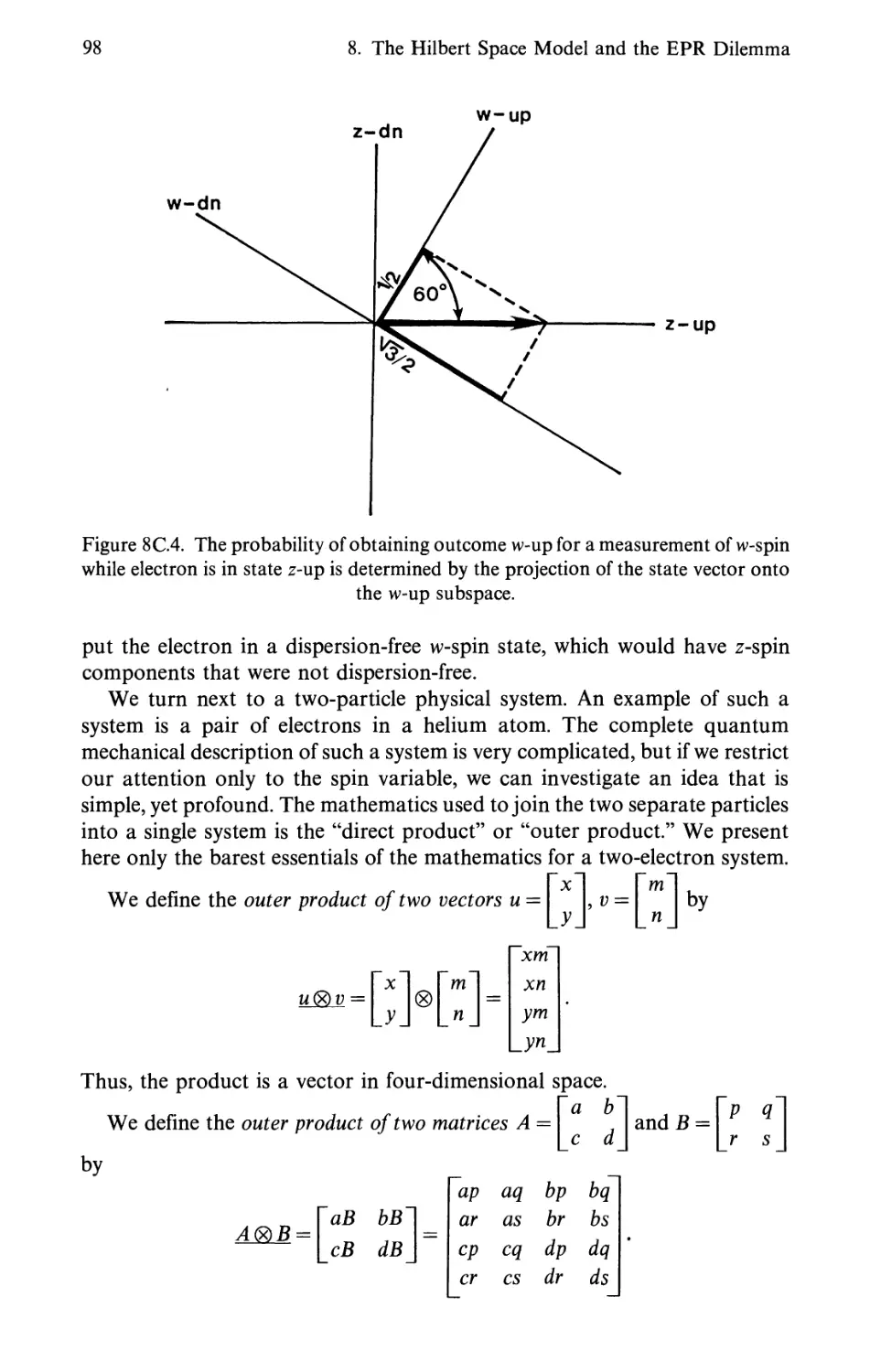
Текст
Problem Books in Mathematics
David W. Cohen
• i •
• T • • •
•
Springer-Verlag
David W. Cohen
An Introduction
to Hilbert Space and
Quantum Logic
With 38 Illustrations
Springer-Verlag
New York Berlin Heidelberg
London Paris Tokyo
David W. Cohen
Department of Mathematics
Smith College
Northampton, Massachusetts 01063
U.S.A.
Series Editor
Paul R. Halmos
Department of Mathematics
University of Santa Clara
Santa Clara, California 95053
U.S.A.
AMS Subject Classification: 46C, 81, 81A12, 47B15, 47A25, 35P05
Library of Congress Cataloging-in-Publication Data
Cohen, David W.
An introduction to Hilbert space and quantum logic/David W. Cohen
p. cm.—(Problem books in mathematics)
Bibliography: p.
1. Hilbert space. 2. Quantum theory. 3. Logic, Symbolic and
mathematical. I. Title. II. Series.
QA322.4.C64 1989
515.733—dcl9 88-24989
Printed on acid-free paper
© 1989 by Springer-Verlag New York Inc.
All rights reserved. This work may not be translated or copied in whole or in part without
the written permission of the publisher (Springer-Verlag, 175 Fifth Avenue, New York.
NY 10010, USA), except for brief excerpts in connection with reviews or scholarly analysis. Use
in connection with any form of information storage and retrieval, electronic adaptation, computer
software, or by similar or dissimilar methodology now known or hereafter developed is forbidden.
The use of general descriptive names, trade names, trademarks, etc. In this publication, even if
the former are not especially identified, is not to be taken as a sign that such names, as understood
by the Trade Marks and Merchandise Marks Act, may accordingly be used freely by anyone.
Phototypesetting by Thomson Press (India) Ltd, New Delhi, India.
Printed and bound by R.H. Donnelley & Sons, Harrisonburg, Virginia.
Printed in the United States or America.
987654321
ISBN 0-387-96870-9 Springer-Verlag New York Berlin Heidelberg
ISBN 3-540-96879-9 Springer-Verlag Berlin Heidelberg New York
Dedicated to
My parents, Rose and Lew
My wife, Doris (mitt trygt punkt),
My children, Bonnie and Sara
My sister, Carol
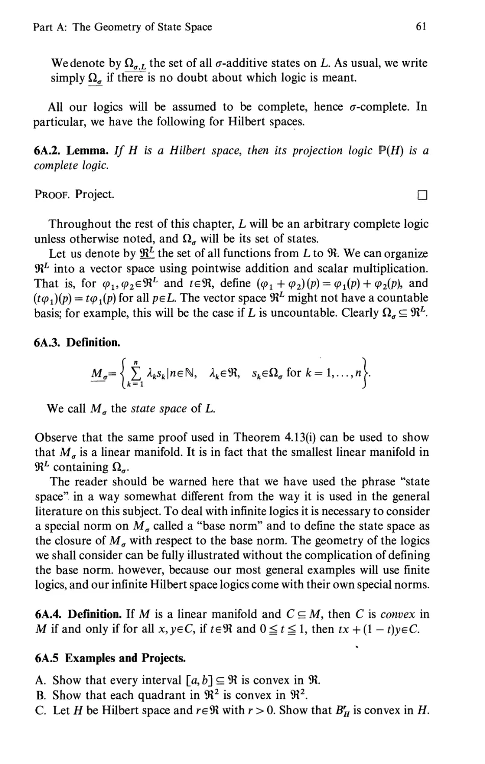
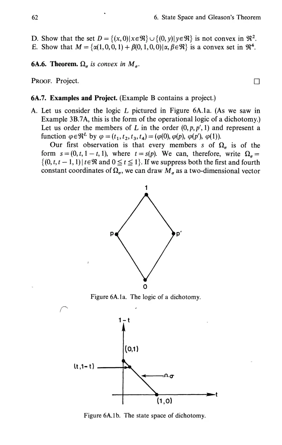
Preface
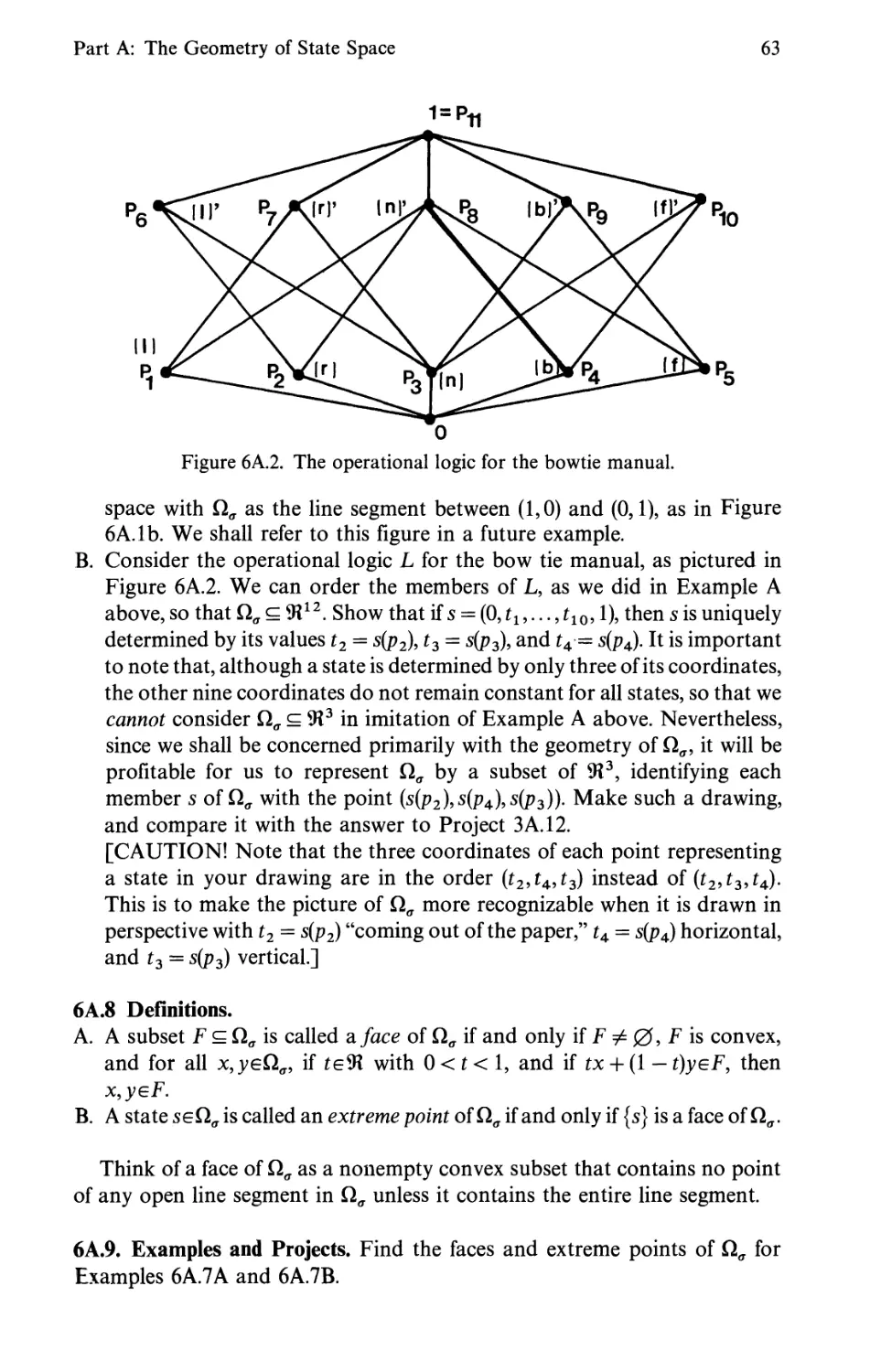
Content
The often-lamented communications gap between mathematicians and
theoretical physicists begins to form at the undergraduate level. Some
undergraduate physics majors learn little mathematics beyond linear algebra and
differential equations, while mathematics majors often see no modern physics.
The result of this gap is that some of the most profound and mathematically
interesting questions about the foundations of quantum physics are accessible
only to those few researchers who pursue mathematics and physics at a very
advanced level.
This book was written to bridge the gap at a lower level. It should be
accessible to undergraduate and beginning graduate students in both
mathematics and physics. The only strict prerequisites are calculus and linear
algebra, but the level of mathematical sophistication assumes at least one
or two intermediate courses—for example, in mathematical analysis or
advanced calculus. No background in physics is assumed. Historically,
nonclassical physics developed in three stages. First came a collection of ad
hoc assumptions and then a cookbook of equations known as "quantum
mechanics." The equations and their philosophical underpinnings were then
collected into a model based on the mathematics of Hilbert space. From the
Hilbert space model came the abstraction of "quantum logics." This book
explores all three stages, but not in historical order. Instead, in an effort to
illustrate how physics and abstract mathematics influence each other, we hop
back and fourth between a purely mathematical development of Hilbert space
and a physically motivated definition of a logic, partially linking the two
throughout, and then bring them together at the deepest level in the last
two chapters.
viii * Preface
To explore the interplay between mathematics and physics I was forced
to make choices not only in the selection but also in the treatment of some
topics. For example, the opening chapter on integrals with respect to measures
on the Borel sets is rather specialized. Topics important to a general
development of integrals are replaced by those more important to quantum
physics such as the idea of integrating the identity function on the reals with
respect to a complex-valued measure. Similarly, the concluding chapter on
quantum mechanics presents the Schroedinger equation with practically no
physical motivation in order to relate it quickly to the general notion of
observables and their mathematical connection to Hilbert space logic.
To be reasonably comprehensive I have included some mathematics whose
proof is beyond the level of this book. The insistence that no result may be
used until its proof has been digested (or at least presented) may breed healthy
skepticism in students, but it also keeps their mathematical horizons rather
narrow. Researchers, on the other hand, frequently use the results of others
without combing through the proofs. I see no reason to withhold from a
reader a lovely presentation of the spectral theorem for bounded Hermitian
operators, for example, as long as the reader can understand the statement
of the theorem—even if its proof is well beyond the level of this presentation.
It is my hope that by combining some deep mathematics with some deep
physics at a level that is not formidable this book can encourage a
reestablishment of links across the communications gap that has been steadily
widening recently—to the detriment of both mathematics and physics.
Format
Nearly all of the proofs and many of the examples are in the form of projects
for the reader to complete. The coaching manual, which follows the main
text, contains hints for completing the easier projects, but mostly it contains
complete solutions.
There are two reasons why the book is written with emphasis on projects.
One is so that a reader who desires merely an acquaintance with this material
can get that by reading only the main text. The other is to provide the more
thorough reader with the opportunity to get deeply into the material by
proving the theorems or by independently investigating important examples.
Some of the projects consist of routine exercises, but many (marked by *)
require some sophisticated ideas, while some (marked by **) I consider really
too difficult for most readers to complete without consulting the Coaching
Manual. I believe there is great value in writing out* a solution to a difficult
project, even if most of the ideas come from the Coaching Manual.
Preface
ix
Use
The format allows using the book for independent study or as a text in a
lecture course. Naturally, an instructor can choose a blend of lecturing about
some projects and assigning others as independent work, depending on how
advanced the students are and how much is to be covered in the time available.
A thorough study of all the topics and completion of all the projects is likely
to require two semesters for very advanced undergraduates or beginning
graduate students. On the other hand, I have successfully taught two
one-semester courses at Smith College based on this material.
In an intermediate level course (junior and senior math, physics, and
chemistry majors) I covered Chapters 3, 4, and 6A. I spent most of the time
on Chapter 3, stressed the finite dimensional cases in Chapter 4, and lectured
on the main ideas in 6A, filling in with material on measure and integration
(Chapter 1) on a "when needed" basis. The projects I assigned were among
the easier ones.
For an advanced course (our best senior math and physics majors) I covered
Chapters 2 through 6, assigning about half the projects for independent work.
Acknowledgment. It is with the greatest pleasure that I acknowledge the
roles of the following people who have helped to make this book possible.
David Foulis and the late Charles Randall got me into this business and
provided constant encouragement and mathematical support. Gottfried
Ruttimann graciously arranged for me and my family to spend a year in
Bern, where under his guidance I found an entire world of fascinating
connections between mathematics and physics. George Svetlichny and James
Henle collaborated with me in research projects that provided valuable
stimulation and insight into mathematical and philosophical questions.
Arthur Swift spent hours helping me sort out the ideas in Chapter 8. Elizabeth
Kumm carefully read every sentence of the manuscript with a critical eye
and was responsible for dozens of significant improvements. Marjorie
Senechal read portions of the manuscript and provided valuable suggestions
and encouragement. Kathy Zaffiro patiently did all the artwork.
One might hope that with all this support I have written a book without
errors. Alas, dear reader, I suspect that this is not the case, and I alone bear
the responsibility for the deficiencies that remain.
David W. Cohen
Symbols Used but Not Defined in the Text
f^J the set of natural numbers.
9t the set of real numbers.
9t°° the extended real numbers: 9tu{oo}.
(£ the set of complex numbers.
[a,ft) {x|xe9t and a^x <b}.
0 the empty set.
A\B {x\xeA and x$B) (A and B are any sets).
u§ the union of the sets in S: {x|xeSfor some Se§}. If § is indexed
by N, we also write [jnSn or \J™=1 Sn for uS.
n§ the intersection of the sets in S: {x|xeS for every Se§}. If § is
indexed by N, we also write f]nSn or f)™=iSn for n§.
sup (T) the least upper bound of the set T, if T is a set of real numbers
bounded above, or oo if Tis a set of numbers not bounded above.
«x„» a sequence indexed by the natural numbers. For additional
clarity we sometimes write «x„» (nef^l) to denote a sequence
indexed by the natural numbers.
lim„«x„» the limit of the sequence «x„». For additional clarity we
sometimes write lim^^^ «x„» for this limit.
f(x) the value of the function f at domain element x.
flA] {f(x)\xeA}.
/-IB] {x\f(x)eB}.
Contents
Dedication v
Preface vii
Symbols Used but Not Defined in the Text xiii
Chapter 1. Experiments, Measure, and Integration 1
Part A. Measures 2
Experiments and weight functions, expected value of a weight
function, measures, Lebesgue measure, signed measures,
complex measures, measurable functions, almost everywhere
equality.
Part B. Integration 8
Simple functions, simple integrals, general integrals, Lebesgue
integrals, properties of integrals, expected values as
integrals, complex integrals.
Chapter 2. Hilbert Space Basics 14
Inner product space, norm, orthogonality, Pythagorean
theorem, Bessel and Cauchy-Schwarz and triangle
inequalities, Cauchy sequences, convergence in norm, completeness,
Hilbert space, summability, bases, dimension.
Chapter 3. The Logic of Nonclassical Physics 21
Part A. Manuals of Experiments and Weights 21
Manuals, outcomes, events, orthogonality, refinements,
compatibijify, weights on manuals, electron spin, dispersion-
free weights, uncertainty.
Part B. Logics and State Functions 33
Implication in manuals, logical equivalence, operational logic,
implication and orthocomplementation in the logic, lattices,
xii * Contents
general logics (quantum logics), propositions, compatibility,
states on logics, pure states, epistemic and ontological
uncertainty.
Chapter 4. Subspaces in Hilbert Space 43
Linear manifolds, closure, subspaces, spans, orthogonal
complements, the subspace logic, finite projection theorem,
compatibility of subspaces.
Chapter 5. Maps on Hilbert Spaces 49
Part A. Linear Functionals and Function Spaces 49
Linear maps, continuity, boundedness, linear functionals,
Riesz representation theorem, dual spaces, adjoints, Hermitian
operators.
Part B. Projection Operators and the Projection Logic 55
Projection operators, summability of operators, the
projection logic, compatibility and commutativity.
Chapter 6. State Space and Gleason's Theorem 60
Part A. The Geometry of State Space 60
State space, convexity, faces, extreme points, properties,
detectability, pure states, observables, spectrum, expected
values, exposed faces.
Part B. Gleason's Theorem 69
Vector state, mixture, resolution of an operator into
projection operators, expected values of operators, Gleason's theorem.
Chapter 7. Spectrality 73
Part A. Finite Dimensional Spaces, the Spectral Resolution
Theorem 73
Eigenvalues, point spectrum, eigenspaces, diagonalization, the
spectral resolution theorem.
Part B. Infinite Dimensional Spaces, the Spectral Theorem 78
Spectral values, spectral measures, the spectral theorem,
functions of operators, commutativity and functional
relationships between operators, commutativity and compatibility of
operators.
Chapter 8. The Hilbert Space Model for Quantum Mechanics and
the EPR Dilemma 85
Part A. A Brief History of Quantum Mechanics 85
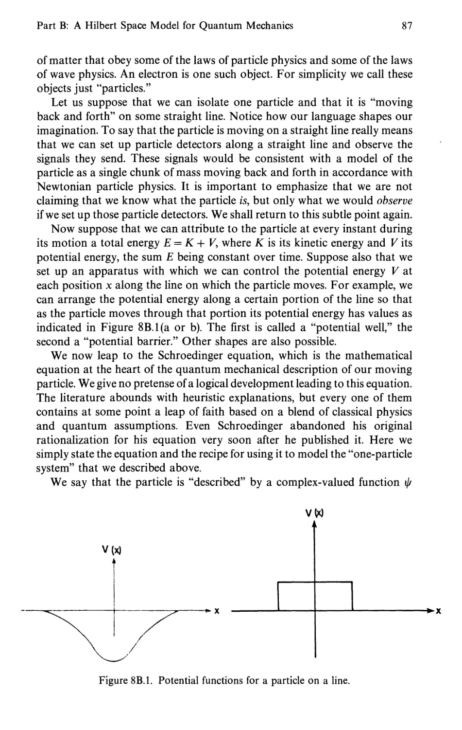
Part B. A Hilbert Space Model for Quantum Mechanics 86
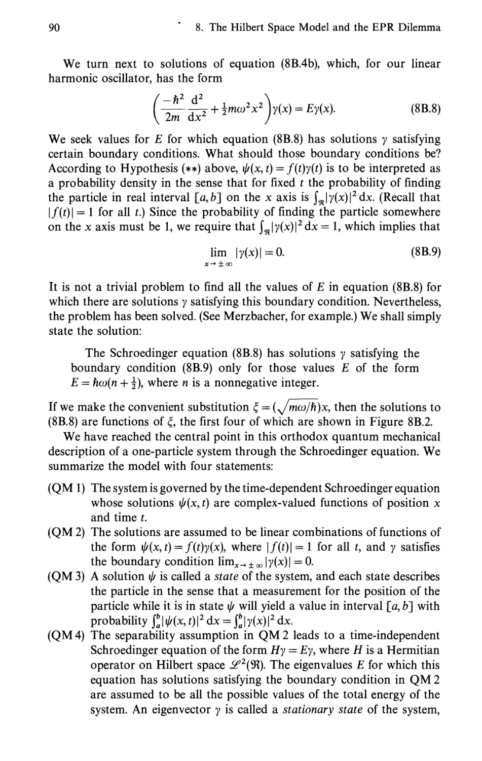
Schroedinger's equation, probability measures, stationary
states, the harmonic oscillator, the assumptions of quantum
mechanics, position and momentum operators, compatibility.
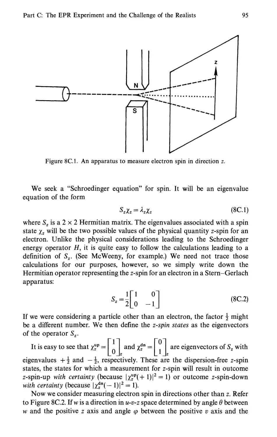
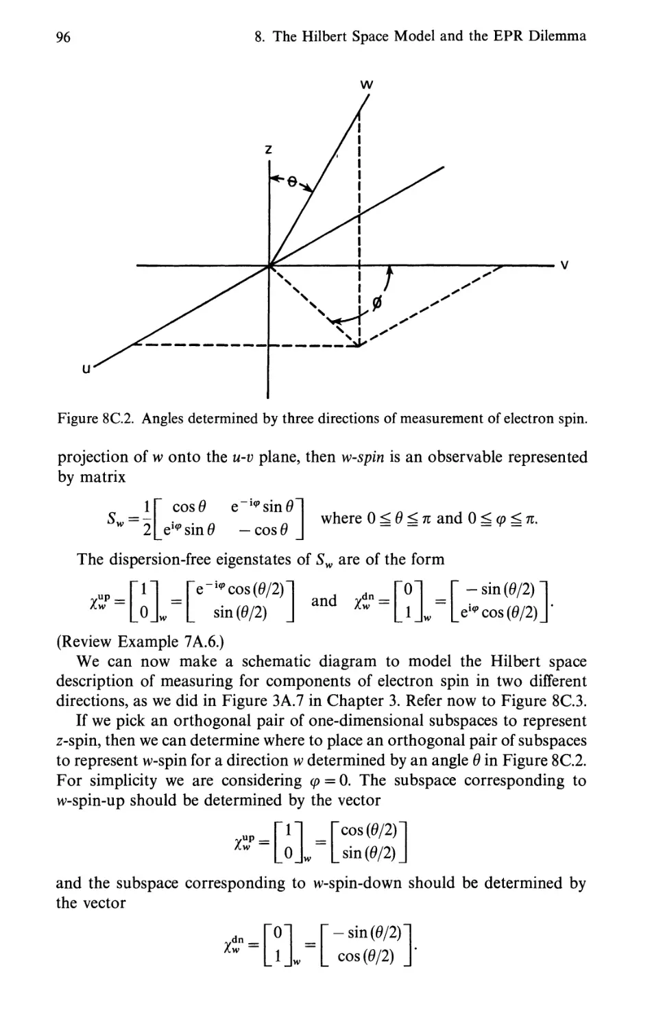
Part C. The EPR Experiment and the Challenge of the Realists 94
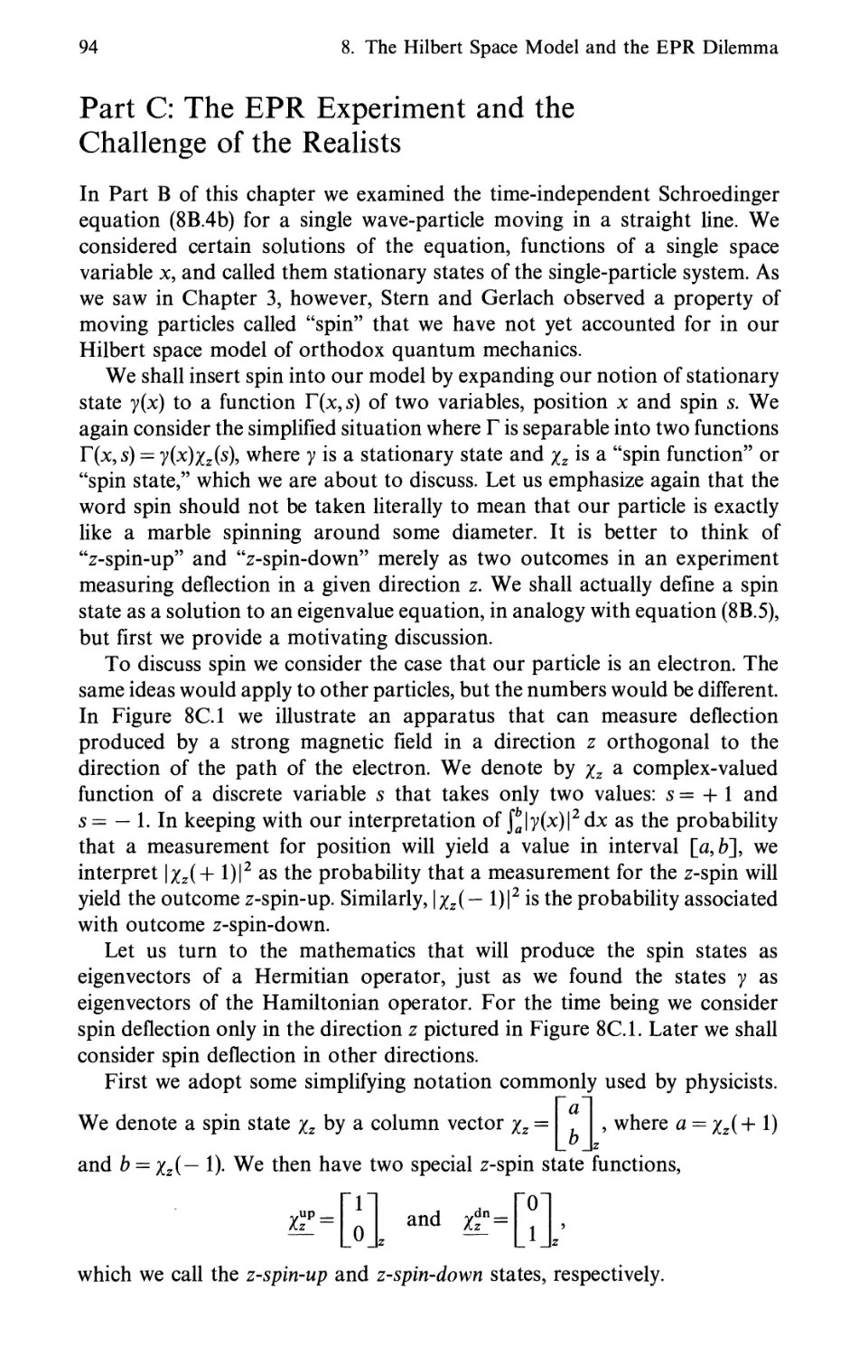
Electron spin, spin states, singlet state, EPR apparatus, the
EPR dilemma.
Index of Definitions
146
CHAPTER 1
Experiments, Measure and Integration
Introduction
We learn about our physical universe by doing experiments. That is, first we
do something such as flip a coin, or touch a hot stove, or measure how long
it takes a marble to drop from a certain height. Then we record what happens
after we do it—the coin comes up heads, we get burned, the marble takes 6
seconds to drop. What we record is called an outcome of the experiment.
We identify an experiment by its outcome set, so we can write C =
{heads, tails} to denote the coin flip experiment.
An experiment is most useful if it is repeatable and its outcomes are
describable precisely. For example, we can flip a coin many times and each
time we can record heads or tails precisely. We can repeatedly drop a marble,
but the set of outcomes depends on how precisely we wish to measure the
time. If we require accuracy only to 1 second, the outcome set could be
M = {5,6,7}, where the numbers denote seconds. If we require accuracy to
one decimal place, we might have an outcome set with 21 numbers in it:
M = {5.0,5.1,...,6.8,6.9,7.0}. In an experiment where we touch a hot stove
it is a little difficult to describe the outcome with precision. Did we get "badly
burned" or only "slightly burned"? A numerical measurement of temperature
or a count of the number of skin cells damaged might serve as a useful
outcome set.
In many experiments the outcomes consist of a set of real numbers. In
fact, it is sometimes convenient to introduce numbers artificially, as, for
example, by assigning the number one to the outcome "heads" and the number
zero to "tails." We begin our study of experiments, therefore, by considering
the real number system.
1. Experiments, Measure and Integration
1
1
1/
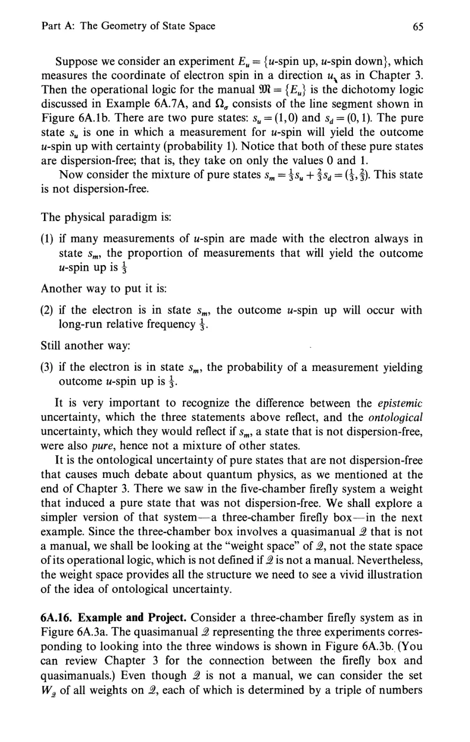
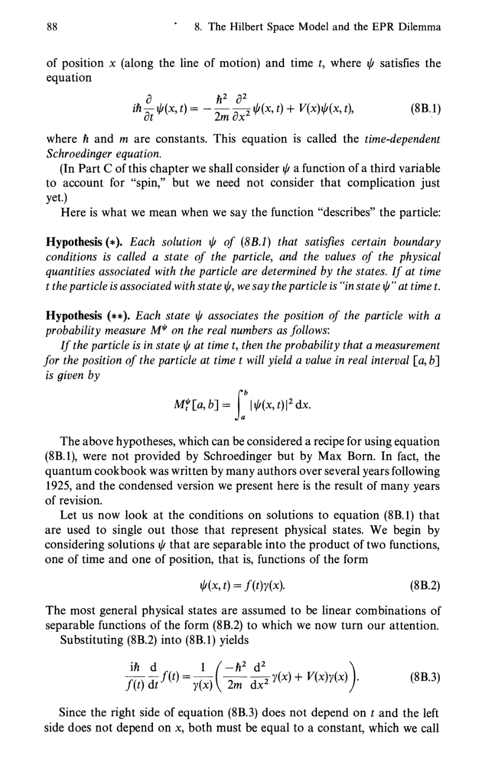
1 2 3 4 5 6 7 8 9 10 11 12 13 14 15 16 17 18 19 20
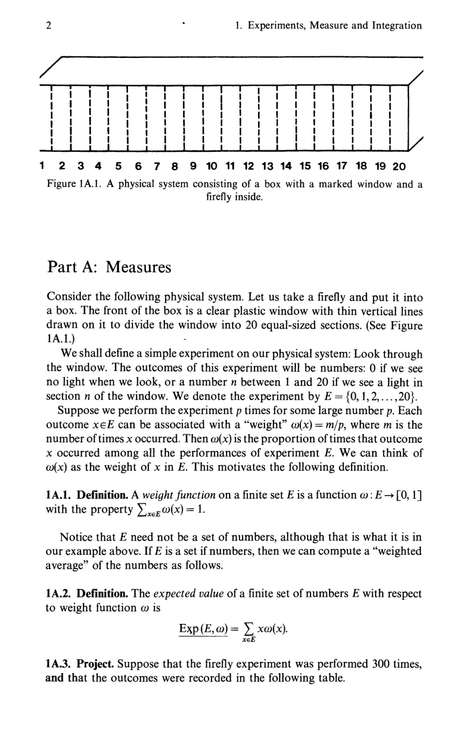
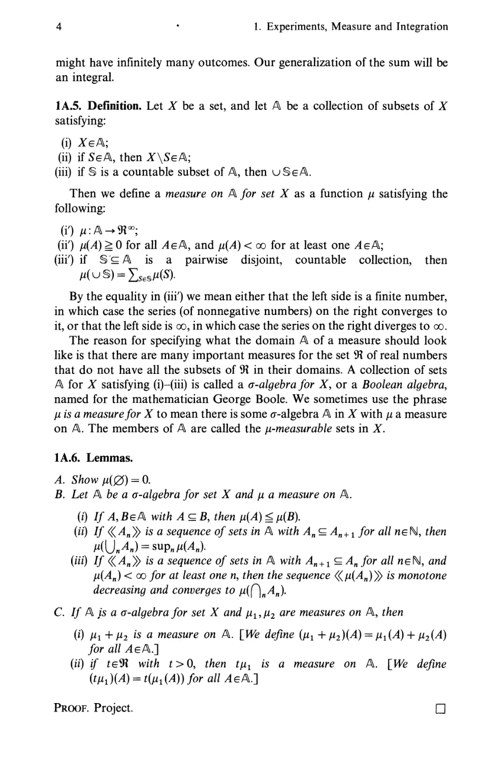
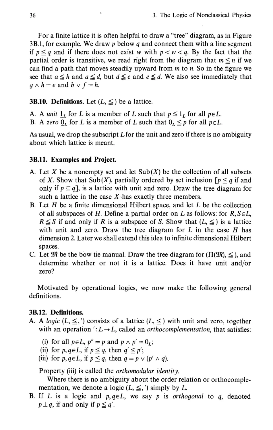
Figure 1A.1. A physical system consisting of a box with a marked window and a
firefly inside.
Part A: Measures
Consider the following physical system. Let us take a firefly and put it into
a box. The front of the box is a clear plastic window with thin vertical lines
drawn on it to divide the window into 20 equal-sized sections. (See Figure
1A.1.)
We shall define a simple experiment on our physical system: Look through
the window. The outcomes of this experiment will be numbers: 0 if we see
no light when we look, or a number n between 1 and 20 if we see a light in
section n of the window. We denote the experiment by E = {0,1,2,... ,20}.
Suppose we perform the experiment p times for some large number p. Each
outcome xeE can be associated with a "weight" co(x) = m/p, where m is the
number of times x occurred. Then oo(x) is the proportion of times that outcome
x occurred among all the performances of experiment E. We can think of
co(x) as the weight of x in E. This motivates the following definition.
1A.1. Definition. A weight function on a finite set £ is a function a>: E -► [0,1]
with the property Xxe£&>M = 1.
Notice that E need not be a set of numbers, although that is what it is in
our example above. If £ is a set if numbers, then we can compute a "weighted
average" of the numbers as follows.
1 A.2. Definition. The expected value of a finite set of numbers E with respect
to weight function a> is
Exp (£, co) = Yj xg)(x).
xeE
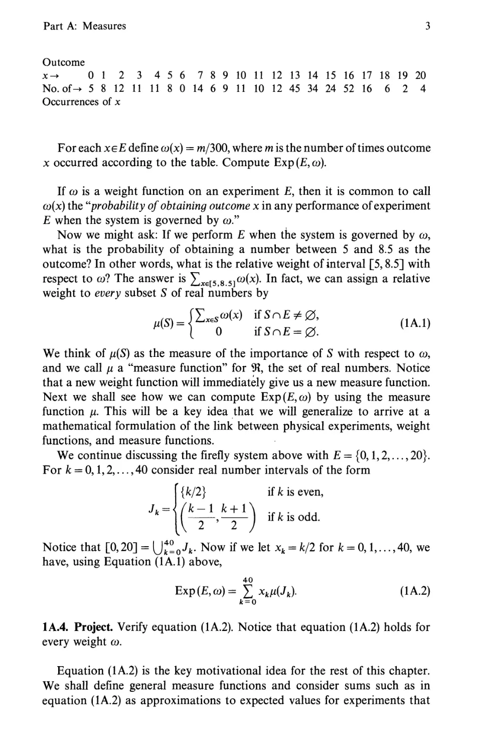
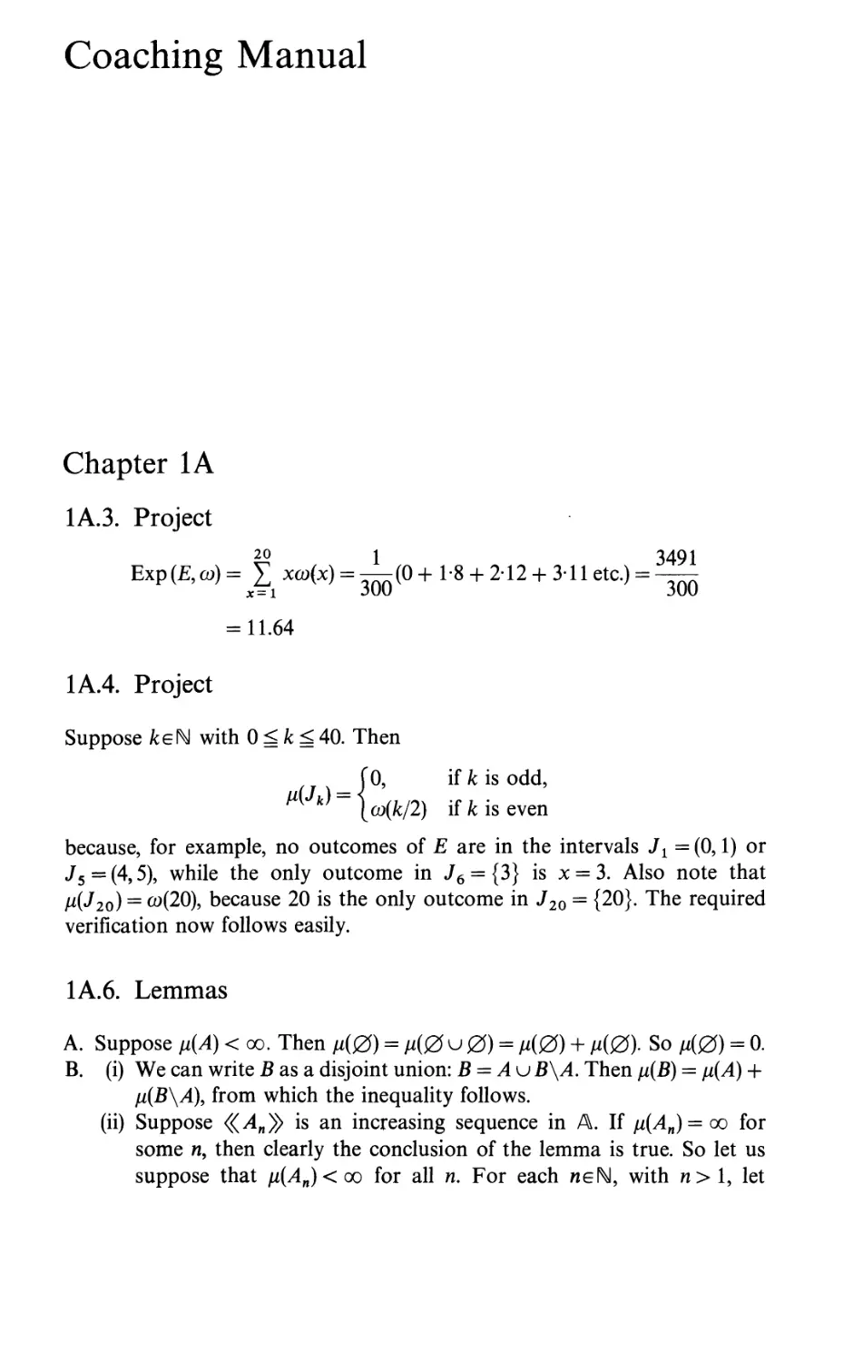
1A.3. Project. Suppose that the firefly experiment was performed 300 times,
and that the outcomes were recorded in the following table.
Part A: Measures
Outcome
*-► 0 1 2 3 4 5 6 7 8 9 10 11 12 13 14 15 16 17 18 19 20
No. of-> 5 8 12 11 11 8 0 14 6 9 11 10 12 45 34 24 52 16 6 2 4
Occurrences of x
For each xeE define co(x) = m/300, where m is the number of times outcome
x occurred according to the table. Compute Exp (£, co).
If co is a weight function on an experiment £, then it is common to call
(o(x) the "probability of obtaining outcome x in any performance of experiment
E when the system is governed by co."
Now we might ask: If we perform E when the system is governed by co,
what is the probability of obtaining a number between 5 and 8.5 as the
outcome? In other words, what is the relative weight of interval [5,8.5] with
respect to col The answer is £xe[5 8 5](o(x). In fact, we can assign a relative
weight to every subset S of real numbers by
We think of fi(S) as the measure of the importance of S with respect to co,
and we call \i a "measure function" for W, the set of real numbers. Notice
that a new weight function will immediately give us a new measure function.
Next we shall see how we can compute Exp(£,co) by using the measure
function \i. This will be a key idea that we will generalize to arrive at a
mathematical formulation of the link between physical experiments, weight
functions, and measure functions.
We continue discussing the firefly system above with E = {0,1,2,..., 20}.
For k = 0,1,2,..., 40 consider real number intervals of the form
if k is even,
if k is odd.
Notice that [0,20] = IJfc = oJ*- Now if we let xk = fc/2 for k = 0,1,..., 40, we
have, using Equation (1A.1) above,
40
Exp (£,co)= £ xkfi(Jk). (1A.2)
k = 0
1A.4. Project. Verify equation (1A.2). Notice that equation (1A.2) holds for
every weight co.
Equation (1A.2) is the key motivational idea for the rest of this chapter.
We shall define general measure functions and consider sums such as in
equation (1A.2) as approximations to expected values for experiments that
4 * 1. Experiments, Measure and Integration
might have infinitely many outcomes. Our generalization of the sum will be
an integral.
1A.5. Definition. Let X be a set, and let A be a collection of subsets of X
satisfying:
(i) Xe/\;
(ii) if SeA, then JT\SeA;
(iii) if S is a countable subset of A, then uSeA.
Then we define a measure on A for set X as a function fi satisfying the
following:
(i') ^:A->5R°°;
(ii') fi( A) = 0 for all Ae/\, and fi(A) < oo for at least one As A;
(iii') if S'cA is a pairwise disjoint, countable collection, then
Mu§) = XsesMS).
By the equality in (iii') we mean either that the left side is a finite number,
in which case the series (of nonnegative numbers) on the right converges to
it, or that the left side is oo, in which case the series on the right diverges to oo.
The reason for specifying what the domain A of a measure should look
like is that there are many important measures for the set 9t of real numbers
that do not have all the subsets of 9? in their domains. A collection of sets
A for X satisfying (i)-(iii) is called a a-algebra for X, or a Boolean algebra,
named for the mathematician George Boole. We sometimes use the phrase
jLi is a measure for X to mean there is some cr-algebra A in X with jll a measure
on A. The members of A are called the jn-measurable sets in X.
1A.6. Lemmas.
A. Show fi(0) = O.
B. Let A be a a-algebra for set X and \i a measure on A.
(0 If A, Be A with A^B, then fi(A) = fi(B).
(ii) If «^4„» is a sequence of sets in A with An^An+1 for all neN, then
(iii) If «-4„» is a sequence of sets in A with An + 1 ^An for all neN, and
jn(An) < oo for at least one n, then the sequence «^(-4„)» is monotone
decreasing and converges to jn(f]nAn).
C. If A /5 a o-algebra for set X and fil9fi2 are measures on A, then
(i) fix + jll2 is a measure on A. [We define (jix + jn2)(A) = jn^A) + fi2(A)
for all Ae/\.']
(ii) if te${ with £>0, then t\ix is a measure on A. \We define
(tiix)(A) = tdi^A)) for all Ae/\.']
Proof. Project.
□
Part A: Measures
5
There is one measure for the reals that is of central importance to a vast
amount of physics and mathematics. We call it Lebesgue measure, and it is
the one that is the link between the integration that one studies in beginning
calculus and the more general integrals we shall study later in this chapter.
We discuss Lebesgue measure by first describing the "Borel sets" in 9t.
1A.7. Definition. Let 0 = {(a, b~\\a, be9t}. We define the collection B of Borel
sets in 9t as the smallest collection of subsets of 9t satisfying:
(i) 0 <= B;
(ii) if fleB, then 9t\£eB;
(iii) B is closed under countable unions.
Note that B must also be closed under countable intersections, because
if § is a countable collection in B, then n§ = 9t\(uSeS9t\S).
1A.8. Lemmas.
A. If a,be9i with a<b, then all of the following are Borel sets:
(— oo, a\ (— oo, a], (a, b\ [a, b]9%0
[a, b\ {a}, [b, oo), {b9 oo), (a, b].
B. The collection B of Borel sets is a o-algebra in 9¾.
Proof. Project. □
Lemma 1 A.8 can be used to prove that most subsets of the reals that we
use in calculus are Borel sets. In fact, the proof that there exists a set that is
not a Borel set is rather difficult, and we shall not concern ourselves with it.
We turn instead to our main reason for considering B, namely to define
Lebesgue measure. The proof of the following theorem is complicated, and
we shall omit it.
1 A.9. Theorem. There exist a o-algebra A for 91 with B ^ A and a measure
fi on A, called Lebesgue measure, such that for all a, be91 with a^b,
fi(a, b) = \i\a, b) = fi(a, b~] = [i\a, b~] = b — a.
The o-algebra A is called the collection of Lebesgue measurable sets.
In other words, the Lebesgue measure of a bounded interval is its length,
irrespective of which endpoints are included in the interval. You can see why
Lebesgue measure is so important. It is the generalization of length in 91 that
coincides with our usual notion of the length of an interval.
1A.10. Examples and Projects. As we indicated, the Lebesgue measure of a
bounded interval is its length. In this sense, then, the measure of a set is an
6 1. Experiments, Measure and Integration
indication of its size. As Example 1A.10B below shows, however, there are
measures that are quite unrelated to size in the usual sense.
A. Let jLi be Lebesgue measure for 9t. Show:
(i) For xe% jll(x, 00) = jll( — oo,x) = oo.
(ii) For xe% fi{x} = 0.
(iii) If C is a countable subset of % then fi(C) = 0.
B. Suppose xe9t. We can define a measure on the Borel sets B "concentrated
at x" as follows: for SeB> define
(* J1 ifxeS'
"(S) = J0 ifxtS.
Show that fi is a measure on B.
We consider next measures which may take on negative or complex values.
Let X be a set and A be a cr-algebra in X.
1A.11. Definition. A signed measure jll on A is a function satisfying:
(i) 0:A-»M°°, or/*:A->9r°°;
(ii) //(^4) < oo for at least one X;
(iii) if § ^ A is a pairwise disjoint, countable collection, then
MuS)=J>(S).
SeS
By the equality in (iii) we mean either
(a) — oo < ju(uS) < oo, in which case the series on the right converges for
all rearrangements of its terms (hence is absolutely convergent); or
(b) /i(u§)= ± oo, in which case the series on the right diverges to oo or
to — oo.
The following theorem shows that every signed measure can be written
as the difference of two measures. We omit its proof.
1A.12. Theorem (Jordan Decomposition Theorem). Let X be a set and jll a
signed measure on a o-algebra A in X. Then there exist two measure fi+ and
jll~ on A, at least one of which assigns finite measure to X, such that
fi = fi+ — \T.
Note that the theorem implies that fi+ and jn~ both have domain A and
that either fi + (X) or fi~(X) is finite.
Next we introduce complex-valued measures. As we shall see, they can be
decomposed into ordinary measures.
1A.13. Definition. Let X be a set and A be a cr-algebra in X. A function
/j:A->£ is a complex measure on A if
Part A: Measures
7
(i) jll(A) < oo for at least one A;
(ii) if § ^ A is a pairwise disjoint, countable collection in A, then
Notice that implicit in condition (ii) is that ju(u§)g£, so that the series
is required to converge. In particular, it is required that fi(X) is finite.
If fi is a complex measure on cr-algebra A, then we can write jll = ^ + ijn2
for two signed measures jll1 and \i2 on A and then write jll in terms of measures
on A as
li = lit ~ Ih + i(^2 - \h. )• (1 A-3)
We shall continue to reserve the word "measure" to refer to extended-real-
valued measures, and we shall refer to the others as "complex measures."
Our final concept in this section connects functions and measures. Briefly,
a real-valued function on a set X for which jll is a measure is called a
"measurable function" if its inverse takes Borel sets to //-measurable sets.
Specifically:
1A.14. Definitions.
A. Let f:X->9l9 and suppose jll is a measure (or complex measure) on
cr-algebra A in X. Then / is called a jn-measurable function if and only if
/«"[B]eA for every Borel set B.
B. If/=/i + if 2 is a G-valued function on X (/l9/2 are real-valued), then /
is called a ^-measurable function if both /x and f2 are //-measurable.
1A.15. Definition. Let X be a set and // be a measure (or complex measure)
on cr-algebra A in X. Let / and # be two //-measurable functions on X. Then
we say / equals g fi-almost everywhere, and we write /=gf^-ae, if and
only if
fi{xeX\f(x)^g(x)}=0.
IA.16. Examples and Projects.
A. Let
J1 if xe[0,1] and x is rational,
[0 otherwise.
Show that / is equal ^-ae to the zero function, (fi is Lebesgue measure.)
B. Find a function that is equal /4-ae to the identity function on % yet
has the value zero at infinitely many points.
1A.17. Definition. Let X be a set and fi be a measure on cr-algebra A in X.
Let / be a //-measurable, real-valued function. We define for all xeX,
/+(x) = max{/(x),0} and /~(x) = max{-/(x),0}.
8 1. Experiments, Measure and Integration
1A.18. Lemma. If X, A, ^, and f are as in Definition 17, then f+ and f~
are nonnegative ^-measurable functions and f = f+ — f ~.
Proof. Project. □
This completes part A. In the next part we shall learn about integration
with respect to different measures for 9t, and later we shall use integrals to
compute expected values for experiments in quantum physics.
Part B: Integration
In this part we use measures to define integrals. The Riemann integral is
usually studied in the first year of calculus, but here we will study the more
general types of integrals needed to handle the discontinuous functions that
arise in quantum physics.
In this part, unless otherwise noted, \i will stand for an arbitrary measure
on a cr-algebra A for the reals 9t with the stipulation that A contains the
Borel sets.
1B.1. Definition. A function f: 9t -► 9t is called simple if the image off is finite.
Here are two examples of simple functions.
1B.2. Examples.
A. Let f be the "greatest integer function" on the interval [0,10].
B. Let f be the function
JO if xe[0,1] and x is rational,
[l if xe[0,1] and x is irrational.
In each of these examples it is easy to see that f has a finite image. Since
we shall be interested in simple functions that are Lebesgue measurable, we
point out that each f is Lebesgue measurable, because f*~{t} is a Borel set
(hence a Lebesgue measurable set) for each £eimage(/). In the first example,
for instance, /*~{3} = [3,4).
Now we shall define the integral of a ^-measurable simple function f.
Suppose image(/) = {al9... ,a„}. For k = 1,...,n, let us denote /""[aj by Ak.
Then we make the following definition.
1B.3. Definition. The ^-integral of f over a set Se/\ is defined by
' n
f dju = X akKA n S)
fc=i
Part B: Integration
when the sum on the right is finite.
We write
f djii = oo if for some k, jn(Ak n S) = oo and ak ^ 0.
In the case where S is the entire domain of/, then we have S=[jnk=lAk,
and so
/c=l
Next we define /^-integrals for functions that might not be simple. Let us
consider nonnegative functions first.
1B.4. Definition. The fi-integral of a /^-measurable nonnegative function f
over a set S e A is defined by
fdfi = sup
hdjn
h is a nonnegative, /^-measurable, simple
function with h{x) f^f(x) for all x in S
We write \sjd/i = oo if in the set on the right Js /z d/^ = oo for any /z or
if the set on the right is unbounded.
We extend this definition to functions that may have negative image values.
Recall from Definition 1A.17 the definitions of /+ and /~ for /^-measurable
function f. If f is a /^-measurable function and SeA, and if either \sf+ dp
or Js f ~ dfi has a finite value, then we make the following definition.
1B.5. Definition.
We write
or
/d/z =
J s „
/+d//-
s J
r r
fdfi= oo if
J s *
s
r c
/d/x=-
JS
oo if
*
s
f d/i.
w
f+ dfi= oo,
/ d/^= oo.
We say / is fi-integrable if and only if / is /^-measurable and both integrals
on the right side of equation (*) have finite values. If \i is Lebesgue measure,
then Js f dfi is called the Lebesgue integral of f over S.
It is not difficult to connect the notion of Lebesgue integral with the notion
of Riemann integral, although we will not go into the details here. Lebesgue
integrals are truly a generalization of Riemann integrals in the following
10 1. Experiments, Measure and Integration
sense: if a function f is both Riemann and Lebesgue integrable over an
interval I, then the Lebesgue and Riemann integrals of/ over I are the same
number. Lebesgue integration is more general in the sense that every function
that is Riemann integrable over an interval I is Lebesgue integrable over /,
while the converse is false. The function in Example 1B.2B is Lebesgue
integrable but not Riemann integrable on [0,1].
Here we encounter a trade-off that mathematicians often face: greater
generality is bought at the price of some important theorems. In this case
the fundamental theorem of calculus, which relates Riemann integrals to
antiderivatives, does not hold for Lebesgue integrals. For example, you may
recall that to compute the Riemann integral of the function f(x) = x2 over
an interval [a, b]9 it is not necessary to compute Riemann sums to approximate
the integral. You can simply find an antiderivative of/, namely F(x) = x3/3,
and use the fundamental theorem of calculus to compute
x2 dx = F{b) - F{a) = b3/3 - a3/3.
a
Of course, it usually is not so easy to find antiderivatives. In this era of
computers, anyone who needs to find the value of a Riemann integral usually
finds an approximation by using numerical methods to find upper and lower
Riemann sums, because even the most sophisticated techniques for finding
antiderivatives fail to work for most functions.
We must be careful not to confuse an integral such as \\x2 dx, which
is a number, with an antiderivative such as F(x) = x3/3, which is a
function. It is easy to confuse them, because the fundamental theorem of
calculus provides a close link between the two and because mathematicians
often refer to an antiderivative as an "indefinite integral." The fundamental
theorem does not apply to Lebesgue integrals, however, and when we must
compute an integral in our work, we shall find it necessary to look for
numerical approximations.
Integrals with respect to general measures do not satisfy all the
properties that Riemann integrals do, but they do satisfy some important
ones.
1B.6. Theorems. Let jll be a measure on o-algebra A/or 9t and suppose Se/\
and f and g are functions that are fi-integrable over S.
A. Ifae% then Jsafdjn = a\sf dju.
B. Iff(x) ^ g(x)for all x in S, then
fdfi^ gdfi.
Part B: Integration
11
C. For any a, b in 91.
(af+ bg) dfi = a
fd/t + b
gdfi.
D. If T and U are disjoint fi-measurable sets in S, then
fdfi =
TuU
fdfi +
fdfi.
u
Proof. The proof of part B is in the Coaching Manual; the proofs of the
other parts are omitted. □
1B.7. Theorem (The Monotone Convergence Theorem). Let fi be a measure
on o-algebra A/or 91 and suppose Se A. If « /„» is a sequence of fi-integrable
functions converging pointwise to f on S, and for each neN, 0 ^/„(x) ^/(x)
for all xeS, then
lim
fndfi )) =
fdfi.
Proof. Omitted.
n
1B.8. Theorems. Let fi be a measure on the Borel sets and S a Borel set.
A. Suppose f is a function fi-integrable over S, and /(x) = 0 \i-ae on S. Then
fdfi = 0.
[Recall that /(x) = 0 fi-ae on S if and only if fi{x\xeS and /(x) ^ 0} = 0.]
B. The following is a partial converse of (A) above. If f is a nonnegative
fi-measurable function and \sfdfi = 0, then /(x) = 0 fi-ae on S.
Proof. Project.
□
1B.9. Examples and Projects. In these examples fi is Lebesgue measure and
I is the interval [0.1].
A. Consider the function
/oW
1 if x is rational and xe/,
0 if x is irrational and xe/.
The function /0 is not Riemann integrable over I. Show, however, that
/0 is Lebesgue integrable over /, and compute J7 /0 dfi.
B. Consider the function
aw=
x if x is rational and xe/,
0 if x is irrational and xel.
12 1. Experiments, Measure and Integration
Use the result of Theorem 1B.8A to compute the Lebesgue integral
/id/*-
C. Let S = [0,7c]. Consider the function
\jq if x = p/q in lowest terms (p,qeZ) and xeS,
2 2 if x is irrational and xeS.
Use the result in Theorem IB.8A to compute the Lebesgue integral Js f2 dju.
Now let us return to the firefly that we put into a box at the beginning
of this chapter. Recall our experiment E = {0,1,... ,20}. Let co be the weight
on E given in Project 1 A. 3, and let \i be the measure for 9t defined by equation
(1A.1). We then have the following result.
1B.10. Lemma.
Exp (£, co) = £ xo)(x)
xeE
<R
where In(x) = x is the identity function on 9¾.
Proof. Project. □
This connection between expected values and the integral of the identity
function is one of the cornerstones of the orthodox formulation of quantum
mechanics. We will return to this theme in Chapters 6, 7, and 8. The main
idea will be to consider measures for 91 that depend on the eigenvalues of
certain linear operators. If the eigenvalues form a discrete set, then a variable
that can assume only these eigenvalues is called "quantized." Our measure
will assign to each Borel set a value that depends on how many eigenvalues
are in the set. We then show how we can formulate the notion that if we
physically measure a quantized variable, such as energy, the probability of
obtaining a value in a given interval I depends in part on the measure of J,
that is, on how many eigenvalues are in J. The expected value of the variable
will then be computed using a Lebesgue integral of the identity function with
respect to this eigenvalue-dependent measure.
To conclude this chapter we define the integral of a complex-valued
function with respect to a complex measure.
Let \i be a complex measure on cr-algebra A for 91 and suppose f is a
real-valued, /^-measurable function on 9t. Suppose further that jll is written
in terms of (real) measures, as in equation (1A.3): jll = ^ — ^ + i{^2 — Ih.)-
Suppose also that SeA, that either \sjdfi^ or \sf^\ is finite, and that
either \sf d^i or \sf ^2 is finite. Then we make the following definition.
Part B: Integration
13
1B.11 Definition. The fi-integral of/ over set Se/\ is
fdfi
fdrf
fdf*i +i
fdfi+2
fdfi2 I-
We write Js f dfi = oo if any one of the four integrals on the right is infinite.
Finally, if ^ is a complex measure, and f = fx + if2 is a /^-measurable
complex-valued function (fx and/2 are real-valued), and SeA, we make the
following definition.
IB. 12. Definition.
fdfi
fi dfi + i
fidfi.
Notice that if fi is a complex measure and f is a /^-measurable, bounded
function, then
fdfi
Js
<
fidfi
Js
+
fidfi
Js
<
supfl/xMMxeSRJIMtt)!
+ sup{|/2(x)| I xeSR}|A£(M)| < oo,-
since, as we remarked after Definition 1A.13, \fi(9i)\ < oo.
Finally, we state without proof a theorem we shall need in Chapter 6A.
1B.13. Theorem. If fi1 and fi2 are finite measures on o-algebra A in 9t, and
tx, t2 e9t, then t1fiut2fi2i and txfix + t2fi2 are all signed measures on A. Further,
iff: 9t -► 9t is integrable over 9t with respect to all of these signed measures, then
fd(t1fi1+t2fi2) = t1
<R
fdfi1+t2
<R
fdfi:
«
This completes our introduction to measures and integrals. We turn now
to Hilbert spaces, and we will consider the deep connection between Hilbert
spaces and measures in Chapter 7 when we discuss the Spectral Theorem.
In the meantime we will have occasion to use integrals to see some important
examples of Hilbert spaces.
CHAPTER 2
Hilbert Space Basics
#
We assume that you know the definition of a vector space if = (V9 + , •) over
the field (£ of complex numbers. Perhaps you recall defining an "inner product"
between vectors in a vector space and using the inner product to consider
angles between vectors. A "Hilbert space" is a vector space with an inner
product. We begin by defining an inner product space.
2.1. Definition. A structure if = (V9 + , •<, >) is an inner product space if
(i) (V9 +, ) is a vector space (over the field of complex numbers);
(ii) <, > is a function that associates a complex number with every pair of
vectors in V subject to the following rules: for all x9y9zeVand Ae£,
(a) <*,}>> = (y,x}* (* is complex conjugate);
(b) <x + j;,z> = <x,z> + <);,z> and <x,j; + z> = <x,};> + <x,z>;
(c) < >bc, y > = A < x9 y > (we follow the usual practice of writing Xx for X • x);
(d) <x,x> is a nonnegative real number, and <x, x> = 0 only if x is the
zero vector in V.
We call <*,}>> the inner product of x and y.
We will adopt the usual practice of denoting an inner product space simply
by its underlying set V, since there will seldom be any doubt about which
inner product structure is under discussion.
2.2. Lemma. If V is an inner product space and x,yeV and AgG, then
(x,Xy} = X*(x,y}.
Proof. Project. □
2. Hilbert Space Basics 15
2.3. Examples and Projects.
A. Suppose n is a positive integer. Let V = (£" be the set of complex n-tuples
organized into a vector space under pointwise addition and scalar
multiplication. For x = (x1,...,xll) and 3> = (3>i,...,3>,,) in V9 define
< x, 3; > = ^ = x xk;y?. Show that <, > is an inner product. We call this inner
product space complex n-space and denote it by £".
B. Let 7 be defined by
V = {«xfc» I «xfc» is a sequence of complex numbers,
00
and the series £ |xfc|2 converges in 9¾}.
/c=l
Using standard results for convergent series, we can show that V can be
organized into a vector space under pointwise addition and scalar
multiplication. Define for each x9yeV
00
Show that the series converges. (The calculation is a bit tricky.) Then show
that <, > is an inner product. (This is more straightforward.) This inner
product space is denoted by I2. (Some authors write /2.)
C. Suppose fi is a complex Borel measure for 9t. Suppose also that S = (a, b)
is a nonempty interval in 9t. Define
V = {{//11//: S -► (£ and | ^ |2 is /Mntegrable over S}.
We can define pointwise addition and scalar multiplication on V by
(i) 0Ai + ^2)(0 = *AiW + <M') for all feS;
(ii) (A-^)(0 = /liA(0 for all teS, Ae(E.
It can be shown that (7, +,•) is a vector space. For all \l/l9\l/2eV9 define
/»
<^1,^2>
ij/^dfi.
s
With a proof similar to the one in Example B above it can be shown that
Jsl^i^*|d^^2(Jsl^il2d^ +Jsl^2l2d^)> so that <^i>^2> is a complex
number.
A slight complication arises, however, if we try to establish property
(ii)(d) in the Definition 2.1 of an inner product. That property states that
< 1//,1//)=0 implies ^ = 0. By Theorem 1B.8B, however, we know only
that if <i//91//> = js^* dfi = JsI\j/ \2 dfi = 0, then | \//\2 = 0 /^-almost
everywhere on S. The way to get around this difficulty is to define an equivalence
relation on V by
i//1 ~ i//2 if and only if 11//1 — i//2 \ = 0 jll-slc on S.
.a.
Denote by V the set of equivalence classes determined by members of V.
16 2. Hilbert Space Basics
We leave as a project the varification that the pointwise addition and
scalar multiplication and the inner product defined on Fcan be transferred
.a.
in a natural way to F The resulting inner product space is denoted in
many books by j^2(a,fc) or ^2(a,b) when \i is Lebesgue measure.
We can use an inner product to define a length in a vector space. For the
rest of this chapter we shall let F be an arbitrary inner product space unless
otherwise noted.
2.4. Definition. The inner product norm on F is a function from Fto 9? defined
for every xeV by ||x\\ = ^(x^x).
2.5. Project. Suppose neN. Show that for x = (xu...,xn)e(£n, ||x||2 = ££ = 1|xfc|2.
This is why || x || is called the "length" of x as well as the norm of x.
2.6. Theorem. The inner product norm satisfies the following for all x.yeV and
(i) || x || ^ 0, and equality holds only if x = 0;
(ii) ||/tac|| = |A| ||x||;
(••*\ii i ii2iii n 2 ^ii ii 2 ■ ^ ii n2
in) || x + y |r + || x — y || = 21| x || + 21| y || .
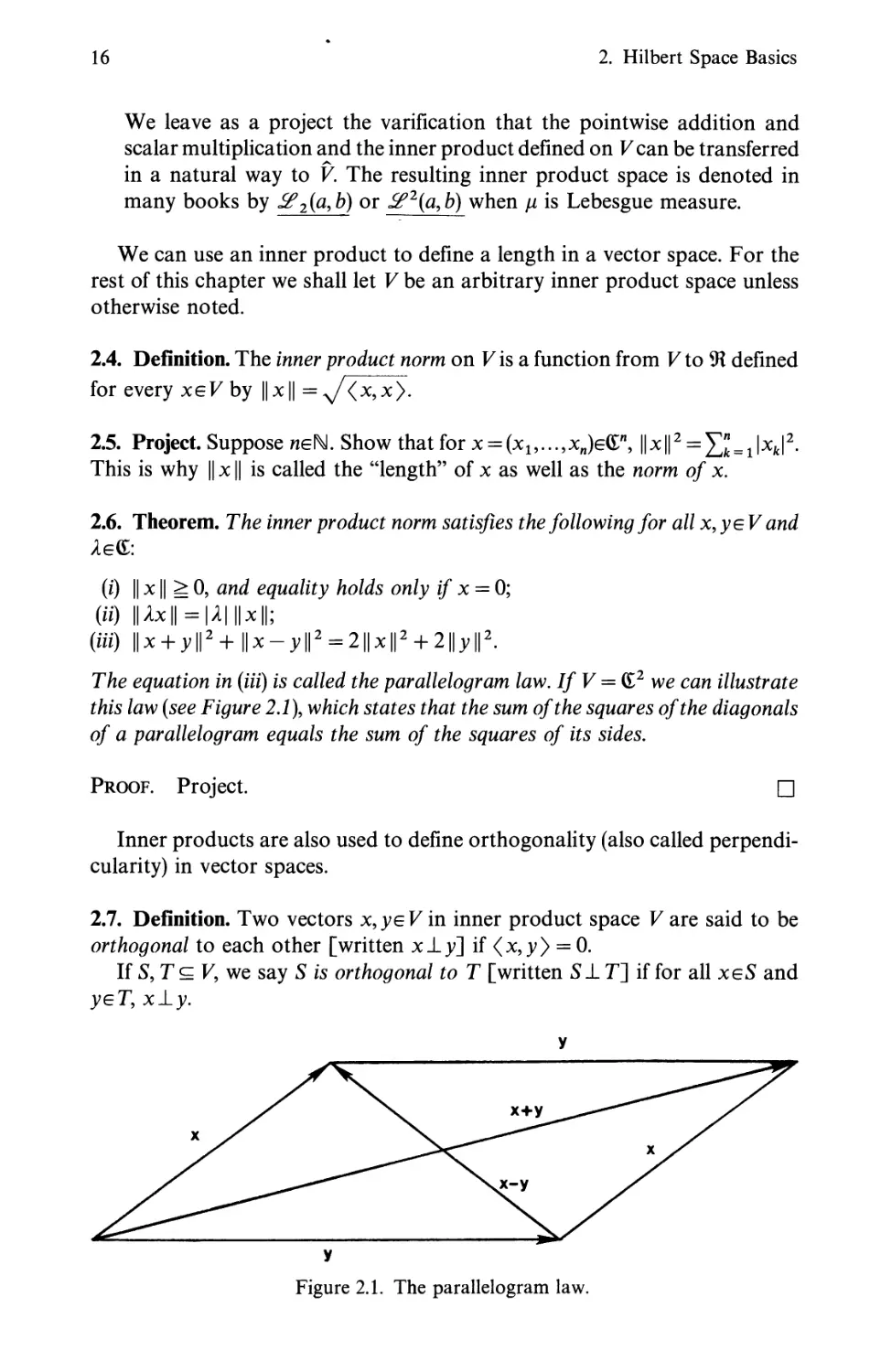
The equation in (Hi) is called the parallelogram law. IfV = &2 we can illustrate
this law (see Figure 2.1), which states that the sum of the squares of the diagonals
of a parallelogram equals the sum of the squares of its sides.
Proof. Project. □
Inner products are also used to define orthogonality (also called
perpendicularity) in vector spaces.
2.7. Definition. Two vectors x.ysVin inner product space Fare said to be
orthogonal to each other [written xl.y] if <*,}>> = 0.
If S, T c F, we say S is orthogonal to T [written SI T] if for all xeS and
yeT, x±y.
y
Figure 2.1. The parallelogram law.
2. Hilbert Space Basics 17
2.8. Lemma. For all xeV, x_LO.
Proof. Project. □
2.9. Lemma.
Ifx±y,then\\x + y\\2=\\x\\2+\\y\\2.
(A sketch using (£2 should make it clear to you why this is called the Pythagorean
theorem.)
Proof. A straightforward computation using <x,};> = 0. □
2.10. Definition. A set S ^ V is called orthonormal if its members are pairwise
orthogonal and all have norm one.
2.11. Theorem (Bessel's Inequality). If {x1?... ,xp} is an orthonormal set in V
then for all yeV,
iKxk>y)\2<\\y\\2.
k=l
Proof. Project.** D
2.12. Corollaries to Bessel's Inequality.
A. If «xfc» is an orthonormal sequence in V(i.e., {xk | keN} is an orthonormal
set), then for all yeV,
00
Xl<xt,y>|2^||3i2.
/c=l
B. IfxeV and \\x\\ = 1, then for all yeV, Kx,)>>| ^ ||}>||.
Proof. Project. D
2.13. Theorem (The Cauchy-Schwarz Inequality). For all x,yeV,
Kx9y>\£ \\x\\ \\y\\.
Proof. Project. D
2.14. Theorems. For all x.yeV,
A. ||x + y\\ ^ ||-xr|| + ||3;||, and
B. \\\x\\ — \\y\\\^\\x —y\\.
Property (A) is called the triangle inequality.
Proof. Project. □
18 2. Hilbert Space Basics
2.15. Definitions.
A. A sequence «xfc» in V converges in norm to a vector yeV if and only if
lim^JIXnyyl^O.
B. A sequence «xk» in V is Cauchy if and only if for every e > 0, there is
an NeeN such that for all n,m>NE, \\xn — xm|| <e.
2.16. Theorem. Ei?er); sequence in V that converges in norm to a vector in V is
Cauchy.
Proof. Project. □
The converse to Theorem 2.16 is not true for general inner product spaces.
We single out those spaces for which it is true.
2.17. Definition. An inner product space V is complete if and only if every
Cauchy sequence in V converges in norm to some vector in V.
2.18. Definition. A Hilbert space is a complete inner product space.
For the rest of this chapter H will stand for an arbitrary Hilbert space
unless otherwise noted.
2.19. Examples and Projects. The examples in 2.3 are all Hilbert spaces. The
proofs of completeness in Examples 2.3A and 2.3B are projects. (The proof
for 2.3B is at level *.) The proof of completeness in Example 2.3C is rather
involved and is omitted.
Recall that finite dimensional vector spaces all have finite bases. That is,
if V is a finite dimensional vector space, there is a finite linearly independent
set B c V such that every vector in V can be written uniquely as a linear
combination of the members of B. A most important fact about a general
Hilbert space is that, as a vector space, it need not have a finite basis.
We turn to that issue now, and we begin by considering infinite sums of
vectors.
2.20. Definition. A sequence «xk» in H is called summable if and only if
there exists xeH such that the sequence «Xfc=ixfc» converges in norm to
x. In that case we write x = ££°= x xk.
2.21. Theorems.
A. If «xfc» is a sequence in H that converges in norm to xeH, then
lim/c->oo \\Xk\\ = \\X\\'
B. If «xk» and «yk» are sequences in H that converge in norm to x and y9
respectively, then
2. Hilbert Space Basics 19
(i) limk^OD{xk9yk} = ^x,y} (we have written (xk,yk} instead of
(ii) lim^ «xfc + yk}} = x + y;
(Hi) for all >ie(£, lim^^ «Axfc» = 2.x.
C. If «X/c» is a summable sequence in H and if yeH, then
00 \ 00
Z xk>y)= Z <xk>y>-
k=l / k=\
D. If S = {xx,x2,...} is a countable orthonormal set in H and x = Z£°= iKxk>
then
(i) for all keN, Xk = <x,xfc>, and
(••\ II II 1 V 00 I T |2
w) \\x\=Lk = x\h\ •
E. If S= {xux2,...} is a countable set of nonzero vectors in H and
Zr=i Wxk\\ < °°> then there exists xeH such that x = Yj7=ixk- V $ *s
pairwise orthogonal and x = Z£°= xxk9 then \\x\\2 = Z£°= x IIxk
2
Proof. Project. □
Theorems 2.2ID and E are a generalization of the Pythagorean theorem.
2.22. Definitions.
A. A countable subset S = {xx,...} of H is called linearly independent if and
only if for all sequences «Ak» in (£, Z/T=i Kxk = 0 implies Xk = 0 for all
keN.
B. A basis for Hilbert space H is a maximal orthonormal subset of H.
2.23. Theorem. Every finite or countably infinite orthonormal set in H is linearly
independent in H.
Proof. Project. □
There is a powerful result known as Zorn's lemma that can be used to
show that every Hilbert space has a basis, possibly one of high cardinality.
In this book we shall assume that all of our Hilbert space bases are finite or
countably infinite. Such Hilbert spaces are usually described as separable.
2.24. Theorem. Suppose H is a Hilbert space and B is a countable, orthonormal
subset of H. Then the following are equivalent:
(i) B is a basis for H\
(ii) if xeH, then xLb for all beB if and only if x = 0;
(Hi) if xeH, then x = YlbeB(x>b}b;
(iv) ifx,yeH, then (x,y) =Y,beB(x,by(b,y};
(v) ifxeH.then ||x||2 =ZfteBl<^^>|2.
20 2. Hilbert Space Basics
The sum in (Hi) is called the Fourier expansion of x with respect to basis
B. The equalities in (iv) and (v) are both referred to as Parseval's identity.
Proof. Project.** □
Recall that for finite dimensional vector spaces it is common to define a basis
as a linearly independent spanning set. The following theorem shows that for
finite dimensional Hilbert spaces maximal orthonormal sets are linearly
independent spanning sets.
2.25. Theorem. If B is a finite basis for Hilbert space H9 then B is a basis
(linearly independent spanning set) for vector space H.
Proof. We know from Theorem 2.23 that B is linearly independent. That it
spans H follows from Theorem 2.24(iii). □
2.26. Theorem. All bases for a given Hilbert space have the same cardinality.
Proof. The proof of this theorem involves a considerable amount of
mathematics, and not less so because we are requiring that all our bases be
countable. To go into the details required would take us too far astray from
the main purpose of this book, so we omit the proof.
2.27. Definition. The dimension of a Hilbert space is the cardinality of any
one (hence all) of its bases.
2.28. Examples and Projects. Show that the Hilbert space of Example 2.3B
is infinite dimensional. Show also that the Hilbert space of Example 2.3C is
infinite dimensional if fi is Lebesgue measure and S = (0,1).
Recall that for neN the Hilbert space (£" has basis B = {bl9...9bn}9 where
bk = (0,0,..., 1,...,0) with 1 in the fcth coordinate. We shall call this the
standard basis for (£".
A word of caution is in order. If H is a Hilbert space of dimension neN,
and if B is an arbitrary orthonormal set of cardinality n, then B is a basis
for H; in other words, it is a maximal orthogonal set. The analogous statement
for infinite dimensional spaces is false. That is, a countably infinite ortho-
normal subset of an infinite dimensional Hilbert space is not necessarily
maximal You can convince yourself of this merely by considering any infinite
proper subset of a basis for an infinite dimensional space.
While Hilbert spaces would be of very little value in physics if it were not
for the infinite dimensional ones, there are some important ideas in the
foundations of physics that can be discussed using only finite dimensional
Hilbert spaces. In the next chapter we reveal the heart of Heisenberg's
uncertainty principle using a Hilbert space of dimension two.
CHAPTER 3
The Logic of Nonclassical Physics
Introduction
In this chapter we introduce a mathematical formulation for the foundations
of quantum physics. Our formulation incorporates three key ideas:
(1) Physical variables come in two varieties, those with a continuous range
of possible values and those with a discrete range of possible values.
(2) There is an irreducible probabilism inherent in nature.
(3) There are pairs of physical variables that cannot be simultaneously
measured to arbitrary degrees of accuracy.
It should be emphasized that historically quantum physics was not born
of this or any other neatly stated set of assumptions. Rather it evolved from
a potpourri of mathematical formulas resembling classical laws and
imaginative recipes for using those formulas. It is only after many years of studying
the applications of the rules for quantum physics that theoreticians are
beginning to extract the foundational assumptions on which these rules rest.
Part A: Manuals of Experiments and Weights
A "physical system" is anything on which we perform experiments. Examples
of physical systems are a pendulum, a little black box with two rods sticking
out of it, or even the entire universe. For example, at the beginning of
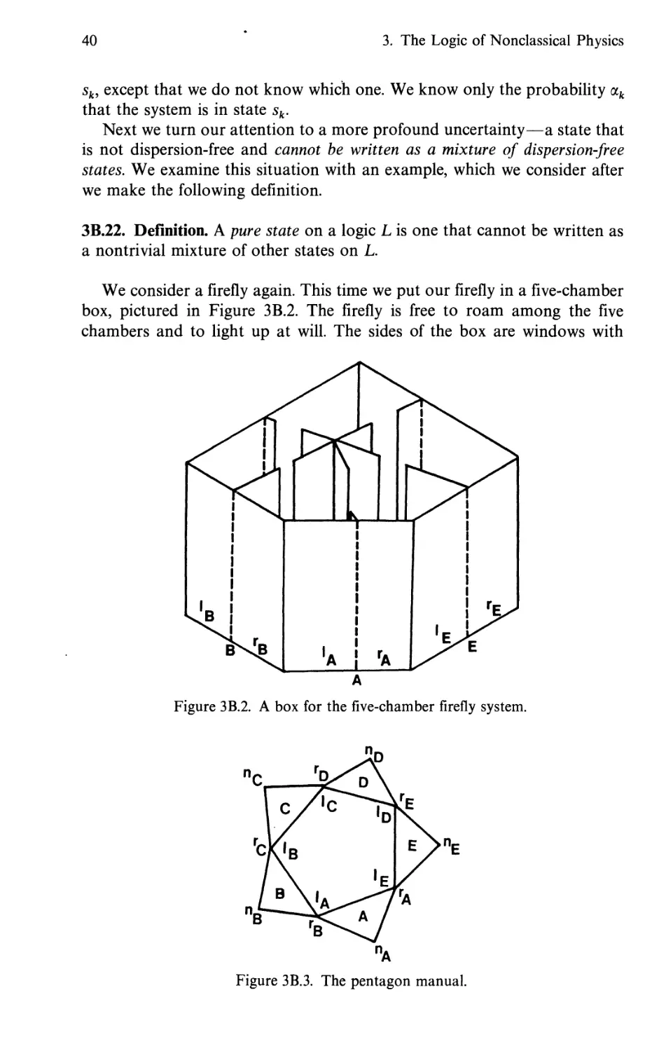
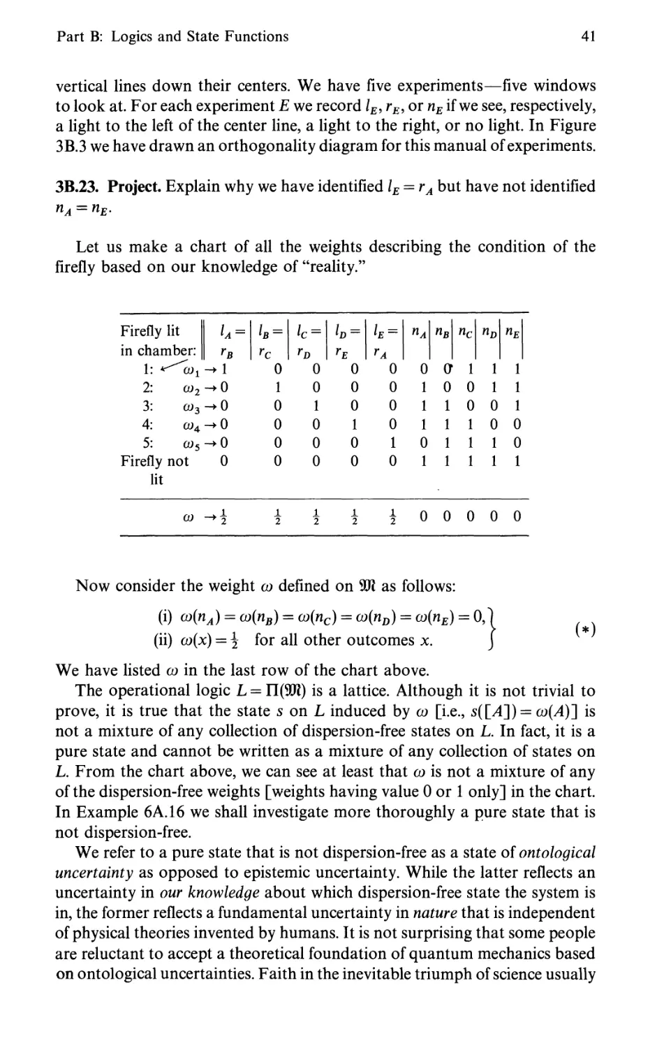
Chapter 1 we considered a physical system consisting of a firefly in a box.
Now we consider a slightly more sophisticated system.
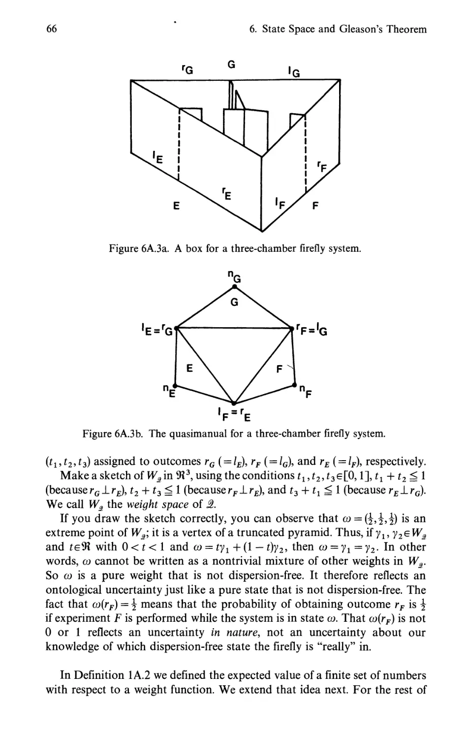
Consider a box with a clear plastic window at the front and another one
22 3. The Logic of Nonclassical Physics
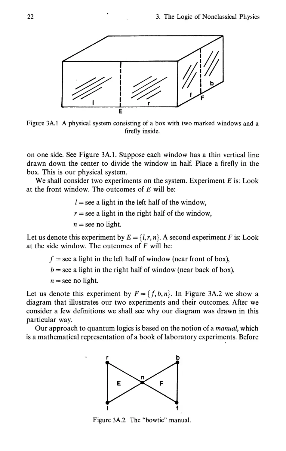
Figure 3A.1 A physical system consisting of a box with two marked windows and a
firefly inside.
on one side. See Figure 3A.1. Suppose each window has a thin vertical line
drawn down the center to divide the window in half. Place a firefly in the
box. This is our physical system.
We shall consider two experiments on the system. Experiment E is: Look
at the front window. The outcomes of E will be:
I = see a light in the left half of the window,
r = see a light in the right half of the window,
n = see no light.
Let us denote this experiment by E = {/, r, n). A second experiment F is: Look
at the side window. The outcomes of F will be:
f = see a light in the left half of window (near front of box),
b = see a light in the right half of window (near back of box),
n = see no light.
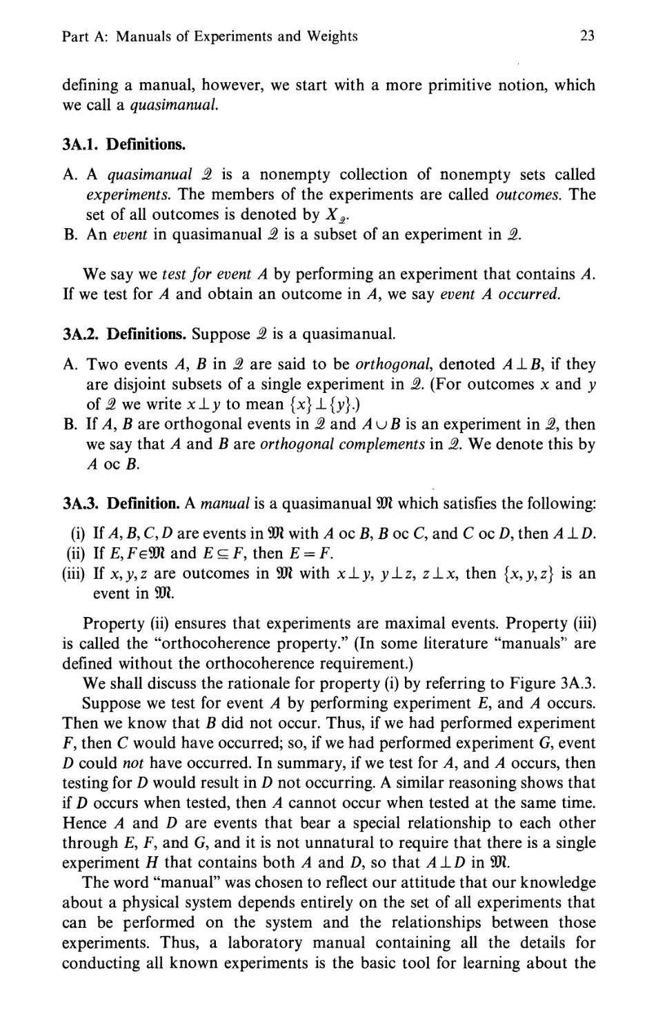
Let us denote this experiment by F = {f,b,n}. In Figure 3A.2 we show a
diagram that illustrates our two experiments and their outcomes. After we
consider a few definitions we shall see why our diagram was drawn in this
particular way.
Our approach to quantum logics is based on the notion of a manual, which
is a mathematical representation of a book of laboratory experiments. Before
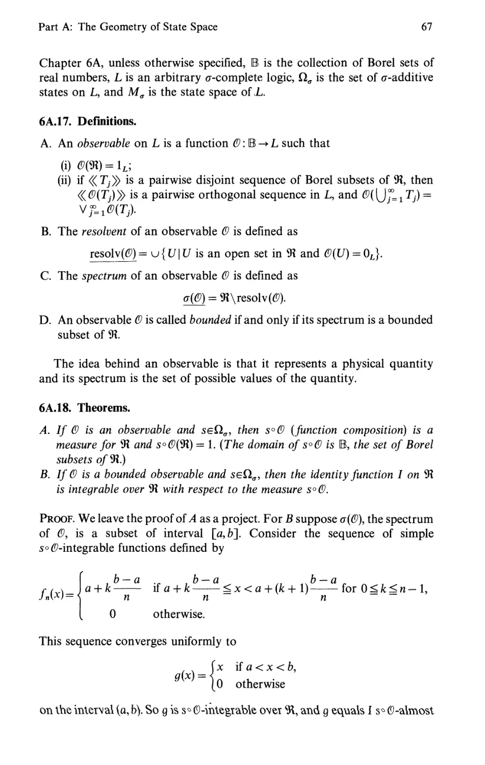
r b
I f
Figure 3A.2. The "bowtie" manual.
Part A: Manuals of Experiments and Weights 23
defining a manual, however, we start with a more primitive notion, which
we call a quasimanual.
3A.1. Definitions.
A. A quasimanual 1 is a nonempty collection of nonempty sets called
experiments. The members of the experiments are called outcomes. The
set of all outcomes is denoted by Xr
B. An event in quasimanual =2 is a subset of an experiment in =2.
We say we test for event A by performing an experiment that contains A.
If we test for A and obtain an outcome in A9 we say event A occurred.
3A.2. Definitions. Suppose =2 is a quasimanual.
A. Two events A, B in 1 are said to be orthogonal, denoted A IB, if they
are disjoint subsets of a single experiment in 1. (For outcomes x and y
of =2 we write xly to mean {x} 1 {>>}.)
B. If A9 B are orthogonal events in 1 and A kjB is an experiment in =2, then
we say that A and 5 are orthogonal complements in .2. We denote this by
A oc B.
3A.3. Definition. A manual is a quasimanual 501 which satisfies the following:
(i) If A9 B9 C, D are events in 901 with AocB9B oc C, and C oc D, then ,41D.
(ii) If E,FeWl and £ c F, then £ = F.
(iii) If x,}>,z are outcomes in 501 with xly, y-Lz, z_Lx, then [x9y9z] is an
event in 501.
Property (ii) ensures that experiments are maximal events. Property (iii)
is called the "orthocoherence property." (In some literature "manuals" are
defined without the orthocoherence requirement.)
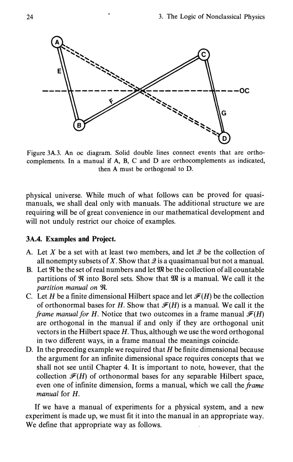
We shall discuss the rationale for property (i) by referring to Figure 3A.3.
Suppose we test for event A by performing experiment F, and A occurs.
Then we know that B did not occur. Thus, if we had performed experiment
F, then C would have occurred; so, if we had performed experiment G, event
D could not have occurred. In summary, if we test for A9 and A occurs, then
testing for D would result in D not occurring. A similar reasoning shows that
if D occurs when tested, then A cannot occur when tested at the same time.
Hence A and D are events that bear a special relationship to each other
through F, F, and G, and it is not unnatural to require that there is a single
experiment H that contains both A and D, so that AID in 501.
The word "manual" was chosen to reflect our attitude that our knowledge
about a physical system depends entirely on the set of all experiments that
can be performed on the system and the relationships between those
experiments. Thus, a laboratory manual containing all the details for
conducting all known experiments is the basic tool for learning about the
24 * 3. The Logic of Nonclassical Physics
Figure 3A.3. An oc diagram. Solid double lines connect events that are ortho-
complements. In a manual if A, B, C and D are orthocomplements as indicated,
then A must be orthogonal to D.
physical universe. While much of what follows can be proved for quasi-
manuals, we shall deal only with manuals. The additional structure we are
requiring will be of great convenience in our mathematical development and
will not unduly restrict our choice of examples.
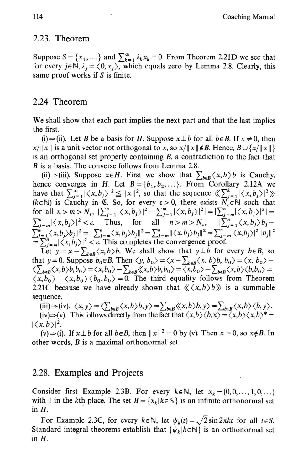
3A.4. Examples and Project.
A. Let X be a set with at least two members, and let 1 be the collection of
all nonempty subsets of X. Show that J is a quasimanual but not a manual.
B. Let 9t be the set of real numbers and let 901 be the collection of all countable
partitions of 9t into Borel sets. Show that $R is a manual. We call it the
partition manual on W.
C. Let H be a finite dimensional Hilbert space and let ^(H) be the collection
of orthonormal bases for H. Show that ^(H) is a manual. We call it the
frame manual for H. Notice that two outcomes in a frame manual ^(H)
are orthogonal in the manual if and only if they are orthogonal unit
vectors in the Hilbert space H. Thus, although we use the word orthogonal
in two different ways, in a frame manual the meanings coincide.
D. In the preceding example we required that H be finite dimensional because
the argument for an infinite dimensional space requires concepts that we
shall not see until Chapter 4. It is important to note, however, that the
collection ^(H) of orthonormal bases for any separable Hilbert space,
even one of infinite dimension, forms a manual, which we call the frame
manual for H.
If we have a manual of experiments for a physical system, and a new
experiment is made up, we must fit it into the manual in an appropriate way.
We define that appropriate way as follows.
Part A: Manuals of Experiments and Weights 25
3A.5, Definition. Manual StU2 is a refinement of manual ^ffl1 if there is
an injection cp:Xm -► Xm such that for every experiment EeWl9 (p(E) =
{(p(x)\xeE} is an event in 9012. We call cp a refinement morphism from 901x to
2R2. We write 901 x < cp9012 to denote that 9012 is a refinement of 901 x under
refinement morphism cp.
Thus, if we design new experiments for a physical system, we must refine
our laboratory manual by making sure that the old experiments are at least
events in the new manual.
3A.6. Definition. If 901 is a manual, A9 B, and C are events in 901, and A oc B
and B oc C, then we say that A and C are operationally perspective, which
we denote by A op C.
3A.7. Project. Suppose A and C are operationally perspective in manual 901.
Show that A occurs (respectively, does not occur) when tested precisely at
those instants when C occurs (respectively, does not occur) when tested.
Now we turn back to Figure 3A.2. This sketch is an orthogonality diagram,
which shows the two experiments E and F with orthogonal pairs of outcomes
connected by line segments. Notice that I and f are not connected by a line
segment, because there is no experiment that contains them both. By the
way, it is this diagram that suggests why we refer to this manual as the bow
tie manual.
Next we consider the notion of "compatibility" of experiments.
3A.8. Definitions.
A. A collection E of events in a manual 901 is compatible if u E is an event in 901.
B. A collection O of outcomes is compatible if O is an event.
Thus, a collection of events in a manual is compatible if and only if there
is one experiment that contains all those events. Performing that one
experiment tests all the events simultaneously.
3A.9. Definition. A manual is called classical if every pair of events is
compatible. Equivalently, a manual is classical if every collection of outcomes
is an event.
It was the classical assumption (perhaps unspoken) prior to this century
that any pair of experiments on a physical system can be performed
simultaneously, at least in theory. Quantum physics challenged that
assumption, and in our simple firefly experiment we see the heart of the simultaneity
issue. If we believe that the bow tie manual is the best possible characterization
of the firefly system, then we believe our firefly in a box is a nonclassical
physical system, because E and F cannot be performed simultaneously. If we
26 . 3. The Logic of Nonclassical Physics
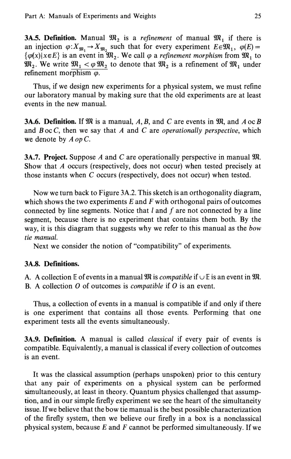
Figure 3A.4. A classical manual for the firefly-in-a-box system.
believe that we can perform E and F simultaneously, perhaps by posting two
observers, one at each window, and assuming that they can communicate
instantaneously, then we believe our system is classical and can be
characterized by a classical manual. In other words, if we have a nonclassical manual
<SJl1 describing a system that we believe is classical, then we believe that there
exists a classical manual 9W2 with 90^ <(p<SR2, so that for all E,Fe9Jlu cp(E)
and cp(F) are compatible in 5R2.
In Figure 3A.4 we have drawn an orthogonality diagram for a classical
manual characterizing the firefly system. Let us examine more closely this
idea of a manual "characterizing" a physical system. A manual is a set of
experiments. To completely characterize a physical system, it does not seem
sufficient merely to show the experiments that can be performed on it. We
should also provide some information about how the system is likely to
behave when we examine it with the experiments. In other words, to
characterize a physical system, we should provide not only a manual but
also information about the likely occurrence or nonoccurrence of the events
in the manual. This brings us to the idea of the "states" of a physical system.
In what follows we need the notion of an ordered sum.
3A.10. Definitions. Suppose £ is a set and co is a function from E to the
nonnegative real numbers. We define
£ (o(x) = lub < Yj o)(x)\S is a finite subset of E >.
xeE IxeS J
We write £xe£ co(x) = oo if the set on the right is unbounded. If A ^ E9 we
abuse notation by writing co(A) for YjxeA ^M-
Part A: Manuals of Experiments and Weights 27
3A.11. Definitions.
A. A weight on a quasimanual ^ is a function a>:X,g->[0,1] such that for
every experiment E in ^, co(E) = 1.
B. The collection of all weights on a quasimanual =2 is denoted
by 0^
We shall be concerned mainly with weights on manuals. We shall consider
that a physical system characterized by a manual 901 is associated at every
instant in time with a weight function co, so that if we test for event A at that
time by performing an experiment that contains A9 then the probability that A
will occur is co(A). Naturally, if we perform experiment £, then no matter
what state the system is in, we shall certainly obtain an outcome in E That
is why we require that oj(E) = 1.
3A.12. Example and Project. A weight oj on the bow tie manual is determined
by its values on r,n, and b. That is because co(l)= 1 — (co(n)-\-co(r)) and
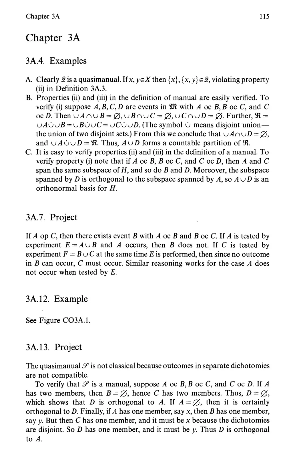
co(f) = 1 — (co(ri) + co(b)). Draw a three-dimensional coordinate system with
axes a, /?, y, and find the region of 9¾3 that represents
wm = {(a>fty)IC0E^sw anc* a = (o(r), ft = co(b% and y = co(n)}.
[The figure will be most easily recognized if you draw the a-jB-y axis system
in the perspective: a comes "out of the paper," /? is horizontal, and y is vertical.]
We turn next to another example of a nonclassical manual, one that arises
in the study of electrons. When behaviour of electrons was studied in the
context of quantum mechanics and relativity theory, it was discovered that
it was not sufficient to describe moving electrons in terms of position and
momentum. Another variable was required to explain outcomes of the
experiments described below.
Suppose we think of an electron as a small round particle that we can
move through space. Modern physics has shown that this is not at all a good
way to think about an electron, but it is sufficient for us at the moment. If
we shoot the electron from a gun and send it on a straight line path, we can
deflect it by passing it through a magnetic field. See Figure 3A.5. We can
measure the deflection by placing a screen in the path of the electron and
recording where the electron hits the screen.
Let us place a two-dimensional coordinate system on the screen with the
origin at the spot the electron would have hit if it had not been deflected.
We can orient the magnets in such a way that the electron will be deflected
only in the y direction, so that it will land at a point (0,}^) for some positive
or negative number yx. We also can orient the magnets so that the electron
will be deflected only in the x direction, landing at a point (0,:^).
The theory of quantum mechanics requires that with every electron moving
through space there is a variable called the spin variable that is associated
with how the electron is deflected by magnets. An experiment that measures
28
D—
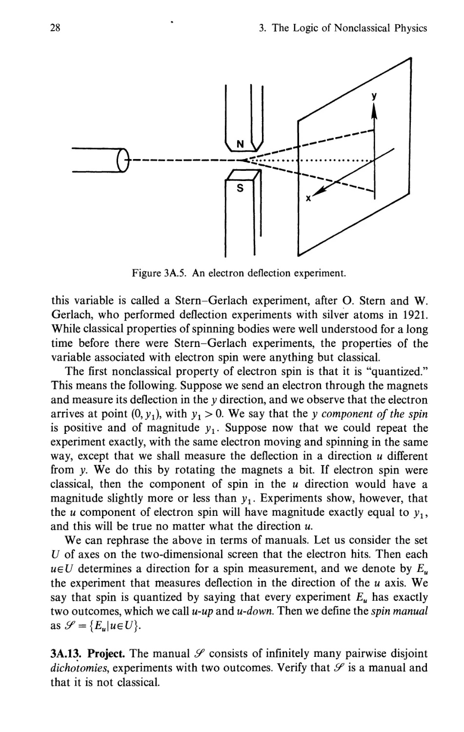
Figure 3A.5. An electron deflection experiment.
this variable is called a Stern-Gerlach experiment, after O. Stern and W.
Gerlach, who performed deflection experiments with silver atoms in 1921.
While classical properties of spinning bodies were well understood for a long
time before there were Stern-Gerlach experiments, the properties of the
variable associated with electron spin were anything but classical.
The first nonclassical property of electron spin is that it is "quantized."
This means the following. Suppose we send an electron through the magnets
and measure its deflection in the y direction, and we observe that the electron
arrives at point (0,)^), with yx > 0. We say that the y component of the spin
is positive and of magnitude yx. Suppose now that we could repeat the
experiment exactly, with the same electron moving and spinning in the same
way, except that we shall measure the deflection in a direction u different
from y. We do this by rotating the magnets a bit. If electron spin were
classical, then the component of spin in the u direction would have a
magnitude slightly more or less than yx. Experiments show, however, that
the u component of electron spin will have magnitude exactly equal to yl9
and this will be true no matter what the direction u.
We can rephrase the above in terms of manuals. Let us consider the set
U of axes on the two-dimensional screen that the electron hits. Then each
ueU determines a direction for a spin measurement, and we denote by Eu
the experiment that measures deflection in the direction of the u axis. We
say that spin is quantized by saying that every experiment Eu has exactly
two outcomes, which we call u-up and u-down. Then we define the spin manual
as£f = {Eu\ueU}.
3A.13. Project. The manual Sf consists of infinitely many pairwise disjoint
dichotomies, experiments with two outcomes. Verify that £f is a manual and
that it is not classical.
3. The Logic of Nonclassical Physics
\JLV
Part A: Manuals of Experiments and Weights 29
Next we consider a second nonclassical property of electron spin. Suppose
we prepare experiment Eu to measure the coordinate of spin in the u direction
and try to predict which outcomes will occur, w-up or w-down. It seems
reasonable to assume that at an instant tx before the electron hits the screen,
we have no idea what the outcome of experiment Eu will be. In other words,
at instant tx we can associate with the electron a weight co1 on manual Sf
such that co1(w-up) = co1(w-down) = ^. At the instant t0 the electron hits the
screen, a weight co0 on manual £f associated with the electron would have
to have co0(w-up) = 0 and co0(w-down) = 1 or vice versa (co0(w-up) = 1 and
co0(w-down) = 0). In fact, at the same instant t0, for a direction v different
from w, if we could perform Ev simultaneously with £M, the weight co0 would
have to have a>0(t;-up) = 1 and co0(t;-down) = 0 or vice versa. To continue our
discussion we make the following definition.
3A.14. Definition. A weight on a manual is called classical if it has value zero
or one on every outcome.
Therefore, a weight on spin manual & that predicts with certainty
(values 0 and 1) the u component of spin for every direction u simultaneously
at the time the electron hits the screen must be a classical weight on y.
Here is a crucial question: Can we physically prepare an electron so that
at some instant t0 its associated weight oj0 on the spin manual is classical?
From everything physicists have learned about electrons so far, the answer
appears to be "no." This is a profound issue at the heart of quantum physics.
It is a principle that all theories about the physics of an electron will be
inconsistent with experimental results if they allow that the electron at some
instant can be associated with a classical weight on the spin manual.
What makes this statement of principle profound (and controversial) is
the fact that it applies to all theories, even those that have not yet been
invented. This is one reason that quantum physics is often a topic of hot
debate. It is natural to challenge the principle by asking its proponents how
they know that it is not the case that either
(i) the way we now associate electrons with weights on the spin manual is
crude, and some day we will discover that the nonclassical weights we
observe are really some kind of mixtures of classical weights; or
(ii) this spin manual is crude and some day we will have a better manual,
perhaps a classical manual, and a way of associating electron spin with
only classical weights on the new manual.
While no one will argue that there is proof that neither (i) nor (ii) will ever
happen, all evidence that we have so far appears to point in that direction.
We shall return to this debate later.
It is important to emphasize that we constructed our manual to reflect
our assumption, based on experimental evidence, that electron spin is
nonclassical. We have not deduced the nonclassical nature of spin from the
30
3. The Logic of Nonclassical Physics
manual. The purpose of the manual in our discussion above is to describe a
theory of electron spin, not to predict it.
Let us now use Hilbert spaces to provide another description of the spin
manual Sf that will enable us to describe how electrons can be "associated"
with weights on y. It will be clear that the electron cannot be associated
with a classical weight in this vector space model.
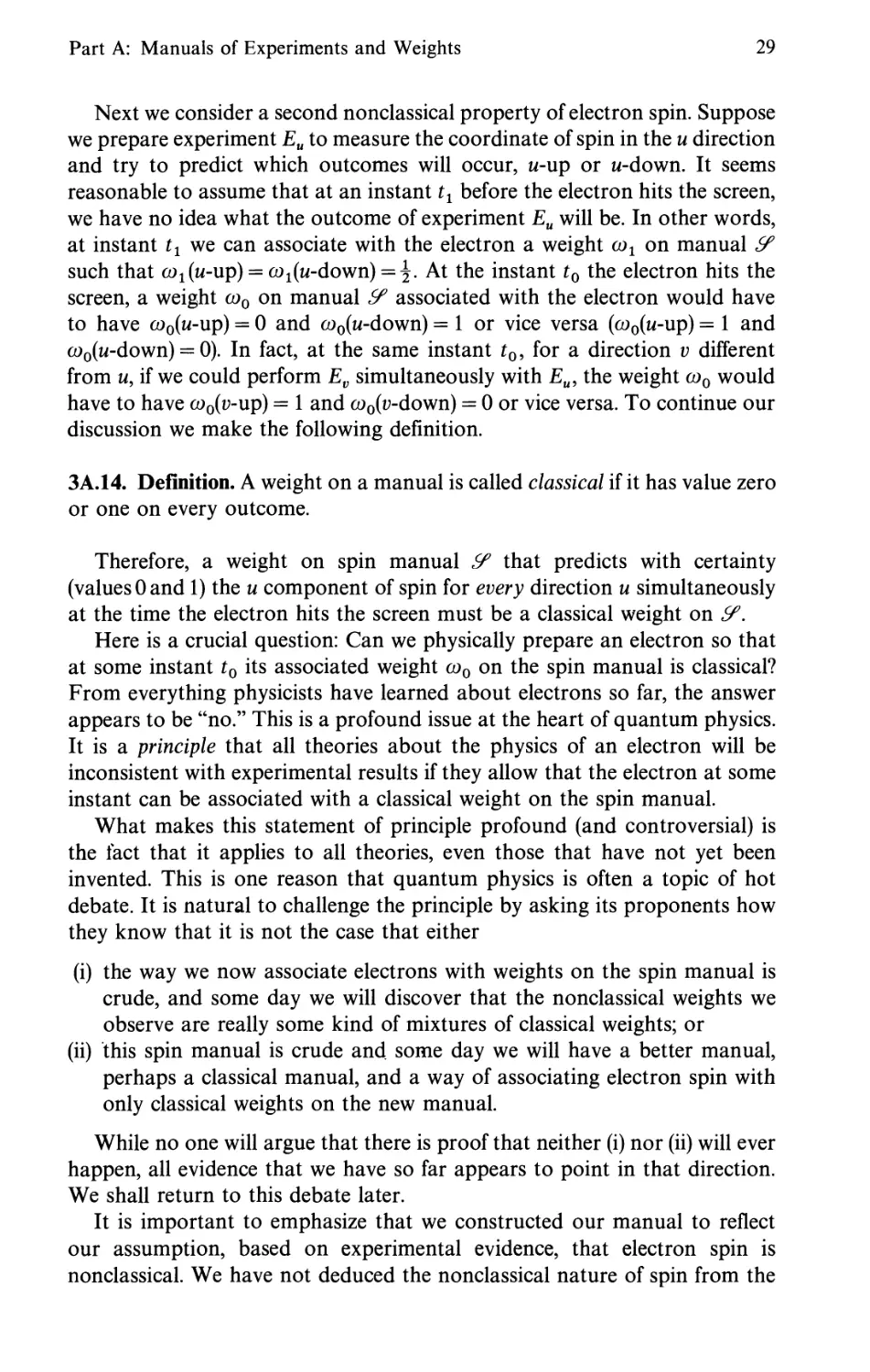
Consider again the set U of axes mentioned above. For each axis u let 6U
be the angle measured counterclockwise between the positive x axis and the
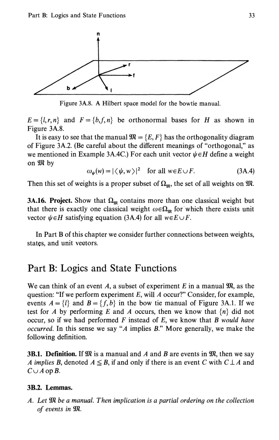
u axis. See Figure 3A.6. Now consider a two-dimensional Hilbert space /J,
and for every uell we associate a pair of subspace in H, EKu = {KU9K„}9
where Ku is the one-dimensional subspace of H oriented at angle 6J2 from
the positive horizontal axis and K^ is the orthogonal complement of Ku
in H. Refer again to Figure 3A.6. (The reason for this technicality involving
angles is explained in Chapter 8.) Be careful not to confuse the axis w, which
appears on the physical two-dimensional screen, with the subspace Ku, which
lies in the abstract space H.
Clearly, there is a one-to-one correspondence between the spin manual
£f and the set § = {EKu\usU}. Each experiment Eu = {w-up,w-down} can be
represented by a pair of orthogonal subspaces of H, one subspace representing
w-up, the other representing w-down. In Figure 3A.7 we have illustrated
experiments Ex and Ey corresponding to the measurement of the coordinate
of spin in the x and y directions shown in Figure 3A.5. Notice that in Figure
3A.5 x and y are orthogonal directions, while in Figure 3A.7 the subspaces
Kx and Ky make a 45-degree angle. We now explore the consequences of
that angle.
Physicists use matrix equations to describe electron spin. Those equations
suggest properties attributed to electrons. We shall not go into the details of
Figure 3A.6. An orthogonal pair of subspaces, Ku and Ku1 representing an
experiment to measure electron spin deflection along the u axis.
Part A: Manuals of Experiments and Weights
31
\
\
\
\
K
/
,Ky
u /,
K.
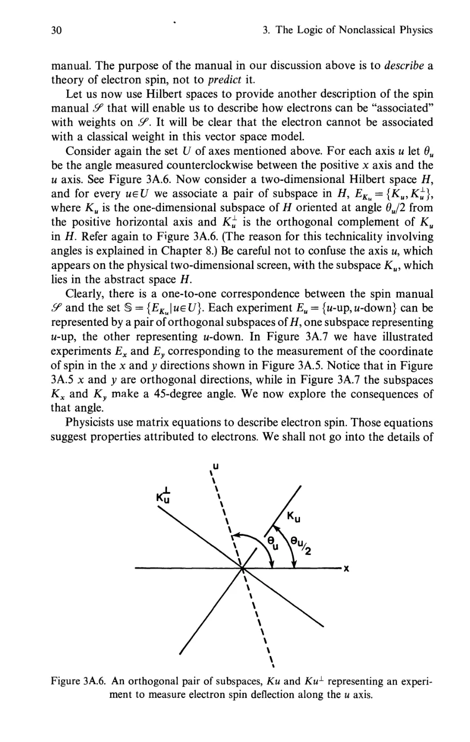
Figure 3A.7. The probabilities of the occurrence of outcomes x-up and y-up are
calculated using the projections of state vector \j/ onto the subspaces Kx and Ky.
the equations, but we shall use the spin manual to state the property that is
of interest to us: An electron in a Stern-Gerlach apparatus is said to exist
at every instant in time in a "state" \j/9 which can be represented by a unit
vector in the Hilbert space H of Figure 3A.7. With each state \j/ is associated
a weight on the spin manual £f as follows: for ueU, co(w-up) is the square of
the length of the projection of if/ onto the subspace Ku, and co(w-down) is the
square of the length of the projection of \j/ onto the subspace K„. (We
shall consider projections more generally in Chapter 4, but we are assuming
here that you have already encountered projections when you studied finite
dimensional linear algebra.)
We write
(3A.1)
%(w-up)=||ProjKt>||2,
co^(w-down) = || Proj^i^ ||2.
Thus, if the electron is in state if/, then we know that the probability of
obtaining the outcome "x-up" if we do experiment Ex is the square of the
projection of state vector i// onto subspace Kx.
3A.15. Project. Show that co given by equation (3A.1) is a weight on £f and
that it is a nonclassical weight.
This description of the spin states of an electron raises some delicate
questions about measurements. Suppose first that we measure for the x
component of spin and obtain outcome x-up. The electron is then in state
\j/. If we assume that we can let the electron pass through the screen and
32 3. The Logic of Nonclassical Physics
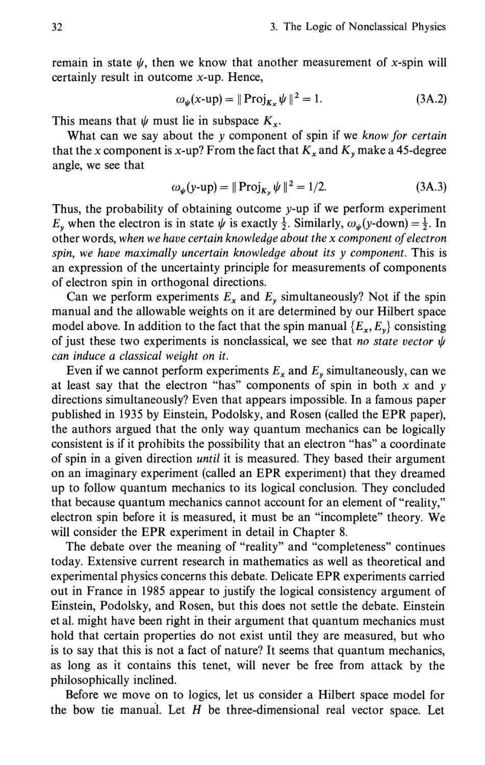
remain in state \j/9 then we know that another measurement of x-spin will
certainly result in outcome x-up. Hence,
co^x-up) = || ProjKx ij/1|2 = 1. (3A.2)
This means that if/ must lie in subspace Kx.
What can we say about the y component of spin if we know for certain
that the x component is x-up? From the fact that Kx and Ky make a 45-degree
angle, we see that
co+iy-up) = II ProJ£y \j/ \\2 = 1/2. (3 A. 3)
Thus, the probability of obtaining outcome y-up if we perform experiment
Ey when the electron is in state i// is exactly \. Similarly, co^y-down) = \. In
other words, when we have certain knowledge about the x component of electron
spin, we have maximally uncertain knowledge about its y component. This is
an expression of the uncertainty principle for measurements of components
of electron spin in orthogonal directions.
Can we perform experiments Ex and Ey simultaneously? Not if the spin
manual and the allowable weights on it are determined by our Hilbert space
model above. In addition to the fact that the spin manual {Ex,Ey} consisting
of just these two experiments is nonclassical, we see that no state vector if/
can induce a classical weight on it.
Even if we cannot perform experiments Ex and Ey simultaneously, can we
at least say that the electron "has" components of spin in both x and y
directions simultaneously? Even that appears impossible. In a famous paper
published in 1935 by Einstein, Podolsky, and Rosen (called the EPR paper),
the authors argued that the only way quantum mechanics can be logically
consistent is if it prohibits the possibility that an electron "has" a coordinate
of spin in a given direction until it is measured. They based their argument
on an imaginary experiment (called an EPR experiment) that they dreamed
up to follow quantum mechanics to its logical conclusion. They concluded
that because quantum mechanics cannot account for an element of "reality,"
electron spin before it is measured, it must be an "incomplete" theory. We
will consider the EPR experiment in detail in Chapter 8.
The debate over the meaning of "reality" and "completeness" continues
today. Extensive current research in mathematics as well as theoretical and
experimental physics concerns this debate. Delicate EPR experiments carried
out in France in 1985 appear to justify the logical consistency argument of
Einstein, Podolsky, and Rosen, but this does not settle the debate. Einstein
et al. might have been right in their argument that quantum mechanics must
hold that certain properties do not exist until they are measured, but who
is to say that this is not a fact of nature? It seems that quantum mechanics,
as long as it contains this tenet, will never be free from attack by the
philosophically inclined.
Before we move on to logics, let us consider a Hilbert space model for
the bow tie manual. Let H be three-dimensional real vector space. Let
Part B: Logics and State Functions 33
Figure 3A.8. A Hilbert space model for the bowtie manual.
E = {/, r, n} and F = \bj, n} be orthonormal bases for H as shown in
Figure 3A.8.
It is easy to see that the manual 901 = {E9 F} has the orthogonality diagram
of Figure 3A.2. (Be careful about the different meanings of "orthogonal," as
we mentioned in Example 3A.4C.) For each unit vector xj/eH define a weight
on2Kby
Gty(w) = |<^,w>|2 for all weEuF. (3A.4)
Then this set of weights is a proper subset of Q^, the set of all weights on 901.
3A.16. Project. Show that Q.m contains more than one classical weight but
that there is exactly one classical weight (joeQ.m for which there exists unit
vector \j/eH satisfying equation (3A.4) for all weEvF.
In Part B of this chapter we consider further connections between weights,
states, and unit vectors.
Part B: Logics and State Functions
We can think of an event A, a, subset of experiment £ in a manual 901, as the
question: "If we perform experiment £, will A occur?" Consider, for example,
events A = {/} and B = {f,b} in the bow tie manual of Figure 3A.1. If we
test for A by performing E and A occurs, then we know that {n} did not
occur, so if we had performed F instead of £, we know that B would have
occurred. In this sense we say "A implies £." More generally, we make the
following definition.
3B.1. Definition. If 9W is a manual and A and B are events in 901, then we say
A implies B, denoted A ^ B, if and only if there is an event C with CIA and
C u A op B.
3B.2. Lemmas.
A. Let WUbe a manual Then implication is a partial ordering on the collection
of events in 9H.
34 3. The Logic of Nonclassical Physics
B. Suppose 901 is a manual coeQ^, and A and B are events in 90¾ with A^B.
Then co(A) ^ co(B).
Proof. Project. □
3B.3. Definition. If 901 is a manual and A and B are events in 901, then we say
A is logically equivalent to B, denoted ,4<->£, if and only if A ^ B and B ^ A.
Clearly, <-► is an equivalence relation on the set of events in a manual.
3B.4. Lemmas. Suppose 901 is a manual.
A. If A, B are events in 901, then AopB if and only if A<r+B.
B. IfE,FeWl, thenE<^F.
Proof. Project. □
3B.5. Lemmas. Suppose 901 is a manual.
A. If A, B, C, D are events in 901 and A<^>C and £<-»D, then A^B if and only
ifC^D.
B. If A is an event in 901 and E, FeSDl, with A<=E and A^F, then F\A<^E\A.
Proof. Project. D
3B.6. Definitions. Suppose 901 is a manual.
A. If A is an event in 901, then we define
[A] = {B | B is an event in 901 and A<-*B}9
and we call [,4] the logical proposition determined by A. We say we test
for proposition [,4] if we test for any event in 901 logically equivalent to
A. An event used to test for [,4] confirms that [,4] is true (respectively,
false) if the event occurs (respectively, does not occur). For outcome x we
write [x] for [{x}].
B. We define 1I(S£R) = { [,4] | A is an event in Wl}.
C. We define a partial order on 11(901) by
M ^ [B] if and only if A ^ B in S01,
in which case we say [,4] implies [£].
D. For [,4]eIT(901), we define the orthocomplement of [,4] by [,4]' = [£\,4],
where E is any experiment in 901 with A^E.
E. If [,4], [£]ell(901), we say that they are orthogonal denoted by [,4] 1 [B],
if and only if [,4] ^ [JJ]'.
F. The set 11(901), together with the implication ^ and orthocomplementation
is called the operational logic of manual 9W.
Part B: Logics and State Functions 35
Lemmas 3B.4 show that the partial order and the orthocomplementation
on 11(901) are well defined.
3B.7. Examples and Projects.
A. Let 501 be a manual consisting of just one dichotomy E = {x,y}. Find the
logic n(50l).
B. Show that if \_A~\ ^ [£], then a test for \_A~] which confirms that [A] is
true at the same time confirms that [£] is' true. That is why we use the
word "implies" to express the relation [A] ^ [2?].
C. Show that \_A\ ^ [£]' if and only if [B] ^ [X]'.
3B.8. Lemma. For events A, B in manual 901, [_A] _L [£] if and only if A IB.
Proof. Project. □
As we shall see in Chapter 4, if ^(H) is the frame manual for a Hilbert
space if, then its operational logic can be identified with the structure of
subspaces of //, which historically was the prototype for a "quantum logic."
We have motivated the notion of an operational logic by considering
physical experiments, and we have seen a sharp distinction between classical
and nonclassical manuals. Next we shall study logics in greater generality to
see how differences between classical and nonclassical physics manifest
themselves in logics.
3B.9. Definition. Let P be a set with a partial ordering ^. Then (P, ^) is
called a lattice if for all p,qeP the set {p,q} has a greatest lower bound and
a least upper bound in P.
We call gib {/?, q} the meet of p and q, and we denote it by p a q.
We call lub {/?, q} the join of p and q, and we denote it by p v q.
a
Figure 3B.1. A tree diagram for a lattice.
36 * 3. The Logic of Nonclassical Physics
For a finite lattice it is often helpful to draw a "tree" diagram, as in Figure
3B.1, for example. We draw p below q and connect them with a line segment
if P ^ q and if there does not exist w with p < w < q. By the fact that the
partial order is transitive, we read right from the diagram that m ^ n if we
can find a path that moves steadily upward from m to n. So in the figure we
see that a ^ h and a ^ d, but d ^ e and e ^ d. We also see immediately that
g a h = e and b v f = h.
3B.10. Definitions. Let (L, ^) be a lattice.
A. A unit 1L for L is a member of L such that p ^ 1L for all peL.
B. A zero 0L for L is a member of L such that 0L^p for all /?eL.
As usual, we drop the subscript L for the unit and zero if there is no ambiguity
about which lattice is meant.
3B.11. Examples and Project.
A. Let X be a nonempty set and let Sub (X) be the collection of all subsets
of X. Show that Sub (X), partially ordered by set inclusion [/? ^ q if and
only if p ^ #], is a lattice with unit and zero. Draw the tree diagram for
such a lattice in the case X -has exactly three members.
B. Let H be a finite dimensional Hilbert space, and let L be the collection
of all subspaces of H. Define a partial order on L as follows: for R, SeL,
R ^ S if and only if R is a subspace of S. Show that (L, ^) is a lattice
with unit and zero. Draw the tree diagram for L in the case H has
dimension 2. Later we shall extend this idea to infinite dimensional Hilbert
spaces.
C. Let SDt be the bow tie manual. Draw the tree diagram for (IT(9W), ^), and
determine whether or not it is a lattice. Does it have unit and/or
zero?
Motivated by operational logics, we now make the following general
definitions.
3B.12. Definitions.
A. A logic (L, ^/) consists of a lattice (L, ^) with unit and zero, together
with an operation ':L^L, called an orthocomplementation, that satisfies:
(i) for all peL, p" = p and p a p' = 0L;
(ii) for /?, qeL, if p ^ q, then q' ^ p'\
(iii) for /?, qeL, if p ^ q, then q = p v (// a g).
Property (iii) is called the orthomodular identity.
Where there is no ambiguity about the order relation or orthocomple-
mentation, we denote a logic (L, ^,') simply by L.
B. If L is a logic and p.qeL, we say p is orthogonal to q, denoted
p _L q, if and only if /? ^ g'.
Part B: Logics and State Functions 37
The members of L are called propositions. For example, if 90¾ is a manual
and A is an event in 901, then the proposition p = [A] is the proposition: "If
we test for event A9 it will occur." Naturally, this proposition may be true
at some instants of time and false at others. In our applications we shall
interpret the proposition p' as the negative of proposition p. Thus, p is true
precisely when p' is false and vice versa.
The relation p ^ q will be interpreted as the statement: "Proposition p
implies proposition q." The propositions p a q and p v q will be interpreted
respectively as the conjunction "p and q" and the disjunction "p or q." When
we consider states on a logic we shall hypothesize that the proposition 1L is
true for all states and that the proposition 0L is true for no state.
There are systems (L, ^/) that satisfy all the properties of logics except
that they are not lattices. If we were to explore logics in more detail, we
would use a more general definition of a logic by requiring only that (L, ^)
be a partially ordered set and by replacing property (iii) with a slightly weaker
version. In nearly all of our examples, however, our operational logics will
be lattices. Moreover, the subspaces of a Hilbert space form a lattice that is'
the logic of orthodox quantum mechanics, and we shall study this in great
detail. That is why we use a slightly less general definition of a logic than
you might find elsewhere.
Since lattices of subspaces of Hilbert space satisfy more properties than
more general logics, it is important to try to determine which of the properties
of a logic are really necessary to describe physical nature and which properties
are superfluous, perhaps even misleading, to theoretical physicists. There is
currently much research being done by mathematicians and physicists trying
to make these determinations. Perhaps you will have some ideas after we
study logics a little further.
3B.13. Theorem (DeMorgan's Law). If Lis a logic and p9qeL9 then
(P v <l)' = P' A 4 and (p a a)' = p' v q'.
Proof. Project. D
Next we consider compatibility in logics.
3B.14. Definition.
A. Two propositions p and q in logic L are called compatible if there exist
u9v9weL such that:
(i) {w, v9 w} is a pairwise orthogonal set in L;
(ii) uv v — p and v v w = q.
We call {u9 v9 w} a compatibility decomposition for p and q.
B. A quantum logic is a logic with at least two propositions that are not
compatible.
38 * 3. The Logic of Nonclassical Physics
C. A classical logic is a logic in which every pair of propositions is a
compatible pair.
3B.15. Theorem. If {w, v9 w} is a compatibility decomposition for p and q in a
logic L, then
(i) u = p a q';
(ii) w = p' a q;
(Hi) v = p a q = (p' v q) a p = (p v q') a q.
Note that this implies that w, v9 and w are uniquely determined by p and q.
Proof. Project.* □
3B.16. Theorem. If p and q are propositions in a logic L, then p and q are
compatible if and only if
(0 P = (P A #) v (P A <i\ and
(ii) q = (qAp)v'(qApf).
Proof. Project. D
Notice that it is always true that (p a q) v (p a q') ^ p. Theorem SB.16 then
states that we generally do not have that p ^ (p a q) v (p a a1) unless p and q
are compatible. In other words, knowing that proposition p is true is not sufficient
for concluding that at least one of the following is true:
(i) p and q are simultaneously true, or
(ii) p and "not-q" are simultaneously true.
This logical structure captures the idea that for some physical systems
there might exist a pair of propositions whose truth values simply cannot be
simultaneously determined. Theorem 3B.16 is the manifestation in the logic
of the notion that pairs of events in a manual might not be simultaneously
testable.
3B.17. Theorem. If A and B are compatible events in manual 901, then [A\ and
[B] are compatible in the operational logic 11(901).
Proof. Project. D
In later chapters we show that we can associate the subspaces of a Hilbert
space H with propositions in a logic, and certain linear operators on H with
physical observables. Then we show that a pair of operators (observables)
commutes if and only if a certain collection of subspaces (propositions) is
pairwise compatible. This neatly ties up the notions of simultaneously testable
observables, commuting operators, and logically compatible propositions in
the Hilbert space model for quantum physics.
Part B: Logics and State Functions 39
3B.18. Definition. Suppose L is a logic. We define a state on L as a function
s: L -► [0,1] such that
(i) for /?, qeL9 if p 1 q, then s(p v q) = s(p) + s(q\ and
(ii)s(lL)=l.
If 901 is a manual with operational logic L = 11(901), then a state 5 on L is
also called a probability measure on L. For if [A~\ is a member of L, then
s( [,4]) is usually interpreted as the probability that the event A (or an equivalent
event) will occur if tested while the system represented by 901 is in state s. That
is why we require that if A and B are orthogonal events, the probability of
the occurrence of their join is the sum of their individual probabilities of
occurring. In this sense their join is interpreted as the disjunction: "either A
or B occurs."
3B.19. Example and Project. Let 901 be the bow tie manual, and suppose co
is a weight on 501. Let s:II(901)-►[(), 1] be defined by s{lA]) = co(A). Show
that 5 is a state on 11(901). We call 5 the state on 11(901) induced by a>.
The notion of a state on a logic provides us with another way to examine
the fundamental uncertainty of nature.
3B.20. Lemma. Suppose L is a logic and {sl9...9sn} is a finite collection of
states on L. Suppose {ol19...9ol„} is a collection of real numbers satisfying:
(i) for all k = 1,..., n, 0 ^ <xk ^ 1;
(") Zfc = ia*=L
Then the function s = Y! = i afc5fc> defined for every peL by
n
s(p)= Yj aksk(p) is a state on L.
k=l
We call s a mixture of the states sl9...9sn9 and we refer to a set of numbers
satisfying (i) and (ii) as a mixing set of numbers.
Proof. Project. □
3B.21. Definition. A state 5 on logic L is called dispersion-free if, for all peL9
either s(p) = 0 or s(p) = 1.
Dispersion-free states are also called classical states.
A key question in the foundation of physics is: When is a state that is not
dispersion-free a mixture of dispersion-free states? For example, in a physical
experiment we might be able to determine that at a certain time a physical
system is in a state that is a mixture s = Y2 = iaksk °f dispersion-free states
sl9...9sn. Then we say 5 is a mixture reflecting an epistemic uncertainty. By
that we mean that we believe the system is in one of the dispersion-free states,
*
40 3. The Logic of Nonclassical Physics
sk, except that we do not know which one. We know only the probability ak
that the system is in state sk.
Next we turn our attention to a more profound uncertainty—a state that
is not dispersion-free and cannot be written as a mixture of dispersion-free
states. We examine this situation with an example, which we consider after
we make the following definition.
3B.22. Definition. A pure state on a logic L is one that cannot be written as
a nontrivial mixture of other states on L.
We consider a firefly again. This time we put our firefly in a five-chamber
box, pictured in Figure 3B.2. The firefly is free to roam among the five
chambers and to light up at will. The sides of the box are windows with
Figure 3B.2. A box for the five-chamber firefly system.
Figure 3B.3. The pentagon manual.
Part B: Logics and State Functions
41
vertical lines down their centers. We have five experiments—five windows
to look at. For each experiment E we record /£, r£, or nE if we see, respectively,
a light to the left of the center line, a light to the right, or no light. In Figure
3B.3 we have drawn an orthogonality diagram for this manual of experiments.
3B.23. Project. Explain why we have identified lE = rA but have not identified
nA = nE.
Let us make a chart of all the weights describing the condition of the
firefly based on our knowledge of "reality."
Firefly lit
in chamber:
1
2
3
4
5
Ia =
rB
' ^CDi -► 1
ci>2->0
W3-+O
a>4 ->0
w5-+0
Firefly not 0
lit
CD -►£
Ib =
rc
0
1
0
0
0
0
1
2
k =
rD
0
0
1
0
0
0
1
2
Id =
rE
0
0
0
1
0
0
1
2
*£ =
rA
0
0
0
0
1
0
1
2
*A
0
1
1
1
0
1
0
"B
a
0
1
1
1
1
•
0
»c
1
0
0
1
1
1
0
»D
1
1
0
0
1
1
0
nE
1
1
1
0
0
1
0
Now consider the weight 00 defined on $R as follows:
(i) ao(nA) = ao(nB) = w(nc) = w(nD) = w(nE) = 0,
(ii) (d(x) = \ for all other outcomes x.
(*)
We have listed co in the last row of the chart above.
The operational logic L = 11(501) is a lattice. Although it is not trivial to
prove, it is true that the state 5 on L induced by co [i.e., s(D4]) = 00(A)'] is
not a mixture of any collection of dispersion-free states on L. In fact, it is a
pure state and cannot be written as a mixture of any collection of states on
L. From the chart above, we can see at least that 00 is not a mixture of any
of the dispersion-free weights [weights having value 0 or 1 only] in the chart.
In Example 6A.16 we shall investigate more thoroughly a pure state that is
not dispersion-free.
We refer to a pure state that is not dispersion-free as a state of ontological
uncertainty as opposed to epistemic uncertainty. While the latter reflects an
uncertainty in our knowledge about which dispersion-free state the system is
in, the former reflects a fundamental uncertainty in nature that is independent
of physical theories invented by humans. It is not surprising that some people
are reluctant to accept a theoretical foundation of quantum mechanics based
on ontological uncertainties. Faith in the inevitable triumph of science usually
42 3. The Logic of Nonclassical Physics
allows uncertainty only as a temporary, incomplete description of a physical
system, not as a fundamental state of nature.
Consider the ontological uncertainty in the five-chamber firefly system.
What is the "real" physical state corresponding to the weight cd that assigns
\ to each of the outcomes corresponding to a light-up? It is hard for us to
imagine how a firefly could behave to produce such a state, tempting us to
say that no such state can exist in "reality"—it is only a mathematical quirk.
But we must be careful before dismissing such a state as "unreal." Perhaps
in this state the firefly can sense our presence and fly immediately to whatever
chamber we look at and light up, half the time on one side of the center line,
half the time on the other. This is a stage-struck firefly! Surely we have made
a strained explanation. What it illustrates is a desperate attempt to fit the
mechanical system (the firefly in the box) to the theoretical model (the logic
and its states).
In physics it is often the case that the theoretical model comes first from
manipulations of equations, and the mechanical system (an "antiparticle,"
for example) is then described to fit the theoretical model. When strained
explanations are required to fit the two, physicists are faced with a choice:
Should they change the mechanical model or the theoretical model? The final
judgements are determined by experiments. The larger the number of
experiments that are consistent with the theoretical model, the more faith
people have in the theory, and then pressure builds to change the mechanical
model. Of course, if an experiment produces results inconsistent with a theory,
that theory is immediately changed or discarded, no matter how nicely it fits
with a mechanical model.
What role does ontological uncertainty play in the evaluation of a
theoretical model? If a model containing an ontological uncertainty fits well
with all experiments known, it seems unwise to throw it out on the basis of
a philosophical prejudice against ontological uncertainty, although one might
cling to the hope that the model eventually will be adjusted to contain only
epistemic uncertainties. How tenaciously to cling to such hope is a personal
decision.
Fortunately, it is not necessary for a physicist or a mathematician to take
sides in the debate about the existence of ontological uncertainty in nature.
We can simply provide the framework in which the issues can be precisely
and unambiguously stated and leave the debate to others. That is what we
shall do in the rest of this book.
CHAPTER 4
Subspaces in Hilbert Space
In Chapter 3 we used two-dimensional Hilbert space to model a manual for
measuring electron spin, because every experiment had only two outcomes:
spin-up and spin-down. Of course, many physical experiments have outcome
sets that are not finite. A measurement of energy, position, or momentum of
a moving particle usually means obtaining an outcome from an infinite number
of possibilities. In this chapter we shall learn about infinite dimensional
Hilbert spaces. In particular, we shall consider the subspace structure of
infinite dimensional Hilbert spaces. These provide the logics for orthodox
quantum physics.
Throughout this chapter, unless otherwise noted, H will denote an
arbitrary Hilbert space with a countable basis. As usual, 9t and (£ denote,
respectively, the real and complex numbers.
4.1. Definition. A set M ^ H is a linear manifold in H if and only if for all
x,yeM and all ae£, x + y and ax both belong to M.
You probably recognize that if H is finite dimensional, a linear manifold
is just a "vector subspace." In the infinite dimensional case, however, the
word "subspace" is reserved for certain kinds of manifolds.
4.2. Definition. A set S ^ H is closed if every Cauchy sequence in 5 converges
in norm to a vector in S.
4.3. Theorem. If S is a collection of closed subsets of //, then n§ is a closed
set in H.
Proof. Project. □
44 4. Subspaces in Hilbert Space
4.4. Definition. If S ^ //, we define the closure of S by
clos(S) = n {C | S c c, and C is closed}.
Observe from Theorem 4.3 that clos(S) is a closed set. From the definition
of intersection, observe that it is a subset of every closed set containing S.
An alternative definition of the closure of S is
clos (S) = {x | there exists sequence «xfc» in S that converges in norm to x}.
It is not difficult to prove that the two definitions are equivalent, but we
shall omit the proof.
4.5. Example and Project. Let H be a two-dimensional Hilbert space* and
let S = {xeH I || x || < 1}. Suppose 0 / xeS, and consider the sequence defined
by xk = (l/||x|| — l//c)x for all keN. Show that xkeS for all keN and that
«*fc» converges in norm to x/||x ||, which is not a member of S. Thus, S is
not closed.
4.6. Definition. A subspace in a Hilbert space H is a closed linear manifold
in//.
Observe that if K is a subspace in //, then K is a Hilbert space.
4.7. Examples and Project. (Example A contains a project, Example B does
not.)
A. Let H = I2. (See Example 2.3B.) Let M = \xeH\x = «xfr», and all but
finitely many xk equal zero}. Show that M is a linear manifold in H that
is not closed. (This project is at level *.)
B. Suppose [a, fc] is an interval in 9¾. Then the following are linear manifolds
in J£2(a>b). (See Example 2.3C.)
C[a, b~\ = {if/1 \j/: [a, fc] -> (£ and ^ is continuous on [a, fc] }.
C°° [a, fc] = {ij/1 t/f: [a, fc] -> 9¾ and i// has derivatives of all orders
on (a, b) and is continuous at a and b}.
Be cautioned that our notation obscures the fact that both sets above are
sets of equivalence classes, where ij/1 is equivalent to \\i2 if and only if
i//1 = i//2 /i-ae on [a,b], where \i is Lebesgue measure.
If y\i is continuous on [a, b\ then |i/^|2 is continuous, hence integrable
on \a,b\ From this and the fact that functions are continuous at all
points at which they are differentiable, we have that
C°°[a,fc] c C[a,fe] c jgf2(a,fe).
That C°°[a,b] and C[a,fr] are linear manifolds in y2(a,b) follows from
standard theorems in calculus. Although we shall not prove it here, neither
of these manifolds is closed in <&2(a,b). On the other hand, the closure of
C[a,fc] is y?2(a,b\
4. Subspaces in Hilbert Space 45
4.8. Theorem. If K is a subspace in H and B is a basis for K, then there is a
basis B0 for H with B^B0.
Proof. B is an orthonormal set in H, so is contained in a maximal
orthonormal set, which is countable by Theorem 2.26. □
4.9. Lemmas.
A. If K is a subspace in H, then there exists basis B for K such that for all
xeH, xeK if and only ifx = XbeP <x, b}b. (This project is at level * because
it requires the use of Zorns lemma.)
B. If K is a subspace in H and B is a basis for K, then for all xeH, if xA.b
for all beB, then x±y for all yeK.
Proof. Project. □
4.10. Theorem. If M is a linear manifold in H, then clos (M) is a linear manifold
in H and is, therefore, a subspace in H.
Proof. That clos(M) is a manifold follows from Theorem 2.2IB. □
4.11. Definition. If S ^ H, we define the span of S by
v S = n {K | K is a subspace in H with S ^ K}.
4.12. Theorem. If S^H, then
(i) v S is a subspace in //; »
(ii) S^vS;
(Hi) for all subspaces K in //, if S^ K, then v S^K.
In other words, v S is the smallest subspace in H containing S.
Proof. Project. □
4.13. Theorem. SupposeS ^HandM = {Y! = iKxkI nsN, Ake£, xkeS}. Then
(i) M is a linear manifold in H;
(U) vS = clos(M).
In other words, the span of S is the closure of the set of all finite linear
combinations of members of S.
Proof. Project. □
4.14. Corollary. If S ^//, then xevS if and only if there is a sequence «xk»
in S and a sequence «Ak» in £ with x = Y,7=i^kxk- If the last equality holds,
we say x is a linear combination of the members of S.
46 4. Subspaces in Hilbert Space
Proof. This is immediate from Theorem 4.13. D
Now we are ready to make the connection between the subspace structure
for a Hilbert space and quantum logics.
4.15. Definitions.
A. If S ^ //, we define S1 = {xeH\ for all 5eS, x 1 s}. We call S1 the orthogonal
complement of S.
B. If S is a collection of subsets of //, we write
VS for v(u§).
SeS
4.16. Lemmas.
A. If S^ //, then S is a countable orthonormal set if and only if S is a basis
for vS.
B. If0czAczB^H(0^A^B)andBisa basis for //, then (BXA)1 = v A.
Proof. Project. □
4.17. Theorem. If S^H, then
(0 S1 n S = {0};
(ii) S1 is a subspace in H (even if S is not);
{Hi) ifS^T^H, then T1 c= S1;
(1¾) S^iS1)1;
(v) if S is a subspace in //, then (S^Y = S;
(vi) if § is a collection of subspaces in //, then (v^gS)1 = f]s ^1 and
(vii) if S is a countable, orthonormal set, then S±n v S = {0}.
Proof. Project.* D
4.18. Theorem. If H is a Hilbert space and I is the collection of all subspaces
in //, then 1(//) = (fl_, ^,1) is a logic with 0 = {0} and 1=//
Proof. If Kl9 K2el, then {Kl9K2} has least upper bound Kx v K2 and
greatest lower bound K1f]K2. So (l, ^) is a lattice. Clearly, {0} and H are,
respectively, the least and greatest members of the lattice. It remains to show
that 1 is an orthocomplementation. Theorem 4.17, however, gives us
everything we need except the orthomodular identity, which we leave as a project
(at level *). D
In example 3A.4C we saw that if H is a Hilbert space, then the collection
^(H) of orthonormal bases for H is a manual, which we called the frame
manual for //. Then in that same chapter, in a remark following Example 3B.8,
4. Subspaces in Hilbert Space 47
we promised that we would eventually link the logic of a frame manual with
the subspace structure of the Hilbert space. We fulfill that promise now.
Let us begin by reviewing the definitions associated with a frame manual
901 = tF(H). The events in 901 are orthonormal subsets of H. For events A
and B in 901, A oc B if and only if A u B is a basis for H; and A op B if and
only if there exists event C such that A oc C and B oc C. We need the
following two lemmas concerning arbitrary events A9 B, C in 901.
4.19. Lemma.
A. A oc C j/* and only if C1 = v A
5. ^ op 5 f/*and on/y if v A= v B.
Proof. Project. □
4.20. Theorem. If A and B are events in frame manual ^(//), then
(i) the following are equivalent.
(a) A op £,
\b) v A= v B,
(c) A<^>B (A is logically equivalent to B in manual ^(H));
(ii) A IB if and only if \_A~] 1 [B].
(Be careful about the two meanings of _L here. The one on the left is
orthogonality in the Hilbert space, hence based on the inner product; the one
on the right is orthogonality in the logic L(//), meaning \_A\ ^ [2*]'.)
Proof. Project. □
Theorem 4.20 sums up the main connections between a Hilbert space
frame manual and its associated logically structure. Part (i) shows that events
A and B are operationally perspective if and only if they are logically
equivalent, which happens if and only if they span the same subspace.
Recall that in Equation (3A.1) we defined a weight on the spin manual
by means of projections of a unit vector \\i onto subspaces of H. We assumed
that you were familiar with the notion of projections in two-dimensional
vector spaces. We turn now to a notion of projection in infinite dimensional
Hilbert space.
4.21. Definition. If IK = {Kl9...} is a countable collection of subspaces in //,
then we define
oo
+ K. = < Y, xj\xjE^j f°r a^ /e^» anc* «*/» is summable
We sometimes write Kx -f K2 + •••, or -V K,- lor +{K1}K2,...}.
48 4. Subspaces in Hilbert Space
4.22. Theorem. If K, L are subspaces in H, and K _L L, then
(i) K + L is a subspace in H;
(ii) K + L = KvL.
Proof. Project. □
4.23. Theorem (The Finite Projection Theorem). If K is a subspace in H, then
every vector x in H can be written in a unique way as x = xx +x2 with xxeK
and x2eKL.
Proof. Project. □
4.24. Theorem. IfK = {Kl9...} is a countable, pairwise orthogonal collection
of subspaces in H, then + IK = v IK.
Proof. Project.** □
4.25. Definition. If K is a subspace in H and xeH, then the projection of x
onto K is the unique vector xxsK such that x = xx + x2 with x2eKL.
4.26. Theorem (The General Projection Theorem). If K = {Kl9...} is a
countable, pairwise orthogonal collection of subspaces in H, then every vector
xevK can be written in a unique way as a sum x = £7=i xj» where XjEKjfor
all jeN. Further, \\x\\2 = yco_1 IIx,II2.
J 5 II II ^_jj — 1 II J M
Proof. Project. D
We conclude this chapter with a theorem about compatibility of subspaces
in a Hilbert space logic that will provide geometric insight in later chapters.
4.27. Theorem. Subspaces K and L are compatible in Hilbert space logic L (H)
if and only if
(0 K = {K a L) v {K a L1), and
(ii) L = (L a K) v (L a K1).
Proof. This is merely an application of Theorem 3B.16 to the logic 1(//).
□
CHAPTER 5
Maps on Hilbert Spaces
Part A: Linear Functionals and Function Spaces
As with all mathematical structures, it is important to know what kinds of
functions from one Hilbert space to another preserve the important properties
of the structure. Besides mathematical interest, the functions on Hilbert space
that we study in this chapter provide a crucial link to the notion of an
"observable physical quantity" in the Hilbert space formulation of quantum
mechanics.
Unless otherwise noted, throughout both parts of this chapter Mx and
M2 will denote arbitrary inner product spaces, which might not be complete.
(We use M to suggest that M is a linear manifold.) To be extremely careful
we should distinguish between the structures in Mx and M2 by writing
<x,y>! and <w,t;>2, as well as + x and +2 etc., to draw attention to the fact
that we might be dealing with two different inner products and manifold
structures. But we shall avoid the notational awkwardness caused by too
many subscripts and rely on the reader to avoid confusion by paying close
attention to the context.
Also, in this chapter H will, as usual, stand for an arbitrary Hilbert space
unless otherwise specified.
5A.1. Definitions. A function A:M1 -► M2 is called a linear map-from Mx to
M2 if for all x,yeM1 and all AeC,
(i) A(x + y) = A(x) + A[y\ and
(ii) A(Xx) = XA(x).
A is called a conjugate linear map if it satisfies (i) and
(ii)' A(kx) = 2,*A(x) for all xeMx and >ie(L
50 5. Maps on Hilbert Spaces
We denote by Lin(M1,M2) the set of all linear maps from Mx to M2.
5A.2. Definitions.
A. If A eLin (Mx, M2), then we say A is bounded if there exists a real number
s such that
|| A(x) || ^ 51| x || for all xeMj.
B. If ^GLin(M1,M2) is bounded, we define
M||=glb{s|s65R,andM(x)|| ^s||x|| for all xeMj.
We call || ,41| the norm of map A.
We write B(M1,M2) for the set of all bounded linear maps from Mx
to M2.
From now on we adopt the convenient notational convention of writing
Ax for A(x\ except occasionally when we think parentheses are needed for
clarity.
5A.3. Lemmas.
A. IfAeUn{MuM2\thenA{0) = 0.
For parts B and C suppose AeU(MuM2).
B. If te$l and \\ Ax\\ <t\\x\\ for all xeM,, then \\ A \\ < t.
m/ II II "■ I I I I *J X. ' II II ™"
C. \A || ^0, and equality holds if and only if Ax = 0for all xeMx.
Proof. Project □
The following definition is useful when talking about bounded linear
maps.
5A.4. Definition. For re9t with r>0, A ball of radius r about the origin in
linear product space M is defined by
BrM = {xeM\ \\x\\ ^r}.
5A.5. Theorem. Suppose A eLin (Ml9M2)- The following are equivalent.
(i) A is bounded,
(ii) There exists reM with r>0 such that A[BrMJ is a bounded subset
ofM2.
(Hi) For every reSR with r > 0, 4 [2¾ J /5 a bounded subset of M2.
(iv) There does not exist a sequence «xfc» of unit vectors in Mx with
lim^Jl^xJ = oo.
Proof. Project.*
□
Part A: Linear Functional and Function Spaces 51
5A.6. Examples and Projects.
A. Suppose n,meN. Show that Lin(£",Gm) = B(C",£m). In other words, all
linear maps from (£" to (£m are necessarily bounded.
B. Let H be a Hilbert space and X a proper subspace in //. For every xe//,
define Px(x) as the unique vector xxeK such that x = x1+x2 with
x2eKL. (SeeTheorem4.23.) Show that PKeB{H,H). We call PK the
projection map of H onto K.
C. Consider interval [a, b~\ c 9¾. Let // be the Hilbert space S£2(a, b).
(See Example 2.3C.) For every ^ej£?2(a,b) define \j/' by
J the derivative of if/ at £, if that derivative exists,
^ [0 otherwise.
Now define a linear manifold in j£?2(a, b) by
M = {ij/eH | the set of points in (a, b) at which if/ is not
differentiate has Lebesgue measure zero, ij/'eH,
and \j/{a) = ^(b) = 0}.
Define map D:M->H by Dil/ = iil/f. Finally, for each neN with n^
2/(fe — a), define function i/^„: 9? —► 9¾ by
(n(t — a) if a ^ £ ^ a + 1/n,
2-n(t-a) if a + 1/n <; £ ^ a + 2/n,
0 if a + 2/n ^ £^ fe.
Show that for all ne N with n > 2/(fe - a), || i//n \\2 ^ 2/n, while || Dt/^ ||2 = 2n.
Thus, «iA„» converges in norm to 0, while lim,,.^ ||/)iA„|| = oo. Hence,
D is an unbounded linear map.
D. Let [a,fc] and H = ^2(a,b) be as in part C above. For each i//eH, define
(Qil/)(t) = ti//(t) for all te(a,b). Let
M = {iI/eH\QiI/eH}.
Then M is a linear manifold in <£2(a,b\ and g:M->// is a linear map.
Show that Q is bounded.
The maps in Examples 5A.6C and 5A.6D play important roles in physics.
We shall see them again in Chapter 8. (See equations (8B.10) and (8B.12).)
5A.7. Definition. If AeLm(Ml9M2\ then we say A is continuous if for every
sequence «x„» in Ml9 if «x„» converges in norm to xeMl9 then «^x„»
converges in norm to Ax.
5A.8. Theorem. If AeLm(Ml9M2% then A is bounded if and only if it is
continuous.
Proof. Project. □
52 5. Maps on Hilbert Spaces
With every Hilbert space there are associated two important collections
of linear maps: the collections Lin (//, H) and Lin (//, (£) ((£ is the set of complex
numbers organized as a Hilbert space as in Example 2.3 A with n = 1). We
study these collections next.
5A.9. Definition. If M is an inner product space, the continuous members of
Lin(M,(£) are called continuous linear junctionals on M. We write M for the
set of continuous linear functional on M.
We usually use lowercase letters to denote the members of M, except in
the following example.
5A.10. Example. Consider interval [_a,b~\ c % and let C[a,b] be the linear
manifold in J^f2(a, b) defined in Example 4.7B. Let I: C[a, b~\ -► (£ be the integral
function defined for all i^eC[a,6] by I(ij/) = ^ij/djn, where jll is Lebesgue
measure. Then /eC[a,fc], as can be established by Theorem 1B.6C.
We call the following theorem the Riesz representation theorem after F.
Riesz, although there are at least two other theorems in mathematical analysis
also called the Riesz representation theorem by other authors. The reader
should be careful when searching the literature.
5A.11. Theorem (The Riesz Representation Theorem). IfH is a Hilbert space,
and feH, then there exists a unique vector zeH such that for all xeH,
f(x) = <x,z>. For this z, ||/|| = ||z||.
(The reader should pay close attention to the two different meanings of the
notation || || in the last sentence of the statement. On the left of the equal sign
is the norm of a linear functional; on the right is the norm of a vector.)
Proof. Project.** □
If // is a Hilbert space, and if we associate with every zeH the map z
defined by z(x) = <x,z> for all xeZ/, then the Riesz representation theorem
assures us that the map z -► z is a bijection from H to H. If we define pointwise
addition and scalar multiplication on the set of functions //, we organize H
into a vector space, and the map z->z is a linear map. Moreover, we can
copy the inner product from H to H by defining for all z19z2eH, (,z1,z2s) =
(zl9z2y. This provides us with an inner product space H. In fact, it is a
Hilbert space, usually associated with H as follows.
5A.12. Definition. The dual space of H is the Hilbert space H defined in the
preceding remark.
We turn next to the space of bounded linear operators on //.
Part A: Linear Functionals and Function Spaces 53
5A.13. Definition. We call the members of U(H9 H) bounded linear operators
on H, and we write B(ff) for B(H9 H).
5A.14. Theorem. If AeU(H\ there is a unique operator A#eB(H) such that for
all x.yeH, (x,Ay) = (A#x,y}. We call A§ the adjoint of A.
Proof. Project.* □
5A.15. Theorem. If Al9 A2sU(H)9 then the following are satisfied.
(0 (x,A#y} = (Ax,y}.
(ii) (A1A2Y' = A%A\. (Juxtaposition means function composition.)
(Hi) Foraine<£9(kAf = X*A*.
(iv) (A1+A2f = A* + A*2.
(v) Am = A.
Proof. Project. □
5A.16. Definition. If AeB(H), we call A Hermitian (or self-adjoint) if A* = A.
Equivalently, A is Hermitian if and only if
(Ax,y} = (x,Ay} for all x,yeH.
5A.17. Examples and Projects. Show that the operators in Examples 5A.6B,
5A.6C, and 5A.6D are all Hermitian.
We now state a technical lemma that we shall cite in later work. Its proof
can be found in many introductory books on finite dimensional vector spaces.
5A.18. Lemma. Suppose n is a positive integer arid ,4eLin ((£",(£").
A. A matrix representation of A? can be found by taking the transpose of the
complex conjugate of the matrix representation of A with respect to the
standard basis for (£".
B. If A is Hermitian, its matrix representation with respect to the standard
basis for (£" /5 symmetric, and its diagonal entries are real.
The key connection between the physical universe and the mathematical
abstraction known as Hilbert space is provided by Hermitian operators.
There are primarily two links in this connection. First, as we shall see in
Chapter 7, every Hermitian operator can be associated with a set of real
numbers known as the "spectrum" of the operator. These are the numbers
that form the set of possible outcomes for physical experiments. Second, every
Hermitian operator can be associated with a set of subspaces in the Hilbert
space on which it operates, and the compatibility of events in physical
experiments is thereby linked to the compatibility of subspaces.
54 5. Maps on Hilbert Spaces
The goal of the Hilbert space model for a physical system, therefore, is to
associate a Hermitian operator with every physical quantity for which the
system can be measured. These quantities are called "observables." The
spectrum of a Hermitian operator is the set of all values possible to obtain
by measuring for the observable, and the compatibility of the subspaces
associated with Hermitian operators reflects the possibility (or impossibility)
of simultaneously determining exact values for a pair of observables.
A Hilbert space model of a physical system provides much more descriptive
value than a catalogue of observables. We shall be able to define a "state"
of a system at an instant in time by a probability measure on the subspace
lattice, as we did for more general lattices in Chapter 3, and thereby describe
the dynamical change in observable values as the states of a system change.
We shall classify states as "classical" and "nonclassical" and once more look
into the question of epistemic and ontological uncertainties.
There is one important fact that we must bear in mind, however, as we
construct this link between Hilbert spaces and the physical universe. While
Hilbert spaces are a convenient mathematical structure for formulating our
assumptions about physics, they are not necessary for that formulation. As
we have seen in Chapter 3, using only elementary set theory we can very
clearly formulate a framework in which to discuss assumptions about the
physical universe. All the notions of outcomes of experiments, uncertainty,
and nonclassical logic can be neatly and completely described without the
deep mathematics required to understand Hilbert space. The question then
arises, of course: why use Hilbert space at all? The answer is complicated.
The first mathematical formulation of the foundation of quantum
mechanics using Hilbert space was made in 1930 by John von Neumann.
His work was widely embraced for at least two reasons. First, it was beautiful
mathematics, bringing clarity to a bewildering array of theories explaining
quantum phenomena. Second, it linked some controversial theories, such as
the uncertainty principle, with well-known mathematical ideas, such as the
noncommutativity of certain pairs of Hilbert space operators. This link was
heralded as justification for the physical theory, particularly since the Hilbert
space formulation fit so nicely with other aspects of physics that were not
so controversial.
Since 1930, however, researchers have demonstrated that the Hilbert space
formulation for quantum physics is mathematically quite restrictive. They
have shown that Hilbert spaces satisfy many properties that are not motivated
by physical considerations, and moreover, the restrictions of the Hilbert space
formulation prevent reasonable alternative physical theories, particularly in
the complicated business of the coupling of physical systems. Yet, while these
mathematical restrictions seem unsupported by physical considerations, they
have not been shown to be inconsistent with any physical experiments yet
devised. So, in defense of the Hilbert space model, many point to its success
in predicting outcomes of experiments performed in the laboratory. The
difficulty with this defense is that those predications do not rely on the
Part B: Projection Operators and the Projection Logic 55
philosophical foundation of the Hilbert space model, but only on solutions
to equations that can be formulated in mathematical frameworks more
general than Hilbert spaces.
It is clear why the question of whether Hilbert space is necessary for
physics is still open and why there is much research spurred by the debate
between the foundationalists who find Hilbert space too restrictive and
physically unmotivated and the experimentalists who find it a tried and true
predictor of events in the laboratory. In this book we shall continue our
development of the foundations of quantum physics, both in the general
operationalist framework begun in Chapter 3 and in the more orthodox
Hilbert space framework for which we are now laying the groundwork. The
hope is that, by studying both, the reader will have a better understanding
of each.
Part B: Projection Operators and the Projection Logic
In this part we establish the main connection between physical observables
and linear operators. First, we need some mathematical results. Unless
otherwise noted, H and E(H) denote the same things that they did in
Part A of this chapter.
5B.1. Theorem. If Al9A29A3eU(H) and AeC, then
(0 AXA29 XAl9 XA2eB(H)9
(ii) (Ax + XA2)A3 = AXA3 + XA2A3 and A1(A2 + /L43) = A1A2 + XAXA3\
(Hi) (^1^2)^3 = ^1(^2^3)-
Proof, (i) Clearly AxAl9 XAl9 and XA2 are linear operators on H. It is easy
to show that they are bounded.
Properties (ii) and (iii) are immediate consequences of the definition of
operator composition. □
It is common to call a structure (A, +, •, °) an associative algebra if (A, +, •)
is a vector space and ° is a binary operation satisfying (i)-(iii) of Theorem
5B.l.Yhus, we call U(H) the algebra of bounded linear operators on H.
5B.2. Definition. If K is a subspace in H and AeB(H)9 we say K is invariant
under A if A[K~\ c K.
5B.3. Theorem. If AeU(H) and K is a subspace in H invariant under A9 then
K1 is invariant under A#.
Proof. Project. □
56 * 5. Maps on Hilbert Spaces
5B.4. Theorem. If AeU(H) and A is Hermitian, then (Ax,x} is a real number
for every xeH.
Proof. Project. □
5B.5. Theorem. If Al9A2sE(H) and both maps are Hermitian, then AXA2 is
Hermitian if and only if AXA2 = A2AX.
Proof. Project. □
5B.6. Definition. A member PeU(H) is called a projection operator on H if
and only if P = PP#. We denote the set of all projection operators on H by
P(H).
5B.7. Theorem. IfPeU(H), then PeP(H) if and only if
(0 P = P#, and
(ii) PP = P.
We write P2 for PP. \If P2 = P we call P idempotent.']
Proof. Project. □
5B.8. Theorem. Let PeP(if), and let K = image (P) = {Px\xeH}. Then
a
(ii
(Hi
(iv
(v
(vi
(vii
(viii
P is the identity map on K;
K = {xeH\Px = x};
K is a subspace in H;
I — PeP(H) (I is the identity map on H) and image (I — P) = K1;
if x = xx + x2 with xxeK and x^K^, then Px = xx and (I — P)x = x2\
ifxeH and ||Px\\ = \\x||, then Px = x;
ifxeH, then <Px,x>= ||Px||2;
IIPII = 1.
We call P the projection of H onto K.
Proof. Project.* □
5B.9. Theorem. If P, Q are projections of H onto K, L, respectively, then the
following are equivalent:
(i) K±L;
(ii) PQ = 0;
(«0 QP = 0;
(ii;) Pm = {0};
(v) QLK] = {0}.
Proof. Project.* □
Part B: Projection Operators and the Projection Logic 57
5B.10. Definition. Two projections P and Q are orthogonal denoted P_L g,
if any one (hence all) of the properties in Theorem 5B.9 hold.
Properties (iii) and (v) in Theorem 5B.8 show that the map P-> image (P)
is a bijection between P(H) and 1(//), the set of all subspaces in H. Moreover,
this bijection "preserves" orthogonality because of the way we defined
orthogonality for projections. Next we shall define an order relation on P(H)
so that we can identify the set of projections with the subspace logic 1(//).
(See Theorem 4.18.) We shall need some theorems about how projections
behave with respect to joins of subspaces.
5B.11. Definition. A sequence «4fc» in B(Z/) is called summable if and only
if « || Ak || » is a summable sequence of real numbers.
5B.12. Theorem. //«^fc» /5 a summable sequence in B(Z/), then for all xe//,
«4/cx» 15 a summable sequence in H.
Proof. Project. □
5B.13. Definition. If «4fc» is a summable sequence in B(Z/), we write
A = Y£= 1 Ak for the function defined by Ax = Y£= x Akx for all xeH.
Using theorems from Chapter 2, it is easy to establish that if «4fc» is a
summable sequence in B(Z/), and A = Yj?=\Ak> then 4 e Lin (//,//). A is also
bounded, because if xe//, then II4x|| < Y?°-i \\Ak\\ ||x|| = ||x||Y?°-i \\Ak\\.
' ' ii ii — L-ik — 1 " K " " 11 11 11 L-ik— 1 " K "
Thus,Xr=1^eB(//).
5B.14. Theorem. //«4fc» is a summable sequence in B(//), and A = Ya = i Ak,
then for all BeE(H\ AB = YI=iAk^ and BA = Ya7=iBAk-
Proof. Project. □
5B.15. Theorem. //«P/c» is a sequence in P(H) summable to PgB(//), then
PeP(H) if and only ifPk±Pjfor all kJeN (fc #;").
Proof. Project.* □
5B.16. Theorem. //'«PJ.» is a pairwise orthogonal sequence in P(H) summable
to PeP(H% and if for every jeN, Kj = image (Pj), then
image (P)= + Kj= V Kj.
Proof. Project. □
5B.17. Definitions. If P,QeP{H) and K = image(P) and L = image(g), then
we define
58 * 5. Maps on Hilbert Spaces
A. P<Q if and only if K cz L {K # L);
B. P v Q (the join of P and Q) is the projection of H onto K v L;
C. P a Q (the meet of P and g) is the projection of H onto Kr\L.
5B.18. Theorems.
A. The map P -► image(P)from P(H) to 1(//) is a bijection that preserves order,
orthogonality, meet, and join.
B. The structure (P(H), ^,1) is a logic with unit IH [the identity map on //]
and zero ZH [ZH(x) = Ofor all xeif].
C. If «Pfc» is a pairwise orthogonal sequence in P(H), then
00 00
v pk= £pt.
/c=l /c=l
Proof. Project. □
Since the projection operators on H are members of a logic, we call them
propositions. They are statements that at any instant in time can be true or
false. But what is the physical meaning of a proposition P? The answer is
provided by the spectral theorem, which we shall see in Chapter 7. Here is
a preview of those ideas.
As we mentioned at the end of Part 5A, we shall associate physical
observables with Hermitian operators and with each such operator a set of
real numbers called its spectrum, which will be th6-sfet of possible values of
the observable. The spectral theorem will associate with each Hermitian
operator (hence each observable) a function from the Borel sets in 9¾ to the
projection lattice P(H). If B is a Borel set and P is the projection operator
that observable (9 associates with P, then the proposition P stands for the
statement: "A measurement of (9 will result in a value in £." Whether that
proposition is true or false at any given instant will depend on the "state"
of the physical system at that instant. The states will assign probability values
to the propositions.
We conclude this chapter by connecting compatibility of subspaces with
the commutativity of the projections onto those subspaces.
5B.19. Theorem. IfP,QeP(H), then
(i) PQ = QP if and only if PQ is a projection;
(ii) if PQ is a projection, then
image (PQ) = image (P)n image (g).
Proof. Project. D
5B.20. Theorem. If P,QeP(H) and K = image(P), L-image(0, then
PQ = QP if and only if K and L are compatible subspaces in the logic L(if).
Equivalently, PQ = QP if and only if P and Q are compatible in P(H).
Part B: Projection Operators and the Projection Logic 59
Proof. Project. □
In Chapter 3 we defined compatibility of propositions in an operational
logic strictly from physical considerations involving simultaneous testability
of events. Now we see that two propositions in a Hilbert space projection logic
are compatible if and only if they commute. This link between logical
compatibility of propositions and commutativity of projection operators has
been a powerful factor in the attractiveness of Hilbert space as a model for
describing the tenets of quantum physics.
\
CHAPTER 6
State Space and Gleason's Theorem
Introduction
We begin this chapter by defining the state space of a general logic. We
examine the geometric structure of the state space and use it to define the
notions of pure states, mixtures of states, and physical properties. Next we
define an observable on a logic, allowing us to consider physical experiments
whose outcome sets are more general than the finite subsets of 9t we saw in
Chapter 1. We shall be guided by Lemma IB. 10, however, when we define
the expected value of an observable as the integral of the identity function
on 9t with respect to a measure determined by a state on the logic.
In Part B of this chapter we see that every observable on a Hilbert space
logic 1(//) can be associated with a unique Hermitian operator on //, and
every state in the state space can be associated with a vector in //. This will
pave the way for the final link between observables, Hermitian operators,
and states, which we establish in Chapter 7.
Part A: The Geometry of State Space
6A.1. Definitions.
A. A logic L is complete if and only if for all D^L, lub(D) exists. We denote
this least upper bound by v D or V deDd.
B. A logic L is a-complete if v D exists for every countable set D ^ L.
C. A state 5 on a logic L is a-additive if and only if for every pairwise
orthogonal sequence «pfc» in L, if V keNpk exists, then 5( V keNpk) = ££1 lS{pk).
Part A: The Geometry of State Space 61
We denote by Qff L the set of all a-additive states on L. As usual, we write
simply Qff if there is no doubt about which logic is meant.
All our logics will be assumed to be complete, hence a-complete. In
particular, we have the following for Hilbert spaces.
6A.2. Lemma. If H is a Hilbert space, then its projection logic P(H) is a
complete logic.
Proof. Project. □
Throughout the rest of this chapter, L will be an arbitrary complete logic
unless otherwise noted, and Qff will be its set of states.
Let us denote by 9t^ the set of all functions from L to 91. We can organize
9tL into a vector space using pointwise addition and scalar multiplication.
That is, for cpl9(p2e9{L and te% define (<Px + ^2)(/7)= <Pi(p) + ^2(/7¾ an<^
(t<Pi)(p) = t<Pi(p) f°r aU peL. The vector space 9tL might not have a countable
basis; for example, this will be the case if L is uncountable. Clearly Qff c= 9tL.
6A.3. Definition.
Mj?=\ £ 4s*l«eN, kks% ske£la for k= 1,...,nl.
We call Ma the state 5/?ace of L.
Observe that the same proof used in Theorem 4.13(i) can be used to show
that Ma is a linear manifold. It is in fact that the smallest linear manifold in
<RL containing Qff.
The reader should be warned here that we have used the phrase "state
space" in a way somewhat different from the way it is used in the general
literature on this subject. To deal with infinite logics it is necessary to consider
a special norm on Ma called a "base norm" and to define the state space as
the closure of Ma with respect to the base norm. The geometry of the logics
we shall consider can be fully illustrated without the complication of defining
the base norm, however, because our most general examples will use finite
logics, and our infinite Hilbert space logics come with their own special norms.
6A.4. Definition. If M is a linear manifold and C^M, then C is convex in
M if and only if for all x,yeC, if te9i and 0 ^ t ^ 1, then tx + (1 - t)yeC.
6A.5 Examples and Projects.
A. Show that every interval [a, fc] ^ 91 is convex in 9t.
B. Show that each quadrant in 9?2 is convex in 9?2.
C. Let H be Hilbert space and re91 with r > 0. Show that BrH is convex in H.
62
6. State Space and Gleason's Theorem
D. Show that the set D = {(x,0)|xeW}u{(0,);)|);eW} is not convex in 9t2.
£. Show that M = {a(l,0,0,1) -f j8(0, l,0,0)|a, j8eM} is a convex set in 9t4.
6A.6. Theorem. Qff is convex in Ma.
Proof. Project.
□
6A.7. Examples and Project. (Example B contains a project.)
A. Let us consider the logic L pictured in Figure 6A.la. (As we saw in
Example 3B.7A, this is the form of the operational logic of a dichotomy.)
Let us order the members of L in the order (0,/7,/7', 1) and represent a
function cpe9tL by <p = (tu t29t3914) = ((/)(0), cp(p\ <p{p')9 (/)(1)).
Our first observation is that every members 5 of Qff is of the
form 5 = (0, t91 — t91), where t = s(p). We can, therefore, write Qff =
{(0, t91 — 1,1) I teW and 0 ^ t ^ 1}. If we suppress both the first and fourth
constant coordinates of Qff, we can draw Ma as a two-dimensional vector
1
Figure 6A.la. The logic of a dichotomy.
1-t
A
u,1-t)
(0,1)
-SLq-
(1,0)
Figure 6A.lb. The state space of dichotomy.
Part A: The Geometry of State Space 63
Figure 6A.2. The operational logic for the bowtie manual.
space with Qff as the line segment between (1,0) and (0,1), as in Figure
6A.lb. We shall refer to this figure in a future example.
B. Consider the operational logic L for the bow tie manual, as pictured in
Figure 6A.2. We can order the members of L, as we did in Example A
above, so that Qff ^ 9t12. Show that if 5 = (0, tx,..., t10,1), then 5 is uniquely
determined by its values t2 = s(p2\ t3 = s(p3), and £4~ s(/?4). It is important
to note that, although a state is determined by only three of its coordinates,
the other nine coordinates do not remain constant for all states, so that we
cannot consider Qff ^ 9t3 in imitation of Example A above. Nevertheless,
since we shall be concerned primarily with the geometry of Qff, it will be
profitable for us to represent Qff by a subset of 9t3, identifying each
member 5 of Qff with the point (s(p2\s(p4.%s{p3)). Make such a drawing,
and compare it with the answer to Project 3A. 12.
[CAUTION! Note that the three coordinates of each point representing
a state in your drawing are in the order {t2it4.,t3) instead of {t2,t3,t4).
This is to make the picture of Qff more recognizable when it is drawn in
perspective with t2 = s(p2) "coming out of the paper," £4 = s(p4) horizontal,
and t3 = s(p3) vertical.]
6A.8 Definitions.
A. A subset F ^ Qff is called a face of Qff if and only if F ^ 0, F is convex,
and for all x,j;eQff, if teW with 0 < t < 1, and if tx + (1 — t)yeF, then
x,yeF.
B. A state seQff is called an extreme point of Qff if and only if {5} is a face of Qff.
Think of a face of Qff as a nonempty convex subset that contains no point
of any open line segment in Qff unless it contains the entire line segment.
6A.9. Examples and Projects. Find the faces and extreme points of Qff for
Examples 6A.7A and 6A.7B.
64 6. State Space and Gleason's Theorem
6A.10. Theorem. If F is a face of£la and s = Yl=itksk *5 a mixture of states
in Qff with seF and tk ^0 for k = 1,..., n, then skeF for k = 1,..., n.
Proof. Project.* □
6A.11. Corollary. If s is an extreme point of£la and s = Y2=i tksk *5 a mixture
of states in Qff with tk^0 for k = 1,..., n, then sk = s for k = 1,..., n.
Proof. This follows immediately from Theorem 6A.10. □
Corollary 6A.11 says that a state that is an extreme point cannot be written
as a nontrivial mixture of other states.
Faces and extreme points give us a mathematical way to define two
important physical concepts: properties and pure states.
6A.12. Definition. A property is a face of Qff.
An example of a property in Qff for the operational logic of the bow tie
manual in Example 6A.7B is the face F = {(t2,t^t3)\t2 = !}• It represents a
property of the system that could be called "right-boldness." To see this,
observe that the proposition p2 = [{r}] can be interpreted as the proposition
"The firefly is lit up on the right side of box." Then
F={5GQff|5(/72)=l}.
In other words, the property F is exactly the set of states for which the
proposition p2 is true with certainty (probability 1).
Similarly, consider proposition Pio = \_{b,n}~\, the proposition that the
firefly is not lit up in the front of the box. The property
G = {seQff|s(/?10)=l}
might be called "front-shyness."
The faces F and G lead us to the following definition.
6A.13. Definition. A property F in Qff is called detectable by a proposition
peL if and only if F = {seQff|s(/?) = 1}.
6A.14. Example and Project. Find all the detectable properties of the state
space of the bow tie manual in Example 6A.7B. List the properties that are
not detectable by propositions in L.
6A.15. Definition. A pure state is an extreme point of Qff.
We turn now to the physical significance of pure states, as illustrated in
the following example.
Part A: The Geometry of State Space 65
Suppose we consider an experiment Eu = {w-spin up, w-spin down}, which
measures the coordinate of electron spin in a direction m% as in Chapter 3.
Then the operational logic for the manual SR = {Eu} is the dichotomy logic
discussed in Example 6A.7A, and Qff consists of the line segment shown in
Figure 6A.lb. There are two pure states: su = (1,0) and sd = (0,1). The pure
state su is one in which a measurement for w-spin will yield the outcome
w-spin up with certainty (probability 1). Notice that both of these pure states
are dispersion-free; that is, they take on only the values 0 and 1.
Now consider the mixture of pure states sm = ^su + f sd = (i,f). This state
is not dispersion-free.
The physical paradigm is:
(1) if many measurements of w-spin are made with the electron always in
state 5m, the proportion of measurements that will yield the outcome
w-spin up is ^
Another way to put it is:
(2) if the electron is in state sm, the outcome w-spin up will occur with
long-run relative frequency ^.
Still another way:
(3) if the electron is in state sm, the probability of a measurement yielding
outcome w-spin up is ^.
It is very important to recognize the difference between the epistemic
uncertainty, which the three statements above reflect, and the ontological
uncertainty, which they would reflect if sm, a state that is not dispersion-free,
were also pure, hence not a mixture of other states.
It is the ontological uncertainty of pure states that are not dispersion-free
that causes much debate about quantum physics, as we mentioned at the
end of Chapter 3. There we saw in the five-chamber firefly system a weight
that induced a pure state that was not dispersion-free. We shall explore a
simpler version of that system—a three-chamber firefly box—in the next
example. Since the three-chamber box involves a quasimanual =2 that is not
a manual, we shall be looking at the "weight space" of =2, not the state space
of its operational logic, which is not defined if =2 is not a manual. Nevertheless,
the weight space provides all the structure we need to see a vivid illustration
of the idea of ontological uncertainty.
6A.16. Example and Project. Consider a three-chamber firefly system as in
Figure 6A.3a. The quasimanual J representing the three experiments
corresponding to looking into the three windows is shown in Figure 6A.3b. (You
can review Chapter 3 for the connection between the firefly box and
quasimanuals.) Even though =2 is not a manual, we can consider the set
W& of all weights on =2, each of which is determined by a triple of numbers
66
6. State Space and Gleason's Theorem
Figure 6A.3a. A box for a three-chamber firefly system.
Figure 6A.3b. The quasimanual for a three-chamber firefly system.
(h'h'h) assigned to outcomes rG ( = /£), rF ( = /G), and rE ( = /F), respectively.
Make a sketch of W^ in 9t3, using the conditions tl9t29t3e[091], t1 + t2t^l
(becauserG 1 rE\ t2 + t3^l (becauserF±rE)9 and t3-\-t1^\ (because rE±rG).
We call W$ the weight space of J2.
If you draw the sketch correctly, you can observe that co = (^,^,¾ is an
extreme point of W/9 it is a vertex of a truncated pyramid. Thus, if yl9 y2eW$
and te$l with 0 < t < 1 and co = tyx + (1 — t)y29 then co = yx = y2. In other
words, co cannot be written as a nontrivial mixture of other weights in W%.
So co is a pure weight that is not dispersion-free. It therefore reflects an
ontological uncertainty just like a pure state that is not dispersion-free. The
fact that a>(rF) = \ means that the probability of obtaining outcome rF is \
if experiment F is performed while the system is in state co. That co(rF) is not
0 or 1 reflects an uncertainty in nature, not an uncertainty about our
knowledge of which dispersion-free state the firefly is "really" in.
In Definition 1A.2 we defined the expected value of a finite set of numbers
with respect to a weight function. We extend that idea next. For the rest of
Part A: The Geometry of State Space 67
Chapter 6A, unless otherwise specified, B is the collection of Borel sets of
real numbers, L is an arbitrary cr-complete logic, Qff is the set of cr-additive
states on L, and Ma is the state space of L.
6A.17. Definitions.
A. An observable on L is a function 0: B -► L such that
a) &(*)=h;
(ii) if «7}» is a pairwise disjoint sequence of Borel subsets of 9t, then
«0(7})» is a pairwise orthogonal sequence in L, and &({J™=1Tj) =
B. The resolvent of an observable 0 is defined as
resolv(0) = u{L/| U is an open set in 91 and 0(1/) = 0L}.
C. The spectrum of an observable 0 is defined as
<r(0) = 9l\resolv(0).
D. An observable 0 is called bounded if and only if its spectrum is a bounded
subset of 9t.
The idea behind an observable is that it represents a physical quantity
and its spectrum is the set of possible values of the quantity.
6A.18. Theorems.
A. If 0 is an observable and seQ^, then s°0 (function composition) is a
measure for 91 and 5°0(91) = 1. (The domain of s°0 is B, the set of Borel
subsets of 91.)
B. If (9 is a bounded observable and seQff, then the identity function I on 91
is integrable over 91 with respect to the measure s°0.
Proof. We leave the proof of A as a project. For B suppose <r(0), the spectrum
of 0, is a subset of interval [a,b~\. Consider the sequence of simple
5°0-integrable functions defined by
fn(x)=<
b — a b — a b — a
a + k if a + k = x<a + (/c+ 1) for Og/c^n-1,
n n n
0 otherwise.
This sequence converges uniformly to
f x if a < x < b,
[0 otherwise
on the internal (a, b). So g is s° 0-mtegiable o\ei %, and g equals I s° (9-almost
68 * 6. State Space and Gleason's Theorem
everywhere because s°0(— oo,a] = s°(9[b, oo) = 0. This completes the proof
of Theorem 6A.18B. □
6A.19. Definition. If (9 is a bounded observable, we define a function
Exp6: Qff -► % by
Exp^(s)
Id{s°(9) for every seQff, where / is the identity function on W.
91
We call Expc;(s) the expected value of 0 for state s.
The physical paradigm for this definition of the expected value is as follows:
For observable (9 and state 5, every Borel set B has measure s((9(B)\ which
is the probability that a measurement of observable ¢, made while the physical
system is in state 5, will yield a value in B. Then the expected value of (9 for
state 5 is the "weighted average" of all real numbers, weighted by the measure
so 0.
Next we view the function Exp^ as a member of a special set of functions
on Ma. x
6A.20. Definition. A function /:Mff->9l is called a bounded linear functional
on Ma if and only if
(i) /eLin(Mff,9t) (that is, f is a linear map from Ma to 9t), and
(ii) {1/(5)1 |seQff} is a bounded subset of ¢{.
We denote by M* the setDf bounded linear functional on Ma.
6A.21. Theorem. If 0 is a bounded observable, then Exp^ can be extended to
afunctional Exp^eMJ such that Exp^|Qff = Exp^. (That is, Exp^(s) = Exp^(s)
for all seQff.)
Proof. It follows from Theorem 1B.13 that Exp^f^ -f t2s2) = tx Exp^sJ +
t2Exp^(52) for all sl9 s2eQff and tl9t2s9l. Then we can extend Exp^ to a
function Exp^ on all of Ma in an obvious way, because every member of Ma
is a linear combination of members of Qff. The resulting extension is clearly
a linear map.
Further, since 0 is a bounded observable, there exists re9t with r>0
such that the spectrum o((9) c= [— r,r~\. Thus for all seQa and all teW, with
|f| g 1, |Expff(fs)| = UwJd(te°0)i ^r|fcs(0([-r,r]))| = r. This establishes that
Exp^ [Qff] (= Exp^ [Qff]) is a bounded set and so completes the proof. □
From now on we write simply Exp^ to denote the expected value function
Exp^ defined on all of Ma.
6A.22. Definition. A face F of Qff is said to be exposed byfeM* if and only
Part B: Gleason's Theorem 69
if there exists te$l such that
(i) Qff £/-(- oo, i], and
(h) F=rw^ff.
Suppose that peL is a proposition. We can define function /p:Mff->9l by
fp(s) = s(p) for all seQff. In a manner similar to that used in the proof
of Theorem 6A.21 we can extend fp to a bounded linear functional
on all of Ma. We call the extended functional (which we also denote by fp)
a propositional functional on Ma. We then have that a face exposed by
propositional functional fp is a property detectable by proposition p. An
important question in current research is: Which members of M* are
propositional functional? This question has been answered for Hilbert space
logics by Andrew Gleason, but it is still open in some more general situations.
The remarkable work of Gleason just mentioned has many manifestations
and we shall devote Part B of this chapter to one of them. The main result
there will be: for a Hilbert space projection logic P(H) every member of M*
is associated with a unique Hermitian operator on H. Then in Chapter 7 we
shall show that every Hermitian operator on H is associated with a unique
observable on P(H). When we are done we shall have bijections linking all
three sets:
MJ—Hermitian operators on H—observables on P(H).
Part B: Gleason's Theorem
We return now to Hilbert space. Throughout this part of Chapter 6 H will
stand for an arbitrary Hilbert space, L its projection logic (which we will
identify with the subspace logic when convenient), Qff the set of cr-additive
states on L, Ma the state space of L, and M* the space of bounded linear
functional on Ma. We begin by defining vector states.
6B.1. Definition. Let x be a nonzero vector in H. We define a function
sx:L->9tby
||Px||2 1
sx(P) = ——^- = Ti—fir ^ ^x>x y f°r every p E l.
..x\\ \\x..
We call sx a vector state.
6B.2. Theorem. If x is a nonzero vector in H, then sxGQff.
Proof. Project. D
6B.3. Definition. A vector yeH is a mixture if there exist a pairwise orthogonal
sequence «xfc» of unit vectors in H and a sequence «£fc» of real numbers
such that
70 * 6. State Space and Gleason's Theorem
(i) 0^tk^l for all feeN;
(ii)Ifc°°=1^=l;
(iii) ^ = 27=1^-
6B.4. Theorem. Ify = Y^= i hxk *5 a mixture in //, then the function sy defined
for all PeL by.
00 00
sy(P)= E tksXk(p)= £ tk<Pxk,xky
k=l k=l
is a member of£la.
Proof. Project. D
For unit vector x, the state sx is commonly called a "pure state."
Consistent with Definition 3B.22, pure states cannot be written as nontrivial
mixtures.
Gleason's theorem asserts that every state seQff is a mixture of the form
sy for some yeH. We shall postpone the formal statement of the theorem
until the end of the chapter, however, so that we can put it in a larger context.
Next we consider a Hermitian operator on H associated with a set of real
numbers in the following way.
6B.5. Definition. If A is a Hermitian operator on //, then a resolution of A
into projection operators is a pair of sequences: a pairwise orthogonal sequence
«^/c» of projection operators on H and a sequence «Afc» of real numbers
such that
(i) ,4 = Xfc°°=14Pfc, and
(ii) ir= i pk [H] = H or, equivalently, ^= 1 Pk = V fc°°= i Pk = h = IB, where IH
is the identity operator on //.
We denote the pair of sequences by «Ak,Pk».
6B.6. Definition. If x is a nonzero vector in //, ,4 is a Hermitian operator on
//, and ((4,^)}. is a resolution of A into projection operators, then we
define the expected value of A with respect to x by
00
Exp {A, x) = X Ksx(Pk)- (*)
k=l
We justify the term "expected value" as follows. Eventually we shall see
an association between a Hermitian operator A and a physical quantity. The
association will involve a resolution «>lfc, Pfc» of A into projection operators,
and the physical paradigm will be that E = {Xk\keN} is an experiment and
that for nonzero vector x, sx induces a weight on E by defining (ox(^k) = sx(Pk)
for all keN. With this paradigm it is clear that (*) is just a generalization
of the definition of expected value given in Definition 1A.2.
V Pk
XkeB
Ol
if£nB#0,
if EnB = 0.
Part B: Gleason's Theorem 71
For the remainder of this chapter, unless otherwise noted, A will be an
arbitrary Hermitian operator on //, and «Ak,Pk» will be a resolution of A
into projection operators.
6B.7. Theorem. For nonzero vector xe//, Exp (,4, x) = (l/||x||2) <Ax,x>.
Proof. Project. □
Next we connect A with an observable as defined in 6A.17A.
6B.8. Definition. If A is a Hermitian operator on H with « Ak, Pfc» a resolution
of A into projection operators, and E = [Xk \ keH], then define for every Borel
set B in the reals
VaW
6B.9. Lemma. (9A is an observable.
Proof. Project. D
6B.10. Theorem. If x is a nonzero vector in H and 0A is defined by 6B.8 and
is bounded, then
Exp<P. (sx) = —y < Ax, x >.
A II Y II
[Exp,,, is defined in 6A.19.]
A.
Proof. Project.* □
Theorems 6B.7 and 6B.10 might be considered, respectively, the physical
and mathematical versions of the same idea. In Theorem 6B.7 the expected
value of A with respect to x is defined (see 6B.6) as the weighted average of
the experimental outcomes \Xk \ fcef\l} with respect to a weight induced by x,
while in Theorem 6B.10 the expected value of (9A for state sx is defined
(see6A.J0j as the integral of the identity function on 9¾ with respect to a /A
measure determined by x; both expected values are then shown to be equal
to(l/||x||2) <^4x,x>.
Now we are ready to state Gleason's theorem.
6B.11. Theorem (Gleason's Theorem). For every cr-additive state 5 on the
projection logic of a Hilbert space H of dimension at least 3, there is a
mixture y = Y.k=\tkxk °f umt vectors in H such that s = sy. Further, if
fsM*9 then there exists a unique Hermitian operator AeU(H) such that if
72 6. State Space and Gleason's Theorem
seQff, and s = sy for some mixture y = X^= x tkxk of unit vectors in H, then
00
f(s)=f(sy)= X tk(Axk9yk>9
k=l
and the sum on the right has the same value for all mixtures y with s = sy.
Proof. Omitted. This is one of the most significant theorems with one of the
most difficult proofs in the entire foundational scheme for orthodox quantum
physics.
We learned in Part A of this chapter that for every bounded observable
0 for a logic L, the expected value function Exp^ is a member of M*. Gleason's
theorem paves the way for a converse for Hilbert space projection logics.
To see this, suppose that feM*. Then we can invoke Gleason's theorem
to obtain Hermitian operator A so that every state seMG satisfies
00
/(5)=/(5^= X h(Axk,xky
k=l
for some mixture y = Y.ik=^kxk^H. But, by Theorem 6B.10, if A happens to
have a suitable resolution into projection operators, then we have the second
equality in the following string:
00 00 / 00
f(sy)= Z tk(Axk,xk}= X tkExpef(sXk) = Exp0[ £ tksXk) = Exp0{sy).
k=l k=l * \/c=l /
So we see that / = Exp^ . In other words, every member of M* is an expected
value function for some observable.
This last argument works only if A happens to have a suitable resolution
into projection operators. Chapter 7 is devoted to the spectral theorem, which
shows that every Hermitian operator is indeed suitably associated with a
family of projection operators.
CHAPTER 7
Spectrality
Introduction
In the last chapter we saw how Gleason's theorem provided us with out first
connection between physical observables and Hermitian operators. Beginning
with a Hilbert space H and its projection logic, we defined an observable as
a logic-valued function on the real Borel sets. Then through expected values
every observable was shown to be associated with a member of M*(H), and
then every member of MJ (H) was associated with a Hermitian operator on
H by Gleason's theorem and the spectral theorem.
Our main result, the spectral theorem, might be called the "fundamental
theorem of Hilbert spaces." For every bounded Hermitian operator A, the
spectral theorem provides a resolution of A into projection operators and a
Borel measure \i such that for every unit vector x in H the value (Ax,x}
can be computed as an integral. As we saw in Theorem 6B.10, if x is a unit
vector, then <>4x,x> is equal to the expected value of an observable on the
projection logic of H.
Part A: Finite Dimensional Spaces, the
Spectral Resolution Theorem
Throughout Part A of this chapter H is an n-dimensional (n ^ 1) complex
Hilbert space, and IH and 0H are, respectively, the identity operator and the
zero operator on H.
74
7. Spectrality
7A.1. Definitions. An eigenvalue of a linear operator A on H is a complex
number A such that A — XIH is not injective. We denote by n(A) the set
of all eigenvalues of A, and we refer to n(A) as the point spectrum of A.
7A.2. Lemma. Let A be a linear operator on H. The following statements are
equivalent:
(i) X is an eigenvalue of A.
(ii) The value of the determinant det (A — XIH) is 0.
(Hi) There is a nonzero vector x in H with Ax = Xx.
Proof. The equivalence of these three ways to say that X is an eigenvalue of
A follows from results found in most textbooks on linear algebra. □
7A.3. Definitions. If X is an eigenvalue of operator A on H, then the eigenspace
of A associated with X is the set
S(A9X) = {x\ xeH and Ax = Xx}.
The nonzero vectors in S(A9 X) are called the eigenvectors of A associated
with X.
7A.4. Lemmas.
A. If A is an operator on H, and if X is an eigenvalue of A, then S(A9 X) is a
nonzero submanifold of A.
B. The eigenvalues of a Hermitian operator are necessarily real numbers.
C. If A is a Hermitian operator on H, and Xl9 X2 are eigenvalues of A with
Xx ^X2, then S(A9X1)1S(A9X2).
Proof. Project.
7A.5. Theorem. If A is an operator on H, then n(A) ^ 0.
□
Proof. If A is an operator on H, then det (A — XIH) is an n-degree complex
polynomial with at least one root. In view of Lemma 7A.2(ii) this completes
the proof. □
7A.6. Examples and Projects. Let H be two-dimensional complex Hilbert
space. For each of the operators on H that have the following matrix
representations, find all eigenvalues and their associated eigenspaces. None
of these has more than two eigenvalues.
1 2
8 11
1 0
0 1
a b
b a
(a, b are real numbers, b ^ 0),
3 0
0 3
cos0 e"^sin0
e^sinfl — cos0
Part A: Finite Dimensional Spaces, the Spectral Resolution Theorem
75
[Hint: Verify that the last
matrix has eigenvectors
■rf °
e~10cos-
2
. e
sin-
2
and
. e
— sin-
2
» 6
e,0cos-
2
]
7A.7. Theorem. If A is a linear operator on //, then there exist linear subspaces
S0, S^,... ,S„ ofH satisfying the following:
(0 {0) = 50^5^...^^ = //.
(ii) If k is an integer with 0 _^ k _^ n, then dim (Sk) = /c, and
AlSk-]^Sk and ^¾]^¾.
If >4[Sfc] ^ Sfc, we say that Sfc reduces A.
Proof. Project.** (Prove this theorem by induction on the dimension of //.
The induction is a little tricky.) □
7A.8. Corollary. If A is a linear operator on //, then there exists an orthonormal
basis BAfor H with respect to which the matrix representation of A is a matrix
in upper diagonal form:
0
**
X
nn
B
with the diagonal entries equal to eigenvalues of A and the entries below the
diagonal all equal to zero.
Proof. Project.
□
7A.9. Theorem. If A is a Hermitian operator on //, then there exists an
orthonormal basis BA = {xl9...,xn} for H with respect to which the matrix
representation for A is in diagonal form (all nondiagonal entries equal to zero):
0
0
and
nJB
(i) Xk is a diagonal entry if and only if Xk is an eigenvalue of A;
(ii) for each /c, xkeS(A,Xk)\
(Hi) for every eigenvalue X of A,
S(A,X) = Span {xk\xkeBA and A = Ak}.
Further,
(iv) ifn(A) is the set of distinct eigenvalues of A, then
//= V S(A,X).
ken{A)
76 7. Spectrality
This theorem is sometimes called the "spectral theorem for finite
dimensional spaces." We shall reserve that name for another statement that is more
readily generalized to infinite dimensional spaces.
Proof. Let A be a Hermitian operator on //. Let BA be a basis for H
constructed as in Corollary 7A.8. Since A is Hermitian, the upper diagonal
matrix representation of A with respect to BA is symmetric, so it is in the
diagonal form desired.
We continue now with the proof of the rest of the theorem.
(i) Since det(^ — XIH) = []J = 1(Ak — X) for every X in (£, we have that X is
an eigenvalue of A if and only if X = Xk for some fc = 1,..., w.
(ii) For 1 ^ k ^ n, the representation of xk with respect to BA is
"0"
1
LoJ
with
1 in the fcth row. It is obvious from this that Axk = Xkxk.
(iii) Let X be an eigenvalue of A9 and let S = span {xk\xkeBA and X = Xk}. For
each k with X = Xk we have from (ii) that xkeS(A, X). Since S(A, X) is a
submanifold of //, we have that S c S(A, X).
To obtain the reverse inclusion suppose xeS(A, X). Write x with respect
to basis BA as x = Yl = i7kxk> so that Xx = Yl = \ tykxk. Now Xx = Ax =
Tl=i 7kKxk- Hence 0 = ^c = 1yk(X — Xk)xk. Since BA is linearly
independent, we have for each k= 1,...,n either X = Xk or yk = 0. Thus, x is a
linear combination of vectors xk in BA for which A = Xk.
(iv) For each integer k with 1 ^ /c ^ n, let gfc be the one-dimensional subspace
of H generated by xk. From (iii) we have that for each eigenvalue X of
A9 S(A,X) = Vxk = xQk. Moreover, for distinct eigenvalues Xx and X2, the
spaces S{A, Xx) = V kk=kl Qk and S{A, X2) = V kk = Al Qk are orthogonal by
Lemma 7A.4C. Hence V ken{A)S{A, X)=Vnk=1Qk = span(BA) = //. This
completes the proof of the theorem. □
7A.10. Corollary. If A is a Hermitian operator on //, then dct(A — XIH) is an
n-degree complex polynomial whose roots are the real eigenvalues of A, and
the multiplicity of eigenvalue X is equal to the dimension of eigenspace S(A, X).
Proof. This follows immediately from Theorem 7A.9. □
We come now to the main theorem of Chapter 7A. This is the result
promised at the end of Chapter 6, at least in the finite dimensional case.
Namely, every Hermitian operator has a resolution into projection operators.
7A.11. Theorem (The Spectral Resolution Theorem). If A is a Hermitian
operator on //, then there exist distinct real numbers Xl9...,Xr(l^r^n) and
Part A: Finite Dimensional Spaces, the Spectral Resolution Theorem 77
a pairwise orthogonal set of nonzero projections {P1,...,Pr} on H such that
(0 Yk=iPk = lH>and
(ii) A=Yk = 1KPk-
Conversely, if [kx,..., kr} is a set of distinct real numbers, {Px,..., Pr} is a
pairwise orthogonal set of nonzero projections on H, and (i) and (ii) hold, then
(?) {Ax,..., Ar} is the set of distinct eigenvalues of A, and
(i?) for each k, Pk is the projection of H onto eigenspace S(A, Xk).
Proof. Let A be a Hermitian operator on H with {Al9..., Ar} the set of its
distinct eigenvalues. Recall from Lemma 7A.4B that these eigenvalues are
real. From Theorem 7A.9(i) we know that 1 ^ r ^ n. For each integer k with
1 ^ k ^ r, let Pk be the projection of H onto S(A, Xk). From Lemma 7A.4C
we know that {Pl9..., Pr} is a pairwise orthogonal set of nonzero projections.
From Theorem 4.24, therefore, we have that Y!k = iPk= ^[=iPk- Then from
Theorem 7A.9(iv), Vrk=1S(A,kk) = H, so Y!k = iPk *s the projection onto H,
namely IH, and (i) is proved.
To prove (ii) let x be any vector in H. From (i) we can write x = IHx =
Tl = iPkx- Then, since PkxeS(A,kk) for each k, we have that APkx = XkPkx
for each /c. Thus, Ax = A(YJ[ = 1Pkx) = Yk = 1A(Pkx) = Yk = i(Wx. This
completes the proof of (ii).
Let us now assume the hypotheses of the converse.
First we show that if/c is an integer with 1 ^ k ^ r, then Xk is an eigenvalue of
A. For such /c, Pk^OH, so there is a nonzero vector x in image(Pfc). Then
Pkx = x, and for m^k we have Pmx = 0. Thus, from (ii) we have Ax =
ZL = i ^mPmx = KPkx = Kx- Hence Xk is an eigenvalue of A.
On the other hand, suppose that X is an eigenvalue of A. Then there is a
nonzero vector x with Ax — kx — 0. From (i) we have x = Yl = i Pkx> and from
(ii) we have Ax = ]T£ = x AkPkx. Thus, 0 = Ax — kx = ^ = x AkPkx — ^Y!k = i Pkx =
Y!k=i^k~ %)Pkx- From the pairwise orthogonality of the projections Pk, we
have that B = {Pkx\ 1 t^kf^r and Pkx ^ 0} is a linearly independent set. Since
x ^ 0, we know that B^ 0, so we have that 0 = YjPkxeB (K ~ %)Pkx- From
the linear independence of B follows the fact that X — Xk = 0 for some k with
l^k^r. This proves that all the eigenvalues of A are in {Al9...9 Xr).
It remains to show that each Pk is the projection of H onto S(A,Xk).
Let xsH, and consider integer k with 1 f^k^r. From (ii) we have A(Pkx) =
T!m = i^mPmPkx = hPlx> the last equality following from the pairwise
orthogonality of the projections Pk. Since Pk=Pk, we have A(Pkx)=kk(Pkx), which
shows that PkxeS(A,kk). This concludes the proof of the spectral Resolution
Theorem. □
7A.12. Definitions. For ken(A), we denote by PA,k the projection of H onto
S(A,X). When the context leaves no ambiguity about which operator A is
under consideration, we write Pk for PAk. The sum J^u) XPk is called the
spectral resolution of A.
78 * 7. Speciality
Part B: Infinite Dimensional Spaces,
the Spectral Theorem
The theorems in the rest of this chapter are based on results we have developed
to this point, but most of their proofs are too complicated to be included in
this book. We expect that the reader can, nevertheless, appreciate the beauty
of the results and their value for the formulation of quantum mechanics
outlined in the next chapter.
We shall state the theorems in this section for bounded operators. Most
of these theorems are true in various forms for unbounded operators, which
are important for some applications of quantum mechanics. But the
statements for unbounded operators are complicated by technicalities that are
not necessary for understanding the foundation of quantum mechanics that
we discuss in Chapter 8, so it suffices for us to use the simpler statements.
For the remainder of this chapter, H will be a Hilbert space of arbitrary
(not necessarily finite) dimension, unless otherwise noted.
The point spectrum of an operator A on a finite dimensional Hilbert
space H was defined in terms of the injectivity of an associated operator
T = A — XIH. If Tis an injective operator on a finite dimensional Hilbert
space //, then by the rank-nullity theorem, T is necessarily surjective onto
//, and T*~ is a bounded operator on //. If T is an injective operator on an
infinite dimensional space, however, even if T is bounded, it might not be
surjective onto //. The domain of T*~ might be H or a proper subspace of
H and in either case might be a linear transformation that is not bounded.
So spectrality in infinite dimensional spaces requires a concept more delicate
than just the injectivity of a linear operator.
7B.1. Definition. A spectral value of a bounded linear operator A on Hilbert
space H is a complex number X such that A — XIH does not admit an
inverse that is a bounded operator on //. We denote by o(A) the set of all
spectral values of A, and we refer to o(A) as the spectrum of A.
Whether H is finite or infinite dimensional, if A is an operator on //, then
its point spectrum n(A) is a subset of its spectrum o(A). (Test your
understanding of the definitions of n(A) and o(A) by making sure you see
why this is true.) As we have said above, all operators on finite dimensional
spaces are bounded, so it is possible that o(A) ^ n(A) only if H is Jinite
dimensional. /^Uv)
The next theorem provides another characterization of a(A).
7B.2. Theorem. If A is a bounded operator on Hilbert space //, then Xea(A)
if and only if there exists a sequence «xfc» of unit vectors in H with
timk_>J(X-AJH)xk||=0.
Proof. Project. □
Part B: Infinite Dimensional Spaces, the Spectral Theorem 79
We move toward integrals with the following generalized notion of a
measure.
7B.3. Definition. Let B denote the collection of Borel sets in % and let P(H)
denote the projection logic of Hilbert space H. A spectral measure over H
is a function M:B->P(if) satisfying:
(i) M(9t) = IH and M(0) = 0H (IH is the identity operator on H; 0H is the
zero operator on H);
(ii) for every pairwise disjoint sequence «X/» in B, «M(KJ)» is pairwise
orthogonal in P(H) and
(oo \ oo
\JKj)=1M(Kj).
7B.4. Lemma. ,4 spectral measure M over Hilbert space H is an observable
on the projection logic P(H).
Proof. This follows immediately from Definition 6A.17 of an observable and
the connection between joins and sums in P(H) provided by Theorem 4.24.
□
This lemma is at the very heart of the development of quantum logic.
Historically, quantum logics and observables on them were defined so that
they had the properties of spectral measures, because the Hilbert space model
for quantum mechanics was the guiding structure for theoreticians trying to
find the abstract, physically motivated essence of quantum physics.
The definition of an observable on a quantum logic in Definition 6A.17
had two motivations—one physical, one mathematical. The physical
motivation was used in Chapter 6; it was the paradigm of the spectrum of an
observable being the allowable values of a physical quantity. The
mathematical motivation is the spectral theorem. It connects Hermitian operators
with spectral measure, which, as Lemma 7B.4 states, are observables on
Hilbert space logics.
We need the following technical lemma about spectral measures.
7B.5. Lemma. If M is a spectral measure over H, then for K, LeB,
(0 IfK^U then
M(L\K) = M(L) - M(K) and M(K) ^ M(L);
{ii) M(K uL) + M{K nL) = M(K) + M{L) and M(K nL) = M(K)M(L)
[in the last equality juxtaposition means function composition of these
two projections'];
(Hi) ifKnL = 0, then M(K) 1 M{L).
Proof. Project.
□
80 * 7. Spectrality
In the following definition we connect spectral measures with ordinary
complex-valued measures.
7B.6. Definition. If M is a spectral measure over H, and if x,yeH, then we
define a complex-valued function [iM^y: B -> (£ by
/%,x,y(*Q = <M(K)x, y> for every K in B.
7B.7. Lemma. Let M be a spectral measure over H and let x,yeH. Then fiM,x,y
is a complex-valued measure. If x = y, then fiM,x,y *5 a real-valued measure.
Proof. Project. □
Now we are ready to state the spectral theorem.
7B.8. The Spectral Theorem. If A is a bounded Hermitian operator on Hilbert
space /J, then there is unique spectral measure M over H such that for all x
and y in H,
(Ax,y} =
I^dfiMfXty. (1^ is the identity function on K.)
<R
Ifx = y9 then the measure fiM,x,y *5 real-valued and the integral is a real number.
It might not be obvious that the spectral theorem is a generalization of
the spectral resolution theorem (7A.11). We shall show that Theorem 7A.11
implies the existence part of the spectral theorem after a word about notation.
Authors use several different notations to write the equality in the spectral
theorem. For example, to emphasize the connection between the complex-
valued measure \iM,x,y and the spectral measure M, some authors write
(Ax,y} = J9{>ld<MAx,};>. This notation can be justified by defining a
projction-valued function from 9t to P(H) by A -► Mk = M( — oo, A]. Then for
real interval (a,fc] we have iiMtXty(aib^ = (^(M{aib"]xiyy) = (<(Mh — Mt)xiyy.
This emphasizes the dependence of fiM,x,y on the endpoints of (a, b~\ and
evokes a version of Lebesgue measure called "Lebesgue-Stieltjes measure."
Another example of a way to write the spectral theorem is to deemphasize
the role of x and y9 since the equality holds for all x and y. Thus we could write
I<x AM or
AdM
This notation emphasizes the relationship of the spectral theorem to the
spectral resolution theorem.
Finally, we draw attention to the fact that in Definition 6A.19 we defined
the expected value of an observable on a quantum logic as an integral, and
in Theorem 6B.10 we connected that integral with an inner product of the
form <^x,x> for an observable defined on a Hilbert space logic. Now the
Part B: Infinite Dimensional Spaces, the Spectral Theorem 81
spectral theorem expresses (Ax,x} as an integral by means of a spectral
measure. Historically, this provided mathematical motivation for defining an
observable in imitation of a spectral measure, as we mentioned after
Lemma 7B.4.
Our next lemma states that Theorem 7A.11 implies the existence part of
Theorem 7B.8 in the case H is finite dimensional. To show uniqueness, even
in this finite dimensional case, requires more machinery than we need to
develop at this level. To state our next lemma we need to define a particular
spectral measure.
Let A be a Hermitian operator on H with point spectrum n(A) = {Xx,..., Ar}
and corresponding projections {Pk\... ,PAr}. Let us define a spectral measure
MA concentrated at the points in n(A) ^ 9t as follows: For every Borel set
K in B, define
f X Pk if n(A)nK ^0,
[ 0H if n(A)nK = 0.
7B.9. Lemma. Let H be a finite dimensional Hilbert space and A a Hermitian
operator on H. Let MA be defined as above.
(i) Then MA is a spectral measure,
(ii) Let x,yeH, and define jllm x as in Definition 7B.6. Then
<Ax>yy= ^ i(Pxx>y> =
ken(A)
91
Proof. Project.* □
One of the most important uses we shall have for the spectral theorem is
to help us make the connection between the commutativity of a pair of
bounded Hermitian operators and the compatibility of the physical observ-
ables they represent. We shall make that connection in the next chapter with
the aid of the results obtained in the rest of this chapter.
For the rest of this chapter the phrase "measurable function" refers to
Lebesgue measure for 9¾.
To define a function of a linear operator we need the following theorem.
7B.10. Theorem. If M is a spectral measure over Hilbert space H, and f is a
complex-valued bounded measurable function on W, then there exists a unique
linear operator B on H such that for all x9 y in H
/■»
(Bx,y}= fdfiMfXfy.
Proof. Project.** □
82 * 7. Spectrality
7B.11. Definition. Let H be a Hilbert space and A a bounded Hermitian
operator on //. Let f be a complex-value bounded measurable function on
9t. Then we define operator f(A) as the one and only linear operator on H
such that for all x, y in H
<f(A)x9y>
/dft
91
7B.12. Theorem. //// /5 a finite dimensional Hilbert space and A is a bounded
Hermitian operator on //, and iff is a complex-valued bounded measurable
function on W, then
/(/1) = £ f(X)PA-\
Xen(A)
(The projections PAk are defined in 7A.12)
Proof. Project.* D
We remark that the hypotheses that f is bounded and measurable in
Theorem 7B.12 are required only because those are the functions for which
we have defined f(A). There is no other use we have for these hypotheses in
our proof of the theorem. If we were considering only finite dimensional
spaces in this chapter, we would have defined f(A) by means of the equation
in Theorem 7B.12 for every complex-valued function f whose domain
contained n(A). Our more general definition, however, allows us to state the
following important theorem for spaces of arbitrary dimension.
7B.13. Theorem. Let A and B be bounded Hermitian operators on Hilbert
space H. Then a necessary and sufficient condition that AB = BA is that there
exist a third bounded Hermitian operator C on H and two complex-valued
functions fA andfB both defined on o(C) such that
A = fA(Q and B = fB(C).
This theorem, proved in 1930 by John von Neumann, was a monumental
achievement in the Hilbert space formulation of quantum mechanics. We
shall take up the proof of this theorem in the case H is finite dimensional.
The proof rests on the following lemmas, which are interesting in their own
right.
7B.14. Lemma. If A is a Hermitian operator on finite dimensional Hilbert
space HyJLhen for every X in n(A) there is a polynomial function Fk with real
coefficients such that
PAk = Fk(A).
Proof. Project.** □
Part B: Infinite Dimensional Spaces, the Spectral Theorem 83
7B.15. Lemma. If A is a Hermitian operator on finite dimensional Hilbert
space H, then an operator B on H commutes with A if and only ifB commutes
with PA,k for every X in n(A).
Proof. If B commutes with PA,k for every A in n(A\ clearly B commutes with
A = YsXen(A) XPA,k. Conversely, if B commutes with A9 then it commutes with
every polynomial Fk(A). By Lemma 7B.14, then, B commutes with PAX for
every X in 71(A). This completes the proof. □
7B.16. Corollary. If A and B are Hermitian operators on finite dimensional
Hilbert space H, then A and B commute if and only if pAk and PB,y commute
for all X in n(A) and all y in n(B).
Proof. If B commutes with A9 it commutes with PA,k for every A in 71(A) by
Lemma 7B.15. To each PAt\ then, we can apply Lemma 7B.15 to conclude
that PAX commutes with PBy for every y in n(B).
The converse follows easily if we write A and B in their spectral
resolutions. □
Now we are ready to prove Theorem 7B.13 in the case H is finite
dimensional.
To prove the sufficiency, suppose
^= E /aMP0'* and B= £ U^'"-
Xen(C) Xen(C)
Then B commutes with itself; hence by Lemma 7B.15 B commutes with each
Pcx. By Lemma 7B.15 again, therefore, B commutes with A.
To prove the necessity, suppose AB = BA. There exists a real-valued
function h of two complex variables that is injective on 71(A) x 71(B). Choose
such an h. Now define
C= Y, h(X9y)PA>kPB>y.
Xen(A)
yen(B)
Next let fA and fB be real-valued functions of your choice on 9¾ such that
fA(Khy)) = k and f^h(X9y)) = y for all (A,y) in 71(A) x 71(B). The proof is
completed by the following lemma.
7B.17. Lemma. Let A9B,C9hJA, and fB be as in the preceding paragraph.
Then C is a Hermitian operator andfA andfB meet the requirements to complete
the proof of Theorem 7B.13 in this case that H is finite dimensional.
Proof. Project. □
Let us conclude this chapter with a summary of the different notions of
compatibility we have seen so far, for it is this idea that is at the heart of
our story of nonclassical physics.
84 * 7. Spectrality
In Definition 3A. 8 we called two events in a manual compatible if they
could be tested by (were subsets of) a single experiment. In Definition 3B.14
we called two propositions in a logic compatible if they could be supported
by a compatibility decomposition. And in Theorem 3B.17 we showed that
in an operational logic 77(901) compatibility of propositions [,4] and [£] is
implied by compatibility of representative events A and B in 901.
In Theorem 5B.20 we proved that for the logic of projection operators on
a Hilbert space two propositions (projections) are compatible in the logic if
and only if they are commuting operators. Finally, in Corollary 7B.16 we
showed that two Hermitian operators A and B on a finite dimensional Hilbert
space commute if and only if the set of all projections contained in their
spectral resolutions forms a pairwise commutative set, which happens if and
only if there is a third operator C that permits the observation of A and B
simultaneously. This leads us naturally to one last notion of compatibility.
7B.18. Definition. Two Hermitian operators on a Hilbert space H are called
compatible if and only if they commute.
This brings us to the conclusion of our presentation of the logic of
nonclassical physics. We have defined logics in two ways: by starting with a
manual, a mathematical concept of a system of laboratory experiments; and
by starting with a Hilbert space, the mathematical structure evolving from
the ideas of pioneers in physics working in the late 1920s. Both ways share
the essential feature of being able to distinguish between a classical logic in
which all propositions are compatible and a nonclassical logic that contains
incompatible propositions.
In the next chapter we investigate a philosophical dilemma arising from
the use of a nonclassical logic to describe physical "reality." It was this
dilemma that caused one of the greatest physicists of all time, Albert Einstein,
to label quantum mechanics an "incomplete theory."
CHAPTER 8
The Hilbert Space Model for Quantum
Mechanics and the EPR Dilemma
Introduction
Throughout this book we have used the phrase "quantum physics" to mean
the collection of all the philosophical viewpoints and all the alternative ways
of dealing with a physical universe behaving in contradiction to classical
Newtonian physics, whereas "quantum mechanics" means a specific set of
working hypotheses about the physical universe. Up to now we have been
exploring quantum physics in general. Part A of this chapter is a brief history
of quantum mechanics. In Part B we outline a set of working hypotheses for
quantum mechanics. In Part C we discuss a philosophical dilemma arising
from these hypotheses and articulated in a famous paper written in 1935 by
Einstein, Podolsky, and Rosen.
Part A: A Brief History of Quantum Mechanics
Many physicists cite December 14, 1900 as the date of the birth of quantum
physics. That was the date on which Max Planck delivered to the Physikalis-
chen Gesellschaft in Berlin a paper that proposed a revolutionary theory of
energy to explain the relationship between the temperature of a glowing
furnace (a "blackbody") and the frequencies of the glowing light. He hypothesized
that when the furnace was glowing with a monochromatic light at a specific
frequency, then the total energy in the furnace was the sum of a finite number
of discrete values of energy. Planck visualized the light in the furnace being
produced by a finite number of linear oscillators of some sort, and one
consequence of his hypothesis was that each oscillator vibrating at a specific
frequency could contribute an energy value only from a discrete set of
86 * 8. The Hilbert Space Model and the EPR Dilemma
possibilities. This idea was startling to the world of physics, because classical
linear oscillators had been studied very thoroughly, and it was well established
that an oscillator at a specific frequency could in general have energies from
a continuum of possibilities. Planck was driven to his "desperate" hypothesis
because every explanation of blackbody radiation based on classical rules
about oscillators had led to relationships between temperature and energy
that were simply not validated by experiments.
Planck's departure from classical physics was roundly criticized, but it was
not ignored because it provided an experimentally verifiable theory of
blackbody radiation that no other theory could produce. For the next 25
years physics was in turmoil. Scientists imitated Planck's approach of dividing
energy into discrete quantities, which came to be called "energy quanta," and
began developing "quantum theories" of specific heat, electromagnetic
radiation, electron energy, and other physical phenomena. The reason for
the turmoil was that while these theories were producing remarkably
successful predictions verifiable by experiment, they appeared totally ad hoc,
without satisfying mechanical models and without the elegant consistency
earmarking all of Newtonian physics, which is founded on Newton's simple
laws of motion.
In 1924 Louis de Broglie introduced one more measure of chaos into
physics. He suggested that the time-honored dichotomy between the physics
of particles and the physics of waves be abolished to produce a single theory
of "matter-waves" that could behave either like waves or like particles,
depending on the experiments performed on them. His idea was an extension
of Einstein's theory of light photons. The importance of de Broglie's work
was that it predicted the wavelike nature of a stream of electrons, and it
provided the philosophical springboard for the invention of quantum
mechanics.
Part B: A Hilbert Space Model for Quantum
Mechanics
The potpourri of ad hoc quantum assumptions was organized into a single
mathematical formulation known as "quantum mechanics" by Erwin
Schroedinger and Werner Heisenberg, who independently developed two
mathematically equivalent versions in 1925 and 1926. We shall look at
Schroedinger's version, known as "wave mechanics," and we shall call this
formulation "orthodox quantum mechanics." Space, time, and prudence will
restrict our discussion to a most rudimentary presentation, requiring of the
reader considerable faith that the hypotheses could be made more plausible
with a more thorough discussion. Bear in mind that our objective is not to
justify the quantum mechanics model presented but merely to illustrate its use.
We begin with the hypothesis that nature contains "wave-particles," pieces
Part B: A Hilbert Space Model for Quantum Mechanics
87
of matter that obey some of the laws of particle physics and some of the laws
of wave physics. An electron is one such object. For simplicity we call these
objects just "particles."
Let us suppose that we can isolate one particle and that it is "moving
back and forth" on some straight line. Notice how our language shapes our
imagination. To say that the particle is moving on a straight line really means
that we can set up particle detectors along a straight line and observe the
signals they send. These signals would be consistent with a model of the
particle as a single chunk of mass moving back and forth in accordance with
Newtonian particle physics. It is important to emphasize that we are not
claiming that we know what the particle is, but only what we would observe
if we set up those particle detectors. We shall return to this subtle point again.
Now suppose that we can attribute to the particle at every instant during
its motion a total energy E = K+V, where K is its kinetic energy and V its
potential energy, the sum E being constant over time. Suppose also that we
set up an apparatus with which we can control the potential energy V at
each position x along the line on which the particle moves. For example, we
can arrange the potential energy along a certain portion of the line so that
as the particle moves through that portion its potential energy has values as
indicated in Figure 8B.l(a or b). The first is called a "potential well," the
second a "potential barrier." Other shapes are also possible.
We now leap to the Schroedinger equation, which is the mathematical
equation at the heart of the quantum mechanical description of our moving
particle. We give no pretense of a logical development leading to this equation.
The literature abounds with heuristic explanations, but every one of them
contains at some point a leap of faith based on a blend of classical physics
and quantum assumptions. Even Schroedinger abandoned his original
rationalization for his equation very soon after he published it. Here we
simply state the equation and the recipe for using it to model the "one-particle
system" that we described above.
We say that the particle is "described" by a complex-valued function \j/
VW
V(x)
** x
Figure 8B.1. Potential functions for a particle on a line.
88 * 8. The Hilbert Space Model and the EPR Dilemma
of position x (along the line of motion) and time t, where \j/ satisfies the
equation
Pi k2 pi2
ih-Mx, *)=-__ i/,(x, t) + V(x)il/(x, t\ (8B.1)
ot 2m ox
where h and m are constants. This equation is called the time-dependent
Schroedinger equation.
(In Part C of this chapter we shall consider if/ a function of a third variable
to account for "spin," but we need not consider that complication just
yet.)
Here is what we mean when we say the function "describes" the particle:
Hypothesis (*). Each solution \j/ of (8B.1) that satisfies certain boundary
conditions is called a state of the particle, and the values of the physical
quantities associated with the particle are determined by the states. If at time
t the particle is associated with state \j/9 we say the particle is ((in state if/" at time t.
Hypothesis (**). Each state if/ associates the position of the particle with a
probability measure M* on the real numbers as follows:
If the particle is in state if/ at time t, then the probability that a measurement
for the position of the particle at time t will yield a value in real interval [a, b~\
is given by
Mffab]
a
ij/(x,t)\2dx.
The above hypotheses, which can be considered a recipe for using equation
(8B.1), were not provided by Schroedinger but by Max Born. In fact, the
quantum cookbook was written by many authors over several years following
1925, and the condensed version we present here is the result of many years
of revision.
Let us now look at the conditions on solutions to equation (8B.1) that
are used to single out those that represent physical states. We begin by
considering solutions i// that are separable into the product of two functions,
one of time and one of position, that is, functions of the form
iA(x, t) = f(t)y(x). (8B.2)
The most general physical states are assumed to be linear combinations of
separable functions of the form (8B.2) to which we now turn our attention.
Substituting (8B.2) into (8B.1) yields
ift d „, 1 /-ft2 d2 \
/(f) dr y(x)\ 2m dx2
Since the right side of equation (8B.3) does not depend on t and the left
side does not depend on x, both must be equal to a constant, which we call
Part B: A Hilbert Space Model for Quantum Mechanics 89
E. Thus, we have
and
ih^f(t) = Ef(t) (8B.4a)
h2 d2
y(x) + V(x)y(x) = Ey(x). (8B.4b)
2m dx2
Equation (8B.4b) is called the time-independent Schroedinger equation or
just the Schroedinger equation. We can write equation (8B.4b) another way:
h2 d2 \
" 2m~ S? + m )y{x) = Ey{x)' (8B'5a)
Equation (8B.5a) is an eigenvalue equation of the form
Hy = Ey, (8B.5b)
where H is an operator on Hilbert space J*?2(9t) and E is an eigenvalue
associated with eigenvector y. (Despite the fact that up to now in this book
we have always used H to stand for a Hilbert space, here we use H to denote
an operator, because nearly every physics book uses H and calls it the
"Hamiltonian operator.")
Continuing our abstraction of equation (8B.5b), if y is a suitable solution
for a fixed value of E, then we call y a stationary state, meaning a state of
total energy E constant with respect to time. Then looking at equation (8B.5a),
we call V(x) the potential energy operator, (— ft2/2m)(d2/dx2) the kinetic energy
operator, and their sum the total energy operator H. It is also common to
call H the Hamiltonian operator.
We arrived at the time-independent Schroedinger equation by considering
solutions if/ of (8B.1) that are separable into functions of t and x. To qualify as
physical states, however, solutions of equation (8B.1) must satisfy a boundary
condition, which we consider in the context of the following example.
Let us consider the potential function associated with a particle moving
back and forth in the manner of a linear harmonic oscillator. This is given by
V{x) = \mo2x2, (8B.6)
where m is called the "mass" of the oscillator and co is its "frequency of
vibration." Note the blend of classical and quantum physics. We are dealing
with a wave-particle, yet we use the terminology, intuition, and formulas
associated with classical particles. Many books on elementary physics explain
why equation (8B.6) is the correct potential function for a classical linear
harmonic oscillator.
Our task now is to find suitable solutions to equations (8B.4a) and (8B.4b).
We can easily solve the differential equation (8B.4a), and we shall restrict
our attention to solutions of the form
f(t) = z{-iEtlh) (8B.7)
so that 1/(01 = 1 for all t.
90 * 8. The Hilbert Space Model and the EPR Dilemma
We turn next to solutions of equation (8B.4b), which, for our linear
harmonic oscillator, has the form
-ft2 d2 \
~2rrT dx^ + zm(°2x2 ) y W = Ey{x)' (8R8)
We seek values for E for which equation (8B.8) has solutions y satisfying
certain boundary conditions. What should those boundary conditions be?
According to Hypothesis (**) above, i//(x9t) = f(t)y(t) is to be interpreted as
a probability density in the sense that for fixed t the probability of finding
the particle in real interval \_a9h~\ on the x axis is j"K|y(x)|2dx. (Recall that
|/(f) | = 1 for all t) Since the probability of finding the particle somewhere
on the x axis must be 1, we require that j"K|y(x)|2dx = 1, which implies that
lim |y(x)| = 0. (8B.9)
x-* ± 00
It is not a trivial problem to find all the values of E in equation (8B.8) for
which there are solutions y satisfying this boundary condition. Nevertheless,
the problem has been solved. (See Merzbacher, for example.) We shall simply
state the solution:
The Schroedinger equation (8B.8) has solutions y satisfying the
boundary condition (8B.9) only for those values E of the form
E = hco(n + ^), where n is a nonnegative integer.
If we make the convenient substitution £ = (y/m(o/h)x9 then the solutions to
(8B.8) are functions of £, the first four of which are shown in Figure 8B.2.
We have reached the central point in this orthodox quantum mechanical
description of a one-particle system through the Schroedinger equation. We
summarize the model with four statements:
(QM 1) The system is governed by the time-dependent Schroedinger equation
whose solutions i//(x91) are complex-valued functions of position x
and time t.
(QM 2) The solutions are assumed to be linear combinations of functions of
the form \j/(x91) = f{t)y{x)9 where 1/(01 = 1 for all t9 and y satisfies
the boundary condition limx_±00 \y(x)\ = 0.
(QM 3) A solution i// is called a state of the system, and each state describes
the particle in the sense that a measurement for the position of the
particle while it is in state \j/ will yield a value in interval [a9 b~\ with
probability £|^(x, t)\2dx = $ba\y(x)\2dx.
(QM 4) The separability assumption in QM 2 leads to a time-independent
Schroedinger equation of the form Hy = Ey9 where if is a Hermitian
operator on Hilbert space J*?2(9t). The eigenvalues E for which this
equation has solutions satisfying the boundary condition in QM 2
are assumed to be all the possible values of the total energy of the
system. An eigenvector y is called a stationary state of the system,
Part B: A Hilbert Space Model for Quantum Mechanics
91
Figure 8B.2. Graphs of solutions to equation (8B.8) corresponding to four values of E.
and while the system is one of these states its total energy is equal
to the corresponding eigenvalue.
We complete our discussion of the orthodox quantum mechanical
description of a one-particle system by asserting that all observables for the
system are associated with Hermitian operators on J*?2(SR). (Recall how
Gleason's theorem provides the underpinning for this assertion.) Let us
consider two observables.
First, consider the Hermitian operator associated with the position of a
particle on a straight line. This operator is defined by
Qy(x) = Xy(x).
(8B.10)
It can be shown that the spectrum of this observable is the entire real line, as it
should be if the spectrum is to be the set of all possible values of the position
observable. That Q is thus not a bounded operator presents some technical
difficulties, but as we mentioned in Chapter 7, they can be dealt with. They
can be avoided altogether if we restrict the motion of the particle to a bounded
92 8. The Hilbert Space Model and the EPR Dilemma
subset of 9t. In either case we can rely on the results in Chapters 6 and 7 in
our discussion of Q.
We know that there exists a unique spectral measure M for 9t such that
for all states yeJ*?2(9t)
Qy(x)y(x)dx = (Qy,yy
<R
Jw<W,y,y (8B.11)
9?
(/^ is the identity function on 9¾).
The left equality follows from the definition of inner product in S£2(9t), and
the right equality follows from the spectral theorem (Theorem 7B.8). The left
integral is simply j^x|y(;>c)|2dx, and you may now see that (8B.11) is a
generalization of the result in Lemma 1B.10: Exp(£,co) = Yix€eX(j0(x) = J«'«^
where E was a finite subset of 91, co a weight on £, and jll a measure for 91
induced by co.
The spectral measure M is the function that maps every Borel set B to
the projection of J?2(9t) onto the subspace defined by
M(fl) = closiyeJ*?2(9t)
Next we consider a second observable, the momentum of the particle,
associated with Hermitian operator P defined by
Py(x) = *£-V(x)- (8B.12)
i ax
We shall not dwell here on the heuristic arguments leading to the identification
of this operator with the physical concept of momentum. (See Merzenbacher,
for example.) The observation we wish to make about operators P and Q is
that they do not commute, which can be verified by a routine calculation.
Hence they are not compatible observables according to Definition 7B.18.
Let us restate this fact in the various ways in which we have defined
compatibility in previous chapters. Let B denote the collection of Borel sets
in 9t.
According to Theorem 7B.13 there does not exist a Hermitian operator
C such that P = fP(C) and Q = fQ(C). That is, the position and momentum
values cannot be written as a function of the spectral values of some third
observable.
If MP and MQ are the spectral measures associated with P and Q by the
Spectral Theorem (7B.8), then
{MP{B) | BeE} u {MQ{B) \ BeB}
is not a classical (pairwise compatible) set of projections.
Let us look at this second statement more closely. It asserts that there
exist Borel sets Bx and B2 such that MpiB^ is not compatible with MQ(B2).
Part B: A Hilbert Space Model for Quantum Mechanics 93
From Theorem 3B.16 we then have that one of the following inequalities is
false:
M^B^^M^B,) a MQ(B2)) v (MABJ a Mq{B2)'\
MQ(B2)^(MP(B1) a MQ(B2)) v (MP(BJ a Mq(B2)).
In our physical paradigm MP(B1) is the proposition: "A measurement of the
momentum of the particle will yield a value in Borel set Bx." The proposition
MQ(B2) is stated analogously. If we suppose, for example, that it is the first
of the two inequalities above that is false, we are faced with the following
logical relationship between propositions:
We cannot conclude from the fact that a measurement of momentum will
yield a value in Bx that either
(i) a measurement of momentum will yield a value in Bx, and a (simultaneous)
measurement of position will yield a value in B2, or
(ii) a measurement of momentum will yield a value in Bx, and a (simultaneous)
measurement of position will not yield a value in B2.
This logical state of affairs is certainly counterintuitive to our classical
understanding of how the world behaves. On the other hand, to insist that
both inequalities in (*) must hold for all Bx and B2 is to tacitly assume that
the momentum and position of the particle can be measured simultaneously
for all pairs of Borel sets—in other words, to assume that the position and
momentum of the particle can be measured simultaneously to arbitrary
degrees of accuracy. This is the assumption that we give up for the sake of
preserving the Hilbert space formulation for the position and momentum of
this one-particle system.
This concludes our sketch of an example of orthodox quantum mechanics
using the Schroedinger equation. As elementary as this example is, it reveals
the heart of the logical structure of the Hilbert space formulation. If this
discussion has done its job, then it has left the reader with many questions:
What are the physical considerations that led Schroedinger to his equation?
What is the metaphysical basis for the acceptance of the fundamental
probabilism in nature implicit in the interpretation of the solutions to the
Schroedinger equation as probability density functions? What experimental
evidence is there that lends plausibility to the orthodox formulation of
quantum mechanics? What are some of the alternative formulations, and
what are their relationships to the orthodox formulation and to current
experimental data? What portion of our universe behaves according to the
tenets of orthodox quantum mechanics? The literature abounds with
volumes addressing these questions, but it is fair to say that the scientific
community has not yet been presented with a definitive set of answers
acceptable to all. Among the prominent displays of the limitations of
orthodox quantum mechanics is the "thought experiment" that we take up in
Chapter 8C.
94 8. The Hilbert Space Model and the EPR Dilemma
Part C: The EPR Experiment and the
Challenge of the Realists
In Part B of this chapter we examined the time-independent Schroedinger
equation (8B.4b) for a single wave-particle moving in a straight line. We
considered certain solutions of the equation, functions of a single space
variable x, and called them stationary states of the single-particle system. As
we saw in Chapter 3, however, Stern and Gerlach observed a property of
moving particles called "spin" that we have not yet accounted for in our
Hilbert space model of orthodox quantum mechanics.
We shall insert spin into our model by expanding our notion of stationary
state y(x) to a function T(x,s) of two variables, position x and spin 5. We
again consider the simplified situation where T is separable into two functions
T(x,s) = y(x)xz(s% where y is a stationary state and %z is a "spin function" or
"spin state," which we are about to discuss. Let us emphasize again that the
word spin should not be taken literally to mean that our particle is exactly
like a marble spinning around some diameter. It is better to think of
"z-spin-up" and "z-spin-down" merely as two outcomes in an experiment
measuring deflection in a given direction z. We shall actually define a spin
state as a solution to an eigenvalue equation, in analogy with equation (8B.5),
but first we provide a motivating discussion.
To discuss spin we consider the case that our particle is an electron. The
same ideas would apply to other particles, but the numbers would be different.
In Figure 8C.1 we illustrate an apparatus that can measure deflection
produced by a strong magnetic field in a direction z orthogonal to the
direction of the path of the electron. We denote by %z a complex-valued
function of a discrete variable 5 that takes only two values: 5=+1 and
5= — 1. In keeping with our interpretation of j^|y(x)|2dx as the probability
that a measurement for position will yield a value in interval [a,fr], we
interpret |#z(+ 1)|2 as the probability that a measurement for the z-spin will
yield the outcome z-spin-up. Similarly, |%z(— 1)|2 is the probability associated
with outcome z-spin-down.
Let us turn to the mathematics that will produce the spin states as
eigenvectors of a Hermitian operator, just as we found the states y as
eigenvectors of the Hamiltonian operator. For the time being we consider
spin deflection only in the direction z pictured in Figure 8C.1. Later we shall
consider spin deflection in other directions.
First we adopt some simplifying notation commonly used by physicists.
We denote a spin state %z by a column vector %z= , where a = #z( + 1)
LbJz
and b = xz(— 1). We then have two special z-spin state functions,
1
0
and x.
dn
z
0
1
which we call the z-spin-up and z-spin-down states, respectively.
Part C: The EPR Experiment and the Challenge of the Realists
95
D-~-
\Jl±/
Figure 8C.1. An apparatus to measure electron spin in direction z.
We seek a "Schroedinger equation" for spin. It will be an eigenvalue
equation of the form
Z A,Z Z A,l
(8C.1)
where Sz is a 2 x 2 Hermitian matrix. The eigenvalues associated with a spin
state xz wiH be the two possible values of the physical quantity z-spin for an
electron. Unlike the physical considerations leading to the Schroedinger
energy operator H, it is quite easy to follow the calculations leading to a
definition of Sz. (See McWeeny, for example.) We need not trace those
calculations for our purposes, however, so we simply write down the
Hermitian operator representing the z-spin for an electron in a Stern-Gerlach
apparatus:
1
1 0
0 -1
(8C.2)
If we were considering a particle other than an electron, the factor \ might
be a different number. We then define the z-spin states as the eigenvectors
of the operator Sz.
It is easy to see that xT
1
0
and %
dn
z
0
1
are eigenvectors of Sz with
eigenvalues + \ and — \, respectively. These are the dispersion-free z-spin
states, the states for which a measurement for z-spin will result in outcome
z-spin-up with certainty (because |#zP(+ 1)|2 = 1) or outcome z-spin-down
with certainty (because \xtn(~ 1)12 = 1)-
Now we consider measuring electron spin in directions other than z. Refer
to Figure 8C.2. If w is a direction in u-v-z space determined by angle 6 between
w and the positive z axis and angle cp between the positive v axis and the
96
8. The Hilbert Space Model and the EPR Dilemma
V
Figure 8C.2. Angles determined by three directions of measurement of electron spin.
projection of w onto the u-v plane, then w-spin is an observable represented
by matrix
1
w
cos 6 e i(psin6
ei(p sin 6 — cos 6
where 0 ^ 6 ^ n and 0 ^ cp g n.
The dispersion-free eigenstates of Sw are of the form
yUP _
AW
1
0
W
e-1* cos (0/2)
sin (6/2)
and %
dn
w
0
1
w
- sin (6/2)
Qi<p cos (6/2)
(Review Example 7A.6.)
We can now make a schematic diagram to model the Hilbert space
description of measuring for components of electron spin in two different
directions, as we did in Figure 3A. 7 in Chapter 3. Refer now to Figure 8C.3.
If we pick an orthogonal pair of one-dimensional subspaces to represent
z-spin, then we can determine where to place an orthogonal pair of subspaces
to represent w-spin for a direction w determined by an angle 6 in Figure 8C.2.
For simplicity we are considering cp = 0. The subspace corresponding to
w-spin-up should be determined by the vector
yuP =
AW
1
0
W
cos (6/2)
sin (6/2)
and the subspace corresponding to w-spin-down should be determined by
the vector
ydn __.
AW
0
1
w
-sin (0/2)
cos (9/2)
Part C: The EPR Experiment and the Challenge of the Realists
97
>z-dn
w-dn
w-up
z-up
Figure 8C.3. Two orthogonal pairs of subspaces representing experiments to measure
electron spin in two different directions.
(This explains the 45-degree angle in Figure 3A.7, because there 0 = 90
degrees.)
Let us apply this model to an example which we shall use later. Suppose
1
0 = 120 degrees. Then if an electron is in state
0
z-spin-up with certainty,
what is the probability that a measurement for w-spin will yield outcome
1
w-spin-up? In other words, what is the square of the component of
0
in
the
1
0
direction? See Figure 8C.4.
w
We write
PI
L°j
= <x
z
[11
L°J
+p
w
[01
j_ 1J
= a
w
cos (0/2)"
sin (9/2)
+ P
sin (0/2)
cos(0/2)
and solve for a and /? to find that /? = sin (0/2) and a = cos (0/2). Thus, the
probability that a measurement for w-spin will yield outcome w-spin-up is
a2 = cos2(60°) = J, and the probability that the measurement will yield
1
outcome w-spin-down is jS2 = sin2 (60°) = f. Notice that the state
0
is one
of certainty with respect to z-spin while at the same time it is a state of
uncertainty with respect to w-spin. As we discussed in Chapter 3, it is the
act of measurement that puts the electron in a dispersion-free state with
respect to the observable measured. Thus, a measurement for w-spin would
98
8. The Hilbert Space Model and the EPR Dilemma
z-dn
w-up
w-dn
• z-up
Figure 8C.4. The probability of obtaining outcome w-up for a measurement of w-spin
while electron is in state z-up is determined by the projection of the state vector onto
the w-up subspace.
put the electron in a dispersion-free w-spin state, which would have z-spin
components that were not dispersion-free.
We turn next to a two-particle physical system. An example of such a
system is a pair of electrons in a helium atom. The complete quantum
mechanical description of such a system is very complicated, but if we restrict
our attention only to the spin variable, we can investigate an idea that is
simple, yet profound. The mathematics used to join the two separate particles
into a single system is the "direct product" or "outer product." We present
here only the barest essentials of the mathematics for a two-electron system.
We define the outer product of two vectors u
X
LvJ
, v =
m
n
by
u<5§v
X
_y_
®
m
n
—
~xm~
xn
ym
Thus, the product is a vector in four-dimensional space.
a b
We define the outer product of two matrices A =
by
d
andE
P q
r s
AMB =
aB
cB
bB
dB
ap
ar
cp
cr
aq
as
cq
cs
bP
br
dp
dr
bq
bs
dq
ds
Part C: The EPR Experiment and the Challenge of the Realists
99
It is easy to check that (A®B)(u(g)v) = Au®Bv, a desirable property for a
two-particle system.
If we identify our two particles in the system as particle 1 and particle 2,
then for direction z in space, the operators representing z-spin for particles
1 and 2, respectively, are (refer to equation 8C.2)
Sis
1 =
1
0
0
-1
(X)
1 0
0 1
1
2
'2z
I®SZ =
I 0
0 1
®
1 0
0 -1
1
2
"1
0
0
_0
"1
0
0
0
0
1
0
0
0
0
-1
0
0 0
1 0
0 1
0 0
0"
0
0
1
0
0
0
1
(8C.3)
The total z-spin for the two-particle system is defined by operator
$z — Slz + $2z —
10 0 0"
0 0 0 0
0 0 0 0
L0 0 0 -1
The total z-spin state functions for the system are eigenvectors of SZ9 and
their corresponding eigenvalues are the magnitude of the total z-spin for the
system. Notice that
"0"
1
0
_0_
^^—•
r
0
(x)
0"
1
and
~0~
0
1
_0_
=
0"
1
(x)
r
0
are eigenvectors of Sz with eigenvalue zero. They represent two states in
which the two electrons have opposite z-spins.
We can make a schematic sketch to consider these states in a four-
dimensional Hilbert space similar to the sketch in Figure 3A.7. In Figure
8C.5 we have shown two dimensions in a four-dimensional Hilbert space.
We have also sketched a state
<A
1
0
(x)
0
1
0
1
(x)
1
0
V2
0"
1
-1
0
(8C.4)
called the singlet state of the two-electron system, which will be important
in the discussion to follow. We now have the tools to set up an EPR apparatus.
In 1935 in Physical Review (Vol. 47, p. 777) Albert Einstein, Boris Podolsky,
and Nathan Rosen published a paper entitled "Can Quantum Mechanical
100
8. The Hilbert Space Model and the EPR Dilemma
I
0
0
1
0
0
1
0
0
1
0
1
-1
0
Figure 8C.5. A representation of a spin state in four dimensions for a two-particle
system.
Description of Physical Reality Be Considered Complete?" The paper
is commonly referred to as "the EPR paper" after the names of its
authors. Their purpose was to prove that quantum mechanics could not be
considered a complete description of the universe. They presented a "thought
experiment," an experiment on a two-particle system that could not be
performed at the time but whose outcomes were predicted by quantum
mechanics. In the past 50 years hundreds of books and papers have been
written about the "EPR dilemma." Below we give a fascinatingly simple and
elegant presentation of the EPR thought experiment based on the work of
N. David Mermin.
We consider a system of two electrons in a single orbit in an atom. We
suppose the system is in the singlet state if/ given by equation (8C.4). We then
arrange to remove the electrons from their orbit and send them flying off in
opposite directions along straight lines, as pictured in Figure 8C.6. This is
collector A
collector B
Figure 8C.6. An EPR apparatus.
Part C: The EPR Experiment and the Challenge of the Realists
101
the "thought" part of the experiment. It was not practically possible to do
this in 1935, although today modern laboratory experiments are beginning
to verify the quantum mechanics predictions cited in the EPR paper.
Suppose now that a collector containing a Stern-Gerlach apparatus is set
up in a region A in the path of particle 1 (moving to the left in Figure 8C.6)
and another in a region B in the path of particle 2. Suppose also that the
collectors are very far apart, relative to the size of the electrons. We arrange
it so that each collector is capable of measuring for the spin of the electron
in one of three spatial directions, z,u,w, each direction making a 120-degree
angle with the other two. The direction z is the same spatial direction for
both collectors, and the same is true for directions u and w. Finally, we rig
up two light bulbs, a green and a red, at each collector. We wire collector
A so that for each of the three directions, if the collector measures an electron
to have spin up in that direction, the red bulb will flash. If spin down, the
green bulb will flash. We wire collector B just the opposite—if for any of the
three directions the collector measures an electron to have spin up, the green
bulb will flash; for spin down, the red bulb.
We now start firing pairs of electrons, all in the singlet state. During these
firings we randomly change each of the collectors independently to measure
for spin in the z, u, and w directions. For each firing we record the color of
the flash at A and the color at B. What does quantum mechanics predict
about the results of our experiment?
Suppose first that we set both collectors to measure for spin in the same
direction, say z. We fire an electron pair, and we call the electron that arrives
at collector A the "left" electron and the other the "right" electron. Suppose
we get a green flash at A. Then we know that the left electron is in state
, so that the measurement has put the pair in the state
"0"
0
1
_0_
=
0"
1
®
z
1
0
z
(Recall that the component of the singlet state with respect to this dispersion-
free state was IJyfl, indicating that we had a 50 percent probability of
obtaining a green flash instead of a red flash.) What color will flash at collector
B? Since the z-spin for the right particle is up, collector B will also flash a
green bulb. On the other hand, if we had seen a red flash at A, then the
measurement must have put the pair in state
also see a red flash at B. In summary:
1
0
®
z
0
1
so that we would
if we set both collectors to measure spin in direction z, then the
collectors will flash the same color for every electron pair fired.
102 • 8. The Hilbert Space Model and the EPR Dilemma
At this stage we see already one of the issues so troublesome to Einstein,
Podolsky, and Rosen. The quantum mechanical description of this experiment
holds that a measurement at collector A puts the system in a certain state
and thus affects what an observer will see at B, which is at great distance
from A. A dilemma, therefore, arises if on one hand the z-spins of the electrons
are considered "local properties," while on the other hand measurements for
these properties send correlation signals over great distances faster than the
speed of light! The EPR authors considered this "spooky action at a distance"
a serious flaw in quantum mechanics. We are about to see, however, that
the EPR apparatus produces an even more dramatic dilemma.
Suppose now that we set collector A to measure for spin in direction z
and collector B to measure for spin in direction w making an angle 6 = 120
degrees with the z direction. (Suppose cp = 0 degrees.) If we fire an electron
oair and collector A flashes green, then we have put the system in state
0
1
®
1
0
as before. What light will flash at B? Since the right particle
is in state
7 we see from the calculation following Figure 8C.4 that the
probability of obtaining a green flash (w-spin up) is | and the probability of
obtaining a red flash (w-spin down) is f. Of course, the same probabilities
for green and red flashes at B obtain if we measure for w-spin at B, since the
u direction also is at an angle of 120 degrees with the z axis. (The nonzero
value for cp for direction u need not complicate matters, because our
orientation in space is arbitrary and the argument for u is exactly symmetric
with our argument for w.)
We are now ready to summarize the quantum mechanics prediction of
the results of running 900 electron pairs through the EPR apparatus, 100
for each of the 9 possible pairs of collector settings. (The number 900 is not
important; we could use any number of electron pairs.) For each pair we
record whether the bulbs flashed the same colors or different colors. The
results are tabulated below:
Collector
settings —>
Same color-*
Different ->
zz
100
0
zu
25
75
zw
25
75
uz
25
75
uu
100
0
uw
25
75
wz
25
75
wu
25
75
WW
100
0
The table shows two facts:
Observation 1: When the collectors are set in the same direction, the two
bulbs always flash the same color, a consequence of the fact that the singlet
state is antisymmetric.
Observation 2: Over all nine possible settings for the two collectors, the
two bulbs flash the same color for exactly half (450) the total number of
Part C: The EPR Experiment and the Challenge of the Realists 103
electron pairs fired, a consequence of the angle 0=120 degrees between
directions.
We shall see a remarkable dilemma arise when we try to account for these
observations by supposing that electron spin is an element of "reality" that
exists before it is measured.
If we suppose that the two electrons heading for the two collectors already
"have" spin components in z, w, and u directions, then each electron can be
considered to be carrying a code that will tell how the collectors should flash
for each of the three directions. For example, the left electron might carry
the code RRG, indicating that in directions z, w, and w, respectively, the spin
components are z-up (red), w-up (red), and w-down (green). If the electrons
carry such codes, then observation 1 above forces us to the conclusion that
both electrons in a pair must always carry the same code. For if the left carried
RRG and the right RGG, for example, then the collectors would flash different
colors when both are set in direction w, contradicting observation 1.
Now consider the following table, in which we indicate, over all possible
collector settings and all possible codes the electrons may carry, whether or
not the bulbs will flash the same color (S) or different colors (D).
Collector
settings ->
Codes I
z-u-w
R R R
RRG
R G R
RGG
G R R
G R G
G G R
G G G
zz
S
S
s
s
s
s
s
s
zu
S
S
D
D
D
D
S
s
zw
S
D
S
D
D
S
D
S
uz
S
S
D
D
D
D
S
S
uu
S
S
S
S
S
S
S
S
uw
S
D
D
S
S
D
D
S
wz
S
D
S
D
D
S
D
S
wu
S
D
D
S
S
D
D
S
WW
S
S
S
S
S
s
s
s
The table reveals a startling fact. Over all possible settings of the collectors
and over all possible codes, the bulbs must flash the same color at least
five-ninths of the time—that is, for at least 500 out of the 900 pairs fired. This
is because no matter which code an electron pair carries, at least five of the
nine settings of the collectors will result in flashes of the same color. But this
is a contradiction to observation 2 above.
Are we forced to conclude that codes do not exist—that electron spin is
not a reality until it is measured? Almost, but not quite. There is one escape
hatch. It could be the case that codes exist but that a measurement at A
changes the code. But then it must change the code for both electrons
simultaneously, because the measurements at A and B could occur
simultaneously. Given the possibility of setting up collectors at a great distance
104 * 8. The Hilbert Space Model and the EPR Dilemma
from each other, this requires a passing of information from A to B at speeds
much greater than the speed of light, contradicting relativity theory.
This then is the EPR paradox:
Either electron spin before it is measured is an element of
"physical reality" necessarily absent from the quantum mechanical
description of the universe, or else measurements at one location
can influence events at other distant locations with a speed greater
than the speed of light.
The EPR paradox was not resolved in Einstein's lifetime, and so this most
revered thinker died at odds with the majority of physicists of his time,
clinging to the view that physical "reality" exists outside the domain of
measurements by humans. Of course, Einstein's view is the one defendable
by the great traditions of Western thought, including Platonism, Western
religions, and classical physics among others. It is understandable that many
people would oppose throwing out all of these merely because a peculiar
model for describing subatomic phenomena is enjoying a high predictive
value at the moment—even if its predictive value seems to increase with
many new experiments introduced every year. This is one reason behind
much of the research in quantum logic. Perhaps the day will come when a
coherent theory of quantum physics will emerge incorporating all the
essential logical features of noncompatibility of observables and all the
computational features of orthodox quantum mechanics, but unencumbered
by the physically mysterious axioms of Hilbert space that lead to the EPR
dilemma and other quandaries. It is little wonder that quantum mechanics
is the object of such intense scrutiny and debate in the worlds of science,
mathematics, and philosophy.
Coaching Manual
Chapter 1A
1A.3. Project
20 i 3491
Exp(£,co)= £ xcd(x) = — (0+1-8 + 2-12 + 3-11 etc.) = —
11.64
1A.4. Project
Suppose keN with 0 ^ k ^ 40. Then
f 0, if /c is odd,
^Jk) = \oj(k/2) if /c is even
because, for example, no outcomes of E are in the intervals Jl = (0,1) or
J5=(4>5)) while the only outcome in J6 = {3} is x = 3. Also note that
fi(J20) = ¢)(20), because 20 is the only outcome in J20 = {20}. The required
verification now follows easily.
1A.6. Lemmas
A. Suppose fi(A) < oo. Then /i(0) = /i(0 u0) = fi(0) + /jl(0). So /j(0) = 0.
B. (i) We can write B as a disjoint union: B = A u £\A Then /*(£) = /^(,4) +
jll(B\A\ from which the inequality follows,
(ii) Suppose «>4W» is an increasing sequence in A. If jn(An)= oo for
some n, then clearly the conclusion of the lemma is true. So let us
suppose that ji(An) < oo for all n. For each neN, with n>l, let
106 Coaching Manual
Bn = An\An_1. Then «#„» is a pairwise disjoint sequence, so for
each n, fi(An) = Ylk = lVfik)- We then have that
J[JAn) = fi([JBn)= £ /1(¾) = sup £ fi(Bk) = supfi(Any
n J \ n
/i = l n k= 1 n
(iii) Without loss in generality, we can assume ^{A^ < co.li B^A1 and
BeA, then (A1\B)nB = 09 so that /^VBHM^HM^i)* from
which it follows that
^i\B) = M^i)-M^). (*)
Since f^c^, We have M^i)-j"(0>A) = M^i\0>A) =
n([JnAi\An) = svipnl<i(Ai\An) from (ii). Then, using (*), we have
iMi)- fi{f]nAn) = supJ^J - /i(An)) = liiAJ - Mnfi(An\ from
which the conclusion of the lemma follows.
C. The only subtlety is showing that there exists a set of finite measure. But
if jn^A) < oo and jn^B) < oo, then ^(AnB) <co by lA.6B(i). Since there
exists A with fi1(A) < oo and there exists B with jn2(B) < oo, we then have
that (fix + fi2)(AnB)< oo.
1A.8. Lemmas
A. The proof consists of 10 equalities, each proving that the set on the left
of the equality is a Borel set by writing it as a countable union or difference
of Borel sets. The fact that the sets on the right of an equality are Borel
sets often depends on a previous equality in the order we present here.
(— oo, a] = (J (a — /c, a];
keN
(fc, oo) = K\( — oo, b]; (— oo, a) = [j I — oo, a — -
keN V K
\b9 oo) = K\( - oo, b); (a, b] = (- oo, b]\( - oo, a];
(a,fc) = (-oo,fc)\(-oo,a];
[a, b) = (- oo, b)\{ - oo, a); [a, b] = (- oo, b]\{ - oo, a);
{a} = [a,a]; 91 = (- oo,a]u(a, oo); 0 = 9i\$i.
B. Since we proved in A that WeB, it is then obvious that B satisfies (i)-(iii)
in Definition 1A.5 of a cr-algebra.
1A.10. Examples
A. (i) ^00) = ^^0(^+^^ + ^+11) = 1^0^ + ^^ + ^+11=1^01
= oo. The other equality is proved analogously.
Chapter IB 107
(ii) fi{x} = fi[x, x] = x — x = 0.
(iii) If C is countable, C consists of a countable union of singletons. The
union is pair wise disjoint, and by (ii) each singleton has Lebesgue
measure zero.
B. It is obvious that the properties in Definition 1A.5 (i') and (ii') are satisfied.
The fact that (iii') is also satisfied follows from the fact that if S is a
pairwise disjoint, countable collection of Borel sets, then x belongs to at
most one SeS.
1A.16. Examples
A. The set {x | f(x) ^ 0} has Lebesgue measure zero because it is the countable
set of rational numbers between 0 and 1.
^ .. . fx if x is irrational,
B. f(x) = < . .
0 it x is rational.
1A.18. Lemma
It is easy to establish that /+ and /~ are nonnegative functions and that
/=/+-r.
To see that /+ is /^-measurable, suppose BeU. We must show that
(rr[£]EA.
In the case OeB, you should be able to show that (/+)*"[£]
= /*~ [B n [0, oo)] u /*" [(— oo, 0]], which is the union of two sets belonging to
A, because f is /^-measurable.
In the case 0<£E, then (/"TCfl] =r[Bn[0, oo)], which belongs to A,
because f is /^-measurable.
The proof that /~ is /^-measurable is similar.
Chapter IB
1B.6. Theorem
B. Our proof will rest on the following claim:
Claim. If /^ is a measure on cr-algebra A in % Se A, and p and q are
nonnegative functions that are /Mntegrable over S, and if p(x) ^ q(x)
for all x in 5, then Jspd/^ ^ Js^^-
Before we turn to the proof of the claim, let us see how it will solve our
108
Coaching Manual
problem. Our task is to show that
f+dfi-
f'dfi^
g+ dfi-
g d/z.
(*)
Since f+(x) ^g+(x) and g (x)^f (x) for all x in S, our claim implies that
/+d/^
g+dfi and
g dfi^
f dp,
and all integrals are finite. From this, inequality (*) is easily established.
It remains to prove the claim. Let
h dfi | h is a nonnegative, //-measurable, simple
function with h(x) ^ p(x) for all x in S.
Let
Q
jdfi\j is a nonnegative, //-measurable, simple
function with j(x) ^ q(x) for all x in S.
Show that every number in P is also in Q. This will establish that
sup(P) ^ sup(g). This will complete the proof of Theorem 1B.6B.
1B.8. Theorems
A. Let // be a measure on B, and let S be a //-measurable set. Suppose f is
a function that is //-integrable over S and /(x) = 0 //-ae on 5.
First, we show that Js / + dfi = 0, as follows. Let T = (x eS | / + (x) ^ 0).
Then Tc=(xeS|/(x) ^0). Suppose h is a simple //-measurable function
with 0^h(x)^f + (x) for all x in S, and suppose image (h) = (al9...9an).
Show that for each /c, if ak ^ 0, then (/**" [ak] r\S)^T. Then show that this
implies that Js/zd/^ = 0. From the fact that h was arbitrary, we have that
Js/+ d// = 0. A similar proof shows \sf~ dfi = 0.
B. Let f be a nonnegative //-measurable function and 5 a //-measurable set
with \sfdfi = 0. For each natural number n define yl„ = {xeS 11/n < /(x)}.
Let T = (J^°= x An. Our problem will be solved if we can show that fi(T) = 0.
By Lemma lA.6B(ii) it suffices to show that fi(An) = 0 for every n. For
every natural number n, consider the simple function
h(x) =
0 if xeS\An._
1/n if x 6.4,,.
Show that A is a //-measurable simple function and that h(x)^f(x) for
Chapter 2 109
all x in S. Hence, by Theorem 1B.6B, we have that §shdfi ^ Js/d^. Then
show that the integral on the left is fi(An)/n, and the integral on the right
is zero.
1B.9. Examples
A. The function f0 is a simple function.
B. Find the measure of the set T = {x \ xel and fx (x) ^ 0}.
C. Find the measure of the set T = {x\xeS and x^2}. The value of the
integral is 2%.
IB. 10. Lemma
For k = 0,..., 40 define
{k/2} if k is even,
Jk=\fk-1 k+l\ .
-t—,-—-I if/cis odd.
Define simple function f by
f k/2 if k is even and xeJk,
\ 0 otherwise.
Then ju(20, oo) = jn( — oo, 0) = 0, and for each odd /c, fi(Jk) = 0. This establishes
that f = Iw ju-ae, hence that j^/d/x = J^/^d/i. The proof is then completed
by observing that the integral on the left of this last equality is the sum on
the right of the equality in equation (1A.2).
Chapter 2
2.2. Lemma
<x,>lj;> = <>l};,x>* = (>l<};,x>)* = >l*<);,x>* = >l*<x,};>.
2.3. Examples and Projects
A. It is not difficult to show from properties of complex arithmetic that <, >
satisfies properties 2.1(ii)(a)-(d). To establish property (d), for example,
observe that for every complex number xx, x1 xj = |x1 \2 ^ 0, and equality
holds only if x1 =0.
B. To see that the series Yjk=ix*>y* converges, note that for every neN,
0^(|xn|-|);n|)2 = |xJ2-2|xJ \yn\ + \yn\2, hence 2\xny*\=2\xn\ \y*\ =
110 * Coaching Manual
2\xn\ \y,\ S \xn\2 + \yn\\ Thus, £t"-i 1¾^I ^(1*°°-! I*J2 + 2-.1 \y„\2),
and both series on the right converge because x9yeV. Since absolute
convergence implies convergence in (£, the proof is complete.
That <, > satisfies the properties of an inner product follows from 2.3A
above and standard theorems about convergent series in (£.
C. To show that pointwise addition and scalar multiplication can be
transferred from V to V we first prove a lemma.
Lemma. If ij/9il/f9y9y'€V9 and i// = il/f jn-ae on S9 and y = y' jn-ae on S9 then
ij/ + y = ij/' + y' fi-ae on S.
Proof. Let A = {teS\ij/(t)^il/f{t)}9 and B = {teS\y(t)^y'{t)}9 and
C = {teS\\l/(t) + y(t)*\l/'(t) + y'(t)}. Then C^AkjB9 so fi(C)^fi{AuB)^
fi(A) + jll(B). But the ^-measures of both A and B are zero by hypothesis, so
the lemma is proved. □
Now let the equivalence class in Vgenerated by if/eVbQ denoted by [^].
We define pointwise addition on V as follows: for [t/f], [y]eF, define
M + M = DA + 7l
To show that these operations are well defined we must show that if
M = DA'] and [y] = [/], then |> -f y] = |>' + /]. But this is exactly what
our lemma says, because [t/f] = [t/f'] if and only if i// = i//' jll-slq on S.
A similar argument is used to define scalar multiplication on V by
A[>] = [Ai/>] for Ae<£ and MeK
The inner product on V is defined for all [i/^], [iA2]G^ by
Again, we must show that this operation is well defined. If [t/^] = [t/^] and
DA2] = IJAi]* ^en ^5 = (\j/'2)* fi-aQ on 5. From our lemma it then follows
that ^1^2 ~ ^1(^2)* = 0 i""ae on ^, and so JstAi «A* d// = Js^i(^2)*d/J by
Theorem 1B.8A.
It is now a routine exercise in complex arithmetic to verify that the inner
product that we have defined on V satisfies the properties in Definition 2.1(ii).
2.5. Project
This is a routine computation in (£ using the fact that for t = a + ibe&9
tt* = a2 + b2 = \t\2.
2.6. Theorem
(i) Since <x,x> is a nonnegative real number, so is its square root. If the
square root is zero, then so is <x,x>, which implies that x is the zero
vector by the properties of the inner product.
Chapter 2 111
(ii) This follows easily from a routine computation using the properties of
inner products,
(iii) This also follows easily from computations using the fact that
2.8. Lemma
<x,0> = <x,x — x> = <x,x> + <x, — x> = <x,x> — <x,x> = 0.
2.11. Theorem (Bessel's Inequality)
Suppose {x!,...,xp} is an orthonormal set in V. Let z = )> —X* = i ^fc^)**-
Then for fc=l,...,p we have that z.L<xk,);>xk. This follows from a
straightforward computation using the fact that <xk,xk> = l for all k
and <xk,x_/> = 0 for all ./#fc. Then by the Pythagorean theorem we
have \\y\\2= \\z + Y,k = 1<xk9y>xk\\2= ||z||2+ ££=1 ||<xk,);>xk||2 = ||z||2 +
Yl= i Kx*j ^ ) I2 = Zfc = i Kx*» ^ ) I2- The last equality follows from the fact that
for every /c, || (xk,y}xk\\2 = |<xk,};>|2||xk||2, and the norm of xk equals one.
2.12. Corollaries to Bessel's Inequality
A. If «xk» is an orthonormal sequence in V9 we conclude from Bessel's
inequality that the nondecreasing sequence of partial sums for the
nonnegative real series X^LJOj**)!2 *s bounded above by ||^||2.
B. Apply Bessel's inequality to the orthonormal set {x}.
2.13. Theorem (The Cauchy-Schwarz Inequality)
If x = 0, the inequality clearly holds. For x^O, ||(l/||x||)x|| = 1. So by
Corollary 2.12B,
7TtI<x»);>1 =
2.14. Theorems
A. ||x + j;||2 = \(x + y,x + y}\ ^ ||x||2 + \(x,y}\ + \(y,x}\ + \\y\\2S
||x||2 + 2||x|| llyll + ll>i2 = (ll*ll + llyll)2- The third step follows from
ii ii ii 11 11 •/ 11 11 •/ 11 \ii II 11 •/ 11 / MT
Theorem 2.13.
B. || x || = || (x — y) + y || ^ || x — y || + || y || from the triangle inequality.
x
x
£\\y
112 * Coaching Manual
Similarly, \\y\\ ^ ||x — y\\ + ||x||. So ||x — y\\ = ||x|| — \\y\\ and ||x — y\\ =
— (IIx II — II y II)» from which the conclusion of the theorem follows.
2.16. Theorem
Suppose that «xk» converges in norm to xeV. Suppose e>0. Then there
exists N£ such that for all k>NE, \\xk — x|| <e/2. Then for all k,j>NE,
IIxk~ xj\\ = IIxk~x + x ~xjII = IIxk — xII + IIx~xjII = s/2 + £/2 = fi.
2.19. Examples and Projects
A. To show that (£" is complete, suppose «xk» is a Cauchy sequence in (£"
with xk = (xl,...,xk) for every keN. We will show that the coordinates
of the xk's form n Cauchy sequences of complex numbers, hence converge
to n complex numbers, which then form the coordinates of the vector in
(£" to which «xk» converges. Here are the details.
For every e > 0 there exists NEeN such that for all k,j > NE and for all
/= 1,..., n, \xk~x)\2 = YjI=i\xk ~xj\2 = \\xk~xj\\2 <£- This shows that
for every /= 1,...,n, the sequence <<x£» (keN) of complex numbers is
Cauchy. Since the complex numbers form a complete field, there exists
for each i = 1,...,n a complex number zl such that lim^^xlk = z\
Now we shall show that «xk» converges in norm to z = (z1,...,zn).
Given s > 0, for each i= 1,..., n there exists NlEe N such that for all k>NE,
\x[ — zi\2<e/n. Let NE = max{NE\ i= 1,...,n}. Then for all k>.NE,
\x[ — zi\2<e/n for all i= 1,...,n. So for k>NE, we have ||xk —z||2 =
2,£=1 \Xk~ z I <e-
B. Suppose «xfc» is a Cauchy sequence in I2, and for all keN,
xk = (xk,...,xlk,...). For every ieN, we can show in the same manner as
in A above that «x£» is a Cauchy sequence in K and so converges to a
complex number z\ Let z = (z1,...,zi,...). We shall show that zel2 and
then that «xk» converges in norm to z.
Note first that for every peN,
lim £ |x$-z'|2 = 0. (*)
./-►oo i=l
Now for every e > 0, there exists NEeN such that for all k,j > NE and for all
peN, Xf=il4-^l2^Z^il4-xJI2=llxfc-"xjll2<£- So for flxed k>Ne
and for all peN,
£ |x'-z<|2= lim £ |x'-z<|2 = lim £ |x<-xj + x}-z<|2 (**)
i=l j-»-ooi=l j-> ooi=l
^lim J |xi-x}|2+ lim £ |x}-z''|2 <e + 0 = £.
j-*aoj=l j-»-ooj=l
Chapter 2 113
From this we conclude that for all k>NE, J]^=1 |x^ — z'|2 <e, so that
xk — zel2. Hence, since xkel2 and (/2, +,•) is a vector space, we have that
z = xk-(xk-z)el2.
Moreover, we conclude from (**) that
00
lim \\xk — z\\2= lim £ \xk — z*|2 = 0,
fc-*oo k-Kx> k= 1
which proves that «xk» converges in norm to z.
2.21. Theorems
A. From Theorem 2.14B, for every keN, \\\x\\ — \\xk\\\^\\x — xk\\. Our
hypothesis implies that lim^^ || x — xk \\ = 0.
B. (i). Using the Cauchy-Schwarz inequality, |<x,j;> — <xk,}>k>| !g
\<x,yy-(x9yky\ + \(x,yk>-(xk,yk>\ = \<x9y-yk>\ + \(x-xk,yk}\^
\\x\\ \\y~ykII + \\x~xk\\ WykW- From part A of this theorem we know
that lim ^^ \\yk\\ = \\y\\, so that the limit over k of both terms in this
last sum is zero.
The proofs of (ii) and (iii) are routine results about sequences of complex
numbers.
C. Let x = Yjk = ixk> anc* f°r every neN, let zn = Yl = ixk so ^at (CO)
converges in norm to x. Then by the result in B above,
oo n I n \
Z <xk>y> = lim Z <*k>y> = lim ( Z xk>y / = lim <^w> = <*>y>>
fc = l n-Kx>k = l n-*oo \fc=l / n-*oo
D. Suppose S = {xl9...} is an orthonormal set in //, and x = Zr=i^xfc-
(i) Foreach;Gf^,/lj = A/xj,xi> = Xr=i^<^^i> = <Zr=i^^^i> =
<x,X;>. The first two equalities depend on the orthonormality, the
third on part C of this theorem.
(n) ||x|| =<x,x> = <2J/c = 1Afcxk,2j/c = 1>lkxk> = 2^k = 1>l/c>l*<xk,xk> =
E. By the hypothesis, «Z* = i Wxk\\ » (weN) is a Cauchy sequence in (£. So
for every e > 0, there exists NEeN such that for all n,m> Ne9 \\Y! = ixk~
Zr= l xk II = II T!k=nxk II = Zr=n II xfc II < e, the first inequality following from
Theorem 2.14A. Therefore, <<Zfc = ixfc)) (nG^0 *s a Cauchy sequence in
H and hence converges. If S is pairwise orthogonal, then we obtain the
third equality in the following string:
/ 00 00 \ 00 00
x|i2 = <x,x> = ( z xk> Z xk )= Z <**>**>= Z ii^ii2-
U = l fc = l / fc = l fc = l
114 * Coaching Manual
2.23. Theorem
Suppose S = {xx,...} and ^°= 1 kkxk = 0. From Theorem 2.2ID we see that
for every jeN,Xj = <0,X;>, which equals zero by Lemma 2.8. Clearly, this
same proof works if S is finite.
2.24 Theorem
We shall show that each part implies the next part and that the last implies
the first.
(i)=>(ii). Let B be a basis for H. Suppose x±b for all beB. If x ^ 0, then
x/1| x || is a unit vector not orthogonal to x, so x/1| x || $B. Hence, B u {x/1| x ||}
is an orthogonal set properly containing B, a contradiction to the fact that
B is a basis. The converse follows from Lemma 2.8.
(ii)=>(iii). Suppose xeH. First we show that X&eB^x>^)^ *s Cauchy,
hence converges in H. Let B = {bl9b29...}. From Corollary 2.12A we
have that Xi°=il<x'fci>l2 - HXH2> so that the secluence «Xj=il<x>&/>l2»
(keN) is Cauchy in (£. So, for every e>0, there exists NEeN such that
for all n>m>NE, lZ;.il<^^>l2-Z7-il<^^>l2l = lZ;-J<^*i>l2l =
E;=J<*,&j>l2<* Thus> for al1 n>m>NE, Wt^^bjybj-
^^bjybjii^iir^^bjybjf
= ^"=m|<x,fci>|2 <e. This completes the convergence proof.
Let y = x — YjbeB^byb. We shall show that y±b for every beB, so
that y^O. Suppose b0eB. Then (y, b0) = {x-YbeB^ ft>ft> bo> = <^ b0}-
<Z6eiA>fc>^o> = <xA>-Z6ei^
<x,b0> — <x,b0><b0,b0> = 0. The third equality follows from Theorem
2.21C because we have already shown that «<x,ft>b» is a summable
sequence.
(iii)=>(iv). <x, ^) = ^^^, 6)^)^) = XfceB<<x'^)^^) = Zfces^'^)^^)-
(iv)=>(v). This follows directly from the fact that <x,fr><b,x> = <x,b><x,b>* =
|<x,fc>|2.
(v)=>(i). If x±b for all beB, then ||x||2 = 0 by (v). Then x = 0, so x$B. In
other words, B is a maximal orthonormal set.
2.28. Examples and Projects
Consider first Example 2.3B. For every keN, let xk = (0,0,..., 1,0,...)
with 1 in the fcth place. The set B = {xk\keN} is an infinite orthonormal set
in//.
For Example 2.3C, for every keN, let \j/k(t) = y/2sin2nkt for all teS.
Standard integral theorems establish that {^k| fee 1^1} is an orthonormal set
in//.
Chapter 3 A 115
Chapter 3A
3A.4. Examples
A. Clearly =2 is a quasimanual. If x, yeX then {x}, {x, y} eJ£9 violating property
(ii) in Definition 3A.3.
B. Properties (ii) and (iii) in the definition of manual are easily verified. To
verify (i) suppose A9 B9 C, D are events in 901 with A oc B9 B oc C, and C
oc D. Then u^nu5 = 0,uBnuC = 0,uCnuD = 0. Further, 9t =
u^0u5 = u5uuC = uC0ui). (The symbol O means disjoint union—
the union of two disjoint sets.) From this we conclude that uAnuD = 0,
and uAOuD = 9t. Thus, AuD forms a countable partition of 9t.
C. It is easy to verify properties (ii) and (iii) in the definition of a manual. To
verify property (i) note that if A oc B9 B oc C, and C oc D, then A and C
span the same subspace of if, and so do B and D. Moreover, the subspace
spanned by D is orthogonal to the subspace spanned by A9 so A u D is an
orthonormal basis for H.
3A.7. Project
If A op C, then there exists event B with ,4 oc B and 5 oc C. If ,4 is tested by
experiment E = AkjB and ,4 occurs, then B does not. If C is tested by
experiment F = B u C at the same time £ is performed, then since no outcome
in B can occur, C must occur. Similar reasoning works for the case A does
not occur when tested by E.
3A.12. Example
See Figure C03A.1.
3A.13. Project
The quasimanual Sf is not classical because outcomes in separate dichotomies
are not compatible.
To verify that Sf is a manual, suppose A oc B9 B oc C, and C oc D. If A
has two members, then B = 0, hence C has two members. Thus, D = 0,
which shows that D is orthogonal to A. If ^ = 0, then it is certainly
orthogonal to D. Finally, if A has one member, say x, then B has one member,
say y. But then C has one member, and it must be x because the dichotomies
are disjoint. So D has one member, and it must be y. Thus D is orthogonal
to A.
116
Coaching Manual
The states are all the triples
in the solid pyramid.
*►&
Figure C03A.1. The state space for the bowtie manual.
3A.15. Project
Suppose ^ is a unit vector. Then for every ueU, the values of w^
on the outcomes w-up and w-down in Eu satisfy: co^w-up) + ^(w-down) =
|| ProjK ^ || 2 + || Proj^i-, ||2 = II iA II2 = I- Further, for every vector ij/ either 0 <
ProjjV II2 < 1 or 0 < || Proj^i] i/^ ||2 < 1, so w^ is nonclassical.
3A.16. Project
Two classical weights on 2R are:
cjo1 (r) = wi (f) = 1, while wi (x) = 0 for x = /, b, n;
and
oj2 (/) = «2 (/) = 1, while (o2 (x) = 0 for x = r, b, n.
The only unit vector if/ inducing a classical weight on 2R is $ = n.
Chapter 3B
3B.2. Lemmas
A. The task is to establish the transitivity property: if A <; B and B <; C, then
^4 ^ C. Suppose there exist event U with A 1(7 and (A u (7) op £ and
event V with 51 V and (5 u V) op C. Then we have the situation suggested
by Figure C03B.la, with L oc (AuU) and K oc (5uF). Then (VuK)
Chapter 3B
117
s»
3
b\v
^^T\Z
K
Figure C03B.la. oc diagram for the proof of Lemma 3B.2.
Figure C03B.lb. a diagram for the proof of Lemma 3B.2.
oc B, so by property (i) in Definition 3A.3 we have (KuX)l(A u U) (see
Figure C03B.lb). This implies that Kl(AuU), so there exists event W
with (^u(7uKu^)ocX, which implies that A^C.
B. Suppose ALU and {A u U) oc L, and L oc B. Then co(A) + co(U) + a>(L) =
1 = (d(L) + a>(B). So co(A) ^ a>(£).
3B.4. Lemmas
A. Clearly, A op B implies A<r+B. For the converse, suppose that A ^ B and
£^,4, so that we have the situation suggested in Figure C03B.la with
C = A. Then, as in the proof of Lemma 3B.2A, we have that there exists
event W such that AuUuVu WuK is an experiment, and all five sets
in this union are disjoint from the others. Since A oc K, however, we
know that AvK is an experiment, so by property (ii) in Definition 3A.3,
U=V=W=0. So A op B.
B. For£,Fe2K,£opF.
3B.5. Lemmas
A. Suppose A<-+C9 £<->£>, and A ^ B. Then C ^ A and B ^ D. By transitivity
we conclude that C^D. Conversely, if C g D, then >4 ^ C ^ D ^ B.
B. Since A oc £\^4 and ,4 oc F\A9 we have E\A op F\A.
118
Coaching Manual
3B.7. Examples
A. The logic consists of [0], [x], [j/], [{x,}>}].
B. If A ^ 5, there exists CLA with (,4uC) op 5. If ,4 occurs when tested,
then AuC occurs, so B occurs. Since an event equivalent to A occurs
(respectively, does not occur) precisely when A occurs (respectively, does
not occur), and the same is true for B, we have established the desired
result.
C. We must establish that if A c EeWl and B <= Fe9W, then A ^ F\B if and
only if B ^ E\A. Suppose A ^ F\B. Then there exists event CIA with
(AuC) op F\B. Then B±{AuC) by property (i) in Definition 3A.3. So
there exists event W with A oc (BuCuW) so that (BO Cu W) op £\A
This establishes that B ^ £\A We have shown that if [A] ^ [B]', then
[B] ^ [4]', and since ,4 and B were arbitrary the converse follows
immediately.
3B.8. Lemma
Suppose [A] ^ [B]' = [£\B] with B c £e2R. Then A ^ E\B, so there exists
event K with KIA and (,4 uX) op E\B. Then by property (i) in Definition
3A.3, Bl(AuK% so BLA. The converse is easily established.
3B.11. Examples
A. The join of two subsets is their union; their meet is their intersection. The
empty set is the zero, and the set X is the unit for the lattice. The tree
diagram for Sub(JQ where X = {x9y9z} is in Figure C03B.2a.
B. The join of two subspaces is the subspace of H generated by the union
03
CO
Figure C03B.2a. The lattice Sub(x) for a set Figure C03B.2b. The subspace lattice
x with three members. for a two-dimensional Hilbert space.
Chapter 3B 119
0
Figure C03B.3. The operational logic for the bowtie manual.
of the two subspaces; the meet of two subspaces is their intersection. The
zero for L is {0H}, and the unit is H. The tree diagram for two-dimensional
space H is in Figure C03B.2b. There are infinitely many one-dimensional
subspaces, which we have represented by a circle.
C. The tree diagram for the bow tie logic is in Figure C03B.3.
3B.13. Theorem
We establish the first equality first. Since p^pvq and q^pv q, we have
(p v q) S p' and (p v q)' ^ q\ hence (p v q)' _^ p' a qf. Conversely, p' a qf ^ p'
and p' a qf ^ q\ so p ^ (// a q')' and q ^ (// a q')\ establishing that p v qf^
(pf A #')'• Thus p' a q' ^ (p v g)'.
The second equality now follows easily. From the first equality, (// v q')' =
p a q. So (p a q)' = // v q'.
3B.15. Theorem
(i) Since u ^ W and w ^ t/, we have u _^ t/ a W = (v v w)' = g'. But also w ^ /?,
so
u^p a qf. (*)
Now p a q' t^ q\ thus w ^ g', implying that g _^ w', so by the orthomodular
120 Coaching Manual
identity [3B.12 (iii)], u' = q v (qf a m'), or u = qf a (q v u). Now qv u =
qv p because they both equal u v v v w, so we have u = q' A(qv p). Now
if r _p and r^#', then r^q' a p^q' A(qv p) = u. This together with
(*) establishes that u = gib{p,^'}=pA #'.
(ii) This is established with an argument symmetric to that in (i).
(iii) First observe that w,m^',sowvm^ t/. By the orthomodular identity,
therefore, t/ = w v u v ((w v u)f a t/), so that v = (w v u)' a (w v m v v) =
((/?' A q) v (p A ^))' a (p v <?) = ((/? v 4') A (// v ¢)) A (p v q). Now t; ^ p, 4,
and we shall now establish that v = gib {p,q}. Let r^p9q. Then
r^((pv q') a (// v #)) A(pvq) = v. This establishes the first equality in
(iii).
For the second equality, observe that u _ t/ so that by the ortho-
modular identity, vf = uv (uf a t/), or v = u' a(uv v) = (// v q) a p. The
third equality is established similarly.
3B.16. Theorem
(i) Since p a q ^ p and p a q' ^ /?, we easily have that (/? a q) v (/? a #') ^ /?
whether or not p and q are compatible. The reverse inequality follows
from Theorem 3B.15; for if {u, u,w} is a compatibility decomposition for
p and #, then p a q = v9 p a q' = u, and uv v = p.
(ii) This follows from an argument similar to the one in (i). Conversely, if (i)
and (ii) hold, we have that {p a q9p a q\q a p'} form a compatibility
decomposition for p and q.
3B.17. Theorem
If A and B are compatible, then {[4\B], [A n J5], [£\^4] } forms a compatibility
decomposition for [A] and [£].
3B.19. Example
If IA] 1 [£] in /7(SR), then A IB by Lemma 3B.8, and [A] v [£] = [X uB].
So 5([>4] v [£]) = s([iu£]) = co(AuB) = co(A) + co(J3) = s([A]) + s([E]).
3B.20. Lemma
If p,qeL and pig, then s(pvq) = ££= x aksk(p vg) = £k = x afc(sfc(p) + sk(q)) =
Z*=j a*%(P)+ZT=ia*5*ta) = 5(P) + 5to)- Further, s(lJ = X;=1a4s4(lL) =
Zfc=iafc=l.
Chapter 4 121
3B.23. Project
If we look into side E and see a light on the left, the firefly is lit in a chamber
such that it would be seen on the right if we had looked into side A. If we
see no light when we look into £, however, we do not know if the firefly is
unlit or is lit in a chamber that we cannot see.
Chapter 4
4.3. Theorem
Suppose «xk» is a Cauchy sequence in n§, which converges to xeH. Then
for all CgS, «xk» is a Cauchy sequence in C, and since C is closed, x must
belong to C. So xen§.
4.5. Example
For all fceN, ||(l/||x||-l/fe)x|| <(l/||x||) ||x|| = 1, so xkeS. It is easy to see
that linifc^ || xk - x/|| x || || = lim*^ (1/fc) || x || = 0.
4.7. Example
Clearly, M is a linear manifold. For each keN define xk = «x£» (jeN), where
Xk \ 0 ifj>fc.
Then «xk» is a Cauchy sequence in M that converges in norm to
x = «%/l/2/» (jgN), which is not a member of M.
4.9. Lemmas
A. Suppose K is a subspace in H. Then by Zorn's lemma there is a maximal
orthonormal subset B of K contained in a basis for H. Since B is contained
in a basis for //, £ is countable and is a basis for K. If xeK, then
x = £fteB<x,fr>fr by Theorem 2.24(iii). Conversely, if «X"=i ^^/)^./))
(neN) is a sequence in K converging in norm to x, then xeK, because
K is closed.
B. Let B be a basis for K. If jn=K, then <y,x> = <XfteB<}>,&>&,x> =
122 * Coaching Manual
4.10. Theorem
To show that clos(M) is a linear manifold suppose x,j;eclos(M). Then there
exist sequences «xk», «)>fc» in M that converge to x and y9 respectively.
By Theorem 2.2IB «xk + yk» is a sequence in M that converges to x + y,
proving that x + j;eclos(M). A similar argument shows that for xeclos(M)
and Ae£, /bceclos(M).
The observation that clos(M) is a closed set completes the proof that
clos (M) is a subspace in H.
4.12. Theorem
(i). It is easy to show that v S is a linear manifold. That it is closed follows
from Theorem 4.3.
Properties (ii) and (iii) follow easily from the definition of intersection.
4.13. Theorem
Property (i) is obvious, so we turn immediately to (ii). From Theorem 4.10
we know that clos (M) is a subspace in H. Since S ^ M c clos (M), we have
from Theorem 4.12(iii) that v S ^ clos (M). On the other hand, v S is a linear
manifold, which implies that every finite linear combination of members of
S is a member of v S. Thus, M ^ v S. Since v S is closed, clos (M) ^ v S in
light of the remark following Definition 4.4.
4.16. Lemmas
A. If S is a basis for v S, it is a countable orthonormal set. Conversely,
suppose xe v S. Then x can be written as a linear combination x =
Y,k = i^kxk with xkES f°r aU fcefU Now for each keN, <x,xk> =
Z7=i ^xfc>x/) = V ^0 if xls for all seS, x = 0. This proves that S is
a maximal orthonormal set in v S.
B. ^4 <=(BV4)\ so v A <= (J3V4)1. Conversely, if xe(BV4)\ then x =
lLbeB\A<x,b}b + X*eB<*>fr>fr = £^ (x,b}be V A
4.17. Theorem
(i) If xeSnS1, then xix, which implies that x = 0.
(ii) If x^eS1, and >ie(£, then for all zeS, <x + j;,z> = <x,z> + <>>,z> =
0 + 0 = 0, and (Ax,z) = A(x,z) = 0. Thus, S^ is a linear manifold.
Suppose «*fc» is a sequence in S1 that converges in norm to xeH.
Chapter 4 123
Then for all zeS, <x,z> — lim^^ <xk,z> by Theorem 2.21B(i). Since
<xk,z> = 0for all keN9 we have that <x,z> = 0. So xg5x, which shows
that S1 is closed,
(iii) Suppose xeT1. For every seS we have 5gT, so that x±.s. Hence, xgS1.
(iv) Suppose xeS. If ^gS1, then x±t. Thus, xetS1)1.
(v) From (iv) we know that S c 511. If 5 / S11, then there exists nonzero
vector xeS±± with x¢S. Let 5 be a basis for S. Let 3; = x — £beB (x>b}b.
Then yeS11, and since x^S, y/0 by Lemma 4.9A. Using the same
technique as in the proof that (ii) implies (iii) in Theorem 2.24, we can
show that ylb for all beB. Then by Lemma 4.9B, yeS1. So yeS^^nS11,
contradicting (i).
(vi) Let us write v § for v SeS S, and write n § for f]Se§ S.
We prove the first equality first. For all Sg§ we have S c v S, so
(v S)1 ^ S1. Conversely, suppose xeQ^gS1. If ye v §, then y is a linear
combination y = £^°=1 Ak);k with ^euS for all keN. Then x±yk for all
/cg^J, hence xLy.
For the second equality, we use the first equality and (v) to obtain
(V sgs ^1)1 = f]SeS S11 = f]Se§ S. Using (v) again gives the second equality,
(vii) If xg v 5, x = Y^=i ^kxk with *kES f°r a^ keN. But Xk = <x,xk> for all
keN by Theorem 2.21D, so if xgS1, x = 0.
4.18. Theorem
To establish the orthomodular identity in L, suppose J9KeL with J ^ K.
We wish to show that K = J v (JLr\K). By Theorem 4.8 there exist bases B
and B0 for J and K, respectively, with B^B0.
First, suppose x g X. Then x = f^beBo < x, 6 > b = ^beB <*,b}b +
YabsB \B^x^b}b. Since B0\B^JL, the second term belongs to JLr\K. Since
the first term belongs to J, we have that x is a linear combination of vectors
in Ju(J1nK), so xgJ v (J^X). This establishes that K^Jv(JLnK).
On the other hand, observe that since both J and J1 c\K are subspaces
of K, so is their join.
4.19. Lemma
A. Suppose ^ocC. Then ^uC is a basis for H. Now Ci = ((iuC)\i)i,
which equals v A by 4.16B.
Now suppose C1 = v A. Then A^ v A = C1, so A±C. Further,
(AuC)1 =/0^ = /0 v^4 = {0}, so that AuC is a maximal ortho-
normal set. This proves that ,4 oc C.
B. Suppose ,4 op B. Then there exists event C with ^ oc C and £ oc C. By
part A, we conclude that v A = C1 = v J5.
124 Coaching Manual
Suppose that v A = v B. Let C = v A. Then C1 = v A = v B, so by
Part A, A oc C and 5 oc C. Hence ^4 op B.
4.20. Theorem
(i) Lemma 4.19 establishes the equivalence of (a) and (b). The equivalence
of (a) and (c) follows from Lemma 3B.4A
(ii) Suppose B c Ee^(H). Then [y4] 1 [£] if and only if there exists event C
with v (A u C) = v (E\B\ which is equivalent to the statement .41B.
4.22. Theorem
(i) Clearly, K + L is a linear manifold. Our proof will be complete when we
show that it is closed. Suppose «x7.+ >>,•» is a Cauchy sequence in H
with XjeK and ^eL for all/elU Then for all e > 0, there exists NE such
that for all m,n>JVC, ||xm-xj|2+11^-^1^= ||xm + ^m-(xn + );„)||2<£,
the equality following from the Pythagorean theorem and the fact that
K_LL. This proves that «xJ-» and «^-» are Cauchy sequences,
and since K and L are closed, they must converge, respectively, to
xeK and yeL. By Theorem 2.21B(ii) we conclude that lini/-,^ <x,- + yj} =
x + yeK + L.
(ii) Since K + L is a subspace, and KvL^ K + L, we have K v L^ K + L
by Theorem 4.12. Conversely, KvLisa linear manifold containing both
K and L, so it clearly contains K + L.
4.23. The Finite Projection Theorem
Since K1K1 and both K and K1 are subspaces, K v K1 is a subspace in
//. If it is a proper subspace, we can find a basis B for it, and a basis B0 for
// with BczB0 (B^ B0). Then there is a nonzero vector xeB0\B, so that
0 ^xe( v B)1 = (K v K1)1 = KLnK = {0}, a contradiction. Thus, K + K1 =
KvK1 = Hso every vector xe//, can be written as x = xx + x2 with xleK
and x2gKx. If also x = yt + y2 with yxGK and y2eK19 then 0= ||0||2 =
ll*i ~ yi + xi ~ yi\\2 = \\xi ~ yi\\2 + 11*2 ~ )>2 II2 by the Pythagorean
theorem.
4.24. Theorem
If x = Yr^ixj with xjeKj for all/eN, then x5e v K for all/eN, so xe v IK.
Thus +kc vK.
To prove the converse, suppose ze v K. By the finite projection theorem
Chapter 5A 125
(Theorem 4.23), for every jeN there exist xjeKj and y^Kf with
z = Xj + yj. We shall show that «Xj» is summable and that its sum is z.
For x^O, <z,xj/1|Xj-1| > = (1/Hxj||)<z,xJ> = (1/Hxj||Xxj+ ^-^^) =
(VIIXjll)(<^*j> + Oj>*/>)= II*; II711*/II = llx/ll- The fourth equality
attains because ^-_L Xj. From Bessel's inequality (Theorem 2.11) £?L x || x_; ||2 =
Yj=i(otx-)\(z>xj/Wxj\\ ^12 = IIZH2- From Theorem 2.21E, therefore, «Xj» is
summable, say to weH. It remains to show that z — w = 0. We shall
accomplish this by showing z — we v Kn( v IK)1.
Since w is a sum of vectors from u IK, we have we v IK, hence z—wev K.
On the other hand, if ke N and veKk9 then <z — w, u> = <xk + yk — Y^= x xj9 v} =
<xk9v} + {yk9v} -YJ=1<xj9vy = {xk9v} - {xk9v} = 09 which shows that
z — weKk. We conclude that z — wef)K€KKf = (v IK)1.
4.26. The General Projection Theorem
From Theorem 4.24 we know that if xe v IK, we can write x as a sum
x = YJ=ixj w^ xjeKj f°r all jef^. Then ||x||2 = Y?=i 11¾II2 by Theorem
2.21E.
To prove uniqueness, suppose that also x = £?1 x yjm Then 0 = £?1 x Xj — yj9
so that 0 = YJ= i II Xj — yj \\2. Hence, Xj = yj for all je N,
Chapter 5A
5A.3. Lemma
A. ,4(0) = A(0x) = 0A(x) = 0 for any xeMx.
B. This is what it means to say that || A || is the greatest lower bound of all
t for which || Ax\\ ^t\\x || for all xeMx.
C. For all te% if xeMx and \\Ax\\ ^t||x||, then, since 0^ Mx||, we have
t ^ 0. Thus, || A || ^ 0.
If A is the zero map, then for all xeMl9 \\Ax\\ ^0||x||. So \\A || ^0 from
B above so M || = 0. Conversely, if M || = 0, then || Ax || ^ || A || || x || ^ 0 for
all xeMl9 which implies that A is the zero map.
5A.5. Theorem
(i) implies (ii). Let r = 1. For ||x|| S. 1» M*ll ^ Mil IIx\\ ^ ||^4||.
(ii) implies (i). Suppose that r,t>0 and for all ysM1 if \\y\\ ^r, then
|| Ay || ^ t. Then for all xeMx with x # 0. || (1/|| x || )rx || ^ r, so (r/|| x ||) || Ax || =
M((l/||x||)rx)|| £t9 which implies that ||>4x|| ^ ||x||t/r. Since this last
inequality obviously holds even if x = 0, the proof is complete.
126 Coaching Manual
(i) implies (iii). Consider r > 0. If yeBrMl, then || Ay \\^\\A || || y || ^ || A \\ r.
(iii) implies (ii). This is obvious.
(iii) implies (iv). This is obvious.
(iv) implies (iii). If (iii) is false, then we can find r>0 with ^[£^]
unbounded. Thus for every keN, there exists yk^0 with ||)>fc||<r and
|| Ayk|| > kr. Let xk = yk/\\yk|| for every k. Then || Axk\\ = \\ Ayk\\/\\yk\\>k for
every /c, and the existence of the sequence «xk» shows that (iv) is also false.
5A.6. Examples
A. Let s/ = [[flij]]i = i,m,j=i,n be the matrix representation of A with respect
to the standard bases for Cn and (£m. We will show that || Ax \\ S t \\ x || for
xeBln, where t is a function of the entries in A. This will complete the proof
in light of Theorem 5A.5(ii).
For x = (xl5..., xn)eB^n, stfx = (£3= iai jxj> • • • >Yj=iamjxj)' Then
ii^ii2^Lk-i.».j=i.»ia*/xji2^Lk-i.».j-i.»ifl*ii2» because W2^1 for
J lj . . . j /1.
B. Let x = x1+x2, ^ = ^1+^2- Then (Xi + y1) + (x2 + y2) is one way of
writing vector x + y as a sum of xx + yxeK and x2 + y2eKL. So it must
be the only way. Thus, PK(x + y) = xx + yx = PKx + PKy. A similar
argument establishes that PK{hx) = XPKx for all AeC
Further, for all xeH, if x = xx + x2 as above, then || PKx ||2 = || xx ||2 ^
II *i II2 + 11*2 II2 = ll*i +X2II2 = II* II2- The second equality follows from
the Pythagorean theorem because xx lx2. So ||PKx || ^ ||x || for all xeH,
which implies that ||P|| ^ 1.
C. Figure C05A.1 shows a sketch of the graph of \j/n9 where n > 2/(b — a).
Then || <M2 = j>J2d/i = n+"'"n\t-afdt+\aa++2l;{2-n{t-a)fdt<
2/n by routine integration.
Observe next that
r n if a ^ £ ^ a + 1/n,
i//'n(t) = < -n if a + 1/n ^ t£ a + 2/n,
U if a + 2/n ^ r^ fe.
Then || v^'n ||2 = Jfc|^|2 d/i = 2n, again, by routine integration.
d. neiAii2=j'ie^i2d/i^fc2j:iiAi2d^=fc2iiiAii2.
5A.8. Theorem
Suppose A is bounded and is not the (obviously continuous) zero map.
Consider sequence «x„» in Mx converging in norm to xeMx. Then for
every s > 0, there exists NeN such that for all n>N, ||xn — x|| <e/|| A ||. Thus
for n>N, ||>4x„ — 4x|| = ||^4(x„ — x)|| ^ ||,4|| ||xn — x|| ^ ||A\\(s/\\A\\) = e9
which shows that <^Axn» converges in norm to Ax.
Chapter 5A
127
^n(t)
i
1 -
t
Figure C05A.1. The graph of a function used in Example 5A.6c.
Conversely, if A is not bounded, by Theorem 5A.5(ii) for every neN there
exists vector xneBl[n with \\Axn\\ >n. Then «x„» converges in norm to 0,
but «,4x„» does not converge in norm to ,40 = 0.
5A.11. Theorem (The Riesz Representation Theorem)
In this proof we revert to the notation/(x) instead of/x to help the reader
wade through some long computations.
We prove existence of z first. If/= 0, let z = 0. Now suppose / ^ 0. Let
K = {xeif |/(x) = 0}. Clearly, K is a linear manifold. It is also closed. (Those
with some knowledge of topology might recognize that K =/*"{()} is closed
because it is the inverse image, under the continuous function /, of a closed
set in 9t. For those without such knowledge we present an alternative proof
that K is closed.) Suppose «x„» is a sequence in K converging in norm to
xeH. Since «x — x„» converges in norm to 0 and/is continuous, we know
that «/(x — x„)» converges in norm to /(0) = 0. But for all neN, f(xn) = 0,
so «/(x - x„)» is a constant sequence: «/(x - x„)» = «/(x) -/(x„)» =
«/(x)». So /(x) = 0, which means xeK.
Now since/ / 0, K ^ H, so K1 ^ {0}. Thus, there is a nonzero unit vector
ZqeK1. Let z = (/(z0)*/<^o»zo>)zo- Then for all xeH, /(z0)x —/(x)z0gK,
which can be verified easily by computing its image under /; hence it is
orthogonal to z0. This will give us the final equality in the following string:
<z,x>
/far
1
<z0,x>
1
X^O'^O/
<z0,/(z0)x>
<z0, /(z0)x -f(x)z0 +/(x)z0 >
<z0> f{z0)x -/(x)z0> + -<z0, /(x)z0> =/(x)*.
\^o?^o/
\^0>^0/
128 Coaching Manual
We have shown that f(x) = <x, z> for all xeH.
To prove uniqueness, suppose also that f(x) = <x, z'> for all xeH. Then
<x,z — z'} =f(x)—f(x) = 0 for all xeH, which proves that z = z'.
To prove || f \\ = \\ z || assume that f ^ 0 so that z ^ 0, because if f — 0,
then z must be zero and the equality certainly holds. Then for all xeH,
l/(x)| = |<x,z>| ^ ||z|| ||x||, so ll/H^ ||z|| by Lemma 5A.3B. Conversely,
||z||2 = |<z,z>| = |/(z)|^ H/ll ||z||, and ||z|| #0.
5A. 14. Theorem
Suppose AeE(H). For each xeH consider function fA:H-►(£ defined for all
yeH by fxA(y) = <Ay,x}.
We show first that fA eH. It is easy to check that it is a linear map. It is
bounded because for all yeH, |/5(^)| = K^,x>|^||^4);|| ||x|| ^\\A\\ \\y\\ ||x|| =
IIA|| ||x|| \\y\\.
Now by the Riesz representation theorem there exists unique zeH such
that for all yeH, {Ay, x> =fA{y) = (y9 z>. We define A#x = z.Then <x, Ay} =
fxA(y)* = <y,A»xy* = (A»x,yy.
To establish that A# is linear, suppose xl9 x2, yeH. Then <^#(xx -f x2), y} =
<xx + x2,Ay} = (xuAy) + (x2,Ay) = (Auxuy} + (A#x2,y} = (A#xx +
A*x2,y}. Since this establishes that <^4#(xx + x2) — (A*x1 + A*x2),y} = 0 for
all y, we see that A* is additive. It is just as easy to show that A\kx) = /L4#(x)
for all xeH and all Ae£.
Finally, M#x||2 = |<y4#x,y4#x>| = |<y4y4#x,x>|^ M,4#x||||x|| ^ M||M#x||||x||
for all xe/f. So if x #0, M#x|| ^ Mil ||x||, hence A# is a bounded linear
map.
5A.15. Theorem
(i) (x,A#y) = (A#y,x}* = (y,Ax)* = (Ax,y).
(ii) For all x,yeH, {x,{A1A2fyy^({A1A2)x,yy = {A2x,A^}^{x,AlA\y},
the first equality following from (i). Thus, for all yeH, <^xi(A1A2fy —
A*A*y} = 0 for all xeH, which implies that (y41A2)# = A\A\.
The remaining properties are established similarly.
5A.17. Examples
Example 5A.6B. If x,yeH and x = xx + x2, y — yi+yi with xx,x2eK and
yl9y2eK\ then <PKx,y} = (x1,y1+y2y = (x1,yiy + (xuy2} = (x1,yiy =
<xi,)'i> + <x2,)>i> = <xx + x2,yxy = <x,PK);>.
Chapter 5B 129
Example 5A.6C. Recall the rule for differentiating the product of two
functions. We use it in reverse to antidifferentiate as follows. For ^1,i^2eM,
<£iAi>2>-0Ai>^2> = <^
#iiW(« -iMtf(fl))»o.
Example5A.6D. For i^,^2eM, (6^1,^2)-^1,6^2>=^i(#2W-
j^iAiMW^M)* df = °, because t is real, so that t = t*.
Chapter 5B
5B.3. Theorem
If xeKl and yeK, then (A*x,y} = (x,Ay} = 0, because ^yeK. Thus,
AeK1.
5B.4. Theorem
<,4x,x>* = <x,,4x>* = <,4x,x>. A complex number equal to its conjugate is
necessarily a real number.
5B.5. Theorem
If AXA2 is Hermitian, A1A1 = {A1A1f = A\A\ = A2AX.
If Ax and 42 commute, then (AxA2f — (A1A1f = A\a\= AXA2.
5B.7. Theorem
If P e P( Jf), P2=PP#PP#=P(PP#P)# = P{PP)#=P{P*P*) = {PP*)P*=PP#=P.
This shows that P is idempotent, and it is very easy to check that PP# is
Hermitian.
If, conversely, P satisfies (i) and (ii), then PP# = P2 = P.
5B.8. Theorem
(i) If x = Py for yeH, then Px = P2y = Py = x.
(ii) Let L = {xeH\Px = x}. From (i), K ^ L. It is obvious that L^K.
(iii) It is easy to show that K is a linear manifold. If «x j» is a sequence in K
converging to xeH, then «Px;» converges in norm to Px by Theorem
5A.8. But «Px;» = «X;» for alljeN, so «Px;» = «X;» converges
in norm to x. So Px = x, thus xelC.
130 Coaching Manual
(iv) It is easy to show that I — P is Hermitian and idempotent. From
property (ii), then, it sufficies to show that I — P is the identity on K1.
If yeKL, then for all xeH, we have that x = xx+x2 with xxeK and
x2eKL. Then <(/ - P)y,x) = (y- Py,xx + x2> = (y,xxy - <P)>,Xi> +
At the same time <y,x> = (y,xx + x2> = (y,xx} + <y,x2> = <y,x2>. So
(J - P)y = y.
(v) First, Px = Pxx+ Px2 = Px1=x1. The reason Px2 = 0 is x2eKL and
Px2eK, so that 0 = <x2,Px2> = <x2,P2x2> = <Px2,Px2>. It is now
easy to show that (I — P)x = x2.
(vi) From (v) we have x = Px + (I — P)x. From the Pythagorean theorem,
then, || x ||2 = ||Px||2 + ||x —Px||2. From the hypothesis, we then have
||x-Px||2=0.
(vii) ||Px||2 = (Px,Px) = <P2x,x> = <Px,x>.
(viii) For all xeH, ||Px||2 = <Px,x) = |<Px,x>| = ||Px|| ||x||.So ||Px|| ^ ||x||,
which implies that ||P|| _^ 1. Conversely, if xeK, then ||Px|| = ||x||, so
that ||P || ^1.
5B.9. Theorem
(i) implies (ii). Suppose K±L and xeH. Then QxeL c K1. So by (iv) and (ii)
of Theorem 5B.8, Qx - PQx = (1- P)Qx = Qx. So PQx = 0.
(ii) implies (i). Suppose PQ = 0 and xeK. Then if yeL, <x,}>> = <Px, Qy} =
(x,PQy} = (x,0} = 0. SoKlL.
We have established that (i) is equivalent to (ii), and a similar argument
will establish the equivalence of (i) and (iii).
(ii) implies (iv). If xeL, Qx = x. Thus, Px = PQx = 0.
(iv) implies (ii). If xeH, QxeL. Thus, PQx = 0.
This proves that (ii) is equivalent to (iv), and a similar proof establishes
that (iii) is equivalent to (v).
5B.12. Theorem
For all xeH, %?= 1II A*|| = £T= x \\ Ak\\ \\x\\ = \\x\\^= x II Ak\\ < 00. The proof
is completed by now employing Theorem 2.2IE.
5B.14. Theorem
If xeH, then (£,*= x Ak)Bx = ££L x AkBx, which proves the first equality. Now
for each xeH, «X£ = 14kx» converges in norm to Ax. Then since B is
continuous by Theorem 5A.8, we have that B(£jkx>=1Akx) is the limit of the
sequence «B^ = 1 Akx» = «^ = 1B^kx», which converges in norm to
Chapter 5B 131
5B.15. Theorem
Suppose Pk±Pj for all k,jeN (/c#;). Then P2 = (^= ip ^7= ipj) =
1*"= i p"&?= i pj) = £*"-1 pl = Z*"= 1^ = ^- The orthogonality was used for
the third equality. Further, if x,yeH, then (Px,y} = C£™=1Pkx,y} =
Z?=1<pkx,y> = Ii?=1<x,pky> = <x,,Z?=1Pky> = <x,Py}. So P is idem-
potent and Hermitian.
Suppose, conversely, that P is a projection. Then if xeimage(PJ for some
fcefcl, we have ||x||2 ^ ||Px||2 = (Px,Px) = <Px,x> = X7=i <Pj*>x> =
ZT=i ll^i^ll2 — H^fc^ll2 = II* II2- The first inequality follows because ||P|| = 1
by Theorem 5B.8(viii). The fourth equality follows from Theorem 5B.8(vii).
The last equality follows from Theorem 5B.8(ii). We conclude from this
calculation that £J°=1 \\Pjx\\2 = ||Pkx||2, so that PjX = 0 for all;efcl with
; # k. Thus, Pj[Pk[H]] = {0} for all;,feeN with; # /c. By Theorem 5B.9, we
conclude that «Pfc» is a pairwise orthogonal sequence.
5B.16. Theorem
We establish the first equality first. If xeP[/T|, then for some yeH,
x = Py = Y^=iPjy> and PjyeKj for all jeN. Conversely, if x = Y,Z= xyj with
yjsKj for all jeN, then x = ^JL, Pjyj9 so Px = £«, (Pj)y} = £« , PiVj = x.
So xeP[Hl
The second equality in the conclusion of the theorem follows from
Theorem 4.24.
5B.18. Theorems
A. As we remarked after Definition 5B.10, the map P->P[ff] is an
orthogonality-preserving bijection. The remaining assertions follow from
the definitions of join and meet in IP (if).
B. The map P^P[H~\ copies the logical structure faithfully from the logic
1(H) to P>(ff).
C. Since the sequence is pairwise orthogonal V nk = x Pk = Y?k = i ^k = Ih f°r a^
neN. This shows that the sequence of projections is summable. The
equality then follows immediately from Theorem 5B.16.
5B.19. Theorem
(i) If PQ = gP, then PQ is Hermitian by Theorem 5B.5 and idempotent
because PQPQ = P2Q2 = PQ. Conversely, if PQ is idempotent and
Hermitian, then PQ = QP by Theorem 5B.5.
(ii) P[6[ff]]^P[ff], and PQtm = Q[P[H^^Q[Hl so PQ[_H^ c
132 Coaching Manual
P[H] nQ[//]. Conversely, if xeQ[//], Qx = x; and if x = QxeP[H~], then
x = Px = PQxePQ[Hl This shows that P[H~\nQ[H~\^PQ[H~\.
5B.20. Theorem
Suppose PQ = QP. Clearly (KnL) v (KnLL)^K. Conversely, suppose xeK.
Then x = Qx + (I — g)x by Theorem 5B.8(v) and Theorem 4.23 (the finite
projection theorem). Thus, x = Px = PQx + P(I — Q)x. By Theorem 5B.19,
therefore, PQxeKnL, and P(I — Q)xeKnLL. Consequently, xe(KnL)v
(KnL1). This establishes the compatibility of K and L by Theorem 3B.16.
If K and L are compatible, there exist pairwise orthogonal subspaces
R,S, Tel{H) with R v S = R + S = K, and R v T = R + T = L. Let /T,S~, T~
be the projections of // onto R,S, T, respectively. Then by Theorem 5B.16
P = R~+S~ and Q = R~+ T~. Now by Theorem 5B.9 PQ = (R~+S~)(R~+ T) =
R~i + R~T~ + S~R~ + S~T~ = R~2 = R~ Similarly) Qp = (R~ + T~)(R~ +s~) =
R~2 _ R~^ an(j faQ proof of the first sentence in the theorem is complete.
Since the logic structure of IP (if) is copied from 1(//), it is obvious that
the second sentence is equivalent to the first.
Chapter 6A
6A.2. Lemma
This lemma follows immediately from Theorem 4.12 and the bijection between
P(H) and 1(H).
6A.5. Examples
A. If x,ye\_a,b~\ and teW with 0 <; t ^ 1, then a ^ tx + (1 - t)y ^ b.
B. A simple sketch should convince you that this is obvious.
C. If x,yeBrH and te^l with 0^ t g 1, then ||fx + (l-f);y|| gt||x|| +
(1 -Oil ^11 ^tr + (l-f)r = r.
D. The point |(1,0) + f (0,1) is not a member of D.
E. It is obvious that for all x,yeM and all te% tx + (1 — OyeM.
6A.6. Theorem
Suppose Sx^eQtf and re9t with 0 ^ r ^ 1. For all peL (ts1 +(1- 052)(p) =
*5i(p) + (1 — 052(p)^[0» 1]» because [0,1] is convex. It is easy to establish the
remaining properties to show that ts1+(l — t)s2 is a a-additive state on L.
Chapter 6A
133
1-(12 + ^)+¾-1-t2
t2+t3'
1-(t2 + t3)=tl
t3 + t4
t5 = 1-(t3+t4)
Figure C06A.la. Values of a state at all outcomes of the bowtie logic once values
t2, t3 and t4 are determined.
6A.7B. Example
See Figure C06A.la and b.
6A.9 Examples
A. In Example 6A.7A there is only one face that is not an extreme point: Qff
itself. There are two extreme points, (0,1) and (1,0). To see that (0,1) is an
(0,1,0)
* A
Figure C06A.lb. The set Qa consists of all points (t2J4.,t3) in the solid pyramid
shown.
134 Coaching Manual
extreme point observe that there do not exist s^s^Q^ and te9l with
t > 0 and (0,1) = tsx +(1- t)s2. Thus, it is vacuously true that for all such
mixtures, sx= s2 = s. The same argument works for (1,0).
B. In Example 6A.7B the faces of Qff consist of Qff itself, the triangular and
square faces of the pyramid, the edges, and the vertices of the pyramid.
The extreme points are the vertices of the pyramid.
6A.10. Theorem
The proof is by induction. Suppose sl9s2eQ.(T, and tl9t2s9i with tx ^0 ^ t2,
tx+t2 = 1, and t1sl + t2s2 f= seF. Then 5 = t1s1 + (1 — t1)s2i which implies
that sus2eF.
Now suppose the lemma is true for every mixture Yl = \ tksk^ and consider
mixture s = £J^j£kskeF with Yjk = itk = 1» anc* ^#0 for fc= 1,...,n+ 1. Let
so = Xk = i(**/(1-'«+i))sfc- Then s = {l-tn + 1)s0 + tn + 1sn + l9 which implies
that s0,sn + 1eF. Further, since Y\k = Atk/(l — tn+1)) — 1, skeF for k = 1,...,n
by the induction assumption.
6A.14. Example
The detectable properties for the state space in Example 6A.7B are shown
in Figure C06A.2 with the propositions that detect them indicated.
0 detects 0
1 detects-H-a
Figure C06A.2. The detectable properties for the state space of the bowtie manual.
Chapter 6B 135
Figure C06A.3. The weight space for the three-chamber firefly manual.
6A.16. Example
The required sketch appears in Figure C06A.3.
6A.18A. Theorem
If IK is a pairwise disjoint countable collection of Borel subsets of % then
(s°0)(uK) = s(VKeK®(K)) = Y,KeKS°0(K)> because the sequence «0(K)» is
pairwise orthogonal in L. Further, 50(^(¾) = s(lL) = 1.
Chapter 6B
6B.2. Theorem
Clearly, sx(lL) = sx(IH) = (1/|| x ||2)<x,x> = 1, where IH is the identity function
on H. If «i\» is a pairwise orthogonal sequence of projections, then
^v^p*) = sx(E:=1n) = (i/nxii2)<£r-iJv.*> = ir-1(i/iixii2)<pkx,x>
= Ysk=isx(Pk\ the first equality following from Theorem 5B.18C.
136 Coaching Manual
6B.4. Theorem
Since 1L is the identity function on H, sy(lL) = X^=1^<**,**> = Y* = itk = 1-
Now if «Pj» is a pairwise orthogonal sequence in L, sy( VjeNPj) =
Z-°= isy(Pj)- The orthogonality of «Pj» was used for the first equality and
the interchange of the summation indices is legitimate because the series
converge appropriately.
6B.7. Theorem
1 1 °° °° 1
—5-<^X,X> = -ir7iiy £ <AkPkX,X>= £ /lkir-1?y<PkX,X>
X|r ||X|rk=i k=i || X
00
Z ^5x(Pk) = Exp(>4,x).
fc = i
6B.9. Lemma
First, $4(9?)= VAe9lPk=lL. Next suppose «7}» is a pairwise disjoint
sequence of subsets*of 91 and let W= [J*>=1 7}. Then C<M?})» = « V ^TjPk^
is a pairwise orthogonal sequence in L, so &A(W) = V XkeWPk = V JL x 0^(7}).
6B.10. Theorem
Let 7 be the identity function on H9 let fi = sx°GAi and let £ = {kk\ keH}.
Then Exp^(sx) = ^/(1//.
We consider first the case Ak ^ 0 for all /ceN. Observe that for all re% if
r$E, then ^{r} = 0. Since E is countable, this implies that I is equal /^-almost
everywhere to the function
Then by Theorem 1B.7 (the monotone convergence theorem) we have
Jgi7diu = J,gi/diu = lim„_+00«J,9l/i„diu», where the simple functions hn are
defined for each neM by
l (t\= J^* if t = Afce{Al9...,An},
" (0 otherwise.
But then for every neN Jwh„d/x = J]^i^Uk} =Yl=iXA°^{h} =
E=14(l/||x||2)<Pkx,x> = (l/||x||2)<^=14Pkx,x>. Taking the limit of
both sides as n goes to infinity completes the proof for this case.
Chapter 7A
137
In case Xk < 0 for some keNy we write Ex = {Xk \ Xk ^ 0} and E2 = {Xk \ Xk < 0}
and observe that
j/d/z= j r*n- i f-dn=$f+dn-$f-dfi.
Then we apply the proof above to both integrals on the right.
Chapter 7A
7A.4. Lemmas
Let A be an eigenvalue for operator A on H.
A. There is a nonzero vector x in H with Ax = Ax, so S(A, A) ^ {0}. A routine
calculation shows that S(A, A) is a linear manifold.
B. Justify each step in the following string of equalities. The proof then
follows easily. Suppose 0^xeS(A,X). Then A<x,x> = <Ax,x>==<>4x,x> =
(x9Ax} = <x,Ax> = A*<x,x>, which shows that (A —A*)<x,x> =0 and
hence that 2. = X*.
C. Suppose XuX2en(A) and X1^X2. Suppose xeS{A,X1) and yeS(A,X2).
Justify each step in the following string of equalities: X1{x,y} =
(X^y) = (Ax,y} = (x,Ay} = <x, X2y} = A|<x,};> = X2(x,y). Thus
(A1-A2)<x,};> = 0, so <*,);> = 0.
7A.6. Examples
The task is to find complex numbers A such that det(>4 — XIH) = 0. The point
of this project is to familiarize the reader with a few basic examples, not to
serve as a complete lesson in finding eigenvalues in complicated situations,
a nontrivial problem. So, while there are many sophisticated techniques for
finding eigenvalues, we use a straightforward approach on these matrices,
which were chosen for their simplicity.
For the first matrix, we write
det
1-A 2
-8 11-A
= (1 - A)(ll - A) + 16 = (A - 9)(A - 3).
Thus, two eigenvalues are Xx = 9 and A2 = 3. Now a vector
if and only it satisfies
b1
is in S{A, 9)
1-9
-8
2
11 — 9
at
A.
0
_0_
(*)
138
Coaching Manual
The solution set for the system of simultaneous linear equations
corresponding to (*) is
bx = 4ax
a
1
4
ae£
Thus S(A, 9) is a one-dimensional subspace of //.
Calculations similar to those just used show that S(A,3) is the one-
dimension*! subspace of H spanned b, \[\
The second matrix has eigenvalues i and 1, and by calculations similar to
those used for the first matrix, it is not difficult to show that
S(AJ)
a
1
0
ae£ > and S(A, 1)
a
0
1
ae£
In the third matrix, we have det (A — XIH) = X2 — 2aX + a2 + b2. From the
quadratic formula, X = (2a + J{4a2 — 4(a2 + b2))/2, so that Xl = a + ib and
X2 = a — ib are two eigenvalues. Calculations similar to those used for earlier
matrices lead to
S(A,X1) = < a
1
i
ae£> and S(A,X2)
OL
1
ae(£
The only eigenvalue for the fourth matrix is X = 3, and S(A, 3) = H.
7A.7. Theorem
The induction proof is a bit trickier than one might at first suspect. Let us
begin naively.
Let n be the dimension of H. If n = 1, let S x = //, and (i) and (ii) follow
immediately.
Suppose now that the theorem is true for all spaces of dimension n or
less, and consider space H of dimension n + 1 and operator A on //. By
Theorem 7A.5, there exist X in n(A) and nonzero vector x in H with Ax = Xx.
Let Sx = span {x}, and let T= S^. Then dim (T) = n. It is time now to invoke
the induction assumption on T, but we must be careful. To invoke the
induction assumption, we need an operator on T. To use the most likely
candidate, A\T, we must show >4[T] ^ T, but this will not generally be true.
From Theorem 5B.3 we know that since Sx is invariant under A, the space
T is invariant under A#. We might try then using the induction assumption
on T and the operator A#\T on T. That doesn't work either, although it
might be instructive for you to try it to see the motivation for the following
maneuver.
Let us amend our second sentence in the preceding paragraph by stating
instead that there exist X in n(A#) and nonzero vector x in H with A#x = Xx.
Chapter 7B 139
Now let Sx =span{x} and let T^S^. Since Sx is invariant under >4#, we
know that T is invariant under A. That is, A \ T is an operator on T. Now
the induction assumption gives us spaces {0} = S0 e Sx ^ ••• ^ Sn = T, where
each Sk is of dimension /c, and reduces A | T, hence reduces A. Letting Sn + 1= H
completes the proof.
7A.8. Corollary
Let A be a linear operator on //. Let S0,...,Sn be subspaces of // satisfying
(i) and (ii) of Theorem 7A.7. Let xx be a unit vector in Sx. Then there exists
An in d with >4xx = /lnxl5 because Sx is of dimension one. Since x1eS1 ^ S2
and dim(S2) = 2, there is a unit vector x2 in S2 with x2-l-xi- Continuing in
this manner, we can construct orthonormal basis BA = {xl9...9xn}9 which is
a basis for Sn = H.
Let us find the matrix representation [[Akj-]]Bj4 for A with respect to basis
BA. For integer k with 1 ^ k ^ n, the /cth column of the matrix is given by
the coefficients in the sum Axk = YJ"j=1Kjxj- Since >4[Sk]^Sk, we know
AxkeSk9 so ^ = 0 for k<j^n. This proves that the matrix is in upper
diagonal form.
Now det (A — XIH) is independent of which matrix representation is used
for A — UH9 and for the matrix with respect to basis BA9 det (,4 — XkkIH) = 0
for each k = 1,...,n because the determinant equals the product of the
diagonal entries in an upper triangular matrix and the /cth diagonal entry in
(A — Xkk)IH is zero. This proves that each Xkk is an eigenvalue of A and
completes the proof of the theorem.
Chapter 7B
7B.2. Theorem
If A — MH is not injective, then there is a nonzero vector xeH with
{A — UH)x = 0, and the constant sequence «x» will satisfy the conclusion
of the theorem. If A — XIH is injective, then by Theorem 5A.5(iv) its inverse
is not bounded if and only if there exists a sequence «}>fc» of unit vectors
with lim^^ || {A — XIHY~yk || = oo. Then a sequence satisfying the conclusion
of the theorem is «xk» where xk = (A — XIH)"yk/1| (A — XIH)^yk ||.
7B.5. Lemma
(i) Since {L\K)nK = 0, M{L\K) + M(K) = M{L). This proves the equality
and also establishes that M(L) — M(K) is a projection. The inequality
140 * Coaching Manual
follows from the fact that the image of M(K) is a subspace of the image
of M{L).
(ii) By breaking KuL into disjoint parts we obtain M(KuL) = M(K\L) +
M(L\K) + M(K n L). Adding M(K n L) to both sides of this equation,
we obtain M(K uL) + M(K nL) = M(K\L) + M(K nL) + M(L\K) +
M(K nL) = M(K) + M(L\ the last equality following from the fact that
Kr\L is disjoint from both K\L and L\K. This proves the first equality.
To prove the second equality, observe from (i) that M(KnL) ^ M(K) ^
M(KuL), whence it follows that M(K)M(KnL) = M(KnL\ and
M(K)M(Kv L) = M{K). If we now multiply (the "multiplication" is
function composition) both sides of the first equation in (ii) by M(K),
we obtain M{K) + M(KnL) = M(K) + M(K)M(L% and this proves the
desired equality,
(iii) If KnL = 0, then 0 = M(KnL) = M(K)M(L) from (ii). Thus, M{K)±
M(L) from Theorem 5B.9.
This completes the proof of Lemma 7B.5.
7B.7. Lemma
It is only required to prove that fiMfXfy is a-additive. If «!£/» is a pairwise
disjoint sequence in B, then £J1 x M{Kj) ^ M(9t) =/H,so the series converges,
and we have ^.,.^7-1^^
Z7= i ^M.x.yCK;)- If x = y> then for each;, < M{K})x, x > is a real number because
the projection M(Kj) is Hermitian.
7B.9. Lemma
Let A be a Hermitian operator on finite dimensional Hilbert space //, and
let MA be defined as indicated.
(i) Let «^j» be a pairwise disjoint sequence in B, and let K = [j'xL1Kj.
If n(A)nK = 0, then MA(Kj) = 0H for all ;, and so 0H = MA(K) =
Z/°= l MA(Kj). Now since n(A) is finite, only finitely many of the terms in
«/£/» are mapped by MA to nonzero projections. It suffices then to
show that MA is pairwise additive. From the spectral resolution theorem
we know that for Xen(A\ Pk is the projection of// onto S(A,X), so that
if Al9 X2sit{A\ and Xx # A2, then P^IP^ by Lemma 7A.4C. Thus if Kh
and Kj2 are disjoint Borel sets, they must have no member of n(A) in
common, and so
MA(Kh)= £ Pk and MA(Kh)= £ J>*
are projections that are orthogonal to each other. Then
Chapter 7B 141
MA(KhuKh)= £ P"= Y. pX+ 1 P"
ken(A)n(Kjl\jKj2) Xen(A)^)Kjl Aen(A)vKj2
= MA(Kh) + MA(KJ2\
and this sum is a projection by Theorem 5B.15.
(ii) The first equality follows immediately from the spectral resolution
theorem and the additivity of the inner product. For the second equality
consider the simple function
nX)~{0 if xe9t and xt*{A)9
which is fiM -almost everywhere equal to the identity function /^ on
9t. It then follows from Theorem 1B.8 that
The integral on the right is then ZAg„U)/(%M^U} =
l,xeMA)^<MAW^y> = ^en(A);i<pXx^>' This completes this proof.
7B.10. Theorem
Suppose M is a spectral measure over Hilbert space //, and f is a C-valued
bounded measurable function on 9t.
Let xeH, and define functional cpx on H by
<Px(y) = I f <W.*.y for all y in H.
First we shall show that cpx is a bounded, conjugate-linear functional on
//. The domain of cpx is //, because f is fiM xf>rintegrable over 9? for all y in
//. This follows from Theorem 1B.7 because f is bounded, and for all yeH,
fiM x y(9t) < oo. To see that cpx is bounded let L = sup {| f(t)\ \ £e9t}. Then by
Theorem 1B.7 for all y in H \cpx(y)\^L\fiMtXty(9{)\ = L\(x9y}\SL\\x\\ \\y\\.
To see that cpx is a conjugate-linear functional, suppose K is any Borel
set in B and yl9 y2eH and ax,a2e(£. Then fjLMtXtaiyi+gi2y2(K) =
<M(X)x, ot1y1 + a2j;2> = af(M(K)x, yx) + a5<M(K)x, y2> = *iVM,x,yi(K) +
a2i"M,x,y2(^)- From this we conclude that
which shows that cpx is conjugate linear.
By Theorem 5A.11, therefore, there exists a unique x0 in H such that
{xo^y} = <Px()0 = Jw/d/JM,x,y for all >> in //. The map B.H-+H defined by
x -> x0 is the required linear operator on H.
142 * Coaching Manual
7B.12. Theorem
Let A be a bounded Hermitian operator on finite dimensional Hilbert space
H, and let f be a complex-valued bounded measurable function on 9t. To
show the required equality it suffices to show that for all x and y in H,
£ f(l)P*Ax,y) = $fdnM^y.
Xen(A) / I <r
Let x.yeH. The function f is equal fiM -almost everywhere to the simple
function
(,\f{i) iUen{A),
9K) \ 0 if (6¾ and (¢71(^).
Thus, the integral on the right of the preceding equality equals
I 0(%¾^{A} = £ /(A) <(A^{A} )*,)/> = X {(f{X)PA-")x,yy
Aen(A) Xen(A) Xen(A)
£ f(X)PAAx>y
Xen(A) )
7B.14. Lemma
Suppose A is a Hermitian operator on a finite dimensional Hilbert space H,
and let n(A) = {Xl9... ,Xr). From the pairwise orthogonality of the projections
Pk one completes a routine calculation to show that A2 = XAe7rU) k2Pk. Using
induction to establish that the last equality is true if the number 2 is replaced
by an arbitrary positive integer n, we arrive at the conclusion that for any
polynomial function i7, F(A) = YakenU) ^W pk-
Let Xken{A) and consider the polynomial function
t — A,
f,m = n
i=iLAi
jfk
"J
A: — Ai
and the linear operator
'A - XjIB
b=FXk(A) = n
jfk
A-k ~~ "j
That each coefficient is real follows from Theorem 7A.4B. We shall show
that B = Pkk.
Let xeH. From Theorem 7A.11 X — 1 jjX = Y!j=ipXix- Let us app!y &to
this sum. First, consider integer j with 1 ^j ^ r and j # k. Now APkjx =
AjPx% so (>4 - ^IH)Pkjx = 0, and thus BPkjx = 0. Second, if ; # /c, then
(^4-^/^^ = ^^-^^ = (^-^^, and hence BPkkx = Pkkx.
Our first and second calculations applied to the sum by which we have
expressed x show that Bx = Pkkx, and our proof is complete.
Chapter 7B 143
7B.17. Lemma
Let A,B,C,h,fA, and fB be as indicated. A rather lengthy but routine
calculation using the definition of C shows that <Cx,j;> = <x, Cy} for all x
and y in H. One step in the calculation uses the fact that h is real-valued,
and another step requires the use of Corollary 7B.16 to establish that
(x,PB>yPA'xy} = (x,PA>xPB>yy} for all X in n(A) and all y in n{B).
To show that A = fA(C) suppose n{B) = {yu..., ys}. By the definitions of
fA and C we have
ken(A)
= (P*vi+ ... +P*ys) £ /LP^A =/Hy4 = A
A similar calculation shows that £ =fB(C\ and the proof is complete.
t
References
The references below do not include many of the well-known books with the words
"quantum mechanics" or "Hilbert space" in their titles. Instead they include references
for some of the more specialized topics in this book. The references are grouped by
subject matter and level of difficulty.
Measure and Integration
Undergraduate Level
Cohn, D., Measure Theory, Birkhauser, Boston, Mass., 1980
Craven, B., Lebesgue Integration and Measure, Pitman, Boston, Mass., 1982
Weir, A. J., Lebesgue Integration and Measure, Cambridge Univ. Press, London and
New York, 1973
Hilbert Space
Undergraduate Level
Halmost, P., Finite-Dimensional Vector Spaces, 2nd ed., Van Nostrand, Princeton,
N.J., 1958
Graduate Level
Halmos, P., Introduction to Hilbert Space and the Theory of Spectral Multiplicity,
Chelsea, New York, 1951
Quantum Mechanics 145
Helmberg, G., Introduction to Spectral Theory in Hilbert Space, North Holland,
Amsterdam, 1969
Quantum Mechanics
Undergraduate Level
Jammer, M., The Philosophy of Quantum Mechanics, Wiley, New York, 1974
McWeeny, R., Spins in Chemistry, Academic Press, New York, 1970
Mermin, N. D., Quantum Mysteries for Anyone, Journal of Philosophy, Vol. LXXVIII,
No. 7, July 1981, p. 397
, Is the Moon There When Nobody Looks? Physics Today, April 1985, p. 38
Merzbacher, E., Quantum Mechanics, John Wiley and Sons, New York, 1961
Advanced Level
Einstein, A., Podolsky, B., Rosen, N., Can Quantum-Mechanical Description of
Physical Reality be Considered Complete? Physical Review, Vol. 47, May 1935,
p. 777
Foulis, D., Piron, C, Randall, C. H., Realism, Operationalism and Quantum
Mechanics, Foundations of Physics, Vol. 13, 1983, p. 813
Hooker, C. A. (ed.), The Logico-Algebraic Approach to Quantum Mechanics, Reidel,
Dordrecht, Holland/Boston, Mass., 1975
Jauch, J., Foundations of Quantum Mechanics, Addison-Wesley, Reading, Mass., 1968
Randall, C. H., Foulis, D., The Operational Approach to Quantum Mechanics, in
Physical Theory as Logico-Operational Structure, Hooker, C. A. (ed.), Reidel,
Dordrecht, Holland, 1978, p. 167
Varadarajan, V. S., Geometry of Quantum Theory, Van Nostrand-Reinhold, New York,
1970
Index of Definitions
A
[A], 34
Almost everywhere, 7
B
Ball, 50
Borel set, 5
Bounded
linear functional, 68
linear map, 50
Continuous
linear functional, 52
map, 51
Converges in norm, 18
Convex, 61
D
Dimension of Hilbert space,
Dual space, 52
C
Classical
logic, 38
manual, 25
weight, 29
Closed set, 43
Closure of set, 44 <
Compatibility decomposition, 37
Compatible
events, 25
Hermitian operators, 84
propositions, 37
Complete
logic, 60
space, 18
E
Eigenvalue, 74
Event, 23
Expected value
Hermitian operator, 70
of set of numbers, 1
Extreme point, 63
F
Face, 63
exposed, 68
Function
integrable, 9
measurable, 7
simple, 8
148
H
Hermitian operator, 53
Hilbert space, 18
I
Inner product
norm, 16
space, 14
Integral, 9
of simple function, 8
with respect to complex
measure, 13
L
Lattice, 35
Linear
function, 52
manifold, 43
map, 49
operator, 53
Linearly independent, 19
Logic, 36
complete, 60
quantum, 37
Logical proposition determined by
event, 34
Logically equivalent events, 34
M
Manual, 23
Measure, 4
complex, 6
signed, 6
Mixture
of states, 39
of vectors, 69
N
Norm, 16
of linear map, 50
Index of Definitions
O
Observable, 67
Operational logic, 34
Operationally perspective, 25
Orthocomplement
function on a logic, 36
of a proposition, 34
Orthogonal
complement
in Hilbert space, 46
in quasimanual, 23
events, 23
projections, 57
propositions, 34, 36
vectors, 16
Orthomodular identity, 36
Orthonormal set, 17
P
Projection
operator, 56
of vector, 56
Property, 64
detectable, 64
Q
Quasimanual, 23
R
Resolution
into projection operators, 70
spectral, 77
Resolvant of observable, 67
S
Span, 45
Spectral
measure, 79
value, 78
Spectrum
of bounded linear operator, 78
Index of Definitions
of observable, 67
point, 74
State, 39
-additive, 60
dispersion free, 39
pure, 40, 60
space, 61
vector, 69
Subspace, 44
Summable sequence, 18
of vectors, 57
U
Unit for lattice, 36
W
Weight
function, 1
on quasimanual, 27
Z
Zero for a lattice, 36
This book explores all three stages of the development of non-
classical physics: the acf hoc assumptions and equations of
"orthodox quantum mechanics", a model based on the mathematics
of Hilbert space, and the abstraction of "quantum logic". Instead of an
historical development, the author presents both the mathematics of
Hilbert Space and the physics of quantum logic first, partially linking
the two throughout, and then brings them together at the deepest
level and connects them to orthodox quantum mechanics in the last
two chapters.
This book is appropriate for advanced undergraduate and beginning
graduate students in both mathematics and physics. The only strict
prerequisites are calculus and linear algebra, but the level of
mathematical sophistication assumes at least one or two intermediate
courses, for example, in mathematical analysis or advanced
calculus. No background in physics is assumed.
ISBN 0-387-968™~Q
ISBN 3-540-96J