/


Теги: electronics digital signals


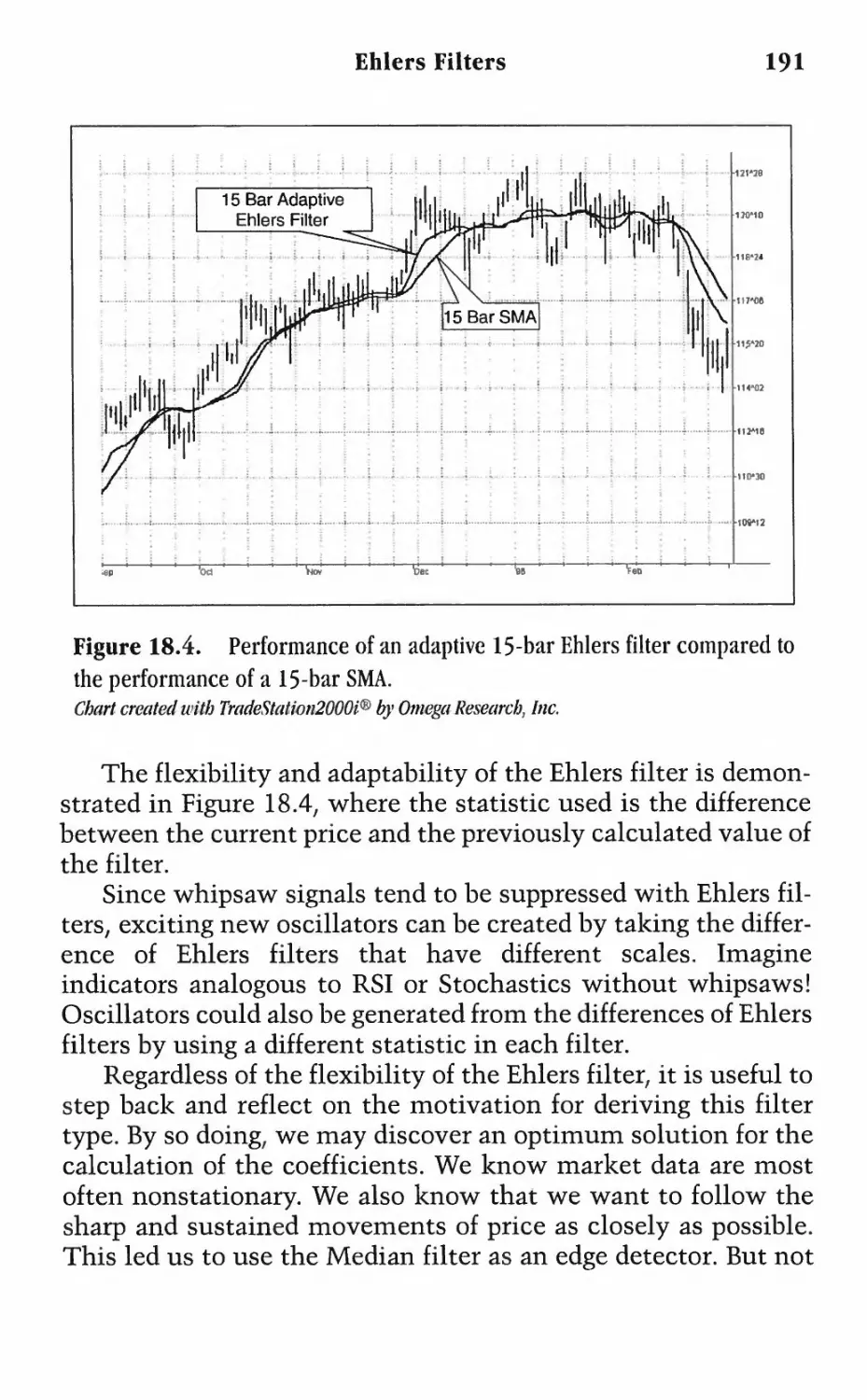
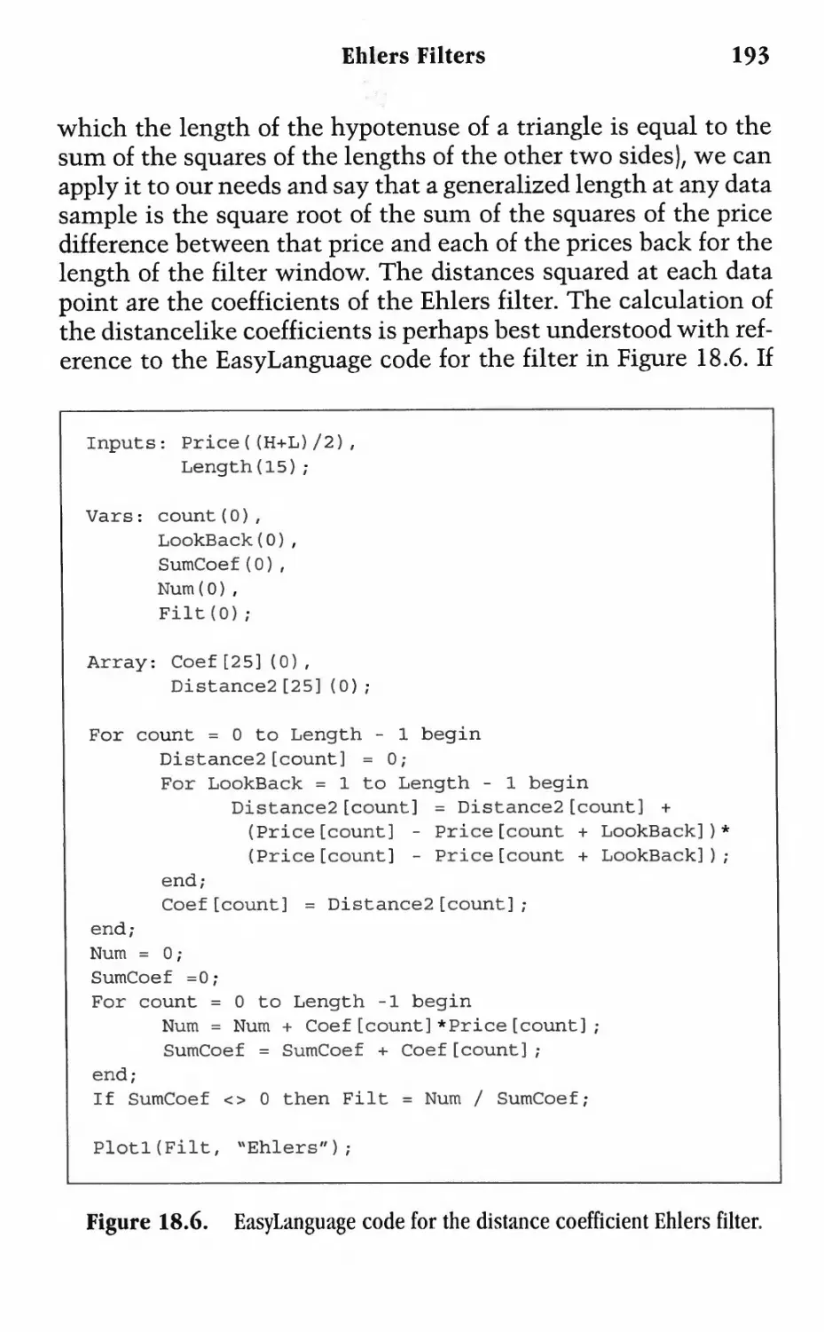
Текст
Chapter 1
INTRODUCTION TO
THE SCIENCE OF
DIGITAL SIGNAL ANALYSIS
Computers are worthless.
They can only give you answers.
—Pablo Picasso
Make no mistake about it. This is a book for traders about digi-
tal signal processing. It is not a book for engineers about trading.
At first glance, the reverse may seem to be true for many traders
because the subject matter is on the cutting edge of technology
and the mathematics behind this technology can be more ad-
vanced than that encountered in school. Recognizing that many
traders want to simply use the technology rather than become
schooled in it, the information in this book is aimed at several
levels. We provide the rationale, derive the equations, and pro-
vide the computer code to implement the techniques. With this
approach, our results can be used in applications ranging from a
cookie-cutter indicator operating within TradeStation or Super-
Charts to the applications that are springboards for still more
advanced technology.
It is common for technical analysis indicators to be described
in terms of a fixed period of time. For example, the standard
length used for a Relative Strength Indicator (RSI) is the last 14
2
Rocket Science for Traders
price bars. One often hears about a five-day Stochastic or a 10/30-
day moving average system. Since the market is continuously
changing, there is absolutely no reason to use static periods in
your indicators. Choosing the correct time period is essential to
using traditional indicators to their maximum potential. While
deriving the tools with which to make indicators adaptive, you
will see novel indicators that surpass the traditional ones in
accuracy and performance.
Digital signal processing is an exciting new field for techni-
cally oriented traders. Many of the indicators that have been
used previously can now be generalized, and the computations
can now be accomplished more precisely using digital methods.
It is interesting to note that many of the digital signal processing
techniques I describe have been known for many years and used
in the physical sciences. My objective is to expose you to these
techniques to make your trading more profitable and more plea-
surable.
Many physical systems involve the use of analog signals that
are represented as continuous time functions. There is an ampli-
tude associated with the signal at each instant in time. There is
an infinite number of amplitude values that the signal may
assume. However, if the signal is frequency bandlimited, there
is no significant energy above the cutoff frequency. Since energy
is required in any physical system to change amplitude, this im-
plies that the signal cannot change amplitude instantaneously.
Therefore, points closely spaced in time will have relatively
similar amplitudes. There are several ways in which a signal can
be represented other than as a continuous analog signal. One
method is to quantize the amplitude and hold that value until
the next quantization is performed. There are a finite number of
amplitudes, but the function is continuous in time. This is in
contrast to a discrete time signal, which has continuous ampli-
tude values but is only defined at discrete instants in time. As
with analog signals, there is an infinite number of levels, but
there are only a finite number of points in time. If a signal is
quantized in both amplitude and time, it is called a digital sig-
nal. The data we deal with in trading are digital signals from
sampling that is done in uniform periods of time (once per day,
once per hour, etc.).
Introduction to the Science of Digital Signal Analysis
3
A discrete time signal can be obtained from an analog signal
by multiplying it by a periodic impulse train. The sampling sig-
nal can be expressed in the time domain as
s|t)= £ 5(t-AT)
k. = —°°
where 5 = the impulse function
T = period between impulses
Using Fourier theory, multiplication in the frequency domain is
synonymous with convolution in the time domain. In other
words, multiplying signals in the time domain is the same as
heterodyning, or mixing, the signals in the frequency domain.
The impulse train has an infinite number of harmonics at fre-
quencies that are the reciprocal of the period between pulses.
The effects of sampling in the frequency domain are illus-
trated in Figure 1.1. The continuous bandlimited signal F(f) is
shown in the top segment (a) as having a frequency rolloff at
some point. In the middle segment (b), the sampling impulse
waveform S(/) has a monochromatic spectral line at the sam-
pling frequency fs and all its harmonics. When the sampling is
performed on the bandlimited signal, the convolved waveform
is shown in the bottom segment (c). Not only is the original band-
limited continuous signal present, but this same signal also
appears as the upper and lower sidebands of each sampling fre-
quency harmonic. Since the lower sideband of the sampling
frequency can extend into the original baseband, the bandlimit-
ing must occur below half the sampling frequency. Half the sam-
pling frequency is called the Nyquist frequency because the
Nyquist Sampling Theorem states that there must be at least
two samples per cycle of the signal to avoid aliasing.
Aliasing is a form of distortion. It results from sampling a
continuous signal less than twice per cycle. This distortion can
be seen in the two waveforms depicted in Figure 1.2. Both the
upper trace and the lower trace have identical sampling points,
denoted by the dots. The samples in the top trace appear to be
valid. However, these same samples plot out the sine wave of
the lower trace, where there are four samples per cycle. The dif-
4
Rocket Science for Traders
Figure 1.1. Sampled data in the frequency domain.
ference is explained by aliasing in the top trace. The samples are
taken at three-quarters of a cycle apart, or two samples every
one-and-a-half cycles. This does not meet the Nyquist criterion
of at least two samples per cycle.
In trading, we can scale all time frames to each bar. Each bar
is a sample. Therefore, to meet the Nyquist criterion, the ab-
solute shortest cycle we can consider is a 2-bar cycle. As a prac-
tical matter, 5- and 6-bar cycles should be considered the shortest
useful cycles.
If the input signal is insufficiently bandlimited, the aliased
frequency components are folded back into the sampled base-
band as false signals and noise. For this reason, data should
always be smoothed before any other operation is performed.
Otherwise, the undesired signal components will have an ad-
verse effect on your computations. Smoothing removes the
high-frequency components, precluding these components from
being folded back into the analysis bandwidth.
Introduction to the Science of Digital Signal Analysis
5
Figure 1.2. Signals must be sampled at least twice per cycle.
The complex waveshapes that describe traders' charts can
be considered as synthesized from more primitive waveshapes,
adding or subtracting from each other depending on their rela-
tive phases. These kinds of waves are called coherent, meaning
the amplitude at any given position can be determined by a vec-
tor addition of the amplitudes. The waveshapes are analogous to
voltage in electric circuits. When we measure the strength of
the signals, we prefer not to use the amplitude of the wave as a
measure because it is dependent on the location, or phase,
within the wave. Rather, power is the preferred measure of
strength. Power is proportional to waveform amplitude squared,
just as the power a 100-W lightbulb consumes from a 115-V cir-
cuit is proportional to the voltage squared. In digital signal
analysis, we are mostly concerned with relative power, or power
ratios. It is convenient to express these power ratios in terms of
decibels.
As an historical aside, one decibel was the power lost in a
telephone signal over one mile of wire (the name was derived
from Alexander Graham Bell). A decibel is one-tenth of a bel.
The bel is the logarithm base 10 of the power ratio. Thus, a deci-
bel is 10*Logio(P2/Pl), and is abbreviated as dB. Working with
6
Rocket Science for Traders
decibels simplifies understanding signal levels both because
large power ratios are compressed into a smaller range of num-
bers due to the logarithm and because adding decibels (i.e., add-
ing logarithms) is easier than carrying out multiplication in your
head. For example, 2*2 = 4 can also be performed with loga-
rithms: Log(2) = 0.3, so that Log(2) + Log(2) = 0.6, which is Log(4).
Memorizing some key ratios makes the identification of relative
power instantly recognizable. A power ratio of 2 translates to +3
dB. If that ratio is ’Л rather than 2, then it translates to -3 dB.
That is, the reciprocal of the power ratio is the same absolute
value of decibels, but the sign is reversed. A ratio smaller than 1
(but necessarily greater than 0) is always expressed in negative
decibels. If we double the power, that is 3 dB. If we double it
again so that the power is 4 times the original, that is 6 dB. Dou-
bling still again to get 8 times the original power, we add another
3 dB to reach a level of 9 dB. Since we have a logarithm base 10,
a power ratio of 10 is 10 dB, and a power ratio of 100 is 20 dB, and
so on. Consider this to further illustrate the use of decibel: If a
filter has half the power coming out of it as was entered, the out-
put power is -3 dB. The filter is said to have a 3-dB loss. If a sim-
ilar filter is placed at the output of the first, the net output power
from the composite circuit would be -6 dB.
The measurement -3 dB is usually a critical point for a filter.
This half-power point in the filter response occurs when the
wave amplitude is 0.7 relative to its maximum value. This is true
because 0.7*0.7 = 0.5, the half-power ratio. The critical point in
the filter is often called the cutoff frequency because frequency
components beyond the cutoff frequency are attenuated to a
greater degree and frequency components within the cutoff fre-
quency are attenuated very little. To simplify, think of the filter
as having a stone-wall response. In this analogy, frequencies
below the cutoff frequency are not attenuated and frequencies
above the cutoff frequency are not allowed to pass through the
filter.
EasyLanguage is currently the most popular computer lan-
guage for traders. Thus, I use this system to generate computer
codes. EasyLanguage is a dialect of Pascal, containing special-
ized keywords unique to trading. Because it reads almost like
Introduction to the Science of Digital Signal Analysis
7
English, EasyLanguage is almost effortless to understand. It is
also easy to translate to other computer languages. When trans-
lating, the reference convention must be understood. The Easy-
Language assumption is that all computations are done with
reference to the current bar. For example, Close means the clos-
ing price of the current bar. If there is a reference associated with
that parameter, it is displayed in square brackets and means the
number of bars back to which it refers. For example, Close[3]
refers to the closing price 3 bars ago. Zero can be used as a refer-
ence, and has the same meaning as the current bar without any
reference (there is no reference into the future). As a further
example, a two-day momentum is written as Momentum =
Close - Close[2];. Each completed line of code must terminate in
a semicolon. For clarity, I always write out the generic descrip-
tion of an action rather than relying on a more esoteric Trade-
Station function call. As a result, the computer code presented
should be easily translated to BASIC, C++, or even an Excel
spreadsheet.
Key Points to Remember
• This book can be read at several levels, ranging from a broad
perspective overview to detailed computer coding.
• Novel and unique indicators are made possible by the math-
ematical techniques to be introduced.
• Even conventional indicator performance can be enhanced
by making them adaptive to current market conditions.
• Time scales of financial data can be dealt with on a per-bar
basis. The absolute time scale of the data is irrelevant for
computational purposes.
• Working with sampled data is distinctly different from work-
ing with continuous information. Sampled data should al-
ways be smoothed to avoid erratic signals.
This Page Intentionally Left Blank
Chapter 2
MARKET MODES
Chaos often breeds life, when order breeds habit.
—Henry Brooks Adams
The whole point of technical analysis is to find a way to exploit
the inefficiency of the market for gain. The general objective
of the market is to provide accurate prices for asset allocation.
That is, investors can choose strategies that allow prices to fully
reflect all available information at any time. Such a market (a
market in which prices always fully reflect available informa-
tion) is called efficient. Much research has been done to prove
that the market is indeed efficient. However, the fact that there
exists a number of traders who are continuously successful is
adequate proof that markets are not necessarily completely effi-
cient. The failure of the efficiency hypothesis in several cases is
sufficient evidence to invalidate the hypothesis itself.
Classical efficient market models are often concerned with
the adjustment of security prices to three information subsets.
Weak form tests comprise the first subset, in which we are sim-
ply given the historical prices. The second subset is semistrong
form tests that concern themselves with whether prices effi-
ciently adjust to other publicly available information. Strong
form tests, the third subset, are concerned with whether in-
vestors have monopolistic access to any information relevant to
price formation. The general conclusion, particularly for the
weak form tests, is that the markets can be only marginally prof-
itable to a trader. In fact, only the strong form tests are viewed as
9
10
Rocket Science for Traders
benchmarks against deviations from market efficiency. These
strong form tests point to activities such as insider trading and
the market-making function of specialists.
The efficient-markets-model statement that the price fully
reflects available information implies that successive price
changes are independent of one another. In addition, it has usu-
ally been assumed that successive changes are identically dis-
tributed. Together, these two hypotheses constitute the Random
Walk Model, which says that the conditional and marginal
probability distributions of an independent random variable are
identical. In addition, it says that the probability density func-
tion must be the same for all time. This model is clearly flawed.
If the mean return is constant over time, then the return is inde-
pendent of any information available at a given time.
I assume that there is an adequate number of traders in-
volved in making the market that a statistical analysis involving
a Random Walk is appropriate. There must be several constraints
to such a Random Walk. The first constraint is that the prices
be constrained to one dimension—they can only go up or down.
The second constraint is that time must progress monoton-
ically.
I have formed my philosophical basis of market action from
extensive work using constrained Random Walks in the physi-
cal sciences.1 The expression of such a Random Walk is that of a
drunkard moving on a one-dimensional array of regularly spaced
points. At regular intervals, the drunkard flips a coin and makes
one step to the right or left, depending on the outcome of the
coin toss. At the end of n steps, he can be at any one of 2n + 1
sites, and the probability that he is at any site can be calculated.
Let the distance between the points on the lattice be AL, and let
the time between successive steps be AT If AL and AT are
allowed to shrink to zero in such a way that (AL)2/AT remains
constant to the diffusion constant D, then the equation govern-
ing the distribution of the displacement of the Random Walker
from his starting point is
‘Weiss, G. H., and R. J. Rubin. "Random Walks: Theory and Selected
Applications." Advances in Chemical Physics 52 (1982): 363-505.
Market Modes
11
8P 82P
8t " 8X2
This rather famous partial differential equation is called the Dif-
fusion Equation. The function P(x,t) can be interpreted in two
ways. It can either be taken to express the probability density or
the concentration of diffusing matter at position x at time t. Fol-
lowing the latter interpretation, it can, for example, describe the
way heat flows up the stem of a silver spoon when placed in a
hot cup of coffee.
To better understand the theory of diffusion, imagine the
way a smoke plume leaves a smokestack. Think about how the
smoke rises compared to how a trend carries itself through
the market. A gentle breeze determines the angle to which the
smoke, or trend, is bent. The widening of the smoke plume
represents the probability density of the smoke particles as a
function of distance from the smokestack. This widening is anal-
ogous to the decreased accuracy of the prediction of future trend
prices further into the future.
The formulation of the Drunkard's Walk has no property
that can be regarded as the analog of momentum. A more realis-
tic model of a physical object's motion needs to account for
some form of memory—we need to know where the object came
from and the likelihood it will continue to move in the same
direction. The simplest modification of the Random Walk is to
allow the coin toss to determine the persistence of motion. In
other words, with probability p the drunkard makes his next
step in the same direction as the last one, and with probability
1-p he makes a move in the opposite direction. The ordinary
Drunkard's Walk occurs when p = 'A, because either move is
equally likely. The interesting feature of the modified Drunk-
ard's Walk is that as the distance between the point and the time
between steps decreases, one no longer obtains the Diffusion
Equation, but rather the following equation:
82P 1 8P _ , 82P
8t2 + T 8t C 8X2
in one dimension, where T and c2 are constants. This is another
famous partial differential equation called the Telegrapher’s
12
Rocket Science for Traders
Equation. This equation expresses the idea that diffusion occurs
in restricted regions, such that x2 < c2t2. That is, the position
must be less than the velocity of propagation c multiplied by
time t. More important, the Telegrapher's Equation describes
the harmonic motion of P(x,t) just as surely as it describes the
electric wave traveling down a pair of wires.
Harmonic motion is ubiquitous. It is the natural response to
a disturbance on any scale ranging from the atomic to the galac-
tic. You can demonstrate the effect by holding a ruler over the
edge of a table, bending the ruler down, and then releasing it.
The resulting vibration is harmonic motion. Alternatively, you
can stretch a rubber band between your fingers, pull the band
to one side, and then release it. The oscillations of the rubber
band also constitute harmonic motion. Since there are plenty of
opportunities for market disturbances, it is only a small stretch
to extend the solution to the Drunkard's Walk problem from
physical phenomena and use it to describe the action of the
market.
The Drunkard's Walk solution can describe two market con-
ditions. In the first condition, the probability is evenly divided
between stepping to the right or the left, resulting in the Trend
Mode, which is described by the Diffusion Equation. The second
condition, the probability of motion direction is skewed, results
in the Cycle Mode, which is described by the Telegrapher's Equa-
tion. The difference between the two conditions can be as sim-
ple as the question that the majority of traders constantly ask
themselves. If the question is "I wonder if the market will go up
or down?" then the probability of market movement is about
50-50, establishing the conditions for a Trend Mode. However, if
the question is posed as "Will the trend continue?" then the
conditions are such that the Telegrapher's Equation applies. As a
result, the Cycle Mode of the market can be established.
The Telegrapher's Equation solution also describes the me-
andering of a river. Viewed as an aerial photograph, every river
in the world meanders. This meandering is not due to a lack
of homogeneity in the soil, but to the conservation of energy.
(You can appreciate that soil homogeneity is not a factor because
other streams, such as ocean currents, also meander in a nearly
Market Modes
13
homogeneous medium.) Ocean currents are not nearly as visible
as rivers and are, therefore, not as familiar to most of us. Every
meander in a river is independent of other meanders, and are all
thus completely random. If we were to look at all the meanders
as an ensemble, overlaying one on top of the other like a mul-
tiple exposure photograph, the meander randomness would also
become apparent. The composite envelope of the river paths
would be about the same as the cross section of the smoke
plume. However, if we are in a given meander, we are virtually
certain of the general path of the river for a short distance down-
stream. The result is that the river can be described as having a
short-term coherency but a randomness over the longer span.
River meanders are like the cycles we have in the market.
We can measure and use these short-term cycles to our advan-
tage if we realize they can come and go in the longer term.
We can extend our analogy to understand when short-term
cycles occur. Rivers meander in an attempt to maintain a con-
stant slope on their way to the ocean. If the slope is too severe,
the meander has the same effect as a skier who weaves back and
forth across a slope to slow the descent. The flow of a river phys-
ically adjusts itself for the purpose of energy conservation. If the
water speeds up, the width of the river decreases to yield a con-
stant flow volume. The faster flow contains more kinetic
energy, and the river attempts to slow it down by changing direc-
tion. At the same time, the river direction cannot change
abruptly because of the momentum of the water's flow. Mean-
dering results. Thus, meanders cause the river to take the path of
least resistance in the sense of energy conservation. We should
think of markets in the same way. Time must progress as surely
as the river must flow to the ocean. Overbought and oversold
conditions result from attempts to conserve the energy of the
market. This particular energy arises from the fear and greed of
traders.
Again, it may be useful to test the principle of energy con-
servation for yourself. Tear a strip about 1 inch wide along the
side of a standard sheet of paper about 11 inches long. Grasp
each end of this strip between the thumb and forefinger of each
hand. Now move your hands toward one another. Your com-
14
Rocket Science for Traders
pression is putting energy into this strip, and its natural response
can take one of four modes. These modes are determined by the
boundary conditions that you force. If both hands are pointing
up, the response is a single upward arc, approximating one alter-
nation of a sine wave. If both hands are pointing down, the
response is a downward arc. If either hand is pointing up and
the other pointing down, the strip response to the energy input
is approximately a full sine wave. These four lowest modes are
the natural responses following the principle of conservation of
energy. You can introduce additional bends in the strip, but a
minor jiggling will cause the paper to snap to one of the four
lowest modes, with the exact mode depending on the boundary
conditions that you impose. The two full sinewave modes are
approximately the second harmonic of the two single alterna-
tion modes.
The market only has a single dominant cycle most of the
time. When multiple cycles are simultaneously present, they are
generally harmonically related. This is not to say that nonhar-
monic simultaneous cycles cannot exist—just that they are rare
enough to be discounted in simplified models of market action.
The general observation of a single dominant cycle tends to
support the notion that the natural response to a disturbance is
monotonic harmonic motion.
It is true that if you are a hammer, the rest of the world looks
like a nail. We must take care to recognize that all market action
is not strictly described by cycles alone and that cycle tools are
not always appropriate. A more complete model of the market
can be achieved by knowing that there are times when the solu-
tion to the Telegrapher's Equation prevails and times when the
solution to the Diffusion Equation applies. We can, therefore,
divide the market action into a Cycle Mode and a Trend Mode.
By having only two modes in our market model, we can switch
our trading strategy back and forth between them, using the
more appropriate tool according to our situation. Since our digi-
tal signal processing tools analyze cycles, we can establish that
a Trend Mode is more appropriate at any given time due to the
failure of a Cycle Mode.
There are many ways to analyze the market using technical
analysis. Regarding indicators, the preferred tools are moving
Market Modes
15
averages or data smoothers for Trend Modes and oscillator-type
indicators for Cycle Modes. In later chapters, we develop supe-
rior indicators for both market modes. At this point, it is impor-
tant to understand that the two modes of a simplified market
model have been directly derived from solutions to the Drunk-
ard's Walk problem. Keep asking yourself, "Will the market go
up or down today?" and "I wonder if the trend will continue?"
Key Points to Remember
• A simplified model of the market has a Trend Mode and a
Cycle Mode.
• The market model is similar to a meandering river.
• Both the Trend Mode and the Cycle Mode are derived from
the Drunkard's Walk.
• Different technical indicators are appropriate for each mar-
ket mode.
This Page Intentionally Left Blank
Chapter 3
MOVING AVERAGES
Trend is not destiny.
—Lewis Mumford
Centuries ago Karl Friedrich Gauss proved that the average is
the best estimator of the random variable. He derived the famil-
iar bell-shaped probability density curve known as the Gauss-
ian, or Normal, distribution. When the probability distribution
of a random variable is unknown, the Gaussian distribution is
generally assumed. In this bell-shaped curve, the peak value, or
the mean, is the nominal forecast. The width of the variation
from the mean is described in terms of the variance. It is cer-
tainly true that the average is the best estimator for the market
in the case where the Diffusion Equation (as described in Chap-
ter 2) applies. The best estimate of the location of any smoke
particle is the average across the width of the plume. This is
probably why moving averages are heavily used by technical
traders—they want the best estimate of the random variable.
All moving averages have two characteristics in common:
They smooth the data and cause lag because they depend on
historical information for computation. By far the most serious
implication for traders is the induced lag. Lag delays any buying
or selling decision and is almost always a bad characteristic.
Therefore, averaging is typically a trade-off between the
amount of desired smoothing and the amount of lag that can be
tolerated.
There are three popular types of moving averages. These are
17
18
Rocket Science for Traders
1. Simple Moving Average (SMA)
2. Weighted Moving Average (WMA)
3. Exponential Moving Average (EMA)
Each of these types of averages has its own respective merit,
and there are times when any one of the three is the appropriate
choice. The discussions in this chapter describe each of the three
moving averages so you can make the comparisons for your own
applications.
Simple Moving Average
An n-day simple average is formed by adding the prices of a secu-
rity over n days and dividing by n. Thus, the weighted price for
each day is the real price divided by n. The simple average
becomes a moving average by adding the next day's weighted
price to the sum and dropping off the weighted first day's price.
Thus, the simple average moves from day to day. This is the
most efficient way to compute a Simple Moving Average (SMA).
Another way to view an SMA is as an average of the data
within a window. In this concept, the window slides across the
chart, forming the moving average from bar to bar, as shown in
Figure 3.1. Figure 3.1 shows a 10-bar window and the moving
average formed by this window. The average is plotted at the
right-hand side of the window, causing the moving average lag.
This is necessary because the window cannot accept data into
the future. So, when a moving average is used in actual trading,
the lag cannot be overcome. Centering the moving average on the
window is not helpful for trading because future data would be
required to get the current value of the average. Obviously, future
data are not available for the last bar on the chart.
The static lag of an SMA can be computed as a function of
the window width. Consider the following case where the data
have a price of zero at the left edge of the window. The price
increases by one unit for each subsequent bar, as shown in Fig-
ure 3.2. The average price is always the price at the center of the
window, expressed mathematically at (n - l)/2. The average is
Moving Averages
19
0 Bar Window
Figure 3.1. A moving average averages data within a moving
window.
Chart created with TradeStatioii2000i® by Omega Research, Inc.
plotted at the right-hand side of the window. Since the price
slope is unity (rises vertically one unit for each unit increase
along the horizontal), the averaged price at the right-hand side of
the window is effectively lagging the price at the center of the
window by (n - l)/2 bars. This lag is simply unavoidable. An
example of a 5-bar window average is shown in Figure 3.2. It is
clear in this example that the lag is two units, equal to (5 - l)/2.
As a trader, you must make a trade-off by choosing between the
amount of smoothing you want from your moving average and
the amount of lag you can tolerate.
A thorough understanding of the impact of moving average
lag is absolutely crucial for successful trading. On the one hand,
a wide averaging window provides a very smooth moving aver-
20
Rocket Science for Traders
Figure 3.2. Computing the SMA lag.
age. However, such a moving average is so sluggish in response
that it may only be useful in working with the longest trends. A
narrow averaging window, on the other hand, does not provide
much smoothing, so the average may be highly responsive but
can produce whipsaw signals due to inadequate smoothing.
Approaching a moving average from the perspective of the fre-
quency domain rather than from the time domain can thus be
useful and instructive.
Assume the data comprise a theoretical sine wave as shown
in Figure 3.3. We can arrange our averaging window to be any
width we choose. The width of Window A in Figure 3.3 is
exactly one half cycle. If the window were narrower, then the
average would not include all the data points in the positive
alternation of the sine wave, and the average would therefore be
less sensitive. If the window were wider than a half cycle, the
average would contain some negative data points as well as all
the data points in the positive alternation. Thus, the average
would also be less sensitive. Figure 3.3 shows the half-period
moving average of a sine wave. The peak value of this moving
average occurs at the right-hand side of Window A because Win-
Moving Averages
21
dow A contains only the positive data points in the sine wave.
As we move the window to the right, the moving average
decreases in amplitude. Reaching Window B, the moving aver-
age is zero at the right-hand edge because Window В contains
exactly as many negative data points as positive data points,
causing the average to sum to zero. Continuing to move the win-
dow to the right, we arrive at Window C. The moving average at
Window C is maximum negative because Window C contains
only negative data points. The moving average is created by slid-
ing the window across the entire data set.
Note that the half-period SMA of a sine wave is another
sinusoid (waves that look like sine waves), delayed by a quarter
cycle. Drawing from our previous knowledge of the lag of an
SMA, we can assert that the lag is half the window width,
expressed in fractions of a cycle period or in degrees of phase. A
quarter-cycle SMA will lag the price by an eighth of a cycle. This
is the equivalent of saying that if the averaging window is 90
degrees wide, the resulting SMA lag will be 45 degrees.
When the market is in a Cycle Mode, it is more important to
think in terms of the phase shift an SMA will induce rather than
in terms of the number of bars of lag that it will cause. For exam-
ple, a 2-bar lag is almost inconsequential for a 40-bar cycle.
Figure 3.3. Half-cycle SMA of a sine wave.
22
Rocket Science for Traders
However, this same 2-bar lag is a full quarter-of-a-cycle phase
shift for an 8-bar cycle. In trading, it is important to always
consider the phases in relative terms, particularly when deal-
ing with shorter cycles. For this reason, it is often preferable
to continuously adapt an SMA window to be a fraction of the
measured market cycle rather than using a fixed window width.
This adaptation enables the SMA to provide the same reac-
tion to price movement regardless of the time period of the dom-
inant cycle.
If we increase the window width to include a full cycle, as
shown in Figure 3.4, we have a very interesting case for the
SMA. Examination of Figure 3.4 shows that in a pure cycle,
when the window width is exactly one cycle, there are as many
data points above the mean as there are below it. Therefore, the
SMA is exactly zero for this special case. We use this phenome-
non later to create the Instantaneous Trendline after we have
measured the dominant cycle. By adjusting the average to have a
window whose width is exactly the measured dominant cycle,
we cancel out the dominant cycle completely. Since our simpli-
fied market model consists of a Trend Mode component and a
Cycle Mode component, we are left with only the Trend Mode
component after the dominant cycle component has been re-
Figure 3.4. The average of a full-cycle SMA is zero.
Moving Averages
23
moved. The Instantaneous Trendline differs from an SMA only
in the respect that the window width can vary from bar to bar.
Since the window width is always a full cycle period for this
indicator, the lag of the Instantaneous Trendline is a half period
of the dominant cycle.
The SMA is also identically zero for a pure sine wave when
the window width is exactly an integer number of cycles wide.
This can be seen in Figure 3.5, in which the window width is 12
bars. Figure 3.5 is attained by changing the frequency applied to
the fixed 12-bar-wide window. The results are plotted after being
normalized to the Nyquist frequency, which is exactly half the
sampling frequency. For example, if the data being used consist
of daily bars, then the Nyquist frequency is 0.5 bars per day.
Since the cycle period and the cycle frequency are inversely pro-
portional, the period of the Nyquist frequency is 2 bars. The
periods of those components that have an integer number of
cycles within the 12-bar window have been noted in Figure 3.5.
The SMA window can be viewed as a transfer function that
multiplies the data falling within the window by 1 and multi-
plies all data outside the window by 0. This transfer response is
a pulse in the time domain. Functions in the time domain are
related to functions in the frequency domain by the Fourier
Transform, as discussed in Chapter 1. A derivation of Fourier
Transforms is beyond the scope of this book, but is covered in
Figure 3.5. The transfer response of a 12-bar SMA.
24
Rocket Science for Traders
many fine texts. Without the derivation, I assert that the Fourier
Transform of the pulse in the time domain is
SMA(Period) = Sin(n* W/P]/[n* W/P]
where W = width of the SMA window
P = period of the cycle being averaged
The SMA is expressed in terms of wave amplitude. This mathe-
matical equation for the frequency domain response of an SMA
exactly describes the function shown in Figure 3.5, except that
the figure is plotted in decibels rather than wave amplitude.
Each time the ratio of the window width to the cycle period is an
integer, the argument of the sine function is a multiple of Pi.
Since the sine is exactly zero for arguments in multiples of Pi,
the transfer response has nulls for these cycle periods.
Figure 3.5 shows that low-frequency components (longer
cycles) are allowed to pass through the SMA with only a small
amount of attenuation, or size reduction. However, high-
frequency components (shorter cycles) are greatly attenuated,
even between the null points. For this reason, an SMA falls into
the category of low-pass filters. Low-pass filtering is exactly
what is desired from a data smoother. The smoothing comes
about as a result of reducing the size of, or attenuating, the
amplitude of the higher-frequency components within the data.
The frequency description of an SMA does not have a null at
zero frequency. At zero frequency, its period is infinite because
cycle period is the reciprocal of frequency. Therefore, although
the numerator goes to zero at zero frequency, the denominator
also goes to zero. In the limit, the ratio of the numerator to the
denominator is unity (a value of 1). We have previously assigned
some significance to the cycle period that is twice the window
width (or more precisely, where the window width was half the
cycle period). In this case, the numerator in the SMA frequency
description rises to become unity and the denominator is л/2.
The cycle period that is twice the width of the SMA window is
a workable and easy-to-remember demarcation between those
cycle periods that have small attenuation and those that have
Moving Averages
25
greater attenuation. For example, an SMA window width of 8
bars would allow those cycle components of 16 bars and longer
to pass nearly unattenuated and would attenuate cycle compo-
nents whose periods are shorter than 16 bars.
We now have the tools to think about SMAs in both the time
and frequency domains. We know that the 8-bar SMA has a lag
of 3.5 bars for trends. This same SMA gives a 16-bar cycle a 90-
degree phase delay and a 32-bar cycle a 45-degree phase delay. An
8-bar cycle component is removed completely. This ability to
think of the impact of averages in both the time and frequency
domains will greatly improve your probability of success as a
trader.
Weighted Moving Average
A Weighted Moving Average (WMA) is closely related to an
SMA. The major difference is the coefficients of the multiplier
for the WMA are not constant across the window width. Rather,
the coefficients are linearly weighted across the window. There-
fore, it follows that the oldest data point is multiplied by 1, the
next oldest data point is multiplied by 2, the third oldest data
point is multiplied by 3, and so on until the most recent data
point is multiplied by n for an n-bar window width. The sum of
the data and coefficient products is divided by the sum of the
coefficients to normalize the averaging process. A 4-bar WMA
code can be written as
WMA = (4*Price + 3‘Price[l] + 3*Price[2] + Price[3])/10;
The transfer response of the 4-bar WMA is shown in Figure
3.6. Since the data are weighted across the window width, there
can be no precise averaging to zero as there was with an SMA.
Nevertheless, the WMA is also a low-pass filter. The point where
the filter attenuation is 3 dB acts as our point of demarcation
between the passband and the stopband. In Figure 3.6, this occurs
at a normalized frequency of 0.25, corresponding to an 8-bar cycle.
Cycles longer than roughly 8 bars are passed essentially unatten-
26
Rocket Science for Traders
Figure 3.6. Frequency response of a 4-bar WMA.
uated, and cycles shorter than 8 bars are reduced in amplitude to
provide the smoothing.
As with SMAs, smoothing of WMAs is improved by increas-
ing the width of the window. For example, the transfer response
of a 7-bar WMA is shown in Figure 3.7. In this case, the -3 dB
point occurs at a normalized frequency of about 0.14, which is a
period of approximately 14 bars. Since the passband is linearly
related to the window width, the passband of a WMA is also
twice its window width, as a reasonable approximation.
A WMA offers a major advantage because it exhibits reduced
lag in its transfer response. The reduced lag results from the
Figure 3.7. Frequency response of a 7-bar WMA.
Moving Averages
27
most recent data being the most heavily weighted. The amount
of lag induced by an SMA or a WMA is the center of gravity of
the transfer response. In the case of the SMA, the center of grav-
ity is at the center of the filter, resulting in a lag of (n - 1 )/2 for
an n-bar window width. The shape of the WMA coefficients
forms a triangle across the width of the filter, resulting in the
center of gravity being a triangle, one-third of the distance across
the window. Thus, the lag of an n-bar WMA is (n - 1 )/3. There-
fore, in our examples, a 4-bar WMA has a lag of only 1 bar and a
7-bar WMA has a lag of only 2 bars.
The weighting functions for a WMA do not necessarily have
to be linear across the width of the window. The linear weight-
ing is nonetheless very simple to compute, and the impact of lin-
ear weighting is easy to remember by recalling the center of
gravity of a triangle. Furthermore, the impact of other weighting
distributions is too subtle for trading purposes. Therefore, there
is no compelling reason to use any weighting factor other than
linear.
Exponential Moving Average
The moving averages discussed thus far are nonrecursive. That
is, previous calculations are unnecessary to compute the cur-
rent value of the moving average. An Exponential Moving Aver-
age (EMA) is different in a major way because it is recursive.
The calculations use a fraction of the current price added to
another fraction of the EMA calculation 1 bar ago. The first
fraction is usually called alpha (a) and can have a value between
0 and 1. The two fractions must sum to unity, so the second
fraction must have the value of 1 - a. The equation to compute
an EMA is
EMA = a*Price + (1 - a)*EMA[l];
The EMA becomes a moving average by moving from bar to bar,
from left to right, across the price data.
The term exponential describes the way an EMA transfer re-
sponse decays in amplitude relative to a single input. Imagine a
28
Rocket Science for Traders
case in which the data set has an amplitude of 1/a at one bar and
an amplitude of 0 everywhere else. When the EMA is applied to
this data, the first output from the filter is unity because there
was no previous value for the EMA. On subsequent calculations,
the price value is 0, and so the sequence of calculations is
EMA(O) = 1
EMA(1) = (1 - a)
EMA(2) = (1 - a)*(l - a) = (1 - a)2
EMA(3) = (1 - a)2*(l - a) = (1 - a)3
EMA(n) = (1 - a)n
Since the quantity (1 - a) must be less than 1, the amplitude
decays as the exponent of each succeeding calculation from an
impulse input. Hence the name Exponential. In principle, a part
of any data input remains in subsequent calculations although
the contribution becomes vanishingly small. This attribute
makes an EMA part of a general class of filters called Infinite
Impulse Response (IIR) filters. HR filters are distinct from the
Finite Impulse Response (FIR) filters, the class to which the
SMA and WMA belong. With FIR filters, the filter provides an
output only so long as the impulse falls within the window.
Thus, in this case, the response to an impulse is finite.
It is instructive to examine the EMA response to a step func-
tion. A step function has a series of constant values and then
jumps to another series of constant values. Assume the price has
been 0 for a long time and then suddenly jumps up to a value of
1 and maintains that value thereafter. On the first bar, the EMA
will have a value of a. On the second bar, the value will be a +
a*(l - a). On the third bar, the value will be a + a*(l - a) + a*
(1 - a)2, and so on. The EMA will gradually approach the value of
1. A common error in programming is to insert a value for a,
such as 0.2, and insert another number for (1 - a), such as 0.9.
The two terms must sum to unity or the recursive algorithm
will lead to erratic results or might even cause your computer to
crash. You should always check your computer code to ensure
Moving Averages
29
the two terms sum to unity. I am so cautious on this point that
I assign the value a as a global variable and write out the EMA
equation in terms of a. By letting the computer do the work, I
know the two terms must sum correctly.
We can easily derive the lag of an EMA for the case of price
that rises linearly at the rate of one unit per bar. Recalling the
form of the EMA calculation,
EMA = a*Price + (1 - a)*EMA[l];
We can assert that the price on day d is d. If we assume the
lag of the EMA is L, then the current value of the EMA is (d - L).
Furthermore, the previous EMA would have a value of (d - L -
I), since price is rising one unit per bar. Putting these values into
the equation for the EMA, we obtain
(d- L) = a*d + (I - oc)*(d - L - 1)
= a*d + (d - L) - 1 - a*d + a*(L + 1)
О = a*(L + 1) - 1
a= 1/(L+ 1)
This equation shows that we can select an acceptable lag, and
from that lag, compute the alpha term of the EMA. For example,
if we can accept a 3-bar lag resulting from the EMA, we would
use a = 0.25.
We can also relate an EMA to an SMA on the basis of their
equivalent static lags. Recalling that the lag of an SMA is (n -
l)/2 for an n-bar SMA, we can substitute this value of lag into
the alpha calculation of the EMA as
a= l/((n - l)/2 + 1)
= 2/((n - I) + 2)
= 2/(n + I)
This is the relationship between an n-bar SMA and the alpha of
an EMA that is quoted in most technical analysis books.
A 12-bar SMA was used to compute the transfer response
shown in Figure 3.5. The equivalent alpha for an EMA is a =
30
Rocket Science for Traders
Figure 3.8. Transfer response of an EMA with delay equal to that of a 12-
bar SMA.
?i3 = 0.1538. The EMA transfer response for this value of alpha is
shown in Figure 3.8. Comparing Figures 3.8 and 3.5, it is obvi-
ous that the EMA normalized frequency passband is much
smaller than the passband of the SMA. Therefore, an EMA pro-
vides much more smoothing than an SMA for an equivalent
amount of lag. Alternatively, you can conclude that an EMA
has much less lag than an SMA for an equivalent amount of
smoothing.
It is also interesting to compare a WMA to an EMA on the
basis of equivalent lag. The WMA that produced the transfer
response depicted in Figure 3.7 had a lag of 2 bars. For a 2-bar lag,
an EMA has a = 0.3333. The transfer response of the EMA is
shown in Figure 3.9. In this case, the EMA response is nearly
equivalent to the response of the WMA shown in Figure 3.7,
with the WMA providing slightly better filtering. Furthermore,
the WMA attenuates those components within the passband a
little less than the EMA for these same components.
We do not yet have the tools to compute the cycle period of
the passband demarcation in the frequency domain in terms of
the alpha of the EMA, but we can assert without proof that this
relationship is
P = -2л/1п (1 - a)
Moving Averages
31
Normalized Frequency (Nyquist -- 1)
Figure 3-9- Transfer response of an EMA with delay equal to that of a 7-
bar WMA.
where In is the natural logarithm. This relationship is proved in
Chapter 13. Computation of the natural logarithm may be
unnatural to most traders, so we simplify the equation with a
little mathematical slight of hand. We can approximate the nat-
ural logarithm with a truncated infinite series because (1 - a)
will always be less than unity as
In (1 - a) = -a - a2/2 - a3/3 - a4/4 ... -an/n
If a is sufficiently small, we can ignore all but the first two
terms of the series. Substituting the truncated series for the nat-
ural logarithm in the passband period calculation, we obtain
P = 2я/(а + а2/2)
= 4л/(а*(2 + а))
Key Points to Remember
Regardless of their formulation, the purpose of moving averages
is to smooth the input data. Their use is a trade-off between the
amount of smoothing you desire and the amount of lag you can
32
Rocket Science for Traders
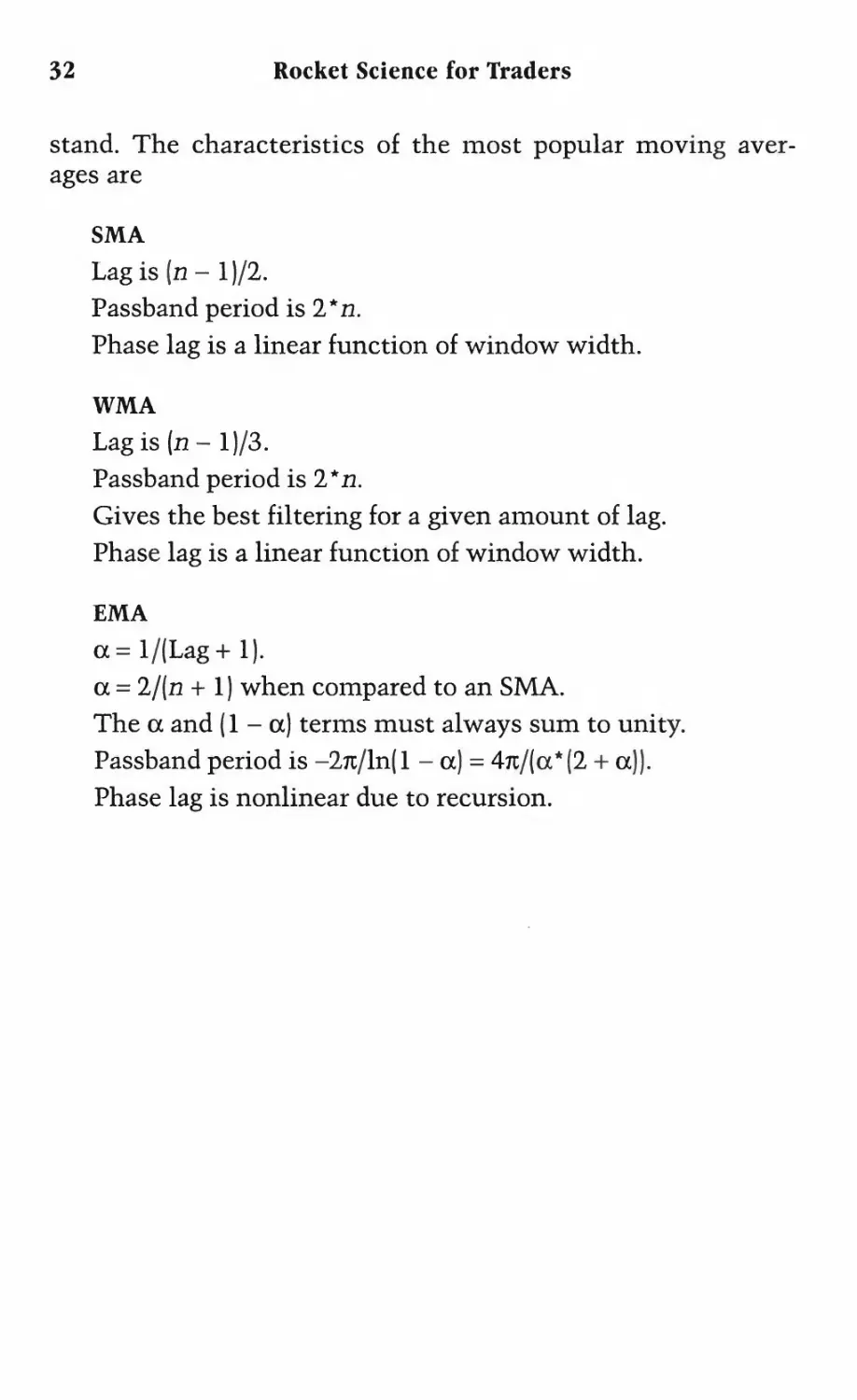
stand. The characteristics of the most popular moving aver-
ages are
SMA
Lag is (n - 1 )/2.
Passband period is 2*n.
Phase lag is a linear function of window width.
WMA
Lag is (n - l)/3.
Passband period is 2*n.
Gives the best filtering for a given amount of lag.
Phase lag is a linear function of window width.
EMA
a= l/(Lag + 1).
a = 2/(n + 1) when compared to an SMA.
The a and (1 - a) terms must always sum to unity.
Passband period is -2я/1п(1 - a) = 4n/(a*(2 + a)).
Phase lag is nonlinear due to recursion.
Chapter 4
MOMENTUM FUNCTIONS
Backward, turn backward,
oh time in your flight. . .
—Elizabeth Akers Allen
I can't begin to tell you the number of traders that has asked me
to make their signals happen just one bar sooner. The typical
question is "Can't you just take a momentum?" In the most
simple case, momentum is just the 1-bar difference in price.
Momentum is deceiving because it can give the illusion of antic-
ipating turning points. In fact, there are cases in which some
form of a momentum can increase the reaction time of an indi-
cator. Even experienced technicians get lured into investigations
in which advancing the indicator signal is impossible. For this
reason, it is instructive to return to basics and thoroughly inves-
tigate the properties of momentum functions.
In the most general sense, momentum functions simply take
the difference of successive values to sense the rate of change.
Just as the sums forming the averages are analogous to integrals
in the calculus, momentum is analogous to derivatives in the
calculus. The impact of momentum can be appreciated by tak-
ing successive momentums as we do in Figure 4.1.
In Figure 4.1, we analyze the successive momentums of a
simple ramp function. The ramp is described as having a zero
slope before an instant in time T and then breaking to a finite
slope at that instant. This is a relatively smooth function. The
first momentum of the ramp is a step. There is no change in the
slope of the ramp before or after time T, so the step function is
33
34
Rocket Science for Traders
Figure 4.1. Successive application of momentum shows that
momentum can never anticipate an event. Also, momentum
functions become increasingly discontinuous.
formed by instantly jumping from an initial slope of zero to the
finite value of the slope of the ramp. Taking the momentum of
the step function, there is no change except the instantaneous
jump from one value to another at time T. This forms an impulse.
An impulse is a mathematical artifice that has infinite height
and zero width in such a way that the area of this "rectangle" is
unity. Put simply, an impulse is a spike at time T. Next, taking
the momentum of the impulse, we obtain a jerk. The jerk is
formed by a two-step process. A positive impulse part of the jerk
is first formed by traversing the leading edge of the impulse
function. This is followed by the formation of the negative
impulse part, which is due to traversing the trailing edge of the
impulse function.
Examination of Figure 4.1 identifies two undeniable truths
about momentum functions. These are
1. Momentum can never lead the event.
2. Momentum is always more disjoint (i.e., noisier) than the
original function.
These truths are obvious when removed from the distractions of
a price chart. There must be a reason why traders expect momen-
Momentum Functions
35
turn to increase the performance of their indicators. That reason
is demonstrated in Figure 4.2, where the momentum of a pure
sine wave is taken. Since momentum is the rate of change of a
function, the momentum of the sine wave is maximum at the
left edge of Figure 4.2 where the sine wave crosses zero. The
momentum decreases as the sine wave increases. It reaches zero
at the point where the sine wave crests. The slope of the sine
wave at this point is zero, causing the momentum to be zero.
Continuing to the right, the slope of the sine wave increases in
the negative direction, causing the momentum to reach its neg-
ative maximum just as the sine wave again crosses zero. The
momentum is traced out by the dashed line in Figure 4.2. This
dashed line has the characteristic that it reaches a crest 90 de-
grees before the sine wave crests and reaches a valley 90 degrees
before the sine wave does.
If the price were a sine wave, it would be easy to conclude
that momentum is a leading indicator. But this is true only
when the market is in a Cycle Mode. It is, therefore, imperative
to first identify the mode of the market before assigning a lead-
ing indicator capability to the momentum. In Chapter 11, meth-
ods to identify market modes are discussed.
.We have already stated that momentum is analogous to a
derivative in the calculus. We can use this fact to analyze the
Figure 4.2. Momentum leads a pure sine wave by 90 degrees.
36
Rocket Science for Traders
behavior of momentum in the frequency domain. From any cal-
culus text, the derivative of a sine wave having the angular fre-
quency co is
d(Sin(cot))/dt = co*Cos(cot)
This equation shows that the derivative of a sine wave does
lead the sine wave by 90 degrees because the result is exactly a
cosine wave, like the dashed momentum shown in Figure 4.2.
The equation also shows that amplitude is directly proportional
to frequency. The amplitude is omega (co), which is 2*n*fre-
quency. We expect the same phenomenon in trading. If we take
the simple difference (momentum) of a 2-bar cycle that varies
between +1 and -1, the difference will be the crest-to-valley
value, or 2. Conversely, if we have a 50-bar cycle swinging be-
tween +1 and -1, then the maximum momentum will be
approximately %s = 0.08. There is no momentum for extremely
long cycles because there is essentially no rate of change that is
useful for trading. The frequency response of a simple 1-bar
momentum is shown in Figure 4.3.
Figure 4.3 shows that a zero frequency signal is almost com-
pletely rejected by the filter. Shorter frequencies are rejected
less. For example, a 10-bar cycle signal has a normalized fre-
quency of 2/Period = %> = 0.2, and is only attenuated by about 10
dB. A 4-bar cycle signal (% = 0.5 normalized frequency) is only
Figure 4.3. Frequency response of a simple momentum.
Momentum Functions
37
attenuated by about 3 dB. Since very-low-frequency components
are rejected and higher-frequency components are passed, Figure
4.3 suggests that momentum can be used as a detrending filter.
However, the passband is too narrow to be of practical benefit.
As you recall from Chapter 3, the half-power point, or -3 dB
point, is the accepted practical cutoff frequency. According to
this definition, only cycles with periods of 4 bars or less would
be pass. We can flatten the frequency response by making the fil-
ter wider. However, in making the filter wider we also increase
the lag. As with an SMA, the lag through an n-bar momentum is
Lag = (n - 1 )/2. Therefore, there is a 1-bar lag for a 3-bar momen-
tum (Lag = (3 - 1 )/2 = 2/2 = 1). The 3-bar momentum is computed
from the equation:
Mo = 0.5*Price - 0.5*Price[2];
The frequency response of this filter is shown in Figure 4.4.
There are two clear benefits from this filter, as opposed to the
simple momentum filter of Figure 4.3. First, the frequency re-
sponse of the filter is much flatter. For example, the attenuation
at the normalized frequency of 0.1 (a 20-bar cycle) is only -10 dB
instead of the approximate -17 dB in Figure 4.3. Second, the 2-
bar cycle (normalized frequency = 1) is nearly completely sup-
pressed. The 2-bar cycle is always suppressed if the order of the
symmetrical filter is odd.
Figure 4.4. A 3-bar detrending filter has flatter frequency response and
rejects the 2-bar cycle.
38
Rocket Science for Traders
Figure 4.5. A 5-bar momentum removes both 2- and 4-bar cycle com-
ponents.
If a little bit is good, a whole lot more is better—maybe. We
can attempt to flatten the frequency response by using a 5-bar
momentum. The equation becomes
Mo = 0.5*Price - 0.5*Price[4];
The frequency response for this 5-bar momentum is shown
in Figure 4.5. Unfortunately, we have introduced another fre-
quency notch at a 4-bar cycle. Once we stop and think about it,
we see that this makes sense because subtracting data from a 4-
bar cycle 4 bars ago will exactly cancel any output from the
high-pass filter.
The frequency notching exhibited in Figure 4.5 can be elim-
inated by making the filter have symmetrical coefficients. For
example, if we write the equation as
Mo = 0.0909*Price + 0.4545 *Price[l]
+ 0 - 0.4545 *Price[3] - 0.0909*Price[4];
we then get the high-pass frequency response shown in Figure
4.6. We have quickly reached the point of diminishing returns
for this approach. For example, the attenuation for the 20-bar
cycle slipped from -5 dB in Figure 4.5 to about -8 dB in Figure
4.6. In addition, the lag from the high-pass filter is 3 bars. The
Momentum Functions
39
Figure 4.6. A 5-bar high-pass filter smoothes passband frequency re-
sponse.
advantage of the 90-degree phase lead due to differencing is
quickly lost due to the lag. The total phase lag as a function of
cycle period due to the 3-bar lag can be written as
Phase lag - 360*3/Period -90 degrees
By setting the phase lag to zero, we find that the shortest cycle
period having no phase lag is a 12-bar period. Longer cycles will
have a phase lead. Since we need to work with cycle periods
even shorter than 12 bars, there is no point in attempting to
make the differencing have a wider passband because additional
lag will be induced. Thus, we have reached our point of dimin-
ishing returns. Further amplitude corrections must be accom-
plished by measuring the dominant cycle and then applying a
correction term for that cycle.
It is interesting to take the momentum of an SMA. To clarify
this point, we refer to prices from the current time as А, В, C, D,
and E. A 4-bar SMA of the prices is
SMA = (A + В + C + D)/4
and the 4-bar SMA of the prices 1 bar ago is
SMA[1] = (B + C + D + E)/4
40
Rocket Science for Traders
When we take the difference of the two moving averages, we get
SMA - SMA[1] = (A - E)/4
The interesting conclusion here is that the momentum of a
4-bar SMA is exactly the same as a 4-bar momentum within
a constant factor of the averaging. This specific conclusion can
be extended to any length SMA.
By the same token, an SMA of four momentums arrives at
the same conclusion. Consider this relationship:
((A - В) + (В - С) + (C - D) + (D - E))/4 = (A - E)/4
It all boils down to the same thing. An n-bar average of momen-
tums is exactly the same as an n-bar momentum.
Key Points to Remember
• Momentum can never lead the event.
• Momentum is always noisier than the original function.
• Momentum can produce a 90-degree phase lead in the Cycle
Mode.
• Improving momentum quickly reaches a point of diminish-
ing returns.
• Amplitude compensation of momentum can be accomplished
by measuring the dominant cycle and applying a correction
for that cycle period.
• The momentum of an л-bar SMA is the same as an n-bar
momentum.
Chapter 5
COMPLEX VARIABLES
Numbers are like people-, torture them enough
and they will tell you anything.
—Anonymous
The mathematical concept of complex variables is introduced in
this chapter to lay the groundwork for the derivation of indica-
tors that are either impossible without complex variables or that
would require enormous computational overhead without them.
Mastering complex variables will give you great insight into the
way market action can be described, and can even suggest new
indicators.
Since you are reading this book, you are undoubtedly com-
fortable with our number system. However, there are some
primitive societies that have no words for numbers larger than
10, other than an equivalent to "many," because they run out of
fingers on which to count. Even more surprising is the fact that
the concept of zero is a relatively modern invention. If you stop
and think about it, "nothing" in the physical world is an
abstract concept, so why would one need a word to describe it?
There was no zero in Roman numerals. In fact, the concept of
zero was not introduced to the Western world until the Renais-
sance when Leonardo de Pisa (1170-1240) (also called Fibonacci)
wrote Liber abaci. Somewhat later, the idea of negative numbers
was introduced. If zero is an abstract concept, how could one
possibly have less than nothing? Clearly, this objection to the
number system existed before the days of margin calls. Today, it
is accepted that the numbering system can be viewed as a con-
41
42
Rocket Science for Traders
tinuum of real numbers ranging from minus infinity to plus in-
finity along a straight line.
There is no reason why numbers must be confined to a line.
We can conceive of numbers as existing in a plane. Following
this concept, any position on that plane can be described by an
ordered pair of real numbers. The first number of the pair
denotes the number of units along the horizontal dimension,
and the second number of the pair denotes the number of units
along the vertical dimension. But describing a position in a plane
is rather clumsy. Also, a need for complex numbers arises in
algebra from the impossibility of finding the square roots of neg-
ative quantities. The clumsy situation has to be avoided, and we
do this by the invention of the imaginary unit
i = V-L
We can then define a complex number as a combination of
(a + ib) formed from the two real numbers a and b, and the imag-
inary unit i. The imaginary unit i not only has the value of the
square root of -1, but also serves as a rotation operator. Thus,
the point on the plane denoted by (a + ib) is a units along the
horizontal and b units along the vertical. In this structure, the
imaginary operator reorients a real number from the horizontal
axis to the vertical, acting as the rotation operator. The two
components a and ib are called the real and the imaginary,
respectively, of the complex number. Numbers along the verti-
cal dimension are often called imaginary numbers. This is an
unfortunate name choice, for this number is no more imaginary
than other numbers. Imaginary numbers is just an assigned
name, like rational numbers or prime numbers. What is impor-
tant is that the use of complex numbers ensures that a polyno-
mial of any order with real coefficients can be factored into
complex roots. For example, the polynomial x2 + bx + c cannot
be factored into real roots if c > b2.
Electrical engineering uses the symbol i to denote electrical
current. Therefore, it is common practice to use the symbol j to
denote the complex operator to avoid confusion with electrical
current. We follow that practice in this book. It is also common
to refer to the horizontal dimension as x and the vertical dimen-
Complex Variables
43
Figure 5.1. Real and imaginary numbers in the
complex plane.
sion as y, so the complex number z is understood to be z = x + jy.
The real and complex numbers forming the complex plane are
depicted in Figure 5.1.
Arithmetic can be easily performed in the complex plane. If
you add a real number to another real number, the result is a real
number that is the sum of the two real numbers. If you add
an imaginary number to another imaginary number, the result
is an imaginary number that is the sum of the two imaginary
numbers. However, if you add an imaginary number to a real
number, the result is a complex number. The real numbers and
imaginary numbers are said to be orthogonal. In this case, ortho-
gonal not only means that the numbers exist at right angles, but
it also means that they are independent of each other. The most
complicated mathematical operation occurs when a complex
number is added to another complex number. In doing this,
the real components are added together and, independently, the
imaginary components are added together. An example of com-
plex addition is shown in Figure 5.2, which shows that the addi-
44
Rocket Science for Traders
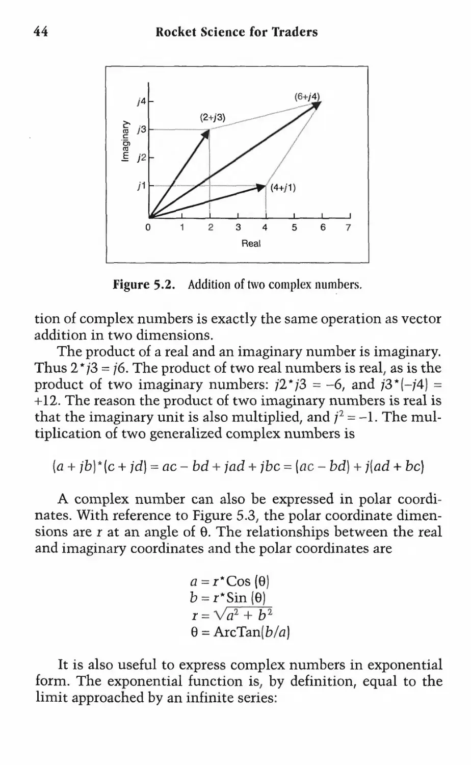
Figure 5.2. Addition of two complex numbers.
tion of complex numbers is exactly the same operation as vector
addition in two dimensions.
The product of a real and an imaginary number is imaginary.
Thus 2*/3 = /6. The product of two real numbers is real, as is the
product of two imaginary numbers: f2*/3 = -6, and f3*(-/4) =
+12. The reason the product of two imaginary numbers is real is
that the imaginary unit is also multiplied, and j2 = -1. The mul-
tiplication of two generalized complex numbers is
(a + /£>) * (c + jd] = ac- bd + jad + jbc = (ac - bd) + j[ad + be)
A complex number can also be expressed in polar coordi-
nates. With reference to Figure 5.3, the polar coordinate dimen-
sions are r at an angle of 0. The relationships between the real
and imaginary coordinates and the polar coordinates are
a = z*Cos (0)
b = r*Sin (0)
r = y/a2 + Ъ2
0 = ArcTan(b/a)
It is also useful to express complex numbers in exponential
form. The exponential function is, by definition, equal to the
limit approached by an infinite series:
Complex Variables
45
Figure 5-3. Components of z.
This series reminds us of the series that defines the trigono-
metric functions:
,Q, 1 02 e4
cos (6) = 1-^Т + 7Г--
e2n
(2n)!
. + (-!)"
лЗ q5
sin Iе'=0 -1
g(2n -1)
The sine and cosine series, although rather like the exponen-
tial series in most other ways, have a reversal of sign of alternate
terms. A similar reversal of sign takes place in the exponential
series, but only if the exponent is imaginary. Consider e'6, which
can be found by letting x = /0 in the exponential series. In this
case we obtain
By comparison to the series expansions for the sine and
cosine functions, we can express the exponential form as
46
Rocket Science for Traders
e'e = Cos (0) + / Sin (0)
Alternately, we can express the Cosine and Sine functions as
e'e + e"'e = 2 Cos (0)
and e'e - er'6 = j2 Sin (0)
This is an important theorem of complex variable theory
known as Euler’s Theorem. Euler's Theorem says that sines and
cosines can be expressed in terms of an exponential function
having an imaginary operator.
We are all familiar with the frequency of a cycle. For exam-
ple, the power coming from our wall plugs is an alternating cur-
rent. The frequency of this alternating current is 60 cycles per
second. Cycles are repetitive. Each time a cycle is completed, it
sweeps through 360 degrees, or 2л radians, of a sine wave. It is
convenient to define the angular frequency as 2л times the reg-
ular frequency by the equation co = 2л/, where co is the Greek let-
ter omega. Using these definitions, cot is the number of radians a
cycle covers in a given amount of time. Since cot is an angle, we
can represent the cycle in exponential form as e’4"1, using com-
plex notation. We thus see in Figure 5.4 that a pure cycle of an
analytic waveform in the time domain can be represented as a
projection onto either the real or imaginary axis.
Figure 5.4. Exponential complex frequency and
its components.
Complex Variables
47
The concept of the exponential form is an extremely impor-
tant one for the digital signal processing of trading waveforms.
The waveform we observe on the charts is called an analytic
waveform. If we can break the analytic waveform into its two
orthogonal components, we can immediately find the amplitude
of the cycle. By examination of Figure 5.4 and using the Pythago-
rean Theorem, we can see that the square of the real component
plus the square of the imaginary component is equal to r2, the
square of the cycle amplitude. Thus, we have a bar-by-bar meas-
urement of the amplitude of the cycle in the time domain. Such
a highly responsive measurement of signal amplitude is an impor-
tant component of all effective trading indicators and systems.
The exponential form also gives us a particularly simple way
to measure the period of the market cycle. The cycle period meas-
urement approach can be understood with reference to Figure
5.5. The initial measurement is made at time tj so that the phase
angle is coti. The second measurement is made at time t2, result-
ing in the measured angle cot2. The difference between the two
phase angles is AG. To measure the cycle period, we simply keep
adding all the AGs until the sum equals 360 degrees. The number
of times we have to add the AGs is, by definition, the period of the
cycle. We discuss exactly how to do this in Chapter 7.
Figure 5.5. Two successive phasor measurements.
48
Rocket Science for Traders
Figures 5.4 and 5.5 are phasor diagrams. Phasor diagrams rep-
resent the cycle as a rotating vector (or, the phasor) in complex
coordinates, where the tail of the phasor is pinned to the origin.
The length of the phasor represents the wave amplitude of the
cycle. The phase angle represents a particular location within
the cycle.
The phasor diagrams we have been discussing only consider
the presence of one significant dominant cycle in the data. Hap-
pily, that is usually the case. The phasor diagram is therefore
useful for comparing the lead and amplitude of momentum
functions to the original data, and also for comparing the lag and
amplitude of smoothing functions to the original data.
But what if there is a secondary cycle present in the data?
Such a cycle is very difficult to identify because it lasts for only a
brief amount of time and the short amount of data we are forced
to use cannot provide enough resolution for filters. Since the
complex variables can be added, the phasor picture might look
something like the depiction in Figure 5.6. The dominant cycle,
having a frequency of coi, is rotating as previously described. The
secondary cycle is assumed to have a smaller amplitude and a
higher frequency (fy- When these two complex variables are
added, the secondary cycle spins like a bicycle pedal at the end of
the crank, which is analogous to the tip of the phasor of the first
Figure 5.6 The addition of two phasors having
different frequencies.
Complex Variables
49
cycle. Assuming the secondary cycle is present only for a short
while, the resultant phasor will look like the dominant cycle
with a little whiffle superimposed on it. These whiffles are
immediately identifiable when the phasor is plotted. In later
chapters, we identify these whiffles in the real data.
Key Points to Remember
• Complex variables are a two-dimensional number set.
• The horizontal dimensions are called real numbers.
• The vertical dimensions are called imaginary numbers.
• j = V-l and is the 90-degree rotation operator.
• A rotating phasor describes a pure cycle from the exponen-
tial complex frequency.
• Relative phases can be described using phasor diagrams.
• Euler's equations describe Cosines and Sines of real frequen-
cies as being comprised of complex frequencies.
• Two simultaneous cycles can be depicted as a bicycle diagram.
This Page Intentionally Left Blank
Chapter 6
HILBERT TRANSFORMS
Ideas are like rabbits. You get a couple
and learn how to handle them,
and pretty soon you have a dozen.
—John Steinbeck
This chapter contains some of the most important concepts
upon which all the following practical applications are based.
First, we derive the Hilbert Transform. The Hilbert Transform is
a procedure to create complex signals from the simple chart data
familiar to all traders. Once we have the complex signals, we can
compute indicators and signals that are more accurate and
responsive than those computed using conventional techniques.
In fact, some of the indicators we will discuss cannot be calcu-
lated at all without the Hilbert Transform.
If we accept that there can be imaginary numbers, then the
concept of negative frequencies should pose no problem. If we
review trigonometric identities, we recall that Cos(-cot) - Cos(cot)
and that Sin(-cot) = -Sin(cot). These identities show that we can
easily accommodate negative frequencies. Further, the power
contained in waveforms is proportional to the average square of
the waveform. The squaring of the sign always produces a posi-
tive power, so there can be no exception to the concept of con-
servation of power if we use negative frequencies.
When data are sampled at a sampling frequency fs, that sam-
pling frequency acts like a radio carrier signal. That is, the real
data being sampled are heterodyned into upper and lower side-
bands of the sampling frequency. Mathematically, heterodyning
51
52
Rocket Science for Traders
is multiplying two frequencies (and then filtering to select the
desired output). So, if we have a baseband data frequency of fbl
the heterodyning can be described as the product of two signals.
By a trigonometric identity, this product results in the sum and
difference frequencies as
0.5*Cos(27t/st)*Cos(27t/bt) = Cos(2tc(/s + fb)t) + Cos(2n(fs-fb}t]
The lower sideband can be considered as a negative fre-
quency relative to the sampling frequency, and the upper side-
band can be considered as a positive frequency relative to the
sampling frequency. Furthermore, every harmonic of the sam-
pling frequency exists. Each harmonic also has an upper and
lower sideband containing the baseband signals.
Since the lower sideband of the sampling frequency exists, it
could extend down into the baseband range of frequencies. For
this reason, the baseband range of frequencies is limited to fs/2.
This is called the Nyquist sampling criteria. In trading, this
means the absolute shortest period we can use is a 2-bar cycle, or
a frequency of 0.5 cycles per bar. The sampling frequency can be
weekly, daily, hourly, and so on, but the shortest period we can
consider in any time frame is a 2-bar cycle.
The sampled data spectrum can be pictured as shown in Fig-
ure 6.1. The baseband signal is depicted as a continuum of fre-
quencies that is bandlimited, either naturally or by a filter, to be
less than half the sampling frequency fs. Several of the harmon-
ics of the sampling frequency are also shown, along with their
respective sidebands. Since we are talking about complex func-
tions, the sampled spectrum can extend below zero frequency as
well. As a result, the complete sampled frequency spectrum
extends from minus infinity to plus infinity, as shown in Figure
6.2. An interesting observation is that either the upper or lower
sideband of any harmonic of the sampling frequency can be
processed with exactly the same result because the same infor-
mation resides in all sidebands. The frequency selection for pro-
cessing is a matter of convenience and is, therefore, usually the
baseband because demodulation of the zero frequency harmonic
is not required.
Hilbert Transforms
53
Figure 6.1. The baseband frequency below half the sampling frequency
appears as sidebands on harmonics of the sampling frequency.
The waveforms with which all traders are familiar are called
analytic signals. Analytic signals are defined as a special case of
a complex function without imaginary values, that have only
positive or only negative frequencies, but not both. We need to
construct more general complex functions to enable more effi-
cient signal processing. This can be done by synthesizing the
analytic signal from a combination of two complex signals that
are odd and even functions around zero.
First, we must recall the trigonometric identities Cos(cot) =
Cos(-cot) and Sin(cot) = -Sin(-cot) and Euler's equations:
and
e'“‘ + e iat = 2 Cos(cot)
- e"'“' = /2 Sin(cot)
We can synthesize the analytic signal by summing the two com-
plex signals as shown in Figure 6.3. The real component of Figure
6.3(a) is summed with the imaginary component in Figure 6.3(b)
to form the complex signal shown in Figure 6.3(c). From Euler's
Figure 6.2. Sampled data spectrum extends to negative frequencies.
54
Rocket Science for Traders
Figure 6.3. An analytic signal is comprised of InPhase and Quadra-
ture components.
equations, the two complex signals can be called the InPhase
(i.e., the Cosine) component and the Quadrature (i.e., the Sine)
component. Quadrature means being rotated by 90 degrees.
The Hilbert Transformer has been derived in a number of
texts, to which you may want to refer for more information.1
One purpose of a Hilbert Transform is to create a complex signal
from an analytic signal. A Hilbert Transformer shifts all positive
frequencies by -90 degrees and all negative frequencies by 90
degrees. Since the frequency response of sampled systems is
periodic, we can describe the Hilbert Transformer in terms of
angular frequency as shown in Figure 6.4 for unity amplitude
components. Since this graph is periodic, we can use the Fourier
series to determine the coefficients of the exponential series
that represents the plot. The Fourier series can be written as
'Rabiner, Lawrence R., and Bernard Gold. Theory and Application of
Digital Signal Processing. Englewood Cliffs: Prentice Hall, 1975.
Hilbert Transforms
55
Figure 6.4. Periodic frequency response of a Digital Hilbert Trans-
former.
’n
If we let z = e'aT with T = 1, the Fourier Transform becomes
and
DO
H(e,<0) = X Cne'“n
n =
This equation describes the coefficients of the digital filter. Solv-
ing the integral equation for the filter coefficients (because the
square wave has the same Sin(x)/x form as the pulse described in
Chapter 3), we obtain
for n 0 and Cn = 0 for n = 0.
The value of n is relative to the center of the filter, so the
center coefficient is always zero. The value of the sine squared
term is always positive and has a unity value for odd values of n.
The coefficients are, therefore, simply 1/n for odd values of n-,
they are positive for the most recent data half of the filter,- and
they are negative in the older data half of the filter. The ideal
Hilbert Transformer extends coefficients from minus infinity to
56
Rocket Science for Traders
plus infinity. The 2/л factor can be ignored here because each
coefficient is divided by the sum of the coefficients to produce a
normalized amplitude response. That is, the desired frequency
components at the output of the filter should have the sample
amplitude they had at the filter input. We can approximate the
Hilbert Transformer by truncating the extent. For example, we
could truncate the filter at n = 7. In this case, where the
detrended Price is represented by P, the Quadrature component
(Q) of the Hilbert Transform can be written as
Q = (P/7 + P[2]/5 + P[4]/3 + P[6] - P[8] - P[10]/3 - P [12]/5
- P[14]/7)/(l + 1/3 + 1/5 + 1/7);
The InPhase component (Z) of the filter is referenced to the cen-
ter of the filter, and can be written simply as
I = P[9]
Note that the lag of this Hilbert Transform is 9 bars.
Since the Hilbert Transformer must be truncated, ideally it
should be sufficiently long to capture a full cycle of the longest
period under consideration. It is not unreasonable to want to
process a cycle that is 40-bars long. This is about two months of
daily data. In this case, we would like to truncate at n = 19. How-
ever, such a Hilbert Transformer would have a lag of 21 bars.
This lag is unacceptable because we would also want to process
cycles with a period of 10 bars or less. The 21-bar lag would be
more than two cycles of the data that have shorter periods.
An alternative way to truncate the Hilbert Transformer is to
use as short a filter as possible. If we truncate the Hilbert Trans-
former at n = 3, the Quadrature component can be written as
Q = (P/3 + P[2] - P[4] - P[6])/(4/3)
= 0.25 *P + 0.75 *P[2] - 0.75 *P[4] - 0.25 *P[6];
This short Hilbert Transformer has a lag of only 3 bars. How-
ever, the severe truncation produces the amplitude transfer
response shown in Figure 6.5. A truncated Hilbert Transformer
has a frequency response similar to that of a momentum function.
Hilbert Transforms
57
Figure 6.5. Amplitude response of a Hilbert Transformer truncated at
n = 3.
The amplitude response of a minimum-length Hilbert Trans-
former can be improved by adjusting the filter coefficients by
trial and error. The resulting Hilbert Transformer filter equation
is
Q = 0.0962*P + 0.5769*P[2] - 0.5769*P[4] - 0.0962*P[6];
The amplitude response of the Improved Hilbert Transformer is
shown in Figure 6.6.
T3
° л -
g -10
о
O-
co
° -20
rr U
CD
0
2 -30
c
СЯ
CD
S -40
0 01 0.2 03 04 05 06 07 08 09 1
Normalized Frequency (Nyquist == 1)
Figure 6.6. Amplitude response of the Improved Hilbert Transformer.
58
Rocket Science for Traders
The response of the Improved Hilbert Transformer is not dis-
similar from the 5-bar high-pass filter described in Chapter 4
(Figure 4.6). The Improved Hilbert Transformer has a more sym-
metrical response, but has a 3-bar lag versus the 2-bar lag of the
high-pass filter. Also, there is less rejection of the intermediate-
length cycles in the Improved Hilbert Transformer. For example,
the attenuation for a normalized frequency of 0.1 (a 20-bar cycle)
is about -6 dB, whereas the rejection of the 5-bar high-pass filter
was about -8 dB at this frequency. The Improved Hilbert Trans-
former also makes a pretty good high-pass filter.
We formed the Improved Hilbert Transformer to satisfy the
criterion of minimizing lag. The penalty we paid for minimizing
lag was the resulting amplitude taper across the frequency band
at which we desire to operate. Since the Improved Hilbert Trans-
former is so similar to a high-pass filter, and the high-pass filter
has an amplitude rolloff directly proportional to frequency, we
can compensate for the amplitude rolloff if we know the fre-
quency. We do not have the frequency directly because we need
the InPhase and Quadrature components to compute it. How-
ever, we do know what the measured cycle period was 1 bar ago.
Since frequency is a slowly varying function from bar to bar, the
cycle period 1 bar ago can easily be used for amplitude compen-
sation.
If the Hilbert Transformer were a pure differentiator, we
know the amplitude correction term would be inversely propor-
tional to co (see Chapter 4). Since the cycle period is the recipro-
cal of the frequency, the correction term would be (Period/2n).
When we examine Figure 6.6, we see that we need an 11 dB cor-
rection for a cycle period of 40 bars (normalized frequency of
0.05) and a 6.2 dB correction for a cycle period of 20 bars (nor-
malized frequency of 0.1). Converting these decibel values to
amplitude and writing a straight line correction equation, we.
have the result
Amplitude correction = (0.075 *Period[l] + 0.54)
This amplitude correction enables us to effectively use a mini-
mum-length Hilbert Transformer to keep the lag to as small a
value as possible.
Hilbert Transforms
59
The purpose of the Hilbert Transform, as explained earlier, is
to create InPhase and Quadrature components from the analytic
waveform. The InPhase and Quadrature components enable effi-
cient computation to find the dominant cycle period, the domi-
nant cycle amplitude, and the phase of the dominant cycle.
From these parameters we can calculate unique and precise indi-
cators, such as the Signal-to-Noise Ratio, the Sinewave Indica-
tor (a Cycle Mode predictive indicator), and an Instantaneous
Trendline. The (nearly) complete code to calculate the InPhase
and Quadrature components is given in Figure 6.7. (The com-
plete code requires the computation of the dominant cycle
period, which is covered in the next chapter.)
In EasyLanguage code, all input values must be defined. In
the case of Figure 6.7, the only input value is Price, and is com-
puted as the average of the High and Low for each bar in the data
Inputs: Price( (H+L)/2) ;
Vars: Smooth(0), Detrender (0), 11(0), Ql(0), Period(0);
If CurrentBar > 5 then begin
Smooth = (4*Price + 3*Price[l] + 2*Price[2] +
Price[ 3 ] ) / 10;
Detrender = (.0962*Smooth + .5769*Smooth[2] -
.5769*Smooth[4] - .0962*Smooth [6])*
(.075*Period[1] + .54);
{Compute InPhase and Quadrature components}
QI = (.0962*Detrender + .5769*Detrender[2] -
.5769*Detrender[4] - .0962*Detrender[6])*
( .075*Period[1] + .54);
Il = Detrender[3];
Plotl(Il, "InPhase");
Plot2(-Q1, "Quadrature);
End;
Figure 6.7. Hilbert Transform EasyLanguage code.
60
Rocket Science for Traders
series. Next, all the other variables must be defined, and their
initial values must be set to zero. The first line of computational
code computes the variable Smoother as a 4-bar Weighted Mov-
ing Average (WMA) of Price. A 4-bar WMA is used to remove
some of the higher-frequency components prior to detrending
the Price. The lag penalty for this smoothing is only 1 bar. The
Price is detrended in the next line of code. Since we have an
amplitude-corrected Hilbert Transformer, and since we want to
detrend over its length, we simply use the Hilbert Transformer
itself as the detrender. We do not particularly care about the
phase of the detrended analytic signal at this point. However, we
do note that detrending has introduced another 3 bars of lag into
the computation. The amplitude correction can be applied after
we compute the period of the dominant cycle. The InPhase and
Quadrature components are contained in the next two lines of
code. The Quadrature component is computed by applying the
Hilbert Transformer a second time. The InPhase component is
computed simply by using the Detrender value referenced to 3
bars ago, the center of the Hilbert Transformer. Therefore, the
calculation of the InPhase and Quadrature components intro-
duces still another 3 bars of delay in the calculation. We now
have a total of 7 bars of delay after computing the InPhase and
Quadrature components.
The InPhase and Quadrature components are only concerned
with Cycle Mode signals because the Detrender removed the
trending components. The 7-bar lag can be converted to a phase
lag by the following process: We divide the 7-bar lag by the dom-
inant cycle period to get a percentage of a cycle and then multi-
ply by 360 degrees. Furthermore, the Hilbert Transformer offers
the advantage of providing 90 degrees of phase lead. The equa-
tion for phase lag is then
Phase lag = 360*7/Period - 90
Therefore, a 28-bar dominant cycle will have zero lag. A 14-bar
dominant cycle will have 90 degrees lag, or a quarter cycle. The
phase lag grows rapidly for still shorter cycle periods. For exam-
ple, a 7-bar cycle will have 180-degrees lag, corresponding to a
Hilbert Transforms
61
half cycle. The phase lag of the InPhase and Quadrature compo-
nents can be a serious consideration when interpreting the
results of some indicators. For example, knowing the InPhase
component is delayed by 7 bars from the time-domain wave-
form, we can anticipate the crest of the time-domain waveform
by projecting when the InPhase component will reach its maxi-
mum 7 bars into the future.
Key Points to Remember
• Both positive and negative frequencies are possible in signal
processing.
• Only positive frequencies or only negative frequencies, but
not both, comprise the analytic signal.
• Complex signals contain InPhase and Quadrature compo-
nents.
• An analytic signal can be synthesized by complex signals.
• Following the preceding two points, an analytic signal can be
decomposed into InPhase and Quadrature components.
• A Hilbert Transformer is the technique used to decompose
analytic signals.
• Hilbert Transformers must be severely truncated to produce
acceptable lag for use in trading.
• Amplitude compensation of the InPhase and Quadrature
components can be accomplished by knowing the period of
the dominant cycle.
• The analytic signal must be smoothed and detrended prior to
computing the InPhase and Quadrature components.
• The amplitude-compensated Hilbert Transformer can be
used to detrend the analytic waveform.
• The phase lag of the InPhase and Quadrature components is
(360*7/Period - 90) degrees.
This Page Intentionally Left Blank
Chapter 7
MEASURING CYCLE PERIODS
. . . but what are we going to do with
all those skinned catst
—Anonymous
One fundamental definition of a cycle is that the process under
consideration has a constant rate of phase change. We can meas-
ure the phase of a complex signal directly. Knowing the phase at
each sample, we need only take the bar-to-bar difference to
obtain the rate of phase change. In this chapter, you are pre-
sented with several mathematical techniques for measuring the
period of the dominant cycle. While mathematically dissimilar,
all these techniques share the common feature of using differen-
tial phase between samples.
Phase Accumulation
The Phase Accumulation technique of cycle period measure-
ment is perhaps the easiest to comprehend. In this technique,
we measure the phase at each sample by taking the arctangent of
the ratio of the Quadrature component to the InPhase compo-
nent. A delta phase is generated by taking the difference of the
phase between successive samples. At each sample we can then
look backward, adding up the delta phases. When the sum of the
delta phases reaches 360 degrees, we must have passed through
one full cycle, on average. The process is repeated for each new
sample.
63
64
Rocket Science for Traders
The Phase Accumulation method of cycle measurement
always uses one full cycle's worth of historical data. This is both
an advantage and disadvantage. The advantage is the lag in
obtaining the answer scales directly with the cycle period. That
is, the measurement of a short cycle period has less lag than the
measurement of a longer cycle period. However, the number of
samples used in making the measurement means the averaging
period is variable with cycle period. Longer averaging reduces
the noise level compared to the signal. Therefore, shorter cycle
periods necessarily have a higher output Signal-to-Noise Ratio.
Implementing the Phase Accumulation method of cycle
measurement with the EasyLanguage code is described with ref-
erence to Figure 7.1. The initial part of the code creates the
InPhase and Quadrature components, Il and QI, as discussed in
the last chapter. It is crucial that II and QI be smoothed before
the arctangent of their ratio is taken. We do the smoothing in an
EMA whose alpha equals 0.15. The instantaneous phase (the
phase at any bar) is computed as the arctangent of the ratio of Q1
to II. This gives the instantaneous phase within a quadrant. The
quadrant ambiguity is removed in the subsequent three lines of
code. We then compute the differential phase (DeltaPhase)
between successive samples. There can be considerable error in
the raw differential phase computation. To keep these large
errors from unduly influencing the outcome, we limit the values
of the differential phase to be between cycle periods of 6 bars
(DeltaPhase = 36% = 60) and 50 bars (Delta Phase = 36%o = 7). The
DeltaPhases are then accumulated until the PhaseSum exceeds
360 degrees. At that point, the cycle period is assigned as the
number of samples required for the PhaseSum to reach the 360-
degree value. The accumulation is done for each bar in the data
set but is limited to a value of 40 bars. The limitation is based on
our assumption that cycle periods of 40 bars and longer result in
a Trend Mode, and detailed knowledge of their periods is not
necessary. If the cycle period has not been identified within the
maximum 40-bar accumulation period, then it is assigned the
value of the cycle period measurement for the previous sample.
It is then smoothed by an EMA whose alpha equals 0.25 to cre-
ate a pleasing presentation. The lag due to this EMA is 3 bars.
Measuring Cycle Periods
65
Inputs:
Price ( (H+D/2) ;
Vars: Smooth(0) ,
Detrender(0) ,
11(0),
QI (0),
Phase(0),
DeltaPhase(0),
InstPeriod(0),
count(0),
PhaseSum(0),
Period(0);
If CurrentBar > 5 then begin
Smooth = (4*Price + 3*Price[l] + 2*Price[2] +
Price[3]) I 10;
Detrender = (.0962*Smooth + .5769*Smooth[2] -
.5769*Smooth[4] - .0962*Smooth[6])*(.075*
Period[1] + .54);
{Compute InPhase and Quadrature components}
QI = (.0962*Detrender + .5769*Detrender[2] -
.5769*Detrender[4] - .0962*Detrender[6])*
(. 075*Period[1] + .54);
Il = Detrender[3] ;
{Smooth the I and Q components before applying
the discriminator}
Il = .15*11 + .85*11 [1] ;
QI = .15*Q1 + .85*Q1[1] ;
{Use ArcTangent to compute the current phase}
If AbsValue(Il) > 0 then Phase =
ArcTangent(AbsValue(Ql/Il));
{Resolve the ArcTangent ambiguity for quadrants
2, 3, and 4}
If II < 0 and QI > 0 then Phase = 180 - Phase;
If II < 0 and QI < 0 then Phase = 180 + Phase;
If II > 0 and QI < 0 then Phase = 360 - Phase;
(continued)
Figure 7.1. Phase Accumulator cycle period measurement.
66
Rocket Science for Traders
{Compute a differential phase, resolve phase
wraparound from quadrant 1 to quadrant 4, and
limit delta phase errors)
DeltaPhase = Phase[1] - Phase;
If Phase[1] < 90 and Phase > 270 then DeltaPhase
= 360 + Phase[1] - Phase;
{Limit DeltaPhase to be within the bounds of 6
bar and 50 bar cycles)
If DeltaPhase < 7 then DeltaPhase = 7;
If DeltaPhase > 60 then Deltaphase = 60;
{Sum DeltaPhases to reach 360 degrees. The sum is
the instantaneous period.}
InstPeriod = 0;
PhaseSum = 0;
For count = 0 to 40 begin
PhaseSum = PhaseSum + DeltaPhase[count];
If PhaseSum > 360 and InstPeriod = 0 then
begin
InstPeriod = count;
End;
End;
{Resolve Instantaneous Period errors and smooth)
If InstPeriod = 0 then InstPeriod =
InstPeriod[1];
Period = .25*InstPeriod + .75*Period[1];
Plotl(Period, "DC");
End;
Figure 7.1 . (Continued).
Total lag through the Phase Accumulation cycle period
measurement consists of 6 bars for the first EMA, 3 bars for the
display smoothing EMA, 7-bars lag to compute the original
InPhase and Quadrature components, and one full cycle of this
accumulation process. Therefore, the total lag is 16 bars plus one
full-cycle period. Since the dominant cycle period is a relatively
slow varying function of time, this lag may be acceptable in
many applications.
Measuring Cycle Periods
67
Homodyne Discriminator
Homodyne means we are multiplying the signal by itself. More
precise, we want to multiply the signal of the current bar with
the complex conjugate of the signal 1 bar ago. The complex con-
jugate is, by definition, a complex number whose sign of the
imaginary component has been reversed. Expressing the signal
in polar coordinates, the arithmetic is
(pe'“‘n)(pe_/“‘n-1) = p2$Mtn-tn-ii = p2e'“
The interesting result is that we get both the square of the sig-
nal amplitude and the angular frequency (2k / Period) from the
product because the difference in time between samples (tn - tn_i)
is just 1 bar. In principle, this means that we can get the instanta-
neous cycle period in just two successive samples. The added
benefit is that we also get the square of the signal amplitude. The
calculations are carried out using the real and imaginary compo-
nents rather than converting them to polar coordinates. Either
way, the results are the same.
The EasyLanguage code for the Homodyne Discriminator is
described with reference to Figure 7.2. The InPhase and Quadra-
ture components are computed using the Hilbert Transformer as
explained in Chapter 6. These components are smoothed in a
unique complex averager and then smoothed by an EMA to
avoid any undesired cross products in the multiplication step
that follows. Consider the result as a composite of signal and
noise represented by (S + N). If we were to multiply this by itself,
we would get S2 + N2 + SN + NS. Of the four products, three are
undesired due to noise. Therefore, we must take every measure
to remove undesired components prior to any multiplication.
The complex averaging consists of applying the Hilbert Trans-
former to both the InPhase and Quadrature components. This
advances the phase of each component by 90 degrees. When the
InPhase component is advanced by 90 degrees, it becomes equal
to the Quadrature component. Similarly, when the Quadrature
component is advanced in phase by 90 degrees, it becomes the
same as the negative InPhase component. So, if we perform a
Hilbert Transform on an InPhase component, it will be aligned
68
Rocket Science for Traders
Inputs: Price((H+L)/2);
Vars: Smooth(0),
Detrender(0),
11(0) ,
Ql(0),
jl(O) ,
jQ (0) ,
12(0),
Q2(0) ,
Re(0) ,
Im(0),
Period(0),
SmoothPeriod(0) ; •
If CurrentBar > 5 then begin
Smooth = (4*Price + 3*Price[l] + 2*Price[2] +
Price [3]) / 10;
Detrender = (.0962*Smooth + .5769*Smooth[2] -
.5769*Smooth[4] - .0962*Smooth[6])*(.075*
Period[1] + .54);
{Compute InPhase and Quadrature components}
QI = (.0962*Detrender + .5769*Detrender[2] -
.5769*Detrender[4] - .0962*Detrender[6])*(.075*
Period[1] + .54);
Il = Detrender[3];
{Advance the phase of II and QI by 90 degrees}
jl = (.0962*11 + .5769*11(2] - .5769*11(4] -
.0962*11[6])*(.075*Period[1] + .54);
jQ = (.O962*Q1 + .5769*Q1[2] - .5769*Q1[4] -
.O962*Q1[6])*(.075*Period[1] + .54);
{Phasor addition for 3 bar averaging)}
12 = Il - jQ;
Q2 = QI + jl;
{Smooth the I and Q components before applying
the discriminator}
(continued)
Figure 7.2. Homodyne Discriminator cycle period measurement.
Measuring Cycle Periods
69
12 = .2*12 + .8*12 [1] ;
Q2 = .2*Q2 + .8*Q2 [1] ;
{Homodyne Discriminator)
Re = 12*12 [1] + Q2*Q2[1];
Im = I2*Q2[1] - Q2*I2 [1] ;
Re = .2*Re + . 8*Re[l];
Im = .2*Im + .8*Im[l];
If Im <> 0 and Re <> 0 then Period = 360/
ArcTangent(Im/Re);
If Period > 1.5*Period[1] then Period =
1.5*Period[1];
If Period < .67*Period[1] then Period =
.67*Period[1] ;
If Period < 6 then Period = 6;
If Period > 50 then Period = 50;
Period = .2*Period + .8*Period[1];
SmoothPeriod = .33*Period + .67*SmoothPeriod[1];
Plotl(SmoothPeriod, "DC");
End;
Figure 7.2 . (Continued).
in phase with the Quadrature component. However, the Hilbert
Transform has a 3-bar lag. The transformed InPhase component
summed with the Quadrature component is therefore the math-
ematical equivalent of the simple average of a signal with the
signal 3 bars ago. The same process applies to performing a
Hilbert Transform on the imaginary component and adding it to
the InPhase component. The net result is that the net complex
averaging lag is 1.5 bars. After smoothing, the signal is multi-
plied by the complex conjugate of the signal 1 bar ago. The
resulting output real component is the product of the two real
components added to the product of the two imaginary compo-
nents. Similarly, the resulting output imaginary component is
the difference of the two input cross products. Both the real and
imaginary output products are smoothed again before the cycle
period is computed. This is done by taking the arctangent of the
69
70
Rocket Science for Traders
ratio of the output imaginary component to the real component.
The rate change of the cycle period is limited to be ±50 percent
of the previous cycle period, and the resultant period is further
limited to be greater than 6 bars and less than 50 bars. Finally,
the period is smoothed for a pleasing display.
Total lag through the Homodyne Discriminator cycle period
measurement consists of the following: seven-bars lag to com-
pute the original InPhase and Quadrature components and
4-bars lag in each of the three EMAs, and 1.5 bars for the com-
plex averaging. Therefore, the total lag is a constant 20.5 bars.
The net smoothing is the same regardless of the measured
period. Therefore, the Signal-to-Noise Ratio as well as the lag is
constant for all cycle periods.
Dual Differentiator
We have seen how the phase angle is computed from a complex
signal as the arctangent of the ratio of the imaginary component
to the real component. Furthermore, we have seen that angular
frequency is defined as the rate change of phase. We can use
these facts to derive still a third way of using complex signals to
measure the cycle period. From the definition of the derivative
of an arctangent, the mathematics of this process are
0 = arctanl — I
„ de -------кvr - i'a0 - QA,I
dt~l + №-\ p ~ P + Q1
Simplifying, and solving for the cycle period instead of fre-
quency, we obtain
Period =
2k(Z2 + Q2)
(ZAQ - QAZ)
The EasyLanguage code for the Dual Differentiator Discrim-
inator is described with reference to Figure 7.3. The InPhase
Measuring Cycle Periods
71
Inputs: Price((H+L)/2);
Vars: Smooth(0),
Detrender(0) ,
11(0),
Ql(0),
jl(O) ,
jQ (0) ,
12(0),
Q2 (0) ,
Period(0),
Smoothperiod(0);
If CurrentBar > 5 then begin
Smooth = (4*Price + 3*Price [1] + 2*Price[2] +
Price [3]) / 10;
Detrender = (.0962*Smooth + .5769*Smooth[2] -
.5769*Smooth[4] - .0962*Smooth[6])*(.075*
Period [1] + . 54) ;
{Compute InPhase and Quadrature components}
QI = (.0962*Detrender + .5769*Detrender[2] -
.5769*Detrender[4] - .0962*Detrender[6])*(.075*
Period[1] + .54);
Il = Detrender[3];
{Advance the phase of II and QI by 90 degrees}
jl = (.0962*11 + .5769*11(2] - .5769*11(4] -
.0962*11 [6])*(.075*Period [1] + .54);
jQ = (.O962*Q1 + .5769*Q1[2] - .5769*Q1[4] -
.O962*Q1[6])*(.075*Period[1] + .54);
{Phasor addition for 3 bar averaging)}
12 = Il - jQ;
Q2 = QI + jl;
{Smooth the I and Q components before applying
the discriminator}
12 = .15*12 + .75*12 [1] ;
Q2 = .15*Q2 + .75*Q2[1];
(continued)
Figure 7.3. Dual Differential cycle period measurement.
72
Rocket Science for Traders
{Dual Differential Discriminator}
Valuel = Q2*(I2 - 12 [1]) - 12*(Q2 - Q2 [1]) ;
If Valuel > .01 then Period = 6.2832* (12*12 +
Q2*Q2) / Valuel;
If Period > 1.5*Period[1] then Period =
1.5*Period[1] ;
If Period < .67*Period[1] then Period =
.67*Period[1];
If Period < 6 then Period = 6;
If Period > 50 then Period = 50;
Period = .15*Period + .85*Period[1];
SmoothPeriod = .33*Period + .67*SmoothPeriod[1];
Plotl(SmoothPeriod, "DC");
End;
Figure 7.3 . (Continued).
and Quadrature components are computed with the Hilbert
Transformer using procedures identical to those in the Dual
Differentiator. These components undergo a complex averaging
and are smoothed in an EMA to avoid any undesired cross prod-
ucts in the multiplication step that follows. The period is solved
directly from the smoothed InPhase and Quadrature compo-
nents. The interim calculation for the denominator is performed
as Valuel to ensure that the denominator will not have a zero
value. The sign of Valuel is reversed relative to the theoretical
equation because the differences are looking backward in time.
The rate change of the cycle period is limited to be ±50 percent
of the previous cycle period, and the resultant period is further
limited to be greater than 6 bars and less than 50 bars. Finally,
the period is smoothed for a pleasing display.
Total lag through the Dual Differentiator Discriminator cycle
period measurement consists of 7-bars lag to compute the original
InPhase and Quadrature components and 4-bars lag in each of the
two EMAs, plus 1.5 bars for the complex averaging. Therefore, the
total lag is a constant 16.5 bars. The net smoothing is the same
Measuring Cycle Periods
73
regardless of the measured period. Therefore, the Signal-to-Noise
Ratio, as well as the lag, is constant for all cycle periods.
Cycle Measurement Comparison
We now have three techniques to measure cycle periods
using complex arithmetic. We only know that they vary in lag
and that the lag is relatively long in each case. The only way to
determine the best technique is to exercise them in a variety of
tests. The first test is designed to see how accurately the cycle
measurement is made using a perfect sine wave. In Figure 7.4,
we have created an analytic waveform as a pure cycle whose
period increases linearly from 10 to 40 bars across the screen.
The cycle length measurements of the three techniques are plot-
ted in the first subgraph. This subgraph is scaled from 10 to 40
bars, so vertical displacement shows the measured cycle period.
Figure 7.4. Cycle period measurements in response to a chirped analytic
waveform.
Chart created with TradeStation2000i® by Omega Research, Inc.
74
Rocket Science for Traders
At first glance, it appears that the Phase Accumulator method is
less accurate than the others. However, recalling that its lag is
longer than the others for longer cycle periods, this apparent
inaccuracy is due solely to the lag associated with the changing
waveform period.
The next stress test for the cycle period measurers deciphers
how rapidly the cycle measurements respond to an instanta-
neous shift of frequency in the analytic waveform. To do this,
we created a waveform that alternately switches between a
period of 15 bars and a period of 30 bars. The response of the
three cycle period measurers is shown in Figure 7.5. Now we can
see some differences. As expected, the Phase Accumulator is the
slowest to respond to this step in the cycle period because of the
Figure 7.5. Cycle measurer transient responses to rapid changes of
cycle period.
Chart created with TradeStation2000i® by Omega Research, Inc.
Measuring Cycle Periods
75
additional smoothing. Also as expected, the Dual Differentiator
reacts the fastest in this test. However, the Dual Differentiator
exhibits some overshoot error. As a result, it appears that the
Homodyne approach has the superior transient response.
Another significant test finds how the cycle period measurers
perform as the Signal-to-Noise Ratio degenerates. Market data
almost always have a poor Signal-to-Noise Ratio, and the ability
to make accurate measurements is crucial. In fact, it was this
stress test that led to additional smoothing prior to the multipli-
cation operations in the Homodyne and Dual Differentiator
cycle period measurers. Without this smoothing, the perform-
ance in low Signal-to-Noise environments was just awful, pro-
ducing measured cycle periods nearly half the correct period. The
performance of the cycle period measurers are compared in Fig-
ure 7.6 as a function of Signal-to-Noise Ratio when measuring a
theoretical twenty-bar sinewave signal. It is clear from Figure 7.6
that the Homodyne approach is not only more accurate at high
Signal-to-Noise Ratios but its performance degrades more grace-
fully as the noise is increased relative to the signal strength.
The real acid test of the cycle period measurers' performance
determines how well they do when acting on real data. We do
this in Figure 7.7. All three tend to give similar measurements
Cycle Measurement Accuracy Versus S/N
-----Phase Accumulation
— Homodyne
-----Dual Differentiator
Slgnal-to-Nolse Ratio (dB)
Figure 7.6. Phase measurer performance as a function of
Signal-to-Noise Ratio.
Measuring Cycle Periods
77
when the market is in a Cycle Mode. However, there is a wide
difference in the measurements when the market is in a Trend
Mode. My observations have led me to conclude that the Homo-
dyne is overall more accurate in measurement of cycles when
the market is in a Trend Mode.
For all these reasons I conclude that the Homodyne Dis-
criminator is the superior approach. This frequency measurer is
used throughout the remainder of this book.
Key Points to Remember
• A basic definition of a cycle is a constant rate change of
phase.
• The Hilbert Transform generates InPhase and Quadrature
components from which the phase at each bar can be meas-
ured.
• The phase rate of change is established as the differential
phase from bar to bar.
• Complex averaging can be accomplished by applying the
Hilbert Transformer to both the InPhase and Quadrature
components, advancing their phase by 90 degrees. The
phase-advanced components are then algebraically added to
their orthogonal counterparts to effect the averaging.
• There are at least three different ways to measure cycle
period using the InPhase and Quadrature components.
• The Homodyne Discriminator is the superior cycle period
measurer.
This Page Intentionally Left Blank
Chapter 8
SIGNAL-TO-NOISE RATIO
Logic is a system whereby one may
go wrong with confidence.
—Charles Kettering
The signal amplitude is simply the length of the phasor. Recall-
ing the Pythagorean Theorem, the length of the phasor is the
square root of the sum of the squares of the InPhase and Quad-
rature components. We therefore have the signal amplitude on a
bar-by-bar basis after we take the Hilbert Transform.
The signal amplitude is not of much use by itself. However,
if we can estimate the signal amplitude relative to the market
noise, we then have a tool that estimates the quality of our tech-
nical analysis. With the kind of market data now available, let
us develop a unique definition of noise. A sampled signal is
shown in Figure 8.1(a) as a sine wave with the sampling uncer-
tainty represented as the high and low of each bar. The high and
low is the uncertainty of each of our perfect sinewave sample
points. We can make good trades as long as our signal amplitude
is much larger than the average daily range of the bars. Another
case for the same signal amplitude is shown in Figure 8.1(b).
When half the average daily range becomes equal to the signal
amplitude, making money on a trade becomes a crapshoot.
Under this condition, it is possible to make an entry at the low
of the bar (which contains the signal high) and make an exit at
the high of the bar (which contains the signal low) for zero profit.
We will therefore term the case where half the average daily
79
80
Rocket Science for Traders
Figure 8.1. (a) Fourteen dB SNR. (b) Zero dB SNR.
trading range is equal to the signal amplitude as our zero decibel
Signal-to-Noise Ratio (0 dB SNR) condition. We want the signal
amplitude to be at least twice the noise amplitude (6 dB SNR) so
that there exists a reasonable chance to make a profit from our
analysis.
We can define the noise as a smoothed average of the daily
trading range. We can tolerate a 9-bar lag to compute such an aver-
age because the range tends not to change much, and so the noise
will be an Exponential Moving Average (EMA) with an alpha of
0.1. The trading range is simply the high minus the low of each
bar. The EasyLanguage code to compute the SNR is given in Fig-
ure 8.2. This code is almost identical to the one we use for the
Homodyne Discriminator with a few additions. First, the noise is
computed as the variable "Range" near the top of the code. Sec-
ond, the signal power is computed by adding the square of the
InPhase component to the square of the Quadrature component.
The SNR in decibels is calculated in a single line of code near
the end. The signal power is divided by the noise power to get a
power ratio. The value in decibels is computed as 10 times the
Signal-to-Noise Ratio
81
Inputs: Price((H+L)/2);
Vars: Range(0),
Smooth(0),
Detrender(0),
11(0) ,
Ql(0) ,
jl (0) ,
jQ(O) ,
12(0) ,
Q2 (0) ,
Re(0),
Im(0) ,
Period(0),
SmoothPeriod(0),
SNR(0);
If CurrentBar > 5 then begin
{Compute "Noise" as the average range}
Range = . 1*(H - L) + . 9*Range[l];
Smooth = (4*Price + 3*Price[l] + 2*Price[2] +
Price[3]) / 10;
Detrender = (.0962*Smooth + .5769*Smooth[2] -
.5769*Smooth[4] - .0962*Smooth[6])*(.075*
Period[1] + .54);
{Compute InPhase and Quadrature components}
QI = (.0962*Detrender + .5769*Detrender[2] -
.5769*Detrender[4] - .0962*Detrender[6])*
(.075*Period[1] + .54);
Il = Detrender[3];
{Advance the phase of II and QI by 90 degrees}
jl = (.0962*11 + ,5769*I1[2] - .5769*I1[4] -
.O962*I1[6])*(.075*Period[l] + .54);
jQ = (.O962*Q1 + ,5769*Q1[2] - .5769*Q1[4] -
.O962*Q1[6])*(.075*Period[1] + .54);
(continued)
Figure 8.2. Computing the SNR.
82
Rocket Science for Traders
{Phasor addition for 3 bar averaging}
12 = Il - jQ;
Q2 = QI + jl;
{Smooth the I and Q components before applying
the discriminator}
12 = .2*12 + .8*12 [1] ;
Q2 = .2*Q2 + . 8*Q2[1];
{Homodyne Discriminator}
Re = 12*12 [1] + Q2*Q2[1];
Im = I2*Q2[1] - Q2*I2 [1] ;
Re = .2*Re + .8*Re[1];
Im = .2*Im + . 8*Im[l];
If Im <> 0 and Re <> 0 then Period =
360/ArcTangent(Im/Re);
If Period > 1.5*Period[1] then Period =
1.5*Period[1];
If Period < .67*Period[1] then Period =
.67*Period[1];
If Period < 6 then Period = 6;
If Period > 50 then Period = 50;
Period = .2*Period + .8*Period[1];
{Compute smoothed SNR in Decibels, guarding
against a divide by zero error}
If Range > 0 then SNR = .25*(10*Log((11*11 +
Q1*Q1)/(Range*Range))/Log(10) + 6) +
.75*SNR[1];
{Plot Results}
Plotl(SNR, "SNR");
Plot2(6, "Ref");
End;
Figure 8.2. (Continued},
Signal-to-Noise Ratio
83
logarithm of the power ratio. Since Easy Language takes only
natural logarithms, the logarithm must be converted to log base
10 by being divided by the natural logarithm of 10. A compen-
sating term of 6 dB must be added due to our definition of signal
to noise. As defined earlier, the signal amplitude is the length of
the phasor. At 0 dB, the peak-to-peak noise signal is twice the
amplitude of the signal. Therefore, when we compute the 0 dB
case, the ratio is calculated to be 10*Log(l/2)A2 = -6 dB. We
must then add 6 dB back into the computation to remove this
bias, establishing our definition of 0 dB SNR.
Assuming the noise is relatively constant, the lag of the
Signal-to-Noise Indicator is just the 7 bars that result from the
Hilbert Transformer plus the 3 bars due to smoothing of the
display.
There is another way to compute the SNR. Recall that in
the derivation of the Homodyne Discriminator, the amplitude
squared fell out of the equation automatically when we solved
for the frequency. In EasyLanguage code, the amplitude squared
is the sum of the variables Re and Im. Therefore, our alternate
solution for the SNR is obtained by replacing (11*11 + Q1*Q1)
with (Re + Im). That is the only change in the code shown in Fig-
ure 8.3. The alternate calculation uses the signal information
that is smoothed by two EMAs, causing a 3-bar lag each, plus the
lag induced by the complex averaging of 1.5 bars. Therefore, we
expect the alternate SNR computation to produce a result that is
smoother and has an additional 7.5-bar lag as compared to the
first (or, primary) calculation. The two SNR computations are
compared in Figure 8.4. Our expectation of a smoother and more
delayed alternate computation is manifest.
The 10-bar lag induced by the computation of the Primary
SNR makes this calculation unusable for practical trading. The
additional lag of the Alternate SNR makes its use unthinkable.
By carefully examining the required conditions, we can arrive at
an SNR Indicator that has an acceptable lag.
The first condition of the Hilbert Transform is that its transfer
response must have a zero transfer response at zero frequency.
That means the signal must be detrended. The first thing we do
after the initial smoothing is to use the Detrender as the Quadra-
84
Rocket Science for Traders
Inputs: Price((H+L)/2);
Vars: Range(0)z
Smooth(0) ,
Detrender(0),
11(0),
Ql(0),
jI(0) ,
jQ(0) ,
12 (0) ,
Q2(0) ,
Re(0) ,
Im(0) ,
Period(0),
SmoothPeriod(0),
SNR(0);
If CurrentBar > 5 then begin
{Compute "Noise" as the average range}
Range = .1*(H - L) + .9*Range[l];
Smooth = (4*Price + 3*Price[l] + 2*Price[2] +
Price [3]) / 10;
Detrender = (.0962*Smooth + .5769*Smooth[2] -
.5769*Smooth[4] - .0962*Smooth[6])*(.075*
Period[1] + .54);
{Compute InPhase and Quadrature components}
QI = (.0962*Detrender + .5769*Detrender[2] -
.5769*Detrender[4] - .0962*Detrender[6])*(.075*
Period[1] + .54);
Il = Detrender[3];
{Advance the phase of II and QI by 90 degrees}
jl = (.0962*11 + .5769*11(2] - .5769*11(4] -
.0962*11 (6] )*(.075*Period[1] + . 54) ;
jQ = (.O962*Q1 + .5769*Q1[2] - .5769*Q1[4] -
.O962*Q1[6])*(.075*Period[1] + .54);
{Phasor addition for 3 bar averaging)}
(continued)
Figure 8.3. Alternate SNR computation.
Signal-to-Noise Ratio
85
12 = Il - jQ;
Q2 = QI + jl;
{Smooth the I and Q components before applying
the discriminate^^.
12 = .2*12 + .8*12 [1] ;
Q2 = .2*Q2 + .8*Q2[1];
{Homodyne Discriminator}
Re = 12*12 [1] + Q2*Q2 [1] ;
Im = I2*Q2[1] - Q2*I2 [1] ;
Re = .2*Re + .8*Re[1];
Im = .2*Im + .8*Im[l];
If Im <> 0 and Re <> 0 then Period =
360/ArcTangent(Im/Re);
If Period > 1.5*Period[1] then Period =
1.5*Period[1];
If Period < .67*Period[1] then Period =
.67*Period[1];
If Period < 6 then Period = 6;
If Period > 50 then Period = 50;
Period = .2*Period + .8*Period[1];
{Compute smoothed SNR in Decibels, guarding
against a divide by zero error}
If Range > 0 then SNR = .25*(10*Log((Re +
Im)/(Range*Range))/Log(10) + 6) + .75*SNR[1];
{Plot Results}
Plot1(SNR, "SNR");
Plot2(6, "Ref");
End;
Figure 8.3. {Continued').
ture component of the Hilbert Transform. If we shorten the
Detrender to a 2-bar momentum, the resulting lag is only 1 bar.
Because of the shorter momentum, we need a more aggressive
amplitude correction as a function of the measured period. We can
measure slowly varying periods as we have done previously before
proceeding with the calculation of the SNR. We also know that if
86
Rocket Science for Traders
Figure 8.4. The alternate SNR computation is smoother and has more lag than
the primary computation.
Chart created with TradeStation2000i® by Omega Research, Inc.
we take a Simple Moving Average (SMA) over half the measured
period, the lag of this average is a quarter cycle. A quarter cycle is
90 degrees of phase lag—exactly the lag needed to create the
InPhase component from the Quadrature component. This filter-
ing also reduces the dominant cycle amplitude by 2/n, so an addi-
tional я/2 amplitude correction term must be included in the
computation of the InPhase component.
All these conditions have been included in the computation of
the Enhanced SNR Indicator, as described in the code of Figure
8.5. In this code, the period of the measured dominant cycle is cal-
culated in exactly the same manner as we calculated it for the Pri-
mary SNR Indicator. Near the end of the code, after the dominant
cycle is determined, we compute the SNR. The Quadrature com-
ponent Q3 is calculated by multiplying the 2-bar momentum of
the Weighted Moving Average (WMA) smoothing by the domi-
nant cycle amplitude correction factor. The correction terms were
derived by observing the output amplitude of the 2-bar momen-
I******************************************************
Description : Enhanced Signal to Noise Ratio Indicator
******************************************************J
Inputs: Price((H+L)/2);
Vars: Smooth(0),
Detrender(0),
11(0),
Ql(0) ,
jI (0) ,
jQ(O) ,
12 (0),
Q2(0) ,
Re(0) ,
Im(0) ,
Period(0),
SmoothPeriod(0)z
count(0),
13(0),
Q3(0) ,
Signal(0),
Noise (0),
SNR(0);
If CurrentBar > 5 then begin
Smooth = (4*Price + 3*Price[l] + 2*Price[2] +
Price [3]) / 10;
Detrender = (.0962*Smooth + .5769*Smooth[2] -
.5769*Smooth[4] - .0962*Smooth[6])*(.075*
Period[1] + .54);
{Compute InPhase and Quadrature components}
QI = (.0962*Detrender + .5769*Detrender[2] -
.5769*Detrender(4] - .0962*Detrender[6])*
(.075*Period[1] + .54);
Il = Detrender[3];
{Advance the phase of II and QI by 90 degrees}
jl = (.0962*11 + .5769*11(2] - .5769*11(4] -
.0962*11[6])*(.075*Period[1] + .54);
jQ = (.O962*Q1 + .5769*Q1[2] - .5769*Q1[4] -
.O962*Q1[6])*(.075*Period[1] + .54);
(continued)
Figure 8.5. Enhanced SNR computation.
87
88
Rocket Science for Traders
{Phasor addition for 3 bar averaging)}
12 = Il - jQ;
Q2 = QI + jl;
{Smooth the I and Q components before applying
the discriminator}
12 = .2*12 + .8*12[1] ;
Q2 = .2*Q2 + .8*Q2[1];
{Homodyne Discriminator}
Re = 12*12[1] + Q2*Q2[1];
Im = I2*Q2[1] - Q2*I2[1];
Re = .2*Re + .8*Re [1] ;
Im = .2*Im + .8*Im[l];
If Im <> 0 and Re <> 0 then Period =
360/ArcTangent(Im/Re);
If Period > 1.5*Period[1] then Period =
1.5*Period[ 1 ] ;
If Period < .67*Period[1] then Period =
.67*Period[1];
If Period < 6 then Period = 6;
If Period > 50 then Period = 50;
Period = .2*Period + .8*Period[1];
Smoothperiod = .33*Period + .67*SmoothPeriod[1];
Q3 = .5*(Smooth - Smooth [2] )*(. 1759*SmoothPeriod +
.4607);
13 = 0;
For count = 0 to Int(SmoothPeriod/2) - 1 begin
13 = 13 + Q3[count];
End;
13 = 1.57*13 / Int(SmoothPeriod/2);
Signal = 13*13 + Q3*Q3;
Noise = . 1*(H - L)*(H - L)*.25 + .9*Noise[l];
If (Noise <> 0 and Signal <> 0) then SNR =
.33* (10*Log(Signal/Noise)/Log(10) ) + .67*SNR[1];
Plotl(SNR, "SNR");
Plot2(6, "Ref");
end;
Figure 8.5. {Continued).
Signal-to-Noise Ratio
89
turn when the chirp waveform of Figure 7.4 was applied. The out-
put amplitudes for the 10-bar cycle period and the 40-bar cycle
period were used to compute the straight line compensation
terms 0.1759 and 0.4607. The InPhase component 13 is computed
as the half-dominant cycle moving average multiplied by the n/2
amplitude correction term. Again, the noise power is computed as
the square of the averaged range of the bars, and the signal power
is computed as the sum of the square of the InPhase component
and the square of the Quadrature component. The total lag of the
Enhanced SNR Indicator is only 4 bars, compared to the 10-bar lag
of the Primary SNR Indicator. This lag comprises 1 bar for the ini-
tial smoothing, 1 bar for the computation of the Quadrature com-
ponent, and 2 bars for the final smoothing of the indicator.
The performance of the Enhanced SNR Indicator is shown in
Figure 8.6 with the same data that we used in the computation
of the Primary and Alternate SNR Indicators in Figure 8.4. The
Enhanced SNR Indicator now has lag properties that make it
useful for trading.
Figure 8.6. The Enhanced SNR Indicator has minimum lag.
Chart created with TradeStation2000i® by Omega Research, Inc.
90
Rocket Science for Traders
I******************************************************
Description : Hilbert Oscillator
★ *★★★★*★★★*****★*★★★*★★★★★★**★*★★★*★★★★★★****★★★**★★** J
Inputs: Price((H+L)/2);
Vars: Smooth(0) ,
Detrender(0) ,
11(0),
Ql(0),
jI(0) ,
jQ(O) ,
12(0),
Q2(0) ,
Re(0) ,
Im(0) ,
Period(0),
SmoothPeriod(0),
count(0),
13(0),
Q3(0) ;
If CurrentBar > 5 then begin
Smooth = (4*Price + 3*Price[l] + 2*Price[2] +
Price[3]) / 10;
Detrender = (.0962*Smooth + .5769*Smooth[2] -
.5769*Smooth[4] - .0962*Smooth[6])*(.075*
Period[1] + .54);
{Compute InPhase and Quadrature components}
QI = (.0962*Detrender + .5769*Detrender[2] -
.5769*Detrender[4] - .0962*Detrender[6] )*
(.075*Period[1] + .54);
Il = Detrender[3];
{Advance the phase of II and QI by 90 degrees}
jl = (.0962*11 + .5769*11(2] - .5769*11(4] -
.0962*11[6])*(.075*Period[1] + .54);
jQ = (.O962*Q1 + .5769*Q1[2] - .5769*Q1(4] -
.O962*Q1[6])*(.075*Period[1] + .54);
(continued)
Figure 8.7. Hilbert Oscillator computation.
Signal-to-Noise Ratio
91
{Phasor addition for 3 bar averaging)}
12 = Il - jQ;
Q2 = QI + jl;
{Smooth the I and Q components before applying
the discriminator}
12 = .2*12 + .8*12 [1] ;
Q2 = .2*Q2 + .8*Q2[1];
{Homodyne Discriminator}
Re = 12*12 [1] + Q2*Q2[1];
Im = I2*Q2 [1] - Q2*I2 [1] ;
Re = .2*Re + .8*Re[1];
Im = .2*Im + . 8*Im[l];
If Im <> 0 and Re <> 0 then Period =
360/ArcTangent(Im/Re);
If Period > 1.5*Period[1] then Period =
1.5*Period[1];
If Period < .67*Period[1] then Period =
.67*Period[ 1] ;
If Period < 6 then Period = 6;
If Period > 50 then Period = 50;
Period = .2*Period + .8*Period[1];
SmoothPeriod = .33*Period + .67*SmoothPeriod[1];
Q3 = .5*(Smooth - Smooth[2])*(.1759*SmoothPeriod +
.4607) ;
13 = 0;
For count = 0 to Int(SmoothPeriod/2) - 1 begin
13 = 13 + Q3[count];
End;
13 = 1.57*13 / Int(SmoothPeriod/2);
Valuel = 0;
For count = 0 to Int(SmoothPeriod/4) - 1 begin
Valuel = Valuel + Q3[count];
End;
Valuel = 1.25*Valuel / Int(SmoothPeriod/4);
Plotl(I3, "I");
Plot2(Valuel, "IQ");
End;
Figure 8.7. (Continued).
92
Rocket Science for Traders
While not related to SNR, the reduced lag procedure that
leads to the Enhanced SNR Indicator suggests a way to develop
a fast and responsive oscillator. If we compute a quarter-cycle
moving average of Q3, it will lag Q3 by 45 degrees. The half-
cycle moving average of Q3 lags Q3 by 90 degrees. Since Q3
leads the cycle component of the signal by 90 degrees, it follows
that the two moving averages will cross 22.5 degrees in advance
of the crests and valleys of a theoretically perfect cycle. Al-
though this will not be a leading indicator because of the 2-bar
lag required to compute Q3, it does prove itself to be superior to
most currently available oscillators. The code to compute the
Hilbert Oscillator is given in Figure 8.7, and its performance is
shown in Figure 8.8. The bandwidth for the computation of
Value 1 is twice the bandwidth of 13. Therefore, the amplitude
compensation will be less, approximately the square root of
1.57, which is about 1.25.
Figure 8.8. The Hilbert Oscillator identifies every major turning point.
Chart created with TradeStation2000i® by Omega Research, Inc.
Signal-to-Noise Ratio
93
Key Points to Remember
The average high to low range of the bars can be considered
noise because the range is the uncertainty of making good
Cycle Mode trades.
The phasor amplitude is the signal amplitude.
Cycle Mode trading should be avoided when the SNR is
below 6 dB.
The Primary SNR Indicator has a lag of 10 bars.
The Alternate SNR Indicator has an additional 7.5 bars of
lag, thus making a total lag of 17.5 bars.
The Enhanced SNR Indicator reduces lag to only 4 bars.
A useful oscillator results from minimizing Hilbert Trans-
form lag.
This Page Intentionally Left Blank
Chapter 9
THE SINEWAVE INDICATOR
A painter can hang his pictures,
but a writer can only hang himself.
—Edward Dahlberg
As noted in Chapter 6, the Hilbert Transform synthesizes the
InPhase and Quadrature components from the analytic wave-
form. We can then immediately compute the phase of the signal
by taking the arctangent of the ratio of these components. In
principle, that should tell us where we are positioned within the
cycle. Unfortunately, this is not true. The first problem is that
the Hilbert Transform induces a lag of 7 bars. That lag is a sub-
stantial portion of most tradable cycles. The second problem is
that even that phase measurement is typically very noisy,
requiring many more bars of data to be used. The lag thus ren-
ders the phase measurement made directly from the Hilbert
Transform unusable.
However, the Hilbert Transform can be used to measure the
dominant cycle period. Since the dominant cycle period is a
slowly varying function of time, the lag of this measurement is
often acceptable. We assume this to be the case for our analyses.
Knowing the dominant cycle period, we can heterodyne the per-
fect dominant cycle with the original price data. Heterodyning
produces the sum and difference frequencies. Since both the
price data and the dominant cycle have the same frequency, we
can isolate the direct current (DC, or zero frequency) component
by filtering. This process gives the phase of the dominant cycle
95
96
Rocket Science for Traders
without lag. Thus, we can compute indicators having zero lag
from this information.
The EasyLanguage code to measure dominant cycle phase is
described with reference to Figure 9.1. The majority of the code
computes the Hilbert Transform and finds the dominant cycle
period using the preferred Homodyne Discriminator. The phase
computation part of the code begins with a comment line as a
flag. The first step is to smooth the price data. Any components
having a cycle period less than 6 bars are not desired and should
be removed before the computations commence. We remove
them by employing a 4-bar Weighted Moving Average (WMA).
The WMA introduces 1 bar of lag that we will want to remove
by compensation later in the calculations. Next, the smoothed
data are multiplied by the real (cosine) component of the domi-
nant cycle and independently by the imaginary (sine) compo-
nent of the dominant cycle. The products are summed then over
one full dominant cycle. We compute the phase angle as the arc-
tangent of the ratio of the imaginary part to the real part. The
phase increases from left to right across the chart. A 90-degree
reference shift is immediately introduced. Next, we must
remove the 1-bar lag that was introduced by the smoothing of
the price. This is done by adding the phase corresponding to a
1 -bar lag of the smoothed dominant cycle period.
Finally, the phase ambiguity is removed for those cases where
the imaginary part is less than zero, providing a 360-degree phase
presentation. Normally, we think of the phase as going from 0 to
360 degrees and then repeating for the next cycle. However, we
perform the cycle wraparound at 315 degrees because there is a
tendency for the phase to be near 0 degrees when the market is in
a downtrend. If the wraparound were at 360 degrees, the swing
from the bottom of the subgraph to the top provides less than a
pleasing display.
The way the phase display behaves in a Trend Mode can
potentially provide some useful information to a trader. First,
phase tends to stop advancing when the market is in a Trend
Mode. That is, there is no rate of change and, therefore, no cycle.
The phase tends to rest near 180 degrees when the market is in
an uptrend and tends to rest near 0 degrees when the market is
The Sinewave Indicator
97
Inputs: Price((H+L)/2);
Vars: Smooth(0),
Detrender(0),
11(0),
Ql(0),
jI(0) ,
jQ (0) ,
12(0),
Q2(0) ,
Re(0) ,
Im(0),
Period(0),
Smoothperiod(0) ,
SmoothPrice(0) t
DCPeriod(O),
RealPart (0),
ImagPart(0),
count(0),
DCPhase(0) ;
If CurrentBar > 5 then begin
Smooth = (4*Price + 3*Price[l] + 2*Price[2] +
Price [ 3 ] ) I 10;
Detrender = (.0962*Smooth + .5769*Smooth[2] -
.5769*Smooth[4] - .0962*Smooth[6] ) *(.075*
Period[1] + .54);
{Compute InPhase and Quadrature components}
QI = (.0962*Detrender + .5769*Detrender[2] -
.5769*Detrender[4] - .0962*Detrender[6])*(.075*
Period[1] + .54);
Il - Detrender [3];
{Advance the phase of II and QI by 90 degrees}
jl = (.0962*11 + .5769*I1[2] - .5769*I1[4] -
.0962*11 [6] )*(.075*Period[1] + .54);
jQ = (.O962*Q1 + .5769*Q1[2] - .5769*Q1[4] -
.O962*Q1[6])*(.075*Period[1] + .54);
(continued)
Figure 9-1. Computing the dominant cycle phase.
98
Rocket Science for Traders
{Phasor addition for 3 bar averaging)}
12 = Il - jQ;
Q2 = QI + jl;
{Smooth the I and Q components before applying
the discriminator}
12 = .2*12 + .8*12 [1] ;
Q2 = .2*Q2 + .8*Q2 [1] ;
{Homodyne Discriminator}
Re = 12*12 [1] + Q2*Q2[1];
Im = I2*Q2 [1] - Q2*I2[1] ;
Re = .2*Re + .8*Re[1];
Im = .2*lm + .8*Im[l];
If Im <> 0 and Re <> 0 then Period =
360/ArcTangent(Im/Re);
If Period > 1.5*Period[1] then Period =
1.5*Period[1];
If Period < .67*Period[1] then Period -
.67*Period[ 1 ] ;
If Period < 6 then Period = 6;
If Period > 50 then Period = 50;
Period = .2*Period + .8*Period[1];
SmoothPeriod = .33*Period + .67*SmoothPeriod[1];
{Compute Dominant Cycle Phase}
SmoothPrice = (4*Price + 3*Price[l] + 2*Price[2] +
Price[3]) / 10;
DCPeriod = IntPortion(SmoothPeriod + .5);
RealPart = 0;
ImagPart = 0;
For count = 0 To DCPeriod - 1 begin
RealPart = RealPart + Cosine(360 * count /
DCPeriod) * (SmoothPrice[count]);
ImagPart = ImagPart + Sine(360 * count /
DCPeriod) * (SmoothPrice[count]);
End;
If AbsValue(RealPart) > 0.001 then DCPhase =
Arctangent(ImagPart / RealPart);
If AbsValue(RealPart) <= 0.001 then DCPhase = 90 *
Sign(ImagPart);
DCPhase = DCPhase + 90;
(continued)
Figure 9-1. (Continued).
The Sinewave Indicator
99
{Compensate for one bar lag of the Weighted
Moving Average}
DCPhase = DCPhase + 360 / Smoothperiod;
If ImagPart < 0 then DCPhase = DCPhase + 180;
If DCPhase > 315 then DCPhase = DCPhase - 360;
Plot1(DCPhase, "Phase");
End;
Figure 9-1. {Continued}.
in a downtrend. The reason for this is that although the price
data have been detrended, there is still some residual trend
across the 6 bars of the Detrender. The summation of the prod-
uct of the pure trend to the complex components of the domi-
nant cycle can be thought of as similar to the integrals
/•2л
Im = x Sin(x)dx = -2л
J о
/•2л
Re = x Cos(x)dx = 0
Jo
The ratio of the RealPart to the Imaginary will always be a
small number when the market is in a Trend Mode. However,
the sign of that number will be negative when the market is in
an uptrend and positive when the market is in a downtrend. As
a result, the phase will be near 180 degrees in uptrending mar-
kets and near 0 degrees in downtrending markets.
We obtain the Sinewave Indicator by plotting the sine of the
measured phase angle. This gives us an oscillator that always
swings between the limits of -1 and +1. We enhance the usabil-
ity of this oscillator by plotting the sine of the phase angle
advanced by 45 degrees. The effect of plotting these two lines is
shown for both the phasor and time-domain presentations in
Figure 9.2. Adding 45 degrees clearly advances the phasor from a
100
Rocket Science for Traders
Figure 9-2. Phasor and time-domain views of the Sinewave
Indicator.
45-degree slant to the vertical position. This phase advance
means the LeadSine waveform will crest before the sine crests.
The LeadSine and Sine lines cross 22.5 degrees, or l/16th of a
cycle, before the turning point of the cycle is reached. If the mar-
ket has a cycle of 16 bars or less, this is a signal to enter or exit a
trade immediately. If the market has a longer cycle, there is
some built-in anticipation time before you pull the trigger.
Compared to conventional oscillators such as the Stochastic
or Relative Strength Indicator (RSI), the Sinewave Indicator has
two major advantages. These are
1. The Sinewave Indicator anticipates the Cycle Mode turning
point rather than waiting for confirmation.
2. The phase does not advance when the market is in a Trend
Mode. Therefore, the Sinewave Indicator tends to not give
false whipsaw signals when the market is in a Trend Mode.
An additional advantage is that the anticipation signal is ob-
tained strictly by mathematically advancing the phase. Momen-
tum is not employed. Therefore, the Sinewave Indicator signals
are no more noisy than the original signal.
The code to compute and display the Sinewave Indicator is
given in Figure 9.3. This EasyLanguage code is identical to the code
given for the phase in Figure 9.1 except for the plot statements.
The Phase and Sinewave Indicators are plotted against both
theoretical analytic waveforms and real-world data to demon-
Inputs: Price((H+L)/2);
Vars: Smooth(0),
Detrender(0),
11(0),
Ql(0),
jI(0) ,
jQ (0) ,
12(0) ,
Q2(0) ,
Re(0),
Im(0),
Period(0) ,
SmoothPeriod(0) ,
SmoothPrice(0) ,
DCPeriod(0) ,
RealPart(0),
ImagPart(0) ,
count(0),
DCPhase (0) ;
If CurrentBar > 5 then begin
Smooth = (4*Price + 3*Price[l] + 2*Price[2] +
Price[3]) / 10;
Detrender = (.0962*Smooth + .5769*Smooth[2] -
.5769*Smooth[4] - .0962*Smooth[6])*(.075*
Period[1] + .54);
{Compute InPhase and Quadrature components}
QI = (.0962*Detrender + .5769*Detrender[2] -
.5769*Detrender[4] - .0962*Detrender[6])*
(.075*Period[1] + .54);
Il = Detrender[3] ;
{Advance the phase of II and QI by 90 degrees}
jl = (.0962*11 + .5769*I1[2] - .5769*I1[4] -
.0962*11[6])*(.075*Period[1] + .54);
jQ = (.O962*Q1 + .5769*Q1[2] - .5769*Q1[4] -
.O962*Q1[6])*(.075*Period[1] + .54);
{Phasor addition for 3 bar averaging)}
12 = Il - jQ;
Q2 = QI + jl;
(continued)
Figure 9-3. EasyLanguage code to compute the Sinewave Indicator.
101
102
Rocket Science for Traders
{Smooth the I and Q components before applying
the discriminator}
12 = .2*12 + .8*12[1] ;
Q2 = .2*Q2 + .8*Q2[1] ;
{Homodyne Discriminator}
Re = 12*12 [1] + Q2*Q2[1];
Im = I2*Q2[1] - Q2*I2 [1] ;
Re = .2*Re + .8*Re[l];
Im = .2*Im + .8*Im[l];
If Im <> 0 and Re <> 0 then Period =
360/ArcTangent (Im/Re);
If Period > 1.5*Period[1] then Period =
1.5*Period[1];
If Period < .67*Period[1] then Period =
.67*Period[1];
If Period < 6 then Period = 6;
If Period > 50 then Period = 50;
Period = .2*Period + .8*Period[1];
SmoothPeriod = .33*Period + .67*SmoothPeriod[1];
{Compute Dominant Cycle Phase}
SmoothPrice = (4*Price + 3*Price[l] + 2*Price[2] +
Price[3]) / 10;
DCPeriod = IntPortion(SmoothPeriod + .5);
RealPart = 0;
ImagPart = 0 ;
For count = 0 To DCPeriod - 1 begin
RealPart = RealPart + Cosine(360 * count /
DCPeriod) * (SmoothPrice[count]);
ImagPart = ImagPart + Sine(360 * count /
DCPeriod) * (SmoothPrice[count]);
End;
If AbsValue(RealPart) > 0.001 then DCPhase =
Arctangent(ImagPart / RealPart);
If AbsValue(RealPart) <= 0.001 then DCPhase = 90 *
Sign(ImagPart);
DCPhase = DCPhase + 90;
(continued)
Figure 9-3. (.Continued).
The Sinewave Indicator
103
{Compensate for one bar lag of the Weighted
Moving Average}
DCPhase = DCPhase + 360 / Smoothperiod;
If ImagPart < 0 then DCPhase = DCPhase + 180;
If DCPhase > 315 then DCPhase = DCPhase - 360;
Plotl(Sine(DCPhase), "Sine");
Plot2(Sine(DCPhase + 45), "LeadSine");
End;
Figure 9-3. {Continued).
strate their performance. Figure 9.4 shows a theoretical sinewave
analytic waveform whose period increases linearly from 10 to 40
bars. The Sinewave and Phase Indicators are displayed in the two
subgraphs. Note how the phase rate of change decreases as the
cycle period becomes longer. The dotted line is a typical point of
reference, illustrating that the analytic waveform and the Sine
line of the Sinewave Indicator crest simultaneously, and the
measured phase is 90 degrees at this point. The LeadSine always
crosses the Sine line before the turning point in the cycle, giving
advance indication of the cyclic turning point. The amount of
advance warning relative to the length of the cycle is less for the
shorter cycles.
A real-world trading scenario is depicted in Figure 9.5. The
market is in a Trend Mode for nearly the entire left half of the
chart, as identified by the lack of phase rate of change and lack of
crossovers by the Sinewave Indicator. The Cycle Mode of the
chart is identified by the rectangle. The Cycle Mode starts when
the phase rate of change is approximately the same as the phase
rate of change of the dominant cycle. The Cycle Mode ends when
the phase rate of change becomes negative—a clear impossibility.
During the Cycle Mode period, the Sinewave Indicator gives
three buy signals and two sell signals. All are excellent except the
last one, which almost always happens when the cycle fails.
104
Rocket Science for Traders
Figure 9-4. The Sinewave Indicator always gives an advanced turning-
point warning.
Chart created with TradeStation2000i® by Omega Research, Inc.
Figure 9-5. The Sinewave Indicator gives correct Cycle Mode signals.
Chart created with TradeStation2000i® by Omega Research, Inc.
The Sinewave Indicator
105
Key Points to Remember
The phase computed from the Hilbert Transform cannot be
used directly because of the lag that results from computing.
The cycle period measurement is a slowly varying function
of time and may be used as the dominant cycle.
The phase of the dominant cycle is computed by heterodyn-
ing the complex dominant cycle with the smoothed analytic
waveform and taking the arctangent of the complex compo-
nents.
The phase hovers near 0 degrees in downtrends and near 180
degrees in uptrends.
The Sinewave Indicator consists of the Sine of the Dominant
Cycle phase and the Sine of the Dominant Cycle phase
advanced by 45 degrees (LeadSine).
The Sinewave Indicator gives entry and exit signals 1/16th of
a cycle period in advance of the cycle turning point.
The Sinewave Indicator seldom gives false whipsaw signals
when the market is in a Trend Mode.
This Page Intentionally Left Blank
Chapter 10
THE INSTANTANEOUS
TRENDLINE
Never mistake motion for action.
—Ernest Hemingway
Perhaps the term instantaneous is a bit presumptuous to apply
to the concepts we discuss in this chapter. Nonetheless, the
term is somewhat appropriate in that our technology enables us
to compute a continuous trendline from which we can rapidly
assess market action. As derived from the Drunkard's Walk
problem in Chapter 1, our model says the market consists of a
Trend Mode and a Cycle Mode. It is more accurate to describe
the general market as a combination of these two modes. Fur-
thermore, in Chapter 3 we prove that we can completely elimi-
nate the dominant cycle component by taking a Simple Moving
Average (SMA) over the period of the cycle. If we take a simple
average over the period of the dominant cycle on a bar-by-bar
basis—because we have been able to identify a continuously
varying dominant cycle—we basically have a variable-length
moving average. This moving average is important because the
dominant cycle component is always notched out. It follows
that if the composite analytic waveform consists of only a trend
component and a cycle component, and if we remove the cycle
component, the residual must be the trend. Of course, this is not
precisely true, because there will always be components other
than the dominant cycle present. However, this is a workable
107
108
Rocket Science for Traders
solution for trading purposes because the secondary cycles usu-
ally have a small amplitude.
We employ a 4-bar Weighted Moving Average (WMA) in con-
junction with the Instantaneous Trendline to give an indication
of when the price crosses the Instantaneous Trendline. Having
only a 1-bar lag, the 4-bar WMA is useful for this purpose. One
way to recognize the onset of a trend is to count backward from
the current bar to the first crossing of the WMA and the Instan-
taneous Trendline. If the count is greater than a half-dominant
cycle, you know that the market is in a Trend Mode. The reason
for this is that if the market were in a Cycle Mode, we would
expect the price to cross the Instantaneous Trendline every half
cycle. Failure to do this is a clear indication of a Trend Mode. In
fact, an amended rule might say that the onset of a Trend Mode
is declared if the price has crossed more than a quarter cycle ago
and does not appear to even try to head back across the Instan-
taneous Trendline. This amended rule will get you into a Trend
Mode trade much earlier. However, as with all anticipatory sig-
nals, you will get caught in an error once in a while. A Trend
Mode is over when the Smoothed Price crosses the Instanta-
neous Trendline.
Because we are taking an SMA over the entire period of the
dominant cycle, the lag of an Instantaneous Trendline is one-
half the dominant cycle. This lag is unavoidable. It is also pos-
sible to take an SMA over half the period of the dominant
cycle. The half-period average has a quarter-cycle lag. The
result is that the quarter-cycle average will cross the Instanta-
neous Trendline just as the Sinewave Indicator reaches a peak
or valley. The half-period average crossing the Instantaneous
Trendline can be used as a confirmation signal, which is
another way of identifying when the price has reached a cyclic
turning point.
The EasyLanguage code to compute the Instantaneous
Trendline is given in Figure 10.1. As in computations in previ-
ous chapters, the code starts with the Hilbert Transform and
measures the dominant cycle using the Homodyne Discrimina-
tor algorithm. The Instantaneous Trendline is computed by
averaging the price over the integer number of bars of the
smoothed dominant cycle. This average is smoothed in a 4-bar
Inputs: Price((H+L)/2);
Vars: Smooth(0),
Detrender(0),
11(0) ,
Ql(0) ,
jI (0) ,
jQ (0) ,
12(0),
Q2(0) ,
Re(0),
Im(0),
Period(0),
SmoothPeriod(0) ,
SmoothPrice(0) ,
DCPeriod(0),
RealPart(0),
ImagPart(0) ,
count(0),
ITrend(0),
Trendline(0);
If CurrentBar > 5 then begin
Smooth = (4*Price + 3*Price[l] + 2*Price[2] +
Price[3]) / 10;
Detrender = (.0962*Smooth + .5769*Smooth[2] -
.5769*Smooth[4] - .0962*Smooth[6])*(.075*
Period[1] + .54);
{Compute InPhase and Quadrature components}
QI = (.0962*Detrender + .5769*Detrender[2] -
.5769*Detrender[4] - .0962*Detrender[6])*(.075*
Period[1] + .54);
Il = Detrender[3];
{Advance the phase of II and QI by 90 degrees}
jl = (.0962*11 + .5769*I1[2] - .5769*I1[4] -
.0962*11[6])*(.075*Period[1] + .54);
jQ = (.O962*Q1 + .5769*Q1[2] - .5769*Q1[4] -
.O962*Q1[6])*(.075*Period[1] + .54);
{Phasor addition for 3 bar averaging)}
12 = Il - jQ;
Q2 = QI + jl;
(continued)
Figure 10.1. EasyLanguage code to compute the Instantaneous Trendline.
109
110
Rocket Science for Traders
{Smooth the I and Q components before applying
the discriminator}
12 = .2*12 + .8*12 [1] ;
Q2 = .2*Q2 + .8*Q2[1];
{Homodyne Discriminator}
Re = 12*12 [1] + Q2*Q2[1];
Im = I2*Q2[1] - Q2*I2 [1] ;
Re = .2*Re + .8*Re[1];
Im = .2*Im + . 8*Im[l];
If Im <> 0 and Re <> 0 then Period =
360/ArcTangent(Im/Re);
If Period > 1.5*Period[1] then Period =
1.5*Period[1] ;
If Period < .67*Period[1] then Period =
.67*Period[1];
If Period < 6 then Period = 6;
If Period > 50 then Period = 50;
Period = .2*Period + .8*Period[1];
SmoothPeriod = .33*Period + .67*SmoothPeriod[1];
{Compute Trendline as simple average over the
measured dominant cycle period}
DCPeriod = IntPortion(SmoothPeriod + .5);
ITrend = 0;
For count = 0 to DCPeriod - 1 begin
ITrend = ITrend + Price[count];
end;
If DCPeriod > 0 then ITrend = ITrend / DCPeriod;
Trendline = (4*ITrend + 3*ITrend[1] +
2*ITrend[2] + ITrend[3]) / 10;
If CurrentBar < 12 then Trendline = Price;
Smoothprice = (4*Price + 3*Price[l] +
2*Price[2] + Price[3]) / 10;
Plotl(Trendline, "Trendline");
Plot2(SmoothPrice, "SP");
End;
Figure 10.1. (Continued).
The Instantaneous Trendline
111
WMA to make the Instantaneous Trendline a little smoother.
The price itself is also smoothed in a 4-bar WMA to provide the
second line of this indicator.
The actions of the Instantaneous Trendline and the Smoothed
Price curves are shown in Figure 10.2. The Smoothed Price
crosses the Instantaneous Trendline during the third week in
August. The measured dominant cycle period during this time
was about 22 bars (see Figure 7.7). Since the price does not even
try to come back to the Instantaneous Trendline, we declare the
trend in force about five days after the crossing, around the first
of September. According to this indicator, the trend stays in
force until the Smoothed Price crosses the Instantaneous Trend-
line again, in mid-January. Other indications from the Sinewave
Indicator would have declared the trend over near the first of
December, however. With reference to Figure 9.5, the Sinewave
Indicator line crossing early in December signals a Cycle Mode
buy signal.
Figure 10.2. The Instantaneous Trendline clearly shows how to trade the
trend.
Chart created with Tradestation 2000i® by Omega Research, Inc.
112
Rocket Science for Traders
Key Points to Remember
• The Instantaneous Trendline is generated by removing the
dominant cycle component of the composite waveform.
This is done taking a simple average over the period of the
dominant cycle.
• A trend is declared in force if the SmoothPrice has not
crossed the Instantaneous Trendline within the previous
half-dominant cycle.
• Asa faster indication of the trend onset, a trend is declared if
the Smoothed Price has not crossed the Instantaneous
Trendline within the previous quarter-dominant cycle and
does not appear to start in the crossing direction.
• A trend is over when the SmoothPrice crosses the Instanta-
neous Trendline.
Chapter 11
IDENTIFYING MARKET MODES
Invention is the mother of necessity.
—Thorstein Veblen
The simplified model of the market, derived from the Drunk-
ard's Walk problem, has only two modes—the Cycle Mode and
the Trend Mode. Through the derivation of the Sinewave Indica-
tor and the Instantaneous Trendline, we have shown several
ways to estimate which mode the market may have for a given
moment. As with most technical indicators, the decision point
between modes is not clear-cut. In fact, trying to automate the
decision often leads to a great deal of chatter and rapid back and
forth switching of decisions.
Since the Cycle Mode exists for the smallest fraction of time
and since most traders make the most money following a trend
rather than a cycle, it is best to assume that the market is in a
Trend Mode unless some very specific criteria are met. There are
only two criteria to establish a Cycle Mode. First, a Cycle Mode
exists for the period of a half-dominant cycle after the crossing of
the two Sinewave Indicator lines. Second, a Cycle Mode exists if
the measured phase rate of change is more than two-thirds the
phase rate of change of the dominant cycle (360/Period) and is less
than 1.5 times the phase rate of change of the dominant cycle.
There is another condition that defines a Trend Mode. This
condition is derived from pragmatic observation, not theoretical
considerations. When the market makes a major reversal, it often
does this with great vigor. When this occurs, the prices have a
113
114
Rocket Science for Traders
wide separation from the Instantaneous Trendline. When the
prices are widely separated from the Instantaneous Trendline, it
is possible for the Cycle Mode conditions to be met—but the
Cycle Mode identification is clearly incorrect. I have therefore
inserted another overriding rule for these cases. That rule is that
if the SmoothPrice (the 4-bar WMA of the Price) is separated by
more than 1.5 percent from the Instantaneous Trendline, then
the correct market mode is the Trend Mode.
We can apply the mode identification in a TradeStation or
SuperCharts Paintbar to visually identify the current market
mode. In addition, the mode identification can be used as a code
fragment as part of an automatic trading system to establish
which set of trading rules will be employed. The EasyLanguage
code to compute the market mode and identify it as a paintbar is
given in Figure 11.1.
Inputs: Price((H+L)/2);
Vars: Smooth(0),
Detrender(0),
11(0),
Ql(0),
jl(O) ,
jQ(O) ,
12(0),
Q2(0) ,
Re(0),
Im(0),
Period(0),
SmoothPeriod(0),
SmoothPrice(0),
DCPeriod(0),
RealPart(0),
ImagPart(0),
count(0),
DCPhase(0),
(continued)
Figure 11.1. EasyLanguage code to identify the market mode.
Identifying Market Modes
115
Itrend(0),
Trendline(0),
Trend(0),
DaysInTrend(0);
If CurrentBar > 5 then begin
Smooth = (4*Price + 3*Price[l] + 2*Price[2] +
Price[3])/10;
Detrender = (.0962*Smooth + .5769*Smooth[2] -
. 5769*Smooth[4] - .0962*Smooth[6])*(.075*
Period[1] + .54);
{Compute InPhase and Quadrature components}
QI = (.0962*Detrender + .5769*Detrender[2] -
.5769*Detrender[4] - .0962*Detrender[6])*(.075*
Period[1] + .54);
Il = Detrender[3];
{Advance the phase of II and QI by 90 degrees}
jl = (.0962*11 + .5769*I1[2] - .5769*I1[4] -
.0962*11 [6])*(.075*Period [1] + .54) ;
jQ = (.O962*Q1 + .5769*Q1[2] - .5769*Q1[4] -
.O962*Q1[6])*(.075*Period[1] + .54);
{Phasor addition for 3 bar averaging)}
12 = Il - jQ;
Q2 = QI + jl;
{Smooth the I and Q components before applying
the discriminator}
12 = .2*12 + .8*12 [1] ;
Q2 = .2*Q2 + .8*Q2[1];
{Homodyne Discriminator}
Re = 12*12 [1] + Q2*Q2[1];
Im = I2*Q2 [1] - Q2*I2 [1] ;
Re = .2*Re + .8*Re[1];
Im = .2*Im + .8*Im[l];
If Im <> 0 and Re <> 0 then Period =
360/ArcTangent(Im/Re);
(continued)
Figure 11.1. (Continued).
116
Rocket Science for Traders
If Period > 1.5*Period[1] then Period =
1.5*Period[1] ;
If Period < . 67*Period[1] then Period =
.67*Period[1];
If Period < 6 then Period = 6;
If Period > 50 then Period = 50;
Period = .2*Period + .8*Period[1];
SmoothPeriod = .33*Period + .67*SmoothPeriod[1];
{Compute Dominant Cycle Phase}
SmoothPrice = (4*Price + 3*Price[l] + 2*
Price[2] + Price[3])/10;
DCPeriod = IntPortion(SmoothPeriod + .5);
RealPart = 0;
ImagPart = 0 ;
For count = 0 To DCPeriod - 1 begin
RealPart = RealPart + Cosine(360 * count
I DCPeriod)*(SmoothPrice[count]);
ImagPart = ImagPart + Sine(360 *
count/DCPeriod)*(SmoothPrice[count]);
End;
If AbsValue(RealPart) >0 then DCPhase =
Arctangent(ImagPart / RealPart);
If AbsValue(RealPart) <= 0.001 then DCPhase = 90*
Sign(ImagPart);
DCPhase = DCPhase + 90;
{Compensate for one bar lag of the Weighted
Moving Average}
DCPhase = DCPhase + 360 I SmoothPeriod;
If ImagPart < 0 then DCPhase = DCPhase + 180;
If DCPhase > 315 then DCPhase = DCPhase - 360;
{Compute Trendline as simple average over the
measured dominant cycle period}
ITrend = 0;
For count = 0 to DCPeriod - 1 begin
ITrend = ITrend + Price[count];
End;
(continued,)
Figure 11.1. (Continued).
Identifying Market Modes
117
If DCPeriod > 0 then ITrend = ITrend / DCPeriod;
Trendline = (4*ITrend + 3*ITrend[1] +
2*ITrend[2] + ITrend[3])/10;
If CurrentBar < 12 then Trendline = Price;
{Assume Trend Mode}
Trend = 1;
{Measure days in trend from last crossing of the
Sinewave Indicator lines}
If Sine(DCPhase) Crosses Over Sine(DCPhase + 45)
or Sine(DCPhase) Crosses Under Sine(DCPhase +
45) Then begin
DaysInTrend = 0;
Trend = 0;
End;
DaysInTrend = DaysInTrend + 1;
If DaysInTrend < .5*SmoothPeriod then Trend = 0;
{Cycle Mode if delta phase is +/- 50% of dominant
cycle change of phase}
If SmoothPeriod <> 0 and (DCPhase - DCPhase[1] >
.67*360/SmoothPeriod and DCPhase - DCPhase[1] <
1.5*360/SmoothPeriod) then Trend = 0;
{Trend Mode if prices are widely separated from
the Trendline}
If AbsValue((SmoothPrice - Trendline)/Trendline) >=
.015 then Trend = 1;
{Paint Bar if in the Cycle Mode}
If Trend = 0 then begin
Plotl(high, "high");
Plot2(low, "low");
End;
End;
Figure 11,1. (Continued).
118
Rocket Science for Traders
Key Points to Remember
• Assume the market is in a Trend Mode unless specific crite-
ria are met.
• A Cycle Mode exists for a half-dominant cycle after the cross-
ing of the Sinewave Indicator lines or when the measured
phase rate of change is within ±50 percent of the phase rate
of change of the dominant cycle.
• A Trend Mode is declared if the 4-bar WMA is separated from
the Instantaneous Trendline by more than 1.5 percent.
• The market mode can be identified as a paintbar or used as a
code fragment in an automatic trading system.
Chapter 12
DESIGNING A PROFITABLE
TRADING SYSTEM
Truth and science triumph again over ignorance
and superstition.
—John Ehlers
In this chapter we develop a completely automatic trading sys-
tem called the SineTrend Automatic System based on the rules
that we develop in the previous chapters. Our fundamental
approach is to trade using the Trend Mode rules when the mar-
ket is in a Trend Mode and trade using the Cycle Mode rules
when the market is in a Cycle Mode. The code shown in Figure
12.1 is a complete trading system using these rules strictly from
a theoretical perspective. There is absolutely no accommodation
for real trading situations or specific personalities of the com-
modity or stock being traded.
This code was first applied to the Treasury Bonds futures
contract because the system trades both long and short with
equal facility. The Treasury Bond data were a back-adjusted con-
tinuous contract covering the period from 9 July 1984 to 16 June
2000, a period of 15.54 years. (A back-adjusted continuous con-
tract is created by stringing real contracts together and adjusting
all prices in the previous contract by the price difference
between contracts at the rollover date. The process is repeated
for each new previous contract.) Adding a $1,000 money-
management stop, the results right out of the box are shown in
119
120
Rocket Science for Traders
Inputs: Price((H+L)/2);
Vars: Smooth(0),
Detrender(0),
11(0),
Ql(0),
jI(0) z
jQ(0),
12(0) ,
Q2(0),
Re (0) ,
Im(0),
Period(0) ,
SmoothPeriod(0),
SmoothPrice(0),
DCPeriod(0),
RealPart(0),
ImagPart(0),
count(0),
DCPhase(0),
DCSine(0),
LeadSine(0),
Itrend(0),
Trendline(0),
Trend(0),
DaysInTrend(0);
If CurrentBar > 5 then begin
Smooth = (4*Price + 3*Price[l] + 2*Price[2] +
Price[3]) I 10;
Detrender = (. 0962*Smooth + .5769*Smooth[2] -
.5769*Smooth[4] - .0962*Smooth[6])*(.075*
Period[1] + .54);
{Compute InPhase and Quadrature components}
QI = (.0962*Detrender + .5769*Detrender[2] -
.5769*Detrender[4] - .0962*Detrender[6])*
( .075*Period[1] + .54);
Il = Detrender[3] ;
(continued)
Figure 12.1. EasyLanguage code for an Automatic SineTrend Trading System.
Designing a Profitable Trading System
121
{Advance the phase of II and QI by 90 degrees}
jl = (.0962*11 + .5769*I1[2] - ,5769*I1[4] -
.0962*11[6])*(.075*Period[1] + .54);
jQ = (.O962*Q1 + .5769*Q1[2] - .5769*Q1[4] -
.O962*Q1[6])*(.075*Period[1] + .54);
{Phasor addition for 3 bar averaging)}
12 = Il - jQ;
Q2 = QI + jl;
{Smooth the I and Q components before applying
the discriminator}
12 = .2*12 + .8*12 [1] .;
Q2 = .2*Q2 + .8*Q2 [1] ;
{Homodyne Discriminator}
Re = 12*12 [1] + Q2*Q2 [1] ;
Im = I2*Q2[1] - Q2*I2 [1] ;
Re = .2*Re + .8*Re [1];
Im = .2*Im + .8*Im[l];
If Im <> 0 and Re <> 0 then Period =
360/ArcTangent(Im/Re);
If Period > 1.5*Period[1] then Period =
1.5*Period[1];
If Period < .67*Period[1] then Period =
.67*Period[1];
If Period < 6 then Period = 6;
If Period > 50 then Period = 50;
Period = .2*Period + .8*Period[1];
SmoothPeriod = .33*Period + .67*SmoothPeriod[1];
{Compute Dominant Cycle Phase}
SmoothPrice = (4*Price + 3*Price[l] + 2*Price[2] +
Price[3]) / 10;
DCPeriod = IntPortion(SmoothPeriod + .5);
RealPart = 0;
ImagPart = 0;
For count = 0 To DCPeriod - 1 begin
RealPart = RealPart + Cosine(360 * count I
DCPeriod) * (SmoothPrice[count]);
(continued)
Figure 12.1. (Continued).
122
Rocket Science for Traders
ImagPart = ImagPart + Sine(360 * count /
DCPeriod) * (SmoothPrice[count]);
End;
If AbsValue(RealPart) >0 then DCPhase =
Arctangent(ImagPart / RealPart);
If AbsValue(RealPart) <= 0.001 then DCPhase =
90 * Sign(ImagPart);
DCPhase = DCPhase + 90;
{Compensate for one bar lag of the Weighted
Moving Average}
DCPhase = DCPhase + 360 / SmoothPeriod;
If ImagPart < 0 then DCPhase = DCPhase + 180;
If DCPhase > 315 then DCPhase = DCPhase - 360;
{Compute the Sine and LeadSine Indicators}
DCSine = Sine(DCPhase);
LeadSine = Sine(DCPhase + 45);
{Compute Trendline as simple average over the
measured dominant cycle period}
ITrend = 0;
For count = 0 to DCPeriod - 1 begin
ITrend = ITrend + Price[count];
End;
If DCPeriod > 0 then ITrend = ITrend / DCPeriod;
Trendline = (4*ITrend + 3*ITrend[1] + 2*ITrend[2] +
ITrend[3]) I 10;
If CurrentBar < 12 then Trendline = Price;
{Assume Trend Mode}
Trend = 1;
{Measure days in trend from last crossing of the
Sinewave Indicator lines}
If Sine(DCPhase) Crosses Over Sine(DCPhase + 45)
or Sine(DCPhase) Crosses Under Sine(DCPhase +
45) Then begin
DaysInTrend = 0;
Trend = 0;
End;
(continued)
Figure 12.1. (Continued).
Designing a Profitable Trading System
123
DaysInTrend = DaysInTrend + 1;
If DaysInTrend < .5*SmoothPeriod then Trend = 0;
{Cycle Mode if delta phase is +/- 50% of dominant
cycle change of phase}
If SmoothPeriod <> 0 and (DCPhase - DCPhase[1] >
.67*360/SmoothPeriod and DCPhase - DCPhase[1] <
1.5*360/SmoothPeriod) then Trend = 0;
{Declare a Trend Mode if the SmoothPrice is more
than 1.5% from the Trendline}
If AbsValue((SmoothPrice - Trendline)/Trendline) >=
.015 then Trend = 1;
If Trend = 1 then begin
If Trend[1] = 0 then begin
If Marketposition = -1 and Smooth
Price >= Trendline then buy;
If MarketPosition = 1 and SmoothPrice <
Trendline then sell;
End;
If SmoothPrice Crosses Over Trendline
then buy;
If SmoothPrice Crosses Under Trendline
then sell;
End;
If Trend = 0 then begin
If LeadSine Crosses Over DCSine then buy;
If LeadSine Crosses Under DCSine then
sell ;
End;
End;
Figure 12. 1. (Continued).
124
Rocket Science for Traders
Figure 12. 2. Phenomenal! The $398 average profit per trade with
a 40 percent success rate on only $12,500 maximum drawdown
is competitive with any commercially available Treasury Bond
trading system. About 80 percent of the profits were made on
long side trades.
I was curious as to how much of the action was contributed
by the Trend Mode and how much was contributed by the Cycle
Mode. I therefore simply deleted the four lines of code that made
the Cycle Mode trades and ran the system again on the same
Treasury Bond data. The results of the Trend Mode-only trading
are given in Figure 12.3.
These results are simply awful! The average profit per trade
dropped to negative territory before any rational allowance for
Total Net Profit
Gross Profit
Total # of trades
Number winning
trades
Largest winning
trade
Average winning
trade
Ratio avg win/
avg loss
Max consec.
Winners
Avg # bars in
winners
Max intraday
drawdown
Profit Factor
$92,875.00
$201,031.25
233
95
$15,468.75
$2,116.12
2.70
5
20
($12,500.00)
1.86
Gross Loss
Percent
profitable
Number losing
trades
Largest losing
trade
Average losing
trade
Avg trade
(win &. loss)
Max consec.
losers
Avg # bars in
losers
Max # contracts
held
($108,156.25)
40.77%
138
($1,156.25)
($783.74)
$398.61
11
5
1
Figure 12. 2. Original SineTrend performance summary on Treasury Bonds—
9 July 1984 to 16 June 2000.
Designing a Profitable Trading System
125
Total Net Profit $19,968.75
Gross Profit $39,093.75
Total # of trades 81
Number winning 15
trades
Largest winning $8,218.75
trade
Average winning $2,606.25
trade
Ratio avg win/ 2.91
avg loss
Max consec. 2
Winners
Avg # bars in 38
winners
Max intraday ($23,343.75)
drawdown
Profit Factor 0.66
Gross Loss ($59,062.50)
Percent profitable 18.52%
Number losing 66
trades
Largest losing trade ($1,000.00)
Average losing trade ($894.89)
Avg trade $246.53
(win & loss)
Max consec, losers 12
Avg # bars in losers 8
Max # contracts held 1
Figure 12. 3. SineTrend trend only performance summary on Treasury Bonds—
9 July 1984 to 16 June 2000.
slippage and commission! The first thing these results indicate
is that the system is being carried by Cycle Mode trades. At this
point, it seems prudent to make a concession to real-world real-
ities and try to modify the Trend Mode rules. One of the easiest
things to do is change the computation of the Instantaneous
Trendline. By increasing or decreasing the Instantaneous Trend-
line SMA length, the resulting Instantaneous Trendline will be
either more reactive or will react slower. If we change the code
by using a CycPart multiplier, the SMA length is still related to
the period of the measured dominant cycle. The code fragment
for the Trendline calculation was changed as indicated in Figure
12.4. After changing the code, optimizing on a CycPart of 1.15,
and increasing the money-management stop to $1,100, the
results indicated in Figure 12.5 were obtained. These changes
and optimizations are not " curve fitting" because the testing
126
Rocket Science for Traders
{Compute Trendline as simple average over the
measured dominant cycle period}
ITrend = 0;
IntPeriod = IntPortion(CycPart*SmoothPeriod + .5);
For count = 0 to IntPeriod - 1 begin
ITrend = ITrend + Price[count];
End;
If DCPeriod > 0 then ITrend = ITrend / IntPeriod;
Trendline = (4*ITrend + 3*ITrend[l] + 2*ITrend[2] +
ITrend[3]) / 10;
If CurrentBar < 12 then Trendline = Price;
Figure 12. 4. Code fragment for optimizable Instantaneous Trendline calculation.
Total Net Profit
Gross Profit
Total # of trades
Number winning
trades
Largest winning
trade
Average winning
trade
Ratio avg win/
avg loss
Max consec,
winners
Avg # bars in
winners
Max intraday
drawdown
Profit Factor
$113,525.00
$205,000.00 Gross Loss ($91,475.00)
191 Percent profitable 44.5%
85 Number losing 106
trades
$16,062.50 Largest losing ($1,125.00)
trade
$2,411.76 Average losing ($862.97)
trade
2.79 Avg trade $594.37
(win & loss)
5 Max consec. 8
losers
24 Avg # bars in 6
losers
($8,137.50)
2.24 Max # 1
contracts held
Figure 12.5. SineTrend performance summary on Treasury Bonds, modified
CycPart= 1.15, money-management stop = $1,100—9 July 1984 to 16 June 2000.
Designing a Profitable Trading System 127
covered a 16-year span and the results carry a substantial trade-
to-parameter ratio.
These results are outstanding! The net profit has been
increased by 22 percent over the original system. The increased
net profit and reduced number of trades have produced nearly a 50
percent increase in the average profit per trade. Further, the max-
imum drawdown over the 15-year period was reduced by 35 per-
cent. Incidentally, going back and checking on the Trend Mode-
only performance after the Instantaneous Trendline was opti-
mized, I got the results shown in Figure 12.6. Now the Trend
Mode has been enhanced to carry its share of the load. The opti-
mization resulted from a minor increase in the period to calculate
the Instantaneous Trendline.
Total Net Profit
Gross Profit
Total # of trades
Number winning
Largest winning
trade
Average winning
trade
Ratio avg win/
avg loss
Max consec.
Winners
Avg # bars in
winners
Max intraday
drawdown
Profit Factor
$43,062.50
$98,906.00
67
24
$16,062.50
$4,121.09
3.17
4
52
($10,956.25)
1.77
Gross Loss
Percent profitable
Number losing
trades
Largest losmg
trade
Average losing
trade
Avg trade
(win & loss)
Max consec.
losers
Avg # bars in
losers
($55,843.75)
35.82%
43
($1,781.25)
($1,298.69)
$642.72
6
13
Max # contracts
held
Figure 12.6. SineTrend performance summary on Treasury Bonds (Trend
Mode-only), modified CycPart = 1.15, money-management stop = $1,500—
9 July 1984 to 16 June 2000.
128
Rocket Science for Traders
The continuous and sustained equity growth of this Sine-
Trend Automatic System over the 15-year period indicates just
how robust this system is. A major contribution to its robust-
ness is the fact that the underlying principles of the system were
based purely on theoretical considerations. Equity growth is
shown in Figure 12.7.
The obvious question to ask now is whether the SineTrend
Automatic System works with contracts other than Treasury
Bonds. Since the system is based purely on theory, the answer is
that it should be universal. There are bound to be some issues for
which it trades better than others, however. To test the premise
that it can be applied to other securities, I applied the modified
SineTrend to the back-adjusted Swiss Franc futures contract over
the period from 13 February 1975 to 1 June 2000. When the Cyc-
Part input was optimized for 1.10 and the money-management
stop was set at $2,200,1 obtained the results shown in Figure 12.8.
The results of the SineTrend Automatic Trading System are
more than respectable—they are on par with the results obtained
by most commercially available trading systems. The average
Figure 12.7. Equity Curve.
Designing a Profitable Trading System
129
Total Net Profit
Gross Profit
Total # of trades
Number winning
trades
Largest winning
trade
Average winning
trade
Ratio avg win/
avg loss
Max consec,
winners
Avg # bars in
winners
Max intraday
drawdown
Profit Factor
$139,212.50
$366,575.00
460
234
$12,712.50
$1,566.56
1.56
9
16
($18,187.50)
1.61
Gross Loss
Percent profitable
Number losing
trades
Largest losing
trade
Average losing
trade
Avg trade
(win &. loss)
Max consec.
losers
Avg # bars in
losers
($227,362.50)
50.87%
226
($3,200.00)
($1,006.03)
$302.64
8
7
Max # contracts
held
Figure 12.8. SineTrend performance summary on Deutschemark, modified Cyc-
Part=1.10, money-management stop = $2,200—13 February 1975 to 1 June 2000.
profit per trade is $302. The probability of success is over 50 per-
cent. The ratio of average win to average loss is 1.56:1. Joe
Krutsinger calls this the "daddy-goes-to-town number," meaning
that every time daddy goes to town he brings home $1.50 when
he is a winner as opposed to giving up $ 1 when he is a loser.
The SineTrend system, as presented, is just a core from
which much more sophisticated and profitable systems can be
spawned. The trading rules I have provided are extremely sim-
ple. There is an infinite number of ways these rules can be
enhanced. For example, we know the Sinewave Indicator crosses
one-eighth of a cycle before the turning point. For longer cycle
periods, we could be entering and exiting the Cycle Mode trades
too early. It would not be terribly difficult to add a lag factor
relating to the measured period before entering Cycle Mode
130
Rocket Science for Traders
trades. There may even be better or more reactive ways to
switch between the Trend Mode and the Cycle Mode. A correct
mode determination is bound to have a profound effect on the
trading system because deciding the mode is the primary deci-
sion to be made before the rules are applied. It is my desire to
turn you loose on making the system better. I look forward to
hearing of your successes.
Key Points to Remember
я» The SineTrend Automatic Trading System switches trading
rules depending on the mode of the market.
ч In the Trend Mode, trades are made on the basis of the
SmoothPrice crossing the Instantaneous Trendline.
ч In the Cycle Mode, trades are made on the basis of the cross-
ing of the Sinewave Indicator lines.
ч The automatic trading system based on theoretical princi-
ples performs on par with commercially available systems
right out of the box.
Chapter 13
TRANSFORM ARITHMETIC
The real danger is not that computers will begin to
think like men, but that men will
begin to think like computers.
—Sydney J. Harris
The purpose for invoking transform arithmetic is to apply a tool
toward solving a differential equation problem by using simple
algebra. Without this tool, many of the problems we encounter
would be intractable. There are many kinds of transforms. For
example, Mellin and Legendre Transforms exist for working in
cylindrical and spherical coordinates. Hankel and Meijer Trans-
forms exist for working with Bessel Functions. The list goes on
and on.
The data with which we deal in trading are sampled data. We
get a sample of the data once per bar regardless of the time frame
of the sample. Many price charts are displayed as daily data. The
sampling basis is equally valid for other sampling periods, such
as weekly, hourly, or even one-minute bars. All information
scales to the sampling period. The correct transform tool to use
for this data is the Z Transform. We describe the Z Transform in
this chapter so that we can later assess the transfer character-
istics of more complicated filters. It is instructive to review
several other transforms so that we can relate our problem solu-
tions to real-world situations, achieving greater insight into
both the problem and its solution. Because most traders have
had no previous exposure to this powerful tool, I explain trans-
form arithmetic in the simplest possible manner and only in
terms of how it applies to trading.
131
132
Rocket Science for Traders
Laplace Transform
The Laplace Transform is used, among other purposes, to solve
for the transient conditions in electrical circuits. As an illustra-
tion, a simple electrical circuit is shown in Figure 13.1. A tran-
sient occurs after the switch is closed. We will show the solution
for how the voltage V changes as a function of time after the
switch is closed. From physics we know that the current flowing
through a capacitor is proportional to the size of the capacitor
and the rate change of voltage across it. The equation for current
flow is
After the switch is closed, current flows through the resistor,
through the capacitor, and is returned to the battery that has a
voltage E. From Ohm’s Law, the voltage V is the battery voltage
less the current multiplied by the Resistance R. That is,
dV
V = E - IR = E - RC-j-
dt
We now have a differential equation to solve for V as a function
of time. Differential equations are pretty scary stuff, so let us
Figure 13.1. A simple electrical circuit for transient analysis.
Transform Arithmetic
133
invoke the Laplace Transform by substituting the Laplace Op-
erator S for the calculus operator (d/dt). Our equation now be-
comes
V = E - RCSV
v =
Amazing! We have solved the problem for the voltage V using
only simple algebra. More precise, V is a function of the Laplace
Operator, and should be written as
V(s) =
In general, the output function Y(s) is equal to the input function
X(s) multiplied by the system transfer response H(s). In other
words, the system transfer response is the X[s)/Y(s) ratio.
We really want the solution for voltage as a function of time.
The way we do this is to compare the relationship between the
Laplace Transform and the solution in the time domain. Trans-
form pairs for these solutions can be found in many handbooks
and textbooks on the subject. In this case, we find that the trans-
form pair is
134
Rocket Science for Traders
By examining like terms, we immediately have the solution for
voltage in the time domain as
V(t) = £(1 - e~£/RC)
Thus, we have solved a relatively complex differential equation
using the Laplace Transform and simple algebra. In the S Do-
main, the output is the input multiplied by the transfer response
of the system. In other words, the transfer response is the ratio
of the input to the output. In this format, the transfer function
can describe filters independent of the input driving function. In
our example, the input is the constant battery voltage E. This
input is multiplied in the S Domain (and in the time domain
because it is a constant) by the transfer response of the RC filter.
We will see this form of equation again when we examine Z
Transforms.
Fourier Transform
What Laplace Transforms are for transient analysis, Fourier
Transforms are for steady-state analysis. Recalling that the
expression for complex frequency is e'“£, when we take the
derivative of the complex frequency we get d(e,mt)/dt = jco e’M. So
the Fourier Transform operator for the rate of change is /co
instead of S. The Fourier and Laplace Transforms share many
common characteristics.
Fourier Transforms are the tools we use to describe relation-
ships in the time domain and frequency domain. For example,
an impulse in the frequency domain is a definition of a pure
monotonic cycle. This cycle is a sine wave in the time domain.
Fourier Transforms have many applications for the solution of
physical problems. For example, the relationship between the
pattern across a lens and the projected image constitute a
Fourier Transform pair. Similarly, the relationship between the
aperture distribution of an antenna and the radiation pattern,
somewhat analogous to a flashlight beam, is a Fourier Trans-
form pair.
Transform Arithmetic
135
Z Transform
Just as Laplace and Fourier Transforms are powerful tools for
continuous systems, Z Transforms provide a corresponding
powerful tool for discrete systems. There are significant paral-
lels between Z Transforms and Fourier Transforms. The Z
Transform can be multiplied by the transfer response of a sys-
tem to obtain a Z Transform of the system output. The sampled
data output for a discrete system can be found by taking the
inverse Z Transform. Because this theory is so important to dig-
ital signal processing, a brief review of Z Transform theory is in
order.
We begin by defining a sequence of samples of the form x0, xh
x2, x3, and so on. We designate the sequence of values by (x(nT)},
or because the sampling period T can be considered unity,
simply {x(n)}. The sequence may consist of a finite number of
samples or can be infinite in extent. The Z Transform of the se-
quence is given as
oo
Z{x(n)} = £ x(n)z-n
n = 0
since all values of x are 0 for n < 0. Suppose the sequence {x(n)j
consists of an infinity of values as
|x(n)} = {a, a2, a3, a4,...) = (a)"
where a < 0. The Z Transform for the sequence is
X(z) - x(n)z-n = (a)nz n = (az ‘J”
n = 0 n = 0 n = 0
Designating the common ratio as r = az-1, the Z Transform is
recognized as the geometric progression 1, i, r2, r3, r4,... . The
sum of the terms of this progression is
136
Rocket Science for Traders
Since r is less than unity and n approaches infinity, the sum sim-
plifies to S = 1/(1 - r). Substituting r = az-1, we obtain
We can now find the Z Transform of a step function where
x(n) = 0 for n < 0 and x(n) = 1 for n > 0. In this case,
One of the more interesting and useful properties of the Z
Transform is the effect of a one sample delay on a function. Sup-
pose a sequence is given by
{x(n)} = (X(0), X(1),X(2),. ..}
the Z Transform of this sequence is
X(z) = x(0) + x(l)z-1 + x(2)z-2 + x(3)z~3 + . ..
Now, suppose the sequence is delayed by one sample time. The
Z Transform of the output sequence then is given by
Y(z) = x(0)z-1 + x( 1 )z 2 + x(2)z 3 + . . .
Or simply
Y(z) = X(z)z-1
That is, a one sample time delay is equivalent to multiplying the
Z Transform by z-1. An additional delay results in an additional
factor of z-1, and so on. This can be seen in equation form as
x(n)
x(n- 1)
x(n - 2)
Transform Arithmetic
137
For a transform to work, there must be an inversion. Since
Z{x(n)} = X(z), then the inverse operation is written as Z-1(X(z)j =
x(n). There are several ways to obtain the inverse transform, but
perhaps the easiest is suggested by the original definition of the
Z Transform. The expansion of X(z) into a sum of inverse pow-
ers of z will exhibit x(n) as coefficients of the expansion. When
X(z) is a rational fraction, the expansion can be made by long
division. For example, we can find the Inverse Z Transform for
the step function whose Z Transform was
X(z) =
Performing the long division, we obtain
2Г3
We have thus re-created the original step function with which
we started. We can also create some common Z Transform pairs
by inspection. For example, we know that
We can substitute e kT = e k for a (since e k is a number less than
unity and the sampling period is unity) and obtain
Z{e~kn} =
We now have a transform pair for an exponential function.
138
Rocket Science for Traders
Another obvious transform pair exists for an impulse func-
tion. The impulse function will have a value only during the
first sample. Its Z Transform is therefore unity. It follows that
the impulse delayed by q samples is z~q.
Approximations of Analog Transfer Functions
Occasionally, it is desirable to convert a known analog transfer
function in the S Domain into a digital transfer function. This is
most often done with the transfer function of a low-pass or band-
pass filter, such as a Butterworth or Chebyshev type, because of
the wealth of development and experience with these filters.
There are two ways to perform this conversion. We describe
only the impulse invariant method because it directly relates
the electrical circuit described earlier in this chapter to an Expo-
nential Moving Average (EMA).
The impulse invariant method consists of finding the
impulse response of the analog filter h(t) and setting t = nT The
Z Transform of the quantized impulse response is taken so that
H(z) = Z[h(nT]}. It is key to factor the analog transfer response
and use a partial fraction expansion so that the equation can be
written in the following form:
W Д
where p, represents the ith pole (the point at which the denomi-
nator goes to zero), A, is the magnitude associated with the ith
pole, and N is the number of poles. The impulse response is
given by the Inverse Laplace Transform, which has the following
form:
h(t) = Z A,ep-‘
i= 1
Since each pole in the S Domain gives rise to an exponential
term in the time domain, at the sample times we have
Transform Arithmetic
139
N
h(nT] = AiCPint
i= 1
We have derived the Z Transform of an exponential as
z
Z[e~nkT] =
-kt
Therefore, the Z Transform of the impulse response is
N
ВД = Z
1 = 1
A,z
(z - e₽,t)
Recalling that the transfer response of the resistor-capacitor ana-
log filter is given by
RC
The transfer response has a single pole located at S = -l/RC. We
can immediately substitute like terms to obtain the digital
transfer response to be
z
H(z) =
RC
z - e~T/RC
Simplifying, by letting (1 - a) = e T/Rc, the equation becomes
H|z| = Tql -«
and the frequency response of the digital filter transfer response
is given as
Д pltoT
140
Rocket Science for Traders
The critical, or cutoff, frequency is that point at which the ampli-
tude of the two terms in the denominator are equal. Since co =
2л/Р0, where Po is the period corresponding to the cutoff fre-
quency, the critical period is
e-2n/Po _ | J _ a)
^ = !n(l-a)
* о
p -__________
° In(l-a)
This is exactly the cutoff period we asserted for an EMA in
Chapter 3. Alternatively, if we know the desired cutoff period,
we can calculate the EMA a as
a = 1 - e 2n/p°
Let us look at the transfer response in greater depth.
H(z) =
Az
Y(z}
X(z)
z - (1 - a)
A
Y(z] - (1 - a) Y(z)z-1 = AX(z)
Converting to the digital domain, and noting that z 1 notates a
one period delay, we get
y-(l -a)y[l]=Ax
y = Ax + (l — a)y[l]
If we have a step function input of unity amplitude, the output
must also reach unity when the number of periods is large.
Therefore, A must equal a. We conclude that the digital equiva-
lent of our resistor-capacitor is
Transform Arithmetic
141
у = осх+ (1 - a)y[l]
This is exactly the equation for an EMA. In other words, the
EMA is the equivalent of a КС low-pass filter in the physical
world.
Key Points to Remember
• Transform arithmetic is used to algebraically solve differen-
tial equation or difference equation problems that would be
intractable otherwise.
• In the Z Domain, the output is equal to the product of the
input and the transfer response.
• The transfer response describes the performance of filters
independently from the input driving function.
• Laplace, Fourier, and Z Transforms are related.
This Page Intentionally Left Blank
Chapter 14
FINITE IMPULSE
RESPONSE FILTERS
There is nothing permanent except change.
—Heraclitus
A Simple Moving Average (SMA) is one example of a Finite
Impulse Response (FIR) filter. Spoken, these filters are alterna-
tively pronounced "eff-eye-are" or "fur" filters. FIR filters have
no corollary in the physical world—they exist only as digital
computations. Their unique characteristic is that their impulse
response is exactly the same as their coefficients. An impulse as
input digital data is simply unity for one sample and zero for all
other samples. As this impulse ages out, that is, as it is succes-
sively delayed, it excites each element of the filter successively,
sweeping out the amplitude of the filter coefficients. Thus, the
impulse response is the same as the filter coefficients. The gen-
eral time response of a FIR filter is
уп = ЬоХ + Ь1Х[1] + Ь2х[2] + Лзх[3]... h{N_l}x[N- 1]
Or, more concisely
N- 1
Уп = Z h^N ~
i = 0
Taking the Z Transform gives us
143
144
Rocket Science for Traders
Y(z) h2X(z)z-'-
i = 0
so that the transfer response is
HIZ|_ Ш) V..,
Note that if the transfer response is expressed as a rational
fraction, the response of the FIR filter is all zeros. That is, there
is no denominator other than unity. From the fundamental theo-
rem of algebra, the Nth order polynomial describing the transfer
response can be factored into N terms, each of which is a zero of
the polynomial. Moving average filters are characterized as hav-
ing all-zero responses.
The lag of a FIR filter is equal to the location along the filter
where the sum of the coefficients is equal to half the sum of co-
efficients in the entire filter. In mathematical form, this condi-
tion is expressed as
Note that the first coefficient, the one with zero lag, is not used.
Perhaps an easier way to picture the lag is to imagine the filter
coefficients describing the height of a geometrical shape. If you
were to draw this shape on a piece of paper and cut it out with a
pair of scissors, the lag would be equal to the center of gravity.
That is, it would be equal to the balance point of the shape. FIR
filters are usually symmetric about their center so that lag is
exactly the center of the filter.
Weighted Moving Averages (WMA) are FIR filters that are
not symmetric about their center point. This gives them the
advantage of having less lag. The output of a 4-bar WMA is
y= (4x + 3x[l] + 2x[2] + x[3])/10
so that the coefficients are 4, 3, 2, and 1. Discarding the first
coefficient, we see that the second coefficient is equal to the
Finite Impulse Response Filters
145
sum of all the coefficients (excluding the first). Therefore, a 4-bar
WMA has a 1 -bar lag. As a second example, the output of a 7-bar
WMA is
у = (7x + 6x[l] + 5x[2] + 4x[3] + 3x[4] + 2x[5] + x[6])/28
In this case, the coefficients are 7, 6, 5, 4, 3, 2, and 1. After dis-
carding the first zero-lag coefficient, the sum of the next two
coefficients is equal to half the total sum. Therefore, a 7-bar
WMA has a lag of 2 bars.
A big advantage of symmetrical FIR filters is that lag is con-
stant regardless of the frequency of the signal being applied to
the input of the filter. This means that there is no time distor-
tion due to the filtering. The phase lag will be linear. Suppose
the time lag is 4 bars. This means there is 180 degrees of phase
lag to an 8-bar cycle period, 90 degrees of phase lag to a 16-bar
cycle period, and only 45 degrees of phase lag to a 32-bar cycle
period.
The phase lag that results from a WMA is nearly linear
throughout the passband of the filter. One nice thing about the
WMA is that higher-frequency components at and above the
critical band-pass frequency are delayed less than the frequency
components within the passband. This means that distortion
tends to work in favor of the trader by delaying the higher-
frequency wiggles less than the lag of the smoothed output.
The truth is that many of the benefits of FIR filters are
unavailable to traders because the length of the filter must be
relatively long to synthesize interesting passbands. As a result,
the induced lag is prohibitive. However, we can perform some
innovative tricks and put FIR filters to good use. For example, in
Chapter 3 we showed how an SMA length can be adjusted to
notch out undesired frequency components. Figure 3.5 is re-
peated here as Figure 14.1 to demonstrate this effect. The SMA
has a notch in its frequency response for those cycle components
having an integer number of cycles across the width of the filter.
An SMA is a FIR filter that has uniform amplitude coeffi-
cients. The transfer response can be viewed as a rectangle over
the finite duration of the filter. The Fourier Transform of this
rectangle is a Sin(X)/X distribution, which is exactly what is dis-
146
Rocket Science for Traders
Normalized Frequency (Nyquist == 1)
Figure 14.1. Frequency response of a 12-bar SMA.
played in Figure 14.1. The numerator of this function goes to
zero each time X goes through a multiple of 180 degrees. If L is
the length of the FIR filter and P is the period of the signal vari-
able being applied to it, the frequency response of the SMA FIR
filter in radian measure is
Note that the Sin(X)/X distribution has lobes in the response
between the notches. Smoothing the time-domain response can
lower these lobes. This means we must taper the coefficients of
the FIR filter. When we taper the coefficients of the filter, the
end elements have a smaller contribution to the filtering action
than they do in the uniform amplitude case. The result is that
there is less filtering action for a given length FIR-tapered filter
when compared to the uniform amplitude coefficient case of the
SMA. We therefore have a trade-off between the degree of out-
of-band filtering and the efficiency of filtering the passband. A
number of amplitude tapers have been invented, each with a
desired characteristic for out-of-band signal rejection. It is im-
Finite Impulse Response Filters
147
Figure 14.2.
FIR filter.
Amplitude response of a three-element linearly tapered
practical for traders to employ these tapers, however, because of
the additional lag induced by passband inefficiency. Linear coef-
ficient tapers are adequate for most trading applications.
It might be instructive to examine the passband of several
linearly tapered FIR filters. Starting with one of the shortest pos-
sible, a three-element filter has a response of
у = (x + 2x[l] + x[2])/4
The lag through this filter is just to the center of the filter, which
is 1 bar. Its amplitude response is shown in Figure 14.2. The nor-
malized frequency corresponds to a 2-bar period. So this short
filter is only useful for canceling the 2-bar cycle.
The next longest FIR-tapered filter has four elements. Its
response is
Y = (x + 2x[ 1 ] + 2x[2] + x[3] )/6
The lag through this filter is 1.5 bars to the center of the filter.
Its amplitude response is shown in Figure 14.3. The additional
term has introduced a second null for a 3-bar cycle at a normal-
ized frequency of 0.67. (The way to navigate between the nor-
malized frequency and the cycle period is to divide the
normalized frequency by 2 and then invert.) The cutoff fre-
148
Rocket Science for Traders
Figure 14.3. Amplitude response of a four-element linearly tapered FIR
filter.
quency, the point at which the amplitude response is -3 dB, is at
a normalized frequency of about 0.33. This corresponds to a 6-
bar cycle.
Continuing our sequence of successively longer tapered FIR
filters, the response of a 5-bar filter is
Y= (x + 2x[l] + 3x[2] + 2x[4] + x[5])/9
The lag of this filter—the distance to its center—is 2 bars. The
amplitude of this 5-bar tapered FIR filter is shown in Figure 14.4.
Figure 14.4. Amplitude response of a five-element linearly tapered FIR
filter.
Finite Impulse Response Filters 149
We can see that something interesting has happened. The can-
cellation of the 2-bar cycle has been lost. Although it is difficult
to see on the large amplitude scale, the cutoff frequency has
been reduced when compared to that of the 4-bar filter, but not
by much. This filter does not seem to be of much use.
By contrast, a six-element linearly tapered FIR filter has some
very interesting characteristics. Its time-domain response is
У = (x + 2x[ 1 ] + 3x[2] + 3x[3] + 2x[4] + x[5])/12
The lag through this filter is 2.5 bars to the center of the filter.
Its amplitude response is shown in Figure 14.5. Not only has the
cancellation of the 2-bar cycle period returned, but also the cut-
off frequency has been reduced to about 0.2, a 10-bar cycle. Fur-
thermore, the 3-bar and 4-bar cycles have been notched out by
this filter. Attenuation between the notches is not uniform, but
is nonetheless substantial. This is an excellent filter for general-
purpose use by traders.
We can now continue with our filter sequence. In so doing,
we would find that we would prefer to have an even number of
elements in our tapered FIR filter so that the normalized unity
frequency, a 2-bar cycle, is always notched out. Longer and longer
cycles constitute the passband as the length of the filter is in-
creased, with the cutoff period being about 1.5 times the length
Figure 14.5. Amplitude response of a six-element linearly tapered FIR
filter.
150
Rocket Science for Traders
of the filter. Never forget that the lag of an N-length filter is
(N - 1 )/2. Lag is the most crucial parameter of filter performance
for a trader.
Key Points to Remember
• A Simple Moving Average (SMA) is a Finite Impulse Re-
sponse (FIR) filter with uniform amplitude filter coefficients.
• Symmetrical FIR filters have no time distortion and, there-
fore, have a linear phase delay.
• The lag of a FIR filter is the center of gravity of the filter coef-
ficients.
• A Weighted Moving Average (WMA) has linear phase delay
across its passband.
• A WMA always has less lag outside the passband than it has
for cycle components within the passband.
• A 4-bar WMA has a lag of 1 bar.
• A 7-bar WMA has a lag of 2 bars.
• A six-element symmetrically, linearly tapered FIR filter is
one of trading's most interesting and useful filters.
• The passband period of a symmetrically, linearly tapered FIR
filter is approximately 1.5 times the length of the filter.
Chapter 15
INFINITE IMPULSE
RESPONSE FILTERS
Everyone is a child of his past.
—Edna G. Rostow
An Exponential Moving Average (EMA) is one example of an
Infinite Impulse Response (HR) filter. Spoken, these filters are
almost always pronounced "eye-eye-are" filters. As the name
implies, HR filters ring out forever (in theory) after being stimu-
lated by an impulse excitation, just like a bell. These filters are
the digital equivalent of filters that can, and have, been designed
and constructed from physical world components. As we show
in Chapter 13, an EMA is one example of an HR filter. The trans-
fer response of the EMA is shown to be
ад=
As opposed to the all-zero response of the FIR filter, the
transfer response of the IIR filter is expressed as a rational frac-
tion. When we examine the Z Transform for the filtered output,
we can understand why this produces the infinite impulse
response. For the EMA, this is
151
152
Rocket Science for Traders
Y(z) = H(z]X(z]
__________gX(z)
1 - (1 - a)z-1
When we multiply both sides of this equation by the denomina-
tor on the right side, we obtain
Y(z) - (1 - a)Y(z)z-1 = aX(z)
Y(z) = aX(z) + (1 - a)Y(z)z-1
This equation says that the current output depends not only on
the current input, but also on the output one sample ago. That
is, the calculation is recursive. This repeats for each subsequent
sample, so that the current output always depends on all previ-
ous outputs.
The HR filters are generally patterned after specific analog
filter shapes such as Butterworth, Chebyshev, or Elliptic designs.
Scaling and accuracy considerations are much more important
for HR filters than for FIR filters because the iterative calcula-
tions compound roundmg errors, and good judgment must be
used to determine if a particular filter is practical given the
number of bits available. We must give special attention to limit
cycles, which are low-level oscillations due to rounding error in
computation. As rounding errors are included in each recursion,
the results can be cumulative. This kind of error causes particu-
lar trouble when using EasyLanguage because TradeStation
rounds floating point calculations to 4 bits. If an IIR filter blows
up on you, the problem may not be a bug in your code, but may
result from limit cycles. If this occurs, you must modify the
design. One thing you can do is compute the filter response in a
Dynamic Linked Library (DLL) that has been compiled at a
higher level of precision, and call up that DLL from your Easy-
Language code.
A pole is a zero of the denominator polynomial of a filter
transfer response. The EMA has a single pole in its transfer
response. More complex filters use a larger number of samples
of previous outputs, and therefore have a higher-order polyno-
mial in the denominator of the transfer response. From the
Infinite Impulse Response Filters
153
fundamental theorem of algebra, we know that this polyno-
mial can be factored into zeros of the polynomial. Since the
polynomial is in the denominator of the transfer response,
these factors are called the poles of the response. These are the
values of z-1 at which the transfer response blows up mathe-
matically because the denominator is zero, giving an infinite
result. This cannot happen in the filters because z-1 is con-
strained to be in integer numbers and the poles never occur at
integer numbers in stable filters. Higher-order filters are called
multipole filters. In trading, we are limited to just a few poles to
calculate HR responses because each pole necessarily brings
additional lag. Without the lag consideration, we could theoret-
ically continue to add an infinite number of poles to our filter
design to create a stone-wall filter response at the critical period.
Butterworth Filters
There is a host of multipole filter designs available. One of the
more common multipole filter responses is called a Butter-
worth filter. This filter is maximally smooth at zero frequency.
That is, it has the highest number of derivatives that have a null
value at zero frequency. The filtering advantage of using multi-
pole Butterworth filters is shown in the comparison in Figure
15.1. All three filters have a cutoff period at a 20-bar cycle. We
clearly get more filtering with each increase in the number of
poles.
The low-frequency lag of Butterworth filters can be com-
puted by the following equation:
Lag = N*P/rc2
where N = number of poles in the filter
P = critical period of the filter
The equations for a two-pole Butterworth filter in EasyLanguage
notation are
154
Rocket Science for Traders
Figure 15.1. Comparison of Butterworth filters that have a 20-bar cutoff
period.
Figure 15.2. Responses for one-, two-, and three-pole filters having a
14-bar cutoff. Increasing the number of poles increases the lag for a com-
mon cutoff period.
Chart created with TradeStation2000i® by Omega Research, Inc.
Infinite Impulse Response Filters
155
a= ExpValue(-1.414*3.14159/P);
b= 2*a*Cos (1.414‘180/P);
y = b*y[l] - a*a*y[2] + (jl - b + a*a)/4)*(x + 2*x[l] + x[2]);
where P = cutoff period of the two-pole filter. The equations for
a three-pole Butterworth filter in EasyLanguage notation are
a = ExpValue(-3.14159/P);
b = 2*a*Cos (1.738* 180/P);
c = a* a-,
y=(b + c)*y[l] - (c + b*c)*y[2] + c*c*y[3]
+ ((1 -b + c)*jl -c)/8)*(x + 3*x[l] + 3*x[2]+x[3]);
where P = cutoff period of the three-pole filter. The merits of the
higher-order filters are shown in Figures 15.2 and 15.3. Clearly,
the higher-order filters offer greater fidelity when the lag is held
constant.
Figure 15.3. One- and three-pole filter responses when equalized for a
2-bar lag. The higher order filter has greater fidelity when the lag is held
constant.
Chart created with TradeStation2000i® by Omega Research, Inc.
156
Rocket Science for Traders
Butterworth Filter Tables
It is often easier to use a lookup table to get filter coefficients
than uniquely calculate the coefficients each time they are used.
In Tables 15.1 and 15.2, the notation is defined as follows: A[0] is
used with the current price data, A[n] is used with the price data
[n] bars ago, A[2] is used with price data 2 bars ago, and B[n] is
used with the previously calculated filter output [n] bars ago.
These tables are sure to make it easier to use higher-order filters.
Gaussian and Other Low-Lag Filters
The first objective of using smoothers is to eliminate or reduce
the undesired high-frequency components in the price data.
Table 15. 1. Two-Pole Butterworth Filter Coefficients
Period A[0]A[l]A[2]B[l]B[2]
2 0.285784
4 0.203973
6 0.130825
8 0.088501
10 0.063284
12 0.047322
14 0.036654
16 0.029198
18 0.023793
20 0.019754
22 0.016658
24 0.014235
26 0.012303
28 0.010739
30 0.009454
32 0.008386
34 0.007490
36 0.006729
38 0.006079
40 0.005518
0.571568
0.407946
0.261650
0.177002
0.126567
0.094643
0.073308
0.058397
0.047586
0.039507
0.033317
0.028470
0.024607
0.021477
0.018908
0.016773
0.014980
0.013459
0.012158
0.011037
0.285784
0.203973
0.130825
0.088501
0.063284
0.047322
0.036654
0.029198
0.023793
0.019754
0.016658
0.014235
0.012303
0.010739
0.009454
0.008386
0.007490
0.006729
0.006079
0.005518
-0.131366
0.292597
0.704171
0.975372
1.158161
1.287652
1.383531
1.457120
1.515266
1.562309
1.601119
1.633667
1.661342
1.685157
1.705862
1.724025
1.740086
1.754388
1.767204
1.778753
-0.011770
-0.108489
-0.227470
-0.329377
-0.411296
-0.476938
-0.530147
-0.573914
-0.610438
-0.641324
-0.667753
-0.690607
-0.710555
-0.728112
-0.743678
-0.757571
-0.770045
-0.781305
-0.791520
-0.800827
Table 15. 2. Three-Pole Butterworth Filter Coefficients
Period A[0]A[l]A[2]A[3]
2 0.170149
4 0.100733
6 0.050373
8 0.027610
10 0.016541
12 0.010629
14 0.007213
16 0.005111
18 0.003750
20 0.002831
22 0.002188
24 0.001726
26 0.001385
28 0.001128
30 0.000931
32 0.000778
34 0.000656
36 0.000558
38 0.000479
40 0.000414
0.510448
0.302200
0.151118
0.082830
0.049622
0.031887
0.021640
0.015334
0.011250
0.008492
0.006565
0.005179
0.004156
0.003385
0.002794
0.002333
0.001967
0.001674
0.001437
0.001242
0.510448
0.302200
0.151118
0.082830
0.049622
0.031887
0.021640
0.015334
0.011250
0.008492
0.006565
0.005179
0.004156
0.003385
0.002794
0.002333
0.001967
0.001674
0.001437
0.001242
0.17014
0.10073
0.05037
0.02761
0.01654
0.01062
0.00721
0.00511
0.00375
0.00283
0.00218
0.00172
0.00138
0.00112
0.00093
0.00077
0.00065
0.00055
0.00047
0.00041
158
Rocket Science for Traders
Normalized Frequency (Nyquist == 1)
Figure 15.4. Lag of a three-pole Butterworth filter with a 10-bar period
cutoff.
Therefore, these smoothers are called low-pass filters, and they
all work by some form of averaging. Butterworth low-pass filters
can do this job, but nothing comes for free. A higher degree of fil-
tering is necessarily accompanied by a larger amount of lag. We
have come to see that this is a fact of life.
The downfall of most trading indicators, lag causes the fail-
ure to react to price changes in a timely manner. A better
approach to filtering, therefore, is to minimize the lag and accept
the resultant smoothing. The importance of lag (group delay is
an engineer's way of saying lag, which distinguishes lag from the
phase delay through the filter) is demonstrated in Figure 15.4.
This illustrates the lag of a three-pole Butterworth filter that
attenuates cycles shorter than 10 bars.
The low-frequency lag of a Butterworth filter can be esti-
mated by the following equation, where N is the number of
poles in the filter and P is the longest cycle period to pass
through the filter:
Infinite Impulse Response Filters
159
Lag = N*P/it2
The lag story gets worse as the frequency components of the
input waveform get closer to the band edge of the filter. The
higher-frequency components within the passband of the filter
are actually delayed more than the lower-frequency compo-
nents. This is exactly the opposite of what a trader desires. We
have to react more quickly to rapid changes in the market, and
we therefore prefer a smoothing filter that has less lag with the
higher-frequency components.
A Gaussian filter is one whose transfer response is described
by the familiar Gaussian bell-shaped curve. In the case of low-
pass filters, only the upper half of the curve describes the filter.
The use of Gaussian filters is a move toward achieving the dual
goals of reducing lag and reducing the lag of high-frequency com-
ponents relative to the lag of lower-frequency components. We
can construct multipole Gaussian filters that provide a desired
degree of smoothing. The group delay of a three-pole Gaussian
filter having a 0.1 cycle per day passband is shown in Figure 15.5
for comparison to the delay produced by a Butterworth filter.
For an equivalent number of poles, the lag of a Gaussian filter
is about half the lag of a Butterworth filter. More important, the
higher-frequency components have even less lag than the low-
frequency components. With Gaussian filters, the lag (as a func-
tion of frequency) goes in the right direction for traders—decreased
lag. However, a Gaussian filter has about half the smoothing
effectiveness as an equivalently sized Butterworth filter. A four-
pole Gaussian filter has about the same smoothing performance
as a two-pole Butterworth filter. Thus, performing the same
amount of filtering, these two filters have about the same low-
frequency lag, but the Gaussian filter preserves the original price
function with greater fidelity because the higher-frequency com-
ponents within the passband are not delayed as much as those
within the Butterworth filter. Comparative filter responses of a
two-pole Butterworth filter and a two-pole Gaussian filter, each
having a 10-bar cycle passband, are shown in Figure 15.6.
There is no magic to the Gaussian filter. It can be defined
simply as the multiple application of an Exponential Moving
Average (EMA). The transfer response of an EMA is
160
Rocket Science for Traders
H|z'=
Applying the EMA N times gives us an N-pole Gaussian filter
transfer response expressed by the following equation:
ни=(,.,/4
At zero frequency, z-1 = 1 because the Z Transform of a function
is just the function itself at zero frequency. Therefore, this low-
pass filter gain is unity. Also, the denominator assumes the
value of aN at zero frequency. The cutoff frequency of the filter
is defined as that point where the transfer response is down by
3 dB, or 0.707 in amplitude. If the transfer response is down by 3
dB, then the denominator, the only term that is a function of
Group Delay (in Samples) о о -k 1». ел о cn cn ...... .... .... _ .. -.
i
— —
— — — — i — * Г - - - - 1
1
] 0.1 0 2 0.3 0.4 0 5 0.6 0.7 0.8 0.9 Normalized Frequency (Nyquist == 1)
Figure 15.5. Lag of a three-pole Gaussian filter with a 10-bar period cutoff.
Infinite Impulse Response Filters
161
Figure 15.6 Comparison of two-pole filters illustrates that the Gaussian filter has
much less lag than the Butterworth filter. The Gaussian filter has less smoothing.
Chart created with TradeStation2000i® by Omega Research, Inc.
frequency, must be up by 3 dB, or 1.414 in amplitude. When this
occurs, we obtain the following relationship:
(1 -(1 -a)z-4N= 1.414aN
where z-1 = e 'ы and to = 2л/Р. Crunching through the complex
arithmetic, we arrive at the solution for alpha as
a = -P + SQR(p2 + 2p)
where P = (1 - cos (co))/( 1.4142/N - 1).
We can use this generalized solution for alpha to compute
the coefficients for any order Gaussian filter. And, because z-1 is
synonymous with a 1-bar lag, we can easily use EasyLanguage
code to form equations from the N-pole transfer response for the
output.
162
Rocket Science for Traders
One pole: у = ocx + (1 - a)y[l]
Two poles: у = a2x + 2(1- a)y[ 1 ] - (1 - oc)2y[2]
Three poles: у = a3x + 3(1- a)y[ 1 ] -3(1- oc)2y[2,] + (1 - <x)3y[3]
Four poles: у = a4x + 4(1- a)y 1 j - 6 1 - a)2y[21
+ 4(1 - a)3y[3] - (1 - a)4y[4]
Gaussian Filter Tables
As we have seen in terms of the Butterworth filter, it is often
easier to consult a lookup table to get filter coefficients than it is
to calculate the coefficients each time they are used. In Tables
15.3-15.6, column A lists the price data coefficient and column
В lists the previously calculated filter output [n] bars ago.
Table 15.3. One-Pole Gaussian Filter (EMA)
Period A[0] B[l]
2 0.828427 0.171573
4 0.732051 0.267949
6 0.618034 0.381966
8 0.526602 0.473398
10 0.455887 0.544113
12 0.400720 0.599280
14 0.356896 0.643104
16 0.321416 0.678584
18 0.292186 0.707814
20 0.267730 0.732270
22 0.246990 0.753010
24 0.229192 0.770808
26 0.213760 0.786240
28 0.200256 0.799744
30 0.188343 0.811657
32 0.177759 0.822241
34 0.168294 0.831706
36 0.159780 0.840220
38 0.152082 0.847918
40 0.145089 0.854911
Infinite Impulse Response Filters
163
Table 15.4. Two-Pole Gaussian Filter Coefficients
Period
A[0]
B[l]
B[2]
2
4
6
8
10
12
14
16
18
20
22
24
26
28
30
32
34
36
38
40
0.834615
0.722959
0.578300
0.457577
0.365017
0.295336
0.242632
0.202250
0.170835
0.146017
0.126125
0.109966
0.096680
0.085633
0.076357
0.068496
0.061779
0.055996
0.050984
0.046612
0.172854
0.299460
0.479080
0.647112
0.791668
0.913103
1.014847
1.100556
1.173357
1.235757
1.289719
1.336777
1.378133
1.414738
1.447346
1.476567
1.502894
1.526729
1.548408
1.568205
-0.007470
-0.022419
-0.057379
-0.104688
-0.156684
-0.208439
-0.257479
-0.302806
-0.344192
-0.381774
-0.415844
-0.446743
-0.474813
-0.500371
-0.523703
-0.545063
-0.564672
-0.582726
-0.599392
-0.614817
164
Rocket Science for Traders
Table 15.5. Three-Pole Gaussian Filter Coefficients
Period A[0] B[2] B[3]
2 0.836701 0.173094 -0.009987 0.000192
4 0.718670 0.312814 -0.032617 0.001134
6 0.558792 0.529009 -0.093283 0.005483
8 0.422292 0.749259 -0.187130 0.015579
10 0.318295 0.951680 -0.301899 0.031923
12 0.242068 1.130321 -0.425875 0.053486
14 0.186612 1.285644 -0.550960 0.078704
16 0.146016 1.420251 -0.672371 0.106104
18 0.115940 1.537154 -0.787614 0.134520
20 0.093340 1.639147 -0.895601 0.163114
22 0.076111 1.728632 -0.996056 0.191313
24 0.062791 1.807607 -1.089148 0.218750
26 0.052354 1.877714 -1.175270 0.245202
28 0.044075 1.940297 -1.254918 0.270546
30 0.037432 1.996460 -1.328618 0.294726
32 0.032045 2.047111 -1.396887 0.317731
34 0.027635 2.093000 -1.460217 0.339582
36 0.023991 2.134754 -1.519058 0.360313
38 0.020956 2.172895 -1.573824 0.379973
40 0.018409 2.207865 -1.624889 0.398615
Inflnite Impulse Response Filters
165
Table 15.6. Four-Pole Gaussian Filter Coefficients
Period A[0]B[l]B[2]B[3]B[4]
2
4
6
8
10
12
14
16
18
20
22
24
26
28
30
32
34
36
38
40
0.837747
0.716200
0.547128
0.400596
0.289459
0.209659
0.153408
0.113779
0.085632
0.065397
0.050648
0.039744
0.031571
0.025363
0.020589
0.016875
0.013953
0.011632
0.009770
0.008263
0.173178
0.320247
0.559812
0.817734
1.066023
1.293310
1.496649
1.676861
1.836187
1.977213
2.102418
2.214012
2.313903
2.403709
2.484797
2.558316
2.625237
2.686378
2.742435
2.794000
-0.011247
-0.038459
-0.117521
-0.250758
-0.426152
-0.627244
-0.839984
-1.054449
-1.264344
-1.466015
-1.657560
-1.838193
-2.007804
-2.166681
-2.315331
-2.454368
-2.584450
-2.706235
-2.820356
-2.927413
0.000325
0.002053
0.010965
0.034176
0.075715
0.135204
0.209527
0.294694
0.386929
0.483104
0.580814
0.678297
0.774311
0.868012
0.958854
1.046508
1.130799
1.211662
1.289107
1.363199
0.000004
0.000041
0.000384
0.001747
0.005045
0.010929
0.019599
0.030885
0.044405
0.059700
0.076320
0.093860
0.111980
0.130403
0.148910
0.167331
0.185538
0.203436
0.220956
0.238049
166
Rocket Science for Traders
Key Points to Remember
• An Exponential Moving Average (EMA) is an Infinite Impulse
Response (IIR) filter, having only one pole in its response.
• Classical filter types, such as Butterworth, Chebyshev, and
Gaussian are IIR filters.
• Lag of an IIR filter is nonlinear as a function of input fre-
quency.
• Low-frequency lag of a Butterworth filter is А*Р/л2.
• Gaussian filters have the least lag of all the multipole fil-
ters. The low-frequency lag is approximately half the low-
frequency lag of an equivalently sized Butterworth filter.
• Calculations involving IIR filters can blow up due to the
cumulative effect of rounding errors in the computation.
Chapter 16
REMOVING LAG
Money is a terrible master
but an excellent servant.
—P.T. Barnum
In 1960, R.E. Kalman introduced the concept of optimum esti-
mation. Since then, his technique has proven to be a powerful
and practical tool. The approach it utilizes is particularly well-
suited for optimizing the performance of modern terrestrial and
space navigation systems. Many traders not directly involved in
system analysis have heard about Kalman filtering and have
expressed interest in learning more about applying it to the mar-
ket. Although attempts have been made to provide simple, intu-
itive explanations, none has been completely successful. Almost
without exception, descriptions have become mired in the jar-
gon and state-space notation of the cult.
In spite of the obscure-looking mathematics (the most impen-
etrable of which can be found in Dr. Kalman's original paper),
Kalman filtering is a surprisingly direct and simple concept. In the
spirit of pragmatism, we will not deal with the full-blown matrix
equations that a thorough explanation of Kalman filtering re-
quires, and we will be less than rigorous in its application to trad-
ing. Rigorous application requires knowledge of the probability
distributions of the statistics. Nonetheless, we end with practical
and useful results. We depart from the classical approach by work-
ing backward from Exponential Moving Averages (EMAs). With
167
168
Rocket Science for Traders
this process, we introduce a method to achieve a nearly zero-lag
moving average. From there, we develop an automatic trading sys-
tem based on the zero-lag principle.
Suboptimal Filters
Tracking filters use a linear model to estimate the position of a
target. The classic example is a gunner shooting at an enemy tar-
get. He estimates the angle of his gun and shoots. The forward
foot soldiers radio back how much deviation there was from the
target. The gunner computes the incremental change required
for his new gun angle from the deviation. An Alpha filter shows
that this model constitutes using the previous estimate plus a
constant times the difference between the last real position and
the last estimate. The equation for this filter is
XA = XA[1] + a(Z- Хл[1])
where X* = estimated next position
Z = last real position
This is exactly the same as the EMA with which you are famil-
iar. Let us rearrange the terms so that the EMA is written as
EMA = a*Price + (1 - a)*EMA[l]
As you know, this EMA equation produces a lag in the estimated
price. We can improve our estimate of position by adding an esti-
mate of the velocity to the last known position. The position
equation then becomes
= XA[l] + a((Z + K*VA)-XA[l])
where VA = velocity estimate
К = gain factor
Removing Lag
169
The velocity estimate is an EMA of the rate of change of posi-
tion, so that
VA = VA[l] + p(V-VA[1])
This is the Beta part of an Alpha-Beta filter. An Alpha-Beta filter
considers not only the change of position, but also the change of
velocity. In trading terms, an Alpha-Beta filter not only consid-
ers the price, but also the change of price (momentum).
We can create a near-zero-lag filter for the special case where
P = 1. In this case, the EMA can be written as
ZEMA = a*(Price + K*(Price - Price[3])) + (1 - a)*ZEMA[l]
where ZEMA is the zero-lag EMA. I took the liberty of using the
three-day momentum as the velocity estimate. Figure 16.1 shows
Figure 16.1. ZeroLag moving average compared to standard EMA with a = 0.25.
Chart created with TradeStation2000i® by Omega Research, Inc.
170
Rocket Science for Traders
an EMA using a = 0.25 compared to a ZEMA using the same
alpha and К = 0.5. This is not a bad zero-lag filter, even if it is sub-
optimal. It is suboptimal because it is not a true Kalman filter.
ZeroLag Trading System
The concepts of the Instantaneous Trendline and the ZeroLag
EMA are very powerful. To demonstrate just how profound these
concepts are, I designed an intraday trading system and applied it
to one of the more exciting and challenging contracts that exist
today—the S&P futures. An intraday trade is defined as any
active trade that is traded and then closed at the end of the day.
Figure 16.2 illustrates the back-tested results of the S&P futures
Total Net Profit
Gross Profit
Total # of trades
Number winning
trades
Largest winning
trade
Average winning
trade
Ratio avg win/
avg loss
Max consec.
Winners
Avg # bars in
winners
Max intraday
drawdown
Profit Factor
$146,450.00
$336,937.50
283
142
$15,000.00
$2,372.80
1.76
7
7
($17,650.00)
1.77
Gross Loss
Percent profitable
Number losing
trades
Largest losing
trade
Average losing
trade
Avg trade
(win & loss)
Max consec,
losers
Avg # bars in
losers
($190,487.50)
50.18%
141
($1,512.50)
($1,350.98)
$517.49
9
4
Max # contracts
held
Figure 16.2. ZeroLag performance summary on S&P intraday—1 January
1997 to 7 June 2000.
Removing Lag
171
market from 1 January 1997 to 7 June 2000. A $1,500 money-
management stop was used. The results included an average in-
come over $40,000 per year per contract at an average profit per
trade of $517, and slightly more than half of all trades were prof-
itable! This system trades an average of 1.5 times a week. The
new part of the code (after the Hilbert calculations, with which
you are familiar) starts where I set yesterday's high and low,
computed by sequentially capturing the highest high and the
lowest low today. The ZEMA is computed using a gain factor of
0.5. Now the trading rules come into play.
Rule number one demands an outside day for any trade to be
taken. That is, either the highest high today must be higher than
yesterday's high or the lowest low today must be lower than yes-
terday's low. Next, a new position is entered only on the second
bar of the day. A new position is established by the condition
that the MarketPosition equals zero (Flat Position). Then, on the
second bar of the day, if the ZeroLag line is above the Instanta-
neous Trendline and the filter conditions are met, a long posi-
tion is established. The filter conditions are as follows: The open
of the second bar must be greater than the open of the first; the
high of the second bar must be higher than the high of the first;
and the close of the first bar must be in the upper two-thirds of
its range. A similar rule exists for the short side trade. That is,
the open of the second bar must be less than the open of the first;
the low of the second bar must be lower than the low of the first;
and the close of the first bar must be in the lower two-thirds of
its range. Also, a crossover rule exists for all bars. If you find that
the following set of conditions is met, then buy: The ZeroLag
crosses over the Instantaneous Trendline, the high of the current
bar is less than the high of the previous one, and the close of the
current bar is in the upper half of the range of the bar. If this set
of conditions is met, then sell: The ZeroLag crosses under the
Instantaneous Trendline, the low of the current bar is greater
than the low of the previous one, and the close of the current bar
is in the lower half of the range of the bar.
The complete code to achieve this performance is given in
Figure 16.3. There is not a lot of new code. The majority of the
code is used to compute the Instantaneous Trendline. We use an
172
Rocket Science for Traders
Inputs: Price((H+L)/2),
alpha(.33);
Vars: Smooth(0),
Detrender(0) ,
11(0),
Ql(0),
jl(O) ,
jQ(0),
12(0),
Q2(0) ,
Re(0) ,
Im(0) ,
Period(0) ,
SmoothPeriod(0),
SmoothPrice(0),
DCPeriod(0),
RealPart(0),
ImagPart(0) ,
count(0),
ITrend(0),
Trendline(0),
ZeroLag(0),
Ht(0) ,
Lt(0),
Yh(0) ,
Yl(0) ;
{initialize ZeroLag}
If CurrentBar = 5 then begin
ZeroLag = (H+L)/2;
End;
If CurrentBar > 5 then begin
Smooth = (4*Price + 3*Price[l] + 2*Price[2] +
Price[3]) / 10;
Detrender = (.0962*Smooth + .5769*Smooth[2] -
.5769*Smooth[4] - .0962*Smooth[6])*(.075*
Period[1] + .54);
(continued)
Figure 16.3. ZeroLag Intraday Trading System EasyLanguage code.
Removing Lag
173
{Compute InPhase and Quadrature components}
QI = (.0962*Detrender + .5769*Detrender[2] -
.5769*Detrender[4] - .0962*Detrender[6])*
(.075*Period[1] + .54);
Il = Detrender[3];
{Advance the phase of II and QI by 90 degrees}
jl = (.0962*11 + .5769*I1[2] - .5769*I1[4] -
.0962*11 [6])*(.075*Period[1] + .54);
jQ == (.O962*Q1 + .5769*Q1[2] - .5769*Q1[4] -
.0962*Q1[6])*(.075*Period[1] + .54);
{Phasor addition for 3 bar averaging)}
12 = Il - jQ;
Q2 = QI + jl;
{Smooth the I and Q components before applying
the discriminator}
12 = .2*12 + .8*12 [1] ;
Q2 = .2*Q2 + .8*Q2[1];
{Homodyne Discriminator}
Re = 12*12 [1] + Q2*Q2[1];
Im = I2*Q2[1] - Q2*I2 [1] ;
Re = .2*Re + .8*Re[l];
Im = .2*Im + .8*Im[l];
If Im <> 0 and Re <> 0 then Period =
360/ArcTangent(Im/Re);
If Period > 1.5*Period[1] then Period =
1.5*Period[1];
If Period < .67*Period[1] then Period =
.67*Period[ 1 ] ;
If Period < 6 then Period = 6;
If Period > 50 then Period = 50;
Period = .2*Period + .8*Period[1];
SmoothPeriod = .33*Period + .67*SmoothPeriod[1];
{Compute Trendline as simple average over the
measured dominant cycle period}
DCPeriod = IntPortion(SmoothPeriod + .5);
(continued)
Figure 16.3. (Continued}.
174
Rocket Science for Traders
ITrend = 0;
For count = 0 to DCPeriod - 1 begin
ITrend = ITrend + Price[count];
End;
If DCPeriod > 0 then ITrend = ITrend / DCPeriod;
Trendline = (4*ITrend + 3*ITrend[1] + 2*
ITrend[2] + ITrend[3]) / 10;
If CurrentBar < 12 then Trendline = Price;
{Set yesterday's high and low}
If Date <> Date[l] then begin
Ht = High;
Lt = Low;
Yh = Ht[1];
Y1 = Lt [1] ;
End;
{Establish today's high and low}
If High > Ht then Ht = High;
If Low < Lt then Lt = Low;
{Compute zero lag filter}
ZeroLag = alpha*(Price + .5*(Price - Price[3])) +
(1 - alpha)*ZeroLag[1];
{Demand an outside day to trade}
If Date >= 0 and (Ht >= Yh or Lt <= Yl) then
begin
{New positions are entered at the end of
the second bar of the day}
If Date = Date[l] and Date > Date [2] and
MarketPosition = 0 then begin
If ZeroLag > Trendline and Open >
Open[l] and High > High[l] and
Close [1] > Low[l] + (High[l] -
Low[l])/ 3 then buy;
If ZeroLag < Trendline and Open <
Open[l] and Low < Low[l] and
Close [1] < High[l] - (High[l] -
Low[l])/ 3 then sell;
End;
(continued)
Figure 16.3. {Continued).
Removing Lag
175
If ZeroLag Crosses Over Trendline and High
< High[l] and Close > Low + (High -
Low)/2 then buy;
If ZeroLag Crosses Under Trendline and Low
> Low[l] and Close > High - (High -
Low)/2 then sell;
End;
End;
Figure 16.3. (Continued).
additional input—the alpha used in the ZeroLag EMA. In this
case, I assigned a value of 0.33 to alpha, corresponding to a 2-bar
lag if the EMA lag was not removed.
Key Points to Remember
• Exponential Moving Average (EMA) lag can be removed by
adding a short-term momentum factor times a gain term to
the current price in the EMA equation.
• A ZeroLag EMA is similar to a Kalman filter with a constant
gain.
• The theoretical Instantaneous Trendline and ZeroLag Indica-
tors are powerful tools even for demanding intraday trading.
This Page Intentionally Left Blank
Chapter 17
MAMA—THE MOTHER OF
ADAPTIVE MOVING AVERAGES
Think like a man of action,
act like a man of thought.
—Henri-Louis Bergson
We have already encountered one method to make Finite Im-
pulse Response (FIR) filters adaptive—setting the cutoff fre-
quency to be some multiplier times the measured cycle period.
In certain special cases, the length of the Simple Moving Aver-
age (SMA) is set not only to smooth, but also to specifically
notch out, some undesired frequency components. The Instan-
taneous Trendline is one such example. We can produce a much
faster response to changes if we introduce nonlinearity into an
Infinite Impulse Response (HR) filter calculation. Nonlinearities
usually depend on price volatility. We briefly describe several of
these approaches before applying the Hilbert Transform for a
unique approach.
Kaufman’s Adaptive Moving Average
Kaufman's Adaptive Moving Average (KAMA) is based on the
concept that a noisy market requires a slower trend than one
177
178
Rocket Science for Traders
with less noise.1 The basic principle is that the trendline must
lag further behind the price in a relatively noisy market to avoid
being penetrated by the price. The moving average can speed up
when the prices move consistently in one direction. According
to Perry Kaufman, who invented the system, KAMA is intended
to use the fastest trend possible, based on the smallest calcula-
tion period for the existing market conditions. It does this by
changing the alpha of the EMA with each new sample. The
equation for KAMA is
KAMA = S*Price + (1 - S)*KAMA[1]
where S = smoothing factor. This is exactly the same equation
that we use for the Exponential Moving Average (EMA) except
the variable S replaces the alpha constant of the EMA.
The equation for the smoothing factor involves two bound-
aries and an efficiency ratio.
S = (E*(fastest - slowest) + slowest)2
Fastest refers to the alpha of the shortest period boundary. Slow-
est refers to the alpha of the longest period boundary. The sug-
gested period boundaries are 2 and 30 bars. In this case, the two
alphas are calculated to be
Fastest = 2/(2 + 1) = 0.6667
Slowest = 2/(30 + 1) = 0.0645
Simplifying the equation for the smoothing factor, we get
S = (0.6022*E + 0.0645)2
The efficiency ratio (E) is the absolute value of the difference
of price across the calculation span divided by the sum of the
'Kaufman, Perry J. Trading Systems and Methods. 3rd ed. New York:
John Wiley & Sons, 1998.
MAMA—The Mother of Adaptive Moving Averages
179
absolute value of the individual price differences across the cal-
culation span. The equation for E is
Price - Price[N]|
= 77
| Price [i] - Price[i + 1]|
i = 0
The default value for N is 10. However, testing to find the best
length is suggested.
Variable Index Dynamic Average
Variable Index Dynamic Average (VIDYA) uses a pivotal smooth-
ing constant that is fixed.2 The suggested value of this constant
is 0.2, corresponding to the alpha of a nine-day EMA. The equa-
tion for VID YA is
VIDYA = 0.2*k*Close + (1 - 0.2*k)*VIDYA[l]
Again, this is exactly the same equation as an EMA except the
relative volatility term к has been included to introduce the
nonlinearity. The volatility term is the ratio of the standard
deviation of Closes over the last n days to the standard deviation
of Closes over the last m days, where m is greater than n. Sug-
gested values are n = 9 and m = 30.
MESA Adaptive Moving Average—a.k.a. MAMA
Forgive the whimsy of the name I attached to this unique indi-
cator, but with that name I'm sure you will always remember it.
Like KAMA and VIDYA, the starting point for MAMA is a con-
2Chandc, Tushar S., and Stanley Kroll. The New Technical Trader. New
York: John Wiley &. Sons, 1994.
180
Rocket Science for Traders
ventional Exponential Moving Average (EMA). The equation for
an EMA is written as
EMA = a*Price + (1 - a)*EMA[l]
where a is less than 1. In English, this equation says that the
EMA is comprised of taking a fraction of the current price and
adding one minus that fraction times the previous value of the
EMA. The larger the value of a, the more responsive the EMA
becomes to the current price. Conversely, if a becomes smaller,
the EMA is more dependent on previous values of the average
rather than the current price. Therefore, a way to make an EMA
adaptive is to vary the value of a according to some independent
parameter. p
The concept of MAMA is to relate the phase rate of change
to the EMA alpha, thus making the EMA adaptive. The cycle
phase goes from 0 through 360 degrees in each cycle. The phase
is continuous, but is usually drawn with the snap back to 0
degrees as the beginning of each cycle. Thus the phase rate of
change is 360 degrees per cycle. The shorter the cycle, the faster
the phase rate of change. For example, a 36-bar cycle has a phase
rate of change of 10 degrees per bar, while a 10-bar cycle has a
rate of change of 36 degrees per bar. The cycle periods tend to be
longer when the market is in a Trend Mode.
The cycle phase is computed from the arctangent of the ratio
of the Quadrature component to the InPhase component. I
obtain the phase rate of change values by taking the difference of
successive phase measurements. The arctangent function only
measures phase over a half cycle, from -90 degrees to +90 de-
grees. Since the phase measurement snaps back every half cycle,
a huge negative rate change of phase every half cycle results
from the computation of the rate change of phase. Measured
negative rate changes of phase can also occur when the market
is in a Trend Mode. Any negative rate change of phase is theo-
retically impossible because phase must advance as time in-
creases. We therefore limit all rate change of phase to be no less
than unity.
The alpha in MAMA is allowed to range between a maxi-
mum and minimum value, these values being established as
MAMA—The Mother of Adaptive Moving Averages
181
inputs. The suggested maximum value is FastLimit = 0.5, and
the suggested minimum is SlowLimit = 0.05. The variable alpha
is computed as the FastLimit divided by the phase rate of
change. Any time there is a negative phase rate of change, the
value of alpha is set to the FastLimit. If the phase rate of change
is large, the variable alpha is bounded at the SlowLimit.
The arctangent function produces a phase response between
-90 degrees and +90 degrees, with a phase wrap back to -90
degrees. There is a huge negative rate change of phase across this
phase wrap boundary. By limiting this negative rate change of
phase to +1, the alpha used in the EMA is set to the FastLimit.
The phase wrap boundary occurs at 0 degrees and 180 degrees of
a theoretical sine wave due to the 90-degree lag of the Hilbert
Transform.
The variable alpha is guaranteed to be set to the FastLimit
every half cycle due to the measured phase snap back. This rela-
tively large value of alpha causes MAMA to rapidly approach the
price. After the phase snaps back, the alpha returns to a typically
small value. The small value of alpha causes MAMA to hold
nearly the value it achieved when alpha was at the FastLimit.
This switching between the relatively large and relatively small
values of alpha produce the ratcheting action that you observe in
the waveform. The ratcheting occurs less often when the mar-
ket is in the Trend Mode because the cycle period is longer in
these cases.
An interesting set of indicators result if the MAMA is
applied to the first MAMA line to produce a Following Adaptive
Moving Average (FAMA). By using an alpha in FAMA that is half
the value of the alpha in MAMA, the FAMA has steps in time
synchronization with MAMA, but the vertical movement is
not as great. As a result, MAMA and FAMA do not cross unless
there has been a major change in market direction. This suggests
an adaptive moving average crossover system that is virtually
free of whipsaw trades.
The MAMA code is shown in Figure 17.1. This code is nearly
the same as the one that computes the Hilbert Transform
Homodyne Discriminator cycle measurement (see Chapter 7,
Figure 7.2), with the additional code to compute phase rate of
change, the nonlinear alpha, and the MAMA and FAMA lines.
182
Rocket Science for Traders
Inputs: Price((H+L)/2),
FastLimit(.5),
SlowLimit(.05);
Vars: Smooth(0),
Detrender(0),
11(0),
Ql(0),
jI(0) ,
jQ (0) ,
12(0),
Q2(0) ,
Re(0) ,
Im(0) ,
Period(0) ,
SmoothPeriod(0) ,
Phase(0),
DeltaPhase(0),
alpha(0),
MAMA(0);
FAMA (0) ;
If CurrentBar > 5 then begin
Smooth = (4*Price + 3*Price[l] + 2*Price[2] +
Price [3]) / 10;
Detrender = (.0962*Smooth + .5769*Smooth[2] -
.5769*Smooth[4] - .0962*Smooth[6])*
(.075*Period[1] + .54);
{Compute InPhase and Quadrature components}
QI = (.0962*Detrender + .5769*Detrender[2] -
.5769*Detrender[4] - .0962*Detrender[6])*
(.075*Period[1] + .54);
Il = Detrender[3];
{Advance the phase of II and QI by 90 degrees}
jl = (.0962*11 + .5769*I1[2] - .5769*I1[4] -
.0962*11[6])*(.075*Period[1] + .54);
jQ = (.O962*Q1 + .5769*Q1[2] - .5769*Q1[4] -
.O962*Q1[6])*(.075*Period[1] + .54);
(continued)
Figure 17.1. MAMA EasyLanguage code.
MAMA—The Mother of Adaptive Moving Averages
183
{Phasor addition for 3 bar averaging)}
12 = Il - jQ;
Q2 = QI + jl;
{Smooth the I and Q components before applying
the discriminator}
12 = .2*12 + .8*12 [1] ;
Q2 = .2*Q2 + .8*Q2 [1] ;
{Homodyne Discriminator}
Re = 12*12[1] + Q2*Q2[1];
Im = I2*Q2 [1] - Q2*I2 [1] ;
Re = .2*Re + .8*Re[1];
Im = .2*Im + .8*Im[l];
If Im <> 0 and Re <> 0 then Period =
360/ArcTangent(Im/Re);
If Period > 1.5*Period[1] then Period =
1.5*Period[1];
If Period < .67*Period[1] then Period =
.67*Period[1];
If Period < 6 then Period = 6;
If Period > 50 then Period = 50;
Period = .2*Period + .8*Period[1];
SmoothPeriod = .33*Period + .67*SmoothPeriod[1];
If II <> 0 then Phase = (ArcTangent(QI / II));
DeltaPhase = Phase[1] - Phase;
If DeltaPhase < 1 then DeltaPhase = 1;
alpha = Speed I DeltaPhase;
If alpha < SlowLimit then alpha = SlowLimit;
MAMA = alpha*Price + (1 - alpha)*MAMA[1];
FAMA = .5*alpha*MAMA + (1 - .5*alpha)*FAMA[1];
Plotl(MAMA, "MAMA");
Plot2(FAMA, "FAMA");
End;
Figure 17.1. (Continued),
184
Rocket Science for Traders
Figure 17.2. MAMA rapidly ratchets to follow price.
Chart created with TradeStation2000i® by Omega Research, Inc.
The unique character of MAMA is shown in Figure 17.2. The
thicker MAMA line ratchets closely behind the price. The thin
FAMA line steps in time sequence with MAMA, but the move-
ment is not as dramatic because its alpha is at half value. From
Figure 17.2 it is clear that the two adaptive moving average lines
only cross at major market reversals. Their action enables the cre-
ation of a trading system that is virtually free of whipsaw trades.
Key Points to Remember
• Most adaptive moving averages use momentum as the basis
of the nonlinearity of alpha in an Exponential Moving Aver-
age (EMA).
• Mesa Adaptive Moving Average (MAMA) uses the Hilbert
Transform phase rate of change to produce a ratcheting
action of the adaptive moving average.
• MAMA is ideal as the basis of a trading system to minimize
whipsaws.
Chapter 18
EHLERS FILTERS
To affinity—and beyond!
—Buzz Lightyear (paraphrased)
The most common filters used by traders are moving averages—
either Simple Moving Averages (SMA) or Exponential Moving
Averages (EMA). These are linear filters. Linear filters are opti-
mal for smoothing stationary, slowly varying signals that are
corrupted with high-frequency noise. Unfortunately, price data
are not stationary much of the time. A coin flip experiment is an
example of a statistical stationary process. However, if weighted
coins are introduced into the experiment randomly, the statis-
tics of the experiment now depend on which coin is used, and
therefore are nonstationary. The signals we deal with can often
be described statistically. For example, human speech has noise-
like statistics. The process is nonstationary because it changes
from moment to moment. Although speech has noiselike char-
acteristics, that is not to say that it does not carry information.
Price data resembles speech in statistical characteristics. The
data are both noiselike and nonstationary. One of the main prob-
lems we encounter in trading when using technical analysis is
that we must attempt to restore signals that are often nonsta-
tionary and are also corrupted by noise. When dealing with non-
stationary signals that have sharp transitions of their mean or
when dealing with impulsive noise, linear filtering techniques
give poor results. In this chapter, I describe how to make some
amazing nonlinear filters that better handle these signals.
185
186
Rocket Science for Traders
The filters I have invented are nonlinear FIR filters. It turns
out that they provide both extraordinary smoothing in sideways
markets and aggressively follow major price movements with
minimal lag. The development of my filters starts with a general
class of FIR filters called Order Statistic (OS) filters. These filters
are well-known for speech and image processing,1 to sharpen
edges, increase contrast, and for robust estimation. In contrast to
linear filters, where temporal ordering of the samples is pre-
served, OS filters base their operation on the ranking of samples
within the filter window. The data are ranked by their summary
statistics, such as their mean or variance, rather than by their
temporal position.
Among OS filters, the Median filter is the best known. In a
Median filter, the output is the median value of all the data val-
ues within the observation window. As opposed to an averaging
filter, the Median filter simply discards all data except the
median value. In this way, impulsive noise spikes and extreme
price data are eliminated rather than included in the average.
The median value can fall at the first sample in the data window,
at the last sample, or anywhere in between. Thus, temporal
characteristics are lost. The Median filter tends to smooth out
short-term variations that lead to whipsaw trades with linear fil-
ters. However, the lag of a Median filter in response to a sharp
and sustained price movement is substantial—it necessarily is
about half the filter window width. The response of a Median fil-
ter that has a 10-bar window width is shown in Figure 18.1. Note
that the filter did not respond to small price movements in
October/November or in January/February, which possibly
could have eliminated several potential whipsaw trades that
would have been produced by linear filters. Finding the median
is a simple sorting problem, and, conveniently, TradeStation
contains a median function. Therefore, I will not provide code
for a Median filter. Median filters can be smoothed with an EMA
to make them more presentable and easier to read. *
‘Pitas, loannis, and Anastasios N. Venetsanopoulos. "Order Statistics
in Digital Image Processing," Proceedings of the IEEE 80/12 (1992):
1893-1921.
Ehlers Filters
187
Figure 18.1. Response of a 10-bar Median filter.
Chart created with TradeStation2000i® by Omega Research, Inc.
Like OS filters, Ehlers filters are robust. Additionally, they
exploit both the rank-order and temporal characteristics of the
data. That is, the Ehlers filter maintains the temporal affinity
between its coefficients and the statistic in use. The generalized
Ehlers filter can be oriented to any statistic of your choice, making
it extremely easy to calculate. The most obvious statistic to use is
price momentum because these data enable the nonlinear Ehlers
filter to rapidly follow price changes (as they enable the KAMA IIR
filter to do the same). The range of statistic used is virtually limit-
less. For example, the Ehlers filter could be nonlinear with respect
to acceleration (the rate change of momentum), Signal-to-Noise
Ratio, volume, money flow (delta price times volume), and so on.
Even other indicators, such as Stochastic or Relative Strength
Indicators (RSIs) can be used as a statistic. This will become more
apparent after we explain the calculating procedure.
The Ehlers filter has a formulation similar to that of the FIR
filter. If у is the filter output and x, is the ith input across a filter
window width n, then the equation is
188
Rocket Science for Traders
у = CjX[ + C2X2 + C3X3 + C4X4 + ... + c„x„
The c's are the coefficients that contain the statistic in which
you are interested. For example, if you are interested in the 5-bar
momentum, each coefficient would be, in EasyLanguage nota-
tion,
Price] count] - Pricefcount + 5]
In this way, the coefficients are ordered according to their size
within the window. For example, c3 could possibly have the
largest momentum and Ci could be the next largest momentum,
and their temporal locations within the filter is retained. Unity
gain of the filter must be retained. This naturally occurs by nor-
malizing each of the filter coefficients by their sum so the signal
output of the filter is expressed as an affine polynomial. So, the
complete formal description of the Ehlers filter is
n - 1
2 = 0
The statistic used in the Ehlers filters should be detrended
for maximum effectiveness. If we do not detrend the statistic,
each of the coefficients will have a large common term relative
to any differences there may be between them. If the coefficients
have a large common term, the Ehlers filter behaves almost
identical to an SMA.
The EasyLanguage code for the Ehlers filter is given in Figure
18.2 for the particular example of a 5-bar momentum.
The example filter has 15 coefficients, although the array of
coefficients is dimensioned to 25 to allow experimentation
using a longer filter. (If a filter longer than 25 samples is desired,
the dimension of the Array must be increased accordingly.) In
the first calculation, we find each coefficient in the filter as the
5-bar momentum. The next computation sums the numerator
Ehlers Filters
189
Inputs: Price((H+L)/2),
Length(15);
Vars: count(0),
SumCoef(0),
Num (0) ,
Filt (0) ;
Array: Coef [25] (0) ;
{Coefficients can be computed using any statistic of
choice------------a 5 bar momentum is used as an
example}
For count = 0 to Length - 1 begin
Coef[count] = AbsValue(Price[count] -
Price[Count + 5]);
end;
{Sum across the numerator and across all coefficients}
Num = 0;
SumCoef =0;
For count = 0 to Length -1 begin
Num = Num + Coef[count]*Price[count];
SumCoef = SumCoef + Coef[count];
end;
Filt = Num / SumCoef;
PlotKFilt, "Ehlers") ;
Figure 18.2. EasyLanguage code to compute Ehlers filters.
as the product of each coefficient and the price at the corre-
sponding sample, and sums the coefficients alone. Finally, the
filter is completed by taking the ratio of the numerator to the
coefficient sum. The performance of this filter is shown in Fig-
ure 18.3.
Figure 18.3 illustrates how the momentum-derived Ehlers
filter clearly responds quickly to rapid price movements while
rejecting minor price movements to a greater degree. This kind
190
Rocket Science for Traders
Figure 18.3. Performance of a 15-bar Ehlers filter using a 5-bar momentum
compared to the performance of a 15-bar SMA.
Chart created with TradeStatio?i2000i® by Oniega Research, Inc.
of filter can be used to quickly respond to changes in trend direc-
tion without producing the whipsaws that are so prevalent when
linear filters are employed. The Ehlers filter can be rendered very
aggressive by squaring each coefficient.
The greater flexibility of Ehlers filters opens up whole
new avenues of technical analysis research. For example, the
statistic can be some tangible parameter of market activity
such as money flow or volume. Also, more arcane parameters
such as Signal-to-Noise Ratio can be used. In this case, the co-
efficients where the Signal-to-Noise Ratio is the greatest would
have the largest weight, discounting the price data values where
the Signal-to-Noise Ratio is less. Also, Ehlers filters can be
adaptive. For example, the length of the 5-bar momentum
Ehlers filter in our example could be adaptive to the length of
the measured cycle period. Such a filter would be both adaptive
and nonlinear.
Ehlers Filters
191
Figure 18.4. Performance of an adaptive 15-bar Ehlers filter compared to
the performance of a 15-bar SMA.
Chart created with TradeStation2000i® by Omega Research, Inc.
The flexibility and adaptability of the Ehlers filter is demon-
strated in Figure 18.4, where the statistic used is the difference
between the current price and the previously calculated value of
the filter.
Since whipsaw signals tend to be suppressed with Ehlers fil-
ters, exciting new oscillators can be created by taking the differ-
ence of Ehlers filters that have different scales. Imagine
indicators analogous to RSI or Stochastics without whipsaws!
Oscillators could also be generated from the differences of Ehlers
filters by using a different statistic in each filter.
Regardless of the flexibility of the Ehlers filter, it is useful to
step back and reflect on the motivation for deriving this filter
type. By so doing, we may discover an optimum solution for the
calculation of the coefficients. We know market data are most
often nonstationary. We also know that we want to follow the
sharp and sustained movements of price as closely as possible.
This led us to use the Median filter as an edge detector. But not
192
Rocket Science for Traders
Figure 18.5. Visualizing the sharpness of an edge.
all edges are the same. We can visualize the sharpness of edges
in Figure 18.5 by imagining looking down on this figure as we
would on a piece of paper, illuminated from above our left shoul-
der, and hanging over the edge of a desk. The edge at the top of
Figure 18.5 is very sharp, as if the paper were creased. Continu-
ing down Figure 18.5, the light diffusion is more dispersed,
giving the illusion that the edge becomes more rounded. In fact,
the shading of Figure 18.5 was generated by a Gaussian function
whose standard deviation increased from top to bottom.
If we consider the gray shading levels in Figure 18.5 as dis-
tances, we have a way of computing filter coefficients in terms of
sharpness of the edge. White is the maximum distance in one
direction from the median gray, and black is the maximum dis-
tance in the other direction. In this sense, distance is a measure
of departure from the edge, taking into account the edge sharp-
ness. Transitioning to price charts, the difference in prices can be
imagined as a distance. Recalling the Pythagorean Theorem (in
Ehlers Filters
193
which the length of the hypotenuse of a triangle is equal to the
sum of the squares of the lengths of the other two sides), we can
apply it to our needs and say that a generalized length at any data
sample is the square root of the sum of the squares of the price
difference between that price and each of the prices back for the
length of the filter window. The distances squared at each data
point are the coefficients of the Ehlers filter. The calculation of
the distancelike coefficients is perhaps best understood with ref-
erence to the EasyLanguage code for the filter in Figure 18.6. If
Inputs: Price((H+L)/2),
Length(15);
Vars: count(0),
LookBack(0),
SumCoef(0),
Num(0),
Filt (0) ;
Array: Coef [25] (0),
Distance2[25](0);
For count = 0 to Length - 1 begin
Distance2[count] = 0;
For LookBack = 1 to Length - 1 begin
Distance2[count] = Distance2[count] +
(Price[count] - Price[count + LookBack])*
(Price[count] - Price[count + LookBack]);
end;
Coef[count] = Distance2[count];
end;
Num = 0;
SumCoef =0;
For count = 0 to Length -1 begin
Num = Num + Coef[count]*Price[count];
SumCoef = SumCoef + Coef[count];
end;
If SumCoef <> 0 then Filt = Num / SumCoef;
Plotl(Filt, "Ehlers");
Figure 18.6. EasyLanguage code for the distance coefficient Ehlers filter.
194
Rocket Science for Traders
Figure 18.7 Performance of the distance coefficient Ehlers filter.
Chari created with TradeStation2000i® by Omega Research, Inc.
the prices across the filter observation window are the same,
then the coefficients of the filter are all the same, and we have
the equivalent of an SMA. However, if the prices shift rapidly,
the distances from the increased price points increase, and
higher weights are given to these filter coefficients. The per-
formance of the distance coefficient Ehlers filter is shown in
Figure 18.7.
The filter coefficients can be made to be even more nonlin-
ear than calculated in Figure 18.6. For example, the distance can
be cubed or raised to the fourth power (by squaring the squared
distance). A reciprocal Gaussian response is an even more non-
linear function of distance that we can use to calculate the filter
coefficients. These more nonlinear responses follow the edges in
price movement more aggressively. However, the very fact that
they are so nonlinear removes much of the gray area in the re-
sponse. The most nonlinear calculations produce results that are
not discernable from median filters. The coefficients become
black and white. The focus of our current research is to identify
Ehlers Filters
195
the onset of the price shift more accurately. The currently cal-
culated distance functions are related to the change of price. In
calculus terms, this is the first derivative. The shift of the rate
change of price is the ideal identifier for the impending price
move. In calculus terms, we can use the maximum of the sec-
ond derivative to pinpoint the onset of the price change. The
challenge is how to translate the second derivative into filter
coefficients without introducing so much noise that the filter
response is unusable.
The opportunities to use Ehlers filters in technical analysis
are limitless. I am sure whole books will be devoted to cata-
loging the various statistics and applications where they work
best. In the meantime, you will have the opportunity to exploit
them for your own fun and profit.
Key Points to Remember
• Market data tend to be nonstationary much of the time.
Therefore, adaptive technique or nonlinear data processing is
required for maximum effectiveness.
• Ehlers filters are easy to compute. Compute the coefficient
at each position in the filter for the chosen statistic. Com-
pute the filter as the sum of the product of the prices times
the coefficients divided by the sum of coefficients.
• Ehlers filters aggressively follow sustained price shifts and
revert to a FIR filter response when the prices are in a trading
range.
• A host of indicators and trading systems can be derived from
Ehlers filters.
This Page Intentionally Left Blank
Chapter 19
MEASURING MARKET SPECTRA
Science is the refusal to believe
on the basis of hope.
—C.P. Snow
All major trading software platforms have the Fast Fourier
Transform (FFT) tool available. Yet, using FFTs for market analy-
sis is analogous to using a chainsaw at a wood-carving conven-
tion. While chainsaws are certainly effective, they are not the
correct tool for the job. Back in 1986,1 wrote one of the first FFTs
for traders using BASIC code for an Apple II computer.1
Although FFTs are powerful tools for many applications, there
are better and more precise tools we can use for market analysis.
A problem with FFTs is that they are subject to several con-
straints. One constraint is that there can only be an integer
number of cycles in the data window. For example, if we have 64
data samples in our measurement window (a 64-point FFT), the
longest cycle length we can measure is 64 bars. The next longest
length has 2 cycles in the window, or *% = 32-bar cycle. The next
longest lengths are *% = 21.3 bars, *% = 16 bars, and so on. There-
fore, the integer constraint results in a lack of resolution. In
other words, a large gap exists between the measured cycle
lengths that can be produced, in the length of cycle periods in
which we wish to work. We cannot tell if the real cycle is 14 bars
'Kaufman, Perry J. Trading Systems and Methods. 3rd ed. New York:
John Wiley & Sons, 1998.
197
198
Rocket Science for Traders
or 19 bars in length. Therefore, the spectrum measurement nec-
essarily has a low resolution.
The only way to increase the FFT resolution is to increase
the length of the data window. If we increase the data length to
256 samples, we reach a 1-bar resolution for cycle lengths in the
vicinity of a 16-bar cycle. However, obtaining this resolution
highlights another constraint. The cycle measurement is valid
only if the data are stationary over the entire data window. This
means that a 16-bar cycle must have the same amplitude and
phase over the total 16 full cycles. In other words, using daily
data, a 16-day cycle must be consistently present for over a full
year for the measurement to be valid. Can this happen? I don't
think so! By the time a 16-bar cycle occurs for more than several
cycles, it will be observed by every trader in the world and they
will destroy that cycle by jumping all over it. Its potential long-
term existence is the very cause of its demise! The only way to
obtain a valid high-resolution cycle measurement is to select a
technique for which only a short amount of data is required.
MESA fills this requirement.
Still not convinced? Let us demonstrate this point with
some measurements. Figure 19.1 shows how we have converted
the amplitude of a conventional bell-shaped spectrum display
into gray density according to the amplitude of the spectral
components. Think of the gray shading ranging from white hot
to ice cold. Shading the amplitude enables us to plot the spec-
trum contour below the price bars in time synchronization. A
white line represents a sharp, well-defined cycle. A wide light
gray splotch tells us that the top of the bell-shaped curve is very
broad and that the measurement has poor resolution. Figure 19.2
is a 64-point FFT measurement of a theoretical 24-bar sine wave.
Since this is a theoretical cycle with no noise, the measurement
should be precise. But it is not! The spectral contour shows that
the measurement has very poor resolution. The measured length
could as easily be 15 bars as 30 bars. Figure 19.3 is a 64-point FFT
taken on real market data. Here, we can barely determine that
the cycle is moving, but cannot definitively identify it. Revisit-
ing these data later using the MESA measurement technique, we
will see just how much more precise the MESA system is.
Measuring Market Spectra
199
10 20 30 40 50
CYCLE PERIOD
Figure 19.1. Spectrum amplitude to shading conversion.
Figure 19-2. A 64-point FFT of a theoretical 24-bar cycle.
200
Rocket Science for Traders
Figure 19-3. A 64-point FFT of March 1996 Treasury Bonds.
The notional schematic for the way MESA measures the
spectrum is shown in Figure 19.4. The data sample is fed into
one input of a comparator. This data sample can be any length—
it can even be less than a single dominant cycle period. The
other input into the comparator comes from the output of a dig-
ital filter. The signal that is input into the digital filter is white
noise (containing all frequencies and amplitudes). This digital
filter is tuned by the output of the comparator until the two
inputs are as nearly alike as possible. In short, what we have
done is pattern matching in the time domain. We have removed
the signal components with the filter, leaving the residual with
maximum entropy (maximum disarray).
Once the filter has been set, we can do several things. First,
we can connect a sweep generator to the filter input and sense
the relative amplitude of the output as the frequency band is
swept. This produces the bell-shaped spectral estimate similar
Measuring Market Spectra
201
Figure 19-4. How MESA measures the spectrum.
Figure 19-5. MESA measurement of a theoretical 24-bar cycle.
202
Rocket Science for Traders
to the one shown in Figure 19.1. This spectral estimate is, in
fact, the cycle content of the original data sample within the
measurement capabilities of the digital filter. Second, because
we have a digital filter on a clock, we can let the clock run into
the future and predict futures prices on the assumption that the
measured cycles will continue for a short time.
The MESA spectrum measurement is notable in several
respects. Most important, only a small amount of data is
required to make a high-quality measurement. The MESA algo-
rithm is, therefore, highly likely to be able to make a measure-
ment using nearly stationary data, as the data need remain
stationary for only a short while. As previously indicated, cycle
Figure 19.6. MESA spectrum measurement of March 1996 Treasury
Bonds.
Measuring Market Spectra
203
measurements are valid only if the data are stationary. Also,
because the MESA algorithm requires only a short amount of
data, we are able to exploit the short-term coherency of the
market. This is entirely consistent with the Telegrapher's Equa-
tion solution to the Drunkard's Walk problem. This means that
when the market is in a Cycle Mode, the measured cycle has
predictive capability. Additionally, the MESA approach makes
high-resolution spectral estimates. The high-quality measure-
ment of the theoretical 24-bar cycle is shown in Figure 19.5,
where only one cycle's worth of data is used in the measure-
ments. Here, the spectral contour is a single line, meaning that
the bell-shaped curve is just a spike centered at the 24-bar cycle
period. Figure 19.6 shows the ebb and flow of the measured cycle
for the March 1996 Treasury Bonds. While clearly illustrated
with the MESA approach, this cycle characteristic was only
inferred in the FFT measurement.
Key Points to Remember
• The Fast Fourier Transform (FFT) is not the proper tool to
analyze market data.
• An FFT can measure only an integer number of cycles within
its observation window.
• An FFT requires a large amount of data to achieve high-
resolution measurements. If we are looking at market data
over a long time span, the FFT is useless because the data
cannot fulfill the requirement to remain relatively station-
ary in order to achieve a valid measurement.
• MESA operates by pattern matching in the time domain.
Data outside the short observation window are rejected.
• There is typically only one dominant cycle in the market at
a time.
This Page Intentionally Left Blank
Chapter 20
OPTIMUM PREDICTIVE FILTERS
The impossible is often the untried.
—Jim Goodwin
Technical analysis is necessarily reactive to the action of the
market. The indicators we develop are largely generated to sense
the direction in which the price is expected to go. The predictive
nature of these indicators is based on correlation to past experi-
ence, so the expectation logic runs as follows: If something
happened before, it will very likely happen again. However, no
indicator is truly predictive in the scientific sense.
In this chapter, I describe a predictive filter, explain how to
generate this filter, and (most important) define the conditions
under which the filter can be most effectively used. Like all
technical indicators, the Optimum Predictive filter cannot be
used universally. However, carefully observing those conditions
where it is appropriate can make the Optimum Predictive filter
a valuable addition to your arsenal of technical analysis
weapons. I extrapolate from the concept of Optimum Predictive
filters and discuss another way to eliminate lag from moving
averages.
Optimum Predictive Filters
An Optimum Predictive filter is simply the difference between
the original function and its Exponential Moving Average
205
206
Rocket Science for Traders
(EMA).1 That's it! It really is that simple! While the implemen-
tation is rather uncomplicated, the derivation is considerably
more complex. In general, the response of an optimum system is
described by the solution of the Wiener-Hopf equation, a discus-
sion of which is well beyond the scope of this book.
Having defined an Optimum Predictive filter, we must
quickly specify the conditions that are required for that filter to
be valid. There are two such conditions. One condition is that
the amplitude swings of the original function must be limited.
The second condition is that the probability of the function pas-
sing through zero value must satisfy a Poisson probability distri-
bution. It turns out that these conditions are easy to satisfy.
Without getting into the math, a Poisson probability distri-
bution tells us that the number of crossings we expect are not far
removed from the average number of crossings. This is simply
another way of saying that the market must be in a Cycle Mode.
An approximation to the Poisson probability distribution can be
achieved using market data if the prices have been detrended. It
is absolutely crucial that we detrend because buy/sell signals are
obtained by the crossing of the signal and the predictive filter
lines. If the price has not been properly detrended to meet the
Poisson probability constraint, the lines will not cross correctly.
Since we desire a predictive filter, lag must be held to an
absolute minimum. However, the price data must have at least
some smoothing to separate the valid signals from the false. We
use a 4-bar Weighted Moving Average (WMA) because it has a
lag of only 1 bar. We detrend by taking the smoothed price less
the smoothed price 2 bars ago. This particular momentum has
the phase characteristics of a Hilbert Transformer and a lag of
only 1 bar. As a practical matter, we need to smooth again after
detrending to minimize the noise that was introduced by the
detrending action. We therefore have 3 bars of lag just to obtain
the proper detrended signal. This will cause some phase distor-
tion of the output. The phase lag due to the 2-bar lag is 3*360/
'Lee, Y.W. Statistical Theory of Communication. New York: John
Wiley &. Sons, 1966.
Optimum Predictive Filters
207
Period. However, the Hilbert Transformer provides a 90-degree
phase lead. Therefore, if the data have a cycle period of 12 bars,
the detrended price will be exactly in phase with the original
price. The detrended price will lead in phase for longer cycle
periods and will lag in phase for shorter cycle periods. When the
market is in a Trend Mode, the cycle periods tend to be longer.
As a result, under Trend Mode conditions, signals that are too
early will be produced. However, the Poisson probability crite-
rion is not likely to be met under these conditions. In any event,
the signals are invalid when the market is in a Trend Mode.
These limitations must be accepted.
The filtered output of the EMA should lag the detrended
price by about 45 degrees in phase. When we see a 45-degree
phase lag, we know that the dominant cycle component is
approximately at the cutoff frequency of the EMA filter. The
phasor diagram in Figure 20.1 shows us why this is so and
demonstrates why the prediction works at all. The Detrender is
a phasor at a reference angle of zero and rotates counterclock-
wise. The DetrendEMA lags the Detrender by about 45 degrees.
Figure 20.1. The predict Phasor Diagram.
208
Rocket Science for Traders
When we subtract the latter from the former in vector arith-
metic, we reverse the direction of the DetrendEMA and then
perform vector addition. When we do this, the Predict vector
results.
Since the DetrendEMA is at the cutoff frequency of the
EMA, its amplitude is about 70 percent of the Detrender ampli-
tude. At a 45-degree angle, the real and imaginary components
are equal at a relative amplitude of 0.5 (0.7*Cos(45)). The vector
subtraction in complex arithmetic is Predict = 1 - 0.5 + /0.5 = 0.5
+ /0.5. Since the two components of the Predict phasor are both
0.5, the absolute amplitude of the Predict phasor is 0.7 from the
Pythagorean Theorem. Therefore, the Predict phasor must be
multiplied by 1.4 to have the same normalized amplitude as the
Detrender phasor.
Frequency components within the EMA passband will not
be attenuated as much as those components outside the pass-
band. Additionally, the EMA passband's frequency components
will have less than 45 degrees of phase lag. If the phase lag is
small, then the vector difference between the Detrender and the
DetrendEMA will be a vector with a very small amplitude. The
small-amplitude Predict vector contributes little as a predictor.
However, if the DetrendEMA lags the Detrender by much more
than 45 degrees, it falls outside the passband of the EMA filter,
thus severely reducing its amplitude. In this case, the Predict
vector will lead the Detrender by less than 45 degrees and will
also have a very small amplitude. Therefore, having the fre-
quency component outside the EMA passband also does not con-
tribute to an effective predictor.
A solution does exist to provide the proper phase relation-
ship. First, we must compute the market cycle, using the Hilbert
Transform. Then, we use the computed cycle period to compute
the desired alpha for the EMA. From Chapter 13, we remember
that the calculation is
a = 1 - e~2n,p°
Figure 20.2 gives us the code to perform all the calculations
for the Optimum Predictor. As we have seen before, the major-
Inputs: Price((H+L)/2);
Vars: Smooth(0),
Detrender(0) ,
11(0),
Ql(0),
jI (0) ,
jQ (0) ,
12(0) ,
Q2(0) ,
Re(0) ,
Im(0) ,
Period(0),
SmoothPeriod(0),
Detrender2(0) ,
Smooth2(0),
alpha(0),
DetrendEMA(0),
Predict(0);
If CurrentBar > 5 then begin
Smooth = (4*Price + 3*Price[l] + 2*Price[2] +
Price[3]) / 10;
Detrender = (.0962*Smooth + .5769*Smooth[2] -
.5769*Smooth[4] - .0962*Smooth[6])*(.075*
Period[1] + .55);
{Compute InPhase and Quadrature components}
QI = (.0962*Detrender + .5769*Detrender[2] -
.5769*Detrender[4] - .0962*Detrender[6])*
(.075*Period[1] + .55);
Il = Detrender[3];
{Advance the phase of II and QI by 90 degrees}
jl = (.0962*11 + .5769*I1[2] - .5769*I1[4] -
.0962*11[6])*(.075*Period[1] + .55);
jQ = (.O962*Q1 + .5769*Q1[2] - .5769*Q1[4] -
.O962*Q1[6])*(.075*Period [1] + .55);
{Phasor addition for 3 bar averaging)}
12 = Il - jQ;
Q2 = QI + jl;
(continued)
Figure 20.2. EasyLanguage code for the Optimum Predictor.
209
210
Rocket Science for Traders
{Smooth the I and Q components before applying
the discriminator}
12 = .2*12 + .8*12 [1] ;
Q2 = .2*Q2 + .8*Q2[1];
{Homodyne Discriminator}
Re = 12*12 [1] + Q2*Q2[1];
Im = I2*Q2[1] - Q2*I2[1];
Re = .2*Re + .8*Re[1];
Im = .2*Im + .8*Im[l];
If Im <> 0 and Re <> 0 then Period =
360/ArcTangent(Im/Re);
If Period > 1.5*Period[1] then Period =
1.5*Period[ 1 ] ;
If Period < .67*Period[1] then Period =
.67*Period[1];
If Period < 6 then Period = 6;
If Period > 50 then Period = 50;
Period = .2*Period + .8*Period[1];
SmoothPeriod = .33*Period + .67*SmoothPeriod[1];
{Optimum Predictor}
Detrender2 = .5*Smooth - .5*Smooth[2];
Smooth2 = (4*Detrender2 + 3*Detrender2[1] +
2*Detrender2[2] + Detrender2[3]) / 10;
alpha = 1 - ExpValue(-6.28/Period);
DetrendEMA = alpha*Smooth2 +
(1 - alpha)*DetrendEMA[1];
Predict = 1.4*(Smooth2 - DetrendEMA);
Plotl(Smooth2, "Signal");
Plot2(Predict, "Predict");
End;
Figure 20.2. (Continued).
ity of the code involves the computation of the period using
the Homodyne Discriminator algorithm. Once the period has
been computed, the Optimum Predictor is found in just a few
lines of code. First, the minimum-length Hilbert Transformer is
used to compute the Detrender2 value from the prices that have
Optimum Predictive Filters
211
been smoothed by the 4-bar Weighted Moving Average (WMA).
Detrender2 is smoothed in the 4-bar WMA to produce Smooth2.
The alpha of the EMA is computed from the computed period,
and the EMA of Smooth2 is taken using that alpha and is called
the DetrendEMA. The difference between Smooth2 and the
DetrendEMA is multiplied by 1.4 to produce the Predict phasor.
Finally, the Smooth2 and Predict phasors are plotted as indi-
cators.
The Optimum Predictor is plotted in Figure 20.3 as the sub-
graph below the price chart. Buy and sell signals occur when the
Predict and Smooth2 lines cross. Most of these signals are in-
deed prescient. The Optimum Predictor could probably work
best in trading systems when used in conjunction with other
rules to eliminate the false signals. Alternatively, the turning
point of the LeadSine of the Sine wave Indicator could be used as
a confirming signal.
Figure 20.3. The Optimum Predictor accurately indicates many price turning
points.
Chart created with TradeStation 2000i® by Omega Research, Inc.
212
Rocket Science for Traders
Predictive Moving Averages
The concept of taking a difference of lagging line from the origi-
nal function to produce a leading function suggests extending
the concept to moving averages. There is no direct theory for
this, but it seems to work pretty well. If I take a 7-bar WMA of
prices, that average lags the prices by 2 bars. If I take a 7-bar
WMA of the first average, this second average is delayed another
2 bars. If I take the difference between the two averages and add
that difference to the first average, the result should be a
smoothed line of the original price function with no lag. Sure, I
could try to use more lag for the second moving average, which
should produce a better predictive curve. However, remember
the lesson of Chapter 3? An analysis curve cannot precede an
event. You cannot predict an event before it occurs.
If we then take a 4-bar WMA of the smoothed line to create
a 1-bar lag, this lagging line becomes a signal when the lines
cross. This is as close to an ideal indicator as we can get. There
Inputs: Price((H+L)/2);
Vars: WMA1(0),
WMA2(0),
Predict(0),
Trigger(0);
WMA1 = (7*Price + 6*Price[l] + 5*Price[2] + 4*Price[3]
+ 3*Price[4] + 2*Price[5] + Price[6]) / 28;
WMA2 = (7*WMA1 + 6*WMA1[1] + 5*WMA1[2] + 4*WMA1[3] +
3*WMA1[4] + 2*WMA1[5] + WMA1[6]) / 28;
Predict = 2*WMA1 - WMA2;
Trigger = (4*Predict + 3*Predict[l] + 2*Predict[2] +
Predict) / 10;
Plotl(Trigger, "Trigger");
Plot2(Predict, "Predict");
Figure 20.4. EasyLanguage code to compute predictive averages.
Optimum Predictive Filters
213
Figure 20.5. Predictive moving average and trigger signal.
Chart created with Tradestation 20001® by Omega Research, Inc.
is no phase distortion. The code to compute this indicator is
given in Figure 20.4. The code could hardly be simpler. A sample
of the indicator is shown in Figure 20.5.
Key Points to Remember
• A theoretically optimum predictor exists.
• The Optimum Predictor is calculated as the difference be-
tween a detrended signal and its Exponential Moving Aver-
age (EMA 1.
• The EMA constant of the Optimum Predictor is computed
using the measured dominant cycle as the cutoff period of
the filter.
• Moving average lag can be eliminated by taking the moving
average of the first moving average, taking the difference
between them, and adding that difference back onto the first
moving average.
This Page Intentionally Left Blank
Chapter 21
WI1AT YOU SEE
IS WHAT YOU GET
Success is a journey, not a destination.
—Ben Sweetland
That famous half-glass of water—optimists see it as half-full and
pessimists see it as half-empty. An engineer sees the glass as hav-
ing been designed with too much capacity. That which we see is
really a matter of perception. Market technicians have designed a
wide variety of techniques to visualize what has happened in the
past in order to infer what the future holds. Candlestick charts
and Point and Figure charts are two examples of charting price
data. When it comes to indicators, there is a plethora of wiggles,
squiggles, zigzags, channels, and so on, that requires volumes to
describe.
I would now like to add to this cacophony of displays one so
new and novel, one so sensitive, that it dramatically pinpoints
variations and anomalies that cannot be removed with mathe-
matical filters—at least within the lag constraints imposed by
trading considerations. All we do is plot the InPhase and Quad-
rature components of the Hilbert Transform. We can certainly
plot these components in a subgraph below the price chart so
they resemble an oscillator. However, if we were to plot these
two components against each other in an orthogonal set of coor-
dinates (an x-y plot), we would be exactly tracing out the phasor
diagram. Plotting the phasor is the objective of this process.
215
216
Rocket Science for Traders
The first step in generating the phasor display is to compute
the InPhase and Quadrature components exactly the way we did
in Chapter 7. The only difference is that we must plot the II and
QI components in a subgraph. Additionally, we must include a
line of code to output the II and QI values into an ASCII file.
Figure 21.1 leads you through this EasyLanguage code.
Inputs: Price ((H+L)/2);
Vars: Smooth(0),
Detrender(0) ,
11(0),
Ql(0),
jl(O) ,
jQ (0) ,
12 (0) ,
Q2(0) ,
Re(0),
Im(0),
Period(0),
SmoothPeriod(0);
If CurrentBar > 5 then begin
Smooth = (4*Price + 3*Price[1] + 2*Price[2] +
Price[3]) / 10;
Detrender = (.0962*Smooth + .5769*Smooth[2] -
.5769*Smooth[4] - .0962*Smooth[6])*(.075*
Period[1] + .54);
{Compute InPhase and Quadrature components}
QI = (.0962*Detrender + .5769*Detrender[2] -
.5769*Detrender[4] - .0962*Detrender[6])*(.075*
Period[1] + .54);
Il = Detrender[3];
{Advance the phase of II and QI by 90 degrees}
(continued)
Figure 21.1. EasyLanguage code to create an ASCII file of InPhase and Quad-
rature data.
What You See Is What You Get
217
jl = (.0962*11 + .5769*11(2] - .5769*11(4] -
.0962*11(6])*(.075*Period [1] + . 55) ;
jQ = (.O962*Q1 + .5769*Q1[2] - .5769*Q1[4] -
.O962*Q1[6])*(.075*Period[1] + .55);
{Phasor addition for 3 bar averaging)}
12 = Il - jQ;
Q2 = QI + jl;
{Smooth the I and Q components before applying
the discriminator}
12 = .2*12 + .8*12[1] ;
Q2 = .2*Q2 + .8*Q2[1] ;
{Homodyne Discriminator}
Re = 12*12(1] + Q2*Q2[1];
Im = I2*Q2[1] - Q2*I2 [1] ;
Re = .2*Re + .8*Re[1];
Im = .2*Im + .8*Im(l];
If Im <> 0 and Re <> 0 then Period =
360/ArcTangent(Im/Re);
If Period > 1.5*Period[1] then Period =
1.5*Period[1];
If Period < .67*Period[1] then Period =
.67*Period[1];
If Period < 6 then Period = 6;
If Period > 50 then Period = 50;
Period = .2*Period + .8*Period[1];
SmoothPeriod = .33*Period + .67*SmoothPeriod[1];
Plotlfll, "I");
Plot2(Ql, "Q");
If Date > Date[l] then Print(File("c:\hilbert\
IQ.csv"), date, , II, QI);
End;
Figure 21.1. (Continued).
218
Rocket Science for Traders
The final line of code creates a file in the HILBERT directory
on your C: drive. You should have created this directory using
Windows Explorer before you run the program. The file is
IQ.CSV, a comma-delimited ASCII file. You will import this file
into Excel to generate the phasor display. Reading the file into
Excel is straightforward. Just click FILE . . . OPEN and position
C:\HILBERT in the Look In dialog box. Change the Files of Type
dialog box to Text Files. The file IQ should then appear in the
main dialog box. Highlight this file and click OPEN, and the
three columns of the file will be displayed.
The phasor is created by highlighting roughly 30 rows of the
two right-hand columns and clicking on the Chart Wizard in the
Excel toolbar. In the first step of the Wizard, select the XY(Scat-
ter) Plot and then choose the option to show the data points con-
nected by smooth lines. Then click NEXT. Accept the defaults
of the Wizard step 2 by clicking NEXT. In the Wizard step 3,
select the Gridlines tab and then unselect the option to show
major gridlines. Skip the Wizard step 4 by clicking FINISH.
Click on the Series 1 legend and press the delete key to remove
it. Finally, click on the chart and drag it so the gray graphical
area is approximately square.
When you finish these operations, you will see a display sim-
ilar to that shown in Figure 21.2, which depicts 29 points of a
theoretical 30-bar sine wave. Due to the sign convention of com-
puting the Quadrature component, the phasor track rotates
clockwise. The cycle period can be estimated by counting the
points in any quadrant and multiplying by 4. A perfect cycle will
plot out as a circle in this kind of display.
We will now follow the phasor display over 120 trading days
of the June 1996 Treasury Bonds contract. I like to use this old
data set because it transitions from a Trend Mode to a Cycle
Mode, and back to a Trend Mode. Since there are no intermedi-
ate modes, this data set facilitates explanation.
Figure 21.4 is a phasor plot for the data in the shaded box of
Figure 21.3. Prices start in a Trend Mode at the left edge of the
box. The starting point is located in the first quadrant of Figure
21.4. Since the market is in a Trend Mode, the phase hardly
advances for about the first 17 bars. Then, due to the price dip
What You See Is What You Get
219
Figure 21.2 Twenty-nine points of a ЗО-bar sine wave. A perfect
cycle plots as a circle in the phasor display.
and recovery, an apparent 12-bar cycle started. I arrived at this
cycle period by counting the points in the left-half plane and
doubling them. After another few points, this cycle fails and the
Trend Mode is reestablished for data to the end of the shaded
box. The data set ends in the Trend Mode in the fourth quadrant
of the phasor plot.
The Trend Mode continues as depicted in the shaded box in
Figure 21.5 and as a phasor in Figure 21.6, starting in the fourth
quadrant. There is no definitive cycle movement in the first 22
bars except for about a half cycle of a 14-bar cycle. I estimated
the period of this half cycle by counting the number of points in
the right half of the plot for this point in time. After this brief
cyclic burst, the phasor wanders almost aimlessly for another 15
Figure 21.3. First 40-bar analysis section of Treasury Bonds. The shaded win-
dow is plotted as a phasor in Figure 21.4.
Chart created with TradeStation2000i® by Omega Research, Inc.
Figure 21.4. Phasor diagram for Figure 21.3 data.
220
Figure 21.5. Second 40-bar analysis section of Treasury Bonds. The shaded
window is plotted as a phasor in Figure 21.6.
Chart created with TradeStation2000i® by Omega Research, Inc.
Figure 21.6. Phasor diagram for Figure 21.5 data.
221
222
Rocket Science for Traders
bars. The path of the phasor even turns counterclockwise dur-
ing this period. A counterclockwise rotation theoretically
means that time is running backwards. This is impossible.
Therefore, the only rational explanation for the path of the pha-
sor is that the market is in a Trend Mode, where the advancing
of phase has no meaning.
A new cycle is established at the top of Figure 21.6, and con-
tinues for 14 bars to the end of the data set. The cycle period is
about 20 bars, estimated by counting the points in the right half
of the plane during this point in time. The cycle shape is cer-
tainly distorted due to large amplitude fluctuations, but it is
rotating about the origin at a relatively constant rate.
Near textbook cycles continue in Figure 21.8 for about 1.5
cycles from the beginning of the data period shown in Figure
21.7. Just by counting the points over one full rotation, we can
estimate the cycle period to be about 16 bars. However, about 21
bars from the beginning of the data set, another anomaly
appears. Two very fast whiffles, or curlycues, appear in the data.
The shorter of these appears to be about a 5-bar cycle superim-
posed on a 12-bar cycle; both of these appear to be superimposed
on the preexisting 16-bar cycle.
Returning to the phasor diagram schematic, this time in Fig-
ure 21.9, we can see an explanation for these whiffles.
A shorter subordinate cycle can be viewed as a phasor that
rotates at the tip of the Dominant Cycle phasor, rotating at a
rate faster than that of the Dominant Cycle. The Dominant
Cycle phasor is rotating at its own rate. Thus, an evanescent
five-day cycle produces a signature like the smaller whiffle in
Figure 21.8. In fact, the shorter whiffle is superimposed on the
longer 12-bar whiffle. The really interesting point is that the
two whiffles indicate that the phase of the dominant cycle
has stopped advancing, signaling the beginning of a Trend
Mode. With this identification, we see that the Trend Mode
started about 17 bars before the end of the data. Having iden-
tified the Trend onset well before the major price movement,
we are well-equipped to maximize the profit of the Trend
movement.
A subordinate cycle does not necessarily have to be a com-
plete cycle. Fractional subordinate cycles can account for erratic
Figure 21.7 Third 40-bar analysis section of Treasury Bonds. The shaded win-
dow is plotted as a phasor in Figure 21.8.
Chart created with TradeStation2000i® by Omega Research, Inc.
Figure 21.8. Phasor diagram for Figure 21.7 data.
223
224
Rocket Science for Traders
Figure 21.9. A subordinate cycle phasor rotates
at the arrowhead of the dominant cycle phasor.
paths in the phasor plot, such as the one that exists near the ori-
gin of Figure 21.6.
Subordinate cycles whose periods are longer than the period
of the dominant cycle are more difficult to visualize. They
throw the trajectory of the dominant cycle off center. Whether
the subordinate cycle is shorter or longer than the Dominant
Cycle, the phasor plot immediately identifies the impact of sub-
ordinate cycles without performing any additional filtering.
Additional filtering would certainly introduce lag that would
make further analysis even more difficult.
The key advantage of being acquainted with the phasor plot
is that you now have a tool to precisely estimate the cyclic turn-
ing points. You want to sell when the InPhase component is at
its maximum and buy when the InPhase component is at its
minimum. These buy and sell rules are subject, however, to the
lag of the computation of the InPhase component. Reviewing
the EasyLanguage code, we see that there is a 1 -bar lag due to the
4-bar WMA, a 3-bar lag due to the detrending (the center of the
filter), and a 3-bar lag for the final computation of II. The buying
and selling opportunity must account for this 7-bar lag in the
computation of the InPhase component. If you have a 14-bar
What You See Is What You Get
225
dominant cycle, the 7-bar lag constitutes a 180-degree shift of
the phasor location (i.e., a half cycle). Keep in mind that the
detrending operation in the computation introduced a 90-degree
phase lead. Thus, you need compensate only for a net 90-degree
lag (a quarter cycle) for this 14-bar cycle. Said another way, you
must anticipate the maximum InPhase component by 3.5 bars
(‘% bars) for a selling opportunity and anticipate the minimum
InPhase component by 3.5 bars for a buying opportunity. This
precision technique is vastly superior to the half-cycle offsets
you may have seen described in most trading literature.
Since the compensation calculation is so important, we will
try to clarify by using another example. Suppose the dominant
cycle is 21 days. The 7-bar lag would be one-third of a cycle, or
120 degrees. Removing the 90-degree lead that occurred due to
detrending, the resultant lag of the InPhase component is only
120 - 90 = 30 degrees. Thirty degrees is one-twelfth of a cycle, or
1.75 days in this example of a 21-bar cycle. So, in this case, you
would have to anticipate the InPhase maxima and minima by
only about two days.
Key Points to Remember
• A phasor diagram can be displayed by plotting the InPhase
and Quadrature components of the Hilbert Transform in an
Excel x-y scatter plot.
• The existence of more than one cycle can be identified by
whiffles in the phasor diagram.
• The phasor diagram can help you anticipate the precise
cyclic turning points in the market.
This Page Intentionally Left Blank
Chapter 22
MAKING STANDARD
INDICATORS ADAPTIVE
When you've finished changing, you’re finished.
—Benjamin Franklin
It is not an uncommon occurrence that when I reach the end of
a seminar, breathless and exhausted, I get a question like "Can I
use the cycle to optimize an RSI?" My immediate unspoken
reaction is "Why would someone want to do that?" I had just
shown the audience the derivation of a theoretically optimum
predictor, described the Sinewave Indicator that has few false
whipsaw signals in the Trend Mode, and introduced an Instanta-
neous Trendline as a Trend Mode trading tool. After all, how can
anything be better than theoretically optimum? Is there really a
need for optimized conventional indicators? Then upon further
reflection, I finally realized that this was exactly the question
that intrigued me about technical analysis. I was unwilling to
use a 14-day period in the RSI just because Welles Wilder said so.
My quest for the best way to adapt to market conditions has led
to all the research I have done, the results of which are chroni-
cled in this book.
So, what is the best indicator? There is no single correct
answer to that question. Everything is relative. Some indicators
work better in one market than another. It may also depend on
the preference of the trader. Using several indicators together
may uncover a synergism unavailable to one indicator alone.
227
228
Rocket Science for Traders
Many serviceable indicators exist. Improving them by mak-
ing them adaptive to current market conditions should be
the objective of every trader and is the object of this book. In
this final chapter, I review three standard indicators: Relative
Strength Indicator (RSI), Stochastic, and the Commodity Chan-
nel Indicator (CCI). This review includes a discussion of making
these indicators adaptive to the measured cycle period using the
Homodyne Discriminator.
RSI
Welles Wilder defined the RSI as1
RSI =100 (100/(1+RS))
where RS = (Closes Up)/(Closes Down)
= CU/CD
RS is shorthand for Relative Strength. That is, CU is the sum of
the difference in closing prices over the observation period
where that difference is positive. Similarly, CD is the sum of the
difference in closing prices over the observation period where
that difference is negative, but the sum is expressed as a positive
number. When we substitute CU/CD for RS and simplify the
RSI equation, we get
RSI = 100 -
100
1 + CU/CD
= 100-
100CD
CU + CD
100CU + 100CD - 100CD
CU + CD
RSI =
100CU
CU + CD
’Wilder, J. Welles, Jr. New Concepts in Technical Trading Systems.
Winston-Salem, NC: Hunter Publishing, 1978.
Making Standard Indicators Adaptive
229
In other words, the RSI is the percentage of the sum of the
delta closes up to the sum of all the delta closes over the obser-
vation period. The only variable here is the observation period.
For maximum effectiveness, the observation period should be
half the measured dominant cycle period. If the observation
period is half the dominant cycle for a pure sine wave, the closes
up is exactly equal to the total closes during part of the cycle
from the valley to the peak. In this case, the RSI would have a
value of 100. During another part of the cycle—the next half
cycle—there would be no closes up. During this half cycle, the
RSI would have a value of zero. So, in principle, half the meas-
ured cycle is the correct choice for the RSI observation period. In
Figure 22.1, the EasyLanguage code measures the cycle period
using the Homodyne Discriminator algorithm. It then uses that
period as the basis for finding CU and CD, and computing the
RSI. Since half the cycle period may not be the universal answer,
we include a CycPart input as a modifier. This input allows you
to optimize the observation period for each particular situation.
The optimized RSI tends to be in phase with the original
price data. This suggests a way to turn a good indicator into a
great indicator. If we subtract 50 from the optimized RSI, we
would get a zero mean and thus tend to have Poisson-like statis-
tics on the RSI's zero crossings. If that were the case, we could
smooth the optimized RSI and make an Optimum Predictive fil-
ter from it. That way we could anticipate signals rather than
wait for signals to cross the 30 percent and 70 percent marks
for confirmation as is done with the standard indicator. I will
leave it to you to decide which method best suits your needs and
purposes.
Stochastic
The name of this indicator is rather amusing because the in-
dicator has absolutely nothing to do with a statistical sto-
chastic process. A stochastic process is defined as a randomly
determined sequence of operations. When the indicator was
forwarded by Rick Redmont to Tim Slater, then president of
230
Rocket Science for Traders
Inputs:
Price((H+L)/2),
CycPart(.5);
Vars: Smooth(0),
Detrender(0),
11(0),
Ql(0),
jl(O),
jQ(0),
12(0) ,
Q2(0) ,
Re(0) ,
Im(0),
Period(0),
SmoothPeriod(0),
count(0),
CU(0),
CD(0),
RSI (0) ;
If CurrentBar > 5 then begin
Smooth = (4*Price + 3*Price[l] + 2*Price[2] +
Price [3]) / 10;
Detrender = (.0962*Smooth + .5769*Smooth[2] -
.5769*Smooth[4] - .0962*Smooth[6] )*(.075*
Period[1] + .54);
{Compute InPhase and Quadrature components}
QI = (.0962*Detrender + .5769*Detrender[2] -
.5769*Detrender[4] - .0962*Detrender[6])*
(.075*Period[1] + .54);
Il = Detrender[3];
{Advance the phase of II and QI by 90 degrees}
jl = (.0962*11 + ,5769*I1[2] - .5769*I1[4] -
.0962*11[6])*(.075*Period[1] + .54);
jQ = (,O962*Q1 + .5769*Q1[2] - .5769*Q1[4] -
.O962*Q1[6])*(.075*Period[1] + .54);
(continued)
Figure 22.1. EasyLanguage code to compute the adaptive RSI.
Making Standard Indicators Adaptive
231
{Phasor addition for 3 bar averaging)}
12 = Il - jQ;
Q2 = QI + jl;
{Smooth the I and Q components before applying
the discriminator}
12 = .2*12 + .8*12 [1] ;
Q2 = .2*Q2 + .8*Q2 [1] ;
{Homodyne Discriminator}
Re = 12*12 [1] + Q2*Q2[1];
Im = I2*Q2[1] - Q2*I2 [1] ;
Re = .2*Re + .8*Re[1];
Im = .2*Im + . 8*Im[l];
If Im <> 0 and Re <> 0 then Period =
360/ArcTangent(Im/Re);
If Period > 1.5*Period[1] then Period =
1.5*Period[1];
If Period < .67*Period[1] then Period =
.67*Period[1];
If Period < 6 then Period = 6;
If Period > 50 then Period = 50;
Period = .2*Period + .8*Period[1];
SmoothPeriod = .33*Period + .67*SmoothPeriod[1];
CU = 0;
CD = 0;
For count = 0 to Int(CycPart*SmoothPeriod) -
1 begin
If Close[count] - Close[count + 1] > 0 then
CU = CU + (Close[count] -
Close[count + 1]);
If Close[count] - Close[count + 1] < 0 then
CD = CD + (Close[count + 1] -
Close[count]);
End;
If CU + CD <> 0 then RSI = 100*CU / (CU + CD);
Plotl(RSI, "RSI");
End;
Figure 22.1. (Continued),
232
Rocket Science for Traders
Compu-Trac, the word stochastic was scribbled in the margin.
Tim thought that was a good name, and it stuck. The indicator
has since been popularized by Dr. George Lane.
The Stochastic measures the current closing price relative to
the lowest low over the observation period. It then normalizes
this to the range between the highest high and the lowest low
over the observation period. In equation form this is
„ , . Close - LL
Stochastic = -7-7-———
HH LL
If the current closing price is equal to the highest high over the
observation period, then the Stochastic has a value of 1. If the
current closing price is equal to the lowest low over the obser-
vation period, then the Stochastic has a value of zero. These are
the limits over which the Stochastic can range.
To optimize the Stochastic for the measured cycle, the cor-
rect fraction of the cycle to use is one-half, as the Stochastic can
range from its minimum to its maximum on each half cycle of
the period. As before, the code for the optimized Stochastic
(given in Figure 22.2) measures the cycle period using the Homo-
dyne Discriminator algorithm and then uses that period as the
basis for finding HH and LL and computing the Stochastic. Since
half the cycle period may not be the universal answer, we in-
clude a CycPart input as a modifier. This input allows you to
optimize the observation period for each particular situation.
The optimized Stochastic tends to be in phase with the orig-
inal price data. This suggests a way to turn a good indicator into
a great one. If we subtract 50 from the optimized Stochastic, we
would get a zero mean and thus tend to have Poisson-like statis-
tics on the Stochastic's zero crossings. If that were the case, we
could smooth the optimized Stochastic and make an Optimum
Predictive filter from it. That way we could anticipate signals
rather than wait for signals to cross the 20 percent and 80 per-
cent marks for confirmation as is done with the standard indica-
tor. I will leave it to you to decide which method best suits your
needs and purposes.
Making Standard Indicators Adaptive
233
Inputs: Price((H+L)/2),
CycPart(.5);
Vars: Smooth(0) ,
Detrender(0) ,
11(0),
Ql(0),
jKO) ,
jQ (0) ,
12(0),
Q2(0) ,
Re(0),
Im(0) ,
Period(0),
SmoothPeriod(0),
count(0),
HH(0) ,
LL(0) ,
Stochastic(0);
If CurrentBar > 5 then begin
Smooth = (4*Price + 3*Price[l] + 2*Price[2] +
Price[3]) / 10;
Detrender = (.0962*Smooth + .5769*Smooth[2] -
.5769*Smooth[4] - .0962*Smooth[6])*
(.075*Period[1] + .54);
{Compute InPhase and Quadrature components}
QI = (.0962*Detrender + .5769*Detrender[2] -
.5769*Detrender[4] - .0962*Detrender[6])*
(.075*Period[1] + .54);
Il = Detrender[3];
{Advance the phase of II and QI by 90 degrees}
jl = (.0962*11 + .5769*I1[2] - .5769*11(4] -
.0962*11(6])*(.075*Period[1] + .54);
jQ = (.O962*Q1 + .5769*Q1[2] - .5769*Q1[4] -
.O962*Q1[6])*(.075*Period[1] + .54);
(continued)
Figure 22.2. EasyLanguage code to compute the adaptive Stochastic.
234
Rocket Science for Traders
{Phasor addition for 3 bar averaging)}
12 = Il - jQ;
Q2 = QI + jl;
{Smooth the I and Q components before applying
the discriminator}
12 = .2*12 + .8*12 [1] ;
Q2 = .2*Q2 + .8*Q2[1];
{Homodyne Discriminator}
Re = 12*12 [1] + Q2*Q2[1];
Im = I2*Q2 [1] - Q2*I2 [1] ;
Re = .2*Re + .8*Re[1];
Im = .2*Im + .8*Im[l];
If Im <> 0 and Re <> 0 then Period =
360/ArcTangent(Im/Re);
If Period > 1.5*Period[1] then Period =
1.5*Period[1];
If Period < .67*Period[1] then Period =
.67*Period[1];
If Period < 6 then Period = 6;
If Period > 50 then Period = 50;
Period = .2*Period + .8*Period[1];
SmoothPeriod = .33*Period + .67*SmoothPeriod[1];
HH = High;
LL = Low;
For count = 0 to Int(CycPart*SmoothPeriod) -
1 begin
If High[count] > HH then HH = High[count];
If Low[count] < LL then LL = Low[count];
End;
If HH - LL <> 0 then Stochastic = (Close - LL) I
(HH - LL);
Plotl(Stochastic, "Stoc");
End;
Figure 22.2. (Continued).
Making Standard Indicators Adaptive 235
Commodity Channel Index
Refer to Figure 22.3 through discussion for EasyLanguage
coding. The Commodity Channel Index (CCI) computes the
average of the median price of each bar over the observation
period.2 It also computes the Mean Deviation (MD) from this
average. The CCI is formed as the current deviation from the
average price normalized to the MD. With a Gaussian probabil-
ity distribution, 68 percent of all possible outcomes are con-
tained within the first standard deviation from the mean. The
CCI is scaled so that values above +100 are above the upper first
standard deviation from the mean and values below -100 are
below the lower first standard deviation from the mean. Multi-
plying the MD in the code by 0.015 implements this normaliza-
tion. Many traders use this indicator as an overbought/oversold
indicator with 100 or greater indicating that the market is over-
bought, and -100 or less that the market is oversold. Since the
trading channel is being formed by the indicator, the obvious
observation period is the same as the cycle length. Since the
complete cycle period may not be the universal answer, we
include a CycPart input as a modifier. This input allows you to
optimize the observation period for each particular situation.
2Lambert, Donald R. "Commodity Channel Index." Commodities
Magazine (October 1980): 40-41.
236
Rocket Science for Traders
Inputs: Price((H+L)/2),
CycPart(1);
Vars: Smooth(0) ,
Detrender(0),
11(0),
Ql(0),
jI(0) ,
jQ (0) ,
12(0) ,
Q2(0) ,
Re(0),
Im(0) ,
Period(0),
SmoothPeriod(0),
Length(0),
count(0),
MedianPrice (0),
Avg(0),
MD (0) ,
CCI(0);
If CurrentBar > 5 then begin
Smooth = (4*Price + 3*Price[l] + 2*Price[2] +
Price [3]) / 10;
Detrender = (.0962*Smooth + .5769*Smooth[2] -
.5769*Smooth[4] - .0962*Smooth[6])*
( .075*Period[1] + .54);
{Compute InPhase and Quadrature components}
QI = (.0962*Detrender + .5769*Detrender[2] -
.5769*Detrender[4] - .0962*Detrender(6])*
(.075*Period[1] + .54);
Il = Detrender[3] ;
{Advance the phase of II and QI by 90 degrees}
jl = (.0962*11 + .5769*11(2] - .5769*11(4] -
.0962*11[6])*(.075*Period[1] + .54);
jQ = (.O962*Q1 + .5769*Q1[2] - .5769*Q1[4] -
.O962*Q1[6])*(.075*Period[1] + .54);
(continued)
Figure 22.3. EasyLanguage code to compute the adaptive CCI.
Making Standard Indicators Adaptive
237
{Phasor addition for 3 bar averaging)}
12 = Il - jQ;
Q2 = QI + jl;
{Smooth the I and Q components before applying
the discriminator}
12 = .2*12 + .8*12 [1] ;
Q2 = .2*Q2 + .8*Q2 [1] ;
{Homodyne Discriminator}
Re = 12*12 [1] + Q2*Q2[1];
Im = I2*Q2[1] - Q2*I2[1];
Re = .2*Re + .8*Re[1];
Im = .2*Im + .8*Im[l];
If Im <> 0 and Re <> 0 then Period =
360/ArcTangent(Im/Re);
If Period > 1.5*Period[1] then Period =
1.5*Period[1];
If Period < .67*Period[1] then Period =
.67*Period[1];
If Period < 6 then Period = 6;
If Period > 50 then Period = 50;
Period = .2*Period + .8*Period[1];
SmoothPeriod = .33*Period + .67*SmoothPeriod[1];
Length = IntPortion(CycPart*Period);
MedianPrice = (High + Low + Close) / 3;
Avg = 0;
For count = 0 to Length - 1 begin
Avg = Avg + MedianPrice[count];
End;
Avg = Avg / Length;
MD = 0;
For count = 0 to Length - 1 begin
MD = MD + AbsValue(MedianPrice[count] -
Avg) ;
End;
MD = MD / Length;
If MD <> 0 then CCI = (MedianPrice - Avg) /
(0.015*MD);
Plotl(CCI, "CCI");
End;
Figure 22.3. (Continued).
This Page Intentionally Left Blank
EPILOGUE: SPLASH DOWN
At Lift Off, we said our goal was to revolutionize the art of trad-
ing by introducing the concept of modern digital signal process-
ing. I hope you agree that this has led to the development of some
profoundly effective new trading tools. More important, we hope
that these new trading tools have given you a new perspective on
how to view the market as well as how to technically analyze it.
Rocket Science for Traders was written on several levels. At
one level you have been given cookbook codes for trading
systems with which you can begin trading immediately. The his-
torical performance of these systems is on par, or exceeds, the
performance of commercial systems that cost thousands of dol-
lars. At another level you have genuinely new analysis tools,
such as the Homodyne cycle period measurer, the Signal-to-
Noise Indicator, the Instantaneous Trendline, the Sinewave Indi-
cator, and more. These indicators view the market from entirely
new perspectives and therefore augment your existing tools. I
invite you to read the book again—perhaps more than once—and
reach the highest level possible. That level constitutes a deep
understanding of both the market and our analysis processes.
This book is by no means the final word on digital signal pro-
cessing as it applies to trading. For example, Ehlers filters are
engaged in a continuing state of research, evolution, and design.
Through these efforts I hope to generate more accurate models of
the market that will lead to even greater profits for traders. I encour-
age you to join me in this journey and boldly go where no trader has
gone before. I look forward to hearing about your adventures in the
market and invite you to share the new horizons you reach.
239
FOR MORE INFORMATION
Research is an ongoing process for me. The latest reports of my
research can be found in technical papers and Power Point sem-
inars on my Internet site www.mesasoftware.com.
Users of SuperCharts do not have a PowerEditor to write the
EasyLanguage code I have presented. Many users of TradeStation
wish to avoid the work of coding and debugging the indicators,
paintbars, and systems although they have the PowerEditor. For
you to maximize the utility of this book, you can purchase the
EasyLanguage Archive (ELA) files for direct transfer into your
trading platform. You can purchase the ELA files from my web-
site www.mesasoftware.com, or by contacting me at
MESA Software
P.O. Box 1801
Goleta, CA93116
(800) 633-6372
Good Trading!
John F. Ehlers
240
GLOSSARY
amplitude Half the peak-to-peak value of the signal. This is
equal to the length of the phasor.
analytic waveform The standard waveforms with which
traders are familiar, like the price history of a stock. An ana-
lytic waveform contains either positive frequencies or nega-
tive frequencies, but not both.
angular frequency Denoted by the Greek symbol omega (co).
Angular frequency = 2* л‘frequency.
attenuate To make the wave amplitude smaller.
baseband The information band of frequencies falling between
zero frequency and half the sampling frequency (the Nyquist
frequency).
Cycle Mode Those times when the market data are short-term
coherent. During these times, effective trading can be done by
trading at the cyclic turning points using oscillator-type indi-
cators.
decibel Ten times the logarithm of a power ratio. Zero dB cor-
responds to a unity power ratio because Log(l)=0. Three dB
corresponds to a power ratio of 2. The measure of -3 dB corre-
sponds to a power ratio of 0.5. Six dB corresponds to a power
ratio of 4. The measurement -6 dB corresponds to a power
ratio of 0.25. Ten dB corresponds to a power ratio of 10.
detrend The process of removing static and slowly varying
components from price data, leaving the residual to be the
cycle components. Detrending can be done in a variety of
ways, the most simple of which is to take a momentum of the
price.
241
242
Glossary
direct current Current flowing from a battery, as opposed to
alternating current, which flows from wall plugs. Direct cur-
rent has zero frequency. Direct current is analogous to the
constant part of market price.
EasyLanguage Computer code created by Omega Research for
traders to write indicators and systems for TradeStation and
SuperCharts. EasyLanguage is similar to Pascal with special
keywords for trading.
Ehlers filter A FIR filter whose coefficients are ranked by a sta-
tistic, but whose temporal location is retained. The coeffi-
cients are normalized to the sum of the coefficients to ensure
unity low-frequency gain. The coefficients may be nonlinear
to support rapid and sustained price movements.
Euler's Theorem Sine and cosine can be expressed as complex
exponential functions.
exponential waveform The response of an Exponential Moving
Average (EMA) to an impulse excitation. The filter output de-
cays rapidly at first and maintains some finite output forever.
Finite Impulse Response (FIR) filter A type of filter that pro-
vides an output only when an impulse is present within the
filter window width. A Simple Moving Average (SMA) is this
type of filter.
Hilbert Transform A mathematical procedure that creates
InPhase and Quadrature components as complex numbers
from the analytic waveform.
Homodyne Using the product of a signal multiplied by itself.
A Homodyne Discriminator results from the multiplication of
a complex signal with the complex conjugate of that signal
delayed by one sample.
imaginary number A real number located on the imaginary
axis in the complex plane.
Infinite Impulse Response (HR) filter A type of filter that pro-
vides an output forever after having an impulse applied to the
input. This is because the output involves an iterative compu-
tation using previous outputs as well as inputs. An Exponen-
tial Moving Average (EMA) is this type of filter.
InPhase component The real part of the complex variable rep-
resentation of the analytic waveform. The InPhase compo-
nent is in phase with the cycle part of the data.
Glossary
243
instantaneous phase Computed as the arctangent of the ratio
of the Quadrature component to the InPhase component.
Instantaneous Trendline The Instantaneous Trendline is cre-
ated by removing the dominant cycle signal component from
the price data, with the result being that the residual is the
trend component. The Instantaneous Trendline is computed
by taking a simple average whose length is equal to the meas-
ured dominant cycle.
Lead Sine An indicator line that leads the sine of the dominant
cycle by 45 degrees in phase.
median filter A filter whose output is the median value of
prices contained within the filter observation window.
Nyquist frequency Half the sampling frequency. This is the
highest frequency that can be assigned to the baseband of
sampled data without inducing aliasing. The Nyquist fre-
quency for daily price data is 0.5 cycles per day (a 2-bar
cycle).
Nyquist sampling criteria The sampled data must have at
least two samples per cycle of the highest information fre-
quency.
Ohm’s Law A basic law of electronics that says that voltage is
equal to the product of current time resistance.
Order Statistic (OS) filter An OS filter is a filter that ranks the
coefficients by a statistic rather than by temporal location
within the filter. For example, a median filter (where the out-
put is the median value of prices within the filter window) is
an OS filter.
passband The band of frequencies that are allowed to propa-
gate through a filter with very little attenuation.
phasor diagram A phasor is a two-dimensional vector whose
tail is attached to the origin in a complex coordinate system.
The phasor rotates with the angular frequency of the data
cycle, and its length is equal to the wave amplitude.
power Power is proportional to wave amplitude squared. Power
is invariant with phase angle.
Quadrature component Quadrature means being at right
angles. The Quadrature component of the complex represen-
tation of the analytic waveform leads the InPhase component
by 90 degrees.
244
Glossary
rotational operator The operator is / = V-l. This operator
rotates a real number by 90 degrees, for example from the real
axis to the imaginary axis.
sideband An information band of frequencies heterodyned
onto the sampling frequency or a harmonic of the sampling
frequency.
Signal-to-Noise Ratio For trading purposes, noise is defined as
the average range from high to low of the price bars. Signal-to-
Noise Ratio is the power ratio of the wave amplitude to the
noise.
SineTrend Automatic Trading System An automatic trading
system that changes rules according to the determined market
mode.
stopband The band of frequencies that are rejected or heavily
attenuated by a filter.
subordinate cycle A calculation failure mode arising from
rounding errors in iterative calculations.
transfer response The characteristic of a filter. The description
of the way a filter processes input data to provide the filtered
output.
Trend Mode Those times in the market when tradable cycles
are not present. Trend Mode trading involves trend-following
indicators, such as moving averages.
unity Having a value of 1.
wave amplitude Half the peak-to-peak value of the signal. This
is equal to the length of the phasor.
zero frequency The cycle period is infinitely long. Direct cur-
rent has zero frequency.
Z Transform A tool for algebraic solution of discrete system
problems.
INDEX
Aliasing, 3
Alpha-Beta filter, 169
Amplitude, 241
Analog signal versus digital
signal, 2
Analog transfer function (converting
into digital transfer function),
138-141
Analytic signal:
InPhase (cosine) component, 53,
54, 59
Quadrature (sine) component, 54,
59
Analytic waveform, 47, 241
Angular frequency, 46, 241
Attenuate, 241
Automatic trading systems
SineTrend Automatic Trading
System, 119-130
ZeroLag Intraday Trading System,
170-175
Averaging, 17
В
Baseband, 241
Bel (compared with decibel), 5
Bessel functions:
Hankel Transforms and, 131
Meijer Transforms and, 131
Bicycle diagram, 48, 49
Butterworth filter, 153, 155
Butterworth filter tables, 156, 157
C
CD (Closes Down), 228, 229
Coherent waveshapes, 5
Commodity Channel Index, 235
Complex addition, 43-44
Complex numbers:
defined, 42
Euler's Theorem, 46
expressed in exponential form,
44-47
expressed in polar coordinates, 44
Complex plane, 43
Complex signals, 53
Complex variables, 41-49
Continuous systems:
Fourier Transforms and, 135
Laplace Transforms and, 135
Cosine functions, 46
CU (Closes Up), 228-229
Cutoff frequency, 6
Cycle measurement comparison,
73-77
Cycle mode, 12, 14, 15, 21, 35, 60,
107, 108, 113, 119, 130, 206, 241
Cycle mode rules and criteria, 113,
119
Cycle period measurement, 63-77
Dual Differentiator technique, 70,
72, 73
Homodyne Discriminator tech-
nique, 67, 69, 70
Phase Accumulation technique,
63, 64, 66
245
246
Index
Cyclic turning points in market (pha-
sor diagrams), 215-225
Cylindrical coordinates:
Legendre Transforms and, 131
Mellin Transforms and, 131
D
Decibel, 5, 241
Detrend, 241
Detrending filter, 37
Differential equation problems:
Laplace Transform and, 132-134
Transform arithmetic and, 141
Diffusion equation, 11, 12, 14, 17
Digital signal, 2
Digital signal processing, 2
Digital signal versus analog
signal, 2
Discrete time signal, 2, 3
Distance coefficient Ehlers filter,
193, 194
Dominant cycle amplitude, 59
Dominant cycle period, 59
Dominant cycle phase, 59
Drunkard's Walk problem, 11, 15,
107, 113, 203
Dual Differentiator technique of
cycle period measurement, 70,
73
Dynamic Linked Library (DLL), 152
E
EasyLanguage, 6-7, 152, 242
EasyLanguage code
for computing adaptive CCI,
236-237
for computing adaptive RSI,
230-231
for computing adaptive Stochastic,
233-234
for computing distance coefficient
Ehlers filter, 193
for computing dominant cycle
phase, 96-99
for computing Ehlers filter, 189
for computing Hilbert Oscillator,
90-92
for computing Instantaneous
Trendline, 108-110
for computing MESA Adaptive
Moving Average (MAMA),
181-183
for computing Optimum Predictor,
208-210
for computing predictive filters,
209-210
for computing signal-to-noise ratio,
80-82
for computing SineTrend Auto-
matic Trading System,
120-123
for computing Sinewave Indicator,
100-103
for computing ZeroLag Intraday
Trading System, 171-175
for creating ASCII file of InPhase
and Quadrature data, 216, 217
for identifying market mode,
114-117
Efficiency ratio, 178
Ehlers, John, 119
Ehlers filter, 185-195
characteristics of, 187
EasyLanguage code for, 189
flexibility and adaptability, 191
formulation, 187-188
performance, 190
statistic, 188
term defined, 242
Euler's equations, 53
Euler's Theorem, 46, 242
Exponential Moving Average (EMA),
27-31, 167-170
characteristics of, 32
computing alpha term, 29
as example of HR filter, 166, 185
in Kalman filtering, 167-170
noise as, 80
Optimum Predictive Filter and,
205-206
Index
247
recursive factor, 27
response to step function, 28-29
Exponential waveform, 242
F
Fast Fourier Transform (FFT) tool,
197
constraints, 197-198
unsuitability for market analysis,
197
Finite Impulse Response (FIR) filter,
143-150
coefficient, 143
definition, 243
examples of, 143
impulse response, 143
lag, 144, 150
Following Adaptive Moving Average
(FAMA), 181
Fourier series, 54
Fourier theory, 3
Fourier Transform, 23, 24, 55, 134
continuous systems and, 135
parallels with Z Transform, 135
steady-state analysis and, 134
G
Gauss, Karl Friedrich, 17
Gaussian distribution, 17
Gaussian filters, 156, 158-162
Gaussian filter tables, 162-165
Group delay, 158
H
Hankel Transform, 131
Heterodyning, 3, 51
Hilbert Oscillator, 92
Hilbert Transform, 51-62, 79, 95,
215, 242
Hilbert Transformer, 54-58, 60, 67,
206, 207
improving amplitude response,
57
minimizing lag, 58
Homodyne Discriminator, 228
Homodyne Discriminator method of
cycle period measurement, 67,
69, 70
Homodyning, 242
I
Imaginary numbers, 42-44, 49
Improved Hilbert Transformer,
57-58
Impulse, 34
Impulse invariant analog/digital con-
version method, 138-141
Induced lag, 17
Infinite Impulse Response (IIR)
filters, 151-165
accuracy considerations, 152
described, 242
limit cycles, 152
rounding errors, 152
scaling considerations, 152
transfer response, 151
InPhase component, 54, 56, 59-61,
63, 64, 66, 67, 69, 70, 72, 77, 79,
80, 216, 242
Instantaneous phase, 242
Instantaneous Trendline, 22, 23, 59,
107-112, 242
Intraday trade, 170
Inverse Laplace Transform, 138
J
Jerk, 34
К
Kalman, R. E., 167
Kalman filtering, 167
Kaufman, Perry 178
Kaufman's Adaptive Moving Average
(KAMA), 177-179
L
Lag, 17-19,31, 64, 95, 158,
159
Lag (removing), 167-176
Lane, Dr. George, 232
248
Index
Laplace Transform
continuous systems and, 135
differential equations and,
132-134
transient conditions in electrical
circuits and, 132-134
Lead Sine, 243
Legendre Transform, 131
Linear filters, 185
Lower sideband, 52
Low-pass filters, 158
M
Market analysis (measuring market
spectra), 197-203
Market cycle, 47
Market efficiency hypothesis, 9
Market mode identification:
Cycle mode criteria, 113
Trend mode criteria, 113-114
Market modes, 9-15
Mean Deviation (MD), 235
Median filter:
characteristics, 186
defined, 243
Meij er Transform, 131
Mellin Transform, 131
MESA Adaptive Moving Average
(MAMA), 179-181
MESA spectrum measurement tech-
nique, 198, 200-203
Momentum
defined, 35
as a detrending filter, 37
and sine wave, 35
Momentum functions, 33-40
Moving averages, 17-32
characteristics of, 17, 32
Exponential Moving Average
(EMA), 27-31
induced lag, 17
predictive moving averages, 212
purpose of, 31
Simple Moving Average (SMA),
18-25
Weighted Moving Average (WMA),
25-27
Multipole filter, 153
N
Negative frequency, 51
Negative numbers (as mathematical
concept), 41
New Concepts in Technical Trading
Systems (Wilder), 228
New Technical Trader, The (Chande
and Kroll), 179
Noise, 79, 80, 83, 93
Nonlinear filters, 185
Normal distribution, 17
Nyquist frequency, 3, 243
Nyquist sampling criteria, 52, 243
Nyquist sampling theorem, 3
О
Ohm's Law, 243
Optimized Stochastic Indicator, 232
Optimum estimation (concept), 167
Optimum Predictive Filters, 205-213
conditions for validity, 206
defined, 205-206
Exponential Moving Average
(EMA) and, 205-206
overview, 205
Optimum Predictor, 208-211
Order Statistic (OS) filters, 186, 243
Orthogonal numbers, 43
P
Pascal computer language, 6
Passband, 243
Periodic impulse train, 3
Phase Accumulation technique of
cycle period measurement,
63-64, 66
Phase shift, 21
Phasor diagrams
for anticipating cyclic turning
points in market, 215-225
defined, 243
Index
249
dominant cycle, 48-49
secondary cycle, 48-49
for Sinewave Indicator, 100
Poisson probability distribution, 206
Pole, 152
Power, 243
Predictive filters, 205-213
Q
Quadrature, 54
Quadrature component, 54, 56,
59-61, 63, 64, 66, 67, 69, 70, 72,
77, 79, 80, 216, 243
R
Ramp function, 33-34
Random Walk Model, 10-11
Random Walks: Theory and Selected
Applications (Weiss and Rubin),
10
Real numbers, 42-44, 49
Redmont, Rick, 229
Relative phases, 49
Relative Strength Indicator (RSI),
1-2, 228-229
Removing lag, 167-176
Rotating phasor, 49
Rotational operator (defined), 243-244
Rubin, R. J., 10
S
Sampled data, 131
Sampling frequency, 51, 52
Sideband, 244
Signal amplitude, 47, 79, 80
Signal-to-noise ratio, 59, 79-89, 244
Signal-to-noise-ratio computation,
80-83
Signal-to-noise-ratio computation
(alternate method), 83, 86-88
Simple Moving Average (SMA), 18-25
attenuation, 24-25
characteristics of, 32
as example of FIR filter, 143, 145,
150, 185
instantaneous trendline, 22-23
lag, 19-20
momentum of, 39-40
phase shift, 21-22
static lag, 18-21
Sine functions, 46
SineTrend Automatic Trading Sys-
tem, 119-130
applied to Deutschemark futures,
128
applied to Treasury bond futures,
119-130
EasyLanguage code for, 120-123
performance after optimizing
instantaneous trendline, 125,
127, 128
performance using complete
system, 124
performance using cycle mode
only, 124
performance using trend mode
only, 124
Sinewave Indicator, 59, 95-105
advantages as a cycle mode predic-
tive indicator, 100
EasyLanguage code for,
100-103
Slater, Tim, 229
Smoothing, 17, 19, 20, 26, 31
S&P futures, 170-175
Spherical coordinates:
Legendre Transforms and, 131
Mellin Transforms and, 131
Statistical Theory of Communica-
tion (Lee), 206
Stochastic Indicator, 229, 232
Stopband, 244
Suboptimal filters, 168
Subordinate cycle, 244
Telegrapher's Equation, 11-12, 14
Theory and Application of Digital
Signal Processing (Rabiner and
Gold), 54
250
Index
Trading Systems and Methods (Kauf-
man), 178, 197
Transfer response, 244
Transform arithmetic, 131-141
Transforms:
Fourier Transform, 134
Hankel Transform, 131
Laplace Transform, 132-134
Legendre Transform, 131
Meijer Transform, 131
Mellin Transform, 131
Z Transform, 131, 135-138
Transient analysis, 132-134
Treasury bonds futures contract, 119,
124, 125, 127
Trend mode, 12, 14, 15, 107,
108, 113, 119, 130,207,
244
Trend mode rules and criteria,
113-114, 119
Trends, 107-112
Trigonometric identities, 53
U
Unity, 244
Upper sideband, 52
V
Variable Index Dynamic Average
(VIDYA), 179
Volatility, 179
W
Wave amplitude, 244
Weighted Moving Average (WMA),
25-27
characteristics of, 32
compared with Simple Moving
Average, 25
as example of FIR filter, 144
reduced lag, 26-27
Whiffles, 49
Wiener-Hopf equation, 206
Wilder, Welles, 227
Z
ZEMA (zero-lag EMA), 169-170
Zero (as mathematical concept), 41
Zero frequency, 244
Zero frequency harmonic, 52
ZeroLag Exponential Moving Aver-
age, 170
ZeroLag Instantaneous Trendline,
170
ZeroLag Intraday Trading System:
EasyLanguage code for, 172-175
trading rules, 171, 175
Z Transform:
defined, 244
discrete systems and, 135-138
parallels with Fourier Transform,
135
sampled data and, 131