Nonlinear Output
Regulation
Theory and Applications
Ji© Huang
Nonlinear Output
Regulation
Advances in Design and Control
SIAM'S Advances in Design and Control series consists of texts and monographs dealing with
all areas of design and control and their applications. Topics of interest include shape
optimization, multidisciplinary design, trajectory optimization, feedback, and optimal control.
The series focuses on the mathematical and computational aspects of engineering design and
control that are usable in a wide variety of scientific and engineering disciplines.
Editor-in-Chief
Belinda King, Oregon State University
Editorial Board
Thanos Antoulas, Rice University
Siva Banda, United States Air Force Research Laboratory
H. Thomas Banks, North Carolina State University
John Betts, The Boeing Company
John A. Burns, Virginia Polytechnic Institute and State University
Christopher Byrnes, Washington University
Stephen L. Campbell, North Carolina State University
Eugene M. Cliff, Virginia Polytechnic Institute and State University
Michel C. Delfour, University of Montreal
John Doyle, California Institute of Technology
Max D. Gunzburger, Florida State University
Jaroslav Haslinger, Charles University
J. William Helton, University of California - San Diego
Mary Ann Horn, Vanderbilt University
Richard Murray, California Institute of Technology
Anthony Patera, Massachusetts Institute of Technology
Ekkehard Sachs, Universitaet Trier and Virginia Polytechnic Institute and State University
Jason Speyer, University of California - Los Angeles
Allen Tannenbaum, Georgia Institute of Technology
Series Volumes
Huang, J., Nonlinear Output Regulation: Theory and Applications
Haslinger, J. and Makinen, R. A. E., Introduction to Shape Optimization: Theory,
Approximation, and Computation
Antoulas, A. C., Lectures on the Approximation of Linear Dynamical Systems
Gunzburger, Max D., Perspectives in Flow Control and Optimization
Delfour, M. C. and Zolesio, J.-P., Shapes and Geometries: Analysis, Differential Calculus, and
Optimization
Betts, John T., Practical Methods for Optimal Control Using Nonlinear Programming
El Ghaoui, Laurent and Niculescu, Silviu-lulian, eds., Advances in Linear Matrix Inequality
Methods in Control
Helton, J. William and James, Matthew R„ Extending H°°Control to Nonlinear Systems:
Control of Nonlinear Systems to Achieve Performance Objectives
Nonlinear Output
Regulation
Theory and Applications
Jie Huang
The Chinese University of Hong Kong
Hong Kong
slam.
Society for Industrial and Applied Mathematics
Philadelphia
Copyright © 2004 by the Society for Industrial and Applied Mathematics.
1098 76 543 2 1
All rights reserved. Printed in the United States of America. No part of this book may be
reproduced, stored, or transmitted in any manner without the written permission of the
publisher. For information, write to the Society for Industrial and Applied Mathematics,
3600 University City Science Center, Philadelphia, PA 19104-2688.
Matlab is a registered trademark of The MathWorks, Inc. For Matlab product information,
please contact The MathWorks, Inc., 3 Apple Hill Drive, Natick, MA 01760-2098 USA, 508-
647-7000, Fax: 508-647-7101, info@mathworks.com, www.mathworks.com
Library of Congress Cataloging-in-Publication Data
Huang, Jie, 1955-
Nonlinear output regulation : theory and applications / Jie Huang.
p. cm. — (Advances in design and control)
Includes bibliographical references and index.
ISBN 0-89871-562-8
1. Servomechanisms—Design and construction. 2. Nonlinear functional analysis. I. Title.
II. Series.
TJ214.H83 2004
629.8'323—dc22
2004052533
is a registered trademark.
Contents
List of Figures	vii
List of Tables	ix
Notation	xi
Preface	xiii
1	Linear Output Regulation	1
1.1	Introduction...................................................... 1
1.2	Linear Output Regulation.......................................... 3
1.3	Linear Robust Output Regulation.................................. 15
1.4	The Internal Model Principle..................................... 26
1.5	Output Regulation for Discrete-Time Linear Systems .............. 29
1.6	Robust Output Regulation for Discrete-Time Linear Systems........31
2	Introduction to Nonlinear Systems	35
2.1	Nonlinear Systems.................................................35
2.2	Stability Concepts for Nonlinear Systems..........................37
2.3	Input-to-State Stability..........................................40
2.4	Center Manifold Theory............................................45
2.5	Discrete-Time Nonlinear Systems and Center Manifold Theory for Maps 47
2.6	Normal Form and Zero Dynamics of SISO Nonlinear Systems..........50
2.7	Normal Form and Zero Dynamics of MIMO Nonlinear Systems .... 59
2.8	Examples of Nonlinear Control Systems.............................66
3	Nonlinear Output Regulation	73
3.1	Introduction......................................................73
3.2	Problem Description...............................................75
3.3	Solvability of the Nonlinear Output Regulation Problem............79
3.4	Solvability of the Regulator Equations............................89
3.5	Output Regulation of Nonlinear Systems with Nonhyperbolic Zero
Dynamics.........................................................101
3.6	Disturbance Rejection of the RTAC System.........................106
4	Approximation Method for the Nonlinear Output Regulation	113
4.1	fcth-Order Approximate Solution of Nonlinear Output Regulation
Problem..........................................................113
v
vi	Contents
4.2	Power Series Approach to Solving Regulator Equations.............117
4.3	Power Series Approach to Solving Invariant Manifold Equation	....	125
4.4	Asymptotic Tracking of the Inverted Pendulum on a Cart...........127
5	Nonlinear Robust Output Regulation	133
5.1	Problem Description..............................................133
5.2	Two Case Studies.................................................138
5.3	Solvability of the kth-Order Robust Output Regulation Problem	. . . .140
5.4	Solvability of the Robust Output Regulation Problem..............145
5.5	Computational Issues.............................................151
5.6	The Ball and Beam System Example.................................153
6	From Output Regulation to Stabilization	159
6.1	A New Design Framework ...............................................160
6.2	Existence of the Steady-State Generator and the Internal Model	....	166
6.3	Robust Output Regulation with the Nonlinear Internal Model.......175
6.4	Robust Asymptotic Disturbance Rejection of the RTAC System	....	179
7	Global Robust Output Regulation	187
7.1	Problem Description..............................................187
7.2	Stabilization of Systems in Lower Triangular Form................192
7.3	Global Robust Output Regulation for Output Feedback Systems	....	201
7.4	Global Robust Output Regulation for Nonlinear Systems in Lower
Triangular Form.........................................................216
8	Output Regulation for Singular Nonlinear Systems	229
8.1	Problem Formulation...................................................229
8.2	Preliminaries of Singular Linear Systems..............................232
8.3	Output Regulation by State Feedback and Singular Output Feedback	240
8.4	Output Regulation via Normal Output Feedback Control..................246
8.5	Approximate Solution of the Output Regulation Problem for Singular
Systems.................................................................253
8.6	Robust Output Regulation of Uncertain Singular Nonlinear Systems	255
9	Output Regulation for Discrete-Time Nonlinear Systems	265
9.1	Discrete-Time Output Regulation.......................................265
9.2	Approximation Method for the Discrete-Time Output Regulation . . . 272
9.3	Robust Output Regulation for Discrete-Time Uncertain Nonlinear
Systems.................................................................279
9.4	The Inverted Pendulum on a Cart Example...............................290
A Kronecker Product and Sylvester Equation	297
В ITAE Prototype Design	301
Notes and References	303
Bibliography	307
Index	315
List of Figures
1.1	Unity feedback control.............................................. 2
2.1	Rotational/translational actuator.................................. 66
2.2	Inverted pendulum on a cart.........................................69
2.3	Ball and beam system................................................71
3.1	Nonlinear output regulation problem.................................74
3.2	The profile of the displacement xi	with e = 0.2, co = 3, and Am = 0.5. .110
3.3	The profiles of the state variables (x2, X3, x4) with e = 0.2, co = 3, and
Am =0.5...........................................................Ill
3.4	The profile of the control input и with e = 0.2, co = 3, and Am = 0.5. ..Ill
3.5	The profiles of the displacement xi when e undergoes perturbation. ... 112
4.1	The profile of the tracking performance of the closed-loop system under
the nonlinear controller with co = 1.5 and Am = 1.........................131
4.2	The profile of the tracking performance of the closed-loop system under
the linear controller with co = 1.5 and Am = 1....................131
4.3	Comparison of the output responses of the closed-loop system under the
nonlinear and linear controllers with co = 1.5 and Am = 4.................132
5.1	Tracking performance: Nominal case Am = 5 and co = ................158
5.2	Tracking performance: Perturbed system with Am = 5 and co = j. ... 158
6.1	The profiles of the displacement xi with e = 0.18,0.2, 0.22, co = 3, and
Am = 0.5..........................................................184
6.2	The profiles of the state variables (x2, x2, x4) with e = 0.2, co = 3, and
Am = 0.5..........................................................184
6.3	The profile of the control input и with e = 0.2, co = 3, and Am = 0.5. ..185
9.1	Tracking performance: Nominal case Am = 1.25 and co = 0.05jt.......294
9.2	Tracking performance: Perturbed system with Am = 1.25, co = 0.05jt,
and Ab = 1.0..............................................................295
vii
This page intentionally left blank
List of Tables
4.1	Maximal steady-state tracking error with Am = 1.............................130
5.1	Maximal steady-state tracking error of nominal system with cd = j. . . . 157
5.2	Maximal steady-state tracking error of the perturbed system with Am = 5
and cd — j..................................................................157
9.1	The maximal steady-state tracking errors of the nominal system.............296
9.2	The maximal steady-state tracking errors of the perturbed system with
Am = 1.25 and cd = 0.05zr...........................................................296
В. 1 Pole locations of ITAE prototype design........................................301
ix
This page intentionally left blank
Notation
Symbol	Usage	Meaning
II-II	INI	the 2-norm of a vector x
II-II	IIAII	the induced 2-norm of a matrix A
Hn	x eK”	«-dimensional Euclidean space
'R.nxm	A e K"xm	The set of all n x m matrix with elements in H1
In		n xn identity matrix
tr(-)	<t(A)	spectrum of matrix A
e	1 e o(A)	X is a member of tr (A)
£	X ?<7(A)	X is not a member of tr (A)
	A® В	Kronecker product
1	а(Х)|Д(Х)	a(X) divides Д(Х)
C-	<т(А) e C-	open left half-complex plane
C+	ст(А) e C+	open right half-complex plane
C_	о (A) e C-	closed left half-complex plane
c+	<T(A) € C+	closed right half-complex plane
deg(-)	deg(a(X))	degree of polynomial a(X)
dim()	dim(/C)	dimension of /С
rank	rank A	rank of matrix A
xi
This page intentionally left blank
Preface
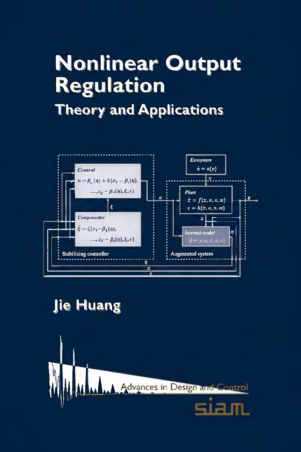
The output regulation problem, or alternatively, the servomechanism problem, addresses
design of a feedback controller to achieve asymptotic tracking for a class of reference inputs
and disturbance rejection for a class of disturbances in an uncertain system while maintaining
closed-loop stability. This is a general mathematical formulation applicable to many control
problems encountered in our daily life, for example, cruise control of automobiles, aircraft
landing and taking-off, manipulation of robot arms, orbiting of satellites, motor speed
regulation, and so forth. Study of the output regulation problem can be traced as far back
as 1769, when James Watt devised a speed regulator for a steam engine. Yet rigorous
formulation of this problem in a modem state-space framework was not available until the
1970s. In contrast to similar problems, such as trajectory tracking, where the trajectory to
be tracked is assumed to be completely known, a distinctive feature of the output regulation
problem is that the reference inputs and disturbances do not have to be known exactly so
long as they are generated by a known, autonomous differential equation. In this book, the
term “exogenous signals” will be used to refer to both reference inputs and disturbances
when there is no need to distinguish them. The autonomous differential equation generating
exogenous signals will be called the exosystem.
The output regulation problem was first studied for the class of linear systems under
various names, such as the robust servomechanism problem (Davison) or the structurally
stable output regulation problem (Francis and Wonham). It was completely solved by
the collective efforts of several researchers, including Davison, Francis, and Wonham, to
name just a few. Solvability conditions for the output regulation problem were worked
out either in terms of the location of the transmission zeros of the system or in terms of the
solvability of a set of Sylvester equations. A salient outcome of this research was the internal
model principle, which includes classical PID (proportional-integral-derivative) control as
a special case. From the control theoretic point of view, the significance of the internal
model principle is that it enables the conversion of the output regulation problem into the
well-known stabilization problem for an augmented linear system.
At almost the same time that research on the linear output regulation problem reached
its peak, in the mid 1970s, Francis and Wonham considered the output regulation problem
for a class of nonlinear systems for the special case when exogenous signals are constant.
They showed that a linear regulator design based on the linearized plant can solve the robust
output regulation problem for a weakly nonlinear plant while maintaining the local stability
of the closed-loop system. In the late 1980s, Huang and Rugh further studied this problem
for general nonlinear systems using a gain scheduling approach and related the solvability
of this problem to solvability of a set of nonlinear algebraic equations.
xiii
xiv
Preface
To establish a general theory for the output regulation problem for uncertain nonlinear
systems subject to time-varying exogenous signals, one must address three important issues:
how to define and guarantee existence of the steady state of the system, and hence charac-
terize the solvability of the problem; how to handle plant uncertainty when it is known that
the linear internal model principle does not work for nonlinear systems in the general case;
and how to achieve asymptotic tracking and disturbance rejection in a nonlinear system with
arbitrarily large initial states of the plant, the exosystem, and the controller, in the presence
of uncertain parameters that lie in an arbitrarily prescribed, bounded set.
None of these three issues can be dealt with by a simple extension of the existing
linear output regulation theory. Because of these challenges, the output regulation problem
for nonlinear systems has become one of the most exciting research areas since the 1990s.
As a result of extensive work, these three issues have now been successfully addressed to a
certain degree.
The difficulty associated with the first issue, existence of steady state, lies in the fact
that the solution of a nonlinear system is not available. Isidori and Byrnes first addressed
this issue for the case when the plant is assumed to be known exactly. By introducing center
manifold theory, Isidori and Byrnes found that it is possible to use a set of mixed nonlinear
partial differential and algebraic equations, called regulator equations in what follows, to
characterize the steady state of the system. This discovery coupled with the zero dynamics
theory of nonlinear systems leads to a solvability condition for the output regulation problem
in terms of solvability of the regulator equations. It turns out that the regulator equations are
a generalization of the Sylvester equations mentioned above. The solution of the regulator
equations provided a feedforward control to cancel the steady-state tracking error. Based
on the solution of the regulator equations, both state feedback and error feedback control
laws can be readily synthesized to achieve asymptotic tracking and disturbance rejection
for an exactly known plant while maintaining local stability of the closed-loop system.
The second issue is concerned with the plant uncertainty characterized by a set of
unknown parameters. The feedforward control approach mentioned in the last paragraph
cannot handle this case due to the presence of the unknown parameters. A design approach
based on the linear internal model principle does not work either, as shown by a counterex-
ample due to Isidori and Byrnes. Huang first revealed in 1991 that the linear internal model
principle failed because, unlike the linear case, the steady-state tracking error in a nonlinear
system is a nonlinear function of the exogenous signals. Based on this observation, Huang
found that if the solution of the regulator equations is a polynomial in the exogenous signals,
then it is possible to solve the output regulation problem for uncertain nonlinear systems
by both state feedback and output feedback control. This approach effectively leads to a
nonlinear version of the internal model principle. The robust output regulation problem
was further pursued by Byrnes and Isidori, Delli Priscoli, and Khalil, generating various
techniques and insights on this important issue.
While the first two issues have been intensively addressed since the 1990s, the investi-
gation of the third issue, the output regulation problem with global stability, has just started
and is rapidly unfolding. In the original formulation of the output regulation problem, as
given by Isidori and Byrnes, only local stability is required for the closed-loop system.
For this case, the stability issue can be easily handled by Lyapunov’s linearization method.
When a global stability requirement is imposed on the closed-loop system, the situation
becomes much more complicated. Khalil studied the semiglobal robust output regulation
Preface
xv
problem for the class of feedback linearizable systems in 1994. His work was further ex-
tended to the class of lower triangular systems by Isidori in 1997. The output regulation
problem with global stability was solved for the class of output strict feedback systems by
Serrani and Isidori in 2000. Up to this point, the problem of output regulation with nonlocal
stability was handled on a case-by-case basis, and only limited results were obtained. Re-
cently, Huang and Chen have established a new framework that converts the robust output
regulation problem for nonlinear systems into a robust stabilization problem. This new
framework has offered greater flexibility to incorporate recent stabilization techniques, thus
having set a stage for systematically tackling robust output regulation with global stability.
This new framework has been successfully applied to solve the output regulation problem
with global stability for several important classes of nonlinear systems.
The scope of research on the output regulation problem is constantly expanding,
and the topic is made richer and more interesting with the injections of new ideas and
techniques from other research areas such as stabilization, adaptive control, neural networks,
and numerical mathematics. For example, the output regulation problem with uncertain
exosystems was studied recently by Chen and Huang, Nikiforov, Serrani, Marconi and
Isidori, and Ye and Huang, respectively. This scenario had not been studied previously,
even for linear systems.
The output regulation problem arises from formulating daily engineering control prob-
lems. Therefore, in addition to the theoretical issues mentioned above, the application of
this theory to practical design should be adequately addressed. A key issue critical to the
applicability of the output regulation theory is the solvability of the regulator equations.
Being a set of mixed nonlinear partial differential and algebraic equations, the solution of
the regulator equations is usually unavailable. Thus it is necessary to develop approximation
approaches to solving these equations. An approximation method based on Taylor series
expansion was developed by Huang and Rugh in 1991 and was also considered by Krener in
1992. The effectiveness of these approximation methods has been demonstrated by many
case studies, including benchmark nonlinear systems such as the ball and beam, the inverted
pendulum on a cart, and the rotational/translational actuator.
This book will give a comprehensive and up-to-date treatment of the output regulation
problem in a self-contained fashion. The book begins with an introduction to the linear
output regulation theory in Chapter 1. Then a review of fundamental nonlinear control
theory is given in Chapter 2. Chapters 3 and 4 are devoted to the output regulation problem
and the approximate output regulation problem for continuous-time nonlinear systems,
respectively. The robust output regulation problem for uncertain continuous-time nonlinear
systems is presented in Chapters 5 and 6. In Chapter 7, the global robust output regulation is
formulated and studied for uncertain continuous-time nonlinear systems. Chapter 8 presents
both the output regulation problem and the robust output regulation problem for singular
nonlinear systems. Finally, in Chapter 9, results on the output regulation problem and the
robust output regulation problem are extended to discrete-time nonlinear systems. The
author seeks to strike a balance between the theoretical foundations of the output regulation
problem and practical applications of the theory. The treatment is accompanied by many
examples, including practical case studies with numerical simulations based on the software
platform MATLAB®.
This book can be used as a reference for graduate students, scientists, and engineers in
the area of systems and control. Readers are assumed to have some fundamental knowledge
xvi	Preface
of linear algebra, advanced calculus, and linear systems. Knowledge needed of nonlinear
systems is summarized in Chapter 2. Some of the present chapters were used in the work-
shops of the 1999 IEEE Conference on Decision and Control, the 2004 World Congress
on Intelligent Control and Automation, and graduate seminars at the Chinese University of
Hong Kong.
The development of this book would not have been possible without the support and
help of many people, including the author’s master’s thesis supervisor, Professor Xiangqiu
Zeng; Ph.D. supervisor, Professor Wilson J. Rugh; and numerous colleagues and students.
Professor Rugh not only guided the author into the area of nonlinear control, but also
personally made substantial contributions to many results covered in Chapters 3 and 4.
Some sections from Chapters 6-9 are adapted from joint publications of the author and
some of his past and current students, including Zhiyong Chen, Guoqiang Hu, Weiyao Lan,
Dan Wang, and Jin Wang. Three current students, Zhiyong Chen, Guoqiang Hu, and Weiyao
Lan, have painstakingly proofread the manuscript several times and checked many examples
with computer simulations. Professors Zhong-Ping Jiang, Zongli Lin, and Wilson J. Rugh
have provided the author with valuable comments and suggestions. Professor Frank Lewis
not only inspired and encouraged the author to embark on this project, but also introduced
him to the SIAM acquisitions editor, Dr. Linda Thiel, who has been extremely helpful and
enthusiastic. The SIAM Developmental Editor Simon Dickey and Production Editor Lisa
Briggeman have done excellent work. The author is greatly indebted to Professor Alberto
Isidori, whose seminal work on the output regulation problem with his coauthors has laid
the foundation for this book.
The bulk of this research was supported by the Hong Kong Research Grants Council
under grants CUHK 4316 /02Е and CUHK 4168 /03Е, and by National Natural Science
Foundations of China under grant 60374038.
Jie Huang
Chapter 1
Linear Output
T Regulation
In this chapter, a concise but self-contained treatment of the subject of the output regulation
problem for linear time-invariant systems is given. The output regulation problem was one of
the central research topics in linear control theory in the 1970s. This research has generated
a salient controller synthesis technique known as the Internal Model Principle. The puipose
of this chapter is mainly to provide the background for understanding the nonlinear output
regulation problem, and the chapter is organized as follows. In Section 1.1, a typical scenario
that leads to the formulation of the problem is described. In Section 1.2, the precise definition
of the output regulation problem is given and the solvability of the problem via both state
feedback control and measurement output feedback control is presented. In Section 1.3, we
further take into account model uncertainties, which leads to the formulation of the robust
output regulation problem. We give the solution of this problem by both state feedback
and error output feedback control. The robust output regulation problem is an enhanced
version of the output regulation problem in the sense that it achieves the same objectives as
the former even in the presence of model uncertainties. In Section 1.4, the solvability of the
linear robust output regulation problem is further examined by introducing what is called
the internal model principle. While the first four sections are devoted to continuous-time
linear systems, results on the output regulation problem and on the robust output regulation
problem for discrete-time linear systems are established in Sections 1.5 and 1.6.
1.1 Introduction
Many practical control problems such as trajectory planning of a robot manipulator, guidance
of a tactic missile toward a moving taiget, attitude control of spacecraft subject to torque
disturbance, weapon system pointing under firing disturbances, and so on, fall into the
domain of the problem depicted in Figure 1.1. Here a plant is given that is subject to
a disturbance d(t), and a controller is to be designed so that the closed-loop system is
exponentially stable, in the sense to be defined precisely later, and the output of the plant
у (r) asymptotically tracks a given reference input r (/) in the following sense:
lim e(t) = lim (y(t) — r(r)) = 0.	(1.1)
1
2
Chapter 1. Linear Output Regulation
Figure 1.1. Unity feedback control.
This problem is conveniently called asymptotic tracking and disturbance rejection of the
output. In the particular case where r(t) = 0, the problem is simply called asymptotic
regulation.
A linear plant subject to a disturbance d(t) can be modelled as follows:
x = Ax + Bu + Edd,
у — Cx + Du + Fdd.	(1.2)
Thus the tracking error is given by
e = Cx + Du + Fdd — r.	(1.3)
The controller can generally be modelled as follows:
и = Kz,
z = Giz + (he-	(1-4)
This controller must guarantee the stability of the closed-loop system composed of (1.2)
and (1.4) while assuring asymptotic tracking of y(t) to r(t) in the presence of the distur-
bance d(t).
In practice, the reference input to be tracked and the disturbance to be rejected usually
are not exactly known signals; for example, a disturbance in the form of a sinusoidal function
can have any amplitudes and initial phases, or even any frequencies, and a reference input
in the form of a step function can have arbitrary magnitudes. It is desirable that a single
controller be able to handle a class of prescribed reference inputs and/or a class of prescribed
disturbances. In this chapter, both the reference inputs and the disturbances are assumed to
be generated by linear autonomous differential equations as follows:
f — Alrr, r(0) = r0, d = Aud, d(0) = do,
where ro and do are arbitrary initial states. The above autonomous equations can generate
a large class of functions; for example, a combination of step functions of arbitrary magni-
tudes, ramp functions of arbitrary slopes, and sinusoidal functions of arbitrary amplitudes
and initial phases.
1.2. Linear Output Regulation
3
Let
r
d
v —
Alr 0
0 Aid
Then the reference inputs and the disturbances can be lumped together as follows:
v = AjV,
v(0) =
G-5)
Thus, the plant state and the tracking error can be put into the following form:
x = Ax + Bu + Ev,
e = Cx + Du + Fv,
(1.6)
where
E I _ Г 0 Ed
f J “ L -1 ъ
Now the problem of asymptotic tracking of y(t) to r(t) can be treated as the problem
of asymptotic regulation of e(t) to the origin when e(t) is viewed as the output of (1.6).
Therefore, it suffices to study the regulation problem described by (1.6) while keeping in
mind that the system (1.5), called the exosystem in what follows, can generate either the
reference inputs or the disturbances or both. Thus, the problem of asymptotic tracking
and disturbance rejection can be called simply the output regulation problem when the
disturbances and the reference inputs are generated by (1.5). Alternatively, the output
regulation problem is called a servomechanism problem.
In (1.6), the plant is defined by six finite-dimensional constant matrices А, В, E, C,
D, and F. These matrices are usually obtained by linearizing a nonlinear system around
an operating condition or by using a certain system identification approach. Due to the
variations in the operating point or the limitations of system identification techniques, these
matrices are invariably inaccurate. Typically, each entry of the matrices А, В, E, C, D, and
F can take arbitrary values in an open neighborhood of its nominal value. Therefore, it is
desirable to further require that the controller be able to maintain the property of asymptotic
tracking and disturbance rejection in the closed-loop system regardless of small variations of
the entries in the matrices А, В, E, C, D, and F. The problem of designing such controllers
is called the robust output regulation problem or the robust servomechanism problem.
The discussion so far has exemplified a scenario of what is called the output regulation
problem and its enhanced version the robust output regulation problem. The solvability of
these two problems will be established in the remaining sections of this chapter.
1.2 Linear Output Regulation
Consider a class of linear time-invariant systems described by
x(t) = Ax(t) + Bu(t) + Ev(t), x(Q) = xq, t > 0,
e(t) = Cx(t) -f- Du(t) + Fv(t),
(1.7)
4
Chapter 1. Linear Output Regulation
where x(t) is the я-dimensional plant state, u(t) the m-dimensional plant input, e(t) the
p-dimensional plant output representing the tracking error, and v(t) the «/-dimensional
exogenous signal representing the reference inputs and/or the disturbances. The exogenous
signal is generated by an exosystem of the form
i>(t) = Aiv(t), v(0) = vo, t > 0.	(1.8)
For convenience, we put the plant (1.7) and the exosystem (1.8) together into the
following form:
x = Ax + Bu + Ev,
v = Aiv,
e = Cx + Du + Fv	(1.9)
and call (1.9) a composite system with col(x, v) as the composite state.
Two classes of feedback control laws will be considered in this section, namely,
1. Static State Feedback:
и = Kxx + Kvv,	(1.10)
where Kx € 1lmxn and Kv € 'R,mxq are constant matrices.
2. Dynamic Measurement Output Feedback:
u = Kz, i = Qiz + Qiym,	(1.11)
where z € TZ"z with nz to be specified later, ym e TZPm for some positive integer pm
is the measurement output, and К e 7£тхЯг, e 7£"гХЛг, & e 7£"zXp'n are constant
matrices. It is assumed that ym takes the following form:
ym(t) = Cmx{t) + Dmu(t) + Fmv(t),	(1.12)
where Cm e TZPm x", Dm e 1ZPmXm, and Fm e 7Zp,nX9. A special case of the dynamic
measurement output feedback control is the dynamic error output feedback control
when Cm = C, Dm — D, Fm — F, that is, ym = e. In many cases, the error
output e is not the only measurable variable available for feedback control. Using
the measurement output feedback control allows us to solve the output regulation
problem for some systems that cannot be solved by the error output feedback control.
Denote the closed-loop system consisting of the plant (1.7), the exosystem (1.8), and
the control law (1.10) or (1.11) as follows:
xc = Acxc + Bcv, xc(0) — Xco,
v = Aiv,	(1-13)
e = Ccxc + Dcv,
where, under the static state feedback, xc = x and
Ac = A -|- BKX, Вс — E -|-
Cc = C + DKx, DC = F + DKU,	(1.14)
1.2. Linear Output Regulation
5
and, under the dynamic measurement output feedback, xc = col(x, z) and
A _ Г A BK	I B _ Г E I
c ~ 6iCm Q\.+QiDmK J ’ Oc~\_QiFm \ '
Cc = \C DK}, DC = F.	(1.15)
To describe the requirements on the closed-loop system (1.13), we first introduce the
following definition.
Definition 1.1. The closed-loop system (1.13) is said to be exponentially stable if we have
the following.
Property 1.1. The matrix Ac is Hurwitz, that is, all the eigenvalues of Ac have negative real
parts.
The closed-loop system is said to have output regulation property if the following holds.
Property 1.2. For all xM and vo, the trajectories of (1.13) satisfy
lim e(t) = lim (Ccxc(t) + Dcv(t)) - 0.
1->OO	Г->00
Linear Output Regulation Problem (LORP): Design a control law of the form (1.10) or
(1.11) such that the closed-loop system satisfies Properties 1.1 and 1.2.
Remark 1.2. In what follows, a control law that solves the linear output regulation problem
will be called a servoregulator. In particular, if the control law is described by (1.10) or
(1.11), then the controller will be called a static state feedback servoregulator or dynamic
measurement output feedback servoregulator, respectively. I
At the outset, we list various assumptions needed for solving the linear output regu-
lation problem.
Assumption 1.1. Ai has no eigenvalues with negative real parts.
Assumption 1.2. The pair (A, B) is stabilizable.
Assumption 13. The pair
L'-'/n	* ml i
A E \
0 Ai )
is detectable.
Remark 13. Assumption 1.1 is made only for convenience and loses no generality. In fact,
if the linear output regulation problem is solvable by any controller under Assumption 1.1,
then it is also solvable by the same controller even if Assumption 1.1 is violated. This is
because Property 1.1 is simply a property of the plant data (А, В, C, D) and has nothing
6
Chapter 1. Linear Output Regulation
to do with the exosystem, and because Property 1.2 is only concerned with the asymptotic
property of the closed-loop system. More specifically, the components of the exogenous
signals corresponding to the modes associated with the eigenvalues of Ai with negative real
parts will exponentially decay to zero and will in no way affect the asymptotic behavior of
the closed-loop system so long as the closed-loop system has Property 1.1. Assumption 1.2
is made so that Property 1.1, that is, the exponential stability of Ac, can be achieved by
a state feedback. Assumption 1.3, together with Assumption 1.2, renders the exponential
stability of Ac by the measurement output feedback. I
Lemma 1.4. Under Assumption 1.1, consider the controller (1.10) or (1.11). Assume the
closed-loop system (1.13) has Property 1.1. Then the following statements are equivalent:
(i)	The closed-loop system has Property 1.2.
(ii)	The controller solves the linear output regulation problem.
(iii)	There exists a unique matrix Xc that satisfies the following matrix equations:
XCA\ = ACXC + Bc,
0 = CcXc + Dc.	(1.16)
Proof, (i) ** (ii). This is self-evident.
(ii)	** (iii). The first equation of (1.16) is a Sylvester equation, which has a unique
solution Xc if Ai and Ac have no common eigenvalues (Appendix A). Since the closed-
loop system satisfies Property 1.1, Ac is exponentially stable. Thus Assumption 1.1 and
the exponential stability of Ac guarantee the existence of Xc, satisfying the first equation of
(1.16). Let* = xc — Xcv. Then,
x — Acx,
e = Ccx + (CcXc + Dc)v.
Since Ac is exponentially stable, lim^oo x(t) = 0. To show (ii) <- (iii), assume the matrix
Xc also satisfies the second equation of (1.16); then
lim e(t) = lim Ccx(f) = 0;
r—>oo	r—>oo
that is, the controller solves the linear output regulation problem. On the other hand, to
show (ii) -> (iii), assume the controller solves the linear output regulation problem; then,
lim (CcXc + Dc)v(t) = 0
f—>oo
for all v(t) = eA,tv(ff) with any v(0) e 1Zq. Due to Assumption 1.1, v(t) does not decay to
zero for v(0) / 0. Therefore, necessarily, CcXc + Dc = 0.	□
Remark 1.5.
(i)	Lemma 1.4 gives a characterization of Property 1.2 in terms of the solvability of a set
of linear matrix equations. This characterization allows the linear output regulation
problem to be studied using the familiar mathematic tool of linear algebra. Further, it
will be seen later that this lemma will render a natural translation of the requirements
1.2. Linear Output Regulation
7
on the closed-loop system into the requirements on the controller, thus leading to the
synthesis of the various controllers.
(ii)	It is seen from the proof of Lemma 1.4 that if the output regulation problem is solvable,
then there exists a subspace in 7Jn+n*+«' defined by the hyperplane Ccxc 4- Dcv = 0
such that the trajectories xc(t) of the closed-loop system will approach this subspace
asymptotically. I
Now let us first consider the static state feedback case where the controller is defined
by two constant matrices Kx and Kv such that the closed-loop system is described by
x = (A -|-BKx)^ 4- (£ -I-
v — AiV,
e = (C + DKx)x + (F + DKu)v.	(1.17)
That is,
Ac — Д -|- BKX, Bc = E 4-
Cc = C + DKX, Dc = F + DKV.
The two matrices Kx and Kv will be called the feedback gain and the feedforward gain,
respectively. The basic idea of designing the static state feedback controller is to use
the feedback gain to make the closed-loop system satisfy Property 1.1 while using the
feedforward gain to drive trajectories of the closed-loop system toward a subspace of Цп+ч
defined by the hyperplane (C + DKx)x + (f + DKv)v = 0. This idea is best illustrated
by the following result.
Lemma 1.6. Under Assumptions 1.1 and 1.2, let Kx render the exponential stability of
(A + BKX). Then the linear output regulation problem is solvable by a static state feedback
controller (1.10) if and only if there exist two constant matrices Xc and Kv that satisfy the
following matrix equations:
XcAi = (A + BKx)Xc + BKV + E,
0=(C + DKx)Xc + DKv + F.	(1.18)
Proof. Under Assumption 1.2, there exists Kx such that (A 4- BKX) is exponentially stable.
Since equation (1.16) is exactly the same as equation (1.18) except that in (1.18) Kv is to
be determined, if Xc and Kv satisfy (1.18), Xc also satisfies (1.16) for the two particular
matrices Kx and Kv. On the other hand, if for some Kx and Kv, Xc satisfies (1.16), then Xc
and Kv also satisfy (1.18). The proof thus follows from Lemma 1.4.	0
Lemma 1.6 immediately suggests the following way of synthesizing the desired static
state feedback controller.
Step 1. Find a feedback gain Kx such that (A 4- BKX) is stable.
Step 2. Solve for both Xc and Kv from the set of linear equations (1.18). Then the static
state feedback controller is given by
и — Kxx 4- Kvv.
(1.19)
8
Chapter 1. Linear Output Regulation
This approach, though straightforward to apply, has a drawback in that Xc and Kv
depend on the feedback gain Kx. Thus, every time, a redesign of the feedback gain neces-
sitates a recomputation of Xc and Kv. A better approach can be obtained by making the
following linear transformation:
X
и
In ^nxm
Xc
Kv
(1.20)
Kx Im
in equation (1.18), which leads to another set of linear matrix equations in unknown matrices
X and U as follows:
XAj = AX + BU + E,
0 = CX + DU + F.
(1-21)
These equations are completely determined by the plant data А, В, E, C, D, F, and Ai. It
is clear that there exist X and U satisfying (1.21) if and only if, for any Kx e 1Zmxn, there
exist Xc and Kv satisfying (1.18). Moreover, (X, U) and (Xc, Xu) are related to each other
by equation (1.20).
Equations (1.21), known as the regulator equations, are instrumental to establishing
the linear output regulation theory. In fact, in terms of the regulator equations, the above
discussion can be summarized to yield the following result.
Theorem 1.7. Under Assumptions 1.1 and 1.2, let the feedback gain Kx be such that
(A + BKX) is exponentially stable. Then, the linear output regulation problem is solvable
by a static state feedback control of the form
и = Kxx + Kvv
if and only if there exist two matrices X and U that satisfy the linear matrix equations (1.21),
with the feedforward gain Kv being given by
K„ = U - KxX.
Remark 1.8. A systemic interpretation to the solution of (1.21) is given as follows. First
consider the special case where the exogenous signal is constant. Since Ai = 0, equations
(1.18) and (1.21) become
0 = (A + BKx)Xc + BKV + E,
0 = (C + DKx)Xc + DKV + F,	(1.22)
and, respectively,
0 = AX + BU + E,
Q)=CX + DU + F.	(1.23)
Equations (1.22) mean, for each constant v, that Xcv is an equilibrium point of the closed-
loop system at which the output is zero. Moreover,
lim xc(t) = Xcv.
t—>oo
1.2. Linear Output Regulation
9
Thus, for each constant v, Xcv is the steady-state state of the closed-loop system at which
the output is zero. On the other hand, equations (1.23) mean, for each constant v, that U v is
the input under which the open-loop plant has an equilibrium state Xu at which the output
is zero. Moreover, since Xc = X, and
lim u(t) = (KxX + Ku)v = Uv,
for each constant v, whether or not the closed-loop system can be made to satisfy the
output regulation property depends on the solvability of the regulator equations. The above
interpretation can be extended to the general case. Under any controller that solves the
linear output regulation problem, the trajectories of the closed-loop system from any initial
state xc(0) and v(0) satisfy
lim (xc(r) - Xcv(t)) = lim (xc(r) - Xv(r)) = 0.
r->oo	f-юо
Correspondingly, the control input satisfies
lim (u(r) - (KxX + Kv)v(t)) = lim (u(t) - Uv(t)) = 0.
t-ЮО	r->00
Thus, if the linear output regulation problem is solvable at all, necessarily, all trajectories
of the closed-loop system approach Xv(t), and the corresponding controls approach U v(t).
Thus, the steady-state behavior of the closed-loop system is completely characterized by
the solution of the regulator equations. For convenience, in what follows, Xv(t) and U v(t)
are called zero-error constrained state and zero-error constrained control, respectively. In
particular, when v is constant, Xu is called zero-error constrained equilibrium. I
An easily testable condition can be given with regard to the solvability of the regulator
equations as shown below.
Theorem 1.9. For any matrices E and F, the regulator equations (1.21) are solvable if and
only if the following holds:
Assumption 1.4. For all X e <r(Ai), where <t(Aj) denotes the spectrum of Ab
rank
A —XI
C
В
D ]=« + P-
(1.24)
Proof. The regulator equations (1.21) can be put into the following form:
(1.25)
Using the properties of the Kronecker product, which can be found in Appendix A, we can
transform (1.25) into a standard linear algebraic equation of the form
Qx = b,
10
Chapter 1. Linear Output Regulation
where
In
Hpxn
Onxm j AB
0	® C D
Vpxm J	[_ V
2 = AtT®
Here the notation vec( ) denotes a vector-valued function of a matrix such that, for any
X e 7£"xm,

vec (X) •
where for i = 1,.... m, X,- is the ith column of X. Thus, equation (1.25) is solvable for any
matrices E and F if and only if Q has full row rank. To obtain the condition under which Q
has full row rank, we assume, without loss of generality, that A i is in the following Jordan
form:
Ji	0	0 •  •	0
0	J2	0 •  •	0
0 0 0 • • • Jk
where J, has dimension n, such that и i + n2 4-1- nk — q and is given by
X,-	1	0	 • •	0	0
0	X,-	1	• • •	0	0
0	0	0	 • •	X, 1
0	0	0 •• •	OX,
A simple calculation shows that Q is a block lower triangular matrix of к blocks with its
ith, 1 < i < k, diagonal block having the form
’ X,£ - A	0	0	  	0	0
£ 1-iE-A 0	•••	0	0
0	0	0	••• XtE-A	0
0	0	0	 • •	E UE-A
where
A В '
C D ‘
0л xm
Opxm
In
£ =
Clearly, Q has full row rank if and only if Assumption 1.4 holds. □
1.2. Linear Output Regulation
11
In conjunction with Theorem 1.7, Theorem 1.9 immediately leads to the following
sufficient conditions for the solvability of the output regulation problem by the static state
feedback control of the form (1.10).
Corollary 1.10. Under Assumptions 1.1,1.2, and 1.4, the linear output regulation problem
is solvable by the static state feedback control (1.10).
Remark 1.11. If the pair (A, B) is controllable and the pair (C, A) is observable, then those
values of A at which the matrix
A — AJ В ‘
C D
is not full rank are called the transmission zeros of the system. It is a generalization of
the notion of zeros of the single-input, single-output systems to multi-input, multi-output
systems. Thus Assumption 1.4 can be paraphrased by saying that the transmission zeros of
the plant (1.7) do not coincide with the eigenvalues of the exosystem, and it is often simply
called the transmission zeros condition. The plant (1.7) is called a minimum phase system
if all of its transmission zeros are on the open left-half complex plane. Thus a minimum
phase system always satisfies the transmission zeros condition. I
Remark 1.12. A systemic interpretation of Assumption 1.4 can also be given in the same
spirit as Remark 1.8. First consider the special case where Ai = 0. For this case, equation
(1.24) actually takes the form
= n+p	(1.26)
A
C
В
D
rank
as Ai = 0. Correspondingly, the regulator equations are given by (1.23). Thus, (1.26) is
both necessary and sufficient for the plant to have a pair of zero-error constrained equilibrium
and input for any E and F. A similar interpretation can be given to the case where Ai / 0.
For every A e o(Ai), let ц» be the eigenvector of Ai associated with A. Then the solution
of the exosystem starting from u(0) = ц» is v(t) = У^е1'. Thus, if the closed-loop system
has Properties 1.1 and 1.2, there exist x^ e Tln and Uoo e 1Zm such that
lim (xc(t) — xxe)J) -- 0,
f->OO
lim (w(t) — Uoo^') = 0.
(-♦OO
Therefore, x^ and must satisfy the following equations:
х00Аел' — Axxekl + Buooek' + Ev^,
0 = Cx^e1' + DUooe^' + Fv^e^,
or, equivalently,
A — A./	В	Xqo
C	D	Uoo
(1-27)
12
Chapter 1. Linear Output Regulation
Clearly, equation (1.27) has a solution хх and ux for any E and F if and only if Assump-
tion 1.4 holds. It should be noted that, for a particular pair of (E, F), the regulator equations
may still have a solution even if Assumption 1.4 fails. This happens when
E
F
vec
e Im(2).
(1.28)
However, this case is not interesting since even arbitrarily small variations in (А, В, E,
C,D,F) may fail (1.28). I
When the state x and the exogenous signal v are not available for feedback but
Assumption 1.3 holds, the measurement output feedback control of the form (1.11) can
be used to solve the linear output regulation problem. In this case,
Ac
Be
A
SlCm
E
QiFm
BK
Si + SiDmK
, Cc = [C DK], DC = F.
(1-29)
Due to Lemma 1.4, we need to find atriple (K, Si, S2) such that Ac is exponentially
stable and (1.16) is solvable for Xc. To this end, we first translate the requirements on the
closed-loop system as given by (1.16) into the requirements on the controller (K, Si, S2) as
given by the following result.
Lemma 1.13. Under Assumption 1.1, suppose there exists a dynamic measurement output
feedback controller (K,Si,Si) such that the closed-loop system has Property 1.1. Then the
following are equivalent:
(i)	The linear output regulation problem is solvable by the measurement output feedback
controller (К, Si, Si).
(ii)	There exists a matrix Xc that satisfies the following matrix equations:
SiCm Si + SiDmK Xc+ GiFm
0=[C DK]XC + F.
(1.30)
(iii)	There exist matrices (X, U, Z) such that X and U are the solution of the regulator
equations
XAi = AX + BU + E,
0=CX + DU + F,	(1.31)
and Z is the solution of the Sylvester equation
ZAi = 61Z + S2(CmX + DmU + Fm),	(1.32)
which satisfies
U = KZ.
(1.33)
1.2. Linear Output Regulation
13
Proof, (i) о (ii). This is actually Lemma 1.4 specialized to the measurement output
feedback case.
(ii) (iii). Assume (ii) holds. Partition Xc as
X

Z
where X e1Znxg and Z e TlnzXq. Then (1.30) is the same as
XAj = AX + BKZ + E,
zAi = g2cmx + (& + GzDmK)z + g2Fm,
0=CX + DKZ + F,	(1.34)
which is the same as
XAt = AX + BKZ + E,
ZA\ = gYZ + g2(CmX + DmKZ + Fm),
O = cx + DKZ + F.	(1.35)
Letting U ~ KZ in (1.35) shows that X and U satisfy the regulator equations (1.31), and U
andZ satisfy (1.32) and (1.33). This completes (ii) -» (iii). On the other hand, assume (iii)
holds. We will show that X and Z satisfy (1.34) or equivalently (1.35). Indeed, substituting
U = KZ into equation (1.31) shows that X and Z satisfy the first and third equations of
(1.35), and substituting U = KZ into (1.32) shows that Z satisfies the second equation of
(1.35).	□
Now we turn to the construction of the triple (K, gt, g2). Since we have already
known how to synthesize a static state feedback controller which takes the plant state x and
the exosystem state v as its inputs, we naturally seek to synthesize a measurement output
feedback controller by estimating the state x and the exogenous signal v. To this end, lump
the state x and exogenous signals v together to obtain the following system:
Ут — [Cm ISnl
+ Dmu.
(1.36)
Employing the well-known Luenburger observer theory suggests the following observer:
n = [Xx Kv]z,
where L is an observer gain matrix of dimension (n + q) by pm.
14
Chapter 1. Linear Output Regulation
Clearly, (1.37) can be put into the form
и = Kz, z-QiZ + Q2ym
with
Theorem 1.14. Under Assumptions 1.1, 1.2, and 1.3, the linear output regulation problem
is solvable by a measurement outputfeedback controller (Kx, КV,L) given by (1.37) (equiv-
alently, (K,Qi, Qf) given by (1.38)) if and only if there exists a pair of matrices (X, U) that
satisfies the regulator equations
XAi = AX + BU + E,
Q — CX + DU + F.
(139)
Proof. The “only if’ part is a consequence of part (iii) of Lemma 1.13. To show the “if’
part, first note that, by Assumption 1.2, there exists a state feedback gain Kx such that
(A + BKX) is exponentially stable, and, by Assumption 1.3, there exist matrices Lj and L2
such that
0 A,
1_ A L\Cm E E\Fm
Li icm rm\- _L^Cm Al_L2Fm
is exponentially stable. Now let (X, U) satisfy the regulator equations, and let Kv =
U -KxX,K = [X\, A7V], and
L2
A simple calculation gives
A BK
Q2cm Gi + g2DmK
A	BKX	BK„
0 A + BKX E + BKV
0	0 A,
0
Ll
l2
[ cm -Cm —Fm ]. (1.40)
In (1.40), subtracting the first row from the second row and adding the second column to
the first column shows that Ac is equivalent to the following matrix
’ A + BKX 0 0		BKX A 0	BKV ' E Ai	+	0 Li l2	[ 0 -Cm		—F„ * m
	 A + BKX		BK		bk„			
=		0	A — L	cm	E —	LlFm		
		0	-L2C	7m	Ai-	L2Fm		
A E
L
(1.41)
1.3. Linear Robust Output Regulation
15
Thus <t(Ac) = <r(A + BKX) U a(AL)\ that is, we have shown that the triple (Kx, K„, L)
(equivalently, (K, Qi, Q2)) renders the closed-loop system Property 1.1. To show that the
closed-loop system also satisfies Property 1.2, let
(1.42)
We will show that the triple (X, U, Z) satisfies the conditions of part (iii) of Lemma 1.13.
Since the pair (X, U) satisfies the regulator equations by assumption, it suffices to show that
ZA^GrZ + QitC.nX + D^ + F^.	(1.43)
Indeed, using the definition of Gi given by (1.38) yields
6iZ =
(A + BKx)X + E + BKV
Ai
AX + B(KxX + Kv) + E
A,
- L((Cm + DmKx)X +Fm + DmKv)
- L(CmX + Dm(KxX + Kv) + Fm).
(1-44)
Using U — KxX + Kv in (1.44) gives
Q\Z =
AX + BU + E
Ai
- L(CmX + DmU + Fm)
Z =
X
I
Ai - L(CmX + DmU + Fm)
ZAr - L(CmX + DmU + Fm)
upon noting that X and U satisfy the regulator equations. The proof is completed by the
equivalence of (i) and (iii) of Lemma 1.13.	0
By Theorem 1.9, the solvability of the regulator equations is guaranteed by the satis-
faction of the Assumption 1.4. Thus we have the following corollary.
Corollary 1.15. Under Assumptions 1.1 to 1.4, the linear output regulation problem is solv-
able by a measurement output feedback controller (Kx, К v, L) given by (1.37) (equivalently,
(K,Gi, G2) given by (1.38)).
1.3 Linear Robust Output Regulation
In this section, we will further consider the linear robust output regulation problem in which
a controller has to be able to tolerate certain plant uncertainty. When the plant uncertainty
is taken into consideration, the class of linear time-invariant systems is described by
x(t) = (A + AA)x(t) + (B + &B)u(t) + (E + AE)v(t), x(0) - xq, t > 0,
e(t) = (C + AC)x(t) + (D + AD)u(f) + (F + AF) v(t),	(1.45)
16
Chapter 1. Linear Output Regulation
where x(t), u(t), and e(t) are the same as what are described in Section 1.2, and v(r) is
again generated by the same exosystem (1.8).
In (1.45), the matrices А, В, E, C, D and F represent the nominal part of the plant
while AA, AB, and so forth represent the uncertain part. The entries of (AA, AB, AE,
AC, AD, AF) are allowed to take arbitrary values.
It is convenient to identify the system uncertainties with a vector w in the Euclidean
space 7£''“ with w = vec	and nw = (n + p) x (n + m + q). Thus, we can
adopt the following convenient notation:
Aw =	A + AA, Bw — В + AB,	Ew — E	-f- AE,
Cw —	C	AC,	Dw — D + AD,	Fw —	F + AE
with
Aq =	A, Bq = B, Eq	= E,
Co =	C, Do = D, Fq	= F.
As a result, (1.45) can be written as follows:
x — A^x “I- ByjU “I- EujVf
e = Cwx + Dwu + Fwv.	(1.46)
For convenience of reference, the plant (1.46) and the exosystem (1.8) can be put together
into the following:
x = Awx + Bwu + Ewv,
ii — Aiv,
e = Cwx + Dwu + Fwv,	(1.47)
and (1.47) will be called the composite system.
We consider two classes of feedback control laws which are somehow different from
those considered in the last section.
3. Dynamic State Feedback:
u = K\x + K2Z,
Z — Giz + Gie,	(1.48)
where z e U"‘ with nz to be specified later, and (E\, K2, Gi, G2) are constant matrices
of appropriate dimensions.
4. Dynamic Output Feedback:
и = Kz,
Z^GiZ + Gie,	(1.49)
where, again, z e 7£"z with nz to be specified later, and (E, Gi, G2) are constant
matrices of appropriate dimensions.
1.3. Linear Robust Output Regulation
17
Remark 1.16. Due to the presence of the uncertain parameter w, the robust output regulation
problem that will be formulated shortly cannot be handled via the approach for solving the
output regulation problem described in Section 1.2. It will be handled by a celebrated
design methodology called the internal model principle. As a result, there exist no static
state feedback control laws that can solve the robust output regulation problem, as will be
shown in Lemma 1.21. On the other hand, as pointed out before, the measurement output
feedback control is more general than the error output feedback case. However, in order
to better illustrate the mechanism of the internal model principle, we will focus on the
error feedback case when it comes to the robust output regulation problem. Remark 1.29
will give a clue on how to synthesize a measurement output feedback controller under some
additional condition. To save the notation, we use the same notation z, Qi, and Qi to describe
the dynamic compensator in various controllers (1.11), (1.48), and (1.49). However, the
dimension of z and the specific structure of the matrices Qi and Qi are totally different
among these three different controllers. I
Denote the closed-loop system consisting of the plant (1.46), the exosystem (1.8), and
the control law (1.48) or (1.49) as follows:
xc -— Aculxc + Bcu,v,
v = Ajv,
e —	+ DCifjV,
(1.50)
where, under the dynamic state feedback, xc = col(x, z) and
Аш 4- BWK\ BWK2 & ____________ Ew
Gi(Cw + DM Si + G2DwK2 J ’ cw " L
Ccw — [Сш + DwKi DwKi],
Dew —
(1-51)
and under the dynamic output feedback, xc = col(x, z) and
Agw —
Au, BWK
GiCu, Qi + QiDwK
Ccw — [Сш DWK],
T^CW -- Pw
(1.52)
Correspondingly, we use (AM, Bcq, C,#, D^) or simply (Ac, Bc, Cc, Dc) to denote the
closed-loop system composed of the nominal plant and the control laws.
To describe the requirements on the closed-loop system (1.50), we first introduce the
following definition.
Definition 1.17. The closed-loop system (1.50) is said to be exponentially stable at w = 0
if the following property holds:
Property 13. The matrix Aco is Hurwitz, that is, all the eigenvalues of A^j have negative
real parts.
18
Chapter 1. Linear Output Regulation
The closed-loop system is said to have robust output regulation property at w = 0 if the
following holds:
Property 1.4. There exists an open neighborhood W of w = 0 such that, for all x^ and vq
and for all w e W, the trajectories of (1.50) satisfy
lim e(t) — lim (Ccu>xc(t) + Dcwv(t)) = 0.
t~>OQ
Remark 1.18. The set W does not have to be small in the statement of Property 1.4. It can
be shown later in Lemma 1.4 that if the closed-loop system (1.50) satisfies Properties 1.3
and 1.4 for some open set W, then it also satisfies Property 1.4 for arbitrary set W in which
Acw is exponentially stable. In the following, we implicitly assume that W is an open set
of w in which Acw is exponentially stable. I
Now we are ready to state the problem precisely as follows.
Linear Robust Output Regulation Problem (LRORP): Design a control law of the form
(1.48) or (1.49) such that the closed-loop system satisfies Properties 1.3 and 1.4.
Remark 1.19. Since Property 1.2 is clearly a particular case of Property 1.4, any controller
that solves the linear robust output regulation problem also solves the linear output regulation
problem. In what follows, a control law that solves the linear robust output regulation
problem will be called a robust servoregulator. In particular, if the control law is described
by (1.48) or (1.49), then the controller is called a dynamic state feedback servoregulator,
or dynamic output feedback servoregulator. It is noted that the dynamic output feedback
control law (1.49) is a special case of the dynamic measurement output feedback control
law (1.11). I
In addition to Assumptions 1.1, 1.2, and 1.4 introduced in the last section, we need
one more assumption in this section.
Assumption 1.5. The pair (C, A) is detectable.
This assumption is made so that Property 1.2 can be achieved by a dynamic output
feedback control.
A result similar to Lemma 1.4 is given as follows.
Lemma 1.20. Under Assumption 1.1, consider the controller (1.48) or (1.49). Assume the
closed-loop system (1.50) has Property 1.3. Then the following statements are equivalent:
(i)	The closed-loop system has Property 1.4.
(ii)	The controller solves the linear robust output regulation problem.
(iii)	For each w e W, where W is an open neighborhood of w = 0 such that Acw is
exponentially stable, there exists a unique matrix Xcw that satisfies the following
matrix equations:
XcwAi = A
cw Xcw + ВCW9
0 = CcwX
cw + D
CW
(1.53)
1.3. Linear Robust OutputRegulation
19
Proof, (i) ** (ii). This is self-evident.
(ii) ** (iii). Since the closed-loop system satisfies Property 1.3, there exists an open
neighborhood W of w = 0 such that, for each w e W, Acw is exponentially stable. Note
that,for each w e W, the first equation of (1.53) is a Sylvester equation, which hasaunique
solution XCU) if and only if the spectra of A i and Acw do not coincide. Thus Assumption 1.1
and the fact that Acw is exponentially stable for w e W guarantee the existence of Xcw
satisfying the first equation of (1.53) for w e W. Let x = xc — Xcu/v. Then,
x
e = Ccw% “1“ (fscw^cw + Dcw)V-
Since Acw is exponentially stable for each w e W, lim^ooi^) = 0. Now if the matrix
Xcw also satisfies the second equation of (1.53) for w e W, then
lim e(t) — lim Ccwx(f) = 0;
f->OO	f~>OO
that is, the controller solves the linear robust output regulation problem. On the other hand,
assume the controller solves the linear robust output regulation problem; then, for each
w e W, such that Acw is exponentially stable,
lim (CcwX
cw + Dcw)v(t) — 0
Г-Ю0
for all v(t) = eAl'v(0) with any v(0) e 1Zq. Due to Assumption 1.1, v(r) does not decay to
zero for v(0) 0 0. Therefore, necessarily, CcwXcw + Dcw = 0.	0
Similar to Lemma 1.4, Lemma 1.20 gives a characterization of Property 1.4 in terms of
the solvability of a set of linear matrix equations that depend on the uncertain parameter w.
This characterization also allows a natural translation of the requirements on the closed-loop
system into the requirements on the controller, thus leading to the synthesis of the various
controllers. Nevertheless, the presence of the uncertain parameter w makes the solvability
of the robust output regulation problem more difficult than the output regulation problem.
In fact, let us first point out that the approach used in the last section cannot be carried over
to the current case. As manifested by Lemma 1.6, under the static state feedback controller,
the output regulation is achieved by appropriately designing a feedforward gain Kv that
is able to annihilate the steady-state tracking error. However, the feedforward gain, as a
solution of equations (1.18), is dependent on the plant parameters. As the plant parameters
(Aw, Bw, Ew, Cw, Dw, Fw) vary, the desired feedforward gain has to vary as a function of
w, too. As a result, there exists no fixed-gain static feedback controller that solves the
linear robust output regulation problem. The above argument can be formally stated in the
following lemma.
Lemma 1.21. There exists no static state feedback robust servoregulator for the linear
robust output regulation problem.
Proof. Assume there exists a static state feedback controller и = Kxx + Kvv that solves
the linear robust output regulation problem. We will lead to a contradiction by using
20
Chapter 1. Linear Output Regulation
Lemma 1.20. To this end, note that since Lemma 1,20(iii) applies to an open neighbor-
hood W of w = 0, it also applies to any subset of W. Now fix W, and define a subset of
W, denoted by Wj, as follows:
Ws = (w eW | ДА = 0, ДВ = 0, ДС = 0, Д£) = 0}.	(1.54)
By part (iii) of Lemma 1.20, for each w e Ws (hence, for each Fw and Ew), there must exist
a matrix Xw such that
ХША1 = (A + BKx)Xw + BKV 4- Ew,
0 = (C + DKx)Xw + DKV + Fw.	(1.55)
Therefore, equations (1.55) define a surjective linear mapping (F : 'R,'”'4 -» 7£/"+p>x9. But
this is impossible since n < (n + p).	□
As a result, we have to employ other techniques to synthesize controllers that do not
rely on the solution of the regulator equations. Again, our starting point is Lemma 1.20.
In particular, part (iii) of Lemma 1.20 lends itself to the following idea of constructing a
controller for the linear robust output regulation problem. Find a compensator (Si, S2) such
that the following augmented plant:
x
z
Aw
S1CW
0
Si
Bw
SzDw
Ew
SiFw
(1.56)
z
u +
v
has two properties:
(i) (1.56) can be stabilized by a state feedback control и = K\x + Kiz or by a partial
state feedback control и — Kz.
(ii) For any state feedback control w = K[X + K^z or any partial state feedback control
и — Kz that makes Ac exponentially stable, the unique solution of the first equation
of (1.53) also satisfies the second equation of (1.53) so long as Acw is exponentially
stable.
In this section, we will show that, under Assumptions 1.1 to 1.3, such a compensator
indeed exists. Further insights into the solvability of the linear robust output regulation
problem will be provided in the next section.
Definition 1.22. Given any square matrix Ai, a pair of matrices (Si, S2) is said to incor-
porate a p-copy internal model of the matrix Ai if the pair (Si, Si) admits the following
form:
Si = T [ f.1	1 T-\ S2 = T
(1-57)
where (Si, S2, S3) are arbitrary constant matrices of any dimensions so long as their
dimensions are compatible, T is any nonsingular matrix with the same dimension as Si,
and (Gi, G2) is described as follows:
Gi = block diag [$1........$р],	G2 = block diag [01,..., <rp],	(1.58)
p-tuple
p-tuple
1.3. Linear Robust Output Regulation
21
where for i = 1,..., p, fa is a constant square matrix of dimension di for some integer di,
and Oi is a constant column vector of dimension di such that
(i) Д and a, are controllable.
(ii) The minimal polynomial of A\ divides the characteristic polynomial of fa.
Remark 1.23. Given any matrix Ai and any integer p > 0, it is always possible to find a
p-copy internal model for the matrix Ai. In fact, let
am(l) = A.""1 +	+------I- a(„„-i)A. 4- a„m	(1.59)
be the minimal polynomial of Ab
	0	1	0		 0 		
	0	0	0		0		
fa =			;	, CF/ =		, i = l,.	,.,p. (1.60)
	0	0	1		0		
	_ ~~аПт			—O'!		1 _		
Then, clearly, the pair (Gi, G2) satisfies the conditions (i) and (ii) of Definition 1.22.
Throughout this chapter, we will always assume Aj = Аь It is clear that, under As-
sumptions 1.1 and 1.4, the matrix Gt with fa being described by (1.60) has the following
property.
Property 1.5. For all A e tr(Gi),
rank
A —XI
C
= n + p.
(1.61)
В
D
I
Remark 1.24. We allow the dimensions of the matrices S2, S3 to be zero and T be an
identity matrix. Therefore, the pair (Gi, Gf) itself incorporates a p-copy internal model of
the matrix Ab In the following, we will call the pair (Gi, G2) a minimal p-copy internal
model of Ai if the minimal polynomial of fa, the characteristic polynomial of fa, and the
minimal polynomial of Ai are the same for all i = 1,..., p. I
Definition 1.25. A dynamic compensator of the form
i = Qiz + Qie	(1.62)
is said to incorporate a p-copy internal model of the composite system (1.47) if the pair
(Qi, G2) incorporates a p-copy internal model of the matrix Ab In particular, the dynamic
compensator
Z = GlZ + G2e	(1.63)
is called a p-copy internal model of the composite system (1.47).
22
Chapter 1. Linear Output Regulation
Lemma 1.26. Under Assumptions 1.1 and 1.2, if the pair (Gy, G2) incorporates a p-copy
internal model of the matrix Aj with G\ satisfying Property 1.5, then the pair
A 0
G2C Gi
В
G2D
(1.64)
is stabilizable.
Proof. Let
В
M(A) =
A - А/
G2C
0
Gi - А/ G2D ’
(1.65)
By the well-known PBH test, the pair (1.64) is stabilizable if and only if
rank M(A) = n + nz for all A e C+.
Since (A, B) is stabilizable, rank [A — А/ B] = n for all A e C+. Also, det (Gi — A/)	0
for all A £ <t(Gi). Thus
rank Af(A) = n + nz VX & tr(Gi) and VA e C.
(1.66)
Write Af(A) = Ml(X)M2(X), where
Mj(A) =
0	0
0 G2 Gi-Af
, m2(A) =
A—kl
C
0
(1.67)
Иг
0
0
В
D
0
Since (Gi, G2) is controllable, for all A e C, Mi (A) has rank n + nz. Since Gi satisfies
Property 1.5, M2(A) has rank n+nz+p for all A e cr(Gi). Hence, by Sylvester’s inequality,1
n + nz > rank M(A) > (n + nz) + (n + nz + p) — (n + nz + p)
= n + nz VA e <t(Gi).
Combining (1.66) and (1.68) gives
rank M (A) — n + nz VA e C_
(1.68)
Thus the pair (1.64) is stabilizable. □
Lemma 1.27. Under Assumption 1.1, assume (Gi,G2) incorporates a p-copy internal model
of Let
A,
_ Г A В
. QiC Gi + Q2D
(1.69)
’rankA + rankB — n < rank A В < min (rank A, ranks} for any matrices A C 'R.m*n and В e 'R.'1*1’.
1.3. Linear Robust Output Regulation
23
be exponentially stable, where А, В, С, D are any matrices with appropriate dimensions.
Then, for any matrices E and F of appropriate dimensions, the following matrix equations:
XAt = AX + BZ + E,
ZA, = SiZ + ff2(CX + DZ + F)	(1.70)
have a unique solution X and Z. Moreover, X and Z satisfy
0 = CX + DZ + F.	(1.71)
Proof. Since Acis exponentially stable, by Assumption 1.1,<t(Ai)A<t(Ac) — 0. Therefore,
there exist unique matrices X and Z that satisfy equation (1.70). We need to show that they
also satisfy (1.71). To this end, let
у =CX + DZ + F
and
f'Z =
9
9
where 9 has as many rows as those of Gi. Then (1.70) implies
9 Ai — Gi9 = Сг/.
(1.72)
(1.73)
(1.74)
Due to the block diagonal structure of Gi and G2, we can assume p = 1 without loss of
generality. In this case, G\= fi\ and G2 = tri. Since (Gi, G2) is controllable, it can always
be put into the following form:
	' 0	1	0	0		' 0 ‘	
	0	0	0	0		0	
Gi =			:	•	, G2 =		(1.75)
	0	0	0	1		0	
	^л*		• —a2	-«1 .		1	
where
det(A/ — Gi) = X"‘ + ajA/"* *> + • • • + й(л*-1)А + ant.
Let 0j, j =	denote the jth row of 9. Then expanding (1.74) gives
	1	1 ь + =ф £> "i + ~ " 1 1 •	1	ф Ф • CTs	U» •	3 + * & 1	1	—	1	1 О О ... a X 1	1	(1.76)
Equating the first (nk -	- 1) rows of (1.76) gives			
9j = 9lA{1, j = 2,...,nk.	(1.77)
24
Chapter 1. Linear Output Regulation
Substituting (1.77) into the last row of (1.76) gives
у = 8, (A"‘4-«tA"4-1 + ... + a„J).
(1-78)
Thus we have у — 0 since the characteristic polynomial of Gi is divisible by the minimal
polynomial of Ap Asa result, X and Z must satisfy (1.71).	□
Remark 1.28. Assume the compensator z — GiZ + Gi? incorporates a p-copy internal
model of (1.47). Define an augmented system as follows:
x = Ax + Bu + Ev,
z = GiZ + Gie,
e = Cx + Du + Fv.	(1.79)
Suppose a state feedback controller of the form и = K^x + K2Z stabilizes the augmented
system (1.79). Then the closed-loop system matrix Ac takes the form (1.69) with A —
A + BKi, В — ВКг, С = C + DKi, D = DKz, E = E, and F = F. Since Ac is
exponentially stable, by Lemma 1.27, the matrix equations (1.70) and (1.71) have a unique
solution for any E and F. But equations (1.70) and (1.71) can be put into the form
XCA\ = ACXC + Bc
0 CcXc -J- Dc,
with
X
z
Xc =
D], DC=F.
, В
The solvability of the above equations means the solvability of equation (1.53) for any w in
an open neighborhood of w — 0. By Lemma 1.20, the dynamic state feedback controller
(1.48) solves the robust output regulation problem of the given system. Similarly, if an
output feedback control of the form и = Kz can stabilize the augmented system (1.79),
then the output feedback control law (1.49) also solves the robust output regulation problem
of the given system. The role of the internal model is to define the augmented system (1.79)
whose stabilization solution leads to the solution of the robust output regulation problem of
the original plant. I
Remark 1.29. Assume, instead of the error output feedback, that we consider the measure-
ment output feedback. Then the augmented system would become
x = Ax + Bu + Ev,
z - Giz + G2ym,
e = Cx + Du + Fv.
(1.80)
From the proof of Lemma 1.27, it is not difficult to see that, if CmX + DmZ + Fm = 0
implies CX + DZ + F — 0 (or, what is the same, that there exists a matrix T such that
C — TCm, D = TDm, F = T Fm), then the stabilization solution of the augmented system
(1.80) would still lead to the solution of the robust output regulation problem of the original
plant. I
1.3. Linear Robust Output Regulation
25
Combining Lemmas 1.20, 1.26, and 1.27 leads to the solvability conditions for the
linear robust output regulation problem by a dynamic state feedback control as follows.
Theorem 1.30. Under Assumptions 1.1 and 1.2, the following are equivalent:
(i)	The transmission zeros condition (1.24) holds.
(ii)	The linear robust output regulation problem is solvable by a dynamic state feedback
controller (K\, Кг, Gi, 62)-
(iii)	There exists an open neighborhood W of w = 0 such that for each w e W, the
following regulator equations:
Xu;A\ — AwXw -J- BwUw “I- Ew,
0 = CWXW + DWUW + Fw,	(1.81)
have a solution (Xw, Uw).
Proof, (i) -» (ii). Due to Assumption 1.1 and the satisfaction of condition (1.24), there
exists a pair (Gi, G2) that is the minimal p-copy internal model of the composite system,
for example, the pair described in Remark 1.23. Let (Gi, Gi) = (Gi, G2). Since the pair
(Gi, G2) is the minimal p-copy internal model of At and Gt satisfies Property 1.5, by
Lemma 1.26, (1.64) is stabilizable. Thus, there exists (X), E2) such that
c~ [ G2(C + DK{) Gi4-G2D#2J	u ’
is exponentially stable. It follows from Lemma 1.27 that there exists Xc that satisfies
equations (1.70) and (1.71) with A = A + BX\, В = BK2, C = C+DKi, D = DK2, Ё =
E, and F = F. By Remark 1.28, the dynamic state feedback controller (Ki, K2, Git G2)
solves the linear robust output regulation problem.
(ii)	-» (iii). Assume that (X), K2, Gj, G2) solves the linear robust output regulation
problem; then by the equivalence of (i) and (iii) of Lemma 1.20, there exists an open
neighborhood W of w = 0 such that for each id e IV, equation (1.53) has a solution
Xcw = [Xu,, zw] with Xw e Hn. Let Uw — K{XW + K2ZW\ then, clearly, Xw and Uw
satisfy (1.81).
(iii)	—> (i). Since (iii) holds for w € W, it also holds for w e Ws. This is the same as
saying that the regulator equations have a solution for any (E, E). Thus, by Theorem 1.9 ,
(i) must hold. □
When the state is not available for feedback, it is possible to construct an output
feedback servoregulator on the basis of the state feedback regulator, as shown below.
Theorem 131. Under Assumptions 1.1,1.2, and 1.5, the following are equivalent:
(i)	The transmission zeros condition (1.24) holds.
(ii)	The linear robust output regulation problem is solvable by a dynamic output feedback
controller (K, Gi, G2).
26
Chapter 1. Linear Output Regulation
(iii)	There exists an open neighborhood W of w = 0 such that for each w e W, the
following regulator equations:
XwAt ~ Ay,Xw “1“ BWUW “1“
0 — CWXW + DWUW + Fw,	(1.83)
have a solution (Xw, Uw).
Proof. We only need to show (i) —> (ii) since the rest follows straightforwardly from
the proof of Theorem 1.30. Due to Assumptions 1.1 and 1.2 and the satisfaction of con-
dition (i), Theorem 1.30 guarantees the existence of a dynamic state feedback controller
(Ki, Кг, G1; G2) that solves the linear robust output regulation problem. Thus (1.82) is
exponentially stable. Also, by Assumption 1.5, there exists a constant matrix L e Ипкр
such that A — LC is exponentially stable. Let К = (K\, K2), and let
и = Kz,
Г A + BKi - L(C + DKi) (B-LD)K21 .[ L '
Z |_	0	Gi J + [ G2 J*
d=Qiz + Q2e.	(1.84)
Then, clearly, the pair (Gt, Q2) incorporates a p-copy internal model of the composite
system. By Lemma 1.27, it suffices to show that
A BK
q2c Gi + g2DK
is exponentially stable. Indeed, a simple calculation gives
A BKi	BK2
LC A + BKi - LC BK2
G2C G2DK\ Gi + G2DK2
(1.85)
(1.86)
In (1.86), subtracting the first row from the second row and adding the second column to
the first column gives
A + BKi BKi BK2
0 A — LC 0
G^C + DKt) G2DKi Gi + G2DK2
(1.87)
Thus the spectrum of (1.87) is given by those of (1.82) and A — LC. That is, Ac as defined by
(1.86) is exponentially stable. Thus, by Lemma 1.27 and Remark 1.28, (K, Glt <72) solves
the linear robust output regulation problem. □
1.4	The Internal Model Principle
In the previous section, we first showed that there exists no static state feedback controller
that solves the linear robust output regulation problem. Then we constructed both dynamic
state feedback and output feedback controllers to solve the linear robust output regulation
problem. One may wonder what the underlying idea is for suggesting the controllers of the
form given by Theorem 1.30, and what the minimal order of the controller is. This section
is aimed to respond to these questions. In fact, we will show that the controllers given in
Theorem 1.30 are of the minimal order.
1.4. The Internal Model Principle
27
Lemma 132. Under Assumption 1.1, assume that (KY, K2, Qi, Qi) is any dynamic state
feedback controller that solves the linear robust output regulation problem. LetS : H14*4 -»
7^"гХ? be a Sylvester mapping such that
S(Z) = ZAi-QiZ.	(1.88)
Let K. be the kernel ofS, that is,
K. = {Z e Hnz*q | 5(Z) = 0}.	(1.89)
Then
dim(/C) > pq.	(1-90)
Proof. Assume that the dynamic state feedback control (Klt Ki, Qi, Qf) solves the linear
robust output regulation problem. Then, by part (iii) of Lemma 1.20, (1.53) holds in an open
neighborhood W of w = 0, and hence holds in the subset of W as defined in (1.54).
Now partition Xcw as follows:
_____ Xw
CW — у
Then we can expand (1.53) for w e as follows:
XWA{ = (A + BK\)XW + BK2ZW + Ew,
ZwAi = QiZw,
0 = (C + DKr)Xw 4- DK2ZW + Fw.	(1.91)
Equations (1.91) can be viewed as a linear mapping 7 :	x K. -> 7£(,'+p)x9 such that
Xw
zw
Clearly (1.92) has a solution Xw and Zw for any Ew and Fw only if
dim(7Z"x*) + dim(£) > dim(TC(n+p)X9).	(1.93)
That is,
nq + dim(/C) > (n + p)q.
Thus, necessarily,
dim(/C) > pq. □
Theorem 133 (Internal Model Principle). Under Assumption 1.1, assume that a dynamic
state feedback control (K\,Ki,Qi,Qi) solves the linear robust output regulation problem,
and the pair (Qt, Qi) is controllable. Then Qi must have exactly p invariant factors, each
of which is divisible by the minimal polynomial of A\.
Proof. Let {8,,i = 1,..., nJ and {e7, j = 1,..., щ} be the lists of invariant factors of Qi
and Ai, respectively, such that
$+1 I 8i, i = 1.....(«1 - 1)>
«/+1I*/, j = l,...,(n2-l),
def Г XwAt - (A + BKi)Xw - BK2ZW ] _
-(C + DKr)Xw - DK2ZW
Ew
Eu,
(1-92)
28
Chapter 1. Linear Output Regulation
where 3i+i | 3,- means 31+1 divides 3,. Let y,-7, i =	j = 1,..., n2, be the greatest
common divisor of 3, and e7. By the result on the kernel of the Sylvester map (Appendix A),
Л1 n2
dim(lC) = ^2 52 de8(ro)-	-94)
1=1 7=1
Thus, using Lemma 1.32 gives
РЧ < 5252deg	(L95)
«=1 ;=i
Since deg(y,7) < deg(e7), we have
И1 «2	«1 W2
52 52 deg^o) - 5212 deg(6>) =•	о -96>
(=i j=i	t=i
Combining (1.95) and (1.96) gives p < щ. On the other hand, controllability of (Qi, Q2)
implies < p. Thus we have m = p; that is, the matrix has exactly p invariant factors.
As a result, we can write (1.96) as
p n2
52 52 des(yij) < pq-	c1-97)
1=1 j=l
Combining (1.95) and (1.97) gives
P "2
52 52 ‘tegfaP = pq-	u-98)
i=l 7=1
Since
52deg(Ku) 52deg =q Vi1.....................u")
7=1	7=1
equation (1.98) is possible only if
deg(ya) = deg(ei) Vi = 1,..., p.	(1.100)
Since 6i is the minimal polynomial of Ab equation (1.100) means that the minimal poly-
nomial of Ai divides each of p invariant factors of the matrix Qt. □
Remark 1.34. Since Qt must have exactly p invariant factors, each of which is divisible by
the minimal polynomial of A i, and since (Qi, Q2) is controllable, the pair (Qi, Q2) necessarily
takes the form given by (1.58) modulo coordinate transformations. Moreover, by Theorem
1.33, the minimal dimension of the matrix Qi is greater than or equal to pnt, where n* is
the degree of the minimal polynomial of Ai. On the other hand, Theorem 1.30 has given
a pair (Qi, Q2) that defines a pnk dimensional compensator. Thus, it is concluded that the
minimal order dynamic state feedback control law is equal to pnk, which is the degree of
the minimal polynomial of Ai multiplied by the dimension of the output e. I
1.5. Output Regulation for Discrete-Time Linear Systems
29
1.5	Output Regulation for Discrete-Time Linear Systems
The discrete-time counterpart of system (1.7) is described by
x(t + 1) = Ax(t) + Bu(t) + Ev(f), x(0) = xq, r = 0,1,...,
e(t) = Cx(t) + Du(t) + Fv(t),	(1.101)
where x(t) is the n-dimensional plant state, u(t) the m-dimensional plant input, e(t) the
p-dimensional plant output representing the tracking error, and v(t) the g-dimensional
exogenous signal representing the reference inputs and/or disturbance, and is generated by
an exosystem of the form
v(t -f-1) = Aiv(t), v(0) — Vq, t = 0,1............... (1.102)
For convenience of reference, we can put the plant (1.101) and the exosystem (1.102)
together as follows:
x(t + 1) = Ax(t) + Bu(t) + Ev(t),
v(t + 1) = A^ft),
e(t + 1) = Cx(t) + Du(t) + Fv(t),	(1.103)
and call (1.103) the composite system.
In this section, we will formulate the output regulation problem for discrete-time linear
systems of the form (1.103) and present the solvability conditions for the problem. For this
purpose, let us first describe two classes of feedback control laws as follows.
5.	Static State Feedback:
u(t) = Kxx(t) + Kvv(t),	(1.104)
where Kx e Tlmxn and Kv e Tlmxq are constant matrices.
6.	Dynamic Measurement Output Feedback:
u(t) = Kz(t),
z(f + 1) — SiZ(t) + 02Ут(О,	(1-105)
wherez e 7£"-' with nz to be specified later, (K, Si, S2) are constant matrices with ap-
propriate dimensions, and ym (t) e И.Рт for some positive integer pm is the measurable
output. It is assumed that
ym(t) = cmx(t) + Dmu(f) + Fmv(f),
where Cm e 1ZPmXn, Dm e TlPmXm, and Fm e 'Rp"‘x4 are constant matrices.
Clearly, controllers (1.104) and (1.105) are discrete counterparts of (1.10) and (1.11),
respectively.
30
Chapter 1. Linear Output Regulation
Denote the closed-loop system consisting of the plant (1.101), exosystem (1.102), and
control law (1.104) or (1.105) as follows:
xc(t + 1) — Acxc(t) + Bcv(t),
v(t + 1) = Aiv(t),
e(t) = Ccxc(t) 4- Dcv(t),	(1.106)
where the four matrices Ac, Bc, Cc, and Dc corresponding to various control laws are defined
by exactly the same equations given in (1.14) and (1.15).
We can define the output regulation problem for discrete-time linear systems as
follows.
Discrete-Time Linear Output Regulation Problem (DLORP): Design a control law of
the form (1.104) or (1.105) such that the closed-loop system (1.106) satisfies the following
two properties.
Property 1.6. The matrix Ac is Schur; that is, all the eigenvalues of Ac have modulus smaller
than 1, and
Property 1.7. For all xc(0) and v(0), the trajectories of (1.106) satisfy
lim e(t) — lim (Ccxc(t) + Dcv(f)) — 0.
(->00	r->00
At the outset, we list the various assumptions needed for solving the above two
problems.
Assumption 1.6. Ai has no eigenvalues with modulus smaller than 1.
Assumption 1.7. The pair (A, B) is stabilizable.
Assumption 1.8. The pair
[Cm Fm] ,
is detectable.
The solvability conditions for the discrete-time output regulation problem can be
obtained in the same way as those for the continuous-time output regulation problem, and
are thereby stated below without proof.
Theorem 1.35.
(i)	Under Assumptions 1.6 and 1.7, the discrete-time linear output regulation problem is
solvable by a static state feedback controller of the form
A E X
0 Ai J/
и — Kxx + Kvv
(1.107)
1.6. Robust Output Regulation for Discrete-Time Linear Systems
31
if and only if there exist two matrices X and U that satisfy the following linear matrix
equations:
XAj = AX + BU + E,
0 = CX 4- DU + F.
(1.108)
(ii)	Under Assumptions 1.6,1.7, and 1.8, the discrete-time linear output regulation prob-
lem is solvable by a measurement output feedback controller of the form (1.105) with
K = [KX Kv],

A
0
В
0
E
Ai
4-
К — L([Cm Fm] + DmK), Q2 = L, (1.109)
if and only if there exist two matrices X and U that satisfy (1.108).
Remark 1.36. Equations (1.108) take exactly the same form as the regulator equations
(1.21) for continuous-time linear systems, and they also play the same role in studying the
discrete-time output regulation problem as equations (1.21) do in studying the continuous-
time output regulation problem. Thus we will call (1.108) discrete-time regulator equations.
Clearly, under Assumption 1.4, the discrete-time regulator equations are also solvable. In
(1.107), the feedback gain Kx is such that (A + BKX) is Schur, and the feedforward gain
Kv is given by Kv = U — KxX. In (1.109), L is such that the matrix
A
0
~L[Cm Fm]
is Schur. I
1.6 Robust Output Regulation for Discrete-Time
Linear Systems
The discrete-time counteipart of the uncertain linear system (1.45) is described by
x(t + 1) = (A + ДА)х(г) + (B + ДВ)и(г) 4- (E 4- AE)v(t), t = 0,1,...,
e(t) = (C + ДС)х(г) + (D + AD)u(t) + (F 4- AF)v(t), x(0)=x0,	(1.110)
where x(t), u(t), e(f) are described as in equation (1.101) and v(t) is also generated by the
same exosystem (1.102).
As in (1.45), the matrices А, В, E, C, D, and F in (1.110) represent the nominal part
of the plant, while ДА, AB, and so forth the uncertain part of the plant. The entries of (ДА,
AB, AE, AC, AD, AF) are allowed to take arbitrary values. Let w = vec **
Then w e 7£""’ with nw = (n+p) x (n+m+q). We will also use the following convenient
notation:
Aw = A 4- ДА, Вш = В ~t~ AB, Ew = E 4- AE,
Cw — C 4- AC, Dw — D 4” AD, Fw = F 4- AF,
32
Chapter 1. Linear Output Regulation
with
Ao — A, Bq — B, Eq  E,
Cq = C, Do = D, Fq = F.
As a result, (1.110) can be written as follows:
x(t + 1) = Awx(t) + Bwu(t) + Ewv(t),
e(t) — Cwx(t) + Dwu(t) + Fwv(t).	(1.111)
For convenience of reference, we can put the plant (1.111) and the exosystem (1.102)
together as follows:
x(t + 1) = Awx(t) + Bwu(t) + Ewv(t),
v(t + 1) = A^ft),
e(t + 1) — Cwx(t) + Dwu(t) + Fwv(t),	(1112)
and call (1.112) the composite system.
As in the continuous-time case, we consider two classes of feedback control laws as
follows.
7.	Dynamic State Feedback:
u(t) — Kix(t) + K2z(t),
z(t-t-l) = £iz(t) + &e(O,	(1.113)
where z e 7£"г with nz to be specified later, and (X), K2, Si, Si) are constant matrices
of appropriate dimensions.
8.	Dynamic Output Feedback:
u(t) = Kz(t),
Z(t + l) = diz(t)+6ie(t),	(1.114)
where, again, z e 11"’ with nz to be specified later, and (K, Si, S2) are constant
matrices with appropriate dimensions.
Denote the closed-loop system consisting of the plant (1.111), exosystem (1.102), and
control law (1.113) or (1.114) as follows:
xc(t + 1) =
Acw%c (0 + ^cw v(t),
v(t + 1) = Aiv(t),	(1.115)
— C'cwxc(?) + D
cw V(t),
where the four matrices Acw, Bcw, Ccw, and Dcw corresponding to various control laws
are defined by exactly the same equations given in (1.51) and (1.52), respectively. Also,
we use (Aco, Bm, Ccq, Dcq), or simply (Ac, Bc, Cc, Dc), to denote the closed-loop system
composed of the nominal plant and the control laws.
1.6. Robust Output Regulation for Discrete-Time Linear Systems
33
We can define the robust output regulation problem for discrete-time linear systems
as follows.
Discrete-Time Linear Robust Output Regulation Problem (DLRORP): Design a control
law of the form (1.113) or (1.114) such that the closed-loop system (1.115) satisfies the
following two properties.
Property 1.8. The matrix Acq is Schur.
Property 1.9. There exists an open neighborhood W of w = 0 such that, for all хл and v0
and for all w e W, the trajectories of (1.115) satisfy
lim e(f) = lim (Ccwxc(t) 4- Dcwv(t)) = 0.
f-+oo	?->oo
In addition to Assumptions 1.6 to 1.8, we need one more assumption as follows.
Assumption 1.9. The pair (C, A) is detectable.
To study the solvability conditions for the robust output regulation problem for discrete-
time linear systems (1.112), we first note that the concept of the internal model as defined
in Definition 1.22 also applies to the discrete-time linear systems (1.112) with the pair of
matrices (Gj, G2) given by (1.58) and (1.60). Moreover, under Assumptions 1.4 and 1.6,
the matrix Gi with Д- being described by (1.60) has Property 1.5. Thus we can readily ob-
tain the following discrete-time counterparts of Lemmas 1.26 and 1.27 and Theorems 1.30
and 1.31.
Lemma 137. Under Assumptions 1.6 and 1.7, if the pair(Gi, G2) incorporates a p-copy
internal model of the matrix Aj, and Gj satisfies Property 1.5, then the pair
/Г A 0 ] Г В
у G2C Gi ’ G2D у
(1.116)
is stabilizable.
Lemma 1.38. Under Assumption 1.6, assume (Gi, G2) incorporates a p-copy internal model
ofA[. Let
A В
QiC Gi + G2D
(1.И7)
be Schur, where А, В, С, D are any matrices of appropriate dimensions. Then, for any
matrices E and F of appropriate dimensions, the following matrix equations:
XAi = AX + BZ + E,
ZAi=GiZ + g2(CX + DZ + F),	(1.118)
have a unique solution X and Z. Moreover, X and Z satisfy
0 = CX + DZ + F.	(1.119)
34
Chapter 1. Linear Output Regulation
Theorem 1.39	. Under Assumptions 1.6 and 1.7, the following are equivalent:
(i)	The transmission zeros condition (1.24) holds.
(ii)	The discrete-time linear robust output regulation problem is solvable by a dynamic
state feedback controller (K\, Кг, Gi, Gi)-
(iii)	There exists an open neighborhood W of w — 0 such that for each w e W, the
following regulator equations:
— AWXW 4" BWUW 4- Ew,
0 = CWXW 4- DWUW 4- Fw,
(1.120)
h&ve a solution (Xw, Uw).
Theorem 1.40	. Under Assumptions 1.6, 1.7, and 1.9, the following are equivalent:
(i)	The transmission zeros condition (1.24) holds.
(ii)	The discrete-time linear robust output regulation problem is solvable by a dynamic
output feedback controller (K,Gi, Gi)-
(iii)	There exists an open neighborhood W of w = 0 such that for each w e W, the
regulator equations (1.120) have a solution (Xw, Uw).
Remark 1.41. Both the dynamic state and the dynamic output feedback controllers for the
discrete-time linear systems can be constructed in the same way as those for continuous-time
linear systems. In particular, under Assumptions 1.6 and 1.7, and the transmission zeros
condition (1.24), there exists a pair of matrices (G i, G2) that incorporates a p-copy internal
model of Ai with Gi satisfying Property 1.5. By Lemma 1.37, the pair
A
G2C
0
Gi
В
G2D
is stabilizable. Thus there exist feedback gains Ki and K2 such that the matrix
A 4- BKi BK2
G2(C 4- DKi) Gi 4- G2DK2
is Schur. Therefore, the dynamic state feedback control law of the form (1.113) solves
the discrete-time robust output regulation problem. Under the additional Assumption 1.9,
there exists an L such that A — LC is Schur. Let (X), K2, Glt G2) be the dynamic state
feedback control law that solves the discrete-time robust output regulation problem. Let
K = (K\, K2),
A 4- BKi - L(C 4- DKf) (B - LD)K2
Gi —
L
Gi
Then, by exactly the same argument as in the continuous-time case, the dynamic output
feedback control law of the form (1.114) solves the discrete-time robust output regulation
problem. I
Chapter 2
Introduction to
’ Nonlinear Systems
In this chapter, we review some fundamental concepts and results on nonlinear control
systems that will be referred to in subsequent chapters. In Section 2.1, we present the
descriptions of various nonlinear systems. In Section 2.2, we summarize the Lyapunov
stability results for both autonomous and nonautonomous nonlinear systems. Section 2.3
introduces the input-to-state stability of a nonlinear control system. Section 2.4 reviews
the center manifold theory. Section 2.5 reviews the discrete-time nonlinear systems and
summarizes the center manifold theory for maps. In Sections 2.6 and 2.7, we study the
normal form and zero dynamics for single-input, single-output and multi-input, multi-output
nonlinear systems, respectively. Finally, in Section 2.8, we close this chapter by introducing
some typical nonlinear systems.
The materials presented in this chapter are well known and can be found in many
textbooks on nonlinear systems. Thus proofs of almost all results are omitted. For an in-
depth treatment of the nonlinear system theory, the reader is referred to books by Carr [7],
Khalil [74], Isidori [63], [64], and Nijmeijer and Van der Schaft [88].
2.1	Nonlinear Systems
A general nonlinear dynamic system is described by
x(t) = f f), x(t0) = x0,
(2-1)
where x e 1Zn, t e [to, oo), and f : 1Zn x Tl -» H”. x is called the state of the system,
xo e 1Z” the initial state, and to e R, the initial time. The components of x and f are
denoted, respectively, by
35
36
Chapter 2. Introduction to Nonlinear Systems
If the function fix, t) does not explicitly depend on the time t, then (2.1) can be
simplified as follows:
x(f) = f(x(t)), x(t0) = x0.	(2.2)
A dynamic system of the form (2.1) is called a nonautonomous system, while (2.2) is
called an autonomous system.
A general multivariable nonlinear control system is described by the following two
equations:
x(t) = f(x(t),u(t),t),	(2.3)
у(Г) - Л(х(Г), u(t), t),	(2.4)
where x e ft" is the plant state, и e the plant input, у e TZP the plant output, and
f : Hn x 'R,m x -> Hn, h :Hn x Hm xH-+ Hp. The components of x, u, y, f, h are
denoted, respectively, by
If neither f(x, u, t) nor h(x, u, t) explicitly depends on the time t, then the system
(2.3) and (2.4) can be simplified as follows:
х(Г) = /(x(r), u(t)),	(2.5)
y(t) = h(x(t), u(t)).	(2.6)
We call the system (2.3) and (2.4) a nonautonomous nonlinear control system and the system
(2.5) and (2.6) an autonomous nonlinear control system.
For many autonomous nonlinear control systems, the function /(x, u) is linear in the
input u, and the function Л(х, и) does not depend on the input и explicitly. In this case, we
can write, with some abuse of the notation, Л(х, и) = Л(х) and f(x, и) = f(x) + g(x)u
for some functions f .'R,n —> Tln, g :Ип -+ 'R.nxm, and h : H” —> Tlp. Therefore, (2.5)
and (2.6) can be further simplified as follows:
x(t) = f (x(t)) + g(x(t))M(t),
у(Г) = Л(х(Г)).	(2.7)
We call (2.7) an affine nonlinear control system.
Note that g(x) can be expanded as g(x) = [gi(x),..., gm(x)], where g, :'R.n -+ Ип
for i = 1,..., m.
2.2. Stability Concepts for Nonlinear Systems
37
The class of nonlinear state feedback control laws takes the following form:
u(t) = k(x(t), t),	(2.8)
where к : Rn x R —> Rm. The composition of the control system (2.3) and the control
law (2.8) gives x = f(x, k(x, t), t), which is a nonautonomous system of the form (2.1).
In particular, when neither the function f(x, u, t) nor the function k(x, t) depends on t
explicitly, we obtain an autonomous system of the form (2.2). Other types of nonlinear
control laws will be introduced in the subsequent chapters.
2.2	Stability Concepts for Nonlinear Systems
In this section, we review the stability concepts for the system described by (2.1) while
viewing (2.2) as a special case of (2.1). Throughout this section, we assume that f :
R" x [to, oo) —> Rn is piecewise continuous in t and locally Lipschitz in x; that is, there
exists a constant L such that
ll/(^,O-/(y.OII <L||x-y||	(2.9)
for all (x, t) and (y, t) in some open neighborhood of (xq, to). Under this assumption, given
xq, there exists some ti > to and a unique continuous function x : [to, tj —> R" that
satisfies (2.1). This time function x(t) is called a (local) solution of (2.1) over the interval
[to, tj]. The solution x(t) is also called the state trajectory or simply the state of (2.1).
A constant vector xe € Rn is said to be an equilibrium point of the system (2.1) if
f(xe, t) = О V t > t0.	(2.10)
If a nonzero vector xe is an equilibrium point of (2.1), then we can always introduce
a new state variable z = x - xe and define a new system z. = f(z + xe, t) which has z = 0
as its equilibrium point. Thus, without loss of generality, we can always assume that the
origin of R" is an equilibrium point of the system (2.1) in this chapter.
Definition 2.1. The equilibrium point xe = 0 of the system (2.1) is
(i)	Lyapunov stable at to if for any R > 0, there exists an r(R, to) > 0 such that, for all
||x(r0)|| < r(R, t0), ||x(r)|| < R for all t > t0.
(ii)	unstable at to if it is not stable at to.
(iii)	asymptotically stable at to if it is stable at to, and there exists a 8(t0) > 0 such that
||x(r)|| -> Oast -> <x> for all ||x(r0)ll < <$0b)-
(iv)	globally asymptotically stable at to if it is stable at to and ||x (t) || —> 0 as t -> oofor
all x(t0) e Rn.
Definition 2.2. The equilibrium point xe = 0 of the system (2. l)is
(i)	uniformly stable if for any R > 0, there exists r(R) > 0, independent of to, such that,
for all ||x(t0)|| < r(R), ||x(r)|| < R for all t > t0.
38
Chapter 2. Introduction to Nonlinear Systems
(ii)	uniformly asymptotically stable if it is uniformly stable, and there exists a 8 > 0,
independent of to, such that, for all ||х(Го) II < 8, ||x(t)|| —> 0 as t —> oo uniformly
in to, that is, for any e > 0, there exists a T > 0, independent of to, such that, for all
||x(t0)II < 3, ||x(t)|| < c whenever t > to 4- T.
(iii)	uniformly globally asymptotically stable if it is uniformly stable, and for any e > 0,
andanyS > 0, there exists a T > 0, independent of to, such that, for all ||x(to)ll < 3,
||x(t)|| < e whenever t > t0 4- T.
A typical nonlinear system whose equilibrium point is globally asymptotically stable
but not uniformly asymptotically stable is given as follows.
Example 23.
x = — -----, x e H.	(2.11)
1 + t
It can be verified that, for any initial state x(to) with any initial time to, the solution of
(2.11) is
1 4“ tn
x(t) = x(to)———, t>t0.
* I I
It can be seen that the equilibrium point is uniformly stable and globally asymptotically
stable. But, given e > 0 and 8 > 0, in order to make ||x(t)|| < e for all ||x(t0)|| < 8, t
must be greater than T =	— 1. Since this T cannot be made independent of t0, the
equilibrium point is not uniformly asymptotically stable. I
For the autonomous system (2.2), if x(t) is the solution of (2.2) satisfying the initial
condition x(to) = xo, then x(f) = x(t 4- to) is the solution of (2.2) satisfying the initial
condition x(0) — x0. Thus, we can always assume t0 = 0 for the autonomous system
(2.2). Moreover, for the autonomous system (2.2), if the equilibrium point is stable (asymp-
totically stable, globally asymptotically stable) at to, it is also uniformly stable (uniformly
asymptotically stable, uniformly globally asymptotically stable).
We now introduce the Lyapunov stability theory to determine the stability of the
equilibrium point of the nonlinear systems (2.1) and (2.2), respectively. Let us first focus
on the autonomous system (2.2). Assume that f(x) is Cl (continuously differentiable) in
an open neighborhood of the origin of 1Zn. Define the Jacobian matrix of f(x) at the origin
as F = |£(0). Then we have the following theorem.
Theorem 2.4. The equilibrium point 0 of the system (2.2) is locally asymptotically stable if
all the eigenvalues of the matrix F have negative real parts, and is unstable if at least one
eigenvalue of the matrix F has positive real parts.
Now consider the control system (2.5) and (2.6). Assume f(x, u) and h(x, u) are C1
in an open neighborhood of (x, u) = (0,0) satisfying /(0, 0) = 0 and Л(0,0) = 0. Let
A = ^(0,0), В = ^(0,0), C = ^(0,0), D=^(0,0).	(2.12)
dx	du	dx	du
2.2. Stability Concepts for Nonlinear Systems
39
Then the system
x = Ax + Bu, у = Cx + Du	(2.13)
is a linear approximation of the system (2.5) and (2.6) and is called the Jacobian linearization
of system (2.5) and (2.6) at (x, u) = (0,0).
Suppose the pair (A, B) is stabilizable. Then there exists an m x n constant matrix
К such that all the eigenvalues of the matrix A + В К have negative real parts. Applying a
linear state feedback controller
и = Kx
to the system (2.5) results in an autonomous system
x = /(x, Kx)
with x = 0 as an equilibrium point. Clearly, the Jacobian matrix of f(x, Kx) at the origin
is given by A + В К. Thus Theorem 2.4 concludes that a linear state feedback control is able
to (locally) stabilize the control system (2.5) provided that the Jacobian linearization of the
system (2.5) at (x, u) = (0,0) is stabilizable. If, in addition, the pair (C, A) is detectable,
there exists a linear output feedback controller of the form
и = Kz, z = Giz + Gzy	(2.14)
such that the equilibrium point of the closed-loop system composed of (2.5), (2.6), and
(2.14) is locally asymptotically stable.
Remark 2.5. The case in which none of the eigenvalues of the matrix A has positive real
parts, but at least one of them has zero real parts, is called the critical case. It can be
shown that, in the critical case, the equilibrium point of the system (2.2) can be stable,
asymptotically stable, or unstable. Thus, the Lyapunov linearization method cannot handle
the critical case. But the Lyapunov direct method to be introduced below or the center
manifold theory to be introduced in Section 2.4 is sometimes applicable to the critical
case. I
Definition 2.6. Let V : X —> H be a C1 function with X an open neighborhood of the
origin of1Zn. V is said tobea(local) Lyapunov function of (2.2) ifV(x) is positive definite
in X, and
^(x) = ^/(x)	(2.15)
“ Эх;	Эх
is (locally) negative semi-definite. If X = Hn, and V(x) is negative semi-definite for all
x e 1Zn, then V (x) is said to be a global Lyapunov function for (2.2).
Theorem 2.7. If the system (2.2) has a Lyapunov junction V (x), then the equilibrium point
xe = 0 is Lyapunov stable. If, in addition, V (x) is locally negative definite in an open
neighborhood ofxe = 0, then the equilibrium point xe = 0 is asymptotically stable.
40
Chapter 2. Introduction to Nonlinear Systems
Theorem 2.8	. Suppose the system (2.2) has a global Lyapunov junction V(x), which is
radially unbounded, that is,
lim V(x) = oo,
||x||->oo
and further, that V (x) is globally negative definite. Then the equilibrium point xe = 0 is
globally asymptotically stable.
Theorem 2.9	. Consider an autonomous system of the form
*1 -	x2), x2 = f2(x2),	(2.16)
where X! e TZ"', x2 e TZ”2, fi(0,0) = 0, and f2(0) — 0. Suppose the equilibrium point
Xj = 0 ofxi = /i(x!,0) is asymptotically stable, and the equilibrium point x2 = 0 of
x2 = /2(^2) is Lyapunov stable. Then the equilibrium point (xb x2) — (0, 0) of (2.16) is
Lyapunov stable.
To describe the Lyapunov stability theory for the nonautonomous system (2.1), we
introduce the class /С and class JCoo functions.
Definition 2.10. A continuous junction a : [0, a) —> 7Z+ is said to belong to class K, if it is
strictly increasing and satisfies a(0) = 0, and is said to belong to class /C<x> if, in addition,
a — 00 and a(r) —> 00 as r —> 00.
Theorem 2.11. Let V : 1Z" x 1Z —» 1Z+ be a C1 junction such that, for some class /С
functions a( ) and a( ), defined on [0, d),
(i)	a(||x||) < V(x, t) < a(||x||),
(ii)	V(x, t)d= + % f (x, t) < Ofor all ||x|| < d and all t > t0.
Then the origin is uniformly stable. If (ii) is replaced by
(iii)	V(x, t) < — a(||x||)/or all ||x|| < d and all t > to,
where a( ) is some class /С function defined on [0, d),
then the origin is uniformly asymptotically stable.
If d = 00 and a( ) and a( ) are class functions, then the origin is uniformly
globally asymptotically stable.
2.3 Input-to-State Stability
In this section, we will review the concept of the input-to-state stability for the system
described by (2.3). This concept was introduced by Sontag in 1989 [100] and has rapidly
become an effective tool in the analysis and design of nonlinear control systems. At the
beginning, we assume that f .1Zn x 1Zm x [0, 00) -> 1Zn is piecewise continuous in t and
locally Lipschitz in x and satisfies /(0,0, r) — 0 for all t > to > 0.
2.3. Input-to-State Stability
41
Definition 2.12. A continuous Junction ft : [0, a) x [0, oo) —> 7Z+ is said to belong to
class IC£ if, for each fixed s, the function $(•, s) is a class K. function defined on [0, a) and,
for each fixed r, the Junction ft(r, ) : [0, oo) —> [0, oo) is decreasing and ft(r, s) —> 0 as
s -> oo.
While the stability of an equilibrium point is a property of the solution of a dynamic
system of the form (2.1) excited by an initial state x0, the input-to-state stability is concerned
with a relation between the trajectory of equation (2.3) and the initial state x(to) and the
input и (t) of (2.3). We will use the notation to denote the set of all piecewise continuous
bounded functions u : [to, oo) -> 7£m with the supremum norm
Ци(-)11оо = sup||u(t)||.	(2.17)
t>t0
Definition 2.13. The system (2.3) is said to be input-to-state stable (ISS) if there exist a
class IC£ Junction ft and a class /С function у such that for any initial state x(to) and any
input function u(t) e L™, the solution x(t) exists andsatisjies
II*(Oil < M*(fo)II, t - to) + Y ( sup ||u(r)|Л , t > to. (2.18)
For an ISS system, the solution x(t) is bounded for all initial states jc(to) and all input
functions u(t) e L1^. In particular, when the input и is held at zero, the solution of (2.3)
starting from any initial state x(to) for any initial time to satisfies
ll*(OII <№(to)l|,t-to).	(2.19)
Thus, the equilibrium point 0 of the unforced system x = f(x, 0, t) is uniformly globally
asymptotically stable.
On the other hand, for any x(t0) and any t0, j0(||x(t0)||, t —10) -> 0 as t -> oo. Thus
limsup ||x(t)Ц < у(||u(-)||oo).	(2.20)
Г—*00
That is, as t goes to oo, the solution x(t) will ultimately be bounded by a class /С function
of ||u( )||. Thus, the class K. function у will be called a gain function of (2.3).
Remark 2.14. Since max{/9, y] < ft + у < max{2^, 2y} for any pair ft > 0, у > 0, an
equivalent way to characterize the input-to-state stability of (2.3) is that there exist a class
IC£ function ft and a class /С function у such that for any initial state x(fo) and any input
function u( ) e , the solution x(t) exists and satisfies
ll*(0ll < max {/?(||x(to)||, t - t0), у ( sup ||и(г)|| )|, t > t0. I (2.21)
I	Vo<r<< / J
Definition 2.15. Let V :Ип xR, —> R,+ be a C1 Junction. It is called an ISS-Lyapunov
function for system (2.3) if there exist class functions a(-), a(), and a() and a class
IC Junction x (•) such that
(i)	«(11*11) < V(x,t) <a(||x||),
dV dV
(n)	— + — /(*, u, t) < —a(||x ||)
dt ox
for all ||x|| > x(||u||), x e Rft, и e L™, andt > r0.
42
Chapter 2. Introduction to Nonlinear Systems
Theorem 2.16. If the system (2.3) has an ISS-Lyapunov junction, then it is ISS with a gain
junction a~l о a о that is, there exist a class IC£ junction f) and a class K, junction
у = а"1 о a о x such that for any initial state x(to) and any input junction u(-) e L^, the
solution x(t) of (2.3) exists and satisjies (2.21).
Now assume V : Rn x R —> R+ is a C1 function and satisfies
av av,
-7- + T-/(x, M> 0 < -«(Wl) + <ЛИМН)	(2.22)
ar ox
for all x e R", и e L^, and t > to, where a( ) is some class function and <r( ) is some
class K. function. Let
. jо (r)\
^(r) — o,-1 ( j	(2.23)
\ e /
with 0 < e < 1. Noting the fact that
M > X(I|M||) => a(l|M||) < ea(lkll)
and using (2.22) gives
dV dV
—+ —f(x,u,t)<-(l-e)a(||x||)	(2.24)
ar Эх
for all ||x|| > x(IIмII), x 6 Rn, и e L£>, and r > t0. Thus, V(x) is an ISS-Lyapunov
function of (2.3). As a result, we obtain the following theorem.
Theorem 2.17. Let V : Rn xR —> R+ be a C1 function satisfying, for some class
junctions a(-), a(-), and a(-) and a class /С function tr(-),
(i)	a(||x||)< V(x, Г) < a(||x||),
av av
(»)	-7- + T-/(x> M> 0 < “«(11*11) + (||иII)
ar Эх
for all x e Rn, и e L1^, and t > to- Then the system (2.3) is ISS with a gain junction
a~l о а о a-1 о for any 0 < e < 1.
Theorem 2.18 (Small Gain Theorem). Consider the following system:
xt = /i(xi, x2, u, t), t > to > 0,	(2.25)
x2 = /г(х1, x2, u, Г), Г > Го > 0,	(2.26)
where, for i = 1,2 and x, e Rni, fa are locally Lipschitz in col(xi, x2, u) and piecewise
continuous in t, и e Rm, and, for all t > to > 0, /1(0,0, 0, r) = 0 and f2(0,0,0, r) = 0.
Assume that the subsystem (2.25) is ISS viewing xi as state and col(x2, u) as input,
and the subsystem (2.26) is ISS viewing x2 as state and col(xi, u) as input; that is, there
exist class K.L. functions Д(., •), j62(-, •) and class K, junctions yfC), yj(•), y“(-), У^ )
2.3. Input-to-State Stability
43
such that for any initial state xi(t0), and any input junctions x2(-) 6 L^, u(-) e L™, the
solution of (2.25) exists and satisfies, for all t > to > 0,
11*1(011
5max|ft(||x1(t0)||,t-to), yf f sup ||*2(r)||) , yf f sup ||u(r)||)|, (2.27)
l	vo<r<i /	/ J
andfor any initial state x2 (to), and any input junctions xi(-) e u(-) e L1^, the solution
of (2.26) exists and satisjies, for all t > to > 0,
11*2(011
< max |ft(||*2(t0)||, t - t0), y2x ( sup ||xi(т)|Л , y2“ ( sup ||u(r)|| )|. (2.28)
I	V0<r<*	/ V0<r<r / J
Further assume that
yf(y/(H) < r, Vr > 0.
(2.29)
Then the system (2.25) and (2.26) is ISS viewing col(xi, x2) as state and и as input; that
is, there exist class ICC junctions ft-, •) and class IC junctions у () such that for any initial
state x(to) and any input junction u() e the solution of (2.25) and (2.26) exists and
satisfies, for all t > to >0,
ft II* (to)||, t - to), У sup ||u(T)||
(2.30)
with the gain junction given by any class IC function satisfying
y(r) > max {2yftr),2yf о y2“(r),2y2“(r),2y2x о yftr)}, Vr > 0.	(2.31)
Two special cases of Theorem 2.18 are worth mentioning, namely, the case where /i
does not depend on x2 explicitly and the case where fa does not depend on и explicitly.
Specializing Theorem 2.18 to these two cases gives the following corollary.
Corollary 2.19. Consider the following system:
*1 = /l(*l,*2,0, t > t0 > 0,
*2 = /?(*!, *2, U, t), t > tQ > 0.
(2.32)
(2.33)
Assume that the subsystem (2.32) is ISS viewing xj as state and x2 as input, and that the
subsystem (2.33) is ISS viewing x2 as state and col(xi, u) as input; that is, there exist class
ICC junctions ft(-, •), thfa, •) and class IC junctions yf(-), y2 (•), У2 (•)> such that, for all
t > to > 0,
11*1(011 < max l^dlx^to)!!, t — t0), ytx ( sup ||x2(r)||M, Vx2(-) e L£,	(2.34)
11*2(011 < max |ft(||x2(t0)||, t - t0), y2 ( sup ||xi(r)||^ , y2" ( sup ||w(r)||
(2.35)
44
Chapter 2. Introduction to Nonlinear Systems
Further assume that (2.29) holds. Then the system (2.32) and (2.33) is ISS viewing
col(xb x2) as state and и as input, with its gain junction given by any class IC junction
satisfying
y(r) > max {2yf о y2 (r), 2y2 (r)}, Vr > 0.	(2.36)
Corollary 2.20. Consider the following system:
*i = /i(x1( и. 0. t > 0,	(2.37)
x2 = /2(xi, x2, u, t), t >tQ>0.	(2.38)
Assume that the subsystem (2.37) is ISS viewing xj as state and и as input, and the subsystem
(2.38) is ISS viewing X2 as state andcdi(xi, u)asinput; thatis, there exist class 1C£ junctions
/Ms •)> /Ms ) and class IC junctions yf (•), /“(•), yfC), such that, for all t > to >0,
IPMOII < max bi(||x1(t0)||, t - to),	( sup ||и(т)||) ) , Vu() e L^,	(2.39)
l|x2(0ll < max ft(||x2(t0)||, t - t0), y} ( sup ||x1(r)||), y2“ ( sup ||u(t)||
I	\'o£r<r	/	voir<r
(2-40)
Then the system (2.37) and (2.38) is ISS viewing col(xi, x2) as state and и as input with its
gain function given by any class IC junction satisfying
y(r) > max {гу^г), 2y2(r), 2y2 о y“(r)}, Vr > 0.	(2.41)
Proof. If the inequality (2.39) holds, then the inequality (2.27) also holds for any class K.
functions yf(). In particular, when yf(r) = min |y2-1 (£),	2(r), r|, (2.29) holds, and
(2.31) becomes (2.41).	□
Remark 2.21. In Chapter 7, we will encounter systems of the following form:
x = f (x,u, p(t)),
(2.42)
where x e 1Zn is the state, и e Tlm is input, and p : [t0, 00) -> E C 7^"* is a piecewise
continuous function with £ being a prescribed compact set of . The function p is used
to model the system’s uncertainty or disturbance. It is assumed that the function f is locally
Lipschitz with respect to x and satisfies f (0, 0, p) = 0 for all p e TZP. For each given
p(t), system (2.42) can be viewed as a special form of (2.3). Thus we can still apply the
input-to-state stability concept to system (2.42). Moreover, if we let EM be the class of
piecewise functions from [to, 00) to E with E, being a prescribed compact set of 7?">‘, it is
possible to define the concept of robust input-to-state stability on (2.42) as follows.
Definition 2.22. Given the system (2.42) is said to be robust input-to-state stable (RISS)
with respect to p if there exist a class KX junction fl and a class IC junction y, both of which
are independent of any p e EM such that for any initial state x(to), any input function
u(t) e L™, and any piecewise continuous junction p e EM, the solution x(t) exists and
satisfies inequality (2.18) or, equivalently, inequality (2.21).
2.4. Center Manifold Theory
45
The ISS-Lyapunov function for (2.3) defined in Definition 2.15 can also be extended
to the RISS-Lyapunov function for (2.42) if, in Definition 2.15, f(x, u, t) is viewed as
/(x, u, p-(t)), and all the class functions a(-), «(•), «() and the class K. function /(•)
are assumed to be independent of /z e Similarly, Theorems 2.16 to 2.18 also apply
to system (2.42) if input-to-state stability is replaced everywhere by robust input-to-state
stability, and all class K.C functions, all class £«> functions, and class K, functions in these
theorems are assumed to be independent of p. e I
2.4 Center Manifold Theory
The center manifold theory will play a crucial role in establishing the solvability of the
nonlinear output regulation problem. In this section, we will present a few results from the
center manifold theory for the autonomous system (2.2) with the assumption that /() is
a locally defined sufficiently smooth function vanishing at the origin; that is, /(•) is a Ck
function for some sufficiently large integer к defined in an open neighborhood of the origin
of R" and f (0) = 0. Readers are referred to Carr [7] for the proofs of these results.
Definition 2.23. Let X be an open set ofR.n. A set of the form
M = {x e X | H(x) = 0},	(2.43)
where H :R,n —> R,ni is a sufficiently smooth function and rank ^y(x) = niforallx e M
is called an (n — ni)-dimensional hypersurface in R.n.
A hypersurface is a special type of a manifold in R". A set M as described in (2.43)
is called a (locally) invariant manifold of (2.2) if the solution of (2.2) starting from xo € M
remains in M for sufficiently small t > 0.
Remark 2.24. If the system (2.2) has an invariant manifold M which contains the origin,
then by the Implicit Function Theorem [93], there exist some partition x = colfx1, x2)
with x1 e Rn' and x2 e R”2 with n2 = « — »i and a locally defined sufficiently smooth
function x1 — <t(x2) satisfying <r(0) = 0 such that Я(<т(х2), x2) = 0. Corresponding to
the partition x = coRx1, x2), we can decompose the system (2.2) as follows:
x1 = fl(xl,x2), x2 = f2(xl,x2).	(2.44)
Letcol(xl(r), x2(t)) be a solution of (2.44) starting from an initial state col(x*(0), x2(0)) e
M. Then the fact that M is an invariant manifold for (2.2) implies that x*(t) = <r(x2(r))
for sufficiently small t > 0. Differentiating xJ(t) = <r(x2(t)) with respect to t gives
xl(t) = fl(a(x2(t)), x2(0) = ^x2(f) = ^f2(a(x2(t)), x2(t)).	(2.45)
dx2 oxz
The function <r( ) must satisfy (2.45) for all solutions of (2.44) contained in M. Thus the
function o(-) must satisfy the following partial differential equation:
^/2(o(x2), x2) = /‘(ofx2), x2).	(2.46)
Эх2
46
Chapter 2. Introduction to Nonlinear Systems
In what follows, (2.46) will be called an invariant manifold equation. On the other hand,
suppose (2.44) is a decomposition of (2.2) with x1 e Hni andx2 e 1Zn2. Let о : H”2 —> TZn'
be any sufficiently smooth function satisfying (2.46) for all x2 in an open neighborhood of
the origin of 1Z.”2. Then it can be easily verified that the solution (х*(г), x2(t)) of (2.44)
starting from any sufficiently small initial state (х’(0), x2(0)) satisfying x^O) — ct(x2(0))
will satisfy xr(t) = <r(x2(t)) for sufficiently small t > 0. Thus, the hypersurface H(x) =
x1 — <t(x2) = 0 defines an invariant manifold for (2.2). I
Now consider the nonlinear system (2.2), and let F e 1Znx" be the Jacobian matrix
of /(x) at the origin. Assume F has 0 < zii < n eigenvalues with nonzero real parts and
n2 — n — «1 eigenvalues with zero real parts. Then there exists a nonsingular matrix T
such that, in the new coordinates col(y, z) = Tx where у e 7£"' and z e TZ"2, (2.2) can be
written as follows:
y = /i(y,z), z = /2(y,z)
(2.47)
with

A В
0 A!
where all the eigenvalues of A have nonzero real parts and all the eigenvalues of Ai have
zero real parts.
Theorem 2.25 (Center Manifold Theorem). Consider the system (2.47). There exist an
open neighborhood Z c 7Zn2 of z = 0 and a Ck~l function у : Z -> 1Zni with y(0) — 0,
such that, for all z € Z,
Эу
7^/2(y(z), z) = /i(y(z), z).	(2.48)
3z
Let
M = {(y,z)e1Zn' xZ|y = y(z)}.
By Remark 2.24, M is an n2-dimensional invariant manifold for (2.47) passing through the
origin. Moreover, (2.48) implies that |^(0) satisfies the following Sylvester equation:
Эу	Эу
--(0)Ai = A-—(0) + В,
3z	9z
which yields
B I Г B(°)
J L ъ
A
0
(2.49)
That is, the tangent space to the manifold у — y(z) at the origin is the invariant subspace
of the linear mapping F spanned by all generalized eigenvectors of F associated with all
eigenvalues of F with zero real parts. For this reason, the manifold M is called a center
manifold for (2.47) at the origin.
2.5. Discrete-Time Nonlinear Systems and Center Manifold Theory for Maps
47
Theorem 2.26. Consider the system (2.47). Let y(/) : Tl"2 —> И"' be a Cl function with
y(()(0) = Oand
^W(z), z) = /i(y(/)(z), z) + O(||z||'+1),	(2.50)
oZ
where О (||z||/) : H"2 —> 7£ni is a sufficiently smooth function such that
is a finite constant for some integer I > 1. Then
y(z) = y(')(z) + O(||z||/+1),	(2.51)
where y(z) is any solution of equation (2.48) satisfying y(0) = 0.
Theorem 2.27 (Reduction Theorem). Consider the system (2.47). Suppose all the eigen-
values of the matrix A have negative real parts. Let y(z) be a solution of equation (2.48)
satisfying y(0) = 0. Then the equilibrium point of the system (2.47) at the origin is Lya-
punov stable (asymptotically stable) (unstable) if and only if the equilibrium point v = Oof
the system
i =	v), t > 0,	(2.52)
is Lyapunov stable (asymptotically stable) (unstable).
Theorem 2.28. Consider the system (2.47). Suppose all the eigenvalues of the matrix A
have negative real parts and the equilibrium point of the system (2.52) at v = 0 is stable.
Let col(y(t), z(r)) be a solution of equation (2.47) with col(y(0), z(0)) sufficiently small.
Then, there exist positive constants 8 and A. such that, for all t > 0,
lly(0 - y(z(O)II < lly(0) - y(z(0))||.	(2.53)
The center manifold described in Theorem 2.28 is called a stable center manifold.
2.5	Discrete-Time Nonlinear Systems and Center
Manifold Theory for Maps
A discrete-time autonomous nonlinear dynamic system is described by the following
equation:
x(t + l) = f(x(t)), x(to) = xo,	(2.54)
where x e 1Zn is called the state of the system, f : Tln TZn, xq e 1Zn is the initial state, to
is an integer called the initial time, and t = to, to +1, t0 + 2,.... Without loss of generality,
we assume to = 0 throughout this book.
48
Chapter 2. Introduction to Nonlinear Systems
A constant vector xe e 1Zn is said to be an equilibrium point of the system (2.54) if
f (xe) - xe.	(2.55)
If a nonzero vector xe is an equilibrium point of (2.54), then we can always introduce
a new state variable z = x — xe and a new system z(t + 1) - f(z(t) + xe) — f(xe) that
has ze — 0 as its equilibrium point. Thus, without loss of generality, we can always assume
that the origin of Hn is an equilibrium point of the system (2.54).
Definition 2.29. The equilibrium point xe — 0 of the system (2.54) is
(i)	Lyapunov stable iffor any R > 0, there exists an r(R) > 0 such that, for all ||x(0)|| <
r(R), ||x(t)|| < R for all t > 0.
(ii)	unstable if it is not stable.
(iii)	asymptotically stable if it is stable, and there exists a 8 > 0 such that ||x (t) || —> 0 as
t —> oo for all ||x(0)|| < 8.
(iv)	globally asymptotically stable if it is stable and ||x(t)|| —> 0 as t —> oo for all
x(0) e тг".
Theorem 2.30. Assume that the function f(x) is C1 in an open neighborhood of the origin
ofR." and f(0) — 0. Let F e Hn*n be the Jacobian matrix of f(x) at the origin. The
equilibrium point 0 of the system (2.54) is asymptotically stable if all the eigenvalues of
the matrix F have modulus smaller than 1 and is unstable if at least one eigenvalue of the
matrix F has modulus greater than 1.
In the following, we will introduce four basic theorems of the center manifold theory
for maps that are parallel to Theorems 2.25 to 2.28. These theorems will play the same
role to discrete-time nonlinear systems as Theorems 2.25 to 2.28 do to continuous-time
nonlinear systems. We will assume that the function f that defines the nonlinear system
(2.54) is Ck for some integer к > 2, and vanishes at the origin. Also assume the Jacobian
matrix F of f(x) at the origin has 0 < zii < n eigenvalues with modulus not equal to 1 and
и2 = n — «i eigenvalues with modulus equal to 1. Then there exists a nonsingular matrix
T such that, in the new coordinates col(y, z) = Tx, where у e Лп' and z € TZ"2, (2.54)
can be written as follows:
y(t + 1) = /i(y(t), z(0),
z(t + 1) - fl(y(t), z(t)),
(2.56)
with
J
[Л
В
A,
where all the eigenvalues of A have modulus not equal to 1, and all the eigenvalues of Ai
have modulus equal to 1.
2.5. Discrete-Time Nonlinear Systems and Center Manifold Theory for Maps
49
Theorem 231 (Center Manifold Theorem for Maps). Consider the system (2.56). There
exist an open neighborhood Z c 1Z"2 ofz = OandaCk~' withk > 2 junction у : Z —> 1Zn'
with y(0) = 0, such that, for all z € Z,
y(/2(y(z),z)) = /i(y(z),z).	(2.57)
It can be easily verified that the function у has the property that the solution col(y (t), z (r ))
of (2.56) starting from any sufficiently small initial state col(y(0), z(0)) satisfying y(0) =
y(z(0)) will satisfy y(t) — y(z(t)) for all t as long as z(f) e Z. In other words, let
Md = {(y, z) e 1Zn' x Z | у = y(z)}.
Then Md is a (locally) invariant manifold of (2.56) in the sense that the solution of (2.56)
starting from this manifold will remain in this manifold for all t as long as z(t) e Z.
Moreover, a relation similar to equation (2.49) holds. For this reason, we call Md a center
manifold at the origin of the map col(/i, /2) :	7£", or a center manifold of (2.56)
passing through the origin.
Theorem 232. Consider the system (2.56). Let у(г) : Л"2 -> 1Zn‘ be a Cl map with
y(/) (0) = 0 and
y(0(/2(y(0(z), г)) = /i(y(/)(z), z) + O(Hz||'+1).	(2.58)
Then
y(z) = y(/)(z) + O(||z||'+1),	(2.59)
where y(z) is any solution of equation (2.57) satisfying y(0) = 0.
Theorem 233 (Reduction Theorem). Consider the system (2.56). Suppose all the eigen-
values of the matrix A have modulus smaller than 1. Let y(z) be a solution of equation
(2.57) satisfying y(0) = 0. Then the equilibrium point of the system (2.56) at the origin
is Lyapunov stable (asymptotically stable) (unstable) if and only if the equilibrium point
v = 0 of the following system:
va + l) = /2(y(v(0),v(0), t = 0,1....................... (2.60)
is Lyapunov stable (asymptotically stable) (unstable).
Theorem 234. Consider the system (2.56). Suppose all the eigenvalues of the matrix A
have modulus smaller than 1 and the equilibrium point of the system (2.60) at v = 0 is
stable. Letco\(y(t), z(0) be a solution of equation (2.56) with col(y(0), z(fyj) sufficiently
small. Then, there exists a solution v(f) of the system (2.60) such that, for allt = 0, 1,...,
llz(r) - v(0ll < ax',
lly(0-y(v(0)ll <ax',	(2.61)
where 8 and A. are positive constants with к < 1.
The center manifold described in Theorem 234 is called a stable center manifold.
50
Chapter 2. Introduction to Nonlinear Systems
2.6	Normal Form and Zero Dynamics of SISO
Nonlinear Systems
In this and subsequent sections, we will review the concepts of the normal form and zero
dynamics for the class of affine nonlinear systems (2.7). This section will focus on the
single-input, single-output (SISO) systems while multiple-input, multiple-output (MIMO)
systems will be covered in the next section. Normal form and zero dynamics provide
structural information on the nonlinear systems and will be used in Chapter 3 for studying
the solvability of the nonlinear regulator equations. We will use a rather casual manner to
present these concepts while referring readers to Isidori [63] for all the proofs.
Throughout this section, we will call a sufficiently smooth function f :1Zn —> TZ" a
vector field in TZ". We begin by introducing some notations and terminology.
Definition 2.35. Let h : 1Zn TZ be a sufficiently smooth scalar junction, and f :1Zn —>
TZ" a vector field. Then
dh def dh dh
dx |_9*i'	' J
L°fh(x) =Z h(x),
Lfh(x) =Z ^(i) =
dXi	dx
i=l
, def i i	dLkf rh
Lkfh(x) =2 Lf(Lkf~1h)(x) = —L—f(x).
Also, let g : TZn —> 1Zn be a vector field; then, for к = 0,1,...,
. def i	dLkfh
LgLkfh(x) = Lg(Lkfh)(x) = -£-g(x).
We will call the gradient of h(x) and Lfh(x) the Lie derivative of the function h
along the vector field f.
Definition 2.36. The system (2.7) is said to have a relative degree r at x° if
(i)
LgLkh(x) = 0	(2.62)
for all к < r — 1 and for all x in an open neighborhood ofx°, and
(ii)
LgLrf~lh(x°) / 0.
(2.63)
2.6. Normal Form and Zero Dynamics of SISO Nonlinear Systems
51
Example 237. Consider a three-dimensional system of the form (2.7) with x = col(xi,
x2, хз), and
0
f (x) =	Xj + x2
Xj + X2 + 0X3
g(x) =
exp(x2)
0
0
Л(х) = x2,
(2.64)
where в is any real number. Simple calculation gives
Lgh(x) — 0, LgL fh(x) — exp(x2).
Thus, by Definition 2.36, this system has a relative degree 2 at any point x° e H3. I
Remark 238. The system may not have a well-defined relative degree at some point x°
when there exists a positive integer r such that
(i)
LgLkfh(x) =0
for all к < r — 1 and for all x in an open neighborhood of x°, and
(ii)
LgLrf~1h(x°) = 0.
However, there exists no open neighborhood of x° such that
LgLrf~lh(x) = 0
in this neighborhood. For instance, in Example 237, if the function exp(x2) is replaced
by sinx2, then the system does not have a well-defined relative degree at x° = 0. It will
be seen later that the ball and beam system to be described in Section 2.8 does not have a
well-defined relative degree at x° = 0, either. I
Assume the system has a relative degree r at x°. Then it can be verified that the
trajectory of the system starting from any x(0) sufficiently close to x° is such that, for
sufficiently small t,
y(t) = Lfh(x(t)),
y^^t) = Lrf~lh(x(t)),
y(r)(t) = Lfh(x(t)) + LgLrf~lh(x(t))u(t),	(2.65)
with
LgLr~lh(x°) /0.
Solving the equation
u(t) — Lrjh(x(t)) + LgLr^lh(x(t))u(t),
52
Chapter 2. Introduction to Nonlinear Systems
where u e His viewed as a new input to the system (2.7), gives a state feedback controller
of the form
(2.66)
-Lrfh(x(t)) + ii(t)
n(t) = ———i--------------
LgLj~lh(x(t))
Applying (2.66) to system (2.7) results in a new system whose input-output relation obeys,
for all sufficiently small t,
y(r)(t) = u(t).
Returning to Example 2.37, a direct calculation gives
у = x, + x2, у = xt + x2 + exp(x2)u.
So the controller
-xi - x2 + и
и =--------------
exp(x2)
gives the relationship
y = u.
Remark 2.39. The control law (2.66) is called the input-output linearizing control law, as it
results in a linear input-output relation between the new input u and the output у. A further
linear feedback control of the form
u(t) = -aoy -aiy---------ar-iy(r~l\	(2.67)
where a0, «1, •  , ar-i are such that
А/ + ar—ikr 1 + •  • + o'] A. + «о
is a Hurwitz polynomial, will make the output у satisfy a stable linear differential equation
as follows:
y(r) + ar_iy(r-1) H-----1- aiy + aoy = 0.
Thus, the output y(t) will approach 0 as t —> oo. The composition of (2.66) and (2.67)
yields a state feedback control law of the form
_ —Lrfh(x) - a/Lyftfx)
which will be called an input-output linearization-based control law. It should be noted that
such a control law may not guarantee the asymptotic stability of the equilibrium point of
the closed-loop system. In fact, the closed-loop system composed of (2.64) and the control
law (2.68) with r = 2 is
it
X2
x3
-xi - x2 - aox2 - (xj + x2)
xi +x2
xj + x2 + Bx3
(2.69)
2.6. Normal Form and Zero Dynamics of SISO Nonlinear Systems
53
The Jacobian matrix of (2.69) at the origin is given by
—(1+ai) —(l+«o + “i) 0
1	1	0
o	i	e
which has a characteristic polynomial
(X2 + ajX + cxo)(X — 6).
By the Lyapunov linearization method, when 6 > 0, the equilibrium point of the closed-
loop system is unstable regardless of the choice of «о and ai. It will be seen later that when
6 > 0, the system is a nonminimum phase system, and the input-output linearization-based
control law can only stabilize a minimum phase system. I
Next we will introduce the normal form and the zero dynamics for the system (2.7)
with m = p — 1.
Definition 2.40. Let T (x) be a sufficiently smooth vector field defined on some open set
X C Tln. T (x) is said to be a local diffeomorphism on X C Hn if there exists a sufficiently
smooth vector field T~l (z) defined on X such that T~l(T(x)) = x for all x e X. IfX = Hn,
then T (x) is said to be a global diffeomorphism on 'R!'.
If T (x) is a diffeomorphism on X c Hn, then we can define a coordinate transforma-
tion z = T(x) for (2.7). Under the new state vector z, the system (2.7) can be expressed as
follows:
Z - ( г- (ZOO + g(x)u)
\ dx
х=Г~'(г)
(2.70)
Moreover, if T (0) — 0, then T 1 (0) = 0. Thus, the origin z = 0 is also an equilibrium point
of (2.70) when T(0) = 0. We will say that (2.7) is diffeomorphic to (2.70) onX C ft".
Remark 2.41. It can be shown that, if the system (2.7) has a relative degree r at x°, then
the following row vectors:
ЭЛ n dLfh „	dLrf lh
— (x°), -i-(x°), ...,	-f—(x°)
Эх dx	dx
are linearly independent [63]. As a result, if, at a point x°, the relative degree r of (2.7) is
well defined, then r < n. For convenience, let
Я(х) =
Л(х)
Ь/Л(х)
(2-71)
Ь7*Л(х)
We will call H(x) the Я-vector of (2.7). Clearly, if the system (2.7) has a relative degree r
at x°, then the rows of (x°) are linearly independent. I
54
Chapter 2. Introduction to Nonlinear Systems
Now assume that the system (2.7) has a relative degree r at x° = 0. Let
Ti(x) = Л(х),
T2(x) - Lfh(x),
Tr(x) = Lrf~lh(x).
By Remark 2.41, there exist n — r sufficiently smooth functions Tr+i(x),..., Г„(х)
such that the vector field
T^x)
T2(x)
L(x) =
Tr(x)
Tr+l (x)
(2.72)
Tn(x)
is a diffeomorphism on an open neighborhood XofO and satisfies T (0) = 0. Let z, = 7}(x),
i — 1, • • • , n. Then z/s satisfy the following equations:
Z1 = Z2>
Zr~ 1 — Zr>
zr = (brfh(x) + LgLTflh(x)uj | ? >,
ir+i = (L/?;+iW4-^7;+1(x)u)|x=7._1(z),
z„ = (L/T„(x) + L^T„(x)w)|x=7._1(z) ,
У = Zi-
(2.73)
We call (2.73) the normal form of the system (2.7).
Remark 2.42. By the Frobenius Theorem, it is possible to choose 7} (x), i = r +1,..., n,
such that T(x) is locally invertible and
LgTfx) — 0, i — r + 1,..., n,
(2.74)
for x in an open neighborhood of x°. It is clear from (2.73) that this set of choices will
render the equations (2.73) a more special expression as follows:
2.6. Normal Form and Zero Dynamics of SISO Nonlinear Systems
55
Z1 = Z2,
Zr—1 — Zrt
Zr
+ LxLrf lh(x)u |	,
8 }	/1х=Г-1(г)
Zr+1 Lf Tr+1 (x)	,
y = Zl- 
(2.75)
Next, we will introduce the notion of a (local) output zeroing manifold for the general
nonlinear system described by (2.5) and (2.6).
Definition 2.43. Let M be a manifold containing the origin ofHn. M is called a (local)
control invariant manifold of the system described by (2.5) if there exists a sufficiently smooth
state feedback control of theform и = k(x) with jfc(O) = 0 such that M is a (local) invariant
manifold ofx = f(x, k(x)), and it is called a (local) output zeroing manifold of the system
(2.5) and (2.6) if it is a (local) control invariant manifold of (2.5) and is contained in the
kernel of the mapping h(x, k(x)); that is, for all x e M, h(x, k(x)) = 0.
Returning to the affine nonlinear system (2.7), assume that the system (2.7) has a
relative degree r at x° = 0 and let the function H(x) be defined as in (2.71). Then there
exists an open neighborhood X of the origin of 12" such that M = {x e X | H(x) = 0}
is a manifold of dimension n — r. We will show that the set M is a (local) output zeroing
manifold of (2.7). In fact, by the definition of H(x), M is contained in the kernel of the
output mapping h(x). Now assume that the normal form of (2.7) is given by (2.73). Define
a state feedback control law as follows:
(—Lrfh(x) + й
---------;----
LgLrf~lh(x)
Then the closed-loop system is given by
Z1 = Z2,
Zr—1 — Zr,
Zr = Й,
(2.76)
x=7'->(z)
(/ —Lrfh(x) + u
LfTi(x) + LgTi(x) I —	.
\ LgLj h(x)
x=T-4z)
i = r + 1,..., n,
У =Z1.
(2.77)
56
Chapter 2. Introduction to Nonlinear Systems
Then it is clear from (2.77) that, under the state feedback control u = 0, for all initial
states z(0) = col(zi(0),...,z„(0)) satisfying zi(0) = zi(0) —	— zr(0) = 0, the
first r components of the solution z(t) of (2.77) starting from z(0) are identically zero for
sufficiently small t. This is the same as saying that, in the original coordinates x, under
the state feedback control u = (—Lyh(x))/(LgLf~1h(x)), for all sufficiently small t, the
solution x(t) of (2.7) starting from any initial state x(0) € M belongs to M. Thus, M is an
invariant manifold of (2.7). Moreover, by the definition of M, h(x) = 0 for all x e M, and
thus M is an output zeroing manifold of (2.7).
Remark 2.44. A system may have several output zeroing manifolds of different dimensions.
An output zeroing manifold M is locally maximal if, for any other (local) output zeroing
manifold M', there exists an open neighborhood X of the origin of H” such that X Г) M' c
X D M. It can be shown that if the system (2.7) has a relative degree r at the origin, then
the manifold defined by the hypersurface H(x) — 0 with H(x) being given by (2.71) is the
(locally) maximal output zeroing manifold of (2.7). In fact, assume that M' is any other
(local) output zeroing manifold of (2.7) under a sufficiently smooth state feedback control
w = fc'(Jt); then, the closed-loop system has the property that, for any sufficiently small
x(0) e M', the solution x(t) of the closed-loop system starting from any x(0) sufficiently
close to x° is such that y(t) — h(x(t)) = 0 for all sufficiently small t > 0. Therefore, the
derivatives of y(t) up to any orders are identically zero for all sufficiently small t > 0. It
follows from (2.65) that x(t) e M for all sufficiently small t > 0. I
We can put equation (2.77) into a more compact form. To this end, let
a(z) = L^(T(-1’(z)),
b(z) = LgLrf-lh(T^(z)),
c(z) =
LfTr+l
LfTn (T-*(z))
d(z) =
LgTr+i (T~l(z))
LgT„
Then equation (2.77) becomes the following:
I — Ar| + Bru,
\ \ A (h	f ~a(^ n) + def
Г) = c($, V) + d<£, T)) I ———-— l = y(|, Г), u),
\	r))	)
у = cre,
(2.78)
where
0 10-0
0 0 1-0
0 0 0- 1
0 0 0 ••• 0
Cr = [1 0 • • • 0].
0
2.6. Normal Form and Zero Dynamics of SISO Nonlinear Systems
57
From (2.78), we can define an (n — r)-dimensional subsystem as follows:
=	(2.79)
which has an equilibrium point at r) = 0. This system is precisely the system that governs the
motion of the last n — r components of z when the motion of the system (2.77) is restricted
to the manifold M. For this reason we call the subsystem (2.79) the zero dynamics of (2.7).
Remark 2.45.
(i)	If a feedback control и = k(x) is required to render the output y(t) of the system
(2.7) zero for all sufficiently small t, then, necessarily, the solution of the system (2.7)
must be on the manifold M and the feedback control и = k(x) must take the form
(2.76) with u = 0. Thus, requiring the output y(i) of the system (2.7) to be zero
for all sufficiently small t > 0 uniquely identifies the zero dynamics (2.79) module
coordinate transformations.
(ii)	The subsystem (2.79) is identified from the normal form (2.73). Thus the represen-
tation of the function у also depends on the way that T (x) is chosen. Nevertheless,
for different choices of T(x), the resulting zero dynamics are locally diffeomorphic
to each other.
(iii)	Let the Jacobian linearization of system (2.7) be
x = Ax + Bu, у = Cx.
(2.80)
Then the transfer function of (2.80) is
P(s) =
—B
0
det(.s/ - A)
On the other hand, it can be verified that the transfer function of (2.80) is also given by
P(s) = CAr'B
delis! - Q)
det(s7 — A) ’
where Q is the Jacobian matrix of y(0, r), 0) at r) = 0. Thus, if the triple (А, В, C)
is controllable and observable, then the eigenvalues of Q coincide with the zeros of
(2.80). Therefore, naturally, we call the system (2.7) minimum phase if all the eigen-
values of Q have negative real parts or nonminimum phase if at least one eigenvalue
of Q has positive real parts. In the critical case when none of the eigenvalues of Q
have positive real parts but at least one eigenvalue of Q has zero real parts, we define
(2.7) to be minimum phase if the equilibrium point r) = 0 of the zero dynamics (2.79)
is asymptotically stable and nonminimum phase if the equilibrium point r) = 0 of the
zero dynamics (2.79) is unstable. Returning to Example 2.37, it can be verified that
the zero dynamics of the system is £3 = 6x3. Therefore, the system is nonminumum
phase when в > 0.
(iv)	It can also be verified that the matrix Q is unaffected under the class of input-output
linearization-based control laws (2.68). Therefore, the input-output linearization-
based control laws can only stabilize a minimum phase nonlinear system.
58
Chapter 2. Introduction to Nonlinear Systems
(v)	The equilibrium point of the zero dynamics is called hyperbolic if all the eigenvalues
of Q have nonzero real parts. Otherwise it is called nonhyperbolic. In Chapter 3, we
will see that nonlinear systems whose zero dynamics has a nonhyperbolic equilibrium
point present a hurdle to the solvability of the output regulation problem. I
Remark 2.46. We can always choose the functions Tr+i(x),... ,Tn(x) to be some n — r
components of x. In this case, the zero dynamics of (2.7) can be represented using these
n — r components of x. This procedure can be detailed as follows:
(i) By Remark 2.41, there exist r components of x denoted by x71,..., x7r such that
	Г <(°) ••	• <(0)
rank		 тй>)
		• ^(0) _
Denote the remaining n — r components of x by x7r+1,..., x7n; then, by the Implicit
Function Theorem, there exist an open neighborhood Xq of the origin of and
a function tr : Xq —> 'Rf satisfying <т(0) = 0 such that
й(х) |(ху|,...,хл)=а(х;г+1.........x,„) — 0,
Ь/Л(х) |(x71,...,;tA)=Cr(xJr+1,...,;tA|) = 0,
L'f lh(x) (x>1,...,X>,)=<7(X>r+1,...,Xy„) =o.
Clearly, the function defined by
	Л(х)
T(x) =	Lr~xh{x) Xjr+i - xj„
is invertible in an open neighborhood of the origin of x° = 0.
(ii) Let | = col(zi, Z2,• • •, Zr) = со1(Л(х),..., Lrf~lh(x)), r) = col(Zr+i, •  •, z„) =
col(x,rxyJ, and
ие(х) = -
Ufh(x)
LgLr^xh(x)
2.7. Normal Form and Zero Dynamics of MIMO Nonlinear Systems	59
Then the zero dynamics as defined in (2.79) has the following representation:
хл+1 = (fjr+i(x) + gir+> (x)ue(xf) 1^. „.„Xjr}^(Xir+.
+	|(x>1,.,x>r)=a(x,r+1...,x>„),
where, for j = 1,..., n, gJ is the у th component of g. It is noted that, in deriving
the above representation of the zero dynamics, there is no need to resort to the normal
form of system (2.7). I
2.7 Normal Form and Zero Dynamics of MIMO
Nonlinear Systems
In this section, we will further extend such notions as the relative degree, normal form, and
zero dynamics to MIMO affine nonlinear systems (2.7) with m > p > 1.
Definition 2.47. For each i = I,..., p, the ith output y, of the system (2.7) is said to have
a relative degree r,- at a point x° if
(i)
L8Lkfhi(x) =Z [LgtLkfhi(x), Lg,Lkfhi(x),.... LgnLkfй,-(х)]
= 0lxm	(2.81)
for all к < г, — 1, and if for all x in an open neighborhood ofx°,
(ii)
LgLr^~lht(x°) / 0lxm.	(2.82)
The system (2.7) is said to have a vector relative degree {ri,..., rp] at a point x° if
(i) for all 1 <i < p, the ith output h> (x) has a relative degree r, at x°, and
(ii) the p x m matrix
’ LgL^hilx) '
LgLrrlh2(x)
D(x) =	7 .	(2.83)
_ LgLrfp~lhp(x) _
has full row rank at x = x°.
60
Chapter 2. Introduction to Nonlinear Systems
Suppose, for each i = 1,..., p, the output y( of the system (2.7) has a scalar relative
degree r, at x = x°. Then the trajectory starting from any x(0) sufficiently close to x° is
such that
y,(t) - Lfht(x),
y/r,-1)(0 =
y-r'\t) = Lrjhi(x) + LgLy~lhi(x)u,
where
LgLrflhi(x°) * 0ixm.
(2.84)
(2.85)
Let
E(x) =
’ гулах) *
£уЛ2(х)
and У(г) -
(2.86)
уГ’
Lrfphp(x)
L Ур
Then У(г) and the input и can be related by the following equation:
У(г) = E(x) + D(x)u.
(2.87)
Further, if the system has vector relative degree at x°, then D(x°) has full row rank; hence
(JD(x)DT (x)) is invertible in an open neighborhood of x°. Thus, the following equation:
u = E(x) + D(x)u
(2.88)
is solvable for u. When p = m, the solution of (2.88) is unique. When p < m, the solution
of (2.88) is not unique. One of the solutions of (2.88) is given by
и = DT(x)(D(x)DT(x))~1(—E(x) + u).	(2.89)
Under this control law, the trajectory starting from any x(0) sufficiently close to x° is such
that, for all sufficiently small t > 0,
У(г)(0 = u(t).	(2.90)
Thus the control law (2.89), which is an extension of (2.66), achieves the input-output
linearization for the system (2.7) for the general case when m > p > 1.
Remark 2.48. For convenience of later reference, we will call D(x) and E (x) the decoupling
matrix and the E-vector of (2.7), respectively. Also, we extend the H-vector defined in (2.71)
2.7. Normal Form and Zero Dynamics of MIMO Nonlinear Systems
61
for single-output systems to multi-output systems as follows:
Ai(x)
Я(х) =
(2.91)
hp(x)
Lfhp(x)
Lr;~lhp(x)
We will still call this vector Я-vector of (2.7). Again, it can be shown that if the system
(2.7) has a vector relative degree {ri,..., rp] at x°, then the rows of ^(x°) are linearly
independent [63]. I
Example 2.49. Consider a two-input, two-output system of the form (2.7) with x =
col(xi, x2, хз, х^):
f(x) =	0 X3 + x4 0	, g(x) =	" 0	exp(x2) ’ 0	0 1	0 0	0	, h(x) =	X1 + X3 + x4 *2
Simple calculation gives					
hi(x) = xi + хз +x4, Lfhi(x) = xi, h2(x) = x2,	Lfh2(x) = хз + x4, Lgh2(x) = [0 0],	LgLfh2(x) = [1 0].				Lgh[(x) L2fh2(x)	= [1 exp(x2)], = *1,
Thus, the system has well-defined scalar relative degree {ri, r2l = {1,2} at any x°. Also,
we have
«<-)=[! ТЧ-
Л-i	1 и
Since rank D(x) = 2 for all x°, the system has a vector relative degree at any x°. Using
(2.89) gives an input-output linearizing controller
и =
й2 - Xi
4]—»2
exp(x2)
which results in
У1 = i<l, У2 = «2- 
To describe the normal form and zero dynamics for MIMO systems, assume the
system (2.7) has a vector relative degree {rb ..., rp} at x° = 0, and by Remark 2.48, if
62
Chapter 2. Introduction to Nonlinear Systems
r = ri H------h rp is less than n, then there exist zi — r scalar functions rr+i(x),..., Tn(x)
such that
' H(x) -
Tr+dx)
T(x) =	.	(2.92)
T„(x)
is invertible in an open neighborhood of x° = 0 and satisfies T(0) — 0. Consider the
coordinates transformation
Z = T(x),	(2.93)
where z is an «-dimensional vector whose components are denoted by
z}
Z2
4
z=
z2p
zP
Zr+1
- Zn _
In terms of z, (2.7) can be represented as follows:
zi=4-
_ । Zr- i
i‘r. = ^L^fti(x) + LgЬу-1Л,(х)и^| ? ),
Zr+i = [LfTr+i(x) 4" LgTr+i(x)u)|x=y--i(z) >
in = (LfTn(x) + LgT„(x)u) |x_j.-i(z) i
yi-z\, i = \,...,p.	(2.94)
Equation (2.94) can be viewed as an extension of (2.73) to the MIMO system and
is called the normal form of the MIMO system (2.7). If 7)(x), j — r + 1,..., n, can
2.7. Normal Form and Zero Dynamics of MIMO Nonlinear Systems
63
be chosen such that LgTj(x) = 0, j = r + 1,..., n, then the last n — r equations of
(2.94) can be made independent of u. Unfortunately, for MIMO systems, it is in general
impossible to make LgTj(x) = 0, j = r + 1,..., n. Nevertheless, it is possible to show
the existence of n — r sufficiently smooth functions 7)(x), j = r + 1,..., n, such that
LgTj(x) = 0, j = r+1,..., n, under the assumption that the distribution span{gi,..., gm}
is involutive near x = 0?
Next, let k(x, u) be any solution of (2.88), for example,
k(x, u) = DT (x)(D(x)DT (x))~\—E(x) + u).	(2.95)
Then, applying the input transformation и = k(x, u) to (2.94) gives
z'l = z'2,
4-i = 4’
4 =«/’
ij = (LfTj(x) + LgTj(x)k(x, m)) |_r=r-i(z) , j = r + 1,..., n,
yi=z'l, i=l,...,p.	(2.96)
It can be seen that system (2.96) exhibits a linear input-output relation.
From system (2.96), it can be seen that, under the state feedback control w = 0, for
all initial states z(0) — (zi(0),..., zn(0)) satisfying Zi(0) = гг(0) = •  • = Zr(0) = 0, the
first r components of the solution z(f) of (2.96) starting from z(0) are identically zero for
sufficiently small t. This is the same as saying that, in the original coordinates x, under the
state feedback control и = ue(x) = k(x, 0), for all sufficiently small t, the solution x(t) of
def
(2.7) starting from any initial state x(0) e M belongs to M, where M = {x e X | H(x) =
0} with X an open neighborhood of the origin of 'R". Thus, M is an output zeroing manifold
of the MIMO system (2.7). Note that though ue(x) may not be unique when p < m, this
manifold is uniquely defined by H(x) — 0.
Next, we can define the zero dynamics of the MIMO system (2.7) similarly to that of
the SISO system. Let z = col(|, rf), where
£(r+l)
Zn
ZrP„
2 See Chapter 5 of [63] for details.
64
Chapter 2. Introduction to Nonlinear Systems
Then the n — r equations of (2.94) governing zr+i,..., zn can be put into the following
compact form:
i) = Y&n,u).
From (2.97), we can identify an (n — r)-dimensional subsystem
jj(t) = y(0, r), ue(T~l(0, /?))).
(2.97)
(2.98)
Similar to the SISO case, this subsystem can be viewed as being induced by the requirement
of rendering the output y(t) = 0 for all sufficiently small t > 0 under the state feedback
control u = ue(x), and is thus called the zero dynamics of (2.7).
Remark 2.50. When p = m,ue(x) is uniquely defined by ue(x) = —D~l(x)E(x). Hence,
the zero dynamics (2.98) is also unique within the coordinate transformations. When p < m,
the zero dynamics (2.98) is not unique because ue(x) is not. In particular, the stability
property of the equilibrium of (2.98) at the origin may depend on the particular function
ue(x). To better illustrate this point, perform a partition и = со1(и1, и2) with u1 e Hp,
u2 e Hm~p. Then there exists a function ku : цп+т-Р цт such that
E(x) + D(x)ku(x, u2) = 0
(2.99)
regardless of the values of u2. Substituting и = ku(x, u2) into (2.97) gives
r) = ytf, t), ku(T~l(g, T)), u2)).
Let 6(£, r/) be any sufficiently smooth function satisfying 6(0, 0) — 0. It can be seen that,
under the state feedback control и — ku(x, 6(0, t?))L=T-|(o,i;)> when col(|(0), z?(0)) e M,
|(t) will be identically 0 for sufficiently small t > 0, and r)(t) will be governed by the
system
r} = y(0,r),ku(T-1(0, ^,6(0, rj»).
(2.100)
Thus, (2.100) can be viewed as a family of the zero dynamics of (2.7) parameterized by
function 6 (0, r)). It is interesting to note that 6 (0, rf) can be used to modify the zero dynamics
of system (2.7). I
Example 2.51. To find the normal form and zero dynamics of the system in Example 2.49,
note that
z} = /ii(x) = xi + x3 + x4,
z2 = h2(x) = x2,
z2 - Lfh2(x) = x3 +x4.
Choose z4 = x4. Then
T(x) =
Xi + x3 + x4
X2
x3 +x4
x4
2.7. Normal Form and Zero Dynamics of MIMO Nonlinear Systems
65
is invertible for all x e H4. The inverse mapping of T (x) can be obtained as follows:
*1 X2 *3 . X4 .	= T~\z) =	1	1 CNCN N?	K? U •h-m	NN N?	N? 1	1
In terms of z, we can obtain the normal form of the system as follows:
zj = zj - Z2 + M1 + exp(zf)M2,
•2	2
Zi = z2,
Z2 =4 -Z2+M1,
Z4 = z} - z2,
У1 = z},
У2 = zt	(2.101)
Further, let
Ml = «2 -z| +Z2,
ill -Й2
“2 =------7K-
exp(zf)
Then equation (2.96) takes the form
•1 *
zf = Mb
•2	2
zj = z?,
Z2 = Й2>
Z4 = z} - Z2,
У1 = Z{,
y2=zt	(2.102)
From equation (2.102), it is clear that (2.97) becomes
• _ „I _2
Z4 — Zj — Z2
so that the zero dynamics of (2.102) is given by, according to (2.98),
Z4 = 0. I
Remark 2.52. Let Q = |^(0,0,0). Then, if the Jacobian linearization of system (2.7) is
controllable and observable, the eigenvalues of Q coincide with the transmission zeros of
the Jacobian linearization of system (2.7). As in the SISO case, we will call system (2.7)
minimum phase if all the eigenvalues of Q have negative real parts, and nonminimum phase
if at least one of the eigenvalues of Q has positive real part. The critical case can also be
classified in a way similar to the SISO case. I
66
Chapter 2. Introduction to Nonlinear Systems
uwub u к пшиж ii <! (]<[ iiMuaitwnvHVii vim iivuNiiMHWHMftmEttuaHflusiiKitKitsifaiiaiiBt/
ивнвпянвикивнвнжпк пвижпих! кн >)}< на n KEt апдл ди ананаижна{| внаиаиаимнапа^
Figure 2.1. RotationaUtranslational actuator.
2.8 Examples of Nonlinear Control Systems
In this section, we introduce three well-known nonlinear systems, namely, the rotational/
translational actuator (RTAC) system, the inverted pendulum on a cart system, and the
ball and beam system. It is well known that the asymptotic tracking and/or disturbance
rejection problem associated with these systems present challenges to conventional input-
output linearization-based method since, as will be seen shortly, all these three systems are
nonminimum phase. Nevertheless, we will further show in later chapters that the output
regulation theory introduced in this book can practically solve the asymptotic tracking and/or
disturbance rejection problem associated with these systems.
The RTAC [2], [3]. The RTAC, depicted in Figure 2.1, consists of a cart of mass M
connected to a fixed wall by a linear spring of stiffness k. The cart is constrained to have
one-dimensional travel. The proof-mass actuator attached to the cart has mass m and moment
of inertia I about its center of mass, which is located at a distance e from the point about
which the proof-mass rotates. Its motion occurs in a horizontal plane so that no gravitational
forces need to be considered. The motion of RTAC is described as follows:
i +1 — e(02 sin# — #cos#) + F,
0 — —eij cos# + u,	(2.103)
where | is the one-dimensional displacement of the cart, в the angular position of the proof
body, F the disturbance, and и the control input. The coupling between the translational
2.8. Examples of Nonlinear Control Systems
67
and rotational motion is captured by the parameter 6, which is defined by
me
y/(J + me2)(M + m)
where 0 < e < 1 is the eccentricity of the proof body.
Letting x = colfxi x2 *з *4) = col(| | 0 0) and у = | yields the following
state-space representation of (2.103):
x = f(x) + gi(x')u + g2(x)F, y = xlt
where
X2
—xt +gxj sinxs
1—COS2 Хз
x4
€ COS Хз (X1 —gxj sin Хз)
1—€2 COS2 Хз
, =
where 1 — e2 cos2 *3^0 for all x3 and e < 1.
When the disturbance F is zero, the RTAC system takes the standard form of (2.7).
Let us consider the problem of finding the normal form and the zero dynamics of the RTAC
system with F = 0. To this end, note that the relative degree of the system at the origin
is 2. Define the coordinates transformation z = T(x) as follows:
Zi = h(x) = xlt
Zi = Lfh(x) = x2,
Z3 = X3,
Z4 = X2 + 6X4 COS X3,
whose inverse transformation is given by
-«1 = Zl,
X2 = Z2,
X3 = Z3,
Z4-Z2
X4 - --------.
6 COS Z3
Under the new coordinates, the system can be described by its normal form as follows:
Zl = Z2,
~zi	sinz3 cos Z3
1 — 62 COS2 Z3	1 — 62 COS2 Z3
Z3 = x3 - x4 =
Z4 -Z2
6COSZ3’
Z4 = X2 + X46 COSX3 — X4X36 sinX3 = —Zl,
(2.105)
(2.106)
У = Zi-
68
Chapter 2. Introduction to Nonlinear Systems
The zero dynamics of the RTAC system can be identified from (2.105) and (2.106), which
can be put into the form
»7 =	»?)>
where < = col(zi, Z2) and r/ — соЦгз, Z4). The zero dynamics of the system is defined by
jj = y(0, t)) or, what is the same,
z3 = Z4 , z4 = 0.	(2.107)
6COSZ3
The Jacobian matrix of the zero dynamics at (0,0) is
J _ Г 0 l/€ '
0	0
Since both of the eigenvalues of J are at the origin, we cannot determine the stability of the
equilibrium point of the zero dynamics of the system based on the matrix J. Nevertheless, it
can be verified that the solution of this equation is given by sin(zs(t)) =	+ sin(z3(0))
andz4(t) — Z4(0). Clearly, the equilibrium point ofthe zero dynamic is unstable. Therefore,
the system is nonminimum phase.
The zero dynamics of the RTAC system with F = 0 can also be identified using the
algorithm described in Remark 2.46. As a matter of fact, simple calculation gives
-6COSX3
O(x) = -----5--5—,
1 — 62 COS2 X3
. -xi+ex^sinx3
E(*) = “i---22------
1 — 62 cos2 x3
-E(x) -xj 4-6x2sinx3	Г xt
=-------—---------2------, H(x) =
D(x)	6COSX3	L X2
Thus, applying the algorithm described in Remark 2.46 gives the partition x = соЦх1, x2),
with x1 = col(xi, X2) and x2 — со1(хз, X4), and the following mapping:
x1 = o(x2) =
as well as the zero dynamics of the RTAC system as follows:
x3 = x4, x4 = x4 tan x3.	(2.108)
It can be easily verified that the two representations (2.107) and (2.108) of the zero dynamics
are locally diffeomorphic to each other under the coordinate transformation Z3 — x3 and
Z4 = 6X4 COS X3.
Inverted Pendulum on a Cart [31]. Shown in Figure 2.2 is a system known as the inverted
pendulum on a cart. The pendulum is freely hinged to the cart, which is free to move on a
2.8. Examples of Nonlinear Control Systems
69
horizontal plane. The control available is a force applicable to the cart. The motion of the
system can be described by
(Af + m)x + ml(§ cos 6 — 02 sin 0) + bx = u,
m(x cos в + 16' — g sin 0) = 0,
where M is the mass of the cart, m the mass of the block on the pendulum, I the length of the
pendulum, g the acceleration due to gravity, b the coefficient of viscous friction for motion
of the cart, в the angle the pendulum makes with vertical, x the position of the cart, and и the
applied force. With the choice of the state variables jq = x, X2 = x, хз =в, x4 = в,
the state-space equations of the system are
ii = x2,
*2 =	—7~-------77 (u + mlx4 sin _ bx2 “ mS со&хз sin x3Y
M + m(sinx3)2 \	/
X3 = x4,
1 /
*4 = 77ГГ.—T-----(<M +	sin x3 - и cosx3
+ m(sinx3)2) V
+ bx2 cosx3 — mlx4 sinx3 cosx3),
у =-ti-
ai 09)
70
Chapter 2. Introduction to Nonlinear Systems
We can put the system (2.109) into the following standard form:
x = f(x) + g(x)u, у - Л(х),
(2.110)
where
Xi
X2
X3
X4
g(x) =
0
1
Af+m(sinx3)2
0
— COSX3
/(M+m(sinx3)2)
f(x) =
Xl
M+mUbxtf (mlx4 sin Xl ~ bx2 - mg cos x3 sin x3)
x4
- icM+mU»?)4)	+ m*8 sin *3 + bxi cos Хз ~ mlx4 sin Хз cos x^ -
and h(x) = xi.
We can now see that the relative degree of (2.109) is 2, and simple calculation gives
O(x) = I-------------=
M + zn (sinxs)2
E(x) =
ue(x) =
Xi
X2
---------:----- (mix? sinxs — bx2 — mg C0SX3 sinxsY
M + wt(sinx3)2 \	/
-E(x)
D(x)
= — (mlx% sinxs — bx2 — mg COSX3 sinxj).
Thus, applying the algorithm described in Remark 2.46 gives the partition x = соЦх1, x2),
with x1 = col(xi, X2) and x2 = со1(хз, x4), and the following mapping:
x1 = <r(x2) = JJ
as well as the zero dynamics of the system (2.109):
g
x3 = x4, x4=ysinx3.	(2.111)
Simple calculation shows that the Jacobian matrix of the zero dynamics has two eigenvalues
at the origin given by ±Vg/C Thus the system is nonminimum phase.
Ball and Beam System. Shown in Figure 2.3 is the ball and beam system. The motion
equation of the system can be derived as follows:
0 = (+ M ) f + MG sin 6» - Мгё2,
X	/
r = (Mr2 + J + Jb)6 + 2Mrr0 + MGr cos 6,
(2.112)
where 6 and r are the beam angle and the ball position, respectively; r is the torque applied
to the beam; J is the moment of inertia of the beam; M and Jb are the mass and moment of
inertia of the ball, respectively; R is the radius of the ball; and G is the acceleration of gravity.
2.8. Examples of Nonlinear Control Systems
71
Figure 2.3. Ball and beam system.
Letting x = col(xi, x2> x3, x4) = col(r, r,6,6) and у = r yields the following
state-space equations:
Xj(O = x2(t),
x2(0 =	— HGsmx2(t),
x3(0 = x4(t),
.	2Mxi(t)x2(t)x4(t) + AfGxj(r)cosx3(r)	r
x4(t) —-----------------т------------------------1----s------------,
Mx^ft) + J + Jb	Mxx(t) + J + Jь
y(O = *i(O,	(2.113)
where =
An input transformation of the form
2Mx\x2x4 + MGxi cosx3	r
Л/Xj + J 4- Jb Mx^ 4~ J + Jb
will further simplify the system into the following:
*1(0 = *2(0.
x2(t) = Ях1(0х4(г) - #Gsinx3(t),
*з(0 = x4(t),
x4(t) = u(t),
y(f) = xi(r),
72
Chapter 2. Introduction to Nonlinear Systems
which is in the standard form of (2.7) with

X2
Hxix% — HG sin%3
X4
0
0
0
0
g(x) =
h(x) = xP
It can be verified that
Lfh(x) = X2, Lyft(x) = Hx\x^ — HGsmxit Lfh(x) = Hxix% — HG x^cosx^
and
Le/i(x) — LgLfh(x) — 0, LgL2fh(x) — 2Hxyx4.
Since there exists no open neighborhood of x° — 0 in which LgL^h(x) = 2Ях1Х4 is
identically zero, the relative degree of the ball and beam system is not well defined at
x° = 0.
Chapter 3

-£•=_ Nonlinear Output
of Regulation
3.1 Introduction
Beginning with this chapter, we turn to the nonlinear output regulation problem, a nonlinear
analog of the linear output regulation problem studied in Chapter 1. The typical scenario
studied by the nonlinear output regulation problem is shown in Figure 3.1, where we have
a nonlinear plant described by
x(t) = F(x(t), k(0.	x(0) = xo,
y(t) = H(x(f),u(f),d(f)), r > 0,
(3-1)
where x(t) is the plant state, u(t) the plant input, y(t) the plant output, and d(t) the distur-
bance signal generated by an exogenous system described by
d(f) = ai(d(t», d(0) = dQ.	(3.2)
In addition, there is a reference input also generated by an exogenous system
r(t) = «2(r(0). r(0) = r0.	(3.3)
The tracking error is defined by
40 = y(0 - r(t).	(3.4)
To handle the nonlinear system described in (3.1), we need to go beyond the class
of linear control laws described in Chapter 1 and resort to the class of nonlinear feedback
control laws. A typical nonlinear feedback control law takes the following form:
u(r) = k(z(O).
z(0 = g(z(O. 40),	(35)
where к and g are some nonlinear functions. This control law can be viewed as a nonlinear
analog of the linear dynamic output feedback control law (1.49) described in Chapter 1.
73
74
Chapter 3. Nonlinear Output Regulation
Figure 3.1. Nonlinear output regulation problem.
The objective of the control law is that the closed-loop system be stable in the sense to be
described later and that the output be able to track the reference input asymptotically in the
following sense:
lim (y(t) -r(t)) = 0.
r—>oo
The control systems as described in Section 2.8 are all nonlinear. To achieve better
system performance, it is desirable to design the control system based on the nonlinear
model, thus leading to the nonlinear output regulation problem.
As in the linear case, we can combine the reference input r(t) and disturbance d(t)
into a single exogenous signal vector v = col(r, d), thereby leading to a more compact
notation,
i>(t) = a(v(t)), v(0) = v0.	(3.6)
As a result, the plant with the tracking error e(t) as the output takes the following form:
X(r) = /(x(0, u(t), v(t)) =f F(x(t), u(t), d(t)),
e(t) = h(x(t), u(t), v(t)) d= H(x(t), u(t), d(t)) - r(t).	(3.7)
Thus, we can focus on the problem of driving the output e of the system of the form (3.7) to
zero asymptotically. It should be noted that the plant (3.7) can be viewed as a nonautonomous
nonlinear system with x as the state, и as the input, and e as the output. On the other hand,
we can put the plant (3.7) and the exosystem (3.6) together as follows:
x(t) = f(x(t),u(t), v(t)),
v(t) = a(v(t)),
e(t) = h(x(t),u(t),v(t)).	(3.8)
Then the system (3.8), which is called a composite system, can be viewed as an autonomous
nonlinear system with col(x, v) as the state, и as the input, and e as the output.
3.2. Problem Description
75
Since the plant inevitably contains uncertainties, it is desirable to further require the
controller to be able to maintain the property of asymptotic tracking and disturbance rejection
in the closed-loop system regardless of model uncertainties. The problem of designing such
controllers for nonlinear systems is called the robust nonlinear output regulation problem,
which will be studied in Chapters 5 to 7. In this chapter, we will focus only on the case
where no uncertainty is present. The results are basically extensions of those of Section 1.2
to the nonlinear setting.
In the reminder of this chapter, we first give a precise description of the nonlinear output
regulation problem in Section 3.2. In Section 3.3, we study the solvability of the nonlinear
output regulation problem. In analogy to the linear case, we give the characterization of
the solvability conditions for the problem in terms of a set of constrained nonlinear partial
differential equations, which are an extension of the regulator equations given in Chapter
1 and are called the nonlinear regulator equations. In Section 3.4, we study the solvability
of the nonlinear regulator equations, through the zero dynamics algorithm, for the class
of nonlinear systems whose zero dynamics have a hyperbolic equilibrium. In Section 3.5,
we study the output regulation problem of nonlinear systems whose zero dynamics is not
hyperbolic. Finally, we study the problem of asymptotic disturbance rejection for the RTAC
system in Section 3.6.
3.2 Problem Description
We consider a nonlinear plant described by
x(t) = f (x(t), u(t), v(t)), x(0) = x0,
e(t) = h(x(t), u(t), v(0), t > 0,	(3.9)
where x(t) is the «-dimensional plant state, u(t) the m-dimensional plant input, e(t) the p-
dimensional plant output representing tracking error, and v(t) the #-dimensional disturbance
signal which can represent either disturbance signal or the reference input or both. It is
assumed that v(t) is generated by a ^-dimensional autonomous differential equation
v(t) = a(v(t)), v(0) — Vq, t > 0.	(3.10)
We will consider two classes of control laws as follows.
1. Static State Feedback:
u(t) = k(x(t), v(t)),	(3.11)
where the function k{-, ) satisfies k(0,0) = 0.
2. Dynamic Measurement Output Feedback:
u(t) = k(z(t)),
z(t) = g(z(t), ym(t)),	(3.12)
where z(t) is the compensator state of dimension nz to be specified later, ym(t) =
hm(.x(t), u(t), v(t)) is the measurement output of dimension pm for some integer pm,
and the functions £(), hm{-, •, •), and g(-, ) satisfy k(0) = 0, Лт(0, 0,0) = 0, and
g(0,0) = 0.
7Ь
Chapter 3. Nonlinear Output Regulation
The two control laws (3.11) and (3.12) are obviously nonlinear analogs of the linear
static state feedback control law (1.10) and the linear dynamic measurement output feedback
control law (1.11) described in Chapter 1. It is noted that the dynamic measurement output
feedback control law (3.12) is more general than the dynamic error output feedback control
as described in (3.5) because it always includes the error output feedback control as a
special case by letting hm(x, u, v) = h(x, u, v). In Section 3.6, we will see that the output
regulation problem for the RTAC system is solvable by a measurement output feedback
control but not any error output feedback control.
Our requirements will be imposed on the closed-loop composite system, that is, the
system consisting of the plant (3.9), the exosystem (3.10), and the controller (3.11) or (3.12)
as follows:
Xc(t) = fc(xc(t), v(t)), Xc(0) = XcO,
v(t) = a(v(t)),	(3.13)
e(t) = hc(xc(f), v(t)), t > 0,
where, under the static state feedback control, xc = x and
/c(xc, v) = f(x, k(x, v), v),
hc(xc, v) = h(x, k(x, v), v),	(3.14)
and under the dynamic measurement output feedback control, xc — col(x, z) and
hc(xc, v) = h(x, k(z), v)),
fc(xc, v) = Г	?	1 •	(3.15)
L #(z, hm(x,k(z), v)) J
For simplicity, all the functions involved in this setup are assumed to be sufficiently
smooth and defined globally on the appropriate Euclidean spaces, with the value zero at
the respective origins. Our results will be stated locally in terms of an open neighborhood
V of the origin in and we implicitly permit V to be made smaller to accommodate
subsequent local arguments.
Nonlinear Output Regulation Problem (NORP): Design a controller of the form (3.11)
or (3.12) such that the closed-loop system has the following two properties.
Property 3.1. For all sufficiently small х1Л and v0, the trajectories col(xc(t), v(t)) of the
closed-loop composite system (3.13) exist and are bounded for all t > 0, and
Property 3.2. For all sufficiently small x^ and v0> the trajectory col(xc(t), v(t)) of the
closed-loop composite system (3.13) satisfies
lim e(t) = lim hc(xc(t), v(t)) — 0.	(3.16)
r—>oo	f—>oo
Remark 3.1. By Definition 2.2, Property 3.1 is guaranteed if the equilibrium point of
the closed-loop composite system (3.13) at col(xC) v) = col(0,0) is stable in the sense
of Lyapunov. Moreover, by Theorem 2.27 and Assumption 3.1, to be introduced later,
3.2. Problem Description
77
the equilibrium point of the closed-loop composite system (3.13) at col(xc, v) = col(0,0)
is stable in the sense of Lyapunov if the closed-loop composite system has the following
property.
Property 3.3. All the eigenvalues of the matrix
|^(0,0)	(3.17)
Эхс
have negative real parts.
As it is quite straightforward to achieve Property 3.3 by using a linear feedback control
under Assumptions 3.2 and/or 3.3 to be given below, we often impose Property 3.3 instead
of Property 3.1 on the closed-loop system. We will say that a controller of the form (3.11)
or (3.12) solves the output regulation problem with exponential stability if it makes the
closed-loop composite system (3.13) satisfy Properties 3.2 and 3.3. I
The output regulation problem that has just been described is of local nature in the
sense that the desirable properties imposed on the closed-loop system hold only for suf-
ficiently small initial states of the closed-loop composite system (3.13). Thus the above
problem can be more precisely called the local nonlinear output regulation problem. Later,
we will further study the global nonlinear output regulation problem in the sense to be
described in Chapter 7.
If there exists a controller such that the closed-loop system satisfies Properties 3.1
and 3.2, we say that the (local) nonlinear output regulation problem is solvable, and the
controller is called a nonlinear servoregulator. In particular, the controller in the form of
(3.11) is called a state feedback servoregulator, and the controller in the form of (3.12)
is called a measurement output feedback servoregulator. Alternatively, we say that the
controller achieves asymptotic tracking and disturbance rejection in the plant.
Various assumptions needed for the solvability of the above problem are listed below.
Assumption 3.1. The equilibrium of exosystem (3.10) at v = 0 is Lyapunov stable, and all
the eigenvalues of (0) have zero real parts.
Assumption 3.1'. The equilibrium of the exosystem (3.10) at v = 0 is Lyapunov stable,
and there is an open neighborhood of v = 0 in which every point is Poisson stable in the
sense to be described in Remark 3.2.
Assumption 3.2. The pair
(^(0,0,0), ^(0,0,0))
\Эх	du /
is stabilizable.
Assumption 33. The pair
([ ^(0,0,0) ^(0,0,0)], Г ^(00°’0)
\	L u	J/
is detectable.
78
Chapter 3. Nonlinear Output Regulation
Remark 3.2. A point v° e is said to be Poisson stable if the solution v(t, v°) exists
for all t e H and for each open neighborhood V° of v° and if for any real number T >
0, there exists a time ti > T such that v(ti, v°) e V° and a time t2 < —T such that
v(t2, v°) e V°. I
Remark 3.3. Assumption 3.1 is more restrictive than its linear counterpart Assumption
1.1. For example, it does not accommodate the ramp function. This is because we require
that all trajectories of the closed-loop composite system (3.13) starting from sufficiently
small initial states be bounded. Thus, we have to exclude any unbounded signals such
as the ramp signal. Assumption 3.1' is a somewhat strengthened version of Assumption
3.1. It always implies Assumption 3.1. Assumption 3.1' is only used for establishing the
necessary condition for the solvability of the output regulation problem and is not essential
for our development. Assumption 3.2 guarantees that the plant can be locally stabilized
by a state feedback control, and Assumption 3.2 together with Assumption 3.3 guarantees
that the plant can be locally stabilized by a measurement output feedback control based
on an estimation of the composite state col(x, v). It is noted that the error output e is
always measurable, but the measurement output ym does not have to be the error output e.
Thus, in some cases, for example, the RTAC system to be studied in Section 3.6, the output
regulation problem may be solvable by the measurement output feedback but not the error
output feedback control. I
Example 3.4 (RTAC). Consider the RTAC system described in Section 2.8. Our objective
is to design a state or measurement output feedback controller such that, despite the pres-
ence of a sinusoidal disturbance of the form F(t) = Am sin cot, the closed-loop system is
asymptotically stable, and the position of the cart can asymptotically approach the origin.
For this purpose, let us introduce the following exosystem:
v = Aiv, t > 0, v(0) — v0,
(3.18)
with
Let Л(х, v) = jq. Then the disturbance rejection problem can be formulated as an output
regulation problem of the following composite system:
x = f(x) + gt(x)u + g2(x) Vi,
v — Ai v, v(0) — vq,
e — h(x, v).
(3.20)
Assuming that the position of the cart jq and the angular position of the proof-mass x3
are measurable, then as will be shown in Section 3.6, the above output regulation prob-
lem is solvable by a dynamic measurement output feedback control with hm(x, u, v) —
col(xb x3). I
Example 3.5 (Asymptotic Tracking of Inverted Pendulum on a Cart). Consider the
problem of designing a state or output feedback controller for the inverted pendulum on a
3.3. Solvability of the Nonlinear Output Regulation Problem
79
cart system described in Section 2.8 such that the position of the cart can asymptotically
track a sinusoidal input yj(t) = Am sin cat. For this purpose, we need to design a feedback
controller to locally stabilize the closed-loop system and to achieve
lim(y(t)-yd(O) = O.	(3.21)
f->OQ
To this end, again we can introduce the same exosystem as described in (3.18) and (3.19).
Then, clearly, yj(t) = vt(t). Let h(x, v) — xj — Then, the above asymptotic tracking
problem can be formulated as the output regulation problem of the following composite
system:
X = f(x) + g(x)u,
v = AiV, v(0) — Vq,
e = h(x, v).	(3.22)
We will show in Chapter 4 that the output regulation problem for this system is solvable by
either state feedback control or error output feedback control. I
3.3 Solvability of the Nonlinear Output
Regulation Problem
The idea of synthesizing a controller to solve the nonlinear output regulation problem is
similar to what has been used to solve the linear output regulation problem, that is, using a
feedback control to achieve Property 3.3 and a feedforward control to achieve Property 3.2.
Since Property 3.3 is a property of the linearization of the plant, it can be achieved by the
same control techniques as used in Chapter 1 based on Lyapunov’s linearization method.
However, in the present case, the feedforward control is much more difficult to find since, as
will be seen shortly, it is determined by a set of nonlinear partial differential and algebraic
equations, which is a nonlinear analog of the regulator equations encountered in Chapter 1.
In this section, we will focus on relating the solvability of the nonlinear output regulation
problem to that of the nonlinear regulator equations. Solvability of the nonlinear regulator
equations will be given only for the special case where the exogenous signals are constant.
The more general case will be studied in the next section.
We first establish a result parallel to Lemma 1.4.
Lemma 3.6. Under Assumption 3.1', suppose the closed-loop composite system (3.13)
resulting from the controller (3.11) or (3.12) has Property 3.3. Then, it also has Property
3.2 if and only if the re exists a sufficiently smooth function ^(v) witht^lOi) = 0 that satisfies,
for v e V, where V is an open neighborhood ofQ e 1Z3, the following partial differential
equations:
dxc
-^-a(v) = fc(Xc(v), v),	(3.23)
0 = Лс(хс(и), v).	(3.24)
Proof. First note that Assumption 3.1' implies Assumption 3.1; thus the exosystem has a
stable equilibrium point at the origin and all the eigenvalues of its Jacobian matrix have zero
80
Chapter 3. Nonlinear Output Regulation
real parts. Since the closed-loop composite system (3.13) has Property 3.3, by Theorem
2.25, there exists a center manifold for the closed-loop composite system (3.13). That is,
there exists a sufficiently smooth function x,.(v) with x, (0) = 0 that satisfies (3.23) for
v e V. Moreover, by Theorem 2.27, the equilibrium point of the closed-loop system (3.13)
at the origin is Lyapunov stable. Thus, the solution of the closed-loop composite system
(3.13) starting from any sufficiently small initial state exists for all t > 0.
(Ifpart): Since the function Xc(v) with Xc(0) = 0 that satisfies (3.23) for v e V defines
a center manifold xc = x^ (v) for the closed-loop composite system (3.13), by Theorem 2.28,
there exist positive constants 8 and A such that for all sufficiently small xe(0) and v(0), the
trajectories col(xc(r), v(t)) of the closed-loop composite system (3.13) satisfy
||xc(t) - xc(v(r))|| < 8e~kl||xc(0) - Xc(v(0))||, t > 0.	(3.25)
Furthermore, there exists a compact set 5C in 'R,n+n’+ci suchthat, fort > 0, col(xc(r), v(t)) e
Sc, col(xc(v(r)), v(t)) e Sc. Also, there exists a finite constant L such that
II||
L-^(xc,v) <L	(3.26)
II II
for (xc, v) e Sc. Thus, if the function Xc(v) also satisfies (3.24), then we have
firn ||e(t)|| = firn ||Лс(хс(Г), v(t))||
- fim ||Лс(хс(0, v(t)) - Ac(xc(v(t)), v(r))||
< lim L||xc(t) - Xc(v(t))|| = 0;	(3.27)
r—>oo
that is, the closed-loop system also has Property 3.2.
(Only if part): Assume the closed-loop system has both Property 3.2 and Property 3.3,
yet (3.24) is not true. Then there exists a sufficiently small Vo 6 V such that the solution
of the closed-loop system (3.13) satisfying col(xc(0), v(0)) = col(Xc(vo), v0), denoted by
col(xc(t, Xc(vo)), v(t, Vo)), exists for all t > 0 and satisfies
lim | |Лс(хс(Г, xc(v0)), v(t, v0)) 11 = 0,	(3.28)
yet
IIMXc(Uo), Vo)|| > 0.
Thus there exists an open neighborhood Vo С V of vq and some real number R > 0 such
that
IIMMv), v)|| > R
for all v e Vo. Clearly, xc(t, Xc(vo)) — Xc(v(t, v0)), since xc(0, Xc(v0)) = Xc(vo) =
Xc(v(0, v0)), and (3.23) implies
-jr = fc(Xc(v(t, v0)), v(t, vo)), t > 0.
at
3.3. Solvability of the Nonlinear Output Regulation Problem
81
But, since the exosystem satisfies Assumption З.Г, we can assume that v0 is small enough
so that it is Poisson stable. Therefore, given any T > 0, there exists tj > T such that
v(?i, vo) e Vb- Thus,
||Лс(хс(/1, xjvo)), v(rb V0))|| = IIMXcM't, ”o)), v(ti, Vo)) 11 > R,
which contradicts (3.28).	□
In what follows, we call the manifold xc = Xc(v), where Xc(v) satisfies (3.23) and
(3.24), a zero error center manifold for (3.13).
Remark 3.7. A systemic interpretation to Lemma 3.6 can be given as follows. First consider
the special case where the exogenous signals are constant. Then, (3.23) and (3.24) reduce
to the following algebraic equations:
0 = /C(Xc(v), v),
0 = hc^tv), v),	(3.29)
since a(v) — 0 in this case. Thus, the solution x<;(v) of (3.29) defines an equilibrium
manifold Mc = {(xc, v) e H"+ni x V | xc = Xc(v) } of the closed-loop composite
system on which the output is identically zero. For the general case, the existence of the
sufficiently smooth function Xc(v) satisfying (3.23) simply says that the manifold Mc is
a stable center manifold of the closed-loop composite system (3.13). Thus the trajectory
col(x(r), v(r)) of the closed-loop composite system (3.13) starting from any sufficiently
small initial state col(x(0), v(0)) will approach this manifold asymptotically. The fact that
xc(v) also satisfies (3.24) means that the center manifold Mc is contained in the kernel
of the output mapping hc(xc, v). Thus, as the trajectory approaches the center manifold,
the output e will approach zero asymptotically. Lemma 3.6 has also led to an equivalent
characterization of Property 3.2 in terms of a set of partial differential and algebraic equations
resulting from the center manifold theory. Thus the asymptotic property of the system can
be addressed using the center manifold theory. Also, we emphasize that Assumption 3.1'
is only used for establishing the necessary condition. It suffices to use Assumption 3.1 to
establish the sufficient condition. I
Next we will establish the solvability of the state feedback output regulation problem
in terms of the given plant.
Theorem 3.8. Under Assumptions 3.1' and 3.2, the nonlinear output regulation problem
with exponential stability is solvable by a static state feedback control of the form (3.11) if
and only if there exist two sufficiently smooth functions x(v) and u(v) defined for v e V
satisfying x(0) = 0 and u(0) = 0 such that
7“«(v) = /(x(v), u(v), v),
dv
0 =/i(x(v), u(v), v).	(3.30)
Proof. Assume a controller of the form и = k(x, v) solves the nonlinear output regulation
problem. Then, by Lemma 3.6, there exists a sufficiently smooth function Xc(v) that satisfies
82
Chapter 3. Nonlinear Output Regulation
(3.23) and (3.24) for v e V. Let x(v) = Xc(v) and u(v) = k(x(v), v). Then, x(v) and
u(v) satisfy (3.30). On the other hand, assume x(v) and u(v) satisfy (3.30) for v e V. Let
Kx e Итхп be any constant matrix such that the eigenvalues of the following matrix:
|^(0, 0, 0) + ^(0,0,0)Kx	(3.31)
dx	du
have negative real parts. Due to Assumption 3.2, Kx always exists. Let
k(x, v) = u(v) + Kx(x — x(v)).	(3.32)
Then, the closed-loop system (3.13) under k(x, v) satisfies Property 3.3. Moreover, letting
Xc(v) = x(v) leads to
Эх	Эх,
/c(xc(v), v) = /(xc(v), k(xM v), v) = /(x(v), u(v), v) = — a(v) = — a(y),
dv	dv
hc(Xc(v), и) = Л(хс(и), k(xc(v), v), v) = fi(x(v), u(v), v) = 0,
as x(v) and u(v) satisfy the regulator equations (3.30). By Lemma 3.6, the controller solves
the nonlinear output regulation problem.	□
Remark 3.9. Equations (3.30) are clearly a nonlinear analogue of the linear regulator
equations (1.21) encountered in Chapter 1. In fact, suppose equations (3.9) and (3.10) are
linear, that is,
f (x, u, v) — Ax + Bu + Ev,
h(x, u, v) — Cx + Du + Fv,
a(v) = AiV,
where А, В, E, C, D, F, and Ai are constant matrices of appropriate dimensions. Let
x(v) = Xv and u(v) = Uv for some matrices X and U. Then equations (3.30) become
XAiV = AXv + BUv + Ev,
Q—CXv + DUv + Fv.	(3.33)
Since equations (3.33) hold for all v eV, they are equivalent to the following:
XAi = AX + BU + E,
0=CX + DU + F,	(3.34)
which are exactly the linear regulator equations (1.21). I
Remark 3.10. We can also give a systemic interpretation to Theorem 3.8. First consider the
special case where the exogenous signals are constant. The nonlinear regulator equations
(3.30) are reduced to the following algebraic equations:
0 = f (x(t>), u(v), v),
0 = Л(х(и), u(v), v).	(3.35)
3.3. Solvability of the Nonlinear Output Regulation Problem
83
The solution of (3.35) gives the desired control u( v) under which the plant has an equilibrium
state x(v) at which the output is identically zero. For the general case, the solvability of
the regulator equations (3.30) simply means that the composite system (3.8) has an output
zeroing manifold characterized by
M = {(x, v) e Hn x V | x = x(v)}.	(3.36)
In fact, the first equation of (3.30) means that M is a control invariant manifold of the
composite system (3.8) rendered by the state feedback control и = u(v), and the second
equation of (3.30) means that this manifold is contained in the kernel of the output mapping
h(x, u(v), v). Thus, Theorem 3.8 can be interpreted as follows: if the composite system
has an output zeroing manifold as defined by the solution of the regulator equations (3.30),
and the plant satisfies Assumption 3.2, then there exists a state feedback control и = k(x, v)
such that the output zeroing manifold M is also a stable center manifold Mc of the closed-
loop composite system (3.13) which is contained in the kernel of the mapping йс(хс, v).
Note that x(v) can be viewed as the steady-state state of the closed-loop system since the
trajectory xc(t) of the closed-loop system starting from any sufficiently small initial state
(xc(0), v(0)) necessarily satisfies, by (3.25),
lim (xc(t) - x(v(t))) = lim (xc(t) - Xc(v(t))) = 0.
Г~>OO	Г—>0O
Correspondingly, the control input also approaches its steady state in the following sense:
fim (u(t) - u(v(r)))
= lim (u(t) - k(x(v(t)), v(t)))
*oo
= lim (u(t) — k(xc(t), v(t))) + lim (k(xc(t), v(t)) — k(x(t), v(r)))
= lim (u(r) - k(xc(t), v(t)))
t->OQ
= 0. I
By the same token as Remark 1.8, we will call the functions u(v) and x(v) the zero-
error constrained input and zero-error constrained state for the plant and the exosystem,
respectively.
In the linear case, the solvability of the regulator equations can be related to the
locations of the system’s transmission zeros. For the nonlinear case, a similar condition can
also be established. Here we only study the special case when the exogenous signals are
constant. The general case will be studied in Section 3.4.
Proposition 3.11. Under the assumption that the exogenous signals are constant, there
exist sufficiently smooth junctions u(v) and x(v) satisfying equations (3.35) if
rank
(0,0,0)
1^(0,0,0)
£(0,0,0)
£(0,0,0)
(3.37)
Proof. The conclusion is a straightforward application of the Implicit Function Theorem. □
84
Chapter 3. Nonlinear Output Regulation
Remark 3.12. Let
x — x — x(v), й — и — u(v).	(3.38)
Then
X = f(x, u, v) d= f(x + x(v), u + u(v), v) - f (x(v), u(v), v),
e = h(x, u, v) d= h(x + x(v), u + u(v), v).	(3.39)
It can easily be verified that f and h satisfy
0 = /(0, 0, v),	0	=	Л(0, 0, v).	(3.40)
Thus, if any state feedback controller of the form и = k(x, v) with k(0, v) = 0 stabilizes
the equilibrium point at the origin of the system x = f (x, u, v), then the state feedback
controller и = u(v) + k(x — x(v), v) solves the output regulation problem of the original
system. Therefore, the solution of the regulator equations provides a coordinate and input
transformation such that the stabilization solution of the transformed system (3.39) leads to
the solution of the output regulation problem of the original plant. I
Remark 3.13. Once the solution of equations (3.30) is available, there are a variety of ways
to synthesize a state feedback servoregulator k(x, v). In fact, it can be verified that any
controller of the form w = k(x, v) satisfying fc(x(v), v) = u(v) will make хДи) = x(v)
satisfy equations (3.23) and (3.24). If, in addition, the controller also renders all eigenvalues
of the matrix (3.31) negative real parts, then the controller solves the state feedback output
regulation problem. Clearly, the controller given in (3.32) satisfies the above conditions.
A more general controller is given as follows:
k(x, v) = u(v) — k(0, v) + k(x(t) — x(v), v),	(3.41)
where k(x, v) is any state feedback control such that the closed-loop system satisfies Property
3.3. For example, let K(v) be a sufficiently smooth function such that all the eigenvalues
of the matrix
Э/	Э/
^-(x(v), u(v), v) + y-(x(v), u(v), v) K(v)	(3.42)
dx	du
are fixed complex numbers with negative real parts for all v in an open neighborhood V of
the origin of Let k(x, v) = К(v)x. Then (3.41) gives
k(x, v) = u(v) + K(v)(x - x(v)).	(3.43)
This controller can uniformly place the eigenvalues of the linearization of the closed-loop
system to be fixed complex numbers for all v e V and is expected to be able to accommodate
larger exogenous signals. I
Example 3.14. To illustrate the mechanism of the design process, consider the following
example:
-Xi - X2 + V1
1 — е~Хг + u ’
e = xi + Vi — v2,	(3.44)

3.3. Solvability of the Nonlinear Output Regulation Problem
85
where the disturbance signal 14 and reference input v2 are generated by the following
exosystem:
Vi =0,	i>2 — 0.
For this simple system, the regulator equations (3.35) can easily be solved to give the
following solution:
X1(V1,V2)	_	t>2 - Vl
x2(vi, V2) J [ 2vi - v2
u(vb v2) = e1'2’2”1 - 1.
The Jacobian linearization of this system along the output zeroing manifold is given by
—(x(v), u(v), V) =
-1
e-2Vi+V2
—(x(v),u(v), v) =
Given a Hurwitz polynomial, for example,
p(l) = (l + 2)2,
we can compute a feedback gain K(yt, t^) such that the eigenvalues of the matrix (3.42)
are given by the roots of the above polynomial for all Vi and v2. Doing so yields
K(vi, v2) = [ 1 -3 - e(V2-2vi) ].
Then a state feedback controller of the form (3.43) is given by
и = k(x, v) = u(vb v2) + K(Vi, v2)(x -x(vi, v2))
= e^-2^ - 1 + (%! - v2 +	- (3 + e(V2“2vl))(x2 - 2vi + v2).	(3.45)
If, instead of controller (3.45), a controller of the form (3.32), that is,
и = к(х, v) = u(vi, v2) + A7(0,0)(x — x(vb v2)),	(3.46)
is adopted, then the Jacobian matrix of the closed-loop system on the manifold {(x, v) | x —
x(v)} is
Э/	ar
~-(x(v), u(v), v) + “-(x(v), u(v), v) tf(0,0) =
Эх	Эи
-1 -1
1	e(V2-2v,) _ 4
which is unstable for all (14, v2) such that 5 — e(V2 2v,) <0. I
When the plant state and/or disturbance state is not available, one can consider using
the measurement output feedback controller to solve the output regulation problem. The
basic idea is similar to what has been used in Chapter 1 and is described as follows. Consider
a dynamic controller of the form
u(t) = k(zi(t),z2(O),
z(O = g(z(t).ym(O),
(3.47)
(3.48)
86
Chapter 3. Nonlinear Output Regulation
where col(zi, Z2) = z with zi e 1Zn and Z2 e Hf and g(z, ym) and k(zi, Z2) are such
that the solution of the closed-loop composite system composed of the composite system
(3.8) and the controller (3.47) and (3.48) satisfies, for all sufficiently small initial states
col(x(0), v(0), z(0)),
lim fz(t) -	= °-
r->oo \	|_ V(f) jy
In other words, the dynamic system (3.48) can be considered as a (local) asymptotic observer
of the composite system (3.8).
To implement the above idea, we first establish a result that translates the requirement
on the closed-loop system as given by Lemma 3.6 into the requirements on the controller
(3.12).
Lemma 3.15. Under Assumption 3.1', suppose there exists a dynamic measurement output
feedback control law of the form (3.12) such that the closed-loop system (3.13) has Property
3.3. Then the following are equivalent:
(i)	The nonlinear output regulation problem is solvable by the dynamic measurement
output feedback controller (3.12).
(ii)	There exists a sufficiently smooth junction Xc(v) with хДО) = 0 such that
dXc
-^a(v) = /c(xc(v), v),
dv
0 = ftc(xc(v), v).	(3.49)
(iii)	There exist sufficiently smooth junctions (x(v), u(v), z(v)) with (x(0), u(0), z(0)) =
(0,0, 0) such that x(v) and u(v) are the solution of the nonlinear regulator equations
(3.30) and z(v) is the solution of the nonlinear partial differential equation
dz
—a(v) - g(z(v), hm(x(v), u(v), v)),	(3.50)
av
which satisjies
u(v) = fc(z(v)).	(3.51)
Proof, (i) о (ii). This has actually been done by the proof of Lemma 3.6.
(ii) о (iii). Assume (ii) holds. Partition хДи) as
X.(V> = [	.	(3.32)
where x(v) e H" and z(v) e TZ”1. Since (fc(xc, v), hc(xc, v)) is given by (3.15), expanding
(3.49) gives
Эх
—a(v) = /(x(v), fc(z(v)), v),
oV
dz
—a(v) = g(z(v), hm(x(v), k(z(v)), v)),
0 — h(x(v), k(z(vf), v).
(3.53)
3.3. Solvability of the Nonlinear Output Regulation Problem
87
Letting u(v) = k(z(v)) gives (3.51), and using (3.51) in the second equation of (3.53) gives
(3.50). Finally, using (3.51) in the first and the third equations of (3.53) shows that x(v)
and u(v) satisfy the regulator equations (3.30). On the other hand, assume (iii) holds with
(x(v), u(v)) being the solution of the regulator equations (3.30). Let z(v) be the solution of
(3.50) that satisfies (3.51). We need to show that (x(y), z(v)) satisfies (3.53). To this end,
using (3.51) in (3.50) gives the second equation of (3.53), and using (3.51) in (3.30) shows
that (x(v), z(v)) satisfy the first and third equations of (3.53). Let Xc(v) be given by (3.52).
Then clearly (3.53) implies that x,:(v) satisfies (3.49).	□
Theorem 3.16. Under Assumptions 3.1', 3.2, and 3.3, the nonlinear output regulation
problem with exponential stability is solvable by a dynamic measurement output feedback
control law of the form (3.12) if and only if there exist two sufficiently smooth functions x( v)
and u(v) with x(0) = 0 and u(0) = 0 that satisfy the nonlinear regulator equations (3.30).
Proof. The necessity part is actually implied by the equivalence of parts (i) and (iii) of
Lemma 3.15. To show the sufficiency part, note that, by Theorem 3.8, under Assumptions
3.1 and 3.2 and the assumption that there exist sufficiently smooth functions x(v) and u(v)
with x(0) = 0 and u(0) = 0 that satisfy regulator equations (3.30), there exists a static
state feedback control law of the form и = k(x, v) satisfying u(v) = k(x(v), v) that solves
the state feedback nonlinear output regulation problem. By Assumption 3.3, there exist
constant matrices Lj and L2 such that all the eigenvalues of the matrix
Al^[ £«X0,0)
£(0,0,0) i r Li *
£(0) J L J
[ ^(0,0,0)
^(0,0,0) ]
have negative real parts. Let z = col(zi, Z2) with zi e Tln and Z2 e Kf and
и = k(z) — k(zi, z2),
z - g(z, ym) =
f(zi,k(zi, z2), Z2) + Li(ym - hm(zi, k(zi, Z2), Z2))
a(z2) + L2(ym - hm(zi, k(zi, Z2), Z2))
This controller yields a closed-loop system with
xc = col(x, Zi, Z2). hc(xc, v) = h(x, k(zi, Zi), v),
and
fc(.Xc, V) =
. (3.54)
f(x,k(ZY,Z2), v)
f(zi, k(zi,Z2), Z2) + Li[hm(x, k(zi, z2), v) - hm(zi, k(zi, z2), z2)l
«(Z2) + L2[hm(x, k(zi, z2), v) - hm(zi, k(zi, z2), z2)l
(3.55)
We first show that the closed-loop system has Property 3.3. For convenience of the notation,
let
A =	^(0,0,0), oX	df В =/(0,0,0), du	df E = /(0,0,0) dv
cm =	^/(0,0,0), ox	Fm = ^(0,0,0), dv	da Ai = r-(0), dv
	^(0,0), dx	Kv = ^(0,0), dv	dfc Ac = /-(0,0). OX?
88
Chapter 3. Nonlinear Output Regulation
Then, a simple calculation gives
A BKX
0 A + BKX
0	0
BK„
E + BKV
Ai
L2
Cm
-Fm ]. (3.56)
0
m
As in the proof of Theorem 1.14, in (3.56), subtracting the first row from the second row
and adding the second column to the first column shows that Ac is equivalent to
A + BKX 0		BKX A	BK„ E	+	0 Li	[ 0 -Cm		-Fm * m
C	0 ‘ A + BKX		Ai BK		В			
—		0	A — L	cm	E -	LiFm		
		0	-l2c		Ai-	L2Fm		
(3.57)
Thus <r(Ac) = <t(A + BKX) U a(AL).
Next we show that there exists a sufficiently smooth function z(v) with z(0) = 0 that
satisfies equations (3.50) and (3.51). Indeed, let (x(v), u(v)) be the solution of the regulator
equations (3.30), let zi(v) = x(v) and z2 (v) = v, and let
z(v) =
Zl(«) 1 _ Г X(v)
Z2<V) J [ V
Then,
fc(z(v)) - kfaty), z2(v)) = fc(x(v), v) = u(v)
(3.58)
and
dz
—<*(”) =
dv
_ Г /(x(v), u(v), v) 
L
= Г /(*(”)> *(z(v)), v) '
a(v)
- g(z(v), hm(x(v), u(v), v)). □
Remark 3.17. From the statement of Lemma 3.15, we can see that a measurement output
feedback servoregulator of the form (3.12) can be characterized as follows:
(i) It makes the closed-loop system satisfy Property 3.3.
(ii) It is such that the following equation:
dz
—a(v) = g(z(v), hm(x(v), u(v), v))
dv
has a local solution z(v) satisfying z(0) = 0 and
u(v) = fc(z(v)).
3.4. Solvability of the Regulator Equations
89
As a result, the controller given in (3.54) is not unique. In particular, similar to Remark
3.13, the observer gains (L\, L2) in (3.54) need not be constant. We can choose sufficiently
smooth functions Li(v) and such that all the eigenvalues of the matrix
|£(x(v), u(v), v) |£(x(v), u(v), v) ‘
L 0	f?(v)
-	[ ^(x(v),u(v),v) ^(x(v),u(v),v) ]
(3.59)
are fixed complex numbers with negative real parts for all v in an open neighborhood of
H9. Then let
k(z) = U(Z2) + K(Z2)(Zl - X(Z2)),
ч Г f(Zl,k(z),Z2) + Li(Z2)(ym~hm(Zl,k(z),Z2))
’Ут L a(z2) + b2(Z2)(jm - hm(Zi, k(z), Z2))
(3.60)
This control law is also expected to be capable of accommodating larger exogenous
signals. I
3.4 Solvability of the Regulator Equations
As we have seen in the last section, the key condition to the solvability of the nonlinear
output regulation problem is the solvability of the regulator equations. By Remark 3.10,
the solvability of the regulator equations is related to the existence of a particular type of
the output zeroing manifold M of the composite system (3.8) described in (3.36). This
manifold must be contained in the maximal output zeroing manifold of (3.8). Thus, we will
begin this section by introducing the following assumption.
Assumption 3.4. There exists a (locally) maximal output zeroing manifold Me for composite
system (3.8), which is characterized by
Me — { col(x, v) | col(x, и) e Ге , He(x, v) = 0 },	(3.61)
where Ге is an open neighborhood of the origin of TZn+q and He(x, v) :	-> Hr for
some integer r is a sufficiently smooth function satisfying Яе(0,0) = 0 and
rank —(0,0) — r.	(3.62)
dx
Remark 3.18. By condition (3.62), there exist some partition x = col(x*, x2) withx1 e TZr
and x2 e 7J"-r and a locally defined sufficiently smooth function x1 = <r(x2, v) satisfying
<r(0,0) = 0 such that ЯД<т(х2, v), x2, v) = 0. Moreover, by the definition given in
Section 2.6, the fact that Me is an output zeroing manifold for (3.8) implies the existence of
a locally defined sufficiently smooth feedback control ue (x, v) satisfying ue(0,0) = 0 such
that, under the control и = ue(x, v), Me is an invariant manifold of system (3.8), which is
90
Chapter 3. Nonlinear Output Regulation
contained in the kernel of the mapping h(x, ue(x, v), v). More specifically, corresponding
to the partition x — соЦх1, x2), we can rewrite system (3.8) as follows:
x1 = f1(xl, x2, u, v),
X2 — /2(х*, X2, u, v),
it = a(y),
e — h(xl, x2, u, v).	(3.63)
Then the fact that Me is an output zeroing manifold for (3.8) means the existence of a (x2, v)
and ue(x, v) such that
—f2(o(x2, v), X2, ue(o(x2, v), X2, v), v) + — a(v)
dx1	dv
=	v), x2, ue(tr(x2, v), x2, v), v),	(3.64)
0 = h(tr(x2, v), x2, ue(tr(x2, v), x2, v), v).	(3.65)
Furthermore, the two functions о (x2, v) and ue(x, v) will induce a subsystem from system
(3.63) as follows:
x2 = <5(x2, v) d= f2(o(x2, v), x2, ue(o(x2, v), x2, v), v),
v = a(v),	(3.66)
which is the zero dynamics of the composite system (3.63). I
Proposition 3.19. Under Assumption 3.4, there exist sufficiently smooth functions x( v) and
u(v) defined for v e V with x(0) = 0 and u(0) = 0 satisfying the regulator equations if
there exists a sufficiently smooth function x2 :V —> Цп~г with x2(0) = 0 such that
Эх2
— a(v) = 5(x2(v), v).	(3.67)
dv
Proof. Assume(3.67)hasasolutionx2(v). Letx^v) = cr(x2(v), v),x(v) — col(x*(v), x2(v)),
and u(t>) — we(x(v), v). Then combining (3.64), (3.66), and (3.67) gives
Эх1
—	a(v) = fl(o(^(v), v), x2(v), мг(<т(х2(и), v), x2^), v), v)
dv
= f^x^v), x^vhuGO, v)
= fl(x(v),u(v), V),
Эх^
—	a(v) = 3(x2(v), v)
dv
= /2(<t(x2(v), v), x2(v), мД<т(х2(и), v), x2(v), v), v)
= /^‘(vhx^vXuGd, V)
= /2(x(v), U(V), V),
3.4. Solvability of the Regulator Equations
91
and using (3.65) gives
0 = Л(<т(х2(и), v), x2^), Me(tr(x2(v), v), x2(v), v), v)
= Afx^vhx^vXufv), v)
= Л(х(и), u(v), v).
That is, the two functions x(v) and u(v) satisfy the regulator equations associated with
(3.63).	□
By Theorem 2.25, if all the eigenvalues of the matrix
A(o,o)
Эх2
have nonzero real parts, then there exists a sufficiently smooth function x2 : V -> 1Zn~r
with x2(0) = 0, which satisfies (3.67). Thus we have reached the following corollary.
Corollary 3.20. Under Assumption 3.4, suppose all the eigenvalues of the matrix
Д(°-о)
Эх2
have nonzero real parts. Then there exist locally defined sufficiently smooth junctions x(v)
and u(v) with x(0) — 0 and u(0) = 0 satisfying the regulator equations.
As described in Remark 2.24, the equation of the form (3.67) is an invariant manifold
equation. In what follows, we will further call (3.67) a center manifold equation if all the
eigenvalues of the matrix
Д(0,0)
have nonzero real parts and all the eigenvalues of |^(0) have zero real parts. Note that it
is the special form of the zero dynamics (3.66) of (3.8), which contains the exosystem as a
subsystem, that reduces the solvability of the regulator equations into that of the invariant
equation (3.67). Also note that the mere existence of an output zeroing manifold for (3.8)
is not enough to make the zero dynamics (3.66) of (3.8) satisfy the desired form. The
additional condition (3.62) has to be imposed on the output zeroing manifold.
From the above discussion, we need to find out the conditions under which the com-
posite system has a maximal output zeroing manifold satisfying condition (3.62). This
issue can be addressed by the concepts of the normal form and zero dynamics described in
Chapter 2. For convenience of notation, we will focus on the class of nonlinear systems
described as follows:
m
x - f(x, v) + ^gi(x, v)uh
l—l
ei—hi(x,v), i = l,...,p,	(3.68)
where x e TZ", Uj, j = 1,..., m, are m scalar plant inputs; ej, j = 1,..., p, are p scalar
plant outputs; / : Ип+ч —> Hn and g} : W*4 —> Hn, j = 1,..., m, are sufficiently
92
Chapter 3. Nonlinear Output Regulation
smooth functions; and hj : 1Z.n+q —> Hl, j — 1,..., p, are sufficiently smooth scalar
functions. Let g(x, v) = [gi(x, v),..., gm(x, v)], and
, h(x, v) =
Л1(х, v)
hi{x, v)
hp(x, v)
Then system (3.68) can be put into the following compact form:
X - f(x, v) + g(x, v)u,
e = h(x, v).	(3.69)
The composite system composed of (3.69) and the exosystem i) — a(v) can be put
into the standard form of the nonlinear affine system as follows:
Xa - fa(xa) + ga(xa)u,
e = h(xa),	(3.70)
where xa - col(x, v), fa(xa) = col(f (x, v),a(v)), and ga(xa) = col(g(x, v), 0?xm).
Also, we can define another nonlinear affine system out of (3.69) as follows:
x - fo(x) + g0(x)u,
e = hQ(x),
where = f(x, 0), g0(x) = g(x, 0), and й0(х) = h(x, 0).
The regulator equations associated with (3.69) can be written as follows:
Эх
—a(v) = f (x(v), t>) + g(x(v), v)u(v),
dv
0 = h(x(v), v).
(3.71)
(3.72)
Remark 3.21. Assume (3.70) has a (vector) relative degree fri, r^,..., rp] at xa
is, that there exist integers r, , i = 1,..., p, such that
(i) for each i — 1,..., p,
— 0, that
logoi'fahi[x, V) — Oixm
for all 0 < к < г,- — 1 and for all xa in an open neighborhood of the origin of 'R,n+q\
and
(ii) the p x m matrix

Lg'.L’f,, hi(x,v)
LgLr£lhAx, v)
(3.73)
^p(X> U)
has full row rank at xa — 0.
Then, from Chapter 2, the hypersurface Ha(x, v) = 0 defines the maximal output zeroing
manifold of the composite system (3.70), where Ha (x, v) is the H vector of (3.70) defined
3.4. Solvability of the Regulator Equations
93
in Chapter 2 and is described as follows:
Ha(x, v) =
Ai(x, v)
Lfahi(x, v)
Mx-”)
(3.74)
fcp(x, v)
Lfahp(x, v)
_ Lfa hp(x,v) _
and the corresponding state feedback control ue(x, v) is governed by the following equation:
Ea(x, v) + Da(x, v)ue(x, v) = 0,	(3.75)
where Da(x, v) is given by (3.73) and Ea(x, v) is the E vector of the system (3.70) defined
in Chapter 2 and described as follows:
Г L?
Ea(x, v) =
fti(x,v) "
l!"f h2(x, v)
Lr£hp(x, v)
We will call the restriction of the flow of the composite system (3.70) to the manifold
Ha(x, v) = 0 the zero dynamics of the composite system (3.70). If the vector Ha(x, v)
further satisfies condition (3.62), then the zero dynamics of (3.70) will admit a form of
(3.66); that is, the zero dynamics of (3.70) will include the exosystem as a subsystem. I
In what follows, we will show that if the composite system (3.70) has a vector relative
degree at the origin, then the vector Ha(x, v) indeed satisfies condition (3.62).
(3.76)
(3.77)
Lemma 3.22. For i — 1,..., p,the junctions hi (x, v), the vector field fa, and the mapping
ga associated with (3.70) satisfy
Lkfjii(x, y) = Lkjhi(x, v) + aT(v)kk(x, v), к = 1,2,...,
LgaLkfhi(x, v) = LgLkf hi(x, v) +nr(v)xt(x, v), к — 1, 2,...,
where, with some abuse of the notation,
Lfkl *
dx
t def dLkf-lhi
“31 —f_----------f k > !
Эх J
dLkhi
—t—g, k> 1,
Эх
and At : Лп+Ч —> 727 х1 and yk : 'R,n+q —> 7^xm are sufficiently smooth functions.
L'h;
LgLkfhj d=
94
Chapter 3. Nonlinear Output Regulation
Proof. By definition,
9h,(x, v)	dhi(x,v)
Lfhi(x, v) = —-------f(x, v) + —------a(v)
ox	oV
— Lfhj(x, v) +aT(v)Xi(x, v),
with (x, v) d= (8hj(x, v))/(9v), and
dLfhi
Lg„Lf„hi(x, v) = J°—ga(x, v)
oxa
dLf hi(x, v)
=	-y- -’ - g(x, V)
dx
dLfht(x, v)	d(aT(y)ki(x, v))
= —------------g(x, v) +----------------g(x, v)
OX	ox
= LgLfhi(x, v) + aT(v)yl(x, v),
where /i(x, v) is some sufficiently smooth function. Thus both (3.76) and (3.77) hold for
it = l.
Next assume that both (3.76) and (3.77) hold for all positive integers less than or equal
to some integer к > 0. Then
,	dLkfhi(x, v)	dLkfhi(x,v)
Lk+lhi(x, v) = -±----------f(x, v) + —-----------a(v)
Ja	dx	dv
dLkhf(x,v)	9(aT(v)kk(x, v))	4 , 9L* h^x, v)
= —------------fix, v) +------------------f{x, v) + —----------a(v)
dx	dx	dv
= Lkf+lhi(x, v)+aT(v)kk+i(x, v),
where А*+1(х, v) is some sufficiently smooth function. Also,
dLk+lhi(x,v)
LgaLk^hi(x, v) - —--------------ga(x, v)
dxa
dLkf+lhi(x, v)
---------g(x, v)
dx
d(Lkflht(x, v) + aT (v)kk+i(x, v))
=-----------------5-------------------8(x, v)
dx
- LgLkf+1hi(x, v) + aT(v)yk+1(x, v)
with yt+i(x, v) some sufficiently smooth function. 0
Corollary 3.23. If system (3.70) has a relative degree {rlt Г2,..., rp] at xa = 0, then system
(3.71) also has a relative degree {rit Г2,   , rp} at x = 0.
3.4. Solvability of the Regulator Equations
95
Proof. Due to (3.76) and (3.77), for i = 1,..., p, and к — 1,2,...,
Lkfahf(x,Q) = Lkfhi(x,Q),
LgaLkfhi(x, 0) = LgLkfhi{x, 0).
Using induction on k, it can be easily verified that
Lkfhi(x, 0) = Lkfohoi(x),
LgLkfht(x, 0) = LgoLkfohoi(x),
where Ло/(х) is the r th component of ho(x). Thus, we have
Lg„L/?/(x,0) = LgoLkfoh0i(x).
As aresult, if LgaLk^hi(x, v) = 0 in an open neighborhood of xa = 0, then LgoLk^hoi(x) =
0 in an open neighborhood of x = 0. Moreover, let Dq(x) be the decoupling matrix of
(3.71). Then
Da(x, 0) = Z>q(x),
and therefore rank Da(0,0) — rank Dq(0).	□
Due to (3.76), let H0(x) and E$(x) be the H and E vectors of (3.71), respectively.
Then
Ha(x,O) = Ho(x),	(3.78)
Ea(x,O) = Eo(x).	(3.79)
Moreover,by Remark 2.48of Chapter 2, the fact that(3.71)hasarelativedegree{ri, r2,  • •, rp]
at x — 0 implies
dH0
rank ——(0) = n + r2 4--------1- rp.
ox
Thus (3.78) implies
rank ^(0,0) = 7*1 4- r2 4-------------------------------\-rp.	(3.80)
ox
Thus, we have reached the following result.
Proposition 3.24. Assume (3.70) has a relative degree {ri,r2,... ,rp] at xa = 0 with
ri 4- гг 4----1- rp — r. Then, the vector Ha(x, v) satisfies condition (3.62).
By Propositions 3.19 and 3.24, if the system (3.70) has a relative degree at the origin,
then it will induce a subsystem of the form (3.66) such that the solvability of the regulator
equations is reduced to the solvability of the center manifold equation (3.67). If the equi-
librium point of the system x2 = 8(x2,0) is hyperbolic, then the center manifold equation
96
Chapter 3. Nonlinear Output Regulation
is always solvable. As discussed in Remark 2.50, when p = m, the subsystem (3.66) is
uniquely determined within the coordinate transformations. However, when p < m, the
subsystem (3.66) is not uniquely determined. Thus, it is of interest to further characterize
the normal form of the system (3.70). For this purpose, let r = rj + r2 4------1- rp. Then,
there are r components of x denoted by xl = col(xy1,..., xir) such that
rank —p(0, 0) = r.
(3.81)
Let x2 = col(x jr+l,... ,x jn). By the Implicit Function Theorem, there exists a sufficiently
smooth function a : TZn+^ -> Tlr satisfying a(0) = 0 such that, for sufficiently small
I eTCr,
£ —	lOlxl=a(£,x2,v)*
Lemma 3.25. Assume (3.70) has a relative degree {r i, r2, • • •. rp} at xa =0 with ri + r2 +
----1- rp — r. Then, (3.70) is locally diffeomorphic to the following system:
z‘ = Arf + В,
Lr‘ahi(x, v) + LgtLrf lh,(x, ”)«)|xl=o(M2 v) >
e, = Ctz1, i = 1,.. -, p,
x2 = tt(£, x2, v, u),
(3.82)
v = a(v),
and
0
0
1
0
Tt($, x2, V, u) =
(Л;+1(х>”) + gJr+l(x, v)u)[^=a^x2,v)
”) + gj°(x< ”)и)1х'=а«,х2.”)
where gji, i — r + 1,   , n, is the fth row of g.
(3.83)
3.4. Solvability of the Regulator Equations
97
Proof. Let
Ha(x, v)
def
Ta(X, V).
Xh
V
Clearly Ta is a local diffeomorphism in an open neighborhood of the origin of 1Z"+<i into its
image.
Now lets'. — L]f~Yhi(x, v),i — 1,..., pand J = 1,..., r,,andletza = col(|, x2, v).
Then the components of za satisfy
zi = zi,
= (Lf.hi(x, v) + L^tx, v)«)| x2 -
\	z 1Л —9Л iV/
et = z'p i = l......p,
xk = (f}SX’ V) + <?*<*> U)“)L=a(M2,v) ’ ' = Г + ’’ • • • ’
v — a(v).
(3.84)
Clearly, (3.84) is in the form of (3.82) with x2 = col(xyr+1,..., xjn) and тг(|, x2, v, u) being
given by (3.83).	□
Since Da is of full row rank at xa = 0, there exists a function ue : Ип+ч -> Hm sat-
isfying (3.75). Letting a(x2, v) = a(0, x2, v) shows Ha(x, u)Li=a(X2,l,) = 0, and defining
8(x2, v) = jt(O, x2, v, ue(a(x2, v), x2, v)) gives the zero dynamics of (3.70) as follows:
x2 — S(x2, u), v = a(v).
(3.85)
Now applying Proposition 3.19 and Corollary 3.20 gives the main result of this section
as follows.
Theorem 3.26. Suppose the composite system (3.70) has a relative degree {и, r2,  • •,
at(x, v) = (0,0) withri +r2-|----------(-r> = r. Assume, for some sufficiently smooth junction
ue(x, v) satisfying (3.75), that there exists a sufficiently smooth junction x2 :И9 Ип~г
with x2(0) = 0 such that
a(v) = <5(x2(u), v).	(3.86)
dv
Then the two junctions x(v) = (x!(v),x2(v)) and u(u) = ue(x(v), v), where x^v) =
a (X2(V), V), are the solution of the regulator equations (3.72).
Corollary 3.27. Suppose the composite system (3.70) has a relative degree {ri, гг,..., rp}
at (x,v) = (0,0) with rt + r2 4--------E rp = r. Then there exist locally dejined sufficiently
98
Chapter 3. Nonlinear Output Regulation
smooth Junctions x(v) and u(n) with x(0) = 0 and u(0) = 0 satisfying the regulator
equations (3.72) if there exists some sufficiently smooth feedback control и = ue(x,v)
satisfying ue(0,0) = 0 such that all the eigenvalues of the matrix
38
7-^(0,0)	(3.87)
Эх2
have nonzero real parts.
Remark 3.28. As discussed in Remark 2.50, if p — m, the feedback control ue(x, v)
is uniquely determined by ue(x, v) = —D~x(x, v)Ea(x, v). Thus, the zero dynamics of
(3.70) is also unique within coordinate transformations. The fact that all the eigenvalues of
the matrix (3.87) evaluated at x2 = 0 have nonzero real parts simply means that the plant
(3.71) has a hyperbolic zero dynamics. If p < m, there exist a partition и — соЦи1, и2)
with и1 e Hp, и2 е TZm~p and a function ки : Цп+ч+т~р цт such
Еа(х, и) + Da(x, v)ku(x, v, и2) = 0	(3.88)
regardless of the values of и2. Letting k(|, x2, v, u2) — ku(x, v, m2)|xi=o(^ >v) and substi-
tuting и = £(£, x2, v, и2) into x2 = я(|, x2, v, и) gives
х2 = л(|, х2, v, k(f, х2, v, и2)).
Thus, for any sufficiently smooth feedback control и2 = 0(x2) satisfying 0(0) — 0, the
following system:
x2 = 8{x2, v), i) = a(y),
where 8(x2, v) = rr (0, x2, v, k(0, x2, v, 0(x2))), is the zero dynamics of (3.70). If, for
some 0(x2), all the eigenvalues of the matrix
have nonzero real parts, then the regulator equations are solvable. Therefore, one can take
the advantage of the m — p extra control components to modify the zero dynamics of system
(3.70). I
Remark 3.29. Though the identification of the zero dynamics of (3.70) involves a coordinate
transformation, there is no need to perform the coordinate transformation in order to solve
the regulator equations. Indeed, similar to the zero dynamics algorithm described in Remark
2.46, we can reduce the regulator equations to an invariant manifold equation of the form
(3.86) through a simple algorithm summarized below.
(i)	Solve the equation
Ha(x, u) = 0
for r components of x in terms of the remaining n — r components of x and v.
By property (3.81) and the Implicit Function Theorem, there exist a partition x =
3.4. Solvability of the Regulator Equations
99
colfx1, x2), with x1 — col(x71,..., xjr) and x2 — col(x7r+l,..., xjn), and a mapping
ст : тг("-г+«) Hr such that
Ha(x, V)lx1 =a(x2,v) = 0*
(ii)	Solve ue(x, v) from the equation Ea(x, v) + Da(x, v)ue(x, v) — 0.
(iii)	Solve the invariant manifold equation associated with the following system
x}i = v) + SJ'(x, v)ue(x, v))|jl=a(jt2 v), i = r + 1,..., n, (3.89)
and denote the solution by x2(u). Let x1 (u) =	v). Then the solution of the
regulator equations is given by x(u) = col(x*(v), x2(u)) and u(u) = ne(x(u), v). I
Remark330. It can be verified that, in the special case in which f(x, v) = f(x),g(x, u) —
g(x), and h(x, v) = h(x) — d(y), if (3.71) has a relative degree {n, r2,..., rp] at x = 0,
then (3.70) also has a relative degree {гь r2,..., rp} at (x, v) = (0,0). Thus, a somehow
simpler algorithm can be obtained. For this purpose, let D(x), E(x), and H(x) be the
decoupling matrix, E vector, and H vector of the system x = f(x) +g(x)u and e = h(x),
and let
Ji(u)
Eadi (v)
			
			IW»)
Hd(v) =		, Ed{y) =	
	dp(v) Ladpty)		_ Lrapdp{v) _
. La' ldp(y) _
Then we can simplify the algorithm described in Remark 3.29 as follows.
(i)	Solve the equation
H(x) = Hd(v)
for r components of x in terms of the rest n — r components of x and v. By property
(3.81)and the Implicit Function Theorem, there exists a partition* = col (x *, x2), with
x1 = col(x71,..., Xjr) and x2 = col(x7r+l,..., x7;), and a mapping ст : TZ^n~r+^> —>
Hr such that
Я(*)1х'=а(х2,0 =
(ii)	Solve ue(x, v) from the equation Ed(y) = E(x) + D(x)ue(x, v).
(iii)	Solve the invariant manifold equation associated with the following system:
Xj, = (/;fW + S7iWMe(JC, V))|xi=a(x2v), i = r + l,...,n,	(3.90)
and denote the solution by x2(u). Let x*(u) = ct(x2(v), v). Then the solution of the
regulator equations is given by x(u) = col(xi (u), x2(u)) and u(u) = ие(х(и), u). I
100
Chapter 3. Nonlinear Output Regulation
Example 3.31. Consider the following system:
xi
X2
*3
X4
Vi
v2
И1
X4 + X3V2
X3 + X4 + sin(xiV2)U2
И2
V2
-Vl
ei 1 _ Г *1 - vi
«2 J L X2 -
(3.91)
It is easy to verify that the system has a relative degree {1,2} at the origin with
Da(x, v) =
1	0
0 1 + v2 sin(xi v2)
-
Ha(x, v) =
Xi - Vi
X2 - V2
x3v2 + x4 + Vl
-v2
(1 +x3 +x4)v2 -X3V1
Furthermore, using the algorithm described in Remark 3.30 gives the zero dynamics of
(3.71) as follows:
x3 = x3.
Thus, by Corollary 3.27, the regulator equations associated with (3.91) are solvable. As
a matter of fact, applying the algorithm described in Remark 3.29 gives the partition x —
col(x*, x2) with x1 = col(xi, x2, x4) and x2 — x3 and the following functions:
x1 = <r(x2, v) =
«1
v2
-X3V2 - Vl
V2
(1 + x3 + x4)v2 — X3V1
1 + v2sin(xiv2)
ue(x, v) —
	V2
Ue(x, V)|X1=CT(X21U) =	X3(v2 - V^ - Vl) + V2 - V1V2 1 + v2sin(viv2)
as well as the zero dynamics of (3.91):
хз
Vl
v2
, .	.	• ,	X3(v2 - V2 - V1) + V2 - V1V2
X3 + (-JC3V2 - V0 - Sin(V!V2)--------------------------------
1 + v2 sin(viv2)
V2
-Vl
As a result, x3(v) can be obtained by solving the following center manifold equation:
dx3	x3(v)(v2 - v2 - vj) + v2 - v3v2
—a(v) = x3(v) + (-x3(v)v2 - vi) - sm(V!V2)---------------------------------
dv
1 + v2sin(viv2)
3.5. Output Regulation of Systems with Nonhyperbolic Zero Dynamics
101
Therefore, the solution of the regulator equations is given by
x(u) =
«1
u2
x3(v)
-x3(u)u2 - Vl
u(u) = ne(x(u), v) —
v2
(1 + x3(v) - х3(у)Уг - V1)V2 - X3(V)V1
1 + v2 sin(ui i^)
Example 332. The RTAC system described in Section 2.8 is also in the form of (3.68). The
composite system has a relative degree 2 at the origin. We have already shown in Section
2.8 that the zero dynamics of the system (3.71) is as follows:
•	•	2
x3 = X4, X4 — x4 tanx3.
The Jacobian matrix of this system at the origin has two eigenvalues at the origin. Therefore,
Corollary 3.27 cannot tell whether or not the regulator equations (3.72) have a solution.
Nevertheless, it is still possible to show, in the last section of this chapter, that the regulator
equations of the RTAC system will admit a solution. I
3.5 Output Regulation of Nonlinear Systems with
Nonhyperbolic Zero Dynamics
As shown in Section 3.4, if the composite system (3.8) satisfies Assumption 3.4, then the
solvability of the regulator equations associated with (3.8) can be reduced to the solvability
of an invariant manifold equation of the form (3.67). In the case when the equilibrium of
(3.66) is not hyperbolic, we cannot guarantee the solvability of the regulator equations, and
hence we cannot guarantee the solvability of the output regulation problem. Nevertheless,
under certain conditions, it is still possible to solve the output regulation problem for systems
with nonhyperbolic zero dynamics. In this section, we will develop a procedure to handle
this case which involves a reduction of the plant dynamics and an augmentation of the
exosystem.
We assume that the system (3.8) satisfies Assumption 3.4. To save the notation,
we can start from the system (3.63) and assume that the zero dynamics of (3.63), that is,
x2 = 8(x2,v), are described by (3.66). Now assume that the equilibrium of 8(x2,0) is
not hyperbolic; then, without loss of generality, we can decompose x2 = 8(x2, v) into the
following:
= Ax2 + gi(xj,xl, v),
x\ = Bx2 4- #2(x2, x2, v),	(3.92)
where x2 e Tln>, x2 e H"2 with «1 + n2 — n — r, all the eigenvalues of the matrix A have
nonzero real parts, all the eigenvalues of the matrix В have zero real parts, and g2 and
102
Chapter 3. Nonlinear Output Regulation
are sufficiently smooth functions satisfying
^(0,0,0) = 0,
—о, 0) = о,
3(X2,X2)'
g|(0,0,0) = 0,
Эе,
—уЦ-(о, о, 0) = о.
Otherwise, we can always find a coordinate transformation matrix T such that, under the
new coordinate z = Tx2, the system x2 = <5(x2, v) can be decomposed as in (3.92).
Since A is hyperbolic, by the Center Manifold Theorem, there exists a locally defined
function x2(x2, v) satisfying x2(0,0) = 0 such that
TT (BjC2 + «2(Х1 (*2- ”)> x2’ *0) + ^~i«(1’)
ox>2	dv
= Ax2(x2, v) + g2(x|(x2, v), x2, v).	(3.93)
In terms of the partition x = col(x*, x2, x2), we can write the composite system (3.8) as
follows
x1 = f1(x1,x2, x2, u, v),	(3.94)
X2 = f\(.x1. X2, x2, u, v),	(3.95)
X2 = fiCx1) xl> x2’ U’ V)’	(3.96)
v = a(v),	(3.97)
e = hfx1, x2, x2, u, v).	(3.98)
Note that in conjunction with (3.92), the notation used in (3.94) to (3.98) implies
/2(o(x2, v), x2, x2, ue(a(x2, v), x2, x2, u), v) — Ax2 + g2(x2, x2, v),
/2(o(x2, v), x2,x2, ue(a(x2, v),x2, x2, v), v) — fix2 +g2(x2,x2, v),	(3.99)
where the functionsa(x2, u)andne(x, v) are defined in (3.64) and (3.65). Now if/^(x1, x2,
x2, u, n) does not depend on col (x1, x2, и), then we may be able to solve theoutput regulation
problem for the plant (3.94) to (3.98) by considering (3.94) and (3.95) as the plant and (3.96)
and (3.97) as the exosystem. However, what makes this problem interesting is that it may be
solved under much less restrictive conditions. Indeed, it suffices to assume the following.
Assumption 3.5. The input и does not appear in the function f2; that is
xj = /^(x^Xpxj, V).
(3.100)
Assumption 3.6.
d/22
Э(х1, x2)
(0,0, 0,0) = 0.
Remark 3.33. Assumption 3.5 is made so that the dynamics of (3.100) is not affected by
any feedback control. This assumption is not as restrictive as it might appear. In fact, it
3.5. Output Regulation of Systems with Nonhyperbolic Zero Dynamics
103
is satisfied for a large class of nonlinear systems. For example, the affine SISO nonlinear
system with well-defined relative degree at the origin always has a normal form described in
Remark 2.42. Clearly, Assumption 3.5 is satisfied for this class of systems. Assumption 3.6
is made for invoking the Center Manifold Theorem (Theorem 2.25) later in the proof of
Theorem 3.34. I
Theorem 3.34. Under Assumptions 3.1 and 3.4 to 3.6, suppose that the pair
/ Г |£(0,0,0,0,0) g(0,0,0,0, 0) 1 Г ^(0,0,0,0,0)
у ^1(0,0,0,0,0) g|(0,0,0,0,0) ’	^(0,0,0,0,0)
is stabilizable and the equilibrium point at the origin of the following system:
v = /22(a(x2(v, v), v, v), x2(v, v), v, u),
v = a(v)	(3.101)
is stable in the sense of Lyapunov. Then there exists a state feedback control law of the form
и = kfx1, x^, x\, v) such that the equilibrium of the composite system (3.94) to (3.98) at
(x,v) — (0, 0) is stable in the sense of Lyapunov, and for all sufficiently small initial states
xq and Vq, the tracking error e(t) satisfies
lim e(t) — 0.
/-»oo
Proof. Let
2,v),x2,v) , ur(x%, v) = ue(xr(x2, v), x2, v). (3.102)
(x22
x2(xj, v)
Then, combining (3.64), (3.65), and (3.93) shows that xr(x2, v) and ur(x2, v) satisfy
"I Г Bx2 + #2(x2(xj, u), xj, v)
J L °(«)
fI(a(xj(x2, v), x2, u), x2(x2, v), x2, ur(x2, u), v)
/2(<t(x2(x2, u), x2, u), x|(x2, i>), x2, ur(x2, u), v)
0 = fc(a(x2(xj, v), x2, v), x^(x2, v), x2, ur(x2, v), v).
xr(x2, v) —
’ Эхг 0 3xr 0
(3.103)
(3.104)
Also, by the stabilizability assumption, there exists a matrix Kr such that all the eigenvalues
of the matrix
' |3(0,0,0,0,0) f£|(0,0,0,0,0) '
И (0,0,0,0,0)	(0,0,0,0, 0)
_ ox	(fX |
have negative real parts. Define a state feedback controller as follows:
X1 — <r(x2(x2, v), x2, v)
xj - xf(xj, v)
' ^(0,0,0,0,0)
^(0,0,0,0,0)
Kr (3.105)
и = k(xl,xj, x2, v) = ur(x2, v) 4- Kr
(3.106)
104
Chapter 3. Nonlinear Output Regulation
We now show that this controller solves the output regulation problem for the composite
system (3.94) to (3.98). To this end, consider the closed-loop system composed of the
composite system (3.94) to (3.98) and the controller (3.106):
X1 = /Чх1, X2, x|, ^(x1, Xj, X^, v)> v)>
x2 = /2(х*, x2, x2, k(xl,xf, x\, u), v),
if = fl(XX ,x\,x\, v),
ii=a(v),	(3.107)
which has the following properties:
(i)	Due to (3.105), all the eigenvalues of the Jacobian matrix at the origin of the reduced-
order closed-loop system composed of (3.94), (3.95), and (3.106) have negative real
parts.
(ii)	Due to Assumption 3.6 and the decomposition (3.92), we have
’ /?(хх,х1,х%, v) 1 _
a(v)
В 0
0 Al
x2
x2
V
+ g(x\ X;, Xj, v), (3.108)
where all the eigenvalues of В and Ai have zero real parts by assumption, and the
function g vanishes at (0,0,0, 0) together with its first-order partial derivatives with
respect tox.
(iii)
fc(o(x2(xj, v), xj, v), X2(x2, v), xj, v) = Ur(xj, v).	(3.109)
These facts, together with (3.103), show that col(x*, x2) = Xr(xj, v) is a center manifold for
(3.107). Since the equilibrium of the augmented exosystem (3.101) is stable by assumption,
it follows from Theorem 2.27 that the equilibrium of the closed-loop system (3.107) is
also stable. Thus system (3.107) satisfies Property 3.1. Moreover, by Theorem 2.28, for
sufficiently small x(0) and u(0), there exist real numbers 8 > 0 and A. > 0 such that the
solution of (3.107) satisfies
И x*(r)-o(x2(x^(t), u(t)),x^(t), v(r)) И
IIL X2(r) - xf(x^(t), v(t)) J ||
< IГ jl(0) - o{x}{x}{0), v(0)), x2(0), v(0)) HI
|[	x;(0)-xJ(xj(0),v(0)>	J|'	(ЗЛ10>
We now show that (3.107) also satisfies Property 3.2. In fact, from (3.104) and (3.109), we
have
e — h(xx,Xi, x£, k(xl, xf, x2, u), v)
— h(xx,Xi, x2, k(xl, xf, x\, u), v)
— h(o(X2(X2, v), x\, v), Х2(Хг, v), x\, k(ff(Xj(X2, V), x|, v), X2(X2> v), x|, v), v).
It follows from the continuous differentiability of h and к and (3.110) that
lim e(t) = 0. □
t-»oo
3.5. Output Regulation of Systems with Nonhyperbolic Zero Dynamics
105
Remark 335. A reduced-order plant can be defined out of the original plant as follows:
x1 = fl(xl, xf, v, u, v),
e = hCx1, xf, v, u, v),	(3.111)
where col(u, v) is generated by system (3.101), which can be viewed as an augmented
exosystem. Then clearly the two functions xr(u, v) and ur(u, u) are the solution of the
regulator equations associated with the reduced-order plant (3.111) and the augmented
exosystem (3.101). Thus, basically, Theorem 3.34 says that if the state feedback control
law и =	v, v) is the solution of the state feedback output regulation problem
with exponential stability for the reduced-order plant (3.111) and the augmented exosystem
(3.101), then the state feedback control law и = k(x*, x3, xj, u) is the solution of the state
feedback output regulation problem of the composite system composed of the original plant
and original exosystem. I
Remark 3.36. By Theorem 2.9, if the equilibrium point v = 0 of the system
v = /22(ct(xJ(u, °)> xi(’5> °)- °)
is asymptotically stable, then the equilibrium point of the origin of (3.101) is also Lyapunov
stable since the exosystem satisfies Assumption 3.1. В
Example 337. Consider the nonlinear system
Xi = x2,
x2 = а(хьx2, x3, x4) 4- b(xi, x2, x3, x4)u,
x3 = xi+x3 + x2x4,
x4 = —(x4)3 + xjx2 + xix3,
У =xi - Vi,
«1 = »2,
v2 = -vlt	(3.112)
where a(-, •, •, •) and b(-, •, •, •) are sufficiently smooth scalar functions, a(0,0,0,0) = 0,
and b(0,0,0, 0)	0. The system is in the form (3.70). Using the approach given in
Section 3.4, we can obtain the zero dynamics and the associated control as follows:
x3 =	+ x3 + u2x4,
x4 = - (x4)3 + VtV2 + V1X3,
i>i = v2,
i>2 = -vi,	(3.113)
and
Ui+a(x1,x2,x3,x4)
Ue(Xl, X2, X3, X4, U1, v2) =--—----------------—.	(3.1 14)
O(.X1, X2, X3, x4)
106
Chapter 3. Nonlinear Output Regulation
Clearly the equilibrium of the subsystem x3 = x3, x4 — — (x4)3 is not hyperbolic. Never-
theless, the subsystem
X3 — Vl + X3 + V2X4,
x4 = -(X4)3 + Vl V2 + V1X3	(3.115)
admits the form given by (3.92). Thus (3.113) has a center manifold denoted by x3 =
x3(x4, vi, V2). Now let the reduced-order plant be
Xi = x2,
X2 = a(xi, x2, X3, v) + t>(xi, x2, x3, v)u,
X3 = xi+X3 +x2v,	(3.116)
and the augmented exosystem be
V	= — V3 + V1V2 + V1X3(V, Vl, V2),
Vl	= V2,
i>2 = -Vi-	(3.117)
It can be verified that the linearization of the reduced plant is controllable. Moreover,
since the equilibrium of v = —(v)3 is asymptotically stable and the equilibrium of iq =
v2> v2 = —Vi is Lyapunov stable, by Theorem 2.9, the equilibrium of (3.117) is also
Lyapunov stable. Therefore, Theorem 3.34 concludes that, for system (3.112), the out-
put regulation with Lyapunov stability can be achieved using the state feedback control
(3.106). I
3.6 Disturbance Rejection of the RTAC System
Now we turn our attention to the disturbance attenuation problem of the RTAC system
formulated in Section 3.2. Let us first consider the solvability of the regulator equations
associated with the RTAC system. As pointed out in Example 3.32, Corollary 3.27 cannot
tell whether or not the regulator equations (3.72) have a solution, since the zero dynamics
of the system with the disturbance being set to zero is not hyperbolic. Nevertheless, we will
show that the regulator equations of the RTAC system admit a solution.
For this purpose, consider the composite system consisting of the RTAC system and
the exosystem as follows:
X2
—X|-f-ex2 sinxa+Di—s(cosx3)u
1—e2 cos2 x3
X4
e cosx3(xi — exj sinx3)—e(cosx3)vi+»	’
1—ё2 COS2 X,
*1
*2
X3
X4
«I
V2
e = X].
(3.118)
3.6. Disturbance Rejection of the RTAC System
107
Differentiating the error output e twice gives
ё = Xi — X2,
—%i + ex? sinx3 + V| — e(cosx3)n
e = X2 =----------------------------------
1 — e2 cos2 x3
Thus the composite system has a well-defined relative degree 2 at the origin with
—€ cosx3
1 — e2 cos2 x3 ’
—Xj 4-еХд sinx3 + v3
1 — e2 cos2 x3
*2
Da(x, v) -
Ea(x, V) -
Ha(X, V) =
Applying the algorithm described in Remark 3.29 gives the partition x = col(x*, x2) with
x1 = col(xi, X2) and x2 — col(x3, x4) and the following functions:
0 ‘
0 J’
—xi + 6X4 sin x3 + Vi
—e cos x3
x1 = <r(x2, v) -
Ea(x, v)
ue(x, v) =	----- = -
Da(x, v)
,	..	ex2 sinx3 + Vi
ue(x, v) ,1=^2.,,) =----------------
—e cos x3
as well as the zero dynamics of (3.118)
x3 = x4,
, «1
x4 = xf tan x3 -I------,
ecosx3
Oj = a>V2,
V2 = —<WU1-
(3.119)
Therefore, the solution of the regulator equations is given by
0
0
x3(v)
_ X4(V) _
x(v) =
, u(v) = ne(x(v), v) = Хд(и) tan x3(v) +
V1
€ COSX3(V) ’
(3.120)
(3.121)
with x3(v) and Хд(п) satisfying
dx3
— A1U - X4(U),
dv
-^Aiv = a(x3(v), X4(v), v) = x£(v)tanx3(v) +--------^-7-7,
dv	6COSX3(v)
where a(x3, x4, v) = x^ tan x3 + ec^-~. Equations (3.121) can be viewed as the invariant
manifold equation associated with the zero dynamics (3.119).
108
Chapter 3. Nonlinear Output Regulation
It is usually impossible to obtain an analytic solution for a nonlinear partial differential
equation of the form (3.121). However, by taking advantage of the special structure of
(3.121), it is possible to solve (3.121) as follows. First note that equations (3.121) hold if
and only if, for all sufficiently small trajectories v(t) of the exosystem,
^3<v)	/ x	юоч
——— = X4(v),	(3.122)
at
dX4(v) 2 sinxj(v) Uj
---;-- = Хд(р)	1---------------------.	(3.123)
at----cosx3(v) ecosx3(v)
Equation (3.123) can be written as
. </x4(v)	>,	.	1 dV2
cosx3(v)——--------x^(v) smx3(v) =--------—.	(3.124)
dt	eco dt
Using the identity
d((cosx3)x4)	dx3	dx4	2	dx4
------------ = — (Sin X3)X4—— + (COSX3)— = -(8ШХ3)Хд + (cosx3)——
dt----------at	at	at
in (3.124) gives
d((cosx3(v))x4(v))	1 dv2
eco dt
dt
which further yields, upon noting x4(0) — 0,
. .	~V2	-1 dvi
X4(v) = ----------- — -----------------
6cvcosx3(v) 6 cv2 cos x3(v) dt
(3.125)
Combining (3.122) and (3.125) gives
dsinx3(v) 1 dv3
dt	ecd2 dt
which further yields, upon noting x3(0) = 0,
Vl
sinx3(v) --------
€COl
(3.126)
or equivalently,
. — Vl
x3(v) - arcsin —t.
ecv2
(3.127)
Substituting (3.127) into (3.125) gives
— V2 1
X4(V) =--------7=
(3.128)
where —ecd2 < vt < ecd2.
3.6. Disturbance Rejection of the RTAC System
109
Once we obtain the solution of the regulator equations, we can obtain a state feedback
controller as follows:
и = u(v) + Kx(x — x(u)),
where Kx is such that f£(0) + gi (0)Kx is Hurwitz. A simple calculation gives
df
^-(0) =
Эх
1 0 0
0 0 0
0 0 1
0 0 0
«1(0) =
Clearly, the pair (|£(0), gi(0)) is controllable for all e > 0. However, it can be verified that
the pair (|£(0,0,0), |£(0,0,0)) is not detectable. Thus the problem cannot be solved by
an error output feedback controller.
Nevertheless, since the angular position of the proof-mass actuator хз is also measur-
able, we can define the measurement output as ym = hm(x, u, v) = col(xlt x3). Let
C„ = [ ^(0,0,0) ^(0,0,0)] =
1	0	0	0	0	0
0	0	1	0	0	0
and
B„ =
dv
x=0,v=0
0
0
0
0

Then it can be verified that the following pair:
(C Г Bv
I	Л A I
\ L 0 J/
is detectable. Thus the problem can be solvable by the dynamic measurement output
feedback control.
Let L = col(Li, L2) with Lx e 7£4x2 and L2 e 7£2x2 be such that
f^(0) Bv 1 _ Г Li
0	Ai J [ L2
(3.129)
is Hurwitz, and z = col(zi, 22) with zi e 7£4 and z2 e H2- Then a dynamic measurement
output feedback controller that solves the output regulation problem for the RTAC system
can be given as follows:
и = k(zx, z2) - u(z2) + Kx(zi - x(z2))>
z = g(Z, Ут)
_ Г /(zi)+ «1(Z1)^(Z1,Z2)+ «2(Z1)[L 0]z2 + Lx(ym - hm(zi,k(zx,z2),z2))
A1Z2 + L2(ym - hm(zi, k(Zb z2), z2))
110
Chapter 3. Nonlinear Output Regulation
Figure 3.2. The profile of the displacement xi with e = 0.2, co = 3, and Am = 0.5.
To evaluate the performance of this controller by computer simulation, let us give
the specific gains Kx and L for the case where e — 0.20 and co — 3. First, letting Kx =
[—16.52 —83.52 —15.4 — 20.7] places the eigenvalues of (0)4-gi(0)tfx at [(-0.848 ±
2.52j), (— 1.25 ± 0.828/)]. The above eigenvalues are based on the ГГАЕ (integral of the
time multiplied by the absolute value of the error) prototype design with cutoff frequency
equal to 1 (described in Appendix B).
Next, letting the eigenvalues of (3.129) be given by
[—0.1871 ± j’3.0918 —0.7065 ± j 1.1866 -1.3627 -12.6325]
gives
3.4152	-3.0473 '
1.9628	5.5501
-3.4819	11.6188
-4.5875	1.6509
-3.3591	-1.0914
-1.0312	-1.7223
Simulation has been run for the initial state x(0) = col(0.1, 0,0, 0), z(0) = 0, and
various values of the amplitude Am. With co = 3, Figure 3.2 shows the profile of the
displacement xi of the closed-loop system, Figure 3.3 shows the profile of the other three
state variables, x2, хз> x4, and Figure 3.4 shows the profile of the control input u(t).
3.6. Disturbance Rejection of the RTAC System
111
Figure 3.3. The profiles of the state variables (хг, хз, x4) with e = 0.2, a> = 3,
and Am = 0.5.
Figure 3.4. The profile of the control input и with e = 0.2, ш = 3, and Am = 0.5.
112
Chapter 3. Nonlinear Output Regulation
1	-------------j---------------।---------------(---------------1----------- ।
— epsilon=0.i8
— epsilon=0.2
0.8 -	| - epsilon=0.22
0.6
0.4
-0.4
-0.6
-0.8
-1
20	30	40	50
Time(Sec)
Figure 3.5. The profiles of the displacement x\ when e undergoes perturbation.
It is known that the feedforward part of the controller depends on the solution of
the regulator equations, and thus demands precise knowledge of the plant. It is interesting
to know what will happen if some parameters of the plant undergo some perturbations.
Figure 3.5 shows the profiles of the displacement xi of the closed-loop system under the
same controller with the parameter e being equal to 0.18,0.20, and 0.22, respectively. It can
be seen that when the parameter e deviates from its nominal value 0.20, the displacement
xi displays a sizable nondecaying oscillation. Thus we have seen that the performance of
this controller is not robust with respect to parameter variations. It is desirable to have a
regulator that can maintain its performance in the presence of small parameter variations.
Such a regulator is called a robust regulator and will be introduced in Chapter 5. A robust
regulator for the same RTAC system will be designed in Chapter 6.
Chapter 4
Approximation
s Method for the
!| Nonlinear Output
Regulation
As we have seen in Chapter 3, the construction of the control laws for solving the output
regulation problem relies on the solution of the nonlinear regulator equations (3.30), which
are repeated below for convenience:
3x(w)
—~a{v) = /(x(v), u(i>), u),
dv
0 = ft(x(v), n(u), u).	(4.1)
Since (4.1) are a set of nonlinear partial differential and algebraic equations, it is rarely pos-
sible to find the closed-form solution for them. Therefore, it is desirable to have a numerical
approach that can solve (4.1) approximately. This chapter will present an approximation
approach to the solution of the nonlinear output regulation problem that is based on the
approximate solution of (4.1) in terms of power series. The chapter is organized as fol-
lows. Section 4.1 introduces the kth-order nonlinear output regulation problem and gives
its solvability conditions by both state feedback and measurement output feedback controls.
Section 4.2 presents an approximate solution of the regulator equations in terms of power
series. Section 4.3 further gives an approximation solution of the center manifold equations
in terms of the power series. Finally, the approximation approach developed in this chapter
is applied, in Section 4.4, to design a state feedback control law to approximately solve the
asymptotic tracking problem of the inverted pendulum on a cart system.
4.1 Arth-Order Approximate Solution of Nonlinear Output
Regulation Problem
In this chapter, we will study the same class of nonlinear plants, exosystems, and control
laws as those described in Chapter 3. All assumptions introduced in Chapter 3 will be
adopted. We will first introduce another property for the closed-loop system described by
(3.13) as follows.
Definition 4.1. LetV be an open neighborhood ofthe origin ofTZq. Afunction : V —► TV
is said to be zero up to kth order if it is sufficiently smooth and vanishes at the origin together
113
114
Chapter 4. Approximation Method for the Nonlinear Output Regulation
with all partial derivatives of order less than or equal to k. The notation o^(v) will be used
to denote a generic function of v which is zero up to kth order regardless of the dimension
of its range space.
fcth-Order Nonlinear Output Regulation Problem (KNORP): Design a control law of
the form (3.11) or (3.12) such that the closed-loop composite system (3.13) has Property
3.3 as well as the following property.
Property 4.1. For all sufficiently small xco and v0, the trajectories col(xc(t), v(t)) of the
closed-loop composite system (3.13) satisfy
lim (e(t) - o*(v(t))) = lim (hc(xc(t), v(t)) - ok(v(t))) = 0.	(4.2)
t-»oo	t-»oo
If the closed-loop composite system has Properties 3.3 and 4.1, then we say that
the steady-state tracking error of the closed-loop system is zero up to fcth order. In what
follows, a controller that solves the fcth-order nonlinear output regulation problem will be
called kth-order servoregulator. In particular, (3.11) and (3.12) are called, respectively,
the kth-order state feedback servoregulator and the kth-order measurement output feedback
servoregulator.
To study the solvability of the Hh-order nonlinear output regulation problem, we
first establish an equivalent characterization of Property 4.1 for the closed-loop composite
system.
Lemma 4.2. Under Assumption 3.1', suppose the closed-loop composite system (3.13) has
Property 3.3. Then the following are equivalent:
(i) The closed-loop composite system (3.13) has Property 4.1.
(ii) There exists a sufficiently smooth function xc(v) with xc(0) = 0 that satisfies, for
v e V, the following partial differential and algebraic equations:
3xc(v)
- a -d(V) = fc(Xe(V), v),
dv
ok(v) = hc(xc(v), v).	(4.3)
(iii)	There exists a sufficiently smooth function xffv) with x^(0) = 0 that satisfies, for
v eV, the following partial differential and algebraic equations:
- ^a(v) = fc(x(k4v), v) + ok(v),
ov
ok(v) = hc(x^(v), v).	(4.4)
Proof, (i)	(ii). Define another system as follows:
Xc(t) = fc(xc(t), v(t)), xc(0) = xM,
i)(t) = a(v(t)), v(0) = vo,
ek(t) = hk(xc(t), v(r)), t > 0,	(4.5)
4.1. kth-Order Approximate Solution of Nonlinear Output Regulation Problem 115
where
hk(xc, v) = hc(xc, v) - ok(v).	(4.6)
Clearly, the system (3.13) has Property 4.1 if and only if (4.5) has Property 3.2. By
Lemma 3.6 of Chapter 3, if (4.5) has Property 3.3, then it also has Property 3.2 if and
only if there exists a sufficiently smooth function Xc(n) with Xc(0) = 0 that satisfies, for
v e V,
dXc(v)
a -- a(v) = /c(Xc(v), u),
dv
0 = hkc^(v), v),	(4.7)
or, equivalently, the function Xc(u) satisfies (4.3).
(ii) (iii). (ii) trivially implies (iii) by letting x®(u) = xc(v). To show that (iii) also
implies (ii), let x^(u) satisfy, for v e V, (4.4). Since (3.13) has Property 3.3, by Theorem
2.26, there exists a sufficiently smooth function хДи) with Xc(0) = 0 that satisfies the first
equation of (4.3). Moreover,
Xc(v) = x®(u) + o*(u).	(4.8)
We need to show that Xc(v) also satisfies the second equation of (4.3). Indeed,
ШН u) = hc(x[k\v) + ok(y), v) = hc(x'4)(v), u) + ok(v) = ok(y). 0 (4.9)
Lemma 4.2 leads to the following characterization of the control law that solves the
£th-order nonlinear output regulation problem.
Theorem 43. Under Assumptions 3.1' and 3.2, the kth-order nonlinear output regulation
problem is solvable by a static state feedback controller
и = k(x, v)	(4.10)
if and only if there exist two sufficiently smooth junctions x(t)(v) and u(i)(u) satisfying
x(t)(0) = 0 and u(t)(0) = 0 such that
Эх( >(V)a(v) = /(x(t)(u), u(t)(u), u) +</(u),
dv
ok(v) = h (x(k> (u), u(i) (v), v).	(4.11)
Proof. Assume that the controller (4.10) solves the jtth-order nonlinear output regulation
problem. Then, by Lemma 4.2, there exists a sufficiently smooth function x^fii) that
satisfies (4.4) for v e V. Let x(t)(v) = x*4)(u) and u(t)(u) = k(x(i)(v), v). Then, clearly,
x(t)(v) and u(t)(u) satisfy (4.11). On the other hand, let x(t)(u) and u(*’(u) satisfy (4.11).
Using the same argument as used in the proof of Theorem 3.8, there exists a state feedback
controller k(x, v) with k(0, 0) = 0 such that the closed-loop system has Property 3.3.
Furthermore, if k(x, v) satisfies
jt(x(t)(u), v) = u(t)(u),
116
Chapter 4. Approximation Method for the Nonlinear Output Regulation
for example,
k(x, v) = u(t)(v) + Kx(x - x{k\v)),	(4.12)
where Kx is some constant feedback gain, then, clearly, this controller is such that the
closed-loop system
x = f(x, k(x, v), v), e — h(x, k(x, v), v)
still has Property 3.3. Moreover, letting x^' (v) = x(i) (v) leads to
fc(x(ck)(v), v) - /(x(t)(v), k(x(k\v), v), v)
= /(x(t)(v), uw(v), v) = ЭХс (v)a(t>) - o*(v),
dv
hc(x^(v), v) = h(x(t)(v), k(x(t)(v), v), v)
= A(x(t)(v), u(t)(v), v) — ok(v).
Thus, by Lemma 4.2, the controller solves the kth-order nonlinear output regulation
problem. 0
Analogous to Lemma 3.15, we can also establish the following result on the solvability
of the kth-order nonlinear output regulation problem via a measurement output feedback
controller of the form
u = k(z), Z = g(z,ym).	(4.13)
Lemma 4.4. Under Assumption 3.Г, assume that there exists a measurement output feed-
back control law of the form (4.13) such that the closed-loop composite system (3.13) has
Property 3.3. Then the following are equivalent:
(i)	The kth-order nonlinear output regulation problem is solvable by the measurement
output feedback controller (4.13).
(ii)	There exists a sufficiently smooth junction x^(v) with x^'(0) = 0 such that
= /с(х?)(1’)> v) +
av
ok(v) = hc(x^k\v), v).	(4.14)
(iii)	There exist sufficiently smooth functions (x(t)(v), u(t)(v), z(t)(v)) with (x(t)(0),
u(i)(0), z(A)(0)) — (0, 0,0) such that x(t)(v) and u(i)(v) satisfy equations (4.11) and
z(t)(v) satisfies
—-—-a(v) = g(z(t)(v), hm(x(k\v), uw(v), v)) + ok(v). (4.15)
av
Moreover,
u(t)(v) = A:(z(t)(v)).
(4.16)
4.2. Power Series Approach to Solving Regulator Equations
117
Proof, (i) +* (ii). The proof is similar to that of Lemma 4.2 and is thus omitted.
(ii)	(iii). Assume (ii) holds. Partition x®(a) as
<417>
where x®(v) e TZn and z(t)(a) e 7£"'. Since (fc(xc, a), hc(xc, v)) is given by (3.15),
expanding (4.14) gives
^T^a(v) = /(x®(a), k(z(k\v)), v) + ok(y),
dv
9Z ^a(v) = g(z®(a), hm(x®(a), k(z®(v)), u)) + ok(y),
dv
ok(v) = h(x®(a), k(z®(a)), v).	(4.18)
Letting u® (a) = k(z®(a)) gives (4.16), and using (4.16), in the second equation of (4.18)
gives (4.15). Finally, using (4.16) in the first and third equations of (4.18) shows that x® (a)
and u®(a) satisfy (4.11). On the other hand, assume (iii) holds. Let (x®(a), u®(a)) be
the solution of (4.11). Let z®(a) satisfy (4.15) and (4.16). We will show that x®(v) and
z® (a) satisfy (4.18). To this end, using (4.16) in (4.15) gives the second equation of (4.18),
and using (4.16) in (4.11) shows that (x®(a), z®(a)) satisfies the first and third equations
of (4.18). Thus, letting x® (a) be given by (4.17) shows that x® (a) satisfies (4.14).	0
Theorem 4.5. Under Assumptions 3.1 to 3.3, suppose there exist two sufficiently smooth
functions x®(a) and u®(a) with x®(0) = 0 and u®(0) = 0 that satisfy (4.11). Then,
there exists a measurement output feedback control law that solves the kth-order nonlinear
output regulation problem.
Proof. Under the assumptions of Theorem 4.5, there exists a state feedback control law of
the form k(x, v) that solves the kth-order nonlinear output regulation problem. By Assump-
tion 3.3, there exist constant matrices Li and L2 such that all the eigenvalues of the matrix
' ^(0.0,0) 15(0,0,0)
0	£(0)
have negative real parts. Now let
k(z) = k(zi,Z2).
, Ч Г /(zb^l,Z2).Z2)-|-^l(ym - hm(zi, k(zi, Z2), Z2))
8( ,Ут [	a(z2) + L2(ym-hm(zi,k(zi,Z2),Z2))
Then, in a fashion similar to the proof of Theorem 3.16, it can be verified that the closed-loop
system under this controller has Properties 3.3 and 4.1. Details are left to the reader. □
4.2 Power Series Approach to Solving Regulator Equations
By Theorems 4.3 and 4.5, the key to the solvability of the kth-order nonlinear output regula-
tion problem is to find the solution of the nonlinear regulator equations (4.1) up to kth order.

— (0,0,0) ^(0,0,0)
Эх	dv
(4.19)
118
Chapter 4. Approximation Method for the Nonlinear Output Regulation
In this section, we will consider a power series approximation approach to solving (4.1). Our
consideration will involve power series representations for the unknown functions x(v) and
u(v), and this entails the following notation. For any matrix K, we will use the Kronecker
product notation
Af(0) = 1, X-(1) = K, Af(0 = K®K	i = 2, 3........... (4.20)
i factors
Then we can write the problem description in terms of the series expansions
f(x,u, v) =	Fijkx^ ®	® v(k\
i>l >+/+*=!
i,j,k>0
h(x, U, V) = У2 У? HijkX^ ® и(7) ® V(i),
I>1 i+j+k=l
i,j,k>0
a(y) =	(4.21)
i>l
To obtain unique representations for the coefficients in series expansions of the unknown
functions x(u) and u(u), the following notation will be used. For the q x 1 vector v =
col(vi,..., vq), let v[/] denote the vector
v[/1 = [Vp	v[~2V2V-3, .. . ,v[~2V2Vq, . . . ,v‘q]T.
(4.22)
Then the Taylor series of the functions x(v) and u(v) can be uniquely expressed as follows:
x(u) = Xivll], u(u) = uivlli’	(4.23)
/>1	/>i
where Xt and Ut are constant coefficient matrices. We need to find these matrices such
that equations (4.1) are satisfied formally. Note that the dimensions of u[/] and u(,) are,
respectively,
q +1 — 1	, i .
’ { x 1, q x 1,
and that there exist matrices Mi and Ni of appropriate dimensions such that
u[/1 = Mtv«\ v<'> = Mv1'1.
(4.24)
(4.25)
For ekample, with q — 2, i/2) and u[2] are given by, respectively,
u<2> =
V2
U1U2
v22
Vl«2
v22
4.2. Power Series Approach to Solving Regulator Equations
119
and М2 and ^2 are given by, respectively,
			" 1 0 0 '
	“ 1 0 0 0 		
			0 1 0
M2 =	0 10 0	,	^2 =	0 1 0
	0 0 0 1		
			0 ° 1 _
Although Mi is not unique, it is easy to check that M1N1 is an identity matrix regardless of
the specific form of Mi.
Our purpose is to derive explicit equations that generate all matrices Xt and U/,
I — 1,2,.... To this end, we first list some useful identities involving the Kronecker
product as follows.
Lemma 4.6.
(i)	Fori > 1,
av(‘>
—— = V v(l ° ® L ® v(l °.	(4.26)
dv
1=1
(ii)	For any integers i, j, k >0, and any matrix T of dimension q by qk,
(u(i) ® lq ® v^)Tvw = (1^ ® T ® i^)V(i+J+k\	(4.27)
(iii)	For к, I > 1, and any matrix T of dimension q by qk,
У2-1) ® т ® "° *'+*-*	(4-28)
—Tv(k> = Mt
dv
Proof. Equation (4.26) follows straightforwardly from the definition of the Kronecker
product. Equation (4.27) can be proved as follows:
(v(i> ® Iq ® vU))Tvw = (v(i) ® (Iq ® vy)))(l ® (Tv(t) ® 1))
= v(i) ® (Iq ® v(/))(Tv<k) ® 1)
=	® (Tv<k) ® u<7))
= (ljf>vV)) ® (Tu(i)) ® u(7)
= (1^ ® T)v(i+k) ® u(7)
= (J?' ® T)v(i+k> ® (I^v(J))
= (1^ ®T® IU)}VU+J+*)'
Note that in deriving equation (4.27), we have repeatedly utilized the identity
(A ® B)(C ® D) = (AC) ® (BD),
which can be found in Appendix A.
120
Chapter 4. Approximation Method for the Nonlinear Output Regulation
To show (4.28) using (4.25), (4.26), (4.27), and (4.25) sequentially gives
,и dv'^	,,,
	Tv(k) = Mt	Tvk>
dv-----------------dv
г I
= Ml	® Iq ® V(l '* T
= Mt

1)

Substituting equations (4.21) and (4.23) into equations (4.1), expanding equations
(4.1) into the Taylor series, and identifying the coefficients of v[,], I — 1,2,..., yields the
following result.
Lemma 4.7. The power series (4.23) formally satisfies equations (4.1) if and only if the
following linear equations are satisfied for 1=1,2,...:
XtMt
where
df	df
Nt = ^-(0,0, 0)Xi + f-(0,0,0)1/, + Et,
dx	du
dh	dh
— (0,0,0)Xt + —(0,0,0)Ut + Ft = 0,
dx	du
(4.29)
df	dh
Ei — Fqoi = — (0,0,0), Fi = Htxn = — (0,0, 0),
du	dv
(4.30)
and, for I = 2,3.....
El =
l-n

Ni,
n=2 i+j+k=*i

к
(4.31)
l-n
Ni,
(4.32)
G‘J =
m
0,
1,
52jt=O^<.<+*
i = j = 0, m > 0,
i = j = 0, m = 0,
j = 0, i = 1, 2,..
i = 0, j = 1, 2,..
i, j = 1,2.....
(4.33)
i,j,k>0
4.2. Power Series Approach to Solving Regulator Equations
121
8ij=	xhMh ®xhMh®"-®xhM^ ' = 1-2..........7	>f,	(4.34)
Jl+h-t-
kj =	У U^Mj. ® Uj2Mj2 ® • • •	i = 1,2,..., j >i.	(4.35)
ji+h+-+Ji=j
Proof. Substituting equations (4.21) and (4.23) into equations (4.1) yields the following
equations:
У X,1,1,1 E AJv<i> = У У2	® uU)(v) ® vW> (4.36)
<>1 J J>1	I>1 i+j+k=I
i,j,k>0
0 = У HtjkX.(,\v) ® u<7,(u) ® u(t).	(4.37)
1>1 i+J+k=l
i,j,k>0
The left-hand side of (4.36) can be written as
Г i
a i+n
—A,.WV^
1>1 Lt=i
(4.38)

J>1
Thus using (4.28) in (4.38) gives
г l	/к
= 12 E XkMk (E 7ГП ® a>-m
l>l L*=l	\i=l
tyyl'l.
(4.39)
Also, we can write
(\(0
У2 xkMkv(k) j = y2 si,tv(l)
k>l	/ l>i
and
(\<0
У2 UkMkv(k>> 1 = У2хг|/У(,),
к>1	I l>i
(4.40)
(4.41)
122
Chapter 4. Approximation Method for the Nonlinear Output Regulation
where 8itt and A,./ are given by equations (4.34) and (4.35). Then
xw(u) ® u<7,(r) ®	=
,(»>)
(t)
52 G‘Jv(‘+j+k+m)'
m>0
(4.42)
where Gm is given by equation (4.33). This permits the right-hand sides of equations (4.36)
and (4.37) to be written as
i
Fioo^i-i + J'bioGffli + FqoiG^i + У 57
n=2 i+j+k=n
i,j,k>Q
Ntvin
(4.43)
and
i
57 HiqqG^j + HqioG^i + floor G^ + 57 57 HijkG‘iL„
/>1	n=2i+j+k=n
i,j,k>Q
Ntvm,
(4.44)
respectively. Using (4.39), (4.43), and (4.44) in (4.36) and (4.37) and equating the coeffi-
cients of v[,] on both sides of the rewritten (4.36) and (4.37) gives, for I > 1,
' l	/ к
E XkMk I £	® A‘-^ ®
_k=l	v=l
N,
/
Fioorf-x + FoioG®!; +	+ 5"^ 57
n—2 i+j+k=n
i,j,k>0
fliooG^j + HoinG^! + floor Gj’Ej
+E E HijkGL
n=2i+j+k=n
i,j,k>0
Ni,
Ni.
Finally, using G^ = <5i,r = XtMt, G^i = ^i,i = UiMh G°° = 1, G^ = 0,1 > 1, along
with the fact that MiNi is an identity matrix, completes the proof. □
Note that E, and Fi depend only on Aj,..., X/_1 and Uk,..., Ut-1, so that equations
(4.29) provide a sequence of linear matrix equations. The following result establishes the
solvability condition for these equations.
4.2. Power Series Approach to Solving Regulator Equations
123
Lemma 4.8. There exists a solution (unique if p = m) of equations (4.29) for any Et and
Fi, I = 1,2,..., if and only if the plant satisfies the following assumption.
Assumption 4.1.
rank
^(0,0,0)-kl
|*(o,o,o)
^(0,0,0)
Tu (°-0-0)
(4.45)
for all к e Л/, where
Л/ = { к | к = ljkl + • • • + Iqkj, l\ + • • • + lq — I, 11, . . . ,lq — 0, 1, . . . , I },
(4.46)
with к!,..., kq being the eigenvalues of the matrix |^(0).
Proof. For a given I, equations (4.29) actually take the same form as the linear regulator
equations (1.21). Thus, by Theorem 1.9, equations (4.29) have a solution for any £< and Ft
if and only if equation (4.45) holds for all к in the spectrum of
A[/] d= Mi
Nh
(4.47)
.i=l
We now show that the eigenvalues of A(/l are precisely those given by (4.46). To this end,
using (4.28) with T = Ai and к = 1 gives
—A>v = A[V’.	(4.48)
dv
Note that the components of v1'1 consist of all products of the variables vlt.. ,,vq taken I at
a time. Therefore, if we deline Pl as the vector space of all homogeneous polynomials in
Vi,..., Vq of degree I, then the components of i),/] give a basis of P1. Now define a linear
mapping LaiV . Pl -+ Pl such that, for each ф e Pl,
Эф
Ьл.ЛФ) = -^Aiv.	(4.49)
dv
Then, using (4.48) shows
7	Г,./ „/“Lt »J“ht	2,, ,,	-./—2-.	-J 1
"Aiv	^2» ’ • • >	^2’	^2^3» • • • >	^2^, ...,
= [Vp 1)^2, •  • ,	v'i~2V2, v'~2V2V3, ..., Vl1~2V2Vq, . . . , v'q ] (Af'])7’.
Thus, (A[/])r is the matrix of the linear mapping under the ordered basis
{l)p v'f^Vi, . . . , fi'1!),, V^~2V2, Vll~2V2V3,...,Vll~2V2Vq,...,V^).	(4.50)
Thus, the spectrum of A[,] is the same as that of the linear mapping (4.49).
124
Chapter 4. Approximation Method for the Nonlinear Output Regulation
Now let the Jordan canonical form of A i be
	Ai =		0 0	0 J2 ••• 0 •••		0 0 Л _	>		(4.51)
where			A,,-	1	0	... 0			
			0	Л,-	1	... 0			
			0	0	0	• • • A.,-		П{ X«|	
is a n, x n, Jordan block with eigenvalue Л,. Suppose the generalized row eigenvectors of
A! are
£11, £12, • • •, £i«i, £21, • • •, £ti, • • •, £tnt,
(4.52)
satisfying
£</Ai =
^•i£ij,	j —
(4.53)
+ £i(/+l),	1 < J < «1-
Clearly,
(£nv)“n (£12V)“12 • • • (£1», »)““ • • • (£hv)““ • • • (£t»t v)“‘”‘
also constitutes a basis for P1. Furthermore,
(4-54)
^-A|v((£i/W) ) —
^i(£i;V)s,
j = nit
skivvy + s(^jv)s 1£i(j+i)i’,
j < nt.
(4.55)
Now define an order on (4.54) in the following “lexicographic” way:
(£nu)“n    (£*„4v)“‘"‘ > (fuv)Al • • • (£t„t v)A"‘
(4.56)
if and only if there exist positive integers i0 and jQ < nio such that
a‘oJo < Piojo and aij — fiij
if i < io, j < n, or i = io, j < jo- Then (4.54) constitutes an ordered basis of P1. Using
(4.55) gives
(k ni	\
12 Ела I (£и«)“п • • • (ь^у*
i=l y=l	/
+ terms greater than (£nv)““ • • • (£tni«)“‘"‘ •
4.3. Power Series Approach to Solving Invariant Manifold Equation
125
Thus, the matrix of the linear mapping L^v on P1 under the ordered basis (4.54) with the
order (4.56) is upper triangular with the diagonal elements being
»1	»2
A. =	+ 2"^ «27 ^-2 + • • • +
J=i	J=i
Therefore, the eigenvalues of LaiV on P1 are exactly given by equation (4.46).	0
Remark 4.9. In the case when the solution of equations (4.29) is such that (4.23) has a
positive convergent radius, then (4.23) is an exact solution of equations (4.1) in power series
form. In particular, if the solution of equation (4.1) is a polynomial in v|Z1, then Lemma 4.7
gives an approach to exactly solving equations (4.1). Note that equation (4.45) represents
the constraints on the transmission zeros of the Jacobian linearization of the plant which can
be viewed as an extension of the transmission zeros condition for the linear output regulation
problem as described in Remark 1.11. I
Remark 4.10. Assume that the transmission zeros condition in equation (4.45) holds up to
some positive integer k. Let
к	к
x(t)(u) =	uw(u) = uivV]-	(4.57)
1=1	1=1
Then, it is not difficult to see from the proof of Lemma 4.7 that x(i)(u) and u(t,(u) are
such that
———a(u) = /(x(t)(u), u(t)(u), u) +o*(v),
dv
h(x<k)(v), uw(u), v) = ok(v).	(4.58)
In conjunction with Theorems 4.3 and 4.5, this observation immediately leads to the fol-
lowing sufficient conditions for the solvability of the £th-order nonlinear output regulation
problem. I
Theorem 4.11.
(i) Under Assumptions 3.1,3.2, and 4.1, the kth-order nonlinear output regulation prob-
lem is solvable by the state feedback control law of the form (3.11).
(ii) Under the additional Assumption 3.3, the kth-order nonlinear output regulation
problem is solvable by the measurement output feedback control law of the form
(3.12).
4.3 Power Series Approach to Solving Invariant
Manifold Equation
As we have seen in Section 3.4, when the composite system (3.8) satisfies Assumption 3.4,
we can reduce the solvability of the regulator equations into the solvability of an invariant
126
Chapter 4. Approximation Method for the Nonlinear Output Regulation
manifold equation of the form (3.67), which is associated with the zero dynamics (3.66)
of the composite system (3.8). Since the dimension of the invariant manifold equation is
smaller than that of the regulator equations, it is more convenient to solve the invariant
manifold equation. To put our technical development in a more general context, in this
section, we will consider a general nonlinear system of the form
x = F(x, v),	(4.59)
where x e 1Z”, v e 1Zq, and F : TZ”+q -> 1Z” is a sufficiently smooth function satisfying
F(0,0) = 0. Associated with (4.59) and the exosystem (3.10) is a partial differential
equation of the form
^^a(v) = F(x(v), u).	(4.60)
dv
This equation can be viewed as a special case of the regulator equations when p = m = 0.
Recall from Chapter 2 that an equation of the form (4.60) is called an invariant manifold
equation. In particular, when the equilibrium point of x = F(x, 0) at x — 0 is hyperbolic
and all the eigenvalues of have zero real parts, (4.60) is called a center manifold
equation.
Similar to the last section, we will seek series of the form
x(v) =	1,1,1	(4.61)
/>i
such that (4.60) is satisfied. For this purpose, we can again write F(x, v) and a(y) in terms
of Taylor series as follows:
F(x, v) = У2 FikX^ ® A
1>1 i+k=l
i,k>0
a(v) = У2	(4.62)
Analogous to Lemmas 4.7 and 4.8, we can obtain the following two lemmas. The
proofs of these two lemmas are omitted since they can be directly deduced from the proofs
of Lemma 4.7 and Lemma 4.8, respectively.
Lemma 4.12. The power series (4.61) formally satisfies equation (4.60) if and only if the
following linear equation is satisfied for I = 1,2,...:
Г '	1 dF
XtMt /Г1) ® ® -° N‘= T-(0,0)X/ + E(,	(4.63)
where
Ei = FOi = —(0, 0)
(4.64)
4.4. Asymptotic Tracking of the Inverted Pendulum on a Cart
127
and, fori = 2, 3,...,
(i	i-i	г t
$2 $2 Fik6,ij+i-n - х^мк ^-1) ® a‘-m ® iti}
n=2i+k=n	Jt=l	_i=l
itk>0
(4.65)
0,
1,
Z2/i+ - +j;=j	® XhMh ® ’ ’ ’ ® XjiMjt,
i = 0,j> 0,
i = o, m = 0,	(4.66)
i = 1,   •, j > i-
Lemma 4.13. There exists a unique solution of equation (4.63) for any Е/, I = 1,2,..., if
and only if none of the eigenvalues of the matrix (0,0) coincides with any Л e A(< where
Л/ = { Л I X = Z1 Al + • •  + lq^-1, ll + • • • + lq = I, ll, . . . , lq = 0, 1, . . . , I }
and where Xi,... ,kq are eigenvalues of the matrix |~(0).
Remark 4.14. In the case that the solution of equation (4.60) is such that (4.61) has a positive
convergent radius, then (4.61) is an exact solution of equation (4.60) in power series form.
In particular, if the solution of equation (4.60) is a polynomial in v[Z1, then Lemma 4.12
gives an approach to solving equation (4.60) exactly. I
Remark 4.15. When the system (4.59) represents the zero dynamics of the system x —
f(x, u, 0), e = h(x, u, 0), the eigenvalues of the matrix |£(0,0) are precisely the trans-
mission zeros of the linearization of the system x = f(x, u, 0), e = h(x, u, 0). Thus
the condition of Lemma 4.13 is consistent with the transmission zero condition given in
Assumption 4.1. Note that this condition is much less stringent than the hyperbolicity as-
sumption of the matrix	because it only prohibits the eigenvalues of the matrix aFj°'0^
from belonging to a countable set. Moreover, the solvability of (4.60) in power series does
not have to rely on the assumption that the eigenvalues of are on the imaginary axis.
In the next section, we will see that the invariant manifold equation associated with the
inverted pendulum on a cart system admits a formal power series solution. I
4.4 Asymptotic Tracking of the Inverted Pendulum
on a Cart
We now return to the problem of the asymptotic tracking of the inverted pendulum on a cart
formulated in Section 3.2. Let us first note that the Jacobian linearization of the inverted
pendulum on a cart system at the origin is as follows:
	Г0	1	0	0 1		г °
8/(0) _ dx	0 0	b M 0	mg M 0	0 1	, g(P) =	1 M 0
	_ 0	b IM	(M+m) IM &	0		1 /М -
which is controllable. Thus the system satisfies Assumption 3.2.
128
Chapter 4. Approximation Method for the Nonlinear Output Regulation
Recall from Section 2.8 that the relative degree of (2.109) is 2, and the zero dynamics
of (2.109) is given by
g .
X3 — x4, x4 = — sinx3,
(4.67)
which has a hyperbolic equilibrium as the eigenvalues of the Jacobian matrix of (4.67) at
the origin are given by ±y/g/l. Thus the solution of the regulator equations associated with
the inverted pendulum system exists. As a matter of fact, it can be further verified that, for
system (2.109),
1
O(x) =
ад =
H(x) =
M + m(sin x3)2’
1 ,
--------:----(mix. sinx3 — bx2 — mgcosx3 sinxs),
M + m(sin X3)2
*2
, Hd(v) =
»1
(VV2
, Ed(v) — -CO2V1.
Thus, applying the algorithm described in Remark 3.30 gives the partition x = colfx1, x2)
with x1 = col(xi, x2) and x2 — col(x3, x4) and the following functions:
x1 = a(x2, v) =
U1
a>v2 ’
ue(x, v) = — (M + m(sinx3)2)cv2v1 — (mlx4 sinx3 — bx2 — mgcosx3 sinx3),
as well as the zero dynamics of the composite system (3.22):
Хз = x4,
a>2	g
x4 = ~vi COSX3 + — sinx3,
Vi — a>v2,
v2 = —a>vi.
(4.68)
We can put (4.68) in the following form:
x2 = 8(x2, v), v = Ai v,
(4.69)
with
x2 =
x3
X4
, <5(x2, v) =
x4
y-vi cos хз + | sin хз
The center manifold equation associated with (4.69) is given by the following partial dif-
ferential equation:
ЭХ (V)Atv = <5(x2(v), v).
dv
(4.70)
4.4. Asymptotic Tracking of the Inverted Pendulum on a Cart
129
Since does not have eigenvalues on the imaginary axis, the Center Manifold Theorem
guarantees the existence of the solution of (4.70). Let
’ x3(u) '
. X4(l>)
be the solution of (4.70). Then the solution of the regulator equations associated with
(3.22) is
x2(v) =
(4.71)
(4-72)
«1
,	COV2
x(l>) =	.
X3(u)
_ X4(v) _
u(v) = — (A/ + msin2x3(u))<w2ui — mlx^(v) sinx3(u) + ba>v2
+ mg cos x3(u) sin x3(v).
It should be noted that even though the solvability of the equation (4.70) is guaranteed by
Theorem 2.25, due to the nonlinear nature of equation (4.68) we are not able to find an
explicit solution for the center manifold equation (4.70). Nevertheless, we will show that
the Taylor series solution of the center manifold equation studied in Section 4.3 will give
an approximate solution to (4.70).
To this end, expand equation (4.70) as follows:
dx3(u)	dx3(u)
—------COV2----------CDVl = X4(V),
dvi	dV2
8x4(11)	3X4(U)	a>2	g	.
----(OV2--------	O)V1 = —V, COSX3(u) + - sinx3(u).	(4.73)
ov2------------------------------------------------------------l	I
We have already known that the equilibrium point of the zero dynamics of a plant with v = 0
is hyperbolic. Therefore, by Lemma 4.13, equation (4.73) admits a power series solution
of the form (4.61). Now let us proceed to find an approximate solution to equation (4.73),
and then an approximate controller based on the approximate solution to equation (4.73).
Though we can use the general method given in Section 4.3 to obtain an approximate solution
to equation (4.73) with the help of a computer program, it is possible to obtain a lower order
approximate solution to equation (4.73) using hand calculation. For this purpose, assume
that the power series expansion of x3(v) and хд(у) takes the following form:
X3(v) = aioVi +aoil>2 + «20^1 + O11V1V2 + О(П»2
+ Лзо«1 +	+ «12«1«2 + °O3t>2 d---->	(4-74)
X4(U) = />10»! + &01 V2 + &20г>? + &>11 Vi	+ &>02 ^2
+ bjQVi + b2lV2V2 + hl2Vlf2 + ^03^2 + ' ' ‘ •	(4.75)
Then, substituting (4.74) and (4.75) into (4.73) and identifying the coefficients gives a
third-order approximation of x3(u) and X4(u) as follows:
x33)(") - «10Vl + «12«1 «2 + a30Vi,	(4.76)
Хд3)(и) = a>aio«2 + <na12V2 + (За^ - 2ai2)v2v2a>,	(4.77)
130
Chapter 4. Approximation Method for the Nonlinear Output Regulation
where
aio =
a12 —
tlx =
a =
P =
—a
P + co2'
a20co2(3cx + Раю)
(» + со2)(» + 9л») ’
aio(P + 7бо2)(3ог + раю)
6(p + co2)(P + Эсо2) ’
CO2
T'
g
I 
Using the expressions (4.71) and (4.72), we can obtain a third-order approximation of the
solution of the regulator equations associated with (4.68) as follows:
Vl
x<3>(v) =	,
x^ (v)
L 43)(v) J
u(3)(v) = -(Af + m(a10Vi)2)<u2vi - ml (coai0V2)2 (а 10щ)
+ bcovz + mg (x£3)(v) - |(ai0Vi)3
Based on x(3)(v) and u(3)(v), an approximate controller is given as follows:
и = u<3)(v) + Kx(x - x(3)(v)),
where Kx is such that the matrix + g(0)Kx is Hurwitz. Let b = 12.98 kg/sec,
M = 1.378 kg, I = 0.325m, g = 9.8m/sec2, m = 0.051 kg, and let the eigenvalues
of the matrix	+ g(0)Kx be [(-0.848 ± 2.52», (-1.25 ± 0.828»]. Then Kx =
[0.0457 13.16 16.7 1.85]. The above eigenvalues are based on the ГГАЕ prototype
design with cutoff frequency equal to 1.
Frequency	Nonlinear controller	Linear controller
co = 1.0	0.00076	0.040
co = 1.5	0.0045	0.065
co = 2.0	0.0210	0.0825
Table 4.1. Maximal steady-state tracking error with Am = 1.
The performance of the controller has been evaluated by computer simulation with
various values of the frequency co and fixed amplitude Am = 1. Table 4.1 lists the maximal
steady-state tracking errors of the closed-loop system for several different frequencies with
Am — 1. For comparison, we also give the maximal steady-state tracking errors resulting
from a linear controller of the following form:
и = u(1)(v) + Kx(x — x(1)(u)),
4.4. Asymptotic Tracking of the Inverted Pendulum on a Cart
131
Figure 4.1. The profile of the tracking performance of the closed-loop system
under the nonlinear controller with co = 1.5 and Am = 1.
Figure 4.2. The profile of the tracking performance of the closed-loop system
under the linear controller with co = 1.5 and Am = 1.
132
Chapter 4. Approximation Method for the Nonlinear Output Regulation
where
Figure 4.3. Comparison of the output responses of the closed-loop system under
the nonlinear and linear controllers with co = 1.5 and Am = 4.
x(1)(u) =
cov2
aioVi
coalQv2 _
u(1’(u) — (—Meo2 + zngaio)ui + bcovi.
That is, this linear controller is a linear approximation of the third-order controller. It is seen
that, in all cases, the third-order nonlinear controller performs much better than the linear
controller. Figures 4.1 and 4.2 show the profiles of the tracking performance of the closed-
loop system under the nonlinear controller and the linear controller, respectively, for the case
co — 1.5 and Am — 1. It can be seen that, under the nonlinear controller, no steady-state
tracking error is visible, while, under the linear controller, a sizable steady-state tracking
error is present. Figure 4.3 further compares the output responses of the closed-loop system
under the nonlinear controller and linear controller with co = 1.5 and Am = 4.
Remark 4.16. We have seen that the coefficients of v[2) of X3 (v) and хДи) are zero. This is
not a coincidence. In fact, it can be seen that if the power series expansion of хз (v) and хд( v)
only contains such terms as v[/1 with I an odd integer, so does the power series expansion of
the expressions on both sides of (4.73). Thus, we can conclude that the power series solution
of equation (4.73) does not contain such terms as v[/] where I is an even integer. I
Chapter 5
Nonlinear Robust
I 4
Output Regulation
We now turn our attention to the nonli near robust output regulation problem in which the same
objectives as described in Chapters 3 and 4 must be achieved via either dynamic state feed-
back or output feedback control in the presence of appropriately defined model uncertainties.
Two robust control problems will be defined for a class of general nonlinear systems
in this chapter, namely, the robust output regulation problem and the kth-order robust output
regulation problem. They are, respectively, the robust enhancement of the output regulation
problem studied in Chapter 3 and the kth-order output regulation problem studied in Chap-
ter 4. The chapter is oiganized as follows. Section 5.1 gives precise descriptions of the two
problems and lists some standard assumptions. An equivalent characterization of the robust
output regulation property in terms of the solvability of a set of partial differential equations
will also be given. Section 5.2 introduces two examples. The first example shows that,
when the exogenous signal is constant, the nonlinear robust output regulation problem can
still be solved by a linear controller that solves the linear robust output regulation problem
of the linearized system of the given nonlinear system. However, this technique does not
work when the exogenous signal is time varying, as illustrated by the second example. In
Section 5.3, we first reveal why the design method for the linear systems fails to work for the
nonlinear system and then proceed to establish the solvability conditions for the kth-order
robust output regulation problem. In Section 5.4, we pass to the robust output regulation
problem. It is shown that if the solution of the regulator equations is a degree к polynomial
in the exogenous signal v, then a controller that solves the kth-order robust output regulation
problem also solves the robust output regulation problem. Moreover, by incorporating the
feedforward control technique, it is possible to solve the robust output regulation problem
for some cases where the solution of the regulator equations is not polynomial. In Sec-
tion 5.5, we address some computation issues. In Section 5.6, the ball and beam example
is used to illustrate the design approach.
5.1 Problem Description
In analogy to the description of the uncertain linear plant given in (1.46) of Chapter 1, we
describe an uncertain nonlinear plant as follows:
x(t) = f(x(t), u(t), v(t), w), e(f) = h(x(t), u(t), v(t), w), t > 0,	(5.1)
133
134
Chapter 5. Nonlinear Robust Output Regulation
with the same exosystem
i>(t) = a(v(t)), t > 0,
(5-2)
where x(t) is the n-dimensional plant state, u(t) the m-dimensional plant input, e(t) the p-
dimensional plant output representing the tracking error, v(f) the ^-dimensional exogenous
signal representing the disturbance and/or the reference input, and w the nw-dimensional
vector representing the unknown plant parameter. It is assumed that 0 is the nominal value of
the uncertain parameter w and that /(0,0,0, w) = 0 and h (0, 0,0, w) — 0 for all w eTZn“’.
The class of control laws are described by
u(t) = k(x(t), v(t),z(t)),
z(t) = g(z(t), e(t)), t > 0,
(5.3)
where z(t) is the compensator state vector of dimension nz to be specified later. With an
abuse of notation, the above controller encompasses three cases:
1.	Dynamic State Feedback Controller: When v(r) does not appear in (5.3), that is,
u(t) = k(x(t), z(0),
z(0 = g(z(t),e(t)).
(5.4)
2.	Dynamic Output Feedback Controller: When x(t) and v(t) do not appear in (5.3),
that is,
u(t) = k(z(0),
z(f) - g(z(t), e(t)).
(5.5)
3.	Dynamic Output Feedback with Feedforward Controller: When x(t) does not ap-
pear in (5.3), that is,
u(t) = k(z(t), v(t)),
z(t) = g(z(t), e(t)).
(5.6)
Letting xc = col(x, z), the resulting closed-loop system can be written as
xc(t) = fc(xc(t), v(t), w), t > 0,
e(t) = ftc(xc(t), v(t), w),
(5.7)
where
fc(xc, v, w) =
f(x, k(x, u, z), n, w)
g(z, h(x, k(x, v, z), v, w))
hc(xc, v, w) — h(x, k(x, v, z), v, w).
(5.8)
For simplicity, all the functions involved in this setup are assumed to be sufficiently
smooth and defined globally on the appropriate Euclidean spaces, with the value zero at
5.1. Problem Description
135
the respective origins. Throughout this chapter, we use V and W to denote some open
neighborhoods of the origins of H9 and , respectively. For convenience of presentation,
we allow V and IT to be made arbitrarily small.
For convenience, let us lump the closed-loop system (5.7) and the exosystem (5.2)
together as follows:
Xc(f) = fc(xc(t), v(f), w), t > 0,
u(t) = a(u(t)),
e(r) = hc(xc(t), v(t), w),	(5.9)
and call (5.9) the closed-loop composite system. It is clear that, for all w, the state
col(xc, v) = col(0, 0) is an equilibrium point of the composite system.
Robust Output Regulation Problem (RORP): Find a controller of the form (5.3) such
that the closed-loop composite system (5.9) satisfies the following two properties.
Property 5.1. For all sufficiently small xc(0), u(0), and w, the trajectory col(xc(t), v(t)) of
the closed-loop composite system (5.9) exists and is bounded for all t > 0, and
Property 5.2. For all sufficiently small xc(0), u(0), and w, the trajectory col(xc(t), v(t)) of
the closed-loop composite system (5.9) satisfies
lim e(t) = lim Ac(xc(t), v(t), w) = 0.	(5.10)
t—>oo	r->oo
kth-Order Robust Output Regulation Problem (KRORP): Find a controller of the form
(5.3) such that the closed-loop composite system (5.9) satisfies Property 5.1 and the follow-
ing property.
Property 5.3. For all sufficiently small xc(0), u(0), and w, the trajectory col(xc(t), u(t)) of
the closed-loop composite system (5.9) satisfies
lim (e(r) - o*(u(t))) = lim (hc(xc(r), v(t), w) — ok(v(t))) = 0,	(5.11)
r-»oo	r-»oo
where к is some given positive integer.
Remark 5.1. It is clear that the robust output regulation problem and the kth-order robust
output regulation problem are extensions of the output regulation problem described in
Chapter 3 and the kth-order output regulation problem described in Chapter 4, respectively,
by further taking into account the uncertain parameter w. On the other hand, the description
of the plant (5.1) includes the linear uncertain plant as described in Chapter 1 as a special
case. Thus the robust output regulation problem described here is an extension of the linear
robust output regulation studied in Chapter 1. Moreover, noting that, for the class of linear
systems, Property 5.3 is the same as Property 1.4, the kth-order robust output regulation
problem described here is also an extension of the linear robust output regulation studied in
Chapter 1. I
136
Chapter 5. Nonlinear Robust Output Regulation
Remark 5.2. The constant parameter w can be viewed as being produced by an autonomous
system w — 0, w(0) = w. Combining this system with the closed-loop composite system
gives
Xc = fc(xc, V, w),
v = a(v),
w = 0,
e = hc(xc, v, w).
(5.12)
This system takes exactly the same form as (3.13), viewing v = a(v) and w — 0 as the
exosystem.- Thus, using the same argument as in Remark 3.1, Property 5.1 is guaranteed
if the equilibrium point of the system (5.12) at col(xc, v, w) = col(0,0,0) is stable in the
sense of Lyapunov. Moreover, by Theorem 2.27 and Assumption 3.1, the equilibrium point
of the system (5.12) at col(xc, u, 0) = col(0, 0,0) is stable in the sense of Lyapunov if the
closed-loop system has the following property.
Property 5.4. All the eigenvalues of the matrix
ЭЛ
7^(0,0,0)	(5.13)
OXc
have negative real parts.
Thus, in this chapter, we will directly impose Property 5.4 instead of Property 5.1 on
the closed-loop composite system. I
The reason for studying the kth-order robust output regulation problem is at least
twofold. First, from a practical point of view, it suffices to require that the steady-state
tracking error be sufficiently small, and Property 5.3 is a reasonable measure of smallness
of the steady-state tracking error. Second, as will be shown in Section 5.4, under some
additional assumption on the solution of the regulator equations, a controller that solves the
kth-order robust output regulation problem also solves the robust output regulation problem.
In what follows, a controller that solves the robust output regulation problem or the kth-order
robust output regulation problem will be called a robust servoregulator or kth-order robust
servoregulator. In particular, (5.4) and (5.5) are called the (kth-order) state feedback robust
servoregulator, and the (kth-order) output feedback robust servoregulator, respectively.
The following result is an extension of Lemmas 3.6 and 4.2 to the case where the
model uncertainty is taken into account. The proof of this lemma is exactly the same as
those of Lemmas 3.6 and 4.2, viewing w as produced by w — 0, and is thus omitted.
Lemma 5.3. Under Assumption 3.1', suppose the closed-loop system (5.7) has Property 5.4.
Then
(i) The closed-loop composite system (5.9) has Property 5.2 if and only if it has the
following two properties:
5.1. Problem Description
137
Property 5.5. There exists a sufficiently smooth function x<(u, w) with xc(0,0) = 0
that satisfies, for v e V and w e W, the following partial differential equations:
dxc(v, w)
----------a(y) =	w), v, w),
ov
0 = hc(Xc(v, w), v, w).
(5.14)
(5.15)
(ii) The closed-loop composite system (5.9) has Property 5.3 if and only if
Property5.6. Thereexistsasufficientlysmoothfunctionx^u, w) withx^*(0,0) — 0
that satisfies, for v e V and w e W, the following partial differential equations:
-Xc-(-—w)a(v) = fc(x^(v, w), v, w),
ov
ok(v) = hc(x^(u, w), v, w).
(5.16)
(5.17)
Various assumptions needed for the solvability of the above two problems are listed
as follows.
Assumption 5.1. There exist sufficiently smooth functions x(t>, w) and u(v, w) with
x(0,0) = 0 and u(0, 0) = 0 satisfying, for v e V and w e W, the following equations:
3x(u, w)
--------a(v) = f(x(v, w), u(v, w), v, w),
ov
0 = h(x(v, w), u(v, w), v, w).
(5-18)
Assumption 5.2. The pair (|£(0,0,0, 0), |£(0,0,0,0)^ is stabilizable.
Assumption 5.3. The pair (|£(0, 0,0,0),	(0,0,0,0)^ is detectable.
Assumption 5.4. For / = 1,2,...
rank
' f(0, 0,0,0)-X/ |^(0,0,0,0)'
|^(0, 0,0,0)	|^(0,0,0,0)
= n + p
(5.19)
for all X given by
{ X I X — /1X1 + • • • + Iq^-q, ll + • • • + lq — I, ll, . . . , lq — 0, 1,2,...,/ },
(5.20)
where Xi,..., X, are the eigenvalues of the matrix (0).
Remark 5.4. Clearly, equations (5.18) are the extension of equations (3.30) and are thus
called the regulator equations of the uncertain nonlinear systems (5.1). Using the same
argument as that in Theorem 3.8, it can be shown that, under Assumption 3.1', the solvability
of the regulator equations is necessary for the solvability of the robust output regulation
138
Chapter 5. Nonlinear Robust Output Regulation
problem for the uncertain system (5.1). However, the solvability of the regulator equations
does not guarantee the solvability of the robust output regulation problem for the uncertain
system (5.1). As will be shown in Section 5.3, an additional condition has to be imposed
on the solution of the regulator equations (5.18). Assumption 5.4 is made to guarantee
the existence of the formal Taylor series solution of the regulator equations (5.18). It is
noted that this assumption does not guarantee the existence of the solution of the regulator
equations (5.18). I
Remark 5.5. If the functions x(v, w) and u(v, w) described in Assumption 5.1 are defined
for all v e Tiq and all w e И"" and satisfy equations (5.18) for all v e TZq and all
w e 7?."", then the functions x(v, w) and u(v, w) are called the global solution of the
regulator equations. I
5.2 Two Case Studies
By Lemma 5.3, a controller that solves the robust output regulation problem must be able
to induce a center manifold defined by the solution Xc(v, w) of (5.14), and, on the center
manifold, the output of the system is identically zero; that is, Xc(v, w) also satisfies equation
(5.15). For the class of linear systems, (5.14) reduces to the Sylvester equation given in
the first equation of (1.53). A controller that incorporates a p-copy internal model of the
exosystem can solve the robust output regulation problem because the employment of the
internal model guarantees that the solution of the first equation of (1.53) also satisfies the
second equation of (1.53). For the class of nonlinear systems, due to the Center Manifold
Theorem, if a controller can make the closed-loop system satisfy Property 5.4, then equation
(5.14) is solvable for a sufficiently smooth function xc(u, w) with Xc(O, 0) = 0. The issue is
whether or not Xc(u, w) also satisfies (5.15) if the controller is such that it solves the robust
output regulation problem for the linearization of the nonlinear plant (5.1).
Case 1: Let us first take a look at a special case where the exogenous signal v is constant,
that is, where v is generated by the exosystem v = 0. Assume that a linear state feedback
controller of the form
и — К^х + K^z, z — e,	(5.21)
makes the closed-loop system (5.7) satisfy Property 5.4. Under this controller, equations
(5.14) and (5.15) become
0 = /c(Xc(v, w), v, w),	(5.22)
0 = hc(Xc(u, w), v, w).	(5.23)
Since fc has Property 5.4, the existence of a sufficiently smooth function x^fv, w) with
xc(0, 0) = 0 satisfying (5.22) is guaranteed by the Implicit Function Theorem. Since
g(z, e) = e, satisfaction of equation (5.22) by хДи, w) implies the satisfaction of equation
(5.23) by Xc(v, w). That is, the controller also solves the robust output regulation problem
for the nonlinear system.
Clearly, the controller given by (5.21) is simply a linear robust controller based on the
Jacobian linearization of the nonlinear system (5.1). The robustness is achieved by having
5.2. Two Case Studies
139
the controller incorporate the p-copy internal model of the exosystem. Unfortunately, such
a technique only works for the spatial case where the exogenous signal is constant. The
following example shows that the above technique is no longer effective for nonlinear
systems subject to time-varying exogenous signals.
Case 2: Consider the following one-dimensional plant:
x = —(1 + wi)x + (I + W2)X2 + u,
У=х,
e = y-Vi=x-Vi,
(5.24)
where the exosystem is given by
1
0
i>i
u2
0
-1
Hl A
— Ai v
v2
(5.25)
and and are two unknown parameters with their nominal values being zero.
The Jacobian linearization of (5.24) is given by
x = —(1 + W{)X + u,
У = х,
e = у — Ui — x — i>i.	(5.26)
It can be verified that the robust output regulation problem for the linear system (5.26) is
solvable by either state or output feedback control. A simple output feedback controller is
given by
и — —Zi,
Zl — Z2>
Z2 = -Zl + e = -Zl + (y - Hl).	(5.27)
However, this controller does not solve the robust output regulation problem for (5.24). To
see this point, it suffices to show that there exists no sufficiently smooth function Xc(ii, w)
that satisfies both (5.14) and (5.15). In fact, assume x(ii, w), zi(ii, w), and z2(v, w) satisfy
(5.14) and (5.15), that is,
- 9x(v,uQ
Эи
dzi(v,w)
dv
dZ2(v,w)
- 3v
All!
— (1 + U>i)x(ll, w) + (1 + Ul2)(x(ll, w))2 — Zi(ll, w)
z2(v, w~)
—Zi(ll, w) + X(ll, w) — 111
and
X(ll, Ul) = Vp
(5.28)
(5.29)
140
Chapter 5. Nonlinear Robust Output Regulation
3z2(u, w~) v2
dv	-Di
Then, necessarily, we have, from equation (5.29) and the first two equations of (5.28),
x(v, w) — l>i,
Z!(v, W) = ~V2 - (1 + W1)V! + (1 + W2)V1,
z2(v, w) = Vi — (1 + u>i)i>2 + 2(1 + u?2)i>iv2.	(5.30)
However, the left-hand and right-hand sides of the third equation of (5.28) are given by
= v2 + (1 + U>1)V1 + 2(1 + ll>2)(U2 — V1)
and
—Zi(v, W) + x(v, w) — Vj = —Z^V, W) = V2 + (1 + Wi)Vj — (1 + W2)Up
respectively, so that the third equation in (5.28) does not hold. This gives a contradiction.
Nevertheless, since the controller (5.27) renders the closed-loop system composed
of (5.24) and (5.27) into Property 5.4, the center manifold equation (5.14) associated with
the closed-loop system has a solution Xc(v, w). Moreover, it is possible to show that this
solution will annihilate the linear term of the right-hand side of (5.15) for all sufficiently
small w. However, the solution of (5.14) may not satisfy equation (5.15), as the right-hand
side of (5.15) is in general a nonlinear function of v.
5.3 Solvability of the Arth-Order Robust Output
Regulation Problem
To pursue the problem a little further, let us first introduce the following notations:
f(x, u, v, w) = A(w)x + B(w)u + E(w)v + f2(x, u, v, w),
h(x, u, v, w) = C(w)x + D(w)u + F(w)v + h2(x, u, v, w),
a(v) — Ajv + a2(v),
f(x, k(x, v, z), v, w) — Ac(w)x + Bc(w)z + Ec(w)v + /c2(xc, v, w),
h(x, k(x, v, z), v, w) = Cc(w)x + Dc(w)z + Fc{w)v + hc2(xc, v, w),
where Ai = |^(0) and A(u>), B(w), and so forth are
df	df
A(w) - —(0, 0,0, w), B(w) = — (0,0,0, w)............
dx	du
For convenience, in what follows, we will use the shorthand notation A, B, and so forth to
denote A(0), B(0), and so forth.
Now assume that a control law of the form (5.3) with g(z, e) — Qiz + Q2e renders
the closed-loop system (5.7) into Property 5.4. Then Theorem 2.25 ensures the existence
of a locally defined sufficiently smooth function Xc(u, w) with Xc(0,0) = 0 such that, for
v e V, w e W,
dxc(v,w)
----------a(v) = /c(Xc(u, w), v, w).	(5.31)
5.3. Solvability of the kth-Order Robust Output Regulation Problem
141
By partitioning Xc(u, w) = col(x(u, w), z(v, w)) with x(u, w) eTZ", (5.31) becomes
3x(u, w)
----------------a(v) = /(x(u, w), k(x(u, w), v, z(v, w)), v, w),
dv
д—У~~а(у) = 0iz(v, w) + 02e(v, w),	(5.32)
dv
where
e(u, w) = h(x(v, w), k(x(v, w), v, z(v, w)), v, w).	(5.33)
For any к > 1, x(u, w), z(v, w), and e(u, w) can be uniquely expressed as
к
x(v, w) =	+o*(v),
1=1
к
z(v, W) = Zlwvl,] + ok(v),
1=1
к
e(v, w) =	+ o*(u),	(5.34)
/=i
where (X/u,, Z/w, Ylw) are constant matrices of appropriate dimensions depending, perhaps,
on w. In analogy to the derivation of equation (4.29), substituting (5.34) into (5.32) and
(5.33), expanding (5.32) and (5.33) into power series in vl/], and identifying the coefficients
of u,/] yield, for I = 1,2,..., k,
XlwAlli — Ac(w)Xiw + Bc(w)Ziw + E/u),
Z/u,Al/] = GiZiw + 02(Cc(w)Xtw + Dc(w)Ziw + Fiu,),	(5.35)
and
Yiw = Cc(w)Xiu> + Dc(w)Ziw + Flw,	(5.36)
where A[/] is as defined in (4.47) and is repeated below:
A[,] = Mt

Nlt
(Eiw, Fiw) = (E(w), F(w)), and, for I = 2, 3,..., (Eiw, Fiw) depend only on Xiw,  ,
X(i—i)w and Ziw,..., Z([—i)iy.
Now we can invoke Lemma 1.27 to yield the following result.
Lemina 5.6. Under Assumption 3.1, assume that a control law of the form (5.3) with
g(z, e) = Qiz + G^e makes the closed-loop system (5.7) satisfy Property 5.4. Then
(i)	For some integer I > 0, let Yiw be the Ith-order term of the Taylor series expansion
ofhc(Xc(v, w), v, w) as a Junction of v. Then Y/w — 0 for all w e W if the pair
(Gi, G2) incorporates a p-copy internal model of the matrix A|,].
142
Chapter 5. Nonlinear Robust Output Regulation
(ii)	The kth-order robust output regulation problem is solvable if the pair (Gi, Q2) incor-
porates a p-copy interned model of the matrix Akf, where
(537)
0	0	• • • A[t]
Proof, (i) Since, for the given I, equations (5.35) and (5.36) take the same form as (1.70)
and (1.71), the fact that the closed-loop system has Property 5.4 means that the matrix
Ac
&2.Cc
Be
Gi + Gi Dc
is Hurwitz. Thus, by Lemma 1.27, Yjw = 0 for all w e W if the pair (Gi, Gi) incorporates
a p-copy internal model of the matrix Atn.
(ii) By the definition of Akf, if the pair (Gi, Gf) incorporates a p-copy internal model
of the matrix Akf, it also incorporates a p-copy internal model of all the matrices A[/] for
I = 1,..., k. Therefore, the control law makes Yiu, — 0 for all I = 1,..., k, thereby
solving the kth-order robust output regulation problem. □
As pointed out in Remark 1.23, given any matrix Akf, it is always possible to find a
pair of matrices (Gi, Gi) such that it is a p-copy internal model of the matrix Akf. Thus we
can define an augmented system as follows:
x = /(x, u, v, w),
z — Giz + Gi«,
e = h(x, u, v, w),
(5.38)
where the pair (Gi, G2) incorporates a p-copy internal model of the matrix Akf. By Lemma
5.6, the kth-order robust output regulation problem is solvable by a control law of the form
(5.3) with g(z, e) = GiZ + Gie if the static feedback control law of the form и = k(x, z, v)
can exponentially stabilize the equilibrium point of the augmented system (5.38). Indeed,
such control laws can be found in the linear form under the assumptions listed in Section 5.1.
Theorem 5.7.
(i) Under Assumptions 3.1, 5.2, and 5.4, for any positive integer k, the kth-order robust
output regulation problem is solvable by a linear state feedback control of the form
и — Kix + K2z, z = Giz + G2e,	(5.39)
where (Gj, G2) incorporates a p-copy internal model of the matrix Akf with Gi
satisfying Property 1.5, i.e.,
rank
A-U В
C D
= n + p
for all к e <r(Gi).
5.3. Solvability of the kth-Order Robust Output Regulation Problem
143
(ii) Under Assumptions 3.1 and 5.2 to 5.4, for any positive integer k, the kth-order robust
output regulation problem is solvable by a linear output feedback control of the form
и = Kz, z = Qtz + Q2e,
(5.40)
where (Qi, ff2) incorporates a p-copy internal model of the matrix Akf, where (Gt, 02)
takes the form (1.57) with Gi satisfying Property 1.5.
Proof, (i) Recall from Chapter 4 that the eigenvalues of the matrix A[/] are given by
{ X | X = /1X1 + • • • + IqLq, 11 + • • • + Iq — I, 11, . . . , Iq — 0, 1, . . . , I },
where Xi,..., X? are eigenvalues of Ab Therefore, Assumption 5.4 guarantees that, for any
fixed integer к > 0, there exists a pair (Gi, G2) that incorporates a p-copy internal model
of Akf with Gi satisfying Property 1.5. By Lemma 1.26, under Assumptions 3.1 and 5.2,
the pair
A	0 "I	Г В
G2C Gi J ’ [ G2D
(5.41)
is stabilizable. Thus there exist feedback gains Ki and K2 such that the eigenvalues of the
matrix
A -p BKi	BK2
G2(C + DK1) Gi + G2DK2
(5.42)
have negative real parts. Thus, under the control law (5.39), the closed-loop system satisfies
Property 5.4. It follows from part (ii) of Lemma 5.6 that the control law (5.39) solves the
kth-order robust output regulation problem.
(ii) Let (Ki, K2, Gb G2) be what was obtained from part (i). Under Assumption 5.3,
there exists L such that A — LC is stable. Let К = [ATi, K2},
A + BKi- L(C + DKi)
(B - LD)K2	L
G, ' fo= C,
Clearly, the pair (Qi, Q2) incorporates a p-copy internal model of the matrix Akf. Moreover,
under the control law (5.40), the Jacobian matrix of the closed-loop system is given by
A	BKi	BK2
LC A + BKi - LC BK2
G2C G2DKi Gi + G2DK2
(5.43)
Subtracting the first row from the second row and then adding the second column to the first
column shows that the spectrum of (5.43) is given by those of (5.42) and A — LC. Thus,
the closed-loop system satisfies Property 5.4. Again, it follows from Lemma 5.6 that the
control law (5.40) solves the kth-order robust output regulation problem. □
144
Chapter 5. Nonlinear Robust Output Regulation
Remark 5.8.
(i)	It is interesting to know that if v satisfies й = Ai v, then v[,] satisfies — Awv[Z1.
Let
Vkf -
v[2]
(5.44)
Then the matrix Akf is such that
dvkf
= AkfVkf.	(5.45)
The system (5.45) can be considered as a generalized exosystem which generates not
only the exogenous signal v (when a(y) = Aiv), but also the higher order terms of
the exogenous signal v up to order k. For convenience, we will call the system (5.45)
a к-fold exosystem.
(ii)	For linear systems, the right-hand side of equation (5.15) is a linear function of v.
Thus, in order to solve the robust output regulation problem, it suffices to require
a linear control law to incorporate a p-copy internal model of the matrix Aj. For
nonlinear systems, the right-hand side of equation (5.15) is a nonlinear function of v.
A linear control law that incorporates the p-copy internal model of the matrix Akf is
able to render the right-hand side zero up to order к in u. But the control law cannot
solve the robust output regulation problem in general.
(iii)	Effectively, Lemma 5.6 asserts that designing a kth-order robust controller for a non-
linear system (5.1) is equivalent to designing a linear robust servoregulator for the
linear system consisting of the linear approximation of (5.1) and the к-fold exosystem
(5.45). I
Remark 5.9. The solvability conditions of the kth-order output regulation problem studied
in Chapter 4 and the kth-order robust output regulation problem are basically the same,
but the design philosophy of the control laws are completely different. The controller that
solves the former problem relies on the approximate solution of the regulator equations, thus
demanding the complete knowledge of the plant. On the other hand, the kth-order robust
servoregulator is designed completely based on the linearization of the given nonlinear plant
at the origin. Regardless of the variations of the uncertain parameter w, the controller can
guarantee the zero steady-state tracking error up to order к of the exogenous signal v. I
Remark 5.10. Assumption 5.4 is an extension of the transmission zero assumption, that is,
Assumption 1.4. For linear systems, the solvability of the linear robust output regulation
problem will necessitate the condition Assumption 1.4. However, Assumption 5.4 may not
be necessary for the solvability of the kth-order robust output regulation problem. This is
because our description of the plant uncertainty does not make the matrices E/w and Fiw
change arbitrarily in an open neighborhood of Ею and Fra as w varies arbitrarily in W.
Thus, even though Assumption 5.4 fails to hold, the linear equation (5.35) may still have a
solution. I
5.4. Solvability of the Robust Output Regulation Problem
145
5.4 Solvability of the Robust Output Regulation Problem
In this section, we will further show that, under some additional assumptions on the solution
of the regulator equations, a controller that solves the fcth-order robust output regulation
problem for the composite system (5.1) and (5.2) also solves the robust output regulation
problem for the same system. Let us begin by characterizing the control law of the form
(5.3) that solves the robust output regulation problem.
Lemma 5.11. Under Assumption 3.1', assume a control law of the form (5.3) is such that
the closed-loop system has Property 5.4; then the control law also solves the robust output
regulation problem if and only if there exist sufficiently smooth junctions (x(i>, w), u(u, w),
z(u, w)) locally defined in v e V, w e W with (x(0,0), u(0,0), z(0,0)) = (0,0,0) such
that x(u, w) and u(u, w) are the solution of the nonlinear regulator equations (5.18), and
z(u, w) satisfies
u(u, w) = k(x(v, w), v, z(u, wf),
(5.46)
3z(v, w)
—-------- a(v) = g(z(v, w), 0).
(5.47)
Proof. Necessity. By Lemma 5.3, there exists a sufficiently smooth function xc(u, w) with
Xc(0,0) = 0 that satisfies (5.14) and (5.15). Partition Xc(u, w) as
x(u, w)
z(i>, w)
Xc(u, w) =
(5.48)
where x(u, w) e 1Zn. Since (fc(xc, v, w), hc(xc, v, w)) is given by (5.8), expanding (5.14)
and (5.15) gives
dx(u, w)
dv
a(v) = f(x(v, w), k(x(v, w), v, z(v, w)), v, w),
dz(v, w)
dv
a(v) = g(z(v, w), h(x(v, w), k(x(v, w), v, z(v, w)), v, wf),
0 = h(x(u, w), k(x(v, w), v, z(u, wf), v, w).
(5.49)
Letting u(u, w) = k(x(v, w), v, z(u, w)) gives (5.46), and using (5.46) in the first and third
equations of (5.49) shows that x(u, w) and u(u, w) satisfy the regulator equations (5.18).
Finally, using the third equation of (5.49) in the second equation of (5.49) gives (5.47).
Sufficiency. By Lemma 5.3, we only need to show that there exists a sufficiently
smooth function xc(v, w) with Xc(0, 0) = 0 that satisfies (5.14) and (5.15). To this end,
define Xc(u, w) — col(x(u, w), z(v, w)). Using (5.8) yields
hc(Xc(u, w), v, w) = h(x(v, w), k(x(v, w), v, z(v, w)), v, w),
fc(xc(v, W), V, w) =
f(x(v, w), k(x(v, w), v, z(v, w)), V, w)
g(z(v, w), hc(Xc(v, w), V, w))
Using (5.46) in (5.50) and (5.51) gives
(5.50)
(5.51)
hc(xc(v, w), v, w) = h(x(v, w), u(u, w), v, w),	(5.52)
fc(Xc(V, w), V, w) =
f(x(v, w), u(u, w), V, w)
g(z(V, W), hc(Xc(V, w), V, w))
(5.53)
146
Chapter 5. Nonlinear Robust Output Regulation
Using the second equation of (5.18) in (5.52) gives
hc(Xc(v, w), v, w) = 0,
that is, equations (5.15) hold. Using (5.15) in (5.53) gives
fc(xc(v, w), V, w) =
f(x(v, w), u(v, w), V, w)
g(z(v, w), 0)
(5.54)
Finally, using the first equation of (5.18) and (5.47) in (5.54) gives
/c(Xc(V, w), v, w) =
^a(v)
Sx^v, w)
—s—«(”);
dv
that is, equations (5.14) hold. □
To solve the robust output regulation problem, we need to impose an additional re-
striction on the exosystem (5.2).
Assumption 5.5. The exosystem (5.2) is linear, that is, v — Aiv, for some matrix Ai.
Further, all the eigenvalues of Ai are simple with zero real parts.
Theorem 5.12.
(i) Under Assumptions 5.1, 5.2, 5.4, and 5.5, assume the solutions x(v, w) and u(v, w)
of the regulator equations are degree к polynomials in v. Then if the state feedback
controller (5.39) solves the kth-order robust output regulation problem, it also solves
the robust output regulation problem.
(ii) Under Assumptions 5.1 to 5.5, assume the solution u(u, w) of the regulator equations
is degree к polynomial in v. Then if the output feedback controller (5.40) solves the
kth-order robust output regulation problem, it also solves the robust output regulation
problem.
Proof, (i) Assume that the controller (5.39) solves the fcth-order robust output regulation
problem. By Lemma 5.11, we need to show the existence of a sufficiently smooth function
z(v, w) that satisfies
u(u, w) = K\x(v, w) + K2z(v, w),	(5.55)
dz(v, w)
—-------AiV — Giz(u, w).	(5.56)
dv
To this end, note that since the closed-loop system has Property 5.4, there exist suffi-
ciently smooth functions x(u, w) and z(u, w) satisfying (5.32). Let e(u, w) be as defined in
(5.33). Again, express x(v, w), z(v, w), and e(v, w) as in (5.34). Then, since the controller
(5.39) solves the fcth-order robust output regulation problem for I = 1,..., k, Xiw and Z/u,
must satisfy (5.35) and (5.36), where Ac(w) = A(w) + B(w)K1(w), Bc(w) = B(w)K2(w),
5.4. Solvability of the Robust Output Regulation Problem
147
Cc(w) = C(w) + D(w)Ki(w), Dc(w) - D(w)Ki(w). Let U[W = KiX[W + K2Ziu,. Then
(5.35) and (5.36) imply, for I = 1,..., k,
XlwA11' = A(w)Xiw + B(w)Uiu, + Eiw,
0 = C(w)Xlw + D(w)Uiw + Fiw.	(5.57)
By Lemma 4.7, there exist sufficiently smooth functions х*(и, w) = ok(v) and щ(и, w) =
o*(u) such that
к
x(u, w) = У X/ujU1'1 + x*(u, w),	(5.58)
/=i
к
u(u, w) = У(К1Х;ц, + K2Ziw)vv} + Ujt(u, w).	(5.59)
r=i
But, by assumption of this theorem, x(u, w) and u(u, w) are degree к polynomials in v, thus
к	к
x(t>, w) = У	u(u, w~) = У UiwVll}.
1=1	1=1
Let
к
z(v, w) = У ZiwvllJ.	(5.60)
i=i
Clearly (5.55) is satisfied. Now using (5.35) and (5.36) and noting that Yiw = 0 for I =
1,..., к gives
ZtwAV} = GiZtw, 1 = 1,2, ...,k.	(5.61)
Multiplying both sides of (5.61) from the right by u[/] and then summarizing from I = 1 to
к gives
У ZlwAmvm = У GiZlwvm.	(5.62)
i	i
Using
Э„[Л
— A1V = v1'1 =
dv
in (5.62) gives
У Zlu,~A1V = Gi (y Zlwv['A,
which is the same as (5.56) upon using (5.60).
148
Chapter 5. Nonlinear Robust Output Regulation
(ii) The proof of part (ii) is almost the same as that of part (i). Assume that a controller
of the form (5.40) solves the fcth-order robust output regulation problem. By Lemma 5.11,
we need to show the existence of a sufficiently smooth function z(v, w) with z(0,0) = 0
that satisfies
u(v, w) = X"z(v, w),	(5.63)
= £iz(v, w).	(5.64)
dv
Let x(v, w) and i(y, w) be sufficiently smooth functions satisfying (5.32), and e(v, w) be
as defined in (5.33). Again, express x(v, w), z(v, w), and e(v, w) as in (5.34). Then, for
I = 1,..., k, Xiw and Ziw satisfy (5.35) and (5.36), where Ac(w) = A(w), Bc(w) =
B(w)K(w), Cc(w) = C(w), Dc(w) = D(w)K(w). Let Utw = KZ/W. Then (5.35) and
(5.36) imply, for I = 1,..., k,
XiwA{n = A(w)Xlw + B(w)Uiu, + Eiu,,
0 — C(w)Xlw + D(w)Uiw + Fiw.	(5.65)
By Lemma 4.7, there exist sufficiently smooth functions xt(v, w) = o*(v) and
u*(v, w) — ok(v) such that
к
x(v, w) = V X/wv[/] + Xjt(v> w),	(5.66)
(=1
к
u(v, w) = KZiwv[l} + ut(v, w).	(5.67)
i=i
But, by assumption of this theorem, u(v, w) is a degree к polynomial in v; thus
к
u(v, w) = ^KZiwvl'\
1=1
Let
к
z(v, w~) = Ziwvlli.	(5.68)
i=i
Clearly (5.63) is satisfied. The proof of the satisfaction of (5.64) is exactly the same as that
of (5.56) and is omitted. □
Example 5.13. Consider
X1 = X2 + (1 + »l)Vp
X2 = -X2 + (1 + U>2)xl + И,
e = xi- vi,
Vl = v2,
v2 = -vi-
5.4. Solvability of the Robust Output Regulation Problem
149
With w = (u>i, W2), we have
Xi(l>, W) = Vi, X2(U, W) = V2 — (1 + Wi)Vp
U(U, w) = V2 — (1 + W1)«1 — (1 + W2)U2 —	— 2(1 + U>1)U1V2.
It is clear that the system satisfies Assumptions 5.1 to 5.5. Moreover, both x(v, w) and
u(u, w) are polynomials in v with k = 2. By Theorem 5.12, the robust output regulation
problem for this system is solvable by either state feedback or output feedback. As a matter
of fact, a simple calculation gives
A[1’ = Aj =
0 1
-1 0
, A[2’ = M2(Ai ®I2 + h® Ai)N2 =
0
-1
0
2 0
0 1
—2 0
Also, the minimal polynomials of A[1] and A[2] are (A2 + 1) and A(A2 + 4), respectively.
Thus the minimal polynomial of the matrix A2/ is
A(A2 + 1)(A2 + 4) = A5 + 5A3 + 4A.
The minimal p-copy internal model for the matrix Л2/ is thus given by
Gi —	'01000' 0 0 10 0 0 0 0 1 0 0 0 0 0 1 0-40-50	, g2 =	 0 ' 0 0 0 1
This pair of matrices together with a pair of feedback gains Kx e "R,2, K2 e "R? that makes
the matrix (5.42) Hurwitz constitutes a state feedback robust servoregulator. I
The polynomial requirement on the solution of the regulator equations is obviously
too restrictive. It is possible to somehow relax this requirement if the exogenous signal v is
available for control.
Theorem 5.14.
(i) Under Assumptions 5.1, 5.2, 5.4 and 5.5, suppose there exists some integer к > 0
such that the solution of the regulator equations takes the following form:
x(v, w) — xw(u, W) + Xfct(u),
u(u, w) = uw(u, w) + uAt(u),
(5.69)
where x[t|(v, w) and u[tl(u, w) are degree к polynomials in v with coefficients de-
pending on w, and Xhk{v) and Uhk(v) are some sufficiently smooth functions of v,
independent of w, vanishing at the origin together with their derivatives up to order
150
Chapter 5. Nonlinear Robust Output Regulation
k. Then if a state feedback controller of the form (5.39) solves the kth-order robust
output regulation problem, then the following controller
и = Kk(x - *hk(vy) + K2z + uAjt(u),
z=Giz + G2e,	(5.70)
solves the robust output regulation problem.
(ii) Under Assumptions 5.1 to 5.5, suppose there exists some integer к > 0 such that the
solution u(v, w) of the regulator equations takes the following form:
u(v, w) = u[i](v, w) + Uhkfv),	(5.71)
where u[i,(v, w) is a degree к polynomial in v with coefficients depending on w, and
Uhk(v) is some sufficiently smooth Junction ofv, independent ofw, vanishing at the
origin together with its derivatives up to order k. Then if an outputfeedback controller
of the form (5.40) solves the kth-order robust output regulation problem, the following
controller:
u = Kz + uhk(v), z = Giz + G2e	(5.72)
solves the robust output regulation problem.
Proof. We will only prove part (i) since the proof of part (ii) is almost the same as the proof
of part (i). Let x(v, w) and u(v, w) be the solution of the regulator equations associated
with (5.1). Let x*t(v) and uAt(v) be as defined in (5.69). Applying a state and input
transformation x = x + xAjt(u), и — u + uAA(v) to (5.1) gives
>	л	Эхл*(и)
x = f(x +-Xhk(v), u+Vkhk(v), v, w)------------A1V,
dv
e = h(x+ xhk(v), и + uAjt(u), u, w).	(5.73)
It can be verified that x(u, w) — Xhk(y) and u(v, w) — uhk(v) are the solution of the regulator
equations associated with the system (5.73). System (5.73) is still in the form of (5.1) and
satisfies Assumptions 5.2, 5.4, and 5.5, and x(v, w) = x(u, w) — xkk(v) and u(u, w) =
u(v, w) — Uhk(v) are degree к polynomials in v. By Theorem 5.12, there exists a state
feedback controller of the form (5.39) that solves the robust output regulation problem for
system (5.73). Thus, a controller of the form (5.70) solves the robust output regulation
problem for system (5.1).	□
Example 5.15. Consider the system
= /i(x, w) 4-----— u,
gi(x)
X2 = f2(X, V),
e = xk — V],
ii = v2,
v2 = -V!,	(5.74)
5.5. Computational Issues
151
where
fl(x, W~) = —JC1 + X2 + aix{ + c(cOSX2 - 1). fl(.X, v) = *1 + d(cos JCi)l>2,
(=1
*2
gi(x)=i, g2(x) = '^/bix[ + l,	(5.75)
(=1
and w = («i,..., atl), that is, a,’s are the only uncertain parameters. Simple computation
gives
xi(u, w) = Vi, X2(V, tv) = —V2+</sin V],
u(v, w) = g2(xi(v, w), x2(v, w))(V2 - /i(xi(v, w), x2(v, w), w)).	(5.76)
Clearly, the solution of the regulator equations satisfies the condition (5.69). I
5.5 Computational Issues
To synthesize a kth-order robust servoregulator, we need to compute the minimal polynomial
of the matrix Akf. Thanks to Assumption 5.5, this seemingly tedious work can be easily
handled due to the following result.
Theorem 5.16. Under Assumption 5.5, the matrix Akf is similar to a diagonal matrix.
Therefore, the roots of the minimal polynomial of Akf are precisely given by all the distinct
members of the following set:
Ajt — { A | A = /1 Al + • • • + Iq^q, h + • • • + lq — I,
l=l,2,...,k, li,...,lq=0,l,...l},	(5.77)
where Ai,..., A? are eigenvalues of the matrix Ai-
Proof. As pointed out in the proof of Lemma 4.8, (A[,])T is the matrix of the linear
mapping La1V : Pl -> P1 as defined in (4.49) under the ordered basis given by (4.50).
Therefore, we only need to show that this linear mapping has C£+/_j linearly independent
eigenvectors since the dimension of A[/| is (f+z-1. To this end, let the row eigenvectors of Ai
corresponding to eigenvalues A, be £f, i = 1,..., q. By Assumption 5.5, lj,i = 1,... ,q,
are linearly independent. Therefore, the following set:

^lj=l, h,...,lq=O,l,...,l
J=1
(5.78)
152
Chapter 5. Nonlinear Robust Output Regulation
consists of Clq+l_l linearly independent vectors. Moreover, noting СЛ1„((£1>)') = sA,(f,v)J
gives
(«	\
(fl»)'1-• «,»)'’•
J=i	/
Thus, (f, v)1' (£> u)'2 •••(£, v)1" is the eigenvector of LaiV associated with the eigenvalue
A = Ai + • • • + Iqhq. 0
Theorem 5.16 leads to a straightforward way to calculate the minimal polynomial of Akf
as follows. Consider the following two cases:
(i) The total number of the distinct members in At is an even number. Then there exist
a positive integer nt and positive distinct real numbers &>1;..., ш„к such that
At — {±ja>lt ±ja>2,...,±ja>nt},
where j = */—! Thus the minimal polynomial of block diag{ A[1],..., A1*1} is given
by
rtk
a*W = fpA.2 + &>)•
i=l
Let
Gi = block diag [ft,..., fip], G2 — block diag [cq,..., ap],
p-tuple	p-tuple
where (ft, <r,), i = 1,.... p, is any controllable pair with a, a column vector and
а* (А) = |AZ - ft |. For example,
ft = block diag
0	&>i
—0
0
0
Clearly, (ft, oy) is controllable and the minimal polynomial of ft is equal to a*(A).
Thus the pair (Gi, G2) is the minimal p-copy internal model of Akf.
(ii) The total number of the distinct values of (5.77) is an odd number; then there exist a
positive integer nt and positive distinct real numbers a>\,, a>nk such that
= {0, ±;mi, ±J&>2,..., ±/<«„3.
Then the minimal polynomial of block diag{A[11,..., A[i,J is given by
5.6. The Ball and Beam System Example
153
Thus, letting
Pi = block diag I 0,
0	a>i
—a>i	0
0
-6>nk о
1
0
1
0
1
leads to a minimal p-copy internal model of Akf.
Example 5.17. Let
0
0
Ai =
0
0 0
0 co
—co 0
Then the minimal polynomial of block diag{A[1], A(2], A[3]} is
Л(Л2 + ю2)(Л2 + (2л>)2)(Л2 + (3<w)2).
Note that the degree of the minimal polynomial of block diag{Afl], A[21, A131} is 7, while
the degree of the characteristic polynomial of block diag{A(11, A[21, A[31} is 19. I
5.6 The Ball and Beam System Example
We will consider the approximate asymptotic tracking problem for the ball and beam system
described in Section 2.8. For convenience, let us duplicate equation (2.113) as follows:
= x2(t),
x2(t) = #xi(t)x4(t) - GHsinx^t),
x3(t) = x4(t),
2Mxi(t)x2(t)x4(t) + MGxi(t) cosx3(t)	x
x4(t) =-----------------т------------------------1---=------------,
Mx}(t) + J + Jb	Mxfr) + J + Jb
y(f) = xi(t),	(5.79)
where x = col(xl5 x2, x3, x4) = col(r, r, 0,0), у = r, H = М/^ь/R1 + M).
The objective is to design a state-feedback controller such that the position r of the
ball asymptotically tracks a sinusoidal reference input Amsmcot, where co is fixed.
As before, we first define the exosystem as follows:
«1(0 "I Г cov2(f)
. v2(r) J [ -wui(r) J’
«1(0) 1 _ Г 0
«2(0) J [ Am
(5.80)
which yields vi(t) = Amsinwt. Thus the error equation is given by
e(t) =xi(t) - «i(t).
(5.81)
154
Chapter 5. Nonlinear Robust Output Regulation
Assume the ball mass M and the moment inertia of the beam J in (5.79) are uncertain
parameters. Let us write
J = Jq 4- Д7, M ~ Mo + ДЛ/,
where Jq and Mo denote the nominal values of J and M, and Д J and ДЛ/ the perturbed
values of J and M. Perturbation of M will also cause the variation of H, which can be
written as H = Ho + ДЯ, with Ho being the nominal value and ДЯ the perturbed value.
Let w = (AM, AJ). Then clearly, (5.79) is in the form of (5.1). Our design will be based
on the nominal plant, that is, the plant (5.79) with Д J = 0 and AM = 0. For this nominal
plant, we can simplify the system by performing an input transformation
r = 2Л/о*1*2-*4 + MqGxi cosx3 + (Moxj + Jo + Jb)u,	(5.82)
which leads to the following:
xi(t)=x2(t),
X2(t) = Hoxi(t)xl(t) - GHosinx3(t),
x3(t) =x4(t),
x4(t) = u,
y(t) = xl(t).	(5.83)
Recall from Section 2.8 that the system (5.79) does not have a well-defined relative
degree at the origin; therefore we cannot assure the existence of the solution of the regulator
equations. Nevertheless, it is easy to verify that this system satisfies Assumptions 5.2 and
5.4. Therefore, for any integer к > 0, the kth-order robust output regulation problem for
this system is solvable. Since the kth-order output regulation problem is the special case of
the kth-order robust output regulation problem, the kth-order output regulation problem for
this system is also solvable for any integer к assuming all the plant parameters are precisely
known. In what follows, we will design both a third-order state feedback servoregulator
and a third-order state feedback robust servoregulator for this system.
A third-order controller for this plant can be designed as follows. First, let us use the
approach described in Chapter 4 to obtain a third-order solution of the regulator equations
associated with the ball and beam system. The scalar form of the regulator equations
associated with the above tracking problem takes the following form:
dxi(u)
—-----Aiu = x2(u),
du
= я0Х1(и)Хд(и) - H0Gsinx3(t>),
OV
Эх3 (v)
——Aiu = x4(v),
dv
xi(u) = Ul-
5.6. The Ball and Beam System Example
155
By inspection, we can obtain the partial solution as follows:
xj(n) = Vj,
X2<n) = <М2,
U(V) = ^^A1V,	(5.84)
du
with two undetermined functions x3(u) and хд(и) satisfying
—co2ui = ffoVi(x4(u))2 — HqG sinx3(u),	(5.85)
= X4(v).	(5.86)
du
Again, by the reason given in Remark 4.16, we can assume that the Taylor series
solution of (5.85) and (5.86) can be expressed as follows:
x3(u) — °ioui d- ^oi^2 + азо^1 + «21^1 w2 + 012^1^2 + яоз^3 d->	(5-87)
X4(u) = &10V1 + fy)l«2 + *30V? + *21U2U2 + &12«1 «2 + b0S»2 d-•	(5-88)
Substituting (5.87) and (5.88) into (5.85) and (5.86) and identifying the coefficients gives a
third-order approximation of x3(u) and хд(и) as follows:
x33)(v) = aioVi 4-озо«1 d-ai2Vi^2>
xf )(v) = 601U2 + ^21«?«2 d- &O3«2>	(5-89)
where
CD2
= GH„'
CO6
азо = —
6G3H3
co6
an =
. <*>3
b°'~GHa-
co7 — AHqCD1
2G’H> ’
CO7
Using the last equation of (5.84) gives the third-order approximation of u(u) as follows:
(3),	.	dx^’(u)
uu,(ui, u2) = —----Ai и
du
co4	«8-4Яо«8 3 (1-7Я0>8 2
GHqV1 2G3H% V1 + G3H% V1"2’
(5.90)
156
Chapter 5. Nonlinear Robust Output Regulation
Thus the third-order approximation of the solution of the regulator equations of the ball and
beam system is given by (5.90) and
Vi
O)V2
X<3)(V1, V2) =
3
2
co3 i
GlTaV2 +
„2
It can be verified that the pair (A, B) is controllable. Thus a feedback gain Kx that
renders the matrix A + BKX Hurwitz can be found. To be more specific, letting Kx —
[—0.2826, —1.1604, 6.8783, 3.1500] will place the eigenvalues of A + BKX at
-0.6360 ± 1.8945j, -0.9390 ± 0.6212;,
which is based on the ITAE criterion with the cutoff frequency equal to 1.5.
Next we consider the design of a third-order robust servoregulator. For this purpose,
we need to find a pair of matrices (Gi, G2) that incorporates a minimal p-copy (p — 1)
internal model of Аз/. But as pointed out above, since the solution of the regulator equations
does not contain the second-order term, the output equation hc(Xc(v, w), v) = x(u, w) — Vj
of the closed-loop system for any state feedback control law of the form (5.39) will not
contain the second-order term either. Thus, it suffices to find a pair of matrices (Gi, G2)
that incorporates a minimal 1-copy internal model of A[11 and A[31. The minimal polynomials
of A|1] and A[3] are computed as follows:
«[(X) = X2 + co2, a3(X) = (X2 + w2)(X2 + 9w2).
The minimal polynomial of block diag{A[1], A[3,J is thus
(X2 + co2)(X2 + 9<w2).
Therefore,
The compensator together with the plant forms an eight-dimensional system. The feedback
gain (Ki, K2) is chosen such that the eigenvalues of the linearized closed-loop system are
-1.0013, -3.1173, —0.3046 ± 1.7661;, -0.5917 ± 1.1218;, -0.9445 ± 0.8351;,
5.6. The Ball and Beam System Example
157
Amp	First order	Third order	Third-order robust
3.0000	0.0180	0.0001	0.0000
5.0000	0.0877	0.0021	0.0003
6.0000	0.1585	0.0058	0.0008
Table 5.1. Maximal steady-state tracking error of nominal system with co = j.
Case	AM	AJ	First order	Third order	Third-order robust
1	0	0	0.0877	0.0021	0.0003
2	0.0100	0.0100	2.6586	2.6882	0.0333
3	0.0150	0.0100	6.4298	6.6523	0.0527
4	-0.0200	0.0100	2.9178	2.8305	0.0417
5	-0.0250	0.0100	Unstable	Unstable	0.0484
Table 5.2. Maximal steady-state tracking error of the perturbed system with Am =
5 and co = y.
which again are obtained based on the ITAE prototype design with the cutoff frequency
equal to 1.5 rad/sec. The resulting feedback gains are
Kt = [-4.4018, -6.0091, 24.8522,7.8000],
K2 = [1.1226, -1.4605,0.0144, 2.6865].
Computer simulation is conducted to compare the performance of the two controllers.
The nominal values of the various system parameters are given as follows: Mo = 0.05 kg,
R = 0.01 m, Jq = 0.02 kg m2, Jb — 2 x 10“6 kg m2, and G = 9.81 m/s2. As a result,
Ho = 0.7134. It is assumed that the initial states of the plant and compensator are zero. The
frequency of the reference input is fixed at co = j, while the amplitude Am of the reference
input takes the values of 3,5, and 6. Five cases are presented:
•	Nominal case: AM = 0.0 kg, and A J = 0.0 kg m2.
•	AM = 0.010 kg, A J = 0.01 kg m2.
•	AM = 0.015 kg, A J = 0.01 kg m2.
•	AM = —0.02 kg, AJ = 0.01 kg m2.
•	AM = —0.025 kg, AJ = 0.01 kg m2.
Comparison is first made for the nominal case. Table 5.1 shows the maximal steady-
state tracking errors of the closed-loop systems under the linear controller, third-order con-
troller, and third-order robust controller for co = тг/5 and Am = 3, 5, 6. It is seen that, in
every case, the performance of the various controllers is quite good, though the third-order
robust controller is superior to the third-order controller, while the third-order controller
is superior to the linear controller. Next, we compare the performance of the various con-
trollers in the presence of the parameter uncertainty with Am = 5 and co = y. As shown
in Table 5.2, the third-order robust controller is quite capable of tolerating the parametric
uncertainties. In various cases of the parametric uncertainty, the maximal steady-state track-
ing errors are kept within the order of IO”2. In contrast, the tracking performance of both the
linear and the third-order controller severely deteriorates when the parametric uncertainties
158
Chapter 5. Nonlinear Robust Output Regulation
Figure 5.1. Tracking performance: Nominal case Am = 5 and <o=
AJ=0.01, AM=0.015
— Reference input
— 3rd order conlroHer
— - Robust controller
Figure 5.2. Tracking performance: Perturbed system with Am — 5 and co = y.
are present. For example, in case 3, the maximal steady-state tracking errors of the lin-
ear and third-order controllers are over 100 times that of the third-order robust controller.
Moreover, in case 5, neither the linear controller nor the third-order controller can stabilize
the system. Also note that while the third-order controller performs much better than the
linear controller in the nominal case, it has no advantage over the linear controller when
the parameter uncertainties are present. Figures 5.1 and 5.2 show the tracking performance
of the closed-loop system resulting from the third-order controller and third-order robust
controllers with co — л/5 and Am — 5.
Chapter 6
From Output
Regulation to
Stabilization
The approach described in Chapter 5 employs an extended version of the internal model
principle introduced in Chapter 1 to handle the robust output regulation problem for nonlin-
ear systems. The design approach consists of two steps. First, augment the given plant by a
linear dynamic system that incoiporates a p-copy internal model of the к-fold exosystem of
the given system. Second, stabilize the linear approximation of the augmented system. This
design method has two fundamental limitations. First, the linearity of the internal model
is incapable of handling nonlinear systems whose regulator equations have nonpolynomial
solution. Second, the linear stabilization method employed is incapable of achieving global
stability of the closed-loop system. In this chapter, we introduce a new design framework
to deal with the robust output regulation problem. This design framework aims to sys-
tematically convert the robust output regulation problem for a given system into a robust
stabilization problem for an appropriately augmented system.
This new framework, on one hand, removes the polynomial assumption on the solution
of the regulator equations, and on the other hand, offers greater flexibility in incorporating
global stabilization techniques, thus setting the stage for studying a robust output regulation
problem with global stability in Chapter 7.
This chapter is organized as follows. In Section 6.1, the notion of the steady-state
generator is introduced which is a dynamic system that can reproduce the solution or partial
solution of the regulator equations of the given plant. The notion of the steady-state generator
leads to a new definition of the internal model. The composition of the given plant and the
internal model is called the augmented system. It is shown that the stabilizing solution of
the augmented system will lead to the solution of the robust output regulation problem of
the original system. In Section 6.2, the existence conditions of the steady-state generator
are established. These conditions in turn lead to the construction of a nonlinear internal
model. Section 6.3 shows that, due to the employment of the nonlinear internal model, it is
possible to design a dynamic output feedback controller to solve the robust output regulation
problem for a nonlinear system whose regulator equations admit a nonpolynomial solution.
In Section 6.4, the new framework is applied to solve the robust disturbance rejection
problem of the RTAC system.
159
160
Chapter 6. From Output Regulation to Stabilization
The notation defined in Chapter 5 will be used freely in this chapter. In particular, we
define
df	df	dh	dh
A = — (0,0,0,0), В =-<-(0,0,0,0),	—(0,0,0,0), D = — (0,0,0,0).
Эх	du	dx	du
Also, for convenience, we will lump the plant (5.1) and the exosystem (5.2) together as
follows:
x(f) = f(x(t), u(t), u(r), w),
v(t) - a(v(t)),
e(t) = h(x(t), u(f), v(t), w).	(6.1)
We will refer to (6.1) as a composite system.
6.1 A New Design Framework
As pointed out in Remark 3.12, the output regulation problem can be viewed as a stabilization
problem about an invariant manifold defined by the solution of the regulator equations. When
the solution of the regulator equations is available for feedback control, one can convert the
output regulation problem into a stabilization problem about the equilibrium point at the
origin of a translated system, as was done in Chapter 3. However, when the plant contains
unknown parameters, the solution of the regulator equations cannot be used for feedback.
One wonders if the solution of the regulator equations can be obtained by some other means
so that the robust output regulation problem can also be converted into the stabilization
problem of some related system. This idea motivates a new design framework to tackle
the robust output regulation problem. This framework includes the following three steps.
First, introduce the concept of the steady-state generator for the system (6.1), which is some
dynamic system that can produce a partial or whole solution of the regulator equations.
Second, define a generalized internal model based on the steady-state generator which,
together with the plant, is called the augmented system. Third, show that, after a suitable
coordinate and input transformation, the stabilizability of the equilibrium at the origin of
the augmented system implies the solvability of the robust output regulation problem of the
original system.
Definition 6.1. Let F : V x W -> TZ1, where V and W are some open neighborhoods of the
origins of1Zq and TZ"'’, respectively, and I is some integer, be a smooth Junction vanishing
at the origin. The Junction F is said to have a generator if, for some integer s, there exists a
triple {0, a, fl], where в : V x W -> 1ZS, a ,TZS -> TZS, and fl :1ZS TZ1 are sufficiently
smooth Junctions vanishing at the origin, such that, for all trajectories v(t) e V of the
exosystem (5.2) and all w e W,
dQ (v, w)
= a(0 (v, w)),
dt
F(v, w) = fl (в (v, w)).	(6.2)
IfV = 1Zq, W = TZn“, then the triple {0, a, fl] is called a global generator of F(y, w).
6.1. A New Design Framework
161
Let the triple {0, a, /3} be a (global) generator of F(v, w). If, in addition, the lin-
earization of the pair \fl(0), a(0)} at the origin is observable, then the triple {0, a, 0} is
called a linearly observable (global) generator ofF(v, w).
Definition 6.2. Let go : 'R!'+m -> "R.1 be a mapping for some integer 1 < I < n + m.
Under Assumptions 3.1 and 5.1, the composite system (6.1) is said to have a (global)
steady-state generator with output go(x, u) if the function go (x (v, w), u (u, w)) has a
(global) generator. The system (6.1) is said to have a (global) steady-state generator with
output g„(x, u) with linear observability if thefunction g„(x (v, w), u (v, w)) has a (global)
generator with linear observability.
Remark 6.3. Existence of a steady-state generator with output go(x, w) means that some
function of the solution of the regulator equations can be reproduced by an autonomous
system of the form
t = а(т), у - £(т),	(6.3)
which is independent of the model uncertainty w and exogenous signal v. As will be seen
later, it is possible to use the information provided by go(x(v(t), w), u(v(t), w)) to design
a controller. In particular, when go(x, u) = col(x, и), the steady-state generator reproduces
the whole solution x(u, w) and u(u, w) of the regulator equations, and when go(^, u) = u,
the steady-state generator reproduces the partial solution u(v, w) of the regulator equations.
In what follows, we will assume that g„ (x, u) = col(x,,, x,2......x/(f, и), where 1 < z’i <
i2 < • • • < id < n for some integer d satisfying 0 < d < n. Without loss of generality,
we can always assume ij = j for j — 1,..., d, since the index of the state variable can be
relabelled to have this assumption satisfied. I
Remark 6.4. The motivation of introducing the notion of the steady-state generator will
be briefly elucidated in Remark 6.11. Here let us first connect this notion to the previous
results obtained in Chapter 5. By Lemma 5.11, under Assumptions 3.1' and 5.2, if there
is an output feedback control law of the form (5.5) that solves the robust output regulation
problem for system (6.1), then there exists a sufficiently smooth function z(u, w) defined
for v e V, w e W with z(0,0) = 0 such that z(u, w) satisfies
u(u, w) = k(z(v, wf),
dz(v, u>)
—--------- a(v) = g(z(v, w), 0).	(6.4)
dv
Let0(u, w) = z(v, w),a(0) = g(0, O),j8(0) = k(0). Then clearly, the triple {0, a(0), 0(9)}
is a steady-state generator of system (6.1) with output g„(x, u) = u. Moreover, denote the
linearization at the origin of the control law (5.5) by the triple (K, Qi, G2)- Then
dfc
-^(0,0,0) =
A
GiC
BK
Gt + GiDK
BK
Gt
DK ].
A
0
0
The fact that the matrix |^(0,0, 0) is Hurwitz implies that the pair
A BK
0 Gt
162
Chapter 6. From Output Regulation to Stabilization
is detectable. Hence, the following decomposition:
A — kl BK
0	- U
C	DK
A—kl О В
0 I 0
C 0 D
I 0
0 01-1/
о к
further shows that the pair (K, 0i) is detectable, too. In particular, when all the eigenvalues
of 0i have zero real parts, then the pair (K, 0i) is observable. Thus, if the robust output
regulation for the system (6.1) is solvable by an output feedback controller of the form (5.5),
then the system (6.1) must have a steady-state generator whose linearization at the origin is
detectable. I
Remark 6.5. It is known that, under Assumptions 5.1 to 5.5, if the solution of the regulator
equations of the system (6.1) is a degree k polynomial in v, then the robust output regulation
for the system (6.1) is solvable by a linear output feedback control law of the form и =
Kz, z = 0iZ + 02«, where the pair (0Ь 0г) incorporates a p-copy internal model of the
matrix Akf. Moreover, by Lemma 5.11, there exists a sufficiently smooth function z(v, w)
locally defined in v e V, w e W with z(0, 0) = 0 such that z(v, w) satisfies
u(v, w) = Kz(v, w),
dz(v, w)
—-------- Aiv = 0iz(v, w).
av
(6.5)
Let 0(v, w) — z(y, w), tx(0) = 010, (i(0) = KO. Then, clearly, the triple is a steady-state
generator of (6.1) with output go(x, u) = u. Nevertheless, the polynomial assumption on
the solution of the regulator equations is restrictive. We will show in the next section that
the steady-state generator may exist even when the solution of the regulator equations is
not polynomial. Before doing this, let us first give a more general characterization of the
concept of the internal model as follows. I
Definition 6.6. Under Assumptions 3.1 and 5.1, suppose the composite system (6.1) has
a (global) steady-state generator with output go(x, u). Let у : Hs+d+m+P _> -Rf be a
sufficiently smooth junction vanishing at the origin. Then we call the following system:
0 = yUl,go(x,u),e)	(6.6)
an internal model of (6.1) with output go(x, u) if
y(6(v, w), go(x(v, w), u(u, w)), 0) — a(0(v, w)).	(6.7)
For convenience at the price of the abuse of the notation, in what follows, we will
always use the notation у(т/, x, u, e) to stand for y(t), go(x, u), e).
Remark 6.7. The reason for defining the internal model this way will be given in Remark
6.11. At this stage, let us first note that the characterization of the internal model here,
on one hand, contains the one described in Chapter 5 as a special case. As pointed out in
6.1. A New Design Framework
163
Remark 6.5, if a linear output feedback control law of the form и = Kz, z = QiZ + (?2e
solves the robust output regulation problem for system (6.1), then there exists a func-
tion z(u, w) such that u(u, w) = Kz(v, w) and Aiv = (?iz(u, w). Moreover, let
0(y, w) = z(u, w), a(0) =	/3(0) = K0. Then the triple {0, a(0), j8(0)} is a steady-
state generator of (6.1) with output go(x, u) = u. Now, let у (т/, x, u, e) = Q10 + @ге- Then
y(0(y, w), x(v, w), u(v, w), 0) = @i0(v, w) = a(0(v, w)). Thus, the internal model de-
scribed here is an extension of what is described in Chapter 5. On the other hand, this
characterization is much more general than the existing one in two aspects. First, it can be
a nonlinear system, and second, the system dynamics can be coupled to the given system
not only through the tracking error e, but also through the state x and input u. We will
see in Section 6.3 that this generality can be used to construct a particularly useful nonlin-
ear internal model. For the time being, we will first show that an internal model defined
this way leads to an augmented system with the property that the stabilizability of this aug-
mented system implies the solvability of the robust output regulation problem of the original
system (6.1). I
Attaching the internal model (6.6) to the given plant yields the following augmented
system:
x = /(x, и, v, w),
0 = у(т],х,и,е),
e = h(x, u, v, w).	(6.8)
Performing on (6.8) the following coordinate and input transformation:
x, = Xi - ft (j?) , i = 1,..., d,
Xi = X; — Xi (v, w) , i = d + 1, . . . , И,
0 = r) — 0 (y, w),
Й = U - [&+1 (j?) ,..., ftt+m (< = и - ft, (Г))	(6.9)
gives a new system denoted by
x = f(x, ij, ii, v, w),
fj = y(x, fj, й, v, w),
e = h(x,T},H,v,w),	(6.10)
where
\ ЭД(гО	.
ji(x, jj, и, v,	w)	=	fi(x, u, v, w)---------у(т),	x,u,e),	i	=	1,..., d,
fi(x, fj, H, v,	w)	=	fi(x, u, v, w)	— fi(x(v, w),	u(v,	w), v,	w),	i	= d + 1,..., n,
y(x, 0, H, v,	w)	=	y(0, x, u, e) — a(0(y, w)),
h(x, fj, й, v,	w)	=	h(x, u, v, w).
The system (6.10) has the following property.
164
Chapter 6. From Output Regulation to Stabilization
Proposition 6.8. Suppose the composite plant (6.1) satisfies Assumptions 3.1 and 5.1 and
has a steady-state generator with output go(x, u) = col(xi,..., xd, u) and an internal
model described by (6.6). Then the augmented system in the new coordinates and input
described by (6.10) has the property that, for all trajectories v(t) e V of the exosystem and
all w e W, where V and W are some open neighborhoods of the origins ofTZ4 and
respectively,
7(0, 0,0, u, w) = 0,
y(0, 0,0, v, w) = 0,
h (0, 0,0, v, w) = 0.	(6.11)
Proof. Consider the augmented system (6.8). Since x(v, w) and u(v, w) are the solution
of the regulator equations, and 0(v, w) satisfies (6.2), the hypersurface {(x, tj, v) | x —
x(u, w), t} = 0(v, u>)} is an output zeroing manifold of the composite system consisting
of (6.8) and the exosystem (5.2) rendered by the feedback control и — u(u, w). Therefore,
the hypersurface {(x, rj, v) | x = 0, fj = 0} is the output zeroing manifold of the composite
system (6.10) and (5.2) rendered by the feedback control й — 0. This is, the origin (x, ij) =
(0,0) is the equilibrium point of the unforced augmented system for all trajectories v (t) e V
of the exosystem, and any w e W, and the error output equation is identically zero at
(x, t}, й) = (0,0,0) for all trajectories v(t) e V of the exosystem and for any w e W.
Thus the proof is completed. 0
Consider a controller of the form
u = k(xi,...,xd, $,e),
i = g$ (xi,   , xd, e),	(6.12)
where| e ft"1 for some integer n^, and к and g% are sufficiently smooth functions vanishing
at their respective origins. Let xc = col(x, fj, %) be the state of the closed-loop system
composed of the augmented system (6.10) and the controller (6.12). Then this closed-loop
system takes the following form:
xc — fc(xc, v, w), e = hc(xc, v, w).	(6.13)
It is possible to show that if (6.13) satisfies Property 5.4, then the following controller:
и = ft W) + к (xj - ft (?}),..., xd - fid (tj), £, e),
= Y (Л, x, u,e),
k = gi (*i - Pi (»?).....xd - ft (rj), £, e)	(6.14)
solves the robust output regulation problem for the original plant (6.1).
Corollary 6.9. If the controller (6.12) is such that the closed-loop system (6.13) satisfies
Property 5.4, then the controller (6.14) solves the robust output regulation problem for the
original system (6.1).
6.1. A New Design Framework
165
Proof. Consider the closed-loop system composed of the plant (6.1) and the controller
(6.14) and denote its state by xc = col(x, r), $). Then
xc — xe + col(/Ji(ij + 0(v, w)),...,	+ 0(v, w)),
x</+i(v, u>).....x„(«,	«>). 0(v, w), 0).
Thus, when v = 0 and w = 0, the state xc of the closed-loop system (6.13) and the
state xc of the closed-loop system composed of (6.1) and (6.14) are related by a dif-
feomorphism xc = xc + colf/J^i)),..., pdifj), 0.........0,	0). Thus the closed-loop sys-
tem composed of (6.1) and (6.14) also satisfies Property 5.4. Next let Xc(v, w) =
col(x(u, w), 0(v, w), 0). Then it can be verified that x<;(u, w) is a zero error center manifold
of the closed-loop system (6.1) and (6.14). The proof is thus completed by using part (i) of
Lemma 5.3.	□
Remark 6.10. Corollary 6.9 concludes that if a controller solves the stabilization problem
for system (6.10), then this controller together with the internal model solves the output
regulation problem for the original system (6.1). Thus the robust output regulation prob-
lem for (6.1) is converted into a robust stabilization problem for (6.10). In particular, the
controller (6.14) can take the output feedback form when d = 0 and the function у is
independent of x, or the full state feedback form when d = n, or the partial state feedback
form when 0 < d < n. The number d depends on how many components of the state x
can be reproduced by the steady-state generator and /or how many components of the state
x are needed for feedback. В
Remark 6.11. Having established Proposition 6.8 and Corollary 6.9, it is possible to fur-
ther elaborate the concepts of the steady-state generator and the internal model as well
as their relationship. For convenience, first assume g„(x, u) — u. Then, from Proposi-
tion 6.8 and Corollary 6.9, it can be seen that, in order to convert a robust output regu-
lation problem for the composite system (6.1) into a robust stabilization problem for the
augmented system (6.8), the dynamic compensator as defined by (6.6) should have two
properties:
(i) The augmented system (6.8) together with the exosystem (5.2) has an output zeroing
manifold {(x, jj, v) | x = x(i>, w), rj — 0(y, w)} rendered by the feedback control
и = u(u, w).
(ii) The output zeroing manifold of the augmented system (6.8) and the exosystem (5.2)
can be made attractive by a feedback control independent of x, v, and w.
Once the coordinate and input transformation (6.9) are introduced, then the second
property can be translated into saying that the equilibrium point of the augmented system
(6.10) with d = 0 can be stabilized by an output feedback controller.
In other words, the first property of the dynamic compensator (6.6) guarantees that
the robust output regulation problem for the original system (6.1) can be converted into a
robust stabilization problem of the equilibrium point of the augmented system (6.10), and
166
Chapter 6. From Output Regulation to Stabilization
the second property of the dynamic compensator (6.6) guarantees that the equilibrium point
of the augmented system (6.10) is stabilizable by an output feedback controller.
Clearly, the internal model as defined in Definition 6.6 renders the dynamic com-
pensator (6.6) the first property explicitly. However, Definition 6.6 does not say anything
about the second property of the dynamic compensator (6.6). The reason is that there is
no uniform concept of the stabilizability for nonlinear systems due to the varieties of the
stability concepts and the complexity of nonlinear systems. The construction of the internal
model (6.6) depends not only on the systems under consideration, but also on the specific
stability requirements on the augmented system (6.10). Nevertheless, the generality of Def-
inition 6.6 has offered the functional flexibility for constructing an internal model with the
second property for a given class of nonlinear systems with a specific stability requirement.
When it comes to local asymptotic stabilizability of the equilibrium point of the augmented
system, it is possible to synthesize a generic internal model having this property. This model
will be shown in Section 6.3. In Chapter 7, we will further address the global robust output
regulation problem. In this case, the stabilizability of nonlinear systems is intractable in
general. We have to address this issue on a case by case basis when the specific form of the
nonlinear systems is available.
It is quite clear that the steady-state generator itself can be viewed as a dynamic
compensator of the form (6.6) with property (i); that is, it can be viewed as an internal
model. However, the steady-state generator can never have property (ii) since the dynamics
r = a(r) of the steady-state generator is not coupled with the plant (6.1), and the equilibrium
point of r) = a(jf) at the origin is not asymptotically stable, as will be shown in the next
section. Thus a more general characterization of the internal model has to be introduced in
Definition 6.6.
The above description also applies to the case where go (x, u) also depends on the state
x or part of the components of the state x. In this case, the state x or part of the components
of the state x is assumed to be available for feedback control. I
6.2 Existence of the Steady-State Generator and the
Internal Model
Let us first show that the steady-state generator exists when the solution of the regulator
equations satisfies certain differential equations.
Proposition 6.12. Assume the exosystem satisfies Assumption 5.5, and let л : V x W -> H
be a sufficiently smooth junction vanishing at the origin. Then n(v,w) has a generator with
linear observability if there exists some set ofr real numbers ai, ai.ar such that
drn(y(t),w)	dn(y(t),w)	</(r-1)7r(u(0, w)
—i?------------<““ W0’ “° - ai—t-----------------------”------------------= °
(6.15)
for all trajectories v(t) e V of the exosystem and all w e W.
6.2. Existence of the Steady-State Generator and the Internal Model
167
Proof. Let T be any nonsingular matrix of dimension r.
0(v, w) = T
n(y, w)
7t(v, w)
d^-^nly, w)
a(0) = ТФТ~10,
0(0) = ФТ~10,
(6.16)
where
	0	1	0
	0	0	1
Ф =			
	0	0	0
		«2	a2
(6.17)
It can be readily verified that the triple defined by (6.16) is a generator of л (i>, w) with linear
observability. □
Corollary 6.13. Let go : 7Zn+m —> TZ! for some positive integer 1 < I < n + m be a
sufficiently smooth junction vanishing at the origin. Under Assumptions 5.1 and 5.5, for
z = l,...,/, Iet7ti(v, w) = goi(x(v, w), u(v, w)). Then the system (6.1) has a steady-state
generator with output go(x,u) with linear observability if, for each i = 1,... ,1, there exist
positive integers r, and real numbers a,j,..., а11Г( such that
dr‘7ti(v(t),w)	dtti(v(t),w)	d(r' l>ni(v(t),w)
-----—-----------w) -	---------------------a,„-------------------= 0.
(6.18)
Proof. For each z, let (0,, ait Д} be a generator ofл,(и, w) with linear observability. Let
0(v, w) =
01 (v, w)
02(v, w)
0/(v, w)
ai(^i)
«2(6*2)
a/(0i)
0101)
02(Ъ)
0iOi)
(6.19)
Then it is possible to verify that the triple {0, a, 0} is a steady-state generator with
linear observability of the system (6.1) with output go(x,u) — col(goi(x, u),...,
go/(x, u)).	□
168
Chapter 6. From Output Regulation to Stabilization
Equation (6.15) is a linear differential equation. It is interesting to find the class of
functions that satisfy this equation. For this purpose, without loss of generality, we assume
that the dimension q of the matrix Ai is an odd integer and Ai takes the following form:
Ai = block diag{5o, Si, • • •, St},	(6.20)
where 50 = 0, and
0	a>i
—a>t	0
, a>t > 0, i = 1,..., k.
(6.21)
Proposition 6.14. Assume that the exosy stem satisfies Assumption 5.5, and let л : V xW -+
11 be an analytic junction vanishing at the origin. Then the following are equivalent:
(i)	There exists some set ofr real numbers ai,a2,... ,ar such that
drn{v(t),w)	dn(v(f),w)	d{r~l}n(v(t),w)
----------------«„МО. Ш) - «2—ъ-------------------------«,------------------= 0
(6.22)
for all trajectories u(r) e V of the exosystem and all w e W.
(ii)	Let Q = {Zi<t>i + • • • + lk«>k > 0, /i,..., I* = 0, ±1, ±2,...,}. Then, there exist
0 — a>o and ct>i,..., d>nt e Cl for some finite integer Пк such that
«к
7r(u(r), w) = V Ci(w, Vo)eja>lt,	(6.23)
where j =	for I > 0, d>i = —d>-i, and C* — C-i, where C* is the
conjugate complex ofCi.
(iii)	There exist some integer щ and real numbers tyifw, Vq), I = 1,..., n(, such that
n(v(t), w) = У^^(и>, u0)v[,](0-	(6.24)
/=i
Proof. For i — 1,..., k, let
Vi =	+ V2/+l(0)e7tan
Then the solution of the exosystem v — A] v is Vi(t) — Ui(0), and for i — 1,..., k,
Viei^ - v*e~ja>i'	VieJa>i' + V*e~ja>i'
v2i(t)=-------------------, V2l+i(t) = -----------------•	(6.25)
2, J	2
6.2. Existence of the Steady-State Generator and the Internal Model
169
(i)	—> (ii). Since tn) is an analytic function of v, we can expand n(y, w) into
a power series in v as follows:
n(y, w~) = У П/(in)v"’,
1=1
where ri((in) is some real number depending on w and the notation n[/] is as defined in
Chapter 4.
Substituting vi(r) = Ui(0) and (6.25) into the power series expansion of w)
gives
л(п(г), w) = У Ct(w, Vo)eia>,t,	(6.26)
/ =—OO
where d>t e £2 and С* = C-i. Using (6.26) gives
= У	vo)eja>", i = 1, 2,..., r. (6.27)
/=—00
Thus equation (6.22) implies
drn(y{t), w)	dn(v(t), w)	dir~l^7t(v(t), w)
S?-------------a,„(vW,w)-ai—-----------------------a,—^---------------
= У pO«i)G(«', Vo)ey“"
I——oo
= 0,
where
р(Л) = V — a\ — а2У. —------arX~Y.	(6.28)
Since p(X) can only have r roots, there must exist an integer nk such that C/(tn, v0) = 0 for
all |/1 > nk. Thus 7t(u(0. u>) must take the form (6.23).
(ii)	—> (i). Let r = 2nk + 1 and at, a2,..., ar be such that
(A.2 + <z>2) = kr -ai-aik--------arXr~l.	(6.29)
Then 7r(u(r), w) as given by (6.23) satisfies
drn(v(t), w)	dn{y(t), w)	d(r-1)7r(u(t), tn)
—5?------------------------------------------------a, ----------------
= У - «1 - a2(jd>i)----------------ar(jd)i)r~1)Ci(w, Vo)eja>", (6.30)
l=-nt
which shows that 7r(n(r), tn) satisfies (6.22) upon using (6.29).
170
Chapter 6. From Output Regulation to Stabilization
(ii)	—► (iii). Note that
V2,+i(t) + J»2,(0 =
V2/+1W “ JV2i(0 = V*e~ja{t.
Also note that there exist integers lk,... ,lk such that <£>/ = ha>i +--F lka>k. For conve-
nience, assume the integers /ь ..., lk are nonnegative. Then,
C,(w, v0)e^" + Cf(w, v0)e~j&lt
= Ct(w, vo)eJha,lt  ..eJlia,t' + C(*(w, vo)^7'1"1' • • -e-74"4'
= Ci(w, voXe7"1')'1 • • • (ejMtt)lk + Cf(w, voXe-7"1')'1 • • •
= C,(w, vo)(Vi)-'-(v3(r) +	   (Vk)-'k(v2k+l(t) + jv2k(t))‘k
+ C*(w, v0)(V*)~'‘(v3(t) - jv2(t))h    (V;)-lk(v2k+1(t) - jv2k(t))'k.
Thus, 7r(v(t), w) must be a polynomial in u(t) with real coefficients depending on both the
uncertain parameter w and the initial state uq- Clearly, the above derivation can be slightly
modified to suit the case where some of the integers 1 < i < k, are negative.
(iii	) —> (ii). It follows straightforwardly from (6.24) and (6.25).	0
Remark 6.15.
(i)	Let n(v, w) be any sufficiently smooth function in v and w. We call a monic poly-
nomial P(k) — kr — a3 — a2k — ••• — arkr~L a zeroing polynomial of n(y, w) if,
along all trajectories v(f) of the exosystem v = Akv, тт(и(г), w) satisfies a differ-
ential equation of the form (6.22). By Proposition 6.14, if л(у, w) has a zeroing
polynomial Р(Л), then л(у(Г), w) must be a polynomial in the trajectory v(r) of
the exosystem or a trigonometric polynomial of the form (6.23). But n(y, w) it-
self does not have to be a polynomial in v. In fact, consider a function of the form
<5(vj + v|)7r(v, w), where л(у, w) satisfies (6.22) and <§(•) is any sufficiently smooth
scalar function. Since i^(t) + v|(r) is actually a constant equal to u2(0) + ^(O),
5(vj(r)+v|(t))jr(v(r), w) = <5(v2(O)-l-vj(O))7r(u(r), w). Clearly, 8(1)2+v|)7r(u, w)
also satisfies (6.22).
(ii)	If n(y, w) is a degree к polynomial in v, we can write
к
7T(V, w) =	П((ш)и[/].
(=1
Let Р(Л) = V — a\ — a2k — ... — arkr~x be the minimal polynomial of the matrix
Akf. Then it follows from the Cayley-Hamilton theorem and equation (5.45) that
P(k) is a zeroing polynomial of n(y, w).
(iii)	A monic polynomial P(X) is called a minimal zeroing polynomial of n(y, w) if P(X)
is a zeroing polynomial of tt(v, w) of least degree. Now assume that л (u(t), w) takes
the form (6.23) and Ci / 0,1 = 0, 1, 2,..., nk-, then, clearly, P(k) = A.n"ij(X2 +
&>2) is the minimal zeroing polynomial of tt(u, w). It is noted that, if P(k) is the
minimal zeroing polynomial of tt(v, w), then all the zeros of P(X) are simple and
pure imaginary. This property will be useful later when the stabilizability of the
augmented system (6.10) is considered. I
6.2. Existence of the Steady-State Generator and the Internal Model
171
By Propositions 6.12 and 6.14, the existence of the steady-state generator of the form (6.16)
requires that the solution of the regulator equations be a polynomial function of u(r) which
is still quite restrictive as it essentially requires that the nonlinear systems contain only
polynomial nonlinearity. We now propose a more general steady-state generator as follows.
Definition 6.16. Let тг,- (v(t), w), i = 1,..., I, for some positive integer I, be I trigono-
metric polynomials oft or polynomials in u(r). They are called pairwise coprime if their
minimal zeroing polynomials Pi(X),..., Р/(Л) are pairwise coprime.
Lemma 6.17. Let go : 'Rn+m -> Hd+m for some integer 0 < d < n be a sufficiently
smooth junction vanishing at the origin. Under Assumptions 5.1 and 5.5, assume, for
i = 1,..., d + m, that there exist pairwise coprime polynomials 7г/ (v, w),..., n.' (v, w),
with rj,..., r-' being the degrees of their minimal zeroing polynomials Р)(к),..., P-‘ (A.)
1
and a sufficiently smooth junction Г,- : 1U> + "+г; -> "R, vanishing at the origin such that,
for all trajectories v(t) e V of the exosystem, and w e W,
goi(x(v, w), u(v, w)) = Г,^тт/(и, w), rr/fu, w),...,
d(r‘-1)rr/(U, W) /	7	d^'-^n’^V, w)\
(V’ W)’ (V’ W)’ • • - ' )• (6-31)
Then
(i) For i = 1,..., d + m, j — 1......Iitlet
0} (u, w)
0?‘(», w)
with Ti being any nonsingular matrix of dimension г/н-h r-‘, ф/ the companion
matrix of P? (L) satisjying 0-(y, w) = Ф/0/(и, w), а,(в,) — T^iT~l0i with Ф, —
blockdiag^!,..., ф/'),ши/Д(0,) = Г,(7}-1ф). Thenthesystem(6.1)hasasteady-
state generator [в, a, fl) with output go(x, u) = col(gol(x, u),..., gO(d+m)(x, ")) as
follows:
0(v, w) —
0i(v, w)
0d+m(.V, w)
a(0) =
ai(0i)
&d+m (0d+m )
3= ТФТ~10,
Pt (01)
P(0) =
(6.32)
Pd+m(0d+m)
where Ф = block diag^i........Фd+m) and T = block diagCT),..., Td+m).
172
Chapter 6. From Output Regulation to Stabilization
(ii) For i = 1,..., d + m, let Ф, = [Ф/,..., Ф(/;] be the Jacobian of Г, at the origin,
where Ф/ e 7^1хгЛ Then the pair (Ф,, Ф;) is observable, hence the generator (6.32)
is linearly observable if
the pair (Ф/, Ф/ ) is observable, i — 1,... ,d + m, j = 1,...,	(6.33)
Proof, (i) The triple (#,«,-, Д) is clearly a steady-state generator of (6.1) with output
gOi(x, u). Thus, the triple defined in (6.32) satisfies# = ТФТ-1# = a(0) and/J(0(v, w)) =
g„(x(v, w), u(u, w))', that is, it is a steady-state generator of (6.1) with output go(x, u).
(ii) To verify the observability of (Ф, , Ф, ), it suffices to show, by the PBH test, that,
for any A,
rank
А/ - Ф,
Ф,
U - Ф*
0
0
А/-Ф?
0
0
= rank
0
Ф/
0
Ф,?
A7 - ф'‘
ф‘‘
(6.34)
It is clear that (6.34) holds for any А £ ст(Ф,). For any Л e ст(Ф,), there exists 1 < к < /,
such that Л e а(Ф*) and A ст(Ф/), j к and 1 < j < I,, since, for any j / к, Р,}(к)
and P*(A) are coprime. Thus
rank
А/— Ф* '
ф*
+ rank [а/ - Фу] = г- 4------1- r/‘,
/=1
А/ - Ф,
Ф,
— rank
since (Ф*, Ф*) is observable. Moreover, the linearization of a(&) and ft(Q) at the origin
is ТФТ~1 and ФТ-1 with Ф = diag^i,..., Фй+т). As a result, the generator (6.32) is
linearly observable. The proof is thus completed. □
Remark 6.18. Denote the eigenvalues of A! by A1,..., A¥. Then, by Proposition 6.14, the
collection of the zeros of all Р/ (A) or, what is the same, the eigenvalues of Ф take the form
ll A] + • • • + Iq^-q, ll + • • • + lq = 1,2,..., l\, . . . , lq = 0, 1. (6.35)
Thus, all the eigenvalues of the matrix Ф are semisimple with zero real parts. I
Remark 6.19. From the proof of part (ii) of Lemma 6.17, it can be seen that it is necessary to
require that, for each i, the zeroing polynomials P/(A), j = 1,be pairwise coprime
to guarantee the observability of the pair (Ф, , Ф,). But, for i / k, the polynomials P/(A),
6.2. Existence of the Steady-State Generator and the Internal Model
173
P/(A), j — 1,	= 1,..., lk, do not have to be different. As we will see in Section
6.4, for some class of systems, the functions Г, and Г*, i / k, may rely on the same set of
polynomials. In this case, one can synthesize a reduced-order steady-state generator. I
Remark 6.20. Suppose a function n(y, w) satisfies equation (6.15), with r as the degree of
its minimal zeroing polynomial. Then defining Г : “R.r -> “R. as a linear function such that,
for all x e Hr, Г(х) = [1,0,..., 0]x shows that
/	d^_^7r(u, u>)\
Г I 7r(u, w), n{v, w),	, -----dtr-l----- I =
Thus, the class of functions satisfying (6.31) includes the class of polynomial or trigonomet-
ric polynomial functions. Moreover, this class of functions is much larger than the class of
the polynomial or trigonometric polynomial functions; for example, the regulator equations
of the system in Example 6.25 to be introduced later admit the following solution:
(—(1 + w)	\	2
—-------z—(t?! + CU1U2) I + (1 - й4)1>3-
1 +cuf	/
Assume л>2 / 1- Let tti(u, w) =	+ «1^2). and ^(v, w) = (1 — <w|)v3. Then
Pi (A) = (A2+<Wj) and P2(A) = (A2+<w2) are the minimal zeroing polynomials of ttj (u, w)
and я2(и, w), respectively. Thus, defining
Г (7Ti(v, w), ?fi(v, w~), 7Гг(и, w), Лг(п> w)) = sin(7Ti(u, u>)) + 7Тг(г», w)
gives
U(l>, W) = Г (Л1 (V, W), ?fi(U, W), JT2(U, w), jt2(u, w)).
Thus, the system has a steady-state generator with output go(xi, X2, u) = u. Moreover, it
is easy to see that
Ф =
0	10	0
0	0	0
0	0	0	1
0	0 — co2 0
and Ф = [1,0,1,0]. Thus this steady-state generator is linearly observable. Note that the
selectionof7r(i>, w) and Г is not unique. Taking the same example as above with a>2 / land
letting 7Ti (u, w) =	(ni + cui U2) + (1 —«2)^3 shows that Pi (A) = (A2+«2)(A2 + «2)
and
w) + Л1(у, w)\ <W?7Ti(ll, w) + Л1(у, w)
—---------5-------5--------- I + —---------5--------1--------
a>2 —	/	«1 — Ct>2
def	,	. .. .	. d37T](U, w)
= Г I 7T1(U, W), 7T1(U, w), JT1(U, w), ------------
\	at5
174
Chapter 6. From Output Regulation to Stabilization
which in turn gives
0	1	0 O'
*	0	0	10
Ф~	0	0	0	1
—0 — — «2 0
and Ф = [1,0,0,0]. Thus, the function u(v, w) has another generator with linear observ-
ability. I
Corresponding to a steady-state generator of the form (6.32), we can construct a nonlinear
internal model as follows. Let Af; e	and N-, e T^r‘+ '+r‘,)xl, i =
1,..	., d + m, be such that is Hurwitz, and (A/,-, Nf) is controllable. Since, for each
i = 1,..., d + m, the spectra of the matrices Ф, and are disjoint and the pair (Ф,, Ф,)
is observable, there exists a unique, nonsingular matrix 7} e 7^<r>‘+ -+r<'>x<r/+ +r>‘) that
satisfies the Sylvester equation (Appendix A)
7}Ф; - MiTt = Ni<L>i.
Let
M — block diag(A/i,..., Md+m),
N = block diag(M,...,^+m),
T = block diag(Ti,.... Td+m).
Then we have the following result.
Proposition 6.21. Under the same assumptions as those of Lemma 6.17, for i — 1,...,
d + m, the following dynamic system:
f) = y(ji, x, u, e) = Mt} + N(go(x, и) - fi(r)) + ФТ”^)	(6.36)
is an internal model of the system (6.1) with output go(x, u).
Proof. Let Yiftii, x,u,e) = Мщ, + Ni(goi(x, и) - Д (%) + Ф,^1^,). Then
Yi (6i(v, w), x(v, w), u(u, u>), 0)
= w) 4- Ni(goi(x(v, w), u(v, w)) - ^(^(v, w)) + Ф/Ту'бДг, w))
= w) + A^,-7}-10,(v, w)
= 7}Ф(7]-10|(п, w) = ai(0i(v, w)), i = 1,..., d + m.	(631)
Putting these equations together with t] — coI(t/i, ..., t}d+m) gives
у (9(v, w), x(v, w), u(v, w), 0) = a(9(v, w)).	(6.38)
Thus (6.36) is an internal model of (6.1) with output go(x, u), where go = col(goi,...,
go(d+m))-	0
6.3. Robust Output Regulation with the Nonlinear Internal Model
175
Remark 6.22. In the next section, we will give conditions for the composite system (6.1)
under which the internal model given by (6.36) will render the augmented system (6.10)
the local asymptotic stabilizability property by the output feedback. We also note that,
in the special case where the solution of the regulator equations is polynomial in the so-
lution v(f) of the exosystem v = Aiu, the function ft(&) is linear with /3(0) = ФТ~19.
Thus the internal model (6.36) reduces to a linear internal model of the form i) = Mij +
Ngo(x, и). I
6.3 Robust Output Regulation with the Nonlinear
Internal Model
In this section, we will apply the framework described in Section 6.1 to establish the solv-
ability of the robust output regulation problem without assuming that the solution of the
regulator equations is a polynomial.
Theorem 6.23. Consider composite system (6.1). Let Assumptions 5.1 to 5.3 and 5.5 hold
and the conditions (6.31) and (6.33) be satisfied with go(x, u) = u. Further, assume
A—XI
C
rank
= n +m
(6.39)
for all A such that P? (A) = to for some i = 1,..., m, and some j = 1.f,.
Then, the robust output regulation problem is solvable by an output feedback con-
trol law.
Proof. Under the assumptions of this theorem, the system (6.1) has a linearly observable
steady-state generator of the form (6.32) with output go(x,u) = u. Corresponding to this
steady-state generator, define the internal model as given by (6.36) with output go(x, u) = u,
and a transformation of the form (6.9) with d — 0. This transformation converts the
augmented system (6.8) into the form (6.10), where
f (x, ij, й, v, w) = f(x, u, v, w) — /(x, u, v, w)
= f (x + x, й + /3(rf), v, w) — f (x, u, v, w)
= f (x + X, й + /3(rj + в), v, w) — f(x, u, u, w),
y(x, ij, H, v, w) = Mt] + N(u — f}(rf) + ФУ’-1»/) — TФТ~10
= Mt]+	- ТФТ~10 + Nil
= (M + УФГ-1) (fj + 0) - ТФТ~10 + Nil
= (M + NVT~l) fj + Nu,
h(x, ij, й, v, w) — h(x, u, v, w)
= h (x + x, й + fl(ij + 9), v, w).
By Corollary 6.9, it suffices to (locally) stabilize the equilibrium point at the origin of (6.10)
with v = 0 and w = 0. To this end, linearizing (6.10) at x = 0, ij = 0, й — 0 with v and w
176
Chapter 6. From Output Regulation to Stabilization
being set to zero gives
x = Ax + Вй + ВФТ-1^,
rj = (M + N^T~l)ri + Nu,
ei = Cx + Du + ОФТ-1^.	(6.40)
Consider the decomposition
’ A-XI ВУТ-1 В
0 M +АФ7”1-V N
_ ’ A-XI 0 Bl
0 M-XI N
0	0
I 0
ФТ-1 I
From Assumption 5.2 as well as the fact that M is Hurwitz, we conclude that (6.40) is stabi-
lizable using the PBH test. To show that (6.40) is detectable, first note that M + ^Ф7’_1 =
TФГ-1 and all the eigenvalues of Ф have zero real parts. Thus, under Assumption 5.3, the
following matrix:
A-XI	ВФТ~1
0 M + N4>T~l-XI
С	ОФТ"1
has full rank for all X ф <г(Ф) and Re{A.} > 0. Next, using the decomposition
' A -XI	ВФТ-1		 A-XI	0	В 	' I	0
0	М-^ФГ-1 -XI	—	0	M-XI	N	0	I
c	ОФТ1		C	0	D	0	ФТ-1
and condition (6.39), we conclude that the matrix also has full rank for all X e <т(Ф). The
detectability of (6.40) then follows from the PBH test. As a result, let К and L be such that
А BVT~l 1 Г В
0 Af+ #Ф7’-1 J + [ N
and
А ВФТ~1
0 M + N^T'1
ОФТ"1 ]
are Hurwitz. Then, system (6.40) can be stabilized by a linear feedback control law as
follows:
й = K$,
l _ Г А ВФТ-1 1 Г в
+ L(et - Ch — Du — ОФТ-Чг),
(6-41)
6.3. Robust Output Regulation with the Nonlinear Internal Model
177
where | = col(|i,|2) with e Hn and |2 e Note that the variable et in the
control law (6.41) is not the true error output of the original plant and may not be mea-
surable. Nevertheless, replacing ei in (6.41) by the true error output of the plant e =
h (x + x, й +	+ 0), v, w) gives an output feedback control law as follows:
й = K$,
2_Г А ВФТ1	"I	Г В "I.
5 [О Л/З^ФТ"1 J* + [ N
+ L(h (x + x, й +	+ 0), v, w) —	— Du — ОФТ-1|2).	(6.42)
Clearly, the linear approximation of the closed-loop system composed of the composite
system (6.1) and this control law at the origin is the same as that of the closed-loop system
composed of the composite system (6.1) and the control law (6.41). Thus (6.42) also solves
the robust output regulation problem of the composite system (6.1).
The control law (6.42) can be written as follows:
й = К$,
i = ее + Le,	(6.43)
where
e = [o M+7*r-'] + ([«]-to)x-z-[c
Finally, using (6.14) with d = 0 shows that the following output feedback control law:
и =	+ K$,
r) = Mr] +	4- ФТ’1»;),
I = Cl + Le,	(6.44)
solves the robust output regulation problem of the original system (6.1).	□
Remark 6.24. In the special case where the system (6.1) is linear, the solvability conditions
of Theorem 6.23 are basically the same as those given in Theorem 1.31, and the controller
also takes a linear form. However, the design method illustrated here is quite different from
that described in Chapter 1. In particular, the dimension of the output feedback controller
given in Chapter I is nq xm+n (assuming m = p), where nq is the degree of the minimal
polynomial of Aj, but the dimension of the output feedback controller (6.44) is 1nq x m+n.
This difference is caused by the need to estimate the state col(x, rj) of the system (6.40).
Next consider the nonlinear system (6.1) and assume the solution of the regulator equations
of (6.1) is a degree k polynomial in v. In this case, the dimension of the output feedback
controller given in Chapter 5 is n* x m+n (assuming m = p), where щ is the degree of the
minimal polynomial of the matrix Akf, while the dimension of the output feedback controller
(6.44) is 2 x К +n (assuming m = p), where К is the dimension of the matrix Ф. К can be
much smaller than n*. For example, given some hypothetical nonlinear system with m = 1,
nw — 1, and # = 2, suppose, for some k > 1, that u(n, w~) = j a^i^wvi)1' (wt^)'2,
178
Chapter 6. From Output Regulation to Stabilization
where i>i = V2, i>2 — — Vi, and are known real scalars. Let n(v, w) = wvi. Then
A(y,w) = wv2. Defining Г(tt(v, w), A(y, in)) = X^+l2=lahl2(n(y, w))l,(A(y, w))'2
gives u(n, in) = Г(л(п, in), A(v, w)). Thus, for this system К = 2 regardless of k, but
и* = 2k + 1 when к > 1. I
Example 6.25. Consider the following nonlinear system:
Xi = Xi + e cos(x3) + d,
*2 - x3,
x3 = — x2 — sin((l + in)xi) + и,
e-X2- yd,	(6.45)
where d and yd are produced by
i>i = a>iV2, i>2 — — Vivi, d = t»i,
U3 = &12U4, »4 = -СОзГ'З, yd = v3
with <wi / a>2- The robust output regulation problem of system (6.45) reflects the objective
of asymptotic tracking of a sinusoidal reference input yd and rejection of a sinusoidal
disturbance d. The system is clearly nonminimum phase. Therefore, none of the inversion-
based control approaches can handle this problem.
By inspection, the solution of the regulator equations is
X!(V, W) =	1 (Vi +«1V2),
1 +
x2(u, w) = v3,
X3(v, W) = CD2V4,
. ( ~ (1 + w)	\	9
u(v, w) = sm I —-------5—(Vi + &>1 V2) + (1 - <w2)^3-
\ 1 + /
Two different steady-state generators with linear observability with output g„(x, и) = и
have been constructed in Remark 6.20. Here we will further construct an output feedback
controller to solve the robust output regulation problem. To give a specific solution, we
suppose a>i = 1, o>2 — 2. As described in Remark 6.20, letting
—(1 + w)
7^(11, w) =-----------(ui + V2), л2(п, w) = —3v3
gives
u(u, w) = Г (7Ti(u, in), n"i(n, tn), тг2(и, in), jr2(n, in))
= sin(7Ti(n, in)) + 7T2(u, in)
and Ф = [1,0, 1,0]. Thus, we can obtain a generator {0, a(0), 0(0)} for u(n, in) with
0(v, in) = T [tti, Ai, 7г2, я2]т,а(0) = ТФТ-10, and0(0) = Г (T-10) for any nonsingular
matrix T and
Ф = block diag ([Фь Ф2]) = block diag
/TO 1 1 Г 0 1 \
\L -1 ° J ’ ~4 0 Jr
6.4. Robust Asymptotic Disturbance Rejection of the RTAC System
179
To obtain an internal model, let
M = block diag
0	1
-3 -2
0
-3
1
-2
Solving the Sylvester equations 7}Ф, — М;Т] = Л7,Ф,, i = 1, 2, gives
T = block diag (Ti, Ti)
= block diag
0.25
0.25
-0.25 1 Г -0.0588 -0.1176 1\
0.25 J ’ [ 0.4706 -0.0588 jj '
The matrices that define the Jacobian linearization of the system (6.45) at the origin are
A =
1
0
-1
1
0
-1
, C = [ 0 1 0 ], D = 0.
0
1
0
0
B —
1
It can be verified that the pair (A, B) is controllable, and (C, A) observable. Also, the
system (А, В, C, D) has only one transmission zero, which is equal to 1, and thus does
not coincide with the eigenvalues of Ф. Hence, it is possible to achieve the robust output
regulation for this system by Theorem 6.23. I
6.4 Robust Asymptotic Disturbance Rejection of the
RTAC System
In Chapter 3, we have formulated the disturbance rejection problem of the RTAC system
as an output regulation problem and solved the problem with both the static state feedback
and the dynamic measurement output feedback controllers. It is seen that while the con-
troller can completely eliminate the effect of the sinusoidal disturbance on the output of the
system asymptotically for the nominal case, its performance deteriorates when the system’s
parameter e is perturbed. In this section, we will further apply the approach introduced in
this chapter to design a robust output feedback controller for the asymptotic disturbance
rejection of the RTAC system.
Let us write e = e0 + w, where is the nominal value of e and w is the perturbation.
Thus the regulator equations of the system can be written as follows:
xi(u, w) = 0,
xi(u, w) = 0,
,	. ( -Vi \
xj(u, w) = arcsin I  ----—r 1,
\(60+ w)co2/
,	.	-V2 I	1	I
(60 + w)(O l/i ( -Vi Л2 /
\y 1	\(fo+uOw2/ /
7	Vl
u(u, w) = X4 (u, w)tanx3(u, w) 4--------------------.
(€o + w) СО8Хз(и, W)
180
Chapter 6. From Output Regulation to Stabilization
We note that the solution of the regulation equations is not polynomial in v, and
therefore the approach given in Chapter 5 cannot solve the robust output regulation problem
of the RTAC system. Nevertheless, assuming that the displacement xi of the cart and the
angular position x3 of the proof-mass are measurable output variables, it is possible to design
a measurement output feedback control law to solve the asymptotic disturbance rejection
problem of the RTAC system in the presence of the variations of the parameter 6. Indeed,
letgo(x, u) = col(xi, x3, u), n(v, w) = n(v, w) =	Then
xi(v,w) = 0 =Z ГХ1(я,я),
x3(v, w) = arcsin I-------------- I = arcsm ( —7
\ (e0 + w)ar- /	\ co2
ГХз(л, л),
Thus letting
Г(тг(и, w), jt(u, w)) —
rxi(n(u, w), n(v, w))
ГХз(л-(и, w), ir(v, w))
Гы(тг(р, W), lf(V, w))
shows that the solution of the regulation equations satisfies condition (6.31).
Since я = —	,, we have it + а>2л = 0; that is, Р(Л) = Л2 + co2 is the minimal
zeroing polynomial of я(и, w).
It is ready to verify that the RTAC system admits a steady-state generator [0, a, /3],
where
0 - T
, Ф =
л
0	1
-co2 0
a(0) = ТФТ~10, &{0) = Г(Т-10) =
’ ГХ1(Г-10) ‘
Ги(Т-10)
A(0)
where T e "R2*2 is any nonsingular matrix. Clearly, the steady-state generator is linearly
observable since the pair (Фи, Ф) is observable, where Фы = [1 0] is the Jacobian of Г„
at the origin. Thus, condition (6.33) is also satisfied
Corresponding to the above steady-state generator, we can obtain an internal model
as follows:
1)-М1? + ^и-А(1?) + ФыТ-1),
(6.46)
where M — 0 1 with cq < 0 and a2 < 0, N — ? , and T is the solution of the
I 471 a2 J	| 1 J
Sylvester equation ТФ — MT = N^u. Since M is Hurwitz and (M, N) is controllable,
the Sylvester equation has a unique nonsingular solution T as follows:
hi tn
hi t22

о <40,2
6.4. Robust Asymptotic Disturbance Rejection of the RTAC System
181
Performing the following coordinate and input transformation:
= Xj - &,(»?),
x2 = JC2 - x2(u, w),
x3 = X3 - j8x3(tj).
X4 = X4 — X4(f, w),
7) = 7) — в(у, w),
Й = и
on the augmented system consisting of the RTAC system and the internal model (6.46)
gives
Xi = X2,
-Xi + (cp + W)(x4 + x4(v, u>))2 sin(x3 4- fe,(f? + &))
1 - (co + w)2 cos2(x3 + рхз(т} 4- 0))
-(C04-W)COS(X3 4- Px3(7] + 0))	, o . nw
; ~ 57г——   - (и + ри(т] + в))
1 - (c0 4- w)2 cos2(x3 4- рхз(т} 4- 0))
1 - (co 4- w)2 cos2(x3 4- Рх3(ч + #)) ’
Д	<	3 9^3(^4-0)t а^3(/? + 0).
x3 = x3 - рХз(т) 4- 0) = x4 4- x4(u, w)-----—-----7)-------—-----0
OTj	av
(€0 4- W)(O
[1 OjT-^Af 4- МФиТ'1)?? 4- [1 0]Г~^й 4- [1
(e0 4- w) cos(x3 4- Px3 (ff + 0))
1 - (co 4- w)2 cos2(x3 4- PX3(7j 4- 0))
x (x! - (co 4- w)(x4 4- ^(u, w))2 sin(x3 4- рхз(т} 4- 0)))
+ ;--~------------2r- l о r~ i aw	+ ^))
1 - (co 4- w)2 cos2(x3 4- Px3{t] 4- 0))
-fa) + m>) cos(x3 4- PX3(7j 4- 0)) v -U1C0 4-
1 - (e04- w)2cos2(x3 +pX3(7j + 0)) * 1	Г vf 1* ’
(e0 + w>[i- (eo+;)V]
7} = (M 4-	4- Nu.
(.6.47)
182
Chapter 6. From Output Regulation to Stabilization
By Corollary 6.9, it suffices to (locally) stabilize the equilibrium point at the origin
of (6.47) with v — 0 and w — 0 by a controller depending on xi and x3 only. To this
end, linearizing the augmented system (6.47) with v and w being set to zero and noting
4*u = [1,0] gives
Xi = x2,
X2 = ----^X! + - - е°2Й + —
1 - eo 1 - eo 1 - eo
йз —	i(M + NWuT l)ij H—
ar-
*4 = ; 6° 2 *1 + - j» +
1 - eo 1 ~ eo 1 - eo
r} = (M Н^ФиГ-1)7) + Л7й.
The above system can be put into the following matrix form as follows:
x — Ax + Bnrj + Вй,
rj = (M + NtyuT~l)f] + Nil,
(6.48)
where
0
0
1
0
01x2
1 eo
^UT-\M + N^T-1)
rb^7”1
1 eo
В =
0
^VuT-'N
i
Moreover, let
Ут — Cm

where
1	0	0	0	0	0
0	0	1	0	0	0
Then it can be verified that the linear system with col(x, ij) as the state, и as the input, and
ym as the output is both stabilizable and detectable.
6.4. Robust Asymptotic Disturbance Rejection of the RTAC System
183
Now let К and L be such that the two matrices
A B„
0 A/ + N’I>„7’-1
‘ В 
N
+ K
(6.49)
and
A B,
0 M + N4'„T“1
-LCm
(6.50)
are Hurwitz. Then a linear output feedback controller that stabilizes (6.47) can be given as
follows;
i —
й = K$,
A B„
0 M±N4'U7’-1
— ti
*3 —
(6.51)
‘ В ‘
N
By Corollary 6.9, the controller that solves the robust output regulation problem of
the original system is given as follows:
и —	± $,(>?),
А В,
0 M + NVuT-1
— Ii
± L _ . . t ,
L -л3о?)j
i =
’ В ‘
N
r) = Mi) + N(u-£и(п) + ФиТ lrf).
(6.52)
A specific controller has been synthesized with the various parameters as follows:
co = 3, co = 0.2,
0
-<o2 0
0
= L “9
-0.0833
0.2500
-0.0278
-0.0833
0
-3
1
—2
N =
Ф =
’ 0 ‘
1
1
1
0
, M =
, and T =
Also,
К = [ 5.9374
-3.4198 -0.9555 -2.5082
5.9333 -1.7874 ],
which is such that the eigenvalues of the matrix (6.49) are
1.2 x [ -0.3099 ± 1.2634j -0.5805 ± 0.7828j
-0.7346 ± 0.2873J ]
and
L =
12.7755
46.6889
-3.1786
-203.9327
-51.6165
-129.3720
0.7210
9.4943
5.9745
-13.7275
7.6811
-54.0792
which is such that the eigenvalues of the matrix (6.50) are given by
[—1.50±/1.50 -2.25 -3.75 -4.50 -5.25 ].
184
Chapter 6. From Output Regulation to Stabilization
Figure 6.1. The profiles of the displacement	with e = 0.18,0.2,0.22, a> — 3,
and Am = 0.5.
Figure 6.2. The profiles of the state variables (*2, xj, X4) with e = 0.2, a> = 3,
and Am — 0.5.
6.4. Robust Asymptotic Disturbance Rejection of the RTAC System
185
TimefSec)
Figure 6.3. The profile of the control input и with e = 0.2, co = 3, and Am = 0.5.
Computer simulation has been used to evaluate the performance of the closed-loop
system with the initial state being x(0) = col(0.1,0,0,0), r?(0) = 0, and |(0) = 0.
Figure 6.1 shows the displacement Xi of the cart under a sinusoidal disturbance =
0.5 sin cot for cases where e =0.18, 0.2, 0.22. As expected, the parameter variations do
not affect the steady-state response of the output. This is in sharp contrast with the nonlinear
servoregulator designed in Chapter 3, where the same parameter variations significantly
affect the steady-state response of the output. Figure 6.2 shows the profile of the other three
state variables X2, хз, X4, and Figure 6.3 shows the profile of the control input u(t).
This page intentionally left blank
Chapter 7
Global Robust
Output Regulation
The robust output regulation problem that we studied in previous chapters is local in the
sense that Property 5.1 only guarantees the boundedness of the trajectories of the closed-
loop system, and Property 5.2 only ensures the asymptotic regulation of the error output of
the closed-loop system when the initial state of the plant, the controller, and the exosystem,
and the uncertain parameter w are all sufficiently small. In practice, it is desirable to design
controllers that render the global boundedness of the trajectories of the closed-loop system,
asymptotic regulation of the error output of the closed-loop system for any initial state of the
plant, the controller, arbitrarily large exogenous signals, and an arbitrarily large uncertain
parameter w. A formal formulation of such a problem is called the global robust output
regulation problem and is the topic of this chapter.
We have already known from Chapter 6 that, under some suitable assumptions, the
robust output regulation problem for a given plant can be converted into a robust stabilization
problem for an augmented system. This design philosophy can also be used to handle the
global robust output regulation problem. However, the global robust stabilization problem
itself is a challenging topic. Only some limited results are available for handling certain
classes of nonlinear systems with special structures. Two such classes of nonlinear systems
are called nonlinear systems in output feedback form and nonlinear systems in lower tri-
angular form, respectively. This chapter will give the solvability conditions of the global
robust output regulation problem for both of these classes of nonlinear systems.
This chapter is oiganized as follows. Section 7.1 describes the problem. Section 7.2
presents some stabilization results for nonlinear systems in lower triangular form. Sections
7.3 and 7.4 establish the solvability conditions of the global robust output regulation problem
for nonlinear systems in output feedback form and for nonlinear systems in lower triangular
form, respectively.
7.1	Problem Description
The plant and exosystem considered in this chapter is described by
x(t) = /(x(t), u(t), v(t), w), ii(t) = Aiv(f), e(t) = h(x(t),v(t),w), t >0,
(7.1)
187
188
Chapter 7. Global Robust Output Regulation
where x(t) is the и-dimensional plant state, u(t) the m-dimensional plant input, e(f) the p-
dimensional plant output representing the tracking error, v(t) the <7-dimensional exogenous
signal representing the disturbance and/or the reference input, and w the nw-dimensional
plant uncertain parameter. The plant is somehow simpler than (5.1) in that the error output
equation does not depend on и explicitly. Again, we assume that all the eigenvalues of the
matrix Ai are simple with zero real parts.
The class of control laws considered here is described by
u = k((x,£,e),	(—g^(x,(,e),
(7.2)
where £ is the compensator state vector of dimension nf to be specified later. The above
control law is called the dynamic state feedback control law. When x does not explicitly
appear in (7.2), that is,
и = к{(£,е),	< = &(£,«),
the control law is called the dynamic output feedback control law. With xc — colfx, £), the
closed-loop system can be written as
xc = fc(xc, v, w), e — hc(xc, v, w),
where
fc(xc, v, w) =
f(x,k((x,t, e),v, w)
gz(x, h(x, v, w))
hc(xc, v, w) = h(x, v, w).
(7.3)
(7.4)
Again, all the functions involved in this setup are assumed to be sufficiently smooth and
defined globally on the appropriate Euclidean spaces, with the value zero at the respective
origins. Also it is assumed that 0 is the nominal value of the uncertain parameter w, and
/(0, 0,0, w) = 0 and h(0,0, w) = 0 for all w e 7J"w. Note that in (7.2), the feedback
control is allowed to rely on the error output e explicitly.
In terms of the closed-loop system, we can describe the problem as follows.
Global Robust Output Regulation Problem (GRORP): For any compact set Vo e TZq
with a known bound and any compact set W e Tt”* with a known bound, find a controller
of the form (7.2) such that the closed-loop system (7.3) has the following two properties.
Property 7.1. For all v(0) e Vb and w e W, the trajectory of the closed-loop system (7.3)
starting from any initial states xc(0) exists and is bounded for all t > 0.
Property 7.2.
lim e(t) = 0.
f-»OO
(7.5)
A few remarks are in order.
7.1. Problem Description
189
Remark 7.1.
(i)	By saying the bound of a compact set X e Rn is known, we mean that there exists a
known number c > 0 such that X c {x | ||x|| < c, x eU" j.
(ii)	Since u(r) is generated by a stable linear system with u(0) e Vo, where Vo is some
compact set of R9 with a known bound, there exists a compact set V e Rq with a
known bound such that v(t) e V for all t > 0.
(iii)	Unlike the local case, Property 7.1 cannot be guaranteed by requiring the global
asymptotic stability of the equilibrium point of the system
xc = fc(xc, 0,0)
at xc = 0. For example, consider the following system:
ii = -xi + v,
X2 = —0.5X2 + *1*2,
v = 0.
The solution of the system is given by
xj(t) = v + (xi(0) - v)e-', x2(t) = x2(0)e(p-o-5),el(X1(O)~,’)(1_e")l.
It can be seen that the equilibrium point of this system i s globally asymptotically stable
when v = 0. Nevertheless, when v 0, for example, v = 1, and col(xi(0), x2(0)) =
col(l, 1), хг(г) = e05' approaches infinity.
Thus, as will be seen later, in order to guarantee the satisfaction of Property 7.1
by the closed-loop system, we need go farther than rendering xc — 0 a globally
asymptotically stable equilibrium point of xc = fc(xc, 0,0). I
When dealing with the (local) robust output regulation problem, it suffices to assume
that the solution of the regulator equations exists in an arbitrarily small open neighborhood
of the origin of R9 x R.',u. To handle the global robust output regulation problem, we
require that the solution of the regulator equations exist globally. Thus, Assumption 5.1 is
modified as follows.
Assumption 7.1. There exist sufficiently smooth functions x(u, w) and u(u, w) with
x(0,0) — 0 and u(0,0) = 0 satisfying, for all v e R9 and w e Hn*, the following
equations:
3x(v, w)
—--------AiU — j(x(v, w), u(u, w), v, w),
0 — h(x(u, w), v, w).	(7.6)
Remark 7.2. Let x(v, w) and u(v, w) be a global solution of the regulator equations
(7.6). Assume that system (7.1) has a global steady-state generator and an internal model
characterized in (6.6). Then the coordinate transformation (6.9) and the augmented system
(6.10) are defined globally. As a result, we can obtain a global version of Proposition 6.8
as follows. I
190
Chapter 7. Global Robust Output Regulation
Proposition 7.3. Suppose Assumption 7.1 and assume that system (7.1) has a global steady-
state generator with output go(x, u) — col(xi,..., xd, u) and an internal model described
by (6.6). Then the augmented system in the new coordinates and input described by (6.10)
has the property that, for all trajectories v(t) e 1Z9 of the exosystem, and all w e
/(0, 0, 0, v, w) — 0,
y(0,0, 0, v, w) = 0,
h (0, 0, 0, v, w) — 0.	(7.7)
Using this proposition, it is also possible to convert the global robust output regulation
problem for the given plant (7.1) into a global robust stabilization problem of the equilibrium
point (ij, x) = (0,0) of the augmented system (6.10) for any v(t) e V and w e W by the
class of controllers of the form (6.12). To this end, recall that the closed-loop system
composed of the augmented system (6.10) and the controller (6.12) is denoted by (6.13) and
is repeated as follows:
xc = fc(xc, v, w), e = hc(xc, v, w),	(7.8)
where xc = col(x, ij, If).
Global Robust Stabilization Problem (GRSP). For any compact set Vb e H9 with a
known bound and any compact set W e П”“ with a known bound, find a controller of the
form (6.12) such that, for any xc(0), any v(0) e Vb, and any w e W, the trajectory of the
closed-loop system (7.8) exists for all t > 0 and satisfies
l|xc(r)|| <^(||хс(0)||,г), t>0	(7.9)
for some class K.T. function fiuf, •) independent of v and w.
Corollary 7.4. Suppose Assumptions 7.1 and 5.5 hold. Given any compact set Vb e TZ9
with a known bound and any compact set W e H"w with a known bound, assume that
controller (6.12) solves the global robust stabilization problem for the augmented system
(6.10). Then a controller of the form (7.2), where t, = col(jy, £),
(x, f, e) = 0U (rj) +k(x1-pi(r]),..., xd-fa (rj) ,£,e),
, „ , Г	Y(t],x,u,e)	1
solves the global robust output regulation problem for the original system (7.1).
Proof. Assume that the controller (6.12) solves the global robust stabilization problem of
system (6.10) for some given compact sets Vb 6 H9 and W e 'ft"”. Denote the state
of the closed-loop system composed of the plant (7.1) and the controller (7.10) by xc =
col(x, f], If). Then
Xc - xc +
col(ft(ij+ 0(u, w)), ...,pd(ij+0(v, w)),Xd+1(v, w),..., x„(v, w), 6(v, w),0).
7.1. Problem Description
191
Let Xc(y, w) = col(x(v, w), 0(v, w), 0). Then
||xc -Xc(v> u>)ll
= l|col(xi +	- £i(0)),..., xd + (£d(>?) - £d(0)), xd+1......x„, if, |)||
< ||xc|| + НсоКЛ^) - £i(0).......£d(r?)	- £d(0))||.
Using inequality (7.9) gives, for all t > 0,
||xc(r) - ^(va), w)|| < £w(||xc(0)II, t)
+
£i (z?(r) + 0(v(t), u>)) - £i(0(v(O> w))
£d0j(0 + 0(v(O, w)) - £d(0(v(t), w»
Note that, for all xc(0), all u(0) e Vo> and all w e W, ij(f) and 0(u(t), w) are
bounded for all t > 0. Therefore, the fact that the functions £ and 0 are C1 and vanish at
their respective origins guarantees the existence of constants £, > 0, i = 1,..., d, such
that, for t > 0,
l£,(^(t) + 0(v(t), w)) - £,(0(u(t), w))| < Lt ||j?(r)||.
Then we further have, for t > 0,
||xc(r) -XcHO, W)|| < £w(||xc(0)||, t) + L||ij(t)||
for some positive constant L. As a result, for all xc(0), all u(0) e Vb, and all w e W, xc(t)
is bounded for all t > 0 and
lim ||xc(r) - Xc(u(r), w)|| = 0.
t—>00
(7.H)
Similarly, since the function h is C1, there exists a constant Lo > 0 such that
||h(x(r), v(t), w) - A(x(u(t), w), u(t), w)|| < L0||x(r) - x(u(t))||, t > 0.
Thus, using (7.11) gives
lim ||e(t)|| = lim ||h(x(t), v(t), w) — h(x(u(t), w), v(t), u>)||
r->oo	t-»oo
< lim L0||x(r) -x(u(r))||
t-»oo
< lim Lol|xc(r) - Xc(u(t), if) || =0. □
r-»oo
Due to this corollary, we have also converted the global robust output regulation
problem for the given plant (7.1) into a global robust stabilization problem of the augmented
system (6.10).
192
Chapter 7. Global Robust Output Regulation
7.2	Stabilization of Systems in Lower Triangular Form
In this section, we will study the class of nonlinear systems in the following form:
z0 = fo (zo. *i. M(0).
Zi = Qi (zo, Zi, - • •, Zi, xi,..., xit ,
Xi = fi (Zo, Z1, . . • , Zi, Xi, . . . , Xi, /z(t)) + bi (fj,(t))xi+1, t > t0 > 0,
i = 1.....r,	(7.12)
where x — col(xi,..., xr) and z = col(zo, zi.......zr) are the states with x, e 1Z, i =
1,..., r, and Zi e ’R."', i = 0,..., г, и e 1Z is the input, and /z : [r0, oo) -> E c 7^"* is a
piecewise continuous function with E a prescribed compact set of 7£и*. The function fo :
7^«<>+1+л„ ^na and functions Qi : 7J«o+«i+-•+«.+i+«(. TZn‘, fi : 7J"o+«i+-+n<+'+«M
R., andb, : 1Zn» -> TZfori = 1,..., r areC1 satisfying/о (0, 0, M) = 0> 0/(0, • • -,0, /z) =
0, and fi। (0,..., 0, fl) — 0 for all /z e 7£и*.
In (7.12), the vector /z represents a set of unknown parameters and/or disturbances
and is called the static uncertainty. On the other hand, the functions Qi may not be known
precisely and/or the state z, may not be available for feedback control. Thus the dynamics
governing zi, i = 1,..., r, are called the dynamic uncertainty of system (7.12) as opposed
to the static uncertainty /z(t). In the special case where system (7.12) involves no dynamic
uncertainty, that is, n, = 0, z = 1,..., r, the system reduces to the following:
Zo = fo (Zo> X1, /z(0),
Xi = /1 (zo, Xi, /z(t)) + bi(/z(t))x2,
Xr = fr (zo, Xi, ..., xr, lift)) + br(/z(t))n.	(7.13)
System (7.13) is called a (strictly feedback) lower triangular system. In the more
special case where /z(t) does not appear on the right side of (7.13), the subsystem zo =
fo (Zo, 0) is the zero dynamics of system (7.13) viewing Xi as the output.
In what follows, we will consider the global robust stabilization problem for system
(7.12) with respect to both static and dynamic uncertainties using a sufficiently smooth
partial state feedback control of the form и — k(x\,,,xr) with k(0,..., 0) = 0. For this
purpose, let us list a few assumptions as follows.
Assumption 7.2. For all /z e TJ"" and all i = 1,..., r, bi(/x) > 0.
Assumption 7.3. The system zo = f (zo, xi, /z(t)), t > to, is RISS with respect to /z with
state zo and input x} and has a known C1 gain function k0( ).
Assumption 7.4. Foralli — 1,..., r, the system z, = Qi (zo, Zi, - - -, z,, xj,..., xit /x(t)),
t > to >: 0, is RISS with respect to /z with state z> and input col(zo, zi,. • •, z(-i, xt,..., x,)
and has a known Cl gain function Ki (•).
Remark 7.5. By the definition of RISS for systems of the form (7.12), Assumptions 7.3
and 7.4 mean the existence of some class KLC function $'(, •), some known C1 class
7.2. Stabilization of Systems in Lower Triangular Form
193
/Coo functions «,(•), i — 0,1,.... r, which are independent of g, such that, for all p :
[Го, oo) -> E c 7^"*, the solution zo(O of system zo = f (zo, *i, m(0) and the solutions
z,(t) of z( = Qi (zo, zi,..., zi, xi,..., Xi, /r(t)), 1 (ii) = 1,..., r, exist and satisfy, for all
t > to > 0,
llzo(t)II < max bo (llzo(to)ll, t - t0), k0 ( sup ||xi(t)|| ) I (7.14)
I	Vo<r<r / J
and
llzi(t)|| <maxb^(||zi(to)||,t-to),*9 f sup ||col(z0......Z/-i,xi,..., x,)(r)|| ) I
I	Vo<r<t	/ J
(7.15)
for all Zi(to) 7Jni, and all col(zo, • • •, Zi-i,*i,..., x() e £m+ +"‘"1+'- Also note that,
under Assumption 7.2, for any compact set E C 7£"*, there exist real numbers Ьмь bml,
i = 1,..., r, such that oo > but > bi(p) > bmi > 0 for all p € E. I
The main result of this section is given as follows.
Theorem 7.6. Under Assumptions 7.2 to 7.4, there exists a sufficiently smooth statefeedback
controller of the form и = k(xi,... ,xr) satisfying k(0,..., 0) = 0 such that the equilibrium
point of the closed-loop system at the origin is globally asymptotically stable for all p :
[to, oo) -> E C 1Z”*.
We will use a recursive approach to synthesize a state feedback controller to globally
stabilize (7.12). The recursive approach will be based on the following proposition, which
handles a special case of (7.12) with r = 1 and «i = 0.
Proposition 7.7. Consider the system
z = <p (z, x, p(t)),
x = ф^,х, p(t)) + ijr(p(t))u, t>to>O,	(7.16)
in which (z, x) € 1Zm x H, p : [to, oo) —► E C H”* is piecewise continuous with
E a prescribed compact set ofR”*, <p(z, x, p) and <!>(z, x, p) are C1 functions satisfying
<p(Q, 0, p) = 0, ф(0,0, p) = 0 for p e E C 7£n". Suppose the following:
(i) The upper subsystem in (7.16) is RISS with respect to p with state z and input x, and
has a known C1 class	gain junction k().
(ii) For all p e TZ”*, ф(р) > 0.
Then, there exists a smooth junction p : 1Z —> [0, oo) such that, under the controller
и = —xp(x) + и,	(7.17)
the closed-loop system (7.16) and (7.17) is RISS with respect to p with state Z = col (z, x)
and input u and has a known C1 class	gain junction kf).
194
Chapter 7. Global Robust Output Regulation
Proof. Consider the system composed of the lower subsystem of (7.16) and controller
(7.17):
X = ф (z, X, p) + ф(р)(-хр(х) + и).	(7.18)
If p(x) can be chosen such that system (7.18) is RISS with respect to p with state x and
input col (z, u), in particular, the solution of system (7.18) exists and satisfies, for some
class IC£. function •), some known class K^o function уг( ), and some known C1 class
/Coo function yu(-), independent of g(t),
|x(t)| < max |^ы(|х(г0)|, t - t0), yz ( sup ||z(r)||), yu ( sup ||й(т)||) J, t > t0 > 0,
I	Vo<T<r	/	/ J
(7.19)
for all x(to) e R, z e L”, u e Lx, and p : [Го, oo) £ c TR"*. Further, if p(x) is
such that
«ЧУгСО) < s, Vs > 0,	(7.20)
then the proof is completed upon using Corollary 2.19 (The Small Gain Theorem) with the
C1 gain function ic(s) being any Cl class /CTO function satisfying
ic(s) > max (2к о yu(s), 2y„(s)}. □	(7.21)
To complete the proof of Proposition 7.7, we need to establish two more lemmas as
follows.
Lemma 7.8. Let f : Ит xTZn xTZp -> TZ be a Cl function satisfying /(0,0, p) = 0 for all
g e E, with E being a compact set of TZP. Then there exist smooth functions Fy : TZm -> TZ
and F2 : 7R" -» 7R satisfying Fi(0) = 0 and F2(0) — 0 such that
\f(x,y,p)\ < F!(x) + F2(y), Vx e 1Zm, у e 1Zn, p e E. (7.22)
Proof Let
/i(x) =	max	\f(x,a, g)|, Vx e Hm
[(а,д) | (a,M)67Z»x£, ||a||<||x||]
and
ЛСу) =	max	\f(b, y, g)|, Vy e 1Zn.
| (fe,M)e7Z»xE, ||t||<||y||)
Then, |/(x, y, g)| < f(x) for all p e E when ||y|| < | |x 11, and |/(x, y, g)| < f2(y) for
all p e E when ||x|| < ||y||. Thus, for all (x, у, p) e Ит x 7J" x E,
l/(x, y, p)\ < /1(х) + ffyy).
Clearly /1(0) — 0 and /2(0) = 0. Moreover, since /(x, y, p) is C1 and E is compact,
there exists a constant L > 0, independent of p, such that |/(x, y, g)| < L(||x11 + ||y||)
7.2. Stabilization of Systems in Lower Triangular Form
195
for all sufficiently small x e Hm, у e1Zn, and all g e E. Thus, for all sufficiently small
x e1Zm,
fi(x) < max L(||x|| + ||a||) < 2L||x||,
[а \аеПп, ||a||<||x||]
that is, fi(x) is linear locally. Similarly, fi(y) is also linear locally. Therefore, there exist
smooth functions Fi(x) and F2(y) with Fi(0) = 0 and F2(0) = 0 such that /i(x) < Fj(x)
for all x e 1Zm, and /2(у) < F2(y) for all у e H".	□
Lemma 7.9. There exists a smooth junction p : H -> [0, oo), such that, under the controller
(7.17), system (7.18) is RISS with respect to p with state x and input col (z, й). In particular,
for any given C1 class function *:(•), p(x) can be chosen such that the solution of (7.18)
satisfies the inequality (7.19) with a known class junction yz(-) satisfying the small gain
condition (7.20), and a known C1 class junction yu(-)-
Proof. By assumption (ii) of Proposition 7.7, there exist Ьм > bm > 0 such that bM >
0(g) > fem for all g e E. Also, since 0(z, x, p) is a C1 function satisfying 0(0,0, p) = 0
for all p e E C 7£n", by Lemma 7.8, there exist smooth functions Fj(x) with Fi(0) = 0
and F2(y) with F2(0) = 0 such that
|0(z, x, g)| < Fi(x) + F2(z), Vz e 1Zm, x e 7Z, and p e E.
Moreover, by Taylor’s theorem, there exist smooth functions 0o( ) > 1 and 0i( ) > 1 such
that Fi(x) < |x|0o(x) for all x e 1Z and F2(z) < ||z||0i(z) for all z 6 Hm. Thus,
|0(z, x, g)| < |x|0oW + llz||0i(z), Vz e 1lm, x e H, and p e E. (7.23)
As a result, the function V(x) = x2 satisfies
dV
— [0(z, x, p) + ф(р)(-хр(х) + и)]
dx
= 2хф(г, x, p) — 2х2ф(р)р(х) + 2хф(р)й
< 2х2фо(х) + 2|x|||z||0i(z) - 2x2bmp(x) + 2хф(р)й
< 2х2фо(х) + x2 + ||z||20i (z) - 2x2bmp(x) + x2b2M + й2
= -х2(-2фо(х) - 1 + 2bmp(x) - b2u) + ||z||20i (z) + й2
for all x e 11, all z 6 L™ , all й e L^, and all p e E.
Now, given any smooth function ao : 1Z -> [0, oo), letting p(x) >0 be any smooth
function satisfying
2fem
gives
^[0(z, X, p) + ф(р)(-хр(х) + й)] < -x2ao(x) + llz||20?(z) + й2 (7.25)
dx
196
Chapter 7. Global Robust Output Regulation
for all x e TZ, all z e L", all й e Lx, and all /z e E. In particular, assume a0(x) is even
and nondecreasing in [0, +oo), and let a (|x |) — x2an (x) for all x e TZ. Then a (•) is a class
ZCqo function.
Since 0i (z) > 1 for all z e TZm, there exists a smooth nondecreasing function c :
[0, oo) [0, oo) satisfying c(||z||) > ф}(z). Letting a(s) = №(1 + c(s)), which is a
class /Coo function, gives
dV
— [0(z,x, /z) + ф(р)(-хр(х) + и)] < —a(|x|) +a(||col(z, и)||)	(7.26)
Эх
for all x 6 TZ, z 6 L", й e Loo, and /z e E. Also letting a(s) = a(s) = s2, which are
class /Coo functions, gives a(||x ||) < V(x) < a(||x ||) for all x e TZ. Thus, by Theorem 2.17
as well as Remark 2.21, the closed-loop system (7.18) is RISS with respect to p with state
x and input col (z, й).
To obtain an estimation of the form (7.19), let az(s) = s2c(s), au(s) = s2, xz(s) =
a~l(8az(s)),andXu(s) — a-1 (8au(s)), where 8 > 2. Then the inequality |x| > max{x2(||z||),
Xu(|й|)} implies
|a(|x|) > тах{стг(||г||), ог„(|й|)},
which in turn implies
3V	„	8 — 2
— [0(z, x, /z) + ф(р)(-хр(х) + и)] <-----— a(|x|)	(7.27)
Эх	8
for all x e TZ, z e L”, й e Loo, and p e E. By Theorem 2.16, an inequality of
the form (7.19) holds, where yz(s) = a-1 о a о /z(s) and yu(s) = a-1 о a о /„(s).
Since a(s) = a(s) — s2, we have yz(s) = /2(s) = a~l(8az(s)) — a~1(3s2c(s)) and
Уи(а) = Xu(s) = a-1 (8au(s)) - or'iSs2).
Clearly, yu (•) is a class /Coo function. It remains to show that, the function a( ), hence
p( ), can be chosen to satisfy the small gain condition (7.20) and y„( ) is C1. To this end,
for the given C1 class /Coo function «(•), let a(s) = 8az(x(2s)) = 8k2(2s)c(k(2s)), which
is a class /Coo function, and satisfies, for all s > 0,
arsons)) = к-1 (I) .
Since x( ) is C1 and x(0) = 0, there exists a C° function a(x) such that a(|x|) = x2a(x)
for all x. Letting ao(x) > a(x) shows that a(s) > a(s), hence,
-i	s
к oyz(s) = к oa (8az(s)) <коа l(8az(s)) - -.
Thus, the small gain condition (7.20) is satisfied. To show that y„( ) is C1, note that
y„-1(s) = s^/a0(s)/y/8. Thus yf1^) is C1 and its derivative with respect to s is greater
than 0 for all s > 0. By the Inverse Function Theorem, y„ (•) is also C1.	□
Remark 7.10. In summary, the function p(x) can be obtained as follows:
(i)	Obtain фо(х) and 0i(z) from (7.23).
7.2. Stabilization of Systems in Lower Triangular Form
197
(ii)	Obtain the function a(s) = 8k2(2s)c(k(2s)), where 5 > 2 and <?(•) is a nondecreasing
smooth function such that c(||z||) > ф1 (z).
(iii)	Let a(s) beaC° function such that a(|x|) = x2a(x), and let a0(*) be a smooth and
even function nondecreasing in [0, oo) such that a0(x) > a(x) for all x e Ti.
(iv)	Obtain p(x) from (7.24). I
Lemma 7.11. Consider the system
x - f(x, u, g(t)), t > t0,
(7.28)
in which x eTZn,u e TZm, p : [to, oo) -> E piecewise continuous with E a compact set
of "Ry", and f(0, 0, p) = Ofor all p e E. Suppose system (7.28) is RISS with respect to p
with x as state and и as input and has a known Cl class /Coo gain Junction k(). Then, for
any square matrix G(u) of dimension m with its entries being sufficiently smooth Junctions
of u, the system
x = f(x, G(u)u, p(t)), t > t0 > 0,	(7.29)
is also RISS with respect to p with x as state and и as input and has a known Cl class ICX
gain Junction y(s) = k(sc(sJ), where c : [0, oo) —► [0, oo) is some Cl nondecreasing
Junction such that c(||u11) > ||G(n)||/or all и e Hm.
Proof. By the assumption, there exist some class ICC function •) and some known
C1 class /Coo function <(•), independent of p(-), such that the solution of (7.28) exists and
satisfies, for all x(t0) e H", all и e , all g e £ and ad t > f0 > 0,
||x(t)|| <maxbw(||x(r0)||,t-t0),/c( sup ||u(r)||')|.
I	Vo<r<r / J
Let y(s) = sc(s). Then y(s) is a C1 class /Coo function satisfying у(||u||) > ||G(u)||||и||.
It is now possible to verify that the solution of (7.29) satisfies, for all t > t0 > 0,
IMOII < max IAllMo)||, t - t0), к ( sup ||G(u(r))u(r)||) |
I	Vo<t<r	/ J
<	max |А||*Оо)11, t - to), к ( sup y(||u(r)||)') I
I	Vo<T<t	/ J
<	max Ьы(||х(Го)||, t - to), к (у( sup (||и(т)||)) |
l	\ to<t<t	/ J
<	max |^ы(||х(г0)||, f — to), У ( sup ||u(r)||) I,
I	Vo<r<r / J
where y(s) = ic(y(s)) = k(sc(s)) is a known C1 class /Coo function. The proof is thus
completed. 0
198
Chapter 7. Global Robust Output Regulation
We are now ready to complete the proof of Theorem 7.6. For this purpose, we consider
the following transformation:
ii = xb
*2 = X2 -ai(ii),
Xj+i — xj+l aj(Xj)
(7.30)
for some integer 1 < j < r, where a7(x7) = —x7p7(x7), with Pj(Xj) > 0 some smooth
scalar function. Then, for any 1 < j < r, under the transformation (7.30), system (7.12)
can be put into the following form:
Zj = F/ZpXy+bM),
Z/+1 = Qj+i(Zj, Zj+i, Xj+l, p),
Xj+l - fj+dzj, Zj+i, Xj+l, fl) + bj+i(fi)Xj+2,
Zi - Gi(zo, • •• ,Zi, Xi,x2 + ai(£i),... ,Xj+1 +aj(Xj),Xj+2,. ..,х/, p),
Xi = fi(zo,. ..,Zi, Xi, x2+ai(xl),..., Xj+l + aj(xj), xj+2.xit p) + b,(g)x,+i,
i—j + 2,...,r,	(7.31)
where z.j = col (zo, zi, Xi,   , Zj, Xj) and the other functions are defined recursively as
follows:
Fj(zj,Xj+i,p) =
Fj-i (z.j-i,Xj,fi)
Qj(Zj-i,Zj,Xj,fi)
fj(Zj-l, Zj, Xj, fl) + bj (fl) (<Xj(Xj) + X>+1)
1 < j < r,
Qj(Zj-i, Zj, Xj, fl) = Qj(zo, ...,Zj, Xi, x2 + ai(xi).Xj + ay-i(x7-i), p),
fj(Zj-i, Zj, Xj, fl) = fj(zo, ...,Zj, Xi, x2 + «1(X1),..., Xj + aj-i(Xj-i), p)
- Vaj-i(xj-i)xj_i,
with Va7 (x7) = aa^x>^ for 1 < j < r. It is clear that system (7.12) itself is also in the form
(7.31) with j = 0 upon defining zo - zo, Fo(zo, xb p) = fo(zo, xi, p), and ao(*o) = 0.
Lemma 7.12. Under Assumptions 7.2 to 7.4, for any 0 < j < r, there exist smooth
junctions pi(),..., Pj(-) such that, with ai(xi) = — xipi(xi),..., (Xj(xj) = — XjPj(xj),
system (7.31) satisjies the following property.
Property 7.3. The subsystem Zj = Fj(zj,Xj+i, p), t > to >0, is RISS with respect to p
with state Zj and input Xj+i, and has a known C1 class gain function icj(-).
Proof. We will prove it by using mathematical induction. When j — 0, Property 7.3
is implied by Assumption 7.3 with the known C1 class /С» gain function being given by
Ko(-) = k0(-).
7.2. Stabilization of Systems in Lower Triangular Form
199
Now assume that, for some integer 0 < J < r, there exist smooth functions
Pi(-). • • • > Pj(-) such that, with ai(xi) = —xipifii).aj(xj) = -ijpj(xj), system
(7.31) with j = J satisfies Property 7.3.
First note that applying a coordinate transformation xJ+2 = xj+2 — otj+1(xJ+i) to
system (7.31) with j = J yields a system of the same form as (7.31) with j = J + 1. Then
we will show that system (7.31) with j — J +1 satisfies Property 7.3. Consider the system
composed of the following three equations:
Zj = Fj(zj, xJ+i, p),	(7.32)
zj+i - Qj+i(zj, zj+i, xj+i, p),	(133)
XJ+1 = fj+i(zj, ZJ+I, Xj+i, fl) + bj+i(fi)xJ+2.	(7.34)
By induction assumption, system (7.32) is RISS with respect to g, with zj as state and
xj+i as input, and has a known class gain function Kj(-). Consider system (7.33). By
definition,
Qj+i(zj,zj+i,xJ+i,fi)
= G/+1(ZO, •••>Zj+i,xi,x2+a1(x1).........Xj+i +aj(xj), p).	(7.35)
Let й/+1 = col(zj, xj+i). Then there exists a square matrix GJ+l(Hj+l) of dimension
no H-----F nj + J + 1 with its entries a smooth function of й j+i such that
col(z0,zi....Zj,xi,x2 +a2(xi).......xJ+i +aj(xj)) = Gj+i(uj+i)uj+i.
Therefore, (7.33) can be written as
Zj+i = 6j+i(zj+i, Gj+i(iij+l)uj+l, p).	(7.36)
By Lemma 7.11, Assumption 7.4 implies that system (7.36), hence (7.33), is RISS with
respect to g with zj+i as state and col(zj, x/+i) as input, and has some known C1 gain
function yj+i(s). Thus by Corollary 2.20, the system consisting of (7.32) and (7.33) is
RISS with col(zj, Zj+i) as state and xj+i as input and has some known Cl gain function
icj+i (s). Finally, note that equations (7.32) and (7.33) can be viewed as the upper subsystem
of (7.16), and equation (7.34) can be viewed as the lower subsystem of (7.16). Applying
Proposition 7.7 to system (7.32) to (7.34) shows the existence of a smooth function pj+l (•)
such that the following system:
Zj = Fj(zj,xj+1, fj,),
zj+i = Qj+i(z.j, zj+i, xj+l, p),
xj+i = fj+i(zj,Zj+i>xj+i,ix) + bJ+1(fj)(aJ+i(xJ+1) + xJ+2),	(7.37)
where a/+i(x/+i) = — xj+ipj+i(xj+i) is RISS with respect to p with zj+i as state and
xj+2 as input and has some known C1 class gain function kj+i( ). The induction is
completed upon noting that the system zj+i = F/+i(zj+i, xj+2, p) is nothing but (7.37)
in a compact form. 0
When j = r, system (7.31) becomes zr — Fr(zr,xr+i,/z), it is RISS with respect tog
with state zr and input xr+i, and it has a known C1 class /CTO gain function icr(-). In particular,
116
4. GRADIENT MAPPINGS AND MINIMIZATION
provided that f (s, t, r, p, q) is again strictly convex in r, p, q for each s, t; see
E 4.4-12. However, Stepleman [1969] has shown that the following is also true:
Suppose that/(i, t, r,p, q) is convex in r, p, q for each fixed s, t, and strictly
convex in p and q. Assume further that f(s, t, r, p, q)-* + oo as рг -f- q2 -> oo
and that the matrix H of (8), (12) has rank n. Then the functional
M	/	n	N	n
g(x) = E Vif lSi > - E tiiXi + E ’ E aHXi
<=1	\	j-1	j=l	;-l
+ E > E + E ДлХ
J=1	J'=l	3-1	'
(18)
with yf > 0, i — 1,..., M, has a unique minimizer. (Note that this holds
regardless of the and £„ .)
More generally, Stepleman has also given results when f is not convex in r,
as well as a treatment of the “nonlinear” discretization (1.5.17).
EXERCISES
E 4.4-1. Conclude that 4.4.1 remains valid provided that there is a constant
с > —A, where A is the minimal eigenvalue of A, such that either (a)
is continuously differentiable and <j>'{x) — cl is symmetric, positive semidefinite
for all x e Rn, or (b) </> is continuous and diagonal and ф-cl is isotone.
E 4.4-2. Let/: [0,1] X jR1 —► jR1 have a continuous partial derivative d2f
which satisfies 02/(t, r) > —тг2 for all t 6 [0, 1] and s 6 jR1. Use E 4.4-1 and
E 2.3-4 to conclude that the system (2) has a unique solution for sufficiently
small h — (n + I)-1. Apply this result to the pendulum problem (1.1.1) with
| С | < 7Г2.
E 4.4-3. Consider the boundary value problem
+ a(t) u' = /(t, u),	u(0) = a, «(1) = /9,
where a is a continuous function on [0, 1] and / satisfies the hypotheses of 4.4.2.
Set a{ = a(ih), i = I...n, and show, by applying 4.4.1 and E 2.3-5, that, for
all h 5$ h9 < (max | a, |)-1, the system of equations
A-2[*,+i — 2-V; +	+ а,(2Л)-х (x,+1 — x.-j) = f(ih, x,), i = 1,..., n,
has a unique solution.
E 4.4-4. Let В eL(Rn) be symmetric, negative definite and suppose that
ф: Rn —> Rn is continuously differentiable and that ф'(х) is symmetric, positive
semidefinite for all x. For any b 6 Rn, show that the equation x — Вфх + b has
a unique solution.
7.3. Global Robust Output Regulation for Output Feedback Systems
201
Remark 7.14. As pointed out before, system (7.13) is a special case of (7.12) when щ =
• •. — nr — 0. Under the transformation (7.30), for 0 < j < r, system (7.13) can be put
into the following form:
Zj = Fj(zj,xj+i,p),
Xj+l = fj+l(Z.j, Xj+l,p) + bj+i(jJ.)Xj+2,
Xi = fi(z, Xi, X2 + ai(ii), . . . , Xj+l + Otj(Xj), Xj+2, .... Xi, p) + bi^Xi+i,
i = j + 2....r,	(7.40)
where Zj = col(z, xi,..., x7) and the other functions are defined recursively as follows:
F (z- x-+, u)= Г -	1 1<l<r
7'7’ 7 ’ L fj(Zj-i,Xj,ix) + bj(p) (pijlXj) 4-X/+1) j ’
fj(.Zj-i, xj, p) = fj(z, xi, x2 + oti(xi).xj + ay_i(xy_i), p) - Va7-i(x7-i)x7_i
with Va7(x7) = for j = 1..........r. I
Since system (7.13) satisfies Assumption 7.4 automatically, we have the following
result on the solvability of the global robust stabilization of the lower triangular system
(7.13) as follows.
Corollary 7.15. Under Assumptions 7.2 and 7.3, for any 0 < j < r, there exist smooth
junctions cti{-~), i = 0,..., j, such that system (7.40) satisfies the following property.
Property 7.4. The subsystem Zj = Fj(zj, x/+i, M) >s RISS with respect to p with state zj
and input x7+i and has a known C1 class /Coo gain function x7().
As a result, there exists a smooth state feedback controller и = k(xx,... ,xr) that
solves the global robust stabilization problem of system (7.13).
Remark 7.16. For system (7.40), for any 0 < j < r, a Cl class gain function K/+i( )
of the subsystem z7 = Fj(ij, x7+i, p) can be more easily obtained from a given C1 gain
function kj(f as follows. In fact, applying Proposition 7.7 to the system consisting of the
subsystem z.j = Fj(zj, Xj+i, p) and (7.38) immediately concludes that the gain function
kj+i(-) is given by any Cl class /Coo function satisfying
iij+i CO > max{2x7 о yij+2 (5), 2уг/+2 (5)},	(7.41)
where yr/+2 (5) is as defined in Remark 7.13. I
7.3 Global Robust Output Regulation for Output
Feedback Systems
Consider the class of nonlinear systems described by
x = F (w) x 4- G (y, w) у + g (w) u,
y = H(w)x + K(y,w)y,	(7.42)
202
Chapter 7. Global Robust Output Regulation
where colfx, y) e 1Zn is the state, у e TZ the output, и e TZ the input, w e 1Zttw is a vector
of uncertain parameter, and all the functions are sufficiently smooth.
Systems described by (7.42) are called nonlinear systems in output feedback form.
The problem of global robust stabilization of such systems by output feedback control has
been well studied in the literature [86]. In this section, we will further study the robust
output regulation problem for a modified version of (7.42) as follows:
x = F (w)x + G (y, v, w) у + g(w) и + Di(v, w),
у = H (w) x + К (у, v, w) у + D2(y, w),
e = у — q (v, w),	(7.43)
where v is the exogenous signal generated by i) = Ai v and (v, w), D2(v, w), and q(v, w)
are sufficiently smooth functions satisfying Di(0, w~) = 0, D2(0, w) = 0, and q(0, w) — 0
for all w e TZn“.
The first step towards solving the robust output regulation problem for system (7.43)
is to convert the system into the lower triangular form through a suitable dynamic extension
and coordinate transformation. For this purpose, let us first make the following assumption.
Assumption 7.5. System(7.43)hasauniformrelativedegreer > 2; that is, for all w e 1Z”U,
H(w)g(w) = H(w)F(w)g(w) =  = H(w)Fr~3(w)g(w) = 0
and
H(w)Fr~2(w)g(w) / 0.
Now define the following dynamic extension:
i = Fe$ + Geu,	(7.44)
where | = соЩь ..., |r_i) with ; g TZ for i = 1,..., r — 1,
with Л,, i = 1,..., r - 1, being positive numbers.
Next we perform on the extended system (7.43) and (7.44) the following coordinate
transformation:
z = X - £>(w)| - h(w)y,	(7.45)
which turns the extended system (7.43) and (7.44) into the following:
z = (F(w) - h{w)H{w))z
+ [(F(u>) — h(w)H(w))h(w) + G(y, v, w) — h(w)K(y, v, w)]y
+ (F(w)D(w) - D(w)Fe -
+ (g(u>) — D(w)Ge)u + D\{v, w) - h(w)D2(v, w),
у = H{w)z + (H{w)h{w) + K{y, v, w))y +	+ D2(v, w),
% = Fet- + GeU.	(7.46)
7.3. Global Robust Output Regulation for Output Feedback Systems
203
Clearly, in order to render system (7.46) a lower triangular form, it suffices to choose
D(w) and h(w) such that, for some scalar function b(w),
F(w)D(w) — D(w)Fe = h(w)H(w)D(w),
g(w) - D(w)Ge,
H(w)D(w)tj = b(w)|i,
or, equivalently, for some scalar function b(w),
F(w)D(w) — D(w)Fe = A(u>)[b(ii>), 0,..., 0],
g(w) = D(w)Ge,
H(w)D(w) = [b(w), 0,..., 0].	(7.47)
Let us first obtain D(w). For this purpose, assume
D(w) = [di(w), d2(w),.... dr_i(w)].	(7.48)
Substituting (7.48) into the first equation of (7.47) gives
di-i(w) = (kJ + F(w))di(w), i = r — 1,..., 2,	(7.49)
with h(w) and b(w) satisfying
(kil + F)di(w) = h(w)b(w).	(7.50)
Substituting (7.48) into the second equation of (7.47) gives
dr-i(w) =g(w).	(7.51)
Substituting (7.51) into (7.49) gives
dr-i(u>) = g(w),
dr-2(w) = (F + Zr_!l)g(w),
dt(w) = (F + k2I) • (F + Xr_!/)g(w).	(7.52)
It is noted that, when r — 2, the last equation of (7.52) should be understood as di (w) =
It is now possible to verify, using Assumption 7.5, that D(w) as defined in (7.52)
indeed satisfies the third equation of (7.47) by letting
b(w) = H(w)F(w)r'2g(w).
Finally, substituting d[ (u>) into (7.50) gives
,, , d(w)
Л(ш) = T7—Г’
b(w)
where
(7.53)
d(w) = (F + kil^F + k2I)  • • (F + Xr_!/)g(w).
204
Chapter 7. Global Robust Output Regulation
With D(w), h(w), and b(w) defined as above, the extended system together with the
exosystem takes the following form:
i = F (w) z + G (y, v, w~) у + D\ (u, w),
у — H (w)z + К (y,v,w)y + b (w) + D2(y, w),
k =	+ GeU,
v = Aiv,
e = y-q(y,w),	(7.54)
where
d(w) -
F(w) = F(w) -
b(w)
(-	d(w) -	\ d(w)	-	d(w) -
G(y, v, w) - ( F(w) -	) —7 + G(y, v, w) - -rr-^K{y, v, w),
\	b(w) / b(w)	b(w)
H(w) = H(wf
d(w)
K{y, v, w) = W(w)-^4 + K(y, v, w),
b(w)
d(w) -
Di(v, w) = Di(v, w) - —~——D2(v, w),
b(w)
D2(y, w) = D2(v, w).
Finally, we will establish a property regarding the matrix F(w) as follows.
Lemma 7.17. Assume Л, > Ofor I — 1,..., r — 1. Then the eigenvalues of the matrix
F (w) have negative real parts for all шей"” if and only if the following assumption holds.
Assumption 7.6. For all w e TZ”W, the linear system
x = F (w)x + g (w) u, y = H(w)x	(7.55)
with у as output is a minimum phase system.
Proof. The numerator polynomial of the transfer function from и to у of (7.55) is given by
	О 1 , 7 1		-«(w)
det	-H s	0
	0 1	0
(7.56)
On the other hand, the numerator polynomial of the transfer function from и to у of the
following system:
x = F (w)x + g(w)u,
у = H (u>) x,
i = Fe^ + Geu
(7.57)
73. Global Robust Output Regulation for Output Feedback Systems
205
is given by
sln-i ~ F 0	0	—g(w)
—H	s	0	0
0	0 slr-i — Fe	—Ge
0	10	0
= det
sl„_i - F
0 -g(w)
s 0
1	0
0 —Ge
0
0
0
s/r-i - Fe
0 -g(w)
s 0 det(s7r-i — Fe).
(7.58)
(7.59)
1	0
Thus, under assumption X,- > 0, i = 1,..., r — 1, system (7.57) with у as output is
minimum phase if and only if Assumption 7.6 holds.
Now by a mere inspection (refer to Remark 2.46), it can easily be found that the zero
dynamics of the following system:
z = F (w) z,
у = H (w)z +
I =	+ Geu,	(7.60)
with у as the output, is given by
z — F(w')z.
The proof follows from the fact that the zero dynamics of systems (7.57) and (7.60)
with у as the output are the same (modulo the coordinate transformation (7.45)), and, from
part (iii) of Remark 2.45, that the eigenvalues of the matrix F coincide with the roots of the
numerator polynomial of the transfer function from и to у of system (7.57).	0
We are now ready to consider the robust output regulation problem of system (7.54).
We need two more assumptions.
AssumptioD 7.7. For all w e Hn“, b(w) > 0.
Assumption 7.8. There exists a sufficiently smooth function z(v, w) with z(0,0) = 0
satisfying, for all v e 1Zq and all w e И"*,
dz(v, w)
--------AiV = F(w)z(y, w) + G(q(y, w), v, w)q(v, w) + £>i(v, w). (7.61)
Sv
Under Assumptions 7.7 and 7.8, let
y(v, w) = q (v, tv),
_	1 /Sa(v, w)
2-1 («, w) =	—--------- AtV - H(w)z(y, w)
b(w) \ dv
— K(q(y, w), v, w)q(v, w) — Di(v, w)J
206
Chapter 7. Global Robust Output Regulation
and
3S,_i(n, tn)
a; (y, w) —---------------Ai v + A.,-—i Cii-i (y, w), i = 2,..., r — 1,
dv
3Sr-i (и, w)
u (v, w) =---------------- Aiii + Ar_j (y, w).	(7.62)
dv
Then it can be verified that the regulator equations associated with system (7.54) have a solu-
tion given by col (z(n, in), у (у, in), E(n, in)) andu(n, in), where E(v, tn) = col(Si(v, tn),
..., Hr_i(v, in)).
Remark 7.18. Equation (7.61) is a type of center manifold equation studied in Section 4.4.
By Lemma 4.13, if none of the eigenvalues of the matrix F(in) coincide with any A given
by { A | A = ZlA-1 + • • • + Iqkq, 11 + • • • + Iq = I, 1=1,2,..., l{, . . . , lq = 0, 1, . . . , I },
where A1;..., Ag are eigenvalues of the matrix Ai, then (7.61) has a formal power series
solution of the form
z(n, in) =	Z((in)v[,],	(7.63)
t>i
where, for all / = 1,2,..., Z/(tn) satisfies the Sylvester equation of the form
Z/A[,](in) = F(in)Z/(in) + G,(tn),	(7.64)
where G/(tn) is such that G(q(y, in), v, w)q(y, in) + £>i(n, in) = £z>1 G/(tn)v[/]. In
particular, when q(y, in)and£>i(n, in) are polynomials in v and G(y, v, in) is a polynomial
in v and y, then for some integer k, G(q(y, in), v, w)q{y, w) + Di(y, in) is a degree к
polynomial in v. In this case, equation (7.61) has a unique globally defined solution which
is a polynomial of degree к in v. I
Next, we will convert the robust output regulation problem for system (7.54) into a
robust stabilization problem for an augmented system. For this purpose, we will follow
the procedure detailed in Section 6.2 to obtain the steady-state generator of (7.54) and a
corresponding internal model.
Lemma 7.19. Assume that there exist pairwise coprime polynomials л i(n, tn),..., nv(v, tn),
with ri, ...,r i being the degrees of their minimal zeroing polynomials Pi(s),..., Pt (s) and
sufficiently smooth junction Г1 : 7£Г|+ +o vanishing at the origin such that, for all
v eft9 and all tn e 7J"w,
Si(u, tn) = Г1^7Г1(п, tn), ifi(n, tn),..., л-^Г1—1)(v, tn),
. . . , 7T/(v, tn), Til (y, tn),..., n^'~l\v, w)j (7.65)
and
for i = 1,..., I, the pair (Ф,, Ф, ) is observable,
(7.66)
7.3. Global Robust Output Regulation for Output Feedback Systems
207
where Ф - (Фь ..., Ф/) is the gradient of Г1 at the origin with Ф, e 7£lxr', and Ф, is
the companion matrix of Pi (s). Then system (7.54) has a linearly observable steady-state
generator {0, a, /3} with output go(z, y, £i, •. •, |r-i, u) = col(|i,..., |r-i, u).
Proof. By Lemma 6.17, system (7.54) has a linearly observable steady-state generator
{0, a, 0i} with output |i. Specifically, let
7Ti(U, w)
7T1(U, w)
0(v, w) = T
7Tjn 1}(u, w)
njly, w)
Ai(v, w)
a(0) = ТФТ~10, 0i (0) = Г1(Т-10),
л7(г'_1)(и, w) _
where Ф = diag^i,..., Ф/) and T is any nonsingular matrix with the appropriate di-
mension. Then, 0 = a(0) = ТФТ~хв and Si(u, w) = 0i(0(u, w)) = rl(T~x0(v, w)).
Now, utilizing the relation (7.62) gives a linearly observable steady-state generator with
output go(z, y, |i,..., |r-i, «) = col(|i,..., |r_i, и) as follows. Let 0(0(u, w)) =
col(0i(0(u, wf),..., 0r(0(u, u>))) where
0,(0(u, w)) = 0i-i(0(u, w)) + Л;_10,_1(0(и, wf), i = 2,..., r.
Then, clearly,
go (z(u, w), y(v, w), Bi (v, w),..., Sr_i (u, w), u (v, w)) = 0(0(U, wf).
Therefore, {0, a, 0} is a steady-state generator with output g„ (z,y,|i,...,^_i,«) =
col (|i,..., |r_i, и). Moreover, since the pair (0b a) is linearly observable, so is the pair
(0, a). D
Note that in synthesizing the steady-state generator with output col(|i,..., |r-i, и),
we have taken advantage of the fact that the functions B,(v, w),i = 1,..., r—l,andu(v, w)
rely on the same set of polynomials. Therefore, the dimension of the steady-state generator
with output col(|i,..., |r_i, u) is the same as that of the steady-state generator with output
|i. Asa result, the dimension of the steady-state generator with output col(|i,..., |r_ i, u)
is much smaller than what would have been obtained by the general approach given in
Lemma 6.17.
Taking advantage of the lower dimensional steady-state generator obtained here, we
can also obtain a lower dimensional internal model. Pick any matrices
M e 7J<n+-+n)x(n+ -+r/) and дг e 7j(n+-+n)xi
such that (M, N) is controllable and M Hurwitz. Then there exists a unique nonsingular
matrix T satisfying the Sylvester equation
ТФ-МТ = ^Ф
208
Chapter 7. Global Robust Output Regulation
since the pair (Ф, Ф) is observable. Let
r] = Mq +	=Z y(0, Ij).	(7.67)
Then
y(0, SO = MO + Л7(Е! - ft(0) + ФГ‘0)
= MO + N^T~l0
= ТФТ~10 = a(0).
Thus, (7.67) is an internal model of system (7.54) with output go(z, y, |i,. - ., $r-i, и)
— col(|b ..., |г_ь и). It will be seen later, in Theorem 7.21, that this particular internal
model will facilitate the solution of the robust stabilization problem of the augmented system
composed of the given plant and the internal model.
Remark 7.20. It is known from Remark 6.22 that in the special case where Si(v, w) is
a polynomial in u, the function Г1 is linear, and therefore fti(r]) — ФТ~1т]. The internal
model (7.67) becomes i) = Mr] + N^. I
Now attaching the internal model (7.67) to system (7.54) yields the augmented system
with the state variables (z, y, £i.£r-i, q). Performing on the augmented system the
following coordinate and input transformation:
z = z — z (v, w),
e = у — q (u, w),
£=&-д(0), i = i,...,r-i,
fj = t] — 0(v, w),
й = и — pr(j])	(7.68)
defines the augmented system in new coordinates and input as follows:
z = F (w) z + G (e, v, w) e,	(7.69)
ё = H (w)z + К (e, v, w)e + b(w) (^(rj + 0) - j8i(0)) + b (w)(7.70)
± ЭД.(п) _
е; = --ф^1-А./£+£+ь i = 1, r - 1,	(7.71)
0= (M + N9T~l)rj + N^,	(7.72)
where
G (e, v, w) e = G(q + e, v, w)(q + e) — G(q, v, w)q,
К (e, v,w)e = K(q + e, v, w)(q + e) — K(q, v, w)q,
and £r = u. It is noted that, in deriving equation (7.71), we have used the following identity:
9Д(0) i
-4^7’07’-10 + A.,J8i(0)-Jei+i(0) = O, i = l,...,r-l.
7.3. Global Robust Output Regulation for Output Feedback Systems
209
By Corollary 7.4, all we need to do is globally stabilize the transformed augmented
system consisting of (7.69) to (7.72). However, this system is not in the familiar lower
triangular form (7.13) yet. Therefore, let us perform on the subsystem (7.72) another
coordinate transformation as follows:
fj = ij — Nb~l(w)e,	(7.73)
which yields
ij — ij — Nb~1(w)e
= (M + W4'7'”1)(rj + Nb~'(w)e) + N&
- Nb~\w)(H(w)z + K(e, v, w)e + h(w)(^(^ + 0) - ^(0)) + b(w)ji). (7.74)
Introducing the notation /?}21(x) to denote the nonlinear part of 0i(x), that is,
’(*) = Ato ~ ^T~lx,	(7.75)
gives
0i(ij + 0) - 01(0) =	+ Nb~l(w)e + 0(v, w)) - /j'2)(0(v, w)) + ФТ^.
(7.76)
Substituting (7.76) into (7.74) gives
fj — Mij — N(f}™(ij + Nb~1(w)e + 0(v, w)) — /1[21(0(и, w))) + ф(г, e, v, w),
(Т.П)
where
ф(г, e, v, w) = MNb~\w)e — b~l(w)N(H(w)z + K(e, v, w)e)
with ф(0,0, v, w) = 0.
Denoting Z = col(z, ij), x = col(xi,..., xr) = col(e, fi,..., $r-i), xr+i =й = lr,
p, — col(v, w), and bi(fx) = b(w), bi(ix) = 1, i = 2,..., r, puts equations (7.77) and
(7.69) to (7.71) into the following form:
Z = fo (Z, xi, n),
xt = fi(Z,Xi,..., Xi, g) + bi (^)xi+1, i = 1.r,	(7.78)
where
F (w) z + G(e, v, w) e
f0(Z,Xi,fl)=	+	+	v>w) >
/1(Z,X1, n) = H (w)z + к (e, v, w)e + b(w)(0i(^ + b~l(w)Ne + 0) - 0i(O)),
and, for i = 1,2,..., r - 1,
ЭД(п) -
fi+l(Z,Xl,.... xi+1, m) = —~-N^i -
9»?
210
Chapter 7. Global Robust Output Regulation
System (7.78) is in the form of the lower triangular systems described in (7.13). By
appealing to Corollary 7.15, we can obtain the solvability conditions for the global robust
stabilization problem for (7.78), and hence the solvability conditions for the global robust
output regulation problem for system (7.54) as follows.
Theorem 7.21. Under Assumptions 7.6 to 7.8, assume that
(i)	the junction Ei(u, w) satisjies conditions (7.65) and (7.66), and
(ii)	system (7.77) is RISS with respect to p viewing fj as state and col(z, e) as input with
a known C1 gain junction.
Then, the global robust output regulation problem for system (7.54) is solvable.
Proof. By Corollary 7.15, it suffices to show that under condition (ii), the subsystem
Z = fo(Z, xi, p) of (7.78) is RISS with respect to p, viewing Z as state and xi as input
with a C1 gain function. This can be done by utilizing Corollary 2.20 as follows.
First, let us show that the following system:
Z — F (w) z + G(e, v, w) e	(7.79)
is RISS with respect to p with a C1 gain function, viewing z as state and e as input. By
Lemma 7.17, the matrix F(w) is Hurwitz for all w g 1Z"w. Therefore, there exists a
symmetric positive definite matrix Q(w) continuously depending on w, such that
Q(w)F(w) + FT(w)Q(w) = -I.
Let Vj(z, w) = zTQ(w)z. Clearly, for all w g W, Vj(z, w) satisfies
«l|z||2 < V-Z(z, w) < a||z||2
for suitable a > 0 and a > 0, and its derivative along (7.79) satisfies
9Vz(z, w)	+ q	< _||z||2 + 2||z||||6(w)||||G (e, v, w)e||.
az
Pick any 0 < e < 1 and let %() be a C1 class /С function satisfying, for all v g V and all
w g W,
X(l|e|l)> y^II2(w)||||G(C, v, w)e||.
Then
dVz(z, w)	~	,
llzll > X(lkll) =►----—----(F(w)z + G(e, v, w)e) < -e||z||2.
dz
Thus, by Theorem 2.16, system (7.79) is RISS with respect to p with state z and input e
and with a C1 gain function yf(s) = af1 о a о %(s) = (a/a)x(s); in particular, for all
t > to > 0,
||z(t)|| < max |/31H(||z(t0)||, t - t0), yf ( sup ||е(т)|Л I (7.80)
for some class K.C function
7.3. Global Robust Output Regulation for Output Feedback Systems
211
Next, note that condition (ii) guarantees the existence of some class /C£ function
and two known C1 class /С functions y2z and У2 suc^ that the solution of system (7.77)
satisfies, for all t > to > 0,
||ij(t)|| < max |$'(ll»K*o)ll, t ~ to), У2 ( sup ||z(r)||) , y2 ( sup ||е(т)|Л |. (7.81)
Since the subsystem Z = fo(Z, xb pi) consists of (7.77) and (7.79), applying Corol-
lary 2.20 to the subsystem Z = fo(Z, xi, pc) shows that this subsystem is RISS with respect
to pi, viewing Z as state and xi as input with a C1 gain function, which is any C1 class К,ж
function /(•) satisfying
y(s) > max {2yi(s), 2y2 (.?), 2y2z о yffy)}, s > 0.	(7.82)
Since y2, y2z, and yf are Cl functions, it is always possible to choose a C1 class /С00 function
у satisfying (7.82). The proof is completed. 0
Remark 7.22. The controller that solves the robust stabilization problem for the lower
triangular system (7.78) takes the following form:
й = ar(xr),
xi+1 = x,+i - at(Xi), i = 1......r - 1,
X1 =X1,
where the smooth functions a, , i — 1,.... r, can be obtained by the algorithm described
in Remark 7.10. By Corollary 7.4, the controller that solves the robust output regulation
problem of system (7.54) is
и = ar(xr) + pr(t}),
x,+i =	- /3,(1)) -а/(х/), i = 1,..., r - 1,
xi = e,
ri = Mt) + N(Si - fii(ti) + ФУ"-1?).
Finally, the controller that solves the global robust output regulation problem of system
(7.43) is given by
и = ar(xr) + Д-01),
*;+i = Si ~ 0i(i}) - ai(Xi), i = 1,..., r - 1,
xi = e,
П = Mt) + N (Si- 0i(r)) + ФТ"1?),
S = FeS + GeU,
which only relies on the error output e of system (7.43). I
Remark 7.23. Since M is Hurwitz, there exists a symmetric positive definite matrix P such
that
PM + MTP = -I.
(7.83)
212
Chapter 7. Global Robust Output Regulation
To guarantee condition (ii) in Theorem 7.21, that is, the RISS property of (7.77), it suffices
to suppose that there exists a positive number ro < 1 satisfying
—2fjTPN + d) - ^2](d)) < (1 - r0)fjTr)	(7.84)
for all r), d. This assumption is to restrict the growth of the nonlinear part of the function
Indeed, rewrite (7.77) as follows:
j) = Mri — N + d(e, v, w)) — /l}21(d(e, v, w))^ + ф(1, e, v, w), (7.85)
where
d(e, v, w) = Nb~1(w')e + 0(v, w),
ф(г, e, v, w) = —N ^}21(d(e, v, w)) — /?{21(0(и, w))^ + ф(г, e, v, w).
Let V(f}) - 7^ТрП- Then ^A.mj-„||fj||2 < V(^) < fauxl|fjII2, where kmax (kmi„) is
the maximal (minimal) eigenvalue of P. And the derivative of V (rj) along system (7.85)
satisfies
-3r(u’l-N
2
= — [2fjT PMfj — 2fjTPN (/J[2](ij + d) — fii2\d)} + 2fjTРф(г, e, v, w)]
ro
= — [—f)Tf) ~ 2f)T PN (/J[21 (f? + d) - /?[2] (d)) + 2f)TРф(х, e, v, w)]
ro
2
<	— [-rotjTrj + 2утРф(г, e, v, w)]
ro
2 Г ro ~ 7	2
<	— -yIMI +—11^<А(г, e, v, w)||2
ro L 2 r0	J
<	-Il^ll2 +v, w)| .	(7.86)
Noting that the function 0(z, e, u, w) is C1 satisfying ф(0, 0, v, w) = 0 and that (u, w) G
V -X.W, with V x W a compact set, we have
2	II
—Рф(г, e, v, w) < ||col(z, e)||ai(z, e)
H)	II
for some smooth function ai(z, e) > 1. And there exists a smooth nondecreasing function
аг( ) satisfying
+ d(e, v, w)) - pl2](d(e, v, w))\ + ф(г, e, и, шЙ
а2(||со1(г, e)||) > ai(z, e).
7.3. Global Robust Output Regulation for Output Feedback Systems
213
As a result, we have
< -llfjll2 +a2 (||col(z, e)||)
at
for some smooth class /Coo function a(s) = sa2(s). Thus, for any 0 < € < 1,
Thus, by Theorem 2.16, choosing a(s) — ~Xmirts2, a(s) = ^kmaxs2, x(s) = -^aCs)
shows that the condition (ii) holds for a known C1 gain function
^max tt(s)
^min 1	€
k(s) > “ Х(«(Х(^))) =
Remark 7.24. The inequality (7.84) is satisfied in at least two meaningful cases. First,
(7.84) holds for some 0 < r0 < 1 if |$2)(ij + d) - ^|2,(d)| <	Th118’ (7-84)
holds if j8[2) is globally Lipschitz, that is, |/j{2|(r? + d) — /3{2,(г7) | < Z,||ij|| for some positive
number L, and the Lipschitz constant L satisfies L < "N[[  Second, when the solution of
the regulator equations is a trigonometric polynomial in t, condition (i) of Theorem 7.21 is
automatically satisfied and the function ^i(-) is linear. In this case, condition (7.84), and
hence condition (ii) of Theorem 7.21, is also automatically satisfied. Thus we obtain the
following corollary of Theorem 7.21. I
Corollary 7.25. Under Assumptions 7.6 to 7.8, assume the solution of the regulator equa-
tions of (7.54) is a polynomial or a trigonometric polynomial in t. Then the global robust
output regulation problem for system (7.54) is solvable.
Example 7.26. Consider the following system:
x = x — 2y — 2sin2(0.1wy) + 10м + (и2 + 20шщ + 20иг),
у = х — 2у —O.luiy — sin2(0. livy) + (lOwvi + Юиг),
e = у - 10vi,	(7.87)
and the exosystem
Vl — t>2,	i>2 = -Vl-
It is assumed that v(t) e V = {u2 + v% < 1} and — 1 < w < 1.
This system is in the form (7.43) with
F(w) = 1, G(y, v, w)y = —2y — 2 sin2(0.1 wy),
g(w) = 10, Di(w) — v2 + 20wvi + 20v2,
H(w) — 1, K(y, v, w)y = — 2y — O.lviy — sin2(0.1wy), Лг(ш) - lOwui + 10i>2-
214
Chapter 7. Global Robust Output Regulation
It can be verified that the system has a uniform relative degree r = 2. Using (7.53) and (7.52)
gives Df,w) = g(w) = 10 and h(w) = 2. Thus, applying the coordinate transformation
z = x — 10|i — 2y, where	+ u, gives the following extended system:
z — -z + 0.2i>iy + v2,
у — z — 0.1 i>iy — sin2(0.1wy) + 10£i + (lOirvi + Юиг),
Ii = -£i +
e = y — Ют.	(7.88)
This system is clearly in the form (7.54) with
F(w) = —1, G(y, v, w)y = 0.2v2y, Di(w) = v2, b(w) — 10,
H(w) = 1, K(y, v, w)y = — O.lviy — sin2(0.1wy), D2(w) = 10wi>i + 10t>2,
Fe = -1, Ge=l.
In order to solve the global robust output regulation problem for this system, let us
first verify, by inspection, that the solution of the regulator equations exists globally and is
given by
z(u, w) — vj,
y(u, w) = 10vb
Si(u, w) = — trvi + 0.1 sin2(wvi),
u(v, w) = Si(v, w) + Ei(v, w)
= — wv2 + 0.2sin(uivi) cos(wvi)wu2 — wvi + 0.1 sin2(wui).
Let 7Ti(u, w) = wvi. Then the minimal zeroing polynomial of (v, w) is Pi(l) =
Л2 + 1 and
Si(v, w) = Г1(Я1, 7Г1) —	w) + 0.1 sin2 7Г1(и, Ul).
Thus, the system has a steady-state generator {в, a, ft] with output col(fi, «), where
7T1(U, W)
^(u, w)
в = T
= T
wvi 1 Г 0
, Ф =	.
WV2	— 1
1
0
and T g T?.2x2 is any nonsingular matrix. Since Ф = [ —1 0 ], the pair (Ф, Ф) is
observable. Thus the generator is linearly observable.
Choose
м =
-1 0
0 —2
’ 0.2 ‘
0.4
, N —
which makes a controllable pair. For this pair of matrices, the solution of the Sylvester
equation MT +	= ТФ is given by
Т =
-0.1	0.1
-0.16 0.08
7.3. Global Robust Output Regulation for Output Feedback Systems
215
which is nonsingular with
Under this design.
10 -12.5
20 -12.5
—O.lwvi +0.1wi>2
—0.16wi>i + 0.8wv2
01
02
and
01(0) =
= —106*1 + 12,56*2 + 0.1 sin2(lO0! - 12.56*2),
ft(0) = 0i(0)+ Pi(0)
= -2001 + 12.56i2 +0.2 sin(106*i - 12.56*2) cos(106*i - 12.56^)(2О6*1 - 12.502)
- 106*1 + 12.56*2 + 0.1 sin2(106»i - 12.56*2).
Using the internal model (7.67) and the coordinate transformation (7.68) gives the following
augmented system:
Z = —Z + 0.2V2C,
/? = (Л/+	F/+
ё = z — sin2(0.1 we + wui) + sin2(wi>i) — 0.1 v^e + lOftO; + 0) — 10^(0) + 10£i,
I i =	+	(7.89)
A further coordinate transformation of the form (7.73) puts (7.89) into the lower
triangular system of the form (7.78) with r = 2, Z — col(z, fj), and x = col(xb X2) =
col(e, ji):
-Z + 0.2l>2*l
Z =
z
ij _ " Mrj-N(0im(rj + d)-0im(d))+<l>(z,e, p)
= /o(Z,Xi,m),
= z — sin2(0.1wjr! +	+ sin2(wvi) — O.lvpCi + lO/Jj (r? + 0) — lOft (0) + 10x2,
where
X2 + й,
/
d =O.lNe + 0,
j3}21(6*) = 0.1 sin^KW! - 12.56*2),
ф(1, e, v, w) = —N (/3‘21 (0.1 Ate + 0) - $2](6*)} + O.lMNe
— 0.1N (z — sin2(0.1 ire + wui) + sin2(u>ui) — O.luie).
216
Chapter 7. Global Robust Output Regulation
To verify condition (ii) of Theorem 7.21, we resort to Remark 7.23. Solving the Lyapunov
equation (7.83) gives
0 0.25
Simple calculation gives
~2ffT Po5 0 251 Io4] (^l21(^ + d) ~
= 0.02(ih + 42) (- sin2 (10(rh + di) - 12.5(^2 + й)) + sin2(10di - 12.5d2))
< 0.021(ih + ih)(10rh - 12.5^2)1 < 0.28||^И2.
Thus, the inequality (7.84) holds for 0 < r0 < 0.72. Therefore, condition (ii) of Theorem
7.21 also holds.
Thus, by Theorem 7.21, the global output regulation problem for system (7.87) is
solvable. Finally, by Remark 7.22, an output feedback controller can be synthesized and is
given as follows:
и = ^2(4) - 1 190x2,
*2 = £i-ft(4)+ 17-3x1,
xi = e,
г) = Мт} + Л^(£1 -	+ U'Z’177),
£i = -£i+«.	
7.4 Global Robust Output Regulation for Nonlinear
Systems in Lower Triangular Form
In this section, we will consider the global robust output regulation problem for the class of
the lower triangular systems described in Section 7.2. When taking into account the effect
of the exogenous signals v, system (7.13) can be modified into the following form:
Z = /(Z,X1,V, w),
ii = fi (z, xi, v, w) + &i(u, w)x2,
Xr — fr (z, Xi, ..., xr, v, w) + br(y, w)u,
ii = Aiv,
e — xi - qd(v, w),	(7.90)
where z G TZm, x, e 7?., i = 1,..., г, и, у g TZ, v g TZg, w g 7?."", and the functions
f, ft, bit i = 1,..., r, and qd, are sufficiently smooth functions satisfying /(0, 0,0, w) =
0, f(0,..., 0, w) — 0, i = 1,..., r, and qd(0, w) — 0, for all w G 7?."“.
7.4. Global Robust Output Regulation for Systems in Lower TriangularForm
217
Again, all the eigenvalues of the matrix Aj are simple with zero real part.
At the outset, let us make the following assumptions.
Assumption 7.9. For i = 1,..., r, bi(v, w) > 0 for all v g TZ4 and w e 7Zn”.
Assumption 7.10. There exists a sufficiently smooth function z(v, w) with z(0,0) — 0
satisfying the following equation for all v g TZ4 and w G :
dz(v, w)
—--------Atv = /(z(u, w), qd(y, w), v, w).	(7.91)
Remark 7.27. Under Assumptions 7.9 and 7.10, the solution of the regulator equations of
system (7.90) exists globally and can be obtained as follows:
xi(u, w) = qd(v, w),
,	.	1	/3x,-i(v, w)
Xi(v, w) = -— ---------I-------------Am
—i(u, W) '	dv
— fi-i(z(v, w), xi(v, w),..., x,--i(u, w), v, w)^, i = 2,... ,r,
1	/ dXr(u, W)	\
u(v, w) = —---------- I -------- AxV - fr(z(v, W), Xi(l>, w),..., xr(v, w), V, w) I.
br(v, w) \ dv	)
The solution of the regulator equations will be denoted by z(u, w), x(v, w), u(u, w) with
x(u, w) = col(xi(u, w),... ,Xr(v, w)). Also, for convenience, we define Xr+Hv, w) =
u(u, w). I
As before, we need to convert the global robust output regulation problem of system
(7.90) into the global robust stabilization problem of an augmented system. For this purpose,
we will assume that the solution of the regulator equations satisfies the following assumption.
Assumption 7.11. For i = 1,..., r, there exist pairwise coprime polynomials xT(y, w),
..., n-'(v, w) with r/,..., r/’ being the degrees of their minimal zeroing polynomials
pT(s),..., and sufficiently smooth function Г, : 1Zri + "+r'' -> TZ vanishing at the
origin such that, for all trajectories v(r) of the exosystem, and w g TZ””,
Il	.1	U ' Ji:	<v j
Xi+i(v, w) = Г, I rrt- (u, w), тг/(и, w),...,- , -------, . . . ,
i i	d^r''	(v, w) \
rr/'(v, w),Л-'(v,w),...,---------/-------I (7.92)
dt^'-v /
and
the pair (Ф, , Ф,) is observable,	(7.93)
where Ф, is the gradient of Г, at the origin, and Ф, = block diag (ф-,..., ф'1) with Ф/,
j = I,...,/,-, being the companion matrix of the polynomial Pi(s).
218
Chapter 7. Global Robust Output Regulation
By Lemma 6.17, under Assumption 7.11, system (7.90) has a linearly observable
steady-state generator {0,-, а,-, Д} with output xi+i, i = 1, 2,..., r. To be more specific, let
^/(u, w)
л}(у, w)
&i(v, w) — Ti
d,r'1 nJr/(v, w)
7г/‘ (u, w)
w)
dir‘‘ (у, w)
dt^-V

where 7} is any nonsingular matrix with the appropriate dimension. Then, 0, = a,(6)) =
Т/Ф/Т}-1#/, and x,+i(u, w) =	w)) = Г((7’;-10,(и, w)).
Further, by Proposition 6.21, the following system:
jj, = Mtr)i + Nj(xi+i -	+ Ф.7;. i = 1,..., r, (7.94)
is an internal model of (7.90) with output xi+1, where the pair (Mit N,) is controllable with
Mi Hurwitz, and 7} satisfies the Sylvester equation 7) Ф, — Af, 7) = Clearly, putting
the r systems given by (7.94) with i = 1,... ,r gives an internal model of system (7.90)
with output go(z, xi,..., xr, u) — col(x2, - • -, xr, «).
Next, define the coordinate and input transformation according to (6.9), which be-
comes
z - z — Z(v, w) ,
f)i = T)i — 6i(v, w)y i — 1, . . . , r,
xi = xi — X] (v, w) = e,
xi+i = xi+i - Pti.rii'), i = 1,..., r - 1,
й = и -Рг(Г)г).
This transformation converts the augmented system composed of the original plant (7.90)
and the internal model (7.94) into the following form:
z - fo (Z,Xi, V, w),
th = (M, +	rji + NiXi+l, i = 1,..., r,
x, = fi (z, rji’   fiii*i, • • •,*t, v, w) + bi(y, w)x,+1, i = 1,..., r, (7.95)
7.4. Global Robust Output Regulation for Systems in Lower Triangular Form
219
where xr+i = й and
fo (z. Xi,v,w) = f (z + г (v, w), Xi + Xi (u, w), v, w)
— f (Z (u, w) , Xi (u, w), v, w),
fl (Z, rji, *1, V, w) = fi (z + z (l>, w) , Xi + Xi (u, w), v, w)
. , ,	, 3xi(u, w)
+ bi(v, w)/3i(»h)------;-------AlV,
dv
fi (I, rjl, . . . , rji, X1, . . . , Xi, V, w) = fi(z + z (V, w) , X1 + Xi (u, w),
*2 + 01 (f)l+9l(v, w)),...,
x, + 0i-i (fji-i + 0;-1 (u, it)) , v, wj
. , . \o t \ d0i-l(T}i-l) .
+ bt(v, w)0i(i)i)------------->7,-1,	(7.96)
i = 2......r.
By Corollary 7.4, the global robust output regulation problem for system (7.90) will be
solved if wecan make the equilibrium point of system (7.95)at (z,x, i?) = (0, 0,0) globally
asymptotically stable for all trajectories v(t) e V of the exosystem, and all w e IV. An
inspection of the structure of (7.95) reveals that (7.95) is in the lower triangular form (7.12)
if we identify zo with z and z, with fj,, i = 1,..., r. However, since Af, +	=
7)-1Ф,7} and all the eigenvalues of the matrix Ф, have zero real part, the subsystems
described by the second equation of (7.95) does not satisfy Assumption 7.4. Therefore,
Theorem 7.6 cannot be directly applied to system (7.95). To circumvent this difficulty,
similar to what has been done in Section 7.3, we further perform on (7.95) another coordinate
transformation:
Zi = i)i — bfl(v, w)NiXit i = 1,..., r,	(7.97)
which yields
.	•	3&.-1(w, w)	r
Zi = rji--------------AtvNiXi - bt (v, w)NiXi
dv
,	db]~l(v, w)
= (Mi + NiViTr1)^ + NiXi+i----------‘ AivNiXi
dv
-	b^^v, w)N( (ft (z, rji,..., rji, Xi,..., Xi, v, w) + bi(v, u>)x,+1)
,	db^l(v, w)
-	(Mi + Ni^iTrl)rji - Ni0i(rji + Gi)----AivNiXi
OV
-	fy~l(v, w)Ni (fi (z, rjl,..., rji, Xi, . . . , Xi, v, w) - bi(v, w)0i(rji + 0;)) •
Using the identity 0t (fjt + 0,) =	T.-1 (rjt + 0,) + 0j2] (rji + 0,) in the above equation gives
Zi = Mitji - Ni^iT^Gdv, w) - Ni0p](rji + Gt) -	A^^x,-
dv
-	bfl(v, w)Ni (f (z, iji,..., rji, xi,..., xi, v, w) - bi(v, w)0i(iji + 0,)) .
220
Chapter 7. Global Robust Output Regulation
Substituting (7.97) into the above equations gives
Zi = MiZt — Mi/3-2l(Zi + bfx(y, w)NtXi + 0,)
/ _i	db]~l(v, w) \	_
+ I b, г(и, w)M,--------------AiV I NiXi
\	dv j
— b[X(y, w)Ni (fi (z, T/l,  , rji, *1, • • • , Xi, V, w)
— bi(y, w)(pi(fji + 0;) — Ф,7^.-10;(и, w))^.
Let zo = z and fi — col(u, w). Then, in terms of the coordinate col(zo, Zi,..., zr, *i,
..., xr), equation (7.95) can be put into the standard lower triangular form (7.12) as follows:
Zo — /o(zo, x1( M(0).
Zi = Qi(zo, Zi,..., Zi, Xi,..., Xi, fi(t)), i = 1,..., r,
Xi = fi (zo, Z1....Zi, x1(..., Xi, fi(t)) + bt(fi(t))xi+i, i = 1,..., r, (7.98)
where, for i = 1,..., r,
fo (zo, Xl, fi) = fo (zo, Xi, V, w),
Qi(zo, zi,.. •, Zi, xi,..., Xi, fi) — MiZi - NiPx2](zi + bfx(fi)NiXi + 0,)
+ У» (ZO, Zl, . . •, Zi-l, Xi,..., Xi, fl),
r<(zo, Zi,..., Zi-i, Xl,..., Xi, fi)= ( b~l(/z)Mt - —AiV ) NiXi
\	ov I
-	b7l(jx)Ni[fi (Zo, rji,..., T}i, Xl,..., Xi, fl)
-	bt(fi)pi(rji + 0,) + bitfi^iTr^fi)^,
fi (zo, Zi,..., Zi, Xl,..., Xi, fl) = fi(zo, Zi + b~l(fi)NiXi,...,
Zi + b~l(fi)NiXj, Xl,..., Xi, fl).
The functions fo, Qt, ft, f are all sufficiently smooth in their arguments.
It is important to note that ft(zo, Zi,..., z,-i, xb ..., xt,fi) does not depend on the
variable zt since, from (7.96),
~	_	3xi(u, w)
/1 (ZO, fji, Xl, fl) - bi(fi)pi(rji + 01) = fi(zo + z(m), *1 + Xi(g), fl)-------A1U,
dv
which does not depend on ifi, and for i =2,..., r,
fi (.Zo, rji.f)i, xi,..., Xi, fi) - bi(fi)0i(rji + 0,)
= fi(zo + z(M), *i + xi(m), x2 + 0i(rji + 0i(fi)),..., xi + ft-i(^-i + 0.-i(M)), /*)
d0i-i(r)i-i) .
-----a--------^-1’
drfi-i
which does not depend on i?,-.
7.4. Global Robust Output Regulation for Systems in Lower Triangular Form
221
It can be seen that, under the coordinate transformation (7.97), the transformed aug-
mented system (7.98) is still in the lower triangular form (7.12) with the dynamics of the
internal model as the dynamic uncertainty. Moreover, the linear approximation of the func-
tion Qj (0,0,..., 0, Z;, 0,..., 0, m) is given by MiZt, with Af, a Hurwitz matrix. Therefore,
as will be seen later in Remark 7.31, in many interesting cases, the subsystems described
by the second equation of (7.98) do satisfy Assumption 7.4. Thus, appealing to Theorem
7.6 immediately gives the following solvability conditions of the global robust stabilization
problem of system (7.98):
Proposition 7.28. Suppose system (7.98) satisfies the following two conditions.
(i) zo = fo (zo, xi, M)15 7?/SS with respect to p, with zo as state and Xi as input and has
a known Cl gain junction xq( ).
(ii) For all i — I,... ,r, it = Qt(zo, Zi, • • •, Zi, *i,..., x(-, p) is RISS with respect to p,
with zi as state and col (zo, Zi,..., z/-i, xb ..., Xj) as input, and has a known C1
gain function Ki (•).
Then, there exists a smooth feedback control й = k(xi,..., xr) with k(0,..., 0) = 0 such
that the equilibrium point of the closed-loop system at the origin is globally asymptotically
stable for all p e V x W.
Combining Proposition 7.28 and Corollary 7.4 gives the solvability condition of the
global robust output regulation problem for the original system (7.90) as follows.
Theorem 7.29. Suppose system (7.90) satisfies Assumptions 7.9 to 7.11, and the same
conditions (i) and(ii) of Proposition 7.28. Then the global robust output regulation problem
can be solved by a dynamic state feedback controller of the form
a = 0r(t)r) + k(e, x2 - 0i(r)i), ...,xr- 0r-i(r]r-i)),
qt = Mji)i + Ni(xi+1 - 0i(r}i) + ^iT~1t}i), i = 1....r. (7.99)
Remark 7.30. The three Assumptions 7.9 to 7.11 of Theorem 7.29 are mainly made for the
existence of the regulator equations and the appropriate nonlinear internal model. Similar
assumptions have to be made even for the solvability of the 0ocal) robust output regulation
problem. Conditions (i) and (ii) of Theorem 7.29 are made so that the augmented system
can be globally robustly stabilized. I
Similar to Remark 7.23, we can identify two nontrivial cases where condition (ii) of
Theorem 7.29 is satisfied as follows.
Remark 731. When the solution ofthe regulator equations, хг(и, w)....*r(.v, w),u(u, w),
are polynomial, the equation governing Zi, i = 1,... ,r, takes the special form as follows:
Qi(Z0, Zl,..., Zi, Xi,..., Х,, p) = MiZi + y,(Z0> Zl, . . • , Zi-i, Xi, . . ., Xi, p).
Thus, for this special case, condition (ii) of Theorem 7.29 automatically holds. In the current
case, condition (ii) of Theorem 7.29 has to be verified. The way that we have already used
222
Chapter 7. Global Robust Output Regulation
in Remark 7.23 can be used directly to verify condition (ii) here and, for convenience, is
repeated here. Fori = 1,.... r, denoted, = b^(v, w)NiXi+0i. Then the second equation
of (7.98) can be written as follows:
ii = M,zi - Ni (/3-21 (zi + di) - 0-21(d/)^ + y,(zo, Zi,..., z,-i, xb ..., x,, g),
(7.100)
where
Yi(z0, zi, • •., Zf-i, xi,..., xi, fx) = y,(z0, zi, • • , Zi-i, xi,..., Xj, /г) - Ni0?\dt).
As in Remark 7.23, let P, be a symmetric positive definite matrix such that
Pi Mi + M? Pt = -I.
(7.101)
We will show that condition (ii) is verified if there exists a positive number/?, < 1 satisfying
-2z,rPiNi (ffXzt + di) - A'21(d,)) < (1 - Ri)||z,-1|2
(7.102)
for all Zi, di. In fact, let Vz,(z,) = |-zf P,z,-. Then ^kmin||z,-1|2 < VZi(zi) < ^kmax||z,-1|2,
where kmax (kmin) is the maximal (minimal) eigenvalue of P,. Further, in exactly the same
way as deriving inequality (7.86), we can show that the derivative of Vz.(z,) along system
(7.100) satisfies
dVZi(Zi)
2	lr
<-||z,ll2+ —P,y,(zo.zi, ...,z,-i,xi, ...,x,-, д) .	(7.103)
Noting that function y, is C1 satisfying y, (0,..., 0, (£) = 0 and /л. e E, with E a compact
set, we have
II	||
— PiYi{zo, zi, • • •, z,-i, xi,..., Xi, м))
< ||col(z0, zi,..., Zj—i, xi......x,)||a,i(zo, Zi.....z,-i, xb ..., x,)
for some smooth function a,i(zo, zi,. . , z,-i, xb ..., x,) > 1. And there exists a smooth
nondecreasing function а,г( ) satisfying
a>2(l|col(zo, zi,..., z,-i, xi,..., xt)||) > a,-i(zo, zi.....z,-i, xb ..., x,).
As a result, we have
dV (z)
—y-2- < -Ilz,ll2 +a,? (l|col(zo, zi,..., Zi-i, xi,..., x,)||)
7.4. Global Robust Output Regulation for Systems in Lower Triangular Form
223
for some smooth class /С», function a, (.v) = .val2(.v). Thus, for any Oct, < 1,
at (||col(zo, Zi, • • , z,-i, .x,)||) dVZi(zi) „ l|2
Zj > ---------------;------------------ =*	—-—<-fi Zill2-
1 — e,	dt
Thus, by Theorem 2.16, choosing %,(s) =	gives that the condition (ii) holds for
the known C1 gain function
K.(s)> ^x.(s}= a^s) .
Vх™» yw-9)
Again, it can be seen that (7.102) holds for some 0 < 7?, < 1 when
Thus, (7.102) holds if Д?21 is globally Lipschitz, that is
|^21(Zi+d) - Д[21(^)| < L,-||z, II
for some positive number Lt, and if the Lipschitz constant L, satisfies L,- < jfpivji f°r
v g V and w e W. I
Example 7.32. Consider the following lower triangular system:
z = -5z3 + wiz2e,
ii = z + 0.1 wie + 12.5x2,
X2 = —0.2i>i + (O.lz — 0.8w2v2)xi + sin2(ir2uix2) + u,
y = xi,
e = y-\0vi,	(7.104)
with the exosystem
i»i = — 0.5i>2,	V2=0.5wi.	(7.105)
These equations formulate the control problem of designing a state feedback regulator to
have the output у of system (7.104) asymptotically track a sinusoidal signal of frequency 0.5
with arbitrarily large amplitude in the presence of two uncertain parameters wltw2- Denote
и = x3. Itcan be verified thatthis system satisfies Assumptions 7.9to7.ll. In particular, the
regulator equations associated with this system have a globally defined solution as follows:
z(u, w) = 0,
xi (u, w) = lOvj,
X2 (v, w) = — 0.4l>2,
u(u, w) = 8W2V1V2 — sin2(0.4w2ViV2).	(7.106)
224
Chapter 7. Global Robust Output Regulation
Let g0(x,u) = col(jt2, m), x}(v,w) = —0.4v2, and ^(v, w) = 8W2V1U2. Then, the
minimal zeroing polynomials of я, (v, w) andr^u, w) are4X2 +1 and X2 +1, respectively.
Assumption 7.11 is satisfied with
fiCrr/Cu, it), x}(v, w)) = x{(v, w),
Г2(тг](и, w), x2(v, w)) = n2(v, w) — sin2(0.05rr](v, w)),
and the corresponding gradients and companion matrices are
Ф1 = Ф2 = [1 0], and Ф] =
0
-0.25
0 1
-1 0
For each i = 1, 2, the steady-state generator with output xi+i is given by
0i(y, w) = TiCdl(7tj(v, w), я/(и, w)),
a;(0) =
Д(0<) - глтгЧ).
where 7} is any nonsingular matrix. To design an internal model, let
Mi = M2 =
Nl = N2 =
Solving the pertinent Sylvester equation gives
Ti =
0.9412
0.8
-0.4706
-0.8
and T2 =
0.8
0.5
-0.4
-0.5
Thus,
0i(Oi) = [ 2.125 -1.25 ] 0i,
02(O2) = [2.5 —2 ] 02 — sin2 ([ 0.125 -0.1] 0г).
Then
/*121(01) - 0,
$21 (02) = - sin2 ([ 0.125 -0.1] 02).
(7.107)
Thus, the internal model is as follows:
rn = Mir}i + Nix2,
>?2 = M2r}2 + N2(u + sin2 ([ 0.125 -0.1 ]0z)).	(7.108)
Using the canonical coordinate and input transformation
rji = Tit - Oj(v, w), i — 1,2,
z = z — z (v, w),
ii — xi — xi (v, w) — e,
X2 = X2 - 0i(T)i),
й = и- ft(j?2),
7.4. Global Robust Output Regulation for Systems in Lower Triangular Form
225
and zo - z, zi = rji — 0.08ЛГ1Х1, z2 = ft — ^2*2 puts the augmented system (7.104) and
(7.108) into the following form:
Zo = -5Zq + W1ZO2X1,
Zi = AfiZi + O.OSAfilViii — 0.08A1 (zo + 0.1 uqjq),
ft = Zo + O.lwift + 12.5ft (zi + O.O82V1X1) + 12.5x2,
z2 = M2Z2 - N2 ($2|(z2 + N2ft + ft) ~ /^21(N2ft + ft)) + M2N2x2
- N2F2(Z0, Zl, ft, ft, V, w) - A2 (0221(W2x2 + ft) “ $21(ft)) ,
ft = F2(zo, Zi, ft, ft, v, w) + ft (z2 + A^ft + ft) - ft(ft) + ft (7.109)
where
ft(Zo, Zl,ft,ft, V, w)
= O.lzo(ft + 10vi) + sin2(w2i>i(ft + ft (ft) - 0.41^))
• 2/лл x no - 9А(Й1Ь
— sm (O.4W2V1V2) — O.8W2V2X1--------——r/l.
drji
Next, we will verify that all the solvability conditions given in Theorem 7.29 are
satisfied. To be specific, we assume that v(t) g V = {uj + Uj < 1} and —1 < w, < 1,
i = 1,2. Let us first verify the condition (i) of Proposition 7.28. Let VZo = |zq. Then
£Zq < Vzo(zo) < oZq with a — a = |. And the derivative of Vzo(zo) along the first equation
of (7.109) is
= zo(-5zo + W1ZO2X1) < -5zq + |zol3|xi|.
Thus, for any 0 < to < 1,
0.2|xd	JVZo(zo)	. 4
Izol > ------- =►	—T.— - ~5eoZo-
1 — 6q	at
Thus, choosing xzo(s) = gives a C1 gain function
k0(s) = 0.21s >a 1 oao %Zo(s) = —'—s.
1 — co
To verify condition (ii), we will resort to Remark 7.31. First, solving the Lyapunov
equation (7.101) gives Px — P2 — £°'q5 0°5 j . When i = 1, it is satisfied since /j}2,(-) = 0.
In particular, let VZ1(zi) = 2ziTPiZi. Then, from (7.103), the derivative of VZ1(zi) along
the trajectories of the second equation of system (7.109) is
dVz^ < -llziII2 + II2P1 (0.08MiNiXi -0.08N1 (zo + 0.1 u^x,)) ||2
< -llzi ||2 + ||[0.16 0.08ЦХ!I + [0.08 0.08] (|z0| + 0.1 |xt|) ||2
< -llziII2 + ||[0.168 0.088]|xiI + [0.08 O.O8]|zo|||2
<-||zill2 +(0.221 ||col(zo, xi)||)2.
Thus, when i = 1, condition (ii) is satisfied with ki(s) = 0.313s > x 0.221s for
someO <	< 1.
226
Chapter 7. Global Robust Output Regulation
When i = 2, the inequality (7.102) becomes
< (1 - Й2)||Z2II2,
(7.110)
where d2 = N2X2 + &2- Letting z2 = col(z2i, Z22) leads (7.110) to
(Z21 + Z22) (sin2 ([0.125 - 0.1](z2 + d2)) - sin2([0.125 - 0.1 ]d2))
<(l-^2)(z^+zl2).	(7.111)
Simple manipulation shows that (7.111), hence the inequality (7.102), holds for 0 < R2 <
0.773, and we choose R2 — 0.77. In particular, let VZ2(z2) — -^z2T P2z2 and note that
l|F2(Z0,Zl,Xi,X2, v, w)||
< |o.ko(xi + 10vi) + sin2(w2vi(x2 + /Si(^i) - 0.4u2))
- sin2(0.4w2i>iv2) -0.8w2u2xi -
I
<	0.1 |zoxi I + |zol + |x2| + 2.47||zi || + 0.24|xj |
+ 0.8|xi| + 3.29|jzi || + 0.14|xi | + 3|x2|
<	0.1|zqXi| + |zol + 5.76||zi || + 1.18|xi| +4|x2|.
Then, from (7.103), the derivative of Vz,(z2) along the trajectories of the fourth equation of
system (7.109) is
dVZ2(z2)
dt
<	-IIZ2II2
u2
M2N2X2 - N2F2(zo, Zi.il, X2, V, w) - N2 ($4n2x2 + 02)- ^2|(02))]
<	-IIZ2II2
+ [2.91|x2| + 1.84(0.1 Izoxi 1 + |zol + 5.76IIZ1II + 1.18|ii| + 4|x2|) + 0.276|x2|]2
<	-Ilz2||2 + [O.184|zoxiI + 1.84|zol + 10.6||zi|| + 2.18|xt| + 10.6|x2|]2
<	-Ilz2||2 + (0.092||col(zo, zi, xi, x2)||2 + 15.3||col(zo, Zi, xb x2)||)2.
Thus, when i — 2, condition (ii) is satisfied with
0.092s2 + 15.3s
1 -e2
k2(s) = 0.14s2 + 21.7s > V2
for some 0 < e2 < 1.
7.4. Global Robust Output Regulation for Systems in Lower Triangular Form 227
By Proposition 7.28, the global robust stabilization problem of system (7.109) is
solvable. In fact, using the procedure described in the proof of Proposition 7.28 shows that
the following controller:
м = —(0.3x2 + 500)2x2,
X2 = X2 + 6.47*!
globally robustly stabilizes system (7.109) for all u(t) g V — {u2 + v2 — П and all
— 1 < w, < 1, i = 1,2. Further, by Corollary 7.4, the overall controller for solving the
global robust output regulation problem for system (7.104) is given by the composition of
the internal model (7.108) and
и = —(03x2 + 500)2x2 + ft(»?2),
x2 = x2 + 6.47x1 - ftGh)- I
This page intentionally left blank
Chapter 8

Output Regulation
for Singular
Nonlinear Systems
Singular systems are dynamical systems whose behaviors are governed by both differential
equations and algebraic equations. Such systems arise in electrical networks, power systems,
laige-scale systems, and so on. In this chapter, we study the output regulation problem for
singular nonlinear systems. In Section 8.1, we give a formulation of the output regulation
problem for singular nonlinear systems. In Section 8.2, we review some basic results on
singular linear systems that will be invoked in subsequent sections. Section 8.3 starts from
a generalized version of the Center Manifold Theorem that applies to singular nonlinear
systems and then presents the solvability conditions of the output regulation problem by
both state feedback control and singular output feedback control. In Section 8.4, we further
give the solvability conditions of the output regulation problem by normal output feedback
control. Section 8.5 studies the approximation of the output regulation problem for singular
systems. Finally, in Section 8.6, we turn to the study of the robust output regulation problem
for uncertain singular systems.
8.1 Problem Formulation
Consider the plant described by
Sx(t) = f(x(t), u(t),	x(0) = x0,
eft) = ftfx(t), v(t)), t > 0,	(8.1)
and an exosystem described by
vft) = a(v(f)), v(0) = v0,	(8.2)
where xft) e TV is the plant state, uft) e Ит the plant input, eft) e Tlp the plant output
representing the tracking error, vft) e TV the exogenous signal representing the disturbance
and/or the reference input, and 5 e "R.nxn a constant matrix. When S is an identity matrix,
(8.1) is called a normal system, and when 5 is singular, (8.1) is called a singular system.
Throughout this chapter, we assume that 5 is singular and denote rank S = ns.
229
230
Chapter 8. Output Regulation for Singular Nonlinear Systems
We will focus on two classes of control laws, namely,
1. Static State Feedback Control Laws:
u(r) = k(x(f), v(t)).	(8.3)
2. Dynamic Output Feedback Control Laws:
M(r) = k(z(t), e(t)),
= <?(z(t), e(t)),	(8.4)
where z(0 is the compensator state vector of dimension nz to be specified later, and
Sz g js a constant matrix.
Equation (8.4) is said to be a normal controller if Sz is an identity matrix. The closed-loop
system composed of plant (8.1), (8.2), and control law (8.3) or (8.4) can be put into the
following form:
Scic(t) = fc(xc(t), l>(0), Xc(0) = XcO,
v(f) — alylfy}, v(0) = Vo,
e(0 = hc(xc(t), u(t)),	(8.5)
where for the state feedback case, xc — x, Sc = S, fc(x, v) = f(x, k(x, v), v), and
hc(xc, v) = h(x, v), and for the output feedback case, xc — col(x, z) and
hc(xc, v) = h(x, v).
(8.6)
Again, all functions involved in this setup are assumed to be sufficiently smooth and
defined globally on the appropriate Euclidean spaces, with the value zero at the respective
origins. As in Chapter 3, the results will be stated locally in terms of an open neighborhood
V of the origin in 1Zq, and we implicitly permit V to be made smaller to accommodate
subsequent local arguments. We denote the dimension of xc by nc with the understanding
that nc — n for the static state feedback case and nc = n + nz for the output feedback case.
Remark 8.1. Unlike the normal systems studied in the previous chapters, the input и does
not appear on the right-hand side of the second equation of (8.1). This is because, as will
be seen later, we usually need to resort to a dynamic control law of the form (8.4) to control
a singular system. Using the simplified output equation can avoid inconsistent feedback
composition of the plant and the control law. I
Before stating the objective of control, let us first introduce some notation and ter-
minologies. Let S, A g 7J"X", В g 1Znxm, and C g Hpxn. Let <r(S, A) = {1 | X g
C, det(XS - A) = 0}, С- = {X | X G C, Re(X) < 0}, and С- = {X | X G C, Re(X) < 0}.
A complex number X is said to be the eigenvalue of (S, A) if X G tr(S, A). (S, A) is said
to be stable if a(S, A) c C_\ (S, A, B) is stabilizable if there exists К G TZmxn such
8.1. Problem Formulation
231
that (S, A + BK) is stable. (5, C, A) is detectable if there exists an L g TZnxp such that
(S, A — LC) is stable. (S, A) is said to be standard if deg det(A.S — A) = rank S. (S, A) is
said to be strongly stable if it is both stable and standard. (S, A, B) is strongly stabilizable
if there exists a matrix К G Итхп such that (S, A + BK) is strongly stable. (S, C, A) is
strongly detectable if there exists a matrix L g TZnxm such that (S, A + LC) is strongly
stable. (A, B) is said to be normalizable if there exists a matrix К G 1Lmxn such that
A + В К is nonsingular.
Our objective is to find a controller (static state feedback or dynamic output feedback)
such that the closed-loop system (8.5) has the following two properties.
Property 8.1. The pair (Sc, Ac) is strongly stable where
. ЭЛ(О.О)
Ac = —-------
dxc
(8.7)
Property 8.2. The trajectory starting from any sufficiently small initial state coICqo, i>o)
satisfies
lim e(t) = lim hc(xc(t), v(t)) = 0.
r-*oo t->co
(8.8)
Remark 8.2. Property 8.1 is slightly stronger than the stability of (Sc, Ac). The additional
condition deg(det(X5c — Ac)) = rank(Sc) guarantees, as will be seen later from the proof of
Lemma 8.9, that the closed-loop system (8.5) will induce a stable center manifold passing
the origin of К.Пс+<! that is crucial for the fulfillment of Property 8.2. Moreover, it is well
known that the response of a strongly stable singular linear system is impulse free, a desirable
property by all practical engineering systems. We will see in Remark 8.10 that this nice
property will also be retained by nonlinear systems with Property 8.1. Thus, Property 8.1
will guarantee that the trajectories of the closed-loop system exist and are bounded for all
t > 0 and for all sufficiently small initial states. I
Many of our results will rely on the properties of the linear approximation of the plant
and the exosystem. Therefore, we introduce the following familiar notation:
df	df	df
A =	—(0,0,0),	В =	—(0,0,0),	£ =	—(0,0,0),
dx	du	dv
C = |^(0,0), F = |*(0,0), Ai = £(0).
As a result, the linear approximation of the plant and the exosystem at the origin can be
described by
Sx = Ax + Bu + Ev,
v = AiV,
e = Cx + Fv,	(8.9)
where 5, A g 1Znxn, В g Tlnxm, E g 7£"x«, C g Прхп, F g Hpxc>, and Ai g ft’*’.
232
Chapter 8. Output Regulation for Singular Nonlinear Systems
Now we are ready to list the following assumptions.
Assumption 8.1. The triple (S, A, B) is strongly stabilizable.
Assumption 8.2. The triple
S
0
0
[C F],
A E
0 Ax
is strongly detectable.
Remark 8.3. Assumptions 8.1 and 8.2 are made to ensure the fulfillment of Property 8.1
by state feedback and/or output feedback control. We note that, in the special case where
S = I, Assumptions 8.1 and 8.2 reduce to Assumptions 3.2 and 3.3 made for the solvability
of the output regulation problem of the normal systems. I
8.2 Preliminaries of Singular Linear Systems
In this section, we will introduce some properties of a singular linear system of the form
(8.9). These properties will be used in the subsequent sections. Let us first note that there
exist two nonsingular matrices T), T2 e TZnxn such that
T1572 =
In, 0
0 0
Let
TiATi = A =
Fi
F2
TiE = E =
CT2 = C - [ Cr C2],
= B =
T^lx = x —
where Аи g 7?.b’x”s, Bi g 11п’хт,Ё1 g HnsXq,Ci G 1lpxn,,xi g 1ln‘, and all other
matrices have appropriate dimensions. Then the coordinate transformation x = T^x on
(8.9) leads to a singular system of the form
xi — Anxi + Ai2x2 + Byu + E^v,
0 = A21X1 + A22x2 + B2u + E2v,
e = Cx + Fv.	(8.10)
From det (T)(XS — A)T2) = det (XS — A), it is clear that (S, A) is standard or
strongly stable if and only if (S, A) is standard or strongly stable. Moreover, system (8.10)
will retain the strong stabilizability and detectability properties of (8.9) as shown below.
8.2. Preliminaries of Singular Linear Systems
233
Lemma 8.4.
(i)	(S, A) is standard if and only if A22 is nonsingular and is strongly stable if and only
if A22 is nonsingular and Ац — А^А^Аг! is Hurwitz.
(ii)	(S, A, B) is strongly stabilizable if and only if (S, A, B) is, and (S, C, A) is strongly
detectable if and only if (S, C, A) is.
(iii)
(P ° f C F 1 Г A Ё Г|
\L ° 4 J ’	1L ° Ai J/
is strongly detectable if and only if
/Т 5 0 Г c F 1 Г A E Ъ
\L 0 1я J *’[0 A! jj
is.
Proof, (i) From
det (1S — A) = det
— ^11
—A21
- 412
—A22
(S, A) is standard if and only if A22 is nonsingular. On the other hand, if A 22 is nonsingular,
then
det (IS — A) = det Г Un* -	j12
V ’	L “A21	-A22 _
= det(—A22) det(l/Hj - (Ац - А^А^АгО).
Thus, (S, A) is standard and is strongly stable if, additionally, Ац — A^A^1 A21 is Hurwitz.
(ii) The proof follows from
det (Ti(XS- (A + BX)) T2) = det (1S- (A + BK)) where К = KT2,
det (7i(IS— (A + LC)) T2) = det (1S— (A + LC)) where L = TyL.
(iii) The proof follows from
7) 0 1 Л Г S
0 4 J \ L 0
_ Г s o'
L 0 }ч .
/Га e '
0
0
/Г а Ё
\L 0 Ai
Li
L2
T2
0
where Li = T\L\.	0
If (S, A) is standard, we can always define a reduced-order normal system from (8.10)
as follows. Let
*2 = -A^ (A21X1 + B2m + E2v) .	(8.11)
234
Chapter 8. Output Regulation for Singular Nonlinear Systems
Substituting (8.11) into the first and third equations of (8.10) gives a reduced-order normal
system as follows:
X! = Arxi + Bru + Erv,
e = Crxi + Dru + Frv,
(8.12)
where
Ar — An — A12A22 Л.21,
Br — Bl — A12A221j®2,
Er — Ё1 — А12А22Ё2,
Cr = Ci — C2A22A21,
Dr = -C2A^B2,
Fr = F -С2А^Ё2.	(8.13)
This normal system has the following property.
Lemma 8.5. Assume (S, A) is standard. Then,
(i) (Ar, Br) is stabilizable if(S, A, B) is strongly stabilizable, and (Cr, Ar) is detectable
if (S, C, A) is strongly detectable,
(ii) The pair
([ Cr
Ar Er
0 Ai J/
is detectable if the triple
/Т 5 0 ] [ c F 1 ГA E В
\L ° h J’ ’L° Ai J/
is strongly detectable.
(iii) For all Л eC,
в '
о
rank
A —XS
C
= rank
Ar - XIn,
Cr
Br
Dr
+ гапк(А2г).
В
0
Proof, (i) By part (ii) of Lemma 8.4 if (S, A, B) is strongly stabilizable, so is (S, A, B).
Thus, there exists a matrix К g TZmxn such that (S, A + BK) is strongly stable.
Denote К = [ Kr K2 ] with Ki e Hmxn‘. Then
det (AS - (A + BK))
det -J2*11 +
\ .	— (A21 + #2^1)
—(A 12 + Bi K2)
— (A22 + B2K2)
8.2. Preliminaries of Singular Linear Systems
235
Using the fact that A22 + B2K2 is nonsingular since (S, A + BK) is standard gives further
det (Г kIn’ t~{A-12 + Ъ
\ _	~ (A21 + 62^1)	— (A22 + B2K2) _ )
= det (— A22 — B2K2) det (XZBj — (An + B1K1)
+ (A12 + BiK2) (A22 + B2K2)	(A21 + #2^1)) 
Noting that A22 is nonsingular since (S, A) is standard and using the following matrix
identity:
(A22 + B2K2) = A22 — A22B2 (K2A22l B2 + l) K2A22
gives
(An + Si^i) ~ (A12 + #1^2) (A22 + B2K2) (A21 + B2K1)
= (An — Ai2A^A21) + (Bi — A12A22B2) Kr = Ar + BrKr,
where
Kr = Ki - (K2a£B2 + /)”* K2A£ (A2i + В2Г1).
Therefore,
det (XS - (A + BK)) = det (-A22 - ВгК2) x det (U„3 - (Ar + BrKr)),
which shows that the pair (Ar, Br) is stabilizable. The detectability of (Cr, Ar) follows from
the fact that (S, C, A) is detectable if and only if (S, AT, CT) is stabilizable, and (Cr, Ar)
is detectable if and only if (Aj\ Cj) is stabilizable.
(ii) Recall from part (iii) of Lemma 8.4 that
ff * 0 1 Г c F 1 Г A Ё Ъ
\L ° ь J’ ’L ° Ai J/
is strongly detectable if and only if
(T 5 0 1 Г c F 1 Г A E В
° h J’ L °	]/
is. Let
~A12A22	0
0
Л1-л,	0
М2 =
Л.	.2	0
A-22 A21	A22	E2	In—n,
0	I4	0
236
Chapter 8. Output Regulation for Singular Nonlinear Systems
These two matrices are clearly nonsingular. A straightforward calculation shows
Mi
Ml
M2
о 0
Iq 0
о 0
An 412
A21 A22
0	0
Ar
0
A21
Ar Er 0
0 Ai 0
0 0 a22
[ C F ] M2 = [ Cl C2 F ]M2
= [ Cr Fr C2 ].
M2
M2
Thus the triple
0 0
Iq 0
0 0
,[ Cr
Fr C2 ],
Ar Er 0
0 Ai 0
О О A22
4,
0
0
s
0
is strongly detectable, which in turn implies the detectability of
Fr
(iii) The proof of the first equality follows directly from
Ti О Г A - kS В 1 Г T2
° }p J L c	° J L °
0 I _ Г A — kS В
Im ~ CO
To show the second equality, let
Then it can be verified that
_° _ 0
—a22a21 —A22B2 I„-„s
0 Im 0
, Г A — kS В
1 c 0
N2 = Ni
An ~ ^-Ins
A21
Ci
A12
A22
C2
Bi
B2
N2
0
Ar - klnj
9
A21
0
C2
A22
Br
0
B2
W2
Ar - kl„s Br 0
C, Dr C2
□
0	0 A22
8.2. Preliminaries of Singular Linear Systems
237
Lemma 8.6. Assume that (S, A) is standard. If a linear output feedback control law of the
form
и = Kzz, z = G\z + G2e
(8.14)
stabilizes the reduced normal system (8.12), then it also strongly stabilizes the original
singular system (8.9).
Proof. Let the closed-loop system composed of (8.12) and (8.14) be denoted by xcr —
Acrxcr + Bcrv with xcr = col(xb z), and the closed-loop system composed of (8.9) and
(8.14) by Scxc = Acxc + Bcv with xc = col(x, z). Then,
Acr
Ar BrKz
G2Cr Gi + G2DrKz
and
„ _ Г S 0 1	_ Г A BKZ
C L 0 J ’ C ~ L G2C Gi
Let
N2 =
Jn’ _
—A22A21
0
0
-a^b2kz
0
In— n,
0
A simple calculation shows
Ti
0 I„z
Ac
T2 0
0 I„z
Ац A12 ByKz
A2i A22 IhKz
G2Ci G2C2 Gi
N2
Ar_
G2Ci
A21
0
G2C2
a22
BrKz
Gx
B2KZ
N2 = Ny
#2
Ar	BrKz	0
G2Cr Gi + G2DrKz G2C2
0	0	A22
T2	0 1 Г In,+n. 0
0 J 2 L о	0
from which we can verify that the stability of Acr and the nonsingularity of A22 imply the
strong stability of (Sc, Ac). □
When (S, A) is not standard, it is possible to employ an output feedback control to
yield a new system that is standard and retains some desirable structural properties of the
original system as shown by the following lemma.
238
Chapter 8. Output Regulation for Singular Nonlinear Systems
Lemma 8.7. Consider a singular linear system of the form (8.9). Assume (S, A) is not
standard but (S, A, B) is strongly stabilizable and (S, C, A) is strongly detectable. Then,
there exists a linear output feedback control
и — Kee + й
(8.15)
such that the following system:
Sx = (A + BKeC)x + Вй + (E + BKeF)v = Ax + BU + Ev,
e = Cx + Fv	(8.16)
satisfies the following.
(i)	(S, A) is standard.
(ii)	(S, A, B) is strongly stabilizable and (S, C, A) is strongly detectable.
(iii)
/SO r „ p I Г A £ 1\
Цо /, ]•[ Но Л,])
is strongly detectable if
S
0
F ]
A E 1\
0 Ai J/
is.
Proof, (i) Using the same transformation matrices 7i, T2 as those used in Lemma 8.4, we
can convert a system of the form (8.16) into the form given by (8.10), in particular,
Л (xs-a) T2 =
kl„s — Ац — В[КеС1 —Ai2 — BtKeC2
—A21 — B2KeCl	— A22 — B2KeC2
Thus,
= deg
— An — BiKeCi
—A2i — B2KeCi
—An — BiKeC2
—A22 — B2KeC2
By part (i) of Lemma 8.4, (S, A) is standard if and only if there exists a matrix Ke g 1Zm x p
such that det(A22 + B2KeC2) / 0.
Since (S, A, B) is strongly stabilizable, there exists a matrix К such that
deg (det (XS— (A + BK)))
= deg I det
X7Bj — Ац — ByKy
—A21 — В2Ку
-An-B^Kj
—A 22 — B2K2
= ns,
where [A",, K2] = KT2. By part (i) of Lemma 8.4, det(A22 + B2K2) / 0; that is, the pair
(A22, B2) is normalizable.
8.2. Preliminaries of Singular Linear Systems
239
Similarly, since (S, C, A) is strongly detectable, there exists a matrix L such that
deg (det (XS— (A — LC)))
— deg I det
— An + LiCi
—A21 + L2C1
—A12 + L1C2 \\
—A22 + L2C2 _ )/
where
Hence, det(A22 — L2C2) / O', that is, the pair (A22, Cf) is normalizable.
We now show that the normalizability of (A22, B2) and the normalizability of (A22, Cf)
guarantee the existence of a matrix Ke G 7?.mxp such that det(A22+ #2^62) / 0- For
this purpose, denote rank A 22 = na. If na = n —ns, A 22 is nonsingular and it suffices to
let Ke = 0 to solve the problem. Otherwise, suppose na < n —ns. Then there exist two
nonsingular matrices P, Q e	such that
pa22Q =
na
0
,PB2 = ?21 ,C2Q = [C2l,C22],
nw	u	J
where B2i G 7Zn-xm, C21 G 7Zpx"a. We now claim that the gain Ke = solves the
problem. In fact,
P(A22 + B2B22C22C2)Q =
0° 0 + I22 ®£^2Г2 [^21.^22]
Ina + B2iB22C22C2i B21B^C^C22
ВггВ^С^Сг! В^В^С^С^п
ina B2l B22	0
0 B22B22	C22C21 CJ2C22
It follows from the above decomposition that the matrix (A22 + B2#22^22^2) is nonsingular
if and only if B22 has full row rank and C22 has full column rank. Now let K2 be such that
A22 + B2K2 is nonsingular and denote K2Q = [AT2i K22], Then
P{A22 + B2K2)Q =
0
0	^21^21 #21^22
0	B22K2i B22K22
B21	4a 0
B22	K21 K22
(8.17)
Thus the nonsingularity of the matrix A22 + B2K2 implies that B22 has full row rank.
Similarly, we can show that the nonsingularity of the matrix A22 — L2CJ implies that C22
has full column rank.
(ii)	To prove part (ii), one only needs to note that, for any matrices К G JZmxn and
L G 7£"xp,
(S, A + BK) = (s, A + B(K - KeC)j
240
Chapter 8. Output Regulation for Singular Nonlinear Systems
and
(S, A — LC) = ($, A-(L + BKe)C} .
(iii)	The proof follows from the fact that, for any L G xp,
A
0
0
S 0
0 At .
_ /Г S
“ \ о
E
Ai .
' A
’ 0
-L[ C F
Ё
Ai .
Li + BKe
L2
where LT = [Lf, Lj]. □
Remark 8.8. If there exist matrices Li and L2 such that
deg I det I X
S 0
0 I4
= deg I det
/Г A E
\L 0 Ai
— An + MiCi
—A21 +J-12C1
Ь2С1
/О))
—A12 + L11C2	—Ei + LnF
—A22 + L12C2	—Ё2 + Li2F
L2C2 klq — Al + L2F
= ns +q,
where
Ln
Ln
= TiLi,
then, necessarily, det (A22 — Li2C2) / 0; that is, the pair (Aj2, Cf) is normalizable. Thus
part (i) still holds if we replace the strong detectability of (S, C, A) by that of
/Т 5 0 1 Г c Fl [ A E В
Цо A? J’L J’[ 0 Ai J;
8.3 Output Regulation by State Feedback and Singular
Output Feedback
It is known that the Center Manifold Theorem plays a key role in solving the output regulation
problem for normal nonlinear systems. In this section, we will establish a generalized
version of the Center Manifold Theorem that applies to the class of singular nonlinear
systems described in (8.5).
Lemina 8.9. Assume that the exosystem (8.2) satisfies Assumption 3.1' and the closed-loop
system (8.5) has Property 8.1. Then,
(i)	there exists a sufficiently smooth function Xc(v) defined for v G V satisfying 2^(0) = 0
and
Эхс(и)
Sc—-—a(v) = /c(xc(v), v);	(8.18)
dv
8.3. Output Regulation by StateFeedback and Singular Output Feedback
241
(ii)	for any sufficiently small	i>o, the solution of (8.5) denoted by col(xc(t), v(t))
exists and is bounded for all t > 0 and satisfies
litn[xc(r) — Хс(и(г))] = 0.	(8.19)
r-^oo
(iii)	The closed-loop system (8.5) satisfies Property 8.2 if and only if there exists a suffi-
ciently smooth function Xc(v) locally defined inveV with (0) = 0 such that
0Xc(u)
Sc—— a(v) = fc(Xc(v), u),	(8.20)
dv
0 = hMv), v).	(8.21)
Proof. Part (i). Rewrite the first two equations of system (8.5) into the following form:
Scxc — Acxc + Bcv + ф(хс, v),	(8.22)
v = Aiu + ф(е),	(8.23)
where ф(хс, v) and ф(е) vanish at their origins together with their first-order derivatives.
Assume rank Sc = r. Then there exist two nonsingular matrices T\ and 7г such that
Let
Acll AC12
Ac21 Ac22
= Т\АсТг, TiBc =
?cl x — T~lx
_ Bc2 J ’ C " 2 ‘
Xcl
Xe2
Tl^fXc, v) =
Ф1(хс1,хс2, v)
fa(xcl,xa, v)
where Acll e TZrxr, Bci e 'R,rxq, xci e H,r, and ф1 e 72.r. Then, premultiplying Ti on both
sides of (8.22) gives
Xcl = AC11XC1 + Ac12Xc2 + BC1V + ф1(хс1, xe2, v),	(8.24)
0 = Ac2ixci + Ac22xc2 + 2?c2v + ф2(хс1, xc2, v),	(8.25)
where 0i(xci, xc2, v) and фг(хл, xC2, w) vanish at col(xcl, xc2, u) = 0 together with their
first-order derivatives.
It follows from the strong stability of (Sc, Ac) that Ac22 is nonsingular. By the Implicit
Function Theorem, there exists a unique sufficiently smooth function a(xel, u) defined in
an open neighborhood of (хсЬ и) = (0,0) that satisfies a(0, 0) = 0 and
0 = Ac2iXci + AC22«(xci, v) + BC2V + фг(хе1, a(xci, v), v).	(8.26)
Furthermore,
3a(xci, v)
3xci
. n —	^c22^c21-
xci—0
v=0
242
Chapter 8. Output Regulation for Singular Nonlinear Systems
Substituting xc2 = a(xcl, u) into (8.24) gives
Xcl = (Асц — Ac12Ac22^c21)xci + BC\V + ^з(Хе1, ^),
where фз(хс1, и) vanishes at (xci, v) = 0 with its first-order derivative.
By part (i) of Lemma 8.4, Асц — Acl2 A^A^i is Hurwitz since (Sc, Ac) is strongly
stable by assumption.
Now consider the following normal system:
Xcl = 71(xcl, v) = (Acll -	+ Bclv + фз(хс1, v),
v = a(u),
e — h(xci,v),	(8.27)
where
Л(хеЬ и) = hc(T2ixci, T22a(xci, v), v)
(8.28)
and T2 = [Til Тгг] with Z21 G 72"cXr. Since all the eigenvalues of (Асц — Acl2A~22Ac2l)
have negative real parts and all the eigenvalues of Ai have zero real parts by Assumption 3.1',
by Theorem 2.25, system (8.27) has a stable center manifold defined in an open neighborhood
of the origin of 7Z9, or, equivalently, there exists a sufficiently smooth function Xd (v) defined
for v G V that satisfies Xci(O) = 0 and is such that
Э*^и-а(ц) = (Асц - Aci2A^Ac2i)xci(v) + Bciv + 73(Xci(v), v).	(8.29)
Эи
Moreover, there exist positive constants 8 and A such that, for all sufficiently small xcl (0)
and u(0), the solution of (8.27) satisfies
l|xci(t) — Xci(v(t))|| < 6e-x'||Xci(0) — Xci(v(0))||, t > 0.	(8.30)
Let
Xc(v) = T2
Xcl(v)
a(Xd(u), v)
(8.31)
Then it can be readily verified, using (8.26) and (8.29), that (8.31) satisfies (8.18).
Part (ii). In terms of the solution xci of (8.27), we can define
xe(t) =
T	Xd(t)
2 [ a(xci(t), v(t))
XcO,
t > 0,
t = 0.
(8.32)
Clearly, for t > 0, xc(t) is bounded and col(xc(t), u(t)) satisfies (8.5). Moreover, by (8.30)
and the sufficient smoothness of a(-, •), we have
lim [xc(0 - Xc(v(t))] = T2
= 0.
lim,(Xci(t) ~ Xci(w(t)))
lim,_>oo(a(Xci(t), i>(0) - a(Xd(v(t)), v(t)))
(8.33)
8.3. Output Regulation by State Feedback and Singular Output Feedback 243
Part (iii). Sufficiency. Assume (8.20) and (8.21) hold for some Xc(v). Then, by part
(ii) of this lemma, for all sufficiently small Xco and uq, the solution of (8.5) satisfies (8.19).
It follows from the sufficient smoothness of h(-, •) as well as (8.21) and (8.19) that
lim e(t) = lim [Ac(xc(t), v(t)) - hc(Xc(v(t)), v(t))] = 0.	(8.34)
t—>OQ	t—*-OO
Necessity. Since the closed-loop system (8.5) satisfies Property 8.1, by part (i) of this
lemma, there exists some sufficiently smooth function xc (u) for и e V with Xc(0) = 0
satisfying (8.20). We will further show that the function Xc(u) also satisfies (8.21) if the
closed-loop system (8.5) satisfies Property 8.2. For this purpose, we first show that the
function Xci(v) defined by (8.29) also satisfies
0 =	u).	(8.35)
In fact, by (8.32), (8.28), and the assumption that the closed-loop system (8.5) satisfies
Property 8.2, we have
lim Лс(хс(г), v(t)) = lim hc(T2xc{t), u(t)) = lim h(xcl(f), v(t)) = 0. (8.36)
f-»OO	t->00
Thus the reduced normal system (8.27) satisfies Properties 8.1 and 8.2. We now recall from
the output regulation theory for the normal system as stated in Lemma 3.6 that if, in addition
to Property 8.1, (8.27) also satisfies Property 8.2, then Xci(u) necessarily satisfies (8.35).
Now noting that Xc(u) and Xci(u) are related by (8.31) gives
hc(iM, v) = h(ici (u), v) = 0.	(8.37)
That is, Xc(v) also satisfies (8.21).	□
Remark 8.10. A distinct feature of singular linear systems from normal linear systems is
that the zero input response of the system may contain an impulsive function. However,
when the system is strongly stable, the zero input response of the system is impulse free.
This nice property is also retained for the singular nonlinear system described by (8.5) if
the linearization of Scxc = fc(xc, 0) is strongly stable. This is evident from the explicit
expression given by (8.32). However, as opposed to the normal system, the response xc(t)
may be discontinuous at t — 0. The magnitude of the discontinuity of xc(t) as given by
(8.32) can be calculated as follows. Let
*co(0+) = lim xe(t)
r-»o+
and
T-i — Г Fi
2 L r2 j ’
where Г\ g Лгх"с. Then the magnitude of the discontinuity of xc(t) at t = 0 is
xc(0+) -	= T2 а(Г1ХЛ1 Vo) _ r2Xd) •
Clearly, this magnitude can be made arbitrarily small by having and uq sufficiently
small. I
244
Chapter 8. Output Regulation for Singular Nonlinear Systems
Remark 8.11. A geometric interpretation of Lemma 8.9 can be given as follows. Let
xa = col(xc, u) and rewrite the system (8.5) as follows:
Saia = = fM' (838)
where Sa = block diag (Sc, lg). Then equations (8.18) and (8.2) can be put into the fol-
lowing:
Эха(и)
$в^Ф) = /А(»)),	(8.39)
dv
where Xa(u) = col(Xc(u), u). Thus the manifold defined by xa — col(Xc(v), u) for v e V
is a locally invariant manifold for the singular system (8.38). What is more, we can show
that Xa(v) is actually a center manifold for the system (8.38) in a meaningful sense. In fact,
denote the Jacobian matrices of fa(xa) andxa(u) at their origins by Aa and Xa, respectively.
It is not difficult to verify, by linearizing (8.39), that
SaXaAy = AaXa.	(8.40)
Since a(Sa, Aa) = a(Sc, Ac) Ua(Ig, Ai) and the matrix A! has only zero-real-part eigen-
values, the eigenspace of (Sa, Aa) associated with the eigenvalues of (Ig, Ai) is the tan-
gent space to the manifold xa = Xa(v) at xa = 0. Thus, the manifold xa = хДи)
can be reasonably called the local center manifold of the system (8.38) passing through
Xa = 0. I
Having established Lemma 8.9, it is possible to obtain the solvability conditions of
the output regulation problem for singular systems via both the state feedback controller
and the output feedback controller as given in the following two theorems.
Theorem 8.12. Assume that the exosystem (8.2) satisfies Assumption 3.1' and the singular
plant (8.1) satisfies Assumption 8.1. Then the output regulation problem for the singular
system (8.1) and (8.2) is solvable by a state feedback controller if and only if there exist
sufficiently smooth functions x(v) with x(0) = 0 and u(v) with u(0) = 0, both defined in
an open neighborhood V of the origin of 113, satisfying the following:
S—r—a(v) = f (x(v), u(u), v),	(8.41)
dv
0 = й(х(и), V).	(8.42)
Proof. Necessity. Assume the state feedback control и = k(x, v) solves the state feedback
output regulation problem. Then, by Lemma 8.9, there exists some sufficiently smooth
function Xc(v) for v e V with Xc(0) = 0 satisfying (8.20) and (8.21). Define x(u) = хДи)
and u(u) = k(x(v), v). Then it is straightforward to verify that x(u) and u(v) satisfy (8.41)
and (8.42).
Sufficiency. Observe that, by Assumption 8.1, there exists a matrix Kx such that
(S, A + BKX) is strongly stable. Suppose equations (8.41) and (8.42) are satisfied
8.3. Output Regulation by State Feedback and Singular Output Feedback
245
for some x(u) and u(v). Let
k(x, u) = u(u) + Kx(x — x(u)).	(8.43)
This controlleryieldsaclosed-loop system withxc = x, Sc = S, fc(xc, v) = f(x, k(x, v), v),
and hc(xc, v) = h(x, v). Then, Property 8.1 is satisfied since the Jacobian matrix of
fc(xc, 0) = f(x, k(x, 0), 0) at the origin is equal to A + BKX. Next, let Xc(u) = x(u).
Clearly, fc(Xc(u), u) = u(u). Thus (8.41) and (8.42) lead to (8.20) and (8.21). It follows
from Lemma 8.9 that Property 8.2 is also fulfilled. 0
Theorem 8.13. Assume that the exosystem (8.2) satisfies Assumption 3.1' and the singular
plant (8.1) satisfies Assumptions 8.1 and 8.2. Then the output regulation problem for the
singular system (8.1) and (8.2) is solvable by an output feedback controller if and only if
there exist sufficiently smooth functions x(v) with x(0) = 0 and u(u) with u(0) = 0, both
defined for v G V, satisfying equations (8.41) and (8.42).
Proof. Necessity. Assume that the output feedback control и = k(z, e), Szz = g(z, e)solves
the output regulation problem. Then, by Lemma 8.9, there exists some sufficiently smooth
function Xc(u) for v g V with Xc(0) — 0 satisfying (8.20) and (8.21). Perform the partition
Xc(v) = colfxjfu), хг(п)) such thatxi(u) G H”. Letx(u) = xi (u) andu(u) = k(x2(v), 0).
Then it is possible to verify that x(u) and u(u) satisfy (8.41) and (8.42).
Sufficiency. By Assumptions 8.1 and 8.2, there exist matrices Kx, Li, and L2 such
that
’ S O'
. ° Iq .
(S, A + BKX) and
A-LiC E-LiF
-L2C Ai - L2F
are strongly stable.
Suppose equations (8.41) and (8.42) are satisfied by some sufficiently smooth func-
tions x(v) and u(v) satisfying x(0) = 0andu(0) = 0. Nowletz = col(zi, Z2) withzi e 1Z"
and Z2 g 114, and
и = k(z, e) = u(z2) + Kx(zi - x(?2)),
5 0 1 Г 1 = Г	+ K^Zi ~ Zd) + Li(e - h(zi, Z2))
° Iq J [ Z2 J L	a(z2) + L2(e ~ h(zi, Z2))
(8.44)
This controller yields a closed-loop system with xc = col(x, zi, Z2):
fe(xc, u) =
f(x, u(z2) + Kx(zi - x(Z2)), v)
/(Zl, U(Z2) + Kx(zi - X(Z2)), Z2) + Li(h(x, v) - h(zi, Z2))
a(z2) + L2(h(x, v) - h(zi, Z2))
(8.45)
and
S
0
0
Sc =
0 0
s 0
0 Iq
246
Chapter 8. Output Regulation for Singular Nonlinear Systems
The Jacobian matrix of fc(xc, 0) at the origin is given as follows:
Ac
A	BKX
0 A + BKX
0	0
BKV
E + BKV
Ai
(8.46)

where Kv = ^(0,0). Some elementary transformation shows that
det(XSc - Ae) = det(XS - (A + BKX))
x det
S 0
0 Iq
A - LiC
-l2c
E-LiF
Ai-L2F
Thus (Sc, Ac) is also strongly stable. That is, Property 8.1 is satisfied.
To verify Property 8.2, let Xc(i>) = col(x(u), x(u), u). Then it is clear that
Лс(Хс(и), v) = h(x(u), v) = 0,
u(u) = k(x(v), v, 0).
(8.47)
(8.48)
Using (8.47) and (8.48) and then (8.41) successively in (8.45) gives
fc<Xc(v), v) =
f (x(v), u(u), v)
f (x(v), u(v), v)
a(u)
ЭХс(и)
a(u).
That is, (8.20) and (8.21) are satisfied. □
Remark 8.14. It is seen that the solvability of the output regulation problem by both state
feedback and output feedback control relies on the same set of equations given by (8.41) and
(8.42). Clearly, this set of equations can be viewed as the singular analog of the regulator
equations introduced in Chapter 3. For convenience, we will refer to (8.41) and (8.42) as
singular regulator equations in what follows. В
8.4 Output Regulation via Normal Output
Feedback Control
The output feedback controller constructed in Theorem 8.13 is also singular due to the
singularity assumption on S. It is known that singular controllers are of high order, and
it is less easy to implement singular controllers physically. Thus, in this section we will
consider how to synthesize normal controllers to solve the output regulation problem for
singular systems. Our approach to studying this problem consists of three steps. In the
first step, we apply the standard coordinate transformation to the singular plant (8.1) to
yield a reduced-order normal system. In the second step, we give the solvability conditions
of the output regulation problem for the reduced-order normal system by a normal output
feedback controller. Finally, we show that this normal output feedback controller also solves
the output regulation problem for the original system.
8.4. Output Regulation via Normal Output Feedback Control
247
Before introducing Lemma 8.15, let us note that there exist two nonsingular matrices
Ть T2 ё 7JBXB such that
7'1S7'2 = s =
Let
TiAT2 = A =
4ii
^21
412
A 22
T1B = в =
TiE = E =
Ex
Ё2
CT2 = C = [ Cr c2 ],
where An e 7£B'X"', B, g Пп’хт,Ё1 g 7£b'x«,Ci G 7£PXB',ii g Hn‘, and all other
matrices have appropriate dimensions. This coordinate transformation leads to the following
singular system:
ii = /i(i, u, v) = Anii +	Ai2x2 + Biu +	Eiv + o(x,	u, v),	(8.49)
0 = f2(x, u, v) = A2iii +	A22x2 + B2U +	Ё2е + o(i,	u, v),	(8.50)
e = h(x, v) = Cx + Fv +	o(x, v),	(8.51)
where the notation o(x) denotes higher-order terms in x, and
fi(x, u, v)
fi(x, u, v)
= Tif(T2x, u, v),
h(x, v) = h(T2x, v).
Lemma 8.15. Assume that the exosystem (8.2) satisfies Assumption 3.1' and the singular
plant (8.1) satisfies Assumptions 8.1 and 8.2. Suppose (S, A) is standard. Then, the output
regulation problem of system (8.1) and (8.2) via a normal output feedback controller is
solvable if and only if there exist sufficiently smooth functions x(u) with x(0) = 0 and u(u)
with u(0) = 0, both defined in an open neighborhood V of the origin ofli4, satisfying the
singular regulator equations (8.41) and (8.42).
Proof. The necessity follows trivially from Theorem 8.13.
The proof of sufficiency can be divided into three steps. In the first step, we apply
the standard coordinate transformation to the singular plant (8.1) to yield a reduced-order
normal system.
Step 1. Let us begin with the system (8.49) to (8.51). By Lemma 8.4, the system
described by (8.49) to (8.51) possesses two properties, namely, that (S, A, B) is strongly
stabilizable and that
/Г $
\L 0
A
0
E Й
Ai . /
is strongly detectable.
248
Chapter 8. Output Regulation for Singular Nonlinear Systems
Moreover, A22 is nonsingular since (S, A) is standard.
By the Implicit Function Theorem, there exists a unique, sufficiently smooth func-
tion a(xi, u, u) defined in an open neighborhood of (xj, u, v) = (0, 0,0) that satisfies
a(0, 0, 0) = 0 and
0= _£(xi,a(xi,«, w), и, v).	(8.52)
It is easy to show that
а(хь u, v) — —A22 (^21*1 + B2U + E2v) + o(*i,	v).
Substituting X2 = a(xi, u, u) into (8.49) and (8.51) gives a reduced-order normal system
as follows:
*i - fr (xi, u, v) = fi (xi, a(xi, u, u), u, v)
— ArX! + Bru + Erv + o(xb u, u),
e = hr (xi, u, v) = h (xi,a(xi, u, u), u)
= Crxi + Dru + Frv + o(xi, u, u),	(8.53)
where Ar, Br, Cr, Er, Fr, Dr are as defined in (8.13).
We are now ready to carry out the second step, which will show that the output
regulation problem for the normal system obtained in Step 1 is solvable.
Step 2. System (8.53) is a normal system. We will show in this step that the output
regulation problem for this system is solvable. By Lemma 8.5, (Ar, Br) is stabilizable and
(Г c F 1 Г Ar Er "П
r r J’ |_ 0 Ai J
is detectable. By Theorem 3.16, it suffices to verify that the regulator equations associated
with (8.53) are solvable.
In fact, let x(u) = T2-1x(u) and denote x(v) — with Xi(u) e 7?."s. Then
u(u) and x(u) satisfy
9X1(V^a(u) = /i(x(u), u(u), v),	(8.54)
dv
о = /2(x(u), u(u), u),	(8.55)
0 = й(х(и), v).	(8.56)
Also, it is clear from (8.52) that
x2(v) — a(xi(v), u(v), v).	(8.57)
Substituting (8.57) into (8.54) and (8.56) gives
3xi(u)
—------a(u) = /,(xi(u), u(u), v),
dv
0 = hr (xx(u), u(v), v).	(8.58)
8.4. Output Regulation via Normal Output Feedback Control
249
Thus, the two functions xi (u) and u(v) are the solution of the regulator equations associated
with system (8.53).
By Theorem 3.16, the output regulation problem for system (8.53) is solvable by a
normal output feedback controller of the following form:
и — k(z), Z = g(z, e),	(8.59)
where z G 1Z"z for some integer nz.
We are now ready to carry out the third step to show that this normal output feedback
controller also solves the output regulation problem for the original system.
Step 3. To show that the controller (8.59) also solves the output regulation problem
for the original system (8.1), we only need to show that the closed-loop system composed
of (8.1) and (8.59) satisfies Properties 8.1 and 8.2. To this end, let the linear approximation
of the controller (8.59) be given by и = Kzz, z = GiZ + Gje, let Acr be the Jacobian
matrix of the closed-loop system composed of (8.53) and (8.59), and let (Sc, Ac) be the
linearization of the closed-loop system composed of (8.1) and (8.59). Then, similar to the
proof of Lemma 8.6, we have
Г Ar BrKz
cr [ G2Cr Gi + G2DrKz
and
c _	Г S	0 1	л _ Г A	BK*
c	L 0 J ’	C L g2c	gi	. ’
It follows from Lemma 8.6 that (5e, Ac) is strongly stable.
Finally, to verify the satisfaction of Property 8.2, one only needs to note that, for
sufficiently small xq and vo,
0 = lim hr(xi(t), u(f), u(t))
r-*-oo
= lim h(x(t), v(t))
t->oo
= lim h(x(t), u(t)). □
r-*oo
The assumption that (S, A) is standard is the key to the validity of Lemma 8.15. This
assumption is of course undesirable and can actually be removed through a linear output
feedback precompensator, as shown in Lemma 8.7. Thus, combining Lemmas 8.7 and 8.15
leads to the main result of this section, as follows.
Theorem 8.16. Assume that the exosystem (8.2) satisfies Assumption 3.1' and the singular
plant (8.1) satisfies Assumptions 8.1 and 8.2. Then the output regulation problem of system
(8.1) and (8.2) via a normal output feedback controller is solvable if and only if there exist
sufficiently smooth functions x(u) with x(0) = 0 and u(u) with u(0) = 0, both defined in an
open neighborhood V of the origin of ИЗ, satisfying the singular regulator equations (8.41)
and (8.42).
250
Chapter 8. Output Regulation for Singular Nonlinear Systems
Proof. The necessity follows trivially from Lemma 8.15. To establish the sufficient condi-
tion, applying a linear output feedback control
и = Kee + й	(8.60)
to (8.1) gives a new system, with ii as an input:
Sx = f (x, U, v) = f(x, Keh(x, u) + U, v),
v = a(y),
e = h(x, v) — h(x, v).	(8.61)
By Lemma 8.7, under Assumptions 8.1 and 8.2, there exists a gain matrix Ke such
that (8.61) satisfies the following:
(i) (S, A) is standard, where A is the Jacobian matrix of f (x, 0,0) at x = 0;
(ii) (5, A, B) is strongly stabilizable, and ° ], [c fj, [ J /J) is strongly detectable.
Now, suppose that x( v) and u(v) are the solution of the regulator equations associated
with (8.1) and (8.2). Then
f (x(v), u(u), u) = f (x(u), Kee + u(v), v)
= f (x(v), Keh(x(v), v) + u(v), v)
= /(x(v), u(v), v) = S^-^a(u),
dv
h (x(u), v) — Л(х(и), и) = 0;
that is, x(u) and u(v) are also the solution of the regulator equations associated with (8.61).
Thus, system (8.61) satisfies all assumptions of Lemma 8.15. As a result, there exists a
normal output feedback controller of the form й = k(z), z = g(z, e) that solves the output
regulation problem for the system (8.61). Therefore, the following normal output feedback
controller:
и = k(z) + Kee, z = g(z, e)	(8.62)
solves the output regulation problem for the original system (8.1) and (8.2).	□
Example 8.17. Consider the following singular nonlinear system:
Xi — 2x2 +x3,
x2 = —4xt + x2 + x4 — vj — 2v2,
0 = x2 + хз,
0 = —xi — sinx2 + u,
e=x4 — Vi,	(8.63)
with the exosystem
i>i — 2v2, i)2 — —2vi.
8.4. Output Regulation via Normal Output Feedback Control
251
This system is already in the standard form (8.49) to (8.51). Linearizing (8.63) at the origin
gives
s = c =	 1	0	0	0	' 0 10 0 0	0	0	0 0	0	0	0 0	0	0	1	]	tn	Sb II	II	 0	2 —4	1 0	1 -1 -1 0	0 -1 -2 0	0 0	0	1 0 ' 0 1 1 0 0 0	**!	Ь0 II	II	' 0  0 0 1	> 0
It is easy to verify that the plant and the exosystem satisfy Assumptions 8.1 and 8.2. More-
over, the regulator equations of (8.63) admit the following unique solution:
xi(v) = Vl,
x2(v) = 2v2,
x3(v) = —2v2,
хд(«) = vi,
u(v) — vi + sin(2v2).
By Theorem 8.16, the output regulation problem for the given plant is solvable by a normal
output feedback controller.
To actually construct a normal output feedback controller, first note that (5, A) is not
standard. Applying the output feedback compensator и = e + й to plant (8.63) gives
Xl = 2X2 + X3,
x2 = -4xi + x2 + x4 — Vi — 2V2,
0 = x2 + x3,
0 = —xi — sin x2 + x4 — vi + u,
e — x4 — vi,
(8.64)
which gives
0	2
-4	1
0	1
-1 -1
1 0
0 1
1 0
0 1
which clearly renders (S, A) standard. Eliminating x3 and x4 from equation (8.64) gives
the following reduced-order normal system:
ii = x2,
x2 = —3xi + x2 — 2v2 + sinx2 — m,
e = xi + sinx2 — m.	(8.65)
252
Chapter 8. Output Regulation for Singular Nonlinear Systems
This system is in the normal form (8.53) with xi = col(X], x2) and
Л(*1, U, V) =
*2
— 3X1 + X2 — 2V2 + sinX2 — Й
hr(xi, U, v) = xi + sinx2 — u.
By Theorem 3.16, the robust output regulation problem for this system is solvable by an
output feedback control of the form (3.54) with ym — e. To be more specific, linearizing
(8.65) gives
Ar
0 1 1 _F 0 1 F Г 0 o
-3 2 ’ r -1 ’ r 0 —2
Cr = [1 1], Dr = -1, Fr = [0 0].
We are now ready to design a controller to solve the output regulation problem of the normal
system according to the method described in Chapter 3 as follows. Letting Kx be such that
the eigenvalues of Ar + BrKx are
-0.7071 ±0.7071 j
gives
Kx = [ -2.0000 3.4142 ],
and letting L be such that the eigenvalues of
Ar E
0 Ai
- L [ Cr F ]
are
-1.2720 ± 3.7890/, -1.8780 ± 1.2423j
gives
-0.1132
8.4132
8.2695
-7.3105
Then, by (3.54), the following controller:
и = k(zi, z2) = u(z2) + Kx(zi - xi(z2))>
z =
/r(zi,k(zi,Z2), Z2)	+L e - hr(zi,k(zi,Z2),Z2)
a(z2)	e - hr(zi,k(zi,Z2),Z2)
where zi G T?2, Z2 G TZ2, Xi(z2) — col (xi(z2), X2(Z2)), solves the output regulation
problem for the normal system. Composition of this controller with the precompensator
и = e + й gives the normal output feedback controller, which solves the output regulation
problem of the original system. В
8.5. Approximate Solution of Output Regulation for Singular Systems
253
8.5 Approximate Solution of the Output Regulation
Problem for Singular Systems
Like normal systems, the key to the existence of either state feedback or output feedback
controller is the solvability of the singular regulator equations (8.41) and (8.42). Due to
the nonlinearity of the plant and the exosystem, it is difficult to obtain the exact solution
x(u) and u(u) for the singular or normal regulator equations. Thus, it is interesting to study
the approximate solution of the singular regulator equations by Taylor series. In fact, by
employing the technique similar to the one detailed in Chapter 4, we can also seek series of
the form
x(u) = У7 a(v) = У7 ^v[Z1
/>i	/>i
(8.66)
such that the singular regulator equations are satisfied formally.
For this purpose, expand the functions f(x, u, v), h(x, v), and a(v) as follows:
f (x, u, v) =	Fijk*(e> ® w(7) ® »(k\
/>1 i*+j+k—l
h(x, v) =	® V(t),
/>1 i+k=l
i,k>0
a(v) =
<>1
(8.67)
Substituting (8.67) and (8.66) into (8.41) and (8.42) and identifying the coefficients
of v[,], I = 1,2,..., yields the following result.
Lemina 8.18. The power series (8.66) formally satisfy the singular regulator equations
(8.41) and (8.42) ifand only ifthe following equations are satisfied for I = 1,2,... :
SXiMt
YjV"®^®1^
.<=1
Nt = AX, + BUt + Et,
0 = CXt + Ft,
(8.68)
where
A — Fioo, В = Гою, E[ = E = Fooi,
C = HW, Fl = F = Hot,
254
Chapter 8. Output Regulation for Singular Nonlinear Systems
and, for I — 2, 3,...,
n=2 i+j+k=n
i,},k>0
l-l	Г к
- $ 22 *кМк 22	® А‘~Ш ®
k=i	Li=i
Nh
(8.69)
Fi =
E E
n=2i+k=n
i,k>0
0,
1,
8iJ+m,
52jb=O $i,i+k ® ^-jj+m-k,
i = j = 0, m > 0,
i — j — 0,m > 0,
у = 0, i = 1,2,...,
i = 0, j = 1,2,...,
i,j = 1,2.....
(8.70)
hj = E XhMh®XhMh®--®XjiMji,	(8.71)
Ji+h+-+ji=j
hJi..Jt>i
^.j = E UhMh®UhMh®---®U)iMh .	(8.72)
ji+h+-+ji=J
Proof. The proof is quite similar to that given in Lemma 4.7 of Chapter 4 and is therefore
omitted. □
Equation (8.68) is an iterative sequence of the singular Sylvester equations. The
following result establishes the solvability condition for these equations.
Theorem 8.19. There exists a solution (unique ifp=m) of (8.68) for any Ei and Fb I =
1,2,..., if and only if
rank
A-kS
C
(8.73)

В
0
= n + p
for all 1 ё Л/, where
A[ — { X | X — ZjXi + • • • + Iq^l, ll + • • • lq — I, ll, . . •, lq = 0, 1, . . . , I },
with Xb ..., kq being the eigenvalues of Ap
8.6. Robust Output Regulation of Uncertain Singular Nonlinear Systems
255
Remark 8.20. Assume that the transmission zeros condition described in equation (8.73)
holds up to some positive integer k. Let
к	к
x(4)(v) = 22 Xi vin, u№)(w) = Vi1,1/1 •	(8.74)
z=i	i=i
Then, it is not difficult to see from the proof of Lemma 4.7 that x(t)(u) and u(t)(u) are
such that
S---------a(v) — /(x(t)(u), u(i)(u), v) + ok(v),
dv
ok(v) = h(x(i)(v), uw(v), v).	(8.75)
Moreover, if we replace x(u) and u(u) in the state feedback controller (8.43), the singular
output feedback controller (8.44), and the normal output feedback controller (8.62) by
x(t)(u) and u(t)(u), then it is not difficult to show that each of these controllers will result
in a closed-loop system that satisfies Property 8.1 and admits a sufficiently smooth function
x® (u) with x^(0) = 0 such that
Sc9Xc a(v) = fe(x®(v), u),	(8.76)
OU
ow(u) = йс(х<*’(и), v).	(8.77)
It can be readily shown, using the argument similar to what was used in Lemma 4.7, that the
closed-loop system resulting from these controllers has the property that, for all sufficiently
small xL-o and uq, the trajectories col(xc(r), v(t)) of the closed-loop system satisfy
lim (e(t) - ok(v(t))) = lim (hc(xc(t), v(t)) - ofc(u(t))) = 0.
?->OO
Therefore, we say that these controllers solve the kth-order output regulation problem for
the singular systems (8.1) and (8.2).	I
8.6 Robust Output Regulation of Uncertain Singular
Nonlinear Systems
In this section, we turn to the problem of the robust output regulation problem for uncertain
singular nonlinear systems described by
Sx(t) = f(x(t), u(t), vfr), w), x(0) = x0,
e(t) = h(x(t), v(t), w), t > 0,	(8.78)
where x(t) G 7?." is the plant state, u(t) G 1Zm the plant input, e(t) G TZm the plant
output representing the tracking error, and v(t) G 1Zq the exogenous signal representing the
disturbance and/or the reference input generated by the following exosystem:
v = AiV.
(8.79)
256
Chapter 8. Output Regulation for Singular Nonlinear Systems
In (8.78), w e TZ"W is the plant unknown parameter and S G TZ"xn a singular constant
matrix, and rank S — ns < n. Also it is assumed that 0 is the nominal value of the uncertain
parameter w.
As in Section 8.4, we will seek a normal dynamic output feedback controller as
follows:
и (t) =	e(r)),
z(0 = <?(z(t), e(t)),
(8.80)
where z(t) is the compensator state vector of dimension nz.
The closed-loop composite system composed of the singular plant (8.78), the exosys-
tem (8.79), and the control law (8.80) can be put into the following form:
Scxc(t) = fc(xc(t), v(t), w),
v(r) = Aiu(t),
e(r) = hc(xc(t), v(t), w),	(8.81)
where
x	SO
fc (xc, v, w) -
f(x, k(z, h(x, v, w)), v, w)
g(z, h(x, v, w))
hc (xc, v, w) = h(x, v, w).
Again, it is assumed that all the functions involved in this setup are sufficiently
smooth and defined globally on the appropriate Euclidean spaces, and /(0,0,0, w) = 0
and h(0, 0, w) = 0 for any w g IT, with W an open neighborhood of the origin of 7Z"W.
Our results will be stated locally in terms of V and IT, with V an open neighborhood of
the origin in TZ4. In what follows, V and W are implicitly permitted to be made smaller to
accommodate subsequent local arguments.
The linearization of the system (8.78) at (x, u, u) — (0,0,0) will be frequently used,
which entails the following notations:
A(w) = — (0,0, 0, w), B(w) = — (0,0,0, w), E(w) — — (0, 0, 0, w),
Эх	du	dv
dh	dh
C(w) = —(0,0, w), F(w) = —(0,0, w).
dx	dv
As a result, the system composed of (8.78) and (8.79) can also be written as
Sx = A(w)x + B(w)u + E(w)v + o(x, u, v, w),
v = Aiu,
e = C(w)x + F(w)v + o(x, v, w),
where o(x, u, v, w) (o(x, v, w)) is a sufficiently smooth function vanishing at (x, u, u) -
(0,0, 0) ((x, v) = (0,0)) together with its first-order derivatives with respect to (x, u, v)
((x, u)) for any w G IT. For convenience, let A, B,..., denote A (0), 13(0),..., respectively.
8.6. Robust Output Regulation of Uncertain Singular Nonlinear Systems
257
As in Chapter 5, we can list two desirable properties of the closed-loop system as
follows.
Property 8.3. The linearization of Scxc = fc(xc, 0,0) at xc — 0 is strongly stable.
Property 8.4. The trajectory starting from any sufficiently small initial state	uq) satisfies
lim e(f) = lim hc(xc(t), v(t), w) = 0.	(8.82)
r-»oo r-*oo
The Robust Output Regulation Problem. Find a controller of the form (8.80) such that
the closed-loop composite system (8.81) satisfies Properties 8.3 and 8.4.
The above problem is clearly the extension of the robust output regulation problem for
the normal systems studied in Chapter 5 to the singular systems. It can also be viewed as an
extension of the output regulation problem of singular systems studied in Sections 8.1 to 8.4
by taking into account the uncertainty. Viewing w as being generated by an exosystem of
the form w = 0, a solvability condition can be obtained by slightly modifying Lemma 8.9,
as follows.
Lemma 8.21. Assume that the exosystem (8.79) satisfies Assumption 8.3 below and that the
closed-loop system (8.81) has Property 8.3. Then the closed-loop system (8.81) also has
Property 8.4 if and only if it has the following property.
Property 8.5. There exists a sufficiently smooth function Xc(v, w) with Xc(0, 0) = 0 that
satisfies, for v g V and w g IT, the following partial differential equations:
3Xr(v, w)
Sc-----------A1U = /c(xt.(v, w), v, w),	(8.83)
dv
0 = hc(Xc(v, w), v, w).	(8.84)
Various assumptions needed for the solvability of the above problem are listed as
follows.
Assumption 83. All the eigenvalues of the matrix Ai are simple and have zero real parts.
Assumption 8.4. The triple (S, A, B) is strongly stabilizable.
Assumption 83. The triple (S, C, A) is strongly detectable.
Assumption 8.6. There exist two sufficiently smooth functions x (u, w) and u (v, w) satis-
fying x(0,0) = 0 and u(0,0) = 0 such that, for v g V, w g W,
Эх(и, w)
5———Ai v = f (x(u, w), u (u, w) ,v,w),
0 = й(х(и, w), v, w).	(8.85)
Remark 8.22. Assumptions 8.4 and 8.5 guarantee the existence of a linear normal output
feedback control to achieve Property 8.3, and Assumption 8.3, together with Property 8.3,
guarantees the boundedness of the solution of the closed-loop system for sufficiently small
initial state xc(0) and u(0). I
258
Chapter 8. Output Regulation for Singular Nonlinear Systems
We will study the above robust output regulation problem by an approach similar to
what has been used to solve the output regulation problem by a normal output feedback
control. For this purpose, let us tentatively assume that (S, A) is standard. Then we can
perform the same coordinate transformation on (8.78) as was done on (8.1) in Section 8.4,
which yields a system of the form
*i = 71 (*i. *2, u, v, w),
0 = f2(xi,x2, u, v, w),
e = h (*i, X2, v, w),	(8.86)
where x = T^lx = col(xi, X2),
/1(Хь X2, и, V, W)
f2(x1,x2,u, V, w)
= Tif{T2x, u, v, w),
h(x, v, w) = h(T2x, v, w),
and |£(0, 0,0, 0, 0) is nonsingular. By the Implicit Function Theorem, there exists a
unique, sufficiently smooth function a(xi, u, v, w) defined in an open neighborhood of
(xi, u, v, w) = (0, 0,0,0) that satisfies a(0,0,0,0) — 0 and
0 = f2(xi, a(xi, u, v, w), m, v, w).
(8.87)
Substituting x2 = a(xj, u, v, w) into the first and third equations of (8.86) gives a reduced-
order normal system
Xl = fr (xb u, v, w) = /i (xi, a(xi, u, v, w), u, v, u>),
e = hr (xi, u, v,w) = h (xi, a(xi, u, v, ui), v, w).	(8.88)
It is now possible to see that the linear approximation of (8.88) at (xi, u, v, w) — (0, 0,0, w)
takes the following form:
xi — Ar(w)xi + Br(w)« + Er(w)v,
e = Cr(w)xi + Dr(w)u + Fr(w)v,
where all the matrices in the above two equations are defined in Section 8.2. We will first
establish the following result.
Lemma 8.23. Assume that the exosystem (8.79) satisfies Assumption 8.3 and the plant
(8.78) is standard, that is, (S, A) is standard. Then, if a controller of the form (8.59) solves
the robust output regulation problem for the normal system (8.88), it also solves the robust
output regulation problem for the singular system (8.78).
Proof. Assume a controller of the form (8.59) solves the robust output regulation problem
for the normal system (8.88). We need to show that the closed-loop system composed of
(8.78) and (8.59) also satisfies Properties 8.3 and 8.4. For this purpose, let the closed-loop
system composed of (8.88) and (8.59) be denoted by
Xcr = fcr(xcr, V, W),
e = hcr(xcr, »).	(8.89)
8.6. Robust Output Regulation of Uncertain Singular Nonlinear Systems 259
where xcr — col(xi, z) and
fcr(xcr, V, w) =
’ fr(xi,k(z),v,w)
g(z, e)
hCr(xcr, v, w) = hr(xi, k(z), v, w).
(8.90)
Also, let the linearization of (8.89) with w = 0 be denoted by xcr — Acrxcr + Bcrv, and
the linearization of the closed-loop system composed of (8.78) and (8.59) with w = 0 by
Scxc = Acxc 4- Bcv with xc = col(x, z). We will first show that the stability of Acr implies
the strong stability of (Sc, Ae). To this end, let the linearization of the controller (8.59) be
denoted by и = Kzz, z = Giz + Сге. Then
Ar BrKz
G2Cr Gi + G2DrKz
and
S 0 ] Г A BKZ
0 J ’ Ac~[ G2C Gi
It follows from Lemma 8.6 that (Sc, Ac) is strongly stable.
Next we will show that the closed-loop system composed of (8.78) and (8.59) satisfies
Property 8.5. Let Xcr (u, w) be a sufficiently smooth function with Xcr (0,0) = 0 that satisfies
ЭХсг(и, w)	- _
-----------A1U = fcr(Xcr(v, w), v, w),
dv
0 — hcr (XcrfV, W), V, W).
(8.91)
Perform a partition Xcr(v, w) = col(xi(u, w), z(y, w)) with Xi(u, w) e TZn’. Then
using (8.90) leads to an expansion of (8.91) into the following:
3xi (u,w)
----------Aiv = Jr(xi(u, w), k(z(y, w)), v, w),
dv
dz(v, w)
—--------Aiv = g(k(z(v, w)), 0),
dv
0 = hr(ii(v, w), k(z(y, w)), v, w).	(8.92)
Now let X2(v, w) = a(xi(i>, w), k(z(y, w)), v, w), where the function a is defined in
(8.87). Then equation (8.87) implies
0 = 7г(Х1(и, w), a(Xi(u, w), Jt(z(v, w)), v, w), k(z(v, w)), v, w) (8.93)
and equation (8.88) implies
/r(xi(u, w), k(z(v, w)), v, w) = fi(xi(u, w), хг(и, w), k(z(v, w)), v, w),
hr(xi(v, w), k(z(y, w)), v, w) = h(xi(v, w), хг(и, w), v, w).	(8.94)
260
Chapter 8. Output Regulation for Singular Nonlinear Systems
Thus combining (8.92), (8.93), and (8.94) shows
—--------Aiu = /i(xi(u, w), X2(u, w), k(z(y, w)), v, w),
dv
0 = /г(Х1(и, u>), X2(u, w), k(z(v, w)), v, w),
3Z(V, W)^^ _
dv
0 = ft(xi(v, w), Хг(и, w), v, w).	(8.95)
Finally, let
Xc(i>, w) -
7г 0
0 7„г
Xl(v, w)
X2(l>, W)
z(v, w)
(8.96)
Then it is possible to verify, using (8.95), that Xc(v, w) satisfies (8.83) and (8.84).	□
The solvability of the robust output regulation for normal systems of the form (8.88)
has been established in Theorem 6.23. Combining Theorem 6.23 and Lemma 8.23 estab-
lishes the main result of this section.
Theorem 8.24. Assume that the exosystem (8.79) satisfies Assumption 8.3, the singular
plant (8.78) satisfies Assumptions 8.4 to 8.6, and the junction u(u, w) satisfies conditions
(6.31) and (6.33) with go(x, u) — u. Further, assume the following assumption.
Assumption 8.7. For all к such that Р/ (A) = 0 for some i = 1,... ,m and some j =
1,...,Л,
В
0
rank
A—kS
C
(8.97)
= n + m.
Then the robust output regulation problem of the singular system is solvable by a controller
of the form (8.80).
Proof. Let us divide the proof into two steps. In the first step, we assume that (S, A) is
standard, and in the second step, we remove this assumption.
Step 1. By Lemma 8.23, it suffices to show that the robust output regulation problem
of the reduced-order normal system (8.88) is solvable. By Theorem 6.23, we need to show
that the reduced-order normal system (8.88) satisfies Assumptions 5.1 to 5.3 and the function
u(u, w) satisfies the conditions (6.31) and (6.33) with go(x,u) = w, moreover, for all к
such that P/(X) = 0 for some i = 1,..., m and some j — 1,..., I,,
rank
Ar - kl„,
Cr
Br
Dr
= ns+m.
(8.98)
By Lemma 8.5, satisfaction of Assumptions 8.4 and 8.5 by (8.78) implies stabi-
lizability of (Ar, Br) and detectability of (Cr, Ar). Next, we verify that (8.88) satisfies
8.6. Robust Output Regulation of Uncertain Singular Nonlinear Systems
261
Assumption 5.1; that is, the regulator equations associated with the reduced-order normal
system (8.88) admit a solution. To this end, let x(u, w) and u(v, w) be the solution of the
regulator equations of the singular plant (8.78). Let x(u, w) = T2-1x(w, w) and denote
x(u, w) = Гwith xi(u, w) e 7?."1. Then u(u, w) and x(u, w) satisfy
3xi(v, w)
---------Aiu = /i(x(v, w), u(u, w), v, w),	(8.99)
dv
0 — fafxiy, u>), u(u, w), v, w),	(8.100)
0 = h(x(v, w), v, w).	(8.101)
Also, (8.87) implies that
хг(и, w) = a(xi(u, w), u(u, w), v, w).	(8.102)
Substituting (8.102) into (8.99) and (8.101) gives
3x1 (u, w)
----------A1U = fr(Xl(y, w), u(v, w), V, W),
dv
0 = hr (xi(u, w), u(u, w), v, w).
(8.103)
Thus, the two functions x^u, w) and u(u, w) are the solution of the regulator equations
associated with the normal system (8.88).
Clearly, u(u, w) still satisfies conditions (6.31) and (6.33) with go(x, u) — u. Finally,
it follows from part (iii) of Lemma 8.5 and Assumption 8.7 that the reduced-order normal
system (8.88) satisfies (8.98).
Step 2. In this step, we will remove the assumption that (S, A) be standard. To this
end, applying a linear output feedback control
и = Кее + й	(8.104)
to the plant (8.78) gives
Sx = f (x, й, v, w) = f(x, Keh(x, v, w) + m, v, w),
e = h(x, v, w) - h(x, v, w).	(8.105)
Suppose x(v, w) and u(u, w) are the solution of the regulator equations associated with
(8.78) and (8.79). Then
f (x(v, w), u(v, w), v, w) -- /(x(u, w), Kee + u(u, w), v, w)
= /(x(u, w), Keh(x(v, w), v, w) + u(u, w), v, w)
= /(x(u, w), u(u, w), v, w)
3x(v, w)
= s—---------AiV,
dv
h (x(u, w), и) = h(x(v, w), v, w) = 0;
that is, x(u, w) and u(u, w) are also the solution of the regulator equations associated with
(8.105) and (8.79). Thus, the system (8.105) satisfies Assumption 8.6 and u(u, w) satisfies
the conditions (6.31) and (6.33) with go(x, й) = й.
262
Chapter 8. Output Regulation for Singular Nonlinear Systems
The linear approximation of (8.105) at (x, u, v, w) = (0,0,0, w) can be expressed as
Sx — A(w)x + B(w)m + Ё(1и)и,
e — C(w)x + F(w)v,	(8.106)
where A(w) = A(w) + B(w')KeC(w) and Ё(т') = E(w) + B(w')KeF(w).
By Lemma 8.7, under Assumptions 8.4 and 8.5, there exists a matrix Ke such that
(a)	(S, A) is standard,
(b)	(S, A, B) is strongly stabilizable and (S, C, A) is strongly detectable.
That is, system (8.105) also satisfies Assumptions 8.4 and 8.5.
Finally, note that, for all X e C,
’ A + BKeC -kS	В 1 _ Г	A - XS	В 1 Г I„	O'
c	° J “ L с	о J L Kec	im _	’
Thus, system (8.105) also satisfies condition (8.97). Since (S, A) is standard, by the first
step of the proof of this theorem, the robust output regulation problem for system (8.105)
and exosystem (8.79) can be solved by a controller of the form (8.59). Therefore, the robust
output regulation problem for the original plant (8.78) and exosystem (8.79) can be solved
by the composition of (8.104) and (8.59), that is, by
u(t) = k{z (0) + Kee{t),
z(0 = S(z(t), e(0),	(8.107)
which is clearly in the form of (8.80).	□
Example 8.25. Let us slightly modify Example 8.17 by introducing an unknown parameter
w in the second equation of (8.63) to yield the following uncertain singular nonlinear system:
ii = 2X2 + X3,
x2 — -4X1 + X2 + x4 - 1>! - 2(1 + w)v2,
0 = x2 + x3,
0 — —xi — sinx2 + u,
e = X4~ Vi,	(8.108)
with the same exosystem:
i>i — 2v2, i>2 = — 2iq.
Correspondingly, the solution of the regulator equations of (8.108) is modified into the
following:
xi(u, w) = (1 + w)vi,
x2(v, w) — 2(1 + w)v2,
x3(v, w) - -2(1 + W)l>2,
X4(v, W) = V1,
u(u, w) = (1 + w)iq + sin(2(l + w)i>2).
8.6. Robust Output Regulation of Uncertain Singular Nonlinear Systems
263
The linearization of (8.108) at the origin with w = 0 is the same as that in Example
8.17. Therefore, the plant and the exosystem satisfy Assumptions 8.3 to 8.6. Moreover, let
rr(u, w) = (1 + w)vi. A simple calculation gives ft(v, w) + 4rr(u, w) = 0. Thus rr(u, w)
has a minimal zeroing polynomial P(X) = X2+4. As a result, there exists a smooth function
Г : T?.2 -> 7?. such that
u(v, w) = Г(тг(и, w), я(и, w)) = n(y, w) + sin(^(u, w)).
Also, Ф = [1, 1] and
Ф =
0 1
—4 0
Thus, conditions (6.31) and (6.33) with go(x, и) = и are also satisfied. It remains to verify
Assumption 8.7. Note that
det
A-kS
C
= —X2 + X — 4,
which has two roots Х^г = 0.5 ± j‘V3.75. Thus Assumption 8.7 is satisfied. By Theo-
rem 8.24, the robust output regulation problem for the given plant is solvable.
The desirable normal controller can be constructed based on the following reduced-
order normal system:
*1 = x2,
X2 = —3xi + *2 - 2(1 + W)V2 + sin*2 ~ Й,
e = xi + sin *2 — Й,
(8.109)
which is modified from (8.65) by taking into account the uncertain parameter w.
By Theorem 6.23, the robust output regulation problem for this system is solvable
by a normal output feedback control of the form (6.44). To actually construct a controller,
linearizing (8.109) gives
Ar
0
-3
0
-1
Cr = [1 1], Dr = -l.
1
2
, Br =
Let
0
1
1
—2
, N =
Solving the Sylvester equation ТФ — MT = NA> gives
0.4118 -0.1765
0.7059 0.4118
Letting the eigenvalues of the following matrices:
Ar
0
ВГФТ~Х
M + NVT-1
Br
N
К
264
Chapter 8, Output Regulation for Singular Nonlinear Systems
and
Ar Br4>T +£[ C D ФТ-1 1
О М + УУФТ-1 J+ L	J
be given by
-0.4240 ± 1.2630J, -0.6260 ± 0.4141 j
and
—1.2720 ± 3.7890/, -1.8780± 1.2423J,
respectively, gives the control gain
К = [ -2.2334 2.0667 1.4333 -2.0333 ]
and the observer gain
‘ -8.3826 "
23.0341
L ~	-5.9852 '
0.1831
Finally, the controller is given by
й =	+ Kt-,
Tl = Mri + N(K$ + ФГ‘ч),
I = Qt + Le,
where i) g TZ2,
27.1040	-7.9415	-3.6325	0.2794
-75.2442	24.5032	9.5482	-0.7344
19.3524	-6.3843	-2.5936	1.1995
-2.8255	2.2620	-2.4873	-2.0394
and 0(t}) = [1 OJT-1 r) + sin([0 Ijr-1»?).
Composition of this controller with the precompensator и = й + e gives the nor-
mal output feedback controller that solves the output regulation problem of the original
system. I
Chapter 9
Output Regulation
for Discrete-Time
Nonlinear Systems
In this chapter, we will study the output regulation problem for discrete-time nonlinear
systems. The contents of this chapter are basically the discrete-time counterparts of what
are covered in Chapters 3 to 5 for continuous-time systems. Whereas in linear systems, the
technicalities for dealing with discrete-time and continuous-time systems are quite similar,
for nonlinear systems, there are some subtle differences between the discrete-time output
regulation problem and the continuous-time output regulation problem. Most notably, as
we will see in the next section, the regulator equations associated with the discrete-time
systems are a set of algebraic functional equations, in contrast with the regulator equations
associated with the continuous-time systems.
Technically, the major tool used for handling the output regulation problem for
continuous-time nonlinear systems is the center manifold theoiy for differential equations
as summarized in Section 2.4, while the major tool used for handling the output regula-
tion problem for discrete-time nonlinear systems is the center manifold theoiy for maps
summarized in Section 2.5.
The chapter is organized as follows. In Section 9.1, we formulate and solve the output
regulation problem for discrete-time systems without involving uncertain parameters. In
Section 9.2, we present an approximation method for a discrete-time output regulation
problem based on Taylor series expansion. In Section 9.3, we study the robust output
regulation problem for a discrete-time systems with uncertain parameters. In Section 9.4,
an example is given to illustrate the discrete-time robust output regulation problem.
9.1 Discrete-Time Output Regulation
We consider a class of discrete-time nonlinear systems of the form described by
x{t + 1) = f (x(t), u(t), v(0), *(0) = Xq,
e(t) = h(x(t),u(t),v(t)), t=0,1,....	(9.1)
where x (I) is the n-dimensional plant state, u(l) the m-dimensional plant input, e(f) the p-
dimensional plant output representing tracking error, and v(r) the -dimensional disturbance
265
266
Chapter 9. Output Regulation for Discrete-Time Nonlinear Systems
signal, which can represent either disturbance signal or the reference input or both. v(t) is
generated by a ^-dimensional autonomous difference equation of the following form:
v(t + 1) = a(v(t)), v(0) = vo, Г = 0, 1,....
(9.2)
For simplicity, all the functions involved in this setup are assumed to be sufficiently
smooth and defined globally on the appropriate Euclidean spaces, with the value zero at
the respective origins. Our results will be stated locally in terms of an open neighborhood
V of the origin in Ti4, and we implicitly permit V to be made smaller to accommodate
subsequent local arguments.
We will also consider two classes of control laws, namely,
1. Static State Feedback:
м(Г) = k(x(f), v(t)),
(9-3)
where thefunctionkf, •) is required to be sufficiently smooth and satisfies k(0,0) — 0.
2. Dynamic Measurement Output Feedback:
u(t) = k(z(t)),
z(t + 1) = g(z(t),ym(t)),
(9.4)
where z(t) is the compensator state of dimension nz to be specified later; ym(t) =
hm(x(t), u(t), v(t)), where hm : 7?.«+m+« -> 7?.p» for some integer pm, and is called
the measurement output; and the functions k( ) and g(-, •) are required to be suffi-
ciently smooth and satisfy k(0) = 0 and g(0,0) = 0.
To formulate the requirements on the closed-loop system, we denote the closed-loop
system consisting of the plant (9.1), the exosystem (9.2), and the controller (9.3) or (9.4) as
follows:
Xc(t + 1) = fe(Xc(t), U(O), Xc(0) = Xco,
v(f + 1) = a(v(t)),
e(t) =hc(xc(t),v(t)), t = 0, 1,...,
(9.5)
where, under the static state feedback control, xc = x, and hc(-, •) and fc(-, ) are described
as follows:
fc(xc, u) = f(x, k(x, v), v),
hc(xc, v) = h(x, k(x, v), u),
(9.6)
and, under the dynamic measurement output feedback control, xc — col(x, z) and hc(-, •)
and fc(; ) arc described as follows:
he(xe, v) = h(x, k(z), v),
fc(xc, v) =
f(x,k(z), v)
g(z, hm(x, k(z), v))
(9.7)
9.1. Discrete-Time Output Regulation
267
Discrete-Time Nonlinear Output Regulation Problem (DNORP): Design a control law
(9.3) or (9.4) such that the closed loop composite system (9.5) has the following properties.
Property 9.1. The equilibrium point of the closed-loop system (9.5) at (xc, v) = (0,0) is
stable in the sense of Lyapunov, and
Property 9.2. For all sufficiently small xc(0) and v(0), the trajectory col(xc(t), v(t)) of (9.5)
satisfies
lim e(r) = lim /ic(xc(t), v(r)) = 0.	(9.8)
f-»oo	t—>oo
Remark 9.1. As a result of Property 9.1, for all sufficiently small xc(0) and u(0), the
trajectories (xc(t), v(t)) of the closed-loop system (9.5) exist and are bounded for all t =
0,1,.... By Theorem 2.33 and Assumption 9.1, to be introduced later, Property 9.1 is
automatically satisfied if the closed-loop system has the following property:
Property 9.3. All the eigenvalues of the matrix
—(0,0)	(9.9)
Эхс
have modulus smaller than 1.
Like the continuous-time case, it is quite straightforward to achieve Property 9.3 by
using a linear feedback control under Assumption 9.2 and/or 9.3 to be given below. We
often impose Property 9.3 instead of Property 9.1 on the closed-loop system. In analogy to
the continuous-time case, we will call the problem of synthesizing a feedback control law
such that the closed-loop system satisfies Properties 9.2 and 9.3 as the discrete-time output
regulation problem with exponential stability. I
If there exists a control law such that the closed-loop system satisfies Properties 9.1
and 9.2, we say that the nonlinear output regulation problem is (locally) solvable and the
control law is called a nonlinear servoregulator. In particular, the control law given by
equation (9.3) is called a state feedback servoregulator, and the control law given by equation
(9.4) is called a measurement output feedback servoregulator. Alternatively, we say that the
control law achieves asymptotic tracking and disturbance rejection in the plant.
Various assumptions needed for the solvability of the problem are listed below.
Assumption 9.1. The equilibrium point of exosystem (9.2) at v = 0 is Lyapunov stable,
and all the eigenvalues of (0) are on the unit circle.
Assumption 9.1'. The equilibrium point of the exosystem (9.2) at v = 0 is Lyapunov stable
and there is an open neighborhood of v = 0 in which every point is Poisson stable in the
sense to be described in Remark 9.2.
Assumption 9.2. The pair
(^-(0,0,0), ^(0,0,0))
\ox	du /
is stabilizable.
268
Chapter 9. Output Regulation for Discrete-Time Nonlinear Systems
Assumption 9.3. The pair
^(0,0,0) ^(0,0,0)],
L о ^(0) J
is detectable.
Remark 9.2. A point u° g ЦЧ is said to be Poisson stable if the solution v(t, v°) of the
exosystem (9.2) exists for all t — 0,1, 2,..., and for each open neighborhood V° of v°
and for any integer N > 0, there exists an integer n i > N such that v(n i, v°) G V°, and an
integer n2 < — N such that v(n2, v°) g V°. I
Remark 93. Assumptions 9.1 to 9.3 are clearly the discrete-time counterparts of As-
sumptions 3.1 to 3.3. They will play the same role in dealing with discrete-time systems
as Assumptions 3.1 to 3.3 do to continuous-time systems. Also, Assumption 9.1' is the
discrete-time counterpart of Assumption 3.1'. This assumption is only needed when the
necessary condition of the solvability of the discrete-time output regulation problem is
concerned. В
We first establish a result parallel to Lemma 3.6.
Lemma 9.4. Under Assumption 9.1', suppose that the closed-loop system (9.5) resulting
from the controller (9.3) or (9.4) has Property 9.3. Then, it also has Property 9.2 if and only
if there exists a sufficiently smooth function Xc(v) with Xc(0) = 0 that satisfies, for v g V,
where V is an open neighborhood ofO G the following algebraic equations:
Xc(a(v)) = fc(Xe(v), v),	(9.10)
0 = hc(Xc(v), v).	(9.11)
Proof. First note that Assumption 9.1' implies Assumption 9.1, and thus the exosystem
has a stable equilibrium at the origin and all the eigenvalues of its Jacobian matrix have
modulus 1. Since the closed-loop system has Property 9.3, by Theorem 2.31, there exists a
center manifold for the closed-loop system (9.5). That is, there exists a sufficiently smooth
function Xc(u) with Xc(0) = 0 that satisfies (9.10) for v g V. Moreover, by Theorem 2.33,
the equilibrium of the closed-loop system (9.5) at the origin is Lyapunov stable. Thus, the
solution of the closed-loop system (9.5) starting from sufficiently small initial state exists
for all t = 0,1, 2,....
If part. Since the function Xc(u) with Xc(0) = 0 that satisfies (9.10) for v g V defines
a center manifold xc — хДи) for the closed-loop system (9.5), by Theorem 2.34, there
exist positive constants 8 and к < 1 such that, for all sufficiently small xc(Q) and u(0), the
trajectories xc(f) of the closed-loop system (9.5) satisfy
||xc(f) -Xc(u(t))|| <8k‘, t =0,1,2,....	(9.12)
Furthermore, there exists a compact set Sc in 7?.'i+'iz+<7, where nz = 0 for state feedback,
such that, for t = 0,1, 2,..., col(xe(t), u(t)) G Sc, col(Xc(u(t)), v(t)) G Sc; therefore,
9.1. Discrete-Time Output Regulation
269
there exists a finite constant L such that
<913)
for col(xc, v) g Sc. Thus, if the function x^(v) also satisfies (9.11), then
fan ||e(t)|| = fan ||Лс(хс(г), v(r))||
= fan ||ftc(xc(t), v(t)) - Ac(xc(v(r)), v(t))11
< lim L||xc(r) - Xc(v(O)11 = 0;	(9.14)
f-»oo
that is, the closed-loop system also has Property 9.2.
Only if part. Assume that the closed-loop system has both Properties 9.2 and 9.3,
yet (9.11) is not true. Then there exists a sufficiently small vq e V such that the solution
of the closed-loop system (9.5) satisfying col(xc(0), v(0)) = col(xc(vo), vq), denoted by
col(xc(t, Xc(vo))> v(t, vo)), exists for all t = 0, 1, 2,... and satisfies
lim ||Ac(xc(t, Xc(vo)), v(t, v0))|| = 0,	(9.15)
t->OO
yet
IIMXcTvq), vo)|| > 0.
Thus there exists a neighborhood Vo С V of vq and some real number R > 0 such that
|IMxJv), v)11 > R
for all v g Vo- Clearly, xc(t, Xc(vo)) = Xc(v(r, vq)), since xc(0, Xc(vq)) = Xc(vo) =
Xc(v(0, vo)) and (9.10) implies
Xc(v(t + 1), Vo) = fc(xc(v(t, Vo)), v(r, Vo)), t = 0,1,2,....
But, since the exosystem satisfies Assumption 9.1', we can assume that vq is small enough
so that it is Poisson stable, and therefore, given any integer N > 0, there exists an integer
ni > N such that v(«i, v0) G Vo- Thus,
||/ic(xc(ni,xc(vo)), v(m, v0))|( - ||/ic(xc(v(ni, vo)), v(nb v0))|| > R,
which contradicts (9.15).	□
Next we will establish the solvability of the state feedback output regulation problem
in terms of the given plant.
Theorem 9.5. Under Assumptions 9.1' and 9.2, the discrete-time nonlinear output regula-
tion problem with exponential stability is solvable by a static state feedback control of the
form (9.3) if and only if there exist two sufficiently smooth junctions x( v) and u(v) satisfying
x(0) = 0 and u(0) = 0 such that
x(a(v)) = f (x(v), u(v), v),
0 = A(x(v), u(v), v).	(9.16)
270
Chapter 9. Output Regulation for Discrete-Time Nonlinear Systems
Proof. Assume that a controller of the form и — k(x, u) solves the discrete-time nonlinear
output regulation problem. Then, by Lemma 9.4, there exists a sufficiently smooth function
Xc(u) that satisfies (9.10) and (9.11) for v G V. Let x(u) = Xc(v) and u(u) = k(x(v), u).
Then, x(u) and u(u) satisfy (9.16). On the other hand, assume that x(u) and u(v) satisfy
(9.16) for v G V. Let Kx G 72.mx" be any constant matrix such that the eigenvalues of the
following matrix:
ЭГ	Э/
^-(0,0,0) + ^-(0,0,0)/G	(9.17)
dx	du
have modulus smaller Лап 1. Due to Assumption 9.2, Kx always exists. Let
k(x, v) = u(u) + Kx(x - x(u)).	(9.18)
Then, under (9.18), the closed-loop system (9.5) satisfies Property 9.3. Moreover, letting
Xc(v) = x(v) leads to
v) = f(*c(v), k(Xc(v), u), i>) = /(x(u), u(u), v) = x(a(u)) = xJcKu)),
hc(Xc(v), v) = h(Xc(i>), fc(Xc(u), u), v) = h(x(u), u(u), u) — 0
as x(v) and u(u) satisfy equations (9.16). By Lemma 9.4, the controller as defined by (9.18)
solves the discrete-time nonlinear output regulation problem. □
Remark 9.6. Equations (9.16) play Ле same role for Ле discrete-time nonlinear output reg-
ulation problem as equations (3.30) do for the continuous-time nonlinear output regulation
problem and are thus called the discrete-time regulator equations. In contrast to Ae linear
case, in which both Ae continuous-time and discrete-time regulator equations take exactly
the same form as follows:
XAi = AX + BU + E,
Q=CX + DU + F,	(9.19)
Ae discrete-time regulator equations are a set of nonlinear algebraic equations Aat are
distinctly different from the continuous-time regulator equations, which are a set of non-
linear partial differential and algebraic equations. It is this difference that necessitates an
independent treatment of Ae nonlinear discrete-time output regulation problem. В
By Ae same token as Remark 1.8, we will call the functions u(u) and x(u) zero-
error constrained input and zero-error constrained state for the plant and Ae exosystem,
respectively.
When Ae plant state and/or disturbance state are not available, one can consider using
Ae measurement output feedback to solve the output regulation problem.
Theorem 9.7. Under Assumptions 9.1', 9.2, and 9.3, the discrete-time nonlinear output
regulation problem is solvable by a dynamic measurement output feedback controller if
and only if there exist two sufficiently smooth junctions x(u) and u(u) with x(0) = 0 and
u(0) = 0 that satisfy the discrete-time nonlinear regulator equations (9.16).
9.1. Discrete-Time Output Regulation
271
Proof. Necessity. Assume that the output feedback control u(t) = k(z(t)), z(t + 1) =
g(z(t), ym(t)) solves the output regulation problem. Then, by Lemma 9.4, there exists
some sufficiently smooth function Xc(u) for v e V with Xc(0) = 0 satisfying (9.10) and
(9.11). Partition хДи) as
Xc(v) =
Xcl(u)
Xe2(v)
where Xd(-) g 72." and Xc2(i>) G TZnz. Substituting (9.7) into (9.10) and (9.11) gives
Xci(a(i>)) = /(Xcdv),*^^)), v),
Xc2(a(u)) = <?(Xc2(v), Mxci(v), fcfx^fv)), u)),
0 - /t(xci(u), к(Хс2(и)), v).	(9.20)
Letting x(u) = Xci(u) and u(u) = к(Хс2(уУ) shows that x(u) and u(u) satisfy (9.16).
Sufficiency. Note that, under Assumption 9.2, there exists a state feedback gain Kx
such that all the eigenvalues of |f (0,0,0) + (0,0,O)KX have modulus smaller than 1.
By Assumption 9.3, there exist constant matrices Li and L2 such that all the eigenvalues of
the matrix
If (0,0,0) |f(0,0,0) '
0	B(0) .
£ [ ^(o,o. o>
^(0,0,0) ]
have modulus smaller than 1.
Suppose equations (9.16) are satisfied by some sufficiently smooth functions x(u) and
u(v) satisfying x(0) = 0 and u(0) = 0. Let z = col(zi, Z2) with zi e 7Zn and Z2 e7Z9, and
k(z) = k(zi, Z2) = и(гг) + Kx(zi - x(z2)),	(9.21)
, ч _ Г f(zi,k(zi,Z2),Z2) +Ldym -hm(zi,k(zl,z2),Z2)) 1
g(z,ym)-^	a(z2) + L2(ym — hm(zi, k(zi, Z2), Z2)) J’ 1 У
This controller yields a closed-loop system with
xc = col(x, Zi, Z2), hc(xc, v) = h(x, k(zi, Z2), v),
and
fc(xc, V) =
f(x,k(Zl,Z2), v)
f(zi, k(zi, z2), z2) + Li(ym - hm(zi, k(zi, z2), Z2))
а(гг) + L2(ym ~ hm(zi, k(zi, Z2), Z2))
(9.23)
The function defined in (9.23) takes a form similar to that given in (3.55). Therefore, the
Jacobian matrix fc(xc, 0) at the origin takes the same expression as the matrix Ac calculated
in (3.56) and is thus exponentially stable, that is, is a Schur matrix.
To verify that the closed-loop system satisfies Property 9.2, let col(x(u), u(v)) be the
solution of the regulator equations (9.16), Zi(u) = x(v) and z2(v) = v, and
z(u) =
’ Zi(v) 1 _ Г x(u)
z2(u) V
272
Chapter 9. Output Regulation for Discrete-Time Nonlinear Systems
Then, from (9.21),
k(z(v)) = fc(zi(u), Z2(v)) = k(x(u), u) = u(u)	(9.24)
and
z(a(u)) =
x(a(u))
a(v)
f (x(v), u(u), v)
a(u)
f (x(i>), k(z(v)), u)
a(v)
(9.25)
LetXc(u) = col(x(u), x(v), u). Then, by (9.24) and (9.25),
fe(xc(u), v) =
/(x(v), u(v), v)
f (x(i>), u(u), v)
a(v)
x(a(v))
x(a(v))
a(u)
= xc(a(u)),
hc(Xc(v), v) = Л(х(и), u(u), v) — 0.
That is, (9.10) and (9.11) are satisfied. □
9.2 Approximation Method for the Discrete-Time
Output Regulation
Similar to the continuous-time case, due to the nonlinear nature of the discrete-time reg-
ulator equations (9.16), it is usually impossible to obtain the exact solution of regulator
equations (9.16). In this section, the kth-order output regulation problem formulated for
the continuous-time systems will be extended to the discrete-time systems; then an approx-
imation method for obtaining the solution of the discrete-time regulator equations by the
Taylor series will be presented, which in turn leads to a method to synthesize both the state
feedback and the output feedback control laws to approximately solve the discrete-time
nonlinear output regulation problem in a similar way to what was done to continuous-time
systems in Chapter 4.
Discrete-Time kth-Order Nonlinear Output Regulation Problem (DKNORP): Given
some integer к > 1, design a control law of the form (9.3) or (9.4) such that the closed-loop
system (9.5) has Property 9.3 and the following:
Property 9.4. For all sufficiently small and u0, the trajectories col(xc(t), v(t)) of the
closed-loop system (9.5) satisfy
lim (eft) - ok(y(t))) — lim (kc(xc(t), u(t)) - ok(y(t))) = 0,	(9.26)
f—>oo	r—*-oo
where ok(y) is some sufficiently smooth function of v zero up to kth-order.
Let us first state some results that are discrete counterparts of Lemma 4.2, Theorem 4.3,
and Theorem 4.5.
9.2. Approximation Method for the Discrete-Time Output Regulation
273
Lemma 9.8. Under Assumption 9.1', suppose the closed-loop system(9.5) has Property 9.3.
Then the closed-loop system (9.5) also has Property 9.4 if and only if there exists a sufficiently
smooth junction x(ck>(v) with x*4)(0) = 0 that satisfies, for v e V, the following equations:
x^(a(v)) = fc(x^(v), v),	(9.27)
o№)(v) = hc(xlk\v), v).	(9.28)
The proof of Lemma 9.8 is quite similar to that of Lemma 4.2 and is thus omitted.
Theorem 9.9.
(i) Under Assumptions 9.1' and 9.2, the discrete-time kth-order nonlinear output reg-
ulation problem is solvable by a static state feedback controller of the form (9.3) if
and only if there exist two sufficiently smooth functions x(i,(u) and u(i)(v) satisfying
x(t)(0) = 0 and u(t)(0) = 0 such that
x(t)(a(u)) = /(x(t)(u), u(t)(u), v) + ok(y),
o*(u) = h(xw(v), uw(u), v).	(9.29)
(ii) Under Assumptions 9.1', 9.2, and 9.3, the discrete-time kth-order nonlinear output
regulation problem is solvable by a measurement output feedback controller of the
form (9.4) if and only if there exist two sufficiently smooth junctions x(t) (u) and u(t) (u)
satisfying xw(0) = 0, u(i)(0) = 0, and (9.29).
Proof. The proof of this theorem can be directly obtained from Lemma 9.8. Here we will
only sketch the sufficient part of the proof. Consider the following state feedback controller:
и = u(i) (v) + Kx (x - x(t) (u))	(9.30)
and the measurement output feedback controller of the form (9.3) with z = col(zi, Z2):
k(z) = k(zi, Z2) = uw(z2) + Kx(zi - x(t)(z2)),
/	. _ Г f(zi,k(zi,Z2),Z2) +Li(ym -hm(zi,k(zi,Z2>, Z2)) 1	,q,n
[	a(Z2) + L2(ym-hm(z1,k(zl,Z2),Z2)>>	J’ ’
which are obtained by replacing x(-) and u( ) in the state feedback controller (9.18) and
the measurement output feedback controller (9.21) and (9.22) with u(t)( ) and x(t)( ). It is
not difficult to verify that each of these controllers will result in a closed-loop system that
satisfies Property 9.3 and induces a sufficiently smooth function x[k)(v) with х^(0) = 0
such that (9.27) and (9.28) hold. Thus, it follows from Lemma 9.8 that (9.30) and (9.31)
solve, respectively, the state feedback and the measurement output feedback kth-order output
regulation problem for the discrete-time nonlinear systems (9.1) and (9.2).	□
As indicated by Theorem 9.9, like the continuous-time kth-order output regulation
problem, the key to solving the discrete-time kth-order output regulation problem is to
obtain a kth-order solution of the discrete-time regulator equations. In what follows, we
will present a method for approximately solving the discrete-time regulator equations by
Taylor series. The approach is similar to what was developed in Chapter 4. Therefore, the
274
Chapter 9. Output Regulation for Discrete-Time Nonlinear Systems
same Kronecker product notation as used in Chapter 4 will be adopted. Let us first write
the problem description in terms of the series expansions
f(x, u, v) = E E Fijkx^ ® u(» ® v,k\
Z>1 i+j+k=l
i,j.k>0
h(x, U, v) = E E
/>1 i+j+k=l
i,j.k>0
a(u) =	(9.32)
f>l
Also, for the q x 1 vector v = [vb ..., vq]T, let u[Z] denote the vector
utZ) = [u'p	, к'гrVg, v{~2v%, v{~2v2v3, ..., v{~2v2vq,v‘9]T.
(9.33)
Then we seek series of the form
хм =	1,1,1 - “(v) = 5217,1,1,1	(9.34)
z>i	z>i
such that (9.16) is satisfied formally. Once again, note that there exist matrices Afz and Ni
of appropriate dimensions such that
u[Z1 =	v(,) = Mi/'1.	(9.35)
Our approach involves substituting equations (9.32), (9.34), and (9.35) into the regulator
equations (9.16) and identifying the coefficients of w1'1, I — 1,2,..., which yields the
following result.
Lemina 9.10. The power series (9.34) formally satisfy the regulator equations (9.16) if and
only if the following linear equations are satisfied for 1=1,2,...'.
XiMiA^Nt = g(0, 0, 0)X, + ^(0, 0, 0)U, + Ez,
dx	du
dh	dh
0 - — (0,0,0)Xz + —(0,0,0)t/z + Fh	(9.36)
dx	du
where
Ei = Мхи = ~(0, 0, 0), Fi = Hooi = — (0,0,0)
dv	dv
and, fori = 2,3,...,
i	i-i
E! = X 12 FijkG^Nt(9.37)
n=2i+j+k=n	k=l
i,j,k>0
Fl
(9.38)
9.2. Approximation Method for the Discrete-Time Output Regulation
275
where
bj = E	j>f>0,	(9.39)
j\+h+-+Ji=j
h.h...Лг1
G^ =
0,
1,
fyi-Hni
2Lt=(A'-'+fc ® ^jj+m-k,
i = j — 0,m > 0,
i — j — 0, m = 0,
j = 0, i = 1,2...
i = 0,j = 1,2,...,
i, j = 1,2,...,
(9.40)
&i,j = E xhMh®xi2Mh®'"®xjiMin J > i > 0,	(9.41)
h +h-i-l-ji—j
bi,j= 52	^,МЛ®1/Л1ИЛ®--.®Г/ЛМЛ, j>i>0.	(9.42)
}l+j2 + ~+Ji=j
jlj2.Ji>l
Proof. Substituting equations (9.32) and (9.34) into equations (9.16) yields the following
equations:
1/1
52АЛО)] =52 52	vw, (9.43)
j>1	/	/>1 i+j+k=l
i,j,k>0
0 = 52 52 ^ri*xW(v) ® uw(v) ® u(i).	(9.44)
1>1 i+j+k=l
The left-hand side of (9.43) can be written as
1,1 / \(0
jsl / i>l V^1	/
= 52*'M<- E E (^,®- -®^>(i)
i>l	*>< jt+-+ji=i
= EE^^-'^’
1>1 k=l
(9.45)
where i is given by (9.39).
276
Chapter 9. Output Regulation for Discrete-Time Nonlinear Systems
The right-hand sides of (9.43) and (9.44) are the same as those of (4.36) and (4.37)
and hence are given by (4.43) and (4.44). For convenience, they are repeated below:
i
^iooG^i + FoioG°2j + FqoiG^! + 52 52 ^‘JkG‘/_n
n=2 i+j+k=n
(9.46)
and
52
10 i zj ✓-*01	। tt z-*00
z-l + ^OlO^z-l T /1001
Niv[,}. (9.47)
Thus, we have, for I > 1,
i
k=l
t? z-’lO I r r’Ol
^lOO^Z-i + ^010<Jz-].
n=2 Z4-j4-fc=w
мл>о
+ Fool G™ +52 52 FijkG‘l-i
n=2 i+j+k=n
i,j,k>0
i
HwoG}^ + HqioG^! + floOlG^j + 52 52 ^ijkG'/Ln
n=2 i+j+k=n
iJ,k>0
Nivln,
Equating the coefficients of v[Z] on both sides of the above two equations, and using
= XiMi, G?^ = Xi,z = UtMh G°° = 1, G“\ = 0,1 > 1 along with the fact
that MiNi is an identity matrix completes the proof. □
An examination of equations (9.36) to (9.42) shows that Ei and Fi depend only on
Xi,..., Aj-i and Ui,..., Ui-i. Therefore, equation (9.36) provides an iterative sequence
of linear matrix equations.
Lemma 9.11. There exists a solution (unique ifp — m) of equations (9.36) for any Ei and
Fi, I = 1,2,..., if and only if the plant satisfies the following assumption.
Assumption 9.4.
rank
|£(0,0,0)-XZ ^(0,0,0)
f (0,0,0)	^(0,0,0)
(9.48)
for all 1 given by
{X | X = kl( xX22 x ••• x 4’, h + ---+Z9=1, h,...,l4 =0,	},
(9.49)
where X1; ..., kq are eigenvalues of the matrix (0).
9.2. Approximation Method for the Discrete-Time Output Regulation
277
Proof. For a given I, equations (9.36) actually take the same form as the linear regulator
equations (1.108). Thus, by Theorem 1.9, equations (9.36) have a solution for any Ei and
Fi if and only if equality (9.48) holds for all A. in the spectrum of
A[Z)	(9.50)
We now show that the eigenvalues of Atzl are precisely those described by (9.49). To this
end, again define P1 as the vector space of all homogeneous polynomials in wb ..., vq of
degree 1; then the components of give a basis of Pl. Also define a linear mapping
LAlV ' P1 Pl such that, for each ф e Pl,
LaiV^) = ф(Ац>).
(9.51)
Note that
(Aiv)w = M/(Aiu)m = Mi(Ai)mvw = Mz(Ai)(0N,u[Z1 = AtZ]v(Z]. (9.52)
Thus (A[ZJ)r is the matrix of the linear mapping Тд|И : Pl		-► Pl under the ordered basis		
c M •— hSL H- T T KA	2	1—2 V2U3,..	1-2 , <4 v2v9, ...,	i/l.	(9.53)
Thus, the spectrum of A[Z1 is the same as that of the linear Now let the Jordan canonical form of A!	be '	Ji	0	•••	O' 0	J2	•••	0 Ai = 0	0	•••	Jk where '	Xi	1	0	• • •	0 0	Xi	1	•••	0 Л — 0	0	0	Xi		mapping (9.51). > J fit xn.		(9.54)
is an n, x щ Jordan block with eigenvalue A.f. Suppose the generalized row Ai are			eigenvectors of	
<11, <12, • • • , <!»,, <21, •  • , <tl,  • • , <tnt,	(9.55)
which satisfy
<0’Ai =
j — ni>
(9.56)
+ </(>+1), j < П,-
Clearly,
«11 Vf" (<l2v)“12 • • • «*1V)““ • • •	V)“‘"‘
(9.57)
278
Chapter 9. Output Regulation for Discrete-Time Nonlinear Systems
also constitutes a basis for Pl. Furthermore, for j = щ,
= W&jvY,	(9.58)
and for j < nt,
LAiu((^v)s) = (^A1Vy	(9.59)
=	+ <’<0 + l)v)5
= ^i«i7^)s + sfkitijvy 1fi(y+i)u H------h (fj(7+1)v)s.	(9.60)
Now define an order on (9.57) in the following “lexicographic” way:
(fn»)’" • • • (<i«tv)“‘"* > (fuw/” • •  (&пли)А”*
if and only if there exist positive integers io and jo (< n,0) such that
aiojo *• A'ojo
and
aij = Pij
if i < io, j < ni or i — i0, j < jo- Then (9.57) constitutes an ordered basis of Pl. Using
(9.58) and (9.60) gives
ЬлЖ!!”)"11 ••(&«* «>)“‘“‘)
M<iiAiv)ai1 ••(&„, Aiv)at“‘
=	x	x • • • x	(fnv)"11    «tB,w)“‘"‘
+ terms greater than (fnv)“11 • •  (&nt 0“*“* 
Thus, the matrix of the linear mapping £д|И on Pl is upper triangular, with the diagonal
elements being
X = x x ... x XiE7=1«W.
Therefore, the eigenvalues of LAlV on Pl are exactly given by equation (9.49).	□
Remark 9.12. If the solution of equations (9.36) is such that (9.34) has a positive convergent
radius, (9.34) is an exact solution of equations (9.16) in power series form. In particular, if
the solution of equations (9.16) is a polynomial in w[/], then Lemma 9.10 gives an approach
to exactly solve equations (9.16). Note that equation (9.48) represents the constraints on
the transmission zeros of the Jacobian linearization of the plant which can be viewed as the
discrete-time counterpart of the transmission zeros condition for the continuous-time output
regulation problem, as studied in Chapter 4. В
Assume that the transmission zeros condition in equation (9.48) holds up to some
positive integer k. Let
к	к
X(i’(u) = 22 w1'1.	= 22Uivm-	(9-61)
Z=1	(=1
9.3. Robust Output Regulation for Discrete-Time Uncertain Nonlinear Systems 279
Then, it is not difficult to see from the proof of Lemma 9.10 that there exist degree k
polynomials x(t)(u) and u(t)(u) such that equations (9.29) are satisfied. By Theorem 9.9,
we immediately obtain the following sufficient conditions for the solvability of the kth-order
nonlinear output regulation problem.
Theorem 9.13.
(i) Under Assumptions 9.1, 9.2, and9.4,forany integer к, the kth-order nonlinear output
regulation problem is solvable by the state feedback control law of the form (9.30).
(ii) Under additional Assumption 9.3, the kth-order nonlinear output regulation problem
is solvable by the measurement output feedback control law (9.31).
9.	3 Robust Output Regulation for Discrete-Time
Uncertain Nonlinear Systems
Consider a discrete-time nonlinear system described by
x(t + 1) = f(x(f), u(t), v(t), w),	x(0) = xq, t = 0,1,2,...,
e(r) = h(x(t), u(t), v(t), w),	(9.62)
where x(t) g TZ" is the plant state, u(r) g 1Zm the plant input, e(t) G Hp the plant output
representing the tracking error, w g 7£n” the plant uncertain parameters, and v(t) g 113
the exogenous signal representing the disturbance and/or the reference input. Again, it is
assumed that v(t) is generated by the autonomous system (9.2).
The class of control laws is described by
u(t) = k(x(t), v(t),z(0).
z(t + 1) = g(z(t), e(t)), t = 0,1,2,...,	(9.63)
where z(t) is the compensator state vector of dimension nz to be specified later. The above
controller encompasses three cases.
3.	Dynamic State Feedback: When v(t) does not appear in (9.63), that is,
u(t) = k(x(t), z(t))>
z(t + 1) = g(z(t), e(t)).	(9.64)
4.	Dynamic Output Feedback: When x(t) and v(t) do not appear in (9.63), that is,
u(t) = k(z(t)),
z(t + 1) = g(z(t), e(t)).	(9.65)
5.	Dynamic Output Feedback with Feedforward: When x(t) does not appear in (9.63),
that is,
u(t) = k(z(t), v(t)),
z(t + 1) = g(z(t), e(t)).	(9.66)
280
Chapter 9. Output Regulation for Discrete-Time Nonlinear Systems
Letting xc — col(x, z), the resulting closed-loop system can be written as
xc(t + 1) = fc{xc{t), v(t), w), xc(0) - xa), t - 0,1,2,...,
v(t + 1) = a(t),
e(t) = hc(xc(t), v(t), w),	(9.67)
where
fc(xc, V, w) =
f(x, k(x, v, z), v, w)
g(z, h(x, k(x, V, z), v, w))
hc(xc, v, w) — h(x, k(x, v, z), v, w).	(9.68)
For simplicity, all the functions involved in this setup are assumed to be sufficiently smooth
and defined globally on the appropriate Euclidean spaces, with the value zero at the respective
origins. Throughout this chapter, we use V and W to denote some open neighborhoods of
the origins of TZ4 and T?."», respectively. For convenience of presentation, we allow V and
IT to be made arbitrarily small.
The discrete-time fcth-order robust output regulation problem and the discrete-time
robust output regulation problem are formulated as follows.
Discrete-Time fcth-Order Robust Nonlinear Output Regulation Problem (DKRNORP).
Find a controller of the form (9.63) such that the closed-loop system (9.67) satisfies the
following properties.
Property 9.5. The matrix (0,0,0) is Schur.
Property 9.6. For all sufficiently small xa), vo, and w, the trajectory xc(t) of the closed-loop
system (9.67) satisfies
lim (e(t) — oi(v(t))) — 0,	(9.69)
t-+CQ
where к is some given positive integer and ok(v) is some sufficiently smooth function of v
zero up to fcth order.
Discrete-Time Robust Nonlinear Output Regulation Problem (DRNORP). Find a con-
troller of the form (9.63) such that the closed-loop system (9.67) satisfies Property 9.5 and
the following:
Property 9.7. For all sufficiently small Xcq, vq, and w, the trajectory xc(t) of the closed-loop
system (9.67) satisfies
lim e(t) = 0.	(9.70)
t—*-oo
The two problems defined above are discrete-time counterparts of the th-order robust
output regulation problem and the robust output regulation problem for continuous-time
systems described in Chapter 5. They can also be viewed as extensions of the fcth-order
9.3. Robust Output Regulation for Discrete-Time Uncertain Nonlinear Systems 281
discrete-time output regulation problem and the discrete-time output regulation problem
studied in the last two sections by further taking into account the model uncertainty. Viewing
w as being generated by an exosystem of the form w(t + 1) = w(t), a solvability condition
can be obtained by slightly modifying Lemma 9.4, as follows.
Lemma 9.14. Assume the exosystem satisfies Assumption 9.1', and the closed-loop system
(9.67) has Property 9.5. Then
(i) The closed-loop system (9.67) has Property 9.6 if and only if
Property 9.8. There exists a sufficiently smooth function xffv, w) withx^fO, 0) = 0
that satisfies, for и e V and w е IV, the following algebraic equations:
х*^(а(и), w) = fc(x^(v, w), v, w),	(9.71)
o*(v) = Лс(х^ (и, w), v, w).	(9.72)
(ii) The closed-loop system (9.67) has Property 9.7 if and only if
Property 9.9. There exists a sufficiently smooth function x^fu, w) with Xc(0,0) = 0
that satisfies, for v g V and w g W, the following algebraic equations:
Xc(a(v), w) = fc(Xc(v, w), v, w),	(9.73)
0 = ftc(Xc(v, w), v, w).	(9.74)
Various assumptions needed for the solvability of the above two problems are listed
as follows.
Assumption 9.5. There exist sufficiently smooth functions x(v, w) and u(v, w) with
x(0,0) = 0 and u(0,0) = 0 such that, for v g V, w g W,
x(a(u), w) = f(x(v, w), u(i>, w), v, w),	_
0 — h(x(v, w), u(u, w), v, w),
where V С TZ9, W C TZ"* are some open neighborhoods of the origin of TZ9 and 1Z"w,
respectively.
Assumption 9.6. The pair
(|f(0,0,0,0), |f (0,0, 0,0)} is stabilizable.
Assumption 9.7. The pair ((0, 0,0,0), |f (0,0,0,0)1 is detectable.
Assumption 9.8. For I = 1,2,...,
rank
(0,0,0, 0) - X/
ff(O, 0,0,0)
1^(0,0,0,0)
11(0,0,0,0)
(9.76)
for all X given by
{X | X = X'1 x x£ x • • • x x£, h +12 + • • • + lq = I,
h,h.................Iq =0,1,2,...},
(9.77)
where Xi, X2,..., X9 are eigenvalues of the matrix |^(0).
282
Chapter 9. Output Regulation for Discrete-Time Nonlinear Systems
We will employ a discrete-time version of the internal model principle to solve the
above two problems. Like continuous-time systems, we can also convert the discrete-time
kth-order robust output regulation problem of the given nonlinear plant with the given
exosystem into a discrete-time robust output regulation problem of a linearized plant with
a к-fold exosystem. For this purpose, let
f(x, u, v, w) = A(w)x + B(w)u + E(w)v + /гС*, M> v. w),
h(x, u, v, w) = C(w)x + D(w)u + F(iv)v + h2(x, u, v, w),
a(y) — Aiv + a2(v),
f(x, k(x, v, z), v, w) = Ac(w)x + Bc(w)z + Ec(w)v + fc2(xc, v, w),
hc(xc, v, w) = Cc(w)x + Dc(w)z + Fc{w)v + hc2(xc, v, w),
where A(w), B(w), E(w), and so forth are given by
A(w) — — (0,0,0, w), B(iv) — — (0, 0,0, w), E(w) — — (0,0,0, w).............
dx	du	dv
For convenience, in what follows, we will use the shorthand notation А, В, E, and so forth
to denote A(0), B(0), E(0), and so forth.
Now, assume a control law of the form (9.63) with g(z, e) — Qiz. + Q2e that makes
the closed-loop system (9.67) satisfy Property 9.5. Then, by Theorem 2.31, there exists a
locally defined sufficiently smooth function ^(v, w) with Xc(0, 0) = 0 such that, for v eV,
weW,
Hc(a(v), w) = fc(Xc(v, w), v, w).	(9.78)
By partitioning Xc(u, w) — col(x(v, w), i(v, w)), (9.78) becomes
x(a(u), w) = f(x(v, w), k(x(u, w), v, z(v, w)), v, w),
i(a(v), w) = Qix(y, w) + S2e(v, w),
where
e(v, w) = h(x(u, w), k(x(v, w), v, i(v, w)), v, w).	(9.80)
Express x(u, w), z(u, w), and e(u, w) uniquely as
к
x(u, w) = У7 ^№|i] + ok(v),
1=1
к
z(v, w) = Zlwvll] + ok(v),
1=1
к
e(u, w) =
V + Ok(v),
(9.81)
9.3. Robust Output Regulation for Discrete-Time Uncertain Nonlinear Systems 283
where (Xiw, Zlw) are constant matrices of appropriate dimensions depending perhaps on w.
In analogy of the derivation of equation (9.36), substituting (9.81) into (9.79) and (9.80),
expanding (9.79) and (9.80) into power series in ulZ], and identifying the coefficients of v[Z1
yield, for Z = 1, 2,..., k,
2f/»Alzl = Ac(w)Xiw + Be(w)Z/w + Eiw,
Z/WA^ — GiZ,w + G2(Gc(w)Xiw + Dc(w)Ziw + F/w),
and
Yiw = Cc(w)Xiw + Dc(w)Zlw + Ftw,	(9.83)
where, for / = l,...,k, A[Z1 = MtA^Nh (Elw, F1UI) = (E(w),F(w)), and, for I =
2, 3, ...,k, (E/w, Flw) depend only on Xiw, • • • , and Zlw,  , Z(i-i)W.
Since, for the given I, equations (9.82) and (9.83) take the same form as (1.118) and
(1.119), the fact that the closed-loop system has Property 9.5 means that the matrix
Ac Bc
GiCc Gi + GiDc
is Schur. Thus, by Lemma 1.38, Y[W = 0 for all w e W if the pair (Gi, G2) incorporates a
p-copy internal model of the matrix AIZ1, Moreover, let
(9.84)
If the pair (Gi, G2) incorporates a p-copy internal model of the matrix Akf, it also incor-
porates a p-copy internal model of all the matrices A[Z) for Z = 1,..., k. Therefore, the
control law renders Yiw = 0 for all Z = 1,..., k, thereby solving the discrete-time kth-order
robust output regulation problem. As a result, we have the following result.
Lemma 9.15. Under Assumption 9.1, assume that a control law of the form (9.63) with
g(z, e) = GiZ + (/2е renders the closed-loop system (9.67) into Property 9.5. Then,
(i) for any Z > 1, Ytw — Ofor all w g W if the pair (£1, G2) incorporates a p-copy
internal model of the matrix A[Z1;
(ii) the kth-order robust output regulation problem is solved if the pair (Gi, G2) incorpo-
rates a p-copy internal model of the matrix Akf.
Now consider the linear approximation of discrete-time nonlinear system (9.62) as
follows:
x(t + 1) = A(w)x(t) + B(w)u(t) + E(w)v(t),
e(t) = C(w)x(t) + D(w)u(t) + F(w)v(t).
(9.85)
284
Chapter 9. Output Regulation for Discrete-Time Nonlinear Systems
Let the pair (Gb G2) be a minimal p-copy internal model of the matrix Akf. Since the
eigenvalues of the matrix A|Z| are given by
{X I X = X,1 x • •  x h + • • • + Iq = I, h,..., lq = 0,1,2,...},
where Xi,..., Xg are eigenvalues of Ai, under Assumption 9.8, Gi satisfies the following
transmission zeros condition: for all X g crfG]),
rank
A-kl
C
= n + p.
(9.86)
В
D
By Lemma 1.37, the pair
A
G2C
0
Gi
В
G2D
(9.87)
is stabilizable. Thus, there exist feedback gains K\ and K2 such that the matrix
A + BKi BK2
(9.88)
G2(C + DKi) Gi + G2DK2
is Schur; that is, there exists a static state feedback control law u(t) = Kix(t) + K2z(t) that
exponentially stabilizes the following system:
x(t + 1) = A(w)x(f) + B{w)u(t) + E(w)v(f),
z(t + 1) — Giz(t) + G2e(t),
e(t) = C(w)x(t) + Z>(w)«(t) + F(w)v(f).	(9.89)
That is, the following dynamic state feedback control law:
M(t) = KlX(f) + K2z{t),
z(t + 1) = Giz(t) + G2e(r),	(9.90)
solves the kth-order robust output regulation problem of the discrete-time nonlinear system
(9.62).
Next, assume that (9.90) solves the kth-order robust output regulation problem of the
original plant. Under Assumption 9.7, there exists an L such that A — LC is Schur. Let
К = [ATi, K2\,
A + BKi - L(C + DKi) (B - LD)K2 1 r _ Г L
0	Gi ’	*2~ G2
(9.91)
Then, by exactly the same argument as in the proof of part (ii) of Theorem 5.7 for the
continuous-time case, the dynamic output feedback control law of the form
u(t) = Kz{t),
z(t + 1) = Siz(t) + G2e(t).
(9.92)
solves the kth-order robust output regulation problem for the discrete-time nonlinear
system (9.62).
9.3. Robust Output Regulation for Discrete-Time Uncertain Nonlinear Systems 285
In summary, we have the following discrete-time counterpart of Theorem 5.7.
Theorem 9.16.
(i) Under Assumptions 9.1, 9.6, and 9.8, for any positive integer k, the discrete-time
kth-order robust output regulation problem is solvable by a linear state feedback
controller of the form (9.90), where (Gi, Gf) is a minimal p-copy internal model of
the matrix Akf.
(ii) Under Assumptions 9.1 and 9.6 to 9.8, for any positive integer k, the discrete-time
kth-order robust output regulation problem is solvable by a linear output feedback
controller of the form (9.92), where (Si, S2) is given by (9.91).
Remark 9.17. Similar to the continuous-time case, if v(t) satisfies v(t + 1) — Ai u(r), then
we have + 1) = A[Z1u[,](r). Let
Vkf —
(9.93)

Then the matrix Akf is such that
Vkf(t + 1) = AkfVkf(t).
(9.94)
System (9.94) can be considered as a generalized exosystem which generates not only the
exogenous signal v (when a(v) = Aju), but also the higher order terms of the exogenous
signal v up to order k. We call system (9.94) a discrete-time Jt-fold exosystem. Now consider
the following linear system:
x(t + 1) = A(w)x(t) + B(w)u(t) + E(w)v(t),
vkf(t + 1) = Akf vkf(t),	(9.95)
e(r) = C(w)x(t) + D(w)u(t) + F(w)v(t).
Lemma 9.15 effectively asserts that designing a discrete-time Jtth-order robust servoregulator
for a discrete-time nonlinear system (9.62) is equivalent to designing a linear discrete-time
robust servoregulator for the linear system (9.95). Theorem 9.16 further gives the conditions
under which the above linear discrete-time robust output regulation problem is solvable. I
Next, we will further show that, under some additional assumptions on the solution
of the discrete regulator equations, a control law solving the discrete-time fcth-order robust
output regulation problem for the given plant (9.62) with the exosystem (9.2) also solves
the discrete-time robust output regulation problem for the same plant and the exosystem.
Lemma 9.18. Under Assumption 9.1, suppose a control law of the form (9.63) is such that
the closed-loop system satisfies Property 9.5. Then the control law solves the robust output
regulation problem if there exist sufficiently smooth Junctions (x(u, w), u(u, w), z(v, w))
286
Chapter 9. Output Regulation for Discrete-Time Nonlinear Systems
locally defined in v e V, w e W with (x(0, 0), u(0,0), z(0,0)) = (0,0,0) such that
x(u, w) and u(u, w) are the solution of the discrete-time nonlinear regulator equations
(9.75) and z(u, w) satisfies
u(u, w) = k(x(v, w), v, z(u, w)),
(9.96)
z(a(v), w) = g(z(v, w), 0).
(9.97)
Proof. By Lemma 9.14, we only need to show that there exists a sufficiently smooth
function Xc(v, w) with хДО, 0) — 0 that satisfies (9.73) and (9.74). To this end, define
Xc(u, w) = col(x(u, w), z(u, w)). Using (9.68) yields
hc(xc(v, w), v, w) = h(x(v, w), k(x(v, w), v, z(v, w)), v, w),	(9.98)
fc(Xc(V, W), V, W) =
/(x(v, w), k(x(v, w), v, z(u, w)), v, w)
g(z(v, w), hc(Xc(y, w), V, w))
Substituting (9.96) into (9.98) and (9.99) gives
(9.99)
hc(Xc(v, w), v, w) — h(x(v, w), u(v, w), v, w),	(9.100)
fc(Xc(v, w), v, w) =
f(x(v, w), u(v, w), V, w)
g(z(v, w), hc(Xc(v, w), v, w))
(9.101)
Using the regulator equations (9.75) and equation (9.97) in (9.100) and (9.101) gives
hc(Xc(v, w), v, w) — h(x(v, w), u(u, w), v, w) = 0,
fc(Xc(V, w), V, W) =
f (x(v, w), u(v, w), V, w)
g(z(v, w), hc(Xc(v, w), V, w))
x(a(v), w) _ x(a(v), w)
g(z(v, w),0) — z(a(u), w)
— Xc(a(u), w).	□
To solve the discrete-time robust output regulation problem, we need to impose an
additional assumption on the exosystem (9.2).
Assumption 9.9. a(v) — Ai v for some matrix Ab and all the eigenvalues of Ai are simple
and lie on the unit circle.
Theorem 9.19.
(i) Under Assumptions 9.5, 9.6, 9.8, and 9.9, assume the solution x(v, w) and u(u, w)
of the discrete-time regulator equations (9.75) are degree к polynomials in v. Then
if the state feedback controller (9.90) solves the discrete-time kth-order robust output
regulation problem, it also solves the discrete-time robust output regulation problem.
(ii) Under Assumptions 9.5 to 9.9, assume the solution u(u, w) of the discrete-time reg-
ulator equations (9.75) is a degree к polynomial in v. Then if the output feedback
controller (9.92) solves the discrete-time kth-order robust output regulation problem,
it also solves the discrete-time robust output regulation problem.
9.3. Robust Output Regulation for Discrete-Time Uncertain Nonlinear Systems 287
Proof. Part (i). Assume that the controller (9.90) solves the discrete-time *th-order robust
output regulation problem. By Lemma 9.18, it suffices to show that there exists a sufficiently
smooth function z(v, w) such that
u(u, w) = Xix(u, w) + JT2Z(v, w),	(9.102)
z(Aiv, w) = Giz(u, w).	(9.103)
To this end, let x(v, w) and i(v, w) be sufficiently smooth functions satisfying (9.79)
with a(v) = Aiu, and let e(u, w) be as defined in (9.80). Again, express x(v, w), z(u, w),
and e(v, w) as in (9.81). Since the controller (9.90) solves the discrete-time fcth-order
robust output regulation problem, for Z = 1,..., k, X[W and Z/w satisfy (9.82) and (9.83)
with Y/w = 0, where
Ac(w) = A(w) -|-	Bc(w) = B(w)K2,
Cc(w) = C(w) + D(w)K\,	Dc(w) = D(w)K2-
Let Ulw = K]Xiw + K2Ztw. Then (9.82) and (9.83) imply, for I = 1,..., k,
XiwAm = A(w)Xiw + B(w)Utu> + Elw,
0 = C(w)Xlw + D(w)Utw -I- Fiw.
By Lemma9.10, there exist sufficiently smooth functions x*(u, w) = o*(v) andu^fu, w) =
o*(u) such that
к
x(u, w) =	4-Xt(u, w),
1=1
k
u(v, w) = У7 + U*(v, w).
/=1
However, by the assumption of this theorem, x(u, w) and u(u, w) are degree к polynomials
in v, and thus
к
X(l>, W) = ^XlwVV},
1=1
к
ll(l>, w) = y^t4u,Uffl.
1=1
Let
к
z(v, w) - y^Z/wvin.
1=1
Clearly, (9.102) is satisfied. Now using (9.82) and (9.83) yields
ZlwAtn = GiZ,w, Z = 1,2,...,*.	(9.104)
288
Chapter 9. Output Regulation for Discrete-Time Nonlinear Systems
Multiplying (9.104) from the right by Vй and then summarizing from I = 1 to к gives
к	к
JJZlwAl,]vll] = ^GiZ/wutZ).	(9.105)
i=i	i=i
Thus,
к	к
z(Aiv, w) = Zlw (A!®)"1 = 22
1=1	1=1
к	к
= ^ZlwM,A(‘)Nlvm = ^2zlwAmvlli
1=1	1=1
к
= 22giz^u[Z1 = giz(u> w)-
i=i
Part (ii). The proof of part (ii) is almost the same as that of part (i). Assume that
a controller of the form (9.92) solves the discrete-time fcth-order robust output regulation
problem. By Lemma 9.18, we need to show the existence of a sufficiently smooth function
z(v, w) with z(0,0) = 0, which satisfies
u(u, w) = Kz(v, w),	(9.106)
z(Aiu, w) = C7iZ(v, w).	(9.107)
Let x(v, w) and z(v, w) be sufficiently smooth functions satisfying (9.79), and e(v, w) be
as defined in (9.80). Again, express x(u, w), z(u, w), and e(v, w) as in (9.81). Since the
controller (9.92) solves the discrete-time fcth-order robust output regulation problem, for
I = 1,..., k, Xiw and Ziw satisfy (9.82) and (9.83) with Yiw = 0, where
Ac(w) — A(w), Bc(u>) = B(w)K,
Cc(w) = C(w), Dc(w) = D{w)K.
Let Uiw = KZiw. Then (9.82) and (9.83) imply, fori = 1,..., k,
XiwAll] = A(w)Xiw + B{w)Uiw + Etw,
0 = C(w)X/w + D(w)Uiw + FZw.
Again, by Lemma 9.10, there exist sufficiently smooth functions х*(и, w) = ok(v) and
Ufc(v, w) = ofc(u) such that
к
x(v, w) = ^TXiwvm + Xfc(u, w),
1=1
к
u(v, w) = ^2,Uiwvin + Ufc(v, w).
1=1
9.3. Robust Output Regulation for Discrete-Time Uncertain Nonlinear Systems 289
However, by the assumption of this theorem, u(u, w) is a degree к polynomial in v, and
thus
к
U(l>, w) =
1=1
Let
к
Z(v, W) =
/=1
Clearly, (9.106) is satisfied. The proof of satisfaction of (9.107) is the same as that of (9.103)
in part (i), and thus is omitted. □
If the exogenous signal v is available for control, it is possible to somehow relax the
restriction on x(u, w) and u(u, w) as shown by the following theorem.
Theorem 9.20.
(i) Under Assumptions 9.5, 9.6,9.8, and9.9, suppose that there exists some integer к > 0
such that x(u, w) and u(u, w) take the following form:
X(l>, W) = XW(V, W) + Xfcjt(u),
u(v, w) — u[t](v, w) + uAA(u),
where x(t|(u, w) and u[t](u, w) are degree к polynomials ofv with coefficients de-
pending on w, and Xhk(v) and uhk(v) are some sufficiently smooth junctions of v,
independent of w, vanishing at the origin together with their derivatives up to or-
der k. If the state feedback controller (9.90) solves the discrete-time kth-order robust
output regulation problem, then the following controller:
u(t) = Ki(x(t) - Xhk(u(t))) + K2z(t) + uAt(u(t)),
z(t + 1) = G1Z(t) + G2e(t)
solves the discrete-time robust output regulation problem.
(ii) Under Assumptions 9.5 to 9.9, suppose that there exists some integer к > 0 such that
u(u, w) takes the form of
u(u, w) = uw(u, w) + иЛА(и).
If the output feedback controller (9.92) solves the discrete-time kth-order robust output
regulation problem, then the following controller:
U(t) = К Z(t) + Uhk(v(t)),
z(t + l) = ffiz(t) + ff2e(t)	’
solves the discrete-time robust output regulation problem.
Proof. The proof of this theorem is almost the same as that of Theorem 5.14 and is thus
omitted. □
290	Chapter 9. Output Regulation for Discrete-Time Nonlinear Systems
9.4 The Inverted Pendulum on a Cart Example
In this section, we will consider the asymptotic tracking problem for the discretized model
of the inverted pendulum on a cart system. The continuous-time model is given in equation
(2.110). Discretizing the continuous-time model (2.110) via Euler’s method with T as the
sampling period gives the discrete-time model as follows:
*1(1 + 1) =xx{t) + Tx2{t),
T
+ 1) = x2(t) + —---------—Z(u(t) + mlxl(t) sinx3(t)
M + m(smx3(r)r
— bx2(t) — mgcosx3(t) sinx3(t)),
x3(t + 1) = x3(t) + Tx4{t),
T
x4(t + 1) = x4(t) + ——--------—-----sinx3(r) - u(t) cosx3(r)
l(M + m (sin x3(t))2)
+ bx2(t) cosx3(t) — mlx%(t) sinx3(t)cosx3(t)),
у(Г) = Х!(0.	(9.110)
Again, consider the asymptotic tracking of the output y(t) to a sinusoidal function ya(t) —
Am sin(tyr). Thus the exosystem is given by
v(f + 1) =	= Aiv(f)
(9.Ш)
with
U1(/j 1, v(0) =
. ”2(0 .
It is clear that vi(r) = Am sin(tyr). Thus, we can define the error equation as follows:
Ai =
cos co sin co
— sin co cos co
, v(t) =
0
Am
e(t) = y(r) - vi(r) = X!(t) - vi(f).
It can be verified that the matrix Ai has two distinct eigenvalues, cos co ± j sin co, which are
clearly located on the unit circle. Thus, the exosystem satisfies Assumption 9.1.
If we consider the coefficient of viscous friction b as an uncertain parameter and
assume that b = bo + txb with bo = 12.98 kg/sec, then the Jacobian linearization of the
discrete-time inverted pendulum on a cart system (9.110) can be calculated as follows:
A =
В =
3/(0,0,0,0) _
dx
' 1
0
0
0
T
1 _^T
1 M
0
b,,T
IM
0
mgT
M
1
(M+m)gT
IM
0
0
T
1
9/(0,0,0,0)
du
0
т
м
0
__T_
IM _
dh(O,0,0,0) r , „ „ „
= [ 1 0 0 0
c =
D =
Эх
dh(O,0,0,0) _o
du
9.4. The Inverted Pendulum on a Cart Example
291
It is now possible to verify that the pair (A, B) is controllable, and none of the
transmission zeros of the linearized plant are on the unit circle. Thus the plant also satisfies
Assumptions 9.6 and 9.8. By Theorem 9.16, for any к > 0, the discrete-time kth-order
robust output regulation problem is solvable by dynamic state feedback control. Of course,
the nominal plant also satisfies Assumptions 9.1,9.2, and 9.4, and thus the kth-order output
regulation problem for this system is also solvable for any integer к assuming b = bo. In
what follows, we will design both a third-order state feedback servoregulator and a third-
order state feedback robust servoregulator for this system.
Third-Order State Feedback Servoregulator: The discrete regulator equations associated
with the inverted pendulum on a cart system are
xi(Aiv) - xi(u) + Tx2(v),
T
X2(A1 v) = x2(u) + ———----------—-r (u(u) + mZx^(u) sin x3(u)
M + m(sinx3(u))z
— Z>x2(u) — mg cosx3(v) sinx3(u)),
x3(Aiv) = x3(u) + TxjJv),
T
X4(A1U) = X4(u) + T-ry-——-------—Т-((М 4-m)gstnx3(v) - u(u)cosx3(u)
l(M + m(sinx3(u))2)
+ fex2(u)cosx3(v) — mZx^(v) sinx3(u)cosx3(u)),
0 = x^v) — up	(9.112)
By an inspection, equations (9.112) can be partially solved as follows:
xi(v) = vi,	(9.113)
x2(u) = [cos «и — 1, sincoju/r,	(9.114)
M + m(sinx3(u))2 .	.	,	,	7
u(u) =-------------------[cosco — 1 sin&>](Ai — Iq)v — mh%(y) sinx3(v)
b
+ — [cos cd— 1 sina>]v+mgcosx3(u) sinx3(u) (9.115)
with x3(v) and X4(u) satisfying the following equations:
x3(Aiu) =x3(u) + 7’x4(u),
/л x / x , ST .	. .	. [cos со-l sin cd] (Ai - Iq)v
X4(Aid) = X4(v) + — sinx3(v) - cosx3(u)----------------—----------— •
(9.116)
The above two equations can be viewed as center manifold equations associated with the
following nonlinear difference equations:
x3(t + 1) = x3(t) + Tx4(t),
. , gT .	[cosCD- 1 sinw](Ai - Iq)v(t)
x4(t + 1) = — smr3(t) + x4(t) - cosx3(t)----------------—--------------.
(9.117)
292
Chapter 9. Output Regulation for Discrete-Time Nonlinear Systems
When v is set to zero, the Jacobian linearization of (9.117) at the origin is
x3(t + 1) = *3(t) + Tx4(t),
x4(t + 1) = ^*3(t) + *4(0-	(9.118)
It can be easily verified that the two eigenvalues of (9.118) are not on the unit circle for
all > 0, and the two eigenvalues of the matrix Ai are on the unit circle. Therefore, by
Theorem 2.31 (the Center Manifold Theorem for Maps), equations (9.116) admit a solution.
However, the complex nonlinearity of (9.116) precludes an attempt to obtain an analytic
solution. Therefore, let us find an approximate solution of (9.116) as follows.
Eliminating X4(v) from (9.116) gives
о J"2
x3(A|u) = 2x3(Aiu) -x3(u) + sinx3(u)
+ COS^U2[-COSC[) _ j sin6U](/9 _ A^u. (9.119)
Therefore, as long as we can obtain the function x3(v) by solving (9.119), we can then
obtain xi(u), хг(и), and u(u) through (9.113) to (9.115) and X4(u) through
X4(u) = (х3(Ац>) - x3(u))/7’.
(9.120)
A third-order polynomial approximation for x3 (u) denoted by (u) can be obtained
by solving (9.119) and is given as follows:
xf\u) = QioUi + Ooii>2 + «зо«? + «2i^«2 + «12^1 vj +	(9.121)
where
b\b3 — (>2^4	^1^4 + ^2^3
aw bj + bl '	°°l bj + b% ’
b\ = (sin2 co — (1 — cosco)2)/!,	b2 = 2(1 — cosco) sinew,
b3 — cos(2&>) — 2(cos w) + 1 — gT2/1,	b4 — 2 sin ы — sin(2«w),
and
«30 «21 «12 «03 J				
	*11	*12	*13	*14
	*21	*22	*23	*24
	*24	—*23	*22	—*21
	—*14	*13	—*12	*11
fjT2 „з 1„2 h
~&aio - 2a10&l
— Д^а20а01 - ^(2awa01bi +afob2)
~^Taioaoi ~ |(2«io«oiA,2 + «qA)
-^а01 - ia01fe2
9.4. The Inverted Pendulum on a Cart Example
293
where
Xu = cos3(2w) — 2cos3(&>) + 1 — gT2/l,
хи = — cos2(2w) sin(2<o) + 2cos2(w) sin (w),
*13 = cos(2co) sin2(2<«) — 2cos(w) sin2(<y),
*14 = — sin3(2co) + 2 sin3 (co),
*21 = 3cos2(2co) sin(2co) — 6 cos2 (co) sin(co),
*22 = (cos3(2co) — 2cos(2co) sin2(2co)) - 2(cos3(co) - 2cos(co) sin2(co)) + 1 — gT2/l,
X23 = (sin3(2<«) — 2cos2(2u>) sin(2<y)) — 2(sin3 (co) — 2cos2(co)sin(co)),
X24 = 3 sin2(2co) cos(2co) — 6 sin2 (co) cos(co).
For example, when co = О.О5тг rad/sec, g — 9.8 m/sec2,1 = 0.325 m, and T = 0.1 sec,
4”(w) = -0.2300ui - 0.0337иг + 0.0039u? + O.OOluft>2 + 0.0012un>j + О.ОООЗи?,
and when co = 0.1 я rad/sec, g = 9.8 m/sec2,1 = 0.325 m, and T — 0.1 sec,
x'3)(u) = -0.7396U1 - 0.1792v2 + 0.13620? + 0.0292u?v2 + 0.0734ою^ + 0.0221 о?.
With Xj3,(o) at hand, we can obtain the third-order approximations of x(o) and u(o),
denoted by x(3)(o) and u(3)(o), by using (9.113), (9.114), (9.120), and (9.115). Thus a
third-order state feedback controller is given as follows:
«(0 = u(3)(o(r)) + Kx(x(t) - x(3)(o(t))),	(9.122)
where the feedback gain Kx is selected such that the eigenvalues of the matrix A + BKX are
0.7488 ± 0.4072j,	0.7679 ± 0.1301 j,
which are obtained by bilinear transformation from the ГГАЕ prototype design for the
continuous-time systems with the cutoff frequency equal to 4.0 rad/sec.
Third-Order Robust State Feedback Servoregulator: To design a third-order robust state
feedback controller, we need to find a pair of matrices (G i, G2) that incorporates a one-copy
internal model of A3/. Since the solution of the discrete-time regulator equations does not
contain the second-order term, the output equation of the closed-loop system under any state
feedback control law of the form (9.90) will not contain the second-order term either. Thus,
it suffices to find a pair of matrices (Gi, G2) that incorporates a one-copy internal model of
Atl] and A131. The minimal polynomials of Afl) and A131 are computed as follows:
а1(Х) = (Х-е>)(Х-С->'и),
a3(A) = (A — e>)(A - e~Ja>)(X - eJ3a>)(k - e~}2a>).
Thus, the minimal polynomial of the matrix block diag (A111, Al3]) is
(A - eJto)(k - e-Ja,)(k - ej3a,)(k - e--'3").
Figure 9.1. Tracking performance: Nominal case Am = 1.25 and ы — 0.05тг.
Therefore, following the discussion in Section 5.5, we can specify Gi and G2 as follows:
	COS ft)	sin co	0	0		" 0 '
	— sin ft)	COS Cl)	0	0		1
Gi —	0	0	cos 3<w	sin 3&>	,	&2 —	0
	0	0	— sin 3ci)	cos 3ci)		1
The compensator, together with the plant, forms an eight-dimensional system. The feedback
gain (Ki, K2) is chosen such that the eigenvalues of the linearized closed-loop system are
0.4128, 0.8283 ± 0.4137j, 0.8188 ± 0.2521J, 0.7591 ± 0.1740j, 0.7644,
which, again, are obtained by bilinear transformation from the ITAE prototype design for
the continuous-time systems with the cutoff frequency equal to 4.0 rad/sec.
Both controllers are designed based on the nominal values of the system parameters,
which are given as follows: bo = 12.98 kg/sec, M = 1.378 kg, I — 0.325 m, g —
9.8 m/sec2, m — 0.051 kg.
Let us first compare the performance of the linear controller, the third-order controller,
and the third-order robust controller for the nominal case, that is, Ab = 0. The frequency of
the reference input is fixed at co = 0.05я rad/sec while the amplitude Am of the reference in-
puttakes Am — 0.75,1.0,1.25, 1.5, respectively. Table9.1 shows the maximal steady-state
9.4. The Inverted Pendulum on a Cart Example
295
2
— Reference input
- 3rd order controller
Robust Controller
-1.5 -
20
80
100
40
60
Time
-2l
0
120

Figure 9.2. Tracking performance: Perturbed system with Am - 1.25, <a =
0.05тг, and Ab = 1.0.
tracking errors of the closed-loop systems under various control laws for a> = 0.05rr rad/sec
and Am = 0.75,1.0,1.25,1.5. It is seen that the tracking performance of all controllers
is quite good. The steady-state tracking error of the third-order robust controller is much
smaller than that of the other two controllers, while the third-order controller is better than
the linear controller. Figure 9.1 shows the tracking performance of the nominal closed-loop
system resulting from the third-order controller and the third-order robust controller with
Am = 1.25 and ш = 0.05rr rad/sec.
Next, we compare the performance of the various controllers in the presence of the
parameter uncertainty with Am = 1.25 and ы - 0.05rr. Assume that the parameter b is
perturbed to b = 12.98 + Ab with AZ> = —1.0, —0.5,0.5,1.0,1.5. Table 9.2 shows the
steady-state tracking error of the perturbed closed-loop systems. As shown in Table 9.2,
the third-order robust controller maintains small maximal steady-state tracking errors when
the value of b varies. In contrast, the tracking performance of both the linear and the
third-order controller greatly deteriorates when the parametric uncertainties are present. It
is interesting to note that, while the third-order controller performs much better than the
linear controller in the nominal case, it shows no advantage over the linear controller when
the parameter uncertainties are present. Figure 9.2 shows the tracking performance of the
perturbed closed-loop system resulting from the third-order controller and the third-order
robust controller with Am = 1.25, <y = 0.05тг, and Ah — 1.0.
296
Chapter 9. Output Regulation for Discrete-Time Nonlinear Systems
Amplitude	ft)	Linear	Third order	Third-order robust
0.75	0.05л-	0.0095	0.0002	0.0000
1.00	0.05л	0.0226	0.0007	0.0000
1.25	0.05л	0.0446	0.0021	0.0002
1.50	0.05л	0.0788	0.0053	0.0008
Table 9.1. The maximal steady-state tracking errors of the nominal system.
Ab	Linear	Third order	Third-order robust
0.00	0.0446	0.0021	0.0002
-1.00	Unstable	Unstable	0.0014
-0.50	0.1502	0.1408	0.0006
0.50	0.1787	0.1792	0.0001
1.00	0.4125	0.4150	0.0001
1.50	0.7367	0.7399	0.0009
Table 9.2. The maximal steady-state tracking errors of the perturbed system with
Am = 1.25 and ы = 0.05 л.
Appendix A
Kronecker Product
< 1 -L- 
and Sylvester
— Equation
Let A —	6 Цтхч and В = [by] g 1lpxn. Then the Kroneckerproduct of A and B,
denoted by A ® B, is defined by
A® В =
оцВ ••• aXqB
OmlB ’ ' ' <hnqB
Let vec : Hnxm —> 7?"mxl be a vector-valued function of a matrix such that, for any
'pnxm
vec (X) =
Xi
Xm
where, for i — 1,..., m, Xt is the i th column of X.
Proposition А.1.
(i) For any matrices A, B,C,D of conformable dimensions,
(A®B)(C®D) = (AC)®(BD),	(A.l)
(A + В) ® (C + D) = (A ® C) + (A ® D) + (В ® С) + (B ® D).	(A.2)
(ii) Let A & Птх«, В g 1lpxn, andXe Hnxm. Then
vec (BXA) = (A7 ® B)vec (X).
Proof, (i) follows directly from the definition of Kronecker product,
(ii)
BXx
vec (BX) =
BXm
В
0
0
= (/m ® B)vec (X)
297
298
Appendix A. Kronecker Product and Sylvester Equation
and
Г	Vя Zl
Z^jt=l xlk&kl
Em
jt=l *2*<*H
vec (XA) =
fc=l xnk&k 1
Em „	_
jt=l xlk^k2
Em v „
jt=l х2квк2
2_sk=l xnkak2
Йц7п б?217n • • GmlJn
^12^227«	‘ ‘ ‘	(2m2^n
Qlqln &2qln	&mqln
Em ~ „
fc=l xlkakq
Em ~	-
fc=l x2k^kq
Em
fc=l xnk@kq
= (AT ® 7„)vec (X).
Thus
vec (BXA) = (AT ® 7p)vec (BX)
= (Ar® Ip)(Im ® 5) vec (X)
= (AT ® B)vec (X). 0
More detailed discussion on the properties of the Kronecker product can be found in [ 1 ].
Consider the linear matrix equation of the following form:
MX A - BXN = Q,	(A.3)
where M,B G 1Lpxn, A, W G TLmxq, and Q G 7?px« are known matrices, and X G TZ"xm
is an unknown matrix. Using property (ii) of Proposition A.l, (A.3) can be converted into
the following standard form:
(AT ® M - NT ® B)vec (X) = vec (Q).	(A.4)
When m - q, n = p, and M and N are identity matrices, (A.3) becomes
ХА - BX = Q	(A.5)
and is called the Sylvester equation. Correspondingly, (A.4) becomes the following:
(AT ® In - Im ® B)vec (X) = vec (Q).	(A.6)
The Sylvester equation has the following properties.
Proposition A.2.
(i)	The Sylvester equation (A.5), where A G TZmxm and В G TZnxn, has a unique solution
if and only if A and В have no eigenvalues in common.
(ii)	Let A G Tlmxm and В G 1Znxn. A linear mapping S : TZnxm -> 72,nxm such that
S(X) = XA-BX	(A.7)
Appendix A. Kronecker Product and Sylvester Equation
299
is called a Sylvester map. Let /С be the kernel of S, that is,
£ = {X g Hnxm | S(X) = 0}.	(A.8)
Let {5,, i —	and {ej,j — 1,..., пг} be the lists of invariant factors of В
and A, respectively. Let yy, i = 1,..., ni, j = 1,..., «2> be the greatest common
divisor qfSj and ej. Then
»1	«2
dim(/C) =	(A-9)
1=1 7=1
(iii)	Consider the Sylvester equation (A.5) with m — n. Assume A and В have no common
eigenvalues and there exist N G TLnxl andW G TZlxn suchthatQ = N4> with (B, N)
controllable and (Ф, A) observable. Then the Sylvester equation (A.5) has a unique
solution X eHnxn which is nonsingular.
Proof. For simplicity, assume that A and В have distinct eigenvalues denoted by {lb ..., lm}
and {jtti,..., pn}, respectively. Suppose a, and are eigenvectors of AT and В corre-
sponding to the eigenvalues 1,- and pj, respectively. By property (i) of Proposition A.l,
a,- ® is the eigenvector of (Ar ® / — / 0 B) corresponding to the eigenvalue 1,- — Pj. Thus,
the eigenvalues of (AT 0 I — I 0 B) are given by {Z, — pj, i = 1,... ,m, j — 1......n).
That is, the matrix (AT ® I — I 0 B) is nonsingular if and only if the matrices A and В
have no common eigenvalues.
Proof of property (ii) is suggested on page 25 of [112] and is outlined here. First
show that (A.9) holds when A and В are in Jordan form. Then letting A = Tfl JATA and
В = T^JBTB, where JA and JB are the Jordan form of A and B, respectively, gives
XA - BX = T~l(YJA - JBY)TA,
where Y - TBXTfl. Let K = {X G 1Z”xm \YJA-JBY = 0}. Clearlydim(K) = dim(K).
Thus (A.9) holds for any A and B.
Property (iii) is a special case of Theorem 7-10 of [10]. The proof is outlined below.
Let the characteristic polynomial of A be
A(s) = det(.v/ — A) = sn + -I-------------1- an.
Then it can be shown that
XA(A) - A(B)X
Clearly, the right-hand side of (A.10) is invertible since (B, A) is controllable and (Ф, A) is
observable. Moreover, A(A) = 0 by the Cayley-Hamilton theorem, and A(B) is invertible
since the eigenvalues of A(B) are {A(/Zi),..., A(/z„)} and A and В have no common
eigenvalues. Thus X is invertible. □
This page intentionally left blank
Appendix В
-у-ч ITAE Prototype
НПЁЕН Design
A convenient way to select the desirable pole locations for a closed-loop system is to make
a member of a set of the so-called prototype polynomials as the characteristic polynomial
of the closed-loop system. There are several sets of prototype polynomials, one of which is
shown in Table B.l.
к	Pole locations for <uo = 1 rad/sec
1	s +1
2	s+ 0.7071 ±0.7071/
3	(s + 0.708DU + 0.5210 ± 1.068/)
4	(s + 0.4240 ± 1.2630/)(s + 0.6260 ± 0.4141 j)
5	(s + 0.8955) (s + 0.3764 ± 1.2920/)(s + 0.5758 ±0.5339/)
6	(s + 0.3099 ± 1.2634i)(s + 0.5805 ± 0.7828j)(s + 0.7346 ± 0.2873/
7	(s+0.6816)(s + 1.2123 ± 1.0070/)(s+ 0.2492 ± 1.0707/)(r+ 0.4214 + 0.5579/)
8	(s + 2.0782) (a + 0.6675)(s + 0.2031 ± 1.1774/)(s + 0.3945 ± 0.7479/)(r + 0.6296 ± 0.5567/)
Table В.1. Pole locations of ITAE prototype design.
This table was worked out by Graham and Lathrop [30] based on the criterion of
minimizing the integral of the time multiplied by the absolute value of the error (ITAE),
that is,
In Table B. 1, the nominal cutoff frequency is coq = 1 rad/sec. Pole locations for other values
of can be obtained by substituting s/coq for s everywhere [27].
301
This page intentionally left blank
Notes and References
Chapter 1.	Various versions of the linear output regulation problem have been thoroughly
studied since the early 1970s. The problem was first treated for the special case where
both the reference input and disturbance are step functions by Johnson [71] and Smith and
Davison [99]. Extension to the general case with various versions can be found in Cheng
and Pearson [18], Davison [21], [22], [23], Francis [28], Francis and Wonham [29], and
Wonham and Pearson [113], to name just a few. A self-contained treatment on this topic was
given by Desoer and Wang [26]. Extensive exposition on this topic can be found in several
textbooks, such as Chen [10], Knobloch, Isidori, andFlockerzi [77], Saberi, Stoorvogel, and
Sannuti [94], and Wonham [112]. The main references for this chapter are Davison [23],
Desoer and Wang [26], and Wonham [112]. Most results in Section 1.3 can be found in [28],
in which the solvability of the regulator equations is tied to the solvability of the regulation
problem. Most results in Section 1.4 can be found in [23] and [26], but the exposition is
more close, in spirit, to Huang [41]. The exposition in Section 5 is based on the work of
[28] and [29]. Frequency domain synthesis of linear regulators can be found in [18]. Output
regulation of linear systems with input saturation was studied by Lin and Saberi [85].
Chapter 2.	The materials in Section 2.2 are quite standard. The notion of input-
to-state stability summarized in Section 2.3 was first proposed by Sontag [100] and [101].
Properties of input-to-state stability were further elaborated by Krichman, Sontag, and Wang
[79], Sontag [102], Sontag and Wang [103], [104], and [105]. A discrete-time version of the
concept of input-to-state stability was treated by Jiang and Wang [70]. A concise yet quite
self-contained introduction to input-to-state stability concepts was given by Isidori [64] for
autonomous systems and by Khalil for nonautonomous systems [74]. The exposition and
notation of Section 2.3 is quite close to Section 10.4 of the book [64] with a major difference
that nonautonomous systems are treated here. Various versions of the Small Gain Theorem
can be found in [36], [37], [64], [66], and [69]. Theorem 2.18 as well as Corollaries 2.19
and 2.20 are taken from [16], and it can be viewed as a special case of Theorem 1 of
[66]. Sections 2.4 and 2.5 are mainly based on Carr [7]. Normal form and zero dynamics
as summarized in Sections 2.6 and 2.7 have now become a standard topic in nonlinear
control textbooks after the trendsetting book of Isidori [63]. Other main references for these
two sections are Khalil [74], Nijmeijer and van der Schaft [88], and Slotine and Li [98].
The models of the three typical nonlinear systems, that is, the RTAC system, the inverted
pendulum on a cart, and the ball and beam system of Section 2.8 are taken from [2], [31],
and [32], respectively.
303
304
Notes and References
Chapter 3.	The output regulation problem for nonlinear systems was first treated for
the special case in which the exogenous signals are constant by Francis and Wonham [29].
Further elaboration of this case was given by Hepburn and Wbnham [33] to [35], Desoer
and Lin [25], and Huang and Rugh [58]. In particular, Huang and Rugh tied the solvability
of the nonlinear robust output regulation with constant exogenous signals to the solvability
of a set of nonlinear algebraic equations, which are a special case of the nonlinear regulator
equations. The nonlinear output regulation problem with time-varying exogenous signals
was first studied in 1990 by Isidori and Bymes without considering parameter uncertainty
[65]. They fundamentally established the solvability of the nonlinear output regulation
problem in terms of the solvability of the nonlinear regulator equations. The formulation
of the nonlinear output regulation given in Section 3.2 is slightly more general than what
was given in [65]. Results in Section 3.3 were basically covered in [65]. Solvability of
the nonlinear regulator equations was investigated in several papers by Cheng, Tam, and
Spurgeon [17], Huang [47], Huang and Lin [56], and Isidori and Bymes [65]. Section 3.4 is
essentially taken from the work of Huang [47]. The output regulation of nonlinear systems
with nonhyperbolic zero dynamics was studied by Huang in [38] and [45]. Section 3.5 is
based on the work of [38]. The output regulation of nonlinear systems was studied in Wang
and Huang [111], and Section 3.6 is a refinement of the work in [111]. The estimate of the
convergence region of output regulation, an important issue but not touched on in this book,
was addressed by very recent work of Pavlov, van de Wouw, and H. Nijmeijer in [90].
Chapter 4. This chapter is mainly based on two papers by Huang and Rugh [59],
[60]. Similar work on the formal Taylor series solution of the regulator equations can be
found in Krener [78]. The proof of Lemma 4.8 in Section 4.2 is from [72]. Section 4.3
is an expansion of Theorem 1 of [45]. Section 4.4 on the approximation solution of the
asymptotic tracking of the inverted pendulum on a cart system is based on the work of
Huang [44]. Approximation approaches based on neural networks were studied in [109]
and [110].
Chapter 5. Francis and Wonham discovered as early as 1976 that, for the special case
where the exogenous signals are constant, the linear internal model that works for linear
systems also works for nonlinear systems. However, this technique does not work for the
general case where the exogenous signals are time-varying, as shown by a counterexample
by Bymes and Isidori [6]. Huang and Lin first revealed in 1991 that the linear internal
model principle fails because, unlike for linear systems, the steady-state tracking error of a
nonlinear system is a nonlinear function of the exogenous signals [51]. They also introduced
the notion of kth-order robust output regulation in [51], [54]. Huang and Lin further showed
that when the solution of the regulator equations is polynomial, the kth-order robust regulator
also solves the robust output regulation problem [39], [53]. Other aspects of robust output
regulation were studied in Bymes et al. [4], [5], Delli Prescoli [24], Huang [40], [43], and
Khalil [75]. Sections 5.1 to 5.3 are essentially based on the work of Huang [39], [43].
Section 5.4 is taken from the work of [40]. kth-order robust control of the ball and beam
system was studied in Huang and Lin [57]. A frequency approach can be found in [42].
Chapter 6. This chapter is mainly based on the papers by Huang [46], Huang and
Chen [49], and Chen and Huang [14]. The new design framework presented in Section 6.1
was first proposed in Huang and Chen [48]. The notion of the steady-state generator is
closely related to the concept of system immersion suggested by Bymes et al. [5]. Using
Notes and References
305
the system immersion concept, Byrnes et al. gave an alternative sufficient condition for
solvability of the robust output regulation problem, which requires that the solution of the
regulator equations satisfy some partial differential equation [5]. This result leads directly
to Proposition 6.12. Proposition 6.14 is based on the work of Huang [46]. Lemma 6.17 of
Section 6.2 and most parts of Section 6.3 are based on the work of Chen and Huang [14].
The example on the RTAC system is based on the work of Huang and Hu [50].
Chapter?. The formulation of the global robust output regulation problem for general
nonlinear systems given in Section 7.1 is taken from Huang and Chen [49]. The main
references for Section 7.2 are [19], [64], [66], [68], and [84]. In particular, the paper by
Jiang and Mareels [66] studied the robust stabilization of lower triangular continuous systems
with dynamic uncertainties. Theorem 7.6 can be viewed as a refinement of the results given
in [68]. The robust stabilization problem of lower triangular continuous systems without
dynamic uncertainties was also treated in Section 11.4 of the book by Isidori [64]. Further
extensions of the results in Section 11.4 of the book [64] can be found in [12] and [84]. Use
of the inequality given in Lemma 7.8 and its variations has been made in several papers, such
as [84] and [91]. The proof of Lemma 7.8 was also suggested in [84] and [91]. The robust
stabilization of the systems in output feedback form was studied by Marino and Tomei in
[86]. A somewhat alternative treatment is also given in Section 11.3 of the book by Isidori
[64]. The global robust regulation of systems in output feedback form for the special case
where the system admits a linear internal model was studied by Serrani and Isidori [95],
and the more general case was studied by Chen and Huang [15]. The result in Section 7.4
is mainly taken from [49]. Examples 7.26 and 7.32 are worked out by my Ph.D. student
Zhiyong Chen. The semiglobal robust output regulation problem for various nonlinear
systems was studied by Isidori in [62], Serrani, Isidori, and Marconi in [96], and Khalil in
[75] and [76]. The adaptive output regulation for systems with uncertain exosystems was
studied in Chen and Huang [13], Nikiforov [89], Serrani, Isidori, and Marconi [97], and Ye
and Huang [107]. A more extensive exposition of global robust stabilization of nonlinear
systems can be found in books by Kristie, Kanellakopoulos, and Kokotovic [80], Marino
and Tomei [87], and Qu [92], and in the papers [73], [67], and [106].
Chapter 8. Output regulation of nonlinear singular systems was first studied in Huang
and Zhang in [61]. A comprehensive treatment for singular linear systems was given by
Dai [20], which is also the main reference for Section 8.2. Section 8.3 is based on the work
of Huang and Zhang in [61]. A major portion of Section 8.4 is taken from [11]. Output
regulation of linear singular systems with input saturation is studied by Lan and Huang
in [81].
Chapter 9. The output regulation for discrete-time nonlinear systems was studied by
Castillo et al. [8], [9] and Huang and Lin [52], [55]. The approximate output regulation
problem for discrete-time nonlinear systems is treated by Wang and Huang [108]. Robust
output regulation for discrete-time nonlinear systems was given by Lan and Huang [82].
The output regulation and the robust output regulation of the inverted pendulum on a cart
example were studied in [82] and [108], respectively.
This page intentionally left blank
Bibliography
[1]	J. W. Brewer, “Kronecker products and matrix calculus in systems theory,” IEEE
Transactions on Automatic Circuits and Systems, Vol. 25, pp. 772-781,1979.
[2]	R. T. Bupp, D. S. Bernstein, and V. T. Coppola, “A benchmark problem for nonlin-
ear control design,” International Journal of Robust and Nonlinear Control, Vol. 8,
pp. 307-310,1998.
[3]	R. T. Bupp, D. S. Bernstein, and V. T. Coppola, “Experimental implementation of
integrator backstepping and passive nonlinear controllers on the RTAC testbed,” In-
ternational Journal of Robust and Nonlinear Control, Vol. 8, pp. 435-457, 1998.
[4]	С. I. Byrnes, E Delli Priscoli, and A. Isidori, Output Regulation of Uncertain Nonlinear
Systems, Birkhauser, Boston, 1997.
[5]	С. I. Byrnes, F. Delli Priscoli, A. Isidori, and W. Kang, “Structurally stable output
regulation of nonlinear systems,” Automatica, Vol. 33, pp. 369-385,1997.
[6]	С. I. Byrnes and Isidori, “Nonlinear output regulation: Remarks on robustness,” Pro-
ceedings of 27th Allerton Conference on Communication, Control, and Computing,
Allerton, IL, pp. 150-158, 1989.
[7]	J. Carr, Applications of the Center Manifold Theory, Springer-Verlag, New York, 1981.
[8]	B. Castillo and S. D. Gennaro, “Asymptotic output tracking for SISO nonlinear discrete
time systems,” Proceedings of the 30th IEEE Conference on Decision and Control,
pp. 1802-1806,1991.
[9]	B. Castillo, S. D. Gannaro, S. Monaco, and D. Normand-Cyrot, “Nonlinear regulation
for a class of discrete-time systems,” Systems and Control Letters, Vol. 20, pp. 57-66,
1993.
[10]	C.-T. Chen, Linear System Theory and Design, 3rd ed., Oxford University Press,
Oxford, UK, 1998.
[11]	Z. Chen and J. Huang, “Solution of output regulation of singular nonlinear systems by
normal output feedback,” IEEE Transactions on Automatic Control, Vol. 47, pp. 803-
813, 2002.
307
308
Bibliography
[12]	Z. Chen and J. Huang, “Global robust stabilization of cascaded polynomial systems,”
Systems and Control Letters, Vol. 47, pp. 445-453, 2002.
[13]	Z. Chen and J. Huang, “Global tracking of uncertain nonlinear cascaded systems with
adaptive internal model,” Proceedings of the 41st IEEE Conference on Decision and
Control, pp. 3855-3862, 2002.
[14]	Z. Chen and J. Huang, “Nonlinear internal model and the robust output regulation
problem,” Proceedings of2003 American Control Conference, pp. 1560-1565, 2003.
[15]	Z. Chen and J. Huang, “Global robust output regulation for output feedback systems,”
Proceedings of IEEE International Conference on Robotics, Intelligent Systems and
Signal Processing, pp. 25-30, 2003.
[16]	Z. Chen and J. Huang, “A variation of the small gain theorem,” Proceedings of the
Eighth International Conference on Control, Automation, Robotics and Vision, Dec.
2004, to appear.
[17]	D. Cheng, T. J. Tam, and S. K. Spurgeon, “On the design of output regulators for
nonlinear systems,” Systems and Control Letters, Vol. 43, pp. 167-179, 2001.
[18]	L. Cheng and J. B. Pearson, “Frequency-domain synthesis of multivariable linear
regulators,” IEEE Transactions on Automatic Control, Vol. 23, pp. 3-15, 1978.
[19]	J. M. Coron, L. Praly, and A. R. Teel, “Feedback stabilization of nonlinear systems:
Sufficient conditions and Lyapunov and input-output techniques,” Trends in Control,
A. Isidori, ed., Springer-Verlag, Berlin, pp. 293-348, 1995.
[20]	L. Dai, Singular Control Systems, Lecture Notes in Control and Information Sciences,
Vol. 118, Springer-Verlag, Berlin, 1989.
[21]	E. J. Davison, “The output control of linear time-invariant multivariable systems
with unmeasurable arbitrary disturbances,” IEEE Transactions on Automatic Control,
Vol. 17, pp. 621-630, 1972.
[22]	E. J. Davison, “A generalization of the output control of linear time-invariant mul-
tivariable systems with unmeasurable arbitrary disturbances,” IEEE Transactions on
Automatic Control, Vol. 20, pp. 788-792, 1975.
[23]	E. J. Davison, “The robust control of a servomechanism problem for linear time-
invariant multivariable systems,” IEEE Transactions on Automatic Control, Vol. 21,
pp. 25-34,1976.
[24]	F. Delli Priscoli, “Robust tracking for polynomial plants,” Proceedings of the European
Control Conference, pp. 369-373,1993.
[25]	C. A. Desoer and C. A. Lin, “Tracking and disturbance rejection of MIMO nonlin-
ear systems with PI controller,” IEEE Transactions on Automatic Control, Vol. 30,
pp. 861-867,1985.
Bibliography
309
[26]	C. A. Desoer and Y. T. Wang, “Linear time-invariant robust servomechanism problem:
A self-contained exposition,” Control and Dynamic Systems, Vol. 16, pp. 81-129,
1980.
[27]	G. F. Franklin, J. D. Powell, and A. Emami-Nieini, Feedback Control of Dynamic
Systems, 3rd ed., Addison Wesley, Reading, MA, 1994.
[28]	B. A. Francis, “The linear multivariable regulator problem,” SIAM Journal on Control
and Optimization, Vol. 15, pp. 486-505, 1977.
[29]	B. A. Francis and W. M. Wbnham, “The internal model principle of control theory,”
Automatica, Vol. 12, pp. 457-465, 1976.
[30]	D. Graham and R. C. Lathrop, “The synthesis of optimum response: Criteria and
control,” Transactions of the American Institute for Electrical Engineering, Vol. 72,
pt. 1, pp. 273-288,1953.
[31]	R. Gurumoorthy and S. R. Sanders, “Controlling nonminimum phase nonlinear
systems—the inverted pendulum on a cart example,” Proceedings of American Control
Conference, pp. 680-685, June 1993.
[32]	J. Hauser, S. Sastry, and P. Kokotovic, “Nonlinear control via approximate input-output
linearization: The ball and beam example,” IEEE Transactions on Automatic Control,
Vol. 37, pp. 392-398, March 1992.
[33]	J. S. A. Hepburn and W. M. Wbnham, “Error feedback and internal models on dif-
ferential manifolds,” IEEE Transactions on Automatic Control, Vol. 29, pp. 397-403,
1984.
[34]	J. S. A. Hepburn and W. M. Wonham, “Structural stable nonlinear regulation with step
inputs,” Mathematical Systems Theory, Vol. 17, pp. 319-333,1984.
[35]	J. S. A. Hepburn and W. M. Wbnham, “The semistable-center-unstable manifold near
a critical element,” Journal of Mathematical Analysis and Applications, Vol. 103,
pp. 321-331, 1984.
[36]	D. Hill and P. J. Moylan, “The stability of nonlinear dissipative systems,” IEEE
Transactions on Automatic Control, Vol. 21, pp. 708-711,1976.
[37]	D. Hill and P. J. Moylan, “Stability results for nonlinear feedback systems,” Automat-
ica, Vol. 13, pp. 377-382,1977.
[38]	J. Huang, “Output regulation of nonlinear systems with nonhyperbolic zero dynamics,”
IEEE Transactions on Automatic Control, Vol. 40, pp. 1497-1500, 1995.
[39]	J. Huang, “Asymptotic tracking and disturbance rejection in uncertain nonlinear sys-
tems,” IEEE Transactions on Automatic Control, Vol. 40, pp. 1118-1122, 1995.
[40]	J. Huang, “Calculation of the minimal order nonlinear robust servo-regulator,” Systems
and Control Letters, Vol. 26, pp. 313-320,1995.
310
Bibliography
[41]	J. Huang, “A simple proof of the output feedback linear robust regulator,” Control-
Theory and Advanced Technology, Vol. 10, pp. 1499-1504, 1995.
[42]	J. Huang, “Asymptotic tracking in uncertain Volterra systems,” Systems and Control
Letters Vol. 31, pp. 215-223, 1997.
[43]	J. Huang, “К-fold exosystem and the robust nonlinear servomechanism problem,”
ASME Journal of Dynamics, Control, and Measurement, pp. 149-153, March 1998.
[44]	J. Huang, “On a control problem of the inverted-pendulum on a cart system,” Pro-
ceedings of the 4th International Conference on Information Systems, Analysis and
Synthesis, pp. 51-56, 1998.
[45]	J. Huang, “Asymptotic tracking of a nonminumum phase nonlinear system with nonhy-
perbolic zero dynamics,” IEEE Transactions on Automatic Control, Vol. 45, pp. 542-
546, 2000.
[46]	J. Huang, “Remarks on robust output regulation problem for nonlinear systems,” IEEE
Transactions on Automatic Control, Vol. 46, pp. 2028-2031, 2001.
[47]	J. Huang, “On the solvability of the regulator equations for a class of nonlinear sys-
tems,” IEEE Transactions on Automatic Control, Vol. 48, pp. 880-885, 2003.
[48]	J. Huang and Z. Chen, “A general framework for output regulation problem,” Pro-
ceedings of2002 American Control Conference, pp. 102-109, 2002.
[49]	J. Huang and Z. Chen, “A general framework for tackling output regulation problem,”
IEEE Transactions on Automatic Control, to appear.
[50]	J. Huang and G. Hu, “A control design for the nonlinear benchmark problem via
the output regulation method,” Journal of Control Theory and Applications, Vol. 2,
pp. 11-19,2004.
[51]	J. Huang and C.-F. Lin, “On a robust nonlinear servomechanism problem,” Proceedings
of the 30th IEEE Conference on Decision and Control, pp. 2529-2530, December
1991.
[52]	J. Huang and C.-F. Lin, “On the discrete-time nonlinear servomechanism problem,”
Proceedings of American Control Conference, pp. 844-848, June 1993.
[53]	J. Huang and C.-F. Lin, “Internal model principle and robust control of nonlinear sys-
tems,” Proceedings of the 32nd IEEE Conference on Decision and Control, pp. 1501—
1513, December 1993.
[54]	J. Huang and C.-F. Lin, “On a robust nonlinear servomechanism problem,” IEEE
Transactions on Automatic Control, Vol. 39, pp. 1510-1513,1994.
[55]	J. Huang and C.-F. Lin, “A stability property and its application to discrete-time nonlin-
ear system control,” IEEE Transactions on Automatic Control, Vol. 39, pp. 2307-2311,
1994.
Bibliography
311
[56]	J. Huang and C.-F. Lin, “On the solvability of the general nonlinear servomechanism
problem,” Control-Theory and Advanced Technology, Vol. 10, pp. 1253-1262, 1995.
[57]	J. Huang and C.-F. Lin, “Robust control of the ball and beam system,” Proceedings of
American Control Conference, pp. 833-837, 1995.
[58]	J. Huang and W. J. Rugh, “On a nonlinear multivariable servomechanism problem,”
Automatica, Vol. 26, pp. 963-972, 1990.
[59]	J. Huang and W. J. Rugh, “Stabilization on zero-error manifolds and the nonlinear ser-
vomechanism problem,” IEEE Transactions on Automatic Control, Vol. 37, pp. 1009-
1013,1992.
[60]	J. Huang and W. J. Rugh, “An approximation method for the nonlinear servomechanism
problem,” IEEE Transactions on Automatic Control, Vol. 37, pp. 1395-1398,1992.
[61]	J. Huang and J.-F. Zhang, “Impulse-free output regulation of singular nonlinear sys-
tems,” International Journal of Control, Vol. 71, pp. 789-806,1998.
[62]	A. Isidori, “A remark on the problem of setniglobal nonlinear output regulation,” IEEE
Transactions on Automatic Control, Vol. 42, pp. 1734—1738, 1997.
[63]	A. Isidori, Nonlinear Control Systems, 3rd ed., Springer-Verlag, New York, 1995.
[64]	A. Isidori, Nonlinear Control Systems, Volume П, Springer-Verlag, New York, 1999.
[65]	A. Isidori and С. I. Bymes, “Output regulation of nonlinear systems,” IEEE Transac-
tions on Automatic Control, Vol. 35, pp. 131-140,1990.
[66]	Z. P. Jiang and I. Mareels, “A small-gain control method for nonlinear cascaded sys-
tems with dynamic uncertainties,” IEEE Transactions on Automatic Control, Vol. 42,
pp. 292-308,1997.
[67]	Z. P. Jiang and I. Mareels, “Robust nonlinear integral control,” IEEE Transactions on
Automatic Control, Vol. 46, No. 8, pp. 1336-1342,2001.
[68]	Z. P. Jiang and L. Praly, “Design of robust adaptive controllers for nonlinear systems
with dynamic uncertainties,” Automatica, Vol. 34, pp. 825-840, 1998.
[69]	Z. P. Jiang, A. R. Teel, and L. Praly, “Small-gain theorem for ISS systems and appli-
cations,” Mathematics of Control, Signals and Systems, Vol. 7, pp. 95-120, 1994.
[70]	Z. P. Jiang and Y. Wang, “Input-to-state stability for discrete-time nonlinear systems,”
Automatica, Vol. 37, pp. 857-869, 2001.
[71]	C. D. Johnson, “Accommodation of external disturbances in linear regulator and ser-
vomechanism problems,” IEEE Transactions on Automatic Control, Vol. 16, pp. 535-
644, 1971.
[72]	W. Kang and J. Huang, “Calculation of the minimal dimension kth-order robust servo-
regulator,” IEEE Transactions on Automatic Control, Vol. 47, pp. 382-386,1997.
312
Bibliography
[73]	I. Kanellakopoulos, P. Kokotovic, and A. S. Morse, “A toolkit for nonlinear feedback
design,” Systems and Control Letters, Vol. 18, pp. 83-92,1992.
[74]	H. Khalil, Nonlinear Systems, Prentice Hall, Englewood Cliffs, NJ, 1996.
[75]	H. Khalil, “Robust servomechanism output feedback controllers for feedback lineariz-
able systems,” Automatica, Vol. 30, pp. 1587-1589,1994.
[76]	H. Khalil, “On the design of robust servomechanisms for minimum phase nonlinear
systems,” International Journal of Robust Nonlinear Control, Vol. 10, pp. 339-361,
2000.
[77]	H. W. Knobloch, A. Isidori, and D. Flockerzi, Topics in Control Theory, Birkhauser,
Boston, 1993.
[78]	A. J. Krener, “The construction of optimal linear and nonlinear regulators,” In Systems,
Models, and Feedback (A. Isidori and T. J. Tam, eds.), pp. 301-322, Birkhauser,
Boston, 1992.
[79]	M. Krichman, E. D. Sontag, and Y. Wang, “Input-output-to-state stability,” SIAM
Journal on Control and Optimization, Vol. 39, pp. 1874-1928, 2001.
[80]	M. Kristie, I. Kanellakopoulos, and P. Kokotovic, Nonlinear and Adaptive Control
Design, John Wiley & Sons, New York, 1995.
[81]	W. Y. Lan and J. Huang, “Semi-global stabilization and output regulation of singu-
lar linear systems with input saturation,” IEEE Transactions on Automatic Control,
Vol. 48, pp. 1274-1279, 2003.
[82]	W. Y. Lan and J. Huang, “On the discrete-time robust nonlinear servomechanism
problem,” Communications in Information and Systems, Vol. 3, pp. 1-26,2003.
[83]	W. Lin and L. Dai, “Solutions to the output regulation problem of linear singular
systems,” Automatica, Vol. 32, pp. 1713-1718, 1996.
[84]	W. Lin and Q. Gong, “A remark on partial-state feedback stabilization of cascade
systems using small gain theorem,” IEEE Transactions on Automatic Control, Vol. 48,
pp. 497-500, 2003.
[85]	Z. Lin and A. Saberi, “Output regulation for linear systems subject to input saturation,”
Automatica, Vol. 32, pp. 29-47, 1996.
[86]	R. Marino and P. Tomei, “Global adaptive output feedback control of nonlinear sys-
tems. Part I: Linear parameterization,” IEEE Transactions on Automatic Control,
Vol. 38, pp. 17-32, 1993.
[87]	R. Marino and P. Tomei, Nonlinear Control Design: Geometric, Adaptive and Robust,
Prentice-Hall, Englewood Cliffs, NJ, 1995.
[88]	H. Nijmeijer and A. J. van der Schaft, Nonlinear Dynamical Control Systems, Springer-
Verlag, New York, 1990.
Bibliography
313
[89]	V. О. Nikiforov, “Adaptive non-linear tracking with complete compensation of un-
known disturbances,” European Journal of Control, Vol. 4, pp. 132-139, 1998.
[90]	A. Pavlov, N. van de Wouw, and H. Nijmeijer, “The local out regulation problem:
convergence region estimates,” IEEE Transactions on Automatic Control, Vol. 49,
pp. 814-819, 2004.
[91	] L. Praly and Z. P. Jiang, “Stabilization by output feedback for systems with ISS inverse
dynamics,” Systems and Control Letters, Vol. 21, pp. 19-33, 1993.
[92]	Z. Qu, Robust Control of Nonlinear Uncertain Systems, John Wiley & Sons, Inter-
science Division, New York, 1998.
[93]	W. Rudin, Principles of Mathematical Analysis, 3rd ed., McGraw-Hill, New York,
1976.
[94]	A. Saberi, A. A. Stoorvogel, and P. Sannuti, Control of Linear Systems with Regulation
and Input Constraints, Springer-Verlag, New York, 2000.
[95]	A. Serrani and A. Isidori, “Global robust output regulation for a class of nonlinear
systems,” Systems and Control Letters, Vol. 39, pp. 133-139, 2000.
[96]	A. Serrani, A. Isidori, and L. Marconi, “Semiglobal robust output regulation of
minimum-phase nonlinear systems,” International Journal of Robust and Nonlinear
Control, Vol. 10, pp. 379-396,2000.
[97]	A. Serrani, A. Isidori, and L. Marconi, “Semiglobal nonlinear output regulation with
adaptive internal model,” IEEE Transactions on Automatic Control, Vol. 46, pp. 1178-
1194,2001.
[98]	J. J. Slotine and W. Li, Applied Nonlinear Control, Prentice-Hall, Englewood Cliffs,
NJ, 1991.
[99]	H. W. Smith and E. J. Davison, “Design of industrial regulators: Integral feedback and
feedforward control,” Proceedings of the IEE, Vol. 199, pp. 1210-1216,1972.
[100]	E. D. Sontag, “Smooth stabilization implies coprime factorization,” IEEE Transac-
tions on Automatic Control, Vol. 34, pp. 435-443,1989.
[101]	E. D. Sontag, “Further facts about input to state stabilization,” IEEE Transactions on
Automatic Control, Vol. 34, pp. 473-476, 1990.
[102]	E. D. Sontag, “On the input-to-state stability property,” European Journal of Control,
Vol. 1, pp. 24-36,1995.
[103]	E. D. Sontag and Y. Wang, “New characterizations of input-to-state stability,” IEEE
Transactions on Automatic Control, Vol. 41, pp. 1283-1294, 1996.
[104]	E. Sontag and Y. Wang, “Notions of input to output stability,” Systems and Control
Letters, Vol. 38, pp. 351-359, 1999.
314
Bibliography
[105]	E. Sontag and Y. Wang, “Lyapunov characterizations of input to output stability,”
SIAM Journal on Control and Optimization, Vol. 39, pp. 226-249,2000.
[106]	J. Tsinias, “Sufficient Lyapunov-like conditions for stabilization,” Mathematics of
Control, Signals, and Systems, Vol. 2, pp. 343-357,1989.
[107]	X. D. Ye and J. Huang, “Decentralized adaptive output regulation for large-scale
nonlinear systems,” IEEE Transactions on Automatic Control, Vol. 48, pp. 276-281,
2003.
[108]	D. Wang and J. Huang, “Solving the discrete-time output regulation problem with
Taylor series Method,” Proceedings of the Chinese Control Conference, pp. 700-704,
2000.
[109]	J. Wang and J. Huang, “Neural network enhanced output regulation in nonlinear
systems,” Automatica, Vol. 37, No. 8, pp. 1189-1200, 2001.
[110]	J. Wang, J. Huang, and S. T. T. Yau, “Approximate output regulation based on univer-
sal approximation theorem,” International Journal of Robust and Nonlinear Control,
Vol. 10, pp. 439-456, 2000.
[Ill]	J. Wang and J. Huang, “A neural-aided controller for asymptotic disturbance rejection
of the RTAC system,” Proceedings of the International Forum cum Conference on
Information Technology and Communication at the Dawn of the New Millennium,
pp. 571-580, 2000.
[112]	W. M. Wonham, Linear Multivariable Control: A Geometric Approach, 3rd ed.,
Springer-Verlag, New York, 1985.
[113]	W. M. Wonham and J. B. Pearson, “Regulation and internal stabilization in linear
multivariable systems,” SIAM Journal on Control and Optimization, Vol. 12, pp. 5-18,
1974.
Index
Asymptotic regulation, 2
Asymptotic tracking, 2, 78, 127
Ball and Beam system, 153
Bilinear transformation, 293, 294
Cayley-Hamilton Theorem, 170
Center Manifold Theorem, 46,102
for Maps, 49
Compact set, bound of, 189
Companion matrix, 171
Coordinate and input transformation, 163,
181,208, 218
Coordinate transformation, 232,247
Critical case, 39
Decoupling matrix, 60
Detectable, 5,77, 137, 234
strongly, see Singular system, de-
tectable, strongly
Diffeomorphism
global, 53
local, 53
Disturbance rejection, 2, 78,106
robust asymptotic, 179
DKNORP, see Output regulation prob-
lem, nonlinear, discrete-time kth-
order
DKRNORP, see Output regulation prob-
lem, nonlinear, discrete-time kth-
order robust
DLORP, see Output regulation problem,
linear, discrete-time
DLRORP, see Output regulation problem,
linear, discrete-time robust
DNORP, see Output regulation problem,
nonlinear, discrete-time
DRNORP, see Output regulation problem,
nonlinear, discrete-time robust
E-vector, 60, 93
Equilibrium point, 37
Exosystem, 3,4,187,266
k-fold, 144
Feedback
dynamic measurement output, 4,29,
75,266
dynamic output, 16, 32, 134, 188,
230,279
dynamic output with feedforward, 134,
279
dynamic state, 16, 32,134,188,279
normal output, 246, 249
singular output, 240
static state, 4, 29, 75, 81, 230, 240,
266
Feedback gain, 7
Feedforward gain, 7
Function
class 7C£, 41
class K., 40
class /Coo, 40
Lyapunov, see Lyapunov function
Gain function, 41,192
Generator, 160, 166
global, 160
linearly observable, 161
steady-state, see Steady-state gener-
ator
Gradient, 50
GRORP, see Output regulation problem,
nonlinear, global robust
315
316
Index
GRSP, See Stabilization problem, global
robust
Я-vector, 53, 61, 92
Hypersurface, 45
Implicit Function Theorem, 83, 99, 241,
248, 258
Input-output linearization
control of, 52
Input-to-state stable, 41
robust, 44, 192, 193,197
Internal model
characterization of, 162
existence of, 166-175
nonlinear, 162,165,174,175,189
p-copy, 20-22,24,33,34,141,162,
283
minimal, 21
Internal model principle, 27
Invariant manifold equations, solvability
of, 126
Inverted pendulum on a cart system, 68,
78, 127,290
ISS, see Input-to-state stable
ITAE, 110,130,293
Jacobian linearization, 39,179
Jordan block, 124
Jordan form, 10,124,277
KNORP, see Output regulation problem,
nonlinear, kth-order
Kronecker product, 9,118,119, 274
KRORP, see Output regulation problem,
nonlinear, kth-order robust
^41
Lie derivative, 50
Lipschitz, locally, 37
LORP, see Output regulation problem, lin-
ear, 18
LRORP, see Output regulation problem,
linear, robust
Luenburger observer, 13
Lyapunov function, 39
global, 39,40
ISS-, 41
RISS-, 45
Manifold, 45
center, 46, 138
stable, 81, 83, 242
zero-error, 81
invariant, 45
control, 55, 83
equation of, 46
output zeroing, 55, 63, 83
locally maximal, 56
maximal, 89
Minimal polynomial, see Polynomial, min-
imal
Minimum phase system, see System, min-
imum phase
Nonlinear systems
in low triangular form, 216
strictly feedback, 192
in output feedback form, 201, 202
Normal form, 54, 62
Output regulation problem, 3
linear, 5
discrete-time, 30
discrete-time robust, 33
robust, 3,18
nonlinear, 76
discrete-time, 267
discrete-time kth-order, 272
discrete-time kth-order robust, 280
discrete-time robust, 280
global robust, 188,190, 201, 221
kth-order, 114
kth-order robust, 135,140-144
robust, 75, 135, 145-151,175
with exponential stability, 77, 87,
267
singular, 240,244, 246, 247
robust, 257
Output regulation property, 5
robust, 18
Pairwise coprime, 171
Index
317
PBH test, 172, 176
Poisson stable, 77,78, 81, 268
Polynomial
characteristic, 21
Hurwitz, 85
minimal, 21,149, 156,170
roots of, 151
trigonometric, 170,171
zeroing, see Zeroing polynomial
Polynomial assumption, 162
Power series, 118,126, 141,169, 253
Radially unbounded, 40
Reduction Theorem, 47,49
Regulator equations, 8, 31, 189
discrete-time, 31
nonlinear, 82
discrete-time, 270
of the uncertain systems, 137
singular, 246, 253
solvability of, 89-101, 125
Relative degree, 50,59,94
vector, 59,92
RISS, see Input-to-state stable, robust
RORP, see Output regulation problem, non-
linear, robust
Rotational/Translational Actuator system,
see RTAC
RTAC, 66,78, 106, 179
Servomechanism problem, see Output reg-
ulation problem
Servoregulator, 5, 267
kth-order, 114
measurement output feedback, 77,
267
dynamic, 5
kth-order, 114
nonlinear, 77
output feedback
dynamic, 18
robust, 18, 136
kth-order, 136
output feedback, 136
state feedback, 136,293
state feedback, 5, 77, 267, 291
dynamic, 18
kth-order, 114
Singular system
detectable, 231
strongly, 231, 233,234
impulse free, 231
normalizable, 231
stabilizable, 230
strongly, 231, 233, 234
stable, 230
strongly, 231,233
standard, 231, 233,234,237, 238
Small Gain Theorem, 42,194
Spectrum, 9
Stabilizable, 5, 22,77, 137, 234, 281
strongly, see Singular system, stabi-
lizable, strongly
Stabilization problem
global robust, 190
of systems in low triangular form,
192
solvability of, 193
Stable
asymptotically, 37,39,48
globally, 37,40,48
locally, 38
uniformly, 38,40
uniformly globally, 38,40
exponentially, 1,5, 17
input-to-state, see Input-to-state sta-
ble
Lyapunov, 37, 39,48
of singular system, see Singular sys-
tem, stable
Poisson, see Poisson stable
uniformly, 37,40
Steady-state generator, 161,165,167,180
existence of, 161,166-175
global, 189
linearly observable, 207
Steady-state state, 9
Sylvester equation, 6, 138, 174,179, 180
Sylvester’s inequality, 22
318
Index
System
autonomous, 36
nonlinear, 74
composite, 74
minimum phase, 11, 57, 65
nonautonomous, 36
nonlinear, 74
nonlinear control, 36
affine, 36
autonomous, 36
nonautonomous, 36
nonminimum phase, 57, 65, 178
singular, 229
Taylor series, 118, 141,155
Transmission zeros, 11, 125, 179
condition, 11, 127, 255, 278, 284
Uncertainty
of plant, 15,188, 279
dynamic, 192
static, 192
Unstable, 37, 38, 48
Zero dynamics, 57, 64,93, 192
hyperbolic, 58
nonhyperbolic, 58, 101
Zero up to fcth order, 113
Zero-error constrained
control, 9
equilibrium, 9
input, 83, 270
state, 9, 83, 270
Zeroing polynomial, 170
minimal, 170