Plasma Physics Series
Series Editors:
Professor Peter Stott, JET
Professor Hans Wilhelmsson, Chalmers University of Technology
Other books in the series
An Introduction to Alfven Waves
R Cross
Transport and Structural Formation in Plasmas
K Itoh, S-I Itoh and A Fukuyama
Tokamak Plasma: a Complex Physical System
B B Kadomtsev
Electromagnetic Instabilities in Inhomogeneous Plasma
A B Mikhailovskii
Instabilities in a Confined Plasma
A B Mikhailovskii
Physics of Intense Beams in Plasma
M V Nezlin
Collective Modes in Inhomogeneous Plasma
J Weiland
Forthcoming titles in the series in 2000
Plasma Physics via Computer Simulation, 2nd Edition
C K Birdsall and A B Langdon
The Theory of Photon Acceleration
J T Mendon9a
Nonlinear Instabilities in Plasmas and Hydrodynamics
S S Moiseev, V G Pungin, and V N Oraevsky
Laser-Aided Diagnostics of Gases and Plasmas
K Muraoka and M Maeda
Inertial Confinement Fusion
S Pfalzner
Introduction to Dusty Plasma Physics
P K Shukla and N Rao
Also of interest
Introduction to Plasma Physics
R J Goldston and P H Rutherford

Plasma Physics Series
The Plasma Boundary of Magnetic
Fusion Devices
Peter C Stangeby
University of Toronto Institute for Aerospace Studies
loP
Institute of Physics Publishing
Bristol and Philadelphia

Contents
Acknowledgements xv
Preface xvii
PARTI
An introduction to the subject of the plasma boundary 1
Simple Analytic Models of the Scrape-Off Layer 6
1.1 Solid Surfaces Are Sinks for Plasmas 6
1.2 The Tokamak: An Example of a Low Pressure Gas Discharge Tube 8
1.3 Tokamak Magnetic Fields 12
1.4 The Scrape-Off Layer, SOL 15
1.4.1 LimiterSOLs 15
1.4.2 DivertorSOLs 17
1.5 Characteristic SOL Time 19
1.6 The ID Fluid Approximation for the SOL Plasma 20
1.7 The Simple SOL and Ionization in the Main Plasma 22
1.8 ID Plasma Flow Along the Simple SOL to a Surface 26
1.8.1 The Basic Features Reviewed 26
1.8.2 Derivations of Results for ID Plasma Flow in the Simple
SOL 29
1.9 Comparison of the Simple SOL and the Complex SOL 52
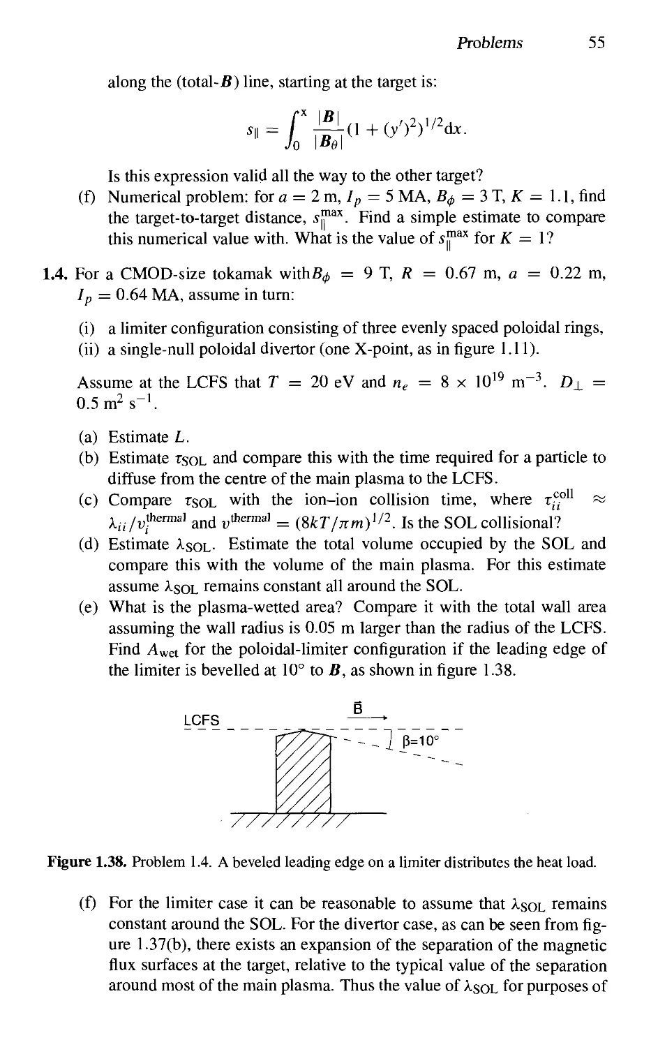
Problems 53
References 59
The Role and Properties of the Sheath 61
2.1 The Bohm Criterion. Historical Background 61
2.2 The Maxwellian Velocity Distribution 64
2.3 The Bohm Criterion; T, = 0. Simple Derivation 70
2.4 The Bohm Criterion when T, / 0 76
2.5 The Particle Flux Density to a Surface 78
2.6 Potential Drop in the Sheath for Floating or Biased Surfaces 79
2.7 Langmuir Probes 84

viii Contents
2.8 The Sheath Heat Transmission Coefficients. Basic Treatment 92
2.9 Some Basic Consequences of the Existence of the Sheath 95
2.10 The Solid Surface at an Oblique Angle to B: The Chodura Sheath 98
Additional Problems 105
References 109
3 Experimental Databases Relevant to Edge Physics 111
3.1 Ion and Atom Back-scattering from Surfaces 111
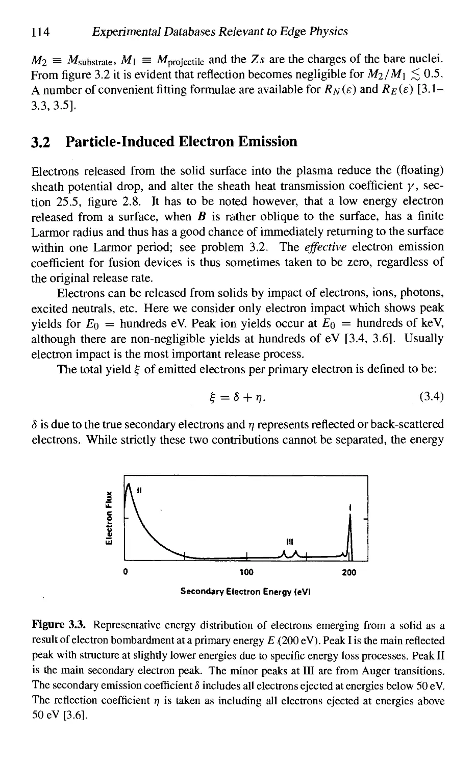
3.2 Particle-Induced Electron Emission 114
3.3 Sputtering 116
3.3.1 Physical Sputtering 118
3.3.2 Chemical Sputtering of C by H 121
3.3.3 The Energy of Sputtered Neutrals 124
3.3.4 Radiation-Enhanced Sublimation, RES 125
3.4 Trapping of Hydrogen in Surfaces 125
3.5 Atomic Databases for Ionization, Dissociation and Radiation Rates 130
3.5.1 Atomic Databases for Impurities 130
3.5.2 Atomic Databases for Hydrogen 138
Problems 146
References 150
4 Simple SOL 153
4.1 The Simple SOL: The Sheath-Limited Regime 153
4.2 'Straightening Out'the SOL for Modelling Purposes 153
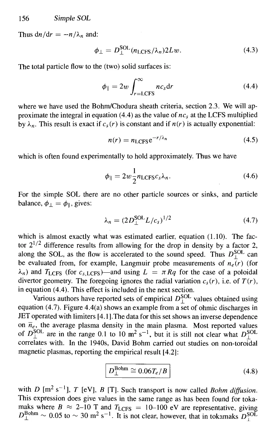
4.3 Relating Density Scrape-Off Length A„ to Df^^ 155
4.4 Modelling k„, kj,, kj., etc Simultaneously 158
4.5 Relating the Properties of Main and Edge Plasmas 161
4.6 Particle Confinement Time, Tp 167
4.6.1 The Case with the Hard Boundary Condition 169
4.6.2 The Case with the Soft Boundary Condition 175
4.6.3 The Global Recycling Coefficient 179
4.7 The Simple versus Complex SOL 181
4.8 Comparison of High Recycling, Strongly Radiating and Detached
Regimes 183
4.9 The Effects of Ionization within the SOL 185
4.10 Parallel Temperature Gradients Along the SOL 187
4.10.1 Calculating r(5jj) 187
4.10.2 Criteria for Existence of Parallel Temperature Gradients 192
4.11 Parallel Temperature Gradients in the Context of Electron-Ion
Equipartition 196
4.11.1 An Initial Estimate of the Role of Equipartition in the SOL 196
4.11.2 Case A. Te = Ti. No T-Gradient 197
4.11.3 Case B. Te = Ti. Significant T-Gradients Exist (Very
Strong Collisionality) 197

Contents ix
4.11.4 Case C. Te y^Tf. No Significant T-Gradients. Weak Col-
lisionality (The Simple SOL) 199
4.11.5 Case D. Tg ^ Ti. Significant Temperature Gradients
Exist. Intermediate Collisionality 201
4.11.6 Equipartition near the Target 201
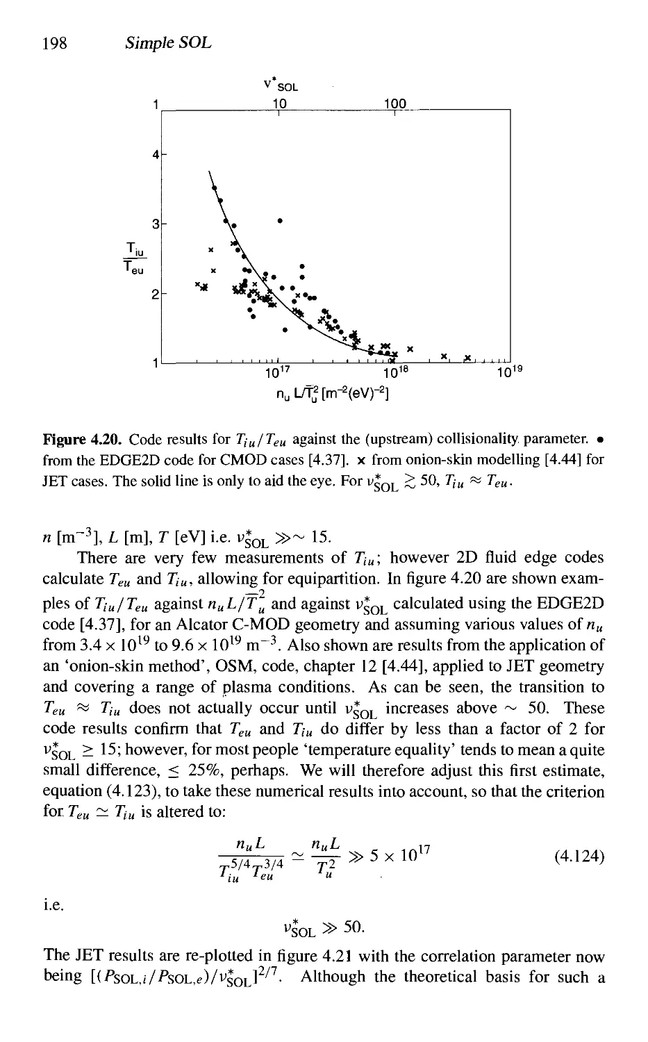
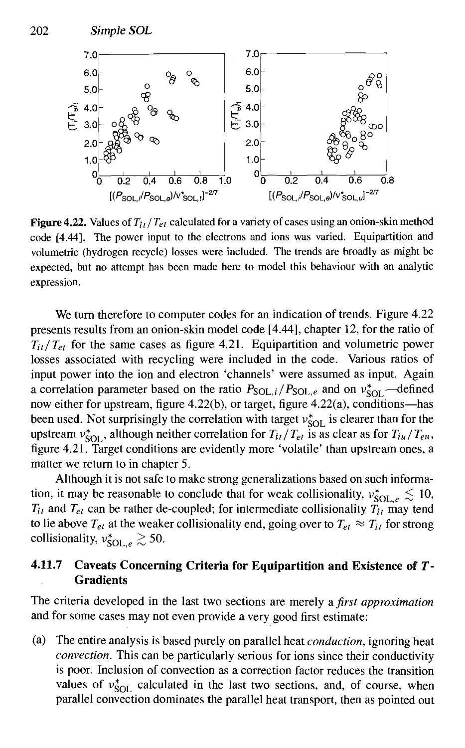
4.11.7 Caveats Concerning Criteria for Equipartition and
Existence of r-Gradients 202
4.11.8 Overview of the Criteria for Equipartition and T-
Gradients. SOL Collisionality 204
Additional Problems 204
References 210
The Divertor SOL 212
5.1 Why use Divertors Rather than Limiters? 212
5.1.1 Production of Impurities by Ion Impact 213
5.1.2 Impurity Production by Neutral Impact on Walls 214
5.1.3 Transport of Impurities to the Main Plasma 214
5.1.4 Removal of the Helium Impurity, Pumping 215
5.1.5 Removal of Hydrogen, Pumping 217
5.1.6 Efficient Use of Magnetic Volume 217
5.1.7 Size of Plasma-Wetted Area 218
5.1.8 Opportunity for Power Removal by Volumetric Loss
Processes 219
5.1.9 Achievement of Plasma Detachment 220
5.1.10 Energy Confinement 220
5.1.11 Conclusions 220
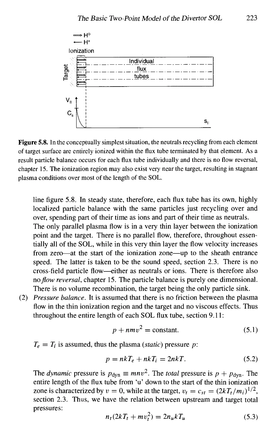
5.2 The Basic Two-Point Model of the Divertor SOL 221
5.3 The Conduction-Limited Regime. The High Recycling Regime 230
5.4 Extensions to the Basic Two-Point Model. 'Corrections' 232
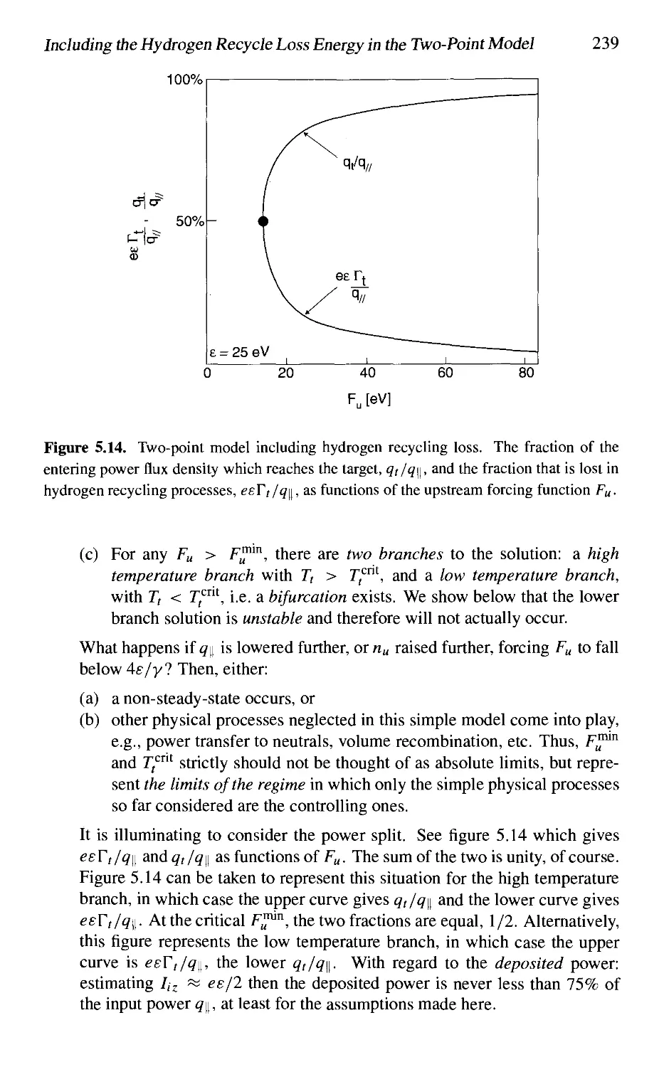
5.5 Including the Hydrogen Recycle Loss Energy in the Two-Point
Model 237
5.6 The Plasma-Wetted Area of Limiters and Divertors. The Parallel
Flux Area of the SOL 245
5.7 Expressions for the Power Scrape-Off Width, etc 252
5.7.1 Introduction 252
5.7.2 Case of Negligible Parallel T-Gradient 252
5.7.3 Case of Significant Parallel r-Gradient 253
5.8 SOL Collisionality and the Different Divertor Regimes 264
5.9 Divertor Asymmetries 267
5.10 The Effect of Divertor Geometry 270
5.11 The Ergodic Divertor 270
Additional Problems 273
References 274

X Contents
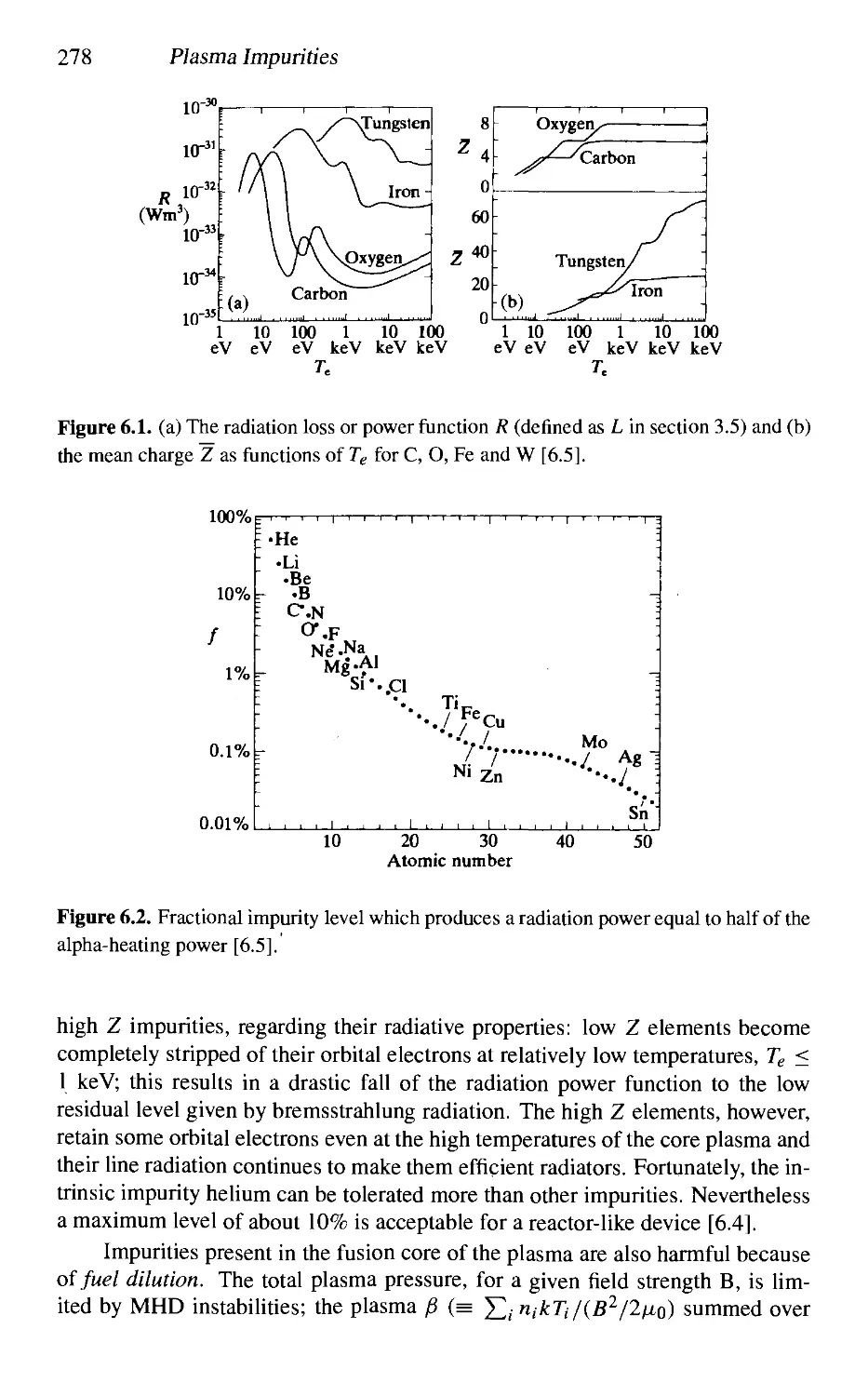
6 Plasma Impurities 277
6.1 Introduction: Harmful and Beneficial Effects of
Impurities 277
6.2 The Three Principal Links in the Impurity Chain 280
6.2.1 The Source 281
6.2.2 Edge Transport 282
6.2.3 Transport in the Main Plasma 283
6.3 Measuring the Impurity Source 283
6.4 Models for ID Radial Transport 287
6.4.1 The Engelhardt Model 287
6.4.2 The Controlling Role of Edge Processes in Impurity
Behaviour 293
6.4.3 The Questionable Concept of'Impurity Screening' 293
6.5 Impurity Transport Parallel to B in the SOL 296
6.5.1 Introduction 296
6.5.2 Defining the 'Simple One-Dimensional Case' for
Modelling Impurity Retention by Divertors 297
6.5.3 The Parallel Forces on Impurity Ions 298
6.5.4 A Simple ID Fluid Model of Impurity Leakage from a
Divertor 303
6.5.5 Estimating Divertor Leakage 313
6.6 Edge Impurity Source/Transport Codes 323
6.6.1 Why Have Codes? 323
6.6.2 Interpreting Edge Impurity Measurements Using Codes 324
6.6.3 Edge Fluid Impurity Codes 328
6.6.4 Monte Carlo Impurity Codes 328
6.7 Helium and Pumping 336
6.8 Erosion and Redeposition of Solid Structures at the Plasma Edge 342
Additional Problems 343
References 355
7 The H-Mode and ELMs 358
References 366
8 Fluctuations in the Edge Plasma 368
References 376
PART 2
Introduction to fluid modelling of the boundary plasma 379
Introduction to Part II 381

Contents xi
9 The ID Fluid Equations 384
9.1 Introduction 384
9.2 The Kinetic Equation 384
9.3 The Conservation of Particles Equation 385
9.4 The Momentum Conservation Equation 386
9.5 Ohm's Law 392
9.6 The Energy Conservation Equation, T^ 392
9.7 The Energy Conservation Equation, Tx 396
9.8 The Parallel Viscous Stress 397
9.9 The Conservation Equations Summarized 399
9.10 The Sheath-Limited Regime 400
9.11 The Conduction-Limited Regime 401
9.12 Self-Collisionality and the Problem of Closing the Fluid Equations 402
References 402
10 ID Models for the Sheath-Limited SOL 404
10.1 Introduction 404
10.2 The ID Isothermal Fluid Model 404
10.3 Isothermal Model. Non-Constant Source 5p 406
10.4 The Effect of Neutral Friction on Plasma Flow Along the SOL 406
10.5 Other ID Models for the Sheath-Limited SOL 408
10.6 The Kinetic ID Model of Tonks and Langmuir. Cold Ions 409
10.7 Kinetic Models for 7; ^ 0 413
10.8 Adiabatic, Collisionless Fluid Models 416
10.9 Adiabatic, Strongly Collisional Fluid Models 419
10.10Adiabatic, Intermediate Collisional Fluid Models 419
10.11 Comparing ID Collisionless Kinetic and Collisionless Fluid Models420
References 422
11 ID Modelling of the Conduction-Limited SOL 423
11.1 Introduction 423
11.2 ID Fluid Modelling for the Conduction-Limited SOL 426
References 436
12 'Onion-Skin'Method for Modelling the SOL 437
12.1 The Concept of a SOL Flux Tube 437
12.2 The Onion-Skin Method ofModelling the SOL 444
12.3 Code-Code Comparisons of Onion-Skin Method Solutions with
2D Fluid Code Solution of the SOL 447
References 449
13 An Introduction to Standard 2D Fluid Modelling of the SOL 450
References 457

xii Contents
PART 3
Plasma Boundary Research 459
Introduction to Part III 461
14 Supersonic Flow along the SOL 462
14.1 The Effect on the SOL of Supersonic Flow Into the Sheath 462
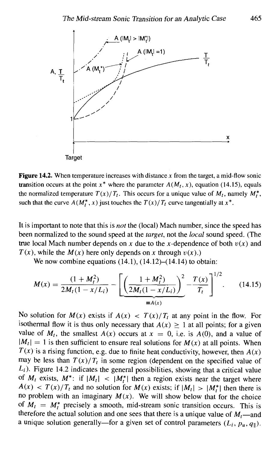
14.2 The Mid-stream Sonic Transition for an Analytic Case 464
14.3 Supersonic Solutions for an Analytic Case 467
14.4 Supersonic Solutions in Numerical Codes 468
References 470
15 Flow Reversal in the SOL 471
References 476
16 Divertor Detachment 477
16.1 Introduction 477
16.2 Background Relevant to Divertor Detachment 478
16.3 Experimental Observations of Divertor Detachment 483
16.4 Understanding Detachment 492
16.4.1 Introduction 492
16.4.2 Low Plasma Temperatures Necessary but Not Sufficient
for Detachment 493
16.4.3 TTie Necessity of Volumetric Momentum and Power Losses493
16.4.4 The Effect of Volume Recombination Acting Alone 495
16.4.5 The Effect of Ion-Neutral Friction Acting Alone 497
16.4.6 The Combined Effect of Ion-Neutral Friction and Volume
Recombination on Detachment 502
16.4.7 2D Fluid Code Modelling of Divertor Detachment using
the UEDGE Code 505
16.4.8 The'Cause'versus the'Explanation'of Detachment 508
References 510
17 Currents in the SOL 512
17.1 Introduction 512
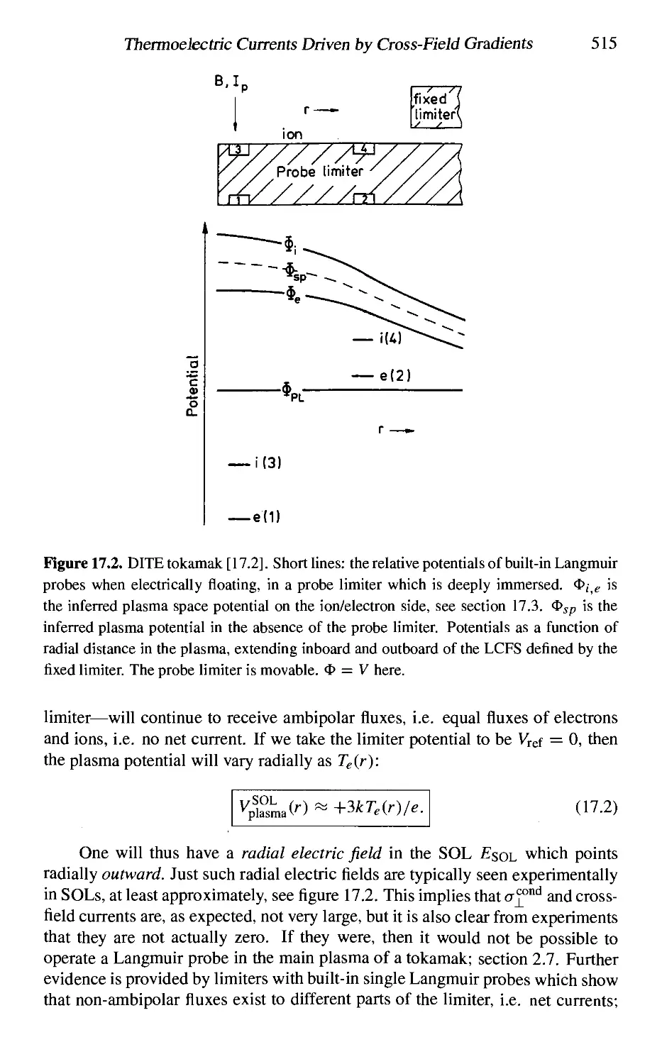
17.2 Thermoelectric Currents Driven by Cross-Field Temperature
Gradients 513
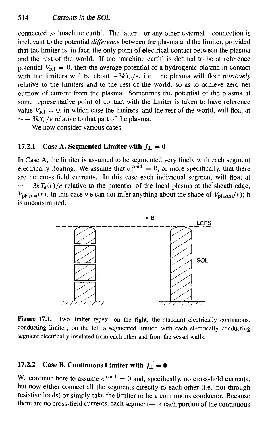
17.2.1 Case A. Segmented Limiter with yx = 0 514
17.2.2 Case B. Continuous Limiter with 7\i = 0 514
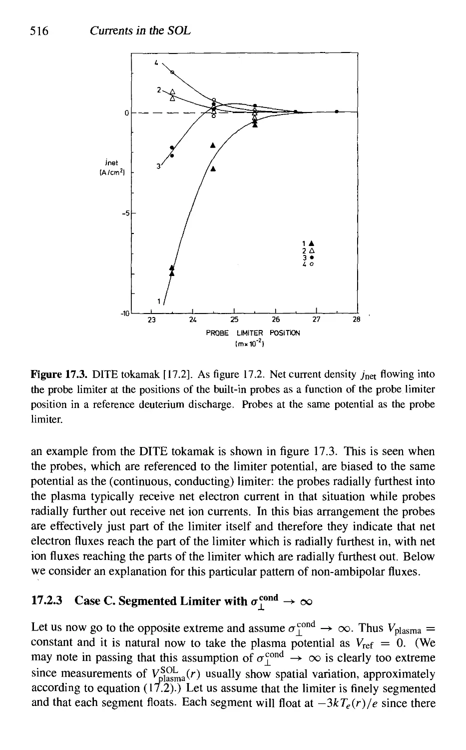
17.2.3 Case C. Segmented Limiter with af""^ -^ oo 516
17.2.4 Case D. Continuous Limiter with af""^ -^ oo 517
17.3 Inferring V^^'^^^ir) from Probe Measurements of VfloatC'') and
Teir) 520
17.4 Thermoelectric Currents Driven By Parallel Temperature Gradients 520
17.5 Cross-Field Currents 525
17.5.1 Experimental Results 525
17.5.2 Simple Models for ax 527

Contents xiii
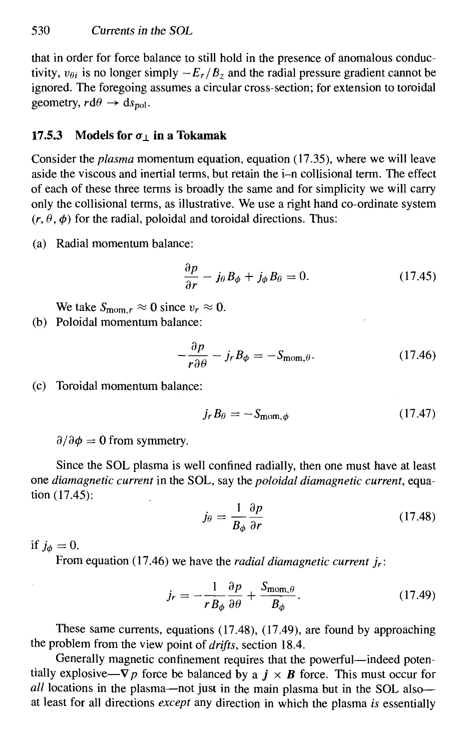
17.5.3 Models for a± in a Tokamak 530
17.6 A Concluding Comment 535
References 535
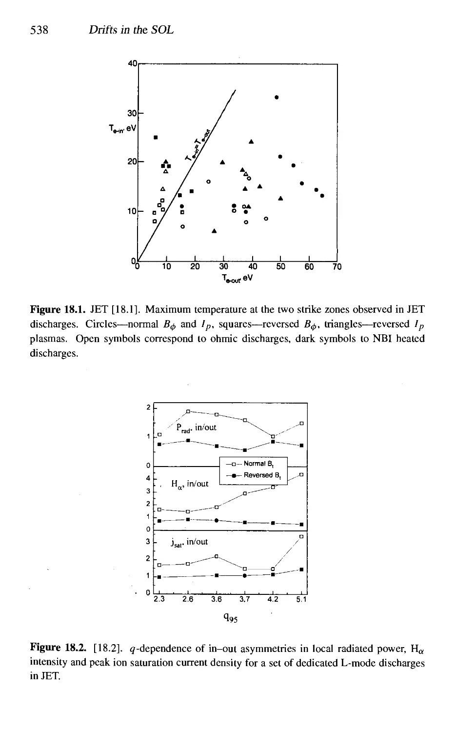
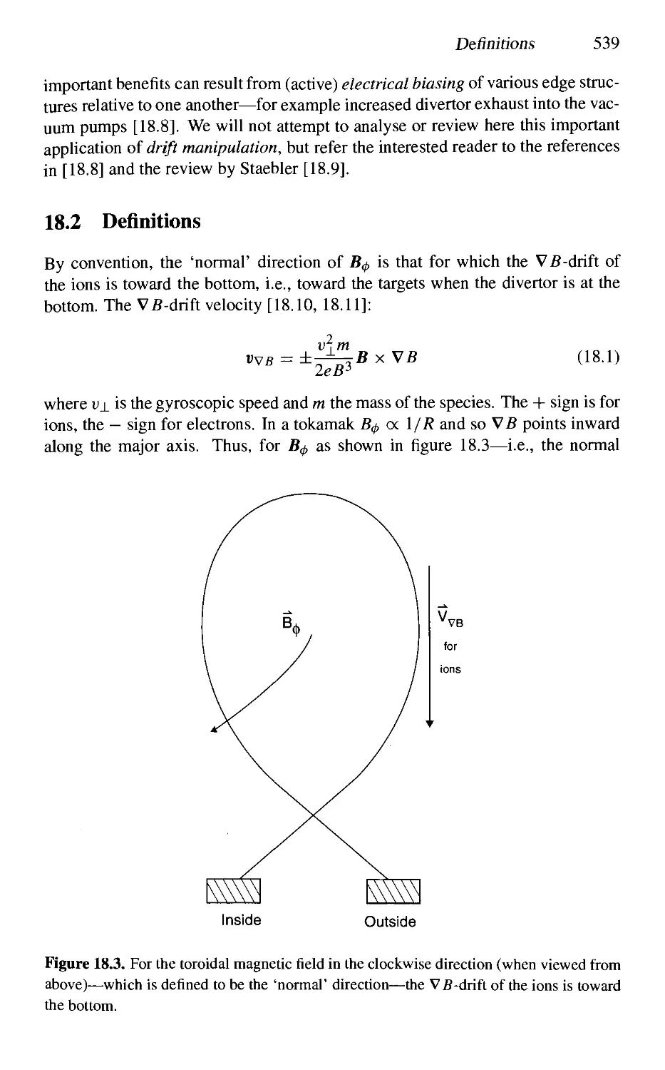
18 Drifts in tlie SOL 537
18.1 Experimental Observations Implying the Presence of Drifts in the
SOL 537
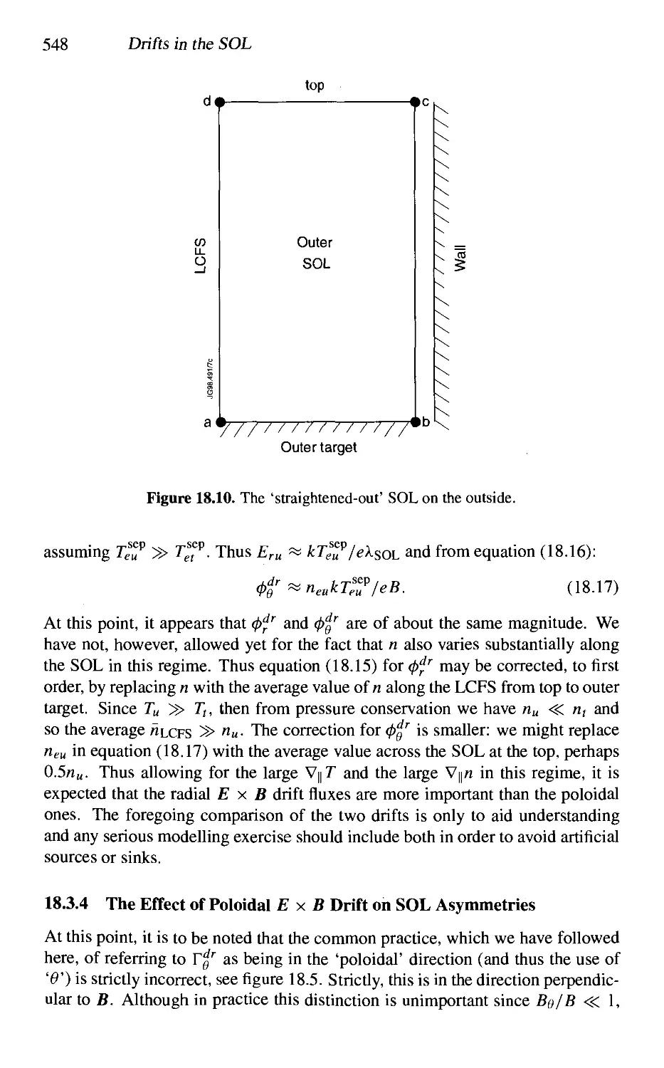
18.2 Definitions 539
18.3 The Consequences of E x B Drifts 542
18.3.1 The Radial and Poloidal E x B Drifts 542
18.3.2 Comparison ofDrift Fluxes with the Basic SOL Fluxes 546
18.3.3 Comparison of Radial and Poloidal Drift Fluxes 546
18.3.4 The Effect of Poloidal E x B Drift on SOL Asymmetries 548
18.3.5 The Effect of Radial E x B Drift on SOL Asymmetries 553
18.3.6 Comments on the Effects of Radial and Poloidal E x B
Drifts 555
18.4 Diamagnetic Drifts and Currents in the SOL 556
18.5 Pfirsch-Schluter flows 561
18.6 Heat Hux Drifts in the SOL 565
18.7 Two Alternative Descriptions of Drifts 565
18.8 A Concluding Comment 568
References 568
19 The Relation Between SOL and Main Plasma Density for Divertors 570
References 574
20 Extracting Xj^^ir) From Target Plasma Data Using the Onion-Skin
Method 575
20.1 The General Method 575
20.2 A Simple Two-Point Model for Estimating xT^ and n„ 580
20.3 Examples from JET 582
References 586
21 Measurements of D^°^, x^°^ and the Decay Lengths for Divertor
SOLs 588
References 602
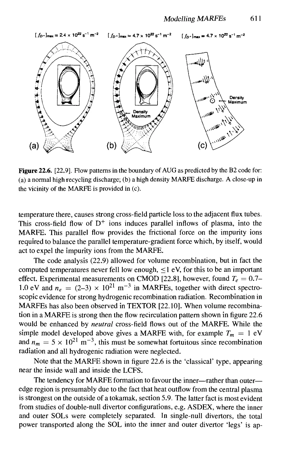
22 MARTEs 603
22.1 Experimental Observations 603
22.2 ModeUing MARFEs 605
22.3 Divertor MARFEs 612
References 614
23 The Radiating Plasma Mantle 615
References 620
24 Zeff, Prad and the Relation Between Them 621
References 628

xiv Contents
25 Further Aspects of the Sheath 629
25.1 The Ion Velocity Distribution at the Sheath Edge 629
25.2 The Case of B Parallel to the Solid Surface 634
25.3 The Bohm-Chodura Boundary Conditions and the Density
Gradient at the Entrance to the Sheaths 643
25.4 The Sheath Boundary Conditions in the Presence of E x B and
Diamagnetic Drifts 645
25.5 Expressions for the Floating Potential, Particle and Heat Flux
Densities Through the Sheath 646
References 655
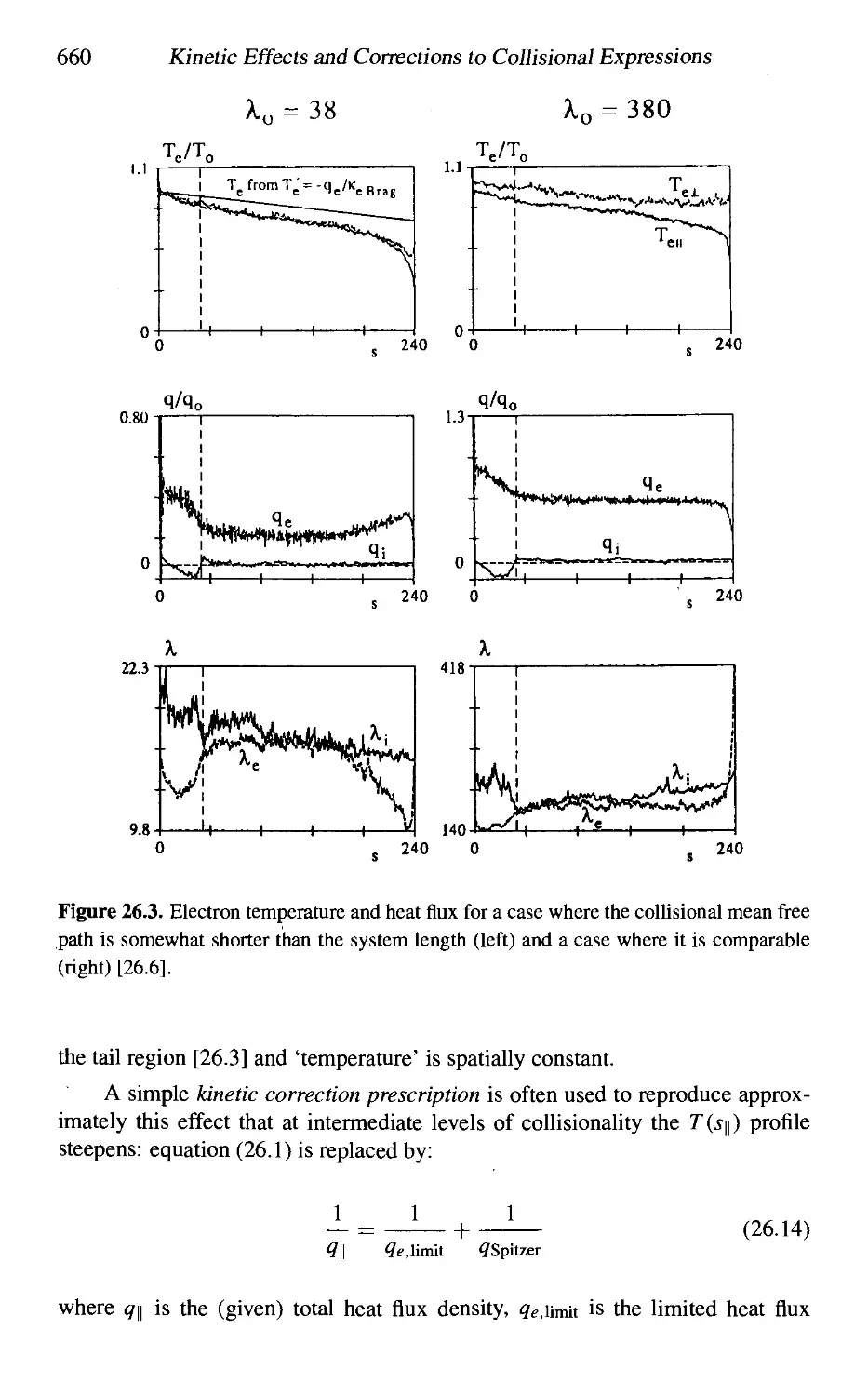
26 Kinetic Effects and Corrections to Collisional Expressions 656
26.1 Introduction 656
26.2 Kinetic Correction for Parallel Heat Conductivity 657
26.3 Kinetic Correction for Parallel Viscosity 664
26.4 Kinetic Correction for the Parallel Temperature Gradient Force
Coefficients 664
References 665
27 Impurity Injection Experiments 667
27.1 Injection of Recycling Impurities 667
27.1.1 Single-Reservoir Model 669
27.1.2 The Garching Two-Chamber Model 670
27.1.3 Modelling which Uses an Edge Impurity Code and Both
Divertor and Main Plasma Spectroscopic Signals 682
27.2 Injecting of Non-Recycling Impurities 683
27.2.1 Simple Analytic Models for the Penetration Factor
(Confinement Time) Based on a 'SOL Sink Strength' Parameter 685
27.2.2 Interpretation Using a Code Such as DIVIMP 688
References 689
Appendix A Solutions to Problems 691
Index 704

Acknowledgements
It is a pleasure to thank the many people who helped me with this book. The
genesis of the book was a mini-course given at JET in 1993 on tokamak edge
physics that Giinther Janeschitz encouraged me to give during a sabbatical year
at JET arranged by the good offices of George Vlases. Ian Hutchinson, prompted
by Garry McCracken, provided me a second opportunity to air the material as a
graduate half-course given at MIT in 1995. In 1997 Peter Stott, acting on the
suggestion of Garry again, asked me to turn the material into a book. Garry has
been my mentor in tokamak edge physics since I spent a sabbatical year with
him at Culham in 1980/81 and I owe him a great debt as a student, colleague and
friend.
To the many friends and colleagues who read sections of the book and
provided much valued suggestions, corrections, comments, and—in some
cases—new results, my sincere thanks: Tine Baelmans, Jose Boedo, Alex
Chankin, Jim Davis, Ralph Dux, David Elder, Michael Endler, Kevin Erents,
Wojciech Fundamenski, Gerd Fussmann, Mattias Groth, Houyang Guo, Tony
Haasz, Lome Horton, Ian Hutchinson, Andre Kukushkin, Brian LaBombard,
Hans Lingertat, Bruce Lipschultz, Steve Lisgo, Geoff Maddison, Guy Matthews,
Garry McCracken, Spencer Pitcher, Gary Porter, Detlev Reiter, Karl-Ulrich
Riemann, Tom Rognlien, Mike Schaffer, Peter Stott, Hugh Summers and George
Vlases. I also must thank the many other colleagues I have had the privilege of
working with in tokamak edge physics—and who will no doubt find much of
their own work in this book—all, I hope, properly acknowledged!
To the graduate students at the University of Toronto Institute for Aerospace
Studies who worked many of the problems in the book and provided valuable
feedback, my thanks: Jasmine El-Khatib, Andrew Pavacic, Patrick Wright—and
a special thanks to Peter Schwanke who co-authored the solutions section with
me and who scoured the text for typos and worse.
My thanks to the artists in the JET Reprographics Department who produced
most of the new figures in the book: Roger Bastow, John Machin and Stuart
Morris. A blessing on the dedicated and tolerant typists who worked on the book
at JET and the University: Karen Clifford, Win Dillon, Pam Peisley, Nicci Povey,
Gail Woolnough—and also my wife Sharron.

xvi Acknowledgements
Most of all I want to thank Sharron for her unfailing patience and support
through the writing of this book—as throughout our 35 years of happy life
together.
University of Toronto Institute for Aerospace Studies,
JET, Oxfordshire
and
General Atomics, San Diego
September 1999 Peter Stangeby

Preface
This book is based on a series of lectures 'Elements of edge physics' given at JET
in 1993, MIT in 1995 and the University of Toronto in 1998. The lectures were
intended as an introduction to the basic ideas about the boundary or scrape-off
layer, SOL, of magnetic fusion devices—particularly of tokamaks—for people
with a plasma physics education. Concepts about the SOL have largely been
developed during the 1980s and 1990s and, as yet, little of this has found its way
into plasma texts. The first part of this book was written with the intention of
filling this gap.
The book is divided in to three parts. Part I attempts to retain the spirit of
the original lecture series, namely that of a quick review of the central ideas about
the SOL. This would be appropriate for an introductory course on the subject.
Derivations are heuristic and physical intuition is emphasized. The reader should
be able to cover this material reasonably quickly, with little need to pause for
careful derivations or to consult related texts.
In part I, problems have been included to aid the student. The problems are
of two types. The first type is embedded in the text and has the character of a
worked example intended to illuminate the point being discussed. The reader is
encouraged to include these problems when reading the text, even if deciding not
to actually work through the maths. Additional problems appear at the end of
each chapter. Solutions, or hints, are included at the end of the book.
Part II provides an introduction to methods of modelling the plasma edge
region of magnetically confined plasmas. A number of sophisticated computer
codes have been developed during the last two decades to model the edge plasma
in all its 2D or 3D glory, including time dependence and employing all the
numerical power of modem computational fluid dynamics, CFD, techniques. As
in other fields, this effort has resulted in creating what now constitutes a third
basic line of attack on our ignorance of the physical world—additional, that is,
to the two traditional lines of experiment and theory. The shear complexity of
code modelling, however, requires that its output be subject to efforts aimed
at interpretation and understanding—just as experiments always have required.
The need for simpler modelling has been enhanced rather than diminished by the
advent of computer code modelling.
Part II of this book is aimed at simple approaches to modelling the plasma
xvii

xviii Preface
edge—although the rudiments of 2D fluid code modelling are also touched on.
Emphasis is therefore placed on ID models of the edge, which often turn out to
provide surprisingly close matches to the output of the sophisticated 2D computer
code models. The modelling material of part II has been included for those
envisaged readers who probably identify themselves as experimentalists, but with a
penchant for interpreting their experimental results—as the best experimentalists
always do. It is also for those who want to try to make sense of the output of
their sophisticated code—i.e., to interpret code results—as the best code scientists
always do. Even ID modelling enterprises can reach the point that they require
recourse to a computer—but simple numerical procedures such as Runge-Kutta
quadrature are often adequate. Thus little maths need come between us and the
physics in this type of modelling work.
Part III of the book is a collection of essays on currently active research
topics in plasma edge physics. The selection of topics is inevitably arbitrary. The
coverage is uneven. The topics tend to reflect the personal interests of the author
The sound of hobby-horses may be heard in the land. The material in Part III will
undoubtedly date more quickly than that in parts I and II—and in the subsequent,
numerous editions of the book, it is anticipated that some of this material may be
revised, replaced or repudiated.
A distinction is made between the plasma edge and the scrape-off layer: the
former includes the SOL, but also extends some distance inboard of the last closed
(magnetic) flux surface, LCFS, or separatrix, into the main or core plasma. This
region just inboard of the SOL is an important one in its own right and warrants
separate treatment. Like the SOL, it is not a region of traditional magnetic
confinement physics; atomic physics processes are also important. Effects such as the
'transport barrier', involved in H-mode confinement, are a feature of this region.
This region is not the subject of this text. We take here the expression 'plasma
boundary of a magnetic confinement device' to mean the scrape-off layer.
In the early decades of fusion energy research, the SOL was little considered,
apparently in the hope that the edge would just sort itself out with little need
for intervention or understanding. This hope was misplaced and by the 1980s
it had been recognized that certain edge problems were sufficiently serious as
to jeopardize the achievement of controlled fusion energy using magnetically
confined plasmas. One of the most serious problems is that of high power
handling or heat removal which results from the very small plasma-interaction areas
characteristic of the SOL. Magnetic fields which are strong enough to provide
adequate confinement of the main plasma are simply too effective for the SOL,
where the characteristic cross-field scale length, i.e. the SOL width, ends up being
only about 1 cm. The total exhaust power thus tends to be deposited on a total
plasma-wetted area of solid surface of a few m^ or less—an area far smaller than
that which is in principle available, i.e. ~1000 m^, the internal wall area in a
typical reactor design. It is turning out to be a challenge to keep the steady-state
heat fluxes incident on the solid surfaces down to ~5 MW m^-^, which is about
the level briefly experienced by the nose cone of a space vehicle re-entering the

Preface xix
Earth's atmosphere.
In addition to this power-removal problem, impurities generated by plasma-
surface interactions (PSI) have been the bane of fusion from the beginning and
continue to be a serious problem. Their presence in the central fusion-producing
plasma reduces power output by cooling the plasma radiatively and by diluting
the hydrogenic fuel. The SOL is both the source and sink for most impurities
and is the key to their control in magnetically confined devices. The one impurity
that is produced in the core of fusion DT plasmas—helium—must be efficiently
removed from the system to avoid poisoning the reaction. Helium removal is also
largely a SOL issue,
In principle, all magnetically confined plasmas have scrape-off layers. While
this text has been written in the context of tokamaks, much of the material applies
directly to other magnetic configurations used in fusion or other applications.
The SOL is a very long and very thin plasma region aligned to the magnetic
field B. Not surprisingly, SOL modelling draws heavily on ID, zero-B analysis.
In most of the analysis in this book, in fact, B does not explicitly appear. Much
of SOL analysis is thus applicable to non-magnetic plasmas, such as those used in
plasma process applications, and students in such fields should also find material
in this text helpful.

XX
We wish to acknowledge the following for permission to reproduce figures.
IAEA: Atomic and Plasma-Material Interaction Data for Fusion, volume 1;
Nuclear Fusion 1979 19 889, 1983 23 869, 1984 24 527, 1985 25 543, 1987 27
1105, 1221, 1988 28 1209, 1989 29 1959, 1991 31 1495, 1991 1 supplement,
1992 32 1835, 2079 1993 33 1695, 1994 34 1431,1995 35 381, 1307, 1391 1996
36 795, 839 1997 37 83, 151, 321 1998 38 331, 1637, 1789, 1999 39 1, 41;
and Plasma Physics and Controlled Nuclear Fusion Research. Springer-Verlag:
Elementary Processes in Hydrogen-Helium Plasmas Janev, Langer, Evans
and Post 1987, figure 2.1.5. American Physical Society: Phys. Rev. Lett.
1982 49 1408. Kluwer Academic/Plenum Publishers: Physics of Plasma-Wall
Interactions in Controlled Fusion ed D E Post and R Behrisch, NATO ASI Series
1986, pp 99-134. American Vacuum Society: Journal of Vacuum Science and
Technology 1980 17 298. American Institute of Physics: Physics of Plasmas
1995 2 2242, 1997 4 1690, 1998 5 1736, 1759, 4305; Physics of Fluids 1966
9 2486, 1980 23 803; Applied Physics Letters 1987 50 1870; and Journal of
Applied Physics 1988 64 4860. Elsevier Science: Journal of Nuclear Materials
1987 145-147 15, 145, 181, 812, 1221, 1989 \62r-\M 138, 300, 574, 1992
196-198 241, 374, 1995 220-222 25, 50, 143, 178, 218, 1997 241-243 37, 182,
149, 199, 358, 450, 645, 1998 255 153, 1999 266-269 99, 189, 587, 917, 1028.
Oxford University Press: Tokamaks J Wesson 1997.

PARTI
AN INTRODUCTION TO THE SUBJECT
OF THE PLASMA BOUNDARY

Introduction
Man-made plasmas almost always involve interaction with the solid state, for
example, electrodes or the walls of a containing vessel. This plasma-surface
interaction, PSI, often has profound effects on both the plasma and the solid.
Energetic plasma particles strike the solid surface, dislodging atoms from
the lattice in a process called sputtering. In time, sputtering can result in
substantial erosion of the surface. The sputtered atoms enter the plasma where they
may be ionized by the impact of plasma electrons. Usually the intended plasma
species—hydrogen isotopes in the case of fusion devices—is different from the
solid species and sputtering thus results in plasma contamination.
Of yet greater importance, the basic properties of the plasma, such as its
density and temperature, are often strongly dependent on the way solid and plasma
interact. At the interface between the solid and the plasma, a thin net-charge layer
called the Debye sheath develops spontaneously. The most important practical
consequence of the formation of a sheath is that it mediates the flow of particles
and energy out of the plasma to the solid surface. It therefore plays a central role
in establishing the temperature, density and other properties of the plasma.
Simple electrical gas discharges—such as a fluorescent light—have solid
electrodes at each end of a long cylindrical tube, whose wall completes the
containment vessel. Air is removed from the vacuum-tight vessel using gas pumps.
A gas, of the same species as is intended for the plasma, is then introduced to the
vessel at a pressure which is simply related to the intended particle density [ions
and electrons per m-'] of the plasma. Once the plasma is formed, the PSI occurring
at the electrodes and walls largely controls the properties of the discharge [0.1].
If the discharge is placed inside a magnetic coil which produces a field B aligned
with the tube axis, then the radial flow of charged particles to the tube walls can be
greatly reduced [0.2] and thus also all aspects of the PSI occurring there. This is
the principle of magnetic confinement of a plasma. Even for the strongest B-fields
the outflow of particles and energy can never, however, be reduced to zero and,
inevitably, PSI is always involved. The PSI occurring at the end electrodes can be
eliminated by bending the cylinder to make a closed, toroidal vessel. If a current
is required along the toroidal axis, this can be induced by use of a transformer,
with the toroidal plasma acting as a single-loop secondary and a coil, made e.g.
of copper, acting as the primary. This is involved in such magnetic confinement

4 Introduction
devices as tokamaks [0.3].
In principle, the fi-field could be so peri'ectly aligned as to be tangential at
every point of the cylindrical or toroidal vessel wall. In that case, the plasma
particles would reach the bounding sheath, and subsequently the vessel walls by purely
radial, that is by cross-field, motion. In practice, such perfect alignment is not
possible. Let us consider what happens when there is even a tiny misalignment.
The plasma particles are not affected by the fi-field with regard to their motion
along B, and they move in this parallel direction with very high speeds, typically,
of order random thermal speeds. The effect of a strong fi-field is to reduce the
cross-field speed of the charged particles by many orders of magnitude relative to
thermal speeds. Thus, if B is not aligned almost perfectly with the vessel walls,
the charged particles will reach the sheath and wall by parallel motion rather than
cross-field motion.
Therefore to understand the most basic aspects of the PSI occurring in a
magnetically confined plasma requires analysis of one-dimensional, parallel-to-fi
motion of charged particles in a system bounded by sheaths at each end. For this
reason, B does not explicitly appear in the analysis, since the magnetic field has
no influence on parallel motion of charged particles. This is greatly simplifying.
It also means that most of the analysis involved is applicable to non-magnetic
plasmas.
Most of the analysis in this book is one dimensional and B does not appear
explicitly.
In chapter 1, the basic features are presented of the simplest system—
namely, the isothermal plasma, where temperature is constant along the ID
flow direction. Since the heat conductivity of plasma is usually very high, the
isothermal assumption is often a good one.
In chapter 2, the basic properties of the sheath are covered. These give the
relation between the plasma temperature and density, on the one hand, and the
outflow rates of particles and energy to the sheath and solid surface, on the other.
Chapter 3 reviews the databases required for analysis of PSI. These include,
for example, sputtering yields, Y, defined as the number of lattice atoms dislodged
per impacting particle.
Chapter 4 returns to the simplest, isothermal case of chapter 1—termed the
simple SOL—covering further aspects of it and also discussing the transition to
the complex SOL. The region at the edge of a magnetically confined plasma where
parallel transport to the surfaces occurs is called the scrape-off layer, SOL. The
Complex SOL can have a number of important differences with the simple SOL,
most importantly the existence of significant parallel temperature gradients along
the length of the SOL.
Chapter 5 covers the most basic features of the complex SOL. Since this
regime is most typically found for geometrical configurations involving divertors,
this chapter is entitled 'The divertor SOL'. The simple SOL is most typically
encountered for geometrical configurations involving limiters.
Chapter 6 deals with the production of impurities arising from PSI and the

Introduction 5
resulting transport or motion of the impurity ions through the plasma.
Chapters 7 and 8 deal briefly with the implications for the boundary
plasma of the important tokamak operational mode—the H-mode (high energy
confinement)—and of plasma fluctuations, which are believed to be the cause of
the otherwise unexplained (anomalous), rapid transport of particles and energy
across B.
These first eight chapters make up part I of the book constituting an
'Introduction to the subject of the plasma boundary'. Part II provides an introduction
to edge modelling, with particular emphasis on ID models. Part III primarily
consists of a collection of essays on current research topics related to the edge.
References
[0.1] von En gel A 1965 Ionized Gases 2nd edn (Oxford: Oxford University Press)
[0.2] Franklin R N 1976 Gas Discharges (Oxford: Oxford University Press)
[0.3] Wesson J 1997 Tokamaks 2nd edn (Oxford: Oxford University Press)

Chapter 1
Simple Analytic Models of the Scrape-Off
Layer
1.1 Solid Surfaces Are Sinks for Plasmas
The most basic cause of fluid flow is the presence of a fluid source and a fluid
sink. UsuaUy some effort and expense is involved in creating fluid sink action,
for example, that achieved with mechanical pumping of gases and liquids. In the
case of a plasma fluid, however, implementation of sink action could scarcely be
simpler: the presence of a solid surface is sufficient. If charged particles happen to
strike a solid surface they tend to stick to it long enough to recombine, figure 1.1.
Plasma
Solid
Figure 1.1. Charged particles tend to stick to solid surfaces, which therefore act as plasma
sinks.
While ions do have a finite probability of back-scattering from a solid
surface, section 3.1, they do so mainly as neutrals, picking up electrons from the
surface. Electrons also stick to solid surfaces, section 3.2. Thus a solid surface

Solid Surfaces Are Sinks for Plasmas
acts as an effective sink for plasma. It is not necessarily a mass sink, however,
since the particles are subsequently released as neutrals.
For solid surfaces which are insulators or are electrically isolated, opposite
charges build up on the surfaces exposed to a plasma, quickly leading to surface
recombination. The resulting neutral atoms generally are not strongly bound to
surfaces and are thermally re-emitted back into the plasma where they can be re-
ionized, usually by electron impact. A steady-state condition can result, termed
re-cycling, whereby plasma charged pairs are lost to the surface at the same rate
as recombined neutrals re-enter the plasma, figure 1.2. While no external source
of particles is then needed, an external source of energy to provide the ionization
power is still required.
-©-
-©-
Figure 1.2. Charged particles adsorbed on solid surfaces recombine. The resulting neutral
is weakly bound to the surface and desorbs back into the plasma. Thus particle recycling
occurs and in steady state the plasma refuels itself.
The solid surface not only acts as a sink for the plasma, but it is intimately
involved in the plasma source mechanism as well. The mean free path of the
neutral for ionization may be large compared with the system size, in which case
the ionization will occur more or less uniformly throughout the system. In other
cases the ionization mean free path is short compared with system size and so the
average location of re-ionization—i.e. the plasma source—and the plasma sink
can be quite close to each other. In that case, the rest of the available volume then
'back-fills' e.g. by diffusion—much as heat fills a room where a heat source, such
as radiator, is usually placed close to a principal heat sink, such as a window.
A solid surface exposed to a plasma initially also acts as a pump in a mass
sense, since all but the promptly back-scattered particles are initially retained in
or on the solid, section 3.4. Such retention saturates at some level and thereafter
a steady-state situation results with the plasma 'refuelling itself. At that point
any external source of fuelling, such as a gas injection, can be turned off and the
plasma density will remain constant, provided no active pumping (cryopumping,
etc) is used.
It is evident that the behaviour and properties of a plasma can be dominated
by the contact it has with solid surfaces. Given the enormous differences in the

8 Simple Analytic Models of the Scrape-Oif Layer
properties of the first (solid) and fourth (plasma) states of matter, this is scarcely
surprising. The powerful sink action resulting from plasma-solid contact is the
controlling feature of tokamak edge plasma behaviour.
1.2 The Tokamak:
charge Tube
An Example of a Low Pressure Gas Dis-
Fluorescent lights and neon signs are familiar examples of low pressure gas
discharge tubes. Neutrals are ionized by electron impact more or less uniformly
throughout the cylindrical volume. The resulting electron-ion pairs 'fall' radially
to the walls, figure 1.3(a), and adhere to the surface until they recombine to form
neutrals. Sooner or later the neutrals are released back into the plasma where they
are re-ionized. Thus steady-state recycling is established and a constant plasma
density results with particles neither being added to nor removed from the system.
Power must be provided continuously—via a longitudinal electric field which
Figure 1.3. Cylindrical gas discharge tubes, (a) Simple cylinder. No magnetic field.
Plasma moves radially and rapidly to the cylinder walls, (b) Simple cylinder. With axial
magnetic field added. Plasma moves radially but slowly to the cylinder walls, (c) Cylinder
with two washer-limiters (poloidal ring limiters) inserted. With magnetic field. Plasma
moves radially and slowly out to radius a, followed by rapid motion parallel to B to the
sides of the washer-limiters. Plasma does not reach the cylinder walls.

The Tokamak: An Example of a Low Pressure Gas Discbarge Tube 9
causes ohmic heating of the electrons—in order to provide for the steady loss
of power to excitation and ionization of atoms and molecules, etc. Most of the
power invested in ionization, excitation, dissociation and elastic collisions ends
up as wall heating. A fraction of the input power ends up in photon energy from
these light sources—which actually shed more heat than light.
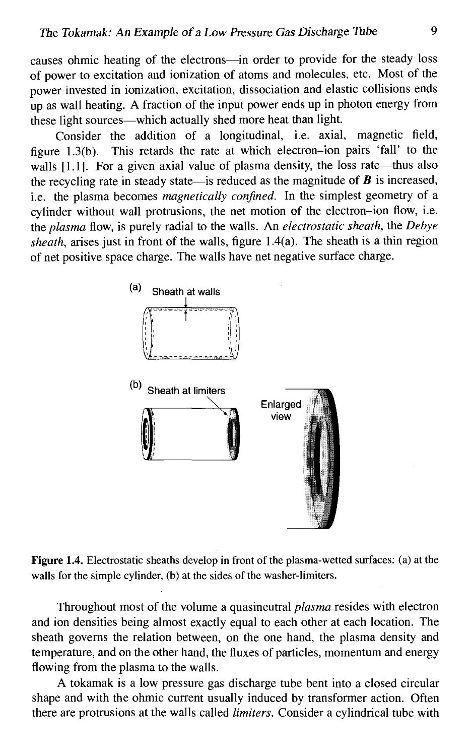
Consider the addition of a longitudinal, i.e. axial, magnetic field,
figure 1.3(b). This retards the rate at which electron-ion pairs 'fall' to the
walls [1.1]. For a given axial value of plasma density, the loss rate—thus also
the recycling rate in steady state—is reduced as the magnitude of B is increased,
i.e. the plasma becomes magnetically confined. In the simplest geometry of a
cylinder without wall protrusions, the net motion of the electron-ion flow, i.e.
the plasma flow, is purely radial to the walls. An electrostatic sheath, the Debye
sheath, arises just in front of the walls, figure 1.4(a). The sheath is a thin region
of net positive space charge. The walls have net negative surface charge.
(^) Sheath at walls
1
(b)
Sheath at limiters
(^
Enlarged
view
Figure 1.4. Electrostatic sheaths develop in front of the plasma-wetted surfaces: (a) at the
walls for the simple cylinder, (b) at the sides of the washer-limiters.
Throughout most of the volume a quasineutral plasma resides with electron
and ion densities being almost exactly equal to each other at each location. The
sheath governs the relation between, on the one hand, the plasma density and
temperature, and on the other hand, the fluxes of particles, momentum and energy
flowing from the plasma to the walls.
A tokamak is a low pressure gas discharge tube bent into a closed circular
shape and with the ohmic current usually induced by transformer action. Often
there are protrusions at the walls called limiters. Consider a cylindrical tube with

10 Simple Analytic Models of the Scrape- Off Layer
two circular washers (limiters) inserted at two locations along the cylinder length,
figure 1.3(c). The outer radius of each washer is equal to the radius of the cylinder;
the inner radius a is specifiable.
Charged particles diffuse very slowly across magnetic fields, compared with
their unrestricted motion along B, which tends to be at velocities of order of the
sound speed due to the strong sink action. Consider a charged particle originating
on axis and diffusing slowly out toward the wall. At the same time it is moving
randomly along B at high speeds due to its thermal energy. For an infinitely
long cylinder (or for one closed into a torus), this parallel-to-fi motion is of no
consequence for the fate of this particle—not, that is, until the particle has diffused
across radius a. Then this motion will cause its rapid removal from the plasma,
by carrying the particle quickly to the sides of the washer-limiter. Thus, in this
geometry the loss of particles to the surface sinks involves first a net radial motion
across the radius of the tube, followed by a parallel-to-B motion near the 'edge'
of the plasma at radius a. In this geometry the sheath forms on the sides of
the washer-limiter rather than at the wall, figure 1.4(b). Indeed the plasma no
longer extends all the way out to the walls; the loss of particles to the sides of
the washer-limiters is so fast that the particles only have time to diffuse a short
distance beyond a. The inner radius of the washer, a, thus tends to limit the radius
of the plasma column to being not much greater than a. Hence the name 'limiter'.
The thin, annular plasma region outboard of radius a is called the 'scrape-off
layer', SOL.
The wall is thus protected by the limiters from contact with the plasma.
One price paid is that the plasma-surface interaction is now concentrated on thin
plasma-wetted areas on each limiter, tending to cause localized over-heating and
other problems.
The first and fourth state of matter do not co-exist easily. Plasma erodes
solids and the eroded material enters the plasma, degrading its desired properties.
Much of the challenge for magnetic confinement fusion is to find a solution that
will allow these two mutually irritating states of matter to cohabit a small space.
The situation would not be so bad if the area of interaction could be made large,
thus diminishing the local intensity of interaction. As we will see, however, a
magnetic confinement arrangement that is effective enough to contain the main,
fusion producing plasma is too good for the SOL, resulting in quite small plasma-
wetted areas, and very intense plasma-solid interactions.
It is often the case that systems are strongly influenced—or even
controlled—by their boundary conditions. In the early days of magnetic
fusion research it was hoped, however, that the edge region 'would take care of
itself. The edge region was not of primary interest to the main thrust of the
fusion enterprise, which focuses on the hot central core region where the fusion
reaction can occur. It became clear fairly early in fusion research that the edge
region was not in fact going to 'take care of itself, but was going to require
significant attention. The power balance in early magnetic devices tended to be
dominated by radiation from impurities in the plasma which had originated from

The Tokamak: An Example of a Low Pressure Gas Discharge Tube 11
the plasma-surface interactions at the edge. The radiative cooUng was so strong
that core temperatures fell far below that needed to achieve fusion.
It would have been surprising, of course, if magnetic confinement fusion had
managed to easily escape serious edge problems. Upon first hearing about the
idea of a miniature star in a solid container, the response of most laymen is that
this must be impossible due to strong interactions between the radically different
states of matter involved. It turns out, unfortunately, that the layman is almost
right. Despite great strides, the problems arising from plasma-surface interactions
continue to threaten the achievement of a viable fusion reactor based on magnetic
confinement. Plasma contamination levels, although much reduced from early
days, are still unacceptable. The erosion rates of the solid edge structures are too
high for practical reactor designs where the replacement of internal components
cannot be frequent.
To make progress, better understanding of the plasma boundary region is
necessary. Our understanding is weak and we have many questions. What
controls the width of the SOL? How can it be manipulated? How can some of the
power reaching the SOL be dispersed before reaching the small, plasma-wetted,
solid surfaces? Can the impurity radiation itself be exploited to achieve this, or
will that cause such contamination of the core plasma that the fusion reaction
will stop there? Can the spatial distribution of the naturally produced impurities
be manipulated so that they do more good than harm? Are there benefits to be
had from injecting non-intrinsic impurities? What is the connection between the
plasma properties of the SOL—its density and temperature—and the fluxes of
particles and power to the solid surfaces? How does the plasma move along the
SOL to the surface? (It turns out, upon closer inspection, that the simple picture
above of free thermal motion along B is inadequate.) What can be achieved
by manipulating the geometry of the edge, or by changing the magnetic fields
at the edge, or by changing the arrangements of the solid structures? Can the
internal structures of the SOL be manipulated to advantage? For example, can
temperature variations be induced to occur along the length of the SOL, so that
at the 'target' (solid) end the temperature is low, while at the 'upstream' end,
where most of the coupling to the main plasma occurs, it is hot? Can the SOL
plasma be 'intercepted' or 'obstructed' before it reaches the solid surface, perhaps
by e-i recombination in the plasma itself, i.e., volume recombination, perhaps by
frictional slowing of the plasma outflow by neutral gas, i.e. by 'clogging the
drain'? Helium produced in the core by DT fusion reactions is an unavoidable
impurity; it must be removed at the edge so that it does not poison the fusion
reaction; can the edge plasma and solid structures be manipulated and configured
to achieve adequate pumping of the helium, using practically achievable pumping
arrangements? Solid material eroded into the plasma eventually re-deposits on
other edge surfaces; virtually none of the material is actually removed through the
vacuum pumps. Will the re-deposited solid surfaces give acceptable performance
of the fusion device? Will the tritium become trapped in such re-deposited
material (co-deposited), resulting in unacceptable radioactive inventories in a reactor?

12 Simple Analytic Models of the Scrape-Off Layer
This list of questions is long but by no means complete.
In order to address these and other questions which will critically affect
the demonstration of the scientific, engineering and environmental feasibility of
magnetic fusion power, we will need to better understand the plasma boundary.
This book addresses these questions and attempts to improve our understanding
of the behaviour of the plasma edge.
1.3 Tokamak Magnetic Fields
There are two principal components of a tokamak magnetic field, figure 1.5, the
toroidal magnetic field B^ created by external magnetic coils and the poloidal, or
self-, magnetic field Bg created by the toroidal plasma curent Ip induced e.g. by
an external transformer.
The resulting fitotai is helical, with each magnetic field line lying on one of
a nested set of toroidal flux surfaces, figure 1.6 [1.2]. Figure 1.7 shows a poloidal
cross-section of a tokamak, displaying the characteristic magnetic contours which
result from taking a poloidal plane slice through the nested toroidal surfaces.
Magnetic field lines which lie on flux surfaces that never make contact with
'plasma
Figure 1.5. The toroidal direction (f> is the long way round, the poloidal 9 the short
way. The two principal magnetic fields of a tokamak are B^ due to external coils and
Bg due to the plasma curent /plasma i" the (t> direction. For a tokamak \B^\^ \Bg\. Thus
^total = B^ + Bq is helical and with a shallow pitch angle.
Figure 1.6. Magnetic flux surfaces forming a set of nested toroids.

Tokamak Magnetic Fields
13
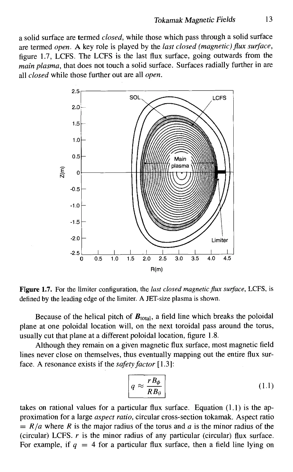
a solid surface are termed closed, while those which pass through a solid surface
are termed open. A key role is played by the last closed (magnetic) flux surface,
figure 1.7, LCFS. The LCFS is the last flux surface, going outwards from the
main plasma, that does not touch a solid surface. Surfaces radially further in are
all closed while those further out are all open.
Figure 1.7. For the limiter configuration, the last closed magnetic flux surface, LCFS, is
defined by the leading edge of the limiter. A JET-size plasma is shown.
Because of the helical pitch of Btotab a field line which breaks the poloidal
plane at one poloidal location will, on the next toroidal pass around the torus,
usually cut that plane at a different poloidal location, figure 1.8.
Although they remain on a given magnetic flux surface, most magnetic field
lines never close on themselves, thus eventually mapping out the entire flux
surface. A resonance exists if the safety factor [1.3]:
rB0
RBg
(1.1)
takes on rational values for a particular flux surface. Equation (1.1) is the
approximation for a large aspect ratio, circular cross-section tokamak. Aspect ratio
= R/a where R is the major radius of the torus and a is the minor radius of the
(circular) LCFS. r is the minor radius of any particular (circular) flux surface.
For example, if ^ = 4 for a particular flux surface, then a field line lying on

14 Simple Analytic Models of Che Scrape-Off Layer
q=4
Start
"^After first
toroidal
circuit
After lialf
a toroidal
circuit
Figure 1.8. The safety factor ^, when an integer, is the number of toroidal transits required
for ^totai to make one poloidal transit. The example shown is for ^ = 4.
Figure 1.9. A single toroidal flux surface has been cut and flattened. The specific example
of ^ = 4 is illustrated, showing that four toroidal transits are required for one poloidal
transit.
that surface makes exactly four large (toroidal) transits to complete one short
(poloidal) transit, closing exactly on itself. Figure 1.9 shows a ^ = 4 magnetic
flux surface which has been cut, opened up and flattened to make a rectangle.
O and O' represent the same location. Since one has from Ampere's law,
approximately:
Be(a)
in a
(1.2)
then q is large for small plasma current and/or large external magnetic field, B^.
One also has the local pitch angle of Btotai:
9pitch ^ Bg/B^ ^ Bg/B
(1.3)

The Scrape-Off Layer, SOL 15
typically 0pitch ^0.1 since the tokamak magnetic field is primarily toroidal.
In the main or confined plasma, i.e. inside the LCFS, the principal
significance of the safety factor q is that the plasma is magnetohydrodynamically
unstable if ^ < 2 at the edge (the LCFS) [1.4], and so such operating conditions
are usually avoided. In the region outside the LCFS, the role of q is primarily
geometrical, as will be shown. It is this necessary avoidance of small values of ^
at the edge that results in small pitch angles of Btotai-
1.4 The Scrape-Off Layer, SOL
As noted, the region radially outboard of the LCFS is called the scrape-off layer,
SOL. Cross-field velocities are of order:
VL ~ Dx/£x (1.4)
where Dj_ is the cross-field diffusion coefficient [m-^ s~^] and lj_[m\ is the
characteristic radial scale length of density. (Fick's law of diffusive motion: F =
— Ddn/dx where F is the particle flux density [particles m"-^ s~^], D is the
particle diffusion coefficient and dn/dx ^ n/£±, and with F related to an
effective cross-field velocity, dj_, F = nv±, one obtains equation (1.4).) To date,
attempts to calculate Dj_ from first principles have been of limited success [1.5].
Dx is generally anomalous compared with classical rates and is obtained from
experiment; see section 4.3. Values of order 1 m-^ s"^ are found empirically [1.5].
The radial density length may be as large as the minor radius, a, which would be
the case if the neutrals were all ionized at the very centre, e.g. for deep injection
of fuel pellets. More typically £j_ is of the order of the ionization mean free path,
mfp, of the recycling neutrals at the edge, ;.Ji^"'r^'. Thus dj_ may be as slow as
^ 1 m s^', while D|| ~ plasma sound speed, Cs, which is typically many orders
of magnitude larger. Cs is calculated in section 2.4 to be:
c^ = k(Te + Ti)/(me + mi)
> ^ [k{Te + Ti)lmifl^.\ (1.5)
For example: for Tg = Ti = 25 eV, and D"*" ions, c^ ^^ 5 x lO'* m s""^
It is this enormous difference between v\\ and dj_ that makes the SOL so thin
relative to its length.
A great variety of geometries are possible for the solid surfaces which cause
the sink actions. They are generally considered to fall into one of the two
categories: (a) limiters, (b) divertors.
1,4.1 Limiter SOLs
Conceptually the simplest limiter sink action is achieved by inserting an annulus
of solid material—a washer—with inner circular radius a—cdWcd a. poloidal
limiter—at one or more toroidal locations, figure 1.10. The magnetic flux surfaces

16
Simple Analytic Models of the Scrape-Off Layer
Limiters
Oivertors
(i) Toroidal Umiler
(ii) Poloidal di«rlor
(ill) Poloidal limiKr
(iv) Toroidal diverlor
(v) Rail limiKr
(vi) Bundle dlvertor
Figure 1.10. Various limiter and divertor configurations [1.37]:
(i) The toroidal limiter consists of a toroidally symmetric, protruding structure attached to the wall,
mounted at the outside of the vessel, as shown here, or at the bottom, etc.
(ii) The poloidal divertor involves a diversion of the poloidal magnetic field near the edge, making
for a toroidally symmetric configuration, analogous to the toroidal limiter
(iii) The poloidal ring limiter, in the simplest case, is a circular annular plate of inner radius r =
"plasma, outer radius r = Owall-
(iv) The toroidal divertor involves a diversion of the toroidal magnetic field near the edge, making
for a configuration analogous to that of the poloidal ring limiter.
(v) The rail or probe limiter involves insertion of a solid object into the plasma at a specific toroidal
and poloidal location,
(vi) The bundle divertor involves a non-symmetric diversion of some portion of the toroidal field
near the edge, creating a configuration analogous to that of a rail or probe limiter.
are assumed to be perfectly circular here. The typical parallel-to-B distance that
a particle has to travel in the SOL before striking a limiter is
TtR
n
(1.6)

The Scrape-Off Layer, SOL 17
where n is the number of poloidal Hmiters (we have implicitly assumed here a
small pitch angle, i.e. a not very small q). L is called the connection length, and
the distance along B in the SOL between two points of contact with the solid
surface is 2L [1.6, 1.7]
A toroidal limiter can consist simply of a (toroidal) circular rail,
projecting inward from, say, the wall at the midplane, figure 1.10. This configuration
involves longer L due to the small pitch angle of B:
nRq.
(1.7)
Values of L of 100 m or more can result for large tokamaks such as JET. However,
due to the very large ratio v\\/v_l, the SOL radial width is still only of order 1 cm.
These first two limiter examples involved either toroidal or poloidal
symmetry. Limiter sink action can also be achieved by inserting any shape of object
into the plasma: since almost none of the field lines close on themselves, but
eventually map out the entire flux surface they lie on, then most field lines which
lie on flux surfaces outside the LCFS will eventually strike the inserted limiter.
Cross-field diffusion within poloidal flux surfaces also helps ensure that all points
in a SOL are actually in contact with a solid surface, i.e. effectively there are no
infinite L values in the SOL. A limiter which is small in poloidal and toroidal
extent will have a particularly large L.
An important variant of the toroidal limiter is the wall-limiter where the
plasma simply contacts, say, the inner wall near the midplane. Typically the wall
would be fully covered by protective tiles. Wall-limiters enjoy the advantage of
particularly large plasma-wetted areas, and thus lower power loadings, W m~-^,
see section 5.6.
1.4.2 Divertor SOLs
For limiter tokamaks the poloidal magnetic field is largely created by Ip and
is approximately circular. A poloidal divertor configuration can be produced
using an external conductor carrying a current Ip in the same direction as Ip,
figures 1.10 and 1.11.
In the poloidal plane, the magnetic field lines make a figure-of-eight shape,
figure 1.11(b). At some point between the two current centres a null in the
poloidal field, and thus a magnetic X-point, exists. The magnetic flux surface
passing through the X-point is called the magnetic separatrix. The flux surfaces
inside the separatrix, surrounding the Ip channel, contain the main or confined
plasma within closed flux surfaces. A sink action is achieved simply by
introducing a solid plane which cuts through the flux surfaces surrounding the Id channel,
figure 1.11(a): any plasma particles which diffuse across the separatrix of the
confined plasma find themselves on open flux surfaces which connect directly to
the solid surface, which are called the divertor targets, and the particles move
rapidly to the target-sinks before diffusing very far cross-field. The separatrix

8 Simple Analytic Models of the Scrape-Off Layer
(a)
Solid surface
SOL introduced to form a
Separatrix piasmasink
(b)
Figure 1.11. The poloidal field sf^^^^ created by /pjasma is diverted by the «^°'' created
by a divertor coil current /q, parallel to /plasma' which is carried by a coil internal or
external to the vacuum vessel.
is the LCFS. A thin SOL results, just as for the limiter geometry. If the targets
are located not too far from the X-point (the case of short 'divertor legs'), then
the length of the average SOL field line is approximately the same as for the
toroidal limiter geometry, with L ^ nRq. There is an important reason to keep
the divertor legs short: the entire configuration shown in figure 1.11 lies inside
the toroidal field coils; magnetic volume is expensive to produce and only the
confined region is hot enough to produce fusion power.
The length of a 'field line on the separatrix is, in principle, infinite, due to
the poloidal field null at the X-point. There is, however, strong magnetic shear
just near the separatrix with the local values of L varying rapidly with radius.
Inevitable field errors effectively prevent infinite L. Further, cross-field transport
has the effect of 'shorting' any extremely long field lines by transport on to
immediately adjacent, shorter field lines. Typically L is quoted for the magnetic
flux surface lying slightly outside the separatrix.
Figure 1.12 shows a close-up of a divertor region, located at the bottom of
the vessel. The region below the X-point and inside the separatrix is called the
private plasma. It contains a thin layer of plasma lying along the two separatrix
arms, terminating at the targets. The private plasma is sustained by the transport
of plasma particles and power from the main SOL, across the private plasma
separatrix.
While the divertor configuration is less efficient in the use of magnetic vol-

Characteristic SOL Time 19
Main
Plasma
Separatrix
X—point
Plasma
Flow
Divertor Targets
'gure 1,12. The SOL surrounds the main plasma above the X-point and extends to
e target. The private plasma receives particles and energy from the SOL by cross-field
sport.
me than the limiter one, there are off-setting advantages. The most important
ne is the opportunity to move the solid surfaces where the intense plasma surface
nteractions occur—the divertor targets—away from the confined plasma. Further
mparisons of the two configurations are discussed in section 5.1.
The divertor geometry shown in figures 1.11 and 1.12 is termed 'poloidal',
ecause it is the poloidal magnetic field which has been diverted by Ip—it is
owever toroidally symmetric—a sometimes confusing fact. Other magnetic di-
rtor configurations can also be produced [1.8], figure 1.10. The limiter shown in
re 1.10 is termed 'poloidal' because it is poloidally symmetric. The 'toroidal'
iter is termed similarly. The presence of the divertor targets is also seen to
mit the radial extent of the SOL in the same way as limiters do.
1.5 Characteristic SOL Time
The most used configurations are the poloidal divertor and the toroidal limiter
since both can provide (relatively) large plasma-wetted areas, the area of solid
surface in contact with significant plasma fluxes, section 5.6. For both, one
has L ^ nRq. Plasma particles which move freely along B in the SOL have
velocities of the order of the plasma sound speed, t>, and so characteristic particle

20
Simple Analytic Models of the Scrape-Off Layer
dwell times in the SOL are
^SOl - L/Cs
(1.8)
Typical edge temperatures are 1-100 eV, section 4.5, thus Cs ^ lO'^-lO^ m s~^
For a JET-sized tokamak /? ~ 3 m; for ^ = 4, then L ~ 40 m, resulting in Tsoi ^
1 ms. Thus, characteristic SOL dwell times are seen to be very short compared
with energy confinement times of the main plasma which, for JET, are of the order
of 1 s, section 4.5. This time is also very short compared with the average dwell-
time of an ion originating at the centre of the main plasma, i.e. ~ cp- jD^ ~ 1 s
for a JET-size plasma, Tcentre ^ ajv^ with ii^ ^ £>j_/a .'. Tcentre ^ cp-jD^.
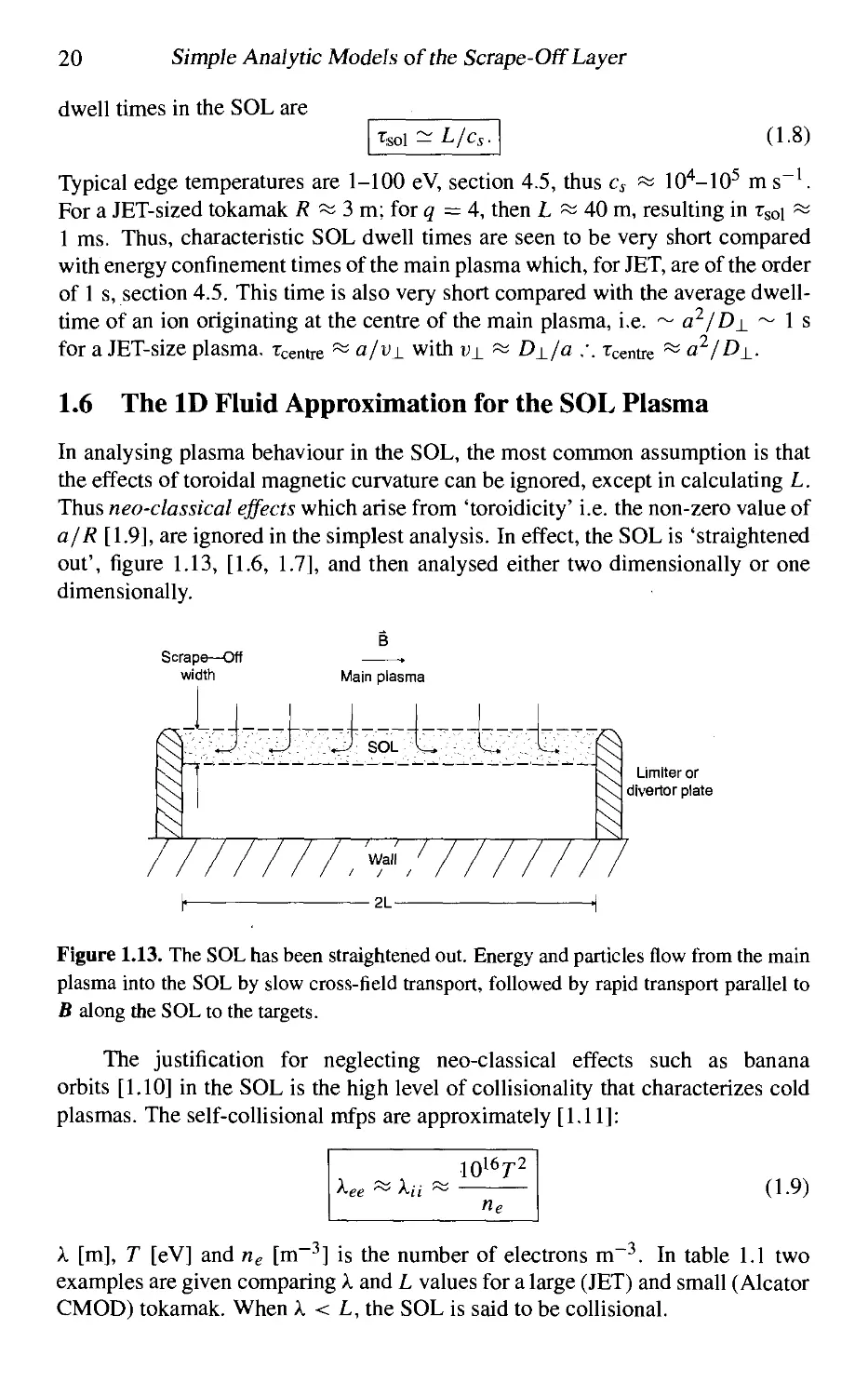
1.6 The ID Fluid Approximation for the SOL Plasma
In analysing plasma behaviour in the SOL, the most common assumption is that
the effects of toroidal magnetic curvature can be ignored, except in calculating L.
Thus neo-classical effects which arise from 'toroidicity' i.e. the non-zero value of
a/R [1.9], are ignored in the simplest analysis. In effect, the SOL is 'straightened
out', figure 1.13, [1.6, 1.7], and then analysed either two dimensionally or one
dimensionally.
Limiter or
divertor plate
h
-2L-
H
Figure 1.13. The SOL has been straightened out. Energy and particles flow from the main
plasma into the SOL by slow cross-field transport, followed by rapid transport parallel to
B along the SOL to the targets.
The justification for neglecting neo-classical effects such as banana
orbits [1.10] in the SOL is the high level of collisionality that characterizes cold
plasmas. The self-collisional mfps are approximately [1.11]:
ke
Xi.
101672
(1.9)
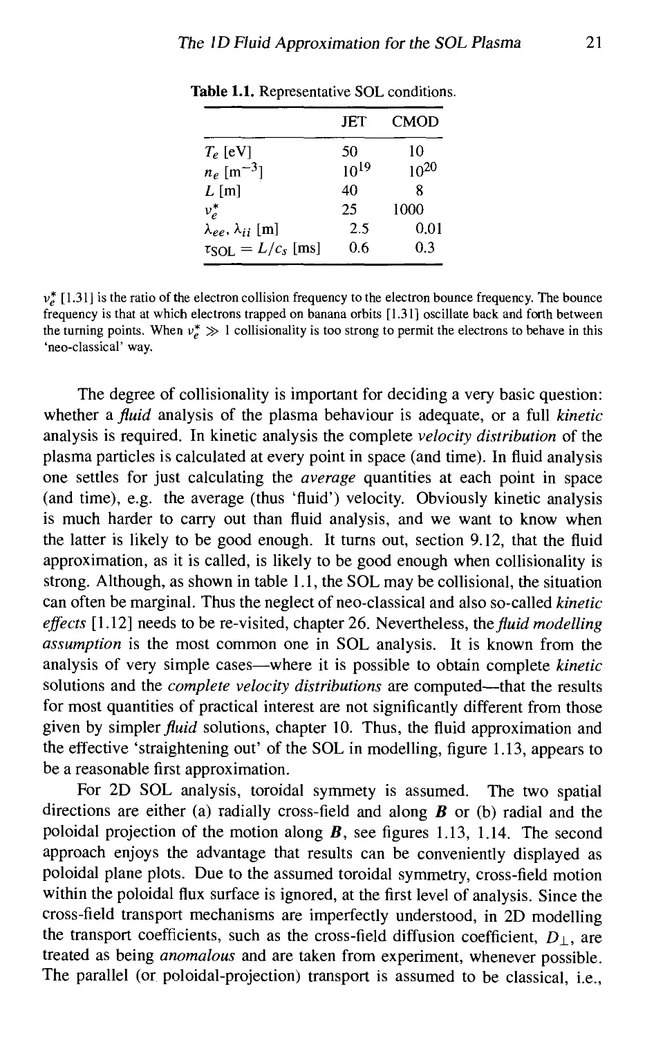
X [m], T [eV] and ng [m"-'] is the number of electrons m"-'. In table 1.1 two
examples are given comparing k and L values for a large (JET) and small (Alcator
CMOD) tokamak. When k < L, the SOL is said to be collisional.

The ID Fluid Approximation for the SOL Plasma 21
Table 1.1. Representative SOL conditions.
Te [eVl
He [m"
L[m]
K
^eC' ^ii
TSOL =
']
[m]
L/cs [ms]
JET
50
IQl"
40
25
2.5
0.6
CMOD
10
1020
8
1000
0.01
0.3
V* [1.31] is the ratio of the electron collision frequency to the electron bounce frequency. The bounce
frequency is that at which electrons trapped on banana orbits [1.31] oscillate back and forth between
the turning points. When v* » 1 collisionality is too strong to permit the electrons to behave in this
'neo-classical' way.
The degree of collisionality is important for deciding a very basic question:
whether a fluid analysis of the plasma behaviour is adequate, or a full kinetic
analysis is required. In kinetic analysis the complete velocity distribution of the
plasma particles is calculated at every point in space (and time). In fluid analysis
one settles for just calculating the average quantities at each point in space
(and time), e.g. the average (thus 'fluid') velocity. Obviously kinetic analysis
is much harder to carry out than fluid analysis, and we want to know when
the latter is likely to be good enough. It turns out, section 9.12, that the fluid
approximation, as it is called, is likely to be good enough when collisionality is
strong. Although, as shown in table 1.1, the SOL may be collisional, the situation
can often be marginal. Thus the neglect of neo-classical and also so-called kinetic
effects [1.12] needs to be re-visited, chapter 26. Nevertheless, the fluid modelling
assumption is the most common one in SOL analysis. It is known from the
analysis of very simple cases—where it is possible to obtain complete kinetic
solutions and the complete velocity distributions are computed—that the results
for most quantities of practical interest are not significantly different from those
given by simp\eT fluid solutions, chapter 10. Thus, the fluid approximation and
the effective 'straightening out' of the SOL in modelling, figure 1.13, appears to
be a reasonable first approximation.
For 2D SOL analysis, toroidal symmety is assumed. The two spatial
directions are either (a) radially cross-field and along B or (b) radial and the
poloidal projection of the motion along B, see figures 1.13, 1.14. The second
approach enjoys the advantage that results can be conveniently displayed as
poloidal plane plots. Due to the assumed toroidal symmetry, cross-field motion
within the poloidal flux surface is ignored, at the first level of analysis. Since the
cross-field transport mechanisms are imperfectly understood, in 2D modelling
the transport coefficients, such as the cross-field diffusion coefficient, Dj_, are
treated as being anomalous and are taken from experiment, whenever possible.
The parallel (or poloidal-projection) transport is assumed to be classical, i.e.,

22
Simple Analytic Models of the Scrape-Off Layer
■ magnetic field lines flux surface
Figure 1.14. The path of a magnetic field hne projected onto a poloidal plane. Distances
along the field hne i|| have corresponding value in the poloidal plane, sg. Analysis of the
plasma behaviour can then be calculated in terms of ^jy or sg.
as if there were no magnetic field. It is usually not possible to carry out any
significant 2D modelling analytically and 2D fluid modelling of the SOL now
uses sophisticated computer codes [1.13].
It can be difficult to gain insight into SOL behaviour from 2D code
modelling, and so the intentive is strong to extract as much as possible from ID
analytic modeUing. Such ID analysis is the principal focus in this book. The
cross-field transport of particles and energy are treated as sources of particles and
energy in the ID analysis along the field B.
1.7 The Simple SOL and Ionization in the Main Plasma
As discussed in section 1.1, hydrogenic neutrals formed by recombination on
solid surfaces enter the plasma and are re-ionized in the fuel recycle process. Once
all solid surfaces are saturated, the plasma density in both the SOL and main
plasma (the confined plasma on the closed flux surfaces inside the separatrix or
LCFS) remains constant, with no new fuelling required unless active pumping is
employed. In the simplest situation the neutrals have a sufficiently long ionization
mfp that they pass through the SOL and are ionized inside the main plasma. This

The Simple SOL and Ionization in the Main Plasma
23
Limiter
Divertor
Figure 1.15. Neutral hydrogen recycling from a limiter tends to be ionized inside the
LCFS, while hydrogen recycling from divertor targets tends to be ionized in the SOL and
private plasma.
has a better chance of happening in limiter configurations—where the recycling
surface, the limiter, is in intimate contact with the main plasma—than for divertors
where the targets may be remote, see figure 1.15. Ionization in the main plasma
results in rapid dispersal of the resulting ions along field Unas, so that by the time
the ions diffuse across the LCFS into the SOL, all details of the actual 2D spatial
distribution of the source have been obUterated, and as far as the SOL is concerned
it experiences a source of particles which is distributed more or less uniformly
along L. Due to this simplification, such deep or main plasma ionization of the
hydrogenic particles is taken to be an important part of the definition of the simple
SOL [1.6, 1.7]; [see section 1.8 and chapter 4].
This regime then yields a particularly simple estimate for the SOL radial
width XsoL' the plasma particles diffuse cross-field beyond the LCFS a
characteristic diffusion distance of about
^SOL — (Oxtsol)
1/2
^SOL = {Dj_L/Cs)
1/2
(1.10)
before being removed (A, sol ^ I'x^soL '
tion (1.10)). For a typical SOL: D_l = 1 m^ s"', L = 50 m, Tsol = 25 eV,
c^ = 5 X 10"* m s~', thus Xsol ^ few cm. One notes how very short a distance this
(0±/A,soL)tsoL, thus giving equa-
,2 e-i

24
Simple Analytic Models of the Scrape-Off Layer
/
target',
Main
plasma
LCFS
SOL
/target target
TTTTTTTT
wall
Main
plasma
LCFS
SOL
/
/target
TTTTTTTT
wall
'SOL
'SOL
SIMPLE SOL
ionization
regions
INON—SIMPLE SOlj
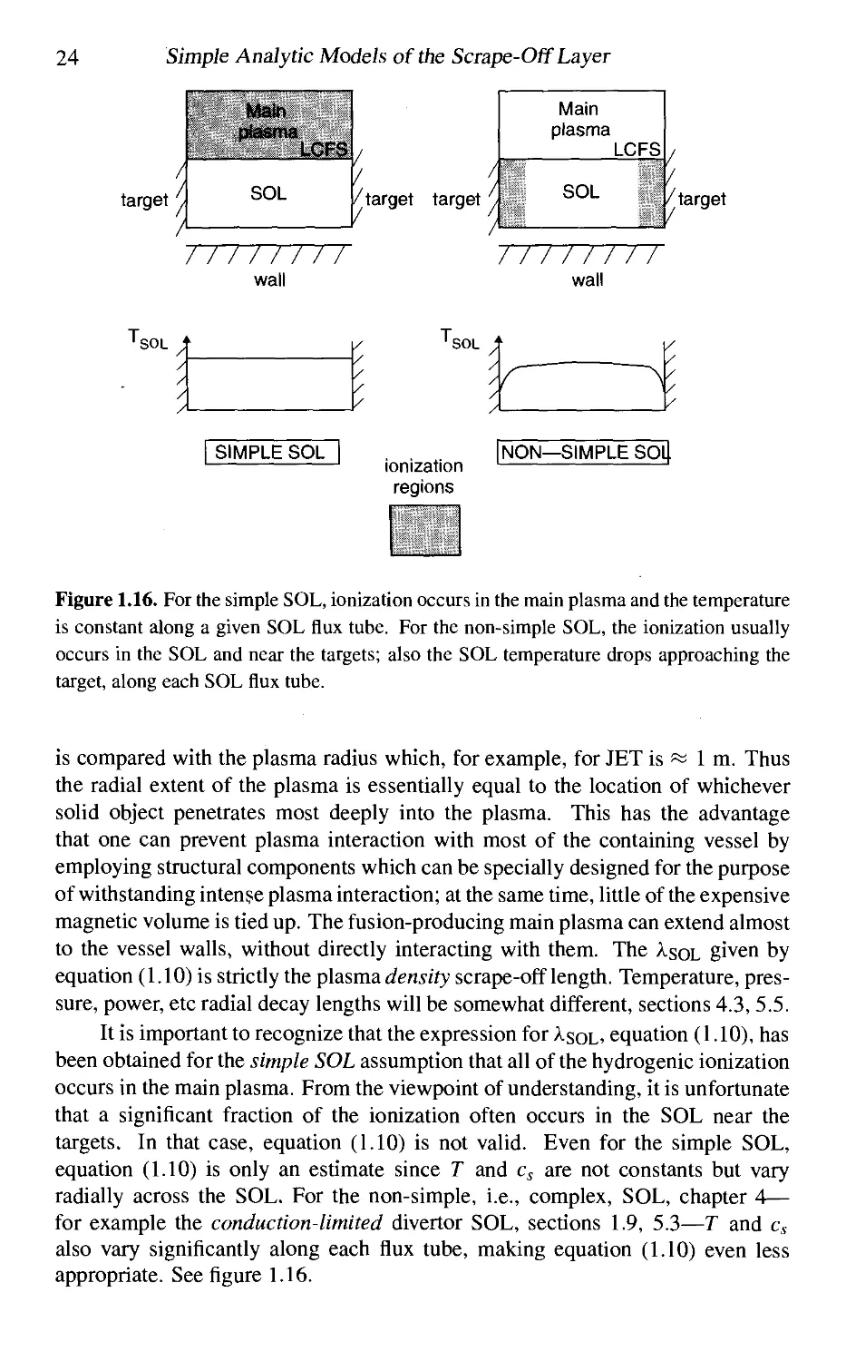
Figure 1.16. For the simple SOL, ionization occurs in the main plasma and the temperature
is constant along a given SOL flux tube. For the non-simple SOL, the ionization usually
occurs in the SOL and near the targets; also the SOL temperature drops approaching the
target, along each SOL flux tube.
is compared with the plasma radius which, for example, for JET is sa l m. Thus
the radial extent of the plasma is essentially equal to the location of whichever
solid object penetrates most deeply into the plasma. This has the advantage
that one can prevent plasma interaction with most of the containing vessel by
employing structural components which can be specially designed for the purpose
of withstanding intense plasma interaction; at the same time, little of the expensive
magnetic volume is tied up. The fusion-producing main plasma can extend almost
to the vessel walls, without directly interacting with them. The AsoL given by
equation (1.10) is strictly the plasma tfeni'ify scrape-off length. Temperature,
pressure, power, etc radial decay lengths will be somewhat different, sections 4.3,5.5.
It is important to recognize that the expression for AsoL^ equation (1.10), has
been obtained for the simple SOL assumption that all of the hydrogenic ionization
occurs in the main plasma. From the viewpoint of understanding, it is unfortunate
that a significant fraction of the ionization often occurs in the SOL near the
targets. In that case, equation (1.10) is not valid. Even for the simple SOL,
equation (1.10) is only an estimate since T and Cj are not constants but vary
radially across the SOL. For the non-simple, i.e., complex, SOL, chapter 4—
for example the conduction-limited divertor SOL, sections 1.9, 5.3—T and Cj
also vary significantly along each flux tube, making equation (1.10) even less
appropriate. See figure 1.16.

The Simple SOL and Ionization in the Main Plasma
25
/////////
U _LCFS
■B,
LCFS
///?7////
B
//JLLU//
LCFS
-►B,
LCFS
/77Y//?//
Figure 1.17. The bevel-sided poloidal limiter B has a larger plasma-wetted area than the
flat-sided A. Toroidal view.
Figure 1.18. The bevel-sided toroidal limiter B has a larger plasma-wetted area that the
flat-sided A. View of the poloidal cross-section.
Unfortunately, the small values of Asol tend to result in plasma-wetted areas
which are very small—and always much smaller than the geometrical surface
area of the vessel, all of which could, in principle, be available for plasma heat
removal. Mechanisms to increase the effective D^^^ are therefore of interest [1.14-
1.17]. For the case of a single, washer (flat sided) poloidal limiter the plasma-
wetted area is Awet = 2[7r(a 4- ^sol)^ — ita^\ » 47raAsoL- Example: a = 1 m,
AsoL = 1 cm, Awet ^0.1 m^, which is minuscule compared with the total wall
area, Awaii ~ InRlna « 100 m^ for i? = 3 m (JET size). One can shape
the poloidal limiter so that its surface only gradually increases in minor radius
in the toroidal direction, thus increasing Awet substantially—although still not
approaching A wall, figure 1.17.
For a single, flat-sided toroidal ring limiter, A^et ^ 47ri?AsoL> i-e. larger
than for the poloidal limiter. One can also shape a toroidal limiter to be almost
tangential to the LCFS, increasing Awet significantly, figure 1.18.
On the TFTR tokamak, the inner wall was employed as a toroidal limiter in
this arrangement, giving Awet «^ 5 m^ [1.18]. Provided the freedom to vary the
plasma shape (and LCFS shape) can be sacrificed, then such toroidal wall limiters
could in principle have Awet so large as to approach Awaii- One would also have
to avoid all wall protrusions in the wetted area, requiring careful alignment of the
protective tiles in order to avoid hot spots [1.19].

26
Simple Analytic Models of the Scrape-Off Layer
NWWN
Figure 1.19. The divertor plasma can be spread over a larger target area, case B, compared
with case A, by expanding the poloidal field at the targets, i.e., by making Bq weaker there.
For poloidal divertors, Awet can be increased above AnRXsoL by exploiting
the fact that the radial separation of the poloidal magnetic flux surfaces near
the target can be increased using external magnetic coils, figure 1.19. This is
considered further in section 5.6.
1.8 ID Plasma Flow Along the Simple SOL to a Surface
1.8.1 The Basic Features Reviewed
For clarity, we start by simply stating, without proof, the basic features of ID flow
along the SOL [L6, L7]. In the subsequent section these results are derived.
(1) The plasma fluid flows along the SOL due to the presence of a particle
source and sink, the limiter/divertor surfaces. But how does the plasma
'know', at each point along the SOL, that it is supposed to be moving toward
the surface? Why isn't the SOL plasma stagnant? Why does it become
accelerated up to a non-zero velocity i;? What is the local force causing
this? It is the parallel pressure gradient which is induced in the SOL plasma
by the presence of source and sink. See figure 1.20. The total pressure
is constant along B, but the static pressure decreases, providing the force:
Ptotai = ^static + Adynamic, where Pdynamjc = mnv^; thus as ^static drops, the
flux of flow momentum, mnv^, increases, and i; increases; see chapter 9.
(2) In the first few /us after the plasma is initiated—that is just after ionization
of the fill gas in the vacuum vessel and before the recycling and ionization
have become established, the electrons, due to their small mass and high
mobility, rush ahead of the ions and strike the solid surfaces, charging them
up negatively.
(3) From that time on, an electron-repelling potential difference exists between
the plasma and the surface, slowing the loss rate of the electrons—while,
at the same time, increasing the ion loss rate. The potential spontaneously

ID Plasma Flow Along the Simple SOL to a Surface
B
27
kTe
Electric ^se~'~^
potential
Plasma
fluid
velocity
Ion and
electron
density
Figure 1.20. Schematic of the variation of plasma pressure, electric potential, plasma
velocity and ion/electron densities in the plasma between two semi-infinite planes. The
thickness of the sheath is exaggerated for clarity. The total length is 2L.
(4)
adjusts, on an isolated or electrically floating surface, until the loss rates
of the two charge species become equal—defined as ambipolar plasma
transport—i.e. an ambipolar electric field arises in the plasma. It will be
found that the solid surface will spontaneously charge up to a potential of
Vwaii ~ —'ikTg/e, for a hydrogenic plasma, relative to Xhe plasma potential.
The plasma is an excellent conductor in the direction along B and can be at
almost a constant potential along any given magnetic field line.
Electrostatic potentials on surfaces contacting plasmas are almost entirely
shielded out within a short distance—regardless of whether the potential
arises spontaneously or is applied as an external voltage on an electrode.
This phenomenon is termed Debye shielding and it occurs over a very short
distance of the order of the Debye length [ 1.20]:
Aoebye = (eokTe/ngC'^)^^'^.
(1.11)

28 Simple Analytic Models of the Scrape-Off Layer
Example: Tg = 20 eV, Ug = 10^' m"^, .-. Aoebye ^ 10"^ m.
This thin region is called the Debye sheath and is a region of net positive
space charge, existing in a dynamic equilibrium: the ions continue to
move through the sheath at high speed. The positive charge density
[coulombs m~^], integrated through the sheath thickness, almost equals
the negative charge density existing on the solid surface. Thus the rest of
the region upstream of the sheath—the essentially neutral plasma itself—is
almost completely shielded from the electric field due to the space charge
density in the sheath.
(5) The shielding is not perfect, however, and a small electric field £ « fc Tg / 2e L,
penetrates throughout the length of the plasma where the particle source
exists. This is called the pre-sheath electric field and it acts on the ions
in the SOL to help move them toward the target.
(6) The surface sink action causes a depression of the local plasma density
creating a parallel density and pressure gradient. The pre-sheath field acts
to retard the electrons, which come into a nearly perfect parallel momentum,
i.e. force, balance between a parallel pressure gradient force pushing the
electrons toward the surface, and the retarding electric field force. The
electrons thus obey, almost perfectly, a Bo/fzmann/actor relation [1.21, 1.22]
n = noexp[eV//tre]. (1.12)
no is the plasma density upstream where the plasma potential is taken to be
V = 0. As the surface is approached V becomes more negative (the pre-
sheath electric field). It is also noted that a parallel ion pressure gradient
exists (equal to the electron one if Tg — Ti), but this adds to the £-force on
the ions. There is a direct link between the pressure and potential gradient
implied in the Boltzmann relation. Assuming quasineutrality, Ug — rii, and
one-dimensional ambipolarity, i.e. Tg = F,- where F = ni; is particle flux
density, the electron fluid velocity must equal the ion fluid velocity. Thus
the electrons cannot actually be in perfect force balance along B. However,
it will be shown that the electron + ion fluid velocity is much less than the
electron thermal speed, Cg = {%kTe/7rmg)^/^, and that the electron force
balance is almost exact. The extreme lightness of the electrons requires that
they be in nearly perfect force balance, otherwise extremely high electron
fluid speeds and currents would occur.
(7) While the ambipolar electric field acts on both the ion fluid and the electron
fluid individually, it can exert no force on the plasma fluid—which is the
sum of the e and i fluids and is therefore (quasi-) neutral. As mentioned in
point (1), the only force accelerating the plasma fluid toward the surface is
the pressure-gradient force. See figure 1.21.
(8) In the foregoing it has been implicitly assumed that the plasma is isothermal
along any given flux tube in the SOL. Since the SOL plasma has very high
heat conductivity this can be a good approximation. The effect of parallel

1D Plasma Flow Along the Simple SOL to a Surface 29
1/
Forces on electrons:
Forces on, ions:
^ "-ax"
->eE
-> dpi
dx
, ^ d(Pe+Pi)
Forces on plasma: ►■—gr
Figure 1.21. The electrons are almost in perfect force balance, while for the ions the
electric field force and the ion pressure gradient force are additive (and equal if Te = Tt,
the case shown here), accelerating the ions. The force on the plasma is due to the total
pressure gradient alone, since an electric field exerts no force on the quasineutral plasma.
T-gradients will be discussed in section 4.10. Here we note that a further
element of the definition of the simple SOL is that parallel gradients be small.
This constitutes the sheath-limited regime; see sections 1.9, 9.10. It will
be shown that both charge species have a fluid speed which reaches the ion
acoustic speed: Cj = [fc(re + r,)/m,]^''^ just as the particles enter the sheath,
that is Vse = Cs, where Vge is the velocity at the sheath edge.
(9) It will be found that the plasma density drops from no at distance L upstream
to rise = 5"0 at the sheath edge.
1.8.2 Derivations of Results for ID Plasma Flow in the Simple SOL
L8.2.1 The ID Fluid Equations
In this section the fluid particle and momentum conservation equations for an
isothermal plasma are derived in an intuitive way. A more systematic derivation
is given in chapter 9.
First we show that the particle flux density F [particles m~^ s~^], is given
by r = nv where i; is the bulk or fluid speed {not to be confused with the
individual particle speed which has a component due to random, thermal motion
as well as the common fluid speed v of all the particles). Here we will follow
the usual custom: the absence of any subscript on i; indicates fluid velocity. If
random, thermal or other types of velocity are intended, appropriate subscripts
are employed. Consider figure 1.22 where a 'slug' of fluid of cross-sectional area
A [m^] drifts at velocity i; past an observer.
In time t [s] a slug of length vt [m] will pass the observer, containing ni;f A
[particles]. Thus the number of particles per m^ per s passing the observer is nv,
which we define to be F.

30 Simple Analytic Models of the Scrape- Off Layer
Flow
At t=0:
'Slug'
of fluid
Observer
Atts:
vt [m]
Figure 1.22. Demonstration that V = nv.
Consider next figure 1.23 and the conservation of particles or mass, in ID
for steady state. We must allow that F can be a function of x, the distance in
the ID flow direction and that a source of particles—perhaps due to ionization
of neutrals—is present of strength Sp [particles m~^ s~']. The net outflow of
particles from the volume shown in figure 1.23 is
r,„ +A;c—-r,„ )A = AxA— (1.1
ax J dx
3)
which must equal the creation rate in the volume:
A;cA5n
(1.14)

ID Plasma Flow Along the Simple SOL to a Surface
31
r =r
A[m2]
Source S [particles/'m^/'s]
°"' dx
Figure 1.23. Demonstration of the particle conservation equation.
thus giving the particle conservation equation:
dr _ d{nv)
dx dx
Sp.
(1.15)
The ID steady-state, momentum conservation equation can be arrived at from
Newton's second law:
dv dv dx dv
F = ma = m— = m = mv —
dt dx dt dx
(1-16)
applied to the n particles per m-', gives
nmv— = nr
dx
(1.17)
and the total force m ^, nf, is due to several contributions:
dp
nF = neE ; «^drag
djc
(1.18)
where neE is the parallel S-force exerted on particles of charge +e. From
figure 1.24 it can be seen that the net pressure force on the particle in the volume
shown is:
-(p + A.g)+p
A
dp
dx
(1.19)

32
Simple Analytic Models of the Scrape-Off Layer
-* X
A[m2
Figure 1.24. Demonstration of the pressure-gradient force.
giving a net /7-gradient force on the particles in one m^ of —dp/dx. One notes
the minus sign: the force is in the opposite direction to the increasing pressure!
The drag force can include various contributions. There can be viscous
drag and drag due to momentum-loss collisions with neutrals, but we start by
neglecting such forces here. There is also an effective drag in the fluid picture due
to the particle source Sp. In the fluid picture afl particles at a given location x have
the same drift velocity i;(;c); we assume here, however, that the newly created ions
come from non-moving neutrals, and so the momentum required per m^ per s to
bring them instantly up to the local speed, mvSp, constitutes a local drag force on
the fluid. Thus we obtain the ID, steady-state momentum equation:
di; dp
nmv— = neE
dx dx
mvS
p-
(1.20)
One can proceed further to derive an energy conservation equation but that is not
necessary if isothermal conditions are assumed, as here. Thus one has two
equations, (1.15) and (1.20), in the two unknowns n{x), v{x)—i.e., the two dependent
variables—in terms of one independent variable x. It may appear that p{x) is a
further unknown; however, for the isothermal assumption one has p{x) = kTn{x)
with T a parameter which has to be found from some other considerations. If the
isothermal assumption is relaxed then one needs the energy conservation equation
also. We can also remove £ as a dependent variable by using the Boltzmann
relation. Sp, m and e must be given.
These two equations will be sufficient to demonstrate the most basic features
of plasma flow along the SOL.

ID Plasma Flow Along the Simple SOL to a Surface 33
1.8.2.2 The Boltzmann Relation for Electrons
Consider the momentum equation for the electron fluid:
dv dpe
nmgV— = —neE meVSp (1-21)
ax ax
giving approximately:
V kTg nv
nmeV— ^ —neE —n— nieV— (1-22)
where L is the characteristic parallel length of spatial variations along the SOL
and we used also the particle conservation, equation (1.15), Sp = d{nv)/dx ^
nv/L. Although we have not yet proved that the characteristic drift speed along
the SOL is Cj, we appropriate that result here; we will have to confirm consistency
at a later point. Thus:
nme— = -neE —^ y^ (1.23)
which, taking Tg = Ti becomes approximately
me2kT ^ nkT me2kT ,,^.^
n— ^-neE n—^ (1.24)
Mi L L m; L
and thus it is seen that, indeed, the inertia term and the drag term are of the
order mg/m, ^ 1 of the pressure-gradient term. The force balance for electrons
is thus between the electric field and —dpe/dx, to an excellent approximation,
figure 1.21. Inserting E = —dV/djc and integrating then gives the Boltzmann
factor relation, equation (1.12). It is to be emphasized again that the electrons can
satisfy the Boltzmann relation quite closely, yet have a substantial fluid velocity
of order Cg ^ Cg. A more rigorous derivation of the Boltzmann relation is given
in section 2.2.
1.8.2.3 Modelling the Ions
Because the electrons experience a retarding f-field in the SOL, modelling has
been seen to be very simple; the Boltzmann factor contains all the electron
information. Also, it can be shown (1.22) that the electron velocity distribution remains
Maxwellian in a retarding f-field (that is sufficiently strong to limit particle loss
from the system), which is a further valuable simplification; the total number of
electrons m^-' merely decreases with increasingly negative V. The ions, on the
other hand, are in an accelerating field which substantially disturbs their velocity
distribution, which may have been MaxweUian far from the absorbing surface.
For the ions it is necessary to retain the terms which could be dropped for the

34 Simple Analytic Models of the Scrape-Off Layer
electrons, last section. We thus have the first two conservation equations for ions:
'-^ = S, (1.25)
^^ ^P' , Z7 c n ^A^
nmv—= \-enE—mvSp. (l-2o)
dx dx
Note that m from now on designates the ion mass, while n, v and Sp need no
subscripts to distinguish between electron and ion, since we are assuming here:
(a) singly charged ions, (b) Wg = n;, (c) ambipolar outflow, Vg = vi, and (d) ions
and electrons produced at the same rates. With the isothermal assumption made
here,
-— =kTi—- (1.27)
djc djc
and so, again, there are only two dependent variables—n and v—and a parameter
Ti (which has to be established by separate considerations). We can thus achieve
the objective of establishing n{x), v{x), V{x). We are able to replace E using the
Boltzmann relation for the electrons:
dn
enE = -kTe— (1.28)
djc
and so can re-write the plasma momentum equation ('plasma' because the
electron and ion momentum equations have been combined):
Av jAn
nmv— =—mc mvS„ (1-29)
djc djc
where Cj is, strictly, the isothermal plasma acoustic speed equation (1.5).
(Retaining the mg-related terms in equation (1.21) and adding the electron and ion
momentum equations together, rather than using the Boltzmann relation for the
electrons, gives equation (1.29) with m = me + mi.) One may note that E does
not appear in equation (1.29). The first term on the RHS is the sum of the e and i
pressure gradient forces, figure 1.21. It is convenient to define the plasma Mach
number:
M = v/cs. (1.30)
The two equations (1.25), (1.29) can be combined to eliminate An/dx and give a
most informative result:
AM _ Sp {\+ M^)
~Ax ~ nc^(l -M2)'
(1.31)

ID Plasma Flow Along the Simple SOL to a Surface
35
Figure 1.25. The rate coefficients for atomic and molecular hydrogen [1.23]. The
numbered reactions are (1): e + H2 ^ H^ + 2e, (2): e + H2 ^ 2H° + e, (3): e + H2 ^
H0 + H+ + 2e, (4):
e + H+
2H'
0
H+ + 2e, and charge exchange (7): H^ + H+ ^ H+ + H^.
(5): e + H+ ^ rO + H+ + e, (6): e + H'
0
1.8.2.4 The Particle Source Sp
The two particle 'source' mechanisms that usually dominate the SOL are: (a)
local ionization of neutrals by the plasma electrons, (b) cross-field diffusion. The
latter is not a true source of ions in the overall system, but appears as such in 1D
analysis.
(a) Electron ionization.
Assuming the electrons are Maxwellian, the basic atomic and molecular
cross-sections from experiment can be integrated over the velocity
distribution (1.25) to give the rate coefficients Wv{Te) [nr' s^^], shown in
figures 1.25-1.28, [1.23, 1.26]. Thus, for example, the rate of ionization
of hydrogen atoms by electron impact, 5,j. [ionization events m'^ s^'],
IS
Siz =
nena^iz, where mh [H atoms m'^] is the atom density and
one uses curve (6) in figure 1.25. Figure 1.25 shows ctiJ,j. values for a
number of important processes for hydrogenic neutral atoms and molecules.
Figures 1.26-1.28 show ctiJ,j. for several important plasma impurities.
Figures 1.29-1.31 indicate the principal hydrogenic reactions schematically.
A certain fraction of the hydrogenic ions recycling from the limiter/divertor
targets are promptly back-scattered as neutral atoms with energies which

36 Simple Analytic Models of the Scrape-Off Layer
Log 10
- lii
-13
" -14
CO
E
r-15
o
<D -16
o
o
s
2 -17
c
o
■Jo
■^ -18
-19
-20
[
r
r
r
[ /
: c+
c"
^"^ -~-
^ ~~~—
^ ——~
/ ^
/7~
/ r5+
1 2
Electron temperature [eV]
^ Log^o ^
Figure 1.26. Ionization rate coefficients for carbon [1.24].
are an appreciable fraction of the ion impact energy; see section 3.1 and
figure 1.29. For these neutrals one uses reaction (6) to calculate ctiJ,z in
figure 1.25. The other particles recycle as neutral molecules, figure 1.29;
some of these will be directly ionized, reaction (1) of figure 1.25, while
others will be dissociated into two Franck-Condon atoms by electron
impact, reaction (2), with those atoms—of energy about 2 eV [1.26]—
becoming ionized, reaction (6), figure 1.30. A most important process
for hydrogenic particles is that of resonant charge exchange, reaction (7),
figure 1.25: the collision of a slow atom entering from the wall and a
hot plasma ion results in the creation of a fast atom which, if moving
inward, can penetrate deeply into the plasma before ionizing. Indeed,
because the resonant charge exchange rate is higher than the ionization
rate, this process may be repeated several times resulting, effectively, in
a 'neutral accelerator'; figure 1.31. Figure 1.25 indicates that a number
of other processes also have to be considered when attempting to model
the behaviour of neutral hydrogen in a hydrogenic plasma. The task is
a complex one to carry out in detail and for this reason, a number of
computer codes have been written over the years to incorporate these and
other processes. Currently the most sophisticated treatments are the Monte
Carlo codes, DEGAS, EIRENE and NIMBUS [1.13]. The 2D or even 3D

ID Plasma Flow Along the Simple SOL to a Surface
37
solid-surface configurations and background plasma, including Tg, Ti and
He as functions of space, are specified as inputs. The recycling neutrals are
then launched from the appropriate locations on the limiter/divertor targets
where ions arrived, and followed until they are finally ionized—perhaps
after a number of wall reflections, charge exchange events, etc.
Impurity particles often enter the plasma as atoms and thus do not usually
experience as complex a set of reactions as hydrogen. Even a molecular
impurity such as N2 will not experience the strong charge-exchange process
that hydrogen does because the N + H+ ^- N+ + H charge-exchange
process is not resonant, i.e., a potential-energy difference is involved.
The use of sophisticated code modelling of the neutrals is appropriate for
coupling to the 2D fluid codes of the SOL [1.13], such as B2, UEDGE,
EDGE2D, etc, chapter 13. For our present purposes of simple ID
analytic treatment we will assume for hydrogen the existence of an effective
ionization rate coefficient Wvi^{Te) as an average of reactions (1) and (6)
of figure 1.25. The effect of energetic back-scattering and the
'acceleration' process of Franck-Condon dissociation and charge exchange is to
make neutral hydrogen penetrate a plasma more deeply before becoming
ionized than would be the case if the neutral only had its original thermal
velocity, corresponding to the temperature of the solid surface. This can be
allowed for, approximately, by assuming that the penetrating neutral velocity
Logio
-Id
-14
;p -15
CO
1-16
c
<u
0 -17
<u
0
0
2 -18
.| -19
N
0 -20
-21
-??
0
0*/ / /o=+
0^1
oL 0^^
1
jo'*
06+
1
~"^^
.
—
1
1 2 3
Electron temperature [eV]
Logi,
Figure 1.27. Ionization rate coefficients for oxygen [1.24].

38
Simplt Analytic Models of the Scrape-Off Layer
1 2 3
Electron temperature [eV]
Logi,
Figure 1.28. Ionization rate coefficients for neon [1.24]. One may note how difficult it is
to ionize the He-like ions C'*+, 0^+, Ne*+.
is greater than the thermal velocity by some specified amount, or using more
sophisticated—yet still simple—estimates, see section 4.6.
We then have:
Sp,iz =nn„'avi^(Te) [ion pairs m"" s^ ] (1.32)
where n = plasma density (strictly Wg) and n„ — neutral density (some
average of atomic and molecular),
(b) Cross-field diffusive 'source'.
Consider now the radial, cross-field direction r, figure 1.32, and the fact
that parallel removal to the soUd surface constitutes a particle sink for the
cross-field particle flux density, r±. Thus, conservation of particles for the
r-direction:
dTx
dr
= Spi. < 0.
(1.33)
This cross-field sink gives the parallel source term Sp^c-f we are seeking:
^P.c-f
= S,
-'pi-
Let us assume further that Fx satisfies Pick's law of diffusion:
r±
^ dn
(1-34)
(1.35)

ID Plasma Flow Along the Simple SOL to a Surface
39
backscattering
adsorption
subsequently
slow
molecule
thermal release
of molecule
Figure 1.29. Hydrogen atomic ions striking a surface may be energetically back-scattered
as a neutral or be adsorbed, subsequently combining with a second atom and thermally
desorbing as a molecule.
The plasma density decays radially with characteristic length AsoL>
section 1.6, and so
(1.36)
Thus:
dn
d^ "
n d^n
>^SOL dr^ ~ A
Sp.c-f = -DinAsQL.
n
2
SOL
(1.37)

40
Simple Analytic Models of the Scrape-Off Layer
Franck-
Condon
dissociation
one-step
ionization
of molecule
to H+ + H°
two-step
ionization
of molecule
to H+ + H°
Figure 1.30. A hydrogen molecule struck by an electron may dissociate by the
Franck-Condon process, creating two atoms of kinetic energy a few eV, or be ionized
in a one-step or two-step process.
One may note that both Spj^ and 5p,c-/ vary directly as plasma density, which
turns out to be rather convenient for purposes of simple analysis.
1.8.2.5 Sonic Flow of Isothermal Plasma into the Sheath
Returning to equation (1.31) we note that the term Sp/ncg is intrinsically positive.
Thus, assuming from symmetry that the flow at distance L from the surface,
i.e. halfway between two surfaces, is stagnant, i.e. i^CO) = M(0) = 0, then

ID Plasma Flow Along the Simple SOL to a Surface
41
Resonant
charge
exchange
Figure 1.31. A neutral hydrogen atom has a large cross-section for charge exchange with
a plasma ion. The neutral can thus, in effect, be strongly accelerated, penetrating deeply
into the plasma. In this figure, imagine that B is parallel to the solid surface and that the
ions move freely along B while experiencing gyroscopic motion about B. If the charge
exchange collision occurs at an instant when, as a result of the ion's gyroscopic motion,
it happens to be moving away from the wall, then the fast atom created by the charge
exchange event will be launched toward the centre of the plasma.
dM/dx > 0 here, the flow accelerates towards the surfaces—as it must, of course.
We note that M cannot exceed unity without introducing an unphysical singularity
in the midst of the flow field. We are, however, attracted to the idea that just at
the plasma-sheath interface M reaches unity [1.6, 1.7]: this will, indeed, imply
infinite gradients for n, v, V at that point—but we know that the sheath, being very
thin, is a region where any finite changes in n, v, V will give gradients that are
extremely large compared with the ones in the plasma. Thus, to the same degree
of approximation that we have employed in treating the plasma as being precisely
neutral, we may accept that all gradients become infinite at the plasma-sheath
interface.
Alternatively, one need not divide the space filled by the charged particles
into the two absolutely distinct regions, i.e. the plasma where «<, = n,- exactly,
and the sheath where ne < n,-. Instead, the entire space can be analysed as one
region, employing Poisson's equation in order to relate the charge imbalance,
(n, — He), to d^y/djc^, i.e. Poisson's equation provides the extra equation when
He ^ «(• In that case no infinite gradients occur and it is found that at the point
where (n,- — «<,)/«,• becomes significant, then M » I [1.27], corresponding in
the simpler, two-region analysis, to the plasma-sheath interface. Such an analysis
must be numerical, however, and much insight is thereby lost.
It should be noted that we have not proven here that M = 1 at the plasma-
sheath interface. What has been demonstrated is that M cannot exceed 1 in an

42 Simple Analytic Models of the Scrape-Off Layer
B
X
r
//
/
-Spx
^x
Main plasma
LCFS
SOL
Sink:
'p-i-
r Decreases
toward
wall
Source:
r„ Increases toward limiter
Figure 1.32. Cross-field diffusion into the SOL constitutes an effective particle source in
ID, along-the-SOL modelling.
(isothermal) plasma. At the same time we are receptive to the idea that the flow
actually attains sonic speed at the plasma-sheath interface, but this remains to be
proven. To do that we will have to carry out an analysis from the sheath side,
thus obtaining the Bohm criterion [1.28], section 2.3. For now, however, we will
proceed on the assumption that M = 1 at the sheath edge.
We are further inclined toward the idea of sonic flow into the sheath from
the general result that a fluid subject to an uncompensated pressure difference of
orderAp '^ p will 'explode', i.e. it is accelerated to a speed of the order of the
sound speed in the direction of the pressure-gradient force, figure 1.33. This may
be seen by combining the ion and electron momentum equations (1.26) and (1.28)
to give for the plasma fluid:
dv dp
nmv— =
dx dx
(1.38)

ID Plasma Flow Along the Simple SOL to a Surface
43
p = 0
♦• r
dp p K
-^ "-J- ■=!> EXPLOSION
Figure 1.33. An uncompensated pressure-gradient force of magnitude
causes a fluid to expand explosively rapidly.
-dp/dr ~ p/r
for a freely expanding, no-source, ID fluid. Here p = Pe + Pi- In the direction
along B the plasma is subject to no other force than the pressure-gradient force.
Since the sheath acts as a perfect sink for the ions, we anticipate intuitively a
large Ap along the flow direction, of order p itself. From equation (1.38) we have
approximately:
nmv^/L^ p/L^nkT/L (1.39)
where L is the gradient scale length and d is a representative velocity. From
equation (1.39) one directly obtains the important result that free expansion of a
fluid occurs at speed v ~ {kT/mi)^!'^, i.e. at the sound speed.
1.8.2.6 The Velocity Distribution Along the SOL
For either Sp^^ or Sp^c-f we may set:
Sp = Cn
(1.40)
with C some positive parameter (whose value must be found from some
considerations other than the two conservation equations). Thus from equation (1.31)
we have
-A^ 1 _ m2 r^ Cdx
I
Jo

44 Simple Analytic Models of the Scrape-Off Layer
which yields the desired v{x), M{x) as an implicit function:
2tan->M-M = —. (1.42)
We now introduce the boundary condition
M{L) = 1 (1.43)
which is the information, additional to the two conservation equations
themselves, needed to constrain C. We have already assumed the upstream boundary
condition M(0) = 0. (We note that, strictly, we should have used [L-(sheath
thickness)] ^[L — A-oebyel above, but we ignore this tiny correction.) Thus from
equation (1.41):
1 - 1 = ^. (1.44)
2 Cs
We note that this informs us that the source strength is constrained by the
size of the space available, L, and by the plasma temperature (cj)—or, at least,
that all three quantities, C, L, c^, must satisfy a constraint. Unless this constraint
is satisfied the plasma cannot exist in steady state.
(a) Ionization source: The constraint gives:
2 CsiT)
Thus, for steady state, the electron temperature is not a free parameter for
a locally self-sustained plasma (i.e. impact ionization due to the plasma's
own electrons), but Tg is a function of the product n„L. This result has been
known for almost a century for low pressure gas discharges [1.29], where
the degree of ionization is usually very small, and so n„ is simply given by
the original gas fill pressure of the discharge tube, while L is replaced by the
radius R of the (cylindrical) gas tube, since the sink action is primarily radial
to the cylinder walls. Thus a TeiPgnsR) relation is anticipated theoretically,
and is observed experimentally, see figure 1.34 [1.29]. Lowering pgas raises
Tg since each electron then 'has to work harder' to maintain particle balance.
Decreasing R also forces Tg up since the volume (producing the particles,
which is proportional to R^) is reduced relative to the surface area (sink,
which is proportional to R). The gas discharge spontaneously achieves the
value of electron temperature required for particle balance, drawing just
the necessary power input from the applied longitudinal electric field (this
process thus sets the value of that field). If some additional external power
input were added, the longitudinal field would decrease and/or steady-state
conditions would be lost. It is a remarkable fact that it is particle/momentum
balance—rather than power balance—which controls the electron
temperature in a locally self-sustained plasma.

ID Plasma Flow Along the Simple SOL to a Surface
45
Je.
E,
0.01
10
10-2 10-
cRPneutra|[Cn^to''''l
Cathode
Anode
Figure 1.34. For low pressure, non-magnetic electric discharges such as fluorescent lights,
Te is a function of the product /'neutral'^ where R is the radius of the cylinder and Pneutral
is the gas pressure, pgas- £; = ionization potential. Constant c: w 4 x 10 -^ for He,
w 6 X 10-2 foj Ne, w 4 X 10-^ for Ar, « 7 x lO"^ for Hg, ^ W^ for H2, «= 4 x 10"^
forN2 [1.29].
It should also be noted, however, that the foregoing simple picture—where
n„ was treated as a fixed, constant, externally controllable parameter—does
not apply to a tokamak SOL. There, n„ varies spatially by many orders
of magnitude, from regions just near the recycling surface, to deep in the
core [1.30]. We therefore do not conclude, even when ionization within
the tokamak SOL is a large part of the ID flow source, that 7; is fixed,
independent of power balance considerations. We return to the matter of
including the power balance implication of ionization within the SOL, in
section 5.5.
(b) Cross-field panicle source. The constraint now becomes:
n
2
1 =
Dj_ L
(1.46)
"•SOL

46
Simple Analytic Models of the Scrape-Off Layer
Figure 1.35. Spatial variation of flow Macii number for tiiree models: A: Sp ex. He; B;
Sp = constant; C: Sp a (1 - M^)/(2M(l + M^)).
I.e.
/^SOL
m'"
(1.47)
We had obtained this result earlier, equation (1.10). That is, the cross-field
density gradient is constrained by particle/momentum balance.
For either type of source the spatial variation is the same, equation (1.42),
curve A in figure 1.35. One notes that M(x) is not too far from being
linear, but it does steepen to an infinite gradient at the sheath edge, x = L.
This non-linear variation results from assuming Sp an; one can show, see
problem 1.20, that n{x) does not vary greatly with changes in the form of
Sp. One may note that even assuming Sp = constant, curve B in figure 1.35,
does not alter the solution very much. One should note that for the 'complex
SOL' v/here Spiz is also important, section 1.9 and chapter 5, n„(a:) probably
varies strongly, neutral density being much larger near the recycling surface
than far upstream. In such cases one anticipates the M{x) would stay small
until the ionization region near the plates was reached, where it would rapidly
rise to unity, see problem 1.20.
L8.2.7 Variation of Plasma Density Along the SOL
Algebraic manipulation of the two conservation equations also gives the 'conser
vative form of the momentum equation':
d
djc
iPe + Pi + mnv^) = 0
(1.48

ID Plasma Flow Along the Simple SOL to a Surface 47
or:
' ' ' (1.49)
Pe + Pi + mnv^ = constant.
One should note here that the intuitive argument used in section 1.8.2.1
justifying inclusion of an effective drag term that we employed in what might
be called the 'inertial form of the momentum equation' must now be viewed as
somewhat suspect: we do not find such a term in the conservative form,
equation (1.49). Why not? The only fully satisfactory answer is to employ a more
rigorous derivation of the momentum equation, section 9.4.
For the isothermal assumption, equation (1.49) simplifies to give:
n{x) =
1 + [M(x)Y
(1.50)
where no = n(0). Note that equation (1.50) is very general since it is completely
independent of the particle source S^—including its spatial variation; see also
problem 1.20. We know M{x) from equation (1.42), therefore n{x) is also now
known. One notes that the variation of plasma density along the SOL is not very
great for isothermal conditions, only dropping by a factor of 2 from upstream to
the sheath edge.
The particle flux density at the sheath edge, Tse, is therefore:
n 1
1 se = 2^QCs.
(1.51)
1.8.2.8 The Average Dwell-Time in the SOL, rsoL
While the flow velocity is not constant along the SOL, equation (1.42), a
representative value of y is ~ j"^*' figure 1.35, for the spatially 'well distributed'
sources which have been considered here. Thus one estimates tsol ^ L/c^,
equation (1.8). Alternately, we may define tsol to be the particle confinement
time in the SOL, which is the particle content of the SOL divided by the particle
outflux, hence tsol = («soL^)/(2"0Ci) ^ L/c^, as before.
For a complex SOL it can be the case that the ionization distances are very
short and the particle source is concentrated very near the solid surface; the latter
way of defining tsol will still give tsol ^ L/cs. In this case, however, flow only
exists very near the target and most of the SOL is stagnant. Thus the average time
in the SOL involves groups of particles with extremely different dwell times in the
SOL. Indeed ions having v ^>- 0 have dwell times -^ oo! We see again that the
result IsOL ^ {Di_L/cs)^^'^, Equation (1.10), is not applicable. It also appears
that the SOL will extend radially all the way to the wall in these circumstances,
assuming that Dx ^ 0, since many of the particles spend very long times in the
SOL. We will return to this matter in chapter 15 onflow reversal and chapter 19
on the relation among SOL decay lengths.

48 Simple Analytic Models of the Scrape-Off Layer
V
A
Effect
of
varying
Sheath
Figure 1.36. Variation of tiie electric potential on a wall or an electrode is almost entirely
'soaked up' witiiin tiie tiiin siieatii, leaving the plasma unaffected. Here tiie potential on
tiie 'far' (rigiit) wall is assumed not to ciiange as tiie potential of tiie 'near' (left) wall is
varied relative to the plasma potential, which is taken to be V = 0 here. See section 2.6
for the case where a potential difference is applied between the two end walls.
1.8.2.9 The Parallel Electric Field in the SOL
We may combine the Boltzmann relation, equation (1.12), with equation (1.50) to
eliminate n, obtaining:
kT
Vix) = -\n[\+iMix)f]
e
(1.52)
we have M{x) from equation (1.42), thus we know V{x) and E]]{x). This gives
the pre-sheath (i.e. the plasma) electric field, figure 1.20. At the sheath edge one
has
kT
e
kTe
~ -0.7—^.
e
(1.53)
If any larger potential than this is applied externally to a plasma—whether
via electrodes connected to a power supply, or the spontaneous surface charging
which occurs when the more mobile electrons rush to the walls immediately after
initialization of the plasma—then the excess potential is shielded out by the Debye
sheath, figure 1.36.
We will show in section 2.6 that the spontaneous wall charging for floating
(ambipolar) conditions results in a negative surface potential of ~ —3kTe/e for
hydrogenic plasmas. Therefore, most of the latter potential appears across the
sheath, with only ~ —0.1 kTe/e penetrating into the plasma—constituting the

ID Plasma Flow Along the Simple SOL to a Surface 49
ambipolar electric field required to help move the ions at each point along the
SOL to the sink, figure 1.20.
1.8.2.10 Flow With/Without Friction
The above results, for the simple SOL, assumed no true drag, i.e. no viscous
drag and no collisional drag due to neutrals. The rather modest drops of n and V
along the SOL given by equations (1.50) and (1.53) then result. When frictional
drag, e.g. due to collisions with neutrals, is significant the parallel pressure and
potential gradients increase in order still to achieve sonic flow at the sheath edge
in the face of such momentum losses, section 10.4, and quite large drops in n and
V can then occur within the plasma.
1.8.2.11 The Validity of the Isothermal Fluid Assumption for the SOL
By assuming an isothermal fluid model of the SOL, it has been possible to develop
a very simple and entirely analytic prescription for all the major features of the
SOL, resulting in quite simple expressions fornix), v{x), V{x). But how reliable
are such results? After all, this model neglects the following real effects, among
others:
(a) there is a natural cooling of a flow as it accelerates to the sonic speed;
(b) self-collisional mean free paths can often be > L, making fluid treatments
strictly invalid, section 9.12;
(c) viscous effects have been neglected. (We have already noted in the last
section that frictional drag on the plasma due to neutral collisions can certainly
have a major effect on the solution and that effect will have to be considered
explicitly, section 10.4).
In this section we will show, by comparisons with other solutions; where the
foregoing three effects have been allowed for, that these effects do not appreciably
alter the results obtained from the isothermal fluid model, and that these results
are therefore a good first approximation for the simple SOL, section 1.9, chapter 5.
Before proceeding, it should be noted that we are not considering here the
effect on the SOL solution of the parallel temperature gradients which arise in the
SOL due to the finite parallel heat conductivity of the edge plasma. This
enormously important regime—the conduction-limited regime, section 1.9, which is
of particular interest for divertor tokamaks—is dealt with separately, section 5.3.
The parallel (ion) temperature gradient being considered here is that caused by
the acceleration of the flow, which converts static pressure into dynamic pressure.
This is a relatively smafl effect and of less consequence.
Chapter 10 discusses in detail other ID plasma solutions where one or more
of the following are included:
(a) the fluid approximation is replaced by a kinetic analysis where the complete
ion velocity distribution fi{x, v) is calculated at each location x along the

50 Simple Analytic Models of the Scrape-Off Layer
flow rather than just the average quantities, n, v, p calculated in fluid
modelling;
(b) the (ion) isothermal assumption is relaxed and acceleration cooling is
allowed for;
(c) the effect of shear viscous drag in the SOL is allowed for (although this is
strictly a 2D effect).
Results for the quantities of principal practical importance are given in table 1.2. It
can be noted that the differences between these various ID models are small, and
indeed could probably not be measured with existing techniques. See chapter 10
for further discussion. Thus, the simple, isothermal fluid model is an adequate,
convenient, analytical tool for describing the behaviour of the simple SOL,
section 1.9.
L8.2.12 Is Supersonic Plasma Flow Possible in the SOL?
It should not be concluded from the isothermal fluid model that supersonic plasma
flow is actually impossible or even that the gradients of n, v, V, p necessarily
have singularities in the plasma solution at the plasma-sheath interface. As will
be shown in chapter 14, when temperature varies with x, a smooth transition to
supersonic flow upstream of the plasma-sheath interface can occur.
Even for the isothermal model one can hypothesize a sufficiently exotic
particle source distribution such that singularities do not occur when the flow
reaches the sound speed. Consider, for example, the (admittedly rather
improbable) source:
C(l -M2)
2M(l + M^)
Sp =..:.,, .:-,. (1-54)
with C some constant. Insertion of this value of Sp in equation (1.31) shows that
the singularity is now avoided. This Sp allows for direct integration, giving the
result:
Mix) = (exp[(ln2)(;c/L)] - l)^^\ (1.55)
This solution for M(x)is plotted in figure 1.35, curve C, which clearly now has no
singularity at M = 1. Reaching M = 1 as a result of such a source will not cause
anything dramatic to happen that would cause us to think that the (quasineutral)
plasma solution could not be extended further in space, i.e. that the sheath must
start when M reaches unity.
Thus, it is not an absolutely general result—even when the isothermal
assumption is made—that analysis of the plasma equations will guarantee that the
sheath-edge velocity be sonic. In order to establish this critical matter more
generally we must examine the sheath equations, which is done in the next chapter,
resulting in the Bohm criterion.

ID Plasma Flow Along the Simple SOL to a Surface
51
■a
o
o M '5
2: .a <s
>/~;
d
d
o
d
o
1/^
d
1/^
d
o
d
o
d
o
in
d
ON
ON
d
00
00
d
p
"
p
^
o
ON
d
ON
d
m
-^
g
^^
d
1
00
d
1
ON
d
1
ON
d
1
d
1
^
d
1
d
1
ON
d
1
r-~
1
1
m
1
m
1
1
ON
1
00
p
1
ON
1
m
d
00
d
d
d
d
d
d
o
d
•I -I
0)
^ O
2 S
i? V. -^ ?
two J> two J> =d
■5.H-i 5
E 5.
ii u
11=..
o -^
C
rj 'ca rn M ■*' S
r7
d
c
u
■a
o
E
'3
S o
o ^
s -•
FT
rn
"u
■a
o
E
3
3
•3
<
(N
?T
rn
^
d
c
u
"3
e
u
E
E
w
o
13
■a
o
E
_o
c
5
m
^
rn
d
c
_o
'5
u
^
3
o
13
■a
o
E
c
2
^
^
in
'—'
00
d
c
-H
13
■a
o
E
v^
VI
"c
V5
'3
E
m
^
m
ON
d
c
II
13
■a
o
E
"m
c
_o
v^
"o
o
■a
'3
E
^
S'
m
:£
5
II
v^
O
o
= VI
3
13
v^
VI
O
o
13
■a
o
E
c
5
r-~
o~
'K"
II
o.
II
t^^
kH
-a
■a
3
kH
S
, ,
m
^
1
rn
r"*
o
v^
"3
u
kH
u
o
a,
E
o
o
"2
13
>
E
o
kH
■a
k-
o
c
c
CS
k-
u
^
"cS
kH
^-1
u
kH
3
M
tC
kJ
O
C/3
<+H
o
o
II
^
rt
oi)
6
E
VI
u
o
s
'o
a,
u
E
E
>^
VI
U
k-
2
kH
Oh
E
E
D
C
o
tl
o
^
13
■a
c
o
o
u
c/5
o
c
. ^
CO
c
_o
+
ffi
. 1^
o
rH
t-N
V
o
u
kH
.C
irT
■a
kH
v^
_3
'5
1>
E
C
o
CO
Oh
E
o
u
VI
^
c
v:
VI
3
O
VI
•a
^
■Oh
E
o
o
u
kH
o
E
CS
kH
-a
o
k-
u
&
.c
u
u
CO

5 2 Simple Analytic Models of the Scrape-Off Layer
1.9 Comparison of the Simple SOL and the Complex SOL
The most important distinguishing property among SOLs is the existence or
absence of a significant temperature drop along the length of the SOL. When
the plasma is essentially isothermal—along each individual flux tube—the SOL
is said to be in the sheath-limited regime: the sheath is the only important
element in the edge influencing the transport of particles and power from the
confined plasma inside the separatrix to the solid surfaces. The acceleration
of the flow to sonic speed at the sheath edge can involve a modest drop in
temperature, chapter 9, as thermal energy is converted to kinetic energy of
flow; however, we will still treat that as an essentially isothermal situation. By
contrast, very large parallel temperature gradients can arise in the SOL owing
to the finite heat conductivity of plasmas and the fact that the heat entering the
SOL from the main plasma must traverse a considerable length, of order L, to
reach the heat sink at the solid surface. It may seem surprising that classical
parallel heat conductivity of a plasma could ever be a constraining factor, but it
should be kept in mind that the SOL is much cooler than the core and classical
conductivity varies as T^''-^, a quite strong function; see section 9.6. As will
be shown in sections 4.10, 5.3, under a wide range of operating condition—
particularly for divertors—the parallel temperature drop can be significant
between the upstream location half-way between targets along the SOL, and
the sheath edge in front of the target. This is called the conduction-limited
regime (although the sheath continues to be an important element in this regime).
Note that the term 'sheath limited' does not imply that Tg drops across the
sheath: for both regimes Te remains effectively constant across the sheath, see
section 2.2.
The use of the term 'limited' should not be misunderstood: for magnetic
fusion plasmas the power leaving the confined plasma is a given, fixed quantity, so
far as the SOL is concerned, and the power will reach the solid surfaces regardless
of what regime the SOL is in (ignoring direct volumetric power losses from the
SOL, such as radiation). It is actually the SOL plasma density and temperature
that are determined or 'limited' by the power entering the SOL, as well as other
parameters.
While the presence or absence of a significant parallel temperature gradient
is the single most important characteristic distinguishing SOL regimes, other
factors, such as the presence or absence of ionization in the SOL, are also
important. We thus also define the simple SOL as one which is not only in
the sheath-limited regime but is characterized by a number of other features
which simplify understanding and analysis, such as the absence of local
ionization. The presence of such complicating factors is used to define the
complex SOL, which would usually be in the conduction-limited regime also.
More complete definitions of the simple and complex SOLs are given in
chapter 4. The distinctions between simple and complex SOLs are summarized
in table 1.3.

Pmblems
53
Table 1.3. The principal distinctions between simple and complex SOLs.
1.
2.
3.
4.
Parallel temperature gradients
Thermal coupling of electrons
and ions
Particle source
Volumetric sources and sinks
of particles, momentum and
energy in the SOL
Simple SOLs
V||r,,;^o
de-coupled
cross-field
transport from the
main plasma
none
Complex SOLs
^\\Te,i^O
coupled
ionization within
the SOL is
important
can be important
Problems. Chapter 1
1.1. Find the value of safety factor q and 0pjtch at the LCFS for a circular JET-size
1.2.
tokamak: Ba
3 T, Ip = 3 MA, R = 3 m, a = \.5 m. During current
'start-up' and 'ramp-down' Ip changes greatly; consider the effect on ^(a).
Note from equation (1.1) that q is not a constant across the plasma, but
depends on r,q{r); 0 < r < a. Assume B^ = constant. The plasma current
concentrates near the centre where the temperature is highest and therefore
the electrical conductivity is highest. Find Bgir) assuming a plasma current
density j^ [A m~^]:
j,pir) = 70
['-ey
Show that qia) = 4^(0), i.e. the g-value at the edge is four times larger
than at the centre. Thus if q (a) = 2-3, which gives a stable tokamak, the
core of the plasma has ^ (0) < 1, which is unstable. This results in internal
disruptions which are observed as sawtooth temporal behaviour of the core
temperature: the temperature on the axis builds up over a period of time
then crashes down as the central confinement is destroyed, dumping the heat
content of the core into the more peripheral regions of the main plasma. In
the latter region inverse sawteeth are observed.
1.3. The magnetic field of a poloidal divertor tokamak. Consider two equal and
parallel line-currents, Ip-. one at x = +a representing the plasma current
(which, in reality, is spatially distributed; see problem 1.2) and one aXx =
—a, representing the divertor coil current:
(a) With the aid of the Biot-Savart law, sketch the pattern of B0(x,y),
approximately. The location where Be = 0 is the 'X-point'; where
is it? Where would it be if lp{a) = 2Ip{-a)l

54 Simple Analytic Models of the Scrape-Oif Layer
(a) -©-
'p
-©-
-►X
Figure 1,37. Problem 1.3. (a) Two parallel line currents create a poloidal divertor magnetic
field, (b) The Sg-field lines. X^ is a constant of integration whose value determines the
location of the field line. (Figures (a) and (b) not to same scale.)
(b) Find Bgix, y, Ip, a) using the Biot-Savart law.
(c) Thus show the slope of the tangent to Bg is:
, _ dy x(a^ ~ x^ — y^)
^ ~ dx~ y(a2 -\-x^ +y^)'
(d) Thus show that the equation of the contours of the Bg-field lines is:
= ±
^r-«^r-)
1/2'
1/2
where A" is a different constant on each Bg-Wns. Show that A" = 1 for
the separatrix; that the A" < 1 lines are either the contours in the main
plasma, or the contours in the private plasma; and that the AT > 1 lines
are in the SOL; see figure 1.37(b).
(e) Suppose a divertor target is created by inserting a solid plane at a: = 0,
extending in the iy-directions. (Is there a private plasma in this case?
Would there be one if the solid plane were inserted at some location
X < 0?) Let there be a toroidal magnetic field B^, in the same direction
as Ip. For flux lines in the SOL, show that the distance s\\ measured

Problems
55
along the (total-J?) line, starting at the target is:
Jo \"6\
Is this expression valid all the way to the other target?
(f) Numerical problem: for a = 2 m, /p = 5 MA, B^ = 3 T, A" = 1.1, find
the target-to-target distance, s^"^- Find a simple estimate to compare
this numerical value with. What is the value of s^^"^ for A" = 1 ?
1.4. For a CMOD-size tokamak withB^ = 9 T, R = 0.67 m, a = 0.22 m,
Ip = 0.64 MA, assume in turn:
(i) a limiter configuration consisting of three evenly spaced poloidal rings,
(ii) a single-null poloidal divertor (one X-point, as in figure 1.11).
Assume at the LCFS that T = 20 eV and n, = 8 x 10^^ m'^. Dx =
0.5 m^ s-^
(a) Estimate L.
(b) Estimate rsoL and compare this with the time required for a particle to
diffuse from the centre of the main plasma to the LCFS.
(c) Compare rsoL with the ion-ion collision time, where Tf°
kii/vf'^""'^ and u*^™^' = (S/fcr/Trw)'/^. is the SOL colHsional?
(d) Estimate A-sol- Estimate the total volume occupied by the SOL and
compare this with the volume of the main plasma. For this estimate
assume A-sol remains constant all around the SOL.
(e) What is the plasma-wetted area? Compare it with the total wall area
assuming the wall radius is 0.05 m larger than the radius of the LCFS.
Find Awet for the poloidal-limiter configuration if the leading edge of
the limiter is bevelled at 10° to B, as shown in figure 1.38.
^coll
Figure 1.38. Problem 1.4. A beveled leading edge on a limiter distributes the heat load.
(f) For the limiter case it can be reasonable to assume that A-sol remains
constant around the SOL. For the divertor case, as can be seen from
figure 1.37(b), there exists an expansion of the separation of the magnetic
flux surfaces at the target, relative to the typical value of the separation
around most of the main plasma. Thus the value of A-soL for purposes of

56 Simple Analytic Models of the Scrape-Off Layer
deposition of particles and power on the target (the plasma-wetted area)
is increased by a flux expansion factor, see section 5.6. Assume here that
this factor is 5 x. Find Awet for the poloidal divertor configuration.
1.5. For the same parameters as assumed in problem 1.4:
(a) Find loebye and compare with L.
(b) Estimate the fi-field parallel to B in the SOL plasma.
(c) If at some point in the SOL the electrostatic potential V = —15 volts,
with the reference potential V = 0 at the point where n = no, find n at
that location in terms of no.
(d) What is the potential drop along the SOL from the midpoint to the edge
of the sheath?
(e) Estimate the pressure gradient force (per particle) on the ions and
electrons. Include signs.
(f) At the sheath edge find pe, pi [N m~-^].
1.6. The particle conservation equation, (1.15), assumes a steady-state.
Redevelop this equation to allow for 8n/8f ^ 0.
1.7. The momentum conservation equation, (1.20), neglects gravity. Assume
gravity acts in the -|-A:-direction and re-develop this equation to allow for
1.8. The Boltzmann relation, equation (1.12), is strictly valid only if the electrons
have no fluid velocity. Estimate the magnitude of the error involved in
using the Boltzmann relation if, in fact, the electron fluid velocity is Cj, the
isothermal plasma sound speed. Assume Tg = Ti and that the ions in the
plasma are D"''.
1.9. Derive equation (1.31).
1.10. Figure 1.39 is a plot of a and Wv, as functions of electron energy E (eV) for
cr, and of electron temperature T (eV) for Wv, for the ionization of H atoms
by electron impact:
e-l-H^ 2e-|-H+.
One can estimate Wv by aHe, where q = (%kTelnme)^l^, the thermal
electron velocity. When is this likely to provide a good estimate? When
not? Explain. Consider specifically the cases for 10, 100 and 1000 eV and
comment.
1.11. Collision frequency VcoU = nf'av where n/ is the density of 'field' particles
that the 'test' particle is colliding with, e.g. electrons in the case of an H-
atom test particle entering the plasma. The collisional mean free path of a
test particle is A-^fp = v,ZcoU, where v, = velocity of the test particle and
Tcoll = V^ji.

Problems
57
10-
10-
rlO-
A
>
VIO-^^
10-
10-
e 4 H(ls)^e + H* + e
10-1
JG99.73/4C
^io-'«
10-1^
10^ 10^
T or E(eV)
Figure 1.39. Problem 1.10. The electron-impact ionization cross-section and ionization
rate for atomic hydrogen [1.26].
(a) Consider a 10 eV H-atom test particle entering a plasma of density
10'^ m"-' and Te = Ti = (a) 8 eV, (b) 80 eV. Find VcoU, ^coU and X^fp
for (a) ionization by electron impact (b) charge exchange. Compare and
comment on the implications.
(b) Consider a 0.2 eV H2-molecule test particle entering the same plasma,
as in (a). Evaluate TcoU and Xmfp for the various processes that the H2
experiences. Compare and comment.
1.12. At f = 0 a carbon atom is injected into a plasma of density lO'^ m"-' and
T = (a) 10 eV, (b) 100 eV. If the C particle only stays in the plasma for
dwell time 1 ms, a typical value of SOL dwell time, what charge state does
the particle spend most time in? Ignore recombination (which, in fact, can
be important).
1.13. Consider a radial profile of density in the SOL that is not the usual
exponential but rather:
n(r) = nQ{\ - ar)&-'"'
where no = density at the LCFS and a = 100 m~'. For no = lO'^ m~^,
T = 20 eV, constant across the SOL, and D± = 0.3 m^ s~', compare the
cross-field particle source, Sp^c-f and the ionization source Spj^ at r = 0
and r = 0.01 m, assuming n// = 10'^ m^-', constant across the SOL.

58
Simple Analytic Models of the Scrape-Off Layer
1.14. It is usually assumed that the plasma speed at the upstream end of the SOL,
X = 0, is 0. Consider the case when the fluid is already moving at x =0,
with Mach number M(0) = 1/2. Assume this is caused by a source of
ionization at the upstream end of the SOL, i.e. there is some ionization
occurring within the SOL. Suppose that otherwise the SOL is supplied by a
cross-field source. We want to calculate A-sol for this case.
(a) Show how equation (1.44) is altered in this case.
(b) Show how eqns. (1.46), (1.47) are altered.
(c) Show as M(0) -^ 1, that A-sol -^ oo. Explain physicafly why this
happens.
1.15. Consider a neon light: a cylindrical discharge tube of radius r = 1 cm, at
pressure 2 torr. What is the electron temperature? Check that equation (1.45)
is reasonably consistent with figure 1.34 for He using the fact that cti^,z =
10~'^ m-' s^^ for Te = 4 eV. Assume a neutral temperature of 300 K to
relate neutral density and pressure.
1.16. Derive equation (1.48).
1.17. Show how the result for the particle flux density at the sheath edge,
equation (1.51), would change if M(0) = j. Explain physically why the density
drop along the SOL would disappear as M(0) ^- 1.
1.18. Consider a plasma contained between two planes a distance 3 m apart;
tie = 10^^ m^-', r = 20 eV. A transparent planar mesh is inserted at
the midplane between the two end surfaces for purposes of applying an
electrostatic potential difference across each half of the plasma, as shown
in figure 1.40.
Mesh
applied
applied
Figure 1.40. Problem 1.18. An electrostatic field applied to a planar plasma between solid
electrodes with a central mesh.
For Vappiied = 100 volts, Calculate how much voltage drop occurs within
the plasma and how much occurs across the sheaths at the end surfaces. For
simplicity assume that no sheath develops at the mesh surface. Assume that
the polarity is such as to bias the end plates at —100 volts relative to the
plasma centre at y = 0. Estimate the magnitude of the electric field in the
plasma and in the sheath; compare and comment.

Problems 59
1.19. Equation (1.31) shows that dM/dx -^ oo as M ^- 1. For the usual
assumptions show that the gradients of n and V also become infinite as
M ^- 1. Show in each case whether the limit is +oo or —oo. Give a
physical interpretation of your findings.
1.20. Consider a one-dimensional, isothermal plasma flow with spatially varying
particle source Sp(x). Define a new independent variable y (1.38):
y
= f Sp(x')dx'.
Jo
(a) Show that nv = y, assuming stagnant upstream conditions.
(b) Show that the momentum equation (1.48) gives vy + nc'^ = constant,
and find the constant.
(c) Thus show that this gives the result of equation (1.50), n/no = (1 +
M^)^', regardless of the form of Sp(x).
(d) Show that M(y) is also a universal result, independent of the form of
Sp(x), and is given by:
y M
Csfio \ + M^'
(e) Evaluate y(L) and thus show that:
Miyn) = yn' - {yn^ ' H'^'
where j„ = y/yiL).
(f) Find M(x/L) and n(x/L) for the case of y a (x/L)" where a is a
positive parameter. Plot iora — ^ and a = 3. Physically, what situation
is indicated when a » 1? When a <^ 17
1.21. Derive equation (1.55).
References
[1.1] Franklin R N Gas Discharges (Oxford: Oxford University Press)
[1.2] Wesson J 1997 Tokamaks 2nd edn (Oxford: Oxford University Press) p 108
[1.3] Wesson J 1997 Tokamaks 2nd edn (Oxford: Oxford University Press) pill
[1.4] Wesson J 1997 Tokamaks 2nd edn (Oxford: Oxford University Press) p 280
[1.5] Wesson J 1997 Tokamaks 2nd edn (Oxford: Oxford University Press) p 186
[1.6] Stangeby P C 1986 Physics of Plasma-Wall Interactions in Controlled Fusion ed
D E Post and R Behrisch (New York: Plenum) p 41
[1.7] Stangeby P C and McCracken G M 1990 Nuclear Fusion 30 1225
[1.8] Wagner F and Lackner K Physics of Plasma-Wall Interactions in Controlled Fusion
ed D E Post and R Behrisch (New York: Plenum) p 931
[1.9] Wesson J 1997 Tokamaks 2nd edn (Oxford: Oxford University Press) p 145
[1.10] Wesson J 1997 Tokamaks 2nd edn (Oxford: Oxford University Press) p 129
[1.11] Wesson J 1997 Tokamaks 2nd edn (Oxford: Oxford University Press) p 666.

60 Simple Analytic Models of the Scrape-Off Layer
[1.12] Chodura R Physics of Plasma-Wall Interactions in Controlled Fusion ed D E Post
and R Behrisch (New York: Plenum) p 99
1.13] Reiter D 1992 J. Nucl. Mater 196-198 80
1.14] Grosman A, Ghendrih P De Michelis C etal 1992 J. Nucl. Mater 196-198 59
1.15] De Grassie J S, Ohyabu N and Brooks N H 1984 J. Nucl. Mater 128-129 266
1.16] Ghendrih Ph, Grosman A and Capes H 1996 Plasma Phys. Control. Fusion 38 1653
1.17] Boedo J A, Shoji T, Sakawa Y et al 1997 J. Nucl. Mater 241-243 857
1.18] Pitcher C S, Stangeby P C, Budny R V er a/ 1992 Nucl. Fusion 32 239
1.19] Ulrickson M 1990 The JET Team and the TFTR Team J. Nucl. Mater 176-177 44
1.20] Goldston R J and Rutherford P H 1997 Introduction to Plasma Physics (Bristol:
Institute of Physics Publishing) p 13
1.21] Goldston R J and Rutherford P H 1997 Introduction to Plasma Physics (Bristol:
Institute of Physics Publishing) pp 14 and 111
1.22] Holt E H and Haslcell R E 1965 Foundations of Plasma Dynamics (New York:
Macmillan) p 134
1.23] Jones E M 1977 Culham Laboratory Report CLM-R 175
1.24] Summers H P 1994 Atomic Data Analysis Structure (ADAS User Manual) JET.
ADAS figures produced by M O'MuUane
1.25] Goldston R J and Rutherford P H 1997 Introduction to Plasma Physics (Bristol:
Institute of Physics Publishing) p 151
1.26] Janev R K, Langley W D, Evans K Jr and Post D E Jr 1987 Elementary Processes
in Hydrogen-Helium Plasmas (Berlin: Springer)
1.27] Self S A 1963 Phys. Fluids 6 1762
1.28] D Bohm 1949 in The Characteristics of Electrical Discharges in Magnetic Fields
ed A Guthrie and R K Wakerling (New York: McGraw-Hill) Chap 3
1.29] von Engel A 1965 Ionized Gases (Oxford: Oxford University Press) 2nd edn p 243
1.30] Ruzic D N, Heifitz D B and Cohen S A 1987 J. Nucl. Mater 145-147 527
1.31] Wesson J 1997 Tokamaks 2nd edn (Oxford: Oxford University Press) p 670
1.32] Bissell R C, Johnson P C and Stangeby P C 1989 Phys. Fluids B 1 1133
1.33] Emmert G A, Wieland R M, Mense AT etal 1980 Phys. Fluids 23 803
1.34] Bissell R C and Johnson P C 1987 Phys. Fluids 30 779
1.35] Scheuer J T and Emmert G A 1990 Phys. Fluids B 2 445
1.36] Chung K-S and Hutchinson I H 1988 Phys. Rev. A 38 4721
1.37] McCracken G M and Stott P E 1979 NF 19 889
1.38] Thanks to Ian Hutchinson for this suggestion

Chapter 2
The Role and Properties of the Sheath
2.1 The Bohm Criterion. Historical Background
The space within the vessel occupied by the charged particles consists of two
regions. Figure 2.1:
(a) the plasma which usually fills the vast majority of the available space. The
plasma is by definition the region where rie = n, (for the case of singly
charged ions, otherwise n^ = X!, ^i^i, sum over all ions), i.e. the plasma is
electrically neutral, or at least rie ^ rii, i.e. quasineutrality holds;
(b) the sheath is a region of net charge, usually in a thin region adjacent to a
solid surface and ne < n, in the sheath.
sheaths
where ri: > n^
plasma
where n^ = n.
Figure 2.1. The space available to charged particles is divided into the quasineutral p/aima
and the sheath, which is characterized by net (positive) space-charge density.
We will later consider the justification of this simplification and will show
that it is often an excellent approximation to the actual situation, where in reality
no crisp distinction exists between plasma and sheath and no precisely defined
sheath edge exists.
When we analysed the plasma side and assumed n^ = n, precisely, we found
for the simplest assumption—of an isothermal fluid model with a particle source
61

62 The Role and Properties of the Sheath
proportional to n—that the plasma fluid velocity could not exceed the
(isothermal) sound speed, Cj = [k(Te + Ti)/mi]^^^, without singularities arising, i.e. the
plasma solution 'blows up' with di;/djc, dn/djc, dV/Ax —>■ ±00, section 1.8.2.5.
Thus we conclude, at least for these assumptions, that:
Vse < Cs (2.1)
where the subscript 'se' denotes the sheath edge. By analysing the sheath side of
the plasma-sheath interface (plasma-sheath edge), we will now show, following
Bohm [2.1], that
(2.2)
Vse > Cs
We will thus conclude that the only possibility is:
Vse = Cs (2.3)
at least for the above assumptions. Relation (2.2) is called the Bohm criterion.
Sometimes, incorrectly, equation (2.3) is called the Bohm criterion, but this is not
the most general result.
In the next section we will give a derivation of relation (2.2) for the
simple case where T; = 0, following Bohm in that regard. Historically this is
an important case and, in fact, gives a more interesting (surprising) result than
occurs when Tg ^ Ti. Non-magnetic, low pressure discharges—which have
been much studied since the 19th century, and which have, in fact, been used
to establish a number of the basic findings of modem physics—are characterized
by Te » Ti « ^ambient [2-2]. This weak energy-coupling between the electrons
and ions is due to:
(a) the fact that ohmic heating power, Pohmio goes preferentially into the lighter
charged species; Fohmic = cr£^, where the electrical conductivity ct a
m-i/2 [2.3];
(b) energy-transfer collision times between particles of dissimilar mass can be
quite long, r^,"^^^'' = (mi/me)zef^^^^ [2.4], and longer than the
characteristic time for electron energy gain by ohmic heating and energy loss by
inelastic, e.g. excitation, collisions and wall collisions (at least at low pressures;
in high pressure discharges, e.g. lightning, Te ^ Ti [2.2]). In magnetically
confined discharges Tg w Ti can hold due to the much increased loss times
to the walls.
For plasmas where Te ^ Ti, it may not be thought too surprising that the ion
flow velocity to a (perfectly absorbing) wall would be of the order (/tr/m,)'/^
since that is, approximately, the ordinary gas sound speed—and, intuitively, one
anticipates that something like sonic velocities would characterize fluid flow into
an all-absorbing sink. For plasmas with Tg y^ Ti, however, the intuitive
expectation that the exit velocity of the ions would be « (kTi/mi)^^^ turns out to be quite
wrong. The fact that i;^°?j » {kTi/mi)^^'^ for low pressure discharges had been

The Bohm Criterion. Historical Background
63
established experimentally by the early decades of the 20th century [2.5], but it
was not for a long time understood. It was Irving Langmuir, first Nobel Prize
Winner in plasma physics—and the originator of the term 'plasma' to describe
the fourth state of matter [2.6]—who first showed why the ion exit velocity is
related to the electron temperature, not the ion temperature (when Te » 7^). This
was demonstrated in 1929 [2.5] from an analysis of the plasma equations (see
section 10.6) and was not as definitive as Bohm's 1949 [2.1] analysis which was
carried out from the sheath side.
We may well ask: 'Why does i;^"? have anything to do with TeT. The answer
lies in the ambipolar electric field which spontaneously arises within a plasma
which is bounded by electrically isolated, i.e., electrically floating, absorbing
walls, and because electrons have very high thermal velocities compared with
ions. The resulting negative charge on the wall adjusts itself spontaneously to
bring about an equal ion and electron loss to the walls, in steady state; figure 2.2.
This results in an electrically floating wall potential V^ which is sufficient to
significantly inhibit the free Maxwellian electron outfluxes. This requires that
Vuj be of order —kTeje, and it means, generally, that the changes of electrostatic
potential along the plasma, scale as kTe/e, rather than as kTi/e, say. The ions
experience the same potential changes, but for them an acceleration is involved, and
hence they gain energy on the scale of kTg, i.e. i;^"? is of the order {kTe/miY^'^.
While this plausibility argument correctly gives a rough estimate of i;^"? —
and does correctly identify the ambipolar electric field as the cause—it is too
crude to tell us whether this is the velocity at the plasma-sheath edge—or the
velocity right at the wall. And what if the wall is electrically biased relative to the
ambipolar
E-field
electrons
electrons
Ions
Ions
Figure 2.2. If the walls are electrically isolated (floating) an ambipolar electric field
spontaneously arises within the plasma and sheath, bringing about zero net outflow of
charge to the walls in steady state (ID system). Only a small fraction of the wall-directed
electrons reach the wall on the first try, but all of the ions do.

64 The Role and Properties of the Sheath
plasma using an external power supply, rather than being allowed to float? (The
result turns out to be the same, so long as the surface is not biased so positively
as to repel ions, section 2.6.) We will need a more careful treatment in order to
proceed further.
2.2 The Maxwellian Velocity Distribution
The sheath is so thin that it is usually collisionless. Many sheath properties are
therefore related to Maxwellian fluxes. We will therefore step back for a moment
from our development of sheath analysis, for a somewhat extended aside on the
properties of Maxwellian distributions.
When a set of identical gas or plasma particles is left alone to interact solely
with each other, collisionally—without other forces being present, and with none
of the particles being lost from the system, nor new ones introduced—then after
a length of time greater than the self-collisional time a steady state called
thermodynamic equilibrium results from this self-collisionality—characterized by a
Maxwellian velocity distribution /'^""(u). It can be proven rigorously [2.7] that
Z'^"" must be of the form:
f^^{v,, Vy, V,) = cexp[-bi\/2)m{iv,-a:,f + {Vy--ayf + {v,-a,f]] (2.4)
with no other dependences being possible; ax, ay, a^, b, c are constants whose
physical meaning we will identify below, m is the mass of each particle and
f{Vx, Vy, Dz)di';cdDj,dDz is the number of particles with velocity in [Djc to Vx+dvx,
Vy to Vy + dfy, Dj to Dj + duj]. All velocities are possible, —oo < Vx,y,z < +oo.
V = (Vx,Vy, Dj). dv = dDjcdUydDj. Note that at this stage the concept of
'temperature' has not yet appeared, and it still remains for us to define 'temperature' and
its relation to these, otherwise unknown, constants.
When any of ax, ay, a^ / 0 we have the drifting Maxwellian distribution,
with drift or mean velocity Umean = (^jc, fly, «?), as will be shown below. For the
moment we take the special case of Umean = 0, giving the ordinary Maxwellian
distribution.
We may transform to spherical (velocity) coordinates by defining the particle
speed:
u; = (i;2 + ^2_^^2)l/2 (2.5)
0 < w < +0O (2.6)
giving
f^'"'(w)dw = 47tw^cexp[-b(\/2)mw^]dw. (2.7)
We require that f^ f^^'^{w)dw = n, the number of particles m"^ as a
normalization. We may use the table of integrals, table 2.1, to then show that the
constants b and c are related by:
c = n(mb/2jt}^/'^. (2.8)

The Maxwellian Velocity Distribution 65
Table 2.1. Some useful integrals.
f^djcx"e'"^' P^dxx"c-"'' f^dyy'^e
-a)'
2«'/2
_!_
2a
,rl/2
.1/2
,1/2
0
.1/2
;r'/2
„l/2
1
a
,rl/2
4q,3/2 2a3/2 2a3/2
3 ^ 0 1
4
2o;2 o;2
371'/^ 371'/^ 371'/^
g„5/2 4„5/2 4(,5/2
5 A 0 2
6
„3 " «3
16a7/2 8a7/2 8a7/2
We may define the temperature T of a set of gas or plasma particles in a
very simple, convenient and physically obvious way as being that quantity which
satisfies the definition equation:
InkT = n[\m{vl + v] + vj)) = j f{v){{m{vl + v] + vl))dv (2.9)
where A: is a constant (the Boltzmann constant) which is required here if we want
to render this definition of 'temperature' consistent with the standard, but less
physically obvious, definition based on the freezing point of water at atmospheric
pressure being 273 K. (If we only ever dealt with monatomic gases or plasmas,
where the only random or 'thermal' energy is that associated with the u, centre of
mass velocities of the particles—then presumably the definition of 'temperature'
would simply have been taken to be {^m{vl + v^ + d^)) Ijoules]. And thus,
we might say: 'It's not too hot out today, only 6 maJ', i.e. 16 °C (maJ = milli
attojoules)). One apparently could have done without the factor 3/2 in
equation (2.9), just absorbing it into the constant; however, from statistical mechanics
it can be shown (2.8) that when other types of thermal energy, 'modes', are also
possible—for example rotational and vibrational modes for diatomic molecules—
then each energy mode has, on average, l/2A:r of energy in equilibrium. The
3/2 in equation (2.9) is then seen to be due to the three independent velocity
components.
Strictly the word 'temperature' should be restricted to cases where / is
a Maxwellian (or possibly a drifting one); however, it is not uncommon for
equation (2.9) to be used to define the 'temperature' of even non-Maxwellian
distributions, a practice we follow here.

66 The Role and Properties of the Sheath
Use of table 2.1, then shows that
thus
Hence
where
also:
b= l/kT
c = n{m/2nkTfl^.
/'^""(w) = n{^/Ttf'^Anw^ex'p{-^w^)
P = m/2kT
f^^^v) = «(^/;r)3/2exp(-^(i;2 + ^2 ^ ^2^^
(2.10)
(2.11)
(2.12)
(2.13)
(2.14)
or, when Umean / 0
^driftMax(„) = n{p/7Tr'^exp[-P{{v, - a,f + iVy - ayf + (v, - a,)']].
(2.15)
(It is easily confirmed that none of the foregoing derivations required that Umean —
0.)
Of course, introducing temperature in the preceding way reverses the order in
which students usually first encounter Maxwellian distributions where we start by
assuming that equation (2.14) describes the distribution, with temperature already
embedded in the expression. That approach, however, leaves this fundamental
quantity—'temperature'—undefined, or at least makes it harder to define.
One can now readily show that
/oo
f^'\v)v,dv = a, (2.16)
-oo
thus confirming that (a^, ay,a^) is, indeed, the mean drift velocity of the
distribution.
It should be emphasized that, strictly, the only velocity distributions
possible in complete thermodynamic equilibrium are either an ordinary, or a drifting,
Maxwellian [2.7].
We also have the Maxwellian energy distribution:
f'^'\E)dE = 2;r-'/2(^r)-3/2„£'/V^/*^d£ (2.17)
obtained from
E = {mw^ (2.18)
and
dw= (2/m)'/2ci£/2£l/2 (2.19)

The MaxwcUian Velocity Distribution 67
where f^^'-{E)dE is the number of particles with (thermal) kinetic energy within
£ to £ + d£.
By integrating over Vy and v^ one also obtains the 1D Maxwellian
distribution:
— oo < Vx < +00. (2.20)
It is straightforward to show that the average particle speed, or thermal
speed, for the non-drifting Maxwellian is
/•oo
(w) = / w/'^'"'(w)dw/n
Jo
\= {%kT/nmyi^ = c
(2.21)
Next, we find the one-way particle flux density in the a:-direction for an
ordinary Maxwellian. We note first that the increment of density with velocity
{Vx,Vy,v^)\&:
8n = f{v)dVxdVydVz (2.22)
thus the increment of particle flux density in the A:-direction is:
SVx = Vx&n = Vxf{v)dVxdVydVz- (2.23)
Hence
/•+00 r+OQ /•+00
pMax ^ / ^Max(„)^^d^^ / ^^^ / ^^^ (2.24)
giving:
r^"" = I «c
using table 2.1. Note that the Ujt-integral is only over [0, -|-oo); the total or net
(both way) particle flux density is zero for an ordinary Maxwellian.
One may note that for a drifting Maxwellian, equation (2.15), there is of
course a total or net particle flux density in the a:-direction:
/•+00 /•+00 f+OO
r-'drift Max i ^drift Max/,,\,, j,, i a , I a ,
^x = . J (vjvxdvx / dDj, ; dDz
Jvx=—oo J—oo J—oo
giving:
' ' (2.25)
r-'drift Max „„ „/,, \
^x =nax = n(Vx).
One notes, therefore, the important distinction between the one-way particle
flux density due to random, thermal motion of particles, and the net particle
flux density due to average or fluid velocity. The integral in equation (2.25)
is called the first moment of the distribution. Recall the similar-looking result

68 The Role and Properties of the Sheath
in section 1.8.2.1, F = nv, figure 1.22. The latter, however, is more general
than equation (2.25) which has been obtained for the specific case of a drifting
Maxwellian distribution. It is not necessary to assume in fluid modelling that
a drifting Maxwellian 'lies behind things', although that can often be a useful
picture.
The next 'moment' of the velocity distribution gives the flux of x-momentum
in the x-direction, which is called the 'pressure' for reasons which will shortly
be seen. The increment of A:-momentum in the a:-direction is the product of the
increment of a:-directed particle flux density, STx, multiplied by the a:-momentum
of each particle, mVx'-
mVxSVx = {mVx)Vx f {v)dvxdvydvz. (2.26)
This time the integral over dvx is from —oo to -|-oo because momentum
is a vector quantity and so the back-^nx of backward-gomg momentum counts
additively with the forward-flux of forward-going momentum. This is perhaps
seen more clearly by considering an elemental volume and the flux of mVx-
momentum across the upstream face, for example. Clearly the volume is gaining,
i.e. importing', mDjc-momentum due to the part of the distribution for which
Vx > 0. However, it is also exporting negative mDjc-momentum due to the part
of the distribution for which Vx < 0. The 'export' of negative momentum has
the same effect as the 'import' of positive momentum. We may also consider the
situation at the perfectly reflecting walls (perfectly reflecting so as not to remove
or add energy, i.e. the gas/plasma is in thermal equilibrium with its surroundings):
particles can only strike the wall from the one side, thus we now have a Vx-
integral only over 0 to -|-oo; however, the change of momentum experienced by
the gas/plasma is 2mVx per collision since the reflection is perfect. It is readily
shown that the integral of mDjc5Fjc from —oo to -|-ooisthesameas2mi;;t:5rjc from
0 to -|-oo. We also now see why this momentum flux is termed the 'pressure' since
it is equal to the force per unit area exerted on the walls: momentum lost by the
gas/plasma equals that gained by the walls. Thus pressure:
/•+00 r+oo /•+00
/?= / imvx)vxf{v)dvx di;;^ / di;^ (2.27)
^Dx = —oo Jvy = — 0O J v^ = — 0O
and using table 2.1, and for / = yMax^ jj j^ readily shown to give the familiar
ideal gas result:
p = nkT. (2.28)
We may note that pressure has nothing directly to do with self-collisions.
For an ordinary Maxwellian one obtains the same pressure for the other
directions, i.e. the pressure is isotropic. For non-Maxwellian distributions one
may have different pressures in different directions; also one needs to consider,
for example, the a:-directed flux of mUy-momentum, which may integrate to a
non-zero value. Then a pressure tensor, rather than the foregoing pressure scalar,
is involved and the pressure is anisotropic [2.9].

The Maxwellian Velocity Distribution
69
A further 'moment' of the distribution is the thermal energy density 'stored'
in each m^:
' ' ' (2.29)
E = UkT
while the one-way heat flux density for a Maxwellian is
,Max
-f
^m(vl + vl + vhv,f'''\
/•+00 /•+C<
v)dvx / di^j, /
= {ikT + \kT + {kT)\nc = 2kT{^nc) = IkTV^^''
2jt7^pMax^^Max
di^z
(2.30)
It may seem surprising that the amount of transported energy is 2kT per particle,
not just (3/2)kT, as it was for the 'stored' energy density. One obtained, in
fact, just (l/2)A:r from each of the duj. and dv^ integrals in equation (2.30),
while it was the D;t-integral that gave \kT, for the total of 2kT. It is the extra
weighting given to the higher 1);^-particles in the distribution that, through the
vl term in the integral of equation (2.30) (contrasting only v^ in the integral
giving equation (2.29)), gives IkT, rather than (l/2)A:r. It will be seen later,
section 10.7, that if one wants to create particles which will have a Maxwellian
distribution, then the energy required to be invested by the source per particle is
not {3/2)kT, but 2kT, for this reason.
We may note that the Uj^-integral is over 0 to +oo, as it was for
equation (2.24), but contrasts with the —oo to +oo domain for p, equation (2.27),
where a scalar quantity, ^m{vl + d^ + f^), was involved. Also note that g^"" is
very close to the standard definition of the conducted heat flux density 5cond,;c
which is the same as equation (2.30) except that the D;t-integral is from —oo
to +0O, and any general f{v) may be inserted. For / = f^^'^ then, due to
symmetry, one obtains ^cond.jc = 0 (only odd powers of v^ are involved in the
integral). In general f{v) may be asymmetric, however, and that will then give
?cond,;c 7^ 0. Still higher 'moments' can also be evaluated, but we leave the
sequence here.
For the drifting Maxwellian, equation (2.15), a net, forward power flux does
exist. It is readily shown that:
drift Max
Vj:,net
(^jkT + ^ma^)nax
where, as before:
drift Max
Vj:,net
(|A:r + \mal)rx,net
^x,mt. = nax
(2.31)
(2.32)
We consider next what happens to a set of particles subject to an external
conservative force field, such as gravity or an electrostatic force. We will show

9/ , eE df
dx m dVx
dt
coll
70 The Role and Properties of the Sheath
that the distribution remains Maxwellian, and only the density changes, satisfying
a Boltzmann factor relation.
That is we will show that the distribution is given by:
f{v,x)=no{P/7t)^'^cxp[-Pivl + vl + vl)]cxp[-<t>{x)/kT] (2.33)
where Boltzmann factor = exp[—<t>{x)/kT] and no is the reference value of
density at O = 0. Thus for an electric potential <S> = qV the Boltzmann factor is
Q-QV/kT
where q is the charge on the particle. A 'potential trough' exists for electrons
in regions where V decreases—say in the approach to a negatively charged solid
surface—since the electron density decreases as the wall is approached, i.e., for
electrons, with charge —e, the Boltzmann factor is e^^''*^^ It is to be noted,
however, that the velocity distribution remains Maxwellian at each point in space
and Te is spatially constant.
The Boltzmann factor can be demonstrated [2.10] from the steady-state, ID
kinetic equation, section 9.2, which for electrons without any source or sink of
particles is:
(2.34)
One can show that / = yMaxg-*/^:?' satisfies this equation: since e~*/*^ is
independent of velocity and since insertion of f^^^ into 9//9? Icoii gives zero,
then insertion of / will also. It is easy to show that / then satisfies the residual
equation.
In practice, there is almost always a source and sink of particles present. The
situation that we are most interested in, in edge plasma physics, involves electrons
almost perfectly trapped in a potential well caused by the presence of negatively
charged walls. The trapping, however, is not perfect; indeed for a floating wall
the outflow of electrons from the plasma equals the ionic outflow. For the ions,
this loss process strongly distorts the ion velocity distribution, which is very far
from Maxwellian at the sheath edge, section 25.1. The distortion is strong for the
ions because there are no backward-going ions at the sheath edge; also, the mean
ion velocity is Cs, which is often of the same order as the ion sound (thermal)
speed c, = {MTi/nmiy^^. While the electrons have the same mean speed as the
ions, this is very small compared with Ce and the electron distribution may deviate
only slightly from Maxwellian. Thus the Boltzmann factor is often an excellent
approximation for the electrons—in situations where it would be grossly in error
for the ions.
2.3 The Bohm Criterion; 7/ = 0. Simple Derivation
We return now to the analysis of the sheath, starting with the simplest possible
case. Consider the sheath where «« ^ n,. For the electron density we assume

The Bohm Criterion; T, = 0. Simple Derivation
71
lEI
U
/
/
/
/
/
/
/
/
/
/
/
/
/{
/
/
/
1 1
] 1
\ 1 pre-sheath ] /
\! E-field y
K^ _^
1
1
Ivl
Ivse'
plasma flow
velocity
Figure 2.3. The potential drop within the plasma, V^e, constitutes the pre-sheath £-field
which accelerates the ions to speed Vse at the sheath edge (se). We wish to find the values
of Vse and V^e-
that the Boltzmann factor relation [2.10,2.11 ] holds, since the electrons find
themselves in a repulsive, i.e. confining, electric field, i.e. an electrostatic well, and
suffer such slow loss that 'i;^°^^' (= Vse) <3C c^. As a result, the electron velocity
distribution is approximately Maxwellian, even in the sheath, (see section 2.5),
Te remains constant, and the electron density at each point in the sheath, where
the local electrostatic potential is V{x), simply falls off according to a Boltzmann
factor:
ne{x)
.exp[e(y-V,,)/A:r,].
(2.35)
Note that here we are taking the reference potential to be V = 0 at a location in
the plasma some distance upstream of the sheath edge: the point of the present
exercise is to find the value of Vse, figure 2.3. Vse describes the potential drop
which occurs upstream of the sheath edge, i.e. in the plasma itself, i.e. the pre-
sheath electric field, section 1.8.2.9. We want to know how strong this pre-sheath

72
The Role and Properties of the Sheatth
potential drop is: for the case of 7^ = 0 together with the assumption that all the
ions originated at a single location upstream of the sheath edge—this is really the
same thing as finding the 'plasma exit velocity' Vse, since with these assumptions:
jw/i;.
= -eAVr
pre-sheath — ^^se-
(2.36)
(Note that in equations (2.35) and (2.36), all V < 0.)
In addition to the assumptions that 7^ = 0 and that all the ions are assumed
to start at a single location upstream of the sheath edge, with zero velocity, it is
assumed that the ions fall collisionlessly through a pre-sheath potential drop V^e-
rise is also unknown, but will cancel out. m, and Te are parameters of the system
which have to be specified. V is a variable, but will also cancel out.
Next, consider the ions. From energy conservation we have at all points in
the sheath and plasma
(2.37)
Equation (2.37) can also be obtained from the ion fluid momentum
equation (1.26); momentum and energy conservation give the same result
when energy conversion to thermal energy does not occur.
Since the only source of ions is at the upstream source point, particle
conservation gives n, v = constant so that, combining particle and energy conservation:
= n,AVse/V)
1/2
(2.38)
Within the plasma we assume «<, = n,-, but in the sheath rig < n, and we
need an equation to relate ««, n, and V. This is given by the Maxwell equation:
V ' E = e{ni - ne)/eo
which, with E = — W, gives the ID Poisson's equation:
dV
eo
-(«,- -He)
V/y \l/2
(-^j -ex^{e{V -Vse)/kTe]
thus
d^y _ e
dj:2 £Q
We now focus on the region just inside the sheath and define:
A = y,, - y(> 0).
Thus we may expand:
m
1/2
1 A
VI 2 Vs.
1 -
1 A
2|y„
eA
exp[e(y - VseMkTe] ^ 1 - Tzr
kTe
(2.39)
(2.40)
(2.41)
(2.42)
(2.43)
(2.44)

The Bohm Criterion; T; = 0. Simple Derivation 73
giving
d^A en^eA ( e 1
±c2 eo \k.Te 1\V,
(-
(2.45)
Now, one may recall a basic property of single, second-order differential
equations of the form y" = ay: y{x) is non-oscillatory if a > 0 and is oscillatory
if a < 0. Under the assumption that an oscillatory sheath potential, V(x), is
unphysical, and, in any case, has never been seen experimentally, we assume that
it is therefore necessary that:
e 1
> (2.46)
kTe - 2\V,e\
or
mivi>kTe (2.47)
or
V.,e > Cs
(2.48)
i.e. the Bohm criterion for the 'plasma exit velocity'.
We may also note from equation (2.45) that
en A e
(2.49)
sheath
where Lsheath is the characteristic scale length of the sheath, thus
i-sheath ~ I —2— ) = '^Debye (,2.DU)
where A-oebye is the Debye length. Example: Te = 20 eV, n = lO'^ m~^, then
^Debye = 10~^ m and one notes how extremely thin the sheath is for typical
tokamak edge conditions.
We can estimate the actual degree of charge imbalance existing in the
plasma. We consider the plasma region but do not assume n^ = ni, rather we
employ Poisson's equation (2.40), as we just did for the sheath. We must also
appropriate the finding of section 1.8.2.9, that the total potential drop within an
(isothermal) plasma, i.e. the pre-sheath drop, is ~ O.lkTe/e, equation (1.53).
Thus defining the charge imbalance in the plasma:
a = Irtg — n,|/ng (2.51)
and taking d^V/dr^ ^ QlkTe/eL? in the plasma where L is the plasma size, and
inserting into Poisson's equation, one finds:
a-|«.-«,•!/«. ^(^)'. (2.52)

74
The Role and Properties of the Sheath
Example: Xoebye = 10~^ m, L = 10 m then the charge imbalance in the plasma is
^ 10"'^. Thus, plasmas are generally neutral to an extremely high order indeed.
The plasma is almost completely shielded by the sheath from external fields such
as those arising from wall charges. This electrostatic shielding, called Debye
shielding, is not perfect, however, and this is manifest by the existence of a
nonzero, small, electric field in the plasma, £piasma ~ O.lkTe/eL and non-zero, but
extremely small, charge imbalance in the plasma.
While the latter is of no practical consequence, the existence of the pre-
sheath or plasma £-field is of critical importance and gives rise to the Bohm
criterion. This field is insignificant compared with the sheath electric field, (£sheath ~
kTe/eXDebye ^ 10^£piasma), but its role is just as dramatic. We may consider the
analogy with a waterfall: the drama of a fall has as much to do with the magnitude
of the flow as it has to do with the magnitude of the vertical drop, figure 2.4.
The former has nothing to do with the latter, but depends only on the upstream
condition including the drop along the river upstream. The particle outflow rate
of plasma to a solid surface is controlled entirely by the forces in the plasma, not
the sheath—i.e. by the conditions upstream of the main drop.
flow rate
Figure 2.4. Analogy between plasma flow through the potential drop of a sheath and a
waterfall. The flow rate over a fall has nothing to do with the magnitude of the drop.
We return to equation (2.35) and the assumption that «« satisfies the Boltz-
mann factor. Strictly, this only holds true when the electron population
experiences no loss whatsoever, as in the last section. Near the sheath edge one can
show that the missing electrons, due to the electron loss to the walls, are only a
tiny fraction of the value given by assuming the Boltzmann factor and so the error
is slight, section 2.6. Fortunately, the Bohm criterion analysis is only concerned
with the region just near the sheath edge. Deeper into the sheath the distortion
caused by the missing electrons increases and finally, just at the wall, fully half
of the Maxwellian distribution is missing—the backward-going half, figure 2.5.
Therefore some error would be involved if one used equation (2.41) to calculate
the spatial variation of V{x) all the way through the sheath to the wall—but
fortunately there is little practical interest in the details of V(x) in the sheath.

The Bohm Criterion; Ti = 0. Simple Derivation
75
Sheath edge
'se
Ions
/\
k<
0 Vcs
'se 1
Electrons /K
^ 1 V yx^
V-' 0
wCUt_
"se
-V2e(V3e-VJ/me
In sheath
f'
A
A,
P
Y^
yCUt
V<^"' (X) =
-V2e(V
-VJ/me
At wall
c
A
1
'w
cut
X = Xyy
v = v„
vr=o
Figure 2.5. The ion and electron velocity distributions at the sheath edge (se), at some
point part way through the sheath, and at the wall (w). The electron distributions are cut
off due to the capture by the wall of the high energy tail of the distribution.
Further, the magnitude of the total potential drop to the wall is unaffected.
Why do we make the unnecessary, and somewhat artificial, division of space
into the non-neutral sheath and the (quasi-) neutral plasma? Why not just apply
Poisson's equation throughout? This has, in fact, been done [2.12, 2.13] and
the numerical results support very well the simpler picture of distinct sheath +
plasma. Although there is then no precisely definable 'sheath', if one arbitrarily
takes the sheath edge to be the location where the charge imbalance exceeds a few
per cent, then the sheath thickness is found to be ~ lOXoebye. see figure 2.6 which
shows the solutions for V{x), iteix), ni{x), Veix) and Vi{x) in the sheath for the
case of Ti = 0. (The correction to allow for the loss of the electrons absorbed
by the wall has also been included here when solving the Poisson equation (2.41)
to obtain these results [2.13].) The picture of plasma + sheath is much more
informative than purely numerical results, and the loss of absolute precision is
rarely of practical importance.
We end this section with a caution: the above derivation is for a case so
simple as to be almost artificial:
(a) the particle source is a delta function in space,
(b) the ions are mono-energetic, T, = 0,
(c) there are no collisions.
Relaxation of assumptions (a) and (b) to more realistic ones results in only modest
changes to c^ and Vse, as in next section, also section 10.6. Ion-ion collisions
are not of much importance, but if the ions suffer momentum-loss collisions to
neutrals, then \Vse\ can become very large, section 10.4.

76
The Role and Properties of the Sheath
-15
-10 -5
(X-X„)ag
^
Figure 2.6. Chodura's computed profiles of potential, tie, n, and average ion and electron
speeds through the sheath [2.13]. Case of 7/ = 0. H"*" ions. Net space charge becomes
significant starting at a distance of about 10 Debye lengths from the wall (x = Xw).
2.4 The Bohm Criterion when I) ,£ 0
Allowing for T; / 0 rather complicates the analysis, but it is nevertheless carried
out the same way as in section 2.3. The final result turns out to be expressible in
a rather compact way, the generalized Bohm criterion [2.14, 2.15]:
f
Jo
f^,iv)dv ^ mi
kTe
.2
(2.53)
where f^^iv) is the ID ion velocity distribution at the sheath edge. For 7i = 0
one has mono-velocity ions at each point and the integral in equation (2.53) just
gives v~^^, and thus the basic Bohm criterion, equation (2.48).
Next, consider a crude approximation to the situation where T, / 0 and let
us take f^^{v) to be the normalized 'top hat' shape, figure 2.7:
fL(v)
- (2c,)-
for Vs
otherwise
Ci <V < Vse + Ci
(2.54)
where we define a = {kTi/mt)^!^, essentially the ion thermal speed. Insertion of
this distribution into equation (2.53) gives the anticipated result:
{{kTe + kTi)lmi\^l^.
Vse > Cs
(2.55a)

The Bohm Criterion when 71/0
77
fse (V)
Figure 2.7. A simple 'top hat' approximation to the ion velocity distribution at the sheath
edge (se). The thermal speed is characterized by c, = {kTi/nii)^!'^, giving the width of
the distribution. The average speed is Vse, to be found.
One may note that the /j^Cf) of equation (2.54) has been purposely devised to
have no backward-going ions at the sheath edge—a physical necessity since all
ions crossing the sheath edge reach the surface and the surface is absorbing. Note
also, that if //g(0) / 0, the integral in equation (2.53) will 'blow up', so that
even zero-velocity ions are ruled out at the sheath edge, see figure 2.5. Further,
one sees from equation (2.53) that the integral is strongly weighted to the slowest
ions. Consider the component 5n; of the total n, that had the value d^^ at the
sheath edge. The decrease in the magnitude of 5n, caused by the acceleration in
the sheath is larger, the smaller the value of v\^\ n; = ^ 5n, must not drop too
fast, specifically not as fast as n^ drops—otherwise there will not be a region of
net positive space charge. We thus see why the inequality of equation (2.53) is in
the direction shown. This inequality can also be seen to be the same as requiring
n; > He just inside the sheath. (Actually, so long as the entrance to the sheath
is characterized by the non-oscillatory build-up of either positive or negative net
space charge density, the same inequality (2.53) results.)
We can now appreciate why Vse must increase with Ti: it is actually due to
the ions in the slow part of the ion velocity distribution: since they make n, more
susceptible to the acceleration-rarefaction effect, the whole distribution has to be
'shifted up'—i.e. v^e increased—in order to 'stiffen up' the ion distribution, i.e.
to make the ions less susceptible to the acceleration-rarefaction effect. Any first,
intuitive thought that perhaps it is the presence of the high energy tail of the ion
distribution which causes Vse to go up with Ti, would be incorrect.
Figure 2.5 shows schematically the velocity distributions of ions and
electrons at three locations: the sheath edge, part way through the sheath and just at
the solid surface. One may note that at the sheath edge there are no backward-
going ions since the wall absorbs all ions reaching it. Acceleration of the ions
through the sheath tends to narrow the velocity distribution. At the sheath edge
there are backward-going electrons; however, the most energetic, forward-going
electrons are absorbed by the wall and thus, at the sheath edge, the high energy

78 The Role and Properties of the Sheath
backward-going tail of the distribution is missing. Sufficiently far from the wall,
electron-electron collisions will replenish this missing part of the distribution,
which thus relaxes toward a full Maxwellian. As a historical aside it is appropriate
to mention here the so-called Langmuir paradox: in the 1920s Langmuir made
measurements of the electron distribution in non-magnetic gas discharges and
reported that he found that the high energy, backward-going tail was not
missing, even in circumstances where electron-electron collisions were not frequent
enough to have replenished the tail. This gave rise to the apparent paradox. Much
speculation arose over subsequent decades to explain this paradox, including a
possible role of plasma fluctuations [2.16]; however, it turned out that when more
sensitive measurements of the electron distribution were made, that the backward-
going tail was, in fact, shown to be missing in weakly collisional plasmas [2.17].
If the electron self-collisionality is extremely weak everywhere in the plasma,
then the high energy tail is not replenished—eventually even in the forward-going
direction, and a more complicated situation results [2.18]; see section 25.5.
Riemann has written extensively on the Bohm criterion including both
comprehensive reviews [2.19, 2.20], as well as much new analysis [2.21-2.30]. In
[2.19] Riemann discusses the generalization of the non-zero Ti Bohm criterion,
which becomes:
Vse >cs = [{kTe + ykTd/miV'^ (2.55b)
with y = 1 for isothermal flow, y = 5/3 for adiabatic flow with isotropic
pressure, section 10.9, and y = 3 for ID adiabatic flow, section 10.8. Riemann points
out that the criterion of (2.53)—which he terms the kinetic form of the Bohm
criterion—is actually only consistent with y = 3, since near the sheath edge the
plasma flow must become ID, adiabatic, with no coupling of perpendicular and
parallel pressures; also see section 10.8, where the latter concepts are discussed.
2.5 The Particle Flux Density to a Surface
We have now succeeded in achieving one of our major objectives in the analysis
of the tokamak edge, namely, the quantification of the particle sink action caused
to a plasma by its contact with a solid surface: that is we can now relate the
particle outflux density, Vse, from a plasma to a surface, in terms of the plasma
properties n and T, equation (1.51):
Tie = nseVse = nseCs ^ ^n^ikiTe + 71)/^,]'/^
(2.56)
One notes that Vse [charged particle pairs m~^ s~'] has no dependence on
how large a potential drop exists in the sheath, section 2.3. Usually (isheath/^) "^
1 so we neglect the small additional particle source occurring in the sheath and
take Vse = ^w, the flux density reaching the actual wall.

PotentiaJ Drop in the Sheath for Floating or Biased Surfaces 79
2.6 Potential Drop in the Sheath for Floating or Biased
Surfaces
We are interested in knowing the potential drop, Vsf, that spontaneously arises
between a plasma and a solid surface in contact with it which is electrically
isolated, thus floating, thus FJ^ — F^^, assuming a ID system. Ambipolar flow is
defined to occur when F^ = F'. The quantity Vsf is important for determining
the ion impact sputtering of the solid surface, section 3.3, and the heat flux to the
solid surface, section 2.8.
We have the ion flux density at the sheath edge, (and reaching the wall):
^u, = '^se =nseCs- (2.57)
For the electrons we invoke the Boltzmann relation equation (2.35), plus
the fact that in a retarding (confining) electrostatic field the velocity distribution
remains Maxwellian with constant Te, section 2.2, plus the fact that the one-way,
random (thermal) particle flux density for a Maxwellian, section 2.2, is:
rMax^l„,= lJ!^y^^ (2.58)
4 4 \7ime /
so that the electron flux density reaching the wall is:
^w = \nwCe = \nsee\^{eVy,/kTe]Ce (2.59)
where V^, is the potential of the wall relative to the plasma potential at the sheath
edge where V = 0. For floating conditions the wall sits at 'floating potential' V^/,
V^ — Vsf<0 ('s' for 'sheath', '/' for 'floating').
Setting F^ = V^ gives:
eVs
sf
kTe
0.5 In
mi l\ T.
(2.60)
See figure 2.8. One may note that V^/ has no dependence on density, since Use has
cancelled out. The natural normalization for Vgf is kTe/e. Note that V,/ < 0, the
wall repels electrons, and that its magnitude decreases as Ti increases: for higher
Ti, FJ^ increases and so the surface now must be less repelling to the electrons to
maintain ambipolarity F^ = Fj^. The voltage drop (absolute magnitude) across
the combined pre-sheath and sheath is ^ -Vsf + OJkTe/e, section 1.8.2.9. For
hydrogenic plasmas, eVsf/kT^ « —3 while for a heavy ion plasma, such as Hg"*",
eVsf/kTe « -6.
Various extensions of the simple treatment here can be made, including
allowing for secondary electron production at the solid surface due to electron, ion
and photon impact, section 3.2. See section 25.5 which contains a more extended
treatment of the topic of this section. The effect of secondary electron emission is

80 The Role and Properties of the Sheath
-4r
Figure 2.8. The potential drop across the sheath for an electrically floating surface, V^f,
as a function of Tj/Te, for various hydrogenic species ('DT' has mass 2.5 amu). The
surface may release secondary electrons due to the plasma electrons strildng the surface,
section 3.2, which influences V^f, section 25.5, equation (25.31). Se is the coefficient of
secondary electron emission.
indicated in figure 2.8; it lowers | V,/] since more electrons from the plasma must
reach the floating surface when it is releasing electrons back into the plasma.
What if the surface is not floating, but has been electrically biased by
applying, by external means, a potential difference between the plasma and solid
surface, so that F^ ^ V'^, i.e. net current is drawn through the external circuit?
This could be achieved in a ID system by applying an external power supply to
the two solid surfaces at each end, figure 2.9. In this way a net current could be
forced to pass through the plasma, and the sheaths at each end, closing through
the external circuit.
Regardless of whether the solid is electrically floating or not, V'^ is still given
by equation (2.57) (unless very large positive bias voltages are applied, as will be
discussed). The change in potential is entirely taken up by changes in the drops in
the two sheaths, while the two pre-sheaths, on each side of the mid-point continue
to have drops of OJkTe/e (isothermal case). The sheaths continue to provide
virtually perfect Debye shielding of the plasma. The Bohm criterion still holds
at the sheath edge at each end, since its derivation was based on small A/kTe
equation (2.42), i.e. the region of the sheath just at the entrance from the plasma,
which is unaffected by the changes at the wall. Also we noted that the analysis
from the plasma side gave a 'blow up' singularity (gradients of n, V, etc went to

Solid Sheath
\ /
Potential Drop in the Sheath
Sheath Solid
81
Figure 2.9. An external power supply applies a potential difference between the two
(electrically conducting) end walls of a ID plasma/sheath system, drawing a current. There
is either no magnetic field, or B lies along the axial, current direction.
Figure 2.10. Problem 2.1. The potential profile for the case of biasing the right end of
the system shown in figure 2.9 by —IkTe/e. Here the plasma potential has been taken as
the reference, V = 0, and it has been assumed that V^f = —3kTe/e. Pre-sheath potential
drops are not shown here for simplicity.
±oo), i.e. formation of a sheath edge as soon as V had dropped to ~ —Q.lkTe/e
(isothermal case). Thus whenever any voltage drop which is more negative than
~ —Q.lkTe/e, is applied across an isothermal, frictionless plasma a// of the excess
voltage will develop across the sheaths.
Consider a symmetrical situation, with floating surfaces at each end, and,
say, Vsf = —'ikTg/e. Next suppose that an external bias is applied to the two
end surfaces such that the right end is biased to —IkT^/e, say, relative to the
left end surface, figure 2.10. Let the voltage drop across the right, and left,
sheaths be Vr, and V^, respectively. Both pre-sheath voltage drops would remain
at ~ —Q.lkTe/e as before (for simplicity these pre-sheaths are not shown in
figure 2.10). The electron flux density reaching the right surface will now be
rw
iHseCpe
eVr/kTe
while
^ rw — f^seCs
^eVsf/kTe
(2.61)
(2.62)

82 The Role and Properties of the Sheath
the same as for Vappiied = 0. Also Use = jm (iscthermal case) as for Vappiied = 0.
At the left surface:
rt^ = in,.Qe^^""^ (2.63)
and
r^^ = „,,c, = in,.Q<^^^//*^^^ (2.64)
by conservation of charge we must have
TL + ^t. = 2«„c, (2.65)
and we also have
Vr-Ve = V^ppm. (2.66)
Combining equations (2.61)-(2.66):
In
2Q>'Vsf/liTe
kTe Ll+e''^''P'"«Yitre.
One also has the net current to the right surface:
(2.67)
jr = e(r^, - r,^,) = -ji (2.68)
= ien,,c.(e^^^//*^^^ - c'"'-"''^) (2.69)
C^e^VsflkTe^^ - t'^Vr-V,f)lkT,^ (2.70)
= en,,c,(l-e^(^^-^^/>/^^-^). (2.71)
Problem 2.1. ¥ov eVsf /kTe = -'i, and ''^'applied/ ^r^ = -1, show that
eVf eVr
—^ = -2.62, —^ = -3.62, figure 2.10.
kTe kTe ^
Also show that
jr =enseCs{\ - e-°-^^) = ().462en,,c,. (2.72)
Note that the right surface receives a (positive) current +Q.A62enseCs, in this
example, while the left surfaces injects -|-0.462e«5.,c^ into the plasma—by receiving
more electrons than ions. There is no true electron emission from either surface.
Fill in the boxes: the right surface receives Denj^c^ of positive ions plus \I\enseCs
of electrons, and thus receives a positive current of HenseCs. The left surface
receives UenseCs of positive ions, but also Den^jc^ of electrons for a net received
current of UenseCs (i.e. a net injected current of Den^gCi).
It is illuminating to consider what happensif Vappiied —^ —oo- Then
kT
Ve,^V,f + —^\nl^ -2.1>kTe/e
y, ^ - 00 (2.73)

Potential Drop in the Sheath 83
That is, virtually all of VappUed is taken up by the right, electron-repelling surface,
while the left, electron-attracting surface saturates as to its sheath voltage drop
and the current, from left to right, attains the ion saturation current level:
j'Li = eriseCs ^ \enoCs.
(2.74)
With regard to the distortion caused to the electron distribution by the loss
to the wall, it is to be noted that only a small fraction of the electrons in the
distribution—only the ones moving toward the target and in the high energy tail of
the distribution—are being removed from the distribution. Thus, for the forward-
going part of the distribution, the full Maxwellian is present, even at the sheath
edge—and this continues to be true even within the sheath, right up to the solid
surface. At the sheath edge most of the backward-going electrons are still present
since the wall potential is sufficiently repelling of electrons that most are reflected
somewhere within the sheath. For locations deeper and deeper into the sheath,
there are fewer and fewer backward-going electrons at all, until just in front of
the solid surface there are no backward-going electrons (assuming that there is no
electron emission); see figure 2.5. Thus at the sheath edge the electron density
is almost the same as if the surface were completely repelling—and the electron
density is almost exactly given by the Boltzmann factor. Now strictly, at the
sheath edge:
/ t-e(V,,-V,e) \ I
ne = noexp[ey,,/;tr,]( 1 + / /^^^(£)d£ J / 2 (2.75)
where no = electron density halfway between the two walls defining the plasma
region, where V = 0 is set as reference, Vse is the potential at the sheath edge
( OJkTe/e), and V^ is the floating wall potential (~ -3kTe/e). The first
contribution in equation (2.75) is due to the forward-going electrons, the second
(the integral) to the back-going ones. The 'missing' fraction is:
where
fraction - .oo .,,2 ■ (2-76)
2'w(i^cmoff)^ = -eiV^ - V,.). (2.77)
Thus
fraction = 1 - erf f'^^^^^-^^A (2.78)
where erf is the error function.
Example: -e(Vu, ~ Vse) = 3kT gives fraction = 0.0075, a negligible
amount.

84 The Role and Properties of the Sheath
One might, however, still be concerned that the electron flux density actually
reaching the surface might not be given by:
re.wall = IneuiCe = ^WseQ exp[e(Vu; - Vse)/kTe] (2.79)
since the electron distribution just at the wall is only a half Maxwellian (forward
going). In fact, equation (2.79) is valid since it only depends on the/orwa«/-going
part of the distribution being Maxwellian at constant Tg. Of course, the foregoing
assumes that the forward-going part of the distribution has been 'replenished'
within the plasma to a Maxwellian form, by some means or other. When colli-
sionality throughout the entire plasma is very weak, this may not be the case and
then Fe^waii can be strongly reduced [2.18].
As noted from table 1.1, the collisionality of the SOL can be marginal and
operating conditions exist where the electron self-collisionality is insufficiently
strong to ensure that the electrons are Maxwellian. In this situation it may
nevertheless happen that the SOL electrons are Maxwellian, for example, the
case where the electrons entered the SOL primarily by cross-field transport from
the main plasma and the electrons happened to be Maxwellian there. The main
plasma, however, may also not be strongly collisional and in addition external
heating processes can bring about non-MaxwelUan distributions of electrons—
and ions—in the main plasma. The weakly collisional SOL (the sheath-limited
SOL, see sections 1.9, 4.1, 9.10) may therefore be characterized by non-
Maxwellian electrons and ions. Such cases are inherently complex since they
depend on both the SOL and main plasmas and cannot be analysed purely in
terms of SOL processes. The usual working assumption is simply to ignore this
possibility, but the fact that the SOL particles are not necessarily Maxwellian in
sheath-limited conditions should be kept in mind.
2.7 Langmuir Probes
The results of section 2.6 directly indicate how a Langmuir probe, LP, works.
Historically, LPs have been one of the most widely used diagnostic techniques
for low temperature plasmas, Tg < 100 eV [2.33], and have also come to be
widely used over recent years for SOL measurements [2.34-2.38].
LPs have, in fact, been the 'work horse' of tokamak edge measurements.
Most of the basic information about the SOL—plasma density and electron
temperature—has been generated by LPs [2.39]. It is therefore appropriate to
include a brief discussion of LP interpretation at this point.
LPs are relatively simple and inexpensive diagnostics, robust and compatible
with tokamak SOL conditions. They are readily deploy able in large arrays built
into the edge structures [2.38]—i.e. limiters and divertor targets—or in
reciprocating drive mechanisms for probing even to just inside the LCFS [2.38]. When
'built in' they are non-disturbing of the edge plasma. The price paid for these
experimental advantages is that probe interpretation is notoriously difficult. Here

Langmuir Probes
85
Fast drive
S S support plate
(c)
Molytxjenum tile
e.6(nm toroidal
spacing
Molytxjenum prat>e
flush to surtace or with
a 'domed* projection of
0.5mm
Flame-sprayed
ceramic-coating
Figure 2.11. (a) Sections through the Alcator C-MOD divertor showing a fast moving
(reciprocating) probe and built-in target probe arrays, (b) Side view of target probes and
(c) front view showing the toroidal arrangement of built-in triple probes. B LaBombard.
Reproduced from [2.38].
we cover only the rudiments of probe theory. For a more detailed discussion
see [2.33-2.45].
The simplest geometrical arrangement is the LP built into the divertor target
or limiter, figure 2.11. Let us define Alp to be the area of the LP and assume that
B is parallel to the normal vector to the probe surface. We also assume that the
LP is biased relative to the limiters or divertor plates which are defined as being
at 'machine potential'.
The LP current must close through the plasma, returning through the limiter
or divertor target surfaces which are in contact with the plasma. In the absence of a
B-field, this 'return current' spreads out over the entire area of the solid structure

86
The Role and Properties of the Sheath
Langmuir
probe
Figure 2.12. Case of no magnetic field and a single Langmuir probe biased relative to the
walls. The wall area involved in the return current is typically much larger than the probe
area, due to the high electrical conductivity of the plasma.
in contact with the plasma, Aretum> with Aretum > Alp, typically, figure 2.12.
This, therefore, is not precisely the same geometry as was considered in the last
section where the areas receiving current from the plasma and injecting current
into the plasma were equal (a ID system). The situation of Aretum > Alp has the
important consequence that the potential drop at the 'return sheath', Vretum, will
need to change only very little in order to accommodate even large changes in the
current passing through the system. Thus when analysing the I-V characteristic
of the LP, Vretum ^ constant and it will play no important role; it is merely an
offset.
In principle the plasma resistance will also influence the LP circuit analysis,
but usually plasma resistance is too small for this to matter. Thus, the only
important element in the LP circuit will usually be the sheath of the LP itself.
We next show that analysis of the LP circuit I-V characteristic can yield
measurements of Tg and rig at the LP. We may take equation (2.71) with / =
jAlp to describe not only the I-V characteristic for the LP sheath, but for the
entire LP internal circuit which, of course, is all that is experimentally accessible,
figure 2.13.
We may assume that such large objects as the limiters/targets will set the
potential drop between the plasma and the outside world, so that we may take
'machine potential' as the reference for all potentials, V = 0 there. In that case
the plasma will float (rather than vice versa) relative to that reference to a potential
of about +3kTg/e (thus still tending to force electrons to remain in the plasma,
of course). Let us take the left side to be the return surface and the right side the
LP, figure 2.14; all potentials are now incremented by | Vj/I ~ +3kTg/e, hence
Vlp = Vr + 3kTg/e and equation (2.71) gives:
Vlp =^ In 1- ,
e \ /+
/LP
sat, LP
(2.80)

Langmuir Probes
87
w probe
yplasma
at
T probe sheath edge
_i VAW
R//
R//
□ return
sheath
v^/^A-;/
v = o
Figure 2.13. Case of non-zero magnetic field and a single Langmuir probe biased relative
to the walls. Because of the weak cross-field electrical conductivity of the plasma, the
probe circuit can be characterized by substantial 'internal' resistances in the plasma and
sheaths, making interpretation of the I-V characteristic difficult.
V/(kVe)
plasma
..sheath
return
surface
variable
Langmuir
probe
Figure 2.14. Single Langmuir probe for 5=0, but now with the main vessel wall (the
'return surface') taken as the reference potential where V — 0. The plasma now floats at
~ +2kTe/e relative to the walls. Changes in voltage applied between probe and vessel
walls are taken up almost entirely by the probe sheath.
Therefore a In plot of /lp against Vlp yields a measurement of Tg. Also directly
'sat,LP '
measurable from the /l? against Vlp characteristic is the value of /1, r d and since
we have:
Ct,L/' = ALpenseCs
(2.81)
this can yield a measurement of rise, the value near the LP, or no ~ '2-nse, the
density far from the LP. It should be noted that in order to deduce a value of rise or
riQ, it is necessary to know the value of Cj. Unfortunately the LP does not provide
a measurement of 7; and so some uncertainty is involved here. Sometimes it can
be inferred from estimate of equipartition rates, section 4.11, that Tj ?« Te. In
any case, since a factor of only (1 + Ti/Te)^!'^ is involved the uncertainty can be
small.

88 The Role and Properties of the Sheath
Strictly, the foregoing applies to a plasma with B — 0. When B ^ 0 one
needs to consider the fact that the plasma current may have to close by cross-field
current paths to reach the limiter/target surfaces. Cross-field resistances are not
well understood, section 17.5, and it may be that /Across can become a significant
element in the circuit [2.40]. The effective resistance of the LP sheath may be
defined by
-1 _ d/Lp
R
LP, sheath
yielding the estimate
dVLP
(2.82)
R
-1
LP, sheath
'L/',sat
2
en.
■CjAlp
Vs
sf
kn
(2.83)
^V.„„e, t V
■€>-
Plasma
aV ^
applied
/
Figure 2.15. Double probe. The entire electrical circuit can be isolated from the vessel
(walls). If the two probes have the same collecting area, the l-V characteristic is
symmetrical.
Uncertainties about the value of /?cross also lead to uncertainties about Aretum
and hence /?retum sheath (since the amount by which the return current spreads out

Langmuir Probes
89
over the limiters/taigets—and whether part of the return path involves the lim-
iter/target surface at the other end of the flux tube in contact with the LP—depends
on the cross-field resistance [2.40]). The standard approach is nevertheless to
assume /?i/>,sheath » Across, ^return sheath and to analyse the I-V characteristic
as if B = 0. This assumption appears often to be fairly safe when drawing
nei positive current by the LP, i.e. for Vlp < Vsf (i.e. < 0 here), where the
maximum current density that can be drawn is +ensgCs. In 2D or 3D situations,
where the 'return' surface which draws net ion current may be very large, one can
draw net electron currents which are substantially larger than engeCg—up to the
electron saturation current density, j^^^. For the ID assumption of section 2.6,
by contrast, it would not be possible to draw an electron current to one of the
surfaces of more than ~2j^^, which would occur when the other surface was
drawing j^^^, and no electrons at all; in that case the first surface would draw a
net current of -\-j^^i — '^j^i — —jtav The I-V characteristic would be completely
symmetrical, figure 2.15. This is also the double-probe characteristic, since it is
what applies also to the arrangement where the 'reference electrode' is changed
from being the limiter/targets to being instead a second LP of the same area as
the first LP [2.33, 2.35]. (In the derivations of section 2.6 the main aspect of
ID that was actually used was that the two particle-collecting elements, 'probes',
had the same area.) The biasing circuit of the double LP, figure 2.15, therefore
floats completely separately from 'machine potential', which can have practical
advantages (e.g., protection of the probe's power supply from voltage surges, etc).
The biasing potential is applied between the two probes—just as it was between
the two sides of the ID system of section 2.6. The double LP therefore also yields
measurements of Tp and n^.
6
m
~ 4
o ^
&>
c
2
0
.
D
1
D
D
.i-^*
^,^ •
-- •
1
D
u^-
-.^^^^^
• ^
•
1
3^
-.-■■^
^--^ •
^
^
^"^^
1
_
_
_
•
12 3 4
nedO'^crr.-')
Figure 2.16. Measurements of "^ in the T-10 tokamak by microwave interferometry
(n) and Langmuir probes (•) [2.42, 2.39]. Two runs of increasing and decreasing density.
In 2D and 3D geometries—i.e. the usual arrangement of a single LP biased
relative to the limiters or targets—equation (2.80) implies that arbitrarily large

90
The Role and Properties of the Sheath
16r
40 44 48 52
r (cm)
Figure 2.17. Measurements of rig and Tg in the TEXTOR tokamak using a lithium beam
(continuous line) and a Langmuir probe (points) [2.43, 2.39].
(negative) currents of electrons could be drawn to the probe. However, when
Vlp > Vpiasma(^ +3kTe/e if the reference is taken to be the 'machine
potential', figure 2.14) one would expect the electron current density to saturate at the
random Maxwellian flux density, section 2.2, thus:
J sat ~ A'^^Ce
(2.84)
which is greater in magnitude than j^^ by the ratio '^ {mi/me)^^'^ ^ 60 for a
D"*" plasma. For values of Vlp this high (and higher), the currents drawn from the
plasma are so large and disturbing that any simple analysis fails. However, it is
often found that a more-or-less well defined, if noisy, electron saturation current
exists. For B = 0 plasmas it is indeed found that [2.33]:
\iLMJli'^imilme)"\
(2.85)
However when B ^ 0 far smaller ratios are usually recorded [2.35]. The reason
for this is still not entirely clear, although theories have been advanced starting
with Bohm's in the 1940s [2.41]. It does appear that the problem is due to the
departure of the net electron collecting part of the characteristic from the standard
form, equation (2.80)—and is due to /?cross and/or /?retum sheath no longer being
negligible compared with /^LP.sheath- Thus, a common practice in tokamaks is to
use only the net ion-collecting part of the I-V characteristic to deduce Tg (and, of
course, I^^ and n^) [2.37, 2.38]. Comparisons with other measuring techniques
in tokamaks show that the agreement can be to within a factor of 2 or better, for
both Te and tie [2.39]. Some comparisons are shown in figures 2.16 [2.42], 2.17,
[2.43] and 2.18 [2.44].

Langmuir Probes
91
r
1:
12 0
^
L.-^
private flux
;RCP data *-S,^'\,
- / '^m
o ^ o o
r o IB
L-r«^
L
L .._->''
Yj^^ii
4
J
^. ♦ , RCP data
SOL
< EFITD65Y
separatrix
i^ DTS data:
xpl_to_87463.dal:
xpl_ls_87463.dal
'♦''■'
,♦ RCP data
♦ ♦♦
♦•«,
♦ ♦< ♦.
♦♦♦* * -
...*......il
>T.!./.
«
«
«
'i
87463_vf.dat;l .
■ 2
1 0;?
„ E
0 w
* r
4 "
—^
2 0 -
40 >
VI
'\°J
■" t
0 5 10 15
height above divertor floor (cm)
Figure 2.18. Vertical profiles of ng and Tg made above the divertor target floor in the
DIII-D tokamak using Langmuir probes (RCP) and Thomson scattering (DTS) [2.44],
A disadvantage to using only part of the I-V characteristic for net positive
current collection is that this means the probe is only sampling the high energy
tail of the electron distribution, figure 2.5. If the distribution is non-Maxwellian
this can result in erroneous—usually too high [2.45-2.47]—values of Te being
indicated by a standard analysis of the LP I-V characteristic.

92 The Role and Properties of the Sheath
2.8 The Sheath Heat Transmission Coefficients. Basic
Treatment
The sheath not only constitutes a particle sink for the SOL plasma, but also an
energy sink. We wish to relate the electron, qe, and ion, qi, power flux densities
[W m~'^] to the plasma conditions, n and T—similar to our relating of particle
out flux density F [ions m~-^ s~'] to n and T. This topic is dealt with in greater
detail in section 25.5. Here we present an abbreviated and heuristic treatment.
Consider first the electrons and assume them to be Maxwellian far upstream
of the sheath. For a Maxwellian distribution, there is a simple relation between
the one-way random flux densities of particles F, and heat^ [W m~-^], section 2.2
q = IkTV. (2.86)
(Of course there is no net flux of either particles or heat for a Maxwellian
distribution.) Right at the solid surface (the sheath-solid interface, ss), however,
the electrons cannot have a perfect Maxwellian distribution, since there are no
backward-going electrons there due to the absorption at the surface (and assuming
for simpUcity no electron reflection or secondary emission), figure 2.5. As to the
forward-going electrons at the ss: it can be shown that this will still correspond to
a perfect Maxwellian of constant Tg since the electrostatic force is conservative,
section 2.2. Thus, the net (also forward-going) electron heat flux density at the ss
is
ql^ = IkTeVss = IkTeVse (2.87)
with Vss = ^se on the assumption that the sheath is so thin that any particle source
there is negligible.
Next consider q^^. At the sheath edge the electron distribution consists of
two parts:
(a) the majority of forward-going electrons are too low in energy to surmount
the repulsive sheath potential to reach the solid surface, and will be reflected
at some point within the sheath, figure 2.2. Therefore there is an equal
backward-going set of electrons at the se. Clearly these electrons contribute
nothing to q^^ or q^^ (nor to F,,, F.^);
(b) the high energy electrons, those with forward-going kinetic energy of at least
k^i/l. will be lost to the soUd surface, and there is no corresponding back-
flow of such electrons at the sheath edge.
The net electron power flow at the sheath edge is therefore
q^,, = i2kTe+\eVsf\)rse (2.88)
since the 'loss electrons' had an energy that was higher at the sheath edge by an
amount \eVsf\ than at the solid surface.
We thus may note that the sheath acts as an electron 'high energy filter',
permitting only the more energetic electrons in the population to escape. The

The Sheath Heat Transmission Coefficients. Basic Treatment
93
L
solid
surface
ss
Electron power
Power transfer
Ion power
I
sheath
<c
J
sheath
edge
se
Figure 2.19. The sheath acts as an electron-ion energy-transfer mechanism, transferring
energy |e V^/1 from the electron to the ion.
sheath therefore constitutes a powerful cooling effect on the electrons, i.e. it is
not just power removing, as it is for the ions, but it is specifically cooling, i.e.,
temperature reducing. (There is not, however, any drop of T^ across the sheath.
Rather, the temperature of the entire 'reservoir' of plasma electrons in the SOL is
reduced.)
It is important to distinguish between the electron power flux received by
the surface—q^^—which is the surface heating power due to the sheath—and
the power flux lost by the plasma electron population—q^^—which we may call
the electron cooling power due to the sheath. For purposes of calculating
thermal loads on the solid structure, q^^ is required. For purposes of modelling the
behaviour of the plasma electrons, q^^ is required.
Where does the 'missing' electron power go? It is transferred to the ions
which are accelerated through the sheath. The motion of ions into the sheath
tends constantly to destroy the electrostatic field of the sheath, caused by the net
negative charge on the solid surface. The electrons must therefore constantly
reinvest energy in the formation of the sheath's electrostatic field, which energy
is constantly being transferred to the ions, giving them a larger kinetic energy, by
an amount IcV?/1, at the ss than they had at the se. The sheath thus also acts as an
e-i energy-transfer mechanism, transferring energy \eVsf\ from electrons to ions
for each charged pair lost to the solid, figure 2.19.
In a similar, smaller way the pre-sheath also acts to transfer a further amount
kVpre-sheathI ~ O.lkTe from the electrons to the ions.

94
The Role and Properties of the Sheath
It is convenient to define the electron sheath heat transmission coefficient Ye
by:
thus
- \e
Qse — Yef^^e^ se
Vsf\/kTe + \eVfr.
-she
Ye^2 + 3 + \ = 5.5.
(2.89)
(2.90)
We see that much more heat is removed from the electron population, per electron
lost, than we might have naively supposed. We might have supposed ye = 1 -5-2,
perhaps.
We turn next to the ions which present a more complicated problem than the
electrons since they are accelerated by the pre-sheath electric field and so, even if
the ion distribution far upstream from the se is Maxwellian, the ion distribution
at the se is seriously distorted from the Maxwellian since the ions are not
experiencing a net force of zero. There are no backward-going ions at all at the se,
figure 2.5. Nor is the distribution even a half Maxwellian since there can be no
ions with i; = 0 at the se, section 2.4. Now, if the ion distribution at the se were,
in fact, a drifting Maxwellian, drifting with velocity Cs, then we would have:
= 0
kTi + }^mici)rs
(2.91)
see section 2.2.
Thus
and
q[^ = lkTrse if Te = Ti
Yi = 3.5.
(2.92)
Detailed analysis of specific cases where it is possible to calculate the complete
ion velocity distribution atthe se shows this value of y,- to be on the high side,
with values yi ~ 2 being more appropriate [2.48]; see section 25.1. Thus q'^^ =
IkTi Vse and the ion power flux actually impacting on the solid is correspondingly:
« {2kTi + ^kTeWse
(2.93)
(here we ignore the question of including |eVpre-sheathl since that is entangled with
the problem of establishing the precise value of yt)-
It is convenient to define the total sheath heat transmission coefficient y by:
so that:
qse = q'se + qte = VkTeVs
y^l-
(2.94)
(2.95)

Some Basic Consequences of the Existence of the Sheath
95
for Te = Tf, comprising ~ 5-6 for the electrons and an estimated ~ 2-3 for the
ions. Note that qss = qse, ie. the power removed from the plasma as a whole,
equals the power received by the solid surface. In section 25.5 more complete
expressions for y are derived, allowing for: (i) non-floating soHd surface, i.e.
electrical bias, i.e. non-ambipolar conditions, (ii) Tg ^ Ti, (iii) secondary electron
emission and electron reflection, (iv) ion reflection and (v) deposition of the
potential energy of atom-atom recombination and e-i recombination on the solid
surface.
2.9 Some Basic Consequences of the Existence of the Sheath
(i) The sheath cools the electrons more strongly than the ions, tending to make
Te < Ti in the SOL.
We may consider two different power channels or flows into the SOL from
the main plasma: the electron and ion channels. Each consists of cross-field
conduction and convection. (In practice we often only have measurements
of the total power into the SOL, Pin [W], but for present purposes let us
assume that we know the along-the-SOL parallel power flux density input
for electrons and ions separately, figure 2.20.) Suppose q^^ = q\^ [W m~-^]
and that e-i equipartition collisions are negligible so that T^ and Ti may be
unequal in the SOL.
In this case
SO that
ql = S.SkTeV.e = (ikTi + im,c2)r,, = 4. (2.96)
For simplicity we have assumed the over-estimate of equation (2.91).
Equation (2.96) yields
Ti/Te = 5/3.
Figure 2.20. In practice, an experimental measurement of the total power entering the
SOL from the main plasma, Pr^ [W], is all that is available. Here, however, we assume
that the parallel power flux densities flowing along the SOL, ^ [W m
for the ion and electron 'channels' separately.
], are known, and

96 The Role and Properties of the Sheath
150
125-
100
75
50
25
1 1 1 1 T 1 1 1 1 1—
T • • Tj IRF A) Single discharge
PIMS)
RFA) Single discharge
''"'-'.' ',lH^n
_l 1 I I 1 I L.
2 3 i
n,(10'VM
Figure 2.21. Measurements of Tg and T, made in the DITE SOL using an RFA, retarding
field analyser, and a PIMS, plasma ion mass spectrometer [2.49], T:
larger than Tg^OL.
SOL
can be significantly
So, we may anticipate Ti/T^ > 2. Although SOL measurements of Ti are
quite sparse, they have been obtained on a few tokamaks using, for example,
gridded energy analysers [2.38]. Ratios of Ti/Te > 2 are typical, [2.49-
2.53]. Figure 2.21 shows an example of measurements made on the DITE
tokamak [2.49], comparing Tg and 7, measured using an RFA, Retarding
field analyser, and a PIMS, plasma ion mass spectrometer.
It has to be noted that the tendency of the sheath to force Tj > Tg in the
SOL can be offset if q^^ > q^^, or if e-i equipartition collisions are effective,
section 4.11. Furthermore, volumetric power losses/gains exist in the SOL
due to hydrogenic recycle processes, impurity radiation etc. These processes,
however, tend to strengthen further the tendency for Ti > Tg-. the hydrogenic
recycle and impurity radiation is almost entirely a cooling action on the
electrons. The hydrogenic recycle may, by contrast, actually heat the ions:
some of the ions are back-scattered from the solid surface, section 3.1, as
energetic neutral particles—carrying back into the plasma part of the \eVsf\
energy that the ions gained from the electrons via the sheath energy transfer
mechanism. When such energetic neutrals are subsequently ionized in the
plasma, they constitute a heat source for the plasma ion population. This
ion heating is also due to the existence of the sheath, and comes from the
electrons.

Some Basic Consequences of the Existence of the Sheath 97
(ii) Sputtering of the solid is increased due to the presence of the sheath.
For physical sputtering at impact energies < a few 100 eV, the sputtering
yield Y (the number of particles of the solid that are ejected for each
impacting particle) is usually a strongly increasing function of the ion impact
energy, ^impact, section 3.3, and is linearly proportional to the ion particle
flux density F. When the solid surface is at the plasma potential there is
no sheath. In that case, F is the one-way Maxwellian value, \nci, which
is not much different from the value when the sheath is present, F ~ ncs,
if Ti ~ Te- On the other hand, ^impact is — 2kTi for no sheath and ~
2kTi+3kTe ^ 5kT with sheath. The 3kTe portion is analogous to the energy
gained by the water falling through the drop of the waterfall, figure 2.4.
Therefore physical sputtering is increased by the presence of a sheath. In
fact, the sheath could increase ^impact from a value below the sputtering
threshold, section 3.3—where there is no sputtering at all (in principle)—to
above threshold. The chemical sputtering yields of carbon for hydrogen and
oxygen impact, section 3.3, are less dependent on ^impact.
(iii) For fixed plasma conditions the sheath reduces the heat flux to the solid
surface.
In some (non-fusion) plasma devices, n and T are fixed, for example to meet
some external requirements such as photon production in a light source. In
that case, the sheath reduces qss ■ (It is important to note that this is not the
situation with the tokamak SOL, which is considered below, (iv).)
For no sheath:
q'^^ = 2kTe\nCe (2.97)
qi^ = 2kTilnCi (2.98)
and q^^ ^ q'^^ since Ce ^ Q, if Ti ^ Te. With a sheath:
^;, ~ 2kTe In exp(-3)Q (2.99)
qi^ ~ (2kTi + 3kTe)jnCs. (2.100)
Thus: the sheath increases q'^^ approximately twofold while decreasing q^^
by approximately 20-fold, giving an overall reduction by about an order of
magnitude. The sheath serves to protect the solid surface from plasma heat,
insulating it.
(iv) For a plasma such as the tokamak edge, where input power is given, the
resulting plasma n and T are strongly influenced by the presence of a sheath.
The sheath properties are the boundary conditions for the edge plasma. For
the tokamak edge the plasma properties n and T are not directly controlled
but are the response to the imposed input power and the imposed plasma
content of the tokamak vessel. From (iii) it is clear that, for a given input
power and total plasma content, the resulting edge n and T will be quite
different with and without a sheath being present at the solid surfaces.

98 The Role and Properties of the Stieath
There is usually not much choice in the matter, it should be noted: while
portions of the plasma-wetted solid surface can be biased sufficiently to
eliminate the sheath, the plasma on average must float relative to the solid
structure, so sheaths tend to be an unavoidable fact of life when plasmas
and solids interact. The real point is that the presence of the sheath very
much affects the connection between the independent variables (input power,
total plasma particle content) and the dependent variables (the edge density
and temperature) and so it is essential to include the sheath properties as
boundary conditions in modelling the edge plasma.
2.10 The Solid Surface at an Oblique Angle to B: The
Chodura Sheath
So far we have assumed that the normal to the solid surface is parallel to B,
which has the result that B does not occur explicitly in the analysis. In tokamaks,
because of the small pitch angle, section 1.3, the angle between the surface normal
and B can be quite large, for the most natural arrangements of toroidal limiters
and poloidal divertors, section 1.4.2. In fact, it is desirable to construct
configurations which employ glancing angles between B and the surface—only a degree
perhaps—in order to make the deposited heat flux density as small a fraction of
the parallel heat flux as possible, section 5.6. In this way the risk of melting and
sublimation is reduced.
The parallel heat flux density is what we have been considering so far,
equations (2.86)-(2.95). Although the latter results were obtained for the normal
sheath, it will be found that this heat flux along B is little changed for the oblique
sheath. Let us call this flux density ^]| and the actually deposited heat flux ^dep-
Then
?dep = ?]| cos l/f (2.101)
where i/f is the angle between B and the surface normal; see figure 2.22. For the
target plasma conditions T p^ 25 eV, n ^ 10^° m~^, equation (2.94) gives q\\ >
10 W m~-^ which is almost two orders of magnitude higher than safe thermal
engineering design. Thus values of i/r up to 89° are potentially of interest.
Even if the target surface normal is parallel to the poloidally projected B,
i.e. Bg, figure 2.23(a), that still implies a large ir, ir > 80°, simply due to the
small pitch angle of the tokamak field, Bg/B^ <^ 1. In order to reduce ^dep still
further, the divertor target can be tilted within the poloidal plane, figure 2.23(b),
so that i/f up to 89 ° can be achieved. (For a discussion of the limit i/r ^ 90 °, see
section 25.2). We wish to know the effect on Vse, Vsf and qse of varying i/f from
0 ° (normal sheath) to ~ 89 ° (strongly oblique sheath). The answer turns out to
be that the effect is surprisingly small.
Here we present a simplified derivation of the properties of the oblique
sheath. Figure 2.22 gives the basic picture, as first identified by Chodura [2.13].
Three regions exist:

The Solid Surface at an Oblique Angle to B: The Chodura Sheath 99
-Ion LarQior radius ~X ^^jj^g
,-'Electron
QQCaXXXXXXXXffiOQQQCiO >
Pre-Sheath Magnetic Sheath Surface
Pre-Sheath
Figure 2.22. Chodura's analysis of the near-surface region for the case of B oblique to the
surface [2.13]. A quasineutral magnetic pre-sheath, of thickness a few ion Larmor radii,
now arises between the (B = 0) pre-sheath and the Debye sheath.
a)
Figure 2.23. The separatrix magnetic field line in the poloidal plane for 'orthogonal'
targets (a) and 'non-orthogonal' targets (b).
(1) The usual electrostatic sheath—or Debye sheath—where n^, < n,-, width a
fewA.Debye-
(2) The magnetic pre-sheath, or Chodura sheath which is quasineutral and is of
width a few ion Larmor radii; p/ — miV±/eB = mtCs/eB.
(3) The usual ordinary pre-sheath, i.e. simply the plasma itself. This is also
quasineutral. Characteristic scale lengths are the distance over which the
particle source exists, or simply the size of the plasma.
The first and third regibns have the same properties as for the normal sheath
situation. Just as before, we may ignore the cyclotron motion of the ions and
electrons in the pre-sheath/plasma, and only the transport parallel to B is of
importance. The Debye sheath is typically so much thinner than an ion Larmor
radius that the ion motion in this region is dominated by the fi-field, as if the B-
field were non-existent. Thus all the properties established in sections 2.3, 2.4 of
the Debye sheath—including the Bohm criterion— continue to apply. Therefore
the drift velocity at the se of the ions perpendicular to the solid surface must be,
at minimum, Cs •

100 The Role and Properties of the Sheath
While it is not immediately obvious why it is true, Chodura was able to
show that the velocity of the ions along B, at the entrance to the Chodura sheath
(the magnetic pre-sheath edge, MPSE) is > c^. The derivation of this key result
is discussed below. This is indeed a critically important result: it means that
the plasma upstream of the MPSE—i.e. virtually the entire system—has no
'knowledge' of whether the plasma flow tube is terminated by a normal sheath or
an oblique sheath. This is the reason why the value of \jr has so little consequence
on any aspect of the plasma properties—yet allows us to have the benefits of
arranging that^dep <5C q\\- (One also has Fdep < Tjj, of course, but this is of little
practical importance since the total sputtered flux is not affected; the product of
plasma-wetted area and Fdep is not changed.) Indeed, virtually no information
can be communicated back to the plasma from points beyond the MPSE where
i^ll > Cs, since the usual 'zone of silence' associated with supersonic flow sets
in [2.15]. The information cut-off is not total because of the electrons which can
convey some information back upstream since v\\ <5C Ce', see below.
The function of the Chodura sheath is thus evident: a region of enhanced
electric field is required in order to turn the sonic/supersonic ion flow from the
parallel-to-B direction to the parallel-to-the-surface-normal direction. The
electrons, with their much smaller Larmor radius, pass almost straight through both
Chodura and Debye sheaths, undeflected.
The particle outflux density from the plasma, for an isothermal plasma is
therefore:
Tjis = nMPSEC.5 « \noCs (2.102)
i.e. just the same boundary condition as for the normal sheath.
Consider next the floating potential to which the surface charges for ambipo-
lar conditions, Vsf. The ions satisfy:
r^dep = rlsurface = «MPSEC, COS l/f. (2.103)
Assuming that the electrons are not deflected at all, then:
rfs =^ 4nMPSEC,exp[ey,//^r,] (2.104)
and so
rdepSrl,^ace=COSlAna. (2.105)
Equating equations (2.103) and (2.105) for the floating surface shows that the
cos i/f term cancels out: Vsf is independent of xjr, to first order, see figure 2.24.
This total potential drop is distributed between the Debye sheath drop, eVos,
and the Chodura sheath (magnetic pre-sheath) drop, eVMPs:
v./= Vds + Vmps- (2.106)
The split depends on i/r: the electrons satisfy the Boltzmann relation at all
points, to the same high approximation as for the standard sheath, essentially (the

The Solid Surface at an Oblique Angle to B: The Chodura Sheath
(a)
101
10 20 30 40 50 60 70 80 90
V (deg.)
10 20 30 40 50 60 70 80 90
V (deg.)
Figure 2.24. To first order the total voltage drop across the magnetic pre-sheath and Debye
sheath is independent of angle f [2.13]. Electrically floating wall, (a) 7} = 0, (b) 7} = Te-
H"*" ions.
missing high energy tail is slightly different, see below), thus we take:
«DSE = «MPSEexp[eVMPs/^re]
(2.107)
where nosE, «mpse are the densities at the Debye sheath edge (referred to simply
as the 'se' previously) and the Chodura sheath edge. For the ions we assume
conservation of flux between the two locations:
nMPSEC.5 cos l/f = HDSECi •
(2.108)

102
The Role and Properties of the Sheath
-80
1
a=1
\|; = 60°
m/me= 1836
magnetic
-60 -40
1 1
-1
pre-
-sheath
-20
1
'(X-
Vex//
el. Stat,
sheath
(X-L)/>.D
Xw)Mc/Cs
0
Cj COS\|/
Figure 2.25. The average ion and electron velocities through the magnetic pre-sheath and
Debye sheath [2.13] for the specific case of i/f = 60°, 7,- = 0, H+ plasma. The magnetic
field strength is specified through the parameter a= Wce/Mpe> where Wce = eB/nie, the
electron cyclotron frequency and Wpe = {nee^/e^nie)^^■^ is the electron-plasma frequency.
Here the case of a = 1 is illustrated.
Combining (2.107) and (2.108) gives the potential drop across the Chodura sheath
as:
kT,
= ln(co&i/f).
(2.109)
Example: i/r = 80°, eVuvs/kTe = -1.75, and so \i eVsf/kTe = -3 then
eVDs/kTe = -l.25.
In the pre-sheath the £-field is required to overcome ion inertia, while in the
Chodura sheath an additional £-force is required to overcome the v x B, Lorenz,
force on the ions. As i/r increases IVMPslincreases.
We may estimate the width of the Chodura sheath, Lmps. and thus also the
electric field £mps, as follows: the Lorenz force on the ion, balanced with the
£-force, gives:
ei;,B~e£MPS . (2.110)
with Vi ~ Cs and £mps — kTe/eLups- Thus:
Lmps * Cs/cod = Pi(Cs)
(2.111)
that is, Lmps is of the order of the ion Larmor radius p, evaluated for velocity c^.

The Solid Surface af an Oblique Angle toB: The Chodura Sheath
(a)
103
a=1
Ti = 0
mi/me = 1836
v = o° ]
V = 60° N,
-150
-100
(b)
(X-X„)cOt,/Cs
a=1
m/tTle = 1836
v = o° ^
V = 60° ^
-150
1
-100
V = 80° ^N
-?° (x-x„)/>.D
-3 ^
-1 'S
3^
(X-X„)c0t,/Cs
Figure 2.26. The potential drop through the magnetic pre-sheath and Debye sheath for
various values of angle f and for 7/ = 0 (a), 7/ = Te (b), for H+ plasma and a = 1, no
secondary electron emission for an electrically floating wall.
coci = eB/nti. Chodura's more detailed analysis yields:
Lmps - V^fe/waOsini/f.
(2.112)
Figure 2.25 shows an example of the variation of ion and electron velocities,
Vix, Vex through the MPS and the DS, illustrating that the scale length of the MPS
is Pi(Cs), and that of the DS, A.Debye- One also may note that at the entrance to
the MPS (far to the left in figure 2.25) Vgx — Cs cos i/r, i.e. i^jjs.mpse = Cs, while
at the DSE, Vex = vix = Cs. Figure 2.26 gives examples of the electrostatic
potential variation in the MPS and DS, showing that as i/r increases, more of the
total potential drop occurs within the MPS (note that the DS is scarcely resolved
in this figure).

104 The Role and Properties of the Sheath
We return to the derivation of the Chodura criterion:
(2.113)
I'llB.MPSE ^ Cs-
Although the mathematics is more complex due to the presence of a magnetic
field, the basic idea is the same as for the derivation of the Bohm criterion,
section 2.3: Chodura [2.13], sets up an expression for the potential variation just
entering the MPS—equivalent to equation (2.45). Chodura does not assume that
quasineutrality holds in the MPS, but employs Poisson's equation, and
demonstrates that the MPS is in fact quasineutral. Then, as with the B = 0 case, a
constraint is found to exist for the ion velocity, in order that the potentials evolve
in a non-oscillating way. Chodura formulates the problem in terms of a small
time-independent 'disturbance' to the potential of the form exp(i/cjr) and finds a
relation between k^ and fue.MPSE (a 'dispersion relation') [2.13]. Only for/c < 0
will the potential 'disturbance' be non-oscillatory. (We used essentially the same
idea in section 2.3). This is found to occur for fue.MPSE ^ Q> equation (2.113).
Proceeding differently from Chodura, Riemann [2.27], assumed the MPS to be
quasineutral and that the electrons satisfy the Boltzmann relation. He then showed
that the existence of a (real) solution requires that relation (2.113) holds—which
we may therefore call the Chodura-Riemann condition [2.54].
By treating the electron flow reaching the target in detail, Chodura found
that eVsf has a slight dependence on i/f, figure 2.24. As with the normal sheath
the electrons would completely conform to the Boltzmann relation right up to
the solid surface, were it not for the loss of the high energy tail of the electron
distribution, which is absorbed by the surface. For the normal sheath this
distortion to the electron distribution has no effect on the electron flux reaching the
solid surface, Fess. since only the 1"^: > 0 electrons are involved. For an oblique
target, the electron absorption involves the Vy and v^ velocity components and the
distortion to the electron distribution now effects Fess somewhat.
The principal conclusions, however, are that, to first order, the sink action
of the solid surface acting on the plasma, with regard to both particle and power
flows, is unaffected by the change from a normal to an oblique target. Further, the
sheath voltage drop and ion impact energy are unaffected, to first order.
At this point it is appropriate to return briefly to the topic of Langmuir
probes, section 2.7. Probes built into limiters and divertor targets, figure 2.11,
have become widely used in tokamaks since about 1990, due to the
increasing levels of power and pulse lengths being employed. Fixed probes standing
proud of the surface, figure 2.27(a), can suffer over-heating. One approach is to
make the probe's collecting surface almost flush with the limiter/target surface,
figure 2.27(b). The heat flux density received on the probe surface is only slightly
higher than at the limiter/target surfaces, while at the same time, the effective
collection area of the probe, /ieff, remains simply defined, namely it is the area of
the probe projected perpendicular to B. For the reasons just discussed above, the
probe analysis can then proceed as if the collecting element were perpendicular

Additional Problems 105
(a) (b) (c)
Figure 2.27. Langmuir probes built into divertor targets or limiters may involve highly
oblique B. The collection area of the probes is that projected perpendicular to B.
to B, and of area A^ff [2.35-2.39]. One would also use the projected area A^ff for
'proud' probes, figure 2.27(a).
The most robust built-in probes are truly mounted flush to the limiter or
divertor target surface, figure 2.27(c). The magnetic field is still oblique to the
collecting surface (we do not consider here the case of B perfectly parallel to the
surface, which is discussed in section 25.2). In this situation the ion flow to the
collecting surface is partly due to parallel-to-B motion, and partly due to cross-
field, E X B drifts (chapter 18 and sections 25.3, 25.4). Riemann and co-workers
have provided a simple and convenient analysis of this case [2.55] which is found
to be in good agreement with experiment [2.56].
Additional Problems
2.2. Before the role of the pre-sheath in accelerating the ions was understood,
it was thought that one could calculate the floating potential of a surface,
Vsf, by assuming that the electron and ion particle flux densities entering the
sheath were simply the one-way Maxwellian fluxes, which are:
pMax,one-way 1 —
' ej — 4'^seCe.i
c = i^kT/nm)^'^.
Show that this incorrect line of reasoning gives the result:
eVsf _ \_ (>^]±
kTe 2 \mi Te
Compare this with the Langmuir-Bohm result, equation (2.60). When is this
a good approximation? When poor? Explain physically why this incorrect
result gives
Vsf -^ —oo when 7]- -^ 0.
2.3. The Maxwellian distribution. It is a general property of systems in
equilibrium at temperature T, that the probability of a particle having an energy

106 The Role and Properties of the Sheath
E is proportional to c\p[-E/kT]. Use this property alone to obtain the
Maxwellian distribution for velocities in two dimensions
^^•^-•^^^ = "(2^)^''P
2kT
K + ^y)
2.4. Show that for a f/;ree-dimensional Maxwellian distribution the particle flux
density F [particles m~^ s~'] through any imaginary surface in one direction
is r = \nc where c = (SkT/nmy^^ (the net flux, of course is zero). Show
that the one-directional energy flow density q [W m~^] through the surface
is q = IkTT. Show that the energy density is \nkT. ExpXdin physically
why q is greater than the product of T and the average energy per particle
2,/2kT.
2.5. Derive equations (2.16), (2.21), (2.28), (2.29), (2.31).
2.6. Debye shielding. In order for shielding to occur, i.e., for a plasma to exist (as
distinct from simply ionized gas) the particle density must be large enough
for some particles to exist, on average, in a distance Xo, the Debye length.
Find what conditions this imposes on n and T. Are fusion plasmas likely
to satisfy this condition? What about interstellar space where, perhaps, n —
10^ m-3, T = 10-2 gv?
2.7. Show that / = /Ma^g-*/*:/" satisfies equation (2.34).
2.8. A large voltage is applied to a ID plasma with n = 2 x lO'^ m~^ and
Te — Ti = 15 eV. The plasma occupies 1 m between the electrodes. Owing
to the presence of the neutrals, the ions suffer collisions in responding to the
electric field and the result is that a 200 V drop develops within the plasma
itself due to friction.
(a) Calculate the charge imbalance in the plasma, i.e., (n^ — n,)/n(..
(b) The sheath thickness, Igh, is not actually a constant, but it increases with
the magnitude of the potential drop across the sheath, AVs^. One can
make a rough estimate of /^^(AVrft) using Poisson's equation together
with the crude assumptions that within the sheath ne ^ Q and n, ^
no, constant, i.e. that the electron density decreases extremely rapidly
compared with the ion density. Assuming that the electric field at the
entrance to the sheath can be neglected, show that:
z,ft«Xo(eAy,ft/^7;)'/2.
Estimate the sheath thickness here [m], if A Vj^ = 150 volts.
(c) Make less crude approximations to show that one obtains the Child-
Langmuir law [2.19]:
Ish « Xoie^V^h/kTef'^.
Hint: see equation (9) of [2.19].

Additional Problems 107
(d) For sufficiently large AV^^, the sheath can be made 'visible' as a dark
region (due to the relative absence of electrons which cause photon
emission by impact with neutrals). Assuming that Ish would need to
be at least 1 mm to be seen, how large a sheath voltage drop would be
required to make the sheath visible in the above plasma?
2.9. Show that the Bohm criterion, equation (2.48), can also be obtained [2.57]
from requiring that:
drii
dx
Arte
se~ ^
that is, as the sheath is entered the electron density decreases as fast as, or
faster than, the ion density (note that both gradients are negative).
Hint: dn/dx = (dn/dV)(dV/dx). Give a physical justification for the above
assumption.
2.10. The derivation of the Bohm criterion in section 2.3 assumed singly charged
ions. Re-derive this criterion assuming a charge of Z on the ions to show
thatu,, > (Z^7;/m,)'/2.
2.11. Demonstration that in a retarding electric field the electron velocity
distribution remains Maxwellian, but the electron density is reduced by the
Boltzmann factor.
(a) Write down the ID Maxwellian velocity distribution.
(b) Write down the expressions for the conservation of energy and particles.
Assume there is no volumetric source or sink of electrons. Let the
velocity distribution at any general location be g{v'), and at the reference
location be /ref(i')> a Maxwellian. From energy conservation:
v'^ = v^ - leVjme
where the reference potential is taken to be V = 0. Argue that particle
conservation gives:
i;'g(i;')di;' = i;/ref(i;)di;.
(c) Thus prove the stated result.
2.12. From the generalized Bohm criterion, argue that either fl^{v) = 0 for i;
below some positive cut-off velocity, or that for small u, fl^{v) a u", and
find the value of a (range). Comment on the significance of your findings.
2.13. Derive equation (2.55a).
2.14. (a) For the electrically biased configuration shown in figure 2.9, and
analysed in section 2.6, calculate the l-V characteristic, figure 2.15.
Assume nse = lO'^ m"-', r^ = 7^ = 10 eV, H+ plasma. Take the

108 The Role and Properties of the Sheath
area of each end plate-electrode to be 3 x 10^^ m^. Plot current / [A]
against Vappiied (V), also the voltage on the left and right plate-electrode,
Ve_ and Vr against Vappiied- Evaluate the saturation current I^^ [A],
(b) Prove that
^/-^stt = -tanh[eVappiied/2/c7;],
the double-probe characteristic.
(c) Show how you could analyse the I-V characteristic (pretending that it
had been obtained by experiment) to extract measured values of rie and
Te- Show that there is a simple relation between Te and dZ/dVappiied^
evaluated at Vappiied = 0. This constitutes a double-probe analysis.
2.15. Derive equation (2.67).
2.16. Repeat problem 2.14(a) but now for a single probe by assuming that the left
plate-electrode probe has area 3 x 10^^ m^ while the right plate-electrode
probe has an area much larger. Assume there is no B-field. In order to avoid
having to deal with the transition to electron current saturation, just calculate
and plot for values of Vappiied which give net ion current collection. As for
problem 2.14(c) find the relation here between Te and d//dVappiied evaluated
at Vappiied = 0.
2.17. For plasma conditions at the se: rig = lO'^ m^ Te = 10 eV, T^ = 20 eV,
and assuming an electrically floating surface, calculate;
(a) r,„ (b) V,/, (c) 9j„ (d) q^e (e) qL, (f) ^L (g) Y and (h) the value ofq'
and q' at a location part way through the Debye sheath, specifically at
the location where V = (1/3) V^/. Use Vse = 0.
2.18. For the same plasma as in problem 2.17, find the values of ql^ and q^^ if
the solid is electrically biased so that there is no potential difference between
the plasma and the solid, i.e. no sheath. Compare with the results of the last
problem and comment.
2.19. The Chodura sheath. Plasma conditions: no = lO'^ m"-', Te = 10 eV,
T-i = 20 eV, D+ plasma, B = 3 T. Take Vmpse = 0 and for i/f = 10 °, 50 °,
, 85 ° evaluate:
(a) the ion flux density parallel to B at the MPSE,
(b) the ion flux density perpendicular to the solid surface at the DSE,
(c) the ion flux density received by the solid surface,
(d) the potential at the DSE,
(e) the potential at the solid surface,
(f) the width of the MPS (estimate),
(g) the electric field in the MPS (estimate),
(h) the electric field in the DS (estimate).

References 109
(i) the heat flux density parallel to B at the MPSE in the ion 'channel', and
in the electron 'channel',
(j) the total heat flux density received by the solid surface.
References
[2.1] Bohm D 1949 The Characteristics of Electrical Discharges in Magnetic Fields ed
A Guthrie and R K Wakerling (New York: McGraw-Hill) chapter 3
von Engel 1965 Ionized Gases 2nd edn (Oxford: Oxford University Press) p 264
Goldston R J and Rutherford P H 1997Introduction to Plasma Physics (Bristol:
Institute of Physics Publishing) p 174
Goldston R J and Rutherford P H 1997 Introduction to Plasma Physics (Bristol:
Institute of Physics Publishing) p 177
Tonks L and Langmuir I 1929 Phys. Rev. 34 876
Goldston R J and Rutherford P H 1997 Introduction to Plasma Physics (Bristol:
Institute of Physics Publishing) p 1
Holt E H and Haskell R E 1965 Foundations of Plasma Dynamics (New York:
Macmillan) pp 114-135
Sears F W 1953 An Introduction to Thermodynamics, the Kinetic Theory of Gases,
and Statistical Mechanics (Reading, MA; Addison-Wesley) p 244
Holt E H and Haskell R E 1965 Foundations of Plasma Dynamics (New York:
Macmillan) p 168
Holt E H and Haskell R E 1965 Foundations of Plasma Dynamics (New York:
Macmillan) p 134
Goldston R J and Rutherford P H 1997 Introduction to Plasma Physics (Bristol;
Institute of Physics Publishing) pp 14, 111
Self S A 1963 Phys. Fluids 6 1762
Chodura R 1986 Physics of Plasma-Wall Interactions in Controlled Fusion
ed D E Post and R Behrisch (New York: Plenum Press) p 99
Harrison E R and Thompson W B 1995 Proc. Phys. Soc. 72 2145
Allen J E 1976 y Phys. D: Appl. Phys. 9 2331
Gabor D, Ash E A and Dracott E D 1955 Nature 176 916
Rayment S W and Twiddy N D 1968 Pmc. R. Soc. A 340 87
Wang W X, Okamoto M, Nakajima N et al 1997 Nucl. Fusion 37 1445
Riemann K-U 1991 / Phys. D: Appl. Phys. 24 493
Riemann K-U 1996 Contrib. Plasma Phys. 36 S19
Riemann K-U 1981 Phys. Fluids 24 2163
Riemann K-U 1989 Phys. Fluids B 1 961
van den Berg H-R Riemann K-U and Ecker G 1991 Phys. Fluids B 3 838.
Riemann K-U and van den Berg H-P 1991 Phys. Fluids B 3 1300
Riemann K-U 1991 Phys. Fluids B 3 3331
Riemann K-U 1992 J. Phys. D: Appl. Phys. 25 1432
Riemann K-U 1994 Phys. Plasmas 1 552
Riemann K-U 1995 IEEE Trans. Plasma Sci. 23 709
Schmitz H, Riemann K-U and Daube Th. 1996 Phys. Plasmas 3 2486
Riemann K-U 1997 Phys. Plasmas 4 4158

110 The Role and Properties of the Sheath
[2.31] Daube Th., Riemann K-U, Schmitz H 1998 Phys. Plasmas 5 117
[2.32] Daube Th. and Riemann K-U 1999 Phys. Plasmas 6 2409
[2.33] Swift J D and Schwar M J 1969 Electric Probes for Plasma Diagnostics (London:
Elsevier)
[2.34] Chen F F 1965A Plasma Diagnostic Techniques ed R H Huddlestone and
Leonard S L (London: Academic)
[2.35] Manos D and McCracken G M 1986 Physics of Plasma-Wall Interactions in
Controlled Fusion ed D E Post and R Behrisch (New York: Plenum Press) p 135
[2.36] Hutchinson I H 1988 Principles of Plasma Diagnostics (Cambridge: Cambridge
University Press)
[2.37] Stangeby P C 1988 Plasma Diagnostics vol 1 ed O Auciello and D (Boston:
Academic) p 157
[2.38] Matthews G F 1994 Plasma Phys. Control. Fusion 36 1595
[2.39] Stangeby P C and McCracken G M 1990 Nucl. Fusion 30 1225.
[2.40] Stangeby P C 1995 Plasma Phys. Control. Fusion 37 1337
[2.41] Bohm D 1949 The Characteristics of Electrical Discharges in Magnetic Fields
ed A Guthrie and R K Wakerling (New York: McGraw-Hill) chapter 2
[2.42] Vasin N L, Vershkov V A, Grashin SAetal 1989 J. Nucl. Mater. 162-164 300
[2.43] Pospieszczyk A, Aumayr F Bay Khetal 1989 J. Nucl. Mater 162-164 574
[2.44] Watkins J G, Moyer R A, Cuthbertson }Wetal 1997 J. Nucl. Mater 241-243 645
[2.45] Stangeby P C 1995 Plasma Phys. Contrvl. Fusion 37 1031
[2.46] Boedo J A, Porter G D, Schaffer Mietal 1998 Phys. Plasmas 5 4305
[2.47] Watkins J G, Batischev O, Boedo J et al 1999 / Nucl. Mater. 266-269 980
[2.48] Stangeby P C 1986 Physics of Plasma-Wall Interactions in Controlled Fusion ed
D E Post and R Behrisch N.A.T.O. (New York: Plenum Press) p 41
[2.49] Matthews G F, Pitts R A, McCracken G M and Stangeby P CI 991 Nucl Fusion 31
1495
[2.50] Wan A S, LaBombard B, Lipschultz B and Yang T F 1987 J. Nucl. Mater 145-147
191
[2.51] Guo H Y, Matthews G F Davies S J ef a/1996 Contrib. Plasma Phys. 36 S81
[2.52] Pitts R A 1996 Contrib Plasma Phys. 36 S87
[2.53] Erents S K, Breger P, Davies Sietal 1997 J. Nucl. Mater. 2A\-2A?> 433.
[2.54] Stangeby P C 1995 Phys. Plasmas 2 702
[2.55] Daube Th, Riemann K-U and Schmitz H 1998 Contrib Plasma Phys. 38 S 145
[2.56] Wolters W, Daube Th, Riemann K-U and Wiesemann K 1999 Plasma Phys.
Control. Fusion 41 721
[2.57] Allen J E and Thonemann P C 1954 Prvc. Phys. Soc. B 67 768

Chapter 3
Experimental Databases Relevant to Edge
Physics
3.1 Ion and Atom Back-scattering from Surfaces
When ions or atoms strike a solid surface they suffer one of several fates:
(a) they may be directly back-scattered or reflected with some fraction of the
impact energy £0 (= ^impact in chapter 2);
(b) they may be implanted in the near surface, where they will become thermally
accommodated, and be subsequently released as a thermal particle;
(c) as (b) but they remain trapped in the solids for some extended period of time.
In this context there are no significant differences between incident atoms
and ions. An ion approaching a solid surface extracts an electron as it enters
the solid, and so the actual interaction with the solid is the same as for an atom,
including any subsequent ionization of the projectile as it collides with the atoms
in the solid lattice. Furthermore, when the particle is reflected, the probability
that it will do so as a neutral is quite high, irrespective of the charge state of
the original projectile, since the velocity of the separation between the reflected
particle and the surface is slow compared with typical electron speeds and there is
time for an electron to be released from the surface and to neutralize a departing
ion. For H"*" impacting on stainless steel, and £0 < 1 keV, less than 10% of the
particles are reflected as H"^ or H~, with > 90% being H" [3.1].
Back-scattering data are expressed in terms of the particle and energy
reflection coefficients Rn and Re, which depend on the impacting and substrate
species, impact energy £0- and the angle of incidence a, measured with respect
to the surface normal [3.1-3.4]. Acceleration of ions across the Debye sheath
tends to make the ions move unidirectionally, normal to the surface, and roughly
mono-energetically. When B is oblique to the solid surface, section 2.10, there
is a strong 'straightening' effect on the ion trajectories in the Chodura pre-sheath
(magnetic pre-sheath), although not enough to achieve normal incidence of the
111

112
Experimental Databases Relevant to Edge Physics
ions as they strike the solid surface. For practical applications, surface roughness
rather diminishes the importance of establishing the actual impact angle, and often
the normal incidence data are assumed to apply. If the data were experimentally
generated, they may well have been obtained for a roughened surface in any
case—if not originally rough, then rendered rough on the atomic scale by the
bombardment itself. Here we only consider normal incidence data.
The particle reflection coefficient Rn is defined to be the number A^ of all
back-scattered particles divided by the number A^o of incident particles [3.1]:
Rn(Eo) = N/No.
(3.1)
Each back-scattered particle has some particular energy E < Eq, spanning a
distribution. The energy reflection coefficient Re is defined as the total energy of
the reflected particles divided by the total energy of the incident particles [3.1]:
Re(Eo) =
EiEo)N EiEo)
EqNq
Eo
Rn(E)
(3.2)
• a EC79 "
V OV80 •■
« ST 79 Exp
♦ EC 79 Cim
> EC 79 Cit
'•"' I 11 mill
H)' 10' 10' 10' 10'
ENERGY (eVI
Figure 3.1. Particle (or number) and energy reflection coefficients for (a) H on Fe, and
(b) D on C versus the impact energy [3.3].

Ion and Atom Back-scattering from Surfaces 113
o
U.
HI
O
o
u.
10 ' r
>-
O
(E
HI
Z
UJ
- 10
HI
(E
_■ 10'
I I I Mir| 1 I I 11 lJl| ■
a = O"
I I I I mil I II I I I I mill I I I I 1 I I illlll 1 I I I Mill
I I I IIMII
Re
I I I Mill 1—I I I mn
ctio
10'
10' 10"
I
10'
10'
Figure 3.2. Particle and energy reflection coefficients versus mass ratio M2/M1, for
different reduced energies e, equation (3.3), at normal incidence [3.3].
where E(Eo) is the mean energy of the reflected particles. (Note: Re is not
simply defined as E/Eq.)
Values of Rn , ^£ are available in some cases from laboratory measurements.
For more extended coverage of projectile and substrate species, R^ and R^ are
calculated using computer codes such as TRIM [3.1-3.3]. Examples for H on Fe
and D on C are given in figure 3.1 [3,3]. From these examples one may note a
number of features:
(1) Rn, Re drop as £0 increases. The projectiles bury themselves in the solid
more effectively at higher £0, figure 3.1.
(2) Reflection is more effective the larger the ratio Mgubstrate/A^projectiie, where
M is atom mass, figure 3.2. Light projectiles reflect from a heavy atom
substrate like a ping pong ball hitting a billiard ball.
For other projectile/substrate pairs one may use calculated universal profiles
such as figure 3.2 [3.3] where the reduced energy e is defined [3.3]:
e = 0.032 534£o[eV]M2/[(Mi + M2)ZiZ2{z\'^ + Z^/^)'/2]. (33)

114
Experimental Databases Relevant to Edge Physics
M2 = A^substrate, M\ = Mprojectiie and the Zs are the charges of the bare nuclei.
From figure 3.2 it is evident that reflection becomes negligible for M^/Mx < 0.5.
A number of convenient fitting formulae are available for RNie) and Re(£) [3.1-
3,3,3.5],
3.2 Particle-Induced Electron Emission
Electrons released from the solid surface into the plasma reduce the (floating)
sheath potential drop, and alter the sheath heat transmission coefficient y,
section 25.5, figure 2.8. It has to be noted however, that a low energy electron
released from a surface, when B is rather oblique to the surface, has a finite
Larmor radius and thus has a good chance of immediately returning to the surface
within one Larmor period; see problem 3.2. The effective electron emission
coefficient for fusion devices is thus sometimes taken to be zero, regardless of
the original release rate.
Electrons can be released from solids by impact of electrons, ions, photons,
excited neutrals, etc. Here we consider only electron impact which shows peak
yields for £0 = hundreds eV. Peak ion yields occur at £0 = hundreds of keV,
although there are non-negligible yields at hundreds of eV [3.4, 3.6]. Usually
electron impact is the most important release process.
The total yield ^ of emitted electrons per primary electron is defined to be:
^ = S + ii.
(3.4)
S is due to the true secondary electrons and t] represents reflected or back-scattered
electrons. While strictly these two contributions cannot be separated, the energy
1
i
1
f\ "
1 -
1 /U^ Jil
100
Secondary Electron Energy (eVI
200
Figure 3.3. Representative energy distribution of electrons emerging from a solid as a
result of electron bombardment at a primary energy E (200 eV). Peak I is the main reflected
peak with structure at slightly lower energies due to specific energy loss processes. Peak II
is the main secondary electron peak. The minor peaks at III are from Auger transitions.
The secondary emission coefficient S includes all electrons ejected at energies below 50 eV.
The reflection coefficient t] is taken as including all electrons ejected at energies above
50 eV [3.6].

Particle-Induced Electron Emission
115
Enargy (kaV)
100
Figure 3.4. Reflection coefficient as a function of incident electron energy for C, Fe and
W [3.6].
1 2
Normalized Incident Energy E/E ^ex
Figure 3.5. Normalized secondary electron emission coefficient S/Smax as a function of
normalized energy E/Efna\- The circles are data for Li, Mg, Al, Si, Ti, Fe, Cu, Ni, Ga,
Ge, Rb, Nb. The other data points are for TaC (x), TiC (A) and ZrC (D). The line is the
semi-empirical curve, equation (3.5), [3.6].
of the electrons emerging from the solid provides a basis for estimates; see
figure 3.3 [3.6]: peak I is due to the back-scattered electrons, peak II to the true
secondaries which typically have only a few eV energy (peak III is due to Auger
transitions). Figure 3.4 [3.6] gives some example values of r]. The form of &, for
many materials, can be approximated by the relation [3.6]
8 T -En
= (2.72)2--iLexp
1/2-
(3.5)
where & has a maximum value of ^max, when E = £max- Values of ^max and £max
for different materials are given in table 3.1 [3.6] and the comparison with data
is shown in figure 3.5 [3.6]. For almost all practical purposes the sum ^ is used;

116 Experimental Databases Relevant to Edge Physics
Table 3.1. Maximum of the secondary electron emission yield, Sma\, and projectile energy
at which it occurs, Emax, for selected elemental metals and certain other materials [3.4].
Target
Be
C (graphite)
C (pocographite)
Al
Ti
Fe
Ni
Mo
W
Tie
TaC
ZrC
TiN
Stainless
steel
Z
4
6
6
13
22
26
28
42
74
"max
0.5
1.0
0.55
1.0
0.9
1.3
1.35
1.25
1.4
1.0
0.84
1.25
0.95
1.22
£max[eV]
200
300
500
300
280
400
550
375
650
460
270
340
350
400
Data are for normal incidence.
S usually dominates over tj, so most of the electrons can be taken to be of low
energy.
It is worth noting [3.6]: 'S is very sensitive to surface conditions and
topography; it is likely to change significantly during operation of a plasma device.
Reliable values ofS can be obtained only by a study of the material in the
condition found in the plasma device'.
3.3 Sputtering
When energetic ions (or neutrals, e.g. from charge exchange occurring in the
plasma) strike a solid surface, sufficient momentum can be transferred to an atom
in the solid lattice to eject it. This removal via momentum transfer is termed
physical sputtering and is distinguished from chemical sputtering. In chemical
sputtering the chemical potential energy of the H atom or ion is involved (the
reactivity of the H2 or O2 with carbon is negligible in comparison with H'', H+,
O'', 0+). This potential energy is available to break C-C lattice bonds, and make
C-H bonds, eventually leading to the formation of volatiles such as CH4 which are
released from the surface. Thus, even H atoms with negligible kinetic energy are
effective—although the chemical reactivity is greatly enhanced for higher impact
energy, section 3.3.2.
Impurities which have been injected into the plasma are ionized but
eventually return to strike a solid surface, giving rise to self-sputtering. Since momentum
transfer between like masses is very effective, this sputtering process can be
particularly damaging.

Sputtering 117
All sputtering processes are characterized by the sputtering yield, Y, which is
the number of atoms or molecules ejected per impacting particle. Y is dependent
on impact energy, Eq, angle of impact a and the two species involved. For
physical sputtering Y is either measured, typically employing an ion accelerator, or is
calculated using, for example, the TRIM code [3.7-3.10]. Chemical sputtering
yields are measured experimentally. Self-sputtering yields often exceed unity,
thus indicating the danger of a runaway self-sputtering cascade. Physical
sputtering yields for H/D/T are generally a few per cent at the maximum. Chemical
sputtering yields of C by H are up to a few per cent. The chemical sputtering of C
by O has about 100% yield [3.11], indicating the importance of achieving clean
vacuum conditions; even if bulk carbon/graphite is not present in the machine,
carbon tends to be ubiquitous in vacuum systems, and a nearly steady-state C
+ O recycling process can occur. Deposition (gettering) on surfaces by reactive
elements such as Li, Be, B, Ti, etc, to form thin layers which rapidly react with
oxygen to form stable oxides, can be used to deal with the stubborn oxygen
problem [3.12].
The charge on the incident particle is relevant inasmuch as an ion will be
accelerated by the sheath. Once the ion reaches the surface, however, it is
neutralized and the yield is the same for ions and atoms of the same energy impacting
the surface. The ejected particles are primarily neutral atoms, atom clusters or
molecules.
For physical sputtering to occur, enough momentum must be transferred to
the lattice atom to overcome the surface binding energy; thus a threshold energy
Eth exists for physical sputtering, below which no sputtering occurs. The value of
Eth can be estimated simply from known, measured values of the surface binding
energy Eg—which may be taken as the heat of sublimation; fsCLi) = 1.67 eV,
Eb(Bq) = 3.38 eV, £a(C) = 7.4 eV, Eb(F&) = 4.3 eV, £b(Mo) = 6.9 eV,
Eb(W) = 8.8 eV for example (3.13). From simple analysis of momentum
transfer in a head-on collision between two particles of mass Mi (projectile) and
M2 (substrate), we know the maximum energy fraction that can be transferred is:
4M1M2 ,-^,
(3.6)
(Ml + M2y
(Note: / here is not to be confused with the sheath heat transmission coefficient
of chapter 2.)
The most common sputtering event for light incident ions involves two
collisions between the projectile and lattice atoms; the first collision occurs in the
lattice reflecting the projectile back toward the layers nearer the surface; the
second collision involves an impact, say on a first-layer atom, from below, ejecting
it. Thus, for sputtering due to collisions which are head-on—the most extreme
case—one has:
Esjscisd = Eoy{\ ~y)-Eb- (3.7)

118 Experimental Databases Relevant to Edge Physics
Thus, when £0 = E,h, then ^ejected = 0 giving:
Eth =
K(l-K)
(3.8)
This provides a good estimate for £,;,; for example, for H on C, y = 0.284,
and one obtains from equation (3.8) Eth = 37 eV, close to the value tabulated
in [3.9] of 35 eV. One should, however, use the fitted values of Eth provided
in [3.7-3.10].
Equation (3.8) also indicates the high Eth for high Z substrates; for example,
H on W, for which y = 0.0215, and Eb = 8.8 eV, equation (3.8) gives Eth =
418 eV. One also sees the reduced Eth for impurity sputtering; for example, for O
on W, for which y = 0.294, equation (3.8) gives Eth = 42 eV.
For substrates such as W, there exists the attractive prospect of having no
sputtering at all: if the plasma temperature at the target is low enough then the
(floating) sheath potential drop may be low enough that £0 < Eth', there will also
then be no self-sputtering. This attractive option is compromised, at least to some
degree, by:
(a) the fact that the impacting H/D/T ions are not precisely monoenergetic, but
there exists a high energy tail of their distribution. The sputtering can be
dominated by this tail [3.10];
(b) the inevitable presence of light impurities such as C and O which result in
impurity sputtering, and subsequently self-sputtering [3.14].
This high Z substrate option (which exploits the fact that generally the higher
the Z, the higher Eth) nevertheless remains a very important one [3.15].
3.3.1 Physical Sputtering
Convenient formulae have been developed [3.7-3.10, 3.16] for Y{Eo, a) covering
many projectile-substrate pairs. As for ion back-scattering, section 3.1, we only
cite here the results for normal incidence ions, a = 0. While for nearly perfect
crystal surfaces Y can change by an order of magnitude with angle, for roughened
(practical) surfaces, at glancing angles, there is much less dependence of Y on
a [3.9]. In addition—as for ion back-scattering—there exists the 'straightening'
effect of the sheaths on the ion trajectories—tending to make the ion impact
approach normal incidence. A first approximation allowing for the effects of
roughness and non-tangential targets could be simply to double the normal
formula for physical sputtering yield [3.17].
Experimentally measured yields for physical sputtering follow the
convenient Bohdansky formula fairly well [3.7-3.10]:
Y(Eo, a = 0) = QSn{e)g(Eth/Eo) (3.9)

Sputtering
119
where Q is called the 'yield factor'. Q depends on the surface binding energy
Eb and the projectile and target masses, Mi and M2, respectively. The analytic
expression for the nuclear stopping cross-section Sn(s), which is based on the
Thomas-Fermi potential, is given approximately by:
Snis)
3.44lVeln(e +2.718)
1 + 6.355Ve + e(6.882Ve - 1.708)'
(3.10)
s is the reduced energy defined by equation (3.3). s = £o/£tf. where £tf is the
Thomas-Fermi energy [3.9]. The function g in equation (3.9) takes into account
threshold effects and is given by;
g(S) = {i-sy^){i-sf
(3.11)
with S = Eth/Eo here (which is not the S of the last section!). Compilations of
£tf. Eth and Q are given in [3.7-3.10]. Sample values [3.9] are given in table 3.2.
One notes from equation (3.11) that indeed y ^^ 0 for £0 ^^ Eth-
Figure 3.6 gives some examples of yields for normal incidence physical
sputtering; these results are from code, TRIMSP [3.10], calculations.
Experimental data are typically within a factor of two of code calculations, which is
also representative of the data scatter. This significant uncertainty in the basic
data of physical sputtering should always be borne in mind when interpreting
tokamak edge experiments. Agreement between modelling and experiment by a
factor better than 2 must be fortuitous. Errors in physical sputtering yields can be
very large near the threshold energy due to uncertainties in the threshold value,
and the very rapid variations in yield involved there. The uncertainties are usually
attributed to variations in surface conditions affecting the binding energy.
3
Q.
CO
0.01
0.001
0.0001
= 0
z /
- /
S--"^
^^e
Typical scatter
in measurements
\\ ^^^
1 1 1 1 mil , , , ,?>iv
0.01 0.1 1 10
Impact energy Eq (keV)
100
1000
Figure 3.6. Normal incidence physical sputtering yields for D on Be, C and W surfaces,
calculated using the TRIMSP code [3.10]. Experimental data are typically within a factor 2
of code calculations, which is also typical of the data scatter.

120
Experimental Databases Relevant to Edge Physics
I/-1 00
fN O
00 ^
vo
o
VO
ON
o
m
VO
00
o
m
00
VO
ON
ON
00
ON
o o 1-
r~- r- ^
ON
NO
00
ON
(N
ON
ON
00
ON
O
an
c
•3
O
ON
O O 1^
m 00 o
^ 00
NO
1/^
ON t— '^
fN 00 o
o
d
!/-> m ON
1/^ 00 o
NO ^ -:
^ ^ o
ON
ON
t-~ ON
o d
NO
NO
NO
o m 2
o
t
— 00 "N
fN O o
CO
O
ON "N
O ^ "^
^ CO o
NO
00 O
00
o r- S
^ r~- S
— ON O
ON
e
Oh
pi
OS <N 5
00 O
O NO O
o r- 2
^5 d
m —
^
^
NO
O
o r- g
=^ ^ d
o
o
ON 00 d
ON —
— r-
o m
(N ON
ON
r-
o
o
^
^
e2
S >
5 «
o
pa
2.S
> >
>
o
11. ,
fej" O) «■ feT til O)
o
> >
o o
kj kj O) -3 tiT til O)
?>
11. ,
> >
g^t« tlTO)

Sputtering 121
One notes the very rapid drop in y as £o -^ E,h- Peak yields occur for
Eq in the hundreds to thousands eV, and drop again for very high Eq where the
impacting ions deposit less energy in the surface layers, penetrating deeper into
the lattice structure.
3.3.2 Chemical Sputtering of C by H
In fusion devices carbon is much favoured for application as the plasma-facing
material used for limiters, divertor targets and walls. Being low Z, it can be
tolerated at the level of one per cent or so in the hot core plasma, without resulting
in the unacceptably high radiation cooling that a high Z element would cause at
such levels. It is also refractory, inexpensive, non-toxic, easy to fabricate, strong
(as graphite fibre material), etc. Unfortunately—as has been long known—carbon
is susceptible to chemical sputtering by hydrogenic species, to produce CH4 and
higher hydrocarbons.
No threshold (kinetic) energy of impact exists for chemical sputtering, and
yields even for sub-eV H'' are not negligible; the yield of CH4 for sub-eV H''
is ~ 5 X lO"'*, while the total chemical yield (all hydrocarbons) is ~ 5 x
10~^ at the maximum (substrate) temperature for chemical sputtering [3.18].
The strong dependence on substrate temperature is one of the key signatures of
chemical sputtering, see figure 3.7 [3.19] with a peak yield occurring at a substrate
temperature which depends on £0, but generally lying in the region of 700 K. A
clear tendency for Y to decrease with decreasing £0 is evident, figure 3.8 [3.20],
but the decrease at low £0 is not as dramatic near the threshold as for physical
sputtering, figure 3.6. One may also note from figure 3.8 that CH4 is only part—
and sometimes a small part—of the total hydrocarbon production.
By comparing figure 3.6 and 3.8, it is evident that chemical sputtering
dominates for £0 £ 100 eV, except at extremely high substrate temperature. For
£0 ^ hundreds eV chemical sputtering yields are comparable to or larger than
physical sputtering yields. It is sometimes thought that chemical sputtering can be
largely avoided by using room temperature substrates, i.e. by avoiding operation
in the T, = 700 K range. While for high £0 ~ 200 eV there is indeed a strong
Y{Tf:) variation, this is much weaker for the low £0 of greatest practical interest,
and room temperature chemical sputtering is seen to be significant, figure 3.7.
Chemical sputtering was originally characterized in the 1970s using
accelerators employing rather high particle energies, typically greater than
10 keV, and starting in the 1980s with accelerators operating in the 100-1000 eV
range. Ion flux densities were also quite low in these experiments, i.e. less than
lO'^'' H+ m~-^ s~^, typically. Under these circumstances quite high yields for
chemical sputtering are found, for example up to F ~ 0.1 for the peak substrate
temperature of ~ 800 K. More recently experiments have been performed at the
higher flux densities and lower particle energies appropriate for divertor target
operation. With regard to flux dependence, figure 3.9 [3.20], the yields reported
for low impact energy span a very wide range. In some cases a significant

122
Experimental Databases Relevant to Edge Physics
500 600
800 900 1000
o
Q
_I
m
>
a
o
Q
_i
m
>
10-3
300 400 500 600 700 800 900 1000
TEMPERATURE (K)
Figure 3.7. Methane yield of pyrolytic graphite as a function of temperature for
(a) hydrogen and (b) deuterium impact at 10, 15, 25, 50, 100 and 200 eV/atom. Spline
curves are drawn to aid the eye [3.19].
reduction is found, while in others even increases are seen. These measurements
cannot be made with accelerators but employ plasma exposure, thus introducing
various uncertainties. For example, spectroscopic measurements of C-influx are
complicated by the uncertainty of the photon efficiency, section 3.5.1, of C+ or
CD-band light from methane (and other hydrocarbons). It is evident that a yield
saturation must set in at some point, but it is still an open question at what flux
density this occurs. Nevertheless, there is some grounds for optimism that yields
may be reduced at the high flux densities characteristic of target plate exposure in
tokamak divertors [3.21]. Wall release of carbon may be a more important cause
of core contamination than target release, due to the closer proximity of the wall
to the main plasma. Since impacting flux densities are not as high at the wall,
this issue (of flux dependence) may not be so critical as is the issue of the yields
at low impact energy.
In tokamaks a useful technique for distinguishing the roles of chemical and
physical sputtering is to replace deuterium with helium as the fuel, keeping the
plasma parameters the same [3.22].

Sputtering
123
10'
10-2
10-5
10-2
I
o
10-'
2
.2 10-»
10-s
10-3
10
^ 100
a) 300 K
b)500 K
C)BOO K
« 7 100
<eV)
Figure 3.8. Incident energy dependence i th»^ ■<=^. methane yield and the total
chemical erosion (i.e., Chemtotai = CH4 + 2(C2H)f <r :;2H4 + C2H6) + 3(C3H6 + C3H8)) of
graphite due to H+ impact. The legend in (d)ilsc» applies to (a), (b) and (c) [3.20].
The field of chemical sputtering mear^
by variations in reported yields, particulailyimr
est interest. Uncertainties are probably giea^ -
are at least a factor of 2.
It is known, from laboratory experiraeiac
a synergistic chemical sputtering process e:^
energetic H+ ions, say at 1 keV, is added
resulting total yield is greatly increased ove=:
separately. The presence of just one energet ii
;=^xnents continues to be characterized
"M^ the low £0 range, which is of great-
^s-r than for physical sputtering—and
"■^ts done since the early 1980s, that
:=»<ists [3.23]; when a small flux of
tzo a larger flux of sub-eV H'', the
i«r that due to the H+ and H'' fluxes
^ «2 ion to 20 low energy atoms raises
the sputtering rate of the atoms to that oftt-^»^^ energetic particle. Solid surfaces
in tokamaks are exposed to a wide range0^ impacting energies—often with the
most intense fluxes occurring at low eneigie^=- ^ but with smaller, high energy
components being present also. When assesses ^zfl separately it may be that neither
component gives significant sputtering, in i^^ ome specific situation—whereas if
synergistic sputtering is a real effect in thioZ»r«^amak environment, then substantial

124
Experimental Databases Relevant to Edge Physics
a
o
o
i
Q
X
o
>-
n.in
0.09
0.08
0.06
o.ot>
0.04
0.03
0.02
0.01
a) 50 eV
'
t
i
X
X
o ~~---~.^.^^
+ ~^"^
0
0
--—-.^4^^
((p/<poKr^^
0
X
O
♦
a
■
&
V
w
"^
w
1*
MGCWtmMv, Owm [36]
aGCfll*ratfir,c/H*[3«]
kxigun.awi^[41]
Roth, COt/D* [44]
nSCES,C/D*l5ll
3LEI3, C/H* [48]
SLEIS, C/D- [48]
TORE SUPRA. CD410* [52]
TORE SUPRA, cm* [52]
TEXTOR.CH4/H*[531
TEXTOR.C/H*[53]
TE)CTOR.CD4/D*[53]
TEXTOR.cm*l531
Bcrln. OHVH* [56]
Barln. C/K" [56]
-
■
-
101» 1019 1020 1021
0.10
0.09
0.08
0.07
0.06
0.05
0.04
0.03
0.02
0.01
FLUX DENSITY / (H
. b) 100 eV
-
■
* /
5» ^~^f^^_. » «
. ° ^-t^^^^^
X- K
1022 1023 1024
or D*/m'sl
X
o ftCC«l«ctcir,CH4M*{36.4B1
X km gun, Oum* [421
+ hNiaun,CtWD*{41]
♦ PISCES, CA1> [49]
♦ nsCES,C/D»[50t
o TORE SUPRA. C04/[>» [52]
■ TORE SUPRA. C/D* [52]
A TEXT0n,CH4/H* [53,55]
A TEXTOn,c/H* [53.55]
V TEXTOfl.CD*/D*£53I
I TEXTOn.cro-159]
X A3DEX-UCD4/D* [54,57]
X ASOEX-U. cm* [54.57]
> «
x''
A V
. • ^-—
10i»
1018 1020 1021 1022 1023
FLUX DENSITY / (H+ or D+Zm^s)
1024
Figure 3.9. Flux dependence data of the chemical erosion of graphite shows very wide
variation, making it difficult to identify a trend [3,20]. (See references in [3.20],)
sputtering may actually occur. To date the role in tokamaks of such a synergism
appears not to have been addressed.
For recent reviews of chemical sputtering see [3.24, 3.25].
3.3.3 The Energy of Sputtered Neutrals
The depth of penetration of an impurity neutral into the plasma before it is ionized
will be shown in section 6.5 to have a strong influence on the resulting impurity
density within the plasma, n^. Impurity penetration depends on the energy with
which the neutral is launched from the surface, and also the angular
distribution of emission. Since practical surfaces are rough, a cosine angular
emission distribution is probably a reasonable approximation. Evaporated and
chemically sputtered neutrals have thermal velocities characteristic of the substrate

Trapping of Hydrogen in Surfaces 125
temperature. Physically sputtered neutrals often obey a Thompson [3.26] velocity
and energy distribution to a first approximation [3.7]:
dY
a
dE, (£, + £b)3
(3.12)
where E^ is the energy of the ejected impurity neutral.
This distribution has a maximum at E^ = 1/2 £g and falls off at high
energies as E^ ^. Note also, from equation (3.7), that there is a maximum energy
E™" which is dependent on the impacting energy;
' (3.13)
£™^ = £o/(1-/)-£b.
For self-sputtering, where like-mass collisions are involved, energy-transfer is
quite effective and E^^" ^ ^o- While a chemically sputtered molecule such as
CH4 is released with thermal energies, its break-up into fragments by electron
impact in the plasma effectively accelerates the fragments to ~ 0.5 eV energy by
Franck-Condon dissociation [3.27],
3.3.4 Radiation-Enhanced Sublimation, RES
In the early 1980s a new and worrying mechanism for carbon release was
discovered in studies using accelerators, radiation-enhanced sublimation,
RES [3.28, 3.29], where for substrate temperatures as low as 1200 K, strongly
enhanced sublimation occurred under ion impact. It is not clear whether RES
occurs in tokamak environments; some studies show clear evidence for it [3.30],
others not [3.31]. High incident fluxes are known to reduce RES [3.32].
3.4 Trapping of Hydrogen in Surfaces
The impacting hydrogen particles which are not instantly back-scattered,
section 3.1, are trapped in the solid for some period of time—perhaps permanently.
When they are released they come off as thermal molecules. The plasma is
refuelled by both types of released neutral and the fraction of the incident particles
re-cycled thus varies from /?jv up to unity (or even, transientiy, > 1 since
previously trapped hydrogen can be released).
The trapping properties of plasma-facing materials are therefore important
for understanding the fuel recycling process. A separate reason that trapping is
important is the radioactive tritium inventory tied up in these components. There
are several different trapping mechanisms—at least for carbon—and the type of
trapping which is most important for re-cycling differs from those which control
inventory.
Initially 100% of the non-back-scattered flux is trapped, when low
temperature solid surfaces containing no hydrogen are exposed to energetic hydrogenic

126
Experimental Databases Relevant to Edge Physics
Graphite
Ooyle et al. [1091
400 500 600
Annealing teinperature (°C)
1000
Figure 3.10. Comparison of thermal annealing of Be and C that were implanted with
deuterium at room temperature [3.36]. (See references in [3.36].)
bombardment. Above a certain total fluence (time integral of the flux), which
depends on £o and the solid temperature Ts, the retained amount of hydrogen
saturates and all further incident hydrogen is promptly released as thermal molecules.
At room temperature, carbon saturates at a maximum concentration of 0.4-0.5
H/C [3.33]; Be saturates at ~ 0.3 H/Be [3.34-3.36]. The H can be released by
then raising the temperature, i.e., by thermal desorption, see figure 3.10 [3.36].
Four types of hydrogen retention have been identified as occurring in carbon:
(a)
(b)
(c)
(d)
Saturation of the implanted layers. This is primarily what is involved in
figure 3.10, and is, in fact, a retention process for all solids.
Co-deposition, an important process for carbon and possibly for other
materials, depending on diffusivity and solubility for hydrogen. In co-deposition,
hydrogen is buried and trapped by re-depositing carbon.
Absorption on internal porosity.
Transgranular diffusion with trapping, which is important for carbon at high
temperatures.
The saturated implant layer retention, (a), dominates re-cycle while the other
retention mechanisms—particularly co-deposition—tend to control tritium
inventory in carbon; see, for example, [3.37].
Figure 3.11 from [3.34] is a schematic representation of the development of
'local saturation and mixing' [3.38] at low fluence 0o and multiples of it. The

Trapping of Hydrogen in Surfaces
127
\
25 ♦„
^ ♦oV
/ I
/ I
/"2 ♦„ \\
~- Cmax
DEPTH
Figure 3.11. Schematic representation of the model of local saturation and mixing,
showing depth profiles at low fluence 4>q and multiples of it [3.34],
0.30
a:
o 0.00
e
o
■* OAO
0.30
0.20
0.00
" ^
- \
-
/
-/
~y
^ '-max
1 300eV
^ 1 \
D-*C
200'C
y- 1
^._j, '^max
V \ \\l 3keV
0.30 0.60 0.90 1.20 1.50
Depth (cm) (10-=)
Figure 3.12. Depth profiles obtained from the model calculations at different implantation
fluences (range of fluences 1 x 10'''to2x lO'^ cm"^ at 3keV, 2 x 10'^to4x lO'''cm"^
at 300 eV). The ion flux is 10'= cm"^ s"' [3.34]
-2 ,-1

128
Experimental Databases Relevant to Edge Physics
V
i 1,5
3keV
D
ISkeV
IkeV
a3keV
fi ^*^
"
Mailer et al
Ooyle et al
Braun/Emmoth
Scherzer et al
D —c
250
500 750
Temperature IKI
1000
1250
Figure 3.13. Saturated retained amounts of deuterium implanted into graphite as function
of temperature and ion energy. Comparison of experimental data and model calculations.
Solid lines: analytical approximation, dashed line: numerical result. The calculations
were performed for an ion flux of lO'^ cm~-^ s~' and a trap concentration of maximum
value 0.42; see [3.34] for details.
GRAPHITE
CHEMIS0RP7I0N
AND SURFACE
DIFFUSION
,;ON,(-10nml
TRANSORANULAR
DIFFUSION
-|im
Figure 3.14. Illustration of the main mechanisms for the formation of hydrogen inventory
in graphite [3.34],
depth of penetration depends on Eq, figure 3.12 [3.34]. It is believed that when
the graphite is locally saturated at a point, then all excess hydrogen recombines
throughout the implantation zone. The hydrogen diffuses as atoms and molecules
(via porosity), mostiy to the surface and is released [3.39]. Diffusion into the bulk
also occurs; but, since the concentration gradient toward the surface is steeper,
most of the particles diffuse to the surface, with the bulk only filling up very

Trapping of Hydrogen in Surfaces
129
I 10"
i
z
<
5
2
10'6
5
-lOOeV H C
Implonted y
Layer \
J 1
600 1200
TEMPERATURE (K)
1800
Figure 3.15. Retained amount of 100 eV hydrogen implanted to saturation from a
model calculation (dashed line), and due to grain boundary or poroxity diffusion, and
transgranular diffusion, from experiment [3.34],
slowly. Diffusion is also enhanced near the surface by the ion bombardment. The
retained hydrogen thus saturates at some level, typically of order 10^' H m~-^ in
C, figure 3.13 [3.34].
The dijfusivity of hydrogen is greater in metals such as Be than in graphite
[3.36]. Thus, hydrogen thermal desorption occurs at lower temperatures,
figure 3.10.
Figure 3.14 [3.34] illustrates types (a), (c) and (d) of retention in graphite.
Figure 3.15 [3.34] shows that, for carbon, the two deeper retention mechanisms,
(c) grain boundary (porosity) diffusion and (d) transgranular diffusion, dominate
over implanted layer retention, so far as inventory is concerned. At the same time,
the (c) and (d) mechanisms are slow responding and thus (a) dominates re-cycling.
Co-deposition, type (b), is however, likely to be the most important retention
mechanism for tritium inventory in graphite (3.35). Carbon sputtered from the
more exposed parts of the limiters and divertor targets tends to deposit on less
exposed surfaces, trapping H/D/T to a concentration level of 0.5 or higher as it
does. That is, regions of net carbon re-deposition build up, which are at the same
time co-deposits of H/D/T. Since there is no apparent saturation for this process,
it appears that virtually unlimited inventories of tritium could build up in this way.
Due to the stress at the interface caused by mis-matched thermal expansion, layers
of thickness >~ 100 /xm tend to flake off due to poor adhesion—but new deposits
continue to form. On the other hand, most of this trapped H/D/T is too deep to
play a role in re-cycle.
The two retention problems—re-cycle and (tritium) inventory—are thus
largely separate, for carbon. Metals with high diffusivity tend not to have a major
inventory problem—although there are exceptions such as Ti and Zr in which
hydrogen is very soluble.

130 Experimental Databases Relevant to Edge Physics
3.5 Atomic Databases for Ionization, Dissociation and
Radiation Rates
In figure 1.25, the reaction rates for some of the most important hydrogen atomic
and molecular volume processes are shown. It is evident that considerable
complexity is involved in hydrogen re-cycling because (a) much of the release from
the surface is as molecules, (b) the charge exchange rate is rather large compared
with ionization rates. It is to be noted that the dissociation process, reaction (2)
in figure 1.25, yields fast dissociation products, so-called Franck-Condon neutral
atoms of about 3 eV kinetic energy [3.40], which penetrate more deeply into
the plasma than the thermal molecules. A survey of the elementary processes in
hydrogen/helium plasmas is provided in [3.40], including the kinetic energy of
the product particles.
Extensive reviews of atomic and molecular data for hydrogen, hydrocarbons
and atomic impurities are to be found in the series 'Atomic and plasma-materials
interaction data for fusion', supplements to the journal Nuclear Fusion 2, 1992; 3,
1992; 4, 1993, 6, 1995. Ongoing literature surveys relevant to atomic and
molecular data for fusion are published in the irregular series International Bulletin on
Atomic and Molecular Data for Fusion published by The International Atomic
Energy Agency, Vienna. These data compilations also include data for line and
other radiation for hydrogen and impurity atoms and ions.
The most useful form of these data are as reaction coefficients oU [m-' s~'],
where, for electron-driven reactions, a Maxwellian distribution of the electrons
is assumed, and so values of "aviTe) can be tabulated. There may also be a
(generally) weaker dependence of cti; on Ug. Thus, for example the electron-
impact ionization rate for hydrogen molecules is:
Su = nenn^Wv^l{Te) [m^^ s"'] (3.14)
where ol>-^{Te) is given by plot (1) in figure 1.25.
For purposes of simple calculations and estimates, such single reaction rates
can be obtained from these databases. For many applications, however, it is
necessary to analyse entire atomic/molecular systems i.e. systems of charge stages and
the excited states of each charge stage interacting via chains of single reactions.
This typically involves so many basic processes that it has to be carried out using
a numerical code.
3.5.1 Atomic Databases for Impurities
Recommended ionization rates for impurities are available [3.41, 3.42]. Examples
for C, O and Ne are given in figures 1.26-1.28. One may note the relatively small
Wvi^ for the He-like (two orbital electrons) charge states. Thus Cf+, 0^+, Ne^+
can be common states in the edge plasma.
Consider first the analysis of an atomic system without transport: the plasma
is assumed to be infinite in extent and of uniform n^ and Te- We may consider

A tomic Databases for Ionization, Dissociation and Radiation Rates 131
as an example, carbon atom and ion populations in a steady state. This implies
a balance of ionization and recombination and of excitation and de-excitation in
such a plasma, which determines the distribution over the seven charge stages
of carbon, and over the various excited states of each charge stage. Further
assumptions are often justified, including the following.
(a) The plasma is optically thin, i.e. no radiation trapping.
(b) The coronal picture also exists: excitation and ionization are by collisions
and de-excitation and recombination involve photon emission. ('Coronal'
from the Sun's corona, where n^ is small.) All excited states, including
metastable ones, decay radiatively on a time scale shorter than any colli-
sional time [3.43], i.e. the electron impact de-excitation time is longer than
the radiative decay time. In some analysis, electron impact de-excitation of
metastables is included [3.44].
(c) Excitation and ionization is due to electron impact only.
(d) Recombination by photon emission including two-body (e and i combine
with a photon being released, taking away the potential energy) and dielec-
tronic (similar but with two photons released); three-body recombination (a
second electron takes away the potential energy of recombination) is not
included if the equilibrium is a coronal one; in some cases charge exchange
re-combination is included, requiring that the neutral hydrogen density and
temperature be specified.
Then, if the picture is coronal, and the system is in equilibrium, the
distribution of the impurity particles amongst the different charge states is purely a
function of Te, with no dependence on n^ [3.45]. Figure 3.16 shows the example
of carbon. As can be seen, at any particular value of Te, most of the carbon is in a
single charge state, i.e. the fractional abundance curves are strongly peaked. One
may note from this figure that the range of temperatures for C to be in the He-like
(C^"*") state corresponds to the typical range of SOL temperatures, Te ~ 10-60 eV.
The ionization-recombination equilibrium in plasmas with realistically high
electron density—although this equilibrium may still be local and not influenced
by transport—is not necessarily given by the coronal picture, since at higher n^,
electron-collisional de-excitation competes with spontaneous emission. Three-
body recombination, with an electron acting as the third body to take away the
recombination energy, ultimately exceeds two-body recombination at high n^.
In that case, the effective excitation, de-excitation, ionization and recombination
rates are functions of both Te and n^ and a charge-state abundance plot such as
figure 3.16 is somewhat different for different values of n^.
The reactions connecting all the charge stages and their excitation states are
included in the analysis, and solution of the linear, coupled population equations
then gives the equilibrium distribution of carbon in every stage and state, as a
function of Te (and n^, which goes over to the coronal picture as n^ -^ 0). At the
same time, the self-consistent production of radiated power—the radiation loss
rate Prad[W m"-'] and the electron cooling rate, Pcooi[W m"-'], Zeff, the average

132
Experimental Databases Relevant to Edge Physics
1.00
0.10
0.01
0.1
1.0 10.0 100.0 1000.0
Electron Temperature (eV)
Figure 3.16. The carbon equilibrium ionization state distribution [3.46].
■s 10'"
:
f
r
r
r
-
r
-
A
/ V
/
/ " 1
\ ' ""^ '
\
L /
CARBON
n, = 5x10"m' -,
"X '
' prB-^ '\V total "
" ~ ' -
'■■.
. pit i
10.0 100.0 1000.0
Electron tennperature (eV)
Figure 3.17. The dependence of the radiative loss function on temperature, for carbon, at
steady ionization balance (no transport effects) [3.46]. The two dominant contributions are
line radiation (pit) and bremsstrahlung radiation (prb).
charge state Zavg, etc are computed.
The radiation loss rate Prad is the rate at which energy is lost by radiation, per
unit volume, in an optically thin plasma [3.44]. This quantity is experimentally
measurable using bolometers. It is to be distinguished from the electron cooling
rate Pcooi. which is the rate at which the plasma electrons lose energy by inelastic
collisions with ions and atoms; it is not directly measurable; its chief use is in

Atomic Databases for Ionization, Dissociation and Radiation Rates
10
133
N
10 100
Electron Temperature (eV)
no/ne
oo
10^^ 10-510^
10^^
10^5
10^"
1000
Figure 3.18. The carbon mean ionic charge (Z), at various values of n^r (solid lines), and
the equilibrium values with neutral hydrogen present (broken line) [3.46]. r is the dwell
time of the impurity in the plasma and thus introduces the effect of transport. riQ is the
neutral hydrogen atom density.
modelling the electron power balance. Figure 3.17 [3.46] gives Pr for carbon for
coronal equilibrium.
What is actually shown in figure 3.17 is the normalized Prad, termed the
radiative loss function or radiative power function, defined as Prad divided by ««
and by the total (all charge stages) impurity particle density n^, i.e., /^rad/^e^z-
The (normalized) electron cooling function is defined similarly.
Figure 3.18 [3.46] gives {Z){Te) for carbon.
The foregoing picture is one in which the transport of carbon atoms/ions can
be neglected (t = oo in figure 3.18). In real situations, carbon atoms might be
sputtered into a plasma of, say, Tg = lOOeV. Figures 3.16 and 3.18 indicate that—
in equilibrium—carbon will be almost completely stripped at 100 eV, existing
mainly as C^+. But with impurity transport taken into account this will not be the
case, and many low charge states of carbon will exist for a steady inflow of C*^
into 100 eV plasma.
In figure 3.18, t is the elapsed time since the carbon neutral entered an
infinite plasma characterized by uniform values of Tg and n^. As can be seen,
for short times r, the carbon will be at a lower charge state for a specified Tg,
than would be the case in ionization-recombination equilibrium, i.e. for t -^ oo.
The results shown in this figure do, however, assume radiative decay processes
only. A separate matter is also indicated by figure 3.18, namely, the effect of
neutral hydrogen, which is also important, through the process of charge exchange
recombination: the equilibrium (n^r -^ oo) value of (Z) is shifted downward for
even small relative abundances of neutral hydrogen, no/ng. Since low charge

134
Experimental Databases Relevant to Edge Physics
states have more orbital electrons they are more efficient radiators (more line
radiation), and the principal consequence of this non-local equilibrium is an
increase radiated power for a given ««, Te, n^; see below. In order to model these
more realistic situations one needs two coupled codes: (a) a transport code and
(b) an atomic system analysis code, such as described above. In this approach,
the transport code follows the motion of the atoms/ions throughout the spatially
varying plasma. It is not assumed that the carbon is in coronal or other equilibrium
at each point in the plasma—at least not as to the distribution of charge stages.
It is, however, assumed that for each individual charge stage, the population of
the excited levels of that stage are in collisional-radiative equilibrium at the local
Te and «« with the ground state population of that particular ionization stage in
a quasistatic balance. Sometimes metastables are treated as separate populations.
a '"-^
: '_:
r rr:
r
■Vci ;
bSs%de ;
/ ^
: ;
100 1000
Temperature (eV)
(b)
Total
Line
lonisation
flGcombination
Bremsstrahlung
100 1000
Temperature (eV)
Figure 3.19. (a) The radiative loss coefficients, i.e. the emissivity, computed for
helium-like carbon as a function of temperature. The various contributions are
indicated [3.46]. (b) The cooling coefficient computed for helium-like carbon as a function
of temperature. The various contributions are indicated [3.46].

Atomic Databases for Ionization, Dissociation and Radiation Rates
135
The transport code thus follows, in effect, the transport of ground state (actually
total) populations of each charge stage, calculating ionization to the next stage
higher and recombination to the stage lower, and using the tabulated Wvu(Te, Ug)
and Wn^iTe, n^) rate coefficients and the local values of Tg, Ug. The atomic
systems analysis code is required to provide P^^^ and P^.-'^^, for each charge stage
j in this approach by provision of the calculated radiative and cooling coefficients
defined as P/^j and P^^^ divided by nen{, where n{ is the local density of carbon
ions of charge j. These coefficients are thus just the single-stage analogues of
Ihe functions for the total ion population, which are not to be used for transport-
influenced equilibrium (so-called 'non-coronal equilibrium').
Figures 3.19(a), (b) [3.46], show the radiative loss coefficient and electron
cooling coefficient for C^^. The different contributions are described in the
figures.
There is much similarity between P^^ and P^/^^, but differences are also
apparent: at low temperature, P^^^ is dominated by radiative cascade and continuum
radiation, while P^^^ is dominated by the rate at which recombining electrons
lose their kinetic energy. It may seem paradoxical that P^^^ > P^^^i', however, it
must be kept in mind that figures 3.19(a), (b) do not represent a true equilibrium
situation: the very existence of C^^ at Tg < 10 eV implies a non-equilibrium
situation, see figure 3.16. The energy to provide the (relatively) large P^^^ at
Tg < 10 eV is drawn from the potential energy transported into the local region
in the form of C^^, and is not taken from the local electron heat content.
10 100
Electron Temperature (eV)
1000
no/ne
Figure 3.20. The carbon radiation power functions, /"rad/C^e^z), at various values of n^r
(solid lines), i.e. for transport-influenced equilibrium ('non-coronal equilibrium') and the
equilibrium functions with neutral hydrogen present (broken lines) [3.46]. Compare with
figure 3.17, the equilibrium ('coronal') case (n^r = oo).

136
Experimental Databases Relevant to Edge Physics
As mentioned above, a major consequence of transport-influenced
equilibrium ('non-coronal equilibrium') behaviour is an enhanced Prad [3.45].
Figure 3.20 [3.46] shows the radiative loss function for carbon, for finite dwell time
in the plasma t; the results can be generalized by using net as the parameter. One
may picture a steady inflow of C atoms injected into a plasma of fixed density ««,
temperature Tg, the atoms staying there for time r [s], then leaving. This radiative
loss function may be compared to the equilibirum ('coronal') result of figure 3.17.
For very long r («« > lO'^ m""^ s), and no neutral hydrogen (i.e. no charge
exchange recombination), the results go over to the 'coronal equilibrium' result.
For shorter t, Prad increases—even by a couple of orders of magnitude—since the
carbon exists as strongly radiating low charge stages for much of their dwell time.
Increasing neutral hydrogen also raises Prad due to the increased populations of
low charge stages, caused by the charge exchange recombination.
The behaviour of impurities in the edge is often reasonably approximated by
the scenario just described, namely direct entry of a neutral atom into a fairly hot
plasma, with a fairly short dwell time, 1 ms or less. In addition neutral hydrogen
densities are highest near the edge. It is thus evident that the transport—i.e. the
finite dwell time—of the particles is as important to model as is the atomic system
itself. The transport modelling, in effect, calculates the dwell time r.
The foregoing example of carbon is only for illustration and similar atomic
system analyses can be performed for other impurities, and also for hydrogen,
next section. Various atomic systems analysis codes are available such as ADAS,
Atomic Data and Analysis Structure [3.46]. Edge impurity transport is
handled in most 2D edge fluid codes and by Monte Carlo impurity codes such as
10-*'
10-'
E
a 10-^
01
01
|,o-«
■D
CO
10
10--
:
■
:
!
i
r /
... /\\ ,'"'\
/ \ '' li'-- / \ \ \
/ V '^ / > \ ''
Kih^ \ /\-"
/ / V / \ '^ '\/ \
/ ^A/U/7\<. \
lii \x \^
; t \ \/f\ \ \
: }' \ 1 \ x '---
1 ;,' / \ / \^ "^'■-.........
; /; / V
■iil 1 1 i ^
>
'\ Kr
"^-
■■\Ar
.^Ne
C
-■'B
..-■
■^^Be
0.1
1.0 10.0 100.0 1000.0 10000.0
Electron temperature [eV]
Figure 3.21. Radiative loss functions ('coronal equilibrium') for Be, B, C, Ne, Ar and
Kr [3.46].

Atomic Databases for Ionization, Dissociation and Radiation Rates
137
50
[keV]
40
30
20
10
n
^rad
k neon
silicon ' \\
X
■II- ■ ' M ■ ■
-
■
a
5 10 15 20 25 eV
Te [eV]
Figure 3.22. Radiation potential versus edge Te, measured in TEXTOR for neon and
silicon [3.55].
DIVIMP [3.47]. The transport of neutral hydrogen is treated by Monte Carlo
codes such as EIRENE [3.48], NIMBUS [3.49], DEGAS [3.50], etc, as well as
using fluid treatments [3.51].
In figure 3.21 [3.46], the 'coronal equilibrium' radiative loss functions are
compared for Be, B, C, Ne, Ar and Kr. The total amount of energy radiated
by a single particle during its lifetime in the plasma is defined as the radiation
potential, ^rad.pot.z [eV, keV, J, etc] [3.53, 3.54], It would greatly simpHfy
modelling if frad.pot.z Were a constant for each element independent of specific plasma
conditions and t^. Unfortunately, this quantity is not constant although for low
Z elements and for typical r^-values of ~ ms, frad.pot.z is typically in the range
~ 1-10 keV. This therefore provides a rough guide for relating impurity particle
influx rates 0^—whether due to sputtering or artificial injection—and the total
radiated power;
' ' (3.15)
Aotal rad = -Erad.pot.z^z [W].
Figure 3.22 gives values of frad.pot for Si and Ne measured on
TEXTOR [3.55], Codes such as ADAS can also be employed to generate
the extremely useful photon efficiency numbers:
PE(Te,ne) = br{crVexcM)/i'^^iz)
(3.16)
where (CTfexc/m) is the excitation rate coefficient for transition from state / to
m, giving rise to the subsequent release of a photon of a particular wavelength,
and where one takes into account the branching ratio br for the particular optical
transition; (avi^) is the ionization rate coefficient to the next charge state. When
an ion or atom enters a plasma sufficiently hot that it will eventually ionize, then

138
Experimental Databases Relevant to Edge Physics
the number of photons of a particular wavelength that will be released during the
lifetime of the particle in that charge state is PE. Thus, by measuring the total
number of those photons released, the particle influx into that charge state can
be deduced. This constitutes photon influx spectroscopy [3.56], If the photons
are from neutrals then a measurement of the original particle influx (pz, e.g. due
to sputtering, is obtained. If the plasma conditions are strongly ionizing and if
none of the atoms/ions are transported out of the measurement region—say by
redeposition on the solid surface—then one can also obtain redundant,
confirmatory measurements of the influx as the ions pass through the various charge states.
Influxes into separate ground and metastable states can also be measured.
It is to be noted that sometimes the inverse of PE is quoted in the literature,
i.e. ionizations/photon, i.e. inverse photon efficiencies.
3.5.2 Atomic Databases for Hydrogen
Figure 1.25 gives the reaction coefficients for direct ionization, e.g. an electron
strikes a hydrogen atom in the ground state and ionizes it in a single step. At
low ne this is the only important electron impact ionization process, but for high
ne, multi-step ionization becomes important where ionization from excited states
contributes significantly. The same process occurs for impurities and is taken into
account, for example, in ADAS, but here we will consider in detail only the case
of hydrogen.
The first consequence of multi-step ionization is the obvious one that the
effective ionization rate ov^^^ increases, figure 3.23 [3.52]. One calculates the
ionization rate Si^ [ion pairs m~^ s~'] for the atoms as S^ = "e^Hol^^^H' where
wh is the total atom density, for all excitation states. Thus one can proceed as if
T (eV)
Figure 3.23. oH^^^, olJ^^ j^, hydrogen ionization and recombination rate coefficients.
For no radiation trapping [3.52].

Atomic Databases for Ionization, Dissociation and Radiation Rates
139
10
1
— 4
1
r
(
1
-4-
i
zt
I
j—
t
m\\\
/
/
:
1
1 Hill
**?
'Ttt
ne/cm "^
I 1.00D+16
: 1.00D+14
I I.00D+I2
■ 1.00D+10
1.00D+08
10*
Electron Temperature (eV)
Figure 3.24. p^ , . , the hydrogen cooling rate of electrons due to ionization [3.48]. For
units [Wm^], multiply by 1.6 x 10~-^^.
all the atoms were in the ground state. One may note from figure 3.23 that for
high He, say 10^^ m~^, oTJ^^jj increases by factors of 2 or more, depending on Te,
compared with low He-
Multi-step processes also influence the hydrogenic cooling rate for
electrons, P^gii^, figure 3.24 [3.48], and the hydrogenic radiation loss rate, P^^j^,
figure 3.25 [3.52]. The subscript iz indicates power associated with ionizing
conditions, to be distinguished from recombining conditions, below. One may
note how much P^^ .^ is reduced for increasing tie, since radiative de-excitation
comes to be replaced by collisional de-excitation. Note also that:
P^ — P^ 4- I- TFTi^ff
(3.17)
where Ij^ = 13.6 eV, the ionization potential energy. Equation (3.17) indicates
that regardless of how many collisional steps are required to ionize the atom, the
non-photon energy 'cost' to the electron population is just It^, since de-excitation
collisions return potential energy to the electrons.

140
Experimental Databases Relevant to Edge Physics
-10"
■10"
--10"
-•10"
■10-°
-10^'
,..,(,22
-10"
10 100
T.(eV)
1000
Figure 3.25. P^^ ■ , hydrogen radiation emission rate coefficients due to ionization. For
no radiation trapping [3.52].
10
10
10
10
IB
iH
3-*i—ii-
i»
= ^111 =eI||5
l^-.l —
::?;: -:
!_., _.
10° 10'
le/cm ''
1.00D+16
1.00D+14
1.00D+12
1.00D+10
1.00D+08
Electron Temperature (eV)
Figure 3.26. P^^ ^^^, the hydrogen radiation rate due to recombination [3.48]. For units
[Wm^], multiply by 1.6 x 10"^^.

Atomic Databases for Ionization, Dissociation and Radiation Rates
141
(0
£
1000
Figure 3.27. alJf „, aHf^^ „, hydrogen ionization and recombination rate coefficients
with Lyman transitions suppressed [3.52].
At very low temperatures, Te < 1 eV, recombination is more important
than ionization, figure 3.23. Again, multi-step processes influence the effective
recombination rate oU^^ jj, causing a dependence on «£. We are also interested
in P^^ ^^, figure 3.26 [3.48], and P^^^ ^^^. which can be calculated from:
cool.rec
rad.rec
A-z^fcH
(3.18)
i.e. the potential energy of recombination heats the electrons, at least for three-
body, collisional recombination. At low n^, where radiative two-body
recombination dominates, it is readily seen that P^^^ ^^^ -^ 0, and the ionization energy
simply converts to photon energy, leaving the electron population neither heated
nor cooled. At high He one can also readily show that P^^^ jgj, < 0, i.e. the
electrons are heated by the (three-body) recombination, with the second electron
taking away the energy.
When the plasma is large in size or mh is high, then the resonance Lyman, La,
photons can be radiation trapped. This raises ctd^^^; compare figure 3.27 [3.52]
and figure 3.23; oU^^^ ^ is also altered, figure 3.27. At the same time, as would be
expected, P^^^i^ decreases; compare figure 3.28 [3.52] and figure 3.25. P^^^^^,
not shown, is also altered.
One of the most important photon efficiencies is for the convenient hydro-
genic Hq. Balmer line at 656.3 nm, since this can be used to deduce hydrogenic
influxes. Figure 3.29 [3.57] gives the so-called Johnson-Hinnov factor (an inverse
photon efficiency). As can be seen there is approximately one Hq, photon released
for every ten or so entering H atoms (all of which are assumed to ionize). Hq,
and Dq, radiation—i.e. atomic line radiation—is also emitted when H2 or D2
molecules enter a plasma: the process of break-up of the molecule by electron

142
Experimental Databases Relevant to Edge Physics
n^ (m')
— 10"
— 10"
-» 10'«
--"--10"
. ,020
— 10^'
-« ,022
-. ,o23
10 100
T (eV)
1000
Figure 3.28. P^. ■ , hydrogen radiation emission rate coefficients, due to ionization and
with Lyman transitions suppressed [3.52].
1000
m
t
Q.
100
lOr
-
/
r /
- /
i/1 i/i 1 i/i // III
/ ^^ne=102im-3
/^ '^^'^lO^"
^ ^10^8
ml "1 11 1 1 1 1 1
III
0.1
1.0 10.0 100.0 1000.0
Electron temperature [eV]
10000.0
Figure 3.29. The Johnson-Hinnov [3.57] factor: number of ionizations per Hq. Balmer
photon released [3.46]. Assumes hydrogen enters plasma as atoms.
impact results in the release of such radiation, which therefore has to be
considered when interpreting H„ or D„ intensities as a hydrogenic particle influx [3.58].
There are further contributions from dissociation of molecular ions and from
negative ions, which are included in the EIRENE code [3.48]. Figure 3.30 [3.46]

Atomic Databases for Ionization, Dissociation and Radiation Rates
143
100.0
10.0
10.0 100.0 1000.0
Electron temperature (eV)
Figure 3.30. Examples of some (inverse) photon efficiencies for ionizing conditions [3.46].
The four lower curves are for low «<.• The two upper curves are for «<. = 5 x 10 m~ .
,26
10'
10'
I 1022
i
I 10^0
10'
0.1
exc, n(,= 1020 m-3_
1.0 10.0
Electron Temperature (eV)
100.0
Figure 3.31. The Ha Balmer photon emission rate due to recombination (rec) and
ionization (excitation: exc), for the particular value of «<. = 10^'^ m~^ and different values
of atom density, no [3.46, 3.59].
shows examples of inverse photon efficiencies for a number of impurity lines, as
well as for H.
At the very low temperatures, Tg < 1 eV, it can be more appropriate to
speak of 'photons per recombination event'. Figure 3.31 [3.59] gives the photon

144
Experimental Databases Relevant to Edge Physics
0.1
r
r
0.01
- 2x10'8
— /■,'■''
- //
-/; 5x1020
-
~// 5xio2»
-/
Recombination
Excitation
. . 1 , . < <
10
Te (eV)
15
20
Figure 3.32. The ratio of Hy/H„ intensities for recombining and ionizing (excitation)
conditions [3.46, 3.59]. Note that since ionization is stronger than recombination for
Te > a few eV, figure 3.23, the recombination curves shown here are not of any practical
significance for such temperatures. Different values of n^.
1x10'
1x10"
Excitation only ^
4 6 8
prindpat quantum number
10
Figure 3.33. Measurements (diamonds) and calculations (lines) of hydrogen excited state
population densities for conditions in the C-MOD divertor [3.61].
emissivity [H„ photons m~^ s~'] as a function of Tg and no (the atom density)
for the specific value of n^ = 10^" m~^, as calculated using ADAS. A useful
signature of the presence of volume recombination is a substantial increase in
the ratio of Hj,/Hq. lines, figure 3.32 [3.59, 3.60]. Under recombining conditions
the population distribution of excited charge states changes radically; instead of
decreasing rapidly with increasing quantum number, the opposite trend occurs.

Atomic Databases for Ionization, Dissociation and Radiation Rates
145
10
v 10
I ^
1
\
'l
\
; ')
\ ^
\
^
»
>
^
'■ '-.
tt
tt
tt
tt
ft
tt
ft
Jin
^=
m--
10° 10' 10^ 10^ 10*
Electron Temperature (eV)
ne/cm
-3
O 1.00D+16
X l.OOD+14
n l.OOD+12
o l.OOD+10
* l.OOD+08
Figure 3.34. The atomic hydrogen electron cooling energy per ionization event, e
[eV/ionization] [3.48]. For n^ = lO''*, lO'^, lO'^, lO^O in22
of Hg the lower the value of e).
10^^ m (the higher the value
figure 3.33 [3.61]. It is this which causes the large change in the intensity ratio
of Hj,/H„ and other line pairs. Clearly the interpretation of line intensities is
radically different if the plasma is not in ionizing conditions.
Terry et al [3.62] have calculated the number of recombination events per
Hy photon as a function of Tg, which can provide a method of measuring the
recombination rate in a plasma. This ratio is rather sensitive, however, to whether
or not the plasma is thick enough to absorb (trap) the Lya^p lines.
It is useful to evaluate the electron cooling energy per ionization event for
atomic hydrogen, e = Pf^^ izl^^uw figure 3.34. At very high n^, the 'cost'
of an ionization event is little more than 7,^, while for lower rig, more energy is
invested in photon production. A 'ball-park' figure is e ^^ 25 eV, i.e. about 2/,^.
The very high values of e at T < a few eV are not of much practical importance
in fusion devices where Tg varies spatially and so neutrals will tend simply to pass
through regions of low Tg, to be excited and ionized at higher temperatures where
e is smaller

146 Expenmetal Databases to Edge Physics
Problems
3.1. Particle and energy reflection coefficients. For the case of normally incident
H"*" on Fe, consider how consistent the specific normally incident H"*" on Fe,
consider how consistent the specific experimental data for Fe in figure 3.1(a)
are with the general forms for Rn and R^ given in figure 3.2. Consider for
10, 10^ and 10"* eV H and comment.
3.2. Prompt re-capture of a secondary electron released from an oblique
target. Suppose the emitted electron has velocity v\\ along B and initially
the velocity v±_ perpendicular to B is in the plane shown in figure 3.35.
The larmor radius is r^e = mgV^/eB. The Larmor frequency is ^e =
eB/me [radians s~']. Find the condition involving *, fj,, v\\ that will allow
the electron to escape from the surface without striking the surface again
during its first orbit.
Figure 3.35. For a surface at glancing angle to B, an emitted electron may be re-captured
during its first Larmor orbit.
Hint: Note that in the figure the projection of the orbit onto the plane is
shown. For the electron which just escapes, what fraction of its first gyro-
orbit has it completed as it just misses striking the solid surface? Show that
escape occurs if v\\ > f{v±, ^), i.e. some function of v± and >!', and that
this result does not depend on the mass of the electron or the magnitude of
B.
3.3. Secondary electron emission yield. Confirm that equation (3.5) for the
secondary electron emission yield is consistent with figure 3.5. Compare 5 for
100 eV electrons for Be, C, Fe, Mo and W.
3.4. Derive equation (3.6). Draw diagrams to illustrate equation (3.7), showing
the energy of each particle at each stage. Consider now a head-on collision
of projectile particle Mi on a substrate particle M2 in the first lattice layer,
and that this M2 then has a head-on collision with a second M2 particle in
the second lattice layer Does this result in the back-scatter ejection of the
first Ml particle? If so, at what energy?
3.5. Energy threshold for physical sputtering. Roughly estimate Eth for D+
impact on substrates of low, medium, and high Z.

Problems 147
3.6. Show that the specific sputtering yields given in figure 3.6 are broadly
consistent with the general formulae, equation (3.9)-(3.11), for the choice of one
of the elements Be, C or W, evaluating for D"*" at ^impact = 2, 20, 200 x £;/,.
How consistent?
3.7. Calculate the rate of carbon removal [atoms m~^ s~'] and [kg m~^ s~'] due
to physical sputtering for a D"*" plasma of n^ = lO'^ m~^, T^ = 30 eV,
Ti = 25 eV. You will need to calculate the D"*" particle flux density striking
the surface and also the floating potential (assume the carbon surface is
electrically floating). Assume the D+ ions are at normal incidence. At what
rate will the surface recede [m s~'] and [m/year], assuming no re-deposition
of the sputtered particles? Would this erosion rate be acceptable for a high
duty-factor reactor?
3.8. Repeat problem 3.7 but for a tungsten surface. Also repeat for W but with
the plasma temperatures raised tenfold. Compare C and W with regard to
their erosion resistance to plasma contact.
3.9. Repeat problem 3.7 for carbon again, but this time assuming chemical
sputtering only. Assume two values of the surface temperature: 300 K, 700 K.
Actually, physical and chemical sputtering are additive. Compare these two
contributions.
3.10. Repeat problem 3.7 for carbon, including both physical and chemical
sputtering, for the surface temperature 300 K, n^ = 10^" m~^, Tg = 2 eV,
Ti = 2.5 eV. Such a cold plasma might be expected to cause almost no
sputtering, but is this true? Compare the sputtering rate here with that for the
hotter plasma of problem 3.9 and comment.
3.11. The Thompson energy distribution of physically sputtered particles,
equation (3.12). Ignoring the cut-off of the distribution at high energy:
(a) Plot dY/dE^, normalized to unity total yield. What is the normalization
factor for equation (3.12)?
(b) Prove that the most probable sputtered energy is jEb-
(c) What is the average sputtered energy? Comment on the implications of
this result.
3.12. Repeat problem 3.11, but now include the effect of the high energy cut-off
and carry out your calculations for the specific case of 100 eV D+ on C.
What is the value of Sf"?
3.13. Repeat problem 3.12 for 100 eV, also 300 eV, D+ on W. Comment on the
comparison with D+ on C.
3.14. Repeat problem 3.12 for carbon self-sputtering. Compare with the results
for D+ on C and comment.

148 Experimetal Databases to Edge Physics
3.15. Distribution of the population amongst the different charge states for
'coronal equilibrium'.
(a) Write down an equation relating the densities in charge states: j — I, j,
7 + 1 in terms of n^ and ofWvj^ and oUrec for the different transitions
that are involved. How does the temperature come into the problem?
(b) For the case of carbon how many such coupled equations are there?
(c) Solution of these coupled equations simultaneously gives the fraction of
the total C in the plasma that is in the different charge states, figure 3.16.
Solution of the complete set of equations cannot be done analytically;
however, by focusing on a narrow r^-band we may check part of
figure 3.16 rather simply. Argue that for 50 eV < 7^ < 90 eV one might
expect the density ratio ofn(^+/nQ5+ to be approximately:
Use the fact that in this temperature range the two-body radiative
recombination rate 011^"^ is almost constant, at 9 x 10~'^ m^ s~'; also use
values ofaU^^ from figure 1.26. Confirm that the density ratios given
in figure 3.16 for n(y\+/nQ5+ for this range of Te are approximately in
accord with this relation.
(d) The ionization potentials for the charge states of carbon are:
State
liz [eV]
cO
11
C+
24
C2+
48
C3+
64
C4+
392
C5+
490
Why do the charge states become depopulated at values of Tg well below
3.16. Assuming the coronal picture, find the amount of power radiated by carbon
from 1 m^ of plasma where n^ = lO'^ m~^, the total carbon density nc =
3 X 10''' m-3, and Te = (a) 5 eV, (b) 50 eV, (c) 5000 eV. Compare and
comment on the implications for a fusion reactor.
3.17. Compare the electron radiative loss function Prad for C^^, figure 3.19(a),
with the electron cooling function Pcooi, figure 3.19(b), at high Te. What is
the main cause of the difference between the two functions there? Confirm
this difference quantitatively by using figure 1.26 and the data from
problem 3.15(d).
3.18. From figure 3.18 it is seen that (Z) decreases with decreasing n^, or
decreasing T, or increasing neutral hydrogen density no- Explain physically
why these trends exist.
3.19. 'Non-coronal' radiated power. Carbon atoms are injected continuously into
a plasma of uniform temperature and density n^ = lO'^ m~^. The carbon

Problems 149
experiences ionization and recombination, spending a total time of 10 ms in
the plasma before returning to a solid surface where it is re-deposited. The
total (all charge states) density of carbon in the plasma is 2 x 10^^ m~^.
Assume the hydrogen neutral density is negligible. Find the radiated power
density associated with the carbon for 7 = 5 eV, 50 eV, 500 eV. Now
repeat the calculations assuming a dwell time of 0.1 ms. Compare results
and comment on the implications.
3.20. 'Non-coronal' radiation and physical sputtering. A carbon target is exposed
to a plasma with n^ = lO''' m'^ Te = 20 eV, 7b+ = 30 eV.
(a) Calculate the impact energy of the ions on the graphite and the physical
sputtering yield, assuming normal incidence. Ignore chemical
sputtering.
(b) The target is at >!' = 85° to B and has a plasma-wetted area of 1 m^, that
is the bombarding particles impact over 1 m^ of actual carbon surface.
Calculate the number of D"*" striking the carbon per second, and the
number of carbon particles sputtered per second.
(c) Assuming the carbon particles are distributed uniformly throughout the
plasma and remain in the plasma for a dwelltime of 10~^ s, and the
total plasma volume is 5 m^, find the total impurity density tic [carbon
particles m~^], the total radiated power [W] and the radiation potential
£rad,pot,z [eV].
3.21. Consider a simplification of a divertor tokamak with a main plasma of
volume 100 m^, at uniform density of 10^" m~^ and uniform temperature 1 keV,
plus a divertor plasma of volume 1 m^ also at uniform density 10^" m~^
but with uniform temperature 5 eV. Either Be, B, C, Ne or Ar is present
as an impurity at a density 5% of n^ in each region. Assuming 'coronal'
radiation, calculate the total impurity radiation power [W]. Compare the
different impurities and the different contributions from the SOL and from
the main plasma, commenting on the implications.
3.22. A flux of 10^^ H atoms per second enters a uniform plasma of 5 m^
maintained at a constant n^ = lO'^ m~^ and Tg = T^+ = 20 eV.
(a) Assuming that all of the atoms become ionized, i.e. none return as atoms
to a solid surface, and that no H"*" recombines, calculate the number of
Balmer H„ photons that are released per second.
(b) Calculate the recombination rate of H"*" and thus show that this process
is indeed unimportant here.
(c) Calculate the average time that the H atoms take before becoming
ionized. Suppose that the average loss time of atoms for re-deposition as
atoms on a 100%-absorbing solid surface is half this ionization time.
What is the number of H„ photons produced per second now? Comment
on the implications.

150 Experimental Database Relevant to Edge Physics
3.23. Repeat problem 3.22, but now assuming T = 300 eV, also 2 eV. Comment
on the comparisons with T =20 eV.
3.24. A steady flux of 10^' C atoms per second enters a uniform plasma of n^ =
lO'^ m~^ and Te = 30 eV. Assume that conditions are strongly ionizing
such that recombination can be ignored and no C particles re-deposit until
they have reached a high stage of ionization. Calculate the total number of
photons released at: 514 nm (a CII line) and 464 nm (a CIII line).
3.25. Consider a pure, uniform hydrogen plasma of volume 3 m^ of T = 20 eV
and various densities rie = lO", 10^^, 10^' m~^. The average neutral atom
density is 5% of n^. Calculate the total hydrogen radiated power [W] with
and without re-absorption of the Lyman transitions. Compare these total
radiated powers with the power radiated just in H„ photons (assume no
radiation trapping). Comment on your findings.
3.26. We wish to sustain a uniform plasma of volume 1 m^ at n^ = 10^" m~^ and
r = 10 eV by injecting a flux of H atoms 0o [H° s~']. We also require that
the neutral density in the plasma be no = 10^" m~^, which we will assume
is uniform over the volume. Assuming the hydrogen enters from the walls as
2 eV atoms, how might it be possible to achieve a uniform density, roughly?
(a) Calculate the ionization time of the atoms.
(b) Find the value of 0o required to result in a neutral density of no =
1020 m-3.
(c) Calculate the rate of production of H„ photons [H„ s~'] in two ways,
and show they are equal:
(i) use the Johnson-Hinnov result of figure 3.29;
(ii) use the results given in figure 3.31.
(d) If the plasma density is to remain constant at n^ = lO^" m~^, what must
the H"*" loss time be?
3.27. Repeat problem 3.26 but now assume that after an initial filling of the
volume with gas and plasma to the level of n^ = no = lO^" m~^, the flux
00 is turned off and assume also that no loss of atoms or ions to the surfaces
occurs. A low temperature is now required to support a steady state. What
temperature? How many H„ photons are now produced [H„ s~']? Although
no particle influx is required to sustain this steady state, what steady external
input is required?
References
[3.1] Eckstein W and Verbeek H 1984 Nucl. Fusion Special Suppl. 12
[3.2] Behrisch R and Eckstein W 1986 Physics of Plasma-Wall Interactions in
Controlled Fusion ed D E Post and R Behrisch (New York: Plenum) p 413

References 151
Eckstein W 1991 Suppl. Nucl. Fusion 1 17
Thomas E W 1984 Nucl. Fusion Special Suppl. 94
Thomas E W, Janev R K and Smith J 1992 Nucl. Instrum. Method. B 69 427
Thomas E W 1991 Supp. Nucl Fusion 1 79
Bohdansky J 1984 Nucl. Fusion Special Suppl. 61
Roth J 1986 Physics of Plasma-Wall Interactions in Controlled Fusion ed D E Post
and R Behrisch (New York: Plenum) p 351
Eckstein W, Bohdansky J and Roth J 1991 Suppl. Nucl. Fusion 1 51
Eckstein W, Garcia-Rosales C, Roth J and Ottenberger W 1993 IPP 9/82 Max
Planck Institute fiir Plasmaphysik
Vietzke E, Tanabe T, Philipps V et al 1997 / Nucl. Mater 145-147 425
Winter J 1990 / Nucl. Mater 176-177 14
Dasent W E 1970 Inorganic Energetics (Harmondsworth: Penguin) p 47
Roth J 1990/ Nucl. Mater 176-177 132
Noda N, Philipps V and Neu R 1997 / Nucl. Mater 145-147 227
Yamamura Y 1988 Nucl Instrum. Method. B 33 493
Verbeek H, Stober J, Coster D P ef a/1998 Nucl. Fusion 38 1789
Roth J, Vietzke E and Haasz A A 1991 Suppl. Nucl. Fusion 1 63
Mech B V 1997 PhD Thesis University of Toronto
Mech B V, Haasz A A and Davis J W 1998 / Nucl. Mater 255 153
Davis J W and Haasz A A 1997 / Nucl. Mater 241-243 37
Kallenbach A, Bard A, Coster D et al 1999 / Nucl. Mater 266-269 343; also 1998
Nucl. Fusion 38 1097
West W P Brooks N H, Fenstermacher ME etal 1999 / Nucl. Mater 266-269 732
Vietzke E and Haasz A A 1996 Physical Processes of the Interaction of Fusion
Plasma with Solids ed W O Hofer and J Roth (Boston: Academic)
Roth J 1999 / Nucl. Mater 266-269 51
Federici G, Anderl R A, Andrew P et al 1999 / Nucl. Mater 266-269 14
Thompson M W 1968 Phil. Mag. 18 377
Ehrhardt A B and Langer W D 1987 PPPL-2411
Roth J, Bohdansky J and Wilson K L 1982 / Nucl. Mater 111-112 775
Philipps V, Raskamp K, VietzkeE ef a/ 1982/ Nucl. Mater 111-112 781
Tobin S J, DeMichelis C, Hogan J T et al 1998 Plasma Phys. Control. Fusion 40
1335
Philipps V, Pospiezczyk A, Schweer B et al 1995 / Nucl. Mater 220-222 467
Philipps V, Vietzke E, Schom R P and Trinkhaus H 1988 / Nucl. Mater 155-157
319
Wampler W R, Brice D K and Magee C W 1981 / Nucl. Mater 102 304
Moller W ] 989 / Nucl. Mater 162-164 138
Causey R A 1989 / Nucl. Mater 162-164 151
Wilson K L ef a/ 1991 Suppl. Nucl. Fusion 1 31
Andrew P Brennan D, Coad iVetal 1999 / Nucl. Mater 266-269 153
Cohen S A and McCracken G M 1979 / Nucl. Mater 84 157
Chiu S and Haasz A A 1992 / Nucl. Mater 196-198 972
Janev R K, Langer W D, Evans K Jr and Post D E Jr 1987 Elementary Processes in
Hydrogen-Helium Plasmas (Berlin; Springer)
Bell K L, Gilbody H B, Hughes J G ef a/ 1981 Culham Report CLM-R216
Lennon M A, Bell K L, Gilbody H G ef a/ 1986 Culham Report CLM-R270

152 Experimental Database Relevant to Edge Physics
[3.43] Summers H P and McWhirter R W P 1979 / Phys. B: At. Mol. Phys. 12 2387
[3.44] Bonnin X, Marchand R and Janev R K 1992 Nucl. Fusion Special Suppl. 2 117
[3.45] Carolon P G and Piotrowicz V A 1983 Plasma Phys. 25 1065
[3.46] Summers H P 1994 Atomic Data and Analysis Structure JET. Plots in this chapter
produced by M O'MuUane
[3.47] Stangeby P C, Farrell C, Hoskins S and Wood L 1988 Nucl. Fusion 28 1945 and
Stangeby P C and Elder J D 1995 Nucl. Fusion 35 1391
[3.48] Reiter D 1992 The EIRENE code Version Jan. 92, User Manual KFA Juelich Report
JUEL-2599 and KFA Juelich Report JUEL-1947 (1984).
[3.49] Cupini E, Matteis A De and Simonini R 1983 EUR XII-324/9 Report
[3.50] Heifetz D B e/ a/1981 A Monte Carlo model of neutral particle transport in diverted
plasmas PPPL-1843
[3.51] Rognlien T D, Milovich J L, Rensink M E and Porter G D 1992 J. Nucl. Mater
196-198 347
[3.52] Post D E 1995 J. Nucl. Mater 220-222 143
[3.53] Pitcher C S, Bures M, de Kock L et al 1990 J. Vac. Sci. Technol. A 8 1760
[3.54] Samm U, Bogen R Claassen HAetal 1990 J. Nucl. Mater 176-177 273
[3.55] Samm U, Bogen P Esser G et al 1995 J. Nucl. Mater 220-222 25
[3.56] Behringer K 1987 J. Nucl. Mater 145-147 145
[3.57] Johnson L C and Hinnov E 1973 J. Quant. Radiat. Transfer 13 333
[3.58] Sawada K, Eriguchi K and Fujimoto T 1993 J. Appl. Phys. Ti 8122
[3.59] McCracken G M, Stamp M F, Monk R D e/ a/1998 Nucl. Fusion 38 619
[3.60] Lumma D, Terry J L and Lipschultz B 1997 Phys. Plasmas 4 2555
[3.61] Terry J L, Lipschultz B, Pigarov A Yu et al 1998 Phys. Plasmas 5 1759
[3.62] Terry J L, Lipschultz B, Bonnin X et al 1999 J. Nucl. Mater 266-269 30

Chapter 4
The Simple SOL and the Transition to the
Complex SOL
4.1 The Simple SOL: The Sheath-Limited Regime
We have defined the simple SOL in chapters 1 and 2 to be characterized by:
(1) Te and 7, constant along each flux tube (and both species are Maxwellian).
(2) Electrons and ions are thermally de-coupled from each other, i.e. thermal
equipartition is weak.
(3) Cross-field transport of particles from the main plasma provides the only
particle source in the SOL. No ionization within the SOL.
(4) No volumetric recombination.
(5) No neutral friction.
(6) The sheaths at the limiters or divertor targets are the only particle and heat
sinks. No radiative or charge-exchange* cooling.
It is assumed that the only source of power is cross-field convection and
conduction from the main plasma.
4.2 'Straightening Out' the SOL for Modelling Purposes
In section 1.6, it was noted that plasma collisionality in the SOL is strong
enough—due to the low temperature—that the charged particles follow B
and neo-classical effects, such as banana orbits, can be ignored. We can thus
'straighten out' the SOL, as in figure 4.1.
The portion of the SOL shown is bounded by the following:
(1) Opposite-facing solid surfaces at each end. These could be the two divertor
targets at each end of a flux tube which extends all the way around the torus.
Or they could be two opposite-facing limiters, or even the back and front
side of a single poloidal or toroidal limiter.
153

154
Simple SOL
Figure 4.1. The SOL 'straightened out'.
(2) The last closed flux surface, LCFS, or separatrix on the top side and the
vessel wall on the bottom side.
(3) The two side surfaces are taken to be separated by width w. One could
take w to be a 1 metre portion of the SOL. Note that the w coordinate is
perpendicular to both the parallel (B) direction and the radial cross-field
direction r. Thus w is in the second orthogonal, cross-field direction.
Therefore, if a circular poloidal limiter is involved, section 1.4.1, and if q is very
large (so that B is almost purely in the toroidal direction, section 1.3), then w is in
the poloidal direction and for w = In a, the poloidal circumference of the limiter,
figure 4.1, would represent the entire SOL, figure 4.2. For a toroidal limiter or
a poloidal divertor, of major radius R, the distance around the machine is 2tiR;
however, since w is orthogonal to B, then w = InRBg/B gives the effective
length orthogonal to B and r, figure 4.3. Also recall, from section 2.10, that
when B is oblique to the actual soli^ surface, the plasma does not 'know' this,
and the parallel-to-B flow is sonic at the Chodura sheath edge. Thus, we must
project the actual length of the limiter perpendicular to B, i.e. w = InRBg/B in
these cases.
w = 27ca 2L = 27cR
Figure 4.2. A single poloidal ring limiter.

Relating Density Scrape-Off Length kn to D^^^ 155
SOL
;^;^^^^^^\\\\-^\\\\\\\\\\\\\\\\\\\\\\\\\\\\v^\\\\"^
toroidal limiter or poloidal divertor target
Figure 4.3. For a single toroidal belt limiter the effective width is u; = 27tR{Bg/B).
Although the solid target surfaces in figure 4.1 are shown to be perpendicular
to B, the actual target surfaces are usually not perpendicular to B. These surfaces
in figure 4.1 are the effective surfaces, so far as the sink action on the SOL plasma
is concerned: they are the surfaces as projected perpendicular to B. The Chodura
sheath criterion, section 2.10, is most useful in justifying this (further) distortion
of the actual geometry: for purposes of analysis the SOL is not only straightened
out, but it is also turned into a 3D rectangular box.
Finally, we may note that—for purposes of calculating the heat load received
by the solid surfaces—one uses the actual surface area, not the projected one. It
is only for purposes of calculating the sink action exerted by the solid surfaces on
the SOL plasma that one uses the area projected perpendicular to B. Thus, while
the plasma does not 'notice' whether the actual solid surface is perpendicular to
B or not, the solid certainly does! By making B more glancing, one can reduce
surface heating and melting, yet without influencing the plasma itself.
4.3 Relating Density Scrape-Off Length X„ to DJ^^
For the simple SOL one can derive a relation between the directly measurable
quantity A.„, the characteristic decay length of density in the radial direction,
and D^^, the cross-field diffusion coefficient in the SOL. Cross-field transport
coefficients such as D± can still not be calculated from first principles, but are
anomalous and have to be extracted, by some means, from experimental data,
i.e. they are empirical. Clearly knowledge about these coefficients is critical to
predicting the confinement properties of magnetic plasmas.
For the simple SOL, where the source of particles for the SOL is entirely
due to cross-field transport, it is apparent that a fairly simple relation should exist
between the radial density profile ne(r) and D^^. Consider figure 4.1. The total
particle out-flow from the confined plasma, crossing the LCFS into the SOL is
given by:
^„
2Lw [particles s~']. (4.1)
0x = -Df^^
dr
LCFS
We define kn to be the characteristic length of radial density decay:
/IdnV'

156 Simple SOL
Thus dn/dr = —n/kn and:
0± = £)i°L(„LCFsA„)2Lu;. (4.3)
The total particle flow to the (two) solid surfaces is:
/<oo
011 =2w ncsdr (4.4)
Jr=LCFS
where we have used the Bohm/Chodura sheath criteria, section 2.3. We will
approximate the integral in equation (4.4) as the value of ncs at the LCFS multiplied
by A.„. This result is exact if Cs(r) is constant and if n(r) is actually exponential:
nir) = nLCFse-''/^'' (4.5)
which is often found experimentally to hold approximately. Thus we have
011 = 2w-nLCFSCi>^n. (4.6)
For the simple SOL there are no other particle sources or sinks, and particle
balance, 4>j_ = 0||, gives:
kn = {2Df^L/Cs)^'^ (4.7)
which is almost exactly what was estimated earlier, equation (1.10). The
factor 2'/-^ difference results from allowing for the drop in density by a factor 2,
along the SOL, as the flow is accelerated to the sound speed. Thus Z)^^^ can
be evaluated from, for example, Langmuir probe measurements of ndr) (for
A.„) and Tlcfs (for c^lcfs)—and using L = nRq for the case of a poloidal
divertor geometry. The foregoing ignores the radial variation Cs{r), i.e. of T{r),
in equation (4.4). This effect is included in the next section.
Various authors have reported sets of empirical D^f^ values obtained using
equation (4.7). Figure 4.4(a) shows an example from a set of ohmic discharges in
JET operated with limiters [4. l].The data for this set shows an inverse dependence
on Tie, the average plasma density in the main plasma. Most reported values
of Z)5°^ are in the range 0.1 to 10 m^ s~\ but it is still not clear what D^f^
correlates with. In the 1940s, David Bohm carried out studies on non-toroidal
magnetic plasmas, reporting the empirical result [4.2]:
^Bohm ^ 0.067;/B
(4.8)
with D [m2 s~i], T [eV], B [T]. Such transport is now called Bohm diffusion.
This expression does give values in the same range as has been found for toka-
maks where B ^ 2-10 T and Tlcfs = 10-100 eV are representative, giving
£)Bohm _ Q Q5 jg _ 3Q ^2 5-1 jj j^ jjQj ^jg^j^ however, that in tokamaks £)^°^

Relating Density Scrape-Off Length A.„ to D
SOL
157
nedO^'m-')
(b)
1.5-;
•D
c
a, 0.5- »-
I I I I I.
ne_tilde/ne
/
re_tilde/ne. — ^
D
» .. - .VP.
-1—I—I—I—r-
90
l_
'' ,ir 0.2 o
■ '
I—p-7—r—I—p-i—r—r-
180 270 360
Poloidal angle (deg)
Figure 4.4. (a) Values of D^°^ extracted from measurements of Xn on JET operated with
toroidal limiters, ohmic discharges [4.1]. Langmuir probe data: O Ip = I MA, A 2 MA,
L 3 MA, a 4 MA, • 5 MA. Solid line: £)_l = lO^^/ng [4.1]. (b) Values of of^^ extracted
from measurements of Xn made on the FTU tokamak operated with a poloidal ring limiter.
^ = 0 is the outer mid-plane, and positive direction is upward [4.5]. ne.tilde/ne is the
normalized density fluctuation level, see chapter 8.

158 Simple SOL
actually does vary as Tg and as B^; some studies report behaviour roughly in
accord with these dependences [4.3], while others show little or no such
correlation [4.4].
Figure 4.4(b) shows values of D^^ extracted from measurements of A.„
made on the FTU tokamak, using equation (4.7) [4.5]. FTU employed a poloidal
limiter and since B is almost in the toroidal direction, individual SOL flux tubes
'sample' virtually a single poloidal angle. Significant poloidal variations of A.„
can thus exist since, with a poloidal limiter, an individual SOL flux tube does
not experience poloidally averaged conditions—as it does for a toroidal limiter.
Such poloidal variations were first observed on the Alcator C tokamak [4.6]. The
FTU results in figure 4.4(b) indicate a D^^ value which tracks Z)^"*"" to within
an approximately constant factor 2. Fluctuation levels were also found to track
D^^, supporting the idea that (anomalous) cross-field transport is caused by
plasma fluctuations, chapter 8. In any case, the Bohm value comes much closer
to matching experiment than does classical cross-field diffusion (based on e-i
collisions in a fully ionized plasma) [4.7]:
£,dassical ^ 2pf"'^'n(kTe + kTi)/B^ (4.9)
where p^^'^^^ is the classical, parallel electrical resistivity of a fully ionized
plasma [4.8].
pf'^"«8x m-'/T^i^
(4.10)
for T [eV], p [ohm m]. For the above range of representative SOL conditions,
and WLCFS = W'^-IO^O m'^, one finds of^^^'^^^ ~ 10"^ to ~ IQ-^ [m^ s"']-
Also one may note that Z)_l classical a B''^,a. much stronger dependence than is
measured.
It is clear that Z)^°^ is highly anomalous. The value of Z)^"^™ may not be a
bad first estimate; but, in the absence of measured values for a specific machine
under specific operating conditions, there may be nothing to justify anything more
than simply taking D^'^ ~ 1 m^ s~'.
Unfortunately, as noted earlier, some of the reported measurements of Z)^°^
have incorrectly applied equation (4.7) to complex SOLs, where local particle
sources due to ionization are involved in the particle balance, and this has
contributed to the uncertainties in this field.
4.4 IVIodelling X„, X 7;, X 7;., etc Simultaneously
The radial decay lengths of 7; and Tt are kj^, Xt^, defined similarly to
equation (4.2). Here we will assume exponential decays:
«('') = «LCFsexp(-r/;.„) (4.11)
Te{r) = r,,LCFS exp(-r/;ir,) (4.12)
Ti{r) = T^-.LCFS exp(-rA7-;). (4.13)

1
r
^P,
1 1
= — + ^—
^n ^Te
Modellingkn,'kT^,'kTi, etc Simultaneously 159
Other quantities varying across the SOL:
Pe(r) = nkTe (4.14)
Pi(r) = nkTi (4.15)
qlir) = ^nCsYekTe (4.16)
q\ir) = ^nCsYikTe (4.17)
where pej are the electron and ion pressures, qf,'' are the parallel electron and
ion power flux densities, Yej are the electron and ion sheath heat transmission
coefficients, section 2.8. (Note the convention of employing Tg in the expression
for qi; see section 25.5.) Equation (4.16) and (4.17) are actually the expressions
for the sheath entrances, but since there are no volumetric power losses in the
simple SOL, q\\ is constant on each flux tube.
We thus have for the pressure decay lengths:
1 1 1
and — = — + -—. (4.18)
One would like to also evaluate A.^1, A.'11. However, since c^ = [k{Te + Ti)/mi]^l^,
this does not result in simple expressions, except for special cases. If, for example,
e-i equipartition is strong and Te = Ti = T at each point in the SOL, then one
has the simple relations:
^ = ^ = ^^^. (4.19)
Problem 4.1. Prove that equation (4.19) follows from the fact that q\\ a ncsT a
nT^I'^. Prove the similar relation, equation (4.33). Hint: A.„ = -((l/n)3n/9r)~',
etc.
The simple SOL regime, however, is not characterized by strong
equipartition. It will be argued below that usually 7] > Tg for the simple SOL, section 2.9.
In fact 7^.^°^ > r/°^ is observed experimentally [4.9, 4.10], although
measurements of r.^°^ are sparse. In this case one has approximately the same results as
equation (4.19) but with T ^>- 7^. It will also be argued below that for the simple
SOL there is a tendency toward A./-, -^ oo; in this case one has approximately:
(4.20)
1
:
1 1
= — -1-
K ^T,
and
1
K\\
1
^ —
A.,,
Applying logic similar to that employed in the last section, but now extending it to
cover electron and ion power balances as well, we obtain equations (4.23)-(4.25)
below. We assume that both cross-field convection and conduction contribute to

160
Simple SOL
the electron power flow into the SOL. We assume the cross-field conduction to
be anomalous and write it in the standard form which, by introducing a factor n,
ensures that xi. and Dj_ have the same units:
dr
-nx±—kT [Wm-2]
dr
(4.21)
Although X-L is anomalous we anticipate xi. * Dj_ from analogy with classical
transport. The cross-field convection may be taken to be:
„conv
9l
5 dn
-kTDx — -
2 dr
Then from particle balance:
, „ "LCFS 1 ,
LOx— = 2^LCFSCs^n
while from electron and ion energy balances:
(4.22)
(4.23)
./ ekTeXCFS ,5 "LCFS \ i ,„ ,,
(4.24)
^1 ^kTii^CFsDj_—^ ) = j'^LCFSCsYikTei^cFS^'oll-
^n
(4.25)
It will be noted that in equation (4.25), we have made the simplifying assumption
thatg^°" ■' <K g^°"^'' which has therefore been neglected. There is some evidence
that in the core plasma cross-field ion conduction can fall to neo-classical levels,
while Xx ^'^^ ^-L remain anomalously high, although there is currently little
information on this for the SOL. This assumption, even if only a rough
approximation to the actual situation, gives some important results which appear to
correspond approximately to experiment. Since the ion sheath heat transmission
coefficient, section 2.8, is approximately y,- ^ (5/2)7]/Tg, we see that each ion
entering the SOL from the main plasma brings with it 5/2A;7]_lcfs (assuming that
only g^°"^'' is involved in qx), while at the sheath edge 5/2kT^^^^^^^ is removed.
Therefore the ions are not cooled in passing through the SOL: in this
approximation Ti{r) = Tlcfs, i.e. >^t, = oo. The ion power flows through the SOL,
being lost to the limiter but without ion cooling. We will thus assume further that
T^.LCFS > TexcFS which makes Cs « (A^T^lcfs/'w,)'^'^ * constant across the
SOL.
Problem 4.2. With these assumptions, show that equation (4.25) reduces to
equation (4.23) which gives the same result for ;.„ as before, equation (4.7). Show that

Relating the Properties of Main and Edge Plasmas 161
equation (4.24) then gives the relation for A.7;:
Thus Xjjkn is a function of x^/Z)±.
Problem 4.3. For the example: Xj_/Dj_ = 1 and ye = 5, section 2.8, show that:
^r,An = 1-64, ^r, = 00, kpj).n = ^^y A„ = 0.62, ^p, A„ = ^;|| An = 1. As
Xl_/D_\_ increases, kjj^^n increases; show that for Xj_/D± = 10, 'kjj'kn = 5.7.
While XtJ^h increases more slowly than Xj_/D±, show that the ratio
^cond,e^^conv,« ^ ^ ^^^ ^^^^ ^^^^^ ^^^^ reaches equality as x1/D]_ -^ 00.
Thus, the electron power entering the SOL is always < 5kTexcvs per
electron, and Teir) must decrease radially in order that the average thermal energy of
the electrons leaving the SOL, and entering the target sheaths, is less than TgLCFS-
That is, the SOL not only removes electron power, but cools the electrons as they
pass through the SOL. This creates a tendency for Tf^^ < 7^^°^, since the ions
experience little cooling in the SOL.
The foregoing analysis may be made more general, at the price of increasing
the complexity of the analysis, by including g^°" '' 7^ 0, etc. Also, in
equations (4.23)-(4.25) the form of the RHS implies that the cross-field flux densities
across the separatrix do not vary along the length of the SOL, although the use
of the factor 1/2 on the RHS implies a density drop along the SOL; this small
discrepancy can also be roughly corrected for by including a factor of ~ 0.75 on
the LHS of these equations, i.e. 'splitting the difference'. Finally, the assumption
of the factor 5/2 in equations (4.22) etc. has resulted in convenient simplifications
which are somewhat modified if a factor 3/2 is used instead, see chapter 8.
4.5 Relating the Properties of Main and Edge Plasmas
The plasma density and temperature in the confined plasma of a fusion power
device must satisfy the Lawson criterion WmainTf > 10^*^ m~^ s. What plasma
conditions in the SOL will correspond to such main plasma conditions? And
generally, what are the relations governing the connection between the plasma
temperature and density in the confined plasma, and those of the SOL?
This central question can be addressed at several levels of completeness and
self-consistency. Here we present an initial treatment which does not treat the
combined main plasma -I- SOL system in a self-consistent way, but takes as given
either:
(a) the total ion (thus also electron) particle flow rate into the SOL from the main
plasma, cP'^'q^^ [charged particles s~'] and the total power flow from the main
plasma into the SOL, P^[^l t^^' o""

162 Simple SOL
(b) the particle and energy confinement times of the system, tp and te [s]. As
shown next, ^sql ^'^'^ ''■e ^r^ simply related. For the simple SOL, which is
all that is being considered here, ^sql ^^'^ ^p ^"^^ ^'^° simply related.
Since most of the particle and energy content lies inside the LCFS one is tempted
to think of ^sql' ''sol' ^p ^'^'^ ^^ ^^ being properties purely pertaining to the main
plasma. This is reasonable for the energy, since the power input is generally in the
main plasma. Particle refuelling, however, is intimately tied up with the SOL and
as will be discussed in section 4.6, ^sql ^^^ ^p therefore have as much to do with
the SOL as with the main plasma. Nevertheless, for this first treatment we will
take 0SOL' ''sol' ^p ^'^'^ ''■e ^s given quantities—independent of the SOL—and
will use them to specify the particle and power inputs to the (simple) SOL. That
is the total particle flow into the SOL is given by either ^^q^ or ^p-
,m ''main ^main r- • -In /a i-vx
"^SOL = ['O'^ P^""^ ^ ] (4.27)
Tp
where Wmain is the average plasma density in the main plasma of volume VmainC*
iTiRjta^). Ignoring for now radiative losses, the total power entering the SOL
from the confined plasma is given by ^sql ^^ '^e since:
pin ^ 3n^ain^rmainV„,ain ^^^ ^4 28)
where the average ion and electron thermal energy per particle in the main plasma
is \kTjaam- Here /'sql '^ nieasured as the total power into the tokamak, P. T£ is
then calculated from measurements of Wmain. T'main. and equation (4.28).
As noted in section 3.5, ^sql ^^^ ^^ inferred from the intensity of the
spectroscopic emission of the recycling hydrogenic atoms, usually the £)„ line.
This can be interpreted to give a value for the total flux of neutrals entering
the plasma, 0neut [neutrals], all of which are assumed to ionize, i.e. to fuel the
plasma, creating ion pairs which eventually enter the (simple) SOL. The particle
content, Wmain Vmain can also be measured, e.g. using interferometry. Xp is then
simply taken to be WmainVmain/^neut i-e. 0SOL — "^neut is assumed. Empirical
expressions have been published for Xp for specific machines operating under
specific conditions. For example, for JET operated with limiters and for ohmic
heating, Cohen et at [4.11] reported:
Xp « 1.3 X 10^^Ra\n^^^)-^-^ (4.29)
for X [s], R, a [m], n [m~^]. Again, it should be emphasized that an
expression such as equation (4.29) for Xp merely correlates Xp with main plasma
conditions—but 'hides' the connection to SOL properties. Thus, as noted, this
first approach does not constitute a fundamental analysis.
The foregoing makes it clear that Xp and xe are not basic, measured
quantities. Rather they are convenient groupings of the basic, measured quantities:

Relating the Properties of Main and Edge Plasmas 163
"main, Tmainy Vmain> 0neut, and P. While it is often more convenient to work with
Tp and T£ than the latter, the origin of Zp and te should always be kept in mind.
It is tempting, but often seriously misleading, to invest these 'confinement times'
with meanings suggested by intuition. This is particularly the case for tp where it
is tempting, but wrong, to think of tp as representing the dwell time of most of the
particles in the plasma, or that Tp depends exclusively on D± and the plasma size
(minor radius) a. This matter is addressed in the next section. So long as these
times are used simply as convenient groupings of other, measured quantities—as
done here—then there is no difficulty. It is also emphasized again that the results
of this section only apply to the simple SOL.
While there are relatively few published correlations for Tp, such as
equation (4.29), by contrast it has always been a high priority in fusion energy research
to correlate Xe with main plasma conditions, machine size, etc. Data fits to
the measured xe values for most past and present tokamaks are published and
updated regularly. An example of such a scaling expression is that for L-mode
confinement [4.12]:
r0.85Dl.2 0.3^0.5c^ . xO.l dO.2 40.5
T™9-P ^ 0.048> " ^^(^ma.n) ^^^^^
for T [s]; /p, the ohmic current [MA]; P, the total power into the tokamak [MW];
"main [10^" ni~^]; B [T]; K = b/a, the plasma elongation (elliptical poloidal
cross-section with a the horizontal minor radius, and b the vertical); A = 1, 2, 3
for H, D, T It is to be noted that expressions for xe such as equation (4.30) are not
calculations from first principles, but empirical fits to measurements. In contrast
with Tp, it does seem plausible that xe is largely or entirely governed by main
plasma parameters.
We now have the information needed to relate the main and SOL plasmas.
Specifically we can now relate the two principal SOL parameters, (wlcfs. Tlcfs)
to the two main plasma parameters, (wmain, 7^main), since we have two relations—
for particle and power balance. From particle balance:
''main ^main ' , /^ oix
= -"LCFSCi.LCFS^ril (4.31)
Xp 2.
where Ary is the target-wetted area for particle flux, measured _L B:
Aril = ;^rw (4.32)
where, following similar reasoning to that used to obtain equation (4.19):
11 1
and here w is the effective plasma-wetted length of target, see section 4.2:
w = AttR{B0/B). (4.34)

164 Simple SOL
Now allowing for radiative loss, power balance gives:
pin _ p __ p ^ . - (] _ p ^ . ip^^nmainkTmainVmain . ,-.
SOL — ^rad.main — V' '^rad,mam/'^ / y^.jjj
= (l/2)nLCFSCj,LCFSKfc7LCFsA,||
where Aq\\ is the target plasma-wetted area for power and Aq\\ = ^q\\w with
l/kq\\ = l/X„ + 3/2X7- ■}/ is the sheath heat transmission coefficient, section 2.8.
We have here allowed for the fact that a significant fraction of P may never reach
the SOL, being radiated as photon energy from the main plasma; this fraction will
have to be included here as an additional specified input. Here te corresponds to
the loss of power by all processes, including radiation. The X„, kj values can be
calculated, section 4.4, although this requires knowledge of D^°^, xi°^- Since,
in reality, any such information probably came from measurements of A„ and kj
in the first place, one might as well take A„, kj s& further empirical input, like
xe and Xp. We now combine equations (4.31) and (4.35), eliminating density, to
obtain a relation between main and SOL temperature:
S^ = -(l-Prad,.a.„//')^4^. (4.36)
7^main Y '^E A,||
For simplicity we take Ary « Aq\\ and y ^^ 10 to obtain
/^^^Q.\5xp/XE (4.37)
J main
where we have also assumed Prad.main/^ = 0.5 as an estimate.
Problem 4.4. For a JET example of ohmic heating [4.13], R = 3 m, a = 1.2 m,
7f^3i„ = 3 X 10'^ m~3, ip = 3.6 MA, P = 2.4 MW, B = 3.4 T, k = 1.5,
D plasma, show that: Xp ^ 0.15 [s], xe ^ 0.71 [s], (actual measurements
for this specific JET shot, No 5507, gave xe = 0.9 s). Show that this gives
TLcFs/T^main ^ 0.032, which compares well with the average of Tg^mmn and
T'i.main ^ 2 keV for this shot, and the measured edge conditions for similar shots,
figure 4.5, of r^.LCFS ^ 60 eV, and thus TLCFs/T'main ^ 0.03.
One can also combine equations (4.31) and (4.35) to obtain an estimate for
Tlcfs by itself:
IT ^P I ^rad.main \ Ar|| . ,„,
kTLCFS = ^ ]-—^. (4.38)
"main'main \ Y / A^||
Taking Tp from equation (4.29), Vmain = 2TTRTza^K,K = 1.5, Prad.main/^ = 1/2,
Y = 7, Arii/A^ii = 1 gives:
Tlcfs = 2 X 1030(nmain)"'^P (4.39)

Relating the Properties of Main and Edge Plasmas
300 r
165
06 0.8 1.0 2
ne(10"m-')
Figure 4.5. Probe results from JET operated with toroidal limiters [4.14]. Tg at the last
closed flux surface, LCFS, as a function of the density in the main plasma TTg, and the
plasma current I p. Ohmic conditions. ■ /p = 1 MA, B = 2.1 T; • 2 MA, 2.1 T; O
3 MA, 3.4 T; + 4 MA, 3.5 T; A 5 MA, 3.5 T. The solid lines are from equation (4.42)
[4.23].
for T [eV], n [m"-'], P [W]. One may note from equation (4.39) the tendency for
edge temperature to decrease rapidly with increasing density in the main plasma:
TlCFS 0C~ (nmain)'
(4.40)
and to increase with power reaching the SOL, Tlcfs oc Psol- In section 4.6 we
will try to explain these dependences in a more self-consistent way.
For JET ohmic discharges P and Ip are experimentally related [4.14]:
P = 0.7 /
1.15
(4.41)
for P [MW], Ip [MA]. Inserting equation (4.41) into (4.39) finally gives a
prediction for Tlcfs in terms of tokamak operational parameters:
,36,
TlCFS ~ 1.4 X lO^Vmain)
-I.87I.I5
P
(4.42)
for T [eV], n [m~^], Ip [MA]. Equation (4.42) is compared in figure 4.5 with
measurements made on JET using Langmuir probes [4.14]. The reasonable
agreement encourages the belief that the controlling phenomena have been at least
approximately accounted for.

166
Simple SOL
z
o
Figure 4.6. As figure 4.5 but for density at the LCFS. Solid lines are from
equation (4.45) [4.14, 4.23].
Equation (4.31):
2n
■^'^iiiain ' main .- .^^
"LCFS = —I (4.43)
t;,Ar||Cj,LCFS
can also be combined with equation (4.35) to give an estimate for nLCFS.
where now we can use equation (4.42) for Tlcfs to calculate q,lcfs =
(2fc7LCFs/'"()'^'^ and equation (4.29) for tp. This yields:
tr; . \2.7
"LCFS OC (nmain) ^^P ^ (Arii)
1/2.
(4.44)
For JET operated with discrete limiters [4.14,4.15], one can estimate Ar\\ roughly
as being that for a single continuous toroidal limiter at the outside wall, Rw ^
4 m, Ar ^ 10"-^ m and magnetic pitch angle ~ 0.1; thus Ar\\ ^ 47TR\ykrO.\ ^
0.1 m^. This quantity varies somewhat with nmain and Ip but this is ignored here,
giving finally for these JET, limiter, ohmic discharges:
nLCFS ^ 1.6 X 10-3'p-'/2(7?^,i„)
2.7
(4.45)
n [m~\ P [W] and P is related to Ip by equation (4.41) for these shots.
Comparisons with values of nLCFS measured with Langmuir probes are shown in
figure 4.6. Again, the reasonable agreement, both as to trend as well as absolute

Particle Confinement Time, Tp 167
magnitude, indicates that the controlling processes have been at least
approximately accounted for.
Let us recapitulate what we have done in this section. We took as input:
"mam, ^main, Vmain, ^neut, P, ^rad.main, K, >-T, and RiBe/B), while we obtained
as output: Tlcfs and klcfs- Thus, for the simple SOL we have achieved our
objective of establishing the dependence of the SOL plasma properties on those
of the main plasma. This approach is based directly on measured experimental
quantities; we have not used extracted quantities such as x± and D^. While this
approach has its advantages we can reduce the required number of input data if
we work with x^^ and D^°^. Since the latter anomalous quantities are actually
derived from the same basic measured data as already used, this does not lead
to anything fundamentally different, but it can be a conceptually more attractive
approach. It can also provide valuable insights. We turn to this approach next.
4.6 Particle Confinement Time, Xp
In section 4.5 we treated Xp as a given parameter so far as the SOL was concerned.
In fact Xp is very much governed by processes occurring in the SOL and should,
therefore, be solved for consistently with the rest of the SOL analysis. To do this
in a complete way is non-trivial but insight is provided by a simple model, the
Engelhardt model [4.16, 4.17], which is described below. This will also serve to
bring out the major difference that in principle exists between energy confinement
time xe, and particle confinement time Xp.
It is important to note, that in contrast with most of the analysis so far, the
geometry considered in this section is radial. We will focus on the radial depth of
the hydrogenic ionization relative to the LCFS. This section is therefore directly
relevant to limiter operation where ionization tends to occur in the main plasma,
figure 4.7. Divertor tokamaks are designed to achieve ionization localized within
the divertor SOL, near the targets, figure 4.8. To the degree that a divertor achieves
that objective, the results of this section are totally inapplicable. In practice, diver-
tors may have significant ionization in the main chamber due to neutral 'leakage'
out of the divertor or (undesired) plasma contact with the main vessel walls. In
that case the results of this section may be applicable to divertor operation also.
Consider a slab geometry, figure 4.9. Two infinite planar walls at r = ±a
define a plasma with B parallel to the walls. (Again note that figure 4.9 is not
the along-B picture that we have been using almost exclusively up to this point in
this book, but is a cross-field view.) We assume all heat input occurs at the centre,
along r = 0, at rate q]_ [W m~^]. We also assume that the walls are saturated
with hydrogen and a steady-state refuelling exists with a uniform neutral influx
of r"^"*'"' [atoms m^2 s~'] occurring from each wall. The neutrals are assumed
to penetrate a distance A,^ from the walls, all of them being ionized at the precise
radial location r = a — Xi^. In steady state that results in a uniform ion out-flow to
the wall at flux density rjf^" = r^^"*'"', the neutral inflow to the plasma. We take

168 Simple SOL
Wall
llmlter
SOL
•LCFS
_^ g Recycling
neutrals
Main plasma
■LCFS
SOL
Wall
Figure 4.7. For limiters, the recycling hydrogen tends to be ionized in the main plasma.
neutrals
ionization
near
targets
Figure 4.8. For divertors, the recycling hydrogen can be ionized near the targets, outside
the main plasma.
simple boundary conditions for plasma density and temperature at the perfectly
absorbing walls: T{a) = n(a) = 0 (the so-called 'hard' boundary condition).
Note that we have no limiters protruding into the plasma here, thus no SOL and
no parallel flows are involved. In this first simple approximation the sink action
is purely radial. We will include SOL action later. It will be found not to change
the basic picture.

Particle Confinement Time, Xp
169
a-X..
Figure 4.9. Radial profiles of temperature tend to be centrally peaked since power input
tends to be central. Radial profiles of plasma density tend to be flat since recycling neutrals
tend to be ionized near the edge, i.e., the plasma particle source is near the edge.
4.6.1 The Case with the Hard Boundary Condition
We now show that the n(r) profile is of plateau shape, figure 4.9, when only cross-
field diffusive transport is involved—which is the most common assumption for
magnetic confinement:
rr = -'D±:r-
dr
(4.46)
Since neither source nor sink exist inside r = a — k-.j, then F'P" = 0 there. Thus:
n = n(0), constant for 0 < r < a — A,^.
(4.47)
For a — Xi^ < r < a, the ion flux density is constant and equal to the neutral
influx density rf"''"':
dn
-^-d7 = ^
neutral
for a — ki^ < r < a.
(4.48)
Together with the boundary conditions n{a ~ A,^) = n(0) and n(a) = 0 this then
gives a linear variation of n(r) in this region and:
Di.
n(0)
kiz
-I neutral
Thus the density profile is given by:
n(r) =
n(0) = k^r
neutral
/D_L 0 < r < a ~ ki
(n(0)/kiz)a(l — r/a) a — ki^ < r < a
(4.49)
(4.50)

170
Simple SOL
i.e. the flat plateau profile shown in figure 4.9. For large tokamaks it is likely
Xiz ^ a and so a very broad, flat density profile is anticipated—and is often
observed, approximately.
It may not seem obvious that the n{r) profile will be flat inboard of the
ionization, i.e. source, location. It must be kept in mind however, that this is
a steady-state result. At early times, following plasma start-up, there will be a
density peak at r = a — X,^ which will 'feed' the central region, 'back-filling
it up'; see problem 6.19. In steady state, random particle fluxes will exist in
this region, both in and out, but the net flux r'°" will be zero. Flat profiles are
the direct consequence of (a) purely diffusive transport, and (b) source and sink
both located close to the outer boundary. (One may consider the analogue of the
temperature profile in a room where the source of heat, e.g. radiators, are placed
right next to the sinks, the windows.)
We consider next the temperature profile T(r) and the power balance. It is
seen that if qj_ is deposited on axis, r = 0, and if it is transported cross-field
purely by conduction (certainly there is no convection for 0 < r < a — X,^ since
0), then:
pion
qj_ = -n(0)x_L-
dkT
dT
and a triangular T(r) profile results, figure 4.9.
kT{r) =
aqi.
n(0)Xi
(l-r/a).
(4.51)
(4.52)
One notes what an important difference the source location makes to profiles.
We can now calculate Tn and te- We take the volume in slab geometry to be
that of depth a and area 1 m^, thus:
Tp^
Xp
n{Q)a
pneutral
(4.53)
where we assume A,^ <<c a so that n{r) ^^ n(0) for all 0 < r < a and used
equation (4.49). JET-size example: a = 1.5 m, A,^ = 0.1 m, D^ = 1 m^ s~',
thus Tp ~ 0.15 s.
To calculate xe, we may note that T = T{0)/2, thus:
T£ ^ 3/2n(Q)kTiQ)a/qj_
XE^a Ixi
(4.54)
For the same JET-size example and x± = 2 m^ s~': T£ ~ Is.

Particle Con/jnement Time, Xp 171
Equations (4.53) and (4.54) indicate why Xp and xe are, in principle, very
different: the source locations are usually very different. Even if Dj_ ~ x±> these
two times are in principle quite different. This means that, while x± and xe just
represent the same information (for a given machine size)—Dj_ and Xp on the
other hand actually contain different information and the one is not equivalent
to the other This state of affairs is unsatisfactory to some people who take the
view: 'But the way you have defined Xp really makes it dependent on 'edge
confinement', not just core confinement'—as if you had any choice in how to
define 'confinement time'! There really is no choice, since 'confinement time' is
understood in all fields of science and engineering to mean (total content) -^ (total
source or loss rate) in steady state. The thought behind such comments, however,
is understandable: some people would prefer Xp to directly and purely indicate
D_L, just as Xe indicates x± directly. They would prefer it if XE/Xp = 0±/x± so
that this ratio would tell us directly about the relative ability of the magnetic field
to confine particles and energy.
While complicated redefinitions of Xp can be formulated in order to achieve
a direct, simple relation between Xp and Dj_, this is probably inadvisable as it can
result in creating more confusion. It is recommended that the classical definition
of Xp just be accepted and that other times be defined to deal with this matter.
If neutrals are injected right to the axis before ionizing, e.g. by pellets, then
A,2 -^ a, and Xp ^■~ cp-jD^. One would also expect total particle content
to show a decay time, tdecay — a^ID]_ following the termination of the source.
One expects the \ni\\a[ filling-up time of the density profile resulting from edge
fuelling to also take about this time. Xp itself is not only a function of the system
parameters, a and Dx, but also of the source location, here A,^.
We turn now to the point that Xpis^ aXi^/Dx_), is largely a function of edge
rather than central plasma processes:
(a) A,2, the penetration distance of the neutrals before ionizing is dependent on
edge ne and Te'-
hz = VnlineOVi^iTe)) (4.55)
assuming all the neutrals have velocity i;„ inward,
(b) If Dj_ varies radially, it is only the average value of D^ in the region, a—ki <
r < a, that influences Xp. The values of D^ radially further in will effect the
filling-up time, Tdecay, but not Xp, which is a steady-state quantity.
An important benefit that results from sticking with the classical definition of Xp
is that both total content and total source rate are measurable—and their ratio
is Xp. The content can be measured from the ngir) profiles using, for example,
interferometry. The source can be measured in one of two ways:
(a) Target Langmuir probes provide values of /+,, i.e. the particle flux density
striking the targets which when measured over the entire targets, and
integrated, gives the total charged particle outflow, assuming negligible volume
recombination.

172
Simph SOL
1000
m
o
o
a
e
100
10
r
• Inboard
0 Outboard
4f
lp=1.2-3MA ■■
B|=3.5-4T
pnbi=4-iimw :
Xp=8-12cm
1
Low Recycling
10
100
O°''{^o"s')
1000
High Recycling
Figure 4.10. Comparisons between the deuterium influx by ionization, i>^", measured
spectroscopically, and the outflux, ttP^^e^ measured on JT-60 [4.19]. The results for
inner and outer divertor regions are represented by closed and open circles, respectively.
Agreement between these two methods of measuring steady-state particle source strengths
is to within a factor of about 2.
(b) Each neutral hydrogen entering the plasma emits about 0.1 Da photon before
becoming ionized, section 3.5. Thus by measuring the total Da intensity the
total fuelling rate can be deduced.
These two methods have been compared and found to agree generally [4.18].
Figure 4.10 [4.19], shows total hydrogenic fluxes measured in these two ways on
the JT60-U divertor for a range of operating conditions. The agreement between
the two methods is to within a factor of two or better. Further improvement
might be achieved by (a) allowing for the contribution of molecule-related Da
radiation, (b) allowing for the spatial distribution of n^ and Tg throughout the Da-
emitting region, as it effects the photon efficiency, (c) including the contributions
of impurities to the probe I^i measurements, etc. Figure 4.11 gives some tp
measurements for several tokamaks using the two methods of measuring the fuelling
rate. The tendency is for tp to decrease with increasing tig and with decreasing
machine size although the dependence on rig is not always strong, as for example
on TEXTOR [4.20].
We will now attempt to explain these basic aspects of tp using the Engelhardt
model [4.16, 4.17]. We estimate A,^ using equation (4.55), that is assuming that
the neutral inward velocity can be estimated using a single, characteristic speed
Vn- In reality, hydrogenic penetration of a plasma is complicated with various
atomic, molecular and charge-exchange processes being involved, section 3.5.
The NIMBUS Monte Carlo neutral hydrogen code, which includes all such
processes, has been used [4.21] to analyse a variety of JET limiter discharges. It
was found that the ionization depth could be well approximated for that situation
by assuming i;„ ~ 3 x 10"* ms~' and using rig = \ng in equation (4.55)

Particle Confinement Time, Xn
173
T-p(s)
10
10
JET
TFR i Theory
Alcator A
10''
10
20
fie (m-3)
Figure 4.11. Particle confinement time. The straight lines are from Tp «i 3 x 10
a/{D±Tie) (see discussion in [4.23, 4.43]) where values of D^ were extracted from
measurements of X„.
with Wviz — 3 X lO"'"* m-' s~'. (He is essentially the main plasma density, in
0 < r < a — A,2.) This neutral velocity is that which ~ 10 eV D atoms would
have and thus indicates that some 'acceleration' by charge-exchange processes
has occurred. This value cannot be taken as being universally valid but may be
reasonably reliable for limiter geometry. We consider other estimates below. The
use of rie = 2^e in calculating A,^ is reasonable since ne(r) rises linearly in the
ionization zone from a low value to ~ He. The use of aU,^ ~ 3 x lO"'"* m'' s~'
is reasonable since this is a close approximation to the hydrogenic ionization rate
for 20 eV <Te < 500 eV, figure 1.39. We thus obtain for the total neutral influx
and ion outflux for the tokamak:
pneutral .
plasma
where Apiasma — 2nR2nuk^/'^.
Combining equations (4.49), (4.55), (4.56):
(4.56)
0 =
cri;,-2 L»_L Apiasma" e
2Vn
(4.57)
Note that total flux (p ocnl

174 Simple SOL
Problem 4.5. For the JET-size example of Apiasma - 200 m^, Dj_ = 1 m^ s"',
show that 4> ~ 10~'^g, so that for «e = 2 x lO'^ m-^ show that 0 ~ 4 x
10^2 s"! ^ 1000 torr litre s"'.
It may be noted that this recycling source strength is much larger than most
external fuelling rates, e.g. from a gas-puffing valve. We also have:
av„
D]_neOVi
(4.58)
The numerical factor 3 x lO'* used in figure 4.11 allows for some inward 'pinch',
see below.
Problem 4.6. Derive equation (4.58).
We may note that Xp ocn~^, which is about as seen, often, for limiter tokamaks,
figure 4.11. Also recall from section 4.5 equation (4.29), the empirical relation
found for JET limiter, ohmic shots: we may compare with the theoretical relation
equation (4.58) for a = 1.2 m, n^ = 2 x lO'^ m'^, D_l = 0.5 m^ s"',
figure 4.4(a), which gives Tp = 0.12 s. This is not too far off the tp = 0.20 s from
equation (4.29) for R = 3 m. Note also from equation (4.58) the prediction that
Tpoca which is also about as seen experimentally, figure 4.11.
Superficially, equation (4.55) for ktz seems to imply that only the ionization
process influences the depth that the neutral hydrogen penetrates before ionizing.
The value of i;„ ~ 3 x 10"* m s"' extracted from the NIMBUS analysis [4.21]
however, is far greater than the thermal velocity of molecules—thus indicating
the contributions principally of:
(a) prompt back-scattering of energetic D+ as D°, section 3.1;
(b) production of 2-4 eV Frank-Condon atoms by electron-impact disassocia-
tion of molecules, section 3.5;
(c) charge-exchange collisions between ~ eV D'' and hotter D+, section 3.5.
Other analytic expressions have been produced for the penetration depth, k^n,
where we have defined the latter term to distinguish it from A,^, equation (4.55).
For example Alexander et al define [4.22]:
Apen = {O^mr^ (4.59)
where ock is an effective cross-section combining the effects of ionization and
charge exchange:
(Teff = {^izi^iz + OVcx))^'^l{kT/m^,om)^'^. (4.60)
Problem 4.7. Show using figure 1.25 that the value of Ceff is approximately
constant for 10 < r < 1000 eV, at ~ 3 x 10"'^ m^ [4.22].
Similar expressions have been used by other authors, see references in [4.23].

Particle Confinement Time, Xp
175
4.6.2 The Case with the Soft Boundary Condition
We now relax the 'hard' boundary condition, n(a) = 0 (which may be appropriate
when the wall itself constitutes the sink rather than limiters, section 25.2), to the
assumption of n{a) = tilcfs t^ 0, which corresponds to a limiter-with-SOL sink,
i.e. the 'soft' boundary condition.
Consider the first case where ionization occurs inside the main plasma. Then
within a ~ Xiz < r < a
r'P" = DAJie - nLCFs)/^,z
(4.61)
and at the LCFS the flow into the SOL is:
r^ = D^ni^cFs/K
SOL
(4.62)
We may note that the strength of the SOL sink action for particles is given by
^SOL ^ (Dj^tsol)'^'^ ~ (D_lL/cs)^^'^, section 4.3: the stronger the sink action,
the shorter is tsol> thus also A^°^; for a given r_L neutral (= F^" ion in steady
state), equation (4.62) shows that klcfs also goes down.
By combining equations (4.61) and (4.62), we thus obtain a simple
expression relating klcfs to n^
"LCFS _ J SOL//J , ,SOLs
(4.63)
which for klcfs <sC ng gives;
«LCFS ^'
SOL
^;z
(4.64)
Thus also:
and
«LCFS
tSOL^^tj. jr2
2Vn
/-I 1 1 SOL\T-ineutral / 7-\
(4.65)
(4.66)
Note that equation (4.65) predicts that klcfs oc (n^)^, which has been seen
experimentally on JET approximately, figure 4.6. Note that relaxation from the hard
boundary condition has increased n^ by the factor (A,^ -|- A^°^), equation (4.66),
compared with just k^, see equation (4.50). tp, equation (4.53), also now has A,^
replaced by (A,^ + kf^^).
Consider now a second case: for sufficiently high edge density the
ionization location will no longer be in the main plasma, but will be in the SOL, at

176
Simple SOL
Plasma
density
a+X
Figure 4.12. Radial profile of plasma density. For sufficiently high edge density, ionization
of the recycling neutrals tends to occur within the SOL, leading to a density peak outboard
of the LCFS, assuming transport is diffusive. The limiter edge, LCFS, is at r = a.
r = a + Xi^. The analysis in this case yields the profile shown in figure 4.12,
given by:
n{r) =
nLCFS for r < a
inLCFs[exp((a - r)/X^°^) + exp((r - a)/X^°^)] for a < r < a + Xi,
n(a + Xi^) exp[-(r - a - Xi^)/X^'^^] for r > a + X,j.
where:
«e = «LCFS
pneutral i SOL
exp(-Xu/xl°^)
and a density peak exists in the SOL at r = a + X,, of magnitude:
«peak = n(a +Xiz) =
pneutral 1 SOL
2£>±
[l+exp(-2X;,AfL)].
(4.67)
(4.68)
(4.69)
Note from equation (4.68) that as the ionization location moves further outboard
of the LCFS, the density in the main plasma, n = nLCFS> drops, exponentially.
This case of a SOL-ionization source brings out the important phenomenon
of plasma fuelling of the main plasma—as distinct from the neutral fuelling which
occurs when neutrals penetrate inside the main plasma. For a SOL-ionization
source, it is to be noted that the entire main plasma fills up, i.e. is 'fuelled', by
charged particles diffusing (or otherwise being transported) across the magnetic
field. Fuelling of the main plasma then is by plasma transport, not neutral
transport.

Particle Confinement Time, Tp 111
The foregoing pure-dijfusion transport can be extended to allow for the effect
of an inward pinch, which adds radial convective transport of plasma to the
diffusion, i.e. an inward drift velocity. Sometimes n{r) is observed in experiments to
be peaked—and not flat as is implied by the combination of pure diffusion plus an
ionization source near the edge. In that case an anomalous inward pinch velocity
may be hypothesized to exist, perhaps of the form ii,„ = SD]_rja^, where S is an
adjustable numerical factor. Provided S is not extremely large then ii,„ is small
compared with the effective diffusive velocity at the edge, fox.eff — Dj_/Xi^,
since X,^ is short, and so the effect of Vi„ is simply to add a Gaussian n(r) profile
on top of the 'density plateau' which is associated with pure diffusion:
n(r) = npiateau exp[0.55(l - r^/a^)] (4.70)
where npiateau is given by n(0) of equation (4.50) (the hard BC), or tie of
equation (4.66) (the soft BC and ionization in the main plasma) or nLCFS of
equation (4.67) (soft BC and ionization in the SOL). Thus if S = 2, for example,
then a modest density peaA:mg/actor of n(0)/npiateau = e' ~ 2.7 results. This
increases the average plasma density to:
"/"plateau = f(S) = 2{c^^^ - l)/S. (4.71)
Problem 4.8. Prove that, including a pinch, Xp, equation (4.58), should be
multiplied by /^ while particle flux (/>, equation (4.57), should be divided by /^.
At this point it is useful to return to the issue of defining Xp. Sometimes,
in an attempt to come up with a re-defined Xp that will be exclusively a function
of processes in the main plasma, some authors have defined a Xp based on the
content of the main plasma, and the ionization rate of neutrals occurring inside
of the LCFS. The latter quantity can be calculated using a neutral hydrogen code
such as DEGAS, NIMBUS, etc. They then define this to be 'the core particle
confinement time'. This is probably inadvisable since the fuelling of the main
plasma may be due to ionization outboard of the LCFS. Consider a mixed case
where the ionization is partly in the SOL, partly in the main plasma—the usual
situation, in fact. Assume for simplicity that the actual spatial distribution can be
approximated by two sources, one inside the LCFS at a distance X"'"", one outside
the LCFS at a distance ^f^°^. From the foregoing we have the two confinement
times for these two sources:
^main iz ^ (;^main ^ x^^OL^^/D^ (4.72)
rf L iz ^ exp(-xfOV^f ^)a^f ^/)± (4.73)
where equation (4.72) can be derived from equation (4.64) and equation (4.73)
from equation (4.68). These two times are the same for xf°^ = kf^'" = 0, of
course. Total particle content A' [particles m"-^] for slab geometry:

178 Simple SOL
Pwblem4.9. For the example a = \.2m, X^ol = xf°L = kf^"" = lO'^ m,
D_L = 1 m^s-', ng = 3 X lO'^ m-^, and r'"'^n iz/pSOL/z ^ jq-', i.e.
taking most of the ionization to be in the SOL, show that: t^^^ '^ = 4.4 ms,
^main iz ^ 24 ms, T"""'" '^ = 5.3 X 10^0 m-2 s"', the content Af due to r^°L iz
is 2.3 X 10'^ m-2 and that due to T""'" '^ is 1.3 x lO'^ m'^, i.e. the content is
due primarily to the SOL ionization. If one were to re-define Xp to be N/ r™'"" '^,
show that this would give 68 ms, which is clearly misleading and not a useful
number.
It is also questionable whether it is useful to define a 'SOL shielding factor',
as is sometimes also done. One might define this to be the fraction of the neutrals
which are ionized inboard of the LCFS, i.e. 'shielding factor' = T"""'" '7 T"""' '^
One might then draw the erroneous conclusion that it is only those neutrals which
fuel the main plasma. As noted, this would be wrong since it ignores plasma
fuelling. Furthermore, this approach also would imply that it is only the ratio
pmain iz/ ptotai iz ^j^^j matters—whereas the actual depth inside the LCFS where
the ionization occurs, X""'", is also critical, equations (4.72), (4.74).
Problem 4.10. For the same values of a and k^^ as in problem 4.9, show that
if one were to approximate the situation by assuming (a) that only r""'" '^(=
5.3 X 10^0 m-2 s"') matters, and (b) Xff"" ~ 0, then one would obtain t^J^"'" '^ =
12 ms and Af = 6.4 x lO'^ m"-^ which is a poor approximation to the actual
Af = 3.6x lO'^m-2.
It is clear that it is as important to estimate X"*"" reliably as it is to estimate
any so-called 'shielding factor', such as F"'"" '^/ F"""' '^. Actually there is no
need to attempt to define 'shielding factors', 'fuelUng efficiencies', etc., since
the quantitative capability of any specific source to fuel the plasma is entirely
expressed by the value of Xp for that source.
The foregoing strictures against the concept of a shielding factor are directed
solely at the matter of understanding the relation between fuelling, Xp and ne{r)
profiles. A separate issue is the presence of neutrals and ionization in the main
plasma, and the attainment of H-mode confinement [4.24], see chapter 7, which
have sometimes been found to be anti-correlated [4.25]. For such studies the
concept of a shielding factor can be useful.
The simple analysis in this section is based on ID radial transport, either
ignoring parallel transport, or treating it using a single parameter, >.^°^, for the
soft boundary condition case. Thus 2D or 3D effects are largely ignored. For
ionization inside the LCFS, even if it occurs in a 2D or 3D localized way, since
parallel transport is so much faster than perpendicular transport, then effectively
the ionization occurs uniformly (poloidally/toroidally) and a ID radial transport

Panicle Confinement Time, Xp 179
analysis is a good approximation, so far as the region inside the LCFS is
concerned. The particles then enter the SOL uniformly along the length and so our
ID, along-B analysis provides a good estimate for tsol and thus ^^^. Thus,
although the SOL is inherently 2D (at least) the ID radial approximation employed
above—where the parallel loss to the targets is simply replaced with an effective
and localized sink, n(r)/tsol—should often be reasonable.
Consider next, the case of a limiter but with most of the ionization occurring
in the SOL. Inevitably this will not occur uniformly along the length of the SOL
but will be strongest near the limiter—and may perhaps be highly localized there.
So long as the SOL is approximately isothermal, however, it does not significantly
affect the SOL average dwell time, tsol, whether the ion particle source is
distributed uniformly along the SOL, or is entirely near the limiter. In either case
the flow velocity at the sheath reaches c^, while the density at the sheath edge,
n, is half the far-upstream density, n«p, equation (1.50) (f for target, rit = rise,
se for sheath edge). The only difference is the spatial distribution of n(.?||) along
the SOL: when the source is close to the sheath, most of the drop occurs very
near the target, rather than occurring in a somewhat more extended region; see
problem 1.20. Since tsol is the total content of the SOL flux tube divided by the
sheath outflux, the spatial distribution of the source along B is of little importance.
Thus, the sink rate of the SOL, ~ n/rsoL, remains about as before. It would also
give a first approximation to take ^f°^ in equations (4.73), etc to be the average
radial location of the ionization, even though it is not actually uniform along B.
Turning to the divertor SOL: when there are no significant parallel T-
gradients the results should be the same as for the limiter case just considered
even if ionization is primarily outside the LCFS and near the targets. When
significant T-variations are present, however, the simple estimate for tsol fails
since (a) n(.?||)-variations are now significant, making the calculation of the
SOL content complicated, and (b) the out flux rate to the targets is a function
of particular values of n and T in the SOL, namely tit and 7}. Therefore X^°^
should not be estimated from {LcDi_/cs)^/^ and Xp is not reUably given by the
expressions derived in this section.
4.6.3 The Global Recycling Coefficient
So far we have only considered the case where the solid surfaces are hydrogen
saturated and so 0^" = 0^^"'^''', and the latter is just the total flux spontaneously
released from the saturated surfaces. Such a situation will exist for long pulse
fusion reactors. It can also occur for present day shorter pulse, devices,
especially when operated at elevated surface temperatures where saturation sets in
more quickly. Otherwise one often has 0^" > (Z)"^""""' (the opposite inequality
can also occur temporarily, for example, when previously deposited hydrogen is
'degassed'), and the only way to achieve a constant Tie is by external fuelling,
e.g. with a gas valve, pellets or neutral beam injection. In addition to this wall
pumping effect, there may be active pumping due, for example to a cryo pump.

180 Simple SOL
For either type of pumping we define the global recycling coefficient R by:
.recycle neutral ~Bj.ion
<P I = «<P_L ■
(4.75)
Thus, if one turns off all external fuelling, n^ will decay with a measured decay
time Xp.
He volume d(ne volume)
t; At
We have that:
/— 1 \ jLrecycle neutral .jon "5jlIou
— (ng volume) =(p^ — (/>![ = R(l>j_ -
and since
tie volume/Tp = (/>|^"
we obtain:
T* ^^
"^-1-^-
-^f
(4.76)
(4.77)
(4.78)
(4.79)
1'^;
0. t;
oo and there is no decay, i.e. 100% recycling. Also
Xp, which corresponds to very powerful pumping and zero
Note that as R
as 'R
recycling.
(Actually, as /? -^ 0, the observed decay time would not actually drop to a
value as low as Xp: equation (4.79) was developed assuming a quasi steady state
where, at all times, the ne(r) profile is in radial equilibrium with the recycling
source. This requires that any changes occur on a time scale longer than what one
might term the 'radial equiUbration time', Tj.eq. ~ a'^/D±. The observed decay
time cannot fall below Tj.eq., which is generally longer than Xp « aXi^/Dj_.)
It is not practical to calculate R from basic data since so many surfaces, with
very different plasma exposures and levels of saturation, are involved, but it can
be found from measured x* and Xp values. Figure 4.13 shows an example of
Tieit) for TFTR operated with a hydrogen-saturated limiter [4.26]. The external
gas puff was turned off at f = 1.5 s, and, as can be seen, Tieit) hardly decayed
at all, indicating x* > 10 s. The carbon walls of TFTR were then depleted of
hydrogen using extensive helium conditioning discharges resulting in hydrogen
discharges with Xp ~ 0.15 s, which is presumably approaching Tr.eq.- Since
without conditioning, x* 2> Xp, it is evident that present day tokamaks usually
operate with R close to unity. This also implies that normally in steady state
^neutral fuel ^ ^neutral recycle ^^^ j^^ tokamaks are Usually largely self-fuelled
and the external fuelling can be ignored for most purposes as a small effect.
The walls—particularly carbon walls—nevertheless constitute pumps for
hydrogen and it can sometimes be necessary (in contrast with figure 4.13) to employ
a constant ^neutraifuei jjj Qj-jer to achieve a constant He- The pumping capacity

The Simple versus Complex SOL
181
-I 0 I '2 3 4 5 6 7
TIME(tl
(d) 0.56r-rT 1 1 r T—1 1 r
"= 0.52
(dl
0.501 1 1 1 1 1 1 1 1—
2.6 2B ia 12 3.4
TIME(s)
Figure 4.13. Measurements of r* on TFTR [4.26]. Going from (a) to (d), the carbon walls
were depleted more and more completely of hydrogen by helium conditioning discharges.
of tokamak carbon walls has been determined experimentally to be in the range
of 100 to 1000 times the plasma content [4.27^.29], indicating that wall pumping
may be effective for up to 1000 particle confinement times—or more, if co-
deposition trapping of hydrogen is significant, section 3.4. Sophisticated models
have been developed to explain transient wall pumping effects [4.30] and have
been successfully used to explain observations in Tore Supra where the plasma
contact with graphite surfaces was moved to induce transient wall pumping
effects [4.31].
4.7 The Simple versus Complex SOL
In sections 1.9 and 4.1, the distinctions between the simple and complex SOL
were introduced. For the complex SOL we must allow for the possibilities of:

182 Simple SOL
(1) parallel gradients of temperature;
(2) ionization of the re-cycling neutral hydrogen within the SOL; volume
power loss due to radiation—both hydrogenic and impurity—and to
charge-exchange neutrals;
(3) momentum loss by the plasma flow to neutral hydrogen;
(4) volume recombination if T drops below a few eV;
(5) collisional transfer of energy between electrons and ions.
Many other complicating effects could also be included, such as viscous
drag, the loss of particles, momentum and energy from the SOL into the private
plasma, etc. As already noted, section 4.4, the level of electron-ion thermal
coupling or equipartition is a moderately complicating effect.
Limiter SOLs are often simple. Divertor SOLs are often complex. A
discussion of the reasons for this will be returned to later. While the complex SOL
is harder to understand and analyse than the simple SOL, for practical reasons
it is most advantageous to operate a tokamak employing a complex SOL. The
following discussion of the reasons for this is mainly pertinent to the divertor
SOL [4.32].
(1) Large T-gradients along the SOL mean that the plasma in actual contact
with the solid divertor targets can be cool—reducing sputtering—while at the
upstream end of the SOL, the edge plasma contacting the confined plasma
can be hot. It was seen in the last section that in the absence of parallel
temperature gradients (the simple SOL), the only way to have a very low value of
Tlcfs is to employ high values of nmain. for a given P, equation (4.39). This
may cause instability of the main plasma which is subject to an upper density
limit [4.33]. Further, it seems plausible that the higher the temperature of
the edge plasma—which constitutes the boundary of the main plasma—the
better will be the energy confinement of the main plasma. Certainly it is
known that the high temperature just inside the separatrix is associated with
good energy confinement [4.34], although the relation of plasma conditions
on each side of the LCFS is not well understood.
(2) When ionization of the recycling neutrals occurs in the main plasma—the
simple SOL—the resulting outflow of plasma particles into the SOL occurs
more-or-less uniformly along the length of the SOL. This gives significant
parallel plasma flow—and hence parallel heat convection—all along the
length of the SOL. This convection means that the parallel conduction carries
less of the power flow along the SOL than it would otherwise—thus
decreasing the parallel drop in T. This, as noted, is not desirable. By contrast, when
ionization mean free paths are short, ionization occurs mainly in the SOL-
and it will also generally occur mainly close to the source of the recycling
neutrals, i.e. to the targets. Thus, the role of heat convection is reduced on
average, and the temperature drop associated with conduction is greater
(3) Volume power losses are desirable since they tend to deposit power in a very
diffuse way over a substantial portion of the total wall area. By contrast.

Comparison of High Recycling, Strongly Radiating and Detached Regimes 18 3
the power deposited on the target by electron and ion impact occurs in a
comparatively small area—the 'plasma-wetted' area—potentially causing
over-heating and melting.
(4) When the plasma temperature near the targets is low, a further benefit results:
the recycling neutrals can cause neutral frictional drag on the plasma flow to
the targets before they are ionized. This obstruction to the outflow reduces its
magnitude for fixed upstream conditions ('plugged drain effect'), i.e. the
intensity of recycle is reduced, i.e. particle confinement (for the entire system,
SOL plus main plasma) increases, chapter 16. This then also reduces the
concentrated particle power deposition on the targets. This neutral cushion
protects the target.
(5) If the plasma temperature at the targets drops still further, to < 1 eV, then
another benefit arises: volume recombination becomes strong [4.35], replacing
the sink action of the solid target, with a gaseous target. Erosion and heating
of the target is then further reduced. This scenario—as well as the neutral
cushion one—generally requires that volume power loss processes remove
most of the power that entered the SOL before it reaches the targets.
4.8 Comparison of High Recycling, Strongly Radiating and
Detached Regimes
As the plasma temperature near the divertor targets, T,, is reduced further and
further, a sequence of progressively more attractive complex SOLs is achieved.
At the high values of n, involved, the ionization occurs close to the targets.
In section 5.2 the means of forcing Tt down are considered. Here are briefly
described the consequences of low T,.
(1) The high recycling regime. It is a remarkable, and perhaps surprising, fact
that as Tt drops, the particle flux to the targets, (/>,, increases, section 5.2.
One's first thought is perhaps that the plasma outflow (/>, ought to be more
constrained, somehow. We are tempted to feel that it must be 'constrained to
match the particle source'. It has to be remembered, however, that when the
solid surfaces become fully saturated with hydrogen, section 3.4, a steady-
state recycle refuelling sets in: no external source of fuel is then required—
and the plasma sustains itself, so far as particles are concerned. Thus the
plasma (ion) outflow, cj)'^ is automatically matched to the neutral inflow rate,
"^recycle—^' whatever level is consistent with the other balances, i.e. those of
pressure and power. Thus the low Tt regime will also be a high recycling
regime, high (/>,.
The high rate of recycling is in itself of no obvious advantage. The chief
practical point about the 'high recycling regime' is that Tt is low, thus also
the sputtering yield is low. Unless the volume power losses change, all the
power still reaches the targets, so the over-heating problem is not affected
(although the SOL width may increase, lowering peak power loads).

184
Simple SOL
Table 4.1. Fraction of ionization occurring with the SOL of limiter tokamaks (using
multi-dimensional neutral codes)".
Tokamak
PLT
(rail limiters)
DITE
(poloidal
limiter)
JET
(eight rail
limiters)
T-10
Refs
Ruzic
etal [4.39]
Maddison
et al [4.40]
Simonini
etal[4A\]
Pigarov and
Vershkov
[4.42]
Code
DEGAS
DEGAS
NIMBUS
TNG
tie
(10'9m-3)
5.5
2
2
1.4
1.6
2.1
2.1
2.6
3.25
1.79
2.6
3.05
3.63
3.95
2.6
(1.8)
"LCFS
(10'*m-3)
5
5
2
1.2
1.7
2.2
2.2
3.0
4.1
2.8
4.0
5.5
7.5
10
4.5
(14.4)
Ionization
fraction in
SOL(%)
31
14
7
21
26
30
25
25
24
28
30
31
31
36
43
63
" For ohmic heating; the two values in brackets are for ECH, electron cyclotron heating.
The terms 'conduction-limited regime', section 1.9, and 'high recycling
regime' are often used interchangeably since the practical point is the
achievement of low 7,. A further practical advantage is that for constant
plasma pressure, n, is large. This tends also to give large neutral densities
near the divertor which aids pumping.
(2) The strongly radiating regime. There is no precise transition from the high
recycling to the strongly radiating regime, since as the intensity of the hydro-
genic recycle increases, the associated strong radiative losses also increase,
section 3.5. Thus, in fact, the high recycling regime already enjoys, partially,
the benefits of this regime. As Tg decreases, the amount of radiative
energy loss per recycling hydrogen increases, figure 3.34 (although note that
s includes /,v, and this potential energy still ends up being deposited on
the targets). This occurs primarily because at lower Te more excitations
occur before ionization. At very low T, below a few eV, recombination
contributes to the radiated power. In addition, the impurity radiation has to
be considered. For low Z elements, the radiation function is largest at very
low Tg, figure 3.21. Thus, for progressively lower T,, an attractive strongly
radiating regime can be achieved. If the radiating zone is close to the targets

The Effects of Ionization within the SOL 185
then the radiative heat load on the targets can be significant, however.
(3) The detached regime. For the lowest T, as already noted in section 4.7,
both neutral frictional drag and volume recombination may become strong,
resulting in the detached divertor state with significantly reduced n,, T, and
F/, chapter 16, which further reduces target sputtering and heating.
These attractive SOL regimes are easier to achieve with divertors than with lim-
iters. The recycling surface of a limiter is in direct contact with the main plasma,
see figure 4.7, and it is unavoidable that a significant fraction of the ionization of
the recycled neutrals will occur in the main plasma. By contrast, in the divertor
configuration, the targets may be located so remotely from the main plasma that
the ionization can occur virtually entirely in the SOL near the targets, figure 4.8.
This avoidance of significant ionization in the main plasma is a pre-requisite for
achievement of the complex SOL, and thus for the attractive regimes described
above.
Table 4.1 gives code-calculated results for the location of the hydrogen
recycle ionization for a number of limiter tokamaks. As can be seen, typically most
of the ionization does not occur in the SOL. At the highest value of nLCFS >
10^^ m^-', this starts to change—but for limiter tokamaks such edge densities are
untypically high, see figure 4.6. By contrast, most of the hydrogen is normally
ionized in the SOL for divertor tokamaks—except at low Tie.
4.9 The Effects of Ionization within the SOL
As already noted, the most important consequence of ionization within the SOL
is the tendency to produce the high recycling/conduction-limited regime,
section 4.8. Here we consider further effects: (a) the influence on the radial density
profile Heir), and (b) the influence on the plasma flow pattern within the SOL.
These phenomena are closely connected.
We start with an idealized scenario where the plasma flow pattern is not
significantly altered. For each neutral ionized in the main plasma, let there be
(Fr — 1) ionizations within the SOL, uniformly distributed along L. (This
uniformity is unphysical, of course, and constitutes the essence of the idealization
involved here.) Thus I < Fn < oo. The total source of particles for the SOL is
now given approximately by:
0+ ^ ILwDf^"^^^ + 2{Fr - l)L«;Df L^^t^ (4.80)
where the first contribution is the cross-field 'source' from the main plasma, as
in section 4.3, and the second contribution is the local ionization source within
the SOL. As in section 4.3 this source is equated to the target sink strength of
"LCFSCs.LCFS'^nW, which then gives the new expression for A.„:

186
Simple SOL
profile
causes
profile
" to become
narrow
Figure 4.14. A schematic representation of one leg of a deep slot divertor with the
separatrix along the centre line. The temperature tends to peak near the separatrix due
to the power inflow from the main plasma, which then tends to cause the ionization to
occur near the separatrix, and peaking of/j^ there.
We may note that the effect of SOL ionization—in this idealized scenario—is to
broaden the SOL: as the SOL becomes more and more 'self-sustained' the density
gradient, which is needed to draw plasma from the main plasma, can gradually
disappear and the SOL plasma would eventually extend indefinitely radially!
The first point to be drawn from the foregoing is that it is not valid to use the
now-familiar expression relating A.„ and D^^, equation (4.7), when ionization
within the SOL is significant.
In the idealized scenario, Teir) would still decay radially since the SOL is
only self-sustained in a particle sense (not in a power sense) and a radial T-
gradient is always needed to conduct power into the SOL. As Te drops, then
at some radius the plasma will become too cold to ionize neutrals which will
just pass through such regions to reach more ionizing regions further in. Thus
the re(r)-profile will always tend to control the n£(r)-profile, even when SOL
ionization totally dominates particle balance.
As a first step toward developing a less idealized scenario we consider
figure 4.14, which could represent one leg of a deep slot divertor. The centre line
is the separatrix, the right side is the SOL and the left side is the private plasma.

Paredlel Temperature Gradients Along the SOL 187
Power balance largely controls the re(r)-profile, which we will therefore take as
being fixed, and then consider how the ne(r)-profile would evolve in response to
this re(r)-profile. However wide ne{r) might have been initially, it will quickly
narrow down to the region where Te > liz, the ionization potential energy. Any
neutrals recycling from the target further out could only ionize within the hotter
region near the separatrix. That creates plasma primarily in the hot region (with
some diffusion on to the colder flux tubes). At the same time the neutrals recycling
from the target in the hotter zone tend to ionize within the hotter zone.
This scenario is still idealized since it ignores the large-scale recirculation
patterns of plasma flow, including ^ow reversal, which are implicit in this
scenario. We return to this effect in chapter 15. It is sufficient to note here that
when ionization in the SOL becomes significant, the power and particle balances
become entangled and simple expressions for A.„ such as equation (4.7) become
invalid. The situation seems to be so complicated that one's first thought is that
no simple relations of any sort are possible for A.„ here. In chapter 21, it will be
shown that some simple relations may nevertheless tend to occur between A.„ and
Xt even in situations where SOL ionization dominates.
4.10 Parallel Temperature Gradients Along the SOL
4.10.1 Calculating r(s||)
For strong parallel T-gradients to form in the SOL, it is generally necessary
(although not sufficient) that parallel heat conduction dominate over parallel heat
convection. Parallel heat convection density ^yconv [W m^-^] for the plasma
(electrons plus ions combined) is, section 9.9, equation (9.65):
?l|conv = i5kT + l/2m;i;|r)r||
(4.82)
assuming Te = Ti. The classical (Spitzer) parallel heat conduction density ^ycond
[W m"-^] is, section 9.6:
5/2 ^^
?)|cond = -KqT -—
ds\\
(4.83)
for each species separately, using Te or Ti in equation (4.83), where the thermal
conductivity K\\ = kqT^I'^, equation (9.46). For a pure hydrogenic plasma, the
coefficients kq for electrons and ions are KQe — 2000, kqi ^ 60, for q [W m"-^],
T [eV], dT/ds\\ [eV m"']. Thus usually ^l^ond ^ ^iicond ^^^ ^O' if electrons and
ions are thermally well coupled, electron conduction is used to approximate the
transport of the total conducted power.
It is important to note the very strong dependence of the heat conduction
coefficient K\\ on T, K\\ a T^/-^. This turns out to result in a number of useful
simplifications. It means that the upstream temperature is a very robust quantity.

li
Simple SOL
depending very little on the power in the flux tube, q\\, and indeed on all other
parameters. Even a large change in qw can be accommodated by a small change
in T since the dependence of K\\ on T is so strong. To within a factor of 3,
■^e"LCFS — ^^^ ^^' ^^^ divertor tokamaks, usually.
A critical factor influencing the formation of parallel T-gradients is the ratio
of heat flux to particle flux density. Let us consider two extreme cases, figure 4.15:
s„=L
a)
b)
:r
- Clrlcond ~ Pir
S„=0
5
'* Hllconv ~ ^in
1 in ^
Pin -^-
Figure 4.15. Two extreme scenarios of divertor SOL behaviour regarding particle source:
(a) with ionization in the main plasma and thus particle inflow more or less at the upstream
end; (b) the high recycling regime with most of the ionization occurring near the targets,
in the SOL.
(a) All the particles and all the power enter at the top end of the flux tube,
figure 4.15(a). The parallel flow will then be at about the sound speed
all along the length, section 9.10, hence ^yconv will carry « 6kT per ion
pair Since the sheath only removes ~ IkT, per ion pair, sections 2.8, 25.5,
there will be little variation of T along the flux tube, provided also that any
volumetric power loss is not too large. This is the sheath-limited regime.
(b) All the power enters at the top end, but all the particle source is immediately
in front of the targets, i.e. the high recycling regime, figure 4.15(b). This
would result from power being purely conducted out of the main plasma,
with q]^g^^ being negligible. In this case ^ycond will have to carry all the heat,
and a large value of dT/dsi\ may be required, depending on the magnitude
of ^11 and kqT^^'^. This is the conduction-limited regime.
Let us consider this latter extreme case then where ^ycond dominates. The heat
enters the SOL from the main plasma with some specific spatial distribution. It
turns out that the resulting T{s\\) profile is remarkably insensitive to the details of
this spatial distribution. We consider two virtually opposite extremes of the heat
input distribution, figure 4.16:
(a) All of PsOL enters at the upper end and is conducted without loss for length
L to the target where it is removed via the sheath, figure 4.16(a).
(b) PsoL enters uniformly over length L, figure 4.16(b).

Parallel Temperature Gmdients Along the SOL
Sii = L , B S|, = 0
189
a)
b)
J^
i
^
i
PS0L<^^
^
t t t t t t t t t t t t t
1 , 1
/^
Aqll
/"
SOL
Figure 4.16. Two extreme scenarios of divertor SOL behaviour regarding power source,
^SOL- (a) ^SOL enters at upstream end; (b) PsOL enters uniformly along the length of the
SOL.
For case (a) we have:
?||cond = (/'sol/Aqll) = -KqT^^^
dT
ds«
(4.84)
where A^y is the total cross-sectional area of the SOL for power flow; see
section 5.7. Aqll is thus perpendicular to the parallel flow direction, i.e. is
perpendicular to B. Here we measure s\\ toward the target, from s\\ = 0 at the upper
end. Equation (4.84) is readily integrated to give T{s\\) in terms of either r„, the
temperature at the upstream end, or Tt, the target temperature:
r(^ii) =
T
7/2
7C^OL/Aq||)£||
2 KO
2/7
also:
^■(^ll)
T>
7/2 , 7 (PsOL/Aq||)(L-.yn)
KO
2/7
(4.85)
(4.86)
We are most interested in the situation where there is a significant temperature
drop along the SOL, i.e. Tu ^ Tt. Now, because of the large exponent involved
for Tt in equation (4.86), then if T is even slightly above Tt, one can neglect this
term, resulting in the important simplification:
Tu
1 (PsoL/Aq||)L
2 KO
2/7
Next for case (b), where Psol enters uniformly along L, figure 4.16(b):
dsi
■(^llcond)
(/'sol/Aqll)
(4.87)
(4.88)

190
Simple SOL
(q,, [W/m^l, factor)
20
40 60
(L-S||) [m]
80
100
Figure 4.17. Some examples of the spatial distribution of temperature along the SOL,
r(i||), assuming parallel (electron) heat conduction only. L = 100 m. For factor = 7/2,
PsoL enters at upstream end. For factor = 7/4, PsoL enters uniformly along length.
911 = (PsOL/Aqi\). (See problems 4.11.)
which gives:
and also:
T{si\) =
T
7/2 7(PsOl/A^||)^||
KO.
(4.89)
T{sn)
j,7/2 7(PsOl/A,||)(^||-L)^
,' 4 L KO
2/7
(4.90)
As for case (a), we are most interested in the situation where r„ > T,, hence:
Tu
1 (Psol/A^||)L
4 KO
2/7
(4.91)
It is clear that these extremely different (in fact, essentially opposite) assumptions
concerning the spatial distribution of the entering Psol have almost no effect on
the upstream temperature r„: the difference between equations (4.87) and (4.91)
is only a factor of (1/2)^/'' ^ 0.82, i.e. 18%. This is a direct consequence of
the very strong temperature dependence of parallel heat conduction: a very small
change in T can accommodate large changes in the magnitude or distribution of
^SOL- Indeed, it can be seen that r„ is remarkably insensitive to virtually all
parameter variations, as noted earlier.
In figure 4.17 several examples of T{s\\) are given. It has been assumed here
that the sheath is the only heat sink, i.e. there are no volumetric power losses such
as Prad> thus from section 2.8:
(/'sOL/Aq||) = ykTitiiC,
(4.92)

Parallel Temperature Gradients Along the SOL 191
We also assumed simple pressure balance with Mu = 0 and A// = 1, thus, see
section 9.9:
tiuTu ^2n,T,. (4.93)
If we assume Psol enters at the upper end then we have from equation (4.85):
T,=
•^7/2 7(PsOl/A,||)L-i2/7
2 /<ro
(4.94)
Problem4.11. Take as specified parameters: nu = 3 x lO'^ m ^, L — 100 m,
/CO = 2000, y = 1, D+ ions and sample values of (Psol/A^h) = lO'', 10^
10^ Wm-2. Combine equations (4.85), (4.92), (4.93), eliminating T,, n,, r„
and obtain the relation for T{s\\) plotted in figure 4.17. For the 10^ W m"-^
case also replace equation (4.85) with equation (4.89) (and the equivalent to
equation (4.94)) in order to illustrate the effect of Psol entering uniformly along
L.
A number of important features of the conduction-limited regime are illustrated
by figure 4.17:
(1) A sufficiently small (!) power flux density, (PsOL/Aqn), is required in
order to achieve a large T-gradient, not a large one as might be one's first
thought. When (Psol/A^ii) is large then T becomes large, making the heat
conductivity, —kqT^^'^, very large—and so a small dT/ds\\ is then adequate
to transport even a large (Psol/A^ii). This result is perhaps counter-intuitive
because of our familiarity with non-plasma heat conductivity which is
approximately temperature-independent. For very high (PsoL/'4q||)> in fact,
the SOL becomes almost isothermal along each field line.
(2) When temperature drops are significant, i.e. Tu/T, ^ 1, then most of the
drop occurs near the target and most of the flux tube is, again ~ isothermal
for most practical purposes.
(3) Tu is far less dependent on Psol than is T,, see problem 4.12.
Problem 4.12. The table below gives examples of temperature changes along
the SOL for conduction-controlled heat transport. Assume the same
conditions as in problem 4.11. Confirm the numbers in the table.
Case
1
2
3
4
(/'sol/A^I,)
[Wm-
10^
10^
10^
10«
-^]
Psol
distribution
In at top
"
"
Uniform
Tu
[eV]
61
117
342
97
Tt
[eV]
1
27
317
39
Estimated Tu [eV]
equation (4.87) or (4.91)
61
117
226
96

192 Simple SOL
One may note that the Tr = 1 eV value for the low power case is not realistic
since volumetric power losses would be important, section 3.5.
(4) The spatial distribution of input power along the separatrix to the SOL is not
very important.
(5) The estimates for r« from equations (4.87) and (4.91) are poor for Tu/Tt <
1.1, as would be expected (last column of table, above).
4.10.2 Criteria for Existence of Parallel Temperature Gradients
We turn next to establishing criteria for the existence of substantial temperature
gradients in the conduction-limited SOL. We define the temperature-gradient
factor fj:
fT^TJTt. (4.95)
One also has the density-gradient factor /„ = nu/nt = l/fj- For PsOL entering
at the top, we combine equations (4.92) and (4.94) which gives fj in terms of the
lumped parameter ntLjT}:
(4.96)
n [m ^], L [m], T [eV], and where:
C, ^ -^^. (4.97)
lyecsQ
Problem 4.13. Derive equations (4.96) and (4.97).
The factor | in equations (4.97) is replaced by ^ when Psol enters uniformly;
e = 1.6 X 10"'^ [J eV"']; qo = sound speed for 7 = 1 eV. The relation between
Tu/Tt and ntLjT} is illustrated in figure 4.18 for D+ ions, Te = Ti, qo =
9788 m s"^', y = 7, /<ro = 2000. We thus have the criteria:
(a) for negligible T-gradient, specifically for r„ < 1.57,:
< 10'^ (4.98)
"hL < inn
n [m-3], L [m], T [eV];
(b) for significant T-gradient, specifically for r„ > 37,:
^^ > 10'^ (4.99)

Parallel Temperature Gradients Along the SOL
193
n,L^,2 [m-2(eV)-2]
Figure 4.18. Predicted relation between Tu/Tt and the collision parameter evaluated for
target plasma conditions. For D~^ plasma, with Te = Ti, y = 1 and all power carried by
parallel electron heat conduction. /'soL entering at the upstream end.
Since target conditions are not necessarily known a priori it is useful to find
the equivalent criteria expressed in terms of n„, L, Tu- This can be obtained by
combining the same operations as before, now adding pressure balance,
equation (4.93), giving:
^ = C2f'r'h^
fr'")
where
4
KO
1 yec^o
(4.100)
(4.101)
This applies when Psol enters at the top; the factor 4/7 in equation (4.101) is
replaced by 8/7 if Psol enters uniformly. For k^ = 2000, y =1, c^o = 9.79 x
10^ m s"' (for D+): Ci = 1.04 x lO'"'. This relation is illustrated in figure 4.19
for the same parameters as for figure 4.18. Comparison of these two figures
illustrates again that target conditions are much more variable than upstream ones.
When expressed in terms of the latter the transition from negligible temperature
gradient to substantial gradient occurs for small changes in the lumped upstream
parametern„ L/r„^: for negligible T-gradient, specifically for r„ < l.ST,:
n.LjTl < 1 X 10'^
(4.102)
n [m ^], L [m], T [eV]. For significant T-gradient, specifically for r„ > 37,:
n^L/T^> 1.5 X 10
17
(4.103)

194
Simple SOL
Clearly these criteria correspond to measures of SOL collisionality. The electron
and ion self-collisionality lengths, section 1.6, are:
Kp
\0''^T}/n kii ^ 10'^7;Vn
(4.104)
for n [m ■'], T [eV], X [m]. It can be useful to define SOL collisionality
parameters based on upstream plasma values:
-16
16.
SOL,e
L/Xee ^ lO-'-'n^L/r/^ y*oL; = L/Xu ^ IQ-^'^nuL/T-i
and when
Te = Ti then VsV = ^l^ee a ^ IQ-^^tiuL/T^.
(4.105)
(4.106)
Thus equation (4.102) states that T-gradients are small when:
VsV^lO (4.107)
while equation (4.103) states that they are significant when:
(4.108)
Also, from equation (4.100) we have that fr (i^sol) '^ given by the solution of:
>^soL > 15.
10'%,
■1/2
SOL
Cilr'-O-fr')-
(4.109)
ee figure 4.19.
8
7
6
5
3
2
1
0
V SOL
10
,
-
-
^^^^
1
1
n„ L/T„2 [m-
2(eV)-2]
20
1
2
x10"
Figure 4.19. As figure 4.18 but plotted against the collision parameter evaluated at the
upstream plasma conditions.

Parallel Temperatme Gradients Along the SOL 195
Problem 4.14. Usually n„ and Tu are not considered to be the independent
parameters characterizing the SOL, but more typically nu and Psol—or here
(Psol/A^ii)—are taken to be the independent parameters; r„ is then a dependent
variable. It is therefore useful to have the above criteria expressed in terms of
tiu and (Psoh/Aqw)- This is achieved using the same set of equations as for the
tiuL/ T^ criteria. Show that this gives:
^^ = c3/,-^/^i - fr'^'r'^' (4.110)
n« L3/4
(Psol/A^II) [W m-2], „ [m-3], L [m], where
Show that this holds for Psol entering at the top and that the factor 7/2 in
equation (4.111) is changed to 7/4 if Psol enters uniformly. Show that this gives the
criteria:
(a) for negligible T-gradient, specifically for Tu < l.ST,
(Psol/A,||) ^ j^_27 (4 112)
for (Psol/A^ii) [W m-2], „ [m'^], L [m].
(b) for significant T-gradient, specifically for r„ > 3T,:
(PS0L/A,||) ^ ^ ^ j^_28 ^4jj3^
Note again that (Psol/A^ii) must not be too large if one wants to achieve a
significant temperature drop.
When there is in fact no significant T-gradient, then equations (4.92) and (4.93)
give the relation between the constant T and the independent parameters
(PsoL/Aqi|)andn„:
2(Psol/A„|)V/^ ^4jj4^
riueycso
Example : D+ ions, Te = Ti, c^o = 9788 m s"', y = 7:
r = 3.2xlO'^('^^5tZMy^' (4.115)
T [eV], (Psol/A^ii) [W m^^], n [m"^]. One notes from equation (4.115), that
—2/3
T (xtiu , indicating an 'energy dilution' effect.
These considerations lead naturally into divertor SOL analysis, chapter 5,
where these matters are considered further.

196
Simple SOL
4.11 Parallel Temperature Gradients in the Context of
Electron-Ion Equipartition
4.11.1 An Initial Estimate of the Role of Equipartition in the SOL
Because of their very different masses, ions and electrons have a tendency to
thermally de-couple, T^ j^ Tj. For sufficiently strong collisionality, however,
Ti —> Te- In general the two temperatures relax toward each other according to:
d7|
df
Te-Ti
^eq
where Tea is the temperature equilibration time [4.36]:
(4.116)
^eq
3n{2n)^^^slmiT,
HeZ^e'^mJ In A
3/2
' 4.2 X lO^^Te^^/rie = C,
eq
t3/2 ,
Te /rie
(4.117)
(4.118)
for r [s], tie [m"''], T [eV] and D"*" ions and we have defined Ceq = 4.2 x lO'^.
One may note that, as with all charge-particle collision times, Zeq decreases for
low temperatures, i.e. as collisionality increases. Thus, even though rsoL is short,
of order ms, Zeq may be short enough in the cool edge to bring about Te ~ T.
We now attempt a first estimate for a criterion which will indicate when
collisionality would be strong enough to force Tt —> Te- We will make what
seems like an innocent assumption, namely that the SOL is isothermal along
its length. We will show in the next section that this is, in fact, an unlikely
combination, i.e. an isothermal SOL with Te ~ Ti. We proceed, however, with
this assumption for now and, by combining equation (4.117) with equation (4.28)
and equation (4.92), estimate the SOL energy confinement time r|°^ as:
^SOL ^
'^E —
3«lcfs^7lcfs^
y^TlcFSlLCFSCi.LCFS
~ 3L/ycs.
(4.119)
We anticipate T -> Te will tend to occur when Zeq <SC r|°^ which gives
"LCFSL ^^ jQ„
T,
i.e. y*oL » 100
(4.120)
LCFS
n [m-3], L [m], T [eV], D+ ions, y = 7.
We note that the criteria of equation (4.120) regarding equipartition involves
the same collisionality parameter as appeared in the criteria of equations (4.102)
and (4.103) regarding the existence of significant parallel T-gradients. It is thus
appropriate to define four SOL types, A-D:

Parallel Temperature Gradients 197
Te
Te
Case A.
^
Te
Ti
Ti
No r-gradient
Type A
TypeC
Significant T
TypeB
TypeD
Ji.Nor-Gradient
-gradient
4.11.2
Equation (4.102) states that there will be negligible gradient when v^q^ < 10.
Equation (4.120), however, requires that v^q^ ^ 100 in order for Te ^ T,. We
conclude therefore that case A is unlikely to exist. This is the reason why the
simple SOL was defined to have negligible gradients and to be characterized by
thermally de-coupled electrons and ions. From the viewpoint of mere
mathematical convenience, the assumption that Te = Ti would have been still simpler, but
it is not realistic. As discussed in section 4.4, case A is not impossible, however.
4.11.3 Case B. T^ = Ti. Significant J-Gradients Exist (Very Strong Colli-
sionality)
Equation (4.103) states that significant T-gradients exist when v^q^ > 15. We
now wish to compare this with the criterion that Te ^ Ti. We cannot use
equation (4.120), however, since this assumed no T-variation along the SOL. We need,
therefore, to derive the equivalent expression to equation (4.120) for the case
where T varies. This is a more complicated situation, and we have to consider
the upstream and target ends separately.
Consider the upstream end where we have seen that when equilibration
collisions were ignored, there is a tendency for Tiu > Teu, section 4.4. We anticipate
that this tendency will be overcome and that Teu -^ Tiu when ^"^ » 1\\,i,u where
(]"q [W m"-^] is the integrated equipartition power transfer occurring above the
X-point. We will generally assume that the X-point-to-target distance is small
compared with the total connection length of the SOL. Assuming that the ion
power is conducted rather than convected, then:
4 -.7/2
Also:
qii.u ^ -KoiTr^/L. (4.121)
^up^r'lneikTiu-kTeu)ds, ^^^^^^
Jo 2 Tea
We take 7^„ < l.3Teu as indicative of approximate temperature equality and using
equations (4.118), (4.121), (4.122) obtain the criterion for Teu - Tiu'.
5747374 =^-^»'-1-5x10'^ (4.123)
eu w

198
Simple SOL
4-
Jm
V SOL
10
100
1
x.
X tf^
1 . . ■
1
L}<» X
, X, ,X
10^^ 10^8
n,UT2[m-2(eV)-2]
10^8
Figure 4.20. Code results for Ti^/Teu against the (upstream) collisionality parameter. •
from the EDGE2D code for CMOD cases [4.37]. x from onion-skin modelling [4.44] for
JET cases. The solid line is only to aid the eye. For v^q^^ > 50, 7;„ ^ Tgu-
n [m-^], L [m], T [eV] i.e. u^ql »~ 15.
There are very few measurements of 7^„; however 2D fluid edge codes
calculate Teu and 7]«, allowing for equipartition. In figure 4.20 are shown exam-
—2
pies of Tiu/Teu against HuL/T^ and against u^q^ calculated using the EDGE2D
code [4.37], for an Alcator C-MOD geometry and assuming various values of n„
from 3.4 x 10^^ to 9.6 x 10^^ m~^. Also shown are results from the application of
an 'onion-skin method', OSM, code, chapter 12 [4.44], applied to JET geometry
and covering a range of plasma conditions. As can be seen, the transition to
Teu ^ Tiu does not actually occur until v^q^ increases above ~ 50. These
code results confirm that Teu and 7)„ do differ by less than a factor of 2 for
^SOL - 15; however, for most people 'temperature equality' tends to mean a quite
small difference, < 25%, perhaps. We will therefore adjust this first estimate,
equation (4.123), to take these numerical results into account, so that the criterion
for Teu — Tiu is altered to:
fXu Lj TluL-' IT
~ —— ^ 5 X 10 '
hu ■'«« "
(4.124)
I.e.
^SOL » 50.
The JET results are re-plotted in figure 4.21 with the correlation parameter now
being [(PsoL,i//'soL,e)/^soL]^^^- Although the theoretical basis for such a

Parallel Temperature Gradients
199
0.20 0.40 0.60
[( ''sOL,/''''sOL, e)''v*SO J
0.80
Figure 4.21. Values of Ti^/Teu computed using an onion-skin method, OSM, code,
applied to JET geometry for a range of conditions [4.44]. Evidently the upstream
temperature ratio correlates well with [(/'sOL,(/''sOL,e)/vsoL]^^^' although the reason
for this is not entirely clear. The solid line is simply to guide the eye.
correlation is not entirely clear, it results in a reduction of the scatter and thus
may indicate a useful predictive relation.
The criterion for significant T-gradients, equation (4.103), is similar to
equation (4.124), but is less demanding, therefore case B corresponds to:
^ > 5 X IQl^
i-e- v^soL ^ 50.
(4.125)
Problem 4.15. In terms of {PsoL/Aq\\) and n„, show that criterion (4.125)
becomes:
nV'LV^
(4.126)
(Psoh/j^qW) [W m 2], n [m ^], L [m]. Note again that this strongly collisional
regime requires that Psol be not too high. Show that for the example
5 X W^ m~\L = 80 m satisfies (4.126).
4.11.4 Case C. Te^Ti. No Significant T-Gradients. Weali Collisionality
{The Simple SOL)
Clearly case C occurs for the opposite conditions to case B, i.e. for very weak
collisionality. It thus corresponds to the simple SOL.

200 Simple SOL
In section 4.9 we derived the v^ql criterion for the existence of T-gradients,
however we assumed Tg = Tt. The alterations to equations (4.100), (4.101) to
allow for the separate treatment of de-coupled electrons and ions are
straightforward and give for Tu/T, < 1.5:
nuL/Tl < 1.5 X lOi'
nuL/Tii < 1016
i.e.
i.e.
^soL,. < 15
^SOL,, < 1
(4.127)
(4.128)
n [m"3], L [m], T [eV], D+ ions.
All the analysis to date has implicitly assumed short mean free paths
compared with any relevant scale length, such as parallel T-gradient lengths, or L,
etc. When this is not true then, strictly, kinetic analysis is required, in which
the details of the particle velocity distributions are calculated. At a minimum,
kinetic corrections should be introduced to the foregoing collisional theory,
chapter 26. We appropriate here one specific finding of kinetic analysis concerning
heat conductivity: it is the high velocity particles which contribute most to the heat
conductivity. The typical hot particle dominating conduction has random velocity
i^hot ~ 3-5i;,/, [4.38], where th indicates the thermal, or typical particles in the
distribution, and so it has a much longer mean free path, Xhot ~ 20X,/,, chapter 26.
Therefore for the electrons the transition to conduction-limited behaviour and the
formation of r^-gradients happens to coincide with L/)J^f ~ 1 and criterion
equation (4.127) may be a valid criterion. For ions, however, the transition given
by equation (4.128) would imply that L/xl""' <<c; 1, and so this criterion is probably
too severe; it may be that when kinetic effects are taken into account for ions, the
transition occurs for nL/T? higher than 10^^, e.g. at lower r,„.
Problem 4.16. Show that one can put criteria (4.127), (4.128) into forms
involving {PsoL/Aq\\e), {P^olIAq\\i) and n:
{PsOUe/Aqw) ^ 27 .4 12m
nl'^L^^ ~
(Psow/A,||) ^ 27^ (4 130)
nTOI^
Assume, for simplicity, FsoL.e = /'sol,; and also assume Ti ^ Te in calculating
c^ and the power flows along isothermal SOLs to the target. Show that for an
ITER-sizeexample: (PsoL/Aq||) = lO^Wm'^L = 100m,n„ =A^\Q^'^m'^,
makes this ratio ~ 1.6 x 10~^^, and so this case would apply. There would be
a major practical problem at the targets where the very high temperature would
result in strong sputtering. One solution would be to raise the density.
From the last section it is clear that if the criterion for Vp r «:* 0 is satisfied,
equations (4.127), (4.128), then the criterion for thermal de-coupling, 7^ / 7;, is likely
to be satisfied, equation (4.125). We return to the latter issue in section 4.11.6.

Parallel Temperature Gradients 201
4.11.5 Case D. Tg / 7;. Significant Temperature Gradients Exist.
Intermediate CoUisionality
Adapting equation (4.100) for separate electrons and ions we obtain the criteria
for significant Tg- and 7]-gradients (specifically for Teu/Tei, Tiu/Tn > 3):
^>2.5xlOi7 i-e.VsV.>25 (4.131)
^ > 1.8 X 1016 i.e. VsV,, ^ 1-8- (4.132)
iu
The actual threshold for this case is given, of course, by equations (4.127),
(4.128) which correspond to TeulTei, TiuITu 5: 1-5-
Tin / Teu requires the opposite of equation (4.124), namely:
"" <5xlOi^. (4.133)
„5/4 3/4
^.■.. i^ Pit
Problem 4.17. Show that the equivalent criteria in terms of power are:
^^^"^//^'"'^ < 0.4 X 10-27 (4 134)
(/'sol,-/A, II) ^ 27 (4 135)
(PS0L../A,||)^/^(PS0L.,/A,||)^/^ ^ j^_29 (4 136)
7/4
L3/4
There thus exists this intermediate level of collisionality which allows 7]„ / r^u
to exist simultaneously with parallel T-gradients: roughly speaking (i.e. ignoring
the distinction between Te and 7)) the window for this regime of intermediate
collisionality is
15<v^OL^50 (4.137)
where we have pushed the lower limit down to 15 to avoid having a gap.
4.11.6 Equipartition near the Target
When T-gradients are significant then 7) is low, n, is high and so collisionality
near the target is generally quite high. One can construct criteria for identifying
when Te, ~ 7),, similar to the foregoing ones for Teu, Ttu ■ However, still stronger
assumptions have to be made to keep the analysis simple. At low 7,, radiative
cooling and other volumetric power loss or gain processes become important and
the relevant comparison is no longer merely between qeq and ^n.

202
Simple SOL
0.2 0.4 0.6 0.8
[(''sOL,;''PsOL,e)'^*SOL,fl"
1.0
0.2 0.4 0.6 0.8
[(PsOL,//PsOL,e)/v*SOL,J-"'
Figure 4.22. Values of 7;, / Tei calculated for a variety of cases using an onion-skin method
code [4.44]. The power input to the electrons and ions was varied. Equipartition and
volumetric (hydrogen recycle) losses were included. The trends are broadly as might be
expected, but no attempt has been made here to model this behaviour with an analytic
expression.
We turn therefore to computer codes for an indication of trends. Figure 4.22
presents results from an onion-skin model code [4.44], chapter 12, for the ratio of
Tii/Tet for the same cases as figure 4.21. Equipartition and volumetric power
losses associated with recycling were included in the code. Various ratios of
input power into the ion and electron 'channels' were assumed as input. Again
a correlation parameter based on the ratio PsoL.i/fsoL.e and on u^q^—defined
now either for upstream, figure 4.22(b), or target, figure 4.22(a), conditions—has
been used. Not surprisingly the correlation with target u^q^ i^ clearer than for the
upstream v^^^, although neither correlation for Tu/Tei is as clear as for TiujTeu,
figure 4.21. Target conditions are evidently more 'volatile' than upstream ones, a
matter we return to in chapter 5.
Although it is not safe to make strong generalizations based on such
information, it may be reasonable to conclude that for weak collisionality, u^q^ ^ 10'
Tu and 7;, can be rather de-coupled; for intermediate collisionality 7}, rtiay tend
to lie above 7^, at the weaker collisionality end, going over to 7;, '^ Tu for strong
collisionality, u^q^ ^ > 50.
4.11.7 Caveats Concerning Criteria for Equipartition and Existence of T-
Gradients
The criteria developed in the last two sections are merely a. first approximation
and for some cases may not even provide a very good first estimate:
(a) The entire analysis is based purely on parallel heat conduction, ignoring heat
convection. This can be particularly serious for ions since their conductivity
is poor. Inclusion of convection as a correction factor reduces the transition
values of u^q^ calculated in the last two sections, and, of course, when
parallel convection dominates the parallel heat transport, then as pointed out

Parallel Temperature Gradients
203
t^
16
14
12
10
8
6
4
0
(a
n
D
n
1^
' DcP _„--—'-'
_ ^ ^^--^equ. (4.96)
1 1 1
0 0.5 1.0 1.5 2
nim-e/dO^O)
16
14
12
„ 10
03
t:= 8
03
1- 6
4
2
0
0
n
D
n
□ n
nSi
[?n
^^R:
n°S^
-55^^^
°"^eqir(4rf00)
0 12 3
(b) n„m-e,/(10^^)
Figure 4.23. Teu/Tei as calculated using an OSM code [4.44], including various
complicating effects such as convection, equipartition and volumetric loss processes, for
a variety of conditions, JET geometry. Figure 4.23(a) shows the correlation with target
•^SOL' ^""^ ^^ ^^^ ^ ^^^" ''^^ effect of the complicating processes is not major; compare
with Figure 4.18. By contrast, these same complicating processes have a major effect when
the correlation with upstream v^q^ is employed; compare figures 4.23(b) and 4.19.
in section 4.10.1, this results in nearly isothermal conditions regardless of
whether the foregoing conduction-based criteria are satisfied or not.
(b) The targets have been assumed to be the only heat sinks. Volumetric losses
and transport loss into the private plasma can be important. Such processes
can cause reduction of T,, even when no significant T-gradient related to
finite heat conduction exists. In section 5.4, equations (5.33), (5.34), it is
shown that volumetric losses of power and momentum can substantially alter
the criteria for the existence of parallel temperature gradients.
(c) Other volumetric sources and sinks have also been neglected, such as
recombination and ion-neutral friction. Since these processes are important at low
temperature, the criteria developed become inapplicable when T, < 5 eV.
As an indication of the effects of including such complicating effects as
convection and volumetric loss processes, the same OSM code results of
figure 4.21 [4.44], are plotted in figure 4.23: figure 4.23(a) is to be compared with
figure 4.18, figure 4.23(b) with figure 4.19. As can be seen, based on target
^SOL' ^^^ Tu/Ti ratio is roughly the same when complicating effects are
included, figure 4.23(a), as for pure conduction, figure 4.18. By contrast, the
same complicating factors have a much more disturbing effect when estimates
are based on upstream v^q^, compare figure 4.23(b) and figure 4.19. When using
upstream v^q^ one is, in effect, attempting to predict the target conditions, and
these results again make it evident that upstream conditions are more 'robust'
than the 'volatile' conditions near the target, an important effect we will return to
in chapter 5. It is also clear that a simple picture based on parallel electron heat
conduction alone is not always a reliable guide.
The criteria derived in this chapter are therefore only a rough guide.

204
Simple SOL
4.11.8 Overview of the Criteria for Equipartition and T-Gradients. SOL
CoIIisionality
Based on upstream v^q^:
(1) For v|ql g ^ 10 one tends to have the simple SOL with:
(a) V|| Te,i ^ 0.
(b) Ti > Te, or even Tt ^ Te-
(2) For 10 < v|qj^ e ^ 50 one has a regime of intermediate collisionality where:
(a) V|| Te is significant.
(b) V|| Ti may or may not be significant.
(C) Tiu> Teu-
(d) Tit > Tet for the weaker colUsionaUty end of the regime and Ta ~ Tgt
for the stronger collisionality end.
(3) For VgQL e ^ 50 one enters the strong collisionality regime where:
(a) Te{s\\)^Ti{s\\).
(b) V|| T is significant.
This picture is summarized in figure 4.24.
100
>
CD
Z3
0]
1-
50
CaseC
ViiTj.i =. 0
SIMPLE
SOL
, """" -1.5x10i^.v*o^, -10
/ T 2
Weak collisionality^^,---'''''''''^ >
^.....--'''''^intermediate collisionality )
/^^''''Strong collisionality
1
-—-^ ViTl
Case B
iV||Ti »0
Case D
Tju > Tqu
IV||Te,|l>Oor.O
Tit>Te,or=.T5,
-:^=5x10",VsoL=50
Teu
1
5 10
n,L[1020m-2]
Figure 4.24. The different collisionality regimes, section 4.11, regarding (a) the tendency
to temperature equality Te ^ Ti and (b) the presence of parallel 7"-gradients.
Additional Problems
4.18. As a check on our picture of SOL geometry, we can calculate the volume of
the SOL in two different ways. The first way is to multiply the surface area

Additional Problems 205
of the plasma, Ap = InrlnR, for a circular 'cylindrical tokamak' of length
R, by the SOL thickness X, giving Vsol = InrlnRX. Next consider the
specific case of a thin toroidal belt limiter at the outside midplane, figure 4.3,
and the 'unfolded' SOL:
Figure 4.25. The shaded regions represent the belt limiter, i.e. it appears twice in this
representation.
(a) Each point marked appears at four different locations in this picture.
Mark the other three C points and D points.
(b) Mark the length L, the pitch angle 0pitch> and the width w (see figure 4.3)
on figure 4.25.
(c) Calculate Vsol a second way based on w and L, confirming the first
calculation.
(d) Argue that figure 4.25 could be altered to a rectangular shape of sides L
and w without changing the plasma behaviour. Are the original, and the
altered configurations equivalent so far as the limiter is concerned, i.e.
are the particle and heat fluxes it receives per unit area of solid surface
affected?
4.19. (a) For the simple SOL and assuming Te = Ti, find the relation between
the ratio of radial decay lengths of pressure and of parallel heat flux
density and the ratio of radial decay lengths of density and temperature,
(b) What is the relation if 7; = i T, at all points?
4.20. Calculating the dependence of X.„ and kj on D± and x± for the case of
Te(r) = Ti{r) across the SOL. (Although e-i thermal collisional coupling
(equipartition) is associated with the existence of the complex SOL, even for
a weakly collisional SOL it can happen by coincidence that 7^ ~ 7}. Little
is known experimentally or theoretically about the split in power, between
ions and electrons, entering the SOL—and, by coincidence, it could happen
that the ratio Pin,i/Pin,e ^ Yi/Ve which would then result in Te ^ T,

206 Simple SOL
when V|| T = 0.) Repeat the analysis of section 4.4, now including c,
(2kT(r)/mip and neglecting, as before, q""""^''.
(a) show that one obtains:
2 2LD± /, A.„
^« = ^ 1 +
Cs,LCFS \ ^kr
(b) Assuming Tlcfs = 40 eV, L = 40 m, k = 8.5 and x±/D± = 2, D+
plasma, find the expected ratio kn/kr ■
(c) Suppose that instead of using the above expression for A.„, one had used
the simple relation between D± and A.„, equation (4.7). How large
would the error be in the value of D± extracted from a measured value
ofA„?
(d) Continuing on from (b), and further, supposing that the measured value
of A.„ is 1 cm. What is the extracted value of D±7 Assuming that, in
fact, x±/D± = 2, what should the measured value of kj be?
(e) If the measured value of kj is found, in fact, not to be this expected
value (based on the assumed ratio x±/D^ = 2) then the implication is
that this is not the correct ratio. Find D± and x± if the measured decay
lengths are k^ = I cm, A.7 = 3 cm. (In reality, of course, one does not
know the values of D± and x± in advance and so one has to work from
the measured values of A.„ and at in order to extract the values of D±
and x±.)
4.21. Relating plasma properties of the main plasma andthe (simple) SOLplasma
for the ohmic, start-up phase of a large, circular tokamak with a toroidal
belt limiter at the outside midplane. Assume: D"*", ^ = 6 m, a = 3 m,
Ip = 15MA, B0 = 5T.
(a) Although L-mode and ohmic confinement times differ, take
equation (4.30) to give an estimate for here. Assume nmain =
5 X 10'^ m~^. In order to calculate the input power P assume a loop
voltage of 1 volt, i.e. the transformer induces an emf of 1 volt per
turn in the secondary, i.e. the tokamak plasma. Find P and show that
te = 2.7 s. _
(b) Find the volume of the plasma and show that Tmain = 1580 eV.
Calculate the loop voltage from the plasma resistivity, assuming the radius of
the current channel is a; comment on what you find.
(c) Assume that Frad.main/^ = 0.3 and that Ar\\/Aq[\ = 1. Show that
Tlcfs ^ 200 eV '
(d) Calculate the magnetic pitch angle and safety factor q at the limiter
radius. Approximate the tokamak as a straight cylinder of length 27tR.

Additional Problems 207
Show that B0/B = 0.2 ^ 0pitch, q(a) = 2.5. Find the connection
length.
(e) Assume A.„ = A.r = 3 cm. Find A.r and show that Ar\\ = 0.4 m'^.
Assuming that at the LCFS 7; = Tt show that/iLCFS ^ 1-5 x 10^^ m~^
(f) Show that the parallel heat flux density at the leading edge of the limiter
is ^ 25 MW m~^. What is the deposited heat flux density actually
experienced by the limiter, assuming it is flat sided, see figure 1.18(A)?
How would you suggest the limiter be designed to make the deposited
heat flux density lower?
(g) Would you anticipate a reasonably long operating life for such a
'startup limiter' made, for example, of graphite? Estimate the plasma
operational time that would cause the loss of 1 cm of C thickness at the
leading edge of the limiter, assuming that no re-deposition occurs at that
location.
4.22. Develop equations (4.85) to (4.91). How small does the ratio Tt/Tu have to
be in order for the approximations of equations (4.87) and (4.91) to give the
value of upstream temperature r„ correct to within 3%?
4.23. Develop the equivalent to equation (4.89) assuming that the power enters the
SOL uniformly over 0 < iy < L^, where Lj^ is the distance from upstream
to the X-point, with Lj^/L = 0.8. Assume no power loss or gain in Lj^ <
s\\ < L. The target is at s\\ = L.
4.24. Repeat problem 4.23, but now assume that 15% of the total power which
entered the SOL above the X-point, is lost uniformly by cross-field transport
to the private plasma over Lj^ < s\\ < L.
4.25. For the sample conditions used in figure 4.17, plot the equivalent curves
obtained in problems 4.23, 4.24. Add your numbers to the table of
problem 4.12. Compare and comment.
4.26. For the four examples shown in figure 4.17 show that the various criteria for
the existence, or non-existence, of significant parallel T-gradients are
consistent with the results of this figure, i.e. the criteria based on: (a) target plasma
conditions, (b) upstream plasma conditions, (c) v^q^, (d) (Psol/A,j||). How
good is equation (4.114) at estimating the (average) temperature in the SOL?
4.27. Derive equations (4.123) and (4.126).
4.28. Derive equations (4.127) and (4.128).
4.29. (a) Show that the values of the constants C\, equation (4.97), C2,
equation (4,101), C3, equation (4.111), for the conditions assumed in
section 4.10.2 are as given in the table below,
(b) In order to evaluate the temperature gradient factors for the case where
electrons and ions are thermally de-coupled, Jt, , fji, these constants

208 Simple SOL
have to be re-computed appropriately. Show that for D+ the values
for the two different assumptions about the spatial distribution of power
entering the SOL (uniformly or all in at the top) are as given in the
following table:
1.
2.
3.
4.
Te & Tj coupled.
PsoL in at top.
Te & Ti coupled.
PsOL enters
uniformly.
Te & Ti de-coupled.
PsoL in at top.
Te & Tj de-coupled.
PsoL enters
uniformly
Ci
5.21 X 10"=
1.04 X 10^''
Cie = 7.3 X 10^^
Cu = 5.5 X 10'5
Cie = 1.5 X 10'''
Cu = 1.09x IQl''
Ci
1.04 X IQl''
2.1 X 10'''
C2e = 1.5 X 10'''
C2i = 1.1 X 10"=
C2e = 2.9 X 10^''
C2i = 2.2 X 10"=
C3
9.4 X 10-28
5.6 X 10-28
C^e = 5.2 X 10-28
C3i = 1.5 X 10-27
C^e = 3.1 X 10-28
C3,- = 8.7 X 10-28
4.30. The effect on the radial density profile given by equation (4.66) of a wall
located radially outside the LCFS: assume that a limiter defines a LCFS
'radius' a in slab geometry and that radially further out at radius ayj, a
wall exists and that the hard boundary condition holds there, nia^) = 0.
Ionization inside the LCFS. Prove that n(0) is then given by
p neutral
n(0) = ^r—[^,z + Af ^tanh[(au, - a)/xl°^]\
and thus show that this gives equation (4.66) when {a^, - a) » '^n°^-
You may find it useful to proceed as follows:
(a) For the region a < r < a^, argue that n{r) must satisfy:
^
— [
Ar\
dn\
-D^—\ --
<ir
n
n
where ry = L/cs. See section 1.8.2.4.
(b) Prove that the general solution to this differential equation is:
n(r) = A exp[-(r - a)/kl°^] + B exp[(r - a)/).^^^]
where ^, B are unknown constants to be evaluated from boundary
conditions and where X^'^^ = [LD^/cs]^^'^.
(c) Argue that the boundary conditions include:
■-.neutral r-. ^^
dr

Additional Problems 209
and thus obtain the above result.
4.31. Objective: to show that the radial density profile, n(r), equation (4.50) that
was calculated for planar slab geometry can be a good approximation for
cylindrical geometry.
(a) For cyhndrical geometry show that the radial density profile satisfies:
— = — / rS(r)dr
dr rD^ Jq
where S is the ionization source rate [ions m~^ s~' ].
(b) Assume that S(r) is a delta-function source located at r = a - A.,^. Take
the neutral particle influx rate to be InaV']^^^'^^ [ions per m length of
cylinder per s]. Show that the radial density profile is given by:
n(r) =
n(a — )^iz) 0 < r < a — ki^
pneutral
n(a — kiz) D— ln(r/a — A.,^) a — ki^ < r < a.
One notes that, as for slab geometry, n(r) is flat inside the source radius.
(c) For kiz small compared with a—which is common for large plasmas—
and assuming the 'hard' boundary condition, n(a) = 0, show that n(r)
becomes the same as for slab geometry, equation (4.50).
4.32. (a) Derive equation (4.67). You will need to make the assumption that a
'hard' boundary condition still applies, but now at the location of a wall
at r = flu, > a, n{a^) = 0. In order to obtain equation (4.67) you will
need to assume that a^ '^ a.
(b) Start with the general case, i.e. do not assume that (a^^ - a) » '^^°^,
and by using the hints in problem 4.30 show that;
pneutral^SOL ,j„h[(a^ _ a + ku)/kl°^]
n(0) = „LCFS = -^5^ ^[(..-.)ASOL] ■
(c) Finally, assume (au, - a) » '^^°^-
4.33. The density profile for a spatially distributed source of ionization [4.17].
Assume slab geometry and that neutrals enter from the edge with constant
inward velocity u„. Take the wall to be far outside the LCFS, (au, - a) »
A.^°^. Assume that the neutral influx is attenuated by the ionization process
so that the neutral density and flux density vary as:
r^^"'^''' ocn„oc e~y^^'^
where y is measured inward starting at radial location r = a + A, with A
being a specified parameter of the problem, l/z is the distance over which

210
Simple SOL
the ionization occurs, a specified parameter. We want to allow for A > 0 or
A < 0, i.e., for the ionization to start at a location, either inboard or outboard
of the LCFS, and to extend Inward. Show that
n(0) =
neutral
.-A/XSOL
Dx
.a/asol
(1-A^"L/^.^)
(4°^/lnf
1 - ^SOL/^.^
Thus, for £,z -^ 0 show that the result goes to that of equation (4.68).
4.34. Derive equations (4.70), (4.71).
4.35. Along the same lines as the example following equation (4.74), find Tie
for the case of a = 0.5 m, ;^^OL ^ 2 cm, kf^^ = 2 cm, kf^''' = 1 cm,
-mainiz _ in21 m-2 c"! ^nH rmain (z / pSOL (z _ q2
D±
0.3 m-2 s-^
10^1 m-^s"' and r'"'"°'V r^-
Also find Tp '^, r?""° '^ and the contribution to the total plasma content
due to the two ionization locations.
References
[4.1
[4.2:
[4.3;
[4.4;
[4.5
[4.6
[4.7
[4.8
[4.9
[4.10:
[4.11
[4.12:
[4.13
[4.14:
[4.15
[4.16
[4.17
[4.18
[4.19
[4.20
Stangeby P C, Tagle J A, Erents S K et al 1988 Plasma Phys. and Control. Fusion
30 1787
Bohm D 1949 The Characteristics of Electrical Discharges in Magnetic Fields ed
A Guthrie and R K Wakerling (New York: McGraw-Hill) chapter 2
Lipschultz B, Becker H and Bonoli P et al 1989 /. Nucl. Mater \62r-\(A 793
Wootton A J, Tsui H Y W and Prager S 1992 Plasma Phys. and Control. Fusion 34
2023
Ridolfini V P Zagorski R, Crisanti F et al 1995 /. Nucl. Mater 22fi-lll 218
LaBombard B and Lipschultz B 1987 Nucl. Fusion 27 81
Goldston R J and Rutherford P H 1997 Introduction to Plasma Physics (Bristol:
Institute of Physics Publishing) p 196
Goldston R J and Rutherford P H 1997 Introduction to Plasma Physics (Bristol:
Institute of Physics Publishing) p 174
Guo nY etal 1996 Contrib. Plasma Phys. 36 S81
Pitts R A 1996 Contrib. Plasma Phys. 36 S87
Cohen S A, Ehrenberg J, Jones TTCetal 1987 Plasma Phys. and Control. Fusion
29 1205
Wesson J 1997 Tokamaks 2nd edn (Oxford: Oxford University Press) p 177
Bickerton R J, Alladio F, Bartlett T>W etal 1986 Plasma Phys. and Control. Fusion
28 55
Erents S K, Tagle J A, McCracken GMetal .1988 Nucl. Fusion 28 1209
Erents S K, Tagle J A, McCracken G Metal 1986 Nucl. Fusion 26 1591
Engelhardt W and Feneberg W 1978 J. Nucl. Mater 76-77 518
Engelhardt W, Becker G, Behringer K etal 1982 / Nucl. Mater 111-112 337
Loarte A, Monk R D, Martin-Solis il et al 1998 Nucl. Fusion 38 331
Asakura N, Shimizu K, Hosogane N et al 1995 Nucl. Fusion 35 381
Gray D S, Boedo J A, Baelmans M et al 1998 Nucl. Fusion 38 1585

References 211
[4.21] Simonini R, Spence J and Stangeby PC 1991 Plasma Phys. and Control. Fusion
33 653
[4.22] Alexander K F, Guenther K, Hintze W et al 1986 Nucl. Fusion 26 1575
[4.23] Stangeby P C and McCracken G M 1990 Nucl. Fusion 30 1225
[4.24] Wesson J 1997 Tokamaks 2nd edn (Oxford: Oxford University Press) p 179
[4.25] Kaye S M, Bell M G, Bol K et al J. Nucl. Mater. 121 1984 115
[4.26] Dylla H F, LaMarche P H, Ulrickson M et al 1987 Nucl. Fusion 11 1221
[4.27] Bosch H-S, Coster D, Dux R etal 1997 Plasma Phys. and Control. Fusion 39 1771
[4.28] Maingi R, Jackson G L, Wade M R ef a/1996 Nucl. Fusion 36 245
[4.29] Grisolia C, Ghendrih Ph, Pegourie B and Grosman A 1992 / Nucl. Mater 196-198
281
[4.30] Sugihara M, Federici G, Grisolia C et al 1999 J. Nucl. Mater 266-269 691
[4.31] Mioduszewski P K, Hogan J T, Owen hWetal 1995 J. Nucl. Mater 220-222 91
[4.32] Vlases G C 1993 Plasma Phys. and Control. Fusion 35 B67
[4.33] Wesson J, 1997 Tokamaks 2nd edn (Oxford: Oxford University Press) p 351
[4.34] ASDEX Team 1989 Nucl. Fusion 29 1959
[4.35] Massey H S W and Gilbody H B 1974 Electronic and Ionic Impact Phenomena
vol IV (Oxford: Oxford University Press) p 2129
[4.36] Goldston R J and Rutherford P H 1997 Introduction to Plasma Physics (Bristol:
Institute of Physics Publishing) p 179
[4.37] Loarte A private communication
[4.38] Chodura R 1992 Contrib. Plasma Phys. 32 219
[4.39] Ruzic D N, Heifetz D B and Cohen S A 1987 J. Nucl. Mater 145-147 527
[4.40] Maddison G P, Allen J, Fielding S } et al 1987 J. Nucl. Mater 145-147 534
[4.41] Simonini R, Spence J, Stangeby P C 1988 Contrib. Plasma Phys. 28 459
[4.42] Pigarov A and Vershkov V 1988 private communication
[4.43] Stangeby P C 1987 J. Nucl. Mater 145-147 105
[4.44] Fundamenski W 1999 PhD Thesis University of Toronto Institute for Aerospace
Studies

Chapter 5
The Divertor SOL
5.1 Why use Divertors Rather than Limiters?
A number of issues are involved in the decision of whether to use a divertor or
limiter. This is a large question. This introduction to the Divertor SOL only
touches on the main issues involved. We will find that two of the most important
benefits of divertors are improved energy confinement (the H-mode, H for high
energy confinement, chapter 7) and better He pumping.
The original motivation for introducing divertors into magnetic confinement
devices was to reduce the impurity content of the main plasma; see review [5.1].
The first few items on the list below therefore pertain to impurities. One can
model impurity behaviour on the basis of three steps, chapter [6]: (i) production,
(ii) transport within the edge, (iii) transport within the main plasma. Production
of impurities is largely due to sputtering—physical and chemical, section 3.3—by
ion and atom impact on limiters, divertor targets and walls. To a first
approximation it is appropriate to treat impurity ion transport within the main plasma as ID,
radial. By some point not very far into the main plasma, any poloidal/toroidal
variations in impurity density caused by the localization of edge impurity
production are 'washed out' by the rapidity of parallel-to-B transport. Indeed, when
the impurity neutrals are all ionized well outside the separatrix, it may be that
the impurity density will be approximately constant all along the separatrix, at
least from X-point to X-point. In that case 'edge transport' would refer to the
impurity motion—both as neutrals and ions—from the sites of production, to the
separatrix, so that 'edge transport' and 'SOL transport' would be synonymous. In
the case of limiters one would include the location of the plasma lying inside the
LCFS to a depth of the impurity ionization, A.?^, in the category of 'edge transport',
figure 5.1.
In the following we consider the differences between limiters and divertors
with regard to impurity: (i) production, (ii) edge transport.
212

Why use Divertors Rather than Liwiters ? 213
Figure 5.1. The region designated as involving 'edge transport' extends to a distance Xj^,
the ionization depth, inside the LCFS.
5.1.1 Production of Impurities by Ion Impact
The location of plasma contact with solid surfaces is usually the strongest source
of impurity production, due to physical and chemical sputtering by ion impact,
section 3.3. Sputtering yields are minimized when the plasma temperature at
the sheath is minimized. Limiter tokamaks almost always operate in the sheath-
limited regime, section 1.9, with little temperature variation existing along the
LCFS. Therefore rather high plasma temperatures can exist at the sheath, at the
strike point, i.e. where the LCFS strikes the limiter, up to ~ 100 eV, figure 4.5.
Divertor tokamaks can be operated in the conduction-limited regime, section 1.9;
while the 'upstream' temperature along the LCFS or separatrix may be high,
> 100 eV, at the sheath temperatures of only a few eV may exist, thus minimizing
sputtering. In principle, it might be possible to arrange for the upstream
temperature to be very low—using either a limiter or divertor tokamak; this, however,
requires low power into the SOL and/or very high SOL density, which is often
not consistent with desired conditions in the main plasma. It seems likely that
the hottest possible periphery of the confined plasma, combined with the coldest
possible plasma in contact with the solid surfaces, is an ideal to be aimed for This
is more readily achieved using divertor configurations than using limiters.
The divertor targets can be located at an arbitrarily large distance (along B)
from the last point where the SOL separatrix flux tube had contact with the hot
confined plasma—i.e. at the X-point—by arranging for the divertor to be as 'deep'
as wanted. The largest parallel 7-drop occurs between the X-point and the targets,
which is the last point along the SOL where heat can enter the flux tube.

214
The Divertor SOL
5.1.2 Impurity Production by Neutral Impact on Walls
Charge-exchange colHsions and Franck-Condon processes result in
bombardment of targets and walls by neutrals over a wide range of energies. The neutral
flux is most intense at very low energy, a few eV, but with some neutrals having
energy equal to the hottest ions in the core plasma. Neutral flux densities are
largest at/on the limiters and divertor targets—i.e. where the recycling occurs—
but finite fluxes exist over the entire inner walls of the vessel to some degree,
figure 5.2. It is thus likely that the temperature of the ions involved in the average
ex collision event is lower for the divertor case than for limiters—so that total
sputtering may also be less. That is not guaranteed however, since the magnitude
of the recycling—perhaps surprisingly—increases as the plasma temperature in
the divertor is reduced, section 5.2, and all associated fluxes, including ex neutral
fluxes are also increased.
Figure 5.2. Due to recycling at the divertor targets, neutral hydrogenic bombardment of
the walls near the target, and also the targets themselves, can be intense. Neutral fluxes, at
lower intensities, also strike the distant walls.
In any event, this region of most intense ex flux may not be the critical region
so far as contamination is concerned, as discussed next.
5.1.3 IVansport of Impurities to the Main Plasma
5.1.3.1 Impurities Produced by Ion Impaet
The limiter is in intimate contact with the main plasma and its leading edge—
which is the site of the most intense ion bombardment—actually defines the LCFS

Why use Divertors Rather than Limiters ? 215
and the edge of the main plasma, figure 5.1. It is therefore not possible to do a
great deal to prevent the transport of impurities into the main plasma. Of course,
the actual depth at which the impurity neutrals are ionized inboard of the LCFS
has a major effect on the impurity content of the main plasma, i.e. the impurity
confinement time t^ ; see sections 4.6, 6.4, regarding the Engelhardt model, which
may be applied to impurities as well as hydrogen.
The shorter the ionization depth, A.?^, the smaller is t^; see equation (4.53).
Thus the higher n^LCFS' Te.LCFS are, the lower will be t^. Unfortunately, such an
intense plasma at the LCFS increases impurity production, and so the net effect
can actually be an increase in impurity content of the main plasma when ng^CFS
and TeLCFS are increased.
The divertor targets may be located at arbitrarily large distances from the
main plasma, reducing or entirely eliminating the penetration to the main plasma
of impurity neutrals from the targets. One must still consider transport as ions,
along the SOL, then cross-field across the separatrix, section 6.5; however, it is
clear that, in principle, the divertor configuration provides opportunities which
are not available to limiters for reducing impurity transport to the main plasma
of ion-sputtered particles. In practice, this ideal is sometimes compromised and
direct plasma (ion) contact with the parts of the main vessel walls—i.e. outside the
divertor itself—may be an important impurity source. That is, the wall clearance
is not always large enough to ensure that 100% of the plasma-solid contact is at
the divertor targets.
5.1.3.2 Impurities Produced by Neutral Impact
The largest part of neutral impact sputtering occurs at/near the limiters or divertor
targets and the same considerations as in 5.1.3.1 hold. Unfortunately, the
relatively weak part of this source, located some distance from the ion-impact regions,
may be an important contributor to the impurity content of the main plasma [5.1].
As is discussed in section 6.5, the sink action exerted by the SOL on such remote
sources can be weak, making the t^ of such contributions long, i.e. their efficiency
of contamination can be very high. It is not clear what differences exist between
limiter and divertor tokamaks in this regard.
5.1.4 Removal of the Helium Impurity, Pumping
While edge impurity production can, at least in principle, be avoided, helium is
unavoidably produced as a contaminant in DT fusion. It must be removed to avoid
unacceptable fuel dilution [5.2, 5.3]. Since this impurity is uniquely created in the
centre of the plasma, its initial confinement time is particularly long, t^""^^ rs
a^/Dj_, section 4.6. When it reaches the edge it must be pumped with good
efficiency since, unlike C, etc, it naturally recycles. Indeed, even with efficient
removal by active pumping, it is probable that the helium recycling source will
exceed the primary (DT fusion) source. Even though the recycle He confinement

216
The Divertor SOL
recycle
time Th^
primary
, the contribution to the total He content of the plasma can
be dominated by the recycle source, see section 6.7.
One needs, therefore, to be able to pump away a reasonably large fraction of
the recycling He atoms, before they re-ionize. When using a limiter, the simplest
approach is to locate active pumps at the walls near the limiters. This was done on
TFTR (Tokamak Fusion Test Reactor) [5.4] (although for the purpose of pumping
hydrogen, not helium) using Zr-Al getter panels mounted on the walls; however,
the removal rate was poor due to the substantial re-ionization within the SOL
and main plasma, i.e. the neutral pressure at the walls is generally very low. The
pumped limiter, figure 5.3, involves a pump duct opening very near the leading
edge of the limiter, and thus the LCFS, and so a significant fraction of the total
ionic outflux from the plasma is neutralized on the target plate within the pumped-
limiter duct. This allows a reasonable fraction of the recycling neutrals to be
transported into the pump itself and removed, without re-ionizing. One drawback
of the pumped limiter is that of sharp leading edges in regions of intense heat
fluxes with attendant risks of melting.
plasma
flow
pump
Figure 5.3. Schematic diagram of a pumped limiter.
The divertor configuration rather naturally allows the divertor plasma leg to
be 'stuffed' into the pump opening, figure 5.4, while at the same time employing
exclusively surfaces which are nearly tangential to B. This can result in strong
compression and the achievement of quite high neutral pressures in the pump
entrance; on CMOD pressures > 100 mtorr (hydrogen) have been achieved—orders
of magnitude higher than pressures at the main vessel walls [5.5]—implying that
He could also be effectively pumped. This makes possible efficient and compact
pumping systems which can minimize the recycle He source.

Why use Divertors Rather than Limiters?
Ill
Cryopump
Figure 5.4. Schematic diagram of the lower divertor of DIII-D showing the location of the
baffle plate and cryocondensation pump. Also shown are two magnetic equilibria with the
outer strike point (OSP) close to the pumping plenum entrance (solid lines) and with the
OSP far away from the entrance (dashed lines) [5.64].
5.1.5 Removal of Hydrogen, Pumping
It is advantageous to employ various processes in tokamaks which have the
consequence of adding to the DT fuelling, even if that was not the primary purpose.
For example, neutral beam injection used to heat the plasma also fuels it. Pellet
fuelling of the centre of the main plasma is used to achieve peaked radial profiles
which give improved fusion performance. It may be useful to puff additional
hydrogen into the SOL, far from the targets, so as to set up SOL plasma flows
to 'flush' impurities out of the SOL. All such fuelling processes can change the
main plasma density he, causing it to deviate from the value specified by other
considerations, for example, the Lawson criterion or the avoidance of density
limits. It is therefore desirable to be able to de-couple fuelling and density control.
This requires active pumps for hydrogen.
This problem thus amounts to essentially the same one as for helium and
the divertor again has an important advantage over the limiter. Although much of
the original motivation for introducing the divertor was for control of impurities
produced by sputtering, it may be that the superior pumping of the divertor
configuration for hydrogen—and even more for helium—is a more important advantage.
5.1.6 Efficient Use of Magnetic Volume
The volume within the toroidal-field magnets is very expensive and ideally as
much of it as possible should be filled with hot, D-T-buming plasma. The limiter
configuration comes closer to this ideal than the divertor. Very 'deep' divertors,
i.e. with long X-point-to-target distances, are particularly inefficient by this
measure.

218 The Divertor SOL
Figure 5.5. Poloidal cross-section of a wall-limiter geometry characterized by a large
plasma-wetted area.
5.1.7 Size of Plasma-Wetted Area
A limiter-controlled tokamak can involve plasma-wetted areas spanning a large
range. At one extreme, a single fistlike 'probe limiter', extending only a few cm
in the toroidal and poloidal directions, can be inserted to define the LCFS. The
plasma-wetted area, where the ions and electrons strike, would then only be a few
tens of cm^, assuming a A.soL of a few cm. Unless the total power is small, or
the pulse is short, the power flux density onto such a limiter would be so high as
to destroy it quickly. Multiple limiters can be inserted, however, increasing the
plasma-wetted area. A very large increase of area can be achieved by carefully
shaping, say, the inner w^ll of the vessel so that it has almost the same curvature
as the magnetic flux surfaces, figure 5.5. On TFTR and TORE-SUPRA this has
resulted in the achievement of very large plasma-wetted areas of- 1-10m^ [5.6,
5.7]. In principle, this approach could be pushed to the limit where the shape
of the entire vessel wall was made to conform almost precisely to that of the
magnetic flux surfaces—causing the entire interior wall to become plasma wetted,
~ 100 m^ for a JET-size tokamak. Such an arrangement would be at the cost of
the loss of operational flexibility in terms of magnetic shape of the plasma. The
required precise positioning of the plasma would be difficult. The engineering of
the protective tiles so as to avoid exposed edges would be demanding, particularly
because A.sol would become very short. Nevertheless, the limiter approach does,
in principle, permit the achievement of very large plasma-wetted areas, and thus
a wide dispersal of the power deposition over the solid structure.
The poloidal divertor configuration can also include arrangements where the
target surface is made almost parallel to B, thus maximizing the plasma-wetted

Why use Divertors Rather than Limiters ? 219
area. Nevertheless, it is evident that the area theoretically available cannot
approach that available to wall limiters—unless the volume occupied by the divertor
approaches that occupied by the main plasma.
This problem of power dispersal in the divertor is a serious one for reactors,
see sections 5.6, 5.7.
5.1.8 Opportunity for Power Removal by Volumetric Loss Processes
As noted under 5.1.7, it is problematical to achieve removal of all the plasma
power by charged particle impact through target sheaths. The power densities tend
to be unacceptably high for reactor conditions. Power reaching the edge can also
be dissipated by volumetric processes, principally (a) radiation (hydrogenic and
impurity) and (b) charge-exchange neutral hydrogen fluxes. The great advantage
of these processes is that the power can be deposited over larger areas, rather than
being restricted to the small plasma-wetted (sheath) areas.
Some hydrogenic radiation always occurs as part of the recycling process.
For the sheath-limited regime, however, the recycle source is not as great as for
the conduction-limited regime, section 5.2, and this favours divertors. Impurity
radiation also occurs naturally, but is enhanced at low Tg, section 3.5—at least
for low Z elements which tend to be favoured for edge structures: at the high
temperatures in the centre of the main plasma, low Z elements have the opposite
property—they radiate little (they are fully ionized and therefore do not line
radiate; also bremsstrahlung radiation is proportional to Z^, thus low). This also
favours divertors, which can achieve low 7"^ near the targets.
One may also increase radiation by puffing impurities such as N or Ne,
etc into the vessel, chapters 22-24. In principle this is risky since the benefits
(power dispersal) may be offset by fuel dilution and cooling of the core. At first
glance the divertor might have the advantage here since it is conceivable that the
injected impurities could be largely confined to the divertor volume, section 6.5,
radiating much of the power away there, while leaving the main plasma relatively
uncontaminated. It is not clear that such efficient divertor retention of impurities
has been achieved to date and when adequate radiative cooling is achieved by
impurity injection, the contamination of the main plasma may be too high for
reactor operation [5.8]. It is also important that as much of the divertor volume
as possible be filled with radiating plasma, but the radiation region can become
localized, forming MARFEs (multifaceted asymmetric radiation from the edge)
chapter 22, thus making the utility of a 'deep' divertor questionable [5.9].
While the limiter configuration would appear to be at a disadvantage
compared with divertors in this respect, neon injection into the TEXTOR limiter
discharges gave about as good a performance as divertors in terms of high Prad
together with a low Zett [5.10]. In this case the impurity radiating layer extends
well inside the LCFS, so a strong link to the central impurity level may be a
problem, although the TEXTOR experiments have achieved low central impurity
levels, chapter 23.

220 The Divertor SOL
Substantial charge-exchange cooling would not be acceptable if it occurred
in the main vessel:
(a) The resulting impurity production through ex sputtering is particularly
effective at contaminating the main plasma, see 5.1.3.2 above.
(b) The achievement of H-mode energy confinement has been negatively
correlated with neutral hydrogen levels in the main vessel in some cases, [5.11,
5.12] (although not in others [5.9, 5.13]).
This favours the divertor where charge-exchange cooling can be restricted to the
divertor volume. For limiters it is not possible to avoid the presence of recycling
neutrals in the main vessel.
5.1.9 Achievement of Plasma Detachment
Limiter detachment can be achieved by injecting neon to create a radiating mantle
at or inside the LCFS, thus reducing Tlcfs to extremely low levels—effectively
detaching the plasma from the limiters [5.10]—at least so far as power flow is
concerned, chapter 23. As noted under 5.1.8, however, substantial contamination
of the main plasma may be a concern.
Divertor detachment also occurs with both target density and temperature,
nt and 7}, dropping to low levels [5.14]. This can be achieved by impurity
injection and radiative cooling, but it can also be achieved simply by raising hg:
for the conduction-limited regime this can reduce T, to low levels, section 5.2. At
sufficiently low 7", volume recombination and ion-neutral frictional drag on the
parallel plasma flow become important, also reducing nt, and thereby 'detaching
the plasma from the targets', chapter 16.
Detached plasma regimes are attractive for reactors since erosion and melting
of edge structure are reduced. Both configurations show promise in this regard.
5.1.10 Energy Confinement
Improved energy confinement modes, typically H-modes, chapter 7, were first
achieved in divertor tokamaks. While the H-mode has subsequently also been
achieved in limiter tokamaks, it is more difficult to achieve and the increase in tg
is less. This is undoubtedly one of the main reasons that divertors are favoured
currently.
5.1.11 Conclusions
Many factors are involved in choosing between limiters and divertors. With regard
to most of the issues understanding continues to evolve. While the balance of
consideration presently favours divertors it is likely that limiters will continue to
find application and could regain their previous widespread use.

The Basic Two-Point Model of the Divertor SOL
221
li3 .
10'^ :
2 5 MW Neutral Beam Injection
Ip -. 360 kA , n, =6-10" cm''
a'A V
T«
"°-o
(eV)
100
X [cm/divj
Figure 5.6. ASDEX: radial profiles of electron temperature and density at two
characteristic positions along the SOL, namely in the torus midplane (upstream) Cn^i,, T^b') and i"
the divertor chamber (target) {'n^^, T^^'), for a beam heated discharge (Pni = 2.5 MW).
The midplane values are measured by laser scattering; the divertor data are obtained from
a Langmuir probe [5.15].
5.2 The Basic Two-Point Model of the Divertor SOL
One of the principal objectives of using a divertor is to achieve a large temperature
drop along the length of the SOL, with the plasma temperature at the target end,
Tt, being low, e.g. < 10 eV. ASDEX was one of the earliest divertor tokamaks to
demonstrate this; in figure 5.6 are shown measurements of the electron
temperature at the target, Tet(x), {'d' = V) where x is measured across the SOL, and
also for the upstream temperature, Teuix) Cb' = 'w') [5.15], demonstrating that
this objective can be achieved. One also notes that the plasma densities behave
inversely, i.e. rieu < net, Teu > Tet-
We describe in this section the basic two-point model of the divertor
SOL [5.16-5.20] in order to model results such as those in figure 5.6. The two
points referred to are:
(a) The upstream, 'u', location which can be taken to be half-way between
targets, figure 5.7. We will see later that there is little change if the
mid-plane is used instead for 'u'. Here we assume a single-null, i.e.

222
The DivertoT SOL
or heat enters here
/
/
Target'
't'
A
Private
Plasma
Divertor
SOL
Main plasma
heat enters SOL
x-point
Main
SOL
upstream
'u'
~~P 7 7 7 7
Wall
cross section
"nil
Figure 5.7. For purposes of simple modeiiing, the divertor SOL is 'straightened out'.
Since (calculated) parallel gradients are usually small at locations far from the targets, the
precise location chosen to represent the 'upstream' point is not critical.
single-X-point, poloidal divertor geometry, with targets at the top or bottom
of the vessel,
(b) The target, 't'. As usual for SOL analysis, we then 'straighten out' the SOL
for conceptual purposes, figure 5.7.
The reason that the model is called 'two point' is that one makes no attempt
to model 7"e(5||), etc, i.e. the temperature as a function of parallel distance s\\
along the SOL. Rather, one is content with the lesser objective of simply relating
Teu and 7"^,, etc, or, generally, upstream and target conditions. This is therefore
the simplest divertor model. It is sometimes called the 'OD' (zero-dimensional)
divertor model.
The principal assumptions for the basic two-point model are now described.
(1) Particle balance. It is assumed that neutrals recycling from the targets are all
ionized in a thin layer immediately in front of the target. Further, a neutral
which resulted from an ion impacting the target while travelling along a
particular magnetic field line is assumed to be re-ionized on that same field

The Basic Two-Point Model of the Divertor SOL
223
=»H°
— H+
Ionization
Jnd[vidual^
' flux
tubes
Figure 5.8. In the conceptually simplest situation, the neutrals recycling from each element
of target surface are entirely ionized within the flux tube terminated by that element. As a
result particle balance occurs for each flux tube individually and there is no flow reversal,
chapter 15. The ionization region may also exist very near the target, resulting in stagnant
plasma conditions over most of the length of the SOL.
(2)
line figure 5.8. In steady state, therefore, each flux tube has its own, highly
localized particle balance with the same particles just recycling over and
over, spending part of their time as ions and part of their time as neutrals.
The only parallel plasma flow is in a very thin layer between the ionization
point and the target. There is no parallel flow, therefore, throughout
essentially all of the SOL, while in this very thin layer the flow velocity increases
from zero—at the start of the ionization zone—up to the sheath entrance
speed. The latter is taken to be the sound speed, section 2.3. There is no
cross-field particle flow—either as neutrals or ions. There is therefore also
no^^ow reversal, chapter 15. The particle balance is purely one dimensional.
There is no volume recombination, the target being the only particle sink.
Pressure balance. It is assumed that there is no friction between the plasma
flow in the thin ionization region and the target and no viscous effects. Thus
throughout the entire length of each SOL flux tube, section 9.11:
nmv = constant.
Te = Ti is assumed, thus the plasma (static) pressure p:
p = nkTe + nkli = InkT.
(5.1)
(5.2)
The dynamic pressure is ;?dyn = rnnv^. The total pressure is ;? + ;?dyn- The
entire length of the flux tube from 'u' down to the start of the thin ionization
zone is characterized by u = 0, while at the target, v, = Cst = (2kT,/mi)^/'^,
section 2.3. Thus, we have the relation between upstream and target total
pressures:
nt(2kTt + mvf) = InukTu
(5.3)

224 The Divertor SOL
i.e.
2n,T,=nuTu. (5.4)
(3) Power balance. Since t; = 0 over almost the entire length L of the flux
tube, parallel heat convection is absent and the parallel power flux density
^11 [W m~'^] is carried by conduction. If it is assumed that q\\ entered entirely
at the upstream end, and was removed at the target, distance L downstream,
then from section 4.10:
T'J' = Tr + lci,-^ (5.5)
where the electron parallel conductivity coefficient Koe is used, assuming
electrons and ions are thermally coupled, and neglecting parallel ion heat
conductivity as comparatively small, section 9.6. It has been assumed that
there are no volumetric power sources or sinks in the flux tube. In principle
there is a temperature change across the ionization zone, but, as this is taken
to be a very thin region, this is ignored and thus T, in equation (5.5) is the
temperature at the target sheath edge. Thus we also have for ^||, section 2.8:
?|| =qt = Yn,kT,Csi (5.6)
where q, is the heat flux density entering the sheath, y is the sheath heat
transmission coefficient, y Rs 7.
Summing up, we thus have three equations in the three unknowns, ni, T,, r„
of the two-point model:
■ ■ (5.4)
(5.5)
(5.6)
with n„ and q\\ as specified control parameters, i.e., the independent variables; L,
Y and Koe are specified constants of the problem.
We have not yet addressed explicitly the question of what radial portion of
the SOL is involved here. In the crudest model we ignore radial variations of n„,
Tu, n,, Ti, etc across the SOL or take the values to be radially averaged ones. In
a more refined approach we apply equations (5.4)-(5.6) to individual ^j«: tubes
within the SOL. The concept of flux tubes is considered further in chapter 12.
Here we take it that the SOL can be sub-divided radially into long, narrow regions,
aligned with B, of constant cross-sectional area, along which the plasma flows to
the targets.
It seems natural to treat n„ and q\\ as the control parameters. The two
principal 'control knobs' available to tokamak operators are the input power P,„ [W]
and the main plasma density n^. In the simplest scenario where all solid surfaces
2n,T,
^7/2
n =
= nuTu
= T^' +
yn,kT,Csi
1
1
1\\^
KOe

The Basic Two-Point Model of the Divertor SOL
riLCFS
n,,
225
Figure 5.9. Relating the upstream density, n„, of ID parallel-to-B analysis, and the ^lcfs
of ID radial analysis. The separatrix constitutes the last closed flux surface, LCFS.
would remain 100% hydrogen saturated from the very start of the discharge, and
no pumping of any form existed, he would simply be given by the number of gas
atoms in the original gas-fill of the vessel—an externally controlled quantity. The
existence of non-saturated surfaces, of hydrogen-releasing surfaces and of active
pumping complicates control of he, but in principle he is a controllable quantity.
The relation between he and mlcfs was discussed in section 4.6. for the limiter
case. Assuming all ionization occurs in the SOL—which is the assumption here—
and assuming only diffusive radial transport in the main plasma, then he = "lcfs-
The presence of an inward drift velocity ('pinch') t;,„ in the main plasma alters
the ratio nLCFs/«e, section 4.6, but for purposes of edge analysis, we may treat
"LCFS as being just as much controlled or imposed as is he.
We next ask: what is the relation between the 'mlcfs' of the ID radial
analysis of section 4.6 (the Engelhardt model) and the '«„' here, which is part
of a ID parallel'to-B model (figure 5.9)? Let us assume here that we are using
the crude approach where n„, etc represent radially averaged values. This still
leaves an apparent problem, however: n is not constant with distance s\\ along the
SOL, raising the question of which location along the SOL to take as the one to
equate to the density mlcfs- It would certainly be questionable to equate mlcfs
and n„ if it turned out that n (.^ii) varied greatly along the flux tube from X-point to
upstream end—i.e. the interface with the main plasma. Fortunately, a key feature
of the conduction-controlled SOL saves the day: we have seen in figure 4.17 that
T{s\\) varies littie except rather near the target, and so is nearly constant above

226 The Divertor SOL
the X-point. We also have from equation (5.1) that pis\\) is constant, therefore
nis\\) is also, approximately. (For the sheath-hmited regime nis\\) is also nearly
constant, of course.) Therefore, we may with littie error equate mlcfs and n„.
In the refined approach we equate mlcfs to n^u^, the upstream density on the
separatrix flux tube, i.e. the first sub-layer of the SOL just outside the separatrix.
Thus, we may treat n„ as being almost as directly controllable a quantity as n^—at
least for purposes of edge analysis.
Of course, just as for limiters, some of the ionization may occur inside the
LCFS and so we do not expect that mlcfs is actually equal to he. Inward pinches
and other radial transport effects such as H-mode transport barriers, chapter 7,
occurring just inside the LCFS also influence the nLCFs/«e. ic- nu/hg, ratio,
chapter 19. These effects occur in the main plasma, not the SOL, and therefore
we will treat nLCFs/«e as a SOL input parameter, to be taken from experiment,
ideally.
We will show shortly that target conditions—nt, T,, etc—turn out to be
strongly dependent on n„. Unfortunately n^u^ is not regularly measured on most
tokamaks. Measuring n^u^, or inferring it from other measurements, is often
difficult. On the other hand, he is always measured. It is therefore of great
practical importance to establish the relation between n^^^ and he. For cases
where it has been possible to measure or infer n^^'', data have been collected on
this important ratio, n^^^/he, see chapter 19. Here, we treat n„ or n^u^ as a SOL
control variable, equivalent to he-
We turn next to q\\. This, unfortunately, is not given directly by the
controllable quantity Pin. These quantities have different units: q\\ [Wm^-^], P,„ [W].
In order to relate q\\ and the power entering the SOL, PsOL = Pin — /'main.rad,
where Pmain.rad is the power radiated from the main plasma, we have to know
A^j, figure 4.16, and thus the power width in the SOL. We return to this matter
in section 5.7. For now we assume that q\\, like P,„, is an externally controllable
variable.
From a mathematica,l viewpoint, of course, one can choose any three of
the quantities in equations (5.4)-(5.6) as being the unknowns, treating the other
quantities as independent variables or parameters. (For purposes of generating
solutions, this in fact is often useful.) We now proceed to obtain n,, T,, Tu in
terms of n„ and^||.
(1) Upstream temperature Tu. We have seen earher, section 4.10, the useful
simplification that occurs when even a slight T-drop exists, sufficient to
make t'^'^ « T^'^, and thus from equations (4.87), (5.5):
(5.7)
T [eV], ^11 [W m \ L [m\.iCQe ^ 2000, section 9.6. Equation (5.7) assumes
all the power enters at the 'top end'. For power entering along the length L,
Tu-
V2 KOe J

The Basic Two-Point Model of the Divertor SOL
227
the factor 7/2 -^ 7/4, equation (4.91). There are a number of important
implications of equation (5.7):
(a) Tu is not a function of n„. It is a remarkable feature of fully ionized
plasmas that neither electrical conductivity nor heat conductivity depend
on the number of carriers, i.e. on tig—something which is quite foreign
to our ordinary experience of material properties. It is this which makes
Tu independent of n„.
(b) Tu is quite insensitive to q\\. Indeed r„ is quite insensitive to all
parameters. This is the consequence of the fact that the heat conductivity
K\\ of a fully ionized plasma is such a strong function of temperature,
K\\ a r^/-^, section 9.6. By changing T a small amount, T^/-^ changes a
lot, and this can accommodate large changes in other factors. This leads
to a relation between q^\ and V|| T which is the opposite of our ordinary
experience, see section 5.3.
(2) Target temperature T,. Combine equations (5.4) and (5.6) to obtain:
(5.8)
T [eV], mi [kg], q\\ [Wm^^], „ [m'^], e = 1.6 x lO'^. It may be noted
that equation (5.8) is actually more general than is needed here, since it
holds regardless of how ^n is transported from 'u' to 't': it holds whether
parallel convection is present or not, since it only assumes pressure and
power conservation. Equation (5.8) is not, however, directly usable since
the unknown Tu also appears on the RHS. This can be eliminated using
equation (5.7) to yield:
T,=
2e )/2e2„2
-4/7
(5.9)
I.e.
T.ocql'^'/L'^^l
(5.10)
This expression for T,, equation (5.9), is of course only for the case where
parallel heat transport is conductive. Now we want T, to be as low as
possible; we may note:
(a) 7f increases faster than linearly with q\^, unfortunately.
(b) T, decreases with increasing length of the SOL, but the effect is rather
weak and this is probably not a practical way to reduce T,, target
sputtering, etc.
(c) Fortunately 7} is a strong function of upstream density, T, a n~^ and
this is the most direct way to drive down divertor temperature—i.e.
operate the tokamak at higher n^. Fortunately, high n^ is also required for

228
The Divertor SOL
(3)
high fusion power. The importance of knowing the relation between he
and Hu, chapter 19, is also evident—but presumably hg and «« increase
together For reactor operation it is necessary that density limits on he
not be so low as to make n„ too low, with unacceptably high T, resulting.
Note that 7} a n~^ is a rather strong form of dilution cooling. From
equation (5.8), which is general and does not assume that a large T-drop
necessarily exists, we see that for negligible drop, r„ ~ 7) and one has
T a n"-^/^, a much weaker dilution cooling effect. The key is, again, the fact
that Tu is virtually a constant for the conduction-limited regime. Thus, this
powerful dilution cooling can also be traced back to the fact that K\\ a T^l'^.
Target density n,. From equations (5.4), (5.7), (5.9):
(4)
7^
2 KOe
4m i
n, ccn^q.
-8/7 , 6/7
(5.11)
(5.12)
One notes that n, is a particularly strong function of n„, n, oc n^.
Particle flux density F,. Recycling rate. The particle flux density onto
the target F, [ion pairs m~^ s^^] is given by F, = qw/yeTt, thus from
equation (5.9):
r.
n|/7^y/W
q\\\2 KQe ) 2mi
V,o:nlq-"'L'l\
(5.13)
(5.14)
(e = 1.6 X 10~'^ C enters these expressions since T is in [eV] in
equation 5.7.) One may note the strong dependence of F, on n„. Thus the
Langmuir probe I^^i.for probes at the target are also expected to show a
variation like I'^i a h^ in this regime (again, assuming that n„ and he are
tightly linked, see chapter 19). The total intensity of the recycling flux at
the targets ^recycle is equal to the product of {Bg/B),V, and the effective
wetted area of target, A wet- One thus also anticipates ^recycle o^ «e- Since
particle confinement time tp = he x volume/0recycie, Tp a.h~^, which was
also seen approximately for limiters, although for quite different reasons,
equation (4.58). One notes again, as in section 4.6, that particle confinement
time is not purely a property of the confined plasma, e.g. of Z)^"'", but is also
very sensitive to the details of what happens in the SOL. Since the ionization
is assumed to occur in a thin layer in front of the targets, the main plasma
is 100% ion fuelled: no ionization of neutrals occurs inside the separatrix.
The entire SOL (above the thin ionization layer) plus the main plasma are all
'back-filled' by particles from the recycling zone right at the targets. Since
the latter regions are self-sustained in a particle sense (neutral inflow = ion

The Basic Two-Point Model of the Divertor SOL 229
outflow) the recycle can operate at any level of intensity—so long as this is
consistent with conservation of momentum and power along the flux tubes,
i.e. equation (5.13) has to be satisfied, i.e. ^recycle oc h^. Otherwise there is
no constraint on the intensity of ^recycle—an initially surprising fact. It is
not correct to assume similarity between power and particle balance in this
regard, since the power input is a specified boundary condition of the system.
Taking n^ = n„ for simplicity, then the particle confinement time, Xp, is
approximately:
Q\\ 2mi volume
nuilq\\L/Koe)'^f^ ye^ A^^iiBg/B),'
As noted Xp a n~', thus approximately Xp a n~^, as for the Umiter
case, equation (4.58). It is clear that this is coincidental since, unlike
equation (4.58), equation (5.15) has no dependence on Z)^"'"; also there
now appears a new dependence, namely on power, Xp a ^ii • ^^ i^
noteworthy that in this scenario Xp has no dependence at all on the cross-
field transport in the main plasma. As discussed in section 4.6, energy
and particle confinement are not necessarily related in any way—which is
perhaps surprising.
Problem 5.1. One may also note how small Xp is in this regime: show for
a JET-size example, q\\ = 10^ Wm"-^, n„ = 3 x lO'^ m~^, L = 50 m,
y = 7, volume = 100 m^ Awet = 1 m^, (Bg/B), = 0.02, D+plasma, that
Xp = 70 ms.
It is noteworthy that the recycle flux, ^recycle and V,, have no important or
significant relationship with other particle fluxes, for example, the net
particle ion flux entering the SOL from the main plasma, ^^cpg: in the present
scenario in fact, 0lcfs ~ ^- ^^ ^^ therefore not useful or informative to define
a quantity such as the 'particle flux amplification, or multiplication factor'
R = 0recycie/0LCFS = ^t/^u, although this is Sometimes done [5.21].
While this does give the result IcT, = qw/yTuR, implying that one needs
to raise R in order to reduce T,—i.e. one needs to achieve a 'high recycling'
divertor with large R—this reasoning is based on the incorrect assumption
that it is r„ or ^j^^pg that are given, rather than n„ or He. As discussed in
section 4.10.1, the reason that high recycling is important is that it allows
conduction to transport most of the power, making possible large Vyr, and
low T,.
Since there is a finite amount of energy radiated for each recycle event,
section 3.5, this also means that by raising He, hydrogenic radiation losses
can be substantially increased.

230 The Divertor SOL
(5) Sputtering production. We have seen generally that the sputtered flux density
1 sput-
Tsput = YV, (5.16)
where Y is the sputtering yield, section 3.3. Targets are usually operated in
the regime where Y is an increasing function of impact energy, hence of 7}.
Since T, a n~'^ while V, a nl it is not immediately clear whether increasing
he and n„ will increase or decrease sputtering. For physical sputtering, Y
can be a strong function of T,, Y oc Tl", with w = 2 or more. In that case
Tsput will decrease with increasing hg. For chemical sputtering of carbon by
hydrogen, section 3.3.2, the dependence of Y on impact energy can be weak,
depending on the carbon substrate temperature. When Y(Tr) varies more
weakly than linearly, the Fsput will increase with increasing he. Chemical
sputtering is therefore a potential problem for this regime.
Before leaving this section we return to the assumption that the ionization region
is very thin: since L enters the expressions for T,, n,, etc only relatively weakly,
this assumption turns out not to be critical. Consider, for example, the effect on
T,. Let afl the ionization occur at distance Li upstream from the target. Starting at
that point, parallel heat convection will be quite strong and, since ^yconv ^ dhTV
for sonic flow, section 9.10, this transport process by itself could carry all of
^ll(= q, Ri lkT,r,) at a value of T slightly above T,. Thus, from the 'ionization
front' to the target, T will be almost constant at approximately the target value, 7},
i.e. strong convection flattens any parallel temperature variation. We now apply
the foregoing two-point model to the region from s\\ = L\ to L, and so obtain the
same results as before, provided L\ is not too large a fraction of L. For example,
for Li /L = 0.2, T, is raised by only a factor (0.8)"'*/'' «i 1.14.
5.3 The Conduction-Limited Regime. The High Recycling
Regime
As discussed in section 1.9, the conduction-limited regime CLR is characterized
by significant parallel T-drops due to the finite value of heat conductivity. The
high-recycling regime HRR is a term inspired by the observation, last section, that
^recycle OC h^ in the CLR. The two regimes are therefore almost coincident, with
the HRR lying toward the higher hg end of the CLR. The use of 'high' raises
the obvious question: high compared with what? Certainly if one kept q\\, L, etc
fixed and raised hg, nu, then the divertor would evolve from the sheath-limited
regime, SLR (which is also the low recycling regime, LRR) to the CLRTHRR
and in doing so ^recycle would rise. But something stronger is intended here by
the expression 'high': namely, one goes from a linear increase of ^recycle with
he to a quadratic (or even stronger) dependence. The increased T-drop 'causes'
the increased ^recycle through the conservation of momentum and power More
correctiy one should say that large ^recycle and low Ti are associated because of
momentum and power conservation.

The Conduction-Limited Regime. The High Recycling Regime 231
lOOOr
100
"^ 5
njj[10i^m-3]
Figure 5.10. For the case of all parallel power carried by (electron) heat conduction,
significant parallel temperature gradients only arise when the heat flux density q\\ is not
too high—i.e., the opposite of ordinary experience. Case of L = 100 m, D+ plasma,
y = 7.
The criteria for the transition to these attractive regimes are therefore quite
important, see section 4.11. In figure 5.10 we plot the criteria based on q\\, n„ and
L from equation (4.110), for the example of L = 100 m. Again, we note that if
^11 is too high then the T-drop will be negligible.
It may be considered that the achievement of a satisfactory temperature
distribution within the SOL requires something more than just a large T-drop. For
example, if Tu/T, = 1000 eV/lOOeV one would still be concerned about the
large value of T, and the problem of sputtering, while if Tu/T, = 10 eV/1 eV one
might be concerned about such a low temperature being present at the boundary
of the confined plasma. Let us require, therefore, that the following criteria be
satisfied simultaneously: (i) Tu » T,, (ii) r„ > 100 eV, (iii) T, < 10 eV.
Using equations (5.7) and (5.9) this requires that just the two following criteria be
satisfied in fact:
5.7 X lO^L"' < ^11 <
(for Tu > 100 eV)
< 3.2 X 10-2lny^L2/5
(for r, < 10 eV)
(5.17)
,-2n
q [W m~^], L [m], n [m~^]. Equation (5.17) used the factor 7/4 in equation (5.7)
for Tu, equation (4.91), i.e. power input is assumed to be constant along the length
L.

232 The Divertor SOL
E
100
50
L
T, > lOev
T^>100eV
/
T, >10ev /
T,j<100eV /
^ 1 1
Mi
/^ Tj< lOev ^\
AC^T >100eV^\
T, < lOev
T,j<100eV
1 1
4 6
n ri0i»m-5]
Figure 5.11. For pure parallel (electron) heat conduction, the four temperature regimes.
For L = 100 m, D+ plasma, y = 7.
The preferred regime is shaded in figure 5.11 for the example of L = 100 m,
D"*" ions, y = 7. What is required is a high enough value of n„ together with a
value of ^11 which is not so low as to cause r„ < 100 eV, nor so high as to cause
r, > 10 eV. It may be appreciated that these are demanding criteria and it may
not be possible for reactors to satisfy them.
Problem 5.2. Consider the example of an ITER-size tokamak where the SOL
cross-section area for carrying the power, A^,,, may be only of order ~1 m^
Show that
3
or less, section 5.7. For Psol = 10^ W, then ^n Rs 10^ W m
achievement of T, < 10 eV for L ~ 100 m would require n„ > 6 x 10^^ m
which might correspond to n^-levels above the density limit of the main plasma.
Show that the achievement of a significant T-drop, however, would require only
n„ > 2.5 X 10'^ m-3, figure 5.10. If n„ = 3.5 x lO'^ m-^ for example, then
show that r„ ~ 120 eV, T, ~ 20 eV.
5.4 Extensions to the Basic Two-Point Model. 'Corrections'
The basic model can readily be extended to provide estimates for the effect of
including various processes which were excluded originally.

Extensions to the Basic Two-Point Model. 'Corrections' 233
Volumetric power losses due to radiation and charge exchange loss, qf^^,
^c?^ [W m"-^] can be included by introducing a/jovver loss factor /power:
C' + ^cf'^^/power^ll. (5.18)
Thus
(1 - /power)?|| =qt = ykT,n,Cs, (5.19)
and so the power equation (5.6) is only modified slightly. At the end of section 5.2
it was argued that the ionization zone need not be vanishingly thin, and that so
long as the ionization zone does not occupy a large fraction of the total SOL length
L, the effect on n,, T,, etc is small. A similar argument holds with regard to the
spatial distribution of qf^^, qc?^- so long as these losses occur primarily below
the X- point one can simply use (1 — /power)?|i in place of q\\ in the expressions
for n,, T,, etc, with little error
The plasma flow toward the target may experience momentum loss due to the
frictional collisions with neutrals, viscous forces and volume recombination. We
define a momentum loss factor fmom-
Pt = fmom\Pu (5.20)
that is:
2n,T, = fmomfluTu- (5.21)
As earlier, it is assumed that M, = \.
In general, parallel heat convection plays some role even if parallel
conduction dominates. The tendency is for convection to reduce T-gradients. The T-
gradient is largely due to the fraction of the parallel power carried by conduction.
It is therefore useful to introduce a conduction factor /cond'.
q II cond = fcondqw- (5.22)
Thus equation (5.5) becomes
jV2^^y2^lfconmL (5 23)
2 KOe
Note that one does not, however, insert the /power factor into equation (5.23) since
it is assumed that the volumetric power losses occur below the X-point. Thus over
most of SOL length L, the conduction equation (5.23) applies: q\\ supplies both
the volumetric and target power losses at essentially the same distance from the
upstream end. It is implied in equation (5.23), however, that the convection occurs
approximately uniformly over length L. At the end of section 5.2 we considered
the effect of convection becoming strong just near the target and showed that this
had no large effect.
The effects of these correction factors on the basic two-point model are
considered next.

234 The Divertor SOL
(1) Upstream temperature Tu- Assuming Tu is at least slightly greater than T,
then:
^^^/Vyeond^y/^ (5.24)
Tu ex /^/Jd- (5-25)
Neither momentum loss nor volumetric power loss affects r„, and the effect
of upstream convection, making /cond < 1, is very small. As before, r„
is insensitive to almost all factors. One notes, nevertheless, that upstream
convection does tend to reduce 7«.
(2) Target temperature T,. It is readily shown that the original result of
equation (5.9) is to be multiplied by a factor such that:
T- - ^^7^7/. (5.26)
/mom/cond
One notes that volumetric power loss strongly decreases Tr while momentum
loss strongly increases T,: the latter is perhaps not intuitively obvious. The
effect of upstream convection is not strong but tends to raise T,. The cooling
effect of volumetric power losses is intuitively obvious, although the strength
of the effect is possibly not. It should be noted that some power loss
processes, e.g. due to charge exchange, would be accompanied by momentum
loss, i.e. ion-neutral collisional friction. Whether the net result will be a
reduction or an increase in T, is not immediately clear and will depend on
the details of the processes involved. Since the tendency for volumetric loss
processes to become important can be strongly dependant on T,—generally
increasing as T, drops—the overall balance may be complicated, chapter 16.
(3) Upstream/downstream T -ratio. Tu/Tt. From the above:
r„/r, a ^cond^mom^ ^5 27)
(1 ~ /power)
One notes, as earlier, the effect of convection is to reduce/eliminate parallel
temperature gradients.
(4) Target density n,. It is readily shown that:
P3 .6/7
-'mom-'cond /<r 'iq\
' OC — -^r-—-2- (5.28)
-'mom-'cond
(1 /power)
The effect on target density of momentum loss by the plasma flow is quite
dramatic, involving a cubic relation. The influence of volumetric power loss
is also quite strong. The role of upstream convection is significant. Since
some volumetric processes, such as recombination, are strongly dependent

Extensions to the Basic Two-Point Model. 'Corrections' 235
on n as well as T, and since power and momentum losses influence n,
oppositely, the overall balance can be made more complex.
(5) Target particle flux density V,. Recycle intensity. One can show that:
V, a :ii!22EZcond (5 29)
1 ~ /power
Momentum loss quite strongly suppresses fluxes to the target ('plugged
drain' effect) and hence, in steady state, the total recycling source; this
probably plays an important role in divertor detachment, chapter 16. Power loss
has the opposite influence on Ff, but is weaker. Since hydrogenic volumetric
power losses are proportional to F,, a positive feedback effect can result.
(6) Sputtering production. Let us assume that sputtering yield Y a 7)'" with m
a parameter. Then, the sputtering flux 0^ a FF, is:
J0„_3
, ^11 (1 ~ /power) ,, ,„,
^^(m-l)„2(m-l) 2(m-l) Jm-2
J mom /cond
'cond
Physical sputtering yield can be strongly dependent on impact energy. For
example, assuming m = 2:
17
phys g|| (1 - /power)
L7„2 f2 f(>n ■ ^^-^'^
'^ "u -'mom-'cond
Thus, it would be advantageous to (a) decrease the power into the SOL (thus
^11), (b) raise the volumetric power loss, (c) raise the upstream density and
(d) minimize momentum loss.
Chemical sputtering yields are rather insensitive to impact energy for some
conditions, section 3.3. Assuming for example m = 0:
2,4/7 f2 fVl
ichem ^ "m^ -'mom-'cond
j^cnem u -^ iiiuiii.^ cong /c o^x
9z «■ 3/7 d - f V ^ -^
q.. \^ J power/
One may note that all the things one would do to decrease physical
sputtering would increase chemical sputtering—for these w-values at least. It is
essential, therefore, to establish which type of sputtering is more important
to know how to control it.
(7) Criteria for existence of large parallel T-gradients. The prescriptions of
section 4.10 for existence of a significant T-gradient, Tu > 3T, specifically,
equations (4.103) and (4.113), are now changed to:
^^15^10i7(W^ (533)
••« /mom/cond
7/4 .3/4
< 4 X iQ-zs ^mom/eond ^^ ^^^
-28 /mom/cond
nV^OI^^^^^^ (l-/power)^/4

236
The Divertor SOL
Tu
rX
f
power
\'
A,
Figure 5.12. The effect of the two-point model 'correction factors', /cond> /mom, /power-
The 'hats' indicate values normalized to values for /cond = /mom = 1 ^ /power = 1 • The
effect on Tr of increasing momentum loss (decreasing /mom), for example, is for T; to rise.
As is intuitively obvious, volumetric power losses make it easier to achieve
significant T-drops: this can be achieved at lower n„L, and higher Tu and ^n
than without power losses. Perhaps less intuitively, momentum loss makes it
harder to achieve large T-drops.
(8) Criteria to achieve T, < 10 eVand Tu > 100 eVsimultaneously. The criteria
of equation (5.17) now become:
5.7 X 10^
^.2/7
-'cond
<m<
3.2xl0-21„y^L2/5^^/5 2/5
(for r„ > 100 eV)
(1 /power)
(for T, < 10 eV)
cond
(5.35)
The effect is mainly on T,: volumetric power loss eases the constraint on q\\
(higher ^n is allowed).
Problem 5.3. For the same conditions as in problem 5.2, ^n = 10^ W m^-^, L =
100 m, then if /power = 1/2, show that a density of n„ > 4 x 10^^ m"-' would be
adequate to ensure T, < 10 eV, compared with n„ > 6 x lO'^ m^^ if /power = 0.

Including the Hydrogen Recycle Loss Energy in the Two-Point Model 237
A number of these SOL variables are plotted in figure 5.12 as functions of fcond,
/mom and /power, to bring out how insensitive to these correction factors the
upstream quantities are, and, by contrast, how extremely sensitive all of the target
quantities are.
5.5 Including the Hydrogen Recycle Loss Energy in the Two-
Point Model
In the case of the electron power sink caused by the hydrogenic recycle process,
it is possible to formulate an explicit treatment, rather than use just the general
form, /power, equation (5.18). If it can be assumed that all of the neutral hydrogen
recycling from the target is excited and ionized near the target in a plasma at
temperature and density T, and n,, then the energy lost by the electrons due to
each recycled neutral e [eV] is readily available, figure 3.34. Although e is a
function of (Te, He), we will take e = 25 eV, constant, here for illustration. Note
that we use the value of e corresponding to the cooling rate, Pcooi, rather than
the radiation loss rate, Prad. section 3.5: the former includes, for example, the
energy of ionization, 7,^, which is excluded from the latter While this energy—
unlike the photon energy lost by excitation—does remain in the plasma, it does
so diS potential energy, and for the purpose of calculating n, T, etc this energy has
'disappeared' just as effectively as has the photon energy. When calculating the
power flux actually deposited on the target, of course, this potential energy flow
density, liz^,, has to be added to the kinetic/thermal power flux density ykT,r,\
one should also include the atom-atom recombination energy in the potential
energy flow. Note that the direct cooling effect of the target on the plasma is
still yA:7;r,.
As before we assume that the region of recycle power loss is below the X-
point. Thus: the power flux density into the recycle region supplies eeV, as well
as the sheath power flow:
^11 = eeV, +q, = eeV, + YkT,r, = y M + ^jkT,r,. (5.36)
The other equations of the two-point model remain unchanged, equations (5.4)
and (5.5), with equation (5.36) replacing equation (5.6): the latter two differ only
by the factor (1 + (e/y)/!,).
(1) Upstream temperature Tu ■ This is unchanged, equation (5.7).
(2) Target temperature Ti. Equation (5.8) is now multiplied by the factor (1 +
{e/y)/T,)~ . Let us define the 'upstream forcing function'' F„ from
equation (5.8):
_ mi 4^(f
" = 'T, 2 2 2t9- (5.37)
2e y^e^n^T^

238
The Divertor SOL
- crit
70
60
50
40
30
20
10
t—»
-
TJeV]
y^
for e=0
1
for e=25 eV
1
20
40
60
Figure 5.13. Two-point model including hydrogen recycling loss. The dependence of T,
on Fu, the upstream forcing function, equation (5.37).
Whenever r„ is even slightly larger than T,, then:
Fu
m;
4?
2e Y^e'^nl \2 KQe
-4/7
(5.38)
Note that F„ depends on the standard control parameters only: q\\, nu and
L. Conveniently F„ has units [eV] (in fact F„ = T,{e = 0)). We thus have
when e ^ 0:
r,=4+fy
(5.39)
F [eV], T [eV], e/y = 25/7 = 3.57 here.
Equation (5.39) thus provides the implicit functional relation Tt(Fu), i.e. the
dependence of T, on the upstream conditions, represented by the lumped
parameter F„; see figure 5.13. We see a number of important results in this
figure.
(a) At high temperature, T, is lowered by an amount 2e/y ~ 7 eV
compared with the case when s = 0. The reduction is greater at low
T, < 15 eV.
(b) The upstream forcing function cannot be reduced below a certain
minimum value F™" = 4e/y ^ 14.3 eV, at which point T, = T^^^ =
e/Y ^ 3.57 eV.

Including the Hydrogen Recycle Loss Energy in the Two-Point Model
239
100%
50% -
/ q/q//
o
e = 25 eV ~~" "
1 1 1 1
20
40
60
80
Figure 5.14. Two-point model including hydrogen recycling loss. The fraction of the
entering power flux density which reaches the target, qtlq\\, and the fraction that is lost in
hydrogen recycling processes, eeTtlq\\, as functions of the upstream forcing function F«.
(c) For any F„ > F™'", there are two branches to the solution: a high
temperature branch with T, > T^"^, and a low temperature branch,
with Tt < T"^'-, i.e. a bifurcation exists. We show below that the lower
branch solution is unstable and therefore will not actually occur.
What happens if ^n is lowered further, or n„ raised further, forcing F„ to fall
below 4e/y? Then, either:
(a) a non-steady-state occurs, or
(b) other physical processes neglected in this simple model come into play,
e.g., power transfer to neutrals, volume recombination, etc. Thus, F™"
and T"^^ strictly should not be thought of as absolute limits, but
represent the limits of the regime in which only the simple physical processes
so far considered are the controlling ones.
It is illuminating to consider the power split. See figure 5.14 which gives
eeVt/qw ^"d qt/q\\ as functions of F„. The sum of the two is unity, of course.
Figure 5.14 can be taken to represent this situation for the high temperature
branch, in which case the upper curve gives qt/q\\ and the lower curve gives
eeVtIqw- At the critical F™", the two fractions are equal, 1/2. Alternatively,
this figure represents the low temperature branch, in which case the upper
curve is eer,/q\\, the lower qt/q\\. With regard to the deposited power:
estimating 7,^ ^ ee/2 then the deposited power is never less than 75% of
the input power ^u, at least for the assumptions made here.

240
The Divertor SOL
.1
iili--.
0.5 ~|
for e=25 eV
60
Figure 5.15. Two-point model including hydrogen recycling loss. Target density
(normalized) as a function of the upstream forcing function, F„.
(3)
One may note that the effect of including e is perhaps stronger than might be
thought at first. For example, r,(e = 0) = 15 eV is reduced to T, « 5 eV
by including e = 25 eV. One might have thought—since at T, — 15 eV,
there is ~ 105 eV carried into the target per ion pair, while only ~ 25 eV
is consumed by recycle processes—that therefore the correction should be
modest. Note, however, that the appropriate comparison has to be made at
the altered temperature, here ~ 5 eV, where only ~ 35 eV is carried per
ion pair into the sheath. Thus /power, equation (5.18), is (1 - /power) ^
35/(35 + 25) ^ 0.58, and so according to equation (5.26) one expects T,
to be reduced by ~ 0.58^ ~ 0.34, i.e. to ~ 5 eV from 15 eV. One notes
again, therefore, how sensitive target conditions are to almost all parameter
variations.
Target density n,. The target density can be represented in a 'normalized'
way which shows that it is solely dependent on upstream quantities:
2'^«^«
(l+(E/y)/T,f/Fu.
(5.40)
See figure 5.15. For a specified F„, the corrections at low T, are very large.
Note, however, that if instead T is taken to be specified then n, is unchanged
since jnuTu = n,Tt.

Including the Hydrogen Recycle Loss Energy in the Two-Point Model 241
(a)
0.20
0.10
-e=0
.1
lower T,- branch
1 upper Tt - branch
(b)
0.20
>"
0.10
1
1
1
\ \
\ \
\ \
\ \
\ \
e=25eV ^~--*^4=^,_____^
1 1 1 1
20 40
T,[eV]
60
Figure 5.16. (a) Two-point model including hydrogen recycling loss. The (normalized)
particle flux density to the target as a function of the upstream forcing function, F„. (b) As
(a), but as a function of target temperature Tt.

242
The Divertor SOL
T, [eV]
Figure 5.17. Two-point model including hydrogen recycling loss. Upstream (normalized)
density against target temperature, Tt, showing that there is a maximum upstream density
for a stable, steady-state solution.
(4) Particle flux density F,. Recycling rate. We now have an expression for
'normalized' r,, i.e. expressed so as to depend solely on upstream parameters:
r,
m/ye
= 1 +
f)--
(5.41)
See figure 5.16(a) plotted against F„ and figure 5.16(b) plotted against T,.
One notes from figure 5.16(b) the standard pattern that the intensity of
recycling, r,, increases rapidly as T, falls—a simple and direct consequence of
the conservation of momentum and power, as already noted. This basic
pattern is not essentially changed by including e. While, from equations (5.39)
and (5.41)^, oc T,r, oc (l + ie/y)/!,)-^ ->■ 0, as T, ->■ 0, on the one hand,
on the other hand, esV, goes on increasing as T, drops. This is the reason
why a minimum ^u exists, i.e. a F™" exists, figure 5.13: enough power must
be 'reserved' to supply eeV,. On the other hand, if e = 0, then ^u may be
lowered to 0, with T, then going to 0 also.
It is illuminating to re-plot figure 5.13 as F„~'^^ against T, which for fixed ^u
and L is effectively a plot of n„ against T,, see figure 5.17. Again one notes the
high Tt and low T, branches. Now it is apparent that a maximum nu exists:
Tu\2e^sy)
1/2
(5.42)

Including the Hydrogen Recycle Loss Energy in the Two-Point Model 243
Problem 5.4. For the example ^u = 10^ W m"^, r„ = 150 eV, D+, e = 25 eV,
Y =1 show that nlf^" = 3.2 x lO'^ m-^.
It has been proposed that this may be a cause of the density limit of toka-
maks [5.19, 5.22] (assuming also the existence of a close connection between
n„ and h in the main plasma, chapter 19). Any higher n„ would reduce F„
below F™'", resulting in either non-steady-state behaviour or the onset of physical
processes not considered in this simple model.
In order to include the effect of friction we combine the formulations of
this section with the /mom-factor of section 5.4 to obtain expressions for the
(normalized) ^n and F, in terms of the normalized T,:
n = ifLmT,ii + (tr^ff^^° (5.43)
f, = ^f ^^Vmomd + (T,r^) (5.44)
where we define:
f, = F,/(C(eeC)-3/iO) (5.45)
^,l=^„/(eeC)^/'0 (5.46)
C = e^ynl\--\ /2m,- (5.47)
f, = T,/ie/Y). (5.48)
For illustration, let us assume that momentum loss increases as T, decreases,
according to the arbitrary, but convenient prescription:
[ 1 for Tt > 3.
One can then calculate f, (^u), figure 5.18, which shows that 'starving the SOL for
power', i.e. reducing ^n for fixed L, n„, etc, will then also drive down the particle
flux to the target. This only happens, however, when a momentum-loss process is
also present, /mom < 1. Figure 5.18 includes the result for /mom = 1, showing
that in that case there is no drop in F, as ^n is reduced. This effect is apparently
a feature of divertor detachment, chapter 16. The foregoing simple assumptions
still give a monotonic dependence of F, on n„, for fixed ^n; if e is also assumed
to increase with decreasing T,, however, then a non-monotonic F,(n„) results.
It is illuminating to consider how the equilibrium values of T, may be found
by using a graphical method, since this will also demonstrate that the lower
branch solutions are unstable, and therefore will not actually occur.

244
The Divertor SOL
1.0
0.5
with no
- momentum loss
/<—withU^ = T/3
0 2 4 6
normalized power flux density ^n
Figure 5.18. Two-point model including hydrogen recycling loss. The (normalized)
particle flux density to the target increases with decreasing power flux into the SOL,
unless momentum loss also occurs. Illustrated for a specific momentum-loss assumption,
equation (5.49).
Problem 5.5. This is best illustrated by considering a concrete example: ^y =
120 MW m~^, L = 50 m, n„ = 5 X 10^^ m"^, D+plasma. Show that this gives
Tu = 101 eV, Fu = 18.7 eV. Show that from figure 5.13 we therefore anticipate
a high temperature solution at 7) ^ 10 eV and a low temperature solution at
ft ^ 1 eV. One has enough information to also calculate esFt and qt individually
as functions of 7); confirm that these are as given in figure 5.19. The only possible
(equilibrium) solutions, of course, occur when the sum esFt + qt equals the input
^11 . Show from figure 5.19 that this does indeed occur for Tt ^ 10 eV and ^ 1 eV.
Now consider the system existing at the high temperature solution and that
a positive perturbation to 7) occurs. This will temporarily increase the total
power loss rate, eer, -I- qt, above the input q^^, which is actually physically

The Plasma-Wetted Area ofLimiters and Divertors
245
E
Figure 5.19. Two-point model including hydrogen recycling loss. Graphical procedure
to find the two solutions that can exist for a given power input ^m. The low temperature
solution is unstable.
possible since—in a time-dependent situation—heat can be drawn from the di-
vertor plasma by it cooling down. The high temperature solution is therefore
stable. A negative temperature perturbation to the high temperature solution also
experiences natural self-stabilization. By contrast, the low temperature solution is
unstable: a negative temperature excursion increases the power loss, thus cooling
the plasma further, and the situation runs away as a result of this positive feedback.
5.6 The Plasma-Wetted Area of Limiters and Divertors.
Parallel Flux Area of the SOL
The
It is important to distinguish between Awet> the plasma-wetted area of the limiters
and divertor targets, and A^^^, the cross-sectional area of the SOL perpendicular
to B, that defines the parallel heat flux density in the SOL (as well as other parallel
flux densities). See figure 5.20(A).

246
The Divertor SOL
(A) (a) B
(B)
(a)
(b)
(c)
,SOL;
Figure 5.20. (A) For both (a) and (b) Aj?"-"^ is the same but (a) has larger Awet- (B) Poloidal
ring limiters: (a) flat sided, (b) rounded, (c) bevelled. For (b) and (c) the plasma-wetted
area is greater than for (a), thus better distributing the power load.
We start by considering a case of such artificial simplicity that in fact Awet =
A?°^: a tokamak of circular cross-section in the cylindrical approximation (i.e.
the torus is 'unwound' to make a cylinder and no toroidal corrections are made)
with a single poloidal flat-plate ring limiter and ^ = 00, i.e. Bg = 0. The
magnetic field lines strike the sides of the limiter at 90°. Then Awet = A?°^ =
47TaX where X is the SOL scrape-off length; for X = Xq^^ the areas are for power
deposition, A^j, while with Xf they are for particle deposition, Ar\\, etc. Now for
this same configuration, let q be finite so that the field lines strike the sides of the
target at angle a = ta.n~^(Bg/B^), figure 5.20(B(a)). Recafl from section 2.10
that the plasma is not 'aware' of whether a SOL flux tube is terminated by a solid
surface which is orthogonal to B, or is at some finite angle. Thus, while Awet
remains as before, A?°^ is now the projected area of Awet perpendicular to B,
A?°^ = 4;raA.coso!. Of course, if Bg/B^ is smafl, as is usual, then cosa ~ 1
and this is not an important correction. Thus, for poloidal flat-plate ring limiters,
A r^ 4 SOL
■^wet -^11
It is desirable, however, to spread the heat load over as large an area of solid
surface as possible, i.e. to increase Awet- Rather than use a flat plate for the
poloidal ring limiter, one may round it, or bevel it, figure 5.20(B(b),(c)), so as
to increase Awet- For a bevel angle p, figure 1.38, Awet is thus increased by the
factor (sinj6)~^ which could be made very large. Note, however that Ap°^ is
unchanged.
Consider next a toroidal flat-plate ring limiter located at the outside of the
torus at radius Ri. Now if ^ = 00 there is no limiter action, but for q finite,
all parts of the SOL contact this limiter. Thus Awet = 47tRlX while A?°^ =
47tRlX(B0/B^), figure 5.21. We may check these formulae by calculating the
SOL volume two ways: Vsol = naAwet = LA
SOL
InalnRX. Let us now

The Plasma-Wetted Area ofLimiters and Divertors
B„
247
Figure 5.21. Toroidal ring limiters: (a) flat-sided, (b) rounded. The latter has increased
plasma-wetted area.
bevel the toroidal limiter, which also increases A wet by the factor (sin^S) but
leaves A^°^ unchanged. On JET such 'toroidal belt limiters' [5.23] achieved
plasma-wetted areas of more than 1 m^.
Consider next the wall limiter where the inner wall, for example, may be
shaped to match the curvature of the flux surfaces closely, figure 5.5. Consider
the simple case of the inner wall being a straight vertical cylinder of major radius
Rs, figure 5.22. Let a be the radius of the magnetic flux surface which is tangential
to the inner wall at the mid-plane, i.e. a is the minor radius of the plasma since this
point of contact with the inner wall defines the LCFS. The flux surface of radius
a + X. cuts the inner wall at z «:; ±(2aA.)'/-^, thus making Awet = 2(2aX.)^/^27tRs.
For all toroidally symmetrical limiters or divertor targets, the value of A?°^ is
essentially the same, here A^°^ ^ AnRs)^{Be/B). When the inner wall has a
compound curvature, with radius in the poloidal plane a^ >a then the foregoing
expression for A wet is changed somewhat, figure 5.5. Inner wall limiters on JET
and TFTR achieved quite large values of A wet ^ 5 m^ [5.6].
Figure 5.22. An (inner) wall limiter can have particularly large plasma-wetted area.
It should be noted that the flux densities actually deposited on limiters with
curved surfaces (and the wall limiter even without double curvature) do not fall
off in a simple exponential way, even if the parallel flux density decays strictly

248
The Divertor SOL
Figure 5.23. Poloidal cross-section of the SOL magnetics for a poloidal divertor. The
cross-sectional shape of a magnetic flux bundle, in black, changes greatly following the
flux line from upstream to X-point to target. The cross-sectional area of the flux bundle,
however, changes much less and it is often assumed to be constant.
exponentially. If fluxes reach the surface purely as the result of parallel motion,
then the deposited flux density at the LCFS for a curved limiter must be zero since
the solid surface at that point is exactly tangential to B. In experiments, however,
fluxes are observed to be incident at such locations. This matter is discussed
further in section 25.2.
We now turn to the poloidal divertor—with a toroidally symmetrical target
system. The variation of Be jB along SOL flux tubes is so great that it is necessary
to account for it, even for first estimates. For example, at the outside mid-plane,
Bq/B might be 1/3 or even larger, while near the X-point, Bg/B ->• 0; it then
increases back to perhaps ~ 1/10 at the targets. The total magnetic field strength
varies much less, B a R~^ [5.24], and so the cross-sectional area A?°^ of any
specific SOL flux tube, i.e. magnetic flux bundle, does not vary too greatly along
the SOL, A^°^ a B~^ a R. The greatest variation in A?°^ is from inside to
outside mid-plane, a factor of ~ 2 for JET, for example, where a/R ~ 1/3. For
simple modelling of the SOL, however, one considers one half of the SOL, and
so the variation of A?°^ is small. Here we ignore such variation.
What does change very substantially, however, is the cross-sectional shape
of the flux tube for different locations along the SOL. Let us picture a flux tube
with square cross-section at the outside midplane, figure 5.23. We take Bq/B ^
1 /4 for illustration. By the time this tube has reached the X-point region, it has
become wide and thin in cross-section: the poloidal flux surfaces have become

The Plasma-Wetted Area ofLimiters and Divertors 249
well separated due to the weak 8$ near the X-point, so in order that A^°^ may
remain approximately constant, the cross-sectional shape has become wide and
thin. Right on the separatrix B/Bq ->■ oo at the X-point, in principle, but a few
mm out, a value of 20 might be representative. By the point where the flux tube
reaches the target, then perhaps Bq/B ~ 1/10 and so the cross-sectional area
is less elongated and thin than near the X-point, but more so than at the mid-
plane. (What is not shown in figure 5.23 is the effect of magnetic shear, since
L decreases across the SOL, an initially square cross-sectional shape does not
remain even rectangular, but it experiences a shear distortion into a parallelogram,
approximately; A?°^, however, still remains approximately constant.)
We thus have that the width of the flux tube in the poloidal plane, I, measured
'radially', varies as:
£iBg/B)^ constant (5.50)
since the width (in the orthogonal direction, within the poloidal plane) varies as
B/Be and we are taking AfP^ = constant. Thus:
A^OL ^ 47tRX^(Bg/B)u « 47tRk,(Bg/B),
We can then define the flux expansion as:
it ^r iBe/B)u
flux expansion = — = — ~
£„ ku {Be/B),
(5.51)
(5.52)
Thus, if the targets are orthogonal to the flux surfaces as projected in the poloidal
plane (which means, of course, that they are already rather oblique to B because
IB^I » \B0\, typically), then Awet is greater than A^°^ by the factor (Be/B)
since:
Awet«^4;r7?-A,. (5.53)
For the above example, this would make Awet/A^P^ ^ 10. In order to further
Awet increase, the targets may be slanted at an oblique angle fi relative even to
the flux surfaces as projected in the poloidal plane, figure 5.24, thus reducing the
angle between B and the tangent to the target surface to < 1°, and increasing the
ratio of Awet/A^P^ to perhaps 100. There are practical limitations to proceeding
further, however, related to divertor target tile edges.
In order to accommodate thermal expansion of the target structure, the target
is usually constructed of separate tiles. This also facilitates target installation
and replacement. At small glancing angles of B the exposed tile edges will
receive a large part of the total heat flux, figure 5.25(a). This heat is deposited
on a small area and can result in damage. In order to protect the tile edges,
the tiles can be tilted slightly so that each tile shields the edge of the next one,
figure 5.25(b). This, however, reduces operational flexibility of the tokamak
since the tilt angle is only ideal for one particular value of the magnetic pitch
at the target, {BeJB)t. For larger (B0JB)t the tile edges are again exposed, while

250
The Divertor SOL
Figure 5.24. Non-orthogonal divertor targets increase the plasma-wetted area. The
poloidal projection of the magnetic field is all that is seen in this figure, thus it is not
apparent that B is already at a shallow angle to the surface, even for p = 0. Increasing fi
makes the angle of incidence yet smaller.
Figure 5.25. By employing a 'ski-slope' design of the target tiles, (b), over-heating of
exposed tile comers can be avoided, (a). 4> is the toroidal direction.
for smaller (B^/B),, shadows are created on the tile front faces, which reduces
Awet and thus necessarily raises qt on the loaded surfaces. Also operation of the
tokamak with reversed direction of B^ or /^ is not possible, reducing operational
flexibility.
Large increases in Awet/A?°^ are possibly necessary since q\\ can exceed
10^ W m^-^ for reactor conditions. Limitations of heat-transfer technology make
heat removal at levels above ~ 5 MW m"-^ problematical. (For comparison, the
heat flux for the interior of a rocket nozzle is about 1 MW m~-^ and for a missile

The Plasma-Wetted Area ofLimiters and Divertors
251
1
private plasma
T, /
"v
J
(Be/B)
/
^
' separatrix
SOL
:^^'^~:^^^^^^^ target
\^i~n,T,3'2
\^qii~ntT,="
/-X r,ep=(Be/B)r||
/TN qdep=(Be/B)q||
1
1
1
The q^jep peak is displaced
from the separatrix.
Figure 5.26. Even if parallel particle, ry, and heat, q\\, fluxes peak at the separatrix, the
deposited fluxes, F^ep, ?dep' "i^y not do so due to strong variation of Bq/B across the
target. The latter occurs, for example, when the X-point-to-target distance is short [5.25].
nose cone during ballistic re-entxy it is about 4 MW m ^.) Assuming the example
/? = 8 m, that A<,„ = 5 x 10"^ m, k^, = 5 ^ lO'^ m, and ^^^^eposited = 0-5 m,
then A wet ^ 50 m^, which for PsoL = 150 MW gives a tolerable ^deposited =
3MWm"2.
Because Tdeposited/ril = 9deposited/9|| ^ ^6 / B (for the case of orthogonal
targets), deposited flux densities do not necessarily peak at the separatrix, even if
the parallel flux densities do [5.25]. For a 'deep divertor' with the targets far from
the X-point, Bq/B ^ constant with distance d, across the target. For a 'shallow
divertor', however, i.e. the X-point very close to the targets, Bq/B is a strongly
varying function of d,, being small near the strike point and rising further out.
When this variation is stronger than the radially decaying parallel flux densities,
then the deposited flux densities peak at some distance away from the separatrix
(strike point), figure 5.26.

252 The Divertor SOL
5.7 Expressions for the Power Scrape-Off Width, etc
5.7.1 Introduction
The power scrape-off width Xq^^ is perhaps the most important parameter of the
edge plasma. All our prescriptions thus far have been expressed in terms of q\\.
We wish to use Psol, instead, since this is much closer to being a true control
variable. That requires relating kq^^ to the control variables, n„, Psol^ L, and
to x±> etc. Assuming that Psol [W] enters the SOL entirely via perpendicular
conduction then:
Psol ^ A_LnuX±kTu/XT, (5.54)
where Kj_ = n«x± is the anomalous heat conduction coefficient; A± is the
surface area of the LCFS from X-point to X-point; Aj_ ~ 2nR2naK^I'^, where k
is the plasma elongation, ic = bja. (Elliptic poloidal shape with a = horizontal
minor radius, and b = vertical; hereafter the k is absorbed into a, converting it
into an effective minor radius.) It has been assumed that ^xcond occurs uniformly
over area A_l. It should be noted that now n„ designates n'u^ specifically, and not
some radially averaged density—which was one of the possible inteipretations of
the two-point model expressed in terms of ^y, section 5.2. Throughout the present
section, nu generally means nu ■
Equation (5.54) identifies a problem: if A_l, n„, x±> Tu, are fixed, then as
Psol is raised, Xju decreases. From equation (5.7) we have the important relation
between power decay length and temperature decay length for the conduction-
limited regime:
^911 - 7^7--
(5.55)
Thus 1^11 will also decrease as Psol increases and we have q\\ a Psol/^^^h oc
Psol/^Tu o' ^sol' '•^- 9ll ^'^^ S''ow even faster than Psol- This is clearly
a concern. We note, however, that n„, x± and r„ are not necessarily constant
and in the following we will take that into consideration. Nevertheless, the final
conclusion is that there is a tendency for ^n to increase at least as fast as Psol-
5.7.2 Case of Negligible Parallel T-Gradient
We start by considering the case of weak parallel gradients . Then instead of
equation (5.55), we have, section 4.4:
^?ii = (^« ' + i^r') • (5-56)
For simplicity take X„ ~ Aj-, thus:
^?ii - 5^^- (5-57)

Expressions for the Power Scrape-Off Width, etc 253
We also have:
PsoL = \ync,kTAf°^ (5.58)
Af°^=47tRKJBe/B)^ (5.59)
'II?
which when combined with equations (5.54) and (5.57) gives:
/, \3/5
(inx±eAj_]
Xq« = —TT? ^ • (5.60)
Ps'/[[(2e/m,)l/2ye„2;r7?(B9/B)„]2/5
One can then express ^n similarly, using equation (5.59), and also the deposited
power flux density ^dep> using the flux expansion and cosj6. For the case of
negligible T-gradients, the decrease of Xq^^ with increasing PsoL is fortunately
quite weak. Indeed the dependence of Xq^^ on all parameters is rather weak. Of
course, it must be kept in mind that x± is anomalous and may turn out to be
correlated with Psol or other variables. One can also extract the temperature
from these same equations:
T = (2PsoL/(2e/mi)^^^yne47tR(Be/B)ukq^f^^. (5.61)
One notes, as earlier, equation (4.114), that the 'dilution cooling' effect, T a
n~-^/^, is much weaker than for the case with T-gradients, where 7) a n~^,
equation (5.10). The 'dilution cooling' is also weaker than was found for the
limiter case, section 4.5, equation (4.39), where T a n~-^ was also found; there,
although there were also no T-gradients, the fact that the ionization occurred
inside the LCFS caused a fortuitous similarity with the case of a divertor with
T-gradients.
Problem 5.6. For the JET-size example Psol = 10 MW, n„ = lO'^ m~^, x± =
2 m^ s"^ A_L = 200 m^, P = 3 m, iBg/B)u = 0.3, D+ plasma, show that
A^ii ^ 5 mm, A^OL ^ q Qg ^2^ j^ ^ 2OO eV, ^p ^ 170 MW m^l
This would clearly be an unsatisfactory divertor characterized by both sputtering
and melting problems. One notes the unfortunate tendency for Xq^^ to be very
small. It is disappointing that a large device, with such a huge area potentially
available for power removal, A_l ^ 200 m^, only utilizes such a tiny area: even
multiplying A^°^ by the flux expansion, and by a further factor allowing for non-
orthogonal targets, still tends to result in A wet < 1 m^,
5.7.3 Case of Significant Parallel T-Gradient
We turn now to the case of greatest practical interest, that of significant
temperature gradients along the SOL, [5.16-5.20], One can formulate an expression for
A^ii in various equivalent ways.

254 The Divertor SOL
(a) First method. From the general behaviour of diffusive transport:
A,„ ^ (xxrf L)'/^ (5.62)
We estimate r|°^ from:
3;^soLVsoL/r|°^ = PsoL (5.63)
with:
VsoL = iAf K (5.64)
From pressure balance:
nkTsoL'^nukTu. (5.65)
Thus:
Xq, ^ (3xxn«A:7;LA^OL/PsoL)'/^ (5.66)
and we may use
-G
(5.67)
to eliminate r„ from equation (5.66). We can also eliminate A^°^ using
equation (5.59). This gives an expression for X.q^^(nu, XJ-y PsoL, L, R,
(B0/B)u), see below,
(b) Second method. From power conservation we have
ds_L dsii
(5.68)
and with q_\_ = —Ki_AT/As]_, ^n = —K\\dTjds\\ one has:
A,,,, ~(^x/^ll)i/2^, (5.69)
Using
K^ = enuXL (5.70)
for T [eV], and
K\\=k^jI'^ (5.71)
one finds essentially the same expression as equation (5,66), Note also the
useful approximate result from equation (5.69):
^<7|| - ienuX^/i^OeTu' )^'^L.
(5.72)
(c) Third method. We combine equation (5.7):
2/7
''<ms

Expressions for the Power Scrape-Off Width, etc 255
with the relation for decay lengths derived from this;
^911 =7^7-. ■ (5-74)
and:
also:
Al'^^ = 4nRKJBe/B)u (5.75)
PsOL = nuxr'^kTuA^/XT,. (5.76)
Note that we are taking a single location along the separatrix—i.e. the
'upstream' point—as being representative of the perpendicular power flux
density for the entire LCFS area Aj_. Although one could choose point 'u' to
be half way from target to target, it is more standard to take 'u' as being
at the midplane. Since there is little variation of T(s\\), etc along the upper
length of the flux tube, see figure 4.17, there is little error in doing this.
The reason for favouring the midplane is that the magnetic flux surfaces are
generally closest together there and, thus, if xi°^ is spatially constant, this
is where most of the power enters the SOL. It would therefore be a good
choice for 'u' when assuming all power enters at the 'upstream end' (and
one would then simply take the region from the midplane to the top to be at
essentially constant T and n ). Sometimes, however, it is hypothesized that
the (anomalous) xi°^ varies proportionately to the separation of the flux
surfaces in the poloidal plane, i.e. xi°^ oc Bg. In that case, power enters
virtually uniformly along the separatrix, X-point to X-point, and the choice
of midplane as the representative location is as good as any. One would be
better to use equation (4.91) in place of equation (5.7) in that case, but the
effect is clearly small.
In proceeding to combine equations (5.7), (5.74) and (5.75) we need to make
a decision about whether or not to attempt to relate {B0JB)u to L. If we make
the circular tokamak assumption then we may use:
a B
and
L^nRq (1.7)
to replace {BjB0)u with either L or q, the safety factor (note: q is not the
power flux density here!). This makes for more convenient expressions and
such formulae are given below for Xq^^, etc. Unfortunately, for the typical
divertor geometry this can introduce substantial errors, particularly for q\\
and for the target region quantities such as T,, etc. Generally (B0/B)u
is substantially larger than the circular tokamak expressions would imply
((fie/B)?/'^"'"'' = an/L) and this can significantly underestimate the size
of A^°^. It is better therefore to retain both L and {Bo/B)u, which can be

256 The Divertor SOL
obtained from magnetics calculations for each tokamak discharge of
interest. In the following therefore we list three alternative expressions for each
quantity such as A^j, namely, in terms of (a) q, (b) L or (c) L and {Bg/B)u.
The last one is preferred.
(a)
For power decay length Xq^:
hw =
(^j (en-'xf'^)"'P,^C>c-,"\"'R'^"' (5.11)
(b)
(c)
r2\5/9
A,„ = (^) (en-'xl'^y^'PslVL'^'i-R)'^' (5.78)
^^^'^^'^^^ .^sep sOL.l/9 p-5/9 -2/9 2/9f D / R-,"2/9^7/9 p5/9
(5.79)
As an example: equation (5.77) is obtained by (i) combining (5.73) and (5.76) to
eliminate Tu, in) using (5.74) to convert Xj^ to A.,,,, (iii) using A\_ = IjrRljta,
L = TtRq, and (B0/B)u = an/L. It is readily shown that these results are
essentially the same as from the first two methods. The expressions can be applied
separately to electrons and ions, or combined when equipartition is strong.
PrvblemSJ. For a JET-size example: P|ql = 5 MW, riu = 2 x lO'^ m"^
xf°L = 4 m^ s-i, /? =• 3 m, L = 50 m, a = 1.5 m, (Bg/B)u = 0.3, use
the (c) formulation to show that: kqy = 10 mm, A^9^ = 0.11 m^, ^n^ =
44 MW m~2. Using the results of section 4.10.2 show that one would therefore
anticipate that this SOL would have a significant r^-gradient.
Next use the (b) formulation to show that X.q\\e = 13 mm, Af^^ — 0.046 m^,
q\\e =110 MW m^-^. Note how much smaller A^9^ is with formulation (b).
(It is necessary consistently to replace (Bg/B)u with an/L in all expressions,
including that for Af^^- which becomes Af?^ = An'^aRXqWelL.) Show that using
the (b) formulation that one would not expect to find a significant T^-gradient.
Comment.
Note: These expressions for Xq\\e—and the ones below for Tu, q\\e, T, etc—are
for a single-null divertor where PsoL, the total power into the SOL, goes equally
to the two targets.

Expressions for the Power Scrape-Off Width, etc 257
Problem 5.8. For analysis of each divertor leg separately, for a single-null diver-
tor PsOL is re-defined to be the power input to the one leg; argue that one also
changes to: Ai = ^IjraljtR and A^'^^ = In Rkq^^{Bg / B)u; argue that one still
uses L^jtRq and (fie/fi)f'^"''^ = an/L.
For analysis of each divertor leg separately, for a double-null divertor, PsOL
is also re-defined to be the power input to one leg; argue that one then also uses:
L « \nRq, (Be/fi)f'""^ = ait/lL, A^O^ ^ 27tRkq^^{Bg/B)^ and Ai =
\2jia2TtR.
The expressions for kq^^, Tu, etc are then re-calculated in a straightforward
way and only the numerical factors change. Find the numerical factors for the two
cases for equation (5.77). These considerations also apply to the case of negligible
parallel T-gradients, section 5.7.2.
A number of observations may be made about these key expressions for the power
width. First, however, it is important to note that since xf^^ is anomalous, it may
well be correlated with riu, Psol, etc, and so these expressions should not be taken
7/9 SOI
to guarantee, for example, that kg oc nu , etc. However if x± is a constant then
a number of important conclusions follow:
—5/9
(1) kq (X PgoL • '^'^'^ '^ unfortunate, as it means that the power flux density will
increase even faster than the SOL power itself. This may be a rather robust
dependence since it is due to the simple and basic point already made in the
discussion following equation (5.54), namely that the principal way the SOL
handles extra power is by reducing kj-.
(2) kq oc L^/^, so it is helpful to increase connection lengths. The dependence
is about the same as for the simple SOL, section 4.3, where k oc L^/-^.
(3) If electrons and ions are thermally de-coupled upstream—a common
situation, section 4.11—then we may apply these relations to them separately.
Unfortunately, little is known about the power split entering the SOL, but if
^SOL ^ -P^OL' and if xf^' « xl°^' then A,||,/A,||,- « (koi/Koe)-^^'^ «
(60/2000)"■^/^ ^ 2.2. That is, the ion power may be less concentrated
than the electron power This may be one explanation of the experimental
observation that power profiles are not always single exponentials.
(4) With regard to the comparison of tokamaks of different sizes: for the same
^SOL, 'bigger is better', i.e. kq is bigger; specifically kq oc Ra^^'^. However,
it is presumably also the case that Psol oc volume oc Ra^ in which case
kq OC R'^/^a~^/^, and so size would have little effect.
7/9
(5) Increasing density is helpful, kq oc nj ; however, the above caveat is noted:
xf°^ may itself depend on nu- One usually wants the highest possible nu,
he in order to increase fusion power
(6) From measurements of kT^(= jA^u) it is possible, in principle, to extract
^SOL fj.Qjjj experimental data using the above expressions, or proceeding
equivalently, chapters 20, 21.

258 The Divertor SOL
In section 5.2 we obtained expressions for Tu, T,, etc, but in terms of ^n rather
than the true control variable Psol- Now that we have kq in terms of Psol- we
may express Tu, etc on the same basis.
It is to be noted that, just as riu represents n^u^ here, so the following
expressions for Tu, q\\u, Tt, tit, F; represent values at the separatrix. In the simplest
situations these are also the peak values in the SOL.
(1) Upstream temperature Tu.
(a)
(b)
(c)
7 \2 P2 ^2 x2/9
II ' \ SOL \
As before, Tu is weakly dependant on all variables.
Problem 5.9. For the same JET-size example as above show Tu = 76 eV from
equation (5.82).
(2) Parallel power flux density q\\.
(a)
75/98-11/9^-23/9/__1_S0I^ \ ^ '^O r*; s^^
/ p2 X 7/9 r 5/9^2/9
ail =75/^8-11/V-28/9 (_L^01^) ^ ''o (584)
(b)
(c)
7/9 ^2/9
^" Unr^xfV L2/9(fi,/fi)y'^/?14/9,7/9-
(5.85)
The leading numerical factors above are: 0.0125, 0.00659, 0.0161. The
same JET-size example gives 44 MW m-2 from equation (5.85). We note
that ^11 (x~ P^^^ which shows, unfortunately, that the power flux density
does tend to increase faster than the SOL power itself (assuming xf^^
constant). Roughly ^11 oc (n«xi°^)~'. so that increasing density is helpful.

Expressions for the Power Scrape-Off Width, etc 259
as also is increased cross-field transport, xj^^- ^^^o q\\ (x~ L'/'^, so that
longer connection lengths are helpful. As to dependence on machine size,
assuming Psol oc Ra^, then q\\ oc /f^/^a'"*/^ oc (size)^, approximately,
which is unfortunate.
(3) The power flux density deposited on the target. The power flux density
deposited on the target, assuming no volumetric power losses in the SOL
and no heat transport from the SOL into the private plasma, is:
(Be/B),
qdep = -PSOL/Avvet = COS P iBg/B)uq\\. (5.86)
(Dg/tl)u
where we have included the cos p factor to allow for a possible tilt of the
targets relative to Bg ('non-orthogonal targets'), figure 5.24. One also notes
that ^dep is increased relative to ^n by the inverse of the flux expansion,
equation (5.52). Thus:
(a)
(5.87)
(b)
qdep = COS P ———1 ' S lit sep sOL
7/9 2/9
''o
^SOL; L^I9ail9RUI9
(5.88)
(c)
,,ep = COS/^^7V^8-"/V-/3( JOL^
(Bg/B)u \enu XI
7/9
'^ ^2/9/J 14/9^7/9 ■ '^''■°'''
The leading numerical factors above are: 1.25 X 10-2,9.65 X 10-3, j gj ^
10-2.
Problem 5.10. For the same JET-size example, and also assuming a flux
expansion of 10, cos/^ = 1 and (Bg/B)u = 1/4 show for the (c) formulation that
qdep/q\\ = 0.025 and^dep = 1-1 MWm-^.
(4) Target temperature Tt.
(a)
Ky^e^yvin':
p20/9 2/9^8/9
seP)28/9(^SOL) 10/9^20/9/J2
(5.90)

260 The Divertor SOL
(b)
(c)
/ m- \ p20/9 2/9^8/9
T ^? y 72/9q-14/9 -40/9 ( ^' \ ^SOL ^ '^O
' W2e37/9;(„^-P)28/9(^SOL)10/9(a/;)20/9
(5.91
r,=2x7^/V-/V-o/3(^_^^
p20/9^8/9
SOL 0 _ (5 92)
(nr)28/9(xfOL)10/9^8/9(fig/5)10/9^10/9/j20/9
The leading numerical factors above are: 9.66 X 10-"*, 7.49 x lO""*, 2.67 x
10-3.
Problem 5.11. For the same example as above show for the (c) formulation that
Tt = 28 eV for D"*" ions and y — 1. Next use the (b) formulations to calculate Tu
and Tt, thus showing that, as anticipated in problem 5.7, this formulation would
predict very little r^-variation along the SOL for these plasma conditions.
To a good approximation:
Tt oc PioJnl (5.93)
and one may note that T, is even more sensitive to control parameters when
the effect on the power width is included; compare this to equation (5.10)
which gave T, oc ^m /n„. One notes that it is particularly effective to raise
the upstream density in order to reduce T, and thus also target sputtering.
(4) Target density tit ■
(a)
(b)
(c)
,4/3,2/9 .4/9 r r!f!!^^ in7?"V\'"Hxf''^)'"R'
^ mt n 16/9 10/9
^ ^SOL ''O
(5.94)
n, = 24/3.2/9_^32/9(^K^^^^^'^y»"'^)^^^'^^^^V/?);f(xr)^/'^
(5.95)
.2„35/9^
V nii J p 16/9 10/9
^ ^ ^SOL ''O
n, = 2^/3^2/9^^/3 r^^ \
(„sep^35/9^10/9^8/9^16/9(^SOL)8/9(g^/g)8/9
^ pi 6/9 10/9 ■ (5.96)

Expressions for the Power Scrape-Off Width, etc 261
The leading numerical factors above are: 293.3, 227.4, 82.2.
Problem 5.12. For the same example as above for the (c) formulation show that
rit = 2.7 X lO" m~^ and confirm this answer using pressure balance directly.
Approximately,
«r cx nl/pld (5.97)
and thus the target density is even more sensitive to the control parameters
than Tt. The sensitivity has also increased compared with the result
neglecting the variation in Xq\\; compare equation (5.97) with equation (5.12) where
3 / 8/7
(6) Target particle flux density Tt- Recycle intensity.
(a)
1/3 5/3fYe'/'\ (nr'')'/\'/3fl2/3( S0L)l/3^
SOL"-0
(b)
'" {rnj p2/3 2/3 (5.99)
(c)
P ' k- '
Problem 5.13. For the above example use the (c) formulation to show that F; —
1.4 X 10^^ ion pairs m~^ s~' and confirm the answer using the value of sound
speed calculated for T, from problem 5.11.
Approximately:
Frcxn^ (5.101)
which is about the same relation as when the variation of kq.. was not
included, equation (5.14).
One may introduce, as in section 5.4, the same correction factors, /power
equation (5.18), /mom, equation (5.20), and /cond, equation (5.23). This
introduces slightly different correction multiplying factors than found earlier when
variations of kq^^ were not included:

262 The Divertor SOL
Quantity
'^911
Tu
^ll'^dep
T,
r,
Tu/T,
Allowing for A.^, variation
(/cond)^/''
(/cond)^/''
(/cond)-^/''
(1 ~ /power)
f2 .8/9
/mom/cond
.3 .10/9
■'mom/cond
(1 ~ /power)
^2 .2/3
/mom/cond
(1 ~ /power)
.2 .10/9
/mom/cond
(1 ~ /power)
Neglecting A.^^ variation
—
(/cond)^/^
—
(1 ~ /power)
^2 .4/7
/mom/cond
^3 ^6/7
/mom/cond
(1 ~ /power)
^2 .4/7
/mom/cond
(1 ~ /power)
.2 .6/7
/mom/cond
(i ~ /power)
The upstream quantities A^n, Tu,q\\ remain robust while the target quantities
are even more sensitive than before. The power width is perhaps the most critical
edge quantity, owing to its great practical impact, and therefore its insensitivity
to virtually all factors warrants further discussion. Note from equations (5.77)
to (5.79) that A.^^ depends only on upstream quantities—and is independent of the
volatility which is characteristic of target quantities—as indicated by the
foregoing table. The power width entering the divertor—even if volumetric losses are
strong—is thus also robust, although in this case the power reaching the actual
target is no longer a robust quantity. One positive consequence of this robustness
is a useful simplification for our understanding of divertor behaviour. A serious
negative consequence, that it is difficult to do anything about the power width,
which given its tendency to being thin, is a major concern.
It may seem not only unfortunate but surprising that A.^^ cannot be influenced
by manipulation of target conditions, for example through the secondary electron
emission coefficient of the target—which does influence power widths for the
simple SOL, the sheath-limited regime: see equation (5.60) which indicates that
A^ii is sensitive to the sheath transmission coefficient y, which in turn is sensitive
to secondary electron emission. Certainly we are free to write the power balance
equation:
AinukT^Xl/^ «^ ATtRkY{B/Be)tnkTtCst (5.102)
where for simplicity we ignore here the fact that 'A' on the RHS is A.r„, while
'A' on the LHS is >^^7^". Together with pressure balance, nuTu = 2n,T,, this
gives [5.20]:

Expressions for the Power Scrape-Off Width, etc 263
From this equation it appears that Xq^^ is sensitive to target quantities, specifically
y,Cst- This is not true however, since it is also necessary to satisfy:
^Tj'^KolL^Yn,kT,Cs, (5.104)
= YCst\nukTu. (5.105)
Since Tu, kq, L and «„ are essentially fixed, then so must be the product ycst, and
thus from equation (5.103) it is evident that one cannot influence Xq^^ by changing
Y-
We thus see that in the conduction-limited regime, the sheath is indeed not
a limiting factor—at least so far as the upstream quantities q\\, A^p T^ are
concerned, and the sheath heat coefficient y therefore does not appear in the
expressions for these quantities. For target quantities, T,, n,, etc, the sheath does play a
role and y appears in the expressions for these quantities.
In section 4.11.3 we showed that significant T-drops occur {Tu/T, > 3)
when:
^11 < 1.3 X lO-^^ny^^L^/^ (5.106)
The corresponding expression in terms of the true control valuable Psol is
obtained by combining this equation with equation (5.82):
PSOL < 4.4 X 10-27ni^/^L5/8[(fie/fi)„/?2fl;(SOL]l/2 (5 ,07)
for P [MW], n [m~^], x [^^ s~'], a, R, L [m]. The previous JET example
gives 4.7 MW and recall that for the assumed P^ql — 5 MW it was found that
Tu/T, = 76 eV/28 eV ^ 3. Equation (5.107) was calculated using Koe = 2000;
— 1/7
the numerical coefficient in equation (5.107) varies as /Cq , thus makmg it
slightly larger for ions.
When the /power and the other corrections are included, then a multiplying
factor:
.7/4 .35/36 2 f
7mom7cond ^ ./mom./cond ,_ .q„,
(1 ~ /power) ' (1 ~ /power)
appears on the RHS of equation (5.107).
Volumetric power loss can be quite effective at changing the SOL from being
sheath limited, VnT ~ 0, over to one having a large T-drop, thus reducing
problems at the target.
Problem 5.14. Consider an ITER-size example: n„ = 3 x lO'^ m~^, P|ql =
lOOMW, x± =4m2s-i, /? = 8 m, a = 3 m, L = 100 m, {Bg/B)u =0.3.
Applying equation (5.107) show that P^ql must be 53 MW for a significant T-drop
to exist, so this SOL will be characterized by Vyr ^ 0. Next use equation (5.61)
to show that Te ^ 150 eV. Clearly sputtering will be extremely strong since ion
impact energies will be of order 1 keV. Show that q\\e ^ 300 MW m~^ so that the
angle between B and the target surface will have to be quite glancing, < 1°, to
avoid deposited heat loads exceeding 5 MW m~^.

264 The Divertor SOL
We may conclude that the situation in problem 5.14 is probably not a practical
divertor solution. One solution would be to raise the density. Let us also consider
a different solution, namely one that includes volumetric power loss, say, /power =
2/3; we will keep /cond = /mom = 1-
Problem 5.15. Use equation (5.108) to show that now values of P^q^^ up to ^
350 MW will still give a large T-drop. Therefore, for the same example as in
problem 5.14, except now with /power = 2/3, use equation (5.79) to show that
X^llu = 8.9 mm, equation (5.82) to show that Tue = 170 eV, and equation (5.92) to
show that T,e = 20 eV, a much lower value and one which will reduce sputtering
considerably. Show that the parallel electron power flux density reaching the
target is 125 MW m"-^, which will make power removal more practical.
We see from problem 5.15 the benefits of removing two-thirds of the SOL
power by volumetric processes. We must, however, also consider how feasible
it is actually to remove such a large fraction of the power. It will probably be
necessary to exploit impurity radiation in order to achieve /power = 2/3, i.e.
67 MW of total volumetric power loss.
Problem 5.16. Consider the hydrogenic recycle radiative loss, say ejgcycie ~
25 eV/recycling neutral, section 3.5. For the last example show that the
target particle flux density is F, = 5.6 x lO^"* m~'^s~', and taking
Ayr ^ A\\g as an (under-) estimate, show that the total recycling flux
becomes ^recycle = 1-5 X lO^"* s~'. Thus show that the recycle radiative
loss = ^recycie'^recycie = 6 MW. There will also be charge-exchange neutral
losses: let us suppose there is one ex neutral deposition event per recycling
neutral. Show that this gives a power loss of ^ \kTe4>rtcydc = 1 MW here.
The total power radiated by impurities, section 3.5: Prad.z = ^rad pot,z0z
where the total impurity influx rate, 0j. = y^recycie and Y is the average yield at
the target. For illustration, take Y = 0.03 and £rad pot.z = 5 keV per sputtered
particle. Show that this gives Prad ~ 40 MW. This is of the order required. Show,
however that this erosion rate for carbon targets corresponds to about 10 cm/year,
neglecting re-deposition, and assuming the target is tilted to the field lines such
that Awet/A|| ~ 100. It is also a concern that the resulting contamination level of
the main plasma may be unacceptably high.
5.8 SOL CoUisionality and the Different Divertor Regimes
In the conduction-limited regime the temperature ratio, Tu/Tt, is a simple
function of the collisionality parameter, v^q^. One can combine equations (4.91),

SOL CoUisionality and the Different Divertor Regimes 265
(4.105), (5.4), and (5.19) to obtain:
Tu
T,
( ley y/ v*0L V
V8 X 10-i6/co(m,/2e)i/2y \\ - fp^-^^J
^ 2.3 X 10"^ 5^t_ (5.109)
V i ~ /power /
where e = 1.6 x 10"'^, kq = 2000, y = 8, m,- = 2 x 1.67 x 10"^'' were used in
equation (5.109) and v^q^^ is given by equation (4.106).
The definition of the transition from the conduction-limited to the sheath-
limited (constant T along flux tube) regimes is somewhat arbitrary, but let us take
the transition to occur at:
r„/r, ^1.5. (5.110)
Thus, taking /power ^ 1/2 as representative, one arrives at the collisionality
criterion for the transition:
l^SOL I cond-e-i/i ^10
(5.111)
This then gives also:
7;icond*..ft ^ 3.2 X 10-^«„L)i/2. (5.112)
Next we consider the transition from the conduction-limited regime to the
detached regime. The properties of the detached divertor are discussed in more
detail in chapter 16. Here we will simply assume that detachment sets in when
T, has been reduced to a few eV, at which point the principal physical processes
governing detachment—ion-neutral friction and volume recombination—become
important. This criterion only involves T,, not Tu, and so strictly we cannot use
the convenient relation between Tu/T, and v^q^, equation (5.109), to obtain a
simple quantitative criterion equivalent to equations (5.111) and (5.112). We may
recall, however, that Tu is rather insensitive to all control parameters and for a first
approximation we may simply take Tu to be 100 eV, fixed. We will also arbitrarily
take T, = 1.5 eV to be indicative of a low enough temperature for detachment to
set in. Thus we insert the ratio Tu/T, = 100/1.5 into equation (5.109) (although
otherwise Tu is left free of course) to obtain the criterion for transition from the
conduction-limited regime to the detached regime:
'^SOLlcond-e-det ^ 85
(5.113)
and thus
7'«lcond**det ^ 1.1 X 10-^«„L)'/2. (5.114)
The obvious benefit of this approximate treatment is that both transitions,
equations (5.112) and (5.114), occur along straight lines on a Tu-{nuL)^^^ plot; see
figure 5.27. One can also then say that, to within a factor of ^ ±50%:
r„^2x 10-^«„L)'/2 (5.115)

266
The Divertor SOL
100
Sheath-limited
Figure 5.27. Values of upstream electron temperature Teu on JET as a function of
(tieuL) [5.26]. The values of Teu and rigu were calculated using onion-skin method
analysis, chapter 12, based on target Langmuir probe measurements. The solid lines are
from equations (5.112) and (5.114). The JET discharges had been pre-selected, before the
OSM analysis, as ones which were known not to be detached. JET tends not to run in
the sheath-limited regime, except perhaps in so-called 'hot ion H-mode' shots, where low
values oihe are employed, together with strong beam heating, in order to maximize fusion
power output [5.65]. Such shots are likely to be low recycling/sheath limited, and had
also been excluded from the original data set. The remaining JET shots might therefore
have been expected to be conduction limited, which is seen in fact to be consistent with
the predictions of equations (5.112) and (5.114). The dashed line is equation (21.13),
chapter 21.
is representative of upstream plasma conditions in the conduction-limited regime.
It is perhaps surprising that r„ and «„ are so closely related in the
conduction-limited regime, but this has been reported for some tokamaks [5.26],
figure 5.27.
It is not necessary to use the assumption that Tu = 100 eV, fixed, although
the quantitative criterion is then no longer expressible purely in terms of v^q^.
We may combine equations (5.7) and (5.8) with the same assumption as before
that detachment sets in at r, = 1.5 eV to obtain:
Tu
cond<->-det
1.7 X XQ-^nuLf'^
(5.116)
where the same values of the constants were used as before. One may note that
the constant in equation (5.116) only depends on T, as T^'^, and so the precise
choice of T, to represent the transition to detachment is not critical.
It is also useful to obtain a criterion for this transition in terms of the power

Divertor Asymmetries 267
entering the SOL. Combining as before equations (5.7) and (5.8) and using the
same constants as before gives:
7;icond^det = 3.6 X 10-21„^/^l2/5 (5.117)
^11 [W m"-^], «u [m"-'], L [m]. The numerical factor in equation (5.117) depends
on the choice of T, as T, .
Problems.]?. For «„ = 3 x lO'^ m"-', L = 50 m show that ^ulcond-e-det =
3.2 X 10^ Wm"^.
It is more useful to express this criterion in terms of PsOL. rather than ^n. We now
use equation (5.91) inserting T, = \.5 eV to give the transition:
/^/'^a7?)5/7
n [m^-'], P [W], L [m], / [m^ s~'], a [m], R [m], and where the same constants
were used as before. The numerical factor in equation (5.118) only depends on
the choice of T, as T,~ ' , and is thus not critical. The dependence on x± in
equation (5.118) is rather weak and we will use x± = 0-3 m s~' for an estimate
here. The dependence on L, thus on safety factor q, is particularly weak and we
will use L = 50 m for an estimate. The dependence on volumetric power loss
in the divertor, /power, is more significant, but for a rough estimate we may take
/power = 1/2, fixed, as before. Thus:
n„lcond*.det = 5.5 X lO^^iPsoL/aRf^^. (5.119)
Problem 5.]8. For a JET-size example, PsOL = 1 MW, a = 1.5 m, R = 3 m,
show that «ulcond++det = 3.6 X lO'^ m"-'. Find the transition for a CMOD-size
example: PsOL = 0.5 MW, a = 0.25 m, R = 0.6 m.
Equations (5.118), (5.119) indicate that «ulcond-e-det oc q/ , where q^ is the
power flux density into the SOL. As noted above, the dependence on /power,
equation (5.118), is non-negligible, 9/14 ^ 0.64, and in reality variations in this
parameter with «u and PsoL would probably weaken the dependence of «„ Icond-e-det
on q^. The foregoing should therefore only be considered as crude estimates.
If we make the further crude simplification that «„ ^ he, see however
chapter 19, then equation (5.119) provides an estimate for the onset of detachment
in terms of the main control parameters of a tokamak, he and power input.
5,9 Divertor Asymmetries
It is important to achieve as large a plasma-wetted area as possible, section 5.6,
and to distribute the power load as evenly as possible over this area. Divertor

268 The Divertor SOL
asymmetries are therefore a concern. An early disappointment was the discovery
that double-null divertors essentially use only the two outer targets for power
loading; see review [5.1]. This appears to be largely due to two geometrical
factors:
(a) A torus has a larger area over its outer half than over its inner half and if the
power outflow density across the separatrix is uniform, the outside SOL will
receive more power than the inside.
(b) The magnetic flux surfaces on the outboard side are usually compressed with
respect to the inboard-side due to the Shafranov shift [5.27] and if the cross-
field heat flux is proportional to radial gradients, the outboard side is further
favoured.
Asymmetries in target power loading are much smaller for single-null divertors—
typically of order 2X, favouring the outside—presumably due to the fact that the
SOL then strongly connects the inside and outside and because parallel transport
is so rapid. The fluctuation levels are different in the inner and outer SOLs [5.1]
presumably indicating that the cross-field transport coefficients vary poloidally.
That would also contribute to the strong inside/outside asymmetries observed for
double-null divertors, but would be smoothed out for single-null divertors.
Even for single-null divertors some asymmetry persists and typically:
dinner ■< ^outer
Winner -* Wouter
prad prad
inner 'outer
ptarget „target ,- .^Q-)
Mnner < '^outer • p.lZU;
As he is raised the inner divertor tends to enter the conduction-limited regime
before the outer divertor and then tends to detach before the outer does.
It is conceivable that these asymmetries are due to an asymmetry in the total
power reaching each divertor leg, Pj?)"':
ptotal _ prad _, ptarget , ,^,,
It may be that the power enters the SOL primarily near the outside midplane
due to strong fluctuations there associated with 'bad curvature' [5.28]. Thus the
distance from source to sink is shorter for the outside target, apparently implying
^outer > dinner Careful measurements of P'^^ and P^£^^^ on JT60-U [5.29],
however, showed not much asymmetry in Pj^y"', figure 5.28. There is not even a
very significant dependence in the JT60-U results on the direction of the toroidal
magnetic field, which might have been expected to have some effect via drifts,
chapter 18. See [5.1] for further references on in/out asymmetries in divertor
tokamaks. Similar near-balance in Pj?)"' (in : out ~ 1 : 1.3) was reported on
DIII-D [5.30]. The picture is not, however, totally consistent, with substantial
asymmetries in PJPJ"', favouring the inside, being reported on JET [5.31].

Divertor Asymmetries
269
>.
=5
TJ
s
Q.
1^
CO —
11
Q.
^^
s,
k
eg
•-
Q.
•D
k
II
^J=
1.0
0.8
0.6
0.4
0.2
0.0
1.0
0.8
0.6
0.4
0.2
r^i|i*ii'ifiii|iii
(a)
Inboard
enhanced
11111111111111
Ion VB drift towards target
V X point MARFE •
■ Outboard □ |-, Jp
' enhanced y*-" ""^
lonVBdrlft away from target
111111111111111 i 11 ■ 1111111111111111111
-(b) Pn«i=6.2^MW
i- ^ ' □ lp/B,=2.5 MA/3.5T
If
0.0
1.0
0.8
0.6
0.4
0.2
"Vr?22F'
•••^
Measured with ITRV
it 0.0
I I I I I I I'TT'l I I I I I I II
(C)
Radiative cooling
Is enhanced
• «a
r
1.0 1.5 2.0 2.5 3.0 3.5 4.0 4.5 5.0
Figure 5.28. Data from JT-60U for the inner divertor share of the radiated power, deposited
power and the sum of the two as a function of density for the two field directions for
L-mode discharges [5.29].
It is not clear at this time what the underlying cause is of these
asymmetries in single-null divertors. It may well be, however, that some small, hard to
identify factor acts as a trigger for a strong, positive feedback effect: if for some
reason the level of P^f^ should increase then Tdiv will drop, and through pressure
balance, «div will rise. Hydrogenic and low Z impurity radiation increases in
efficiency with decreasing Te, section 3.5, and increases in absolute intensity with
increasing rie. Thus a positive feedback results, further raising P^f^ and tit while
reducing P^^^ and T,, etc. The feedback would be further strengthened by the
great sensitivity of «, and T, in the conduction-limited regime as discussed in
section 5.4:
Tt CC {\ — /power) > «r OC (1 — /power)
(5.122)
A number of effects have been proposed as possible asymmetry triggers, including
thermoelectric current instabilities [5.32-5.34], gyro-orbit effects [5.35], etc.

270 The Divertor SOL
5.10 The Effect of Divertor Geometry
The volume devoted to the divertor involves a reduction of the volume available
for the main, fusion-producing plasma within the expensive toroidal magnets. It
is therefore important to optimize the geometry of the magnetic field and the
solid structures within the divertor, so as to maximize the dispersal of the exhaust
power, while minimizing structural erosion and leakage of impurities and hydro-
genic neutrals to the main plasma. It is also desirable to compress the helium
impurity produced as DT fusion ash, in the divertor to facilitate efficient removal
at the pumps.
In the 1990s, substantial variations of divertor geometry were evaluated
on JET [5.9, 5.13, 5.36-5.38]; ASDEX-U [5.39-5.42]; JT-60 [5.43-5.45];
DIII-D [5.46, 5.47]; CMOD [5.48-5.50]; JFT-2M [5.51]. This topic is a complex,
multi-faceted one that we cannot examine further here. Broadly, it is found that
changes to divertor geometry tend not to have large effects on the main plasma
properties, but can result in significant changes to the way the divertor itself
performs, primarily with regard to the neutral pressure near the divertor, where a
pump is most naturally located. Given the major cost implications,of this issue, it
will remain an evolving focus of tokamak research.
5.11 The Ergodic Divertor
As was pointed out in chapter 1, magnetic confinement is actually too good at
the plasma edge, making scrape-off layers thinner than is desirable for good
spatial distribution of the power exiting the plasma and depositing on the solid
structure. It would therefore be advantageous if one could engineer an 'edge de-
confined volume' [5.52], i.e. a region localized at the edge where the magnetic
confinement is significantly degraded. Such an approach—termed the ergodic
divertor—was proposed by Feneberg in 1977 [5.53-5.55], involving creation
of a layer in the plasma by applying an harmonic perturbation to the tokamak
magnetic equilibrium using special magnetic coils. This introduces ergodicity
to the magnetic field at the edge and a stochatization of the edge plasma. A
chain of magnetic islands is created near the edge. When overlapping of the
islands occurs, stochasticity of the field lines is generated. Particles can thus
move across the equilibrium (unperturbed) magnetic field because of what is, in
fact, motion along the actual, local magnetic field. The result is effective cross-
field transport coefficients, which are much enhanced over the usual anomalous
ones. On TORE SUPRA, x^*^ values exceeded 10 m^ s^' over the perturbed edge
region, exceeding 100 m^ s^' at its outer boundary [5.52].
The result of such enhanced cross-field transport can be significant flattening
of radial profiles. Figure 5.29 shows an example of the flattening of the Te(r)
profile on the TEXT tokamak with/without an ergouic magnetic limiter [5.56].
One of the original, explicit motivations for the creation of ergodic layers.

The Ergodic Divertor
271
0.70
0.80
0.90 1.00
Figure 5.29. Edge temperature profile in the TEXT tokamak in the limiter and ergodic
magnetic limiter (EML) configurations [5.56].
B(CVI)/<n^^> (a.u.)
1000
<n > (10" m"^)
Figure 5.30. TORE SUPRA. Carbon content of the bulk plasma in limiter and ergodic
configuration as a function of {ng). The squares are for shots with pellet injection [5.57].
and enhanced radial transport, was the reduction of impurity levels in the main
plasma [5.54]. As found in section 4.6 central density levels are inversely
proportional to D± (in section 4.6 this was demonstrated for the hydrogenic plasma, but
the arguments apply equally to impurities, section 6.4.1). Indeed, such reductions
have been found experimentally, see figure 5.30 [5.57], which shows a reduction
of the carbon content in TORE SUPRA. The explanation of such reductions,
however, may be more complex than originally thought [5.52].

272
The Divertor SOL
n<,iv(10"m-3)
0.20 0.25 0.30 0.35 0.40 0.45
V TS2191(H
o TS219ir
A TS21909
3.0 3.5 4.0
<n,>(10"m-^
Figure 5.31. TORE SUPRA. Experimental evidence of divertor density regimes aciiieved
witii tiie ergodic divertor wiien {rie) is increased [5.62, 5.63]. Parameter fa is tiie value of
{rie) as a function of the Greenwald density limit, section 22.1. For fa < 28%, naiv 's in
the linear regime with detachment setting in aL fc ~ 33%. The lines in lower figure, for
Tdiy, are from a ID model which assumed different impurity fractions, c^.
Another principal motivation for use of ergodic layers was the wider
dispersal of exhaust power over the solid edge structures, i.e. larger plasma-wetted
areas. It turns out that the heat flux deposition resulting from ergodic layers is
not homogeneous, as might have been expected from original thinking, largely
because a non-stochastic, laminar layer (classical SOL) exists near the solid
structures, with the stochastic layer existing radially further in [5.58-5.60]. The large
volume of the ergodic region gives particularly high levels of radiative cooling of
the edge [5.61].
The same three regions as observed with standard divertors—sheath
limited, conduction limited and detached—have been found on TORE SUPRA,
figure 5.31, [5.62, 5.63]. At low density «div varies lineariy with he, then at high
density, a more rapid variation is found, «div oc~ (he)^, finally resulting in
detachment, i.e. a drop in «div, chapter 16 [5.63].
The ergodic divertor thus involves much of the same physics as standard
(X-point) divertors, but with possibilities for larger divertor plasma volumes and
increased operational flexibility.

Additional Problems 273
Additional Problems
5.19. Derive equation (5.13).
5.20. (a) Basic two-point model. Use equation (5.7) for Tu and equation (5.9)
for T, to confirm the results shown in figure 4.17; «„ = 3 x lO'^ m"-',
L = 100 m, /CO = 2000, y =1,D+ ions.
(b) For the examples shown in figure 4.17 use the two-point model to find
n,, r, and the average impact energy of D"*" ions on the targets.
(c) Assuming a plasma volume of 1000 m-', a plasma-wetted area of 10 m^
and (Be/B) = 0.03 at the target, estimate the total recycling flux and
the particle confinement time. Take the average plasma density to be
approximated by «„.
(d) For the above assumptions, and assuming a carbon target, use the
sputtering yields of section 3.3 to estimate physical and chemical sputtering
rates. Assume the carbon temperature is 600 K. If the average
impurity density in the plasma is 3 x lO'^ m"-', estimate the impurity ion
confinement time.
5.21. Use the basic two-point model to calculate how large a value of «„ would
be required to result in negligible sputtering of tungsten targets. Assume
PsOL = 10^ W, A^ii = 0.3 m^, L = 100 m, kq = 2000, y =7, D+-ions.
The sputtering yield for D"*" on W is given in figure 3.6.
5.22. The effect of raising nu on ^recycle, ^p and Ha production. Use the basic
two-point model with the assumptions ^n = 10^ W m^-^, L = 50 m, kq =
2000, y = 7, D+-ions, Awet = 0.5 m^, yp^n^a = 100 m^, (Be/B) at
the target of 0.02, to calculate 0recycie> ^p and the Ha production rate as a
function of «„. Plot your results for a range of «„. For the sheath-limited
regime use equation (4.115), etc. Use figure 3.29 for Ha production rates.
Compare your rp(«u) plot with figure 4.11 and comment.
5.23. Plot the equivalent of figure 5.10 for L = 50 m, for 10 m. Discuss the effect
of changing L.
5.24. Plot the equivalent of figure 5.11 forL = 50 m, for 10 m. Discuss the effect
of changing L.
5.25. Derive equations (5^27), (5.28).
5.26. Derive equations (5.17), (5.35).
5.27. Extended two-point model, section 5.4. In a tokamak, the upstream density
was raised in two steps, from «„ = 4 x lO'^ m~^ to 5 x lO'^ m"-', then to
6 X lO'^ m ■', with all other control parameters held fixed. It was observed
that at the lowest density 35% of PsoL was radiated in the SOL, increasing
to 45%, then 65% as «„ was raised. At the two lowest densities, probe

274 The Divertor SOL
measurements upstream and at the targets showed pu = 2p,, but when «„
was increased to 6 x lO'^ m"-', the plasma detached, chapter 16, and the
target pressured plunged, pt -^ O.lpu- Predict the relative variation of the
target recycle flux (p^^^^i^ as «„ was changed.
5.28. Including the hydrogen recycle loss energy in the two-point model,
section 5.5. Assume PsOL = 10^ W, A^j =0.1 m^, L = 70 m, H+ ions,
y = 8, Koe = 2000, e = 32 eV. Find as a function of «„, from lO'^ m"-' up
to «;f'"': Fu, T,, n,, r,, q,. What is the value of «|f'"'? Assuming that half
of e is due to radiation, find the maximum radiation loss fraction. Assume
friction to be absent.
5.29. Calculate the total plasma-wetted area for a double-null poloidal divertor
configuration, assuming /? = 3 m, a = 1 m, A,u = 10"-^ m, (B0/B)u = 0.3,
{Be/B), = 0.03, and with non-orthogonal divertor targets at an oblique
angle j6 = 60° relative to the local poloidal field (figure 5.24). What is the
angle between B and the target surface?
5.30. Inner wall limiter. For the geometry of figures 5.5, 5.22, derive the result
thatAwet ^4;T/;,(2aA,)V2.
5.31. (a) Power scrape-off widths. For the example of PsOL = 2 MW, n^u^ =
3 X 10'^ m-^, L = 50 m, {Be/B)u = 0.3, a = \ m, R = 3 m,
^SOL _ J jjj2 g-1^ D+plasma, y = 7, find A.^^ for a single-null poloidal
divertor.
(b) Find A^j and q\\, assuming orthogonal targets.
(c) Find Tu and use equation (5.72) as a rough check of the value of A.^^
found in part (a).
(d) Find the peak deposited heat flux density, assuming (Bq/B), = 0.02
andj6 =70°.
(e) Find T,, n, and V,.
(f) Find the value'of P^^^ required to lower T, to 4 eV.
5.32. Show that equation (5.66) gives essentially the same result for A.^^ as
equation (5.78).
5.33. Derive equation (5.109).
5.34. Derive equation (5.118).
References
[5.1] Pitcher C S and Stangeby P C 1997 Plasma Phys. Control. Fusion 39 779
[5.2] Reiter D, Wolf G H and Kever H 1990 Nucl. Fusion 30 2141
[5.3] Behrisch R and Prozesky V 1990 Nucl. Fusion 30 2166

References 275
Dylla H F and the TFTR Team 1987 J. Nuci. Mater. 145-147 48
Niemczewski A, Hutchinson I H, LaBombard B et al 1997 Nucl. Fusion 37 151
Pitcher C S. Stangeby P C, Bell MGetal 1992 J. Nucl. Mater. 196-198 241
Guilhem D, Hogan J, Aniel T et al 1999 J. Nucl. Mater 266-269 272
Matthews G F, Allen S, Asakura N et al 1997 J. Nucl. Mater 241-243 450
Vlases G C, Horton L D, Matthews G Fetal 1999 J. Nucl. Mater 266-269 160
Messiaen A M, Ongena J, Samm U et al 1996 Nucl. Fusion 36 39
Stambaugh R D, Wolfe S M, Hawryluk Rietal 1990 Phys. Fluids B 2 2941
Groebner R J 1993 Phys. Fluids B 5 2343
Horton L D, Vlases G C, Andrew P et al 1999 Nucl. Fusion 39 1
Matthews G F 1995 J. Nucl. Mater 220 104
Keilhacker M, Becker G, Behringer K et al 1982 Plasma Physics and Controlled
Nuclear Fusion Research (Vienna: IAEA) Vol III p 183
Hobbs G D and Wesson J A 1966 Culham Report CLM-R61
Keilhacker M, Lackner K, Behringer K et al 1982 Phys. Scri. Till 443
Mahdavi A M, DeBoo J C, Hsieh C L ef a/ 1981 Phys. Rev. Lett. 47 1602
Lackner K, Chodura R, Kaufmann M et al 1984 Plasma Phys. Control. Fusion 26
105
Harbour P J 1984 Nucl. Fusion 24 1211; Harrison M F A, Harbour P J, Hotston E S
1983 Nucl. Technol. Fusion 3 432
Post D E, Langer W D and Petravic M 1984 J. Nucl. Mater 111 171; Post D E and
Lackner K 1986 Physics of Plasma-Wall Interactions in Controlled Fusion ed
D E Post and R Behrisch (New York: Plenum) p 627
Borrass K 1991 Nucl. Fusion 31 1035
Stott P E 1989 J. Nucl. Mater 162-164 3
Wesson J 1997 Tokamaks 2nd edn (Oxford: Oxford University Press) p 106
Loarte A and Harbour P J 1992 Nucl. Fusion 32 681
Erents S K, Stangeby P C and LaBombard B Nucl. Fusion at press
Wesson J 1997 Tokamaks 2nd edn (Oxford: Oxford University Press) p 119
Vershkov V A and Chankin A V 1989 Sov. J. Plasma Phys. 15 371
Asakura N, Hosogane H, Tsuji-iio S et al 1996 Nucl. Fusion 36 795
Leonard A W, Lasnier C J, Cuthbertson i S^ et al 1995 J. Nucl. Mater 110-111
325; Lasnier C J, Hill D N, Petrie TWetal 1998 Nucl. Fusion 38 1225
Chankin A V, Campbell D J, Clement S et al 1996 Plasma Phys. Control. Fusion
38 1579
Staebler G M 1996 Nucl. Fusion 36 1437
LaBombard B, Goetz J A, Hutchinson IHetal 1997 J. Nucl. Mater 241-243 149
Hayashi N, Takizuka T, Hatagama A et al 1999 J. Nucl. Mater 266-269 526
Shimada M and Ohkawa T 1999 J. Nucl. Mater 266-269 906
Matthews G F, Balet B, Cordey } G et al 1999 Nucl. Fusion 39 19
McCracken G M, Bamsley R, Guo HY etal 1999 Nucl. Fusion 39 41
Monk R D and the JET Team 1999 Nucl. Fusion 39 1751
Bosch H-S, Fuchs J C, Gafert J etal\ 999 Plasma Phys. Control. Fusion A 41 401
Schneider R, Bosch H-S, Coster D et al 1999 J. Nucl. Mater 266-269 175
Schweinzer J, Sandmann W, Haas G et al 1999 J. Nucl. Mater 266-269 934
Coster D P Borrass K, Schneider R et al 1999 J. Nucl. Mater 266-269 804
Asakura N, Sakurai S, Hosogane N et al 1998 17th IAEA Fusion Energy Conf.
(Yokohama 1998)

276 The Divertor SOL
[5.44] Hosogane N, Tamai H, Higashijima S et at 1999 J. Nucl. Mater. 266-269 296
[5.45] Asakura N, Hosogane N, Itami K et al 1999 J. Nucl. Mater. 266-269 182
[5.46] Allen S L, Fenstermacher M E, Greenfield CMetal 1999 J. Nucl. Mater 266-269
168
[5.47] Wolf N S, Porter G D, Hill D N and Allen S L 1999 J. Nucl. Mater 266-269 739
[5.48] Lipschultz B et al \ 996 IAEA Fl -CN-64/A4-5
[5.49] Lipschultz B, Goetz J A, Hutchinson IH ef a/ Proc. 22nd EPS Conf. on Controlled
Fusion and Plasma Physics (Bournemouth, 1995) vol 19C, part III p 325
[5.50] Pitcher C S, Goetz J A, and LaBombard B et al Proc. 26th EPS Conf. on Controlled
Fusion and Plasma Physics (Maastricht, 1999)
[5.51] Ogawa H, Miura Y, Fukumoto N et al 1999 J. Nucl. Mater 266-269 623
[5.52] Grosman A 1999 Plasma Phys. Control. Fusion 41 A185
[5.53] Feneberg W Proc. 8th EPS Conf. on Controlled Fusion and Plasma Research
(Prague, 1977) vol l,p4
[5.54] Engelhardt W and Feneberg W 1978 J. Nucl. Mater 76-77 518
[5.55] Feneberg W and Wolf G H 1981 Nucl. Fusion 21 669
[5.56] Evans T E, DeGrassie J S, Jackson GLetal 1987 J. Nucl. Mater 145-147 812
[5.57] Monier-Garbet P et al 1993 Plasma Physics and Controlled Nuclear Fusion
Research vol 1 (Vienna: IAEA) p 317
[5.58] Ghendrih Ph and Grosman A 1997 J. Nucl. Mater 241-243 517
[5.59] Nguyen F, Ghendrih Ph and Grosman A 1997 Nucl. Fusion 37 743
[5.60] Grosman A, Ghendrih Ph, Capes H et al 1998 Control. Plasma Phys. 38 82
[5.61] Monier-Garbet P, DeMichelis C, Ghendrih Ph et al 1999 J. Nucl. Mater 266-269
611
[5.62] Meslin B, Loarer T, Ghendrih Ph and Grosman A 1999 J. Nucl. Mater 266-269
318
[5.63] Ghendrih Ph, Grosman A, Gunn J et al 1999 J. Nucl. Mater 266-269 189
[5.64] Wade M R, Hogan J T, Hillis DLetal 1995 J. Nucl. Mater 220-222 178
[5.65] Guo H Y, Balet B, Conway G et al 1999 J. Nucl. Mater 266-269 825

Chapter 6
Plasma Impurities
6.1 Introduction: Harmful and Beneficial Effects of
Impurities
Ideally, DT fusion would involve the presence of only hydrogenic species in the
plasma. Plasma impurities, however, are unavoidable. At a minimum. He ash
from the DT fusion reactions will be present. Plasma-surface interactions are also
inevitable, resulting in the release into the plasma of atoms and molecules from
the solid structural components by evaporation, sputtering, etc.
Plasma impurities have both harmful and helpful consequences. The
principal harmful consequence is cooling of the main plasma, an effect which
historically limited progress toward the high central temperatures needed for fusion [6.1,
6.2]. In the magnetic fusion devices of the 1950s, the combination of (a) poor
vacuum conditions—including the lack of baking, (b) the use of medium Z, non-
refractory structural materials such as steel in contact with the plasma and (c)
imperfect magnetic field geometry resulted in impurity radiation accounting for
almost all the energy loss from the central regions of the main plasma. The heat
insulating effect of the magnetic field was thus sabotaged. During the 1960s and
early 1970s the impurity problem was considerably improved by introduction of
ultra-high vacuum technology, control of stray magnetic fields and the use of
refractory materials such as tungsten and molybdenum for the limiters. Starting in
the mid-1970s, low Z materials were largely used for limiters and divertor target
plates, particularly the refractory, carbon. Gettering with low Z materials such
as Li, Be, and B [6.3] is used regularly on many devices to control the stubborn
problem of oxygen contamination.
The radiation power function, section 3.5, varies greatly amongst elements,
see figure 6.1. That fractional impurity level which results in radiation power
equal to 50% of the alpha-heating power is shown in figure 6.2. Such impurity
levels would make ignition impossible, ruling out practical fusion reactors. Clearly
it is much more damaging to have high Z elements present in the core, than
low Z ones. Figure 6.1 brings out a second critical difference between low Z and
277

278
Plasma Impurities
(Wm')
1 10 100 1 10 100
eV eV eV keV keV keV
1 10 100 1 10 100
eV eV eV keV keV keV
Figure 6.1. (a) The radiation loss or power function R (defined as L in section 3.5) and (b)
the mean charge Z as functions of T^ for C, O, Fe and W [6.5].
100%
10% ^
l%r
0.1% r
0.01%
=-!■ 1 1 1 1 1 1 1 . 1
:.He
•Li
•Be
^ .B
: e.N
O-.F
Ne* .Na ,
Mg-Al
Si-.,CI
••
:
-
1
1 1 I 1 1 1 1 r
Tic
Ni Zn
1 1 1 1 1 1 1 -
-
—
:
■
.
-
-
Mo
'"< '■
Sn"'
< 1
10 20 30
Atomic number
40
50
Figure 6.2. Fractional impurity level which produces a radiation power equal to half of the
alpha-heating power [6.5].
high Z impurities, regarding their radiative properties: low Z elements become
completely stripped of their orbital electrons at relatively low temperatures, T^ <
1 keV; this results in a drastic fall of the radiation power function to the low
residual level given by bremsstrahlung radiation. The high Z elements, however,
retain some orbital electrons even at the high temperatures of the core plasma and
their line radiation continues to make them efficient radiators. Fortunately, the
intrinsic impurity helium can be tolerated more than other impurities. Nevertheless
a maximum level of about 10% is acceptable for a reactor-like device [6.4].
Impurities present in the fusion core of the plasma are also harmful because
oifuel dilution. The total plasma pressure, for a given field strength B, is
limited by IVIHD instabilities; the plasma fi (= J2i nikTi/(B^/2fj.o) summed over

Introduction: Harmful and Beneficial Effects oflmpurities 279
electrons and all ion species cannot exceed the Troyon beta limit [6.6]:
2 8/
ySmax [%]=—/ (6.1)
aB
Ip [MA], B [T], a [m]. The electrons released by the impurities can 'use up' a
lot of this permitted maximum plasma pressure even for impurity fractions which
are rather low. One cannot just 'overwhelm' the impurity content with more fuel
particles.
Problem 6.1. For the example of carbon and nQb+jrie = 4%, show that nox/we =
0.76 and Zeff = 2.2 and that, for fixed n^ and T, the fusion power is reduced by
a factor (0.76)^ = 0.58, i.e. almost half. Such a degradation of performance
would be equivalent to the loss of the improvement of te by two times, i.e. what
is obtained in H-modes, chapter 7, and is therefore unacceptable.
Low Z impurities radiate rather near the edge of the main plasma, where
Te is low enough that the ions are not fully stripped. This is potentially very
advantageous, as will be discussed. It is also potentially harmful. Sufficiently
strong radiation in the periphery of the confined plasma can reduce the electrical
conductivity so much that the tokamak current profile contracts leading to an
increased destabilizing current gradient inside the ^ = 2 surface [6.7]. This then
results in a disruption of the current. This is effectively a type of density limit
disruption since the impurity radiative power is proportional to the product tieti^.
Density limits are also often preceded by the formation of MARFEs, (mul-
tifaceted asymmetric radiation from the edge), see chapter 22, which are also
characterized by strong, low Z impurity radiation near the edge. In contrast with
the first-described case involving the ^ = 2 surface, MARFEs involve poloidally
localized radiation, typically at the inner wall or the X-point.
Unless impurity levels are kept below a critical level, there is the risk of
a sputtering run-away catastrophe. While the normal incidence ion yields of
hydrogenic species on all substrates are less than unity, self-sputtering yields
often exceed unity [6.8]. Since most sputtered neutrals become ionized within the
plasma they can return to the solid surfaces as multiply charged ions and be
accelerated by the sheath potential drop to very large impact energies. (Fortunately, this
would cool the edge plasma due to impurity radiation, giving a negative feed-back
effect and reducing the risk of catastrophe.)
Plasma impurities are not all bad news and we consider next their beneficial
effects. As already mentioned, the greatest benefit of impurities is volumetric
power loss, so long as it occurs either in the SOL or near the periphery of the
main plasma, and does not compromise the energy confinement of the magnetic
device: after all, 100% of the heat must be lost at the edge one way or another.
Such disposal of the exhaust power is greatly preferable to the intense, highly
localized power deposition by particle impact on the very small plasma-wetted
areas, ~ 1 m^, that tend to characterize magnetically confined devices, section 5.6.

280 Plasma Impurities
The photons can distribute the exhaust power over most of the very large wall
area—hundreds of m^ for a reactor-like device. Furthermore, photons do not
cause sputtering. It is almost certainly essential that reactor-like devices dispose
of a substantial portion of the exhaust power through SOL radiation—and with
much of it as impurity radiation. Experimentally, it has been demonstrated in
most divertor tokamaks that by injecting impurity gases such as N, the radiated
power can exceed 50% of the input power [6.9-6.17].
Peripheral radiation by impurities in the main plasma also shows
considerable promise. This was first proposed in the 1970s [6.18, 6.19], and called the
cold plasma mantle. An early successful demonstration of peripheral radiation
was on TFTR [6.20]. On TEXTOR [6.10] neon puffing has been used to radiate
85% of the input power in plasmas attached to the limiters, see chapter 23.
Because hydrogenic species have only one orbital electron, which they
quickly lose in even a cool plasma, the spectroscopic diagnostic possibilities are
much less than for impurity species. Even if impurities were not naturally present
in magnetic confinement plasmas, they would be injected for diagnostic purposes.
Atomic beams of impurity atoms have been injected into plasmas in order to
make core measurements of ^-profiles [6.21] and to make edge measurements
of ne and T^ [6.22]. High Z beams are used to measure the electric potential
within the core plasma and also fluctuations [6.23]. The Doppler shift of impurity
radiation can be used to infer rotational velocities of the hydrogenic plasma,
while impurity line widths provide measurements of local temperature, assuming
equilibration, T^ = Tt (background). Injection of impurities in short bursts, by
laser blow-off or brief gas puffs, is used to deduce the transport coefficients in
the main plasma. In the SOL the 2D spatial distribution of impurities provides a
multitude of opportunities for inferring the properties of the SOL 'background
plasma', section 6.6.
The plasma impurity story is also an important one to understand because
of the information it can provide about the erosion of the solid structure. In
experimental devices this is not a problem, but for reactors with their long duty
cycles it will be a major concern. Even for experimental devices, the erosion
problem is important when tritium is used: the eroded material, when it re-deposits,
traps H/D/T and this re-deposition trapping—or co-deposition—is the principal
removal mechanism of H/D/T when carbon structures are used, secdon 3.4.
Therefore, if magnetic fusion cannot live without impurities, it will have to
learn how to live with them. Impurities are not an extraneous detail but an intrinsic
part of the fusion story. We must therefore understand how they enter plasmas,
how they behave while they are there, and how they are removed.
6.2 The Three Principal Links in the Impurity Chain
In the simplest case the source and sink of impurities are the same, namely the
limiters or divertor targets. Impurity neutrals are released at these solid surfaces.

The Three Principal Links in the Impurity Chain
281
typically by sputtering or evaporation. Most neutrals enter the plasma and are
ionized. Most impurity ions promptly return to the solid surface but some are
transported further into the plasma and some reach as far as the centre of the main
plasma. All iors, however, eventually return to the limiters or targets, in this
simplest case, i.e. to these particle sinks. Let us consider the impurity chain of
processes connecting the source of impurities at the limiter/targets to the impurity
density at the centre of the main plasma. This chain may be considered to consist
of three principal links, see figure 6.3:
(1) the source;
(2) edge transport;
(3) transport in the main plasma.
Taking each of these links in turn:
Figure 6.3. The three principal links in the impurity chain; (1) the source, (2) edge
transport, (3) transport in the main plasma.
6.2.1 The Source
Section 3.3 describes the principal source of intrinsic impurities—sputtering.
Unusually, other processes can also release impurities from edge structures [6.2].
Ideally, the only plasma contact is with the limiters or divertor targets. In
practice this is not always achieved and ion-impact sputtering can occur on the
walls and on the structure at the entrance to the divertor. Even if there is no
plasma-wall contact, charge-exchange neutrals bombard all edge surfaces,
including walls. The largest component of such neutral fluxes is too low in energy to

282
Plasma Impurities
.19
10
Jio^«
|io^'
X
s
>< .16
O10
..15
r
i\"?* =
|rsi ■»-
r V ■*■*
\ +
u—. . 1
,
S.Zxlo'^m^
+ ""~-^.,^
+
1
.,..,, . , , ^
AUG 7888
Hydrogen ;
-
■
-
e
:
,_*
-
_^J I . . < J . i ■ l . < ,—
'"0 200 400 600 800 1000 1200
Energy (eV)
Figure 6.4. Neutral hydrogen flux spectrum measured at the walls of the ASDEX-U
tokamak using the LENA diagnostic, for two different separatrix densities [6.24].
cause physical sputtering, but it causes chemical sputtering where carbon is used,
section 3.3.2. Figure 6.4 shows the measured flux of neutral hydrogen reaching
the outside wall of ASDEX-U, near the midplane [6.24]; the most probable energy
is ~25 eV; the spectrum shifts to lower energies as the plasma density is increased,
since the charge-exchange neutrals then come from regions closer to the edge of
the plasma.
For recycling impurities (i.e. naturally gaseous ones), either the intrinsic
He, or injected ones such as Ne, the source remains at the limiters or targets.
Here, however, one is interested in an additional link, namely that coupling the
ionic population in the SOL—say next to the divertor target plates—and impurity
neutral density or pressure in a pumping duct adjacent to that edge plasma region,
section 6.7. Understanding and modelling this link requires solution of a neutral
transport problem.
In section 6.3, we consider measurements of impurity sources in tokamaks.
In section 6.7, we briefly consider the special helium impurity case. In chapter 27,
the general case of recycling impurities is taken up.
6.2.2 Edge Transport
For impurity (or hydrogenic) transport purposes we may define the 'edge' as
follows.
(a) When ionization of neutrals occurs entirely outside the LCFS, then 'edge
transport' is considered to be that which occurs outside the LCFS.
(b) If the ionization of the neutrals extends inside the LCFS some distance A,;^
then 'edge transport' is considered to be that which occurs outside radius
r = a — Xiz, figure 5.1.

Measuring the Impurity Source 283
In either case the impurity transport inboard of the edge region—i.e. the
transport in the main plasma—can usually be taken to be a ID (radial) ion
transport problem. Even if all the neutrals were ionized at a single toroidal and poloidal
location at some point radially inboard of the LCFS, parallel transport is generally
so much faster than cross-field transport that the impurities will have become
uniformly distributed toroidally/poloidally before they have moved radially very
far from the ionization radius. For the case of ionization entirely outside the
LCFS, there can be spatial variation of impurity density along the LCFS itself,
but at radial locations even slightly inside the main plasma, the spatial distribution
will be uniform.
In the simplest picture, the behaviour of impurities is modelled using the
quasi-ID Engelhardt model, as applied in section 4.6 to hydrogen. This model
applies equally to impurities and is not repeated here. Generally, however, ion
impurity transport in the edge is 2D, or even 3D. Also, in edge transport one
must consider both neutral and ionic transport. Edge impurity transport is usually
inherently more complex than transport in the main plasma—since the latter can
often be taken to be ID radial.
6.2.3 Transport in the Main Plasma
The ID radial transport in the main plasma is usually described by.
dn
r_i_ = -Dj_- fpinch" (6.2)
dr
where rj_ is the (generally outward) perpendicular flux density of hydrogenic or
impurity species of density n. The cross-field transport coefficients, Dj_ and fpinch
(= Vin, inward drift velocity) are not yet calculable from first principles; they
are anomalous, with typical values of the cross-field diffusion coefficient, Dj_ ~
0.1-1 m^ s^', and the pinch velocity, fpinch ~ 10 m s"' [6.25]. Experimentally
measured values of Dj_, fpjnch are often found to vary radially.
If I'pinch = 0 inboard of the edge region, as defined above, then in steady
state n is radially constant, whether Dj_ is radially constant or not, figure 4.9.
That is, the density throughout the main plasma is entirely given by the source
and by the edge transport. Even when fpinch / 0, the radial density profile may
still be rather simply related to the edge density, section 6.4.1.
6.3 Measuring the Impurity Source
To start at the beginning, the first and principal quantity that must be measured
in order to understand impurity behaviour in a fusion plasma is the impurity
source(s). One needs to know:

284 Plasma Impurities
• the impurity species;
• the locations of all significant sources—walls, limiters, RF wave antennas,
divertor plates, etc;
• the absolute magnitude of the influxes;
• the location of first (neutral) ionization.
Until the 1980s, such impurity measurements were rarely made in tokamaks,
and spectroscopic impurity studies focused on the central plasma to measure
impurity levels there. Such impurity information is essential, but it provides only
Hmited information on the cause of the impurity problem and little indication of
how to solve it. First on ASDEX and then on JET, Behringer [6.26], developed
the technique of measuring impurity influxes on the basis of visible wavelength
emission spectroscopy; this powerful technique is now used on most magnetic
confinement devices. The method involved absolute measurement of the photon
intensity Iph [photons m~-^ s~' sterad"'] of specific fines of C I, C II,..., 0 1,
O II,... Cr I, etc, in the immediate vicinity of the sources. The particle influx of
impurities r,„ ;. [particles m"-^ s^'] is then given by:
r,„,, =47r/p,,/PE
(6.3)
where PE(ne, Tg) is the photon efficiency, section 3.5, equation (3.16). The units
of PE are discussed below. Examples of calculated photon efficiencies, given
in figure 3.30 (which actually gives inverse PEs), emphasize the importance of
knowing the local electron temperature in the emission zone. The technique
can require sophisticated corrections when densities of atoms in the metastable
state are comparable to ground state densities; for Be I, for example, 50-70%
of the population can be in metastable states [6.27]. Table 6.1 gives examples
of measured influxes of Be, Cr, Ti, D and O from both walls and limiters in the
ISX-B tokamak [6.27] using Be limiters. It is noted that the limiters are, not
surprisingly, the main source of Be influx, although the walls are significantly
contaminated by Be, causing some influx; the influx from the wall increased by
more than an order of magnitude after the limiters suffered melting, indicating
that a large fraction of the wall was covered by Be. It may also be noted that the
ratio 'i'f^/^f^„ ~ 7 X lO""* for the limiters corresponds to the physical sputtering
yield for BeO at 40 eV D+ impact [6.27], ($ in [particles s~']). The wall is seen
to be the dominant source of oxygen—a stubborn contaminant which can enter
vacuum systems by many routes.
The particle influxes given in table 6.1 were calculated assuming a constant
Te = 30 eV for the photon efficiencies, a va;lue estimated to be characteristic
of the plasma conditions in the emission region. One may obtain such estimates
from Langmuir probe measurements of Te at, say, the LCFS near a limiter, or at
the separatrix 'strike point' on a divertor target. Unfortunately «« and T^ can vary
rapidly in space near impurity sources making it difficult or impossible to come
up with a meaningful single temperature on which to base the photon efficiency.

Measuring the Impurity Source 285
Table 6.1. Integrated fluxes from the wall and limiter" on ISX [6.27].
Conditions
Before
melting
of Be
(115kA)
Melting
sequence
(150 kA)
After
fluence test
(115kA)
Ion
Bel
Crl(a
'S)
Ti II (a^^F)
Ti II (a^F)
DI
on
Bel
CrI
Bel
CrI
Bel
CrI
Bel
Crl
1.6 X
1.2 X
4.7 X
2.0 X
5.0 X
2.9 X
1.1 X
5.0 X
7.3 X
4.5 X
5.5 X
3.3 X
3.9 X
lO'^
10"^
10'«
10'«
10^'
10l8
10"^
10'«
ioi«
1018
ioi«
10'«
10'«
(s-l)
1.1 X lO'^
1.7 X 10'8
4.7 X lO'''
1.6 X lO'''
1.5 X lO^l
1.2 X lO'*^
3.6 X lO'''
1.3 X 10^0
3.2 X lO'''
1.39 X 10'*^
8.3 X lO'''
7.2 X lO'*^
4.6 X lO'''
fw/'i'L
0.14
6.9
10.0
12.8
3.3
19.0
0.25
32.0
0.04
24.0
0.3
6.6
0.05
8.4
Time point in
discharge (ms)
280
280
280
280
280
280
150
150
340
340
150
150
290
290
"The electron temperature is assumed to be 30 eV.
This is one reason to employ an impurity code, section 6.6, in order to deal with
such spatial complexity.
When the line emission is from the neutral state, then equation (6.3) can be
used to deduce the impurity particle source rate, assuming:
(a) that the plasma is sufficiently strongly ionizing that it is opaque to neutrals,
i.e. that 100% of all neutrals are, in fact, ionized without redepositing first
on a solid surface: one notes that, strictly, equation (6.3) does not give the
entry rate of neutrals but rather their loss rate to the singly ionized state.
The implicit assumption in any simple, direct use of equation (6.3) is that
the entry rate equals the (ionization) loss rate. The idea behind the PE-based
approach is that both the excitation and the ionization rate vary as the product
HeH^ and so the number of photons emitted before a neutral or ion is ionized
depends only on the ratio aU^/'avi^x(= PE, essentially). This ratio is
mainly dependent on the value of Te in the region involved, and hence if Te
is known then the theoretical value of this ratio can be used, together with a
measurement of Iph to deduce the value of r,„—all assuming strongly
ionizing conditions. One thus sees that the units of PE are [number of excitations
per ionization] or [photons/ionization] or [photons per entering particle].
(b) The plasma is hot enough that ionization totally dominates over
recombination, so that there is 'once-through traffic'. For 7; > a few eV this is a good
assumption for neutrals, but under cold, e.g. detached, divertor conditions,
chapter 16, this assumption may not hold.

286 Plasma Impurities
Equation (6.3) can also be applied to higher ionization stages, if the above
mentioned assumptions hold also for the higher stages—thus providing confirmatory
measurements of the source rate. It is less and less likely, however, that these
assumptions do continue to hold as one proceeds to higher ionization stages:
(a) plasma forces on the ions, section 6.5, can result in the low ionization stage
particles being lost back to the limiters/targets, i.e. re-deposition, before they
can ionize to the next stage;
(b) recombination becomes more probable for higher ionization stages.
It is necessary to employ an impurity source/transport code to deal with such
compUcating effects, section 6.6.
It is equally important to know the average location of ionization of the
neutral impurities. As illustrated by the ID radial case of the Engelhardt model,
next section, the depth of ionization relative to the LCFS, i.e. A.,^, is just as
important as the source rate in setting the impurity density in the main plasma,
n^. As for PE, one can use simple estimates of the depth of penetration of the
neutral impurities using information on «« and Tg near the source.
Problem 6.2. Consider the example of physical sputtering of C by D"*" ions and
assume a uniform plasma temperature of 20 eV over the entire plasma-wetted
area. Take the impact energy to be £'"'?'"=' = 2kTi + 3kTe, section 2.9, Simpact =
100 eV; show that for a Thompson energy distribution of the physically sputtered
neutrals one obtains a most probable C'^ energy of £^0''' = ^£5 ~ 3.7 eV,
with a maximum energy S^o" ^ 18 eV; this gives an average neutral energy of
E(^o ^ 10 eV, section 3.3.3. Sputtered energies can sometimes be rather low; for
the example T = 10 eV, H+ on C, show that E^^"" ^ 3 eV; this gives 'E^o ^ 1 eV.
One can then estimate the penetration distance from A.,^ = vo/ineoUi^). For the
example: E^o = 10 eV (.-. no = 8900 m s'^), n^ = lO^*^ m^^ 7; = 20 eV show
that A.;^ = 0.019 m, using figure 1.26 for oU/^.
In reality a number of complications occur:
(a) Plasma temperature generally varies substanrially across the plasma-wetted
surface. Thus the yield, ^impact and Ezo vary greatly in space.
(b) tie and Te generally vary significantly in the plasma region where the neutrals
are ionized, making the simple estimate, k;^ = uo/CweoU/^), of uncertain
validity.
(c) The use of a single energy, E^o, or velocity to characterize the sputtered
neutrals does not always adequately account for the effects of the energy/velocity
spectrum involved.
(d) Self-sputtering will also be present, generally, introducing a second set of
spatially varying E20, etc.

Models for ID Radial Transport 287
Again, it is necessary to employ an impurity source and transport code to deal
with such complications, i.e. to perform the 'book keeping'.
While the measurements of the influx of impurity atoms and ions, where
PE values are often available, can be relatively straightforward, the PE values for
molecular species, such as the fragments of CH4, are harder to establish [6.28,
6.29]. On TEXTOR, Philipps has demonstrated using 'sniffer probes' [6.30,
6.31], that the production rates of volatiles such as CH4 can be measured by mass
spectroscopy, providing an alternative approach.
6.4 JModels for ID Radial Transport
6.4.1 The Engelhardt Model
In principle, impurity generation need not be damaging to tokamak operation. If
the impurities are ionized near the source and return to it directly, then there is
no net erosion and the main plasma i.s not contaminated. That such situations
can exist is indicated in figure 6.5 [6.26]. For JET discharge 6574, the carbon
limiter, contaminated with Cr, became hot late in the discharge and Cr evaporated
from it, as shown by the Cr I signal directly from the limiter; however, virtually
no Cr (Cr XXII) was seen in the centre of the plasma. By contrast, shot 7536—
a more conventional case evidently characterized by physical sputtering only—
showed low (Cr I) influx throughout, but relatively high central levels (Cr XXII).
The qualitative explanation is that the slow evaporated atoms were ionized in the
SOL near the limiter, where they were subject to drag and electrostatic forces
associated with the SOL plasma flow to the limiter, section 6.5, and promptly
returned to the surface. The faster sputtered atoms, by contrast, penetrated the
plasma to greater distances where the limiter directed forces were weak or absent,
and the resulting ions had a greater probability of reaching the core plasma before
eventually returning to the edge, figure 6.6.
We now attempt a quantitative description of these processes. First, we
briefly consider the overall impurity transport picture of the tokamak. Impurity
transport within the main plasma, section 6.2.3, has been a much studied subject
in fusion research and will not be dealt with in any detail here. Such studies are
based either on natural impurities or on injected ones, e.g. from laser ablation.
These studies generally take up the story starting at a point fairly far into the
plasma radially and with the impurity already highly stripped of electrons, i.e.
the complex processes near the edge and in the SOL are essentially ignored, and
the intensity and radial location of successive rings of the different ionization
stages are measured and modelled. Such studies provide information on D±
and iipinch for the main plasma. In some circumstances, a very high Upinch is
measured, associated theoretically with neo-classical impurity transport [6.32],
and experimentally with impurity accumulation, non-steady-state conditions and
even radiation collapse—a radiative catastrophe. Often, however, Upinch is found
to be low and the transport is dominated by diffusion with D™'' ^ D^*^' =

288
Plasma Impurities
ng=2-l0'^m"^
Figure 6.5. JET limiter: intensities of Cr I (oc chromium influx) and Cr XXII (oc Cr density
in the main plasma) for cases of hypothesized sputtered Cr (top pair) and hypothesized
evaporated Cr (bottom pair) [6.26].
a) evaporated Cr°
b) sputtered Cr°
Figure 6.6. (a) Slow neutrals, e.g. from evaporation, can be ionized within the SOL and
promptly returned to the limiter by the plasma flow while (b) fast neutrals, e.g., from
sputtering, may be ionized in the main plasma. The latter may have a long dwell time in
the plasma, efficiently contaminating it.

(a)
(b)
(c)
Models for ID Radial Transport
®B i [/
289
^
0
I
p neut 1 1 p neut
y ion [^ !~^ y ion
-'/i
i\i"
T . T
1 i yiz i 1
i
K
i i ♦"z ;
1 \.^^
J
~~—-^^ 1
iL
Figure 6.7. Engelhardt model of radial profiles of impurity density n^ir): (a) (cross-field)
diffusion, no inward pinch, and 'hard' boundary condition, (b) as (a) but soft boundary
condition, i.e. a SOL is present, (c) As (b) but with inward pinch also. Central density
nj:(0) increases as (a) —>■ (b) —>■ (c).
1 m s~' and Upinch ^ D±r/a^, or less [6.32]. Whatever the form of the central
transport, however, the boundary conditions are always, in a sense, controlling—
and it is therefore critical to understand the latter in order to deal with the ultimate
question of relating the central impurity density n^ to the neutral impurity influx
<!>,„ [neutrals s~']. For the case of low Upinch, this relation appears, in principle,
to be quite simple and dominated by conditions near the edge; the conditions
within a few centimetres of the LCFS set the level of n^, with little dependence
on processes elsewhere in the plasma—a remarkable situation.
We consider the work of Engelhardt and Feneberg [6.33, 6.34], which
provides a simple and useful model for relating central impurity levels to edge
conditions. The same model was appHed in section 4.6 to the fuel species. Consider
figure 6.7. Over a plasma surface area Ap, a uniform, radial neutral influx density
of impurities ^^„/Ap is assumed; <I)^^ in [particles s~']. All the neutrals are
assumed to be ionized at a distance A?, inside the LCFS.
Assuming perpendicular transport to be governed purely by diffusion, the
resulting impurity ion density profile is very simple: a linear (in slab geometry)
decay to a level n, (a) at the LCFS and a profile inside r = a—A?^ which gradually

290 Plasma Impurities
'back-fills' up to a constant value in reaching steady state. One thus has, for the
hard boundary condition:
</Ap = r+. ^ D^h-JX^. (6.4)
Using the 'soft' boundary condition as discussed in section 4.6, equation (4.61):
To+t = DAfiz - nz(a))A?, = ^1^ (6-5)
where Asol is the characteristic decay length of impurities in the SOL. Thus,
(6.6)
<(A?, + Asol)
D^Ar
and the edge plasma properties are seen to play yet a further role. The effect of
going from the hard boundary condition to the soft one is that h^ is raised, all else
being equal; compare figures 6.7(a) and (b). If ionization is in the SOL, X^^ < 0,
then it can be shown, section 4.6, that:
(6.7)
«z = <I>?„^SOLexp(Af^AsOL)/£*lA/,
i.e. essentially equation (4.68).
Problem 6.3. These simple models can give reasonably correct predictions.
Consider, for example, a typical limiter JET case where carbon sputtered from the
Hmiter governs <I>^^. Spectroscopic measurements (C II, C III Ught) of influx
(also approximately confirmed by sputtering calculations based on the Langmuir
probe measurements of the JET SOL properties) give 'i'^/'i' of the order 10^',
where $ is the hydrogenic flux and <i>^^ is of the order of 10^' s~'. Take D^°^ ~
0.5 m^s~' and Ap ^ 200 m^. From Langmuir probe measurements, one
measures or calculates X.^^ ^ ksoL ^ 2 cm. These values of D± and A.sol(^«) are for
the D+ plasma, but are presumably also roughly indicative of impurity behaviour.
Insert these values into equation (6.6) to show that He ^ 4 x lO'^ m~^, i.e. a few
percent of n^, which is, in fact, of the order of the central carbon levels measured
in JET and other tokamaks, chapter 24.
As in the case of the fuel ions, a number of further refinements to the simple
model can be readily incorporated. A weak, anomalous pinch Upinch ^ 2SD^r/a^
(with the pure-number parameter S ^ I), often appears to be necessary to
'explain', i.e. replicate, slightly peaked n,(r) profiles. In steady state there is no
net radial motion and a balance exists between convective inflow due to Upinch
and diffusive outflow driven by the density gradient associated with the peaked
profile. For a pinch of this form, the flat part of the profile is simply multiplied

Models for ID Radial Transport 291
B
Figure 6.8. For ionization in iiic main plasma, the ion source can be effectively uniform
along B because parallel transport is so much faster than perpendicular transport—even if
the actual ionization was localized near the limiters.
by a factor exp[S(l — r^/a^)], figure 6.7(c). For stronger pinches the plasma may
never attain a steady state, since the impurity accumulation can cause sufficiently
high radiation levels in the core to disrupt the discharge. Assuming, however, that
a steady state is reached, edge processes may still estabUsh a 'base level', given by
equation (6.6) or (6.7), on which the inward convection builds the central impurity
density profile. This would require that the diffusive velocity at the edge, D±/X.^^,
exceed local convective velocities, which should usually be satisfied considering
the small value of A.?^.
These expressions for h^ are valid strictly only for a toroidally/poloidally
uniform influx of impurity neutrals, for example, a uniform wall source. Most
impurity sources are highly localized, e.g. from limiter sputtering. Real wall
sources are also typically quite non-uniform. One thus might think that these
ID model results would be unrealistic. In many situations, however, a ID model
is likely to be a good first approximation:
(a) When A? > 0, i.e. ionization is inside the LCFS, parallel transport is so rapid
compared with radial transport that a local source is an effectively uniform
one, figure 6.8. Thus the above estimate of core carbon density for a JET
limiter source can be reasonably accurate.
(b) Most wall sources, even if not uniform, and even if A.?^ < 0, will result
in ionization not concentrated too closely to the limiter/divertor-target sink.
Thus parallel transport can again achieve reasonably uniform dispersal of the
ions before they are Ictt to the sink. In that case equation (6.7) can again be
a reasonable approximation.
Problem 6.4. For a limiter or divertor-target source, with k^^ < 0, e.g.
figure 6.6(a), a ID radial model may not be appHcable. Nevertheless, it is
noteworthy that equation (6.7) for k^^ < 0 already gives a smaller n^ than
equation (6.6) for k^^ > 0; show that the ratio of central densities for an example
ofk^^ = ±AsoL is ~5, while for kf^ = ±2Asol it is ~22.
As indicated by the JET Cr results shown in figure 6.5, however, yet larger
ratios have to be explained. This cannot be achieved with a purely ID radial
model, since the ionization of the evaporated Cr is so close to the limiter that it

292 Plasma Impurities
is not effectively uniform. Such situations require the use of an impurity-source-
plus-transport code, and we will return to this discussion in section 6.6.
Following Tokar [6.35], the Engelhardt model can also be used to estimate
the impurity total radiated power F^™''—due to line, bremsstrahlung, etc
radiation—when the impurity particle source is effectively uniform, typically for
A? > 0, and the impurity radiation is in a uniform 'radiating mantle' inside the
LCFS. Let us also approximate equation (6.6) using:
5 '^'A
(6.8)
i.e. taking the hard boundary condition of ^^(a) ^ 0, section 4.6. We also use:
where, for simplicity, we will take n^ constant in the main plasma, and ctu^^ is the
ionization rate for the impurity neutrals.
We have that the radiation loss rate, section 3.5, due to impurities
F,,JWm-3]:
Pr,z = nen^L^ (6.10)
where L^ is the radiative loss function, section 3.5, and «« and n^ are the values
in the radiating volume and are taken as constants here, n^ = n^, equation (6.8).
Thus the total impurity radiation power, Frad.z [W]:
^rad.z =«enz^zVrad (6.11)
where Vrad is the radiating volume. The latter is taken to be a uniform layer of
thickness Srad, and of area equal to that of the LCFS, i.e. the radiation is in a thin
mantle at/near the LCFS. We may estimate S^d by:
5rad '^ (Oltrad)^/^ (6.12)
where trad is the time it takes for the impurity ion to be ionized to a sufficiently
high charge-state that its value of L^ drops significantly; this occurs when the ions
are reduced to the He-like state with two orbital electrons. Thus:
trad ~ (n.CTU*^)"' (6.13)
where ctTJ*, is the ionization rate of the Li-like state, figures 1.26-1.28.
Combining equations (6.8)-(6.13) then gives:
^rad,. = ^ Z^—*.U2 ^?«• (6.14)
m^^{neD±(TvJ^y/^
We also have from equation (3.15) that:
^rad,z = £rad,pot<I>?„ (6.15)

Models for ID Radial Transport 293
where £rad,pot is the radiation potential. Thus £rad,pot and L^ are related:
£rad,pot = =17- =-^=7-772 ^z- (6.16)
Problem 6.5. Use equation (6.16) to estimate Erad.not for a carbon example.
Assume Te = 30 eV, ne = 10^^ m~^, D± = I m s~^ no = W m s~' From
figure 1.26 find oTi£. and ctU*, = aU^^ and from figure 3.19 find L^ (assume a
value for non-coronal radiation, i.e. a short dwell time r). Show that this gives
^rad.pot = a few keV per entering atom.
The result from problem 6.5 is comparable to the values for the low Z
impurities Si and Ne which have been measured on TEXTOR, figure 3.22, and
is much larger, of course, than for hydrogen, ~25 eV, figure 3.34. This type of
estimate, however, can only be rough. As can be seen from figures 1.26-1.28,
Wv*^ varies extremely rapidly with Te', and figure 3.20 shows that L^ also varies
extremely rapidly with Tg and r; from simple estimates one is uncertain about
what values of Te and r to assume; an impurity source/transport code is needed
for more reliable estimates.
6.4.2 The Controlling Role of Edge Processes In Impurity Behaviour
It is remarkable, and perhaps surprising, that the impurity 'story' is largely one
of edge processes. First, the source of impurities—for intrinsic ones—is entirely
due to processes occurring at the edge. Even for He, whose original source is
in the core, the recycling He source dominates the total He source unless the He
pumping is very strong, and so even in this case the source depends on edge
processes. As to the edge transport link, this is obviously entirely dependent
on the properties of the edge plasma. Regarding the third link in the chain,
transport in the main plasma: in the simplest case of Upinch = 0, and for steady-
state conditions, the entire impurity content of the plasma is simply given by the
density of impurity ions at the edge of the main plasma—regardless of the value,
or variation, of D±(r) in the main plasma.
The value of D^ used in equations (6.6) and (6.7) is D^^^^, the average value
of D± outboard of the ionization radius. Thus, in this case, the impurity density
throughout the main plasma—which is of size a ~ several metres perhaps—is
entirely governed by processes occurring in the edge—typically in a region of
radial extent a few cm only.
6.4.3 The Questionable Concept of 'Impurity Screening'
We have an intuitive sense that the edge plasma can be seen as having a greater
or lesser 'impurity screening' effect on the main plasma. While this concept may

294 Plasma Impurities
Main plasma ^
LCFS
SOL plasma ("^sol tV
Vacuum layer "^ <D° (y) = 0°^ (0)e'y"iz
Wall
Figure 6.9. A uniform wall influx of impurities, 'i>^„{0), is attenuated with characteristic
(radial) decay length Ij^, starting at the 'outer edge' of the SOL, >> = 0.
be intuitively satisfactory, it turns out to be somewhat difficult to give it a precise
quantitative definition and the utility of this concept is questionable.
A simple and common definition of 'screening efficiency' is the fraction
Jjscreen of the neutrals which are ionized within the SOL. The screening concept
appears to be based on the erroneous idea that only the neutrals ionized inside
the LCFS contribute to h^. Thus for a wall source of impurities one might define
*? screen •
JJscreen = 1 " exp(-Asol//J!.) (6.17)
where Asol is the total thickness of the SOL and /?. is the (radial) attenuation
length of the impurity neutrals as they are ionized while entering the SOL from
the wall, figure 6.9. It is reasonable to estimate Asol as being ^ Asol- On the
other hand, k^^ and if^ differ: A.?^ represents the single radial location, relative to
the LCFS, where all of the ionization is taken to occur; on the other hand, /?^ is
an attenuation length, implying a radially distributed ionization source. Let us
for illustration, however, consider the case of Asol/ ^^ J5> 1, i-e. all the ionization
occurs right at the edge of the SOL, i.e. A.^, = —Asol- While one then has
'7screen — 1, apparently implying negligible contamination of the main plasma,
equation (6.7) gives a significant impurity level, h^ ^ 0.31<S>^^X.sol/DiAp. Even
for more penetrating neutrals, so long as all of the ionization occurs in the SOL,
any simple definition of 'screening' would still give ?7screen = 1-
'Screening' concepts make too great a distinction between neutrals which
are ionized just inside and just outside the LCFS; in fact, a source of neutrals
ionized just inside the LCFS results in virtually the same value of n^ as a source
of neutrals ionized just outside the LCFS! (Compare equations (6.6) and (6.7).)
This, of course, is the same point that was made in section 4.6 with regard to
the concept of a 'SOL shielding factor' as applied to the hydrogenic species. For
both impurities and hydrogen it is important to recognize that the main plasma
can just as well be fuelled/contaminated by ion fuelling as by neutral fuelling.
Indeed, it may well be that the neutrals, whether hydrogen or impurities, may all
be ionized in 'a remote comer' of the 2D or 3D system—typically near a divertor

Models for ID Radial Transport 295
target plate—with all the rest of the plasma being fuelled by the parallel, and
perpendicular transport of ions.
Clearly the modelhng of such situations is difficult or impossible to do
analytically and impurity source/transport codes are required. We do not deal with
that topic until section 6.6; but, we wish to consider here the basis for defining a
meaningful measure akin to the questionable Jjscreen- We will define an impurity
reduction factor f^^^:
//dn-«z/nf (6.18)
where fif^ is the value calculated from the analytic formulae of equations (6.6)
or (6.7) (which assumes uniform neutral influx) and n^ is the code-calculated
value for the actual (spatially localized) source; the same values of <I>^„, D±, Ap
are assumed in each case. Note that with such a definition, f^^^^ is essentially
insensitive to the value of Upinch, since it will affect n- and ii'^^^ virtually equally.
The DIVIMP impurity transport code, section 6.6, was used to generate sample
values of f^^^^. For example, for Tlcfs = 25 eV, mlcfs = 8 x lO'^ m~^,
>.„ = Xj- = oo, D± — I m^s~', Upinch = 0, a = 1.2 m, L = 40 m. A
value of /j.jj^ = 0.013 was obtained for a source of carbon neutrals that are
all ionized at a point at a depth of 1 cm outside the LCFS and 2 cm along B,
away from a flat-sided limiter; n^''^ was then calculated for k^^ = — 1 cm and
AsoL = {D^L/cs)^^^ in equation (6.7). This shows that such a locahzed source
would be only 1.3% as effective as a uniformly distributed source, both located
at the same distance outside the LCFS. This is thus an approximation to the JET
evaporative Cr cases described in section 6.4.1, figure 6.5. The f^^^ value has
to be calculated using a code for each case of interest (e.g. for limiter sources:
Tlcfs> wLCFS'.^n'.^r, i'l. I'pinch, ^, limiter shape, impurity species, ionization
source location). One may eliminate the source location as a required input by
calculating instead the spatial distribution of neutral ionization using a code. It is
then appropriate to change the definition of n'^^ since the ionization does not all
occur at one radius. An arbitrary but convenient re-definition ofn''^^ is that value
which would hold if all the ionization occurred uniformly along the LCFS:
«f = <^SOL/£>iAp (6.19)
with
AsoL = (-L£)i/c,ji/2 (6 20)
Csa = value of sound speed at LCFS; now values of /^^ < 1 correspond to
sources located deep in the SOL, near a limiter; values of f^^^ > 1 correspond to
sources deep in the main plasma.
As with the hydrogenic species there is no need to attempt to define
'screening factors', etc, since the confinement time, here r^, for each specific impurity
source, entirely expresses the quantitative capability of that source to contaminate
the plasma.

296
Plasma Impurities
k\\\\\\\\\\\^
Figure 6.10. Impurities can reach the main plasma by neutral transport, or ion transport,
or by a combination.
6.5 Impurity Transport Parallel to B in the SOL
6.5.1 Introduction
The original motivation for employing a divertor, in magnetically confined plasma
devices, was to suppress the level of edge-produced impurity ions in the main
plasma. It seems plausible that if the location of the most intense plasma-surface
interaction is made more remote from the confined plasma, then core
contamination will be reduced for a given impurity production rate. This would certainly
be true if the impurity particles were only transported from their release point to
the confined plasma as neutrals: a limiter is, by definition, in intimate physical
contact with the confined plasma since its inner tip defines the last closed flux
surface. Thus some of the neutral impurity particles sputtered, evaporated, etc.,
from the limiter tip always penetrate the confined plasma before being ionized. By
removing the divertor targets some distance from the confined plasma it should
be possible to prevent virtually all target-released neutrals from penetrating to
the confined plasma before ionizing. As already noted, we must also consider
the possibility that the impurity will be transported as an ion from its point of
ionization along the scrape-off layer (SOL) flux tubes—to the periphery of the
confined plasma where, by cross-field transport, it will gain entry to the main
plasma, figure 6.10. Even if the impurity can travel only a short distance as a
neutral from the target before being ionized, it is possible that leakage as an ion
may be very effective. For divertors this SOL parallel transport aspect of edge
impurity transport is almost always a critical link in the impurity chain connecting
the sources to the impurity density in the core plasma—i.e. the divertor leakage
or divertor retention problem.

Impurity Transport Parallel to B in the SOL 297
This parallel transport aspect of divertor impurity behaviour is the focus of
the present section. It is only the first step in answering the larger question of
whether a divertor can be expected to be an effective means of impurity control in
a tokamak. In order to answer the larger question one also has to consider:
(a) Such leakage as depends strongly on transport as neutrals, for example,
volatile impurities such as noble gases released at the target. Such volatiles
can make multiple bounces off solid surfaces to reach the main plasma,
figure 6.10.
(b) Wall-released impurities; these could be released by energetic charge
exchange neutral hydrogen bombardment of the walls or by chemical
sputtering, etc, figure 6.10; the released material may include, not just the original
wall covering, but material from the targets which migrated by successive
sputtering steps along the walls.
(c) The core-produced impurity, helium.
It is appropriate to make some comments on these last three processes by
way of putting the present section in context. Divertor retention of volatiles such
as helium, neon and argon is an important impurity problem. Unfortunately, there
are a number of different routes by which impurities could reach the confined
plasma in such cases, and it is not straightforward to assess the relative importance
for each route: (a) the original puff location is generally not right at the target
plate and the core contamination is probably strongly dependent on puff location;
(b) some of these gases can be strongly recycling and the secondary source,
associated with recycling at the targets, can quickly become much stronger than
the primary (puff) source. Furthermore, the recycling coefficient is not necessarily
spatially or temporally constant.
It is beyond the scope of the present section to consider the case of strongly
recycling impurities that traverse a large part of the distance from the target to the
main plasma in the neutral state, perhaps via multiple wall reflections. We will,
however, consider the final step of such a process, namely, starting at the point
where the neutral is finally ionized—typically at some appreciable distance from
the target. This will be termed the 'deep injection' case.
Here then we take the impurity ion to be injected at a specified and arbitrary
distance from the target, either shallow or deep.
6.5.2 Defining the 'Simple One-Dimensional Case' for Modelling Impurity
Retention by Divertors
We define the simplest possible case that will still contain the most basic elements
of a divertor as they pertain to the retention/leakage of impurities:
(a) We start with the particle as an ion at some specified distance from the target
and assume that the impurity ions can move only along B, i.e. we are only
considering a JD picture. The definition of 'leakage' is based either on

298 Plasma Impurities
the fraction of the injected ions that leak past a specified upstream point
(corresponding to the target-to-X-point distance, for example) or on the ratio
of impurity density far upstream to the impurity density near the target. The
background plasma, here taken as D^/e, is assumed to flow towards the
target at all points, or to be stagnant. Thus, flow reversal of the background
plasma, chapter 15, is not allowed, although in reality such two-dimensional
(2D) behaviour may be an important leakage mechanism. The ID plasmu
background is taken as specified, and not directly altered by the impurities.
(b) Impurity-impurity collisions are not included.
(c) Diamagnetic and E x B drifts, chapter 18, are not included.
(d) Steady state is assumed.
(e) The ionization state is taken to be frozen, typically as C^'^ ions, with ioniza-
tion/recombination turned off.
(f) The impurity ion is taken to be everywhere in thermal equilibrium with the
deuterons or other background ion, T^ = Tp.
6.5.3 The Parallel Forces on Impurity Ions
We will start with the physically plausible assumption that the force on an
individual impurity ion of mass m^ and charge Z in the direction parallel to B can be
represented by:
Fz = hm^ : h ZeE + ae— V Pi— h ~ (.6.2.)
n, as r, as as j
where s is distance measured in the parallel direction from the target in the
upstream direction; the subscript / indicates the background ion species, e.g. D"*".
Equation (6.21) can be derived from first principles. We do not attempt that here,
but start with a heuristic demonstration, in the same spirit as was used for the fluid
equations of chapter 1. We consider each of the terms in equation (6.21):
(1) FPG = —(l/nj)(d/7^/ds) is the impurity pressure gradient force. It has
the same heuristic explanation as in section 1.8.2.1, figure 1.24. A more
basic derivation is given in chapter 9, equation (9.14). One thus sees that
equation (6.21) constitutes a prescription for following individual particle
behaviour, based on di fluid description.
(2) FF = m^ivi — Vz)/rs is iht friction force on the impurity ions moving with
fluid parallel velocity v^ exerted by the background ions moving with fluid
parallel velocity v, ■ Xs is the stopping time, discussed below. In this heuiistic
approach one takes this term simply as a physically plausible hypothesis.
Below we will substantiate this hypothesis from more basic considerations.
(3) FE = ZeE is the straightforward, and fundamental electrostatic force
exerted by the parallel electric field E in the SOL.
(4) FeG = ae{d{kTe)/ds) is the electron temperature gradient force, where ac
is a coefficient of order Z^.

Impurity Transport Parallel to B in the SOL 299
(5) FiG = Pi(d(kTi)ds) is the ion temperature gradient force, where /}, is a
coefficient, also of order Z^.
These last two forces are not as intuitively obvious as the others. Their
origin lies in a fundamental aspect of the Coulomb interaction that occurs between
charged particles: the cross-section for momentum transfer decreases strongly
with the relative speed of the colliding particles. As a result the collision
frequency has a—perhaps suiprising—inverse dependence on temperature, see
section 9.4:
..mom _ Cn^^ (5 22)
1/2^3/2
mJ Te
Cn 7^
,,mom ^ ^iizt^ /'A T3\
"iz ~ 1/2^3/2 (6.23)
where C = a constant. Therefore the electrons and background ions that strike
the impurity ion from the cold side impart more momentum to it than do the
particles striking it from the hot side. The result is forces that push the impurity
up the temperature gradients, dr^.z/ds. We may estimate the dependences and
magnitudes of these forces from the following simple model, illustrating for the
caseof FeG.
The electrons striking the virtually stationary impurity ions at io from the left
(cold) side, had experienced their last collision with another electron at so — ^ee,
while those from the right (hot) side had done so at so -|- 'kee- Thus the impacting
cold electrons have temperature T^e — y^eeidTdds), and the hot ones, T^e +
"keeidTglAs). Therefore the net forward (to the right) force on the n^ impurity
ions per m^ at location so is approximately:
F,, ^m,Q«, [y™'^(so-X,,)-v,7"'(so + X,,)] [N m'^] (6.24)
i.e., y^""^ is evaluated at the two locations. Expanding and assuming
Xee(dre/ds)/r^ <^ 1 (i.e., assuming temperature gradient lengths are larger than
Xfe), then:
17 ^ - mom ' d(Kig)
F^, ^ nteCeneV^^^ -——- Ke- (6.25)
kie as
Noting that Xee ^ Ce/v'^f"^ and taking equation (6.22) to give v^""^
approximately when Z = 1, one obtains:
F,, «.n,z2^^. (6.26)
ds
The force F,^ is derived similarly. We thus see that the FiG, FeG forces on each
impurity ion are as shown in equation (6.21) and with the coefficients a^, ft each
being of order Z~. More refined treatments have been carried out [6.36-6.38J

300
Plasma Impurities
target
Figure 6.11. The principal parallel forces acting on impurity ions in the SOL.
The friction, FF, and electrostatic, FE, forces are usually toward the target while the
electron- and ion-temperature gradient forces, FeG, FiG, are usually away. Typically
|FF| > |FE|,|FiG| > |FeG|.
giving:
Pi
where
:0.71Z2
3(m -I- 5v^Z^(l.l/iV^ - 0.35^3/2) _ ^)
2.6 -2iJ, + 5.4/Li2
M =mz/{m^ + m,).
(6.27)
(6.28)
(6.29)
For/Li^ I, Pi -^ 2.6Z2.
Therefore FiG tends to be more important than FeG. This tendency is
reinforced by the fact that ion heat conductivity is weaker than electron conductivity,
which tends to make dTi/ds > dTe/ds. It is important to remember that FeG and
FiG are, in fact, due to collisions since this fact is no longer obvious after the
cancellation of the similar.collision term involved in kee and v^°"^, equation (6.25).
Other forces, such as due to viscosity (forces dependent on velocity
gradients), etc, may also be important, but usually the above forces are thought to be
the controlling ones.
In principle each of the above forces can be in either direction—toward
or away from the target. However, in the simplest case the hydrogenic flow is
directed toward the target at all points, i.e. we assume no flow reversal and thus
FF is generally toward the target, i.e. it tends to suppress divertor leakage. This is
usually the principal parallel force acting on the impurities to make the SOL act
all along its length as an impurity sink, see figure 6.11.
The parallel temperature gradient is usually positive, dT/ds > 0, and so FeG
and FiG push the impurity ions in the upstream direction, toward higher T, i.e.
they tend to increase divertor leakage. It is readily shown that usually FiG > FeG.
Thus the force 'competition' tends to be between FF and FiG. Typically FE is in
the same direction as FF but weaker.

Impurity Transport Parallel to B in the SOL 301
It will be seen that FF weakens as plasma temperature increases, while FiG
strengthens. Thus the basic expectation is that divertor leakage will increase as
the divertor plasma temperature is raised. There thus exists this further
practical reason to achieve low divertor temperatures. The impurity pressure-gradient
force generally acts in both directions, away from the location where the ions
are created by neutral ionization. The pressure-gradient force can be interpreted
on an individual ion basis as parallel diffusion (although se//-collisions need
not be involved). Consider the simple case when (a) the only forces are the
impurity pressure gradient force and the force of friction with a stagnant plasma,
i.e. Vi = 0 — E = dTe/ds = dTi/ds, (b) collisionality is strong enough that the
ion inertial term, m^{dv^/dt), can be neglected, the ions are in force balance, i.e.
Ftotai = 0 and (c) T^ = Ti, constant in space. One can rearrange equation (6.21)
to give:
TckTy dn^ driy
r, = n,v, = -^^~ = -D\\ -^ (6.30)
m^ ds ds
where we have defined a parallel diffusion coefficient:
D\\ = XskT^/m^ = r^Uj^h (6.31)
where Vth is the thermal velocity of the impurity ion:
v,h ^ {kTJm,)"^. (6.32)
Let us now take a second look at equation (6.21) and try to justify it from
a more fundamental viewpoint. Consider an impurity ion moving with parallel
velocity v^. What could cause v^ to change in time? The most important effects
are a parallel electric field E and collisions with electrons and ions. All of the
terms in equation (6.21) are due to these effects. In a time Af, one expects v^ to
change by amount Au^ = ZeEM/niz just due to the electric field. To this we
need to add the Af^ resulting from collisions with electrons and ions. All three of
the forces, FPG, FF and FiG, are largely due to a single process: collisions with
ions. Ion collisions tend to dominate over electron collisions due to the fact that
m, ;» m^; only FeG is due to electron-impurity collisions.
Let us focus, therefore, on the effect of ion collisions and try to improve
on our initial, purely heuristic approach. The collision rates between charged
particles (Coulomb interaction) have been calculated from first principles by
Spitzer [6.39] who formulated the problem in terms of the changes of velocity
caused by collisions, rather than changes of spatial location. Thus, the slowing
down rate of velocity (in the parallel, i.e. 'forward', direction defined by the initial
velocity) is calculated, also the diffusion of velocity in the parallel direction.
(The velocity diffusion in the perpendicular direction is also calculated, but
here we will not consider this further since it relates, in the present case, to
the gyroscopic motion of the impurity ions as their guiding centre moves along
B—an effect which is not of first importance.) It is readily shown from Spitzer's
analysis that the slowing down process relates to r^ and governs FF while the

302 Plasma Impurities
parallel velocity diffusion relates to a different collisional coefficient and governs
FPG. By establishing this correspondence between our heuristic development
of equation (6.21), and Spitzer's analysis, we can directly put two of the terms,
FF and FPG, on a more fundamental basis. (For the moment, however, we will
continue to carry along the heuristic forms of FeG, FiG.)
We may consider the change in parallel velocity Av^ of a particle at each
small time step At which can be written following Spitzer:
Av, = (Aw\\}At + [{(Aw;||)2)Ar]5rG + + — —,
\ ntz m^\ as J
where the collisional information calculated by Spitzer is entirely contained in
the Spitzer collisional coefficients {Aw;||) and {(Aw;||)^) which, despite
appearances, are two quite different functions of n,, T,, mi,m^, T^. Clearly they give
the changes in v^ due to collisions. The Spitzer coefficients include the effect of
both small angle and large angle Coulomb collisions between the impurity and
background ion species. Owing to the small mass of the electrons, they do not
contribute significantly to these terms, re is a number drawn randomly from a
Gaussian distribution with average value (r^) = 1.
We will now extract from Spitzer's expressions simpler, more intuitive
expressions to use in modelling impurity behaviour. This will also allow us to relate
FF and FPG to the Spitzer collision coefficients. Allowing for the average velocity
of Vi of the plasma background it is readily shown that one can re-write Spitzer's
results to give:
{A«,.||) = (i;,-i;,)/r, (6.34)
where the value of r^ is extracted from Spitzer's results, his table 5.2; for
simplicity we may use Spitzer's tabulated value for jc = Ifw = v/{2kTi/mi)^l'^ <^\{x
and Ifw are the symbols used by Spitzer) which gives:
1.47 X 10i3m^7;(7;/m,)i/2
(1 + nii / m^)niZ^\n h
(6.35)
r [s], T [eV], m [amu], n [m""^] and for convenience, we take the Coulomb
logarithm In A = 15, constant. Clearly this gives the friction force, FF. Turning
next to the impurity pressure gradient force, FPG, and its equivalent, parallel
diffusion, we can also rewrite from Spitzer:
(6.36)

Impurity Transport Parallel to B in the SOL 303
where we have defined a parallel collisional diffusion time r\\:
_ 1.47 X 10i3m^r^(r,/m,-)i/2
^" ~ n,Z2lnA
(6.37)
r [s], T [eV], m [amu], n [m""^]. While it is convenient to use this representation
for parallel diffusion and while it does make this process appear to depend on T^,
through the T^ in equation (6.36), it should be noted that the parallel diffusive
steps (in velocity space) do not actually depend on T^ (for the assumption here
1/2
of m^ ^ rtii): Vth (x T^ , however r|| oc T^, also, and therefore a cancellation
results in equation (6.36).
We now replace r^ with ry in equation (6.31) to obtain an improved
expression for the spatial diffusion coefficient D\\:
^11 = 4^11
(6.38)
Interestingly, comparisons of velocity and spatial diffusion—using
equation (6.38) for the latter—give very similar results [6.40], except for cases where
mean free paths are long compared with the problem scale length.
Finally we return to FeG and FiG. If it is really the case that FiG is also due
to ion collisions, then why is this force not automatically covered by the Spitzer
coefficients (Aw;||) and {(Aw;?)), as FPG and FF were? Why do we continue to
include the heuristic form of FiG and FeG in equation (6.33)? The reason is that
Spitzer assumed a constant temperature in his analysis. In the analysis of [6.36-
6.38], however, the Spitzer approach was extended to include the effect of a
temperature gradient and the average effect on an ensemble of impurity ions—
i.e., the fluid forces—were calculated. We have appropriated these convenient
fluid expressions, dividing by n^, to obtain estimates for the forces on individual
impurity ions. These expressions are strictly appropriate only for fluid analysis of
impurity behaviour. For analysis which involves following the specific velocity
of individual particles, as in Monte Carlo analysis, these expressions are only
approximately valid since they do not include the effect of the specific velocity of
the impurity ion. Recently Reiser et al [6.41] have extended the Spitzer approach
to include the effect of an ion temperature gradient, and casting the results in a
form which is appropriate for following individual particles, allowing for their
specific velocity at each instant; thus one would replace the Spitzer coefficients
in equation (6.33) with Reiser's coefficients, and drop the heuristic/fluid FiG
expression (the FeG term would remain, however).
6.5.4 A Simple ID Fluid Model of Impurity Leakage from a Divertor
6.5.4.1 Introduction
The Engelhardt model provides a simple and useful picture of the ID radial
behaviour of impurities, section 6.4. It would be useful to have an equivalent model

304
Plasma Impurities
nz(s)
Ti
Figure 6.12. General impurity density profile along B allowing for friction, temperature
gradient forces, parallel diffusion, etc. For simplicity we consider the (background) plasma
flow velocity to be a step function.
for the ID parallel impurity behaviour in the SOL, particularly for a divertor We
outline such a model here. As with the Engelhardt model it will be necessary to
make strong assumptions, for example, that all the neutrals are ionized at a single
location—which here will be at some distance s^j ('inj' for 'injection') upstream
from the target.
It is useful to consider three regions, figure 6.12:
(a) Region A, closest to the target, 0 < 5 < Smj will be termed the 'plateau' or
'prompt-loss region'.
(b) Further upstream, region B, will be termed the 'impurity density decay'
region, Smj S s < Sy where Sy is defined as the limit of the hydrogenic
recycle region, and thus will be taken, in this simple picture, to be the region
over which vi is non-zero.
(c) Yet further upstream, s^ < s < L, is region C, the 'impurity build-up' or
'trap' region. Since flow reversal, etc is assumed to be absent, then u, = 0,
for Sy < s < L. Here FF ^ 0 and FiG is unopposed, thus causing a build-up
of impurity density, i.e. an 'impurity trap'. It is necessary to emphasize the
assumption made here that Vi = 0 for 5 > 5^. In reality significant flow
may well exist over much or all of 0 > 5 < L, perhaps due to flow reversal,
chapter 15, or drift effects, chapter 18, but for this first, simple treatment we
assume such flows to be absent.
It is from this upstream SOL reservoir of impurities that particles diffuse into
the main plasma. Our principal object therefore is to relate the upstream impurity
density to the impurity injection rate Fj," and to the parallel forces in the SOL.

Impurity Transport Parallel to B in the SOL
B
305
LCFS
-/V-
rl" [neutrals/m^/s]
Figure 6.13. The Engelhardt model is used to analyse radial profiles, and one needs to
specify r?.
K\;\\\\'
r||"[particles/m2/s]
poloidal view toroidal view
Figure 6.14. For analysis of parallel impurity profiles one needs to specify r\;
ri" [part;icles m ^ s '] is to be understood in a geometrically different way than
was used in the Engelhardt radial model, where 4>q" [particles s~'], section 6.4,
could be written T^Ap, i.e. as an influx in the radial direction, where F^ is in
particles per s per m^ of total plasma surface area, Ap = InalnR, figure 6.13.
By contrast, rj," is the injection rate of impurity ions per second per square metre
of area perpendicular to the plasma flow or parallel direction, figure 6.14. Thus,
if 4>q" represents the total influx of impurities for the entire tokamak then:
^in pj« 4SOL
(6.39)
see sections 5.6 for the precise definition of A^°^. In reality of course, FJ," is
unlikely to be a constant across the SOL. Here, however, we simply take FJ,"
as a control parameter of the problem. We can estimate Ff" for the case of a
source due to target sputtering characterized by yield F, i.e. <I>q" = 7$?"'. Since

306
Plasma Impurities
nz(s)
//
0
®inj
■'plateau
»
s
Figure 6.15. In the absence of parallel forces on the impurity, with only parallel diffusion
acting, a parallel density profile results which is the analogue of the radial profile given by
the Engelhardt model (for perpendicular diffusion with no inward pinch).
SOL
r,r, i.e. the particle flux density of the background ions striking the
target, then:
r||" = YVu. (6.40)
This result is only approximate since r,, varies across the target and the impurities
sputtered from one part of the target are not necessarily ionized on the same flux
tube.
6.5.4.2 Region A: The Plateau or Prompt-Loss Region
Let us start with the simplest situation of u, = 0 = £ = dT^/ds = dTi/ds.
Assuming all the impurity ions are injected at location 5inj, then in steady state
the impurity density profile ofnzis) wifl be the simple one shown in figure 6.15,
with a 'plateau' density
«z(5inj) =np !=»5injrj|"/D||.
(6.41)
A symmetry or reflection point is assumed to exist a\.s = L > s\n], where L is the
connection length, section 1.4.2.
Problem 6.6. The result in equation (6.41) is approximate since the density just
in front of the target, n^^iO), has been assumed to be negligible compared with n^;
argue that in fact, n^(0) « rM"/t;th- By considering some example conditions,
however, show that often Vth ij> t^diff> where
t^diff = P>\\/s
my
(6.42)
We used Udiff = t^jV^/'^'nJ = t'thC^mfp/^inj) here, where
■^mfp — VthT^s-
Note that since we take 7^ = T,- in this first treatment, therefore r., '
argue that when the mean free path for collisions between impurity and plasma
ions Xmfp is much less than Sm] one can neglect n^iO) compared to n^.
(6.43)
. Thus

Impurity Transport Parallel to B in the SOL 307
Since r^ oc T^^^/niZ^, D|| oc T^^^^ and so Up oc 7;"^/^. For this case rip = riu,
the upstream density, i.e. the density adjacent to the main plasma, this density
directly gives the leakage to the main plasma. Thus, the leakage will actually
decrease strongly with increasing T, which is the opposite of expectations (and also,
one should emphasize, the opposite of more realistic situations, as considered
below). This result is not very physical, and therefore should not be considered
further.
For the collisionless extreme, ^mfp/'^inj » 1, we expect that rip ^ r',!^/vth
which gives a weaker, but still inverse temperature dependence, n^(L) oc T~'/'^.
Consider next the case where the force of friction, FF, dominates all other
forces and also assume strong collisionality so that the acceleration (inertia) can
be neglected. In this case one has v^ -^ vi and thus rip ^ rj|"/u,-.
When the ion temperature force, FiG is dominant, with strong collisonality
and Vi = 0, then one has, from equation (6.21)
V, ^ VT, = pixAd(kTi)/ds)/m,. (6.44)
(For T in [eV], rather than [degrees], replace k with e = 1.6 x 10~'^ C.) One
therefore expects for the general case that approximately
r\C/v,h for ;imfp » 5inj (6.45)
I
II
rr/t^prompt loss for ^mfp «: 5inj (6.46)
where
with
and
t^prompt loss = t^diff - (Vi +Ve - Vj^ - Vj^) (6.47)
VE = XsZeE/m,, (6.48)
VT=aetAmTe)/ds)/m,. (6.49)
Note the negative sign applied to equation (6.47): our convention here is that the
positive direction is away from the target. Equation (6.47) is directly derived from
equation (6.21) by neglecting inertia, assuming T = constant, and approximating
~dn^/ds by n^/s-my The expression is only approximate since Tj = constant was
used to estimate Udiff, but clearly that cannot be assumed when calculating vj^ ■
The signs in equation (6.47) assume the usual situation where FF and the electric
force, FE, are towards the target, while FiG and FeG are away from the target. As
earlier noted, it often turns out to be the case that |FF| > |FE| and |FiG| > |FeG|,
so that in the following FE and FeG are usually neglected for simplicity. (It is
not always true that |FF| > |FE|, of course; for weakly collisional cases FF ^- 0
while FE remains finite.)
The existence of a density 'plateau' extending from Sm] to L, figure 6.15,
assumes u,- = ATi/As = 0 in the region upstream of ijnj. If, in fact, |FF| < |FiG|
in this latter region, then there will not be any density plateau, but rather the

308 Plasma Impurities
density will build up, implying truly catastrophic leakage to the main plasma.
Clearly, then, a necessary (but, as will be shown, not sufficient) criterion for the
avoidance of leakage is that |FF| > |FiG| in the region upstream of the injection
point. This is the basis of the leakage criteria given by Neuhauser et al [6.42] and
by Krasheninnikov etal [6.43].
Problem 6.7. The Neuhauser criterion to avoid leakage is that
Mi\>ku/kT (6.50)
where M, = Mach number of the 'background', e.g. deuterium, plasma flow,
Xii = the mean free path for collisions between deuterium ions and Xt is the
characteristic scale length for variations of Ti along s. One has FF ^ MiCsm^/Xs
where c^ = background plasma acoustic speed and
FiG = ePiTi/Xj ^ eZ^Ti/Xr. (6.51)
With Xii ^ CsXii (c, ~ Cs for Ti = Tg) and tn/xs ^ rriiZ^/m^ show that
requiring |FF| > |FiG| is the same as equation (6.50).
Problem 6.8. The Krasheninnikov criterion to avoid leakage is that
(6.52)
I (,convi I /.condi
lqii I > l9|| I
where ^J'^™^ and q'f°"'' are the parallel ion heat flux densities along 5 carried
by convection and conduction, respectively. Neglecting, for simplicity, the con-
vected flow energy of jmivfniVi one has ^J"'^™^ = jn/Uj/tr, while 9||,-,cond=
-KioT^^^(dTi/ds), where kiq ^ 60 for Tt [eV], dTi/ds [eV m"'], q [W m'^].
Show that requiring |FF| > |FiG| is the same as equation (6.52).
In the following we focus on the case where |FF| > |FiG| just upstream of
5 = 5inj since it will turn out that even when this necessary condition is satisfied,
leakage may nevertheless occur We also note that when |FF| > |FiG|, then
generally there is not a density plateau at 5 = Smj, but rather a density peak
occurs, constituting a base level from which there is catastrophic leakage to the
main plasma. We will therefore call region A, 0 < 5 < Smj, the 'prompt-loss
region' and n^ = n^(siaj) will refer to this 'prompt-loss' or near-target impurity
density. The definition of efficient divertor retention or low divertor leakage will
then be that nu/np < 1, where n„ is the impurity density upstream, say at the
X-point, where the SOL first comes into contact with the confined plasma. For
the background plasma one often has ntu/nip «: 1 (owing to the tendency for
Tiu/Tip » 1 and also assuming pressure balance holds) but simple pressure

Impurity Transport Parallel to B in the SOL 309
balance does not apply to the impurity species. One may note that the question of
what constitutes acceptable divertor leakage, is a larger question, of course; that
also depends on the charge, Z, of the impurity element and the absolute impurity
production rate Fli", as well as the consequences of a specific absolute level of n^
existing in the main plasma.
6.5.4.3 Region B: The Impurity Density Decay Region
To recapitulate, we consider n(s) profiles such as those shown in figure 6.12,
consisting of three regions:
(a) Region A, the prompt-loss region, 0 < 5 < 5inj, characterized by a density
np typically near 5 = Smy
(b) Region B is defined by ijnj < s < Sy, where u, 7^ 0 but Vi ^- 0 at
5 = Sy. We assume that |FF| > |FiG|, hence that this is a region where
n^(s) decays. The characteristic scale length along 5 for t;,-, i.e. the value
of Sy, is given by the spatial distribution of the ionization of the deuterium
(or other background) neutrals recycling from the plate. To calculate this
precisely requires sophisticated neutral codes such as DEGAS, EIRENE or
NIMBUS. Vlases and Simonini [6.44], guided by NIMBUS code results for
JET geometries, have obtained the approximation:
Sy ^ 0.25/{ne X IQ-^*^) [m] (6.53)
where «« is the plasma density near the target. (Note that Sy is measured
along B, and not in the poloidal direction.)
(c) Region C where we will assume vi = 0 and FiG is only opposed by (back-)
diffusion in this impurity build-up region. Region C spans Sy < s < L.
The principal objective is to evaluate Fieak. the forward flux of impurities at
Sy, and also nu/np. In steady state, of course, the forward and backward fluxes at
Sy are equal.
Region B is a stagnant zone for impurities since it is upstream of both the
source (^inj) and the sink (at 5 = 0), thus v^ = Ftotai = 0 here. (Other sources of
impurities, e.g. He produced in the main plasma as ash from DT fusion, have to be
analysed differently.) Assuming T^ = Tj, one can then integrate equation (6.21)
to obtain the result [6.44-6.46]:
n^(s) = np exp[FFf(5) + ¥Ei{s) + ¥tGi{s) + ¥iGf{s)]
(6.54)
where the 'f' refers to 'factor' and
FFf(s)= / I'' 'ds' (6.55)
C ZeE(s') , [^ Ze ,

310 Plasma Impurities
(A-i)(d(fcr,o/d/),_,
kTi
FiGf(5) = f ~ -^v"vv.,y/^. /^^
= (/3,-l)ln[7;(5)/rifenj)] (6.57)
(the — 1 in /3, — 1 comes from the T, dependence of the impurity pressure gradient
force); finally
FeGf(.).r^^l^^^^^d/. (6.58)
Js i^Ti
In cases where the variation of Ti is small over ijnj < s S Sv one can ignore
the variations of 7^(5) and Xs{s), making the evaluation of FFf(5), FEf(5) and
5/2
FeGf(5) much simpler. (Note that kTiVs ocTj . Since these factors appear m an
exponential, small corrections to them can be important. For some cases one then
has to allow for this variation in the integral, but this is straightforward. Of course,
one cannot neglect 7^-variations in FiG since this force depends directly on the
gradient of 7^.) Let us take the case where this correction is unimportant; we
adopt also the convenient assumption that u, (s) = vi,, a constant over 0 < s < 5„;
Vi, < 0 since flow is assumed to be toward the target. The subscript't' indicates
target values. Then for s < s^:
FFf(5) ^ -—— = —5 = -— (6.59)
where we have also assumed that s, s-u » ijnj and defined X^ = —D\\/vit.
Therefore, if we ignore the other forces we find that n^{s) decays with characteristic
length k\\, which is directly related to the prescription of Roth et al [6.47] that to
avoid leakage one needs a short k\\, and thus low temperature (since D\\ oc T^f'^,
then X\\ oc 7^). Generally, however, one should include at least FiG, since /3,
can be quite large, for example, about 32 for C^"*" in D"*", and so even a weak 7}-
gradient can influence the density decay length in region B, Xdecay Nevertheless,
X\\ gives a first estimate of ^decay
Thus, an impurity density minimum occurs at Sy, figure 6.12:
n^{s,) ^ Up exp[FFf(5,) + FiGf(5,)] (6.60)
from which a build-up can then occur in region C.
When the variation of Ti in the denominators of equations (6.55)-(6.58) can
be ignored, then it is useful to define an impurity potential:
^-JF.,s.
V, = - I F,ds. (6.61)
Then:
n,(s) = exp[Vz/A:7;:] (6.62)
i.e. a Boltzmann factor relation.

Impurity Transport Parallel to B in the SOL 311
6.5.4.4 Region C: Impurity Density Build-Up or Trap Region
In regions C, equation (6.54) applies again with n^isv) replacing np. While one
could combine regions B and C there are good reasons not to do this, as discussed
below.
Neglecting diffusion, leakage of impurities past point Sy is given by the flux
density
Heak = t^r,«z(5j (6.63)
neglecting vt, ; in equilibrium, diffusion gives an equal leakage back out of the
trap located upstream of 5„, i.e. region C. The density maximum in region C
generally occurs dX s = L and can be of enormous magnitude since |FiGf(L)|
can be much larger than |FFf(L)|(= |FFf(5^)|), and the difference in these factors
appears in an exponential. It turns out that this result, fortunately, is an artificial
and physically unrealistic one. It is the consequence of assuming a strictly ID
system, where the ions can only move along B, i.e. along 5. It can readily be
shown that even very small cross-field losses will stop such an impurity build-up
from occurring [6.42]. We can define the parallel de-trapping time (based on loss
of ions, by diffusion, from the trap region back past Sy in steady state) by:
de-trap ^ N^.p ^ "trapL
where ntrap is the average impurity density in the trap, ntrap ~ «« and Mrap is
the total trap particle content. This time may be much more than 1 s. Consider,
however, the effect of a competitive loss mechanism, say, cross-field transport
into the private plasma or out to the periphery of the SOL, which will take rx ~
10~^ to lO"'^ s (for Dx ^ 1 m^ s~' and cross-field distances of the order of
centimetres). While there exists little understanding of how impurity ions behave
in these peripheral regions of the edge plasma, these may be regions of weak
collisionality and we will assume that ions which reach such flux tubes move
along B to reach solid surfaces in impurity thermal transit times, i.e. milliseconds.
That is we assume that an impurity trap does not exist on peripheral flux tubes; it
is therefore to be noted that this is a critical hypothesis. Proceeding then;
^actual _ r^.,'^'="''■^P^-l _i_ .^-h-l
^de-trap — L*^^|| > + ^x J
and so tj^'^j.^' ~ tx • Thus, the actual value of ntrap is
"trap = rieaktx/i- = n^(Sy)VTir±/L (6.65)
^11 (nz(Sv)\ tx
n,.p = - -I^^J^t;.
^prompt loss \ ^p / I'
(6.66)
where Upromptioss is given by equation (6.47), n^(sy)/np is given by
equation (6.60), vt^ is given by equation (6.44) and equation (6.46) has

312 Plasma Impurities
9E+20
8E+20
7E+20
0.00 10.00 20.00 30.00 40.00 50.00 60.00 70.00 80.00
Distance Along Field Line (m)
Figure 6.16. Calculated C^+ profiles using DIVIMP for a 'deep injection' case;
rji" = 1.73xl023[c4+^-2g-l] „^ ^ lO'^m-^rr =50eV,iinj = 5 m, i„ = 10.85 m,
Md =0.1, /cond = 1 (discussed in section 6.5.5.1) and various values of r_i. Evidently,
only for tj^ < 10 ms is divertor retention good for this value of 7}, and for these
parameters [6.40].
also been used assuming Xmfp ^ ■^inj- Thus, fortunately ntrap/wp can be much
less than unity, i.e. divertor retention of impurities can be much better than is
indicated by a strictly ID analysis. One may note from equation (6.65) the
usefulness in being able to calculate the one-way leakage rate at Sy, Fieak. since
together with an estimate of r± this gives the result of chief interest, namely the
value of rttrap. Figure 6.16 shows the effect of tj_ ^ oo.
Although the original objective here was to develop a one-dimensional
model for impurity behaviour, we see that if we stick strictly to ID impurity
transport the departure from reality can be enormous. One must, therefore,
include at least this one particular 2D effect, which, fortunately, requires only
the foregoing simple correction. This correction is, however, only conceptually
simple since we now need to know how actually to evaluate Xj_. We return to this
below.
It is thus seen that the larger the value of Dj_ (i.e. the smaller the value of tx),
the smaller will be ntrap and thus, in steady state, the smaller will be the impurity
content of the main plasma. This, possibly counter-intuitive, conclusion is strictly
dependent on the assumption that the impurity content of the main plasma does
indeed reach steady-state equilibrium with the upstream impurity density in the

Impurity Transport Parallel to B in the SOL 313
SOL, ntrap- In other circumstances, such as ELMing discharges (ELM = edge
localized modes) where the main plasma is periodically purged of impurities,
chapter 7, there will be offsetting dependences on D±: large values of D± will,
as before, carry impurities more effectively across the SOL into the (assumed)
sink at the far periphery of the SOL, lowering ntrap; however, large values of D±
will rapidly replenish the impurity content of the main plasma between ELMs,
perhaps increasing the time-averaged impurity content there. The analysis of such
time dependent situations is not undertaken here.
It is unfortunate that our ability accurately to calculate the impurity density in
the main plasma, n™^'", which is given essentially by the value of ntrap, is directly
dependent on r±, equation (6.66), since we do not know very much about this
quantity. It may depend on the properties of the 'far periphery' of the SOL, which
is a poorly understood region. For modelling the background plasma as well as
the impurities, it is generally found that the boundary conditions at the periphery
of the SOL influence solutions—and this remains an important issue in all edge
modelling, calling for attention. While our ability accurately to calculate n^^'"
is poor, fortunately it turns out that we can more reliably estimate the divertor
plasma conditions n, and T,, which correspond to efficient divertor retention. The
reason for this is that the leakage probability is a strong function of n, and T,, and
so the precise value chosen for Xj_ is not greatly important for this purpose. We
may also roughly bracket the value of r±:
(a) on the short side, by the time required for an ion to move at the hydrogenic
sound speed a distance along the SOL to the target, about 1 ms typically;
(b) on the long side, by the time required for an ion to cross-field diffuse out
to the wafls, a distance of about Ar ~ 0.1 m, typically; Ar ^ (D±tx)'/'^,
which for D± ^ 1 m^ s~' gives about 10 ms.
We may thus estimate 10~^ s < n < 10"-^ s.
6.5.5 Estimating Divertor Leakage
6.5.5.1 The Case of Ionization of Impurities Near the Target
We may now use equation (6.66) to calculate the divertor leakage Fieak and the
impurity density upstream in the SOL, ntrap. We will consider two cases:
(a) Near-target 'injection' of impurities, i.e. the ionization of impurities occurs
near the target. This would be the typical situation for sputtering of
non-recycling impurities from the targets, e.g. C. For such cases we will
assume particularly simple approximations for the integrals in equations
(6.55)-(6.58).
(b) 'Deep injection', considered in section 6.5.5.3.
We will assume that the parallel force balance is between the FF and FiG
forces. Because an exponential is involved, the n^(sy)/np factor, equation (6.54),

314 Plasma Impurities
can be the most sensitive one, and we start by considering it. For 'shallow
injection' we will assume that the integrand in equation (6.55) can be taken as
constant and be evaluated for the target values. Thus:
FFf(..) = \ ' (6.67)
where M,- = the (absolute magnitude of) Mach number of the background plasma
averaged over^inj < 5 < 5„, M,- = \vi\/Cst.
As S Sv -5inj. (6.68)
One also then has:
FFf(5„) = -M,A5/;i||, (6.69)
where
;i||, = ^^ (6.70)
m^Cst
i.e. the value of the Roth-Fussmann friction length, X\\, equation (6.59), evaluated
for conditions at the target. Subscript t for target. For Tf in [eV], rather than
[degrees], replace k in equation (6.70) with e.
To evaluate FiGf(5i,), equation (6.57), we will assume for simplicity and
illustration a constant temperature gradient exists over sinj < s < 5i; of the
value just at the target. (In reality the gradient right at the target differs from
that upstream, e.g. at s^.) Thus:
Ti(s) = TiiSinj) + (S ~ Sinj)T; (6.71)
where the derivative 7/ can be evaluated from the heat conduction equation
-KqT^'^T^ = /condor- (6.72)
Here it is assumed that over the region ^inj "S ^ 'S ^v ^ fraction /cond of the total
parallel power flux density q\\ is carried by conduction, /cond < 1- The target
power flux density:
qt = ~yn,Cs,kT,. (6.73)
For 7) in [eV], rather than [degrees], replace k with e. The effect of volumetric
power loss, e.g. radiation, in Smj < s < 5^ is to increase \q\\\ and thus 7/. In
an approximate way we can allow for this quantitatively by using values /cond
greater than unity. Thus we are interested in values of this generalized parameter,
in the range 0.1 < /cond < 10, roughly.
From equation (6.57) we have:
FiGf(5„) = In M + A5 -f j . (6.74)

Impurity Transport Parallel to B in the SOL 315
By combining equations (6.71)-(6.74):
FiGf(5i,) = In l-\ T (6.75)
where
c,, = £,,tI'^ (6.76)
T [eV]; e appears in equation (6.75) because T is in [eV] here. Thus for D+
-plasma, and T^ = Ti,Cst = 9788 m s~^ Equation (6.75) is convenient and
informative. It emphasizes the powerful effect of the FiG force on impurity
leakage since (/3; — 1) is often a very large number; for example, for C^+, fii =
32.8. Thus even a modest temperature gradient can result in strong leakage.
Unfortunately, this formulation does not lend itself very well to a direct
comparison of the effects of the FiG force and the FF force. In order to do that we
will employ the approximations that ln( 1 + x) ~ x for x small, which then gives:
FiGf(5i,) ~ . (6.77)
kqT,
T in [eV]. In the following we will sometimes be considering situations where the
condition of this approximation is not well satisfied and, strictly, equation (6.75)
should be used.
Comparison of equations (6.67) and (6.77) show, perhaps surprisingly, that
the ratio of these two terms is independent of almost all the parameters of the
problem, and specifically is independent of n,, T, and As. The ratio is also
approximately independent of the impurity species—of m^ and Z. Both terms
vary simply as;
AsntZ^/T^. (6.78)
For a D+ plasma, with y -1,ko = 2000, In A = 15, /3,- ^ 2.6Z^, one finds:
FiGf(5„) „ /cond
;";--0.1^. (6.79)
FFf(5^) Mi
Assuming M,- of the order of j, within s-mj < s < 5„, and /cond of the order
of 1, then one sees that fortunately the FF force is stronger than the FiG force,
tending to lead to effective divertor retention. Ratios of /cond/M, are conceivable,
nevertheless, which would violate this. In addition, even when FiGf(5^) can be
neglected compared with FFf(5^), the absolute magnitude of Fieak and ntrap may
not actually be acceptable, as discussed below.
We may therefore use:
rizisv)
= exp
MjAs^^ ^ j/condV
(6.80)

316 Plasma Impurities
Problem 6.9. Consider the example of C'^+, m = 10^^ m-^ 7) = 50 eV, Ai =
1 m, Mi = /cond = 1. D"*" plasma and show that this gives r^r = 16 /xs, ^||r =
0.09 m, n^(si,)/np = e~^-^ = 5.7 x 10~^, i.e. the divertor retention is quite
efficient (although we must also evaluate the other terms in equation (6.66)).
We may note that:
^^^^ ocexp[-A5nrZ^/7;^] (6.81)
and so this ratio is very sensitive to the control parameters of the problem.
Problem 6.10. Show that changing 7) to 25 eV and 100 eV in the above changes
nz{sv)/np to (5.7 x lO-^)^ ~ lO"'^ and (5.7 x lO-^)!/^ ^ o.l, respectively,
i.e. quite enormous changes.
The onset of divertor leakage is a particularly strong function of the plasma
temperature in the divertor [6.44]. One also notes the following.
(a) The more extended is the ionization zone of the background plasma, i.e. the
larger is s^,, then the greater is the divertor retention;
nz(Sv)/np oc exp[-(5i, - Si„j)].
(b) The closer to each other are the ionization zones of the impurity and the
background species, the greater the leakage.
(c) The higher the divertor plasma density, the lower the leakage: n^{sv)/np oc
(d) The higher the charge state, the less the divertor leakage: n^(si,)/np oc e~^ .
One should note, however that the impurities tend to ionize rather quickly in
typical SOL conditions, up to the He-like state, and so estimates of leakage
should be made for such charge states. Hence the choice of C'^+ used here.
We turn next to the other terms in equation (6.66), starting with
rj|"/t^prompt loss- The first step is to establish whether Xmfp is greater than
or less than s\n], equations (6.45)-(6.47), for the particular case of interest. For
illustration here we will assume ;imfp < ^jnj. Next we may note that the ratio
VTi/vi in the prompt-loss region is essentially the same ratio as FiGf(5^)/FFf(5^),
equation (6.79), friction dominates and so here we will take t^promptioss — Cst-
Hence:
^11 /fprompt loss = 1^11 /Cst- (6.82)
Next we evaluate the vt^ term in equation (6.66). Using equation (6.72) and
now neglecting the /cond term as having a small effect here, also using \qt\ ^
'^k^qTu /7L, one obtains:
7/2
t^T, = -Pi[^]\~\ Cst. (6.83)
Hm)

Impurity Transport Parallel to B in the SOL 317
Thus the normalized leakage rate Fieak is:
Heak = ^ = ^A(|)'''(^e--^Aii') (6.84)
where for simplicity we have neglected the contribution of FiG to n^{sy)/np,
equation (6.80), and taken M,- = 1.
From equation (6.84) one may note:
(1) The term dependent on the Roth-Fussmann length X\\t tends to dominate
leakage through the exponential, which is the same point as made earlier
regarding n2(5^)/np.
(2) Leakage increases strongly with temperature variation along the SOL,
{Tu/Tt)^^'^ » 1, all else being equal. It should be noted, however, that
the highly collisional conditions required to achieve large Tu/Tt in the first
place, section 4.11, will tend to make the X\\t term strongly suppressing of
leakage, i.e. .^||r small.
We will therefore take it that efficient divertor retention, i.e. Fieak ^ 1. will be
given by:
A^Ailr > 10. (6.85)
It is readily shown using equations (6.36) and (6.70) that the Roth-Fussmann
length:
X\^t = 6.8 X 10'^7;^/n,Z^ (6.86)
k [m], T [eV], n [m~^] where In A = 15, D+ plasma and mt/m^ -^ 0 have been
used. Combining equations (6.85) and (6.86) we thus obtain the critical divertor
temperature above which the divertor will start to leak, T}^'^^:
tI^""^ ~ 3.8 X 10-^Z(n,A5)'/^ (6.87)
Thus, for the case of carbon where we will assume Z = 4 and taking Ai = 1 m
for illustration:
7/'='*-1.5x lO-^n'/l (6.88)
So, for nt = lO^"^ m^^ T}^^^ ~ 150 eV while for n, = lO'^ m'^ T}^"^ ^ 50 eV.
One may note that these are rather high temperatures for a divertor—so
high as to cause unacceptable sputtering in the first place. That is, the source
of impurities would already be unacceptably strong, without even considering
impurity transport. It thus appears that divertors are unlikely to leak for near-
target sources. Of course, such complications as flow reversal have not been
included here so the result merely indicates a strong tendency for divertors to
efficiently retain particles released by near-target sources.

318 Plasma Impurities
Problem 6.]]. For the example of Tu/T, = 10, c4+(/3,- = 32.8), L = 50 m,
Ai = 1 m, As/k\\t = 10 show that Fieak = 2.7 x 10^^, i.e. the divertor retention
is indeed efficient. Suppose further that rit = lO'^ m^^, T, = 50 eV and that
the sputtering yield Y = 0.03. Show from equation (6.42), that rj" = 2.1 x
10^^ [m"^ s"']. Thus show that Tieak = 5.7 x lO'^ [m"^ s"']- If we assume
Tx = 10"-^ s then from equation (6.66), show that Wtrap = 1.1 x 10'^ [m~^],
which would be a quite tolerable carbon density in the main plasma.
Before leaving this section, we consider the neglect of FeG compared with
FiG, and of FE compared with FF. One has FeG/FiG ~ (0.71/2.6) (T;'/?;') and
since equipartition tends to hold near the targets, then FeG/FiG ~ 5. Also FE/FF
~ ZeE/(m^Cst/Tst) and assuming E — kTg/eL, then FE/FF ~ ZX\\,/L, which
is small here.
6.5.5.2 Estimates of Hydrogenic and Impurity Ionization Lengths
As equation (6.87) makes evident, divertor retention of impurities depends
predominantly on As = Sy — Sin], i.e. on achieving a region of significant hydrogenic
flow velocity that extends as far as possible upstream of the point where the
impurities are ionized. (It is generally not sufficient to have high flow velocity
merely at the impurity ionisation point.) Fortunately, even natural hydrogenic
recycling tends to result in Sy > ijnj for most impurities. For 'deep injection'
cases, for example, recycling gases such as neon, special efforts may be required
to increase Sy, for example, strong hydrogenic pumping at the target region,
combined with gas puffing of hydrogen far upstream.
Table 6.2. Ionization distances for deuterium, Sy, calculated using the NIMBUS code.
The 'perpendicular' distances, i.e. in the poloidal plane, are shorter by the factor Bq/B,
i.e. about 10 x shorter.
rie (m ^)
1019
1019
1019
1019
1020
10^0
10^0
1020
Te (eV)
10
100
10
100
10
100
10
100
Ti (eV)
10
10
100
100
10
10
100
100
Sy (m)
3.0
0.93
2.3
1.1
0.061
0.026
0.22
0.049
For present purposes we only seek an estimate of Sy for natural recycling.
Fortunately, T}^^^ depends only on the square root of As.

Impurity Transport Parallel to B in the SOL 319
Hydrogenic neutral penetration into a plasma, allowing for the effect of
charge exchange, can be roughly estimated using equation (4.55) for the
penetration length. This penetration distance is essentially in the poloidal plane, and
so allowing for a typical magnetic pitch of Bq/B = 0.\, one obtains the estimate:
0.3
(6.89)
10-20„,
Sv [m], rtg [m~^], which is very close to the estimate given by Vlases and Si-
monini [6.44], equation (6.53).
The foregoing neglects ionization of molecular hydrogen and so the
NIMBUS code was used to generate more realistic estimates for a particular JET
grid [6.40] and assuming a range of plasma conditions—various n^, Tg and T,,
(spatially constant). The value of Sy was taken here to be given by:
Sv =
Jo
r,(5)d5/r;(0) (6.90)
where F,- (s) is the deuterium ion flux density given by n, (s)vi (s), calculated along
the separatrix flux tube, using the ionization source directly from NIMBUS. The
results are shown in table 6.2. As can be seen the approximation of equation (6.89)
is within a factor of 2 forng = lO'^ m~^ but is somewhat high forng = lO^'^m"^.
We will therefore take equation (6.89) only as a guide for estimating Sy. For
example, the situation will be different for 7 < 10 eV, where detached divertor
operation is approached.
Turning next to the impurities, we will take carbon physically sputtered by
D"*" as an example. Suppose the energy of the sputtered carbon is ;=» 10 eV, thus
uc ^ 10* m s~'. Suppose the plasma background is Tg = 50eV, Ug = lO'^ m~^,
then the (poloidal) ionization distance is ~ 1 cm, and so Smj ~ 0.1 m (distance
along B). The DIVIMP code, section 6.6.4, was used to refine this estimate, for
the same particular JET grid [6.40] and with Tg = 7b+ = 50 eV and n^ =
lO'^ m~^, constant in space. The average sputtering energy was calculated to be
12.5 eV and the average ijnj was found to be 0.11 m, in close agreement with the
simple estimate. A spatially varying plasma background was also used, with T
decreasing from 50 eV, on the separatrix, to 14 eV at 4 cm out into the SOL (at
the target), and n^ decreasing from 10^^ to lO'^ m~^. The average carbon energy
was calculated to be 9.9 eV and the value of 's^j = 0.24 m, averaged over all
the SOL flux tubes. It thus appears that simple estimates for ijnj will be adequate
for present purposes. Neutrals released by self-sputtering will be somewhat more
penetrating.
From equations (6.81) and (6.85) we have the prediction that fieak oc exp
[AsHiZ'^/T^]. This theoretical relation, including the factors that give the
absolute magnitude, is shown in figures 6.17 and 6.18, solid lines. The conduction-
controlled expression given in the next section was used to provide T(s) with
/cond = 1- Also assumed: C^+, Vi = -0. Ic^, (figure 6.17) or -c^, (figure 6.18)

320 Plasma Impurities
^■2
F /F
^ leak'^ in
(Tt[eV])-'^x10-
Figure 6.17. Points show DIVIMP calculated values of rieak/r,„, as a function of
Tt. Highly collisional case, A^fp < 0.1 m. The solid line shows the result from
equation (6.80).
&+ [6.40].
= 10-
,20
■'inj
= 0.15 m, sy = 1.2 m, M,- = 0.1, fcond = 1,
and Sv = 1.2 m. The injection was quite 'shallow', i.e. near the target: ^inj =
0.15 m. For figure 6.17, tig = 10^° m"^, corresponding to A.mfn < 0.1 m, i.e.
strongly collisional conditions. For figure 6.18, «« = lO'^ m~^, A.mfp < 1 m,
i.e. a marginally collisional case. The points in both figures are from DIVIMP
code results, section 6.6.4, showing that the simple analytic model does best for
strongly collisional conditions, as expected. For weak or marginal collisionality
the quasi-kinetic Monte Carlo approach should be more reliable. Leakage is again
seen to be slight unless T, is high, > 100 eV.
We can therefore conclude that for physically sputtered impurities, such as
carbon (and even more so for heavier elements), s^j is small compared with s^.
For chemically sputtered carbon, or evaporated atoms, one will have an even more
extreme situation, ^inj <K s^. Back-scattered helium, on the other hand, can have
■^inj > Sy; consider the example of a 50 eV He° atom entering a plasma with 7; =
50 eV and n^ = lO'^ m"^, giving a (poloidal) ionization distance of ~0.3 m, and
thus an ^inj perhaps 10 times larger, which is comparable to s^. The ability of a
divertor to retain He is thus a concern, section 6.7. Studies on CMOD [6.48],

Impurity Transport Parallel to B in the SOL 321
^leak'^^in
(T,[eV]r2x10
1-4
Figure 6.18. As figure 6.17 but for case with n^ = lO'^ m
3, Mi
1. For this marginally
coUisional case, where Aj^fp ^ 1 m, the agreement with equation (6.80) (solid line) is less
good. The simple fluid model overestimates the leakage [6.40].
comparing the divertor retention of He, Ne, A and Kr, show a strong correlation
with the ionization distance, ^inj. He being rather poorly, and Kr rather strongly,
retained. The energy reflection coefficient, /?£, of He is much higher than that of
Ne, making the recycling He neutrals particularly penetrating [6.49].
6.5.5.3 The Case of lonisation of Impurities Far from the Target
For 'deep injection' of impurities the ionization of the impurities occurs in the
SOL, but rather far from the target. This would sometimes be the case for
recycling impurities such as He and Ne which, by multiple reflections from side
walls, could penetrate deeply into the SOL before ionizing, figure 6.10. This
would also apply to sputtering of non-recycling impurities by charge-exchange
neutral hydrogen atoms striking side wall surfaces, figure 5.2. Such sources
extend around the entire vessel, but are strongest near the targets, and it may
be that these sources, although weaker in strength than the target sources, leak
so much more effectively that they dominate N^^^". In this case less simple
approximations have to be used for the integrals in equations (6.55)-(6.58).

322 Plasma Impurities
^leak/Tin
10-'
10-2
10"^
10"
1 1 1
_ , T| = 50 eV
' .UOeV
\ .\3OeV
■\ \
1 • 20eV
i 1 1
-
-
-
3 xlO'
(T,[eV])-
Figure 6.19. Calculated rieak/r,„, using DIVIMP for a 'deep injection' case (points).
The solid curve is for the simple fluid model allowing for the spatial variation of kT[)ts
in the friction force integral, equation (6.55); the dashed line neglects that variation.
= inl9
ne = \0
sinj =5m,s^=l0 m, M; = 0.1, f^ond = h C4+ [6.40].
For entry of impurities into the SOL upstream of s^ obviously leakage to
the main plasma will be extremely high (neglecting flow reversal, etc). Even for
entry below Sy, Mi may be rather small, which would make convection small
also, hence /cond ^ 1. While we cannot use the 'shallow injection' results of
section 6.5.5.1 directly here, equation (6.80) still indicates the trend: for M, < 0.1
and /cond '^ 1, divertor leakage will be catastrophic, even for s^ > sinj.
For 'shallow injection' we could approximate the integrals in
equations (6.55)-(6.58) by evaluating the integrands at the target values. Now we
must allow for the variation of the integrands, which can be quite substantial:
kTiZs, for example, varies as T^ ^ . We therefore need to have a more detailed
model of the plasma background and the variations of vtis), Tiis), etc. For
example one might assume that Tis) satisfies a modified conduction equation,
chapter 5.4:
r(.)/r, = (i + Z^H2^y''. (6.91)
icqT,
7/2

Edge Impurity Source/Transport Codes 323
One might then obtain niis) from the assumption of pressure balance, based
on a specified value of n, and assuming Mt = —1. For simplicity assume M;
equal to a specified constant value for purposes of evaluating FFf(5). Inserting
such variations iuto equations (6.55)-(6.58) is a straightforward algebraic exercise
and the details are left to the reader. For illustration, see figure 6.19 which shows
Tieak against 7, for the specific case: T{s) from equation (6.91) with /cond =
1, rit = 10'^ rti~^, ^inj = 5 m, ^i, = 10 m, d,- = —O.Iq, (constant). The
solid line in figure 6.19 allows for the ^-dependence of the integrands in FFf(5i,),
FiGf(5^), while the dashed lines took them to be constant at the target values,
as for 'shallow injection'. As can be seen, the prediction of the latter modelling
that Fieak oc e '' is now somewhat modified, and the absolute level changes
substantially: the 'deep injection model' predicts much more leakage for a given
set of parameters than does the 'shallow injection model'. (The solid points in
figure 6.19 are from DIVIMP code modelling, section 6.6.4.)
Since the parameters characterizing deeply injected impurities are, already,
indicative of more efficient leakage, it is clear that any deep sources are likely
to be particularly important at contributing to the impurity content of the main
plasma.
6.6 Edge Impurity Source/Transport Codes
6.6.1 Why Have Codes?
Why are we interested in developing and using edge impurity codes? We should
be realistic about expectations. One could play the devil's advocate, and make the
argument that there are so many basic uncertainties involved that one might as
well stick with crude analytic models. Without doubt the list of basic uncertainties
is a sobering one:
(1) The scatter in the basic accelerator-generated sputtering yields under the best
circumstances is a factor of 2, section 3.3. Further uncertainty is involved
with regard to dependence on the bombarding flux density, surface
roughness, sputtering properties of re-deposited material, the angular and velocity
distributions of emitted particles, etc.
(2) The boundary conditions for impurities at the outer edge of the SOL are
virtually unknown, but may control the dwell time of impurities in the SOL,
upstream of the frictional zone near the targets, section 6.5.5.1, thus
controlling the relation between the impurity source and «™^i", i.e. the problem of
estimating tj_.
(3) There are very few data and also limited understanding of flow reversal,
chapter 15, which could strongly influence parallel transport of impurities in
the SOL since it involves FF and FiG being reinforcing rather than opposing
forces.
(4) Understanding of E x B and other drifts, chapter 18, is still emerging.

324 Plasma Impurities
(5) The temperature-gradient forces are essentially theoretical concepts and little
direct experimental confirmation has been obtained of their existence and
magnitude.
(6) The upstream SOL is only weakly collisional, making all simple theoretical
evaluations of FF, FiG, etc strictly invalid. In addition, the existence
of the background parallel temperature gradient itself is theoretically
questionable—due to the weak collisionality; it is also impractical to
measure it directly since the temperature differences involved are so
small, and the problem of identifying a specific SOL flux tube at different
poloidaiytoroidal locations is very difficult. It is therefore not proven that the
upstream SOL impurity trap actually exists.
(7) D^^ and i^^^^i, for impurities are essentially unknown. They may vary
substantially throughout the SOL given that n and T vary so greatly.
It would not be difficult to add to this list. Unfortunately a computer code
can do nothing to help with most of these problems. As with all code results,
however, the computer output often has the superficial appearance of authority
and reliability, and there is the risk of being misled and of gaining false
confidence. One needs to be constantly reminded of the truth about codes: 'Rubbish
in. Rubbish out'.
On the other hand, to abandon edge impurity source/transport codes would
involve ignoring the obvious fact that a great deal of straightforward 'book
keeping' is called for if one does not want to add to the problems we already have.
It is clearly not helpful, for example, to ignore the fact that n and T vary across
plasma-wetted surfaces, and to simply calculate sputtering yields, photon
efficiencies, penetration depths, etc. for the values of n and T at, say, the LCFS. Yet, to
take such variations into account within analytic formulations would be
impractical. Clearly codes are ideally suited to handle such book-keeping tasks. This,
then is their main function. They cannot reduce the basic—and substantial—
uncertainties implicit in modelling edge impurity behaviour, but they can help us
make the best use of the information that we have.
6.6.2 Interpreting Edge Impurity Measurements Using Codes
We therefore have good reason to employ edge impurity codes even if only to
carry out purely predicative studies, e.g. of nf'^ for a future ITER-like machine
or reactor. The capability of codes to handle detailed book keeping is even
more valuable for interpretative studies, where one may have a large amount
of experimental data concerning the impurities, throughout the SOL and main
plasma. Such experimental measures are themselves typically rich in detail. For
example, one may have measurements of the absolute intensity of some particular
CII line, say, as a function of poloidal angle across the divertor region, made with
fine spatial resolution; an example is shown in figure 6.20 [6.50]. It is clear that no
analytic interpretive procedure can really do justice to such detailed information.

Edge Impurity Source/Transport Codes
325
Pulse No. 24719
Cg(904A)
1O0 104 108
Poloidal angle (deg)
Pulse No. 24719
(b)
/
• \ V
CIE(312A)
• KT1 vertical
Code, target
+wall source
Code, target
source only
••^>>-^.
^- '_»_*^'J^
100- 104 108
Poloidal angle (deg)
Figure 6.20. VUV poloidal profiles of (a) C II and (b) C IV obtained with the KTl vertical
viewing system, looking into the JET divertor [6.50]. DIVIMP code results.
Previously, spectroscopic measurements were largely confined to the main
plasma, but recently it has become common on all tokamaks to have increasingly
detailed measurements made of the edge including:
(1) Spatially resolved, absolutely calibrated measurements of various hydro-
genic lines, almost always H„ but with many other lines often, including
ones in the UV.
(2) Similar measurements for most of the charge states of the low Z impurities,
particularly for C.
(3) Sometimes impurity ion temperatures and drift velocities are measured from
Doppler widths and shifts [6.51].
It may well be that the quantities we are ultimately interested in modelling,
explaining and predicting are such 'bottom line' quantities as nf^^ and Pz^nd-
Because of the many uncertainties involved in the chain of processes leading to
these quantities, however, our ability to do so is rather modest. It is therefore most
helpful when we have as many intermediate impurity measurements as possible,
for example, the spatial distributions of line intensities of C I, C II, C III, etc,
throughout the edge region. This allows us, in effect, to isolate sub-components
for the overall impurity behaviour, and to study and try to understand each part
separately. For example, if modelling of the lowest charge state lines, e.g. of C
I and C II, is successful, then we may be confident that we have understood the
source mechanism. In another situation, there may be a problem in sorting out
the source, but perhaps the modelling can succeed in matching the progression
through middle charge states, e.g. the relation between the C III, C IV, C V, etc;
in such a situation we would have some confidence that we understood the SOL
transport part of the chain.

326 Plasma Impurities
The most practical way of confronting detailed experimental measurements
of edge impurities in such a way as to extract the underlying physics—i.e. to
perform interpretative studies—is by the use of impurity source/transport codes.
With regard to the source aspect of the impurity chain: codes include the
effect of the spatial variation of n and T across the plasma-wetted surfaces—
which govern the spatial variation of impacting flux density and energy, and
thus the sputtering production rate. If the yield is dependent on the substrate
temperate—e.g. chemical sputtering of C by H—then the code can include that
effect. The angular and velocity distribution of the sputtered neutrals is often
incorporated. Self-sputtering can be included—although that then brings transport
into the picture.
With regard to modelling the specific line emissions, the spatial variations
of rie and Te are allowed for in the code as they set the photon efficiency,
section 3.5. The code calculates the local density of each charge state of the impurity
which, together with information on the local rig and T^, gives the calculated local
emissivity which can be compared with experimental measurement. Sometimes
a sufficiently comprehensive set of lines of sight are used to produce the
experimental data, that a tomographical reconstruction can be performed on the data to
produce a 2D (in the poloidal plane) set of experimental emission contours, which
can then be compared with the code. This is not actually necessary, however,
since every line of sight used in the experiment can be simulated by the code
to produce a calculated signal which can be directly compared with the raw (i.e.
not deconvolved) light-of-sight measurement. Since deconvolution of data always
degrades the experimental information to some degree, it is usually preferable to
make direct comparisons. In some situations a 3D comparison of experiment and
code may be involved.
The transport aspect of the problem requires that the code allow for 2D
motion of the impurity particles (neutrals and ions)—typically done within the
poloidal plane. Toroidal symmetry is usually assumed, but in some cases 3D
motion is allowed for. The 'radial' cross-field transport is usually assumed to be
anomalous, with the values of D_l, and Upjnch if required, taken to have assigned
values. The parallel transport is assumed to be classical, section 6.5.3. The
parallel transport may be followed in the actual parallel-to-B direction, with final
results for impurity density, etc then being projected onto the poloidal plane for
further analysis or for display. Alternatively, the parallel motion of the
particles may be followed as motion projected onto the poloidal plane, with Upoi =
{B0/B)v\\, where {Bq/B) is the local value input to the code; see figure 6.21.
There are many unknowns governing the impurity sources and transport. In
some cases these uncertainties translate directly into individual adjustable
parameters in the code. D±_ is such an example. By adjusting these parameters until a
fit with the experimental data is achieved, one indirectly deduces the values of
such parameters. In other cases, it is not a simple matter of a single parameter
characterizing an unknown aspect of impurity behaviour—but rather one is trying
to decide between different scenarios. Again, however, the basic idea is that

Edge Impurity Source/Transport Codes
327
Figure 6.21. Two different orthogonal coordinate systems for toroidal geometry.
if/when a good match is obtained with the measurements then one assumes that
the correct scenario has been identified.
The uniqueness of the solution that one finds in this way can be questioned.
While it is not possible to prove the uniqueness of a solution mathematically, it
is intuitively clear that the more data that can be successfully matched
simultaneously by the code, the greater will be one's confidence that the correct physics
has been identified. Such edge impurity interpretative studies thus require a
reasonably comprehensive set of measurements with which to confront the code
output.
Since the impurity behaviour depends so greatly on the plasma background
it is important that the code simultaneously confront as much of the background
plasma data as possible also. At a minimum this should include:
(1) Spatially resolved absolute intensity measurements of hydrogenic line
radiation—at the very least Hq.. This provides information on the intensity
of the bombarding hydrogenic flux.
(2) Langmuir probe measurements of Tg and I^^ should be made at as many
locations as possible. At a minimum these should be made across the plasma-
wetted surfaces, using built-in probes, figure 2.11. It is also very valuable
to have fast reciprocating probes deployed at upstream locations to provide
radial scans of Te{r) and I^^ir) there (fast so as to avoid over-heating when
used to probe deeply).
(3) Pressure gauges provide hydrogenic pressure measurements at various
locations around the vessel.

328 Plasma Impurities
Other hydrogenic data may be available such as Hy/Ha ratios, which are
sensitive to the presence of very cold, recombining regions, section 3.5. On some
devices Thompson scattering systems provide 2D measurements of Wg and Te in
the divertor plasma. Line-of-sight measurements of Wg may be available from
interferometry. 7]-measuring probes are sometimes employed, etc.
It is therefore important that the interpretive code not only model the
impurity behaviour, but the hydrogenic background as well. The latter is needed to
calculate the parallel transport of impurities, their progress through the successive
ionization stages including the effect of recombination, the thermalization of the
impurities, etc. At the same time the code can produce simulated signals of the
hydrogenic diagnostics for comparison with experiment.
6.6.3 Edge Fluid Impurity Codes
The edge plasma can be modelled as a set of fluids, at a minimum including
separate electron and hydrogenic-ion fluids. To study impurity behaviour, multi-
fluid modelling is carried out, where an additional fluid is included for each charge
state of the impurity. Fluid models of the edge are the subject of part II of this
book and will not be discussed further here. See chapter 13.
6.6.4 Monte Carlo Impurity Codes
In the Monte Carlo, MC, approach to edge impurity modelling individual impurity
particles are followed in time as they move in 2D or 3D within a given or specified
'plasma background', where the 2D or 3D spatial distribution of ne,Te, Ti, v\\,
HH, Th, etc have been provided as input to the MC code. Each particle is followed
from its creation point as a neutral, for example due to sputtering from some point
on the divertor target. The particle is followed as it ionizes to higher and higher
charge states, perhaps also experiencing recombination, until it strikes a solid
surface—the targets or walls—where, in the simplest case, it will be assumed to
just re-deposit, figure 6.22.
A new neutral will then be launched and followed similarly. When enough
particles have been launched and followed to give acceptably good statistics—
typically a few thousand particles—then the results are averaged to give as output:
(a) The 2D or 3D spatial distribution of each charge state density nj
[particles m~^].
(b) The erosion, re-deposition and net erosion rates for all solid surfaces
[particles m"^-^ s~'].
(c) The leakage rate, in [particles s"'] or [particles s~' m"' toroidally], of
impurities across any specified surface within the plasma, for example the
LCFS. Since in steady state the flux of particles across many internal surfaces
is zero, with equal fluxes existing in each direction, the leakage rate across
the LCFS is taken to be the one-way flux.

Edge Impurity Source/Transport Codes
329
sputtering
private plasma
Figure 6.22. Monte Carlo impurity codes, such as DIVIMP, follow individual particles
starting as sputtered neutrals which move freely across B, subject only to ionizing
collisions with electrons and momentum-transfer collisions with background ions and
neutrals. Once ionized, the parallel and cross-field transport of the ion are followed. The
ion eventually returns to a solid surface where it re-deposits, causing self-sputtering.
(d) By drawing on an atomic database such as ADAS to provide photon
efficiencies, section 3.5, the intensity of various spectroscopic lines can be calculated
in [photons m~^ s~' sterad"']. In order to compare with a line-of-sight
(LOS) measurement the viewing coordinates of the diagnostic, its angle of
view and acceptance angle of photon collection are input to the code so that
a computed code value for the LOS signal is generated for comparison with
measurement.
The 2D or 3D distribution of the total impurity radiation Prad [W m~^], also
broken down by charge state, and by line, bremsstrahlung, recombination,
etc contributions.
The 2D or 3D distribution of Zeff and of the fuel dilution, nDT/«e-
The 2D or 3D distribution of the temperature of each impurity ionization
stage. One of the advantages of the MC approach compared with the fluid
approach is that it is not computationally very costly to follow the
temperature of each charge state separately. The LOS, intensity-weighted average T^
for each charge state can be calculated for comparison with a LOS Doppler-
width measurement.
(h) The 2D or 3D distribution of v\\ for each charge state can be processed,
similarly weighted as for the temperature.
(i) The relative contributions to the impurity content of the main plasma due to
the different sputtering mechanisms, source locations, etc. Also the fraction
of the production of each source type and location that enters the main
plasma.
(e)
(f)
(g)

330 Plasma Impurities
(j) The average impurity dwell time in the SOL, the main plasma, etc.
(k) The energy and charge state distribution of the impurity ions for each element
of solid surface they deposit on; such information is needed for calculation
of self-sputtering.
(1) Since it is necessary to run a coupled hydrogenic neutral code such
as EIRENE anyway, e.g. to find nn, it is convenient also to output
the calculated 2D/3D distributions of hydrogenic atomic and molecular
densities, the intensities of the various hydrogenic lines (including LOS
simulations), etc.
With regard to the launching of the sputtered neutral, the spatial distribution
across the targets of the sputtering source is first calculated from the input
information about the variation of Wg, Te and 7} across the targets and the sputtering
yield. The source is then normalized by the total, integrated production rate per
metre toroidally. The location for the launch of an impurity neutral is then selected
in a Monte Carlo way from this normalized distribution: let the fraction of the
total sputtering that occurs on a target element j be fj where YTj=i fj = ^' ^^^d
there are n target elements. Draw a random number |, uniform on [0,1 ]. Suppose
I falls in X!;=i fi<^< Z!;=i fj + A' then the neutral is launched from target
element k. As to the angle and velocity of the sputtering neutral, this is similarly
selected in a Monte Carlo way from specified angular, e.g. cosine and velocity,
e.g. Thompson, distributions, section 3.3.
Each sputtering mechanism—physical and chemical—is treated this way.
The wall and target sources due to charge exchange sputtering are also calculated
using as input the flux and energy of impacting hydrogenic neutrals calculated by
e.g. EIRENE. Each neutral is then followed in 2D/3D until it is ionized. In the
simplest treatment the neutral is assumed to move in a straight line until ionized.
The neutral is followed in time, using time steps A? which are smaller than all
collisional times, including the ionization time:
.,, = (ne^,)-' (6.92)
with '0' indicating the neutral. At each time step a random number |, uniform
on [0,1], is drawn and if 0 < | < Ar/T,^, then ionization is deemed to have
occurred at that time step, otherwise the trajectory is continued. The effect of
scattering collisions, both neutral-neutral and neutral-ion, can be included by, for
example, changing the trajectory direction ±90° (randomly chosen) whenever at
a particular time step a random number |, uniform on [0,1], falls within 0 < f <
'^t/xscii, where:
^scat = niavfj'' + n„av'^„^' (6.93)
and oU?^"', oDf^'- are the 90°-scattering rates for striking ions and neutrals
respectively.
When a neutral becomes ionized, the singly charged ion is then followed in
its 2D motion parallel and perpendicular to B. The parallel motion was described

Edge Impurity Source/Transport Codes 331
in section 6.5. At each time step At the cross-field location r is changed by:
Ar = ±(2D_LA0'''^-i'pinchA? (6.94)
with the ± chosen randomly. Equation (6.94) is appropriate for rectangular
geometry only. For circular, or more complicated 'grid' geometries it is necessary
to make appropriate corrections to equation (6.94) to avoid artificial drifts.
The plasma background values of Wg, Te, v\\, E\\, etc must all be provided as
functions of {s\\, Sj_), i.e. for each grid cell, as input to the MC code. Two methods
for generating such information:
(a) 'onion-skin' method, OSM, modelling can be used, chapter 12.
(b) A 2D fluid edge code can be used, chapter 13.
Since in the Monte Carlo method the particles are followed, not just in space,
but in time, this method lends itself to the analysis of time-evolving situations
where the background plasma and/or impurity source are changing in time. The
most common applications, however, are to steady-state situations. How, then,
to compute the steady-state 2D spatial distributions of the different charge states
from the basic MC output? Consider a slice of the tokamak which is 1 metre
in toroidal extent. The volume of each cell in the grid is thus numerically equal
to the cell area in the poloidal plane. Say A^ particles in total are launched in a
MC run. Let each cell be divided into 'bins', one for each charge state. Define
C{m, n,Z,t) to be the number of particles of charge Z, in grid cell number (m, n)
at time t s after the particle was sputtered. One obtains C by launching all A^
particles and dividing the count in each cell bin by A^, to obtain an average value.
The total number of particles sputtered during the time interval of length dt at the
time t s before ? = 0 is (f)^"dt where (j)^" is the number of particles sputtered
per second per metre toroidally. The total, un-normalized number in the cell
bin is therefore C{m, n, Z, t)(p'^"dt and the grand total, integrating (time running
backwards) from ? = 0 to oo is the steady-state impurity number of charge Z in
cell (m,n):
n(m,n,Z) = (/)^" / C{m,n, Z, t)dt. (6.95)
Jt=o
One therefore does not need actually to calculate the specific time
dependence of C{m, n, Z, t) if only the steady-state density is required since it is
sufficient simply to increment the count in each cell bin at each At step by an amount
1 At, dividing the final total by A^, i.e. 'integration on the fly'.
To handle ionization and recombination of a particle in charge state j, a
random number |, uniform on [0,1], is drawn at each time step Ar If 0 < | <
At/xch then a 'change of state' is deemed to have occurred, where:
(Tc/i)~' = «eOU/^ + "eOU^irec + «//5u4rec- (6.96)

332 Plasma Impurities
If an 'event' occurs, a second random number is drawn and if 0 < | < Tchneoljj^,
then the change is deemed to be ionization to state 7 + 1, etc.
In the simplest case it is assumed that any impurity ion reaching a solid
surface re-deposits and that particular particle history is terminated. Other options
are:
(a) In order to allow for self-sputtering, the value of ^impact is calculated and
the self-sputtering yield Ygs < 1 is used to launch a new neutral of assigned
weight Yss < 1 (the particles originally sputtered by background ion impact
are assigned weight unity). This particle is followed as before and when
it returns to a solid surface this self-sputtering cascade continues, but now
with the launch of a particle of weight given by the product Yss[Yss2- This is
continued until the particle weight becomes negligibly small.
(b) A recycling impurity such as He involves the launch of a new particle with
weight /?recycie < 1, an assigned value. The appropriate fractions that are
energetically back-scattered and thermally released can be allowed for. If
^recycle = 1 for all Surfaces bounding the system then the code-run will
never terminate, obviously, and it is necessary to allow for some or all of the
bounding surfaces to act as pumps, with /?recycie < 1 •
In reality, the impurity ions do not instantly thermalize with the background
ions, but have a finite thermalization time given by the Spitzer energy transfer
time:
0.71 X 10^^ mJi{Ti/mi)^^^
Tt ^
n;Z-^ln A
(6.97)
T [s], m [amu], T [eV], n [m ^]. Thus the simplest way to follow the evolution
of T^ is to increment it at each time step A? using the formula:
Ar/ = {Ti - 7/)A?/Tr (6.98)
where the superscript / indicates that the temperature has been calculated from
this formula. Since the velocity dijfusion is also calculated, equation (6.33),
one can separately confirm that this formula is valid; the mean value of the
random kinetic energy is, after all, simply related to the temperature—at least
in conditions where the collisionality is strong enough to ensure the existence of
a Maxwellian distribution. These expectations have been confirmed [6.40].
Conditions may well not be sufficiendy collisional to ensure the existence of
Maxwellian distributions, particularly for short lived, low charge states. In that
case, it is strictly incorrect to use equation (6.98) to calculate T^, and the average
random thermal energy, i.e. the effective T^, should be computed direcdy from the
dispersion of parallel velocity, see below.

Edge Impurity Source/Transport Codes 333
The most basic mode of employing a Monte Carlo code is the non-feedback
mode, where the plasma background solution is kept fixed, and the MC code is run
once for this background. In feedback mode the MC code is coupled iteratively to
the code calculating the plasma background.
Monte Carlo impurity codes include pioneering work by Sengoku et
al [6.52], followed by a number of other codes including REDEP [6.53],
ZTRANS [6.54], DIVIMP [6.55], IMPMC [6.56], BBQ [6.57] and MCI [6.58].
In some Monte Carlo codes both the gyroscopic and parallel motion of the
ions are followed. A rather complete formulation has been provided by Reiser et
al [6.41] who have also calculated collisional terms which combine FPG, FF and
FiG. Since all of these forces are the result of collisions, it is most natural to treat
them in a combined way.
In its most basic mode of operation, a Monte Carlo impurity code employs
the trace impurity approximation. This is sometimes taken to indicate that FPG,
the impurity pressure gradient force, is therefore neglected. This is incorrect.
As was shown in section 6.5.3, inclusion of parallel diffusion in a MC code
incorporates this important force. The impurity ions diffuse via collisions with
the hydrogenic ions. What is neglected in the trace impurity approximation is
the effect of impurity-impurity collisions—on all the parallel forces. Strictly
therefore the trace approximation is invalid once the Z-Z collision frequency
exceeds the Z-i collision frequency. This turns out to be an overly strict
criterion, however, because the corrections for impurity-impurity collisions affect the
opposing forces on the impurity approximately equally.
The two most important forces in the impurity parallel force balance are
usually FF and FiG, section 6.5.3. We have that FF a (t^^~')~^ equation (6.21),
(the stopping time for impurity ions striking background ions), thus FF a n,,
equation (6.35). Therefore, compared with a pure plasma, FF is reduced by a
factor («;/«(,) for a given ng. The correction for FiG follows the simple
derivation of FeG in chapter 9, equations (9.25)-(9.27), with appropriate substitutions,
including the replacement of Xgg by the thermalization mean free path X^ for
background ions in the presence of both background ions and impurity ions. It is
then readily shown that FiG is reduced by a factor ^ {\ + {m^ /m^){n^/ni)Z^)~^.
Example: C'^+ in D+ with n^+/ne = 0.1. Then Zf°L = 2.2 and if the core
n\^ jne is also 0.1, then Z^°^^ = 4.0, and so this is certainly a strongly
contaminated plasma. One finds nijne = 0.6, so FF is reduced by a factor of
0.6. The FiG correction factor is 0.69, i.e. about the same. Thus, the force
balance between FF and FiG is almost unchanged, even for this high level of
impurity content. It can thus be expected that the trace impurity
approximation will hold up fairly well even when impurity levels are higher than trace
ones.
The foregoing considerations concerning the trace assumption only pertain
to the parallel force balance. Impurity radiation can strongly influence the plasma
properties, particularly the temperature. Inclusion of the latter effect should
therefore be the first correction made to improve a trace analysis.

334 Plasma Impurities
It is useful to compare fluid and Monte Carlo edge impurity codes, which
may be done under the following categories.
6.6.4.1 Self-consistency
Multi-fluid 2D edge codes automatically treat the hydrogenic and impurity
components in a self-consistent way. Thus, for example, the impurity transport is
strongly influenced by the Wg, Te, Tt, v\\, etc of the hydrogenic plasma; conversely,
the resulting Prad.z can strongly influence the hydrogenic temperature, etc. In the
most basic mode of operation, Monte Carlo impurity treatments, employing for
example a 2D fluid code to compute the 'plasma background', do not include
such coupling. For predictive work the multi-fluid approach is therefore superior
The strongest linkage between the hydrogenic and impurity species is usually via
^rad,z so this is the most important element to include in an iterative, feedback
coupling of a fluid 'plasma background' code and a Monte Carlo impurity code.
6.6.4.2 Trace Versus Non-Trace Impurity Levels
As already discussed, the Monte Carlo approach probably retains validity up to
higher levels of n^/n, than would be indicated by simple comparisons of collision
times, i.e. it extends into the regime of non-trace impurity levels. Nevertheless,
for particularly strongly contaminated plasmas it is necessary to employ either a
multi-fluid code, or a coupled fluid/MC code where all three of the conservation
equations for the fluid analysis are updated iteratively to include the impurity
contributions. The latter have not been developed to date.
6.6.4.3 Input of Experimental Data and 'Onion-Skin' Method Modelling
Uncertainties are substantial even regarding the modelling of the hydrogenic edge
plasma. Uncertainties are therefore compounded when one attempts to model
edge impurity behaviour since a kind of 'uncertainty-squared' effect arises. For
interpretative work, therefore, it is desirable to take as input in the analysis, as
much experimental data as possible about the hydrogenic plasma, so as to be
obliged to calculate as little as possible, i.e. about the impurities. Ideally, one
would take the 2D distributions ofn^, Te,Ti, uy, ^n from measurement, in which
case the only quantities remaining to be computed would be the impurity ones.
This would then permit focusing specifically on impurity behaviour, and should
greatly aid in its elucidation. Unfortunately such complete experimental
descriptions of the hydrogenic edge plasma are not presently available. What are usually
available are Langmuir probe data across the targets, from which it is possible to
carry out onion-skin method, OSM, analysis of the edge plasma, see chapter 12.
This may be supplemented by other hydrogenic-plasma-related data, e.g. spatial
distributions of H„ intensity, 2D Thompson scattering measurements of Wg and
Te, etc. Thus an OSM can be constructed which, although also dependent on
theoretical concepts, is strongly based on experimental data.

Edge Impurity Source/Transport Codes
335
noF 01
1 .OOE-06 -
1.00E-06 -
-jiij.—-.
//i:-.\
/ / '1 -. \
1 y^—J J—; :, ^-
■■. ^
■■/
— ■ ■■ ,.,'', :
, 1 1 1 . 1 1
-
-
■-C1 +
■■■C2+
- C3+
— C4*
-10 0 10
Square of Normalized Velocity
Figure 6.23. Velocity distributions of different charge states for 1 eV C"*" ions injected
into a plasma of Tg = Tq = 50 eV, ng = lO'^ m~^ and allowed to thermalize and
ionize. The finite thermalization of the lower charge states is evident. It is also clear that
the lower charge states are less fully Maxwellianized, particularly the high energy tails.
Calculated using the DIVIMP code [6.40]. The horizontal scale is in units of kTo/mc.
Thus if the carbon ions are fully thermalized to the D"*", their distribution would vary as
exp(—mcv^/2kTo), which is approximately the case fortheC4+.
The combination of experimental data input, an OSM, plus a Monte Carlo
impurity code is therefore a useful one for interpretive studies,
6.6.4.4 Finite Thermalization of the Impurity Ions
In edge multi-fluid modelling it is considered to be computationally too costly to
include a separate energy equation for each ion species and charge state, and it is
assumed that all ions share a common (local) temperature. Further it is implicitly
assumed that the ion velocity/energy distributions are Maxwellian. Near the
targets impurity ion transit times can be shorter than thermalization times, zj,
equation (6.97), and these assumptions become invalid. Monte Carlo codes include,
at negligible computational cost, the separate tracking of the temperature of each
species and charge state, and if the velocity distributions are non-Maxwellian,
this is automatically allowed for as well. An example of the finite thermalization
process is shown in figure 6.23. The DIVIMP code was used to calculate the
velocity distributions of the different charge states of carbon. C+ ions were
injected into an infinite D+ plasma with To — Te ~ 50 eV, n^
lO'^ m-

336 Plasma Impurities
The initial temperature of the C+ was 1 eV. The ions were removed at 100 ms
after injection. The finite thermalization of the lower charge states is evident. It is
also clear that the lower charge states are less fully Maxwellianized, particularly
the high energy tails. For C^^ the Maxwellianization time is ~20 ms and thus the
0^*+ distribution is expected to be almost perfectly Maxwellian, as is seen to be
the case in the DIVIMP results.
6.6.4.5 Finite Mean-Free-Path Effects
All fluid models implicitly assume strong collisionality, short collisional mean
free paths, see section 9.12. The edge plasma is, in fact, often of marginal
collisionality and a variety of 'kinetic corrections' can be required to try to extend the
validity of fluid models, chapter 26. By contrast Monte Carlo modelling is quasi-
kinetic and all variations of mean free path are automatically allowed for (at least
for the impurities themselves). As was already noted regarding figure 6.18, Monte
Carlo and fluid results can diverge significantly even for marginally collisional
conditions.
6.6.4.6 Modelling Recycling Neutrals
Recycling neutrals such as He, Ne, etc move as neutrals around the periphery
of the plasma—in the 'vacuum' region—as well as doing so as ions within the
plasma. The modelling of these two quite different types of transport is
difficult/impossible to do using a fluid code, and a Monte Carlo code is usually used
to track the neutrals, in combination with a fluid code for the ions. Alternatively,
the Monte Carlo code can directly track impurity particles through both regions.
6.6.4.7 Computational Time
Convergence of 2D multi-fluid codes is typically slow and computationally
expensive. Convergence is not involved in MC modelling and computational times
are usually short.
6.7 Helium and Pumping
He is the one completely unavoidable impurity for DT fusion and the requirement
to remove it efficiently motivates much edge design. Failure to remove the He
from the plasma adequately will cause the DT fusion process to poison itself. One
of the primary purposes of a divertor is to compress the neutral gas—including
He—as much as possible, in some region of the edge, in order that it can be
removed through small ducts to compact pumps.
The He production rate is directly given by the DT fusion power and it can
be shown [6.59, 6.60], that in order to achieve a stationary and ignited burning

Helium and Pumping 337
DT plasma it is necessary that:
r*/rE < 10 (6.99)
where r* is the global alpha particle confinement time and Te is the energy
confinement time. That is, the particle confinement time must not be too good.
See [6.61] for a further assessment of He removal requirements.
The global confinement time r* is experimentally determined by turning the
original alpha source off and observing the time decay of the total alpha particle
content of the plasma, Na:
dNa/dt = -Na/r*. (6.100)
We employ a simplified form of the analysis of Reiter etal [6.59] in the following.
The relation of r* to D± is complex because two populations of alpha particle are
present in the plasma:
(a) The first generation alphas which were bom in the central plasma and have
not yet reached the wall. Let their content be Nai and their mean dwell time
in the plasma be r„ i.
(b) He which has recycled from the wall and re-entered the plasma; total content
Na2 and mean dwell time r„2-
If Vpinch = 0 then r„i ~ a^/D±_ since the first generation alphas must diffuse
across most of the plasma radius. Xai <^ ^ai since the recycled He particles are
ionized rather near the edge. For the Engelhardt model, section 6.4, one would
anticipate Zai ^ aX^^/D±_ where X9^ is the ionization depth inboard of the LCFS.
For a high density divertor the latter expression is unlikely to be applicable, but
the point remains that r„i is likely to be much larger than r„2- Clearly r* is a
weighted average of r^i and ra2, with the weight set by the strength of the two
sources. While a pump can do nothing to influence tai, it does reduce Zai, and
thus also reduces r*, to the degree that the pumping is effective. We wish to relate
r* to the pumping. dNaiit) satisfies:
dNalit) Nal , NdNtWvf /^,r.,x
— = 1 (6.101)
df r„i V
where TVd, Nj are the total content of the plasma of volume V and Wvf is the
average fusion reaction rate in V. If the fusion reaction ceases at f = 0 then:
Nalit) = {Xa\NDNT'^FlV)t'"^'". (6.102)
With regard to the recycling population, we will assume that a fraction /?eff,
the effective recycling coefficient, of the fluxes leaving the plasma, 0out, re-enters
the plasma. Thus
<Aout = 1 (6.103)
dNa2it) Na2it) ^ „ fNa2(t) ^ Nal{t)\
—1 = \-Reffl \ . (6.104)
df r„2 V r„2 r„i /

338 Plasma Impurities
/?eff is not a simple surface reflection coefficient since it implicitly contains
information about the pumping. Thus in steady state (at t <0):
Nai = raiNpNToUf/V. (6.105)
7V„2 = 7^—^«i (6.106)
1 — Keff ^a 1
Na = N^i + N„2 = (NDNTWvF/V)(r„i + ^ ^'^ r„2J. (6.107)
The time-dependent solution [6.59] gives:
1 - /^eff
(6.108)
A number of important consequences of equation (6.108) may be noted;
(a) If the recycling is too strong, /?eff —>■ 1, then it will not be possible to achieve
the low value of r* required, equation (6.99).
(b) In steady-state reactor-like conditions, where the walls are fully saturated
with hydrogen, the only way to make /?eff < 1 is with active pumping.
(c) There is no benefit, however, in installing so much pumping as to make
/?effr„2/(l - Reff) « r„l.
We wish to now relate /?eff to the properties of the pump, Sp, by defining:
</>pump = £p</>out- (6.109)
We may analyse Sp by defining the 'collection efficiency' of the pump, ecou:
</>coii = ecoii</>out- (6.110)
4>con is the flux striking the pump opening, ecoii is the fraction of the wall area that
is effectively occupied by the pump opening. Not all neutrals entering the pump
opening will actually be removed by the pump, as some will return to the main
vessel. One thus defines the 'removal efficiency' of the pump, erem, by
</>pump = erem</>coll ■ (6.111)
Thus
fip = eremecoll- (6.112)
From the above result we have the following:
/?eff = 1 - £p = 1 - eremecoU- (6.113)
One wants as large a pump opening as possible, as large an ecoii as possible.
If the neutrals struck the entire wall surface uniformly in a reactor over a wall

Helium and Pumping 339
area ~10-' m^, then it would probably be impractical to have ecoii as large as
even 10~^. This, therefore, is the motivation for the use of divertors and pumped
limiters, where by concentrating the cpout in a small space, it is practical to raise
£coii. perhaps to the order of lO"'. It is also advantageous to direct the neutrals
into the pump opening, thus decreasing the probability the neutrals will return,
i.e. raising erem- This, therefore, is the advantage of divertor designs, figure 5.2,
where the plasma flow and resulting neutral flow can be channelled into the pump
opening.
Most of the foregoing analysis applies equally well to the fuel species, where
a central source of particles may exist due to neutral beam injection or pellet
injection. Effective pumping of fuel particles is then necessary in order to achieve
control of the plasma density.
Clearly it would also be helpful if the He were enriched in the divertor The
helium enrichment factor r]^"'^^ is defined [6.62, 6.63]:
(6.114)
where «^'"''(«^"'^'') are the He (H2) gas densities at the edge of the plasma, near
the pumps, and n^^'" is the He-ion density in the main plasma where the average
plasma density is «jlj^'" (we neglect plasma dilution due to He here, «g ^ «h)-
Unfortunately, virtually all experiments to date have shown rj^"'"^^ somewhat less
than unity, i.e. a modest re-enrichment; see the review in [6.64]. Presumably this
is due to the fact that He*' is hard to ionize (ctu^^ is small) and some of the He
ions recycling at the target does so as energetically back-scattered neutrals—thus
penetrating more deeply into the plasma than does the recycling hydrogen. As
was shown in section 6.5.5, when impurities ionize further from the target than
the hydrogen does, divertor leakage of impurities is increased.
As with all impurities, there are a number of links in the chain that connects
the 'two ends'—in this case nj^^'" and "h"'"''. It is useful to bring this out by
defining a number of concentrations:
Cn,ain = «Se'"/«r" (6-115)
C,,^,^nZ"'''/2n^^r (6.116)
CsoL = 4?^/nH°^ (6.117)
Cdiv = n^';/n^'^ (6.118)
Note: SOL indicates the upstream end of the SOL, adjacent to the main plasma;
div indicates the region next to the target. Note: C^^in, Csot, Qiv, are ratios of
ion densities; Cpump is a ratio of wewfra/densities. Thus:
'? ^ ^pump/t-main (6.119)

340 Plasma Impurities
and by extension we may define:
nlZlUn^CsOL/Cm.in (6.120)
Cv%OL - Qiv/CSOL (6.121)
'Jp^mt/div = Cpump/Cdiv (6.122)
SO that:
„enrich _ „enrich „enrich enrich (fi, ^'y'^\
1 — '?SOL/main'?div/SOL'/pump/div (.a.izj;
These latter definitions emphasize the fact that there are three links in the transport
chain, figure 6.3:
(1) radial (ionic) transport in the main plasma;
(2) parallel (ionic) transport along the SOL;
(3) neutral transport from the divertor plasma into the pump.
The transport coefficients D±_ and Upinch in the main plasma have been
measured on a number of tokamaks and do not differ significantly from the hydrogenic
coefficients [6.65]. Thus, ri^urmin appears to be reasonably well understood.
Parallel impurity transport in the SOL was discussed in section 6.5.5 and is still
very much an evolving field; '?ji^/'soL ^^ ^^^ ^^^^ ^^^^ ^'^ hand.
The quantity r]^^\^^^ depends on the coupling of plasma in the divertor
fan and the neutral gas density outside the fan. This coupling is not simple even
for the hydrogenic species itself. On DIII-D it is possible to adjust the location
of the outside strike point so as to be able to 'stuff the divertor plasma leg into
the opening of the cryo-pump—to an adjustable degree, figure 5.4 [6.66]. For
attached discharges, i.e. at relatively low density, this resulted in large variations
in the hydrogen pumping rate, varying up to fivefold between the extremes of
positioning. By contrast, for partially detached conditions, i.e. at higher plasma
density, the variation of pumping rate with positioning was rather slight. The
difference was attributed to the short ionization length of the neutrals at high
density, and the tendency of neutrals to be 'trapped' or pumped by the plasma itself.
Changes in the geometry of the divertor structural components can significantly
influence the pumping [6.67, 6.68].
Other more complicated effects also appear to be involved—again, even
for hydrogen—as now briefly described. Fielding reported results from DITE
bundle divertor [6.69] that the H2 outside the divertor plasma fan was impeded
in penetrating the plasma due to the 'backwash' of energetic Franck-Condon and
charge-exchange neutrals emanating from the plasma fan, in high pressure/density
operation. In this finding it was concluded that neutral-neutral collisions strongly
influenced the coupling between the particle population within the divertor plasma
fan, and the neutral density just outside the fan. Allen et al reported apparently
related difficulties in explaining D^ measurement on DIII-D [6.70]. Haas and
co-workers [6.71, 6.72] reported a similar effect, but in this case it was attributed
to H^-H+ elastic back-scattering collisions acting to impede the coupling of the

Helium and Pumping
341
_ 20
Q
**t
00
^^^
i SheathLim
A Transition
Y Recycling
^Detached
05 1.0 1.5
Figure 6.24. CMOD divertor neutral pressure plotted as a function of the integrated ion
flux striking the vertical target plates (inner and outer) below the divertor nose (entrance).
The outer strike point is on the vertical target and the divertor pressure is measured with a
capacitance gauge [6.73].
two populations. Niemczewski et al [6.73] reported on a similar effect in CMOD
with code-computed neutral densities near the divertor plasma fan being an order
of magnitude below experimental values. Figure 6.24 shows divertor neutral
pressure on CMOD against the integrated ion flux to the targets for the different
regimes: sheath limited, 'transitional', 'recycling' (i.e. conduction limited) and
detached. For the latter two regimes the divertor pressure is particularly high,
evidently due to H2-H'' and H2-H+ collisions.
It seems likely that the coupling between He ions in the divertor fan, and
the He gas density outside the fan, will be influenced by similar processes;
understanding of '?pJI^p/di^, is thus still evolving. Elucidation of the complex
processes involved—whether just for the hydrogen behaviour alone, or for He in
hydrogen—requires use of sophisticated neutral codes such as EIRENE,
incorporating all of the complicated atomic and molecular collisional processes
implied by the observations described in the previous paragraphs [6.74], including
neutral-neutral collisions.
Since /j^""ch j^ ^^ ^^ order of unity, our interest then focuses on achieving
the highest possible hydrogenic gas densities in the divertor adjacent to the plasma
legs. Since the earliest divertors were operated it has been observed that the
neutral pressure in the divertor was considerably higher than in the region in
the main vessel just outside the plasma, i.e. a strong divertor compression was
achieved [6.75, 6.76]. In the high density CMOD tokamak [6.73], particularly
high divertor pressures—greater than 150 mtorr [6.48]—and high compression
ratios—up to 100—have been achieved, figure 6.25. Such high gas pressures in

342
Plasma. Impurities
60
f
1
5
3
a.
&
20
- ■ SheathLim
. ATransition
^Detached
.
■
■
■
•
■■■*
▲
1
^.
"¥
'J^
-
♦ •
♦;
-
■
-
1.0 1.5
n, [10" m-'j
Figure 6.25. CMOD. Compression ratio (divertor to midplane neutral pressure)
dependence on core plasma density n^, showing the SOL plasma transport regimes with different
symbols. The outer strike point is on the vertical target, and the divertor pressure is
measured with a capacitance gauge [6.73].
the divertor are valuable for efficient removal of He—and are also of value for
controlling the hydrogen itself: it can be advantageous to fuel the plasma using
neutral beam injection or pellets, in which case equal outflows of particles must
be pumped to achieve steady state. The achievement of high compression, to
the degree this involves low pressures in the main vessel, may be advantageous
as this has been correlated with achievement of H-mode confinement in some
studies [6.77], although not in others [6.78].
6.8 Erosion and Redeposition of Solid Structures at the
Plasma Edge
Plasma-surface interactions are generally mutually harmful to both of the states
of matter involved. The plasma becomes contaminated with particles released
from the solid structures at the edge, degrading plasma performance (for the
most part). At the same time, the solid structures are eroded, a process which
eventually degrades their functionality. In present experimental devices the total
exposure time of the edge structures to plasma is generally too short to result in
very significant erosion and the emphasis to date has therefore primarily been
on the effect of impurities on the plasma. This situation will change as fusion
development proceeds to more reactor-like operation.
The study of plasma erosion in fusion devices is already well established,
with the pioneering work of J. N. Brooks dating back to the early 1980s. It is

Additionsil Problems 343
evident that this aspect of 'impurity' behaviour is more complex and challenging
that the plasma-contamination processes which constitute but the first step in the
net erosion process. Virtually all of the solid material released into the plasma
will eventually redeposit on some part of the edge structure—and it is the net
deposition which is of principal interest. Therefore in order to unravel the full
erosion/redeposition story it is necessary to unravel all of the impurity
production and transport processes—including the processes involving the return of the
impurity particles to the edge structures.
We do not attempt here to analyse or review the studies carried out in this
field of increasing importance, but refer the reader to the work of Brooks [6.53,
6.79-6.85], Naujoks [6.86-6.89] and others [6.90-6.97].
Additional Problems
6.12. Variation of collisionality of different charge states. Assume a uniform
plasma of «e = lO'^ m"-' and values of T^, = Tq+ = 7c = 10 eV, also
100 eV. Calculate the dwell time in each charge state, also the collision times
Ts, and XT- What do you conclude about the collisionality of the different
charge states? Repeat for «« = lO'^ m~^,ne = lO^*' m"-'.
6.13. Consider a point source of 5 eV C-'^ ions at a location in the SOL where
Te = 30 eV, 7d+ = 100 eV and w^ = lO'^ m"-'. The plasma background is
stationary.
(a) How long is r,^, the time for the C-'^ to become ionized to C'*+, i.e. its
'lifetime' in this charge state?
(b) How far will a 5 eV C-'^ ion, with its velocity purely along B, travel
before a momentum-loss collision with the background plasma? How
much time will that take? Will such a collision actually occur within the
lifetime oftheC3+ion?
(c) What is the thermalization time of the C-'+? What would the
temperature of the C^+ be at f = rr, 2rT, Srr? Will the C^+ actually have time
to reach this temperature? Show that the average temperature of the C-'^
over its lifetime is 87 eV.
(d) In part (b) we considered some aspects of the dispersal of the C-'^
ions along B during their lifetime. How long would it be before the
C-'^ experienced a (parallel) diffusion collision? Estimate this time by
assuming a value for the C-'^ temperature equal to the time-average
value of T^ over the C-'^ lifetime, T^. Calculate D\\, also assuming
this Tj.-value, equation (6.38). Estimate the diffusive spread of the C-'^
ions along B. Compare this with the distance that a 5 eV and a 100 eV
C-^+ would travel collisionlessly in its lifetime; compare also with the
momentum-loss mean free path calculated in part (b); comment.
(e) What do you think of the suggestion that the dispersal of the ions in

344
F7asma Impurities
.diff
(f)
the parallel direction due to diffusion collisions, Ai'? , can be
estimated by calculating the distance that an ion would travel collisionlessly
with a parallel velocity corresponding to T^, i.e. ^s'.M Find the latter
quantity here and compare with A.?]?'^^. Comment. Show that generally
A.s'J^/As^^^ = (t,z/2t||)''''^ and comment on the implications.
Assume that the cross-field diffusion coefficient is D]_ = 0.5 m^s~'.
Estimate the diffusive spread of the C^+ cross-field. Compare with the
parallel diffusive spread and comment.
-3
6.14. Repeat problem 6.13 for n^ = (a) lO'^ m'^, (b) lO^o m
6.15. Parallel transport of impurity ions in the presence of friction and an electric
field.
Consider an impurity ion of charge Z and mass m^ located at sq at time
t = 0, with parallel velocity v^a- The plasma background has a flow velocity
vi and and a parallel electric field E is present. Show that the location of this
ion at time t, s{t), and its parallel velocity, v^{t), are given by.
s{t) = so ■
fZeXs\
E[t - T,(l - e~'"')] + Vit + rs(v,o - 1^,0(1 - &-'"-')
t/r,
fZeXs
MO =
E{1
-'^'0 + Vi + {v,o-Vi)c-'^'^.
6.16. Consider the same situation as in Problem 6.13, but now with Vj ^ 0, £ ^
0. For the values of i;, and E take those of a simple, isothermal pre-sheath
plasma as described in sections 1.8.2.6-1.8.2.9.
(a) If the plasma background Mach number is 0.5 at the injection point,
show that the Ideation of the injection is .? = 0.252L, where .? is
measured from the target. What is the value of i;,- [m s~']? What is the
sign?
(b) By differentiating equation (1.52) show that:
E = -(n -2)
kT,
M
eL 1 -M2
Assuming L = 100 m, show that the value of E at the injection location
is-0.23Vm-i.
(c) Make a first estimate of the shape of the 'C^+ cloud', by calculating the
distance the C^+ travels in the two parallel directions (with and against
the flow) in its lifetime, neglecting parallel diffusion effects. Neglect the
spatial variation of M and E, taking their values at the injection point
for purposes of this estimate. Assume initial velocities corresponding

Additional Problems 345
to 5 eV, moving upstream or downstream. Which has more effect, the
electric field or friction? Compare these distances with the distances
that the ion would have travelled at the plasma background velocity, and
comment,
(d) On the basis of part (c) you might be tempted to conclude that the C^+
ion 'cloud' would span between these two limiting locations. But taking
parallel diffusion into account shows that this is not realistic. Using the
results of problem 6.13(d) together with those of 6.16(c), estimate the
central location of the C^+ ion 'cloud', and its spread along B.
6.17. Repeat problem 6.16 for n^ = (a) lO'^ m'^, (b) 10^° m'^
6.18. (a) For fff^ defined by equation (6.19) show that for a uniform wall source
that;
Jrdn
°z/^SOL, 4
1+O^SOL, ^l>0
IZ
Plot /rdn(^?z/^SOL) for -3 < Af^/AsoL < +3.
(b) Consider next a limiter source of impurity neutrals, ionized at rather
small distances, along B, from the limiter. For ionization inside the
LCFS, A? > 0, assume that the impurities have become distributed
uniformly along B by the time they have diffused out to the LCFS. Will
the above formula for f^^^^ apply for such a source?
(c) As in part (b), but now consider the case of impurities ionized in the
SOL, kf^ < 0. Assume: (a) that the ionization occurs at distance
L,z, along B, from the limiter, (b) that the impurities are so strongly
coupled by friction to the background plasma that they are convected
at the plasma flow speed back to the limiter and (c) that, over length
L,z, the plasma is moving at the sound speed. Although, in reality, the
impurity ions will not be distributed uniformly along the length of the
SOL, make the crude approximation that they are, but that their dwell
time in the SOL is reduced to Li^/csa- By considering the derivation of
equation (4.68) argue that one can use equation (6.7) to calculate Mj, but
now using A|ql s {Li^D_i/csa)^^^ in place of Asol- Thus show that:
//,„ = (L,-,/L)i/V?.Ar^L.
For the example of L = 10 m, L,^ = 0.1 m, Dx = 0.5 m^ s~', 7^ =
25 eV, D+ ions, A°^ = -5 x lO'^ m, show that //^^^ = 6.7 x lO"'*.
Consider figure 6.5 and comment.
6.19. Time-dependent evolution of a radial density profile. Consider the case of
slab geometry and a 'hard' boundary condition at jc = 0 and la, figure 6.26.
The neutrals are all ionized at x = A,z and la — A,j. Consider two increments
of particles, T^St [particles m~^], launched at time ? = 0. We will follow

346
Plasma Impurities
UU
©B
2a-?tw
2a
Figure 6.26. Two equal particle sources are located at distance A,j. from each wall in a
slab geometry configuration, f < f i.
the evolution of the particles starting at jc = A,^; the other increment behaves
in a symmetric way. We will approximate the particle spatial distribution
by a triangular profile of half-base width equal to 2-^2D±t. Justify this
approximation to a diffusion profile by considering the actual Gaussian shape
which is calculated from classical physics [6.98].
Assume that no particles will be lost until time t\, where:
2y^2Dxti = ki^
(6.124)
For 0 < ? < ?i the centre of the triangle remains at x = A,^. For t > t\
the inside edge of the triangle continues to advance toward the far wall as
2V2£>_L?, while the outside edge remains fixed thereafter at jc = 0. The
triangle is assumed to remain symmetrical, however, so the location of the
peak of the distribution moves inward for t > t\, figure 6.27.
i
^
^
^
t1
^iz
^t^tg
■
2w(t)
n
©B
5"peak
i
Figure 6.27. Approximate behaviour of a density profile evolving in time due to diffusion,
t\ t^t < t2- Only the density due to the left source of figure 6.26 is shown.
At ? = ?2 the leading edge of the triangle reaches the opposite wall. Let the
location of the leading edge be 2w{t), thus:
2w{t) = 2^2Dxt + ki^
The total content of the increment is SC{t):
SC(t) = w{t)Snpeak
(6.125)
(6.126)

Additional Problems 347
where c5npeak is the peak density for the increment.
(a) For t < t\ argue that:
&C{t) = Tod?, constant. (6.127)
(b) For t\ < t < t2 argue that:
-i[SC(0] = ——^-^^^. (6.128)
dt w
(c) For t > ?2 argue that:
±[SCit)] = ^=1R^^!^. (6.129)
at w
(d) Thus show that:
i5«peak(0 =
roS?/2V2Dj7 for t < h
roSa,-.eO-5-^'^/2w/y,2 fo^ti<t <t2.
(6.130)
(e) Define a normalized time i = t/t\. Calculate and plot &C{t)/{TQ&t).
(f) Find the values of &n{t2) and &C{t2). Why is it reasonable to take these
quantities to be approximately zero?
(g) Assume now that a continuous influx of neutrals occurs at a constant
rate Fq [neutrals m"-^ s^' ], and that this can be approximated as a series
of increments of particle addition, in amounts Tq&i [particles m"-^]
occurring every &t seconds. Argue that the total content of the plasma at
time t after the start of the influx is:
C(0 = I SC{t) = [ w{t)Snp,,^{t) (6.131)
Jo Jo
and thus use equation (6.130) to show that for A/^/a <^ 1:
C(t) ^ -y^ (6.132)
i.e., the same result as we would obtain from the steady-state Engelhardt
model, section 6.4.1, allowing for the contribution from the source at
X = 2a — Xi^. Hint: Show that the exponential factor in equation (6.130)
differs very little from unity.
6.20. Continue with the analysis of problem 6.19:
(a) Consider the distribution of particle confinement times, df/dxp, where
(d//dTp)dTp, is the fraction of the ions which have a dwell time in the
plasma between Xp and Xp + dxp. Argue that:
dfirp) 1 d(SC{t))

348 Plasma Impurities
and thus show that for t\ < t < ?2-
d/ _ Dj_kue°-^-^-^f^"
dT„ u^
(6.134)
where u = (2DxTp)'/^ + A,-J2.
(b) For the specific case of A,j. = 0.02 m, a = 1 m, Dx = 0.5 m^ s~' plot
d/(Tp)/dTp against Tp.
(c) The average particle dwell time, usually just written as Xp, is:
J^mm aXp
dXn
(6.135)
Find T™". Show for A,^ « a that;
Xp ^ aX.iJ2D_i
which was also obtained from the steady-state Engelhardt model,
section 6.4.1.
Mark Xp on your plot from part (b). Note that Yp is dominated by the
few ions which stay in the plasma for a long time, while most of the ions
spend only a time much shorter than Xp in the plasma. For the example
of part (b) find the fraction of the particles which have Xp >Yp.
6.21. Repeat problems 6.19 and 6.20, now allowing, in an approximate way,
for 'soft' boundary conditions at the walls, as follows: now assume that
no particles are lost until ti where: 2^2Dj_ti = A,j. + Asol- Replace
w{t) by: 2w(t) = 2.>/2Dj_t + A;^ + Asol- Otherwise proceed as before.
Show that the expressions of problems 6.19 and 6.20 are merely altered by
changing A,^ -^ A,^ + Asol- Illustrate for the same specific example as in
problem 6.20, now assuming also Asol = 0.02 m.
6.22. A localized impurity source. Consider an elaboration on problem 6.20
where the ionization is localized in the direction along B: let the coordinate
be y parallel to B, figure 6.28.
B
-►y
Limiter
\\\\\\\\\\'<5('\\\\\\\\\\ Wall
Figure 6.28. A point source of impurities at {x, y) = (A,^, 0) in a rectangular system.

Additional Problems 349
The situation approximates that of sputtering from a limiter with the
ionization occurring at {x,y) = (A,^, 0). Crudely approximate the motion of the
impurity ions along y as involving an expansion of the fronts of the impurity
'cloud' in the y-direction, with speed ±i;||, where v\\ is a specified parameter
here. Thus the one-sided y-extent of the 'cloud' is y(t) = v\\t. Argue that it
would be reasonable to then define
asolCO = —-^soL = —j^—•
where ^^l '^ ^^^ usual, specified value and L is the connection length.
Repeat problem 6.21 assuming L = 30 m and v\\ = IC* m s~'. Experiment
with the effect of changing A,z, L, v\\, Dx; how does Yp depend on these
parameters, roughly?
6.23. The lifetime of a particular charge state of an impurity atom or ion depends
on the local electron density and temperature since this sets the time for
ionization to the next charge state. Thus, if the elapsed time in a charge state
can be observed—for example, by monitoring the line radiation specific to
that charge state—then it may be possible to infer the local values of n^ and
Te. In a steady-state situation it might be possible to infer n^ and 7^ from the
spatial extent of particular charge states—say parallel to B—if the velocity
of expansion of the charge state 'clouds' is known. The latter can be a non-
trivial task to calculate, see for example, problems 6.13-6.15; however, for
illustration let us assume that the impurities travel along B with velocity
corresponding to 15 eV.
(a) For He = lO'^ m~^ confirm, using figure 1.26 the results for the
ionization mean free paths for the carbon examples in figure 6.29.
(b) Using the information in this figure, suggest a diagnostic method for
estimating the local value of n^, in the absence of any information about
Te.
(c) Similarly, how might one base a diagnostic method on this information
that would permit a measurement of Tg, lacking any information on n^l
6.24. Extract the expression (6.35) for the stopping time from Spitzer's
results [6.39]. Discuss the effect on Xs when v/{2kTi/mi)^!'^ is not very
small.
6.25. Extract the expressions in equations (6.36), (6.37) for parallel diffusion
from Spitzer's results [6.39].
6.26. Calculate D\\, equation (6.38), for C^^ ions in a D+ plasma background
with He = 10'^ m~3, 7b+ = Tq4+ = 40 eV. Compare with typical values of
D]_ and comment on the implications.

350
Plasma. Impurities
X|^[cm]
Te [eV]
Figure 6.29. Mean free path for ionization A,^ for particles moving with 15 eV kinetic
energy as a function of 7^; ite = lO'^ m~^. For certain species, such as Li", A,-^ is
essentially constant over a wide range of Te- The vertical bars indicate the Te range over
which A;^ varies by less than ±10% [6.99].
6.27. Consider a C^^ ion in the process of thermalizing with a D+ plasma, Ug =
10''^ m-3, 7b+ = 40 eV.
(a) When 7^ = 2 eV find how much the parallel velocity i;^ will change,
on average, in a time interval of 0.3 /^s, as a result of parallel diffusive
conditions. Calculate how much T^ changes in this time interval, using
the temperature formula equation (6.98). Compare this with the change
in kinetic energy associated with the change in i;^.
(b) Carry out the same calculations when T^ = 30 eV.
(c) Comment on the connection between parallel velocity diffusive
collisions and thermalizing collisions.
6.28. The plateau or prompt-loss region, section 6.5.4.2. Figure 6.30 shows the
C^^ peak density, np, calculated using the DIVIMP code (points) and the
simple fluid model (line), equation (6.46) for the case: T^ = 7'o+ = 10 eV,
dT/ds = 1.38 eV m"', £ = 0, Me = lO'*^ m'^, C^ injected at sinj =
0.15 m, rji" = 1.73 X 10^3 [C'*+ m'^ s^'], and a range of values of i;,;
. {= vb); negative values indicate flow toward the target).
(a) Confirm that this is a highly collisional case by comparing A^fp with
other relevant distances.
(b) Calculate each of the velocities in equation (6.47), compare and
comment.
(c) Thus confirm the simple fluid model result in the figure.
6.29. Figure 6.31 shows a similar result to that of problem 6.28, but for: n^ =
10^° m-3, various T^ = 7b+, i;,- = -0.1c,, .?inj = 0.15 m, £ = 0, rj" =

Additional Problems
351
[102° n,-3]
800
1000
1200
1400
-Vo[m/s]
Figure 6.30. Impurity density peak value near the target rip: comparison of the values from
equation (6.46) (solid line) and the results (squares) from the DIVIMP code, for conditions:
ToiO) = 10 eV, dTo/ds = 1.38 eV m"
10
19
-3 -7.
Ha]
and various values of the background deuterium velocity, vg = vq
[C^+m-^s"']. This is a highly colUsional case, A^ifp '^ 1 cm [6.40].
0.15 m, i„ = 1.2 m
rf" = 1.73 X 10^3
1.73 X 10^^ [C^^ m^-^ s~']. In this case the temperature gradient is assumed
to be given by modified conduction, equation (6.91) with /cond = 0.1; the
gradient is evaluated at.? = 0. Also assumed: y = 7, atq = 2000. The
points in the figure are from DIVIMP code runs; the dashed line is the simple
analytic result of equation (6.45) for weak collisionality, while the solid line
is the simple fluid result of equation (6.46).
(a) Find the approximate temperature, dividing the weak and strong
collisionality regimes.
(b) Calculate {AT/ds)t\ calculate the different velocities involved in
estimating Hp and confirm the results shown in this figure.
6.30. The Neuhauser criterion for divertor retention. It is clear that for all of
the flow velocities shown in figure 6.30 there is good divertor retention in
the prompt-loss region itself. For vg = —800 m s~' what is M,? A,,?
kjl kr = {\/T)(dT/ds)~^. Show that the Neuhauser criterion is
satisfied, equation (6.50). At what velocity vg would this criterion predict the
onset of leakage? Compare with the detailed calculation as in problem 6.28;
comment.

352
Plasma Impurities
[102°m-3]
Figure 6.31. Plateau density, itp. For conditions: n^
1020 m-
^inj
0.15 m.
Sy = 1.2 m, M = 0.1, /cond = Ol^ temperature gradient from equation (6.91) with
/cond = 0.1 evaluated at i|| = 0, and various values of T;,. rj," = 1.73 x 10^^ [C'*+
m~^s~ ]. The solid line results from the simple fluid theory, assuming high collisionality
assumption, np = (^,„/yth; the points show DIVIMP results. For Tn = 110 eV,
^mfp ^ ^inj. thus one expects the results to approach 4>in/'^pl for low Tit and 4>in/vth.
for high Tjt, approximately as seen [6.40].
6.31. The Krashninnkov criterion for divertor retention. Fotvb = —800ms"^^ in
figure 6.30, calculate gj''^°"^ and gj"'^™'*, confirming that the Krashenninikov
criterion, equation (6.52), is satisfied. At what value of vb do you predict
the onset of leakage using this criterion?
6.32. Derive equations (6.54)-(6.58).
6.33. Roth-Fussmann impurity density decay. Figure 6.32 shows results for a
density decay region where only parallel diffusion and friction are operating,
E = dT/ds = 0, a situation corresponding to Roth-Fussmann density
decay, equation (6.59). Conditions: r||" = 1.73 x lO^^ [C^+m-^s"!],
.?inj = 0.15 m. The points are for different DIVIMP runs:
19
"^rD+ = lOeV, UD = -112ms^i;
, 7b+ = 100 eV, VD = -3.55 x lO'* m s"
(i) diamonds: n^ = 10
(ii) squares: n^ = 10^^ m
(iii) triangles: n^ = 10^^ m^^, T^+ = 100 eV, vd = -3.55 x 10^ m s"^!.
(a) For each of the three cases evaluate Amfp-

Additional Problems
353
l.OOE+14
1.00E+13
0.00 1.00 2.00 3.00 4.00 5.00 6.00 7.00 8.00
S(m)
Figure 6.32. Density decay region. The only forces are friction due to D+ flow at specified
velocity, and parallel diffusion. DIVIMP results for various plasma densities, temperature
and D+ flow velocities. These plasma conditions were chosen so as to give the same value
of Ay = 0||/iiD = 1 m here; such a slope is shown as the line without points. Clearly
the simple fluid model is approximately satisfied for both highly collisional and highly
coUisionless regimes for region B, the density decay region. Here Jjjy = 0.15 m, which
causes the peak ats «^ 0.15 m [6.40].
(b) For each of the three cases evaluate Ay and confirm that the line without
points in the figure gives the Roth-Fussmann result, i.e., confirm X\\ is
the same for each of the above cases.
6.34. Effect of the degree of collisionality on Roth-Fussmann density decay. It is
clear from figure 6.32 that even when A^pf ^ ^|h the density decay follows
the Roth-Fussmann prediction, a surprising result since the derivation of
equation (6.59) is based on a fluid treatment. Explain this absence of a
dependence on collisionality as follows.
(a) Consider an ion launched from s = 0 with initial velocity vq > 0.
Integrate the momentum equation to show that the distance St that the
ion will travel upstream against the D+ flow before being stopped and
turned around by friction is:
.?, = T,[|i;,|ln(l-i;o/|i;,|) + i;o]. (6.136)
Argue that this result is valid for all degrees of collisionality.

354
Plasma Impurities
(b) Consider that there is a distribution of launch velocities, with vq being
the average value. Divide the various velocities in the above equation by
VQ, define Vr = uo/i^o, .^mfp = vq/Ts, vo = (kT/m)'^^^, D\\ = kTxs/m,
and show that:
St — ^mfp
^mfp
In
(1 + I..1M
V ^mfp / .
(c) Consider the collisionless limit, Amfp/.^|| -^ 00 and show that:
(d) Note that the number of ions in a Maxwellian distribution with
velocity i; is proportional to e\-p{—mv^/2kT) and use this to argue that the
number of ions reaching st is proportional to exp(—jc/A||), i.e., the Roth-
Fussmann result holds even for weak collisionality.
6.35. Calculation ofn^a^p. Use equation (6.66) to confirm, approximately, the
DIVIMP results given in figure 6.33. The results given in this figure
correspond to the same conditions as figure 6.31, problem 6.29, explicitly for
7d+ = 100 eV and Sy = 1.2 m. We therefore read from figure 6.31 that
np = rj|"/i;promptioss ^ lO'^m"^, also seen in figure 6.33.
1.00E+20
10.00
30.00
S(m)
50.00
60.00
80.00
Figure 6.33. Calculated n{s) profiles of d'+ using DIVIMP for plasma conditions,
T, = 100 eV, ?inj = 0.15 m, i„ = 1.2 m, and for various values of rx. rf," = 1.73 x lO'
i23
[C + m ^s ']. The point is calculated from the simple fluid model for rx = 00. Clearly
divertor leakage is catastrophic unless rx £ 100 ms [6.40].

References 355
(a) Calculate nz{Sv)/np using equation (6.60). Use equation (6.91)
to demonstrate that FiGf(.?„) is negligible; this is not surprising at
such a high temperature, section 4.10.2. Calculate FFf(5„) from
equation (6.55), approximating the integrand as constant, evaluated at
the target values. Thus show that n^{sy)/np '^^ 0.05, approximately, as
seen in the DIVIMP results of figure 6.33 (corresponding to the initial
density decrease seen in front of the target on this large-scale plot).
(b) Use equation (6.72) to estimate vr^, evaluated at the target. Will the
value be very different at.?„? Thus show vj. ^ 600 m s~'.
(c) Thus confirm that the DIVIMP results in figure 6.33 for ntrap are roughly
given by equation (6.66).
6.36. Confirm that the solid lines shown in figures 6.17 and 6.18 are given by the
simple fluid model.
6.37. Confirm that the solid line shown in figure 6.19 is given by the simple fluid
model. It is necessary here to allow for the variability of the integrand in
equations (6.55)-(6.58).
References
[6.1] Wesson J \991Tokamaks 2nd edn (Oxford: Oxford University Press) p 534
[6.2] McCracken G M and Stott P E 1979 Nucl. Fusion 19 889
[6.3] Winter J 1990 J. Nucl. Mater. 176-177 14.
[6.4] Parker R, Janeschitz G, Pacher H D ef a/ 1997 J. Nucl. Mater. 241-243 1
[6.5] Wesson J 1997 Tokamaks 2nd edn (Oxford: Oxford University Press) pp 209-210
[6.6] Wesson J 1997 Tokamaks 2nd edn (Oxford: Oxford University Press) p 323
[6.7] Wesson J 1997 Tokamaks 2nd edn (Oxford; Oxford University Press) p 353
[6.8] Eckstein W, Bohdansky J and Roth J 1991 Suppl. Nucl. Fusion 1 51
[6.9] Matthews G F, Allen S, Asakura N et al 1997 J. Nucl. Mater 241-243 450
[6.10] Samm U, Bertshinger G, Bogen P et al 1993 Plasma Phys. Control. Fusion B 35
167
[6.11] Matthews G F, Balet B, Cordey i G et al 1999 Nucl. Fusion 39 19
[6.12] Allen S L, Bozek A S, Brooks N H ef a/ 1995 Plasma Phys. Control. Fusion A 37
191
[6.13] Itami K and the JT-60 Team 1995 Plasma Phys. Control. Fusion A 37 255
[6.14] Lipschultz B, Goetz J A, LaBombard B et al 1997 J. Nucl. Mater 241-243 771
[6.15] Matthews G F and the JET Team, 1995 Plasma Phys. Control. Fusion 37 A227
[6.16] Neuhauser J, Alexander M, Becker G et al 1995 Plasma Phys. Control. Fusion A
37 37
[6.17] Matthews G F 1995 J. Nucl. Mater 220-222 104
[6.18] Gibson A and Watkins M L 1977 Proc. 8th EPS vol I p 31
[6.19] Lackner K and Neuhauser J 1981 Proc. IAEA Tech Comm. Meeting on Divertors
and Impurity Control (Garching 1981) ed M Keilhacker and U Daybelge
(Vienna: IAEA) p 58
[6.20] Bush C E, Schivell J, Strachan JDetal 1990 J. Nucl. Mater 176-177 786

356 Plasma Impurities
Wesson J 1997 Tokamaks 2nd edn (Oxford: Oxford University Press) p 526
Pospiesczyk A, Aumayr F, Bay H L ef a/1989 J. Nucl. Mater. 162-164 574
Wesson J 1997 Tokamaks 2nd edn (Oxford: Oxford University Press) p 522
Verbeek H, Stober J, Coster D P e/ a/1998 Nucl. Fusion 38 1789
Wesson J 1997 Tokamaks 2nd edn (Oxford: Oxford University Press) p 186
Behringer K 1987 / Nucl. Mater. 145-147 145
Isler R C, Behringer K, Kallne E ef al 1985 Nucl. Fusion 25 1635
Behringer K 1990 / Nucl. Mater 176-177 606
Naujoks D, Coster D, Kastelewicr H and Schneider R 1999 266-269 360
Philipps V, Vietzke E and Erdweg M 1989 / Nucl. Mater 162-164 550
Philipps V, Pospieszczyk A, Esser H G ef a/ 1997 J. Nucl. Mater 241-243 105
Wesson J 1997 Tokamaks 2nd edn (Oxford: Oxford University Press) p 203
Engelhardt W and Feneberg W 1978 J. Nucl. Mater 76-77 518
Engelhardt W, Becker G, Behringer K ef al 1982 J. Nucl. Mater 111-112 337
Tokar M Z 1994 Nucl. Fusion 34 853
Braginskii S I 1965 Reviews of Plasma Physics vol 1, ed M A Leontovich (New
York: Consultants Bureau) p 205
Rutherford P H 1974 Phys. Fluids 17 1782
Chapman S 1958 Proc. Phys. Soc. 72 353
Spitzer L 1962 Physics of Fully Ionized Gases 2nd edn (New York: Wiley) p 120
Stangeby P C and Elder J D 1995 Nucl. Fusion 35 1391
Reiser R, Reiter D and Tokar M Z 1998 Nucl. Fusion 38 165
Neuhauser J, Schneider W, Wunderlich R and Lackner K 1984 Nucl. Fusion 24 39
Rrashenninikov S I, Kukushkin A S and Soboleva T K 1991 Nucl. Fusion 31 1455
Vlases G C and Simonini R 1991 Controlled Fusion and Plasma Physics (Proc.
I8th Eur Conf (Berlin, I99I) vol 15C Part III (Geneva: EPS) p 221
Igitkhanov Yu L 1988 Contrib. Plasma Phys. 28 477
Zagorski R and Romanelli F 1994 Contrib. Plasma Phys. 34 331
Roth J, Krieger K and Fussmann G 1992 Nucl. Fusion 32 1835
Goetz J A, Lipschultz B, Pitcher C S et al 1999 J. Nucl. Mater 266-269 354
Hillis D L, Hogan J, von Hellermann M ef al 1999 J. Nucl. Mater 266-269 1084
Matthews G F, Stangeby P C, Elder JDetal 1992 J. Nucl. Mater 196-198 374
Isler R C, Brooks N H, West V^ P et al 1999 Phys. Plasmas 6 541
Sengoku S, Azumi M, Matsumoto Y ef al 1979 Nucl. Fusion 19 1327
Brooks J N 1983 Nucl. Technol. Fusion 4 33
Brooks J N 1987 J. Nucl. Mater 145-147 837
Stangeby P C, Farrell C, Hoskins S ef al 1988 Nucl. Fusion 28 1945
Shimizu K, Kubo H, Takizuka T ef al 1995 J. Nucl. Mater 220-222 410
Hogan J ef al Proc. I6th IAEA Int. Conf. on Plasma Phys. and Controlled Fusion
Research (Montreal, 1996) vol 2 p 625
Evans T E, Finkenthal D F, Fenstermacher M E ef a/1999 / Nucl. Mater 266-269
1034
Reiter D, Wolf G H and Kever H 1990 Nucl. Fusion 30 2141
Behrisch R and Prozesky V 1990 Nucl. Fusion 30 2166
Gray D S, Boedo J A and Conn R W 1997 Nucl Fusion 37 1437
Shimada M, Nagami M, loki K ef a/ 1981 Phys. Rev. Utt. 47 796
De Boo J C, Brooks N H, DeOrassie } S et al 1982 Nucl. Fusion 22 572
Pitcher C S and Stangeby P C 1997 Plasma Phys. Control. Fusion 39 779

References 357
Hogan J 1997 J. Nucl. Mater. 197 241-243 68
Petrie T W, Maingi R, Allen SLetal 1997 Nucl. Fusion 37 643
Horton L D, Vlases G C, Andrews P et al 1999 Nucl. Fusion 39 1
Bosch H-S, Fuchs J C, Gafert J et al 1999 Plasma Phys. Control. Fusion A 41 401
Fielding S J, Johnson P C and Guilhem D 1984 J. Nucl. Mater 128-129 390
Allen S L, Resink M E, Hill DNetal 1989 J. Nucl. Mater 162-164 80
Haas G, Bachmann P Duchs D et al 1992 J. Nucl. Mater 196-198 481
Bachmann P, Reiter D et al 1995 Contrib. Plasma Phys. 35 45
Niemczewski A, Hutchinson I H, La Bombard B et al 1997 Nucl. Fusion 37 151
Reiter D ElRENE-1999 private communication
Keilhacker M, Lackner K et al 1982 J. Nucl. Mater 111-112 370
Shimada M, Nagami M, loki K et al 1982 J. Nucl. Mater 111-112 362
Kaye S M, Bell M G, Bol K et al 1984 J. Nucl. Mater 121 115
Vlasas G C, Horton L D, Matthews G Fetal 1999 J. Nucl. Mater 266-269 160
Brooks J N 1993 Atomic and Plasma-Material Interaction Processes in Controlled
Thermonuclear Fusion ed R K Janev and H W Darwin (Amsterdam: Elsevier)
p403
Brooks J N 1990 Fusion Technol. 18 239
Brooks J N 1990 Phys. Fluids B 2 1858
Brooks J N, Brice D K, DeWald A B and McGrath R T 1989 J. Nucl. Mater 162-
164 363
Hua T Q and Brooks J N 1992 J. Nucl. Mater 196-198 514
Brooks J N and Whyte D G 1999 Nucl. Fusion 39 525
Brooks J N, Alman D, Federici G et al 1999 J. Nucl. Mater 266-269 58
Naujoks D, Roth J, Krieger K et al 1994 J. Nucl. Mater 210 43
Naujoks D, Behrisch R, Coad } P et al 1993 Nucl. Fusion 33 581
Naujoks D, Asmussen K, Bessenrodt-Weberpals M et al 1996 Nucl. Fusion 36 671
Naujoks D 1997 Nucl. Fusion 37 1193
Guo H Y, Coad J P Davies SJetal 1997 J. Nucl. Mater 241-243 385
Kreiger K, Roth J, Annen A et al 1997 J. Nucl. Mater 241-243 684
Kreiger K, Maier H, Neu R, 1999 J. Nucl. Mater 266-269 207
Philipps V et al 1997 J. Nucl. Mater 241-243 105
Stangeby P C and Farrell C 1988 Contrib. Plasma Phys. 28 495
Whyte D G, Bastasz R, Brooks JNetal 1999 J. Nucl. Mater 266-269 67
Wampler W R, LaBombard B, Lipschultz B et al 1999 J. Nucl. Mater 266-269 217
Apicella M L, Maddaluno G, Ridolfini Y P et al 1999 J. Nucl. Mater 266-269 429
Jost W 1952 Dijfusion in Solids, Liquids and Gases (New York: Academic Press)
pl6
[6.99] Stangeby P C and Elder J D 1991 Plasma Phys. Control. Fusion 33 1435

Chapter 7
The H-Mode and ELMs
In order to increase core plasma temperatures to the levels needed for fusion to
occur strongly, auxiliary heating—i.e. additional to ohmic heating—is often
employed, for example using energetic particle beams or RF waves. Disappointingly,
the energy confinement time ze of the tokamak plasma is found to decrease with
applied power P, thus partially off-setting the effect of the additional heating.
In the most basic operating mode, called the L-mode ('L' for low confinement),
the measured ze for a large number of tokamaks is found to be well fitted by an
expression termed the ITER89-P confinement time [7.1], see equation (4.30).
Fortunately a number of improved confinement modes have subsequently
been discovered, one of the first and most important being the H-mode ('H' for
high confinement), first reported on the divertor tokamak ASDEX in 1982 [7.2]
and since observed on most tokamaks. When the P is raised above some threshold
power an L -^ H transition suddenly occurs and ze approximately doubles in
magnitude, albeit still showing an inverse dependence on P. Data from a large
number of tokamaks are found to be well fitted by an expression termed the ITER
97H-P(Y) energy confinement time [4.3]:
r0.90 d2.03^0.92 (jr, i r,20^0.40 d0.20 a 0.20„0. 19
^ITER97H-P(Y) ^ q q2<) ^ ' ) ^ ^ g ,^ j.
po.66 ■ y ■ >
(This is the value for H mode discharges which have ELMs, see below.) k = b/a,
s = a/R, a = horizontal minor radius, b = vertical minor radius. r[s], /[MA],
P [MW], B is the toroidal magnetic field [T], A = 1, 2, 3 for H, D, T One also
defines an H factor relating the measured ze to r^ given, say by equation (4.30):
H ^ ZE/zj^
(7.2)
Typically // «s 2 for H-mode plasmas. H modes are more commonly observed in
divertor tokamaks but have also been achieved with limiters.
Figure 7.1 shows the central electron temperature measured on ASDEX
during an H-mode, compared with the level in a comparable L-mode [7.2]. The
358

The H-Mode and ELMs
359
Figure 7.1. ASDEX. Time dependence of central electron temperature for L- and
H-mode discharges. Tiie neutral injection heating phase is indicated by the hatched time
interval [7.2].
Figure 7.2. Sequence of density profiles measured on ASDEX through and following an
L-H transition. The profiles in (a) are at the times shown in (b), which gives the time
dependence of n^ and the //„ signal [7.19].
central density also increases. It was subsequently established by spatially well
resolved measurements of ne(r) and Te(r) that the improved particle and energy
confinement occurs primarily just inside the separatrix where very steep
density and temperature gradients arise. Figure 7.2(a) shows the time evolution of
rieir) in ASDEX at the L -^ H transition. Thus temperature and density edge
pedestals are observed, which are ascribed to an edge transport barrier. The
underlying cause of the L -^ // transition and of this transport barrier is still
being sought [7.3-7.6]. The role of neutral hydrogen particles in the dynamics of
enhanced confinement is examined in [7.7]. See also [7.8-7.10].
Usually the most readily observed feature of the L -^ // transition is a
more-or-less sudden drop in the //„ signal observed at the targets, see location 2
in figure 7.2(b), indicating an increase in the particle confinement: a reduction

360 The H-Mode and ELMs
ASDEX-U Operating Space
0.5 1
neBjOO 20m-3T)
1.5
Figure 7.3. Operating space for obtaining H mode and different kinds of ELM in
ASDEX-U. Space between shaded regions is ELM-free and type 3 ELM region. O
ohmic, A L mode, • ohmic H-mode, ♦ ELM free, + dither, x type 3, ■ ICRH, ▲
type 1 [7.6,7.12].
in the hydrogen ion out-flow from the main plasma into the SOL, thence to the
targets, results in a reduction in the neutral hydrogen recycling at the target, and
thus also the //„ signal there—within the SOL particle transit time, of the order
of ms.
A universal expression for the L -^ // threshold power has not yet been
estabUshed, although such have been identified for individual tokamaks.
Figure 7.3 shows that on ASDEX-U, the required power scales as tieBj [7.6] and
more specifically:
/'sep/Asep = 0.044ne Bt.
(7.3)
P [MW], A [m\ He [10^" m"^], B [T], and where Asep is the surface area of
the separatrix surface, InRliraK^^-^. It appears that the controlling parameter is
the power flux density aqtually crossing the separatrix, Psep/^sep, rather than the
total power into the tokamak.
A dramatic effect usually characterizing the H-mode are temporal features
called ELMs, edge localized modes. These are most readily observed as //„
spikes, figure 7.2(b), clearly indicating that ELMs involve periodic expulsion of
particles (and it turns out, of energy also) from the confined plasma into the SOL.
It is thus also evident that ELMs act to limit the enhanced confinement associated
with the H-mode. This can be seen, for example, in the behaviour of the iieit),
the temporal rise of which during the H-mode is stopped at each ELM burst,
figure 7.4. Spatially and temporally resolved measurements of ne(r, t), Te(r, t)
at the edge show that the ELM acts to suddenly eject into the SOL particles
and energy that had built up in the pedestals, figure 7.5. The ejection occurs
in ~10"'^ s typically; the power—particularly that conducted by the electrons—is
transferred more rapidly than the particles.
Although many of the consequences of ELMs are deleterious, as will be

The H-Mode and ELMs
361
Figure 7.4. H^ emission showing ELM activity during H-modes with neutral injection in
ASDEX, (a) with continuous bursts, and (b) with separated large ELMs. The figure also
shows the response of the electron density [7.11].
Shot 87456
-0.04 -0.03 -0.02 -0.01 0 0.01 0.02 0.03
700
600
>
0)
—e—2510.00
--a--2560.00
..«..2560.10
--X--2560.20
--+--2560.40
—i- 2560.60
-0.04 -0.03 -0.02 -0.01 0 0.01 0.02 0.03
5 R [m]
Figure 7.5. Radial profiles of electron density and temperature before (2510 ms) and
during type 1 ELMs in DIII-D starting at 2559.9 ms [7.12].

362 The H-Mode and ELMs
ASOEX data
4 5 6 7 8
Beam Power (MW)
Olll-O ELM Data
■ ' '
[total energy (in+out)!
Ill ^-^
'" ft? fi
"•4 1* r 1, i
(c)
MA
:
;-' ' t ii
!l.4 MA
1 ■
iTotal power 1
-I (In+out) I ^
0
o ■
■ ,^^
0 ■*—"
o«l)
- 1.4 MA
- 1.8 MA
2 4 6 8 10 12 14
Beam Power (MW)
Figure 7.6. Power scaling of energy loss per ELM and time-averaged power due to type
ELMs in ASDEX-U and DIII-D [7.12].
discussed, they are probably necessaiy in order to control impurity accumulation
in the core which tends to occur in those H-modes which are (un-typically) ELM
free—and are thus stationary [7.11]: with regard to particles, ELMs free H-mode
confinement can be too good. The non-stationary characteristic of ELM H-modes
is important for impurity control of the main plasma.
ELMs have been categorized into three types [7.12]:
(1) Type 1. Giant ELMs. When heating power is well above the L ^- //
threshold, > 20%, relatively isolated, low frequency, 1-100 Hz, large amplitude
ELMs occur, as in figure 7.4(b). These giant ELMs can eject up to 10% of the
stored energy in the main plasma in each ELM, AE/E < 10%. The time-
averaged contribution to the energy confinement is nevertheless modest, 10-
20%. The frequency of type 1 ELMs increases with heating power, which is
part of their defining properties. On ASDEX-U and DIII-D [7.12] the energy
loss per type 1 ELM is approximately constant, independent of beam power,
figure 7.6. Thus the ELM power loss (averaged through the ELMs) increases
linearly with beam power, remaining a constant fraction of the beam power:
15% and 2% at the inner and outer targets respectively on ASDEX-U. It is
a general finding that the ELM power goes preferentially to the inside target
of a single-null divertor, but the reason is not known.
(2) Type 2. Grassy ELMs. These are observed in highly shaped plasmas and are
relatively uncommon. The energy loss per ELM is quite small, AE/E <§:

The H-Mode and ELMs
363
0.01 and does not pose practical problems.
(3) Type 3 ELMs. Type 3 ELMs occur for heating powers just above the L ^ H
threshold, within < 20% of it. The frequency is higher than for type 1,
0.1-1 kHz with amplitude AE/E ~ 1%. Frequency falls with increase of
heating power—the opposite trend to type 1 ELMs, and is, in fact, the basis
of defining type 3 ELMs.
The pattern of ELM behaviour on ASDEX-U is indicated in figure 7.3. It is
evident from figure 7.5 that ELMs have a major effect on the SOL. Type 1 ELMs
produce a loss of up to AN = 10-15% of the total particle content of the main
plasma [7.12], and the time-averaged loss rate, fAN, matches the initial density
rise dN/dt, thus indicating that it is the ELMs that bring about time-averaged
steady-state particle balance. The effect of the type 1 ELM can be simulated in
models by a jump in the cross-field transport coefficients by an order of
magnitude. The SOL plasma density profile thus also broadens considerably and can
cause plasma-wall contact and sputtering; see figure 7.7. Although the ELM
itself (i.e., the underlying MHD event) lasts only < 10'"* s, the particle parallel
transport time and recycling/ionization time can be long enough that the SOL
density profile remains enhanced—both in magnitude and width—even between
ELMs. Figure 7.8 shows such an example. Parallel heat transport along the SOL,
however, is more rapid and in the between-ELM periods the temperatures are
typically low, figure 7.8.
900
800
o
o
a
1 700
Q.
E
2
a
§"600
500
I
j
f
- I
1
1
i
!
■
< 45 cm ►
1
1
JAR = 18 cm
1
i
's
i
'i
< 27 cm >\
;
I
1
!
i;
''tm0
Before ELM
AR = 0
1 During ELM
!
1 '.
2.40
2.58 2.85
Major radius (m)
Figure 7.7. JET. Surface temperature distribution on the divertor target plate before and
during an ELM (shot 35273) [7.13].

364
The H-Mode and ELMs
Figure 7.8. Midplane Thomson scattering data in DIII-D showing a broader density SOL
after the onset of rapid ELMs at 3 s. The electron temperature in the SOL is largely
unaffected in the time-average sense. The separatrix is at 80 cm [7.12].
The most serious consequence of giant ELMs is the high peak heat loads
which can cause melt damage of the targets. Peak loads range up to 10 times
the time-averaged level, and values up to 10^ W m '^ have been measured [7.12],
see figure 7.9. During the ELM, n^ and Te near the targets increase significantly,
figure 7.10. The resulting increase in target sputtering can dominate the time-
averaged impurity production from the targets.
Various methods of controlling ELMs have been tested [7.12]. Injection of
a radiating gas such as neon can reduce the power flow through the separatrix to
a level near the L ^- // threshold, thus changing the ELMs from the damaging
type 1 to the benign typp 3.
The evolution of a tokamak discharge involving the H-mode is usefully
displayed using the edge operating diagram [7.13]. An example from JET is shown
in figure 7.11 [7.8], where the Te and «<. are measured just inside the separatrix, at
the top of the 'pedestals'. The gas fuelling is increased, and the L ^- // transition
occurs (circles), followed by a period of small, transition ELMs (squares). An
ELM-free period ensues with the edge pressure rising to a critical value,
precipitating large ELMs which cause both Tg and «,. to drop. The discharge is then
reheated and refueled to this pressure, or pressure-gradient, limit and cyclical
behaviour sets in.
Gas addition increases the maximum «,. (reached just before the ELM crash),
reducing the maximum Te, but such that the maximum pressure remains about
constant (diamonds). The ELM frequency increases with fuelling rate. At very
high gas rates, the Te is driven so low that the plasma falls below the H-mode
threshold and reverts to the L-mode. See also [7.14-7.17].

The H-Mode and ELMs
365
^4 ASDEX Upgrade
„i #7664
Outer plate
Location /min
Type-I ELMs
Inner plate
Inner Plate Location/mm Outer Plate
Figure 7.9. Divertor heat flux profiles during ELMs in ASDEX-U as measured by an
infrared line array detector. Top: 3D isometric plot showing temporal evolution. Bottom:
radial profiles at selected times showing faU-off lengths in mm [7.6, 7.12].
_ 12
\ ^0
2 8
S 6
t:
S 2
0
120
too
> >"
a 60
'" ' 40
20
0
86B86 ELM dts data
^ :...:...:.:..:...:..:..:,.:..:..:..:..:..:..:...:..:j
l\ELM 1
:
:
.. 1 .... 1 .... 1 .
;
;
--
ar^z:
"J>'^-.
-135 -130 -125 -120 -t1
T ^ T
Target plate X-point
Figure 7.10. Vertical profiles of density and temperature along the outer divertor leg in
DIII-D as measured by Thomson scattering. Dashed—quiescent H-mode between ELMs,
solid—during a type 1 ELM [7.12].

366 The H-Mode and ELMs
3
>
End
Transition -► ,,•
ELIVls
d ■
L-H
1
Type 1 \
ELIVls V
Increasing
D2 gas rate
Pressure gradient
limit
^^
\^^V^
\ ^^
»■
H-mode threshhold
1 1 1 1
3 4
ne(10i9m-3)
Figure 7.11. JET. Plot of edge electron temperature versus edge electron density for a
series of vertical target ELM H-modes with varying rates of gas fuelling. The temperature
and density values at the pressure gradient limit (diamonds) are representative of values
at the top of the edge pedestal taken just prior to an ELM. The edge electron temperature
and density at the L-H transition (circles) and at the end of the period of transition ELMs
(squares) are shown for comparison. At the highest gas fuelling rates, the edge electron
pressure begins to deviate from the curve of approximately constant pressure (the dashed
arrow). In a few cases, transitions back to L-mode have been observed; here the curve for
the H-mode threshold is schematic [7.8].
Understanding of all aspects of H-modes, including ELMs, is still
evolving. It is clearly important to establish how to scale ELMs to future large
devices [7.18].
References
[7.1] Cordey J G 1997 Plasma Phys. Control. Fusion 39 B115
[7.2] Wagner F, Becker G, Behringer K et al 1982 Phys. Rev. Lett. 49 1408
[7.3] Zohm H 1996 Plasma Phys. Control. Fusion 38 105
[7.4] Connor J W 1998 Plasma Phys. Control. Fusion 40 191
[7.5] 1996 Papers of the 5th IAEA Technical Committee Meeting/US-Japan Workshop
on H-Mode Physics, Plasma Physics and Controlled Fusion vol 38

References 367
[7.6] Ryter F, Buchl K, Fuchs C et al 1994 Plasma Phys. Control. Fusion 36 (Supplement
7A) A99
[7.7] Itoh S-I, Itoh K and Fukuyama A 1995 J. Nucl. Mater. 220-222 117
[7.8] Horton L D, Vlases G C, Andrew P et al 1999 Nucl. Fusion 39 1
[7.9] Kaufmann M et al 1997 Fusion Energy 1996, Proc. 16th Int. Conf. (Montreal,
1996) vol 1 (Vienna: IAEA) p 79
[7.10] Saibene G, Campbell D J, Horton LDetal 1997 J. Nucl. Mater 241-243 476
[7.11] ASDEX Team 1989 Nucl. Fusion 29 1959
[7.12] Hill D N 1997 J. Nucl. Mater 241-243 182
[7.13] Lingertat J, Tabasso A, Ali-Arshad S et al 1997 J. Nucl. Mater 241-243 402
[7.14] Suttrop W, Mertens V, Murmann H et al 1999 J. Nucl. Mater 266-269 118
[7.15] Lingertat J, Bhatnagar V, Conway GDetal 1999 J. Nucl. Mater 266-269 124
[7.16] Osborne T H, Burrell K H, Groebner Rletal 1999 J. Nucl. Mater 266-269 131
[7.17] Owen L W, Carreras B A, Maingi R et al 1999 J. Nucl. Mater 266-269 890
[7.18] Leonard A W, Herrmann A, Itami K et al 1999 J. Nucl. Mater 266-269 109
[7.19] Wagner F et al 1991 Plasma Physics and Controlled Nuclear Fusion Research.
Proc. 13th Int. Conf. (Washington, 1990) vol 1 (Vienna: IAEA) p 277

Chapter 8
Fluctuations in the Edge Plasma
Cross-field transport of particles and energy generally occurs at rates considerably
faster than can be accounted for by classical coUisional effects, and it is widely
believed that such anomalous transport is due to fine-scale fluctuations, that is
cross-field transport is turbulence induced [8.1].
A fluctuating poloidal electric field, Eg, will result in a fluctuating Eg x B^
radial drift velocity, 0^ = Eg/Btj,, chapter 18; more precisely, it is the component
of E perpendicular to the total magnetic field which results in 0^ • If the density
n is non-fluctuating, then no net (time-averaged) radial drift flux occurs. If,
however, there is a fluctuating component of the density, n, and if the relative
phase between h and Eg fluctuations is such that h is positive when Vr is also,
and negative when Vr is also, then a net time-average outward radial particle flux
density, F^, results. Thus:
rf = -^{iiEg)
Drh
(8.1)
where {• • •> indicates an average over time. The superscript 'ES' designates
electrostatic, to distinguish this type of turbulence-induced transport from the type
involving fluctuating magnetic fields, B, see below.
In the edge plasma it is possible to measure h. Eg and their time correlations
using Langmuir probes [8.2-8.6]. In the simplest method of interpretation the
measured fluctuating signal I^^ is taken to give h, i.e. /stt/^sat = "/" '^ assumed.
That is, the influence of any temperature fluctuations—which would affect the
sound speed q, and thus break the simple relation between I^i and h—is ignored.
The probe is also used to measure the fluctuating floating potential Vf. It is then
assumed that the local floating potential and the local plasma potential are related
by the usual sheath relation, chapter 2. Thus for a hydrogenic plasma:
Vp ^ Vf + 3kTe/e (8.2)
368

Fluctuations in the Edge Plasma
369
: (a)
11,..
p: -
A\;
■ •••"' I I nil"
102 10^
10'
0J/2ir (kHz)
I!
io-»
10*
1:
(b)
10"
:-/ ^
I S(Ky)
I I Mill
10"
10'
Ky (cm"'')
Figure 8.1. Pretext tokamak: examples of integrated fluctuation spectra. Note the power
law trend for the asymptotic portion of the spectra. <p = Vp here [8.7].
Again, in the simplest interpretation, any fluctuations of Te are ignored and so it
is assumed that:
V„
Vf
(8.3)
In order to obtain a value of Eg from values of Vp it is necessary to employ
a spatial array of probes, so as to measure the poloidal wavelength kg of the
fluctuations or ihe poloidal wave number kg = In/kg, giving:
kgVp
(8.4)
The fluctuations are found to span a range of frequencies, with most of the power
in the 10-100 kHz, kg = 0.1-10 cm~' ranges, figure 8.1. The phase angle
between I^i and Vf is typically found to be in the range Jt/4-7r/2 for the
frequency range containing most of the power [8.5]. When measured, the phase
angle between h and Tg is found to be close to 0. In the direction parallel to the
magnetic field, the fluctuations are correlated over quite long distances, of the
order of 10 m, for both I^i and Vf. The plasma edge turbulence is therefore two

370
Fluctuations in the Edge Plasma
iJOr
0.4
az
ai-
ao4-
ao2
Ofll-
0004,
■ (b)
-
;
-
~
-
1.1.
Cnltcch^
\ir. "- ■ Wt
Mocrolor . JijS
:■- PLT .y/
\ .1.^1.-1 1—1—1—
MU IL_
ii -
^EXT
K>
^
-
-
0.5
r/o
IJO
Figure 8.2. Relative fluctuation levels n(r)/n{r) versus r/a measured in several
tokamaks [8.2].
dimensional with filaments extending only a few cm across B, but many metres
long along B. These filaments have been observed on high speed cine film [8.5].
Thus the total cross-field particle flux density is [8.7]
-ES
= — I n
B J
(co)Vp(a>)k0(a>)y(a>) sin(a(a>))da>
(8.5)
where a(a>) is the phase angle between n and Vp and y((o) is the degree of
mutual coherence between n and Vp. The rms values of n and Vp are used in
equation (8.5).
The relative magnitude of fluctuations, such as h/n, generally increases
strongly with radius. Figure 8.2 shows radial variation of n/n for a variety of
tokamaks. Fluctuation measurements can also be based on Ha radiation [8.8],
microwave or far-infrared laser collective scattering [8.9-8.11], Li-beam
measurements [8.12] and microwave interferometry and reflectometry [8.13]. Diagnostics
for plasma fluctuation measurements have been reviewed by Bretz [8.14].
A net magnetic fluctuation flux can also occur: an effective radial velocity,
Vr, results when the radial magnetic field fluctuates, Br i^ 0, of magnitude:
v\\Br/B
(8.6)
where v\\ is the parallel velocity which is very high, of the order of c^. Thus even
a relatively small Br/B could in principle result in rapid cross-field transport.

Fluctuations in the Edge Plasma
371
25:
20-
15:
10-
5-
-5
0
1
i 1 1 1 1 II
il
1
,1 1
u
1
lllll J
1
1
1 1
J
1 II
,1 iilll -
llllWIi^l'lM'iPlillI'I'lWilPllVl'I'l "i^!,ifflfvPiPiliiffW
' rp'' ii-rrjri -1- "p-^ T-|rT M.-f.| ■!■ p. ir--| T--r|.[M
1
2
3
time, t [ms]
4
5
Figure 8.3. Time signal of the radial particle flux Fr due to radial E >: B drift
at the midplane of ASDEX (normalized to its mean value). Temperature fluctuations
were neglected when calculating Fr from floating potential and ion saturation current
fluctuations. The data were taken 1 to 2 cm outside the separatrix. The transport is
directed radially outward during 75% of the time, and the integrated transport in the
outward direction is larger by a factor of 15 to 20 than the integrated transport in the
inward direction. Of the transport directed outward 20% (50%) is accomplished within
2.5% (10%) of the time (intervals for which Fr is above the upper (lower) horizontal line)
[8.4].
Magnetic field fluctuations can be measured using magnetic pick-up coils. The
net electromagnetic radial flux density is:
pEM /-„ ^r
(8.7)
where, as with Vf^, there is only a net, time-averaged outward flux for specific
correlations of n and fir ■ Measured levels are typically very small, in the range
Br/B ~ 10^^ to 10~^ [8.2] and this type of fluctuation-driven transport appears
not to be important, usually [8.5, 8.15-8.17].
There are also fluctuation-based cross-field heat flux densities—convective
and conductive, electrostatic and electromagnetic:
Tconv
IkTVf^
(8.8)
EM _ 3^7-pEM
'/conv — 2 r
&=l'^ikfEo)
«™d = -«.X(fir)^.
(8.9)
(8.10)
(8.11)

372
Fluctuations in the Edge Plasma
The value of x(^r) is model dependent; Rechester and Rosenbluth [8.18], for
example, give Xe(Br) = qRvteiBr/B)^. There is a discussion in [8.19] of
whether a factor of 3/2 or of 5/2 is appropriate for equations (8.8)-(8.10).
These flux expressions can be used to calculate the associated diffusion
coefficients and heat conductivities, e.g.
Dx s -r,/(dn/dr)
(8.12)
where (dn/dr) is the measured (average) density radial gradient. However, this
does not imply that Tr necessarily depends on the density gradient nor that D]_ is
even positive!
It is, nevertheless, usually observed that the time-averaged fluxes are
outward. Figure 8.3 shows a time signal of T^ obtained on ASDEX, using Langmuir
probes, located 1-2 cm outside the separatrix at the midplane [8.4].
As can be seen Tr{t) is outward (positive) most (~75%) of the time. The
time-integrated F
outward
is ~ 15-20 times larger than the F
inward
About 20%
(50%) of the F""**^'^'' is accomplished within 2.5% (10%) of the time (intervals
for which Fr is above the upper (lower) horizontal line in figure 8.3). Figures 8.4-
8.6 provide information from this ASDEX study, on radial variations of both the
fluctuating and mean-value quantities. Figure 8.4 shows the mean values for
0-
-10-
E -20-
©"
-30-
-40-
(a)
4
*
1^ ^ *1H^4.*
WBS^i
-lis-
204 205 206 207 208 209 210 211
R [cm]
204 205 206 207 208 209 210 211
R[aa]
Figure 8.4. Radial profiles of floating and plasma potential, electron temperature and
density (mean values). The data were taken by the fast reciprocating Langmuir probe
in the midplane of ASDEX during inward and outward movement of the probe in one
discharge and during inward movement in another discharge (different symbols). The grey
area indicates the radial position of the separatrix which is uncertain by ~1 cm [8.4].

Fluctuations in the Edge P/asma
373
0.3^
0.2-
0.1-
n.n
m \
^^H^^
0.8-
0.6-
0.4-
0.2-
on
(b) ■
AaIM
I J,i
1 +4V ,
204 205 206 207 208 209 210 211
R [cm)
204 205 206 207 208 209 210 211
Rlcm]
Figure 8.5. As figure 8.4. Radial profiles of density and potential fluctuation levels
(absolute and relative). Discharges and symbols are the same as in figure 8.4, and the
temperature profile of figure 8.4 was used to calculate n from /sat, neglecting temperature
fluctuations [8.4].
204 203 206 207 208 209 210 211
Rlcm]
204 205 206 207 208 209 210 211
Rlcm]
Figure 8.6. As figure 8.4. Radial profiles of the fluctuation-induced radial particle
transport Fr and an equivalent radial plasma velocity Vr- Temperature fluctuations were
neglected when calculating these quantities [8.4].
Vf, Vp, Te and ««; the grey area indicates the radial position of the separatrix
which is uncertain by ~1 cm. Figure 8.5 shows the fluctuating Vf, Vf/Tg, he,
^sl^t/^sap the latter is taken to also give h/n. There is a trend for normalized
fluctuation amplitudes to increase with radius into the SOL, as seen also in
figure 8.2. Figure 8.6 shows the deduced values of Vf^ and v^. One can use
rp, figure 8.6(a), or vf^, figure 8.6(b), and dn/dr, figure 8.4(d), to deduce a
value of D^_ using equation (8.12): in the region of the separatrix Xn ~ 1 cm,

374
Fluctuations in the Edge Plasma
1 ■ T "
- I
o
■ }
1 1
1 1
o
o
i
1 1
2 3
n, (10'J C1.-J)
Figure 8.7. TEXT tokamak: global particle confinement (+) and particle confinement
time predicted from electrostatic fluctuation measurements (O) versus chord-averaged
electron density. For this scan, Bj = 2.0 T and Ip = 200 kA [8.20].
giving Dj_ ~ knvf^ ~ 1.5 m-^ s~'. Radially further out n(r) is virtually flat,
perhaps implying very large D_l, although it may be that this situation should be
interpreted in terms of a convected radial flux rather than as a diffusive flux.
Since this value of inferred Dj_ is of the same order as that which is
typically measured in the SOL, section 4.3, it appears that electrostatic turbulence is
the lilcely cause of anomalous transport in the SOL. This important matter was
addressed in more detail in a study on the TEXT tolcamalc [8.20]. In figure 8.7 the
particle confinement time measured from Ha intensities, section 3.5, is compared
with the fluctuation-inferred confinement time, r^^ s Ne/rf^Aj_, where A^^
is the total plasma particle content and A±_ is the surface area of the plasma
(the LCFS). The results show good agreement, which is particularly remarlcable
considering the assumption of toroidal/poloidal symmetry, also the inherent
limitations of deducing Xp from Ha measurements and the uncertainties associated
with the neglect of temperature fluctuations.
The increasingly held view is that electrostatic fluctuations are the cause of
anomalous cross-field particle transport, with electromagnetic fluctuations
generally playing a lesser role. Similar conclusions apply to cross-field heat
transport [8.5]. Evaluation of qf^^^^, equation (8.10), requires that the temperature
fluctuations T be measured, which can be done for the electron temperature using
Langmuir probes [8.5, 8.21].
Many microinstability mechanisms have been identified as being possible in
a plasma confined by a magnetic field [8.22], and these are thought to be the
source of the plasma turbulence that results in fluctuation-driven, 'anomalous'
transport. (Presumably when the matter has been completely resolved the
'anomalous' characterization will be dropped.) The most basic microinstability is that

Fluctuations in the Edge Plasma
375
_Vn_
B0
X
n n
higher lower
A
(a)
■
B i
C •
D □
E Q
F 0
G ■
H i
n and E in
n»o
1 i n»o
line
A
of constant n
(b)
■
B i
C •
D □
E 0
F 6
G ■
H i
1 «
phase
"
4
4
4
-
1 -
^
n and E out of phase
n»o
n>o
n=o
n<o
n«o
n<o
n=o
n>o
n»o
--
JG9
1
r-
E
8.676/3C
Vexb
VexB
Vexb
Vexb
Vexb
Figure 8.8. Illustration of the mechanism of the unstable drift wave microinstability which
can result in 'anomalous' cross-field transport.
due to unstable drift waves [8.23] since this occurs even for the simplest systems:
the presence of a straight B-field and a density gradient Vn perpendicular to B is
sufficient, figure 8.8. This is therefore often considered to be the most basic cause
of fluctuation-driven transport [8.5, 8.22].
Consider first the case of a stable drift wave, figure 8.8. Consider a line in the
y-direction along which the mean density n is constant and imagine a perturbation
to the density, h, such that at t = 0, h S> 0 at locations A, I, etc; h > 0 at B,
H, etc; h = 0 at C, G, etc; n < 0 at D, F, etc; n «; 0 at E, etc. Under the
simplest assumption, this plasma density perturbation will be in equilibrium with
a perturbed electrostatic potential field V, satisfying the (linearized) Boltzmann

376 Fluctuations in the Edge Plasma
relation, section 1.8.2.2:
-=eV/kTe. (8.13)
n
As seen from figure 8.8, this results in a perturbed E-field, which then gives
a perturbed, cross-field E x B drift, which convects plasma into the elemental
volume at locations A, B, For location B, where h > 0 at / = 0, this convects
lower density plasma (note Vn is the negative :c-direction) into the elemental
volume at B, thus reducing h at B, and making h tend to go to 0, i.e. to become
like it was earlier at location C at ? = 0. At location D, where n < 0 at / = 0,
again the cross-field convection reduces h there, making it tend toward n <SC 0,
i.e. to become what it was earlier like at E at / =0. At location F, where n < 0 at
/ = 0, the convection is in the opposite direction, thus convecting higher density
plasma into the region, raising h, and tending to make it approach n = 0, i.e.
to become what it was earlier like at G at / = 0, etc. Thus the perturbation
is seen to become a moving wave whose phase velocity is in the -t-y-direction.
This is readily shown to be the electron diamagnetic drift direction, chapter 18,
and indeed the magnitude of the phase velocity actually equals voe [8.22, 8.23].
These waves are sometimes called electron drift waves.
For the simple assumptions that have been made so far this wave neither
grows nor decays, however, various real effects act to shift the phase between V
and h—so as to make V lag h [8.24]. Consider figure 8.8(b) where the lag has
become so substantial that now high density plasma is convected into the regions
A, B, H, I which already had h > or S> 0, thus making the positive perturbations
yet larger; at the same time, low density plasma is convected into regions D, E,
F, where h was already low, thus making the negative perturbations yet greater.
Thus drift waves are unstable.
Any mechanism that restricts electron motion along B interferes with the
Boltzmann Relation between h and V, equation (8.13), being achieved, thus
introducing a phase lag. Such mechanisms include classical, parallel (Spitzer)
resistivity, collisions with neutrals, etc. Such processes are generally stronger at
the edge region of magnetically confined plasmas. Also in the SOL the electron
currents required to allow the Boltzmann relation to be satisfied are restricted
by the sheath resistance, section 2.7, introducing further destabilization to drift
waves. The role of the sheath in edge turbulence is analysed in [8.25-8.31].
References
[8.1] Wesson J 1997 Tokamaks 2nd edn (Oxford: Oxford University Press) p 193
[8.2] Liewer P C 1985 Nucl. Fusion 25 543
[8.3] Wootton A J, Huang L K, Finkenthai M et at 1990 Phys. Fluids B 2 2879
[8.4] Endier M, Niedermeyer H, Giannone L et al 1995 Nucl. Fusion 35 1307
[8.5] Endier M 1999 J. Nucl. Mater. 266-269 84
[8.6] Moyer R A, Lehmer R, Boedo J Aetal 1999 J. Nucl. Mater. 266-269 1145
[8.7] Levinson S J, Beail J M, Powers EJetal 1984 Nucl. Fusion 24 527

References 377
[8.8] Zweben S J, McChesney J and Gould R W 1983 NucL Fusion 23 825
[8.9] Mazzucato E 1976 Phys. Rev. Lett. 36 792
[8.10] Equipe T F R 1983 Phys. Plasmas 25 641
[8.11] Holzhauer E, Dodel G and ASDEX Team 1990 Rev. Sci. Instrum. 61 2817
[8.12] Zoletnik S, Fiedler S, Kocsis G et al 1998 Plasma Phys. Control. Fusion 40 1399
[8.13] Hartfuss H J, Geist T and Hirsch M 1997 Plasma Phys. Control. Fusion 39 1693
[8.14] Bretz N 1997 Rev Sci. Instrum. 68 2927
[8.15] Ritz Ch P, Bravenac R V, Bengtson RD etal 1987 J. Nucl. Mater 145-147 241
[8.16] Fiksel G, Bengtson R D, Cekic M et al 1996 Plasma Phys. Control. Fusion 38
A213
[8.17] Scott B 1997 Plasma Phys. Control. Fusion 39 1635
[8.18] Rechester A B and Rosenbluth M N 1978 Phys. Rev Lett. 40 38
[8.19] Ross D W 1989 Comments Plasma Phys. Control. Fusion 12 155
[8.20] Rowan W L, Klepper C C, Ritz CP etal 1987 Nucl. Fusion 27 1105
[8.21] Stangeby P C and McCracken G M 1990 Nucl Fusion 30 1225 p 1350
[8.22] Wesson J 1997 Tokamaks 2nd edn (Oxford: Oxford University Press) p 392
[8.23] Goldston R J and Rutherford P H 1997 Introduction to Plasma Physics (Bristol:
Institute of Physics F^iblishing) p 363
[8.24] Chen F F 1984 Introduction to Plasma Physics and Controlled Fusion 2nd edn
vol ] (New York: Plenum) p 222
[8.25] Nedospasov A V 1992 J. Nucl. Mater 196-198 90
[8.26] Berk H L, Cohen R H, Ryutov DD etal 1993 Nucl. Fusion 33 263
[8.27] Xu X Q 1993 Phys. Fluids B 5 3641
[8.28] Cohen R N 1994 Contrib. Plasma Phys. 34 232
[8.29] Budaev V, Fuchs G, Ivanov R and Samm U 1993 Plasma Phys. Control. Fusion 35
429
[8.30] Nedospasov A V and Tokar M 1994 Problems of Plasma Physics vol 18 ed
B Kadomtsev (New York: Plenum)
[8.31] Nedospasov A V 1996 Contrib. Plasma Phys. 36 197

PART 2
INTRODUCTION TO FLUID
MODELLING OF THE BOUNDARY
PLASMA

Introduction to Part II
Why do we want to model the SOL anyway? It is worth thinking carefully about
this question. The answer will effect how we carry out the modelling. The SOL
constitutes the interface between the astronomically hot fusion-producing plasma,
and the ordinary solid-matter world of the tokamak's solid structure. The SOL is
driven by strong source and sink actions. Power enters the SOL from the main
plasma and exits from it to the limiter or divertor targets. In the simplest situations
the plasma particle source also lies in the main plasma, feeding the SOL, with
exhaust again being to the solid surfaces. Clearly if fusion reactors are to be made
practical it will be essential to understand how this interface functions and how it
responds to its interactions with these two very different states of matter.
Evidently the basic properties of the SOL plasma—its density and
temperature—are established by this interaction. We want to know how to
calculate n and T—and not just the average values in the SOL, but how they
vary spatially along the SOL, since conditions may be significantly different at
the interfaces than on average, and the interface values are likely to be important.
How are particle and power flows reaching the solid surfaces related to n and T
in the SOL? This governs the heating and erosion of edge structural components.
The details of the plasma flow field and electrostatic fields are likely to govern
the transport of impurity ions, released at the targets and walls—governing in
part the probability that such particles will reach the confined plasma, where they
can have deleterious effects. Parallel temperature gradient forces also influence
impurity ion transport.
We want to know how n, Tg, Ti, v\\, E\\ vary spatially in the SOL, and their
connection to particle, momentum and power fluxes into and out of the SOL—
including out-fluxes both to solid surfaces and to volumetric loss processes such
as radiation. This is the basic reason we want to model the SOL.
The simplest, most basic analysis tool for modelling the SOL is the two-point
model, 2 PM, which has been considered in detail, chapter 5. As the name implies,
however, the 2 PM only provides information at two points along the SOL—the
'target' and the 'upstream' ends. The 2PM is therefore sometimes called a 'OD
model'. For various purposes—such as impurity transport analysis, chapter 6—
we need to have further information, in particular n,Te,Ti,v\\, E\\ as functions of
distance s\\ along the SOL (along B). Since parallel plasma transport is classical,
381

382 Introduction to Part H
i.e. is largely understood, it is therefore appropriate to aim at carrying out at least
ID, along-B modelling of the SOL, based on the classical laws of conservation
of particles, momentum and energy.
What should we do about the strong cross-field variations of the SOL
plasma? The most basic approach is to take the cross-field SOL width from
experiment, or from simple analytic estimates, sections 4.3, 4.4, 5.7; the ID,
along-B model is then taken to provide a description of the average conditions
across the SOL. At the next level of sophistication an 'onion-skin method',
OSM, model of the SOL can be constructed, chapter 12: the SOL is taken to
consist of separate, along-B, flux tubes nested inside each other ('onion skins')
and ID, along-B modelling is carried out for each flux tube separately, with the
cross-field terms treated more or less simply. The boundary conditions for each
flux tube can be taken from measurements made across the target of Te, etc, for
example using Langmuir probes. OSM analysis therefore constitutes a method of
carrying out 2D modelling of the SOL. The 2D solution is achieved by analysing
the parallel and cross-field balances sequentially and iteratively. In OSM analysis
values of D^^ and x^°^ are outputs rather than inputs.
At the next level of sophistication are the standard 2D edge fluid codes
which employ the 2D conservation equations and which use upstream boundary
conditions, typically the density on the LCFS and the power entering the SOL.
The values of D^^ and x^^ are inputs. The parallel and cross-field balances
are treated simultaneously. The two directions can be (a) cross-field 'radially', and
(b) along B or, alternatively, the projection in the poloidal plane; see figure 6.21.
In either case toroidal symmetry is assumed. When toroidal symmetry is absent
then a 3D treatment is required based, for example, on the radial, poloidal and
toroidal directions.
In chapters 9-11, ID models are considered in some detail. Onion- skin
method modelling is dealt with in chapter 12. Chapter 13 provides a brief
introduction to standard 2D fluid SOL modelling; 3D modelling is not considered
here.
Once the choice has been made as to what dimensionality to use—whether
OD, ID, 2D or 3D—the next important question is: does one require a kinetic
treatment, or will a fluid model be adequate?
In kinetic modelling one endeavours to calculate the complete velocity
distribution of the ions and electrons at each point [9.1-9.6]. Even if one assumes
a single spatial dimension, this still involves the formidable task of calculating
f(x, Vx, Vy, v^) at each location x along the SOL.
The fluid approach, on the other hand, settles for just finding how certain
average quantities, such as n(x) and v(x) (the average or fluid velocity of the
particles), depend on x. This is usually an easier task.
From the foregoing considerations the fluid approach is indicated as possibly
being adequate. Accordingly, most SOL modelling to date has adopted the fluid
approximation and the focus here will be primarily on this approach.
One should not accept this assumption uncritically, however. While it is not

Introduction to Part 11 383
immediately obvious, the fluid approximation is only justified—at least strictly—
when collisionality of the plasma particles is strong, i.e. mean free paths, mfp,
are very short compared with all characteristic lengths of the problem such as
connection length L and the parallel gradient lengths. As pointed out in chapter 5,
this situation is often only marginally satisfied in the SOL, or even is violated.
Section 9.12 discusses the connection between self-collisionality and the
trustworthiness of the fluid approach.
For moderate to long mfp situations, the strictly correct approach is that
the fluid approximation has to be abandoned, and one is obliged to undertake
the more demanding kinetic analysis. Fortunately, this appears to often be an
overly strict view: for reasons that are not entirely clear the fluid models can
often reproduce rather closely the principal results of practical interest obtained
by kinetic treatments. Unfortunately, there are not many examples where such
comparisons can be made, owing to the limited availability of kinetic solutions.
We consider a few such comparisons in chapter 10.
Nevertheless, ultimately SOL conditions are encountered where kinetic
treatments—or at least 'kinetic corrections' to the fluid treatments—become
necessary. The key question is: do significant parallel temperature gradients
exist along the SOL or not? When they exist, parallel heat conductivity is
important—and the finiteness of its value for the SOL plasma is controlling.
This regime is termed conduction-limited, sections 1.9, 9.11. When parallel
temperature gradients are small, parallel heat conduction is unimportant, and the
heat transmission properties of the sheath control SOL behaviour, thus giving the
sheath-limited Kgime, sections 1.9, 9.10.
The fluid approach can encounter certain difficulties in the conduction-
limited regime, but is often adequate for the sheath-limited regime. The latter
may be a surprising fact since the sheath-limited regime is characterized by weak
collisionahty, section 4.11; the evidence for this claim is presented in table 10.2.
The reason for the difference has to do with the closure problem which is
always encountered in fluid modelling [9.4], This is discussed in section 9.12,
but to anticipate the conclusion: if one can ignore heat conduction—as for the
sheath-limited regime—then the fluid equations can be closed in a simple way.
This evidently makes the fluid approach rather reliable, as bom out by detailed
comparisons with the few ID kinetic treatments available. Sections 10.6, 10.7.

Chapter 9
The ID Fluid Equations
9.1 Introduction
The ID fluid conservation equations for a plasma can be derived at various levels
of rigour and sophistication. Zawaideh et al [9.1] have provided a rather complete
derivation of two-fluid (electrons and ions) equations that are valid from colli-
sional to weakly collisional limits. In the highly collisional limit their equations
reduce to those of Braginskii [9.2]. Here we undertake a simpler derivation of the
conservation equations, and obtain results that are essentially identical to those of
ZNC and Braginskii for one dimension.
9.2 The Kinetic Equation
The steady-state, spatially one-dimensional velocity distribution, f{x,Vx-,Vy,v^),
of particles of mass m is given by the x-component of the Fokker-Planck
(collisional) kinetic vector equation [9.1-9.7]:
(9.1)
Derivatives with respect to y and z are assumed to be zero, /(x, Vx, Vy, Dj.)
dvxdvydv^ is the number of particles m"^ at location x with velocity in the
domain Vx to Vx +dvx, Vy to Vy +dvy, Vz to v^ +dv^. E is the electric field, 9//9r|coii
is the change due to collisions other than events where particles are created or
destroyed and S is the difference between particle creation and destruction rates.
For example, if S is due to ionization of neutrals which have a drifting Maxwellian
distribution characterized by a temperature T„ and average velocity d„, then in the
kinetic equation for the ions that are created one uses:
Six,V) = Spix){^\ Q-Pn(v,-Vn)\-Pnvl.^-finvl (92)
384
9/ eE 9/
Vx 1
9x m dvx
_9/
dt
+S{x, v).
coll

The Conservation of Particles Equation 385
where Pn = m„,/2kT„ and Sp{x) gives the spatial variation of the (particle)
source. The 9//S?|coii term includes i-e and i-n momentum-transfer collisions.
When both electric and magnetic fields are present, the full kinetic equation
involves f{x, v), i.e. six independent variables, and both B and E. One can
average over the rapid gyro-motion in the y and z directions, however, to obtain
the Gyro-Averaged Kinetic Equation [9.1,9.3], which is essentially the form given
here in equation (9.2). Strictly, we have also assumed B constant and that E
and B are parallel; these assumptions avoid the appearance in our expressions of
E X B drifts and VB and curvature drifts [9.8,9.9]; see chapter 18 regarding the
latter drifts.
As will be discussed in chapter 10, solutions of the kinetic equation have
been produced for simple cases. Generally kinetic analysis is difficult, however
and we now develop from the kinetic equation, a hierarchy of fluid equations by
successively multiplying the kinetic equation by dv, mu^idu, jm(i;^ +v'^ + v'^)dv,
etc. and integrating to obtain various average values of the velocity
distribution [9.1, 9.6, 9.10, 9.11]. It is often found easier to solve the resulting fluid
equations for the average quantities than it is to try to find f{x,v).
9.3 The Conservation of Particles Equation
We multiply equation (9.1) by dv and integrate. The first term gives:
/•+00 gy .+00 y.+oo d f f f d
/ U;c—du;c / duj, / dv,= — Vjcfdv = —nv (9.3)
Jv,=^oo ox Jvy = -oo Jv, = -oo dx J J J dx
where
/ + 00
fdv
-oo
/ + 00
afdv/n (9.4)
-oo
V = {U;c).
We follow here the standard convention and use no subscript when the fluid
velocity is intended. It is to be emphasized that v represents the fluid or average
velocity of the entire ensemble of particles at x. Note that therefore v is not
(vl + v^ + vj)^^'^ here, i.e. |d|, since u, Vx, Vy, v-, here refer to the particular
velocity of a particle.
The second term involves:
/.+00 gy /.
/ ^—du;c = / 9/ = fivx = +00) - f{Vx = -oo).
J-oo aVx J
»+oo
(9.5)
It is assumed that f{vx = ±oo) = 0.

386 The ID Fluid Equations
The third term is zero since whatever is gained by one part of the distribution
due to df/dt Icon, another part loses. The fourth term is the net particle source:
/^
S{x,v)dv = Sp{x). (9.6)
Thus, the particle conservation equation is obtained:
(9.7)
d
(nv) = Spix).
dx
We note that we have obtained only one equation but with two unknowns
(dependent variables) n{x), v{x) in terms of the independent variable x. We thus
have not obtained a closed set of equations. We proceed to construct further
averages of the distribution function, i.e. 'higher moments of the kinetic equation'
in the hope of obtaining a further relation for n and v. This will succeed, but
unfortunately new terms will appear, requiring further equations. The hierarchy
of fluid equations never, in fact, closes and one can only achieve closure by some
postulate introduced from outside this process of generating fluid equations.
9.4 The Momentum Conservation Equation
Multiply equation (9.1) by mvxdv and integrate. The first term is
/ mvl—dvjc / dvy dv^ = — mvlfdv. (9.8)
We define the individual random velocity Ux ■
Ux=Vx-v (9.9)
and thus this term becomes:
9 /• 2 9 /■ 9 2 f
— ; mu^fdv+ —2v / muxfdv + —v / mfdv
= —imn{ul))+0-\ (mnv^). (9.10)
djc djc
The second term is zero on the assumption that / is symmetrical in the random
velocity, at least to first order
While one can now continue using (u^) as one of the principal (average)
fluid quantities, it is more common to define this to be the 'temperature'. Strictly
one should not use the term temperature unless / is a Maxwellian, or a drifting
Maxwellian. We do not have to assume either of the latter to establish the fluid
equations, but let us suppose that / in fact is a drifting Mawellian of temperature
T, average velocity v.
f{x,v) = nix)(^\ Q-P(^^-^)\-P4t-ti^l (9.11)

The Momentum Conservation Equation 387
where /S = m/2kT. Then one can readily confirm that, indeed (v^) = v and also
show that:
{ul)=kT/m. (9.12)
Hereafter, for clarity, we will employ kT/m in place of (m^) but this should
not be taken as an assumption that / is necessarily a (drifting) Maxwellian.
At this point it is worth distinguishing rj from Tj_ and thus also the pressures
p\\ and p± where p\\ = nkTp p± = nkT±. The parallel direction is the x-
direction here, with the perpendicular direction corresponding to the gyro-motion
of the particles. As a flow accelerates, it is well known that the pressure drops,
i.e. flows are driven locally by the local pressure gradient, usually. But which
pressure? If self-collisionality is weak, then it will be shown shortly that the
increased momentum flux, represented by the flow at velocity v, arises at the
expense of a decrease in the random momentum flux in the parallel direction
only, that is p\\. So, acceleration of a flow tends to be accompanied by a drop
in r||-but not in T±, if self-collisionality is weak. It is therefore important to
distinguish between Tj_ and T^.
For illustration (only) we might consider / to be a drifting Maxwellian with
different T\\ and T±, and drift velocity v.
f = „(;c)lill^e-/'iiC--')^-^^C?+^?) (9.13)
where P\\ = m/2kT\\, Pj_ = m/2kTj_ thus (m^) = kT\\/m = (m?) and {vi) =
{vl) = kT^/m = [v]).
Strictly one should use {u\) and (u]^) in the fluid equations, not T\\ and
Ti, but for clarity we will use the latter expressions even if / is not a (two-
temperature, drifting) Maxwellian.
Thus, from the first term we have
— {p\\+mnv^) (9.14)
djc
which emphasizes the point that the flow momentum, mnv^, grows at the expense
of ;?l[, typically. This also emphasizes that the dp/Ax term which usually appears
on the RHS of the momentum equations as —dp/djc, and is thus often thought
of as part of the force acting on the fluid, is, in reality, part of the 'ma' of
Newton's 2nd law 'F = ma', i.e. part of the inertia: it is the part of the rate
of momentum change associated with random, thermal motion, while the mnv^
is the part associated with the average or fluid motion.
We now turn to the second term, which includes a true force, that due to E.
We obtain, integrating by parts and assuming f{Vx = ±oo) = 0 that:
eE
m
/ mvx~dv = -eEn. (9.15)

388 The ID Fluid Equations
While one could treat £ as a quantity which is externally specified, that
would be quite unsatisfactory since this field can arise spontaneously within the
plasma due to the ambipolar constraint that positive and negative charges move
with the same v. In other cases Ve / v,, i.e. a net current exists, but nevertheless
E{x) is as much of an unknown that we must solve for as is n{x) or v{x).
Fortunately E appears in both the electron and ion momentum equation as ±eEn.
Thus by adding these equations to obtain the plasma momentum equation, E
drops out. For various purposes, however, we want to know E{x)\ that can be
obtained from the electron momentum equation expressed as Ohm's law, see
section 9.5.
We turn next to the 9//9;|coii term. From rudimentary considerations [9.12]
we obtain for the case of ion-neutral momentum-loss collisions the collision
frequency:
Via = 'aVinrin
thus:
9/
dt
= -miivi ~ Vn)avinnnn (9.16)
coll
where aUi^ has to be calculated from experimentally measured cross-sections
c^mom. and then averaged over the relative approach velocities of the neutral and
ion distributions. In practice such complex calculations are often avoided and an
approach velocity based on some average thermal velocity of ions and neutrals is
used.
Of great importance are momentum-transfer collisions between electrons
and ions since they occur even in fully ionized plasmas. We will consider first the
situation with no r^-gradient. From basic plasma physics we have the electron
collision time Xe [9.13]:
^-1 ^ ^mom ^ Q 9J7 ^ iQ-l^in ^Zine/T^'^ ~ ]0-^^Z;n^/rj'/^ (9.17)
V [i~^], n [m~^], Te [keV]. InA is the Coulomb factor, see below. Z/ is the
ion charge. It may seem surprising that v^., decreases as T^ increases, since
Vei a Ve and Ve a Tg . The cross-section a^°™ a T~^, however, and
^^mom ^ ^.^^^mom jjjj^ dependence of CT^7°'"(r^) is a fundamental property of
the Coulomb interaction. One can estimate a™°™ by considering a 90 ° deflection
of an electron by an (essentially stationary) ion in a single collision. The total
electron momentum is lost, hence we may write
meVe = feffectiveAreffective (9.18)
where the Coulomb force is taken to have a constant, effective value FeffectWe
during a finite interaction time Areffective- We may roughly estimate
Ze2
f'effective « , ' , (9.19)

The Momentum Conservation Equation 389
where rmin is the distance of closest approach for a head-on, i.e. 180 °, collision.
Thus also
Areffective ^ rmm/Ve- (9.20)
Intuitively, the cross-section which the ion presents to the electron must be
roughly a'^°'^ sa r^^. Using also Vg = {kTe/nie)^^^ one then obtains:
niZ}e'
(9.21)
(4;r£o)2my^(^r,)3/2
which, with He = Zjiii, is quite close to equation (9.17). The principal deficiency
of this simple estimate is the neglect of the cumulative effect of small angle
collisions which can be shown to be more important at transferring momentum
than the relatively rare, single, large angle (90°) scattering collisions [9.14]. The
final result is an enhancement of v^ by a factor of In A, the Coulomb/actor [9.14],
In A ^ 17, for typical fusion plasma conditions. All the parameter dependences
of equation (9.21) still hold, nevertheless.
Thus in the momentum equation for electrons the friction force term arises:
Ru = -meive - i;,)v7'"n (9.22)
and the same term, of opposite sign, occurs in the ion-momentum equation.
Spitzer [9.15], allowing for the distribution of electron velocities and for
e-e collisions, found that a value of almost precisely half of that given by
equation (9.17) should be used for Ru [9.16]:
mora
ei
0.51
ImJ
= 0.468
= 0.795
e^ln AZ/He
slilnkTef'^
X 10"^^lnAZ,njrj'/^
X IQ-'^^Zine/Te'^
for rjkeV]
with In A =
= 17.
(9.23)
When dTe/dx / 0 a second collisional force arises for the electrons [9.17]:
{dkTe\
RT = -0.1\n[ -\ (9.24)
due to the fact that the electrons which strike the ion from the colder side have a
larger v^""", equation (9.17), than do those from the hot side. Thus the electrons
tend to push the ions in the direction of increasing Tg, and the same force acts
oppositely on the electrons.
It is important to keep in mind that this temperature gradient force Rj is
every bit as much due to collisions as is Ru, although due to a coincidental,
complete cancellation of various terms, this is not apparent. This may be seen
from the following simple model for estimating Rj- The electrons striking the
ions (essentially stationary) at xq from the left side, had experienced their last

390
The ID Fluid Equations
collision with another electron at xq — Xee, while those from the right had done
so at xo + A-ee- Thus the electrons from the left have temperature Tq — XeedT/dx,
assuming that e~e temperature equilibration requires only about one collision,
which is approximately the case for like-mass collisions [9.18]. Therefore the net
forward force on the n ions at xq is approximately:
\xQ + ^ee)]
(9.25)
which expression, assuming XeeidT/dx)/T <«c 1, can be expanded. (This latter
condition is merely the physical one that the temperature gradient length not be
shorter than Xee-) Thus:
d{kT)
'■ meCenvf°'^3^e
kTdx
(9.26)
Noting that A.^.
— /..mom
Ce/V,
i.e. ignoring the same factor of two difference
mentioned above, one sees that the collision frequency cancels out, giving finally
d{kT)
dx
(9.27)
i.e. close to —Rt, equation (9.24). Thus, while the final form of Rj does not
indicate that it is due to collisions, we see that this is actually the case. It is the
electron temperature, rather than Ti which controls Rt, due to the greater thermal
velocity of the electrons (assuming T^ not to be extremely small compared with
Ti). As regards T-gradient forces on impurities, however, there exist both T^- and
7^-gradient forces; section 6.5.2.
The total ei collisional force is defined to be
R = Ru+Rt
Finally the fourth term:
/
mVxS{x, v)dv
(9.28)
which for the example of ions created by ionization of a neutral population with
a drifting Maxwellian distribution, equation (9.2), gives:
miV„S{x, v)
(9.29)
i.e. a momentum gain. We shall ignore electron momentum due to sources as
srhall.
We thus have the momentum equation for ions:
d . 2
— {minv + piii)
dx
— eEn =
~rrii{vi -v„)avi„n„n
+ meive - Vi)v^'''"n
.o.„„(«)
+ miV„Sp(x).
(9.30)

The Momentum Conservation Equation
391
and for electrons:
dx
-OJln
^dkTA
(9.31)
where we have dropped most of the terms with trie as being small.
We have also anticipated the result that due to the (generally) strong self-
collisionality of electrons, see equation (9.21), v a m~'/'^:
T\\e = T±e
P±e = P\\
(9.32)
It is most useful to add these two equations (9.30) and (9.31), to obtain the
plasma momentum equation since many terms cancel:
djc
(m/ni) + p\\i + Pe) = - ntiivi - v„)avi„n„n
+ miV„Sp{x).
(9.33)
The plasma momentum equation brings out the obvious point that the electric
field cannot exert a force on the plasma fluid which is (quasi-) neutral. Rather, the
main 'force' accelerating the flow, i.e. increasing minv^, is usuafly the plasma
pressure-gradient 'force', — (d/djc)(;?li; -|- pe) (negative sign when moved to the
RHS of the equation, as is the custom). The ion momentum equation (9.30) brings
out the fact that the electric force +eEn (positive sign when moved to the RHS)
truly does accelerate the ion flow, adding to the —dp\\i/dx 'force'. Similarly the
electron momentum equation (9.31) shows that the —eEn force (on RHS) acts to
slow down the electrons, almost precisely off-setting the —dpe/dx 'force'.
These three equations (9.30), (9.31), (9.33) are written here in the
'conservative form'. We can now resolve the uncertainty encountered in section 1.8.2.7
where the heuristic arguments used to obtain the momentum equations left us
somewhat uncertain whether a {—ntivSp) term should appear on the RHS or not:
when written in the conservative form, above, the answer is 'no'; when written
in the inertial form with nunv dv/dx on the left (by combining the particle and
momentum equations), the answer is 'yes'. In both cases a (-|-m,u„5p) term
appears on the RHS if the neutrals being ionized were, in fact, flowing.
Returning to the problem of closing the fluid equations, we find that we now
have a second equation involving n and v, but unfortunately a new unknown has
appeared, T\\i (or p\\i = nkTp). The other terms involve quantities that have to
be externally specified, like Sp(x), aUmom, v„,nn. We thus proceed to a further
higher moment of the kinetic equation. We are going to want to bring T±i and
pn into the analysis-so we need two energy equations, sections 9.6, 9.7. First,
however, we discuss Ohm's law.

392 TTie ID Fluid Equations
9.5 Ohm's Law
For various purposes we will want to know E{x), for example, to compute forces
acting on impurity ions. The electron-momentum equation (9.31) can be seen to
be a form of Ohm's law, since we define the parallel current density j\\:
ill = enivi - Ve) (9.34)
(assuming Z, = 1) and parallel electric conductivity for a fully ionized plasma
[9.19]:
givmg:
' ii 0.71 dkTe 1 dpe
E{x) =
an e dx en dx
(9.36)
a\\ is derived assuming balance between the f-force and e-i friction force, only:
neE =-me(Ve - Vi)v'^°'^n (9.37)
together with with the definition:
an =;■„/£. (9.38)
Thus (9.16):
CT|i[ohm"^ m"^] «a 3.6 x lO'^ [Te [keV]]^/^ (9.39)
In the simplest cases one assumes local ambipolarity, i\\ = 0, and thus
E{x) is given entirely in terms of quantities already being calculated. When
7ll / 0 further information is required, since one has a new unknown, j\\ (or
alternatively one has the two unknowns, Ve and u,- instead of just one v). This
requires that further information be provided about the current externally provided
to the plasma, i.e. one then requires a current continuity equation, see section 17.4.
One may note that the Boltzmann relation, equation (1.12), is obtained from
equation (9.36) for the case of Te = constant and j\\ = 0.
9.6 The Energy Conservation Equation, T\\
Multiply the kinetic equation by ^mtvl and integrate. The first term gives:
1 /■ ,9/ 1 9 /■ ,
-m,j.,-d.= -m.-j(«,+.)/d.
= —{\minv^ + Immviul) + ^m/n(M^)]. (9.40)

The Energy Conservation Equation, T^ 393
The second term in equation (9.40) is just 3/2p\\v, while the third term is a
new and most important one. It is the ion-conducted heat flux density:
q\\i,cond = '^min{ul). (9.41)
Our attempt to close the equations has once again generated a new dependent
variable or unknown. We can proceed to yet higher moments, but the most direct
approach is to stop the hierarchy here by some method. We need some assumption
or idea from outside this analysis process.
The simplest approach is to just set ^||/,cond> (ul) = 0. This can be justified
in certain circumstances. For example, strong (self-) collisionality force velocity
distributions toward Maxwellian [9.20] (or drifting Maxwellian) for which it is
easily shown that (u^) = 0 due to symmetry.
Let us, however, look outside the present analysis procedure to simple gas
kinetic theory [9.21] to try to answer the question: why would a velocity
distribution have a non-zero (m^), anyway? What would make it asymmetric in
that way? There could be many reasons, of course, but one obvious reason is
a finite Xg, the mean free path for self-collisions, together with the presence of
a temperature gradient: at some location xq, the ions moving one way have a
velocity distribution characteristic of the location where they experienced their
last(thermalizing)collision, say atXQ —A.^ where T{xo—^s) ^ T{xo)—^sdT/dx.
Ions moving the other way, at location xq, have a distribution characteristic of the
location xq -|- A.^, where T{xq -\- Xs) ^ T{xq) -\- XsdT/dx). Thus a velocity
asymmetry arises for /(xq, v), and so {u\) / 0. Let us employ this picture from
simple gas kinetic theory to develop an approximation for ^ucond- It is readily
shown, section 2.2, that for a Maxwellian distribution the one-way random flux
density of particles is:
V — 4"'-
c = (%kT/Tzm)^'^ (9.42)
while the one-way random flux density of energy (here heat) is:
q^^"" = IkTYf^"". (9.43)
Let us use these as approximations for the actual distribution, i.e. we assume
a small perturbation from Maxwellian. The net heat flux due to random particle
motion is
.r = 2.(ro_..^_(ro...-))i
dkT
= -K—— (9.44)
dx
with K = ncXs, the heat conduction coefficient. Taking A.^ = c/Vs, where Vs is
the self-collision frequency we obtain:
kT
K = n (9.45)
mVs

394
The ID Fluid Equations
This is the classical gas kinetic result [9.21].
For collisions between charged particles we have Vs ocm
tion (9.23), giving:
-1/2
nT
-3/2
equa-
KqT
5/2
(9.46)
a very strong function of T. Thus, often plasma heat conductivity is so high that
isothermal conditions prevail. In the low temperatures of the SOL, however, this
can break down, giving rise to substantial temperature gradients along flux tubes.
One also may note that K a m^^^'^ and thus electron heat conductivity is
much larger than ion conductivity. For ions, convection is often more important
than conduction.
The foregoing provides a good first estimate for Ke^i- More detailed
analysis [9.2] gives the results:
^lle.cond = — '^e-r- = —KQele -7—
djc djc
^l|i,cond
djc
djc
(9.47)
with:
(9.48)
where T [eV], dT/dx [eV m~^], q [W m"-^], m, [amu] and where the
approximate values in equation (9.48) assume Z, = 1, m; = 2, In A = 15.
Equation (9.48) assumes a single ion species, charge Z;.
Thus, from the multiplication of equation (9.1) by ^m,u^, the first term
gives:
d
djc
1
+ 2P\\^ +?llcond
(9.49)
The second term from multiplying equation (9.1) by ^m; v^ is readily shown
to give —eEnv. When Ve = d, this is simply the energy transfer from electrons
to ions as a result of the ambipolar electric field.
The third term involves collisions associated with heat transfer. Here one
could include, for example, heating associated with ion-neutral collisions. For
simplicity we do not include any such specific terms here, except those involving
charged particle coflisions as follows:
(a) For the transfer of heat due to self-collisions which couple T\\ and T±, Q±^ \\,
we may write:
_ nkTj^ — nkT\\ p± — pu
Qa
r±-
r±-
(9.50)

The Energy Conservation Equation, T\\
395
thus defining t_l^||, the (ion) pressure anisotropy relaxation time. It may be
noted that it is 2.5 times longer than the usual ion collision time [9.1]. Often
Tj_^ll is simply written as t, or xj but we wish to emphasize the specific
nature of this collision time,
(b) The joule heating due to the net drift of the electrons: against the dissipative
(collisional) force R. By convention R, Ve, and u, are positive, therefore the
heating due to the electron drift is —Rve while that due to the ions is +Rvi;
thus this heating term is:
Qr = -R(ve - vi)
(9.51)
and goes all to the electrons, essentially, since me ^ m,.
(c) Thermal equilibration collisions between electrons and ions gives an ion
heating term [9.2]:
3m e
where v,
eq
Qeq = ^^nVeqikTe - kTi)
,v[^^'^ln[m^\Te[eyi
m
2.9 X 10~l2„jjj^T-3/2
(9.52)
„2h„ =
The fourth term is
/ S{x,v)\mV^^dv = Qe\\
which for an ionization source of Maxwellian neutrals gives:
Qe\\ = \kTnSp{x).
Thus, for ions and for Ty or p\\ we have:
(9.53)
(9.54)
— [\minv} + \p^^iVi] + —
-KO:
j.5/2 dTi_
' dx
= enviE + 2_L^|| + Qeqw + Qe
(9.55)
while for electrons:
d
dJc
= — envpE
Qeq\\ + Qr + Qe\\
(9.56)
where, again, we are anticipating isotropic electrons and also dropping the me-
terms.
As anticipated we have introduced another unknown pi_i since Q^_^\\ =
iPLi — P\\i)/''^L^\\- However, we will find an equation for that in the next section.
One can use Ohm's law, equation (9.36), to substitute for Eix) in equations (9.55)
and (9.56). The electron power terms which are associated with ionization sources
Se,, are very important and are discussed separately in section 5.5; generally
there is an important and substantial power loss by the electrons associated with
ionization.

396 The ID Fluid Equations
9.7 The Energy Conservation Equation, Tj.
Multiply the kinetic equation by ^m{v^ + vj) and integrate to obtain for ions:
-7-iP±iVi) = -Q±^\\ + Qeq± + QeU
and for electrons:
djc
{pLeVe) = -QeqL + QEJ_e-
(9.57)
(9.58)
For ionization from Maxwellian neutrals:
QE±i = kTnSpix). (9.59)
One combines the two electron energy equations, anticipating p\\e — P±e-
where
-—^ = -enVeE - Qeq + 2i? + QEe
dx
Qeq = QeqL + Qeq\\
(9.60)
(l\\e ^= ^lle,convection i ^|le,conduction
= 5,
^||e,convection^ ^ 2'^ief^^
,5/2
dTe
^lle,conduction = I^Oe^e ,
ax
(9.61)
One now has six equations for the six unknowns n, Ve, vi, Ty, Txt, Tg as
functions of x: the particle conservation equation (9.7), the electron- and ion-
momentum equations (9.30) and (9.31), and the electron-energy equation (9.60).
If local ambipolarity is assumed, Ve = vi = v then the plasma-momentum
equation (9.33) is used in place of the separate e and ; ones.
When ion self-collisionality is strong then T\\i = Tj_i = T;, p\\i = pu = Pi,
and one adds the two ion-energy equations to obtain:
djc
^li; =enViE + Qeq + Qei
(9.62)
where:
^11' — ^lli,convection i ^Ui,conduction
gUi.convection = {jmivf + jkTi)nVi
^lli,conduction
ion = '<^0i ■' / ~;
djc
^lli.convection = (j'^iVi + ^Pi)nVi.
(9.63)

The Parallel Viscous Stress
397
(One notes an ambiguity involved in the expressions for ^||i,conduction>
also Qeg-.
which Ti is one to use when T^^i / rj_/? This is just one of the limitations of the
simple expressions used above.)
In this case one has four equations for the four unknowns, n, v, Tj, T^,
equations (9.7), (9.33), (9.60), (9.62).
If collisionality is so strong that equipartition occurs, 7^ =Te, section 4.11,
then one adds the e and ; energy equations:
(9.64)
where:
^11 — ^llconvection i ^Uconduction
^Uconvection = {\miV^ + 5kT)nv
-,5/2 d?;
' dx
? 11 conduction
-KOe
(9.65)
where one has used the fact that /cq, ^ i^Oe- One thus has the most basic set
of three conservation equations—equations (9.7), (9.33), (9.64)—for the three
unknowns n, v, T as functions of x.
9.8 The Parallel Viscous Stress
For very weak collisionality tj_^ii -^ oo and only the —d;?[|,7djc — dp^/dx
'forces' are available to accelerate the flow. p±i / ;?[[,■ and one should—strictly
speaking—use the two ion energy equations (9.55) and (9.57). When tj_^ii has
intermediate values some of the paraflel flow acceleration comes from —dpj_i/dx.
One can still employ the two ion energy equations for pn and p^i but a common
practice is to introduce instead the parallel stress tensor n:
(9.66)
so
^ = liPW - Pl)
p = {pn+2p^)/3
+ Ti and p]_ =
P-
"2"
(9.67)
(9.68)
and then to work with p and n, rather than p^_ and p\\.
Clearly n is directly related to the coupling of T\\ and T^ and will be
important in the momentum equation (9.30). We must use the energy equation, however,
in order to estimate n, since the coupling of the two pressure 'reservoirs' is really
an energy coupling. Let us note first that tzi is indeed the term we need in the ion
momentum equation (9.30), which using (9.68) gives:
d ,
— {minv^ + Pi + m) = RHS of equation (9.30) (9.69)

398 The ID Fluid Equations
{—eEn has been moved to the RHS) and so one sees that, in moving d;T;/dj: to
the RHS one obtains another 'force' on the flow, namely -d;T;/djc in addition to
the usual —dpi/dx 'force'. Just as for the latter, —d;T,7djc is really part of the flux
of momentum in the flow direction associated with random, thermal motion, i.e.
part of'ma', inertia.
We turn now to the task of estimating ;t;. We are seeking an expression
which will relate the power transfer rate Qj_^\\ to the dominant term in the
energy equation associated with the temperature drop which accompanies flow
acceleration. To obtain a reasonably simple estimate it is necessary to make some
rather strongly simplifying approximations, including the neglect of all the S-
source terms in the ion fluid equations. We also drop the f-terms and q\\i^cond and
ignore the electrons:
(9.70)
(9.71)
(9,72)
(9.73)
2t_l^11
Subtract (9.73) from (9.72):
— {rmnv^ + {2pi + l7Zi)v) = -^^^. (9.74)
Expanding the LHS of equation (9,74), using equations (9.70) and (9.71) and
dropping terms involving tzi itself as small, one obtains the final result [9,1, 9,2]:
d
— (nu) = 0
djc
d 2
-—{minv + Pi +7Tj) = 0
dx
-—{minv' + 3piiiv) = 2 =
dx T_L^||
d , , {p±i - P\\i) 3 7Ti
— (n 1 ill) = — =
—3;t;
4 dv dv
-9'''^^-»d^"-''»d^
(9,75)
where /j|| is defined as the parallel viscosity coefficient.
We can thus see that the cooling effect on the flow associated with
acceleration is primarily through the pidv/dx term, which is balanced by 2_l^||, giving
an expression for ;t,. The latter appears not only in the energy equation, but
in the momentum equation also. The change to the momentum equation is as
shown, equation (9.71)—and so the two previous unknowns ;?p and pn have
been replaced by two new unknowns pi and ;t;. For the latter, however, we use
the simple relation, equation (9,75)—and so we still have enough equations to
match the unknowns, although we use only a single ion momentum equation,
constituting a valuable simplification.
The ion energy equations are similarly combined by adding them:
^[(IPh + Pu)vi] = RHS (9.76)

The Conservation Equations Summarized
399
and substituting equation (9,68) gives:
5 d d
- — {piVi) + —i7TiVi)=RHS
2 djc djc
(9.77)
where (d/djc)(7r,Ui) is the heat generated by the parallel viscous stress.
We note that r^^jj/T^^U w (me/m,)^/^ which is the reason for generally
assuming that electron self-collisionality is strong enough to ensure electron
pressure isotropy.
Although kinetic corrections are not discussed until chapter 26, it is worth
noting at this point that for weakly collisional situations the foregoing
approximation for 7ii becomes quite unphysically large: as tj_-^|j -^ oo, n, -^ oo. It is
readily seen that this is unphysical since the largest (negative) value ;t/ can take is
—pi: as r±-y\\ ->■ oo, pn becomes completely de-coupled from ;?||;, which can
therefore drop to very low values as v increases. The lowest values p\\i can attain
is zero, of course, making izi = —;?/, which is the largest (negative) value possible
for TZ;. More detailed considerations, chapter 26, indicate « —0.5;?; as the limit.
If, however, the uncorrected 'Braginskii' [9.2] viscosity, equation (9.75), is used
in weakly collisional situations, an unphysically strong forward force is exerted
on the flow, sometimes resulting in strange fluid behaviour, such as pressure
increasing as the flow accelerates.
9.9 The Conservation Equations Summarized
To summarize, a widely used form of the conservation equations is the zero-
current one for j\\ = 0, and u„ = 0 (a non-drifting neutral 'background'):
(1) Particle conservation,
— (nu) = Spix)
dx
(9,78)
from equation (9.7).
(2) Momentum conservation.
-—(minv -\- Pi + Pe + T^i) = —mivavi„nn„
dx
from equations (9.33) and (9,68), with:
4 dv
(9,79)
(9,80)
(3) Energy conservation. For ions:
d
djc
/S 1 9 \ 5/2 d7/
[^Pi + jruinV" +7Ti)v - KoiT- —
= envE + Qeq + Qei
(9,81)

400 The ID Fluid Equations
from equations (9.62) and (9.77). For electrons:
d
dx
5 „5/2 dTe
-PeV - KQeTe —-
2 djc
= -envE - Qeq + Qr + Qec
(9.82)
from equations (9,60) and (9.61).
(4) Ohm's law
E =
0,71 dkTe 1 dpe
e dx en dx
(9.83)
This provides six equations for the six unknowns, n, v, m, T^, Ti, E as
functions of X (and pej = nkTej). It is also common to ignore m (see section 11.3 for
a discussion of the justification for doing so) and to assume T^ = Ti, p = pe + pi,
resulting in the simpler set of three equations in three unknowns n, v, T:
— [nu] = Sp
dx
d 2
-—[{miV + 2kT)n] = — miVaVi„nn„
dx
d
djc
l\ 2 , CI t\ rrS/ldTe
(^rriiv +5kT]nv — KQeTe
= Qr + Qe.
(9.84)
(9.85)
(9.86)
The above equations are essentially identical to those of Braginskii [9.2] and
ZNC [9.1] for one dimension.
9.10 The Sheath-Limited Regime
Further to sections 1.9,4,10 and 5,3 we note that there are two important situations
where the plasma is approximately isothermal in the parallel direction:
(a)
(b)
Parallel heat conductivity may be very high and weak temperature gradients
can be enough to carry all the power which entered the flux tube. Thus,
regardless of whether significant plasma flow—and thus parallel heat
convection—exists or not, the flux tube can be nearly isothermal.
Even if the heat conductivity is low, if it happens that most of the particles
enter the flux tube far upstream from the target, parallel convection can carry
most of the power. This also reduces parallel temperature variation: as shown
in section 2.8 the heat flux density through the sheath is typically:
qsh ^ IkTnv.
(9.87)
Since ^Uconvected = (^m,u^ + 5kT)nv = 6kTnv (when Mach number = 1) most
of the parallel power can be carried by convection in such cases—and with little
change of T therefore being required along the flux tube. Indeed if the sheath
transmission coefficient were slightly smaller, ~6, rather than ~7, and if the

The Conduction-Limited Regime 401
particle source were entirely at the upstream end, then the flow would be at M « 1
throughout its length, the convected power would equal the sheath power—and all
this would occur with T precisely constant. Even relaxing from this extreme still
implies a tendency for strong flows to flatten parallel temperature profiles.
This is termed the sheath-limited regime, section 1.9, since the SOL is
essentially isothermal along a given flux tube and it is the heat transmission properties
of the sheath that are defining of SOL properties.
Ohm's law thus reduces to
£ = _1^=_^^ (9.88)
en dx e dx
which integrates to give the Boltzmann relation, equation (1.12). One can then use
that E in the ion energy equation (9.81) so it is not necessary to assume isothermal
ions in situations where the electrons—due to tiieir very high conductivity—may
well be isothermal.
As pointed out in section 2.6, in the sheath-limited regime SOL collisionality
may be too weak to ensure the electrons—or ions—are Maxwellian and,
depending on the source of particles, the distributions may or may not be Maxwellians.
If the electrons are non-Maxwellian one still anticipates tiiat the distribution will
remain roughly constant along the length of die system because the mean free
paths for self-collisions exceed the system length.
9.11 The Conduction-Limited Regime
Here the opposite situation is assumed, convection is not strong, parallel
(electron) conduction is limiting and temperature drops along the SOL are substantial.
The Boltzmann relation cannot be used in this case and whenever the £-field
is needed. Ohm's law is employed, equation (9.36). It is common to assume
equipartition, T^ = 7}, and to ignore tti, i-n friction, and Qr. Consistent with
convection not being important, it is implicitiy assumed that the recycle ionization
occurs very close to the solid surfaces, and so flow effects, including convection,
are relegated to a thin layer immediately adjacent to the solid surfaces. This thin
region is ignored except for the transition of v from 0 to the plasma sound speed,
and the associated density drop.
One now needs only momentum and power equations, and the former takes
an extremely simple form:
d ,
— [nimiV^+2kT)]=0
dx
(9.89)
with V = 0 over the vast majority of the SOL, i.e. p — nkT = constant =
/'upstream- In the thin particle source layer, m,u^ increases from 0 to 2kT at the
target, so /"target = l/2/'upstream-

402 The ID Fluid Equations
The power equation is also simple:
^(--^'"S) = '^=w
(9.90)
where Qe (jc) is the net energy source density along the flux tube, including cross-
field power.
9.12 Self-CoUisionality and the Problem of Closing the Fluid
Equations
When self-collisionality is very strong ^nconduction -^ 0 and so the fluid equations
close naturally with an energy equation which involves only convection. (One also
has ;t; -^ 0, which is convenient but not necessary for closure.) Self-collisions
drive particle distributions toward (drifting) Maxwellian ones [9.20] for which
(m^) = 0 and ^uconduction oc (m^). For somewhat less collisional situations, one of
two approaches is usually taken:
(a) a rough approximation for ^n conduction is obtained from simple gas kinetic
theory, yielding ^llcond = —KoT^^^dT/dx. Presumably if the colHsionality
is not too weak, the approximate nature of this expression will not introduce
substantial error into the overall results—particularly for the lower moment
quantities nix), vix). When collisionality does become very weak, this
approximation becomes seriously wrong, see chapter 26.
(b) One retains ^||,cond or (u^) but continues to calculate still higher moments
of the Boltzmann equation, (u^), etc. Presumably, if collisionality is not too
weak, one can employ approximations for these higher moments to close
the fluid equation hierarchy at that higher level—and, presumably, the errors
then introduced for lower moments, including ^||,cond, will not be too large.
For very weak collisionality however, this approach should also fail—at least
strictly speaking. '
Fortunately, it appears that nature is more forgiving than the foregoing
consideration would imply. In sections 10.6, 10.7 we compare results obtained for
some simple systems which are completely collisionless, i.e. mean free paths
are much longer than system size—comparing a fully kinetic treatment which
properly allows for the collisionlessness, and simple fluid models which should,
strictly speaking, not be applicable. As will be seen, the principal quantities of
practical interest turn out to be about the same as calculated by the two methods.
The reason for this good agreement has not been fully explained to date.
References
[9.1] Zawaideh E, Najmabadi F and Conn R W 1986 Phys. Fluids 29 463
[9.2] Braginskii S I 1965 Reviews in Plasma Physics vol 1, ed M A Leontovich (New
York: Consultants Bureau) p 205

Self-CoUisionality and the Problem of Closing the Fluid Equations 403
[9.3] Goldston R J and Rutherford P H 1997 Introduction to Plasma Physics (Bristol:
Institute of Physics) p 219
[9.4] Wesson J 1997 Tokamaks 2nd edn (Oxford: Oxford University Press) p 56
[9.5] Holt E H and Haskell R E 1965 Foundations of Plasma Dynamics (New York:
Macmillan) p 134
[9.6] Scheuer J T and Emmert G A 1990 Phys. Fluids B 2 445
[9.7] Bissell R C and Johnson P C 1987 Phys. Fluids 30 779
[9.8] Wesson J 1997 Tokamaks 2nd edn (Oxford; Oxford University Press) p 44
[9.9] Goldston R J and Rutherford P H 1997 Introduction to Plasma Physics (Bristol:
Institute of Physics) pp 21, 33
[9.10] Wesson J 1997 Tokamaks 2nd edn (Oxford: Oxford University Press) p 77
[9.11] Holt E H and Haskell R E 1965 Foundations of Plasma Dynamics (New York:
Macmillan) p 156
[9.12] Goldston R J and Rutherford P H 1997 Introduction to Plasma Physics (Bristol:
Institute of Physics) p 149
[9.13] Wesson J 1997 Tokamaks 2nd edn (Oxford: Oxford University Press) p 662
[9.14] Goldston R J and Rutherford P H 1997 Introduction to Plasma Physics (Bristol:
Institute of Physics) p 165
[9.15] SpitzerLJr \962 Physics of Fully Ionized Gases Ind edn {^e•v^ York: Interscience)
p 131
[9.16] Wesson J 1997 Tokamaks 2nd edn (Oxford: Oxford University Press) p 71
[9.17] Wesson J 1997 Tokamaks 2nd edn (Oxford: Oxford University Press) p 89
[9.18] Holt E H and Haskell RE 1965 Foundations of Plasma Dynamics (New York:
Macmillan) p 99
[9.19] Goldston R J and Rutherford P H 1997 Introduction to Plasma Physics (Bristol:
Institute of Physics) p 174
[9.20] Holt E H and Haskell R E 1965 Foundations of Plasma Dynamics (New York:
Macmillan) pp 114-135
[9.21] Sears F W 1953 An Introduction to Thermodynamics, The Kinetic Theory of Gases
and Statistical Mechanics (Reading, MA: Addison-Wesley)

Chapter 10
ID Models for the Sheath-Limited SOL
10.1 Introduction
The simplest ID fluid model is the isothermal fluid model, where T is taken to be
constant along the flow direction. It is very convenient to use this simple model
when considering the sheath-limited SOL, and we are therefore interested in
comparing it with other ID models, both fluid ones—e.g., adiabatic fluid models—
and, particularly, kinetic models. We are especially interested in comparisons
with collisionless kinetic models since the sheath-limited regime is characterized
by weak collisionality, section 4.10, raising questions about the validity of fluid
treatments, section 9.12. In this chapter we consider these various models and
compare the principal results from them. It turns out, fortunately, that the main
results vary little amongst the models, and so it is often adequate to use the
isothermal fluid model when analysing the sheath-limited SOL.
10.2 The ID Isothermal Fluid Model
The two temperatures, Tg and 7^, are treated as constant parameters that have to
be established by some constraints on, or information about, the system other than
the fluid equations. The fluid energy conservation equations are thus not used.
Collisions are neglected in the momentum equations. Thus from equations (9.78),
(9.79) we have the two equations:
— {nv) = Sp
ax
d 2
-—{minv + nkTe + nkTi) = 0
ax
(10.1)
(10.2)
i.e. two equations in the two unknowns, n(x), v(x), as functions of the single
independent variable x. These are the same equations as used in section 1.8.2.1,
although there the momentum equation was not written in the conservative form
404

The ID Isothennal Fluid Mode/ 405
as it is above. We have also neglected nt for simplicity, but we will see in
section 10.7 that this is a good approximation.
Assuming Sp a n, as for an ionization source or a cross-field diffusive
source, one has M(x) from equation (1.42) where M = v/cs, Qiso s [k(Te +
Ti)/mi]^^^, the isothermal acoustic speed. If Sp = constant then M(x) is not
greatly changed:
X 2M
- = ^ (10.3)
L 1 + M2
see figure 1.35, and therefore it can be expected that for any approximately
uniformly distributed Sp(x) source, M(x) will have broadly the same form. For cases
where Sp(x) is localized, M(x) will rise from ~0 upstream of the source to ~1
on the target side of the source.
Regardless of the form of Sp(x), in general we have for the isothermal
plasma:
"(^^ ' (10.4)
no
1 +M2
where no is the density far upstream where M = 0 is assumed. The Boltzmann
relation for the electrons holds, equation (1.12), and combining it with
equation (10.4), one has for all Sp(x) the electrostatic potential:
kT
V{M) = ln(l + M^). (10.5)
e
One also has, for all Sp{x), the electric field:
-dV ISpkTe M{\ + M^)
and if Sp
E(M) = = —^—^—^ y^
dx eriQCs (1 — M^)
= constant then:
kTe M(l + M^)
Eix) = EiMix))=^l (1-mV
(10.6)
(10.7)
since ^nocs = SpL in that case. L is the system length over which the constant
source Sp exists.
We thus have generally, for any Sp(x), the principal results related to particle
and momentum balance:
(a) nse = 0.5no, where 'se' indicates the sheath edge, i.e. plasma-sheath
interface.
(b) Vse = —0.69kTe/e, the pre-sheath, i.e. potential drop in the plasma.
(c) i;,, = Ciso = [k(Te + 7^)/w,]i/2.
(d) Vse = 2ioc.i,iso the particle flux density exiting the plasma, striking the solid
surface.

406 ID Models for the Sheath-Limited SOL
10.3 Isothermal Model. Non-Constant Source Sp
When Sp = constant, or Sp a n^, then the solutions for M(x), etc are particularly
simple. It is also possible to allow for some simple but useful x-dependence of
Sp(x), while still achieving analytic expressions for M(x), etc. It may be, for
example, that the particle source is due to ionization near the surface. Although
such localized particle sources are more commonly a feature of the high recycling
regime, section 4.8, and to a situation where T(x) is not isothermal, nevertheless
combinations are conceivable where T(x) ^ constant, yet Sp(x) is not constant.
In problem 1.20 it was shown that it is useful to define a new independent
variable y:
fX
Sp{x')dx'. (10.8)
Jo
and also
where
and
to the
general
n/
result:
M{y)
'no =
= y~
y =
y(L)
(i+M^r
' - (y-' -
y/y(L)
= jCsno
-1
ly
1/2
This then leads to the general result, independent of the form of Sp(x):
(10.9)
(10.10)
(10.11)
(10.12)
Once the form of Sp(x) has been specified, M(x) is then obtained from
equation (10.10), n(x) from equation (10.9), V(x) from equation (10.5) and E(x)
from equation (10.7).
10.4 The Effect of Neutral Friction on Plasma Flow Along the
SOL
Neutral hydrogen present in the SOL not only contributes to the local particle
balance, via ionization, but also causes drag on the parallel plasma flow through
ion-neutral, i-n, collisions—i.e. collisional drag. The momentum equation (10.2)
now becomes
— {nunv^ + nkTe + nkTi) = -nnvnyZ""" (10.13)
d;c
where v™™ is the i-n collision frequency for momentum transfer:
v,™"' = nnvamom (10.14)
where n„ is the neutral density (one should allow for both atomic and molecular
neutrals);
I'CTmom is the average over the collision (approach) velocities of the ions

The Effect of Neutral Friction on Plasma Flow Along the SOL
407
and neutrals; cTinom includes both ordinary i-n collisions and charge-exchange
ones (for the atoms). It has been assumed here that the neutrals have no average
velocity in the plasma flow direction x.
Consider a simple ID system, figure 10.1, where the neutrals recycled from
the target penetrate through a cool non-ionizing region before reaching a hotter,
ionization region further upstream [10.1]. We define an ionization front to exist
at X = 0, with the target at x = L. The region [0, L] has no ionization but only
momentum collisions. Thus the conservation of ions is simply:
nv
nfVf= titCs
(10.15)
where n/Vf is the ion flux density toward the target at the front and ritCs is the ion
flux entering the target sheath, assumed to occur at sonic speed. For simplicity
we again assume isothermal conditions. Defining as before the Mach number as
M = v/cs, we have the plasma density ratio across the collisional region:
nt/rif = Mf.
(10.16)
We will show that the effect of momentum collisions is to drive Mf down from
unity (for no collisions) toward zero (strong collisionality). Combining the
particle and momentum equations (10.13) and (10.15) gives:
CD
Elastic collision zone
(no ionization)
x=L
Ionization
front
x=0
n=n,
I Ionization
zone
Figure 10.1. Schematic of a cool recycling region where neutrals recycling from the target
pass first through a region too cold to ionize them, but where they cause frictional drag to
the plasma flow to the target—a 'neutral cushion'. Further upstream Te is high enough to
ionize the neutrals, creating the plasma flow into the 'cushion'.
(M^ - 1)
dM
Ax
-M^vT^/c,
(10.17)
which is solved for boundary conditions M = Mf at x = 0 (note: we are trying
to find the value of Mf) and M = \ a.tx = L. M(x) is given by the solution of:
M + M ^ = Mf +M~f
^X/Cs
(10.18)

408
ID Models for the Sheath-Limited SOL
where Mf is given by tiie solution of:
Mf+M/-2 = v^'""L/c,.
From equation (10.15) one also has n(x) from:
n(x)/nf = Mf/M(x).
For strong collisionality MT' dominates, giving:
Estimating the i-n momentum transfer mean free path >.™™ as:
1 mom ,^ „ /,,mom
gives:
Ht/nf = Mf
■\ mom
/L.
(10.19)
(10.20)
(10.21)
(10.22)
(10.23)
Thus, when many i-n momentum collisions occur in the cool region, i.e.
X™°™/L <iC 1, the plasma density drop across the collisional region is very large,
fit/nf <<C 1. Since the plasma flux density to the target is simply proportional
to Tit, T; = TitCs, the major effect of i-n momentum collisions is to reduce the
particle flux to the targets—i.e. the intensity of recycle—for given upstream
plasma conditions, i.e nf. That is, the effect of collisional drag is to increase the
particle confinement time—since the plasma content is essentially proportional
to nf. Qualitatively this is an obvious result: anything which impedes outflow
from a system, increases the confinement of the system. The confinement time
of water in a bathtub, for example, is increased by any solid matter clogging the
drain.
This reduction in particle outflow to the targets is evidently involved in the
phenomenon of divertor detachment, chapter 16.
Unless neutral collisions are extremely frequent, the electrons continue to
satisfy the Boltzmann relation throughout and so we have for the potential drop,
across the collisional zone:
e^V/kTe^-\n{L/Xf^n
(10.24)
which can be much larger in magnitude than the pre-sheath voltage drop for
V™™ = 0 of ~ — 1/2, section 1.8.2.9. The extra potential drop is required to
accelerate the ions to the sound speed in the presence of i-n momentum loss.
10.5 Other ID Models for the Sheath-Limited SOL
As discussed in sections 9.1, 9.10, 9.11, the most important distinction to make
in SOL modelling is between the sheath-limited regime, where electron parallel

The Kinetic ID Mode/ of Tonks and Langmuir. Cold Ions 409
heat conduction is strong enough that T is approximately constant along each flux
tube in the SOL—and the conduction-limited regime where parallel T-gradients
are significant. We will slightly extend the definition of the sheath-limited regime
to include the possibility of significant ion temperature gradients, related to the
flow acceleration, and the fact that parallel ion heat conductivity is weaker than
for electrons by ~(we/w,)'/'^, section 9.6. For all the models considered in this
chapter, however, the isothermal electron assumption—and thus the Boltzmann
relation, equation (1.12)—are assumed to hold. The latter is the most basic and
common characteristic of sheath-limited models.
In the following we consider a number of ID plasma models which are
relevant to the sheath-limited regime of the SOL. These models were developed
starting from the 1920s with the application in mind of low temperature,
nonmagnetic gas discharges, but they are equally applicable to the ID analysis of the
SOL. A principal conclusion drawn from comparing the results of the different
models is that none of them result in significant differences, for the quantities of
most practical consequence, from the results obtained using the simplest model—
i.e. the ID isothermal model, section 10.2. Since the latter model is analytic,
convenient and transparent it is fortunate that it is also so reliable.
10.6 The Kinetic ID Model of Tonks and Langmuir. Cold Ions
In the history of plasma-surface interactions one of the most important modelling
results is that by Irving Langmuir and Lewi Tonks in 1929 [10.2], who analysed
the classical gas discharge problem. They provide results for both the free-fall
regime where (A.e„, >.,„ ^ a); X^n, (>.,„) s mfp; for electron- (ion-) neutral
momentum-loss collisions, and a is the system scale length (the radius of a
cylindrical tube, or the separation of the two planes for planar geometry, or the radius
of a spherical plasma). They also give results for the neutral-collision-dominated
radial diffusion regime (Xen, Xtn <iC a). We consider here their planar, free-fall
result where they assumed T^, ^ 7^, as is typically the case for non-magnetic,
low pressure (free-fall) gas discharges [10.3] and presented a complete kinetic
analysis. That is, they calculated the actual velocity distribution of the ions at
each radial location x,0 < x < a.
Consider the planar, long mean free-path case. The freely falling ions at x
came, in part, from the particle source at x'. The increment to the ion particle flux
at X due to the source at x' is given by:
SViix) = vi(x,x')Sni(x) = Sp(x')dx' (10.25)
where Vi(x, x') is the velocity gained by ions in falling, without collisions, in the
ambipolar £-field:
\mi {Vi{x, x')]^ = -e{V{x) - V(x')). (10.26)

410 ID Models for the Sheath-Limited SOL
Thus we have for n; (x):
Sp(x')dx'
Hi (x) = /
Jo
(10.27)
[-(2e/mi)(V(x)-V(x'))V/^'
For the electrons the Boltzmann relation is assumed, equation (1.12):
ne(x) = noexp [eV/kTe] = noe"'' (10.28)
with
77 = -eV/kTe. (10.29)
Assume Sp a n^, as for impact ionization of electrons, or a cross-field diffusive
source (if ng = n;):
Spix') = Anoe-''<^') (10.30)
where A is a constant. Thus
mix) = Ano(w,/2/fcr,)l/2 /" t-'^^'^'Hriix) - r]{x'))-^l^dx'. (10.31)
One may now insert Ug and n, into the Poisson equation:
d^V
—y = -e(n,- - ne)/eo (10.32)
to obtain the plasma-sheath equation, valid for both plasma and sheath:
(^)S--'-(ik)""7.'-''-'•-"-'=»■<-"
One notes the appearance of the Debye length:
^Debye = (eo^r./e^no)^/^ (10.34)
demonstrating again that the natural scale length in the sheath (where the first
term is not negligible since n^ ^ n,) is the Debye length. In order to solve the
plasma equation, where n^ = n, is assumed, the first term is dropped. Defining:
a~A{mi/2kTe)^l^, s s ax (10.35)
then
e-vM _ f e-i(''\r,(s)-T](s'))-^^^ds' = 0. (10.36)
^) _ r e-^(^')(r^(s) - r](s'))-^^^ds' = 0.
^0
Tonks and Langmuir found a series solution for r](s); actually, it turned out to
be more convenient to obtain the inverse function s(r]), and the first few terms of
their solution are given by:
^■1
<-l-'~-l (10.37)

The Kinetic ID Model of Tonks and Langmuir. Cold Ions 411
We may readily confirm from equation (10.37) that al x = 0, midway between
the two ion-absorbing surfaces, /? = 0, ds/drj = oo, dr]/ds = 0, i.e. the electric
field is zero. We have for the normalized electric field:
dr]
di
|(l,-l/2_l,l/2__^,3/2...)'
(10.38)
and at some value r] = rjo, one finds that the field goes to infinity—the plasma-
sheath edge is encountered. Retaining just the first two terms in the expansion,
one finds t]o = I. Retaining more terms one finds 770 = 0.854. That is the
pre-sheath potential drop is —O.S54kTe/e, and so tise/no = e^°'^^^ = 0.426.
Inserting 770 = 1 into equation (10.37) and retaining just the first two terms,
one finds that the plasma-sheath interface occurs at 5 = 50 = 4/3:7r = 0.424;
retaining more terms gives ^o = 0.405. We note further that this must correspond
(to within the normally thin and negligible width of the sheath) to the actual space
available for the plasma to exist, i.e. xq, the actual (half) separation (in metres,
say) of the two solid plane walls, that is:
so = 0.405 = axo. (10.39)
We thus see again, section 1.8.2.6, that a constraint exists on the source strength
Sp in order that the plasma fit into the space available:
A(mi/2kTe)^^^xo = 0.405. (10.40)
For an ionization source we have:
A = nnav-(Te) (10.41)
and so this result is seen again, section 1.8.2.6, to constrain T^, to have some
specific value, dependent on the product n„xo, if a steady-state, self-sustained
plasma is to exist.
The ion particle flux density at the sheath edge:
r,^ = / Sp(x')dx' = / Anoe-''<^ W
Jo Jo
= ^^^^ f e-''d(/Ao) (10.42)
« Jo
and the integral is a pure number defined to be ho and found from the series
expansion to be ho = 0.851. Thus:
r,, = VlnohosoikTe/mty^^. (10.43)
We may define the sheath edge velocity i;^^ by:
Vse = nseVse = noe~''°Vse (10.44)

412
ID Models for the Sheath-Limited SOL
Table 10.1. Comparison of isothermal fluid model and the Tonks-Langmuir kinetic model
(Ti = 0) [10.2].
1.
2.
3.
4.
5.
6.
7.
8.
9.
10.
Quantity
Plasma density at the sheath edge, rise
Plasma flow velocity at sheath edge, Vse
Plasma potential at sheath edge, V^e
(Floating) wall potential, Vwall
Particle outflux density, Vse
Ion energy outflux density, qi^gg
Electron energy outflux density, qe,se
Total energy outflux density, q^^
Electron cooling rate, ^e,cooling
Sheath heat transmission coefficient,
Ysh = (Ise/kTeVse
Normalization
factor
"0
(/:r,/m,)V2
kTe/e
kTe/e
noy:7i/m,)'/2
nokTeikTe/mO^/^
nokTeikTe/nify^^
nokTeikTe/mO^^^
nQkTeikTelmi)^^
Model
Isothermal
fluid
0.5
1
-0.69
-3.53
0.5
0.25
2.42
2.67
2.67
5.34
Tonks &
Langmuir
0.425
1.144
-0.854
-3.56
0.487
0.34
2.29
2.63
2.63
5.40
thus
i;^^ = \/2e'"'/ioioCj,is
= 1.144c,
1-5,180
(10.45)
which is essentially the Bohm criterion result obtained by David Bohm in the
1940s, from analysis of the sheath equation, section 2.3. Cjjso = isothermal
sound speed = {kTg/mi)^/'^ when Ti = 0. The results for the principal quantities
of interest are given in table 10.1. These results are independent of the specific
form of Sp{x) [10.4]. (There is an error in the original results of [10.2].)
Tonks and Langmuir were the first to establish two critically important
features of the plasma-sheath interface:
(a) the electric field at the sheath edge Ese -^ oo;
(b) the velocity of the sheath edge Vse ^ {kTe/rm)^/^.
Before Langmuir's work it was thought that the ions must leave the plasma with
a speed of order {kTi/mi)^/'^, and since it was understood that Tg !» 7^' in a low
pressure gas discharge (due to ohmic heat going to the electrons, while it could
be argued that the ions and neutrals would have temperatures about equal to the
wall), it was not understood why the ion velocity was found experimentally to be
so much higher. Langmuir had thus established the essence of the Bohm criterion,
a few decades before Bohm did.
It may be noted from table 10.1 that the differences for these quantities,
which are the ones of greatest practical interest, is slight between the isothermal
fluid model and the kinetic results of Tonks and Langmuir In the light of the fact
that the kinetic modelling assumed complete collisionlessness it is remarkable
that a fluid model can do so well in matching the kinetic results.

Kinetic Models forTj ^0 413
10.7 Kinetic Models for Ti # 0
For non-magnetic, low pressure discharges T^ » 7^ „, typically, but for toka-
mak SOLs—where both electrons and ions receive heat input from the confined
plasma—one is more interested in the case of Ti ^ Tg. In particular we are
interested to establish the effect of ion acceleration cooling, which can occur
even if the electrons are isothermal. Completely collisionless, kinetic treatments
are particularly valuable since they describe the one extreme. Two such solutions
have been published: (a) Emmert et al. [10.5], hereafter referred to as EWMD,
(b) Bissell and Johnson [10.6, 10.7], hereafter referred to as BJ. The principal
differences of the two treatments is the assumption about the ion sources:
S{x, i^^)ewmd = Sp{x){mi\Vx\/2kTs)tx^{-mivl/2kTs) (10.46)
Six, v,)Qi = Sp{x){mi/2nkT,) exp(-w,i;^/2fcr,) (10.47)
where Ts is a (specified) 'source temperature'. These two sources are clearly quite
similar, but differing in that the BJ source is that which would result from electron,
or photon, etc (i.e. neutral velocity-independent) ionization of a one-dimensional
Maxwellian distribution of neutrals with r„ = Ts. Perhaps surprisingly, such a
source does not result in a Maxwellian distribution of ions [10.6, 10.7]—even
assuming no £-field or other ion forces—since the source must provide forward-
going particles at a high rate in order to sustain Maxwellian fluxes. The EWMD
source, on the other hand, does result in a Maxwellian ion distribution (if E = 0).
The ion sources are then inserted into an equation equivalent to that for the
analysis of Tonks and Langmuir, equation (10.33), and the Boltzmann relation
is again used for the electrons. It is readily shown that the energy sources are
slightly different for the two source assumptions:
5£,EWMD = 2kTs 5£,Bj = \kTs (10.48)
where in each case 2 x \kTs is due to averaging jw, (i^^ + i^^) while for EWMD
(BJ) one obtains 1 {\/2)kTs due to averaging ^mv^. Thus it is seen that, indeed,
EWMD gives a Maxwellian flux of ion energy, see equation (2.30).
The quantities of practical interest, calculated from EWMD and BJ, were
given in table 1.2 for the assumption of Ti = T^, where they are compared with
the results for the isothermal fluid model, section 10.2. The flow acceleration
causes Tn, ^^ < Ti\i(x = 0); for example for BJ T^\ije/Te = 0.16 (for the case
of r||/(0) = 7xi(0) = Te). Nevertheless, as can be seen from table 1.2, the
agreement with the isothermal fluid model is quite close for these quantities of
practical importance (considering r||/ not to be in the latter category).
The approximation for heat conductivity obtained from simple gas kinetic
theory, section 9.6, would imply q^ond -^ oo for very long mean free paths,
since K oa kg. Clearly this is unphysical and kinetic corrections are needed
when kJL -^ oo, or Xs/It -^ oo, where It = [dr/d;c)/r]~' is the parallel

414
ID Models for the Sheath-Limited SOL
0.8
Figure 10.2. The ion distribution against m = Vx/(2kTi/mi)^/^ at the mid-point of the ID
system (V^ = 0), at a location part way to the sheath edge (xlf = i'i/3), at the sheath edge
(xlf = V^i) and at the wall (-ij/ = ^u>) [10.5]. Note how non-Maxwellian and asymmetric
the ion velocity distribution is, except at the mid-point. Note also the absence of back-going
ions at the sheath edge.
temperature characteristic length, chapter 26. It was also noted in section 9.6
that often ion heat conductivity is, in any case, neglected compared with ion
heat convection. These collisionless {l-s/L = oo) kinetic solutions provide an
opportunity to assess just how important (as it turns out, unimportant) ion heat
conduction is, in a situation where it is the strongest it can possibly be. Here the
ion velocity distribution is extremely unsymmetrical, see figure 10.2, implying,
one would think, a large (m^), i.e. large <?,,conduction- It turns out, however, that
l<?i,conductionl/(<?i,convection) is neverthless quite small, see figure 10.3 [10.8].
Surprisingly ^,,conduction is actually weakly negative, carrying heat in the upstream
direction, but its small magnitude makes this of no practical importance.
This example should not, however, be taken to prove that 9,,conduction is never
important. In the high recycling regime of divertor operation, section 4.8, there is
no plasma flow far upstream from the target, and so <?,-,convection ^ 0 (assuming
also that there is no ^ow reversal, chapter 15, or drift effects, chapter 18); in
such situations <?,,conduction can become important and then kinetic corrections
may be required, chapter 26. In these present collisionless cases, however, a
spatially uniform source was used, Sp(x) = constant, and so l^ and ^Z,convection ^fS
substantial at all locations.
Consider also the ion parallel viscous stress, tti, which, in the absence of
any kinetic correction would go to -oo for these completely collisionless cases,
^±^11 ^- oo, :7r ^- —oo, section 9.8. From the computed rjj; it is possible
to calculate jii at each location, since tti = |(/7||,: - pj_i) = |n/fc(ri|, - Tj_i),
section 9.8, and Tn(x) = Tn(0) = ^i(0), constant. One thus finds :t,(0) = 0

Kinetic Models for T, ^ 0
415
4.0
3.5
3.0
Sr 2.5
^ 2.0
c? 1.5
E
°" 1.0
0.5
0
-0.5
-
-
y
y^^^^"^
1
Cy/^ J
X A/^
B .,
1 , _ D ^
0.2
0.4 0.6
s/s.
0.8
1.0
Figure 10.3. Completely collisionless case. Contribution of the normalized conducted heat
flux density to the total heat flux density as a function of distance calculated from a full
kinetic analysis [10.7]: (A) total for the BJ source, (B) conducted for BJ source, (C) total
for EWMD source, (D) conducted for EWMD source. Spatially constant particle sources,
Sp{x). Clearly, parallel heat conduction is not important here even though the plasmas are
completely collisionless.
and at the sheath edge one obtains the following results for the EWMD source:
nse
no
0.677
T'\\i,se
To
0.254
To
1
P\\i,se
PO
0.169
PJ.i,se
PO
1
Pi,se
PO
0.501
PO
-0.33
^i,se
Pi,se
-0.66
where rx,(0) = T\\i{0) = Te = To, po = nokTo. In chapter 26 kinetic
corrections are considered; one analysis [10.9] estimates that Jit should be limited
to —(4/7)Pi, which is close to the result above at the se for this extreme of
complete collisionlessness. One can also see that—for this extreme case—about
as much of the 'push' on the flow comes from the viscous stress as comes from
the pressure drop: Apt = OA99po, Ajii = 0.33/70- This should not mislead
us from noting, however, that all of the 'push' actually comes from the 'p\\-
reservoir', Ap\\! = O.S3po, since none of the '/^x-pressure reservoir' is available
to accelerate the flow when there are no self-collisions.

416 ID Models for the Sheath-Limited SOL
10.8 Adiabatic, Collisionless Fluid Models
We now turn to fluid models, and allow T\\i(x) to be non-constant (due to flow-
acceleration cooling). In this section all collisions are neglected, including Q±^\\
and Qeq, and only the equation for rp,-, i.e. p\\i, is used, equation (9.72). Also
ion conduction is neglected as the method of closing the set of fluid equations;
although that is strictly not justified for weak/no collisions, we have seen,
figure 10.3, that the error involved can be quite small. Thus the three fluid equations
are, see chapter 9:
(10.49)
(10.50)
(10.51)
(10.52)
(10.53)
d
— (nv)
ax
= Sp(x)
d 2
-—(minv + p\\i
ax
nv^ + \
+ Pe) =
PWiv) =
0
— V
dx
+ Sewi
together with Te = constant, T±i = constant; Seih is given by:
E\\i ~ 2 s P^-*^^
r.EWMD
'£11|-
5^r"- = fcr,5p(x)
The Boltzmann relation is assumed for the electrons.
One notes that while the flow is termed 'adiabatic' there is in fact the energy
addition associated with the particle addition, ^kT^ (BJ), kTs (EWMD). The flow
is truly only adiabatic in the sense that no additional heat input occurs, such as
perpendicular heat conduction. Because <2±^|i = 0 there is no 'help' from the
/'Xi-pressure reservoir and all the 'push' comes from p\\i and p^. Because one
does not need to consider px/ or 7j_,-, only the Tji-energy equation is needed and
one does not introduce viscous stress Jii.
Various assumptions have been made by different authors at this point:
(1) Bissell et al [10.7] solved the equations for S^^(x) = constant and assumed
the 'source temperature' Ts = 37b, also setting Te = Tq. The reason for
this odd-looking assumption for Ts is that, as can be noted from examining
equation (10.51), as x ^- 0, where i; ^- 0 is assumed to hold, the amount
of heat carried per ion is jkT^\i(0), but the BJ source only provides jkTs
per ion. Therefore, if one wants to have the convenient, upstream boundary
condition that 7; = 7'||,(0) then one is obliged to specify 7; = 3ro for the
'source temperature'. 7j_; can be freely assigned and so one chooses here
Te = T\\i(0) = 7x,(0) = To. The arbitrariness of assuming a particular
value of Ts may seem surprising, but it should be noted that the 'source
temperature', Ts, is not generally a physically measurable quantity or even
a physically meaningful quantity. For the specific case of electron-impact

Adiabatic, CoIIisionless Fluid Models 417
ionization of Maxwellian neutrals at temperature 7),, it is true tiiat one should
use the BJ source, equation (10.47), and set Tg = Tn, where r„ is indeed a
measurable, physical quantity. However, cross-field diffusive sources are
common in the edge, in which case one asks what meaning T, has, for either
the BJ or EWMD source, equations (10.46), (10.47)? The answer is that
one should simply consider it to be a purely mathematical parameter which
one is free to adjust, for example to achieve Te = Ti far upstream from
the target—or some other ratio, if one has experimental information about
the upstream temperature ratio. It is precisely this freedom which has been
exploited here.
T\\i{x) drops considerably along the flow, reaching Twi^se/TwiiO) = 0.18,
which is quite close to the kinetic result of the last section, namely 0.16.
(2) Scheuer andEmmert [10.8] used 5^^'^^(x) = constant, also Sf{x) =
constant, but with T; = Te = T(t assumed. Thus for BJ they had Tn, (0)/ro = 5
and for EWMD, r||,(0)/7b = \. The principal results are given in table 10.2.
While it would almost never be the case that the upstream temperature ratio
would just happen to have these particular values, since the principal purpose
here is to demonstrate how slight the differences are with the isothermal fluid
mode, we simply make comparison with the latter for the same upstream
temperature assumption, see table 10.2 which contains the comparisons. For
BJ, Ti\i,se/To = 0.162; for EWMD, ^i,se/To = 0.282. By straightforward
algebraic manipulation, one can rearrange equations (10.49)-(10.51) to
produce three equations of the form:
^ = /(n, i;, r,,,-, Sp, T,, Te)/(v^ - ^^ - kTe/m,) (10.54)
d;c \ mj /
^ = g(n, V, %, Sp, T,, Te)/(v^ - ^^ - kTe/m,) (10.55)
^ = h(n, V, r,,,, Sp, T,, Te)/{v^ - ^^ - kTe/m,) (10.56)
djc "^ \ mi )
with /, g, h some (not particularly interesting) functions. One notes the
appearance of the common factor in the denominator:
'Xh-T'
v^ ^^-kTe/mi. (10.57)
When this quantity reaches zero the solutions 'blow up', all the derivatives go
to zero, i.e. a singularity is encountered, precisely in the same way that occurred
with the isothermal fluid model, section 1.8.2.5. As before, we interpret this as
indicating the location of the plasma-sheath interface, the sheath-edge. At this
point the flow is sonic, when based on the local collisionless, 'adiabatic' sound
speed:
' ^^^ (10.58)
c'';^r ^''' ^{(ik^i +kTJmi)V

418
ID Models for the Sheath-Liwited SOL
d
Z
T3
cd
d
z
o
6
O
6
a
B
o
"cd
O
d
d
So
O
'
d
d
1
d
1
5
d
1
1
o
1
d
d
1
^
U-1
—'
U-1
en"
en
en
en
O
en
iri
O
00
5'
3
^'
5 2°
Z 6 .2
I ij
cy
;-j cs O en \q \o -^^ O
•^ ^ I I o —" en u-{
O— Oeno —^eniri
0^ 0^
i^^^en^Qf^ — vo
X — Oenu-100 —^en
S C -l -l Q $ ^ ^
oocscsen0^oo^O■^
■^_ ^ f^. '^. "^ —; ""l "^
O —■ O en O —' en -^
I I
.=" h- lP L? L?
^ ^ ^
■-^ -^ -^ -^
0000
;lll
ffj!
a*
00
6 6
6 - .a
cu E cu
l3^
K"
^
d t:rt-r
—, -a ^
■0 '? hT
,"o =
CO m
1111
■a -a 6 6
5=
Q
—
yT
"c
0
;n
Q
'—'
yT
_1>
"c
0
Vi
1
Q
■3
c
0
;2
1
Q
.—1
13
.2
c
0
D
-a
0
0
B
0
'cd
Xi
cd
cd
D
fm 6f
cd td cd cd D __
XI XI XI XI fi Id
W W cd cd '?^ c
-O -a T3 T3
cd cd cd cd
^ CN »n ^
z z
o o
Z Z
o
X
c
t?
-^
"^
+
cs
\D
0
X
m
—IrN
+
— liN
+
■^IrN
+
^
d
X
ri^lrJ
d
£
^^
^C
h-
0
c:
00
'—;
II
o
2 Z
, , , O -t3 (U
0000 a >Ji E
s s s s

Adiabatic, Strongly CoUisional Fluid Models
419
Insertion of the above values of T\\i^se confirms the tabulated values of Vse,
table 10.2, at which the singularity was encountered.
10.9 Adiabatic, Strongly CoUisional Fluid Models
Scheuer and Emmert [10.8] considered the opposite extreme to that of the last
section, assuming now r_L^|| -> 0, i.e. T\\i = T±i = Tj. This would correspond
to strong (self-) collisionality and Jtj —> 0 The fluid equations are now:
(10.59)
(10.60)
(10.61)
plus the Boltzmann relation for the electrons. They used S^Hx) = constant, also
^EWMD(^) = constant.
d
— (nu) = Spix)
ax
d 2
— (rriinv + pi + Pe) =
Ox
d /1 2 'i \
0
dx
oBJ
■^Ei
pEWMD
2'CiiOp(X)
2kT,Sp(x).
(10.62)
(10.63)
Assuming Ts = Te = Tq gives the result that for BJ, Ti(0)/Ts = 3/5; forEWMD,
Ti(0)/Ts = 4/5. As in the last section, singularities are now encountered when v
reaches the local collisional 'adiabatic' sound speed:
CoUisional
^s,ad
= [{\kTi+kTe)lmi\
1/2
(10.64)
i.e. the familiar adiabatic sound speed for a monatomic gas. The principal results
are given in table 10.2. ForBJ, Ti^se/To = 0.418; forEWMD, T^.^/Tq = 0.547.
The ion temperature and pressure drops are less, in bringing the flow up to sonic
speed, when the full pressure reservoir is available, i.e. for strongly collisional
conditions.
10.10 Adiabatic, Intermediate Collisional Fluid Models
Examination of table 10.2 shows little difference for the principal results of
practical interest between the two extremes of zero (self-) collisionality, and infinitely
strong (self-) collisionality. For conditions of intermediate collisionality, the fluid
formulation is more complex than the models used in the last two sections, since
7ti is now involved, with its complex dependence on n, T and du/djc. In light of
the small differences found for the two extremes of collisionality, it may not be
considered to be worth introducing such complexity. The inclusion of the parallel

420 ID Models for the Sheath-Limited SOL
viscous stress will usually not result in much effect, although some special cases
can disobey this generalization [10.10].
Complexity is also introduced by inclusion of intermediate collisionality as
regards equipartition although the formulations are relatively simple for the two
extremes of Te = Tj and, on the other hand, complete de-coupling of the electron
and ion energy equation. It is evident that, in the sheath-limited regime, i.e. where
heat conductivity is not limiting, that the degree of equipartition will make little
difference. We have just considered the extreme of Te and Tj fully de-coupled and
Te(x) = constant. Consider the opposite case of Teix) = r,(jc); if collisionality
is strong enough to force Te = Ti it is certainly strong enough to force r^, =
T\\i, so consider the results of section 10.9 where we found that 7^ only dropped
about 30% as the flow accelerated to sonic. With the electron pressure reservoir
now also available to drive the flow, the T-drop will be still less. The local sound
speed is now:
c, = {IkT/mif'^ (10.65)
which, with Tse < 7b, gives a value of Vse < 1.63(A:ro/m;)'/-^, which is not
greatly different than for the other models, table 10.2. The other results of
practical interest will also be little changed.
10.11 Comparing ID Collisionless Kinetic and CoUisionless
Fluid Models
The adiabatic collisionless fluid model of section 10.8, which is essentially the
same as the double adiabatic collisionless fluid model of Chew et al, CGL [10.11,
10.10], cannot, of course, be expected to give precisely the same results as a
collisionless kinetic treatment, such as that of EWMD and BJ, section 10.7. It is
remarkable, however, how close the results from these very different treatments
can be—at least for the simple cases where they have been compared [10.8], Some
of the results of this comparison were given in table 1.2, compare models 3, 4, 5
there. See Scheuer and Emmert [10.8] for further details of these comparisons.
This confirms that the assumptions used in closing the fluid equation hierarchy for
the adiabatic collisionless fluid model—namely (a) to neglect ^jjonduction ^^^ ^^^ ^^
treat px^ and Tx_ as constants—are evidently good ones to make. Considering how
strongly non-Maxwellian the ion distributions are for collisionless conditions,
figure 10.2, it seems surprising that the agreement can be so good. Figure 10.4
compares the n(s) profiles for the two collisionless kinetic models of EWMD
and BJ with the collisionless fluid model of Scheuer and Emmert (i.e., essentially
CGL); a spatially constant source was assumed [10.8]. The agreement is indeed
quite good all across the plasma. Figure 10.5 is similar, but for the parallel
heat flux density. As might be anticipated, the agreement is not quite as good
for this higher moment, but it is nevertheless quite close. Evidently, so long as
particles, momentum and energy are conserved, one usually will not go too far

References
All
wrong in using an appropriate (collisionless) fluid model, rather than a full kinetic
analysis—even in the extreme case of no collisions at all.
Figure 10.4. Completely collisionless case. Normalized density profile for a spatially
constant source [10.8]: (A) from kinetic analysis using BJ source, (B) collisionless fluid
model using BJ source, (C) from kinetic analysis using EWMD source, (D) collisionless
fluid model using EWMD source. Here Te = Ts = Tq. There are small differences
between curves A and B near .s/.si = 1, which are not obvious here.
Figure 10.5. As figure 10.4 but for normalized energy flux density.

422 ID Models for the Sheath-Limited SOL
References
[10.1] Stangeby P C 1695 Nucl. Fusion 33 1993
[10.2] Tonks L and Langmuir I 1929 Phys. Rev. 34 876
[10.3] vonEngelA 1965/onize£/Ga.se.s 2nd edn (Oxford: Oxford University Press) p 265
[10.4] Harrison E R and Tliompson W B 1959 Proc. R. Soc. 72 2145
[10.5] Emmert G A, Wieland R M, Mense AJetal 1980 Phys. Fluids 23 803
[10.6] Bissell R C and Jolinson P C 1987 Phys. Fluids 30 779
[10.7] Bissell R C, Jolinson P C and Stangeby P C 1989 Phys. Fluids B 1 1133
[10.8] Scheuer J T and Emmert G A 1990 Phys. Fluids B 2 445
[10.9] Radford G J 1992 Contrib. Plasma Phys. 32 297
[10.10] Zawaideh E, Najmabadi F and Conn R W 1986 Phys. Fluids 29 463
[10.11] Chew G G, Goldberger M L and Low F E 1956 Proc. ^. Soc. A 236 112

Chapter 11
ID Modelling of the Conduction-Limited
SOL
11.1 Introduction
Modelling of the sheath-limited SOL, using say the isothermal fluid model,
requires very little attention to the question of boundary conditions: one can specify
either the 'upstream' density, n„, or the target density, n,. For \Mt\ = 1 these
are simply related, n„ = 2nf. One usually makes no explicit assumption about
power input, but rather the spatially constant temperature is specified as a SOL
parameter. Modelling of the conduction-limited SOL, on the other hand, requires
more attention to the boundary conditions, including the location chosen where
they are to be imposed. Assuming that a fluid model is used based on the three
conservation equations of particles, momentum and energy, it might seem that
three boundary conditions would need to be specified. With regard to particles and
energy one choice would be the upstream density n„ and the power entering the
system, P,„ [W]. Actually, in ID modelling one needs to work with ^,„[W/m^] =
Pin/A^'^^, section 5.2, the power flux density parallel to B in the SOL; if one
wishes to use P,„ as the basic, specified power quantity, then one needs to also
specify A,sol in order to evaluate A?°^ : Am°^ f^ 47tRXsohiBe/B)^, for
example, for a single-null poloidal divertor, where A,sol and (Bg/B)m are specified
at the midplane, section 5.6. A decision is also required as to how P,„, ^;„ are
spatially distributed over the length of the SOL, L; fortunately, as noted already,
figure 4.17, the solutions are usually rather insensitive to the spatial distribution
of Pin(S\\),qin(s\\).
With regard to the momentum equation, in some approaches \Mt\ = 1 is
specified. This, however, automatically rules out the possibility of supersonic
solutions, or requires that, if the flow has become supersonic at some location
upstream of the target, it is forced to return to sonic flow velocity at the target—
which seems non-physical. As will be discussed below, it is unnecessary—and
incorrect—to impose any specific value of |M,| > 1; rather one requires (a) that
423

424 ID Modelling of the Conduction-Limited SOL
I Mr I have some value > 1, the Bohm criterion, chapter 2, and (b) that there be
no singularities or discontinuities in n, i;||, T, etc, at any point in the flow, see
chapter 14; singularities right at the target are permitted, however, i.e., at the
sheath edge. This matter of requiring smooth solutions does not have an analogue
in two-point model analysis, and in the 2PM there is no choice but to specify the
value of Mr.
If the parallel power were carried entirely by convection, then it would not
be necessary to introduce any further boundary conditions. Consider the case of
no volumetric momentum or power sources or sinks; then from chapter 9
Pu = 2n,kT,(l + Mf) (11.1)
where pu is the upstream pressure and we assume Te = Ti for simplicity. Also:
qtn = i5kT,+kT,Mf)n,c„\M,\. (11.2)
Thus, if Pu and qin are specified, and Mr is either specified or found by requiring
that the solutions be continuous, one has enough information in these two
equations to establish the values of the two unknowns, nt and Tt. There is also enough
information to establish n(s||), r(s||), i;(s||), etc.
Parallel heat conduction is usually important or dominant in the SOL,
however, and since this introduces a derivative of T(qcond = —'^^o^^'' dr/d?||) it is
then necessary to introduce more boundary condition information—specifically
in the form of the sheath heat transmission coefficient y, section 2.8. Thus, for
the case of pure conduction:
ds||
= Yn,kT,n,Cst\M,\. (11.3)
If Te /: Ti then one employs two power equations with q^^ and q'-^ being
specified, also y^ and y,; equipartition power transfer may be included.
An alternative choice of location to specify the boundary conditions is
entirely at the target—rather than the mixed-location approach described in the
foregoing. Typically experimental information is available across the target from
built-in Langmuir probes, giving T^tir) and I^tjir). In the (usual) absence of
information about r,r(r) one might, for simplicity, assume Tn = T^t. Since
^sat.r/^ = nt\Mt\cst, one then has enough boundary condition information to
specify the problem completely—taking, as above, yej to be given and Mr to be
specified or found as before. Thus, no upstream boundary condition information
is used at all. This method fits naturally with onion-skin method modelling,
chapter 12. The solution of the conservation equations discussed in the next
section is in the context of such target-only boundary conditions. Extension to
treatments based on mixed-location boundary conditions is straightforward and
wifl not be discussed here.
In ID analysis the method of calculating the volumetric sources and sinks
requires some thought. For the particle balance equation one needs to know

Introduction 425
5/2(^11) [particles m"-' s~'], the spatial distribution of the ionization rate of
neutrals; for the momentum equation one needs to know the volumetric 5'niom('5||)
[(kg m s~') m~^ s~'], the spatial distribution of momentum loss or gain by the
plasma flow to or from the neutrals; for the energy equations one needs to know
QEeis\\) and Qei (s\\) [W m"-'], the volumetric power gain or loss associated with
the hydrogenic recycling processes, including ionization, excitation, dissociation,
charge exchange, etc. We note that, as for qin, it is necessary to divide these
source densities by A^P^ for use in ID models; here we do not employ a
different symbol, and the appropriate units, and the implied division by A^P^, are
understood, as appropriate. The energy equation also requires specification of the
volumetric power loss due to impurity radiation, 2^ [W m~^]. The preferred
way to find ^jzCsy), ^momC^n)- QEiis\\), QEeis\\) is to usc a Monte Carlo neutral
hydrogen code such as EIRENE, NIMBUS, DEGAS, etc, section 1.8.2.4. Since
neutrals are not constrained by magnetic fields, these codes have to follow the
neutrals in 2D or even 3D. It is also not enough to restrict the computational
zone to the simple geometry of a straightened-out SOL, as used for the plasma
modelling itself. Since the neutrals interact with the solid walls, the entire, actual,
solid structural geometry has to be provided as input to these neutral codes.
Clearly there is a problem of geometrical incompatibility between these
2D/3D neutral codes and ID plasma modelling of the SOL. What then to do for
the volumetric terms in the plasma equations? One approach is not to use the
neutral codes, at least directly, but to specify arbitrarily the spatial distribution of
the volumetric terms, perhaps using simple analytic expressions. One might, for
example, specify that 5,2(^11) fall off exponentially along s\\ with some specified
characteristic 'ionization length', and that /q Si^ds\\ = \Mt\ntCst, the flow into
the sheath. One could use a neutral code for guidance in specifying the ionization
length: once the ID plasma solution is found, a 2D (poloidal plane) plasma grid,
see section 6.6, can be used, to specify a 'plasma background' in the SOL part
of the grid, over a specified SOL radial width A,sol; plasma conditions can be
specified in the main plasma part of the grid from experimental measurements;
the solid surfaces, walls and targets, are included in the computational domain
of the neutral code. The neutral code is then run for this specified plasma
background, and from the calculated spatial distribution of 5,2(s||) one can
extract estimates for the ionization lengths to be used in the analytic prescription.
In a more sophisticated variant of this approach, the analytic prescription is
dispensed with and the neutral and ID plasma codes are directly coupled in an
iterative mode of operation: the plasma solution from the previous iteration is
used as the background for the neutral code, which calculates the neutral-related
source and sink terms (averaged radially across the SOL to give ID expressions
for 5,2(^11), etc) for the plasma equations used for the next iteration. This method
has been used in the EDGE ID code [11.1] employing the NIMBUS neutral code,
and with mixed-location boundary conditions.
For calculating the impurity radiation sink, 2^ [W m~^ or W m^-^], an

426 ID Modelling of the Conduction-Limited SOL
impurity Monte Carlo code such as DIVIMP [11.2] can be employed in a similar
way. Alternatively a multi-fluid plasma model can be used, where in addition
to the e and D+ (say) fluids, additional impurity fluids, e.g., C+, C^+, etc, are
included. The EDGE ID code, for example, models impurities in this way.
We consider next the cross-field or radial span of the ID system. In true ID
analysis of the SOL, such as EDGE ID, the radial span is taken to be the entire
width of the SOL, which can be estimated using simple analytic expressions,
chapters 4, 5. In onion-skin method, OSM, modelling, chapter 12, the radial
span is taken to be that of an individual flux tube within the SOL, which is
taken to be composed of many such nested flux tubes. This modelling method—
which is actually 2D—is described in chapter 12. Briefly, this also uses iterative
coupling of ID plasma solvers to neutral and impurity Monte Carlo codes, but
now including radial variation across the SOL, rather than a radially averaged
solution, as above. The radial variation enters naturally from the imposed boundary
conditions across the SOL, taken from measurements, for example at the targets;
the SOL width, A,soL> is not specified nor are there any input assumptions about
cross-field transport coefficients, D±, x±, etc. The latter, in fact, can be extracted
from the analysis, i.e., in effect from the measured radial variations, e.g., across
the targets, chapter 12.
In addition to cross-field sinks and sources associated with the neutral
hydrogen and with impurities, there are cross-field sources and sinks resulting from
cross-field (plasma) transport. In section 1.8.2.4, for example, the cross-field
particle source, Sp^c-f-, was estimated as Dj_n/A,^gj. Similar terms arise in the
other balances. One can employ such simple approximations in ID modelling. In
the onion-skin method, opportunities arise to treat such terms in less approximate
ways using iteration of the solution; see chapter 12.
11.2 ID Fluid Modelling for the Conduction-Limited SOL
The boundary conditions are taken here to be at the target, in the form of T^, r,
and n^ at locations across the targets—ideally from experimental measurements.
The application may be to limiters or divertors but here the discussion will be
primarily in a divertor context.
We start where we left off in chapter 10, with the sheath-limited SOL and
Tf, and 7^ constant. We will assume that the particle source is due to ionization
occurring uniformly over some specified length L,^, section 6.5.5.2 starting at the
target and that the total integrated strength of the source is equal to the particle
outflux density to the target, njc^;, where subscript t indicates the target, boundary
values. We assume \M,\ = 1 for now. We appropriate the ID isothermal model
of section 10.2 making the change:
i||=L-x (11.4)
where, as before L is the connection length, i.e. half the distance to the other

ID Fluid Modelling for the Conduction-Limited SOL 421
target along B. Thus equation (10.1) becomes:
d{nv)
ds\i
0 <s« < L
Li, . -^" ^'^ (11.5)
0 L,z < s\\ < L.
One may note that equation (11.5) ensures that there will be no ^ow reversal,
chapter 15, in this case since we have arranged that the total, integrated particle
source equals the outflow rate to the targets:
i
L
Spds\\ = n,Cst. (11.6)
One may note that Sp > Q and i^r = —c^,. Thus for Sp constant over Q S s\\ < Li,
we have:
Sp = -n,Cst/Li, (11.7)
which was used in equation (11.5) along with ds\\ = —dx.
The momentum equation (10.2) gives:
«(^ii)M = Y:^- (11-8)
Combining equations (11.5) and (11.6) with equations (11.7) and (11.8) gives the
flow Mach number M{s\\) as the solution of the equation:
sh 2M
— = 1 + T (11-9)
Li, ^ 1 + M2
for 0 < S|| < Li,, while for Li, < s\\ < L,M(s\\) = 0. Since the flow is
isothermal we also have i^(.?||) from equation (11.7) given implicitly by:
for 0 < S|| 5 Li,, while for Li, < s\\ < L we have i^(.?||) = 0. Thus one has n(s\\)
from equation (11.8) and also the electric field from equation (10.7):
E{s\\) =
kTe M(l + M^)
^ (1-M2) "^^11^^- (11.11)
0 Li, < s\\ < L.
One may note that £(^11) < 0, i.e. it points toward the target.
In this simplest approach, if the boundary conditions are different at the two
targets, then there will be discontinuities in n(s\\), etc at the mid-point location in
the SOL since each half of the SOL is solved separately.
We now relax the isothermal assumption, which is unacceptable for
the conduction-limited regime. One can readily replace the prescription of

428 ID Modelling of the Conduction-Limited SOL
constant temperature with, for example, the parallel heat conduction equations,
equations (4.89), (4.90). In the most basic conduction case one assumes Te = Ti
at all points and thus, since Koe ^ Ka, the heat is conducted essentially by
electrons. Thus one obtains:
r(^ii) =
where:
2K0e
2/7
(11.12)
qf' = Yn,Cs,kT, (11.13)
and y is the sheath heat transmission coefficient, section 2.8. Equation (11.12) is
based on the further assumptions that:
(a) all of the heat entered at the 'top end', at s|| = L (small changes are involved
if it is assumed instead that the heat input, required to provide the heat flux
density at the target, gf*', entered uniformly over the length L);
(b) there are no volumetric sources or sinks of power in the flux tube.
One may note from equations (11.12) and (11.13) that the solution for T{s\\) for
each flux tube is given completely once the target conditions are specified. One
may also note that, conveniently, T{s\\) can be fully solved for independently of
the solutions for n{s\\) and i^(.?||) in this (pure conduction) case.
One then proceeds to the particle conservation equation which we now write
in a more general way as:
r(i||) = n(i||)i;(s||) = n,c,r + / 5p(4)d4. (11.14)
*' U
Here 5^(^11) may be specified, as earlier, to be a constant over some length—or
of some more complex form, see below. One may also include a volume
recombination sink in Sp as a negative contribution, see below. Unless one specifies the
absolute magnitude of Sp to be such that equation (11.6) continues to hold then
there will exist either a state of over-ionization on the flux tube, with v{L) > 0,
i.e. flow reversal, chapter 15, or there wifl be under-ionization with v{s\\) < 0 at
all points including v(L) < 0. Such a situation may exist in actuality, of course,
but is not compatible with the simplest assumption of a stagnation point existing
at S|| = L. We return to this point later.
Next we consider the momentum equation:
nisii) [2kT(s\\) + mi{v(s0f] = 4n,kT,. (11.15)
One may note that in all of the particle and momentum equations so far, sonic
target conditions have been assumed. We note also that in writing equation (11.15),
it has been assumed that there are no volumetric sources or sinks of momentum,
for example ion-neutral friction or viscosity.

ID Fluid Modelling for the Conduction-Limited SOL
429
Since T(s\\) has been independently solved for, equation (11.12), we may
note that we have just two coupled equations (11.14) and (11.15) for the two
dependent variables (unknowns) n(s\\) and i^(.?||) in terms of the one independent
variable s\\. One can therefore obtain a solution forn(s\\) by eliminating i; to give:
2 4n,kT, r'
n 5-n + ^r- = 0.
(11.16)
One knows T{s\\) at each point from equation (11.14) and Cj(r(s||)) at each point
from equation (11.12). Having obtained n{s\\) from equation (11.16), one then
obtains v{s\\) from v{s\\) = T(s\\)/n{s])).
Alternatively one may eliminate n to obtain for i;(.?||) or M{s\\):
M^ —-M + 1
miCsV
which is solved to give:
1/2
(11.17)
(11.18)
Equation (11.18) illustrates the problem of a supersonic transition occurring at
some point upstream of the target, chapter 14. The assumption and thus
assignment as boundary condition of M, = 1 at sy =0 can run into trouble since
\M\ > 0 is possible at some upstream point. The term {IntkTt/miCsT) < 0,
since F < 0. For s\\ -^ 0 this term -^ —1 and so M ^- —1 which causes
no difficulty. For s\\ > 0, however, it is necessary to ensure that there is no
imaginary root in the equation for M(s\\). This will happen, however, if T(s\\)
(i.e. Cs(T(s\\)) rises very rapidly while r(s\\) falls slowly, since this can make the
term \2ntkT,/miCsr\ < 1. As discussed in chapter 14, if this happens then one
must increase the specified |Mr | to that particular value greater than unity that will
give smooth solutions forn(s||) and all boundary conditions must then be changed
to allow for \Mt\ ^ 1.
Turning to the electric field £(^11): since n(s\\) and T{s\\) are now known, all
the information is available to calculate E from Ohm's law, section 9.5, assuming
no current, j\\ = 0. Thus we have, for each flux tube the values of T^, Ti, n, M
and E at each location s\\, see figure 11.1.
Variation on this conduction model would include allowing for Te(s\\) and
Ti(s\\) to be independent:
r,-(^ii)
2/7
-,2/7
(11.19)
(11.20)

430
ID Modelling of the Conduction-Limited SOL
0.8
0.6
0.4
0.2
0
-0.2
-0.4
-0.6
-0.8
-1.0
' X. n.
/ - ®
/Te.Ti
r
..« -"i^;!**-
f^ /
/m
1
—
yj
1
0
50
S|| (m)
100
Figure 11.1. An example of ID solutions for the simple conduction-controlled case.
Te(s{) = TiC^ii). Tr = 20 eV, nt = lo'^ m^-'. Conditions are the same at each target.
Total length of the flux tube, target to target, 101 m. The ionization source is assumed
to decay exponentially from the target with decay length of 5 m. All parallel power
carried by electron heat conduction. Here: r"""" = 57 eV, n"""" = 1.25 x lO'^ m"^,
nf = 0.70 X lO'^ m-3, M'"'^ = 1. As M ^ 1, £ ^ oo, equation (11.11)-, however,
for purposes of display the E-plot is cut off here at E"""" = 49 V m~ , thus providing a
scale.
where
q[ = YekTetn,Cst
q'l = YikTetn,Cst.
(11.21)
(11.22)
Equipartition collisions have been neglected. The momentum equation becomes:
n{kTe + kTi +miv ) =2nt(kTet + kTu)
(11.23)
and the solution proceeds essentially as before.
Radiative loss is often important in the SOL. This can be included by altering
equation (11.19) to give:
TeisO =
^^^'''+2i(^'^"-r"'<ir'''^"^'^^^'i'0]''' '''■'''

ID Fluid Modelling for the Conduction-Limited SOL 431
where the electron cooling power Qr{s\\) [W m"-^] has to be prescribed
analogously to ^pC^ii). Qr(s\\) may be given by some simple, analytic prescription
or it may be more sophisticated, see below. One may note that a power sink,
Qr < 0, causes Teis\\) to rise faster than it would if Qr were neglected, see
equation (11.24). This occurs here, of course, because s\\ increases in the upstream
direction.
The flow field, vis\\) is one of the most important aspects of the SOL. This
controls the friction force on impurities—and if flow reversal occurs, the
consequences for impurities may be quite important. The flow also controls parallel
heat convection, which is not always negligible compared with conduction. If
one uses a simple prescription for 5^(^11), such as it being constant over 0 <
s\\ < Li^, thereafter dropping to zero—as above—then one may be seriously
in error regarding the calculation of the flow field and the processes it affects.
An important improvement of the method is therefore to couple it iteratively to
a neutral hydrogen code, such as EIRENE, NIMBUS, DEGAS, etc, as already
discussed.
This then allows for a physically more realistic treatment of parallel heat
convection which is now included. For electron power balance, from section 9.9:
hlenv - '^0.7;^^^^ j = -Qeq + Ql + Qec (11.25)
where we have dropped the-eni;^ term, but this could be included, also adding
Ohm's law, equation (9.36), to the set of simultaneous equations.
The electron cooling term, Qr, has been divided into a part due to hydrogen
Qec, and a part due to impurities, 2|. The hydrogen neutral code provides
QEeis\\) for each flux tube. The values of 2i('*||) can be estimated analytically
or can be taken from an iteratively coupled impurity code such as DIVIMP.
One notes the presence now of parallel electron convection, the jlcTgnv term
in equation (11.25). One notes the presence of three dependent variables
(unknowns) in equation (11.25): Teis\\), n{s\\), v(s\\). The Qeq term, equation (9.52),
is a function of n(s\\), Te(s\\), Ti(s\\), and so all four independent variables are
implicit in equation (11.25).
Power balance for ions, equation (9.81):
d f/s • ~ ' ,2\,, ^ rj,5/2dTi
-0
ds
(inlcTi + \minv )v - KotT-
. ds\\
= Qeg + QEi (11.26)
where viscosity and the envE term have been neglected. The neutral hydrogen
code provides the values for Qei is\\) for each flux tube, including both ionization-
related and charge-exchange gains/losses. Results shown in figure 11.2 are for the
same conditions as for figure 11.1 except that now the ion and electron powers
are carried separately, and also conduction and convection are now both included.
The weak ion collisionality is not compensated for by the ion heat convection and
as a result rj"""" is much larger than in figure 11.1. Since the electrons now only
have to transport their own target power, T/^"'^ drops compared with figure 11.2.

432
ID Modelling of the Conduction-Limited SOL
Figure 11.2. Conditions are the same as in figure 11.1 except that now the ion and electron
powers are transported separately, and both conduction and convection are included. No
other power terms. Here: rj""" = 49 eV, r^."""" = 115 eV, nf"" = 1.25 x lO'*' m'^,
n"/ = 0.49 X 10'*' m-3, M"""" = 1, (E"""" = 60 V m"', for scaling).
Results shown in figure 11.3 are for the same conditions as in figure 11.2
except now the power lost by electrons in the recycle process is included, raising
rf" slightly.
Results shown in figure 11.4 are the same as in figure 11.3 except that now
the effect of electron cooling due to impurity radiation is included, assuming a
total amount of radiation equal to twice the electron power reaching the target,
distributed uniformly over the first 10 m from each target. This causes rj"""* to
rise more substantially. ,
The particle conservation equation, equation (9.78):
d
ds\\
-j—(nv) = -Sp (s\\) + Sp (S||)
(11.27)
where the signs of the terms reflect the direction of increasing s\\. The ionization
source calculated by the neutral hydrogen code gives 5'p°""''^'^(s||). The sink term
is due to volume recombination, which can include two-body and three-body
recombination:
S^"^ = n.m^rec (11.28)
The momentum equation, equation (9.79):
d?i
{niinv + nkTg -\- nkTt) = —mivavinnrin
(11.29)

ID Fluid Modelling for the Conduction-Limited SOL
433
Figure 11.3. Conditions are the same as in figure 11.2 except that now the electron
cooling due to hydrogen recycle is included. Here: rj""" = 52 eV, r^'"'"' = 115 eV,
nf^ = 1.24 X lO'*' m-3, n"/ = 0.47 x lO'*' m'^, M"""" = 1 (E"""" = 60 V m"', for
scaling).
-0.6
100
Figure 11.4. Conditions are the same as in figure 11.3 except that now impurity radiative
cooling of the electrons is included, assuming a total amount of radiated power equal to
twice the electron power reaching the target. Here: TJ""" = 74 eV, r.."""" = 115 eV,
«?'"'= 1.23 X 10
scaling).
19
-3, n"/ = 0.42 X lO'*' m-3, M"""" = 1 (E"""" = 60 V m^
,for

434 ID Modelling of the Conduction-Limited SOL
where viscosity has been neglected. The neutral hydrogen code provides the
neutral density, n„(s||) and the ion-neutral frictional collisional rate, oU,„(s||).
One thus has four equations, equations (11.25), (11.26), (11.27) and (11.29)
for the four dependent variables n, i;, T^, 7} to be solved for as functions of the
independent variable s\\. If one includes the ±envE term in the power equations
then one also needs Ohm's law, equation (9.36). Since the equations are so
strongly coupled now, it is necessary to solve them using appropriate numerical
methods such as:
(a) Runge-Kutta solvers which start from the target boundary conditions, for
each flux tube, and calculate in the upstream direction [11.3];
(b) more sophisticated CFD (computational fluid dynamic) methods which relax
the entire solution simultaneously [11.4, 11.5].
We must allow for the possibility that \Mt\ ^ 1; the Runge-Kutta solver used
in [11.3] contains an explicit algorithm which searches for the unique value of
M, which gives smooth solutions everywhere; the CFD solver used in [11.4]
and [11.5] automatically evolves to smooth solutions, at the same time finding
the value of |Mr| > 1. Thus for the particle conservation equation the target
boundary condition is:
r, = riiVt = M,n,Cst- (11.30)
For the electron power one uses:
q^, = yeM,kTetn,Cst (11.31)
where one might take \Mt\ > 1 into account when calculating the floating
potential, but since the effect is not large, the standard value of Ye * 5, section 2.8,
may be adequate. For ion power we may note from equation (9.63) that as s\\ -^ 0
then:
9||;,convection ^ HkTu + \M}{kTe, + kTi,))T,. (11.32)
Thus, in order to avoid a situation where ^n;,convection near the target carries
more power than q\—therefore requiring that 5||j,conduction carry heat away from
the target, making Ti{s\\) initially drop for increasing s\\ (which one might prefer
to avoid as possibly being unphysical)—one will then have to re-define the ion
sheath heat transmission coefficient to be:
^_{\kTu + \M}{kTe,+kT,,)) ^^^^^^
kTet
and
q\ =yiM,kTetn,Cst. (11.34)
Since we are not sure what the value of y, is precisely, even for |M;| = 1,
section 25.1, it may not be unreasonable to allow ourselves this freedom. For
Tet = Tit this gives yi = \ + m} which together with ye = 5 gives the total
coefficient y = 1.5 + m}, as assumed in chapter 14.

ID Fluid Modelling for the Conduction-Limited SOL
435
0.6
0.4
0.2
0
-0.2
-0.4
-0.6
-0.8
-1.0
/
1
^■■■p:^—
-( M
-
.y""
Ti
1
—
"-^
\
\
\
y>
i
50
S|,(m)
100
Figure 11.5. The results here assume parallel conduction (only) for each channel, no
convection, no recycle or impurity radiation losses. In contrast with the results of the earlier
figures, the target density has been raised to n, = 5 x lO'^ m"-', in order to raise the parallel
power sufficiently to induce a midstream sonic transition, which occurs here at about 0.6
m from the targets. Here: rj""" = 104 eV, r,."""" = 364 eV, n^" = 7.38 x 10 '
19
„"P.
4.1 X lO'^m"
3^ ^max ^ 2.95 (E"""" = 123 V m^', for scaling).
For momentum the total (static plus dynamic) pressure at the target is:
pj°«''i = nKi+M2)(^r,,+^r,r).
(11.35)
With regard to the input to each flux tube, we start by considering the power. The
simplest assumption is that the total power enters at the 'top end', at s\\ = L,
and of a magnitude equal to the sum of the power removed at the target, qt, plus
the integral sum of the volumetric power loss. Since the latter is only known
once the complete solution has been obtained, one generally has to proceed by
iteration. The electron and ion power 'channels' can be treated separately. It
was shown in section 4.10.1, see figure 4.17, that the spatial distribution of the
power input has little effect on the shape of r(s||). For the (effectively) opposite
assumption of the power entering uniformly over length L, the T{s\\) profile is
slightly flatter, figure 4.17. Any assumption about the spatial input of the power is
readily incorporated. Since we do not know whether the anomalous x_l is spatially
constant in the SOL it is fortunate that the input power spatial distribution has so
little effect on the solutions.
Results shown in figure 11.5 assume parallel conduction (only) for each
channel, no convection, no recycle or impurity radiation losses. However, the
target density has been raised to n, = 5 x lO'^ m"-' in order to induce a sonic

436 ID Modelling of the Conduction-Limited SOL
transition, which occurs here at about 0.6 m from the targets.
The integrated, net particle flux along the SOL will generally not match the
particle outflux to the target since some of the neutrals will be ionized in the main
plasma. In the simplest approach one just ignores this and adjusts the strength
of the ionization source so that the target ion outflow equals the total ionization
calculated to occur within the SOL. That is, one takes only the spatial distribution
Sizi^w) from the neutral code, not the absolute magnitude. At a next level of
approximation, one specifies an additional cross-field source, perhaps spatially
uniform over L, and of total strength equal to the calculated total ionization rate
in the main plasma. In onion-skin method modelling further refinements are
possible, chapter 12.
References
[11.1] Keilhacker M, Simonini R, Taroni A and Watkins M L 1991 NucL Fusion 31 535
[11.2] Stangeby P C and Elder J D 1995 Nucl. Fusion 35 1391
[11.3] StangebyPC, Elder JD, FundamenskiWeta/ 1991J. Nucl. Mater. 241-243 358
[11.4] Fundamenski W, Stangeby P C, Elder }Detal 1999 J. Nucl. Mater. 266-269 1045
[11.5] Fundamenski W 1999 PhD Thesis University of Toronto Institute for Aerospace
Studies

Chapter 12
'Onion-Skin' Method for Modelling the
SOL
12.1 The Concept of a SOL Flux l\ibe
Chapters 9-11 describe a number of ID models, as also does section 1.7 and much
of chapters 4 and 5. But can their application be justified to the plasma contained
within arbitrarily chosen magnetic flux bundles, i.e. individual flux tubes in the
SOL? Can one usefully analyse the SOL in terms of 'flux tubes'—i.e. as a set
of SOL 'onion skins'? (Here a flux tube is defined to be an elementary volume
aligned with a magnetic line of force B such that a constant value of magnetic
induction is contained in the flux tube, i.e. BA\\ = constant, where A\\ is the
cross-sectional area of the flux tube normal to B, e.g. A^P^ of section 5.6.)
After all, the SOL has the thickness that it does have, A,sol> precisely because
particles, momentum and heat have sufficient time to diffuse a radial distance of
^soL before being removed at the targets. This raises the question: what sense
does it make to apply the parallel conservation laws to individual flux tubes in the
SOL? Should pressure, for example, not be 'smudged' or averaged over the entire
SOL, thus making invalid any concept of pressure balance, etc on an individual
flux tube?
It might be thought that the mere fact that transport is so strongly
anisotropic for plasmas in strong magnetic fields might justify the flux-tube
concept. Anisotropic transport, however, only ensures that the SOL will be long
and thin, leaving unanswered the question of the viability of analysis based on
individual flux tubes within the SOL.
But if pressure balance along a single magnetic flux line in the SOL—which
we may consider to be the thinnest of all possible flux tubes—is not satisfied, then
other basic issues are raised. For example, the often-used method of identifying
the location of the separatrix (for attached conditions, chapter 16) at an upstream
Langmuir probe location by assuming pressure equality along B, and knowing the
separatrix location ('strike point') at the divertor target [12.1], would be invalid.
437

438 'Onion-Skin' Method for Modelling the SOL
Consider also the widely used expression relating A,„ and D± for the simple
SOL, xl w D±L/cs, section 4.3. In addition to assuming D± is spatially
constant, these derivations implicitly assume that the entire SOL can be characterized
by a single value of k„. (Because the poloidal flux surfaces vary in their 'radial'
separation for different poloidal locations, radial scale lengths automatically vary
simply due to this effect of magnetic geometry, even if there are no other causes
of variation. We remove this type of variation from consideration here,
however, since we will always consider any local radial scale length as having been
mapped to some reference location, e.g. the outside mid-plane.) Thus, consider
for example the derivation of A,„(Dj^) in section 4.3, equation (4.3): the LHS of
the equation assumes that the density decay length all along the LCFS and just
at the LCFS, is a constant X„, and also the characteristic decay length across the
SOL at the target is this same A,„. (We also assume that the entire simple SOL is
characterized by this same value of Xn— say across the SOL upstream—although
we did not need to use that result in this particular derivation.) But are such
assumptions justified? Why, if cross-field transport is capable of moving around
particles and power over radial distances of order A,„, is there any connection
between radial profiles at different locations within the SOL?
We must address therefore the question of the utility—for purposes of
analysis—of the concept of individual flux tubes (sub-layers) of the SOL, and of
parallel pressure balance, etc. Unless such a picture of the SOL can be justified
then most approximate SOL analysis is unsound. Also, the successful application
of the 'onion-skin' method of modelling SOLs, which has been shown to be
capable of quite wefl replicating 2D code solutions [12.2], section 12.3, would
not be understandable.
The basic question then is that of the utility of the flux-tube approach, i.e.
(a) of choosing a control volume which is thinner than the SOL and aligned with
B, and then
(b) applying one-dimensional, along-B, analysis of the conservation equations,
treating the other, ctoss-field directions as giving rise to more or less simple
'cross-field sources and sinks' in the ID conservation equations, then
(c) analysing the cross-field balances, subsequently.
The implicit assumption of such a procedure is that the along-B and cross-field
analysis can be largely de-coupled and carried out sequentially—to a first
approximation. That is, it is not necessary simultaneously to solve the balances
in both directions. We wish to demonstrate that it is possible to do this.
It is important here to distinguish between the simple types of OSM
modelling where the solution is not iterated, and types of OSM modelling
which involve solving the parallel and perpendicular balances iteratively. The
very simplest type of non-iterative OSM modelling involves the application
of the two-point model, section 5.2, to individual flux tubes. The inclusion
of the effects of cross-field sources/sinks is then necessarily approximated in
highly simplified ways, e.g., all the entering power is assumed to enter at the

The Concept of a SOL Flux Tube 439
upstream end, or uniformly along L, etc, section 4.10. The necessity of justifying
the OS method is therefore essential for such non-iterative approaches. This
matter is not critical for iterative OSM approaches but the computational time
required to reach a converged solution will be less if the OS method of treating
perpendicular and parallel balances separately and sequentially is valid. In
iterative OSM the perpendicular flux densities of particles, momentum and power
can be made proportional to the local values of the second derivatives, in the
perpendicular direction, of density, etc, the standard assumption of diffusive
cross-field transport. In that case the OSM approach is simply an alternative
numerical procedure for carrying out 2D modelling—although retaining a
key advantage that boundary condition information taken from experiment
spans the SOL radially, section 12.2, and therefore one can extract x±^^ froni
OSM analysis, chapter 20. All types of OSM modelling are actually two
dimensional, although the simplest versions treat the cross-field transport in a
rough way.
One is certainly free to choose any triad of orthogonal co-ordinate directions,
and any control volume, and then to pick any co-ordinate as the 'preferred' one
to be subject to ID analysis, with the effects of the other directions treated as
'orthogonal-direction sources and sinks'—but generally it will not be possible to
achieve any useful degree of de-coupling of the analysis in the three directions
and one will be stuck with a complicated, multi-coordinate, coupled analysis. No
simple, approximate treatment will be possible.
We will now demonstrate the general result that the flux-tube approach does
result in a useful degree of de-coupling—or rather one should say, a useful
simplification of the coupling—between the along-B and cross-field directions, for
both the sheath-limited and conduction-limited regimes. We will also demonstrate
a specific and important result of flux-tube analysis; total pressure tends to be
approximately constant along a flux tube, or, more to the point, it is not sensitive
to the details of cross-field transport.
We take flux tubes, then, as our control volumes. In that case the ID form
of the conservation equations can be used with s\\ parallel to B, and all cross-field
terms then appear as sources/sinks in these equations, see chapter 11. We must
now demonstrate that:
(a) This leads to simple boundary conditions.
(b) Pressure will (usually) be constant in a flux tube and, more to the point, it is
not much affected by cross-field terms.
(c) As many other quantities as possible will either be constant, not affected by
the cross-field terms, or will be insensitive to their spatial distribution, etc.
(d) One can then address cross-field balance, i.e. subsequently, i.e., sequentially.
As to point (a), boundary conditions, certainly the flux tube is a good choice of
control volume since we apply the Bohm criterion and sheath heat transmission
coefficients, chapter 2, at the target end. At the upstream end one can assume there

440 'Onion-Skin' Method for Modelling the SOL
are no influxes (symmetric geometry assumed), or the analysis can be carried out
from target to target.
We turn next to the key question of pressure constancy and start with the
simple SOL case, T constant along the flux tube. We start with the tentative
hypothesis that the first two, basic ID conservation equations, section 9.9, will
adequately describe the system:
^{nv) = 5p(^||) (12.1)
d.?ll
d ,
-—imnv^ + Pe + Pi) = 0 (12.2)
d.?ll
where
d^n
dp
Sp{s\\) = Sp^c-fis\\) = D±-^. (12.3)
We have assumed cross-field transport is diffusive, see section 1.8.2.4. We could
include the effects of volume recombination and i-n friction but since these are
not cross-field terms they are not of interest with regard to justifying flux tubes as
useful control volumes.
Equation (12.2) is just the statement of the constancy of total pressure in the
flux tube:
ptotal = mnv'^ + Pe+ Pi (12.4)
and so we appear to be off to an excellent start: the only cross-field term present,
Sp,c-fis\\), has no effect on /Jtotai!
Although we will now look more carefully at the assumption that there really
are no important cross-field terms left out of equation (12.2), the final conclusion
below is that this indeed is usually the case and this critically important conclusion
therefore will stand.
So, we now ask: is equation (12.2) really satisfied—even for the simple
SOL? After all, equation (12.2) assumes that there is no cross-field transport
of momentum into the flux tube. The first way this assumption would be
violated would be if the newly 'created' particles (from Sp^^-f) entered the flux tube,
carrying some i'n-momentum. For 5,^, i.e. ionization of neutrals, it may often
be reasonable to assume that the new ions are created 'dead in the water' from
random neutrals and so there is no momentum source or sink, ^mom^ needed on
the RHS of equation (12.2). But for Sp^^-f is this true? The flux tube closest to the
separatrix imports ions from the main plasma—presumably having no birth s^-
momentum—but it exports ions with i'n-momentum to the next flux tube further
out. Thus, that flux-tube does indeed suffer a net momentum loss due to cross-
field particle diffusion, ^mom < 0. All the flux tubes further out are net importers
of both particles and momentum—and so for them ^mom > 0. Averaged over the
entire SOL, Snom = 0, for this process; however, equation (12.2) is not strictly
valid for any individual flux tube.

The Concept of a SOL Flux Tube 441
We must therefore estimate the magnitude of this effect. We assume for a
start that dwy/dr = 0 (but we will also allow for velocity shear and shear viscous
stress next). Thus the momentum source density due to this process is:
Smom,D± = mv\\Sp^c-f = mv\\D^{i^n/Ar'^) = mv\\D^n/l}^. (12.5)
For the whole length of a tube this gives a total:
/
^Di_ds\\= LnvwD^im/k^ (12.6)
where ~nv\\ is the average flux density along the SOL. At this point we use one
of the results that we are trying to prove here, namely that for the simple SOL n
drops by a factor of only two, tiu/n, = 2, along the flux tube's length (we will
thus only be demonstrating consistency, finally). For Sp^c-f{s\\) approximately
constant:
nv\\ Ri \ntCs ~ \nuCs. (12.7)
Thus the total from equation (12.5) compared with the upstream pressure peu +
Piu = mnucj is:
LnvjD^m/^ \
where we have used A,^ = 2D±L/cs (again we will only demonstrate consistency
here). We are justified in ignoring this small correction, equation (12.8), in our
simple analysis in light of the other, cruder approximations already involved in
such analysis.
There is in addition the cross-field diffusion of momentum due to
perpendicular shear stress, at rate proportional to ri± (dwy /dr), where ri± is the (anomalous)
shear viscosity coefficient.The value of ri^^ is poorly known but a reasonable
guess may be r]± ^ nmD±, based on analogy with classical transport [12.3].
This gives:
>5'mom,r,j. = W||77_l/A,^ (12.9)
where A,„ is the (parallel) velocity radial decay length. Assuming A,„ is of order
A.„ and 77j_ ~ nmD±, it is readily seen that this contribution is of the same order
&s 5mom,Dx ^^^ therefore can also be neglected.
Although parallel viscous stress, section 9.8, is not a cross-field term, for
completeness we mention it here. When 77 n is limited by an appropriate kinetic
factor, chapter 26, this effect also makes only a small contribution to pressure
balance.
We are thus able to substantiate our initial proposition: for the simple SOL,
the choice of flux tubes as control volumes has the most valuable simplification
that cross-field transport does not greatly affect the constancy of pressure within
the tube.

442 'Onion-Skin' Method for Modelling the SOL
This then leads to other valuable simplifications, principally that n(i'||) only
changes by a factor of 2 in this sheath-limited regime that we have been
considering, as the isothermal flow accelerates to the sound speed. This in turn
justifies our simple picture that its characteristic decay length A,„ applies upstream,
downstream and along the LCFS boundary.
From the last point we can also conclude that the boundary condition along
the cross-field boundary, i.e. the LCFS, is also simple and convenient, namely the
cross-field particle flux density is approximately constant along the LCFS. This
retrospectively justifies use of equation (12.7).
(One can extend the simple SOL analysis to cases where D± is not constant
with s\\,OT where cross-field gradients vary because the separation of poloidal flux
surfaces varies with s\\ due to Bg/B varying along a flux tube [12.4]. While the
cross-field influx density across the LCFS is no longer constant with s\\, it varies
in a readily calculable way and the basic, controlling factors continue to hold,
namely:
(a) Aotai ^ constant in the flux tube;
(b) n,/nu ^ 1/2.
This is still adequate justification for using flux tubes as control volumes. That
is, the fact that Sp^c-f(s\\) may vary with s\\ because of specified factors such as
magnetic geometry does not compromise the utility of the flux-tube approach.)
Note we have also demonstrated that the analysis of the cross-field particle
balance can be done after having carried out along-B analysis. That is, it is
reasonable to take A,„ as constant along a field line. This was the key in establishing
Xn ~ {D^L/Cs)^l^ for the simple SOL.
Continuing with the question of pressure constancy, we turn next to the more
interesting conduction-limited regime, adding to equations (12.1) and (12.2) the
conduction equation (9.90), to give T{s\\). The first and most important fact is that
/'total is still not very much influenced by cross-field terms. Indeed we show below
that ^mom.Dj. and ^mom.rjx tend to be even less important than for the simple SOL.
T{s\\) is, of course, influenced by the cross-field heat sources—however, as
shown in section 4.10, the precise spatial distribution of the heat source qin{s\\)
has remarkably little influence on the form of T{s\\), thanks to the very strong
dependence of classical parallel conduction on T, namely K\\ a T^/'^. Thus here
also a major simplification is enjoyed for the choice of flux tube as control volume.
T{s\\) tends to be mainly sensitive to the total integral heat input, f qin{s\\)ds\\,
and not the details of spatial distribution. This makes for valuable simplifications
regarding the cross-field boundary (the LCFS) for heat input to the SOL.
Because the conduction-limited regime tends to correlate with the high
recycling regime and with particle (ionization) source, Sp = 5,^, being localized
rather near the targets, then T(s\\) = nv\\ only increases very near the target,
making nv\\ much smaller in equation (12.6) than for the simple SOL. One notes
further that there will not generally be any compensating increase in Sc-f, just

The Concept of a SOL Mux Tube 443
because the region where v^ / 0 is smaller: Sp is now largely due to 5;^. This
makes ^mom.Dx ^i^d ■^'mom.f/x smaller still for the conduction-limited regime.
We thus note that—as for the sheath-limited regime—the cross-field
balances, now including heat balance, can be carried out sequentially to the along-B
analysis. In section 5.7 we obtained approximations for Xq\\ and Xj based on the
implicit assumption that such characteristic lengths are constant all along B. Thus
we could use equation (5.54), for relating total power into the SOL Psol [W] and
Xt:
PsOL = nuX±lcTuAp/XT,. (12.10)
Parallel heat conduction is so strong, for any reasonably high value of r„, that
T{s\\) tends to be nearly constant over most of the upstream end of the flux tube,
figure 4.17, i.e. the region above the X-point which is in contact with the main
plasma where Psol enters the SOL. It is for this reason that A,r„ can be treated
as being constant, to a first approximation, over the entire surface area of the
plasma A p. We note also that riukTu, i.e. the plasma pressure, tends to be constant
along a field line—which also simplifies greatly the use of equation (12.10) in
formulating simple approximate expressions for A,r, Xq\\: everything on the RHS
of equation (12.10) is constant, if x± is.
It is thus seen that an element of propitiousness is involved in the
almost complete de-coupling of parallel and perpendicular heat balance for
the conduction-limited SOL: were K\\ independent of T, for example, there
would be a more complicated coupling, making any simple analysis difficult or
impossible. For ^Tn constant, for example, then T{s\\) would not be insensitive to
the details of the spatial distribution of the cross-field heat flux, nor would r„ be
a robust quantity. This would make flux-tube-by-flux-tube two-point modelling
impossible, as well as all other non-iterative OSM modelling approaches.
Iterative OSM modelling would still be viable, but the computational time
required to relax to a converged solution would be increased.
Note that the foregoing only demonstrates the consistency of an analysis
approach based on flux tubes rather than constituting a strict proof. Further, such
complications as drifts, chapter 18, have not been considered here and so what
has been established is a tendency, rather than something absolute.
Thus for both sheath-limited and conduction-limited regimes, analysis of
the SOL based on individual flux tubes makes possible a simple approximate
treatment because the coupling of the particle and heat balances in the parallel
and perpendicular directions is so simple that these balances can be assessed
separately and sequentially. It is true that the features of the SOL are powerfully
influenced by cross-field transport. But major simplification happens to hold
that is analogous to the flow of water down a mountain side which has been
sculpted into a series of terraces—for example paddy-fields on sloping terrain:
while gravity dominates the pattern of water run-off down such terrain, the flow
pattern is from one terrace-reservoir to the next one lower down, and occurs—or
could be arranged to occur if desired—as a uniform cascade all along the length

444 'Onion-Skin' Method for Modelling the SOL
of each terrace. Water run-off down a natural hillside would usually follow far
more complicated three-dimensional patterns. For the SOL, however, the analogy
of a radial series of reservoirs is good first approximation, making it useful to
develop an 'onion-skin' method for modelling the SOL, section 12.2.
12.2 The Onion-Skin Method of Modelling the SOL
In the onion-skin method, OSM, the boundary conditions are usually taken to be
at the target, in the form of T^, Tt and n^ at locations across the targets—ideally
from experimental measurements. The essential point is that boundary condition
information—i.e., solution-constraining information—should be input (a) from
experiment and (b) across the SOL, radially—thereby constraining each separate
flux tube. Such experimental input need not be across the targets, nor be from
probes, although we start from this for illustration.
OSM modelling can be carried out at a wide variety of levels of
sophistication. In the earliest applications [12.5], very simple, analytic OSM models were
included within the DIVIMP code, in order to generate 'plasma backgrounds' into
which (Monte Carlo) particles could be launched. At that time, no actual
experimental data were employed as boundary conditions, but illustrative examples only
were used. At the next stage of development [12.6], experimental measurements
of ne and Te across (JET) limiters were used as boundary conditions—while
still using simple, analytic OSM models. Next, full ID fluid models as
described in chapter 11 were introduced, together with experimental boundary
conditions [12.7, 12.8] and further evolution of the OS method has continued [12.2,
12.9-12.15].
One could start by considering the particularly simple case where each flux
tube in the SOL is assumed to be in the sheath-limited regime with Te and Tt
constant along each flux tube, but varying radially in accord with the radial
variation of the boundary valpes at the target. Thus one would employ the balance
equations given in section 10.2, equations (11.4)-( 11.11). For each flux tube
this gives the values of Te, Tt, n, v and E at each location s\\. Since Te, Tt
and n generally vary across the targets, this OS method thus generates a 2D
solution of the SOL. It may be seen that the information needed to give the
radial variations at each location along the SOL entered the solution directly
from the target boundary conditions. In contrast with the standard 2D fluid
model approach, chapter 13, this information does not enter via imposed cross-
field transport coefficients—D±, x±, etc—which, in fact, are not imposed in the
OS method. Indeed, these coefficients can be extracted, in effect from the target
boundary conditions, using the OS method, chapter 20.
In the standard 2D fluid code approach the boundary conditions are imposed
at one point, e.g., the density at the upstream separatrix location, or along a
single flux surface, e.g., the power flow across the separatrix. By contrast, in the
OS method, the boundary conditions, or solution-constraining information, are

The Onion-skin Method of Modelling the SOL 445
specified radially across the entire SOL—making it unnecessary to assume values
for the cross-field transport coefficients. Tiiis spatially distributed constraint
input can be from probes—at targets or upstream—or from spectroscopic
measurements, etc [12.14]. Input of so much experimental information as
to over-constrain the solutions can be handled by employing algorithms to
minimize the variance between the experimental input, in total, and the computed
values [12.15].
The foregoing is the simplest OSM model based on the conservation
equations (here only particle and momentum). We may apply the term 'OSM model'
to refer to such solutions based on conservation equations. For various
applications one may wish to have more freedom, namely to directly prescribe spatial
variations of n{s\\), Tej{s\\), v{s\\), etc. For example, when using a Monte Carlo
neutral hydrogen code such as EIRENE, or a Monte Carlo impurity code such as
DIVIMP, which require a 'plasma background' into which to launch the Monte
Carlo particles, one may use 'OSM models', or alternatively one may use what
one might better call 'OSM prescriptions' in which any or all of n{s\\), Te{s\\),
7;(^l|), i'(^ii), E(s\\) are arbitrarily prescribed without considering whether these
quantities satisfy the conservation equations. Such flexibility can be useful when
trying to discover what sort of plasma background is implied to exist by the
measured hydrogenic and impurity spectroscopic signals, see section 6.6.4. A
wide range of prescribed plasma backgrounds can be generated easily, and since
a Monte Carlo run is also very quick on current computers, a wide range of
possibilities can be easily explored. Having discovered what plasma is present one
can then better consider how such a plasma could exist, i.e., consistent with the
conservation equations. That is, one can obtain guidance from such a procedure in
identifying what physical processes are likely to be operating in a given situation.
This can be particularly useful for complex regimes, such as divertor detachment,
chapter 16, where one may not be confident about one's ability to model fully
(with the conservation equations) all the critical features of the problem.
Returning to the 'OSM models', a number of important refinements are
worth including: parallel heat conduction and convection, volumetric sources and
sinks for particles, momentum and energy, etc, i.e., the comprehensive ID model
given in section 11.2, equations (11.12)-(11.35). The models are applied to each
flux tube separately. The ID plasma solver is used to generate 2D SOL solutions,
which are iterated with a neutral hydrogen code such as EIRENE. For inclusion
of impurity effects, the ID plasma equations can be extended to a multifluid
mode; alternatively a Monte Carlo impurity code such as DIVIMP can be operated
iteratively with the ID plasma solver.
The integrated, net particle source along a flux tube would only by
coincidence match the particle outflow to the target for that flux tube. The particle
excess or deficit is attributed to cross-field particle fluxes. Flow reversal,
chapter 15, is therefore often present on some flux tubes. If a flux tube has a particle
excess, then this excess is assigned to an additional particle sink, S^^f^'°'"^^{s\\),
distributed spatially in some specified way, and of absolute magnitude such that

446 'Onion-Skin' Method for Modelling the SOL
fo ■^s'ink"°"'''('^ll)*^'^ll '^ ^1"^ t° ^^^ particle excess on that flux tube. A similar
procedure is used for any flux tube in particle deficit, by using an 5goyj'g°"^H'^||)-
The simplest assumption is that these additional sinks or sources are distributed
uniformly along the flux tube, but they may be assigned in a weighted way,
for example weighted by the local value of d^n/dr^, the second derivative of
the radial density gradient (which is established iteratively). Such a weighting
would be appropriate if D^ were hypothesized to be spatially constant in the
SOL. Indeed this method would result in the extraction of an essentially
experimentally measured value of D^. Since cross-field transport is anomalous, we
do not know, however, if D± is spatially constant. Therefore, the assumption
of spatially constant cross-field sources and sinks may be all that can really be
justified.
Some OSM solvers [12.9, 12.15] solve the conservation equations from
target to target on each flux tube. Experimental target boundary conditions are
unlikely to result in equal (total) pressures at each target. It is not uncommon
for the inner target plasma, of a single null poloidal divertor, to be quite cool, and
volumetric pressure loss processes—^principally due to ion-neutral friction—can
account for much of the pressure imbalance between the two targets. Whatever
pressure discrepancy remains after all such processes have been explicitly allowed
for is attributed to cross-field momentum transport—both diffusive, i.e.,
proportional to shear viscosity r]x—and convective. Appropriate momentum sources
or sinks are then assigned, similar to the assignment of the cross-field particle
sources and sinks, to give pressure balance.
Thus, while in its simplest form, OSM modelling simply ignores particle and
momentum cross-field sources and sinks, and takes all the cross-field power input
to be distributed in some simple way—in more sophisticated versions, spatially
distributed sinks and sources of particles, momentum and energy are included
to give balances. In the most sophisticated treatments these sources and sinks
are spatially distributed along each flux tube, weighted by the second (radial)
derivative of the n, v\\, T^^i profiles, established through iteration. For the most
part inclusion of cross-field contributions, even at the crudest level, is usually
found not to change the solutions very much: as noted in chapter 5, SOL solutions
based on target boundary conditions are rather insensitive to most modelling
assumptions.
Various OSM models and OSM prescriptions have been implemented as
background plasma 'SOL options' within the DIVIMP code [12.10]. 'SOL
Opt. 22', for example, gives the Runge-Kutta solution of equations (11.25)-
(11.35), allowing for flow reversal, supersonic transitions, etc, and with coupling
to the NIMBUS or EIRENE neutral hydrogen codes. 'SOL Opt. 23' has most of
the same physics as 'SOL Opt. 22' but uses a CFD solver [12.9, 12.15] which is
better able to model detachment than is 'SOL Opt. 22' and is also stable to the
inclusion of the equipartition power term Q^q and parallel viscosity for which
'SOL Opt. 22' can be unstable. 'SOL Opt. 21' is a hybrid model prescription for
detached divertors.

Code-Code Comparisons ofOnion-Skin Method Solutions 447
12.3 Code-Code Comparisons of Onion-Skin Method
Solutions witli 2D Fluid Code Solution of the SOL
The Intended mode of operation for the onion-skin method is to take the
downstream, i.e. target, boundary conditions from experiment. It constitutes an
important test of the vahdity of the OS assumption and method, however, if instead
one takes these boundary conditions from a 2D fluid code such as B2, EDGE2D,
UEDGE, etc—and then compares the 2D OSM solution that resuhs with the 2D
fluid code solution throughout the entire SOL. Results from such a code-code
comparison involving the EDGE2D code [12.16] and an OS model in DIVIMP
('SOL Option 23', see last section) [12.9, 12.15], are now considered.
The EDGE2D/NIMBUS solution, shown in figure 12.1, was obtained with
the following input: power flux across the separatrix of 1 MW (split equally
between electrons and ions), separatrix density of 5 x 10^^ m""^, cross-field
coefficients Dx = 0.15 m-^ s~^ xl = xl = 1 m-^ s""^ and boundary conditions,
Ye = 5, Yi = [2.5 + m2(7;,o + T,-,o)/(2r,,o)].
Results are only displayed for the separatrix ring and the sixth ring out for
the computational mesh used. (The 'rings' refer to the flux lines in the poloidal
plane, see figure 13.2, i.e. to the individual flux tubes; 'knots' are the
individual grid points lying along each ring.) The plasma is well attached and in the
conduction-limited regime, with some asymmetry between inner and outer targets
(increasing with distance away from the separatrix) and with significant radial
gradients across the SOL.
The OSM/NIMBUS solutions were obtained by using the EDGE2D target
values of /g^t (particle flux density) and Te as the boundary conditions. The OSM
used NIMBUS to calculate the neutral source/sink terms, and thus included the
same atomic physics as EDGE2D. The same sheath heat coefficients. Ye, Yi were
also used. There were no impurities in either case. The parallel heat conductivity
employed the same kinetic correction, see chapter 26 in the OSM and EDGE2D.
In OSM modelling the total cross-field source of particles, momentum and
energy—integrated over the length of each flux tube—is set equal to the total loss
for that flux tube, i.e. loss to the two targets and to volumetric processes. As
noted already, the spatial distribution of these cross-field sources (or sinks) is,
however, freely specifiable. Since the solutions are iterated it is possible to make
the cross-field particle flux density, for example, proportional to d^n/dr^, as holds
if cross-field transport is assumed to be purely diffusive and with a constant D±.
Usually the spatial distribution is not of first order importance. (This is a valuable
result since we do not, in fact, know if cross-field transport is purely diffusive,
nor if diffusive, how Dx varies.) For the results shown here the cross-field source
assumptions were as follows;
(a) particle flux densities were made proportional to the local density, n;
(b) momentum flux densities were made proportional to the local value of nv;
(c) the electron energy input was assumed to be uniform from X-point to

448
'Onion-Skin' Method for Modelling the SOL
0.0 03 OA J n ■'■' '■' ^■° ^ °'' " V-ll °' °' '■°
:nu[10^m-V']
/
V 0.2 OJ 0.6 0.8 S|^| 1 > J,,
1-
o.s<
-0.6 •
-1.
M[-]
p"^ oj
OJ
0.6
0.8 S|/L|| 1
0.26^
0l2.
: ne[10^m-^
0Ll6i
-K:^:^^
0i061^^4!t55^___^~^
''■'!■'
J
^
■' 1 ■' ■'
'^/L,
p,+Po+mnu [Pa]
T-'X::^
^-:i>>-^
' ' I ■ ■ - ■
0.2 OA e,/! , Oi6 0.8 1.0 00 0.2 0^ 5/1 0.S 0.8
VL||
Figure 12.1. Along-B plots comparing 2D fluid code (EDGE2D) results and OSM
modelling results. Details of the case are given in the text. The boundary conditions
for the OSM were taken from the EDGE2D target values, and therefore agreement at those
points is exact. Solid line is the OSM on the separatrix ring, dashed line the EDGE2D.
The dotted line is the OSM for the sixth ring out into the SOL, the dot-dashed line the
EDGE2D. Agreement throughout the computational domain is typically to within ~10%.
mid-point, with the ratio of inputs to each half of the flux tube adjusted,
through iteration, to achieve matching to the required boundary conditions
{Tet, I^i) at each target;
(d) the total ion energy input was set equal in magnitude to the total electron
energy input for each flux tube and distributed spatially in the same way as

References 449
for the electrons. Since, when working from input from a 2D fluid code,
boundary condition information is available for the ions, i.e. Tn, then the ion
energy input can be handled completely separately from the electrons, and in
the analogous way. Anticipating the experimental situation, however, where
generally Tit is not measured, this alternative approach was employed here.
As can be seen from figure 12.1 the level of agreement between the 2D fluid
code and the OSM results is quite good, even though the cross-field fluxes were
treated in the above simple way in the OSM analysis. Other such comparisons are
given in [12.2], based on the less sophisticated SOL Opt. 22 in the DIVIMP code.
Similarly good agreement was reported there for a number of different plasma
conditions. Typically agreement is found to be within a few tens of per cent or
better. These code-code comparisons are therefore encouraging for the intended
application of the OS method where the target boundary conditions are taken from
experiment rather than from another code.
References
[12.1] Davies S J, Erents S K, Stangeby PCetal 1999 J. Nucl. Mater. 266-269 1028
[12.2] Stangeby P C, Elder J D, Fundamenski W et al 1997 J. Nucl. Mater. 241-243 358
[12.3] Hutchinson I H 1987 Phys. Plasmas 30 3777
[12.4] Stangeby P C, Erents S K, De Kock L and Tagle J A 1990 Plasma Phys. Control.
Fusion 32 475
[12.5] Stangeby P C, Farrell C, Hoskins S and Wood L 1988 Nucl. Fusion 28 1945
[12.6] Stangeby P C and Farrell C 1990 Plasma Phys. Control. Fusion 32 677
[12.7] Stangeby P C and Elder J D 1992 J. Nucl. Mater 196-198 258
[12.8] Shimizu K, Itami K, Kubo H et al 1992 J. Nucl. Mater 196-198 476
[12.9] Fundamenski W, Stangeby P C and Elder J D 1999 J. Nucl. Mater 16^169 1045
[12.10] Stangeby P C and Elder J D 1995 A Guide to the DIVIMP Code
Elder J D and Stangeby P C 1996 DIVMP Reference Manual available from the
author
[12.11] Monk R D, Horton L D, Loarte A et al 1995 J. Nucl. Mater 220 612
[12.12] LaBombard B, Goetz J, Kurz C et al 1995 Phys. Plasmas 2 2242
[12.13] LaBombard B, Goetz J A, Hutchinson I et al 1997 J. Nucl. Mater 241-243 149
[12.14] Lisgo S PhD Thesis UTIAS, in preparation
[12.15] Fundamenski W 1999 PhD Thesis UTIAS
[12.16] Simonini R, Corrigan G, Radford G, Spence J and Taroni A 1994 Contrib. Plasma
Phys. 34 368

Chapter 13
An Introduction to Standard 2D Fluid
Modelling of the SOL
We start by considering a basic 2D fluid edge model for the pure plasma. We will
assume toroidal symmetry and thus the problem reduces to 2D. One direction is
radial, cross-field, designated by coordinate r. For the second coordinate there is a
choice: (a) .?||, measured along B, or (b) sg, the projection of the parallel direction
in the poloidal plane, se = s\\{B0/B), figure 6.21. It is perhaps conceptually
easier to work with s\\, which we will start with here. We could simply 'straighten'
out the SOL, as in the simple approach of chapter 1, but since the model will have
to be solved using a computer code there is little penalty in taking the actual
SOL geometry into account. As a simple illustration here we will give the model
equations for a perfectly circular SOL, of a cylindrical tokamak of length 2L.
The three parallel, ID conservation equations which are developed in
chapter 9 only need minor extensions to include what are effectively 'cross-field
sources'. Indeed, such sources were used even in the simplest formulation of
section 1.8.2.4. We therefore write, following the equations in chapter 9, the
following.
(1) Particle balance
9 ^ 1 9 / 9n \
—-(nun) =-—r Di—+ni;pinch +5ij(r, .?ll) (13-1)
ds\\ r dr \ dr )
where D^ and Upinch are specified anomalous cross-field transport
coefficients. Si^{r,s\\) is the ionization source whose calculation generally
requires the use of a coupled hydrogen neutral code such as DEGAS, EIRENE,
NIMBUS, etc. The latter codes require as input the spatial distribution of n^,
Te and Ti, and the code then outputs the 5,^, 5mom. Qse, Qei sources and
sinks due to the plasma-neutral interactions. The plasma model and the
neutral model must thus be solved iteratively.
450

An Introduction to Standard 2D Fluid Modelling of the SOL
(2) Momentum balance
9 2
-:—iPi + Pe+ minvu + Jti) = S^omir, s\\)
ds\\
451
1 9
+ -—r
r dr
1 9
-I ''
r dr
{ dn \
mivdD±— +ni;pinch I
ri±
dr
(13.2)
Compare with equation (9.79). The second to last terai Is due to the
convection of parallel momentum cross-field, and the last term the diffusion of
such momentum. The divergence of these fluxes constitutes a momentum
source/sink for the parallel equation (13.2). Similarly the divergence of the
cross-field particle flux density
nvr sTr = —D±
dn
97
WDpinch
(13.3)
gives an effective particle source in equation (13.1). The cross-field
viscosity r]± is generally taken to be anomalous and may be of order r]± ^
nmi D± [13.1]. Sj^om tends to be a sink due to friction with the neutrals, but
includes the momentum gained if the neutrals being ionized have a non-zero
average velocity in the parallel direction. Such neutral motion will, in fact,
be a result of the presence of friction.
(3) Ion energy balance
dsii
r5 ,1 2 , \ 7,5/2 97}
[iPi + 5W;ni;|| +7Ti)v\\ -KoiT. —
"■^11
= +eni;||£'|| + Qeq + Qsiir, s«)
1 9
r or
nxi^-(f^7;+^m,i;2)r.
(13.4)
Compare with equation (9.81). As in section 9.5, ^n is given by Ohm's law:
0.71 d{kTe) 1 dpe ill
e as\\ en dsu crii
Often y'li is neglected; if it is included then appropriate boundary conditions
have to be included at the targets, section 17.4. It is still less common to
include cross-field currents, section 17.5. The last term in equation (13.4) is
due to the conduction and convection of energy cross-field. The cross-field
heat conduction is taken to be anomalous with x^ ^ D±.

452 An Introduction to Standard 2D Fluid Modelling of the SOL
(4) Electron energy balance
9
9^11
5 -7-5/2 9 Te
-PeV\\ -KOeTe' —-
2 9^11
= - enu||£|| - Qeq + Qr + Qec
1 9
r dr
5 e^ikTe)
-kTeVr+nx^—z
z or
(13.6)
Compare with equation (9.82).
E X B drift contributions, chapter 18, to all four balance equations can be
included, but often these are neglected.
Solving these four balance equations gives the four unknowns n, v\\, Te, Ti,
as functions of sf, also pej = nkTe,i-
With regard to boundary conditions; one notes that there are now four
boundaries of the SOL, see figure 13.1: (a) the two targets, (b) the LCFS, or more
typically a closed flux surface somewhat deeper in the main plasma, (c) the
outside, wall side. The target boundary conditions are as before. The main plasma
conditions are typically: (a) a specified density n^ mid-way between targets on
the LCFS, or inner flux surface used as the boundary, (b) the total heat inflow in
the electron and ion 'channels'. Various wall-side boundary conditions are used,
for example: (a) n^; = Tew = Tiw = 0, or (b) dn/dr !„,, dr^/drlu,, dTl/dr !„, = 0,
or some specified values. As pointed out in section 6.5.5, unfortunately these
wall-side boundary conditions can have significant effects on the SOL solutions,
and since very little is known about plasma conditions in this region, unanswered
questions arise.
Wall
Wall
Targets
Target
Figure 13.1. Schematic outline of the field line geometry at the plasma edge showing
parallel flow to the divertor plates and perpendicular flow from the main plasma to the
SOL.

An Introduction to Standard 2D Fluid Modelling of the SOL 453
Impurities can be included by adding extra 'fluids', one for each charge state
of each impurity species. Thus, there will be a particle conservation equation
for the electrons and for each 'ion fluid', with overall neutrality imposed, n^ =
^ zjnj,ihe sum being over all the ion fluids. Similarly, extra momentum
equations are added for each impurity ion fluid. These equations are coupled through
the parallel impurity forces, section 6.5.3. In order to limit the computational
requirements, individual energy equations are not generally employed. Instead
it is assumed that 7] = T^ for all impurity species and charge states. Boundary
conditions for the impurity fluids involve as yet unsolved problems with regard
to the velocity entering the magnetic pre-sheath and Debye sheath. In reality,
each impurity fluid will have a different U||bmpse< which will also differ from
the U||BMPSE of the hydrogenic ion fluid, depending on the details of where the
impurities entered the SOL, the degree of collisional coupling, etc. This, however,
is very complicated and typically it is assumed that the U||bmpse of the impurity
fluids equals the hydrogenic U||bmpse or is given by the impurity ion sound speed.
In the absence of information on the matter, the specified values D± and Upinch
are usually taken to be the same as for the hydrogenic ions.
The source and sink terms in the particle balance equation for each impurity
ionization stage j are given by:
Sp = neUj-iovl' - netijaHJ^ - neHjOvl-^^^ - nhtijmji^,^^
+ Weny+iCTUgi^g^ + nnnj+iavi^,^ (13.7)
where oUeiitdTe, «e) is the e-i recombination rate due to two-body and three-
body recombination and CTUcxrec(7e, Tj, Tn,ne) is the charge-exchange
recombination rate. The coupled neutral code provides the calculated local value of the
hydrogenic density needed for the latter process.
Examples of 2D fluid codes which are multi-fluid, i.e. contain impurity fluids,
are B2 [13.2], EDGE2D [13.3], UEDGE [13.4], UEDA [13.5].
The entire 2D fluid code calculation—as is also the case for the Monte
Carlo approach, section 6.5—is carried out on a mathematical 2D 'grid' which
is generated by a separate code. For predictive work, e.g. for a future machine,
the grid is calculated from the specified spatial distribution of B^ and Be. For
interpreting an experiment, the values of the magnetic field are measured by
pickup coils. The parallel direction in the grid is that of B. The cross-field direction,
within the poloidal plane, is orthogonal to Bq at each point. Thus a curvilinear
and (primarily) orthogonal coordinate system is generated; figure 13.2 is such
an example. Because the grid is also necessarily finite (not infinitely fine) the
straight-line cell boundaries of the grid are not perfectly orthogonal and this
requires attention to avoid non-conservation of particles, momentum and energy.
Even in the poloidal plane, the target surface elements are usually not orthogonal
to Be, and so the grid is distorted into a non-orthogonal shape near the targets,
figure 13.2. This necessitates further attention to avoid non-conservation effects.
The grid generator code outputs the 2D coordinate of each cell comer in tokamak

454 An Introduction to Standard 2D Fluid Modelling of the SOL
iR,z) coordinates and also the values at the cell centres of the two orthogonal
coordinates sg and s±. Here, sg indicates distance measured from outside target
to inside target in the poloidal plane. (Increments of these two distances are
given by the local value of Bg/B, also output by the grid generator code.) The
grid code also outputs the metric coefficients hg and h± for each grid cell. In a
2D orthogonal coordinate system of coordinates sg and s±, the length of a line
element ds is given by:
ds^ = hlidsgf + hl{ds±f. (13.8)
Let the two unit vectors be ig, i^, then:
1 9<* 1 9<*
V<^=--^ie + —-^i± (13.9)
hg asg n^ ds±
1
hghj
7—^±Ae + -—{hgA±)
asg asj_
(13.10)
etc {(j) is any arbitrary scalar quantity and A any arbitrary vector quantity.) Thus,
if the grid is perfectly circular then dsg = rdO where r is the radius of the poloidal
surface and:
ds^ = r^de^ + dr^ (13.11)
1 d<p d<p
'^<P = -l^io + ~i± (13.12)
r dO or
\dAe 19
V-A=--f+ - —(rAi), (13.13)
r dd r or
etc.
For complete derivations of the 2D fluid equations, including curvature, E x
B and diamagnetic drifts, see the PhD thesis of M Baelmans [13.6]. A reduced
form, as originally used in the B2 code originated by B J Braams [13.7] and
including the time dependence is as follows.
Particles:
^M + TirT-^^'-"^'') + Tir^^^snvr) = Si,. (13.14)
Ot hrhg OSg hrhg Or
Momentum:
9 19/ hr i (iv\\
19/ hg ^^v\\
hrhg dr V hr dr
Bg 1 dp
= 5„,oml'||--^ —-f^. (13.15)
B hg dSg

An Introduction to Standard 2D Fluid Modelling of the SOL
DIV 43759 X
(a) s "^
455
(b) .
R (M)
Figure 13.2. Example of a (primarily) orthogonal grid for JET: (a) overview, (b) close-up
view of divertor. Note that the grid becomes non-orthogonal near the targets to
accommodate the 'non-orthogonal targets'.

456
An Introduction to Standard 2D Fluid Modelling of the SOL
Electron energy:
9 .3 .„. 1 9 /. 5
¥M^^^ + l^e^eV'~2"'''^''t''^'
hr ^dkTe
dSg
= Q
19/5 he ,dkTe
I hg-nVrkle Xr
hrho dr\ 2 hr dr
rtg dS0 hr or
(13.16)
Ion energy:
dt
{InkTi + \pvfi
1
hrhe dsg
hr ( , dkT, , \_ ,. H
,dkTi , 1 ^dvj
he V^" dse
hr{^nvekTi + \pvevf\)
1 9
hrhe dr
he{jnVrkTi + jpvrvj)
hrK'^''' dr
V0 dpe _ Vr dpe
he dse hr dr
(13.17)
where
Snio^ ^11 = volume sources of parallel momentum
fjg, f;J. = poloidal and radial ion viscosity coefficients
Xe' ' Xr'
thermal conductivities
ve = vdBe/B).
Most of the terms in equations (13.14)-(13.17) can readily be related to those in
equations (13.1)-(13.6). For inclusion of impurity terms and equations see, for
example, [13.8].
Figure 13.3 gives an example of B2-EIRENE modelling of ITER [13.9].
The plots give the radial profiles of n^., Te, and total plasma pressure p at the
upstream end and at the target plate. For both cases the results are 'mapped'
along B to the outside mid-plane and plotted against the radial location of the B-
line there. For this case 200 MW enters the edge from the main plasma with 120
MW being radiated in the edge by impurities—the core-produced He, sputtered
C and injected (0.2%) Ne. One notes that the e-folding lengths for n^, Te, p (at
the outside mid-plane) are 2 cm, 2 cm, 1 cm, respectively. In the divertor there
is a cold region close to the separatrix with Te otherwise rather constant radially.
There is a drop in plasma pressure near the separatrix, corresponding to'partial
detachment', chapter 16. B2/EIRENE has also been used for systematic studies
of operating tokamaks, C-MOD, DIII-D, JET and JT-60U, aimed at reproducing
experimental measurements in order to assess code reliability [13.10].

References
457
CO
0)
c
1022
1020
1018
■ u
1
ITER
1
.^.^^^t
1
B2-Eirene
-.
^~---^^^^2is»^ -i
1 1 J_.
200
>
100 -
CO
Q.
Figure 13.3. Example of B2/EIRENE code solutions for ITER [13.9]. Radial profiles of
te, Te and total plasma pressure p at the upstream end (u) and at the target (t) (mapped to
the outside mid-plane).
References
[13.1] Hutchinson I H 1987 Phys. of Fluids 30 3777
[13.2] Braams B 1987 A multi-fluid code for simulation of the edge plasma in tokamaks
NET report E\]K-¥\] IXII-80-87-68
[13.3] Simonini R, Taroni A, Keilhacker M et al 1992 J. Nucl. Mater 196-198 369
[13.4] Rognlien T D, Milovich J L, Rensink M E and Porter G D 1992 J. Nucl. Mater
196-198 347
[13.5] Ueda N, Itoh K and Itoh S I 1989 Nucl. Fusion 29 173
[13.6] Baelmans M 1991 PhD Thesis Ecole Royale Mililtaire, Belgium, Report No 100

458 An Introduction to Standard 2D Fluid Moddling of the SOL
[13.7] BraamsB 1986 P/jD r/!e«\$ University of Utrecht
[13.8] Keilhacker M, Simonini R, Taroni A and Watkins M L 1991 Nucl. Fusion 31 535
[13.9] Kukushkin A S 1999 ITER JCT Garching, private communication
[13.10] Loarte A, Kukushkin A S, Pacher HDetal 1999 J. Nucl. Mater. 266-269 1123

PART 3
PLASMA BOUNDARY RESEARCH

Introduction to Part III
Part III of this book is a collection of essays on more-or-less active research
topics in plasma edge physics. The selection of topics is inevitably arbitrary.
The coverage is uneven and the topics chosen tend to reflect the personal interests
of the author. The material in this part will undoubtedly date more quickly than
that in parts I and II, and in any subsequent edition of the book, it is probable that
some of this material would be revised, removed or replaced.
461

Chapter 14
Supersonic Flow along the SOL
In section 1.8.2.5 it was shown that for isothermal flow along the SOL, the Mach
number cannot exceed unity; otherwise singularities would exist somewhere
upstream of the sheath entrance. Analysis of the sheath itself, chapter 2, shows
that the flow entering the sheath must be sonic or supersonic. It is shown in
section 14.2 that smooth (non-singular) sonic transitions can occur in the flow
upstream of the sheath entrance when the flow is non-isothermal with the flow
entering the sheath at M, < —1 [14.1]. In the next section we consider first the
effect of supersonic flow on the SOL properties.
14.1 The Effect on the SOL of Supersonic Flow Into the Sheath
Pressure balance, section 9.4, gives:
n{2kT+miV^) = n,(2kTt + mtvj) = 2n„fcr„ = p^ (14.1)
where we assume Te = T, here. For illustration we assume that parallel heat
conduction controls T(x):
[T(x)f/^ = Ti'^^ + lqi\x/Ko (14.2)
section 4.10. Assuming no volumetric power loss, then the power flux density
enters the sheath and from section 2.8:
q\\=YntkT,\M,\Cs,. (14.3)
We will allow for the dependence of the sheath heat transmission coefficient y on
M,. We do not attempt a complete treatment but estimate:
Y{M,) = 1.5 + M^ (14.4)
based on the assumptions that:
462

The Effect on the SOL of Supersonic Flow Into the Sheath
463
(a) the ion power flux density into the sheath equals the parallel convective
heat flux density at speed M,Cst, i.e. (f/tT, + ^mvj)rt or (^ + M^)kT,r,,
section 9.9;
(b) the electron heat flux density can still be approximated as5kT,r,; strictly the
sheath potential drop decreases in magnitude as the flow becomes more
supersonic, reducing the factor 5 somewhat, but we ignore this small correction
here.
The foregoing equations can be combined to give:
4??
r, = /r,(M,)
leyfe^nlT^j
and since y\ =8.5 is the value for |M( | = 1, we can write:
(14.5)
/r,(M,)^
8.5(1+M,^)
2|M,|(7.5 + m2)
(14.6)
which we call the Mach number target temperature factor. The rest of the terms
on the RHS of equation (14.5) are as before for |M, | = 1, equation (5.8), and thus
we may write:
T, = fT,(M,)Tn (14.7)
and also:
nt = fn,(M,)nuTu/2Tn = fn,{M,)n,\
(14.8)
where r,i and n,i are the values that would have existed if \M,\ had equalled
unity, and where:
/„,(M,) = 2/[/r,(M,)(l+M2)]
(14.9)
is the Mach number target density factor. The particle flux density to the target
becomes:
where:
T; = fr,{M,)n,\Cst\
/r,(M,)s|M,|/„,(M,)[/7-,(M,)]
1/2
(14.10)
(14.11)
is the Mach number target fiux factor. These factors are plotted in figure 14.1.
Strongly, supersonic flow can cool the plasma significantly, at the same time also
rarifying it significantly. Perhaps surprisingly, however, the particle flux to the
targets is not greatly affected by supersonic flow, and is still largely governed by
the upstream parameters, equation (5.13). As |M, | -^ oo, /r, -^ 4/y ^ 0.47.

464
Supersonic Flow along the SOL
Figure 14.1. Mach number target temperature, equation (14.6), density, equation (14.9),
and flux, equation (14.11), factors show that as \Mt\ increases, both Tt and n, drop
substantially, but the particle flux to the target only changes by a factor <0.5.
14.2 The Mid-stream Sonic Transition for an Analytic Case
It might appear from the last section that A/, is a completely free parameter.
Yet we saw from the two-point model, section 5.2, that the system is uniquely
specified by imposing just two parameters, say n„ and q\\, while it was always
imposed that Mt have the specific value of unity. If A/( is now to be 'free', what in
fact constrains its value? And how, generally, is a unique solution specified? We
address this question in this and the next sections by considering a simple analytic
case. The situation for numerical codes is briefly addressed in section 14.4.
For illustration we assume a constant particle source localized near the target:
r-/ \ / ^ / ^ \ ntVti\ ~X/Li) for X < L: /,.,^N
r(x) =n(x)i;(x) = { ' '' ' - - ,' (14.12)
[0 for X > L,
where x is measured upstream from x = 0 at the target and L, is the specified
length of the source region. We wish to establish the circumstances under which
this source can drive the flow supersonic, |D(| > Cst (note; v and Vt < 0). The
sound speed at the target:
c,t = i2kT,/miy^\ (14.13)
It is convenient to define a dimensionless speed A/(x):
Mix) = v{x)lc,t.
(14.14)

The Midstream Sonic Transition for an Analytic Case
465
. A(IM,I > 1M*1)
A, T
Target
Figure 14.2. When temperature increases with distance x from the target, a mid-flow sonic
transition occurs at the point x* where the parameter A{Mi, x), equation (14.15), equals
the normalized temperature T{x)/Tt. This occurs for a unique value of M,, namely M*,
such that the curve A{M*, x) just touches the T{x)l Tt curve tangentially at x*.
It is important to note that this is not the (local) Mach number, since the speed has
been normalized to the sound speed at the target, not the local sound speed. (The
true local Mach number depends on x due to the x-dependence of both v{x) and
T(x), while the M{x) here only depends on x through v{x).)
We now combine equations (14.1), (14.12)-(14.14) to obtain;
Mix) =
(1 + Mf)
2A/,(1 -x/Li)
1 + A/2)
2Mt{\ -x/Li)
=A(x)
Tjx)
Tt
1/2
(14.15)
No solution for M(x) exists if A{x) < T{x)/T, at any point in the flow, For
isothermal flow it is thus only necessary that A(x) > 1 at all points; for a given
value of A/(, the smallest A(x) occurs at x = 0, i.e. is A(0), and a value of
\M,\ = 1 is then sufficient to ensure real solutions for A/(x) at all points. When
^(x) is a rising function, e.g. due to finite heat conductivity, however, then A(x)
may be less than T(x)/T, in some region (dependent on the specified value of
ij). Figure 14.2 indicates the general possibilities, showing that a critical value
of Mt exists. A/*: if |A/,| < \M*\ then a region exists near the target where
A(x) < T{x)/T, and no solution for A/(x) exists; if \M,\ > \M*\ then there is
no problem with an imaginary A/(x). We will show below that for the choice
of Ml = M* precisely a smooth, mid-stream sonic transition occurs. This is
therefore the actual solution and one sees that there is a unique value of A/,—and
a unique solution generally—for a given set of control parameters (L,, Pu,q\\)-

466 Supersonic Flow along the SOL
Thus the previous boundary condition that \Mt\ = 1 is now replaced by the
constraint that v(x), n(x), etc have no mid-stream discontinuities.
Before proceeding to this demonstration, we may note that one way to view
the cause of supersonic flow is as a competition between the rates of change of
r(x) and T(x) [14.2]. If r(x) drops only slowly (L; long) compared with a rapid
rise of T(x), then A(x) will be less than Tix)/T, unless \Mi\ is large. Thus we
may view supersonic flow as being 'caused' by temperature-parallel scale lengths
being shorter than particle-flux-parallel scale lengths. Consider the situation just
at the onset of supersonic flow so that \Mt\ = 1 and thus:
A(x)»(l-x/L,)-2. (14.16)
We are interested in locations very near the target where the flow will first
become supersonic, thus A(x) « 1 + 2x/L,-. We may introduce a characteristic
temperature scale length Lj-:
r(x)/r, « l+x/Lr. (14.17)
Thus, the flow at the target will remain subsonic (no imaginary root for
equation (14.15) provided:
Lt > Li/2 (14.18)
We see that the temperature scale length at the target must remain longer than half
the particle-source scale length if the target conditions are to remain sonic.
We consider next the specific T{x) profile given by conduction,
equation (14.2):
^'^-(■-^)
2/7
2koT,'
Thus:
T/T,^l + ~^ (14.19)
for X small. The criterion for avoiding supersonic flow now becomes a condition
on the absolute value of target temperature T,:
Ti>T^'^'~{q\\Lil2K(>fl\ (14.20)
If Tt is driven lower then supersonic flow will result. We may obtain a criterion
in terms of the control parameters q\\ and /?„ by relating c,, (thus 7)) to ^n and
Pu using equation (14.3). Thus by combining equations (14.1), (14.3), (14.14),
(14.15):
,. . M^^ ,,4.2,,
Therefore supersonic flow will occur when:
,„ > ,- = i^ll(2^0/.|,L0'/^ ^^^^^^
Y{2e/miyl^

Supersonic Solutions for an Analytic Case 467
where \Mt\ = 1 was used in equation (14.21) to obtain the onset of supersonic
flow. Thus, for a given heat flux, the flow will go supersonic if it is 'pushed hard
enough', i.e. if /?„ is large enough. Equation (14.21) can also be re-written to give
a criterion in terms of ^||, showing that for a given upstream pressure /?„ (thus a
given upstream density «„ since r„ is so insensitive to all variations, section 5.2)
supersonic flow will occur when:
q\\ < C' = [(y/'«(2e//n;)'/V4]^/^(L,72^o)'/^ (14.23)
That is 'starving the SOL for power' can drive it supersonic. One may note
that raising n„ or lowering q\\ are also ways of causing divertor detachment,
chapter 16, and so a number of processes are likely to set in at the same time when
low values of T) occur—including also strong radiative power loss, section 5.5.
The present criteria for the onset of supersonic flow should therefore only be taken
as rough indicators.
Example: q\\ = 10^ Wm^^, L,- = 1 m which gives r,'^"' = 18 eV from
equation (14.22). This value is somewhat unrealistically high because of the
assumption that T{x) is controlled entirely by heat conduction, equation (14.2). In
fact, for X < Li heat convection carries much of the parallel power flow, and just
at the target—which is the location where the flow just goes supersonic—it carries
most of the power. This effect can be allowed for by including a factor /cond in
equation (14.19)—multiplying q\\, section 5.4. For /cond = (8.5-6)/8.5 = 0.294
(see last part of section 5.2) then T^^"^ is reduced by (/cond)^''^ * 0,7, making
T,""^ = 12.8 eV. Also /j™', equation (14.22), is multiplied by (/cond)"^'/'' while
^jr"', equation (14.23), is multiplied by (/cond)'''^- For the above example and
assuming also L = 100 m one obtains: /j^"' = 1.3 x 10^ N m~-^, n^"' =
1.6 X 10^0 m-3, r™' = 117 eV, n^"' = 3.6 x lO''' m-^
14.3 Supersonic Solutions for an Analytic Case
In this section we obtain expressions for the characteristics of supersonic solutions
including the target Mach number M, (which is also the true local Mach number
at that location), the location of the sonic transition x*, etc, for the simple analytic
case set up in the last section.
We differentiate equation (14.15) to obtain for x < L,-:
M' __ T'/T, - (M^ + T/T,)HMi/M)/(Li(l + Mf))
M ~ T/T,-M^ ^ ■ ^
The sonic transition occurs when the denominator of equation (14.24) is zero. In
order for the transition to be smooth, the numerator must simultaneously go to
zero [14.3]. Thus at the sonic point:
T/T, = M^ (14.25)
{M^ + T/T,)Hm,/M)

468 Supersonic Flow along the SOL
Note that, since A/ < 0, equation (14.25) gives:
{T/T,y'^ = -M. (14.27)
From equation (14.2) we also have:
T/T, = il+axf^^ (14.28)
where
The preferred control parameters of this problem are Pu,(}\\ and L,-; however, it is
convenient to replace pu with T, as a control parameter. Later we will obtain an
expression relating /?„ and 7), so that pu can then be used instead.
From equation (14,28) one obtains a second expression for T' and when this
is equated to equation (14.26) and equations (14.25), (14.27), (14.28) are used
one obtains the principal result:
(1 + A/2) 7 0,7
^,, ' = -iiccLi + l)/8)^/^ (14.30)
which gives M, in terms of the control variables (a, L,), i.e. using
equation (14.29), the control variables {q\\, T,, Li). One also obtains the location of
the sonic transition;
X* = ((T*/T,y^^ - l)/a (14.31)
where T* is the temperature at the sonic point:
T*/T, = {{aLi + l)/Sf'\ (14.32)
One can combine equations (14.1), (14.3), (14.13) to obtain the relation between
Tt and Pu-.
2g||(l+A/,2)_ 2g||(l + A/,2)
For the same example as above (but leaving out the /cond factor) one obtains
MtiTt), figure 14.3(a) and M,{pu), figure 14.3(b). The sonic point moves out to
the limiting position x* = L,78 as |A/,| -^ 00.
14.4 Supersonic Solutions in Numerical Codes
For the onion-skin model, OSM, based on Runge-Kutta, 'one-way marching' of
the solution, upstream from the target, section 12.2 (e.g. 'SOL Opt. 22' in the
DIVIMP code), the unique value of M, required to give a smooth sonic transition
is found by a straightforward, explicit search technique. Successively refined
estimates for the specified Mt are made until the magnitude of the discontinuities at

Supersonic Solutions in Numerical Codes
469
M,
~1U
. -5
-1
- \
-
1
5
1
10
q,,=108w/m2
L;4lm
L=100m
1
15
T,[eV]
T crit
't
(b)
-lU
Mj -5
-1
-
l,Pu"'
q.plO^/m^
L-lm
L=100m
1
1000
2000
Pu [N/m2]
Figure 14.3. For the particular case of <^|| = 10^ [W m"^], L = 100 m, L,- (length of
ionization region) = 1 m: (a) the target Mach number Mt and target temperature Tt are
uniquely related. For Tt > T/^"' the flow at the target is sonic, (b) Mt and upstream
pressure pu are also uniquely related. For pu < p^^^ the flow at the target is sonic.

470 Supersonic Flow along the SOL
the sonic point fall below some specified value. For more sophisticated numerical
analysis based on computational fluid dynamics, CFD, techniques, e.g. the ID
OSM 'SOL Opt. 23' in DIVIMP [14.4], or in 2D edge fluid codes, the solution
naturally evolves smooth sonic transitions as it iterates, since the entire flow field
is 'relaxed' simultaneously. The value of |A/(| > 1 evolves without being forced
to any specified value.
References
[14.1] Stangeby P C 1991 Plasma Phys. Control. Fusion 33 677
[14.2] Harbour P J and Loarte A 1994 Contrib. Plasma Phys. 34 312
[14.3] Chodura R Physics of Plasma-Wall Interactions in Controlled Fusion ed D E Post
and R Behrisch (New York: Plenum) p 99
[14.4] Fundamenski W 1999 PhD Thesis University of Toronto

Chapter 15
Flow Reversal in the SOL
In the absence of E x B drifts, chapter 18, and other such complicating effects,
plasma flow only occurs between particle source and particle sink regions. The
particle source for limiter SOLs is often cross-field diffusion from the confined
plasma and so the particle source—and the resulting parallel plasma flow—tends
to be well distributed along the SOL, with the flow direction being toward the
target at all points. Divertor SOLs, on the other hand, can be in the high recycling
regime, section 5.3, with the recycle ionization occurring quite near the divertor
targets. In the simplest, purely ID picture this then implies stagnant plasma over
most of the SOL, extending between the ends of the ionization zones at each
target. Such a situation would be undesirable from the viewpoint of impurity
transport: any impurities entering the stagnant part of the SOL, e.g. from wall
sputtering by charge-exchange neutrals, would experience no 'flushing' action by
plasma flow to the targets (sinks) and would cause unacceptable contamination of
the main plasma, section 6.5. This picture would also be difficult to understand
regarding the radial profile of rieir) upstream: one anticipates that ne{r) will
be a decreasing function of r, and indeed experimental measurements of ne{r)
confirm that to be the case (which is fortunate if strong plasma-wall contact is
to be avoided!). But how could such ngir) profiles exist? If cross-field transport
is due solely to diffusion (no radial 'pinch' effect) then a decaying ngir) profile
implies a source of particles at/near the separatix, or a flux of particles entering
the SOL across the separatrix. That, however, appears to be ruled out here. In
principle one could solve this puzzle by invoking a convective radial 'pinch' drift
process directed inward that was just such as to balance the outward radial flux of
particles, but such a solution raises questions of credibility.
A more credible explanation is that of ^ow reversal [15.1-15.8] under high
recycling conditions. This is inherently a two-dimensional effect.
For illustration, consider a deep 'slot' divertor with solid walls along each
side of the divertor 'plasma leg' which terminates at the target, figure 15.1. In
this picture the separatrix lies along the axis of the 'slot', with the SOL on the
right side, private plasma on the left. Generally Te(x) will vary with distance
471

472
Flow Reversal in the SOL
y
/
/
/
/
/
/
y
_ /
5"
/
/
/
y
y
y
y
y
y
y
y
y
Colder
\ ^
^/"^
y y y y
To the
1
'
H
t /
^ y y y
.
main plasma
1 y
^^,^j Separatrix
«— ]
1
j
1
*i
j Colder
f^^v^^^
1 ^"^^^^^
_ 1 ^^
\l /
t/\ i\ /
y y y y y y y
y
/
/
/
/
/
/
/
y
y
y
/
/
/
/
/
/
/
/
/
Target
■Te
Figure 15.1. Schematic of a deep slot divertor with separatrix along the centre line. The
temperature tends to peak on the separatrix due to power influx from the main plasma,
which makes for more ionizing conditions there. Recycling neutrals—from all parts of the
target—therefore tend to be ionized near the separatrix, resulting in 'over-ionization' on
those flux tubes, and flow reversal.
r across the 'plasma leg', being highest—and thus usually most ionizing—^near
the separatrix. Therefore, neutrals recycling from the target near the separatrix
will tend to be re-ionized within flux tubes near the separatrix—hut so will the
neutrals recyling from the outer parts of the target. Thus the flux tubes near the
separatrix tend to have a source excess while the outer flux tubes suffer a source
deficit. That is, in the near-separatrix flux tubes there is a stronger source of
particles than the (target) sink, while for the outer flux tubes, the opposite occurs.
Overall particle balance is satisfied by flow reversal in the source-excess tubes:
a 'watershed' forms at some point within the ionization region in those tubes,
figure 15.2. Between the 'watershed' and the target, plasma flow is toward the
target. Upstream of the 'watershed' flow is away from the target. The latter is the
reversed flow and would exist, in a symmetrical divertor tokamak, all the way to

Flow Reversal in the SOL
473
(0
Q.
O
hot
(B) V
®
cold
(0
5
Target
0
Figure 15.2. Flow reversal schematic. In the 'over-ionized' (hot) flux tubes, a 'water-shed'
forms at i|| = Sws with plasma flow in region A being toward the target and away from
it in regions B and C. The ionization occurs over regions A and B. The 'under-ionized'
(cold) flux tubes are fed by cross-field diffusion from the hot flux tubes. Thus a large scale
convective cell, involving flow reversal, is established.
the midpoint between the two targets. The reversed flow velocity would drop to
zero by the midpoint as a result of 'drainage' of particles via cross-field diffusion
into the outer flux tubes. The latter acts as a distributed source for the outer tubes
which are therefore characterized by parallel flow toward the target, all along their
length.
An impurity 'flushing action' can thus still exist even in high recycling di-
vertor SOLs. One also has an explanation for the existance of upstream, radially
decaying neir) profiles without need to involve an inward pinch.
(Sometimes the term 'flow reversal' is used [15.9] to refer to what might
better be called the 'backflow of impurities' [15.10] out of a divertor—due, for
example, to a strong temperature-gradient force, chapter 6. Here we will restrict
the term 'flow reversal' to refer to the main (hydrogenic) species.)

474 Flow Reversal in the SOL
Since this phenomenon is dependent on the spatial details of the ionization
pattern, and since the excess/deficit levels are usually small compared with the
target flows [15.8], it is difficult to make any simple quantitative estimates, and
the use of hydrogenic neutral codes is necessary. Experimental evidence for flow
reversal has also been reported, however [15.3, 15.11-15.19].
We now outline a simple model which provides a rough estimate for the
velocity in the flow-reversed region, and which serves to illustrate the basic physical
processes involved. Consider the right-hand side part of the 'plasma leg' shown
in figure 15.1. We will assume that the n and T profiles in the near-target region
are given. The radial profiles are exponential:
n(r) = noe-''/^" (15.1)
Tir) = Tae-'I^T (15.2)
where no, Tq, X„, kj are given. We assume that T is constant along B on each
flux tube throughout the ionization zone. We will approximate the ionization rate
coefficient for hydrogen, figure 1.25, ctiJ,^, as being zero for Te < 10 eV and
constant above 10 eV and thus all the ionization of the recycling neutrals occurs
in 0 < r < a, where a is given by Toe^''^^'^ = 10 eV. We model the SOL
as consisting of two flux tubes, figure 15.2: the hot tube 0 < r < a, near the
separatrix, with the cold tube outboard of it representing the rest of the SOL.
There are three zones along the hot tube:
(A) from s\\ = 0 to s\\ = s^s, where s^s is the location of the 'watershed', the
flow is toward the target;
(B) from S|| = Sws to Send, where Send is the end of the ionization region; here the
flow is reversed and increases from v\\ = 0 at Su,s to Dend at Send',
(C) from S|| = Send to the halfway point to the next target the flow is also reversed
but decreases to v\\ = 0 as the excess particles are 'drained off to the cold
tube by cross-field diffusion.
We wish to estimate the value of Dend, the maximum reversed velocity.
The total target flow is 0,:
^0
oo
rArHr -
roe-'f^^dr = ToAr (15.3)
where
r||(r) = roe-^Ar (15.4)
To = nocso (15.5)
^F' = V'+(2^7-)^' (15.6)
section 4.4. {(p,, and also the fluxes below, should be multiplied by Bq/B at the
target to obtain the actual deposited fluxes per metre toroidally around the torus.)

Flow Reversal in the SOL 475
The total flux reaching the hot tube target is 0}'°':
0h°' = r Toe-^/^rdr = 1° (1 - g-^/^r) (15.7)
Jo ^r
while the total flux to the cold target 0^°''':
cold _ f°^ Voe-'^^^dr = ^e-'^/^r (15.8)
"r
/•oa
= 1
Now ^f'"' is equal to the total ionization occurring within region A, while 0^°''' is
equal to the total ionization occurring within region B, i.e.:
•/-excess = ^r'"- (15-9)
Assuming isothermal conditions along the hot tube throughout regions A and B,
then the plasma density increases from rit at s\\ = 0 to 2nr at s\\ = s^s (isothermal
flow, section 1.8.2.7). Density then drops again to n^nd at s\\ = s^nd, where
A/ = A/end. V = Vend-
From momentum balance in region B:
2n,r = nendm + A/2„d)- (15.10)
One notes that in this crude model we have now replaced the radial variations of
n and T within the hot tube with radially averaged values there. Thus particle
balance gives for region A:
n,c,a = (p^°^ (15.11)
and for region B;
nendA^endCjO = <p excess•
(15.12)
Combining equations (15.7)-(15.12) gives an equation for M^nd'-
^end - 2(6''/"'^ + l)A/end +1=0. (15.13)
Example; say X„ = Xj = a/In 3, 7b = 30 eV. Thus e''/^^ ^ 3^ Qa/Xr ^ 52^
<P\"'^/(pexcess * 6.2 and A/end * 0.085. Taking T ss 20 eV as a radially-averaged
temperature in the hot tube gives c, = 4.4 x 10"* m s~' (D+ ions) and so i;end ^
3.7xl03ms~'.
In Region C, v\\ decreases and M\\ decreases even more rapidly since Tis\\)
increases.
This crude estimate merely serves to illustrate the processes involved and
indicates that reversed flow Mach numbers may be significant.
In section 1.8.2.8 we considered the consequences of an ionization source
being close to the targets, thus apparently implying v ^0 over most of the length
of the SOL—and that this in turn appeared to imply that the SOL width would
extend radially until plasma contact occurred at the walls. If this were actually

476 Flow Reversal in the SOL
to happen then limiters and divertors would not, in fact, limit the radial size of
the plasma, but rather the walls would—^possibly an undesirable result. In fact,
flow reversal means that the high recycling SOL is not generally characterized
by D * 0 and there are not SOL particles with SOL dwell times -> oo. Thus
SOL decay lengths remain finite. The quantitative implications of flow reversal
for SOL widths are considered in chapter 21.
Flow reversal velocities have been measured on a number of tokamaks, based
on the Doppler shifts of various impurity lines observed in the SOL [15.11-
15.15], and with Mach probes [15.16-15.19]. It is not necessarily the case,
as noted earlier, that the impurity ion motion is in the same direction as the
(hydrogenic) fuel ions. In some situations it can be argued that the neutral and
ionic hydrogen will be so strongly coupled colli sionally that they will have almost
the same velocity along B. In such cases, measurements of the Doppler shift of
the H^ line have been used to establish the fuel ion velocity [15.9] (although in
this particular case (fuel ion) flow reversal was not observed).
It should be noted that the presence of plasma flow away from the nearest
target may be due to processes other than the ionization-driven flow reversal
considered in this chapter. In chapter 18 it is shown that 'return' flows along
B in the SOL can be driven by radial and poloidal drifts (i.e., across B). The
latter flows, however, can be expected to reverse direction with a change in the
direction of B. This might also occur for ionization-induced reversed flow, but
would seem to be less likely.
References
[15.1
[15.2;
[15.3
[15.4
[15.5
[15.6
[15.7
[15.8
[15.9
[15.10:
[15.11
[15.12
[15.13
[15.14
[15.15
[15.16
[15.17
[15.18
[15.19
Nedaspasov A and Tokar M Z 1983 Proc. Xllth EPS Conf. (Aachen, 1983)
Harbour P J, Johnson P C, Proudfoot G et al 1984 J. Nucl. Mater. 128-129 359
De Kock L er a/ 1988 Proc Xllth IAEA Conf. (Nice, 1988)
Petravic M, Heifetz D, Heifetz S et al 1984 J. Nucl. Mater. 128-129 91
Reiter D 1992 J. Nucl. Mater 196-198 80
Cooke P IH and Prinja A K 1987 Nucl. Fusion 27 1165
Krasheninnikov S II992 Nucl. Fusion 32 1927
Maddison G P, Reiter D, Stangeby P C and Prinja A K 1993 Proc. 20th EPS Conf.
(Lisbon, 1993) pp 4-57
Gafert J, Behringer K, Coster D et al 1999 J. Nucl. Mater 266-269 365
Neuhauser J, Schneider W, Wunderlich R and Lackner K 1984 J. Nucl. Mater 121
194
Isler R C, Brooks N H, West W P et al 1999 Phys. Plasmas 6 541
Gafert J, Behringer K, Coster D etal 1997 Plasma Phys. Control. Fusion 39 1981
Pitcher C S, Goetz J A and LaBombard B 1999 J. Nucl. Mater 266-269 1009
Isler R C, Brooks N H, West W Petal 1999 7. Nucl. Mater 266-269 376
Isler R C, Brooks N H, West W P and Porter G D 1999 Phys. Plasmas 6 1837
LaBombard B, Goetz J A, Hutchinson I et al 1997 J. Nucl. Mater 241-243 149
Boedo J A, Porter G D, Schaffer MJetal 1998 Phys. Plasmas 5 4305
Boedo J A, Lehmer R, Moyer R A etal 1999 J. Nucl. Mater 266-269 783
Tsios N, Dom C, Kyriakakis G etal 1999 J. Nucl. Mater 266-269 1230

Chapter 16
Divertor Detachment
16.1 Introduction
As we have seen, sections 5.6, 5.7, a magnetic confinement arrangement that is
effective enough to contain the main, fusion producing plasma is too good for the
SOL, resulting in quite small plasma-wetted areas, and very intense plasma-solid
interactions.
It appears that we can do little to reduce n and T at the upstream end of
the SOL, i.e. adjacent to the main plasma, since the plasma conditions there are
essentially set by n and T in the main plasma; those quantities have to satisfy
the Lawson criterion [16.1], and density-limit criteria related to stability [16.2].
In the absence of volumetric power- and momentum-loss processes in the SOL,
the plasma power flux at the target and the plasma pressure there are also fixed.
We have seen, section 5.3, that the target particle flux is not fixed, however, and
quite large fluxes occur in the high recycling regime (conduction-limited regime),
sections 1.9,5.3, 9.10,9.11. This is a most valuable effect since it directly reduces
the target plasma temperature by 'dilution', thus reducing physical sputtering
yields. There is also an effect due to the volumetric radiative power loss associated
with the ionization of each recycling neutral, section 5.5. While the latter effect
is helpful in reducing the power flux density on the target, the help is limited:
every recycled neutral creates an ion-electron pair which returns to the target,
depositing the recombination energy there. As was shown in section 5.5, the
power actually deposited on the target (thermal kinetic and potential energy) is
never less than about 75% of the input power for the simple conditions assumed
there.
Impurity radiation—from either intrinsic or injected impurities—could
dissipate most of the power entering the SOL by volumetric loss processes,
section 5.7.3. However, the contamination of the main plasma may be
unacceptable. We are therefore interested in finding a way to decrease the particle flux
reaching the target, for given upstream conditions in the SOL. Such a state has
been found and is called divertor detachment, section 16.3. Although it is the
477

478 Divertor Detachment
particle balance that we seek to control^ we will see that—as was the case in
achieving high particle fluxes in the high recycling regime—it is the momentum
and power balances that actually have to be manipulated in order to control the
particle balance. As is always the case for a (particle) self-sustained plasma, the
particle fluxes are not directly constrained to exist at any particular level, but are
only constrained indirectly by momentum and power balances. We will return
to this point in section 16.4 on understanding divertor detachment. In the next
section we consider some relevant background material and in section 16.3 the
experimental observations of divertor detachment in tokamaks are reviewed.
16.2 Background Relevant to Divertor Detachment
The desirability of operating an ITER-like device 'in a regime similar to MARFES
or detachment' was recognized at an early point [16.3], Earlier stifl, Tenney and
Lewin [16.4] in 1974 proposed a way to 'extinguish' a SOL plasma by terminating
it in a gas box maintained at high pressure, ~1 torr. Ion-neutral collisions and
radiative loss from injected argon gas would drop the temperature to < 0.1 eV
where volume recombination would take over, replacing surface recombination
as the particle sink. The solid surface would thus experience little particle and
power load.
This 'gaseous divertor' concept was tested by Hsu et al [16.5] in the
Princeton QED (quiet energetic dense) device, figure 16.1. QED consisted of a
cylindrical vacuum vessel in which an axial magnetic field was generated by a series
of external circular coils. The plasma was generated in an arc jet and flowed
down the axis of the device through two limiting apertures for a total distance of
about 1.2 m before striking the end collector The parallel power density in the
1-2 cm diameter beam was ~5 MW m~-^ in the central section of the machine
giving electron temperatures around 5 eV, densities around 10^*^ m~^ and plasma
pressures ~600 mtorr.
Hsu showed that stable detached plasmas could be produced by puffing gas
into the 'divertor' chamber Figure 16.1(b) shows the decrease in the axial heat
flux seen on calorimeter Ca and the associated rise in the radial heat flux Cr as
the neutral pressure in chamber D was raised. The QED results were modelled by
Hsu assuming that the dominant process for energy and momentum removal was
collisions between ions and neutrals. At sufficiently high neutral pressures the
electron temperature fell to Te ~ 0.2 eV and the plasma appeared to recombine.
The fact that ion-neutral friction can decrease plasma particle flow to a
surface, for given 'upstream' conditions has been known since the 1920s from
the gas discharge work of Schottky [16.6], (The fact that friction decreases mass
outflow for given upstream conditions was known earlier, e.g. clogged drains
in bath tubs!) We replicate here the essence of Schottky's analysis (see also the
closley related analysis by Tonks and Langmuir of 1929 [16.7]).
Schottky considered the classical gas discharge (no magnetic field) in a long

Background Relevant to Divertor Detachment
479
(a) ^
^^JL
V
^@"
-60 cm-
Cr=S=
-90 cm-
Figure 16.1. (a) Schematic of the Princeton QED used for exploring the gaseous divertor
concept. C^ and C/j are calorimeters for measuring the axial and radial heat fluxes
respectively, (b) Scaling of calorimeter signals with gas pressure in 'divertor' chamber
D at various distances, z, from L2 [16.5]. C^ -^ F/, C^ -^ Fr.
cylinder with the ionization rate taken to be, section 1.8.2.4:
Siz = n„noVi^.
(16.1)
The neutral gas density ng is considered to be a given quantity (we may note
that this is not the case iii a tokamak, section 16.4). Here we will consider slab
geometry with an axis of symmetry at a: = 0 and infinite planar walls at a: = ±L.
The ions are impeded in their flow to the wall suffering ion-neutral collisions:
kin < L, where A,,„ is the ion-neutral mean free path for momentum loss. The
outflow rate is taken to be given by ambipolar diffusion [16.8]:
dn
^W = -Damb^-
dx
(16.2)
where for Tg » T, % Tg, as is common for low/medium pressure gas

480 Divertor Detachment
discharges [16.9], one has:
kT
Z>amb * (16.3)
miVin
[16.8] where v,„ in is the ion-neutral momentum-transfer frequency:
Vi„ ^ {kTg/miy^/Xin- (16.4)
Particle balance gives:
dr
— = Suix). (16.5)
ax
Thus one obtains the differential equation for the plasma density n{x):
—T+an = 0 (16.6)
dx^
where
a = rigOVi^/D^^b (16.7)
is taken to be a constant.
The solution to equation (16.6) is:
n{x) =nQCO&{^x) (16.8)
with no = "(0), the density on axis. Schottky, also Tonks and Langmuir, took
the wall to occur at the first zero of the cosine function (also the first zero of the
zeroth order bessel function for cylindrical geometry). Thus, the requirement for
the plasma 'to fit into the space available', section 1.8.2.6, gives the usual type of
constraint, which here is:
V^L = 7r/2. (16.9)
This becomes, as usual in gas discharge theory [16.10], a constraint giving the
value of Te required for steady state, in terms of the neutral density and the system
size:
avu(Te)/kTe = TC^KAngOmiVin). (16.10)
A similar result was found in section 1.8.2.6 for collisionless plasma flow to the
walls. Note that while n ->• 0 at the wall in this model, the wall particle flux is
non-zero:
r - n ''^
' wall — ^i-'amb^"
ax
= [ Si,{x)dx=nD^^kno/2L (16.11)
Thus
tkT,
^-"-"«(t)(2;;^4^:^i- <'^'^)
(.Tg/miY

Background Relevant to Divertor Detachment 481
We thus have obtained the key result of gas discharge theory relevant to divertor
detachment: forgiven upstream plasma conditions, no <^Tid To, the particle flux to
the surface Fwali decreases with increasing ion-neutral collisionality:
Fwall OC ikin/L). (16.13)
Another way to put it is that the particle confinement time tp increases as i-n
collisionality increases.
Tp = A^/rwall (16.14)
N= I n{x)dx (16.15)
which gives:
that is:
Tp =
4L2 _ / L \/4L{kTg/mgy^^
Tp OC (L/Xin).
(16.16)
(16.17)
The electrons are assumed to still satisfy the Boltzmann relation, section 1.8.2.2,
giving:
kT
V{x) = —^ ln(cos(V^A:)). (16.18)
e
Tonks and Langmuir [16.7] reported experimental confirmation of the equivalent
of this result for cylindrical geometry, figure 16.2. As can be seen, the model is
found to be in good accord with experiment in this regard as indeed it has turned
out to be generally; e.g. light emission from gas discharges can be reliably
calculated using such models, etc. One may note from figure 16.2 that the ambipolar
electric field increases for increasing ion-neutral collisionality. As we would put
it today, this increased field is required to accelerate the ions to the Bohm speed,
section 2.3, in the presence of friction.
In 1966 Self and Ewald [16.11] elaborated further on Schottky's
collisional model, expressing n{x), and Fwaii in terms of the parameter
A = (1 + Vjn/ngoU,^)"'; see figure 16.3. Their results reduce to that of Schottky
for Vin ^ v,2 = ngWvi^, A —>• 0 and also extend to the case of no v,-,, collisions,
A —>• 1. In this more refined analysis the unphysical assumption of n{L) ^ 0
was avoided (by including ion inertia, which is neglected in diffusion models) but
the key features remain the same as in Schottky's analysis of 1924, namely Fwaii
falls with falling A, i.e. with increasing v,„/n^CTT^. It is clear that this effect
requires low temperatures where oU,^ is small.
At low temperatures other processes also set in, however, including volume
recombination which is also an important process in divertor detachment [16.12-
16.18]. Figure 3.23 shows that recombination becomes more important than
ionization at 7^ < 1.3 eV. It is noteworthy that at Tg = 1 eV, however, the absolute

482
Divertor Detachment
(b)
o gg af
az
a€
aa
10
AZ
A4
M ^gg.
7
•\
»HOmr-\
X N
ivou-
»/K- r/a
1
N
■t
V
1
»
k M
\
a> J. / art
Ti» /»,900*K
//- ppesstMc 3.*)i lO'* mm
Af^pox. ION nf£c p^rH, f'lts cm
KATIO f/a '0.37
Figure 16.2. Measurements by Tonks and Langmuir [16.7] of the spatial distribution of
the plasma electrostatic potential across the radius (a = 3.1 cm) of a cylindrical gas (Hg
vapour) discharge tube, r] = —eV/kTe- No magnetic field. Comparison with theory for
free-fall and collisional motion (solid lines); probe measurements (points), (a) Very low
pressure, p = 2 x 10"'* torr; thus long mean free path for ion-neutral frictional collisions,
A,„ = 31 cm » a. (b) Higher gas pressure, p = 5.4 x 10~^ torr; thus short mean free
path, A.,„ = 1.15 cm < a. The potential drops more rapidly with radius for shorter A.,„/a;
thus, via the Boltzmann factor, "^(r) drops more rapidly and thus also does the ion flux
reaching the cylinder walls.
LO
0<»
as
0,7
0.6
05
Q4
Q3
02
01
-
-
-
^^^5::>^^ FFEE-Ffla
^*^Si>^>^.^ /^ THEORY
VV. \ ^'^^S^
"^X X ^ X
X\ \\
■^ \ \ ^ \
'^ \ X "^ \
> \ \ \ \
LINEAR / \ \ \ \ '
AMBIPOLAR DIFFUSION —^ \ \ \ \
THEORY \ \ \ 1
\ \ \
^ \ \
■^ \ \
'^ \ 1
■^ \ '
\ \
\ \
\ \
\ \
\
N-
0 0.1 0.2 0.3 04 Q5 0.S 07 0.8 Q9 1.0
Figure 16.3. Self-Ewald theory [16.11]. Density profiles for plane-symmetric discharge,
compared with those of the free-fall (Tonks and Langmuir) and linear ambipolar diffusion
(Schottky) theories. A = (1 -t-CTVinom/ol?,-^). No magnetic field. The stronger the friction,
the more tise decreases, hence also the particle flux to the walls.

Experimental Observations ofDivertor Detachwent 483
recombination rate is rather low, ~10~'^ m^ s""', so that for rig = 10^° m^^,
for example, the recombination time, Tree ^ 10~^ sec. This is somewhat long
compared with typical SOL dwell-times and unless the parallel flow speed is
slowed significantly below sonic levels, volume recombination would not have
time to act as a. significant sink [16.19]. A synergistic effect can exist, however,
between i-n friction, slowing the flow, and volume recombination [16.21, 16.20].
16.3 Experimental Observations of Divertor Detachment
One of the eariiest sets of measurements of Tgt, Tit, net as functions of «« for a
divertor are shown in figure 16.4, from ASDEX [16.22]. For present purposes let
us assume a tight coupling exists between n„ and n^, chapter 19, and that we may
consider the horizontal axis of figure 16.4 to be n„, effectively. This figure then
encompasses all three divertor regimes, sections 1.9, 4.8, 5.3, 9.10, 9.11;
(a) The sheath-limited or low recycling regime at the lowest n^,, where n,
increases approximately linearly with n^ and 7) is fairly high, > 10 eV.
2 0
15
E
% 10
c
0.51-
1 1 1 1 1
/
•
\ f
Ld *• /
A '0 V •
\. .•' >
5>£AAV
T 1
'1
\ .
-
•^.v J?-^-^
1 1 1 1 1
1 I
30
- 20 £
10
0 1 2 3 4 5 6 7
Figure 16.4. ASDEX, ] 983. Scaling of the electron temperature and density measured by a
Langmuir probe, and the ion temperature deduced from Doppler-broadened CIII radiation
of the ASDEX divertor plasma with the main plasma density [16.22]. The decrease in
ngj{= net) at the highest density would, today, be attributed to divertor detachment.

484 Diveitor Dstachmsnt
(b) The conduction-limited or high recycling regime where nt increases rapidly,
at least quadratically, with «<,, section 5.2.
(c) The detached regime where n, saturates and starts to fall.
The significance of this startling n,-'rollover' was not fully appreciated at the
time, and the concept (and term) 'divertor detachment' was not invoked until the
early 1990s.
(It is worth noting that, while the feature tit * «« is indeed a defining
property of the sheath-limited regime, this does not necessarily imply Hu 'y-ng-. if
significant ionization occurs in the main chamber, inside the LCFS, then n„ and Tie
can be coupled non-linearly as is the case for limiter operation, equations (4.49),
(4.69). Therefore the relationship between rit and ««, expected on the basis of
SOL theory, does not necessarily imply the same relationship between rit and Tie.)
By the early 1990s, the detached divertor state had been observed on most
divertor tokamaks; see the early review by Matthews [16.23]. See also [16.24-
16.29]. Figure 16.5 [16.30], shows a typical result as observed on JET for an
ohmically heated discharge using no impurity injection. Detachment in this case
was achieved simply by puffing D2, figure 16.5(b), so as to raise Tie slowly, (c), in a
quasi-steady-state evolution. JET was operated with 'sweeping' of the location of
the strike point in order to reduce local heating of the target. The sweep frequency
of 4 Hz, caused the j^^^ signals, (d), (f), to show a 4 Hz structure as the strike point
was swept over them (therefore one should focus on the envelope of the j^^^ plots).
The characteristic, in fact the defining, observations of detachment are:
• 'roll-over' and decrease of the ion saturation current, j^^^, of Langmuir
probes built into the inner and outer divertor targets, (d), (f), i.e. the
'n^-rollover' seen on ASDEX, figure 16.4;
• the Dq; radiation from the target regions does not roll over/decrease, but
continues to increase with Tie, (e), (g).
This anti-correlation of j^^^ and D„ is perhaps the most characteristic feature of
detachment. It stands in contrast with the tight, positive correlation that exists
in the attached regimes (sheath and conduction limited) where indeed these two
methods of measuring steady-state in/out fluxes of neutrals/ions usually agree
in absolute magnitude to within a factor of 2, typically [16.30]; see also
figure 4.10. One may note from the y'sttC^e) behaviour that the two divertors legs
pass through the sheath-limited regime {j^^^ <x Tie) and conduction-limited regime
Ostt o<^ («e)'^. approximately) before entering detachment, with the inner divertor
leg preceding the outer one. A further feature of detachment is that it occurs
when the target Langmuir probes indicate low temperatures, Te ^ a few eV or
less [16.23, 16.30].
A useful concept for quantitatively assessing when detachment starts, and
also the 'strength' of the detachment, is given by the degree of detachment
DOD [16.30, 16.31], defined as:
DOD = ^calculated ^^measured (16.19)

Experimental Observations of Diveitor Detachment
.Pulse No. 34866
485
10 11
12 13 14
Time (s)
15 16
Figure 16.5. JET [16.30]. Evolution of the measured main plasma and divertor plasma
parameters in an ohmic density ramp where the following are plotted from top to bottom:
(a) ohmic power and radiated power, (b) D2 gas fuelling, (c) main plasma line-averaged
density, (d) inner divertor ion flux, (e) average inner divertor Dq. photon flux (note the
increase of Dq. as the ion flux decreases, characteristic of divertor detachment), (f) outer
divertor ion flux, (g) average outer divertor Dq. photon flux, (h) radius of the inner strike
point on the divertor target (4 Hz strike point sweeping), (i) neutral hydrogen flux in the
subdivertor module at the cryopump location, (j) main plasma Zgff.
where (p^^^"^^'^ is the measured flux of ions to the target, measured by built-in
Langmuir probes, and:
^calculated ^ C(n,)2 (16.20)

486
Divertor Dstachmsnt
2.0
1.5
C
I 0
ll.5
|i-o
Inner divertor
Outer divertor
0
2 10
^ 6
I 4
1 2
0
io
^
• ScpAntm
-nj tcatng
• •
• Peak
••nJ tcaing ..-•''
. . . :•••....
• Magral
■--nJ (Cling
oSaparatrix
••nJ tcaling
^?.T-- 0 0
oPaak
-nJ scaling
^o- • 0 e o«
0 kiMgral
•- nJ scaling
11 ■ 1 L
0.5- ..♦'
3 4 5 2 3 4 5
Line averaged density (10"m-3)
Figure 16.6. JET [16.30]. Measured and extrapolated ion fluxes to the inner and outer
divertors for an ohmic density ramp. The same quadratic law is used for the separatrix ion
flux, the peak ion flux to the divertor and the integral ion flux to both the inner and the
outer divertor.
is the calculated, extrapolated 'attached' target ion flux. Equation (16.20) is based
on the prediction of the basic two-point model, equation (5.14), that (pi a n^ in
the high recycling reginie, plus the further assumption that «„ oc Tie. C is a
normalization constant which is obtained experimentally from the low density
phase of the discharge where «« is ramped up, and where it is assumed that the
discharge is in the high recycling regime. Figure 16.6 shows some examples for
JET ohmic discharges. The DOD may be based on the ion flux to either inner or
outer target; alternatively, it can also be based on the peak in the ion flux density,
or on the total flux to the target. Figure 16.7 shows the variation in DOD, as
variously defined, for the same JET discharges as shown in figure 16.6. One of the
advantages of using the concept of DOD to quantitatively characterize detachment
is that it is based exclusively on measurements made at the targets. A problem,
however, is the necessity of assuming that n„ a tie, chapter 19.
A substantial drop of plasma pressure along the SOL is another key
characteristic of divertor detachment. This is shown in figure 16.8 for CMOD data,
employing divertor target probes and an upstream reciprocating probe [16.32].

Experimental Observations of Divertor Detachment
487
I
100
Pulse No. 31627
-Inner divertor
~ Outer divertor
ZJS 3.0 3.5 4.0 4.5
Line averaged density (10" nr^)
5.0
Figure 16.7. JET [16.30]. Measured degree of detachment, DOD, for the discharge of
figure 16.6 for the separatrix, peak and integrated ion fluxes for both the inner and the outer
divertor, versus line-averaged density. Note the large DOD reached at the inner divertor,
typical of total divertor detachment.
Ideally one would consider total pressure (ions and electrons); however,
measurements of T^^*-*"" are only rarely made and here pe is plotted as an (assumed)
indicator of total pressure behaviour. Again the three regimes are evident for
different values ofng-.
(a) In the sheath-limited case, there is not much change in Tg along the SOL and
pressure is also conserved.
(b) In the conduction-limited case substantial parallel Tg-gradients occur but
pressure is still conserved on a field line.
(c) In detachment—which occurs here only near the separatrix—substantial
pressure loss exists along the flux tubes. One may note that 'detachment'
should not be taken to mean total loss of plasma contact with the target—and
'partial detachment' is a more appropriate term [16.24, 16.32, 16.33]. For
one thing, the loss of pressure often only occurs near the separatrix, with the
outer part of the SOL remaining attached. Even in the pressure-loss region,
however, some plasma contact remains.
Further information on the loss of pressure along the SOL is shown in
figure 16.9 [16.32], also from CMOD. As Tg (Langmuir probe) at the target drops
below ~5 eV, the p'^/p" ratio drops from a value of ~ unity by an order of

488
DJvertor Detachment
n^U)»w^
1.5x10»
. 1.8X10M
Figure 16.8. CMOD [16.32]. Comparison of the electron temperature and pressure profiles
'upstream' and at the divertor plate for three values of «<,. Divertor plate pressures are
multiplied by a factor of 2 to account for the dynamic pressure in the sound speed flow
there.
magnitude or more. At the same time the heat flux reaching the target decreases
(as calculated using sheath theory, section 2.8, together with probe measurements
of Te and y+t)-
Pressure-drop results, such as these in figures 16.8 and 16.9, would suggest
that perhaps the defining observations of detachment should be taken to be the
loss of pressure along a SOL field line. This has the advantage of not requiring
an assumption to be made of a linear variation between n„ and Tie, as is explicitly
required for application of the DOD concept, and is also implicit in the association
of the onset of detachment with 'rollover' and a decrease of j^^ as «« continues
to rise. (In principle, however, a drop in j^i could be attributed to a hypothetical
drop in nu/rie, since the latter ratio is often unknown.) This approach has the
disadvantage, on the other hand, of requiring the availability of an upstream probe,
in addition to target probes—and assumes that one can identify the flux tube
location of the upstream probe with great precision. The latter, difficult problem
is discussed further in chapter 19.
A further characteristic of divertor detachment often observed is a change
in the ratio of certain hydrogenic emission lines from the divertor, indicative of
the presence of volume recombination, figure 3.22 [16.24, 16.34, 16.35]. In some
studies, as on JET [16.24, 16.36], the rollover of y+t coincides precisely with the
sudden increase in the Dy/Da ratio, implying that volume recombination is an
essential and necessary element in divertor detachment. On ASDEX-U, however,
the recombination rate is found to be too small at the point of rollover to account
for the drop in particle sink/source rate [16.37]. Also in other studies, for example,
on JT-60U [16.38], and for auxiliary-heated discharges in CMOD with nitrogen

Experimental Observations of Divertor Detachment
489
3 »
I-
= 1.0
^—
•Eci
m
10|
m
i 1
o
'" 0.11
^100
E
i A^
,0
■r 1
(a) Electron »^
Ratio r*t*^ fi^JlWr
.*5*
-I—I—I I I 1111
(b) Divertor
Electron
Pressure
A A
A
A
(c) Density
I I I 111
%g
."',
Detached
Regime
Attachea
Regime
H 1 -t ■ I I t M f—
•ivJ
(d) Parallel
: Heat Flux
r<
,«»
1
10
Divertor Te (eV)
Figure 16.9. CMOD [16.32]. Outer divertor conditions on the p = 2 mm flux
surface (at the outside mid-plane) versus electron temperature at the outer divertor target;
(a) upstream/divertor electron pressure ratio, (b) divertor electron pressure, (c) divertor
density, (d) parallel heat flux at divertor surface, inferred from sheath theory with y = 7.
injection [16.35], recombination appears to play a secondary role in detachment
and is evidently not a critical element in the detachment process [16.35, 16.39,
16.40, 16.41].
Measurement of Tg, near detachment has been problematical. It appears
that Langmuir probes are often not trustworthy in tokamaks at the very low
temperatures of detachment, ~ a few eV, evidently due to the presence of
significant electrical resistances internal to the plasma (additional, that is,
to the probe's sheath resistance) which form part of the complete electrical
circuit of the probe, and also to kinetic effects, see section 2.7. Fortunately,
the spectroscopic measurements of the D^/Da ratio [16.24], and other
spectroscopic information [16.34, 16.35] provide rather precise measurements
of Tg in detached plasmas and confirm values of Tg = 0.4-1.5 eV [16.34,
16.35]. On DIII-D [16.21] Thompson scattering measurements provided
separate confirmation of values of Tg = 0.8-2 eV in the target region during
detachment, while Langmuir probes in the target register erroneously high
values of Tg, two to three times higher [16.42]. On DIII-D the onset of
detachment can coincide with an abrupt drop in the divertor Tg, accompanied

490
Divertor Detachment
120
15
40
0
1 1
b)
:-s>r
2 3 4!
T1me(s)
T, divertor Thomson
1
m
^. \ikkik.
0 1
ShKMHB
2 3
Time (9)
Figure 16.10. DIIl-D [16.43]. (a) The ratio of La to Lp as measured by a vertical view
of the divertor from a VUV spectrometer. The lower ratio after gas puffing indicates that
plasma recombination is responsible for a significant fraction of the deuterium radiation,
(b) The electron temperature of the divertor as measured by Thomson scattering. The
higher-temperature points after the transition to detached operation are due to ELMs
occasionally captured by the diagnostic.
by a change in the hydrogenic line ratios indicative of the change from an
ionization-dominated plasma to a recombination-dominated one, figure 16.10
[16.43]. The Thompson scattering diagnostic on DIII-D provides a spatially
resolved picture of ng, Tg and pe in a detached divertor plasma, figure 16.11
[16.44]:
(a) near the separatrix: the temperature remains very low, ~ 1 eV, over a very
considerable (parallel) distance, extending from the target to near the X-
point; over this region n^ and Te rise (going upstream), implying the
existence of an 'ionization front' at some distance upstream from the plate where
Te finally starts to rise and n,, is also large;
(b) for flux tubes further out: here the pattern of ne{s\\), Te{s\\), Pe{s\\) is more
like that of attached plasmas with pressure approximately constant along B,
and He falling and Te rising, figure 4.17.
The fact that D^ radiation tends to increase during detachment, even though j^^^
is falling, may be due less to the increased efficiency of the Da-emission process
at very low Te, figure 3.29, than to the contribution of D^ from recombination-
driven processes, figure 3.32. Overall, the most intense radiating region during the
high recycling phase is near the targets, but as detachment proceeds the radiating

Experimental Observations of Divertor Detachment
491
Otoclurgt liaK7
v.-11X10-1.002
¥i,:1J)10-1JI20
S 10 15
PifilM dttifin from pitk (m)
Figure 16.11. DIII-D [16.44]. Along-B profiles of electron density, temperature,
and pressure for two values of ^jr (flux surface identifier) during the L-mode phase of
deuterium-induced radiative divertor operation: (a) near the separatrix, jjr = 1.000-1.002;
and (b) further out in the SOL, jjr = 1.010-1.020. Note that near the separatrix substantial
pressure drop (factor of 4—5) is observed between the X-point and the target plate. Pressure
is roughly constant further out in the SOL plasma.
zone tends to move away from the targets and settles near the X-point [16.29,
16.30, 16.33, 16.35, 16.41, 16.44, 16.45] where it can form an intense, localized
radiation zone like a MARFE [16.46], chapter 22. On DIII-D a tangential TV
system provides 2D images of D^, Dy and CIII radiation in the divertor and X-point
regions, from attached to (partially) detached conditions [16.47]. In detachment,
recombination-dominated hydrogenic radiation is strong near the outer target,
with ionization-dominated hydrogenic radiation occurring further upstream, part
way to the X-point and then strong CIII radiation near the X-point. This location
of these different types of radiation are as expected from atomic physics, given
values of 7,, < 1 eV near the target (strong hydrogenic recombination), 7,, ~ 5 eV
further upstream where hydrogenic ionization increases, and Tg ~ 6-8 eV near
the X-point where excitation of CIII lines is strong.
A further feature of detachment is that the neutral (D2) pressure in regions
adjacent to the divertor leg does not decrease as 7'+^ falls, but continues to
increase just as the Da emission does [16.30, 16.33]. This apparently contradictory
feature is returned to in the next section. On DIII-D, D2 puffing induced
detachment and the measured (infrared camera) power received by the targets dropped

492
Divertor Detachment
Figure 16.12. DIII-D [16.33]. (a) Heat flux across the divertor floor as a function of the
major radius coordinate (R) at two time shces for shot 79 342: (i) pre-puff (t ^ 2,45 s)
and (ii) after w 0.5 s of D2 injection (t «» 3.0 s). The arrows represent the inboard and the
outboard divertor separatrix strike points determined by the EFTTD magnetics code, (b) An
expanded view of the heat flux profile under the outboard divertor leg. A small outward
shift in the outboard divertor separatrix strike point occurred during deuterium injection
(shaded area).
substantially with peak heat flux densities decreasing by a factor of 3-5,
figure 16.12 [16.33]; about half the power loading is radiative [16.49]. The attractive
implications for reactors are evident.
In H modes, if the plasma is detached between ELMs, it tends to re-attach
during the ELM [16.31, 16.48], evidently a 'bum-through' effect.
16.4 Understanding Detachment
16.4.1 Introduction
Divertor detachment clearly involves quite low temperature plasma, T < few eV,
where a rich complexity of atomic/molecular processes occurs, not otherwise
encountered in fusion devices. It seems unlikely, therefore, that any simple,

Understanding Detachment 493
universal model for detachment will be valid. It appears that ion-neutral friction
may generally play an important role. Volume recombination appears always
to be present, although it apparently does not necessarily play a central role.
Understanding of the importance of supersonic flow, chapter 14, drift effects,
chapter 18, radiation trapping, section 3.5, thermal instability [16.45, 16.50], or
molecular activated recombination, MAR [16.51-16.53], etc is evolving. It seems
likely that different detachment scenarios exist, each with a different combination
of these basic physical effects (and possibly others not yet identified) controlling
the detachment. Here we attempt to identify some of the factors and constraints
which evidently play a role in explaining detachment.
16.4.2 Low Plasma Temperatures Necessary but Not Sufficient for
Detachment
Experimentally it is clear that Ti < few eV is necessary for divertor detachment
to occur. The simplest way to induce detachment is to raise Tie (thus presumably
nu also, chapter 19) and from the basic two-point model, 2PM, section 5.2, i.e.
simply from conservation of momentum and power along flux tubes, we obtain
the result that T, a n~^, equation (5.10). The same basic 2PM, however, also
shows that low T, is not sufficient:
• Since r, = qw/yekT,, the particle flux density reaching the target actually
rises, the opposite of the defining property of detachment which is that j^^,
i.e. Tt falls.
• Pressure is still conserved along each flux tube, which is not in accord with
the very large drops observed.
• All of the power into the SOL still reaches the target, which is also not in
accord with the observed substantial reductions.
Clearly volumetric losses of momentum and power are involved in detachment.
We therefore consider this next in terms of the extended 2PM, section 5.4.
16.4.3 The Necessity of Volumetric Momentum and Power Losses
Since the defining characteristic of detachment is often taken to be a drop of
particle flux to the target, the first explanation of detachment that comes to mind
involves a replacement of the surface recombination sink by a volume
recombination sink. Such a thought, however, is based on the implicit assumption that the
particle source is fixed, given. This is an incorrect notion, which may originate
in the uncritical assumption of a close equivalence between SOL particle and
power balances. The power source for the SOL is essentially given, of course. In
steady-state operation, however, the particle balance involves self-sustained
recycling which is free to settle down at any level of intensity whatsoever, thereafter
resulting in the situation: source gives sink, gives source, gives sink, etc. In such a
situation the intensity of the recycle rate is therefore set by the constraint that the

494 Divertor Detachment
other conservation equations—for momentum and power—have to be satisfied.
Since the conservation equations are coupled, this then indirectly constrains the
particle balance, F;. This constraint does not, in any way, rule out volume
recombination as a factor in detachment, obviously. Recombination is not, however,
logically necessary in order to explain a decrease in particle recycling.
We may recall that the two-point model, 2PM, chapter 5, is the most basic
form of the simultaneous conservation of particles, momentum and power. Let
us consider the extended 2PM, section 5.4, and the two generic correction
factors /mom and /power- (We distinguish here between, on the one hand, generic
processes involving loss of momentum or power, which we have characterized
by /mom and /power- and on the other hand, specific physical processes, such
as collisions of ions with neutrals, volume recombination, etc. The latter physical
processes may involve one or other or both of the generic processes.) First we will
consider if momentum loss, i.e. a drop in /mom- on its own, would be sufficient to
explain the main observed features of detachment:
(a) The drop in F,: from equation (5.29) we have that F, a /mom ^'^ ^°' indeed,
momentum loss would have a very strong effect on reducing particle flux to
the target.
(b) The drop in pc: since by definition p, a /mom. then obviously the loss
of plasma pressure would also be explained. One would also have an
explanation, in principle, of the observation that the neutral pressure near the
divertor continues to increase with Tie in detachment; the momentum of the
plasma is transferred to the neutrals, increasing their pressure.
(c) The drop in qc'. the power reaching the target, however, would not drop,
equation (5.19).
Thus, momentum loss acting on its own would not be sufficient to explain the
principal features of detachment.
Next we consider whether power loss, i.e. a drop in (1 — /power), on its own
would be sufficient:
(a) The drop in F, : from equation (5.29) we have that F, a (1 - /power)~' and
so F, would actually rise with increased power loss (this is essentially the
same effect on F, as reducing Ti).
(b) The drop in p,: there would be no drop.
(c) The drop in q,: since by definition 9, a (1 - /power) equation (5.19), then
obviously the power drop would be explained.
Thus, volumetric power loss acting on its own would not be sufficient to
explain the principal features of detachment either, (While some authors have
contended otherwise [16.41], i.e., for the idea that one can 'power-starve the SOL
into detachment', such arguments are not based on satisfying all three balances
simultaneously—particle, momentum and power—as is involved in the 2PM
analysis employed above. If considerations are restricted to power balance alone,
then it is readily seen that if the power reaching the recycling region is reduced.

Understanding Detachment 495
then ionization, hence also F,, must drop. The question of how that can occur
consistently with momentum balance, however, is left begging.)
Evidently both volumetric power and momentum loss processes are required
to explain detachment. We may note, however, that these two loss processes
compete with regard to their influence on F,: power loss raises Fi while momentum
loss reduces F,. The /mom and /power factors are generic; the actual physical
processes causing the volumetric momentum and power losses, for example ion-
neutral collisions or volume recombination, usually involve both types of loss.
This further complicates any detailed explanation of detachment and simple
generalizations will probably not be valid. The balances may be delicate and are
likely to ultimately hang on the details of the basic processes, and on the specific
geometry involved, etc. This means that any analytic models of detachment will
be of only limited use. Computer codes will only be able to do significantly
better if they incorporate correctly all the details of the basic physical processes
involved; it is not clear if we currently know how to do that.
16.4.4 The Effect of Volume Recombination Acting Alone
In the last section we considered generic volumetric momentum and power loss.
Next we consider actual physical processes which could cause such losses. In this
section we consider volume recombination. In the following section we consider
ion-neutral collisions. Volume recombination is clearly the first candidate to
consider for explaining detachment. Experimentally its presence is directly
observable through the increased Dy/Da line ratio, section 16.3, and it is evidently
always present during detachment. Unlike ion-neutral collisions, it can directly
reduce r, by replacing the surface particle sink with a volumetric particle sink.
Also, as just noted, it can also in principle, reduce r, indirectly through volumetric
loss of momentum and power (which losses would, however, have to occur in the
right ratio, see equation (5.29); the latter equation does not include the direct
effect of volume recombination in removing particles). At the same time, the loss
of pi and qt could also be accounted for by volume recombination.
The main cause of the power loss is unlikely to be the volume recombination
process itself. While it is true that sufficiently strong volume recombination would
reduce the power actually reaching the target (as thermal, kinetic and potential
energy), since volume recombination occurs at 7 < 1 eV, most of the SOL input
power was probably lost before it reached the region of volume recombination
itself. Radiative processes in the SOL, both hydrogenic and impurity—occurring
further upstream where T is higher—probably removed most of the SOL input
power to achieve the low temperature needed for volume recombination to be
possible. One notes from equation (5.25) that T, a (1 - /power)^"^, and so
power loss is as effective at reducing T, as is raising nuifie)- It is true that the
volume recombination process itself involves some radiative electron cooling;
however: (a) much of the radiation may be trapped, section 3.5, and (b) three-body
recombination, which appears to be the dominant process [16.34], retains some

496 Divertor Detachment
of the potential energy of recombination in the electron thermal energy content
of the plasma (indeed, when three-body recombination dominates, the electron
temperature can even rise somewhat in the recombining region, as seen in code
results [16.54]).
There is also the direct loss of the thermal energy content of the recombining
ions, which goes into neutral heating; however: (a) much of this energy is
recaptured by the plasma when those neutrals are re-ionized, rather than reaching
the walls as true energy loss, and (b) the temperature is so low in the recombining
region that there may be little thermal or kinetic content left in the plasma anyway.
The effect of volume recombination on reducing r, would appear to be
straightforward. We will, however, next show that the total of the volume plus
surface recombination rate, for fixed upstream conditions, would not be expected
to decrease with the onset of volume recombination unless some other mechanism
also removes momentum from the plasma.
In section 1.8.2.3 it was shown that a volumetric particle source, such as
ionization, drives a plasma toward sonic speed. The analysis for a volumetric
particle sink essentially involves changing the sign of Sp in equation (1.31) (other
less important changes also occur, see section 16.4.6) showing that volume
recombination drives a flow away from sonic speed. Since detachment does not
involve complete loss of plasma contact with the solid surface, the Bohm criterion
still applies at the sheath edge and so the flow must still achieve |M,| > 1 there.
The only simple way to meet all these constraints is that in the hotter, ionizing
region upstream of the volume recombination zone, the plasma must accelerate
to |M| = 1 at the interface between the ionizing and recombining zones. In
the recombining zone, the flow would then be expected to accelerate further to
supersonic speeds and subsequently enter the sheath at |Mi| > 1. Thus the basic
flow constraints can be satisfied that |M| is driven toward unity in regions where
there are particle sources, and driven away from \M\ = 1 in regions where there
are particle sinks.
Consider now the location of the interface between the volumetric source and
sink regions where IMjntl = 1: so far as the plasma flow upstream of this interface
'knows', this could just as well be a sheath edge in front of a solid target. (Strictly,
the power flux density across the interface would be slightly smaller than across
a sonic sheath edge and so the two sonic interfaces would not appear as being
perfectly identical to the flow.)
Thus the two-point model results of section 5.2 would essentially hold, but
now relating the upstream conditions of pu, q\\, etc to the conditions at the
interface. Therefore the particle flux crossing the interface would obey the usual 2PM
result, equation (5.13)—and there would be no decrease of Tint but rather just a
continuance of the standard high recycling result that 1 int OC n^, 1 int oc n^. Tint,
of course, represents the total source/sink. Thus the total recycling flux would
continue to grow with n^, although F, could decrease.
There is not, at present, a great deal of experimental information on total
recycling intensities, and in some tokamak detachments it may well be the case

Understanding Detachment 497
that the total recycling source/sink does in fact continue to grow with n^; in most
cases all that is known experimentally is that j^^, F, decrease. On CMOD,
however, measurements of the total intensity of source/sink have shown cases
where the total drops substantially and a simple swapping of sinks is clearly
not what is involved [16.35, 16.39, 16.41]. It therefore appears that volume
recombination is neither necessary nor sufficient on its own to explain the basic
features of divertor detachment. It is nevertheless apparently usually present
during detachment and thus clearly plays a role in the process. It may be that
it does this in a synergism with some other process, such as ion-neutral friction,
see section 16.4.6. It may also be the case, of course, that for some particular
cases of detachment it is, in fact, a necessary and sufficient explanation. Simple
generalizations appear to be questionable regarding detachment.
To sum up the main conclusion from this 'gedanken experiment', where a
scenario has been postulated involving volume recombination alone: the flow
Mach number. Mint, is expected to be unity at the interface between ion source and
ion sink, and thus, no significant departure is anticipated from the basic feature
of the high recycling regime that source-sink rates increase rapidly with increase
in nu,ne- We are therefore motivated to look for a mechanism which can cause
Mint to decrease below unity, so as to give a decreased source-sink rate, even in
the face of increasing n„, n,.. One candidate is ion-neutral friction, which can
provide such a mechanism in a divertor, next section.
16.4.5 The Effect of Ion-Neutral Friction Acting Alone
We have seen from the gas discharge theory of Schottky and others, section 10.4,
that ion-neutral friction can reduce the plasma particle flow to a solid
boundary surface for fixed upstream plasma conditions, i.e. can increase the particle
confinement time. These studies are clearly relevant to divertor detachment, but
there are also major differences which prevent any direct application of these
non-tokamak findings to the detachment phenomenon in divertors. The principal
difference lies in the origin and properties of the 'neutral cushion' involved. In
gas discharge theory, almost always (with rare exceptions [16.55]) the gas density
can be taken as a fixed, given, parameter independent of the plasma density or
temperature. Thus the 'neutral cushion' is fixed and the neutral density given; it
is also assumed that the neutrals have no directed velocity themselves. In QED,
section 16.2, the plasma source and the 'neutral cushion' were made completely
independent of one another by use of a separate, differentially pumped chamber,
figure 16.1(a). By contrast, in a divertor the 'neutral cushion' is self-sustained:
the neutrals doing the cushioning of inflowing ions will all become ionized
themselves, and will then in turn be cushioned on their way out of the plasma by
other recycling neutrals. Clearly the cushioning effect is constrained in a way that
does not occur in discharges or QED. This raises the question whether the neutral
cushioning effect can be strong enough actually to remove the plasma momentum.
(Aside: note that the term 'self-sustained' as here applied to the cushioning effect,

498 Divertor DetachmcTt t
refers to something different from the previous use of the term as applied to
particle balance. A gas discharge is self-sustained in a particle balance sense,
but not in a cushioning, momentum sense.)
The relation between temperature and neutral density is also different in
these different systems. In QED, Tg was set by the arc jet conditions totally
independent of the gas density in the cushion. In a gas discharge Tg is largely
set by the value of the neutral density (parameter), section 1.8.2.6, section 16.2.
One of the most basic objectives of gas discharge modelling is to identify this
dependence which, as we have seen, derives largely from particle balance. In
the divertor case, the relation between Tg and the neutral density is not primarily
a consequence of particle balance, but rather of momentum and power balances:
Ti is partly controlled by upstream pressure and power input, equation (5.9), and
partly by volumetric momentum and power losses, equation (5.26). Secondly, in
the first two devices Tg is either constant spatially or the spatial variations are of
no importance, while in detached divertors the fact that Tg varies strongly along
the field lines is important. The latter means that ionization, ion-neutral friction
and volume recombination need not—and almost certainly will not—occur at the
same places, nor at the same temperatures. Since the relation between temperature
and neutral density is central to the processes involved in divertor detachment, it
is clear that the findings from gas discharge studies, and research using plasma
simulators such as QED, are only indirectly applicable to divertors.
We therefore start again and consider the case of a neutral cushion, self-
sustained by the neutrals recycling from a solid surface [16.19, 16.56]. Since a
description for a self-consistent gas target is sought, it is appropriate to consider
the fate of an individual recycling neutral—and specifically the number of elastic
collisions it experiences before being ionized—rather than the neutral density in
the divertor, as the parameter that governs the model. We will also take Tg as a
free parameter since it is not rigidly linked to the neutral density, as it is for gas
discharges.
One is seeking an operating condition where there are copious elastic (one
also includes charge-exchange collisions in a broadened definition) collisions
before ionization, since a recycling neutral that is ionized inmiediately upon entering
the plasma causes no (collisional) momentum loss to the plasma flow. One is
therefore drawn to consider low plasma temperatures—which, of course, is also
suggested by the low Tg measured in detachment. The controlling parameter is N,
Xhe number of elastic/charge-exchange collisions a recycling neutral experiences
before ionization. For entry into an infinite plasma at constant Tg and Ti, the value
of N (per recycling atom) is roughly N = aUj^^/aUi^. A more refined estimate
is given by [16.19]:
Af = (avi^ +o-i;dis)
-1
"1 Dz , ex f'^Vdm\
(16.21)
where a viz is the ionization rate (taken to be equal for atoms and molecules),
oUdis is the dissociation rate, ctU;J^ is the elastic collision rate for D2 on D+

Understanding Detachment
499
Figure 16.13. N versus Te (eV). N is the calculated number of elastic and ex
collisions before ionization for hydrogen molecules entering a uniform, infinite plasma
at temperatures Tg and T/ [16.19].
and aU^^^ is the charge exchange rate [16.57, 16.58]. The latter two quantities
are calculated assuming the velocity of the encounter is dominated by the ion
temperature. Atom production from dissociation of molecular ions has been
neglected. The results are shown in figure 16.13. Clearly, in a uniform plasma
at low Te, for example less than 3 eV, the number of collisions that each recycling
neutral experiences before ionization would be quite large, even more than 100.
We should note, however, that Af is an upper limit to the effective number
that would actually occur: as already pointed out, the ionization is not likely to
occur at low temperatures. Rather, most of the neutrals will travel through the
cool cushion, to be ionized further upstream, above an ionization front where Tg
is higher, figure 10.1.
In order for a neutral to remove an ion's momentum totally in a collision, the
neutral must, on average, have no velocity in the same direction as the ion velocity.
Neutrals which have not suffered an ion collision since they last had contact
with a solid surface will have an approximately isotropic velocity distribution
and so such neutrals will, on average, remove most of the ion's momentum when
they do have their first i-n collision. After that collision, however, the neutral
will be moving with approximately the plasma flow speed and any subsequent
collisions of that particular neutral with ions will not be effective at removing ion
momentum. In order for all i-n collisions to be effective at removing momentum,
the neutral would have to 're-visit' the solid surfaces between each collision,
thus transferring the momentum out of the system. (The latter considerations

500
Divertor Detachment
apply when neutral-neutral collisions are infrequent; for high neutral densities
the effectiveness of i-n collisions at removing plasma momentum depends on the
subsequent transfer of momentum to the walls by neutral-neutral collisions, i.e.
on neutral viscosity [16.59, 16.60].)
Thus we should only extract the basic, qualitative point from figure 16.13
that low plasma temperatures, < 5 eV, are needed to cause significant ion-neutral
friction.
Next we consider how plasma flow will be affected by the presence of a
uniform density of neutrals, n„—that is neutrals which have no average velocity.
This is analysed in section 10.4 for the situation of present interest, namely,
conditions so cold as to give no ionization in the friction (cushion) zone. The
ionization source of particles is taken to exist further upstream where conditions
are hotter. The two regions are separated by an 'ionization front'. The result is that
r, is reduced from the value it would have had in the absence of i-n collisions,
Ti.ref. (i-C- for fixed upstream conditions) according to equation (10.21), that is
approximately:
^c/ Ti^ref — Cs/LcushionVi„
I i^cushion
(16.22)
0.5
1 N/100
"/"cushion/^ /
/ / n/^f
-0.5
-1
Figure 16.14. N, "i/ncushion and ni/n/ as a function oiMf for a neutral cushion [16.19].
"i, Uf are the plasma densities at the target and ionization front, see figure 10.1. "cushion
is the average plasma density in the cushion region and Mf is the flow Mach number at
the ionization front.

Understanding Detachment 501
where Lcushion is the length of the neutral cushion, figure 10.1, i.e. the region
within which there is a constant neutral density, n„ causing momentum loss but
no ionization. The ion-neutral momentum collision frequency yF""":
y,7- = n„avf^^. (16.23)
Equation (16.22) shows that the reduction in particle flux to the target is
approximately equal to the inverse of the number of mean free paths of the neutrals for
ion-neutral momentum collisions within the cushion.
We now relate the collision parameter Cs/Lcushionvf^'^ to A^. The average
dwell-time of an ion in the cushion is:
'^cushion^^cushion /i^i/i\
Tcushion = (16.24)
n,Cs
where ncushion is the average plasma density in the cushion, and one can
calculate n;/ncushion in terms of Mf, the Mach number at the ionization front, from
equation (10.20), figure 16.14. The number of collisions experienced by each ion
in traversing the coUisional zone is v,™°™Tcushion- which is also the number A^ of
collisions for each neutral, assuming complete recycling and steady state.
Thus:
A^ = («cushion/nr)(icushionC"/c,), (16.25)
see figure 16.14. Finally then we obtain V,/ Ff^ref as a function of A^, figure 16.15.
One thus sees that at low temperature, where A^ is large, there can be a substantial
reduction in target particle flux due to ion-neutral friction.
As noted, the question of the effectiveness of the i-n collisions is an
important one, but, unfortunately, is not readily assessed by simple analytic modelling.
Another factor making impossible any strong generalizations about the role
of i-n friction in detachment is the competition between momentum and power
loss, as these influence F,, equation (5.29). As with volume recombination, last
section, most of the power loss probably occurs upstream from the cushion and
will usually be due to hydrogenic and impurity radiation—with the momentum
loss occurring nearer the target and being due to i~n collisions. When such
different mechanisms are in competition, any simple assessment is difficult.
Experimentally it is known that, as the divertor evolves from high recycling into
detachment, the power reaching the target drops, i.e. (1 — /power) does decrease,
figure 16.12. Also it is known from experiment that large pressure losses set in,
i-S- /mom decreases, figure 16.9. It does indeed appear to be the case
experimentally that the relative momentum loss is greater than the relative power loss. (It is
to be noted that there is already significant power loss in the high recycling regime
before detachment, but no momentum loss; it is the changes in these factors that
are involved in explaining detachment.) In experiments, however, many effects
than other i-n friction may be occurring in detachment, and it is not warranted
to interpret these observed changes as conclusive evidence that i-n friction is
the principal cause of the observed drop in F;(7s^,). Computer modelling can

502 DivertOT Detachment
100
Figure 16.15. The decrease in particle flux density reaching the target as a function of N,
the number of elastic collisions per ionization [16.19].
provide guidance, but since balances may be delicate and the number of important
processes may be large, it is not certain that the basic physics processes are being
included with adequate accuracy.
16.4.6 The Combined Effect of Ion-Neutral Friction and Volume
Recombination on Detachment
When friction and volume recombination occur in the same region, we have for
particle conservation:
djc
(nv) = Srec = -« CTLir,
while momentum conservation gives, section 10.4:
(16.26)
--[nilkT + mv^)] = -mvSr,
ax
mv(l - Vn/v)Smom
where:
'Jmom — nHnCfVYi
(16.27)
(16.28)
It may be noted that the frictional term used here [16.39] is slightly different from
the one employed in section 10.4: here allowance is made for the fact that the
neutrals have some average velocity i;„ in the flow direction, thus reducing the

Understanding Detachment 503
effectiveness of the ion-neutral collisions for momentum transfer by the factor
(1 — v„/v). Assuming isothermal conditions and defining Mach number M =
v/{2kT/mi)^l'^ as before, then gives:
dM _ 5rec M^{\ - Mn/M)S^o^
dx ~ (1 - M^)ncs (1 - M^)ncs
We may note a number of important facts from equation (16.29):
(a) The process of friction, acting alone, is consistent with a flow situation where
the flow speed is changing toward sonic. Since in the ionization region,
upstream of the friction region, the Mach number increases from zero, and
since the Bohm criterion requires that | M, | be at least 1, the effect of friction,
by itself, will be to lower the Mach number at the interface between the
ionization region and the friction ('cushion') region. In section 10.4 it was
shown, equation (10.16), that the smaller this interface Mach number is, the
smaller the particle density is at the point where \M\ = 1, thus the smaller
the particle outflow is. The effect of friction, by itself, therefore is to reduce
the total sink rate, and hence in steady-state recycling conditions, the source
rate. This same point was made earlier.
(b) Volume recombination, acting alone, is consistent with a flow situation
where the flow speed is changing away from sonic. A situation where
\M,\ > 1 is a required boundary condition means that the Mach number
at the interface between the ionization zone and the volume recombination
zone must be supersonic. Since information cannot be transmitted upstream
in supersonic flow the total source and sink will therefore be fixed, for fixed
upstream conditions, irrespective of what occurs downstream of the sonic
point. This same point was also made earlier.
Turning to the case where both friction and volume recombination are
present: at least for the simplest detachment scenarios, one requires a subsonic
interface between source and sink, which then requires that the 'friction be
stronger than the volume recombination'; specifically:
< 1 (16.30)
5momM2(l - Mn/M)
is required. This criterion is approximately:
'Jrec CT free
5mom(l - Mn/M) (1 - Mn/M){nn/n)av„
< 1. (16.31)
This ratio has been calculated [16.39] for the specific example of 7"^ = T]- = 1 eV,
rin/n = 0.1 and is shown in figure 16.16 against n with Mn/M treated as a
parameter. As can be seen from this figure, so long as the neutrals are not actually
moving at virtually the plasma speed, i.e. so long as M„/M < 0.99, then this

504
DivertoT Detachment
Te = Ti=1eV
10
nn = 0.1 n
CO
c
E
o
0.1
0.01
0.001
-
-
_
:
-
__
:
-
M„/M = Vp/v = 0.999^^^^^
0.99 ^^^^
0^,...^^^
^^^^'^ ^^^
^^^^^
0^^^'^
^^^-^^
w
1020
10^
1022
n (m-3)
Figure 16.16. [16.39]. The ratio R of recombination rate to friction rate, equation (16.31),
for various conditions. i)„ is the average neutral velocity in the parallel direction, v is
the plasma velocity in that direction, n is the plasma density. For the particular case of
r^ = T; = 1 eV and n„ = 0.1 n.
criterion will be satisfied. The plasma flow will then remain subsonic up to the
target sheath edge. The contribution of volume recombination to the pressure loss
will be small compared with that of the /-n friction. As density drops, due to
the cushioning and the volume recombination, the latter process 'turns itself off'
rather quickly compared, with friction, since three-body recombination is such a
strong function of density.
It is also clear from equation (16.29) that the effect of volume recombination
is to generally oppose the effect of i-n friction (we saw earlier that these two
processes exert opposite influences on 7)). This means that the tendency of i-n
friction—which is to reduce the Mach number entering the cushion, M/, thus
reducing the total source/sink (equation (10.16))—is offset to some degree, or
even completely, by the effect of volume recombination. This evidently occurs
in some code studies of detachment [16.20]—see also the code results of the
next section. That is, compared with i-n friction acting alone, the additional
effect of volume recombination is to raise Mf, i.e. to raise the strength of the
total source/sink. Of course, just as with volume recombination acting alone in
a supersonic region, section 16.4.4, there is still some degree of replacement or
swapping of the surface sink for a volume sink and so V, (j^f) could very well
decrease by adding volume recombination to i-n friction.

Understanding Detachment
505
46.4.7 2D Fluid Code Modelling of Divertor Detachment using the UEDGE
Code
The UEDGE code is a 2D multi-fluid plasma code, chapter 13, which can be run
with a variety of geometries [16.54, 16.61, 16.62]. Parallel transport is assumed
to be classical with flux limits imposed to simulate kinetic effects, chapter 26, and
prevent excessive parallel thermal transport in steep temperature gradient regions.
For the present code runs, perpendicular transport was assumed to be anomalous
with spatially constant transport coefficients: Dj_ = 0.5 m-^ s~', xn = X_Le =
0.7 m'^ s"^. Neutrals which arise from recycling of the ion current to the plate
were also treated as a fluid with the neutral diffusivity determined by charge
exchange and elastic scattering rates. An equation for the parallel momentum
of the neutral fluid was included to permit determination of momentum transfer
from the ions to neutrals via charge exchange.
The UEDGE code can be run in either a steady-state or time-dependent
mode. In the steady-state mode, the particle, energy and momentum balance
equations are solved with the time derivative terms set to zero. The solution is
said to be converged when the sum of all residuals is less than a specified constant,
typically 10~^. The solutions described here were obtained in the steady-state
mode.
Although the UEDGE code is capable of properly handling the full geometry
of a divertor tokamak, here a simple slab model was chosen to examine the
effect of charge exchange friction and volume recombination on detachment.
The plasma is 5 cm thick radially (the y-direction), and 1 m poloidally (the x-
direction), as shown in figure 16.17. The toroidal field is assumed constant at
5.0 T, and the poloidal field is constant at 0.3 T, giving a field pitch angle of
3.43 °. The field line length is 16.67 m.
0.04
0.0
-0.01
0.0
Main plasma
0.75
1.0
Figure 16.17. UEDGE code calculation [16.54]. Slab geometry used for the analysis.
Dimensions are in metres, the toroidal field is 5.0 T, and the poloidal field 0.3 T. Total
radial (y) extent = 0.05 m; total poloidal (x) length extent = 1 m.
UEDGE was run by fixing the temperature at the main plasma boundary
{y = -0.01 and 0.0 < jc 5 0.75), and the behaviour of the divertor plasma was
examined as this temperature was varied. Increasing the main plasma temperature
is equivalent to increasing the power flowing into the SOL. Te = Tt was assumed
at the inner boundary {y = -0.01 m) for all runs reported here. The plasma

506 DivertoT Detachment
density at the boundary was assumed to be 0.7 x lO'^'^ m ~^, and was held fixed
for all runs. The radial temperature gradient was assumed to be zero, and the
radial particle flux was likewise assumed zero, at the outer wall and the private
flux wall. The plasma boundary conditions at the entrance to the sheath, i.e. the
end of the calculational domain, were essentially the standard sheath conditions,
section 2.8. If the plasma flow velocity upstream from the divertor plate was
greater than Mach 1, then a zero gradient boundary condition (du|| /ds = 0) at the
plate was assumed, rather than forcing Mach 1. (See chapter 14 on the matter of
not fixing the exit Mach number, other than requiring that it be sonic/supersonic.)
In order to elucidate the roles of ion-neutral friction and volume
recombination, it was arranged that the code could turn either process off/on. For fixed
upstream T^^^ = 25 eV the results were as follows.
Friction
off
off
on
on
Volume
recombination
off
on
off
on
I,
[Am-']
453
463
366
243
'ioniz
[Am-']
453
464
366
476
'rec/'ioniz
0
0.003
0
0.49
Te,
[eV]
0.58
1.09
0.56
0.61
/(is the total particle flux (multiplied by the elementary charge e = 1.6 x 10-'^ C)
to the target per metre of depth into the page of figure 16.17, i.e. per metre
toroidally. /rec is the total volume recombination rate and /ioniz the total ionization
rate. As can be seen, volume recombination by itself causes no reduction of
particle flux to the target for this case (indeed, a slight increase occurs); (three-
body) recombination is particularly ineffective here because of a slight heating
effect on the electrons.
Friction by itself causes a drop in the target particle flux and the ionization
rate, i.e. the particle confinement time rises due to the 'partly plugged drain'
effect. Figure 16.18 shows the Mach number as a function of (poloidal) distance
approaching the target. The effect of friction is seen to reduce the flow speed near
the target from supersonic to very low subsonic—which is the plugging effect.
One may also note from this figure that recombination by itself still involves
supersonic flow near the target, as anticipated from the simple analysis of the
last section.
The combination of friction with volume recombination causes a substantial
drop in the target flux. For the conditions here, the total ionization source is not
reduced, but even rises slightly. This is associated with a Mach number which
can be seen to rise slightly, figure 16.18—the effect referred to in the last
section, namely that recombination opposes the effect of friction on Mach number.
Evidently, the code results presented here are not universally representative of
detachment conditions, since they would not correspond to the cases observed in
CMOD of a drop in the total source-sink rate [16.35] (in the latter experiment

Understanding Detachment
507
10
0)
I ^
c
O 0.1
(0
S
0.01
: 1 1
1
E
1
1 1 I 1 1 1 1 1 1 1 1 1 1 1 =
,■•■1 BS"
y^
1 1 I < 1 1 1 1 1 1 1
:
E
, , ,'
0.8 0.85 0.9 0.95
L ,[m]
pol ■■ J
Figure 16.18. UEDGE code calculation [16.54]. Poloidal profile of Mach number for
the four cases with varying assumptions of charge-exchange and recombination effects.
Squares: friction and recombination off. Diamonds: friction off, recombination on.
Crosses: friction on, recombination off. Circles: friction and recombination on.
the power entering the SOL decreased as detachment proceeded, which would
correspond here to reducing the upstream boundary temperature—which was in
fact fixed in these code runs).
It is illuminating to consider also the spatial distribution of ionization and
recombination, figure 16.19, and also of Te, figure 16.20. For the code run with
both friction and recombination turned off, the ionization region ends with
approximately sonic flow, followed by acceleration to supersonic conditions. Teis)
remains rather constant from the end of the ionization region to the target,
figure 16.20; here most of the parallel heat flow is carried by the powerful convected
heat flux characteristic of sonic/supersonic flow, and conduction contributes little,
hence Vy Tg ~ 0. With both friction and volume recombination turned on, the
source/sink interface occurs at Lpoi ^ 0.97 m, where the flow is quite subsonic,
\M\ Rs 0.1. From this point to the target the parallel heat flux is again carried
virtually entirely by convection [16.42-16.44, 16.63]. One may note the contrast
between these 7(5)-profiles which are flattened by convection near the targets,
and the extremely steep 7'(i:)-profiles that are typical of pure conduction,
figure 4.17. Upstream of the particle sources, the 7(5)-profiles steepen into those
characteristic of pure conduction.
A synergism may be noted between friction and volume recombination: the
friction, in slowing the flow, gives the volume recombination process sufficient
time to act that it can become a strong particle sink [16.21, 16.20, 16.64]. At
supersonic speed it is readily shown that, in its short transit time through the low
temperature region where the volume recombination rate is significant, the flow
will experience very little recombination. On ASDEX, the plasma flow velocity
has been measured near the targets, showing that when detachment occurs, the
parallel velocity drops by a factor of about 3 [16.65]. Studies of detachment

508
Divertor Detachment
<#!
2
c
p
0.7 0.75 0.8 0.85 0.9 0.95
L ,[m]
pol ' ■■
Figure 16.19. UEDGE code calculation [16.54]. Spatial distribution of ionization and
recombination for various assumptions of charge-exchange and recombination effects.
Circles: ionization rate with friction and recombination on. Diamonds: ionization rate
with friction and recombination off. Squares: recombination rate with friction and
recombination on.
^^
>
0)
'a
0)
1-
10
5
;''<>.,|^
^^^
^^»j
\ X
, -
0.8 0.85 0.9 0.95 1
L ,[m]
pol "■ •■
Figurel6.20. UEDGE code calculation [16.54]. As figure 16.18 but for T^. Symbols have
the same meaning as in figure 16.18.
using the EDGE2D/NIMBUS code found that strong recombination alone was
not sufficient to produce complete divertor detachment, but that it had to be
accompanied by strong charge-exchange momentum removal [16.66].
16.4.8 The 'Cause' versus the 'Explanation' of Detachment
One can induce divertor detachment simply by raising n^, e.g. by D2 puffing. This
sets in motion a train of effects which will result in the detached state. Equally
one can, for a fixed ««, induce/cause detachment by puffing an impurity gas

Understanding Detachment 509
into the tokamak. This also precipitates a number of processes whose combined
consequence is detachment. Indeed, simply reducing the divertor temperature to
a few eV—by any means, apparently—will precipitate detachment.
At a basic level one might take the view that detachment is caused by
reducing the power into the divertor region ('power starving')—and certainly, as shown
above, unless such loss occurs, detachment would appear not to be possible.
Volumetric power loss then is a necessary condition for detachment. From an
operational point of view it is also sufficient since it will precipitate a state of
affairs in the divertor where i-n friction will become strong and so both
momentum and power losses will have been induced to occur. Alternatively, one
could take the view that detachment is caused by increasing i-n friction in the
divertor and certainly that also seems to be a necessary condition for detachment.
For momentum, in principle, there exists an operational equivalent to 'forcing the
divertor into detachment by starving it of power': if, for example, it were practical
to pump away all the ions reaching the target, and then to re-inject them at high
velocity counter to the plasma flow direction, then presumably one could 'force
the divertor into detachment by starving it of momentum'. In that case the volume
power loss mechanisms would 'simply have to sort themselves out', just as one
might have taken the view in the 'power-starvation' scenario that the momentum
loss mechanisms 'would simply have to sort themselves out'.
In fact both momentum and power reduction evidently must exist for
detachment to occur and any adequate explanation of detachment has to explain how
each of the momentum and power balances can actually be satisfied. It is not
sufficient—for an explanation at least—to leave either mechanism 'to sort itself
out'.
Despite this, there is an inevitable tendency to wish to ascribe a single, simple
explanation to a prominent phenomenon, such as divertor detachment. The first
question that arises when it is learnt that F, actually drops as n^ is raised beyond
some critical point is; 'Where did the particles go?'. The best answer to that
is probably: 'They didn't go anywhere. They just stayed longer. The particle
confinement time simply went up because the drain got partly plugged'. The
partial plugging is likely due to i-n friction which, since it is not a feature of
the regimes preceding detachment, is therefore the 'new player' and thus, might
be called the 'explanation of detachment'. While volumetric power loss must
also increase in detachment, such losses were already occurring in the preceding
regimes, and so it perhaps lacks the 'novelty' feature sought by some people to
be viewed as an 'explanation'.
Such disputes are essentially semantic. The basic point is that all three
conservation equations must have a satisfactory explanation, simultaneously.
Experimentally, volume recombination is generally a feature of detachment
but it is not clear as yet whether it is an essential part of the loss of particles,
momentum and power—or is incidental. There may be no single detachment
scenario.

510 Divertor Detachment
References
[16.1
[16.2
[16.3
[16.4
[16.5
[16.6
[16.7;
[16.8
[16.9
[16.10:
[16.11
[16.12
[16.13
[16.14
[16.15
[16.16:
[16.17
[16.18
[16.19:
[16.20:
[16.21
[16.22:
[16.23
[16.24
[16.25
[16.26
[16.27
[16.28
[16.29:
[16.30
[16.31
[16.32:
[16.33
[16.34:
[16.35
[16.36:
[16.37
Wesson J 1997 Tokamaks 2nd edn (Oxford: Oxford University Press) p 11
Wesson J 1997 Tokamaks 2nd edn (Oxford: Oxford University Press) p 353
Cohen S A, Werley K A, Harrison MF A etal 1992 /. Nucl. Mater. 196-198 50
Tenney F H and Lewin G 1974 Princeton Plasma Physics Laboratory Report
MATT 1050 p 75
Hsu W L, Yamada M and Barrett P J 1982 Phys. Rev. Lett. 49 1001
Schottky W 1924 Phys. Z. 25 635
Tonks L and Langmuir J 1929 Phys. Rev. 34 876
Goldston R J and Rutherford P H 1997 Introduction to Plasma Physics (Bristol:
Institute of Physics) p 193
von Engel A 1965 Ionized Gases 2iid edn (Oxford: Oxford University Press) p 264
von Engel A 1965 Ionized Gases 2nd edn p 243
Self S A and Ewald H N 1966 Phys. Fluids 9 2486
Post D E 1995 /. Nucl. Mater 220-222 143
Krasheninnikov S 1, Yu Pigarov A , Knoll DA etal 1997 Phys. Plasmas 4 1638
Borrass K, Coster D, Reiter D and Schneider R 1997 /. Nucl. Mater 241-243 250
Porter G D, Allen S L, Brown M et al 1996 Phys. Plasmas 3 1967
Krasheninnikov S 1 and Soboleva T K 1996 Phys. Plasmas 3 2280
Knoll D A, McHugh P R, Krasheninnikov S 1 and Sigmar D J 1996 Phys. Plasmas
3 293
Napiontek B ef a/1997 ControlledFusionandPlasma Phys: Proc. 24th Eur Conf.
(Berchtesgaden, 1997) vol 21A, part IV (Geneva: European Physical Society)
pl413
Stangeby P C 1993 Nucl. Fusion 33 1695
Porter G D 1996 23rd EPS Vol. 20C. Part 11, p 699
Isler R C, McKee G R, Brooks N H ef a/1997 Phys. Plasma 4 2989
Shimomura Y Keilhacker M, Lackner K et al 1983 Nucl Fusion 23 869
Matthews G F 1995 /. Nucl. Mater l'2fi-lll 104
McCracken G M, Stamp M F, Monk KDetal 1998 Nucl. Fusion 38 619
Pitcher C S and Stangeby P C 1997 Plasma Phys. Control Fusion 39 779
Lipschultz B, Goetz J, LaBombard B et al 1995 /. Nucl. Mater 220-222 50
Allen S, Bozek A S, Brooks N H er a/ 1995 Plasma Phys. Control. Fusion A Til
191
Neuhauser J, Alexander M, Becker G et al 1995 Plasma Phys. Control. Fusion A
Asakura N, Hosogane H, Tsuji-lio S et al 1996 Nucl. Fusion 36 795
Loarte A, Monk R, Martin-Solis IKetal 1998 Nucl. Fusion 38 331
Horton L D, Vlases G C, Andrew P et al 1999 Nucl. Fusion 39 1
LaBombard B, Goetz J, Kurz C et al 1995 Phys. Plasmas 2 2242 and
LaBombard B, Goetz J, Hutchinson 1 H 1997 /. Nucl. Mater 241-243 149
Petrie T W, Hill D N, Allen SLetal 1997 Nucl. Fusion 37 321
Lumma D, Terry J L, and Lipschultz B 1997 Phys. Plasmas 4 2555
Lipschultz B, Terry J L, Boswell C et al 1999 /. Nucl. Mater 266-269 370
McCracken G M, Monk R D, Meigs A et al 1999 /. Nucl. Mater 266-269 37
Wenzel U, Behringer K, Carlson A et al 1998 Proc. 25th EPS Conf. on Controlled
Fusion and Plasma Physics (Praha) ECA vol 22C 504

References 511
[16.38] Kubo S etal 1998 Proc. 25th EPS Conf. on Controlled Fusion and Plasma Physics
(Prague) vol I p 56
16.39
16.40
16.41
16.42
16.43
16.44
16.45
16.46
16.47
16.48
16.49:
16.50
16.51
16.52
16.53
16.54
16.55
16.56
16.57
16.58
16.59
16.60
16.61
16.62
16.63
16.64
16.65
16.66
Pitcher C S, Goetz J A, LaBombard B et al 1999 /. Nucl. Mater 266-269 1009
Goetz J A, LaBombard B, Lipschultz B et al 1999 Phys. Plasmas 6 1899
Lipschultz B, Terry J L, Boswell C et al 1999 Phys. Plasmas 6 1907
Boedo J A, Porter G D, Schaffer M J etal 1998 Phys. Plasmas 5 4305
Leonard A W, Porter G D, Wood RD etal 1998 Phys. Plasmas 5 1736
Fenstermacher M E, Allen S L, Brooks NH etal 1997 Phys. Plasmas 4 1761
Krashininnikov S I, Rensink M, Rognlien TDetal 1999 /. Nucl. Mater 266-269
251
LipschultzB, LaBombard B, Marmar ES etal 1984 Nucl. Fusion 24 977
Fenstermacher M E, Allen S L, Hill DNetal 1999 /. Nucl. Mater 266-269 348
Bosch H-S, Fuchs J C, Gafert J et al 1999 Phys. Plasmas 41 A401
Lasnier C J, Hill D N, Allen Shetal 1999 /. Nucl. Mater 266-269 577
Hutchinson I H 1994 Nucl. Fusion 34 1337
Janev R K, Post D E, Langer WD etal 1984 /. Nucl. Mater 121 10
Krasheninnikov S I, Yu Pigarov A, Soboleva J K etal 1997 /. Nucl. Mater 241-
243 283
Reiter D, Chr. May, Baelmans M and Bomer P 1997 /. Nucl. Mater 241-243 342
Porter G D private communication
Stangeby P C, 1970 DPhil Thesis Oxford
Ghendrih P 1994 Phys. Plasmas 1 1929
Janev R K, Langley W D, Evans K Jr, Post D E Jr 1987 Elementary Processes in
Hydrogen-Helium Plasmas (Berlin: Springer)
Haas G, Bachmann R Duchs D et al 1992 /. Nucl. Mater 196-198 481
Krasheninnikov S 1, Catto P J, Helander P et al 1995 Phys. Plasmas 2 2717
Wising F, Krasheninnikov S I, Sigmar D]etal 1997 /. Nucl. Mater 241-243 273
Rognlien T, Milovich J, Rensink M, Porter G 1992 /. Nucl. Mater 196-198 347
Rognlien T et al 1994 Contrib. Plasma Physics 34 362
Fenstermacher M E, Boedo J, Isler KC et al 1999 Phys. Plasma Control Fusion
A 41 345
Wenzel U, Behringer K, Buchl K et al 1999 /. Nucl. Mater 266-269 1252
Gafert J, Behiinger K, Coster D et al 1999 /. Nucl. Mater 266-269 365
Maggi C F Horton L D, Corrigan G et al 1999 /. Nucl. Mater 266-269 867

Chapter 17
Currents in the SOL
17.1 Introduction
The SOL plasma is a good electrical conductor. Spitzer parallel conductivity (due
to e-i collisions only) at Te = 100 eV is about equal to that of stainless steel,
although it does drop rapidly with decreasing Tg, namely as cr?°"'^ ocTe [17.1].
At the same time the SOL is characterized by substantial temperature differences
along and across B. One therefore anticipates the existence of thermoelectric
currents. Two types of thermoelectric current are discussed here—driven by
either radial or parallel T^-gradients, sections 17.2, 17.4.
Since the SOL has non-negligible electrical conductivity, it responds to the
tokamak transformer action. Toroidal currents—in the expected direction and of
the calculated magnitude—have been measured [17.2]. These currents will not be
discussed further here.
One often speaks of the plasma inboard of the LCFS as being the 'confined
plasma', almost implying that the SOL plasma is not confined. The latter is
only true, however, with regard to the parallel-to-B direction where the plasma
essentially 'explodes'; it is driven by an uncompensated pressure-gradient force,
characterized by Ap ^ p, at speeds up to sonic, section 1.8.2.5. In all other
directions—and although even stronger pressure-gradient forces are involved—
there is a compensating force, namely the j x B force, and so the SOL plasma
does not 'explode' in those directions, nor does it necessarily even move very
quickly, i.e. it is confined in those directions. There must therefore also be
such confinement-related currents present in the SOL. These are discussed in
section 17.5.
We anticipate that a«°"'^ ^ ct^™'^, but nevertheless cross-field currents arise
and we wish to know something about cross-field conductivity. These are related
to the confinement currents, section 17.5. It is assumed that the parallel electrical
conductivity is classical and is given by the Spitzer value plus the appropriate
addition for the effect of electron-neutral collisions [17.3].

Thermoelectric Currents Driven by Cross-Field Gradients 513
It is also important to bear in mind that currents can be driven in a medium
by processes other than the force exerted by an electric field, i.e. ohmic currents,
for which conductivities, such as ct,?™'^ and ct^°"'^, are the appropriate parameters
characterizing the medium. Consider, for example, the current constituted by
the charge carried on the mechanically driven belt of a van de Graaf generator.
This current is not driven by an S-field (and indeed it exists in the face of an
opposing E-field). It would therefore be quite inappropriate in this case to define
a conductivity by dividing the current by E (for one thing, this would give a
negative conductivity!). In a plasma subject to a B-field we will see that currents,
for example diamagnetic currents, move across the field lines, yet no E-field need
be present and no a^"'^ is to be associated with the process. We will also see that
radial S-fields can exist in tokamaks while there is no radial current at all. The
concept of ct^™'^ may therefore seem to be rather suspect. On the other hand, an
electrode such as a Langmuir probe, inserted inside the LCFS, is generally found
to draw positive (negative) current when a positive (negative) potential difference
is applied between the vessel walls and the electrode. It is therefore appropriate to
define a dynamic a^"'^ based on changes of current and field, see section 17.5.3.
17.2 Thermoelectric Currents Driven by Cross-Field
Temperature Gradients
Even for the simple SOL, chapter 4, where no parallel T-gradients exist,
perpendicular 7"-gradients still exist. We therefore start with an analysis of the
thermoelectric currents which might be driven in that case [17.4]. (Even if parallel T-
gradients do exist, the picture of cross-field thermoelectric currents is essentially
the same as given in the following, provided that the perpendicular T-gradients
are evaluated just in front of the sheaths.)
For simplicity we will assume that n{r) and T{r) decay radially with the
same scale length A,:
T{r) = 7be-^/^ nir) = noe~'/\ (17.1)
We assume Tg = 7; here. We will not make any assumption about the radial
variation of the electric potential of the plasma, Vpiasma(''). but will attempt in the
following to deduce its shape, i.e. the radial electric field. As an aid to
understanding we will consider a number of limiter (or divertor target) arrangements:
the limiter may be segmented into a radial set of slices, figure 17.1, or it may be a
continuous, electrical conductor. Each of the separate segments may be allowed to
float electrically or they may be connected, perhaps through an external resistive
load. For either the segmented limiter or for the continuous limiter we assume
that the plasma contact with the outside world is exclusively with these solid
surfaces. Thus the net current to the limiter, as a whole, is zero and the limiter
floats electrically relative to the plasma in an average or integral sense. In practice,
electrically continuous limiters/divertor targets are the norm and they are often

514
Currents in the SOL
connected to 'machine earth'. The latter—or any other external—connection is
irrelevant to the potential difference between the plasma and the limiter, provided
that the limiter is, in fact, the only point of electrical contact between the plasma
and the rest of the world. If the 'machine earth' is defined to be at reference
potential Vref = 0> then the average potential of a hydrogenic plasma in contact
with the limiters will be about +3kTe/e, i.e. the plasma will float positively
relative to the limiters and to the rest of the world, so as to achieve zero net
outflow of current from the plasma. Sometimes the potential of the plasma at
some representative point of contact with the limiter is taken to have reference
value Vref = 0, in which case the limiters, and the rest of the world, will float at
-— 3kTe/e relative to that part of the plasma.
We now consider various cases.
17.2.1 Case A. Segmented Limiter with j± = 0
In Case A, the limiter is assumed to be segmented very finely with each segment
electrically floating. We assume that a^^^ = 0, or more specifically, that there
are no cross-field currents. In this case each individual segment will float at
3kTe{r)/e relative to the potential of the local plasma at the sheath edge,
VpiasmaC'')- In this case we can not infer anything about the shape of VpiasmaC''); it
is unconstrained.
-♦B
LCFS
//////////
SOL
//;///////
Figure 17.1. Two limiter types: on the right, the standard electrically continuous,
conducting limiter; on the left a segmented limiter, with each electrically conducting
segment electrically insulated from each other and from the vessel walls.
17.2.2 Case B. Continuous Limiter with jj. = 0
We continue here to assume aj^^^ = 0 and, specifically, no cross-field currents,
but now either connect all the segments directly to each other (i.e. not through
resistive loads) or simply take the limiter to be a continuous conductor. Because
there are no cross-field currents, each segment—or each portion of the continuous

Thermoelectric Currents Driven by Cross-Field Gradients
515
— e(1)
Figure 17.2. DITEtokamak [17.2]. Short lines: the relative potentials of built-in Langmuir
probes when electrically floating, in a probe limiter which is deeply immersed. <I>,_e is
the inferred plasma space potential on the ion/electron side, see section 17.3. ^sp is the
inferred plasma potential in the absence of the probe limiter. Potentials as a function of
radial distance in the plasma, extending inboard and outboard of the LCFS defined by the
fixed limiter. The probe limiter is movable. $ = V here.
limiter—will continue to receive ambipolar fluxes, i.e. equal fluxes of electrons
and ions, i.e. no net current. If we take the limiter potential to be Vref = 0> then
the plasma potential will vary radially as Te{r):
ySOL . .
plasma'- '
+3kTe(r)/e.
(17.2)
One will thus have a radial electric field in the SOL ^soL which points
radially outward. Just such radial electric fields are typically seen experimentally
in SOLs, at least approximately, see figure 17.2. This implies that 0'^°"'^ and cross-
field currents are, as expected, not very large, but it is also clear from experiments
that they are not actually zero. If they were, then it would not be possible to
operate a Langmuir probe in the main plasma of a tokamak; section 2.7. Further
evidence is provided by limiters with built-in single Langmuir probes which show
that non-ambipolar fluxes exist to different parts of the limiter, i.e. net currents;

516
Currents in the SOL
PROBE LIMITER POSITION
Figure 17.3. DITE tokamak [17.2]. As figure 17.2. Net current density ^net flowing into
the probe limiter at the positions of the built-in probes as a function of the probe linuter
position in a reference deuterium discharge. Probes at the same potential as the probe
limiter.
an example from the DITE tokamak is shown in figure 17.3. This is seen when
the probes, which are referenced to the limiter potential, are biased to the same
potential as the (continuous, conducting) limiter: the probes radially furthest into
the plasma typically receive net electron current in that situation while probes
radially further out receive net ion currents. In this bias arrangement the probes
are effectively just part of the limiter itself and therefore they indicate that net
electron fluxes reach the part of the limiter which is radially furthest in, with net
ion fluxes reaching the parts of the limiter which are radially furthest out. Below
we consider an explanation for this particular pattern of non-ambipolar fluxes.
17.2.3 Case C. Segmented Limiter vf ith a^"^ -^ oo
Let us now go to the opposite extreme and assume a^"^ -^ oo. Thus Vpiasma =
constant and it is natural now to take the plasma potential as Kef = 0. (We
may note in passing that this assumption of crf"^ ^ oo is clearly too extreme
since measurements of Vp^i°^a('') usually show spatial variation, approximately
according to equation (17.2).) Let us assume that the limiter is finely segmented
and that each segment floats. Each segment wifl float at -3kTeir)/e since there

Thermoelectric Currents Driven by Cross-Field Gradients 517
will be ambipolar fluxes to each segment.
17.2.4 Case D. Continuous Limiter with a^"^ -^ oo
As for case C, we assume ct™"'' -^ oo but now take the limiter to be electrically
continuous. This approximates to most actual limiter situations, at least so far as
the pattern of non-ambipolar currents is concerned. As in case C, the plasma is an
equipotential which we take to be at Vref = 0. We take the equipotential limiter
to be at V/. The plasma and limiter potentials will evolve to a steady state where
V/ will attain that value which will make the total, i.e. integral net current to the
limiter zero. We will now evaluate V/. The total, integral flux of electrons to the
limiter per metre poloidafly, see section [2.2], also figure 17.4, is:
-.total
/•oo
= / dr\n{r)ce{r)exp[{eVi/kTo)e'/^]
Jo
/•oo
= \noCeO^ I djce~^''/^exp[7j/e-*]
Jo
(17.3)
where tj/ = eViJkTo is the normalized limiter potential; subscript '0' indicates
values at the LCFS. It is convenient to define:
/•oo
F{r]i)= / djce"^-'/^exp[7j/e^]
Jo
(17.4)
which is plotted in figure 17.5. The total integral ion current is not influenced
by V/, assuming that all parts of the limiter remain at negative (ion-attracting)
potential, thus:
r
with
/•oo
f'^'= / drin(r)c,(r)
Jo
c,o = (2A:ro/m,)'/^
(17.5)
toroidal
Figure 17.4. Schematic of poloidal limiter geometry for a 'straightened out' SOL.

518
Currents in the SOL
18
16
14
F(T1,) ^2
vT"
k 10
8
6
4
2
1
1
1
\
\
\
\
\
\
1 1 1 1 \ 1 1
-1 -2
-3 -A
Figure 17.5. Radial current function F, defined in equation (17.4).
The condition of zero net current, F'"'^ = rj"'"', then gives the relation for
m--
F{m)
2/ me\
3 \ rrii )
1/2
(17.6)
Example: D+ ions, then tj/ = —2.45 which is to be compared with an
ambipolar floating potential of: 7?/,amb = \ \n{7rme/mi) = -3.53. Thus at the tip
of the limiter, r = 0, V/ = -2A5kTe/e, i.e. the limiter potential is less repefling
of electrons than is the case for ambipolar floating conditions and thus there is
net electron current to the limiter near the tip. Radially further out there is net
ion current to the limiter. For example, at r = A, T = exp(-l)ro = 0.37ro
and so V/^amb = -3.53 x 0.31kTo/e = -l3kTo/e which is to be compared
with the actual value here of V/ = -2A5kTo/e. Thus the limiter potential at
that radial location is more repelling of electrons than is the case for ambipolar
floating conditions and thus there is net ion current to the limiter there. The
crossover from net electron to net ion current occurs at r/X « 0.37, i.e. rather near the
tip. Figure 17.6 shows the two spatial distributions of electron flux to the surfaces.
This result evidently explains the observations described earlier; however, it
has to be noted that the magnitude of the effect is over-estimated here: in reality

Thennoelectric Currents Driven by Cross-Field Gradients 519
10-1
D"*" ions
Finely segmented wall
r/X
Figure 17.6. The radial distribution of the electron current density to an electrically
continuous limiter, and to a finely segmented limiter, see figure 17.1 [17.4].
,cond
uj_ remains finite, indeed cross-field conductivity and currents are relatively
weak and so Vp^i°^a('') is not at all constant, but approaches that for case B with
-cond
^SOL
CT™" = 0. Thus, in reality, Viasi^a('') approaches the relation of equation (17.2)
and therefore conditions are closer to being ambipolar at each radial location.
The tendency remains, however, for net electron collection to occur near the tip,
with net ion collection further out. We may also now quantify what we mean by
'relatively weak cross-field currents' as being ones which will not result in current
densities to the solid surface which at any point are large compared with encs-
The existence of these thermoelectric currents has a number of implications:
(1) As shown in figure 25.12, the heat flux density to a solid surface is a function
of the sheath voltage drop, being nearly a minimum for local ambipolar
floating conditions. An electrically continuous limiter or divertor plate therefore
extracts more heat from a given SOL plasma (given n and T) than would a
segmented limiter where each segment was allowed to float individually. In
particular, the tip of the limiter, which already experiences the greatest heat
load, suffers the largest increase.
(2) Direct, thermoelectric power generation would be achieved using a

520 Currents in the SOL
segmented limiter and with the segments connected through the external
load [17.4]. Compared with the use of an electrically continuous limiter,
this would also reduce the enhanced heat load just mentioned, since the
non-ambipolar currents would be smaller.
17.3 Inferring y^OL ^^.^ fj.Qjjj Probe Measurements of
" plasma ^ ^
Ffloat(r) and Teir)
Consider the case of an electrically continuous limiter or divertor plate at
reference potential Vref = 0. We therefore anticipate V^i°s^a('') > 0. We assume
that there is a set of built-in Langmuir probes in the limiter or plate providing
measurements of VfioatC'') and T^ir), or that a separate movable probe provides the
same radial information. It is assumed that at each radial location the probe floats
at a potential relative to the local value of K^i^^^C'') which is the theoretical one,
section [2.6], i.e. the local plasma potential Vp^^Jna^'') * ^float('') + 3kTe{r)/e,
and thus from the measurements of Te{r) and VfioatC''). the values of V^i°s^a('')
are obtained. One notes, therefore, that Vp^i°^(r) obtained in this way is not a
purely experimentally measured quantity, but is partly inferred from theory—with
the theory giving the floating sheath potential drop. Some uncertainty is therefore
involved: for example, the effective secondary electron emission coefficient may
not be known, which can come into the calculation of the drop. An example of
y^[°^jj(r) obtained in this way is shown in figure 17.2.
17.4 Thermoelectric Currents Driven By Parallel
Temperature Gradients
In the complex SOL, typically a divertor but also including some operating
conditions with limiters, parallel temperature gradients exist. For a divertor
having in/out symmetry of the two divertor regions, there will be no thermoelectric
currents, but when the two divertor plasmas have different temperatures then, as
for the case of radial temperature differences examined in the previous section,
(positive) current will flow through the plasma from the hot region to the cold
one. Such currents were first reported from JET by Harbour [17.5]. Harbour also
provided a theoretical analysis which is extended here.
Consider figure 17.7 with the hotter plasma at the left end, the colder at the
right end. Without pre-judging that the plasma current will, in fact, flow from hot
to cold, we take the convention that the positive current direction is from left to
right. Note that we are analysing a current parallel to B in this section, j\\. We
will make a number of simplifying assumptions:
(i) Ti^Te;
(ii) a,^°nd^oo;

Thermoelectric Currents Driven By Parallel Temperature Gradients
V
521
1—-^ Jh
<=^k
Figure 17.7. Electrothermal currents flow along the SOL. Here, the direction of positive
current is simply defined to be from left to right; however, it is proven that the current
direction turns out to be from hot to cold, i.e., jn is positive, figure 17.8. The voltage
reference is taken to be V/, = 0, at the hot end.
(iii) CT^""'' = 0, and specifically, that there are no cross-field currents, therefore
ID current transport;
(iv) no parallel pressure gradients, V\\p = 0;
(v) no applied voltage between the ends and no external load impedance. The
two ends are assumed to be at the same potential, e.g. 'machine earth'.
Because of ct,?""'' —> oo there is no voltage drop in the plasma between each
pre-sheath entrance, figure 17.7. We will show that there is net electron current to
the hot-end target and net ion current to the cold-end target. We have for the total
current at the hot end:
jh = eiV, - rl) (17.7)
where Fj^'^ are the (vector) particle flux densities of ions and electrons:
rj, = - rihCsh
rl= - \nhCehCxp[-eV^^^^/kn]
(17.8)
(17.9)
where rih is the density at the magnetic pre-sheath entrance, MPSE, at the hot end.
Similarly:
jc = e{r', - r^)
r^ = ricCsc
(17.10)
(17.11)
(17.12)
and
rir = n
MPSE

522 Currents in the SOL
We assume that, at each end, a potential drop of A:nn2 exists across the
pre-sheath, where the ionization source occurs and the flow is accelerated up
to the sound speed in the parallel direction at the magnetic pre-sheath entrance,
section 1.8.2.8:
PSE indicates pre-sheath entrance. Current continuity gives:
jh = j\\ = jc- (17.14)
Defining the temperature ratio:
rr = Th/Tc (17.15)
also
m = eVr^^/m (17.16)
and
a = ^imi/jtme)^^^ (17.17)
we obtain a relation for the floating potential at the hot end V/, in terms of rr and
Th-.
-1 + ae"™ = rj./^(l - 2'''-'ae-''''"'). (17.18)
We have also used parallel pressure balance here, rih/ric = TdTh- One can
also obtain the normalized current density:
y,! = —^^ = -l-Fae-'"'. (17.19)
erihCsh
In figure 17.8, the normalized floating potential tj/, and j\\ are shown as functions
of rj for the case of D"*" ions. As one can see, j\\ is in fact always in the positive
direction, i.e. the net eleptron flow in the plasma is toward the hot end and, as
rj increases from 1, \Vh\ fafls and j\\ increases. For r^ —> cxd, V/, —> 0 and
7ll —> \{mi/TTme)^/'^ — 1, i.e. the current saturates. One may note that the
saturation value of j\\ is large compared with 7/,,sat. ie. enuCsh, but is vanishingly
1^ 1/2
smafl compared with 7c,sat. ie. ericCsc- For intermediate values of rr, j\\ oc r^' ,
as is evident from figure 17.8. As rj -> 1, tj/, -> Ina = 0.51n(m,74:rmf),
which may be recognized as the normalized floating potential drop when Te = Ti,
section 2.6.
For the simple geometry assumed here jy is constant along B. In a tokamak
the cross-sectional area of flux tubes varies poloidally due to toroidal effects and
it is actually the poloidal current between poloidal flux surfaces that is constant.
It can be useful to relax the simplifying assumptions made above. The
parallel electrical conductivity is finite and the resistance of the flux tube may be
significant. The potential profile would then be expected to look like figure 17.9,
where we have also allowed that one might wish to apply an external bias between

Thermoelectric Currents Driven By Parallel Temperature Gradients 523
5r
Figure 17.8. The nomialized thermoelectric current density yy, equation (17.19), and
the normalized potential of the plasma at the hot end, r;/,, equation (17.16). Note that
the thermoelectric current in fact flows from hot to cold end, i.e., j\\ is positive, i.e., the
electron flow is from cold end to hot end. Note the r;/, > 0 here because the reference
potential has been taken to be at the wall at the hot end, V/, = 0.
cold
plasma
Figure 17.9. Thermoelectric currents allowing for (a) the application of a voltage
difference between the two targets and (b) finite electrical resistance of the plasma.
the targets and so Vo, the potential of the cold end, is made adjustable, i.e. AV
applied = Vc — Vh = Vq- We have Ohm's law for a\\ from section 9.5:
As as\\ n As
(17.20)

524
Currents in the SOL
and we will now also allow for the existance of a parallel pressure gradient. a\\ is
a function of Te and so depends ons\\, section 9.5:
3.6 X 10^ Te'^
(17.21)
o- [ohm"' m-^],T [keV].
We therefore define an average ct:
(17.22)
where the integral is from the hot end to the cold end.
We can then integrate equation (17.20) to obtain:
J\\ = ~Y
where
eVP^ eV,
PSE
kTh
kTh
-o.7i(^-iV-r-^d^ii
(17.23)
y =
(y\\kTh
e^LrihCsh
(17.24)
We can eliminate V^^^ and V^''^^ to obtain a relation for j\\ by noting that:
eVF^^ = eV,
MPSE
+ kTh\n2
eV^^^ = eV^^^^ + kTc ln2
7/, = — 1 + ae '"', as before while
where
As before:
;, = r-'rf'/^(l-«e-(^c^
r„ s Hh/ric.
jc = j\\ = jh-
-Vo)kTc)
(17.25)
(17.26)
(17.27)
(17.28)
Combining equations (17.23)-(17.28) gives an equation for j\\ as a function
of n/j, Th,rn,rT, Vq. cr|| and the pressure integral:
ill = - K
+ ln
eVo / 1 \
7-!^+ —-1 (ln2-0.71+lna)
kTh Jh n di||
1 + ill
(l-r„4/^;i|)l/rrj
(17.29)
Since the sheath heat transmission coefficient depends on the actual potential
difference between plasma and surface, section 25.5, and thus on the current
density 7'||, it is useful to consider power flows in this analysis [17.6, 17.7], including

Cross-Field Currents
525
(a)
I
P„>4-1>MW
• Inboard ™ » Inboard = <i,id»«-'
O" o Outboard *" » Outbomil ■.<»«'» »
20
10
10
20
; ' 1 '
.
■I-ri .
1 1
^^^ ft ft
-J—. 1 . 1 «.J
, , . , -r..(
** AM-^
■ /viV^
.Jf^ *
jfl**
.1.11
'^ !>-:
-
-
_
■
-
\ .
■10 0 10
J,,""" (10* A/m')
20
(b)
I
P^-4-16HW
Detached and ♦ Inboard a ^,.,i,i»_-j
X-point MARFE « Outboard *.>»>"• »
20
10
0
10
7,0
. ' 1
-
-
_ ^^
r<\ ■
■ r ' 1 ' 1 ■'■'I ' 1 '
^iSnr '
i^^ ;
1 . 1 . 1 . 1 . 1 .
T I^-".
^— -
■
■
-
J
1,1,1.'
-20
J,,""" (10* A/m')
20
Figure 17.10. JT60-U [17.15]. Comparison of calculated jtheory ^^^ measured SOL
currents 7|| at the position of peak J\\. (a) In ohmically heated (OH) and neutral
beam (NB) heated L-mode discharges under attached divertor conditions, and (b) under
detached divertor conditions and during the X-point MARFE. The discharge parameters
were /p = 1.2 and 1.8 MA, Bt = 2.0 and 3.5 T and /^b = 4-22 MW.
the possibility of a thermal instability, leading to in/out divertor asymmetry [17.8-
17.10]; we do not discuss this further here. For further analysis of parallel electric
currents see [17.11-17.14].
Parallel currents passing through the inner and outer targets of single-null
divertor discharges in JT60-U have been measured using Langmuir probes built into
the targets [17.15]. Figure 17.10 shows the experimental results for (a) attached,
(b) detached conditions. For attached conditions the measured currents agree
well with the theoretical thermoelectric currents—both as to direction (toward the
cold, inside target) and magnitude. In detachment, the outer target plasma became
the colder end and, as predicted, the current direction reversed; the magnitude
of the currents in detachment, however, were found to be somewhat larger than
theoretical levels.
17.5 Cross-Field Currents
17.5.1 Experimental Results
It is clear that cross-field conductivity is non-zero. Unless cr_L is non-zero the
thermoelectric currents discussed in section 17.2 could not exist, nor could
Langmuir probes draw any current when located inside the LCFS—which, in fact,
they do. That is, when the potential applied to a probe is varied, in general the

526
Currents in the SOL
divertor Central plasma
plate
,i,m=o
Figure 17.11. Tokamak de Varennes [17.16, 17.17]. Plasma biasing modelling geometry.
The SOL field lines are presented as straight lines bounded at both extremities by three
types of electrode: neutralization plates, insulated limiters and vessel walls. Typical
perpendicular and parallel currents are also shown.
current reaching it varies—and this current must have crossed field lines if the
probe is located inside the LCFS. We may therefore speak in some general sense
of a cross-field conductivity cr_L, although, as mentioned at the beginning of this
chapter, cross-field currents are not the result of cross-field £-fields only.
A further important body of experimental knowledge about cr_L is
generated by edge-biasing experiments, including unipolar, divertor bias
experiments [17.16, 17.17]. In this biasing configuration on the Tokamak de
Varennes, figure 17.11, an external voltage difference AV was applied between:
(a) the two divertor target plates of the single null divertor, shorted together, and
(b) the wall. A radial gap existed between rp = r^, containing SOL plasma,
whose value of crj_ or 7xj_ (a s en/x) was established by measuring /j_ and
Ay. Ideally the region between rp and r^, would have magnetic field lines
closing on themselves, i.e. have no solid end-plates—but this is impractical.
Alternatively, if the end-plates in this region were insulators, this would also
make for a simple interpretation of I±_ against AV in terms of /x^. In the TdeV
experiments the end-plates were actually floating conductors (graphite) which
makes interpretation less certain; nevertheless, taking a simple interpretation of
the measurements [17.17] gave an empirical value of /x_l ^ 10~^ m^ V~' s~';
see figure 17.12. Interestingly, this value is not greatly different from that given
by the classical Einstein relation:
Z)//x = kT/e
(17.30)
assuming D_i_^ Inr s and T ~ 25 eV, typical SOL values.

Cross-Field Currents
527
c
i
3
O
O)
c
'w
a
m
200
100
0
•100
-200
■ n,= 4.7x1 O^'m"^
. T,= 18eV
|i|= 0.006 m^/Vs
t^
- ^^^""^
-
^
exp. *
model
-300 -200 -100 0 100 200 300
Biasing voltage (V)
Figure 17.12. Tokamak de Varennes [17.17]. I-V characteristics of the divertor plates in
a typical hydrogen TdeV discharge (Tie = 2.5 x lO'^ m~^, Ip = 210 kA). Tg and ris are,
respectively, the electron temperature and the density at the separatrix. The best fit to data
is obtained with a mobihty of 0.006 m V^' s~ .
17.5.2 Simple Models for a±
How to explain non-zero crj_? In a fully ionized plasma, the e-i collisions result
in a negligible classical crj_ [17.18]. A first thought is that cross-field transport
of current may be just as anomalous as the transport of particles, momentum
and heat. Bohm [17.19], followed by others, simply took /xj_ to be anomalous
and to be related to Z)j_ by the Einstein relation. If the transport mechanism is
indeed completely unknown, then this may be a reasonable starting hypothesis.
It may be, however, that cross-field transport is due to electrostatic, quasineutral
fluctuations, chapter 8, which have the property of being locally ambipolar, i.e.
they would give no net current j_i_ [17.16]. If the transport is due to magnetic
fluctuations, however, then a net (non-ambipolar) j± can exist.
The topic of cross-field conductivity remains substantially conjectural,
despite many years of study, and the following discussion should be viewed in that
light.
In the SOL the neutral density is not negligible and it may be that i-n
momentum-loss collisions can explain rj_ values. Consider an infinite cylinder
Figure 17.13. A cylindrical plasma with axis aligned to B. A voltage is applied between
the cylinder wall, as one electrode, and a wire lying along the axis, as the second electrode.

528 Currents in the SOL
with B along the axis, figure 17.13. Let the cylinder wall be one electrode with
a wire along the axis being the other, and let a cross-field potential be applied
creating a radial electric field E±_ and drawing current density j_i. An E y. B
drift, chapter 18, is created and the electrons and ions drift poloidally with speed
Do = ~E_i_/B. Collisions with neutrals cause momentum loss to this drifting
plasma—essentially to the ions due to their larger mass. In steady state, this
frictional forces balance with a poloidal j x B force, here —j±B. Balancing
this force with the frictional force of —m/ny^nfo, where y,„ is the ion-neutral
momentum-loss frequency, y,„ = WnO'i'™'", then gives:
7± = —^y-£± (17.31)
hence
rtiinvin niiVi,
ax = --r- MX = -^. (17.32)
Shear viscous forces—anomalous or not—can lead to a similar result.
Indeed all forces in the poloidal momentum equation need to be included.
We may also consider how the plasma would respond if both relations had to
be satisfied simultaneously, i.e., an anomalous cr^" was simply required to hold,
yet at the same time, force balance had to still be satisfied, of course.
Since we will need to employ the complete 3D momentum equation in the
next section, it is convenient to introduce it at this point. It is a generalization of
the ID result of section [9.9] [17.20]; for the steady state:
mnv . Vt) + Vp + V. n ^en{E + v x B) ± R = Smom (17.33)
where the upper sign is used when applied to ions, the lower sign when applied to
the electrons. The collisional force between e and i is given by:
R = en(-^+^ ^J- )-OJl\nVTe (17.34)
, Vo-ll (cr||/0.51)/
(neglecting a small term). 11 is the viscous stress tensor and includes both parallel
(classical) viscous stress, as discussed in chapter 9, and cross-field viscous stress,
generally assumed to be anomalous. We will not deal specifically with 11 here.
For ions Smom = —m,ny,„D, assuming stagnant neutrals. Smom for electrons is
neglected as small. Note that for electrons the inertia term, the first one on the
LHS of equation (17.33), is also negligible.
If we add together equation (17.33) for e and i, ignoring 11, we obtain
the plasma momentum equation and the useful relation for current density j
(including jj_):
minvi -V Vi+Vp-jxB = Smomj- (17.35)
Here
P = Pe + Pi (17.36)

Cross-Field Currents 529
and
j = en{vi - Ve). (17.37)
At this point let us re-derive the earlier result for crj_ based purely on i-n
collisions: we apply equations (17.33) and (17.35) in cylindrical geometry. The
radial component of the ion equation (17.33) gives:
/ dVri VgidVri dVri\ dpi
min\ Vri— \ ^TT+^z'^T' ] +^+en{Er + V0iB:,) + Rr = -minvinVn.
\ dr rdO dz ) or
(17.38)
For toroidal geometry further terms appear, e.g. due to centrifugal forces.
We now need an equation for jV which can be obtained from the poloidal
component of the plasma equation (17.35):
min\ Vri— \ —- +i'z/—— + -— + JrB;. = -minvinVei. (17.39)
\ dr r 36 dz / r dO
If we could justify dropping all the terms in equation (17.38) except the one
containing £r and B^ then we obtain the earlier result, ug, = —Er/B^^, and if we
can justify dropping similar terms in equation (17.39), we also obtain the earlier
relation between jV and vei, hence also the result of equation (17.32) for cr^. We
now consider how to justify these deletions.
From geometry d/dO = 0 and d/dz = 0. We assume that Vr—even if due
to anomalous transport—is very small and drop such terms. We simply assume
(tentatively) the absence of a radial pressure gradient here. Assuming a\\ is large
and 7_L small, then Rr ^ 0.
Now what if the relation between jr and Er is additionally imposed:
jr = al"Er (17.40)
where cr^" is a specified, anomalous value. If we drop all the above terms now
then the problem will be over-constrained. We therefore relax the assumption that
dpi/dr = Q.
Thus
^-^+en{Er + veiB,) = Q (17.41)
dr
jr B, = al" Er B, = -minvin vei (17.42)
which give:
a1"ErB,
V0i = - -^ (17.43)
minvin
dpi /. al^BlX
i^= -en[\-^-^]Er. (17.44)
dr V minvinj
Thus assuming that B^, a^", y,„ and n have been specified, then for an imposed
Er, one finds jr, vei, dpi/dr from equations (17.39), (17.43), (17.44). We see

530 Currents in the SOL
that in order for force balance to still hold in the presence of anomalous
conductivity, vgi is no longer simply ~Er/B^ and the radial pressure gradient cannot be
ignored. The foregoing assumes a circular cross-section; for extension to toroidal
geometry, rdO -^ dipoi-
17.5.3 Models for a± in a Tokamak
Consider the plasma momentum equation, equation (17.35), where we will leave
aside the viscous and inertial terms, but retain the i-n collisional term. The effect
of each of these three terms is broadly the same and for simplicity we will carry
only the collisional terms, as illustrative. We use a right hand co-ordinate system
(r, 0, <p) for the radial, poloidal and toroidal directions. Thus:
(a) Radial momentum balance:
dp
j9B4, + UBg=0. (17.45)
or
We take iSmom.r ^ 0 since Vr ^ 0.
(b) Poloidal momentum balance:
dp
^ ~ jr^'t' = -'^mom.e- (17.46)
rdO
(c) Toroidal momentum balance:
jrBe = -5mom,0 (17.47)
d/d(p = 0 from symmetry.
Since the SOL plasma is well confined radially, then one must have at least
one diamagnetic current in the SOL, say the poloidal diamagnetic current,
equation (17.45):
1 dp
Je = -^t- (17.48)
B^ dr
if 70=0.
From equation (17.46) we have the radial diamagnetic current jr'.
> = - —^ + ^!=2M. (17.49)
rB^de B^
These same currents, equations (17.48), (17.49), are found by approaching
the problem from the view point of drifts, section 18.4.
Generally magnetic confinement requires that the powerful—indeed
potentially explosive—V p force be balanced by a j x B force. This must occur for
all locations in the plasma—not just in the main plasma but in the SOL also—
at least for all directions except any direction in which the plasma is essentially

Cross-Field Currents 531
'exploding'. Only in the SOL and only for the parallel direction is the latter
situation the case, with the plasma accelerating to the sound speed or faster. In
the poloidal direction within the SOL the plasma is not exploding, indeed for a
single-null divertor its exit speed at the targets is ^ iBg/B),Cs <^ Cj. Thus,
the very strong {\/r)dp/dO poloidal pressure-gradient force must be virtually
completely balanced by the > B^ force at each poloidal location in the SOL.
While the pressure-gradient force is usually dominant—since fluids are
usually controlled by Vp forces—it is possible that other forces may be significant
in the poloidal pressure balance, such as neutral friction. In that case the > B^
force will be balanced with all the forces involved, as equation (17.49) indicates,
not just (l/r)/dp/d0, and it would not be appropriate to then call jr a purely
'diamagnetic current'.
Let us consider this basic case, then, where:
I dp
(17.50)
This current was first analysed by Gerhauser and Claassen [17.11], in
toroidal geometry, and by Rozhansky and Tendler [17.21, 17.22], in cylindrical
geometry. While locally such radial currents must exist in the SOL, it is perhaps
surprising that there is no total, i.e. integrated radial current (for cylindrical
geometry). This is shown in chapter 18 on drifts by considering the details of
the spatial distribution of jr. It is also readily seen from equation (17.50). The
integral current through the LCFS, or through any complete flux surface within
the SOL, is:
ninnerSE j g^
/radial =/ - —T^ (17.51)
JouterSE r U^ dt^
where the integral is from (Debye) sheath edge to sheath edge. For targets
employing glancing angles of B, which is standard, the plasma density, and thus
pressure, at the se is very small, section 2.10. For a cylindrical tokamak (not
toroidal) rB^ -^ aB^, constant, and so /radial = 0 for all closed flux surfaces in
the SOL. For a torus one also needs a factor of IjtR in equation (17.51), which
gives the current per unit length (of cylinder); note that R can vary substantially
withe.
It is noteworthy that if it were physically justifiable to stop the integration
at the magnetic pre-sheath entrances, MPSEs, then a very different result would
hold: usually an inside/outside pressure asymmetry exists—for example due to
ExB drifts, chapter 18. Thus pMPSE.inside ^ ^MPSE.outside^ ^^^ generally neither
pressure is negligibly small. In that case, a net /^adiai would exist. Further, one
could change £radiai by external biasing, thus changing the poloidal E x B drift,
and thus the in/out pressure asymmetry. One would thus be able to change /radial
externally by imposing some AVradiai across flux surfaces by an electrode
arrangement. The cross-field electrical conductivity could then be calculated. None

532 Currents in the SOL
of this, however, appears to be justifiable—within the basic picture as developed
here—since it is not evident why rf^^^ should be ignored, or the integral for
/radial Stopped at the MPSE, rather than at the se. Thus in the basic picture there
is no evident explanation in the foregoing for the experimental observation that
a substantial /radial can indeed be drawn by applying a AVjadiai- A variety of
explanations for this cr_L ^ 0 may be considered:
(1) As for the simpler analysis of section 17.5.2, it may just be that crj_ is
anomalous and one should simply insert jr = cr^" Er into equation (17.46) and
calculate the poloidal rotational velocity then required for momentum balance.
(2) The foregoing classical analysis of diamagnetic currents is for a cylindrical
tokamak. When toroidicity is allowed for, finite /radial is found [17.23],
including a finite /radial for A V^^^^ = 0 and a variation with A V^^^^^ ;
thus cr_L ^ 0. Although the currents found are comparable to experimental
ones [17.23], the variation of these currents with Sradiai. which defines cr_L,
is small compared with experiment.
(3) It has been suggested [17.24] that turbulence within the MPSs may
block r,^P^, in which case various physical processes affecting
^MPSEinner/^MPSEouter_3y^,j^ as poloidal £ X B drifts (including externally
applied ones), neutral friction, viscosity, etc—might explain the observed
/radial - ^Kliilx'^ relations.
(4) As mentioned, usually the poloidal pressure gradient force would be
expected to dominate the poloidal pressure balance; however, if friction (or
viscosity) is strong enough, then, even if the dp/dO term does integrate
to zero, the other terms may give a finite /radial- Such strong friction and
viscous forces have been considered in [17.25]. To see how this works
out for the case of i-n friction, let us assume very strong friction such that
equation [17.47] for toroidal plasma pressure balance gives:
jr = -5mom,0/Be = ' ^- (17.52)
We now need an equation relating to Er and ii,^. Consider the ion
momentum equation (17.33) which does contain Er in the radial component:
1 dpi Er Ba,
enBg dr Eg Bg
(We may note in passing that if we apply equation (17.53) to the main
plasma, where S™'" is not constrained by the same considerations as Ef^^,
equation (17.2), but adjusts itself freely to satisfy ion radial momentum balance,
and if also d,^ and vig are damped and small, then SJ"^'" must be in the opposite
direction to Ef^^, i.e. pointing inward, and the ions in the main plasma are largely
confined electrostatically. In that case one also has the interesting situation of
Er ^ 0 while Ir = 0, since there can be no net radial current across closed
magnetic flux surfaces.)

Cross-Field Currents 533
It is clear that we are not going to obtain a simple relation involving only
jr and Er, as in a usual Ohms law. Let us then define a /x_l and a± based on a
differential relation:
/xx^-||- (17.54)
en dEr
and thus we put the non-Er terms in equation (17.53) aside. This then gives:
cr± = ^—. (17.55)
In obtaining this result we have assumed for simplicity that changing Er
will not change vig or dpi/dr, which may very well not be true. It is
noteworthy that the value of a±_ here—for the SOL of a toroidal magnetic confinement
geometry—is larger by the factor {B^/Be)^ than the simple expression found
earlier, equation (17.32). The reason for the difference is that we are now
considering a closed toroidal geometry—rather than an infinitely long cylinder—and
here it is meaningful to consider the frictional damping of the toroidal velocity,
which gives a larger crj_ than the damping of poloidal velocity, which is all that
could be involved in the infinite cylindrical case.
A very strong viscous stress could similarly result in a finite /radial [17.21].
It should be noted that these currents are still only local ones, and in carrying out
the integral to obtain /radial, the substantial off-setting currents through the MPSs
have to be included.
It is a remarkable and noteworthy fact that even without the application of
any external electrical biasing to the SOL, both an Er and a (local) jr exist—yet
they have essentially nothing to do with each other. As discussed in section 17.1,
Er arises largely due to the fact that Tgir) decays radially. The plasma-wetted
surfaces are electrically conducting, and particle fluxes to these surfaces tend to
be locally ambipolar. Completely independently, the poloidal force balance in the
SOL, equation (17.50), gives rise to a non-zero (local) jr. It would thus make no
sense to take the ratio of these two unrelated quantities to define a no-bias value
of a^. This also means that a definition of a with-bias cr_L or /x^ has to be based
on changes in Er and /r, equation (17.54).
In toroidal geometry other drifts are important which have not been
considered here, specifically the V B drifts, see section 18.2. In toroidal geometry,
diamagnetic drifts are not completely divergence free, due to the V B and
centrifugal drifts primarily, see section 18.7. These have associated cross-field currents
which close within the plasma by flowing along the field lines, including within
the SOL and reaching the targets [17.14, 17.26]—the Pjirsch-Schliiter currents;
see section 18.5.
Figures 17.14 and 17.15 show examples of SOL currents in JET, measured at
the inner target, near the inner strike point (ISP) and the outer strike point (OS?)
[ 17.26]; figure 17.14 is for the ion VB-drift towards the X-point (downwards), and
figure 17.15 the reverse. The measurements are from Langmuir probes built into

534
II
Currents in the SOL
ISP
4
2
0
_ 6
E° 4
^^ 2
1.5
o 5. 0.5
0.0
>
20
10
-1
0 1
A fmid (cm)
OSP
" Joii
~ J sat
Pe
Te
^
\
K
K
v^—,~-
1 . 1
Joii
_J
l-^^^:^w^vc--vv\-—
J sat ;
Pe
Te
i , 1 , 1
0 1
A fmid (cm)
Figure 17.14. JET [17.26]. Vfi-drift toward X-point (down). Profiles of 7||(= 7o||)forISP
(inner strike point) and OSP regions for discharge 30 589. Also shown are probe-derived
profiles of ion saturation current J^i projected onto the magnetic field, electron pressure
Pe and electron temperature Tg ■ The profiles are mapped to the outer mid-plane and plotted
as a function of r^^, the mid-plane radial distance from the nominal separatrix.
the targets. Most of the j\\ profiles can be attributed to the thermoelectric currents
due to parallel temperature gradients, section 17.4: one sees for figure 17.14,
where rj'"t«'' > ^^'""«^ that j'n is for the most part a positive current flowing out of
the divertor target where the plasma is hotter (the outside here) and into the target
where the plasma is colder (the inside here); for figure 17.15, tJ""^"' > T°"^^
and, as expected, most of the j]\ current reverses. For these attached discharges
^mside ^ poutside q^^ ^^y ^^^^ ^j^^jj pg^ks in the j\\ profiles very close to the
strike points which have opposite polarity to most of the j\\. In [17.26] it is shown
that these are due to Pfirsch-Schluter currents in the SOL. Similar current patterns
have been measured on COMPASS-D [17.27]. Such current patterns have been
reproduced in code modelling [17.28].
We conclude by noting that there are many contributions to cross-field
currents and it is still an open question whether cr_L can be fully computed from
classical/neo-classical considerations or whether cr_L has a directly anomalous
component (we allow here that anomalous cross-field viscous damping of toroidal
or poloidal velocities still falls within the category of 'classical', although that
makes cr± indirectly anomalous).

cy tn
£ o
A Concluding Comment
OSP
535
A rmid (cm)
0 1
A rmid (cm)
Figure 17.15. JET [17.26]. VS-drift away from X-point (up). Profiles of 7|| for ISP and
OSP regions for discharge 31 485. Otherwise as figure 17.14.
17.6 A Concluding Comment
The analysis of SOL currents in this chapter only constitutes an introduction to
what is clearly a complex subject. Only the basic aspects of some of the effects
have been illustrated here. Experimental reality is certain to be more complex. For
a start, SOL currents and drifts, next chapter, are closely coupled. Interactions of
other types are also likely and could be such as to offset the trends found on the
basis of the simple analysis used here. In order to elucidate more adequately
these complex effects it is necessary to employ 2D or 3D fluid codes which
incorporate currents and drifts self-consistently with realistic ionization patterns,
etc, and to confront the code output with experimental data. Such studies are now
in progress [17.28-17.30].
References
[17.1] Goldston R J and Rutherford P H 1997 Introduction to Plasma Physics (Bristol:
Institute of Physics F^iblishing) p 175
[17.2] Pitcher C S 1987 PhD Thesis University of Toronto Institute for Aerospace Studies

536 Currents in the SOL
[17.3] Holt E H and Haskell R E 1965 Foundations of Plasma Dynamics (New York:
Macmillan) pp 263-73
[17.4] Stangeby P C 1981 Culham Laboratory DITE Memo 294
[17.5] Harbour P J 1988 Contrib. Plasma Phys. 28 417
[17.6] Staebler G M and Hinton F L 1989 Nucl. Fusion 29 1820
[17.7] Stangeby P C 1990 Nucl. Fusion 30 1153
[17.8] Staebler G M 1996 Nucl. Fusion 36 1437
[17.9] LaBombard B, Goetz J A, Hutchinson I et al 1997 J. Nucl. Mater 241-243 149
[17.10] HayashiN, TakizukaT, HatayamaA, OgasawaraM 19997. Nucl. Mater 266-269
526
17.11] Gerhauser H and Claassen H A 1990 J. Nucl. Mater \16-\11 721
17.12] Gerhauser H and Claassen H A 1987 KFA Juelich Report JUEL-2125
17.13] Chankin A V, Clement S, de Kock L et al 1992 J. Nucl. Mater 196-198 739
17.14] Chankin A V 1997 J. Nucl. Mater 241-243 199
17.15] Kamagai A, AsakuraN, Itami K etal 1997 Plasma Phys. Control. Fusion 39 1189
17.16] Staebler G M 1995 J. Nucl. Mater 220-222 158
17.17] Lachambre J L, Quirion B, Boucher C et al 1994 Nucl. Fusion 34 1431
17.18] Goldston R J and Rutherford P H 1997 Introduction to Plasma Physics (Bristol:
Institute of Physics Publishing) p 196
17.19] Bohm D 1949 The Characteristics of Electrical Discharges in Magnetic Fields ed
A Guthrie and R K Wakerling (New York: McGraw-Hill)
17.20] John Wesson 1997 Tokamaks 2nd edn (Oxford: Oxford University Press) p 89
17.21] Rozhansky V and Tendler M 1994 Phys. Plasmas 1 2711
17.22] Roshansky V and Tendler M 1993 Proc. 20th EPS Conf on Controlled Fusion
Plasma Physics (Lisbon) vol 17C part 2 p 843
17.23] Chankin A V and Stangeby P C 1996 Plasma Phys. Control. Fusion 38 1879
17.24] Rozhansky V A and Tendler M 1998 Comments Plasma Phys. Control. Fusion 18
323
17.25] Van Schoor M and Weynants R 1998 Plasma Phys. Control. Fusion 40 403
Van Schoor M and Weynants R 1999 J. Nucl. Mater 266-269 1240
17.26] Schaffer M J, Chankin A V, Guo H-Y et al 1997 Nucl. Fusion 37 83
17.27] Silva C G, Fielding S J, Axon K B and Booth M G 1999 J. Nucl. Mater 266-269
679
17.28] Rognlien T D, Ryutov D D, Mattor N and Porter G D 1999 Phys. Plasmas 6 1851
17.29] Baelmans M, Reiter D, Weynants R R and Schneider R 1995 J. Nucl. Mater 220-
222 982
[17.30] Chankin A V 1999 personal communication

Chapter 18
Drifts in the SOL
18.1 Experimental Observations Implying the Presence of
Drifts in the SOL
In/out divertor asymmetries, observed in single-null divertor tokamaks, were
discussed in section 5.9. These asymmetries are observed to change—although not
necessarily completely reversing—when the direction of the toroidal field, B^,
is changed. Figure 18.1 [18.1] shows the maximum value of Te measured at
the inside and outside targets of JET. For the 'normal' B^ (see next section for
definitions), Tg tends to be higher on the outside, being more symmetric, or even
sometimes switching to the inside when B^ is reversed. The direction of the
toroidal current, 7^, is less important. Figure 18.2 [18.2] shows that in/out Prad^
Ha and j^^ ratios on JET exceed unity for the normal direction of B^, reversing
(or at least diminishing significantly) when B^ is reversed. Similar behaviour is
observed on other tokamaks [18.3], although inconsistencies exist [18.1, 18.2].
Possible explanations of these observations are VB and E x B drifts in the
SOL [18.1-18.6] since the direction of such drifts depends on the direction of
B^ (but not 7^). The principal part of the diamagnetic drift, section 18.2, does not
appear to be directly involved [18.2, 18.7].
Taking into consideration the observations, figure 5.28, that the total power
entering the divertor 'legs' is often symmetrical, one is inclined to start by seeking
an explanation in terms of particle drifts, rather than power drifts. Any particle
drift which transported particles preferentially toward the inside target, for normal
B^, would tend to increase the plasma density there. This increases volumetric
power losses there and so temperature decreases, in accord with observation,
figure 18.1. Also, as pointed out in section 5.9, a positive feedback effect would
then be expected to set in, with rig rising further, Te dropping further, while F,,
Ha, Prad> 7sat would rise—also in accord with observation, figure 18.2.
We will therefore start by considering the effect of E x B particle drifts.
Before proceeding, it is to be noted that we will only be considering here
the £ X B and other drifts which arise naturally in the SOL. A number of
537

538
Drifts in the SOL
40
30-
20-
10
■ y
J
— * 7 *
■ ■ /
A /
^ / m
/■
o /
°„/ •
- 0 y 0
o/
/ill
/ •
A
•
•
*A
o
A •
• OA
o •
O °
1 1 1
10
20
30
40
50
60
70
Figure 18.1. JET [18.1]. Maximum temperature at the two strike zones observed in JET
discharges. Circles—normal B^ and Ip, squares—reversed B^, triangles—reversed Ip
plasmas. Open symbols correspond to ohmic discharges, dark symbols to NBI heated
discharges.
, H„, in/out
-n— Normal B,
-•— Reversed B,
-0'
Jsar '"'0"t
2.3 2.6 3.6 3.7 4.2 5.1
195
Figure 18.2. [18.2]. ^-dependence of in-out asymmetries in local radiated power, H^
intensity and peak ion saturation current density for a set of dedicated L-mode discharges
in JET.

Definitions
539
important benefits can result from (active) electrical biasing of various edge
structures relative to one another—for example increased divertor exhaust into the
vacuum pumps [18.8]. We will not attempt to analyse or review here this important
application of drift manipulation, but refer the interested reader to the references
in [18.8] and the review by Staebler [18.9].
18.2 Definitions
By convention, the 'normal' direction of B^ is that for which the VB-drift of
the ions is toward the bottom, i.e., toward the targets when the divertor is at the
bottom. The VB-drift velocity [18.10, 18.11]:
(18.1)
where vx is the gyroscopic speed and m the mass of the species. The + sign is for
ions, the — sign for electrons. In a tokamak B^ oc l/R and so VB points inward
along the major axis. Thus, for B^ as shown in figure 18.3—i.e., the normal
Outside
Figure 18.3. For the toroidal magnetic field in the clockwise direction (when viewed from
above)—which is defined to be the 'normal' direction—the VS-drift of the ions is toward
the bottom.

540
Drifts in the SOL
Poloidal view
inside outside
inside outside
inside outside
Toroidal view
En
inside target
En
inside target
En
inside target
En
inside target
inside
Figure 18.4. For toroidal B^ in the 'normal direction' the ion (ohmic) drift side is always
toward the inner target, with the electron (ohmic) drift side toward the outside target,
regardless of the direction of the toroidal plasma current /^ (= Iq, here).

Definitions 541
direction—uvb for ions is toward the targets, toward the bottom. Since the VB-
drift is in opposite directions for opposite charges, this drift results in currents and
charge separation, top/bottom of the plasma. For 'reversed' field, uvb for ions is
away from the targets, toward the top.
Since B x VS drifts (and also the curvature drifts [18.11]) are up/down,
they do not directly contribute to in/out asymmetries (although they may do so
indirectly, see section 18.5), and so we will, for a start, only consider them for
purposes of unambiguously defining the B^-direction. By contrast the £ x B
drifts are capable of directly causing in/out asymmetries, and so we start by
considering them.
The transformer action of a tokamak induces a toroidal electric field E^
which causes the toroidal plasma current /^ (= I^) to flow. E^ is also present
in the SOL and, although the resulting toroidal currents are smaller than exist in
the main plasma due to the greater resistivity, nevertheless the SOL ions do drift
to some degree in the direction parallel to E^ and the SOL electrons drift anti-
parallel. These currents have been measured, chapter 17. One can thus speak of
the 'ion drift side' and the 'electron drift side' of the targets, as the sides receiving
these £0-drifts. (All targets, of course, also receive both ions and electrons due to
the usual 'sink action', section 1.1.) As shown in figure 18.4, for B^ normal the
ion drift side is always on the inside, with the electron drift side on the outside,
regardless of the direction of E^, I^.
It is almost inevitable that radial and poloidal (parallel) gradients of electric
potential—i.e., electric fields—will arise spontaneously in the SOL—even
without any attempt to impose external potentials, see section 17.2. These result in
E X B drifts [18.12, 18.13]:
E X B
VExB = —p-. (18.2)
Note that vexB is independent of species, charge or mass. It therefore does not
give a net current.
It is also inevitable that radial and poloidal gradients of plasma pressure will
exist in the SOL. These result in diamagnetic drifts [18.14]:
B X Vp
vvp= ^. (18.3)
Equations (18.2) and (18.3) can be derived from the ion radial momentum
equation (17.53), using the sign conventions of figure 18.5. Note that vs/p does
depend on sign of the charge and so diamagnetic currents arise. A more complete
treatment of these and other drifts is discussed in [18.2], [18.7], [18.15]-[18.18].
Drift effects have now been included in 2D fluid edge codes [18.16], [18.19-
18.22]; see review by Baelmans et al [18.23].

542
Drifts in the SOL
inner target
outer target
Pololdal Plane:
Toroidal Vlaw:
X
® X
^ „ ® Z
'//////////Z////////.'^-'.'
outer target
^total
'^
/
/
s./,
~——-J.t____^ ■ '-
~*^s,
r y
'///////////////////////
outer target
y'
■j'/y/Zy'/yy
oute
r
r target
Figure 18.5. The different coordinate systems used in the analysis of E x B drifts.
18.3 The Consequences of E x B Drifts
18.3.1 The Radial and Poloidal E x B Drifts
There are two E x B drifts in the SOL:
(a) The poloidal E x B drift due to the radial electric field across the SOL.
(b) The radial E x B drift due to the poloidal electric field along the SOL.
A radial electric field can arise in the SOL for various reasons but the simplest is
the one discussed in chapter 17: limiters and divertor targets are usually
electrically conducting and may be used to define Vref = 0; plasma flow to the plasma-
wetted surface is usually found to be approximately locally ambipolar and so, at
each radial location in the SOL, the plasma potential is VpiasmaC'') '^ +3kTe(r)/e\

The Consequ&nc&s ofExB Drifts 543
Inside
Outside
Figure 18.6. The radial electric field in the SOL is usually outward. Therefore for B^ in
the 'normal' direction, the £ x B poloidal drift direction is clockwise.
since Te(r) decays radially, dTe/dr < 0, therefore dV/dr < 0 and so the radial
electric field, Er = -dV/dr is
3kTe
(18.4)
i.e., it points radially outward in the main SOL (but oppositely in the private
plasma). The resulting E x B drift in the main SOL is then in the poloidal
direction, from inside to outside for B^ normal, see figure 18.6, giving poloidal
flux density Fg'' [electrons and ions m"-^ s~']:
^dr
3kTen
(18.5)
eXr.B
Parallel electric fields exist in the SOL, as given by Ohm's law, section 9.5:
Jl
0.71 dTe 1 dpe
en ds\\
ds
(18.6)
In the sheath-limited regime, dTe/ds\\ ~ 0 and taking for simplicity j\\ = 0, one
obtains from the fact that p drops by ^ along the SOL that E\\ » -kTe/2eL

544
Drifts in the SOL
directed toward each target. The projection of £|| in the poloidal plane gives a
larger value, Eg « {B/Bg)kTe/2eL, figure 18.7. The resulting radial E x B
particle flux density V^'':
■^dr
{B/Bg)nkTe/2eLB
(18.7)
is directed from the outer SOL into the main plasma (and into the private plasma
below the X-point), also from the main plasma (or private plasma) into the inner
SOL—for normal B^; see figure 18.7.
Figure 18.7. Parallel electric fields tend to be toward the targets, thus for B^ in the
'normal' direction the radial E x B drift direction is (a) for locations above the X-point:
from the outside SOL into the main plasma, and out again into the inner SOL, and (b) for
locations below the X-point: from the outer SOL into the private plasma and out again into
the inner SOL.
For the conduction-limited regime this radial E x B drift is stronger since
the thermoelectric term in equation (18.6) can be large. Here E\\ « —kTeu/eL,
where Teu is the upstream temperature. Thus Eg » {B/Bg)kTe/eL and vf'':
■^dr
{B/Bg)nkTeu/eLB
(18.8)
and the directions are as for the sheath-limited regime, figure 18.7.
Next we consider how the SOL responds to these E x B drift flows of
particles. It does so rather differently for the two drift directions. The poloidal

The Consequences ofExB Drifts 545
drift flux in the main SOL Fg'' is effectively in the same direction as the usual,
no-drift, parallel flows to the target Ty—i.e., the standard flows resulting from the
ionization of hydrogen. It thus combines with this flow. In effect, it 'pushes the
flow forward' to the outer target in the main SOL while 'working against' the flow
toward the inner target—for normal B^. As a result, the plasma density/pressure
is raised at the outer target while being reduced at the inner. This situation is
analysed in more detail below.
r^'', unlike Vg'', does not directly 'compete' with ry. In the simplest
picture, this radial drift forms its own closed loop of recirculating flow, figure 18.8,
where we have assumed that the recycle patterns at each target are also locally
closed—i.e., the 'high recycling' divertor situation (the neutrals recycling from
the outer/inner target all ionize close to the outer/inner target, creating a local
plasma flow back to the outer/inner target; we exclude ionization-pattem-induced
flow reversal in this simplest picture). In this case, the flow pattern caused by Fr
would consist of flow from the outer SOL, across the LCFS into the main plasma,
out again across the LCFS into the inner SOL, with the circuit being completed by
parallel-to-B flow along the SOL over the top side of the plasma. Clearly much
more complex flow patterns could arise resulting in direct interaction (i.e., co-
mingling) of the Tr-flow fields and those associated with the spatial distribution
SOL
flow induced
byV
local
recycling zones
at targets
Figure 18.8. [18.5]. For the situation where the poloidal E x B drift can be neglected
compared with the radial E x B drift, a return flow is induced along the SOL, from inside
to outside target regions ('forward' direction of B assumed). Here, it is also assumed
for simplicity that the local recycling zones at each target are very close to the target in
question, and thus the two types of parallel flow (E x B induced, and ionization induced)
do not directly interact, i.e., do not 'co-mingle'.

546 Drifts in the SOL
of ionization. Here, however, we will only consider the simplest possible case as
indicated in figure 18.8. In this simplest case, if Fr = 0, then the entire region
in the SOL, between the recycling zones localized near the two targets, would be
stagnant; it is only due to Fr / 0 that there is any parallel-to-B flow in most
of the SOL, for these assumptions. In the presence of dissipative forces, such as
friction or shear viscosity, the parallel flow needed to close this loop, results in
parallel pressure drops along the SOL, giving in/out asymmetries. This case is
considered in section 18.4.
18.3.2 Comparison of Drift Fluxes with the Basic SOL Fluxes
Parallel fluxes projected onto the poloidal direction give Vg:
rl^nc,Be/B. (18.9)
We can compare Vg'', equation (18.5), with Pj:
rf/rU^^p.eAr, (18.10)
where Pse = Cs/une and a),e = eBg/mi, the ion poloidal gyro-frequency.
We can also compare Vf'', equation (18.8), with the cross-field anomalous
particle flux density:
r^" =^nDx AsoL (18.11)
by estimating Xsol ^ (D^L/cs)^''^--
rf7r««=^fteAsoL (I8.12)
i.e., essentially the same result as equation (18.10).
Example: T = 25 eV, Eg =0.3 T, D+, giving pse * 3 mm, which is
not negligible compared with typical A-sol values of the order of 1 cm. One thus
anticipates that while drifts would not usually dominate SOL behaviour, they may
be expected to modify it noticeably. Drift effects may be anticipated to be more
important for high temperature parts of the SOL since Pse/^sol oc T^I^D'^ ' .
18.3.3 Comparison of Radial and Poloidal Drift Fluxes
Consider first the sheath-limited regime with V\\T w 0. We integrate Tg'',
equation (18.5), over 1 m toroidally and across the width of the SOL, A-sol (taken to
be Xje here) to obtain the total flow (along the main SOL):
cp^' ^3nkTe/eB. (18.13)
We integrate rf'', equation (18.7), over 1 m toroidally and along the entire length
of the LCFS from the top of the machine to the outer target, which is a length
{Bg/B)L in the poloidal plane:
0^' » nkTe/2eB. (18.14)

The Consequences of E x B Drifts
547
Inside
Outside
Figure 18.9. The total poloidal, 0g'^, and radial, 0J?'', E x B fluxes integrated over the
tokamak.
(j)g'', (pf'' [particles/m toroidally /s] are siiown sciiematically in figure 18.9.
Clearly, in this regime, the poloidal drift dominates and, to first order, one can
neglect the radial drift.
Consider next the conduction-limited regime where Vy T is large, T^u ;» r^,.
From equation (18.8) we then obtain:
t.dr
(j)''/ » nkT,l''/eB
(18.15)
(the potential drop across the MPS, -^2>kTet, is ignored since r^, <5C Teu) while
the total poloidal flux at the top of the machine:
4>\
dr
neuEru^SOL/B.
(18.16)
Eru no longer has very much to do with the variation of potential or T^ across the
target in this situation, and is governed instead by the evolution of plasma
potential V along the SOL. Consider figure 18.10. We assume the plasma temperatures
Th ^ Tc ^ 0 while T^ = T^^'^, Ta = T^u^ are the separatrix values. Taking
Vb = 0, then V« =^ 3kT^^'^/e;
Vc^Vb+ OJlikTc - kTb)/e ^ 0
Vd^Va+ O.lHkTd - kTa)/e ^ kT^u^/e

548
Drifts in the SOL
Outer target
Figure 18.10. The 'straightened-out' SOL on the outside.
assuming r/^'' ::§> T^f^. Thus Eru
kdr
kTgu /eXsoL and from equation (18.16):
0^ ^ n,ukTrj/eB
(18.17)
At this point, it appears that (pf'' and (pg'' are of about the same magnitude. We
have not, however, allowed yet for the fact that n also varies substantially along
the SOL in this regime. Thus equation (18.15) for (pf'' may be corrected, to first
order, by replacing n with the average value of n along the LCFS from top to outer
target. Since Tu ^ T,, then from pressure conservation we have «„ <K «( and
so the average /jlcfs ^ ««■ The correction for cpg'' is smaller: we might replace
rieu in equation (18.17) with the average value across the SOL at the top, perhaps
0.5n„. Thus allowing for the large V\\T and the large Vyn in this regime, it is
expected that the radial E x B drift fluxes are more important than the poloidal
ones. The foregoing comparison of the two drifts is only to aid understanding
and any serious modelling exercise should include both in order to avoid artificial
sources or sinks.
18.3.4 The Effect of Poloidal E x B Drift on SOL Asymmetries
At this point, it is to be noted that the common practice, which we have followed
here, of referring to Tg'' as being in the 'poloidal' direction (and thus the use of
'9') is strictly incorrect, see figure 18.5. Strictly, this is in the direction
perpendicular to B. Although in practice this distinction is unimportant since Bg/B <K 1,

The Consequences of E x B Drifts 549
it is potentially confusing. Here we will continue with the common practice
of writing vg for i;x and Fg for r±, etc, but will nevertheless take the correct
components. Hence, the total flux in the true poloidal direction y of figure 18.5:
Ty =cos6»rf+sin6»r||. (18.18)
Thus
Tj, = n(cos0i;f+sin0i;||) (18.19)
where Vg'' is the 'poloidal' drift velocity:
i;f = Er/B (18.20)
i.e., strictly one should write this as v"^. Thus one has the particle conservation
equation:
—I = — [n(cos6»i;f + sin6»i;||)] = 5„ (18.21)
dy dy
where Sp is the particle source rate due to ionization or cross-field diffusion,
section 1.8.2.4. Also:
e = sin-\Bg/B)^ Bg/B. (18.22)
Note that one could re-write equation (18.21) as:
-—[nsinev\\] = Sp + sf (18.23)
where
Sf = ---[ncosev^'']. (18.24)
That is, one has an effective particle source due to cross-field drift, specifically
given by the negative of the divergence of the cross-field flux density, in precise
analogy to the effective cross-field diffusion source, section 1.8.2.4.
This then leads naturally to a formulation of the parallel momentum equation
allowing for drifts starting from the form in section 1.8.2.3:
mnv\\^ = --fi + neE\\ + si' - mv«Si'' - mv«Sp (18.25)
d5|| dill
where 5^'^ and S^l are the particle and momentum 'source' rates, respectively, for
the parallel direction due to the divergence of the drift flow at speed Vg''.
For simplicity we take the isothermal approximation, thus the first two terms
on the RHS of equation (18.25) become:
9 dn
-cfm—- (18.26)
dill

550
where
Drifts in the SOL
c]
= k{T,
Ti)/m. (18.27)
Defining the coordinate pair (iy, Si_) in the {x, >')-plane, see figure 18.5, we have:
d>' = cos0d5x, djc = cos0d5||, etc. (18.28)
Then:
Therefore,
si: = -T^(mi;||n<). (18.29)
dsx
S^^ -mvi^Sf' = -cos6>OTni;f-^. (18.30)
Combining expressions (18.25), (18.26), (18.28) and (18.30) gives:
dy Vtane
' \ ,dn Sp
, i;,, =-c?-- -i^ii^^. (18.31)
tan6» 7 ' dy "sin6»
If one treats Vg'' as specified, and also TV, 7}, Sp{y), 0{y), then we have two
equations (18.21) and (18.31), to give the two quantities n(y) and i^||(>'). Here
we assume that 6 is constant along y. We combine the particle balance
equation (18.21) and the momentum equation (18.31) to obtain:
dy Vtane 7 " dy [ Vtan0
T dn
= -c] — . (18.32)
dy
We define
v = v\\ + j^ (18.33)
and we can now integrate equation (18.32) to give:
nl i;
2 I „2
i^i;:
dr
ct — = G, a constant. (18.34)
' tan6»'
At this point, the boundary conditions are needed to specify v\\ (or i;) at the
entrance to the magnetic pre-sheath in front of the target plates, i^ubmpse. allowing
for the presence of poloidal drift. This has been evaluated in [18.24], [18.25]. To
a first approximation, the 'intuitive' result is obtained:
M, = 1 - 2y (18.35)
where
Mt = i^||BMPSE/Ci (18.36)
and
ydr
y = ^ ^ ^- (18.37)
2caan0 ^

The Consequences of E x B Drifts
551
See also [18.4], [18.26], [18.27]. The term 'intuitive' is used because one could
derive this result simply by assuming that the total velocity (the vectorial sum of
drift and parallel velocity) at the MPSE is the sound speed. The analysis employed
in [18.25] and [18.26] is, nevertheless, from first principles and broadly follows
the same line of reasoning used to establish the Bohm, sections 2.3, 2.4, and
Chodura, section 2.10, boundary conditions, by considering the entrance speed
required to result in a sheath and magnetic pre-sheath where the potential varies
in a non-oscillatory way.
Thus one has the simple result for the boundary condition on i;:
Vt =Cs
(18.38)
to be used with equation (18.34). From equation (18.34) we thus have the density
just in front of the target:
2c2(l - y)
We can thus calculate the in/out density ratio n\" /n°^^—which, since the
isothermal assumption is made here, is also the pressure asymmetry. We will assume Vq'',
)/""' > 0 at the outer target and y'" = -y""' (= y). Thus from equation (18.39):
nT/nT =
1-K
1 + K
Figure 18.11. Thus as the poloidal drift becomes strong, i.e., y -
and pressure ratios go to zero, i.e., an extreme asymmetry exists.
(18.40)
1, the density
Figure 18.11. Asymmetry in density at inner and outer divertor targets due to E x B
poloidal drift. The strength of the drift is given by y = Er/(2Bcs tan 0). Effect shown for
the main SOL.
The total out flux density to the target:
Fyt = ritCs sinf
(18.41)

552 Drifts in the SOL
and thus the target particle fluxes are also in this ratio. Using equation (18.41),
one can relate the constant G to the total integrated source, Sp, per m toroidally:
G = C,(l - )/2)5total/^jjjg, (18.42)
It is also useful to relate n, to /imax. the maximum of n in the flux tube—roughly
midway between the targets and thus the value that should be associated with
the 'upstream' density in the SOL, i.e., the main plasma density in the simplest
picture. From equation (18.34) we have n{v). Differentiating we find:
- - ^^'^' (18.43)
(1 - y^)
Thus:
-^ = ^. (18.44)
"max -^
Thus, at the inside, for very strong drifts, /'" -^ —1, one would obtain
complete disappearance of the plasma, i.e., complete plasma detachment. Cohen and
Ryutov, however [18.27], argue that some finite density, rather than zero, will
remain. The influence of the poloidal E x B drift on the SOL structure was
first analysed by Tendler and Rozhansky [18.28]. They noted that the pressure
asymmetry between the strike points causes plasma flow along the field lines,
giving rise to a net toroidal velocity of order Er/Bg. In [18.29] they also argued
that toroidal rotation in the same direction can be driven near the separatrix by
anomalous radial transport in the presence of shear of the poloidal rotation.
It should not be assumed that a poloidal E x B drift toward, say, the outer
target will necessarily involve net transport of plasma from the inner divertor
to the outer. In the simplest situation (with no ionization-driven flow reversal,
chapter 15) each divertor region is locally self-sustained as to particle balance,
with the total ionization that occurs in each divertor equalling the particle outflow
to the local target. In that case there can be no net transfer of plasma between
the two target regions. If a poloidal E x B drift raises the density and pressure
in the outer divertor, then the magnitude of the recycle rate there will increase—
and the target flux will rise—but since that process is entirely locally sustained,
there is no need for plasma to be transported into the outer divertor volume,
once a steady state has become established. The Er x B drift must therefore
be compensated by a 'return flow' of some sort. The simplest type of return flow
is a parallel flow, from the outside (higher pressure) to the inside (lower pressure)
(the normal direction of B assumed) at velocity i;!,^'"™. There is zero net transfer
of plasma when {Bg/B)vf^'^ = {B^/B)Er/B, i.e., approximately vf^""" =
Er/Bg. Such flows, all along the SOL, can be substantial: say Er * kTe/ekr *
50 [eV]/0.02 [m] = 2500 [V m"'] and Bg = 0.25 [T], then 1;^"^ = lO"* m s^'.
A significant fraction of the £ x B flow simply forms a natural re-circulation
pattern in the edge, turning to pass along the magnetic pre-sheaths (as Eg x B

The Consequences of E x B Drifts 553
flow) in front of the targets, then returning along the private plasma (as Er y. B
flow), closing on itself, see section 18.4, point (V), and figure 18.15.
Finally, it is worth commenting on the heuristic treatment used here to es-
tabhsh the particle balance and momentum balance equations (18.21) and (18.25).
In this non-rigorous approach the effects of the drifts have had to be introduced
explicitly using expressions for vexb, equation(18.2), whose origin is not
necessarily clear. Equations (18.2) for vexb and (18.3) for vyp can, for example,
be obtained by analysing single-particle motion to obtain these guiding centre
drifts [18.30], section 18.7. It might therefore appear that it is necessary to 'patch'
guiding centre drifts into fluid equations. This is not correct. When the complete
3D form of the momentum equation is used [18.2, 18.31]:
V{nmvv+ P) = en{E + v x B) (18.45)
then all drifts are automatically included—including ones involving toroidicity
(finite a/R) [18.2], section 18.7. The only reason that we had to 'patch up' the
momentum equation used here, equation (18.25), was that we did not use the
complete 3D momentum equation, but a simplified ID form. The same applies to
the particle balance equation. For a rigorous derivation, see Baelmans [18.15].
18.3.5 The Effect of Radial E x B Drift on SOL Asymmetries
The postulated flow pattern induced by the radial E x B drift is shown in
figure 18.8. The flow along the SOL required to close this flux loop is simplified
to slab geometry in figure 18.12. We have a v'.^^"^ due to this parallel return flux
needed to close the loop. This is in addition to any i;|| associated with ionization or
cross-field diffusion sources. Assuming that Eg is largest near the X-point, where
the pitch angle is smallest and therefore poloidal T-gradients are often largest,
then most of the influx to the SOL caused by vf'' is near the inside end of the SOL
flux tube, and most of the outflux (back into the core via v^'') is near the outside
end of the SOL flux tube. In figure 18.12, we have simplified to the extreme of
all influx at the inside end, all outflux at the outside end. Although i;!,^'"™ will
vary along the flux tube due (a) to the very fact that n varies (i.e., the effect we are
trying to extract here), and (b) to the fact that the cross-sectional area of the flux
tube varies poloidally (by a factor ^ a/R)—we will simply take here a constant
value of i^ij^'"™ as being representative of the magnitude of the induced parallel
flow along the SOL.
The total out/in flux is given by:
<p » \2na2nRnvf''. (18.46)
Assume this flux is carried by a SOL flux tube of thickness A-sol, we have:
<j> = 2nR{Be/B)nv]^"'"'ksoL. (18.47)

554
Drifts in the SOL
Inner
end
SOL
plasma
In flow
due to Vf
^B
V/SOL
^0
Main
plasma
''■'confined
LCFS
Outer
end
Out flow
due to Vf
Figure 18.12. Case of radial E x B drift. The SOL has been straightened out. The wall is
on the top side; the confined plasma is on the bottom side. The parallel return flow, dusol.
is induced by the radial E x B flux which, here, is taken to enter the SOL near the inner
target and to exit back to the confined plasma at the outer end. This induced parallel flow
generally suffers frictional loss, thus making the plasma pressure at the inner target higher
than at the outer target—which is the opposite pattern of the poloidal drift.
Thus:
Taking:
gives:
anv:
4r
i;f =
Ee
kT
B eanB
kT
(18.48)
(18.49)
(18.50)
" eBeXsoL
Example: T = 100 eV, c, = 10^ ms"', Bg = 0.5 T, Xsol = 10"^ m, one
finds i;j|^'"™ » 2 X 10^ m s~' which is significant compared with the sound speed.
We therefore can anticipate significant drag on this SOL flow caused by shear
viscosity and perhaps by neutral friction. For simplicity, we assume here that the
plasma just inside the LCFS is stagnant. We also assume a no-slip condition at
the LCFS. The shear stress acting on the SOL flow is then:
di;S'
where we make the approximation:
di;f'"""
dr
LCFS
dr
(18.51)
(18.52)
LCFS
where 8 is the boundary layer shear viscosity thickness, given by the usual
Reynolds expression:
1/2
(18.53)

The Consequences ofExB Drifts 555
(which is readily derived by assuming that the shear stress acting on the flow in a
layer of thickness 5, length L, removes all the flow momentum). Thus:
Atli^f""^
(AtxL/mni;f"™)i/2-
(18.54)
In order for the SOL flow to close the loop a pressure drop Ap must exist along
the SOL to balance the shear force, thus:
tL ^ ApXsoL (18.55)
using
Atx = mnD± (18.56)
(by analogy with classical results); also:
p = 2nkT (18.57)
(18.58)
P
c^ = 2kT/m
return
CJXSOL "
givmg:
^ ^ ,iretum
"LDx)i/2. (18.59)
Example: T = 100 eV, vf^"" = 2 x 10"* m s"', c, = 10^ m s"', ksoL = lO'^ m,
L = 50 m, D± = 1 m^ s~' gives Ap/p = 0.2 from the inside to the outside.
Clearly, the foregoing is a rough estimate and all that can be concluded from
it is that for reasonable assumptions about the edge parameters one finds Ap =
0(p), i.e., there is a substantial pressure difference from inside to outside, due to
flows induced by radial E x B drifts.
Neutral friction would contribute further to the existence of a pressure
difference along the SOL—with the higher pressure existing at the inside end of the
SOL for normal B—in order to drive the parallel return flux to the outside end
against these momentum losses.
At the inner target the increased pressure corresponds to /mom > L
section 5.4, which for fixed upstream conditions then reduces 7), equation (5.26),
while raising n,, equation (5.28), and raising T,, equation (5.29). This will
increase volumetric power losses which generally increase with decreasing 7} and
increasing rit and r,, thereby causing a positive feedback effect.
18.3.6 Comments on the Effects of Radial and Poloidal E x B Drifts
It is thus seen that:
(a) poloidal drifts tend to be more important than radial drifts in the sheath-
limited regime, with the roles reversing in the conduction-limited regime;

556 Drifts in the SOL
(b) for normal B^, poloidal drifts in the main SOL tend to raise the pressure at
the outside divertor while the radial drifts favour the inside;
(c) For normal B^, poloidal drifts in the private plasma are from outside to inside
and tend to raise the pressure at the inside divertor; this can be a larger effect
than the poloidal drift in the main SOL [18.32].
As discussed in section 5.9, there exists a positive feedback effect in the
conduction-limited regime. Thus if the inside density is raised, either by radial
E X B drifts or by poloidal E x B drifts in the private plasma, one anticipates a
further enhancement of density and temperature asymmetries.
On a separate issue, it may be noted that poloidal E x B drifts can be
quite sizeable and can be observed experimentally, for example, by spectroscopic
observation of impurity 'plumes' resulting from injection of impurities into the
SOL [18.33]. We may estimate:
.f - ^^- (18-60)
Example: 7; = 25 eV, kr, = lO"^ m, B = 3 T giving Vg' « 2500 m s"'. This is
comparable to the poloidal projection of parallel flow sonic speeds and so is quite
detectable.
18.4 Diamagnetic Drifts and Currents in the SOL
There are at least two important differences between ExB drifts and diamagnetic
Vp-drifts:
(a) V/7-drifts are largely divergence free [18.7] which means that the flux
patterns form closed circuits within the plasma and do not constitute fluxes onto
external surfaces siich as targets and limiter surfaces. See section 18.7.
(b) V/7-drifts constitute not only particle flows but currents also, since the sign
of the drift velocity is charge dependent, equation (18.3).
These two properties of Vp-drifts have a number of important consequences. We
deal first with the divergence-free property. This can be demonstrated in some
generahty [18.2, 18.7], section 18.7. Here we consider a simple demonstration
for the case of a cylindrical (not toroidal) tokamak with a 'toroidal' limiter,
figure 18.13. Consider the orthogonal co-ordinates x and y with x measured radially
outward from the LCFS and y measured poloidally. As with ExB drifts, we
will take the Vp-drifts to be in the purely radial and poloidal directions, although
strictly the two directions are radial and the second direction perpendicular to B.
Then:
-y' = -^'i^ (18.61)
enB ax

Diamagnetic Drifts and Currents in the SOL 557
>-x
Figure 18.13. Poloidal cross-section of a cylindrical (i.e., not toroidal) tokamak with a
longitudinal rail limiter (or poloidal divertor) at the bottom.
The sign in equation (18.61) is in accord with convention (for ions); however, in
the SOL dpi/dx is negative and so Vy ^ is actually in the clockwise direction in
figure 18.13. Also:
enB dy
(18.62)
where the negative sign in equation (18.62) is necessary for the choice of x
direction here. Since pressure increases away from the target, i.e. dpi/dy > 0
on the outside, dpi/dy < 0 on the inside. Thus Vx ^ is radially inward on the
outside, carrying particles from the outer SOL into the main plasma; on the inside
it carries particles from the main plasma into the inner SOL.
We now consider the resulting particle fluxes at various locations to show
that the flow is divergence free, see figure 18.14:
(1)
4>y
L
LCFS@top
nvy^dx
-I
J_dpi.
eB dx
dx =
Pi
top.LCFS
eB
(18.63)

558
Drifts in the SOL
L,
Outer MPSE
Inner
target
Outer
target
Figure 18.14. Detailed accounting of the radial and poloidal E x B fluxes for a cylindrical
tokamak.
(2)
(p [ions/m poloidally /s] throughout.
ftop.LCFS
<p:
outer SOL
/
J 01
outer MPSE, LCFS
-ii
B dy
dy
top, LCFS , outer MPSE, LCFS
-Pi + Pi
eB
(18.64)
Note that this is just the radial flux crossing the LCFS between the top and
the outside magnetic pre-sheath entrance, MPSE.
(3) d)""^" MPSE
f
LCFS ©outer MPSE
eB dx
nVy '^ax
outer MPSE, LCFS
-Pi
eB
(18.65)
(4)
<t>\
outer MPS
/
J 01
outer MPSE, LCFS
outer SE, LCFS
outer MPSE,LCFS
i
eB
^Pa
Pi
,outer SE
(18.66)

Diamagnetic Drifts and Currents in the SOL 559
where SE is the (Debye) sheath entrance.
top.LCFS _ inner MPSE.LCFS
(5) pinner SOL ^ ;Pi Pi (18.67)
^ ' ^^ eB
_ inner MPSE.LCFS
(6) pinner MPSE ^ _Pi (18.68)
' eB
inner MPSE.LCFS _ inner SE.LCFS
(7) ^innerMPS^:Pi Pi (jg 59)
We are now in a position to demonstrate a number of important results. First we
may simpHfy equations (18.66), (18.69) by dropping pp as small since, for the
usual glancing angle targets, the potential drop in the MPS + Debye sheath occurs
almost all in the MPS and, from the Boltzmann equation for the electrons, then
^SE ^ „MPSE^ ^JJ^g pSE ^ pMPSE^ section 2.10. Thus we may note the following
results:
(I) </,o"terMPSE ^ pouter MPS^ jg jl^g poloidal diamagnetic flux entering the
outside MPS is entirely deflected away from the outside target and enters the
main plasma. This flux therefore leaves the plasma and does not reach the
target. A similar deflection occurs on the inside and the poloidal flux entering
the inner SOL from the MPS is entirely provided by the radial inflow into
the inside MPS from the main plasma. Because no fluxes leave the system
by this mechanism, the diamagnetic drifts are not expected to influence the
Bohm-Chodura criterion, which remains as in its basic form (or if £ x B
drifts are important, then as given by equation (18.35), see [18.24], [18.25]).
(II) In general, the flux patterns close internally:
|</,^°P| = |</,™<=f SOL| ^ i^inner MPSE| ^ |^outer SOL| ^ |^outer MPSE|^ ^j^
For a single-null divertor configuration, the patterns are slightly more
complex, since the private plasma is involved; however, an analysis along the
foregoing lines gives the pattern shown in figure 18.15. Again, the poloidal
diamagnetic flows are deflected in the MPSs and do not reach the solid
surfaces, closing internally.
(III) With regard to the diamagnetic currents involved: all the foregoing applies
to the electrons, but in reverse directions; hence, positive currents flow is
in the same directions as the ion particle flows. Although the foregoing
considerations focused on the LCFS, any flux surface in the SOL gives a
similar result. One may thus consider the implications for diamagnetic radial
currents:
h = e(ri - r^) (18.70)
j [amps m^-^]. For Te = Tj-.
jx=2er^. (18.71)

560
Drifts in the SOL
Figure 18.15. The diamagnetic drift fluxes form closed loops which pass along the
magnetic pre-sheaths at each target, not actually reaching the targets. The E x B drift
fluxes form similar patterns, but with some of the flux reaching the solid surfaces, typically.
While such currents can certainly exist locally, there is no total, i.e.
integrated, radial current. This may be seen by adding the various contributions
in figure 18.14, but is also simply the result of integrating F^ ^ from the SE
of one target to the sheath edge of the other, as shown in section 17.5.3.
(IV) Poloidal diamagnetic currents are given by the poloidal particle fluxes:
jy = e(r;
Combining with equation (18.61):
yj
leV\
jyB = jx BU =
dx
dx
(18.72)
(18.73)
Which gives the radial magnetic confinement force balance, section 17.5.3.
Since the SOL plasma is certainly not exploding radially, it must be in force
balance—and the foregoing is the main part of this balance. These currents
are not insignificant:
InkT
jy = ipoloidal ^ ^TT • (18.74)
r = 25 eV, B = 3 T, Asol = lO'^ m, which gives
, and is the equivalent of a value of j\\ which is perhaps
Example: n
7poi « 3000 A m
lOi"* m3

Pfirsch-Schluter ffows 561
ten times larger. This can be comparable to typical j^i values; however, the
comparison is not very meaningful since these diamagnetic currents do not
reach the solid surfaces, but close via internal loops within the plasma. One
should also note that jpoi is a net current while fluxes to solid surfaces tend to
be ambipolar^—i.e. no net current—and one can only draw a net ion current,
j^i, to an element of surface by biasing it so as to repel the electrons.
(V) Turning to E x B flows in contrast with the diamagnetic flows, which are
divergence free (in cylindrical geometry, at least), the £ x B flows are not
divergence-free (even in cylindrical geometry). The E x B flows would be
divergence free if n were either a constant or depended solely on electrostatic
potential V. Thus, if we start by ignoring density variations then we may
anticipate that a flow pattern similar to the closed diamagnetic flow pattern
of figure 18.15 will exist [18.7]. Such flow patterns, involving closure by
poloidal E X B flows along the private plasma, have been deduced from
probe measurements in the private plasma of DIII-D [18.34]. Taking density
variations into account modifies this picture somewhat, such that some of the
poloidal E X B flow reaches the solid surface.
18.5 Pfirsch-Schluter flows
In toroidal geometry there exist almost vertical VB and centrifugal (individual
particle) drifts of electrons toward the top of the torus and ions toward the bottom,
for the normal direction of B, reversing with reversal of field direction. For pn =
p± the total vertical drift velocity is readily estimated to be:
Vdr « ±2p/enBR (18.75)
where the signs are different for ions and electrons. The resulting charge
separation drives parallel currents called Pfirsch-Schluter, P-S, currents and the
corresponding parallel particle flows are called Pfirsch-Schluter, P-S, flows. These
drifts can also directly influence the plasma density in the divertor. The density is
mainly determined by the transport of ions as the heavier, less mobile component.
One should then expect a larger density in the divertor (at the bottom) for normal
B^ than for reversed B^.
In [18.2], see also section 18.7, it is shown that the VB and centrifugal
(individual particle) drift fluxes are almost exactly equal to the non-divergence-
free part of the diamagnetic (fluid) drift flux, equation (18.3). It is only the latter
part that results in the effective source of ions and electrons that drives the P-
S currents and flows. Although E x B drifts do not generate currents they do
constitute particle flows and a contribution to the P-S ion flow is due to the non-
divergence-free part of the poloidal E x B drift, equation (18.2). We therefore
start our analysis of P-S flows by considering the sum of these two vertical fluid

562 Drifts in the SOL
drifts, see figure 18.5:
The drift flux density nv± is not divergence free because of the ^-dependence of
the magnetic field, B oc \/R, which also causes a second effect through geometry.
Let us start with the latter effect. The cross-sectional area of a magnetic flux tube,
say for power, A^jj'^, chapter 5, varies inversely with magnetic field, A^°^ a
\/B. In chapter 5 we neglected this variation but we will take it into account here.
Since B a \/R in toroidal geometry, A?°^ a R. The ID particle conservation
equation is readily adapted to allow for variable A?°^, giving for example:
if v± is divergence free; see for example [18.35]. Therefore for a divergence-free
v± one has Rnv± = constant and nv± oc \/R—even before taking into account
the specific dependences of v±_ on B. From equation (18.76) we see that the latter
introduces a further B-dependence so that overall we may write:
nv"^;^ = nvAB/BQf (18.78)
where 'd-f indicates the 'divergence-free poloidal drift velocity', which is the
form of equation (18.76) that would hold for cylindrical geometry, i.e. evaluated
for B = Bo; also:
B = BoRo/R (18.79)
and
R = RQ + r cose. (18.80)
See figure 18.16. We may thus define a 'non-divergence-free poloidal drift veloc-
'"•''"■^ -'• ■ - "f. (18.81)
ity',);];'^"-'', by
It is then readily shown, by taking the approximations (1 -|- (r/Ro) cos 6)^ — 1
(2r cos6>)/«o and (1 + (r/Ro) cosff)-' ^ 1, that:
Ro
v"/^=v''/~cose. (18.82)
The E X B drift is always non-divergence-free, even in cylindrical geometry,
since it is proportional to ngEr, which cannot be written as a gradient, so strictly
speaking we mean here that we are including in u]^'^"^ that part of the £ x B drift
which is due to B a l/R.

Pfirsch-Schluter fiows
563
Figure 18.16. Toroidal tokamak geometry. Poloidal cross-section.
Let us assume, for simplicity, that there is no parallel flow due to ionization
or other causes, and the only parallel flux density nv\\ that exists is that required
to compensate for nv", ; then:
n-d-f
nvY-\B^/B)=nv\\{Be/B)
(18.83)
where the components in the true poloidal direction y have been taken,
figure 18.5. One thus obtains:
v\\ — v^qcosd
(18.84)
where q = rB^/RoBg has been used. For simphcity we have also assumed n, p,
etc constant along the SOL.
The same result is obtained by employing more systematic analysis than the
foregoing [18.36,18.37], to give finally the Pfirsch-Schluter velocity:
PS r»
i;| = 2q COS!
)(Er'-
-VrP
en
Bo
Bl
(18.85)
Thus, in the simplest situation, i;^ is maximum at the outside of the tokamak,
zero at top and bottom, and a negative minimum at the inside. Its direction
changes when the field direction is changed. Probe measurements in the SOL
of JT-60U [18.38] and on JET [18.39] indicate parallel flows roughly consistent
with the magnitude and direction given by equation (18.85), although the spatial
variation has not been fully established and a return flow due io Er x B poloidal
drift, section 18.4.3 should also be considered.
The diamagnetic portion of equation (18.85) also gives currents—Pfirsch-
Schliiter, P-S, currents. The currents and ion flows are in the anticlockwise
direction on the outside when the VB-ion drift is toward the bottom of the tokamak.
P-S currents also exist in the main plasma, but are smaller than in the SOL for
two reasons:

564 Drifts in the SOL
(a) radial gradients are larger in the SOL,
(b) Er and —VrP are usually in the same direction in the SOL, reinforcing
each other, whereas in the main plasma they are in opposite directions and
can even cancel (consider the radial ion pressure balance equation (17.53);
if Viif, and Vig are small then the ion pressure gradient is almost entirely
balanced by the radial electric field, i.e. the ions in the main plasma tend
to be confined electrostatically; the electron-ion ensemble, the plasma, is
confined by the j x B force, of course, since an electric field exerts no force
on the quasineutral plasma).
From equation (18.85) one may estimate the magnitude of the ion parallel
return flux density at the outside midplane (9 = 0):
nk-T
rf^'^^lq-p—. (18.86)
This is ~9 times larger than the poloidal drift density itself, equation (18.60).
It is comparable to the parallel drift flux density driven by radial E x B drifts,
equation (18.50)—although flowing in the opposite direction along the SOL. Flow
velocities at a significant fraction of the sound speed are therefore indicated, and
have been reported [18.38, 18.39].
As remarked at the beginning of this section, these non-divergence-free drifts
(both diamagnetic and E x B), for normal B^, tend to raise the density and
pressure at the bottom (thereby driving the parallel return flows back toward
the top, as just discussed). While that does not directly contribute to any in/out
asymmetry, it can do so indirectly: assuming the divertor is located at the bottom,
then an increased divertor density has a cooling effect on the target plasma—
which will generally be a stronger effect on the inside than the outside since the
inside already tends to be cooler and denser. As mentioned earlier, lower target
Te leads to more radiation and interaction with neutrals, which further increases
tie and reduces Te by a positive feedback effect—similar to the effect of the basic
radial E x B effect.
We may consider a further consequence of the P-S flows [18.40]; these
parallel flows will inevitably be associated with parallel variations in plasma
pressure. Poloidal variations of plasma pressure therefore also exist and, according
to equation (17.50), will cause radial currents, jr [A m"-^], to flow. In cylindrical
geometry, owing to in/out symmetry, there will be no net, integrated radial current,
but in toroidal geometry there is a net current, /r^net [A], because the outside is of
larger area than the inside and the field is weaker there. At least such a current
is able to flow in the SOL where net radial current can close through the targets;
in the main plasma /rnet = 0 even for toroidal geometry because all the field
lines are closed. It can be shown [18.40] that this gives a force on the SOL ions
of magnitude (jr)Bg which causes an additional parallel mass flow (additional to
the basic P-S flows) from the outside to the inside, for the normal field direction.
This flow can result in a net parallel ion flow from the outside target region to the

Heat Flux Drifts in the SOL 565
inside. This force can also raise the pressure on the inside, thus offering another
potential explanation of divertor in/out asymmetries, in addition to the effect of
radial E x B flows discussed in 18.3.5.
18.6 Heat Flux Drifts in the SOL
Similar to the diamagnetic B x Vp particle fluxes, there exist heat fluxes
associated with Vr [18.7]:
(a) conducted: qvt = ^-^^ x "^T (18.87)
2efi2
5 kT
(b) convected: qyp=-—:^BxVp (18.88)
(c) total: qii^^=-^BxVipT). (18.89)
These fluxes are, however, largely divergence free, closing on themselves within
the plasma and not depositing heat on solid structures—in analogy with the
diamagnetic particle fluxes.
The E X B drifts, on the other hand, can carry plasma heat flux out to solid
surfaces [18.3, 18.4, 18.41]:
qExB = l^E X B (18.90)
Since E x B drifts usually generate return flows along the SOL, it is necessary
to allow for the heat convected by such parallel-to-B heat flows. It was noted
in section 5.9 that the power reaching the outer and inner divertor fans is often
relatively symmetrical (irrespective of the ion Vfi-drift direction) and thus it may
be that the net effect of heat flux drifts—when the return heat flows along the SOL
are also allowed for—may not be large. It is clear that this situation is complex,
and varying behaviour is likely, perhaps explaining why power symmetry, in/out,
is observed in some tokamaks, but not others, section 5.9.
18.7 Two Alternative Descriptions of Drifts
So far in this chapter we have, without explicitly noting doing so, switched back
and forth between what are in fact two alternative ways of describing drifts—fluid
drifts and guiding centre drifts. It would lead to error if one were to add drifts
from one approach—say the guiding centre Vfi-drift, equation (18.1)—to one
from the other approach—say the fluid diamagnetic drift, v\jp, equation (18.3).
For a systematic treatment of these two alternative and equivalent approaches
to describing drifts it is recommended that the reader refer to the text by Goldston
and Rutherford, G&R [18.42]. In chapters 2 and 3 of G&R the single particle

566 Drifts in the SOL
analysis for uniform and non-uniform B-fields is given—generating the guiding
centre drift expressions. Here terms such as the Vfi-drift, equation (18.1), are
obtained. As can be noted from equation (18.1), the specific, total velocity of the
individual particle appears—in this case, the component of the individual ion's
velocity perpendicular to B, i;_l. Of course one is free to average over the entire
distribution of ions, which will then generate a term involving the perpendicular
pressure, p_i, where:
Pj^ = nkT_i (also p\\ = nkT\\) (18.91)
and
{\miv]) = kTj_ (also (2^,1;^) = ^kT^^) (18.92)
where '( )' indicates the average over the distribution of particles. This gives an
expression for a guiding centre drift flux density:
PJ-
eB^'
In chapter 7 of G&R the alternative fluid drift analysis is presented, which
starts from the standard form of the momentum equation, equation (17.33) (note,
however, that this then gives rise to ^uidparticle drift fluxes!). From this analysis,
terms such as the fluid diamagnetic drift follow, equation (18.3).
As G&R note: 'The crucial point is that, while the two approaches are very
different, if they are each carried through consistently to the same order, they give
the same answer for any observable quantity at that order' They then go on to
demonstrate for some simple but important examples that this is indeed the case.
Chankin [18.2] provides relatively complete expressions for the particle flux
densities for these two approaches. For the fluid approach:
B n 1 1
nvf(= nv) = nv\\— + ^E x B + -^R x B + -pB x Vpj_
(p\\-pj_+nmvh /B
n{vac) = -^B X VS. (18.93)
+ —^ 5 ^BxB-V — . (18.94)
Here we may use the subscript / to emphasize 'fluid' treatment, but since the
absence of any subscript is usually taken to mean the fluid velocity, this is
unnecessary and will be dropped here. The E x B drift term, equation (18.3), may be
recognized in equation (18.94). The term involving the electron-ion friction force
R we will not consider further here. The first term on the RHS is just the non-drift
part of V, while the last term is a higher order one.
For the average over the ion distribution Chankin gives the average guiding
centre flux density:
B n „ pj_ iPW +nmvh
n(V> = «(VII> g +^ExB + j^B X Vfi + -J^T^B

Two Alternative Descriptions of Drifts 567
The Vfi drift, equation (18.1), is recognized as the third term, while the fourth
term is the curvature drift; both are important for non-uniform B-fields, as in
tokamaks, and are of comparable magnitude and in the same direction, although
oppositely directed for electrons and ions. Thus they create currents. One could
add to equation (18.95) a term involving R. The last term is a higher order one.
The diamagnetic drift is an extremely important one for magnetic
confinement systems. Consider the case of a straight cylindrical plasma with a uniform
axial field B^; see figure 9.1 of G&R. The powerful pressure gradient force, -
dp/dr, is balanced by a jeB^ force, but where does the je come from? There
are no ohmic currents involved in this simple system. The jg arises entirely
spontaneously within the plasma, simply from the presence of B^ and the p-
gradient. Indeed je is just the familiar diamagnetic current: as can be seen from
equation (18.3) this drift is charge dependent. The ions and electrons drift in
opposite 0-directions, thus making a net current. (The E x B drift, which is not
charge dependent, generates no currents.) So, for purposes of calculating/j/a^wa
currents it is essential to retain the complete form of the fluid diamagnetic drift
flux. If, on the other hand, one is only interested in modelling the particle flows,
then it is useful to take advantage of an important fact: the diamagnetic flux is
almost entirely divergence free.
The diamagnetic term can be rewritten [18.2]:
B X Vp I 9 2p_L pi
^ = -curi [(pj_/eB^)B] + —B x Vfi -f- -^curiB. (18.96)
e
fi2 ^^''-^' ' ' eB^ efi2
For the case of a uniform B, the last two terms are zero and one sees that
since the diamagnetic flux can be written as the curl of a quantity, it is divergence
free. If in some particular problem we are not interested in calculating currents,
but just the flows themselves, their effects on pressure, their contributions to fluxes
reaching solid surfaces bounding the system, etc, then we would do well to drop
the divergence-free part of the diamagnetic flux term completely. Its retention can
lead to nothing useful and, on the other hand, can create problems of accumulating
errors in the numerical computational scheme. Such terms have therefore been
dropped in some numerical codes [18.2, 18.20, 18.21, 18.32].
Consider next the case of the non-uniform B of a tokamak where |Vfi| ^
|curlfi| Rs B/R, where here R is the major radius (not the ei-friction force). One
thus sees that the last two terms in equation (18.96) are small compared with the
diamagnetic flux (LHS) (and also to the first term on the LHS): they are ~A.sol/^
smaller. It is therefore also advisable to retain only these non-divergence-free
components of the diamagnetic drift in numerical code work [18.20].
Equation (18.96) also provides a further important insight: with the aid of
the identity:
B X Vfi-f-ficurlB -B(B.curi(--j j = B x B-V ( —j (18.97)
one can show that the fluid drift flux, equation (18.94), and the average guiding

568 Drifts in the SOL
centre flux density, equation (18.95), become identical—and the divergence-free
part of the diamagnetic drift is dropped. We are therefore able to see that the well
known effect of the (guiding centre) Vfi and curvature drifts, which is to cause
top/bottom charge separation in tokamaks, resulting in force-free Pfirsch-Schliiter
return currents along B—is also implicit in the fluid drift treatment, although
this was not at first apparent. Conversely, one also sees that the guiding centre
approach does indeed encompass the effect of a pressure gradient, V/7_l, although
that also was not immediately obvious.
18.8 A Concluding Comment
We must conclude on the same cautionary note as the previous chapter on SOL
currents: the analysis of SOL drifts in this chapter only constitutes an introduction
to what is clearly a complex subject. Just the basic aspects of some of the effects
have been illustrated here. Experimental reality is certain to be more complex. For
a start, SOL currents and drifts are closely coupled. Interactions of other types are
also likely and could be such as to offset the trends found on the basis of the simple
analysis used here. In order to elucidate these complex effects more adequately it
is necessary to employ 2D or 3D fluid codes which incorporate currents and drifts
self-consistently with realistic ionization patterns, etc, and to confront the code
output with experimental data. Such studies are now appearing [18.15, 18.16,
18.20-18.22, 18.32].
References
[18.1] Chankin A V, Clement S, Erents S K et al 1994 Plasma Phys. Control. Fusion 36
1853
[18.2] Chankin A V 1997 J. Nucl. Mater. 2A\-2A?> 199
[18.3] Hinton F L and Staebler G M 1989 Nucl. Fusion 29 405
[18.4] Staebler G M 1991 Nucl. Fusion 31 729
[18.5] Stangeby P C and Chankin A V 1996 Nucl. Fusion 36 839
[18.6] Hutchinson I H, LaBombard B, Goetz J Aetal 1995 Plasma Phys. Control. Fusion
37 1389
[18.7] Chankin A V and Stangeby P C 1994 Plasma Phys. Control. Fusion 36 1485
[18.8] Schaffer M J, Maingi R, Hyatt A W and Ali Mahdavi M 1996 Nucl. Fusion 36 495
[18.9] Staebler G M 1995 / Nucl. Mater 220-222 158
[18.10] Wesson J 1997 Tokamaks 2nd edn (Oxford: Oxford University Press) p 46
[18.11] Goldston R J and Rutherford P H 1997 Introduction to Plasma Physics (Bristol:
Institute of Physics Publishing) p 32
[18.12] Wesson J 1997 Tokamaks 2nd edn (Oxford: Oxford University Press) p 44
[18.13] Goldston R J and Rutherford P H 1997 Introduction to Plasma Physics (Bristol:
Institute of Physics Publishing) p 24
[18.14] Goldston R J and Rutherford P H 1997 Introduction to Plasma Physics (Bristol:
Institute of Physics Publishing) p 97

References 569
18.15] Baelmans M 1994 PhD Thesis Juelich Report JUEL-2891 Katholieke Universiteit
Leuven
18.16] Baelmans M, Reiter D, Weynants R R and Schneider R J 1995 J. Nucl. Mater.
220-222 982
18.17] Gerhauser H and Claassen H A 1987 KFA Juelich Report JUEL-2125
18.18] Gerhauser H and Claassen H A 1990 J. Nucl. Mater. 176-177 721
18.19] Rognlien T D, Milovich J L, Rensink M E and Porter G D 1992 J. Nucl. Mater
196-198 347
18.20] Radford G J, Chankin A V, Corrigan G et al 1996 Contrib. Plasma. Phys. 36 187
18.21] Chankin A V personal communication
18.22] Rognlien T D, Ryutov D D, Mattor N and Porter G D 1999 Phys. Plasmas 6 1851
18.23] Baelmans M, Reiter D and Weynants R R 1996 Contrib. Plasma Phys. 36 117
18.24] Stangeby P C and Chankin A V 1995 Phys. Plasmas 2 707
18.25] Stangeby P C 1995 Phys. Plasmas 2 702
18.26] Hutchinson I H 1996 Phys. Plasmas 3 6
18.27] Cohen R H and Ryutov D 1993 Comments Plasma Phys. Control. Fusion 35 1271
18.28] Tendler M and Rozhansky V 1990 Comments Plasma Physics Control. Fusion 13
191
18.29] Tendler M and Rozhansky V 1992 J. Nucl. Mater 196-198 912
18.30] Goldston R J and Rutherford P H 1997 Introduction to Plasma Physics (Bristol:
Institute of Physics Publishing) p 19
18.31] Goldston R J and Rutherford P H 1997 Introduction to Plasma Physics (Bristol:
Institute of Physics Publishing) p 97
18.32] Rognlien T D, Porter G D and Ryutov D D 1999 J. Nucl. Mater 266-269 654
18.33] Jablonski D, La Bombard B, McCracken G Metal 1997 J. Nucl. Mater 241-243
782
18.34] Boedo J A, Schaffer M J, Maingi R et al 1999 Proc. 26th EPS Int. Conf. on Plasma
Physics and Controlled Fusion (Maastricht, 1999)
18.35] Chankin A V and Stangeby P C 1996 Plasma Phys. Control. Fusion 38 1879
18.36] Hugill J 1992 J. Nucl. Mater 196-198 918
18.37] Wesson J 1997 Tokamaks 2nd edn (Oxford: Oxford University Press) p 152
18.38] Asakura N, Sakurai S, Hosogane N et al 1998 IAEA
18.39] Erents S K, Chankin A V, Davies S } et al 1999 Proc. 26th EPS Int Conf. on
Plasma Phys. and Controlled Fusion (Maastricht, 1999)
18.40] Chankin A V and Stangeby P C 1999 to be published
18.41] Hutchinson IH, Goetz J A, Jablonski D Fetal 1996 Plasma Phys. Control. Fusion
A 38 301
[18.42] Goldston R J and Rutherford P H 1997 Introduction to Plasma Physics (Bristol:
Institute of Physics Publishing)

Chapter 19
The Relation Between SOL and Main
Plasma Density for Divertors
The divertor two-point model, sections 5.2,5.7, shows that the 'upstream' density,
tiu—and specifically the value of «„ on the separatrix, n^u^—is the most
influential of all the SOL 'control parameters'. Unfortunately n^u^ is not measured on a
regular basis on most tokamaks—and its measurement, directly or by inference
from other measurements, is problematical. The value of «<,, on the other hand, is
invariably measured on tokamaks. We are therefore interested in establishing—at
least experimentally—the ratio of n^u^ /He, using such data as are available for
n'u^. One might then assume that this ratio holds generally and could use it to
establish n'u^—as needed for modelling the SOL using two-point models,
onionskin models, or 2D edge fluid codes.
The 'upstream' location is most commonly taken to be at the outside mid-
plane, rather than at the mid-point between targets along the SOL. (For concrete-
ness the present discussion assumes a single-null poloidal divertor at the bottom of
the vessel.) Since—at least theoretically—plasma conditions vary little between
these two locations, this should be inconsequential. In any case, when SOL
radial profiles oindr), Tdr) are measured somewhere in the region above the X-
points—i.e. the 'main SOL', as distinct from the 'divertor SOL' between X-points
and targets—then the usual practice is to map the profiles to the outside mid-
plane by taking into account the flux expansion between the actual measurement
location and the outside mid-plane. Thus, the characteristic radial decay lengths,
£, at the two locations are related by:
<'meas
^mid (fie/-B)meas
see section 5.6.
Radial profiles of upstream Heir) and Te{r) are made using movable Lang-
muir probes on some tokamaks. In order to avoid over-heating the probe, it
must be rapidly moved—usually involving reciprocation—if it is used to reach
570

The Relation Between SOL and Main Plasma Density for Divertors 571
the separatrix or further in. On some tokamaks these profiles are obtained by
non-probe techniques such as Li beams or laser Thompson scattering.
A major difficulty arises in attempting to extract the separatrix values from
such data, nfu, T^u^. At the divertor targets, the location of the separatrix is often
apparent from the radial measurements of Tei(r) and I^i^ir) themselves: often
these quantities have peaks which can often—although not always—be taken to
indicate the location of the separatrix. By contrast the upstream radial profiles
usually vary smoothly through the location where the separatrix is thought to be,
providing no direct indication of its location.
The locations of all magnetic surfaces within the plasma—including the
separatrix—are mathematically constructed from measurements by magnetic
pick-up coils located outside the plasma. The accuracy of this construction is
therefore only moderate, and the uncertainty in the location of the separatrix
at the outside midplane can be a centimetre or more. Since upstream radial
characteristic lengths are also of this order, large uncertainty in identifying T^u^
and n^fu from the profiles can arise. Various methods of dealing with this problem
have been used [19.1-19.5]. One approach is to identify the location of the
separatrix at the target by taking the peaks in the Tet (r) or I^^ (r)-profiles to give
the location there. Then, for discharges far from detachment, where it is believed
that total pressure (electron plus ion, static plus dynamic) is constant along B,
the upstream location of the separatrix is identified as the location where the
total pressure is the same as at the target, separatrix. In some cases, the required
shift in the location of the upstream separatrix obtained this way—relative to
that deduced from the magnetic pick-up coils—is quite small, only ~ 1 mm for
CMOD [19.3], but it is usually larger, of order ~1 cm. For detached conditions it
then has to be assumed that the location of the separatrix remains fixed.
An alternative approach to establishing values of nfu and T^u^ is to employ
target measurements as the exclusive experimental input, together with
onionskin modelling, OSM, chapter 12. Briefly, in OSM the target data are used as
boundary conditions for ID, along-B modelling of the SOL, based on the
conservation equations for particles, momentum and energy—thus giving a complete
2D plasma solution for the SOL, including calculated values of n^^'', T^u^, etc.
On JET the onion-skin method approach has been used to analyse ohmic,
L-mode and H-mode discharges. Figure 19.1 shows a sample of results for ohmic
and L-mode shots, obtained with JET operating with the so-called gasbox
divertor [19.5]. These OSM-calculated values of nfu are in good agreement with
values measured using a fast reciprocating probe at the top of the torus—provided
the probe's profiles are shifted to give a pressure match with the OSM-calculated
pressure at the probe—i.e. momentum conservation is assumed to hold between
the target and upstream probe.
OSM analysis was also applied to H-mode discharges (between
ELMs) [19.4]. The principal correlation was found to be with ELM frequency,
but also with dependence on the shape of the main plasma (its triangularity)
and target configuration (horizontal versus vertical divertor targets). Figure 19.2

572
The Relation Between SOL and Main Plasma Density forDivertors
i
1.00-
0.80-
0.60-
0.40-
0.20-
0.00-
•
•"^
• •>
•
•
• ^
•
•
• y-SE-ISx"""
R' = 0.5756
0.E+O0 1.E+19 2.E+19 3.E+19 4.E+19 5.E+19
<n,> (m"')
Figure 19.1. Ratio of separatrix to volume average density against separatrix density. For
a set of JET ohmic and L-mode discharges. JET operated with the gasbox divertor [19.5].
15 20 25
ELM Frequency (Hz)
Figure 19.2. Variations of n^J'/rie as a function of ELM frequency for JET horizontal
target operation. Mkll divertor [19.4]. Low triangularity (LT'^^P) and high triangularity
(HT'^^P) discharges. Also shown is n^ /Tie, where n^ is the 'pedestal density'.

The Relation Between SOL and Main Plasma Density forDivertors
573
_ 102'
I
I
E. 10'9,
Q.
(0
+ -ASDEX X-AUG
Z-COMPASS-D D-CMOD
0-DIII-D A-JET
Y - JT-60U
Ohmic H-mode L-mode
1019 ^q20
<na> (m-3)
Figure 19.3. The dependence of the separatrix density on the line-averaged core density
for a number of tokamaks [19.1].
shows n^fj'/ne against ELM frequency for horizontal targets, for high and low
triangularity. Also shown in figure 19.2 is the 'pedestal density' ratio, n^^ /Tie,
where n^ is the density measured a short distance inside the separatrix at the top
of the sharp density rise—i.e. pedestal—that characterizes H-modes, chapter 7.
It is very valuable when measurements of n^ are available as this makes it
possible to remove from consideration the various transport processes that occur
in most of the main plasma—i.e. inboard of the 'transport barrier' (pedestal
region) that exists just at the edge of the main plasma in H-modes.
One may note from figure 19.2 that n
Sep
n^ as ELM frequency
increases. It is not presently clear what this indicates about the nature of the H-mode
transport barrier.
Figure 19.3 gives an extensive collection from a number of tokamaks of n^u''
against Tie [19.1], largely obtained from direct measurements upstream. As can
be seen, at low Tie, n^eu <^ "e, but with rising Tie, n^eu ^•~ «e> ie- the same trend
as seen in the JET data, figure 19.1. This tendency is the one expected from the
Engelhardt model, section 4.6: as density increases, the fraction of the neutrals
ionized inside the separatrix increases. This leads to nfu -^ Tie and a flat ne{r)
profile in the main plasma—assuming that radial transport is purely diffusive and
there is a steady state with no pinch, etc. This has not actually been proven by
detailed analysis and it may be that this faster-than-linear rise of nfu with Tie
could be an indication of a fi-dependence, the basic nature of which has also not
been identified: the high Tie data in figure 19.1 are largely from CMOD, which
has high B. If one assumes that n'^u depends on Tie, only then does a best fit to

574 The Relation Between SOL and Main Plasma Density for Divertors
the data of figure 19.3 give:
Cocn^■^ (19.2)
A best fit that also allows for dependences on elongation k, and toroidal
field strength B^, gives a more linear dependence on Tie (for ohmic and L-mode
shots) [19.1]:
nfj" = 0.002 36n]-'^^/c'-"fi^''^ (19.3)
The physical basis for either (19.1) or (19.3) is not clear as yet. In any case,
an earlier assumption/prescription that nfu/ne =0.3 turns out, according to
this extensive compilation, to be pessimistic for an ITER-like tokamak where
for He = \0^^ m~^ one obtains nf,^ ~ 0.6 x lO^'^ m~^. Such an increase of a
factor of 2 in nfu has large—and very positive—imphcations for divertor
operation, since, from two-point modeUing one predicts that T, ~ n~^ and «; ^ n^,
section 5.7—and thus physical sputtering will be greatly reduced, while radiative
power exhaust (which increases with increasing n, and decreasing 7)) will be
raised.
In conclusion, while much work remains to be done in order to explain the
relation between the principal SOL 'control parameter' n^fu, and the main plasma
density, «<,, a substantial, empirical database has now been established which
allows one to carry out SOL analysis based on the actual control parameter, «<,—a
quantity which is regularly measured for tokamak discharges.
References
[19.1] Porter G D, Davies S, LaBombard B et al 1999 J. Nucl. Mater. 266-269 917
[19.2] Porter G D, MoUer J, Brown M and Lasnier C 1998 Phys. Plasmas 5 1410
[19.3] LaBombard B, Goetz J A, Hutchinson I et al 1997 J. Nucl. Mater. 241-243 149
[19.4] Davies S J, Erents S K, Stangeby PCetal 1999 J. Nucl. Mater 266-269 1028
[19.5] Erents S K, Stangeby P C, LaBombard B et al Nucl. Fusion to be published

Chapter 20
Extracting x^^i^) From Target Plasma
Data Using the Onion-Skin Method
20.1 The General Method
The power to the divertor targets of tokamaks must not exceed the critical values
where melting or sublimation will occur. A key parameter in this respect is the
power decay width of the scrape-off layer, SOL, which is controlled by the cross-
field heat thermal diffusivity, x^°^. In common with other cross-field transport
coefficients this cannot yet be derived theoretically from first principles, but is
anomalous and must be extracted from experimental data.
One approach to inferring x^°^ is to employ 2D fluid code calculation of
the SOL, section 6.6.3, where x^°^ is one of the input assumptions—along with
the power into the SOL, P,„, and the 'upstream' plasma density, i.e. the density
at the edge of the core, n„. If one has experimental data on n and T at some
locations in the SOL, then one can vary the input assumptions in the 2D code—
including Xj^^—to try to match the measurements of density, n, and temperature,
T. When a match is achieved one could conclude that the value of Xj^^ has been
established.
A different approach is based on onion-skin method, OSM, analysis,
chapter 12. In this approach one does not need to input xf°^, but rather xi°^ can be
extracted from the 2D plasma solution generated by the OSM. In other words, the
experimental data input for the target—and specifically the radial variations of n
and T across the target—implicitly contain the information about Xj^^-
Movable Langmuir probes—or fast reciprocating probes, FRPs—are used on
some tokamaks to measure SOL plasma radial profiles in the upstream regions.
This can, in principle, give a measurement of r„, n„, but only provided the
location of the separatrix at the FRP is known very reliably. The separatrix location
calculated from magnetic pick-up signals is sometimes not reliably known to
within a centimetre or more—which is comparable to the characteristic radial
575

576 Extracting xf^^ (r)
decay lengths of the SOL upstream. Thus FRP measurements of Tu, «« can be
somewhat uncertain.
By contrast, Langmuir probes built into the divertor targets sometimes show
clear maxima in measured Tg and/or the ion saturation current, I^i, which one
can identify with the separatrix at the target. That is, it may be easier to identify
the location of the separatrix at the target than upstream.
This then allows the approach where one works entirely from the target data
using the OSM and calculates the upstream conditions, Tu,nu- For Langmuir
probe measurements, it is actually the particle flux density to the target, as given
by /j^t' ^i^d the target electron temperature, Tgi, that are measured; in the (usual)
absence of direct measurements of the target ion temperature Tu, it is necessary
to assume or infer some value for 7}, as well as a value for the plasma flow Mach
number, M(, at the target in order to infer the value of plasma density net, and
to complete the set of needed boundary conditions. Since one has generated a
complete 2D edge solution using the OSM, the calculated values for the radial
gradients of n and T are available at every point, and one can perform particle
and power balances to extract D^^ and xf°^. One has expressions for the local
value of particle flux density, r_L, and heat flux density, q_L (for ions and electrons
separately, if required; we treat the combined situation here):
r± = D^n/Xn (20.1)
qj_ = XJ.nkT/kT + lD_i_nkT/Xn (20.2)
where A.„, X± are the local radial scale lengths as calculated by the OSM,
which also provides calculated values for the local n and T, leaving just D^^
and Xj^^ as unknowns. It is to be noted that A.„ = —((l/n)dn/dr)~' and
^T = —ii^/T)dT/dr)~^ are the local radial scale lengths at radial location r
and one should not assume A.„(r) and Xjir) constant with radius. Factor 5/2 or
3/2 in equation (20.2), chapter 8. Consider a closed volume of the edge, say that
bounded by the separatrix ring, the outermost ring in the grid and the two divertor
targets, figure 20.1. Then global particle and power balances give:
Ox = ^VxSAx = -J:Si, + E5recomb + ^^pSA, (20.3)
Qx = ^qx8Ax = EPvol + ^q\\t8A, (20.4)
where:
• 5A_L are the elemental areas along the separatrix flux surface and along the
outermost flux surface, and flows can be locally either into or out of the
closed volume.
• E^jj is the total hydrogenic ionization occurring within the closed volume,
as calculated by the neutral hydrogen code, e.g. EIRENE.
• E 5recomb is the total hydrogenic two- and three-body recombination in the
closed volume, calculated in the OSM.

The General Method
577
target
mam
plasma
j\r^
-r\^
wall
target
Figure 20.1. The SOL 'straightened out'. A power balance analysis can be used to extract
X^ from the 2D plasma solutions produced by OSM. A similar particle balance analysis
can be used to extract D^P^.
• r||( and q\\t are the target flux density of particles and heat, which are known
from the boundary conditions. Note that this is the experimental input which
contains the principal information giving D^^, x^ ^■
• Er||(5A( and Tiq\\t&At are the sums over the two targets, with 8At being
the elements of divertor target area, multiplied by the cosine of the angle
between B and the target normal vector.
• E Fvoi = Gvoi is the total volumetric power loss/gain by the ions and
electrons due to (a) hydrogenic processes such as charge exchange (ions),
excitation, ionization, etc (electrons)—as calculated by the neutral hydrogen
code; (b) radiated power (electron cooling) which could be taken, e.g., from
DIVIMP or could be estimated from measurements of Frad and (c) electron-
ion equipartition power, if one treats the electron and ion power balances
separately.
One thus has two equations for the two unknowns D^^^ and xi°^. and so finds
their average value along the separatrix (strictly the outermost ring is also involved
but its contribution may be small). One can then define a new closed volume by
using the next flux surface out into the SOL and repeat the exercise, etc. Thus one
can, in principle, establish the radial profiles of D^f^{r) and x^^{r).

578 Extracting x^^(r)
It is evident from equations (20.3) and (20.4) that for reliable extractions of
D^^ and xi°^ one requires that the terms which contain these quantities not
be too small compared with the other terms—otherwise errors and uncertainties
will make the extracted values unreliable. For xi°^ ^nd the power balance this is
not a problem since the source of energy for the SOL is always the main plasma,
and the cross-field power terms must always be at least comparable to the other
terms.
For D^^ and the particle balance, however, it may well be the case that most
of the ionization occurs in the SOL, making the term involving D^^ small. Then
D^^ cannot be reliably extracted. In the light of this one can proceed by just
using the power balance and dropping cross-field convection, thus D^^, thereby
obtaining an effective Xx°^- Alternatively, there is the option of specifying some
assumed ratio of D^^/xJ^^, for example 0.4 [20.1], and including
perpendicular convection in the power balance, without needing to solve the particle balance.
In section 4.10.1, figure 4.17, it was shown that upstream temperatures
depend very little on the assumed spatial distribution of the cross-field power source.
Indeed Tu is seen to be rather insensitive to variations in all input assumptions—
thus n„ is also. In short, upstream plasma conditions are quite robust to variations
in all inputs and assumptions and so, if the plasma conditions have been matched
downstream—as input boundary conditions—then a good match overall is more
or less assured. This is the principal reason why OSM solutions can match
2D fluid code solutions rather well—at least when working from downstream
boundary conditions. When calculating in the downstream direction from
upstream boundary conditions, «„ and F,„, the opposite situation is encountered
with calculated downstream conditions then being very sensitive to most inputs.
With regard to the xi°^ extraction: the calculated cross-field temperature
gradient will only differ by a factor of 2^/^ «i 1.2 for the two rather opposite
assumptions about the spatial distribution of the cross-field power source (i.e. of
Pin all at .?|| = L versus uniformly over L). Furthermore, even that small variation
is cancelled out when extracting xi°^' since the cross-field conduction coefficient
is given by Kj_ = nxi°^, and due to pressure balance the upstream density
changes just inversely to 7. It is assumed, however, that the divertor plasma has
not detached, which results in loss of parallel pressure balance, chapter 16.
All this can be brought out in another way: one extracts xi°^ from analysis
of the expression, simplified from equation (20.4).
E9I|5A||, = E5Ax(n^r)x±Ar. (20.5)
Assuming pressure conservation, the factor nkT is not dependent on the
assumption made in the OSM of how the cross-field power source was distributed—the
same point as already made above. For high recycling assumptions, as made
here, Xt = 2^q, i.e. Xt is given by the input plasma conditions at the targets,
and so that factor is also independent of the assumption about power input
distribution. This indicates again why the OSM-extraction procedure is not dependent

The General Method
579
'3.76 3.77 3.78
R outer midplane (m)
3.76 3.77 3.78
R outer midplane (m)
'3.76 3.77 3.78
R outer midplane (m)
3.76 3.77 3.78
R outer midplane (m)
Figure 20.2. Extracted Dj^, x_l for a 'moderate recycling' JET case. Transport coefficients
from the 2D onion-skin model solutions as a function of ring location at the outside
mid-plane. EDGE2-D input values, dashed [20.2].
on the assumption used in the OSM as to how the cross-field source was spatially
distributed—at least for the 'classical' high recycling case considered here.
When volumetric momentum and power sinks/sources are present, the
analysis obviously becomes more complex, and no simple consideration along the lines
of the foregoing demonstration of robustness appears to be possible. The OSM-
extraction procedure contained in the DIVIMP code allows for these effects, at
least those due to the hydrogen recycling, by employing the NIMBUS code to
calculate the volumetric terms, iterating with the OSM plasma solver. Impurity-
related terms, calculated by DIVIMP, could be used or an analytic expression
for Frad(>?||), with the magnitude taken from experimental measurement. For such
cases one can only show that, in fact, the extraction can still be reliable—as shown
in [20.2] for a moderately high recycling case based on an EDGE2-D solution

580 Extracting xf^^ (r)
where the input xi°^ was known and the OSM-extracted value of xi°^ was
found to be in good agreement with it.
Results are shown in figure 20.2 for this 'moderately conduction-limited'
case. The extraction procedure gives values of Dj_(r), xl'C'') as functions of
radius. Here the input coefficients used in the EDGE2-D code were, in fact,
spatially constant with: Dj_ = 0.1 m^s~', x±_' = 1 m^s~'. The extraction
procedure has worked satisfactorily over most of the radial span of the SOL, with
the extracted values matching the input values, usually to within a few tens of
per cent. By extracting D^^ first, cross-field convection could be included in the
power balance to then extract xi°^- The D^^ values extracted in this case would
be expected to be roughly reliable since the NIMBUS calculations showed that
about 10% of the neutrals were ionized inside the separatrix, thereby providing a
reasonably strong cross-field particle flow.
These tests of the onion-skin method, i.e. of successfully extracting the
input x±-values, are demanding since the extraction procedure uses the entire 2D
density and temperature fields. A particularly demanding aspect is that the OSM
solution must successfully generate the radial variation of n, Tg, Ti—in fact, the
second derivatives of these quantities in the radial direction. Most applications
of OSM solutions do not demand such fidelity—for example, calculating the
upstream separatrix density from target data, chapter 19.
Inclusion of the NIMBUS-calculated hydrogenic ionization pattern makes it
possible to calculate the 2D plasma parallel flow field and hence the parallel heat
convection. As noted earlier, ion parallel heat convection can be important and the
difference between the upstream conditions calculated by the DIVIMP/NIMBUS
OSM and the simple two-point model, next section—which necessarily neglects
parallel convection—are largely due to this.
20.2 A Simple Two-Point Model for Estimating xf^^ and n„
A problem with the use of complex codes is that conceptual transparency is lost
and the analysis tool appears to be just a 'black box'. In the present case the
use of the complicated OSM to generate the 2D plasma solution and then the
use of a similarly complicated 'x^°^-extractor' code can leave one with little
feeling for what is essentially responsible for the extracted xi°^('') pattern—
which tends to be due to the fact that xi°^ increases with radius, often [20.1,
20.3, 20.4]. To address this problem, in this section we develop a much simpler
and cruder analysis procedure based on the standard divertor two-point model,
2PM, section 5.2. This approach is more transparent and makes it clear that the
radial dependence of x^^ir) is almost directly implied by the observed tendency
for kj{r) to be an increasing function of radius. One would hope that this cruder
extraction procedure would replicate the trends of xi°^('') and be reasonably
close in absolute magnitude—compared with the more complete treatment. This
will be seen to be the case.

A Simple Two-Point Model for Estimating Xx ^'^"«
581
Target
1/2 Q„
Plasma Lpoi-»Qx
Target
1/2 Q„
Figure 20.3. A crude x5*^^-extractor using the simple 2PM, two-point model.
Although the simple two-point model neglects many processes included in
the full approach—principally heat convection and volumetric sources/sinks—it
turns out that these factors are not controlling for this particular problem. The
two analysis procedures complement each other: one is reluctant to trust a crude
estimate on its own because of what is neglected, while a complicated approach
raises 'black box' concerns.
The principal deficiency of the simple 2PM is its neglect of parallel ion
heat convection, and so upstream r,„ can differ sometimes by a factor > 2. By
contrast, n„ and Tgu do not usually differ greatly between 2PM and the OSM.
One can use the simple 2PM to construct a simple xf°^-extractor procedure
along the following lines: consider the SOL in the poloidal plane representation,
figure 20.3. The volume considered extends 1 m toroidally (into the page of the
figure). One has total cross-field power Qj_:
Lpo\nt
ukTeuxT'^/^T,^
(20.6)
where Lpoi is the target-to-target length in the poloidal plane. The total power
(per m toroidally) along the SOL and entering the target (we ignore volumetric
losses), Qf
ClI = 2yn,kT,Cs,^g,(Be/B^), (20.7)
where (Be/B^), = cosine of angle between B and normal-to-target surface;
^qt = power width of SOL at the target.
The factor of 2 in equation (20.7) assumes the same plasma at inner and outer
targets. Assuming Q\\ = Qj_ and pressure balance, gives the estimate for x±^^-
SOL
/y(Be/B^),\
Cst^TeuK
eu ill '
(20.8)
When one has both target and upstream probe data, then experimental values
for all the quantities on the RHS of equation (20.8) are available, and one has a

582 Extracting xj°^(r)
quick, convenient estimate for xi°^> and a quick check on the value extracted
by the more involved DIVIMP/NIMBUS OSM xi°^-extractor. Also, often
(y(B0/B^)t/Lpoi) ^ constant and one can readily check to see whether the
radial variation of x^^ir) is directly apparent from the experimental data, since
then:
xr'^ocTj/hr^^X,,. (20.9)
If one has only target probe data then one can use the fact that, for the conduction-
limited regime:
^r,„ ^ l^q, (20.10)
together with the magnetic flux-expansion relation, section 5.6:
KiBe/B^)^ = A,(Be/B^), (20.11)
where A is the radial separation of two flux surfaces.
Hence:
^qSBe/B^\ = Xg,(B0/B^), (20.12)
and
SOL^/Z_(M?^V,,;,2 (20.13)
o:Tj/hl. (20.14)
It is often observed that cross-field decay lengths k increase moving away from
1/2
the separatrix into the SOL and, since Tg, has relatively weaker radial variation,
this implies xi°^('') increasing radially in the SOL.
20,3 Examples from JET
The DIVIMP/NIMBUS OS method was applied to divertor target probe
measurements of Te(r) and I^i(r) for a number of discharges [20.4]. The discharges
spanned a wide range of parameters—Ip, B, Pin and confinement type (ohmic,
L-mode, H-mode). Convection was allowed for in the x±-extraction by assuming
D^°L = 0.4xi°^; it was not attempted to extract D^f^ separately. Tu = Tet was
assumed. The range of conditions covered by this data set is best summarized by
figure 20.4 where the ratio of density and electron temperature at the mid-plane to
that at the target «„/«(, Teu/Tgt, are plotted as a function of v^q^, section 4.10.2,
for separatrix values of Tgu and n„ from the complete dataset. Densities and
temperatures at the target and upstream are seen to be similar for discharges with
low collisionality, but Tgu/Tet can increase by a factor of up to 5 for discharges
with high collisionality.
Clearly the larger the value of n„, i.e. high Vsol' '^^e further the SOL is into
the high recycling, conduction-limited regime where Teu/Tet is large. The data

Examples from JET
583
■D
■ TeLAet
° Heu/net
■
■
■
■
■
■ ■ ■
■y^
o o *^
1
■ /
■ /
/ ■
■ /
■
■
■
■
1
■
■
o
I
■
o
1
■
o
20
40 60
Collisionality v%oi
80
1000
Figure 20.4. Results from OSM analysis of a large number of JET shots [20.4].
Upstream-to-target ratios of rig and Tg against upstream collisionality parameter v^q,-
Solid lines from simple 2PM theory, section 4.10.2.
set extends down to low levels of collisionality where the sheath-limited regime
is approached.
One can compare the /„ = tiu/ Tu and fye = 7e« / Tei ratios in figure 20.4
with what is predicted in section 4.10.2 using the basic 2PM. Since only the
electrons are involved we use yg = 5 in evaluating C2, equation (4.101). The results
shown in figure 20.4 used a factor 6/7 in equation (4.101), i.e. mid-way between
assuming all the power input at the 'top' (the 4/7 factor in equation (4.101)), or
uniformly over the flux-tube length (the 8/7 factor in equation (4.101)). Clearly
the basic 2PM matches the OSM results for /„ and fr^ not badly, even though
neglecting the convection and volumetric losses included in the OSM.
Density and temperature scale lengths A.„^„, kr^^ are often assumed constant
across the SOL, and are often used in models together with separatrix densities
and temperatures for estimation of the total power to divertor targets, for example.
The common expectation that X(r) = constant may stem from probe
measurements in the shadow of limiters, where «<,« ('') and Teu (r) radial profiles were
often found to be exponential over two or three decades in the limiter SOL [20.5].
In divertor plasmas, SOL scale lengths on JET are not constant with radius and
^Teu can vary by as much as a factor of 5 over a mid-plane distance of 15 mm.
Density SOL scale lengths do not change as much with increasing radius, but still
show an increase. Examples of this behaviour are shown in figure 21.3 for A.7- (r)
and in figure 21.4 for A.„^„ (r), derived from gradients between each 'skin' in the
OSM.

584
Extracting xj^^i^)
100
E
E
-=10
-
-
-
~
~
-
-
-
• •
^ ■
^\B
■ *\
•
▲
A
A
>.Teu=35.8e-°°2tT,„
R2 = 0.58
1 1 1
*A
A
A
A*
A A
A
1
• Ohmic
■ L-mode
*H-mode
A
A
■
A
1
20
40
60 80
Teu(eV)
100
120
Figure 20.5. Radial decay length of upstream Tg, from OSM analysis of a number of JET
discharges [20.4], shows a significant correlation with upstream Tg.
There did not appear to be a strong correlation of A,-value with any main
plasma parameter, but Xt^^ did show a correlation with local parameters, in
particular Tgu- This is shown in figure 20.5. The clear fall in SOL thickness with
increasing separatrix temperature mirrors the increasing SOL scale length with
radius as the temperature falls across the SOL for each discharge. The best fit
to this data is an exponential fall in Xj,^ with Tgu, shown as the solid line in
figure 20.5. A selection of xf°^(r) profiles is shown in figure 20.6 for JET ohmic,
L-mode and H-mode discharges. Most radial profiles show Xj^^ increasing with
radius, also reported on JT60 [20.3] and CMOD [20.1].
The increase x^°^ with radius is not what would be expected from a Bohm
type of behaviour, equation (4.8), and is chiefly a consequence of the
experimentally observed increasing Xt^^ with radius, equation (20.9). A comparison of
X^°^ close to the separatrix deduced from the OSM and that calculated from the
simple model formulated in section 20.2, equation (20.8), is shown in figure 20.7.
There is generally reasonable agreement between the simple model extractor and
the OSM extractor. While the OSM extractor is required in order to obtain the
more trustworthy value—since more terms are included in the power balance—
the advantage of the simple extractor is its transparency and direct connection
with the input data. The good agreement between the two methods as to trend, and
approximately as to magnitude, shown in figure 20.7 constitutes a useful check
on the more complete procedure of the OSM and xx-extractor.
No clear scaling of xi°^ with main plasma parameters (Ip, B^, (ne)) was

Examples from JET
585
O
1 r
0.1
0.01
35171 Ohmic
34866 Ohmic
39850 Ohmic
35426 L-mode
35703 H-mode
38012 H-mode
38880 H-mode
5 10 15
Distance from separatrix at outer mid-plane (mm)
,SOL
Figure 20.6. JET. Radial variation of x± ('') extracted using OSM analysis for a number
SOL^
of JET discharges [20.4]. The general trend is for xV^^ (/■) to rise with r or be constant.
0.001
0.001
0.01 0.1
Xx simple model (m^-s"^)
Figure 20.7. JET. As for figures 20.5, 20.6, comparison of x^^ extracted from OSM
analysis and a simple 2PM analysis showing reasonable agreement [20.4].
found and indeed there seems to be no clear scaling with local plasma parameters
with the exception of upstream temperature, T^u, derived using the OSM. The
scaling of xf°^ with Teu is shown in figure 20.8 for x^^ (i.e. the value close
to the separatrix) taken from the complete database. Also shown in figure 20.8
is the best fit to the data, which is approximately xj^^ oc T^~^. Clearly both
xi°^('') and x±^^ fall with increasing Teu, although there is considerable scatter
in the data.

586 Extracting xj°^(r)
— 0.10r
O
?^ 0.01
0.001
10
100
Midplane Tg
AOhmic
■ L-mode
• H-mode
Zx=500T„
1000
,(eV)
Figure 20.8. JET. As for figures 20.5-20.7. Extracted x^°^ (near separatrix) values show
a significant correlation with upstream Tg [20.4].
The OS method of extracting Xj^^, ^s applied in the foregoing, is subject to
at least two errors and uncertainties:
(a) The target heat flux q, is not actually measured, but is inferred from the
Langmuir probe measurements of Te,{r), I^^,{r)—plus theoretical values
for the sheath heat transmission coefficient y, chapter 2. The latter assumed
Tet = Tit and other simplifications such as no (effective) secondary electron
emission from the target, etc. Thus y was taken to be constant across the
target. As seen from equation (20.8), the extracted Xj^^ will be directly
and linearly affected by any changes in y—including any radial variations
of y(r).
(b) Often overall power accounting in a tokamak is imperfect and 'missing
power' is unaccounted for. Such was the case for many of the JET shots.
Since the extraction procedure is based on a power balance analysis,
uncertainty is implied.
Uncertainties will be reduced for this method when the experimental input data is
supplemented by measurements of Tn (also Tiu) and by infra-red thermographical
measurements of the target heat deposition [20.6].
References
[20.1] LaBombard B, Goetz J A, Hutchinson IH etal 1997 J. Nucl. Mater. 241-243 149
[20.2] Stangeby P C, Elder J D, Fundamenski W et al 1997 J. Nucl. Mater 241-243 358

References 587
[20.3] Shimizu K, Itami K, Kubo H et al 1992 J. Nucl. Mater. 196-198 476
[20.4] Erents S K and Stangeby P C 1998 Nucl. Fusion 38 1637
[20.5] Erents S K, Tagle J A, McCracken GM etal 1988 Nucl. Fusion 28 1209
[20.6] Lasnier C J, Hill D N, Petrie TWetal 1998 Nucl. Fusion 38 1225

Chapter 21
Measurements of D^^, x^^ and the Decay
Lengths for Divertor SOLs
The power scrape-off length, Xq\\, is one of the most important practical quantities
of the SOL since it controls the amount of solid surface involved in plasma power
exhaust—and thus it governs the problems of target heat removal, melting, etc.
The principal unknown involved in Xq\\ is xf^°^, the anomalous cross-field heat
diffusivity in the SOL. For the conduction-limited regime the two-point model
predicts Xq\\ a (xj^^)^^^, section 5.7. We are therefore interested in
measurements of A,q|i and/or Xj^^-
One may consider the temperature decay lengths, A,7;, A,7;., and the density
decay length, A,„, to be the fundamental lengths, with the others—for power
particle and momentum fluxes, etc—then being expressed in terms of these basic
ones. For example, for the conduction-limited regime one has the particularly
simple relation: A^n = ^Xt, section 5.7.
One's first thought is that A,„ should be related to D^°^, and one might be
inclined to use the relation for the simple SOL, A,„ = (2D^°^L/Cs)^/^,
equation (4.7). For divertors, typically operating in the high recycling, conduction-
limited regime, with most of the ionization occurring outside the separatrix, the
SOL is therefore not simple and there is no obvious reason for this expression to
be valid.
The Xn and Xt are also important because they control the penetration into
the plasma of recycling hydrogen neutrals—and also of edge-produced impurity
neutrals—i.e. they control 'edge screening'.
An edge database of tokamak divertor scrape-off lengths has been
established [21.1]. An example is shown in figure 21.1, where Xt, and A,„ have been
plotted against Tgu^. The common practice of quoting characteristic radial lengths
at the outside mid-plane is used throughout this section. For the conduction-
limited regime we may calculate from equations (5.77) and (5.80) the expected

Measurements of Of^^, xf°^ 5 89
.1 :
01 ■
01 -
—1—_>—■—1—l^fj—■ 1 ■ ■ 1, I ■ ■
O AUG
A C-MOD
0 JET_MKI
0 JET_MKI(L)
m jT-«ou
Tes [eV]
T ' ' • 1 •—•
o 9
(a)
—1—1—1 1—1
.01
. f ■, ■ 1 I ■—»-
+ •
A,ne [ml .
♦•It
+ x4tt
Tes [eV]
•
O 0
*i^lK+
%r*
+ ASDEX y
O AUG
A C-MOD
0 JETJVIKI
0 JT-60U J
+
t *•
(b)
20
40 60 80 100
Figure 21.1. Value of upstream radial decay lengths of Tg for a number of tokamaks
plotted against upstream Te [21.1].
relation between Xg\\ or Xt and 7„:
-5/4
Xt. a Tr'^(n,xr'^y''qR
SOL s, 1/2
(21.1)
The tendency for Xj^ to decrease with increasing Tgu^ seen in figure 21.1
may thus be explained. One may also note the tendency for A,7^ to be longer for
larger machines—apparently a reflection of the /^-dependence of equation (21.1).
Note however, that n„ is not a constant and probably xf°^ is not either. It is
necessary to know the dependence of x^°^ on 7„, n„, q, R, B, etc if one is to
fully test theoretical predictions of X^n, Xt, etc.
Complicating the situation is the common observation that the radial profiles
of n and T are often not representable by single exponentials, i.e. by a single
decay length X„ or Xt. Often the characteristic radial decay lengths £„ and £7-:
in(r) =
Idn
n dr
T —[7?]"'
(21.2)
are functions of radial distance into the SOL, typically increasing with r. The
database for the CMOD tokamak is particularly extensive [21.2] since a fast

590
Measurements ofD^^, x±
SOL
5 10 15 20
p (mm)
5 10 15 20
p (mm)
Figure 21.2. CMOD. [21.2]. Cross-field density, electron temperature and electron
pressure profiles at an upstream fast-scanning probe location. The cross-field coordinate,
p, labels the local flux surface according to its distance outside the LCFS at the plasma
mid-plane.
100
^10
-
-
/ 7" \
. ^:>^
:7
1
■^7^
-^
^
— -
■
■■^'' ■—y'"""
35171 Ohmic
36848 Ohmic
39850 Ohmic
35426 L.mode
35703 H-mode
38880 H-mode
1
5 10 15
Distance from separatrix at outer mid-plane (mm)
Figure 21.3. Radial variations of the radial decay length of upstream Te, (-jeu' for ^ number
of JET shots, from OSM analysis [21.3]. The general trend is for the Ij^^ (r) to increase
with r.
scanning (Langmuir) probe, FSP, scans through the upstream SOL on almost
all discharges. Figure 21.2 shows exponential plots of ne(r), Te{r) and electron
pressure, ne{r)Te{r) for a range of CMOD conditions, indicating this common
pattern of £„ and Ij increasing with r. A similar pattern is seen in the collection of
JET ohmic, L-mode and H-mode shots shown in figure 21.3, £r^„, and figure 21.4,

Measurements ofD^^, xf
SOL
591
100f
' ^y \ / \ ' 35171 Ohmic
V ■ / V 34866 Ohmic
^^ 36848 Ohmic
39850 Ohmic
35426 L-mode
35703 H-mode
38012 H-mode
. . 38880 H-mode
5 10
Distance from separatrix at outer mid-plane (mm)
Figure 21.4. As for figure 21.3 but for upstream n^.
£„^„ [21.3]. These JET data were calculated from measured plasma conditions
across the outer target, TeA^) and /s^t,r('')' ^^ using the onion-skin method,
chapter 12, to calculate the upstream profiles of neu(r) and Tguir). The tendency
for the lengths to increase radially is more pronounced in these JET data for
i-Teui'') than for €ne„('')' One may note a rather complicated variation amongst
the three different confinement regimes, and with variation of «(,, Ip, q, B. The
basic properties of these dependences has not been established.
A larger collection of CMOD data are given in figure 21.5 for £„^„, Ijeu
and tp^^ (electron pressure), plotted against Teu—for a variety of operating
conditions—high recycling, low recycling, detached and 'death ray' (a state
sometimes seen in association with detachment)—with individual points
representing specific radial locations across the SOL [21.2]. Substantial scatter
may be noted, presumably indicating other dependences of these lengths than on
Teu- Neverthless, a clear trend with Teu is apparent: all three lengths show an
inverse dependence on Teu- A curve for T^u^''^ is overlain on the £p^„ plot; the
rough match may be a reflection of the dependence of Itu on Tu predicted for the
conduction-limited regime, equation (21.1). As can be seen from figures 21.3-
21.5, tj^^ and £„^„ are of comparable magnitude, within large scatter. One notes
that tn and tj can be rather small, less than 1 cm, indicating Xq \\ of only a
few mm. While these are the outside mid-plane values, the power width at the
divertor is still likely to be only ~ 1 cm for any likely flux expansion.
The deposited power width on the divertor targets can be directly measured
using infra-red thermography or indirectly using target Langmuir probes, and a
database has been assembled [21.4]. Since the deposited power profile may not be

592
Measuremtnts ofD^^, xj^^
50
c
2
50
E
E
10
I 10
a
A High Recycling
0 Low Recycling
< Detached
Death Ray
0 20 40 60 80
Te(eV)
Figure 21.5. CMOD [21.2]. Local cross-field gradient scale length density (£„^„), electron
temperature (^re„) and electron pressure (Ip^^), versus local electron temperature (Tg) at
the scanning probe location.
characterized by a single decay length, it is convenient to define an effective width
as being that which when multiplied by the measured peak flux density equals
the measured integrated flux deposited on the target. As noted above, the basic
unknown in calculating Xq\\—and thus for a given flux expansion and given target
geometry, A,/''°*'"^ —is xf°^. If cross-field convection is also important, then
the unknown D^°^ is also involved. Assuming for simplicity that cross-field heat
flux is dominated by conduction and, generally, that all of the other assumptions
of the basic two-point model of section 5.7 hold—including the dominance of
conduction in the parallel heat transport, Tit/T, » 1, etc—then we may again
appropriate the analytic results of section 5.7, equation (5.77), to relate kq to
xf°^ (hereafter we will not distinguish between ;.,|j and ;.^'=P°''"='*^ assuming that
they have a constant ratio for all machines and operating conditions, which is not
true in reality, of course). None of this will get us anywhere so long as x^°^ is
completely unknown. One may therefore hypothesize that perhaps xf°^ depends
on various quantities as a product of powers, say [21.4]:
xi°^(x7>,VB|i?^Z,V (21.3)
where a, p,Y,S,s,ri are constant coefficients which have to be found. There is no

0.05
0.04
f 0.03
■3 .2
O -D
■^ 0.02
0.01
0.00
0.00
Measurements ofOf^^, xl°^ 593
'-
f
• ASDEX-Up
0 Dlll-D
4.JT-60U
a JET
^ ^*-'
^
0.01
0.02
0.03
0.04
0.05
..Scallng-LI .,
Figure 21.6. Measured outer divertor power width for ohmic and L-modes versus scaling
law, equation (21.5), for the ITER power deposition database [21.4].
physical basis for this hypothesis, but it is convenient and may be as good as any
other hypothesis about this anomalous, i.e. unknown, quantity. Such hypotheses
are often made concerning such quantities as the energy confinement time, xe,
characterizing the main plasma [21.5]. Obvious problems with such hypotheses
are: (a) other parameters may also be important, (b) the dependence may not be as
a product of powers of the parameters, but rather sums or differences may be
involved, as well as off-sets. One can readily show that combining equations (5.77),
(5.80) and (21.3) gives:
1 rv p(2«-5)/(9+2a!) (7/i+7)/(9+2a!) (4a+7y+4)/(9+2a)
"? "^ 'SOL " "
„75/(9+2a) „(7£+14)/(9+2a) y(lr]+2a+2)I(9+7m)
(21.4)
Zgff has also entered from the dependence of the parallel electron heat
conductivity coefficient kq a (Zeff)"\ equation (9.48).
Since the SOL upstream separatrix density, n„, is often not known, it was
replaced by the main plasma density He, on the assumption that n„ a n^. We have
seen, chapter 19, that the ratio nu/rie is not in fact constant and this will therefore
introduce some error. The measured power deposited on the outer target, Pdep.out.
was used in place of Psol, since this was more readily available in the study,
although that meant that volumetric power losses in the SOL were not allowed
for.
Measurements of k^^'°^ for a number of tokamaks, for ohmic and L-mode
discharges, were then fitted by equation (21.4), with the choice of the power
coefficients being adjusted for best fit, figure 21.6, [21.4]. This gave the fitting:
, dep.out
(6.6) X 10
-4^1.21 p
-0.19 _0.59„0.54 70.61
dep.out^
rt.
-eff
(21.5)

594 Measurements ofD^^, x^^
X, R[m], P [MW], n[l0^^m~^]. The corresponding best fit for xi°^ was:
xi°L a n;0-02r;„i7^'0.29^-0.0120^41 (21.6)
One may note the absence of any correlation with the magnetic field, and so
Bohm diffusion is not indicated (xx°'''" <^ T/B), although the T-dependence is
Bohm-like. One may also note the substantial discrepancy with the dependence
X± oc T^^ extracted using the onion-skin method analysis on JET data,
chapter 20. As discussed, the errors and assumptions involved in these methods of
extracting x^°^ remain substantial, and such discrepancies are likely to persist
until these techniques are better refined.
Another database for x^°^ has been produced based on the total power
entering the SOL, Psol, and equation (20.3), see [21.6, 21.7]:
Ai.
= 2xf nukTu/^T. + iDf'^nukTu/K, (21.7)
where A±_ is the area of the separatrix surrounding the confined plasma, Aj_ ^
2nR2na; the factor of 2 assumes Tg = Tj and Xe = Xi- It was assumed
that D^^/xj^^ = 0.24, and so just the one unknown was involved in
equation (21.7). PsoL was taken to be the difference between the tokamak input power
and the power radiated in the main plasma, both measured quantities. The plasma
quantities n„, Tu, ^Tu and kn„ were taken from upstream measurements from, for
example, a reciprocating Langmuir probe. As already discussed in chapter 19,
a major difficulty in using upstream measurements is identifying the location
of the separatrix—particularly in H-modes where the radial decay lengths may
be only millimetres, while the uncertainty in the location of the separatrix—as
calculated from the magnetic pick-up coils—is of order ~1 cm. Various methods
were employed to try to correct for this uncertainty [21.6], including the technique
described in chapter 19 of re-adjusting the upstream separatrix location in order to
obtain electron pressure equality with measurements made at the target, where the
separatrix may be more reliably located. Results for xi°^ are given in figure 21.7
for ohmic, L-mode and H-mode discharges, plotted against Psol/Aj_. The very
large scatter is attributed to uncertainties in the location of the separatrix. The
H-mode diffusivities are smaller than the ohmic and L-mode values.
Three Xx°^"extraction methods are summarized and compared in table 21.1:
(a) the onion-skin method, chapter 20;
(b) the Xq °^ method described in this section;
(c) the upstream data method described in this section.
In addition, 2D fluid codes are used to model individual shots and the input
values of D^^, xf°V are adjusted until a best fit is achieved to all the available
measurements for that shot—both upstream and target profiles of plasma
parameters, also spatial distributions of hydrogenic line intensities such as Da, etc. In this
way databases can be produced for xj°^ and its functional dependence on Tu, n„,

Measurements ofof^, xf
SOL
595
100
+ -ASDEX X-AUG
Z-COMPASS-D D-CMOD
0-DIII-D A-JET
Y-JT-60U
Ohmic H-mode L-mode
lO"* 105
Pto/Asep(W/m2)
Figure 21.7. Variation of the radial thermal diffusivity at the separatrix with the surface
radial power density. Data from a number of tokamaks. xi. extracted using the 'upstream
data method', see text [21.6, 21.7],
Table 21.1. x^°^-extraction methods.
1.
2.
3.
4.
5.
Principal
experimental input
Model used
Constraints on x^^
Other critical
assumptions
Radial information?
The onion-skin
method
chapter 20
Tetir)
OSM
none
• any missing
power does not
reach target
• y known
yes
.j.j^^ ^deposited
method
deposited, >
Basic 2PM
with a, p ...
adjustable
• nu/fie constant
constant
no
The upstream
data method
p pmain
Tu
none
• location of
separatrix is
reliably known
• £>SOL/^SOL
known
. „SOL _ ^SOL
no

596 Measurements ofOf^, xi°^
B,p, etc can be established in the form of equation (21.3), or otherwise. A simple
approximation to this method has also been developed [21.8] using a model which
assumes that perpendicular and parallel heat fluxes are purely conductive, neglects
volumetric power losses and uses both target and upstream probe data as input.
A number of theories have been developed to predict from basic principles
how Xx°^ should depend on T,n, B, etc. These have been incorporated into the
general relations between kg and xi°'"> equations (5.77)-(5.79), and comparisons
made with experimental databases [21.9-21.11].
We turn next to the upstream density profile and A,„^. While X.q\\, X.^^^ and
kr^ may be more or less simply related to x^^ as given by the two-point model,
section 5.7, it is not immediately clear what A„ depends on for the high recycling,
conduction-limited regime where it is assumed that all of the ionization occurs
within the SOL plasma immediately in front of the divertor targets. The general
tendency that is expected when ionization of the recycling hydrogen occurs in
the SOL, rather than the main plasma, is for A„ to broaden, section 4.9. Let us
imagine a SOL where the neutrals are also confined by B, and so the recycling
neutrals that are created by the ionic outflux to the target for one particular flux
tube are all re-ionized within the same flux tube. Since each flux tube is self-
sustained in a particle-balance sense, it would seem that there is no reason for
nir) to vary radiafly at all, i.e. A,„ -^ oo. This picture runs into two difficulties
(over and above the idea of neutrals being confined by B!):
(a) krir) will still decay radially since the power input occurs in the main
plasma. Thus at some radial depth into the SOL, Tg will become too cold
to cause ionization. The flux tubes further out could not be sustained in this
hypothetical scenario, and so n^ir) would be approximately a step function,
dropping to zero where Te became small compared with ionization potential
/(•j., figure 4.6.
(b) Unless Dj_ = 0, there could not be any radial variation of ngir) at all, in
fact—not even near the radius where Tg ~ /,j.—since that would result in
cross-field particle fluxes, according to Fj, = —Dj_dn/dr. That would be
inconsistent with the flux-tube-by-flux-tube particle balance hypothesized.
Next we consider the realistic situation where recycling neutrals are not
constrained by B. Since the conditions are highly ionizing, i.e. with short mean free
paths of the neutrals to be ionized, the situation is not very much different from
the first scenario: each flux tube is nearly in individual local particle balance with
most of the neutrals being ionized within a specific flux tube having originated
from ions exiting that flux tube onto the target. Therefore we appear to still be
obliged to contemplate a scenario where the ionization on each flux tube occurs
just in front of the target, and the total ionization source on each flux tube equals
the target out-flux for that flux tube. That then implies a stagnant region extending
over most of the SOL, i.e. the entire region upstream of the ionization region.
This picture, however, is incompatible with non-zero Dj_ and observed
upstream radially decaying ne(r) profiles, where A„„ ^ Xt^, figures 21.3, 21.4: no

Measurements ofOf^^, xi°^ 597
upstream source of particles exists in this picture to support the cross-field fluxes
implied by Dj_ / 0 and A„^ ^ oo.
One resolution of this problem lies in^ow reversal, chapter 15: the flux-tube-
by-flux-tube particle balance is not, in fact, perfect, and a large scale convection
cell arises within the SOL. This picture is obviously a complex one and we cannot
expect to find simple analytic models for A„^ as was the case for Aj;, section 5.7.
We can, however, extract some rough idea of what to expect theoretically for A„^
from this flow reversal picture.
With regard to the flow-reversed region, the dwell time of particles within
the SOL is still roughly tsol ^ L/csu since the parallel plasma velocity is still of
order Csu, albeit somewhat smaller, chapter 15, perhaps O.lcsu, and the distance
involved between source and sink is still ^ L. Thus, particles will diffuse cross-
field a distance of order (D^^^tsol)''''^, just as for the simple SOL, chapter 4,
i.e. one still anticipates that A„^ will be of order (D^^L/cs)^^'^, a little larger
perhaps. Drift effects, chapter 18, involving large scale flows along the SOL,
would lead to broadly similar conclusions.
This estimate for A„^ may be compared with the rough estimate of Xt^
obtained from equations (5.55), (5.72):
^ f 49 en^xT^L^V
\n ] (21.8)
KoTu
giving an estimate for the ratio:
where the colHsionality parameter u*ql = lO~^^nuL/T^, equation (4.105),
Cso = 9788 m s"' (the speed for D+ plasma at 7 = 1 eV). Using kq = 2000,
e = 1.6 X 10"'^ and assuming D^°^ = xi°^ and u^q^ = 50, as a representative
value for the conduction-limited regime, section 5.8, we find:
^n.Ar„ ^ 1- (21.10)
Thus, one anticipates that the upstream decay lengths for density and
temperature—based on a picture of the high recycling regime which involves flow
reversal—to be roughly comparable. This is sometimes observed experimentally,
figures 21.3, 21.4.
Figures 21.8, 21.9, [21.12], show larger collections of measurements
^"u/^Teu for JET shots in the conduction-limited regime, figure 21.8, and
similarly for CMOD, figure 21.9. The KJ^t,^ ratios have been plotted against
Tet as a rough indicator of operating regime: for very low Tet the transition to
detachment is occurring while for high Tgt the transition to the sheath-limited
regime sets in. The JET data span from the C-L regime up toward the S-L

598
Measurements ofD^^, xf
SOL
oBoOnS Oo op
20 30
Te,(eV)
40
50
Figure 21.8. Ratio of upstream radial decay lengths of n^ and Te, from OSM analysis,
of a number of JET discharges, and for various locations across the SOL [21.12], Plotted
versus target electron temperature. Attached discharges.
= 2
^
0
- 0
0 O
0 ft
0 0 C^O 0 Oqo
0 o o
1 1
0
0
0
0
0
1
0
0
0
4
Te,(eV)
Figure 21.9. Ratio of upstream radial decay lengths of rig and Te measured using an
upstream reciprocating probe on CMOD [21.2] versus target electron temperature. At the
lowest values of Tei, detachment is starting to occur.
regime. While the data scatter is substantial, there does appear to be a tendency
for this ratio to be ~2 in the C-L regime, increasing somewhat perhaps as the
transition to the S-L regime is approached. The CMOD data spans from the
C-L regime down toward/into detachment. The ratio again appears to be ~5
in the C-L regime, increasing as detachment is approached. The SOL widens,
in a particle sense, as detachment sets in. Similar results have been reported
from JT-60U [21.13, 21.14]. This picture is not, however, a universal one. On
AUG, kn^ tends to be significantly larger than Xt,^ [21.15]. The reason for these

Measurements of Df ^, xi°^ 599
inconsistencies remains unresolved at this time.
We may arrive at roughly the same theoretical expectation for A„^ /Xt^ from a
different consideration of the conduction-limited SOL: in section 5.8 it was shown
that in the C-L regime one expects that the upstream density and temperature are
related, roughly, according to:
?-„ a (n„L)i/2. (5.116)
If the SOL stays at approximately the same collisionality across its radial extent,
•^SOL °*- "«^/^i?' ^-^^ equation (5.116) holds across the SOL, then this means that:
^n„~2^r„. (21.11)
That is, we again anticipate that the two scale lengths will be roughly equal.
The foregoing, however, begs the question: but why should collisionality
remain constant across the SOL? It may very well be the case that on the separatrix,
equation (5.116) holds for cases in the conduction-limited regime—and so, if in
the first place one chooses the cases to be in this regime on the separatrix—as was
done for the JET data shown in Figure 5.27, for example—then it is perhaps not
too surprising that n^u^, Tu^^ and L^^P should be related. The data in figure 5.27,
however, are for flux tubes at various locations across the SOL, and not just the
separatrix. It appears that there exists a tendency for the SOL to remain, roughly
at constant collisionality across the SOL width.
We may turn to the basic two-point model of section 5.2, and its extensions,
section 5.4, for insight on this matter. Equations (5.4), (5.6), (5.7) may be
combined to give:
/49e3 2x1/5
^" = Ut^ T,inuLfl\ (21.12)
Now, if it can be argued that T,{r) is not expected to vary greatly across the
target—or at least that T(' is not expected to vary greatly—then the theoretical
relation of equation (21.12) matches rather closely to the experimental
observations of figure 5.27. Even the absolute magnitude matches reasonably well: taking
Tt = 10 eV, constant, as representative, and y = 7, m^, ko = 2000 gives:
Tu = 1.7 X 10"''(n„L)°'* (21.13)
T [eV], n [m~^], L [m]. Equation (21.13) is shown as the dashed line in
figure 5.27. We thus have an explanation of the tendency for the collisionality to
remain constant across the SOL—with all the implications already shown of that
state of affairs—provided we can explain the tendency for [T^r)]^/^ to not vary
greatly across the target. It might be thought that, since such a small exponent
(1/5) is involved, this is essentially guaranteed. This, however, is not the case
since the target conditions—n^, Tt, Ft—are strong functions of upstream
conditions, i.e., they are 'volatile', not robust, quantities; see discussion in section 5.2.

600 Measurements ofof^^, xf°^
Indeed, it is readily shown that the foregoing argument is actually circular,
precisely to the degree that the collisionality is constant across the SOL—to that
degree, and only to that degree, is [7; (r)]'/^ constant. (This should not be
surprising: after all equation (21.12) was obtained directly from the basic relations of the
two-point model, just as the expressions of section 5.8 were. The only additional
assumption needed in section 5.8 in order to obtain equations (5.112) and (5.114)
were that the values of collisionality be approximately constant. In this section, on
the other hand, the only additional assumption is that [Tt(r)]^^^ ~ constant. Thus
the two assumptions are equivalent, even if that is not immediately obvious.) In
order to close this argument, therefore, we require a completely separate reason
why Tt(r) should tend not to vary too greatly.
An explanation is that parallel heat convection tends to be important in the
outer part of the SOL—even when parallel conduction dominates the regions
closer to the separatrix—and this prevents 7}(r) from dropping as rapidly from
its separatrix value as it would if conduction dominated everywhere.
It is evident that if the parallel plasma flow is significant over much of the
length of a flux tube, then parallel heat convection will be important, the
conduction will carry less of the power and so the parallel temperature drop will decrease.
One can bring this out in an approximate and quantitative way by including the
factor /cond—the fraction of the parallel power carried by conduction—in the
extended two-point model, sections 5.4, 5.7. In the table in section 5.7 we see
—4/7 —8/9
that 7; <x /(-ond (without A^ II-variation) or a f^.^^^ (with A^y-variation). Also
rr irr r6/7 rlO/9
The tendency for the conduction-limited regime to result in flow reversal,
with target-directed flow occurring in the outer part of the SOL, would make
parallel heat convection more important in the outer part of the SOL, where
conduction is also weaker due to lower Tg—and may explain the tendency for
Tt{r) not to drop as rapidly with r as would be the case were conduction alone
involved.
This and other speculations as to the cause of Tt{r) tending not to vary
strongly, or for A„„ to tend to be of order kj^, or for collisionality to tend to
be constant across the SOL—all of which have been seen to be equivalent—are
discussed in [21.12].
It is clear from figures 21.8 and 21.9 that, at most, the relation >.n„/'*-r„ ~ 1
is merely a tendency of the conduction-limited regime. Much scatter and many
exceptions are thus to be expected. It seems likely that the modelling for A„„ will
always be more difficult than the modelling for Xt^ and kq; particle balance in the
C-L regime is inherently more complicated than power balance.
Turning finally to a target variable, the particle flux density F^, or equiva-
lently the ion saturation current density I^^^, = ePf: the basic equations of the
two-point model, equations (5.4), (5.6) and (5.7), can also be combined to give:
7/10/T,,^, X 4/10
r 1+ 1^ I ~ \ lYeLX „-3/l0„14/l0 ,„, ,..
n = Cu/e = ( ^;;r ) \ ~J^) T, ' nj . (21.14)

Measurements of of^, xj°^ 601
n.,/-^L°
Figure 21.10. Measured values of the Langmuir probe ion saturation currents for a
number of JET discharges plotted against n\-^L'^-^. The straight line is from theory,
equation (21.14) [21.12], L is the connection length, n^u is the upstream density for
each flux tube.
Figure 21.11. As figure 21.10 but for CMOD [21.12].
Thus, again, if one can argue that 7}—or at least T, *^^—should not vary greatly
across the SOL, then one expects the simple correlation 7+^^ a~ n]^^ to hold.
Equation (21.14), evaluated for m^, y = 7, 7^ = 10 eV constant, kq = 2000
gives the soUd lines in figure 21.10, compared with JET data, and figure 21.11,

602 Measurements ofD^^, x
SOL
i
^?ir
^qWt '
Ar,-
^r, ^
K'
^n„^
^r, ^
«>-9ll«
» oo
«>.,ll
-1^7.
"^ 7^q\\
compared with CMOD data; the variation of L has also been allowed for. Within
substantial scatter the theoretical relation matches experiment reasonably well.
It is often stated that I^^^ a~ n„ is characteristic of the C-L regime,
equation (5.14), but that is the theoretical prediction when q\\ is fixed—which is not
assumed in equation (21.14).
One thus also anticipates the tendency for the relation to hold:
Xrt=^,+ ^1.4A„„ (21.15)
'sat,/
a relation also reported from comparisons of the two-point model with 2D code
results [21.16, 21.17]. Thus in the C-L regime the relations between the radial
scale lengths are anticipated to have a rough tendency toward:
(21.16)
(21.17)
(21.18)
(21.19)
(21.20)
(21.21)
(21.22)
The caveats mentioned in connection with the ratio ^-n^/^Tu ^PPly to ^H of these
relations: only a rough tendency is likely to exist and numerous exceptions can
be anticipated.
References
[21.1] McCormick K, Asakura N, Bosch S et al 1999 J. Nucl. Mater. 266-269 99
[21.2] LaBombard B, Goetz J A, Hutchinson lYietal 1997 J. Nucl. Mater 7A\-2A2, 149
[21.3] Erents S K and Stangeby P C 1998 Nucl. Fusion 38 1209
[21.4] Loarte A, Bosch S, Chankin A etal 1999 J. Nucl. Mater 266-269 587
[21.5] Wesson J 1997 Tokamaks 2nd edn (Oxford: Oxford University Press) p 175
[21.6] Porter G D, Davies S, LaBombard B et al 1999 J. Nucl. Mater 266-269 917
[21.7] Porter G D and the DIII-D Team 1998 Phys. of Plasmas 5 4311
[21.8] Umansky M V and LaBombard B 1999 J. Nucl. Mater 266-269 721
[21.9] Itoh S I and Itoh K 1994 Plasma Phys. Control. Fusion 36 1845
[21.10] Connor J W, Counsell G, Erents SYietal 1999 Nucl. Fusion 39 169
[21.11] Counsell G F, Connor J W, Erents S K ef a/ 1999 J. Nucl. Mater 266-269 91
[21.12] Erents S K, Stangeby P C, LaBombard B etal Nucl. Fusion at press
[21.13] Asakura N, Koide Y, Itami K ef a/1997 J. Nucl. Mater 241-243 559
[21.14] Sakurai S, Asakura N, Hosogane N et al 1999 J. Nucl. Mater 266-269 1191
[21.15] Schweinzer J, Sandmann W, Haas G et al 1999 J. Nucl. Mater 266-269 934
[21.16] Maddison G P Stangeby P C, Pitcher C S 1996/nt. Workshop on Theory of Fusion
Plasmas (Varenna)
[2LI7] Maddison G P and Stangeby P C to be published

Chapter 22
MARFEs
22.1 Experimental Observations
A tokamak density limit associated with a disruption of the plasma current (or, if
an H-mode is involved, transition back to L-mode), occurs when n^ is raised above
a critical level, noL [22.1], Measurements of noL from a number of tokamaks
have been found to be well described by the empirical Hugill diagram and the
Greenwald Limit [22.2]:
pg^^l (22.1)
where _
np
/p/7ra^
with He [\{p-^ m~^], Ip [MA], a [m]. The physical basis for the density limit is
not entirely understood, and quite different density-limiting processes appear to
be controlling, depending on operating conditions—auxiliary heating, pumping,
safety factor, pellet fuelling, etc [22.3, 22.4]. Some of these processes are
essentially edge phenomena [22.5], while others primarily involve the main plasma,
e.g., the effect of impurity radiation on power balance, leading to a contraction of
the current channel due to thermal collapse radially [22.1]. We do not consider
further here this very important, but complex, matter.
At somewhat lower values of p, MARFEs often form. The density threshold
for MARFE formation is found to be in the range [22.6]:
PMARFE ^ 0.4-0.9. (22.3)
A MARFE is a toroidally symmetric belt of intense radiation typically appearing
near the inside wall of a tokamak, figure 22.1. 'MARFE' is an acronym for
multifaceted asymmetric radiation from the edge. It is asymmetric poloidally and
is usually quite localized. It is thus distinct from the poloidally uniform radiating
mantle, chapter 23. It is also localized radially, existing in the SOL and just
inside the LCFS. The MARFE is cold, 7^ ^ a few eV, and dense, ne >ne, and
603

604
MARFEs
I 1
\ \
\ \
LIMITER SHADOW
PLASMA
iJ t M
"MARFE" 1
REGION ' "»
r - MINOR RADIUS
Rg- MAJOR RADIUS
0 - LIMITER RAOIUS
8- POLOIDAL ANGLE
^- TOROIDAL ANGLE
o
POLOIDAL RING
LIMITER
Figure 22.1. Illustration of the toroidal nature of the MARFE. The poloidal ring hmiter
radial extent is indicated by the cross-hatched area [22.6].
Table 22.1. Conditions for occurrence of MARFEs and disruptions on various toka-
maks [22.6].
Machine
ALC-C
ASDEX
D-m
DITE
FT
JET
TFTR
«(m)
0.64
0.577
0.705
0.64
0.64
1.65
1.65
1.4
1.4
1.17
1.17
0.83
2.96
2.5
2.5
A(m)
0.165
0.1
0.1
0.165
0.165
0.4
0.4
0.4
0.4
0.26
0.26
0.2
1.25
0.82
0.82
(10^0 MA-1 m-1
B^ (T) K MARFE
6-10
8
8
8
8
2.2
2.2
2
■ 2
2.7
2.7
6-8
2.5-3.4
4
4
0.5 ± 0.05
0.5 ±0.05
0.5 ± 0.05
0.5 ±0.05
0.75 ± 0.05
0.7 ±0.05
0.85 ± 0.05
0.45
.4 0.32
0.55
0.55
0.75 ±0.05
.2-1.6 0.55-0.3
0.4 ± 0.05
0.8 ±0.05
)
Disruption
1
1
1
1.5
0.75
0.6
1
1
0.7-0.5
0.7
1.0
Comment"
1,2
1,3
1,3,4
1,5
^ Comments: 1—constant plasma current; 2—pellets; 3—diverted;
4—neutral beam injection; 5—falling plasma current.
can radiate a significant fraction of the power reaching the edge. The MARFE
appears often to be a precursor to the density limit disruption. When the cold,
radiating region penetrates sufficiently far into the main plasma to reach the ^ =2
surface it may precipitate MHD instability and disruption.
The radiation for the MARFE is typically hydrogenic and from low—but

Modelling MARFEs 605
not the lowest—impurity charge states, e.g. CIII, thus confirming that Tg is low in
the MARFE. The radiation is generally from low Z elements, C typically, which
radiate most strongly at low T^, figure 3.21.
MARFE thresholds for several tokamaks are given in table 22.1 [22.6].
While the scaling of n^'^'^^ goes primarily as Ip/na^, the threshold is raised
somewhat with pellet injection and with neutral beam heating. The threshold
density is also lowered somewhat by injection of impurities [22.7].
22.2 JModelling JMARFEs
The basic cause of MARFEs is thought to be radiation thermal instability. The
radiative power loss rate coefficient L^{Te) is a strong function of T^, see
figure 3.21; L^ = Prad/«e«z- One may also note that for low Z elements, radiation
power increases with decreasing Tg, at the low values of Tg at the edge, i.e.
AL^/dTe < 0. For carbon, for example, the 'coronal' values of L^ increase by
several orders of magnitude when Te decreases from ~30 eV to ~10 eV; 'non-
coronal' effects reduce this temperature sensitivity, figure 3.20. If for any reason
the temperature decreases in some region, then Prad will increase, thus tending
to cause a further decline in Tg. At the same time the heat transport into the
radiating zone will increase and, if the transport is strong enough, the drop in Te
will stabilize at a slightly lower value. At low temperatures, as is characteristic of
the edge plasma, the electron parallel heat conduction is weak, K\\ oc T^/-^, and
assuming conduction is the primary heat transport mechanism, a thermal collapse
to quite low temperatures will occur.
The collapse is contributed to further because of parallel pressure
conservation: as T drops in the radiation zone, the plasma density n^ rises, thus further
increasing Prad- If we assume a constant impurity fraction a^ = n^/ne, then
^rad will increase still faster with decreasing T. This effect—a MARFE—is more
generally termed a radiative condensation.
If L^iTe) does not increase indefinitely as Tg decreases, the temperature in
the MARFE will finally stabilize at a quite low value, a few eV, possibly low
enough for volume recombination also to occur. Since recombination rates are a
strongly increasing function of density, the high density in a MARFE increases the
likelihood of this process. The enhanced recycling that results adds to radiative
power loss.
We may gain some further insight into MARFE behaviour by considering
a quite idealized situation where only parallel electron heat conduction occurs
and the impurity fraction a^ is a constant. We will ignore hydrogenic radiation.
Consider a flux tube of length L which may be inside or outside the LCFS. We
assume the heat enters the flux tube uniformly over its length L and is entirely
radiated in a MARFE extending over a length L^, at one end of the flux tube,
figure 22.2. We assume for simplicity that L^ scales with L, i.e. L^/L = fm,
a constant. We will characterize the plasma conditions in the flux tube by the

606
MARFEs
^<--^-^yA
^u
MARFE ^
radiation
HoTo
Figure 22.2. A simple model of a MARFE. A flux tube of length L is hot at one end,
temperature Tq, and cold at the other end, T^ <S: Tq, with Um 2> no due to pressure
balance. The conditions at the cold end are such as to result in strong hydrogenic and
impurity radiation which, together with the finite parallel heat conductivity, sustains the
strong T-variation.
density, n^, and temperature, 7o, at the opposite end from the MARFE. We take
Te = Ti = T. If the flux tube is inside the LCFS then L is half the total
circumference of the tube; in the SOL, L is approximately the connection length.
Tm is the temperature in the MARFE. Thus, from section 4.10.1 power balance
gives:
)/L = a^nj^L^{Tm)L„
(22.4)
We will also assume here that there is no particle flow along the flux tube,
no recombination, no friction, etc, and that pressure balance gives:
f^tn i m
noTo.
(22.5)
One can combine equations (22.4) and (22.5) to find Tmim) and rimino), with L,
To, a^, /m and the radiating species being specified as control parameters. There
are three solutions in general. As can be seen from figure 3.20, for T^, > 30 eV,
L^ is very small (for coronal equilibrium radiation). Therefore, providing Tq >
30 eV, and provided a^/^L^n^ is not extremely large, then one solution is the
weak radiation i.e. non-MARFE, solution with Tm ^ Tq and n^ ^ no-
We turn then to the more interesting cases where Tm <?C Tq, which per-
7/2
mits neglect of the Tj term in equation (22.4), and in combination with
equation (22.5) gives:
L^(Tm) 4ko T,
3/2
Ta^fm L^nj.
(22.6)
LziTm)/T^ is plotted in figure 22.3, using L^ for carbon for coronal equilibrium,
figure 3.20. As can be seen, L^/T^ has a maximum which occurs atT f^ 4 eV.
Therefore, the RHS of equation (22.6) must not exceed a certain threshold if a
strongly radiating solution, i.e. a MARFE, is to be possible. For a specified L
and Tq this means that a MARFE can only exist for values of no greater than
a critical value given by equation (22.6) and by the maximum value of L^/T^,

Modelling MARFEs
607
Figure 22.3. Plot of L^{T)/T'^ against T, where L^ is the electron radiative cooling
function for carbon, section 3.5. L^ = Prad/"e"z-
which for coronal C is «3 x 10~^^ [W m^ (eV)"-^]. This finding would therefore
broadly accord with the experimental observation of the existence of a MARFE
density threshold. For no exceeding the threshold, there are two solutions: one
with T^ > 4 eV, and one with 7)„ < 4 eV. We will show below that the higher
temperature solution is usually unstable to temperature collapse.
For illustration, figures 22.4 and 22.5 give T^ (no) and n^ (no) for the specific
example of Tq = 50 eV, L = 50 m, a^ = 0.03 and /„ =0.01. For completeness
the weakly radiating solutions are also shown. The calculated values of Prad are
of order 10^ W m~^, which are approximately as observed in experiment [22.7].
For these parameters the critical value of no, ng"\ is wl.3 X lO''' m-l For
«o < ng"\ only the weakly radiating solution is possible. For no > ng"' there
are two equilibrium solutions which are strongly radiating. We next consider the
stability of these two solutions.
Consider a negative perturbation to Tm- For the colder solution, this causes
Prad to decrease and at the same time the heat conducted into the MARFE
increases. Therefore T^ rises and this solution is seen to be stable. For the hotter,
strongly radiating, solution a decrease in T^ causes both Prad and the conducted
heat flux to increase. This solution will be stable if the heat conduction increases
faster than Prad, otherwise it is unstable. Introduce a small perturbation ST^ to

608
MARFEs
50
10
>
0)
/
Weakly radiating solution -^
Carbon
L = 50m
To = 50eV
0^=0.03
fm=0.01
Unstable
.. Strongly radiating
solutions
Stable ^^^^
10
nJIO^Sm-3]
Figure 22.4. Results of the simple MARFE model of section 22.2 giving the temperature
in the MARFE, Tm, against the density in the flux tube far from the MARFE, no- For the
particular parameters shown. There are two stable solutions and one unstable one. The
coldest, strongly radiating solution is stable—the MARFE solution.
equation (22.4). Instability occurs when:
oizfmn]nL\L^{J^ - ST„,) - L,iT„,)]
^ 4 rT^/^
n7/2.
{T„ - 57^)7/2] - ^^oLT-Q - T^' I (22.7)
This gives:
dL,{T^)
IkqT,
5/2
(22.8)
Lj [W m3], T [eV], n [m-\ L [m]. Again we see that the colder solution, where
dL^/dr > 0, is stable. The hotter, strongly radiating, solution is also stable if a^

Modelling MARFEs
609
f- 10^1
1020
Stable
Unstable
10
no[10^Sm-3]
Figure 22.5. Results of a simple MARFE model of section 22.2 giving the plasma density
in the MARFE, n^ > against the density in the flux tube far from the MARFE, no- There are
two stable solutions and one unstable solution. The highest density, most strongly radiating
solution is stable—the MARFE solution.
is very small or L extremely short, etc—but typically this solution is not stable.
It is readily shown for the foregoing example that the inequality (22.8) is satisfied
by a large margin for all T^ values of interest, T^ < 20 eV, i.e. for cases that are
actually strongly radiating.
^"'^ from equation (22.6) using [L^{Tm)/T^]max ^ 3 x
We may calculate n^
10
-33
[Wm^ (eV)-2] f^l.lx 10^ [m^ J~l];
4koTi.
3/2
-11/2
n
(22.9)
for n [m-3], T [eV], L [m], LJT^ [m^ J"!]. We may replace L with plasma
current Ip by using L = nRq, q = aB^/RBg and Be = fj^olp/lna, section 1.3,
to obtain;
JjL±
na^ Bd,
f^oKoTr
3/2
0
ni/2
n
(22.10)

610 MARFEs
I [A], B [T], all else as before. We may note that some of the experimental
observations concerning the MARFE threshold are in accord with this very simple
model, namely:
(a) n^* oc Ip/na^;
(b) Mg"' is somewhat reduced by the addition of extra impurities;
equation (22.10) gives n^"' oc a~^^^.
It is also evident, however, that this model must be too simple since it predicts
the dependence ng"' oc BV which is not observed. We do not have to look far to
identify neglected effects and unjustified assumptions;
(a) perpendicular heat conduction has been neglected;
(b) perpendicular and parallel heat convection have been neglected. At the low
temperature of the MARFE, neglect of convection is particularly serious;
(c) equation (22.10) has no predictive capability so long as Tq is a free parameter.
All we can extract from the present analysis is that To cannot be much greater
than ~100 eV, for values of no and L of interest, if MARFE formation is to
be possible. Thus one only expects to find MARFEs near the edge;
(d) the assumption that a^ and fm are constants is unjustified;
(e) the value of n™' relates to a density near the edge, which is not generally
identical to n^,, chapter 19;
(f) hydrogenic radiation has been neglected, although it can be a major con-
tributer to measured Prad from MARFEs [22.8]; power consumption due to
strong, localized hydrogenic recycling at the MARFE may play an important
role [22.5];
(g) pressure balance along the MARFE's flux tube could be substantially
affected by volume recombination and ion—neutral friction, etc.
The foregoing model is therefore presented merely for illustration of the
principles that are involved in MARFE analysis. Nevertheless, if we use the foregoing
example values of oij, etc, equation (22.10) gives:
„crit^l3_^ 1 (22.11)
na^ B^
n [10^0 m-\ I [MA], a [m], B [T]. For B^ of a few T, equation (22.11) is seen
to be in reasonable agreement with the measured values of pmarfe> section 22.1.
A satisfactory model to explain pmarfe—and poL also—remains
outstanding. Strong temperature-gradient forces (parallel to the magnetic field) exist at
the MARFE, resulting in strong forces on the impurity ions acting in the direction
away from the MARFE, section 6.4. It is therefore not immediately obvious how
the MARFE remains intact. A convincing picture of the particle, momentum and
energy balances of a MARFE emerges from a B2 multifluid (D ions plus C ions)
code analysis carried out for ASDEX-U single-null divertor geometry [22.9],
figure 22.6. The high plasma density at the MARFE, associated with the low

Modelling MARFEs
611
[/o*l™, = ^4x 10»3-'m-= [/o*l™, = 4.7x 10^s-'m-= [/o*lm« = 4.7 x lO^s
(b)<|;«
Figure 22.6. [22.9]. Row patterns in the boundary of AUG as predicted by the B2 code for:
(a) a normal high recycling discharge; (b) a high density MARFE discharge. A close-up in
the vicinity of the MARFE is provided in (c).
temperature there, causes strong cross-field particle loss to the adjacent flux tubes.
This cross-field flow of D+ ions induces parallel inflows of plasma, into the
MARFE. This parallel flow provides the frictional force on the impurity ions
required to balance the parallel temperature-gradient force which, by itself, would
act to expel the impurity ions from the MARFE.
The code analysis (22.9) allowed for volume recombination, but in fact the
computed temperatures never fell low enough, < 1 eV, for this to be an important
effect. Experimental measurements on CMOD [22.8], however, found T^ = 0.7-
1.0 eV and «« = (2-3) x 10^^ m~^ in MARFEs, together with direct
spectroscopic evidence for strong hydrogenic recombination radiation. Recombination in
MARFEs has also been observed in TEXTOR [22.10]. When volume
recombination in a MARFE is strong then the flow recirculation pattern shown in figure 22.6
would be enhanced by neutral cross-field flows out of the MARFE. While the
simple model developed above gives a MARFE with, for example T^ = 1 eV
and n„i = 5 X 10^^ m~^, this must be somewhat fortuitous since recombination
radiation and all hydrogenic radiation were neglected.
Note that the MARFE shown in figure 22.6 is the 'classical' type, appearing
near the inside wall and inside the LCFS.
The tendency for MARFE formation to favour the inner—rather than outer—
edge region is presumably due to the fact that heat outflow from the central plasma
is strongest on the outside of a tokamak, section 5.9. The latter fact is most evident
from studies of double-null divertor configurations, e.g. ASDEX, where the inner
and outer SOLs were completely separated. In single-null divertors, the total
power transported along the SOL into the inner and outer divertor 'legs' is ap-

612 MARFEs
proximately equal, due to the strong parallel heat conductivity—but nevertheless,
any region near the inside edge—whether inside or outside the LCFS—is more
susceptible to radiative condensation and MARFE formation, since the (parallel)
connection length to the effective source location at the outside is greater. Since
an instability is involved in a MARFE, it may not require very much asymmetry
between inside and outside to trigger a MARFE at the inside.
In summary, the defining characteristics of MARFEs are:
(a) a toroidally symmetric, poloidally localized, strongly radiating region;
(b) ne is high,re low in the MARFE;
(c) a thermal instability, a radiation condensation, is involved.
22.3 Divertor MARFEs
Much of the analysis in the last section carries over to the modelling of a strongly
radiating divertor, i.e. where the targets provide additional power sinks. The same
tendency to radiative condensation occurs, although the general practice is not
to call the strongly radiating regions immediately in front of ('anchored to') the
targets 'MARFEs', but to reserve that term for situations where the radiation zone
is 'floating away' from solid surfaces. The tendency for divertor radiation to be
stronger at the inside than the outside, section 5.9, appears to be due to the same
reason as MARFE formation favouring the inside. As He is raised, the divertor
configuration would seem to be a natural one for 'spawning' MARFEs: once the
radiating region constitutes a stronger energy sink than the target, the 'anchor' to
the target is weakened or lost, and the radiative condensation region might now
be expected to 'float off' as a MARFE. Such conjectures are broadly in accord
with observation. The general evolution is that, as density is raised, the divertor
first detaches—usually at the inside—and then with further increase of density a
MARFE forms [22.11-22.13].
Figure 22.7 gives the line-integrated radiated power in the JT-60 tokamak
looking at the divertor from above for various values of n^, and ~11 MW of neutral
beam injection, NBI, heating [22.11]. At low Ug (earliest times in these shots),
two identifiable radiation peaks appear corresponding approximately to the two
strike points (separatrices) on the graphite targets. For high n^ (later time in the
shots) the two radiation peaks coalesce to form a single peak in the vicinity of the
X-point. Measurements from other views confirm that the radiation region slips
vertically away from the plates as rig is raised and moves towards the X-point,
or above it, where the radiation stabilizes. Similar results have been reported
from DIII-D [22.12, 22.13], and other divertor tokamaks [22.14]. It is found
that essentially 100% of the power that flows into the SOL can be radiated at or
near the divertor at the highest««; figure 22.8 [22.15] shows this for the CMOD
tokamak. These regions are referred to as 'X-point MARFEs', or as 'divertor
MARFEs' (appearing between the X-point and the outer strike point). Whether
such regions are truly 'MARFEs' might be questioned; it is not clear that thermal

Divertor MARFEs
613
(a) lonVBdriftI
31 S2&3S4363B37S8
E
■o
0)
O)
0)
c
2.7 2.8 2.9 3.0 3.1 3.2 3.3
Major radius at target (m)
Figure 22.7. [22.11]. The horizontal chord-averaged radiation distribution in JT-60U at
four densities as viewed from above. Density increases with time. An X-point MARFE
has clearly formed at 10 s.
0.8
0.6
0.2
■
■
• r
on
a
:
o
Q
o
a
° y^p °
4ipttjSfc5i
^^^^
rf^S
(iBU
■
° Prad,di»
° Prad,di» ' ^SOL
. . , . 1 . . . .
- 0.8
0.6 S
0.4 I
h 0.2
0 0.5 1 1.5 2
n, (1020m-3)
Figure 22.8. CMOD [22.15]. Radiated power in the divertor region (D) is plotted versus
'*«'■ ^AD,div/^SOL. the fraction of the power flowing in the SOL which is radiated, is
plotted as well (O).
instability is involved in the same way as for 'classical' MARFEs. Modelling
indicates that chemical sputtering of carbon is central to the formation of this
type of MARFE [22.16-22.18].

614 MARFEs
It has thus been demonstrated that a radiating divertor solution can be
achieved—although the fact that much of the radiation power does not occur
within the divertor 'legs' themselves raises an important issue about the divertor
design: does one need long divertor legs, which have large volumes, in order
to radiate away the power reaching the edge? Such divertor designs are very
expensive since they use up valuable space inside the magnetic field coils which
could otherwise be used to contain more hot, fusion-producing plasma. Some
divertor designs call for such configurations, but, if it turns out that the radiation
zone will always coalesce into a compact MARFE at or near the X-point, a large
divertor volume may not be needed or justified.
It is also a concern that the MARFE often ends up inside the confined plasma,
where its cooling effect may MHD-destabilize the confined plasma and be a
contributing factor in the density limit process.
References
[22.1
[22.2
[22.3;
[22.4
[22.5
[22.6;
[22.7
[22.8;
[22.9
[22.10:
[22.11
[22.12:
[22.13:
[22.14:
[22.15
[22.16:
[22.17:
[22.18
Wesson J 1997 Tokamaks 2nd edn (Oxford: Oxford University Press) p 353
Wesson J 1997 Tokamaks 2nd edn (Oxford: Oxford University Press) p 631
Maingi R, Mahdavi M A, Jemigan TCetal 1997 Phys. Plasmas 4 1752
Maingi R, Mahdavi M A, Petrie TV^etal 1999 / Nucl. Mater. 266-269 598
Borrass K, Schneider R and Farengo R 1997 Nucl. Fusion 37 523
Lipschultz B 1987 /. Nucl. Mater 145-147 15
Lipschultz B, LaBombard B, Marmar ESetal 1984 Nucl. Fusion 24 977
Lipschultz B, Terry J L, Boswell C et al 1998 Phys. Rev. Lett. 81 1007
Kastelewicz H, Schneider R and Neuhauser J 1995 Plasma Phys. Control. Fusion
37 723
Samm U, Brix M, Durodie F et al 1999 / Nucl. Mater 266-269 666
AsakuraN, Hosogane H, Tsuji-iio S et al 1996 Nucl. Fusion 36 795
Petrie T W, Hill D N, Allen SLetal 1997 Nucl. Fusion 37 321
Petrie T W, Maingi R, Allen SLetal 1997 Nucl. Fusion 37 643
Pitcher C S and Stangeby P C 1997 Plasma Phys. Control. Fusion 39 779 p 815
Lipschultz B, Goetz J, LaBombard B et al 1995 /. Nucl. Mater 220-222 50
Shimizu K, Hosogane N, Takizuka T et al 1994 15th IAEA 431
Shimizu K, Takizuka T and Sakasai A 1997 /. Nucl. Mater 241-243 167
Fenstermacher M E, Allen S L and Brooks N H 1997 Phys. Plasmas 4 1761

Chapter 23
The Radiating Plasma Mantle
High Z impurities retain some of the orbital electrons even at the highest
temperatures in the centre of fusion plasmas, and therefore strongly radiate in such
conditions, cooling the plasma and reducing fusion reactivity. Low Z impurities
only radiate significantly at the lower temperatures near the edge. They may
therefore be compatible with an attractive power removal option—the radiating cold
plasma mantle—[23.1]. In this regime, the energy confinement across most of the
radius of the main plasma would still be achieved by the effect of a magnetic field
in reducing convection and conduction. Therefore the overall energy confinement
time would be the same, regardless of how the power reaching the edge was
finally dissipated. By dispersing this exhaust power via a poloidally and toroidally
thin radiation layer near the LCFS, however, considerable advantages could be
realized compared with exhaust through plasma-wetted surfaces; (a) the plasma
contacting the solid surfaces could be made quite cold, reducing or eliminating
sputtering, (b) the power could be deposited approximately uniformly over the
entire wall area of the containment vessel—perhaps of the order of 10^ m-^ for
a reactor—rather than in small plasma-wetted areas, thereby greatly easing the
practical problems of power transfer to coolants without melting damage.
These same benefits can, in principle, attend power removal by a strong
MARFE, chapter 22; however: (a) the radiation power is then less uniformly
distributed over the walls, (b) the MARFE may be more destabilizing than a
uniform radiative edge—although the latter can also be de-stabilizing, and has
been associated with the density limit disruption [23.2].
An early demonstration of the cold radiating mantle was reported for the
ISX-B tokamak with neon puffing and neutral beam heating [23.3]. An
unanticipated improvement in energy confinement time rg was found in these so-
called Z-mode discharges. In the absence of auxiliary heating, experiments on
the JET [23.4], TFTR [23.5], DITE [23.6] and TEXTOR [23.7] tokamaks showed
that by increasing Tie, a cold radiating mantle could be produced even without
injection of extrinsic impurities. This was accompanied by a state termed limiter
detachment where the plasma density and temperature at the LCFS—and also
615

616
The Radiating Plasma Mantle
:(a) Normal
E
4.10
I-- 10
10
0.0
-10
; •
/
/
/
'>'i
J('ff,
"«"!■} il(j[
I i.i.
rLimiter
-■■«|,
(b)Detached
'^
if''^i«,l
Limiter
0 22 02* 0.26 028 022 0 2* 0 26 0 28
Minor radius (m)
Figure 23.1. DITE tokamak [23.6]. Plasma edge profiles for normal and detached
discharges (discharge (a), 100 kA and discharge (b), 130 kA). Measurements made at
450 ms at the top of the torus.
extending some distance,inside the LCFS—remained at quite low levels. That
is, plasma contact with the solid surfaces of the limiter was greatly reduced—
analogously to the state of divertor detachment, chapter 16 [23.8]. Figure 23.1
shows radial profiles of ne{r) and Te{r) for such a detachment limiter state on
DITE. While the reduction in limiter sputtering is a benefit of limiter detachment,
it is not clear that this is a reactor-relevant mode of operation, since the weak
limiter contact could make helium pumping inefficient.
The most extensive experimental investigation of the radiating plasma
mantle was carried out on TEXTOR during the 1990s [23.9-23.12]—and using
auxiliary heating and gas injection, typically of neon. The plasma temperature at
the (limiter) LCFS remains fairly high, figure 23.2, even as the radiated fraction
Y = ^rad/fheat reaches as high as 95%. These limiter discharges are therefore
not considered to be detached. Again, as with the ISX-B Z-mode, the energy
confinement actually improves with y, figure 23.3. Remarkably, the density
limit is raised at the same time, with densities in the main plasma exceeding the

The Radiating Plasma Mantle 617
n. [10"m']
(P=a) 8.0
4.0
0
T,, % [eV]
(r=a) 80
40
0
^„[10=m]^
1.0
0
80
40
0
a)
oD
* He
• Nc
c)
* *
D
D
a a
• a
. *
'K^^
•
•
••• •
•
•
• a
a ftT>m neutral influx
■ ftT>m diflusive outflux
a
d) S-
« 0
■\-..
qp o
■ ■ "
4.0
2.0
0
0.4
0.2
0
0.05
0
0.05
0
0 20 40 60 80 100 0 20 40 60 80 100
Y = P»d/P»-[*] Y = P^/P^[%1
Figure 23.2. TEXTOR [23.9-23.12]. (a) Electron density tig, electron temperature Tg
and ion temperature T; at the last closed flux surface plotted against radiation level y
Up = 400 kA, Tie = 0.9-1.0 ncw. Plot = 2.2-2.7 MW); (b) decay length X of electron
density and temperature in the scrape-off layer and diffusion coefficient D±^ at the LCFS
plotted against radiation level y; (c) penetration depth A/q of deuterium, helium and neon
atoms into the confined plasma and fraction of ionization inside the LCFS /o, D against
radiation level y; (d) particle confinement time of deuterium Tp o and energy confinement
rg time against radiation level y.
1.2-
1.1-
1.0-
Q9-
-
07-
06-
fH93
*
D-.Q5<|- |<07 ^ * **
r:07<-^<09 , ii^^
*:09<l"=l'l<1.15 ,Y}f/r**f
^ f ^h\ *''7 -rf*
'>*
Ip=tOOkA [
-
* r
^PWy
r
vJ^
■
02
Qt 0.6
08
1.0
Figure 23.3. TEXTOR [23.9-23.12]. Values for the energy enhancement factor /h93
as a function of the radiated power fraction y at a plasma current Ip = 400 kA. The
corresponding values for the normalized density neo/"eO,GR are indicated, where n^cGR
is the Greenwald density, equation (22.1).

618
The Radiating Plasma Mantle
1.2
'H93
1.1 -I
1.0
0.9 :
0.8 :
0.7 -
0.5
Greenwald - density
O no impurity seeding
A neon seeding
X argon seeding
0-6 i lp=350kA
2.0 < Fiot< 2.5 MW
I I I I '
0.2
0.4
0.6
-'—|—^
0.8
^ 1 '
1.0
-"ELM- free H-mode"
:"ELMy- H-mode"
1.2
Figure 23.4. TEXTOR [23.9-23.12]. Enhancement factor fngj with respect to the
ITER93H-P scaling plotted against Greenwald number ngo/"GW at a plasma current of
Ip = 350 kA for discharges with neon (open triangles)/argon (crosses) seeding and without
additional impurity seeding (open circles).
100
#68800-68813
no / n, I
80
60
401-'
20
0,
plasma edge ^
(from impurity
'flux ratios)
plasma centre (CXRS)
0
20
plasma edge
(using neutral
deuterium flux and
ion sound velocity)
40
60
80
Y [%1
100
Figure 23.5. TEXTOR [23.9-23.12]. Deuterium concentration no/rie in the plasma
centre and at the plasma edge plotted against radiation level y.
Greenwald limit, chapter 22, figure 23.4. It is also remarkable that the dilution
caused by the injected impurities, while substantial at the edge—at the radiating
mantle—is not substantial in the centre of the main plasma, figure 23.5. That is,

The Radiating Plasma Mantle
619
«6136 t-2.5s
1^ Rlml '-^
Figure 23.6. Distribution of the radiation emissivity obtained from bolometry (left)
over the poloidal cross-section of ASDEX-Upgrade (right). Most of the radiation is
concentrated near the separatrix and there is an absolute maximum close to the X-point
(shot 6136, ;= 2.5 s) [23.16].
the impurity level is high where it is wanted, in the mantle, but not where it would
do harm, in the hot core of the main plasma. This promising mode of operation
has been tested on other tokamaks such as DIII-D [23.13] and ASDEX-U [23.14-
23.16], in both limiter and divertor configurations. See the review of multi-
machine results in [23.17].
On ASDEX-U, operating with a divertor, this mode is called CDH-mode—
for 'completely detached high confinement mode'. Neon and deuterium are
puffed with careful feedback control into auxiliary heated discharges so as to
achieve a rather precise radiation profile, see figure 23.6: about half the input
power is radiated in an approximately uniform mantle inside the separatrix, while
about the same fraction is radiated in the SOL and divertor. Very little power
reaches the targets. It is necessary to keep the main plasma radiation level just
below that where the H-mode will be lost (//->■ L transition), chapter 7. This not
only achieves the standard H-mode good energy confinement, but the ELMs are
the relatively harmless type-Ill ELMs, characteristic of operation just above the
L-H transition rather than the damaging, high-power type-I ELMs, chapter 7. At
the same time, since Pj.^j^' ^ P,„, the target power load is reduced to technically
feasible values—the usual benefit of detachment, chapter 16. Figure 23.7 shows
a schematic of the operating window for the CDH mode.
The benefits of these attractive regimes, based on substantial mantle
radiation, have yet to be reproduced on large tokamaks, perhaps because the atomic
physics scale lengths that are involved do not scale with machine size. Reactor
relevance is therefore an issue.

620
The Radiating Plasma Mantle
1
«
■5
(A
•0 +
III >
"■-'■s
Q.
Q
\^
■•v
, ^^ H-mode
vm-
*■ ^^y*A/C
■:■■■ efms ;^
Lmode
_►
"v^
^s
^^s
\ typei ltypeint\ ^,
^ i y. ■ 1 ^ i'-' >v ^v
V .1. ■. >^ ^^
0 rad 1
P / P
main heat
Figure 23.7. ASDEX-U. Schematic representation of the CDH regime in terms of radiated
power inside the separatrix and power loss in the scrape-off layer plus divertor. The
CDH mode requires a high total radiated power fraction to minimize the target load
(divertor detachment), and radiation inside the separatrix adjusted such that the remaining
power outflow is slightly above the H-L threshold (in order to obtain the type-Ill ELM
regime) [23.16].
References
[23.1] Gibson A and Watkins M L 1977 CF & PP, Proc. 8th EPS (Prague, 1977) vol 1, 31
[23.2] Wesson J 1997 Tokamaks 2nd edn (Oxford: Oxford University Press) p 353
[23.3] Lazarus E A, Bell J D, Bush CEetal 1985 Nucl. Fusion 25 135
[23.4] O'Rourke J, Campbell D, Denne B et al 1985 Proc. 12th EPS Conf (Budapest,
1985) vol 1 155
[23.5] Strachan J D, Moody F P, Bush C E et al 1985 Proc. 12th EPS Conf (Budapest,
1985) vol 1 339 ■
[23.6] McCracken G M, Allen J, Axon K et al 1987 J. Nucl. Mater 145-147 181
[23.7] Samm U et al 1987 KFA Juel Report 2123
[23.8] Matthews G F 1995 J. Nucl. Mater 220-222 104
[23.9] Messiaen A M, Ongena J, Unterberg B et al 1997 Phys. Plasmas 4 1690
[23.10] Unterberg B, Messiaen A M, Ongena J et al 1997 Plasma Phys. Control. Fusion
B 39 189
[23.11] Unterberg B, Brix M, Jaspers R et al 1999 J. Nucl. Mater 266-269 75
[23.12] Tokar M Z, Rapp J, Reiser D et al 1999 J. Nucl Mater 266-269 958
[23.13] Jackson G L, Murakami M, Staebler G Met al 1999 J. Nucl. Mater 266-269 380
[23.14] Gruber O, Kallenbach A, Kaufmann M et al 1995 Phys. Rev. Lett. 74 4217
[23.15] Kallenbach A, Dux R, Mertens V et al 1995 Nucl. Fusion 35 1231
[23.16] Neuhauser J, Alexander M, Becker G et al 1995 Plasma Phys. Control. Fusion A
37 37
[23.17] Ongena J, Messiaen A M, Unterberg B et al 1999 Plasma Phys. Control. Fusion
A 41 379

Chapter 24
Zeff, Prad and the Relation Between Them
With regard to the role of impurities in magnetically confined devices, the two
'bottom line' quantities of the greatest importance are the Zeff in the core plasma
and the radiated power, Prad. which is usually dominated by impurities. These two
quantities are therefore the best documented impurity quantities for confinement
devices. We do not attempt a comprehensive survey of these data here, but instead
review the results for a specific machine, JET, the most reactor-relevant device
operated to date. The focus will also be on the intrinsic impurities, as being
more fundamental than injected ones. As yet there are no significant data on
the intrinsic He ash impurity (but only for injected He) and so it is the role of
impurities produced from the edge structures that is considered here.
The fundamental questions are:
(a) Are there discernible correlations between Zeff and Prad. on the one hand,
and the machine control parameters n^ and P,„, on the other?
(b) If so, can we understand and explain such correlations?
(c) Is there at least a correlation between Zeff and Prad?
(d) If so, can we understand and explain it?
Unfortunately, the answer to most of these questions may be 'no'.
Often it is found that the data scatter for Zeff and Prad is so large that it can
be hard to discern correlations. In order to help to identify any patterns it can be
useful to select data for very restricted sets of operating conditions. Figure 24.1 (a)
shows an example of Zeff measurements made on JET for ELMy H-modes,
Chapter 7, with Pin restricted to the range 10-14 MW, and with no wave-heating, Ip
restricted to 2.4-2.7 MA and a restricted set of plasma shapes ('triangularity' <
0.25) [24.1]. Two different divertor configurations were involved, Mk I and Mk II,
and with either C or Be targets for the Mk I. Despite the tight restriction of control
parameters the Zeff values still show such a wide scatter as a function of rig that
it is difficult to discern trends. One trend which is just discernible is for Zeff to
decrease for the highest rig, a trend that has been widely seen in tokamaks [24.2],
and is sometimes much clearer than here, see e.g. results for CMOD [24.3]. The
621

622
Zeff, ^rad and the Relation Between Them
A Mkl 1995 C Target
o Mkl 1995 Be Target
•0-MklM996CTarget
o^^^.V-°-°
° .0,
4 6 8
Density n,(x10"m-3l
A Mk 11995 C Target q
o Mkl 1995 Be Target
•0-Mkll 1996 C Target
^rad ^^°"^ equation 24.2—
0. O^^®°0
0
(b)
2 4 6 8
Density fig(xlO^'^m"^)
? 10^8
■e
: AMkI 1995 C Target
o Mkl 1995 Be Target
OMklM 996 C Target
■'d'A
o
^
(c)
o°o
aP oP°
f°%
P^ A
to A
2 4
Density ng(x10^^m~^
Figure 24.1. JET [24.1 ]. (a) Zgff for different divertors, Mk IC, Mk IBe and Mk II, during
ELMy H-mode campaigns, against core plasma density. Total input power Pj in the range
10-14 MW, with 2.4 <lp < 1.1 MA, triangularity 8 < 0.25 and no ICRH or LH heating.
The target temperature in the Mk I divertor was ~400 K and in the Mk II divertor it was
600 K. (b) Prad dependence on core plasma density, H^. The solid curve represents the Tie
result of equation (24.2). (c) Carbon density versus n^.
plot of Prad against n^ for the same JET shots shows the same substantial scatter,
figure 24.1(b). It was found on JET that even for Be divertor targets, C constitutes
the main contributor to Zeff and Prad> perhaps indicating that the divertor targets
are not the most important impurity source for the main plasma—although the Be
targets had become contaminated with C. It is also not uncommon to find that C
dominates Zeff and Prad, even in tokamaks which contain no graphite components;
in CMOD, employing Mo plasma-facing components, before boronization, C was
the largest contributor to Zeff [24.3], presumably arising from C impurities in the
Mo. Measurements of the central C density in JET for the same shots also show
great scatter, figure 24.1(c).

Zeff, Prad and the Relation Between Them
623
O2-3x10'^m-3
A3-4x10'Sm-3
o4-6x10'Sm-3
(a)
o 2 - 3 x10" m"^
A 3-4x10"m"^
o4-6x10"m-^
(b)
0<4MW
A4->6MW
o 6 - >8MW
V8->10MW
o 10->12MW
■C->12MW
(c)
2 3 4 5
Density Fie {x10^^ m"^
0<4MW
A 4 - >6MW
o 6 - >8MW
"
O^^
O
v8-
o 10
>10MW
->12MW
•0->12MW
Prad from equation 2 -
O^
feo
(H)
2 3 4 5
Density n, (x1 o" m"^)
Figure 24.2. JET [24.1]. Parametric dependence of Zgff and Prad on tot^' input
power and core plasma density in JET Mk 11 diverted discharges, ELMy H-modes, with
2.4 < Ip .< 2.7 MA, ohmic and neutral beam heating only and triangularity h < 0.25:
(a) dependence of Zgff on input power for various densities, (b) dependence of Pjad on
input power for various densities, (c) dependence of Zgff on density Tjg for various input
powers, (d) dependence of P^^^ on density He for various input powers. The solid curve is
a fit from equation (24.2).
Figure 24.2 focuses on the JET Mk II shots and looks to possible correlations
of Zeff and Pjad with P,„ as well as rtg. For the most part trends are again hard
to discern. It might be hoped that L-mode operation (thus no ELMs) might show
more discernible trends, and this can be the case. Figure 24.3, [24.4] shows a
comparison of Zeff against n^ for JET L-mode discharges for three different variants of
the JET Mk II divertor: (a) with plasma contact on the horizontal targets, (b) on
the vertical targets, (c) for the 'gas box' variant. See [24.4] for further details;
here we merely note that the divertor is progressively more 'closed' to recycling

624 Zeff, Prad and the Relation Between Them
„ ^ L mode
2.0
1.5
1.0
A
Mg
-
1
L^
"^v^
* M
• ••
•
•
A
^^
w» ^
''&Cf
•%
A Mk II (H)
A Mk II (V)
• MkllGB
•
•
1
1.0
1.5
2.0 2.5
ne(10"m-3)
3.0
3.5
Figure 24.3. JET [24.4]. Zgff in L-mode plasmas appears to decrease with divertor closure
to recycling neutrals going from Mk II horizontal target -> vertical -> Mk IIGB. This may
not be obvious in H-modes due to strong impurity sources produced by ELMs depositing
power outside the divertor
hydrogenic neutrals, going from (a) to (b) to (c), i.e. there is less leakage of
hydrogen neutrals out of the divertor. Figure 24.3 shows a clear trend to decreased
Zeff as the divertor closure is increased—perhaps indicating the importance of
sputtering of the main chamber walls by energetic neutrals.
Even if the correlations between these 'bottom line' impurity quantities and
the machine control parameters, ng and Pi„, can often be hard to discern, we
might hope that correlations would be more evident for quantities that are directly
related to the impurity production rate. Unfortunately, it can be equally hard
to discern trends in these data. Figure 24.4 gives plots of central C density as
functions of the intensity of C^+ (CIII) light released when C is sputtered into
the plasma at (a) the inner wall, (b) the inner target, (c) the outer target. The
large scatter in these plots may indicate that the variability has largely to do with
transport, rather than production of impurities. The reasonable success achieved
at modelling the low charge state spectroscopic lines, which are released very near
the production site, e.g. figure 6.20, using local probe measurements of ne and
Tg, also encourages the hope that we may have not too deficient an understanding
of production—at least when it is due to physical sputtering.
We may attempt to identify some of the reasons why our understanding of
the factors controlling Zeff and Prad remains weak:

Zeff, Prad and the Relation Between Them
625
1018
ini7
■ (a)
k'^
***
1*
o"*- *>
„.%.
X^^H^^
A i^JbS^^B
o^^l^SB
i'e^^^^jffi'
m^ ■fi
U '
!» ^
°/
A
' t
1
o
A Ukl 1995 C Target
OMkI 1995 Be Target
iCJMkll 1996 C Target
f
E
fr
12
1
O
10"
10"
: (b)
-
- AMk
OMk
'-A
^^
^
1995 C Target
1995 Be Target
£> Mk 111 996 C Target
o
o
o
*o
,
101? IQie
Inner Wall CHI Flux (photons sH m^^s^i)
IQie 1019 1020
Inner Target cm Flux (photons sH m-^s-^)
O 1017
: (c)
-
-
AMk
■ OMk
iCiMk
A
1995 C Target
1995 Be Target
l1996CTaiget *
?"5
B^
J
1018 10^9 1020
OuterTargetCIII Flux (photons sri m-2s-i)
Figure 24.4. JET [24.1]. Comparison of the photon fluxes from CIII (465.0 nm) in
the three campaigns for different divertors, Mk IC, Mk IBe and Mk II, with the core
carbon density measured by charge exchange at r/a = 0.2. ELMy H-modes. Operating
conditions: total input power Pj in the range 10-14 MW with 2.4 < Ip < 2.7 MA,
triangularity S < 0.25. No ICRH or LH heating, (a) Horizontal midplane CIII photon flux,
(b) inner target CIII photon flux, (c) outer target CIII photon flux.
(1) There is uncertainty about the location of the most important sources. The
entire plasma-facing structure can release impurities. It is not enough to
identify the strongest source since the efficiency of contaminating the main
plasma probably varies greatly with location. A relatively weak source may
be controlling. Wall sources are particularly a concern and may be due, not
only to neutral hydrogenic bombardment, but also to (unplanned for) plasma
contact [24.5].
(2) The 'bottom line' quantities, Zgff, Prad, «z (0) are the result of a long chain of

626 Zeff, Prad and the Relation Between Them
processes, with substantial uncertainties characterizing each individual link
in the chain.
(3) It appears that changes in fie may influence production and transport
oppositely, similarly for /*,„—which would tend to obscure trends.
(4) Carbon appears to usually be the most important contaminant in plasma
devices. This is unfortunate since this is one of the most difficult elements to
understand with regard to plasma-surface interactions:
(i) Both chemical and physical sputtering occur, section 3.3. RES,
radiation-enhanced sublimation, section 3.3.4, may also occur. Not
just methane, but also higher hydrocarbons are produced in quantity
by chemical sputtering. Carbon has unity sputtering yield for atomic
and ionic oxygen impact. Carbon forms a variety of hydrogenated
re-deposition solids, with varying sputtering properties. Carbon, of
course, is the basis of life and reacts in highly diverse, complex ways
with the rest of the elements in the periodic table. It is unfortunate, but
perhaps inevitable, that we are obliged to struggle with this versatile
actor.
(ii) The dependence of chemical sputtering on bombarding flux density and
metal contaminants is uncertain.
(iii) The break-up kinetics of CH4 and the higher hydrocarbons is not well
known and lack of knowledge about the probability of sticking to solid
surfaces of the molecular fragments, arising by electron impact in the
plasma, adds further uncertainty.
(iv) Carbon tends to be ubiquitous in vacuum systems and is not readily
removed through the vacuum pumps. It migrates from graphite
components to the surfaces of non-C components. It is present as a significant
impurity in many metals. It is left on surfaces by human contact.
(v) Carbon is transported inside the containment vessel in both volatile and
non-volatile forms.
What is required in order to move forward on this clearly difficult problem?
Since there has been some success in modelling production, it would seem that
the best procedure is to try to extend modelling and understanding to the next
stages—the intermediate charge states, which are still located in the edge, but at
some distance from the source. By moving up the chain of charge states it may
eventually be possible to piece the entire transport picture together and to succeed
in relating the 'bottom line' quantities to machine control variables.
Against this rather sobering back-drop, a surprising and encouraging
discovery has been made: surveying results from a large number of tokamaks, for
both divertor and limiter operation, Matthews has shown that a simple correlation
exists between Zeff and P^i [24.6, 24.7]. Behringer found a similar result earlier
for JET limiter operation [24.8]. Although this correlation is also not understood,
it is most valuable information. The level of Prad required to achieve adequate
radiative cooling for reactor operation can be estimated and at the same time the

Zeff, Prad and the Relation Between Them
627
sf
* ASDEX V C Mod
O AUG A JT60-U
* JET (92) ■ ITER
O JET (Mk 1) « TEXTOR
<1 Dlll-D
cgB^^K^ O A ^
1p7 ,
'SSi'^
^^
o
1
<^^
1
3
1 +5.6
Sl.OSp 1.95
Figure 24.5. (24.6), (24.7). Matthews' law. Zgff versus a scaling law close to that
of equation (24.2) for experimental data from CMOD, ASDEX, AUG, DIII-D, JT60-U,
TEXTOR and JET. The desired ITER operating points are also indicated.
permitted level of Zgff (for tolerable fuel dilution) is known. Therefore
information on the connection between these two quantities is invaluable.
Provided that radiation occurs near the edge of the main plasma, or outside
the LCFS, the ratio Zeff/Prad constitutes & figure of merit: the lower this ratio, the
better. It is understood here that Zgff is the value in the centre of the main plasma,
and therefore Zgff is closely related to the central dilution factor, no/ne'-
no/rie
Z - Zgff
(24.1)
for a single impurity species of charge Z. Assuming a density limit restricts rie,
then fusion power is proportional to {no/ne)^, and thus it is important to have Zgff
be as low as possible. Example: for C^+ and Zgff = 2.5 one finds no/ne = 0.7
and the fusion power is reduced by half.
A high value of (edge) Prad is desirable as a means of dispersing the exhaust
power over the large wall area.
A survey of a large group of tokamaks has revealed a remarkably robust
relationship to exist between measured values of Zgff and Prad [24.6, 24.7],
figure 24.5. The data are fitted reasonably well by:
Zgff = 1 +
TPrad
(Si.nl)
(24.2)

628 Zeff, Prad and the Relation Between Them
Prad [MW], Tie [10^° III"^], and 5_L, the surface area of the main plasma, ^
InaK^I'^-lTiR [m^]. The robustness of this empirical 'Matthews law' is
important as it implies that extrapolation to reactors may be reasonably reliable. In
figure 24.5 are shown points for the desired operation of an ITER-like device,
which is seen to fall near this scaling relation. The solid lines in figures 24.1(b)
and 24.2(d) are essentially equation (24.2).
Although this scaling is also found in computer code analysis, the robustness
of the relationship is still not fully understood. Let us assume that the radiated
power comes from a uniform shell of thickness Arad, then the radiating volume
is VxaA = 'S'± Arad- Let US define 'compression' factors C„ s ng^rad/^e and Q s
«z,rad/«z5 where /ig^rad and n^^rad are the average values of electron and impurity
density within the radiating volume, and n^ is the average impurity density in the
main plasma. We have, section 3.5:
PraiW] = Kadn e,rad1z,rad^z
(24.3)
and hence, defining the average impurity ion concentration /^ s n^ftie, we obtain
fz = Pra<i|{S^^raiCnC,n]L^) (24.4)
thus also:
Z(Z - l)Prad
Zeff ^ 1 + Z(Z - 1)/, = 1 + ^ ;; ^^ . (24.5)
■JxArad^n Cz«(.i-z
Comparing equations (24.2) and (24.5) we see that if Z{Z — l)/AjniC„C^L^ ^
constant, then the simple, observed relation of equation (24.2) would be
explained. It is not evident, however, why this parameter grouping should be
constant, although it is found to be so for a wide range of computer code cases
analysed using the DIVIMP code, section 6.6; while each of the individual factors
Arad. Cn,C^, L^, averaged over the radiating zone was found to vary by an order
of magnitude or more, the parameter group remained constant within a factor of
2. Only if extreme and unphysical plasma conditions were imposed, e.g. a cold,
< 50 eV plasma everywhere including the main plasma, was the robust relation
broken in the code analysis. This finding remains unexplained.
References
[24.1] McCracken G M, Bamsley R and Guo H Y 1999 Nucl. Fusion 39 41
[24.2] Stangeby P C and McCracken G M 1990 Nucl. Fusion 30 1225
[24.3] Lipschultz B, Goetz J, LaBombard B et al 1995 J. Nucl. Mater. 220-222 967
[24.4] Guo H Y 1999 private communication
[24.5] Umansky M V, Krasheninnikov S I, LaBombard B and Terry J L 1998 Phys.
Plasmas 5 3373
[24.6] Matthews G F, Allen S, Asakura N et al 1997 J. Nucl. Mater. 241-243 450
[24.7] Matthews G F, Balet B, Cordey i G et al 1999 Nucl. Fusion 39 19
[24.8] Behringer K et al 1986 Proc. 11th Int. Conf. on Plasma Physics and Controlled
Nuclear Fusion Research (Kyoto, 1986) IAEA-CN-47/A-IV-l

Chapter 25
Further Aspects of the Sheath
25.1 The Ion Velocity Distribution at the Sheath Edge
It is important to know the velocity distribution of the ions at the sheath edge, se,
for at least two reasons:
(a) to establish the ion heat outflux and the ion sheath heat transmission
coefficient;
(b) to be able to calculate ion sputtering rates. Note that the task is to calculate
the Djc-velocity distribution, where x is the parallel direction, i.e. into the
sheath edge; generally it is taken that the two perpendicular directions are
characterized by Maxwellian distributions.
The crudest approximation is to assume a drifting Maxwellian at the se,
equation (2.15), with drift velocity equal to the sound speed. This is, however, unphysi-
cal since at the se there are no backward-going ions, which a drifting Maxwellian
contains. The ion heat flux convected into the se by a drifting Maxwellian is
unphysically high.
When the sputtering yield is not a strong function of impact energy, then it
is acceptable to calculate the sputtering rate for an ion impact energy ^impact ^
2kTi + 3kTe, where the 2kTi is roughly the thermal energy of the ions at the se,
and the 3kTe represents the energy gained in the sheath potential drop (hydro-
genic plasma assumed). For low temperature plasmas, the average ion energy
estimated in this way can be near, or below, the threshold for physical sputtering,
section 3.3.1. Near threshold, yields vary extremely rapidly with impact energy
and so in such cases it is necessary to take the actual velocity or energy distribution
of the ions into account. The task is to calculate tjiis distribution at the se, allowing
for the further acceleration through the sheath is straightforward.
The electron velocity distribution at the se can be known precisely, see
figure 2.5; it is a truncated Maxwellian, cut off at the energy corresponding to the
potential drop in the sheath. Unfortunately, there is no unique ion velocity
distribution at the sheath edge. This distribution depends on the details of the physical
processes occurring in the pre-sheath, including the degree of collisionality and on
629

630 Further Aspects of the Sheath
the velocity distribution of the ions when they were created. Strictly, a full kinetic
analysis (wherein the complete velocity distributions are calculated at each point
in space) is required for each case of interest. Such analysis are, however, rarely
available. We will consider examples of a complete kinetic analysis for the case
where the ions are accelerated collisionlessly from their source points to the se
which, it may be hoped, are indicative of the more general case where ion-ion
(self) and ion-neutral collisions occur.
The only constraint that exists on the ion velocity distribution at the se is the
generalized Bohm criterion [25.1-25.5]; section 2.4:
f
Jo
f-''(Vx)dVx rrii
1)2 - kTe
(25.1)
This constraint, in fact, permits a rather wide latitude for the ion velocity
distribution fi'^iVx)- We note first that expression (25.1) is not even an equality.
Supersonic flow into se, the chapter 14, corresponds to the '<' in (25.1). No
kinetic analysis for a pre-sheath giving rise to supersonic flow into the se has been
produced as yet, and we will not deal with this case further here. In chapter 14 we
made the rough estimate that the sheath heat transmission coefficient is ^(M,) =
7.5 + m}. Hereafter we will consider cases where the equality holds in (25.1)
corresponding to the more common case of sonic flow into the se [25.6].
Relation (25.1) is still not very constraining as will now be seen. Tonks and
Langmuir solved the fully collisionless, 7) = 0 case, section 10.6. Subsequently
it was shown [25.1] that the f^'^ivx) calculated by Tonks and Langumir does
satisfy the equality form of (25.1). This distribution is shown in figure 25.1. One
may note the sharp cut-off at the high velocity end, corresponding to ions which
have fallen all the way from the symmetry plane between the two absorbing walls
(planar geometry). Note also the low energy cut-off at Vx = 0, since there are no
backward-going ions at the se.
Riemann has produced one of the few kinetic solutions which include
collisions in the pre-sheath [25.3]. It is, however, only for Ti = 0 and the collisions
are ion-neutral charge-exchange ones, which are rather different in their effect on
fiivx) from ion-ion (self-) collisions, which are often more important for fusion
applications. Riemann's solution for fi'^iVx) is also given in figure 25.1; it also
satisfies the equality form of (25.1). One notes that again there are no backward-
going ions; there is now no upper velocity cut-off.
For fusion applications we are likely to be more interested in the case T^ ^
Ti. Two kinetic analysis are available for 7) / 0, both of them collisionless: the
Bissell and Johnson, BJ, and the Emmert et aU EWMD, solutions, introduced in
section 10.7. The f^'^ivx) for these two analyses are shown in figure 25.2 for
the case of 7] = T^. Both satisfy the equality form of (25.1). For comparison,
a drifting Maxwellian, drift velocity equal to (2^r/m,)'/2, is also shown in
figure 25.1. It is evident that the ion heat flux associated with the latter distribution
will be significantly higher than for the kinetic analysis results, owing to the more

The Ion Velocity Distribution at the Sheath Edge
631
D
\
B/
A
C
; 1 ^$5:^j.
v^(2kVmi)^'2
Figure 25.1. Various ion velocity distributions at the plasma/sheath interface. Only the
distribution in the direction toward the surface is shown. All distributions normalized,
f^^ f(u)Au =; 1. (A) Tonks and Langmuir; coUisionless ions, the Ti = 0. (B) Riemann;
coUisional ions, 7; = 0. (C) Emmert et al\ coUisionless ions, only the Tg = T,- case is
shown. (D) Chekmarev et al\ coUisional ions, only the Tg = Ti case is shown. (E) A
drifting Maxwellian, with drift velocity % = Cj, i.e., /(«) oc exp[(—m — 1)^]. See [25.33]
for further details and references.
'i Bissel and Johnson
Emmert et al
u = v,/(2kVm|)"2
Figure 25.2. The normalized ion velocity distribution at the sheath edge, /■'"^(%) from
coUisionless kinetic analysis for two source assumptions, that of Bissell and Johnson, and
that of Emmert et al. See section 10.7.

632 Further Aspects of the Sheath
extended high energy tail. The backward-going ions are also unphysical. The
drifting Maxwellian contains more high energy ions than the kinetic distributions,
which could result in substantial over-estimates of physical sputtering when the
average impact energy is near or below the threshold for sputtering.
Figure 10.2 shows fp^^°(v^) at various locations: (a) the symmetry point;
(b) the se; (c) the wall. It may be noted that /^"^^^(Vx) is a Maxwellian at the
symmetry point, which could be viewed as a satisfactory 'upstream' boundary
condition. This, however, can be disputed. As pointed out in section 10.7 the
BJ source—which does not give a Maxwellian fi{Vx) at the symmetry point—is
the one that would be appropriate if the ions were produced by electron-impact
ionization of a Maxwellian distribution of neutrals, with temperature Tj,
where Ts is the 'source temperature' characterizing the BJ or EWMD sources,
equations (10.46), (10.47). This apparent paradox may be resolved by noting
that in order to produce a Maxwellian distribution of ions, one must produce
the higher velocity ions at a faster rate than the lower velocity ions—i.e. one
must achieve Maxwellian yZjwes—but that does not occur for electron-impact (or
photon-) ionization of a Maxwellian distribution of neutrals, since the ionization
rate is independent of the neutral velocity (assuming the neutral velocity is not
extremely high).
It has to be noted that a 'source temperature' is not a physically
measurable quantity. Rather, it is a purely mathematical parameter characterizing these
sources. One is free to choose values of Ts to achieve whatever 'upstream'
velocity distribution one wants—or strictly, whatever average ion thermal energy
('temperature') one wants. There is no general answer to the question: 'Which
of these sources is more physical?' Possibly neither is entirely representative of
any particular situation. Nevertheless, we will assume that either of the sources
is roughly representative of the case where 'upstream Tg = Ti' when we set Ts
equal to Te. Fortunately, as can be seen from figure 25.2, the f['^{Vx) are not too
different for these two sources. Of course other sources could also be employed
which might cause greatpr variation.
We now proceed to calculate the ion sheath heat transmission coefficients for
these sources. We first define two different ion heat flux densities at the se:
(1) ^: e,total ^^ ^^^ ^'^^ ^^''■^ ^^^ density resulting from both the energy input from
the ion source, as well as the energy gained from the electrons in the pre-
sheath q"^, roughly O.SkTe per ion, section 1.8.2.9.
(2) qt
e,cooling = ^L,total ~ ^ps • ^^^ purposes of modelling the heat-sink effect of
the sheath on the ion population of the SOL one uses q'^^ cooling- ^°^ purposes
of calculating the heat load on the solid surface one would use q^^ j^j^j adding
to it the energy gained in the sheath potential drop, plus the potential energy
of recombination.
Likewise one defines for the electrons ^;^ ,„,3, and ?;,,eooiing = ?.'.,totai +??'. ■

The Ion Velocity Distribution at the Sheath Edge 633
Table 25.1. Predictions of the principal quantities of interest by four models for the case of
Te = T'j^iO) = r,| (0) = Tq, temperature at the symmetry point; no = density at symmetry
point; H+ ions [25.7].
ISO. Ad. EWMD B&J Ave
(1) Plasma density «o 0.50 0.49 0.66 0.52 0.54
at sheath edge nse
(2) Plasma flow speed (/fero/m,)'/^ 1.41 1.6O 1.35 1.27 1.41
at sheath edge Vse
(3) Plasma potential kTo/e -0.69-0.72-0.41 -0.65-0.62
at sheath edge V^g
(4) Potential of kTo/e -3.19-3.08-2.91 -3.26-3.13
electrically floating
solid Vuj
(5) Particle outflux «o(*7"o/'";)'^^ 0.71 0.78 0.89 0.66 0.76
density T^e
(6) Ion heat outflux nokToikTo/mi)^'^ 2.49 2.40 2.08 1.33 2.08
density q'^^,
(7) Electron heat «o*7b(/(:7()/m,)l/2 320 3.40 4.00 3,04 3.41
outflux density q^^
(8) Total heat outflux «o*7b(/(:7b/m;)l/2 5.69 5.80 6.08 4.37 5.49
density qse
(9) Ion cooling nokToikTo/mi)^/^ 2.08 1.95 1.78 0.99 1.70
rate ql
(10) Electron cooling nokTo(kTo/mi)^/^ 3.60 3.85 4.30 3.38 3.78
rate q^
(11) Ion heat transmission 2.93 2.50 2.00 1.50 2.23
coefficient y,;
(12) Electron heat 5.07 4.96 4.83 5.12 5.00
transmission
coefficient yg
(13) Total heat 8.0 7.46 6.83 6.62 7.23
transmission
coefficient y
The sheath heat transmission coefficients are defined based on ^ie,cooling-
Results are shown in table 25.1 [25.7] where comparison is made with the isothermal
(Iso.) and adiabatic (Ad.) model result. For the isothermal model one has that
^L.total = IkTFse for Te = T, equation (2.92). In chapter 2 we therefore took
our first estimate for yt as 3.5, based on this. We now see, however, that for a
start this is an over-estimate because we should use q^^ jj^ which would drop
Yi down by ~0.5 (actually down to yi = 2.93, table 25.1). It is still further on the
high side due to the fact that a drifting Maxwellian is implied in a fluid model. We
therefore should not use the yi from any fluid model of the pre-sheath, isothermal
or other.

634 Further Aspects of the Sheath
As can be seen from table 25.1, yi for the two kinetic analyses are
significantly smaller, as anticipated, just 1.75 when averaging the two results.
It is to be noted that these two kinetic analysis of the pre-sheath are
completely collisionless. For some situations this may be a good approximation to
reality. Consider the case of a high recycling divertor with the ionization source of
neutrals located near the targets in the SOL. Equation (6.89) provides an estimate
of the scale length of the particle source (measured along B). For riet = I0^^m~^,
a length of 1 m is representative. The self-collisional length is A.,-,- f^ lO^^T^/ne
which can exceed this source length for Tn > 40 eV. Ion-neutral collision lengths
may also be longer. For other cases, however, ion-ion collisions will occur over
the length of the SOL where the ions are 'created' by cross-field transport or
ionization—i.e. in the pre-sheath—and these collisionless kinetic analyses will
not be strictly valid. The ions are also probably not Maxwellian upstream, usually,
making these analyses still less valid.
The effect of ion-ion collisions will be to broaden fl^ivx), i.e. increasing the
high energy population, thus raising yi- This effect was seen for the 7] = 0 case,
figure 25.1, where the effect of collisions is rather strong. The effect of collisions
for 7^/0 will be less dramatic since f^^ivx) extends to Vx —>■ oo even without
collisions.
Although no generally valid value for y; can be specified, it may be
reasonable to increase the value obtained from these collisionless kinetic solutions
somewhat, to allow for the (likely) presence of collisions, to give:
yt ^ 2.5 (25.2)
as a recommended value.
For purposes of calculating sputtering yields at a detailed level, in the
absence of a kinetic solution for the specific case being treated it may be reasonable
tousethe/^^[[(u;() ofEimnerte?a/, figure 10.2. This is only part of the refinement
that can be introduced when detailed sputtering calculations are attempted: the
foregoing only gives the distribution of the velocity in the forward direction, Vx ■
One can calculate the distribution of impact angles and total impact energies by
assuming Maxwellian velocity distributions for Vy and v^. Laboratory
measurements of sputtering yields, section 3.3, have been made as a function of impact
energy and impact angle. It is questionable, however, that much refinement of this
sort is sensible since, in practice, solid surfaces are quite roughened by plasma
exposure. It is also to be noted that, to this point, we are still only considering the
case of B perpendicular to the solid surface.
25.2 The Case of B Parallel to the Solid Surface
The Chodura analysis of the oblique sheath, section 2.10, cannot be applied
to V^ = 0, i.e. B perfectly parallel to the solid surface. It is not clear how

The Case ofB Parallel to the Solid Surface
635
VACUUM VESSEL
Figure 25.3. Vertical section through the TFTR vacuum vessel showing the plasma core
and the first wall limiter. The minor radius of the limiter is L and the minor radius of the
plasma core is pg- (25.9).
charged particles reach a soHd surface in this situation. It is known
experimentally, however, that fluxes of particles and heat to solid surfaces parallel to B can
be surprisingly high. Matthews et al [25.8] carried out a Langmuir probe study on
the DITE tokamak using a 6 cm diameter probe head whose angle to B could be
changed with the probe in situ. Langmuir collecting elements were flush mounted
in the end of this tilt probe which could be positioned from xj/ = 45° to 100°. It
was found that the ion saturation current to the collector elements followed the
expected cos ij/ dependence for \j/ not too close to 90°; for \lr within a few degrees
of 90° the flux did not decrease further, but instead remained constant at a level
equal to about 5-10% of the normal incidence (i/f = 0) level.
Several tokamaks such as JET, TFTR and TORE SUPRA have been operated
using the inner wall as a large area limiter—the 'wall-limiter', figure 5.5. The
poloidal plane geometry of the plasma surface contact is approximately that of
two circles in contact at the inner mid-plane with the wall curvature somewhat
larger than the plasma radius of curvature; figure 25.3 illustrates for TFTR [25.9].
According to the standard cosine xj/ model of deposition there should be a null in
deposited flux densities to the inner wall at the midplane since if = 90° there,
figure 25.4 [25.9]. At locations above or below the mid-plane, the deposited flux
densities would be expected to increase. With increasing distance from the mid-
plane, the gap between LCFS and wall increases introducing a partially off-setting
effect, assuming parallel flux densities decrease with radial distance outside the
LCFS—which here is the magnetic surface that touches the inner wall at the
mid-plane. The predicted result is readily shown to be a double-peaked poloidal
distribution of deposited particle and heat flux densities, figure 25.4, with a null
at the mid-plane [25.9].
The inner wall on TFTR was viewed with CCD cameras employing filters
which provided poloidal and toroidal profiles of D„, CII, etc. light [25.10].

636
Further Aspects of the Sheath
Figure 25.4. The poloidal distribution of the flux scraped off at distance Lg from the
midplane plotted for two values of scrape-off length X [25.9].
0.0
vertical z (m)
Figure 25.5. Experimentally measured poloidal profiles at the TFTR inner wall for
Da, Hel and CII radiation. Supershot discharges with Ip = 0.8 MA, Bj = 3.5 T,
/^Bi «^ MW, Tie ^ 1.9 X 10^^ m"3 [25.10, 25.11]. One may note the absence of any
mid-plane null; compare figure 25.4.
Typically, the mid-plane null is not observed; a relative minimum at the
mid-plane was sometimes found, but at a level not much different from the
upper and lower poloidal peaks; in some cases there was no minimum at all;
figure 25.5 [25.10,25.11]; see also [25.12]. On TORE-SUPRA [25.13,25.14]
similar mid-plane deposition has been observed. On TEXTOR, operated with a

The Case of B Parallel to the Solid Surface 637
pumped limiter whose front face is parallel to B over an extended region, about
0.15 m poloidally, substantial recycling fluxes were observed (Da light) along
the front face [25.15].
Clearly then, substantial fluxes can reach solid surfaces even at i/f = 90°.
On the other hand, experimental evidence superficially at variance with the above
results was reported by Matthews et al for the DIII-D divertor plate tiles [25.16].
Because of alignment variations, each divertor tile had a slightly different ^jr,
although all within 88° < \j/ < 90°. The deposited heat flux measured for
individual tiles was found, however, to follow approximately the standard cos \j/ values
up to = 89.5°. It is thus evident that some subtlety characterizes this situation.
Theoretical understanding of the i/f = 90° case is still evolving. Since the
ion Larmor radius, p,, is larger than the electron Larmor radius, pe, it would
seem plausible that the solid surface would charge up positively, i.e. opposite to
the standard if / 90° situation. An analysis based on such a picture, and for
the specific case of p, '^ ^Debye, showed that plasma instabilities gave rise to
turbulent, cross-field transport to the solid surface [25.17]. In practice it is likely
that, while some of the plasma-wetted surfaces may have if = 90°, that there
will be other plasma-wetted surfaces in the same device with i/f / 90°, and that
all of the solid surfaces will be connected together, i.e. be at the same potential.
Thus, even the solid surface at V^ = 90° may be charged negatively relative to the
local plasma, as usual. An analysis has been reported for this situation, assuming
Pi ^ ^Debye. and taking the cross-field diffusion to be due to charge-exchange
collisions with cold neutrals [25.18].
There does not yet appear to be any general and complete analysis of the
\j/ = 90° situation. We therefore do not know the equivalent of the Bohm criterion
for perpendicular plasma velocity to a solid surface, v±s- The lack of this
critical boundary condition prevents definitive conclusions, although as will now be
shown, provided Vj_s is not too small, we may still arrive at some useful findings.
Consider again the Engelhardt model, sections 4.6, 6.4, but now with the
LCFS coinciding at all points with the solid surface. Let us suppose that we
did, in fact, have the prescription for v±s- We would then write as before,
equation (4.61):
pneutral ^ pion ^ ^^^-^ _ ^^^p,)/^.^ (4.61)
but now instead of equation (4.62):
r'T = £>xnLCFs/^^°^ (4.62)
where A.^°^ characterizes the sink action, we would use:
rr = riLCFSV^s (25.3)
where Vj_s now characterizes the sink action. Combining equations (4.61) and
(25.3) then provides the complete solution giving:
pneutral/ ^ ^
n. = ^r— 1 + T . (25.4)

638 Further Aspects of the Sheath
We do not, however, know the value of v±s and so this solution is not immediately
useful.
We may recall from equation (4.66) for the SOL-sink case, however, that,
provided A.^°^ can be neglected relative to A.,z, the solution becomes independent
of the value of A.^°^, i.e. of the strength of the SOL sink. That is, if the limiting
part of the transport occurs inside the LCFS, then the precise value of the SOL-
sink strength parameter drops out of the solution. An analogous situation exists
here with regard to equation (25.4): provided v±s is large compared with the
effective diffusion speed:
Vdiff = D^/Xi, ■ (25.5)
then v±s drops out of the solution. That is, one goes over to the 'hard' boundary
condition where mlcfs <K ««> ic- we may take mlcfs '^ 0.
Since, at the present time, we are only in a position to be able to work
usefully with the hard boundary condition case, let us explore the implications
of this case. We should not, however, forget that this boundary condition may not
be valid for a specific case of interest. Any findings here are therefore tentative.
Let us see if this boundary condition can be used to explain the
experimentally observed fluxes to V^ = 90° surfaces [25.19]. Consider the 2D probelike
case of a limiter shown in figure 25.6. Cross-field motion of particles directly
onto the front face of the limiter constitutes a local sink, causing a depression of
the plasma density in front of the limiter. Assuming the hard BC we postulate that
for flux surfaces close enough to the LCFS, this density depression is strong, i.e.
n drops by a factor of more than ^ from the distant value, and is thus sufficiently
strong to induce sonic plasma flow along B in the flux tubes just inside the limiter
face, extending inward over some radial distance Xf. We now evaluate Xf. The
particle flux density onto the front face is:
Tx ^ Di_n/kf (25.6)
and particle balance gives:
Ti_2Lf = (2){\nc,)Xf (25.7)
where 2L/ is the length of the front face. The factor of 2 on the RHS is due to the
collection from both sides, while the factor \ is due to the density drop at sonic
conditions, section 1.8.2.7; n is the distant, unperturbed density. Equating (12.6)
and (25.7) gives:
kf = {2LfDJcs)'l^ (25.8)
as the characteristic length of radial decay of density just in front of the front face
of the limiter. For the 'soft' BC, ux^ would also appear in the expression for Xf,
thus complicating matters.
The flux density to the limiter sides is:
\ncs. (25.9)

Plasma Flow
The Case ofB Parallel to the Solid Surface
, I
.?=____!
Core
t
LCFS
SOL
639
Figure 25.6. Schematic of a blunt-nosed limiter or probe with the front face, of length
2Lf, parallel to B. Because of cross-field loss directly onto the front face, the density
is depressed there, causing transport along B inside the LCFS. Owing to this 'funnelling'
effect, more loss occurs at the front face than would happen if parallel motion inside the
LCFS could not occur [25.19].
The total flux to the front surface is:
(t>_i = 2LfD±n/kf
and the flux to the two side surfaces is:
(2)(inc,)^,
where
k, = (ILDJcs)
1/2
(25.10)
(25.11)
(4.7)
equation (4.7), is the SOL density decay length, with 2L being the distance
between limiters. One thus obtains:
rx/r,| = (2Dx/L/c,)'/2
(25.12)
(25.13)
Applying this to the experiment with the V^ = 90° tilt-probe case [25.8]: Lf ^
0.03 m, Dx f«0.5m2s-l,rf« 15eV,c, ?« 4 x lO^m s-\ giving Tx/T ?» 0.03,
which is of the same order of magnitude as the experimental result, ~0.05-0.1.
Such a simple model should not be expected to provide better agreement; we may
also note:
(a) The above picture describes a 2D funnelling effect since the front face
captures more than 'its fair share' of outgoing particle flow thanks to parallel
motion inboard of the LCFS. The tilt probe actually involves a 3D funnelling
effect, which would be stronger than the 2D one analysed above.

640 Further Aspects of the Sheath
(b) The value of Xf for this particular case is so short, ~1 mm, that in reality
complications related to finite p, would be involved.
It can be noted from equation (25.13), for the total fluxes, that this substantial
diversion—or 'funnelling'—of outflux directly onto the limiter by 2D motion can
only be expected when L/ is a substantial fraction of L. This can occur in the case
of inner wall limiters as on TFTR. Such limiters do not involve surfaces perfectly
parallel to B. One can estimate the equivalent value of L/ as being that of the
plasma-wetted extent, i.e. that within distance Xs of the LCFS. For TFTR that
was of the order of L/ ~ 0.5 m (in the poloidal plane) while L = jia (also in the
poloidal plane) ^ 2.5 m. Thus, from equation (25.13), (/>±/</>|| ^ (0.2)'/^ f» \,
and it can be expected that a substantial fraction of the total outflux would go
directly onto the TFTR wall limiter by cross-field motion and the 'funnel effect'.
This is hypothesized to explain the substantial infilling of the conventionally
expected mid-plane dip in deposited fluxes, figure 25.5 [25.19].
It can be noted from equation (25.13) that there exists an actual diversion
of outflux onto the front surface, raising the (p±/(p\\ ratio beyond that which
would be expected on the basis of geometry alone, which would be (p±/(p\\ ^
Lf/L—thus the description 'funnel effect'. It should be noted that the funnelling
action occurs in the confined plasma, inboard of the LCFS, in a situation where
a solid surface is adjacent to the confined plasma—over a portion of the LCFS;
this geometry has no direct equivalent in the divertor configuration, presumably
explaining Matthews' observation that the standard cosine law was found to hold
at the DIII-D divertor targets [25.16].
Nevertheless, cross-field transport within the divertor plasma itself will cause
deposition on surfaces tangential to B, V^ = 90°. Consider figure 25.7, which
shows several divertor tiles, each of length L, toroidally; two are properly aligned
so that xj/ < 90°, while one tile is out of alignment such that \j/ = 90° happens to
hold for that tile. Within the distributed region of height X, in figure 25.7 (shaded),
ions are lost to both the xjf = 90° surface and to the exposed end of the aligned tile,
while this region is supplied by a nearly sonic flow of flux density ncs along B.
Adopting the 'hard' BC again, and thus the picture that the density in the shaded
region drops from the undistributed value n at a distance A., above the xj/ = 90°
tile surface to a small value at the tile surface then a total flux ■^^ncsXtLp goes
to the if = 90° tile where Lp is the poloidal width of the plasma 'footprint' on
the tile. Flux balance to the \j/ = 90° surface gives:
jX,nCs = D_i_nLi/k, (25.14)
so that:
^, = (2DxL,/c,)V2. (25.15)
The cross-field flux density onto the i/f = 90° surface is therefore:
Tx = 0.5X,nCs/L, = (Dj_/2L,Cs)^^^ncs (25.16)

The Case ofB Parallel to the Solid Surface
641
Misaligned tile
such that 9 = 0here
Figure 25.7. Schematic of two divertor tiles showing one misaligned tile such that its
surface is precisely tangential to B. Within the shaded region, direct cross-field transport
onto the misaligned tile removes about half the particles travelling along B, with about
half continuing on to the exposed end of the adjacent, aligned tile. Thus the tile surface
tangential to B does receive some deposition, whereas in the standard model it would
not [25.19].
which is independent of \j/ (although the foregoing implicitly assumed that A., <
L, cosxj/). The flux density onto the xj/ = 90° surface is therefore reduced from
the parallel flux density, ncs, by the factor (Dj_/2LiCs)^^'^, rather than the factor
cos V^.
FortheDIlI-D divertor tiles [25.16], L, = 0.13 m. The plasma temperature
and the D± value in the divertor were not given, but for 7 = 10 eV and Dj_ =
0.25 m"^ s~', the reduction factor is 6 x 10" . The DIII-D study reported that heat
flux densities onto the tiles with if = 90° were < 5 x 10~^ of the parallel value.
These observations may thus be explained, although further tests using different
tile lengths, L,, are needed. It is also to be noted that the DIII-D measurements
were of heat, rather than particle, flux density.
Returning to limiter geometry, the B2 code was modified to study the
funnelling effect for a large area limiter, approximating the ALT-II limiter in the
TEXTOR tokamak [25.21]. A toroidal limiter extended poloidally from 9\ =
—26.5° to 02 = —63.5°, with the front face lying on the circle of minor radius
a = 0.45 m, giving L/ = 7ra((9\ - 92)/360) = 0.15 m. It is readily shown
that for this geometry the simple model is modified to include the effect of the
magnetic pitch angle, ^pjtch, equation (1.3):
^/ = (2DxL//f^pitchC.)'/2
r± = noovfs where v'H = {Opi^bCsD^/lLf)^'^
<P±/<P\\ = (Lf/ajr)^'^.
(25.17)
(25.18)
(25.19)
The subscript oo is used to emphasize that this is for the density far from the
limiter on the same flux surface as the front face, rather than the local density
along the front face. The code runs used ^pitch = 0.086, constant. In the grid cells
lying along the front face, the B2 code was modified to include perpendicular

642
Further Aspects of the Sheath
fluxes onto the front face at flux density r± = nv±s, where n is the local density
in the cell calculated by the code and v±s is assigned specific, constant values that
were varied from code run to code run.
The first test was to see if Fj, saturated as v±s was assigned values large
compared with u^^. For the specific plasma conditions employed in the runs,
jT ?« 40 eV, thus Cs ^^ 6.3 x IC^ m s"^ A value of Dx = 1 m^ s"^ was used
for all runs. Thus, Uj^^ ^ 130 m s ^. Figure 25.8 shows rj_ for the cells across
the front face, numbered 9 to 18. As can be seen, r_L does, in fact, saturate for
v±s >~ 1300 m s"^ i.e. » v'^f^g, over most of the front face. The flux densities
are higher at the edges, which may be an artifact associated with inadequate grid
resolution near the sharp comers of the limiter used for the code calculations.
10 11 12 13 14 15 16 17 18
[ Cell number across toroidal limiter face [
Limiter Limiter
edge edge
Figure 25.8. B2 code modelling of flues onto a surface parallel to B [25.21]. See text.
The absolute magnitude of the average saturated value of r± calculated
by the code, ~5 x 10^" [D+ m"^ s~'], was also roughly in agreement with
equation (25.18), evaluated for the value of
Moo ^ 1 y. 10^^ m ■' on the same
flux surface as the front face, at the poloidally opposite side of the tokamak:
nooV% « 9 X 10^0 [D+ m"2 s'^]. The fluxes onto the front surface, (t>±, are
approximately in accord with equation (25.19), and are thus substantial compared
with the total parallel fluxes to the sides of the limiter—broadly in accord with
what has been observed on TEXTOR [25.15].

The Bohm-Chodura Boundary Conditions
643
The code gave the Mach number and rie profiles along the front face flux
tube, figure 25.9, shows the anticipated decrease of «« to values small compared
with Moo, and \M\ -^ 1 at the edges of the flux tube that passes the front face.
The value of kf extracted from the code results, ~6 mm, was close to that given
by equation (25.17), 7.4 mm.
,ne[10i^m-3]
Limiter
+1r
Grid cell number
Figure 25.9. B2 code modelling of flues onto a surface parallel to B [25.21]. See text.
So long as a general theory of the xj/ = 90° case is lacking, and thus the
equivalent to the Bohm criterion for vj_s is missing, the above findings must
be tentative. It is nevertheless an encouraging—and experimental—fact that the
plasma-wetted area of wall limiters is even larger than is already indicated by
simple geometry. Whether or not this is actually due to the 'funnelling effect'
described above, remains to be seen.
25.3 The Bohm-Chodura Boundary Conditions and the
Density Gradient at the Entrance to the Sheaths
At the entrance to the Debye sheath, the ion flow velocity into the sheath must
be at least equal to the acoustic speed, i.e. the Bohm criterion, chapter 2. Within
the sheath we may consider the densities n,, and n,- to be functions of the spatial
variable .S|| in the flow direction, with .S|| = 0 at the sheath entrance where Ug =
Hi = no—or of the potential V, where V = 0 al s\\ =0 and V necessarily
decreases going into the Debye sheath, if that is to be a region of net positive
space charge density, section 2.3. Unless the Bohm criterion is satisfied, the rate
of decrease of n,—with respect to either s\\ or V—will be greater than the rate of
change of Ug, section 2.3. That will result in the contradiction of the Debye sheath
having a net positive charge density. This is readily demonstrated by assuming for

644 Further Aspects of Che Sheath
the electron density the Boltzmann relation (and Te = constant), equation (1.12):
ne = noexp(eV/kTe) (1.12)
while for the ions one has the conservation of particles and momentum, chapter 9:
— («,u)=0 (25.20)
ds||
dv dpi
miriiV—= \-eniE (25.21)
ds|| dsji
where we assume no volume sources, or sinks, or friction, and no change of cross-
sectional area of the flux tube, etc. From (1.12) we find, using E = —dV/ds, and
assuming the Bohm criterion in the marginal form—where «e and «, decrease
exactly together to give quasi-neutrality as the flow enters the Debye sheath—
that:
T T d«
ds\\
= 0 (25.22)
0
where vq = v{0) at the sheath edge, Cs s [k{Te -\- Ti)/mi]^l^ and we have
assumed isothermal ions. Clearly the only value of uq that will permit the plasma
density to decrease entering the sheath edge, dn/ds\\ \s\\=Qi ^ 0 is uq = c^, i.e. the
Bohm criterion. We may note that if we could assume £ = 0 in equation (25.21)
then we would appear to obtain the false result that at all points v = Cs\ this is
incorrect because if £ = 0 then n = constant, equation (1.12), i.e. dn/ds\\ = 0,
and so one does not conclude that v{s\\) = c^ is necessary in that case; it is only
when the presence of an electric field is required, as in the sheath, and thus n
cannot be constant, equation (1.12), that equation (25.22) results and vq = Cs is
required to hold.
The case of d«,7ds|| \s\\=Qi may be termed the 'gentle entry' into the sheath,
giving the Bohm criterion in its marginal form. For |d«e/ds|| | > |d«,7ds|| | at the
se one has supersonic flow at the sheath edge, |uo| > Cs-
When B is at an angle V^ > 0° to the solid surface, Chodura has shown that,
in addition to the Debye sheath with its strong electric field, there arises a
magnetic pre-sheath, MPS, where a significant electric field also exists, section 2.10;
see also Riemann's separate proof [25.20]. This field is needed to accelerate the
ions in the MPS to reach the acoustic speed perpendicular to the solid surface at
the Debye sheath edge.
The Chodura-Riemann criterion gives that the flow velocity of the ions along
B as the flow enters the MPS is also Cs ■ The demonstration of this is the same as
the above—although now, since the MPS is quasi-neutral, with ne ^ «,
throughout, the requirement is that ne and «, decrease together; it might appear that
this would require that uubmpse = Cs precisely, precluding the possibility of
supersonic flow at the MPSE; however, it can be shown that when the effect of
ion inertia in the £ x B direction within the MPS is taken into account, then
|w||BmpseI > Cs is also possible [25.22].

The Sheath Boundary Conditions in the Presence ofExB 645
25.4 The Sheath Boundary Conditions in the Presence of
E X B and Diamagnetic Drifts
In chapter 18 the sheath boundary condition, in the presence of E x B drifts, was
found to be the 'intuitive BC:
i^,|BMPSE/c. = l-^-^^, (25.23)
One says 'intuitive' since one's first thought, perhaps, is that at the MPSE:
Ex cos 9 dpi
Vy = sinfluito +COS0-— r^^— = sinflc^. (25.24)
\B\ en\B\ ax
See chapter 18 for definitions. Equation (25.24) is based on the assumption that
the total parallel-to-B velocity at the MPSE is the vector sum of the parallel
velocity, the £ x B drift and the diamagnetic drift, and equals the sound speed.
We should neglect the diamagnetic term in equation (25.24) since it is almost
entirely divergence free, section 18.4, that is, while the component of particle
flux density Fvp; in the y-direction does decrease with s\\ or V, this decrease
is just compensated by the increase in the ;c-component of Fvp;, i.e. along the
surface. Thus for the V B ion drift toward the bottom targets, thus B^ and Btor
in the negative z- direction, then vf'' = —Ex/\B\, and equation (25.24) gives
equation (25.23).
This thinking is not really justifiable, however, since it is not derived from
the fundamental physical requirement that the ne and «, decrease together at the
MPSE. Consider equations (18.21) and (18.31) from section 18.3.4 on poloidal
E X B drifts—the drifts involved here. Neglecting particle source Sp and
assuming Vg'' constant along s\i or y, then these equations can be combined to give:
""« + S^ -'^
dn
d^
= 0. (25.25)
MPSE
Thus, by the same arguments used in section 25.3, we now have proven that the
'intuitive BC, equation (25.23) is, in fact, valid [25.23]. A separate, elegant
proof has been given by Hutchinson [25.24]. This BC is also used by Cohen and
Ryutov [25.25].
The 'intuitive BC is, however, only a first approximation. For example, Vq''
is not constant with s\\ or y since E^ varies at the MPSE. This and other factors
have been taken into account in a more general formulation of the sheath boundary
condition in the presence of E x B drifts [25.23].
Cohen and Ryutov [25.26] have derived the sheath boundary conditions
as applied to currents entering the sheath, allowing for £ x B drifts—
and also diamagnetic drifts which, unlike mass flow, influence currents,
section 18.7. They also assess the effects of structural irregularities on the solid
surface [25.27,25.28].

646 Further Aspects of the Sheath
25.5 Expressions for the Floating Potential, Particle and Heat
Flux Densities Through the Sheath
In this section we seek to establish expressions for nine key sheath quantities,
namely: the potential drop across the sheath and the electron (and ion) particle
(and energy) flux densities to floating (and biased) surfaces. The derivations here
are an extension of those given in sections 2.6, 2.7.
We seek to relate these nine quantities to the plasma density and temperatures
(ion, electron), and in the case of the biased surface, to the bias voltage.
The Bohm criterion, section 2.3, is the starting point in this undertaking since
it provides a value for the ion particle flux density from a plasma to a surface (thus
also the electron particle flux density if the surface is floating). The ion current
density entering the sheath and reaching the solid surface is:
j+ = enseCs = enseiHTe + W/mi)^^^ (25.26)
If in flowing through the plasma the ions do not suffer momentum loss due to
collisions with other particles, and if Te and Tt are spatially constant, then we can
also relate j"*" to conditions far from the surface, namely:
j+ ~ \/2enoCs{Te, W. (25.27)
In more complex plasmas the relation between «o and nse can be quite
different and temperature variations in the flow direction can also occur. In such
cases detailed modelling of the plasma (pre-sheath) is required in order to relate
n, Te and Ti at the sheath edge to values far away. Such modelling is the subject
of chapters 9-11 and will not be dealt with further here. Equation (25.26) is
generally true, however; that is one can express the particle flux to the surface in
terms of the local plasma density and temperature.
We are now in a position to deduce a value for the floating voltage V/, the
potential at which a solid surface floats to receive zero net current. We wish
to allow for secondary electron emission from the surface, arising from electron
impact, since this is significant even at rather modest energies, Te > 30 eV (by
contrast, ion-induced secondary electron emission is usually only important for
ion impact energies of >1 keV), section 3.1. We thus have that the secondary
electron current density is:
■'sec ~ ^ejjoj = ^eUfi^j + 7sEC^ (25.28)
where: 8e = secondary electron emission coefficient (includes both true s.e.e. and
electron back-scatter, section 3.1), jj^y^ = total electron current density striking
the surface, y-g^ = j-^^ - j-^ = (1 _ 8e)jjoT
We thus have that:
JNET = l/4e«,eCe(l - Se) txp(eVfkTe). (25.29)

Expressions for Densities Through the Sheath 647
For floating conditions we have that:
7net = J^ (25.30)
hence equating equations (25.26) and (25.29) one has
eVf
—^ =0.5 In
-S)('^^ >*'-«"
(25.31)
Equation (25.31) does not include the pre-sheath voltage drop and one may
add ^^kTe/e to find the potential difference between the surface and the plasma
far from the surface, section 1.8.2.8. The value of V/ equation (25.31), is shown
in figure 2.8. As can be seen, Vf is reduced by increasing Ti/Te or by increasing
secondary electron emission. The often-quoted statement that 'the floating
voltage is about —3kTe/e can thus be in error. It is also quite different for heavy ion
plasmas, being about —6kTe/e for Hg vapour plasma, for example. The Bohm
criterion, which is implicit in equation (25.26), is dependent on &e [25.4,25.29],
but unless S^, ^^ 1, the effect is small and is generally ignored.
We consider next the energy transmission of the sheath. As indicated in
section 2.6, the electron distribution at the sheath solid interface can still be
Maxwellian, at least in the forward direction. We may therefore use the fact that
for a Maxwellian distribution the energy flux in the ;c-direction is just 2kT times
the particle flux in the ;c-direction, equation (2.30).
If we wish to calculate the power removal rate from the plasma electron
population, then we must note that these escaping electrons actually possessed a
higher kinetic energy as they were removed from the plasma, namely, one higher
by the amount \eVf\. Thus the electron power flux density removed from the
plasma is:
qe = (IkTe - eVf)^-^^^ + eVf^-^^. (25.32)
e e
(Note that Vf is negative.)
The last term in equation (25.32) represents the energy re-injected into the
plasma by secondary electrons accelerated to energy —eVf. We neglect the
thermal energy of the secondary electrons since it is only a few electron volts.
Thus we can write for the electron energy crossing the se:
'ie.e=[j^^-eVfy-. (25.33)
For purposes of modelling the energy balance of the SOL electron population, it
is useful to define ^e,cooiing, the energy flux density of cooling the plasma electron
population, i.e.
?e,cooling = qe,se + ^p^ (25.34)
where ^^^ is the power transferred form the electrons to the ions in the pre-
sheath to accelerate the ions up to sound speed. Now q'jjjij^/e) is less than

648 Further Aspects of the Sheath
the total pre-sheath potential drop since not all of the ions fall through the entire
pre-sheath. Approximately, q"^ « 0.5kTej~^/e but the specific value will vary
somewhat depending on precisely what model assumptions are made about the
pre-sheath. This aspect of the result is therefore not just a property of the sheath
itself. Fortunately this is a relatively small contribution. We thus take:
?e,cooling - qe,se + i-")0-5kTe(j~^/e). (25.35)
We consider next the ion energy flux crossing the se. To calculate this we
need to know the actual ion velocity distribution at the se, which is a rather
unusual one, having no back-going ions in the distribution since the sheath is
100% absorbing of ions, see section 25.1. Here, for a first estimate we will use
the expression for ^n;,convection, equation (9.65) and assume isotropic ions:
?||i,convection = {jkTi + \miV^)nV. (25.36)
Thus, taking v = Cs and n = Use'-
j+
qi^se = 3.5kTinseCs = 3.5kTi —. (25.37)
e
Assuming that this corresponds to a drifting Maxwellian (which does, in fact,
have back-going ions), then this result is in some error—on the high side, see
section 25.1, and the factor 3.5 should be replaced by 2.5, equation (25.2).
We also have the ion cooling rate due to sheath loss:
?i,cooling - qi,se - 0.5kTe{j~^/e). (25.38)
The electric field in the sheath serves to transfer energy from the electrons to
the ions. Thus the electron heat flux density actually received by the solid surface
is:
2kTe j+
^e.surface = "; ; (25.39)
1 — dg e
while the ion thermal plus (directed) kinetic energy flux density actually received
by the solid surface is:
/+
^/.surface = (2.5^7;- - eVfY—. (25.40)
e
To this total flux, ^surface = ^e.surface + ?i,surface, should be added the potential
energy associated with e-i and molecular recombination, if the actual heating
effect on the solid surface is required, equation (25.55), below.
It is useful to define the electron ion and total energy sheath transmission
coefficients. Ye, Yi, Y'-
Ye = qe,coo\ins/(kTej+/e) (25.41)
Yi = qi,coo\mg/{kTej+/e) (25.42)
Y = iqe,coolms + qi,coo\mg)/(kTej~^ /e) (25.43)

Expressions for Densities Through the Sheath
649
and so:
2
^' " 1-5,
while for the ions:
- 0.5 In
27T-
m.
mi
l + ^Vl-Se)-'
Yi ^ 2.5
The total energy transmission factor:
Ti
0.5.
+ ~0.5
(25.44)
(25.45)
2.57^- 2
Y^ - + --0.51n
^ Te \-&e
^^S)0+?^^^-^^^"
(25.46)
Relation (25.46) is shown in figure 25.10 for D+ ions.
40
30
20
10
83=0.6/
1 1
y^
1
10
T^e
15
Figure 25.10. The sheath heat transmission coefficient y, equation (25.46), as a function
of Tj I Tg and secondary emission coefficient, Se [25.34]. D"*" ions.
Note: when 5^ = 1 - [(2;rme/m,)(l + T^/T;)]'/^ then Vf = 0; for example
for Ti = lOTe and H+ ions this occurs for S^ ^ 0.8. Then the electrons reach
the surface unimpeded by any sheath, so ^e,surface = l/4nce2kTe and the surface
heating rate can be extremely high.
The inclusion of the effect of secondary electron emission in the calculation
of eVf (thus also of y) warrants further discussion. In their pioneering work
on this problem, Hobbs and Wesson [25.29] fully accounted for the existence of
secondary electrons by allowing for the presence of injected secondary electron
in the plasma far from the sheath (thus reducing the density of primary electrons

650 Further Aspects of the Sheath
there below the ion density). It turns out that this has a negligible influence on V/,
provided Se ^ I, and the Hobbs-Wesson value for V/ is the same as that given in
equation (25.31) (taking Ti = 0, their assumed value). These authors also found
the (electron) heat flux density through the sheath to be:
qe,se = l/4noCe2kTeF(Se) (25.47)
where they define
F{8e) =1
K 8m,- ,
)'"
\2nme/mi ^
^5-5.1
(25.48)
For Ti = Q equation (25.33) gives the same value for qe,se as obtained by
Hobbs and Wesson except that:
(a) These authors (incorrectly) take 7+ = etiQCs, neglecting the pre-sheath
density drop; thus the «o in equation (25.47) should read Use-
(b) Hobbs and Wesson include a pre-sheath energy contribution, 2^Te in
equation (25.47).
Clearly neither equations (25.46) nor (25.47) can be applied for strong
secondary electron emission, S^ > 1 since a singularity occurs at S^ = 1. Hobbs
and Wesson, in fact, showed that for &e ^ 0.8, an electron space charge layer
will occur at the surface inhibiting any further secondary emission. Thus these
equations do not apply for strong secondary electron emission, which can set in
atTe > 100 eV, section 3.1.
We should, in principle, also include secondary electron emission due to
ion, photon, metastable atom impact, etc. Usually ions will not create significant
amounts of secondary electrons for fusion edge conditions since the required
energy, >1 keV, normally implies intolerable levels of sputtering and surface
heating. Photon fluxes are only ~ 1 W cm~^ on average in the edge region
(contrasted with the tens to thousands of W cm~^ of charged particle power flux
along the magnetic field lines to surfaces) and so usually one can neglect this
process compared with electron impact s.e.e.; however, near probes, limiters, etc
high gas levels are often present (due to the release of hydrogen initially deposited
in the solid as ions), and so strong local sources of radiation can exist arising
from electron impact with this gas. These photons may increase s.e.e. locally to
substantial levels.
Equations (25.28) to (25.31) can be generalized to allow for these additional
s.e.e. processes by simply replacing &e with 5 where
5 = (5e + 8i + j)/{\ + 5; + j) (25.49)
and 5, = ion s.e.e. coefficient, j = jphown/iseCs, 7'photon = s.e.e. flux density due
to photons, metastable atoms, etc.
Now that we have dealt with the particle and energy flow to an electrically
floating surface, let us examine the case of an electrically biased surface. We

Expressions for Densities Through the Sheath
651
®( ^plasma "*" ^«i
Figure 25.11. The normalized current as a function of the applied potential to a surface,
i.e., the Langmuir 1-V characteristic, equation (25.51) [25.34]. V = Vgurface "" ^plasma-
D"*" ions.
will restrict out attention to the case of surfaces which are biased negatively with
respect to the plasma. As we shall see, as the surface potential approaches the
plasma potential, the heat flux can reach extremely high values.
So long as the surface is negative with respect to the plasma, a sheath still
exists, although its thickness varies. We thus have that the ion current is still given
by y+ = enseCs- The net electron current is:
^ET = (l/4)«ieCee(l - S) exp(eV/hTg)
(25.50)
where V is the negative potential applied to the surface relative to plasma
potential. The net total current density can therefore be written
(25.51)
Relation (25.51) is shown in figure 25.11. The net total current reaches the
'saturation ion current' j^i, which is just the y+ of equation (25.26), at sufficiently
negative potentials. Increasing the potential above the floating potential causes an
exponential increase in the electron current. In the simplest model, the electron
current attains the saturation value j^^ = il/4)nseCee at V = 0 and this then
(l/4)enseCe
[(-1)
(2Timg\
V '"/ /.
1/2
-d-
-'^^^P©-

652
Further Aspects of the Sheath
remains constant for all V > 0. Often a true saturation electron current is not
observed but the current continues to rise with V; however, the increase is slower
than exponential. The solid-plasma interaction is difficult to model for V > 0
since no sheath is present and the applied electric field penetrates far into the
plasma causing a significant perturbation.
Next consider the power flux density to an electrically biased surface. The
ion power is
?/.surface(V) « j+(2.5kTi - eV) (25.52)
while for the electrons
?e,surface(^) — ^'^'^eJjQfi-
(25.53)
(We neglect ^^^ as small here.) Note that we use jy^p in the last expression
rather than j^^j since every electron striking the surface deposits, on average,
IkTe there. Again, we neglect the thermal energy of the emitted secondaries.
Thus we may write the total power flux density reaching the surface in the form
of a transmission coefficient
gsurface(V) ^ ^y. _eV_ '^_^ ^
kTe(j + /e) kTe Te
Innit
Ti
Te J \ m
-1/2
exp
eV
We
(25.54)
Note that 5 does not appear in this last expression. Relation (25.54) is shown in
figure 25.12. The power removed from the plasma as a function of V is qsei^) =
?surface(^) — 7Tcn"(^)l^l- ^^ ^^ important to distinguish between the power to
biased and floating surfaces, i.e. equation (25.54) versus equation (25.46), [25.30,
25.31].
Note that the heat flux is nearly a minimum at the floating potential [25.32].
At potentials below floating, the power flux increases slightly due to the increasing
impact energy of the ions. For potentials above floating, the electron particle, and
thus energy, flux increases exponentially fast. Operation at potentials near or
above the plasma potential is often hazardous due to this strong heating.
The foregoing analysis applies to the case of no magnetic field. Provided ion
motion is along B-field lines, this theory should also apply when B ^ 0. For ion
motion oblique to magnetic field lines, as occurs when the plane of the collecting
surface is not parallel to the B-field, further analysis is required, section 2.10.
Further requirements that can be added to the ^surface—values already
calculated include:
(a) Ion back-scatter. The impacting ions tend to be reflected from the surface
(usually as neutrals), depositing only a fraction Rie of their impact energy
there, section 3.2.
(b) The e-i recombination energy xi should be added.

Expressions for Densities Through the Sheath
653
o
S
o
Q.
eAV/kT„
Figure 25.12. The (normalized) heat flux to a surface as a function of its potential relative
to the plasma (electrically bias suri'ace), and of t = Ti/Te [25.34]. AV = V here. D+
ions.
(c) Atom-atom recombination energy Xr should be added (if molecular
formation ensues). Here also an ion particle reflection coefficient Rin, should be
allowed for.
(d) Electron back-scatter, section 3.1. For purposes of computing particle fluxes
(hence floating potential) it is not necessary to distinguish between electron-
induced secondary electron emission and electron back-scatter. For purposes
of calculating heat flux and ye, however, the distinction can be worth making
since a secondary electron only removes a few eV from the solid, while the
back-scattered electron can return a sizeable fraction of 2kTe to the plasma,
section 3.1.
(e) Pre-sheath contributions. As indicated above, pre-sheath contributions can
also be added. In the simplest case this introduces (^)^kTe to y^, but for
more complex pre-sheaths, other values may be appropriate, see section 25.1.
Including these latter refinements one may rewrite
^surface ,^
+ epre.sh. +Xi +Xr(l -
Rin)-
(25.55)

654 Further Aspects of the Sheath
Example:
H+ on W, Ti = 20 eV, Te = 10 eV. Then Xi = 13.6 eV, Xr = 2.2 eV,
S ^ 03, RiN ^ 0.5, RiE^03, ReE ^ 0.15, eVf =-l.lkTe
and thus
hence
^^^l!^ = 49.7-l_ 24.3 + (~ 5) + 13.5 + 1.1 !^94eV
7 + /e
^surface
kTei+/e
9.4 = Y-
Ideally one should employ values of RiE, ReE< RiN and 5 which are
appropriate for the actual incident angle of the particles. In practice, surface roughness
implies that one should probably use average values. The effect on heat flux and
y of terms, which are independent of Te and Ti, such as Xo is only significant
when Te and Ti are rather small, i.e., generally smaller than Xi- For many edge
plasma conditions, e.g., the foregoing example, the T-independent contributions
to y are not great and can be ignored, to first order. In some divertor devices,
however, very low temperature (and high density) plasmas have been achieved
near the surface, with T < 1 eV (detachment, chapter 16). In such cases one
should include further T-independent contributions to y, for example, the energy
removed from the solid for each secondary electron emitted, a few eV. For a non-
floating surface the solid will also gain (lose) the electron work function energy
corresponding to the net gain (loss) of an electron from the plasma. For the case
of a high density edge, plasma neutrals emitted from the solid into the plasma will
be dissociated (into Franck-Condon atoms of a few eV energy), electronically and
vibrationally excited and ionized all quite close to the surface. One should then
include in the calculation of heat flux to the actual surface, contributions due to
Franck-Condon atoms, photons, excited neutrals, etc impacting on the surface.
Clearly the calculation of heat flux to a surface for high density, low temperature
edge plasmas requires special treatment, and this will not be dealt with further
here.
As noted in section 2.4, when electron self-collisionality is extremely weak
throughout the entire plasma, then even the forward-going, high energy tail of
the electron velocity distribution may be missing since there is no collisional
'replenishment' of the Maxwellian distribution. This situation is a complex one
since the actual distribution will then depend on assumptions about the electron
source, however, the general tendency will be for \Vf\ to decrease, since the
electrons reaching the solid surface are, of necessity, average ones, rather than
high energy ones [25.33]. The sheath heat transmission coefficient therefore also
decreases.

References 655
References
[25.1] Harrison E R and Thompson W B 1959 Proc. Phys. Soc. 72 2145
[25.2] Allen J E 1976 J. Phys. D: Appl. Phys. 9 2331
[25.3] Riemann K-U 1981 Phys. Fluids 24 2163
[25.4] Riemann K-U 1991 J. Phys. D: Appl. Phys. 24 493
[25.5] Riemann K-U 1996 Contrib. Plasma Phys. 36 S19
[25.6] Stangeby P C and Allen J E 1970 J. Phys. A: Math. Gen. 3 304
[25.7] Bissell R C, Johnson P C and Stangeby P C 1989 Phys. Fluids B 1 1133
[25.8] Matthews G F, Fielding S J, McCracken GMetal 1990 Plasma Phys. Control.
Fusion's! 1301
[25.9] Budny R V 1980 J. Vac. Sci. Technol. 17 298
[25.10] Budny R V and the TFTR Group 1990 J. Nucl. Mater. 176-177 427
[25.11] Pitcher C S, Stangeby P C, Bell UGetal 1992 J. Nucl. Mater 196-198 241
[25.12] Skinner C H, Hogan J T, Brooks J N er a/1999 J. Nucl. Mater 266-269 940
[25.13] Seigneur A, Guilhem D, Hogan J et al 1993 20th EPS (Lisbon) vol 2, p 603
[25.14] Guilhem D, Hogan J, Aniel T et al 1999 J. Nucl. Mater 266-269 272
[25.15] Gray D S, Baelmans M, Boedo J Aetal 1999 Phys Plasmas 6 2816
[25.16] Matthews G F, Hill D N and Ali Mahdavi M 1991 Nucl. Fusion 31 1383
[25.17] Theilhaber K and Birdsall C K 1989 Phys. Fluids B 1 2260
Theilhaber K and Birdsall C K 1989 Phys. Fluids B 1 2244
[25.18] Daube Th, Riemann K-U and Schmitz H 1998 Phys. Plasmas 5 117
[25.19] Stangeby P C, Pitcher C S and Elder J D 1992 Nucl. Fusion 32 2079
[25.20] Riemann K-U 1994 Phys. Plasmas 1 552
[25.21] ReiterD 1999 private communication
[25.22] Stangeby P C 1995 Phys. Plasmas 2 702
[25.23] Stangeby P C and Chankin A V 1995 Phys. Plasmas 2 707
[25.24] Hutchinson I H 1996 Phys. Plasmas 3 6
[25.25] Cohen R H and Ryutov D D 1995 Comments Plasma Phys. Control. Fusion 16
255
[25.26] Cohen R H and Ryutov D D 1999 Phys. Plasmas 6 1995
[25.27] Cohen R H and Ryutov D 1998 Phys. Plasmas 5 2194
[25.28] Cohen R H, Cid R E, Hooper EB etal 1999 J. Nucl. Mater 266-269 258
[25.29] Hobbs G D and Wesson J A 1966 Culham Laboratory Report CLM-R61
Hobbs G D and Wesson J A 1967 Plasma Phys. 9 85
[25.30] Staebler G M and Hinton F L 1989 Nucl. Fusion 29 1820
[25.31] Stangeby P C 1990 Nucl. Fusion 30 1153
[25.32] Kimura H, Maeda H, Ueda N et al 1978 Nucl. Fusion 18 1195
[25.33] Wang W X, Okamoto M, Nakajima N et al 1997 Nucl. Fusion 37 1445
[25.34] Stangeby P C 1986 Physics of Plasma-Wall Interactions in Controlled Fusion ed
D E Post and R Behrisch (New York: Henum) p 41

Chapter 26
Kinetic Effects and Corrections to
Collisional Expressions
26.1 Introduction
Parallel transport coefficients are explicitly or implicitly functions of the collision
mean free path. The conducted parallel electron heat flux density, section 9.6:
dT
?t|cond = -'^Ik:^— (26.1)
ds||
q [W m-2], T [eV], s [m], with
Kile ~ eWeWte^te ^ 20007^^^^ (26.2)
e = 1.6 X 10~'^, n [m"-'], v [m s~'], A, [m], where Ute is the typical thermal
velocity of the electrons:
Vt, = {kTe/mey^^ (26.3)
and A,te is the electron collisional mean free path for the typical electrons for
(collisions with charge particles only):
A.te = Wte/l'te (26.4)
where Vte [s~' ] is the electron collision frequency.
We may recall that the introduction of such transport coefficients as K\i and
the parallel viscosity coefficient rjn, section 9.8, are approximations introduced
to close the set of fluid equations in a reasonably simple way. It is appropriate
therefore to consider when these approximations will involve significant errors
and what corrections can then be included to try to extend the utility of the
convenient ^w/c? modelling approach. These corrections are termed kinetic corrections
since a fully kinetic analysis—in contrast with a fluid analysis—does not require
such corrections. Kinetic analysis is often prohibitively difficult, however, and
therefore the incentive is strong to retain a fluid approach as far as is possible.
656

Kinetic Correction for Parallel Heat Conductivity 657
The development of the estimate for ^n given in section 9.6 makes it clear
that an implicit assumption was involved in equation (9.44) that the temperature
scale length Lj- is much longer than A,te. It is also implicit that Xte is shorter than
the length of the system L. Generally, the approximations underlying all
parallel transport coefficients implicitly assume short collisional lengths, i.e. strong
coUisionality:
(26.5)
where Lscaie is the appropriate parallel gradient scale length, e.g. Lj, in the SOL;
^system is the length to the nearest solid surface, thus Lsystem < i-
Various prescriptions for kinetic correctors for fluid transport coefficients
have been reported, and in some cases, comparisons have been made with kinetic
analysis to test the prescriptions and to provide guidance for the specification
of what would otherwise be arbitrary adjustment factors in the kinetic
correctors. It is unlikely that any single kinetic corrector prescription will be useful
in all circumstances. There is inevitably an ad hoc spirit to this approach. One
cannot expect complete consistency. Indeed, the approach has been subject to
criticism [26.1, 26.2] in this regard. Since complete kinetic treatments are not
generally possible, however, there seems to be little alternative to 'patching up'
the fluid transport coefficients as best as possible [26.3].
26.2 Kinetic Correction for Parallel Heat Conductivity
As A,te -^ 00, the classical (Braginskii [26.4], Spitzer-Harms [26.5]) parallel
electron heat conduction coefficient K\\e -^ oo, equation (26.2). This can lead
to unphysical results since even a slight temperature gradient would result in
unlimited heat fluxes. The one-way Maxwellian heat flux density, equation (9.43):
(pf'"' =2kT\nc (26.6)
presumably provides some indication of a limit on the actual heat flux density for
A,te -^ 00. Thus we might assume the existence of a limited heat-flux density:
?e,limit = UenVi^kTe (26.7)
where a^, is some numerical factor of order unity.
From the detailed Braginskii-Spitzer-Harms analysis for ATjie, it can be
shown [26.6] that most of the heat is carried by electrons in the high velocity tail
of the distribution:
^SpiUer = -ene Ute he^ / giv/Vte)div/v,e) ^ -2.9 X 10''^«eliteA.fe
dTe
II Jo as II
(26.8)
The distribution g, figure 26.1, shows that most of the contribution to the heat flux
comes from hot electrons with velocities:
Uhe ^ 3-5i;te. (26.9)

658
Kinetic Effects and Corrections to Collisional Expressions
6 — v/(T/mJ''
Figure 26.1. Contribution of electrons with different velocities v to the heat flux qe [26.6].
In section 9.4 we saw that collision frequency Ve oc v~^, hence the mean free
path, A,e ^ Ve/ve OC v^. That is, hotter electrons are much less collisional that
the typical electrons. For the situation to be collisional, so far as heat transport
is considered, is therefore much more demanding than simply satisfying A,te <
iscaie. ^system. It is necessary that A,he < ^scaie, ^system, thus [26.6]:
^te ^ O.OlLscalo i
system
(26.10)
has to be satisfied.
If we take Lscaie = Lt as being the relevant length for comparison then,
combining equations (26.2) and (26.9) gives [26.6]:
q\\e < qte = 0.03e«elitere
(26.11)
for T [eV]. For the case of no volumetric power sinks in the SOL we may take
the target electron power flux density to be indicative of SOL fluxes:
?te = YekTeitltC^i
with Ye ^ 5, chapter 2. Thus at the target:
gte _ 5 /Inie
ql ~ 0.03 V rrii
1/2
(26.12)
(26.13)
for D"*" and Te ^ Ti. Thus, the classical conductivity is marginally invalid near
the sheath edge. This should only be taken as an indication that the situation
is marginal since heat convection—which is generally strong near the sheath,
reducing the flux that has to be carried by conduction—has been neglected, as
have volumetric power sinks/sources, etc.
When A,he > Lt, where Lj is characteristic of the typical electrons, then
the fast, heat-carrying electrons penetrate into the cold region. Thus the actual
temperature scale length which governs the heat flux is not as short as Lt, but is
longer and is of order A,he. Therefore, the effective coefficient K\\eK reduced when
calculating q\\e based on equation (26.1) with Te the average electron energy. That

Kinetic Correction for Parallel Heat Conductivity
659
1.0
0.8
0.6
OS
0.4
03
02
ni
^^f
-^^ f
//
_• /
/
/ J
/ Moc
ei
10 20
50
100
L/X
tnfpo
Figure 26.2. Heat flux normalized to Spitzer value as a function of the ratio of the field-line
length to the mean free path. The model used ag = 0.15, equation (26.16) [26.3].
is, the actual ^n^, will be less than —K\\e{i^Tel^\) based on the classical value of
K\\e, equation (26.2). The magnitude of this reduction can be gauged from a
selection of cases which have been analysed using a full kinetic treatment [26.3,
26.6]. Figure 26.2 shows ^f[^"'="7[-/^||^(d7;/d5||)] as a function of Lr/A.te [26.3].
One thus anticipates that in a situation such as the SOL where q^e is
essentially given, imposed by Psol. the power flow into the SOL—then as collision-
ality is weakened the temperature gradient will have to increase in order to carry
the same power. That is, Lj will become still shorter. This situation could be
induced to occur by reducing the plasma density. Figure 26.3 shows an example
of such steepening of the parallel temperature profile Teis^) for a kinetic analysis,
compared with the profile that would be calculated for the kinetically calculated
q^e and using the classical ^n^ [26.6].
It may seem surprising that the allowance for kinetic, i.e. long A., effects
results in a steepening of the Te{s{) profile. After all, when A.te is extremely
long compared with Lsystem> we know that isothermal conditions will set in,
i.e. Te{s<^ ^ constant. It has to be noted, however, that this steepening
effect is characteristic of intermediate collisionality. For very strong collisionality,
^he <^ i-scaie. i-system. nf> kinetic Corrections are needed, of course, while for
very weak collisionality, A.he » ^system, one obtains approximately the same
answer whether one uses a kinetic or a fluid treatment, namely T(s\\) ^ constant:
as was shown in section 4.10.2—where all derivations were based on classical
K\\e—when collisionality is weak, i.e. when v^^^ = L/X,e < 10, then T{s\\)
approaches constancy. In a kinetic treatment, as the mean free path becomes
longer, the weakly collisional tail of the distribution becomes more depleted as
these electrons can become lost in one transit through the system. For this case,
the particle and energy loss rates are determined by velocity-space scattering into

660 Kinetic Effects and Corrections to Collisional Expressions
X., = 38
Xo = 380
I.I
Te/To
1 T from T ■ =
y^'**-*'-^^
■• 1
U 1 1
-Ic/'^cBrag
■**^^^^Cr~~
"\
1_
1.1
T /T
'e' 'o
0.80
22.3
Figure 26.3. Electron temperature and heat flux for a case where the collisional mean free
path is somewhat shorter than the system length (left) and a case where it is comparable
(right) [26.6].
the tail region [26.3] and 'temperature' is spatially constant.
A simple kinetic correction prescription is often used to reproduce
approximately this effect that at intermediate levels of collisionality the T{s\\) profile
steepens: equation (26.1) is replaced by:
1
1 1
+
(26.14)
1\\ delimit ^Spitzer
where q\\ is the (given) total heat flux density, delimit is the limited heat flux

Kinetic Correction for Parallel Heat Conductivity 661
density given by equation (26.7) and q\\ is given by equation (26.8). Thus:
g-=-(^or^/2(V-Cumit))"'- (26.15)
Since necessarily q\\ < ^ejimit then it is seen that the inclusion of the heat limiter
delimit is always to increase the steepness of the T{s\\) profile, similar to the effect
seen in figure 26.3 of [26.6].
An estimate for the value of Ue can be obtained by fitting the relation of
equation (26.14) to the sample kinetic results of figure 26.2, using equation (26.8):
^" ^ (26.16)
^Spitzer 1 + i'^/oie)he/Lt
This is compared with the sample idnetic results in figure 26.2 for the choice of
ae = 0.15, which is seen to give a reasonably good fit.
The effect of including qe,iimH may be illustrated by considering the simple
example of ^n =constant, i.e. all the power enters at the upstream end, atx =0,
and exits through the sheath at x = L. Thus the analysis is the correction to
that of section 4.10.2. The upstream conditions, n„, r„, are again taken to be
the control parameters of the problem—along with L, and now a^,. Also, as
before, the lumped collisionality parameter v^q^{= L/Xte ^ 10~'^n„L/r„^) is
largely controlling. The target temperature 7), given in equation (4.109) in terms
of fr = Tu/T,, is now given by the implicit equation:
^ = ^(/-3 - 1) + (/V2)(l _ ^-V/2) (26.17)
10.4 (Xe
where
C4 ^ ^ (26.18)
12i;te0
and cso = (2/tr/m,)^2, ^teo = mT/nme)^''^ for T = 1 eV. For D+ and y =1,
Co = 9.79 X 10^ m s-\ i^teo = 6.7 x 10^ m s"' and C4 = 0.060.
The complete T{x) profile is then obtained:
L 10.4 Ue
+ f'r"
(26.19)
The relation Ttiv^Qi) is shown in figure 26.4 for the value of a^, = 0.15. As can
be seen, the effect of the heat limiter is not very large, for this simple case, for any
value of collisionality v|oL' ^^^ ^^^ effect is largest at intermediate collisionality,
and is in the direction of increasing the T-gradient, as anticipated. This is seen
in further detail from example T{x) profiles, figure 26.5. Even for this simple
case, the effect of the heat limiter is not insignificant with respect to the value of
Lj near the target: for intermediate collisionality, vl^^ ^ 10, the value of Lr

662
Kinetic Effects and Corrections to Collisional Expressions
VSOL
Figure 26.4. The target temperature, normalized to the upstream temperature, Tt/Tu, as
a function of the (upstream) colhsionahty parameter d^q, for a value of the heat-limiter
parameter Ue = 0.15, and for no heat limiter, cte = oo; equation (26.19). The effect
of including this heat limiter is not great, and manifests itself primarily for intermediate
coUisionality, making the T-gradient somewhat steeper.
is reduced by a factor of ~5. This would significantly increase the T-gradient
force on impurities, section 6.5, significantly; however, the coefficient for the
r-gradient force also requires kinetic correction, section 26.4. It could well
be that for less simple cases—with localized power loss due to radiation—that
heat-limiter corrections could be yet more important. On the other hand, parallel
heat convection has been neglected in the foregoing, an effect which reduces the
fraction of the power carried by conduction, and thus also the importance of any
conductive heat limiter.
A full kinetic analysis carried out numerically via a Fokker-Planck
approach [26.7] shows in detail the modest increases in temperature drop for

Kinetic Correction for Parallel Heat Conductivity 663
1.0
T„
0.5
-
-
-
1
v*soL=2.5
it; — ■ » / (X = i^w
^^^:o;^L=io ^^^Q^g
\X,,„^\^ = °°
v*soL=40-XX X
\ \ "e =
ae = 0.15\ ^
or oo \
(1
1 1 1 1
0.2
0.4
0.6
0.8
1.0
Figure 26.5. Temperature profiles for different levels of coUisionality, with and without a
heat hmiter. As with figure 26.4 it is clear that the effect of this heat limiter is greatest for
intermediate coUisionality.
intermediate levels of coUisionality, v^q^ ^ 5-20, compared with the classical
result.
As already noted, the simple heat limiter used above does not encompass the
transition to very weak coUisionality where one knows that T-gradients must
diminish, and isothermal conditions must be approached. In order to allow for such
a transition, more complex heat-limiter prescriptions have been developed [26.3].
The simple heat limiter used above has also been criticized [26.2] for leading
to unphysical results for some parameter ranges. It is readily shown, for example,
that equation (26.19) gives non-monotonic T{x), for all values of VgoL' whenever:
2l^te0
(26.20)
for example, for ae < 0.05 if y =7, Cso
6.7 X 10^ m s''^ This is a concem since
CsO = 9.79 X lO-' m s ' and i^teo =
(a) the appropriate value to use for a^.

664 Kinetic Effects and Corrections to Collisional Expressions
is uncertain and may be less than 0.15 for some circumstances, and (b) the value
of y can be larger than 7, section 25.5. When relation (26.20) is satisfied, the
simple heat-limiter prescription gives unphysical results for all collisionality—
for this simple case of constant parallel power flux density ^n. There is thus some
concern for the use of such a prescription, generally.
Such kinetic correctors to fluid models as heat-flux limiters are invariably ad
hoc. They are not likely to be completely consistent, or capable of addressing all
aspects of any particular problem. Unphysical results may also occur for some
cases. Nevertheless, for the foreseeable future there appears to be no practical
alternative to their use for most problems.
26.3 Kinetic Correction for Parallel Viscosity
As pointed out in section 9.8, as collisionality is reduced, the classical, Bragniskii
parallel viscous stress :t,- -^ —oo and the viscosity coefficient r/y -^ oo, typically
resulting in a very strong, unphysical forward force on the plasma flow. From
equation (9.68), however, it is seen that under no circumstances can ni be smaller
than—p,.
By extending the fluid approximation to include more moments (21),
Radford [26.8] showed that, in fact, ni could never become more negative than -^pt.
This corresponds closely to the results given in section 10.7 for a completely
collisionless case where it was possible to calculate nt precisely using kinetic
modelling. This case corresponds to the strongest possible viscous stress. As
reported in section 10.7, ni at the sheath edge reached —0.33/?,, for p, taken to
be the upstream ion pressure, and -0.66/?,, for pi taken to be the pressure at the
sheath edge.
It is thus appropriate to employ a viscous-stress limiter analogous to the heat-
flux limiter, which prevents |:t,| from exceeding ~0.5p,-, regardless of how steep
the parallel velocity gradient becomes. When this is done, it is usually found
that the parallel viscous stress plays a relatively small role in the parallel pressure
balance.
26.4 Kinetic Correction for the Parallel Temperature Gradient
Force Coefficients
The expression for the frictional force exerted by the 'background' plasma fluid
on the impurity fluid, equation (6.34), contains the collision time t^ explicitly,
thus emphasizing that the friction force is directly dependent on the degree of
collisionality. Since the expressions for the temperature-gradient force coefficients,
equations (6.27) and (6.28), do not explicitly contain t^, it may seem that these
forces are not the result of collisions. This is incorrect, as the simple estimate of
section 9.4, equation (9.26), makes clear: the coflision time t^ enters in two ways,
which in the high collisionality limit happen to cancel exactly. For less coflisional

Kinetic Correction for the Parallel Temperature Gradient Force Coefficients 665
conditions, complete cancellation does not occur and so a kinetic correction is
needed.
A prescription used in the UEDGE code [26.9] is to multiply the classical
r-gradient coefficients by a factor:
/vr = (1 + aFiX/Lg,^d)Y^ (26.21)
where af is an adjustable numerical factor of order unity,
), = Xti + kte (26.22)
where
Xtc ~ \O^^T^/ni (26.23)
and Lgrad is taken to be the smallest of the Tg, Tj, tig, or pressure parallel scale
lengths. Thus when collisionaHty is weak, A, » igrad and /vr -^ 0, i.e. the
T-gradient forces disappear, just as the frictional forces do.
In the Garching applications of the B2 code [26.10], a different type of
kinetic corrector is sometimes used. The value of the T-gradient that is actually
used to compute the forces on impurities, (dr/d.$||)used> is taken to be the smaller
of the code-calculated (classical) value, (dr/d.$||)code> and Q.3T /{ufk), where ap
is an adjustable numerical factor of the order of unity.
In the DIVIMP code, a further corrector is sometimes included: the T-
gradient forces on impurities are set to zero within distance A, of the target. As
noted in section 6.6.4, when using Monte Carlo modelling of impurities, it is
not necessary to employ ad hoc kinetic correctors for the 7^-gradient force if the
complete expressions are used for the collision terms [26.11].
Although the electric field force on impurities does not directiy involve
collisions at all, the parallel electric field itself is calculated from Ohm's law,
section 9.5, which requires kinetic correction for weak collisionality. A simple
prescription sometimes used in DIVIMP is to replace the fluid-model-calculated
value of £11 with ^kT/leL (the colHsionless pre-sheath value, section 1.8.1.9),
whenever A, > L, where L is the connection length.
References
[26.1] Prasad M K and Kershaw D S 1989 Phys. Fluids B 1 2430
[26.2] Day M, Merriman B, Najmabadi F and Conn R W 1996 Contrib. Plasma Phys. 36
419
[26.3] Cohen R H and Rognlien T D 1994 Contrib. Plasma Phys. 34 198
[26.4] Braginskit S I 1965 Reviews in Plasma Physics vol 1, ed M A Leontovich (New
York: Consultants Bureau) p. 205
[26.5] Spitzer L and Harm R 1953 Phys. Rev. 89 977

666 Kinetic Effects and Corrections to CoUisional Expressions
[26.6] Chodura R 1992 Contrib. Plasma Phys. 2>1 219
[26.7] Kupfer K, Harvey R W, Sauter O et al 1996 Phys. Plasmas 3 3644
[26.8] Radford G, 1992 Contrib. Plasma Phys. 32 297
[26.9] Rognlien T D 1997 private communication
[26.10] Schneider R 1997 private communication
[26.11] Reiser R, Reiter D and Tokar M Z 1998 Nucl. Fusion 38 165

Chapter 27
Impurity Injection Experiments
For some time studies have been carried out of transport in the main plasma by
the injection of non-recycling impurities, e.g. by laser blow-off. Although the
impurity neutrals may become ionized in the edge plasma, in these main plasma
studies no attempt is made to follow the low ionization stages which can, in
principle, provide information on edge transport (in the SOL, divertor, pumps, etc).
Here we discuss the situation where the behaviour in the edge of the injected
impurities is the principal objective.
The recycling and non-recycling cases are sufficiently different that they
are discussed separately here: section 27.1, recycHng case; section 27.2, non-
recycling case.
For a non-recycler the specific injection location can strongly influence the
level of impurity in the main plasma, i.e. the impurity confinement time. Thus
one may have an opportunity to study the local forces acting on the impurities
near the injection point. Non-recyclers constitute local edge probes, potentially.
For a recycler the initial injection location tends not to matter. One, however,
has an opportunity to investigate the compression or retention of impurities in the
divertor and any pumping which may exist.
One therefore tends to investigate somewhat different aspects of impurity
behaviour in the edge with recyclers versus non-recyclers.
27.1 Injection of Recycling Impurities
Impurity injection experiments involving recycling gases such as neon have been
carried out on various tokamaks. The interpretation methods used, however,
are phenomenological and are not adequate for extraction of well defined
values of divertor retention and pumping. The importance of impurity injection
to achieve radiative divertor operation justifies increased effort to interpret these
experiments. In section 27.1.3 a possible method is described for a more
ambitious interpretative approach, based on the measurement of at least two calibrated
spectroscopic signals—one in the divertor, one in the main plasma—together with
use of an interpretive impurity code such as DIVIMP, section 6.6.
667

668 Impurity Injection Experiments
It is important to be clear as to what it is we want to understand and
measure when injecting recyclers. There are at least three different basic types of
information potentially of interest here:
(a) Divertor retention or compression of the impurity, i.e. the ratio of the total
impurity content of the divertor region (neutral plus ion) to the total impurity
content inside the separatrix. This is one of the main things one is interested
in when puffing radiators like Ne, Ar, etc.
(b) Pumping. For He one is not directly interested in divertor retention and
compression, but in removing (pumping) the impurity and in the divertor
exhaust gas impurity enrichment. Conversely, for Ne, Ar, etc one is less
interested in pumping away these gases; one would just as soon they did
not pump (except perhaps to permit feed-back control); the presence of
pumping just complicates the analysis and understanding of what is going
on; nevertheless it is a complication one has to deal with since one of the
ways to achieve good divertor compression may be to puff and pump the
fuel gas, e.g. D2, [27.1-27.10], in which case the impurity will probably also
get pumped whether one wants that or not.
(c) 'Fuelling efficiency', i.e. for a recycler like Ne, the total Ne particle content
of the plasma divided by the number of Ne atoms injected into the torus.
Although this is a readily measured quantity, it is generally not of primary
interest: it may be largely indicative of the recycling coefficient of partially
saturated surfaces far from the principal plasma-wetted surfaces; such
coefficients probably vary greatly from machine to machine, or even for a given
machine, with conditioning, etc. It is not obvious what one would do with
such information.
The simplest model is the single-reservoir model, section 27.1.1. This is adequate
to provide basic understanding of such things as:
(i) pumping;
(ii) how it is possible that decay time can be infinite, t* ^ 00, yet 'fuelling
efficiency' may be <^ 1.
The single-reservoir model is not, however, adequate for modelling divertor
retention and compression. For that one needs at least a two-reservoir model,
section 27.1.2, ideally with at least two unknown (fitting) time constants Tpump
and T£), the latter being the characteristic time for transfer of particles from the
divertor reservoir to the main plasma reservoir. With these two characteristic
times one can obtain rough estimates of (a) pumping, (b) retention.
Even the two-reservoir model with an extension to include full (radial)
modelling of the main plasma, as used by Roth, Krieger and Fussmann [27.11] and
Dux et al [27.12], is not adequate for getting at the true divertor retention. An
approach which might achieve this, based on (i) calibrated spectroscopic signals
from the divertor, and (ii) an impurity code such as DIVIMP, is discussed in
section 27.1.3.

Injection of Recycling Impurities 669
27.1.1 Single-Reservoir Model
We follow the picture of McCracken et al [27.13]. The single population N here is
just that of the impurities inside the plasma (the main plasma, SOL and divertor);
the gas content inside the vacuum vessel is ignored. Let there be a single value of
the global recycling coefficient R, which can include the effect of an active pump.
Then:
N RN N ^^,,
N = cPi„- — + ^<Pin-— (27.1)
Tp Tp Tp
where 0,„ [particles s~^] is the actual gas puffing rate in this simplest case, Zp is
the particle confinement time, i.e., the replacement time, and r* = Tp/(1 — R) is
the decay time.
Thus, for start-up, and assuming 0,„ = constant and N{0) = 0 one obtains
Nit) = T;(Pi„il-e'/'h- (27.2)
Note that from a measurement of the initial slope of Nit) one can deduce or
confirm the value of 0,„ since N{0) = (pin-
Note: A^oo = ''^p'Pin, thus one can extract r* either from a measurement
of A^oo or from the measured rise time of N(t). Thus one obtains, for example,
a measure of pumping: one obtains a single and simple indicator—albeit phe-
nomenological—of how the pumping changes, e.g. with puff and pump of D2,
or with Ee, or with P,„, etc. Such an indicator is of great value even if one also
carries out detailed code modelling of N(t) to identify the physical details of the
pumping. Clearly it will always be useful to have such a simple, global indicator
of pumping.
Note: in practice one cannot very easily use the start-up phase to find r* since
(pin is not constant in time, as the valve often gives a 'dribbling' inflow. A more
fundamental problem is that the radial equilibration 'settling down' time of the
main plasma, Tmain ^ ci'^/D± can be comparable to r*, preventing interpretation
based on such a simple equation as equation (27.2).
For decay, with the gas inflow turned off, cpi„ = 0, one has:
N = Ar(0)e^'/V* (27.3)
and so, in principle, one can also extract r* including the effect of pumping. One
still has the problem, however, that r* and Tmain may be comparable, in which
case equation (27.3) does not apply.
It seems likely that the 'fuelling efficiency' effect often has to do with
(possibly) low values of '^far', i.e. the value of wall/target reflection (perhaps also
including the effect of any active pump) at remote locations where the fuel
particles initially enter and where surfaces may not be saturated. Suppose that each
particle recycles n times characterized by a value ^far before entering the region
where the 'principal' value of R applies, e.g. the intensely bombarded strike point

670 Impurity Injection Experiments
regions where surfaces may be saturated (and so the 'principal' R may be ^
unity). The effective gas fuelling rate is then:
0ff = 0,«(^far)" (27.4)
which may be much smaller than 0,„. It would be difficultyimpossible to model
^far or n reliably, and it is not obvious that anything very useful would result even
if one could. It may be worth noting, however, that this effect only changes the
results for this single-reservoir model slightly:
(i) the initial slope is now N{0) = (pf^, which, aside from the problems with
valve 'dribble' and Tmaim would provide a measure of (pf^ and thus a check
on the measured 'fuelling efficiency', since A^oo = <Pfn''^p'^
(ii) the characteristic growth and decay times are still r* unchanged (although
there remain the problems re 'dribble' and Tmain)-
Note: the Zp used here is the true particle confinement or replacement time,
i.e. in steady state
Tp = Af/0total (27.5)
where 0totai is the total number of impurity particles being ionized per second
(both from any puff, (pin, plus the recycling source(s)), at any location in the
plasma, and N is the total impurity content of the plasma (main plasma, SOL,
divertor). Unfortunately Tmain is sometimes, incorrectly, called the 'confinement
time' and written as Zp [27.11]. It is important to distinguish between these two
times. In this single-reservoir model, Tmain does not appear and so one cannot
allow for the fact that the observed decay time, r* might have largely to do
with transport in the main plasma, i.e. the time required for the main plasma
to equilibrate radially. In order to allow for that effect one must employ a two-
reservoir model at least, with one of the reservoirs taken to be the main plasma,
i.e. the region inside the separatrix, next section.
27.1.2 The Garching Two-Chamber Model
Starting in the mid-1980s Garching researchers have pioneered these studies
beginning with the paper of Fussmann et al at the Symposium on Energy Removal
and Particle Control in Fusion Devices (Princeton, NJ, 1984) [27.14] and the
1986 Nuclear Fusion paper of Janeschitz, Fussmann et al [27.15]; see [27.11]-
[27.31 ]. The analysis procedure commends it and has evolved over this period and
the most complete description is given by Roth, Krieger and Fussmann [27.11].
The total impurity ion content in the main plasma (the first reservoir) is
A^main- The total impurity neutral content of the divertor (the second reservoir)
is A^div (there is, presumably, also an impurity ion content of the divertor, but this
is not explicitly referred to; this will be seen to be one of the deficiencies of this
analysis procedure, below).
The most physically satisfactory way to describe particle transfers is in terms
of fluxes (p [particles s~']. This, however, does not lead to a convenient, simple

Injection of Recycling Impurities 671
formulation of the problem where one would like to be able to characterize the
various processes by a single phenomenological parameter. The latter is best
achieved by defining characteristic times for the various transfer processes in
terms of a 'reservoir content' and an associated flux (p. There is a price paid for
this convenience: usually the 'reservoir content' is not well defined physically—
but only phenomenologically. Thus, one tends to extract only trends from such
an analysis procedure. Nevertheless, the relative simplicity of this approach
commends it and has resulted in its widespread use. It is also a good place to start in
the understanding and analysis of the problem.
One has for A^div'.
A^div = 0+ - Y<PD - 0pump + 0e1l (27.6)
where
(a) 0_|_ is the ionic outflow across the separatrix into the SOL/divertor. In order
to introduce the finite equilibration time of the main plasma, this model
assumes that (j)+ = Nmnin/ ^main (Roth et al call Tmain the 'plasma confinement
time' and write it as t^; this will be avoided here, but the relation to Roth's
symbols should be kept in mind). Again it is to be emphasized that the first
chamber/reservoir in this model is the main plasma itself.
(b) cpD is the fuelling rate of the main plasma from the divertor. Conceptually,
the simplest case is when the main plasma is neutral fuelled, i.e. neutrals
escape from the divertor at rate cpo then 'attack' the main plasma radially,
becoming ionized in a symmetrical shell either inside or outside the
separatrix, see figure 27.1. It is assumed that (po oc A^dw, the total neutral content
of the divertor, and then (po is replaced by Ndiv/ro, where tq is a 'divertor
retention time' of some sort. The precise physical meaning of tq is not clear
and it is best to consider it to be a phenomenological quantity. In any case it
is unknown and is found by fitting the model to measured Nmmnit) (or some
related main plasma quantity) as discussed below. The main plasma may,
however, be ion fuelled, i.e. the neutrals are ionized within the divertor and
cross into the main plasma as ions. Ndiv/ro is still used to represent cpo,
but then the physical meaning of A^div and td is even less clear and, again,
they should be thought of as phenomenological quantities. Presumably, for
ion fuelling, (po oc N^'', the ion content of the divertor, but perhaps we may
assume that N^" a Wdw; thus, for ion fuelling, the value of tq is assumed
to 'soak up' this relation. We know that the neutral density must vary greatly
throughout the divertor volume, and these variations themselves will vary
with plasma conditions; thus the value of tq must indeed be particularly
phenomenological, and it should be established experimentally for each
different plasma condition. The y-factor is explained below.
(c) 0pump is also taken to be proportional to Ndh (although one might ask if this
'Afdiv' is reafly the same 'A^div' as used in cpo = Ndiv/ro; presumably these
'A^divs' are at least proportional to each other so, again, the ts have to 'soak

672
Impurity Injection Ex^periments
(a)
Ndiv / Td
Divertor
Nrflv / tn,
(b)
t
Separatr/jt
N,/T^
Figure 27.1. (a) In the simplest picture of the two-reservoir model one imagines a divertor
gas box (the first reservoir) of neutral content A^^j^ (divertor ion content is ignored) which
leaks neutrals at a rate (po = N^n/XD into the vacuum region surrounding the confined
plasma. Neutrals may also be removed by a pump at rate A'div/^pump- (b) The second
reservoir is the confined plasma inside the separatrix of content A'^- (neutrals ignored)
which loses ions at rate N+/T^^[n (where Zmam = a^/D^"'", say) into the SOL, which
immediately transfers these ions into the divertor, i.e., the SOL is not itself a reservoir
here but merely a conduit of particles, (c) Although a flux A'dw/^D exits the divertor
as neutrals, the effective ionic fuelling across the separatrix is only yN^n/Toiy < 1),
where y depends on the radial location of ionization and thus on the assumed values of
Eq, ne(r), Teir). Thus thfe effective transfer rate from divertor reservoir to core reservoir
is only yN^x^/to- One finds y by setting A^^^/Tn^ain = y4>d ('ss' for steady state) and
knowing Tmain
(e.g., a2/£)main •, ^^^ ^^ ^^^^^ N^^/4>D (e.g., from the Engelhardt model).
(d) The resulting particle flow balance for the analytic version of the two-reservoir model.
(e) When using the ZEDIFF radial code one does not use the y factor. Instead the full
influx (po = A'div/T/) from the divertor is considered to enter radially and uniformly with
given energy £0 into a given rieir), Te{r) plasma (SOL and main plasma), thus ionizing
in some specific radial pattern. ZEDIFF uses this source, together with assumed values of
SOI 1-..-.
D}_, iipinch, T|| ' to calculate nzir, t) for all charge states. ZEDIFF also then calculates
the loss rate <j)+ from the main plasma back to the divertor, as shown. The main plasma
should no longer be spoken of as a 'reservoir' since its contents are now analysed in radial
detail; one might speak instead of a 'population', which would now be the entire content
of SOL and main plasma—usually dominated by the main plasma (except at start-up). The
divertor reservoir remains as before, bottom of (d), except now 4>+ replaces N+lx^ain and
N&mI'^D replaces yN^^/xo-

Injection of Recycling Impurities
673
Ndiv / to
from divertor
(as neutrals)
N./%
(1-Y)Ndiv/-tD
back to divertor
(as ions from SOL)
I y Ndiv / to
Divertor
Ndiv
Ndiv ' "^pump
Wall
(e)
<t>D = Ndiv / to
from divertor
(as neutrals)
. = r n./x,s
separatrix
to divertor
(as Ions)
Figure 27.1. Continued.

674 Impurity Injection Experimen ts
up' unknown—and probably varying—relations). Thus one writes 0pump =
A^div/Tpump with Tpump a second, unknown phenomenological quantity which
is also to be extracted by fitting model results for Nmmn(t) to the measured
Nmainit) for each plasma condition. That is a fwo-parameter fitting exercise
is required,
(d) 0g^t is a prescribed, external injection rate into the divertor which can be
time dependent. One might choose to replace it with an effective value, as
per equation (27.4).
Thus the two reservoirs are fully described by;
Ar,,i„=-i^^+2^^+0-in (27.7)
^main ^D
• ^main K^div ^div div ,^-^ o\
A'div = h </>ext (27.8)
^main ^D ^pump
where ^^f" and/or 0^|^ may be zero, and are, in any case, given.
Note: one has two equations for the two unknowns, Nmam(t), Ndivit) in
terms of (the assumed known) Tmain and the two unknown parameters tq, Tpump-
The latter two quantities have to be extracted from the measured Nmmn(t) decay
in a two-parameter fitting.
One also notes the presence of a shielding factor y, discussed next.
The simplest case to consider is neutral fuelling of the main SOL by neutrals
which leak out of the divertor at a rate Ndiv/ro. These neutrals are imagined to
distribute themselves uniformly around the edge of the main plasma, and then to
penetrate radially in some distance where they are ionized. See figure 27.1(c). For
simplicity assume all the neutrals are ionized at some distance from the separatrix,
^iz i^iz > / < 0 for ionization inside/outside LCFS). Note: one needs to specify
a radial neutral energy Eq in this model in order to be able to calculate A,;^.
Now in steady state, and for ^^f" = 0, and no pumping, we must have:
lySS AfSS
^mn=y^^ = y^E. (27.9)
Tmain T/j
(SS for steady state) which now indicates why a shielding factor is required when
one assumes (p+ = Afmain/Tmain, which we do here: the ratio Nmain/fpD will
depend on the value of Eq, i.e. A,;^. Equation (27.9) also indicates how y is to
be calculated. We can illustrate using the Engelhardt model, section 4.6, for slab
geometry, wall plates separated by distance 2a; the impurity ion density in the
main plasma, assuming only diffusion and no pinch, is given by:
„ _ frz)(A,-,+AsoL)/Z?r" for ^iz>0 .„7,..
with
^SOL = (iJ^'-TifOL)^ ^27.11)

Injection of Recycling Impurities 675
where To is in units [particles m~^ s~']. One relates Fto (p using (p/V = Ag,
surface area of the plasma.
One has:
^mL ^ anmain[ions m'^]. (27.12)
Suppose
Tmain = aV£>±. (27.13)
It is then readily shown, starting with equations (4.72), (4.73) that:
f ^rV^/z + ^soLN
^(-i-) ,,.„
± ; " (27.14)
^SOL ^iz < 0-
a
Typically y <^ I; Roth et al give sample values of y =* 0.25 and 0.08 for
He and Ar for a specific plasma example. One finds A,,^ using Eq and given radial
profilesof ne(r), Teir).
Note: at this point a problem must be pointed out. One recognizes, of course,
that T£) reflects all the unknown, complex physics of impurity transport in the
edge; the whole point of this analysis procedure is to 'push' all those unknown
phenomena into to, and to then extract tq from the experimental Nmamit) decay
profile. So that is alright. Unfortunately, precisely the same unknown physics
governs t,?*-"', thus A,sol> and thus y. In the procedure here this is ignored and
values of T|?°^ are simply assumed, typically a ms, or so. This is a logical flaw
in this analysis method. We will have to keep track of its consequences in the
following. To sum up: y is treated in this method as if it can be known a priori, a
given—although, in reality, it is not and probably varies as much as does t/j, i.e.
with variations in n^., P,„, etc.
Now, as noted already, the main plasma may not actually be refuelled by
neutrals leaking out of the divertor region, which enter the main SOL but rather
may be ion fuelled by particles which were ionized in the divertor plasma and
then were transported as ions to the main plasma. In this case the calculation of
y needs separate consideration, as discussed below.
Note: the shielding factor y is not a shielding factor as one thinks of
normally, i.e. one that depends only on the conditions in the plasma edge, i.e. on A,,^
and A,sol; one notes that Tmain, D^"'" (and any v^^^^^ ) are also involved, owing
to the specific way that y is introduced here, equation (27.9).
In steady state one obtains from equations (27.7) and (27.8) the steady state
content ratio, i.e. the divertor retention that we are looking for;
-^ = rn,ain(-^ + -^) (27.15)
where one has used the fact that, in steady state:
0ext = A^div/Vrnp. (27.16)

676 Impurity Injection Experiments
Suppose Tpump :^ td/y then
Nil..
(27.17)
TVf, td/y
which clearly illustrates two important points:
(a) One improves divertor retention either by reducing divertor leakage (a long
td) or by better shielding by the boundary plasma surrounding the main
plasma SOL (a small y).
(b) Only the ratio td/y matters for divertor retention, A^^ain/^dW' ^^^ ^^ °^ ^
separately. It will turn out, as discussed below, that it is tq /y that is extracted
from the measured Nmmnit) decay—and thus the uncertainties concerning y
do not affect the calculation of the divertor retention ratio.
In the case of an ion-fuelled main plasma what do we mean exactly by 'leakage
from the divertor'; after all, no neutrals leak at all, they are all ionized in the
divertor. Thus one would perhaps start by assuming that one should use (po = 0rec>
the total recycling source at the targets (also adding in any external 0ext)- Then,
provided one knew all the, possibly complicated, physics governing impurity
transport in the edge, one could use a code like DIVIMP to find the ratio between
^main ^^^ "^O' ^^^ ^^^ particular 2D ionization distribution calculated for the
recycling source and taking the neutral energy to be known, etc. One would then
insert that computed N^^^^/cpo into equation (27.9) and find y. Clearly, however,
this is assuming the very thing that we are acknowledging from the outset that
we do not know, i.e. the edge impurity transport physics—i.e. precisely the same
problem as was encountered with neutral fuelling. This has to be avoided, clearly.
Proceeding anyway, let us imagine that, effectively, the ion-fuelling case amounts
to neutrals being ionized along the separatrix of the main plasma. Then one knows
the effective y^*^ from equation (27.14):
y''=%L— (27.18)
which should then be used together with an effective r^^. So one would have, for
example:
AfSS AfSS
^eff^ = -EBiH (27.19)
'^ 'main
whereas, in fact, it should be:
AfSS AfSS
actual div main /-ny OQ)
'^ .^actual T ■ ' \ ■ ■'
~Q 'main
We may note, however, that:
^actual/.^actual ^ ^eff/.^eff ^27.21)

Injection of Recycling Impurities
677
and since it is only the td/y ratio that comes into the expression for the divertor
retention, i.e. N^i,[JN^^, it makes no difference to use y^^/r^—which, we will
then simply call y/ro-
Note: however, there is still a fly in the ointment. While it is perfectly
obvious that we do not want to attempt to calculate y*"^'""' a priori—it is not
actually any easier to calculate y^^ since A,sol, thus T|?°^, is involved. While the
latter expression may look innocent, all the complicated edge impurity transport
physics that govern td or y^'^tuai ^j^^ govern y^^. Happily, it is only the ratio
To/y that comes into the divertor retention ratio, equation (27.15), so that aspect
is no problem. As with the case of neutral fuelling, however, one cannot reliably
extract the value of tq itself from this analysis procedure (although publications
using this method usually do, unfortunately).
To re-capitulate: equation (27.15) provides us the answer to our principal
question, namely, what is the divertor retention? It does so in terms of two
unknowns, Tpump> td- How are we to evaluate these quantities? In this
analysis procedure it is done by measuring a single quantity—the temporal decay of
Nraainit) or some related main plasma quantity such as the ArXVI intensity; see
figure 27.2 as an example from the paper of Roth et al. It should be emphasized
that in this analysis procedure these are the only impurity input data. Neither
Ndi\it) nor any related divertor impurity signal is used. (One does however, also
need information about D^"'", v^^^, e.g. from laser blow-off injection studies;
in any case, the transport in the main plasma is assumed to be known, i.e. Tmain-)
100
^ 10
Figure 27.2. ASDEX [27.11]. Temporal decay of the ArXVI line measured in the main
plasma after Ar injection in ohmic discharges.
Roth et al [27.11] give the analytic solution to equations (27.7) and (27.8)
for decay, i.e. after (A^f", (/>ext. are set to zero:
A^main(0 = A exp(-r/Tshort) + B exp(-r/Tiong) (27.22)
where the two observable decay times involved, Tiong and Tshort, are related to the

678 Impurity Injection Experiments
unknown system time constants by:
^short^long
(27.23)
"•main
TD/y = ^^hortTlongTpump^ ^27.24)
(.^main ^short) (.^long ^pump)
Thus, provided that one can actually discern a Tshort and a Tiong in the decaying
^main(0 signal—as is the case for the examples of Roth et al in figure 27.2—
then one can find the two basic unknowns, Tpump and tdIy- Note that it is the
combination td/y that is extracted, which is fortunate, since this combination
appears in the expression for divertor retention, equation (27.15).
Inverting equations (27.23), (27.24) one obtains:
l/Tshort(long) = {2xr\\ + (-)[1 - 4TVTmainTpump]^''^) (27.25)
where
^'^ = ^mi + (^D/y)-^ + (Tpump)-^ (27.26)
For the case of not too strong pumping, i.e. Tpump ^ ^o/y. ^main. one has a
conveniently simple regime: one can show from equations (27.25), (27.26) that:
Tdecay ^ ^long ^^ ^pump
(^ + lE^^ (27.27)
also
So:
I.e.
main
A^SS
Tmain/(TD/y). (27.28)
( ^mainA
Tdecay * '^pumpl 1 H ?F~ I {2l.2y)
wSS I A^SS irSS
^^main ^ ^^div _ ■'^div
(27.30)
Tdecay "^pump
which just corresponds to the two reservoirs decaying, while staying in steady-
state equilibrium with each other. This is the situation referred to in [27.30],
[27.31]. Thus, from a knowledge of Tpump—perhaps using some estimate based
on known pumping speeds and volumes in the system (although proceeding that
way confuses the important distinction between phenomenological and physical
pumping time constants)—and a measured Tdecay—one directly obtains the diver-
tor retention N^^^JN^^ from equation (27.29). This is the simplest version of
the two-chamber model.
In ASDEX, the divertor retention was investigated extensively for inert gases
[27.11]. Short gas puffs were applied in the main chamber and the decay of the

Injection of Recycling Impurities 679
impurity line radiation in the main plasma was monitored. Figure 27.2 shows
the temporal decay of the ArXVI line after Ar injection into the ohmic phase
of discharges with various values of the safety factor q. Two exponential decay
times can be discemed, as expected for a two-chamber model. The fast decay
largely results from the outflux from the main plasma into the divertor, eventually
reaching equilibrium. The slow decay is largely the result of Ar pumping of the
divertor chamber by the extemal pumps.
In fact. Roth et al [27.11] did not use the analytic analysis procedure
above. This procedure is simply for insight and illustration. Tiong — Tpump,
equation (27.24), can be small, causing uncertainties. The value of
subject to uncertainties. Also, one may be able to measure a number of charge
states in the main plasma, and by fitting all of these to the model, the extractions
of td and Tpump should be more reliable. Furthermore, the use of Tmain only
very approximately deals with the effects of transport in the main plasma: for
times short compared with Tmain, different charge states will have different time
behaviour in the main plasma. Also, a time-dependent 4>en is usually involved,
making analytical modelling difficult. Accordingly Roth et al used a fully
time-dependent ID (radial) impurity transport code, ZEDIFF [27.11], to model
the main plasma. Dux et al [27.12] used the similar STRAHL code.
ZEDIFF and STRAHL give as output n^{r,t), the impurity density in the
main plasma of each charge state at each radius, at each time—thus a computed
^^main(0 and all other main plasma quantities. (Thus, it is not really a 'two-
reservoir model': there is one 'reservoir', that of the neutral content of the
divertor, A^div—while the second population, the ion content of the main plasma,
is modelled in ID spatial detail, and so should not be referred to merely as a
'reservoir'.) ZEDIFF and STRAHL require as input:
(i) specified radial «<?(''), Te{r) in the main plasma and the SOL;
(ii) assigned values of cross-field transport, D™"'", v'^^\
(iii) an assigned sink action strength in the SOL, nz/Ti?°^, where T|?°^ has an
assigned value, e.g. ~1 ms;
(iv) assumptions about where the neutrals are ionized; the total strength of the
ionization source is again simply set to equal A^div/^D. which is the fuelling
rate of the confined plasma by the divertor; the spatial distribution of the
ionization source, however, is also of importance; if one thinks that the confined
plasma is actually fuelled by neutrals entering around the edge of the main
plasma, then, taking some assigned value of the neutral energy £o, and given
ne{r), Te{r), one calculates the radial distribution of ionization (assuming
the neutrals enter radially from a wall, rather than from divertor targets,
however); if estimates of neutral penetration indicate that most neutrals are
ionized in the divertor, and thus that the confined plasma is ion fuelled, i.e.
by ionic diffusion across the separatrix from the SOL, then the ionization
source is simply taken to be at the separatrix, as in the analytic approach.
This then gives a closed set of equations for A^main and iVdiv. Input parameters

680 Impurity Injection Experiments
and data, to repeat, are: «,,('•), Te(r), D^^", d^^J5,, T|^°^, £0- One also has,
as before, the two unknown, phenomenological quantities td and Tpump which
one finds by adjusting them in the modelling of A^main(0 until the latter fits the
measurements, e.g. of ArXVI intensity in the main plasma or any other measured
quantity in the main plasma.
One final aspect is needed to close the equations: the value of (p+ needed in
equation (27.6) is calculated from the ZEDIFF output:
/•wall
</)+ = / nJrf^^dV (27.31)
./separatrix
i.e. an integral over the volume of the SOL.
At the end of this analysis procedure one also has, from the model, calculated
Ndnit) and A^main(0- The 'divertor retention' can then be taken to be N^^/iN^^+
^main^' ^^y—although, since A^dlv does not include A^^", and since, in fact, its
exact physical meaning is not entirely clear, this measure of 'divertor retention'
only gives trends—for example as tokamak heating is increased—rather than
absolute quantities.
It is thus seen that the ZEDIFF-based approach is not fundamentally different
from the analytically based one:
(a) In both cases one has to assume that tieir), Tdr) D^"'", v^^^^, T|^°^, £0
are given, thus Tmain also. One has to assume the same simple geometrical
patterns of fuelling the main plasma.
(b) In both cases Tpump and xo are unknowns which have to be extracted by
matching a model result to an observed decay signal of an impurity quantity
in the main plasma. In the analytic approach td/y always appears as this
combination, although one can calculate y separately—albeit with major and
questionable assumptions. In the ZEDIFF-based approach the parameter td
appears by itself, although the same questionable assumptions that were
involved in explicitly calculating y in the analytic approach are still implicitly
present in the analysis.
For both methods it can be said that
The great strength of this approach is that one does not need to measure
any quantity in the divertor One just measures A^maln(0> or some main plasma
quantity such as ArXVI.
In fact, even if one had a measurement of some divertor quantity, e.g. the
impurity recycle influx at the targets, one would not know how to incorporate
that information into this analysis procedure. The reason is that A^div is really a
phenomenological quantity, rather than an actual neutral particle count. If one
measured the total impurity recycle flux at the target, or the total Aril intensity or
the Ar+ density in the divertor, etc, one would not know how to relate that to A^div-
The information that is obtained, then, from this procedure, is the trend of
td with, for example, changes in auxiliary heating of the tokamak, or changes in
Tie, etc. Clearly, higher to simply means better divertor retention.

Injection of Recycling Impurities 681
The actual impurity ion content of the divertor—which may represent a
significant part of the impurity content of the divertor—is assumed to be proportional
to A^div. and so the effectiveness of divertor retention will be indicated, as to trend,
by the ratio of A^div/A^main, which this procedure calculates. One cannot go further
with this method, and calculate the actual ratio of impurity particle content of the
divertor to that of the main plasma.
Dux et al [27.12] have employed a variant of the Garching method. It can
be the case that Nmmnit) does not clearly show two distinct decay times, which
makes a two-parameter extraction problematical. For this situation Dux et al
calculated Tpump from first principles, i.e. the known speed of the ASDEX-U turbo
pump and the volume of the divertor (3 m^). As previously discussed, however,
Tpump in this analysis method is strictly a phenomenological quantity which really
should be extracted from the experimental data for each plasma condition—by
fitting to A^mainCO-
Dux et al also make the point that, while T|^°^ may well not be known, the
divertor A^divCOZ-^mainCO retention is found to depend on the ratio of Ti?°^/td—
and the (extracted) value of td is found to increase together with the (assumed)
value of Tif°^. This relates to the same point made earlier, namely that (a) it is
the ratio td/y that governs divertor retention and (b) that it is this ratio which
is actually extracted from the analysis of the A^main(0 decay; further, (c) one can
see from equation (27.14) that indeed y does increase with T|?°^ (although not
linearly).
To summarize: the two-chamber model is an advance over the one-reservoir
model since (a) it allows for radial transport in the main plasma, and (b) it permits
extraction of a characteristic divertor retention time td (both models can yield
extracted values of Tpump )■ Thus divertor retention, A^liv/^main' ^^^ ^^ estimated.
The only impurity data input is for the main plasma, specifically temporal
decay of the main plasma content or a specified spectroscopic line in the main
plasma. No divertor signals are used.
The divertor content is defined in a phenomenological way, thus rendering
td and Tpump phenomenological also. Thus only the approximate trends of
divertor retention can be estimated.
Major and questionable assumptions have to be made regarding (a) the loss
time from the SOL to the divertor, T|?°^, (b) the spatial distribution of the
refuelling of the main plasma due to 'leakage' from the divertor.
The great strength of the approach is that a single main plasma signal is
sufficient input. However, it is probably too much to expect that quantities which
primarily have to do with processes at the edge—Tpu^p and Td—could be
extracted with great reliability from such restricted input data.
Nevertheless, the Garching two-reservoir model is the most sophisticated
tool employed to date to extract information on impurity pumping and divertor
retention. It is the place to start in order to understand and analyse recycling
impurity experiments. We will see in the next section why it will not be easy to

682 Impurity Injection Experiments
improve on this analysis procedure. It is also reassuring that calculations using the
full edge code B2/EIRENE replicate the trends found using the Garching reservoir
model [27.32].
27.1.3 Modelling which Uses an Edge Impurity Code and Both Divertor
and Main Plasma Spectroscopic Signals
Putting aside the uncertainties in the definitions and measurements of td, Tpump
and divertor retention, N^^/N^^^^—suppose that we had, in fact, extracted valid
numbers for these quantities, and knew how they varied with Tie, Pin, the
magnitude of puff and pump of D2, q, machine size, etc. Then, even without any
modelling or understanding of the processes underlying the impurity transport
in the edge (and this phenomenological analysis procedure does not, of course,
involve any consideration of such matters), we would still know something
extremely valuable, namely something that is the equivalent of knowing how energy
confinement T£ scales with n,,, /*,„, etc. With a sufficiently extensive database
we would be able to scale to a reactor, for example, and would know what the
divertor retention and pumping would be—and all without considering the details
of parallel force balances on impurities in the SOL, etc.
That, then, would be a first—and highly useful—level of analysis of the data.
We could go further, nevertheless—to a second level of analysis, as one
might propose along the lines described in this section. There are two reasons
for attempting this. First, as discussed above, the phenomenological analysis
procedures do not even give fully satisfactory extractions of td, Tpump and divertor
retention. Secondly, we want to be able to relate these global, phenomenological
quantities to the underlying edge physics processes. We would like, for example,
to understand how and why changes in the plasma flow along the SOL (say due to
puffing D2) or changes in the parallel temperature gradients (say due to changes
in Pin), and the associated impurity forces, affect divertor retention and pumping.
This second level of analysis requires the use of a model/code of the edge
and main plasma. A way of proceeding to do this is described in the following.
Impurity codes like DIVIMP calculate all the quantities needed to evaluate
the actual divertor retention: the ionic and neutral impurity particle content at
all points through the main plasma, SOL and divertor regions. The problem, of
course, is to be sure that the calculations are credible. The best way to do that is to
compare as many other code-calculated quantities as possible with experiment—
particularly impurity line intensities of as many charge states, at as many
locations, as possible. If the code matches those signals then the credibility of the
other code calculations, such as divertor retention, is increased. At a minimum
one should measure a low charge state in the divertor and a high one in the main
plasma. Credibility is increased, however, the more data are matched.
The simplest experimental situation to interpret in order to extract
divertor retention is the steady-state one (in contrast with the one- and two-reservoir
model approaches where one is obliged to work with time-varying signals) where
impurity and plasma are constant in time everywhere. For a non-recycler this

Injecting of Non-Recycling Impurities 683
requires a constant </>ext ('bleed'). For a recycler with pump off, a brief puff
is adequate—while with pump on, a steady 'bleed' is needed. Since the codes
operate most naturally in calculating steady-state conditions, this is the easiest
situation to interpret.
All the usual code input information is needed, e.g. for DIVIMP, the plasma
conditions across the target. One also needs to make input assumptions about
Df^, I'pSdi' ^r'"' ^^nih' ^"d Heir), Teir) in the main plasma. The 'plasma
background' throughout the SOL has to be calculated—using an onion-skin
model, chapter 12, or an edge fluid code, chapter 13. One does not of course,
introduce parameters T|f°^ and td; these are, in effect, calculated by the code.
In order to match the spectroscopic signals it is necessary to know the photon
efficiencies for the lines used. Unfortunately, the database is often weak for the
low charge states—which are important in the divertor.
The pumping/removal would be handled as follows when using DIVIMP:
(a) For a non-recycler, every neutral and ion which strikes any solid surface is
removed. The primary source location has to be specified.
(b) For a recycler with pump off: neutrals and ions are recycled from every solid
surface with unit probability (actually a value slightly less than 1 is used so
that the calculation will terminate). The primary source location has to be
specified in the code, but has no effect on the final result, since the recycle
source dominates.
(c) For a recycler with pump on: DIVIMP can achieve pumping by specifying
the reflection coefficients < 1 for specified segments of wall and/or target
for neutrals and/or ions.
It may well be the case that the calculated steady-state divertor and
spectroscopic signals in the main plasma will not be particularly sensitive to the details of
the pumping—nor perhaps even to whether the pump is on/off in the code. While
analysis of the steady state may be the best way for deducing divertor retention,
it may not be adequate for reliably deducing the pumping. For the latter one will
probably have to use temporal decay experiments.
27.2 Injecting of Non-Recycling Impurities
Consideration of the injection of non-recyclers tums out to be an appropriate
occasion for reviewing soirie basic facts about our understanding of edge plasmas.
Generally: we still know very little about edge impurity transport. Little is
known about cross-field transport coefficients for impurities in the edge. Theories
about impurity parallel transport are still largely unconfirmed experimentally.
Specifically: we do not know if the theoretically anticipated accumulation
of impurities upstream from the target, due to the parallel temperature-gradient
force, is really a problem or not. Do long range plasma flows exist in the SOL—
perhaps due to flow reversal, or E x B drifts, etc—which overcome this 'SOL
impurity trap' effect, section 6.5? Will extra, externally induced SOL plasma

684 Impurity Injection Experiments
flows have to be induced by 'puff and pump' of D2, in order to flush out the SOL,
compressing the impurities into the divertor and/or enhancing their removal into
the pumps? If so, how much puffing is needed? We know little about the far
periphery of the SOL, which may be collisionless, and thus may provide an impurity
sink action back to the divertor targets—even when the friction and T-gradient
force balance in the main part of the SOL is such as to cause a 'SOL impurity trap'
to exist there; or is transport out to the walls a rapid process in the far periphery?
Does the far periphery, in fact, constitute an important sink action of the SOL?
Despite much effort on studying the problem of edge impurity transport,
our level of understanding remains partial. The reason is largely due to the fact
that there is a problem within a problem: even if we knew the SOL/divertor
plasma background perfectly—i.e. rie, Te, Ti, E\\, v\\ in complete 2D detail—
we would then still have to sort out how the perpendicular and parallel transport
of impurities behaved in that given plasma background. Establishing the plasma
background is thus the first step.
Unfortunately we have incomplete information on the plasma background.
Nor can we have a high level of confidence in our edge models/codes—
particularly regarding, i;||. On CMOD, substantial i;|| has been measured at both
inside and outside SOLs near the midplane (by a Mach probe and by modelling
the 'plume' from impurity puffing [27.33]), where codes and models often show
rather stagnant conditions. Such flows presumably arise from more complicated
recycling patterns than we currently understand—or are due to E x B drifts, that
we also understand imperfectly. Since friction and the ion-temperature-gradient
force are the most important forces on impurities in the edge, this is a major
concern. Adding to this concern is our very limited knowledge about 7] which
enters even more strongly than i;|| into the expression for the friction force—and
also governs the 7]-gradient force.
In order to sort out edge impurity transport we will require more information
on the edge plasma background—-particularly on Ti and v\\.
The injection of non-recyclers provides valuable opportunities to address
these problems.
It is surprising that impurity injection has not been used more for edge
probing than it has, considering its potential to tackle the problem at both levels,
i.e. measurements of the edge plasma background plus direct monitoring of the
impurity transport itself. Injection of recyclers can provide a valuable diagnostic,
e.g. He injection [27.34]; however, non-recyclers provide the greatest scope for
edge probing since there is no 'competition' between the primary injection and
any recycling source.
Injection of CH4 and N2 into the edge of CMOD has provided measurements
of the local plasma conditions at the injection location, including both parallel and
poloidal drift velocities [27.33]. This requires spatially resolved measurements of
the lower charge state distribution, e.g. by CCD cameras, near the injection point.
Recyclers could also be used for such measurements, provided there is no local
recycling surface—and provided the injection is not so prolonged as to cause a

Injecting of Non-Recycling Impurities 685
large build-up of background.
The use of a non-recycler makes it possible to get almost directly at the
question of whether a 'SOL impurity trap' exists and whether (and how much)
puff and pump of D2 is needed to overcome such a trap: the amount of the
impurity reaching the main plasma can be measured, e.g. by CX spectroscopy; one
knows the (quite localized) impurity source and its strength since recycle sources
are absent; thus one can infer the 'SOL screening' or 'penetration efficiency' or
'local SOL sink strength', etc—for that injection location. One can then vary
the injection location, thus carrying out a localised probing of the 'SOL sink
strength', etc. This cannot be done using a recycler
Such studies have been carried out on CMOD using N2 and CH4 [27.35],
with the main plasma impurity content A^main being measured by emission
spectroscopy together with the MIST ID (radial) code. A steady-state 'bleed' 0ext
(rather than a brief 'puff') of impurity was used and the 'penetration factor' was
defined:
PF = Arn,ain/0ext [s] (27.32)
which is simply the particle confinement time, tp, of course. It is preferable to use
the term 'confinement time' rather than 'penetration factor' since the latter can be
misleading: suppose D± is increased, all else held fixed; then Zp is reduced and
the content is reduced—yet, because of the higher D±, it is clear that an individual
particle can 'penetrate' the plasma more deeply (also leaving more quickly).
Note that one does not have the problem here that one has for a recycler,
equation (27.4), where uncertainties about the partial nature of the recycling at the
less exposed surfaces renders a measurement of PF, tp unusable for a 'recycler'.
Here the impurities only have 'one go' at contaminating the main plasma—i.e.
from the initial ionization source—and recycling uncertainties do not arise.
The measurement of PF, tp, then, is the experimental input to the model or
code which one seeks in order to establish the 'SOL sink strength' {which requires
definition, see below), as a function of injection location, n^, P,„, amount of puff
and pump of D2, etc. This sought-for 'SOL sink-action' parameter is the principal
output of the analysis, just as divertor retention and tpump were for the analysis
of recycler injection.
In the next section we consider some simple analytic models to illustrate the
procedure. In section 27.2.2 a procedure based on the use of an interpretive code
like DIVIMP is outlined.
27.2.1 Simple Analytic Models for the Penetration Factor (Confinement
Time) Based on a 'SOL Sink Strength' Parameter
In reality, the injection of a non-recycler results in a highly localized ionization
source. We will start by considering the simpler case of a toroidally/poloidially
uniform source. Later we will show that, so far as the modelling of PF, tp is
concerned, the localized nature of the source does not matter (this important fact
also applies to the code-based analysis).

686 Impurity Injection Experiments
For illustration we will consider three analytic cases here:
(a) A 'standard' Engelhardt model case where the sink action is parallel, along
the SOL to the divertors.
(b) A modified Engelhardt case with both parallel sink action and perpendicular
sink action, as to a wall surrounding the edge of the SOL
(c) A case without parallel sink action in the main part of the SOL, but with a
parametrized sink action in a 'far peripheral' region, i.e. an outer SOL (where
the loss is parallel and/or perpendicular).
The general result for the Engelhardt model for the case of ionization
occurring within the SOL is given by [27.36, 27.37]:
"main = „cr.T ^SOL sinh
D
SOL
^SOL
/cosh
^SOL
(27.33)
for slab geometry with To particle influx density [neutrals m~^ s~']; Asol =
{'CsolD^^)^^^, where tsol is the parallel loss-time to the divertor; radial
locations are measured outward from the main plasma with r = Oj being the location
of the separatrix, a, the location within the SOL where all neutrals are assumed to
ionize, and am the wall location. A 'hard' boundary condition is assumed at the
wall, n(aui) = 0, and so there can also exist significant (perpendicular) loss to the
walls.
One can show that the Engelhardt result already quoted for this case,
equation (27.10), also equation (4.67), can be derived from the more general
equation (27.33) assuming {aw ~ ai) ^ (a, — Oj), i.e. a distant wall, i.e. neglecting
perpendicular sink action. We define A,^ = (a^ — a,), i.e. negative here. For
A;^ > 0 there is a general form equivalent to equation (27.33), see (27.36), but we
will simply use the approximation of equation (27.10a) here.
Note: the parameter tsol is the simple, single parameter we need to describe
the 'SOL sink-action strength' or 'SOL screening effectiveness', etc. We would
like to be able to infer this quantity from experiments and establish its dependence
on Tie, Pin, puff rate, etc.
(a) 'Standard' Engelhardt model (purely parallel sink action). For this case we
use equation (27.10). For slab geometry A^totai = as«main[ions m~'^] with To
in [neutrals m~^ s~'] giving:
^ ^pp^ Q^"main ^ j {X,, + Asol)^,//)^'" A;, > 0
" To 1 AsoLe^-^^«°La./Df L Xu < 0.
One can easily show that PF, Xp increases with tsol, ie. with weakening of
the SOL sink action strength, as intuitively expected.
Note: from a measured value of PF, Xp one can thus extract tsol from
equation (27.34)—provided one knows Dx and can reliably calculate A/j.
We will return to this critical point.

Injecting of Non-Recycling Impurities 687
(b) Ionization within the SOL and with both parallel and perpendicular sink
action. For this case we use equation (27.33) and, for simplicity also assume
\^iz\/^soL -SC 1, i.e. ionization rather near the wall, i.e. shallow penetration
of neutrals, giving:
To ^IZ AAsoL
D
SOL
e"^/^soL (27.35)
where A = (aw — as), the total width of the SOL. As with case (a), PF,
Tp = a^nmain/ To and so again, from a measurement of PF, tp one can extract
T^SOL—provided D±, A and Xi^ are known.
(c) No parallel loss. Only 'far peripheral' loss. Assume no parallel loss in the
SOL itself. This might be due to the existence of a temperature-gradient
'SOL impurity trap', in the absence of plasma flow (or only weak flow). We
also assume that impurity ions are somehow lost in a 'far peripheral' region
outside the main part of the SOL. Such loss might be due to collisionless
parallel loss to the targets (assuming no T-gradient trap existing there due
to the collisionlessness), or due to perpendicular loss to walls—or perhaps
due to a combination of parallel and perpendicular losses to various solid
structures existing in the far edge. We characterize any/all such loss by a
'far peripheral loss time', t^'', which is thus now the single-sink-parameter
equivalent of t^'-'^. It is probably best to consider t^'' to be phenomeno-
logical since it may not be feasible to calculate it and it may be due to a
number of unidentified processes. For this case we have, as a variation of
equation (27.10):
nmain = i^iz + X^^)ro/Df (27.36)
with
X>^^ ^ (D'-'x^yi' (27.37)
and Xi^ (> 0) is here measured inward from the outer edge of the SOL itself,
i.e. the interface between the SOL and the 'far peripheral' region. As before
PF, Tp = a^nmain/ Tq and so, again, from a measurement of PF, Xp one can
extract the sink strength parameter, here t^. One needs to know A,^, A,
D^ to do this.
The foregoing shows how, in principle, one can extract the sink action
strength parameter, t^°^ or t^, from a measurement of PF, Xp. It is clear,
however, that unless one has some further experimental input this will be
problematical since one has to also know A,, and Dx. How can one obtain
information on the latter? Probably the best prospects are to supplement
the PF, Xp measurements with spatially resolved spectroscopic/CCD camera
measurements of the low and medium charge states in the vicinity of the injection
point. This, however, really requires the use of an edge interpretive code like
DIVIMP and is thus beyond the scope of the simple analytical interpretations
described in this section. Such procedures are discussed in the next section.

688 Impurity Injection Experiments
In conclusion, then, given only a measurement of PF, tp for a non-
recycling, injected impurity—it is possible to extract the value of an (essentially)
phenomenological 'SOL sink-action strength parameter', t^'-'^ or t^''—although
only approximately since one will only have estimates for Xi^ and D±. (One
must also assume the applicability of simple, symmetrical models for PF,
Tp(T^°^, ki:,, Dx), equations (27.34)-(27.37).) It is all too likely that changes
in tie, Pin, puff rate, etc will alter A,z and/or D±, just as much as t^'-'^—and the
concern is that without more measured information than just PF, tp values one
may not be correctly relating changes in n^, etc—to changes in 'SOL sink-action
strength'. One presumably has Langmuir probe measurements for different n^,
etc—and so it should be possible to roughly estimate ki^ (and perhaps D^f^ )
and their changes. Nevertheless, it is clear that such procedures—based solely
on PF, Tp values, essentially—should be viewed as just an initial approach to
analysing such experiments.
Before leaving this section, we turn to the unfinished matter that, in
reality, the impurity injection is not toroidally/poloidially symmetrical, but is highly
localized.
Let the complete peripheral area of the confined plasma be A]_
{^ InRlnas), and the effective area over which the injected particles
enter the confined plasma be some fraction / of this. Let the injection rate be 0o
[neutrals s~']. Then, had this influx actually been symmetrical, one would have
uniform influx density F™' = 0o/^±. e.g. to be inserted in equations (27.33)-
(27.36). In reality, the localized influx density is Fq"'^ = <po/fAj_—which, if this
had actually occurred over the entire surface area of the plasma, would result
in a value of nmain larger by a factor /^' than F™' would give. However, the
localized injection is diluted by this very same factor /"' before the particles
have traversed very much radial distance inside the separatrix, owing to the
rapidity of parallel transport. Thus, the main plasma content, hence PF, tp, is
virtually the same whether the injection is local or symmetrical.
Note that this only holds for ionization in the main plasma. The distribution
of impurities in the SOL is, of course, quite non-symmetrical and any modelling
of that aspect should take the full three dimensionality of the problem into
account [27.33], see next section.
27.2.2 Interpretation Using a Code Such as DIVIMP
When using an interpretive code like DIVIMP to model PF, Tp one does not use
an adjustable input parameter such as t^°^. Rather the parallel forces on the
impurity are specified, related to the background plasma properties—tie, Te, 7],
i;||, E\\, also the perpendicular transport is followed based on assumed values of
Dj_ and/or i^pinch- t^sol is calculated as an incidental output of the code. The
code calculates PF, Tp and many other aspects of the impurity behaviour. By
adjusting various 'knobs' in the code—corresponding to the various unknowns
such as d5°^—one can, in principle, match the experimental PF, Tp values.
Since there are numerous knobs/unknowns one should have as many experimental

References 689
constraints, i.e. additional measurements, as possible. Ideally one would have
measurements of. (a) the 2D or 3D spatial distributions of line intensities for each
charge state from the neutral state up; and (b) Doppler-measured ion temperatures
and drift velocities for each charge state. One would, ideally, also have non-
impurity data with as much spatial detail as possible, including D„, Langmuir
probe measurements, etc.
If one can match all of the experimental data simultaneously then one can be
reasonably confident that D^^, ki^, etc have been correctly found. The code does
not assume single values of A,z, of course, but computes the actual 2D or 3D
spatial distribution of ionization; the point remains as before, however, that one needs
to account for changes in D]_ and ionization spatial distribution—associated with
changes in operating parameters such as n^, P,„, puff rate, etc—to be sure that any
changes in PF are actually due to changes in the parallel/perpendicular impurity
ion transport in the SOL—i.e. the 'SOL sink-action strength'.
What then, finally, is extracted from such a procedure? The following,
ideally:
(a) One would know if a 'SOL impurity trap' exists and what the nature and
magnitudes of the forces causing it were.
(b) The effect of puff and pump of D2—as to magnitude and location—would be
understood in terms of the changes this causes to the parallel force balance
for impurities, D]_, the spatial ionization pattern, etc.
(c) One would find D^f^, also spatially resolved i;||, 7,-.
(d) It is useful to have a single, simple parameter indicative of the 'SOL sink-
action strength'; that would be available as the code-calculated value of
(e) A modelling of /'rad/Zeff would have been achieved—which would be useful
for understanding, but perhaps more useful as part of the effort to develop
radiative divertor solutions for reactors. One would have established the level
of divertor retention, just as for the recycling case.
(f) Various detailed outputs would be available which should, in principle, guide
efforts in maximizing Prad/Z^'". For example, the impurity particle
confinement time would be established for each grid location where neutrals
are ionized; it may, sometimes, be the case that a small fraction of the total
ionization source is responsible for most of Z"^'"; in that case, identifying
the 'culprit' could assist in finding ways to maximize Prad/Z^'", e.g. by
manipulation of edge baffles, etc.
References
[27.1] Wade M R, Hogan J T, Allen S L ef a/1998 Nucl. Fusion 38 1839
[27.2] Bosch H-S, Coster D, Dux R et al 1997 Plasma Phys. Control. Fusion 39 1771
[27.3] Horton C D, Vlases G C, Andrew P et al 1999 Nucl. Fusion 39 1
[27.4] Higashijima S, Kubo H, Sugie T et al 1999 J. Nucl. Mater. 266-269 1078
[27.5] Itami K, Hosogane N, Konoshima S et al 1999 J. Nucl. Mater 266-269 1097

690 Impurity Injection Experiments
[27.6] Bosch H-S, Dux R, Haas G etal 1996 Phys. Rev. Lett. 76 2499
[27.7] Schaffer M J, Wade M R, Maingi R el al 1995 ]. Nucl. Mater. 241-243 585
[27.8] Schaffer M J, Whyte D G, Brooks NHetaH 995 Nucl. Fusion 35 1000
[27.9] Wade M R, West WR Wood RD etal 1999 J. Nucl. Mater. 266-269 44
[27.10] Bosch H-S, Ullrich W, Bard A et al 1999 J. Nucl. Mater 266-269 462
[27.11] Roth J, Krieger K and Fussmann G 1992 Nucl. Fusion 32 1835
[27.12] Dux R, Kallenbach A, Bessenrodt-Weberpals M et al \ 996 Plasma Phys. Control.
Fusion 38 989
[27.13] McCracken G M, Samm U, Stangeby PC etal 1993 Nucl. Fusion 33 1409
[27.14] Fussmann G, Poschenrieder W Bemhardi K et al 1984 J. Nucl. Mater 121 164
[27.15] Janeschitz G, Fussmann G, Kotze PBetal 1986 Nucl. Fusion 26 1725
[27.16] Neuhauser J, Aratari R, Bessenrodt-Weberpals M ef a/ 1991 Plasma Physics and
Controlled Nuclear Fusion Research 1990, Proc. 13th Int Conf. (Washington,
DC, 1990) vol. 1 (Vienna: IAEA) p 365
[27.17] Janeschitz G, Gianella R, Jaeckel H } et al 1990 Controlled Fusion and Plasma
Heating, Proc. 17th Eur Conf. (Amsterdam, 1990) vol. 14B, part III (European
Physical Society) 1365
[27.18] Janeschitz G, Gottardi N, Jaeckel H et al 1991 Controlled Fusion and Plasma
Physics, Proc. 18th Eur Conf. (Berlin, 1991) vol. 15C, part III (European
Physical Society) p 97
[27.19] Lippmann S, Mahadavi A, Roth J, Krieger K, Fussmann G and Janeschitz G
1991 Controlled Fusion Plasma Physics, Proc. 18th Eur Conf (Berlin. 1991)
vol. 15C, part III (European Physical Society) p 201
[27.20] Hillis D L, Finken K H, Hogan } J etal 1990 Phys. Rev. Lett. 65 2382
[27.21] Finken K H, Hillis D L, Dippel K H e/ a/ 1990 J. Nucl. Mater \16-\11 816
[27.22] McCracken G M, Samm U, Bertschinger B et al 1992 J. Nucl. Mater 196-198
199
[27.23] McCracken G M, Bombarda F, Graf M et al 1995 / Nucl. Mater 220-222 264
[27.24] Harbour P J, Bamsley R, Campbell D et al 1995 Proc. 22nd EPS Conf on
Controlled Fusion and Plasma Physics (Bournemouth)
[27.25] Schaffer M J, Whyte D G, Brooks N H ef a/ 1995 Nucl. Fusion Lett. 35 1000
[27.26] McCracken G M, Lipschultz B, LaBombard B 1995 et al Proc. 22nd EPS Conf
Controlled Fusion and Plasma Physics (Bournemouth)
[27.27] Hillis D L, Hogan J T, Finken K H ef a/ 1992 ]. Nucl. Mater 196-198 35
[27.28] Wade M R, Hogan J T, Hillis Dh etal 1995 J. Nucl. Mater 220-222 178
[27.29] Janeschitz G, Ran L B, Fussmann G, Krieger K, Steuer K H and ASDEX Team
1990 Max-Planck-Institut fur Plasmaphysik, Garching Report IPP III/147
[27.30] Kallenbach A, Dux R, Mertens V et al 1995 Nucl. Fusion 35 1231
[27.31] Richard N, Terreault B, Haddad E et al 1997 J. Nucl. Mater 241-243 760
[27.32] Coster D R Schneider R, Neuhauser J et al 1997 J. Nucl. Mater 241-243 690
[27.33] Jablonski D, La Bombard B, McCracken GMetal 1997 ]. Nucl. Mater 241-243
782
[27.34] Davies S J, Morgan P D, Ul'Haq Y et al 1997 J. Nucl. Mater 241-243 426
[27.35] McCracken G M, Granetz R S and Lipschultz B 1997 ]. Nucl. Mater 241-243
777
[27.36] Fussmann G 1986 Nucl. Fusion 26 983
[27.37] Post D E and Lackner K 1986 Physics of Plasma-Wall Interactions in Controlled
Fusion ed D E Post and R Behrisch (New York: Plenum) P. 627

Appendix A
Solutions to Problems
This appendix was co-written with Peter Schwanke.
Chapter 1
1.1. q{a) = 3.75, ^pitch(a) = 0.13 radians.
1.3. (a) For Ip{a) = Ip{-a) the X-point is at {x,y) = (0, 0). For Ip{a) =
2Ip{—a) the X-point is at (—a/3, 0), i.e. closer to the weaker current.
(b) ^e = {Bqx, Bey)
_ i^oJp ( ~y y
In \{a-x)^ + y^ (a-hx)2-hy2'
(a + x) (a — x)
2-L v2
{a+xY + y^ {a-xY + y
(c) The expression for .?|| is only valid to the halfway point, then the sign of
djT has to be changed.
(f) Simple estimate from Be{a) ^ fioIp/27ta = 0.5 T and L ^ nRq
with q{a) ^ aB^/RBg, thus L ^ 38 m. Or, using the fact that the
separatrix is roughly a circle of diameter 2^^-^a in the poloidal plane
gives L ^ 21 m. Numerical integration gives L ^ 21 mforA" = 1.1.
As A" ->• 1, s^'^'' ->• 00 because Bg ->• 0 at the origin (X-point).
1.4. (a) (i) L = 0.70 m, (ii) 10.7 m.
(b) (i) TsoL = 16 fis, (ii) 240 fis. For both Tmain ~ 97 ms.
(c) (i) T;^°L = 1 lis. Collisional.
(d) (i) ksoL = 2.83 mm, Vsol = 0.016 m^.
(ii) >^soL = 11 mm, Vsol = 0.062 ml Vmam = 0.64 ml
(e) (i) Awet = 0.023 m^, (ii) 0.094 ml Awaii = 7.14 ml With bevelling
Awet increases by a factor 1/sin 10° = 5.76, so for (i) Awet = 0.13 m^.
(f) Awet = 0.47 ml
1.5. (a) Aoebye = 3.7 /tm.
691

692 Solutions to Problems
(b) (i) £11 « 20 V m-\ (ii) E^ ^ 1.3 V nrK
(c) n = 0.47no.
(d) 14 volts.
(e) (i) 2.3 aN, (ii) 0.15 aN. For ions, force is toward sheath, for electrons
away.
(f) 128Nm-2.
dn d{nv)
1.0. = On-
dt dx ^
1.7. A term nmg appears on the RHS.
1.8. Retain the term on the LHS of equation (1.24), use E ^ kT/eL, to obtain
n ^ noexp[{eV/kTe){l + Inie/mi)]. Thus for D+, factor is exp[l +
1/1836] « 1.0005.
1.10. The approximation is good for Te = 100, 1000 eV but is useless for 10 eV
where ionization is due to the high energy electrons in the tail of the
distribution, not the average ones.
1.11. (a) For r = 8 eV:
vil,, = 3 X 10^ s~\ xll,, = 33 MS, X%,, = 1 m
.-11 = 13 X 10^ s-l, r-i = 7.7 ^s, A", = 0.24 m
for r = 80 eV:
u^^^il = 30 X 10^ s-\ rll^ = 3.3 ^s, Kin = 0-1 m
Cu = 50 X 10^ s-\ r-j = 2 fis, A^n = 0.062 m
(b)
Process i;coii[s '] AcoU [m]
e + H2 ^ Hj + 2e 3 x 10^^/40 x 10"^ 0.10/0.008
e + H2 ^ 2H" + e 7 x 10^/3 x 10^ 0.043/0.10
e + H2 ^ Ho + H+ + 2e -0/2 x 10^ long/0.16
Values are shown in the table above for T = 8/80 eV.
1.12. Ionization times:
c"
c+
c^+
C3+
q4+
r = lOeV
5 fis
50 lis
1.4 ms
long
long
100 eV
1 lis
3 lis
20 lis
100 Ats
long

Solutions to Problems 693
Thus if the dwell time is 1 ms then C^+ is the typical state at 10 eV, C^+ at
100 eV.
1.13. At r = 0, Sp,c-f = 3noa^D_i_ = 9 x 10^2 m-^ s"' and Spj^ = 2 x
1023m-3s-i.'
At r = l/a = 0.01 m, Sp^c-f = 2e~^noa'^D± = 2.2 x 10^2 m-^ s"' and
1.14. (a) 2tan-i(l)-l-2tan-i(i) + i =CL/c,,i.e. 0.144 = CL/cj,instead
of 0.571 = CL/cs.
(b) ksoL = (DxL/(0.144c,)) 1/2 = 2.64(DxL/c,)'/2 compared with
(DxL/(0.571cJ)'/2 ^ 1.32(DxL/cj'/2 fhyg ;^gQj^ approximately
doubles.
(c) The numerical value of the LHS of equation (1.44) drops from 0.571
to 0.144 to 0 as A/(0) increases to 1. Thus ksoL -> oo. Then all of
the particles are provided by ionization and there is no need for any
cross-field source.
1.17. For A/(0) = J, m — |no, r,e = |noc,; for A/(0) ->• 1, ni ->• no since
there is no longer the need for a /^-gradient force to drive the flow up to
sound speed at the sheath edge.
1.18. AVpiasma ^ 0.69kTe ^ 14 volts, thus sheath drop is ~86 volts. Lsheath ~
^Debye ~ 10"^ m. ThuS ^sheath ~ 10^ V m~' while ^plasma ~ 10 V m~^
It is as if E has a singularity at the sheath edge.
1.20. (b) Constant is hqc^.
(e) yil) = jnocj.
(f) For a = 1/3 the source is near the 'upstream' end and most of the
increase of M occurs there, while for a = 3 the source is near the
sheath end and M only rises from low values to reach unity near the
sheath.
Chapter 2
2.1. The right surface receives [l]enj(.Cj of positive ions plus [0.538]enj(.Cj of
electrons, and thus receives a positive current of [0.462]enj(.Cj. The left
surface receives [l]enj(,Cj of positive ions, but also [ 1.462]enjgCj of electrons
for a net received current of [—0A62]enseCs (i.e. a net injected current of
[0.462]enj(,Cj.
2.2. Not a bad approximation when 7} > Tg. For 7^ = 0 no ions reach the
floating surface, and to prevent any electrons reaching the surface requires
Vsf -y -00.
2.6. Require n^^^/T^ < eo/e for n [m'^], T [eV], thus n^^^/Te < 5 x 10\
Satisfied by fusion and interstellar plasmas.
2.8. (a) -10"^.
(d) Ad ~ 2 X 10-5 m, AV^h ~ 2800 volts from the Child-Langmuir law.
2.9. Unless tie decreases with x at least as fast as n,- there will not be net positive
space charge in the (monotonic) sheath, to balance the net negative charge

694
Solutions to Problems
2.11.
2.12.
2.14.
on the solid surface to give shielding.
(c) g{v') = n{me/27tkTey^^ exp[-m{v')^ /2kTe]cxp[eV / kTel
Require a > 1. The number of slow electrons must not be too great or the
ion density will be too susceptible to the 'acceleration-rarefaction' effect
and n, will drop too rapidly upon entering the sheath.
(a)
(b) kTe
4- = 21 A.
.-,(:
,d(^/A
+ )
dVapplied
,-1
^applied-
2.16. /+t = 21 A, as for problem 2.14(a), but here
kTe
"• dVapplied
Vapplied=0'
no factor of 2.
I.e.
2.17. (a) Vse = 3.79 x 10^3 m'^ s"'.
(b) Vsf = -26.4 volts.
(c) q',,= 1.21MWm-2.
(d) qia = 2.81MWm-2.
(e) qi, « 4.03 MW m'^.
(f) qle « 2.43 MW m'^.
(g) y = 8.6.
(h) At the point where V =
1,
fV,/, q' = {IkTe + \\eVsf\)Vse and q' =
2.18.
2.19.
{2kTe+^\eVsf\)Vse-
There is no pre-sheath density drop.
34 MWm"
1.6 MW m ^. Thus total power to the surface is reduced by the presence of
the sheath (for given plasma conditions).
(a)
(e)
(i)
(b)
ri|BMPSE=1.9x 1023 m2s '.
^surface = -26.4 VOltS.
The heat fluxes are just double those in problem 2.17 since in the latter
He at the sheath edge is lO'^ m~3, while here that is the upstream
density.
(c), (d), (f), (g), (h), (i):
'A
[°]
10
50
85
TdSE received
[10^3 m-^s-l]
1.9 1.9
1.2 1.2
0.17 0.17
kTe
-0.15
-0.44
-2.44
^MPS
[10-" ml
1.1
5.0
6.4
£mps
[V m-1]
-1300
-8900
-38 000
£ds
[Vm-'l
-4.0 X 10*
-3.4 X 10*
-7.5 X 10^
total
"received
[MW m-^l
5.2
3,4
0,46
Chapter 3
3.1. Agreement is sometimes no better than a factor of ~2.

Solutions to Problems 695
3.2. Electrons escape if i;|| /v± > (2/3:r) tan ij/.
3.4. The first M2 particle tends to transfer all its energy to the second one and so
has no energy with which to escape.
3.5. E,h = Esfyil - y) gives E,h = 30 eV (C), 37 eV (Fe), 216 eV (W).
3.6. Sometimes the agreement is no better than a factor of ~2.
3.7. Vse = 2.57 X 10^3 m-2 s'K V^f = -87 volts, £0 ~ 140 eV. Take Y «
0.01. Thus Tc ~ 2.6 x 10^' C m"^ s^\ and for a solid carbon density of
~2 X 10^ kg m~^, Fc ^ 5 X 10~^ kg m~^ s~^. Thus the gross erosion rate
~ 2.6 X 10~^ m s^' ^ 0.8 m/year. Such a loss would be unacceptable as
a net loss; however, re-deposition has to be allowed for.
3.8. For £0 « 140 eV, F ~ 0. For £0 « 1400 eV, F «i 8.1 x lO^^ m'^ s'^ and
at r = 300 K, y « 0.007. Thus Fiy « 6 x lO^' W m'^ s"' and for W solid
density of «:< 2 x 10^ kg m~^, the erosion rate is ^ 1.7 x 10~^ kg m~^ s~^.
Thus the gross erosion rate is ~ 9 x 10~^ m s~' r^ 2.5 m/year. For given
plasma conditions (and not too hot) W has an apparently enormous
advantage over C, since there is no W sputtering at all. (In reality this picture
is modified since: (i) the impacting D+ have an energy distribution and
some of the high energy D+ will sputter, (ii) low Z impurities such as C
are probably unavoidable and they may have sufficient energy to sputter,
(iii) therefore self-sputtering will also occur.) Even at extremely high edge
temperatures—and quite beyond anything seriously contemplated—the W
erosion rate is not much more than the C rate at much lower temperatures.
Such W rates, however, would cause completely unacceptable
contamination of the core plasma, see figure 6.2.
3.9. Using the total chemical sputtering yields of figure 3.8, at 300 K, physical
+ chemical sputtering rate Rs (5 x 10"^ -|-4 x 10"^) kg m"^ s"'; at 700 K:
« (5 X 10^5 -h 3 X 10-"^) kg m-2 s'K
3.10. £0 ^ 10 eV, giving a chemical sputtering rate ^1 x 10~^ kg m~^ s~^. While
the physical sputtering may be negligible here, the chemical sputtering is
about the same as in problem 3.9.
3.11. (a) Normalization factor A = IYqEb-
(c) 00, i.e. the integral used to calculate £ diverges. Therefore the
cut-off is important if one wants to find the average penetration of the
sputtered neutrals into the plasma before ionizing, or the power carried
away by the sputtered particles, etc.
3.12. (a) Normalization factor A = FoL^b' - {Eb + £max)"' + Eb/{2{Eb +
£max)2) - £b/(2£2)]-1.
(b) Eb/2\s still the most probable energy of the sputtered neutrals provided
Emax > EbI"^, which is the case here.
(C) £ = A[ln(l+£max/£B)+2£B/(£B + £n,ax)-£|/(2(£B + £max)^-
3/2].
3.13. For 100 eV D+ on W, £n,ax is calculated to be negative, i.e. there is no
sputtering since £0 = 100 eV is below the sputtering threshold. For 300 eV
D+ on W:

696 Solutions to Problems
(a) ^max = 3.5 eV, normalization factor A = 220 eV.
(b) Now
Emsix < Ebj2, and since Y{E) is an increasing function for E <
Eb/2, therefore the most probable energy is Emax-
(c) £ = 2.2eV.
The sputtered C neutrals, problem 3.12, will penetrate the plasma much
more deeply than the W neutrals, since (i) their average energy is higher,
(ii) their velocity is higher still, because of the lighter mass, (iii) ionization
rates are not greatly different.
3.14. (a) Emax = £0 = 100 eV. Normalization factor A = 17 eV.
(b) Most probable energy is Eb/2 = 3.7 eV.
(c) £ = 22eV.
Thus neutral particles from self-sputtering are more energetic than ones
from D+-sputtering, and will penetrate the plasma more deeply before
becoming ionized.
3.15. (a) nenjoHJ^+nenjoli^c = nefij-iovj^ -t-nen^+loUj/ec .TheoUdepend
(primarily) on Te.
(b) 7.
(d) Ionization becomes strong even for values of Te well below 7,^ due to
the high energy electrons in the tail of the distribution.
3.16. Prad « 10^ 10^ 2 X 10^ W m-3 at r = 5, 50, 5000 eV. Low Z impurities
are useful for radiatively dissipating the power that reaches the plasma edge,
where T is low, but do not cool the hot plasma core significantly.
3.17. Consider as an example 7 = 10^ eV where /'rad.ioss/ne'Ju ~ 10~^^ W m^,
figure 3.19(a), and Pcooi/weWu ~ 4x 10~^^ W m^, figure 3.19(b). Pcooi
contains the ionization power, oU,^ ^+ /,j which Prad does not. From figure 1.26,
oU,., 4+ Ri 4 X 10-16 m-3 s"' and from problem 3.15(d), /,;. = 392 eV,
which then gives oU,^4+/,j ^ 3 x 10~^^ W m^, i.e. approximately the
difference.
3.18. The shorter r is, the less time there is to ionize to higher states; similarly
the smaller n^ is. The larger no is, the more charge exchange recombination
occurs, which reduces (Z).
3.19. For UeT = 10^'' x lO'^ = 10"" s m'^, p^^^ % lo^, 500, 300 W m^^ for
T = 5, 50, 500 eV, figure 3.20. For n^r = 10^'' x lO'^^ = lO'^^ s m-^
Prad «^ 6 X 10"^, 10^, 6 X 10^ W m-3 for T = 5, 50, 500 eV. Thus for
T = 50, 500 eV, for shorter dwell times the radiated power is much larger
(although the radiated energy is not so different). For 5 eV the radiated
power is not affected very much since the temperature is nearly the most
efficient for coronal radiation already, figure 3.17.
3.20. (a) £0 « 105 eV, Y ^ 0.008.
(b) r^^ = 2.5X 1023D+ m-2 s-i, Vgl = 2.1 x 10^20+ m-2 s"', r^" «
2x 1020Cm-2s-i.
(e) He ^ 3.4 X 10'*^ C m-3, Prad «^ 7 X 104 W, £rad,pot,z « 2500 eV.

Solutions to Problems 697
3.21.
Element
Be
B
C
Ne
Ar
pmair
^rad
1
1.5
3
10
25
'[MW]
P,|°L[MW]
0.04
20
20
0.4
5
The low Z elements tend to be powerful radiators at the low temperatures
characteristic of the edge plasma (although Be requires particularly low Te
to radiate strongly), while the high Z elements radiate strongly at the high
temperatures characteristic of the main plasma.
3.22. (a) «6x lO^'H„ s"'.
(b) ^2 X lO'^ recombinations s~^
(c) r,z ~ 8 /is~', rioss ^ 4 /as" ', and only half the H„ radiation is released.
Therefore, in order to interpret easily a measured H„ intensity as an H^-
influx rate, one must be sure that the H'' stayed in the plasma long enough
to be ionized.
3.23. H„ radiation will be almost constant for 20 eV < 7; < 300 eV. At 300 eV
recombination is negligible. At 2 eV the H„-rate increases to ^ 3 x
10^^ H„ s~'; recombination increases to «:< 5 x 10^' recombinations s~^
which is still negligible (consider however what happens at 1 eV). In all
cases if the loss time of H'' is cut in half then the H„ rate is also. In
reality, at low T, however, the H'' will have a greater chance of escaping the
plasma before being ionized and the H„ rate could fall below that for higher
temperatures. In order to interpret H„ measurements as particle influxes
therefore requires detailed modelling of the neutral transport.
3.24. (a) ^5 X 10^' photons s~' of 514 nm radiation, Ri^lO^' photons s~' of
464 nm radiation.
3.25. For tie - lO'^ m~^, Prad ~ 10^ W, with/wo re-absorption of Lyman lines.
For lO^'' m-^ Prad ^ 10^ W without re-absorption, and ^lO^ W with. For
10^' m"^ Prad ^ 10^ W without re-absorption, and ^^5 x 10^ W with. For
He = 10^' m~^: total ionization rate ^5 x 10^^ s~' and the total H„ rate
is thus ^ lO^^Ha s~^ figure 3.29, which for 1.9 eV per H„ photon, gives
a power of » 3 MW. Thus the H„ radiated power is a small fraction of the
total if Lyman radiation is not re-absorbed, but is a major part of the total if
the Lyman is re-absorbed.
3.26. The ionization mean free path for 2 eV H'' in this plasma is a few cm. Thus
a slab geometry with a gap of a few cm, and a large area, would approximate
the situation.
(a) r,;. ^ 2 /AS.
(b) 0o«6x 10^-5 s^'.

698 Solutions to Problems
(c) (i)and(ii)«1024H<,s-i.
(d) It must be the same as ztz . One can check to see if such a loss time
is Hkely for this geometry: say the gap is 4 cm, area 25 m^: 2«eCi ^
2x ]0^^H+ m~^ s~'; thus foratotal area of 50 m^ for ion loss, the loss
rate is Ril02^H+ s"^ i.e. roughly <po, thus OK.
3^7. A state with /?,;, = /?rec is achieved at T^ ^ 1.2 eV, figure 3.23. From
figure 3.31 one finds that the Ha rate is «:< 2 x 10^'Hq, s^' from each of
the excitation and recombination processes. Power input is still required to
provide the radiation losses.
Chapter 4
4.18. No.
4.19. (a) kp/Xgii = 0+3kr,/2kT)/0 + K/^t).
(b) The same.
4.20. (b) Kl>-T = 0.6.
(c) A„ here is 1.14 times larger than the value from equation (4.7).
(d) Dx = 0.06 m^s-^Ar = 1.67 cm.
(e) Dx = 0.066 m^ s^K x± = 0-32 m^ s~K
4.21. (b) Vioop = 0.25 volts, which is smaller than the assumed loop voltage in
part (a). Note, however, that the effective radius of the current channel,
fleff. is smaller than a, the radius of the LCFS, since the conductivity
peaks on axis. This smaller Oeff raises the resistivity and the loop
voltage.
(e) L = 47 m.
(f) ?dep ^ 5 MW m"2. Bevel the limiter.
(g) Vfs ^ 600 volts, £0^10^ eV, thus sputtering yield is of order Y ^
4.23.
10-2, r,, R:;'1023 m-2s-l, Trfep « 2 X 10^2 m-^s"', Tc ~ 2
X
lO^f' C m-2s-i ^4x 10"^ kg m^^ s"' «i 2 x 10^'' m s'^ Thus 1 cm
is eroded in ^5 x 10^ s » 50 days. This may be acceptable for a
startup limiter since its total exposure time to plasma may be brief (before
the plasma is transferred to, say, divertor targets for the majority of the
exposure time in each discharge).
4.22. If r„ > 1.9T, then the error in either expression is < 3% compared with the
complete expressions.
T(sO =
r^7/2 7PsOL^^ -|2/7 n<c </
■'« ~ ITa T" 0 < s« < Lj,
4Aq\\KoLx-
2Aq\\K0

Solutions to Problems
699
4.24.
T{s»)--
+ -
TPSOLS^ -|2/7
(.0A5)7PsoLisj
^x) 7PsOLis\\+L,)l2/7
' '-n
2Aq\\K0
0<s» < L^
Lr < S\\ < L.
4.35. He = 1.45 X lO^o m-3, r^'" '^ = 0.05 s, zf^^ '^ = 0.0045 s. Contributions
5 X lO'^ m ^, and from SOL ionization,
-p "."-. ^, -p
from main ionization is AT""*™
^SOL _ 2,25 X lO'^ m~-^, so ionization within the main plasma is more
important in this case.
Chapter 5
5.20.
Case
n,
[10
I'^m-^i
r,
[10^4
m-2 s-h
[eV]
(prec
[10-
,24 ^-H
[ms]
1
2
3
4
92
6.5
1.6
3.7
9.0
3.3
2.8
2.3
5
140
1600
200
2.7
0.49
0.84
0.69
11
30
36
43
Case
fphys
^chem [1022 s-1] ^^^^
-0
-0.007
-0.006
-0.008
-0.006
-0.015
-0.02
-0.02
-1.6
-2.2
-2.2
-1.9
'19
'14
'14
'16
5.21. For T, = 20 eV,
£^impact * 100 eV, and so W sputtering would be slight.
This gives «„ = 8.2 x lO'^ m"^.
5.22.
J-H
riu Ti n, (prtc J-H Hq, tp
[10"^m"3] [eV] [10"^m-3] [10^2 s"!] factor [102° s"'] [s]
1
2
4
8
150 0.13
94 1.1
22 8.6
5.6 69
0.59
0.94
4
16
-13
-20
-60
-160
-4.5
-4.7
-6.7
-10
0.17
0.21
0.20
0.10

700 Solutions to Problems
For «„ < 2 X lO'^ m"^ the sheath-limited expressions apply here, and for
«„ > 2 X lO'^ m"^ the conduction-limited ones. For the latter regime,
Tp = 8 X 10'^/«„, which is in approximately in agreement with the JET
results of figure 4.11.
5.27.
5.28.
[10'^m~3] f^^^^ f^^^ Relative <^rec
4 0.35 1 25
5 0.45 1 46
6 0.65 0.2 4
Relative <^rec = (nu/lQ^YfLm/C^ - /power).
n« Tt Fu n, V, q,
[lO'^m-3] [ev] [eY] [io20ni-3] [10^^ m'^ s''] [MW m'^]
1.5 42 51 0,19 1.7 92
2 20 29 0.54 3.3 83
2.5 8.3 18 1.6 6.3 67
2.67 4.0 16 35 9.8 50
F™" = 16, r™" = 4 eV, n™'^" = 2.7 x lO''^ m-^ q^f = q\\/A.
5.29. Awet = 15m2,cosiA = {Bg/B), coiP,f = 89.1°.
5.31. (a) A.^||=5.6mm.
(b) Aq\\ = 0.063 m^ q\\ = 31 MW m^^.
(c) Tu = 69 eV.
(d) ?dep = 0.7 MW m-2.
(f) Tt = 7.5 eV, «, = 1.4 X lO^o m-^ r, = 3.7 x lO^"* m^^ s"'.
(g) /power = 0.27, P,|OL ^ j 45 ^W.
Chapter 6
6.12. For«g = lO'^ m"^, and using figure 1.26, and In A = 15: for Tg = 10 eV:
State
C+
C2+
C3+
C4+
C5+
Cb+
^<z
[/iS]
50
2 000
50000
long
long
long
rs
[/iS]
22
5.7
2.5
1.4
0.81
0.56
Tt
[/iS]
12
3.1
1.4
0.77
0.49
0.34

Solutions to Problems 701
for?;
State
C+
C2+
C3+
C4+
c'+
C6+
= 100 eV
^iz
IflS]
5
14
70
33 000
long
long
rs
[flS]
696
174
77
43
28
19
tt
[fis]
390
97
43
24
16
11
At Tg = 10 eV all charge states are coUisional with the D+ and one
anticipates that all C ions will tend to have the same temperature and (fluid)
velocity as the D+. At 100 eV the C+ and C^+ are only weakly collisional
and so will tend not to move with the D+ fluid velocity and will tend to be
colder (assuming the C started as cold neutral atoms). The C^+ is marginally
collisional while the higher states are collisional.
6.13. (a) r,z = 330 ixs.
(b) A-mom = 0.7 m, 80 fis, yes.
(c) 45 ixs. T,it) = Ti- (Ti - r,o)e-'/^^ T,(tt) = 65 eV,
]j(2rT) = 87 eV, T^iStr) = 95 eV.
l_z = ^,l' /o'" T^ziDdt = Ti + (Ti - 7;o)(rr/r,-,)(e-^'^/^r - 1), so here
r, = 87 eV.
(d) r|| = 69 Ats, D\\ = 9.6 x 10^ m^ s"', A^j^'*^ ^ (2D||r,;.)l/2 % 8 m.
v,h at 100 eV is 4 X 10"* m s"', u,/,r,v, = 13 m, v,h at 5 eV is 0.89 x
lO"* ms"', Vihtiz = 3 m. The ion is collisional and so one is not
surprised that A-mom is shorter than t^,/jr,z . On the other hand it may
perhaps be surprising that, as a result of the chaotic, thermal motion of
diffusive collisions, the C^+ 'cloud' can spread out (in both directions)
by an amount much greater than A-mom-
(e) vth at 87 eV is 3.7 x 10"* m s"', A.sJ'' = t;,/,r,-. = 12 m > Asf^ . One
notes that As'^^'/As'^^^^^ = (r,v,/2r||)'/^ so in general this is not a good
estimate.
(f) As± ^ (2D_Lr,z)i/2 ^ 0.02 m. Cross-field diffusive transport is
enormously slower than parallel diffusive transport, thus from an initial
point source the ion 'cloud' will become very long and thin.
6.16. (a) 2tan~i M - M = (jt/2 - \)ix/L). For M = i, x/L = 0.748, thus
s/L = 0.252. cs = 7.9 x 10^ m s^', u, = -4 x 10^ m s"' (toward the
target).
(c) SQ = 25.2 m. For vq > 0, .^(r,,) = 15.8 m. For vq < 0, sizj^) =
14.4 m. The effect of friction is much greater than the effect of E. For

702
Solutions to Problems
Vj = -4 X 10^ m s ', the ions would be at ^ = 13.2 m if they moved
with the D+, i.e. they would have moved further from the starting point
^0 •
(d) Estimate of 'cloud' centre: s = (15.8 + 14.4)/2 = 15.1 m, with spread
~ iA^**^ = ±8 m, thus spanning ~7 m < ^ <~ 23 m.
6.20. (a) See figure Al.
10-
10-3 10-2 .,0-1
Tp (sec)
10
Figure A.l.
(c) r™" is given by 2(2D_Lr™") '/^ = Xt^. Yp = 0.02 s. There is no
maximum Tp but d//drp, which is already a rapidly decreasing function of
Tp for Tp < Tpa, where tpa is given by 2(2Dj_rpa)'/-^ -|- A.,j = 2a,
decreases even faster for r„ > T^pa- Thus we may take tp^ as an
estimate for r?^"". Here tpa = 1 s. We may cut the distribution
off abruptly at r^ = 1 s, ignoring the small error this introduces to
the normalization, f^i„ ^dtp ^ f^Z jf'^'^p * '■ '^^e fraction of
particles with r^
6.26. D|| =4200m2s-i.
6.27. (a) vc changes by Ave
-20%.
±4100 ms-l, l/2mc(At;c)^ = 1.1 eV.
AT^ = 1.8 eV, a comparable change.
(b) Ave is the same as in (a). At/ = 0.47 eV.
(c) These are essentially the same processes and when Tz is significantly
less than 7,- then l/2m^(Au^)^ ^ AT^
f

Solutions to Problems 703
6.28. (a) vih = 8900 m s"', Vihts ^ 0.01 m <5C Smy
(b) udiff = 872 ms"', ve = -45 ms"', vt^ = 495 ms^',
VT^ = 176 m s"', t^prompt-loss = 246 m s"' - Ufl.
(c) np = 1.73 X 102V(246 - vb), which for vb = -1000 ms-' gives
np = 1.4 X lO^^m^^
6.30. Mi = -0.026, kii = 0.1 m, ;.r = 7.25 m, ^h/Xt = 0.014, hence the
Neuhauser criterion is satisfied. Leakage is expected for M,- = —0.014,
Vb = —430 m s"'. From problem 6.28 vti = 495 m s"' and so one expects
leakage to occur for |t^fl| < 495 m s^', allowing only for FF and FiG, i.e.
approximately the same result.
6.31. qf"""^ ^ 2.6 X 10^ Wm-2, ^|f°"^ ^ 3.2 x 10^ W m-^ and so the
Krashininnikov criterion is satisfied. Leakage onset is expected when
I ub I = 650 m s"', roughly as before.