/


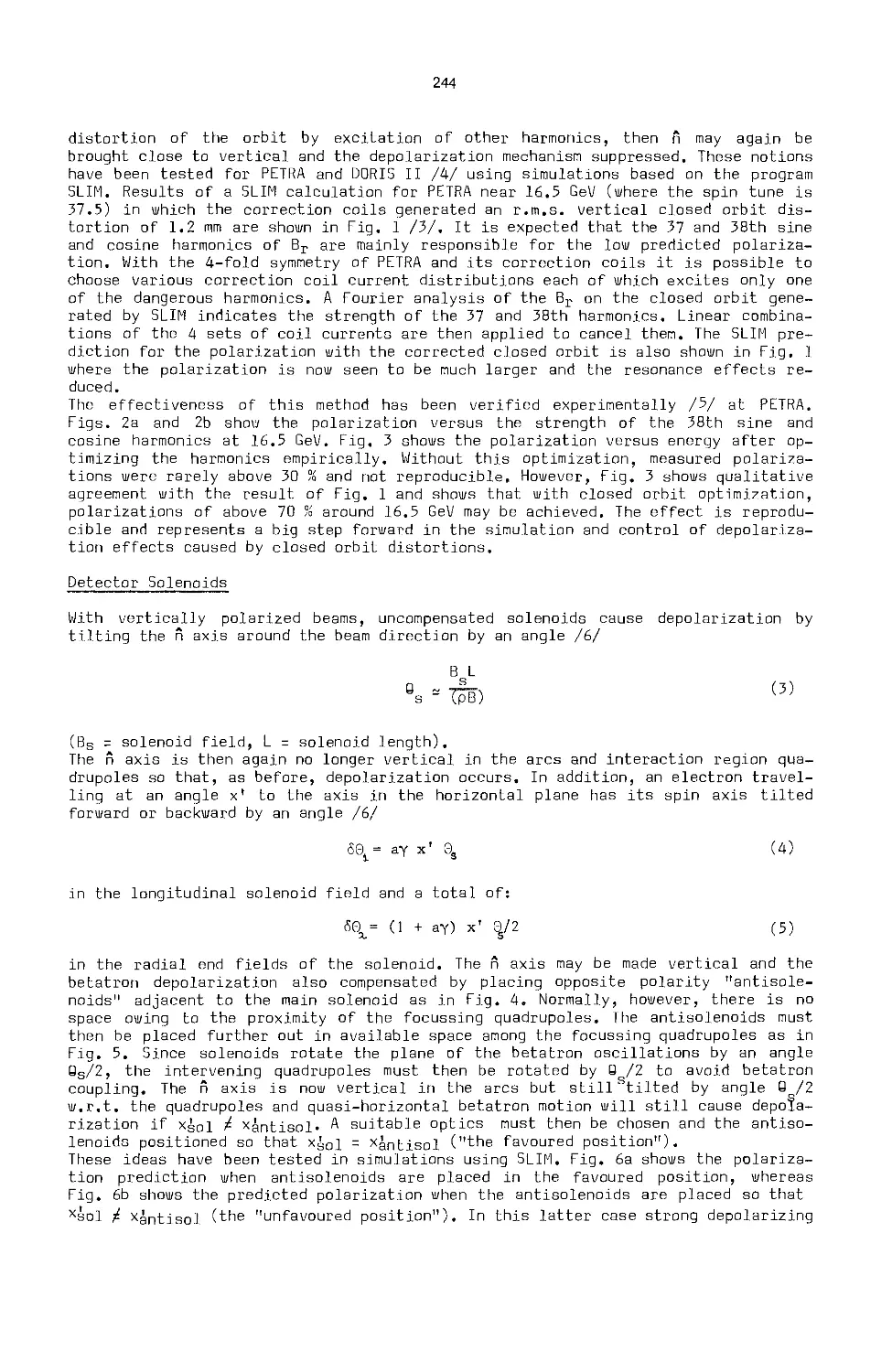


Автор: Busse W. Zelazny R.
Теги: nuclear physics lecture notes in physics accelerators
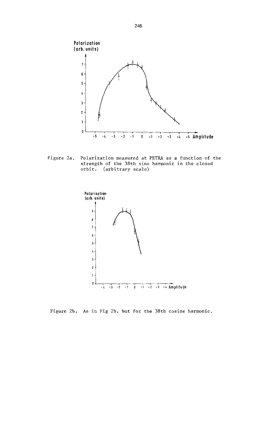
ISBN: 3-540-13909-5
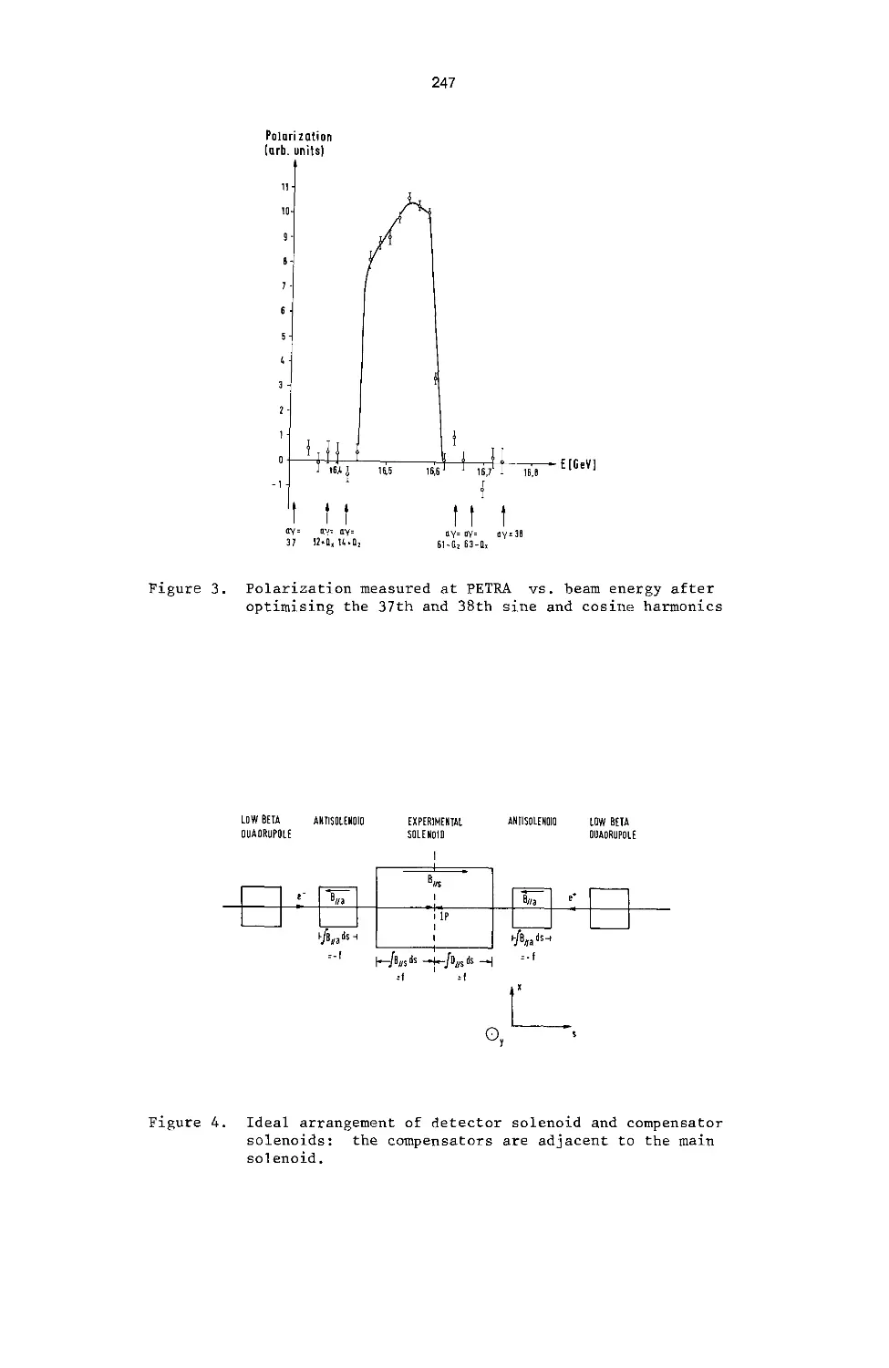
Год: 1984


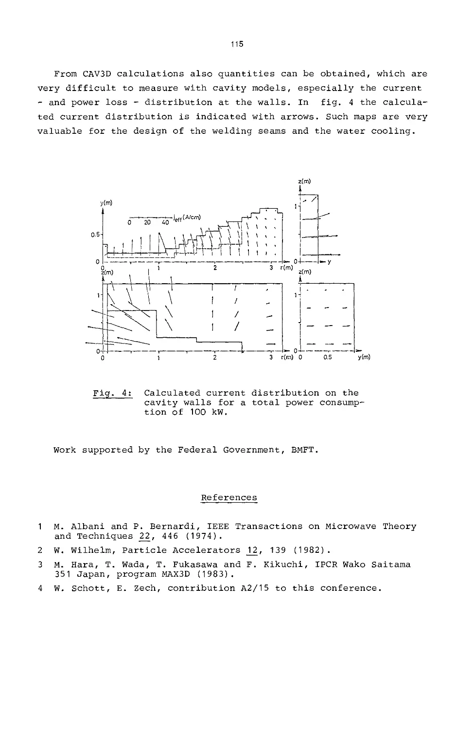
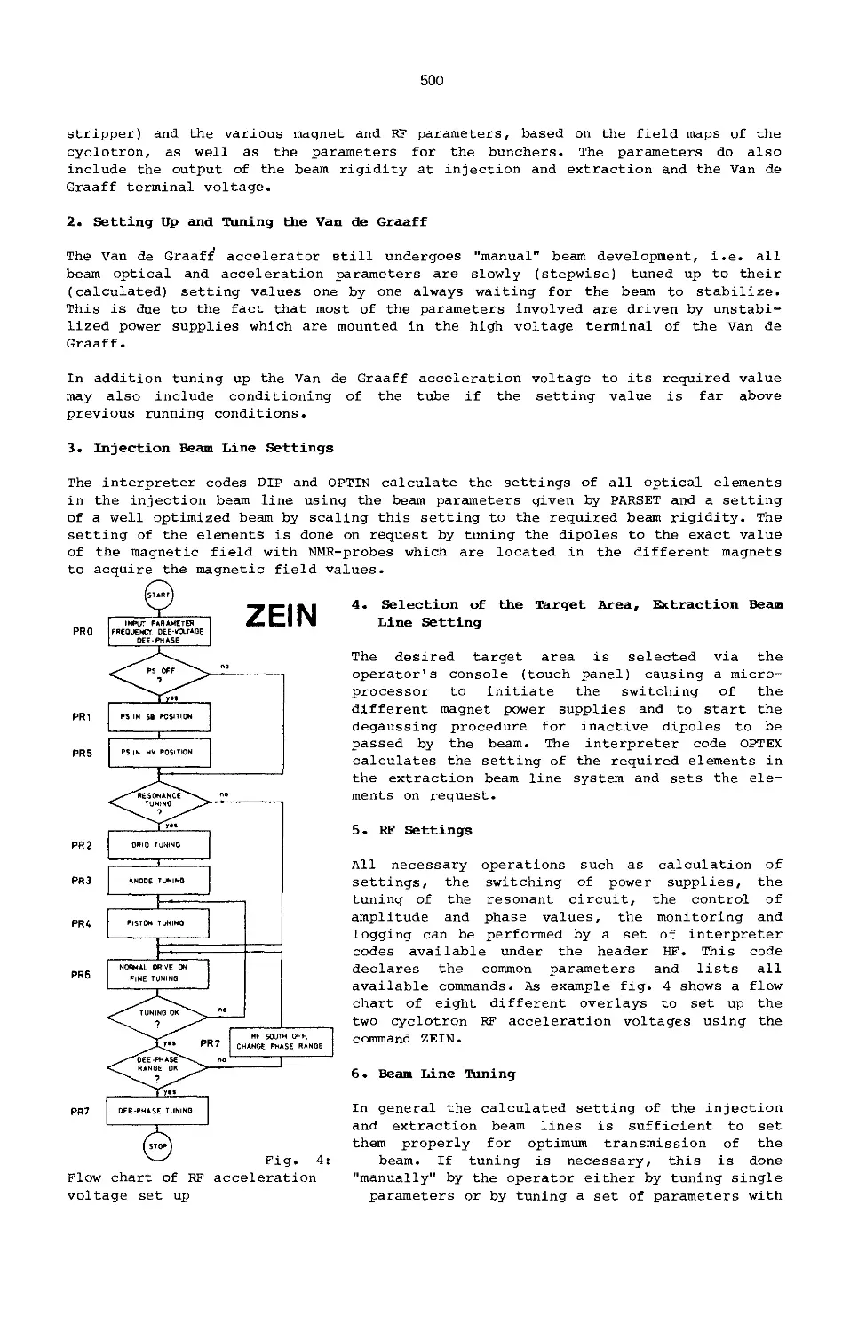
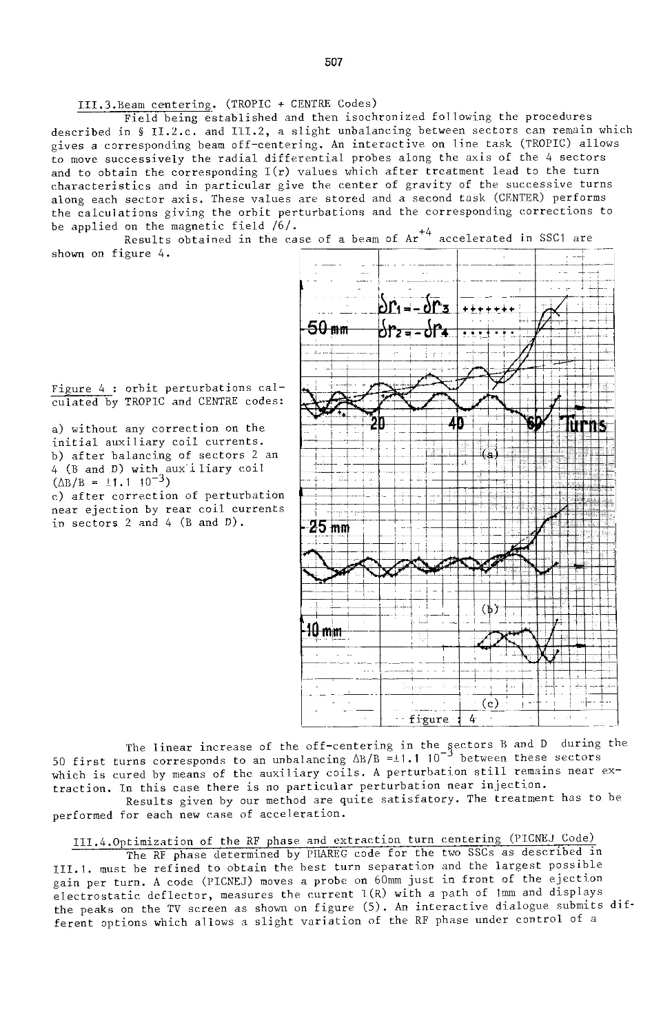
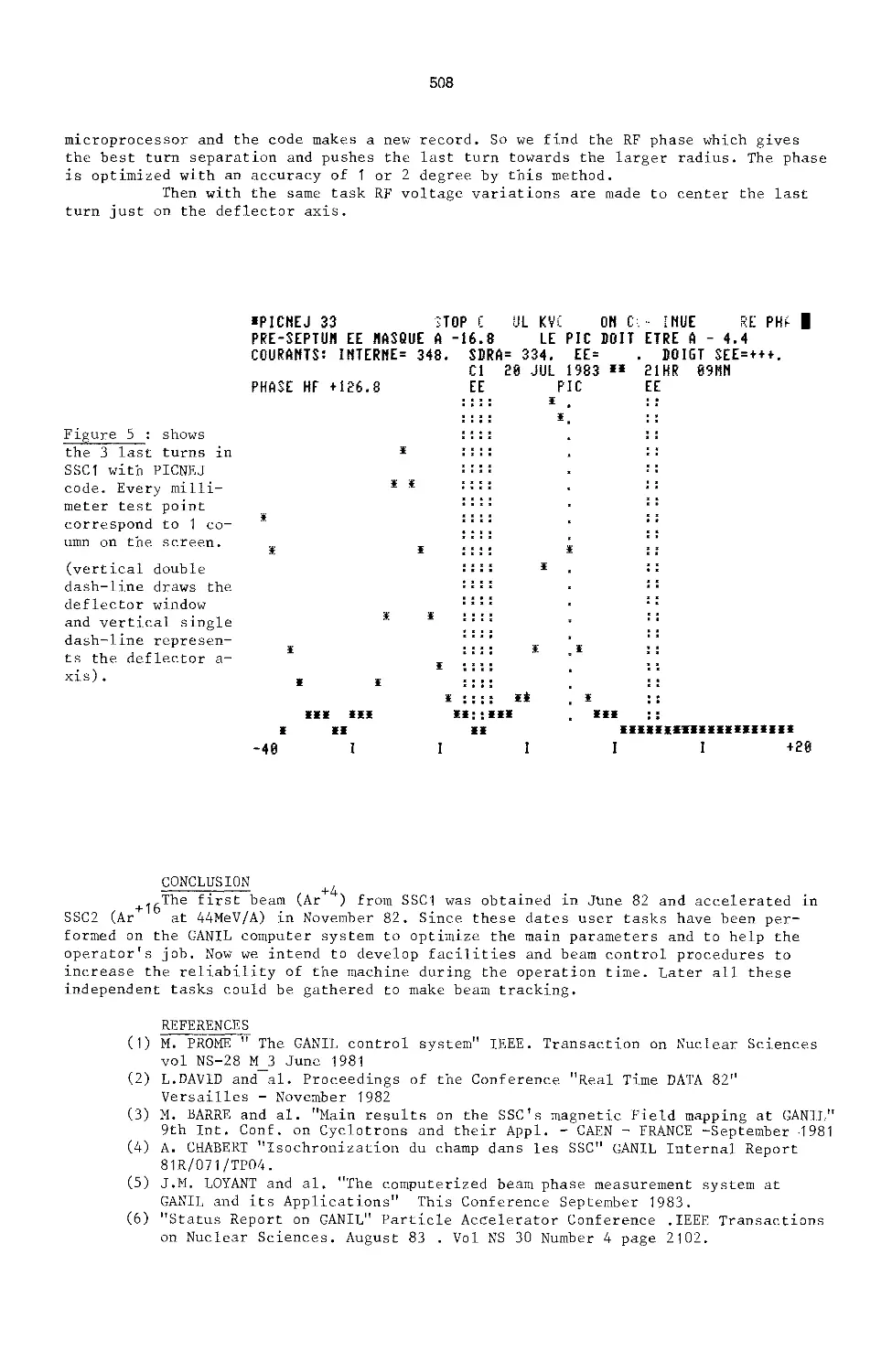
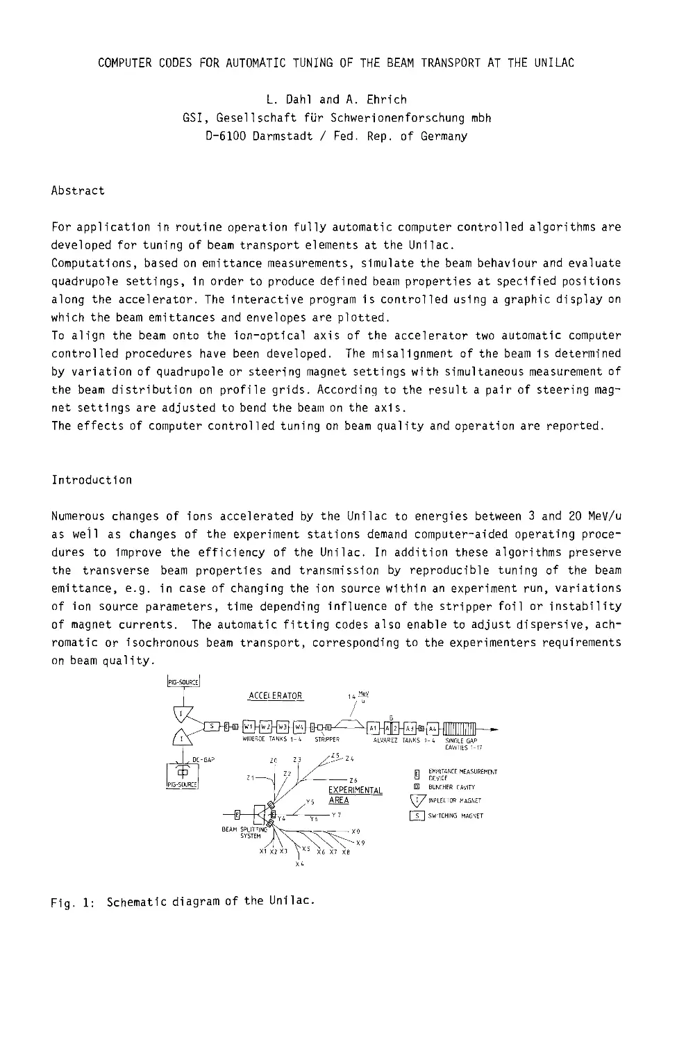
Текст
Lecture Notes
in Physics
Edited by H. Araki, Kyoto, J. Ehlers, Munchen, K. Hepp, Zurich
R. Kippenhahn, Munchen, H. A. Weidenmuller, Heidelberg
and J. Zittartz, Koln
215
Computing in
Accelerator Design
and Operation
Proceedings of the Europhysics Conference
Held at the Hahn-Meitner-lnstitut
fur Kernforschung Berlin GmbH
Berlin, Germany, September 20-23,1983
Edited by W. Busse and R. Zelazny
Springer-Verlag
Berlin Heidelberg New York Tokyo 1984
Editors
Winfried Busse
Hahn-Meitner-lnstitut fiir Kernforschung Berlin GmbH
Bereich Kern- und Strahlenphysik
Glienickerstr. 100, D-1000 Berlin 39
Roman Zelazny
RCC CYFRONET, IAE
PL-05-400 Otwock-Swierk, Poland
ISBN 3-540-13909-5 Springer-Verlag Berlin Heidelberg New York Tokyo
ISBN 0-387-13909-5 Springer-Verlag New York Heidelberg Berlin Tokyo
This work is subject to copyright. All rights are reserved, whether the whole or part of the material
is concerned, specifically those of translation, reprinting, re-use of illustrations, broadcasting,
reproduction by photocopying machine or similar means, and storage in data banks. Under
§ 54 of the German Copyright Law where copies are made for other than private use, a fee is
payable to “Verwertungsgesellschaft Wort", Munich.
© by Springer-Verlag Berlin Heidelberg 1984
Printed in Germany
Printing and binding: Beltz Offsetdruck, Hemsbach/Bergstr.
2153/3140-543210
PREFACE
Accelerators became long ago a very important research tool in nuclear physics and
its industrial and medical applications.
Recently we have observed their impressive development, so well illustrated by the
design and construction of very large accelerator systems like the CERN-SPS
in Geneva and Fermilab in Batavia. New and still larger accelerators are under
study and will be built with international support, for example LEP, once again on
the CERN site in Geneva.
During feasibility studies, design and construction, and also during operation,
computing plays a very essential role in enabling designers and operators to
perform their duties properly. In all these phases of the accelerator life-cycle
computers are used very extensively.
It is difficult to state in which of these phases the application of computers is
most important. Some people claim that without digital control the usage of accel-
erators in research would not - at present - be possible. Additionally, physical
experiments with particle-accelerator beams cannot be conceived without the
decisive role of computers in acquisition and processing of experimental data.
All this means that computers and accelerators are tightly affined to each other.
This symbiosis is the essence of progress in both fields.
This explanation makes it obvious that a conference on computing in accelerator
design and operation had to be organized. Due to the initiative of one of us
(R.Z.) while a member of the Computational Physics Group of the European Physical
Society, the board of the CPG decided to convene such a conference under the
Europhysics Conference label. The European Physical Society supported this idea
vigorously. The sponsoring organizations are acknowledged with gratitude. Without
their support and assistance the idea would not have materialized.
The conference was organized around three topical subjects: computing for design
applications, for digital control of accelerators and for operational aspects. The
subjects of invited lectures as well as the lecturers were carefully selected by
the Scientific Advisory Committee. The invited lectures were the only oral presen-
tations in plenary sessions. Each subject was introduced by a 15-20 minutes talk by
a leading prominent personality in the field. Invited lectures were given 45 min-
utes for presentation and discussion. All contributed papers were presented at
poster sessions, a format which was positively accepted by the participants. In the
framework of the conference two workshops were organized on request. The first was
devoted to lattice calculations of accelerator structures, the second to local area
network concepts in the field of digital control of accelerators.
It was felt that this conference was necessary to bring together accelerator de-
signers, builders and users, because a common understanding between them is still
to be created. Therefore, as an important corollary, both the Scientific Advisory
Committee and the participants of the conference endorsed unanimously the idea of
organizing such a conference each third year. The Computational Physics Group Board
has been approached with this suggestion. Let us hope that the year 1986 will be
the year of the next Europhysics Conference in Accelerator Design and Operation.
Roman Zelazny
Regional Computing Centre CYFRONET
Otwock-Swierk, Poland
Winfried Busse
Hahn-Meitner Institute
Berlin, Germany
International Scientific Advisory Committee
R. Zelazny RCCA, Otwock-Swierk Poland (chairman)
F. Beck FNAL, Batavia USA
W. Busse HMI, Berlin Germany
M. C. Crowley-Milling CERN, Geneva Switzerland
M. Edwards RAL, Didcot United Kingdom
G. N. Florov JINR, Dubna USSR
0. Houssin CGR MeV, Buc France
E. Keil CERN, Geneva Switzerland
W. Klotz BESSY, Berlin Germany
S. Kulinski INST, Otwock-Swierk Poland
F. Peters DESY, Hamburg Germany
M. Prome GANIL, Caen France
J. Schwabe INP, Krakow Poland
H. Sherman Daresbury Lab., Warrington United Kingdom
A. N. Skrynski INP, Novosybirsk USSR
P. Strehl GSI, Darmstadt Germany
Local Organizing Committee
W. Buchholz BESSY
W. Busse HMI P - VICKSI (chairman)
К. H. Degenhardt HMI D/M
H. Kluge HMI P
W.-D. Klotz BESSY
G. Liar de Martin HMI P - VICKSI (conf•secretariat)
К. H. Maier HMI P
R. Maier BESSY
B. Martin HMI P - VICKSI
R. Michaelsen HMI P - VICKSI
B. Spellmeyer HMI P - VICKSI
K. Ziegler HMI P - VICKSI
Sponsors
European Physical Society
Deutsche Physikalische Gesellschaft
Regional Computation Centre of Atomic Energy, Otwock-Swierk, Poland
Hahn-Meitner-Institut fur Kernforschung Berlin GmbH
Commercial Sponsors
DANFYSIK - Jyllinge, Denmark
HEINZINGER Regel- und MeBtechnik - Rosenheim, Germany
INCAA Special Systems for Industry and Science - Apeldoorn, Holland
KINETIC SYSTEMS INTERNATIONAL SA - Geneva, Switzerland
KNURR AG - Munchen, Germany
LEYBOLD-HERAEUS GmbH - Koln, Germany
SILENA Wissenschaftliche Instrumente GmbH - Hasselroth, Germany
Welcome Address by
Prof. K.H. Lindenberger, Scientific Director of the
Hahn-Meitner Institute, Berlin
Dear Colleagues,
On behalf of the Hahn-Meitner Institute I welcome you heartily to our town. We are
pleased and feel honoured that you have chosen Berlin as the place of your confer-
ence. By helping to organize this meeting we can, in a certain way, pay back some
of the debt which we owe to the community of accelerator builders.
When, more than ten years ago, we started to convert our small Van de Graaff in-
stallation into a heavy-ion facility, we had little experience in accelerator tech-
nology, especially in how to run such a system with the help of a computer. In this
situation we thought it best to ask the professionals for help and we got this help
in a really generous way. This talk is not the right opportunity to give a full
record of this story, but I would like to mention as an example two outstanding
members of your community whose skill, ambition and enthusiasm had great impact on
the project and who were essential for its success.
Prof. Hagedoorn from Eindhoven contributed much to the understanding of the orbit-
dynamics in our cyclotron. One direct result of this is a programme by which the
control computer can center and isochronize the beam. Dr. Susini from CERN was in
charge of the design and the construction of the RF-systems of our cyclotron and he
did it in such a way that they are really computer-compatible. In the meantime, our
accelerator crew has joined your community, and that you meet at our place may be a
hint that they now are passing as professionals. But to say it once more: without
your assistance we would not have been able to get such a system running with the
very good performance that, as we think, we now have at our disposal. I am glad
that I can use this opportunity to express our gratitude.
CERN was an especially important source of information and also of very practical
help. So I am very pleased that the opening honorary lecture will be given by
Dr. Adams, who was twice responsible for the construction of the large accelerators
in Geneva. We all know how brilliantly this job was done, what high technical stan-
dards have been achieved and what important experiments can be done with those
machines. Here I would like to пике a remark on the sideline: I was always very im-
pressed how effective and smooth is the international cooperation in the field of
particle physics and accelerator building. I think it would be of great value for
all of us if, in other technical and political matters of world-wide impact, the
same efficiency of cooperation could be achieved as in particle physics. Once more
my special welcome to you, Dr. Adams, here in Berlin.
It is according to the hopes I just mentioned that the chairman of your conference,
Prof. Zelazny, comes from Poland, from the Nuclear Research Centre at Swierk. The
Hahn-Meitner Institute has a number of scientific contacts with this institute and
we are happy that we can cooperate with you, Prof. Zelazny, in running this confer-
ence. But, as I mentioned, we have also other contacts to Swierk: the volleyball
team of Swierk beat the Hahn-Meitner crew 2:1 when they met at Swierk in 75. Best
welcome also to you Prof. Zelazny. I hope the local staff will make life easy for
you in your job as a chairman.
I would like to thank the Free University that we can hold the conference in this
place. We had to do so because, at our institute, we have no facilities to handle a
meeting of this size.
Now nothing is left but to wish you a lively and interesting conference which gives
you new ideas for your work at home. But I also hope that beside the work here you
will find some time to stroll around Kurfiirstendamm, to meet Nefretiti at the
Egyptian Museum or to find out what else is going on in our town. After the
afternoon session today, however, we would be very pleased if you could visit us at
the Hahn-Meitner Institute to have a look at our installations and to join us for a
cocktail. Once more, welcome to Berlin and good luck for your conference.
Thank you.
Welcome Address by the chairman of the conference,
Prof. Roman Zelazny, CYFRONET
Otwock-Swierk, Poland
Ladies and Gentlemen, Dear Colleagues,
All of you may observe the enormous development of activities in the field of
accelerator construction and their application in research, industry and medicine.
New accelerators are proposed, are under design and construction, start their
operation.
Computers play a very important role in the design, in feasibility studies and in
operation of accelerators. They are applied in many interesting and innovative
ways: for computer-assisted design, for digital control, for beam administration
and particularly in experiments with beams of accelerator particles.
The conference organized under the auspices of the European Physical Society and
its Computational Physics Group is devoted to various aspects of computing in ac-
celerator design and operation.
Originally scheduled to be organized in Poland in September 1982, it has been
postponed and moved to Berlin. I wish to thank very much the Hahn-Meitner Institute
authorities, particularly Prof. Lindenberger and Dr. W. Busse for their willingness
to take over the organization of the conference. In a short period of time the
local organizers performed a very good job, enabling us to meet today to open this,
as I do hope, interesting and important meeting.
Using this chancezI wish to thank not only the Local Organizing Committee headed by
Dr. Busse but also other sponsoring organizations: the Deutsche Physikalische
Gesellschaft and the Regional Computing Centre of Atomic Energy CYFRONET. It is my
special pleasure to thank all members of the Scientific Advisory Committee for
their effort concerning the scientific programme of the conference and all invited
lecturers for accepting the invitation to deliver the invited talks. Their contri-
butions make the conference an important and interesting event.
Particular thanks are due to Sir John Adams for his acceptance to deliver the hon-
orary lecture at this conference. It seems to me that the community of European
physicists shall consider that this homage to his activities in the field of ac-
celerator development is well deserved and that they join the Scientific Advisory
Committee's opinion with applause.
I welcome sincerely all the participants. Without you all the conceptual and
organizational efforts would be empty. You are the salt of the earth. It is done
for you, you will make it finally a success by the contribution of your papers,you
make it vivid by discussion and exchange of views and experience. All the or-
ganizers have done their duty. The critical mass for a chain reaction necessary to
create a peaceful explosion of ideas, concepts, interactions among interesting
people has been prepared. Let it go. I declare the Europhysics Conference on
"Computing in Accelerator Design and Operation" open.
Thank you very much for your attention.
CONTENTS
Future High Energy Accelerators (Honorary Invited Lecture) 1
J. Adams
A: COMPUTING for ACCELERATOR DESIGN
Beam Optics and Dynamics 11
E. J. N. Wilson
Design of R.F. Cavities 21
T. Weiland
Computer Aided Magnet Design 33
C. W. Trowbridge
Beam Instabilities and Computer Simulations 50
A. Piwinski
Calculation of Polarization Effects 59
A. W. Chao
Particle Tracking in Accelerators with Higher Order Multipole 75
Fields
A. Wrulich
Programs for Designing the Accelerating Cavities for Linear 86
Accelerators
S. Kullnski, L. Sawlewicz, J. Sekutowicz
The MAGMI Program for Double Pass Electron Linear Accelerators 92
T. Czosnyka, K. Deutschman, S. Kullnski, S. Zaremba
A FORTRAN Program (RELAX3D) to Solve the 3 Dimensional Poisson 98
(Laplace) Equation
H. Houtman, C. J. Kost
Calculation of Three Dimensional Electric Fields by Successive 104
Over-Relaxation in the Central Region of a Cyclotron
S. Oh, R. Pogson, M. Yoon
The Design of the Accelerating Cavity for SUSE with the Aid of 110
the Three-Dimensional Cavity Calculation Program CAV3D
W. Wilhelm
The Further Development of the Calculation of the Three 116
Dimensional Electric Field in the Central Region of the INR
Cyclotron
Mao-bal Chen, Wen-bin Sen
Particle Tracking Using Lie Algebraic Methods 122
A. J. Dragt, D. R. Douglas
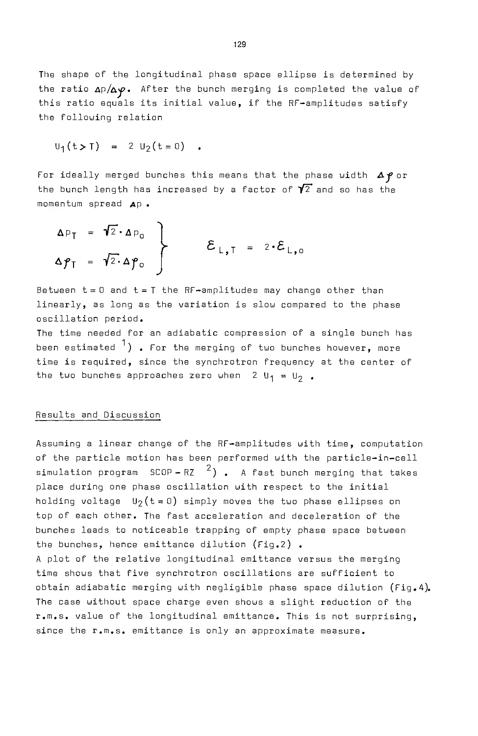
Numerical Investigation of Bunch-Merging in a 128
Heavy-Ion-Synchrotron
I. Bozslk, I. Hofmann, A. Jahnke, R. W. Muller
VIII
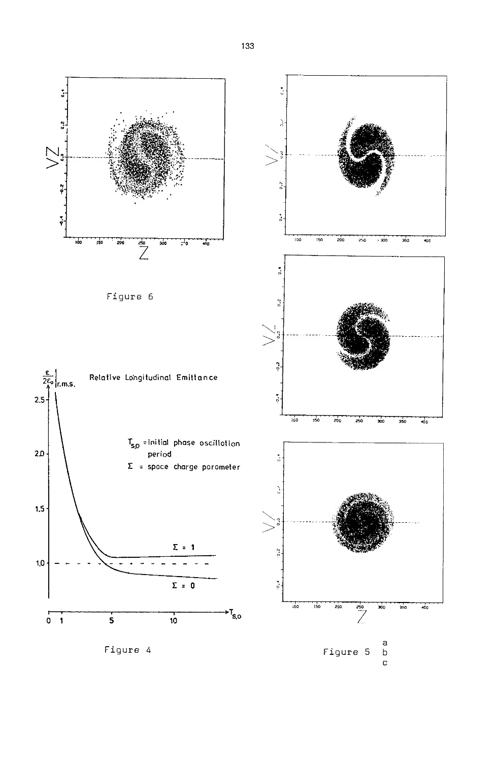
Nonlinear Aspects of Landau Damping in Computer Simulation of 134
the Microwave Instability
I. Hofmann
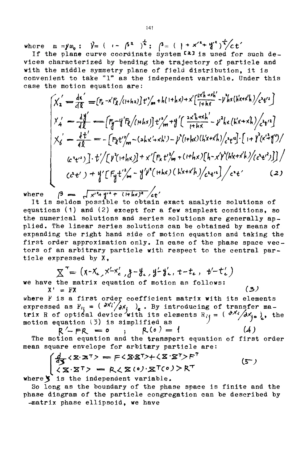
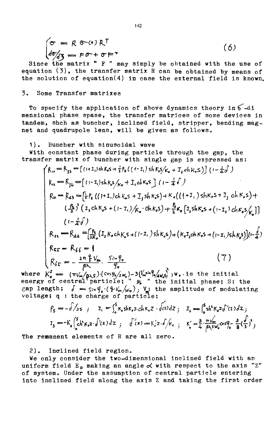
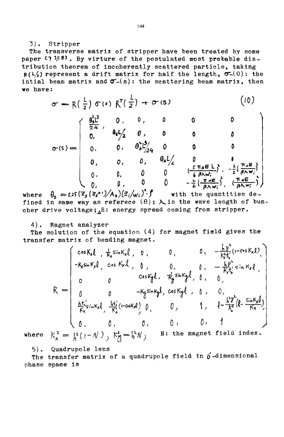
The Transport Theory of Particle Beam-Congregation in 140
Six-Dimensional Phase Space
Cao Qing-xi, Guan Xia-ling
The MAD Program (Methodical Accelerator Design) 146
F. Ch. Iselin
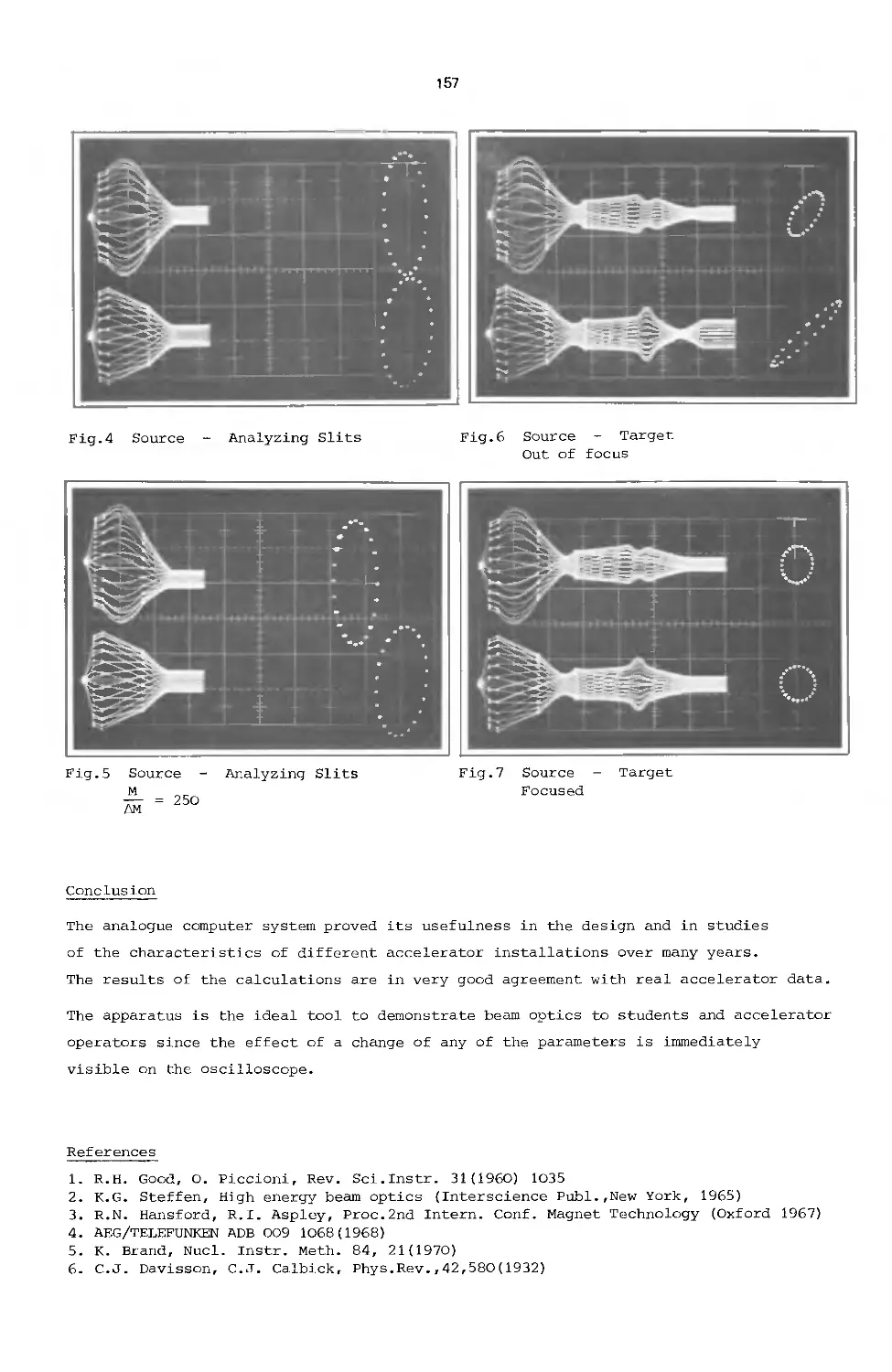
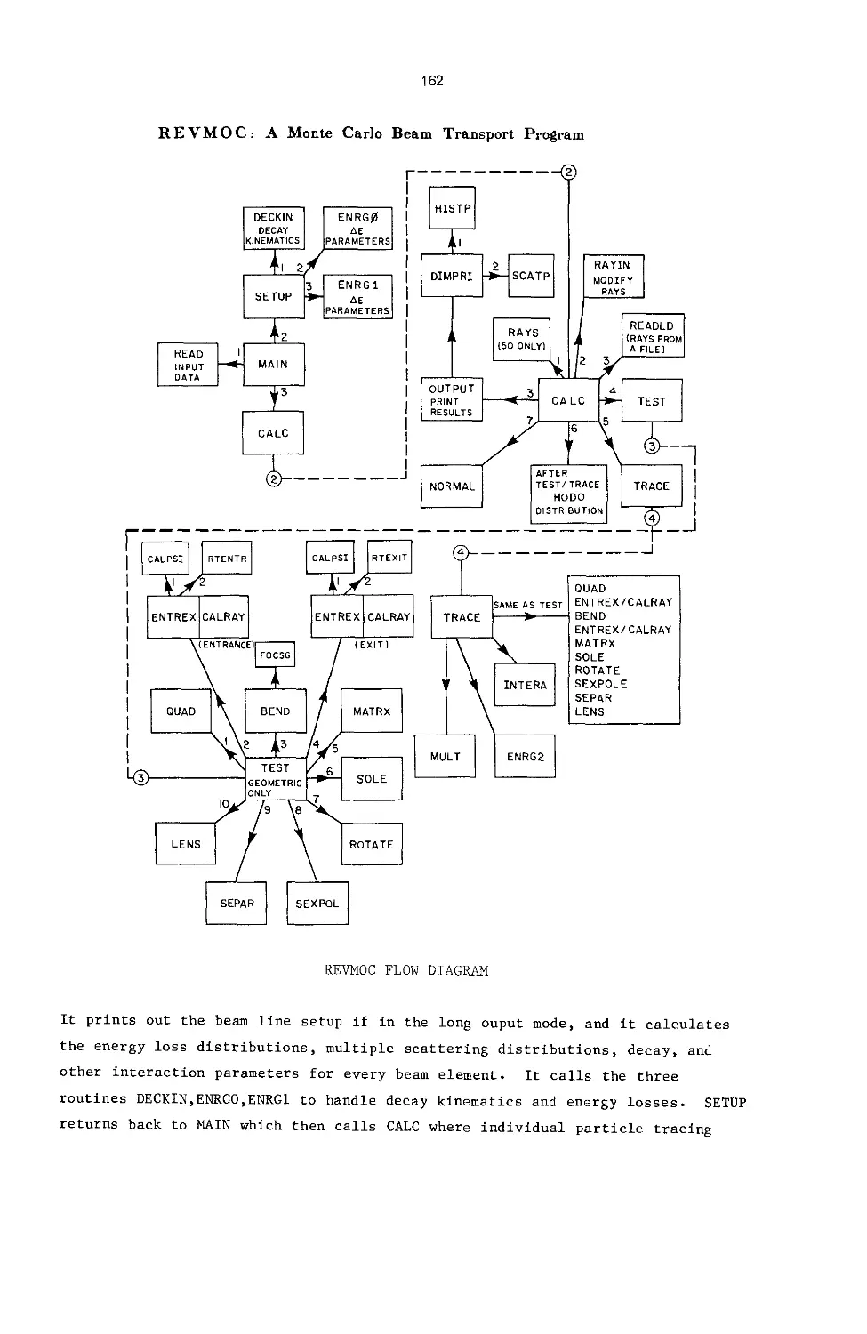
Analogue Computer Display of Accelerator Beam Optics 152
K. Brand
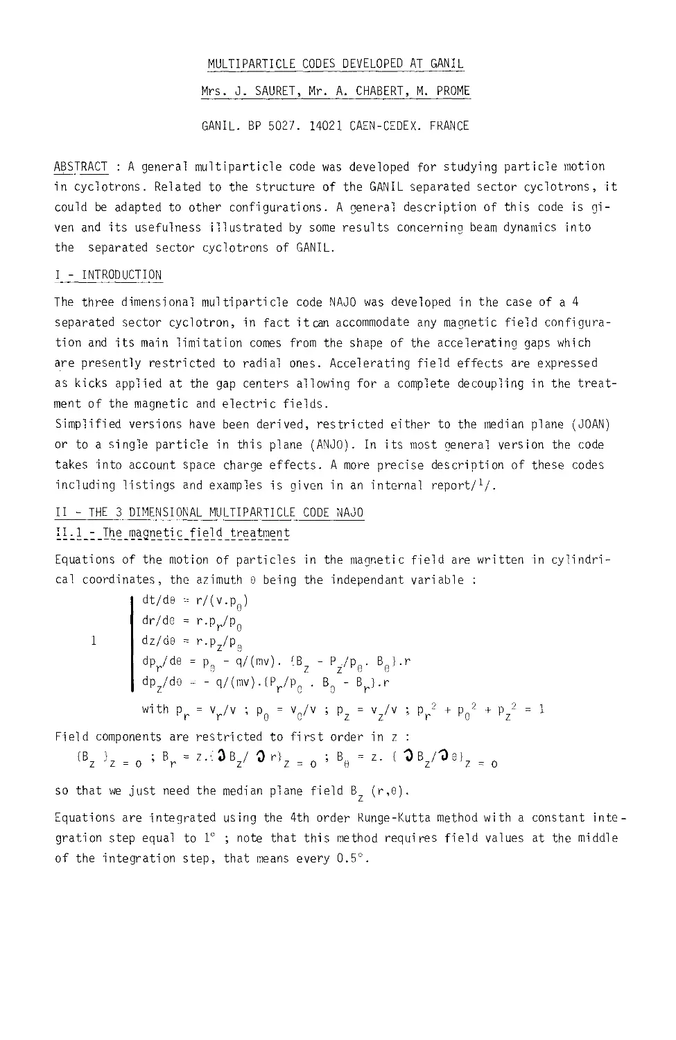
A Monte Carlo Beam Transport Program, REVMOC 158
C. Kost, P. A. Reeve
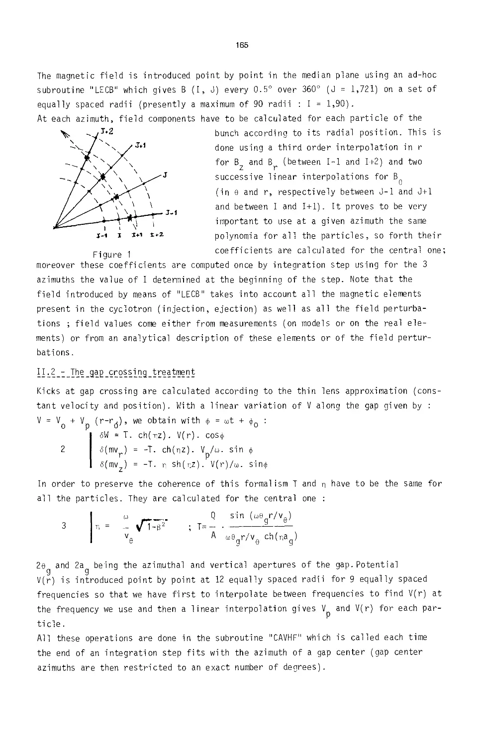
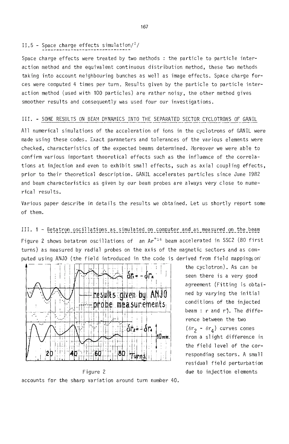
Multiparticle Codes Developed at GANIL 164
J. Sauret, A. Chabert, M. Prone
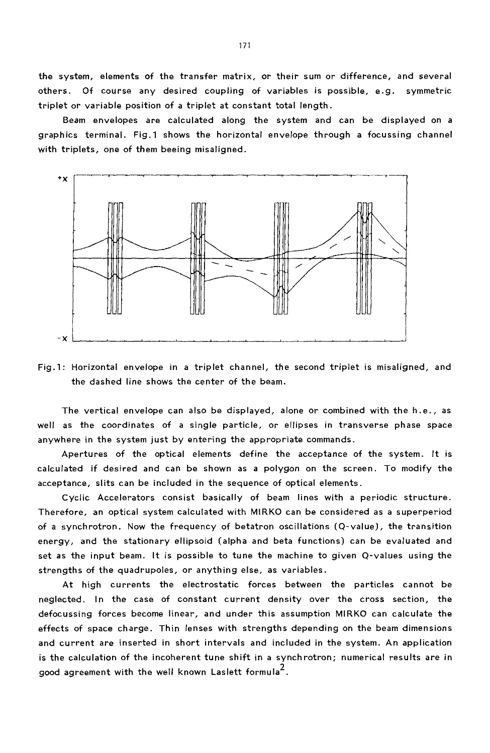
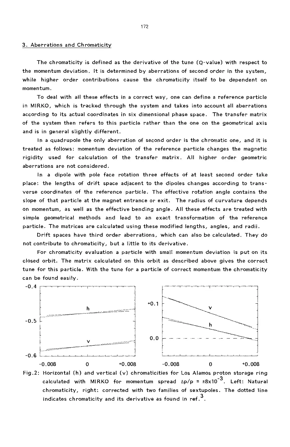
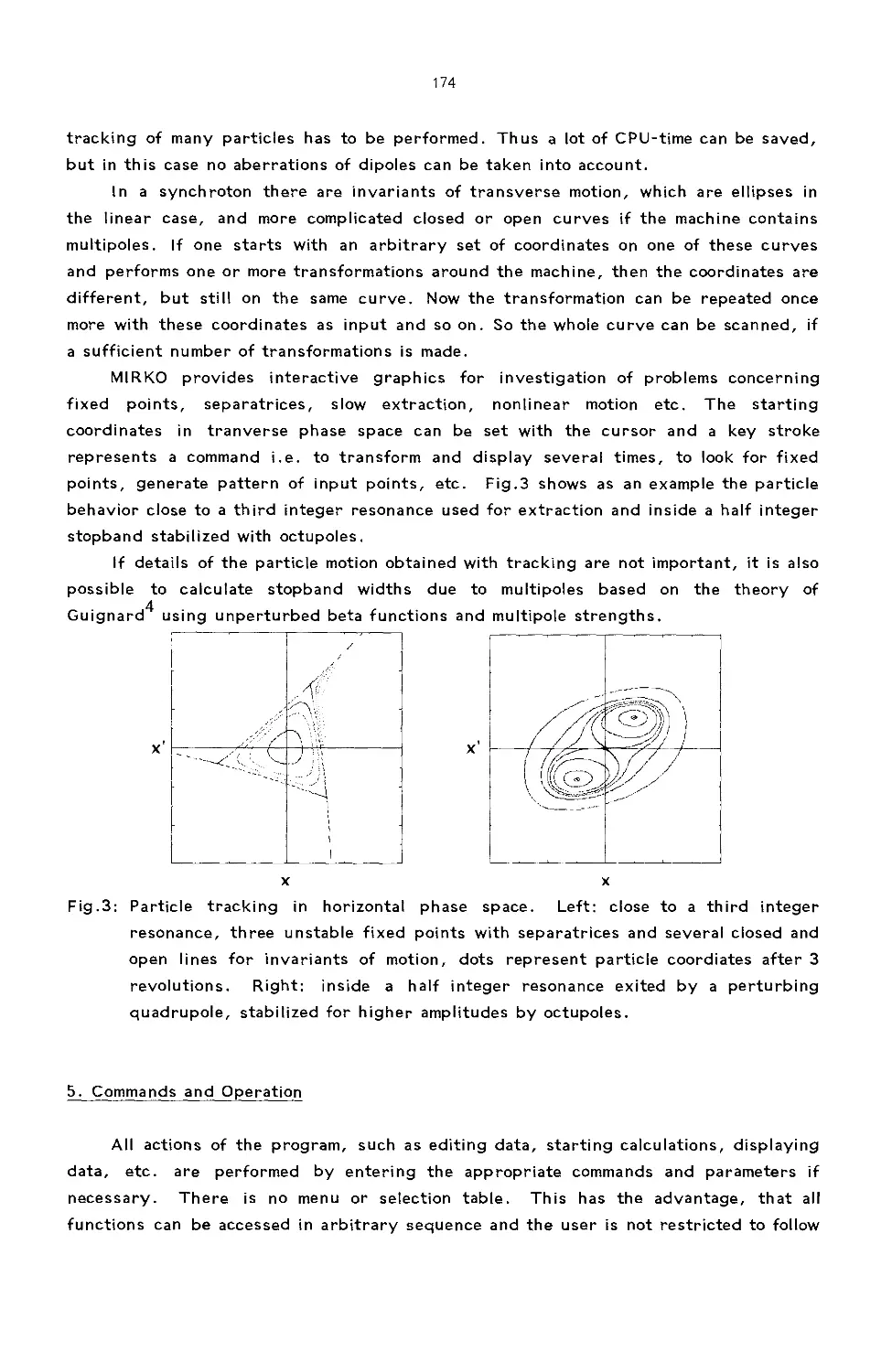
MIRKO - An Interactive Program for Beam Lines and Synchrotrons 170
B. Franczak
Aperture Studies of the BNL Colliding Beam Accelerator with 176
Reduced Superperiodicity
G. F. Dell
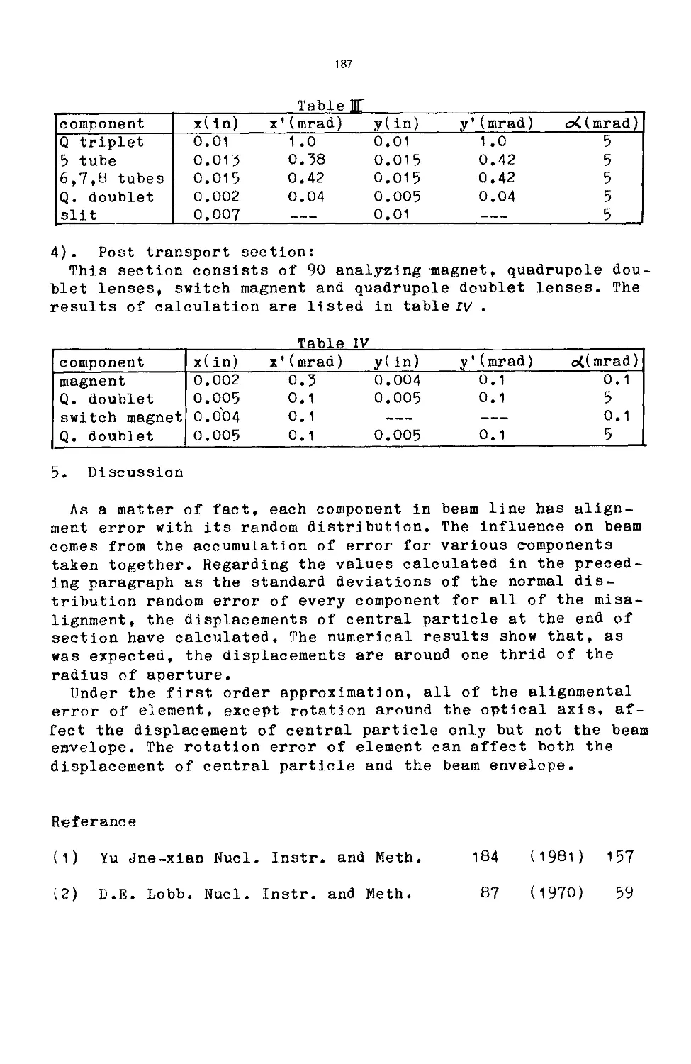
The Study of Misalignment Characteristics of Beam Optical 182
Components of HI-13 Tandem
Guan Xia-ling, Cao Qing-xl
Calculations for the Design and Modification of the 2 Cyclotrons 188
of S.A.R.A.
P. S. Albrand, J. L. Belmont, F. Ripouteau
Magnetic Field Optimization and Beam Dynamics Calculations for 193
SUSE
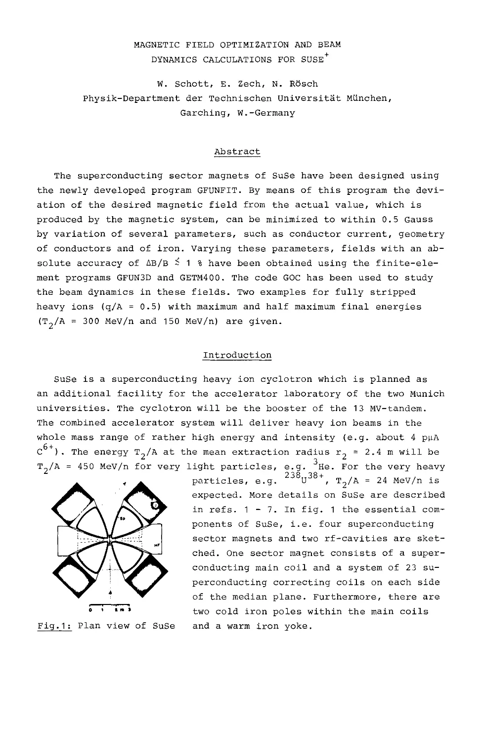
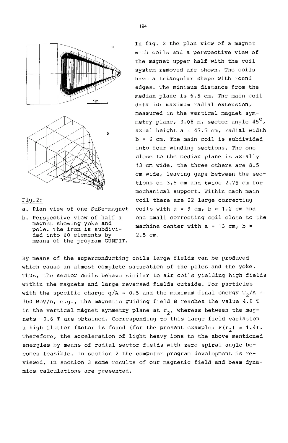
W. Schott, E. Zech, N. Rosch
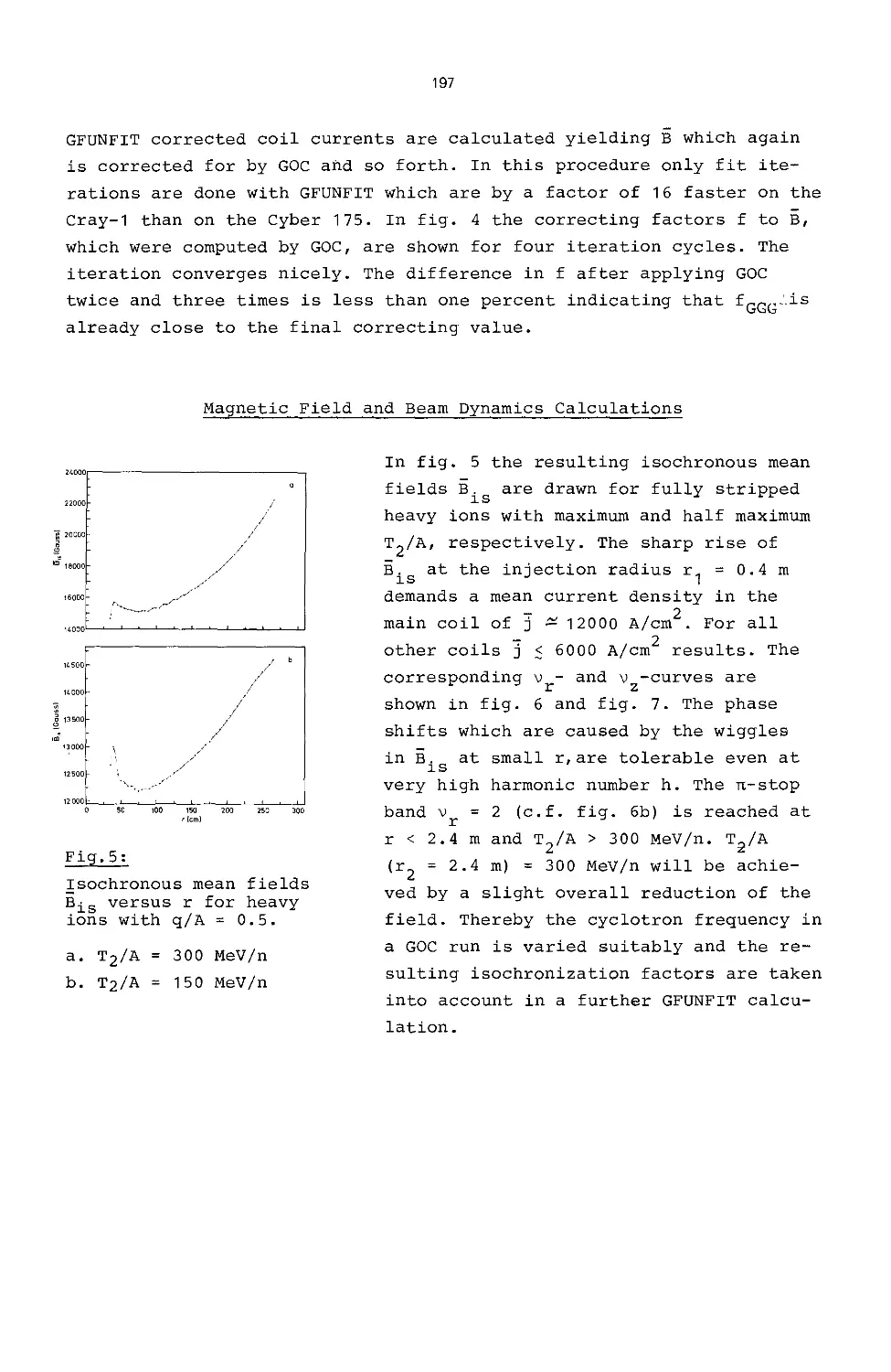
•DFLKTR' The Code for Designing the Electrostatic Extraction 199
System for Cyclotrons
R. C. Sethi, A. S. Divatia
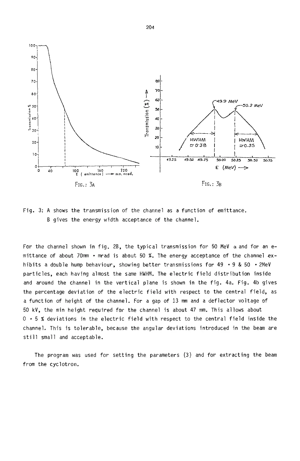
RFQ Design Considerations 206
P. Junior, H. Deltlnghoff, K. D. Halfmann, A. Schempp, N. Zoubek
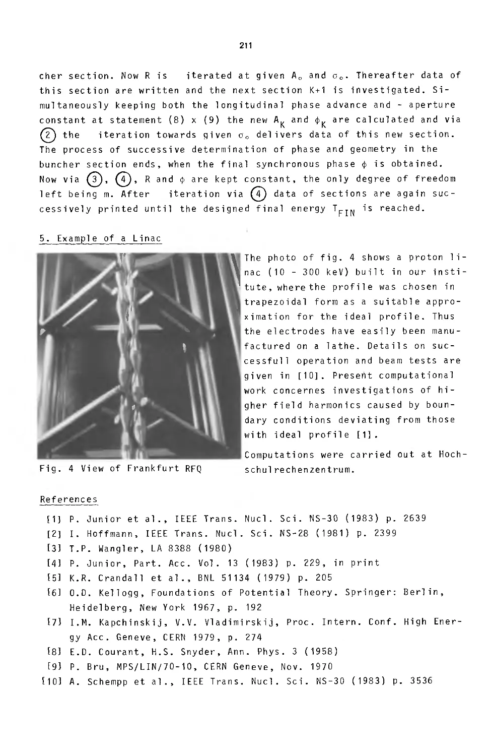
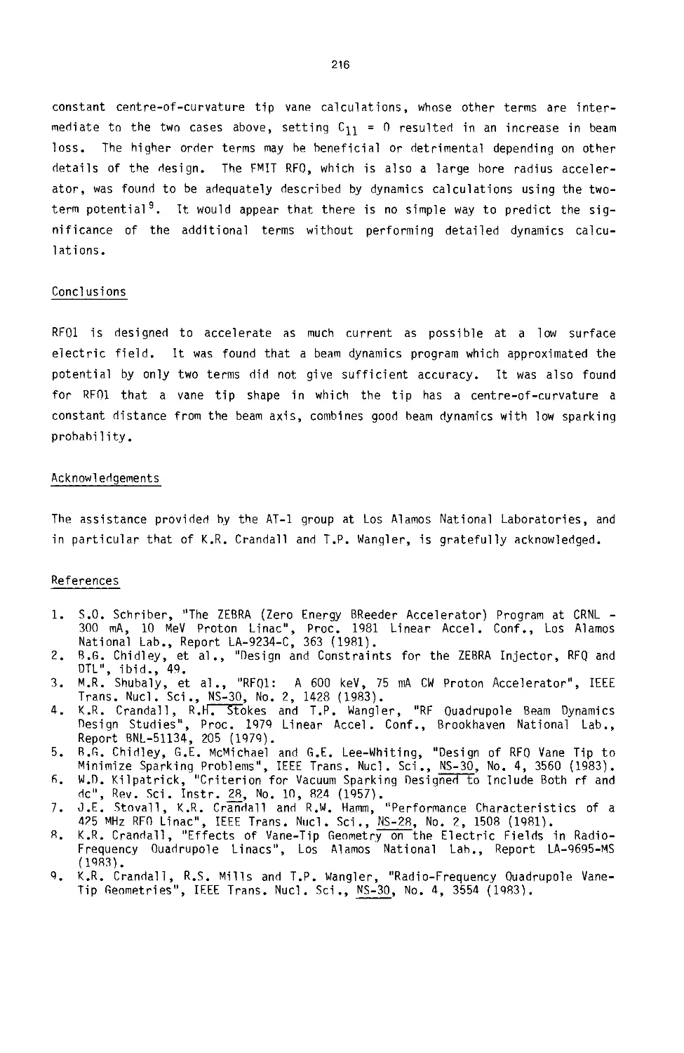
Effects of Higher Order Multipole Fields on High Current RFQ 212
Accelerator Design
G. E. McMichael, B. G. Chidley
Versatile Codes and Effective Method for Orbit Programming with 218
Actually Existing First Harmonics in Cyclotron
Mao-bal Chen, Sen-lln Xu, Wen-bin Sen
Calculations of the Heavy Ion Saclay Tandem Post Accelerator 224
Beams
S. Valero, B. Cauvin, J. P. Fouan, P. M. Lapostolle
IX
Electron Injector Computer Simulations 231
D. Tronc
Numerical Simulations of Orbit Correction in Large Electron 237
Rings
G. Guignard, Y. Marti
Simulation of Polarization Correction Schemes in e+e- Storage 243
Rings
D. P. Barber, H. D. Bremer, J. Kewisch, H. C. Lewin, T. Limberg,
H. Mais, G. Ripken, R. Rossmanith, R. Schmidt
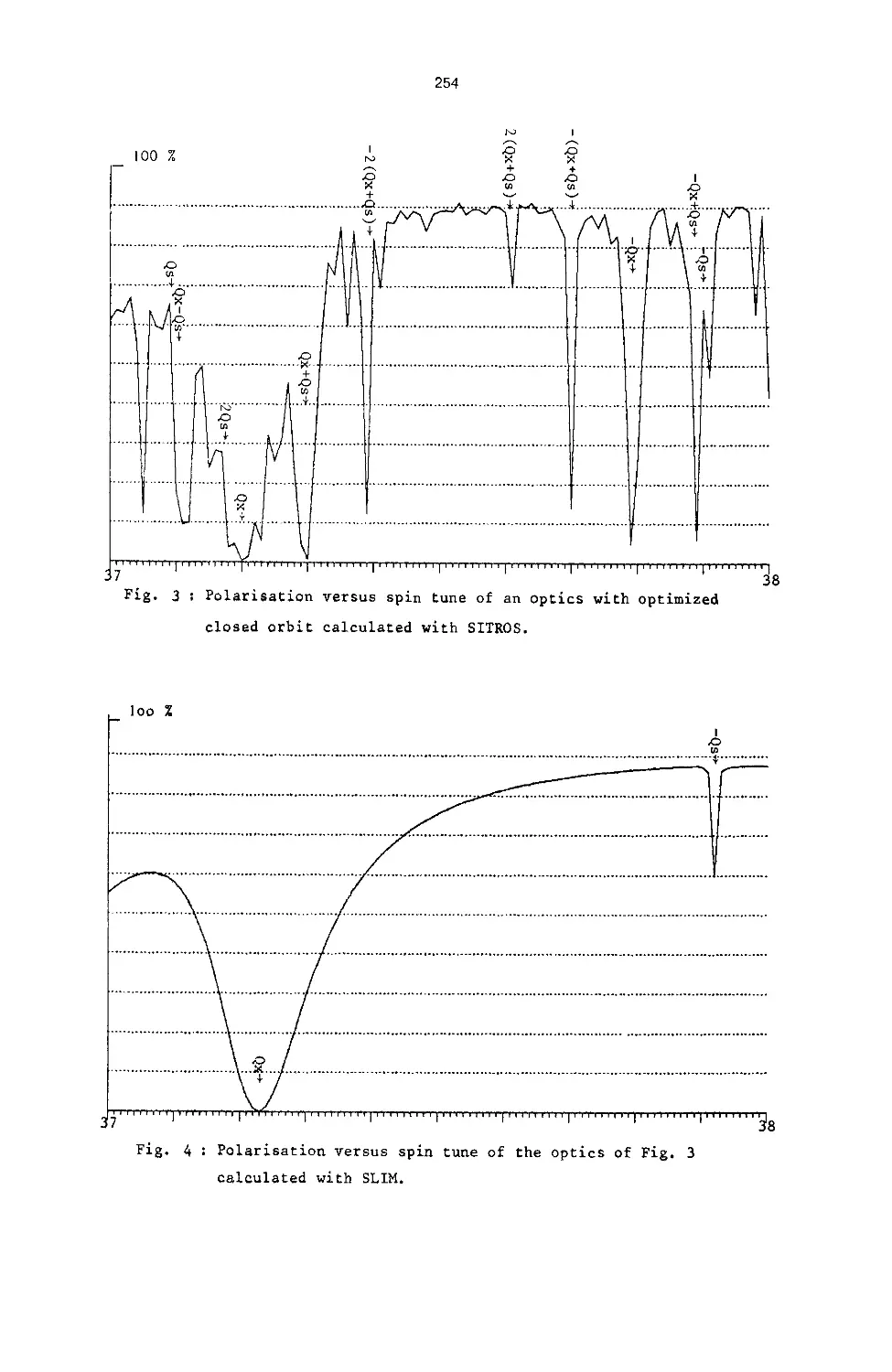
Computation of Electron Spin Polarisation in Storage Rings 249
J. Kewisch
ARCHSIM: A Proton Synchrotron Tracking Program Including 255
Longitudinal Space Charge
H. A. Thiessen, J. L. Warren
A Method for Distinguishing Chaotic from Quasi-Periodic Motions 261
in Orbit Tracking Programs
J. M. Jowett
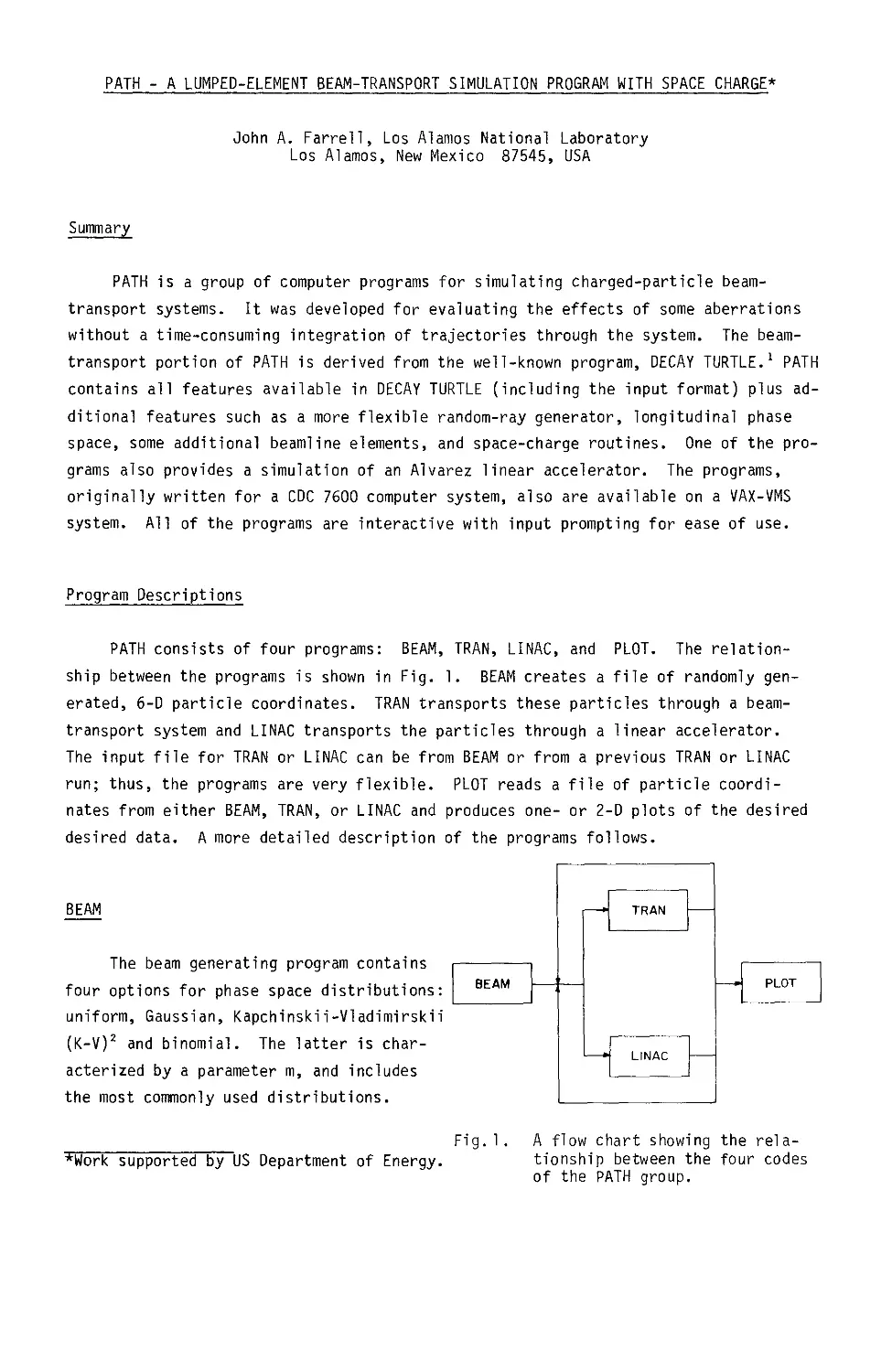
PATH - A Lumped-Element Beam-Transport Simulation Program with 267
Space Charge
J. A. Farrell
WORKSHOP No.1: Computer Programs for Lattice Calculations 273
Bi DIGITAL CONTROL OF ACCELERATORS
Digital Control of Accelerators - The First Ten Years 275
H. Frese
Distributed Digital Control of Accelerators 278
M. Crowley-Milling
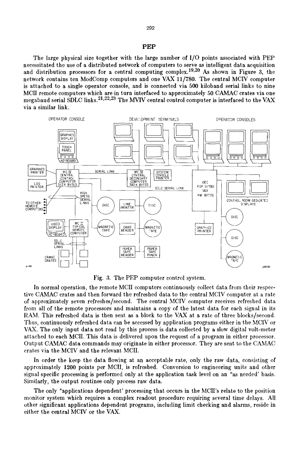
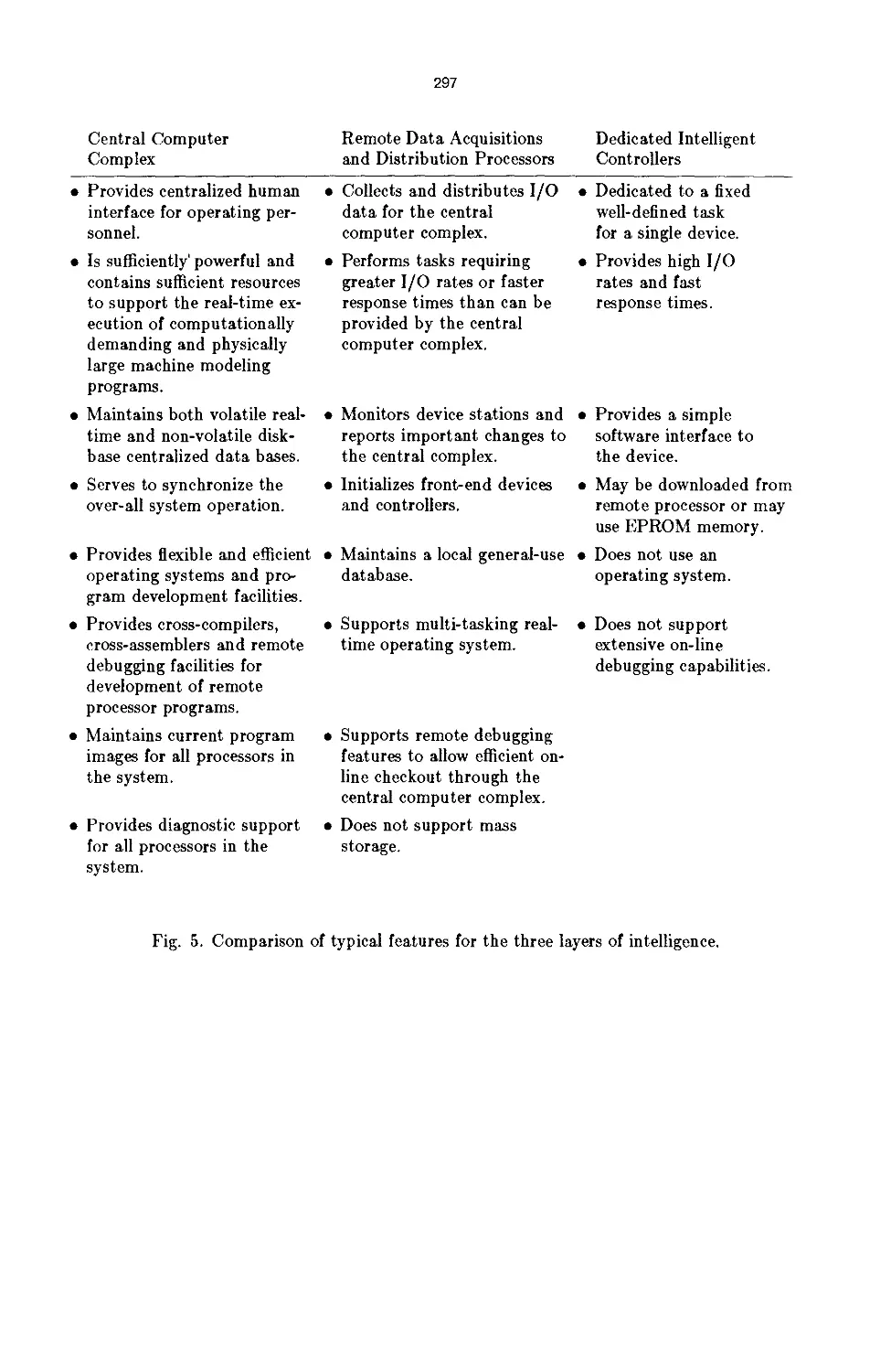
Centralized Digital Control of Accelerators 289
R. E. Melen
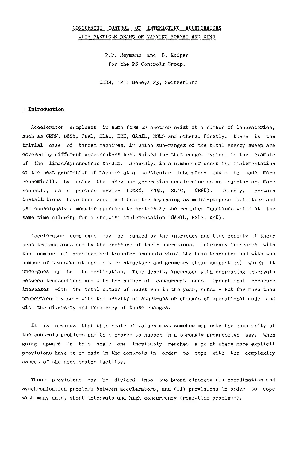
Concurrent Control of Interacting Accelerators with Particle 300
Beams of Varying Format and Kind
P. P. Heymans, B. Kuiper for the PS Controls Group
Integrated Control and Data Acquisition of Experimental 311
Facilities
F. Bombi
Software Engineering Tools 316
R. Zelazny
Centralization and Decentralization in the TRIUMF Control System 332
D. A. Dohan, D. P. Gurd
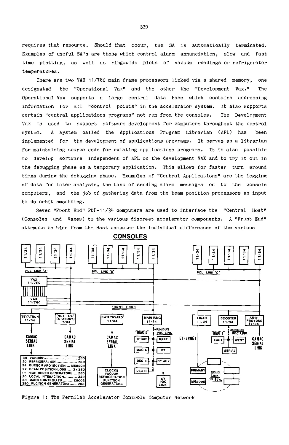
The Fermilab Accelerator Controls System 338
D. Bogert, S. Segler
X
The Control System for the Daresbury Synchrotron I&diation 344
Source
D. E. Poole, W. R. Rawlinson, V. R. Atkins
The Microprocessor-Based Control System for the Milan 351
Superconducting Cyclotron
F. Aghlon, S. Diquattro, A. Paccallnl, E. Panzer!, G. Rivoltella
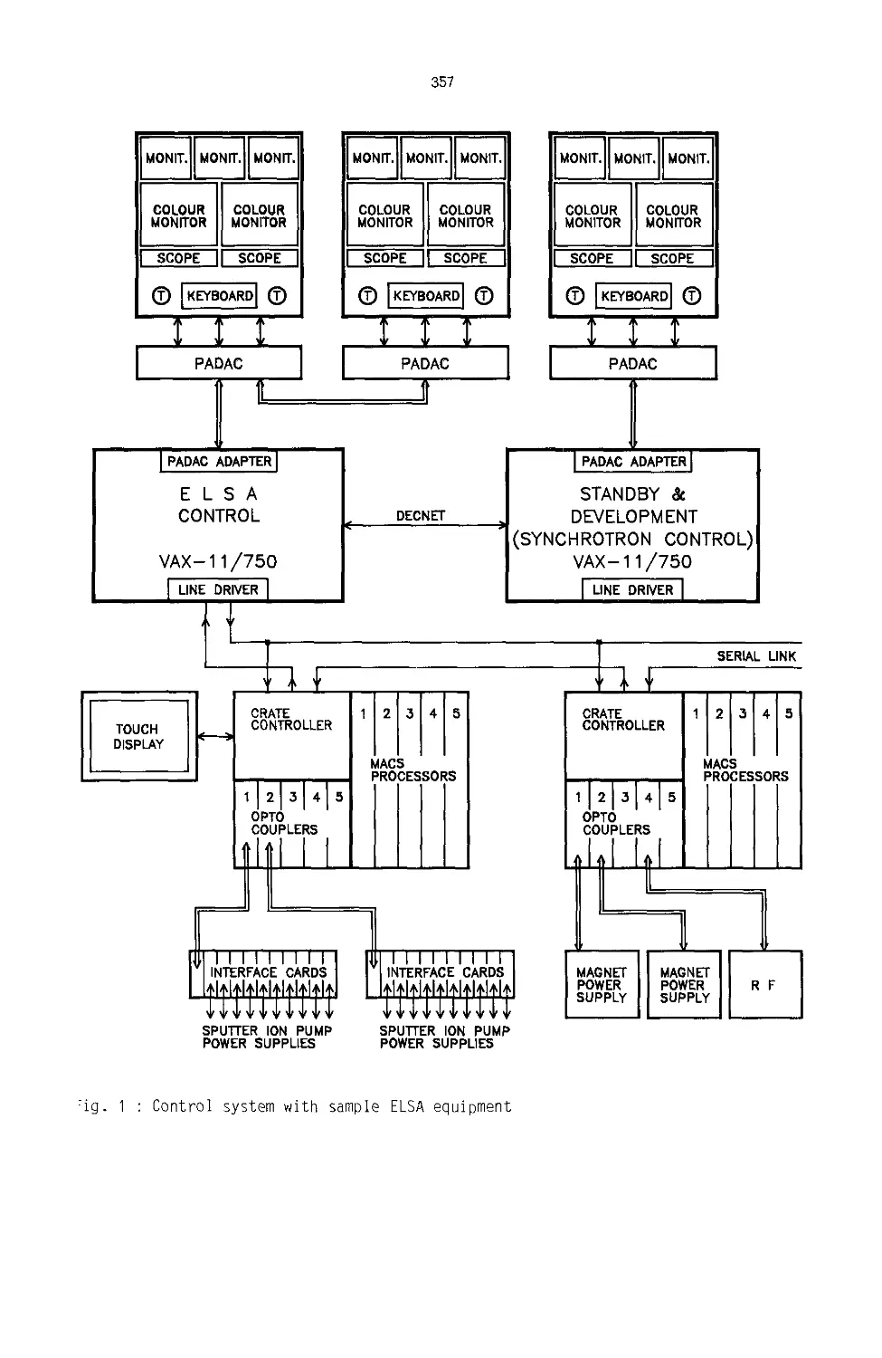
The ELSA Control System Hardware 355
Ch. Nietzel, M. Schillo, H. J. Welt, C. Wermelskirchen
Computer Control System of Polarized Ion Source and Beam 361
Transport Line at KEK
J. Kishlro, z. Igarashi, K. Ikegaml, K. Ishii, T. Kubota,
A. Takagi, E. Takasaki, Y. Mori, S. Hukumoto
Computer Control System of TRISTAN 367
A. Akiyama, K. Ishii, E. Kadokura, T. Katoh, E. Klkutanl,
Y. Kimura, I. Komada, K. Kudo, S. Kurokawa, K. Oide, S. Takeda,
K. Uchlno
The System for Process Control and Data Analysis Based on 372
Microcomputer and CAMAC Equipment in the LAE 13/9 Linear
Electron Accelerator
Z. Zimek, J. R. Zablotny
Some Features of the Computer Control System for the Spallation 377
Neutron Source (SNS) of the Rutherford Appleton Laboratory
T. R. M. Edwards
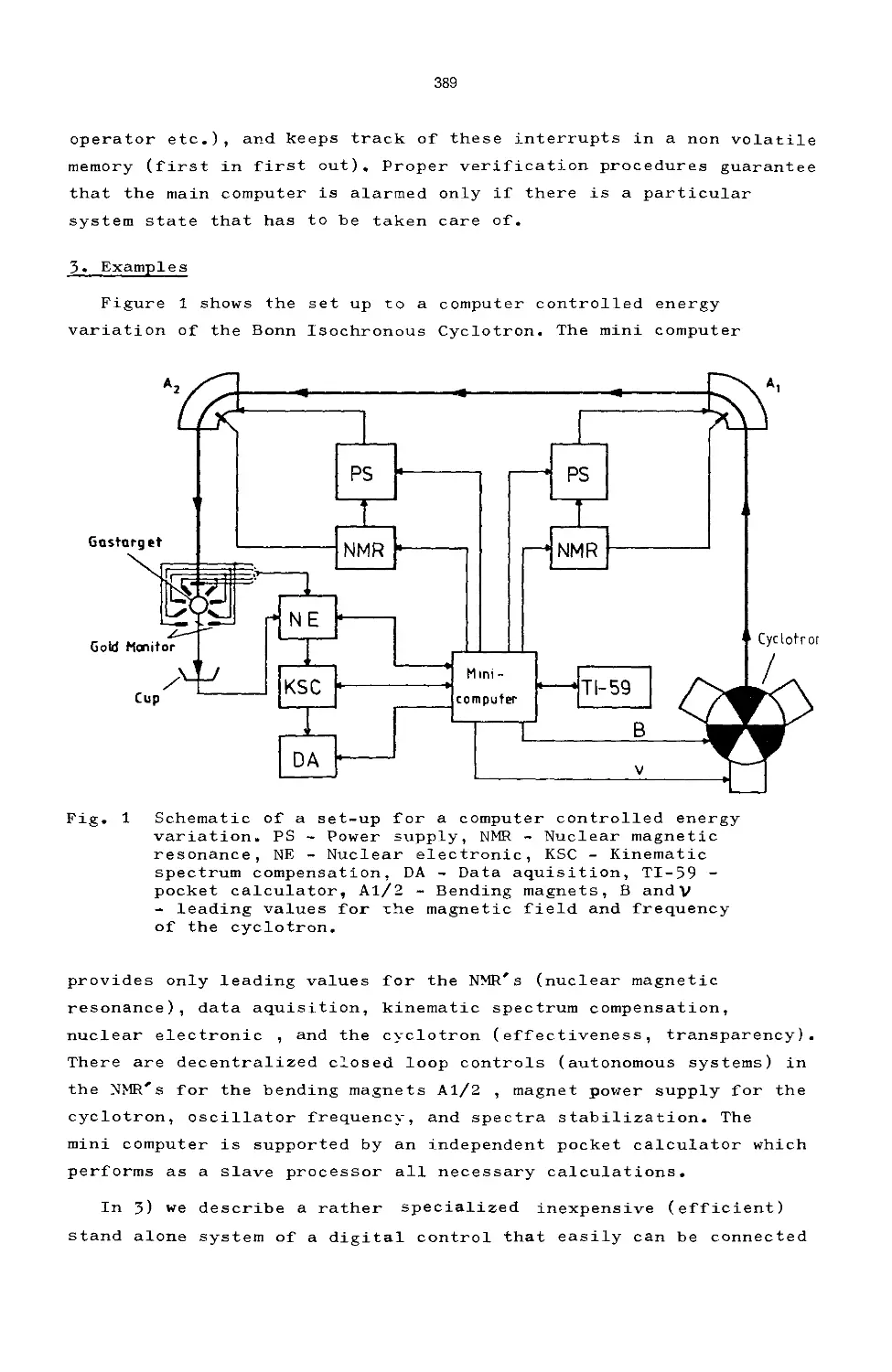
Design Criteria for the Operation of Accelerators Under 386
Computer Control
P. D. Eversheim, P. von Rossen
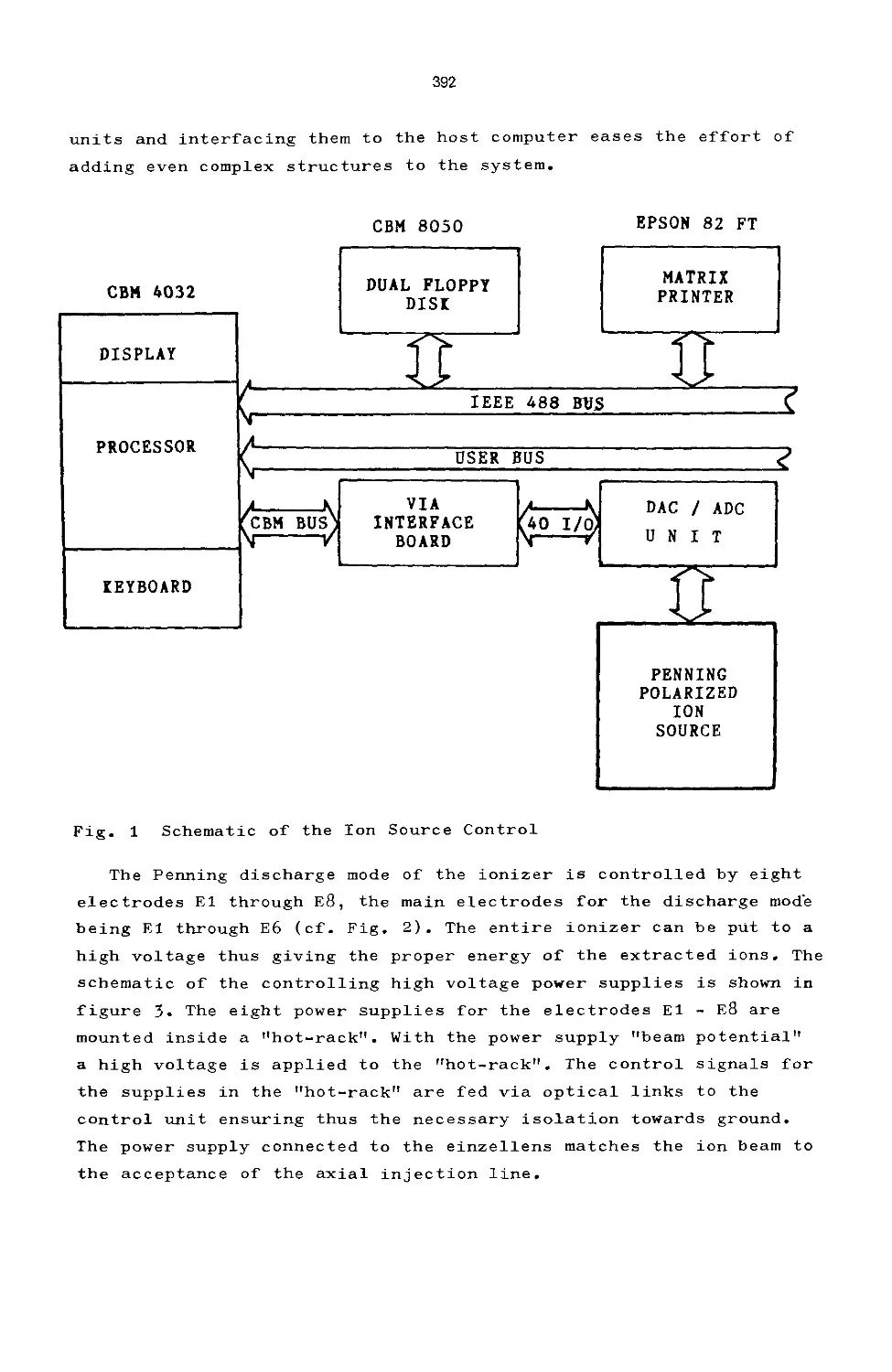
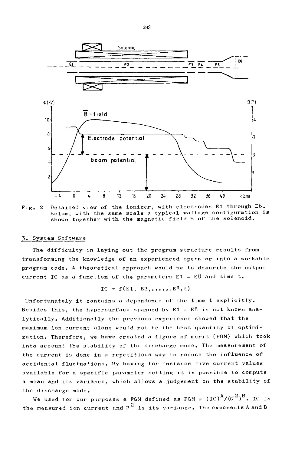
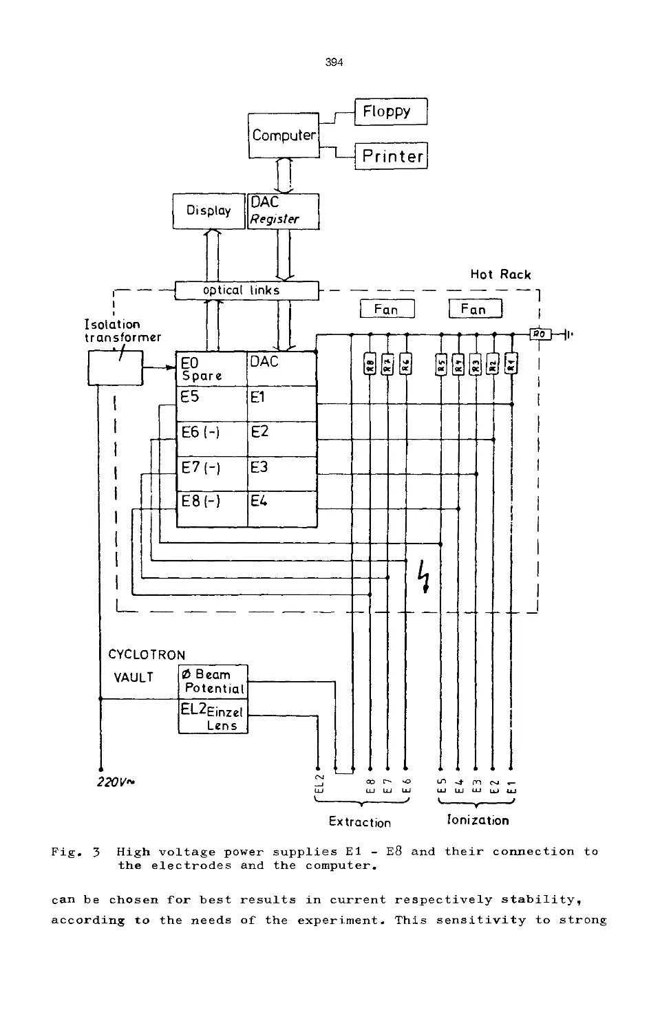
Computer Aided Control of the Bonn Penning Polarized Ion Source 391
N. W. He, P. von Rossen, P. D. Eversheim, R. Busch
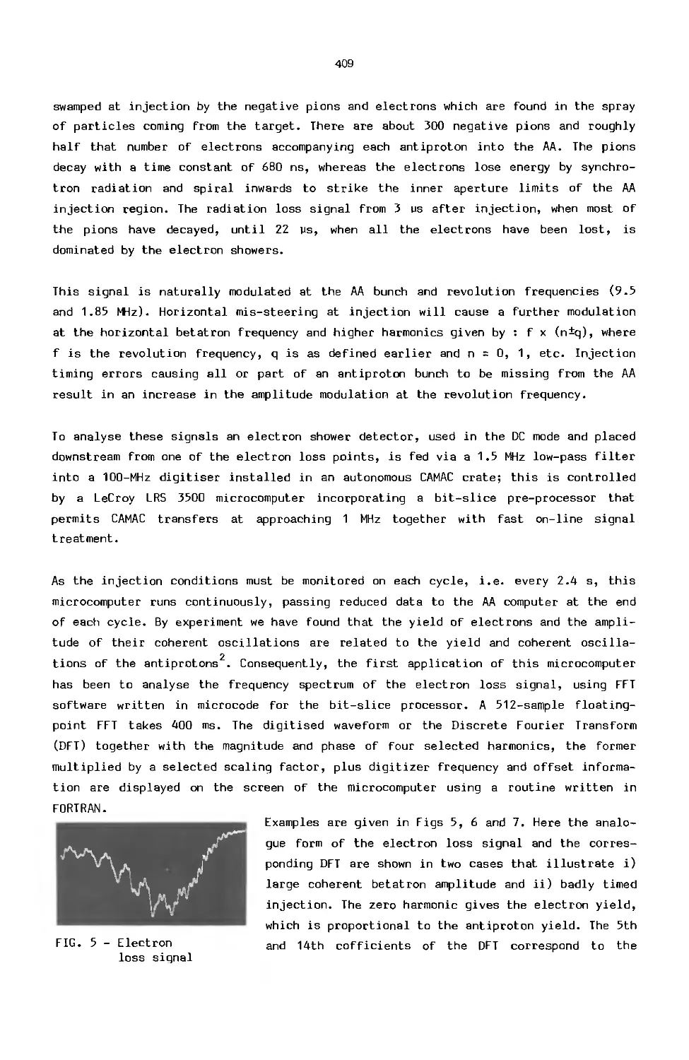
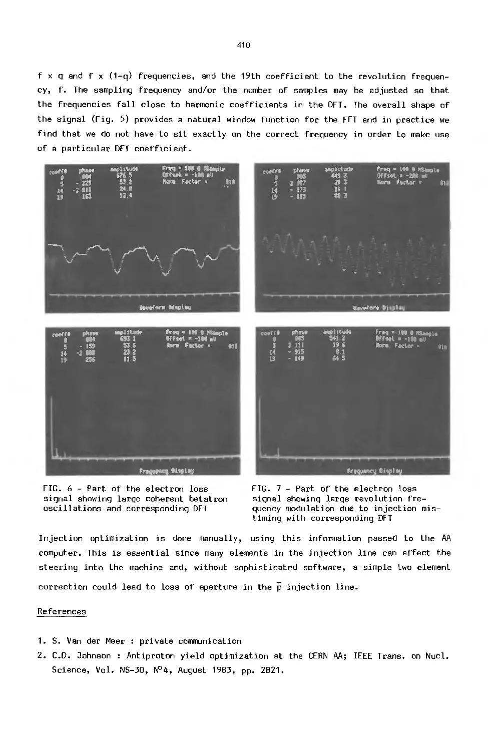
Treatment and Display of Transient Signals in the CERN 398
Antiproton Accumulator
T. Dorenbos
Fast CAMAC-Based Sampling Digitizers and Digital Filters for 405
Beam Diagnostics and Control in the CERN PS Complex
V. Chohan, C. Johnson, J. P. Potler, M. Miller
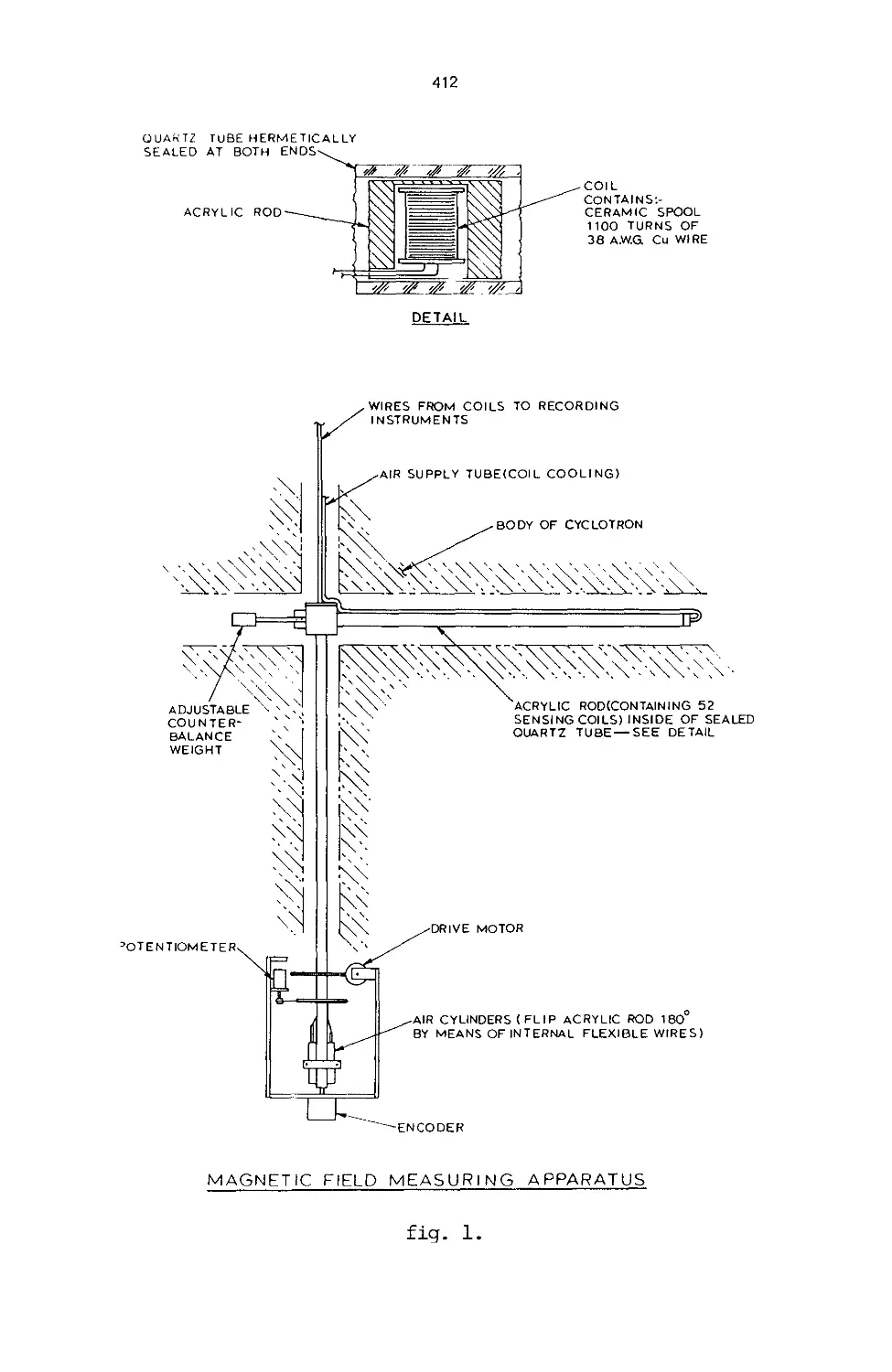
Automated Cyclotron Magnetic Field Measurement at the University 411
of Manitoba
V. Derenchuk, J. Bruckshaw, I. Gusdal, J. Lancaster,
A. McIlwain, S. Oh, R. Pogson, J. S. C. McKee
On the Problem of Magnet ftimping 416
E. Bozoki
High Level Control Programs at NSLS 420
E. Bozoki
The Minicomputer Network for Control of the Dedicated 425
Synchrotron Fteidiation Storage Ring BESSY
G.v.Egan-Krieger, W.-D. Klotz, R. Maier
XI
The Electronic Interface for Control of the Dedicated 436
Synchrotron Fteidiation Storage Ring BESSY
G.v.Egan-Krieger, W.-D. Klotz, R. Maier
WORKSHOP No.2: Which IAN to Use for Accelerator Control 445
C: COMPUTING IN ACCELERATOR OPERATION
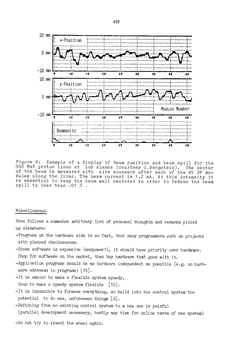
Introduction to Computing for Accelerator Operation 446
W. Joho
Man-Machine Interface Versus Full Automation 455
V. Hatton
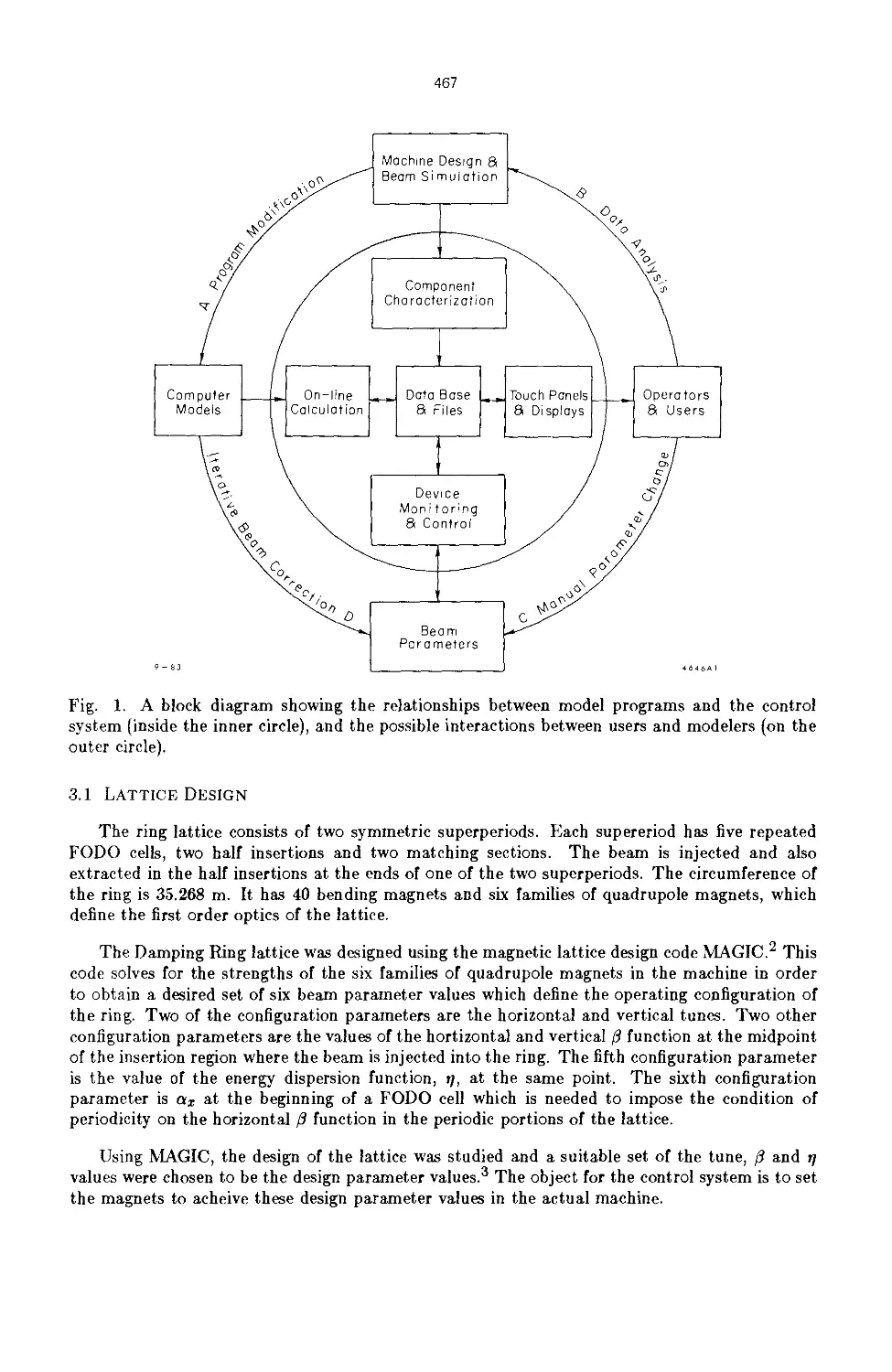
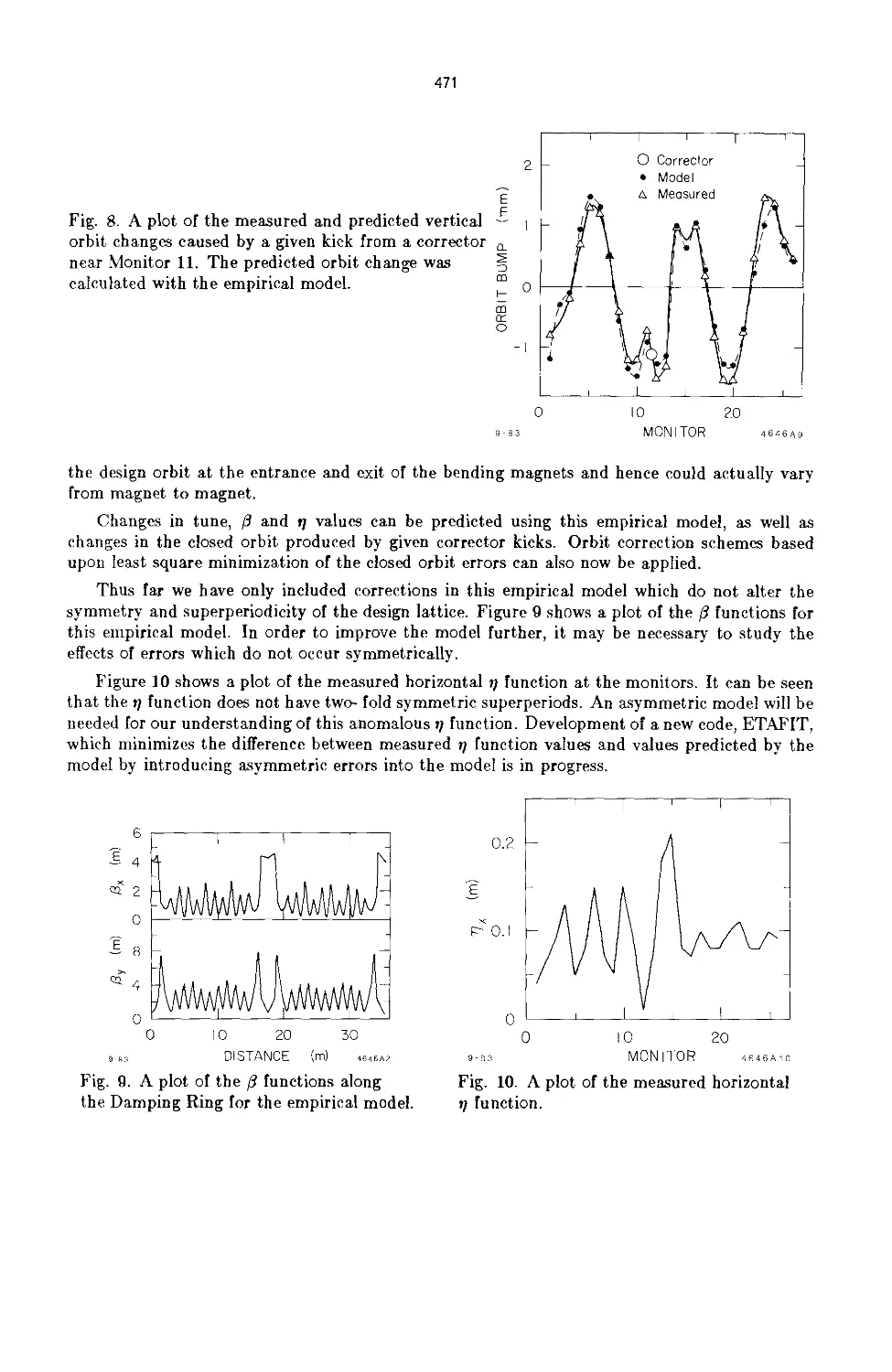
Models and Simulations 465
M. J. Lee, J. C. Sheppard, M. Sullenberger, M. D. Woodley
Operations and Communications Within the Daresbury Nuclear 473
Structure Facility Control System
S. V. Davis, C. W. Horrabln, W. T. Johnstone, K. Spurllng
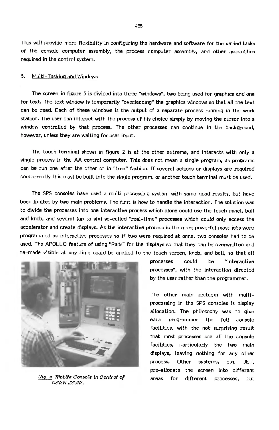
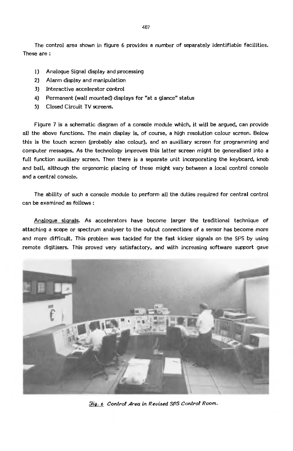
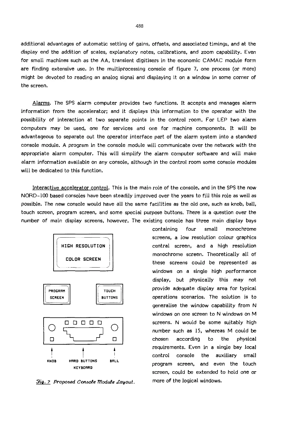
Consoles and Displays for Accelerator Operation 481
G. Shering
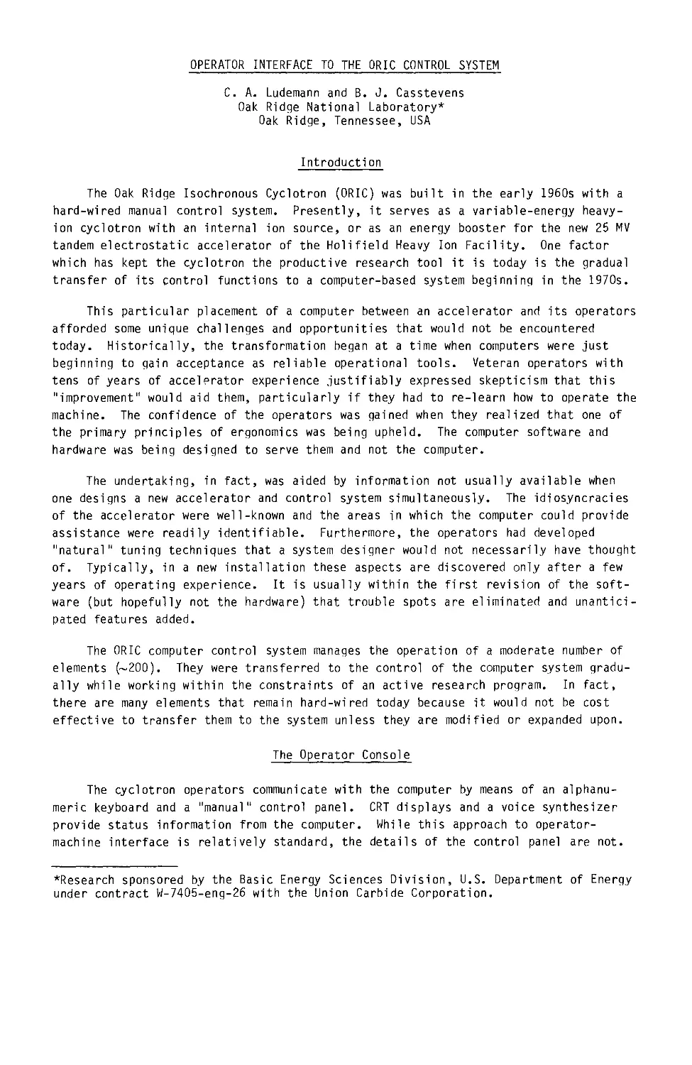
Operator Interface to the Oric Control System 491
C. A. Ludemann, B. J. Casstevens
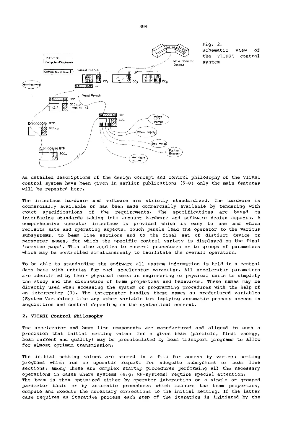
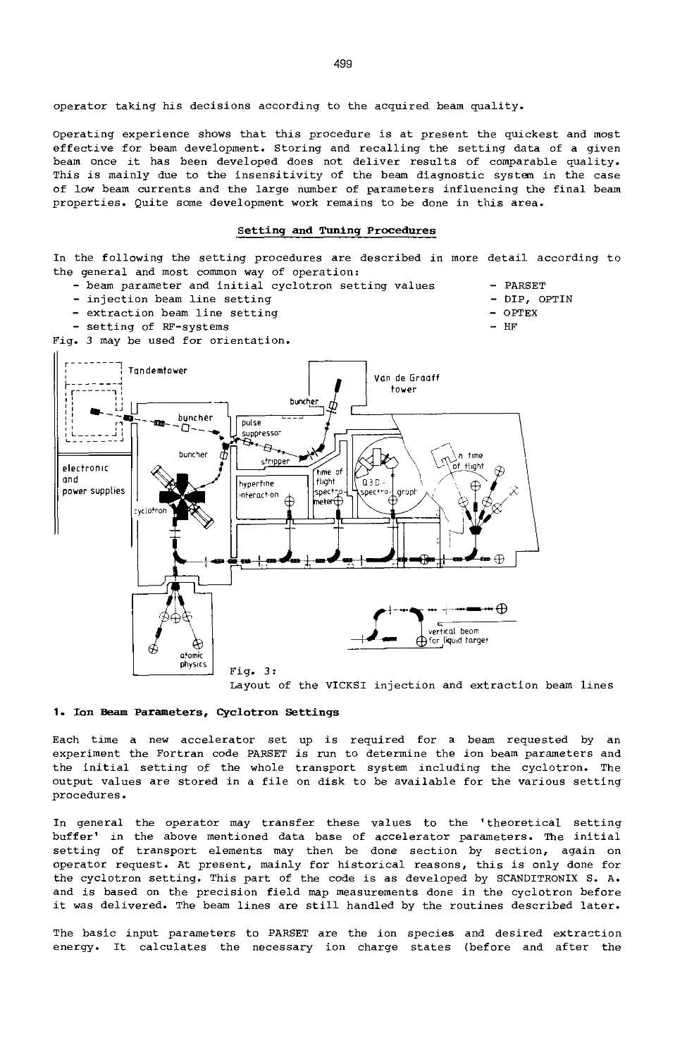
Computer Aided Setting Up of VICKSI 497
W. Busse, B. Martin, R. Michaelsen, W. Pelzer, B. Spellmeyer,
K. Ziegler
GANIL Beam Setting Methods Using On-Line Computer Codes 503
GANIL Operation Group and Computer Control Groups
A Multi-Processor, Multi-Task Control Structure for the CERN SPS 509
C. Saltmarsh
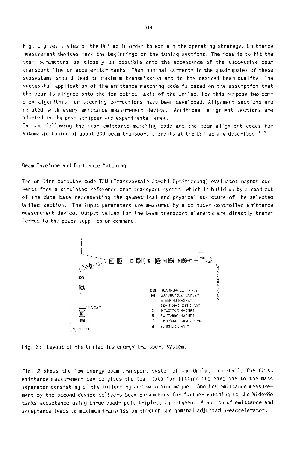
Computer Codes for Automatic Tuning of the Beam Transport at the 518
UNILAC
L. Dahl, A. Ehrich
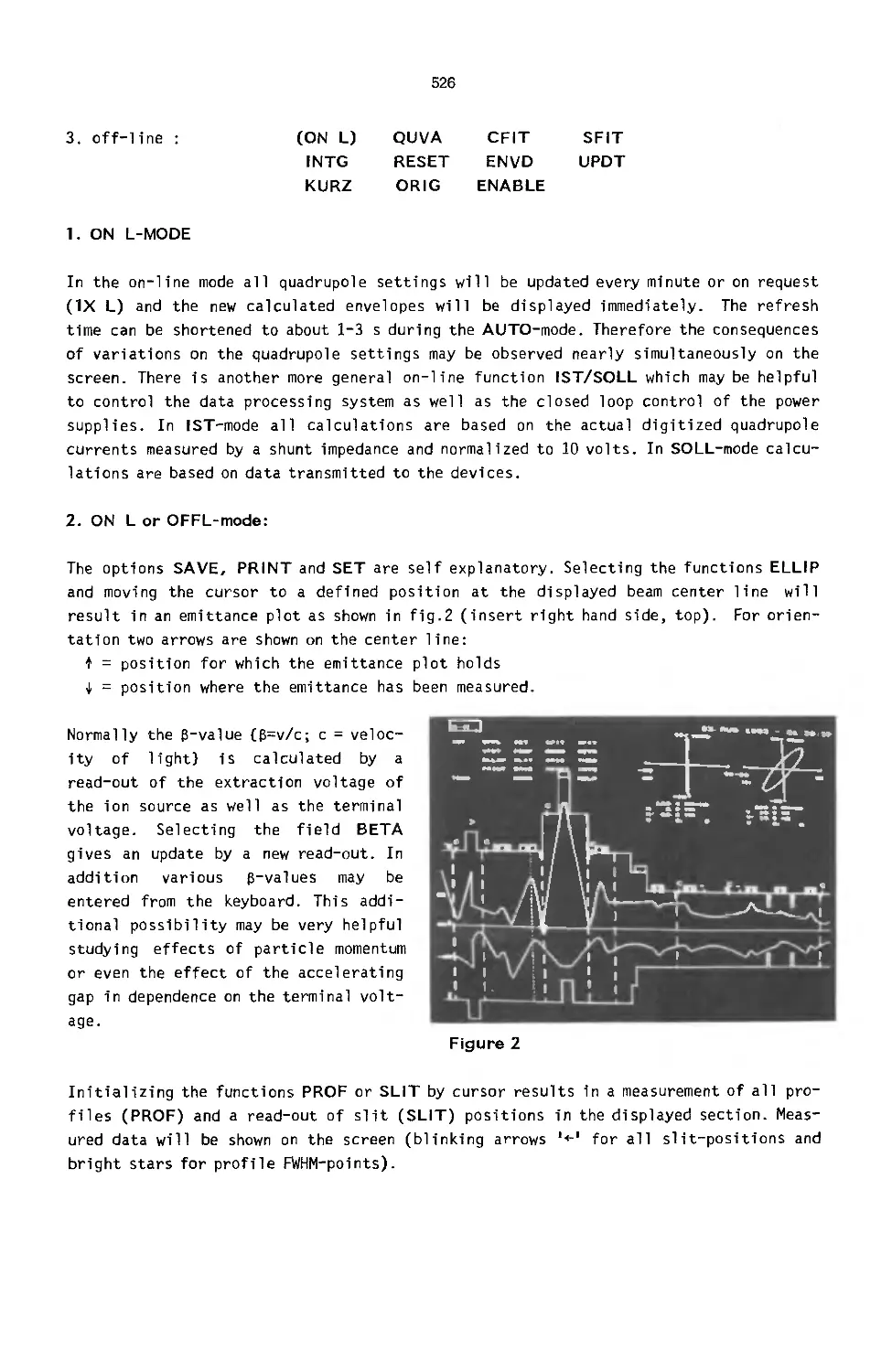
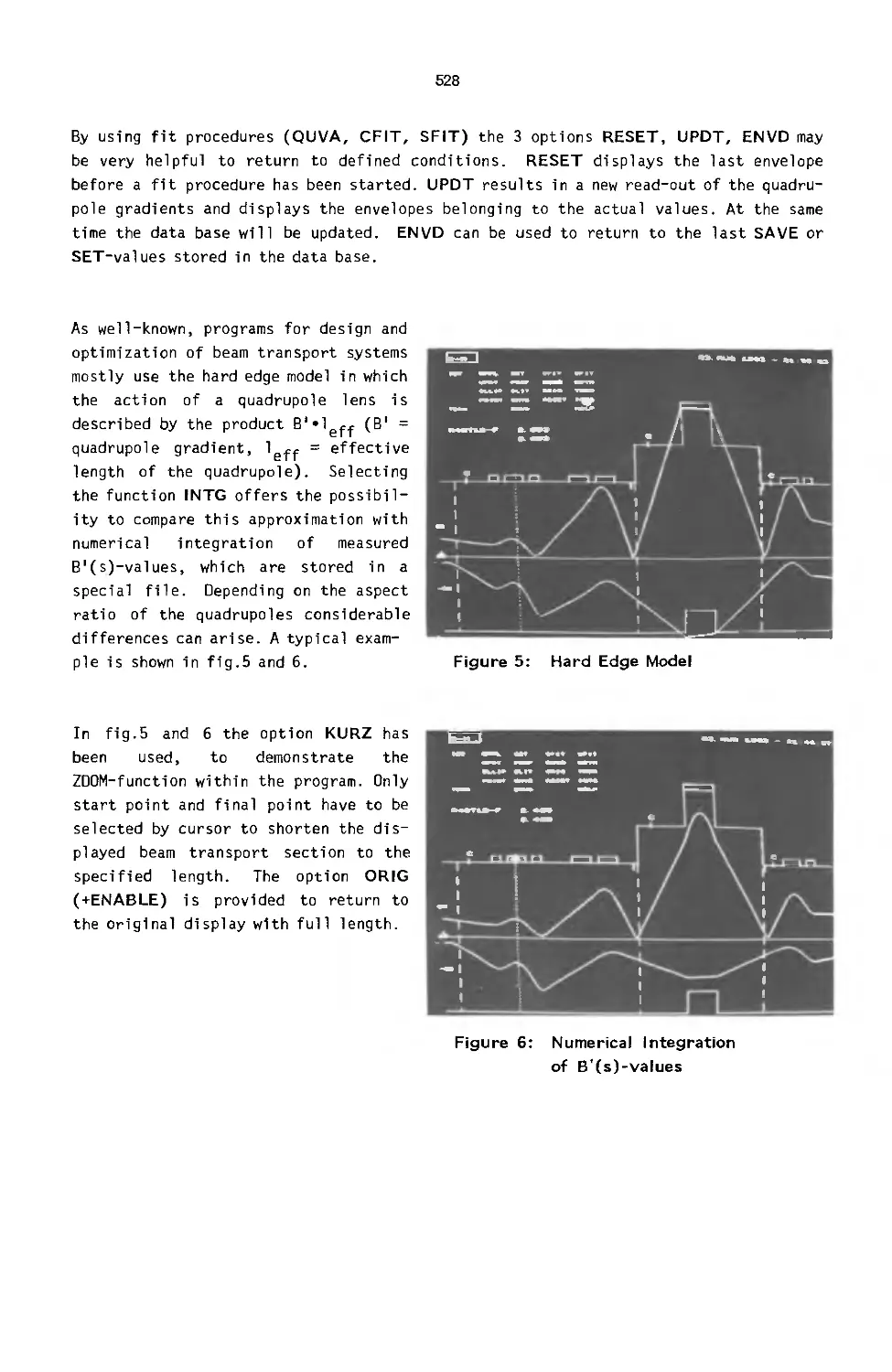
Interactive Testprogram for Ion Optics 524
V. Schaa, G. Fliss, P. Strehl, J. Struckmeier
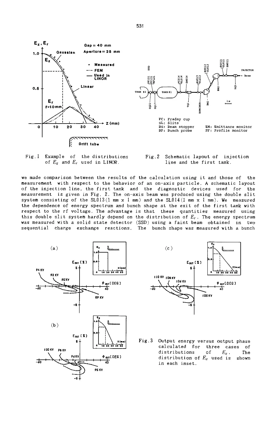
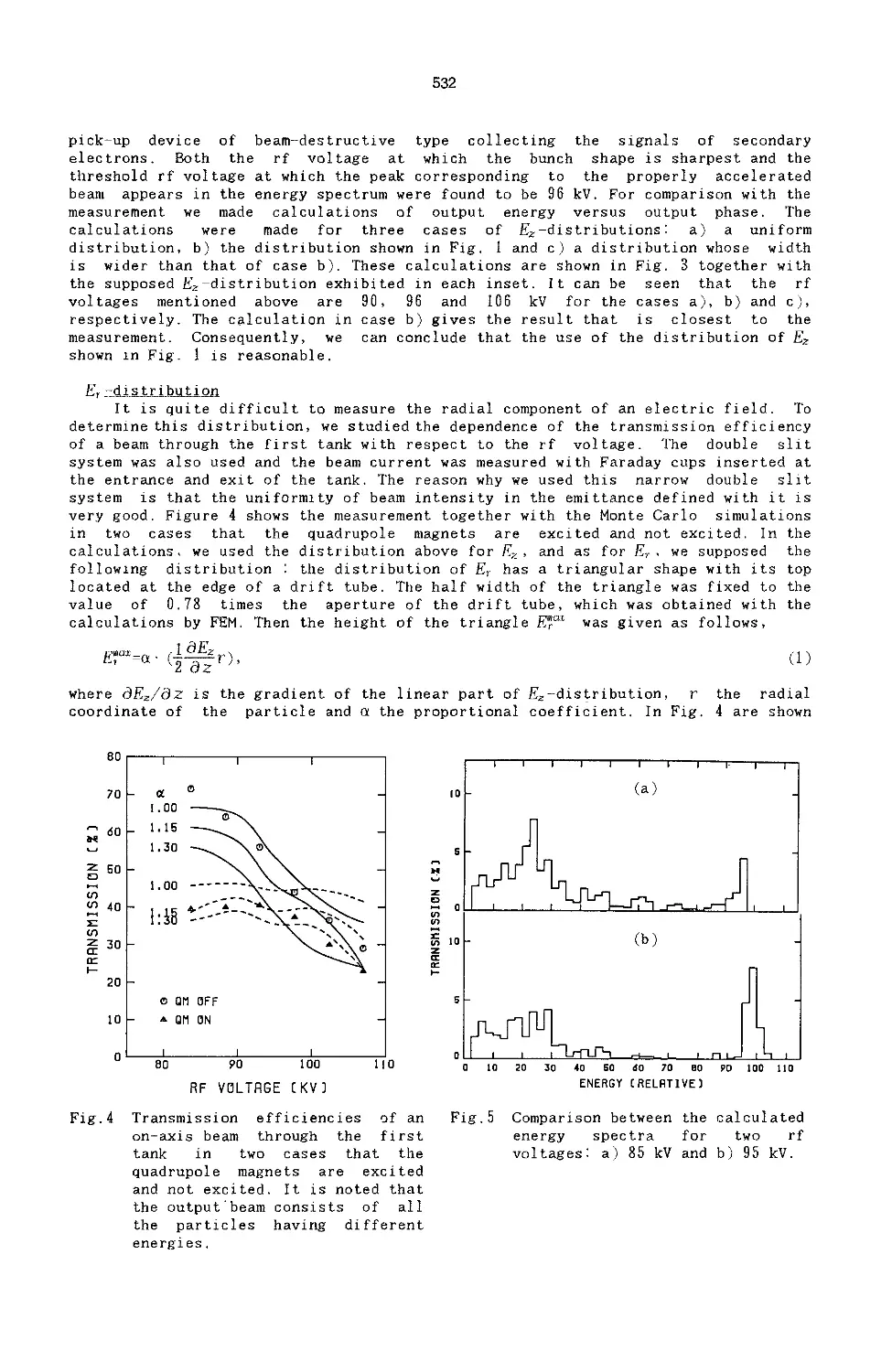
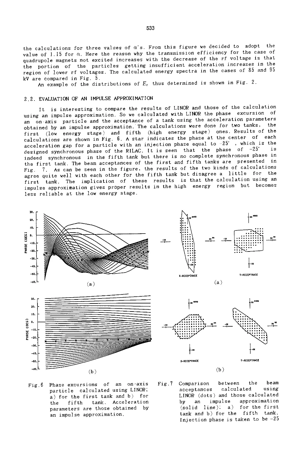
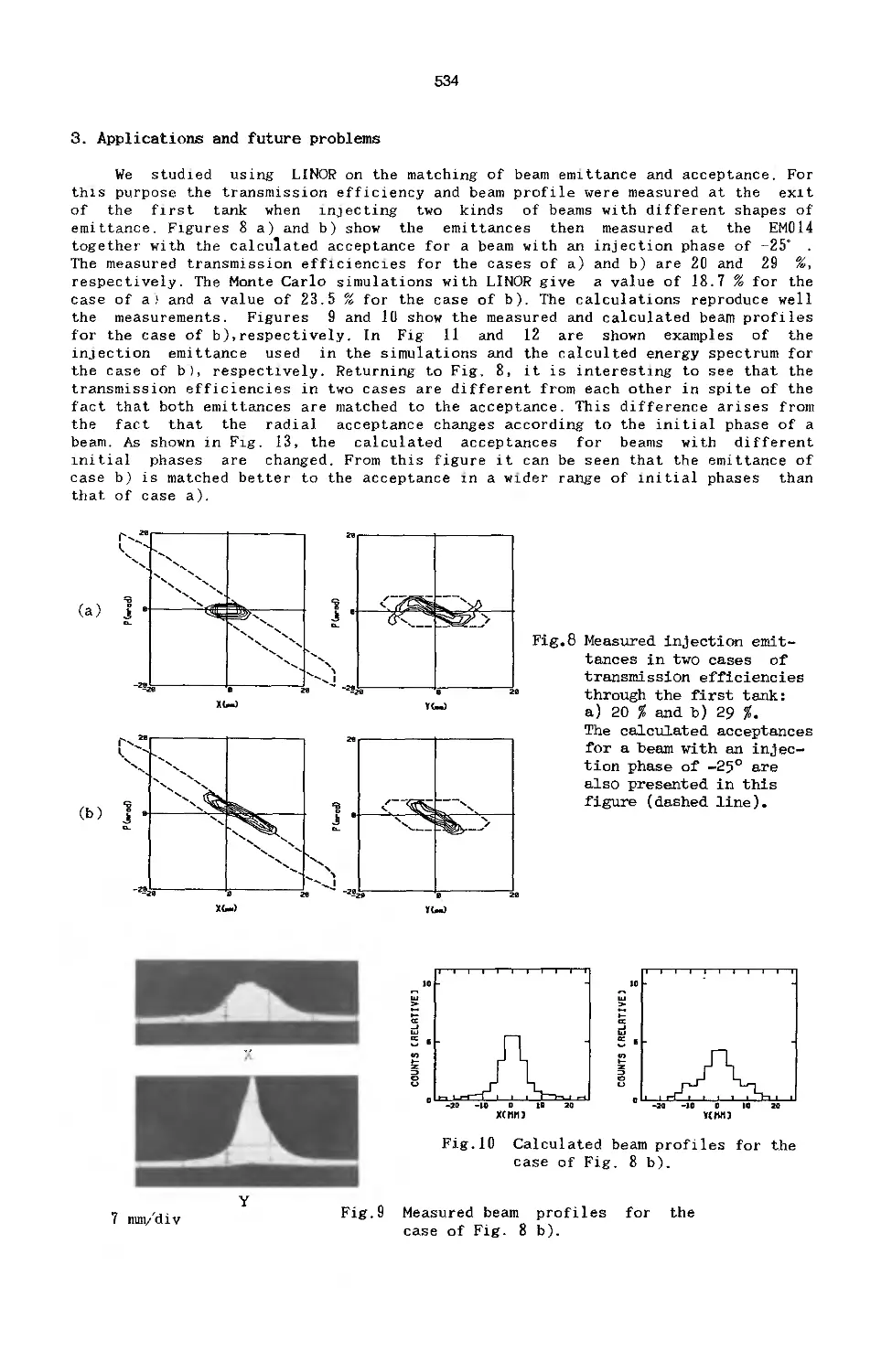
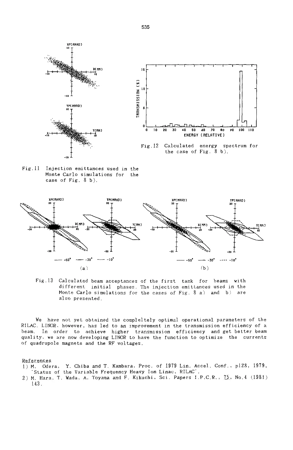
Numerical Orbit Calculation for a LINAC and Improvement of Its 530
Transmission Efficiency of a Beam
A. Goto, M. Kase, Y. Yano, Y. Miyazawa, M. Odera
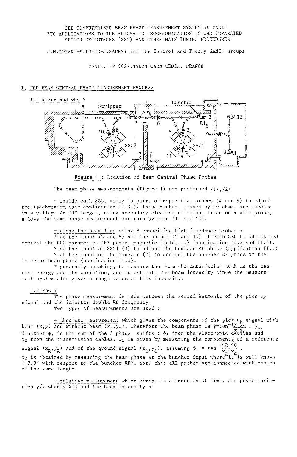
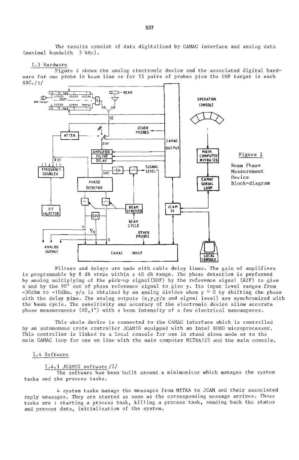
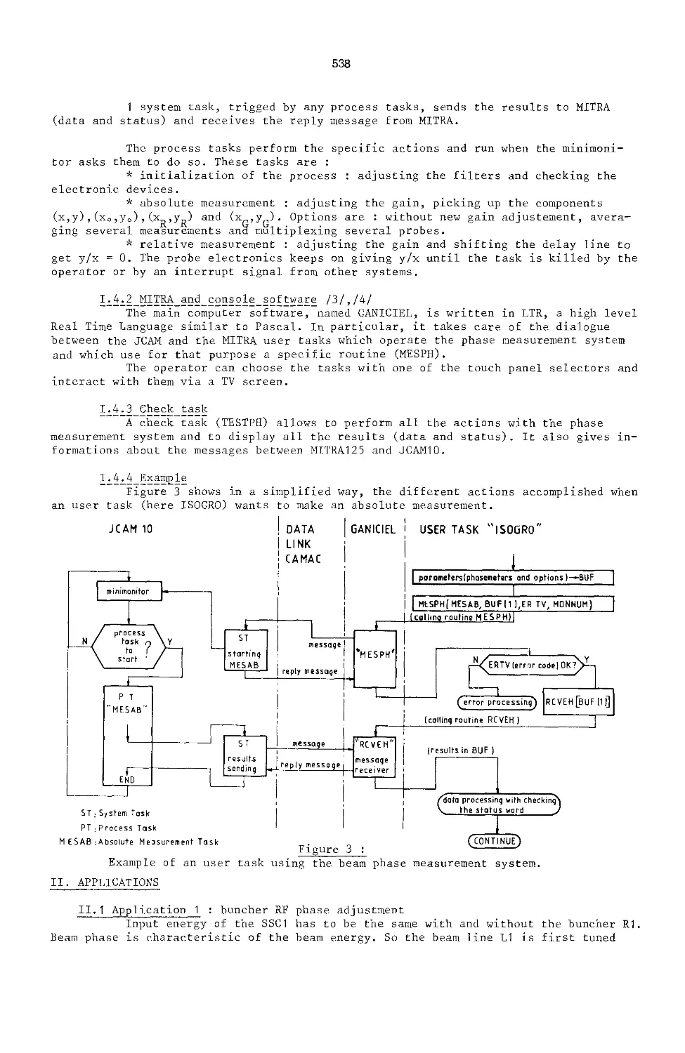
The Computerized Beam Phase Measurement System at GANIL - Its 536
Applications to the Automatic Isochronization in the Seperated
Sector Cyclotrons (SSC) and Other Main Tuning Procedures
J. M. Loyant, F. Loyer, J. Sauret
On-Line Optimization Code Used at SATURNE 542
J. M. Lagniel, J. L. Lemaire
XII
Automatic Supervision for SATURNE 553
C. Fougeron, J. Gontier, J. M. Lagniel, P. Mattei
A Local Computer Network for the Experimental Data Acquisition 557
at BESSY
W. Buchholz
Closing Remarks 561
M. C. Crowley-Milling
Conference Attendees 563
Author Index 573
FUTURE HIGH ENERGY ACCELERATORS
John ADAMS
European Organization for Nuclear Research (CERN)
1211 Geneva 23 - Switzerland
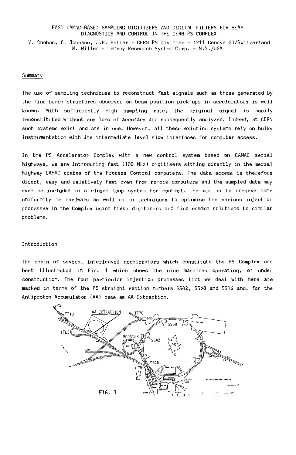
Introduction
I feel very honoured to be asked to give the opening talk at this
conference on computing in accelerator design and operation. The subject of my talk
is future high-energy particle accelerators and colliders, that is to say machines
that may be built after those that are now in operation or under construction. The
reason for this choice of subject is that I believe that these future machines will
make even heavier demands on computing than the present ones, especially on computer
control systems. I realise that this is not a very original thought since it only
follows the trend which has been evident in recent years. Nevertheless, we are a
still a long way from the cybernetic machine proposed many years ago by scientists
at the Radio Technical Institute in Moscow but I believe future machines will push
us much further in this direction.
The needs of the research
In presenting this subject to you I thought that I should start by saying
something about the needs of the research in the years ahead, since it is these
needs which should determine what kind of accelerators and colliders are built in
the future. These research needs are usually determined by theoretical predictions
so one may ask the question, what does theory predict?
The most depressing prediction is that nothing much will happen after the W
and Z particle energy range of about 0.1 TeV until one reaches energies which are
well beyond any accelerator or collider that can be conceived today. In other
words, there stretches before us a featureless desert whose further boundary is way
beyond our reach. This view is based on two assumptions. Firstly that there are no
new gauge forces except the know SU(3), SU(2) and U(l) operating between the
2
presently accessible energy range and some very much higher energy level and
secondly that no new particles will occur in this energy range which upset the value
of the Weinberg angle , sin2 6 = 3/8. With these two assumptions and the
w
known quarks and leptons, the renormalization group extrapolation shows that the
effective couplings of the three gauge forces converge to the same value at the same
upper energy level and that this level has the very high value of 1011 TeV.
Beyond that energy level there is another at about 10le TeV which comes from the
supergravity ideas and the possibility of unifying gravity with the other forces.
Thus the desert stretches from 0.1 TeV out to at least 1011 TeV. This
prediction is not, of course, very encouraging to experimentalists and machine
builders nor is it very much use in fixing the characteristics of future machines,
at least not until we know how to get to 1011 TeV. In fact, it led Abdus Salam
to entitle a talk which he gave last year on this subject at the International
Particle Physics Conference "The impending demise of high energy accelerators" and I
am indebted to that talk for the explanation of the desert syndrome which I have
just given you. Incidently, he concluded his talk with the advice - "Do not ask
theorists which energy to aim at for future machines. Aim at the highest possible".
A more useful prediction, at least for machine builders, is that there may
be flowers blooming this side of the desert which with a great effort we might be
able to reach. This view is based on the observation that the present so called
standard model based on the unified electroweak theory of Glashow, Weinberg and
Salam and the QCD theory of strong interactions cannot be the final answer. For
example, it does not predict the numbers of families of quarks and leptons or their
masses or their mass ratios. Also there is the all important symmetry breaking
which causes the gauge bosons that mediate between the weak interactions, the W
particles, to acquire very large masses whereas those that mediate between the
electromagnetic interactions, the photons, are massless. The "deus ex machina" is
said to be the Higgs mechanism with its scalar Higgs particle. Unfortunately,
nothing seems more elusive than the Higgs particle. Is it a particle or a set of
particles or - and I quote - "an approximation of dynamical effects which manifest
themselves at energies a few times the inverse square root of the Fermi weak
interaction coupling constant", i.e. roughly 1 TeV 1 Clearly the search for and
study of the Higgs particle or its equivalent is of the highest interest and
priority and fortunately the energy range in this case could conceivably be reached
by particle colliders in the forseeable future.
The machine energies required to explore the Higgs sector depend on whether
the machine is a proton collider or an electron collider. A rule of thumb is that
an electron-positron collider of one sixth to one tenth the centre of mass energy of
a hadron collider will explore the same general domain of hard processes or heavy
particle production. So, if the Higgs sector has a mass scale of about 1 TeV, the
3
future electron-positron collider should give about 2 TeV in the centre of mass
system and a proton-proton collider about 20 TeV.
This seems for the moment the best guide we can get from theory concerning
future machines but before turning to these machines, I should point out that past
predictions about the future needs of the research show a marked lack of correlation
between the reasons given for building the machines and the important discoveries
they made.
T. D. Lee in a recent talk at Brookhaven listed the twenty most outstanding
discoveries made using accelerators and colliders during the last 35 years starting
with pion production at the 184 inch cyclotron at Berkeley in the late 1940's and
ending with the intermediate vector bosons at the SPS collider at CERN this year.
He pointed out that only two of these twenty landmark discoveries, the anti-nucleons
at the Berkeley Bevatron and the intermediate vector bosons at the CERN collider
were anticipated at the time the relevant machines were approved. Another
remarkable feature he found was that the major discoveries arrived very regularly
over the 35 years - almost one every two years. It seems that Nature reveals her
secrets unexpectedly but rather regularly, but she does not read machine
prospectuses.
After these cautionary remarks I will
now pass on to the machines
themselves.
Future accelerators and colliders
Two machines have emerged in recent years as possible candidates for the
accelerators and colliders of the future. The first is a hadron collider, either
proton-proton or proton-antiproton, which might also be used as a fixed target
machine and the second is a linear electron-positron collider. Both of these
machines were studied in some depth at two workshops organized by the International
Committee for Future Accelerators (ICFA) in 1978 and 1979. More recently, the
hadron collider, under the name of the Desertron, or Superconducting Super Collider
(SSC), has been taken up enthusiastically in the USA. There was a Summer Study on
particle physics and future facilities held at Snowmass in Colorado in July
1982.This was followed by a Technical Workshop on a 20 TeV hadron collider held at
Cornell University in March 1983 and by a Workshop on hadron collider detectors held
at Berkeley in April 1983.
From all these studies and workshops, the
general conclusion emerges that a
hadron collider with a centre of mass energy of about 20 to 40 TeV is technically
4
feasible, that it would cost about 2 billion dollars and maybe more, and that
detectors could be designed to measure the events produced in the collisions at
these high energies and extract the relevant data. To reduce the machine cost down
to 2 billion dollars it is thought that 3 or 4 years of design and development work
will be needed on its components before construction can start. There is less
agreement on how long all this would take assuming, of course, that the U.S.
government is willing to agree to such a large and expensive project. Estimates
range from 9 years to 15 years. In other words, if approval is given to this
venture in 1984, the collider might be operating at the earliest in 1993 or at the
latest in 1998; let us say sometime in the second half of the 1990's.
Let me now say something about this machine. Since it is assumed that new
particles or sets of particles beyond the W will have smaller production
1/2
cross-sections following roughly the s law, the highest machine luminosity
seems to be desirable and this can best be achieved by a proton-proton collider,
i.e. an intersecting ring machine like the ISR or CBA in which luminosities
approaching 1033 per cm2 per second are thought possible.
The magnet system for this machine will have to use superconducting coils
to reduce its electrical power consumption to an acceptable level. Three magnet
systems were studied at the Cornell Workshop, the first used bending magnetic fields
of 2-3 Tesla, the second 5-6 Tesla and the third 8-10 Tesla. The first would use
iron to shape the field and superconducting coils to save power. The second would
be based on Tevatron or CBA technology using NiTi conductor at 4.5° K. For the
third, 8 Tesla could be reach with NiTi conductor by operating at 2°K, but 10
Tesla would need Nb Sn conductor. A 3 Tesla machine for 20 TeV beam energy
3
would be about 160 km in circumference, a 5 Tesla machine 100 km and an 8 Tesla
machine about 60 km. For comparison, the largest machine now under construction is
LEP which is 27 km in circumference. This future machine is therefore several times
the size of LEP. Curiously enough rough estimates of the total cost of the machine
made at Cornell showed little difference whichever bending field level is chosen as
can be seen in Table 1.
Table 1
Estimated Machine Costs (Million Dollars) [20 + 20 TeV.pp]
3 Tesla 5 Tesla 8 Tesla
Fixed costs [1] Enclosure, etc. [2] 540 + 300 ± 450 ± 350 ± 80 120 150 80 540 + 190 ± 710 ± 280 ± 80 70 240 60 540 + 130 + 780 ± 230 + 80 50 260 50
Magnets [3] Accelerator components [4]
TOTAL 1640 ± 320 1720 ± 360 1680 + 360
5
[1] Fixed costs include the site infrastructure (but not the cost of the site)
the injector machines, experimental areas and the magnet factory.
[2] Enclosure costs include the machine tunnel, access roads, service
buildings and power distribution.
[3] Magnet costs include all magnet elements and their cryogenic systems.
[4] Accelerator components costs include the refrigerators, vacuum, RF,
controls, injection and abort systems, power suppliers, robots, etc., and
installation costs.
One of the tasks during the initial development period of this machine
will be to chose between these three magnet systems. Another even more important
task is to see whether the present cost estimates are realistic since if one
compares them with superconducting magnet machines like the Tevatron or CBA, one
sees that large reductions have been made in the unit costs of the components to
get the total machine cost down below 2 billion dollars.
The size of these reductions can be seen from estimates made by R.B.
Palmer for a 5 Tesla 20 + 20 TeV pp collider based on the latest Fermilab cost data
for Tevatron magnets. He arrived at total cost of 6.6 billion dollars compared
with the 1.7 of Table 1 and cost reduction factors for magnets and tunnels ranging
between 4 to 6. Achieving such large cost reduction factors will not be easy.
Even the alternating gradient focusing principle, when it was introduced in 1953,
only reduced total machine costs by a factor of 2.
Different ways are proposed to make these cost reductions, for example,
using a very small magnet aperture giving a good field region of about 20 - 30 mm
diameter and getting the beam once round the machine by coaxing it sector by sector
round the 100 km circumference; installing the bending magnets of each ring side by
side in the same cryostat to reduce heat losses and save refrigerator power; using
very small cross section tunnels, in the limit only sufficient for the machine but
not for human beings; and using modern techniques to reduce production costs of
machine components.
Let me now turn to the other future machine, the linear electron-positron
collider. At the ICFA Workshops of 1978 and 1979, a tentative design was made for
such a machine to give 700 GeV in the centre of mass system. A linear machine was
chosen since limiting synchrotron radiation losses in circular electron machines
with beam energies above about 250 GeV gives machine circumferences which are
6
prohibitively large. Two solutions were studied, a linear collider using room
temperature RF cavities and one using superconducting RF cavities. On balance the
room temperature solution looked more feasible although it required a peak RF power
of the order of 10* MW for driving the cavities. Since then the Novosibirsk and
SLAC laboratories have continued with these studies. At SLAC the construction is
going ahead of a machine called SLC using the existing 30 GeV electron linac
upgraded to give 50 GeV. Both electrons and positrons will be accelerated in this
linac and at the end of it the electrons will travel round one semi-circular arc to
meet head on the positrons which travel around a second arc. To reach the desired
luminosity of 6 x 10³° per cm2 per second the two beams, or rather bunches
of particles, have to be focused down to a diameter of about 1 or 2 microns. High
precision and stability are necessary in space and time to ensure that such small
diameter bunches actually hit each other at the collision point. This machine,
which is planned to come into operation in 1987 will give the first opportunity to
study experimentally the problems likely to be encountered in linear colliders
particularly the disruptive effect which one bunch has on the other when they
collide.
In addition to this experimental machine a tentative study has recently
been made of a linear electron-positron collider to give 2 TeV in the centre of mass
system based on existing technology. Some of the parameters of such a machine are
given in the next table.
Table 2
1+1 TeV electron-positron linear collider
RF frequency 2856 MHz (S band)
Length 2 x 50 km
RF gradient 20 MV/m
Repetition rate 185 Hz
Bunches per pulse 12
Bunch length 2 mm
No of particles per bunch 1.4 . 1010
No of klystrons 2 x 3500
Peak klystron power 330 MW
Average klystron power 23 kW
Total peak RF power 2.4 . 10® MW
Total average RF power 160 MW
7
The total length of this machine, 100 km, is about the same as the
circumferential length of the 20 TeV hadron collider and a very rough estimate of
its cost suggests a figure about twice as large.
One of the problems of linear colliders is that there is only one region
where the two beams meet head on. To run as many experiments as with a circular
hadron collider which has several interaction areas around its circumference, the
experiments of a linear collider have to be placed side by side and the linac beams
switched to each experiment in turn on a pulse to pulse basis. Since the beams
consist of bunches 2 mm long and a few tenths of microns in diameter, colliding the
bunches at the correct place inside each experiment does not seem so easy.
I can hardly leave this part of my talk without mentioning the pressing
need for new ideas for accelerating particles in order to reduce the size and cost
of the accelerators and colliders. The two future machines which I have just
described really are monsters; 100 km in circumference or length and costing several
billion dollars each. It is by no means certain that governments or even groups of
governments will be willing to finance such machines and we may be forced to find
cheaper solutions or stop building very high energy accelerators. Let me try to
explain what these new ideas should be aiming to achieve.
To reduce the size of future machines higher accelerating gradients are
needed, the accelerating gradient being defined as the maximum particle energy of
the machine divided by its length or circumference. Electron linacs are now
approaching gradients of 20 MeV/m although short test cavities have reached voltage
gradients of up to 150 MV/m. In the case of proton synchrotrons the accelerating
gradient as I have defined it is set by the maximum bending magnetic field. A 5
Tesla machine achieves 150 MeV/m and a 10 Tesla machine would achieve 300 MeV/m.
Therefore the new ideas of accelerating particles if they are to enable smaller
machines to be built should aim at accelerating gradients of several 100 MeV/m and
preferably at a few GeV/m. Since at a few 100 MeV/m it becomes impossible to
maintain the necessary voltage gradients between metal surfaces, the accelerating
field has then to be established in a medium such as a plasma column or an intense
electron beam. Some of the new ideas aim in this direction, for example the beat
wave accelerator in which two laser beams running along a plasma column have a
frequency difference equal to the plasma frequency and by beating together set up
intense localised charge concentrations and hence very high field gradients which
can then be used to accelerate particles. Several GeV/m are promised by this scheme
at least theoretically. However, these new ideas are still in their infancy and
even if they are found promising experimentally, it will take many years to develop
them into an accelerating system for a machine to give several TeV beam energy.
8
Also they must at least hold out the promise of less cost per GeV. A shorter but
more expensive machine is not a solution to this problem.
Future machines and computers
I would like to end now with a few remarks about the implications of future
machines to computing and so try to link my talk with the subject of this conference.
There are, as everyone knows, five distinct but overlapping phases of
machine building. These are the design phase, the construction phase, the
installation phase, the commissioning phase and finally the operating phase. I
notice that this conference only covers computing for the design and operating
phases. I would like to suggest that for future machines the other three phases
will also need a great deal of computing.
Let me illustrate this point by taking first the construction phase. Until
bright new ideas actually succeed in reducing the size and cost of future particle
colliders, we are faced with machines which will be of the order of 100 km in
circumference or length. These machines will contain thousands of components of a
limited number of types - magnets, RF cavities and power units, vacuum pumps and so
on. These components will have to be cheaply mass produced to very tight
tolerances. Up to now machine builders and industrial firms have used manufacturing
technologies which, although achieving the desired products to the required
tolerances, are relatively primitive compared with the methods now employed in the
most advanced mass production industry. In the case of superconducting magnet
production, Fermilab and Brookhaven have set up their own factories on site but the
Tevatron and the CBA are very small machines compared with a future 20 + 20 TeV
hadron collider. To manufacture the magnets of the latter in the same time as it
took for the Tevatron one would need 20 Fermilab factories working in parallel. It
seems therefore that much more automation in production perhaps using robotic
systems under computer control will be needed for future machines. This will also
allow a closer quality control which can then be integrated into the production
process rather than be superimposed as periodic inspection as has been the case up
to now. This same technology will be required for all the other machine components
which will be needed in their thousands.
Turning now to the assembly stage, the problem is to install thousands of
components in the correct order via a limited number of access points in a tunnel
100 km in circumference or length and to align them to a very high accuracy. If all
this is to be done in a reasonable time, like two or three years, it will require
superb logistic organization and a great deal of automation. There is first the
9
storage of finished components on the surface in sufficient number to ensure a
smooth supply for installation and their distribution to the access points. There
is then the transport of these components into and around the tunnel in the correct
sequence, since, for economic reasons, its size will not allow vehicles to overtake
each other in the tunnel. Each component must then be installed at the correct
place and finally there is the alignment of the components and their connection to
preinstalled electrical and other supplies. For the SPS machine at CERN, a computer
system was used for keeping track of all the components and their installation in
the correct place, and a fleet of free moving vehicles was used for transporting
them in the tunnel. For LEP a more elaborate data base system will be used for
marshalling the components and a relatively fast monorail for their transport in the
tunnel. For a future machine it may be necessary to use robots under computer
control both for marshalling components and transporting them to their allotted
position in the tunnel in the right order. And if the tunnel is so small that human
beings cannot work in it, then, in addition, the robots will have to put the
components in place, align them and connect them to their supplies. I leave the
experts to imagine the computer control system necessary for this kind of operation.
I come now to the commissioning stage. As I have already mentioned, cost
saving in future machines will require that the vacuum chamber and the good field
region of the magnet be as small as possible. If no allowance is made for initial
closed orbit deviations the machine will have to be aligned using the beam section
by section round the machine. Non-linear effects particulary of the dipole fields
on the beam dynamics will have to be studied in advance with elaborate tracking
programmes and more feed-back systems used to control the beam in the machine. The
multi-TeV hadron collider presents an additional problem. Circulating beams of
several amperes inside a small bore superconducting magnet for hours on end without
letting a very small fraction of the beam, a few milliamperes, reach a magnet
element and quench it will call for very precise and reliable beam control.
Scraping the beam, as regularly done in the ISR machine at CERN in order to prepare
it for experiments, without the scraped-off part hitting a magnet is another
problem. And finally, dumping the beam safely outside the superconducting magnet at
the end of each run or in an emergency without spraying magnet units with secondary
particles is yet another. Hopefully, solutions to these problems will be found and
tried out with machines like the Tevatron before the large hadron collider design
is finalized but whatever the solutions that are found, I am sure more computers and
computing will be required.
Finally, there is the problem of the maintainance of a machine 100 km in
circumference or length so that it achieves a high operating efficiency in terms of
hours per year for physics research. The planning of how the machine will be
subsequently maintained has, of course, to form part of its initial design. To a
10
large extent, the operating efficiency will depend on how quickly faults can be
detected and localised and then corrected either by adjustments or component
replacements. Given the size of the machine and the time needed to reach a
component, maintainance could take a very long time unless it is carried out by fast
robots backed up by computer systems.
Conclusion
I hope that these remarks about future machines and computing convince you
that more computer systems will be needed in the future and that they will be used
not only in the design and operating phases of future machines but also in their
construction, installation, commissioning and maintainance. This is the rather
cheerful message which I would like to pass on to you at the beginning of this
conference.
BEAM OPTICS AND DYNAMICS
E.J.N. Wilson
European Organisation for Nuclear Research (CERN)
1211 Geneva 23, Switzerland
Abstract
After introducing the fundamental equations which determine the optics of beams in
circular machines and how computers find their solutions, the paper describes how a
typical matching problem of designing a low-beta region might be tackled. The limit-
ations of existing optics programs are also discussed.
1. Introduction
I shall not attempt to describe in depth the art of designing synchrotrons or to dis-
cuss the frontiers of the theory of particle dynamics. Later papers in this conferen-
ce will provide material to tax the intellect. The aim of this paper is to explain to
the computational specialist who knows more about programming than about acceler-
ators, an outline of accelerator theory1, the way in which computers apply this
theory to help the designer and to suggest a few directions which might be explored
to improve the tools available.
As we shall see, the analysis of the optics of synchrotrons is largely a matter of
multiplying together a large number of matrices, each describing the transport of a
particle through a magnet. Regular patterns of magnets, or lattices, can be calcul-
ated in closed form but computers can be used to graft in special regions of the ma-
chine, where other components such as rf cavities or extraction magnets replace bend-
ing magnets or where the beam is focused to a narrow waist to collide with another
beam.
2. The Lattice Structure
A typical pattern of magnets or lattice of a modern accelerator, the SPS, is shown in
Fig. 1. The first element in a cell is a horizontally defocusing magnet, a quadru-
pole, characterised by its normalised gradient.
к - (1/B p) еВу/ Эх
12
where x, у are transverse to the beam direction. Half a cell later is a defocusing
quadrupole of opposite sign. There are four bending magnets between each quadrupole
and the 64 m long cell is repeated 108 times around the circumference of the acceler-
ator. In some places the bending magnets are omitted leaving space for equipment and
in others, special patterns of magnets called insertions interrupt the regular
lattice to make the beam very narrow.
Dj B2 B2 Bl В1 B1 B1 [|~B2 [b2~~|
Figure 1 - Lattice Functions in a Cell.
In the naive approximation used in the days before computers, quadrupoles, length, X,
were treated as thin lenses of focal length f = 1/kX. But, to a higher degree of
exactitude the circulating particles obey Hill's equation2:
2
£4 + k(s)X = о .
ds2
This equation and its solution:
x = e1/,2₽1/,2(s) cos[<k(s) + X]
1/2
are reminiscent of harmonic motion with a phase advance Ф and an amplitude ₽ (s),
which is envelope of the motion. The quantity e, the emittance, is constant depending
13
only on the size of the injected beam and its subsequent history. The difference is
that the amplitude like the restoring force both vary with s, the distance round the
ri ng.
In solving the equation of motion we wish to calculate ₽(s), from the lattice pattern
k(s) and to do so we use the fact that the solution of a linear differential equation
can be written as a transport matrix from a point Sjon the circumference to a point
s2:
operating on the displacement from the central orbit x and its derivative x' = dx/ds.
The transport matrix is simply the product of a number of matrices, one for each
element either a quadrupole or the drift length between lenses.
drift length quadrupole
1 X\ / cosH< X l/ИГ sinfk X
0 1/ \.ИС sin/F X cosHT X
Dipole magnets are slightly different from drift lengths in that their ends have a
focusing effect. One complication is that a quadrupole which is focusing in the hori-
zontal plane is defocusing vertically and vice-versa. The matrix multiplication must
be carried out independently for x and у motion. The defocusing matrix comprises hy-
perbolic terms and is obtained by substituting -k for к in the matrix above.
The transport matrix from a point around one complete turn can be computed numerical-
ly by matrix multiplication of the several thousand elements or it can be expressed
analytically in terms of the betatron amplitudes at the start/finish point:
(cos p + a sin p ₽ sin p \
j
-y sinp cos p - a sinp /
where a = -₽'/2,
Y = (1 + a2)/₽,
p = phase advance/turn = 2-itQ.
14
The four numerical elements of the computed matrix can be compared with the algebraic
expression and solved to find:
p = cos_1{TrM/2) ,
₽ = M12/sinp ,
a = (Ми - M12)/(2 sinp) .
It is the task of the lattice program to perform this calculation starting at each
point in the ring and for both planes and forming a table of щ f and a around the
ring. Fig. 2 shows a typical output for one cell.
LENGTH ANGLE «(V) ALPHA(P) 8ETA(H) ALPHA(HJ MUH/2PI BE TA (V J ALPHA( V ) muv/2Pi AM/2 av/;
3 , оаьооо 0,000000 •,015063 1 , 3864401 04 ,884855 2,452160 ,004571 19,011703 -,520345 ,026571 05,715663 9,917560
,360000 0,000000 0,000000 1,374653103,127965 2,428089 ,005122 19,395014 •,544408 ,029555 64,547513 10,017039
6,260000 ,008445 0,000000 1,196124 75,348859 2,009521 ,016433 28,828710 •,962519 ,072198 64,0043/1 12,212911
,400000 0,000000 0,000000 1 , 186405 73,75J94J 1 ,982775 ,017287 29,609417 -,989248 ,074377 54,751341 12,376825
6,260000 ,008445 0,000000 1,060742 5J ,548094 1 ,564207 , 033474 44,610910 •1,407071 , 101928 54,174091 15,192432
,390000 0 , 000000 0,000000 1 , 054559 50,338 J82 1,538130 ,034692 45,718585 •1,433122 ,103302 45,428681 15,37944/
6,260000 ,008445 0,000000 ,98J762 33,701223 1,119563 ,058975 66,274961 •1,850527 ,121441 44,905056 J8,5J7478
,380000 0,000000 0,000000 ,978948 32,860011 1 ,0*4 154 ,060793 67,691002 • 1 ,875896 , 1 22344 36,980337 18,713705
6,260000 ,008445 0,000000 ,959017 21 ,78 1 569 ,675566 ,09838J 93,787676 •2,292753 ,134861 36,534921 22,028267
2,342700 0,000000 0,000000 ,961450 18,98314© ,518942 , 1 J6758JO4,B96272 «2,449038 ,138621 30,069327 23,295624
3,085000 0,000000 ,015037 1 , 034354 18,983068 •,518916 ,143368104,901620 2,447388 ,143191 26,349412 23,716525
,350000 0,000000 0,000000 1 , 0507 30 19,354500 •,542318 ,146275103,196611 2,424067 ,143726 28,638028 23,296218
b , 26 0 00 0 ,008445 0,000000 1 , 37 0047 28,764399 •,960879 ,18901 J 75,452122 2,007802 ,155027 35,089639 23,106121
,380000 0,000000 0 , 000000 1 , 39 1 035 29,504322 • ,986287 ,191088 73,935822 1 ,982463 , 155836 35,546047 19,757412
6 , 260000 ,008445 0,000000 1 ,763219 44 ,472640 • 1 ,4 04847 ,218731 5 1 , 724094 1 ,5656 1 0 ,171975 43,750575 19,557880
,390000 0,000000 0 , 00000 0 1,786053 45,576591 • 1 ,430924 ,220109 50,513067 1,539589 ,173189 44,298587 16,358398
6.260000 ,008445 0,000000 2,213103 66,1 1 3699 • 1 ,849464 ,238298 33,849177 1,122280 ,197377 53,470174 16,165762
,400000 0 , 000000 0,000000 2,241952 67,603985 • 1 ,876229 ,239251 32,962034 1 ,095579 ,199283 54,079136 13,233307
6,260000 ,006445 0,000000 2,719866 93,714254 •2,294790 ,251780 21 ,859390 ,677943 ,236745 63,830251 13,058741
2,352700 0 ,000000 0,000000 2,909420104,882261 •2,452099 ,255558 19,038995 ,520847 ,255140 67,592709 10,634409
3,085 00 0 0,000000 •.015063 2,94601 01 04 ,882266 2,452098 ,260129 19,038106 -,520546 ,281673 68,853088 9,924676
,360000 0,000000 0,000000 2,925443103,125421 2,426027 ,260680 19,421551 •,544579 ,284653 67,665889 10,023890
6 , 260000 ,006445 о, oooooo 2,594240 75,347037 2,009467 ,271992 28,854181 •,962177 ,327246 67,1 05 1 94 J2 , 21 8305
,400000 0,000000 0,000000 2,574765 73,750162 J ,982722 ,272846 29,634602 •,988874 ,329424 57,546939 12,382087
6,260000 , 008445 0,000000 2,296428 5 1 ,546933 1,564162 ,289032 44,628208 •1 ,406 185 ,356957 56,950167 15,195377
.390000 0,000000 0,000000 2,280734 50,337057 1,538085 ,290251 45,735180 • 1 ,432204 ,358331 47,899567 15,382238
6,260000 ,008445 0,000000 2,055264 33,700612 1,119525 .3J4534 66,276862 • 1 ,849098 ,376466 47,356928 16,517744
,380000 0,000000 0,000000 2,043182 32,859428 1 , 094 Ц7 ,316352 67,691805 • 1 ,8744 35 ,377369 39,127022 18,713817
6,260000 ,008445 0,00000 0 1,870577 21,7613*5 ,675557 , 35394 j 93,766993 •2,290782 ,389888 38,663082 22,025838
2,342700 0.oooooo 0, oooooo 1 ,6j 5875 18,983101 ,518917 ,373316104,865902 •2,446875 ,393648 31 ,892336 23,292251
3,085000 0,000000 ,015037 1 ,873603 18.98 31 78 -.5J6943 , 3969261 04,86254 4 2.447912 ,398220 30,027986 23,7125^8
Figure 2 - Lattice Program Output for One Cell.
Another quantity of great importance is the dispersion, ap, which is the function
which describes the horizontal displacement per unit error in beam momentum, p. Beam
width is in fact the sum of a betatron term and a dispersion term:
w(s)
2 Г/^RJ + a (s)
p P
Dispersion arises because each time a particle with a momentum error, ip, is bent on
radius p, it gets an additional kink in its orbit which modifies Hill's equation:
£2S + k(s)x .
ds p(s) p
15
In terms of the computed matrix elements:
“p
= da /dS = + (1-Мц)М2з _
P (1 - Nn)/(1 - M22) - M21M12
ap = (м12 “p + M 13)/(1 - «11)
3. Matching
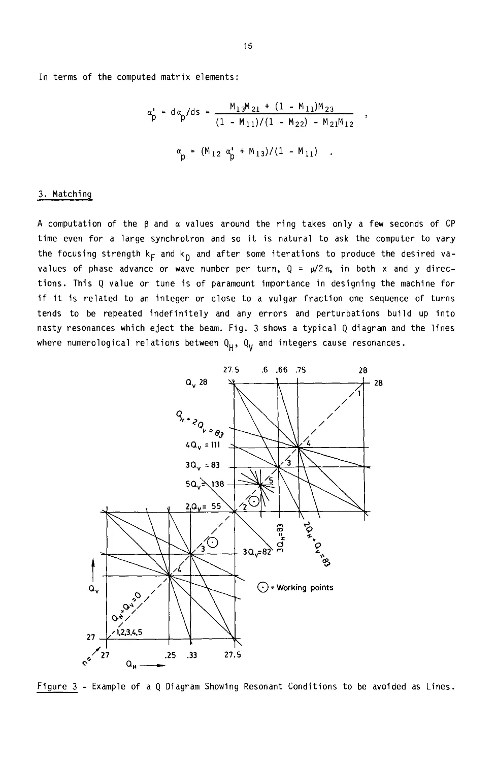
A computation of the ₽ and a values around the ring takes only a few seconds of CP
time even for a large synchrotron and so it is natural to ask the computer to vary
the focusing strength kp and kp and after some iterations to produce the desired va-
values of phase advance or wave number per turn, Q - р/2-rt, in both x and у direc-
tions. This Q value or tune is of paramount importance in designing the machine for
if it is related to an integer or close to a vulgar fraction one sequence of turns
tends to be repeated indefinitely and any errors and perturbations build up into
nasty resonances which eject the beam. Fig. 3 shows a typical Q diagram and the lines
where numerological relations between Q^, Qy and integers cause resonances.
27.5 .6 .66 .75 28
Figure 3 - Example of a Q Diagram Showing Resonant Conditions to be avoided as Lines.
16
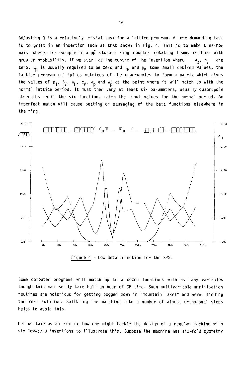
Adjusting Q is a relatively trivial task for a lattice program. A more demanding task
is to graft in an insertion such as that shown in Fig. 4. This is to make a narrow
waist where, for example in a pp storage ring counter rotating beams collide with
greater probability. If we start at the centre of the insertion where are
zero, otp is usually required to be zero and and some small desired values, the
lattice program multiplies matrices of the quadrupoles to form a matrix which gives
the values of ₽y, o^, cty, <Xp and a? at the point where it will match up with the
normal lattice period. It must then vary at least six parameters, usually quadrupole
strengths until the six functions match the input values for the normal period. An
imperfect match will cause beating or sausaging of the beta functions elsewhere in
the ring.
Figure 4 - Low Beta Insertion for the SPS.
Some computer programs will match up to a dozen functions with as many variables
though this can easily take half an hour of CP time. Such multivariable minimisation
routines are notorious for getting bogged down in "mountain lakes" and never finding
the real solution. Splitting the matching into a number of almost orthogonal steps
helps to avoid this.
Let us take as an example how one might tackle the design of a regular machine with
six low-beta insertions to illustrate this. Suppose the machine has six-fold symmetry
17
and reflection symmetry about the centre of each superperiod. It is only necessary to
consider one twelfth of the ring i.e. a series of regular cells (Fig. 1) followed by
a sequence of quadrupoles which match into a waist at the end of th sequence which is
the centre of the long straight section (Fig. 4).
The first step is usually to compute the characteristics of a machine consisting of
normal periods matched to some nominal phase advance 60 or 90° per cell with cell
length chosen to give the desired number of periods, total bending angle and adequate
space for hardware in the final ring.
The aim of the matching is then to find a pattern of 8 quadrupoles to transform the
₽□> ₽w> “u> <*.,> “ and at the exit of the normal cell into the values desired in
M V M V P P
the centre of the straight section and to make up the phase advance in each plane to
give a safe value of Q. Altogether there are eight conditions to satisfy.
In most cases we require <Хр and <? to be zero throughout the long straight section
and this is best achieved by inserting a dispersion suppressor as the first special
element in the sequence following the normal periods. The dispersion suppressor must
contain at least one bending magnet and two variables either quadrupole strengths or
drift lengths, to match from the normal ctp and to zero at the exit of the bending
magnet. If the cell phase advance is 90° or 60° dispersion suppressors are just
normal cells with some magnets omitted3.
We are now left with six variables and six conditions. One may rapidly arrive at a
minimum beta value in both planes at the centre of the long straight section by
asking for and to be zero there. These are the slopes of ₽ and, if zero, will
automatically ensure a minimum. Only two quadrupoles F and D are needed to achieve
this. Stepwise adjustment of their spacing and position can then be combined with a
little experience to arrive at the actual values of beta needed at the low beta point
thus satisfying a further four conditions.
Finally, one is left with the task of ensuring that the total phase advance of the
ring gives safe Q values. Here one must choose between adding additional variables to
the last procedure or returning to the beginning and adjusting the number of periods
and/or period length as necessary. Either procedure usually converges rather rapidly.
Final polishing of the match once we are confidently in the correct valley, may con-
sist of adjustments to lengths and positions of quadrupoles to ensure that they have
the same strength and may be powered in series. It may also be necessary to introduce
extra variables to restrain the excursion of the ₽ functions within reasonable li-
mits. In this context not only geometrical aperture but sensitivity to chromaticity
argues for modest beta values.
18
Other more sophisticated tasks include shaping the dispersion function to arrive at a
desired value of n = (1/y2 - 1/y^ ) and designing special insertions for the extrac-
tion of beams from synchrotrons to fixed target experiments.
4. Limitations of Linear Programs
So far we have ignored that off-momentum particles see either more or less focusing
strength than the др/р = 0 particle. The ₽ and p for these particles will differ from
the reference particle. The first effect of this is to modify the Q and the first de-
rivative of Q with respect to Др/р is known as the chromaticity. This must be correc-
ted if the beam is not to be an extended line in the Q diagram which cuts across dan-
gerous resonances. The remedy is a "quadrupole" whose strength varies as horizontal
position i.e. as Ор(др/р). A sextupole has such a field and modern computer programs
handle such higher order non-linear lenses and match them to make Q independent of
momentum.
The chromaticity may be written as the sum of two terms integrated around the ring.
The first term due to the normal quadrupoles is the natural chromaticity, the second
may be due to sextupole errors in dipole magnets or may be the sextupole pattern used
to make 5=0.
5= (AQ/Q)/(21p/p) = [-l/4ifl(Bp) ]ДВ'(5) + B"(s)ap(s) ]₽(s)ds
where Bp is the magnetic rigidity,
B' is the gradient in a quadrupole,
B" is the second derivation or strength of a sextupole.
Of course, there are higher order derivatives in the expansion of otp , Q and ₽ as a
function of ₽ and much attention has been given to minimising these higher order
terms by subdividing sextupole correction into families and by careful choice of the
position of these elements. However, here most orbit programs which are linear in
concept break down and one must turn to others like HARMON1*.
Orbit programs developed with approximations for large rings give notoriously bad
results in small rings which have large angles of bend and in which, like the Anti-
proton Accumulator, the fringe fields of magnets play an important role. In particu-
lar the fact that beam envelopes change within the fringe field produce extra non-
linear effects5*6. A new small ring program ORBIT7 is under development specifically
to provide accurate results for these small ring machines.
19
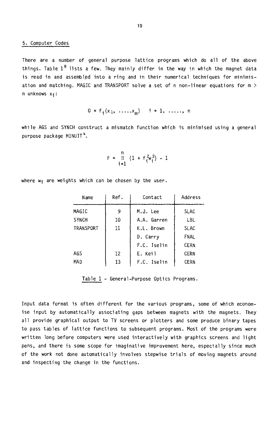
5. Computer Codes
There are a number of general purpose lattice programs which do all of the above
things. Table I8 lists a few. They mainly differ in the way in which the magnet data
is read in and assembled into a ring and in their numerical techniques for minimis-
ation and matching. MAGIC and TRANSPORT solve a set of n non-linear equations for m >
n unknows xj:
0 = f,(xi.......xm) i = 1........... n
while AGS and SYNCH construct a mismatch function which is minimised using a general
purpose package MINUIT4.
n F = П i-1 (1 + ffw?) - 1
where wj are weights which can be chosen by the user.
Name Ref. Contact Address
MAGIC 9 M.J. Lee SLAC
SYNCH 10 A.A. Garren LBL
TRANSPORT 11 K.L. Brown SLAC
D. Carry FNAL
F.C. Iselin CERN
AGS 12 E. Keil CERN
MAD 13 F.C. Iselin CERN
Table 1 General -Purpose Optics Programs.
Input data format is often different for the various programs, some of which econom-
ise input by automatically associating gaps between magnets with the magnets. They
all provide graphical output to TV screens or plotters and some produce binary tapes
to pass tables of lattice functions to subsequent programs. Most of the programs were
written long before computers were used interactively with graphics screens and light
pens, and there is some scope for imaginative improvement here, especially since much
of the work not done automatically involves stepwise trials of moving magnets around
and inspecting the change in the functions.
20
Conclusions
Lattice programs are a standard tool of the designer of a modern accelerator or stor-
age ring. They solve the linear optics problem efficiently and new developments are
directed towards including the end effects in small rings. Their limitation to essen-
tially linear solutions have spawned other programs which track by simulation14-18
which are described elsewhere in these proceedings.
References
1. E.J.N. Wilson, CERN 77-07 (1977).
2. E.D. Courant and H.S. Snyder, Ann. Phys. 3, 1 (1958).
3. E. Keil, CERN 77-13, p. 29 (1977).
4. M.H.R. Donald, PEP Note 311 (1979).
5. G. Wusterfeld, ANL/AAD-N-26 (1982).
6. S.X. Fang, CERN, PS/AA/LT/Note 26, Part. 9 (1982).
7. B. Autin, M. Bell, Private communication.
8. E. Keil, CERN Academic Training Course (1983).
9. A.S. King, M.J. Lee and W.W. Lee, SLAC-183 (1975).
10. A.A. Garren and J.W. Eusebio, UCID-10153 (1975).
11. K.L. Brown, D.C. Carey, Ch. Iselin and F. Rothacker, CERN 80-04 (1984).
12. E. Keil, Y. Marti, B.W. Montague and A. Sudboe, CERN 75-13 (1975).
13. F.C. Iselin, Private communication (1983).
14. F. James and M. Roos, CERN Library Program D506 (1967).
15. K.L. Brown and F.C. Iselin, CERN 74-2 (1974).
16. H. Wiedemann, PEP Note 220 (1976).
17. K. Steffen and J. Kewisch, DESY PET 76/09 (1976).
18. E. Close et al., PEP Note 271 (1978).
DESIGN OF R.F. CAVITIES
T. Weiland
Deutsches Elektronen-Synchrotron DESY
NotkestraBe 85, 2000 Hamburg 52
In linear accelerators and electron storage rings the r.f. accelerating system
represents a major part of investment and operating cost. For many years r.f.
cavities have been designed with the aim of maximising shunt impedance so as to
minimise the power input for a given gradient. Many parasitic collective effects
are caused by the cavities such as beam loading, instabilities, bunch lengthening,
head tail turbulence and beam break-up. In recent years these effects have been
found to cause severe performance limitations in many high energy physics
facilities. As a consequence, the design goal for cavities has to be redefined in a
much broader perspective. With recently developed computer codes the overall
effects of accelerating cavities can now be studied ranging from shunt impedance
considerations to the most complicated beam dynamic aspects.
Introduction
The physics of charged particle acceleration deals with two kinds of forces which
form together the driving term is Newton's law:
q (t + v x Й) - ? - m a . (1)
We distinguish external forces (such as bending and focusing forces of magnets) and
self forces (such as space charge). The external forces are dominant in the limit
where the charge of the accelerated particles vanishes. These forces are directly
under our control and consist mainly of bending- focusing- and accelerating forces.
A major part of an accelerator physicist's work is to design apparatus for bending
and focusing magnets or static deflectors. Subsequently the particle's motion under
the influence of these forces is studied. For both of these tasks many
computational tools have been developed and are the subject of papers in this
volume /1/2/3/.
In this paper we deal primarily with the external forces which act parallel to the
particle velocities and serve as means for acceleration. With few exceptions these
forces are applied by means of r.f. electromagnetic fields in resonators, the
so-called accelerating cavities (or often just cavities). However, as a result of
practical experience with cavities, in many existing accelerators it is found that
such cavities produce many parasitic effects which severly limit the performance
(e.g. beam break-up, emittance growth, head tail turbulence and all kind of
instabilities). The strength of these effects is proportional to the accelerated
charge (collective effects). Since the maximum charge or the maximum current that
can be accelerated is probably the most important design and performance criterion,
the design of a cavity must take these effects into account. Thus we will have to
deal with the combined action of external driven and self excited forces.
For over 30 years work has been published on how to design a cavity in order to
accelerate particles efficiently. For over 20 years computer codes have been used
to optimize realistically shaped structures. Quantitative prediction about
collective effects however became possible only very recently ( last five years)
with new computational tools and theories about the complicated collective
interaction between charged moving particles and surrounding cavities (or other
structures).
After a brief review of the long history of "conventional" cavity design we will
present "unconventional" design procedures that optimize the over-all effect of
accelerating structures. All modern design tools are large computer codes needing
of the order of one megaword of core and an enormous amount of cpu time. However,
the striking results from these codes in recent years underline that this is the
way to go.
22
Some Definitions
A very simple r.f. accelerating cavity device is shown in figure 1: a cylindrically
symmetric "pill-box" with small side tubes. The tubes are large enough to fit the
beam dimensions and small enough so as not to perturb the field pattern of the
driven mode very much. The TM010 re onance is driven by an external power supply.
This mode has a longitudinal electric field and thus can accelerate charged
particles. 'When a charged particle with charge q traverses this structure it
experiences a force yielding a net change in energy after the particle has left,
for constant offset a and constant velocity v - Be 2 we find for the energy change
AU: +L . ,
AU - q Re{vJ , V. - f E (г=а,(р=ф! ,z=Bct)eluZ CeX dz . (2)
-L z
For small beam ports, L does not extend very far and can basically taken as the gap
length. ¥ is an arbitrary phase between the cavity mode and the particle's arriving
time. In order to obtain a large net effect one must make sure that the oscillating
term in eq.2 does not change sign within the significant range of integration.
Obviously any cavity design must take the particle's speed into account and
cavities will be very different for different 0. The first step is to adjust the
cavity shape so that a high AU is obtained for a given amount of the externally
supplied power. Several amplitude independent quantities are defined, the г/Q ("r
over Q"), the loss parameter к and the shunt impedance as:
к - X V*/4W (W = stored energy) , (3)
r/Q r 4 к/ш , (4)
R^ = (r/Q)"Q (or R^ - (r/Q)'Q/unit length) . (5)
Note that all these quantities assume a constant speed of the particle and that
they all depend on В in a complicated way. к and r/Q are purely geometric
quantities that do not invoke the conductivity of the cavity material. For a given
geometry the shunt impedance then depends on the quality factor Q. Unfortunately
the shunt impedance (and the r/Q) is then also defined by:
P - V V*/R . (6)
---s
This power law misses a factor of two in the denominator compared with a.c.-circuit
theory. (The shunt impedance R in a RLC model is then R - R /2). Given a power P
and a structure of shunt impedance R the maximum energy gain of a particle
becomes:
U = q Zp~R~ (7)
max s
The actual energy gain varies as cos^, see eq.2.
Eq.7 indicates that R is the figure of merit as are r/Q and Q. The r/Q can be
optimized by changing the geometry, Q is influenced by the choice of material
(copper, aluminum or superconducting materials).
In large accelerators cavity cells are grouped together in mechanical units and
used as travelling wave or standing wave modules. Just to give the two most
outstanding examples in linac and circular accelerator technology: The SLAC linac
is an arrangement of over 80 000 cavity cells with more than 3.000 m length; the
world largest e e storage ring PETRA now has over 800 cavity cells with over 200 m
length.
23
History
The history of optimization of accelerating cavities by means of computers dates
back to the 50's. Starting from a closed pill-box cavity as shown in figure 2
(which can easily be solved analytically) chains of pill-boxes with connecting beam
tubes were analysed. See figure 3. The method uses eigenmode expansions in simply
shaped subregions and matches the expansion coefficients at interface areas. By
this method both cylindrically symmetric modes (monopole) and modes with variation
in azimuthal direction (dipole, quadrupole, etc.) can be analysed. Among many other
authors I give here only a few references to Bell, Gluckstern, Hahn, Helm,
Hereward, Nakamura and Walkinshaw /4-9/.
In the 60's the first mesh codes (MESSYMESH by Edwards /10/ and LALA by Hoyt and
Simmonds /11/) were used to calculate arbitrarily shaped cavities of cylindrical
symmetry. Apart from a few rare objects such as r.f. kickers or r.f. quadrupoles
most cavities were built cylindrically symmetric and driven in the TM010 mode. Thus
there was no need to develop mesh codes for deflecting modes and the existing codes
(which were restricted to cylindrical symmetry for the fields and the geometry)
could cover the necessary work for optimizing accelerating structures.
In the same decade accelerating cavities attracked the machine physicist's interest
from a different point of view. Any cavity with small beam ports has - among TM010
- many other resonances which couple to a beam. While gaining energy from the
driven TM010 mode, particles also loose energy into all higher order modes (and
into the TM010 mode reducing the effective voltage seen).
The total parasitic energy loss is given by the sum of the partial energies lost
into the individual modes. In order to obtain this number the existing methods had
to be extended. SUPERFISH by Halbach and Holsinger /12/ could compute some ten's of
cylindrically symmetric modes in otherwise arbitrary cavities. KN7C by Keil /13/
and TRANSVRS by Bane and Zotter /14/ were able to compute hundreds of modes in
chains of pill-box with beam tubes for cylindrically symmetric fields and for
fields with azimuthal variation.
Anomalous bunch lengthening in storage rings indicated that apart from loosing
energy into a cavity there is a serious effect of the potential well inside the
beam originating from the beam cavity interaction. Bane and Wilson /15/ could
construct this potential well from the calculated modes (by KN7C and later
TRANSVRS). Although this approach was limited to disk loaded waveguides it could be
used as a model for many existing structures.
In recent years the problem of the potential well has been studied by a quite
different approach in Novosibirsk /16,17/ and CERN /18/ (BCI). Instead, of
calculating the many modes that are needed one can solve Maxwell's equations
directly in time domain and obtain all fields and forces. Furthermore it can be
shown that frequency and time domain approaches give the same results /19/.
Some additional contributions have come to the subject of field computation in the
last two years: The mesh codes were extended to calculate now modes with azimuthal
variation. Similarly the PRUDE-code by Daikovskii, Portugalov and Riabov /20/ and
ULTRAFISH by Gluckstern, Halbach, Holsinger and Minerbo /21/ both solve for dipole
and higher resonances. Another code named URMEL /22/ was developed last year and
has already been used in many laboratories for studying deflecting modes. The time
domain code BCI was generalized to TBCI /42/ and now calculates transient fields of
off-axis beams. Finally, the history of calculating fields in rotationally
symmetric cavities comes to end and only minor improvements are still being worked
on.
24
A somewhat similar history could be outlined for cavities of translational symmetry
(or constant cross-section cavities). Since such a cavity can be considered as a
waveguide section we have to refer to many r.f. studies outside the accelerator
field. It should be only briefly mentioned here that this chapter is also well
closed and covered by rather sophisticated programs /23-26/.
Although 3D calculations with mesh codes have been made for over ten years (e.g.
Albani and Bernardi /27/) they are not yet incorporated in standard design
procedures due to their inherent problems with accuracy and computational effort.
Recently two more 3D resonator codes were described by Wilhelm /28/ and Hara, Wada,
Fukasara and Kikuchi /29/ and a 3D code using the FIT-theory /30/ is being worked
on (furthermore, this code will also solve the 3D time domain problem).
Figure 1:
Accelerating cavity of cylindrical symmetry
with beam ports (t indicates the electric field
of the TM010 accelerating mode)
Figure 2:
Simple pill-box cavity and direction of the
electric field of TM010 mode
Figure 3:
Chain of cylindrically symmetric cavities with
beam hole (disk loaded waveguide)
Figures 4, 5, 6:
Typical accelerating structures of cylindrical
symmetry
4: nose cone slot coupled тт-mode structure
5: disk and washer cavity
6: elliptical-elliptical superconducting
cavity
25
Conventional Design
In a "conventional cavity design" all complicated beam cavity interaction is
neglected. The optimization is mainly concerned with the shape of the cavity.
Starting from a simple pill-box cavity with side tubes "nose cones" were introduced
which shorten the significant path length of integration in eq. 2 and consequently
weaken the oscillating term /31-33/, see figure 4. This cavity type is now standard
in storage rings. A further increase in shunt impedance was promised by the "disk
and washer" cavity /34-35/ and at many places this structure is under
investigation, see figure 5. Higher order mode loss calculations have been taken
into account in the recent LEP design /36/ but did not influence the final shape.
A different design procedure is applied to superconducting cavities where R is
less important than other effects resulting from the high surface field strength
. However, this procedure is still conventional and the task is to have a high
field in the TM010 and damping antennas for higher order modes. Considerations
other than those connected with r.f. have not been taken into account. A typical
cavity of elliptical-elliptical shape is sketched in figure 6 /38-39/.
The conventional design procedure makes use of resonator programs results (see e.g.
figure 7) and is by now well established.
Monopole 500 MHz
fHcp = const lines
Dipole 1981 MHz
electric field
Dipole 1981 MHz
magnetic field
TM020 2015 MHz
r*Hcp - const, lines
Figure 7:
d)
f- Ч \ X ч .
I* , < * , ,
L — _______
TM020 2015 MHz
electric field
Quadrupole 2970 MHz
electric field
Typical computer output for the new PETRA cavity (a, b, c) and the DESY
superconducting cavity prototyp (half cell) (d, e, f)
26
Unconventional Design
The fact that the maximum beam current in PETRA was limited by a transverse
instability /40/ which was found to be mainly due to parasitic cavity effects /41/
was one of the first indications that the parasitic effects caused by accelerating
cavities are much stronger than originally expected.
In order to understand this phenomenon we forget for a while that cavities are used
for acceleration and consider just undriven cavities and their interaction with
particle beam. The results in figure 8 showing transient fields excited by a
Gaussian bunch traversing three PETRA cells have been calculated with the previous-
ly mentioned time domain code TBCI /18,42/. These self excited fields act back on
the particles inside the bunch. After the passage of the structure each individual
particle will have experienced a certain deceleration and deflection due to the
fields. The wake potentials inside a Gaussian bunch are shown in figure 9.
Each accelerator component generates wake potentials but it has been found
experimentally and theoretically that the cavity contributions are dominant. This
statement applies to all cavities, i.e. also bellows, pumps and separator tanks. As
a consequence one preceeds as follows: Compute wake potential due to the
unavoidable accelerating cavities, compute wake potentials due to other objects and
try to remove all objects that contribute significantly in comparison with the
accelerating structures. This recipe was qualitatively applied years before one
could calculate such effects and PETRA has been built with careful avoidance of any
unneccessary cavities. A typical design procedure using the computational means now
available is being undertaken along with the LEP design /43/.
Handy quantities for the wake potential effects are the total loss and the total
kick:
ktot = fp(s)wN(s) ds/( Jp(s)ds)2 (8)
kj_ = fp(s)wx(s) ds/( fp(s)ds)2 (9)
wH(s) decelerating wake potential (Др(()
Wj_(s) deflecting wakd potential (Дрх)
p (s) charge density along the bunch
Since that portion of the total energy loss that goes into the fundamental mode is
not lost, one usually defines the parasitic loss parameter as the total loss minus
the fundamental loss:
Since the cavity is used to accelerate particles it seems suitable to compare the
parasitic effects with the desired effects by defining the "goodness"-functions:
g (X/o) = к /к , (11)
о par fund
g/Vo) - kx/kfund
X = r.f. wave length of accelerating mode
a r rms bunch length (12)
к , ki for a Gaussian charge distribution
par X
These functions basically give the "loss per shunt impedance" and "deflection per
shunt impedance" (Higher order g functions for parasitic quadrupole, sextupole
field are defined analogously). Since the natural bunch length is somewhat propor-
tional to the rf wavelength as a result of some beam dynamics equations it seems to
use X/о as parameter ratner than the bunch length a itself. A typical range in
storage ring operation is 20 < X/o < 100.
21
Figure 8:
Electric field excited by a Gaussian bunch
(a = 2 cm) traversing a 3-cell cavity as a
function of time (lines of r’Hcp r const.)
Figure 9:
Wake potentials inside a Gaussian
bunch (charge lp.C,o =2cm) after the
passage of a single PETRA cavity cell
at a distance 0.5 cm off axis as a
function of particle position
(leading particles on the left)
wf|(s) = energy loss due to axis-
symmetric (monopole) fields
Wj_(s) = transverse change in momentum
due to dipole fields
Figure 10:
Ratio of parasitic mode loss to fundamental
loss parameter (TM010 shunt impedance) as a
function of l/o (r.f. TM010 wave length
divided by rms bunch length) for LEP, PETRA
and SMC structure
Figure 11:
Ratio of average transverse change in mo-
mentum and fundamental loss parameter as a
function of X/q.
28
Figures 10 and 11 show g and g for the LEP cavity /36/, the original PETRA five
cell cavity /33/ and a r§cently1developed SMC-cavity /44/. Surprising result: the
non-computer-optimized PETRA cavity has better g and g values when compared to
the fairly well optimized LEP cavity. The SMC cavity (.Single №ode Cavity) beats
both. In particular g^ is about five times lower than the LEP value.
The shape of the SMC cavity is shown in figure 12. Although this structure was
developed for superconducting rf, it could in principle be made out of copper as
well. In this case R' would be 16 МЯ/m (compared to 24 МЯ/m for PETRA and 26 М$Ут
for LEP). 3
Since PETRA is (and LEP is believed to become) limited by transverse wake potential
effects such a cavity would allow for twice (PETRA) or five (LEP) times the maximum
beam current. Note that a) the comparison takes into account the different bunch
Length at different frequencies and b) a factor of five in beam current means 25 in
luminosity in the present design and c) that the power per integrated luminosity is
reduced by more than a factor of ten, although the instantaneous power in increased
by about 50 percent).
Compared to the superconducting cavity being developed at DESY /39/ this SMC type
would result in an increase of a factor of three in single bunch current. There is
an important byproduct: this cavity was designed - by means of URMEL - so that it
has only one monopole mode, the TM010. There is no higher order resonance of TMO
type and only two weakened dipole modes. Thus multiturn effects carried by resonant
modes are eliminated. Figure 13 shows the standard PETRA superconducting nine cell
unit in the ТМОЮ-тт mode and the corresponding SMC structure.
Although g and g are rough figures giving only integrated averaged quantities,
they can serve as 2a preliminary design aid. It takes only a few short TBCI runs to
obtain these functions and the cpu time consumption is about the same as the time
going into the mode calculations. Once a - 10 % optimized cavity is found, one has
to go one step further and investigate the full beam dynamics taking into account
all details of the wake potentials.
Just recently it became possible to study beam dynamics with wake potentials for
realistic accelerators (The ingredient missing for long time were the wake
potentials, the theory was known). These tracking codes simulate the particle
motion by some thousands of "super particles" which are tracked through an
accelerator lattice. When the particles pass a cavity, wake potential effects are
added according to the charge distribution and by this one obtains a self
consistent solution of the combined equations of motion and electromagnetic field
equations.
About two years ago measured and simulated bunch lengthening in PETRA were found to
agree very well /45/. The full equations of motion (including betatron
oscillations) are meanwhile being combined with the wake effects in storage ring
codes /45,46,47,48/ and in linac tracking codes /49/.
The only drawback so far is that these codes - .expecially for storage ring
application - need an immense amount of cpu time even in the most primitive
versions. Several ten hours on an IBM 3081 may be necessary to obtain results such
as maximum beam current versus tune. Just as a typical example (in figures 14 and
15) we give a result of WAKERACE /48/ for PETRA at injection energy. The
theoretically predicted mode coupling /41/ is verified and it yields a beam blow
up.
So far computer tools for an electromagnetic analysis of accelerator structures are
quite advanced but computer tools for beam dynamics with collective effects are
still subject to research. Current tracking codes are too complicated and too
unreliable to become widely used.
29
Approaching the ultimate design procedure
The unconventional design procedures described in the previous section invoke
various computer codes for guite different tasks. In order to make the entire
package useful and easily usable the user should not need to know all details. The
ideal situation would be that the input data contain the lattice, the cavity
geometry and some beam data. The output would be the particle motion versus time
displayed j'ust like real experiments are in control rooms.
To some extent the above reguirements are met by the computer codes
TBCI-URMEL-WAKERACE-WAKETRAC /18,22,48,49/. From a single input deck for the cavity
geometry, TBCI and URMEL calculate wake potentials, decelerating and deflecting
modes. Results are fed via storage disk to the two tracking codes for linacs
(WAKETRAC) and storage rings (WAKERACE). Lattice parameters are input to the
tracking codes from existing data sets used for beam optics calculations. The
storage ring tracking code is an extension of RACETRACK /50/ which simulates higher
order multipoles in lattice elements.
Present work focusses on extending the beam tracking codes in order to include as
many effects as possible. Furthermore 3D versions of TBCI and URMEL are being
developed in order to complete the wake potentials which so far include only the
contributions from the accelerating structures and not the contributions from e.g.
separator tanks. The ultimate goal is to have one single code that can be used for
computer experiments in the same way that one now uses accelerators.
Figure 12:
Half cell of superconducting
multicell cavity
a) DESY prototyp of
elliptical-elliptical
shape
b) Single Mode Cavity (SMC)
structure with reduced
parasitic effects
Figure 13:
Accelerating тт-mode in
9-cell cavities
a) DESY prototyp of
elliptical-elliptical
shape
b) Single Mode Cavity (SMC)
structure with reduced
parasitic effects
30
Future Development
a) Electromagnetic codes for cylindrically symmetric structures
Existing computer codes are still being improved with respect to accuracy and speed
/52,53,54,55/ and extended to codes solving for the r.f. heating problem /56/. An
ultimate version of URMEL /22/ including triangular meshes and arbitrarily shaped
blocks of anisotropic magnetic or electric material will be available soon. TBCI
has recently been improved enormously /51/ and can now (in principle) solve for
"infinetely" long structures using a mesh with "unlimited" number of nodes.
Probably next year or soon after, the chapter on calculating electromagnetic
properties of cavities of cylindrical symmetry can be closed. Another few years
later these codes will be a standard tool for any rf cavity design.
b) Cavities with translational symmetry
Cavities of an arbitrary shape in a plane and no change of shape perpendicular to
the plane occur less often in accelerator technology. Such cavities can be
considered as just a section of a waveguide. Thus all the work done for waveguide
theory can be applied and results in sophisticated computer codes solving for
arbitrarily shaped anisotropic magnetic, dielectric and conducting materials (e.g.
the LW-code, now in the CERN computer program library T201/202).
c) 3D electromagnetic codes
The real challenges are still fully 3D codes. For the last ten years papers have
been published on this subject /25,26,27,28,29/ but none of these computer codes is
without problems when applied to realistic structures. There is of course the
problem of the enormous cpu time and need of storage locations but there is also a
theoretical problem hidden in the equations. For time harmonic fields in vacuum,
Maxwell's equations can be written as (with к = ш/с):
curl H - к E , (13)
curl t = к , (14)
or as
curl curl t = k2 t (15)
The eigenvalue spectrum obviously contains zeros since any static electric field
Obeying curl t = 0
div t = p
is also solution of eq.(15) with к = 0. In order to "repair" this situation (which
yields to a matrix problem with many unwanted solutions) one has to impose .the
condition
div E = 0 (16)
on the solution. However there is a free parameter left and it is necessary to
study the dependence of к on this parameter in order to find out whether a solution
is valid or not /29/.
Another approach is ti implement the divergence condition right away and to solve:
(v2 + k2) t = 0 (17)
31
Any correct solution of the above equation has no static contents. However,
numerical solutions seem in some case to have such spurious results /28/ and the
reason is probably hidden in the fact the method of numerical solution is not
consistent with all four Maxwell's equations. The FIT ansatz /30/ - which is also
some kind of finite difference method - does solve all four Maxwell equations and
very recently a new 3D-code has been written by the author. This code is not yet
completed; figure 16 shows an output example of the mesh generator.
In order to economize the coding this new program will become a complete system
including 3D-BCI, 3D-URMEL and the existing 3D codes for magneto- and electrostatic
problems /57/ and 3D eddy currents /58-60/. However, the everyday use of these 3D
codes will not take place before the next generation of computers is available.
d) Particle dynamics codes with collective effects
Probably the most difficult area of near future research is that of particle
dynamics codes. Present codes must make crude approximations for many complicated
effects and as a consequence results are not more reliable than within some factor
of five (say).' The problem is solely in
necessary theoretical components are
optics theory).
20
well
the speed of present computers - the
understood (basically F = ma and beam
Figure 15:
Beam spectrum in PETRA obtained from
computer simulation
zero current (no synchrotron side bands)
above threshold current of the trans-
verse instability (many synchrotron side
bands)
a)
b)
Figure 14:
Beam height in PETRA versus time as
obtained from computer simulation
including transverse wake field
effects (r^zsynchr. damping time)
Figure 16:
3D view of two slot coupled
square box cavities
Acknowledgements
The author wishes to thank D. P. Barber for careful reading of the manuscript.
32
References
/1/ C. W. Trowbridge, this conference
/2/ E. Wilson, this conference
/3/ A. Wrulich, this conference
/4/ W. Walkinshaw et al., AERE report TM/104 (1954)
/5/ M. Bell, H. Hereward, CERN/63-33/1963
/6/ H. Hahn, Rev. Sci. Inst. 34 (1963), p. 1094
/7/ R. L. Gluckstern, 1961 Internal. Conf, on High Energy Accel.,p.129
/8/ M. Nakamura, Japanese Journal of Applied Physics 7,(1968) ,p.257
/9/ R. H. Helm, SLAC-PUB-813, 1970 and references therein
/10/ T. Edwards, MURA rep. 622 (1961)
/11/ H. C. Hoyt, D. D. Simmonds, W. F. Rich, Rev. Sci. Instr. 37(1966), p.755
/Y2J K. Halbach, R. F. Holsinger, Part.Accel. 2(1976), p. 213
/13/ E. Keil, NIM 100(1972), p.419
/14/ K. Bane, B. Zotter, Xl-th Int.Conf. on High Energy Accel.,Geneva 1980,p.581
/15/ K. Bane, P.B. Wilson, SLAC, PEP-226A (1977)
/16/ V. E. Balakin et al., SLAC-TRANS-188(1978)
/17/ A. V. Novokhatskij, Inst, of Nucl. Phys., Siberian Div. of the USSR, Preprint
82-157 (in Russian) and references therein
/18/ T. Weiland, Xl-th Internal.Confl. on High Energy Accel., Geneva 1980, p.575
/19/ K. Bane, T. Weiland, SLAC-AP1,(1983) and 12th Conf.on High Energy, 1983
/20/ A. G. Daikovskii, In. I. Portugolov, A. D. Riabov, Part. Accel. 12, p.59/1982)
/21/ R. L. Gluckstern et al., 1981 Linear Accel. Conf., Santa Fe, p.102
/22/ T. Weiland, DESY 83-005, 1983 and DESY M-82-24(1982)
/23/ Z. J. Csendes, R. M. J. Silvester, IEEE MTT 18(1970), p.1124
/24/ J. S. Hornsby, A. Gopinath, IEEE MTT 17(19697? p.684
/25/ S. Akhtarazad, P. B. Johns, IEEE Vol.122(1975), p.1134
/26/ T. Weiland, AEU 33,( 1979), p.170
/27/ M. Albani, M. Bernardi, IEEE MTT 22(1974), p.446
/28/ W. Wilhelm, Part. Accel. 22(1982), p.139
/29/ M. Hara et al., IEEE-NS 30, (1983), p.3639
/30/ T. Weiland, AEU 31(1977) , p.116
/31/ M. A. Allen and P. B. Wilson, Proc, of the 1974 Internal. Conf, on High Energy
Accel., Stanford, p.92 and references therein
/32/ M. A. Allen et al., IEEE, NS-24(1977), p.1780
/33/ H. Gerke et al., DESY PET-77/08(1977)
/34/ S. 0. Schriber, LASL report, LA-UR 79-463(1979)
/35/ J. M. Potter et al., 1979 Particle Accelerator Conference, San Franzisko(1979)
/36/ LEP design report, CERN/ISR-LEP/79-13
/~5~l/ e.g. discussion and references in: M. Tigner, H. Padamsee, Cornell, CLNS82/553
/38/ P. Kneisl et al., NIM 188(1981), p.665
/39/ W. Ebeling et al., IEEE NS-30(1983), p.3357
/40/ D. Degele et al., XI Internal. Conf, on High Energy Accel., Geneva 1980,p.16
/41/ R. D. Kohaupt, XI Internal. Conf, on High Energy Accel. Geneva 1980,p.562
/42/ T. Weiland, DESY 82-015 (1982)
/43/ H. Henke, LEP note 454 (1983)
/44/ T. Weiland, DESY 83-073(1983)
/45/ T. Weiland, DESY 21-088(1981)
/46/ R. H. Siemann, CBN 82-27, 1982
/47/ D. Brandt, LEP note 444, 1983
/48/ T. Weiland, A. Wrulich, WAKERACE-Code, to be published
/49/ T. Weiland, F. Willeke, 12th Int. Conf. Accel., 1983
/50/ A. Wrulich, RACETRACK-Code, being published
/51/ K. Bane, T. Weiland, 12-th Internat. Conf. Accel., 1983
/52/ R. L. Gluckstern, Proc, of the IV-th Compumag Conf., Geneva 1983, being publ.
/53/ В. B. Fomel et al., Part. Accel. 11,(1981), p.173
/54/ P. Fernandes, R. Parodi, Part.Accel.12(1982),p.131
/55/ J. Tuckmantel, CERN/Ef-RF/83-5
/56/ R. F. Holsinger, S. 0. Schriber, IEEE NS-30(1983),p.3545
/57/ H. Euler et al. AfE 65(1982), p.299
/58/ T. Weiland, AfE 60(1978), p.345
/59/ H. Euler, T. Weiland, AfE 61(1979), p.103
/60/ T. Weiland, Archiv der etz 2(1979), p.263
Computer Aided Magnet Design
C W Trowbridge
Rutherford Appleton Laboratory
Chilton, Didcot , Oxon , 0X11 OQX, UK
Introduction
The purpose of this paper is to review the status , and highlight some of the
difficulties, in the computer aided design of electromagnetic devices for
particle accelerators, beam lines and detectors. Magnet design is a complex
activity involving many techniques and so the material presented here will be
limited to those aspects on the computer modelling of magnets vhich are used to
predict the fields, forces etc, ie to those techniques concerned with the
numerical solution of the field equations. In 1972 the author carried out a
review of this subject which was presented at the 4th international magnet
technology conference at Brookhaven^); in this report an attempt was made
to review the then state-of-the-art in magnet computation and concluded that
idealised two dimensional time independent models, could be analysed to high
accuracy (< 0.1%) and that a number of viable computer codes were available for
routine use. It was also a period of vigorous activity in constructing
reliable algorithms for solving the corresponding three-dimensional problem and
several promising developments were described.
Furthermore the period between 1965 and 1972 was very productive with many
active groups of researchers involved in developing magnet computation
throughout the world and it was also an exciting period because of the advent
of the large digital computer. At the Brookhaven conference it was predicted
that the decade following would see numerous achievements in algorithm devel-
opment and a rapid expansion in the use of interactive graphics techniques.
This has happened to some extent; the evolution of the multiuser mini-
computer (MUMs) in the mid-seventies provides a more democratic use of
high-speed graphics terminals with some real-time interactive capability, and
more recently the introduction of new single user mini-computers (SUMs) with
raster operations is changing methods of working.
A prediction that has not been realised was the wide-spread use of
automatic optimisation, ie it was confidently expected that the ’inverse
problem* would be routinely solvable by 1980, in vhich a designer specifies a
field shape and a computer program is used to compute the model shape. At
present this procedure is only practical for extremely simple cases which is
34
disappointing since the essence of design is optimisation^) , A major
effort needs to be made in order to take up the advanced numerical techniques
in optimisation because the difficulty is not only a lack in available
computing power.
In this paper the elements of a computer aided magnet design system will be
outlined then the methods of solving the field equations will be briefly
reviewed followed by a survey of available codes; next some particular
examples of the use of the RAL codes in solving 3D magnetic design problems
will be given. In the final section some of the likely future developments
will be discussed.
2. The Elements of a Computer Aided Magnet Design System
The flow diagrams in Figure 1 illustrate the software components of a typical
CAMD system. An idealisation of the design process is shown in Figure 1(a) ii
which the designer usually iterates toward a satisfactory solution by a
heuristic approach. There are three conceptual stages involved, thus: (a)
Data input or pre-processor for defining geometric and material data, (b)
Solution Processor for solving the equations numerically, and (c) Post-
processor for examining and extracting the results, ie fields, gradients,
integrals and forces, etc. All three processors should be file driven and
access a common data base. The pre- and post-processors will be interactive
utilising interactive graphics techniques and reside in a multi user machine
environment. Except for small problems the solver processors will reside on
Figure 1(a) Heuristic Design
35
Pre-Processor
for Data
Input
Adaptive
Solution
Processor
Post-Processor
for results
and design
parameters
Figure 1(b) Components of the Ideal Numerical
Modelling Software System
Pre-Processor
for Input
Data and Mesh
Solver
Processor
Post-Processor
36
a mainframe with file transfer between machines locally networked or perhaps
widely distributed. In Figure 1(b) and 1(c) the components are specified in a
little more detail; the user can be imagined as controlling the pre- and
post-processing phases at a graphics terminal using heuristic techniques to
optimise his design. Because the problem is to be solved numerically the
model has to be discretised, ie meshes of elements have to be generated to
conform to the data-model and the accuracy of the result will depend upon the
level of discretisation. In the ideal system shown in Figure 1(b) this
discretisation process is taking place inside a solver generating sufficient
mesh to achieve a specified accuracy. It is a current limitation that this
ideal has not yet been satisfactorily met , at least for three dimensional
systems despite considerable research under way. The present systems usually
follow the scheme outlined in Figure 1(c) in which the pre-processor includes
a mesh generation stage. There are some software packages that do not have
interactive pre- and post-processing facilities at all and have to be run in a
’batch mode’.
3. Solving the Field Equations
3.1 Differential and Integral
There is no need to give a detailed review of the various field formulations
and numerical algorithms here since this subject has been exhaustively covered
elsewhere^), it will suffice to give some general remarks on the main
methods that have been successfully used. The first point to make is that
only statics and eddy current effects will be considered; this at once ’rules
out’ all considerations of high frequency devices from the scope of this
paper.
The customary starting point is the low frequency sub set of Maxwell’s
equations^) , these equations plus the non-linear constitutive laws define
the electromagnetic field for slowly-varying time-dependent and static fields.
Those equations are differential and , in many cases , the normal approach to
their solution is to eliminate the field vectors by introducing scalar and
vector potentials to produce a set of partial differential equations.
Provided the essential boundary conditions for the problem are prescribed
these equations are then solved numerically by a more or less standard
technique, eg Finite Differences^), or Finite Elements?). In order
to do this the problem space must be discretised into points or elements to
allow the non-linear continuum problem to be transformed into a linear
algebraic problem. Hence the heart of solution process is one of linear
37
algebra characterised by a system matrix of coefficients. For the
differential equation formulation the following two points apply:
(a) The system matrix is sparse: since the differential nature implies only
local coupling of equations.
(b) The whole problem space, including the external world, has to be
discretised.
There is an alternative formulation based on the integral forms of the field
equations, ie Gauss ’theorem1 is the integral form of Poisson’s equation. If
the field integral forms are used instead of the differential formulation,
the discretised equations are algebraic with a system matrix of a very
different character, ie
(a) The system matrix is fully populated: since every point is coupled to
every other point.
(b) Only the material regions of the problem space have to be discretised.
This is because the integrals are only defined for the active regions
which implies that the boundary conditions are intrinsically satisfied ,
and that the far field problem has been automatically taken into
account. Another important consequence is that for linear problems only
the surfaces of the active regions have to be discretised.
At first sight it may appear that the integral approach will be superior to
the differential approach since the mesh generation problem is far far
simpler - the empty space does not have to be filled with elements and the
far field boundary conditions are automatically satisfied. However, there
are very significant difficulties because the matrix, although smaller, is
fully populated and the solution times will vary as the cube of the number of
degrees of freedom. Where as for the differential case, although the matrix
is larger it is sparse and possibly symmetric and the solution times will
vary, at most, as the square of the number of degrees of freedom.
Extensive comparisons have been made^j^) between differential and
integral methods and some guidelines have been evolved governing the
choice^). One general remark is appropriate here; if the problem is
relatively simple in that it can be discretised into a modest number of
elements , depending upon the power of the computer available , then the
integral method offers an accurate technique involving a minimum of data
preparation and yields smooth solutions.
38
3.2 Solution Potential
There is also considerable latitude of choice of solution potential; for the
two dimensional case the simplest and probably the most effective selection is
the single component vector potential but in three dimensions there is no
single choice. In this case it is usual to separate out the statics case, for
which it is possible to define a scalar potential , from the time-dependent
case which by its nature must be vector field problem at least in the eddy
current regions. The type of scalar potential for the statics 3D case also is
not self-evident since there is more than one possibility. The essential
consideration here is that if prescribed currents are to be included the total
scalar potential (H = -у у ) may be multivalued and it is usual to introduce a
1)
reduced scalar potential by subtracting the source fields for the currents ,
however exclusive use of the reduced potential will introduce serious
numerical cancellation errors^-) due to subtraction of large quantities
so it is better to use a combination of both potentials, the total potential
everywhere except in conductor regions when the reduced potential should be
used^-2) 9
The more complex 3D eddy case is receiving considerable research attention
with only test and research codes available, see table 4. Some of these
developments are showing considerable promise and in the next few years viable
packages should become available^). However the full non-linear
transient case, will require enormous computer power.
3.3 Available Codes
Tables 1 to 3 attempt to list the codes that, in the author’s opinion, should
be of practical use to the magnet designer. The list is not exhaustive and
there could well be omissions due to ignorance or oversight. The references
should be consulted for technical details and for information on validation
and the accuracies achievable, however, some results for the RAL codes^)
will be given in section 4.
4. CASE STUDIES
4.1 SNS Trim Quadrupole Type QT137
The GFUN integral code^) was used in the design stage of this magnet
which had the design parameters shown in table 5.
Table 1. 2D Differential Electromagnetics Codes
Date Name/Centre Authors Formulation Numerical Method and Discretisation Remarks Environment
1964 POISSON(Trim)/ Lawrence Livermore Berkeley USA Winslow Colonias Halbach Holsinger etc Vector potential Variational and finite difference Plane XY Axlsymmetry First Order triangular mesh with fixed topology Non-Linear Magnetostatics Batch
1974 MAGGY/ NV Philips Eindhoven Holland Munro Polak Wachters Van Wellj Vector Potential Finite Element Plane XY Axisymmetry First Order quadrilaterals mesh with fixed topology Non-Linear Magnetostatics Permanent Magnets Batch
1976 PE2D/RAL Oxford UK Simkin Trowbridge Armstrong Biddlecombe Dlserens Vector Potential Scalar Potential Finite Element Plane XY Axisymmetry First Order and Second Order triangle elements with variable to pology Non-Linear Magnetostatics Permanent Magnets Eddy Currents Steady State Eddy Currents Transients Electrostatics Batch plus interactive Pre- and Post- processor on a MUM
1977 FLUX/ Laboratoire d'Electro- technique de Grenoble Sabonnadiere Meunier Mo rel Vector Potential Scalar Potential Finite Element Plane XY Axisymmetry First and Second Order Isoparametric Elements with Variable Topology Non-Linear Magnetostatics Eddy Currents Steady State Electrostatics Batch plus interactive Pre- and Post- processors on a MUM
1978 MAGNET-11 McGill Montreal Canada Imperial College London UK Lowther Silvester Freeman Vector Potential Finite Element Plane XY First Order Triangle Elements with variable topology. Non-Linear Magnetostatics Interactive Pre- and Post- processor and Solver on a MUM
1979 AOS/Magnetic AOS Data Systems Milwaukee USA Brauer Bodine Larkin Vector Potential Finite Element Plane XY First Order Non-Linear Magnetostatics Eddy Currents Steady State Skin effect Batch
1982 APPLE RAL Oxford UK Simkin Trowbridge Vector Potential Scalar Potential Plane XY Axisymmetry First Order Triangle Elements with fixed topology Linear Magnetostatics Electrostatics Flow Interactive Pre- and Post- processor with Rubber Banding on a SUM
Table 2. 3D Magnetostatic Codes
Date Name/Centre Aut hors Formulation Numerical Method and Discretisation Remarks Environment
1972 PROFI - Program for calculation of Fields Technische Hockschule Darmstadt W Germany Muller Krueger Wolf Reduced Scalar Potential Differential Finite Difference Non-Linear Magnetostatics Electrostatics Batch
1977 TOSCA/RAL Oxford UK Simkin Trowbridge Mixed Total and Reduced Scalar Potential Differential Formulation Isoparametric Finite Elements First and Second Order Hexahedra Variable Topology Non-Linear, Permanent Magnets Electrostatics Distributed Conductors Sources. Avoids cancella- tion errors associated with exclusive use of the reduced scalar potential Batch plus Interactive Pre- and Post- processor
1981 PADDY/NV Philips Eindhoven Holland de Beer Polak Wachters van Welij Mixed Total and Reduced Scalar Potential Differential Finite Element First Order hexahedra fixed topology Non-Linear , Permanent Magnets. Filament Sources See Tosca above Batch
Table 3. Integral Operator Codes for Magneto statics
Date Name/Centre Authors Formulation Discretisation Remarks Environment
1970 1973 1975 GFUN/RAL Oxford UK Newman Trowbridge Turner Collie Diserens Armstrong Simkin Magnetisation Integral Equation Moments Point Matching Constant Magnetisation Prisms Tetrahedra Non-Linear Magnetostatics 2D and 3D Batch with Interactive Pre- and Post- processor on Main Frame
1976 1981 BIM/RAL Oxford UK Armstrong Collie Diserens Simkin Trowbridge Simkin Scalar Potential Point Matching Linear Quadratic and Cubic Triangles Galerkin Linear Magnetostatics 2D 3D Interactive Batch
Table 4. 3D Eddy Current Research Codes^)
Project/Centre Authors Formulation Numerical Method Remarks
GEC Stafford UK Preston Reece Riley (T ,й) Curl T = J H = T + vfl Finite Element Normal component of T discontinuous at conducting interface
RAL Oxford UK Biddlecombe Heighway Simkin Trowbridge (R,s) Curl R = J H = R + S Rs = 0 Finite Element Field Vector R zero over interface; cancel- lations may be problem
RAL Oxford UK Emson Simkin (A,<S) Curl A = В div a A=0 Finite Element Maximum economy for potentials achieved Avoids electric scalar potential in conducting regions. Magnetic Scalar Potential in air
GE/Schenectady Chari Konrad Palno Angelo (A,V) div A=0 Finite Element Vector potential throughout space
TRIFOU/ Electricite de France Bossavit Verite (H) Finite Element Coupled Boundary Integrals Maximum economy for Fields achieved , 3 unknown per mesh point in conducting region. Infinite Exterior region handled by Boundary elements
Bath University UK Balchin Davidson (H,E) Circuit analogue method (Finite Differences) Coupled Electric and Magnetic Circuits
Bath University UK Rogers Eastham (Е.Ф) Finite Element Achieves maximum economy and avoids electric scalar potential in conducting regions
EDDYNET/ Argonne USA Turner (J) Integral Circuit Analogue (Wire Grid) Conductors only but includes transients
42
Table 5 QT137 Design and Computed Parameters
Aperture dia 0.274 m Peak. Gradient Integral G 0.1832 T
Iron Length 0.2034 m (mean of 23 magnets)
Peak. Current 300 A Effective Length measured
Peak. Gradient 0.6026 T/m at 300A 0.304 m
Turns/pole 15 (mean of 23 magnets)
Effective Length calculated
by GFUN at 29OA 0.307 m
GFUN Error in Length LQ + 1%
Twenty-three magnets were built and measured. The average change in the
gradient integral, AG/Go, is shown for the 9=0 plane, compared with GFUN at
300A. See Figure 2. The asymmetry in measured values between left (power)
and right (non-power) sides can be seen to be significantly less than the
error in the GFUN values. The effective length predicted by GFUn is 1% more
than that measured. The change in effective length with current from 50A to
300A is about 1.5%.
Figure 2 Model and Field Gradient Integrals
Although the measurements are self-consistent and the GFUN prediction is
outside the 90% confidence limits the search coils used for the measurement
were not properly compensated for the higher harmonics of field and this may
have contributed to the discrepancy between the calculation and measurement.
43
The figure on the left shows the elements used in GFUN to represent one octant
in X-Y. With 3 layers in the z direction there were 360 tetrahedra in l/16th
of the entire magnet. The coils are racetracks. This example is near the
limit of applicability of GFUN, with 360 elements, the computing time hour
IBM 195) will be dominated by the cube law and any further refinement of the
model, say factor of 2, will require hours of computing. However the
designers were able to construct a prototype according to the calculated
dimensions which was sufficently close to the prediction that no modifications
were required before going into production.
4.2 EVB2 Magnet16)
The Spallation Neutron Source synchrotron, has a vertical extraction system
for the 800 MeV proton beam. After the fast-pulsed vertical-kick magnets the
extracted beam is bent by a d.c. septum magnet through an angle of some
22° to clear the following main-ring dipole. Above the main dipole is
placed the EVB2 magnet which restores the extracted beam to the horizontal
plane.
EVB2 is required to produce a sector field of 1.9 T-m on a radius of 3.56 m,
with an aperture of 0.24 m radially x 0.14 m axially. The original design
consisted of a C-yoke , bent through 22° with the open side down towards
the top of the main dipole. The effect of the main dipole on the leakage
field from the C was not allowed for until the magnet was out to tender; the
tenderers asked for some design modifications to be investigated, including
the effects of changing various coil parameters and estimates of the forces on
the C, when it was realised that there were several defects in the concept.
The design was then changed to an asymmetric straight window-frame yoke with
extra radial aperture to accommodate the beam sagitta and wedge-shaped
pole-ends to produce the sector field. Although this is no cheaper, the
leakage field towards the main dipole is quite negligible, so there is no
field distortion. The straight coil and yoke are easier to make, and the yoke
is much stronger than the C. The wedge shim is clearly visible near the coil ,
and is also shown on the computer model Figure 3. The wedge angle is
12°, which is about one degree more than the angle required in the
effective field boundary, (e.f.b.); this offset was established for the
Oxford Spectrometor, and is approximately correct for EVB2.
The TOSCA^ ,17) differential code was used for the calculations, including
tracking some protons through the end-field to estimate how far the sector
44
Y
ЛЕ 3
ЛЕ 3
Figure 3 Computer Model of EVB2
field requirement had been met. It was too difficult to measure the field
along the notional proton tracks; instead the field was measured along
straight lines in the median plane, and re-calculated as nearly as possible at
the measurement positions. Figure 4 shows that the e.f.b. from the tracking
(T) is very close to that from straight-line integrals (15), which confirms
the value of the latter. The e.f.b. (17) was calculated from field values at
the same position, current, gap and, as near as possible, B-H data as the
measurements (m) at the non-powered end of the magnet. The discrepancy of 2mm
(0.3% of the effective half-length) arises from the difference in the calcu-
lated field at the position under the coil where the field gradient is
highest.
Contours of the difference between TOSCA and measurement at the non-powered
end are shown in Figure 5. It is not possible at this stage to know how much
of the difference comes from manufacturing and measurement errors , and how
much from calculation errors: the contours show some correlation with the
TOSCA mesh, but they are typically of the same height as those obtained from a
comparison between the two ends of the magnet (Figure 6). The latter are
substantially the same at the lower current of 1445A, showing that the
differences between the actual magnet and the TOSCA model are probably
significant.
45
Figure 5 EVB2 Calculation cf Measurement at 1835.53 A
46
END ASYMMETRY: Contours of (Ву(Х’°ду(^ p Bytx.o.z)) x 100,
Two possible sources of error which remain to be explored are the mesh
distortion used to model the wedge-shaped pole ends , and errors in either the
coil field or its integration to find the scalar potential (r.h.s. in the
equation). A full analysis of these results will be given in reference 16.
5. CONCLSUIONS AND FUTURE DIRECTIONS
Clearly good results are obtainable with computer codes for predicting fields;
the accuracy achievable will depend on the degree of discretisation and on
having a precise knowledge of the properties of the materials involved. The
degree of discretisation depends critically on the complexity of the design
47
and on the computing power available. It is difficult to estimate a priori
the discretistion errors although some significant work has been carried out
and should make possible the adaptive mesh schemes already mentioned^ ,19).
At present the answer to the question 'How accurate is your code?' still is
'that depends on and perhaps more importantly on 'who is to carry out
the work?'. There is no doubt that the users with considerable expertise in
both electro- magnetics and numerical modelling are prerequisite to achieve
Figure 7 2D Model , Mesh and Solution of an Asymmetric Quadrupole
using the ICL PERQ Single User System. The Software is
written in Pascal and Allows Real Time Interaction of
20)
Geometry and Mesh.
48
What does the future hold in store? Apart from the three dimensional eddy
current codes using differential operator finite elements there should be a
considerable revitalising interest in integral methods vhen the impact of
parallel processing hardware is assimilated; also to be optimistic single
user machines networked together sharing file servers and accessing larger
machines as required, should create a truly democratic interactive environ-
ment^), See Figure 7. Computing is moving into the 5th generation
era^l) in vfaich far greater emphasis will be placed on features like
man-machine interfaces , data flow architectures , logic programming and
knowledge-handling capabilities.
These developments will have a considerable impact on engineering design and
at some stage, the sooner the better, detailed thought must be given to use of
these techniques in numerical modelling and hence computer aided magnet
design.
6 . ACKNOWLEDGEMENTS
The author is indebted to Alan Armstrong of CAG Group RAL for providing the
information on the EBV2 magnet and for his skill and patience in solving field
problems. He is also grateful to Mrs Pam Peisley for her skill and patience
with word-processing in preparing the typescript.
REFERENCES
1. Trowbridge, C W, "Progress in Magnet Design by Computer", Proc 4th Intern Conf
on Magnet Technology, Brookhaven Laboratory, 1972.
2. Armstrong, A G AM, Fan, M W, Simkin, J, Trowbridge, C W, "Automated
Optimisation of Magnet Design using Boundary Integral Method", IEEE Trans Mag,
vol. Mag-18, No.2, March 1982.
3. Trowbridge, C W, "Numerical Solution of electromagnetic Field Problems in Two
and Three Dimensions", Contributed chapter in "Numerical Methods in Coupled
Systems", pub: John Wiley and Sons, 1983.
4. Compumag Conference Proceedings: Oxford 1976, published, Rutherford Appleton
Laboratory, Ed: J Simkin.
Grenoble 1979, published, Laboratoire
d’Electrotechnique de Grenoble, ERA 524
CNRS, Ed: J C Sabonnadiere.
Chicago 1981 , IEEE Transactions in
Magnetics, vol. Mag-18, No.2, March 1982.
Genoa 1983 , IEEE Transactions in Magnetics ,
November 1983.
49
5. Stratton, J A, "Electromagnetic Theory", McGraw Hill, New York, 1941.
6. Smith, G D, "Numerical Solution of Partial Differential Equations", OUP 1971.
7. Zienkiewicz, 0 C, "The Finite Element Method", 3rd Edition, McGraw Hill 1977.
8. Trowbridge, C W, "Three Dimensional Field Computation", IEEE Transactions in
Magnetics, vol. Mag-18 , No.l, January 1982.
9. Simkin, J, "A Comparison of Integral and Differential Equation Solutions for
Field Problems", IEEE Transactions in Magnetics, vol.Mag-18, No.2, March
1982.
10. Simkin, J, Magnet Technology Conference, Invited Paper on Field Computation,
Grenoble, September 1983.
11. Simkin, J, and Trowbridge, C W, "On the Use of the Total Scalar Potential in
the Numerical Solution of Field Problems in Electromagnets", Int J Numer
Methods Eng, vol.14, pp423~44O.
12. Simkin, J, and Trowbridge, C W, "Three-Dimensional Non-Linear Electromagnetic
Field Computations, Using Scalar Potentials", Proc Inst Elec Eng, vol.127,
part B, no.6, Nov 1980.
13. Emson, C R I, Simkin, J, "An Optimal Method for 3-D Eddy Currents", to appear
IEEE Trans Mag, November 1983 (COMPUMAG Conference).
14. "Computing Aids for Engineers", Computing Applications Group, Rutherford
Appleton Laboratory, Chilton, Didcot, Oxon 0X11 OQX.
15. Newman, MJ, Trowbridge, C W, and Turner, L R, "GFUN: An Interactive Program
as an Aid to Magnet Design", Proc 4th Conf Magn Technol, Brookhaven National
Laboratory, Brookhaven, NY, pp.617-626 , 1972 .
16. Armstrong, A G A M, "Design Calculations Compared with Measurements on the
EVB2 (SNS) Magnet". To be published. Rutherford Appleton Laboratory.
17. Armstrong, A G A M, Riley, С P, Simkin, J, "Tosca User Guide - Version 3.1",
Rutherford Appleton Laboratory Report, RL-81-070 (1982).
18. Polak, S J, den Heijer, C, Bielen, J, "A Future of Mesh Adaptive Solving" ,
IEEE Trans in Magnetics, vol. Mag-18, No.2, March 1982.
19. Penman, J, Lees, P, Fraser, J R, Smith, J R, "Complementary Energy Methods in
the Computation of Electrostatic Fields", to appear IEEE Trans Mag, November
1983 (COMPUMAG Conference).
20. Simkin, J, Trowbridge, C W, "Electromagnetics CAD Using a Single User Machine
(SUM)", to appear IEEE Trans mag, November 1983 (COMPUMAG Conference).
21. Simons, G L, "Towards Fifth-Generation Computers", published by NCC
Publications 1983.
22, Lari, R J, Comparison of eddy current programs4, to appear IEEE Trans Mag,
November 1983 (COMPUMAG Conference).
BEAM INSTABILITIES AND COMPUTER SIMULATIONS
A. Piwinski
Deutsches Elektronen-Synchrotron DESY
NotkestraBe 85, D-2000 Hamburg 52, W. Germany
1, Introduction
The most important instability which limits the luminosity in existing electron-po-
sitron storage rings is caused by beam-beam interaction. But also synchro-betatron
resonances are a serious problem and can limit the luminosity. The beam-beam inter-
action leads to a blow-up of the beams which reduces the luminosity and the life ti-
me of the colliding bunches. Synchro-betatron resonances or satellite resonances oc-
cur if the relation
kQx + LQ2 + mQs = n
(1)
is satisfied where к, £, m and n are integers and Qx, Qz and Qs are the betatron and
synchrotron frequencies in units of the revolution frequency. With increasing bunch
current the number and the width of the satellite resonances increase such that fi-
nally the currents are limited.
These satellite resonances are mainly excited by dispersions in the accelerating ca-
vities and by transverse fields with a longitudinal gradient in the cavities. Satel-
lite resonances due to the chromaticity are usually prevented by sextupoles. Disper-
sions in the cavities cannot be supressed completely. Especially during energy ram-
ping when the optics is changed and the orbit is shifted by small amounts, spurious
dispersions are produced. Transverse fields with a longitudinal gradient are genera-
ted when passing the cavities off-axis which is difficult to avoid during energy
ramping. An analytical treatment of satellite resonances is difficult. Especially
the increase or decrease of the oscillation amplitudes during many revolutions can-
not be calculated. Computer simulations, however, can show the general behaviour of
the particles on such a resonance.
Satellite resonances can also be excited by the beam-beam interaction when the beams
cross at an angle or when the dispersion at the interaction point is not zero. In
that case many satellites of nonlinear betatron resonances appear which were found
by computer simulations and seen in the storage ring DORIS I, where the beams cros-
sed at an angle. This mechanism might also become important for the new ep-project
HERA.
The blow-up of the beams at head-on collision is caused by the strong nonlinearities
of the space charge forces. Many resonances can be excited, especially coupling re-
sonances of horizontal and vertical betatron oscillations such that the oscillation
energies between the horizontal and vertical plane are exchanged. The beam height,
which is usually much smaller than the beam width, is then increased drastically
whereas the width remains nearly constant. An analytical treatment of this effect
is, at the moment, not yet possible. Computer simulations are, therefore, the best
way to investigate the dependence of the blow-up on various machine parameters and
to find cures to suppress the blow-up as far as possible.
51
2. Synchro-betatron resonances
2.1 Excitation caused by dispersions in a cavity
For each particle with an arbitrary energy deviation exists a closed orbit that can
be described as the product of the dispersion D times the relative momentum devia-
tion or approximately, the relative energy deviation:
xC.o. W = DXW « Dx(Jl)
(2)
Around this closed orbit the particles perform betatron oscillations. The dispersion
can be horizontal or vertical and we consider horizontal or vertical satellite reso-
nances. In the cavity the energy is changed and therefore the closed orbit is shif-
ted. Since the total coordinates x and x' cannot be changed in such a short interval
the betatron coordinates are changed:
6x = - Dx
<SE
E
«X'
n-
x E
(3)
(4)
6E = ell(sin(^ + 2tts/X) - sinp ) (5)
with e = elementary charge, U - cavity voltage, ф = synchronous phase, s - longitu-
dinal position, X = wave length of the voltage.
We take into account only that part of the energy change which varies with the syn-
chrotron frequency. The other constant part which replaces the radiation losses does
not play a role for a resonance. The longitudinal position is changed in the curved
sections of the machine. The change of s per revolution is given by
- AjX + A2x' - C —(6)
Fx (1 - cospx) - A2ax
Fx sinPx
= У — (x + D ~
7 P x E
with A - - (D sinPv
1 Bx x x
A2 = - Dx (1 - cospx) -
ац] is the momentum compaction factor and C is the circumference, pis the radius of
curvature and px is the betatron phase advance per revolution.
x and x' are the betatron coordinates at the beginning of the revolution.
A simulation of the coupled synchrotron and betatron oscillations on a digital com-
puter has been done for small currents taking into account the natural nonlineari-
ty of the synchrotron oscillation (Eq. (5)). The simulation has the following steps:
In the cavity the longitudinal coordinate s of the synchrotron oscillation remains
constant whereas the energy is changed according to Eq. (5). The change of the beta-
tron coordinates is given by Eqs. (3) and (4). In the arc the change of s is given
by Eq. (6) whereas the energy deviation is constant. The betatron coordinates x and
x' are transformed with
M =
Fig. 1 shows
Fig. la shows
cosyx + ax sin Ux
- (1 + ax) sinUx/6x
0X sinUx
cosjjx “ ctx sinUx
(7)
V /
the typical behaviour of the amplitudes during 1200 revolutions,
the betatron and synchrotron amplitudes for a sum resonance where al-
ways, one amplitude increases while the other one decreases. Fig. lb shows that on a
difference resonance both amplitudes increase or decrease at the same time. In this
case the beat is larger than in the first case.
QB + Qs = n
1000 revolutions
1000 re vp1utions
СЛ
synchrotron amplitude
QB - Qs = n
1000 revolutions
Fig. 1: Betatron and synchrotron amplitudes in arbitrary units as a function of time
a) on a sum resonance b) on a difference resonance
1 (ЯЛТ”г evolutions
----.---------------4-—-----
53
2.2 Excitation caused by transverse fields with a longitudinal gradient
Transverse fields which vary with the longitudinal position of a particle in a bunch
can be caused by the accelerating voltage due to an angle between the cavity axis
and the closed orbit or due to asymmetries in the cavities2) and by the bunch itself
due to off-center passage or due to cavity asymmetries3). The vertical kick of a
particle produced by transverse fields is given by
5z' = | J (Ez + vBx) dt (8)
where Ez and Bx are the electric and magnetic fields and v is the particle velocity.
The integral is taken along the path of the particle between two limits where the
fields vanish. The region of the fields is assumed to be short as compared to the
wave length of the betatron oscillation.
We consider that part of 6z’ which varies linearly with the longitudinal position s
of a particle in the bunch and obtain with Maxwell's eguations
. p , ae7 эвх „ ЭЕЧ
Sz' = s — J (’ + v u“') dt = s J — dt = As (9)
p ' 3s 3s p 3z
If the transverse fields have a longitudinal gradient the longitudinal field must
have a transverse gradient,.and that means that the betatron oscillation influences
the synchrotron oscillation. That part of the energy change which varies linearly
with the transverse position of a particle in the bunch is given by1*)
6E e f 3l2s v2 . „ /1ГП
-=- = z r J -— v dt = —Az = Az (10)
E L 3 z cz
A comparison of Egs. (3), (4) and (9) shows that the increase of betatron oscilla-
tion depends in the same way on the synchrotron oscillation, namely on s. The two
mechanisms, caused by a dispersion and by transverse fields, can at least for slowly
changing synchrotron amplitude compensate each other. This is also possible for
higher harmonics of the synchrotron freguency produced by nonlinearities. Then the
compensation depends on the amplitude of the synchrotron oscillation and on the
bunch current.
2.3 Excitation caused by the beam-beam interaction at a crossing angle
Fig. 2: Orbit distortion due to a cros-
sing angle
We consider a particle which has a distan-
ce s from the center of its own bunch.
This particle does not pass through the
center of the other bunch and hence gets a
vertical kick. The kick has the direction
indicated in Fig, 2 if we assume particles
with different signs as electrons and po-
sitrons. Because of this kick the axis of
the bunch cannot be the closed orbit for
the considered particle, but the closed
orbit must look like the dotted line.
The kick,
form
i.e. the change of the vertical betatron angle z’ can be written in the
6z’ = f(z + 8Ф)
(ID
where f describes the space charge forces as a function of the vertical position z
and the longitudinal position s.
54
The synchrotron oscillation is also influenced by the betatron oscillation since the
energy is changed for a particle that crosses the bunch at an angle. The energy
change is understandable, if one takes into account that the kick or momentum change
is vertical. One can then decompose the change of the momentum and obtains a longi-
tudinal component ps which is given by $pz. The energy change is then
6E 6p <SPs . z «г ,
-p- = .x = .— - ф —— = Фог* - ФТСг + зф) (12)
E p p p
If the effective cross section is circular as in DORIS I (azefa ax = a) an exact ex-
pression for the function f (Eq. (11)) can be obtained:
f(u) = (e 2? _ (13)
with re = electron radius, Nj, = number of particles per bunch, у = particle energy
divided by its rest energy, a = standard deviation of the Gaussian-like particle
distribution.
A simulation of the betatron and synchrotron oscillation including the nonlinear
coupling (Eq. (13)) has been done on a digital computer. Between the interaction
points the oscillations were transformed linearly. Fig. 3 shows the ratio of the ma-
ximum to the minimum betatron amplitude during 2000 revolutions for Ф = 12 mrad,
Nj-, = 8*109, у - 3500, о = .23 mm, Qs = .034, 6Z = 1 m. More than 1000 Qg-values be-
tween 6.02 and 6.48 are investigated but only those resonances are shown which reach
an increase of more than 50 % of their initial amplitude. Measurements with the sto-
rage ring DORIS I have proved that exactly at these frequencies the life time of the
bunch dropped to a few seconds5).
Analytical investigations and the latest measurements with DORIS II have shown that
also a dispersion at the interaction point can excite similar synchro-betatron reso-
nances5’6).
Fig. 3: Maximum betatron amplitude as a function of the betatron frequency
55
3. Beam-beam interaction
In simulating the beam-beam interaction on a digital computer, significant progress
was made in 19807’ 8’ 9’ 10). Since that time, many simulations were done by several
authors, and a better understanding of the mechanism of the blow-up was achieved. In
the following the simulations for PETRA are briefly described.
Ihe space charge forces are exactly calculated for a relativistic bunch with a Gaus-
sian particle distribution. Ihe change of the betatron angles x' and z’ at each in-
teraction point is then given by
Ax’
Az’
(14)
i/ a /a 1 x2 . _1 z2 г reNbBx,z
v = z/ x> a = 2 aj - 02 i° - 2 a; - a* ’ bx,z -
X X Z A f t- A 4-
Ihe kicks were calculated for a two-dimensional grid of points and then interpolated
quadratically for calculating the transverse kick of a particle at each passage. Ihe
longitudinal motion of the interaction point seen by a particle due to its synchro-
tron oscillation is always taken into account. Between the interaction points the
horizontal and vertical betatron oscillation and the synchrotron oscillation are
transformed linearly. The radiation damping is included. The quantum fluctuation is
simulated by applying random kicks on all three modes of oscillation. The motion of
particles is observed over several damping times, i.e. over a large number of revo-
lutions. Both cases, "weak-strong" and "strong-strong" were investigated.
As an example Fig. 4 shows the vertical motion of a single particle in the phase
diagram. The horizontal axis gives the position and the vertical axis the angle of
the vertical betatron oscillation at a symmetry point of the machine for each revo-
lution. The vertical amplitude of the particle starting with zero amplitudes remains
within one or two standard deviations of the Gaussian distribution of the opposing
bunch during the first 8000 revolutions (a). Then its amplitude increases rapidly
due to quantum fluctuation and the nonlinearity of the space charge forces, and it
moves into a third order resonance where the phase advance is about 2л/3 + 2it x
integer (b). After about three quarters of a damping time it comes out of resonance
and leaves the three fixed points, but is immediately captured by other three fixed
points of the third order resonance (c) which are a mirror image and equivalent to
the first three points (without optical asymmetries). After about 600 revolutions
the particle leaves the third order resonance (d),
A similar behaviour can be observed for several resonances. More often, however,
coupling resonances between horizontal and vertical betatron oscillations appear.
These resonances can be found by counting the betatron oscillations and by obser-
ving the variation of the amplitudes. In all cases the particles usually do not
stay longer than a damping time on a resonance. Due to quantum fluctuation and dam-
ping they can leave the resonance and can then be captured by another resonance.
The computer simulations have shown that small disturbances of the ideal machine
increase the number and strength of the resonances which can be excited. Those dis-
turbances are small differences in betatron phase advance between the interaction
points and spurious dispersions at the interaction points. Thus machine imperfec-
tions enlarge the blow-up of the beams and become more important with increasing
number of interaction points.
56
N = 1 -> 7729
Fig. 4:
Particle motion in the phase diagram
(Qx = 25.2, Qz = 23.52, Qs = .07, 5 x
4 interaction points, 1 damping time
z-z'
= 5 2 = .04, d*/d* = 15,
~ 3000 revolutions)
сл
Fig.
: Increase of beam height as a function of the vertical and horizontal betatron frequency
a) without machine imperfections b) with machine imperfections (6Qx,z = - -03. ± -01.
D* = ± 8.5, ± 2.8 em, D| = ± 1.3, + .4 cm)
58
The increase in beam height is given by the root mean square of the vertical beta-
tron coordinates of many particles over many revolutions:
<2B
Z zBi
1=1
(15)
N includes all particles at all interaction points and all revolutions after 4 dam-
ping times.
Fig. 5 shows the influence of machine imperfections on the blow-up. To reduce the
computer time these simulations were done only for the case "weak-strong", however,
simulations of the case "strong-strong" have shown that the dependence on the wor-
king point is very similar in both cases. The assumed phase asymmetries can be pro-
duced by the usually observed orbit displacements in the sextupoles, and the magni-
tude of the spurious dispersions at the interaction points is scaled from measure-
ments of the dispersions in the straight sections outside the mini beta insertion.
References
1. A. Piwinski, A. Wrulich: Excitation of Betatron-Synchrotron Resonances by a Dis-
persion in the Cavities, DESY 76/07 (1976)
2. N.A. Vinoburow et al.: Synchrobetatron Resonances at Zero Value of Chromaticity,
10th Intern. Conf, on High Energy Accel., Protvino, 254 (1977)
3. R.M. Sundelin: Synchrobetatron Oscillation Driving Mechanism, IEEE Trans. Nucl.
Sci. NS-26, 3604 (1979)
4. A. Piwinski: Synchro-Betatron Resonances, 11th Intern. Conf, on High Energy
Accel., Geneva, 562 (1980)
5. A. Piwinski: Limitation of the Luminosity by Satellite Resonances, DESY 77/18
(1977)
6. H. Nesemann, K. Wille: Operational Experience with DORIS II, 12th Intern. Conf,
on High Energy Accel., Fermilab (1983)
7. J. Tennyson, Univ, of Calif., Berkeley (1980) (unpublished)
8. S. Peggs, R. Talman: Observations at CESR and Theory of the Beam-Beam Luminosity
Limitation, 11th Intern. Conf, on High Energy Accel., Geneva, 754 (1980)
9. A. Piwinski: Computer Simulations of the Beam-Beam Interaction, 11th Intern.
Conf, on High Energy Accel., Geneva, 751 (1980)
10. A. Piwinski: Computer Simulation of the Beam-Beam Interaction, DESY 80/131
(1980)
CALCULATION OF POLARIZATION EFFECTS
Alexander W. Chao*
Stanford Linear Accelerator Center
Stanford University, Stanford, California 9J305
1. Introduction
Basically there are two areas of accelerator applications that involve beam polarization. One
is the acceleration of a polarized beam (most likely a proton beam) in a synchrotron. Another
concerns polarized beams in an electron storage ring. In both areas, numerical techniques have
been very useful.
2. Accelerating Polarized Beams in a Synchrotron
In a proton synchrotron, a polarized beam is injected and then accelerated with its polarization
parallel to the guiding magnetic field. If particles see only the guiding field, then there will be
no depolarization effects. But perturbing magnetic fields, such as the quadrupole magnetic fields
seen by an off-axis particle, will cause the particle spin to deviate from the vertical direction y.
This spin deviation will then precess around у with a precession frequency a^frev, where frev is
the revolution frequency, 7 is the Lorentz energy factor and a is a fundamental constant given by
{1.793 proton ...
0.001160 electron
The quantity
v = 07 (2)
is called the spin tune.
If v is close to i/q which satisfies a resonant condition
i/0 = nxvx + nyvy + nsvs + n , (3)
a small perturbing magnetic field will lead to a substantial deviation of the spin direction which
then gives rise to depolarization. In Eq. (3), vx, vy and vs are the horizontal, vertical and
synchrotron tunes of the orbital motion of the particles and n, nx, ny, ns are integers.
The degree of this depolarization depends on the distance between v from i/q. The closer v is
to i/q, the stronger is the depolarization. The width around i/g within which the polarization is
reduced by >50% is defined to be the depolarization resonance width. It is designated by e and
it depends on the strength of the perturbing magnetic field.
The problem comes from the fact that the spin tune is proportional to the particle energy.
As a result it varies as the beam is being accelerated and in doing so crosses resonances. We then
need to calculate the amount of polarization lost due to each crossing. This is done by applying
the Foissart-Stora equation1
P+oo=P-oo(2e-’r£2/2a-l) (4)
where a is the crossing speed of v relative to i/q, P-<x> and P-j-co are the beam polarizations before
and after crossing, respectively.
'Work supported by the Department of Energy, contract DE-AC03-76SF00515.
60
According to Eq. (4), there are two ways to assure a small polarization loss.2-5 We either
quickly cross a weak resonance (e2/a 1) or slowly cross a strong resonance (e2/a 2> 1). In the
later case, the polarization will be flipped after crossing. Anything in between the two extreme
cases (e2/a ~ 1) will be harmful for polarization.
The resonance crossing speed a is a strightforward kinematic quantity given by
a = — (aAq - Ai/0) (5)
27Г
where Aq and A I'd are the changes of q and i/q per revolution during acceleration. Fast crossing
speed can be obtained by fast acceleration rate Aq. For resonances that involve the orbital tunes,
it can also be obtained by jumping the orbital tunes as the beam is being accelerated through
the resonance by using pulsed quadrupole magnets.
The quantity in Eq. (4) that remains to be calculated is the resonance width e. This needs to
be done for all depolarization resonances crossed by the spin tune during the acceleration process.
3. Calculation of the Depolarization Resonance Widths
The basic equations of motion — the Thomas-BMT equation6 — for the spin S in a magnetic
field is
§ = Й x 3 (6)
where
Й = [(1 + a,7)S-L+(1 + a)Sll]
where Sy and are the magnetic field components parallel and perpendicular to the instanta-
neous direction of motion, respectively. Note that the spin motion depends on the orbital motion
since it is the orbital motion that determines the magnetic field seen by the particle. This is one
reason why the spin motion is more difficult to analize than the orbital motion. The depolar-
ization resonance width, for example, can be calculated only after the orbital motion has been
analized.
More quantitatively, e is defined as the Fourier component of Q at the resonance frequency,1,7,8
i.e.,
е = ^(^-и)-Гл^Й(в)р(9Н (7)
Z7TC J TtO
where x and z are the horizontal and longitudinal unit vectors, p(d) is the bending radius and в
is the accumulated bending angle that increases by 2?r every revolution.
It turns out that the strongest depolarization resonances belong to the two families7-10
v = n : imperfection resonances excited by vertical closed orbit distortion; (8а)
v = nS ± Uy : intrinsic resonances excited by vertical betatron motion of
particles (S is the periodicity of the accelerator.) (86)
For these resonances, we need only to keep in Q those terms linear in the orbital coordinates.8
When this is done, Eq. (7) becomes
£ ~ 4FГ GW yW p{e} de (9)
61
where G is the quadrupole strength. From Eq. (9), we see that most of the depolarization action
results from having vertical excursion in quadrupoles. In deriving Eq. (9), we have assumed that
the accelerator has a planar geometry by design and there is no solenoidal field.
The widths of the imperfection resonances are obtained by setting y=closed orbit distortion
in Eq. (9). To do a calculation, it is necessary to input a Monte Carlo simulation of the closed orbit
error with a certain given rms. The intrinsic resonance widths on the other hand are obtained
by setting =betatron excursion in Eq. (9) and do not require any random number generations.
Their strengths are calculated once the accelerator lattice is determined and the beam emittance
is known.
Table 1 shows the number of imperfection and intrinsic resonances that the polarized proton
beam has to cross for several accelerators. Obviously the high energy synchrotrons will have more
resonances to cross than the lower energy ones.
Table 2 shows the intrinsic resonance widths7 for three synchrotrons using the program
DEPOL.8 The results are for particles whose emittance is the average beam emittance. Res-
onance widths have also been calculated for ZGS,9 КЕК-PS4 and SATURNE.3
4. Acceleration to High energies
To accelerate polarized proton beams to very high energies requires special effort. This is first
of all due to the fact that the total number of resonances to be crossed is simply very large. (See
Table 1.) Secondly, high energy synchrotrons typically have strong focussing lattices which tend
to give stronger resonances than the weak focussing lattices. Thirdly, resonance widths tend to
increase as energy goes higher.
Somewhat more quantitatively, let us take the resonance widths to be very roughly11
£int « 0 02(^/25 GeV)1/2
Grap 3 X 10⁻⁴(£/25 GeV)
(10)
The imperfection resonance width is meant to be that after an orbit correction has been applied. If
we then take the fast crossing approach, the total loss of polarization after crossing all resonances
is
ДР V- 7ГС? 7ГС?
p~ E — + E —-
‘ i=int aint i=imp aimp
(И)
If we assume that the acceleration speed is determined by a given rf acceleration per unit distance
while the i^-jump is determined by jumping vy by 0.2 in 1 ^sec, then the resonance crossing speeds
scale like
aint « 0.05(Ё/25 GeV)
aimp 5 X 10"5(£/25 GeV)
(12)
where Ё is the maximum energy of the synchrotron. Note that part of the increase in reso-
nance widths with energy is compensated by the increase in crossing speed for higher energy
synchrotrons.
Substituting Eqs. (10) and (12) into Eq. (11) and assuming a periodicity of S = 8, we obtain
ДР
P
6 X 10⁻³£(GeV) + 1.5 X 10⁻⁴£(GeV)2
(13)
62
Note that for very high energy synchrotrons, the imperfection resonances dominate the
depolarization.12 If we demand ДР/Р < 50%, the maximum energy that a polarized proton
beam can be accelerated to is then found to be about 40 GeV, which is not too much beyond the
AGS energy.
Table 1
Accelerator Energy (GeV) Number of Intrinsic Resonances Number of Imperfection Resonances
ZGS 12 10 22
SATURNE 3 2 6
FNAL (booster) 8 1 14
KEK-PS 12 10 21
AGS 30 9 56
CERN-PS 30 12 55
CERN-ISR 11.5-31.4 10 38
FNAL (main ring) 8-400 250 749
SPS 10-400 249 745
FNAL (Tevatron I) 150-1000 541 1626
Table 2
CERN-PS AGS FERMILAB (main ring)*
U 7 Id u 7 Id u 7 Id
10-l/j; 2.06 .00005 12 -Vy 1.82 .0054 ° + ^ 10.84 .0256
0 + l/j; 3.53 .00933 0 + ^ 4.89 .01535 6 + l/j; 14.19 .0060
20 — Vy 7.64 .00045 24 -Vy 8.52 .00059 12 4* Uy 17.54 .0035
10 + Vy 9.12 .00047 12 4* Uy 11.59 .00539 18 4* Uy 20.89 .0016
30 — Vy 13.23 .00087 36- Vy 15.22 .01373 24 + Vy 24.25 .0025
20 + Uy 14.70 .00050 24 4* Uy 18.29 .00101 30 4* Uy 27.60 .0049
40 — Vy 18.82 .00077 48 -Vy 21.93 .00148 36 4* Uy 30.95 .0062
30 4* Uy 20.29 .00309 36 4* Uy 25.00 .02663 42 + Vy 34.30 .0057
50 — Vy 24.40 .14192 60 — Vy 28.63 .15666 48 4* Uy 37.65 .0028
40 + Vy 25.88 .00174 48 4* Uy 31.70 .00233 54 + Vy 41.01 .0021
60 — Vy 29.99 .00195 60 + Vy 44.36 .0048
50+ Vy 31.64 .16773 66 + Vy 47.71 .0098
72 4* Uy 51.06 .0133
78 4* Uy 54.41 .0198
84 4* Uy 57.77 .0321
90 + Vy 61.12 .0518
96 + Vy 64.47 .1653
192 4* Uy 118.10 .0560
288 4* Uy 171.73 .2952
384 4* Uy 225.36 .0921
480 + Vy 278.99 .2138
576 + Vy 332.63 .0998
672 4* Uy 386.26 .2995
768 4* Uy 43,9.89 .0244
Only dominant ones.
63
In view of this, a better way of acceleration to high energies is needed. One such possibility is
called harmonic matching. Another is to install Siberian snake devices in the accelerator. These
two topics are discussed in the following two sections.
5. Harmonic Matching
The idea of harmonic matching is to make e = 0 at the moment of crossing a resonance so
that there will be no loss of polarization due to the crossing. For the imperfection resonances,
the condition for achieving this is given by13 (cf. Eq. (9))
1 f 2’
/ exp(«i/o0)d0 <7(0)з/со(0) = 0
27Г J 0
(14)
where 0. is the vertical closed orbit distortion. Equation (14) is a Fourier harmonic of the
vertical closed orbit, thus the name harmonic matching. Since (14) is a complex quantity, it
imposes two conditions on yc.o. for each resonance to be crossed.
Before applying (14), there needs to be a good orbit correction in the rms manner. The orbit
is then slightly changed to fulfill (14). The amount of change is rather small and is obtained not
by the beam position monitor measurements but by empirically optimizing the polarization.
Harmonic matching for the imperfection resonances has been used successfully in ZGS and
SATURNE. On-line controls have been applied so that a vertical orbit distortion with the right
harmonics is generated shortly before crossing and switched off shortly after crossing the reso-
nance. The control program makes orbit distortions in symphony with the acceleration process.
To accelerate polarized protons in high energy synchrtrons using the harmonic matching
technique, however, one needs to do a more accurate matching than ZGS and SATURNE so that
the imperfection resonance widths are much narrower than Eq. (10) gives.
To harmonic match the intrinsic resonances is more difficult. The quantity to be matched is14
lQ exp p(i/o0 - ^(0))] dO G(0) У^Д0) = 0
(15)
where tpy and fly are the vertical betatron phase and beta-function, respectively.
At the moment of crossing, the quadrupole strengths are changed to satisfy (15). To minimize
the effect on the betatron motions, this may have to be done keeping the tunes constant during
the crossing process. Note that the quadrupole strengths are calculated by a lattice fitting routine
rather than found empirically.
So far harmonic matching for intrinsic resonances has not been applied to existing syn-
chrotrons. It is conceivable, however, that some intrinsic resonances (in the smaller synchrotrons
for which Siberian snakes are not applicable) can be crossed this way.
6. Siberian Snakes
A Siberian snake15 is a series of horizontal and vertical bending magnets that does two things:
1. Makes spin tune v equal to 1/2, and
2. Does not affect the beam orbit outside the device.
A Siberian snake therefore makes the spin tune independent of the beam energy and thus elimi-
nates the need to cross resonances.
There are two types of snakes:
Type I rotates the polarization by 180° around the longitudinal г-axis, and
Type П rotates the polarization by 180° around the horizontal f-axis.
64
One way to use the snake is to insert a type I snake at a symmetry point in the synchrotron.
Another way is to have a type I snake at a symmetry point and another type П snake at the
opposite symmetry point. The spin tune in both cases will be 1/2.
There are several possible designs of Siberian snakes. An explicit example of a type I snake
is16
V H V H V H V H V
(45) (45) (-90) (-90) (90) (90) (-90) (-45) (45) ' *
where H and V mean horizontal and vertical bending magnets and the quantities in parentheses
are the spin precession angles in degrees.
An explicit example of a type II snake is16
V H V H V H V
(-90) (90) (90) (-180) (90) (90) (-90) *
To make spin to precess by fixed angles like the snake magnets do, the magnet strengths have
to be independent of beam energy even during acceleration. One consequence of this is on the
beam-stay-clear requirements. Although there is no net effect on the beam trajectory outside of
the snake, the orbit distortion in the snake is not negligible, especially at the lower energies. (For
this reason, Siberian snakes are not applicable to synchrotrons of low injection energy.) This
beam-stay-clear requirement imposes strong constraints on the snake aperture and is a major
concern facing the snake designers.
Error effects with snakes also need attention. Some analytical work has been performed,17
which concludes that if a resonance existed before inserting the snake, then it may still have a
remnant depolarization effect after the snake is inserted. In particular, if the accelerator has a
resonance width e in the absence of the snake, and if the two circular arcs of the accelerator
contribute equally to the resonance width, then after the snake is inserted the resonance will shift
the spin tune away from 1/2 according to17,11
single snake : i/= i-Ь |e| cos<^>
2 (1°)
double snake : cos ли = cos 2ф sin2(fljt|/2)
where ф is the phase factor of the complex resonance width. Clearly if the spin tune is shifted to a
value that satisfies a resonant condition, then even the great snakes do not save the polarization.
Numerical simulation of errors and tracking the spin motion crossing resonances in the presence
of a snake will yield useful information here.
7. More studies
In this section, we mention a few additional effects that can be studied by numerical means.
(1) The imperfection and the intrinsic resonances are not the only ones encountered during
acceleration. The other resonances, although weaker, can still contribute to loss of polarization.
Among them are
v = n ± Uy : excited by quadrupole field errors that destroy the periodicity (8c)
v = n ± ux : excited by horizontal excursion in skew quadrupoles (8<Z)
v = nS ± vx ± Vy : excited by sextupoles (8e)
Furthermore, multipole field errors will excite higher order resonances. Widths of these res-
onances need to be calculated. The programs that are used to calculate the imperfection and
intrinsic resonances can be extended easily to calculate for resonances of type (8c) but not for
types (8d) and (8e).
65
It should be pointed out that Eq. (9) is a result after linearization. To calculate the width of
a nonlinear resonance, the more general result, Eq. (7), must be used in which nonlinear terms
up to the proper order are included in fi. One step toward this direction has been made in Ref.
18; the spin rotations are calculated to second order for quadrupoles and for sextupoles.
(2) The Froissart-Stora equation assumes a single isolated depolarization resonance. This as-
sumption is not valid if the synchrotron oscillation plays a role during the resonance crossing.
According to the F-S equation, the polarization after crossing versus the resonance strength
is a simple exponential function given by Eq. (4). What was observed in SATURNE for the
imperfection resonance v = 2, however, looks like Fig. 1(a).3 The discrepancy has been re-
cently explained by the SATURNE group19 using a tracking simulation taking into account of
synchrotron oscillations. Part of their results is shown in Fig. 1(b). The agreement is rather
convincing.
RESONANCE STRENGTH
Fig.l. (a) measured polarization after crossing the v = 2 res-
onance in SATURNE versus the resonance strength which is
controlled by exciting a vertical orbit distortion, (b) result of
a simulation taking into account of synchrotron oscillations.
(3) In performing a slow crossing of an intrinsic resonance, particles with small emittance may
not get flipped since their resonance widths are narrow. Simulation may help in estimating
polarization loss due to this effect.
(4) Crossing is not necessarily done with a uniform speed from u—uq = —00 t° +00- For instance,
when crossing an intrinsic resonance, the crossing speed may be temporarily much enhanced by
a t'j-jump. This makes the Froissart-Stora equation not applicable.
Equivalents of the F—S equation exist for a few special cases of crossing scheme.8,20 However,
one might still need to consider complicated crossing schemes in practice. One reason is that the
pulsed quadrupoles generally have complicated time response. Another reason (perhaps minor) is
that the crossing speed assumed in the F—S equation is uniform in the variable в (the accumulated
bending angle), while in practice the energy accelerations are made at the rf cavities. Numerical
tracking will of course be useful for general crossing schemes.
(5) When crossing an intrinsic resonance with a i^-jump, the pulsed quadrupoles alters the
accelerator focussing lattice. Effects of this on the orbital motions - and thus on the depolarization
resonance width — should be studied.
66
8. Polarization in an Electron Storage Ring
In a proton synchrotron, the main problem is to accelerate a beam crossing depolarization
resonances. In an electron storage ring, we have a different problem. The beam energy is constant
in time and depolarization comes from the noise associated with synchrotron radiation.
Another difference between protons and electrons is that a stored electron beam will slowly
polarize itself through the Sokolov-Ternov mechanism.21 If an unpolarized beam is injected into
a storage ring, its polarization will build up exponentially along the vertical у direction according
to
р(')=пУ1-ехр(-^^ 01
1 + x L \ тр /J
TD
(19)
where Pq = 8/5 y/3 = 92% is the polarization level reachable in the absence of depolarization
effects, тр is the polarization time constant given by
Tp = 99 sec
R{m)p{m)2
TfGeVjS"
(20)
with R the average ring radius and p the bending radius.
The depolarization effects are lumped into the parameter rp. In a planar ring without errors,
there is no depolarization effects and rp = oo. Otherwise тр needs to be calculated. In the next
two sections, we will describe a program SLIM that offers such a calculation.
9. SLIM Without Spin22
Before going on to discuss the polarization calculations, we will first describe the part of SLIM
that calculates the orbital quantities regardless of spin since the technique used here is different
from the conventional method and will be useful in describing the spin calculations later.
We begin with the vector23
(21)
that describes the orbital deviations of an electron. All beam-line elements (bends, quads, rf
cavities, skew quads, solenoids and drifts) are then described by 6 X 6 matrices. Sextupoles are
included by linearization around the closed-orbit.
The most distinct feature of SLIM is that it employs an eigen-analysis and all interested
physical quantities are expressed in terms of the eigenvalues and eigenvectors resulting from the
analysis. This is in contrast to the conventional technique which expresses the physical quantities
in terms of the various machine functions (the /^-functions and phases, the dispersion functions,
etc). The adavantage is that by using a 6 X 6 formalism, all coupling effects among the three
dimensions are included. As a comparison, the /^-functions are undefined when there is x-y
coupling. This advantage becomes critical when performing the polarization calculations because
spin motion depends sensitively on the orbital motions and it is necessary to include the spin-orbit
couplings between spin and all three orbital degrees of freedom.
67
Once the storage ring lattice — including the quadrupole misalignments and orbit correctors
— is determined, a closed-orbit is calculated in the 6-dimensional phase space.
As shown in Fig. 2, there are two places (indicated by dotted boxes) where SLIM makes detours
to calculate the unperturbed and the perturbed machine functions. These are for display only
and not used later.
Fig. 2. Flow chart for SLIM.
4643A3
Knowing the matrices of all the beam-line elements, we multiply them sequentially to obtain
a total 6X6 matrix. The eigenvalues of this total matrix form three complex conjugate pairs. If
the linear lattice is stable, all eigenvalues have absolute value of unity. Otherwise the motion is
unstable and the program is stopped. The eigenvalues then give the three tunes according to
= exp(±j’2?ri/^) к = I, П,Ш
(22)
Radiation damping constants are calculated by slightly modifying the 6X6 matrices. For
example, the rf cavity matrix will take into account of the reduction in a/ and y1 due to the
acceleration by changing the 22- and the 44-elements from 1 to 1-eV/Е. The bending magnets and
the quadrupoles will also be similarly modified. After these modifications, we multiply matrices
to obtain a total 6x6 matrix whose determinant is no longer unity. The eigenvalues of this
matrix then give the radiation damping constants
X^ = exp (—a^ ± Или/с) к = I, П, П1 (23)
The beam is stable if all three damping constants are positive. Otherwise, the program is termi-
nated.
The program also gives the beam distribution in the 6-dimensional phase space by calculating
the second moments:
(r,ry)(S) = 2 £ (|Afc|2) Re [ВДЕ^)]
(24)
68
with
(1Л12) = 7.2 X IO"28 J- f ds 1 -
ak J Ж13
where E^s) is the /.'-th eigenvector (complex) of the 6x6 matrix for one revolution around s and
Ем is the i-th component of Ef.. We have assumed that the eigenvectors have been normalized
and all lengths are expressed in meters. Eq.(24) of course contains information on the x- and
Remittances, bunch length, beam energy spread, tilting angles in x — J, y — tf, x — y planes, etc.
If the flag command for doing the spin calculations is on, we then proceed to the next section.
10. SLIM with Spin24’25
Knowing the electric and magnetic fields along the closed orbit, spin motion of a particle
that follows the closed orbit can be determined by the Thomas-BMT equation. Each beam-line
element is then associated a 3 X 3 rotation matrix that describe the spin precession in this element.
Multiplying all these 3X3 matrices together gives a total rotation matrix T.
The beam polarization at equilibrium is going to lie along a direction n (s) at position s. It is
given by the rotational axis of the rotation T, i.e.
T n = n (25)
A fully polarized particle will have its spin along n. Two axiliary unit vectors th and i are then
defined so that n, th, and I form an orthogonal set and precess according to the Thomas-BMT
precession along the closed orbit. In general, a slightly depolarized electron will have spin
S = n + am +
(26)
where |a,/3\ 1.
The spin part of SLIM is a generalization of the orbital part. The difference is that the spin
degree of freedom is included in addition to the three orbital degrees of freedom. The vector
instead of (21) is now
x
x'
У
У1
z
SE/E
a
Id
(27)
The next step is to form the corresponding 8X8 matrices for all beam-line elements that transform
the vector (27). The upper-left corner of these matrices will be simply the 6X6 matrices used in
the orbital calculations. The upper right 6X2 will be zero because spin motion does not affect
orbital motions. The lower-right 2X2 gives the spin precession while the lower-left 2X6 gives
the critical spin-orbit coupling coefficients. The matrix looks like
' TRANSPORT
spin—orbit
coupling
0
spin
precession
(28)
We then multiply all 8 X 8 matrices in sequence to obtain the total matrix and calculate its
eigenvalues and eigenvectors. Three pairs of the eigenvalues and eigenvectors are the orbital ones
69
obtained before. The fourth eigenvalue gives the spin precession tune, while the fourth eigenvector
is used to calculate rp *
r^sec-l) = 8.64 X 10“19 £ f [(im £ E*k5 Ek7}2 + (im £ E*k5 (29)
where C is the circumference of the ring. Eq. (29) is the final result. The procedure of spin
calculation is illustrated in Fig. 2.
To simulate the depolarization effects, we start with a perturbed lattice with a known dis-
tribution of orbit distortion dipoles representing quadrupole misalignments. The resulting orbit
distortion is then corrected by a set of orbit correctors to an rms value similar to that observed.
Such a distorted lattice, including sextupoles, are fed into SLIM to calculate the equilibrium
polarization, Pq/(1 + x) of Eq. (19). The results are typically plotted while scanning the beam
energy.
If the beam energy is such that the spin tune v = aq is close to one of the linear depolarization
resonances
v ± vXtVtS — n (30)
SLIM predicts a strong spin-orbit coupling and thus a loss of beam polarization. Due to the
matrix technique used, SLIM does not give any information on the nonlinear resonances.
Figure 3 is the result of a simulation for the storage ring SPEAR. The rms orbit after correction
is 1.2 mm. Figure 3 also shows the experimental results.26 As can be seen, the agreement is
satisfactory except that the nonlinear resonance v—vx+v3 = 3 has been missed by the simulation.
It should be emphasized that the orbit distortion in the simulation is the one after correction.
The Fourier contents of a corrected orbit and an uncorrected orbit are very different - yielding
very different predictions on polarization - even if the two have the same rms value. See Fig. 4.
Fig. 3. SLIM simulation compared with
the measured data for the storage ring
SPEAR.
(a)
(b)
Fig. 4. (a) orbit before correction;
(b) orbit after correction.
* More accurately what is calculated is the so-called spin-orbit coupling vector, or
equivalently the spin chromaticity. Such details are omitted in this work.
70
Clearly calculations of e for a proton synchrotron and Tp for an electron storage ring are
closely related. It has not been demonstrated explicitly how this can be done and how programs
can be applied to both cases. If this is established, then for instance the eigen-analysis can be
applied to proton synchrotrons as well and vise versa for the proton programs.
11. Nonlinear Effects
As mentioned before, one serious drawback of the SLIM technique is that it does not treat the
nonlinear resonances. These include the sextupole resonances (8e) and the synchrotron sideband
resonances v ± vx>y ± kv3 = n with к 0. These resonances have been observed in SPEAR26
and will only be stronger for the higher energy rings because
— the sextupoles tend to be stronger, and
— the energy spread is larger and synchrotron motion becomes important
37.0 37.5 37.0 37.5 38.0
w-83 SPIN TUNE v 4643C6
Fig. 5. (a) results of SITROS tracking for the storage ring PETRA;
(b) SLIM results for the same lattice.
One effective way of studying the nonlinear effects is by numerical simulations, as done by
Kewisch using the program SITROS.27 The result for the storage ring PETRA is shown, in Fig.5(a).
It clearly contains a structure of nonlinear depolarization resonances. Fig.5(b) gives the linear
SLIM calculation for the same lattice. There is a general qualitative agreement between these
results.
A simulation program can also be used to study the effect of beam instabilities on polarization.
One might expect that if the beam intensity becomes high enough so there is a significant blow-up
of the beam emittance, the effect on polarization will not be negligible.
One more possible application of a tracking program is to simulate the spin motion when
two beams collide. The beam-beam interaction is a very nonlinear effect, potentially exciting
depolarization resonances of high orders.28 In this respect, there has been suggestions29,30 of
imposing a special set of spin matching conditions (see next section) exclusively for the beam-
beam interaction. One such suggestion30 is based on the argument that, although higher order
resonances are excited, beam-beam depolarization is dominated by the linear v±vv = n resonance
with the higher order resonances smaller by a factor of the order of тга^/тр (where 7ra(j is the
radiation damping time) which is 1. If such a beam-beam spin matching can indeed be achieved,
the beam-beam interaction will no longer cause depolarization. These expectations need to be
confirmed by a large amount of tracking efforts.
71
12. Longitudinal Polarization and Spin Matching
Up to now, we have been talking about a vertical beam polarization. The experimenters,
however, may request for a longitudinal polarization at the interaction points (IP) where beams
collide. To do that, we install a "spin rotator” which consists of a few horizontal and vertical
bending magnets on one side of the IP to rotate the polaeizarion from у to г-direction and similarly
on the other side of the IP to restore the polarization from г- back to у-direction. In the rest of
the ring, polarization is along y.
One design of spin rotator is the "mini-rotator” for HERA.31 On one side of the IP, the
rotator consists of
V H V H V H ,p
аГС (-38.925) (-62.3) (77.85) (90) (-38.925) (44.353)
On the other side, the H magnets are symmetric with respect to the IP while the V magnets are
anti-symmetric. The total length of the section (31) is 45.5 m. The H magnets are part of the
normal bending in the ring geometry. There are no quadrupoles in the insertion.
Fig. 6 shows the lattice and beam envelopes for HERA with mini-rotator. A typical problem
for the spin rotator designs is the orbit distortion inside of the rotator (just like for the Siberian
snakes) and the associated stringent beam-stay-clear requirements. The mini-rotator has a 17 cm
maximum vertical orbit displacement at 27.5 GeV and varies with the beam energy.
There is another more subtle problem: rotators are very strong depolarizing devices. To avoid
their depolarization effects, it is necessary to fulfill a set of conditions on the quadrupole distri-
bution of the ring called the spin matching conditions.32 The exact number of these conditions
vary with details of the rotator design. Typically there are 10 conditions with several of them
automatically satisfied due to symmetry of the lattice.
Fig. 6. HERA lattice with the mini-rotator.
For the mini-rotator, there are 4 nontrivial spin matching conditions to fulfill.31 Two of them
are imposed on the regular arc sections:
G fiy cos V’spin cos Фу ds = 0
f G fiy sin V’spin sin фу ds = 0
(32)
72
where ^spin and V’y are the spin precession phase and the vertical betatron phase defined to be
zero at the midpoint of the arc. The other two conditions are for the interaction region:
(33)
where are set to zero at the IP.
A fitting program is needed to simultaneously perform the optical and spin matchings. For
the mini-rotator, quadrupole strengths in the interaction region and in the arc are used as fit-
ting variables. Such a fitting program eventually will become part of the on-line lattice control
program.
13. Imperfections and Harmonic Matching
Depolarization resonances are excited by imperfections. It turns out that for each resonance,
there exist two conditions that would eliminate its strength. (This is similar to the proton syn-
chrotron case, remember that e is a complex quantity and to make e = 0 requires two conditions.)
In PETRA, the beam polarization has been shown to improve from 30% to 80% by varying a
certain Fourier components of the vertical closed orbit.13 Such a procedure is called harmonic
matching. The change in orbit to reach the best polarization is hardly noticeable. These effects
have been simulated on SLIM, yielding Fig.7.33
Fig. 7. Simulation of improving beam polarization by harmonic matching.
The spin matching and harmonic matching described above are linear effects. Strong nonlin-
earities may contaminate these matchings and cause depolarization. This is especially a question
for the higher energy storage rings such as LEP, as explained before. A tracking program would
provide useful information here.
Each depolarization resonance caused by imperfections requires two knobs for harmonic
matching. The number of nearby resonances then determines the total number of knobs needed to
optimize the polarization. Since the spin matching and the harmonic matching are both based on
73
the principle of eliminating the resonance strengths, it is conceivable that some of the harmonic
matching knobs can be conveniently provided by the quadupoles that are used to spin match the
rotators. The right hand side of eqs.(32) and (33) are then replaced by values that an operator
desires to tweak into the storage ring.
Acknowledgement
I would like to thank J. Laclare, E. Grorud, D. Barber, H. Mais, W. Bialowons, G. Ripken
and J. Kewisch for providing me very useful information. Barber, Mais and Ripken also pointed
out a mistake of mine in the oral report of this work.
References
1. M. Froissart and R. Stora, Nucl. Inst. Methods, 7, 297 (1960).
2. T. Cho et al., Conf. High Energy Physics with Polarized Beams and Polarized Targets,
AIP Proc. No. 35, Argonne, 1976, page 396.
3. E. Grorud et al., Conf. High Energy Spin Physics, AIP Proc. No. 95, Brookhaven, 1982,
page 407.
4. S. Hiramatsu and K. Muto, Conf. High Energy Physics with Polarized Beams and Polarized
Targets, Lausanne, 1980, Experientia Suppiementum, Vol. 38, page 475.
5. L. G. Ratner, Ref. 3, page 412.
6. V. Bargmann, L. Michel and V. L. Telegdi, Phys. Rev. Lett. 2, 435 (1959).
7. L. Teng, Conf. High Energy Physics with Polarized Beams and Polarized Targets, AIP
Proc. No. 51, Argonne, 1978, page 248.
8. E. D. Courant and R. D. Ruth, Brookhaven Report BNL-51270 (1980).
9. T. Khoe et al., Part. Accel. 6, 213 (1975).
10. E. Grorud, J. L. Laclare and G. Leleux, IEEE Trans. Nucl. Sci., NS-26, 3209 (1979).
11. R. Ruth, 12th Int. Conf. High Energy Accel., Chicago, 1983.
12. E. D. Courant, Conf. High Energy Spin Physics, AIP Proc. No. 95, Brookhaven, 1982,
page 388.
13. H. D. Bremer et al., Ref. 3, page 400.
14. A. W. Chao, Ref. 3, page 458.
15. Ya. S. Derbenev and A. M. Kondratenko, Proc. 10th Int. Conf. High Energy Ac-
cel.,Protvino, 1977, Vol.2, page 70.
16. K. Steffen, DESY Report 83-058 (1983).
17. E. D. Courant, Ref. 4, page 102.
18. D. Carey, Ref. 3, page 454.
19. J. Laclare, E. Grorud, private communications (1983).
20. A. Turrin, IEEE Trans. Nucl. Sci., NS-26, 3212 (1979). Also, A. Turrin, Ref. 3, page 461.
21. A. A. Sokolov and I. M. Ternov, Sov. Phys. Dokl. 8, 1203 (1964).
22. A. W. Chao, J. Appl. Phys., 50, 595 (1979).
23. A similar technique has been used in A. Garren and A. S. Kenny, SYNCH program.
24. A. W. Chao, Nucl. Instr. Methods 180, 29 (1981).
25. H. Mais and G. Ripken, DESY report 83-062 (1983).
26. Reports by J. Johnson and R. Schwitters, Workshop on Electron Storage Ring Polarization,
DESY M-82/09 (1982).
74
27. J. Kewisch, DESY report 83-032 (1983).
28. A. M. Kondratenko, Sov. Phys, JETP 39, 592 (1974).
29. K. Steffen, Ref. 26.
30. J. Buon, Orsay report LAL/RT/83-04 (1983), also talk presented in the 12th Int. Conf.
High Energy Accel., Fermi Lab., 1983.
31. K. Steffen, DESY notes HERA-83/09 and HERA-83/16 (1983), unpublished.
32. Reports by K. Steffen, R. Rossmanith, Y. Yokoya, S. Holmes, J. Buon and A. Chao, Ref.
26.
33. R. Schmidt, Ref. 26. Also, D. Barber and H. Mais, this conference.
Particle Tracking in Accelerators with
Higher Order Multipole Fields
A. Wrulich
Deutsches Elektronen-Synchrotron DESY
NotkestraBe 85, 2000 Hamburg 52
1. Introduction
A good linear optics does not, in itself, guarantee a proper functioning of the ac-
celerator. Deviations from the linearized equations may arise from geometrical ef-
fects of higher order, intrinsic field distortions due to the finite magnet size and
higher order multipoles which may be artificially introduced as for instance the
sextupoles to compensate the natural chromaticity.
In terms of general fields, the transverse motion of a particle in the nonlinear
lattice can be expressed by
_ [k(s) . ]x = +S_ Bz(x, z, s)
(1)
7T + k(s) z = - — Bx(x, z, s)
ds Po
where x and z are the horizontal and vertical coordinates respectively, к the focu-
sing strength and p the radius of curvature.
Bx and Bz are the transverse components of the additional magnetic field that
depends nonlinearly on particle coordinates.
It is practical to use a multipole expansion for the analytical description of this
field
Bx + i Bz = Bo E (bn + ian)(x + iz)n (2)
n=o
with Bo being the normal bending field and bn and an the normal and skew multipole
coefficients. If the multipole ansatz is compared with a Taylor expansion, the coef-
ficients may be expressed as derivatives of the magnetic field components.
Since there exists no simple analytical solution for these equations anymore, a com-
puter simulation must be performed to investigate the particle dynamic in the pre-
sence of arbitrary nonlinear fields.
76
2. Simulation Program (The program RACETRACK1) is described as an example)
Equation (1) is solved piecewise for each element. For linear elements the solution
may be expressed by a matrix transformation for the coordinate and its derivative.
To make the nonlinear equation solvable, a thin magnet approximation is used
v-4 = + — 6(s) • f В (x, z, s) ds (3)
ds p z
That means the integrated effect is concentrated in a thin magnet element with zero
length and the corresponding transformation merely changes the direction of the
particle trajectory.
Thus the tracking is performed by transforming an ensemble of particles with
different initial trajectory coordinates through the structure, corresponding to
= M(l|o)
x ] N 0
+ E M(l|i)
x'Jo i=l l<Si(xi,zi)
w
The index о indicates the initial coordinate vector and the index 1 the final vector
after one revolution. 6 is the deflection at the position of the nonlinear element;
it depends on the particle coordinates at that position. M denotes the linear
transformation matrices.
Initial coordinates
The initial coordinates are distributed on the phase plane ellipses, defined by the
twiss parameters В and a at the starting point.
Regarding the initial position of horizontal and vertical beam motion (described by
the emittance ratio K) an elliptical distribution should be taken for electrons and
a rectangular distribution for protons. In case of closed orbit distortions the ini-
tial orbit vector will be added to the trajectory vectors.
An ensemble of particles is found to be stable if all particles during all revolu-
tions remain within the physical aperture which is introduced in the program by
aperture limiting insertions. They can be placed at any point in the structure and
might be of rectangular or elliptical shape.
rectangular: xj < ApX л zj < ApZ
elliptical:
xi ; 2
Apx
zi
Apz
77
RACETRACK allows to vary optical parameters and introduce distortions in an easy
way. Each task may be activated by introducing an additional data block or a switch
in the input stream.
Closed orbit distortions:
Positions of dipole errors and of orbit displacement monitors may be defined in the
lattice. A random set of dipole errors will be scaled to give desired rms orbit
errors measured at the monitor positions.
Tune variation:
The tune may be adjusted to desired values by changing two quadrupole families.
Chromaticity adjustement:
The chromaticity can automatically be adjusted to zero or any other value by tuning
two sextupole families.
Synchrotron oscillations:
Another possible feature is the variation of energy corresponding to the actual
synchrotron oscillation. One or more cavities may be placed around the circumferen-
ce .
78
3. Tracking results for the HERA proton ring
HERA2) is a large electron proton colliding beam machine where 820 GeV protons col-
lide with 30 GeV electrons at four interaction points. The arcs are built of a FODO
structure of 26 proton cells and 52 electron cells per octant. The proton cell has 3
bending magnets per half cell and sextupoles are introduced adjacent to the
quadrupoles.
The acceptance of the proton ring will mainly be influenced by
- normal chromaticity correcting sextupoles
- field errors; since the field accuracy of superconducting magnets depends on
mechanical tolerances of the coil, they tend to be larger than in conventional
magnets
- at low energies by sextupoles induced by currents flowing in the superconductors;
they are one or two orders stronger than in conventional magnets3)
The maximum stable initial amplitude (or emittance) was found by tracking an
ensemble of 16 particles through the structure. An amplitude was assumed to be
unstable if at least one out of all 16 trajectories belonging to the same amplitude
was unstable. Due to the fast particle loss at the stability limit, 100 revolutions
were assumed to be sufficient for tracking. The half aperture was 30 mm in the
regular part of the normal cell structure. The systematic part of the persistent
sextupole was assumed to be compensated by a commonly powered coil in each magnet.
Only a random fluctuation of 10 % of the normal strength was taken into account.
To get a feeling how the two nonlinearities given by normal cell sextupoles and
multipole errors superimpose, the pure sextupole case was treated separately.
For the on energy case the influence of small tune changes on the dynamical aperture
is shown in Fig. 1. The height of the mountain range is proportional to the maximum
stable initial amplitude at the starting point, which is a horizontally focusing
quadrupole in the normal cell. The decreasing amplitude at the right hand side comes
from the intrinsic 3rd integer sextupole resonance 3 Qp| = 100. By eliminating
sextupoles in the straight sections, the driving term could be reduced by a factor
of 4.
The optimal tunes were selected to be QH = 33.15 and QV = 35.08. For this best
choice, the nonlinear chromaticity, i.e. the variation of tune with momentum (after
correcting the linear part of the chromaticity) was calculated and plotted in Fig.
2. The variation is rather weak over the energy range of - 1.5 %o, which is the
total energy spread of the proton beam at 40 GeV.
The number of revolutions for which tracking can be performed is limited by the
available computer time. Note that the calculation of stable amplitude for one
energy point with constant tune, random multipole set and orbit distortion takes
about 10 minutes for HERA (in this case an ensemble of 16 particles is transformed
through 100 revolutions and the amplitude resolution is determined by 8 amplitude
steps).
In Fig. 3 is shown that an increase of revolution number does nearly not affect the
results (if the tune is far away from a low order resonance). Once the particle
starts beyond the stability limit, it gets lost very fast. Below the limit, an
amplitude reduction of less than 1 mm increases the number of stable revolutions
from 10 to more than 1500.
79
In the results discussed so far only sextupoles are considered. Multipole errors
were introduced in the following way:
For an arbitrary set of random multipoles the same tune optimization as before was
performed. Then for the optimal values 20 different sets of fluctuations were
calculated as shown in Fig. 4. For each calculation the tunes were readjusted and
the dipole errors were scaled to give an orbit rms value of 1 mm measured at the
positions of normal cell sextupoles. One set out of the central part of the
resulting distribution was used for subsequent calculations.
Fig. 5 shows the maximum stable initial amplitude as a function of relative energy
deviation. The dotted line corresponds to the pure sextupole case, the solid line
describes the case where multipoles and orbit distortions with 1 mm rms value are
included. The single point at zero momentum deviation shows the result for multi-
poles only and chromaticity correcting sextupoles switched off. Thus the effects of
sextupoles and multipoles on dynamical aperture are more or less comparable.
Fig. 6 shows the change of maximum stable amplitude with increasing orbit
distortions. Horizontal and vertical orbit distortions were scaled simultaneously to
the same rms value. There are two effects influencing the stable amplitude: the
linear aperture reduction due to the orbit displacements and the modified multipole
pattern. In the presence of orbit distortions each multipole excites all lower order
components in addition.
Only parts of tracking calculations which have been performed for the HERA proton
ring were shown here. In addition several specific problems had to be investi-
gated.1*’5) For instance, the Sagitta effect of straight magnets, the tolerable
systematic 14- and 18-pole, different cell lengths and different phase advances.
Each modification step in the design period was and will be accompagnied by these
tracking calculations.
References
1. A. Wrulich: RACETRACK, a Computer Code for Simulating Particle Motion in the
Presence of Higher Order Multipole Fields, to be published
2. HERA, A Proposal for a Large Electron-Proton Colliding Beam Facility at DESY,
DESY HERA 81/10, July 1981
3. A Report on the Design of the Fermi National Accelerator Laboratory, Supercon-
ducting Accelerator, May 1979
4. A. Wrulich: Aperture Limitations in the HERA Proton Ring due to Nonlinear Fields,
DESY HERA 82-04, April 1982
5. A. Wrulich: Tracking Studies in HERA, DESY HERA 82-07, June 1982
80
HERA^O - "tune, va/icUicvt
HaxintiliM jlabtc luiliaC
dyUp6i>L-izi<ХЛ- V'p, Ц-Й-1Л&
Гсс^й1иаи1<Я4- Ьс&ли £
S&<AiS'peLce.> о<л1уь< v+i.u^O
егшН«.ис£ t&ko k-o.S'
Сланец cUuisIacm
<S+a=S2+<IQ^z/ Q.u - 35v
N»e^= ЮО
Fiq Л
81
НЕРАЧо -епе паи dependence el 4 йен ел
SSISZ
82
пм-mber o{ </$. jui4n<a,C Ам?1Л&4&
ге£±аи4(л1вг Ьелии .
лех+арЖдл с(лЬ^ >кдг=о
40000— вии’сНаисг rtfJio К= О.о
83
5
(О
15
10
84
агпрЬЛслдии vs. &\Ati^t^ cU(/idke<A
redciurf<AG%4 Uea w<
Jex-k^pfcU^ du^ iuutex>t>(^S
&1/и< (таисе »ся4йо K=(!).5'
©И«Ъ3.15/(2и=23. 1^
(Uieu »|ОО
©rb'i-l- fmz-etror ₽ | щки
85
Ч&ЛА_<30 — ©।ки! иск кя-косл
rccU<vi^Lx!zE^ bfca
т°'
На^се-
vu
К«Л-О
A (.Mrt/1
Maxiwi, J4<aUic
in»ha/ сяvtzj)U-l<x?A
Jo—
+,,.fe
PROGRAMS FOR DESIGNING THE ACCELERATING CAVITIES FOR LINEAR ACCELERATORS
S. Kullnski, L, Sawlewicz, 0. Sekutowicz
Institute for Nuclear Science end Technology
05-400 Swierk, Poland
Recently two programs were developed for the calculation of
the parameters of accelerating cavities for linear accelerators. The
first - semianalyticel - divides the cavity into few parts in such a
manner that some parts can be treated analytically, the others nume-
rically using the finite-difference overrelaxation method. Proper
matching at the common boundaries yields the desired solution of the
problem, although the number of equations can be considerably reduced.
The second approach uses the finite element method with curvi-
linear triangles to describe more precisely the boundaries of the ca-
vi ty,
Both methods give good results in a reasonably short time. It
seems also that proper connection of these two methods can still redu-
ce the time of calculation.
THE PROBLEM
The problem of finding the electromagnetic field in the acce-
lerating cavities of linear accelerators was treated by many authors
[1-5] . Since usually the cavities have axial symmetry the problem,
can be conveniently formulated in terms of the potential U = rH^ , whe-
re isthe azimuthal component of the magnetic field. The potential
U must fulfill the equation :
Л -iiU + + |?U = 0 (4)
о- Эт Ъг*
inside the cavity, together with boundary conditions stating that the
derivative of U in the direction normal to the boundary is zero every-
where on the boundary except on the axis /cf. Fig. 1 . /where U=0 .
/ N,B. it can be shown that this normal derivative vanishes also on
the axis /. Equation for the eigenvalue of the wave number к is usu-
ally obtained from the variational principle and can be written in
the form :
87
к = min —в--------------------------. (2)
UiCdtdz
J т
D
D is the cross-section of an accelerating cell reduced in our case to
1/4 of the actual cell because of existing symmetries.
The most common method of numerical solution of the above sta-
ted problem is by transforming equations (1} and (2) together with
boundary conditions into corresponding finite-difference equations
which are then solved by some iterative procedure, e.g. succesive over-
relaxation / SOR / method C1.23 . As a rule these methods require ra-
ther large memories of the computer and are time consuming. However,
in many cases the compound analytical-numerical method can be used
based on division of the cavity into few parts in such a way that so-
me parts can be treated analytically, the others numerically
Proper matching of partial solutions at the common boundaries gives
the solution for the whole cavity. Depending upon the shepe of the
cavity this method can lead to substantial reduce of the computatio-
nal time and required computer memory. A brief description of this
method for the cavity of Fig. 1 . is given in the next section.
Recently, in connection with the development of finite element
method, there is a trend to apply this method also to solve the prob-
lems connected with electromagnetic cavities ^,6,7j • As is shown
in the third section this method can be a competitive one to overre-
laxation especially for the cases when many eigenvalues for the same
cavity are desirable.
THE COMPOUND ANALYTICAL-NUMERICAL METHOD
This method is well suited for the cavity shapes with long
rectilinear boundaries between which analytical solution is available.
Such are for instance Alvarez type cavities with right angles in the
outer regions. In that case it is enough to divide the cavity into
two parts : one part in the vicinity of the axis with complicated bo-
undary shapes where the numerical treatment is necessary and the ot-
her fer from axis where analytic solution is possible. To assure qui-
ck convergence of matching between the analytical and numerical solu-
tions it is convenient to make these parts overlapping and to use the
procedure similar to the Schwartz Alternating Method for overlapping
regions. The existing programs ^3,4"] written with the aid of this met-
88
hod do really show some advantages
such as smell number of nodes in the
grid /in fact the grid can be limi-
ted only to the lower part / and qu-
ick convergence of the iteration
process caused both by smaller num-
ber of equations and overlapping of
the regions.
The principles of this met-
hod can be also applied to more com-
plicated cavities. Consider for in-
stance thefi shaped cavity presen-
ted on Fig. 1 . To apply the method
we divide the cavity into three do-
mains : D1: 0^T$ Rqi , D2: R0^T< ^02;
05: R01^ T $ R
In the domains DI and D3 the conve-
ntional finite-difference overrela-
xetion method of solution is used.
For the domain D2 there exist ana-
lytical solutions of Eq. (l') of the
where: on ~ (4 )
Xt>> 8Ге Bessel and modified Bessel functions correspondingly.
The solution to the problem is now obtained as follows :
1. The grids are imposed in the domains DI and D3
2. Initial values of U(r,z)and к are calculated by some approximate
method
3. Some number of iterations / 10-12 / is done in the domains DI and
D3 keeping the values of U not changed along the lines r=Ro<l end
r=RDZ regarded as Dirichlet boundary lines
4, Fourier expansion cofficients are calculated for the domain D2
using the values of U along the lines r=Rp^ and r=R^ .with the
aid of equations :
UCRa.z)= Ra(A0+
U(.Rk(z.)= Rj, (Bo + £ B*w» t-оь^х)
89
Comparison of equations (з) and (_5) allows for the calculation of fi-
nite number of coefficients c__, d__ , m=O,l,,..M. Usually M is of the
order of 10.
With the aid of Eq. (3) new values of U are calculated along
the Dirichlet lines r=RQ^ and r=Ro2,- Also the new value of к is obta-
ined by use of Eq. C2) in which the integrals in the domains DI and
D3 are calculated numerically and in the domain D2 analytically. Ana-
lytical integration recjuires the knowledge of the integrals of the type
I (I; = J *4:
Rl
where f^ and f^ ere the Bessel functions end modified Bessel functions
of the order 0 end 1. The integrals of the above type are given as some
algebraic expressions of f;.« f^ and are easy for calculetions.
The operations of points (3) and (4) are repeated until the
desired accuracy of к and U is obtained. Applying this method a modi-
fied version of the program used in^4^jwas written for CDC6600 com-
puter. The test calculations showed that one can obtain decrease of
necessary memory and computation time requirements. This decrease de-
pends upon the relative participation of subspace D2 in the whole spa-
ce D.
THE FINITE ELEMENT METHOD
The electromagnetic problem, as stated above, can be also sol-
ved by Finite Element Method /FEM
Fig. 2 .
/. The computer program 00LA1 using
this method was specially written
for this purpose. The potential fun-
ction U(r,z)=rH,| is now treated as
an element of the Sobolev space
H4(D,l/r) , where D is 1/4 of the
cavity cross-section and 1/r is a
weight. Domain D is then divided in-
to triangles. Some of these triang-
les have one curved side placed on
the boundary 'bD of domain D. Typical
triangulation of D is shown on Fig.2
All straight sides of triangles ere
represented exactly in the program.
Curvilinear sides are approximated
by third order Hermitian polynomials.
The use of curvilinear triangles a-
voids the necessity of more dense
90
triangulation near the curved parts of D required for better boundary
approximation if only straight lines are employed, allowing thus for
diminishing the number of triangles.
Function u(r,z) is approximated by the function U*(r, z)£H(p
c(B),where c(d) is the space of continuous functions in D. Function
U* is constructed as follows [б] . All triangles are transformed onto
standard triangle To / cf. Fig. 3 / .
Fig. 3 .
In triangle To third order polynomial w(x,y) is uniquely determined
by ten parameters associated with the nodes w0, w^ , w^, w^. The fun-
ction U(r,z) over each triangle is defined by the formula :
U*Cr,i)= (6)
The function JV-2) is an element of finite-dimensional subspace of
space .then the problem can be led to the solution of an
eigenvalue problem:
Av-ABv=O (7)
The dimensions of matrices A and В depend on the number of triangles.
The coordinates of eigenvector v are the values of functions ,
U
2— in the interpolating nodes.
The above eigenvalue problem can be solved by different met-
hods including iterative ones. The method chosen in the program tran-
sforms Eq.(?") into eigenvalue problem of tridiagonal matrix what all-
ows for calculation of ell eigenvalues without additional computat-
ions.
The program 3OLA1 wes tested on the CDC 6600 computer. In ta-
ble I the results for a cylindrical cavity with the radius r=4cm /the
theoretical value of the lowest frequency is f=2.86856283 GHz / are
presented :
91
TABLE I
N matrix dimension 11 37 121 164
Error % 4«l(Ta 2.6«1CJS 1.7*id3 3.6*
_Exec. time t /sec/ 2.2 10.7 82 166
Time t es given in the teble is the time of computation of N resonant
frequencies. Obviously the error decreeses with dimensions of A and В
matrices.
To test the influence of boundary approximation by straight
lines and Hermitian polynomials the cavity treated by Hoyt [1] and
Konrad [7] was analysed. Calculations were done for the triangulation
given on Fig. 2 . The dimensions of the matrices were N=56. Results are
given in table II. The first row contains the numbers of triangles for
which the third order Hermitian polynomials were used. The second row
contains the lowest resonant frequency which according to Konred equals
808.799 ,and to Hoyt 804.8 MHz. Both Hoyt and Konrad used Lagrange in-
terpolation for boundary approximation.
TABLE II
Triangle numbers - 1,2,3,4 3,4,5,6 1-6
f [MHz"] 834.812 801.948 832.999 801.162
The execution time was t=100 sec and the program 00LA1 computed 56 re-
sonant frequencies and E and H field distribution for the lowest one.
As it is seen from table II application of Hermitian polyno-
mials interpolation for curvilinear boundaries allows to decrease mat-
rix dimension without loss of accuracy. To compare with the analytical
numerical method the Alvarez cavity for 200 MHz wes also computed.The
results obtained with codes FITA end 00LA1 were 201.998 and 202.489MHz
and execution times 66 and 100 sec, correspondingly.
LITERATURE
1. C.H. Hoyt et el. Rev. Sci. Instr. 37, 6 ,1966
2. A.Katz SFFS TD 65/20
3. M.Mertini, D.O.Werner CERN Report 68-11, 1968
4. S.Kuliriski INR Report 1612/xxv/PL/A
5. K.Halbach et al. Proc. 1976 Proton Lin. Acc. Conf. , Chalk River
6. M.Zlemel Leet, on the FEM, Techn. Hochschule KMS 1974
7. A.Konrad Comp. Phys. Comm. 14, 1978
THE MAGMI PROGRAM FOR DOUBLE PASS ELECTRON LINEAR ACCELERATORS
T. Czosnyka, K. Deutschman, S. Kullnski, S. Zeremba
Institute for Nuclear Science and Technology
05-400 Swierk, Poland
The MAGMI / MAGnetic Mirror / program was written for desig-
ning the magnetic mirror for electron linear accelerators enabling
electrons to be accelerated twice by the same accelerating structure.
Depending upon the incoming beam parameters such as: emittan-
ce of the beam, energy and admissible energy variation of electrons,
the program minimizes the necessary number of magnets and optimizes
their shape, distribution and magnetic field intensity to obtain a
possibly perfect reflection of the beam by the magnetic mirror. After
optimization the orbits of electrons are also calculated.
I. INTRODUCTION
The increasing interest in medical and industrial applicat-
ions of linear electron accelerators has resulted in a number of new
ideas and solutions. A very promising one is to employ magnet systems
to deflect the outcoming beam back into accelerating structure to
achieve further acceleration. Multipass system with magnetic mirrors
has been proposed in 1967 [1J and its simplest variation, a double
pass linear accelerator has been found to be especially attractive
for medical purposes. Double acceleration enables to cover the energy
range up to 30-40 MeV, i.e. the full range needed for medical treat-
ment, using magnetron based rf power supplies. The whole device can be
thus relatively compact and inexpensive,in addition providing flexible
energy regulation in a wide range just by adjusting mirror-accelera-
ting structure separation.
The magnetic mirror for a double pass accelerator should pro-
vide beam optics to reflect the beam acceptable for accelerating stru-
cture in a wide range of incident energies. Energy independence of mi-
rror operation assures stability of the whole system despite the load
increase with two beams being accelerated simultaneously. For the sa-
me reason different energy electrons time of flight should be kept
approximately constant. The above requirements assure easy and simple
accelerator operation in out-of-laboratory conditions.
93
The design of a magnet system providing the necessary beam
transmission properties must be very precise. Widely used first and
second order beam optics approximations are generally not applicable
in our case, so the extensive computer simulation remains the only
viable way to solve the problem. Tn this paper design methods for the
magnetic mirror operating with the 10 MeV accelerator ere presented.
IT. PRELIMINARY DESIGN
The assumed energy-independent time of flight can be achieved
by double focusing of different energy beams in median plane possible
with a system of four magnets, as schematically shown at Fig. 1 .
Similar magnet system, a simplest one to provide isochronism,
has been studied in Chalk River [2] . Initially, the problem has been
treated as the transmission of e single electron beam spreaded ener-
getically /8-11 MeV / around central trajectory of 9.5 MeV. This ap-
proach, although in most aspects inadequate, allows to determine the
basic optical properties and to set the reasonable ranges of parame-
ters for more detailed calculations. For central /9.5 MeV / trajecto-
ry the reflection condition can be expressed in terms of deflection
angles of magnets 1, 2 and end .orbit radii of curvature
inside magnets r^ , r2, and r^ .and drift lengths 1^2 and 1^ as:
dpin ф. = l1z ton cot & + /r2(s;n & -CO$(pJ+/ri('|-U)SU>|)
For the whole beam the reflection will take place if central
trajectory intersects the symmetry axis at right angle end at this
point the angular dispersion 0 vanishes. Using the first order appro-
ximation, one can express beam transmission through a magnet with ma-
trix equation:
94
cosip HT-Sinip cosij 0 *0
= -Sinip4- COS Si‘n ©o (2)
0 0 4 ^IJj <1 1
Using realistic input parameters it was found that most promising con-
figuration is obtained with endtfe = <fi5~% . This configura-
tion was further examined with CERN beam optics code TRANSPORT [j3 •
The calculations showed the sufficient focusing strength of the sys-
tem even if the exit edges of magnets 1 and 2 above symmetry axis
/ Fig. 1 / were not curved. However, TRANSPORT results have been fo-
und inadequate for actual design due to too wide energy spread /se-
cond order corrections comparable with first order-terms / and the
well-known £4] parallel displacement of central trajectory if sharp
cutoff of magnetic field is assumed instead of realistic distribution
in the vicinity of magnet edges. TRANSPORT results were thus used
only as input parameters for the computer design code MAGMI, written
for this specific purpose.
ITT. PROGRAM MAGMI
The electron beam is represented in MAGMI by a finite number
of electrons lying on the beam envelope and the one determining cent-
ral trajectory. Relativistic equations of motion are numerically in-
tegrated using continuous, analytically given magnetic field distri-
bution being a function of magnet shapes. With the magnet system shown
on Fig. 2 ,it is defined by 14 parameters: 7 parameters of arc-shaped
edges /only one variable for magnet 1/, 4 parameters of straight ed-
ges and 3 values of magnetic induction. Fringing field is calculated
using empirical formula of Enge |*4J :
°BZ = Bz(o) • h (s) (3)
where Bz°\s maximum induction inside magnet and h(s) is the magnet-
dependent distribution function, s being the distance to the magnetic
effective edge in units of magnet aperture. It was assumed that in
the vicinity of magnet edges the lines of constant Bz are parallel to
them. In this approximation one can find that curlB=O yields
Bx = BzO)'(dh(s)/<ds}-cos cp-(z/g) , x
By = Bz°>-( clln(s)/ds)’SiH
95
where is azimuthal angle of a vector perpendicular to the magnet ed-
ge end g denotes the aperture. One can also extend (з) to the second
order in z:
With induction В defined by (4) end (5) the trajectories of
the electrons ere found by numericel integration of the system of re-
lativistic differential equations of motion up to some user-defined
in terms of x exit point. The ray-tracing module of the code is driven
by minimization routines of well-known CERN program MTNUTTS £5 J in or-
der to minimize the penalty function F built of exit parameters of the
where y; end z; are taken at given exit point, while y^ and z;^ de-
note у and z coordinates of i-th electron after some time interval set
by the user. <5- assumes value of О if Z;jt+y;k<‘R|c end value of 1 other-
wise / Rk is connected with the aperture of accelerating structure and
its focusing strength and is also specified by the user /. First term
thus tends to minimize the spatial dimensions of the beam, while sec-
ond term prevents beam divergence from becoming unacceptable. Third
term of (s) enforces proper vertical focusing, maximum over z taken
along the whole trajectory, with switch A,=0 if |2тах|< end 1 other-
wise. The lest term of is provided to assure isochronous proper-
ties of the mirror, electron 1 used conventionally as reference. User
specified weights U/z an allow to shift the relative importance of
different effects at current stage of minimization.
Penalty function F is logically modified by the program if any
of the electrons was not reflected back to the exit point and its va-
lue is defined to provide continuous minimization. At the initial sta-
ge of design simplex minimization £5] allows to treat not necessarily
continuous F function, while close to the minimum variable metric gra-
dient method £5] can be switched on. Dependent on the current stage
of design there is also a possibility to choose sharp cutoff magnetic
fields instead of tail distribution to accelerate initial optimiza-
tion. The user can also switch off and on second order expression for
Bz working in fringing fields mode. With all user-defined performance
96
conditions the accuracy obtained can match current needs, thus essen-
tial amounts of computer time can be saved at initial optimization
stages.
TV . RESULTS AND CONCLUSIONS
A number of trials with different starting parameters has been
made to determine technologically most desirable solution. Several lo-
cal minima have been found and examined. The design accepted for rea-
lisation fulfills the beam optics requirements with relatively low
magnetic field / about 0.5, 0.4 and 0.85 Tesla in magnets 1, 2 and 3,
respectively / and small system size /trajectory length of about 80
cm / . The magnetic mirror outline and different energy trajectories
are shown on Fig. 2 . The system also displays satisfactory isochro-
nism.
The analytic description of fringing fields is the only pos-
sible source of systematic error. The measurements of magnetic field
of the megnet system manufactured according to the presented design
showed however an excellent agreement of experimental and assumed va-
lues of this field. Therefore the methodics used has been proved to
be adequate and well suited to the problem. The MAGMI code can thus
be utilized to perform the magnetic mirror design calculations for
the systems with various technological and performance requirements.
LITERATURE
1. A.A. Kolomensky Proc. 6 Int. Conf, on High Energy Accelerators,
Cambridge, 46, 1967
2. S.O. Schreiber, E.A. Heighway IEEE Trans. Nucl. Sci. NS-22, No.3,
1975
3. K.L. Brown et al. CERN Report 73-16, 1973
4. H.A. Enge Rev. Sci. Instr. 35, No.3, 1964
5. F. Carnes, M. Roos CERN Computing Centre Report D-506
97
Fig. 2 . Central trajectories of 8, 9, 10 and 11 MeV
electron beams in the magnetic mirror.
Irrelevant magnet edges are marked with
dotted line.
A Fortran Program (RELAX3D)
to Solve the 3 Dimensional Poisson (Laplace) Equation
H. Houtman*, C.J. Kost
TRIUMF, University of British Columbia
Vancouver, B.C., Canada
1) Introduction
RELAX3D is an efficient, user friendly, interactive FORTRAN program which
solves the Poisson (Laplace) equation V^0 * p for a general 3 dimensional
geometry consisting of Dirichlet and Neumann boundaries approximated to lie on a
regular 3 dimensional mesh. The finite difference equations at these nodes are
solved using a successive point-iterative over-relaxation method 1>2). A menu
of commands, supplemented by an extensive HELP facility controls the dynamic
loading of the subroutine describing the problem case, the iterations to converge
to a solution, and the contour plotting of any desired slices etc.
Basic parts of the program were developed in 1973 3) based on work by
others4>5)
with the idea in mind that appropriate applications would be found
for it at some future date when computers could run it in a practical manner.
Fortunately, our view into the crystal ball turned out to be accurate and the
program has found many problems to solve both at TRIUMF and elsewhere.
2) Method
Finite difference methods, dating back to Gauss can be used to obtain
numerical solutions, to any desired accuracy, for all static electric and
magnetic fields in uniform media and time-varying fields where eddy currents can
be neglected. We will restrict ourselves to problems given in TABLE 1. The
partial differential equation for the field, being replaced by a set of finite
difference equations at discrete points in a mesh occupying the volume of
interest, results in a large number of equations connecting the potential 0 at
each point with those of adjacent points and is solved by an iterative
procedure known as relaxation. The basis of the iteration procedure is that the
potential 0 at each grid point (that is allowed to vary) on each iteration is
replaced using the finite - difference equation. The over-relaxation method
accelerates the convergence by replacing the old 0 by
Current address Physics Department, University of British Columbia,
Vancouver, B.C., Canada.
99
0 _ , 4- R * (0_ - 0 , ,) where usually 1 < R < 2
old U old
The patterns of points used to form the finite difference equations are commonly
called "templates”, "molecules” or “stencils”.
Let the uniform grid spacing
along the x, у , and z axes
be hx, hy, and hz respectively
where in general these may all
be different.
The 3 dimensional molecule is shown in Fig. 1 for the Poisson equation V2# = p
resulting in the finite difference equation
0q ~ W^(0|+02) + ^(0 з+0 ц) + (0 j4-0 6) - p/C
2 2 2 1 1 1
where C ----------1----1— , W « — , W = — , W = —
h2 h2 h2 X Ch2 У Ch2 Z Ch2
X у Z X у z
and P = P (x0,y o,zo)
For cylindrical co-ordinates with rotational symmetry
W
0Q= Wx(01+02) + Wy(03+04)+ (04-03) - p/C
where
W - —— . W = —
x Ch2 y Ch2
X у
Г 2Ch2 2
У
and axis of symmetry is along x axis and radius
R is along у axis,
while for R = 0 (on axis)
00 = ^(01+02) + W 0if ” p/C
n 2 -L 4 TT 1 TT 4
C a — + — , w = — , w = —
h2 h2 X Ch2 У Ch2
X у X у
P a P (x0,y 0) = p(z,R)
100
3. Boundaries
RELAX3D handles three types of boundaries. The first type is a DIRICHLET
boundary, that is a boundary (usually metal) on which the potential 0 is known
(and hence fixed) . These boundary points are always specified as negative in the
user written subroutine BND (describing the user problem geometry) and
consequently will not be allowed to change during the relaxation procedure.
The second type is a NEUMANN boundary. All or some of the points on the
faces of the 3 dimensional box (cylinder) can be of this type (default). The
charge density, permittivity (where applicable) and potential on adjacent points
orthogonal to such a symmetry plane point (one inside the box and the other a
"fictitious” one outside the box) are assumed to be equal and hence the normal
gradients of charge density, permittivity and potential are zero for these
symmetry boundary points. Thus equipotential lines always cross perpendicular to
NEUMANN boundaries.
The third type is a dielectric boundary between two media of different
permittivity (currently restricted to 2D problems). Although dielectric
boundaries must be restricted to lie on the grid points their precise position is
not very important to the fields a few mesh points away, only the existence of
the boundary having the dominant effect.
Although restricting the boundaries to lie on the grid (mesh) points limits
the resolution with which one can describe a particular geometry (given the
maximum number of allowed grid points) this greatly simplifies the program
structure and consequently its execution speed.
4) Rate of Convergence
The rate of convergence to where the sum over all mesh nodes of the absolute
fractional value change is reduced below a user specified tolerance depends
strongly on the over-relaxation factor and types of boundaries describing the
geometry, Dirichlet boundaries being much better than Neumann type. A lot of
time can be saved by making some initial guess, no matter how crude, of the
potentials at each mesh point which is free to vary.
5) Variable Mesh Size
To speed up convergence the initial iteration can be done on a coarse mesh
using the ”REDU" command. Expansion to a finer mesh (“EXPA”) by doubling the
number of mesh points in each dimensions is simply accomplished by linear
interpolation (this being of the same accuracy as the difference equations).
This process is continued until a sufficiently fine mesh is attained (the initial
specified mesh) over the region of particular interest. To improve convergence
successive sweeps over the volume are performed in alternate directions.
101
The Intrinsic error is proportional to the second power of the grid spacing.
Where the solution of one problem can be used as the starting point for a similar
problem much computational time can be saved.
A "typical'' Laplace problem requires a few hundred sweeps over the volume to
converge to <1% error (although in some cases involving largely Neumann boundary
conditions or non-zero p several thousand sweeps may be required). For a 20,000
point grid a single sweep over all points takes about 1.0 sec on the VAX/780.
The CPU time for other problem sizes will be in direct proportion.
6) Friendly Features
Some friendly features built into RELAX3D are:
a) Extensive HELP facility.
b) Reprompts on bad user data making program virtually "bomb" proof.
c) Ability to abort to main menu, e.g. contour plotting may be terminated at
any stage.
d) Display or write to a file the status of a node, a line of nodes, or a
box of nodes. This feature is particularly useful in monitoring
convergence in critical regions.
e) Single command (ITER) to automatically converge to a user specified
residue.
f) Save or restore the problem so as to be able to continue at some later
date
g) User "hooks" to BND routine for more sophisticated control of boundaries
(e.g. explore multiple geometries).
7) Examples
The following is an example of the "textbook" Poisson equation
= хгеУ in a 3 dim. region with Dirichlet boundary conditions that
0 = хгеУ at the edges of the region.
The listing of the corresponding BND subroutine is shown below.
SUBROUTINE BND2 (I,J,K,PHI,RHO,LL)
ccccccccccccccccccccccccccccccccccccccccccccccccccccccccccccccccccccccccccccc
C BND SUBROUTINE FOR RELAX3D C
C C
C TO SOLVE THE EQUATION DEL**2(PHI)=X*Z*EXP(Y) C
C C
C WITH PHI=X*Z*EXP(Y) ON THE BOUNDARIES. C
C C
C EXACT SOLUTION IS PHI=X*Z*EXP(Y) C
ccccccccccccccccccccccccccccccccccccccccccccccccccccccccccccccccccccccccccccc
C==Initial values for interior of region:
PHI=1.0
102
C==Dimenslons of problem
IMAX=21
JMAX=21
KMAX=21
C==GrId s рас ing:
HX=.100000
HY=.200000
HZ=.400000
X=(FLOAT(I)-1.0)*HX
Y=(FL0AT(J)-l.0)*HY
Z=(FL0AT(K)-1.0)*HZ
C
RH0=X*Z*EXP(Y)
IF(I.EQ.1.0R.J.EQ.1.0R.K.EQ.1.0R.
# I.EQ.IMAX. OR. J.EQ.JMAX .OR. K.EQ.KMAX) PHI=-(X*Z*EXP(Y))
C===Freeze zeros at boundary by setting small negative:
IF(PHI.EQ.O.O)PHI=-l.OE-25
C==Exact solution:
IF(LL.EQ.1)PHI=X*Z*EXP(Y))
RETURN
END
A simple parallel plates capacitor (infinitely repetitive) having voltage on
the facing plates of +1.0 and -1.0 volts would have median plane symmetry so we
need only examine the upper half. Actually we need only look at one quarter, but
to test program symmetry we include entire upper half.
The user coded routine describing this geometry would be
SUBROUTINE BND (I,J,K,PHI,RHO,LL)
PHl=0.5
IF (K .EQ. 1) PHI=-.000001 (freeze median plane)
IF( (I.LT.12).OR.(I.GT.22).OR.(J.LT.12).OR.(J.GT.22) ) RETURN
C set voltage on a plate
PHI—1.
RETURN
END
The commands to the program to "solve" this problem and contour plot the J=16
slice were
33 33 21 OPT 1 111 LOAD INIT REDU ITER EXPA ITER PLOT 16 J 0 (specify problem size) (specify this is a Laplace problem) (specify hx=hy=hz=l) (load the object module describing geometry) (initialize problem by calling BND) (reduce to coarse grid) (relax coarse grid) (expand to fine grid) (relax fine solution) (plot contours, desired list follows) (specify which slice) (terminate slice requests)
103
The equipotentials plot shown in Fig. 2 would then be produced.
3D Cartesian 2D Cartesian 2D Cylindrical
LAPLACE Yes Yes Yes
LAPLACE Dielectric No Yes No
POISSON Yes Yes Yes
TABLE 1 RELAX3D Capabilities
References
1. K.J. Binns, P.J. Lawrenson, ’’Analysis and Computation of Electric and
Magnetic Field Problems”, Chap.11,
2. Leon Lapidus, George F. Pinder, “Numerical Solution of Partial Differential
Equation in Science and Engineering", Chap- 5, John Wiley & Sons (1982).
3. H- Houtman, TRIUMF Design Note (unpublished) TRI-DN-73-22 (1973).
4. D.L. Nelson, "Relaxation Code", University of Maryland, Technical Report 960
(1969).
5- R.J. Louis "A Guide to Relaxing at U.B.C.", TRIUMF Design Note (unpublished)
TR-DN-69-13 (1970).
6- C.F. Gauss, Brief an Gerling, Werke 9, 278-281 (December 26, 1823).
Acknowledgment
The authors would like to thank Fred Jones for making significant upgrades to the
program.
CALCULATION OF THREE DIMENSIONAL ELECTRIC FIELDS BY SUCCESSIVE
OVER-RELAXATION IN THE CENTRAL REGION OF A CYCLOTRON
S. Oh, R. Pogson and M. Yoon
University of Manitoba Cyclotron Laboratory
Winnipeg, Manitoba, R3T 2N2, Canada
Summary
Successive Over-Relaxation has been used to calculate the detailed three
dimensional electric field in the central region of the University of Manitoba
Cyclotron. The potential near the dee tips was represented by a regular array of
256 X 128 X 13 in recently designed dee tips to accelerate H ions. A size of 0.25
millimeter mesh was used near the injection point to avoid time consuming
interpolation near the boundary. Considerable reduction in computing time was
obtained by assigning integer rather than floating point values of potential. The
program is currently running on the VAX-11/750 computer.
Introduction
The simulation of the motion of the charged particles during the first several
turns requires detailed knowledge of the electric and the magnetic fields in the
central region of the cyclotron. The magnetic field can be obtained by measurement.
The electric field, however, can not be calculated analytically, since it depends on
the complicated geometry of the electrodes. Measuring electric fields, by mapping
in an electrolytic tank, requires a model with a complicated electrode structure and
a large number of manual measurements. Varying the design of the electrodes would
be expensive and time-consuming. Moreover, random errors can occur during the
measurements. The numerical solution of the Laplace equation by means of a digital
computer avoids these difficulties. We developed a package of FORTRAN programmes to
obtain the three dimensional electric fields in the central region of the University
of Manitoba Cyclotron. With this method, specifying a three dimensional boundary
numerically, there are difficulties such as, estimating accuracy, long computational
times and obtaining the memory space needed to store the hundreds of thousands of
potential values. The laboratory minicomputer permitted us to overcome most of
these difficulties by providing a virtual memory computer architecture, 32 bit words
and a speed of approximately one million instructions per second.
105
Relaxation method
Numerical solution of the Laplace equation can be obtained by changing the
differential equation into the difference equation. By averaging each potential of
the surrounding points, the potential at the point (i,j,k) is given by
V = 1 / 6 ( V + V + V + V + V + V 1
ijk ' 1 1-1 1+1 j-1 j+1 k-1 k+l?
where the higher order terms are neglected. The successive over-relaxation formula
can be described by the iterative sequence
n+1
Vijk
n n+1 n
Vijk + C ( 1 / 6 ( V,-! + V1+1
n+1 n n+1 n
4- V + V 4- V
j-1 J4-1 k-1 k4-l
n
VUk
where is the nfc calculated value of the potential at the point (i,j,k) and C
is a constant which controls the convergence rate. To get the most rapid
convergence, the value of C was taken 1.5 fo£ the three dimensional case compared
with the two dimensional case which is 1.9 . With 01.5 the coeffieicients become
extremely well suited to the computation with a binary computer, division by 2 being
simply a single bit position shift. 01.5 gives
1/2 ( 1/2 ( V —+ + V* ~
n + vn+1+ vn
j+1 k-1 k+1
Vijk
106
Structure of the Program
The relaxation program consists of five main programs as described below. In
addition, several specialized subprograms are incorporated; namely, an assembler
language subroutine RLXFOR, a user supplied subroutine BOUND which describes the
geometry of the boundary, and subroutines GET and PUT which read and write the data.
1. VINIT
This is the program to initialize all the potential array. Outer surfaces of
the array are set up by Dirichlet and Neumann conditions. All non-boundary mesh
points are arbitrarily assigned to a half of the maximum potential. If the mesh
point lies in the boundary, as determined by calling the subroutine BOUND, then its
potential value is marked by a set sign bit, and it is not changed during the
relaxation process. The results are put into the subroutine PUT.
2. RLXCRNCH
This program first calls the subroutine GET to read the initial potential
array. Then, subroutine RLXFOR is called repeatedly to do a three dimensional
relaxation. This routine is very frequently executed and uses about 30 percent less
time when coded in assembler language. The relaxation coefficient Is taken to be
1.5 for convenience of coding with integer operations. A forward and a reverse pass
are made at each call to RLXFOR so that the corrections near the boundary points
propagate to the whole region rapidly. All the boundary points are indicated by a
set sign bit, and are not altered during iterations.
3. EXPAND
This program makes a finer mesh over the potential in the region of interest
close to the injection point. The original volume is reduced by a factor of eight,
and the array dimensions are kept constant. Subroutine BOUND is called so that
boundary points are re-initialized. Two-dimensional relaxation method is applied by
calling subroutine RLX2D over the outermost surfaces of array except the median
plane. Subroutine RLX2D is used on relaxations over planes not in contiguous memory
locations by copying the desired plane to a temporary two dimensional array. This
minimizes the paging in a virtual memory system.
4. LAYER
In the initial study of the beam orbit dynamics only the linear portion of the
particle's vertical motion is of interest. Thus, keeping the data over the whole
layers in the disk are not always necessary for computer simulation of the motion of
the particle. To conserve disk storage, this program copies the potential values of
selected layers from the whole array. The user is prompted to supply the number of
layers copied. Usually the two layers consisting of the median plane and the one
above it (k=2) are copied.
107
5. VLIST
The user should be able to confirm the results of the relaxation. This program
generates a crude contour plot by expressing the potential at each point as a digit
number or character corresponding to its potential value. The user has the choice
whether only the potentials of the boundary points are displayed or those of both
the boundary and the non-boundary points are displayed.
Two dimensional geometry of the
cyclotron central region on the
median plane
108
Computational Details
To check the accuracy and the convergence, a test program which calculates the
potential by concentric cylindrical shells was made. Since the values of the
potential for this geometry can be obtained analytically, we can easily compare the
relaxed value with the analytic one. Without changing the relaxation coefficient,
the program calculates the average of the residuals and the average of the
difference between the analytic and the relaxed value per each iteration. The
accuracy was 10 % approximately when small mesh was used. Following table shows
the average change per iteration.
Two mm One mm Half mm Quarter mm
Average Change io-4 io-5 io-6 io-6
At the early stage of the study, the starting mesh size was 2 mm, which
resulted in a dimension of К to be at least 20 to cover the whole boundary points in
к direction. With this dimension of к and the starting mesh, the total time taken
for relaxation and expansion up to the final mesh was about 12 hours CPU time. By
taking 4 mm as the starting mesh size, and taking 13 as a dimension of K, the CPU
time could be decreased down to around 6 hours. This number was taken so as to
cover the whole vertical opening of the particle's first turn by the smallest
meshes. Larger mesh size( such as 2 mm ) is acceptible at a larger radius from the
center of the cyclotron because the variation in the electric field becomes
proportionately gradual with radius and also the effect of this electric field on
the vertical focusing of the charged particles rapidly diminishes with radius. The
two dimensional geometry on the median plane is given in Fig. 1. And the two
dimensional vertical geometry for x= -29.5 mm is shown in Fig. 2. This plane
includes the first accelerating gap. As can be seen in the figure, the quarter
millimeter mesh points cover the whole vertical gap of the ground shield and the rf
dee structure except the space between them and above z= 3 mm. The z component of
electric field variation along the x= -29.5 mm and z= 1 mm line is shown in Fig. 3,
which compares the two mm mesh with the quarter mm mesh.
Page faulting and computing time became excessive on the VAX-11/750, when the
relaxation method was introduced. The enormous paging comes from the three
dimensional iterations over the hundreds of thousands of mesh points which will not
fit in one user's memory allotment. This makes the CPU time usage quite
inefficient. Recently, the program was changed to test direct input and output
access to minimize the paging though more time is used in read and write procedures
in this case. Computing time was decreased by using integer rather than floating
point arithmetic for the value of the potential at each mesh point. Integer
arithmetic is four or five times faster than floating point arithmetic.
Since this is the relaxation with a finite mesh size, the boundary can not be
fitted into the mesh points exactly. As mensioned above, the vertical dimension of
the boundary is much smaller than the horizontal dimensions, thus, taking fine
meshes in the region closer to the injection point rather than doing interpolation ,
can be regarded as the better means of the boundary correction. The systematic
error involved in the method is proportional to the fourth power of the mesh size.
Though the intrinsic error could be decreased by taking the weighted average rather
4
than the simple average , it is questionable that it would compensate for the
additional computing time needed.
109
Fig. 2
Two dimensional geometry of
the cyclotron median plane
Fig. 3
Electric field variation along
the line perpendicular to the
dee gap
The result of the relaxation is used for the computer simulation of the charged
particle's motion in the cyclotron. Details of this program will be presented in
future conference .
References
1. R. Louis, Ph.D. Thesis,TRIUMF,TRI-71-1,6-19, 1971
2. D. Nelson, H. Kim and M. Reiser, IEEE Trans. Nucl. Sci., NS-16, 766, 1969
3. Mao-bai Chen and D.A. Lind, IEEE Trans. Nucl. Sci., NS-28, 2636-2638, 1981
4. D. Nelson, Univ, of Maryland, Technical report No. 960, 1969
5. S. Oh et al., To be published, Tenth International conference on cyclotrons and
their applications, 1984
THE DESIGN OF THE ACCELERATING CAVITY FOR SUSE WITH THE AID OF THE
THREE-DIMENSIONAL CAVITY CALCULATION PROGRAM CAV3D
W. Wilhelm
Physik-Department der Technischen Universitat Munchen
D-8046 Garching, Germany
Abstract
SuSe is a project study at the Munich Accelerator Laboratory for a
superconducting sector cyclotron to access the medium energy range up
to 300 MeV/u for heavy ions. The RF-system for SuSe consists of two
large cavities in opposite valleys. The cavities are driven in the ТЕ
101-mode and have a radially increasing voltage distribution. The fre-
quency can be tuned in a wide range between 59 MHz and 74 MHz by
movable acceleration lips and two plunge tubes. It was a difficult
task to find a cavity geometry that fits into the narrow place between
the SuSe-magnets and has a high enough voltage at the injection-radius
of 0.4 m, a large frequency range and the best possible shunt impe-
dance. A very valuable tool for optimizing the cavity geometry was the
three-dimensional cavity calculation program CAV3D2, together with mo-
del measurements. CAV3D calculates the frequency, voltage distribution,
Q-factor and electromagnetic fields of low modes of arbitrarily formed
three-dimensional cavities with an accuracy of several percent.
Introduction
Computer codes for RF cavities with constant cross section and,
especially, cylindrical symmetry are used for a long time and estab-
lished as a very fast and precise tool to calculate all characteristic
data of such cavities. For the fully three dimensional case very few
1-3
codes have been written up to now . The main problems besides the
enormous amount of memory space in the computer are edges in the ca-
vity geometry, at which the field lines are sharply kinked. If such
singularities are not properly handled, a drastic loss of accuracy is
caused; therefore the code MAX3D^ and, probably, also the code of
Albani and Bernardi can calculate only cavities with smooth boundaries
without edges. In the code CAV3D2, this problem has been overcome with
the aid of a simple additional term in the difference equations for
111
mesh points near edges. But the cavity geometry has to be approximated
by a set of cubes, curved or oblique boundaries are stairlike approxi-
mated. Therefore the accuracy of CAV3D-results is only in the percent
range, much worse than users of two-dimensional codes are accustomed.
So, the designer of a fully three-dimensional cavity cannot do it com-
pletely without measurements on cavity models. But from the computer
calculations he can get valuable hints what to do for a requested
change in the cavity characteristics.
An improvement of the program CAV3D in comparison with the published
version is the use of a penalty method. The eigenvalue problem is now
(Д + k"2 + s • grad div) H = 0,
where к = o/c is the eigenvalue and s is a penalty parameter chosen
between zero and 1.5. With this penalty term, solutions without physi-
cal meaning, i.e. div H 4= 0, can be shifted away from the correct so-
lution. This was very useful for the calculations of the SuSe-cavity,
as a parasitic frequency was very close to the correct one without the
penalty term, and the respective field solutions were mixed and not
clean.
The RF-system for SuSe
SuSe is a project study at the Munich Accelerator Laboratory for a
superconducting sector cyclotron as a booster for the 13 MV tandem to
4
access the medium energy range up to 300 MeV/u for heavy ions . The
RF-system for SuSe consists of two large cavities in opposite valleys.
The cavities have to provide a maximum accelerating voltage of 1 MV at
the extraction radius of 2.40 m with a moderate power consumption, a
frequency variability in the range between about 59 MHz and 74 MHz to
accelerate all heavy ions to energies changeable within a factor of
two at harmonic numbers between 5 and 16, and a radially increasing
voltage distribution to get a phase compression. At the injection ra-
dius of 0.40 m, the voltage should be not lower than 20 percent of the
maximum voltage to allow an injection system with an electrostatic de-
flector.
Fig. 1 shows a SuSe-cavity schematically. The shape is mainly de-
termined by the space released by the SuSe-magnets. It is driven in
the TE101-mode, so it has the wanted radially increasing voltage di-
stribution. The frequency can be adjusted in a wide range by varying
112
Fig. 1: SuSe-cavity drawn schematically. 1-ac-
celeration lips, p-plunge pistons for
frequency fine tuning, e-ears and
c-cheeks.
Fig.2a; Geometry of the SuSe-cavity with stair-
like CAV3D-approximation (dashed). Calcu-
lated (drawn)and measured (circles) vol-
tage distribution of the cavity with nar-
row acceleration gap.
the gap size
between the capaci-
tively loaded lips;
the outer part of
the acceleration
lips is movable and
can be turned around
a vertical axis at
r = 1.20 m (fig.1).
The fine tuning is
done with two plun-
ge tubes at the top
and the bottom of
the cavity.
The frequency
variation with the
movable lips is
very favourable for
accelerating all
sorts of heavy ions.
With narrow accele-
ration gap the fre-
quency is low and
the transit time
factor high, just
as it is needed for
the slower, heavier
ions which are ac-
celerated at high
harmonic numbers.
On the other hand,
the cavity with wi-
de acceleration gap
is well adapted for
the fast, light
ions, which are ac-
celerated at high
frequencies and low
harmonic numbers
and which need the
highest voltage.
113
As the acceleration gap is wide, nevertheless the electric field
strength remains at moderate values.
Fig. 2b: The same as fig. 2a for the ca-
vity with wide acceleration gap.
The cavity design
The cavity geometry was
optimized mainly with the
aid of a small 1:8 scale
model, which could be
quickly changed, and CAV3D
calculations. Fig. 2 shows
the geometry and the stair-
like CAV3D approximation
of the final cavity version
with narrow and wide acce-
leration gap, and the mea-
sured and calculated vol-
tage distributions. A typi-
cal computer run for the
SuSe-cavity with 3300 mesh points needs a
computing time of 1100 CPU
seconds on a Cyber 175. In table 1 the respective frequencies, Q-values
and shunt impedances can be seen. The surfaces of this small cavity are
not very good, so absolute measurements of the shunt impedance Rs are
not possible. But the related quantity Rg/Q may be compared between
Table 1: Frequency v, Q-factor Q, shunt impedance R_ and R/Q, as
1 о о
measured at the cavity model and calculated with CAV3D for
narrow and wide acceleration gap. All values are scaled to
the full size cavity. The measured Q and Rg are too low due
to bad surfaces.
CAV3D Measurement
narrow gap V = 53.70 MHz V = 60.2 MHz
Q = 21936 Q = 10160
RS = 3.01 МЛ Rs = 1.27 MH
Rs/Q = 1370 Rs/Q = 1250.
wide gap V = 65.0 MHz V = 69.6 MHz
Q = 19832 Q = 7570
RS = 2.14 Mfi RS = 0.68 MO
Rs/Q = 108 П Rs/Q = 90 0
114
calculation and measurement. The deviation between the measured and
calculated numbers is in the order of ten percent, but the relative
voltage distribution is well reproduced by the computer calculation
The main problem was to get enough voltage at the injection, espe-
cially with narrow acceleration gap. Curve a in fig. 3 is the measured
percentage Ujnj/Umax versus the frequency of the first cavity version.
This first cavity version had no "cheeks", smaller "ears" and capaci-
tive plates at the acceleration lips as shown in fig. 1. The frequency
range was large, but the injection voltage too low in the whole range.
To enhance it, the cavity cross-section in the machine center was ex-
panded into the neighbouring valleys as far as possible with larger
"ears", and the cross-section in vertical direction was not kept con-
stant but widened 0.7 m above and below the particle plane at the nar-
row region with "cheeks". Furthermore, the capacitive plates at the ac-
celeration lips were made smaller with increasing radius (fig. 2a).
Fig. 3: Measured percentage U. •/U versus
—. i t- ini шах
the frequency. J
a) First cavity version with small
ears, large capacitive plates and
without cheeks.
b) Final cavity version. The four cur-
ves respect to several positions of
the plungers, between 5 and 50 cm
wide into the full size cavity.
The curves b in fig. 3
show the resulting
U. ./U versus the
iny max
frequency for several
positions of the
plunge tubes. Through
the "cheeks" and
"ears" more magnetic
flux is fed into the
machine center, so
18 percent of the
maximum voltage are
reached at the injec-
tion radius at the
lowest frequency of
59 MHz. Inserting the
plunge pistons lowers
the injection voltage
and raises the fre-
quency, whereas the
shunt impedance re-
mains fairly constant
over the whole fre-
quency range.
115
From CAV3D calculations also quantities can be obtained, which are
very difficult to measure with cavity models, especially the current
- and power loss - distribution at the walls. In fig. 4 the calcula-
ted current distribution is indicated with arrows. Such maps are very
valuable for the design of the welding seams and the water cooling.
Fig. 4: Calculated current distribution on the
cavity walls for a total power consump-
tion of 100 kW.
Work supported by the Federal Government, BMFT.
References
1 M. Albani and P. Bernardi, IEEE Transactions on Microwave Theory
and Techniques 22 , 446 (1974).
2 W. Wilhelm, Particle Accelerators 1 2, 139 (1 982).
3 M. Hara, T. Wada, T. Fukasawa and F. Kikuchi, IPCR Wako Saitama
351 Japan, program MAX3D (1983).
4 W. Schott, E. Zech, contribution A2/15 to this conference.
THE FURTHER DEVELOPMENT
OF THE CALCULATION OF THE THREE DIMENSIONAL ELECTRIC FIELD
IN THE CENTRAL REGION OF THE INR CYCLOTRON
Mao-bai Chen and Wen-bin Sen
Institute of Nuclear Research, Shanghai, China
Abstract
A number of special problems with general sense are given arising
from the calculation of the three dimensional electric field in the cen-
tral region of the INR cyclotron.
INTRODUCTION In the previous paper1 a simpler geometric central region
of the Colorado cyclotron was calculated. Recently, a more complicated
configulation for the INR cyclotron was computed with 20° rotation of the
ion source-puller position with respect to the dee-dummy dee gap line.
A number of special problems arising from such configulation were to be
solved in the calculation of the three dimensional electric field. This
paper will give a brief discussion about what wasn't mentioned in the
previous paper and has been developed since then.
SELECTION OF COORDINATES The origin of the mesh coordinate is usually
set at the center of the machine to coincide with the one of the magnetic
field. With the rotation of the ion source having rectangular periphery,
a large number of boundary smoothing corrections would be involved in such
coordinate. Then a so called " Ion Source Coordinate (X,Y) " is adopted
to keep a large part of the ion source-puller boundary away from the heavy
correction, the origin of this coordinate is located at the center of the
exit slit of the ion source as shown in Fig 1. Two additional " Chamber
Coordinate (XV,YV) " and " Dee Coordinate (XX,YY) " are also introduced
for the convenience of positioning the relaxed mesh points relative to
the dee structure, their origins are both located at the center of the
machine. Through the transformation among these coordinates, the complex
calculation is thus simplified; the program is shortten and much calcu-
lation time is saved.
Results from our calculated map2
117
indicated that for our geometry at a distance inside the dee or dummy dee
of about 1.2d and 1.5d, the potential was about 99 percent and 99.9 percent
of a constant value respectively. Accordingly, the dee and dummy dee shou-
ld both be truncated at 2d, from beyond it the exact uniform field region
is reached. However, after adopting the " Ion Source Coordinate ", the
practical calculable region, along abscissa Y (Fig 1), is restricted by
the above requirement. The limited region with 1 mm mesh size is too small
to proceed to the centeral region research. Therefore, an enlarged field
region using 4 mm mesh size is first calculated. Subsequently, a smaller
region around ion source-puller is re-calculated using 1 mm mesh size and
taking the map value of the calculated large field region at appropriate
points, where it is assumed that the potential is not sensitive to the
trivial geometric change of the ion source-puller, as the specified boun-
dary value of small field region being calculated. In so doing, not only
the calculable region is enlarged, also around the ion source-puller re-
gion, where the field is important for the central region study, a more
accurate field map is guaranteed by using a fine mesh size.
DEFINITION OF THE BOUNDARY VALUE Potentials are specified for all boun-
daries. As mentioned earlier^, one can specify an artificial appropriate
boundary either with a given potential as is the case described above,
or with an uniform field assumption. For the boundaries at both ends of
abscissa Y (Fig 1), it is assumed that the equi-potential lines are pa-
rallel to the dee-dummy dee gap line and the potential at U'(1) is equal
to U(1) instead of U"(1). (Fig 2)
Fig. 1
Fig. 2
118
GENERAL BOUNDARY SMOOTHING CORRECTION COEFFICIENTS The most trouble pro-
blems involved in the relaxation method are the " boundary smoothing cor-
rection " and the " higher order correction " required for the precise
result. Here the general boundary smoothing correction coefficients sui-
table to any mesh size are formulated corresponding to the three different
1
methods . The relation
a^V g2y
+—- = AxVa+AyVb+AzVc+BxVd+ByVe+BzVf-(Cx+Cy+Cz)Vo (1)
эх2 ay2 sZ2
is the finite difference three dimensional equation for Laplaces equation
with boundary smoothing correction coefficients:
a). Southwell's method sets:
hH hH hH
Ax=— ; Ay=— ; Az=— ;
Si Sj Sk
Bx=1 <0H; By= 1 .OH; Bz=1.OH;
Cx=Hi-Ax ; Cy=H<-Ay ; Cz=H+ Az ;
of which h is the mesh size and Si, Sj, Sk are the fraction of the mesh
size (Fig 5). ( Н-1/h2 ).
b). Fox's method sets:
Ax= ; Si(s i+h) Ay- 2 5 Az=—2 Sk(Sk+h) I
Sj(Sj+h)
Bx= ; h(Si+h) ВУ h(Sj+h) 5 Bz= h(Sk+h)
Cx=— ; Sih c). In our modified method Cy=— Sjh for which we 5 set: Cz=— Skh 5
1 1 1
Ax=—-y ; Ay=—я- ; Az=—» ;
Si Sj^ Sk
Bx=— ; By=— ; Bz=— ;
hSi hSj hSk
Cx=Ax+Bx ; Cy=Ay+By ; Cz=Az+Bz ;
In the program whichever method is available. However, the third method
is preferred, since this method yielded the best results^ yet needn't have
higher order correction, which makes it possible for a small computer such
as PDP-11 to be applied in the calculation of the three dimensional field,
because more memories for data storage and much time for reading-writting
119
data storaged are substantially saved.
GENERAL FORMULATION FOR DIFFERENT MESH SIZE CORRECTION By the method c) ,
the general finite-difference equation for Laplaces equation is derived
with different mesh size correction at points encompassed by different
mesh size: ( only one dimension is shown ) (Fig 5(d))
о
S V Va Td , 1 1
ss - —— 4- ——— —\ x+. ) Vo (2)
az h hSk h hSk
ig 3 BOUNDARY MESH POINT INTERPOLATION SCHEMES
3(d)
DETERMINATION OF THE RELAXATION FACTOR In the relaxation method, the value
of Vo at the relaxed point is corrected by the value of fR/6. R is the
residual value and f is a relaxation factor which determines the conver-
gent rate. However, our calculation with above correction indicated that
f value varied from 0.04 to 1.4 depending on the special situation. It is
impossible to make the trial to get an appropriate f in the tedious three
dimensional calculation. We,therefore,use fR/C instead of fR/6, where C=
Cx+Cy+Cz is the coefficient of the Vo in expression (1), and f can then
be fixed at value of 1.4 or 1.5 without overflow occurred in running code.
JUDGEMENT OF THE RELAXATION RESULT The best way for the judgement of the
relaxation result is the magnitude of the residual value R, which is defi-
ned as the value of the right side in equation (1). According to the phy-
1
sical meaning of the residual R, the residual R must be zero at all non-
boundary mesh points through relaxation to meet Laplaces equation. The
smaller the residual R is, the more accurate the results will be. Never-
theless, such concept was sometime confused by the fact that for a three
dimensional central region the maximum residual R value among all mesh
points after completing the calculation swung from 10+^ to 10+^ other than
approaching to zero value. It is attributed to those mesh points, which
120
are closely adjacent to the boundary with distance Si or Sj or Sk much
smaller than 1, thus the corresponding coefficients of equation (1) become
much bigger than 1. Consequently, the unnormal R value is resulted even
for the resonably small potential data error. Therefore, a code called
CHANGE was written to serve as a judgement mean as discribed earlierl.
IMPROVEMENT OE THE PROGRAMS The codes for the calculation of the three
dimensional electric field have been extended and improved recently. It
consists of thirteen sub-programs with versatile function. The flow chart
of the whole calculation process is shown in Fig 4. One iteration calcu-
lation should take about 5 minutes on the computer PDP-11/70 and one com-
plete calculation should proceed about 300-400 iterations.
Fig 4
RESULTS The distribution of the calculated equi-potential lines around
the ion source-puller region at both vertical plane and horizental plane
are shown in Fig 5 and Fig 6 respectively. The obtained three dimensional
field map has been used in the orbit programming for the remodelling of
the INR cyclotron^
Acknowledgement
We are indebted to Dr.
Sen-lin Xu for his helpful discussion.
121
Fig 5
Fig 6
Reference
1. Mao-bai Chen and D. Lind I.E.E.E. Trans NS-28 (1981), 2636
2. Mao-bai Chen CU Internal Report (1981)
3. Mao-bai Chen and Sen-lin Xu. The Proc, of 2nd China-Japan
Symposium on Accelerators (1983)
4. Mao-bai Chen, Sen-lin Xu and Wen-bin Sen This Conference
PARTICLE TRACKING USING LIE ALGEBRAIC METHODS*
Alex J. Dragt
University of Maryland, College Park, Maryland 20742
David R. Douglas
University of California, Berkeley, California 94720
I• Introduction
A study of the nonlinear stability of orbits in an accelerator or storage
ring lattice usually includes particle tracking simulations. Programs such as
PATRICIA^ typically trace rays through linear and nonlinear lattice elements by
numerically evaluating linear matrix or impulsive nonlinear transformations. For
large lattices with many nonlinear elements, this can be time consuming because of
the necessity of evaluating a separate transformation for each group of linear
elements and every individual nonlinear element. Moreover, the validity of the
impulsive approximation for nonlinear elements can be questioned. Finally,
"linear" elements are really not linear.
An alternate approach is to trace rays using the first and second order in-
formation about trajectories through beamline elements as provided, for example,
9 3
by the second order matrix code TRANSPORT . DIMAT works this way. Such an ap-
proach has the advantage of being exact through second order. Moreover, it offers
the possibility of trying to represent the effect of several elements by a single
transfer map thereby increasing the speed of tracking computations. However, be-
cause the second order matrix transformations for single elements and collections
of elements are in fact generally only correct through second order, they are
generally not symplectic (canonical) beyond second order. The errors due to third
and higher order violations of the symplectic condition, which condition must hold
for Hamiltonian systems, may in some cases build up over long tracking runs, and
may, if not properly understood, lead to improper conclusions.
It should be emphasized that the failure to be symplectic beyond second order
is not due to any error in second order codes. Rather, it is simply a consequence
of the fact that the symplectic condition generally requires the retention of
terms of arbitrarily high order if it is to be satisfied.
II. The Program MARYLIE
The purpose of this paper is to describe a third approach and its realization
in MARYLIE, a Fortran-language beam transport and tracking code developed at the
*Work supported in part by the U.S. Department of Energy under Contract
Nos. DE-ACO3-76SFOOO98 and DE-ASO5-8OER1O666.A001.
123
University of Maryland.MARYLIE employs algorithms based on a Lie algebraic for-
malism, and is designed to compute transfer maps for and trace rays through single
or multiple beam-line elements. This is done without the use of numerical inte-
gration or traditional matrix methods; currently all nonlinearities (including
chromatic effects) through third (octupole) order are included. Thus, MARYLIE in-
cludes effects one order higher than those usually handled by existing matrix-
based programs. Moreover, if desired, MARYLIE can be run in a mode which main-
tains the symplectic condition to all orders.
Presently, the following idealized beam-line elements are described by
MARYLIE:
drifts magnetic sextupoles
normal-entry and parallel-faced dipole bends magnetic octupoles
hard-edged fringe fields for dipoles electrostatic octupoles
magnetic quadrupoles axial rotations
hard-edged fringe fields for quadrupoles radio frequency bunchers
In addition, there are provisions for user specified transfer maps (through non-
linear terms of degree 3) that make it possible to handle real fringe fields and
non-ideal magnets.
A beam transport or tracking code must compute and manipulate some represen-
tation of the transfer map describing particle trajectories through beam lines.
Matrix codes, for example, do this by computing coefficients in the Taylor series
expansion of the transfer map for a beam line. MARYLIE deals directly with the
nonlinear transfer map itself; it computes the following approximate representa-
tion for the transfer map,
M = exp(:f2:) exp(:f3:) expGf^:) . (1)
The lowest order part of any transfer map is described by the factor exp(:f2:).
In MARYLIE (as in matrix codes) this portion is represented by a real 6x6 matrix.
The nonlinear behavior of a transfer map is specified (through third order) by the
polynomials f^ and f^.
When operated in a transport mode, MARYLIE will provide the user with the
linear matrix and polynomials f^ and f^ for any beamline element or collection of
beamline elements. Alternatively, if desired, the code will provide second and
third order transfer matrices.Also, upon request, MARYLIE will provide tunes,
first and second order chromaticities, first, second, and third order eta
functions, etc. At present, MARYLIE has no provisions for fitting.
When operated in a tracking mode, MARYLIE will perform ray traces which are
correct through first, second, or third order. If desired, with a slight increase
124
in computation time, MARYLIE will perform ray traces which are correct through
third order and symplectic through all orders. Tracking may be carried out either
element by element, or through various collections of elements with each collec-
tion treated as a lumped element. This flexibility in types of ray traces and in
collections of elements to be lumped together facilitates the study of tracking
errors, the importance of "cross coupling" between nonlinearities, and the impor-
tance of maintaining the symplectic condition.?
In summary, MARYLIE contains remedies for deficiencies which can be present
in other tracking procedures. First, if desired, it is completely symplectic. No
spurious damping or growth of emittance (phase space) will then occur. Secondly,
it incorporates the nonlinear aspects of the so-called linear elements (drifts,
dipoles, and quadrupoles). Thirdly, it uses finite length rather than impulsive
nonlinear elements. Finally, if desired, single transformations may be employed
for groups of linear and nonlinear elements. When sufficiently accurate, this
procedure can increase the speed of computation significantly.
III. Examples
A. Los Alamos LAMPF II
One lattice under consideration for a proposed fast cycling synchrotron at
Los Alamos would accelerate protons from the LAMPF linac to 32 GeV. This lattice
has 60 cells (each consisting of 4 combined-function bends and 4 sextupoles). One
finds that trajectories in this lattice can be tracked without obvious difficulty
using second order matrix methods provided the tracking is carried out element by
element. If, however, single element maps are combined to compute the second
order transfer map for an entire cell, and if this cell transfer map is used in
second order tracking, the result exhibits a spurious growth in the single-par-
ticle phase space. Figure 1 illustrates this growth in the vertical phase space
during 200 turns of cell-to-cell tracking.
This striking effect is purely an artifact of the tracking procedure. As ex-
plained earlier, it is due to the fact that second order transformations for
single elements and collections of elements are, in general, only symplectic
through second order. Indeed, one expects a close examination of second order
tracking even when done element by element would also reveal a spurious (but much
smaller scale) phase space behavior.
Figure 2 shows the result of tracking with MARYLIE for 48,000 turns. The
initial conditions are the same as in Figure 1. The results of Figure 2 agree
closely with those obtained from element by element tracking in second order.
However, the MARYLIE tracking was carried out using a transfer map which lumped
120 cells (2 complete turns) together! Because MARYLIE is completely symplectic,
125
no spurious growth of the vertical phase space is seen. Because it is third
order, it is possible to track 2 complete turns per transformation (with an atten-
dant increase in speed) without loss of relevant cross-couplings amongst elements.
We therefore conclude that there are cases for which it is very important to
maintain the symplectic condition to higher than second order.
B. Prototype SSC Lattice
Preliminary studies have been made of orbits in a proposed prototype SSC lat-
Q
tice. The lattice contains 6 interaction points. Each interaction point is sur-
rounded by an insertion composed of dispersion suppressor cells, dipoles that pro-
duce crossing of the two beams, special quadrupoles to reduce the betatron func-
tions at the interaction point, drifts, and assorted sextupoles. Each beam is
transported between interaction regions (insertions) by a regular lattice con-
sisting of 72 cells. Each such cell contains 2 quadrupoles (focussing and de-
focussing), 2 sextupoles, 12 dipoles, and various drifts between magnets.
For simplicity, we have devoted our initial studies to the behavior of par-
ticles in a storage ring composed entirely of those cells which make up the
regular portion of the lattice. (A later study will include as well all the
special elements surrounding the interaction point.) Figure 3 shows the results
in horizontal phase space arising from a MARYLIE cell by cell tracking through
24,000 cells for a particular initial condition. Figure 4 shows the result of
using MARYLIE to combine the effect of 139 cells into a single map and then
tracking through this "lumped element" 173 (= 24,000/139) times. Evidently, the
results of figures 3 and 4 are in excellent agreement. This example illustrates
that it may well be possible with MARYLIE to represent the effect of all the
elements between any two interaction points in the SSC by a single map! (When in-
sertions are included, the number of elements between interaction points is about
the same as the number in 139 cells.) Thus, there appear to be circumstances
where MARYLIE is considerably faster as well as more accurate than impulsive codes
such as PATRICIA.
As a final example, figures 5 and 6 show a dynamic aperture study made for
the regular part of the SSC lattice using MARYLIE. It was performed by combining
67 cells into a single map, and then tracking through this lumped element 24,000
times for a variety of initial conditions. The vertical scale is in radians, and
the horizontal scale is in meters. The outer horiztonal phase space tracing has
the same initial condition as that of figures 3 and 4, and illustrates the compli-
cated behavior orbits exhibit when the betatron amplitude is not sufficiently
small.
126
IV. References
1. Wiedemann, H., User's Guide for PATRICIA, Stanford Linear Accelerator Center,
PTM-230 (February 1981).
2. Brown, K.L., SLAC-75, revision 3 (1975).
3. Servranckx. R., DIMAT, future SLAC PEP note.
4. Dragt, A.J. and D. Douglas, in Proceedings of the Workshop on Accelerator Or-
bit and Particle Tracking Programs, Brookhaven National Laboratory, BNL-31761
(1982).
5. Dragt, A.J., Lectures on Nonlinear Orbit Dynamics, A.I.P Conference Pro-
ceedings, 87 (1981); Douglas, D.R., Ph.D. Dissertation, University of Mary-
land, 1982 (unpublished); Dragt, A.J. and E. Forest, Computation of Nonlinear
Behavior of Hamiltonian Systems Using Lie Algebraic Methods, to appear in J.
Math. Phys., December 1983. Dragt, A.J., R. Ryne and D. Douglas, MARYLIE, A
Program for Charged Particle Beam Transport Based on Lie Algebraic Methods
(in preparation). Douglas, D.R. and A.J. Dragt, IEEE Trans. Nuc. Sci., NS-
30, p. 2442 (1983). Douglas, D.R. and A.J. Dragt, Lie Algebraic Methods for
Particle Tracking Calculations, to appear in proceedings of 12th Interna-
tional Conference on High Energy Accelerators (1983).
6. In all cases encountered to date, it is found that the second order transfer
matrices as given by TRANSPORT and MARYLIE are in complete agreement. This
is reassuring for the correctness of both programs, because their contents
were derived independently by two completely different procedures.
7. It is widely known from experience with tracking simulations, and with the
well-known programs TRANSPORT and TURTLE, that nonlinear lattice elements of
a given order "cross-couple" to generate effects of even higher order. See,
for example, the paper of K. Adams, IEEE Trans. Nuc. Sci., NS-30, p. 2436
(1983). MARYLIE presently truncates products of Lie transformations to the
form (1). Hence, cross-couplings of fourth and higher order are eliminated.
The number of elements which can be described by a single transformation is
therefore ultimately limited. Criteria to quantitatively specify this limit
have not yet been developed. Experience with tracking simulations for dif-
ferent types of storage rings indicates, however, that low emmitance, very
strongly focussing rings (with strong nonlinearities) require more care in
this respect than do large emittance rings with weaker focussing and weaker
nonlinearities. See reference 4 above.
8. Garren, A., 20 TeV Collider Lattices with Low Beta Insertions, to appear in
proceedings of 12th International Conference on High Energy Accelerations
(1983).
127
Fig. 4. Horizontal pbaee space for SSC lattice
computed using MARYLIE.
Fig. 3. Horizontal phase space for 8SC lattice
computed using MARYLIE.
1 cell/pase x
24,000 passes
139 cells/pass
173 (« 24,000/139) passes
NUMERICAL INVESTIGATION OF BUNCH-MERGING
IN A HEAVY-ION-SYNCHROTRON
I. Bozsik, I. Hofmann, A. Jahnke
Max-Planck-Institut fur Plasmaphysik, D-8046 Garching, Germany
R.U. Muller
GSI, P.O.B. 110541, D-6100 Darmstadt, Germany
Summary
We study longitudinal merging of two bunches without phase space
dilution by slowly switching to half the RF-frequency. By repeating
this process, all particles accelerated in a heavy~ion~synchrotron
are merged in a single bunch.
The problem is to determine the rate of change of RF-amplitudes,
such that the merging of buckets is sufficiently adiabatic and the
phase space dilution is minimized.
The use of a simulation program permits to take into account the
effect of intra-bunch and bunch-bunch space charge forces.
Introduction
Reducing the number of bunches in a heavy-ion-synchrotron by
merging the bunches without longitudinal phase space dilution leads
to an increased peak current. For conservation of the longitudinal
emittance a slow variation of the RF-amplitudes is necessary.
A possible way of switching the RF-voltage to half of its initial
frequency is a linear change of amplitudes by keeping the total
voltage constant (Fig.1).
U(t) = U2 + U-]'v(l —— )sin(2y>)+2 — sin^yj for 0 < t <T
u(t) = U(T) for T<t
This gives a simultaneous decrease of U2 and increase of U-] .
The resulting change of the shape of the RF-potential is shown
in figure 1 .
129
The shape of the longitudinal phase space ellipse is determined by
the ratio др/ду. After the bunch merging is completed the value of
this ratio equals its initial value, if the RF-amplitudes satisfy
the following relation
U1 (t> T) = 2 U2(t = 0) .
For ideally merged bunches this means that the phase width Ay or
the bunch length has increased by a factor of "/2* and so has the
momentum spread др .
APT = V^-APo ]
£ L,T = 2*£l,o
дут = УГ-ду0
Between t = 0 and t = T the RF-amplitudes may change other than
linearly, as long as the variation is slow compared to the phase
oscillation period.
The time needed for an adiabatic compression of a single bunch has
been estimated ) . For the merging of two bunches however, more
time is required, since the synchrotron frequency at the center of
the two bunches approaches zero when 2 U-| = U2 •
Results and Discussion
Assuming a linear change of the RF-amplitudes with time, computation
of the particle motion has been performed with the particle-in-cell
simulation program SCOP - RZ ) . A fast bunch merging that takes
place during one phase oscillation with respect to the initial
holding voltage U2(t=0) simply moves the two phase ellipses on
top of each other. The fast acceleration and deceleration of the
bunches leads to noticeable trapping of empty phase space between
the bunches, hence emittance dilution (Fig.2) .
A plot of the relative longitudinal emittance versus the merging
time shows that five synchrotron oscillations are sufficient to
obtain adiabatic merging with negligible phase space dilution (Fig.4).
The case without space charge even shows a slight reduction of the
r.m.s. value of the longitudinal emittance. This is not surprising,
since the r.m.s. emittance is only an approximate measure.
130
Another criterion for the degree of adiabaticity is the number of
particles that are contained by a phase space ellipse enclosing
an area that equals the sum of the initially separated ellipse
areas (Fig.3) .
When space charge is taken into account, it is useful to define
a space charge parameter Z . ( 1 + z ) is the factor by which
the holding voltage has to be increased in order to compensate
space charge repulsion.
z
e Eo «
A m0 c2#2 &2
( 1 + 5)
The results in Fig.3 and Fig.4 are calculated without space charge
(5 = 0 ) and with S = 1 for the initially separated bunches.
The time scale is in units of the space charge depressed
synchrotron oscillation period for the separated bunches.
As for the case S = 1 a higher voltage is applied, the particle
velocity in z-direction rises above the value for S = 0 during
the bunch merging. This reduces the average synchrotron period by
up to 17 % for 2=1 and by about 50 % for £ = 5 .
Therefore a common synchrotron period for the merged bunches does
not exist.
Concerning the time dependence of the bunch merging general trends
have to be pointed out. The effect of a too fast varying RF-voltage
has already been described (Fig.2). The longer the merging process
becomes the more the final phase space figure is twisted and the
smaller is the distance in phase space between the two bunches
(Fig.5 a, b, c). The total phase space dilution caused by a bunch
merging taking more time than five synchrotron periods is
practically independent of the merging time.
The structure of the final phase space figure is smeared out by
space charge forces which also produce a halo (Fig.6) . We have
also calculated a case with stronger space charge corresponding
to 5= 5 , and we found that during five synchrotron periods still
85 % of the total intensity lies within the initially available
phase space area. This justifies to assume that five synchrotron
oscillation periods are sufficient for adiabatic bunch merging,
independent from the intensity.
131
Conclusion
Bunch merging by slouly varying the amplitudes of tuo harmonics
RF-voltages uas investigated. Calculations uith a particle-in-cell
simulation code shou an adiabatic merging for RF-suitching times
longer than five synchrotron oscillations in the initially
separated bunches.
A faster bunch merging leads to a considerable phase space dilution.
This result holds for space charge parameters from S = 0 to 3=5,
References
) G. Guignard, Selection of Formulae Concerning Proton Storage
Rings, CERN 77 - 10, p. 16
2
) I. Hofmann and I. Bozsik, Multi-Dimensional Computer Simulation
of Intense Beams ,
Proc, of the Symposium on Accelerator Aspects of Heavy
Ion Fusion , GSI - 82 - 8 , Darmstadt, 1982, p. 181
Legend to Figures
Fig.1 Potentials generated by the time-dependent mixing of tuo
harmonics RF-holding-voltages
Fig.2 Tuo bunches shoun in the longitudinal phase space before
and after merging during one synchrotron oscillation
Fig.3 Intensity in a phase space area representing a merged bunch
uithout dilution as a function of merging time
Fig.4 The r.m.s. longitudinal emittance of the merged bunch as a
function of merging time in units of initial synchrotron
oscillation periods
Fig.5 Merged bunches in the longitudinal phase space uith a
merging time of 4.5 6.5 and 12.5 synchrotron
oscillations and space charge parameter 2 = 0
Fig.6 same as Fig.5 (first case) uith Z= 1
132
Figure 3
Tso = initial phase oscillation period
£ = space charge parameter
133
Figure 6
Figure 4
a
Figure 5 b
c
NONLINEAR ASPECTS OF LANDAU DAMPING IN COMPUTER SIMULATION
OF THE MICROWAVE INSTABILITY
I. Hofmann
Gesellschaft fur Schwerionenforschung mbH - GSI
Postfach 110541, D - 61 Darmstadt 11, Germany
Computer simulation with the multi-dimensional particle-in-cell code SCOP-RZ is applied
to the study of nonlinear saturation phenomena of the resistive microwave instability
of a coasting high-current ion beam. Due to the option of a fast Poisson-solver em-
ploying r-z geometry the code is particularly suitable for long beams with strong
space charge effects due to non-relativistic energy. It is shown here that for currents
far above the Keil-Schnell limit the instability due to a broad-band resonator near
teh cut-off frequency saturates at a relatively low level without severe degradation
of the momentum distribution, provided that the resistive part of the impedance is
small compared with the reactive (space charge dominated) part: The final distribution
shows Landau damping due to a thin stabilizing tail towards smaller momenta.
I. INTRODUCTION
The linearized theory of microwave instability (see for instance Ref. 1) describes
exponential growth of a given harmonic starting from infinitesimally small initial
amplitudes. The dispersion equation for a mode with mode number n and frequency w can
о
be written in the frequently used form using a normalized dispersion integral and the
scaled impedances U* 1, V1. The stability boundary in U', V1 resulting from a Gaussian
momentum distribution is shown in Fig. 1. De-scaling to the impedance Z(n) is per-
formed according to:
(1) V1 + i U = .............21 q-----(ReZ/n + i ImZ/n)
r MQCZ B2y|n| (~b)2
For vanishing momentum spread the dispersion integral yields
(2) - nfJo)2 = 2^M°c22g^ (Im Z/n - i Re Z/n)
Assuming that the impedance is only due to a resonator at frequency w with quality Q
we find for the growth rate у (Re Z)1/2 at resonance, where ImZ is negligible. Such
a case has been investigated by simulation in connection with the ISR in Ref. 3. The
growth rate predicted from linear theory agreed well with the simulation. In addition,
it was found that an initially unstable beam levels off at a final momentum width -
after saturation of the instability - which is worse than the threshold predicted from
135
linear theory (Keil-Schnell limit). This "overshoot" phenomena which provides more
Landau damping than actually necessary is a nonlinear effect that was also confirmed
experimentally in the ISR
An entirely different situation can arise for a non-relativistic beam, for which space
charge gives a large capacitative contribution to the impedance of the order of ksi's.
In the long wave-length limit it can be written for a perfectly conducting smooth vacuum
chamber of radius h as :
(4) Im Z/n = . g
with the geometry factor g = 1 + 2 In h/b. For 6y2 < 1 and the assumption Re Z << Im Z
we obtain from Equ. (2) a large real frequency shift of the microwave mode Im Z/n
and a growth rate which is small due to a reduction factor :
(5) у (Re Z)1/2 . (Re Z / Im Z)1/2
It is the purpose of this work to show by means of computer simulation that with this
assumption new features appear in the nonlinear behaviour of the microwave instability.
The problem has been stimulated by performance studies of high-current heavy ion
storage rings for inertial fusion drivers when the question was raised^ whether several
э-foldings due to a broad band impedance would lead to deterioration of an initial
Tiomentum distribution whose width is typically a factor 5 below the Keil-Schnell limit.
II. SIMULATION PROGRAM
The multi-dimensional simulation program SCOP-RZ is capable of tracking particles
in 6D phase space along with their self-consistent field calculated in r-z geometry.
5
It is an extension of the previously developed transverse simulation program SCOP-2
and is based on the particle-in-cell method using a fast Poisson solver. This method
4 5
is advantageous for the simulation of a large number of super-particles (10 ... 10 )
in order to reduce statistical noise effects. A mesh in r and z is defined within a
conducting pipe of circular cross section. For each time-step the charge of a particle
is distributed to the nearest mesh points and Poisson's equation is solved to deter-
mine the direct self-field. In addition to this the beam density can be Fourier
analyzed and the effect of resonators is then incorporated by using the resonator
impedance function Z(n)/n. Arbitrary bunching voltages and (rotationally symmetric)
transverse focusing forces of an earlier version of SCOP-RZ without the resonator
option are described in Ref.'s 6, 7.
The input beam distribution in 6D phase space can be produced with a random number
generator and a large number of options for the distributions in transverse and
longitudinal phase space. For problems where no longitudinal-transverse coupling is
expected it is also possible to turn off the transverse motion. Output options allow
for phase space projections into arbitrary 2D-planes, line densities, momentum
136
distributions and Fourier spectrum of the line density. The code employs periodic
boundary conditions in z and is thus suitable for bunched or coasting beams in circular
accelerators. The actual computation is performed in the rest frame of the beam.
Obviously the periodicity length depends on the number of harmonics that are to be
treated simultaneously. An increase in periodicity length is at the expense of compu-
ting time, since it requires a larger mesh and - for a coasting beam - more simulation
5
particles. At our best we have made runs with an r-z mesh of 16 x 1024 cells and 10
super-particles. This requires over an hour of computer time on the Cray 1 at the Max-
Planck-Institut fiir Plasmaphysik, Garching, if the final state of microwave saturation
for a non-relativistic beam with small growth rate was to be observed.
III. RESULTS
Our main concern is to study the effect of a broad band ( Q ~ 1) resonator centered
R
at about the lowest magnetic cut-off frequency шс = у in order to describe the
effect of many cross section variations (bellows, tanks etc.). The corresponding
impedance has a (resistive) real part of which can be typically of the order of
10 я. We consider a coasting beam of nonrelativistic ions (g typically - 0.3), which
has a large reactive space charge impedance of a few kQ and choose a geometry where
the period length exceeds sufficiently the beam pipe circumference (= cut-off wave
length). In the examples shown below the cut-off frequency is the 17th harmonic of
the fundamental mode, which is equivalent to a pipe diameter : length ratio of 1 : 53.
The broad band (Q = 1) resonator has been centered around the 12th harmonic. Obviously
the spacing of permissible harmonics is not as dense here as in a real machine, where
the cut-off frequency is at harmonic 100 ... 1000 of the revolution frequency. The
choice of a mesh with 512 cells in z direction allows the resolution of as many as
256 Fourier harmonics. In the problems shown all harmonics above about the 60th are
not distinguishable from statistical noise due to the relatively limited number of
simulation particles. To start the simulation independent of the noise level we found
it practical to impose on the beam a sinusoidal density perturbation of 10% on the
12th harmonic, where the resistive impedance has its maximum. The values of U' and V'
for the cases considered in this paper are shown in Fig. 1.
Case A : weak space charge effect (Fig. 2a, 3a, 4a)
This case is as usually considered for relativistic energies. We have assumed a ratio
1 : 2 for the resistive : reactive impedance at harmonic n = 12. To give an example:
for a broad band resonator impedance of Re Zn/n = 10 q this corresponds to a space
charge (reactive) impedance of 20 ft or, according to Equ. (4) with g = 2, a g = 0.97
(y = 4.4 assumed to be below transition). The initial momentum width was a factor 2.2
below the Keil-Schnell threshold. The microwave instability sets in rapidly with a
wave velocity outside of the distribution of particles velocities. Hence there is no
Landau damping initially, but the wave starts decelerating particles down to its own
shifted velocity, where they get trapped and build up a new, but broadened distribution
137
with enough Landau damping. The final momentum width (fwhm) is about doubled. There
is no evidence for noticeable overshoot in contrast with Ref. 3; we attribute this to
the presence of the reactive impedance, which is responsible also for the shifted wave
velocity (coherent frequency shift).
Case В : strong space charge effect (Fig, 2b, 3b, 4b)
Moving more in direction of non-relativistic energies we now assume a ratio of 1 : 16
for resistive : reactive impedance (at n = 12). For the previous example, this would
correspond to g = 0.81 (y = 1.7). We choose an initial momentum width, which is even
a factor 4 below the Keil-Schnell threshold and find a very different result now:
again there are particles trapped at the shifted coherent wave velocity, but this is
a relatively small fraction, whereas the main part of the distribution changes very
little only. The tail apparently provides enough Landau damping to stop further micro-
wave growth. Note that for the starting distribution the linear theory e-folding
period is 330 ysec, hence the total run shows good stability over as many as 13 such
periods. We have also simulated a case with twice the resistivity as in В and found
again a tail developing, yet with about twice as many particles.
IV. INTERPRETATION OF RESULTS
The early saturation of the broad band resistive microwave instability for a non-re-
lativistic beam found by simulation can be explained as follows: as is seen in Fig.
4b the coupling of the initial amplitude to higher harmonics is faster than resistive
growth. Since these harmonics are above cut-off, their impedance is much less than
according to Equ. (4) if n >> n . Hence, their corresponding point in Fig. 1 is
shifted downwards towards the Landau-damping regime and thus the initial perturba-
tion energy dies out. The resulting tail is also linearly stabilized by Landau-
damping as was shown in Ref. 7. An experimental verification of this stabilizing
effect would be very desirable, in order to use it with confidence for the design of
heavy ion fusion storage rings.
ACKNOWLEDGEMENT : The author is grateful to I. Boszik for performing the computa-
tional work.
REFERENCES
1. V.K. Neil and A.M. Sessler, Rev. Sci. Instr. 36, 429 (1965)
2. K. Hiibner and V.G. Vaccaro, CERN-Rep. ISR-TH/77-44 (1970)
3. E. Keil and E. Messerschmid, Nucl. Instr, and Meth. 128, 203 (1975)
4. D. Mbhl, Proc. Heavy Ion Fusion Workshop, Berkeley, LBL-Rep. 10301, 315 (1979)
and J.L. Laclare, Proc, of the Symposium on Accel. Aspects of HIF, Darmstadt,
GSI-Rep. 82-8, p.278 (1982)
5. I. Boszik and I. Hofmann, Nucl. Instr, and Meth. 187, 305 (1981)
6. I. Hofmann and I. Boszik, Proc, of the Symposium on Accel. Aspects of HIF, GSI
Darmstadt, p. 181 (1982)
7. I. Hofmann, I. Boszik and A. Jahnke, IEEE Trans. Nucl. Sci. NS-30, 2546 (1983)
138
Fig. 1 (left): Stability boundary (dashed area
stable) in scaled impedance plane
for a Gaussian momentum distribu-
tion, showing cases A, В at
resonator center.
Fig. 2 (bottom, left): Momentum distribution
for case A with linear
e-folding time 40 psec
Bump at 150 psec indi-
cates shifted coherent
wave velocity.
(bottom,right): case В with e-folding
time 320 usee.
"’"i4oo= 1400
^2ioo_2 100
^Э500=35ОО
T42OO = 420O
139
Tgoo -ЗОО
*S45-6
1~2ioo~2 100
#S53-21
Fig. 3: Momentum space projections after about 7 linear theory e-fol dings for
case A (left) and В (right)
Fig. 4: Fourier spectrum during first 150 psec showing exponential growth for
case A (left) and dominance of coupling for case В (right).
Note initial 12th harmonic modulation in both cases 10% (scales differ)
THE TRANSPORT THEORY OF PARTICLE BEAM-CONGREGATION
IN SIX-DIMENSIONAL PHASE SPACE
Cao Qing Xi Guan Xia Ling
Tandem accelerator laboratory, Institute of Atomic
energy, Academia Sinica. Beijing
Abstract
By way of the analysis of dynamics of particle beam-con-
gregation for a tandem Van de Graff accelerator, the equations
of motion of particle in a six-dimensional phase space are de-
rived. The first order transfer of the pulse beam-optics and
the -matrix transmission are also discussed. The matrix for-
mulae describing the transfer of beam congregation passing
through various optical components are given.
1. Introduction
Since 1977, it has been in progress for us to study systema-
tically the transport theory of particle beam congregation and
some papers have been published Although the similar
discussion has been made, for example by I. Benzvi,t5)we con-
sider it is convenient to use "t" and as longitudinal
coordinates in 6-dimensional phase space to describe the beam
behaviour in longitudinal as well as transverse motions. With
a different coordinate system and a different method, a study
in detail about motion equation in this phase space and its so-
lution for some devices being used in tandem are given.
2. Basic equations
For a weak beam, the phase point motion can be described in
a 6-dimnsional phase space. When the Cartesian coordinate sys-
tem is used as the real space of particle motion, a axial di-
rection variable Z is taken as the independent variable, and
x,x’,y,y',t,t' as the coordinates of this phase space. The ma-
tion equations of phase point are :
v/' _4X _ ,/ _u/ . j/
(О
^=4'=CFri'Rlt'2A
141
where m ~/m0 ; 7~ ( ' ~ ft1 )* ; ~ ) '/et'
If the plane curve coordinate system ClJ is used for such de-
vices characterized by bending the trajectory of particle and
with the middle symmetry plane of field distribution, it is
convenient to take ”1” as the independent variable. Under this
case the motion equation are:
fa -
t/(pWx?l+/ft 1-(г4х?[1>-хЖ+^/гсЧ'Ух]/
alt') + ~ нАх;( /^' <*)
where /3 •= J x'’-+ г (и /t'
It is seldom possible to obtain exact analytic solutions of
equations (1) and (2) except for a few simplest conditions, so
the numerical solutions and series solutions are generally ap-
plied. The linear series solutions can be obtained by means of
expanding the right hand side of motion equation and taking the
first order approximation only. In case of the phase space vec-
tors of an arbitrary particle with respect to the central par-
ticle expressed by X,
we have the matrix equation of motion as follows:
X' = FX
where F is a first order coefficient matrix with its elements
expressed as F,- = ( ^'/^X.- )e . By introducing of transfer ma-
trix R of optical device ^with its elements R,-- = ( )e, the
motion equation (3) is simplified as J '
PR. = 0 j fU« < (4)
The motion equation and the transport equation of first order
mean square envelope for arbitary particle are:
Z^.<x-2T?
— ^^C^‘^.’rCo)>KT
whereJS is the independent variable.
So long as the boundary of the phase space is finite and the
phase diagram of the particle congregation can be described by
-matrix phase ellipsoid, we have
142
'er = R (5-0-) pj
Since the matrix " F " may simply
equation (3), the transfer matrix R
the solution of equation(4) in case
(6)
be obtained with the use of
can be obtained by means of
the external field is known.
3. Some Transfer matrixes
To specify the application of above dynamics theory in(T-di
mensional phase spase, the transfer matrices of some devices in
tandem, shch as buncher, inclined field, stripper, bending mag-
net and quadrupole lens, will be given as follows.
1) . Buncher with sinusoidal wave
With constant phase during particle through the gap, the
transfer matrix of buncher with single gap is expressed as:
= S»= '4to-r to/к. + т2<4k.s)J (I-ioT)
(i-£O
g», - =p-Ps ((1+ rjcA Kas f I3sU.s)Ч- К.((| J $hKest I3 Л K.s)-f
(A)4 (ildiKes+(i-ij/k/eliM;-f-|K0[i1sUeS4((-if)c(1Ke^/J]
('-дчО
+( l~zt квь^-+-(к012с|) k.s ч (i-i,
Ker ' = I
о ₽ (7)
/5К ’ ft
where • is the initial
energy of central/particle; ” <p„ " the initial phase; S: the
gap length; / — V: the amplitude of modulating
voltage; q : the charge of particle;
ps =-/Z$ ; I, ^K.sblc.J.cU.Z-JcVjZ; 11«=(%А1К0х-(Г'а)</2.;
1, —к. (llVzJ'Wa ; ;'<•) -К>^/к. ; K-7<тЛ
The remanent elements of R are all zero.
2) . Inclined field region.
We only consider the two-4imensional inclined field with an
uniform field E6 making an angle o< with respect to the axis "Z"
of system. Under the assumption of central particle entering
into inclined field along the axis Z and taking the first order
143
approximation the elements of transfer matrix of inclined field
are:
£11 “° —
Ru - jLcoiVG/fl HXcWVJ
= - it a>3zci ( /pg c J7* <, J
Pxx =[« )ft^ c+^ -x;e;J/f£es‘x-ja ( j§ - х/.-^/б
& ( “ (' ~ ^'c/r^-Ja - ( jzf - х.Ц^ / tc'. J
= zl/f (jj[+(i +-ХЛ -tfr<£
|?4.4 = </fc в $’<x • ( JQ-) C '+Xcet^ ?J (8 )
= - iL tj<* • -t.'t//гщ (t) C l+X«>J^?J
Rd =2l t.-'./гл (jfi *•; f.; J
t^/coo^ot'
( 1+ x'ctx^)\^ (Jfl
where | + ^cK-|-Et t',-/, . )
L is the length of field; q the charge of particle.
The remanent elements of matrix are all zero. The central
particle parameters Xf|< can be obtained by means of the solu-
tion of non-lfnear equation as follows:
z Xt = Xo+L cnxX[zX; /fan) -b+^J
К = (Д)
i’ = (Л -x/y»qj
tc = io
e ii/[^ CJ^-X;'^;]
144
3) . Stripper
The transverse matrix of stripper have been treated by some
paper cV.c81. By virture of the postulated most probable dis-
tribution theorem of incoherently scattered particle, taking
g(L/£) represent a drift matrix for half the length, o'-(o) : the
intial beam matrix and<f-(s): the scattering beam matrix, then
we have:
о) “1- Qo;
( 0, 0 . 0, 9«% 0 > 0 0 0 0 0 ' b
o-Cs) — 0, °' 0 0 0
where Qs = 0*5 I fined in same » 0, 0, o, 0- o. ° 0, 0 , 0 ray as referece (8); S‘LX 0 (- 0 with X.is the 0 0 S-TTaElf | ± Л^-. л a-1 pxw;} • k > the quantities de- wave length of bui 1-
cher drive voltage;ДЕ: energy spread coming from stripper.
4) . Magnet analyzer
The solution of the equation (4) for magnet field gives the
transfer matrix of bending magnet.
' , о, o, °, i4x 4 1
, ces , о, о, о, — •M' *?>»' ,
о « 0,“H- «• * X о b
R = 0 bx , 4 0. 0, 0, 0 , , 6 , b 0- °' . 1
where k1 = > = Ы: the magnet field index.
5) . Quadrupole lens
The transfer matrix of a quadrupole field in ^-dimensional
phase space is
145
C«sKeZ -j^s.HlCoZ 0 0 0 0
-Kos.-hK„z C₽$Koz о 0 о 0
= p 0 c|>KeZ "jce^KeZ. о Q
0 0 KoSkQ ^K«z 0 0
0 0 0 ° 1 X
0 0 0 0 0 I
where i? „/
14
4. Conclusion
In above discussion, the strict and general equation of mo-
tion in d-dimensional phase space are given without any ap-
proximation. Bv means of the particle beam congregation trans-
fer theorem, the linear matrices for some major optical dive-
ces of tandem have been given. Using these results we can in-
tegrate the longitutinal and transverse theory in the dynamics
of accelerator. Since the longitudinal coordinates t and t' are
used, it is possible to ensure the rigor for the motion equa-
tion.
The authors gratefully acknowledge Prof. Chen Jarer, Beijing
university, for his great help and thank prof. Wang Chuan-Ying
and Xie-Xi comments on this mamuscript.
Reference:
(1) Cao Qingxi and Guan Xialing,-
Chinese J. ” particle accelerator " (1977) 415
(2) Cao Qingxi and Guan Xialing,
Chinese. J. Nucl. phys. 2.1 (1980) 67
(5) Cao Qingxi Nucl. Instr, and Meth. 184 (1981) 269
(4) Cao Qingxi and Guan Xialing,
Chinese J. Nucl. phys. 4.4 (1982) 563; 5.1 (1983) 83
(5) I. BEN-Zvi and Z. segalov particle Accelerator
10 (1979) 31
(6) A.L.Uymnikov at al. Nucl. lustr. and Meth. 148 (1978) 567
(7) J.Joy Nucl. Instr, and Meth. 106 (1973) 237
(8) J.D.Larson. Instr, and Meth. 122 (1974) 53
(9) A.B.Banford " the transport of charged particle beam ” 5.2
(10) K.L.Brown SLAC-75 (1972).
THE MAD PROGRAM
F. Christoph Iselin
CERN, Geneva, Switzerland
SUMMARY
The program "MAD" (Methodical Accelerator Design) has been written at CERN to
provide a standard user interface for solving problems arising in accelerator
design. Its aim is to solve these problems using a common input data structure.
The program performs basic computations like computing Twiss parameters,
chromaticities, or machine geometry; and it is able to feed other programs with the
basic results. It also provides flexible ways of matching various parameters of the
machine.
MAD uses a format-free input language which is easy to learn and yet flexible enough
to describe even very large accelerators in a few lines. Once an accelerator
structure is defined, solving a new problem just requires a feu lines of additional
information.
BASIC COMPUTATIONS AVAILABLE IN MAD
Twiss Parameters. MAD tracks the Tuiss parameters for any arbitrary beam line. The
initial conditions are normally given by the periodic solution. They may also be
specified by the user. If a periodic beam line is symmetric, only half of it need
to be entered, and the computing time is halved. The user is free to select any
position(s) in the beam line where the Twiss parameters will be printed. MAD also
computes chromaticities, transition energy, as well as the largest values of В and
dispersion for each plane. Optionally MAD also computes the chromatic functions12.
The transfer matrices are computed by the methods of the program TRANSPORT3.
Momentum-dependent effects are treated by using the second-order terms delivered by
the TRANSPORT formalism. Should this prove inadequate, it is easy to plug in a
different method.
Particle Tracking. At the time of uniting, investigations are being made on the
most appropriate methods for particle tracking to be added in MAD. It is planned to
include tracking in the presence of synchrotron oscillations, and of field and
positioning errors. Simulation of synchrotron radiation may also be provided.
Survey (Machine Geometry). For large accelerators it is a tedious task to compute
the position in cartesian space for all magnets. MAD computes these positions as
well as the direction angles.
147
DEFINITION COMMANDS
When running the MAD program, the user enters a set of commands which are obeyed in
the order read. Some commands serve to define beam elements:
DRIFT,Di,L=5
QUAD.QF,L=2,K1=-0.01345
SBEND,В,L = 4,ANGLE-0.0113
The above commands define a drift space DI, a quadrupole QF, and a sector bending
magnet В respectively. Blanks may be used freely in commands, and commands can
continue on as many input lines as required. An ampersand C£) denotes continuation
on the next line. Having defined a set of beam elements, the user may combine them
uith the LINE command to form sequences:
LINE,PER=(D1,B,D2,QF,D3.SF,D1,B,D2,QD,D3,SD)
This command defines a simple FOOD cell. For more complex sequences, beam lines can
be nested to any level and/or repeated:
LINE,INS1=C...)
LINE,INS2=(...)
LINE,SUP=CINS 1,8*PER,INS2)
This defines a superperiod SUP consisting of 8 cells uith the name PER, sandwiched
between tuo insertions called INS1 and INS2. The definitions of INS1 and INS2 must
of course be filled in.
Frequently the same beam line is used several times uith small variations. Assume
that in the above example the odd-numbered cells contain the sextupoles SF1 and SD1,
while the even-numbered cells contain the sextupoles SF2 and SD2. To avoid defining
tuo different cells, the sextupoles in the line PER are made formal arguments:
LINE,PER(SF,SD)=(D1,B,D2,QF,D3,SF,D1,B.D2,QD,D3,SD)
When this beam line is used, the arguments are replaced by the corresponding actual
arguments:
LINE,SUP=CINS 1.4*CPERCSF1,SD1),PERCSF2,SD2)),INS2)
This will be expanded to eight cells, as defined above.
Using the above facilities and suitable element definitions, the complete element
sequence for the LEP machine can be written in 14 beam line definitions:
LINE,LEP=C4*SUP)
LINE,SUP=(OCT,-OCT)
LINE,OCT =(LOBS.RFS,DISS,ARC,DISL,RFL,LOBL)
LINE, LOBS = CL 1,QS1,L2,QS2,L3,QS3,L4,QS4)
LINE,RFS=CL5.QS5,L5,QS6,Lо,2*CQS7,L5,QS8,L5))
LINE.DISS=CQS11,L25.BW.L22,QS12.L25,B4,L22,QS13.L25,B4.L22.8
QS14,L25,B4,L31,QS15,L25,B4.L32,SF,L23,QS16)
LINE,ARC=CL21,B6,L22,SD,L23,QD,7*CCELLCSF1,SD1),CELLCSF,SD)),£
CELLCSF1,SD1),L24,B6,L41,QF,L21,B6.L22,SD4,L23,QD.£
148
7*(CELL(SF4,SD3).CELL(SF3.SD4)).CELL(SF4.SD3), £
L24,B6,L22,SF3,L23)
LINE,0ISL=(QL16,L34,B4,L22,QL15,L33,B4,L22,QL14,L25,B4,L22.£
QL13,L25,B4,L22,QL12.L25,ВЫ,L22,QL11)
L INE, RFL-(2*(L5,QL8,L5,QL7). L5,QL6,L5,QL5,L5)
LINE,LOBL=(QL4,L14,QL3,L13,QL2,L12,QL1,L11)
LINE,ВЫ=(2*Ы,L26,2*Ы)
LINE,B4=C2*B,L26,2*B)
LINE, B6=(2*6,L26,2*B,L26,2*B)
LINE, CELL(SF,SB) = (L24,B6,L22,SF.L23,QF,L21.B6,L22.SB,L23,QB)
The beam lines ВЫ, B4 and B6 represent strings of bending magnets. For preliminary
calculations one will rather define them as single magnets. Having found a suitable
design it is easy to replace them by the actual sequences.
ACTION COMMANDS
Another set of commands requests specific actions on the machine structure. In
order to do any computations, the user first specifies which beam line is to be
studied. This is done by a command like
USE,OCT,SUPER=4,SYMM
All subsequent computations refer to the octant OCT, made symmetric by appending its
mirror image, and repeated 4 times.
Twiss Parameters and Chromatic Functions. The actual computations are requested by
a TUISS command. This command computes the Twiss parameters for several
user-specified values of Sp/p. By default the program prints results at both ends
of the beam line. The user may however request additional positions for printing
1 ike
PRINT.QD[1/15]
PRINT,*27/30
These are requests for print-out after the 1st to 15th QB. and after the 27tn to
30tn physical element. As an option, MAO also prints the chromatic functions for
the same beam line and the same values of 8p/p. The print positions are selected by
the same mechanism as for the Twiss parameters.
Survey. After a USE command the user may also enter a SURVEY command. This command
causes MAD to print a table of positions and angles in cartesian space for all
magnets in the accelerator. The print positions are selected by the same mechanism
as for the TUISS command. The initial position and direction can be chosen freely.
Matchi ng a Cell. Having defined a machine period PERIOD. one may match this beam
line as a period:
149
CELL,PERIOD
VARY.QDtKI ]
VARY.QFtKI]
CONSTR,»E,MUX = 0.25,MUZ = 0.166666667
MI GRAD.TOLER=1.0E-10
ENDMATCH
The CELL command initiates matching of a periodic structure. The strengths of the
quadrupoles QF and QD are varied such as to obtain phase advances of one quarter and
one sixth of 2ir in the horizontal and vertical plane respectively at the end
(position #E) of the period. The matching methods available are in essence the same
as the ones used in the MINUIT program11. The user makes his choice by entering e.g.
MIGRAD or SIMPLEX. Matching mode is left by entering the ENDMATCH command.
Matching an Insertion. A simple insertion INSERT may be matched as follows:
MATCH,INSERT,LINE=CELL
CONSTR,#E,LINE=CELL1
VARY,QI[KI]
! OTHER VARY COMMANDS REQUIRED
SIMPLEX
MIGRAD
ENDMATCH
The MATCH command initiates insertion matching mode and defines the beam line and
initial conditions to be used. The above CONSTR command imposes conditions at the
end (position #E). Thus the line INSERT is adjusted such that it fits between the
two periodic lines CELL and CELLI. There is no need to enter numeric values for
Twiss parameters at either end. The program computes these values and fills in the
constraints. It is however permissible to enter numeric values instead of phrases
like "LINE=CELL". Here the user wants to run first the SIMPLEX method, followed by
the MIGRAD method. The ENDMATCH command terminates matching.
Sometimes it is desired to make part of an insertion look like a period, i.e. the
Twiss parameters should be equal in two positions. This is requested by the command
COUPLE,Ml,М2
where Ml and М2 identify the two positions. They may both be any names occurring in
the beam line. The phase advances from Ml to М2 can also be fixed with this
command.
ADDITIONAL FACILITIES
Auxiliary Input. MAD has a mechanism to imbed predefined input files in its input
stream. This allows to keep the accelerator structure in a data base, and to enter
only the actions to be performed.
150
Ancillary Programs. A link is available to run the HARMON program56 as a
subroutine. Any modified sextupole strengths will be replaced in the MAD data
tables. All tables generated by MAD may be written out on coded disk files. A set
of other programs is available to read these files and to perform additional
calculations on the lattice. This idea had already been realized with the AGS
program7. This program however writes the Twiss parameters in binary format. To
allow easier transfer of results between different computers, MAD uses coded files.
AN EXAMPLE FOR MATCHING
A complete example for a matching run is shown below. Element definitions have been
left out in order not to overload the example.
! DEFINE BEAM LINES
LINE,CELL = (QDH,L24,B6,L22,SF,L23,QF,L21,B6, L22, SO, L23, QDH)
MARKER,MARK
LINE.DISL = (QL16,L34.B4,L24,QL15,L33,B4,L24,QL14,L25. B4,L24, £
QL13,L25,B4,L24,QL12,L25,BW,L24,QL11)
LINE,RFL=(2*(L5,QL8,L5,QL7H,MARK,QL7H),L5,QL6,L5.QL5,L5)
LINE,LOBL-(QL4,L14,QL3,L13,QL2,L12,QL1,L11)
LINE,INSL = (QDH,L24,B6,L22,SF3,L23,01SL,RFL , LOBL)
! ENTER MATCHING MODE AND DEFINE INITIAL VALUES
MATCH,INSL,LINE=CELL
! VARIABLE PARAMETERS
VARY,QL1[К 1],STEP = 0.DO 1
VARY,QL16IK1],STEP=0.001
! REPLACE DEFAULT MATCHING WEIGHTS
WE IGHT,BETX=10,BETZ=50,ALFX = 10,ALFZ = 10,MUX =10,MUZ = 10,DX = 10,DX' = 100
I CONSTRAINTS FOR INTERACTION POINT
CONSTR,#E,BETX=3.2,BETZ=0.2.ALFX=0,ALFZ=0,MUX=1.771875,MUZ=2.0125,DX=0,DX'=0
! CONSTRAINTS AT TWO INTERMEDIATE POINTS (MARK OCCURS TWICE IN RFL)
CONSTR,MARK,ALFX=0,ALFZ=0,DX=0,DX'=0
! LIMITS FOR DISPERSION IN BEAM LINE DISL
CONSTR,DISL,DX>0,DX<1.25
! PERFORM MATCH AND LEAVE MATCHING MODE
MIGRAD,TOLER=1E-9
ENDMATCH
151
HOM TO GET ACCESS TO MAD
The MAD program is written in standard FORTRAN 77. The source code is available
from the author. The documentation consists of a reference manual8 and a primer’,
both of which are available in print or in machine-readable form from the author.
MAD has been tested successfully on the CERN CDC 7600 computer as well as on the
CERN IBM 3081 / Siemens 7880 system. The only restriction is that HARMON cannot be
run on the CDC machine due to space limitations. It is hoped that this restriction
can be overcome with future systems.
REFERENCES
1. B. Autin and A. Verdier, Focusing Perturbations in Alternating Gradient
Structures, CERN ISR-LTD/76-14.
2. B. Montague, Linear Optics for Improved Chromaticity Correction, CERN, LEP Note
165, 30.7.1979.
3. K. Brown, D.C. Carey, Ch. Iselin and F. Rothacker, TRANSPORT, a Program to
Compute Charged Particle Beam Transport Systems, published simultaneously as
CERN 73-16, FNAL 91, SLAG 91, revised as CERN 80-4.
4. F. James and M. Roos, MINUIT, A Package of Programs to Minimize a Function of n
Variables, Compute the Covariance Matrix, and Find the True Errors, CERN
Program Library code D 506.
5. M.H.R. Donald, P.L. Morton and H. Uiedemann, Proc. Particle Accelerator
Conference, Chicago, 1977, (IEEE Trans. Nucl. Sci. NS-24, No. 3 (1977) 1200).
6. M. Donald and 0. Schofield, A User's Guide to the HARMON Program, CERN, LEP
Note 420, 9.12.1982.
7. E. Keil, Y. Marti, B.W. Montague and A. Sudboe, AGS, The ISR Computer Program
for Synchrotron Design, Orbit Analysis, and Insertion Matching, CERN 75-13,
1975.
8. Ch. Iselin, MAD, Methodical Accelerator Design, Reference Manual. Available
from the author.
9. Ch. Iselin, MAD, Methodical Accelerator Design, A Primer. To be published.
ANALOGUE COMPUTER DISPLAY OF ACCELERATOR BEAM OPTICS
K. Brand
Ruhr-Universitat Bochum
Dynamitron-Tandem-Laboratorium
UniversitatsstraBe 150
4630 Bochum 1, Germany
Introduction
Analogue computers have been used years ago by several authors (1-4) for the design
of magnetic beam handling systems. At Bochum a small analogue/hybrid computer was com-
bined with a particular analogue expansion and logic control unit for beam transport
work (5). This apparatus was very successful in the design and setup of the beam hand-
ling system of the tandem accelerator. The center of the stripper canal was the object
point for the calculations, instead of the high energy acceleration tube a drift length
was inserted into the program, neglecting the weak focusing action of the tube.
In the course of the installation of a second injector for heavy ions it became neces-
sary to do better calculations. A simple method was found to represent accelerating
sections on the computer and a particular way to simulate thin lenses was adopted.
Mathematics
The motion of a charged particle through the different ion optical elements is
described in the first order theory by a set of linear differential equations listed
in table 1.
An actual beam transport system consists of a sequence of elements - drift spaces,
lenses, acceleration sections as well as quadrupole and dipole magnets. The calcula-
tion of a particle track through such a system requires a sequence of the said differ-
ential equations to be solved corresponding to the arrangement of the elements. The
values of the displacement (x,y) and the divergence (x',y’) of the particle after
passage through one element are the initial conditions for the particle track in the
next element and so on.
Analogue circuit
All the equations of table 1 are second order differential equations of the form
z' 1 +az' ±bz±c=O
z stands for x or y.
To obtain the analogue circuit the equation is solved for the highest derivative
z'’ = -az’ ± bz ± c
This derivative is integrated twice to obtain the lower order terms -z' and z (refer
to figures 1 and 2). The lower order terms are fed into the appropriate components as
called for by the equations. Their output is connected to the input of the first inte-
153
Figure 1. Analogue circuitry
grator via the individual element switch. In
case no element switch is closed the two in-
tegrators 00, 01 solve the equation of the
drift space.
The control signals to execute the program
are shown in fig. 3.
At the begin of each cycle the integrators
accept the initial conditions under the con-
trol of the signal IC.
Potentiometer
High Gam Amplifier
Inverter
Integrator
Quarter Square Multiplier
Digitally Controlled Analogue Switch
Electronic Comparator
General Purpose Gale
Figure 2. Symbols
154
Element X - plane у - plane Comments
Drift space dax dsa = 0 = 0 dsa s Displacement (cm) Distance along direction of beam (cm)
Quadrupole, focusing in x dax ds 2 + day G _ ds2 Bp Y BP Stiffness (kG*cm)
G Gradient (kG/cm)
Quadrupole, defocusing in x dax dsa - day , G _ dsa Bp Y
Dipole dax dsa + 1 , . =E ra * P F? = ° dsa p Radius of curvature(cm) Momentum Deviation
Field edge f = Thin lens r with f r f Focal length (cm)
of dipole tg(a,S) a, В Entrance and exit angles
Accelerating section dax ds2 + = 0 2V ds dfy + VJ dy = о dsa 2V ds Equation of motion for linear potential rise V(s) = Vo + v'*s V* = constant field on axis (kV/cm) Entrance and exit fringe fields are approximated by thin lenses (6)
Thin lens Xi = xl : Xo Xo , f + Xo У1 = Уо yl = - + yi Artificial element of length 0. No equation of motion. xo(xA),yo(yA)(xl),y<(yl) dis- placement and divergence before(o) and after lens(1). f = focal length
Table 1. Equations of motion in the first order theory
The signal OP controls the switch between the
two main integrators defining the end of the
computing time.
Up to 22 elements signals EL can be placed
within the limits set by the signals IC and
OP. The signals OP and EL are adjustable in
length in order to correspond to the lengths
of the individual beam transport elements and
the total length of the system under cosid-
eration.
The plane signal Q which is alternating from
cycle to cycle reverses the polarity of the
analogue signal feeding into the element po-
tentiometers of quadrupoles and lenses which
are focusing in one plane and defocusing in
the other (output of inverters 02, 03).
Thus the computer calculates the particle
tC Initial Conditions
Op Operate
EL Element Signal
Q Ptane Signal
(alternating!
TRIG Display Signal
Fig. 3. Logic control signals
155
track with the given initial conditions alternately in the two planes. In case of
dipoles the signal Q suppresses the element signal via gate 3 during the у - plane run.
The display circuit consists of integrator 06 producing the sweep proportional to s
and the potentiometers 06 through 11. These potentiometers determine the scales of
z, z* and s to'gether with the sensitivities of the oscilloscope inputs. The traces
of the two planes are separated from each other on the oscilloscope screen by the sig-
nal Q which is added to the computer output. The signal TRIG switches from ray tracing
mode to phase space mode at the end of each cycle.
Whereas quadrupoles and dipoles are represented by potentiometers (i.e. constant coef-
ficients in the equation of motion), accelerating sections are described by the term
az' with the variable coefficient
V’ _ V'
a “ 2V 2 (Vo + Vs)
The axial potential V is generated by integrator 07. at the output of amplifier 17
is divided by V using the multiplier (QSM) and then multiplied by the constant axial
field V1 to obtain z' .
Since V' is required twice a tandem potentiometer is provided.
Thin lenses are not described by an equation of motion. The coordinates zo, z6 of a
particle change after passage through the lens to
. 1
z1 = zo Zi = - - zo + z6
This is represented on the computer by opening the switch 18U between the two integra-
tors at the time of arrival of the particle. Thus the value of z calculated for this
position is stored. It is then fed into the element potentiometer to generate ± .
While the element switch is closed the value of z' stored in integrator 01 is changed
accordingly. The time required for this change, i.e. the fictitious length к of the
lens must be subtracted from the total length of the system. The s - sweep for the dis-
play oscilloscope is stopped for the same amount of time.
In order to study the behaviour of a full beam the initial conditions are automati-
cally altered along the phase space ellipse at the origin. This is done using the sine/
cosine generator composed of integrators 12,13. The circuit it controlled by the sig-
nals IC and OP in such a way that tracks with the same initial condions are calculated
in both planes before the circuit moves to the next point on the ellipse. The number of
points on the ellipse is determined by the potentiometers 22,23.
Overloading of the operational amplifiers is avoided by the circuit composed of the
comparators 18,19. In case the variable z reaches the preset value (pot 13) in either
polarity the control unit is reset and a new calculation is started with different
initial conditions.
156
Technical realization
As can be seen from figure 1 the commercial analogue/hybrid computer contains all the
components of the basic analogue circuitry. For the readout of potentiometer settings
and amplifier outputs it is equipped with a digital voltmeter.
The analogue expansion and logic control unit provides the analogue components for
the 22 element loops as well as the logic control signals (fig. 3). These signals are
taken from a four decade counter counting the 100 kHz clock pulses which are gener-
ated by a quartz oscillator in the main computer. Begin and end of the element sig-
nals as well as the end of the computing time are set by four decade thumbwheel
switches. The fixed length signals are proportional to the maximum computing time
which can be selected in steps from 0.1 sec up to 40 sec for recorder output.
The display oscilloscope is a 2-channel x,y-storage oscilloscope with variable per-
sistence. This characteristic makes it the ideal instrument since the persistence can
be adjusted to a few seconds which is about the time required for a full run around
the phase space ellipse.
Scaling
Scaling, i.e. relating the computer variables voltage and time to the problem vari-
ables displacement, divergence, element length, gradient etc. is required to make the
computer circuit consistent with the original problem equations.
The result of the scaling procedure is the specification of the gains of the different
amplifiers and integrators and a list of scale factors expressed in terms of the maxi-
mum values of the problem variables per unit computer reference.
Potentiometer settings and amplifier outputs are always present as the ratio of the
actual value of a problem variable to its maximum value.
Example
Figures 4-7 show the computer output for the optics of a small single stage acceler-
ator.
Scales:
Particle tracks: 5 mm/div vertical Phase space: 5 mrad/div vertical
75 cm/div horizontal 2 mm/div horizontal
The top diagrams on each figure are related to the x - plane.
The system consists of the ion source followed by an einzel lens, double focusing
90° - analyzing magnet, acceleration tube and electrostatic quadrupole triplett. The
particles are extracted from the ion source at an energy of 30 keV and accelerated
up to a final energy of 350 keV.
24 individual tracks were calculated in either plane in the fastest mode of the com-
puter requiring about 3,5 seconds for a complete run.
157
Fig.6 Source - Target
Out of focus
Fig.4 Source - Analyzing Slits
Fig.5
Source -
250
Analyzing Slits
Fig.7 Source - Target
Focused
Conclusion
The analogue computer system proved its usefulness in the design and in studies
of the characteristics of different accelerator installations over many years.
The results of the calculations are in very good agreement with real accelerator data.
The apparatus is the ideal tool to demonstrate beam optics to students and accelerator
operators since the effect of a change of any of the parameters is immediately
visible on the oscilloscope.
References
1. R.H. Good, O. Piccioni, Rev. Sci.Instr. 31(1960) 1035
2. K.G. Steffen, High energy beam optics (Interscience Publ.,New York, 1965)
3. R.N. Hansford, R.I. Aspley, Proc.2nd Intern. Conf. Magnet Technology (Oxford 1967)
4. AEG/TELEFUNKEN ADB 009 1068(1968)
5. K. Brand, Nucl. Instr. Meth. 84, 21(1970)
6. C-J. Davisson, C.J. Calbick, Phys.Rev.,42,580(1932)
A Monte Carlo Beam Transport Program, REVMOC
C. Kost
TRIUMF, University of British Columbia,
Vancouver, B.C. Canada.
P.A.Reeve
TRIUMF, University of Victoria,
Victoria, B.C. Canada
1) Introduction
REVMOC is a Monte Carlo program which does second order optics for charged
particle beam lines and includes the effects of multiple scattering, decay,
nuclear scattering and energy loss. The program is similar to TURTLE1) but
includes more sophisticated algorithms for atomic and nuclear scattering. Also
user defined or internally generated 5 dimensional phase space distributions,
such as uniform, Binomial2), Sangford Wang3), etc., can be specified.
Program output includes beam loss bookkeeping and plots or multi-dimensional
histograms of beam distributions, for both the original and/or particles which
have undergone interactions or decay. Histogram correlations up to a maximum of
3 dimensions can be output at or between any labelled elements in the beam
line.
2) Beam Optics
The beam optics is done using second order matrices, including cross coupled
produced second order terms. Available beam elements include drift,
quadrupoles, dipoles, fringe fields, pole edge rotations and curvature,
sextupoles, solenoids, separators, filters, alignment and arbitrary transfer
matrix. A dipole magnet can have second order pole surface shaping. Fringing
fields of bending magnets include linear drop, clamped Rogowski and square
edged. For sextupoles the actual momentum of the particles is used, therefore
the chromatic abberations are accurately calculated. Separators can be crossed
field devices, with D.C. or R/F operation. Transfer matrices are first order
only, although the actual momentum of the particle is used. The phase of the
fundamental and harmonic voltages can be set to correspond to the time of
arrival of the beam at this element by knowing the central path length from the
target to this element and the central ray velocity. The filter element is used
to remove unwanted particles from the calculations, mainly to save CPU time.
The rotate element, rotates the coordinates at a given point in the beam line
159
allowing the user to orient a magnet differently from its normal configuration
or to simulate a rotational misalignment of an element about the beam axis. The
centroid shift element shifts the beam coordinates of each particle by adding
the shifts to the current values. Thus a single beam line element may be
misaligned by putting a beam shift before and after the element. Drift lenghts
can include degraders or collimators, and both atomic and nuclear effects are
calculated. A collimator has two apertures, an inner aperture which contains
vacuum and an outer aperture which is opaque, with a region of matter between
them. A collimator can have cross-sectional shapes which are rectangular, or
elliptical, and along the beam direction be straight or cone shaped. The user
can control the maximum step size in tracking through collimator material.
3) Atomic Effects
For multiple scattering calculations, both scattering angles and
displacements are calculated in both planes and are chosen randomly
from distributions deduced by Moliere^). The program assumes that the
particle energy is constant and equal to its value half way through the
scattering region. Up to three atomic species may be specified in each region,
and the calculations take account of the Hungerford^) relativistic
correction and are done up to and including the second order correction terms in
the Moliere distribution.
For energy loss calculations the program uses either a Gaussian, or a
Landau^) distribution, depending upon the effective thickness of the
degrading material. As the particles are traced through the system,
the ionization energy loss for each region is selected randomly from an
internally generated table, the accuracy of the table is optimized for 600 MeV
protons and 200 MeV pions, for a wide range of materials.
For electrons the radiative energy loss is calculated using a formula due to
Rossi?). Any photons or secondary electrons which might be emitted in the
radiative energy loss process are neglected. The program assumes that the
central momentum of the beam does not change during energy loss process,and it
does not calculate energy loss for decay products. Spin polarisations for
muons can be set and tracked through beam systems.
4) Nuclear Effects
The decay length of particles is calculated from the lifetime and central
momentum of the beam. A two body final state is assumed to result from
particle decay. The decay angle is chosen randomly from a uniform distribution
in the center of mass of the decaying particle. This is correct only if the
final state has orbital angular momentum of zero. The energies of the decay
160
products are then determined from their masses, which are specified as input
data. Only the first decay product is tracked through the rest of the system.
It is assumed that this decay product undergoes no absorption, nuclear
scattering, energy loss or decay in traversing the rest of the system.
Multiple scattering, however, is allowed to occur. Up to two different two
body decay modes may be specified. The branching ratios and masses for the
decay products are given as input data.
For each region in the system, a nuclear absorption length is calculated.
For each atomic species, the absorption cross section per nucleus is calculated
from an empirical formula by Williams®)» From the density of material in
the region and the proportions by weight of each atomic species, which are
specified as input data, the absorption length is calculated. The nuclear
scattering length Ag is obtained from the nuclear absorption Aa by means of
the relation.
Ae = ( па/ ае) Aa
where is the nuclear scattering cross section per nucleon in mb and cia is
the absorption cross section per nucleus in mb. Thus beam elements of differen
materials will have different elastic scattering cross-sections. The angular
distribution of the elastically scattered particles is assumed to be a forward
diffracting peak of the form:
я tA -(eiab/e“)2
d c/dco = a e
0 666
where 02 = 0.333 A * (Po/M c)2
71
M^ = mass of pion
A = atomic weight of nucleus
This distribution is in reasonable good agreement with experimental
data in the GeV energy range. When a particle is being traced through the
system and a nuclear scattering occurs, the atomic species on which the
scattering takes place is determined with probabilities given by the
proportion by weight and total elastic cross section for each species.
The scattered particle is then traced through the rest of the system, in
which further interactions such as decay, absorption, scattering or energy
loss may occur.
For each region of the system a total interaction length is defined by the
relation
A" 1 = AT1 + Aa~ 1 + Ae- 1
As a particle is traced through the system the distance L to the next
interaction is determined at the beginning of each region by the usual
Monte Carlo technique, from the distribution exp(-L/A). If L is greater then
161
the length of the region, then no interaction is assumed to occur, and the
particle is traced through to the beginning of the next region. If L is less
than the length of the region, then the particle is traced up to L, where an
interaction is asssumed to occur. The type of interaction is decided with
probabilities determined by the relative magnitudes of the interaction
lengths.
5) Input/Qutput Data
For the input beam parameters, the default distribution is a uniform
distribution in momentum and position and angle, but other distributions
such as the BINOMIAL can be specified. The binomial distribution can be used
to produce hollow, uniform, quadratic and Gaussian shapes. Sangford Wang
distributions for pion and kaon production with protons can also be used. Both
the central position and the widths of beam distributions can be set. The
initial coordinates for each particle are chosen randomly within the specified
input distributions. The seed for the first random number may be chosen if
required. The number of particles to be tracked is also chosen on input. For
checking optics parameters or to continue a previous case the starting ray
coordinates may be read from an input file while the phase space coordinates
of the rays at any element(s) may be written to an output data file. Also a
fitting routine may be invoked to determine the 1st, 2nd and the important 3rd
order aberration coefficients (transfer matrix coefficients), from the Monte
Carlo data.
Data can be output in several different ways, ranging from the phase space
coordinates of individual rays to plots and histograms. Data can also
be output in up to three dimensions, which may be all at the same position
in the system; or one or more dimensions may be at different positions.
For example the spatial coordinates at an experimental target, can be outputed
against an angular coordinate at a production target at the beginning
of the beam line. Also the type of particle can be selected, it can be all
particles, the initial particles only, or the decay and scattered particles
only. Also for the decay particles the user can chose between only decay
particles which get to the end of the system, or the distribution of all decay
particles and their parent particles, whether they reach the end of the system
or not, etc.
6) Program Flow Chart
The order in which the subprograms are called are as follows. The MAIN
program calls READ which reads in all the data from unit 5 (and performs most of
the error checking done by the program). Next the MAIN program calls SETUP.
162
REVMOC: A Monte Carlo Beam Transport Program
REVMOC FLOW DIAGRAM
It prints out the beam line setup if in the long ouput mode, and it calculates
the energy loss distributions, multiple scattering distributions, decay, and
other interaction parameters for every beam element. It calls the three
routines DECKIN,ENRGO,ENRG1 to handle decay kinematics and energy losses. SETUP
returns back to MAIN which then calls CALC where individual particle tracing
163
begins by the selection distribution, a read from unit 3, or specified by a call
to a user supplied routine RAYIN which may respecify some or all of the
previously specified coordinates of the ray.)
First, there is an initial run with no decay, multiple scattering,
absorption, or nuclear scattering. The task of tracing one particle down the
entire beam line is done by TEST (called from CALC). Then there is the final
run where decay and all interactions can occur (collimators and absorbers
material have an influence). The task of tracing one particle down the entire
beam line being done by TRACE again called from CALC. If binning is requested
(for output distribution printing) subroutine HODO is called immediately after
calls to TEST and TRACE from CALC. The optics is handled by RTENTR, BEND,
RTEXET, QUAD, MATRX,SOLE,ROTATE, SEPAR, and SEXPOL called by both TEST and
TRACE. TRACE also calls MULT for multiple scattering, INTERA to handle decay,
and nuclear scattering and absorption and calls ENRG2 for energy losses. After
CALC is finished with tracing it calls OUTPUT which prints out all the outputs
except histograms and 2D-bins demanded by NSPACE cards, these being done by
DIMPRI called by OUTPUT.
The program then returns to MAIN which again calls READD to handle
possible replacement cards to the current case. If none exist the program
terminates. If they do exist then READD updates the current status of the
case to be run and runs this new case as before. More details on the program
are available in ref.9).
7) Acknowledgments
The authors would like to thank their colleages at TRIUMF, in particular,
B. Henin, W. Hsieh, P. Kitching, D. Lobb, and G. Stinson for making significant
contributions to the development of this program, and to NSERC for funding.
References
1) K.L. Brown, Ch. Iselin, 'DECAY TURTLE' CERN 74-2 (1974).
2) W. Joho, Representation of Beam Ellipses for Transport Calculations,
SIN-REPORT TM-11-14 (1980) 18-30
3) J.R. Sanford, C.L. Wang, BNL-11479 (1967)
4) G. Moliere, Z. Naturforsch. 2a (1974) 133,3a (1948) 18, 10a (1955)
177;Nuovo Cimento 7 (1958) 720, Z Physik 156 (1959) 318.
5) E-V. Hungerford et al. Nuclear Physics A197 (1972) 515-528
6) L. Landau, J. Phys. (USSR) 8 (1944) 201
7) B. Rossi, High Energy Particles, Ch. 5 (Prentice-Hall, New York (1952)
8) R-W. Williams, Reb. Mod. Phys. 36 (1964) 815
9) C. Kost, P. Reeve 'REVMOC A Monte Carlo Beam Transport Program' TRI-DN-82-28
MULTIPARTICLE CODES DEVELOPED AT GANIL
Mrs. J. SAURET, Mr. A. CHABERT, M. PROME
GANIL. BP 5027. 14021 CAEN-CEDEX. FRANCE
ABSTRACT : A general multiparticle code was developed for studying particle motion
in cyclotrons. Related to the structure of the GANIL separated sector cyclotrons, it
could be adapted to other configurations. A general description of this code is gi-
ven and its usefulness illustrated by some results concerning beam dynamics into
the separated sector cyclotrons of GANIL.
I - INTRODUCTION
The three dimensional multiparticle code NAJO was developed in the case of a 4
separated sector cyclotron, in fact i t can accommodate any magnetic field configura-
tion and its main limitation comes from the shape of the accelerating gaps which
are presently restricted to radial ones. Accelerating field effects are expressed
as kicks applied at the gap centers allowing for a complete decoupling in the treat-
ment of the magnetic and electric fields.
Simplified versions have been derived, restricted either to the median plane (JOAN)
or to a single particle in this plane (ANJO). In its most general version the code
takes into account space charge effects. A more precise description of these codes
including listings and examples is given in an internal report/* 1/.
II - THE 3 DIMENSIONAL MULTIPARTICLE CODE NAJO
LL cl _Ihe jmagnetfc_f iel_d-treatment
Equations of the motion of particles in the magnetic field are written in cylindri-
cal coordinates, the azimuth 0 being the independant variable :
dt/de = r/(v.p0)
dr/de = r.pr/p0
1 dz/de = r.pz/p0
dpr/de = Pg - q/(mv). {Bz - Pz/P0- Bghr
dp /de = - q/(mv).{P /р . В - В }.r
Z. I и и г
with p = v /v ; p = v„/v ; p = v /v ; p 2 * * * * * + p 2 + p 2 = 1
1 r r ’ He ez 1 z z ’ 1 r He Hz
Field components are restricted to first order in z :
{Bz }z = 0 ; Br = Z-{3BZ/ H = 0 ; Be = z. { DBZ/Oejz = o
so that we just need the median plane field Bz (r,0).
Equations are integrated using the 4th order Runge-Kutta method with a constant inte-
gration step equal to 1° ; note that this method requires field values at the middle
of the integration step, that means every 0.5°.
165
The magnetic field is introduced point by point in the median plane using an ad-hoc
subroutine "LECB" which gives В (I, J) every 0.5° over 360° (J = 1,721) on a set of
equally spaced radii (presently a maximum of 90 radii
I = 1,90).
Figure 1
moreover these coefficients are
have to be calculated for each particle of the
bunch according to its radial position. This is
done using a third order interpolation in r
for В and В (between 1-1 and 1+2) and two
z r '
successive linear interpolations for В
0
(in e and r, respectively between J-l and J+l
and between I and 1+1). It proves to be very
important to use at a given azimuth the same
polynomia for all the particles, so forth their
coefficients are calculated for the central one;
computed once by integration step using for the 3
azimuths the value of I determined at the beginning of the step. Note that the
field introduced by means of "LECB" takes into account all the magnetic elements
present in the cyclotron (injection, ejection) as well as all the field perturba-
tions ; field values come either from measurements (on models or on the real ele-
ments) or from an analytical description of these elements or of the field pertur-
bations .
Ht?_C_I(l?_9ag_crossing_treatment
Kicks at gap crossing are calculated according to the thin lens approximation (cons-
tant velocity and position). With a linear variation of V along the gap given by :
V = V + V (r-rx), we obtain with ф = wt + ф •
о p о' о
6W - T. ch(-nz). V(r). созф
2 <5(mvr) = -T. ch(nz). Vp/ш. sin ф
<5(mvz) = -T. n sh(nz). V(r)/u. з1пф
In order to preserve the coherence of this formalism T and л have to be the same for
all the particles. They are calculated for the central one :
Ш _ Q sin (ш9 r/v )
3 n = - VW2 ; T= — • ----------------5-----
ve A wV''ve ch^ag>
2e and 2a^ being the azimuthal and vertical apertures of the gap. Potential
V(r) is introduced point by point at 12 equally spaced radii for 9 equally spaced
frequencies so that we have first to interpolate between frequencies to find V(r) at
the frequency we use and then a linear interpolation gives and V(r) for each par-
ti cle.
All these operations are done in the subroutine "CAVHF" which is called each time
the end of an integration step fits with the azimuth of a gap center (gap center
azimuths are then restricted to an exact number of degrees).
166
1.1. i3_2_The_wjecti on _of particles
Beam dimensions are always defined as two times the RMS value of the related distri-
bution, that means :
| »x
Ax = 2o with о = J u2p(u) du / J_x p(u) du
On the same way, two dimensional emittances are defined by :
5 lex//'"' ~ 4 {(ДХ2 AX2) (Лх12 - AX72) - (ЛХ.ЛХ1 -AX.AX1)2 I1/2
Particles are injected at a given azimuth (usually the center of a valley) where
the 6 coordinates of the central one (W , ф , r , r' , z , z1 ) and the characteris-
о о’ о’ 0 o’ o'
tics of the uncorrelated bunch (AW/W, Аф, e^, Ar, e z, Az) are given.
The 6 dimensional phase space is filled with particles whose coordinates are randomly
distributed inside ellipsoids of axis equal to 1 (usualy 2 distributions, one in the
AW, Дф, дг, Ar1 phase space and the other in the az, az1 space). By means of linear
transformations, the coordinates are centered and the distributions corrected to
obtain a unitary covariant matrix. Then we introduce the dimensions of the bunch to
obtain r.m.s. sizes and emittances equal to the input values. With this method a num-
ber of 40 particles is enough to obtain bunch sizes and emittances with a good pre-
cision, that means than variations of these values between different cases are
clearly seen. We then introduce correlations in the following order (subscript "de"
being related to an uncorrelated value :
AW/W = (AW/W)dc + С л (Дф^с
W. ф
Ar = (Ar)dc + C^. , (Ap^)dc + 0.5. Cw (aW/W)
6
Дф = (Дф)ос - Cw.r (дрг) de
Z = ( Z)dc + Cz_z, (Apz) de
All these operations are done inside the subroutine "REMPLI".
II.4 - The_outputs_of_the_code
The characteristics of the accelerator and of the injected beam being now defined,
the code simulates the acceleration of a bunch of particles ; the integration step
being 1°, the beam characteristics can be obtained every degree. Usually ouputs
are asked each time the bunch crosses a particular point (center of a valley or of
a magnetic sector). Anyway at the end of integration step we can obtain, calling
for the subroutine "STATIS", the various characteristics of the beam at this
azimuth(size , emittances) and the coordinates of the central particle. Graphical
displays of the bunch projection on various planes are available on request by cal-
ling for the subroutine "DGRAF" and "GRAFPR". At the end of the acceleration process,
a graphical display of various parameters against the number of turns at the azimuth
0° can be asked for (subroutines "DGRAF" and "G.RAFEV").
167
II.5 - Space charge effects simulation/2/
Space charge effects were treated by two methods : the particle to particle inter-
action method and the equivalent continuous distribution method, these two methods
taking into account neighbouring bunches as well as image effects. Space charge for-
ces were computed 4 times per turn. Results given by the particle to particle inter-
action method (used with 100 particles) are rather noisy, the other method gives
smoother results and consequently was used four our investigations.
Ill. - SOME RESULTS ON BEAM DYNAMICS INTO THE SEPARATED SECTOR CYCLOTRONS OF GANIL
All numerical simulations of the acceleration of ions in the cyclotrons of GANIL were
made using these codes. Exact parameters and tolerances of the various elements were
checked, characteristics of the expected beams determined. Moreover we were able to
confirm various important theoretical effects such as the influence of the correla-
tions at injection and even to exhibit small effects, such as axial coupling effects,
prior to their theoretical description. GANIL accelerates particles since June 1982
and beam characteristics as given by our beam probes are always very close to nume-
rical results.
Various paper describe in details the results we obtained. Let us shortly report some
of them.
III. 1 - Betatron oscillations as simulated on computer and as measured on the beam
Figure 2 shows betatron oscillations of an Ar+16 beam accelerated in SSC2 (80 first
turns) as measured by radial probes on the axis of the magnetic sectors and as com-
puted using ANJO (the field introduced in the code is
Figure 2
derived from field mappings on'
the cyclotron). As can be
seen there is a very good
agreement (Fitting is obtai-
ned by varying the initial
conditions of the injected
beam : r and r1). The diffe-
rence between the two
(6rg - бг^) curves comes
from a slight difference in
the field level of the cor-
responding sectors. A small
residual field perturbation
due to injection elements
accounts for the sharp variation around turn number 40.
168
III.2 - Emittance_growth_associated_with_phase compression /3/
Figure 3
At high energy (v depends on W) and with
phase compression a special type of coupling
appears between radial and azimuthal motions
due to the fact that we need a precessional
injection.
The figure 3 (obtained from results given
by JOAN) shows the influence of the injec-
tion phase on the phase and energy spreads
and on the radial emittance at the end of
acceleration : an ad-hoc main field correc-
tion allows to obtain a good coincidence
of the two AW and minima giving thus a
good tuning. Tolerances on the field level
BQ and on the phase of injection ф^
are clearly seen.
III.3 - Axial_emittance_effects_on_median_plane_phase_space/3/
Due to the Z energy gain dependence there
-III.4 - Space_charge_effects/1*/
Using NAJO with space charge forces
is a couoling between axial and median
plane phase spaces. Using NAJO we are able
to see this effect. On figure 4 we show the
the Лф-лИ distributions at the end of acce-
leration for particles having the same
initial median plane distribution and two
different axial emittances (Z,Z'»0 and
Z,Z'=0) : arrows indicate the shift for
each particle in the Лф-aW plane.
With usual values of axial emittance this
effect is very small and at least in the
case of GANIL there is an almost total de-
coupling between axial and median plane so
that most of our investigations were res-
tricted to median plane using JOAN.
included, we were able to simulate longitudinal
and radial space charge effects. Typical results are shown on figure 5 : for the 2
cases emittances at injection are : eL = 7.5° * 5.10 3 ir (дф.дЫ/И), er = 41.8 Trmm.mrd
ez = 30.2 ir mm.mrd.
169
AW hev/A
10
Longitudinal ...eLf
Figure:. 5 .A
ect.
ДЧ°
1o“*
Figure 5.A
200 mA beam of C+2 accelerated
from 0.33 to 5.3 MeV/А and simu-
lated by 100 particles.
Isochronism is preserved but due
to space charge forces front and
tail particles gain or lose energy
as seen from the tilt of the
AW-Лф distribution.
Radial eftect.
Figure 5.В
.200 pA beam of Ц+б accelerated
from 16 to 33 kW/А and simulated
by 100 particles.
Under strong radial space charge
forces, outer particles of the
bunch move toward the tail and inner
ones toward the head producing du-
ring acceleration alternate phase
and radial expansion or compression.
Figure 5.В
Figure 5
IV,- CONCLUSION
These codes were very usefull during the design period of GANIL. Now, due to the
very good agreement between simulated and measured beam characteristics. The same
codes are currently used to obtain, from beam measurements, more precise machine
properties and then deduce corrections to apply in order to increase beam quality.
Acknowledgments_
Mr GENDREAU and Mr LAPOSTOLLE took a major part in the theoretical studies and the
exploitation of the code results.
References
Z1/ Groupe Theorie-Parametres : "Les programmes ANJO, JOAN, NAJO".
GANIL 80 R/132/TP/06. Octobre 1980.
/2/ A. Chabert, T.T. Luong, M. Prome : "Separate sector cyclotron beam dynamics with
space charge". I.E.E.E. Vol. NS -22 n°3 June 1975, p.1930.
/3/ P. Lapostolle : "Recent developments on beam dynamics in cyclotrons" 9th Int.
Conf, on Cyclotrons and their Applications. 1981. CAEN, France.
/*/ A. Chabert, T.T. Luong, M. Prome : "Beam dynamics in separate sector cyclotrons"
7th Int. Conf, on Cyclotrons and their Applications. 1975. ZURICH, Switzerland.
MIRKO - AN INTERACTIVE PROGRAM FOR BEAM LINES AND SYNCHROTRONS
B. Franczak
GSI, Gesellschaft fur Schwerionenforschung
Postfach 110541, D-6100 Darmstadt 11, Fed. Rep. of Germany
1. Introduction and Summary
The ion-optical design of beam lines and synchrotrons is usually not done by a
single run of one program. It takes many iterations of calculation, examination of
results, and modification of input data. In most cases the first order design has to be
followed by the investigation of higher order effects, i.e. chromatic and geometrical
aberrations or resonance phenomena.
The interactive computer program MIRKO is operated from a terminal and has a
command structure, which enables the user to edit data, perform calculations, and to
obtain alpha or graphics output on the terminal in any desired sequence. With graphics
one can recognize the properties of an optical system much faster than with numbers
only. Thus modifications of input data depending on the results of calculations can be
made easily without stopping and restarting the program.
Higher order effects can sometimes influence the first order design. Therefore,
particle tracking capability was included in MIRKO as well as the calculation of stop
band widths for synchrotrons. Consequently a large variety of phenomena can be
studied with one program in one session based upon exactly the same data for the
optical system and the possibility of fast switching between the different features.
2. Linear Optics
Optical elements as well as the beam are represented by 6x6 matrices. The theory
has been described elsewhere^. The following elements can be treated: drift space,
quadrupole, dipole, pole face rotation, beam rotation, misalignment, and arbitary
matrices. For nondispersive systems the matrix dimensions can be set to 4, thus
reducing the required CPU-time considerably.
As an alternative to the ellipse notation single particles can also be transformed
through the system. This allows the investigation of the behavior of particles with
different momenta in dispersive systems.
It is easy to calculate the properties of a given optical structure, but difficult to
find parameters (i.e. settings or positions of quadrupoles) to achieve given properties.
Therefore, up to 6 parameters of the optical elements can be defined as variables to
meet some fitting constraints. These can be elements of the beam matrix at the end of
171
the system, elements of the transfer matrix, or their sum or difference, and several
others. Of course any desired coupling of variables is possible, e.g. symmetric
triplet or variable position of a triplet at constant total length.
Beam envelopes are calculated along the system and can be displayed on a
graphics terminal. Fig.1 shows the horizontal envelope through a focussing channel
with triplets, one of them beeing misaligned.
Fig.1: Horizontal envelope in a triplet channel, the second triplet is misaligned, and
the dashed line shows the center of the beam.
The vertical envelope can also be displayed, alone or combined with the h.e., as
well as the coordinates of a single particle, or ellipses in transverse phase space
anywhere in the system just by entering the appropriate commands.
Apertures of the optical elements define the acceptance of the system. It is
calculated if desired and can be shown as a polygon on the screen. To modify the
acceptance, slits can be included in the sequence of optical elements.
Cyclic Accelerators consist basically of beam lines with a periodic structure.
Therefore, an optical system calculated with MIRKO can be considered as a superperiod
of a synchrotron. Now the frequency of betatron oscillations (Q-value), the transition
energy, and the stationary ellipsoid (alpha and beta functions) can be evaluated and
set as the input beam. It is possible to tune the machine to given Q-values using the
strengths of the quadrupoles, or anything else, as variables.
At high currents the electrostatic forces between the particles cannot be
neglected. In the case of constant current density over the cross section, the
defocussing forces become linear, and under this assumption MIRKO can calculate the
effects of space charge. Thin lenses with strengths depending on the beam dimensions
and current are inserted in short intervals and included in the system. An application
is the calculation of the incoherent tune shift in a synchrotron; numerical results are in
2
good agreement with the well known Laslett formula .
172
3. Aberrations and Chromaticity
The chromaticity is defined as the derivative of the tune (Q-value) with respect to
the momentum deviation. It is determined by aberrations of second order in the system,
while higher order contributions cause the chromaticity itself to be dependent on
momentum.
To deal with all these effects in a correct way, one can define a reference particle
in MIRKO, which is tracked through the system and takes into account all aberrations
according to its actual coordinates in six dimensional phase space. The transfer matrix
of the system then refers to this particle rather than the one on the geometrical axis
and is in general slightly different.
In a quadrupole the only aberration of second order is the chromatic one, and it is
treated as follows: momentum deviation of the reference particle changes the magnetic
rigidity used for calculation of the transfer matrix. All higher order geometric
aberrations are not considered.
In a dipole with pole face rotation three effects of at least second order take
place: the lengths of drift space adjacent to the dipoles changes according to trans-
verse coordinates of the reference particle. The effective rotation angle contains the
slope of that particle at the magnet entrance or exit. The radius of curvature depends
on momentum, as well as the effective bending angle. All these effects are treated with
simple geometrical methods and lead to an exact transformation of the reference
particle. The matrices are calculated using these modified lengths, angles, and radii.
Drift spaces have third order aberrations, which can also be calculated. They do
not contribute to chromaticity, but a little to its derivative.
For chromaticity evaluation a particle with small momentum deviation is put on its
closed orbit. The matrix calculated on this orbit as described above gives the correct
tune for this particle. With the tune for a particle of correct momentum the chromaticity
can be found easily.
-0.008 0 +0.008 -0.008 0 +0.008
Fig.2: Horizontal (h) and vertical (v) chromaticities for Los Alamos proton storage ring
-3
calculated with MIRKO for momentum spread Лр/р - ±8x10 . Left: Natural
chromaticity, right: corrected with two families of sextupoles. The dotted line
3
indicates chromaticity and its derivative as found in ref. .
173
3
A. Dragt describes a method for exact numerical calculation of chromaticity . He
also gives detailed lattice data for the proposed proton storage ring at Los Alamos.
-4
Using these data chromaticity calculations with MIRKO differ less than 10 from his
-3
results. Also with sextupoles for chromaticity correction the difference is about 10
How sextupoles are treated in MIRKO will be described in the next Chapter. Some of
the results are shown on Fig.2. It should be noted that the slope of chromaticity is
calculated from the 7th or 8th significant digit of the tune and since no aberrations of
3
quadrupoles are considered, the agreement with seems to be quite satisfactory.
4. Tracking through Nonlinear Elements
If an optical element is sufficiently described by a first order matrix, then a se-
ries of such elements will be represented by the product of matrices that is also of first
order. If second order terms have to be included in the description of an element, then
the multiplication of such matrices generates higher order terms, which may be of
considerable importance, but have to be neglected if one is resticted to second order in
matrices.
Therefore, in MIRKO no attempt was made to adopt a second order matrix
formalism. Instead, normal elements are represented by first order matrices only and
all multipoles are introduced by thin nonlinear lenses. This approximation seems to be
tolerable, since multipoles are usually weak compared to the normal elements. Such a
thin lens leaves the transverse spatial coordinates of a particle unchanged, while a
contribution depending on these is added to the slopes (kick). Thus phase space is
conserved when passing a thin multipole.
The magnetic potential of a multipole of order n is ~i(x + iy)n, where the real part
corresponds to skew and the imaginary part to normal multipoles. The forces are
obtained by differentiating with respect to the transverse coordinates. So the equations
to calculate the kick can be obtained. For a normal sextupole (n=3) one gets:
2 2
Ax = w x (x - у ) and Ay = w x (-2xy). w is a constant proportional to the
sextupole strength B". Multipoles from dipole (n=1) to dodecapole (n-6) can be treated
in MIRKO using the coordinates of the reference particle.
If one is interested in the behaviour of particles in the vicinity of the reference
particle, the matrix of the multipole has to be evaluated. It is done by partial
differentiation of the kicks with respect to the transverse coordinates. For n>2 the
result is a matrix, that contains the coordinates and is, therefore, valid only for these
particles since different particles produce different matrices. Usually the matrix
contains coupling terms between x and y, but it is always symplectic. It is used for the
calculation of chromaticities in presence of sextupoles, or eigenvectors of the motion
close to an unstable fixed point.
Since the optical properties of all linear elements do not change for different
particles, all elements between two multipoles are replaced by a single matrix, if
174
tracking of many particles has to be performed. Thus a lot of CPU-time can be saved,
but in this case no aberrations of dipoles can be taken into account.
In a synchroton there are invariants of transverse motion, which are ellipses in
the linear case, and more complicated closed or open curves if the machine contains
multipoles. If one starts with an arbitrary set of coordinates on one of these curves
and performs one or more transformations around the machine, then the coordinates are
different, but still on the same curve. Now the transformation can be repeated once
more with these coordinates as input and so on. So the whole curve can be scanned, if
a sufficient number of transformations is made.
MIRKO provides interactive graphics for investigation of problems concerning
fixed points, separatrices, slow extraction, nonlinear motion etc. The starting
coordinates in tranverse phase space can be set with the cursor and a key stroke
represents a command i.e. to transform and display several times, to look for fixed
points, generate pattern of input points, etc. Fig.3 shows as an example the particle
behavior close to a third integer resonance used for extraction and inside a half integer
stopband stabilized with octupoles.
If details of the particle motion obtained with tracking are not important, it is also
Fig.3: Particle tracking in horizontal phase space. Left: close to a third integer
resonance, three unstable fixed points with separatrices and several closed and
open lines for invariants of motion, dots represent particle coordiates after 3
revolutions. Right: inside a half integer resonance exited by a perturbing
quadrupole, stabilized for higher amplitudes by octupoles.
5. Commands and Operation
All actions of the program, such as editing data, starting calculations, displaying
data, etc. are performed by entering the appropriate commands and parameters if
necessary. There is no menu or selection table. This has the advantage, that all
functions can be accessed in arbitrary sequence and the user is not restricted to follow
175
any fixed procedure. On the other hand this freedom means, that one has to know,
what the program can do and how to explain to the program, what he wants to do.
To make the beginning easier, an information system is included in MIRKO, which
is activated any time the user types a "?" at the terminal. If it is typed immediately
behind a command, this will be explained instead of beeing executed. Typing it as
response to prompting for parameters will cause these to be explained. A "?" instead
of a command gives information about the command executed before or, if repeated, a
general introduction to MIRKO.
The input format of the commands is flexible; abbrevations are permitted,
prompting for parameters can be skipped by entering them in advance. One may type
as many commands at a time, as fit into one input line. If sequences of commands have
to be repeated several times, the definition of command procedures is possible. At
present about 110 commands are available and the following list gives an impression of
what can be done with MIRKO:
• Editing of optical systems - input of new elements, copy, move, delete groups of ele-
ments, change parameters, define variables, list elements on the terminal
• Optimization and fitting - define constraints, list on terminal, perform fitting
calculations, restore previous status if iteration failed
• Graphics - plot of ellipses, envelopes on a graphics display, fit envelopes using the
cursor, define mode of envelopes
• Alpha output on terminal - envelopes, ellipses at the end, kind of particle, beam
current, behavior of reference particle, momentum resolution in phase space, trans-
fer matrix, elapsed CPU-time
• Synchrotron design - define normal period, number of periods, evaluate tune,
chromaticity, transition energy, closed orbit, tune the machine to given values, for
multipoles: calculate stopband widths, perform particle tracking, find fixed points
and separatrices
• Documentation - list all data describing the system on the line printer, plot envelopes
and ellipses on the plotter, prepare data for auxliary programs: plot of tune and
chromaticity vs. momentum, transition energy vs. tune
• Data storage - save system and beam on direct access dataset, save quadrupole
settings only, save procedures, read system, rename, delete in dataset, skip to
another system, list all stored systems.
References
1 - K.L.Brown, SLAC-Report 75 (1969)
2 - I__I.Laslett, Proc. 1963 Brookhaven Summer Study on Storage Rings, pp. 324-367
3 - A.J.Dragt, Exact Numerical Calculation of Chromaticity in Small Rings, Particle
Accelerators Vol.12 (1982), pp.205-218
4 - G.Guignard, A General Treatment of Resonances in Accelerators, CERN 78-11
APERTURE STUDIES OF THE BNL COLLIDING BEAM ACCELERATOR
WITH REDUCED SUPERPERIODICITY*
G.F. Dell
Brookhaven National Laboratory
Upton, New York 11973
Summary
Chromatic properties of the Brookhaven CBA (Colliding Beam Accelerator) with one
low |3 insertion in each of the three superperiods have been studied using the
PATRICIA particle tracking program. Systematic multipoles of order 5 < n < 10
as well as random multipoles of order 1 £n <_ 10 are, along with random closed
orbit errors and sagitta effects, included when determining the aperture of the
lattice.
1.0 Introduction
Aperture studies on the CBA have been made with the PATRICIA^ particle track-
ing program. Results for the machine operated in the standard mode have been
2
reported previously. The present report documents changes in aperture that re-
sult for operation of the CBA in a mode having three low В insertions designed to
... 33-2-1
produce luminosities in the 10 cm sec range.
The CBA lattice has 366 dipoles, 174 quadrupoles, and 540 multipole elements
that are used to represent the higher order fields of the dipoles and quadrupoles.
In addition, all dipoles in the 42 regular cells have either a focusing or defo-
cusing chromaticity correcting sextupole at each end.
Separate sets of multipole coefficients are input for focusing quadrupoles,
the defocusing quadrupoles, and the dipoles of the regular cells as well as for
the dipoles and quadrupoles of the insertions. Each multipole set contains mean
values as well as rms deviations for both normal and skew coefficients. The
3
values of the multipole coefficients were obtained from the CBA Parameter List .
The average values of all multipoles of order n < 5 have been set to zero using
the consideration that correction coils will be used to cancel the contributions
of these multipoles.
For each magnet a set of normal and skew coefficients was generated accord-
ing to a gaussian distribution that extends to three standard deviations on each
side of the mean. The normal and skew coefficients were then combined to yield
complex multipole coefficients used by PATRICIA.
Random closed orbit errors were generated according to a gaussian distribu-
1 /2
tion whose modulus varied as кВ . The rms values of the resulting errors were
*Work performed under the auspices of the U.S. Dept, of Energy.
177
determined at the focusing and defocusing quadrupoles of the regular cells, and
the factor к was adjusted to give an rms closed orbit error of 0.5 run in the x
and у directions at the focusing and defocusing quadrupoles, respectively. In
the particle tracking the treatment of the closed orbit errors was limited to the
extra kick associated with them.
2.0 CBA Aperture Scans
2.1 Standard Configuration
Aperture scans were made for the standard CBA having no low beta insertions
at a working point of \?x = 22.631 and = 22.620 with a chromaticity of 2.0 in
both the x and у planes at ДР/Р = 0.0 and with the requirement of a 2 percent mo-
mentum aperture at the injection energy of 30 GeV. The working line for the lin-
ear machine was determined for momentum deviations up to ± 1 percent. This
working line was used as a reference for all subsequent aperture scans. An
aperture scan was made for the CBA without multipoles. A second scan was made
for which the influences of magnetic multipoles and closed orbit errors were
included. For this scan the strengths of the quadrupoles in the regular cells
were adjusted to bring the tunes at each ДР/Р back to the tunes of the reference
working line.
At each ДР/Р particles having increasingly large x and у amplitudes and zero
x’ and y’ were tracked.
An emittance ratio of €y/ex
1.0 was maintained as
the
amplitudes in the x and у directions were increased until a point was reached
where the particle survived the requested number of turns at one amplitude but was
lost within that number of turns at the next amplitude. Particles were tracked
2 2 1/2
for 300 turns. A particle was considered lost when its amplitude (x + у )
exceeded the machine aperture of 40 mm in any of the multipole elements.
The results of these scans are shown in Fig. 1. The bars on each point are
used to signify that the particle survived the requested number of turns at the
lower amplitude but was lost within that number of turns at the larger amplitude.
The solid line denotes the expected physical aperture defined by beam size in the
insertion quadrupoles for -0.6 < ДР/Р £ 0.6 percent and by dispersion in the regu-
lar cells for |ДР/Р| > 0.6 percent. The aperture obtained by tracking without
magnet multipoles and closed orbit errors agrees with the physical aperture
derived from the machine functions. When the effects of magnet multipoles and
closed orbit errors are included, the aperture is reduced by J* 4.5 mm. The
dashed line has been included to identify the data for the scan with multipoles.
2.2 Low В Configuration
. . 33 -2 -1 . .
To provide luminosities of j* 10 cm sec , insertions have been designed
with sets of dipoles between the crossing point and the first quadrupoles. These
dipoles can be energized to reduce the crossing angle between the two beams, and
178
the insertion quadrupoles can be adjusted so that either the standard or low beta
options are possible. One insertion capable of operating in either the standard
or low beta mode is included in each of the three superperiods.
As before, aperture scans were made with and without multipoles. At each mo-
mentum the quadrupoles in the regular cells were adjusted to make the tune equal
to that of the reference working line. The resulting aperture scans are shown in
Fig. 2. As before, the solid line delineates the physical aperture obtained from
the machine functions at each value of Ap/P. The reduced aperture results from
the large beta functions in the quadrupoles nearest the crossing points as well
as from the strong momentum dependence of these beta functions- see Fig. 3.
The aperture at Др/р = 0.0 is reduced by a factor of 1.7 for operation in
-1/2
the low beta mode. Since the aperture varies as e t and e varies inversely as
the energy, the operation of the CBA in the low beta mode at ф 95 GeV would give
the same aperture as that of the standard CBA at 30 GeV. Hence injection into
the normal CBA at 30 GeV and dynamic switching to the low beta mode at 100 GeV
is anticipated.
To assess the limitation to the aperture by the quadrupoles adjacent to the
crossing points, scans were also made when the radial apertures of the first two
quadrupoles on each side of the low beta crossing point were increased from 40 to
Fig. 1 Fig. 2
Fig. 1. Aperture scan for the CBA operated in the standard mode. A/Ao is the
relative amplitude with Ao = eo (Rx + By^^2 and with £o = 0.5-ff • 10“^m radians,
the nominal beam emittance. The upper curve denotes the aperture scan without
multipoles; the lower curve denotes the aperture scan when multipoles and closed
orbit errors are included.
Fig. 2. Aperture scan without (upper curve) and with (lower curve) multipoles
for the CBA in the low beta mode-of operation. The radial aperture of all ma-
chine elements is 40 mm.
179
Fig. 3
Fig. 4
Fig. 3. Maximum values of Rx and Ry in the insertions for normal (CBA) and low
beta (3D3) modes of operation.
Fig. 4. Aperture scan without (upper curve) and with (lower curve) multipoles
for the CBA in the low beta mode of operation when the radial aperture of the
first two quadrupoles on each side of the crossing points is 50 mm.
50 mm. These results are shown in Fig. 4.
In this case the low beta option has
the same aperture at 60 GeV that
the standard CBA has at 30 GeV.
3.0 Aperture Reduction From Sagitta
The magnetic length of the CBA dipoles is 4.36 m, and the radius of curva-
ture in these dipoles is 252.5 m. The sagitta in the dipoles is 9.8 mm; an addi-
tional 3.4 mm reduction results from the projection of the bore tube beyond the
magnetic length of the dipole. The dipoles are positioned to divide this
aperture reduction equally relative to the trajectory of an on momentum particle;
the reduction is 6.6 mm.
At each multipole element a test is made to determine whether or not the
particle has exceeded the radial aperture of the associated magnet. These
multipole elements are located at the center of quadrupoles and at the downstream
end of dipoles. The position of a particle is measured relative to an on momen-
tum particle having zero amplitude rather than with respect to the centerline of
the magnet. Since an on momentum particle makes an excursion of 6.6 mm on each
side of the center line of a dipole, the effect of sagitta on reducing the physi-
cal aperture of a dipole has been treated by increasing lx] by 6.6 mm when the
test for aperture is made. Hence the condition for staying within the dipole
aperture of 40 mm is:
180
Fig. 5(a). Aperture scan for the CBA without multipoles. Solid curve denotes
aperture without sagitta; dashed curve denotes aperture when sagitta is
included.
Fig. 5(b). Aperture scan for the CBA in the low beta mode of operation. Solid
curve denotes the aperture scan without sagitta; dashed curve denotes the
aperture scan when sagitta is included.
(|x|+ б.б)^ + 1600
(1)
A partial aperture scan for the standard CBA was made for |AP/p|> 0.4 per-
cent, the region where the aperture is limited by dispersion in the regular
cells. A significant reduction was observed and is shown in Fig. 5(a). In the
CBA the aperture reduction due to bore tube projection in the dipoles nearest the
horizontally focusing quadrupoles is reduced nearly a factor of two by rotating
these dipoles 1.5 mrad about their vertical axis. This correction has not been
included in the present studies; consequently the reduction of aperture from
sagitta and bore tube extension is approximately half that indicated in Figs.
5(a) and 5(b).
4.0 Conclusion
The present studies document the expected aperture vhen the CBA is operated
in the low beta mode. To maintain the full aperture indicated in Fig. 1, injec-
tion at 30 GeV in the standard mode and switching at J* 100 GeV to the low beta
mode is anticipated. Increasing the radial aperture of the first two quadrupoles
on each side of the crossing point in the low beta insertion from 40 to 50 mm in-
creases the aperture so that the low beta option could be used at an energy as
low as 60 GeV. In Fig. 4 the expected aperture (solid curve) disagrees with the
aperture obtained by tracking in the region -0.8 < ^P/P < 0.0 percent. This may
181
be an indication that the aperture is limited by the dynamic aperture rather than
the physical aperture in this region; this point has not yet been investigated.
It should be noted that the quantity A/Aq in all the aperture scans denotes
the amplitude A relative to the amplitude Aq that corresponds to the nominal beam
emittance of 0.5^ 10 m radians and that the CBA aperture is limited to 2.0^
• 10 6 m radians (A/A e 2.0) by an injection septum. Hence, the aperture in the
low beta mode without multipoles (Fig. 2) is almost adequate for operation at 30
GeV. Possible increases in aperture by reducing the strong momentum dependence
of (Fig. 3) by including extra families of sextupoles is being studied. Fi-
nally, aperture reduction from sagitta effects may become important at a 2^
10 6 m radian emittance for |Ap/p| > 0.8 percent.
References
1. H. Wiedemann, PEP-220, Stanford Linear Accelerator Center, September, 1976.
2. G.F. Dell, IEEE Transactions on Nuclear Science, Vol. NS-30, No. 4, August
1983, 2469-2471.
3. H. Hahn, CBA Parameter List, Brookhaven National Laboratory, Upton, NY.
July 1, 1982.
THE STUDY OF MISALIGNMENTAL CHARACTERISTICS OF
BEAM OPTICAL COMPONENTS OF HI-13 TANDEM
Guan Xia-Ling Cao Qing-xi
Tandem accelerator laboratory, Institute of Atomic
Energy. Academia Sinica. Beijing, China.
Abstract
In this paper, the principle and method of alignment error
design of tandem accelerator are discussed. The transfer ma-
trices of alignment error for the optical components are given.
The alignment error criteria are determined by means of statis-
tical method. Finely the numerical results of alignment error
of HI-13 tandem are calculated with the aid of the optic- pro-
gram modified to meet the needs of the alignment investigation.
1. Introduction
f 'J
A tandem accelerator HI-13 with terminal voltage 13 Mv is
going to be installed in Institute of Atomic Energy, Beijing,
by High Voltage Engineering Corporation. In order to guarantee
that the installation is done in such a way that the machine
has a batter operation performance, the alignment error design
of accelerator will play a important role. Some people, for ex-
ample D. E. lobb £аЭ , have given certain contributions about
this problems. In this paper aimed at the HI-13 tandem,we shall
discuss the principle and method of alignment error design. The
numerical results for this machine are given in detail. Here
we consider the first-order alignment error of component only. '
2. Content and method
We shall consider all possible alignment error of various op-
tical devices of which tandem is composed. But the inherent to-
lerance of devices itself and the electritic error will not be
included in this paper. The following five kinds of misalign-
ment are included in our discussion namely: the horizontal pa-
rallel displacement дХ, the horizontal inclination increase^Xl,
the vertical displacement дУ, the vertical inclination increase
ДУ; and the rotation o< around the optical axis.
For convenience of consideration, at first let us set up both
element coordinate system, X,Y,Z, with its Z axis coinciding
with the axis of element, and space coordinate system, x,y,z,
with its z axis coinciding with one of the ideal beam axis of
183
accelerator system. Under perfect alignmental circumstance,
these two coordinate systems coincide exactly each other;
otherwise they are separate, as shown in fig. 1.
Let us take V; as a coordinate
vector of phase point with res-
pect to the space coordinate
system at the input element, Д
yT- (XbX,-, ,j;, -/p. <). \ ------д
and T; as a coordinate vector \ Д-"-" / \
of that phase point with res- /2
pect to the element coordinate A " \/
system at the same point. ____________ V r
Ju'
Under first order approxima- / I
tion, vector T; is a linear / I
function of vector Vj , i,e, y' /
T; = @.V; in which the con- y< J
version matrix depends uponzH/ ^y
the misalignment of element d
only. By the subscript "i" we fig» 1»
mean the input end of an ele-
ment .
We refer to "To" as the coordinate vector of corresponding
phase point with respect to the element system at the output
element, and we have
transfer matrix of this element.By the subscript
the output end of an element. If we take Ve as
vector with respect to the space system at the
in the same way as input end, we have the li-
with matrix in general, being dif-
where R is the
" о ", we mean
the coordinate
output element,
near relation Ve =®eTe»
ferent from matrix^),-»
By coordinate transformation,
ed as follows C15 ;
matrices 0. and@ecan be express-
doSOU 0 0
®.= 0 0 - s.'HtA,-
0 0
к 0 0
0 0
0 S.*^' 0 .X;
0 0
0 0
0 0 I 0
0 0 0 1 )
184
' CoS<^i 0 0 0 -aK-,-LaX- '
for non-bendin 0 0 S.'ncX; fl coscAy 0 SintA,' о 0 & D 0 0 0 g element; Г о о d Co^ 0 -S-и 4 у dos1^ о - StHiA; 0 Ct>3d; 0 0 V 0 0 0 о 0 1 0 0 1
for bending el In above matri о 0 D 0 0 0 < 0 D 0 0 ement. ces, if = -CeJ f 0 1 0 > У 0 / is the total bending
angle of central ray;JP : the radius of curvature of central ray
and L; the effective length of element.
If we take Veo as the coordinate vector with respect to the
space system at the output element under the cass of ideal ali-
gnment, the deviation increase resulting from misalignment of
element is expressed as:
.V. -V.-K. = l 6.R®.-
3. Criteria of alignment error
In the case of HI-13 tandem, there is a beam line as long as
90 meters from ion source to target, as shown in fig. 2. The
beam line can be divided into four section according to their
beam optical characteristics, namely:
injector section: from ion source to object aperture be-
fore tandem tube;
--------low energy accelerating section.from the object point
before tank to the terminal stripper;
high energy accelerating section: from the stripper to
object slit of analyzing magnet;
post transport section: to target.
The deviation increases, дХ and дУ, of beam central particle
at the end of each section in horizontal and vertical plane are
the functions of the total effect of various possible misalign-
ment of all components. They are
185
д2? “ Н ( 2Llx,£»x i....ZZtvx )
s 17*^,..............
where Z.x and 27;»-represent the total effect of various mis-
alignment error for i-th component in this section. The fac-
tors of i-th component itself in 4X and AY are expressed as AX,-
and aYj, they are
= p, (o,...ziXt.....o)
* =x °'................. & )
For various optical components of accelerator, since the align-
ment error is a random error, we have
In order to derive the criteria of alignment error in ins-
tallation of tandem, we assume that each component in a section
have the identical probability of the deviation of central par-
ticle resulting from misalignment mounting. That is
We usually define the standard deviation as one third of li-
miting deviation. It is made as a rule that the limiting devia-
tion of central particle coming from the accumulation of ali-
gnment error for all components taken together should not go
beyond the radius of the aperture located at the end of the
186
section and that the allowable maximum standard deviation for
each component, corresponding with what has been said above, is
taken as the alignment error criterion, i. e. the allowable de-
viations of central particle at the end of section for each
component are
3 J А/
4. Calculation results
4Л; -=
-T —
According to the principle and criteria of alignment error
design, we have calculated the alignment error of HI-15 tandem
with the aid of optic- program modified to meet the needs of
misalignment investigation.
1). Injector section
There are six components in this section, namely: ion source,
trim lens, bending magnet, preacceleration tube, gridded lens
and object aperture with a diameter of 0.574" . The allowble
alignment errors for each component in the section are listed
in table J .
Table I
component x (in) x’(mrad) У (in) y'(mrad) c4( mrad)
ion source 0.010 0.5 0.010 0.5
trim lens 0.010 5.0 0.010 5.0 — аъаа»
bending magnet 0.005 0.8 0.005 0.1 0.1
preacele. tube 0.015 1.5 0.015 1.5 —
gridded lens 0.010 5 0.010 5 — —
object apert. 0.020 5 0.020 5 —
2). Low nenrgy accelerating section
This section is composed of four tubes and a stripper with
diameter of 0.54 inch. The results are shown in table j[.
Table II
component x (in) x'(mrad) У (in) y'(mrad) </(mrad)
1 tube 0.005 0.15 0.009 0.25 5
2 tube 0.015 0.55 0.015 0.42 5
5,4 tubes 0.015 0.42 0.015 0.42 5
stripper 0.012 0.5 0.012 0.5 — — —
5). High energy accelerating section
In this section, there are seven components namely: a quadru-
pole triplet lenses in terminal, four tubes, a quadrupole dou-
blet lenses and a object slit of magnet. The allowable align-
ment error can be found in table ill .
187
Table ДГ
component x(in) x'(mrad) y(in) y'(mrad) <X(mrad)
Q triplet 0.01 1 .0 0.01 1.0 5
5 tube 0.013 0.38 0.015 0.42 5
6,7,В tubes 0.015 0.42 0.015 0.42 5
Q. doublet 0.002 0.04 0.005 0.04 5
slit 0.00? • —- 0.01 — 5
4). Post transport section:
This section consists of 90 analyzing magnet, quadrupole dou-
blet lenses, switch magnent and quadrupole doublet lenses. The
results of calculation are listed in table IV .
Table IV
component x( in) x'(mrad) y(in) y’(mrad) oC(mrad)
magnent 0.002 0.3 0.004 0.1 0.1
Q. doublet 0.005 0.1 0.005 0.1 5
switch magnet 0.004 0.1 — — — — 0.1
Q. doublet 0.005 0.1 0.005 0.1 5
5. Discussion
As a matter of fact, each component in beam line has align-
ment error with its random distribution. The influence on beam
comes from the accumulation of error for various components
taken together. Regarding the values calculated in the preced-
ing paragraph as the standard deviations of the normal dis-
tribution random error of every component for all of the misa-
lignment, the displacements of central particle at the end of
section have calculated. The numerical results show that, as
was expected, the displacements are around one thrid of the
radius of aperture.
Under the first order approximation, all of the alignmental
error of element, except rotation around the optical axis, af-
fect the displacement of central particle only but not the beam
envelope. The rotation error of element can affect both the
displacement of central particle and the beam envelope.
Reference
(1) Yu Jne-xian Nucl. Instr, and Meth. 184 (1981) 157
(2) D.I 2. Lobb. Nucl. Instr, and Meth. 87 (1970) 59
CALCULATIONS FOR THE DESIGN AND MODIFICATION OF
THE 2 CYCLOTRONS OF S.A.R.A.
P.S. Albrand, J.L. Belmont, F. Ripouteau
Institut des Sciences Nucleaires, 53, avenue des Martyrs
38026 GRENOBLE CEDEX, France
Present address :
Grand Accelerateur National d'lons Lourds, B.P. 5027
14021 CAEN CEDEX, France
INTRODUCTION
S.A.R.A. (1,2) is a heavy ion accelerator constituted by 2 cyclotrons. The
second cyclotron (post-accelerator) was entirely calculated at the I.S.N. The pole
tips of the first cyclotron which is much older, have recently been modified.
An almost identical procedure was used for the calculation of each element
of the post-accelerator of S.A.R.A. and also for the modifications to the first cy-
clotron.
1) - The basic design is predetermined by analytic means.
2) - The fundamental choice of parameters is made after calculation of beam
dynamics with the programme (TRANSPORT). The matrices which result from this program-
me can also be used in certain analytic calculations. With a few precautions we obtain
within a few per cent the definitive values, for example the angles of the magnets,
and of their faces, v , V , admittances etc.
r z
3) - The measurement of field maps permits the simulation of the movements
of ions subjected to these fields with a precision better than one millimetre.
The superposition of electric fields or of additional magnetic fields is performed
analytically by the programmes (TRAJ 30, ANJO etc...). The quality of the accelera-
tion depends on the quality of the field measurements.
189
CALCULATION OF THE MAGNET SHAPE
The shape of the elements with an axis of revolution is predicted with the
aid of the programmes MAGNET and POISSON. We made evaluations of the complementary
field flux which cannot be calculated by the above programmes and thus completed the
magnetic circuits.
In the case of the principal magnets these elementary calculations had to
be verified and completed by measurements on a model (1/7). Althoutgh the use of a
model is fruitful. The fine adjustment of the shape of the pole is done by successi-
ve shimmings.
THE FIELD MAPS
After acquisition and pretreatment (programmes CARP and NEWETAL) we obtain
a field map В(azimuth, radius) in Tesla for regular steps of the azimuth and radius.
Qualitative analysis and hence judgement of the analytical studies is however diffi-
cult with an ensemble of around 7000 pts (for 1/4 of the accelerator). We often wor-
ked with a hard-edge equivalent of the magnets, obtained from the calculation of
mean fields.
The use of mean fields <B> also permitted the calculation of the magnet
shims, and the correcting coils. The biggest difficulty lies in the definition of the
mean field. The best would be to average along an isochronous orbit, but these are
known only after the calculation, thus we used trajectoiries of simplified geometry
("hard-edge”) or simply along the arcs of circles.
For four different levels of the magnetic field we nedd
- The field maps of the magnet without any correcting coils
- The field maps of the effect of each correcting coil (11 and 15 coils).
The accuracy of the field measurements must be such that no smoothing is
necessary, for each treatment of the data reduces the credibility of the results.
The aim of the calculations of the magnets of the second cyclotron is to
obtain a synchronous field for a particular ion, without correcting coils. We chose
the ion at 32 MeV/A.
Starting with the measured field map one calculates the "isochronous" maps
(by homothetic variation of the field B(0) using the programmes TRAJ22 or ORBISO. By
190
comparison of these 2 maps, or rather, the mean fields obtained under the same con-
ditions, we calculate the shims and the currents required in the correcting coils.
TAILORING OF THE SHIMS OF THE PRINCIPAL MAGNETS OF THE POST-ACCELERATOR
From the difference between the <B> obtained along the same path in an un-
corrected field and that obtained in an ’’isochronous" field we obtain the average
variations <AB> (R) which should then be redistributed along the trajectory to obtain
the desired synchronous field. However this variation <ДВ> (R) is aplied only locally
at the position of the shim. The trajectory obtained with this local modification is
different from that previously calculated. Moreover the local modification of a gap
where the trajectory passes influences the neighbouring trajectory a little. The con-
tinuity of trajectory and fields (the absence of an abrupt perturbation) leads to a
convergence of an iterative process of modification of the shims and calculation.
A second problem encountered is that the local effect of the shim is not very preci-
sely known. We precalculated this effect using MAGNET then mesured it with a model.
One must take into account the apparent length of the shim under the considered tra-
jectory.
An error of several per cent on <дв> is unavoidable in the calculation of a pertur-
bation of <ДВ> /<В> of one per cent.
The process converges quickly and after 5 iterations the precision of the calculation
was better than that possible for the machining of the steel.
CALCULATION OF INTENSITIES OF CORRECTING COILS
A similar procedure to that
described above is
followed
to calculate the
corrections which must be applied for a particular ion.
From the field measurements we obtain the effect dB(I.,r)
3
correcting coil at a particular point r.
of a current I , in the j^”^
J
The sum of the effect at radius R, of all
the correcting coils is given by :
ABW-Eae(4j,R)
J-'
In matrix form for radius R.
&b(r). £ т
Where n = 12 for the first cyclotron
Where n = 16 for the second cyclotron
The nth coil represents the adjustement
of the principal field.
191
The effect was measured for 58 and 54 values of R for the two cyclotrons respectively.
Let
Bli = th6 mean field calculated along a path which follows the coil shape,
in the measured field.
= the mean field calculated under the same conditions but in the iso-
chronous field.
I. = the current in the coil.
3 th
T. , - the matrix of the effects of unit current in the j coil at the
point R^.
We seek to minimise
where
% - вг1- (вн. IlijX ]j)
3"
The solutions found for (by the programme REPEND) can in general be directly ap-
plied to the correcting coils.
CALCULATION OF THE INJECTION AND EXTRACTION
As already indicated, the calculations using TRANSPORT were completed by
the exact calculations of trajectories in magnetic and electric fields.
In order to determine the limiting conditions of injected or extracted beams we seek
equilibrium orbits with the programmes ANJO or TRAJ30. These orbits are calculated
either in the synchronous field (results of ORBISO or TRAJ22) or in the reconstituted
corrected field (result of REPEND).
The shape of the septa and the diaphragms was determined by the observation of the
shadow of these elements in phase space (programme OMBRE).
TABULATION OF OPERATING CONDITIONS
- The tabulation of correcting coil currents is the result of a systematic
use of the programmes described above, starting from the 4 measured incorrected fields
and the measured effects of the correcting.
- The geometry of the trajectories transferred between the machines is cons-
tant, so currents in optical elements obey a linear relation.
192
PROGRAMMES USED
- TRAJ22, TRAJ30
J. Ferine - Ganil, Caen.
- ORBISO
J. Sauret, A. Chabert - Ganil, Caen.
- ANJO
Groups Theorie - Ganil, Caen.
- POISSON, MAGNET, TRANSPORT
C.E.R.N.
- REPEND, OMBRE, CARP, NEWETAL
I.S. N., Grenoble.
REFERENCES
- 1. M. Lieuvin - "SARA a low cost heavy ion accelerator for 10 to 40 MeV/A"
IEEE - Vol NS - 30, № 4, p. 2072 - 1983.
- 2. M. Lieuvin - "SARA Grenoble status report"
th
9 int. Conf, of Cyclotrons - Caen 1981.
- 3. J.L. Belmont, G. Bizouard, F. Ripouteau - "Design of injection, extrac-
tion and magnetic fields in SARA".
th
9 int. Conf, of Cyclotrons - Caen 1981
MAGNETIC FIELD OPTIMIZATION AND BEAM
DYNAMICS CALCULATIONS FOR SUSE+
W. Schott, E. Zech, N. Rdsch
Physik-Department der Technischen Universitat Munchen,
Garching, W.-Germany
Abstract
The superconducting sector magnets of SuSe have been designed using
the newly developed program GFUNFIT. By means of this program the devi-
ation of the desired magnetic field from the actual value, which is
produced by the magnetic system, can be minimized to within 0.5 Gauss
by variation of several parameters, such as conductor current, geometry
of conductors and of iron. Varying these parameters, fields with an ab-
solute accuracy of ДВ/В ~ 1 % have been obtained using the finite-ele-
ment programs GFUN3D and GETM400. The code GOC has been used to study
the beam dynamics in these fields. Two examples for fully stripped
heavy ions (g/A = 0.5) with maximum and half maximum final energies
(T2/A = 300 MeV/n and 150 MeV/n) are given.
Introduction
SuSe is a superconducting heavy ion cyclotron which is planned as
an additional facility for the accelerator laboratory of the two Munich
universities. The cyclotron will be the booster of the 13 MV-tandem.
The combined accelerator system will deliver heavy ion beams in the
whole mass range of rather high energy and intensity (e.g. about 4 рц.А
C6+). The energy T?/A at the mean extraction radius ro = 2.4 m will be
t2/a =
— 2-
450 MeV/n for very
Fig.1:
3 2
light particles, e.g. He. For the very heavy
particles, e.g. 238^38+, t2/A = 24 MeV/n is
expected. More details on SuSe are described
in refs. 1 - 7. In fig. 1 the essential com-
ponents of SuSe, i.e. four superconducting
sector magnets and two rf-cavities are sket-
ched. One sector magnet consists of a super-
conducting main coil and a system
perconducting
of the median
of 23 su-
each side
two cold iron
correcting coils on
plane. Furthermore,
poles within the main coils
and a warm iron yoke.
there are
Plan view of SuSe
194
Fig.2:
a. Plan view of one SuSe-magnet
b. Perspective view of half a
magnet showing yoke and
pole. The iron is subdivi-
ded into 60 elements by
means of the program GUNFIT.
In fig. 2 the plan view of a magnet
with coils and a perspective view of
the magnet upper half with the coil
system removed are shown. The coils
have a triangular shape with round
edges. The minimum distance from the
median plane is 6.5 cm. The main coil
data is: maximum radial extension,
measured in the vertical magnet sym-
metry plane, 3.08 m, sector angle 45°,
axial height a = 47.5 cm, radial width
b = 6 cm. The main coil is subdivided
into four winding sections. The one
close to the median plane is axially
13 cm wide, the three others are 8.5
cm wide, leaving gaps between the sec-
tions of 3.5 cm and twice 2.75 cm for
mechanical support. Within each main
coil there are 22 large correcting
coils with a = 9 cm, b = 1.2 cm and
one small correcting coil close to the
machine center with a = 13 cm, b =
2.5 cm.
By means of the superconducting coils large fields can be produced
which cause an almost complete saturation of the poles and the yoke.
Thus, the sector coils behave similar to air coils yielding high fields
within the magnets and large reversed fields outside. For particles
with the specific charge g/A = 0.5 and the maximum final energy T2/A =
300 MeV/n, e.g., the magnetic guiding field В reaches the value 4.9 T
in the vertical mdgnet symmetry plane at r2, whereas between the mag-
nets -0.6 T are obtained. Corresponding to this large field variation
a high flutter factor is found (for the present example: F(r2) = 1.4).
Therefore, the acceleration of light heavy ions to the above mentioned
energies by means of radial sector fields with zero spiral angle be-
comes feasible. In section 2 the computer program development is re-
viewed. in section 3 some results of our magnetic field and beam dyna-
mics calculations are presented.
195
Computer Program Development
g
Some software work had to be done in order to use the program GFUN3D
as a serious tool for designing the SuSe magnet system.
The ANSI-version of GFUN3D of September 1976 including release 3
(July 1979) was implemented at a Cyber 175. The graphics is used off-
line. The magnetization is calculated by means of GETM400. When the num-
ber of iron elements exceeds 40, a linear equation solver with partiti-
oned submatrices of the size 60 x 60 is used. By means of GETM400 and
GFUN3D detailed field maps in the median plane are calculated. For the
SuSe magnet system (c.f. fig. 1 and 2) with a subdivision of the magnet
iron into 60 elements GETM400 takes 40 min. for 50 iterations, GFUN3D
takes about 200 min. for 1200 points in a 45°-sector. Comparing these
results with a calculation based on 245 iron elements the absolute er-
ror of the field ДВ/B is estimated to about 1 %.
The program GFUNFIT has been developed in order to optimize coil and
iron parameters in such a way that the deviations from a given field are
minimized. Coil currents or linear dimensions of current and iron ele-
ments may be taken as fitting parameters. As fitting objects either
magnetic field components at fixed points or derived functions, e.g.
field integrals, fourier components or a combination of these quantities
can be used. GFUNFIT is based on a general minimization routine with
9
under-relaxation which uses a strongly reduced version of GFUN3D for
computing the magnetic fields. By means of this version the unique part
of the iron, which cannot be represented by mirror reflections (i.e.
one fourth of one SuSe magnet), is subdivided into 90 iron elements at
maximum. Up to 1000 fixed points and 30 parameters can be specified.
The calculation of one SuSe field map takes several CPU-hours at the
Cyber 175. Therefore, for an optimization with variation of many para-
meters time consuming intermediate results must be put on mass storage.
The coefficients, which describe the geometry dependent effect of the
current and iron elements at the fixed points, are calculated and
stored first. For a given coil and magnet design and for a given choice
of fixed points these coefficients are constants. Different field
shapes can be fitted using these constants, only adjusting currents.
At the Cyber 175 the calculation of the coefficients for the above men-
tioned magnet (c.f. fig. 2) and 54 fixed points takes 105 min., the
fitting of a field with four iterations 40 min.
A typical result is given in fig. 3. The azimuthally averaged field
В has been fitted to the desired mean field В in a radial width
s
196
Fig.3:
Deviation of the produced
mean field В (azimuthal
average with r = const)
from_the desired field
Bs; Bs = Bo-y for
r = 0.38...2.7 m with
Bo = В (r = 0, q/A = 0.5,
T2/A = 300 MeV/n) versus r.
Fig.4:
Field correction_factors
versus r. fHs = bhs/bS'
Bhs results from_Hagedoorn,
Schulte"! 2 . _fG = BG/Bg,
fGG = BGG/BS etc- BG is
the corrected field_after
applying GOC once, Bqq
after two iterations etc.
Ar = 0.38 Ш...2.70 m. Ar is slightly lar-
ger than the range of particle orbits.
At small radius the deviation AB = В - В
s
reaches 100 Gauss and changes sign bet-
ween the radial positions of two adja-
cent correcting coils. This is tolerable
because the turn separation is large.
For r > 1.6 m AB is compensated to AB <
0.5 Gauss which is extremely small per-
mitting an operation of the cyclotron
even at very high harmonic numbers
(h > 16).
Because of the relatively small core
available at the Cyber 175 (128 К words
at maximum) running GFUNFIT requires an
intense communication with background
storage devices. Thus, for the above
mentioned fit of 2400 s CPU time 10,000
SRU are necessary. To overcome these 1/0
problems GFUNFIT has now been implemented
at a Cray-1 computer. To exploit the ar-
ray processing capabilities of the Cray-1
subroutines which are often used, such
as DBEND and STRBAR, had to be rewritten
into a completely "vectorized" form by
avoiding inner loops. The above menti-
oned coefficient computation is now done
in 12.5 min. Most of the computing time
during a fit run is used for the itera-
tive determination of the magnetization.
This is done by solving a general system
of linear equations many times. By means
1 0
of a fully "vectorized" solver the
time for one fit iteration is reduced to
35 sec. This improvement is especially
important for computing isochronous mean
fields. Thereby, corrections to a given
В are calculated by the beam dynamics
11
program GOC in a superimposed itera-
tion cycle, in the subsequent run of
197
GFUNFIT corrected coil currents are calculated yielding В which again
is corrected for by GOC and so forth. In this procedure only fit ite-
rations are done with GFUNFIT which are by a factor of 16 faster on the
Cray-1 than on the Cyber 175. in fig. 4 the correcting factors f to B,
which were computed by GOC, are shown for four iteration cycles. The
iteration converges nicely. The difference in f after applying GOC
twice and three times is less than one percent indicating that fggg
already close to the final correcting value.
Magnetic Field and Beam Dynamics Calculations
Fig.5:
Isochronous mean fields
Bis versus r for heavy
ions with q/A = 0.5.
a. T2/A = 300 MeV/n
b. T2/A = 150 MeV/n
In fig. 5 the resulting isochronous mean
fields В are drawn for fully stripped
heavy ions with maximum and half maximum
T2/A, respectively. The sharp rise of
B.s at the injection radius r^ = 0.4 m
demands a mean current density in the
_ 2
main coil of j — 12000 A/cm . For all
- 2
other coils j < 6000 А/cm results. The
corresponding v - and ^-curves are
shown in fig. 6 and fig. 7. The phase
shifts which are caused by the wiggles
in В. at small r,are tolerable even at
is
very high harmonic number h. The n-stop
band v = 2 (c.f. fig. 6b) is reached at
r < 2.4 m and T2/A > 300 MeV/n. T^/A
(r^ = 2.4 m) = 300 MeV/n will be achie-
ved by a slight overall reduction of the
field. Thereby the cyclotron frequency in
a GOC run is varied suitably and the re-
sulting isochronization factors are taken
into account in a further GFUNFIT calcu-
lation.
198
40 80 120 160 200 240
* г (cm)
Fig.6: vr and vz for q/A = 0.5,
T2/A = 300 MeV/n
a. vz ( vj.) , b. vr (r) ,
c. vz(r)
Fig.7: Analog fig. 6 for
T2/A = 150 MeV/n
+Supported by the
German Ministry of Research and Technology
References
1. H. Daniel et al., IEEE Trans, on Nucl. Science, NS-28, 2107 (1981)
2. W. Schott, Proc. Ninth Int. Conf, on Cyclotrons and their Applica-
tions, Caen, 177 (1981)
3. W. Schott et al., IEEE Trans, on Nucl. Science, NS-30, 2624 (1983)
4. G. Hinderer et al., op. cit., p. 2812
5. U. Trinks et al., op. cit., p. 2108
6. W. Wilhelm et al., op. cit., p. 3450
7. U. Trinks et al., Proc. Eighth Int. Conf, on Magnet Technology,
Grenoble (1983), to be published in Journal de Physique
8. A.G.A.M. Armstrong et al., Report RL-76-029/A, Rutherford Labora-
tory (1976), unpublished
9. C. Reinsch, private communication
10. S. Piper, private communication
11. L.B. Maddox, G.S. McNeilly, Rep. ORNL/CSD/TM-53, Oak Ridge Nati-
onal Laboratory (1979)
12. W.M. Schulte, H.L. Hagedoorn, Nucl. Instr, and Meth., 137 (1976) 583
~DFLKTR~ THE CODE FOR DESIGNING THE ELECTROSTATIC
EXTRACTION SYSTEM FOR CYCLOTRONS
R. C. Sethi* and A. S. Divatia
VEC Centre, Bhabha Atomic Research Centre
Calcutta - 700064, India
* present address: Hahn-Meitner-Institut,Berlin
1. Introduction
The main consideration in the design of any extraction system is to obtain
as high extraction efficiency as possible for multienergies and multiparticle ma-
chines. The major deciding factors which effect the extraction efficiency are, the
quality, the turn separation of the beam and the configuration of the channel. The
acceleration history of the beam inside the cyclotron decides the quality and the
turn separation of the beam whereas configuration of the channel is mainly decided by
the effects prevailing at the extraction. By properly evaluating the above mentioned
factors, an optimum configuration of the channel for getting reasonable extraction
efficiency, can be obtained. For the given set of conditions the program DFLKTR eval-
uates the above mentioned factors and gives a suitable configuration of the channel.
2. Description of the Procedure
The basic requirements for the design procedure are to determin the proper
radial and azimuthal position, the length, the profile, max. electric field required
and its max. height to gap ratio, to ascertain the proper field in the vertical
plane.The demands for the better efficiency requires positioning the channel in a re-
gion of high turn separation which has to meet the conflicting requirements of beam
stability and quality. Whereas the other factors are evaluated mainly by the beam e-
mittance, max. rigidity of the beam and the dispersion effects prevailing in this re-
gion.
(a) Position of the channel:
The efficiency of the system n defined by
n = 1 - a/ Ar
(1)
200
requires the turn separation zyto be as large as possible to achiev better effici-
ency. Under the precessional extraction mechanism, Ar(total) is given by (1,2)
/^(Acc.) + /^(Prec.)
/^(Prec.) = 2iA/1 - \y/
Ap(Acc.) = R.(AT/T)( y/ytl)(l/K+l) (2)
Y = 1 + T/E о
and К = (Э<В>/Эг)(г/<В>) = f2-l
For this, the equation (2) demands a region where is less than unity,which
corresponds to a region where the field falls off with the radius. But this region
can give rise to radial and vertical instabilities and beam may blow up under certain
situations, specially when it encounters \у=1 and \y.=2vz resonances. The other
problem is the R. F. phase slipping in this non-isochronous region. If the field fall
off is not controlled properly, the de-acceleration of the beam may take place.First,
the field profile is decided by the amount of tolerable phase slip and then by using
this field profile, the beam properties; the stability, the max. amplitude, turn se-
paration etc. are evaluated right from the inner radii (< К\у=1) to the outermost
radii.On the basis of this evaluation, DFLKTR determins the suitable position or re-
gion for placing the channel.
(b) Profile of the channel:
After getting the position of the channel, a working point (R, e) and its angle
are selected just outside the cyclotron in such a way that the beam after passing
through the extraction system, should come approximately at that position.Since the
region of extraction system being a region of field fall off, the dispersion will
play a dominant role. The beam will go on getting wider and wider as it passes
through the extraction system and the region beyond that. To accommodate such a situ-
ation, the gap between the electrodes is made to follow a series function of the
form,
ge = go + gi( e- So) + gz( e- 0o)2 + дз( e- So)3 + ••• (3)
201
here go is the gap at the start of the channel and g i, дг, 9з,... etc. are the
flaring parameters, go is decided by the amount of radial amplitude of the beam.
The approximate length 1 , of the channel in the beginning is decided by the appro-
ximate required amount of deflection 6 .
6 = (ze/2m) [E-Bf](cl V) (4)
where В is the magnetic field and В is the velocity of the particle.The widening
or flare of the channel is made to obey the sparking limit criteria (V.E.law),to
avoid impractical solutions of voltages for the channel. Under these initial condi-
tions and constraints the program calculates the first optimum parameters, 1, Vd,
a, go» gi, 92, дз,..., and gives a suitable profile, which is further optimised for
as high transmission as possible. This profile is then used as an initial configur-
ation for different energies and different particles and by optimising further and
further a final configuration giving reasonable extraction efficiency is obtained.
Once the profile has been finalysed, it calculates the field distribution inside
the channel by solving the Laplacian Equation by the bindary value approach. This
information is used to get the required minimum height to gap ratio of the channel
to accomodate the beam in the vertical plane by confining the field deviations in
this plane to such a value so that the beam is not effected adversly.
3. Brief Description of the Program:
The program DFLKTR consists of various routines , the function of some of them
is explained below. The basic input parameters to the program are the particle, en-
ergy, charge state, Dee voltage and the field profile.
(A) ORBIT :It computes equilibrium orbit parameters as well as the information un-
der the accelerated orbit approach.
(B) MATRIX Computes the submatrices of the system at various stages, wherever this
information is required.these matrices are particularly helpful in determining the
dispersion effects.
(C) EORBIT :It calculates orbits under crossed electric and magnetic fields.
(D) SRCH :This optimises the various parameters under the given conditions and con-
straints.
(E) CHANEL :This prints the profile of the channel.
202
(F) EFCNCY :The efficiency calculations are done through this routine.
(G) LAPLAC :This computes the electric field distribution and the electric fields
for a given geometry in the vertical plane.
4. Discussion and Results:
For checking the functioning of the program, the studies were done by using
the field profile of the а-beam. A working point at 150° with radius equal to
1-84/m and an angle of 0.238 rad with respect to cyclotron axis, was selected
as the point, outside the cyclotron, for the reference orbit. The behaviour of
the internal orbit, till extraction radius is shown in fig. 1(A, В, C).
930 940 950 ' 990 970 9Я0 990 1000 Г010
RADIUS ( m.m)
Fig,: 1a
70-
OeatlS DISPLACEMENT
Fig,: 1b
Fig. 1: A shows the turn separation vs. Radius for different azimuthal angles.
В and C show the orbits in the (r,pr) space under accelerated
approach, including the effects of first harmonic at different
azimuths.
203
Fig. 1(B,C) show that the orbits are quite stable till the extraction radius.These
orbits include the effect of first harmonic which is located at radial position of
= 1. The enhancement in turn seperation due to precession is clearly evident.
Fig. 2A gives the required min. angular length and the electric field for the chan-
nel. Fig. 2B shows the typical profile of the channel. The typical required angular
length for 130 MeV a beam is - 100° for an electric field of 125 KV/cm. The whole
channel can be made to have radial movement and also the whole length can be divided
into two orthree parts. This will help in adjusting the channel with the orbits of
different energy and particles.
Fig.:2a
Shows the typical
profile of the
channel computed
under conditions,
explained in the text.
Fig.: 2b
Fig. ЗА and 3B shows the transmission as a function of emittance and as well as the
energy spread.
204
Fig. 3: A shows the transmission of the channel as a function of emittance.
В gives the energy width acceptance of the channel.
For the channel shown in fig. 2B, the typical transmission for 50 MeV a and for an e-
mittance of about 70mm • mrad is about 50 %. The energy acceptance of the channel ex-
hibits a double hump behaviour, showing better transmissions for 49 • 9 & 50 • 2MeV
particles, each having almost the same HWHM. The electric field distribution inside
and around the channel in the vertical plane is shown in the fig. 4a. Fig. 4b gives
the percentage deviation of the electric field with respect to the central field, as
a function of height of the channel. For a gap of 13 mm and a deflector voltage of
50 kV, the min height required for the channel is about 47 mm. This allows about
0 • 5 % deviations in the electric field with respect to the central field inside the
channel. This is tolerable, because the angular deviations introduced in the beam are
still small and acceptable.
The program was used for setting the parameters (3) and for extracting the beam
from the cyclotron.
205
Fig,: Ча
Fig. 4: A gives the electric field distribution in the vertical plane
В gives required min. height of the channel as a function of percentage de-
viation of the field w.r.t. the central field.
5. References:
1. F.J.M. Farley , Progress in nuclear techniques and instrumentation, vol 1, north
holland publishing co., Amsterdam, 1965.
2. G. E. Tripard and W. Joho, Nucl.Instr. & Meth. 79 (197o) 293
3. A. Jain, R.C. Sethi and A.S. Divatia, 9th int. conf, on cyclotrons and their
applications, held at Caen, sept. 1981.
RFQ DESIGN CONSIDERATIONS
P. Junior, H. Deitinghoff, K.D. Halfmann, A. Schempp, N. Zoubek
Institut fur Angewandte Physik, Universitat Frankfurt am Main,
Robert-Mayer-Str. 2 - 4 , 6000 Frankfurt am Main
For the determination of the appropriate electrode geometry within the
buncher and accelerator part of a Radio Frequency Quadrupole (RFQ) struc-
ture the following steps are performed by corresponding computer programs:
1. Iterative computation of that state of undepressed phase advances,
where longitudinal and transverse beam current limits turn out iden-
tical, giving the maximum beam current transportable.
2. Generation of corresponding accelerating and focusing parameters.
3. Determination of the electrode geometry required by above para meters.
The availability of our design principle is demonstrated by the construc-
tion of a compact proton linac (10 - 300 keV, 108 MHz) and its success-
full beam performance.
Introductory Remarks
RFQ linacs are well suited for the acceleration of slow particles (g =
-3
10 ) and offer a significant progress in the handling of high beam cur-
rents. This capability has mainly two reasons, the feasibility of adia-
batic bunching and the possibility of simultaneous strong focusing and
effective acceleration. In this paper a design principle with regard to
maximum beam current and corresponding computer programs are presented.
IMAX is concerned with the correlation between maximum beam current and
undepressed transverse phase advance ao and is based on the postulate
that all three phase advances per gx period and maximum beam bunch dimen-
sions are kept invariant in all buncher sections. With given data e/m -
specific charge of ion to be accelerated, V - electrode voltage, w = 2irf
- radio frequency, фо - synchronous phase at buncher input, ф - at last
buncher section (in the following quoted as reference section), vo - syn-
chronous velocity at buncher input and the invariances mentioned the
beam current represents an invariant as well and is calculated in the
reference section, where the final synchronous phase and the final elec-
trode aperture are arrived at.
GENERATION considers two parts of the accelerator, i. e. the buncher,
where three degrees of freedom in constructing a section namely the in-
* Work supported by BMFT
207
ner aperture R, the modulation m and the synchronous phase match the in-
variances given. In the linac part the degree of freedom left is utilized
such that the modulation matches the still unchanged transverse phase ad-
vance. Thus a diagram like fig. 1 calculated with the IMAX code informs
on beam current limits at given
ao, where the optimum cjo can be taken as
the basis of GENERATION.
Fig. 1 Current limits vs. undepressed trans-
verse phase advance leading to the proton RFQ
Input data must meet limi-
tations, such as peak sur-
face fields [1] or tune
depressions [2]. For small
phase advances analytical
estimations of Imax and
ao can be assigned [3,4].
The exact design, however,
requires the computer.
This paper has to restrict
on foundations, a more de-
tailed discussion will be
reported elsewhere.
1. Formulas used
The following linear equations form a complete set for our considerations
d2X
a) transverse motion + fx(t)y = 0 (1)
y 3QF (a ,a ,a ... f e г7Аш2з1пф - VX . , . У X У Z Wlth m 8v(t)2 + R2 1 4reoaxayaz -] (la)
Я 2 у b) longitudinal motion + g(t)z = 0 (2)
with g(t) = - [— X ’ - У ’ Z ] [5] 3 m 4v(tJ2 4reoa a a x у z (2a)
Symbols stand for: eo - dielectric constant, Q - charge of bunch ell ip-
soid with uniform charge density, semiaxes a a a and corresponding form-
factors F F F being given by elliptic integrals [6]. Space charge is
expressed by the KV setting [7] extended to three dimensions with the
usual reservations in selfconsistence, giving the mean beam current
(3)
I = 0ш/2л
With input velocity v. output and mean velocities v . resp. v are in
III О U L
sufficient approximation
208
= v + eVAlTCQS<t>
out vin 2mvin
(4a )
+ еУАттсозф
vin 4mv-n
(4b)
Acceleration and focusing parameters A and X for the ideal profile de-
pend on modulation [5]
2
» таЛ-)\11.(ВД <5’> X ’ - <Sb>
Maximum envelope radii are taken as
a = R (6) az max = ~ 4>ct9* (7)
y,max z,max ш
where equ. (7) represents the elliptic approximation of the separatrix.
The invariance in longitudinal phase advance means for any two sections
i and к with equs. (2), (2a) and (4b)
A.sind>. A.sinf,
i y i ___________ = к y к___________ ,o\
eVA .iTCOSf . eVA. ircosf. A 7
(v + _____1____11)2 (v + _______к____%2
k i 4mv. 7 lvk 4mv, 7
i к
as the bunch length equ. (7) is claimed constant, equ. (4b) gives
eVA^ircosf. е7А|,ттсО5ф|,
(v. + ——I------1)/1 - ф . c tg<T7 = (v. + -ф-------)/1 - ф, ctgf. (9)
' i 4mvi ' м x к 4mvk ^k к
2. IMAX
With input parameters R, V, a, w, vo, ф, фо (the index o refering to the
first buncher - the omitted index to the reference section) and regar-
ding fig. 2 the program starts at statement (7), where A and Q corres'pond
to a supposed starting situation of fig. 1. Then a statement (8) x (9)
follows, where the two equs. (8), (9) are solved with respect to two un-
known quantities behind OUT. BEAM determines the undepressed transverse
phase advance of the reference section , where for the first time both
the RFQ inner aperture and the maximum transverse beam envelope are iden-
tical. This is not the case for the first buncher section, the conver-
sion of velocities using (8) x (9) is inevitable therefore. The subrou-
tines BEAM, ACCEPT and ITER will be topics of the next chapter. Then all
depressed acceptances and phase advances together with the matched beam
envelopes are calculated by ACCEPT at statement (7). Supposing a situa-
tion 1 of fig. 1 with logical FLAG1 "false" ITER73 iterates the bunch
charge Q towards that longitudinal stability limit, where cospz = 1 (si-
tuation 2 in fig. 1). Symbols p stand for depressed phase advances. As
this situation generally does not correspond to the transverse limit al-
ready, FLAG1 is set true and ITERJ4 iterates the transverse phase ad-
209
Fig. 2 Flow chart of code IMAX
vance such that point 3 in fig. 1 is reached. Now via statement (7) (fig.
2) the distance between points 2 and 3 (fig. 1) is divided into halves
leading to point 4. In a normal run the peak 5 of fig.1 corresponding
to the maximum beam current transportable is thus obtained stepwisely.
However, when we start at situation 6 of fig. 1 with FLAG1 = "false" state-
ment with cospz = 1 cannot be reached, because ACCEPT cannot find a
transverse acceptance and situation 7 of fig. 1 arises. Now via state-
ments (To) or (П) , (jj) and (7) ao is successively altered, until 4 (fig.
1) is obtained and the run normally proceeds towards 5. As fig. 2 indi-
cates logical FLAG1 decides, if Q or ao is varied. A favourable starting
situation 1 or 6 can easily be found, when smooth approximation formulas
[5] are used.
3. BEAM, ACCEPT, ITER
BEAM determines the transverse phase advance per period at Q = 0 with
given parameters eV/m, R, A, v, ф, w for Mathieu's equ. (1) using equs.
(4b), (5a), (5b). Here the time of flight through a section corresponds
to BX and is subdivided into many time elements (90 in our calculations).
The time dependent coefficient in equ. (1a) is approximated by a step-
function. The matrix product of all 90 submatrices then leads to the
phase advance.
ACCEPT at first considers anyone of the three components of motion and
determines the corresponding envelope function along this section at gi-
ven envelope slopes of the other two components. The routine starts with
zero space charge and calculates the elements of the transfer matrix in
the same way as in BEAM. From these the В-function along the section for
the matched beam follows, then an acceptance and an envelope function
210
ao(t) result [8]. After space charge i s switched on this ao(t) together
with the other two unchanged envelope slopes give a new acceptance and
a new envelope function both depressed. Formfactors now appearing in equ.
(1a) and (2a) are evaluated with a Gaussian procedure [9], where the en-
velope functions are also approximated by stepfunctions. The process of
improving the envelope function is stopped, when successively following
acceptances agree within 1 %. As this still involves approximations of
the other two components of envelope motion, where for a zero order start
all envelopes are set constant according to equs. (6) and (7), the
iteration of a 11 time dependent envelope functions alternates successively
between the transverse and the longitudinal motions, ending up, when si-
multaneously all three depressed acceptances resp. agree with those of
the foregoing step. When space charge causes instability, an extraordi-
nary return to either (To) , (П) or (7|) of fig. 2 goes ahead.
ITER is based on the regula falsi, where the zero root of a numerical
function is successively determined to given accuracy. So when a deci-
sion - say coso0 = 1 YES (fig. 3) - appears, iteration stops.
4. GENERATION
This program determines the geometrical parameter set successively from
one BX section to the next. The flow is illustrated in fig. 3. Starting
with data as in IMAX, the reference section is iterated via (7). Then
statement fz) for К = 0 is reached with the correct Ao of the first bun-
Fig. 3 Flow chart of code GENERATION
211
cher section. Now R is iterated at given Ao and oo. Thereafter data of
this section are written and the next section K+1 is investigated. S i -
multaneously keeping both the longitudinal phase advance and - aperture
constant at statement (8) x (9) the new A., and ф are calculated and via
I' I'
the iteration towards given co delivers data of this new section.
The process of successive determination of phase and geometry in the
buncher section ends, when the final synchronous phase ф is obtained.
Now via (4^, R and Ф are kept constant, the only degree of freedom
left being m. After iteration via (4J data of sections are again suc-
cessively printed until the designed final energy T^is reached.
5. Example of a Linac
Fig. 4 View of Frankfurt RFQ
The photo of fig. 4 shows a proton li-
nac (10 - 300 keV) built in our insti-
tute, where the profile was chosen in
trapezoidal form as a suitable appro-
ximation for the ideal profile. Thus
the electrodes have easily been manu-
factured on a lathe. Details on suc-
cessfull operation and beam tests are
given in [10]. Present computational
work concernes investigations of hi-
gher field harmonics caused by boun-
dary conditions deviating from those
with ideal profile [1].
Computations were carried out at Hoch -
schulrechenzentrum.
References
[1] P. Junior et al., IEEE Trans. Nucl. Sci. NS-30 (1983) p. 2639
[2] I. Hoffmann, IEEE Trans. Nucl. Sci. NS-28 (1981) p. 2399
[31 T.P. Wangler, LA 8388 (1980)
[41 P. Junior, Part. Acc. Vol. 13 (1983) p. 229, in print
[5] K.R. Crandall et al., BNL 51134 (1979) p. 205
[6] O.D. Kellogg, Foundations of Potential Theory. Springer: Berlin,
Heidelberg, New York 1967, p. 192
[71 I. M. Kapchinskij, V.V. Vladimirskij, Proc. Intern. Conf. High Ener-
gy Acc. Geneve, CERN 1979, p. 274
[81 E.D. Courant, H.S. Snyder, Ann. Phys. 3 (1958)
[91 P. Bru, MPS/LIN/70-10, CERN Geneve, Nov. 1970
[101 A. Schempp et al., IEEE Trans. Nucl. Sci. NS-30 (1983) p. 3536
EFFECTS OF HIGHER ORDER MULTIPOLE FIELDS ON HIGH CURRENT RFO ACCELERATOR DESIGN
G.E. McMichael and B.G. Chidley
Atomic Energy of Canada Limited
Chalk River Nuclear Laboratories
Chalk River, Ontario, Canada KOJ WO
Abstract
Focusing and accelerating fields in a radiofrequency quadrupole (RFO) accelerator
are usually obtained from a potential function limited to two terms. The higher
order multipole terms are not included because they are difficult to calculate and
their effects on beam dynamics are usually negligible. However, if an accelerator
is designed with a large aperture for high current, or if the vane tips are shaped
to reduce sparking, the two terms may not be sufficient to accurately describe the
potential. This paper describes the design of RFQ1, a 75 mA, 100% duty factor
(cw), 600 keV proton accelerator, for which the two-term approximation was not suf-
ficient. The effect on the beam dynamics of including the higher order terms, and
the selection of a vane tip profile to minimize critical terms, is discussed.
Introduction
The 7.ERRA1 (Zero Energy RReeder Accelerator) program at Chalk River is the first
stage of a development program leading to an accelerator breeder which could pro-
duce fissile fuel for nuclear power reactors. Recause the breeder must be competi-
tive with the other sources of fissile fuel, high efficiency and reliability are
essential requirements for the accelerator. Thus for ZEBRA, and for the develop-
ment work preceding ZERRA, the goal is to accelerate high currents, in highly beam
loaded structures, that are operated with reasonable safety margins to minimize
surface sparking from excessive surface fields.
The reference design2 for ZEBRA, includes (a) a 75 keV, 375 mA de proton injector,
(b) a 2 MeV output energy, 305 mA cw RFO accelerator, and (c) a 10 MeV output
energy, 300 mA cw Alvarez accelerator. To obtain pertinent design information and
operating experience prior to ZERRA RFO construction, RFQ13 is being built to
accelerate 75 mA of protons from 50 to 600 keV. RFQ1, operating at 2.5 times the
ZERRA frequency and at a lower surface electric field, will have relatively similar
space charge and beam loading to ZERRA. RF01 has been designed for conservative
electric fields and modest currents so that operation near the space charge limit
can be conveniently studied.
213
This paper investigates the design of high current RFO accelerators from a beam
dynamics viewpoint. The design of RFQ1 is used as an illustrative example.
RFO Dynamics Design
Designing a high current RFO accelerator is a multi-step process. Using basically
a linear analysis of the RFO, Crandall et al4 showed how to define principal RFO
parameters as functions of distance "z" along the accelerator axis. Their programs
CIIRLI and RFOUIK provide a simple means to design an RFO for beam currents with
small space-charge forces.
For RFCs with appreciable space charge forces in the beam, CURLI and RFQUIK do not
always produce good designs. Instead, over the region of parameter space where the
linear analysis predicts possible designs, CURLI/RFQUIK are used to generate many
"best linear" designs, and the multi-particle simulation code PARMTEQ is used to
select which is actually the best. The principal parameters of the RFQ (intervene
voltage "V", bore "a(z)", vane modulation "m(z)" and synchronous phase "<t>s(z)",
calculated by CURLI/RFQUIK, are input to PARMTEQ. An idealized vane shape is
assumed such that the electric potential is a simple algebraic function of these
parameters. Vanes with this idealized shape are unacceptable5 for an accelerator,
whereas actual vanes have a more complicated potential that requires considerable
computer calculations. Near the beam axis (i.e., for "r" small relative to the
cell length), the simple function is a good approximation for the real potential.
However, for large bore, high current RFC's such as RFO1, it may be necessary to
use a more accurate approximation for the potential, making the RFO design more
di fficult.
The Electric Potential in the Beam Region of an RFQ
In the quasi-static approximation, the space dependent part of the electric
potential in the vicinity of the beam axis of an RFQ can be written as follows5:
*(r,e,z) = У C„ (kr)n cos(ne) + У cos(kmz) У С I (kmr) cos(ne)
s=0 us m=l s=0 ms n
where: к = тт/L (L = cell length = gX/2)
n = As if m is odd, n = (As + 2) if m is even
In = modified Bessel function of order n.
214
For the idealized vanes assumed in PARMTEO, CURLI and RFOUIK, only the Cqq and
Oxo tennis are non-zero, ( "two-term potential vanes"! and:
Ф(г,е,г) = Cpgfkr)2 cos (26) + Cjo Ip(kr) cos (kz).
PARMTEO dynamics calculations have heen modified to use the 8 lowest order terms
(Cfio, Сщ, Cpg, С.ц, C^o, C^i, C30, C31) when they are included as
part of the input data. This modification makes it possible to study the effects
of complicated potentials on beam dynamics and to optimize the vane shape for both
minimum sparking and "best" dynamics.
RFQ1 Initial Design
The initial design of RF01 used the procedure outlined above. Approximately 150
possible designs suggested by CURLI/RFQUIK were checked with PARMTEO. From beam
dynamics considerations, the choice was reduced to four designs with best trans-
mission (but with different input energies or surface electric fields). Manu-
facturing and operating considerations influenced the selection of the lowest
field, lowest input energy design as the reference design for RF01. Its basic
parameters are as follows:
Input Energy
Output Energy
Input Current
Vane Length
Intervene Voltage (peak) V
Average Bore Radius r0
Maximum Electric Field
Input Emittance (normalized)
50 keV
600 keV
90 mA
2.32 m
73 kV
0.464 cm
20.72 MV/m (1,25*Ki 1 patrick6 limit)
3 r (mm-mrad)
Vane Tip Profile Selection
Initially, it was assumed that differences between the real potential and the two-
term approximation would not influence the beam dynamics, so a vane cross-section
was sought that would reduce the peak surface electric field and minimize the
probability of sparking5. Ease of machining was an additional consideration. A
profile that appeared acceptable was one with a fixed tip radius of curvature which
was 0.75 of the mean bore radius r0. The enhancement factor "к" (the ratio of
peak surface field to V/r0) for such vanes is lower than that for the vanes used
on the first operating RFO, POP7 at LANL (which more closely approximated two-term
potential vanes). Higher vane voltages are possible with a lower "к", which should
yield better transmission. However, the expected improvement in transmission was
215
not found when the actual potential function for such vanes (calculated using the
program CHARG3D8) was used in PARMTEQ calculations. Further investigation showed
that the
Сц l4(kr) cos(kz) cos(4ke)
term caused the degradation in transmission. The computer program POTRFQ5 was used
to plot vane profiles which would give a potential with Cqo and Сю terms
identical to the two-term potential, hut with Сц = 0. An approximation to this
profile, that is simpler to visualize and machine, has a tip with a centre of
curvature a fixed distance (1.75*r0) from the beam axis and a longitudinal
profile identical to POP style vanes.
Calculated output currents as functions of input current for three different RFQ1
vane profiles are shown in Figure 1. The vane voltage was adjusted for each
profile to give a maximum surface field of 1.25 *Kilpatrick limit. Included for
comparison are the two-term potential predictions with V chosen to give
1.25*Kilpatrick by assuming к = 1.355 (the value used in the initial design stage
by GURU). For each case, the modulation was adjusted to keep the first order
ratio of longitudinal to transverse focusing (Сю/Соо) the same as the ratio
for the two-term potential. Current plans are to use the constant center-of-
curvature style vanes for RF01.
Di scussi on
The necessity of including the multipole harmonic terms of the potential in beam
dynamics calculations for an accelerator like RFQ1 is evident from Figure 1. How-
ever further studies are required to determine why their effect is greater for some
designs than for others and to be able to predict when the extra terms must be
included. Averaged beam properties for the different profiles and potentials show
that although beam emittance along the RFQ is rather similar, beam loss is notice-
ably different. PARMTEQ has been modified to plot trajectories of two particles
each starting with identical momentum and position, but with the two-term potential
used for one particle and the eight-term potential for the other. Figure 2 shows
an example of the loss at cell 240 of the particle seeing the eight-term
potential. After about 150 cells, the cumulative effects of the different forces
have caused large differences in the particle trajectories. An investigation of
many such pairs shows that the probability of being lost is lower for those
particles seeing only the two-term potential, but does not explain why.
For both the constant radius and POP style tips, beam loss decreased significantly
when the Сц term was set to zero for the RFQ1 calculations. However, for the
216
constant centre-of-curvature tip vane calculations, whose other terms are inter-
mediate to the two cases above, setting Сц = 0 resulted in an increase in beam
loss. The higher order terms may be beneficial or detrimental depending on other
details of the design. The FMIT RFO, which is also a large bore radius acceler-
ator, was found to be adequately described by dynamics calculations using the two-
term potential9. It would appear that there is no simple way to predict the sig-
nificance of the additional terms without performing detailed dynamics calcu-
lations.
Conclusions
RFQ1 is designed to accelerate as much current as possible at a low surface
electric field. It was found that a beam dynamics program which approximated the
potential by only two terms did not give sufficient accuracy. It was also found
for RFO1 that a vane tip shape in which the tip has a centre-of-curvature a
constant distance from the beam axis, combines good beam dynamics with low sparking
probability.
Acknowledgements
The assistance provided by the AT-1 group at Los Alamos National Laboratories, and
in particular that of K.R. Crandall and T.P. Wangler, is gratefully acknowledged.
References
1. S.O. Schriber, "The ZEBRA (Zero Energy BReeder Accelerator) Program at CRNL -
300 mA, 10 MeV Proton Linac", Proc. 1981 Linear Accel. Conf., Los Alamos
National Lab., Report LA-9234-C, 363 (1981).
2. B.G. Chidley, et al., "Design and Constraints for the ZEBRA Injector, RFQ and
DTL", ibid., 49.
3. M.R. Shubaly, et al., "RFQ1: A 600 keV, 75 mA CW Proton Accelerator", IEEE
Trans. Nucl. Sci., NS-30, No. 2, 1428 (1983).
4. K.R. Crandall, R.lTL Stokes and T.P. Wangler, "RF Quadrupole Beam Dynamics
Design Studies", Proc. 1979 Linear Accel. Conf., Brookhaven National Lab.,
Report BNL-51134, 205 (1979).
5. B.G. Chidley, G.E. McMichael and G.E. Lee-Whiting, "Design of RFQ Vane Tip to
Minimize Sparking Problems", IEEE Trans. Nucl. Sci., NS-30, No. 4, 3560 (1983).
6. W.D. Kilpatrick, "Criterion for Vacuum Sparking Designed to Include Both rf and
de", Rev. Sci. Instr. 28, No. 10, 824 (1957).
7. J.E. Stovall, K.R. Crandall and R.W. Hamm, “Performance Characteristics of a
425 MHz RFO Linac", IEEE Trans. Nucl. Sci., NS-28, No. 2, 1508 (1981).
8. K.R. Crandall, "Effects of Vane-Tip Geometry on the Electric Fields in Radio-
Frequency Quadrupole Linacs", Los Alamos National Lab., Report LA-9695-MS
(1983).
9. K.R. Crandall, R.S. Mills and T.P. Wangler, "Radio-Frequency Quadrupole Vane-
Tip Geometries", IEEE Trans. Nucl. Sci., NS-30, No. 4, 3554 (1983).
217
Fig. 1 Transmission of RFO1 for different vane tip profiles. Calculated with
PARMTEO using an R-term potential with the vane voltage adjusted to make
the peak field = 1.25*Kilpatrick limit.
Fig. 2 X and Y trajectories for idential input particles experiencing either 2 or
8-term potentials. Space-charge effects from the rest of the beam are
i ncluded.
VERSATILE CODES AND EFFECTIVE METHOD FOR ORBIT PROGRAMMING
WITH ACTUALLY EXISTING FIRST HARMONICS IN CYCLOTRON
Mao-bai Chen, Sen-lin Xu and Wen-bin Sen
Institute of Nuclear Research, Shanghai, China
A brief description of the program peculiar features is given, the
effective method and systematic procedure for orbit programming with ac-
tually existing first harmonics Dy using above codes are summarized.
Description and_fearures_of_the_cod.es
A series of versatile codes suitable to the small computer PDP-11 have
recently been developed with the characteristics of MSU’s,but with a lot
of improvements. The motivation behind developing these codes is that only
small computers PDP-11 are available in our laboratory,consequently the
present advanced routines such as MSU’s can not straightforwardly be app-
lied on such computers. Several new considerations in orbit programming
also make it necessary to develope our own codes:
(a) . It was found that inan actual three dimensional electric field,the
assumption of the linearity in axial motion is not so appropriate as the
case in a two dimensional electric field (Fig 1). Therefore, the three
dimensional electric field calculated by using the relaxation method'’ is
carried in ZMOTION routine.
(b) .It was measured that the natural first harmonics in the cyclotron
Figi.Non-linearity of Z motion in 5-dimensional fieldza) Z2(0)=2Z1(o),
but Z2(r)=3Z1(r); b) almost the same Z(r) for the different initial Pz(O).
219
could be cancelled down to less than 0.1 gauss at all radii by using val-
ley coils. The residual first harmonics, though small, have an lasting
effect on the particle motion. Hence, all first harmonics existing in the
cyclotron including both static one and acceleration one are incorporated
into the main magnetic field, of which the static first harmonics are ca-
used by magnet, sectors, coils and magnetic extraction devices, and the
acceleration one are produced by the electric gap crossing resonance and
the asymmetric dee voltage during the successive gap crossings.
(c) . Generally speaking, the initial conditions of the particles emerged
from the ion source are determined by five parameters Xo,Yo,To,and Bo,Qs
(excluding space charge) (Fig 2),Xo,Yo—the location of the source exit
slit; Qs—the rotating angle of the source exit surface with respect to
the dee-dummy dee gap; To—initial r.f time; Bo—magnetic field along the
emerged particle path. However, we have to mainly rely on the inner valley
coils instead of varing the two parameters Xo and Qs, to center the beam
by adjusting the current magnitude la and argument Iq of the inner valley
coils,since the ion source in our case can only be moved along Y axis. A
program VATOTE was then developed in which la and Iq were taken as the
amplitude and argument of an equivalent first harmonic.
(d).Without the existing static first harmonics considered and without
the gap crossing resonance involved,the approach of the beam centering can
be achieved by using the so called "matrix method", which in principle is
the same method as in finding out an equilibrium orbit . With the matrix
method,a program Й5Р is used to reset the ion source position. However,
with the gap crossing involved, and the actually static first harmonics
considered, the above method is not appropriate since the real first har-
monics make a lasting and extending effect on the particles. Especially
the beam will be centered mainly by the valley coils as the case in our
cyclotron, the usual way in finding the so called "quasi-fixed point"^or
Fig 2. The scheme of the central region.
220
к
"A£O,Mis also not proper due to the undetermined valley coil current and
argument. Then the trial and error method has to be applied even though
much time has to be taken.
(e) .In view of the difficulty in adjusting the source position, the op-
tion of a constant orbit geometry is preferred. According to the simila-
rity theorems^,if L^B^(e/A)1/и.]=1|в|(е/А)g/Ug ion trajectories both
cases are similar. Apparently it is just appropriate to the uniform mag-
netic field. Since the isochronous field with radius are different for
both similar orbits required, so B^(r)/B (r^constant and it is not proper
to get Ug from through the above relation. For exemple, the difference
in R between the "reference orbit" and the "similar orbit" would be 7 mm
at R=55cm, if the central field of both orbits were substituded for B^ and
Bg in above relation. Therefore a program DEEVP has been written, in which
a central ray of the "reference orbit" is simultaneously accelerated both
in its own isochronous field and in the one of the "similar orbit" to be
calculated. The average values B^ and Bg of fields experienced in each in-
tegrated step by this particle are substituted for B1 and Bg. Then the ob-
tained U„ will trace the central ray of the "similar orbit" in its own fi-
k 7
eld with excellent similarities on the computers.
(f) . To make beam energy focusing and to make the "similar orbit" have
almost the same phase history at specified points as the one of the "refe-
rence orbit", the "energy focusing" relation^ putforward by M.M.Gordon was
introduced in the program, where SINF=J sinO/cos^Q dE and Q is the phase
as particles are crossing the accelerating gaps.
(g) .Since the plotter is not available in our laboratory, so a series of
plotting routines have to be written to meet the needs of the orbit prog-
ramming.
Apart from these peculiar features, the device of the codes is similar
о
to the one of MSB's both in mathematic mode and in physics mode . This
group of programs consist of seven major programs. Of which programs
LINEAR and RMOTION are the two main routines. The program LINEAR is used
to investigate the static behaviour of the particle and to estimate the
features of the magnetic field. The program RMOTION is used to study the
particle dynamics in the median plane. This program consists of three parts
of the cyclotron, and can start and end at any part of the three parts,also
can run backward. A simplification of the PART 1 of RMOTION, called SP is
used to fix the relative position between the ion source and puller, and
to set the preliminary source-puller position with respect to the center
of the cyclotron. A complete description of the programs can be found in
2
an internal report .
221
Method and_procedure_of_orbit_programming
With the above codes, the work of the orbit programming has just been
completed for the remodelling of the INR cyclotron. Thus an effective me-
thod and systematic programming procedure have been explored and are sum-
marized in following discussion.
(a) . Static correction of the radio frequency
Running LINEAR to examine a measured magnetic field, it would show that
-4 -5
the deviation of the isochronism is a few of 10 rather than a few of 10
as in the calculated field trimmed. Changing the central magnetic field
Bo would make the isochronism of the measured field better than 1*10-^
corresponding to an adjacent isochronous field, thus the radio frequency
fo (fo=QBo/2Xmc) is preliminarily corrected.
(b) .Running program SP
To select the favourable initial phase To according to the maximum ene-
rgy gain £ during first gap crossing by the particle emerged from the cen-
ter of the source slit. The To should be set at the flat part of the curve
of Fig? to get minimum energy spread.
To fix the relative position (Fig2) between the source and puller by
passing through particles emerged from two sides of the source slit with
maximum emerged angle of ?0°;
To set the preliminary source-puller position (in Y direction) with re-
spect to the center of the machine at 3/4 R1, where R1 is the average ra-
dius of the first quarter turn (Fig 4).
(c) . Determination of the bump field
99
98
97
95
---1----1----1---1____i ।
-20 -/6 -/2 -8 -4 0
T, (DEGREE)
Fig 3.Initial phase vs energy gain.
Fig 4.The first quarter turn.
222
The bump field trimmed can analytically be expressed with approximate
form of В^цпр(г)=ВоАе-^^г/1, where the magnitude A is set at such a
value that makes the particle have positive average phase during first
turns to provide enough electric focusing, and the f—the shape factor of
the bump is selected by making the phase of the particles approaching to
0° phase when entering the isochronous region to get maximum energy gain.
It can be obtained by running PABT 1 and PAET 2 of program EMOTION.
It should be pointed out tnat the achievement of positive average phase
not only depends on the bump magnitude, also the rotation angle of the
ion source. In our case the source has been fixedly rotated for 20°,and
the bump magnitude A is restricted by both the amount of the phase shift
required within bump region and practical capacity. So sometime it is ne-
cessary to change the initial phase.
(d) . Positioning the ion source-puller
Beam centering is obtained either by positioning ion source or by ad-
justing inner valley coils. However, even though the latter is adopted,
this procedure is still necessary for:
a. furnishing the initial conditions for the calculation of the outer
valley coils to accomplish the precessional extraction.
b. determining the source-puller position in Y direction.
c. changing the initial phase to compensate the unchangable Qs which
ought to be changed.
d. making acceleration correction of the radio frequency.
In so doing, all static first harmonics are temporarily set at zero in
program, on the other words, are presumably cancelled by valley coils.Then
the "matrix method" can be approximately applied to find out the accele-
rated equilibrium orbit due to the small effect of the gap crossing effect
, the center error is determined by compareing the r and pr of the accele-
rated orbit with the one of the correspoding static equilibrium orbit at
three azimuth of 120° interval.
After determining Xo,Yo and Qs,the beam will well be centered at large
radius, from where the extraction calculation starts.
(e) . Acceleration correction of the radio frequency
Since an accelerated equilibrium orbit by no means coincides with the
static equilibrium orbit at all radii, consequently, the radio frequency
should be modified according to the "energy focusing" to make SINE as sma-
ll as possible.
(f) . Adjusting the outer valley coils
Owing to the extensive effect of the outer valley coils on the inner
centered beam, the outer valley coils should first be calculated according
to the demand of the precessional extraction by using program VATUNB with
223
all first harmonies involved.. In such calculation, the trial and error
method has to be adopted, and either the results of the procedure (d) or
the data of a static equilibrium orbit with appropriate energy are taken
as the initial conditions-
(g) . Adjusting the inner valley eoils
After the outer valley eoils are fixed, with Xo,Qs set at mechanically
prescribed values (in our ease Xo=-0.3om and Qs=O°) and with To changed
to appropriate value,the inner valley coils can then be calculated to find
out an accelerated equilibrium orbit by using VATUlffi code.
(h) . Optimizing the radio frequency
Due to the coupling effect between the radial motion and longitudinal
motion, the radio frequency should be once again modified to obtain the
"energy focusing". Thus far, an accelerated equilibrium orbit with good
behaviour has been achieved.
(i) . Exact similarities of the orbits
To obtain the constant orbit with exact similarities, the program DEEVP
is used to get dee voltage required. Furthermore, the fine adjustment of
the frequency would make the "similar orbit" have the same phase history
at specified points as the "reference orbit". Since the first harmonics
are not included in the similarity theorems,and are different for both
orbits, it is clear that both inner and outer valley coils should be rea-
djusted for the "similar orbit" by repeating the procedure (f) and (g).
(j) . After getting an accelerated equilibrium orbit (AEO),all aspects of
the beam behaviour can then be studied, and the orbit programming can be
7
proceeded. Their results have been discussed in paper .
We would like to give credit to Prof.M.M.Gordon of Michigan State Uni-
versity. A lot of his talent ideas have been incorporated in this work.
Reference
1 .Mao-bai Chen and T,ind . D I.E.E.E. Trans NS-28 (1981 ),2636
Mao-bai Chen and Wen-bin Sen This Conference
2 .Sen-lin Xu and Mao-bai Chen INR Internal Report (198?)
3 .Gordon.M.M and Welton.T.A. 0IWL-2765 (1959)
4 . Gordon.M.LI I.E.E.E. Trans DS-13 (1966), 48
5 .Gordon.M.M N.I.M. 169 (1980) ,332
6 .Reiser.M The CFS Conference (1962) 370
7 .Mao-bai Chen and Sen-lin Xu The Proceeding of 2nd China-Japan
Symposium on Accelerators (1983)
CALCULATIONS OF THE HEAVY ION SACLAY TANDEM POST ACCELERATOR BEAMS
S. Valero, B. Cauvin, J.P. Fouan
CEN Saclay, France
P.M. Lapostolle
GANIL Caen, France
1. INTRODUCTION
The funding for the construction of a superconducting linear postaccelerator for the
Saclay 9 MV FN Tandem started mid 1981. The output energies from 12C (14 MeV/А) to
72Ge (7 MeV/А) and the beam qualities will be equivalent to those of a 25 MV Tandem
with two strippers. Excellent energy or time resolution are also available from such
independent cavities linac. The original cavity design and development was done by
and with the Karlsruhe group. It consists in a solid niobium tapered helix structure
(with fQ = 135 MHz, Bo = 0.08 and dW = 560 keV/charge) (fig. 1,2,3).
Fig. 2 - Accelerating field as
obtained on axis by bead per-
turbation measurements. Maximum
field at the surface of the he-
lix 16 MV/m.
Fig. 1 - Solid niobium superconducting
cavity. Tapered helix structure designed
by the Institut fur Kernphysik (Karl-
sruhe) frequency 135 Hz. Quality factor
5 x 10⁸. Forced flow of helium through
helix.
Fig. 3 - Accelerating voltage ver-
sus velocity. Maximum accelerating
voltage : 560 KV (i.e. 2,2 MV/m)
A single type of ca-
vity will be used throughout the
machine.
225
It is expected that the construction of the machine will be completed in 1986. In the
present paper we discuss the optics and dynamics of this machine.
2. CALCULATIONS OF THE HEAVY ION TANDEM POSTACCELERATOR
2.1 General _eguations_of_el_ectric_and_magnetic_fjelds
In the following we shall assume that our cavity is running through a TM^ n mode,
implying cylindrical symmetry around the optical axis Oz, and we shall treat the pro-
blem in cylindrical coordinates (r, 6, z).
The fields E and B, solutions of the Maxwell equations are given by :
Ez(r) = M соз(с1Л+ф) E A^ IQ(K^r) sinx.z (1-a)
E (z) = r M X-A. - соз([1Л+ф) X I ( i=1 Ki 1 IGr) cosX.z (l.b)
B0(r,z) M A, = sin(cL>t+<(>) ~ X I C2 i=1 Ki (ICr) sinX^z (1.c)
with : and
where L is the electric length, w the pulsation and ф the phase.
We can get by bead perturbation measurements the actual values of the field Ez(r=0).
These values are treated by least square fitting procedures. We then obtain the best
values of the coefficients A^ (for a given number M of spatial harmonics).
2.2 Motion_of_a_charged_garticle
Let us denote m, v, q respectively the mass, velocity and charge of a particle of the
beam. The radial motion is given by the following second order differential equation
g = i(Er(z) - VzBQ(r,z)) (2.a)
or approximately, with r' = by :
(E (z) - V В (r,z)) (2.b)
dz mV2 r z e
The longitudinal velocity Vz can be obtained from the differential equation :
226
we shall obtain the motion of the particle inside each cavity from the simultaneous
resolution of equations (2) and (3).
2.3 Resolution_of_motion_eguations
As velocity increases (or decreases) throughout the cavity, it is convenient to solve
the differential system (2) anc (3) by numerical integration, dividing the electric
length L is small steps. Then we can assume that the longitudinal velocity remains
constant along the length of one step.
Our objective is twofold :
- define the optical line and the beam optics,
- simulate the beam behaviour and determine the values of the parameters critical to
buncher focussing and the values of the phase of the accelerating cavities.
In order to attain these two goals, two programs have been developped.
2.3.1 Beam optics calculations
The widely used transport program has been modified to include accelerating cavity
matrices, Tandem matrix, and the angular straggling introduced by the high energy
stripper. In particular, the velocity changes were included in the fitting procedures.
Let us examine the computation for an accelerating cavity. When (k^r) is small, the
asymptotic expansion of the modified Bessel function 1г(к.г) is given by :
In this case, we can rewrite (l.b) and (l.c) :
Er(z) = r E*(z) and BQ(r,z) = r B*(z) (4)
where E*(z) and B*(z) are independent of the radial coordinate r.
The evolution of the radial coordinate r from step i to step i+1 can be expressed in
terms of current values of r^ and r^ following the Euler method
ri+1 = +hr!
where h is the length of a step. If we consider equation (2.b) we can write :
r(i+l)h q r- r(i+1)h
dr' = r' - r! = -------- (E*-v. B*(z)) dz (5)
Jih 1+1 1 v? Jih '19
227
We can then see immediately that the transfer matrix from
step i to step i+1 in terms
of current values of r-, H and is given by
With 1 a
4 = A L ((E*r'vi Be(z» dz
mvi Jih
The longitudinal velocity at step i+1 is defined in terms of the current values of v^
and r. by :
i r (i +1) h
vi + 1=vi+— L E (4) dz (7)
mV., h h
The relation (7) is directly deduced from equation (3). All the integrals are evalu-
ated by Simpson's rule.
2.3.2 Beam dynamics program
К six dimensional ray tracing program has been developed using equations(2.b) and
(3). These equations must be integrated to a very high degree of accuracy in order to
insure that the errors do not grow too rapidly. The purpose of this section is to
discuss in which way the perturbations due to the numerical approximations can be
bounced.
Methods_of_calcul_ations
First we will examine the calculation of the phase variation throughout a cavity. Let
us suppose that the current longitudinal velocity v^ remains constant along the length
of one step. In this case, the phase at step i+1 may be related to that at step i by :
*i+1=*i+VT (8)
As the velocity of the accelerated particles is small (particularly in the case of the
heaviest ions) the phase varies very rapidly along the trajectory in the cavity and
equation (8) introduces a truncature error. This error will be approximated for each
step by :
The effect of the total amount of error introduced in phase calculations is discussed
in detail in ref. 1.
To reduce that truncature error, we will make use of the higher accuracy semi empir-
228
ical relation
3 Ы (vi+rvi-1)h“ 1 (vi+Tvi-1)2 h“
фт+1 " фт + “v’.~7 + 2------ 2 з
1+1 1 1-1 Vi C V.
(10)
Integration of equations (2.b) and (3) are performed with the predictor-corrector
formula due to Milne and originally derived from the Adam-Bashfort explicit multi-
step method. Let :
У1 = f(x,y), fk = f(xk,yk) and h = Хк+Гхк
The predictor-corrector formula which we used is the following :
Predictor : yk₽+1 = V3 • ? <2fk - fk-1 + 2fk-2> + ^h5 y54>
Corrector : yk+i = yk-1 + I (fk+1 + 4fk + fk-P i h5 y5(n2) (11)
where fk+1 = f(xk+1’ yk+1} and xi < V < xi+1
These two particular multistep equations have given us the best results in terms of
absolute stability against step size and magnitude of the error.
Pe2i20_°f_ttie_beam_dynamics _program
The program computes the evolution of a beam burst (which can include up to 100 par-
ticles) as it travels along the machine. Each particle can be followed individually
in the six dimensional phase space through the different optical lenses and dynamical
components of the beam line (Tandem, stripper, bending magnet, quadrupole, solenoid,
cavity). The beam envelope can also be observed anywhere in the machine. This envelope
is described in the program by the concentration ellipse of the statistical distribu-
tion of individual particles in the 3 two-dimensional phase subspaces. In the energy-
phase subspace the area of the concentration ellipse is given by
A = 4tti /FUw^2 ХЦ)2 " (EAw^i).)2
(12)
where Aw^ and Дф. are the energy and phase displacement of each trajectory with re-
spect to the center of gravity of the beam burst. Concerning classical lenses, sev-
eral options included in the program allow the computation to proceed using either
transfer matrices, either analytic field or map field measurements. For bending ma-
gnets, the program is able to provide computations of astigmatic and spherical ab-
errations.
229
3. RESULTS OF COMPUTATION
3.1 Beam_ogtics
The new features implemented in the TRANSPORT
for beam optics calculations. We present here
program (fig. 4).
program did not affect its versatility
the machine lay-out computed with this
. Machine Layout
Fig. 4
The particles outgoing the Tandem are injected together with second stripping and
bunching through an achromatic 2 x зо° bend. Each accelerator module consists of a
cryostat housing 8 cavities and 2 focussing solenoids at 4°K. In order to house the
machine in the available space and to switch the beam back to the existing experimen-
tal equipment, the six accelerator modules are separated by an isochronous U turn
followed by a single cavity rebuncher. The quadrupole triplets preceding the two
accelerator legs are used to focus the beam into a cylindrical waist (x=y=5mm) which
matches the solenoid soft focussing in order to minimize the radial oscillations of
the beam envelope.
The calculations were performed with an overestimated emittance corresponding to the
geometrical size of the Tandem terminal stripper canal. Actual measurements of 2 and
5.5 mm.mrd for 50 MeV 12C and 69 MeV 56Fe respectively are well below this safe limit
3.2 Beam_dynami_cs
At the present day the study of the beam dynamics is not fully completed. However,
with the help of the ray tracing program, we already have obtained enough informations
to define a dynamic matching mode for the machine. It showed us that the values of
the buncher focussing parameters and the phases of the accelerating cavities could be
roughly guessed from the theory developed for relativistic proton linacs. The full
analysis of the beam burst concentration ellipses, obtained with the exact ray-tracing
program, shows that by slightly modifying the above mentioned guess values, it is
possible to keep down the beam size in the Energy-Time subspace (figs. 5-14).
REFERENCE
1. P.M. Lapostolle, Equations de la dynamique des particules dans un accelerateur
lineaire a protons. AR/Int. SG/65-11 (31.5.1965).
CONCENTRATION ELLIPSES (SOLID LINE) IN THE PHASE SPACE AND INDIVIDUAL TRAJECTORIES (DOTS).
5+, post stripping charge 7+ (75 trajectories). Emittance in Tandem stripper x = у = ф = О
± 1 x 10~u,±5 x Ю-1* ; At = 0, + 2 x 1O-los, ± 5 x 1O-los. Matching mode : cavities 1
to 48 ф0 = - 15 deg
1G0 Tandem energy : 51 MeV, charge
; Э = 0 mrd, ± 5 mrd ; dp/p = 0,
to 5 ф0 = - 30 deg, cavities 6
Fig. 5 - Evolution
of the coordinates
in energy time sub-
space of accelerated
particles whose ini-
tial values are
closed to the ini-
tial (Tandem strip-
per) concentration
ellipse (see fig.
6).
Fig. 7 - High energy buncher input
Fig. 8 - High energy buncher out-
put
input
ELECTRON INJECTOR COMPUTER SIMULATIONS
D. TRONC
CGR MeV - 551 rue de la Miniere - 78530 BUC France
Introduction
We present contributions for electron injector computation and design, describing a
simple but complete simulation code implemented on a personal computer, giving the
1 2 3
main design choices taken for the BCMN and LEP ’ high intensity injectors and for
the ORION self-focusring injector.
Electron dynamics are characterized by the predominant effect of the first "accele-
rating" cell, in contrast with proton dynamics^. In this region shorter than an RF
half-wavelength the non-linear bunching and acceleration can only be simulated in a
step-by-step procedure. Analytical "adiabatic" approach cannot help the designer but
he can take advantage of non-repetitive features to obtain radial RF seif-focuss,ing
5
together with longitudinal bunching .
The simulation code
An interactive code is the preliminary condition for design work. The 1973 ESPEL
code® took only account of the preexistent fields E^, and of the space charge
fields E\ E^. (axis z, radius r, overscripts p for preexistent and i for space
z r 2 7
charge). A 1980 version written in a collaboration between CGR MeV and Orsay LAL ’
included E^, B^ and Bg. Personal computers availability led us to write a condensed
interactive 1983 version. It includes B^, data are easier to use and computation
speed is increased. Table 1 presents the structure of this version :
1) The longitudinal calculation is made in a space representation. The z-axis is
divided into successive domains delimited by abcissa input values z,E^,bP and RF
phase data corresponding usually to perturbation measurements. Each domain is subdi-
vised into subdomains for precise axial and radial calculations with E^ and b|
linearly interpolated. In a subdomain length h, for peak field EqP, for dephasing 0
between the RF field and the electron of energy V and of relative speed В = v/c,
iterative calculation is made with :
V1 = V0 + h<Eoz + Ф cos
232
2) The radial calculation utilizes the field values given by :
= - - 5Ez gP = _ r dBz gP _ r 1 3Ez
r 2 3z ’ r 2 dz 9 2 c2 at
eJ - — bJ = eJ (1 - g2)
r dt Ы r
in the following equations integrated with help of a F’ac-Laurin expansion limited to
two terms :
Ц = £ (EP + (1 -в2) eJ + Г de BP
dr m r z dt z
2
d£ BP) + r(d£)
dt dt
В dB dz
' ’ ----------
1 - В dt dt
2 dr d9 В dB d9
r dt dt 1 - В dt dt
3) The space-charge calculation uses a predetermined cylinders geometry of radius r
and of lengths r, 2r, 4r, 8r, centered at the abcissa of the "electron" under influ-
ence. r is the mean bunch radius and two successive cylinders delimite pair of cases
between them. E^ calculation uses the differences of the cases populations for each
pair, weighting predetermined characteristic coefficients of the geometry. E^ calcu-
lation uses the cylinder which includes at least half the population included in the
model and takes account of the difference between r and the radius value for the
"electron" under influence. Such a rough simulation of the beam envelope behaviour
is valid when space-charge effect is not predominant.
The LEP high intensity injector
A total charge of 0.15 10”®C 0-5 A current, 10~®s RE pulse length) is bunched and
accelerated for positron production. Figure 1 shows the geometry of the critical
beginning of the injector.
The heavy short pulse beam loading is the main cause for the beam eneray spead. It
decreases when RF energy stacked per m increases. The limit is set by field break-
down and thermal constraints. We choose a triperiodic S-band SW structure with thick
rounded irises®. For шЬш = 60 IO'*'2 , I = 15 A , т = 10”®s , E(t=O) = 16 10® V/m
(the on-axis peak field reach 30 10® V/m), the relations :
E2
We = WQ - Wt , Wo = , We = It Et/2 ,
gives W = 4.1 J , E = 14 106 V/m , W = 2.0 J , W = 2.1 J
J о ’ т/2 ‘ ’ e т
233
The next constraint is the space charge expansion effect : for an elementary spheri-
cal bunch of diameter 0.01 m and charge 5 10 C, E^ = 0.5 10 V/m. It is easily
compensated axially by large but needs a strong B^ confinement field. All stray
magnetic field on the cathode must be avoided and a "gap" of field after the gun
crossover induces scalloping. The experience gained on BCMN injector led us to design
solenoidal coils of increasing diameter ("a conical current distribution") and ade-
quate iron shields. The reduced diameter of the first coil insures a very steep
rise at the crossover and limited stray field.
Dimension choices for the best dynamic behaviour can now be made :
1) The 90 kV, 25 A gun geometry was derived from the PIERCE design. Simulations
showed how the nice gun diode beam laminar flow becomes a turbulent one when grid
control is used in a triode configuration. For intense short pulses, grid potential
cannot be set at its equipotential value calculated for the diode configuration. As
its potential rises much higher the bending of electron trajectories depends on their
proximity to the bars of the grid. In fact the beam emittance is determined by the
first millimeters of its trajectory.
2) Prebunching increases the density inside the acceptance phase space of the follo-
wing periodic structure. Beam radius increase must be limited by the choice of a
short distance between the modulation cell and the first accelerating cell.
3) The length choices for the first cells of the periodic structure results from a
compromise between axial compression and enemy spread.
The ORION self-focussing injector
This S-band SW biperiodic structure of 0.22 m length delivers 0.2 A at 5 MeV. It is
used for medical or industrial application. The first design simulations showed the
disastrous effects of preexistent intense E^ . In the LEP case the use of strong B^
limited their effects as well as space-charge ones. Here lower beam energy injection
makes thinas worse. The traditional approach of optimizing the longitudinal dynamics
and then compensating for adverse radial behaviour led to a critical magnetic lens
located near the gun, to the loss of many electrons along the structure and to a
large (simulated) target spot. We discovered that radial control was indeed possible
4 9
by choosing a greater than usual length for the first cell ’ . The beam behaviour
can be analysed on figure 2 as follows :
1) Axial compression occurs at the very beginning of the cell, from A to B. One-
third of the electrons are bunched in one-sixth of an RF period for low injection
energy of 10 keV to 20 keV. They will constitute the accelerated bunch. At the same
time a complex radial evolution occurs. First electrons increase their distance to
234
the axis ("radius") when they enter in a decelerating defocussing field (trajectory
a). Central electrons see an average zero field (trajectory b). Last ones enter in an
accelerating focu.ss.ing field and decrease their distance to the axis (trajectory c).
After some millimeters electrons are bunched in phase but dispersed in radius and in
energies.
2) In the "central" part of the cell from В to C a tenfold increase in energy occurs.
C would be at the exit of the cell in a conventional design and a radial defocussing
would occurs (dotted trajectories).
3) The length increase C to D insures that the bunch will cross the cell exit when
RF field is zero or focussing (and decelerating).
4) The bunch enters the second cell when the field is already large and focussing.
Afterwards the high energy reduces the radial effects.
Conclusion
Electron injector designs must optimize axial and radial behaviour together. This is
easy with the advent of personal computers and a code implemented on less than 12
koctets. This short presentation was limited to the design guidelines as detailed
simulation results are available in references given below.
References
1. A. BENSUSSAN, J.M. SALOME, NIM 155 (1978) 11-23
2. D. TRONC, J.L. AZAN, C. PERRAUDIN, J.P. GEORGES, M. AMMAD, CGR report ST 8029 ’
(1980)
3. J.P. GEORGES, CGR report ST 8225 (1980)
4. D. TRONC, NIM 105 (1972) 335-347
5. French patent n° 83 14090
6. D. TRONC, thesis, Orsay (1973) 175
7. B. MOUTON, SA-LAL notes, Orsay (1980)
8. A. BENSUSSAN, D.T. TRAN, D. TRONC, NIM 118 (1974) 349-355
9. S. HADDAB, thesis, Paris 6 (1983)
235
Table 1 : ESPEL83 code structure
Input beam and structure data, precalculations and printings.
For each domain :
For each electron, space charge calculation :
r, g, cylinders phases
For each neighbouring electron : Population accounting by phase comparison
tests : next neighbour.
Ej. cylinder selection, and E1 calculations
r r z
Next electron.
For each subdomain : For each electron
Iterative longitudinal calculation
Radial calculation
Next electron : Next subdomain.
Results printing
Next domain.
Figure 1. L E P high intensity injector (beginning)
236
Figure 2. ORION self-focussing injector (beginning)
NUMERICAL SIMULATIONS OF ORBIT CORRECTION IN LARGE ELECTRON RINGS
G. Guignard, Y. Marti
CERN
1211 Geneva 23
1. INTRODUCTION
A computer program which simulates effects of possible error sources on the beam op-
tics and the improvements due to orbit correction is a necessary tool for the study
and design of large electon rings. Such a program called 'PETROS'1) exists at the
DESY laboratory. PETROS can work in two modes.
1. Uncoupled transverse motions are assumed and the usual three-dimensional mat-
rices are used in each plane.
2. Coupled transverse motions are considered and five-dimensional matrices are
used throughout.
It treats non-linear fields, effects of the radiation losses due to bending. It
computes the linear transformation matrices of a ring structure, the corresponding
betatron and dispersion functions, betatron and synchrotron frequencies. It calcu-
lates the five synchrotron radiation integrals, the damping partition numbers, the
damping times, the length deviation of off-momentum orbits, beam emittances, bunch
length, relative energy spread and synchrotron lifetime, the effect of prescribed or
random distortions, taking into account the radiation losses due to bending. It
simulates closed orbit corrections and gives the corresponding kick amplitudes.
This program has been installed at CERN on the IBM computer by J. Kewisch and B.
Zotter2).
REFERENCES
1. K. Steffen, J. Kewisch, Study of integer difference resonances in distorted
PETRA optics, DESY PET-76/09 (1976).
2. B. Zotter, A short guide for the use of program PETROS at CERN, LEP-7O/37
(1978).
238
2. PETROC PROGRAM
Since the orbit correction methods were not well suited for large electron machines
with variable phase advance,we improved at CERN the existing methods and we added
new methods in the simulation program PETROC3) (CERN version of PETROS). PETROC
can correct the closed orbit in different ways according to the needs in the
different parts of the machine. These correction methods are based either on local
bumps or on a minimisation. In particular, a very powerful method MICADO4) based
on the least squares theory and using a small number of correctors has been
installed. In order to exploit all the results, statistics on the corrector
strengths and on the orbit deviations at the monitors, in the presence of reading or
setting errors have been implemented.
2.1 Orbit Correction Methods
Four methods to correct the closed orbit are available in the program PETROC:
a. CORB: calculates the strengths of given orbit correctors by using a bump
method. The closed orbit is corrected by successive local bumps. They are
created by three correctors, i.e. the first, the second and the last one in a
group of NK correcting dipoles. The remaining (NK - 3) dipoles are not used
and NK can be 0, 3, 4, 5. (NK = 0 is used for skipping over correctors.) The
number of pick-up monitors cannot exceed twice the number of correctors, since
only two pick-ups can lie between two correctors. This arbitrary restriction
does no harm, because increasing further the number of monitors would make the
correction system too redundant.
Monitor number: 13 14 15 16 17 18 1 1 v
11 12 x_| 1
Y 1 1
Corrector number: Ci II C2 c3 Сц 1 1^ Cs
Kicks: E er2 0 0 ErNK
The ratio between the corrector strengths are given by
V ₽2 Sin(bNK ' P2)
c
NK = /₽1 Sln(p2 ‘ Pl)
rNK ~ ~ ~ 7~, Г
C1 V₽NK sw(pNK - p2)
(1)
(2)
239
HNK ' R2 must be different from a multiple of it. That is why NK is a vari-
able input parameter depending on the phase advance per cell. In addition the
phase advance may differ from the regular one in some regions of a large
machine and it is useful to have different NK values in the lattice and in
these regions. Therefore two NK-values are given in the input: NK3 and NK4.
The names for the orbit correctors may contain an F as 4th character, which is
used as a flag to exchange the NK-values. If in spite of these facilities
sin(p.[\|K - p2) remains too small, the program tries to use C3 instead of C2.
The bump can also be skipped. The orbit amplitudes due to the bumps are given
by:
y. = e/pjP. sin(pi- - щ) at the pick-ups i = 11 and 12 (3)
y. = e/₽7[/₽I sin(p. - щ) + r(2)/₽7 sin(pi - p2)] at pick-ups 13 to 18 (4)
and the bump strength characterized by the kick e at the first corrector, mini-
mizes the following function:
18
S = [ (y, + ymi)2 + W2p1₽2 sin2(u - pje2 (5)
i=ll 1 ml s
with ps = p2 if ц2 - щ < n/2 and ps = щ + ir/2 if p2 - Pi > it/2. The
quantities ymi are the orbit distortions before correction and W is the
weight attributed to the minimisation of the corrector strengths.
b. CORM: calculates the strengths of given orbit correctors by using a matrix
inversion, a straightforward minimisation of the orbit distortion at all the
monitors and of the corrector strengths with a weight attributed to them. With
the matrix inversion routine (REQINV NAGLIB) it is possible to invert 450*450.
matrices rather accurately but the method is time-consuming and should
preferably be used for small machines, or for a preliminary correction of the
effects of the insertions only using a small number of correctors.
c. CORL: The closed orbit is corrected by using a small number of magnets with
the MICADO method based on the least squares theory and the Householder's
transformations. The method is based on the minimisation of the Euclidian norm
of the closed orbit distortion. On the first step, each magnet is tested
singly and the one giving the minimum norm is retained. On the second step,
pairs of magnets containing the one already chosen are tested and the pair
giving the minimum norm is selected. The process is repeated until the peak
amplitude of the residual orbit is smaller than some value given in advance or
until a given number or the totality of the magnets has been used.
240
d. CORI: It is sometimes necessary to correct locally the effects of the inser-
tion doublets which serve to create a low-beta value at the interaction point.
These doublets are strong and are source of large orbit distortions. The
unperturbed orbit patterns on both sides of the insertion are described by:
y(p < pj = /₽(p) • (ax cos p + bj. sin p) (6)
y(p > p2) = /₽(p) • (a2 cos p + b2 sin p) (7)
Measuring the orbit at a few well distributed positions at both sides of the
insertion allows to calculate the coefficients a and b. Taking into account
that the orbit for p > p2 is the superposition of the orbit for p < pi and of
the kick effect, we can write:
y(p > p2) = /₽(p)[a1 cos p + bi sin p + sin(p-pi) + 62/₽^ sin(p-p2)] (8)
by equating (7) and (8) we get the kick amplitudes as function of a and b. It
is then possible to introduce opposed kicks in correctors placed nearby the
insertion doublets.
REFERENCES
3. G. Guignard, Y. Marti, PETROC users' guide, CERN/ISR-BOM-TH/81-32 (1981).
4. B. Autin, Y. Marti, Closed orbit correction of A.G. machines using a small
number of magnets, CERN ISR-MA/73-17 (1973).
241
3. RESULTS AND CONCLUSIONS
First, we present results concerning the simulation of the orbit correction in the
LEP-115) machine with Qx = 58.34 and Qz = 66.20. The following r.m.s. values
of positioning errors and field dispersion were used for the simulation: for bending
magnets, horizontal displacement = 0.12 mm, tilt and twist = 0.24 mrad, field dis-
persion = 0.00025 and for quadrupoles, horizontal displacement = 0.12 mm, vertical
displacement = 0.12 mm, tilt and asymmetry = 0.23 mrad, field dispersion 0.0005. In
table 1, the CORL method was used and the number of correctors NC was varied.
Table 1: Variation of the closed orbit correction with respect to the number of
correctors
NC X Л Z <x> <z> Л 9x Л 9z Computing time
on IdM t sec)
0 35.06 22.55 7.92 5.91 21
10 5.37 5.99 1.06 1.40 0.611 1.38 52
20 3.26 3.71 0.84 0.88 0.508 1.06 57
50 3.11 3.08 0.69 0.69 0.363 0.708 73
100 2.58 2.56 0.66 0.79 0.353 0.813 97
200 2.45 2.42 0.63 0.72 0.363 0.757 135
where x,z = maximum deviation of closed orbit in x,z-plane (mm)
<x>,<z> = root meansquare deviation of closed orbit in x,z-plane (mm)
0x’6z = maximum kick amplitude in x,z-plane (IO-1* rad).
Table 2 shows the results of the simulation on 10 machines correcting first near the
insertions (CORI) and then with the bumps' method (CORB).
The amplitude reduction due to the correction is 9 for x, 12.5 for z and 4.8 for
Л
Dz- Because of the decrease of the vertical dispersion and orbit, the average
emittance ratio is 40, i.e. larger than the design value of 16.
Secondly, we present results related to the energy loss by radiation. The discon-
tinuous replacement of the radiated energy induces opposite optical aberrations for
electrons and positrons and miscrossings at the interaction points due to the com-
bined effect of misalignments and aberrations6). The simulation of closed orbits
before correction was done in the presence of radiation for positrons and electrons
with Qx = 90.34, Qz = 94.20 and RF stations near 12 and 16 (voltage of
357.6 MV). Table 3 gives the ratio of the r.m.s. value of Дх,Дг (difference of
closed orbit for electrons and positrons at the interaction points) to the r.m.s.
beam dimension a*,a* for the optically equivalent interaction point IP.
242
Table 2 Effects of closed orbit correction in LEP-11
Parameter Unperturbed ring Before orbit correction After orbit correction
Closed orbit (mm) <x> 0.0 6.83 + 2.94 0.42 + 0.14
<z> 0.0 11.72 ± 4.23 0.49 +
X 0.0 26.87 ± 10.54 2.92 ± 1.56
z 0.0 46.51 ± 17.01 3.64 ± 1.04
Dispersion <Dx> 1565.5 1566.7 ± 13.8 1566.1 ± 0.6
<Dz> 0.0 597.6 ± 225.6 145.7 ± 65.4
6x 2235.6 2927.3 ± 231.1 2321.6 ± 40.3
Dz 0.0 2711.3 ± 997.2 558.1 + 255.2
Short insertion V 1.60 1.53 ± 0.18 1.58 + 0.02
<₽z> 0.10 0.16 ± 0.07 0.11 ± 0.02
<Dx> 0.0 14.96 ± 1.12 9.21 ± 0.61
<D > z 0.0 1.06 ± 0.18 0.25 ± 0.03
Table 3 Ratio of the r.m.s. miscrossings to the r.m.s. beam sizes
IP a(Ax)/a* a(Az)/0*
2/6 0.177 1.739
1/3/5/7 0.137 1.058
4/8 0.084 1.439
The largest miscrossings appear at the interaction points near the RF stations where
the momentum is rapidly changing with the azimuthal coordinate.
These results show the high efficiency of the program and in particular of the CORL
correcting method.
REFERENCES
5. A. Hutton, Parameter list for LEP version 11, LEP note 289 (1981).
6. M. Bassetti: Effects due to the discontinuous replacement of radiated energy
in an electron storage ring, Proc. 1980 Particle Accelerator Conf., Geneva, p.
650.
SIMULATION OF POLARIZATION CORRECTION SCHEMES IN efe~ STORAGE RINGS
D.P. Barber, H.D, Bremer, J. Kewisch, H.C. Lewin, T. Limberg,
H. Mais, G. Ripken, R. Rossmanith and Ruediger Schmidt
Deutsches Elektronen-Synchrotron DESY
Notkestr. 85, D-2000 Hamburg 52, W. Germany
Abstract
Spin polarization in ее” storage rings may be destroyed by various effects. Simula-
tions based on the program SLIM have been performed so that ideas for correction of
these depolarization effects could be tested. Application to studies of the conse-
quences of closed orbit distortions and use of solenoids is discussed.
Introduction
It has long been recognised that electron and positron beams in storage rings can
become vertically polarized as a result of emission of synchrotron radiation by the
Sokolov-Ternov effect /1/. The maximum achievable polarization by this mechanism is
92.4 %.
In addition to the polarizing mechanism the spins also experience depolarizing per-
turbations as the electrons execute betatron and synchrotron oscillations with ran-
dom amplitudes and phases in the fields of the machine magnets /2/. These effects
are strongest when the following resonance conditions are satisfied
а у = к i Qj, I = x, y, s (1)
(a = (g-2)/2, у = Lorentz factor, к = integer)
and represent a severe limitation to attainable polarization at high energy.
Closed Orbit Distortion
One of the chief contributions to resonance depolarization arises when the ring is
not completely flat.
The polarization points along the equilibrium spin axis, the so-called axis /2/
which is a periodic unit vector whose direction can in general vary from point to
point around the ring.
In a perfectly aligned (flat) storage ring particles travelling on the closed orbit
feel vertical magnetic fields and the n axis is vertical.
In reality storage rings are never flat and the vertical profile of the closed orbit
is "wavy". Since electrons on the closed orbit now feel the radial fields of the
quadrupoles, the n axis is no longer exactly vertical.
Using the first order perturbation theory of SLIM /2/ it may then be shown that the
spin vectors of individual particles which are executing horizontal betatron oscil-
lations experience varying degrees of precession around the vertical depending on
their amplitudes and phase. The ensemble of spin vectors thus becomes smeared or de-
polarized. These effects are strongest near the Qx and Qs resonances of Eqn. 1, and
they increase with energy.
Clearly, the effect of horizontal motion can be suppressed if the n axis can be re-
turned to vertical with the aid of the correction coils which control the vertical
closed orbit so that horizontal and spin motion are decoupled. It may be shown that
the angular deviation of the n axis from the vertical is proportional to /3/
[ifB^Cs) sincps ds]2 + [jf B^Cs) coscps ds]2 (2)
where cps is the spin precession phase and Br(s) is the radial field on the closed
orbit. The chief contributions to these integrals come from Fourier harmonics in the
periodic Br(s) which are closest to the spin tune and which may comprise only a
small part of Br, If these harmonics can be empirically suppressed by selective ex-
citation of vertical correction coils in a way that does not cause undue additional
244
distortion of the orbit by excitation of other harmonics, then n may again be
brought close to vertical and the depolarization mechanism suppressed. These notions
have been tested for PETRA and DORIS II /4/ using simulations based on the program
SLIM. Results of a SLIM calculation for PETRA near 16.5 GeV (where the spin tune is
37.5) in which the correction coils generated an r.m.s. vertical closed orbit dis-
tortion of 1.2 mm are shown in Fig. 1 /3/. It is expected that the 37 and 38th sine
and cosine harmonics of Br are mainly responsible for the low predicted polariza-
tion. With the 4-fold symmetry of PETRA and its correction coils it is possible to
choose various correction coil current distributions each of which excites only one
of the dangerous harmonics. A Fourier analysis of the Br on the closed orbit gene-
rated by SLIM indicates the strength of the 37 and 38th harmonics. Linear combina-
tions of the 4 sets of coil currents are then applied to cancel them. The SLIM pre-
diction for the polarization with the corrected closed orbit is also shown in Fig. 1
where the polarization is now seen to be much larger and the resonance effects re-
duced.
The effectiveness of this method has been verified experimentally /5/ at PETRA.
Figs. 2a and 2b show the polarization versus the strength of the 38th sine and
cosine harmonics at 16.5 GeV. Fig. 3 shows the polarization versus energy after op-
timizing the harmonics empirically. Without this optimization, measured polariza-
tions were rarely above 30 % and not reproducible. However, Fig. 3 shows qualitative
agreement with the result of Fig. 1 and shows that with closed orbit optimization,
polarizations of above 70 % around 16.5 GeV may be achieved. The effect is reprodu-
cible and represents a big step forward in the simulation and control of depolariza-
tion effects caused by closed orbit distortions.
Detector Solenoids
With vertically polarized beams, uncompensated solenoids cause depolarization by
tilting the n axis around the beam direction by an angle /6/
В L
Ss Tpb) (3)
(Bs - solenoid field, L = solenoid length).
The n axis is then again no longer vertical in the arcs and interaction region qua-
drupoles so that, as before, depolarization occurs. In addition, an electron travel-
ling at an angle x' to the axis in the horizontal plane has its spin axis tilted
forward or backward by an angle /6/
601= ay x' 03 (4)
in the longitudinal solenoid field and a total of:
50^= (1 + ay) x' 0s/2 (5)
in the radial end fields of the solenoid. The n axis may be made vertical and the
betatron depolarization also compensated by placing opposite polarity "antisole-
noids" adjacent to the main solenoid as in Fig. 4. Normally, however, there is no
space owing to the proximity of the focussing quadrupoles. The antisolenoids must
then be placed further out in available space among the focussing quadrupoles as in
Fig. 5. Since solenoids rotate the plane of the betatron oscillations by an angle
Ss/2, the intervening quadrupoles must then be rotated by В /2 to avoid betatron
coupling. The n axis is now vertical in the arcs but still tilted by angle S /2
w.r.t. the quadrupoles and quasi-horizontal betatron motion will still cause depola-
rization if Xsoi / Xantisol- A suitable optics must then be chosen and the antiso-
lenoids positioned so that XgOg = Xgntisol ("the favoured position").
These ideas have been tested in simulations using SLIM. Fig. 6a shows the polariza-
tion prediction when antisolenoids are placed in the favoured position, whereas
Fig. 6b shows the predicted polarization when the antisolenoids are placed so that
xsol / Xantisol (the "unfavoured position"). In this latter case strong depolarizing
245
resonance effects are seen, whereas these effects are strongly suppressed if the
antisolenoids are correctly positioned.
Conclusion
The examples discussed show that the polarization simulation program SLIM provides a
convenient and powerful means of testing ideas for improving polarization in elec-
tron-positron storage rings. It is now used routinely at DESY in this role.
References
/1/ A.A. Sokolov and I.M. Ternov, Sov. Phys. Dokl. 8:1203 (1964)
/2/ A.W. Chao, Nucl. Inst. Meth. 180:29 (1981)
A.W. Chao, in Physics of High Energy Particle Accelerators,
R.A. Carrigan ed. American Institute of Physics No. 87, New York
(1982)
/3/ R. Schmidt, DESY M-82-22, Hamburg (1982)
/4/ H. Nesemann and K. Wille, DESY M-83-09, Hamburg (1983)
/5/ H.D. Bremer et. al., DESY 82-026, Hamburg (1982)
/6/ D.P. Barber et. al., DESY 82-076, Hamburg (1982).
Acknowledgements
We wish to thank Prof. Dr. G.-A. Voss for continued support and encouragement.
Figure 1. Polarization vs. beam energy for PETRA near 16.5GeV
as simulated by SLIM with r.m.s. vertical closed
orbit distortion of 1.2mm. The curves show the pred-
iction before and after harmonic correction.
246
Polarization
5 Amplitude
Figure 2а. Polarization measured at PETRA as a function of the
strength of the 38th sine harmonic in the closed
orbit. (arbitrary scale)
Polarisation
(arb. units)
•2 *3 Amplitude
Figure 2b. As in Fig 2b. but for the 38th cosine harmonic.
247
Polarization
Figure 3. Polarization measured at PETRA vs. beam energy after
optimising the 37th and 38th sine and cosine harmonics
LOW BETA AHTISOLEHOIO EXPERIMENTAL ANUSOLENOIO LOW BETA
QUADRUPOLE SOLENOID OUAORUPOLE
I
Figure 4. Ideal arrangement of detector solenoid and compensator
solenoids: the compensators are adjacent to the main
solenoid.
248
Figure 5.
Solenoid compensation arrangement where the compensators
are separated from the main solenoid by rotated low-beta
quadrupoles.
favoured antisolenoid unfavoured anhsoienoid
position position
(a) (b)
Figure 6. Polarizations predicted by a SLIM simulation for PETRA
at 16.5GeV and for a typical detector solenoid. The
curves show the polarization when the compensators are
placed in the "favoured" position and the "unfavoured"
position.
COMPUTATION OF ELECTRON SPIN POLARISATION IN STORAGE RINGS
Jorg Kewisch, Deutsches Elektronensynchrotron (DESY)
Notkestr.85
2000 Hamburg 52
1 . Abstract
A new tracking program "SITROS" which enables simulation of polarising and
depolarising effects in electron-positron storage rings is presented. The
effectivness of the simulation is illustrated for the storage ring PETRA.
2 . Introduction
Electrons or positrons circulating in a storage ring can become polarised during
emission of synchrotron radiation by the Sokolov-Temov effect /1/. The maximum
possible degree of polarisation is 92.4$
Experimental studies on polarisation at PETRA /2/ have led to the achievement of a
maximum measured degree of polarisation in PETRA of about 80%. This degree of
polarisation could only be achieved when the uncompensated solenoidal detector fields
were switched off and after a careful optimization of the vertical closed orbit.
The failure to reach the theoretical maximum degree of polarisation is caused by
various depolarising effects. The first computer program capable calculating
depolarising effects in electron-positron storage rings was the program "SLIM"
developed by A. Chao /4/. SLIM calculates only the linear coupling between spin
rotation and particle oscillations and is therefore restricted to the calculation of
depolarising resonances of first order. The influence of higher order effects on
polarisation driven by nonlinear forces (sextupoles, chromaticity, beam-beam force)
is not taken into account. Since experimental work /2/ has indicated that nonlinear
effects are important it has become necessary to develop a new program.
In Contrast to SLIM which calculates the polarisation by a perturbation method,
this new program is based on a tracking algorithm. Trajectories and spin vectors of
a number of representative particles are traced over many revolutions and both linear
and nonlinear effects and quantum emission are taken into account. The program is
called SITROS.
5. Transformation Algorithm for a Section of the ring
The first task of SITROS is the calculation of the closed orbit. In an ideal
machine the closed orbit goes through the center of the quadrupoles. In a real
machine the closed orbit deviates from the ideal owing to magnet errors and the
nonuniform distribution of cavities. All other trajectories will oscillate around
this closed orbit. Thus the closed orbit defines the center of the bunch and can be
taken as the average trajectory.
The motion of an electron is described by a 6 dimensional vector
X = (x,x',z,z',s,6) > where x,z,s are the horizontal, vertical and longitudinal
displacements of the particle relative to the closed orbit particle and 6 is the
relative energy deviation.
In linear approximation the space coordinates are transformed from a point sQ to
an other point S1 by a constant matrix M :
X(S1) = M • X(s0)
250
SITROS includes 2nd order effects by using a transformation:
X (s j) = F (x, x', z, z', s, d, x2, xx'..................s <5,6 2)
which is applied not only for a single magnet but for bigger sections of the ring.
The spin direction of a particle is described by a vector
rotation of the spin of a particle moving in an electromagnetic
classically by the well known BMT-equation /6/:
The
field is described
dd! = ? x + 5
$xE
c
У
y+1
A rotation is fully described by a vector Я, whose direction is the rotation axis and
it's length |fi| defines the rotation angle. The rotations in successive magnets in a
section are combined into a single rotation vector /8/. This vector depends on the
electromagnetic fields along the particle trajectory and can be written in the
following way:
+ ^(X)
c.o.
where Я is the rotation vector on the closed orbit. The rotation vector
n = SI ’ ’ for a whole revolution in an ideal flat machine is given by:
c.o.
n = (0, 2ттуа,0); V = ya
The quantity v is called the spin tune. If the spin rotation angle is not too close
to a multiple of 2тг > these quantities can be described in a good approximation by
first and second order terms.
|fi| , Ях , Qg = F (x,x' , z, z ', s, 6,x2 ,xx' .s6,62)
An electron loses energy stochastically by the emission of photons. Each photon
emission excites synchrotron oscillations which are in general coupled to betatron
oscillations. The stochastic character of the emission leads to a random phase and
amplitude distribution of the oscillations, and together with the damping defines the
beam size/Ю/. Coupling of the spin motion to these oscillations will result in
depolarisation.
In order to save computing time the random energy jump in the SITROS program is
only made in two bending magnets. This has the advantage that the transformations
can be performed for a whole section containing many bending and quadrupole magnets,
so that the computing time for the spin tracking is strongly reduced. The strength
of these random jumps is chosen in such a way that the horizontal emittance of the
beam is the same as in the PETROS program.
Since particles with different energies differ much less in their trajectories
than in their spin behaviour, it is a good approximation to calculate the
polarisation at different energy points by using the same space parameters at each
energy so that in this version of SITROS 100 different energy points can be
calculated in one job. This saves a factor of two in computing time.
4. Evaluation of the Degree of Polarisation
The SITROS program, as described so far, calculates the depolarisation rate of a
perfectly polarised beam. The program starts with all particles on the closed orbit
and with the spin vectors pointing in the direction of the so called n-axis /4/ which
is the spin rotation axis on the closed orbit for one revolution. For particles
251
remaining on the closed orbit this spin direction will be preserved.
Since the particles experience random energy kicks they will leave the closed
orbit and the spins are kicked away from the direction of the n-axis by the
quadrupole and sextupole fields.
The average deviation of the spin from the n-axis is zero far away from the
depolarising resonances but accumulates to a non zero value near resonances.
We define a polarisation vector:
? = ’ I s. x s
к u i
where к ist the number of tracked particles and ?£ is the spin vector of the ith
particle. The length P of the vector will decrease with the number of revolutions.
In SITROS, it is assumed that the function P(t) can be described by the exponential
function:
P(t) = Po exp( t )
Td
Taking two samples of this function at to and tl the depolarisation time is:
1 = ln P(t0)/P(ti)
id rl " to
T,j converges after a few betatron damping times to the final value and the
calculation can then be stopped.
The build up time of the polarisation is given by:
т = 98.
R3 <R>
E5 R
where E is the beam energy in GeV, R is the magnet radius in meters and <R> is the
average radius of the ring in meters.
From the values of Tp and the equilibrium degree of polarisation can be
calculated using /5/ :
P«o = 92.4 % 1 ,
тр + id
5. Simulation Results for PETRA
Fig. 1 shows the degree of polarisation versus the spin tune for a M15 optics
with a vertical closed orbit shape generated by a random distribution of kicks in the
vertical correction coils. The rms amplitude of the closed orbit is 1.5 mm. The
decrease of polarisation from the theoretical value of 92.4$ can be explained by the
occurence of various resonances. In general these resonances occur, when the
condition
v+iQx+jQz+kQs=m
is fulfilled, where i,j,k,m are integer. The resonances are expected to be strongest
when the integers are small. The resonances v + Qx = m and v + Qs = m are most
strong. Other strong resonances are v ± 2(Qx+Qs) = m.
252
The resonances with j 0 (Qz resonances) do not appear strongly in this
calculations. Due to the fourfold symmetry, the driving terms of these resonances
cancel each other in the different parts of the ring.
For comparison Fig. 2 shows the corresponding results of SLIM. The shape of the
curves in Fig. 1 and 2 are roughly the same hut SLIM can only detect the linear
resonances v ± Qx = m and v ± Qs = m. Due to the thin lens approximation of SLIM the
Q-values are slightly different to those in Fig. 1.
It has been shown /7/ that the strength of depolarising resonances can be reduced
by a special orbit correction scheme. The closed orbit is adjusted, so that harmonic
components near the spin tune vanish.
Fig. 3 shows the polarisation of an optics where, with special symmetric kicks,
the vertical closed orbit is distorted so that only the 4nth harmonic component
exists. Thus the closed orbit is perfectly corrected with respect to the spin in the
range between у = 37 to 38.
The main resonances are seen in both the corrected and uncorrected optics, but in
the optimized optics the resonances are smaller and the polarisation between them is
higher. However, the correction scheme does not cure all problems as the
corresponding SLIM calculation would suggest (Fig. 4).
Only two resonances can be seen in the SLIM result: v - Qx =14 and
v + Qs =38. The resonances у + Qx = 51 and у - Qs = 37 are compensated by the
symmetry of the machine.
6. Summary
This report introduces a new simulation program for calculating the degree of
polarisation in electron positron storage rings and presents the first results
achieved with this program. This program differs from the well known program SLIM in
that it is a tracking program which allows computation of nonlinear and nonstationary
effects.
Nevertheless, it is a common problem of all tracking programs that for exact
calculations unlimited computing time is neccessary. This time is not available and
therefore some simplifications and restrictions must be used. This report shows that
despite these approximations and the classical treatment SITROS is a useful tool for
the understanding of depolarising effects.
7. References
/1/ A.A. Sokolov and I.N. Ternov, Sov.Phys.Doklady 8 (1964) 1203.
/2/ H.D. Bremer et al. DESY 82-026 (1982)
/3/ H.D. Bremer et al. DESY M82-26 (1982)
/4/ A. Chao, SLAC-PUB.-2564
/5/ A. Chao, SLAC-PUB.-2781
/6/ for example J.B. Jackson "Classical electrodynamics",
Wiley, New York 1975
/7/ R. Schmidt, DESY M82-20
/8/ R. Neumann and R. Rossmanith, Nuc.Instr.Meth. 204(1982) 29
/9/ J. Kewisch, Diplomarbeit, Univ. Hamburg 1978
/10/ M. Sands, SLAC-PUB.-121
/11/ J. Kewisch, DESY 83-032 (1983)
253
Fig. I : Polarisation versus spin tune of an optics with normal
distributed vertical kicks calculated with SITROS,
P « loo 2
Fig. 2 : Polarisation versus spin tune of the optics of Fig.I
calculated with SLIM.
254
Fig. 3 : Polarisation versus spin tune of an optics with optimized
closed orbit calculated with SITROS.
Fig. 4 : Polarisation versus spin tune of the optics of Fig. 3
calculated with SLIM.
ARCHSIM: A PROTON SYNCHROTRON TRACKING PROGRAM
INCLUDING LONGITUDINAL SPACE CHARGE*
Henry A. Thiessen and John L. Warren
Los Alamos National Laboratory
Los Alamos, NM 87545, USA
Summary
A particle-tracking program has been written for simulating the acceleration
cycle of a rapid-cycling proton synchrotron. A lattice can consist of up to 100
cells and rf cavities. Transport of the beam in six dimensions includes all second-
order optical terms. The rf field and proton velocity are treated exactly. Longitu-
dinal space charge is handled in a self-consistent manner. The fluctuations due to
the finite number of particles are handled by a Gaussian smoothing algorithm. The
program runs on a VAX 11/780 and can track 100 particles without space charge through
the full acceleration cycle from 0.8 to 32 GeV in 49 minutes. A thousand particles
with space charge takes about ten hours of computer time.
Introduction
The motivation for writing this tracking program was the need to explore the
effect of various rf accelerator-cavity parameters on the beam dynamics and stability
of a proposed 32-GeV rapid-cycling synchrotron called LAMPF II.1 LAMPF II is being
designed for 100-pA average current. Initially there was some concern that space-
charge forces might cause a strong blowup as the beam passed through the negative-
mass phase transition at M2-GeV. Simulation using ARCHSIM has demonstrated that
probably there will not be a problem at transition.2
The reference design for the accelerator has a superperiodicity of 5. The
straight sections are dispersion-free to reduce the possibility of synchrotron-
betatron coupling effects. It is proposed that there be 60 rf cavities to provide a
peak acceleration voltage of 14-MV/turn.
This paper will describe the organization of the program and the special
features of the main subroutines. This will be followed by a discussion of runtime
experience on the VAX 11/780.
Program Description
Figure 1 shows a simplified flow chart. INPUT reads in parameters characteri-
zing the accelerator. It calls three subroutines whose purposes are to calculate the
*Work supported by the US Department of Energy.
256
Fig. 1. Flow chart for ARCHSIM.
transition gamma y-j-, to initialize certain arrays for the space-charge calculation
and to check (and if necessary correct) the transport matrices to ensure that they
are equivalent to symplectic matrices. These transport matrices are obtained from
programs such as DIMAT3 or TRANSPORT1* and were not intended to be used the 60 000
times necessary to simulate an acceleration cycle--small inaccuracies are magnified
by such cycling. Making the matrices symplectic to the accuracy of the computer
ensures that the phase-space volume of the bunches is not artificially increased
during transport between rf cavities.
The main DO-loop on N is not intended to be terminated by the 10 000 turn maxi-
mum, but rather by the time, TMAX, that it takes to achieve the maximum energy. Par-
ticles are injected during the first NI turns. Particles are represented in the
program by 9-D vectors. The first six components are the usual TRANSPORT variables
(x,0,y,cp,!I,6)The other three components are the difference between the time
taken by the particle to reach a certain location on the ring and the time that a
synchronously accelerated particle would have taken; the difference in energy between
the particle and the synchronous particle; and a tag (0 or 1) to determine if the
particle has been lost, that is, if at some time its transverse (x,y) coordinates
have exceeded apertures of the accelerator. This tag is changed in subroutine LOST.
The particles are transported from node to node around the ring by second-order
transport matrices in subroutine ADV. This subroutine also calls subroutine PFUN,
which changes the synchronous momentum. At each node several things may occur,
257
depending on control parameters: The particles may have their longitudinal momentum
and energy changed by a simulated rf cavity, in subroutine ACC. They may receive a
linear change in transverse momentum in a thin-lens, time-dependent quadrupole (TDQ)
or a skew quadrupole (SKQ). They may be given a nonlinear kick in an octupole (OCT).
The longitudi'nal space-charge force is represented as a nonlinear kick (SCK) at the
nodes. The size of the kick depends on the charge distribution, which is updated at
a node (SCD). Because the longitudinal charge distribution changes slowly, it is
not necessary to update it more than once per turn. At each node, one has the option
of printing out various kinematic parameters such as synchronous momentum, rf-voltage
and phase, synchrotron tune, relative changes in bucket area, Laslett tune shift,
etc. One can also make plots of cross sections of phase space; for example, x-0,
у-m, x-y, X.-6, etc. Because there is a special concern about the phase-space
behavior near phase transition, special provision has been made for extra plots and
printouts near y^. The width of the region of interest near transition is controlled
by an input parameter DEL. Finally, printing and plotting occur at the end of the
run when TIME TMAX.
INPUT. The input is organized into 13 sections dealing with (1) global parame-
ters and universal constants, (2) injection, (3) longitudinal space charge, (4) ma-
chine apertures for subroutine LOST, (5) rf acceleration, (6) time-dependent quadru-
poles, (7) skew-quadrupoles, (8) octupoles, (9) tranport matrices, (10) node parame-
ters (IPRT, IPLT, ..., IOCT, NADV) that define the sequence of operations at nodes
and the choice of transport sections between nodes, (11) synchronous momentum, (12)
miscellaneous initializations, and (13) (for the future) restoration of arrays and
variables in the restart mode. When running on a small time-share computer, it is
impractical to simulate during one continuous run a complete acceleration cycle for
1000 pseudoparticles with space-charge effects. Soon the code will have a provision
to store arrays and other parameters at TIME=TMAX for restart at a later time.
The need to check that transport matrices are equivalent to symplectic matrices
has been mentioned above. First- and second-order matrices derived from TRANSPORT or
DIMAT are not symplectic because transport variables are not canonical, that is, the
variables 0, cp, and 6 are not the canonically conjugate momenta corresponding to x,
y, and I. For first-order transport, the symplectic conditions are equivalent to
requiring that certain subdeterminants, for example, RiqRgg ~ R12R2I’ be ип^У’
There are five such conditions in first order; second-order conditions are more com-
plicated. The process of symplectification is described in a forthcoming Los Alamos
internal report.5
INJ(ECTION). This subroutine has three sections. The first section generates a
random point in a 6-D, tilted, phase-space ellipsoid to simulate a particle in the
injected bunched beam. The emittance of the bunches from LAMPF are quite small com-
pared to the desired emittance for LAMPF II. To avoid the transverse space-charge-
force limit, steering magnets will be used to transversely offset injected bunches
258
from the designed closed orbit. This is simulated in INJ by adding a sinusoidally
varying offset to the particle's (x,0,y,(p)-coordinates, where x and у can have a
different sweep frequency. The longitudinal phase-space enlargement is handled in
two parts. The variable St, can be given a constant offset in INJ; then, the synchro-
nous phase <t>DC can be varied sinusoidally in subroutine ACC during the injection
Hr
period. The third section of INJ corrects 5 for the fact that the synchronous
momentum is changing from turn to turn, even during injecton.
ADV(ANCE). The main purpose of this subroutine is to multiply the first six
components of the ray vectors describing particles by the first-order (6 by 6) and
second-order (6 by 36) transport matrices. This is the most time-consuming part of
the program, and special effort has gone into making the multiplication efficient.
There are only 13 nonzero, nontrivial elements in the first-order matrix and 39 in
the second-order matrix. They are put into nonarray variables to speed look-ups.
Instead of doing matrix multiplications with DO-loops, explicit formulas are written
out that use only the nonzero elements of the transport matrices. When desired, one
can skip the second-order transport matrices for more speed. ADV calls PFUN, which
updates the synchronous momentum ps^n and hence changes 6 = (p - PSyn)/PSyn for eac^
particle. The variables 0 and cp also are renormalized by the change in synchronous
momentum.
PFUN. The momentum rises as a function of time according to the formula
PFUN = (PMAX + PMIN)/2. - (PMAX - PMIN) * COS (TWOPI * FREQ * TIME)/2., where FREQ
is read in and corresponds to the inverse of the time for a complete acceleration
cycle. Of course the purpose of ARCHSIM is to make changes in PFUN and ACC to see
what effect they have on beam dynamics.
ACC(ELERATE). The current version of this routine attempts to keep the bucket
area constant until the synchronous phase rises to М>0°. The change in synchro-
nous energy required to keep up with the synchronous momentum change is
DW = ^(P2 + M2) - <1^7) = V sin (ф) , (1)
where P is the synchronous momentum at the present node and is the momentum at
the previous node where ACC was called; V is the maximum voltage and ф the phase of
the rf power. From Bovet et al.6 the relative bucket area is
A/Ao =«(Ф)(В/В0)</О-¥ ’
у о о
where а(ф) is a tabular function, W is the proton's energy, IB is the usual relativ-
istic proton velocity and
259
The subscript о means these quantities are evaluated at the beginning of the acceler-
ation cycle. Setting A/Aq = 1, gives an expression for V as a function of ф that can
be substituted into Eq. (1). This transcendental equation is solved numerically for
ф. As у approaches Ф will increase toward 90°. The rise is cut off at ^60° and
Ф is held constant until transition; after transition, ф is always changed to 180°-ф.
V is allowed to rise to the maximum required (0И/з1пф) and is not allowed to decrease.
Toward the end of the cycle when DW gets small, this has the effect of bunching the
beam in longitudinal space to produce the short pulses that will be required for some
of the physics experiments.
SCK. The effect of longitudinal space-charge forces is included in the kick
approximation. The energy (and hence 6) of each particle is changed at the nodes
according to the formula
Ли = LlL (h)2 [] + 2 An (b/a)] L ,
У*- К аф
2 2
where Гр is the classical proton radius, me the rest mass energy, me у the proton
energy, h the harmonic number, 2ttR the machine circumference, b the beam-pipe radius,
a the beam radius, Х(ф) the linear density of charge along the beam, and L the dis-
tance along the ring since the last kick.7 The variable ф is proportional to the
difference in the time the particle arrives at the node and the synchronous particle
arrives at the node. The charge density and its derivative are calculated in sub-
routine SCD. With only 1000 particles, the density would have troublesome statisti-
cal fluctuations that would make dX/Ьф unrealistic. We get around this by making a
Fourier transform of Х(ф), multiplying by a Gaussian smoothing function, taking the
derivative of the function by multiplying the Fourier transform by the Fourier-
transform variable, and then taking the inverse Fourier transform. The amount of
Gaussian smoothing is controlled by an empirically adjusted parameter.
PRTPLT. The phase-space plots are done on the line printer using subroutines
adapted from a high-energy physics program.8 This makes the program more trans-
portable but produces somewhat low-quality output as shown in Fig. 2. Our plans are
to augment this plot routine with one that can produce plots for graphics terminals.
Run Time Experience
By varying the number of particles and choice of options for second-order trans-
port and space charge, one can vary the run time from minutes to many hours. To
examine characteristics of a certain rf-voltage and phase program, one can run using
only one particle and no phase-space plots, except near transition and at the end.
An acceleration cycle of 6700 turns with 5 nodes runs in about 2.5 min. One can get
a better feel for the phase-space behavior by running with 100 particles and no
space-charge effects. This takes about 49 min. A full 1000 particles with no space
260
112 1
1223322221
1 1344233431111
23432232222211
233221143312 23
1131322 235651122
12242337866532221
1 3252137*56552211
11136556*752332111
21334567962162412
2112254511 1443321
121311253 121222
11333123222232
211233524431 1
1222211331
12 121
3 THETA AGAINST X
830517 TEST OF NEW CODE WITH 2ND ORDER,AND SPACE CHARGE. (830718)
TURN= 127 P= 1.4373 TIM= 0.5730E-03 U = 0.6000E-02 PHAS»0.00 MHZ= 40.038
THETA US. X
0.500E-02+
+
0.466E-09+
+
-0.500E-02+
+ + + + + + +
-0.5000E-01 -0.1667E-01 0.1667E-01 0.5000E-01
MEAN-Y » 0.6746E-05 SIGMA-Y = 0.1728E-02 MEAN-X = -0.1479E-04
SI8MA-X = 0.1162E-01 CORR = 0.8500
Fig. 2. Typical output of subroutine PRTPLT.
charge takes 7.4 hours. Space-charge calculations add considerably to the run
time. At present, one can run 1000 particles through 2300 turns with space charge
and full second-order transport in about 3.4 hours.
Acknowledgments
The authors would like to acknowledge important contributions to the code from
R. K. Cooper, and useful discussions with E. P. Colton.
References
1. Henry A. Thiessen, submitted to Proc. 12th Int. Conf, on High-Energy
Accelerators, Fermi Natl. Acc. Lab., Batavia, IL, USA, Aug. 11-16 (1983).
2. J. L. Warren and H. A. Thiessen, submitted to Proc. 12th Int. Conf, on High-
Energy Accelerators, Fermi Natl. Acc. Lab., Batavia, IL, USA, Aug. 11-16 (1983).
3. R. Servranckx, Proc. 11th Int. Conf, on High-Energy Accelerators, Geneva,
Switzerland, July 7-11, 1980, p. 556 (1980).
4. K. L. Brown, Adv. Particle Phys. J_» P- 71 (1971).
5. E. Forest and J. L. Warren, "Application of Symplectic Conditions to Second
Order Transport Theory," Los Alamos National Laboratory Accelerator Technology
Division, Group AT-6 internal report ATN-83-17.
6. C. Bovet, R. Gouiran, I. Gumowski, К. H. Reich, "A Selection of Formulae and
Data Useful for the Design of A. G. Synchrotrons," CERN/MPS-SI/Int. DL/70/4 23
April, 1970.
7. A. Hoffmann, Proc of First Course of Int. School of Particle Accelerators,
Erice, 10-22 November, 1976; published as CERN 77-13 (19 July 1977), p. 143.
8. R. Mischke, private communication.
ft METHOD FOR DISTINGUISHING CHAOTIC FROM QUASI-PERIODIC
MOTIONS IN ORBIT TRACKING PROGRAMS
John M. Jowett
CERN, Geneva, Switzerland
In the design stage of an electron storage ring, its dynamic aperture (non-linear
acceptance) is evaluated by means of orbit tracking programs. The closed orbit cor-
responds to an elliptic fixed point of the complete one-turn transfer map. Moving
outwards from it, one generally observes a transition from regular stable motion to
either unstable chaotic motion or quasi-periodic motion. For finite tracking times
a band of sufficiently stable but chaotic motion is usually included in the notional
dynamic aperture.
In order to distinguish quasi-periodic from chaotic motions one can calculate frac-
tal dimensions of the computed power spectra of the motion. A method for provision-
ally assigning a dimension d to a sample of power spectra of an orbit is described
and illustrated. A value of d sufficiently different from unity is the hallmark of
chaos.
INTRODUCTION
In regent years there has been a degree of interest among storage ring physicists in
the chaotic motion which is a universal feature of non-linear deterministic dynami-
cal systems. Usually, this has been in the context of performance limitation by the
beam-beam effect. However, even a single particle moving through the non-linear
magnetic elements of a lattice can exhibit this kind of behaviour. A large and
important part of the designer's job is to arrange for the motion to be regular
("integrable") in as big a volume of phase space as possible. This task has become
more difficult as the size of storage rings has increased and their natural chroma-
ticities have taken larger values, necessitating more complicated chromaticity cor-
rection schemes with several families of sextupoles. Guidance on the choice of sex-
tupole strengths is available from programs like HARMON1) but finding a good
arrangement of sextupoles remains a difficult art.
Evaluation of the quality of a given scheme is the domain of orbit tracking pro-
grams. Usually these ignore the radiation effects on the motion of an electron so
the system considered is Hamiltonian and periodic in azimuth s. In fact it is only
in terms of this fictitious system that one can define the dynamic aperture of an
electron ring. This is the largest connected part of the region of phase space in
which the particle motion is not found to be unstable when tracked for a certain
262
number, NT, of turns around the machine. At present, computing time limits
usually oblioe one to make do with a scan of a two- or three-dimensional slice
through this six-dimensional object.
SPECTRA OF CHAOTIC AND QUASI-PERIQDIC ORBITS
The linear lattice optics is arranged so that an elliptic fixed point (corresponding
to the closed orbit) of the complete one-turn transfer map lies somewhere in the
middle of the dynamic aperture. In a neighbourhood of this point the motion is
linear and, in an excellent approximation, contains only three frequencies (the
linear betatron and synchrotron tunes).
Moving outwards from the fixed point, the motion may become either integrable
(regular) or non-integrable (chaotic). It follows from Liouville's Theorem2) on
integrability that, in the integrable case, the particle is confined to a 3-
dimensional surface in phase space, and that there exists a canonical transformation
to action-angle variables J-j, ф-j (i = 1,2,3). The Ji label this surface and
the ф-j change by an amount 2^Qi (_J) on each turn. Any linear combination, f, of
phase-space coordinates is quasi-periodic. That is, its value on the kth turn may
be written
f(k) = У a(n) exp [2itikn*£(J)] (1)
n
where £ = (n1,n2,n3) is an integer vector and a(nj is a complex number satisfying
|a(_n)| < F exp [-X(|n!| + ] n21 + | n31) ] (2)
for some positive numbers F and X (independent of nJ.
One may ask the question: does the region of regular (quasi-periodic) motion corre-
spond to the dynamic aperture? The answer appears to be negative. The trajectories
of some particles which get dubbed "stable" in a dynamic aperture scan appear wildly
irregular and are presumably not quasi-periodic. One should therefore be wary of
including them in the notional stable region because of their propensity to leak out
on longer time-scales. Generally, the initial conditions for such particles are
found near the edge of the dynamic aperture.
Among the methods available for distinguishing chaotic from quasi-periodic motion, a
spectral analysis technique due to Blacher and Perdang3) is conveniently applied
to orbit tracking programs. We have adapted the well-known program PATRICIA1*) to
illustrate it.
263
Although based on conjectures about difficult mathematical questions [the possible
ways in which (1) and (2) may break down as f(k) becomes chaotic], their method has
considerable (computer-)experimental evidence in support of it. Io summarise just
one of the arguments in Ref. 3, suppose that, in the chaotic case, (1) may be re-
written as a "Fourier integral"
f(k) = fo(k) + f dw e'ik“ a(w) (3)
with fo(k) quasi-periodic. Then f(k) remains bounded and, if a(w) were integrable,
it would follow from the Riemann-Lebesgue lemma that f(k) - f0(k) + 0 as к +
Since this is not true one may conclude that a(w) is not integrable. If it is
bounded and well-behaved at ±“>, this means that a(w) is discontinuous on a set of
non-zero measure.
Indeed, the computed power spectra of apparently chaotic storage ring orbits exhibit
broad jagged humps around low order resonances. As the resolution of the power
spectrum increases, more and more structure is revealed, suggesting strongly
that |a(w)|2 is, in reality, a "fractal" curve5). That is, an object somewhere
between an "ordinary" one-dimensional curve and a two-dimensional space-filling
curve. The irregular sort of fractal, which we presume our power spectra to be, is
characterised by a statistical form of internal homothety, and a dimension d.
Several different definitions of d exist3.5) but they all satisfy 1 < d < 2 and
differ from unity together. We adopt one based on the way in which the length of
the graph of a given (discrete) numerical approximation to the power spectrum
increases with frequency resoluton Aw.
Each approximate power spectrum is first renormalised so that its maximum value is
unity. Then the lengths are fitted to an expression of the form
L(Aw) ~ (const.)(Aw)^ as А ш + 0 .
(4)
Clearly d = 1 for a one-dimensional curve, all of whose detail can be resolved for
some sufficiently small Aw. A power spectrum satisfying (1) and (2) also has d =
1. On the other hand all estimates of d > 1 must be provisional, pending better
frequency resolution.
In Figs. 1 and 2 we show the power spectra of both horizontal and vertical betatron
motion for two different initial conditions in a typical LEP lattice, with frequency
resolution Aw = 10-3. Figures 3 and 4 are logarithmic plots of the lengths of such
curves for several different values of Aw (obtained by tracking for different
numbers of turns).
264
LEP 13 - 60'/period
0.0 0.1
0.2 0.3 0.4
Fig. 1
LEP 13 - 60*/period
0.0 0.1 0.2 0.3 0.4 0.5
B*la Iron o»cl 11 «lion traquaney Д0.»0.31в ДО«0.153 CL-0.113
epactr* of parllcla No.) <
Fig. 2
265
Fig. 3
Fig. 4
266
[in the least squares fits of Figs. 3 and 4 a weighting factor of (log Дш)Р,
p = 6, is applied to emphasize the behaviour at small Дш]. The values of d are
close to or less than 1 in the first case, which is identified as a regular orbit,
and around 1.6 in the second. On a terminal screen, the latter particle is observed
to jump about erratically, and we infer with some confidence that it lies in a
chaotic region of phase space.
In the first case the fit is rather poor because Дш does not get sufficiently small
for (4) to be a very good approximation. Nevertheless it is difficult to mistake a
quasi-periodic orbit for a chaotic one, because the fitted values of d tend to be <
1. On the other hand, the available resolution seems to be adequate to establish
the validity of (4) in the chaotic case.
We conclude that the method of Blacher and Perdang may be a useful addition to an
orbit tracking program. The Fast Fourier Transform algorithm provides an efficient
way of generating the sample of spectra from just one tracked orbit.
REFERENCES
1. M. Donald and D. Schofield, CERN LEP Note 420 (1982).
2. V. Arnold, Les methodes mathematiques de la mecanique classique, Editions MIR,
Moscow (1976).
3. S. Blacher and J. Perdang, Physica 3D, 512 (1981).
4. H. Wiedemann, PEP Note 220 and PEP Technical memo 230 (1976).
5. B. Mandelbrot, Les objets fractals, Flammarion, Paris (1975).
PATH - A LUMPED-ELEMENT BEAM-TRANSPORT SIMULATION PROGRAM WITH SPACE CHARGE*
John A. Farrell, Los Alamos National Laboratory
Los Alamos, New Mexico 87545, USA
Summary
PATH is a group of computer programs for simulating charged-particle beam-
transport systems. It was developed for evaluating the effects of some aberrations
without a time-consuming integration of trajectories through the system. The beam-
transport portion of PATH is derived from the well-known program, DECAY TURTLE.1 PATH
contains all features available in DECAY TURTLE (including the input format) plus ad-
ditional features such as a more flexible random-ray generator, longitudinal phase
space, some additional beamline elements, and space-charge routines. One of the pro-
grams also provides a simulation of an Alvarez linear accelerator. The programs,
originally written for a CDC 7600 computer system, also are available on a VAX-VMS
system. All of the programs are interactive with input prompting for ease of use.
Program Descriptions
PATH consists of four programs: BEAM, TRAN, LINAC, and PLOT. The relation-
ship between the programs is shown in Fig. 1. BEAM creates a file of randomly gen-
erated, 6-D particle coordinates. TRAN transports these particles through a beam-
transport system and LINAC transports the particles through a linear accelerator.
The input file for TRAN or LINAC can be from BEAM or from a previous TRAN or LINAC
run; thus, the programs are very flexible. PLOT reads a file of particle coordi-
nates from either BEAM, TRAN, or LINAC and produces one- or 2-D plots of the desired
desired data. A more detailed description of the programs follows.
BEAM
The beam generating program contains
four options for phase space distributions:
uniform, Gaussian, Kapchinskii-Vladimirskii
(K-V)2 and binomial. The latter is char-
acterized by a parameter m, and includes
the most commonly used distributions.
Fig.l. A flow chart showing the rela-
*Work supported by US Department of Energy. tionship between the four codes
of the PATH group.
268
A K-V distribution is obtained with m=o, uniform projections for m=0.5, and a
"waterbag" for m=l. A Gaussian would be obtained for infinite m. The input beam
parameters may be entered in either TRANSPORT notation3 or Courant-Snyder
notation1*. BEAM contains a table of particle masses for convenience of input.
TRAN
TRAN is a modification of DECAY TURTLE. The input format is identical to TURTLE
and TRANSPORT except that the title and initial beam-defining elements are not used.
Calculations are done to second order in most elements; however, some elements include
third-order calculations. It is anticipated that most elements will be extended to
third order in the future. Longitudinal phase space has been included, also to
second order, to permit the study of bunched beams and rf elements. The major addi-
tion to the program is a 3-D space-charge routine. This allows an element to be
broken up into a specified number of segments with the space charge applied after
each segment. The space charge is computed by summing forces between macroparticles
to minimize artificial collision effects. The 2-D space-charge routines in r-z or
x-y are also available. Generation of histograms is done slightly differently from
TURTLE. The insertion of a 50; element causes the particle coordinates at that point
to be written on a file for subsequent analysis by PLOT. The particle coordinates at
the end of the system are automatically written to a file for use as an input file to
TRAN or LINAC.
LINAC
LINAC simulates a conventional Alvarez linear accelerator. It is a modified
version of the code PARMILA5 and includes the capability for generating the drift-
tube table. The space-charge routine is 2-D in r and z and normally is applied at
the center of the rf gap where the beam is circular.
LINAC is relatively inflexible. It is also possible to simulate a linac with
TRAN by individually putting in the quadrupoles and rf gaps. This simulation with
TRAN may be preferable if one wishes to study the effects of misalignments, quadru-
pole harmonic errors, or perturbations to a single rf cell.
PLOT
PLOT is designed to produce graphic output on a Tektronix 4000-Series terminal.
Because it is a separate program, one could write various versions to accommodate
different output devices. The present version can produce 1-D histograms of any
269
coordinate, either self-scaled or user scaled. It can also produce 2-D scatter plots
or contour plots of any coordinate versus another. Another option is all six 1-D
histograms, self-scaled on a single plot. Scatter plots of any phase-space projec-
tion can be made also. An encircled energy plot is available for convenience in
analyzing the energy distribution of the beam on a target.
In addition to the graphic output, PLOT also produces a summary table giving
the rms beam parameters at the end of the system and the number and locations of
particles stopped by apertures.
EXAMPLES
Figure 2 shows a bending system consisting of a periodic system of four 90°
phase-shift cells, each containing a dipole and two quadrupoles. This system
automatically is achromatic to first order and can be made achromatic to second
order by the addition of two sets of sextupoles located at the quadrupoles6.
Figure 3 shows the results of a second-order PATH run through this system for a low-
emittance, high-momentum spread beam with no sextupoles; Fig. 4 is the same system
with the sextupoles turned on. The calculation was done using a uniform distribution.
Figure 5 shows a set of four, 60° bending magnets used to transport an electron
beam. A slit is located at the center of the system to trim the momentum spread
from 1 to 0.1%. The system was designed with TRANSPORT so that the monochromatic
beam diameter was greater than or equal to the dispersion of a 0.1 % momentum-spread
beam to ensure maximum transmission; Fig. 6 shows the result of the PATH simulation
with a Gaussian beam. The summary table indicates that the transmission was 10%.
Figure 7 is a PATH calculation for a 20-keV proton beam accelerated to 100 keV
by an electrostatic accelerator column. The beam current was assumed to be fully
neutralized (0 current) on either side of the column and 0.1 A within the column.
The calculation for the accelerator column was done to third order and a uniform
distribution was used to enhance the visibility of the aberrations.
Figure 8 shows a longitudinal phase-space calculation for an rf buncher using
a 750-keV proton beam. A plot was made every 0.5 m from the buncher to show the
bunching action. Again a uniform distribution was used.
The 180° achromatic bending system
consisting of four identical cells
Sextupole magnets are assumed to be
incorporated within the quadrupoles.
270
Fig
3. A PATH calculation for the system shown in Fig. 2 with no sextupoles.
Shown are scatter and contour plots for (X,X'), (Y,Y')> and (X,Y) plans.
Fig. 4. A PATH calculation identical to Fig. 3 except with the sextupoles turned on.
271
QI Q2
03 04
Fig. 5. An achromatic, four-bend momentum analyzing system.
Fig. 6.
x rent
«Г2- Q*.DSS GES-
A PATH plot of ДР/Р before and after the slit in the system of Fig. 5.
A Gaussian input beam was used.
Y (CM)
Fig. 7. A PATH simulation of a de accelerating column that accelerates a 20-keV
proton beam to 100 keV showing the effect of third-order aberrations.
272
Fig. 8. Longitudinal phase-space plots
showing the action of a single
rf buncher at distances of 0.5,
1.0 and 1.5 m after the buncher
Conclusions
PATH has proven to be a versatile and useful beam-transport simulation that has
been applied to a wide variety of problems. The code is written in a modular fashion
to facilitate inclusion of additional beam-transport elements as well as improved
subroutines for existing elements. The compatibility with TRANSPORT and the inter-
active nature of the program make it easy to use.
Acknowledgment
The author is indebted to Ann Aldridge, Rob Ryne, and Dan Rusthoi for assisting
in the development of the program.
References
1. Brown, K. L., and Iselin, Ch., CERN Report 74-2 (1974), DECAY TURTLE, A
Computer Program for Simulating Charged Particle Beam Transport.
2. Kapchinskii, M. and Vladimirskii, V. CERN (1959), p.274, International
Conference on High Energy Accelerators.
3. Brown, K.L., Carey, D. C., Iselin, Ch., and Rothacker, F., SLAC Report 91, Rev.
2 (1977), TRANSPORT, A Computer Program for Designing' Charged Particle Beam
Transport Systems.
4. Courant, E. D. and Snyder, H. S. , Ann. Phys. 3, p.l (1958), Theory of the
Alternating Gradient Synchrotron.
5. Austin, B. et al, MURA Report 713 (1965), The Design of Proton Linear
Accelerators for Energies up to 200 MeV.
6. Brown, K. L., IEEE Trans. Nucl. Sci. 26, p. 3490 (1979), A Second-Order
Magnetic Optical Achromat.
WORKSHOP NO. 1. COMPUTER PROGRAMS FOR LATTICE CALCULATIONS
Convener: E. Keil, CERN
Notes by K.H. Reich, University of Dortmund
The aim of the workshop was to find out whether some standardisation could be
achieved for future work in this field. A certain amount of useful information was
unearthed, and desirable features of a "standard" program emerged. Progress is not
expected to be breathtaking, although participants (practically from all interested
US, Canadian and European accelerator laboratories) agreed that the mathematics of
the existing programs is more or less the same.
Apart from the NIH (not invented here) effect, there is a - to quite some extent
understandable - tendency to stay with a program one knows and to add to it if
unavoidable rather than to start using a new one. Users of the well supported pro-
gram TRANSPORT (designed for beam line calculations) would prefer to have it fully
extended for lattice calculations (to some extent already possible now), while SYNCH
users wish to see that program provided with a user-friendly input, rather than
spending time and effort for mastering a new program.
Nevertheless there was a certain consensus about the desirable "new" features of
such a program:
- "modern" input format,
- preferably interactive ;nput and output,
- graphics routines not part of the program (but provision to use the graphics
package of the user laboratory),
- hardcopy of interactive session (for analysis of improvements or failure),
- precision treatment of the effects of various magnet end fields,
- print-out of maximum values, wherever they occur,
(- active support of "authorised" version).
ANSI FORTRAN 77 was proposed as standard programming language but does not appear to
be generally available. Also some feature or other desired by certain users (like
an overlaid version) may not get enough support to be implemented early. Neverthe-
less, the prospects for a more general use of a single program (set) did not appear
to be entirely negative.
274
As the main candidates MAD, SYNCH and TRANPORT stand out. Some of the attractive
features of MAD, like the provision of linking the output to various specialised
follow-up programs, was pointed out by a user. There was also a suggestion to con-
sider MARYLIE as a candidate for the forthcoming tracking addition to MAD.
Clearly, the priority is in practice to add new features to existing programs rather
than to improve them for easier use by newcomers. However, with active user sup-
port, even such improvements might not be totally out of the question, particularly
if after this start interest continues. One could envisage to form a user community
and to report on progress in this direction at the next conference.
DIGITAL CONTROL OF ACCELERATORS
THE FIRST TEN YEARS
H . Frese
Deutsches Elektronen Synchrotron (DESY)
2000 Hamburg 52, W. Germany
While both accelerators and digital computers have existed for more
than forty years, it was not until the mid seventies that they were suc-
cessfully united to form the computerized accelerators that are standard
today.
When the first mini computers became available circa 1965 they were
immediately employed at accelerator sites - for experiments. The physi-
cists were very quick to put them to use in spite of their deficiencies:
assembler programming, no operating system to speak of, and limited reli-
ability. Controls people were sure that they did not need them and agreed
that knobs and dials were the "natural" interface between men and machi-
nes anyhow. Also, a potentiometer setting was far cheaper and more rel-
iable than a value in core storage plus its associated ADC.
Nevertheless, computers started creeping into control systems, took
over the tedious tasks such as setting magnet currents and logging them,
but always on a two-ported basis via an added connector guarded by that
little switch that enabled good old manual control. Of course, computer
breakdowns were entered into logbooks besides traditional obstacles such
as water leaks or power supply failures.
Today we know that computers wouldn't become reliable until people
decided to rely on them.
And the minis grew up, soon reaching the mature age of seven or
eight, operating systems emerged, higher level languages, vector display
screens - a powerful device was waiting for full scale employment when
the demands came in the early seventies: FERMILAB and the CERN SPS, acce-
lerators in the five km vs. the previous 500 m range which ruled out in-
dividual cabling of process equipment the to control room, complexities
of acceleration and deceleration requiring the coordinated operation
of various subsets of the equipment and injection and ejection switch-
yards just as difficult.
New tools for man/machine communication were emerging: the TV screen
(possibly even in color), the touch panel, and the tracker ball. The
computer console panel with its lights and toggle switches and the console
teletype of old would leave the control room and be replaced by an inte-
grated man/machine communication device designed to operate accelerators
276
instead of computers. The hardware and software interface of the control
computer would become double sided: software filters and translation pro-
grams were introduced between the operating elements and the control pro-
gram proper as well as out towards the process equipment. This means that
inside this filter all process variables, be they touch panel hits or
position monitor values, can be treated in the same fashion by one common
control language, and I think it is very appropiate to name a date here:
it is year One of NODAL, the language with integrated equipment handling
facilities developed for the CEBN SPS. Two more points need to be ob-
served: One mini is not enough, so use a school of them and interconnect
them with a communication system of sufficient bandwidth. Also, provide
a BASIC-like language interpreter for typed in user commands as well as
complete operating programs. Would the ambitious scheme work? You all
know the answer.
When PETRA and PEP were built four or five years later, a number of
restraints were beginning to loose their significance:
Operating systems were getting more comfortable - industry supplied
multi-user systems would actually work.
MOS memory started its logarithmic growth, storage cost ceased to
be an obstacle both for program execution and for bit-map type raster
scan displays. RGB screens could be used in numbers to provide a back-
drop of constantly updated displays of various parts of the accelerator
complex that the operator can switch to by simply turning his head.
Standardization of interface equipment was carried out in two alter-
native ways: While many people preferred the established CAMAC standard
(which never could win on electrical or financial grounds), PETRA decided
to integrate the formerly separate functions such as digital input/output,
ADCs, and DACs in such a way as to provide a one-to-one correspondence
between a piece of accelerator equipment and its 'responsible' control
module .
After setting up the equipment and threading the first beams, people
soon began to realize the intrinsic computer power of their control syst-
ems for coordinated operations such as controlling magnets in families to
provide beam bumps. This, of course, was only the first step towards re-
questing a complicated operation, using a computer model of the acceler-
ator to calculate the necessary ingredients and exspected effects, asking
the operator for permission, and carrying it out. The execution provides
the ultimate test of the validity of the model and probably will improve
it for the next round. It should be noted that such a computer program
acts as a digital model of the vast analog computer otherwise known as
277
the accelerator, to which it is coupled through measuring and steering
devices with only limited resolution and repeatability: real answers
will only be provided by the real thing. Thus, machine study shifts will
not disappear from accelerator schedules any too soon.
Control system designs for small accelerators were quickly following
the examples of theis larger counterparts, both for new accelerator sites
and for the tedious task of upgrading the outmoded control systems of
existing accelerators to the new standard.
Meanwhile, back in Silicon Valley, micro computers started to grow,
going through infancy much the same way as the minis had done ten years
before: assembler programming by hand, no operating systems, but far more
reliable than their ancestors. Today, a certain stage of maturity has
been reached, but everybody agrees that at the current pace of develop-
ment, he'll have the equivalent of a VAX/780 in his desk drawer in less
than five years for less than 10000 deutschmarks or Swiss francs.
Control system uses for micros are self-evident: they can replace
the mini computers for operator console control, message transfer, and
equipment control. Besides, they'll replace a lot of random TTL or CMOS
logic in remote control modules and the equipment itself. In short, the
micros are taking computer power into the process hardware itself. Be-
cause of their cheap price, sharing a CPU becomes a thing of the past.
While elaborate multi-user systems are being designed by the industry,
dedicated micros would not have much use for them. What they need is
message transfer bandwidth and a system hierarchy that will keep long
distance transmission of values of local interest to a minimum.
Also, while there are many micros already at work at the different
laboratories for a vast variety of tasks, a coordinated, generalized, and
systematic use of micro computers remains yet to be demonstrated.
These are the problems of the control system designers of today,
with LEP, SLC, TRISTAN, and HERA under way and the BESERTRON entering
serious discussions.
DISTRIBUTED DIGITAL CONTROL OF ACCELERATORS
M.C. Cr owley-Mi11ing
CERN
Geneva, Switzerland
1• INTRODUCTION
I must start by defining what I mean by distributed digital control, since the word
’'distributed” can be used in many different ways. I am going to consider the case of
distributed intelligence - a system made up of a number of separate computers, each
performing a significant number of tasks in a semi-autonomous way. This definition
excludes the master-satellite type of system, if the satellites are just multiplexing
data and control signals between them and the master, even if they are geographically
distributed; on the other hand, it includes systems where the intelligence is
distributed over a number of computers, even if they are gathered together in one
room. The distributed intelligence also implies at least some distribution of the
system data-base, if the inter-computer transactions are to be kept to a reasonable
level.
I would also like to point out that there is a significant difference between a
generalized distributed computer system and a distributed control system. In most of
the distributed computer systems discussed in the literature, the aim has been to
provide the user with a system where computations can be carried out on his behalf
whenever spare capacity exists, and he has no interest in where this is, as long as
the result is output to his local screen or printer. However, for distributed
control systems, the hardware to be controlled is connected to specific computers,
and so at least part of his programs must be executed at fixed locations.
I think the earliest example of a distributed control system, in the sense I have
defined above, was that for the AGS at Brookhaven in the middle 1970’s. Previously,
a number of PDP-8 computers had been added to the control system to carry out speci-
fic and unconnected duties, but in about 1974 these were connected to a PDP-10, to
coordinate their activities^-). In contrast, the SLAC accelerator had a single PDP-9
computer, to which was added eight PDP-8 computers, distributed along the machine,
but these only acted as remote multiplexors, and so this system, as it was then^),
does not come into my definition of a distributed control system.
Distribution can be geographical, systematic, functional or mixed. Geographical
distribution is used when an accelerator (and I include storage rings in the term
accelerator) exceeds a certain size and the equipment to be controlled is concentra-
ted at a limited number of points round the ring where access can be obtained, or, in
279
the case of a Linac like SLAC, where the equipment repeats periodically along the
accelerator. Then, a computer placed at each of these points can control a portion
of each of the systems that extend all round the ring, power supplies, vacuum, beam
monitoring, etc. Such general purpose computers can have almost identical software,
which has to include the high level drivers for all the different types of equipment
connected. One advantage of geographical distribution is that it can allow local
operation of equipment consisting of a number of sub-systems, without connection to
the rest of the network. For example, running the RF equipment can involve the
vacuum system and power supply system.
Systematic distribution is more usual for smaller accelerators, where all the
components of a given system, RF, vacuum, beam monitoring, etc., can be joined to and
controlled by a single computer. In this case the software is different in each
computer, but needs the high level drivers for only a restricted number of
equipments. In a systematic distribution the systems can be subsystems of an
accelerator, as in the examples given above, or complete accelerators in a complex of
accelerators, as in the CPS, where the booster, the main ring, the antiproton
accumulator, etc., each have a system computer^).
Functional distribution is used to describe the situation where the duties carried
out by a central computer are split up between a number of separate computers. An
example of this is in the SPS system^), where separate computers are used to drive
the consoles, to provide a system library, to drive displays, to analyse alarms, for
program development, etc.
The way control systems for past and present major accelerators have been distributed
is shown in Table I. This has been compiled from published articles, and may not
reflect the present situation, as control systems, like accelerators, evolve
continuously.
In recent years, the development of microprocessors has had a considerable impact on
distributed control systems. Up till now, these have mostly been incorporated in the
interface system, usually in CAMAC modules, to carry out some task autonomously^).
Now they are beginning to invade the equipment itself, taking over the duties of
sequencing, function generation, surveillance, local servo loops, etc., which were
previously carried out by the process computer or specialized hardware^).
This tendency eases the process computers of some of their load, but it also
introduces difficulties, as will be shown later.
The essential parts of a distributed control system are the computers, the data
network to connect them together, the interface to the equipment, the software system
280
to make them operate together, and the timing system to ensure synchronism Let us
look at each of these in turn.
2. THE COMPUTERS
The same type of computers can be used for both centralized and distributed systems,
but in general distributed systems use simpler computers but more of them, since each
computer is performing fewer different tasks. Distribution is proposed to be carried
out even further in the control system for LEP, where the usual multi-tasking mini-
computers will be replaced by an assembly of micro-computers, each performing a
single type of task?).
3. THE DATA network
In many of the early systems, special developments were necessary to interconnect the
various processors, since few manufacturers could offer equipment for this purpose
and even where such facilities were available, they were too slow for real-time
applications. The first large network, at Fermilab, was of the single-master,
multiple-slave type, using specially developed high-speed serial links®). The next
large system, for the SPS, used a store-and-forward packet-switching system which
treated all computers as equals, allowing any one to take temporary mastership^).
More recently, the widespread development of Local Area Network (LAN) systems^) and
attempts to get standards for them adopted could reduce the necessity for '’in-house”
development for future distributed control systems.
Data networks are usually classified by the topography; star, ring, highway, etc.,
and most of the networks for accelerator control so far have been of the star type.
In this, each computer is joined by a separate line to a node which is responsible
for routing the various messages. Large systems can have interconnected stars with
several nodes (the SPS/CPS network presently has 5 nodes and about 60 computers, not
all involved in controlling the accelerators). The switching at a node can be either
circuit-switching or packet-switching. Circuit-switching operates in a similar
manner to a telephone exchange; a connection is established between the two compu-
ters that want to communicate and this link is maintained until the transaction is
complete. In a packet-switching system, messages are broken up into blocks or
packets with headers giving address information and these packets are dynamically
routed at the node, interspersed with packets from other sources for other destina-
tions.
In store-and-forward systems, the node has buffer space to store temporarily the
packets, so that a computer can send a packet at any time, without having to make
certain that the recipient is ready for it.
281
Although some of the LANs being developed for general computer and terminal intercon-
nection use the star topography, the majority are of the highway or ring type. In
the highway LAN, all stations are connected to a single highway and when any one
transmits, all receive the message, but it is only accepted by the one whose address
corresponds to that in the destination header. There must be a mechanism to avoid
errors if two stations try to send messages at the same time, and this can be done by
allocation of time slots, at fixed or variable intervals, the latter being achieved
by the circulation of a permit-to-transmit, known as a token. An alternative re-
quires a station to listen and make sure that no-one else is transmitting before
doing so. It must then continue to listen to check that no-one started to transmit
simultaneously. In such a case, the station has to stop transmitting and wait a ran-
dom time before trying again. This mechanism is known as Carrier Sense Multiple
Access/Collision Detection (CSMA/CD). The best known system using this is
ETHERNET^), which has a 50-ohm coaxial cable as a highway, carrying signals at
10 Mbits/s. Such a system works well if lightly loaded, but is not very suitable for
use in a distributed control system, since a maximum response time cannot be guaran-
teed, and there is no provision for priority access to the highway.
In the case of the ring type of LAN, the stations are connected to their immediate
neighbours to form a closed ring round which messages or packets circulate in one
direction. Each station, on receiving a packet, checks the address, copies it if the
address coincides with the station address, and then repeats the packet to its down-
stream neighbour. When the originating station gets the packet back, it removes it
from the ring. There are two main methods of providing controlled access to such a
ring. In the first of these, packets are continuously circulated round the ring,
either ’’empty” or containing a message. When it has a message to send, a station
waits until it receives an empty packet, puts the message or part of it into the
packet and sends it on. The Cambridge Ring is an example of this type^-). In the
second method, a token is circulated and a station must wait until it receives a free
token before it can send a message. The latter method seems preferable for an
accelerator control network, since it allows the use of a priority scheme for access
to the ringl2),
Another division in LANs is between ’’baseband” and "broadband” systems. In baseband
systems, the data stream is the only signal on the cable, and a bandwidth of not more
than twice the data rate is required. A broadband system can be used for many
services simultaneously, each being allocated a portion of the bandwidth.
In an attempt to avoid the chaos resulting from all the possible variations in these
different types of LAN, an American IEEE working party has been drawing up proposals
(P8O2) for standards in this field^). it recognizes that different configurations
282
are required for different purposes, and so the proposed standards allow both ring
and highway in a number of variations which means that their value is somewhat
limited.
As far as I know, no “standard1’ commercial LANS are yet being used for accelerator
control, but the LAN principles are being applied. For example, SLAC are using a
CSMA/CD broad-band highway system of their own design^) anj TRISTAN will use a
slotted ring^), a token ring system is being considered for LEP.
Data transmission is usually carried out on coaxial or twisted pair cables, but the
use of optical fibre cables is planned for a number of new machines, e.g. TRISTAN and
LEP. One of the disadvantages of optical fibres is their low resistance to
radiation, so that normally they cannot be used inside an accelerator tunnel.
4. THE INTERFACE
With the conventional minicomputer systems, there is no fundamental difference in the
interface requirements between a centralized and a distributed system, although there
may be detailed differences due to the distances involved, etc. The basic
requirement is to transfer a number of digital or analogue values between the
equipment and the computer, making the necessary transformations (D-А, А-D) on the
way. This is normally carried out in a Command/Response manner, using a standard
code, e.g. CNAF in CAMAC.
However, the situation changes when microprocessors are incorporated in the
equipment. This primary interface is now between the equipment and its internal
microprocessor, and a different kind of interface is needed between the equipment
microprocessor and the process computer. Since there is intelligence in the
equipment, communication does not need to be limited to Command/Response, and
messages can be exchanged between the two parties. Instead of a series of CNAFs, the
equipment can be told what to do in a message in the form of a string of characters,
which can be meaningful to the user. This has the advantage that the equipment can
be tested in isolation, using a simple terminal.
The physical links between the equipment microprocessor and the process computer have
similar requirements to the intercomputer network, and a single type of LAN could be
used for both purposes. However, the differences in distances, number of
connections, etc., means that a single type that will cover all requirements will be
more expensive than using two separate types, optimized for the application. For
LEP, we intend to use the aircraft MIL/STD-1553B multidrop highway system^) to
connect between the process computers and the equipment.
283
Although there are considerable advantages in putting microprocessors into the equip-
ment, such as off-loading some of the work of the process computers, and making the
equipment self-surveying and self-testing, there are also some disadvantages.
The main one is that the response time for simple actions is slowed down. With a
conventional system, with equipment connected through CAMAC to a process computer,
the latter can perform some action on the equipment in the time it takes to output a
few CAMAC commands - of the order of 10-100 ps even with a slow serial loop.
However, with a microprocessor in the equipment, when the process computer sends a
message, the microprocessor has to interrupt its present task, interpret the message,
carry out the required action, compose a reply message and send it to the computer.
This may take times in the range of 10-100 ms. In some cases, this increase in
reaction time can be partly offset, if similar actions have to be taken on a number
of equipments, by making provision for them to be taken in parallel, while a conven-
tional system would have to take them sequentially.
A second disadvantage, more organizational than affecting performance, is that, since
the primary interface between the equipment and the microprocessor becomes the
responsibility of the equipment design group, and not the controls group, it is more
difficult to obtain standardization of the hardware used.
5. THE SOFTWARE SYSTEM
The software system for a distributed control system has a number of requirements
additional to those needed for a centralized system. They affect the applications
language, the operating system and the database.
5.1 The Applications Language
While a distributed system could be programmed in any language, the applications
programmers’ task is made much easier if the language contains explicit provision for
writing a program, different parts of which can be designated to run in different
computers, with the necessary provisions for synchronization of returns and for
exception handling. As far as is known, NODAL^?) was the first language to provide
these facilities, through its EXECUTE, REMIT, WAIT and exception (!) commands.
Only recently have other languages become available with some of these features, the
best known being ADA with its separate tasks and rendezvous mechanism. Even newer is
OCCAM^), which tries to provide the same facilities in a simpler package, aimed
specifically towards process control.
284
5.2 The Operating System
A centralized system requires a computer with a very comprehensive operating system,
since one computer has to perform so many tasks. Unfortunately, it seems that the
more sophisticated an operating system becomes, the slower its response for real-time
tasks, unless special tricks are used.
In a distributed system, the process computers controlling the equipment can have
relatively simple multi-tasking executives, which can reside entirely in main memory,
removing the need for discs, which is important for geographically distributed
systems. One or more of the control computers must have an operating system with the
full facilities, but this need not be involved in the fast real-time operations.
Of greatest importance is the communications package, which provides the means for
the operating systems in the various computers to communicate in a homogeneous way.
In most distributed systems in operation today, it has been necessary to write this
specially for the system, as manufacturer’s implementations, such as DECNET, are
usually too slow for real-time control systems.
5.3 The Data Base
A distributed control system usually involves a distributed data base, since a
central data base would require a computer to access this data base even when
performing a local, autonomous action, which would increase the data network traffic
appreciably, and slow the system down. Sometimes this difficulty is overcome by
having a central data base containing all data, and then having subsets in the other
computers, according to the duties they perform. This brings the usual problem of
keeping up-to-date multiple copies of a data base.
In my opinion, a control system data base should be divided into a number of subsets,
each subset being located where it is most appropriate, and any program requiring
data should retrieve it from the computer holding the subset.
As an example, let us take the case of the extreme distribution, as proposed for LEP,
where there are microprocessors incorporated into the equipment. Each of these
microprocessors should hold the data table concerning that piece of equipment, such
as, in the case of a power supply, demanded and measured values, maxima and minima,
tolerances, conversion and calibration factors, etc. Although access to these data
should be available from other computers, this is normally only required for fault-
finding, etc. For most transactions, the equipment is sent a message to perform some
action, or read or set a value in engineering units, the reply informing the
requester if it is not able to do so.
285
At the next higher level, that of the process computer, the sub-data base takes the
form of a directory, linking mnemonic names with the equipment addresses on the
interface system, and holding information concerning interaction of one equipment
with another on the same computer, etc.
Above the process computers, at the central control level, we need a data base that
holds what I will call the machine physics parameters, the required values of Q,
beta, chromaticity, etc., and the required settings of the various machine elements
to give these values. This is the data base with which the control programs will
mainly interact. The required settings will probably be obtained through some model-
ling or simulation programs, which in the past have necessarily been run off-line,
but more and more frequently are being run on-line, as the computing power in the
control system increases, and then access to a further data base is needed, that
holding the machine optics parameters.
Other ’’central” data bases are those for the alarm system, allowing coded messages
from the process computers to be analyzed and appropriate messages displayed to the
operator, those containing ’’help” messages to guide the operator when in doubt, and
those containing inventories of the equipment, with information on who to call when
there is trouble, and where to find them.
From the above, which by no means includes all the data bases concerned with the
operation and maintenance of an accelerator, it can be seen that the design and
decomposition of the data base for a distributed control system is extremely impor-
tant, and a badly designed system can result in continual frustration.
Allied with the subject of data bases is program storage. Some distributed systems
use computers with sufficient local storage to hold all or most of the programs
needed, but it is more usual to have some computers with a minimum of local storage
and a central library from which they can load programs and run them as required.
6. The Timing System
In most accelerator systems there are three precisions of timing that are required;
of the order of a second, of a millisecond and of a microsecond or less. For opera-
tions involving decisions by an operator, it is satisfactory if the system can
respond in a time of the order of a tenth to one second. Most data transmission
systems used with distributed control systems will allow responses on this time
scale, even when several computers are involved, so no special provisions have to be
made.
286
In the millisecond range, where, for example, synchronism between ramping power
supplies controlled by different computers is required, or a closed orbit acquisition
at a particular part of the cycle must be made, or a beam extraction started, it is
unwise to rely on signals transmitted between computers, as to achieve a precision of
even 5 ms requires special provisions. The problem can better be solved by providing
a separate network carrying timing signals which can be distributed to the equipment
with time critical requirements. Such timing signals can include a series of clock
pulses, say at 1 ms intervals, with coded event markers interspersed. Then, rather
than try to get a message through the system to say "do something NOW", one can pass
a message at leasure, well beforehand, to say "do something on the nth clock pulse
after event code X". With this system, it is possible to get synchronization, with a
resolution depending on the clock pulse interval, to within the order of a few
microseconds between hundreds of pieces of equipment, irrespective of the number of
computers in the system.
Synchronism to precisions less than a microsecond usually are limited to the radio
frequency or beam monitoring systems, and it is usual to make special separate
provision for this, the computer system not being involved, except in setting
programmable delays, phase shifts, etc.
7. Conclusion
The special properties, requirements and limitations of distributed control systems
have been described. The main advantages of distributed over centralized systems can
be summarized below, not necessarily in the order of importance.
(a) For geographically distributed systems, complete systems can be operated locally
even when links to the centre and the central system are unavailable.
Similarly, parts of the equipment can be tested and commissioned separately
during the construction period.
(b) Distribution of tasks between a number of computers gives the possibility of
parallel processing with a corresponding gain in speed and reduction in response
time.
(c) Computer configurations and operating systems can be tailored to suit the
application. New requirements can be catered for by the addition of one or more
computers to the network without disturbance of the existing system.
(d) Local surveillance and testing can reduce the load at higher levels which only
need to be informed if anything goes wrong. Diagnosis of faults can be easier,
despite the increase in number of units, as they can be arranged to test each
287
other. Maintenance can be easier in a modular system, by exchange of modules,
and it is easier to provide redundancy in vital parts of the system.
(e) Different groups can work on different parts of the system with the minimum of
interference.
(f) The needs for bandwidth in the communications system for a large machine are
lower for a decentralized than for a centralized system.
(g) A distributed system can have economic advantages. It may require more
hardware, which is becoming cheaper, but the software, which, if anything, is
becoming more expensive, is generally simpler, and replicated.
References
1. "Use of a General-Purpose Time-Shared Computer in Accelerator Control”,
M.Q. Barton et al. Proc. 9th Int. Conf, on High Energy Accelerators, Stanford,
May 1974.
2. "Initial Experience with a Multi-processor Control System", K.B. Mallory.
Proc. 9th Int. Conf, on High Energy Accelerators, Stanford, May 1974.
3. "The Improvement Project for the CPS Controls", G. Baribaud et al. IEEE Trans.
Nuc. Sci., NS-26, 3, June 1979.
4. "The Design of the Control System for the SPS", M.C. Crowley-Milling.
CERN 75-20. Dec. 1975.
5. "A Versatile CAMAC Crate Controller and Computer", C. Guillaume et W. Heinze.
Nuc. Instr, and Methods 177 (1980) 327-331.
6. "Integrating Local Intelligence into the LEP Power Supplies", J.G. Pett.
Proc. 5th Int. Solid-State Power Conversion Conference, Geneva, Sept. 1982
(Intertec).
7. "Replacing Mini-computers by Multi-microprocessors for the LEP Control System",
J. Altaber et al. IEEE Trans. Nuc. Sci., NS-30, 4, Aug. 1983.
8. "Intercomputer Communications in Real Time Control Systems", S.R. Smith et al.
IEEE Trans. Nuc. Sci. NS-20, 3, June 1973.
9. "Untangling Local Area Networks", R. Parker and S.F. Shapiro. Computer Design,
March 1983.
10. "Ethernet : Distributed Packet Switching for Local Computer Networks",
R.M. Metcalf and D.R. Boggs. Communications of the ACM, Vol. 19, 7, July 1976.
11. "The Cambridge Digital Communications Ring", M.V. Wilkes and D.J. Wheeler.
Proc, of Local Area Communications Networks Symposium, N.B.S. May 1979.
12. "A Token-ring Network for Local Data Communications", R.C. Dixon et al. IBM
Systems Journal, Vol. 22 No. 1/2 1983.
13. "Local Area Networks : A Pair of Standards”, M. Graube. IEEE Spectrum,
June 1982.
288
14. "Wide-band Cable Systems at SLAC", W. Struven. IEEE Trans. Nuc. Sci. NS-30, 4,
Aug. 1983.
15. "Design of the Control System for TRISTAN", H. Ikeda et al. IEEE Trans. Nuc.
Sci. NS-28, 3, June 1981.
16. "Serial Digital Bus Heads for Industrial Systems". Electronic Design. 28, 19,
Sept. 13. 1980.
17. "The NODAL System for the SPS", M.C. Crowley Milling and G. Shering.
CERN 78-07.
18. "Process Oriented Language meets demands of Distributed Processing", R. Taylor
and P. Wilson. Electronics. Nov. 1982.
Table
Publication date Machine Type of Distribution
Geographical Functional Systematic
1973 NAL X X
1973 SPS X X X
1977 PETRA X
1979 PEP X
1979 CPS X X
1979 CESR X
1980 SNS (RHEL) X X
1980 ISABELLE X X
1981 SLAC X
1981 TEVATRON X X
1981 MEA (NIKHEV) X X
1981 FMIT (LAMPF) X
1981 Stonybrook X
1981 TRISTAN X X
1983 LEP X X X
Distributed Accelerator Control Systems
CENTRALIZED DIGITAL CONTROL OF ACCELERATORS
R. E. Melen*
Stanford Linear Accelerator Center
Stanford University, Stanford, California 94305
Introduction
In contrasting the title of this paper with a second paper to be presented at this conference
entitled “Distributed Digital Control of Accelerators,”1 a potential reader might be led to believe
that this paper will focus on systems whose computing intelligence is “centered” in one or more
computers in a centralized location. Instead, this paper will describe the architectural evolution
of SLAC’s computer based accelerator control systems with respect to the “distribution” of their
intelligence. However, the use of the word “centralized” in the title is appropriate because these
systems are based on the use of centralized large and computationally powerful processors that
are typically supported by networks of smaller distributed processors.
Linac and Beam Switchyard Computer Control System
Computers were first introduced into SLAC’s accelerator control systems approximately 17
years ago when a SDS 925 was used in the beam switchyard area to provide monitoring and
control for less than 50 power supplies and 1000 digital status bits.2’3’4 In those times, the high
cost of even simple computers combined with relatively primitive operations requirements made
the use of computers in control systems a hotly debated subject. Several factions of SLAC felt
that the advantages (or disadvantages) of computers did not justify their expense. Hence, several
years elapsed before a Digital Equipment Corp. PDF 9 was installed in the main linac control
system.5,6
The primary motive for using a computer in this system was for status monitoring. Another
motivation was to provide automated reconfiguration of the linac after taking one of its 240
klystrons was taken off-line because of a failure and replaced with a spare unit. Ironically, this
very complex problem remains today as one of the most demanding procedures that must be
implemented in the new SLC control system.
Since the linac control system was originally designed as a manually operated system, the PDP
9 was essentially placed in series between the existing manual human interfaces and operators. The
computer’s intelligence was used to provide a more flexible man-machine interface and to extend
the scope of the operators’ observation abilities by providing extensive automated monitoring
functions.
Before the first implementation of the PDP 9 computer system was complete, it became
evident that a two control room approach was expensive and irrational and the switchyard and
linac control rooms were merged into the switchyard control room, now known as Main Control
Center (MCC).7’8 Further, it soon became evident that the flow of information to and from the
linac through the original manual interfaces was intolerably slow. Therefore, eight PDP 8s were
placed along the 2-mile klystron gallery and used as intelligent data acquisition and distribution
Q 10
processors. ’
The system was later expanded by the use of fixed program micro-processor controllers in-
terfaced to the PDP 8s via serial links to provide specialized dedicated controllers to implement
beam guidance,11 phasing,12 and triggering13 functions.
With the exception of updating the system by replacing the PDP 9 and SDS 925 comput-
ers with PDP 11 computers, the basic concepts and architecture of the system remain rela-
tively unchanged today.14 It is serving the intended purpose as a very efficient “look-and-adjust”
system.15,16’1'
‘Work supported by the Department of Energy, contract number DE-AC03-76SF00515.
290
Fig. 1. The linac/switchyard
computer control system.
SPEAR
Two considerations dominated the choice of computer architecture for the SPEAR computer
control system18 (Figure 2), which was implemented in 1970-72. First, a very tight budget and
short construction cycle dictated a minimum cost and manpower effort. Secondly, there was a
strong desire to provide a system that would provide extensive support of machine physics efforts
via the use of real-time machine modeling. This concept would allow the machine operators to
specify desired operating conditions such as tunes, beta values, dispersion, and energy and have
the computer automatically calculated and set up the appropriate magnet and RF settings.
The second requirement exceeded the capabilities of the then current mini-computers. So it
was decided that all of the objectives could be met by combining the control system computational
needs with the needs of the two experimental areas, and a XDS Sigma-5 “timesharing” system
was purchased.
Although the original computer configuration was woefully inadequate in terms of memory
and disk space, it was expanded and both the control system and one experiment coexisted
peacefully for several years. This sharing worked successfully primarily because the storage ring
required very little “tuning” when the experimenters were taking data and vice versa.
The use of a large and computationally powerful processor in the centralized SPEAR con-
trol system had many advantages. The sophisticated CP-5 operating system, when combined
with an advanced FORTRAN compiler, provided an excellent software development environ-
ment. Secondly, the resources available through the use of the Sigma-5 eliminated the need for a
distributed system to acquire and process data from the physically small, 720 foot circumference
291
facility, which greatly simplified the software task. These advantages allowed the applications
software to be developed quickly with a small staff.
Probably the most significant weakness of this architecture was the fact that the CP-5 op-
erating system had a relatively slow time-shared response-time. However, this weakness never
really impacted the system performance since a storage ring has little need for faster than human
response times (1-2 seconds). Further, the few needs for a fast response time were accomplished
by providing carefully written “real-time’ foreground tasks.
Through the succeeding years after its initial implementation, there has been very little need
or interest in expanding the architecture of the system. New additions or changes have been
easily implemented within the existing structure. However, maintenance support concerns for
both the outdated hardware and the long neglected control programs finally forced a decision
to replace the Sigma-5 and its in-house designed interfaces with a dedicated VAX 11/750 and
CAMAC based data acquisition hardware. The new software system and human interfaces are
based on the PEP control system while the CAMAC hardware uses elements from PEP, SLC,
and SLAC experimental systems. This new system will go on-line within the next ten days.
Fig. 2. The SPEAR computer
control system.
Development Terminals
292
PEP
The large physical size together with the large number of I/O points associated with PEP
necessitated the use of a distributed network of computers to serve as intelligent data acquisition
and distribution processors for a central computing complex.19,20 As shown in Figure 3, the
network contains ten ModComp computers and one VAX 11/780. The central MCIV computer
is attached to a single operator console, and is connected via 500 kiloband serial links to nine
MCII remote computers which are in turn interfaced to approximately 50 CAMAC crates via one
megabaud serial SDLC links.21,22,23 The MVIV central control computer is interfaced to the VAX
via a similar link.
In normal operation, the remote МСП computers continuously collect data from their respec-
tive CAMAC crates and then forward the refreshed data to the central MCIV computer at a rate
of approximately seven refreshes/second. The central MCIV computer receives refreshed data
from all of the remote processors and maintains a copy of the latest data for each signal in its
RAM. This refreshed data is then sent as a block to the VAX at a rate of three blocks/second.
Thus, continuously refreshed data can be accessed by application programs either in the MCIV or
VAX. The only input data not read by this process is data collected by a slow digital volt-meter
attached to each MCII. This data is delivered upon the request of a program in either processor.
Output CAMAC data commands may originate in either processor. They are sent to the CAMAC
crates via the MCIV and the relevant MCII.
In order the keep the data flowing at an acceptable rate, only the raw data, consisting of
approximately 1200 points per MCII, is refreshed. Conversion to engineering units and other
signal specific processing is performed only at the application task level on an “as needed’ basis.
Similarly, the output routines only process raw data.
The only “applications dependent’ processing that occurs in the MCII’s relate to the position
monitor system which requires a complex readout procedure requiring several time delays. All
other significant applications dependent programs, including limit checking and alarms, reside in
either the central MCIV or the VAX.
293
The VAX executes nearly all of the higher level applications and modeling programs.24,25’26
However, the MCIV does execute some display programs requiring fast refresh rates as well as a
minimal set of programs for control and monitoring functions that can be employed in the event
of a VAX hardware failure.
The addition of the VAX to the system architecture was a deviation from the original system
design. This addition was necessitated by a general concern that although the hardware was
adequate, weaknesses in the MCIV software prevented it from serving effectively as a stand-along
central processor in the system. The software weaknesses existed in three areas.
First, the general quality of the operating system in terms of software development support
left a lot to be desired. The general level and quality of support features were substantially below
those provided by the Sigma-5 system at SPEAR and eventually by the VAX. This weakness had
a significant impact upon the time required to develop and maintain applications software.
Secondly, the operating system lacked “robustness’ in terms of its ability to continue running
without crashing when it was asked to execute more programs than it could store in its RAM.
This weakness was a significant problem because many of the modeling tasks required large blocks
of memory.
Thirdly, the operating system was not “bullet-proof’ in that relatively insignificant applica-
tions programming errors could cause a system crash or could degrade the system response to
uselessness.
In contrast The VAX VMS operating system provides a stable, user-friendly, relatively bullet-
proof system on which applications programs may be developed and run. The symbolic debugger
is an especially valuable tool for debugging and maintaining real-time software. The relatively slow
response time of the VAX is overcome by the use of the MCIV which serves as a dedicated front-end
processor and generally handles procedures requiring faster than human response times. Further,
acceptable system response times are achieved because PEP is a single purpose accelerator, and
hence typically must support only three-four operating stations controlled by one or two operators.
SLC
In its final state, the SLC computer control system27 will be an order of magnitude larger and
more complex than any of SLAC’s other accelerator control systems. In addition to modernizing
and streamlining the operation of the present linac/beam switchyard system, the SLC system must
provide a system based on machine modeling28,34 to support the extensive accelerator development
efforts required to develop an accelerating system meeting the tight SLC beam requirements.
In its final configuration, the SLC computer system will provide a combination of two VAX
11/780 central processors networked to 70-100 powerful micro-processor clusters, as shown in
the block diagram in Figure 4. The micro-processor clusters interface with the equipment to be
monitored and controlled through the use of CAMAC. These clusters will be located in each of
the 30 linac sector alcoves and near the damping ring, electron and positron sources, and the SLC
arcs and final focus.
The dual-VAX complex will serve to provide a centralized human interface for the machine
operators and will be used to provide the on-line execution of the large modeling programs.
In addition, these computers will serve to provide an environment for fast, efficient program
development and maintenance for both the VAX and micro-processor clusters.
The distributed micro-processor clusters are based on the Intel Multibus architecture.29 This
architecture provides support for and arbitrary number of single-board computers (SBC) which
communicate with each other through the use of shared memory and interrupts. The micro-
processor clusters contain an Intel 86/30 SBC, 768 kilobytes of RAM and 8 kilobytes of EPROM.
Various benchmark tests have shown that each micro-processor cluster has somewhere between
1/10 and 1/7 the processing power of the VAX 11/780. The micro-processor clusters are interfaced
to CAMAC through a high-speed direct memory access (DMA) device based on the use of a bit-
sliced micro-processor.
294
Central Processor Typical p~ Processor Cluster
Fig. 4. The SLC computer control system.
Intelligence for the system is also distributed into the CAMAC crates via the use of dedicated
controllers. One of these devices, the Smart Analog Monitor (SAM), is a Zilog Z80 based CAMAC
module that continuously scans 32 analog channels and provides their floating point voltage values
in either VAX or 8086 formats.
A second device, the Parallel I/O Processor (PIOP) CAMAC module, is a general purpose
processor based on the Intel 8088 micro-processor chip and presents a standardized interface
to the CAMAC data highway. This module provides a front panel port which is a differential
transmitter/receiver version of the micro-processor’s bus structure. This port provides a simple
and straight forward method for interfacing special purpose “heads’ that interface to specific
devices or processes. So far this module has found use in the monitoring of the 270 linac klystrons’
phase and amplitude30 and also for their general monitoring and control.31
Programs for the PIOP may be developed by use of a cross-compiler or cross-assembler on
the VAX. The compiled or assembled code may then be downloaded to the PIOP or it can be
“burned’ into EPROM’s to provide a non-volatile program source.
295
There are two types of operator consoles in the system. The primary type has been given
the name of console-on-wheels (COW) because it is a fully portable unit which may be connected
at any point of the system’s communications backbone. The second type is called a CALF and
consists of an Ann Arbor Ambassador terminal with a modem which also allows it to be plugged
into the communications backbone. Both the COW and the CALF communicate directly with
the VAX. Software in the VAX allows the CALF to emulate a subset of the COW functions.
The number of COW’s and CALF’s that can be supported by the system is limited only by the
system’s processing power.
The communications backbone for the system consists of a broadband (5-300 MHz) Cable
Television (CATV) system that has the capability to support several hundreds of frequency-
modulated signals on a single cable.32
Several sub-systems currently use the cable for communication. A high-speed, one Megabaud,
polled network has been developed at SLAC to interconnect the micro-processors with the VAX’s.
A bit-sliced micro-processor is used to direct the sequential polling on the system and serve as a
DMA channel to the VAX. This unit provides a maximum poll rate of 1000 polls/second. The
use of this network structure is a departure from our earlier plans. We originally contracted
with a commercial firm to provide a Carrier-Sense Multiple-Access Collision-Detect (CSMA/CD)
network similar to that specified by Ethernet.33 However, the development effort for this system
turned out not to match our schedule needs, so an in-house solution was developed.
The CATV cable also supports terminal/VAX communications with equipment using protocols
similar to Ethernet. The cable has a capacity for several hundred terminals. The same cable is
also used to support television channels, voice channels, and point-to-point two megabaud data
channels.
As previously mentioned, essentially all of the SLC software development is performed through
the use of the VAX. Wherever possible, FORTRAN 77 is used for applications programming in
both the VAX and the micro-processor clusters. FORTRAN 77 was chosen as the standard
language because of its extensive support in the VAX, and because it is the most universally
understood language. Although alternative languages could be used for the micro-processors, the
consistency provided by standardizing on FORTRAN 77 has been a great advantage for both the
development and support of applications programs.
A significant effort has been expended by SLAC to create an efficient and user-friendly envi-
ronment for the development of micro-processor software. In collaboration with the Intel Corp.,
FORTRAN 77 and PLM 86 cross-compilers, a cross-assembler, and a cross-linker have been de-
veloped to support the 8086/8088 series of micro-processors. Further, a symbolic debugger has
been developed to allow the remote debugging of micro-processor based programs.
Applications tasks executed in the VAX are written as structured subroutines which are
attached to a VAX process that provides interface routines to the operator console, and to a
structured database. This process also provides a scheduling service for the subroutines.
The micro-processor clusters provide local control algorithms for the operation of the technical
equipment. In general, the micro-processors receive an operational configuration in engineering
units for their equipment from the VAX. The micro-processors then insure that the equipment
is set to that configuration and will only report back to the VAX when it is unable to achieve
or maintain the desired configuration. The micro-processor clusters also provide monitoring
information in engineering units to the VAX upon request. They also support a “pass-thru’ mode
for I/O commands from the VAX. The commands may originate from a VAX applications process
or from a system user via individual, or a file of, interpretive commands. Micro-processor systems
will be used in the future to implement time-sensitive digital control loops wherever required.
The first phase of the SLC control system implementation was brought on-line beginning
August 1. This phase provides a single VAX 11/780 computer and micro-processor clusters in the
first 10 sectors of the linac, the injector, and the Damping Ring. Several of the sub-systems are
now operational and we are currently working hard to bring additional subsystems on-line.
296
It is much too early in the shakedown process to make any generalizations regarding the
eventual performance of the system. However, two observations seem to be in order. First,
the importance of on-line debugging and diagnostic aids cannot be overemphasized. In a complex
system, it is extremely important to be able to trace problems efficiently in the system’s operating
environment. Although an extensive effort has been applied to providing these tools, we will
continue to direct significant resources in this area. Secondly, the number of simultaneous users
of the system has been overwhelming at times. It is not unusual to have 5 COW’s, 5-7 CALF’s,
and 5-7 program development terminals simultaneously active. This concern has been partly
alleviated by shifting some of the program development efforts to a second VAX. Though current
response-times for the system may be tolerable even under heavily loaded conditions, with our
current configuration it is evident that we will have to do battle with a response-time problem as
the system expands to its fully-implemented state.
Summary
Upon careful examination of the architecture of SLAC’s computer control systems described
above, it becomes evident that the distribution of the systems’ intelligence generally falls into
three tree-like layers.
The first layer typically consists of a central computer complex incorporating one or more
relatively large and powerful processors. The more modern systems use state-of-the-art 32-bit
processors with several megabytes of RAM and several hundreds of megabytes of disk memory.
Further, they support extensive user-friendly operating systems and program development facili-
ties.
The second layer typically consists of several smaller processors which are downloaded from
the central complex and whose primary task is to provide data acquisition and distribution. The
more modern systems are 16-bit processors with several hundred kilobytes of RAM and no disk
memory.
The third layer typically consists of several tens or hundreds of micro-processors, each ded-
icated to a single device. The micro-processors for these “dedicated intelligent controllers’ are
small and inexpensive and typically require less than 32 kilobytes of RAM or EPROM memory.
Their hardware may be general purpose in nature or may be built into the architecture of the
device itself. Figure 5 illustrates several of the relevant features of each of these layers.
This paper serves to illustrate that “for better or for worse,” SLAC is committed to the
centralized digital control of its accelerators.
Acknowledgements
The list of key people contributing to SLAC’s control systems over the last 15-20 years is too
extensive to single out individuals. Instead we have tried to reference publications that reflect
the many hundreds of man-years of effort that has been applied to the design, implementation
and support of these systems.
297
Central Computer
Complex
• Provides centralized human
interface for operating per-
sonnel.
• Is sufficiently' powerful and
contains sufficient resources
to support the real-time ex-
ecution of computationally
demanding and physically
large machine modeling
programs.
• Maintains both volatile real-
time and non-volatile disk-
base centralized data bases.
• Serves to synchronize the
over-all system operation.
• Provides flexible and efficient
operating systems and pro-
gram development facilities.
• Provides cross-compilers,
cross-assemblers and remote
debugging facilities for
development of remote
processor programs.
• Maintains current program
images for all processors in
the system.
• Provides diagnostic support
for all processors in the
system.
Remote Data Acquisitions
and Distribution Processors
• Collects and distributes I/O
data for the central
computer complex.
• Performs tasks requiring
greater I/O rates or faster
response times than can be
provided by the central
computer complex.
• Monitors device stations and
reports important changes to
the central complex.
• Initializes front-end devices
and controllers.
• Maintains a local general-use
database.
• Supports multi-tasking real-
time operating system.
• Supports remote debugging
features to allow efficient on-
line checkout through the
central computer complex.
• Does not support mass
storage.
Dedicated Intelligent
Controllers
Dedicated to a fixed
well-defined task
for a single device.
Provides high I/O
rates and fast
response times.
Provides a simple
software interface to
the device.
May be downloaded from
remote processor or may
use EPROM memory.
Does not use an
operating system.
Does not support
extensive on-line
debugging capabilities.
Fig. 5. Comparison of typical features for the three layers of intelligence.
298
References
1. M. Crowley-Milling, “Distributed Digital Control of Accelerators”, paper to be presented
at lecture session LS-B1 of this conference.
2. S. K. Howry, R. Scholl, E. J. Seppi, M. Hu, D. Neet, “The SLAC beam switchyard control
computer,” IEEE Trans, on Nuclear Science, NS-14,3, 1066 (1967).
3. S. K. Howry, SLAC Report CGTM 10, “BSY Control Computer System Language,” (1966).
4. S. K. Howry, SLAC PUB-248, “A Concise On-Line Control System,” (1966).
5. К. B. Mallory, “The Control System for the Stanford Linear Accelerator Center,” IEEE
Trans, on Nucl. Sci., 1022-1029, (1967).
6. К. B. Mallory, “Some Effects of (Not Having) Computer Control for the Stanford Linear
Accelerator Center,” IEEE Trans. Nucl. Sci., NS-20 (1973).
7. K. Breymeyer, et al., “SLAC Control Room Consolidation Using Linked Computers,” IEEE
Trans. Nucl. Sci., NS-18 (1971).
8. S. Howry, R. Johnson, J. Piccioni, and V. Waithman, “SLAC Control Room Consolidation-
Software Aspects,” IEEE Trans. Nucl. Sci., NS-18, 403-303 (1971)
9. К. B. Mallory, “Initial Experience with a Multi-Processor Control System,” Proceedings
9th International Accelerator Conference on High Energy Accelerators, (1975).
10. К. B. Mallory, “Control Through a System of Small Computers,” IEEE Trans. Nucl. Sci.,
NS-22, 1086-1087 (1975).
11. W. C. Struven, К. B. Mallory, “Two Micro-computer Controller Applications at SLAC,”
IEEE Trans. Nucl. Sci., NS-24, (1977).
12. S. K. Howry, A. Wilmunder, “A Micro-procesor Controller for Phasing the Accelerator,”
IEEE Trans. Nucl. Sci., NS-24, 1804-1806 (1977).
13. S. K. Howry, “Trigger Pattern Generation by Computer,” SLAC TN-75-5 (1975).
14. V. Davidson and R. Johnson, “Present SLAC Accelerator Computer Control System Fea-
tures,” IEEE Trans. Nucl. Sci., NS-28 (1981).
15. D. Fryberger and R. Johnson, “An Innovation in Control Panels for Large Computer Con-
trol Systems,” IEEE Trans. Nucl. Sci., NS-18, (1971).
16. K. Crook, “CRT Touch Panels Provide Maximum Flexibility in Computer Interaction,”
Control Engineering Magazine, 33-34, July 1976.
17. K. Crook and R. Johnson, “A Touch Panel System for Control Applications,” SLAC PUB-
1861 (1976).
18. A. M. Boyarski, A. S. King, M. J. Lee, J. R. Rees, and N. Spencer, “Automatic Control
Program for SPEAR,” IEEE Trans. Nucl. Sci., NS-20, 580-583, (1973).
19. A. Chao et al., “PEP Computer Control System,” IEEE Trans. Nucl. Sci., NS-26, 3268-
3271 (1979).
20. R. Melen, “The PEP Instrumentation and Control System,” Proceedings of the 11th In-
ternation Conference on High-Energy Accelerators, pp. 408-420 (1980).
21. J. D. Fox, E. Linstadt, and R. Melen, “Applications of Local Area Networks to Accelerator
Control Systems at the Stanford Linear Accelerator Center,” IEEE Trans. Nucl. Sci.,
NS-30 (1983).
22. J. R. Kersey, “Synchronous Data Link Control”, Data Communications, McGraw-Hill
Publications, 49-60 (May/June 1974).
23. A. Altmann, R. Belshe, R. Dwinell, J. Fox and N. Spencer, “CAMAC Micro-processor
Crate Controller, Revision J,” PEP internal document.
299
24. М. Н. R. Donald, Р. L. Morton and Н. Wiedemann, “Chromaticity Correction in Large
Storage Rings,” IEEE Trans. Nucl. Sci., NS-24, 1200-1202 (1977).
25. E. Close, M. Cornacchia, A. S. King and M. J. Lee, “A Proposed Orbit and Vertical
Correction System for PEP,” IEEE Trans. Nucl. Sci., NS-26, 3502-3504 (1979).
26. M. Donald et al., “Some Schemes for On-Line Correction of the Closed Orbit, Dispersion
and Beta Function Errors in PEP,” IEEE Trans. Nucl. Sci., NS-28, (1981).
27. R. Melen, “A New Generation Control System at SLAC,” IEEE Trans. Nucl. Sci., NS-28
(1981).
28. M. Lee et al., “Mathematical Models for the Control Program of SLAC Linear Collider,”
IEEE Trans. Nucl. Sci., NS-28, (1981).
29. Intel Multibus Specification Manual 98006832-02, Intel Corporation (1979).
30. J. D. Fox and H. D. Schwarz, “Phase and Amplitude Detector System for the Stanford
Linear Accelerator Center,” IEEE Trans. Nucl. Sci., NS-30, (1983).
31. R. Keith Jobe, “A New Control System for the SLAC Accelerator Klystrons for SLC,”
IEEE Trans. Nucl. Sci., NS-30 (1983).
32. W. Struven, “Wide-Band Cable System at SLAC,” IEEE Trans. Nucl. Sci., NS-30 (1983).
33. The Ethernet, Digital Equipment Corporation, Intel Corporation, and Xerox Corporation
(1980).
34. M. J. Lee et al., “Models and Simulation,” paper to be presented at lecture session LS-C2,
this conference.
CONCURRENT CONTROL OF INTERACTING ACCELERATORS
WITH PARTICLE BEAMS OF VARYING FORMAT AND KIND
P.P. Heymans and B. Kuiper
for the PS Controls Group.
CERN, 1211 Geneva 23, Switzerland
1 Introduction
Accelerator complexes in some form or another exist at a number of laboratories,
such as CERN, DESY, FNAL, SLAC, KEK, GANIL, NSLS and others. Firstly, there is the
trivial case of tandem machines, in which sub-ranges of the total energy sweep are
covered by different accelerators best suited for that range. Typical is the example
of the linac/synchrotron tandem. Secondly, in a number of cases the implementation
of the next generation of machine at a particular laboratory could be made more
economically by using the previous generation accelerator as an injector or, more
recently, as a partner device (DESY, FNAL, SLAC, CERN). Thirdly, certain
installations have been conceived from the beginning as multi-purpose facilities and
use consciously a modular approach to synthesise the required functions while at the
same time allowing for a stepwise implementation (GANIL, NSLS, KEK).
Accelerator complexes may be ranked by the intricacy and time density of their
beam transactions and by the pressure of their operations. Intricacy increases with
the number of machines and transfer channels which the beam traverses and with the
number of transformations in time structure and geometry (beam gymnastics) which it
undergoes up to its destination. Time density increases with decreasing intervals
between transactions and with the number of concurrent ones. Operational pressure
increases with the total number of hours run in the year, hence - but far more than
proportionally so - with the brevity of start-ups or changes of operational mode and
with the diversity and frequency of those changes.
It is obvious that this scale of values must somehow map onto the complexity of
the controls problems and this proves to happen in a strongly progressive way. When
going upward in this scale one inevitably reaches a point where more explicit
provisions have to be made in the controls in order to cope with the complexity
aspect of the accelerator facility.
These provisions may be divided into two broad classes: (i) coordination and
synchronisation problems between accelerators, and (ii) provisions in order to cope
with many data, short intervals and high concurrency (real-time problems).
301
2 Controls issues in accelerator complexes
The pressure of the numerous physics groups around some of the present accelerator
complexes can be high and one can respond to this need by the technique of CYCLE
SHARING. In this scheme the various physics groups are concurrently supplied with
beams, each group with the particles and beam properties of their choice. These are
produced in interleaved cycle sequences which are periodically repeated in a so-
called SUPERCYCLE. Each physics group has the impression of being the sole user of
the accelerator complex since they receive only their specified beam in periodic
bursts at the location of their experiment. They may only be aware of the cycle
sharing through the interval between beam bursts, which may match or exceed the time
necessary for processing their previous particle burst's data. Control-wise, the
problem is complicated by the fact that the beam may traverse several accelerators
and different ones for different users. The supercycle therefore looks different for
each accelerator in the complex. A situation as described creates a strong pressure
for short acceleration cycles and at the CERN PS accelerator complex their duration
can be as short as one second. The cited facts have a number of consequences in terms
of controls :
(a) In the relevant accelerators of the complex it becomes necessary to change beam
properties (intensity, time structure, geometry, kind of particles) from cycle to
cycle. This implies cycle-to-cycle refreshment of the process hardware's working
registers (if one excludes multiplication of the latter) and cycle-to-cycle proc-
essing of acquisitions and refreshment of displays. In the CERN PS complex this
technique is in use since 1975 and is called PULSE-TO-PULSE MODULATION (PPM).
(b) The pressure of operations makes that, during agitated times (change of mode,
start-up, fault chasing), several operators have to interact with one and the same
accelerator. If one excludes multiple dedicated consoles for each accelerator in the
complex, this requirement points to general purpose consoles. Furthermore, the quick
succession of different cycles imposes temporary assignment of each console to one
chosen cycle type, excluding information from other cycles. The operator thus gets
the impression of working alone on one accelerator with only one beam, while in
reality sharing the same physical accelerator with other consoles working on
different beams. At the CERN PS complex this VIRTUAL ACCELERATOR facility is in
operation since 1980.
c) Although it would be conceivable to set up the cycle sequences and relevant beam
exchanges separately in each of the cooperating accelerators, this would be a highly
mistake prone approach since the intricacy of beam transactions makes it near to
impossible to oversee the overall context. As changes of supercycles may happen daily
or even several times a day, the above approach would reduce the stable operation
time to a small portion. It is a much safer approach to compose an overall programme
302
by choice of compatible cycle sequences and their operations from finite sets of
previously tried options. This may be done by interaction on synoptic displays that
signal or even forbid incompatible or incoherent combinations (intelligent editor).
Programs using the edited input must also assure the cycle-to-cycle concertation of
operations in the accelerators. In the CERN PS complex this coordinating task is
performed by a computer assisted system called the PROGRAMME LINES SEQUENCER (PLS),
in use since 1975.
d) Several consoles may interfere by acting on the same parameters within the same
cycle. This danger can be eliminated by PARAMETER RESERVATION for the first calling
console; the second one can then only acquire but not control that parameter.
Parameter reservation has sometime been controversial since costing extra programming
effort to implement, some extra interaction response time and an emergency release
for hangups. In simple accelerators like the CeRN SPS it could be avoided by personal
contact of operators. In highly intricate complexes like the PS, operators may lose
track of individual parameters of working-sets and more so when interacting by more
abstract parameters such as SIN or COS orbit deformations, which is a growing trend.
For these reasons parameter reservation is in use at CERN PS since 1980.
e) In each accelerator, one or more sophisticated beam Instrumentation systems must
be addressed from and return relevant acquisitions to different consoles working on
different contexts, often on the same cycle. This problem is further complicated by
the fact that each of the contexts may require different options of the same
instrumentation system. Potential conflicts must therefore be prevented and
arbitrated. In the CERN PS complex this is done by the facility MULTIPLE TRIGGER for
MEASUREMENTS (MTIM), in use since 1982;
f) The pressure for strong parallelism requires that the console hardware and
software support a substantial number of SIMULTANEOUS interactive programs and dis-
plays on the same console.
g) The pressure for short cycle durations creates stringent real-time problems. In
accelerator complexes these are severely aggravated by the need of substantially more
parallelism in displays in order to keep adequate overview of the intricate context.
A number of REAL TIME DEVICES may then become necessary in order to help the
application software meet its goals.
303
Fig.1 : The PS accelerator complex.
We limit ourselves to a citation from the recent "Woods Hole" conference report
1)
: "... °The Proton Synchrotron (PS) ... at CERN, is an immensely versatile
machine. It accelerates protons, antiprotons, deuterons, and alpha particles more or
less on demand, serving as injector to CERN's higher energy accelerators and storage
rings, as well as providing beams for its own fixed-target program. It is being
modified to serve as the injector of electrons and positrons for LEP...". A detailed
2) 3) 4)
coverage may be found in References
3.1 Beam Transactions
They are best summarised by the synoptic diagram (Fig.2). It represents a fictive
supercycle in which all the above mentioned beam transactions are shown together;
although fictive on the operationnal side, this supercycle could be implemented
controls-wise.
The PS can receive particles from three sources : (i) protons, deuterons or alphas
from one of the two Linacs, (ii) antiprotons from the Antiproton Accumulator (AA),
and after 1985, (iii) electrons and positrons from the LIL and EPA complex.
It can send these particles to different users : (i) protons to its own 25 GeV
physics experiment area (EAST zone), (ii) any particle to one of its beam dumps
(internal or external), (iii) protons to the neutrino experiment line, (iv) protons
to the Antiproton Accumulator line where they are converted to antiprotons on a
target and then accumulated in AA, (v) protons (and/or antiprotons) to one of the two
rings of the Intersecting Storage Rings (ISR), (vi) protons (and/or antiprotons) to
the SPS, (vii) antiprotons to the Low Energy Accumulator Ring (LEAR), and after 1986,
(viii) electrons and positrons to SPS for LEP.
304
/SR
P LINE —
DUMP —
LEAR W —
EAST AREA -
PS
PS USSR:
TF
4.
f£UT
iSR+
MO LEAR
РНГ25 APAl APAS
SPSP
T
т
I
T
I
PSB ЛлЛАА_ЛАдЛ^
SL/EL
LINAC
Fig.2 : Beam Transactions in a "Fictive" Supercycle.
In addition, for parasitic Machine Experiments (ME), intermediate Linac pulses may
be sent to its own Spectrometer (SL) or Emittance (EL) Lines or to the PS Booster
(PSB) which may send it to its Measurement Line (ML) for ME's.
3.2 Controls System Layout
Main operator consoles work on process hardware through a network of ND-10 and ND-
„ . . 5)
100 minicomputers . Communication is via an SPS type packet switching system, using
a central store-and-forward message handling computer (MHC) in a star configuration.
The controls system has thus a process oriented part and a common, i.e. operations
and systems oriented part. The structure of the former follows the one of the
process and there are no general purpose computers like in SPS. The use of serial
CAMAC makes this possible since computers do not have to be geographically
distributed. Consequently the consoles predominantly communicate with one process
computer at a time although there may be a growing number of exceptions to this as
the accelerator complex grows more intricate.
305
The short cycle times exclude massive program file transfers over the network and
require that a large fraction of the application programs be compiled. Thus there is
no use for a library computer like in SPS and program files are stored on the
relevant computers’ discs. There is further decentralisation of files and processing
into the microprocessor based Auxiliary Crate Controllers (ACC) in near to every
CAMAC crate. They handle time critical transactions such as cycle-to-cycle refreshing
of process parameters and buffering and preprocessing data bursts from the beam
instrumentation.
Synchronisation is twofold : by computer settable preset counters on pulse trains
from clocks and stepping integrators of the magnetic field, and by so-called program
lines, i.e. serial telegrams containing information about the imminent cycle and the
next one. The serial telegrams are distributed by the Program Lines Sequencer (PLS)
to the interface and computers.
On the common side, the CONSole computers for the main operator consoles, assisted
by microcomputers for displays. The TREES computer manages the data-bases for the
touch-panel trees as well as for the so-called working-sets. These are sets of
process parameters relevant to typical operational contexts and reserved when calling
the latter. The computer also handles alarm messages and drives the analog Signal
Observation System (SOS) through CAMAC. The MCR computer drives the logging printers,
the graphics plotter and handles tasks like the link with the CERN main computing
centre.
As mentioned in section 2, the new PS control system includes a number of devices
to cope with the specific problems of interacting accelerator complexes. Below these
are discussed under two headings : coordination and synchronisation on the one hand,
and software devices on the other.
3.3 Coordination and Synchronisation
The coordination of the accelerators and their operations is done by a dedicated
master programmer, called Program Lines Sequencer (PLS) . It determines what
control values the relevant pieces of process hardware will use in each cycle. This
includes the special case of simple gating. The PLS does this by referring to
preprogrammed options (coherent sets of values) through messages encoded in the so-
called PLS TELEGRAM, which is distributed to relevant process hardware, interfacing
hardware and computers.
Synchronisation between processes is by exchange of pulses, derived from pulse
trains via presettable counters started by key pulses from the process. The values
set in these counters are in turn subject to the PLS telegram's message.
306
Due to the important number of concurrent physics experiments and the frequent
changes of beam sharing between them, including unscheduled ones in response to
temporary inability of one experiment or beam facility, the coordination system must
be extremely flexible. The coordination includes also a safety aspect handled by
including so-called external conditions which, if not fulfilled, may stop or modify
the programme through modification in real time of the PLS telegram. SPARE USERS are
preprogrammed and may be then given beam automatically instead of the normal user if
the latter is unable to receive it.
A PLS telegram is a serial message of 256 bits, containing information about the
imminent cycle and also about the next one (for equipment needing advance notice).
The telegram contains all necessary information for selection of the relevant sets of
parameters in the PPM scheme (see sec. 3-4), i.e. magnetic field cycle, intensity
level, RF harmonic number, beam destination, etc. The PLS telegram is derived from
data on normal and spare user, entered Interactively at the console. It is generated
by a set of real-time tasks in the PLS computer, on receipt of an interrupt, every
Linac pulse and every supercycle.
The telegram is subject to "external conditions" from (i) the process (e.g. a
switching magnet ON or not), (ii) the security chains, or (iii) "no beam request"
from a user. Conditions are interrogated before each cycle and if not fulfilled, the
PLS will try to set up a telegram for a pre-programmed spare user, or otherwise dump
the beam.
Creation and modification of sequence is done interactively from the Main Consoles.
It is possible, through the main tree touch-panel, to set any "global" information
(see below) about the accelerators' behaviour, to create a new supercycle or to
modify an existing one; to store it into an archive or to retrieve it, possibly to
modify the archive, and to send it to the PLS working data-tables. One may also read
and modify the influence of external conditions affecting the PLS telegrams.
Firstly, the accelerators to participate in the supercycles to be created, and
how they participate, is entered interactively on the graphics sreen. Secondly, the
operational characteristics of each different user for each accelerator are set
interactively on the colour screen (Fig.3). When doing this on a running sequence,
the changes will be sent also to the on-line data-tables.
In order to create a supercycle, the beam users are then entered successively, the
Linac pulse counter being automatically incremented according to the corresponding PS
cycle length. If the operational mode corresponds to a PSB injection at 800 MeV into
the PS, then the PS user is automatically copied to the corresponding PSB cycle, and
the PSB cycles not used by PS are available for PSB Machine Experiments (ME1 or ME2)
307
or the Linac beam is
routed to its own Spectrometer Line (SL) or Emittance Line (EL):
see Figure 2.
CYCLE TYPE...
HARNUHIC HB..
IE BORIC POINT
HE HORN POINT
INJECTION....
L1HAC JEST...
SIN'IP=B<VzH)
7BAR INTERS
INTERNAL DUMP
EJ16 DEST
’ISC DP •
’ISC CP i
UPERhTIONS
1KP 93 TIMING
BMP 97 TIRING
PS - CYCLE HOIIF.IBOOHEV) 19B3/SEP/lB-09'09'0!
PS CYCLE HO S SANE AS > LINAC PULSE HO' 7
HORHAL PRUGRANNE' SPARE PROGRAHNE-’
USER >1SR >PHYE5
HE. OPS ->FE16I SEGR
FEKIL
RISC 0P1 -.>-
RISC OPE
EJ16 DEST ->FTI
»BAR INT
INT BUNP-7193
IUHP 93 TIH-> AGO
Fig.4 : On-line Modification of
Fig.3 : User characteristics.
the PS supercycle.
Modifications of the sequence (Fig.4) can be made on-line any time during
operation : the user, the spare user, or some of the operations involved by these
users (Fig.3) may be changed interactively after reading the actual situation.
A repetitive display of the PLS on-line conditions, refreshed at Linac pulse rate,
is available on request on the colour-TV screen and on the Video distribution
network. This gives immediate information about elements in bad state, leading to
user substitution (spare user) or dumping the beam.
There exist programs for so-called global operations on the PLS functionning :
(i) SET-UP reloads from disc all the data required by the sequencing (data-tables,
running of the PLS real-time tasks, PLS-decoder settings, specific hardware, clock
delays, etc.), (ii) PAUSE makes the corresponding accelerator refuse the beam, (Hi)
FULLSTOp stops the beam in all accelerators; (iv) another facility permits quick
exchanges of 2 sets of supercycle data between 3 disc buffers and the working buffer.
A number of specialists programs allow : (i) changing the PLS information names or
logic; (ii) changing the external condition matrices; (Hi) displaying the internal
PLS tables driving the supercycles; (iv) archiving actual PLS supercycles, displaying
chosen archives, modifying them, or loading the PLS computer with a previously
archived PS supercycle.
Two safety devices may be mentioned : (i) any modification made to any of the PLS
information is first saved on disc before being sent to the computer memory. This
feature allows for recovery in case of a computer crash or power-fail; (ii) secondly,
a special PLS reservation scheme, as distinct from the working-set reservation
mentioned in sec.2-d, exists to prohibit two operators at two different consoles to
308
interfere and modify concurrently any bit of the PLS sequence or condition.
3.4 Software Issues
Pulse-to-Pulse Modulation. (PPM) Microprocessor based Auxiliary Crate Controllers
(ACC’s) in nearly every CAMAC crate contain data-tables relevant to each cycle of the
supercycle. Each table contains the control values of the operations programmed in
that cycle as well as locations for the acquired values of the same. The control
values of each table are transferred to the working registers in the interfacing
CAMAC modules at specific instances, upon receipt of interrupts by key timing pulses
in the cycles. The table is for each cycle chosen according to the PLS telegram
received. The latter is decoded in a CAMAC module PLS-RECEIVER which is interrogated
by the ACC before the transfer. Acquisitions are made and placed in the table,
following other interrupts, relevant to the process in question. Control values,
labelled with one of^the PLS conditions, are entered asynchronously into the
Equipment Modules (EM) in the relevant minicomputer. Acquired values are likewise
8)
requested through the EMs. The PPM scheme is described in detail in
Virtual Accelerators. The cycle to which the console will be locked is first chosen
as an option on the main tree touch-panel. This results in an automatic labelling of
all control values set from the console and of the acquired values requested. Since
the cycle type and not the cycle number is set as label, the console will set all
cycles of the same type and receive refreshed data from all cycles of that type, as
long as there is no overload. The operator is protected by the parameter reservation
scheme against interference by other consoles in the chosen cycle.
9) 10)
Parameter reservation . Parameter reservation in PS is per so-called Working-
Set, i.e. a set of process parameters whose use has proved typical in a particular
operational context. When going down the touch-panel tree, the context and thereby
the working-set is chosen at a level below which the relevant parameters are looked
up in a data-base located in the TREES computer, whereupon control but not
acquisition of these parameters is blocked for other consoles. In order to also
protect against interference from terminals directly connected to the process
computer, the blocking is done at the Equipment Module level. When going up the
TREE, the parameters of the working-set are released. There is a separate emergency
release for the case that the regular one fails.
11)
The MTIM facility . As a further refinement of the virtual accelerator scheme, one
may work with several consoles close to independently on one and the same beam
measurement system inside the same accelerator cycle. This scheme allows to select
and reserve different sets of measurement instants of one and the same instrument
while the respective measured data are returned to the requesting console as if each
309
f them were the sole user of the instrument. A condition is that the interval
'etween the first and last chosen instant for one console does not overlap with the
lorresponding interval in the other consoles. The facility, which solves some
stringent real-time and arbitration problems, is structured as a general purpose
framework so that it may be used for a variety of beam measurement instruments. It
is successfully in use for ten different instruments.
12)
concurrent Interaction and Display . The systems software in the console supports
up to 5 interactive programs concurrently. It also supports the possibility of
sharing the same physical screens between several independent application programs.
The colour-TV and graphics screens are divided in a number of zones which the
programmer may combine or use separately. There are independent and protected
software access channels, which allow an application to run on part of screen without
perturbation of concurrent programs, even interactive, sharing that screen.
13)
Some real-time devices . Transmission of the intense data flow for concurrent
refreshed displays at cycle times of the order of one second has problems of its own.
The PS Control system has dedicated software mechanisms for limiting the transmission
load. This mechanism exists at two levels : in the process computers and in the
console computers for image generation.
4 Conclusions
Complexes of interacting accelerators, if used intensely with frequently changing
programmes, have controls problems not normally occuring in simple accelerators or
tandems. These relate to : (i) coordination in real time of operations in the
cooperating accelerators, (ii) fast and reliable composition of overall operational
programmes, (iii) efficient switchover from one such programme to another, and (iv)
strong concurrency hence real-time problems. Such complexes therefore benefit from
controls structures delibarately laid out to cope with their particular requirements.
Amongst the world's accelerator complexes, the CERN PS occupies a singular place
by its high versatility and intricate beam transactions and by the pressure of its
operations. The problems (i), (ii) and (iii) are solved by the PLS system. The
problem (iv) is dealt with by powerful console hardware and software, by distributing
intelligence in the process interface and by sophisticated real-time software
devices.
The PPM scheme with its centralised coordination by the PLS makes control of the
complex homogeneous. Central interactive supercycle composition allows to oversee the
whole context. The PLS application programs give great flexibility for the many
changes in the operational schedule and make switchover efficient. This centralised
310
coordination approach also works for
consoles and the concurrency of the
change of context and trouble shooting.
reliability. The strong parallelism of the
applications software are indispensable for
In the coming adaptation of the PS accelerator complex to its function of an
electron/positron injector to LEP, the PLS system might be extended to at least 16
users, some historical compromises will be corrected and some improvements suggested
by operational experience will be included. More powerful microprocessors will be
introduced at the process side and at the displays, and the existing software will be
further decentralised towards the microprocessors in the interface. The overall
solutions as described above would, however, all be conserved.
References
1) US Department of Energy. Report of the 1983 HEPAP subpanel on New Facilities
for the US High Energy Physics Program. Washington D.C. 20545 July 1983.
2) The PS staff, presented by R.Billinge, The CERN PS Complex : a multipurpose
Particle Source. 12th Int.Conf.High En.Accel. 1983 Fermilab. (CERN/PS/83-26).
3) R.Billinge and E.Jones, The CERN Antiproton Source, 12th Int.Conf.High En.Acc.
1983, Fermilab (CERN/PS-AA/83-25).
4) LEP Injector Study Group, The Chain of LEP Injectors, IEEE, Trans. Nucl. Sci.,
Vol.NS-30 nr.4, p.2022 (1983).
5) G.Baribaud, S.Battisti, G.P.Benincasa et al. The Improvement Project for the
CPS Controls. IEEE, Trans. Nucl. Sci., Vol.NS-26 nr.3, p.3272 (1979).
6) J.Boillot, G.Daems, P.Heymans, M.S.Overington, Pulse-to-pulse Modulation of the
Beam Characteristics and Utilization in the CERN PS Accelerator Complex.
IEEE, Trans. Nucl. Sci., Vol.NS-28 nr.3, p.2195 (1981).
7) A.Daneels, E.Malandain, M.Martini, and P.Skarek, Standard Software Modules for
Equipment and Composite Variable Control. PS/CO/WP/83-77 submitted to IFAC 84.
8) G.P.Benincasa, F.Giudici, and P.Skarek, Fast Synchronous Beam Property Modu-
lation using a large Distributed Microprocessor System. IEEE, Trans. Nucl.
Sci., Vol.NS-28 nr.3, p.2192 (1981).
9) J.Boillot, M.Boutheon, D.Dekkers et al. Operation Oriented Computer Controls
for the CERN PS Complex. IEEE, Trans. Nucl. Sci., Vol.NS-28 nr.3, p.2261 (1981).
10) D.Heagerthy, P.Heymans, J.Kenaghan, Ch.Serre, Interactive Control of the CERN
Proton Synchrotron Complex. PS/CO/WP/83-79 17/6/83 submitted to IFAC 84
11) G.P.Benincasa, F.Giudici, and N.Vogt-Nilsen, A Multi-user Microprocessor-based
Meas. System for the CERN PS Accel.Complex, PS/CO/WP/83-76, submitted to IFAC 84
12) F.Perriollat et al. Les Consoles Centrales du Nouveau Systeme ae Controle du PS.
CERN/PS/CCI/Note/77-28 1977.
13) L.Merard, Th.pettersson, Ch.Serre, Concurrent Execution of Real-Time Displays.
PS/CO/WP/83-78 17/6/83 submitted to IFAC 84
INTEGRATED CONTROL AND DATA ACQUISITION OF
EXPERIMENTAL FACILITIES
F. Bombi, JET Joint Undertaking, Abingdon (Oxon, UK)
Introduction.
JET is the largest single project of the co-ordinated nuclear fusion research
programme of the European Atomic Energy Community (EURATOM) aimed at proving the
feasibility of nuclear fusion as a new energy source [ 1 ]. The JET machine was
successfully started in June of this year after the conclusion of a five year
construction phase [2]. The experiment is using the tokamak magnetic field
configuration and will have a greater performance capability than any other machine
of this type in the world. Size and complexity of the machine, its large pulsed
power supplies, additional heating systems and sophisticated diagnostic measurement
systems require a comprehensive and high performance control and data acquisition
sytem.
This paper describes the architecture of the distributed computer system and
of the interface electronics used to connect the computer with the experimental
facility. The essential software components and their engineering are also
described, and the solution given to the problem of safety in the complex
distributed system is discussed. Finally cost, manpower and implementation timescale
are analysed.
1. Objective and Basic Design Features.
The main objectives of the JET Control and Data Acquisition System (CODAS)
can be summarised in the following points:
- centralised control and monitoring of all actions to be performed during
normal operation;
- capable of handling a large number of data, up to 10**5 engineering data
per pulse and in excess of 10**6 plasma diagnostic data per pulse;
- availability during commissioning of the apparatus with the capability of
independent operation of each subsystem;
- extendibility with regard to future demands;
- safe and reliable in the sense that pulsing should be prevented in the
presence of faults or operator errors and automatic shut down should be initiated by
a fault in an essential part of the plant.
To meet these demands CODAS was conceived with the following main features:
- use of computers of the same family for control, monitoring, data
acquisition, storage and analysis;
- distributed system with a high degree of modularity and capability of
autonomous operation;
- use of CAMAC as a computer-independent standard interface to the process
and to the operators' consoles;
- integrated operation through three communication paths: computer
communication system, Central Interlock and Safety System, Central Timing System;
- integrated acquisition and archiving system to file and retrieve all
acquired data which are stored together with the machine settings;
- connection to the computer facilities of the Host Laboratory for off-line
data storage and analysis of experimental results.
The system is logically organized alongside the hierarchical structure
depicted in Fig. 1. At the top level (Level 1 or Supervisory Level) a number of
computers are in charge of the overall experiment supervision, co-ordinating the
activities of a number of other computers, each in charge of the data acquisition
312
and the control of a
functionally homogeneous part
of the experiment called a
subsytem. The collection of all
the subsystems constitute the
next layer in the system
hierarchy ' (Level 2 or
Subsystems Level). Each
subsytem is, in turn, composed
of a number of local units at
the lower level in the
hierarchy (Level 3 or Local
Units Level).
Communication in the
system follows the hierarchy in
the sense that interaction
LOGICAL STRUCTURE
sppeevieoBY
FieST LEVEL
SUBSYSTEMS
SECOND LEVEL
LOCAL UN ITS
THIRD LEVEL
Fig. 1
between local units in a system is achieved through the subsytem computer and
co-ordinated operation of the subsystem is the responsibilty of the supervisory
level.
This architecture has the advantage of being simple and easy to understand.
It is open ended in the sense that more local units can be easily added to a
subsystem and more subsystems can be added to the complete system. It is
particularly well suited for a step-wise integration. In the case of JET this has
been achieved starting with the commissioning of the local units followed by their
integration in the various subystems. Each subsystem has been in turn integrated
into the supervisory level obtaining a complete working environment. A top down
integration could have also been proposed from the beginning if sufficiently clear
goals for the overall operation had been defined early enough, a top down approach
will certainly be used in the future for the addition of new subsytems while the
experiment is in operation.
The major disadvantage of the hierarchical architecture is related to the
inherently unpredictable response speed to the commands sent through the computer
communication and the insufficient reliability inevitable in a high complexity
distributed system. Both problems were clear at the design phase and have been
overcome by the use of separate paths to distribute timing signals (Central Timing
System) and of an independent high reliability interlock (Central Interlock and
Safety System).
2. Computer network
Although the system is
functionally and logically
organized in a hierarchical
structure, a symmetrical
double-star network is used to
provide communication paths
between the computers (Fig.2).
The computers at the centre of
the network (hubs) have the
sole role of switching messages
to the proper destination. The
initial design of the network
included two hubs in
consideration of throughput and
reliability factors, but the
use of two computers proved
also convenient from the
operation point of view, as it
allows the splitting of the
network in two independent
HARDWARE STRUCTURE
Fig. 2
313
halves - one on-line and the second used for software and hardware
development.
Links within the network are implemented using modified HDLC boards
(MEGALINK) [3] capable of operating at the speed of 1 Mbit/s in full duplex.
Off-site communication with the Host Laboratory IBM-CRAY relies on a standard HDLC
link operating at 300 kbit/s over a 2.048 Mbit/s British Telecom digital line. The
network uses standard Norsk Data software (XMSG-M) which provides task to task
communication between remote machines. The basic vendor-supplied software is
supplemented by a JET developed layer which provides fully transparent communication
services to the user programs. The system can handle short high priority messages
(used for control purposes) and long messages (used for high throughput data
acquisition). The communication software is protected by a comprehensive end-to-end
protocol which prevents global crashes in the event of network overload or localized
computer failures.
The time required to send a short message between two tasks active in remote
machines is of the order of 10 ms, typical throughputs of the order of 40 kByte/s
can be achieved during file transfer, which involve three computers (source,
destination and one hub).
3. Subsystem structure
Subsystems are designed in order to be able to operate either independently
or connected to the supervisory level. Each subsystem is equipped with a computer
and a CAMAC serial loop. Two different configurations are used: for the control
subsytems 16 bit ND-100 computers are used with .5 MByte of main memory and one 75
Mbyte disk drive, 32 bit ND 500 computers with 1.25 Mbyte of main memory and two 75
MByte disk drives are used for the diagnostic subsystems.
Between 3 and 12 crates are used in each subsystem in accordance to its
complexity. The highway, which connects the crates, is driven by a fast driver board
housed directly into the computer bus. The driver can provide concurrent DMA and PIO
transfers, in DMA the driver can fully exploit the highway speed operating in
pipelined block transfer at 5 MHz. The serial highway driver in conjunction with
the handler implements most of the error detection and correction procedures
recommended by the ESONE Committee [4].
To overcome long distances and the high electromagnetic noise environment
typical of the JET experiment, the serial highways are implemented with fiberoptic
links through the use of U-port adaptors. The adaptors provide facilities to bypass
each crate, to select the main or the back-up loop and to loop collapse partially
incomplete or faulty loops. Each U-port adaptor is equipped with an auxiliary D-port
normally used to drive a mobile operator console during commissioning runs.
CAMAC crates are housed in cubicles of standard configuration, each cubicle
providing interface to one or more local units in accordance to their geographical
distribution. Plant cables are terminated into screw terminal strips and then routed
to signal conditioning modules built in Eurocard mechanics. Signals are finally
connected to the CAMAC modules (Fig. 3).
The majority of the circuits carry on/off control and monitoring signals
which are conditioned by the Line Surveyor Driver (LSD) modules. An auxiliary HL
Logic bus drives the LSD modules which provide isolation, fan in and fan out to a
standard CAMAC module. Each LSD module appears as a sub-address of the driving CAMAC
module.
A number of TMS 9900 microprocessor based auxiliary controllers are used as
programmable function generators, to drive large relay multiplexers, to provide fast
real time control actions and to interface non standard equipment.
4. Basic Software structure
The software used in the system is based on the standard Norsk Data operating
system Sintran III (the release H is used at present) with minor "patches". The most
314
noticeable addition to
the system is the CAMAC serial
driver handler, developed by
Nork Data UK against JET
specifications. On top of the
basic operating system the
application programs rely upon
the use of a real-time database
and a set of CAMAC drivers. The
real-time database holds in a
table called hardware tree, the
description of the crates
connected to each computer. In
conjunction
with the appropriate
driver routines it allows
access, using a symbolic name,
to an input or output
calibration factors, etc. The
memory resident table used to
interface cubicle structure
Fig. 3
line (a point) and it defines access rights,
hardware tree is converted, at load time, into a
translate, with the help of a disk resident point
names dictionary, symbolic names into physical addresses. Point names are unique
through the system and application programs can access with the same type of calls
both local and remote points.
to be resolved without the need
The next layer of software can be divided into two categories, namely, the
programs used to operate the experiment facility and the auxiliary plant on a
continuous basis, and those used to manage each experimental pulse. In the first
group we can name: MIMIC, the console package, the plant Status Image program,
Continuous Monitoring Program and the Alarm Handling package. MIMIC provides graphic
colour pictures dynamically updated as a function of the status or value of a
defined set of points. Together with the touch panel and the trackerball handler
they constitute the main operator/machine interface. The Plant Status Image program
manages points in the computer memory, either the image of plant variables or the
result of a software action, eg limit checks. The Continuous Monitoring System
links dynamically actions to specific events, in conjunction with the other products
named allows the majority of control requirements
for special purpose software.
The pulse related software is constituted
by the suite: General Acquisition Program (GAP),
Pulse File Manager (PFM) and Immediate Pulse File
Program (IPFP). GAP and PFM provide a generalised
facility for the setting up of an experimental
pulse and for the subsequent data acquisition. The
package is driven by a database which describes
the actions to be performed before and after each
pulse. Before the pulse, to prepare the files
required to store the experimental data and to
initialize the CAMAC interface to the conditions
required for the pulse, and after the pulse to
retrieve the experimental results from the
interface memories and accumulate them in a disk
file (JET Pulse File).
The creation of a central JET Pulse File is
achieved in two stages (Fig. 4). First the
experimental data are collected in a file at the
subsystem level. In a second phase the subsystem
files are transferred in a global file at the
supervisory level. Two identical copies of the
file are created simultaneously, one in the
Storage and Analysis computer and the second in
the remote IBM-CRAY mainframe used for off-line
GfcN&BAL
AquiSition
PsoGBiM
PbCMANBNT
JPF
Fig. 4
data analysis and reduction.
315
The Author aknowledges the high professional skill and dedication of the
CODAS Division staff and of the contractors working at the design and implementation
of the system who made possible its timely start in June 1983.
[1] EUR 5791e (EUR-JET-R8): The JET Project - Scientific and Technical Development
1966, Published by The Commission of the European Communities (1977).
[2] P.H. Rebut and B.J.Green: Status and Programme of JET, to be published on Plasma
Physics (Jan 1984).
[3] ND-12.018: HDLC - High Level Data Link Control Interface (Nov 1978).
[4] ESONE/SD702: Recommendations for CAMAC Serial Highway Drivers and LAM Graders
for SCC-L2.Commission of the European Communities (1977).
SOFTWARE ENGINEERING TOOLS
Roman Zelazny
RCCAE CYFRONET, 05-400 Otwock-Swierk, Poland
The tools we are trying to use and the language or notation we are
using to express or record our thoughts are the major factors de-
termining what we can think or express at all!
The Humble Programmer
E.W. Dijkstra
INTRODUCTION: LIFE-CYCLE MODEL AND ITS TOOLS
The invention and usage of tools created a man, made him "a professional". Every
profession has its tools of trade, which are the products of long development and
evolution.
Such situation exists also in the field of software development. After the initial
period of enchantment and magic spell caused by the first successes of programming
there came a period of reflections and criticism. Some of the confronted problems
were connected with the following phenomena plagueing the computer applications
[1
cost/schedule overruns, maintenance difficulties,
poor visibility into development status, inconclusive verification,
unreliability, inadequate or nonexistent documentation
Complete change of goals and demands with respect to programmers and software de-
velopers have transformed the field into a discipline of software engineering,
which undergoes the process of continuous development and refinement. A more sys-
tematic analysis of the software development and the maintenance process disclosed
that this activity can be divided into phases with reasonably well formulated
inputs and outputs. Although there are slightly different formulations of such a
division due to different authors, however to big extent, the common consensus
casts the software development and maintenace process into the following life-cycle
phases:
1. Requirement analysis and definition 4. Implementation (coding)
2. Architectural (global) design 5. Validation and verification
3. Detail design 6. Operation and maintenance
Generally speaking the first phase should, on the basis of end-user requirement
formulation and analysis, end up in the requirement documentation (specification),
specifying the end-user contractual wishes with respect to the ordered software
system (its functional and performance capabilitiesj.The next phase, the global
architectural design, should analyse and produce the global functional structure of
the systems (model), which is to fullfil (achieve) the requirements (specifica-
tions). The detail design phase should be devoted to the analysis and specification
of functional objectives of components (modules) together with their interface
characteristics. The next phase, coding or implementation, should, on the basis of
the former phase documentation (specification), produce source code implementation
of components (modules) and the whole system. The validation and verification
phase checks the consistency of individual modules and the whole system with the
design and requirement specifications from the point of view of functionality and
performance criteria. Output of this phase is the adequately documented system,
ready for operation and maintenance.
317
It is again a common consensus that the careful management throughout the life-cy-
cle is critical to the success of any software project. Although teams working on
software projects should be as small as possible and consist of the best profes-
sionals contemporary software, due to its size and complexity, is being produced
collectively. Being an intangible and collectively performed product software must
be carefully managed. Unfortunately software mangement is not yet well developed
and understood. Again software management requires the tools and visibility. Part
of this is to be accomplished by imposing discipline, standards, documentation and
verification procedures. To assist in all those activities during the life-cycle
phases and management of software projects a big amount of various tools has been
created and developed. They can be categorized as cognitive, augmentive and nota-
tional tools. Cognitive tools enhance the intellectual capabilities of software de-
velopers providing problem-solving techniques, such as hierarchical decomposition,
information hiding, structured coding etc. Augmentive tools increase the practi-
tioner's "power". Usually they are software systems themselves and include such im-
plementation-oriented tools as compilers, text editors, debugging packages as well
as tools for the pre-implement at ion (requirement definition and design) and post-
implementation (verification, testing and maintenance) phases. Notational tools,
i.e. languages, modelling formalisms, provide media of expressing and communicating
ideas, concepts, structures, processes, relations. The lists of such tools used in
various phases of the software development life-cycle and management supervision
can be found in [2].
Soon it was realized that the variety of tools and methods needs an integration in
a methodology, it means creation of software development environments or software
development systems. There is a number of requirements or desirable characteris-
tics, which are to be met by a methodology , if it is to enhance the productivity
and effectiveness of the software development activities. Let us formulate after
[3] some of them:
1. The methodology should cover the entire software development life-cycle.
2. The methodology should facilitate transitions between all phases of the
cycle (both forward and backward).
3. The methodology must support achievement and determination of systems
correctness throughout the development cycle from the point of view of
functionality and performance of the system.
4. The methodology must support the software development team, organization
and management, enhancing communication within a team and with the external
world, creating the visibility in the extent of progress, remaining tasks,
various system characterisics, even those which were not explictely
provided in the course of development.
5. The methodology must be able to cover a large class of software projects.
6. The methodology must be user friendly minimizing training (learning
efforts) for all parties involved.
7. The methodology must be supported by automated tools, which are integrated
in a uniform, compatible and flexible environment.
To make these concepts feasible, there is again a common consensus, that the basis
of the software development system (environment) must be a data base with a proper
data management system, sometimes called software engineering data base. In this
data base all relevant information concerning the whole software development phases
is performed with the assistance of respective methods and tools using effectively
the content of data base.
The possible architecture of such a software development system is presented sche-
matically in the Fig. 1. It is based on the notion of four processors or front-end
"machines" corresponding to the distinct four phases of the development process:
requirement definition, design, coding and verification. These processors allow the
developers to formulate their concepts and plans in a more or less formalized lan-
guage and to perform a suitable analysis to end-up with a more or less formalized
specification of requirements, global design architecture, system components
318
(modules) and codes (programs) which are finally the basis for validation and veri-
fication process.
According to other views [1] the process of verification and validation should per-
meate all activities of the development process. Particularly transitions from one
phase to the other require the verification and testing (validation) to check
whether the considered phase fullfilled the objectives formulated not only by the
previous phase with its respect but also by the former ones. The visibility of
achieved objectives and testing of performance constraints imposed on the problem
solution is in all software projects, particularly large ones, the utmost vital
goal of management procedures. This point of view considers, that validation and
verification cannot be treated as a separate life-cycle phase, but should be a part
of each of the life-cycle phases, performed during the transition to the next pha-
ses. These concepts are illustrated by Fig. 2 and Fig. 3.
PROGRAMMING SUPPORT ENVIRONMENTS (PSE)
Let us now discuss problems connected with integration of tools into an environment
or a system and the ideas and examples of realizations which encompass the whole
life-cycle model of the software development process.
Historically speaking the first attempts to create the environment of development
tools were based on the implementation (coding) phase concepts. Using operating
system and programming language capabilities with a couple of such tools as text
editor (formatter) one can control the source code versions and produce relevant
system documentation. A notable example is the UNIX-system based software environ-
ment, which is better called programming support environment, as well as the Pro-
grammer's Workbench based on the UNIX-system [4]. The great advantage of the UNIX-
system is its capability to hook processes together using the pipe mechanism com-
bined with the notion of standard input and standard output. The operating system
manages the buffering and control necessary to feed the standard output of the
first process as a standard input to the second process. This capability allows to
link many existing or newly prepared tools (programs) to create a larger system in
an easy and convenient way. Such philosophy to "think small" is a basis of enormous
power and effectiveness of such environments. One must however admit, that the
UNIX-system has been created rather for experienced and highly sophisticated pro-
grammers, which are able to use it very effectively for well conceived technical
tasks. The easiness of creating, on the basis of the UNIX-system, a more "integrat-
ed" programming and documentation environment is again demonstrated by SOLID, a
SYSTEM FOR ON-LINE INFORMATION DEVELOPMENT [5]. It allows archiving all the source
for programs and documents, executable programs and formatted documents and trans-
lating via procedure-generation all types of source into final products. The pre-
implementation activities based on different methodologies and metaphores must be
performed manually and incorporated in a way dependent on personal preferences, ex-
periences and views. Analogous plans based on the much higher level language ADA
are well known under the cryptonime STONEMAN [6]. The ADA program support environ-
ment (APSE) is to be developped for embedded computers. This fact is of importance
for contemporary physical experiments on the bean of accelerator particles and
accelerator control systems, where computer systems are also embedded in larger
physical environments.
The APSE must provide a well-coordinated set of useful tools with uniform inter-
tool interfaces and with communication through a common data base, which acts as
the information source and product repository for all tools. Those tools should be
composable, user selectable and able to communicate through the common data base.
The environment should facilitate the development and integration of new tools and
the improvement, updating and replacement of tools. The system shall provide a
helpful user interface, satisfying the human engineering requirements, both for in-
teractive and batch users. Communication between users and tools shall be according
to uniform protocol conventions. Whenever possible the concepts of the ADA language
should be used in APSE allowing to use it as a command language. This is to be
319
achieved through lower levels within the APSE; the kernel (KAPSE) and the Minimal
toolset (MAPSE), Fig. 4. Those levels can be characterized, following [6], as fol-
lows:
Level 0: Hardware and host software.
Level 1: Kernel ADA Program Support Environment (KAPSE), which provides
data base, communication and runtime support functions to enable the
execution of an ADA program (including MAPSE) and which present
a machine-independent portability interface
Level 2: Minimal ADA Program Support Environment (MAPSE), which provides a
minimal set of tools, which are both necessary and sufficient for the
development and continuing support of ADA programs. These tools
will be written in ADA and supported by KAPSE.
Level 3: ADA Program Support Environments (APSEs), which are constructed by
extentions of MAPSE to provide fuller support of particular
applications or methodologies.
This model provides a consistent user interface through the KAPSE, which defines
the host system interface. Additional tools, written in ADA, can easily be added
and subsequently transported to another APSE. Thus the KAPSE may be viewed as vir-
tual machine for ADA programs, including tools written in ADA. The presented model
emphasizes the support of the implementation phase of the software project, whereas
the support to earlier phases is mostly textual. The power of a language is not
utilized to the full extent. However, the concept of a package or module and the
distinction between its specification and implementation (body) allows the develop-
er to make at least some conceptual steps towards detail and global design. The
possibility to generate the structural elements of a system creates new capabili-
ties, which can be used to develop new tools, as for example the System Composition
and Generation Tool of the Gandalf system [9]. However, more is to be expected. An
analogous approach of creating a program development environment centered around
one single language, this time the system implementation language CDL2, is the so-
called CDL2 Laboratory [10], developed at the Technical University of Berlin and
commercialized by Epsilon. The language and Laboratory have the following proper-
ties, which are relevant for our discussion:
- CDL2 programs are created with the usage of the hierarchy PROGRAM/MODULE/
LAYER/SECTION/PROCEDURE/CALL/PARAMETER/OBJECT.
- The EXPORT/IMPORT interface at the module level and the EXTENSION/AB-
STRACTION interfaces at the section level.
- The same language serves as a command language (more complex commands may
be written as CDL2 procedures).
- Logging, filing, editing, compiling and debugging facilities are merged
into a uniform development process, controlled by one simple, high level
language.
- The information available in the data base forms a hierarchy according to
authorship and language contructs.
- It deals with the source text and interfaces as well as annotations to the
text. Input retrieval and manipulation of information is supported by a
general selection mechanism and by options. The mechanism is entirely in
terms of the language and the software.
- There is a provision for separate compilation of modules and integral
compilation of programs as well as any intermediate forms.
- Reanalysis of modules and programs can be based on incremental analysis of
sections.
The Fig. 5 gives an overview of the components of the laboratory. All presented
examples attacked the problem from the implementation (coding) concepts and tried
to extent their capabilities toward design phase (and possibly towards testing and
verification activities). The higher level programming languages constructs make
320
FROM THE REQUIREMENT FORMULATION
There are views that the whole problem should be attacked in a more systematic way
starting from the requirement analysis and definition, which should be machine-
readable and allows for automated analysis. Informal formulation of the require-
ments in natural language introduces ambiguities and misinterpretation. It is worth
while to mention only the early attempt [11] to create a system, called SAFE, which
could transform informal specifications into formal ones through context match with
interactive participation of the user. Further results of this attempt are not
known to the author. The general approach is then to formulate the requirements in
a more or less formalized language with specific syntax and semantics. Thus to for-
mulate "what" is to be achieved by the information system some kind of modelling
formalism must be applied, which allows us to discribe this part of the "real
world" or the "universum of discourses" which is of interest. Basic components are
"things", "processes" (entities), relations among them, and their "properties" (at-
tributes). Thus we have arrived at the ERA (entity, relationship, atribute) model
[7]. This model is a basis of one of the most succesful and pioneering approaches
to the problem of requirement definition and analysis due to D. Teichroew and his
group at the Michigan University [8], known as the ISDOS PROJECT. Fundamental con-
cepts of this approach are PROBLEM STATEMENT LANGUAGE (PSL), PROBLEM STATEMENT
ANALYZER (PSA) and DATA BASE.
The PROBLEM STATEMENT LANGUAGE is constituted from such elements (types) as "ob-
jects", "relationship" and "properties". Dependent on the number of types of those
three constituents a specific version of PSL can be created automatically by the
META SYSTEM (sometimes this version is called SXL, System Description Language for
Methodology X). Those versions or methodologies are to be applied to specific ap-
plication domains (various parts of the "real world"). One can create as many as
necessary but fixed amount of object types such as : input, output, process, pro-
cessor, set, group, entity, element etc. The user gives his/her names to particular
instances of those types. Those objects may be connected via different relation-
ships. There must be again a fixed amount of such relations. They describe various
aspects of information processing systems such as: system boundaries (RECEIVES,
GENERATES).system structure (PART OF), data structure (CONTAINED IN, IDENTIFIES),
data derivation (USES, DERIVES, UPDATES), size (VALUES) and dynamics (TRIOGGRES)
etc. The relationships permitted between objects depend on their types; consequent-
ly many inconsistencies may be detected automatically. Moreover most relationships
appear in both directions (binary relationships). The statement that the object one
uses the object two is exactly equivalent to the statement that the object two is
used by the object one. This makes it possible to produce on demand a "where-used
list" for any object. This gives also the user a list of all objects which may be
affected, in particular which object is to be modified. Each object can be de-
scribed by assigning values for various properties (attributes). These include sy-
nonyms, key words and descriptions (any text desired to describe the object). New
properties may be also defined.
The PROBLEM STATEMENT ANALYZER operates on the PSL statemnents recorded in the data
base to produce a number of useful summaries and analyses, such as :
Formatted problem statement
Directories and keywords indices
Hierarchical structures reports
Graphical summaries of flow and relationships
Statistical summaries.
Some of these capabilities are well suited to supporting system design and analysis
activities, going beyond the requirement definition and analysis. At any time PSA
can be asked to produce reports on all or any selected part of the data. The data
presented in any given report may have been entered by different analysts at diffe-
rent times. This is very important from the point of view of the collective usage
of the PSL/PSA resources by a team of developers. PSA uses a specified set of com-
321
mands with the help of which different queries can be formulated to produce re-
ports, analyses and summaries useful for the system developers or supervision of
the management. Summing up, PSL/PSA gives the possibility of formalized statement
of the functional properties of the system development with the very powerful ana-
lysis tools and reports. The user interface requires training and skills but the
results are rewarding. The missing dimension is the performance description. This
is at the moment the most difficult aspect of the information systems to deal
with. The ISDOS PROJECT proposes the method to tackle this problem to some extent.
On the basis of the content of the data base the automatic generator generates the
simulation package, which can produce the required performance figures to be con-
fronted with demands. A version of PSL used for this purpose is sometimes called
DSL (DYNAMIC STATEMENT LANGUAGE)[12]. PSL/PSA have many followers. One of them was
DAS, which has been transformed into AIDES, used by Hughes Aircraft Company [13].
Another, RDL (REQUIREMENTS AND DEVELOPMENT LANGUAGE) developed and used by Sperry
Univac [14], has been generated by means of the quoted META SYSTEM of the ISDOS
PROJECT. The peculiarity of the latter language (RDL) is the existence of objects,
defined distinctly for other phases of the software life-cycle. These characteris-
tics allow more systematic tracing of objectives, concepts, implementation, tests
for management and verification purposes.
More known and better described in the literature is the SOFTWARE REQUIREMENT
ENGINEERING PROGRAM (SREP) or METHODOLOGY (SREM) [15,16,17,18] developed by the US
Army Ballistic Missile Defensive Advanced Technology Center. It owes much to the
concepts of the ISDOS PROJECT and certain parts are strongly derivatives of
PSL/PSA. Its language and analyzer is called REQUIREMENTS STATEMENT LANGUAGE (RSL)
and REQUIREMENTS EVALUATION AND VALIDATION SYSTEM (REVS), its data base is called
ABSTRACT SYSTEM SEMANTIC MODEL (ASSM). The main new aspects of the SREM can be
briefly characterized as follows. RSL is an extensible language in the sense that
some primitive type concepts have been initially built in, which can in turn be
used to define additional necessary language concepts. Those primitives types are:
elements, attributes, relationships and structures. The first three primitives cor-
respond to PSL primitives. The basic difference is that one can define new types of
these primitives by the extension capability of RSL. The permanent non-extensible
primitives of RSL are structures, the representations of two-dimensional flow
graphs, so called requirements networks, or R-NET's. They consist of nodes, which
specify processing operations, and of the arcs which connect them. The basic nodes
include ALPHA'S, which are the specification of functional processing steps, and
SUBNET'S, which are specifications of processing flows at a lower level in the
hierarchy. The SUBNET is an ALPHA, which is expanded to include internal details of
the processing. More complex processing flow situations are expressible in RSL by
the use of structured nodes, which fan-in and fan-out to specify different process-
ing paths. The structured nodes are the AND, OR and FOR EACH. The syntax of struc-
tures in R-NET's is similar to the syntax of many structured programming languages
and enforces a discipline on the user through the use of a fixed set of flow primi-
tives (they are not extensible). Such approach allows to express not only function-
al but also performance requirements in terms of constraints on processing paths
(flows). Statements in RSL are being translated by the RSL translator and entered
into ASSM. The design of ASSM is different from the one used in PSL/PSA. It pro-
vides a decoupling between the input language, RSL, and the analysis tools, REVS.
This decoupling permits for the extension capability of RSL and great freedom in
the design of REVS. The tools merely access the ASSM and are in no way dependent on
the RSL syntax. They can be modified and added with the evolution of SREM. Among
the variety of tools in REVS one should mention the interactive R-NET generation
tool, which provides graphic capabilities through which the requirement engineer
may input, modify or display R-NET's. The graphic or RSL language representation of
R-NET's are completely interchangeable. Another important REVS tool is the automat-
ic simulator generator, which takes the ASSM representation of requirements of the
data processing system and generates from it simulators of the system. They are of
the discrete event type and are driven by externally generated stimuli. There are
two distinct types of simulators. The first one uses functional models of the proc-
essing steps. This type of simulation serves as a means to validate the required
322
flow of processing against higher level system requirements. The other type of
simulator uses analytical models. It is used to define a set of algorithms for the
system, which have the desired accuracy and stability. Both types of simulators are
used to check dynamic system interactions and performance criteria. Simulation
codes are written in PASCAL. Of course, there exists also a group of tools which
check statistically (whithout simulation) for completeness and consistency in the
requirement specifications. They detect deficiencies in flow processing and data
manipulations’ stated in the requirements.
In summary SREM appears to have met most of its goals of producing unambiguous,
testable requirements for data processing functions and performance. Within the
framework of this research the various decomposition alternatives were considered:
the verification graphs method, the Petri Net method and Finite Machine approach.
The latter approach uses the graph model of decomposition as a relation between
function and composition (i.e. a graph) of subfunctions. An important requirement
is the computability of funtion performance indices from the performance indices of
the composition of subfunctions. The automated aids (REVS) were transported to CDC
host computers and run times reduced by a factor of one hundred to yield a cost ef-
fective engineering tool. It is becomming at present a proven engineering tool for
defining and validating software requirements in a stand-alone fashion. The initial
research objectives of achieving a smooth transition from software requirements
into process design is still a research topic of current interest. Adding the
PROCESS DESIGN ENGINEERING phase to SREM makes from it a SYSTEM DEVELOPMENT SYSTEM
(SDS). The objective of the PDE part of SDS is to provide decomposition techniques
for mapping the processing onto a software architecture described by a process
design language, to provide the tools for verification of the design, for evolving
the design into the complete code and for preventing or detecting errors as soon as
possible. The resulting PROCESS DESIGN METHODOLOGY (PDM) [19] and PROCESS DESIGN
LANGUAGE (PDL) [20] provide an integrated approach to the outlined problems. The
methodology provides procedures for partitioning requirements into tasks and de-
fining scheduling techniques for meeting response time requirements. Top-level
designs specify processor assignments, task interfaces, and control characteris-
tics. Process design tools to support the methodology include software library
management and configuration control aids, process construction aids for composing
functional models or algorithm level simulations from a library, aids for automatic
recompilation of modified code and specification of data collection techniques.
PDL2 is based on PASCAL. In addition to the PASCAL features of strong data typing,
block structuring and scope to variable it contains primitives for task synchroni-
zation, assertions, variable lenght arrays, and escape statements. Experience
gained on PDL2 was an input to the requirements of ADA.
The development of the SDS resulted in advancing the state-of-the-art of software
engineering in several ways [18]:
1. Formal languages, tools, and methodologies were developed for all phases
of the software development process proving the feasibility of their
ideas and setting directions of further developments.
2. SDS demonstrated that errors can be caught early in the software develop-
ment process to improve reliability and reduce software costs and
software risk.
3. Both SREM and PDM demonstrated that simulations can be produced from
requirements (design specifications) with the help of automated tools
reducing the risk of programmers misinterpretation.
4. Both SREM and PDM demonstrated that a methodology can be defined in terms
of objective milestones. Automated tools can be used to verify the
satisfaction of those criteria.
Experience with SDS has led to the identification of a number of issues, which are
important for software engineering environments:
323
1. The software engineering environments must start at the top system level,
and address the decomposition and allocation of functional and
performance requirements of the system. Without this foundation one runs
the risk "of soving the wrong problem".
2. The utility of methodologies is greatly enhanced by the existence of
smooth transitions between system requirements, software requirements,
software design and implementation. The unified model of software
requirements, design and code is necessary in order to achieve full
integration of methodologies. Until this problem is solved, gross
inefficiencies will occur at the interfaces between methodologies.
MORE CONTEMPORARY APPROACHES
Research and feasibility demonstrations of SDE's were carried out by many groups
and institutions. Let us mention briefly other efforts and lessons learned on their
experience and achievements, based on some more contemporary approaches. Extremely
important new concepts of the decade were the concepts of abstractions. They origi-
nated from pioneering works of Parnas on the concepts of mudularization [21] and on
specification techniques [22], as well as from class concepts in SIMULA [23]. These
kinds were later on developed by Guttag, Zilles and others [24, 25, 26, 27, 28] and
form a basis of recent developments in software engineering.
One of good examples of such developments is the HIERARCHICAL DEVELOPMENT METHOD-
OLOGY (HDM) originating at the Stanford Research Institute [29, 30, 31, 32]. HDM
requires that a system be structured horizontally and vertically. A system is first
of all decomposed into separate levels or abstract machines. Each level provides a
set of facilities to the next higher level in the hierarchy. The facilities provid-
ed by the top level are those available to the user. The lowest level is called the
primitive machine, upon which the entire hierarchy rests. The primitive machine
provides all the facilities the designer regards as given, whether it be a hardware
machine, the abstract machine presented by the operating system, or a hypothesized
machine provided by a higher-level language processor (e.g. a PASCAL machine). An
abstract machine in HDM consists of a set of internal data structures, which define
its state and a set of operations, which can access and modify the state. An opera-
tion invocation causes a state transition, and a program invocation causes a
sequence of state transitions. Besides the vertical decomposition into levels of
abstract machines, any stem of any size must be also decomposed horizontally within
each level into distinct units or modules. One way to modularize an abstract
machine is by facility: each facility is encapsulated in a distinct module. Then
the effects of likely future changes can be minimized. It isalready a commonly ac-
cepted fact, that each module's external behaviour must be separable from its in-
ternal details. This is the precise role played by the module's specifications. It
defines external behaviour of a module without revealing the module implementa-
tion. Independent specification allows independent implementation and proof. Thus
the system developmennt process, as well as the system structure, can be modular,
and can proceed in a step-by-step manner. Central to HDM is its specification
language, SPECIAL (SPECIFICATION AND ASSERTIONLANGUAGE). A substantial subset of
SPECIAL has been formalized within the framework of the theory of Boyer-Moore [33,
34]. This formalized subset serves as the basis for the SRI verfication systems. An
HDM module is composed of data structures and operations. The state defining data
structures are characterized by their functional behaviour,they are referred to as
state-functions. The specification of a state-function provides the state-
function's signature and constraints on its initial value. A state change is
described by relating the post-invocation values of state-functions to their pre-
invocation values. A returned value is defined by constraints it must satisfy. An
exception return occurs when an exception conditionassociated with the operation is
satisfied. An exception return precludes a state change. For historical reasons the
constructs provided by SPECIAL do not describe operations and state-functions but
rather V-functions, О-functions and OV-functions derived from Parna's terminolgy
[22].
324
Besides the module specification language SPECIAL, which is also used to specify
mapping functions, HDM uses other languages as well. HSL (HIERARCHY SPECIFICATION
LANGUAGE) is used to describe the structuring of modules into abstract machines and
of machines into systems. ILPL (INTERMEDIATE LEVEL PROGRAMMING LANGUAGE) is the ab-
stract machine programming language, used to record module implementation decis-
ions. In addition an executable language (e.g. PASCAL OR MODULA) is used for final
implementation code.
A very strong feature of HDM is its verification capability, due to its formal ba-
sis. There are two forms of verification possible, the design proofs and implemen-
tation proofs. Design proofs show that the system specification possesses certain
properties. Implementation proofs are to show that the systems implementation meets
its specification. The specification checkers include the usual parsers, type chec-
kers, and prettyprinters for SPECIAL, HSL and ILPL specifications. They also en-
force various external consistency criteria, concerned with how the individual spe-
cification fits into the entire system specification. The multilevel security
verifier is used to verify that the design, as given by a set of SPECIAL module
specifications, satisfies a particular security model. It uses the augmented
version of the Boyer-Moore automatic theorem prover. The HDM approach to implemen-
tation proofs is based on the Floyd-Hoare method, in which a program is proved
correct with respect to entry and exit assertions. A full description of the method
of hierarchical proofs is given in [35]. There are also implemented MODULA and
PASCAL verification systems.
On the basis of the demonstrated, evident appropriateness of HDM particularly for
module design, specification and verification the HDM "second generation" methodo-
logy is under way. SPECIAL is to be extended to keep up with other current language
designs and is to put data abstraction on a par with procedure abstraction. There
are plans to integrate ADA with HDM. The ADA-oriented tools should allow to check
mechanically properties of HDM modules implemented in ADA. The specification is to
be oriented not only toward design goals but also to much bigger extent toward re-
quirement presentation. There are tendencies to use SREM capabilities, like R-NETs,
in SPECIAL, as well as other SREM approaches, like theadvanced development data
base concept for recording design decisions, maintaining versions and configura-
tions and coordinating the diverse designs and analysis tools of the environment.
It is to be studied how the concept of a library of modules can help the user in
coordinating requirements, specifications, implementation and documentation (data
base module specifications). It will be evidently very interesting to observe the
further HDM development, oriented toward more uniform Software Development Environ-
ment, using a kind of wide-spectrum language, being a symbiosis of specification
and implementation language, with requirement specification possibilities and
powerful computer assisted verification capabilities.
Another interesting approach is proposed by Higher Order Software, Inc. and known
under the name of HOS [36,37,38]. The HOS theory is based on a set of six axioms
that describe the properties of hierarchical system structures, called controllers
or modules, which execute functions. The modules exist at the node, just immediate-
ly higher on the tree relative to the functions it controls. A module has the re-
sponsibility to perform a function. Every function receives input from and produces
output for its controller either directly or indirectly. Systems are decomposed
into HOS control maps. This is done via AXES, a specification language of HOS. It
is a complete and well-defined language capable of being analyzed by acomputer. It
provides mechanisms to define data types (in order to identify objects).functions
(in order to relate objects of types) and structures (in order to relate func-
tions). F; ;»i the axions of HOS a set of three primitive control structures has been
derived. The primitive control structures identify control schemata on sets of
objects. A mechanism for defining an algebra for each distinct set of objects is
provided in AXES. To form a system new control structures are defined in terms of
primitive structures or in terms of other nonprimitive control structures. Once we
have a library of control structures, data types, operations and derived operations
we are ready to form a particular AXES definition using these mechanisms. Those de-
325
finitions are entered to the computer interactively, either graphically or textual-
ly. The machine-readable form enables the ANALYZER to automatically check logical
completeness, detect interface errors, timing or data conflict errors, data defini-
tion errors, and control errors. Detected errors are displayed to the analyst, who
can correct them using a graphical editor. AXES specifications proven to be logi-
cally consistent by the ANALYZER are automatically passed to the RESOURCE ALLOCA-
TION TOOL (RAT). RAT is to map the proven functional specifications into the target
environment generating code for the target machine. It is an automatic programmer
converting specifications received from the ANALYZER directly into source or object
code for the selected machine. Those programs are guaranted to be consistent with
the proven specification. They can be converted to FORTRAN, ADA, COBOL etc. The
HOSUSE. It provides means of executing programs at any stage of development. Par-
tially completed programs can be executed by simulating uncompleted branches of the
program structure. The system prompts the analyst to enter data for the unimple-
mented branches. This simulation mode gives the analyst and the user a chance to
modify and refine the functional and performance requirements of the system, Fig.
6. Thus the HOS-methodology provides a totally automated implementation of any
definable system from machine-readable, logically verifiable, correct specifica-
tions. The specifications may utilize any syntax that is automatically converted
into the AXES specification language via an interactive graphic editor. No human
intervention is required to convert the specification into code and system docu-
mentation. HOS evidently displays capabilities which complement many existing
methodologies and proves that automation of implementations is feasible and practi-
cal .
This review shows that the idea of software development environments is not far
from practical implementation. Many concepts and activities, tools for requirement
definitions, specifications, various stages of design, implementation, verification
and maintenance have been elaborated and tested in experimental setups proving
their practical capabilities. We are not too far from the implementation of such
systems as for example COMPASS, encompassing almost all of the existing state-of-
the art concepts of software engineering [39].
But what about a possibility of still another approach?
Interesting views and proposals of other concepts appear in the literature in con-
tinous way. See, for example, the paper of Winograd [40] on Higher Level Programm-
ing Systems and of Wasserman and Gutz [41] on the future of programming. There is
going on much in the field of algebraic specifications. Let me particularly quote
the DFG-project ACT on algebraic specification techniques in Berlin [42, with refe-
rences herein] developing ideas of ADJ group. "But this is a material for another
story".
CONCLUSIONS
The software development systems are being constructed and applied in many branches
of research and industry with success, improving software products as concerns
costs, reliability, maintenance problems, effectiveness.
If this is the case the question arises, which of contemporary and future software
engineering tools and systems could be adapted and applied in the field of physics,
particularly in the field of physical experimments on the beam of accelerator
particles (both high and intermediate energy). This class of experiments seems to
be at the moment well defined, with sharply determined profile, which has a tenden-
cy to stability over a reasonably long period of time ahead. Those experiments are
heavily based on intensive computer applications. These applications have been and
are to be developed still in a more or less spontanic, non-correlated, non-coordin-
ated fashion. It is a fact of life, that on the other hand, those experiments on
the beam of accelerator particles are being carried out by larger and larger teams
consisting of people from many laboratories. This tendency will build up converging
with the tendencies of building larger and more unical accelerators, using interna-
tional support. The access to those accelerator-monstres will be then more diffi-
326
cult, the experiments themselves will be more complicated, carried out by more
people, from a larger number of laboratories. There appears then a question: could
the usage of accelerators and organization of experiments on them be optimized by
the more effective and refined usage of computers both for accelerator control,
beam supervision and administration and experiment data acquisition and processing?
Many efforts in this direction have been already undertaken. Some of them were pre-
sented in the framework of this conference. More concerted and organized effort is
necessary. One of the ways is to consider the development of Software or System De-
velopment Environments fitted to particular fields, applications. Evidently it can
be conceived to consider the digital control of accelerators and the beam adminis-
tration as well, contained, specific branches, for which modelling and specifica-
tion concepts could be well defined and necessary tools and environment contructed
to make the system development more effective and useful.
The same can be told about the experiments on the beams of accelerator particles.
Some concepts and thoughts about so-called Experiment Information Systems have been
proposed recently by the author of this review and his collaborators [43]. They can
be very briefly summarized, that software development environment envisaged for
those experiments could be the basis not only for the development of necessary
software but also through the distributed computing facilities could give possibi-
lities of more coordinated, concerted usage of experimental data, data processing
programs and methods, logical experiments, reevaluation of published results etc.
Such research, possibly organized within the framework of the LEP-Project, is
worthwhile of careful consideration and is convergent with other efforts already
undertaken by ECFA and CERN, as well as by other European and American institutions
and organizations.
This paper is devoted to the 10-th anniversary of the creation and starting of com-
putational activities of the Regional Computing Center CYFRONET of the former
Institute of Nuclear Research, Otwock-Swierk, Poland. On this occasion I would like
to thank all my coworkers and friends for their active participation in and contri-
bution to the conceptual, organizational scientific, technical activities of the
Center. Particular thanks and gratitude are due to them for their support, acts and
words of appreciation and farewell expressed by them after my dismissal from the
post of the Director of the RCC CYFRONET on 18-th of July 1983. This dismissal has
been due to the differencies in opinion between me and the authorities of the
National Atomic Agency on the policy directions concerning the further development
of the CYFRONET Center.
REFERENCES
1. L.J. Osterweil, A Software Lifecycle Methodology and Tool Support, in
W.E. Riddle and R.E. Failey/Ed/, Software Development Tools, Springer
Verlag, Berlin, Heidelberg, 1980
3. W.E. Howden, Contemporary Software Development Environments, Com. of the ACM,
25, 318,1982
3. A.I. Wasserman, Automated Tools in the Information System Development Environ-
ment, in H.J. Schneider and A.I.Wasserman/Ed/,Automated Tools for
Information Systems Design, North-Holland, Amsterdam,New York,Oxford, 1981
4. R.W. Mitze, THe UNIX-System as a Software Engineering Environment, in
Н.Нйпке/Ed/, Software Engineering Environments,North-Hol land, Amsterdam,
New York, Oxford,1981
5. M.H. Bianchi, R.J. Glushko, J.R. Mashey, A Software-Documentation Environment
Built from the UNIX Toolkit, in H.J. Schneider and A.I. Wasserman/Ed/,
Automated Tools for Information System Design, North-Hol land,Amsterdam,
New York, Oxford, 1982
327
6. J.N. Baxton.L.E. Druffel, Requirements for an ADA Programming Support Environ-
ment: rationale for STONEMAN, in H. Hunke/Ed/, Software Engineering
Environments, North-Holland, Amsterdam, New York, Oxford, 1981
7. P.P. Chen, The Entity-Relationship Model - Toward a Unified View of Data, ACM
Transactions on Database Systems, 1,9/1976
8. D. Teichroew, E.A. Hershey, PSL/PSA: A Computer-Aided Technique for
Structured Documentation and Analysis of Information Processing Systems,
in IEEE Trans, on Software Eng. ,Vol.SE-3, 41/1977
9. A.N. Haberman, D.E. Perry, System Composition and Version Control for ADA, in
H. Hiinke/Ed/, Software Engineering Environments, North-Holland, Amsterdam,
New York, Oxford, 1981
10. M. Bayer, B. Bohringer, J.P. Dehottay, H. Feuerhahn, J.Jasper, C.H.A. Koster,
U. Schmiedecke, Software Development in the CDL2 Laboratory, in
H.Hunke/Ed/,Software Engineering Environments, North-Holland, Amsterdam,
New York, Oxford, 1981
11. R. Balzer, N. Goldman, D. Wile, Informality in Program Specifications,
IEEE Trans, on Software Engineering, SE-4, 94/1978
12. D. Teichroew, S. Spewak, E.A. Hershey III, Y.Yamamoto, C. Starner, Computer-
Aided Modelling of Information Systems, Proc. COMPSAC 79
13. R.R. Willis, AIDES: Computer-Aided Design of Software Systems-II, in H.Hunke/
Ed/, Software Engineering Environments, North-Holland, Amsterdam,New York,
Oxford, 1981
14. H.C. Heacox, RDL: A Language for Software Development, ACM Sigplan Notices,
14, 71/1979
15. C.G. Davis, C.R. Vick, The Software Development System, IEEE Trans, on Software
Eng., SE-3, 69/1977
16. M.W. Alford, A Requirements Engineering Methodology for Realtime Processing
Requirements, IEEE Trans, on Software Eng.,SE-3, 60/1977
17. T.E. Bell, D.C. Bixler, M.E. Dyer, An Extendable Approach to Computer-Aided
Software Requirements Engineering, IEEE Trans, on Software Eng., SE-3,
49/1977
18. M.W. Alford, C.G. Davis, Experience with the Software Developmment System, in
H.Hunke/Ed/, Software Engieering Enviroments, North-Holland, Amsterdam,
New York, Oxford, 1981
19. S.N. Gaulding, J.D. Lawson, Process Design Engineering - a Methodology for
Real-time Software Requirements, Proceedings 2nd International Software
Engineering Conference, 1976
20. R. Kopang, Process Design System - An Integrated Set of Software Development
Tools, Proceedings 2nd International Software Engineering Conference, 1976
21. D.L. Parnas, On the Criteria to be used in Decomposing Systems into Modules,
CACM, _15, 1053/1972
22. D.L. Parnas, A Technique for Software Module Specification with Examples, CACM,
15, 330/1972
23. O.J. Dahl, C.A.R. Hoare, Hierarchical Program Structures, in O.J. Dahl,
E.W. Dijkstra, C.A.R. Hoare, Structured Programming, Academic Press, 1972
24. J.V. Guttag, J.J.Jorning, The Algebraic Specification of Abstract Data Types,
Acta Informatica, 10, 27/1978
25. J.V. Guttag, Abstract Data Types and the Developmment of Data Structures, CACM,
20, 396/1977
26. B. Liskow, S.Zilles, Specification Techniques for Data Abstractions, IEEE
Trans, on Software Eng., SE-1, 7/1975
27. B. Liskow, Modular Program Construction Using Abstractions, in D. Bjorner/
Ed/, Abstract Software Specifications, Lecture Notes in Computer Science
nr 86, Springer, Berlin, Heidelberg, New York, 1980
28. S.N. Zilles, Algebraic Specification of Data Types, Project MAC Progress
Report, MIT, Cambridge, 1974
29. K.N. Levitt, L. Robinson, B.A. Silverberg, The HDM Handbook, Volumes I-III,
Computer Science Laboratory, SRI International, June 1979
30. J. Goldberg, Hierarchical System Development, Final Report, Computer Science
Laboratory, SRI International, June 1978
328
31. В.A. Silverberg, On Overview of the SRI Hierarchical Development Methodology,
in Н.Нйпке/Ed/, Software Engineering Environments, North-Holland,
Amsterdam, New York, Oxford, 1981
32. W.D. Elliot, B.A.Silverberg, K.N. Levitt, A Critique of HDM, Technical Report
CSL-131, Computer Science Laboratory, SRI International, November 1981
33. R.S. Boyer, J.S. Moore, A Formal Semantics of SRI Hierarchical Program Design
Methodology, Computer Science Laboratory, SRI International,November 1978
34. R.S. Boyer, J.S. Moore, A Computational Logic, Academic Press, 1979
35. L. Robinson, K.N. Levitt, Proof Techniques for Hierarchically Structured
Programs, CACM 20, 271/1977
36. M. Hamilton, S. Zeldin, Higher Order Software - a Methodology for Defining
Software, IEEE Trans, on Softw. Eng. SE-2, 9/1976
37. M. Hamilton, S. Zeldin, The Relationship between Design and Verification, The
Journal of Systems and Software, 29/1979
38. M. Hamilton, S. Zeldin, The Functional Life Cycle Model and its Automation:
USE.IT, technical Report Nr. 36, Higher Order Software, Inc. Cambridge
MA, December 28, 1982
39. H.J. Schneider, Techniques and Formal Tools for Design, Realization and
Evaluation of Evolutionary Information Systems, Interner CIS Bericht 8/81,
Technical University Berlin, Institut fur Angewandte Informatik, 1981, to
be published in: I.Hawgood/Ed/, Proc. IFIP TC-8
Working Conference on Evolutionary Information Systems, North-Holland,
Amsterdam, New York, Oxford
40. T. Winograd, Beyond Programming Languages, CACM,22, 391,1979
41. A.I. Wasserman, S. Gutz, The Future of Programming, CACM, 25, 196,1982
42. H. Ehrig, W.Fey, A Method for the Specification of Software Systems: From
Formal Requirements to Algebraic Design Specifications, Preprint May 1982,
Technical University Berlin, Institut fur Software und Theoretische
Informatik. Short version of this paper is published in: W. Bauer/
Ed/,Informatik-Fachberichte 50, Springer Verlag, 1981
43. T. Czosnyka, J.Grabowski, P. Strzalkowski, R. Zelazny, Experiment
Information Systems/а Proposal/, Preprint of the Institute of Nuclear
Research, Otwock-Swierk,October 1981
329
Fig. 1
REQUIREMENTS GLOBAL DETAIL
VERIFICATION DESIGN DESIGN
verificati ci; verificati on
LIFE-CYCLE VERIFICATION
LIFE-CYCLE VALIDATION
Fig. 2
330
Fig. 3
Fig. 4
331
Fig. 6
HOL* s i
Centralization and Decentralization
in the TRIUMF Control System
D.A. Dohan and D.P. Curd
TRIUMF, 4004 Wesbrook Mall, Vancouver, B.C., Canada V6T 2A3
1.0 INTRODUCTION
The increased demands of an expanding accelerator laboratory have made it
timely to consider strategies for expansion of the TRIUMF Control System. These
requirements have led to reflections on one of the major themes of this conference -
centralized vs distributed digital control systems for accelerators. This paper
discusses the way in which the TRIUMF system successfully combines elements of both
approaches.
2.0 CENTRALIZED AND DISTRIBUTED CONTROL
The phrase "distributed processing" does not have any single, simple and
precise meaning. We have identified four aspects of digital control systems;
hardware, software, data bases, and operator control stations, all of which may be
distributed to varying degrees in different system configurations.
2.1 Hardware. Multiple distributed processors economically provide more
CPU and Input/Output cycles per unit time, as well as the possibility of hardware
redundancy. The degree of centralization, however, is not determined by the power
of the processors, nor by their geographic distribution.
What most clearly characterizes such a system is the topology of the
communication system linking its processors. Some topologies may require all
messages to pass through a single computer node, whereas others may permit any
processor to communicate directly with any other. Topology and software together
should be designed to minimize the interprocessor communication required.
2.2 Software. The software analogue to the distribution of processors
is the distribution of "tasks,” which may be grouped according to geography, equip-
ment type or by function. The amount and level of task grouping determines the
selection of an operating system, which may range from multi-user multi-task to
dedicated single task systems. One advantage of the former is the ease of intertask
and application-driver communication. However considerable overhead results from
task and process switching and the possibility exists of one task or user
interfering with another. A potential disadvantage of the latter case is the
overhead of increased communication, which can be minimized by designing tasks which
are as independent as possible.
2.3 Data Base. An element of any control system which may be more or
less distributed is its data bases. Several data base types, each of which may be
distributed to a different extent, are discussed below-
333
Firstly, there is a fixed data base frequently referred to as the "device
tables," which describes machine parameters such as device name, access method, and
operational limits. Closely associated with this data is the software required to
use it. These tables and associated software might exist in one place only or could
be distributed for easy access by those processors requiring them.
A second conceptually distinct fixed data base describes console devices, such
as buttons, knobs, and displays. Again, this requires fixed, descriptive data, and
programs which refer to it.
A third data base describes complete machine parameterizations required to
achieve specific operating conditions, such as energies and timing structures. In
situations where the operating mode requires rapid or frequent changes, this must be
immediately accessible to the processors using it.
The final type of data base is the "live" or variable data which represents the
current state of the accelerator. This includes raw single parameters, such as
magnet fields or beam current, as well as calculated parameters, such as beam
polarization or emittance.
2.4 Consoles. The widespread use of redundant, fully assignable
operator consoles imposes constraints on the distribution of hardware, software, and
data bases. A completely general console must have access to all accelerator
processors, processes, and data. This may be achieved in several ways, ranging from
one processor responsible for all consoles, to a number of Interconnected
processors, each responsible for a separate part of the console process. Some
degree of local control is also required for many subsystems. This may be achieved
by truly local control stations having access only to the hardware, software, and
data required; or by the "soft" dedication of an otherwise fully assignable
console.
Regardless of how multiple control stations are implemented, the possibility of
conflicts between different stations requesting access to the same parameter must be
resolved. The complexity of the resulting protocols will depend largely upon
strategies adopted for the distribution of processors, tasks and data bases.
3.0 THE TRIUMF CASE
The TRIUMF control system is considered to have three levels: a CAMAC level,
an executive level, and an applications level. Each level is discussed with a view
to showing how its design has incorporated characteristics of both "centralized" and
"distributed” digital control. Figure 2 is a schematic representation of the
complete system, showing the rather arbitrary division between levels.
3.1 The CAMAC level. The lowest, or CAMAC, level is a conventional
parallel branch system having seven branches and 43 crates. No attempt is made to
centrally store the distributed "live" data base of raw machine parameters contained
within this system.
334
Many crates house TRIUMF designed intelligent controllers known as TRIMAC (2),
which has recently been upgraded to accommodate 5K of RAM and 32K of EPROM. Figure
1 shows three sample applications of TRIMAC processors in the CAMAC layer, where
distributed architecture is most clearly represented at TRIUMF. Each interacts with
the CAMAC system and executive layer in a somewhat different fashion, and represents
differing degrees of distributed control. One (fig. lb) Is a stand-alone system,
passing data to a dual-ported memory in a central system crate. Another (fig. 1c)
is an independent control system using a PDP 11/34 and serial CAMAC highway, with
TRIMACs for local control.
la lb 1c
Figure 1
Typical TRIMAC System Configurations
Figure la represents a dedicated TRIMAC based beam steering system designed to
centre and align the low intensity polarized proton beam being delivered to a
sensitive asymmetry measuring experiment. Signals read from secondary emission
plates (SEMs) are averaged, misalignments determined, and a matrix inversion used to
calculate corrections to four beam steering elements.
Control is passed from the operators to this loop by the setting of a flag,
matrix elements and other loop parameters in the shared memory. In this case the
"local" control console is located in the experimental data acquisition room. The
data is also made available in machine readable form to the data acquisition system.
All relevant loop parameters are directly available to the TRIMAC, except for one
steering magnet whose controller is housed In another crate, and whose TRIMAC
calculated set point must be moved by an executive level computer. The overall
system configuration makes this extremely easy to do, but it Is annoying nonethe-
less. Another bus structure, such as FASTBUS, would eliminate this limitation which
is imposed by the CAMAC system structure.
3.2 The Executive Layer. Elements of both centralization and
335
decentralization are to be found in the "executive" layer, which is discussed under
the headings used to characterize distributed processing: hardware, software, data
base, and consoles.
3.2.1 Hardware. The distinguishing feature of the executive level hardware is
the use of multiple mini-computers, all centrally located In the main control room,
and of three independent interprocessor channels: the Multi-processor Communica-
tions Adaptor or "MCA"; the Multiport memory or "MPM": and CAMAC (See figure 2).
TO VAX
(TO CYCLOTRON AND CONSOLE)
Figure 2
The TRIUMF Control System
The MCA is a vendor supplied parallel direct memory access bus which links the
executive level computers, and allows several processors to work together in truly
distributed fashion to perform a single function. For example the "CY" computer
collects data which is passed to "CN" for display on the main console. The link
also allows programs to be loaded quickly and easily directly from the program
development computer.
The MPM Is a TRIUMF designed multi-ported memory, housed in a CAMAC crate (2).
In principle, ports adapted to any computer bus could be designed compatibly.
Programmed I/O, DMA, and message passing modes are all available.
The TRIUMF CAMAC interface is a multi-sourced system based upon the GEC Elliott
"Executive Crate" architecture, which provides a versatile multi-processor data flow
node. The present system of six computers is soon to be expanded to eight by the
addition of two active executive crate extenders, and of a third crate to
accommodate new source interfaces. This extension will permit direct interfacing of
the 32 bit VAX 11/730. Further expansion is limited by bandwidth (now only 15 - 20%
used) to a maximum of 30 sources.
3.2.2 Software. Executive level software consists of a small, real-time
multi-tasking scheduler as well as the common subroutines in the Supernovas. These
routines, which together occupy about 14 К words in each 32 К word computer, give
access to the MCA, MPM and CAMAC. TRIUMF has examples of three types of operating
336
systems: multi-user, multi-task in the VAX and Eclipses; single-user multi-task in
the Novas and some TRIMACs; and single task in other TRIMACs. Program development
is carefully isolated in a separate system.
3.2.3 Data Base. The TRIUMF executive layer provides access to the various
data base types described in section 2.3, and it is here that the blend of central-
ized and distributed concepts is most apparent. Device tables are located in the
fully centralized MPM, yet each central system processor has direct access to them.
The interpretation of these tables, however, is by common subroutines repeated in
each computer.
There exists at present no data base in the TRIUMF system to describe console
devices - each program contains Its own dedicated subroutines for that purpose.
This deficiency is characteristic of neither centralized nor distributed data bases
- it is simply poor design.
Finally, the 'live' data base describing current machine parameters is distri-
buted throughout the CAMAC system (1). Nonetheless, every parameter is directly
accessible to any computer source on the CAMAC system. This includes calculated
parameters which may be evaluated by any processor at any level and then stored
either at a CAMAC address or in the MPM. Thus all machine parameters will be
directly available to the VAX when it is interfaced to the executive crate, and any
complex parameter which it might calculate, such as beam emittance, will be readily
available to all central system computers, with no need for any communications
protocol or overhead. This example demonstrates the value of an appropriate mix of
centralized and distributed philosophies in the TRIUMF design.
3.2.4 Consoles. The implementation of several categories of operator consoles
at TRIUMF provides another example of the mixture of centralized and distributed
ideas at TRIUMF.
The unique main console is largely dedicated, requiring specialized software,
not universally accessible, to interface to it. By interfacing the central console
to a CAMAC branch, it becomes directly available to all executive and applications
level computers. This permits a high level application to attach a complex control
algorithm to a main console knob directly.
The REMCON consoles provide unsophisticated readback and control of all accel-
erator variables (1). They are perhaps the earliest examples of fully assignable,
redundant consoles. Interfaced via CAMAC, but distributed geographically around the
laboratory the panels are all serviced by the same computer, labled "RC” in
figure 2. They offer truly distributed control as a result of their access to both
the distributed (CAMAC) and centralized (MPM) data bases.
The TRIMAC-serviced operator consoles in the CAMAC layer are truly local,
having access only to that data collected within the local subsystem.
Although the TRIUMF configuration would make a protocol to eliminate conflicts
easy to implement, no such precaution has been taken. Conflicts seldom arise, and
they are most efficiently resolved by direct oral-aural inter-operator communication
on the voice band.
337
3.3 The Applications Layer. The applications layer currently consists
of a DEC VAX and the six Data General Novas, linked to the executive level as shown
in figure 2.
Application level software in the Novas is distributed by function, rather than
by accelerator subsystem, and the symmetry of executive level interfacing allows any
processor to run any program. A consequence is that if one computer should fail,
some degree of control is maintained over all cyclotron subsystems.
The VAX has been added to introduce a more sophisticated level of accelerator
physics into cyclotron development and operation. For these purposes a powerful CPU
capable of executing complex fitting and analysis codes was required. A 32 bit VAX
11/730 was selected, in part because a large amount of relevant software, developed
at other accelerator laboratories, was available. The VAX communicates with one
Central Control System computer, known as ''HLL," by an RS232 link. This allows HLL
to act as a "front end" to the VAX for some processes, and provides an indirect
connection to the MPM tables. The VAX has an independent serial CAMAC highway, and
will shortly be interfaced directly to the central CAMAC system. In addition, it
has a direct RS232 DECNET link with the TRIUMF Data Analysis Centre VAX 11/780.
Considered on its own, the VAX is a highly centralized system using a multi-
user, multi-task operating system (VMS) to perform all operations in a single
processor. It operates on its own higher level data bases incorporating logical
beam dynamic parameters made up of combinations of single parameters.
The use of HLL as a "front end" and MPM port Introduces some decentralization,
as will the planned Interface to the distributed CAMAC data base, which will also
give the VAX access to the main control console, and make possible the development
of a powerful graphics console on the VAX VT640 terminal.
Finally, a planned Ethernet local area network will expand the applications
layer upward and make possible the distribution of a variety of applications
throughout a network of processors large and small.
4.0 CONCLUSIONS
Distributed control is characterized by a number of different concepts
relating to hardware, software, data bases, and control stations. Although some
control system designs are more centralized than others, all contain elements of
both approaches. In particular, the TRIUMF system contains a unique blend of
centralized and distributed attributes, deriving primarily from the multi-sourced
CAMAC and memory systems at its executive node.
REFERENCES
(1) D.P. Gurd, D.R. Heywood, and R.R. Johnson. Proceedings of the Seventh
International Conference on Cyclotrons and their Applications (Birkhauser,
Basel 1975) p.561.
(2) D.P. Gurd, D.R. Heywood, and J.V. Cresswell. Proceedings of the Ninth
International Conference on Cyclotrons and their Applications (Les Editions de
Physique, Les Ulis, 1981) p.565.
THE FERMILAB ACCELERATOR CONTROLS SYSTEM
D. Bogert and S. Segler
Fermi National Accelerator Laboratory*
P.O. Box 500
Batavia, Illinois 60510
U.S.A.
The Fermilab Accelerator Controls System has been substantially increased in
scale and capability to support the new superconducting accelerator. New
controls have been designed specifically for the superconducting system, and
these controls involve more than 500 micro-processors distributed around the
accelerator complex. In addition, the accelerator's original central control
computer system has been replaced by a new network of two DEC VAX 11/780's and 21
DEC PDP-11/34's and the Linac has been reinstrumented.
All the components for the Fermilab accelerator complex (200 MeV/с Linac,
8 GeV/с Booster, Main Ring, Tevatron, future P-bar source, Fixed Target Switchyard,
Collider Interaction Region) are controlled from one central "Main Control Room". An
overview of the entire controls network is found in Figure 1. There are fourteen
identical control consoles. Each console is supported by a DEC PDP-11/34. A partial
list of the salient features is:
1) RSX 11 operating system supporting up to four simultaneous user tasks.
2) All console equipment is supported from a CAMAC crate connected to the
PDP-11/34 via a serial link. This permits the physical location of the console to be
arbitrarily far from the supporting PDP-11/34.
3) A keyboard, touchpanel, "track ball," and interrupt button for operator
interaction.
4) Two Hitachi color Monitors each supported by an in-house designed hardware
driver, a Lexidata Inc. high precision colorgraphics monitor, and Tektronix 613
monochrome storage scope with monochrome hardcopier unit.
Programs of two types, "Primary" and "Secondary" Applications "pages" (PA's and
SA's) permit the Consoles to serve as the human interfaces to the controls system.
The PA's have access to the complete hardware resources of the console system. One
example of a PA is the "parameter page" which is a general purpose program for
presentation of data in real time for any desired set of devices known to the system
data base, including analog readback, setting, digital status, and alarm limits for
each device. This set of devices can then be saved for future perusal. Other
specific PA's include the refrigerator loop control page, the orbit control page
which calls up the orbit smoothing program on the VAX, and the accelerator clock page
which allows one to set up the timing of all the various accelerator clock events. A
SA can run as a background task at a given console independent of what PA may be
running at that console. The SA controls a given hardware resource only until a PA
•Operated by Universities Research Association Inc., under contract with the
U.S. Department of Energy.
339
requires that resource. Should that occur, the SA is automatically terminated.
Examples of useful SA's are those which control alarm annunciation, slow and fast
time plotting, as well as ring-wide plots of vacuum readings or refrigerator
temperatures.
There are two VAX 11/780 main frame processors linked via a shared memory, one
designated the "Operational Vax" and the other the "Development Vax." The
Operational Vax supports a large central data base which contains addressing
Information for all "control points" in the accelerator system. It also supports
certain "central applications programs" not run from the consoles. The Development
Vax is used to support software development for computers throughout the control
system. A system called the Applications Program Librarian (APL) has been
implemented for the development of applications programs. It serves as a librarian
for maintaining source code for existing applications programs. It is also possible
to develop software independent of APL on the development VAX and to try it out in
the debugging phase as a temporary application. This allows for faster turn around
times during the debugging phase. Examples of "Central Applications" are the logging
of data for later analysis, the task of sending alarm messages on to the console
computers, and the job of gathering data from the beam position processors as input
to do orbit smoothing.
Seven "Front End" PDP-11/34 computers are used to interface the "Central Host"
(Consoles and Vaxes) to the various discreet accelerator components. A "Front End"
attempts to hide from
the Host computer the individual differences of the various
CONSOLES
Figure 1: The Fermilab Accelerator Controls Computer Network
340
subsystems. This allows the "Host" to treat all requests for receiving or sending
data identically. Individual software drivers such as that for CAMAC and those for
communicating with the "smart" subsystems are located in the appropriate Front End.
The Front End also has the task of scanning for any alarms and then alerting the Host
as to devices which are at values outside their nominal limits. This includes the
unsolicited messages generated by the "smart" subsystems as well as LAM's which can
be generated by "dumb" CAMAC modules such as power supply controllers.
A variety of bus and computer configurations are used to connect the various
accelerator components to the several Front Ends. These include:
1) The revised Linac system, which is a set of 15 distributed Motorola 68000
based multibus microcomputer systems interconnected by a fiber-optic SDLC link. One
68000 microcomputer, designated the "primary station," is interfaced via an Ethernet
link to the Linac Front End.
2) The original 8 GeV/с Booster system, interfaced to three Lockheed MAC 16
minicomputers via an in-house designed Unibus to MAC-16 PDC crate link.
3) The original Main Ring System is also interfaced to Lockheed MAC-16 crates.
4) A number of independent serial CAMAC systems, each of which is driven by a
Front End with essentially identical driver code. CAMAC is used for the Tevatron,
the Anti-proton Source, and new switchyard equipment.
In some of the systems, but most significantly the Tevatron Control system, a
very extensive use of distributed processing has been made. As indicated, in the
case of the Tevatron, several hundred processors are involved. All 21 PDP-11/34's
and the two VAXes are interconnected with DEC PCL (parallel communications link)
buses. Three such buses are used since the fixed time slice architecture does not
permit a very high multiplicity on any one bus.
The Tevatron Clock System incorporates a clock encoder which is controlled via
an 11/34 Front End. The encoder serves to set up a 10 bit encoded message with a
start bit and parity bit on a 50 mhz modulated rf serial link with 100 nsec precision
in real time. A clock decoder chip was developed at Fermilab which can be programmed
to "listen" selectively for any eight of the 256 possible encoded events. This
system makes possible time synchronization of the various systems with the beam.
There are two classes of clock events. There are events which occur regularly in
time cycle after cycle and can serve as triggers for predet timers. Then there are
events which are encoded and sent in real time based on some specific requirement
having been met.
The former accelerator control system consisted in total of approximately 6000
control points. The introduction of the distributed processor systems to support the
cryogenic refrigeration plant, quench protection, extensive beam position/beam loss
monitors, correction function generation, and similar tasks has raised the potential
number of control points and the words of information for read back to over 100,000.
It is therefore no longer possible to update every piece of information from the
entire accelerator complex into a central data pool at 15 hz as was done for the
341
original 6000 control points. The new system is based upon the philosophy of
"selective data acquisition" of only those items currently required at the Host
system level. Although an individual refrigeration control microcomputer may gather
several hundred pieces of information constantly, and use this information for the
closed loop control of a satelite refrigerator, only a small fraction of this data
may ever be returned to the host. Within a given console computer there is one data
pool area shared by all of the possible four simultaneously running applications
programs for the return of selective data. To acquire a piece of data using the data
gathering services of the control system, an applications program first makes a
request to the "Data Pool Manager" task resident in that particular console PDP
11/34. This request is usually quite minimal; the "device name" and a "frequency
time descriptor" are sufficient. The frequency time descriptor is a specification of
how frequently the data is to be read: examples might be 15 hz, 1/2 hz, once only, or
" on every event Frequencies greater than 15 hz are supported, but with the
intervention of intermediate processors which may buffer the data and provide an
ordered (or even time stamped) list as a vector packet delivered to the console at 15
hz. Very slow repetitive data acquisition (e.g once a minute) may use the "once
only" acquisition mode, wherein the request for data is actually cancelled and
recreated once a minute to conserve buffer space. Data gathering "on event ’i’"
permits one to specify particular events on the Tevatron serial clock as that point
in time when one wishes a reading to be made. This is particularly useful when
studying behavior at times when voltages and currents are being rapidly ramped, such
as for injection or extraction "bumps."
The "data pool manager" then makes a request across the PCL network to the
central data base for the complete set of addressing information for the particular
"property" (such as ’reading1 in this example) for the device name specified. This
process is repeated for all devices specified to the data pool manager by the
applications program. All requests for services for devices connected to a
particular front end are transmitted as a "list" in a single network request to that
front end. The information transmitted to the front end consists of the rest of the
addressing instructions which it will need to service the data request. This
information will vary markedly for different types of front ends and for different
devices within a given front end. For example, in the case of the Tevatron there are
both "intelligent" and "dumb" modules distributed around the serial CAMAC system. A
request for a periodic reading of a "dumb" device at 15 hz is serviced by the
Tevatron front end itself. A request for the periodic reading of data from an
"intelligent" subsystem, such as an ADC reading from a refrigerator microcomputer, is
passed on as part of a list to the refrigerator computer system. The addressing is
only distributed to the subsystem once at list set-up time; from then on the front
end is permitted to request the return of data (readings) in the list at the
appropriate frequency using only a list identifier for description. The subsystem
has the obligation to have gathered the data at the appropriate frequency and to have
342
it available when so requested. The Front End then assembles a response list of the
appropriate data at the appropriate frequency and transmits the data to the
requesting console system. The console’s data pool manager stores the received data
in the data pool and notifies the applications program of the arrival of new data.
The applications program may then plot, display, or calculate with the newly arrived
data as desired.
Additional examples of the variations in data acquisition in different Front
Ends are the Linac and Main Ring systems. In the case of the Main Ring, the older
MAC-16 subsystems are programmed to deliver all data to the central host in a fixed
order list at 15 hz. The Main Ring Front End PDP-11/34 accepts all data (i.e. it is
not selective) but then only sends data to the applications programs in lists in
response to requests made to it. This approach is possible because of the relatively
minimal number of data points collected, so sufficient storage is available in the
Main Ring Front End to store all of the data. The Linac is slightly different. All
Figure 2: The Tevatron Controls System showing Serial Link, CAMAC crate, Serial Crate
Controller (TSSC), distributed microprocessors, Local Interaction (RLI), and Clock
343
the data is collected at 15 hz in the distributed M6800O microcomputer systems, but
only passed to the primary and the Linac Front End by lists as requested.
Certain other simplifications of data gathering specification have been
introduced to minimize network traffic and to conserve list specification buffer
space. An especially useful example is the "wild card device." This device permits
one to invoke the great symmetry of the Tevatron control system. For example, one
may request the reading of a single ADC channel in a refrigerator microcomputer
system to be returned to the application from all such systems, and in a logically or
geographically sensible order (i.e. in order around the ring.) Thus, one may
recieve an ordered reading of a given device at 30 locations with just one request.
In addition, ordered arrays of information from a particular processor may be
specified, and these arrays may be gathered as "wild cards."
The distributed processors provided for the Tevatron control system are
indicated in Figure 2. Microcomputers have been provided for vacuum scanning,
refrigerator and compressor control, magnet protection, beam position/intensity/loss
monitors, real time function generation, power supply excitation, quadrupole
extraction resonance control, and fast time plotting of ADC channels. The larger
systems could not be supported on sufficiently few CAMAC cards so as to be sensibly
organized. Systems such as the refrigerator microcomputer require eight standard
multibus cards, and are therefore housed in an individual multibus crate. An
inter-computer protocol for handling Front End to microcomputer subsystem
communication is used to communicate to all the intelligent subsystems capable of a
variable set of readings and settings. This protocol has been coded for the varying
processors used in these subsystems so that the Front End has need of only one driver
for all these systems. Some hardware options have been included so that even byte
ordering differences in two-byte long words are handled when speaking to Zilog Z8O's
as compared to Motorola 68000's.
It has by now been possible to gain considerable experience in utilizing the
controls system for the various parts of the accelerator complex. The controls for
the 24 satellite refrigerators and the six sets of compressors have run dependably
over many months of testing. The controls system has been used "on-line" to do orbit
smoothing. This application utilizes the beam position processors to gather data on
beam position. The Operational VAX then calculates corrections to the existing orbit
and sets up new waveforms for the 216 dipole correction elements around the ring.
This application utilizes almost the entire controls system and has worked very well
in the initial tuning of the Saver. For the Tevatron RF, control is required for
supplies as well as curve generators which drive the RF and monitor its stability.
The RF system has performed well from the first time it was turned on, successfully
captured the Saver beam, and accelerated it. At present, beam has been accelerated
to 600 Gev/c at an intensity of 2x10**12 and to 700 Gev/c at lower intensity. Beam
has been successfully captured and circulated at 512 Gev/c for 800 seconds with a
loss of only a few percent.
THE CONTROL SYSTEM FOR THE DARESBURY SYNCHROTRON RADIATION SOURCE
D.E. Poole, W.R. Rawlinson and V.R. Atkins*
Science & Engineering Research Council
Daresbury Laboratory
Warrington WA4 4AD
England
*Now with Shell Research Ltd.
1. INTRODUCTION
The Daresbury Synchrotron Radiation Source [1] is the world’s first electron storage
ring purpose built to provide intense beams of VUV and x-rays for research embracing
a wide range of scientific disciplines. The source comprises three accelerators, a
12 MeV linac, a 600 MeV synchrotron and the 2 GeV storage ring itself. The control
system uses a two level computer network which is linked to the Daresbury site cen-
tral computer, the latter being used for software preparation and applications
requiring bulk data storage. This paper describes the design of the system hardware
and software, and the interfaces to the plant and the operators. The facility has
been fully operational for over two years and operational experience and proposed
future developments are discussed.
2. COMPUTER SYSTEM
The system is based on the use of a two level network of computers, as shown in Fig-
ure 1. One minicomputer system is dedicated to each of the three accelerators, with
a fourth system providing controls for the experimental beam lines. The main func-
tion of these machines is control of the plant interface. The main computer of the
control system provides network communication, utilities for maintaining the system
and the operator interface.
Hardware
The computers are all from the Perkin-Elmer (Interdata) range. The four minicompu-
ters are model 7/16s and 8/16s with 64 Kb memory. They have no mechanical peripher-
als and all interfacing is via CAMAC. All programmes are resident together with a
345
CAMAC _
parallel C______D
branch т т
ControLconsolf
ControLconsol^
Figure 1. SRS Control system block diagram.
subset of the control system database. The emphasis is on very high reliability
since re-initialisation at this level could lose a stored beam.
The main computer is a model 7/32 with 320 Kb of memory, two 10 Mb disc drives and a
line printer. The operator control consoles are interfaced via CAMAC together with
several VDU’s and printer terminals. Re-initialisation of this system causes no
change in the state of the plant.
System Software
The 16 bit machines use the Perkin-Elmer operating system OS/16-MT which has been
enhanced to provide support for CAMAC and network communications. The 32 bit
machine uses the manufacturer’s multi-tasking operating system OS/32-MT. This has
346
good support for real time applications, but to provide an efficient control system,
three levels of enhancements were added.
Support for CAMAC is in the form of an additional supervisor call enabling tasks to
access CAMAC modules, and also enabling special operating system device drivers to
be written so that peripherals interfaced via CAMAC are treated as standard. User
tasks are prevented from accessing CAMAC modules for which a system driver is
present.
The network communications package uses a protocol developed as a site standard for
Daresbury Laboratory. CAMAC to CAMAC serial data links operating at 614 kbits/sec
are used, with all the line level protocol being handled within a special operating
system device driver. An extra supervisor call handles the network protocol at the
call level, and thus an efficient communication system is available to user tasks.
The third extra supervisor call provides access to plant parameters [2]. A user
task may request access to a table of parameters which may be selected at random
from the full database, and may then monitor or control the analogue settings or the
status of those parameters. Only one user task is allowed to control a parameter at
any time, but any number may monitor it. An important feature of the process con-
trol package is that it allows parameters to be defined which compute their values
from groups of other parameters. These "virtual parameters" may be selected and con-
trolled from user tasks as normal parameters. Examples are the storage ring average
vacuum pressure and the booster energy. The storage ring contains 16 multipole mag-
nets [3] which can be programmed to produce any correction field up to duodecapole.
The virtual parameter facility makes it possible to present these to the operator as
if they were normal magnets.
Application Software
The high level language selected for application level programming is RTL2 [4]. A
cross compiler which runs on the central computer and a self compiler for the Perkin
Elmer machines have been produced at Daresbury together with a comprehensive library
of support procedures. A large number of application tasks exist, but for routine
operation, only about eight are required. These provide for:-
1) Execution of a sequence of control operations defined in command files.
2) Random control of any parameters directly by the operator.
3) Selection of "Fill storage ring" mode by the timing system.
4) Selection of "Stored Beam" mode.
5) Ramping of the storage ring energy.
6) Application of correction field patterns on the multipole magnets.
347
7) Plotting graphs of any parameters against other parameters or against time.
8) Supervision of the personnel safety system during search and lock-up of the
machine areas•
There is a suite of tasks which are scheduled for periodic execution at varying
intervals, which together provide a comprehensive data logging facility, including
an archived operational history of the machine over its life. A further group of
tasks of a rather specialist nature assist with accelerator physics investigations
into machine behaviour, and there is the usual collection of utilities and diagnos-
tics programmes for maintenance and fault finding on the control system itself.
3. OPERATOR INTERFACE
It seemed logical to interface the control consoles to the main computer of the con-
trol system, because the criterion of high reliability which justifies the minicom-
puters interfacing the plant does not apply, and interposing another minicomputer
would simply slow down data transfer to and from the consoles. It is also more dif-
ficult to interface an operator than a plant item, and the more powerful 32 bit com-
puter with better facilities for asynchronous I/O performs this duty more effective-
ly. The two main operator consoles are equipped with:
a) A keyboard which has an additional function key pad seen as a separate device by
the operating system, and five special keys used to initiate execution of the
most frequently used tasks;
b) A colour display of which the screen is divided to provide two logical devices.
The lower portion, 5 lines with scrolling, echoes input from the keyboard and is
accessible for displaying messages written by any user task. The upper portion
of 26 lines can be operated in page mode or scroll mode and is normally used ex-
clusively by one task at a time.
c) A tracker ball, used to manipulate a cursor on the colour display.
d) A light pen which can be used interactively with the colour display.
e) A control knob which can be used to adjust any analogue parameter on the system,
f) A high resolution refreshed vector graphics display.
For plant commissioning and fault finding small portable control consoles are avail-
able, interfaced at the 16 bit minicomputer level which can be plugged in local to
the plant.
348
4. PLANT INTERFACE
The CAMAC Serial Highway was chosen as the means of bridging the distance between
the computer room and the accelerators. The storage ring uses a highway 700 m long
operated in byte mode. One or more serial CAMAC crates form the nucleus of a plant
control station (Figure 2). Positions for control stations are chosen to minimise
problems of cabling between them and the plant. The linac has one, the booster
three and the storage ring six.
To next
control station
From previous
control station or
computer room
Figure 2. Components of a typical control station
Analogue control is achieved by commercially available CAMAC modules providing
either two channels at 15 bits + sign resolution or sixteen channels at 11 bits +
sign resolution. Analogue monitoring of the higher resolution signals is via reed
relay multiplexers and for the lower resolution signals, CAMAC modules providing 32
channels are used.
For controlling and monitoring of plant status, a specially designed multiplex system
external to CAMAC is used. This combines in a modular system the hardware to test
the state of contacts in the plant via a pulsed highway 20 times per second, the con-
version from electronic logic levels to potential free contacts able to switch relay
circuits within the plant, and all interlock protection functions. Periodic self-
checking of the protection logic is incorporated to ensure that this system is at
349
least as fail-safe as conventional relay logic.
A further special multiplex system is used to convey analogue signals for oscillo-
scope monitoring in the control room. Eight co-axial cables link all the control
stations. Four of these terminate on each of the two control consoles and the oper-
ators may request any signal which is interfaced to the system to be fed into any of
the four cables serving his console.
5. OPERATIONAL EXPERIENCE AND FUTURE DEVELOPMENT
The system has been in use since 1978 for commissioning of the accelerators and since
early in 1981 for scheduled operation of the facility. The machine system has been
expanded to cater for control of the beam outlet ports as new beam lines have been
constructed, and the additional 16 bit computer for controlling beam line hardware
has been added. The reliability of the computer hardware has been excellent, and
the 16 bit systems routinely run untouched for a complete machine cycle of six to
eight weeks. The policy of keeping the function of the 16 bit systems as simple as
possible without any dependence on mechanical peripherals has proved to be
justified. The mean time between failures of the 32 bit systems is typically a few
days but can fluctuate considerably, improving as errors are found and eliminated,
deteriorating after the installation of a major modification.
Response to operator commands when several application programmes were executing was
initially unsatisfactory. The decision to provide access to the whole accelerator
complex from any task means that requests to access the process control package are
queued and the speed of transmission of data packets over the networks was found to
be the principal cause of delays. Features originally specified, but not available
at the time of machine start up have subsequently been installed, doubling the speed
of network operations. These include hardware vectoring of interrupts from CAMAC,
multichannel direct memory access for the six data links on the 32 bit computer and
rewriting the call handler for the 16 bit computers. For speed of implementation,
this was originally produced as application tasks written in RTL/2, but the new
version is modelled closely on the more efficient call handler in the 32 bit machine.
Once the facility had become fully operational, the amount of time available for op-
erating system development has been negligible, even during machine shutdowns the
control system is still needed. Since considerable effort is involved in incorpora-
ting the special enhancements into any new release of the operating system, the pol-
icy adopted was to move to a new release only if it offered additional features of
350
relevance to the control system. The 32 bit operating system currently in use is 3
revision levels out of date. It is now important to bring it up to date in order to
avoid the problem of obsolescence which several accelerators have already encounter-
ed. It is quite common for the construction period and useful life of an accelera-
tor to exceed the time for which it is economical to maintain the hardware of one
computer generation. It is expected that the SRS computers will be replaced in 1985
by which time they will be 11 years old, and that instead of four 16 bit minicom-
puters there will be two 32 bit machines, one for the linac and booster, and one for
the storage ring and beam lines. These will be linked to a larger 32 bit machine as
at present. The new hardware requires the latest release of the operating system,
and one machine from the Perkin-Elmer 3200 series has been purchased in order to
carry out the necessary development work to prepare for the changeover.
The status control and monitoring system has proved the versatile and reliable faci-
lity that it was intended to be and the number of crates in service is now 30. The
fail-safe features incorporated in the logic have successfully ensured that the in-
terlock protection has never failed in a dangerous situation. However, a signific-
ant number of intermittent problems in the electronics have caused difficulties in
diagnosis, and it is felt that a new design incorporating a microprocessor could pro-
vide a more intelligent checking process, and more versatile control for certain spe-
cial items and it is planned to develop this soon.
REFERENCES
1. SRS Design Study Team. Daresbury Laboratory Report DL/SRF/R2 (1975).
2. Daresbury Laboratory Technical Memorandum DL/SCI/TM19A.
3. R.P. Walker, Proceedings 7th Int. Conf, on Magnet Tchnology, Karlsruhe, June
1981.
4. J.G.P. Barnes and R.J. Long, Proceedings, IEE Conference on Software for
Control, Warwick, July 1973, P75.
THE MICROPROCESSOR-BASED CONTROL SYSTEM
FOR THE MILAN SUPERCONDUCTING CYCLOTRON
F.Aghion, S.Diquattro, A.Paccalini
E.Panzeri, G.Rivoltella
Universita degli Studi di Milano
Istituto Nazionale di Fisica Nucleate
1. INTRODUCTION
The present status of the design of the computer control system for the
Superconducting Cyclotron,under construction since two years at the Uni-
versity of Milan,is here discussed.
We may briefly recall that this new machine has been designed to have a
KFOC= and a K= 800, enabling energies of 100 MeV/n for fully strip-
ped light ions and 20 MeV/n for uranium; the Cyclotron will allow ope-
ration with both internal ion source or injection from a Tandem; even-
tually axial injection from an external ions source could be implemented.
The magnetic field will span between 22 and 48 Kgauss and the R.F. range
will be between 15 and 48 MHz., for 100 KV dee voltage, and harmonic ope-
ration for h=1 to h=4.
Two years ago,an outline of the main ideas in the design of the control
system was presented at the International Conference on Cyclotrons held
in Caen. (1)
Since then, first achievements as well as the continuous progress in lar-
ge scale integrated circuits have strengthen our decisions.
Not only microprocessors are becoming more and more reliable,powerful,
and cheap but also analogue-to-digital converters,digital-to-analogue
converters and high-speed communication components are becoming convi-
nient giving us the chance to integrate intelligence in every part of
the equipment we think useful, thus reducing interaction between the
latter and the control system to a high-level flow of informations.
2. THE CONTROL NETWORK
Designing distributed control systems, several solutionlare attractive,
but two main schemes are usually taken into account: CSMA/CD configura-
tions and token-passing rings. (2-5)
Usually CSMA/CD techniques are popular in transaction oriented environ-
ments, such as computer-to-computer communications where access delays
can be tolerated.
In real-time applications where access must take place before a fixed
time for an event to occur, token-passing schemes are generally prefer-
red .
A deeper look at the most up-to-date solutions proposed by control com-
panies and laboratories, reveals an interesting point: the more the con-
trol stations become powerful the more indeterminate access methods such
as CSMA/CD are becoming popular also in time critical processes.
In fact it turns out that real-time applications are assured by the con-
trol stations that would be still operable in case of failure of the com-
munication system and this latter becomes a computer-to-computer not ti-
me critical link.
352
Advantages of a distributed architecture can be briefly underlined:
- control stations can be designed and tested,for a large percent, as
stand-alone controllers
- communication on the network can be in a high-level message form, and
for instance, ASCII characters easy to be viewed on a terminal or prin-
ted, can be used
- each control station can be detached,for maintenance or improvements
implementations, from the control system and operated by means of a
local terminal or a portable console.
3 HARDWARE ARCHITECTURE
An optical bus with a star topology will connect through an Ethernet net-
work a PDP 11/44 with up to fifteen microprocessor-based peripheral con-
trol stations, (fig.1)
The mini-computer provides large programs execution, interfaces with sto-
rage disks, magtapes and printers, and will act as a supervisor in the
system.
The control stations,directly interfaced with the machine, are based on
a crate using the proposed IEEE 796 standard bus (Multibus) architecture.
Such a crate supports an arbitrary number of single boards computers,
thus allowing to control contemporaneous processes in parallel.
3.1 Inside the control stations
We have specified four different functions inside each programmable con-
trol station :
- interface to the analogue world
- processing capability
- communication
- display capabilities
Fig.1 - Lay-out of the control system
353
Each function has a dedicated processor and Multibus is used for data
exchange.
Intel SBC 86/14 has been chosen as our standard microcomputer. It is ba-
sed on a 16-bits microprocessor (1APX86) and supports anumeric data pro-
cessor (1SBC337), up to 64 Kbytes of RAM and up to 64 Kbytes of on-board
EPROM.
A small number of standard boards for controlling the Ethernet network,
for A/D and D/А conversion and for graphics, has been selected from the
market. Limiting the range of different boards allows an easier design
and simplified maintenance.
Nethertheless we are convinced that the choice of a standard bus like
Multibus gives us the chance to remain open to meaningful improvements
in technology, with a minimum effort for upgrading.
3.2 The optical bus
Interest in designing a local area network like Ethernet, in which cables
are replaced by optical fibers, essentially derives from the following
technical advantages that seem quite interesting in accelerating machine
environments :
- inherent ground isolation
- no crosstalk due to signal radiation
- immunity to electromagnetic fields interference
- frequency-independent attenuation
Choice of a network topology with optical fibers is limited by physical
reasons; thus a complete likeness with Ethernet is not possible.
In fact a linear bus system with optical fibers should require as many
T-couplers as many drops are considered in the design.
It is easy to calculate that only a very small number of stations can be
connected to the bus, owing to the high attenuation introduced by each
T-coupler (about 3 dB).
On the other hand a star topology allows for a constant attenuation value
that can be considered in the flux budget calculations.
At present, transceivers must operate with a maximum power attenuation
of 27 dB, in a network with sixteen stations appended to the bus. This
value takes into account losses introduced by connectors, the star cou-
pler, and cable allowing 500 meters spacing between each node.
Some investigation is actually in progress on nuclear-radiation effects
on fibers ordered from different manufacturers, in a simulation of a
cyclotron environment and
results will be meaning-
ful before the end of this
Fig.2 - The power-supply control
year.
4 . SOFTWARE
It is well known that sof-
tware has become the most
important item in a man-
hours and costs budget for
a control system.
At present we are investi-
gating on a software de-
sign methodology using si-
licon software components
as a potential solution
to this kind of costs and
efforts.
No standardisation will be
done on languages even if
we espect that PLM/86 will
be extensively used at bo-
ard level, FORTRAN for cal
354
culations and Assembler for time critical routines.
5. THE POWER SUPPLIES CONTROL STATION
Two home-made power supplies will feed the main coils of the machine wit]
a maximum current of 2000A, while 30 commercial power supplies will be
connected to the trim-coils.
Closed -loops, regulations,sequencies,ramps and status acquisitions are
performed by the programmable control station, while A/D and D/А conver-
ters plus alocal control unit for manual operation are fitted in each
power supply.
At present we are debugging this control stationthat will be fully ope-
rating for the first magnetic measurements on the machine.
REFERENCES
1. F.Aghion, G.Rivoltella, L.Troiano - Outline of
the control system for the Milan Superconducting
Cyclotron - Ninth Int. Conf, on Cyclotron and
their applications - Caen 1981
2. W.Busse - Advantages and constraints of mo-
dern accelerator control systems - Ninth Int.
Conference on Cyclotrons and their applica-
tions - Caen 1981
3. H.D.Lancaster, S.B.Magyary, J.Glatz, F.B.Selpha
M.P.Fahmie, A.L.Ritchie, S.R.Keith, G.R.Stover
and L.J.Besse - A Microcomputer Control System
for the Superhilac third injector - Proc, of the
1979 Linear acc. Conf. - Montauk N.Y.
4. R.Melen - A new generation Control System at
SLAC - Proc, of the 1981 Part. Acc. Conf. IEEE
Trans. Nucl. Sci. NS-28 N.3 part 1
5. M.C. Crowley-Milling - The Control System for
LEP - Proc, of the 1983 Part. Acc. Conf. IEEE
Trans. Nucl. Sci. NS-30 N.4 part 1
6. Multibus is a trademark of Intel Corp.
THE ELSA CONTROL SYSTEM HARDWARE
Ch. Nietzel, M. Schillo, H.J. Welt, C. Wermelskirchen
Physikalisches Institut der Universitat Bonn
NuBallee 12, D-5300 8onn 1
Introduction
1 2
ELSA is an Electron Stretcher and Accelerator ring ’ fed by the Bonn 2.5 GeV
Electron Synchrotron and has been designed to provide electron and bremsstrahlung
beams with high duty cycle.
In stretcher mode operation electron pulses from the synchrotron are injected
into ELSA with a maximum rate of 50 Hz. The electrons are then ejected from ELSA
at a constant rate within 20 msec or more. The duty cycle will be of the order of
95%.
When used as a post accelerator to yield up to 3.5 GeV electrons ELSA is fed
with 1.75 GeV electrons from the synchrotron. Times for ramping up and down are
both fixed to 150 msec. With a maximum length of the high energy flat top of 500
msec and a 20 msec injection plateau a duty cycle of up to 60% will be achieved.
ELSA is planned to operate in the stretcher mode at the end of 1985 and as a
post accelerator about one year later.
Requirements
A suitable computer based control system is required to operate the accelerator
in its different modes.
In the stretcher mode fast electron transfers ( < 1 psec) from the synchrotron
to ELSA and subsequent continuous extraction with constant external beam intensity
have to be handled.
In the post accelerator mode synchronous control of a multitude of different
magnets (dipoles, quadrupoles, sextupoles, kickers, septa) and the RF system in
predetermined sequences must be achieved. To provide individual shapes of the
ramps for these elements is one of the major tasks of the control system.
Human interaction is to be done through central operating consoles. Here
particular emphasis has to be given to the aspect that the new accelerator will
not be operated alone by trained staff but also by the experimentalists them-
selves.
All the support equipment (vacuum pumps, valves, cooling, and interlock) has
also to be controlled by the system.
Furthermore we have to take into account the future integration of the 2.5 GeV
synchrotron. Its present manual control will be partially discarded and its
elements connected to the new control system.
356
Components
The overall structure of the projected control system was considerably influ-
enced by related systems already in existence at CERN and DESY. There are three
main sectors (fig. 1).
a) Computer Configuration
The central computing resources will be provided by two VAX-11/750 computers
from Digital Equipment. One of these is in continuous use for the operation of
ELSA (Control processor). The other one will be utilized for development of new
control software. It will also serve as a standby for possible failures of the
first processor, being able to take over its tasks at short notice.
Later on the control of the synchrotron will be a further task for the standby
processor.
Both computers will be linked via DECnet (a serial data link provided by
Digital Equipment). It will be mainly used to copy the actual set of machine
parameters to the standby processor at regular intervals for backup purposes and
archiving on its more extensive set of peripherals.
The control processor forms the link between process peripherals and console
elements. Here the main tasks are:
- maintenance of a database for machine parameters
- display of the actual parameters for the operator
- distribution of operator commands to the microprocessors of the process
control
- supervision of the total control system and reaction to alarm messages
- logging of accelerator operations and equipment status
- calculation of correlated parameters (ramps, beam lines).
b) Operating Consoles
The consoles are to display the machine status in a comprehensive manner.
Thus the application of colour graphic video devices is an essential requirement.
Because of financial and staff limitations we were fortunate to be allowed to
3
use the PADAC console system interface standard developed by DESY.
ELSA is controlled by two equal priority operating consoles. Both contain two
19" colour TV monitors, an alphanumeric keyboard, and several trackballs.
They can be used together with displayed cross-hair cursors as menu selectors or
to input analogue data (replacing dials and knobs). The raster-scan colour
monitors offer a resolution of 256*512 pixels with 7 possible colours. Space is
provided for additional equipment, eg. up to three 12" monitors, oscilloscopes
357
SPUTTER ION PUMP SPUTTER ION PUMP
POWER SUPPLIES POWER SUPPLIES
:ig. 1 : Control system with sample ELSA equipment
358
etc. An extra operating console attached to the standby processor will prove to
be of great convenience for the development of control programs and their graphi-
cal output in the initial stage and will be used later on for the control of the
synchrotron and its injector (LINAC).
Through the extensive sacrifice of bulky manual controls all the operating
equipment for ELSA can be placed in the existing synchrotron and linac control
room.
c) Process Interface
The interfacing of a variety of different equipment (eg. magnets, RF, vacuum,
valves, cooling, and interlock) forms a vital aspect in the design of the control
system. The use of CAMAC was excluded by its prohibitively high costs. Similarly
the utilization of the DESY built SEDAC^ system required the development of a
multitude of different specialized modules, ruled out for reasons of the limited
manpower available. The serial process interface MACS (Microprocessor-Aided
Accelerator Control System) was designed to be the solution. It resembles
SEDAC's structure, but simplifies the hardware development through the use of
standardized microprocessor modules. These modules will also relieve the host
computer of most of the simple monitoring tasks.
The following elements make up the system (fig. 1):
- line driver (UNIBUS module)
- crate controller for the processor crates
- microprocessor modules
- opto coupler modules
- interface cards in subcrates.
The line driver transmits serialized data and commands from the control
computer to the processor crates and receives messages from the microprocessors.
Data transfer between control computer and processor modules is achieved by a
5
DMA method. The serial link is planned to obey the HDLC protocol. Blocks of
data up to 16 kbyte can be sent in a single "frame" with 1.25 Mbit/sec. Trans-
mission error detection and recovery is according to the HDLC protocol. This way
it is possible to transfer the different ramps given by up to 1500 data items
directly to the memory of the processor modules employed.
A different competitive serial technique is the MIL-STD-1553 specification. A
decision in favour of either has yet to be made.
MACS uses the SEDAC topology: a star network for the down transfer from the
control computer to the MACS crate controllers and a daisy-chain for the way up.
359
Hence no collisions can occur in the down transfer of data and commands. Response
messages are always synchronized by the daisy-chain mechanism and the automatic
polling of the line driver.
The double-height eurocard processor modules reside in the processor crates
together with opto coupler modules and the crate controller. Bytewise data
transfer takes place between processor modules and the crate controller, which
serializes/parallelizes the data and monitors the HDLC protocol.
A terminal connection is available on every crate controller. This allows
testing and maintenance as commands to individual modules can be given locally
and even without the use of the control computer.
The identical processor modules (fig. 2) form the lowest intelligent level in
the whole control and monitoring system. They are adapted to the particular
equipment controlled through the use of dedicated software. In the development
stage that software will reside in the processor modules' RAM and after thorough
testing in EPROM. Through these especially taylored programs the individual
microprocessors know the characteristics of "their" equipment enabling its
autonomous control. Under ordinary operating conditions only messages concerning
faults are transmitted up to the control computer.
The different types of equipment are differently interfaced to the system.
All devices requiring short reaction times (magnets, RF, beam transfer) have
their individual processor modules directly connected through device dependent
opto coupler cards.
Equipment used for the control and monitoring of vacuum, temperature, and
interlock, where hundreds of parameters are to be handled, utilizes processor
modules in conjunction with subcrates containing the necessary interface elec-
tronics like ADCs, DACs, switches, inputs. The reduced speed of their readout
matters little as independent circuits for the safety of personnel and equipment
are employed. Acquisition is used here mainly to obtain data for comprehensive
status displays and diagnostics at the operating consoles.
An example for the subcrate architecture is the following structure of the
vacuum control: The power supplies for the 50 sputter ion pumps are installed in
5 racks each containing 10 power supplies and a MACS subcrate. Each power supply
is connected to an individual eurocard module of identical type containing
optically isolated inputs and output latches and a 12 bit ADC. One processor
module serves each power supply rack (subcrate) to which it is connected through
opto couplers. All the processor modules for the power supplies reside in one
processor crate.
For the local control of the vacuum system a touch display connected to this
processor crate is used to directly monitoring and switching the individual
vacuum pumps.
360
Status
The mentioned subcrates for the sputter ion pumps have already been built and
are fully tested. The first version of a MACS processor module exists and runs
special diagnostic software. The design of the turbomolecularpump (TMP) interface
is finished and the magnet power supply connections have been defined.
References
1) Vorschlag fur den Bau eines Stretcherringes am 2.5-GeV-Elektronensynchro-
tron der Universitat Bonn
Internal Reports BONN-IR-79-31 (Oct 79)
BONN-IR-82-17 (May 82)
2) D. Husmann, Invited Talk for the US Part. Acc. Conf., Santa Fe 1983
Internal Report BONN-IR-83-6 (March 1983)
3) G. Hochweller, H. Frese IEEE NS-26, 3382 (1979)
4) H. Frese, G. Hochweller IEEE NS-26, 3385 (1979)
5) ISO 3309, Entwurf DIN 66221
8 bit bidirectional 48 bit in/out ELSA synchronization
10 control signals
Fig. 2: MACS processor block diagramm
COMPUTER CONTROL SYSTEM OF POLARIZED ION SOURCE
AND BEAM TRANSPORT LINE AT KEK
J. Kishiro, Z. Igarashi, K. Ikegami, K. Ishii, T. Kubota,
A. Takagi, E. Takasaki, Y. Mori and S. Hukumoto
National Laboratory for High Energy Physics, Japan
1. Introduction
A new project to accelerate the polarized proton up to 12GeV is now in progress at
National Laboratory for High Energy Physics in Japan (abbreviated KEK)[1,2]. The pro-
ject includes the construction of an optical pumping polarized H ion source, a new
750keV preinjector and a beam transport line with the length of about 40m. The ion
source and the beam line are consisted of so many magnets and power supplies, about a
handred in whole, that we developed a computer control system with the use of the se-
rial data transfer linkages. Because of the inclusion of the equipments with the
different electrical potential in this system, the optical fiber cables are used for
the serial highways to ensure the high noise margin and electrical isolation.
2. Layout of the preinjector and the beam line
When the project of polarized proton acceleration was authorized, there was no
enough space around the present preaccelerator building. Thus, the new building was
decided to be built behind the present one and the accelerated polarized H” ion would
be transported by a 40m beam line to the injector linac.
The polarized H~ ion source is placed in a 750kV high voltage terminal and consists
of 32 power supplies for its equipments [3]. The beam transport line, called LEPBT,
connects between new preaccelerator and the present injector linac and consists of
54 quadrapole magnets, 5 bending magnets and a solenoid magnet.
All of these many magnets and power supplies are controlled at the local control
station beside the new preaccelerator building. A small computer is placed at another
side of that building because of the cleanest condition at there.
3. Power supply control
We made standards for the control procedures of the power supply and other equip-
ments as follows;
1) ON/OFF function should be carried out by a power relay which should be
driven by a small relay controlled by a TTL circuit,
2) Out put current of each power supply should be controlled by a low level
reference voltage ranging from 0 to 10V,
362
3) The monitoring of the out put current should be carried out by observing
the induced low level voltage in a shunt resistance and it should be
ranging from 0 to 10V,
4) The break down function at emergent condition of each power supply or
magnet should be carried out by a relay logic circuit and the status of
such condition could be transfered to an interface circuit and
5) It should be electrically isolated between the interface circuit and the
control one.
4. Layout of the control system
The control system is consisted of a sixteen bits small computer with its standard
peripheral equipments. Two CAMAC crates are installed in this system. The first
one is connected to the buss-line of the CPU with the use of a dedicate crate control-
ler. In this first crate, a CAMAC serial driver (SD) is installed in order to extend
the CAMAC serial highway. The second crate is connected to this CAMAC serial highway
with the use of a serial crate controller (SCC).
This configulation of the crates enables us;
1) The extention of the system will be accomodating in future and
2) The system can be easily supported at the break down period of the main
CPU with the use of a single auxiliary crate controller which will be
installed in the first crate.
From those CAMAC crates, the four power supply serial highways (PS SHW) are extend-
ed to the power stations. These serial highways are consisted of the optical fiber
cables. The optical fiber cables enable us to connect many equipments with different
electrical potential in a single system and also make us easy to place those in the
much noisy surroundings.
At the power station, the power supply interface modules which were developed at
KEK are connected to the power supply serial highways by the so-called multi-drop
style. The system configulation is shown in Fig. 3.
The control station is placed beside the new preaccelerator building. At this
station, one color CRT graphic display and two blak/white CRT character display units
are placed in order to monitor the system equipments. There are three manual con-
trollers and one key-boad terminal at the conrol station which enable us to control
the power supplies according to the standards mentioned in previous section (Fig. 1).
The manual controllers are connected to one of the CAMAC crates in order to control
the power supplies manually. However, in the usual case, the out put current and the
363
status of each power supply are observed by a software program and the long term de-
viation of each current are compensated by this software program automatically.
Fig. 1 Control station
5. Module description
We developed three modules at KEK.
1) Power supply interface modules,
2) CAMAC serial tranceiver modules and
3) Electrical/optical signal converters.
The power supply interface circuit is constructed in a double width NIM module case.
It contains both the TTL logic circuit which acts as the interface circuit between
MIL-1553B signal and the power supply function signal and the small relay logic cir-
cuit which delivers the interlack functions (Fig. 2).
The interface circuit contains the serial/parallel converter, address decoder and
status register. And also it contains a digital/analogue converter which delivers
the low level reference voltage corresponding to the out put current of the power
supply and an analogue/digital conveter which enables us to observe the out put cur-
rent. Both of these converters are electrically isolated in order to ensure the high
noise margin of each circuit and to sustain a possibility of connencting to the power
supply with floating elecrical potential.
The CAMAC serial tranceiver acts as a serial/parallel converter between the CAMAC
parallel signal and MIN-1553B pallel one.
364
Fig. 2 Power supply interface module.
6. Software program
The control program was developed at KEK. It consists eight tasks and the signi-
ficant tasks are as follows;
1) Scanning task
The status and the out put current of all the equipments are observed
every thirty seconds by this task. And the out put current deviation
is compensated sumiltaneously.
2) Interlock task
When a power supply or a magnet is suffered from an emergent condition
the interlock circuit cuts off its out put power without software pro-
gram concerned. At the same time, the interface module transferee the
status word indicating which emergent condition be caused. This task
is triggered by this status word and tried to recover that condition.
If this recovery action has failed the task indicats it on the color
CRT display and awakes an operator to it by ringing a buzzer.
3) Manual control task
This task is triggered when a manual controller is operated. This task
interprets the bottom operation and transfers it to the power supply
interface module concerned.
The control program should be executed on the fore-ground. And the back-ground is
reserved to the application programs. This configulation enables us to develop an
application program independently to the control one. The access from an application
365
program to one of the system equipments is enabled by the fourth task;
4) Fore-gound/back-ground communication task
This task provides twenty-four subroutines which should be called by
supervisor mode from user application programs.
7. Conclusion
The test operation were started from this January. During this operation some de-
bugings of the software program and hardware circuit were carried out and the const-
ruction of this system was successifully completed by this April.
We took much cares of the electrical isolation between equipments. Namely, we used
the optical fiber cables to extend the serial highways. And in a power supply inter-
face module, a part of the interface circuit connected directly to the power supply
is isolated electrically from other control circuit. This isolation is very efficient
to construct a system in a noisy surroundings and also to sustain a possibility of
connecting many equipments with different electrical potential in a single system.
Especially, our system contains a very high voltage equipment, Cockcroft preaccelerator
with 750kV, and sometimes it causes much noises by the discharge phenomenon. However,
our system has not suffered from those large noises.
References
1. S. Hukumoto et.al. Proc, of Particle Accelerator Conf.
Washington, D.C., U.S.A. 1981.
2. S. Hiramatsu et.al. Proc, of 5-th Lin. Sympo. on High Energy Spin Phys.
BNL, 1982.
3. Y. Mori et.al. Proc, of 5-th Int. Sympo. on High Energy Spin Phys.
BNL, 1982
366
Fig. 3 System block diagram.
COMPUTER CONTROL SYSTEM OF TRISTAN
A. Akiyama, K. Ishii, E. Kadokura, T. Katoh, E. Kikutani
Y. Kimura, I. Komada, K. Kudo, S. Kurokawa, K. Oide
S. Takeda and K. Uchino
National Laboratory for High Energy Physics
Oho-machi, Tsukuba-gun, Ibaraki-ken, 305, JAPAN
Abstract
The 8 GeV accumulation ring and the 30 GeV x 30 GeV
main ring of TRISTAN, an accelerator-storage ring complex at
KEK, are controlled by a single computer system. About
twenty minicomputers (Hitachi HIDIC 80-E's) are linked to
each other by optical fiber cables to form an N-to-N token-
passing ring network of 10 Mbps transmission speed. The
software system is based on the NODAL interpreter developed
at CERN SPS. The KEK version of NODAL uses the compiler-
interpreter method to increase its execution speed. In
addition to it, a multi-computer file system, a screen
editor, and dynamic linkage of datamodules and functions are
the characteristics of KEK NODAL.
Introduction
TRISTAN is an electron-positron colliding beam facility now being
constructed at KEK [1] . It consists of three cascade accelerators: a
2.5 GeV linac, an 8 GeV accumulation ring (AR) and a 30 GeV x 30 GeV
main ring (MR) . Last two are controlled by a single system, namely
TRISTAN control system.
The first beam injection to AR is scheduled in November 1983,
while MR is now under construction and the target date for the first
collide is 1986.
At present, nine minicomputers form a network for AR control.
368
System architecture
The complexity and the size of TRISTAN compel us to adopt a dis-
tributed computer control system. About twenty 16-bit minicomputers
(Hitachi HIDIC 80-E's) are distributed around the accelerators. These
computers are linked together by optical fiber cables to form an
N-to-N token-passing ring network. A token is circulating along the
network. If a node wants to transmit a message to another node, it
must catch a free token before it sends a message as a packet; the
destination node copies the message, while the packet on the ring
travels to the source node, where the packet is destroyed and a free
token is sent again to the ring. The function of message switching is
distributed among the receiving nodes; each node recognizes the
message addressed to it. The transmission speed on the optical fiber
cables is 10 Mbps and the overall transmission capacity is
approximately 600 kbytes/sec. Figure 1 shows the layout of the
TRISTAN control system.
KEK Central
computer center
Fig. 1 Schematic layout of the TRISTAN control system.
369
The minicomputers are classified into two groups: the system
computers and the device-control computers. The system computers are
located in a central control room. Each system computer processes one
of the control center functions such as the operator's console func-
tion, the alarm and logging function, the program library and database
function, and the program development function. These computers as a
whole make a control center of the system. The device-control comput-
ers control the hardware equipments such as magnets, power supplies,
radio-frequency systems, etc. They are installed in the site build-
ings around the accelerators.
From each computer, a 2.5 Mbps bit-serial CAMAC highway extends
to the equipments. The number of CAMAC crates for AR control is 40,
while that for MR is 140. The advantages of CAMAC and CAMAC serial
highway are: (1) we can easily make a test bench with a low-cost
microcomputer, since CAMAC is computer independent, (2) many kinds of
CAMAC modules are commercially available from many venders, (3) CAMAC
serial highway is one of the most powerful, commercially available
standards for the long-distance process control data-highway, and (4)
the bypass and the loop-collapse functions of CAMAC serial highway are
useful for maintenance.
Tasks that are not manageable with the minicomputers are done by
the KEK central computer (Hitachi M200H). One minicomputer in the
network and the central computer are connected by KEKNET [2], an
in-house high-speed network at KEK.
NODAL system
The software system of the TRISTAN control is based on NODAL
developed at CERN SPS [3]. This language is an interpreter and
enables us to develop programs interactively. Moreover the multi-
computer programming facility of NODAL is effective for the unifica-
tion of a distributed computer system.
The KEK version of NODAL has the following enhancements over the
SPS NODAL: (1) the fast execution speed due to the compiler-inter-
preter method, (2) the multi-computer file system, (3) the screen
editing facility, and (4) the dynamic linkage of datamodules and
functions.
370
To overcome the slow execution speed of NODAL due to the inter-
preting scheme, we adopt the compiler-interpreter method in KEK NODAL.
When a programmer writes one line of a source code and presses the re-
turn key, the compiler part of NODAL translates the source code to an
intermediate code. The interpreter part of NODAL interprets the
intermediate codes at run time. This method can save time for chang-
ing a constant in ASCII string form into a floating point form, time
for rearrangement of the order of operators and operands, etc. at the
interpreting phase. As a result, two to three times speedup is
achieved. Table 1 summarizes the result of a benchmark test for KEK
NODAL. It shows the necessary time for a command to be executed in
msec.
In SPS NODAL the user can save and load NODAL program files
freely among minicomputers. In KEK NODAL data files also can be
read/written without any restrictions among computers. Moreover, the
user can freely input/output from/to line printers, magnetic tapes and
typewriters attached to the different computers.
To ease the programming, the screen-editing facility is imple-
mented in KEK NODAL. The user can make and change NODAL programs by
moving a cursor on the CRT screen to the desired position to change,
insert or delete characters.
Datamodules and functions are written in PCL, a FORTRAN-like
compiler language for process control programming on HIDIC 80-E. The
KEK NODAL system has a screen editor for PCL programming, too. The
specifications of this editor are same as those of the NODAL editor.
Each datamodule or function
memory or disk. The KEK NODAL
of a datamodule or a function at
There is no need for re-linking
interpreter when a new datamodule
in the static linkage method, time
is compiled, linked and loaded on
interpreter searches the location
run time and links it dynamically,
a datamodule or function to NODAL
or function is added to the system;
-consuming re-linking is necessary.
Acknowledgements
We wish to thank Professors T. Nishikawa, S. Ozaki, T. Kamei and
S. Shibata for their supports and discussions. We also wish to thank
Dr. H. Ikeda for his contribution to the early stage of this work.
371
Table I Result of benchmark test
FOR LOOP 0.319 msec
SET A=1 0.463 msec
SET A=B 0.668 msec
SET A=A+1 1.066 msec
SET A=A-1 1.063 msec
SET A=A*0.9999 1.066 msec
SET A=A/0.9999 1.059 msec
SET A=A'0.9999 1.453 msec
SET DI(4)=1 1.150 msec
SET D2(4,4)=1 1.414 msec
SET D3(4,4,4)=l 1.673 msec
IF B>1; 0.771 msec
WHILE B< = 1; 0.769 msec
DO 33.20; 33.20 RET 0.612 msec
DO 5 4 ; 5 4.10 GOTO 54.20; RET 1.152 msec
$SET C="A" 0.879 msec
$SET D="A" "B" 1.683 msec
$SET DS(4)="A" 1.134 msec
$IF C="X"; 1.113 msec
$SET C=1 3.664 msec
$DO "S A=l" 265.306 msec
SET A=SIN(1.001) 1.569 msec
SET A=SQRT(1.001) 1.522 msec
SET A=DEF(1.001) 3.173 msec
* DEF is the name of a defined function, which
consists of only one line: 4.10 VAL X.
References
1. T. Nishikawa and G. Horikoshi, contributed paper to 1983 Particle
Accelerator Conference held at Santa Fe.
2. Y. Asano et al., Nucl. Instrum. Methods 159 (1979) 7.
3. M.C. Crowley-Milling and G.C. Shering, CERN 78-07 (1978).
THE SYSTEM FOR PROCESS CONTROL AND DATA ANALYSIS BASED ON MICRO-
COMPUTER AND CAMAC EQUIPMENT IN THE LAE 13/9 LINEAR ELECTRON
ACCELERATOR
Z.Zimek, J.R.Zablotny
Institute of Nuclear Chemistry and Engineering
Dorodna 16, PL-03-195, Warszawa, Poland
The linear electron accelerator LAE 13/9 had been installed
in Departament of Radiation Chemistry and Technology, Institute
of Nuclear Chemistry and Engineering in 1972. It has been in
constant use since than. Technical and running parameters of
LAE 13/9 allow to apply this machine both for research within
radiation chemistry and for the radiation processing at the semi
technical scale. LAE 13/9 is a linear waveguide accelerator in
which electrons are accelerated in the field a traveling electro
magnetic wave. This wave propagating itself within two sections
diaphragmatic waveguide powered by a single klystron. The basic
parameters of the linac are as follow
energy
energy spread
average beam power
pulse current
pulse duration
two exit of the beam:
"direct"
"bent and scanned"
UHF energy
No computing equipment had
accelerator.
5 -13 MeV
i 6 %
9 kW
0.5 - 1.5 A
0.5, 2.5, 5.5 ps
0 10 mm
25 x 500 mm
1818 MHz
been originally installed in
373
Further exploitation of LAE 13/9 had showed that computer could
be used on two ways: in a data handling system for pulse radiolysis
experiments where fast kinetics have been recorded and analysed
and for digital control of accelerator. According to that two
partly independent systems have been developed.
The system for acquisition and analysis the data consist of
Mera 60-£0 minicomputer /PDP 11/03 equivalent/ with peripherals,
transient recorder and CAMAC units. A time-resolved transient
absorption or emission produced by a single pulses of radiation
is measured. The basic scheme of the system is showed on Fig. 1.
AN Mot- PA TA To Acc
374
The Mera 60-30 computer has 28 к memory with word size 16 bits.
It has been equiped with: linear printer, display, tape reader
and puncher, dual floppy disk, dual mag tape and CAMAC interface.
It will be operating on-line with experiment. Aflow diagram for
the computer processing of the pulse radiolysis data is showed
on Fig. 2.
X'X
Fiq.2.
The syste/n will be programmed in FORTRAN or BASIC with
diskettes running under RSX-11. Interfacing to the experiment is
done by means of CAMAC. Some DVM as the analogue-digital
converters have been used for gathering auxiliary data of pulse
radiolysis experiments.
375
The digital control of electron beam parameters can be also
important part of experiment. That program has been started from
the control of the conditions of large scale irradiation processes.
The system showed on Fig. 3. allows to keep the constant dose
rate despite of accelerator instabilities. It has first class
importance for the most of radiation processes.
TO I MONiroR.
Flq.3.
The CAMAC units and equipment belonged to accelerator have been
used to fulfil all necessary functions like: reading true value
of beam current and spead of conveyor, programming the constant
376
dose rate for the certain process, adjustment of speed of conveyor
according beam current instabilities, signalize to high and to low
level of the beam current and the stop the process when the proper
dose rate can not be reach.
The other parameters will be stabilized by the sys-
tem in future. One the of profit of this approach is that system
can be installed part by part. The full project has been developed
by staff of accelerator division at a minimum cost, both in
money and also in manpower.
to Fig. 1.
TR-1 - transient recorder 106 - CAMAC interface
360 - driver register 559 - display driver
222 - programmable ROM SqG - sequence generator
I - analysing light level D - dose rate monitor
to Fig. 3.
SS - signalize system 131 - processor
DVM - digital voltmeter 201 - memory
I - beam current BPU - by-pass unit
V - spead of conveyor 222 - programmable ROM
MPS - motor power driver 360 - driver register
DDP - digital display and 321A - input gate
programmer
SOME FEATURES OF THE COMPUTER CONTROL SYSTEM FOR THE SPALLATION NEUTRON SOURCE (SNS)
OF THE RUTHERFORD APPLETON LABORATORY
T. R. M. Edwards
Rutherford Appleton Laboratory
Chilton, Didcot, Oxon 0X11 OQX, ENGLAND
1. Introduction
The Spallation Neutron Source (SNS) is a high intensity pulsed neutron source
currently under construction at the Rutherford Appleton Laboratory, Chilton, England.
It is based on an 800 MeV proton synchrotron, which has a pulse repetition rate of 50
Hz. From a control point of view, the SNS consists of several hundred operating
parameters and over a thousand status indications which must be set and monitored by
the control system. This is achieved by a hierarchy of computers consisting of GEC
4070 minicomputers at the higher level and microprosessors at the lower level.
2. Aim and Philosophy of the Control System
The main aim of the control system is to provide the means for centralising both
acquisition of data from the accelerator equipment and control over that equipment.
The accelerator can then be operated in an integrated manner from a central control
room. As a consequence of the design, local control of major subsystems of the
accelerator, eg. the 70 MeV Injector, is also achieved. Indeed, this philosophy of
'local' individual control is also extended to certain individual items of
equi pment.
A further aim is to provide a system with sufficient flexibility to allow, on the one
hand, direct interactive development of sophisticated control algorithms and on the
other, semi-automatic or push-button operation. In addition, it has to be simple to
use, so that these functions can be programmed by the physicist directly without the
need for computer experts.
From a functional point of view, the two factors that impinge most on the design of
the control system are the high beam intensity and the pulse rate of 50 cycles/sec.
The former is such, that the loss of two consecutive pulses through the beam pipe
cannot be tolerated, while the latter allows, at most, 20msecs computation time
between pulses. The phiolosophy is, therefore, that all equipment protection and
personnel safety interlocks are hardwired and that the computers take no active part
in their operation. In general, the control over equipment is supervisory and the
378
system acts in a set point and monitoring mode.
It is also intended that wherever possible, dedicated control/monitori ng functions be
off-loaded onto microprocessors, which become part of the equipment. Their operation
need only be supervised by the higher levels of the control system, thus reducing
data traffic to the main computers.
3. Overall System
Figure 1 shows the main consituents of the computer control system. It is based on a
distributed star network of GEC 4070 computers. Each computer is configured with 256
kbytes of main memory, 9.6 Mbytes of disc storage plus floppy discs. The computers
run under the SNS Control Operating System (SCOS) which has been developed by the
Controls Group. The console computer acts as the node and is connected to 3
satellite computers. A second console computer will be incorporated at a later
stage. The program development computer is linked into the network and is used for
offline system software development. Each satellite supervises the operation of a
major subsystem of the accelerator viz Injector, Synchrotron, Extracted Proton Beam
and Target. The console computer interfaces the main control desk from which the
operation of the accelerator is coordinated and supervised. Local control consoles
are also provided at each satellite.
The primary interface to the computer is CAMAC and the devices and facilities on the
control consoles are driven through this. The accelerator equipment itself is
interfaced via the 'general purpose multiplex' system (GPMPX). This is a system
developed for the SNS providing a set of standard interface modules which are located
in crates near the equipment.
4. The Network
The SNS control network provides complete interconnection between the GEC 4070s of
the control system. Via this network, operators/physicists are able to access
information from any item of accelerator equipment by the use of simple commands.
The network is packet switching, with a layered protocol. At the physical level, the
interconnection is made via CAMAC to CAMAC links. The Message Transfer Unit (MTU)
has been designed as the interface and this provides a full duplex, 8 bit parallel
data link. The unit has 2 x 1024 byte buffers and handshakes data at both byte and
complete packet level. The unit performs error checking by appending CRC words to
the data stream and automatically re-tries in the event of failure. The transmission
rate over the physical link is 250 kbytes/sec.
379
The protocol adopted at the packet level is a subset of level 3 of X25. Each packet
carries source/destination address and control information. The packet size is
variable up to a maximum of 1024 bytes.
5. The Control Language GRACES
One of the most fundamental decisions in the design of the Control System was the
adoption of an interpreter as the command/control language. This philosophy had
proved very successful at the SPS, CERN with N0DAL1. An interpreter is a program
which executes instructions in a high level language directly rather than translating
them into machine code and then executing the compiled program. The chief advantages
are ease of learning by a 'non-expert' and the rapid debugging loop possible. A
disadvantage is the slower speed of execution; however, since the SNS control system
is supervisory in nature, this is not a drawback.
The interpreter developed for SNS is GRACES? ^GEC-Rutherford Accelerator £ontrol
Executive System). All control/monitoring of the SNS will be performed via the
GRACES language. In fact, GRACES is not a pure interpreter like NODAL, but a
semi-compiling interpreter. This means that statements are compiled into a
convenient internal form and this is then interpreted. This approach means that
GRACES runs about 10 times faster than NODAL and about 10 times slower than FORTRAN.
In addition to acting as a programming language, GRACES serves as the operating
system command language providing commands for handling disc files, displaying data
files, editing programs etc.
5.1 Interrupt Handling
GRACES provides a simple and consistent way of handling interrupts from three sources
- interval timer (TIME), CAMAC (LAMs), SNS multiplex system interrupts (MINTS). The
commands available are:-
SET interrput WAIT interrupt ON i nterrupt GOTO RESUME NORESUME CANCEL interrupt to identify the interrupt expected for synchronous interrupt handling for asynchronous interrupt handling to return and continue from where the program was i nterrupted to ignore return to cancel receipt of the interrupt
These features have proved very useful in the writing of control programs to cope
380
with external stimuli.
5.2 Scheduli ng
In addition to the ability to switch control within a running program in response to
an interrupt, the GRACES programmer can also request that a completely independent
program be run in response to an interrupt. This is termed scheduling and the
command is of the form:-
RUN 'filename1 2 ON interrupt.
The interrupt is defined as in 5.1. The program 'filename' is then run on a
different copy of GRACES (see section 6). Alarm handling and regular surveillance
programs are scheduled in this way.
5.3 Network Commands
A very important requirement in a distributed computer control system is the ability
for programs to communicate and interact across the network. On the SNS four
categories of exchange are catered for:-
1. Remote Filing
Complete files can be transferred from one computer to another. These can be GRACES
programs or data files. The transfers can be from file store to file store or file
store to device, eg. line printer, etc. This feature is used to downline load new
system generation files from the program development computer. An example of the
syntax is:
COPY file 1 TO Eremote computer! file 2
this copies file 1 from the local computer to file 2 in the remote computer.
2. Remote Job Submission
All or part of a GRACES program may be sent across the network for immediate
execution on a remote computer. Data may also be exchanged. This feature is very
necessary for the supervisory and coordinating activity of the console computer.
Global information can be gathered on the accelerator by sending routines for
execution, in parallel, on the satellites with subsequent remission of data. An
example of the command is:
381
EXEC Cremote computer J n, A
where n constitutes the group of GRACES line numbers to be executed on the remote
computer and A is the data array exchanged.
3. Remote Terminal Access
A user at the console computer can connect his terminal directly to any of the
computers on the network. This facilitates 'immediate mode1 communication with a
GRACES on the remote computer. The command is simply:
REMOTE Ecomputer no]
4. Remote Scheduling
An extension of the scheduling commands mentioned in 5.2 allows programs to be
scheduled remotely. This means that an interrupt on a satellite computer can cause a
program to be run locally and also schedule a program on the console computer, say.
The GRACES command to instigate this takes the form:-
RUN Cremote computer] 'filename' ON interrupt
This will cause the program 'filename' to be run on the remote computer on receipt of
the interrupt.
5.4 FORTRAN Interface
Normal use of GRACES does not demand much floating point arithmetic and indeed for
extended numerical calculation it is slow. To overcome this problem, a
GRACES/FORTRAN interface has been provided. Users can write time consuming routines
in FORTRAN, compile/link them and then call them from a GRACES program. GRACES data
arrays can be exchanged. Entry to the FORTRAN is by a simple call:-
CALL FSUB (A,B,...) A,В are arrays
6. The GRACES Environment
The 'Environment' is the overall software system on a given computer, incorporating
GRACES, which provides all the facilities necessary for operators/physicists to
control the accelerator. Various copies of GRACES are provided on each computer to
satisfy the differing requirements (see fig 2).
382
Scheduling (LGRAC, SGRAC)
One of the most important requirements is the capability to run background
monitoring/survei11ance tasks at regular intervals and/or run programs in response to
hardware generated interrupts eg. alarms. LGRAC together with a scheduling process
(SCHED) provides for this. The GRACES programs are stored as files on the disc
storage medium of the computer. A later extension will be the addition of a 'short
term scheduled GRACES', SGRAC, to run certain high priority programs at a higher
repetition rate. These will be short programs held in the online memory.
Inter-Computer Programming (XGRAC, RGRAC)
As discussed above, two situations are catered for - remote submission of GRACES
programs with remission of data and remote terminal access. XGRAC receives and
executes routines sent from remote computers, while RGRAC acts as an interactive
GRACES to a remote terminal.
Operator Interaction (IGRAC, QGRAC)
Any operator/programmer situated at a control desk will communicate directly or
indirectly with the interactive GRACES, IGRAC. Normal operator initiated access to
the accelerator is done through this. A second operator linked GRACES is also
provided at the control desks for use in conjunction with IGRAC - this is the
'Quickie', QGRAC. This allows operators to suspend IGRAC activity eg. during lengthy
test loops and execute independent commands. On completion of these, IGRAC resumes
execution.
Roving Terminal (TGRAC)
This GRACES caters for terminal input from various sites around the accelerator. It
is used for simple equipment testing or program development without the sophisticated
input/output of the control desks.
In addition to the various GRACES, the environment also provides the means of
accessing the accelerator hardware. This is based on the Data Module System
developed at the SPS3. An important feature of the software system is that it is
identical on all computers, except for the hardware specific Data Modules. As a
result of this, system changes need only be done on the offline program development
computer and the system files subsequently transferred across the network. In
addition, a method of dynamic linking has been developed for the Data Modules such
that these can also be changed and loaded separately without stopping the computers.
7. Microprocessors
Microprocessors are used on the SNS where subsystems have complex acquisition or
383
control requirements. As mentioned earlier, the high pulse rate means that pulse by
pulse monitoring is not practical through GRACES on the main computers. Rather this
is achieved by interfacing microprocessors directly to the equipment. The main
control computers then supervise and direct the microprocessors' control and
acquisition function. Many of these set-ups exist on the SNS and a standard
microprocessor interfacing module (type E) has been included in the GPMPX system,
driven by a standard Data Module, to cater for this. It has been used to interface
Motrola 6800, RCA 1802 and INTEL 8080A systems.
Microprocessors have also been installed in the control desk to reduce the load on
the console computer. The Analogue Waveform Selection (AWS) system is driven in this
way as well as the Operator Selection Tree (OST).
A single board microprocessor based on an Intel 8080 has been developed as a standard
for SNS applications. The user friendly philosophy has been extended to this and a
high level language, microGRACES^, has been provided. This forms a subset of
GRACES, with the range of commands limited so that the complete editor/compi1 er is
held in ROM on a single board. A GPMPX interface is also provided so that stand
alone microGRACES systems can be configured to control major items of equipment.
8. Summary
The system described has been used to date to commission the 70 MeV Injector from its
local console and has achieved the design aims of user-friendliness and subsystem
control. The next phase will be overall control of the SNS from the main console.
REFERENCES
1. M C Crowley-Milling, G C Shering, 'The NODAL System for the SPS', CERN 78-07
(1978).
2. R Brewer, P P Haskell, 'GRACES Reference Manual', Rutherford Report, RL-79-31
(1979).
3. M C Crowley-Milling, 'The Design of the Control System for the SPS', CERN 75-20,
(1975).
4. D David, G G Hicks, R H C Morgan, 'Microprocessors in the SNS', Proceedings Uth
International Conference on High Energy Accelerators, (1980) p444.
MICPOPRDCfcSSOe
CONIftOLLtD
CONSOLE S4STAAAS
MA|N CONTROL CONSOLft.
384
ACCt-LfcRATOR fcQUlPMSNT
FIG 1 Schematic Diagram of Overall System
STATION 2
385
Design Criteria for the Operation of Accelerators Under
Computer Control
P.D. Eversheim and P. von Rossen
Institut fur Strahlen und Kernphysik
der Universitat Bonn
Nussallee 14-16
D - 5300 Bonn
West Germany
Abstract
The control of technical systems is achieved by means of software
and/or hardware. Some features of control systems are discussed like
flexibility, reliability, effectiveness, speed, and transparency that
lead to criteria how to balance hardware against software and how to
design soft and hardware. Examples are given in terms of:
i) A computer controlled energy variation of the Bonn
Isochronous Cyclotron, beam handling system, data
aquisition, and kinematic compensation
ii) A computer controlled polarized ion source.
1. Introduction
The design and the set-up of a computer control for accelerators
in general turns out to be a little bit frustrating for various
reasons. Since usually the work is split up among several colleagues
each of whom solving problems in his special field there is often
something the authors like to call "pointing moment". This is the
moment when something does not work out as it was intended to and every-
one is pointing at each other with the words:" It's your fault".
To avoid this situation it is very important that every coworker
understands to a high degree the problems that are involved with the
handling of the accelerator, the connection of the accelerator to
the hardware, the interfaces, and the software. Then there is a good
chance that an "optimum" solution to a problem is found. Often there
are competing solutions which involve soft- or hardware only. The
best solution lies usually in between a pure soft- or hardware
solution with respect to costs (efficiency), reliability, flexibility
, speed, and transparency.
The authors found that giving account of these just mentioned
terms for even detail problems clarified the way to an appropriate
solution. Therefore, these terms are discussed in more detail in the
following, whereby it is shown that there are some criteria which
387
these terms have in common.
2. Discussion of the terms
Reliability is perhaps one of the most important (and most diffi-
cult) properties that has to be achieved. It is clear that adding a
sophisticated computer system to a complex accelerator each of which
having its own limited reliability does not lead in general to a
system with a better overall reliability. Certainly some controlling
circuits can be added but each of these circuits has a limited relia-
bility too. It is an interesting question to find for a given system
rhe relation between added control circuits and improved reliability.
In the practical approach one tries to make each system as relia-
ble as necessary right away. Critical in terms of reliability are
1)
compared to integrated circuits moving mechanical parts like relais
, connectors etc.. For this reason fast serial ports are desirable
since only a few integrated circuits are necessary and one coax cable
to establish the communication to different stations in the accele-
rator area and the main computer. Thus only a few parts are used and
little hardware which as such improves reliability.
Moreover caring for redundancy of critical parts of the system
increases reliability too. This may even lead to an odd number of
naain computers which run parallel. In case of a malfunction the
proper decision is made on the base of the majority.
Flexibility in this sense is a property which has to do with the
future. Since every accelerator facility has to meet the developments
in science there is a steady (and necessary) process of changes. A
computer control for an accelerator puts a corset on it with respect
to cables, special interfaces, and software. The software for
instance usually is developed for a certain set of applications and
has an underlying concept. If a new requirement has to be met which
breaks this concept the software gets "spoiled" and complicated. If
this happens it shows up in extensive programming time. Therefore
only a "simple" concept is able to meet even future requirements.
Such a concept is a structured, segmented tree like block concept,
where the connection from one program block to the next is done by
well defined and for all blocks alike parameter sets.
Now a new application for the software involves only the exchange
or addition of some program blocks. With the above mentioned serial
ports it makes no difficulty to add a new parameter or to change its
destination. Only new cables have to be pulled from the probably new
388
interface in the next nearest station.
Effectiveness deals with the costs of the system with respect to
the hours spent to design and set up the system, the hardware costs
and the maintenance. Software costs are held down if the above
mentioned block concept is realized. Programmers can work parallel
and since block connections are well defined and alike this helps
to have the whole program run without major difficulties. To keep
the software costs low the main computer should not be involved in
closed loop controls for parts of the system, since this is rather
time consuming to program. Such closed loop controls should be
2)
rendered to autonomous subsystems which get via a station their
leading value. To have these autonomous systems cuts the maintenance
costs too since these systems have well defined tasks that can easily
(without support of the main computer) be checked upon.
The speed of the computer control system is kept high if it is
not -as mentioned above- involved in a closed loop control for a
part of the system. If such a closed loop control has to be digital
a decentralized slave processor can do the job.
The serial ports for in- and output should be "intelligent" and
transfer from and to certain memory areas of the main computer the
data. Thus the serial ports look from the point of view of the main
computer like normal memory locations. The computer memory should be
large enough to keep the whole program.
The concept for the main computer should aim at rendering as many
tasks as possible to decentralized autonomous systems and to have it
handle solely the algorithm for the control of the system. The output
to the stations are leading values only. The output to the operator
is prepared by a special processor that has access in the above
mentioned way to all relevant memory areas of the main computer.
2)
By transparency the authors understand all aspects of a system
that enable an easy and fast judgement on the state of the system.
Since reliability is limited there will always be some malfunction.
To find the faulty part or logic structure in a complex system is
often very difficult and time consuming. Autonomous systems with well
defined tasks and a clear block concept for the software help to
diagnose and overcome the malfunction.
Interrupts, however, usually are not "transparent". Especially in
order to trace accidental interrupts caused by spurious spikes it
helps to have a special interrupt processor. This processor sorts
out, verifies, handles minor interrupts (like informations to the
389
operator etc.), and keeps track of these interrupts in a non volatile
memory (first in first out). Proper verification procedures guarantee
that the main computer is alarmed only if there is a particular
system state that has to be taken care of.
3. Examples
Figure 1 shows the set up to a computer controlled energy
variation of the Bonn Isochronous Cyclotron. The mini computer
Fig. 1
Schematic of a set-up for a computer controlled energy
variation. PS - Power supply, NMR - Nuclear magnetic
resonance, NE - Nuclear electronic, KSC - Kinematic
spectrum compensation, DA - Data aquisition, TI-59 -
pocket calculator, Al/2 - Bending magnets, В and V
- leading values for the magnetic field and frequency
of the cyclotron.
provides only leading values for the NMR's (nuclear magnetic
resonance), data aquisition, kinematic spectrum compensation,
nuclear electronic , and the cyclotron (effectiveness, transparency).
There are decentralized closed loop controls (autonomous systems) in
the NMR's for the bending magnets Al/2 , magnet power supply for the
cyclotron, oscillator frequency, and spectra stabilization. The
mini computer is supported by an independent pocket calculator which
performs as a slave processor all necessary calculations.
In 3) we describe a rather specialized inexpensive (efficient)
stand alone system of a digital control that easily can be connected
390
to other computers (flexibility, speed, transparency).
4. Conclusions
A dominant concept in all these considerations turned out to be
segmentation. Segmentation on the hardware level, segmentation on the
software level. The main computer should be relieved from as many
tasks as possible. These tasks should then be rendered to autonomous
systems. A fast serial link cares for the communication between the
main computer and the subsystems. A computer control fulfilling these
criteria will be an effective means in the operation of accelerators.
Literature
1) Winfried Gdrke, Zuverlassigkeitsprobleme elektronischer
Schaltungen, Bibliographisches Institut, 820/820a (1968)
2) P.D. Eversheim, P. von Rossen, B. Schuller, F. Hinterberger,
and, K. Euler, Nucl. Instr. Meth. 157 (1978) 311-314
3) N.W. He, P. von Rossen, P.D. Eversheim, and R. Busch, Computer
Aided Control of the Bonn Penning Polarized Ion Source, This
Proceeding
Computer Aided Control of the Bonn Penning Polarized Ion Source
N.W. He ,P. von Rossen,P.D. Eversheim, and R. Busch
Institut fiir Strahlen und Kernphysik der Universitat Bonn
Nussallee 14-16
D - 5300 Bonn
West Germany
+Tianjin University Department of Basic Science
Tian j in
Peoples Republic of China
Abstract
A CBM computer system is described which has been set up to
control the Bonn Polarized Ion Source. The controlling program,
besides setting and logging parameters, performs an optimization of
the ion source output. A free definable figure of merit, being com-
posed of the current of the ionizer and its variance, has proven to
be an effective means in directing the source optimization. The
performance that has been reached during the first successful tests
is reported.
1. Introduction
A substantial improvement in the operation of the new supercon-
1)
ducting penning ionizer of the Bonn Polarized Ion Source has been
obtained through the use of a CBM-4032 desk-top computer. The purpose
of the computer control was not only to speed up the setting and
logging of the source parameters, but to do an optimization of the
source's output parameters under program control. Such a feature was
especially desirable, as the optimal setting of the source's para-
meter tends to drift due to varying vacuum and surface conditions
inside the ionizer.
2. Hardware Configuration
The computer system is arranged of a CBM-4OJ2 desk-top computer
with a floppy disk as mass storage for programs and data and a matrix
2)
printer for hard copies of records . The schematic layout is shown
in figure 1. An added PC-board with two versatile interface adapter
IC's (6522) gives additional 40 I/O channels for the communication
with peripheral devices. The system is designed to allow future
extension not only to the axial injection line but to the cyclotron
as well. Especially the possibility of using other low cost computer
392
units and interfacing them to the host computer eases the effort of
adding even complex structures to the system.
CBM 8050 EPSON 82 FT
Fig. 1 Schematic of the Ion Source Control
The Penning discharge mode of the ionizer is controlled by eight
electrodes El through E8, the main electrodes for the discharge mode
being El through E6 (cf. Fig. 2). The entire ionizer can be put to a
high voltage thus giving the proper energy of the extracted ions. The
schematic of the controlling high voltage power supplies is shown in
figure 3. The eight power supplies for the electrodes El - e8 are
mounted inside a "hot-rack". With the power supply "beam potential"
a high voltage is applied to the "hot-rack". The control signals for
the supplies in the "hot-rack" are fed via optical links to the
control unit ensuring thus the necessary isolation towards ground.
The power supply connected to the einzellens matches the ion beam to
the acceptance of the axial injection line.
393
Fig. 2 Detailed view of the ionizer, with electrodes El through Еб.
Below, with the same scale a typical voltage configuration is
shown together with the magnetic field В of the solenoid.
3. System Software
The difficulty in laying out the program structure results from
transforming the knowledge of an experienced operator into a workable
program code. A theoretical approach would be to describe the output
current IC as a function of the parameters El - E8 and time t.
IC = f (El, E2,.....,E8, t)
Unfortunately it contains a dependence of the time t explicitly.
Besides this, the hypersurface spanned by El - E8 is not known ana-
lytically. Additionally the previous experience showed that the
maximum ion current alone would not be the best quantity of optimi-
zation. Therefore, we have created a figure of merit (FGM) which took
into account the stability of the discharge mode. The measurement of
the current is done in a repetitious way to reduce the influence of
accidental fluctuations. By having for instance five current values
available for a specific parameter setting it is possible to compute
a mean and its variance, which allows a judgement on the stability of
the discharge mode.
We used for our purposes a FGM defined as FGM = (IC)^/(<7 )^. IC is
2
the measured ion current and<7 is its variance. The exponents A and В
394
Ionization
Extraction
Fig. 3 High voltage power
the electrodes
and
supplies El - E8 and their connection to
the computer.
can be chosen for best
according to the needs
results in current respectively stability,
of the experiment. This sensitivity to strong
395
fluctuations helps also to avoid being trapped by instable modes.
3)
The optimum is searched for by a modified grid search . A para-
meter is varied until the maximum is exceeded. With the last three
points, a parabula is calculated and the parameter is set to the
optimum. Then the next parameter is optimized and so on until it
starts with the first parameter again. Since it turned out that the
parameters are relatively independend from each other this method
works out well, though provisions are made to define pseudoparameters
by which the problem of coupled parameters could be overcome. A pseu-
doparameter is defined by being a function of the setting of some
other parameters i.e. E1...E8.
In order to guarantee fastest data handling all essential parts
4)
of the code are programmed using an assembler language besides multi
tasking is provided to control the ion source in the hold mode, when
not much CPU time is necessary. A detailed documentation of the soft-
ware is given in .
4. Practical Tests of the Optimizing Software
As stated before no exact knowledge of the dependence of the FGM
concerning the eight parameters exists. Therefore, it was important
to experience whether the developed algorithm would establish a stable
digital closed loop control system. Fig. 4 shows copies of a chart
recorder plot with the total ion current (Y-axis) versus time (X-axis).
Fig. 4 Ion current with different tuning procedures
396
The charts show the ionizer under computer control on the left side.
Only the ion current was taken as FGM. Beginning at the time marked
with an arrow it was tried manually by various operators to improve
the current. As can be seen the manual attempts resulted in a poorer
performance in both cases.
Fig 5 Ion Current under different Figures of Merit
Fig. 5 shows a study with different definitions of the FGM. On the
far left only the current signal IC is optimized. As soon as the FGM
4 2.5
is changed to IC /(O' ) the settings of the ionizer are altered by
the computer to give lower but more steady current. Weighing the
current stronger leads to an improvement in current until with the
definition IC^/(o^)’^^^ nearly the old current value is reached.
Another example that demonstrates the behaviour of the control
loop is shown in Fig. 6.
397
The ion source, after having been optimized manually, is deliberately
detuned and control is rendered to the computer. The numbers on the
X-axis show the iteration cycles. Already after one iteration cycle
of all parameters a current value is obtained that exceeds the old
maximum. The next cycle gives additional improvement of the current
and reaches nearly the steady state.
5. Conclusion
This work has shown that by means of a low cost desk-top computer
system it is possible to optimize even such a complex apparatus like
a polarized ion source. The difficulties result not that much from
the hardware and the interfaces but from the establishment of a
reliable program code which incorporates the operation experience
thus far obtained in manual tuning.
The algorithm used has proven to be a potent means for finding
an optimum under various conditions of the ion source. The successful
test showed clearly the superiority of the computer tuning versus
manual tuning procedures.
Literature
1) H.G. Mathews, Dissertation, IAP Bonn, 1979
2) R. Busch, Diplomarbeit, ISKP Bonn, 1983
3) P.R. Bevington, Data Reduction and Error Analysis for Physical
Sciences, New York, 1969
4) J. Scanlon, 6502 Software-Design, Indianapolis, 1980
5) Nai Wen He, Computer Optimization of the Bonn Polarized Ion Source
ISKP Report, 1983
TREATMENT AND DISPLAY OF TRANSIENT SIGNALS
IN THE CERN ANTIPROTON ACCUMULATOR
T. Dorenbos
European Organization for Nuclear Research (CERN)
1211 Geneva 23, Switzerland
Introduction
The CERN Antiproton Accumulator (AA) is a storage ring for antiprotons. These are
produced by a high energy proton beam striking a tungsten or copper target. The anti-
protons are focused with the aid of special devices like a magnetic horn and pulsed
electromagnetic quadrupoles, and, with the aid of fast pulsing kicker magnets, put
onto an orbit in the AA ring. Here the antiprotons are cooled stochastically (reduc-
tion of momentum spread) during about 2 seconds, after which they are slightly dece-
lerated and stacked on orbits where they receive a further cooling treatment and
where they stay stored. During normal production runs, this process is repeated every
2.4 seconds, and antiproton beams have been stored for over a month. If the anti-
protons are needed for experiments, the stack, or part of it, is accelerated slight-
ly, and the particles put onto the ejection orbit. When the experiments are ready to
receive antiprotons, first three bunches of protons are accelerated to 270 GeV/c
through the complex via the proton synchrotron (PS) and super proton synchrotron
(SPS). Then three bunches of antiprotons are ejected from the AA and accelerated also
to 270 GeV/с but, of course, are stored in the SPS in a manner such that they are
circulating in the opposite direction to the protons. The experiments are carried out
at points where the counter rotating bunches of protons and antiprotons collide
(Fig. 1).
Although the AA is a DC machine, the injection and ejection procedures are very much
time-related to the PS. Therefore, a good display of injection and ejection para-
meters, together with their time relationship, is of great help to the operators who
can then, based on this observation, take proper action to improve the efficiencies
of the various processes.
In the past these signals were mainly displayed on blurry storage oscilloscopes with
very often maximum intensity, shortening the tube life to a minimum. Now, with the
advent of microprocessors, fast digitizers and cheap memory, things can be done in a
much more convenient was, having the signals available nearly full time on relative
cheap oscilloscopes using normal settings.
399
Figure 1 - CERN p Source.
Requirements
The requirements for the analog signals to be displayed, were specified by the PS
Operation Group responsible for day-to-day operation. They are the following (Fig.
Figure 2 - Antiproton Accumulator: General Layout.
400
1. The signal of the beam current transformer placed just in front of the target;
it represents the proton beam current hitting the target (length: ~ 0.5 ps).
2. The gate of the electronic equipment, integrating the above signal; this is to
check whether the timing of this equipment is correct with respect to the beam
signal (1.5 ps).
3. The current of the magnetic horn. The magnetic horn is a thin walled (0.5 mm)
cylindrical device installed just after the target. During injection a current
of about 150 kA is fed through it, creating a very strong focusing field. The
horn current has about a half sinewave shape with a length of 40-50 ps, and is
created by a capacitor discharge. The timing of the discharge should be such
that the top of the discharge curve coincides with the beam hitting the target
in order to provide maximum antiproton collection.
4. The signal representing the sum of the currents through the injection kickers
(kicksum). The injection kicker is a pulsed deflection magnet, which kicks the
injected antiprotons onto their orbit in the AA-ring. It consists of 10 modules,
each one pulsed at about 4000 A with a pulse width of about 700 ns. Timing of
this device is also very improtant and has to take into account the time of
flight of the antiprotons from the target to the injection point in the AA-
machine.
5. The signal of the tachometer connected to the shutters. The shutter consists of
many slabs of ferrite, closing the gap of the precooling kickers, thereby elimi-
nating the influence of the kicker signal on the stack. Once the injected beam
is pre-cooled, the shutter is opened and the beam is displaced onto the stack
orbit. The signal of this tachometer shows the proper working of the shutter
mechani sm.
6. The signal of the voltage program for the radio-frequency (RF) cavity. This
signal shows the modulation function of the RF amplitude, for the accelerating
cavity, when the injected beam is decelerated to be put on the stack.
All the above signals are related to injection. For ejection the following sig-
nals must be available:
7. The signal of the ejection kicker. This is the same signal as mentioned under 4,
however coming from the ejection kicker which kicks the beam out of the AA-ring
into the transfer channel.
8. The signal of the beam current transformer placed in the transfer line about
12 m downstream of the ejection point of the machine. It shows the ejected bunch
of antiprotons ejected towards the PS.
9. The gate of the integrator for the above signal. This is the same signal as men-
tioned under 2, however with a different timing.
10. The signal of the injection kicker for the PS. The timing of this signal takes
into account the time of flight from the AA to the PS.
401
11. The signal of an electrostatic pick-up station which normally shows the bunch of
antiprotons on the ejection orbit. The fact that it is located near the ejection
kicker has the advantage that it also picks up a spurious signal when this
kicker is pulsed, that is when the beam is ejected. The signal then shows clear-
ly the position of the ejected bunch within the kicker pulse.
Hardware
In designing the system, use has been made of
standard commercially available equipment. The
digitizers are made by LeCroy, USA. Most of
the signals can be handled by the same model,
which is the TR 8837F. This is a 32 Msample/
second, 8 bit transient recorder with 8 kbytes
of built in memory. It has 16 MHz analog band-
width and a DAC is built in for reconstruction
of the signal on an oscilloscope. It is housed
in a one-wide CAMAC module (Fig. 3). Original-
ly a 200 MHz digitizer was planned for use
with the transformer signal but this could not
be realized, due to delays in manufacture. The
Figure 3
digitizers are driven by a LeCroy 3500C microcomputer. This is a 8085 based, multi-
bus-driven microcomputer with built in CAMAC minicrate and which can drive 7 extern-
al CAMAC crates via a parallel link. Another 8085 processor is used to drive the
built in 256 x 512 pixel graphic display and a third built in processor, the 9511
Arithmetic Processing Unit,
is
used to speed up mathematical problems. The 3500C
comes with a dual floppy disc unit and is using Digital
Research CP/M 2.2 operating system.
The reconstructed analog signals are displayed on 10 Tek-
tronix type SC502 dual-beam oscilloscopes. They are housed
three in a crate, each one displaying two time-related
signals (Fig. 4).
Timing is provided by the general timing system in the AA,
i.e. a prepulse 300 ms before injection resets all digit-
izers and starts them digitizing. Another pulse, 1 ps be-
fore injection, stops them, keeping account of the select-
ed number of pretrigger samples.
Figure 4
402
The display-DAC of all the digitizers are triggered externally in order to start the
display memory at the same time.
Software
The software delivered with the LeCroy 3500C microcomputer is either BASIC or
FORTRAN. Both are standard products of Microsoft Inc. and the BASIC is available as
an interpreter and in a compiled version. CAMAC-functions, timing- and plotting-
routines are available as relocatable files, which can be called from BASIC as well
as from FORTRAN programs.
The program to drive the digitizers is kept very simple for the time being. It starts
initializing all the digitizers, sets their clock frequencies, amount of memory and
number of pretrigger samples. Then it waits for a LAM, generated by the injection
prepulse, which starts the digitizers. Stopping of the digitizers is done hardware-
wise as explained above and the program waits for the next prepulse to restart the
cycle.
Results
Some of the results for injection can be seen in Figs. 5-8.
Figure 5 represents the transformer signal together with the integrator gate.
Figure 6 shows the kicksum together with the current of the magnetic horn. Note that
only part of the horn current (only the top) is visible due to differences in length
of both signals.
Figure 5
Figure 6
403
Figure 7 shows the same horn current, however now together with the transformer-
signal .
Figure 8 finally shows the RF-voltage program with the shutter movement.
I____I 780 nsec. I----1 100 msec-
Figure 7 Figure 8
Ejection results are shown in Figs. 9-12.
Figure 9 shows the signal of the ejection transformer with its integrator gate.
Figure 10 shows the ejection kicker signal and the signal of pick-up 22. The slight
shift between the two signals is due to a difference in cable length.
Figures 11 and 12 show two different signals from an electrostatic pick-up station.
Figure 11 shows the beam bunched into a 50 Hz RF bucket right in the middle of the
ejection kicker signal. Figure 12 shows the same procedure, however with a 200 Hz
bucket. As can clearly be seen it would have been advantageous if the kicker had
fired 150-200 ns earlier.
404
780 nsec. I_____| 780 nsec.
Figure 12
Figure 11
Future Developments
Although the system is now continuously used, it is not yet fully operational, in the
sense that it needs no specialist intervention. One of the first improvements will
consist of choosing a signal to be displayed on the video screen of the 3500 micro-
computer; the selection will be done using the lightpen instead of the keyboard. It
will ease the signal transmission to the PS main control room. This will include also
the use of a special bit-slice processor in the 3500, which will speed up data treat-
ment considerably. With this special processor an error detection on the digitized
signal becomes also possible. Finally a communication link is foreseen with the PS
controls network in order to control the 3500 microcomputer from the main control
room.
FAST CAMAC-BASED SAMPLING DIGITIZERS AND DIGITAL FILTERS FOR BEAM
DIAGNOSTICS AND CONTROL IN THE CERN PS COMPLEX
V. Chohan, C. Johnson, J.P. Potier - CERN PS Division - 1211 Geneva 23/Switzerlsnd
M. Miller - LeCroy Research System Corp. - N.Y./USA
Summary
The use of sampling techniques to reconstruct fast signals such as those generated by
the fine bunch structures observed on beam position pick-ups in accelerators is well
known. With sufficiently high sampling rate, the original signal is easily
reconstituted without any loss of accuracy and subsequently analyzed. Indeed, at CERN
such systems exist and are in use. However, all these existing systems rely on bulky
instrumentation with its intermediate level slow interfaces for computer access.
In the PS Accelerator Complex with a new control system based on CAMAC serial
highways, we are introducing fast (100 MHz) digitisers sitting directly in the serial
highway CAMAC crates of the Process Control computers. The data access is therefore
direct, easy and relatively fast even from remote computers and the sampled data may
even be included in a closed loop system for control. The aim is to achieve some
uniformity in hardware as well as in techniques to optimise the various injection
processes in the Complex using these digitisers and find common solutions to similar
problems.
Introduction
The chain of several interleaved accelerators which constitute the PS Complex are
best illustrated in Fig. 1 which shows the nine machines operating, or under
construction. The four particular injection processes that we deal with here are
marked in terms of the PS straight section numbers SS42, SS58 and SS16 and, for the
Antiproton Accumulator (AA) case as AA Extraction.
406
Injection Processes
The currently operating interleaved circular machines in the Complex imply one
machine feeding another essentially for two purposes namely (a) as a normal beam
supply of protons or antiprotons (p) for whatever ulterior usage and (b) test proton
beams which test out the transport lines and injection/ejection in the opposite sense
to the normal p usage. Four processes falling within the above two categories may
then be identified :
i) The 4-ring, 20 bunch, 800 MeV/с Booster feeding the PS at SS42 (case (a))
ii) The single bunch p beam from the AA to the PS at 3.5 GeV/с at SS16 (case (a))
iii) The single bunch p test beam at 26 GeV/с from the SPS to the PS via the Transfer
Tunnel TT70 at SS58 (case (b))
iv) The single bunch p test beam at 3.5 GeV/с from the PS to the AA via the Transfer
Tunnel TTL2 (case (b)).
A badly injected beam has transverse oscillations and gives unwanted Emittance
increase hence, for the cases i) and iii), it is the relevant injection process of
the PS ring which needs to be adjusted and optimised while in the case iv) it is for
the AA ring. Case ii) adjustment is not usually done because it is just the reverse
of case iv) where adjustments are made. A fifth process of p beam from the production
target to the AA is sufficiently different to be dealt separately (see below).
In all four cases it is the Injection process comprising of kicker/septum deflection
magnets and vertical steering elements in the recepient machine and the transport
line leading to it which needs to be adjusted for optimum beam trajectory. An added
complexity for the PS ring is that each of the three injection processes are
different in energy, and in physical location, implying different data reduction and
analyses as well as adjustment of different kickers, septums and steering elements.
In addition the beam intensity may vary from 10 to 2 x 10 particles in 1 to 20
bunches on a pulse to pulse basis, necessitating the use of both difference (Л) and
sum (%) pick-ups for observation.
Present Adjustment Techniques
1) Recepient machine PS
i) The 4-ring Booster usually injects into the PS either 20 proton bunches of 50 ns
each with all 4 rings or just 5 bunches with a single ring. The bunch separation is
125 ns. The injection process is adjusted by hand either (a) by looking at a position
(Л) pick-up on an oscilloscope over several turns and normalising for intensity
variations by the % pick-up or (b) by looking at a fast orbit display over the first
and second turns and correcting till the orbits overlap. In both methods, we are
limited in diagnosis because several pulses are needed and we rely on the stability
407
of the systems. In addition, the Booster is a stacked 4-ring machine and the 20
bunches are obtained by recombining 4x5 bunches and therefore may have different
characteristics. Overall, upto an hour can be taken by such adjustments at machine
start-up or set-up.
ii) For the p physics in the SPS, ISR or LEAR, the AA sends a single p bunch, BO ns
long at 3.5 GeV/с to the PS. The injection oscillations in the PS are not corrected
at present because this is complementary to the case iv) below; however, we need to
observe them for diagnostic purposes.
iii) To tune the p trajectory, the SPS returns a single proton bunch less than 4
ns at 26 GeV/с to the PS via TT70. In fact the origin of this test bunch is the PS
itself, which sent it via the TT10 tunnel to the SPS at 26 GeV/с on the previous
cycle and is re-injected into the PS via TT70. The injection oscillations in the PS
are observed on a high sensitivity pick-up and are manually corrected over several
re-injections. Again, considerable time is involved in setting-up and adjustments.
2) Recepient machine AA
iv) The PS sends a bunch of 2 to 3 x 10 protons nominally 60 ns long at 3.5 GeV/c
via the TTL2 loop. The injection oscillations in the AA are observed on a 4 pick-up
over several turns (540 ns revolution period) and are digitised using a stand-alone
instrument (200 MHz Tektronix digitiser) connected to the CAMAC Serial highway by a
GPIB Interface. The corrections are applied after the acquisition and analyses of
digitised data in the local AA computer1. However, for remote access from console
computers in the Main Control Room, the existing closed loop correction is difficult
to implement and is mainly governed by speed of data access over the CAMAC-GPIB
interface.
Proposed Techniques
Hardware layout : The 100 MHz digitisers modules sit directly in a CAMAC crate, as
FIG.2
shown in Fig. 2 which illustrates the PS Injec-
tion application. A pair of the digitiser
modules is sufficient to handle all the 3
different PS Injections in conjunction with the
routine modules to switch the appropriate high
sensitivity pick-ups and timing stop triggers.
Fig. 3 illustrates the diaqramatic layout of
the AA application which does not need the
pick-up routing modules. In both cases, an
attenuator module is desirable to bring down
408
the amplified pick-up signal levels within the dynamic range (0 to 510 mV) of the
digitisers. Whilst in the AA the digitiser pair could be used for AH and AV signals
for a fixed intensity single bunch test beam, it is more appropriate in the PS to use
the % and Д signals to allow individual bunch intensity normalisation and make sepa-
rate acquisitions for each of the transverse planes, i.e., over two pulses.The
100 MHz standard configuration modules are capable of storing upto 32 К samples per
module ; however for the AA application needing say the first ten turns, about 600
samples per module are sufficient while for the PS, about 2 К samples/module are
needed. Fig. 4 gives an example of the typical ДН and AV signals, reconstructed from
the digitised data for the single bunch p test beam in the AA. For the SPS re-injec-
tion into the PS, the bunch is less than 4 ns long and therefore some intermediate
level electronics would be necessary to expand the bunch prior to digitising.
FIG. 3 - AA 100 MHz Digitiser System to
observe coherent oscillations.
Data handling and correction : The digitised samples are accessible from the Inter-
preter language NODAL using standard intermediate level software to access CAMAC.
Whilst for the single bunch applications the data is readily applicable for treat-
ment, the multi-bunch application needs software filtering and reduction so that the
coherent oscillations may be observed on one particular bunch over several turns.
Given the fractional part of the number of betatron oscillations per turn, q a
general sinusoidal approximation may be applied to the amplitude modulated bunch
peaks over the necessary number of turns; by minimising the summed least-squares
error over this interval, values for the coefficients of the general sinusoid may be
obtained. The changes in the kicker and Septum values or the vertical steering
elements are then obtained from these coefficients using known and experimentally
found conversion factors.
Fast Repetitive Analysis of Antiproton Injection
The beam of 6 x 10⁶ antiprotons from the production target currently injected into
the AA is too weak to be seen on even the most sensitive pick-ups. In any case, it is
409
swamped at injection by the negative pions and electrons which are found in the spray
of particles coming from the target. There are about 300 negative pions and roughly
half that number of electrons accompanying each antiproton into the AA. The pions
decay with a time constant of 680 ns, whereas the electrons lose energy by synchro-
tron radiation and spiral inwards to strike the inner aperture limits of the AA
injection region. The radiation loss signal from 3 us after injection, when most of
the pions have decayed, until 22 us, when all the electrons have been lost, is
dominated by the electron showers.
This signal is naturally modulated at the AA bunch and revolution frequencies (9.5
and 1.85 MHz). Horizontal mis-steering at injection will cause a further modulation
at the horizontal betatron frequency and higher harmonics given by : f x (n±q), where
f is the revolution frequency, q is as defined earlier and n = 0, 1, etc. Injection
timing errors causing all or part of an antiproton bunch to be missing from the AA
result in an increase in the amplitude modulation at the revolution frequency.
To analyse these signals an electron shower detector, used in the DC mode and placed
downstream from one of the electron loss points, is fed via a 1.5 MHz low-pass filter
into a 100-MHz digitiser installed in an autonomous CAMAC crate; this is controlled
by a LeCroy LRS 3500 microcomputer incorporating a bit-slice pre-processor that
permits CAMAC transfers at approaching 1 MHz together with fast on-line signal
treatment.
As the injection conditions must be monitored on each cycle, i.e. every 2.4 s, this
microcomputer runs continuously, passing reduced data to the AA computer at the end
of each cycle. By experiment we have found that the yield of electrons and the ampli-
tude of their coherent oscillations are related to the yield and coherent oscilla-
2
tions of the antiprotons . Consequently, the first application of this microcomputer
has been to analyse the frequency spectrum of the electron loss signal, using FFT
software written in microcode for the bit-slice processor. A 512-sample floating-
point FFT takes 400 ms. The digitised waveform or the Discrete Fourier Transform
(DFT) together with the magnitude and phase of four selected harmonics, the former
multiplied by a selected scaling factor, plus digitizer frequency and offset informa-
tion are displayed on the screen of the microcomputer using a routine written in
FORTRAN.
FIG. 5 - Electron
loss signal
Examples are given in Figs 5, 6 and 7. Here the analo-
gue form of the electron loss signal and the corres-
ponding DFT are shown in two cases that illustrate i)
large coherent betatron amplitude and ii) badly timed
injection. The zero harmonic gives the electron yield,
which is proportional to the antiproton yield. The 5th
and 14th cofficients of the DFT correspond to the
410
f x q and f x (1-q) frequencies, and the 19th coefficient to the revolution frequen-
cy, f. The sampling frequency and/or the number of samples may be adjusted so that
the frequencies fall close to harmonic coefficients in the DFT. The overall shape of
the signal (Fig. 5) provides a natural window function for the FFT and in practice we
find that we do not have to sit exactly on the correct frequency in order to make use
of a particular DFT coefficient.
FIG. 6 - Part of the electron loss FIG. 7 - Part of the electron loss
signal showing large coherent betatron signal showing large revolution fre-
oscillations and corresponding DFT quency modulation due to injection mis-
timing with corresponding DFT
Injection optimization is done manually, using this information passed to the AA
computer. This is essential since many elements in the injection line can affect the
steering into the machine and, without sophisticated software, a simple two element
correction could lead to loss of aperture in the p injection line.
References
1. S. Van der Meer : private communication
2. C.D. dohnaon : Antiproton yield optimization at the CERN AA; IEEE Trans, on Nucl.
Science, Vol. NS-30, bP4, August 1983, pp. 2B21.
AUTOMATED CYCLOTRON MAGNETIC FIELD MEASUREMENT AT THE UNIVERSITY OF MANITOBA
V. Derenchuk, J. Bruckshaw, I. Gusdal, J. Lancaster,
A. McIlwain, S. Oh, R. Pogson and J.S.C. McKee
Cyclotron Laboratory, Department of physics,
University of Manitoba,
Winnipeg, Manitoba, R3T 2N2
ABSTRACT
The magnetic field of the University of Manitoba compact cyclotron has been
measured in high vacuum by polar scanning with 52 flip coils. This was a unique in-
vacuo operation was required because the Curie effect on invar material is used to
trim the field. The data acquisition controller was a Digital Equipment Corporation
LSI-11 with CAMAC and IEEE-488 interfaces. Filtering, display and conventional
equilibrium orbit analysis were performed off-line by means of a VAX-11/750 computer.
A description of the apparatus and software is given.
INTRODUCTION
The University of Manitoba Spiral Ridge Cyclotron is a compact 50 MeV cyclotron
with a unique method of field trimming through the use of invar blocks, whose per-
meability changes rapidly with temperature. A detailed and accurate mapping of the
cyclotron magnetic field was required due to recent problems with H depolarization
and poor transmission of D beams. The mapping was carried out in vacuum in order
to avoid disturbing the temperature distribution of the invar blocks, which are
vacuum insulated, and to reduce heat transfer to the iron in the magnet. Except for
the requirement of operation in vacuum with air cooling, the principle of operation
12 3)
of the mapping system is the same as described elsewhere ' '
4)
The mapping apparatus (Fig. 1) consists of 52 flip coils of the Chalk River
design inserted into an acrylic rod at 12.7 mm intervals. This rod is housed within
a quartz tube which provides support and an avenue for air cooling. The quartz tube,
which also houses two temperature sensors, is inserted in a Delrin block that contains
the flipping mechanism and provides the means for azimuthal rotation for the arm.
Azimuth measurement was by means of a shaft encoder having a resolution of Pi/32768.
The flip coil leads are brought out axially along the top central hole of the cyclo-
tron and attached to their' respective integrators. The field is measured by means
of a precision voltmeter switched from one integrator to another.
The complexity of the mechanism and the number of measurements involved in a
complete mapping make it necessary for a computer to manage all the repetitive
operations in order to complete a field scan in approximately one hour. The
information from the 52 flip coils, obtained at intervals of one degree azimuth,
results in 18,720 field measurements per scan. To measure integrator voltage and
to correct for integrator drift required 3 voltage measurements and 2 coil flips.
Noise interference was avoided by the introduction of a time delay after each
412
QUARTZ TUBE HERMETICALLY
SEALED AT BOTH ENDS
ACRYLIC ROD
DETAIL
COIL
CONTAINS:-
CERAMIC SPOOL
1100 TURNS OF
38 A.W.Q Cu WIRE
MAGNETIC FIELD MEASURING APPARATUS
fig. 1
413
movement of the arm or change of voltmeter input by the multiplexer.
A CAMAC system was chosen as the interface standard for most of the electronics,
with the voltmeter (an HP3456) using an IEEE 488 interface. All data and control
signals were handled by a Digital Equipment Corporation LSl-11/23 microcomputer
which was in turn linked to a VAX-11/750 computer. (Fig. 2).
Fig. 2. Field Mapping Schematic
CONTROLLER
The controller computer programme was entirely written in FORTRAN except for
some CAMAC library routines. The clock interrupt service and shaft encoder interrupt
service routine were also written in FORTRAN. The LSI-11 architecture permits re-
entrant routines to be written in a high level language but there are some res-
trictions on FORTRAN in the RT-11 system. Certain RT-11 system service routines
are not re-entrant and calls to these had to be avoided.
There are four levels in the mapping programme. The highest level performs the
initialization of the system including checks on power supplies, coarse positioning,
and interfaces. After initialization the programme accepts a command from the user
and scans a command table. If the command is present the appropriate command sub-
routine is executed. The third level contains sixteen such subroutines, each named
after the command implemented, and which call combinations of very simple second
level routines which manipulate a single element of the system. Elements are the
voltmeter, the multiplexor, the*integrator reset relays, pneumatic cylinders which
414
flip the arm, the azimuthal stepping motor, and the counting circuits of the shaft
encoder. Some of the second level routines merely set a flag so that the first level
of interrupt service routines will take the correct action when activated. The
second level routines often wait til the desired clock phase to take some action.
The synchronization of operations was accomplished using the 60Hz clock of the
LSI-11. On each clock interrupt an interrupt service routine was entered to advance
the state of a four state data structure. Higher level routines tested the system
state while waiting for settling times of multiplexor relays or stepping motors.
The interrupt service routine performed the triggering of the voltmeter, and the
switching of the multiplexors on different phases of the system clock when requested
by higher level routines which set global flags. (The mains period delay was
excessive in most cases but it is better to err on the safe side). Quoted settling
times for the multiplexor relays were about 2ms.
To begin operating the system, all power supplies are activated by the user and
the command given to start the programme. The programme checks the approximate
position of the flipping arm by reading the potentials on a potentiometer. If the
position is outside of a safe range, the operator must explicitly request a movement
in order to move the arm. If the arm is more than five degrees outside of the safe
circle, the computer will always refuse to move the arm further in the wrong
direction. This prevents the arm from damaging the cables leading to the rotating
apparatus. The user then has the responsibility to move the apparatus past the zero
reference of the shaft encoder to initialize the accurate position measurement.
Afterward, the programme will have three redundant position measurements, the potent-
iometer, the count of step commands given to the stepping motor and the count of the
number of angular steps measured by the shaft encoder. Each of these has successively
greater precision and all are reliable to prevent damage to the equipment. The last
two are sufficiently accurate to be used for measurement.
Once initialized, the programme can take charge of the major portion of the
mapping operation. By typing a single command and supplying an angular range and a
step size, the operator can scan any sector of the magnet. The programme makes the
decision about which end of the angular range is nearer the current position and
begins mapping from that point if the origin does not need to be crossed to reach the
starting point. Mapping can proceed in a clockwise or counter-clockwise sense. At
each point of azimuth, the programme generates a sequence of operations to reset the
integrators, read the zero voltage of the integrators, flip the coils, read the
integrator voltages, flip the coils and read the integrator voltages. The three
integrator measurements permit first order drift compensation. All voltage
measurements are stored in the Hewlett-Packard 3456 programmable voltmeter and are
transferred to the LSI-11 during the movement of the arm to the next point. The
LSI-11 transfers the measurements to a flexible disc storage device or the VAX
computer for further drift correction, conversion to Tesla and continuity checking.
415
Other useful features of the programme are the recording of the cyclotron magne
power supply shunt potential at each point and the automatic incrementing of a run
number stored on a flexible disc. There is a calibration routine which generates a
calibration table when the arm is in the gap of a standard magnet. The control
sequences are identical to those carried out while mapping except that time delays
replace movements in azimuth. An option to generate calibration pulses for the
integrator inputs was conceived but never used because it was deemed too complicated
to interchange coils in our system. Potentially, one could devise a system in which
each coil and integrator would be calibrated and an interchange could be taken into
account. This would permit replacement of a faulty integrator without the need to
recalibrate the coil and integrator pair.
INTERFACES
The CAMAC crate held 6 single width CAMAC modules electrically connected to the
measurement hardware. The crate controller (Bi-Ra Systems Inc. 1311-1) resided on
the Q-bus of the LSI-11 and was accessed by means of standard calls to a software
library provided by Effective Systems Inc. The CAMAC modules used in the measure-
ments were one 16-bit Input Gate/Output Register (Kinetic Systems 3061T IGOR) which
transmitted control signals to the flipping relay and stepping motor and which
generated a LAM signal when the shaft encoder reached the zero reference position,
one hex-scaler (Kinetic Systems 3610) which counted clockwise and counter-clockwise
rotational pulses from the shaft encoder, and four analogue relay multiplexors of
sixteen channels each, designed and fabricated in the Physics Department.
CONCLUSION
The computer control of the mapping system and data collection worked extremely
well. Mechanical problems that were encountered in using the apparatus are being
corrected prior to a further field mapping scheduled for November 1983. The
original computer control system will remain intact.
REFERENCES
1. J. Ormrod, C.B. Bigham, K.C. Chan, E.A. Heifway, C.R. Hoffman, J.A. Hulbert,
H.R. Schneider and Q.A. Walker, IEEE Trans. Nucl. Sci. NS-26 (1979) 2034.
2. P. Miller, H. Blosser, D. Gossman, B. Jeltema, D. Johnson and P. Marchand,
IEEE Trans. Nucl. Sci. NS-26 (1979) 2111.
3. S.W. Mosko, E.D. Hudson, R.S. Lord, D.C. Hensley and J.A. Biggerstaff,
IEEE Trans. Nucl. Sci. NS-24 (1977) 1269.
4. J. Bruckshaw, V. Derenchuk, I. Gusdal, J. Lancaster, A. McIlwain, S. Oh,
R. Pogson and J.S.C. McKee, N.I.M. 207 (1983) 493-495.
On the problem of magnet ramping*
Eva S. Bozoki
National Synchrotron Light Source
Brookhaven National Laboratory, Upton, New York 11973
1. Introduction
In the accelerator rings, the momentum of the beam is being changed. It is
necessary to ramp (up or down) all magnets in the ring in perfect synchronism and
precisely according to a desired ramping function to prevent beam losses or unwanted
changes in the beam characteristics (e.g. tune or chromaticity).
2. Function Generators
At the NSLS the power supplies are ramped by a Function Generator,* which is
controlled and programmed by a p-processor. When the FG is programmed by a so called
vector information (see Fig. 1), it can change the current as specified by the vector,
with a rate of change (slope) as also specified by
Fig. 1.
the vector. Actually, the FG will change the cur-
rent by 1 (or 16) count at every (l/S)-th "tick" of
it's clock. This poses severe restrictions on the
programming vector; both, the Al current change and
1/S = At/AI inverse slope has to be integers. In
addition, the duration of the vector has to be
longer than the time necessary to download thein-
formation into the FG.
3. Ramping Functions
The basic requirement for ramping is given in terms of beam momentum. The P(t)
ramping function is the specification of how one wants to change P in the accelerator
ring as a function of time. This, in turn, specifies the necessary time dependence on
the dipole's magnetic field since B^p [KG] = 33.356 * P [GeV/с]/p[m] . On the other
hand, the gradient field of the quadrupoles are determined at any time, by the dipole
field, momentum and the tune. Thus, prescribing the time behavior of the tune (nor-
mally, one wants to keep it unchanged during ramp) in addition to the momentum, the
time dependence of the quadrupole fields can be obtained. From magnetic field one can
* Work supported by the U.S. Department of Energy
417
easily calculate the exitatlon current in the magnets (using actual magnet measure-
ments). Thus, the P(t) ramping function can be "translated" into a set of I(t) ramping
functions, one for each magnet family* in the ring (for more detailes see [ref. 2j).
In the most general case the F(t) ramping function (P(t) or I(t)) can be described
as a piecewise function, i.e. it consists of a number of regions in which F(t) is a
different mathematical function (see Fig. 2).
Fig. 2.
4. Segmentation
The problem is how to best approximate (in any accelerator/deceleration region)
the I(t) ramping functions with a set of segments (vectors) while satisfying the hard-
ware imposed restrictions. For detailed analysis see ref. [3].
The constraints (а) Al = integer
(b) At/Д1 = integer and larger then 2
(c) At > Atmin
suggest to solve the mathematical problem in the x = I, у = = t' coordinate system.
The segmentation now is reduced to the following problem as shown on Fig. 3:
Approximate the t'(l) function by a T'(I) step-function, which runs on the integer
grid. Each step represents a segment. For the i-th step, the inverse slope is T'-^
*Identical (within manufacturing tolerances) magnets, powered by the same power supply
and thus controlled together.
418
Fig. 3.
and the total change in the current is AI^ = 1ц-х “ Ii- The goodness of the
approximation for the i-th segment can be characterized by = t^+x _ T^+x,
where t^+x = t (1ц-Х) is the time corresponding to the end of the i-th segment on
the t(I) ramping function and Tx+x is the time corresponding to the end of the i-th
segment. At each step, there are two possible values for the inverse slope:
Integer (tp
Integer (tp + 1.
i
One should always choose the value which makes e = £ r. smaller, thus forcing the
j=l J
consecutive segments to "overshoot" and then to "undershoot" the ramping function. The
average goodness of the segmentation is defined as
<e> is determined by the t(I) function and by the choice of a AImxn minimum
stepsize*. Small AImxn yields small <e>, but the number of segments will be large,
which might not be desirable. Thus for a given function one always has to choose a
stepsize, which yields acceptable accuracy as well as acceptable number of segments
*The resulting AIx steps are a multiple of
the same T'. . , . , .
1 values are combined into one
AImin> since the adjoining segments with
segment.
419
In Algorithm was developed [ref. 3], based on the above considerations.
5. Implementation
A program, RAMP, was written which can:
(a) "translate" a user defined P(t) ramping functions into a set of corresponding
I(t) ramping functions for the dipole and all other ramping elements in the
accelerator/storage rings and
(b) segment the ramping function while satisfying the imposed hardware critera.
The program has color display capabilities and offers a create/modlfу option for
the input data file which contains the description of the ramping function(s) and
hardware restrictions.
References
1. От V. Singh, Introduction to NSLS Function Generator NSLS Tech Note #24,
1979.
2. Eva S. Bozoki, Automatic Generation of the Ramping Function for Dipoles and Quadru
poles, BNL-26857, 1979.
3. Eva S. Bozoki: An Algorithm for Programming Function Generators Comp. & Math with
Appls. 7, 1, 1981.
4. Eva S. Bozoki, A Program for segmenting Ramping Function NSLS Tech Not #52, 1980.
Eva S. Bozoki, NSLS Tech Note #142, 1983.
High level control programs at NSLS*
Eva S. Bozoki
National Synchrotron Light Source
Brookhaven National Laboratory, Upton, New York 11973
Overview
The mathematical model of an accelerator can be used to control its operation
and also to simulate its behavior. Through the use of such modeling programs it is
possible to control a few important machine parameters rather than the many
individual magnets. Such programs have been implemented for the current generation
of accelerators.
At the NSLS, two control program systems have been developed; TRANCO1 for the
2
transport lines and RING for the accelerator/storage rings. These systems are
modular, can be used independently or in conjunction with each other, can
communicate with each other via sequential and random access data files and has a
common data base. There are modules for computation, control, display,
measurements, data base manipulation, etc. [Fig. 1 shows the interaction of some of
the main modules and the data flow.]
Fig. 1.
* Work supported by the U.S. Department of Energy
421
The programs are data-driven, so that they can be used for any tranport line or
ring. The characteristics of the different lines and rings are in the system's data
base and they "drive" the program to call on the appropriate models.
All programs can be used (a) on-line for measurements and control or (b)
off-line as a tool for exploration and design. Color graphics are available in
either mode.
In the on-line mode, they access the appropriate p-processors to obtain the
current settings of the magnet's power supplys and/or the current digitized monitor
readings. They also accept operator input specifying desired conditions and
options.
The programs then calculate a new group of settings and the corresponding
derived variables which will result from these settings. Upon examination of the
results (colored graphic and alphabetic displays are available) the new settings may
be transferred to the power supplies.
Calculations & Operations
TRANCO uses first order 6x6 transport matrices (similarly to the TRANSPORT
code) to calculate phase ellipses, beam matrices and emittances. The following
operations can be performed. (1) phase ellipse matching at the end of the transport
line by adjusting designated quadrupoles (2) waist can be made at the desired
location by adjusting designated quadrupoles, (3) phase ellipses can be positioned
at the end of the transport lines with respect to the acceptance elipse by using H &
V correction dipoles (in some cases the septum magnet is used in lieu of one of the
correctors) (4) beam can be steered through the desired trajectory by adjusting the
strenghts of correction dipoles (5) emmittance can be calculated.
RING uses two (H & V) first order 3x3 transport matrices (similarly to SYNCH)
to calculate beam and lattice parameters such as tune, Twiss parameters, dispersion,
chromaticity, beam sigma, synchrotron Integrals and the like. The following
operations can be performed (1) tune (or other lattice parameters) can be changed by
adjusting certin quadrupoles (2) the chromaticity of the ring can be changed by
adjusting sextupoles (3) closed orbit can be measured (4) closed orbit can be
globally corrected by finding the most effective correction dipoles and adjusting
their strengths (5) closed orbit can be distorted locally to achieve a specified
displacement or slope at a given point by adjusting the nearest correction dipoles,
(6) orbit changes as a consequence of specified kicks around the lattice can be
calculated.
422
Data Base
Conceptually, all data fall into one of four categories and are treated
,. , 3
accordingly.
1) Permanent data, characteristic of the transport line or ring. These data
"drive" the program and are kept in disk data files which are read by the
program.
2) Temporary data, including operation to be performed and options selected in
addition to temporary values of accelerator parameters. These quantities
are entered by the operator via the control desk keyboard or other
terminal.
3) Variable data. These include magnet strengths and measured data from
position monitors, profile measuring devices, etc. These parameters are
read (a) from the microprocessors controlling the devices in the on-line
mode or (b) from data files in the off-line mode.
4) Calculated data. Data calculated by RING or TRANCO are stored in random
access disk data files. The data in these files can be printed or
displayed and redundant calculation is avoided by sharing results between
the program modules.
Model Calibration
The control and predictions from the above programs are as good as the models
themselves which are used by the programs. All models represent a simplification,
thus introducing deviation of the real machine from its mathematical model. The
accuracy of the model is limited by the approximations made in describing the
structure and components of the accelerator and the behavior of the beam, by the
omission of some effects from the model and also by the errors and uncertainties of
magnet calibrations which are incorporated into the model.
An alternative or complimentary method to the magnet calibrations, a method
which empirically eliminates the effect of all inaccuracies is the calibration of
the model4 itself through calibration of "physics" quantities (e.g. tune,
dispersion, chromaticity, etc.) from measurements on the operating machine (see
Fig. 2).
This is possible, since all NSLS rings were designed to have modular control
features; that is certain groups of magnets are used to control only specific
"physics" quantities. There is one family of quadrupoles in each ring which is
adjusted to control dispersion, there are 2 (or 3) families of quadrupoles to
control the H&V tunes (and one other measurable machine parameter in the X-ray
ring), there are 2 families of sextupoles to control the H&V chromaticities.
423
Fig. 2.
The advantage of this method is, that it compensates for any inaccuracy in the
magnet measurement. Actually, there is no need for magnet measurements at all,
which might be of great help for super large accelerators where accurate measurement
of all magnets is very time consuming and costly.
There are effects, not directly included into the model, whose significance are
different under different operational conditions. This introduces some inaccuracy
into the model calibration. For example, as the beam intensity is increased,
different beam instabilities will be important and they effect the measured tune.
424
References
1. Bozoki, E. , Control Program for the Linac-to-Booster Transport Line (TRANCO),
BNL-25473.
Bozoki, E., Users's Guide of TRANCO Program, BNL-28752.
Bozoki, E., The TRPLOT Display Program, BNL-29829.
Bozoki, E.", Emittance Calculation programs, Technote No. 118.
2. Bozoki, E., High Level Computer Control of the NSLS Accelerator and Storage
Rings, BNL-31361.
Bozoki, E., Color displays for the NSLS rings, BNL-31261, (1982).
Bozoki, E., Incorporation of the coupled beam size and Touschek Lifetime into
the RING Program, Technote No. 119.
Bozoki, E., Orbit Measurments through the use of the PUEREAL Program, BNL-32899,
(1983).
3. Bozoki, E., Some Thought on the Application control Program System, Technote
No. 17.
4. Bozoki, E. Calibration of the RING Model for the NSLS Rings, IEEE Trans, of
Nucl. Sci. 1983.
THE MINICOMPUTER NETWORK FOR CONTROL OF THE DEDICATED
SYNCHROTRON RADIATION STORAGE RING BESSY
G.v. Egan-Krieger, W.-D. Klotz and R. Maier
Berliner Elektronenspeicherring-GeselIschaft fur
Synchrotronstrahiung mbH (BESSY)
1000 Berlin (West) 33, Lentzeallee 100
Summa ry
The architecture and the system software aspects of the BESSY-control system are
presented. The network consists of four minicomputers (HP 1000F) which control the
800 MeV storage ring, the booster, a separated function alternating gradient syn-
chrotron, and the preinjector, a 20 MeV microtron. All machines with their magnet-,
vacuum-, rf- and interlock-, as well as their beam diagnostic components are connec-
ted via a simple bit-parallel byte-serial electronic interface system to the mini-
computers. The software system handles about 1000 bytes of 1/0-channels. With the
exception of the producer's software the largest part of programming (about 90%) was
done in FORTRAN. A description and summary of the organization and the features of
the control system software is given.
I. Introduction
Equipments associated with the 800 MeV electron storage ring and the injector of
BESSY1)2) are controlled by a local area network of four minicomputers. The hardware
(magnet power supplies, vacuum, RF-system etc.) is connected to this network by a
commercially available electronic interface system3)1*). The total amount of the I/O
channels controlled by the software system is given in tab. 1.
II. The computer network
The process computer network consists of four identical Hewlett-Packard 1000F 16 bit
processors. They are equipped with hardware floating point arithmetic, microcoded
fast FORTRAN, scientific and vector instruction sets. The installed semiconductor
memory ranges between 256 Kbyte and 1 Mbyte per processor. Two processors share a
mass storage of 20 Mbyte. One of them has an additional disc space of 120 Mbyte. The
minicomputers are linked by a local network called DS/1000. This network is a stan-
dard bit serial communication package for HP-1000 computers with a hardware transfer
rate of 1 Mbyte/s. The two computers equipped with mass storage devices are running
RTE 4B, a disc based real-time multiuser multiprogramming executive. A smaller memo-
ry resident version of this operating system, RTE Mill is running on the two sa-
tellite processors. The layout of the process computer network and the control
system hardware is shown in fig. 1 and 2.
An additional link delivers the storage ring status online to the radiometry la-
boratory of the Physikalisch-Technische Bundesanstalt.
III. The software system
The software system is organized in a hierarchy of different layers. About 90% of
the programming was done in FORTRAN. Mainly for reasons of time optimization the
rest was written in ASSEMBLER.
426
III .l Basic system software
Message transfer system
Despite the fact that the producer's software includes powerful tools for program-
to-program communication in the network, a general message transfer system layer has
been put onto the executives. This layer, which consists mainly of a message hand-
ling processor, a program called IPCCM (interprocessor communication & control moni-
tor) is responsible for storing and retrieving messages through the whole network.
The IPCCM was written in FORTRAN, uses 12 Kbyte for code and 4 Kbyte of dynamic
buffer memory. It runs with high priority in real-time forground and is locked into
semiconductor memory in order to prevent disc accesses for message transactions.
Each node of the network contains one IPCCM program. All IPCCMs are permanently
available to all programs, they are initialized on system start up. The main control
flow in each IPCCM is shown in fig. 3. The IPCCM keeps track of two dynamic linked
lists. One is the list of pending messages (LPM) the other the list of waiting re-
ceivers (LWR). For every request from a user's program an entry in one of these
lists is created or deleted. If a user's program makes for instance a send request,
to pass a message to another program, this request is either passed to the waiting
receiver program or entered into the LPM, if no such receiver is waiting. On the
other hand, if a program asks the IPCCM to receive a message an entry in the LWR is
created, if no pending message is available at that moment. In this case the pro-
gram, which has issued the receive request is put into a wait state by the IPCCM.
In order to avoid pile up of the entries in these two lists, a request time-out
can be passed to the IPCCM. In case that a message is pending for a longer time than
specified by the time-out without being requested by another program, it will be
discarded by the IPCCM. A program which waits for a message longer than the speci-
fied time-out will continue to run on its point of suspension. For implementing this
time-out feature the IPCCMs are repeatively scheduled by the operating systems in
intervals of 0.5 seconds, which define the time-out unit.
The messages, which can be up to 256 words long at maximum, are actually stacked
in the available memory of the operating systems, and only their message identi-
fiers, called class numbers, are processed by the IPCCMs. Therefore the list entries
which the IPCCMs are handling are rather short (10 words). Fig. 4 shows the contents
of such an entry.
Message exchange between different nodes is automatically done by the IPCCMs
based on a store-and-forward mechanism. Sending and receiving messages is completely
transparent to the programmer. To achieve this, the IPCCMs are able to communicate
directly with each other via remote EXECUTIVE calls (fig. 5). The path of the messa-
ges through the network, once the sender's and receiver's node are known, is found
by a network description table, which is common to all IPCCMs.
Besides that the IPCCM can be scheduled to give status information of the message
transfer system within its node on any terminal.
By means of this message exchange layer a transparent nucleus was established,
which allows asynchronous program to program communication within the whole network.
Program synchronisation can be simply achieved by performing message exchanges with
acknowledge (handshake).
Test runs showed, that for message blocks of 64 words, the total turn around time
for a message from a sender to a receiver and back to the sender is 20 msecs, if
both programs are on the same node and 90 msecs, if they are on neighbouring nodes.
Experience showed that this is more than sufficient for conventional control system
applications, since hardware components like high current power supplies or vacuum
valves are much slower.
427
Hardware access
I/O to the electronic interface
For I/O’s without interrupt a subroutine, called DEV is loaded with the user pro-
gram. A call to this routine switches off the executive’s interrupt for the duration
(typ. 10 microsecs) of the directly programmed I/O (fig. 6).
For interrupt driven I/O's a driver has to be generated into the operating
system. This driver handles the interrupts and schedules interrupt service rou-
tines.
Depending on the different card types (tab. 2), especially for the lEEE-bus, a
library of FORTRAN callable I/O-routines is used. For instance the call IA16
(<crate>, <slot>, <value>) outputs a 16 bit word, IE16 (<crate>, < siot> , < value> )
inputs a 16 bit word, DEVIB (< crate>, < slot> ) initializes the lEEE-bus, IBWRT (<bus
logical unit>, <command string>, <length>) sends information to the bus listener.
Peripheral interface modules
A common problem in control system design is the large number of different equipments
and subsystems which have to be handled by the software system. All peripherals are
grouped into classes of equal or very similar equipments. For instance: 4 groups of
power supplies, each containing about 20 to 40 equipments, 2 groups of power supp-
lies for ion getter pumps, 1 group of vacuum valves etc.
Access (I/O and control) to equipments of one group is performed by peripheral
interface modules (PIM). In the system there is no other path to equipments than via
PIMs and therefore only these programs contain device dependent code (fig. 7). The
PIMs communicate with programs, performing control algorithms, through the message
transfer system by exchange of messages in a standardized format. For each equipment
a PIM owns a device description table (DDT). All DDTs of a group of equipments form
the data table (DT). The DT can be visualized as a 2-dimensional sequential list.
The first index points to the equipment, the second to entries in the DDT. For in-
stance :
DT ( 1,5) = I/O-address of power supply # 1
DT (16,21) = status of power supply # 16
DT (20,16) = actual current of power supply # 20 etc.
A user program can activate a PIM by sending a message to it, specifying the
equipment # and an operation code (OP-code) in the message. The user specifies the
OP-code by a 4 character string which is internally converted into a definite 16 bit
i nteger:
#CUR = read current
#STA = read status
# SET = set current
# 0N = switch on
# 0FF = switch off
When the PIM receives a message, it performs a binary search for the requested
OP-code in an ordered index-table of all available OP-codes to get the appropriate
JUMP-label for the operation to be done. Having performed the requested task, the
PIM sends an acknowledgement to the caller and goes back into the receive state.
428
The data base
After initialization of all PIMs, all DTs in the different nodes represent a distri-
buted data base. Access to this data base is exclusively done by the PIMs (fig. 8).
Besides the actual data base of the running system represented by the DTs in the
PIMs, there is need for a disc resident data base for the following reasons:
i) in order to initialize the system, the PIMs have to read their DTs from a
back up file,
ii) in order to update permanent data in the data base, the DTs have to be re-
sident on disc,
iii) There must exist a directory of equipments in the system, so that programs
which want to perform a control operation on an equipment can get an iden-
tifier, specifying the equipment # and the PIM which is responsible.
Each equipment in the system is definitely defined by a 6 character string. A
program which wants to perform an I/O operation has to do the following steps:
i) to get its own program identifier
ii) to ask the data-base-directory monitor (DBDM) to convert the equipment name
into an identifier
iii) to send a message to the corresponding PIM
iv) to issue a receive request to get an acknowledgement from the PIM.
In the initializing phase the PIM asks the DBDM for the complete DT. The DBDM
then reads the DTs from the data base file and puts all equipment names Into its me-
mory resident directory. After initialization the DBDM does not have to perform fur-
ther disc accesses. All entries of the directory are accesses by an hash algorithm
performed on the strings of the PIMs and the equipment names.
In addition there exists a memory resident string library of about 10 Kwords
of buffer space. It contains ASCII strings for equipment descriptors, units, status-
bit descriptors, formats, alarm-messages etc. ... In the data base only pointers to
these strings are stored.
III.2 Operational software
As basic man-machine interface a monitor program exists which can be scheduled at
any terminal on the site. This program allows the operator to step interactively
through a tree structured menu field. Depending on the type of terminal this menu is
either offered with programmable softkeys or by simple alphanumeric I/O. Through
this dialog the operator finds all necessary tasks, like setting power supplies,
reading status, switching polarities, opening and closing valves etc. ... He also
has the opportunity to write simple procedure files in an unstructured command lan-
guage, like switching on 20 power supplies one after the other. In order to perform
control algorithms in a structured language, he has the possibility to schedule a
real-time BASIC interpreter to which the library of system calls was added.
An example:
10 LET A$ = "DIPRR "
20 FOR C = 600 TO 700 STEP 0.5
30 CALL SET (A$,C): FAIL GOTO <Error>
40 WAIT (1000)
50 NEXT C
Within the loop the power supply named DIPPR will be ramped from 600 A to 700 A
in steps of 0.5 A, one step per second.
429
To manage more advanced features the tree offers to the operator the possibility
to schedule different utility programs. He can run an optics program which reads the
actual settings of the storage ring and calculates online lattice functions and
other physical ring parameters which are presented in graphical form on the operator
console. Start up, stand by, ramping and protocol procedures are available as well
as online hardware diagnostic tools. To produce closed orbit bumps or to vary inde-
pendently the horizontal or vertical tunes at least two power supplies have to be
ramped at the same time. This is an example of a generalized control parameter of
vector type. In order to control vector type variables a multiparameter handler was
installed. This feature consists of a configuration-and an online execution-pro-
cessor. The configurator sets up the vector variable as a linked list of vector com-
ponents. Each vector component holds complete information about one equipment like
I/O-address, conversion and scaling factors. All these informations are read out
from the distributed database in the configuration phase. The configurator sends
this list to the execution-processor. Once the multiparameter processor is confi-
gured, on recept of the master parameter, it simply steps through this linked list.
For each component of the vector it converts the master parameter to the scaled
setting and performs the corresponding output operation. The master parameter can be
entered to the execution processor either interactively, from computer controlled
knobs or by other programs.
III.3 User 1ibraries
To free the programmer from taking care about internal details, libraries of system
calls have been established. All library calls are available in BASIC, FORTRAN and
PASCAL.
Library call examples:
BASIC
10 LET A$ = "QUAP1R"
20 CALL CUR(A$,X): FAIL GOTO< Error>
FORTRAN
REAL X
INTEGER CUR
IERR = CUR(6HQUAP1R,X)
IF(IERR .LT. 0) GO TO <Error>
PASCAL
TYPE
STRING = PACKED ARRAY [1...6] OF CHAR;
VAR
ERROR: INTEGER; NAME: STRING; X: REAL;
FUNCTION CUR $ALIAS 'CUR' $(NAME: STRING; X: REAL): INTEGER; EXTERNAL;
BEGIN
NAME: = 'QUAP1R';
ERROR: = CUR (NAME, X);
IF ERROR 0 THEN .... ELSE ....
END.
All calls read the current of the quadrupole power supply named QUAP1R and return
in X the actual current in amperes.
430
The system library is organized in three levels. On the lowest level there are
the send and receive calls to the message tranter system (fig. 9). On this level the
user has to care about system details like message buffer format, getting program
and equipment indentifiers and organizing message exchanges. On the next level a ge-
neral purpos’e process I/O interface is available. Here the user has only to specify
the ASCII strings of OP-codes and equipment names and the reply buffer. The message
exchange and string conversion is done by this layer. On the highest level for each
OP-code a seperate call is available. For example the FORTRAN statement
CALL OFF (6HDIPPR )
switches off the dipole power supply named DIPPR.
CALL SET (6HDIPPR , 900)
sets the current of the same power supply to 900 amperes.
References
1) G.v. Egan-Krieger, D. Einfeld, H.-G. Hoberg, W.-D. Klotz, H. Lehr,
R. Maier, M. Martin, G. Mulhaupt, R. Richter, L. Schulz and E. Weihre-
ter; IEEE NS-30 (1983) 3094
2) G.v. Egan-Krieger, D. Einfeld, W.-D. Klotz, H. Lehr, R. Maier, G. Mul-
haupt, R. Richter and E. Weihreter; IEEE NS-30 (1983) 3103
3) FREY Analogtechnik, Marathonal lee 33, D-1000 Berlin 19, FRG
4) G.v. Egan-Krieger, W.-D. Klotz and R. Maier; this conference
5) Donald E. Knuth, The art of computer programming, ADDISON-WESLEY,
PUB.COMP., INC. (1973) 2nd Ed.
Tables
digital register outputs 173
digital register inputs 641
output pulsed (commands) 121
Tab. 1: Total number of 1/0-channels in units of bytes.
typ
name
DOR 16 bit output register with handshake or interrupt digital output register
HR 16 bit input register with handshake or interrupt isolated input register
SPO 16 bit input register with handshake or interrupt 8 bit pulse output status input & pulse output
PSC 12 bit output register 8 bit input register 5 pulse output power supply controller
MCC 17x16 bit counters with RAM-sequencer control and FIFO I/O-buffer multichannel counter
HP-IB 16 bit open collector I/O HP-IEEE bus interface
Tab. 2: standard I/0-cards
431
fig.1:Process computer network
fig.2: Control system network
fig.3: Main control flow in the IPCCM
432
433
WORD CONTENTS
1 1 i nk-word
2 meeeage priority <0—32767)
3 local sender ID
4 local receiver ID
5 time out parameter
6 message eequence number
7 message origin (eource ID)
8 wait clock
9 meeeage claee number
10 node of meeeage origin
11 node of meeeage deetination
fig.4: IPCCM list entry contents
USER PROG.
fig.5: Data paths in the
MESSAGE TRANSFER SYSTEM
434
fig.6:
Standard DEV subroutine
INPUT / OUTPUT
fig.7: Peripheral Interface Module (PIM)
435
fig.8: The distributed DATA BASE
THE INTERFACE TO—THE MESSAGE TRANSFER SYSTEM
A program, whloh «onto to w*o th*
mooooga tronofor oyotem ho» to i**u*
®lth.n о SEND or о RECEIVE call.
CALL SEND CRN. SN. MSQN, PR 10, BUFR. LEN. TMO. ERR>
CALL RECEV CRN. SN. MSQN. BUFR, BUFL. LEN. TMO. ERR>
param»
parameter
SN i actual »»nd»r ID
MSQN t aotuol m»»»ag» »»quar>o» nurnb»r
BUFR । me»»ag» data buFF»n
LEN I actual me»*ag» length in word»
ERR error oode
fig.9: Send/Receive calls to the
message transfer system
THE ELECTRONIC INTERFACE FOR CONTROL OF THE DEDICATED SYNCHROTRON
RADIATION STORAGE RING BESSY
G.v. Egan-Krieger, W.-D. Klotz and R. Maier
Berliner Elektronenspeicherring-Gesel Ischaft flir
Synchrotronstrahi ung mbH (BESSY)
1000 Berlin (West) 33, Lentzeallee 100
Summa ry
The commercially available electronic interface system, called DEV 12 and the deve-
loped BESSY-standard I/0-cards and hardware tools are presented. The DEV 12 system
is a simple bit parallel byte-serial data multiplexing system, connectable in a tree
or chain structure. Six different types of I/0-cards were developed. 3/4 of all
equipments are interfaced only by a single card. The rest uses combinations of seve-
ral cards. For reading back analog signals the voltage to frequency conversion is
used. The computer and equipments are multiple optically insulated from each other.
Computer controlled knobs were developed, becoming the most important hardware for
machine adjustment. For units without digital remote control capability an interface
module called 'General Purpose Interface GPI1 was built to match any equipment to
the standard I/0-cards. An intelligent 'GPI' is in construction to get rid of any
specialized type of equipment and part of the so far used interface system. The ge-
neral design philosophy, the hardware structure, and the features of the control
system hardware is given.
I. Introduction
Equipments associated with the 800 MeV electron storage ring and the injector of
BESSY are controlled by a local area network of four minicomputers3). The hard-
ware (magnet power supplies, vacuum, RF-system etc.) is connected to this network by
a commercially available electronic interface system1*), new developed I/0-cards,
'GPI' units, and computer controlled knobs. The total amount of the 1/0 channels
controlled by the system is given in fig. 1.
II. General design features
The general philosophy for the interface system design was determined by boundary
conditions like:
1) electrical insulation by opto couplers
2) current driven transmission lines up to 100 meters
3) symmetrical driven twisted pair interconnection
4) lEEE-bus facility which overcomes the range limitations imposed by the cabling
rules of the standard lEEE-bus
5) interrupt capability
6) if possible, use only five different cards
7) locally present service work shop
III. The commercially available interface system
A 12 bit parallel data multiplexing system, called DEV 12, is used. The system is
connected via full duplex interfaces to the computers. It uses 1 byte for data and
addresses, 4 bits for control (fig. 2). Each 1/0-card is addressed by a slot (0-15)
and a crate (1-15) number. Up to 8 crates (DEV 12.1) can be connected to one distri-
butor (DEV 12.4) The diagrams of the crate and the distributor are shown in fig. 3
437
and 4. The physical slot positions define the interrupt piority. All crates and
distributors are optically isolated from each other. Cables of 25 symmetrically
driven twisted pairs are used as interconnections. The system is completely program
controlled by the computers.
IV. Standard I/O-cards
For data output registers differential line drivers are used. The input registers
are optically coupled insulators with a reserve current photodiode to get a symme-
trical circuit. That means, this circuit works as a differential receiver. All
settings and status readings are done with this send/receive pairs.
The commands like ON or OFF switching are performed in pulse logic. The pulse
outputs are driven by optically insulated darlington transistors with a maximum
steady drive current of 0.5 A and a breakdown voltage of 70 V. That allows also di-
rect coupling of relays.
The readout of analog signals was done in two different ways. Voltage to frequen-
cy conversion directly from the equipment is used up to an accuracy of 12 bits, with
the advantage of one twisted pair line for every signal and galvanic decoupling. For
signals with higher accuracy up to 16 bits, a digital voltmeter with analog scanner
(lEEE-bus controlled) is in operation.
All peripherals are grouped into classes of equal or similar equipments. Five
different cards were developed. The physical dimensions are approximately of euro-
card format (100 x 225 mm ).
1) The power supply controller 'PSC (fig.5)
controls about 85% of all power supplies. This card consists of
12 bit data output register
8 bit status input register
5 pulse outputs for commands.
2) The status input and pulse output modul 'SPO' (fig.6)
is the typical card for equipment without data input (like valves, pumps,
etc.) it contains a
16 bit status input register and
8 bit pulse outputs for commands.
3) The digital output register 'DOR' (fig.7)
handles 16 bit differential outputs with handshake or interrupt facility
4) The insulated input register 'HR' (fig.8)
is a board with 16 bit optocoupler inputs with handshake or interrupt
5) The multichannel counter card 'MCC (fig. 9 and 10)
contains 17 x 16 bit counters with FIFO buffer controlled by a RAM sequencer
on an other board. The advantage of this modul is the parallel counting and
the asynchroneous mode from the process computer
3/4 of all equipments are interfaced by a single card. The rest uses combinations
of several cards. For the lEEE-bus a 16 bit open collector input/output card is in
operation.
V. General purpose interface
To manage the interfacing of equipments without or with other electrical connections
for remote control an adapter modul, called 'GPI', is used. This module consists of
a 4/12 AEC NIM cassette and up to four eurocards, with digitai-signal-conditioning,
DAC and VFC functions (fig. 11).
438
VI. The operator console devices
Alphanumeric terminals
To enter commands interactively the operator simply has to push programmable keys in
the keyboard to step down a tree-structured menu until he reaches a task like
setting a power supply's current or reading an equipment status
Colored TV-raster scan monitors interactive cursors
Independently from the terminals the operator has the possibility to get status in-
formation and to control the machines by stepping through a menu by means of inter-
active tracker-ball units connected to two colored raster scan monitors. The refresh
memory of the raster scan monitor has a resolution of 256 x 512 pixels with 8 bit
depth per pixel.
Computer controlled knobs
The most important devices for adjustment of machine parameters are six computer
controlled knobs. The knobs are assignable to any controllable variable of the ma-
chines, so that the operator can for instance change power supply's current in a
quasi analogeous manner. The actual and the demanded values of the controlled
variable are displayed on-line on a small TV-monitor. The knob consists of an incre-
mental angle encoder with 500 counts per revolution. The TV-monitor is connected to
a character generator which produces an alphanumeric display of 8 lines with 16 cha-
racters per line. When the incremental encoder is turned, the first pulse of the
pulse train triggers a gate circuit which opens an up-down counter input for 100 ms.
When the gate circuit closes again, an interrupt to the computer is generated. After
reading out the counter the computer enables the gating circuit again. With one knob
in action a total turn around time, starting from the interrupt, sending a new value
to the equipment through the message transfer system and receiving the actual value
on the display, of about 100 ms is achieved. Additionally the device contains four
programmable interrupt keys. The knobs have already successfully been used for mul-
tiparameter control tasks, like producing bumps on the closed orbit, where at least
three power supplies have to be varied at the same time with definite proportions.
VII. Future hardware updates
At the time of construction no adequate ADCs for 16 bit were available. The market
now offers 16 bit hybrid ADCs at reasonable prices. Therefore, now a solution of in-
stalling the high accuracy conversion inside of the equipments is preferred.
Under construction is an intelligent 'GPI' with the possibility of interfacing
equipment without custom designed remote control facility. This 'IGPI's' may be
connected directly to the process computers or to distributors. With the internal
Z80 processor many tasks like magnet ramping, scaling, drift correction etc. can be
done front end.
References
1) G.v. Egan-Krieger, D. Einfeld, H.-G. Hoberg, W.-D. Klotz, H. Lehr, R. Maier, M.
Martin, G. Mlilhaupt, R. Richter, L. Schulz and E. Weihreter; IEEE NS-30 (1983)
3094
2) G.v. Egan-Krieger, D. Einfeld, W.-D. Klotz, H. Lehr, R. Maier, G. Mlilhaupt, R.
Richter and E. Weihreter; IEEE NS-30 (1983) 3103
3) G.v. Egan-Krieger, W.-D. Klotz and R. Maier; this conference
4) FREY Analogtechnik, Marathonallee 33, D-1000 Berlin 19, FRG
440
BIT 2й
fig.5: Power Supply Controller PSC
441
DEV 12 X/0
fig.6: Status input & Pulse Output SPO
442
o/l tl АЗО
fig.7: Digital Output Register DOR
2
fig.8: Insulated Input Register I R
443
POWER ON RESET
<S1T REQ
444
INTRODUCTION TO COMPUTING TOR ACCELERATOR OPERATION
W. JOHO
SIN
CH 5234 VILLIGJN, SWITZERLAND
Today the key role of computers for the operation of an accelerator is fully recog-
nized. The good old days of manual control are clearly over (compare fig. 1 and 2) and
the statement "no computer, no beam" (or at least "no good beam") has been finally
accepted like similar statements as "no RF,no beam". As a beam physicist working on
a cyclotron I am only a user of a control system, and therefore not qualified to
speak about topics like distributed intelligence, file handlers or semiduplex modem
couplers etc. The control of an accelerator is too important to be left to computer
specialists only, hence I take the liberty in this introduction to look at the
problem from my point of view as a machine physicist.
Dealing with the computer control of an accelerator we have to consider a wide
spectrum of operating modes, users and computer tasks as shown below.
Operating modes
-setup of accelerator
-routine operation
-beam development
-trouble shooting
-maintenance
Users
-operators
-machine physicists
-hardware people
(cont rol+devi ces)
-software people
(system+appli cat i ons)
Computer control tasks
-device setting
-cook book procedures for setup
-logging
-status display
-alarm handling
-closed loop beam monitoring like:
beam centering,
correcting magnet drifts,
ion source current stabilisation.
-beam development programs
with measurements of:
emittance, tune, chromaticity,
acceptance diagrams,
influence matrices etc.
With such a wide variety, it is clear, that the different users of a control system
should enter the picture very early in the game. One can take as an example the or-
ganisation of the data base; this is at the heart of any control system [1] and re-
quires careful planning and early exposure to all prospective users.
447
Figure 1: Control
plant in Oak Ridge,
luted intelligence
room for calutrons at the uranium isotope separation
1944, showing an early and pretty example of distri-
(courtesy U.S. Department of energy, ORO).
Figure 2: Control room for the SPS accelerator complex at CERN with
five independent consoles (courtesy V.Hatton).
448
Optimizing the performance of an accelerator
The steps to bring an accelerator from the design stage to routine operation are shown
in fig.?. For a discussion of computer models for the design of accelerators I refer
the reader to the corresponding papers of this conference.
Due to inaccuracies in the accelerator models, in the calibration curves of compo-
nents, in construction and alignment, there will be discrepancies between the ideal
and actual beam parameters. To reach the ideal parameters one can use two main
strategies which, in my opinion, complement each other.
The first strategy is to use an iterative cycle of beam development, fitting of beam
measurements, modifications to models or calibrations, till agreement between theory
and experiment is reached (see e.g. [2]). The most likely sources of discrepancy are
the magnets (errors in effective length due to saturation or end effects, inaccura-
cies in gradient etc.)
The second approach is online optimisation, sometimes called "knob twiddling", and
often disregarded by "purists" . For this approach the operating crew should be pro-
vided with some means of evaluating quickly the status of their machine. It is thus
essential to display continuously parameters like beam current, luminosity, beam
losses, etc. At the SIN cyclotron , where we have a continuous beam, the introduction
of a so called BONUS value (see figure 4) has been quite successful in stimulating
the operators to minimize the activation induced by beam spill. For pulsed accelera-
tors like synchrotrons the application of this bonus concept mi^it be a bit trickier.
ACCELERATOR DESIGN
I
CONSTRUCTION
I
COMMISSIONING OF ACCELERATOR
BEAM DEVELOPMENT, -----------► ONLINE OPTIMISATION
FITTING OF RESULTS V (KNOB TWIDDLING)
ROUTINE OPERATION
Figure ?: Flow chart for the steps to bring an accelerator from the design stage
to routine operation.
449
Optimizing an accelerator is often done by using one knob at the time in random
sequences. But close to an optimum the target functions are quadratic leading to
elliptic contour lines for the case of two variables; using the ellipse axes as pre-
fered directions for a two dimensional search, leads to a fast convergence towards
the optimum (see fig-5). The correlations between parameters can be either calculated
from models or measured directly. The desired parameter-couplings can be obtained by
introducing pseudo devices which are then controlled by so called "superknobs". I
could imagine that using the "mouse"-device, made popular by the personal computer
APPLE LISA, would be quite useful for a two dimensional search. Pushing this idea of
online optimisation even further I dream about a six dimensional search, where an
operator controls three coordinates with each hand similar to a manipulator of a hot
cell ! The danger is, of course, that too much "fiddling" may occur, which is unpopu-
lar with experimenters wanting stable beam conditions. Furthermore there is always a
possibility that one gets trapped in a local optimum (mountain lake phenomena).
Computing for beam development
A generous allocation of beam time for accelerator development is generally a good
investment. Progress in understanding an accelerator better usually pays off with
faster set up times (time is money !) and higher intensities for production runs.
A good example for this policy is the CERN antiproton accumulator (AA-ring), where
only by careful tuning were the luminosities achieved that made the spectacular
discoveries of the W and Z bosons possible! In order to fully benefit from beam
development periods, one should have on the hardware side extensive beam diagnostic
equipment, and on the software side online access to a large computer with the asso-
ciated library of beam optics and accelerator codes like TRANSPORT (3], AGS 1_4] etc.
As an example fig.6 shows the processing (in a matter of seconds) of a distorted beam
profile at SIN with a fast fourier transform (FFT) [5]. The clean profiles can then
be used immediately as input for beam fitting with the TRANSPORT code or for beam
tomography as in fig. 7 (6,7].
Let me make a side remark about fitting of beam results: We have to distinguish bet-
ween calibration of magnets, which is hopefully done once and for all, and fitting of
beam emmittances, which can vary from day to day. Calibration of magnets is best done
by purposely displacing the beam, followed by fitting the measured displacements with
a program like TRANSPORT. This procedure is quite accurate, since there is a linear
relationship between displacements along the beam trajectory. Beam emittances on the
other hand are obtained by fitting beam envelopes, which depend nonlinearly on other
parameters. A relatively large number of measurements, especially in the neighbour-
hood of beam waists, are thus required to give meaningful results.
A special problem is encountered in low energy, high intensity beams, where space-
charge plays an important role. Neutralization by the residual ^is is then an addi-
tional parameter, which has to be included in the fitting process.
450
Bonus as a function of beam loss L
1. encouragement part
B1 = £
2. penalty part:
B2 = -d L2
total Bonus: В = Bj + B2
Figure 4: Bonus function as a measure of accelerator performance. It
is desirable to give the operation crew a feeling for the overall per-
formance of an accelerator complex. One possibility is to convert beam
losses at crucial points, e.g. injection, extraction and beam transfer,
into so called bonus values, which can be summed up to a single number.
Proper Choice of the weights a, c and d of these individual bonus func-
tions allows tuning of the accelerator towards an overall minimum of
the induced activation level.
Figure 5: Minimizing beam loss with two parameters x and у. Close to
a minimum the beam loss is a quadratic function of x and у and contour
lines of equal loss are given by ellipses. Searching a minimum alter-
natively in x and у from a starting point A leads to an infinite path
1-2-3-4••towards the minimum. However if the search is conducted along
the main axis of the ellipses , the minimum is reached in two steps
from any arbitrary point A' over the path 1'-2' . The feature of a
so called "superknob" can couple the parameters x and у in the desired
directions of the main axis, enabling this fast search for a minimum.
451
Figure 6: Online processing of beam
profile. Top left shows measured profile
of a 600 MeV proton beam with unusually
bad 50 Hz ripple of .8 mm on horizontal
beam position. Top right shows the cor-
responding Fourier spectrum and cut-off
at 19 Hz. The picture on the left shows
the decomposition into a reconstructed
smooth profile and a noise contribution.
Figure 7: Emittance plots for a 600 MeV proton beam at SIN. The left
part shows an example of a contour diagram of equal intensity in the
horizontal phase space (x,x'). This plot was constructed from beam pro-
file measurements using a beam tomography program developed at Los
Alamos. The right part of the figure shows a plot of log(1-f) versus
emittance, where f is the fraction of beam inside a given emittance.
This representation has the advantage that Gaussian beam profiles lead
to a straight line. Deviations from a Gaussian are thus easily spotted.
452
Some additional remarks on beam development:
-To use his allocated beam time efficiently, the beam developer should be able to
assume that everything is working properly (including e.g. the hardcopy unit!), and
he should not have to worry about data transfer, device access, interfaces etc. [8].
-The control system should provide working files besides reference and active files,
and should have the flexibility to introduce pseudo devices quickly.
-Beam development time should not be misused for maintenance on the computer system;
one should rather use the maintenance periods to test or upgrade programs.
Computing for routine operation
Computer codes for setup and routine operation should be very reliable and provide
frequent feedback with intermediate results for the operating crew. Data should be
presented in a simple form (as shown e.g. in figure 7 or 8) using calibrated values
and engineering units, if possible. The programs should be selfprotected against
"fatal operator errors" or at least terminate decently. Take as an example again the
case of the AA ring at CERN : During the early stage of operation one could kill a
priceless stack of antiprotons through the "itchy fingers" of an operator, but this
deficiency has been corrected since.
The use of default values in regularly used set-up programs is both convenient for
the operator (not so much typing) and reduces the possibility of wrong parameters
being used. The growing confidence in online computing has resulted in the increased
use of closed loop control functions, like keeping the beam centered in the accelera-
tor or in the beam lines. A constant check on the quality of high intensity beams is
so important, that a single computer may be dedicated for online beam tomography
using the light from residual gas [9]•
A controversial subject is the responsibility and standard for the different computer
programs. One common problem is, that machine physicists tend to write programs for
their personal use only and in an ad hoc (and hence a bit sloppy) manner. Very often
these codes turn out later on to be useful for routine operations, but the original
author is then quite reluctant to rewrite his piece of software with the standard
necessary for regular use by the operating crew.
Interaction between a user and the control system occurs via input and output devices.
Popular input devices are the touchscreen, knobs and alphanumeric keyboards. On the
output side we have TV raster displays, hi$i resolution graphic screens, oscilloscopes
for analog signals etc. These ggdgpts are to be discussed in a special paper of this
conference. Do we see soon sone voice input/output in our control rooms?
Communication between the accelerator crew and the experimentalists is bidirectional:
The experimentalist is interested in beam parameters like energy, intensity, cycle
structure etc. The control room, on the other hand, can get valuable information from
the users like interaction rates, beam jitter in time and position.
453
j Beamspill ”''
S 10 13 20 23 30 33 «0 «3
Figure 8: Example of a display of beam position and beam spill for the
800 MeV proton linac at Los Alamos (courtesy J.Bergstein). The center
of the beam is measured with wire scanners after each of the 45 RF mo-
dules along the linac. The beam current is 1 .2 mA. At this intensity it
is essential to keep the beam well centered in order to reduce the beam
spill to less than .01 % .
Miscellaneous
Here follows a somewhat arbitrary list of personal thoughts and remarks picked
up elsewhere:
-Progress on the hardware side is so fast, that many programmers work on projects
with planned obsolescence.
-Since software is expensive (manpower!), it should have priority over hardware.
Shop for software on the market, then buy hardware that goes with it.
-Application programs should be as hardware independent as possible (e.g. no hard-
ware adresses in programs) [10].
-It is easier to make a flexible system speedy,
than to make a speedy system flexible [10].
-It is impossible to foresee everything, so build into the control system the
potential to do new, unforeseen things [8].
-Switching from an existing control system to a new one is painful
(parallel development necessary, hardly any time for online tests of new system)
-Do not try to invent the wheel agp-in.
454
-Last but not least: BREAK THE JARGON BARRIER !
If you need help from software people they always work on things like :
remote debugging of relocatable data manager,
pipelined virtual memory task builder,
bootstrapping of partitioned foreground/background blocktransfer processor,
whereas the hardware people are fixing things like:
channel adapter for the bit sliced auxiliary crate controller,
pulse code multiplexed CMOS-logic circuit,
asynchronous handshaking with memory protected interrupt requests.
Beam dynamics people are no better of course, but here I can offer some help.
If next time somebody wants to impress you with his new computer code which
"corrects the chromaticity in the linear collider with interleaved mini beta
insertions" the proper answer is: "Did you include the beam beam tune suppressor
in the LANDAU-damped momentum compaction matching section ?"
References
[l] M.C.Crowley Milling, IEEE Trans, on Nuc. Sci. NS-JO, 2142 (1985)
[2] J.C.Sheppard et al. , ibid. p.2J20
[j] K.L.Brown et al. , CERN 80-04 (1980)
[4] E.Keil et al. , CERN 75-1J (1975)
[5] U.Rohrer, SIN , private communication
[6] U.Rohrer, W.Jcho, SIN Annual report 1982
[7] O.R.Sander et al. , Proc. 1979 Lin. Acc. Conf. BNL-511J4, 314
[8] V.Hatton, CERN, private communication
[9] D.D .Chamberlin et al. , loc. cit. ref.1 p.J247
[1O] S.C .Schaller, P.A.Rose, loc. cit. ref.1 p.2J08
EUROPEAN ORGANIZATION FOR NUCLEAR RESEARCH
CERN - SPS DIVISION
SPS/AOP/Note/83-9
MAN-MACHINE INTERFACE VERSUS FULL AUTOMATION
V. Hatton
ABSTRACT
As accelerators grow in size and complexity of operation there is an increasing
economical as well as an operational incentive for the controls and operations
teams to use computers to help the man-machine interface. At first the computer
network replaced the traditional controls racks filled with knobs, buttons and
digital displays of voltages and potentiometer readings. The computer system
provided the operator with the extension of his hands and eyes.
It was quickly found that much more could be achieved. Where previously it was
necessary for the human operator to decide the order of the actions to be executed
by the computer as a result of a visual indication of malfunctioning of the
accelerator, now the operation is becoming more and more under the direct control
of the computer system. Expert knowledge is programmed into the system to help
the non-specialist make decision and to safeguard the equipment.
Machine physics concepts have been incorporated and critical machine parameters
can be optimised easily by the physicists or operators without any detailed
knowledge of the intervening medium or of the equipment being controlled. As
confidence grows and reliability improves, more and more automation can be added.
How far can this process of automation replace the skilled operator?. Can the
accelerators of tomorrow be run like the ever increasing robotic assembly plants
of today?. How is the role of the operator changing in this new environment?.
Paper presented at the
Computing in Accelerator Design and Operation Europhysics Conference
Berlin, September 20-23, 1983
456
1. INTRODUCTION
The operation of present day accelerators relies heavily on the use of computers*
Their impact on accelerator control can be appreciated by noting how few operators
are required on shift in spite of the considerable increase in amount and
complexity of equipment to be controlled. The operators interface with the
machine has been eased and made more sophisticated and some processes have been
handed over to the computer for automatic control.
Using examples from the operation of the SPS this paper will show how the
man-machine interface has been improved in all operations tasks, the directions in
which automation have been made possible and those areas of operation for which
there is still a long way to go.
2. WHAT IS ACCELERATOR OPERATION
The Cyclotron was one of the first accelerators and was manually operated before
the introduction of computers- The philosophy of operation and the controls were
much the same as was to be found in any production process plant in industry* The
equipment was patrolled and surveilled by the operator and values recorded or
adjustments made as he did his tour of the building. He decided what needed to be
adjusted and interacted with the individual elements of the accelerator ; a
multifaceted role which required considerable and varied skills.
Today our accelerators have much more equipment than before, and is distributed
over a greater area, sometimes in inaccessible and hostile places* The number of
parameters in the process has increased considerably and the modes of operation
and the performance requirements are invariably at the limit of what is
technologically feasible. Even the cyclotron of today is heavily dependent upon
the use of its computer with its needs for different energy/particle modes
of operation beam matching, etc*
The accelerator operation itself is multiphased, with separate yet overlapping
control requirements. These phases include the initial and subsequent
commissioning phases, the steady daily production and the study and improvement
phase.
457
Used in its most general meaning, the term "Operator", means, a person interacting
with a physical system. Todays accelerator operator is not only the classical
machine minder, but also the equipment specialist and the machine physicist. The
man-machine interface and automation must assist him in carrying out his separate
operational tasks.
The question therefore for todays accelerator designers is not whether or not the
computer should be used but rather in what way they should be used to control the
accelerator complex. Among the many questions to be answered by the designer and
user is to what extent the operator must be part of the control loop or how
successfully can the computer replace him. The balance to be found is between the
open and closed loop systems of control, the man-machine interaction versus full
automation.
3. USE OF COMPUTERS, EXTENDED HAND AND EYE
The SPS consist of more than 10 km of tunnels on average of 40 meters below the
ground containing thousands of individual elements. They are controlled by a
network of computers to constrain, accelerate and deliver protons for the use of
the European Particle Physics community. Protons at various energies up to 450
GeV are extracted for collision with stationary targets in external halls, caused
to collide at 270 GeV with antiprotons inside the accelerator itself.
Individual computers are responsible for the control of the equipment in local
zones or for particular parts of the process (acceleration, extraction, etc.) and
communicate with the Main Control Room through the system of data links. The
man-machine interface at the centre is a computer driven console whose programmes
are in a tree structure and activated by means of a touch panel. The displays are
all standard raster TV generated by microprocessor controlled CAMAC modules.
There are at present 35 computers in the network of NORD lO’s and NORD 100’s
arranged in nodes which serve the Main Control Room of the SPS. A high level
interpreted language called NODAL is used for the operations programmes which are
written mostly by the equipment groups and the operations team.
How these many systems were brought together and used to control and operate the
2)3)4)
accelerator has been described in detail elsewhere.
458
The SPS is an example of how computer control of accelerators is being approached
today.
a) The operator no longer has to patrol the building to check the state of
the machine and change the equipment settings* An effective surveillance
and alarm system checks the state of the equipment every few seconds and
reports any variation from the desired state to the operator . The
operator then calls up the control of that element on his console and
makes the necessary adjustments* This has been referred to as "the
extended hand and eye" function of the control system.
b) Files of equipment settings, can be saved on the computers, loaded and
compared with previous sets. Complicated equipment functions are easily
generated and modified according to operational requirements.
c) Operator training and skills are greatly improved by the use of console
programmes written by system experts or by members of the operations
group. Protection against faulty manipulation is assured by limitations
built into the software at the computers-equipment interface.
d) Machine physics concepts are included in the computer programmes in a
natural way and the operator, is able to correct the orbit, adjust Q,
chromaticity, etc without the need to know what current is being sent to
which dipole, quadrupole or sextupole in the ring.
These are some of the more obvious ways in which the man machine interface has
been improved by the introduction of computers and the increased complexity of
operation compared to our early cyclotron model has been made possible.
459
4. DEVELOPMENT OF USE OF COMPUTERS TOWARDS AUTOMATION OF OPERATION
A. AUTOMATION IN THE SETTING OF THE MACHINE MODE OF OPERATION
The setting up of the accelerator from a previously optimised state by loading
files of equipment settings is a familiar feature of computer control» In
addition sequences of programmes can be run by the operator, or more likely
automatically, to change from one machine state to another, This is used in
cyclotron operation when a sequence of energy scans is needed and in synchrotrons
(for example Petra) when it is necessary to move from one working point to another
via intermediate points to avoid resonances.
It is clear that the accelerator must be operated as an integrated process. All
equipment must function not only reliably but in the way requested by the central
control room. The required mode of operation must be communicated to the
equipment and the equipment must be able to report back any deviation from this
state.
In the SPS the Engineer in Charge chooses the machine mode from a list of possible
modes of operation based on precomputed magnetic cycle of the main power
supplies. From his choice a Master File is generated which can be accessed by all
the equipment systems software. The master file contains all the information
concerning the machine physics parameters, times in the cycle of injection and
extraction, which zones will receive beam and when, etc.^ The applications
programmes for the individual equipment systems have a button ’’Update to Master”
which adapts all the settings for the equipment thus changing voltages, currents
and timings accordingly. In addition the machine mode requirements are
distributed to all the local computers so that the required states of the elements
are defined, surveilled and communicated back to the control centre in case of any
malfunction.
The changeover from one state to another within a given overall mode of operation
was a problem highlighted when the SPS runs in collider mode. Up to 24 hours were
needed to produce enough antiprotons in the Antiproton Accumulator (AA) for a
reasonable fill of the SPS for Physics.
The processes for ensuring their reliable and efficient transfer had to be well
defined and implemented with the minimum of equipment malfunction and human error.
460
Antiproton transfer to and acceleration in the SPS is the most critical period and
so a series of preparatory states of operation before the final transfer were
identified. The first was to extract protons from the SPS and transfer them to
the CPS up the line that the antiprotons would use later. The second was to
transfer pilot pulses of antiprotons and accelerate them. Finally the day’s
production of antiprotons would be transferred in 3 bunches at 26 GeV, accelerated
and made to collide with 3 dense bunches of protons at 270 GeV within a time
interval of about 25 seconds.
The change from one state to the next was carried out by a sequence of programmed
tasks and checks in each local computer which was initiated from the centre. As
operating experience grew so did the list of checks to be carried out and with it
the efficiency and reliability of the transfer operation increased. A synchronous
sequence of checks took care of the synchronisation of the 3 machines, AA, CPS and
SPS.
This automatisation of the transfer process was very successful; there were no
losses of antiproton bunches due to the malfunction of equipment covered by this
procedure. More details of the "Sequencer" are reported elsewhere in this
conference by C. Saltmarsh.
However we are still a long way from the operations managers dream of a single
button "SWITCH ON" which eliminates all the problems encountered after a long
shutdown.
B. AUTOMATION OF THE STEADY STATE OPERATION
After a setting up or commisioning period the accelerator normally enters a phase
of steady running. In this production phase the operation looks most like other
industrial production processes.
Minor optimisations of the particle production occur during this time, the status
of equipment and values are recorded, usually automatically by the computer
system, and the alarm/surveillance system informs the control centre of any
abnormalities.
461
The steady state is a desired state of operation but often it is not achieved due
to equipment failure or operational faults.
Frequently the time taken to diagnose a fault is far greater than the time
required to correct it. The fault diagnosis and remedy for the cyclotron operator
was far simpler than in our present day complex accelerator. However today with a
good, well maintained alarm and surveillance system the operator is kept well
informed of the state of the equipment and from his experience - aided by the
control system text facilities for example - he is able to decide on the correct
cause of action to be taken. Most alarm systems have the facility to eliminate
consequential alarms to some degree hence highlighting the root cause of the
malfunction. Other more advanced systems based on previous known fault conditions
offer the operator a recommended course of action; not many systems correct the
fault themselves fully automatically. There are particularly interesting
developments in the nuclear power industry, post Three Mile Island, on fault
diagnosis and correction. In the field of the automation of fault diagnosis the
computers can contribute in the future to improve efficiency of operation. With
accelerator downtime at between 10 and 20% there is a strong incentive for further
development of this application.
Production performance, equipment parameters recording, automatic log book entries
are all aspects of the steady state operation that can and are being helped by the
computers but are not yet fully automated. Control by voice commands seems a long
way in the future. Perhaps the accelerator control would be a suitable test bed
for the Fifth Generation Computers.
Some of the standard daily optimisation processes are being nearly fully automated
and as an example of this evolution consider the steering of a beam down a beam
line. In the SPS, this programme displays the position of the beam in mm in the
horizontal and vertical planes each time it passes the monitors in the two
independent planes. The operator chooses one position and corrects the
displacement by changing the current through the corresponding steering magnet
upstream of the point selected by the computer. The process of operation has been
well modelled to make it simple for the operator to understand what is required
from him.
462
However there are certain limitations in the model;
a) there is no guide to the operator as to how much current should be put
into the magnet corresponding to a given mm displacement at one point.
b) his action at one place can cause displacements to be worse at others.
c) throughout the time that he is steering with this programme the quality
of the beam is reduced because of some blowing up of the beam by the
monitors.
The skill and experience of the operator is relied upon to carry out the task
quickly and efficiently. The task in fact has not been sufficiently well modelled
and for this we have to return to the design of the beam line and include in the
model more of the underlying machine physics.
An automatic programme has now been implemented which takes the measurement of the
beam properties, emittance etc., and the displacement of the beam at all positions
down the line. Knowing the lattice transfer matrix and its inverse, the required
currents to be modified are computed. The whole line is then resteered. The
model is sufficiently good that the steering process can be completed with two
iterations taking only a few pulses of the machine.
At the SPS the operator is still offered the final decision to accept the new
currents although with added confidence in the programme and equipment reliability
this man machine interaction can be eliminated. The next step would be to let the
control system fully optimise the line whenever it sees the need. The necessary
algorithms for this step have not yet been worked out.
C. AUTOMATION, MACHINE PHYSICS AND MODELLING
There are immediate reactions from machine physicists and others when one talks
about the automation of studies on the accelerator. After all, studies by
definition, imply an uncertainty in direction and results. There is a logical
sequence of studies first then automation. Nevertheless, machine physics
investigations on the accelerator require man-machine interactions and with the
power of the computers available, the potential for easing the burden on the
machine physicists is as great as for helping the other accelerator operators. In
the end we will not expect to see full automation in this field but will surely
see much more and more powerful man machine interaction.
463
The machine physicist would like to communicate with the accelerator in his own
particular way. His design model centres around the behaviour of the beam in
terms of betatron Q values, bucket sizes, chromaticity, etc. He does simulations
on larger computers which allow him to interact in terms of these beam parameters
and produce "normalised” machine parameters which the equipment specialist
translates into hardware. Once the hardware becomes a reality in the form of an
accelerator, the machine physicists are again called upon to help commission and
develop the machine. The machine physicists need to measure and modify the beam
parameters using the control system to translate these requests into volts and
amps in particular items of equipment. The modelling used for designing the
accelerator can be then usefully transferred directly for its control and
operation.
Take for example the correction of chromaticity in the SPS:
The machine physicists’ model identify three major components in each plane
contributing to the chromaticity of the machine, the natural chromaticity which is
constant through the cycle, a term which reduces with increasing energy coming
from remanent field effects and a term proportional to the rate of change of
field, the eddy current contribution. Sextupoles in arranged family groups, are
used to correct these and any other unknown effect which individually contribute
to the horizontal and vertical chromaticity correction depending upon their
physical location in the accelerator.
The computer, via the applications programme, automatically converts the desired
correction into particular currents in the sextupoles at well defined times
through the cycle- Once this relationship is established and programmed the
machine physicist or operator can ignore the existence of sextupoles (the alarm
surveillance system will warn him of any equipment faults) and can interact with
the accelerator only in terms of his familiar machine parameter, chromaticity.
To set the chromaticity the physicist must first make measurements on the beam.
These measurements require the concerted use of kickers and beam monitors, timing
modules and computers, data links, CAMAC and multiplex. There are many possible
sources of error which can lead to faulty measurements results. The principles of
control used for setting the machine in a given mode need to be applied to these
measurement subsystems. The computer system is better adapted to this complicated
routine task than the human operator. The machine physicist should need only to
specify his measurement and the system should guarantee the correct result. Until
this becomes operative, no automatic correction will be possible.
464
CONCLUSION
The computer has made possible the efficient operation of todays accelerators and
the operator role has considerably changed from the pre-computer days* The
man-machine interaction has become more than just the ability to bring the control
of equipment to the operator in the central control building. The tools for
understanding the working of the accelerator have become more sophisticated and
the accelerator equipment can be controlled as an integrated process. Many of the
routine operator tasks are carried out by the computers and the operator relieved
of the drudgery is thus freed to study those aspects of development of the machine
performance not yet covered by the system with a view to including his findings in
tomorrows automation.
REFERENCES
The computer aided control system of the VICKSI Accelerator
W« Busse, IEEE Trans Nuc Sci Vol NS-26 No.2 April 1979
- The Design of the Control System of the SPS
M.C.Crowley-Milling, CERN 75-20
Experience in the Control System of the SPS
M.C.Crowley-Milling, CERN 78-09
Controlling an Accelerator - The operation viewpoint
V. Hatton & G. Shering, CERN SPS/80-12 (AOP)
- Master file 1983
R. Lauckner, SPS/AOP/Note/82-9
A Multi-Processor, Multi-Task Control Structure for the CERN SPS
C. Saltamarsh, SPS/AOP/Note/83-8, This Conference
MODELS and SIMULATIONS
M. J. Lee, J. C. Sheppard, M. Sullenberger, M. D. Woodley
Stanford Linear Accelerator Center
Stanford University, Stanford, California 9J305
1. Introduction
On-line mathematical models have been used successfully for computer controlled operation
of SPEAR and PEP. The same model control concept is being implemented for the operation of
the LINAC and for the Damping Ring, which will be part of the Stanford Linear Collider (SLC).
Errors in construction and modification may cause an actual machine to be different from
the ideal machine conceived in the design. When the machine parameter values calculated from
the model are substantially different from the measured values, the model cannot be used for
computer controlled machine operations such as changing operating configuration or correcting
closed orbit errors or trajectory errors.
Simulations can be used to develop an empirical model based upon the measured values of
beam parameters. The effects produced by suspected errors can be studied by simulating them
with a model and comparing the results with measured values. In some cases, changes in the
model can be found which minimize these differences. This is a possible method for finding an
empirical model to represent an actual machine.
We have used this procedure to find an empirical model for the Damping Ring, which has been
in operation for several months. Based upon the measured changes in closed orbits produced by
known kicks from orbit correctors, an empirical model has been found which correctly predicts
these measured orbit changes.
The purpose of this paper is to describe the general relationships between models, simulations
and the control system for any machine at SLAC. The work we have done on the development of
the empirical model for the Damping Ring will be presented as an example.
2. Modeling Programs and the Control System
For initial operation of a machine under computer control, it is very important that the on-line
model of the machine be the same as the model used in the design calculations and error studies.
Since the control model is the design model, the model works by definition albeit a system may
not perform as predicted by the modeling. If such an event occurs, it would then be reasonable
to investigate errors in other areas (design, fabrication, installation, or calibration), but not to be
concerned with the accuracy of the modeling.
By the same reasoning, it would be desirable to incorporate the programs used in a machine’s
design into the control system in order to eliminate another possible source of error. A drawback to
the use of the designer’s programs for on-line machine control is that such programs are typically
large, general purpose routines which require relatively large amounts of computer memory and
are not as fast as one would like for an automated control system. Once a new system has
been brought on-line and understood, faster and more compact programs should be developed
and installed in place of the original design codes. To ease the process of code modification and
replacement it is important that modeling programs be modular in nature. This is accomplished
by requiring the specific modeling codes to accept input vectors and to return output vectors
of information from or to appropriate driver programs. Modeling program replacement then
becomes a minor localized perturbation on the control system.
'Work supported by the Department of Energy, contract DE-AC03-76SF00151.
466
Communication through the database is a tool by which modularity of modeling programs
can be insured. Use of the database also allows simultaneous development of interacting models
by several different people. The database provides a well structured method by which modeling
programs can communicate with those portions of the control program associated with the actual
adjustment of power supplies while also isolating the task of modeling from the remainder of the
control system.
In general, each of the modeling programs can be considered to be a stand alone computer code
which computes the value of an output vector corresponding to the value of a desired input vector.
Input vectors to the models include the users’s specifications, usually entered from options selected
using a touch panel, as well as other necessary data which is stored in the computer database.
The information in the output vector is in turn saved in the database or in library files. For
example, in a storage ring lattice model an input vector may contain such values as tunes, /3 and
T] at some specific locations, beam energy, etc.; the output vector may contain the values of the
strengths of the ring elements. Database entries have been reserved for information relating to
the state of elements in the machine. This includes the locations, lengths, current settings, and
integrated field strengths of magnets, the beam energy gain associated with each klystron and
the locations of beam position monitors. Information resulting from a modeling calculation that
is not involved with the setting of power supplies (such as the calculated machine functions or
the results of calculations which will appear on a graphics display) is not included in the database
but is stored in local data files.
From a modeling point of view, it is considered poor practice to operate a machine by “tweak-
ing” power supplies. It is possible to adjust the value of any or all of the beam parameters which
are elements of an input vector by using a model. In addition, given that the power supply set-
points have been changed manually, models enable a user to calculate the corresponding machine
parameter values. For example, it is possible to find the values of tunes, /3 and r) for a storage
ring lattice from the known values of the setpoints of the ring elements. Furthermore, an on-line
model can be used to study the effects of changes on the beam parameter values without actually
changing the setpoints of the elements. Such an “ignore hardware” feature allows a user to read
the extant system settings, to calculate a change, and to predict the results of such a change
before it is implemented. In this “ignore hardware” mode, models enable the user to evaluate the
effects of any desired change in the machine and the subsequent effectiveness of schemes designed
to compensate for those effects; this can be applied, for instance, to the study of error effects and
possible error correction schemes.
It is possible to summarize the relationships between the modeling programs and the control
system in a block diagram as shown in Fig. 1. The portion of the control system relevant to
modeling calculations is enclosed in the inner circle. The possible interactions between the users,
machine physicists, modelers and operators are indicated by the arrows on the outer circle. This
structure was developed for the model calculations of PEP and will be used for SPEAR and SLC.
3. Simulations
In the design stage, simulations can be used to study the effects of changes in the machine
element strengths on the beam parameter values, which includes the study of error effects and
their correction.1 Once the machine is operating, the beam parameter values can be measured
and the imperfections of the machine can be studied by simulating their effects using models.
Errors can be introduced into the model and their effects calculated. Machine imperfections may
be located by inserting errors into the model which yield the measured effects. This method
has been used to locate imperfections in the Damping Ring. The results of this study will be
described in the following sections in order to illustrate an application of model simulation and to
demonstrate some of the interactions between the users and the modelers as described in Fig. 1.
467
Fig. 1. A block diagram showing the relationships between model programs and the control
system (inside the inner circle), and the possible interactions between users and modelers (on the
outer circle).
3.1 Lattice Design
The ring lattice consists of two symmetric superperiods. Each supereriod has five repeated
FODO cells, two half insertions and two matching sections. The beam is injected and also
extracted in the half insertions at the ends of one of the two superperiods. The circumference of
the ring is 35.268 m. It has 40 bending magnets and six families of quadrupole magnets, which
define the first order optics of the lattice.
The Damping Ring lattice was designed using the magnetic lattice design code MAGIC.2 This
code solves for the strengths of the six families of quadrupole magnets in the machine in order
to obtain a desired set of six beam parameter values which define the operating configuration of
the ring. Two of the configuration parameters are the horizontal and vertical tunes. Two other
configuration parameters are the values of the hortizontal and vertical /3 function at the midpoint
of the insertion region where the beam is injected into the ring. The fifth configuration parameter
is the value of the energy dispersion function, t], at the same point. The sixth configuration
parameter is ax at the beginning of a FODO cell which is needed to impose the condition of
periodicity on the horizontal /9 function in the periodic portions of the lattice.
Using MAGIC, the design of the lattice was studied and a suitable set of the tune, and tj
values were chosen to be the design parameter values.3 The object for the control system is to set
the magnets to acheive these design parameter values in the actual machine.
468
3.2 On-line Lattice Model
We have developed a general purpose lattice computation program, COMFORT,4 which is
smaller and faster than MAGIC. COMFORT is intended to be the replacement of MAGIC for
modeling and simulation of storage rings. In the control system, the Damping Ring model is a
COMFORT dataset. The input vector to the model is the set of desired values of tune, and r)
as described in the previous section. These values can be changed via touch panel commands as
desired by the user. COMFORT calculates the the output vector, which contains the values of
the magnet strengths, and sends it to the database. The control system converts these strength
values to magnet current setpoint values and then adjusts the power supplies accordingly.
When the machine is operating under computer control, the values of the quadrupole strengths
are converted into power supply setpoint values using magnetic measurement data which resides
in the database. (See Fig. 1).
3.3 Beam Parameter Test
The Damping Ring has been operating for several months under computer control but not
using the on-line model. When it was first turned on, the users tried to store beam using the
design configuration but failed. As a last resort, they “tweaked” the power supplies manually via
software knobs which can be assigned to each power supply with a touch panel command. They
succeeded in storing beam in this experimentally obtained configuration. The beam parameters for
this configuration have been measured and studied extensively. In addition, in order to study the
variation of /9 functions in the lattice, changes in the closed orbit caused by known kicks at many
of the orbit correctors have also been measured. It was found that the measured tune, and t}
values were substantially different from the ideal values corresponding to the design configuration.
Furthermore, when the strengths of the ring elements from the experimental configuration were
used in the model, unstable tunes were predicted. It was impossible to change the machine tune,
and values from the measured values to the desired design values or to correct the measured
orbit errors conveniently without a working model.
3.4 Model Modifications
In order to compensate the natural chromaticities of the ring, the pole faces of the bending
magnets have been modified to produce sextupole fields. At one end, a “nose” piece was added,
while at the other end a “hole” was cut from the pole face. It was discovered that the design
lattice calculation had not been updated to include the effects of these modifications.
To correct this omission, the model was changed such that one thin-lens quadrupole, Qn, was
added to the end of the bending magnet with a nose and another thin-lens quadrupole, Qh, was
added to the other end. We assumed that the value of Qn or Qh would be the same for all of
the bending magnets. Using COMFORT, we found the values of Qn and Qh needed to fit the
measured horizontal and vertical tune values. The result was a configuration which was totally
different from the design configuration, as can be seen in the differences between the machine
functions of the design lattice and of this model lattice as shown in Figs. 2 and 3.
Using this model, we calculated the changes in closed orbit values at the beam position
monitors for the corrector kicks which were actually used in perturbed orbit measurements. We
found that the orbit changes produced by the horizontal corrector kicks agreed very well with
the results of the model calculation, while the vertical orbit changes did not, as shown by two
typical cases in Figs. 4 and 5. These results indicate that there are errors in the actual machine
which effect the beam in the vertical plane and not in the horizontal plane.
469
Fig. 2. A plot of the /? functions along
the Damping Ring for the design model.
£ 4
of 2
0
1 8
01 4
0
0 10 20 30
9-03 DISTANCE (m) 4646аз
Fig. 3. A plot of the /3 functions along
the Damping Ring after correcting the model
to include the edge focusing effects from
the bending magnets.
Fig. 4. A plot of the measured and pre-
dicted horizontal orbit changes caused by
a given kick from a corrector near Moni-
tor 12
Fig. 5. A plot of the measured and pre-
dicted vertical orbit charges caused by a
given kick from a corrector near
Monitor 11.
3.5 Error Simulations
We assumed that the focusing error would be in one of the three families of horizontally defo-
cusing quadrupoles where the vertical /3 function is large compared to the horizontal /3 function
since the discrepancies were observed to be in the vertical plane.
A program, ORBFIT, was written to study the effects of this type of error on the closed orbit.
The following tasks were performed by ORBFIT in this study:
1. For any given error to be studied the values of Qn and are varied to fit the measured
tune values using COMFORT.
2. COMFORT also computes the transfer matrix between a kick at any corrector and the
change in orbit at any monitor for the lattice obtained in step 1.
3. Using this matrix, the value of corrector kick is adjusted to minimize the difference between
the predicted orbit changes and the measured changes for a given corrector.
4. Step 3 is done for all of the correctors used in the measurements.
470
It was hoped that an error in one of the three families of defocusing quadrupoles could be
found such that the changes in closed orbit predicted by the model would agree with the measured
changes for known corrector kicks. The outputs from ORBFIT for cases with different errors in
each of the three defocusing quadrupole magnet families can best be compared by considering
the value of the rms ratio, which is defined as the rms of the difference between predicted and
measured values divided by the rms of the measured values. The rms ratio would ideally be zero
for a perfect fit between the prediction and the measurement.
The ORBFIT output for a reference case whithout any errors in the ring quadrupole magnet
families is shown in Fig. 6. Since the rms values of the measured orbit changes are typically 0.5
mm, an rms ratio of 0.2 corresponds to about 0.1 mm, which is the order of magnitude of the
errors in the measurements. It can be seen that the model predictions work well for the horizontal
plane but not for the vertical plane.
Many different values of errors in each of the quadrupole families have been studied. Com-
parison of the results indicates that errors in the QDI magnet family give the smallest rms ratio
values. QDI is the defocusing magnet nearest the insertion where the beam is injected or ex-
tracted. Since identical errors were introduced into each of the four QDIs, the resultant lattice
has the same symmetry as the design lattice. The ORBFIT result for a -3% error in the QDI
gradient is shown in Fig. 7.
Fig. 6. A plot of the output from ORBFIT
to be used as a reference case in the error
simulation study.
Fig. 7. A plot of the output from ORBFIT
for the case with an error of —3% in
the strength of the insertion defocusing
quadrupole magnets.
By comparing Figs. 6 and 7, it can be seen that the rms ratios for the vertical plane have
been improved substantially in the empirically fitted model. For example, the orbit changes due
to kicks by the vertical corrector in position 16 have an rms ratio of 0.608 using the reference
lattice; the rms ratio has been reduced to 0.195 by using the empirical lattice. The orbit changes
predicted for a kick by this corrector using the empirical lattice is shown in Fig. 8, which can be
compared with the plot in Fig. 5 to see the improvement.
3.6 Empirical Model
We have seen that it is possible to modify the model empirically by studying the measured
closed orbit changes due to known corrector kicks. In the empirical model, the QDI family is
assumed to have an error in the calibration used to convert the quadrupole strength to magnet
current. An error of -3% has been found to be optimum. The values of and Qn needed to
model the edge effects in the bending magnets in this model are equivalent to pole face rotations
of -5.5 and -11.5 degrees, with the minus sign indicating horizontal focusing effects. These values
are somewhat dependent upon the anglular and positional displacements of the beam away from
471
Fig. 8. A plot of the measured and predicted vertical
orbit changes caused by a given kick from a corrector
near Monitor 11. The predicted orbit change was
calculated with the empirical model.
the design orbit at the entrance and exit of the bending magnets and hence could actually vary
from magnet to magnet.
Changes in tune, /3 and r) values can be predicted using this empirical model, as well as
changes in the closed orbit produced by given corrector kicks. Orbit correction schemes based
upon least square minimization of the closed orbit errors can also now be applied.
Thus far we have only included corrections in this empirical model which do not alter the
symmetry and superperiodicity of the design lattice. Figure 9 shows a plot of the functions for
this empirical model. In order to improve the model further, it may be necessary to study the
effects of errors which do not occur symmetrically.
Figure 10 shows a plot of the measured horizontal i) function at the monitors. It can be seen
that the t] function does not have two- fold symmetric superperiods. An asymmetric model will be
needed for our understanding of this anomalous i) function. Development of a new code, ETAFIT,
which minimizes the difference between measured i) function values and values predicted by the
model by introducing asymmetric errors into the model is in progress.
0 10 20
MONITOR
6
1 4
a? g
0
1 8
4
0
0 10 20 30
э-ез DISTANCE (m) «взелз
Fig. 9. A plot of the fl functions along
the Damping Ring for the empirical model.
Fig. 10. A plot of the measured horizontal
t] function.
472
Acknowledgements
We would like to thank J. Jaeger for his help in analysis of the magnetic measurements and
calibrations, G. Brown for writing the program ORBFIT and G. Hall for data analysis using
ORBFIT.
The many hours of hard work on commissioning and operation of the Damping Ring, and
on the measurement of its properties, by T. Fieguth, L. Rivkin, P. Morton and the rest of the
Damping Ring crew are also greatly appreciated.
References
1. A. W. Chao, M. J. Lee, E. Linstadt and N. Spencer, IEEE Trans. Nucl. Sci. NS-28, March
1979.
2. A. S. King, M. J. Lee and W. W. Lee, SLAC-183, Aug. 1975.
3. Helmut Wiedemann, private communication.
4. M. D. Woodley, M. J. Lee, J. Jaeger and A. S. King, IEEE l¥ans. Nucl. Sci. NS-30, Aug.
1982.
OPERATIONS AND COMMUNICATIONS WITHIN THE DARESBURY
NUCLEAR STRUCTURE FACILITY CONTROL SYSTEM
S.V. Davis, C.W. Horrabin , W.T. Johnstone, K. Spurlina
Science Engineering research Council,
Daresbury Laboratory,
Daresbury Warrington WA4 4AD, UK.
INTRODUCTION
The Nuclear Structure Facility at Daresbury is a 20Mv Tandem Van
de Graaff heavy ion accelerator. The design of the machine requires
beam handling, vacuum, diagnostic and machine control equipment to be
distributed within the accelerator in control sections maintained at
different high potentials (fig 1).
Fig.1 The accelerator stack containing multiplex electronics
All equipment also has to withstand huge electrical discharges.
It is not possible to communicate directly with equipment across wires
and although in previous machines a limited range of control functions
have been carried out using electro-mechanical means the number of
control and monitoring channels required on the NSF, the limited
space, and the hostile environment led to the decision to design a
distributed analogue and digital multiplexing system housed in special
double screened enclosures. The outstation crates of this system are
interconnected by a serial digital communications ring using a mixture
of free space or fibre optic infra-red light links, or transformer
coupled coaxial cable transmission as appropriate. Each area of the
474
accelerator is served by one A/D multiplex ring of this type which
carries the entire data for control and monitoring within that area.
The system makes extensive use of micro processors which organise
communications over these rings. One crate on each ring provides a
port for the connection of a control system computer. The NSF control
system is thus based on a computer compatible connection with the
accelerator over which all information passes, whatever its purpose
within the overall control strategy.
OPERATIONS
The Analogue and Digital Multiplexing system and the special
precautions applied to protect electronics in the hostile environment
enable extensive monitoring and control features to be designed into
the accelerator. For a machine of this complexity this is desirable
not just to allow adequate control of the many machine parameters but
to enable sufficient information to be presented about the operation
of the accelerator to facilitate further understanding of the complex
processes which determine overall machine behaviour. It is a prime
function of the Control System to allow the collection of this
information from the accelerator and provide for it to be processed
and presented in the most easily understood and assimilated way. Add
to this facilities to accept control requests in a manner convenient
to the operating staff plus the ability to implement automatic control
functions and sequences and the main requirements of a control system
are satisfied. In this way a small operations team is able to oversee
and direct the large complicated array of devices which together
constitute the accelerator.
From the operations view point the system can be described by the
way in which it tries to achieve these objectives. The NSF machine
operations consoles in keeping with modern practice are designed to
provide general control facilities so that together with application
programs in the system computers any part of the accelerator may be
selected and controlled.
Fig. 2 One of the NSF Machine control consoles.
475
The optimum presentation of information depends on both the
nature of the data and the use which is to be made of it. Reflecting
this the NSF consoles cater for 2 basically different types of
display. For normal running the operator must be informed of the
condition of a wide range of parameters. This we achieve through
colour displays showing schematic representations of parts of the
accelerator indicating in real time the current values of selected
parameters. Such displays require extensive processing of the raw
information available but updating of this information need only be
done at relatively long intervals. On the other hand investigation of
a specific problem on the machine often requires detailed time varying
information from one or a small number of parameters. In these cases
it is essential to collect data at high sampling rates to preserve
bandwidth. Presentation with a minimum of processing as a simple
oscilloscope trace is then often sufficient. With such information at
his disposal the researcher can proceed with his investigations, if
necessary involving and directing further non real time processing of
the signals as appropriate. The operators interact with the control
system through the displays using light pen and touch screen and
perform other control actions using control knobs and keyboard.
In addition to the real time communications with the operators
through the control consoles the system allows the status of the
system to be continually monitored, exception conditions being
presented on an alarms screen. A continual log of machine operation is
maintained, and various levels of automatic control and sequencing are
performed.
THE NSF CONTROL SYSTEM
The control system used on the NSF to implement the operational
facilities described above is best described in two sections, the
distributed analogue and digital multiplexing system and the computer
control network. Fig. 3 is a block diagram of the multiplex system.
This is a network of distributed interconnected electronic crates each
with a specific function.
The Outstation Crates (ОС) are the interface with the accelerator
signals. They are positioned around the accelerator each connecting
the control and monitoring points within its locality. All conversions
between analogue and digital form are done in these crates, the
remainder of the network being all digital. Each Outstation Crate
contains a micrо-processоr which controls the operation of the crate
and allows the implementation of basic functions (ramping,
local/remote control, interlocks, device control).
Each Plant Base Crate (PB) controls the serial communications
loop connecting a number of Outstation Crates. Such a set manages the
operation of each subsystem of the accelerator. The PB also contains a
micro-processor. This provides some subsystem control functions (area
interlocks, autonomous read/write channels) but its prime function is
the organisation of communications within the subsystem. This includes
the ОС crate ring, a slave connection to a Main Ring interconnecting
all base crates, and a parallel channel for a control system computer
- the normal system access for accelerator information.
The function of the Main Ring is to provide fast channels to
Console Base Crates (CB). These are located at machine control
consoles and provide the simple high bandwidth displays of machine
parameters on normal oscilloscopes. A parallel port is provided on
these crates to allow an external control computer to control the
selection of channels for display and take snapshot frames of display
information for further processing or presentation. All base crates on
the Main Ring are slave crates, communications on this ring being
supervised by the Main Ring Controller (RC).
476
Fig.3 The NSF multiplex system network
Source
Console
Machine
Console
1
Machine
Console
2
Plant
Console
Fig. 4 The complete NSF Computer Control System
477
The Main Ring Controller polls Console Base Crates (CB) for fast
channel requests from which it sets up the appropriate Plant Base
Crate(PB).It also generates the transfers for each active high
bandwidth Plant to Console Base Crates channel over the Main Ring.
Fig.4 shows in block form the complete control system with the
mini computer network included with the multiplex network described
above. The computer network distributes the processing requirements
over a number of 16 bit mini computers functioning as Plant Mini
Computers (PMC), or Console Mini Computers (CMC) and a single larger
32 bit computer which we call the Midi computer (MIDI) .
The Plant Mini Computers (PMC) provide front end processing for
accelerator signals. Each contains a data base for its area of the
machine so that requests for plant information from local control
programs or from the Midi computer are made using a parameter naming
system, and values are handled in appropriate engineering units, with
protection limits applied. Other functions provided are local, area
surveillance, equipment test, and direct digital control.
The Midi computer is the main control computer in the system.
This machine runs the main programs, for a wide range of applications
including interactive operator control, alarm handling, logging, and
accelerator control and control sequences. In addition it is the
system communication node, the hub of the network. Through the Midi
computer the NSF system has a connection to the Daresbuгу/SERC packet
switched network. This gives access to other computer systems at
Daresbury including the NAS 7000 mainframe and to other network
resources for example interactive VDUs.
The Console Mini Computers (CMC) provides support for the machine
consoles. Programs in these machines augment the basic console
devices. This eases the burden on the Midi computer of manipulating
the various operator devices and reduces the communications necessary
for device control. They are local to the consoles and communicate
with the Midi computer over network data links.
SYSTEM COMMUNICATIONS
As already noted our solution to the unusual control problem of a
high voltage electrostatic accelerator have resulted in a system in
which for much of the accelerator all information used in i.ts
operation is constrained to the data paths shown in the system block
diagram, fig 4. As explained in the last section the actual path along
which particular data flows depends not only on its source and
destination but also the purpose for which it will be used. This
section examines the transmission methods used over the various links
and our operating experience with these.
Closest to the accelerator are the links forming a ring between a
number of outstation crates and a Plant Base Crate. These links employ
serial transmission at 5 Mbits/sec. using diphase encoding. Over
these links all requests including those derived from blocks in the
control computers become multiple independently addressed transfers.
Autonomous transfers for local control functions within the loop are
also single in nature. Thus the links are required to read or write
single values to a single accelerator monitor or control point.
Consequently a protocol is chosen which optimises a single read or
write operation on a single address in a single crate. The format of
the 32 bit data packet used is shown in fig. 5. These packets are
transmitted round the ring by the Plant Base Crate. Each packet
contains a 4 bit crate address (CO - C4) which selects the target
Outstation Crate, from a maximum of 15 on a ring. Within each crate a
single addressing scheme is used for both local memory and hardware. A
packet is able to address a 1024 word window (AO - A9) of this address
478
range which covers all the functional hardware input/output addresses
(512 words) and a 512 word area of memory. With the mode bit (M) and
16 data bits (DO - D15) the packet can thus access a single address in
a selected crate as required.
0 ------Command/Address------1 5ll 6----------Data -----------3 1
Fig.5 The Multiplex system transmission
packet format.
The generation, reception and decoding of these packets is
performed by hardware in each crate. All communication originates in
the Plant Base Crate, Outstation Crates are not able to initiate
transfers .
The Main Ring uses the same hardware, transmission technique, and
protocol as above. This again works well as by far the greatest volume
of traffic over these links is the repetitive sampling data for each
active channel. To give the maximum bandwidth in real time, data for
each channel is passed one value at a time, the Main Link control
micro-processor uses time division multiplexing to provide up to 18
channels. Only when the parameters of a channel are redefined does the
need arise to pass small blocks of information between the
participating base crates and the Main Ring Controller. These are
easily handled by the Main Ring Controller working into a small
predefined fixed memory block in each base crate.
Closely coupled to the Plant Base Crates by a conventional
parallel Camac interface are the Plant Mini Computers. Each has a link
to the Midi computer. Their prime function is the collection and
processing of data from their local area of the accelerator in
response to Midi requests. Most of these requests are for display
update or logging data of many machine parameters and are thus ideally
suited for organisation into blocks for transmission between
processors. Other logically independent processes carried out by the
Plant Mini Computers require block communications with the Midi (e.g.
Plant Surveillance). These links use a protocol able to handle block
organised data and carry a number of independent calls. The standard
packet switched protocol in use at Daresbury at the time these links
were implemented satisfied the requirements and was used. The links
are implemented with pairs of commercial Camac modules (Sension 1121
fast serial data link). These provide full duplex operation using a
four twisted pair cable - one data and one response pair for each
direction. Sixteen bit data words are transmitted as a twenty bit
serial data stream. These bits are a start bit, 16 data bits, 2 parity
bits, and a stop bit. A handshake response from the receiving end is
used to control word transmission timing. Data rates up to 5Mbits/sec.
are possible with these modules if suitable cable is used, but in our
system we operate at 625 Kbits/sec.
479
The network protocol is implemented in software as special
purpose drivers and operating system modules in the mini and Midi
computers. In practice the links are a weak point in the system. The
communications are always between predefined tasks, and their special
nature has so far precluded the use of a standard higher level
protocol. The data links used are of high integrity and the transfers
short, so sophisticated recovery techniques are unnecessary. Many
transfers including virtually all used to set values require very
short blocks. The result is that the communications over these links
incur a high penalty in both machine resources and performance for
very little advantage.
Communication between the control system and the operations staff
passes between the Midi and Console Mini Computers. The latter augment
the basic hardware of the console input/output devices to generate
intelligent text oriented devices. This has the effect of reducing the
communications required, and is highly suitable for block data
transfers to the advantage of both the processors and communications
system. In our implementation the console devices look logically
independant and require logically independant communications. The
standard Daresbury packet switched protocol is again used. The results
for these links are a much better justification for the choice.
Console devices organised to operate in an interactive text oriented
mode can use standard higher level protocols designed for this
purpose. Efficient use of data transmitted in large blocks reduces the
overheads of using the protocol. The ability to vary the communicating
parties is also beneficial. An operator's screen can be coupled to an
accelerator control program in the Midi computer, or just as easily
access facilities in the Daresbury main frame (for NSF documentation
for example). Conversely programs in the Midi computer can, if
designed to operate from a basic interactive terminal, be controlled
from any terminal on the Daresbury Network. In particular this makes
possible access to the control system from staff offices or over a
dial up line by staff at home. Access to these latter resources and to
other computing resources outside the control system itself come
through the Midi connection to the Daresbury/SERC network. This packet
switched network serves the whole SERC computing community using a
range of standard protocols. Our connection uses the same link
hardware and Daresbury standard protocol as for our other links with
the Midi computer.
FUTURE DEVELOPMENTS
The NSF control system uses different communications paths and
protocols to carry control system information to meet the overall
function requirements of the different aspects of accelerator control.
Other communications are necessary to successfully set to work,
operate, and maintain a geographically distributed accelerator. Voice
and video channels are necessary for commisioning, fault finding,
calibration, and safety often between the same points as control
information. Today high bandwidth multi-channel systems are becoming
available for use in local area networks in a wide variety of
applications. On the NSF we believe that such equipment will be
eminently suitable for accelerator control systems. Together the
development of suitable protocols and communications hardware should
make it possible to implement for the next generation of accelerator
control systems a totally integrated, standardised communications
netwo г к.
480
FURTHER REFERENCES
1/ Operational Experience of the Computer Control of an
Electrostatic Generator. - T. W. Aitken, С. W. Horrabin, W. T.
Johnstone, K. Spurting. - Control Systems and Methods.
2/ Stabilisation of an Electrostatic Generator using a Digital
Computer - T. W. Aitken, I. Goodall, K. Spurting. - Nuclear
Instruments Methods No. 153.
3/ The Organisation and Support of Colour Displays for a Nuclear
Research Accelerator. - K. Spurting. - IEE Publication No. 172, Trends
in On-line Computer Control Systems - 1979.
4/ Single Line Serial Transmission at 5 Mbits in Di-phase Code
using Phase Locked Clock Recovery for Minimum Clock Degradation in
Transmission. - С. W. Horrabin. - Daresbury Laboratory Technical
Memorandum DL/NSF/TM 23.
5/ Remote Real Time Oscilloscope Displays for Accelerator
Diagnostics on the Tandem Van de Graaff at the Daresbury Laboratory. -
J. C. Beech, S. V. Davis, С. W. Horrabin, W. T. Johnstone, W.
Siversides, K. Spurting. - Proceedings of the 6th Tandem Conference,
Chester U.K. 1983 - Nuclear Instruments Methods.
CONSOLES AND DISPLAYS FOR ACCELERATOR OPERATION
G. Shering
CERN, 1211 Geneva 23, Switzerland.
1. The operator's control desk
Before the introduction of computers, most accelerator control rooms had rows of racks
with separate controls and indications for each piece of equipment. Some of the most important
controls and indications were often grouped together with the telephones and intercom
equipment on a central control desk, but the role of this control desk in the operation of the
accelerator was very limited. Computers were initially used in applications where the human
operator was not very effective, such as orbit correction, or the logging and comparing of many
accelerator settings. A simple set of hardware buttons to select the programs, and a printer or
storage scope to display the results, sufficed as operator communication.
An important step forward came from the first accelerator designed from the start for
complete computer control. This was the 800 MeV proton linac at Los Alamos7. The
accelerator equipment was connected to the computer by a multiplex system and the operator
had access, via the computer, from a control desk containing displays and other devices
designed to interface the operator to the computer. This was the first of the "consoles" as we
know them today, and sparked off a lot of interest in console design. The challenge was to
replace the myriads of conventional hardwired controls and indications with "remote hand and
eye" operation from a console, through the computer.
Important advances were the touch panel from the switchyard control at SLAC , the
3
use of an interpretive language from beam line control at the Rutherford Laboratory , and
the tracker ball and cursor from the bubble chamber film scanning experience. Many of these
ideas, together with experiments with displays, were tried as additions to existing accelerator
control systems. A completely new accelerator, however, provides the best opportunity for a
fully thought out synthesis, and this took place in the early 1970's for the SPS control
system ’ . Figure 1 shows an SPS console as used during the commissioning of the SPS.
This was a milestone in console development and provided inspiration for subsequent machines
such as VICKSI, PETRA, and JET.
482
2. The Mobile or Mini-Console
Mobile or mini-consoles have played an important part in the commissioning of the CERN
Antiproton Accumulator (AA), JET, and the CERN Low Energy Antiproton Ring (LEAR). This is
a more important development than it might seem at first sight. In the early days of computer
control it was difficult to persuade equipment builders to economise and leave local controls
and indications off their equipment. With the improvement in computer literacy and the
microprocessor revolution, people now expect to interact with their equipment through some
form of computer device. The problem is to maintain some form of coherence despite the large
numbers and variety of the controls required. This coherence should be maintained between
local and central controls, both from the point of view of the user and of the
implementor/programmer.
One approach is to make the mini-console a subset of a full console, as shown in figure 2.
Three of these mini-consoles were used for the commissioning and initial operation of the
CERN AA. These consoles are quite similar to those used at PEP in that they consist simply of
a touch screen and a display screen. This might suggest that a simple console is adequate when
the underlying applications software is powerful and comprehensive. Another three of these
mini-consoles, further reduced by using the touch screen also for the graphic display, are in use
in the SPS control room for subsidiary duties. The main criticism of this approach is that the
software is not compatible between the mini-console and a main console. A solution to this
3t<?, 1 SPS Console during Snitiaf Operation 1976-77.
483
problem is to make the mobile console an exact miniaturised version of a full console as shown
in figure 3. This ensures complete software compatibility but is expensive and so is limited in
its range of applications. Figure 4 shows the mobile console used in the commissioning of LEAR.
It is perhaps intermediate between the two and nearest the optimum.
LEP will require many local and mini-consoles. Separate consoles for machine components
and supporting services may be required at each access point "village”. Also some of the
machine subsystems, such as the RF plants, will require dedicated consoles for local
maintenance and repair. Central operational control will be from the SPS control building, but
as the office complexes are spread over several buildings in both the Swiss and French sites,
additional consoles will be required.
The major challenge in the design for LEP is to achieve the triple objectives of low cost for
the many mini-consoles, adequate power for central operational control, and compatibility
between the central and local consoles. Subset compatibility would be a minimum requirement,
but there are strong feelings that complete compatibility is required, so that any program can
run on any console. The rest of this paper develops ideas on how this can be made possible.
3. The Personal Work Station
The recent development of personal work stations such as APOLLO, PERQ and SUN, is of
great significance for the design of accelerator consoles. Up till recently most work on console
design has been in specialised areas such as accelerator control, aircraft cockpits, nuclear
power station control, computer aided design, where the numbers involved are quite small. The
cost per unit has not been an important factor, but the total manpower devoted to their
development has been limited. The personal work station, however, is finding mass applications
2 3ouch terminal in Control of
Antiproton Accumulator.
in office automation, education, research,
and business. A large amount of effort,
both from industry and research
establishments, is being devoted to their
development, and this will have a big
impact on accelerator control.
The personal work station consists of
three main elements: a high performance
CPU; a display with high (1000 point)
resolution and cursor capability; and a
network connection. Figure 5 shows an
APOLLO, one of four different makes of
personal work stations currently installed
at CERN for evaluation. More
484
important even than the hardware are the software concepts being developed for, or applied to,
the personal workstations. Multi-processing, display windowing and network wide random file
access, are the most relevant to accelerator consoles.
How this impact will be realised is not yet clear. Will consoles be built on the core of a
personal workstation? Will some of their modules, hardware and/or software, be incorporated in
a console built in a standard bus system? Or will they simply provide new directions and set new
standards? Whichever way it goes, console design is poised for a big leap forward.
4. Networking
Early systems had the operator interface and the control of the accelerator equipment
integrated into a single computer. This approach can be quite successful as it is easy to obtain a
high bandwidth between the equipment and the operator. As the system becomes larger,
however, this approach breaks down partly due to the complexity involved, partly due to lack of
CPU power. Where the equipment to be controlled can be broken down into subsystems, or
separate machines, the integrated approach can be given new life by having separate
semi-autonomous computer systems loosely linked by a network for transmitting shared
parameters.
3lg. з Mobile console in Control of
PS iioo^ter.
A radically different technique is being
developed in other fields of computing
centred round the emerging technology of
local area networks. Here each "node" or
computer is function oriented, i.e.
dedicated to, and optimised for, a
particular job. Examples are a network
with a file server, a print server, a
gateway to other networks, and several
personal work stations.
In accelerator terms this translates into
separation of the equipment management
functions and the console functions into
separate machines connected by the
network. This approach has been used
successfully by the SPS control system
since the beginning. For economy,
however, the same type of computer and
operating system were used for both the
consoles and the process computers. For
LEP a modular system based on a
standard (VME) bus will be used6.
485
This will provide more flexibility in configuring the hardware and software for the varied tasks
of the console computer assembly, the process computer assembly, and other assemblies
required in the control system.
5. Multi-Tasking and Windows
The screen in figure 5 is divided into three "windows", two being used for graphics and one
for text. The text window is temporarily "overlapping" the graphics windows so that all the text
can be read. Each of these windows is the output of a separate process running in the work
station. The user can interact with the process of his choice simply by moving the cursor into a
window controlled by that process. The other processes can continue in the background,
however, unless they are waiting for user input.
The touch terminal shown in figure 2 is at the other extreme, and interacts with only a
single process in the AA control computer. This does not mean a single program, as programs
can be run one after the other or in "tree" fashion. If several actions or displays are required
concurrently this must be built into the single program, or another touch terminal must be used.
The SPS consoles have used a multi-processing system with some good results, but have
been limited by two main problems. The first is how to handle the interaction. The solution was
to divide the processes into one interactive process which alone could use the touch panel, ball
and knob, and several (up to six) so-called "real-time" processes which could only access the
accelerator and create displays. As the interactive process is the more powerful most jobs were
programmed as interactive processes so if two were required at once, two consoles had to be
used. The APOLLO feature of using "Pads" for the displays so that they can be overwritten and
re-made visible at any time could be applied to the touch screen, knob, and ball, so that all
3ig. a Wobile Console in Control of
С£КП£гЛК.
processes could be "interactive
processes”, with the interaction directed
by the user rather than the programmer.
The other main problem with multi-
processing in the SPS consoles is display
allocation. The philosophy was to give
each programmer the full console
facilities, with the not surprising result
that most processes use all the console
facilities, particularly the two main
displays, leaving nothing for any other
process. Other systems, e.g. JET,
pre-allocate the screen into different
areas for different processes, but
486
this of course reduces the effective resources available to any single task. This problem is
solved by the "window" technique. Each process can be given a display window, the equivalent
of a whole screen, and can even "borrow" additional windows if necessary. Thus the programmer
has no a priori restrictions. Whether these windows use the full physical screen(s), and whether
they are overlapped or at the top of the pile, is not specified to the programmer, but
determined by the user.
Another problem with multi-processing is the sharing and communication of data between
processes. In the SPS this is mainly done using files on the library computer. With the increasing
use of multi-processing in the consoles there has been a demand for more rapid and random
access to common data. Experiments are under way to provide this for cooperating processes
within one console. This could lead to two separate techniques for shared data, one for
processes in the same console, another for processes in different consoles. The personal
work-stations have attacked this problem by supporting "paging over the network". This is made
possible by the high speeds of modern local area networks, and of course sophisticated software.
This could form a mechanism for any process to have rapid random access to common
accelerator data.
6. The modular control desk
Three consoles of the type shown in figure 1 were originally installed in the SPS control
room, so that one could be used for primary operation, another for auxiliary control duties, and
one say as a spare or for program development. After a few years' operational
3ig. 5 ЛРО££О Personal Work Station
at C£R7l.
experience a fourth console was added
and the control room was re-arranged to
give two operating areas, each with two
consoles. One of these operating areas is
shown in figure 6. This was done partly
because the console limitations discussed
previously often required the use of two
consoles together, but also because many
aspects of accelerator operation,
particularly machine development and
setting-up, are team efforts. Space and
facilities for up to half a dozen people are
often required at such times. Similar
concepts of a large control desk with
duplicated or repeated control facilities
can be found elsewhere, for instance
VICKSI7.
487
The control area shown in figure 6 provides a number of separately identifiable facilities.
These are :
1) Analogue Signal display and processing
2) Alarm display and manipulation
3) Interactive accelerator control
4) Permanent (wall mounted) displays for "at a glance" status
5) Closed Circuit TV screens.
Figure 7 is a schematic diagram of a console module which, it will be argued, can provide
all the above functions. The main display is, of course, a high resolution colour screen. Below
this is the touch screen (probably also colour), and an auxiliary screen for programming and
computer messages. As the technology improves this latter screen might be generalised into a
full function auxiliary screen. Then there is a separate unit incorporating the keyboard, knob
and ball, although the ergonomic placing of these might vary between a local control console
and a central console.
The ability of such a console module to perform all the duties required for central control
can be examined as follows :
Analogue signals. As accelerators have become larger the traditional technique of
attaching a scope or spectrum analyser to the output connections of a sensor has become more
and more difficult. This problem was tackled for the fast kicker signals on the SPS by using
remote digitisers. This proved very satisfactory, and with increasing software support gave
6 Control .Area in Reuined SPS Control Room.
488
additional advantages of automatic setting of gains, offsets, and associated timings, and at the
display end the addition of scales, explanatory notes, calibrations, and zoom capability. Even
for small machines such as the AA, transient digitisers in the economic CAMAC module form
are finding extensive use. In the multiprocessing console of figure 7, one process (or more)
might be devoted to reading an analog signal and displaying it on a window in some corner of
the screen.
Alarms. The SPS alarm computer provides two functions. It accepts and manages alarm
information from the accelerator; and it displays this information to the operator with the
possibility of interaction at two separate points in the control room. For LEP two alarm
computers may be used, one for services and one for machine components. It will be
advantageous to separate out the operator interface part of the alarm system into a standard
console module. A program in the console module will communicate over the network with the
appropriate alarm computer. This will simplify the alarm computer software and will make
alarm information available on any console, although in the control room some console modules
will be dedicated to this function.
Interactive accelerator control. This is the main role of the console, and in the SPS the now
NORD-lOO based consoles have been steadily improved over the years to fill this role as well as
possible. The new console would have all the same facilities as the old one, such as knob, ball,
touch screen, program screen, and some special purpose buttons. There is a question over the
number of main display screens, however. The existing console has three main display bays
HIGH RESOLUTION
COLOR SCREEN
_________________)
| PROGRRH
I SCREEN
TOUCH
BUTTONS
KEYBOARD
3ig. 7 Proposed Console Module Xai/out.
containing four small monochrome
screens, a low resolution colour graphics
central screen, and a high resolution
monochrome screen. Theoretically all of
these screens could be represented as
windows on a single high performance
display, but physically this may not
provide adequate display area for typical
operations scenarios. The solution is to
generalise the window capability from N
windows on one screen to N windows on M
screens. N would be some suitably high
number such as 15, whereas M could be
chosen according to the physical
requirements. Even in a single bay local
control console the auxiliary small
program screen, and even the touch
screen, could be extended to hold one or
more of the logical windows.
489
Accelerator computations. In the SPS the large computations required for modelling, data
reduction, and other calculation oriented control functions, are done in the console, usually as
FORTRAN sub-routines called by the NODAL interpreter. The proposed console module must
also have this capability, even though an array processor may be attached to the LEP network
for the heaviest particle tracking computations. This should not be a problem as the console
module will be based on a powerful 16/32 bit micro-processor. The MC68000 is the current
CERN 16/32 bit standard and is also used in the APOLLO and SUN personal work stations. At
CERN trials have shown that it is possible to take large programs from the central computers
and run them with little modification on APOLLO. From the speed point of view, there should
also be no problem. The current prototype of the console module uses a standard 8 MHz 68000
and can interpret NODAL faster than the NORD. Substantial improvements in the 68000 line of
microprocessors are expected to increase the performance to levels approaching super-mini
CPU's. Also the console will use multiple processors6, one processor per process. Local
control consoles may support only a few processes for cost reasons, whereas the main central
consoles could have more.
Closed circuit TV. Ideally we would like to transmit TV pictures over the standard console
digital connection, then display them on any window on a screen. The bandwidth and processing
power required for this are at the limits of current technology. Two areas of development are
promising, however. The first is TV "CODEC” techniques of data compression already in use for
video-conferencing. The second is the use of cameras with low resolution and low scan rate
based on new semiconductor digital video sensors with resolution in the 300 x 200 region.
7. Conclusion
Given that all the functions described can be supported over the network by the single type
of console module shown in figure 7, then complete compatibility between local and central
control can be achieved as :
a) The central control area can be made up of a number, say 6, of the modules.
b) Local control with only one module can have complete access to all data, restricted
only by the number of windows reasonable to use at one time.
490
References
1) H.S. Butler, B.L. Hartway, D.R. Machen, and T.M. Putnam, An Operator's Console for the
LAMPF Accelerator, IEEE Trans, on Nuclear Science, NS-18(1971), p. 419.
2) D. Fryberger and R. Johnson, An Innovation in Control Panels for Large Computer Control
Systems, IEEE Trans, on Nuclear Science, NS-18(1971), p. 414.
3) Peter Adams, Beamline Computer Control by Interpreter, IEEE Trans, on Nuclear Science,
NS-18(1971), p. 361.
4) M.C. Crowley-Milling, The Design of the Control System for the SPS, CERN 75-20.
5) F. Beck, The Design and Construction of a Control Centre for the CERN SPS Accelerator,
CERN SPS-CO/76-1.
6) M.C. Crowley-Milling, The Control System for LEP, IEEE Trans, on Nuclear Science,
Accelerator Conference 1983.
7) W. Busse, The Computer Aided Control System of the VICKSI Accelerator, IEEE Trans, on
Nuclear Science, NS-26, 1979.
OPERATOR INTERFACE TO THE ORIC CONTROL SYSTEM
C. A. Ludemann and B. J. Casstevens
Oak Ridge National Laboratory*
Oak Ridge, Tennessee, USA
Introduction
The Oak Ridge Isochronous Cyclotron (ORIC) was built in the early 1960s with a
hard-wired manual control system. Presently, it serves as a variable-energy heavy-
ion cyclotron with an internal ion source, or as an energy booster for the new 25 MV
tandem electrostatic accelerator of the Holifield Heavy Ion Facility. One factor
which has kept the cyclotron the productive research tool it is today is the gradual
transfer of its control functions to a computer-based system beginning in the 1970s.
This particular placement of a computer between an accelerator and its operators
afforded some unique challenges and opportunities that would not be encountered
today. Historically, the transformation began at a time when computers were just
beginning to gain acceptance as reliable operational tools. Veteran operators with
tens of years of accelerator experience justifiably expressed skepticism that this
"improvement" would aid them, particularly if they had to re-learn how to operate the
machine. The confidence of the operators was gained when they realized that one of
the primary principles of ergonomics was being upheld. The computer software and
hardware was being designed to serve them and not the computer.
The undertaking, in fact, was aided by information not usually available when
one designs a new accelerator and control system simultaneously. The idiosyncracies
of the accelerator were well-known and the areas in which the computer could provide
assistance were readily identifiable. Furthermore, the operators had developed
"natural" tuning techniques that a system designer would not necessarily have thought
of. Typically, in a new installation these aspects are discovered only after a few
years of operating experience. It is usually within the first revision of the soft-
ware (but hopefully not the hardware) that trouble spots are eliminated and unantici-
pated features added.
The ORIC computer control system manages the operation of a moderate number of
elements (~200). They were transferred to the control of the computer system gradu-
ally while working within the constraints of an active research program. In fact,
there are many elements that remain hard-wired today because it would not be cost
effective to transfer them to the system unless they are modified or expanded upon.
The Operator Console
The cyclotron operators communicate with the computer by means of an alphanu-
meric keyboard and a "manual" control panel. CRT displays and a voice synthesizer
provide status information from the computer. While this approach to operator-
machine interface is relatively standard, the details of the control panel are not.
*Research sponsored by the Basic Energy Sciences Division, U.S. Department of Energy
under contract W-7405-eng-26 with the Union Carbide Corporation.
492
Physical Layout. The elements of the operator interface were installed in one
100 cm "wing" of the existing U-shaped hard-wired console (Fig. 1). The components
replaced approximately 40 potentiometers, 40 panel meters, and 80 switches. The
hard-wired console had been designed to minimize operator fatigue by making all
controls readily visible and accessible. The computer components were organized to
conform to this example. Not shown in the foreground of the figure is a 30-cm hori-
zontal shelf that permits the operator to rest log books or arms while tuning the
machine. This shelf is 77 cm above the floor with adequate clear space for legs and
feet. The 30 cm by 48 cm panels that hold the alphanumeric keyboard and one portion
of the control panel are inclined approximately 10 degrees above horizontal. The CRT
faces and current metering panel are almost vertical. The 11 cm transition piece
that supports hard-wired controls above the keyboard on the left, and the second
portion of the control panel on the right, are inclined approximately 35 degrees.
Since the console height is only 112 cm above the floor, the operator has an almost
unobstructed view of the remainder of the control room. The shield that was placed
above the CRTs to reduce their illumination by overhead room lighting, also serves as
a convenient shelf for resting materials during conversations between the operators
and other staff members.
CRTs. The three 23 cm (diagonal measure) monochromatic CRTs are refreshed by CAMAC
modules. Each screen is capable of presenting 24 lines of 64 alphanumeric charac-
ters. This information is easily readable by most operators at the console. Some
difficulty in reading has been experienced, however, by a staff member who uses tri-
focal spectacles. Intensity variation and blinking characters are used rather than
color to inform operators of equipment status and error conditions. This is because
the fringe magnetic field of the cyclotron is of the order of 1—2 mTesla in this area
of the control room. The left-hand CRT records major equipment malfunctions detected
by the system, echoes characters from the keyboard, and displays "prompt questions"
Figure 1. The components of the ORIC operator's computer interface mounted in the
existing control console.
493
and reply messages from programs that the operator has entered by means of the
keyboard. The center CRT displays equipment status or can be switched to monitor
television images of equipment in the experimental caves. The third CRT presents the
status of equipment that the operator is tuning with the control panel.
Control Panel. In order to tune the accelerator, operators need to have a large
number of controls available to them rapidly and in logical order. Menu-picking and
cursor manipulation to assign controls were considered to be undesirable distractions
to the tuning process and were to be avoided. These considerations led to the design
of a panel comprised entirely of LED-lighted and LED-labeled pushbutton switches.
The upper portion of the control panel has four rows of LED-lighted switches.
On the top row are the "command" switches, the next row is for "page selection", the
third row performs functions that modify the format of the CRT pages or the control
page that has been selected, and the final row determines the rate and size of
changes that will be performed by the controls on the lower portion of the panel.
This last row also furnishes "save" and "restore" capabilities.
Eleven of the twelve page selection switches permit the operator to rapidly
select functional groups of controls. The left to right order of these switches
corresponds to sub-systems that accelerate or transport the ion beam from the center
of the ORIC to the final target station. The controls selected by two of the
switches are determined by target station information entered by the operator via
the keyboard. The beam from the ORIC can be directed to 14 different areas, and the
tandem beam to 8 stations under control of this system.
The depression of a page switch selects up to 16 operating parameters (coil
currents, coefficients of functional relationships, etc.) for operator manipulation.
The name of each control (up to eight characters) appears in LEDs next to a pair of
pushbutton switches in the two leftmost columns of switches on the lower portion of
the panel. Each pair of switches becomes the "manual" control for a parameter.
These controls appear on the panel in the order of beam transmission, alternating
from left to right columns. The switches are recessed below the surface of the panel
so they will not be depressed inadvertently by placement of books or arms on the con-
sole. The LED-labels are not coplanar with the red plastic covers but are mounted at
an angle to permit easier viewing by the operator seated at the console.
The labeled switches permit the operator to raise or lower the currents in
magnets, move motor-driven elements in or out, etc. The sense, or direction, of
control is that the left (red) switch generally increases the value of the operating
parameter, and the right (blue) switch decreases it. The rate and increment of
change is determined by the states of the LED-lighted switches on the fourth row of
the upper portion of the control panel. Changes occur once or sixteen times per
second and can have three magnitudes: one bit, approximately one quarter percent
full scale, and one percent full scale. The actual magnitude of change depends on
the element being controlled. The rate and increment size switches make it possible
for the operator to change the current from a power supply from zero to full output
in as little as six seconds, or as long as 4.3 minutes if the supply is driven by a
12-bit DAC.
The settings of all parameters on a control page can be "saved" by depressing
494
a LED-lighted switch next to the increment rate and size switches. The settings for
each page are saved independently and remembered as the operator moves from page to
page. If a parameter is altered from its saved setting the difference is recorded on
the CRT next to its present setting. An operator may return a single element to its
saved value by adjusting its controls to make the difference zero, or may restore all
elements on a page to their saved values by depressing the switch next to the save
switch — the "restore" switch.
The column of eight pairs of LED labeled switches on the right side of the
control panel allows the operator to control any 8 functions regardless of the page
that is selected on the left portion of the control panel. These controls are
assigned by use of the keyboard and have an independent set of rate, increment size,
save, and restore switches.
The top row of LED-lighted switches represents commands that can be performed on
most of the other switches on the panel. Once depressed these commands remain active
for up to three seconds as indicated by their flashing LEDs. For example, by touch-
ing the "PDF" command key and then, within three seconds, a page selection key, all
power supplies associated with that page are slewed to zero current and turned off.
Similarly, the operator can touch POF and a single switch on the control panel and
that individual supply will be turned off. Other command keys that affect power
supplies include:
ZAP - set the reference voltage to zero and turn the supply off immediately,
PON - turn the power supply on,
RSET - slew the supply's current to its value when last POFed or ZAPed.
Other command keys are used to open and close vacuum valves, etc.
The twelfth page selection key is labeled "ALL". It is used in conjunction with
the command keys to affect all elements connected to the system. As an example,
depressing ZAP and then ALL effectively SCRAMs the accelerator.
Keyboard. The alphanumeric keyboard is used to communicate with tasks that are
entered by the use of keywords. These tasks permit the operator to ramp any power
supply to a prescribed current, calculate the beam energy, file all the operating
parameters on disk storage, search for and set the machine up from recorded settings,
etc. All information entered through the keyboard is examined for commands (i.e.,
ZAP, POF, etc.) before it is passed to the task. This preprocessing permits the
operator to perform critical operations (e.g., ZAP ALL) at the keyboard regardless of
the task being executed. To limit the keystrokes needed to perform these command
sequences, the function keys on the left side of the unit have the same labels as the
command switches on the control panel and the keypad on the right side includes the
names of all the page selection switches.
Use of the Control Panel
The design goal of any control system, hard-wired or computer-assisted, is to
have the resulting system support the operating process and not confuse it. In
describing the operator's console in the previous section it would appear that the
principle just mentioned was being violated. The transformation of single-turn,
ten-turn, and three-decade potentiometers into pushbutton switches was the initial
concern of the operators and system designers as well. The concept was proposed
495
because it provided the high density of well labeled controls the operators desired.
Furthermore, it would eliminate the awkward and tiring arm and wrist positions neces-
sary to tune with an individual potentiometer or shaft encoder without inadvertently
disturbing others. In order to test the approach, a single trimming coil power
supply was operated using a panel with a pair of control switches. When it was found
that the operators had no difficulty adjusting the supply, a panel with rate, incre-
ment size, and twelve pairs of control switches was constructed. The ten trimming
coil power supplies were controlled with this panel. The question as to whether the
new panel led to confusion was in reality the question whether the machine could be
tuned as well, or better, than with the hard-wired controls. The answer was "as
well". The operators wished to know why so much effort was being expended to do
something they could do previously. Their question was answered when the panel was
used to control the harmonic coil power supplies.
The ORIC has three sets of three pairs of windings that are used to cancel
imperfections in the magnetic field caused by asymmetric cyclotron elements such as
the extraction system. Proper tuning of each set requires adjustment of their
currents in such a manner that their contribution to the azimuthally averaged field
is a constant while their resultant cancellation field can be altered in strength and
azimuth. This was accomplished in the hard-wired system by modifying the voltage
references to the electrically floating power supplies. Batteries, linear poten-
tiometers, and potentiometers whose resistance was proportional to the SINE of the
angle of their shaft rotation were used. Reproducible operation was possible pro-
viding the coupling between potentiometer shafts remained fixed and the batteries
were new. Under the computer system, the same strength, azimuth, and average field
level controls were provided. However, the data values sent to the DACs providing
the reference voltages to the supplies were generated by the appropriate trigono-
metric expressions modeling the process. The results were a significant increase in
reliability, reproducibility, and resolution in control of the harmonic coils. It
was at this point that the final version of the control panel could be completed and
installed in the control console. It was the computer's computational capability
that provided the endorsement from the operators.
It is interesting to observe the operators fine tune the ORIC today. Their
concentration is directed primarily to the beam current metering panel and the video
display of diagnostic devices, as it should be. They can move rapidly from one con-
trol subsystem to another as they work the beam through the machine to the experimen-
tal station. It often appears that a Braille system is being used by the operator as
his hands move down the lower panel balancing one control element against another.
The fear of "getting lost" has almost disappeared because of the save and restore
features. This lack of intimidation is unfortunate in some instances. If these
features are used indiscriminately, one can rapidly detune the machine from a pre-
calculated configuration with little hope of return.
Functional Control - Additional Remarks
Since the original implementation of the harmonic coil controls, other elements
of the ORIC have been linked by functional relationships. There are two comments to
be made which might be helpful to others who are about to attempt such a control
strategy. First, the use of pushbutton switches to increment and decrement functional
496
parameters provides a software advantage over an absolute control (e.g., absolute
shaft encoder). If the operator attempts to exceed the range of a parameter, further
requests for change can be ignored easily. With absolute devices it is necessary to
maintain the new "dial reading" in RAM or in the external hardware. Second, regard-
less of the hardware method, when functional parameters are used as controls, the
designer should always provide means for the operator to break the relationship. As
with the harmonic control outlined above, if a power supply fails, the operator must
be able to control that supply for testing and repair purposes. In our system, the
supply can be assigned to one of the right hand pairs of control switches. When this
is done provision must be made in the software to calculate the new functional param-
eters using inverse relationships (even if they are outside what would be considered
normal bounds). Another equally practical reason for permitting the relaxation of
functional control, especially during its original implementation, is to provide the
accelerator physicists the ability to test the validity of the function itself.
Concluding Remarks
The considerations that went into the design of the human interface for one of
the first applications of a computer to the control of a cyclotron have been
described. Space does not permit an outline of the error detection and reporting
schemes, the file management approach taken for the recording of operating data and
automatic setup of the machine^), or the extensive software for the operator interac-
tion with tasks entered by means of the keyboard.
Perhaps the most important practice exercised in this undertaking is one that is
valid for the design of any new system: It is imperative that the system designer
work in close communication with the operating staff through all stages of the pro-
ject. After all, they are the ones that must use the system day after day. The suc-
cess of the entire operation rests upon their ability to operate the machine.
Acknowledgements
The authors wish to express their appreciation for the early contributions by
S. W. Mosko and J. M. Domaschko of the Physics Division, and E. Madden and the late
E. McDaniel of the Instrumentation and Controls Division to this endeavor. We wish
to thank also C. L. Viar and the entire ORIC operations staff, past and present, for
their patience and constructive criticism and suggestions.
Reference
1. B. J. Casstevens and C. A. Ludemann, Database Automation of Accelerator Operation,
ORNL/CSD/TM-191.
497
COMPUTER AIDED SETTING UP OF VICKSI
W. Busse, B. Martin, R. Michaelsen, W. Pelzer, B. Spellmeyer, K. Ziegler
Hahn-Meitner Institute, Postfach 39 01 28, D-1O00 Berlin 39
Introduction
The VICKSI accelerator facility at the Hahn-Meitner Institute in Berlin has been in
routine operation since 1979, It is a combination of a single ended 6 MV
Van de Graaff accelerator and a four-fold symmetry separated sector isochronous
cyclotron. The beam line between the injector and the cyclotron contains two
bunchers, a stripper and all the other necessary elements to optimally adapt the
Van de Graaff beam to the requirements of the cyclotron. After extraction from the
cyclotron the beam may be transported to different target locations. A plan view of
the installation is given in fig. 1. It also shows the Tandem injector which is
presently being added to the system as part of an improvement program.
Detailed descriptions of the specific
VICKSI installation have been given in
design considerations and features of the
earlier reports (1-4). Therefore it is only
recalled that positive ions are extracted
from an axial Penning ion source in the
high voltage terminal of the Van de Graaff
accelerator. After charge state selection,
prebunching and optical adaptation to the
accelerator tube the beam is accelerated
with termimal voltages of up to 6 MV. In a
gas or foil stripper the ions are stripped
to higher charge states and then acceler-
ated by the cyclotron to about 17 times
the injection energy. The prebuncher in
the terminal and the two bunchers in the
beam line between the two machines allow
to compress about 60 % of the ion-source
dc-output into a 6° phase interval of the
cyclotron RF.
All the existing equipment is interfaced
to a computer assisted control system
which provides access to any parameter for
both, the operator and the automatic
setting up or tuning procedures.
Fig. 1:
Layout of the VICKSI facility with 6 MV
type CN van-de-Graaff and 8 MV Pelletron
Tandem injectors
VICKSI Control System
1. Иге VICKSI Control System Features
The control system is based on a PDP-11/44 (Digital Equipment Corp.) as control
computer and the parallel and serial CAMAC system standards as control interface.
The operator consoles and several serial CAMAC loops are connected to the control
computer via a parallel CAMAC highway. The serial loops run each along part of the
accelerator system and the beam lines where the machine components are almost
evenly distributed. Fig. 2 gives a schematic view of the control system hardware.
498
Fig. 2:
Schematic view of
the VICKSI control
system
As detailed descriptions of the design concept and control philosophy of the VICKSI
control system have been given in earlier publications (5-8) only the main features
will be repeated here.
The interface hardware and software are strictly standardized. The hardware is
commercially available or has been made commercially available by tendering with
exact specifications of the requirements. The specifications are based on
interfacing standards taking into account hardware and software design aspects. A
comprehensive operator interface is provided which is easy to use and which
reflects site and operating aspects. Touch panels lead the operator to the various
subsystems, to beam line sections and to the final set of distinct device or
parameter names, for which the specific control variety is displayed on the final
’service page’. This also applies to control procedures or to groups of parameters
which may be controlled simultaneously to facilitate the overall operation.
To be able to standardize the software all system information is held in a central
data base with entries for each accelerator parameter. All accelerator parameters
are identified by their physical names in engineering or physical units to simplify
the study and the discussion of beam properties and behaviour. These names may be
directly used when accessing the system or programming procedures with the help of
an interpreter (9). The interpreter handles these names as predeclared variables
(System Variables) like any other variable but implying automatic process access in
acquisition and control depending on the syntactical context.
2. VICKSI Control Philosophy
The accelerator and beam line components are manufactured and aligned to such a
precision that initial setting values for a given beam (particle, final energy,
beam current and quality) may be precalculated by beam transport programs to allow
for almost optimum transmission.
The initial setting values are stored in a file for access by various setting
programs which run on operator request for adequate subsystems or beam line
sections. Among these are complex startup procedures performing all the necessary
operations in cases where systems (e.g. RF-systems) require special attention.
The beam is then optimized either by operator interaction on a single or grouped
parameter basis or by automatic procedures which measure the beam properties,
compute and execute the necessary corrections to the initial setting. If the latter
case requires an iterative process each step of the iteration is initiated by the
499
operator taking his decisions according to the acquired beam quality.
Operating experience shows that this procedure is at present the quickest and most
effective for beam development. Storing and recalling the setting data of a given
beam once it has been developed does not deliver results of comparable quality.
This is mainly due to the insensitivity of the beam diagnostic system in the case
of low beam currents and the large number of parameters influencing the final beam
properties. Quite some development work remains to be done in this area.
Setting and Tuning Procedures
In the following the setting procedures are described in more detail according to
the general and most common way of operation:
- beam parameter and initial cyclotron setting values - PARSET
- injection beam line setting - DIP, OPTIN
- extraction beam line setting - OPTEX
- setting of RF-systems - HF
Fig. 3 may be used for orientation.
Layout of the VICKSI injection and extraction beam lines
1. Ion Beam Parameterst Cyclotron Settings
Each time a new accelerator set up is required for a beam requested by an
experiment the Fortran code PARSET is run to determine the ion beam parameters and
the initial setting of the whole transport system including the cyclotron. The
output values are stored in a file on disk to be available for the various setting
procedures•
In general the operator may transfer these values to the ’theoretical setting
buffer’ in the above mentioned data base of accelerator parameters. The initial
setting of transport elements may then be done section by section, again on
operator request. At present, mainly for historical reasons, this is only done for
the cyclotron setting. This part of the code is as developed by SCANDITRONIX S. A.
and is based on the precision field map measurements done in the cyclotron before
it was delivered. The beam lines are still handled by the routines described later.
The basic input parameters to PARSET are the ion species and desired extraction
energy. It calculates the necessary ion charge states (before and after the
500
stripper) and the various magnet and RF parameters, based on the field maps of the
cyclotron, as well as the parameters for the bunchers. The parameters do also
include the output of the beam rigidity at injection and extraction and the Van de
Graaff terminal voltage.
2. Setting Up and Tuning the Van de Graaff
The Van de Graaff accelerator still undergoes "manual" beam development, i.e. all
beam optical and acceleration parameters are slowly (stepwise) tuned up to their
(calculated) setting values one by one always waiting for the beam to stabilize.
This is due to the fact that most of the parameters involved are driven by unstabi-
lized power supplies which are mounted in the high voltage terminal of the Van de
Graaff.
In addition tuning up the Van de Graaff acceleration voltage to its required value
may also include conditioning of the tube if the setting value is far above
previous running conditions.
3. Injection Beam Line Settings
The interpreter codes DIP and OPTIN calculate the settings of all optical elements
in the injection beam line using the beam parameters given by PARSET and a setting
of a well optimized beam by scaling this setting to the required beam rigidity. The
setting of the elements is done on request by tuning the dipoles to the exact value
of the magnetic field with NMR-probes which are located in
to acquire the magnetic field values.
the different magnets
PRO
PR1
PR5
PR 2
PR3
PR 4
PR6
PR 7
Flow chart of RF acceleration
4. Selection of the Target Area,
Line Setting
voltage set up
Extraction Beam
The desired target area is selected via the
operator’s console (touch panel) causing a micro-
processor to initiate the switching of the
different magnet power supplies and to start the
degaussing procedure for inactive dipoles to be
passed by the beam. The interpreter code OPTEX
calculates the setting of the required elements in
the extraction beam line system and sets the ele-
ments on request.
5. RF Settings
All necessary operations such as calculation of
settings, the switching of power supplies, the
tuning of the resonant circuit, the control of
amplitude and phase values, the monitoring and
logging can be performed by a set of interpreter
codes available under the header HF. This code
declares the common parameters and lists all
available commands. As example fig. 4 shows a flow
chart of eight different overlays to set up the
two cyclotron RF acceleration voltages using the
command ZEIN.
6. Beam Line lining
In general the calculated setting of the injection
and extraction beam lines is sufficient to set
them properly for optimum transmission of the
beam. If tuning is necessary, this is done
"manually" by the operator either by tuning single
parameters or by tuning a set of parameters with
501
vma - опте
©-гаке а зя?
mi
rm : NE-H
END® IE : ?. 8 «V
STKh t ж
,W
MW> Ml
Fig. 5: Example of an emittance display
the help of several programs which
alleviate the fine tuning. Among
these are for example:
- the coupling of injection beam
line elements between the
stripper and the cyclotron to
correct for energy loss of the
beam in different stripper foils
- the coupling of the last three
quadrupole triplet lenses in
front of the cyclotron to opti-
mize the emittance and dispersion
matching to the cyclotron
- the coupling of quadrupole
triplet lenses to the operator’s
choice
Emittance measurements can be done
after the van de Graaff and before
and after the cyclotron. The
emittance measurement devices are
driven by a special interpreter
program which also evaluates the
data and displays the result on a
graphic storage scope (see fig. 5).
7. The Cyclotron IXining
The injection of the beam into the cyclotron onto the first turn is done by the
operator without any special computer assistance. However, to extract the beam with
high energy resolution and good stability, isochronisation of the particle
revolution frequency with the frequency of the acceleration voltages and good
centering of the internal beam must be achieved. Various interpreter programs as
part of the main code EVA (10) are available for this purpose.
Isochronisation:
The code dedicated to this task is called PHOP. Using a correction matrix from
PARSET and a phase measurement of the beam versus the RF reference at ten different
radii the necessary trim coil current changes can be calculated to optimize the
magnetic field shape for constant revolution frequency. The correction setting is
done automatically if the values appear to be acceptable. In general 2 to 5
iterations are sufficient to minimze the phase deviation.
Centering:
After injection the beam is usually not on the equilibrium orbit. Therefore
centering has to be achieved by creating a radially localized first harmonic field
distortion ("field bump") by means of current changes in two harmonic trim coils.
Several programs are involved in this procedure. The following list illustrates the
sequence of subsequent steps:
- Ran the radial differential probe to acquire the present turn pattern (code
IRPSAV initiating a microprocessor to acquire the data and transferring them
to a disk file for evaluation)
- Analyse the pattern and calculate the turn separation (codes AUTOTURN, DRPL,
SAVENULL)
- Change the field bump and remeasure the turn separation (codes SAVESIN,
SAVECOS and others)
- Calculate, from the resulting turn separations of the different field bumps,
the trim coil settings which center the particle turns (code AUTOCENT).
The criterion for a well centered beam is a smooth curve without oscillations in
the graph of the turn separation versus radius. An example is given in fig. 6.
502
Fig. 6: Turn pattern delta-R-plot taken with the radial differential probe
Extraction:
The optimisation of the extraction parameters is done by varying the first harmonic
component of the magnetic field in the extraction region by adjusting the current
in the outermost harmonic trim coil. Phase and amplitude of this first harmonic
field distortion are available as control system variables and can as such be
assigned to knobs on the control desk. Changing the setting values of these
variables automatically implies the setting change of the corresponding trim coil
power supplies.
Conclusion
In general beam development following the described setting and tuning procedures
takes about 8 hours including hardware changes which must be done locally by the
operator (as e.g. coil changes in the bunchers). It may be possible to cut down
this time by still improving the computer assistance, by installing a still more
sensitive beam diagnostic system which might allow for automatic beam line tuning
and last not least by replacing some of the hardware.
With respect to computer assistance, the introduction of further system variables
for the coupled operation of beam line elements can replace the more tedious
running of corresponding computer programs. Further automatic starting up and
tuning procedures may also help in gaining time.
Experience has shown, however, that always a certain amount of time is used to keep
the accelerator hardware in shape to cope with the requirements of automatic
control.
References
( 1) К. H. Maier, Proc. 7th Int. Conf, on Cyclotrons and Their Applications
(Birkhauser, Basel, 1975) p. 68
( 2) VICKSI Collaboration, IEEE Trans, on Nucl. Sci., Vol. NS-24, No.3 (1977) 1159
( 3) K. Ziegler, IEEE Trans, on Nucl. Sci., Vol. NS-26, No.2 (1979) 1872
( 4) VICKSI Group, IEEE Trans, on Nucl. Sci., Vol. NS-26, No.3 (1979) 3671
( 5) W. Busse and H. Kluge, IEEE Trans, on Nucl. Sci., Vol. NS-22, No.3 (1975) 1109
( 6) W. Busse and H. Kluge, Proc. 7th Int. Conf, on Cyclotron and Their
Applications (Birkhauser, Basel, 1975) 557
( 7) W. Busse, IEEE Trans, on Nucl. Sci., Vol. NS-26., No.2 (1979) 2300
( 8) W. Busse and H. Kluge, IEEE Trans, on Nucl. Sci., Vol. NS-26, No.3 (1979) 3401
( 9) W. Busse and К. H. Degenhardt, HMI Report B-251 (1978)
(10) G. Hinderer, IEEE Trans, on Nucl. Sci., Vol. NS-26, No.2 (1979) 2355
GANIL BEAM SETTING METHODS USING ON-LINE
COMPUTER CODES
OPERATION GROUP AND COMPUTER CONTROL GROUP
GANIL. BP 5027. 14021 CAEN-CEDEX. FRANCE
ABSTRACT : Two families of routines have been developed to help operation group.
The first family using off-line pre-calculated parameters (PARAM Code) sets
all the current values in the Separated Sector Cyclotron (SSC) magnets (main-coils
and trim-coils) and in the transfer lines (bending-magnets and quadrupole magnets).
In this family are included the automatic RF voltage and RF phase control processors
as well as the magnet sectors balancing routine.
The second routine family which requires the beam acceleration makes easy
the fine beam parameters adjustments specially into two SSC. The essential automatic
on-line computered parameters are : injection beam phase, RF resonators and RF buncher
phase, isochronization with use of beam central phase probes, ejection turn centering.
It is explained how independent processors are used to perform local tasks
and how various independent beam, electrical and mechanical sensors are associated to
the main computer for on-line operation.
I . THE GANIL CONTROL SYSTEM (1,2)
It consists of three types of processors, linked one to the other via CAMAC.
First, there are two MITRA125 minicomputers, one being used on line and the other for
back up and developments. Second,there are 15 JCAM10 microprocessors, 6 of them taking
care of the consoles, the 9 others being devoted to special subsystems like RF cavi-
ties, phasing mechanisms, and beam data collection. Third come 15 programmable con-
trollers mainly in charge of the vacuum system ; every request from a console is sent
to this computer ; in turn, it sends the relevant CAMAC order to perform what has been
asked for either directly to the equipments, or to a JCAM10 which will take over.
At the present time 1200 equipments (motors, power supplies...) can be con-
trolled by the computer system. Each equipment is known by its "operational name” which
is chosen so as to be easily memorised by an operator. Moreover, the operator has
never to type such a name (except when writing a program); taking benefit of a large
number or touch panels, the console proposes sets of names between which the operator
chooses with a single finger ; the console has no alphanumerical keyboard.
Consoles can be used at two levels. At the elementary level one deals with
equipments on the basis of one hand - one equipment. At the more sophisticated level
one runs programs (called via touch-panels), selecting options in the program by run-
ning a cursor on a TV screen. All the programs are written in LTR, a real time struc-
tured language. It proved to be very convenient not only for application programs, but
also for the layer of software which had to be added to the monitor to take care of
the CAMAC : Look-At-Me treatment, equipment handlers and data base, data links mana-
gement .
504
A
Figure 1 :
: Parallel crate controller
: Serial crate controller
: JCAM10
: Serial driver
: CAMAC-CAMAC Data link
: Programmable controller
Data link
/ : CAMAC Accelerator link
D
P
S
II . INITIAL SETTINGS
II.1. Calculation of initial values of the parameters (PARAM Code) :
A fortran code (PARAM) computes all the parameters necessary to start the
machine. This code is at the present time operational for 3 cyclotrons (the injector
and the two Separated Sector Cyclotrons). Calculations for the beam lines will be
included later. Results are stored on a disk file for use by the on-line tasks.
For a given particle (charges Q1 at the source, Q2 after stripping, atomic
mass M, RF frequency, harmonic numbers) the program computes a large number of para-
meters :
a.general parameters such as energy, Bp at the extraction of each cyclotron,
stripping efficiency etc.
b.for the injector I
- RF and magnetic parameters by interpolation between magnetic field maps
(27 magnetic field levels obtained with DC currents ranging from 500A to 1900A).
c.RF voltage for the buncher R1
d.for each SSC
- RF parameters : voltage and phase deviation between the two cavities (zero
degree on even harmonic number, 180 degrees on odd harmonic number).
- magnetic parameters :
. the required field level on the sector axis at the reference radius
R = 2.330m and the associated currents for the main and auxilliary coils.
. the remaining injection perturbation 6B (R) on each sector at the re-
quired level by interpolating between the six referenceC?evels data, and then using a
least mean square method and the appropriate matrix TC (N), the currents in the ’’nose”
coils for each sector.
. the currents for isochronism coils using a very efficient method (3,4).
This method requires very few memory for its data, the code being itself very fast and
small.
- injection and ejection parameters (not yet included).
c.beams characteristics such as energy spread, emittances, theorical magnetic
field along the sector axis etc...
The small size of the data table (only about 15000 reals for the three
cyclotrons) and the short running time are very useful and allow this code»at present
running on UNIVAC computer, to be executed on the GANIL computer.
505
II.2. Methods of setting :
All the individual equipments (= 1200) are designated by an operational
name and can be controlled one by one with a shaft encoder. In order to reduce the work
of the operators, specific user tasks have been written to control a group of equip-
ments of the same family (for instance power supplies).
Sophisticated systems which are controlled by microprocessor are managed
only by user tasks (for instance RF system).
a^gower-Sugplies : about 160 regulated current power supplies for magnets
and quadrupoles (not including those of the experimental area) are automatically set
up by different tasks. Interactive facilities allow the control to be exercised sec-
tion by section and relevant messages appear on the TV screen for operation guidance.
The magnetic field in the SSC main magnet is first cycled under the control
of a microprocessor. The other power supplies are set up only when the final main coil
current is reached.
bMUF system : five RF systems are controlled by three local microprocessors
(one by cyclotron). The RF phases adjustment system centralized for all resonators is
controlled by a dedicated microprocessor. All RF parmeters (Dee voltage, RF phase va-
lue), RF starting and stopping processing and status are controlled by user main com-
puter tasks. These systems are similar to the beam phase measurement'system described
in another paper presented in this conference /5/.
£±™a£D£t_s££t2Is_kalancing_routine : four Hall probes movable with a tight
arm through the yokes are used to measure the field level on the four sector axis. Rou-
tine EQUSEC controls the probes. It reads the four values of magnetic field at the re-
ference radius 2.330m, computes and sets the current in each auxiliary coils to balan-
ce or to reach the field level introduced in data for each sector.
In SSC2, the field along the sector axis can also be measured using inte-
grated signal of a moving coil. The two gaussmeters are on line controlled, the accu-
racy of the balancing or desired field being + 1 gauss.
The Hall gaussmeter uses a 6809 microprocessor to interpolate in calibra-
tion table, and adequate field value is directly sent to the main computer.
Ill . SSCs ON-LINE TUNING
Major procedures using beam diagnostics have been carried out for automatic
tuning of the SSCs.
Ill.1. Determination of the cavity RF phase (PHAREG Code)
Using the method described in /5/ the code PHAREG computes for each SSC
the cavity RF phase according to the buncher phase and the beam absolute phases mea-
sured in different points along the beam line.
The ± 10 degrees accuracy is good enough to tune the injection system and
to accelerate the beam until the extraction.
Ill.2.Isochronization (ISQGRO Code)
Starting from precalculated values the magnetic field is then automatical-
ly isochronized via the beam phase history measured by 15 capacitive probes located
in the SSC valley. An on-line code (ISOGRO) developped for this purpose is described
in details in /5/.
Figure 2 gives the results obtained for the first beam accelerated on SSC1
(Ar at 3.4 MeV/А). Remarks about this figure are :
- the beam was accelerated to extraction radius after one adjustment of the
main magnetic field (about 5.10-^).
- a total deviation of = 10 degrees of the beam central phase was measured
as expected. After two iterations tuning the trim-coil currents with the help of
ISOGRO, the magnetic field has been isochronized and the desired beam central phase
law fitted within ± 1 degree.
506
Figure : 2
Beam central phase curves mea-
sured after each step of the isochroni-
zation procedure.
a) with precalculated trim-coil
values (PARAM Code).
b) after one iteration of trim-
coil currents with ISOGRO.
c) after a second iteration of the
trim-coil currents.
The isochronization process
as described above takes about 15 mi-
nutes including central phase measuf-
ments, calculations and power supply-
current settings. It has to be done
only once for each type of particle
and energy, since the final trim-
coil current ensure a good reproduc-
tibility of the magnetic field.
Similar results have been ob-
tained on SSC2 for Ar+16 accelera-
ted at 44MeV/A.
---- Beam central phase curve measured
--------- Beam central phase curve desired
At the beginning of beam experiments on SSC1, acceleration tests have been
done without using bunch length compression. This process gives expected results and
is now used to operate SSC1. The program can adjust the required phase law for bunch
compression as shown on figure 3.
«IS062 33 MESURE PHASES CENTRALES VALLEE CSS Cl.BIA.PC
31 AOU 1983 « 17HR 49MM AUTRE ECHELLETi MOtl
- 32.8 i i i i i ii a i i
- 36.3. « . . . .
- 39.8 » . + 273
. + '270
- 47.8 i
+ 266
- 6Й.9 I Figure 3 : Bunch length compression + c58
phase law + 248
+ 245 + 243 + 242
- 86.3* —1.0 —- 1-2—3- -- 1 s - о ft — 0 4 + 236 + 234
4 5 c. V -6 C v n -10—11-12
507
Ш.З.Веат centering. (TROPIC + CENTRE Codes)
Field being established and then isochronized following the procedures
described in § II.2.c. and III.2, a slight unbalancing between sectors can remain which
gives a corresponding beam off-centering. An interactive on line task (TROPIC) allows
to move successively the radial differential probes along the axis of the 4 sectors
and to obtain the corresponding l(r) values which after treatment lead to the turn
characteristics and in particular give the center of gravity of the successive turns
along each sector axis. These values are stored and a second task (CENTER) performs
the calculations giving the orbit perturbations and the corresponding corrections to
The linear increase of the off-centering in the sectors В and D during the
50 first turns corresponds to an unbalancing ЛВ/В =±1.1 10 between these sectors
which is cured by means of the auxiliary coils. A perturbation still remains near ex-
traction. In this case there is no particular perturbation near injection.
Results given by our method are quite satisfatory. The treatment has to be
performed for each new case of acceleration.
Ill.4.Optimization of the RF phase and extraction turn centering (PICNEJ Code)
The RF phase determined by PHAREG code for the two SSCs as described in
III.1. must be refined to obtain the best turn separation and the largest possible
gain per turn. A code (PICNEJ) moves a probe on 60mm just in front of the ejection
electrostatic deflector, measures the current I(R) with a path of 1mm and displays
the peaks on the TV screen as shown on figure (5). An interactive dialogue submits dif-
ferent options which allows a slight variation of the RF phase under control of a
508
microprocessor and the code makes a new record. So we find the RF phase which gives
the best turn separation and pushes the last turn towards the larger radius. The phase
is optimized with an accuracy of 1 or 2 degree by this method.
Then with the same task RF voltage variations are made to center the last
turn just on the deflector axis.
«PICNEJ 33 STOP C UL KVC ON C . I HUE RE PH + I
PRE-SEPTUN EE NASQUE A -16.8 LE PIC DOIT ETRE A - 4.4
COURANTS: INTERNE^ 348. SDRA= 334. EE= . DOIGT SEE=+++.
Cl 28 JUL 1983 »« 21HR 09MN
PHASE HF +126.8 EE PIC EE
::;: i , ; •
:::: i ::
Figure 5 : shows
the 3 last turns in
SSC1 with PICNEJ
code. Every milli-
meter test point
correspond to 1 co-
umn on the screen.
(vertical double
dash-line draws the
deflector window
and vertical single
dash-line represen-
ts the deflector a-
xis) .
i : *
in :•
11И11ЖТ111111111111
I I +28
CONCLUSION +4
+ ^The first beam (Ar ) from SSC1 was obtained in June 82 and accelerated in
SSC2 (Ar at 44MeV/A) in November 82. Since these dates user tasks have been per-
formed on the GANIL computer system to optimize the main parameters and to help the
operator’s job. Now we intend to develop facilities and beam control procedures to
increase the reliability of the machine during the operation time. Later all these
independent tasks could be gathered to make beam tracking.
REFERENCES
(1) M. PROME ” The GANIL control system" IEEE. Transaction on Nuclear Sciences
vol NS-28 M_3 June 1981
(2) L.DAVID and al. Proceedings of the Conference "Real Time DATA 82"
Versailles - November 1982
(3) M. BARRE and al. "Main results on the SSC’s magnetic Field mapping at GANIL"
9th Int. Conf, on Cyclotrons and their Appl. - CAEN - FRANCE -September -1981
(4) A. CHABERT "isochronization du champ dans les SSC" GANIL Internal Report
81R/071/TP04.
(5) J.M. LOYANT and al. "The computerized beam phase measurement system at
GANIL and its Applications" This Conference September 1983.
(6) "Status Report on GANIL" Particle Accelerator Conference .IEEE Transactions
on Nuclear Sciences. August 83 . Vol NS 30 Number 4 page 2102.
EUROPEAN ORGANIZATION FOR NUCLEAR RESEARCH
CERN - SPS DIVISION
SPS/AOP/Note/83-8
A MULTI-PROCESSOR, MULTI-TASK CONTROL STRUCTURE
FOR THE CERN SPS
C. Saltmarsh
ABSTRACT
In response to particular operational needs of the part-time use of the CERN SPS as a
proton-antiproton collider, a multi-processor, multi-task control structure has been developed.
Known as the "SEQUENCER", it is used to prepare the SPS configuration just before
injection and to ensure data collection in cases where single programs prove too cumbersome
or too difficult to operate. It controls the execution of existing application programs which
are still usable as "stand alone" code.
The preliminary version was coded almost entirely in the SPS high-level language,
NODAL, and required very little disturbance to either the single processor systems or to the
network.
The structure itself and the user service routines are described, with some comments on
lessons learnt and refinements foreseen. A properly configured system will require more
low-level restructuring.
GENEVA, August 1983
510
INTRODUCTION
The increasing demands on the running time of the CERN Super Proton Synchrotron - as a
fixed target physics machine, a pp collider, soon as an electron-positron injector for LEP and
always as a test bed for the machine physicists - require that the operation group be able to
put the machine into different well understood states as quickly and reliably as possible, A
few examples illustrate this point:
1. PROTON/ANTIPROTON INJECTION
In collider operation, energy matching of the CPS and SPS and setting up of the antiproton
transfer is done by extracting protons back to the CPS via the antiproton transfer tunnel.
Moving from one mode to the other involves changing the electrostatic septum polarity
and adjusting timings for the RF, the inflector and position monitors. These operations
should be done in a given order to facilitate consistent software images of the machine
and thus avoid confusing alarm reports.
2. ANTIPROTON INJECTION
Before antiproton injection, a large amount of hardware must be checked for correct
operation. Data acquisition hardware must be set up and armed and acquisition software
used in normal operation must be stopped. Immediately after successful injection, the
main magnet power supplies must be told to stay at coasting energy, various hardware
must be switched to a safe state and data acquired at injection must be taken from local
temporary storage and saved for future reference. Software for the acquisition of
coasting beam data must be launched. Once the machine is in coast, final tuning and
checks must be made before data taking by the physics experiments can start.
3. UPDATING OF THE "MASTER" DATA BASE
A primary operational date base, called the MASTER FILE exists to define the
machine state for the current operational requirements. (The actual state may not be the
same, although it should be a subset of that defined by the MASTER file). Editing
facilities are used to generate future master files as operational requirements change.
511
At the time of such a change, the operation team will update the master file from the
previously prepared "NEXT" file. For small changes, this is all that is required, as the
majority of software refers to the master file for operational parameters. Thus alarm
messages are generated with reference to the master data-base - irrelevant alarms do
not appear whereas emergent faults will be reported according to the change of master
file.
However, larger changes in the machine definition - changes of cycle length or flat top
duration, for instance - imply re-configuration of both hardware and software; some of
these changes are by no means obvious and many are interconnected.
The expertise necessary to carry out operations or "sequences" such as described above
is distributed among the SPS groups. In particular, software control of the equipment of many
hardware groups - RF, Beam monitoring and so on - must be executed under the control of a
structure designed by the operations group.
The environment under which these operations are to be carried out is the SPS control
network plus some specialised central computers in the control room, all connected through a
few message handling computers to a star-configuration switching network.Previous
operations of this sort have been done by large programs with full control localised in the
central console computer, and using the remote execution possibilities built into the SPS
NODAL control language. Problems can arise from this approach: typically, one programmer
must cope with a wide range of hardware; the program is vulnerable to small faults which
should not stop the whole of the operation; and the program structure is confused by the
necessity for complex book-keeping.
512
THE SEQUENCER
It was decided to construct a control structure to allow these sequences to be defined and
implemented by the appropriate experts whilst freeing them from as much of the overall
control of software as possible - a sort of multi-processor Job Control Language. Certain
guidelines were recognized:
1. The separate "tasks" going to make up a sequence should have little or no reference to the
formal sequence structure. These tasks are more or less complex, and may be used,
perhaps with different input parameters, in more than one sequence. Where relevant they
should give sensible results if run outside the sequence structure.
2. The overall sequence structure - the logical connection between tasks - should be
definable in a simple fashion and this structure should be available for easy inspection and
modification.
3. It should always be possible for operators to drive a sequence by hand - to bypass faults
for instance, or inhibit task execution until faults outside the sequence structure are
cleared.
4. Real-time reporting of the status of a sequence should be made by the control software
and should be available to individual task programmers.
In addition, two implementation details were deemed important.
5. Parallel processing should be used as much as possible, and traffic over the links
minimised. This meant that polling was not used to drive the sequence - for instance, the
message "RUN TASK A" is generated when the conditions for running are satisfied, by the
CPU that completes these conditions, and is sent to the CPU which has responsibility for
TASK A. In turn, this mean that there is no single "MASTER" CPU, although at a given
time the whole sequence may be dependent upon a single computer's actions.
6. The project was experimental but could not be satisfactorily tested except under real
operating conditions. Thus, for speed of implementation and to avoid expenditure of
effort on a possible white elephant, NODAL, the SPS interpreter, was used for almost all
coding. Execution speed requirements and space limitations meant that some of the
coding is far from elegant, but NODAL coped well enough to encourage further work.
513
Rather than attempt a formal description of the sequencer, I shall describe its use in
the implementation and running of the (hypothetical) sequence illustrated in fig.l. Here, in
each of four computers a checking task is run to verify that software and hardware are
correctly configured for this sequence. On a satisfactory report from this program in
computers 1 and 2, a setting routine loads hardware controlled by 2. A hardware fault in this
task will provoke a full reset of that hardware, otherwise the reset task is skipped. In
computer 3, a successful check routine will trigger the running of data gathering software, but
only when an operator gives authorisation. Finally, hardware on computer 4 is activated when
all preparation reports success.
"A hypothetical sequence using four computers to control
equipment after preparatory hardware checks and data gathering.'
514
Having decided that this is the sequence of operations needed, the user responsible for
the sequence definition uses an editor to create a description file for each task:
TASK : (20) <123> RESET
DESCRIPTOR: FULL RESET GP2 HARDWARE
RUN IN GP2
EXEC OF TASK 5 FAULT
IGNORE IF TASK 5 OK
START BLOCK 20
PRIORITY 0
OPERATOR AUTORISATION: NO
SET ARGS = 1,3
OWNER : D.SPART
This example details:
- The computer number, disk index and filename of the program.
- A description string
- The computer in which the task is to be run
- The condition for running the task (if task 5 - SET - reports a fault)
- The condition for ignoring the task. That is, task 5 giving the status "OK” will cause
a status "OK" to be given for RESET without reference to the program RESET itself.
- Program RESET will be started from block 20 - i.e coding in lines 1.01 to 19.99 will
be skipped -
- A priority level is set low.
- The task can run without waiting for operator intervention.
- The first two standard input arguments are set to 1 and 3 (there are 16
floating-point arguments).
- The program RESET is the responsibility of D. SPART.
515
These descriptions files are then treated by two processes somewhat similar to
compilation and link-editing. The result is a series of disk files, one for each computer used in
the sequence, containing the description file information in a compressed and reorganised
format. The most important reorganisation translates statements such as "EXEC IF TASK 5
FAULT" into an instruction to computer 2 to set a given trigger bit associated with RESET
when task 5 reports a fault. Comparison of the resulting trigger bit pattern with a locally
stored reference pattern shows if the conditions for running RESET are fulfilled or not.
The message is translated from the input format, implying that the target task asks if
the conditions are right for starting, into the systems format. The system stores each
component of a trigger condition until it is fulfilled, and only then is the target task
contracted.
The coding of individual tasks is now completed and tested by those responsible.
Various facilities are offered:
- By allowing different starting points, a given file can contain code for different
parts of the same task, or similar tasks for different computers, with entry points
defined in the sequence description.
- Access is given to the standard arguments mentioned above; either private
arguments for a given sequence reference or global arguments defined at sequence
run-time
Each task reports to the local sequencer management by simple statements like:
SET SEQ(#ST1) = #OK (summary status is "OK”)
SET SEQ(#ST1) = #FLT (summary status is "FAULT")
SET SEQ(#ST1) = #RER (the task may be restarted at a new entry point,
after a demanded elapsed time during which the CPU can be used for
other tasks).
Task reporting to the operator can be made by ASCII strings sent to a real-time status
screen, or to a disk file, or to both.
516
Test software exists for running single tasks, for de-linking the output files of the
"edit-compile-link” processes, and so on.
Finally, the sequence can be run. A short initialisation program is run in one of the
central SPS console computers. This sets up initial arguments and loads the
"edit-compile-link” output files for the required sequence into data areas in the relevent
computers. A management program is then started in each of these computers and the
sequence is launched, with the console now free of sequence control and available for
monitoring the operation.
The real time report screen shows, on one line for each active computer, the actions of
the management program as it starts tasks and reports their finishing status. User-generated
messages may also be shown here, and as each computer runs out of work the management
program reports END on the appropriate line. Additionally, the operator may acquire the
status of all programs at any time, and may act on the sequence by re.running tasks, ignoring
faults, inhibiting or authorising tasks and so on.
All control and reporting of the sequence tasks is done by a single management
program, a copy of which is kept in each active computer's memory. This program runs at the
same priority as the tasks themselves and only when necessary. The exact CPU in which the
decision to trigger a given task is completed is not in general known when the sequence is
constructed. It is dependent upon run-time execution details. This is symbolised in fig. 1 by
putting the logical connection symbols outside the task lists.
PRESENT USE AND FUTURE DEVELOPMENTS
At the present time, there exist five major sequences of 20 to 70 tasks which were used
during the two major collider operational periods.These sequencers carried out all the main
operational changes such as example above. It controlled the preparation and final
countdown to antiproton injection. Although a large minority of countdowns contained one or
more individual task faults or crashes, no antiprotons were lost due to sequence failure;
showing that the integrity of the software structure is not threatened by the majority of
hardware faults or task module bugs. The sequences were continually modified as new
requirements were recognized and logical faults in the definition of the sequence showed
themselves.
517
The application of the sequencer to fixed target operation is now being considered - in
particular example 3) above. This is in fact a more complex problem - the fixed target
machine is more complicated, and there is a huge amount of existing software to be brought
under sequencer control.
For the future, there are a number of facilities which could be added to the existing
SPS computer systems to make the sequence easier to use and more comprehensive in the
structural definitions possible. Finally, however, more control is needed at the system level to
configure and control suites of task modules driven by program-program data communication
rather than operator intervention - echoes of the "processes" and "pipes" of UNIX.
ACKNOWLEDGEMENTS
Thanks are due to many colleagues in the SPS Division for help and arguement, and in
particular A. Ferrari, R. Hopkins, R. Lauckner and D. Thomas for more concrete aid in coding
and implementing the sequence.
REFERENCES:
1) R. Lauckner, SPS/AOP/Note/82-9
2) M.C. Crowley-Miiiing, The design of the control system for the SPS
CERN 75-20
COMPUTER CODES FOR AUTOMATIC TUNING OF THE BEAM TRANSPORT AT THE UNILAC
L. Dahl and A. Ehrich
GSI, Gesellschaft fur Schwerionenforschung mbh
D-6100 Darmstadt / Fed. Rep. of Germany
Abstract
For application in routine operation fully automatic computer controlled algorithms are
developed for tuning of beam transport elements at the Unilac.
Computations, based on emittance measurements, simulate the beam behaviour and evaluate
quadrupole settings, in order to produce defined beam properties at specified positions
along the accelerator. The interactive program is controlled using a graphic display on
which the beam emittances and envelopes are plotted.
To align the beam onto the ion-optical axis of the accelerator two automatic computer
controlled procedures have been developed. The misalignment of the beam Is determined
by variation of quadrupole or steering magnet settings with simultaneous measurement of
the beam distribution on profile grids. According to the result a pair of steering mag-
net settings are adjusted to bend the beam on the axis.
The effects of computer controlled tuning on beam quality and operation are reported.
Introduction
Numerous changes of ions accelerated by the Unilac to energies between 3 and 20 MeV/u
as well as changes of the experiment stations demand computer-aided operating proce-
dures to Improve the efficiency of the Unilac. In addition these algorithms preserve
the transverse beam properties and transmission by reproducible tuning of the beam
emittance, e.g. in case of changing the ion source within an experiment run, variations
of ion source parameters, time depending influence of the stripper foil or instability
of magnet currents. The automatic fitting codes also enable to adjust dispersive, ach-
romatic or Isochronous beam transport, corresponding to the experimenters requirements
on beam quality.
Fig. 1: Schematic diagram of the Unilac.
519
Fig. 1 gives a view of the Unilac in order to explain the operating strategy. Emittance
measurement devices mark the beginnings of the tuning sections. The idea is to fit the
beam parameters as closely as possible onto the acceptance of the successive beam
transport line or accelerator tanks. Then nominal currents in the quadrupoles of these
subsystems should lead to maximum transmission and to the desired beam quality. The
successful application of the emittance matching code is based on the assumption that
the beam is aligned onto the ion optical axis of the Unilac. For this purpose two com-
plex algorithms for steering corrections have been developed. Alignment sections are
related with every emittance measurement device. Additional alignment sections are
adapted 1n the post stripper and experimental area.
In the following the beam emittance matching code and the beam alignment codes for
automatic tuning of about 300 beam transport elements at the Unilac are described.1 2
Beam Envelope and Emittance Matching
The on-line computer code TSO (Transversale Strahl-Optimierung) evaluates magnet cur-
rents from a simulated reference beam transport system, which is build up by a read out
of the data base representing the geometrical and physical structure of the selected
Unilac section. The input parameters are measured by a computer controlled emittance
measurement device. Output values for the beam transport elements are directly trans-
ferred to the power supplies on command.
<D
QUADRUPOLE TRIPLET
ffl QUADRUPOLE DUPLET 2_
a STEERING MAGNET S
□ BEAM DIAGNOSTIC BOX
I INFLECTOR MAGNET
S SWITCHING MAGNET
E EMITTANCE MEAS DEVICE
В BUNCHER CAVITY
Fig. 2:
Layout of the Uni lac
low energy transport system.
Fig. 2 shows the low energy beam transport system of the Unilac in detail. The first
emittance measurement device gives the beam data for fitting the envelope to the mass
separator consisting of the inflecting and switching magnet. Another emittance measure-
ment by the second device delivers beam parameters for further matching to the Wideroe
tanks acceptance using three quadrupole triplets in between. Adaption of emittance and
acceptance leads to maximum transmission through the nominal adjusted preaccelerator.
520
Fig. 3: Computer simulated envelope matching for mass separation.
Fig. 3 is a copy of the screen displayed representation of the fully automatic program.
Reference input-, output-emittance and envelope are Indicated by dotted lines. Measured
input emittance and optimized envelope are drawn in solid lines. Cursor interrupt by
the operator executes the setting of the monitored magnet currents as well as the nomi-
nal magnet currents of the connected subsystem.
The mathematical problem is to minimize the error function of real and reference param-
eters of the ion beam:
F(p)=X f2(p)=X (i; ip)-ns(p)}2= mm
i=i Ы
4 (p). Ijs(p) measured, reference beam properties
p=(p,..,pn) beam line parameters.
In general the system of equations
(Pj-pJ) = (/f-A)1 - A1 (r. r,”)
has to be solved to match the beam to design values.
A is a functional matrix with partial derivatives Sf^/бр^
1 = 1,...,m and к = 1,...,n.
Because f.(p) are complicated transcendent functions, the functional matrix A is
approximated by difference quotients Af./Ap^.
The computer code TSO uses the "conjugate gradient method" to solve the linearized sys-
tem of equations in an iterative procedure. A solution is found, if one exists, within N
(order of the system) iterations. The reference quadrupole currents are taken as ini-
tial guess. The coefficient matrix A may be arbitrary. Because the areas of emittances
are constant over the defined matching sections, the number of transverse beam parame-
ters is four. The number of quadrupoles is minimumly four, which means that the system
of equations is exact or underdetermined. In the latter one of several solutions is
calculated. All computations are carried out with double precision (64 bit).
521
Different errors affect the success of the tuning procedure, e.g. limited precision of
the emittance measurement, deviations in magnetic field calibrations, tolerances in
physical and geometrical data. The extensive beam diagnostic system of the Unilac
proved to be extremely valuable for a postcorrection of the transport elements.
The computed envelope will be checked by numerous profile grids.3 While the emittance
orientations at the position of the profile grids considered correct, unpermissibly
deviating beam widths are transformed back to the entrance of the defined focusing
channel. For subsequent treatment they are used as input and form a consistent dataset
together with the optimized quadrupole gradients.
The residual error
F*(p)=S 1<(р)-г3(р))2 = min
is minimized as before. This second matching of the beam transport line usually results
in quite rapid convergence of computer simulated and real beam behaviour.4
Beam Alignment Algorithms
To prevent restrictions in the computer evaluated adjustment of quadrupole lenses two
procedures for automatic beam alignment have been developed.
------Deadjusted Beam
1 Aligned Beam
Fig. 4: Alignment section with
one profile grid
Fig. 5: Alignment section with
two profile grids
The first one is illustrated in Fig. 4. The goal is to determine displacement xQ and
slope x 1 of the beam center at the beginning of the section by measuring the beam cen-
ter on a profile grid at different quadrupole settings. According to the result a pair
of steering magnets are adjusted so that the beam crosses the center of the second
steering magnet which bends it onto the accelerator axis.
The beam center is defined as the center of gravity under the current distribution of
the profile grid. To calculate the beam center deviation xQ and slope x 1 at the
entrance of the system two different quadrupole settings and profile measurements
(n = 1,2) are sufficient by theory.
From the single particle transformation
Yln)\ /nlnl n<nl\ /v \
x3 I _ lu11 u12 | I *2|
vlHl tn<n) n(n) J I «I I
x 3 / \u21 Q22/ \X2/
522
which describes the transport of the beam center from the first quadrupole to the pro-
file grid, a relation follows for the beam center parameters at the entrance of the
first quadrupole:
X2=(xr»a®-x®a">) /2
xJ=(x®a"l-x”>Q;’>)/Z where Zxo^Q^-Q^Qra .
The changes in transverse divergence induced by the deflecting magnets is described by
the known product k^I^. This enables to transform x2, x2' back to the entrance of the
section:
X()=x2-4 (L, +L?) + k2 I2 L,
x^xj-k, I, - k2I2 .
The condition Xi = 0 delivers the current of the first steering magnet:
x^Xg + Цх^ + к^Ц If) . Hence Ii =-
The remaining transverse angle x 1 = - xQ/L3 is compensated by the second steering mag-
net: —
Iz- xo/k2
The second beam alignment option is based on a more empirical method.5 Displayed in
Fig. 5 the alignment arrangement consists of a pair of steering magnets, followed by
two profile grids and arbitrary located quadrupoles.
The following linear system of equations describes the steering magnet effects on the
beam center displacement at the two profile grids considering also the influence of the
dln (n = 1,2) variations of the steering magnet currents
beam center displacement at the profile grid m caused by steering magnet n.
The partial derivatives are approximated by difference quotients which are measured. In
order to compensate the deviations x3 and x4 of the beam center from the accelerator
axis at the two grids, the composed effects of both steering magnets have to be consid-
ered' x -х|1>4.х|2,-ЛТ* Лх"’ +лт* x . JD+Х(2)_Л1* Дх£ лг« Дх?
x3-x3+x3-aii ^j+&I2 , x4-x4 +x4 -ai, Д11 +ai2 .
The difference quotients constitute matrix elements a^ (i=j=l,2). From the two
equations the modifications Д13 and Д12 of the actual steering magnet settings neces-
sary to produce an aligned beam, can be found:
Д1* = (х3-х4 §g)/Z1 where Z^Icnr^JfO , AI2‘ = (x4-x3 g)/Z2 where Z2=(a22-^) =f0
The slopes x3' and x4' of the beam center at the profile grids automatically are zero
unless the transfer matrix between the two grids satisfies a special symmetry
condition.
523
Experiences at the Unilac turned out that accumulation and propagation of errors affect
the reliability of both alignment procedures in case of only two variations of magnets.
Therefore the computer codes execute up to ten variations of quadrupole or steering
magnet settings and analyze the measurements by the least-squares-method. Both align-
ment algorithms are designed as fully automatic computer codes using the same data base
as the emittance matching code. Horizontal and vertical plane are optimized simultane-
ously. Magnet current variations with corresponding observation of the profile grids
and setting of the evaluated steering magnet currents are carried out just by pressing
a button related to the section to be treated. In case of failure another button permits
to reproduce the original state of the transport line adjustment.
Operational Experiences and Planned Improvements
The beam emittance matching code TSO is applied all over the Unilac. In addition to the
above mentioned matching channels in the pre-stripper part, another emittance measuring
device in front of the stripper permits automatic transverse beam matching onto the gas
stripper tube and subsequent adaption for the charge separator and post-accelerator
acceptance. The beam splitting system at the high energy end demands different options
for emittance matching, depending on the number and positions of experiments running
simultaneously. Finally emittance measurement devices in each of the three primary
experiment beam lines give the possibility to match the beam achromatically, disper-
sively or isochronously onto aperture configurations of the experiment.
Beam alignment with one profile grid is mainly used for transport lines, whereas the
second algorithm described above is well suited for steering corrections through accel-
erator tanks because of the arbitrary arrangement of quadrupoles.
All computer codes are simply applicable and reliable. The operator decides on a fur-
ther treatment or setting the computed values. The procedure takes about three minutes.
Also of short duration are the activities of the beam alignment codes, which can be
observed by a monitored profile grid measurement.
The programs improved the efficiency of the Unilac tuning procedure as well as the beam
quality especially in the experimental area and unburden operators from manual knob
rotating and try and error procedure. Because of the reproducibility of the methods
quadrupole control knobs of the Wideroe accelerator have been taken out from the opera-
tors console. It is planned also to eliminate the Alvarez accelerator quadrupole con-
trol knobs. The latter would be a first step to the future time share operation for
different energies with pulsed magnets only in the intertank sections.
References
XL. Dahl, Computer Aided Tuning Procedures at the Unilac, Ninth International Confer-
ence on Cyclotrons and their Applications, Caen 1981.
2L. Dahl et al., Longitudinal and Transverse Beam Optimization at the Unilac, Pro-
ceedings of the 1979 Linear Accelerator Conference, Montauk, BNL 51134.
3V. Schaa et al., Interactive Testprogram for Ion Optics, these proceedings.
“W. Kneis, Rechnergesteuerte Strahldiagnostiк und Strahloptimierung am Karlsruher Iso-
chronzyklotron, KfK 2835 (1979).
5B. Franczak, Einstellung von Steerern, GSI Arbeitsnotiz 220776 (1976).
INTERACTIVE TESTPROGRAM FOR ION OPTICS
V. Schaa, G. Fliss, P. Strehl, J. Struckmeier
GSI, Gesellschaft fur Schwerionenforschung mbH D-6100 Darmstadt, Fed. Rep. of Germany
Abstract
For testing of beam transport systems, elaboration of standard data sets, and tuning
procedures during accelerator experiments an interactive program has been developed.
The structure of beam transport sections, which have to be studied, are built up auto-
matically by a read-out of data bases representing the accelerator structure.
In on-line mode the calculation of beam envelopes is always based on measured emittanc-
es and quadrupole currents. Therefore, consequences of manipulations on beam transport
elements or even the usefulness of various models for the mathematical description of
quadrupoles are discernible immediately for the accelerator physicist. In order to
check the envelope calculation, on-line measured beam profiles, slit positions and beam
currents can be shown simultaneously on the same display.
In off-line mode the program offers various features and options for envelope calcu-
lation and optimization, which will be described in detail.
Introduction
There are numerous excellent programs like TRANSPORT, TURTLE or MIRKO for the
design and optimization of beam transport systems. However, for the accelerator physi-
cist, confronted with the hardware including all the tolerances, inaccuracies of meas-
ured data and imperfections the use of such off-line programs will be a troublesome,
time consuming procedure. Taking the complexity of a multiparticle, variable energy
machine like the UNILAC into account an on-line program including options as well-known
from the programs mentioned above can improve the efficiency of machine studies and
accelerator experiments considerably. Therefore at GSI an on-line program
(ENVelope TRansformation) has been written which offers some interesting features for
on-line manipulations on the beam including simultaneous observation of envelopes and
other beam parameters.
525
Structure of program
The block diagram in fig.l shows the
CHANNEL!: CHANNEL 2:
emittance measurements emittance measurements
BY QUADRUPOLE VARIATION BY SLIT-DETECTOR-SYSTEM
ANO PROFILE MEASUREMENTS
CHANNEL 3:
EXTENDED VERSION
OF CHANNEL 2
Figure 1
actual quadrupole settings received from the
organization of the program. The
main program may be triggered by the
INIT routine when emittance data
are transmitted from one of the 4
input channels. Channels 1-3 are
coupled directly to the on-line
emittance measurement systems posi-
tioned along the UNILAC. After meas-
urement has been finished a picture
as seen in fig.2 will be built up
automatically on a large graphic
display. The section of the beam
transport system displayed will be
determined by the position of the
emittance measurement system. Type
of elements as well as their
arrangement within the selected
section with respect to drift
spaces, apertures and beam diagnos-
tic elements like harps, Faraday
cups and slits are determined by
read-out of the corresponding UNI-
LAC data bases. In on-line mode the
displayed envelopes are based on
computer controlled data processing
system. As can be seen in fig.2 the complete menu list of all interactive options is
also displayed (fig.2 left hand side, top), offering a multitude of possibilities for
manipulations on the beam or envelopes, respectively.
Menu
All options of the menu field may be classified into 3 groups:
1. on-line :
(OFFL) IX L AUTO STOP
2. on-line or off-line: (ON L) (OFFL) SAVE PRINT
ELLIP BETA SET PROF
SLIT ENABLE
526
3. off-line : (ON L) QUVA CFIT SFIT
INTG RESET ENVD UPDT
KURZ ORIG ENABLE
1. ON L-MODE
In the on-line mode all quadrupole settings will be updated every minute or on request
(IX L) and the new calculated envelopes will be displayed Immediately. The refresh
time can be shortened to about 1-3 s during the AUTO-mode. Therefore the consequences
of variations on the quadrupole settings may be observed nearly simultaneously on the
screen. There is another more general on-line function IST/SOLL which may be helpful
to control the data processing system as well as the closed loop control of the power
supplies. In IST-mode all calculations are based on the actual digitized quadrupole
currents measured by a shunt impedance and normalized to 10 volts. In SOLL-mode calcu-
lations are based on data transmitted to the devices.
2. ON L or OFFL-mode:
The options SAVE, PRINT and SET are self explanatory. Selecting the functions ELLIP
and moving the cursor to a defined position at the displayed beam center line will
result in an emittance plot as shown in fig.2 (insert right hand side, top). For orien-
tation two arrows are shown on the center line:
f = position for which the emittance plot holds
4 = position where the emittance has been measured.
Normally the ₽-value (₽=v/c; c = veloc-
ity of light) is calculated by a
read-out of the extraction voltage of
the ion source as well as the terminal
voltage. Selecting the field BETA
gives an update by a new read-out. In
addition various fj-values may be
entered from the keyboard. This addi-
tional possibility may be very helpful
studying effects of particle momentum
or even the effect of the accelerating
gap in dependence on the terminal volt-
age.
Figure 2
Initializing the functions PROF or SLIT by cursor results in a measurement of all pro-
files (PROF) and a read-out of slit (SLIT) positions in the displayed section. Meas-
ured data will be shown on the screen (blinking arrows l<-1 for all slit-positions and
bright stars for profile FWHM-points).
527
3. OFFL-mode
The function QUVA offers two possibilities for envelope manipulations:
a) After selection of a quadrupole by
cursor and positioning the cursor with-
in the limits of the transfer lines
(comp, fig.3) the quadrupole gradients
can be changed with a percentage pro-
portional to the distance of the cursor
from the center line. Cursor positions
above the center line correspond to
changes within +0.25% and +5%,
where-as positions below result in
decreasing gradients (-0.25% to -5%).
b) The quadrupole gradients can be
changed also directly by entering val-
ues between 0.005 and 9.998, which cor-
Figure 3: HELp-Display
respond to the range of normalized
voltages (0-10V).
c-FIT
MATHEMATICAL PROCEDURE [example for a duplet ] :
1. STEP: CALCULATION OF
REQUIREDx - f, (Bq’.B?)!
.REQUIREDy-f2 (Bf, B?°) J
fq,f2 TRANSFER-FUNCTIONS
2. STEP: CALCULATION OF
Qqq = [fqlBq + ABq ,B2) - f, (Bq ,B2) 1 I AB,
(Qu a,2\ a12 = [fq (B,,B2*AB2) - f,(B,,B2)] / AB2
= U 022 a2, = (f2[B1-AB1.B2)-f2(B1.B2)]/AB,
a22 = [f2 [Вт.Вг-ЛВз) - f2[B„B2) ] IAB2
With the option CFIT a mathematical
fit procedure will be started, which
is explained schematically in
fig.4. The position where the envel-
opes have to be fitted is selected
by cursor on the beam center line.
After this, selection has been done
the required values have to be spec-
ified by cursor, too. A maximum of
3 lenses will be varied automat-
ically by the program using
CFIT-option. For optimization of
larger sections the option SFIT is
recommended, using the well-known
TRANSPORT-algorithm.
3. STEP- SOLUTION OF
AX = R with X= ( Xq ,X2)T - VECTOR OF CORRECTION
4. STEP: REPLACING B° BY
B’ = Bc + eX with e = /В/ -0.001/ IXl
Figure 4: CFIT-A1 gorithm
5. STEP: CALCULATION OF
X2= IR I2
6. STEP: e —2e IF Xq2<X02 ELSE NEXT ITERATION [IT)
7. STEP:ENDOF ITERATION (IT) IF IT>100 OR y2<0.01 ORxJT>xfT.q
528
By using fit procedures (QUVA, CFIT, SFIT) the 3 options RESET, UPDT, ENVD may
be very helpful to return to defined conditions. RESET displays the last envelope
before a fit procedure has been started. UPDT results in a new read-out of the quadru-
pole gradients and displays the envelopes belonging to the actual values. At the same
time the data base will be updated. ENVD can be used to return to the last SAVE or
SET-values stored in the data base.
As well-known, programs for design and
optimization of beam transport systems
mostly use the hard edge model in which
the action of a quadrupole lens is
described by the product B'»l (B' =
quadrupole gradient, le^^ = effective
length of the quadrupole). Selecting
the function INTG offers the possibil-
ity to compare this approximation with
numerical integration of measured
B'(s)-values, which are stored in a
special file. Depending on the aspect
ratio of the quadrupoles considerable
differences can arise. A typical exam-
ple is shown in fig.5 and 6.
In fig.5 and 6 the option KURZ has
been used, to demonstrate the
ZDOM-function within the program. Only
start point and final point have to be
selected by cursor to shorten the dis-
played beam transport section to the
specified length. The option ORIG
(+ENABLE) is provided to return to
the original display with full length.
Figure 5: Hard Edge Model
Figure 6: Numerical Integration
of B'(s)-values
529
Example of application
For the implementation of computer controlled optimization procedures the correct math-
ematical description of transfer matrices becomes essential. At the UNILAC the acceler-
ating gap behind the ion source acts like a very strong electrostatic lens. A gap matrix
was derived on the base of constructional details using well-known programs for numer-
ical integration of Laplace- and Poisson-equation, respectively. The experimental test
of the solution was performed with the program ENVTR.
HF - TERMINAL
GROUND POTENTIAL
REMARK
WAIST TO WAIST TRANSFORMATION = f (UHae-Uex, а,рЛ; L; GAP MATRIX)
Figure 7 shows a layout of the section under discussion. For comparison between theory
and experiment the following procedure was applied: A waist was produced at the posi-
tion of the first profile grid (belonging to the emittance measurement system) by means
of the quadrupole duplet in front of the grid. As may be seen in Fig. 7 the transfer
matrix to the next profile grid is determined only by drift spaces and the action of the
gap. By varying the gap voltage a waist was also produced on the second profile grid.
Detection of a waist by means of a grid is very sensitive. In comparison to this exper-
imental procedure the envelopes displayed by ENVTR correspond to the theoretical
action of the gap, including also the change of {5-value within the whole range. Excel-
lent congruence was achieved. In fact a waist was calculated by program at the exact
position of the second grid, which confirms the correct calculation of the gap matrix.
NUMERICAL ORBIT CALCULATION FOE A LINAC. AND
A. Goto, M. Kase, Y. Yano, Y. Miyazawa and M. Odera
The Institute of Physical and Chemical Research (RIKEN)
Wakoshi, Saitama 351, Japan
Abstract
A computer program named LINOR has been developed that can deal with orbit
calculations for a linear accelerator of Widerde type. This program is applied to
the RILAC. Description on LINOR is given as well as comparison between the results
of the measurement and the calculations obtained using it.
1. Introduction
A variable frequency heavy ion linac (Riken Linear Accelerator, RILAC)1) is
under operation at RIKEN. Its acceleration frequency can be set between 17 and 45
MHz. The operation is going on without any serious troubles. The transmission
efficiency of an accelerated beam, however, has not yet been so high compared with
the design goal, especially at the low energy stage.
In general, an impulse approximation becomes less reliable in the region of low
beam velocity. Therefore, we have developed a computer program named LINOR with
which beam trajectories are traced by numerically integrating the equation of
particle motion in the realistic electro-magnetic fields. LINOR will be very useful
to improve transmission efficiency and beam quality in the RILAC.
2. The computer program LINOR
2.1. CONTENTS OF PROGRAM
The RILAC consists of an array of six acceleration tanks(cavities), in each of
which 10 to 18 drift tubes are incorporated1) . Focusing quadrupole magnets are
arranged in the tubes at the earth level. The first tank operates in тг-Зтг mode and
the others in тг-тг mode. The length of each tank is 3 m and the tanks are located
1.5'- 2.0 m apart from each other. In each of the sections between the tanks are set
quadrupole singlets as well as such beam diagnostic devices as a beam profile
monitor, a bunch pick-up monitor and a Faraday cup.
Using the program LINOR the following calculations are made for the above six
tanks individually: 1) the rf phase excursion of an on-axis particle, 2) the
acceptance of a tank and 3) a beam behavior when injected with certain emittance. In
3) a transmission efficiency through a tank, the energy distribution and the beam
profile at the exit of the tank are obtained with the Monte Carlo simulations.
In order to get proper results with this kind of program, it is essential to
use an electro-magnetic field distribution as close as possible to the real one. We
used the measured magnetic field distribution for a quadrupole magnet. On the other
hand, as for an rf electric field, such a distribution is difficult to measure,
especially for its radial component. Therefore, an effort was devoted to deducing
the electric field distribution which should be used in the calculation. We
determined independently its axial and radial components (Ez and Er , respectively)
tn the following way;
Ez-distribution
As for this distribution, we have the data measured using a model cavity. We
also made calculations for it by a finite element method (FEM)2) . It was found that
the calculated field distribution reproduces well the measured one. Therefore, we
decided to use in LINOR the distribution approximated by such a simple function as
to fit the above distributions. An example of these distributions is shown in Fig.l.
In order to check the justification of the above Ez -distribution used in LINOR,
531
Fig.1 Example of the distributions
of Ег and Er used in LINOR.
FCs Fraday cup
SL: Slits
BS: Beam stopper EM: Emittance monitor
BP: Bunch probe PF: Profile monitor
Fig,2 Schematic layout of injection
line and the first tank.
we made comparison between the results of the calculation using it and those of the
measurement with respect to the behavior of an on-axis particle. A schematic layout
of the injection line, the first tank and the diagnostic devices used for the
measurement is given in Fig. 2. The on-axis beam was produced using the double slit
system consisting of the SL013(l mm x 1 mm) and the SL014 (1 mm x 1 mm). We measured
the dependence of energy spectrum and bunch shape at the exit of the first tank with
respect to the rf voltage. The advantage is that these quantities measured using
this double slit system hardly depend on the distribution of Er . The energy spectrum
was measured with a solid state detector (SSD) using a faint beam obtained in two
sequential charge exchange reactions. The bunch shape was measured with a bunch
Fig.3 Output energy versus output phase
calculated for three cases of
distributions of Ez . The
distribution of E-. used is shown
in each inset.
532
pick-up device of beam-destructive type collecting the signals of secondary
electrons. Both the rf voltage at which the bunch shape is sharpest and the
threshold rf voltage at which the peak corresponding to the properly accelerated
beam appears in the energy spectrum were found to be 96 kV. For comparison with the
measurement we made calculations of output energy versus output phase. The
calculations were made for three cases of Ez-distributions: a) a uniform
distribution, b) the distribution shown in Fig. 1 and c) a distribution whose width
is wider than that of case b). These calculations are shown in Fig. 3 together with
the supposed Ez-distribution exhibited in each inset. It can be seen that the rf
voltages mentioned above are 90, 96 and 106 kV for the cases a), b) and c),
respectively. The calculation in case b) gives the result that is closest to the
measurement. Consequently, we can conclude that the use of the distribution of Ez
shown in Fig. 1 is reasonable.
E, -distribution
It is quite difficult to measure the radial component of an electric field. To
determine this distribution, we studied the dependence of the transmission efficiency
of a beam through the first tank with respect to the rf voltage. The double slit
system was also used and the beam current was measured with Faraday cups inserted at
the entrance and exit of the tank. The reason why we used this narrow double slit
system is that the uniformity of beam intensity in the emittance defined with it is
very good. Figure 4 shows the measurement together with the Monte Carlo simulations
in two cases that the quadrupole magnets are excited and not excited. In the
calculations, we used the distribution above for Ez, and as for Er . we supposed the
following distribution : the distribution of E, has a triangular shape with its top
located at the edge of a drift tube. The half width of the triangle was fixed to the
value of 0.78 times the aperture of the drift tube, which was obtained with the
calculations by FEM. Then the height of the triangle E'al was given as follows,
(1)
where dEz/dz is the gradient of the linear part of Ez-distribution, r the radial
coordinate of the particle and a the proportional coefficient. In Fig. 4 are shown
Fig.4 Transmission efficiencies of an
on-axis beam through the first
tank in two cases that the
quadrupole magnets are excited
and not excited. It is noted that
the output'beam consists of all
the particles having different
energies.
ENERGY tRELATIVE!
Fig.5 Comparison between the calculated
energy spectra for two rf
voltages: a) 85 kV and b) 95 kV.
533
the calculations for three values of h's. From this figure we decided to adopt the
value of 1.15 for h. Here the reason why the transmission efficiency for the case of
quadrupole magnets not excited increases with the decrease of the rf voltage is that
the portion of the particles getting insufficient acceleration increases in the
region of lower rf voltages. The calculated energy spectra in the cases of 85 and 95
kV are compared in Fig. 5.
An example of the distributions of Er thus determined is shown in Fig. 2.
2.2. EVALUATION OF AN IMPULSE APPROXIMATION
It is interesting to compare the results of LINOR and those of the calculation
using an impulse approximation. So we calculated with LINOR the phase excursion of
an on-axis particle and the acceptance of a tank using the acceleration parameters
obtained by an impulse approximation. The calculations were done for two tanks, the
first (low energy stage) and fifth (high energy stage) ones. Results of the
calculations are shown in Fig. 6. A star indicates the phase at the center of each
acceleration gap for a particle with an injection phase equal to -25’ , which is the
designed synchronous phase of the RILAC. It is seen that the phase of -25" is
indeed synchronous in the fifth tank but there is no complete synchronous phase in
the first tank. The beam acceptances of the first and fifth tanks are presented in
Fig. 7. As can be seen in the figure, the results of the two kinds of calculations
agree quite well with each other for the fifth tank but disagree a little for the
first tank. The implication of these results is that the calculation using an
impulse approximation gives proper results in the high energy region but becomes
less reliable at the low energy stage.
PHASE С DEG)
Fig. 6
Fig. 7
Phase excursions of an on-axis
particle calculated using LINOR;
a) for the first tank and b) for
the fifth tank. Acceleration
parameters are those obtained by
an impulse approximation.
Comparison between the beam
acceptances calculated using
LINOR (dots) and those calculated
by an impulse approximation
(solid line); a) for the first
tank and b) for the fifth tank.
Injection phase is taken to be -25
534
3. Applications and future problems
We studied using LINOR on the matching of beam emittance and acceptance. For
this purpose the transmission efficiency and beam profile were measured at the exit
of the first tank when injecting two kinds of beams with different shapes of
emittance. Figures 8 a) and b) show the emittances then measured at the EM014
together with the calculated acceptance for a beam with an injection phase of 25‘ .
The measured transmission efficiencies for the cases of a) and b) are 20 and 29 %,
respectively. The Monte Carlo simulations with LINOR give a value of 18.7 % for the
case of a) and a value of 23.5 % for the case of b). The calculations reproduce well
the measurements. Figures 9 and 10 show the measured and calculated beam profiles
for the case of b),respectively. In Fig 11 and 12 are shown examples of the
injection emittance used in the simulations and the calculted energy spectrum for
the case of b), respectively. Returning to Fig. 8, it is interesting to see that the
transmission efficiencies in two cases are different from each other in spite of the
fact that both emittances are matched to the acceptance. This difference arises from
the fact that the radial acceptance changes according to the initial phase of a
beam. As shown in Fig. 13, the calculated acceptances for beams with different
initial phases are changed. From this figure it can be seen that the emittance of
case b) is matched better to the acceptance in a wider range of initial phases than
that of case a).
Fig.8 Measured injection emit-
tances in two cases of
transmission efficiencies
through the first tank:
a) 20 % and b) 29 %.
The calculated acceptances
for a beam with an injec-
tion phase of -25° are
also presented in this
figure (dashed line).
Y
7 mm/div Fig.9
Fig.10 Calculated beam profiles for the
case of Fig. 8 b).
Measured beam profiles for the
case of Fig. 8 b).
535
Fig.11 Injection emittances used in the
Monte Carlo simulations for the
case of Fig. 8 b).
Fig.12 Calculated energy spectrum for
the case of Fig. 8 b).
Fig. 13 Calculated beam acceptances
different initial phases.
Monte Carlo simulations for
also presented.
of the first tank for beams with
The injection emittances used in the
the cases of Fig. 8 a) and b) are
We have not yet obtained the compleltely optimal operational parameters of the
RILAC. LINOR. however, has led to an improvement in the transmission efficiency of a
beam. In order to achieve higher transmission efficiency and get better beam
quality, we are now developing LINOR to have the function to optimize the currents
of quadrupole magnets and the RF voltages.
ReUgrances.
1) M. Odera, Y. Chiba and T. Kambara. Proc, of 1979 Lin. Accel. Conf., pl28, 1979,
"Status of the Variable Frequency Heavy Ion Linac, RILAC”.
2) M. Hara. T. Wada. A. Toyama and F. Kikuchi, Sci. Papers I.P.C.R., U_, No.4 (1981)
143.
THE COMPUTERIZED BEAM PHASE MEASUREMENT SYSTEM at GANIL
ITS APPLICATIONS TO THE AUTOMATIC ISOCHRONIZATION IN THE SEPARATED
SECTOR CYCLOTRONS (SSC) AND OTHER MAIN TUNING PROCEDURES
J.M.LOYANT-F.LOYER-J.SAURET and the Control and Theory GANIL Groups
GANIL. BP 5027.14021 CAEN-CEDEX. FRANCE
I. THE BEAM CENTRAL PHASE MEASUREMENT PROCESS
Figure 1 : Location of Beam Central Phase Probes
The beam phase measurements (figure 1) are performed /1/,/2/
2 inside each_SSC, using 15 pairs of capacitive probes (4 and 9) to adjust
the isochronism (see application II.3.). These probes, loaded by 50 ohms, are located
in a valley. An UHF target, using secondary electron emission, fixed on a yoke probe,
allows the same phase measurement but turn by turn (11 and 12).
~_al°ng the beam line using 8 capacitive high impedance probes :
* at the input (3 and 8) and the output (5 and 10) of each SSC to adjust and
control the SSC parameters (RF phase, magnetic field,...) (application II.2 and II.4).
* at the input of SSC1 (3) to adjust the buncher RF phase (application II.1)
* at the input of the buncher (2) to control the buncher RF phase or the
injector beam phase (application II.4).
* generally speaking, to measure the beam characteristics such as the cen-
tral energy and its variation, and to estimate the beam intensity since the measure-
ment system also gives a rough value of this intensity.
1.2 How ?
The phase measurement is made between the second harmonic of the pick-up
signal and the injector double RF frequency.
Two types of measurements are used :
Z_aks°luteJFeasurement which gives the components of the pick-up signal with
beam (x,y) and without beam (x0,y0)* Therefore the beam phase is ф=1ап'1У2Ул + фо#
Constant ф0 is the sum of the 2 phase shifts : ф1 from the electronic devices and
ф2 from the transmission cables. Ф1 is given by measuring the components of a reference
_ 1 У У Q
signal (x ,y ) and of the ground signal (x ,y ), assuming ф1 = tan -------- .
R R G G Xr”Xq
Ф2 is obtained by measuring the beam phase at the buncher input where it is well known
(-7.9° with respect to the buncher RF). Note that all probes are connected with cables
of the same length.
~_relative_measurement which gives, as a function of time, the phase varia-
tion y/x when у £ 0 and the beam intensity x.
537
The results consist of data digitalized by CAMAC interface and analog data
(maximal bandwith 3 kHz).
1.3 Hardware
target in each
Figure 2 shows the analog electronic device and the associated digital hard-
ware for one probe in beam line or for 15 pairs of probes plus the UHF
Figure 2
Beam Phase
Measurement
Device
Block-diagram
Filters and delays are made with cable delay lines. The gain of amplifiers
is programmable by 8 dB steps within a 40 dB range. The phase detection is performed
by analog multiplying of the pick-up signal(SHF) by the reference signal (R2F) to give
x and by the 90° out of phase reference signal to give y. Its input level ranges from
-30dBm to -lOdBm. y/x is obtained by an analog divider when у = 0 by shifting the phase
with the delay pine. The analog outputs (x,y,y/x and signal level) are synchronized with
the beam cycle. The sensitivity and accuracy of the electronic device allow accurate
phase measurements (±0,1°) with a beam intensity of a few electrical nanoamperes.
This whole device is connected to the CAMAC interface which is controlled
by an autonomous crate controller JCAM10 equipped with an Intel 8080 microprocessor.
This controller is linked to a local console for use in stand alone mode or to the
main CAMAC loop for use on line with the main computer MITRA125 and the main console.
1.4 Software
I *4^1__JCAMW_S2£2™2£2 /2/
The software has been built around a minimonitor which manages the system
tasks and the process tasks.
4 system tasks manage the messages from MITRA to JCAM and their associated
reply messages. They are started as soon as the corresponding message arrives. Those
tasks are : starting a process task, killing a process task, sending back the status
and present data, initialization of the system.
538
1 system task, trigged by any process tasks, sends the results to MITRA
(data and status) and receives the reply message from MITRA.
The process tasks perform the specific actions and run when the minimoni-
tor asks them to do so. These tasks are :
* initialization of the process : adjusting the filters and checking the
electronic devices.
* absolute measurement : adjusting the gain, picking up the components
(x,y),(xo,yo)s(x^,y^) and (x ,y^). Options are : without new gain adjustement, avera-
ging several measurements and multiplexing several probes.
* relative measurement : adjusting the gain and shifting the delay line to
get y/x = 0. The probe electronics keeps on giving y/x until the task is killed by the
operator or by an interrupt signal from other systems.
I-4±2_MITRA and_console_software /3/,/4/
The main computer software, named GANICIEL, is written in LTR, a high level
Real Time Language similar to Pascal. In particular, it takes care of the dialogue
between the JCAM and the MITRA user tasks which operate the phase measurement system
and which use for that purpose a specific routine (MESPH).
The operator can choose the tasks with one of the touch panel selectors and
interact with them via a TV screen.
1д4._3_СЬеск task
A check task (TESTPH) allows to perform all the actions with the phase
measurement system and to display all the results (data and status). It also gives in-
formations about the messages between MITRA125 and JCAM10.
I.4л4_Ехатр1е
Figure 3 shows in a simplified way, the different actions accomplished when
an user task (here ISOGRO) wants to make an absolute measurement.
! DATA I GANICIEL । USER TASK “ISOGRO"
LINK j
CAMAC I I
JCAM 10
"MESAB"
—FT
ST
starting
MESAB
Iporometersfphosemeters and options—BUF I
zz_z iz • z:~ г.
I MESPHfMESAB, BUF [1 J,ER TV, MONNUM) |
(cglhnq routine ME^PH)|
lessaqe।
message
message
'MESPH
| p^ERTV (error code} OK?
I (calling routine RCVEH )
f—I— ---------------------------------------
(error processing^ RCVEHfBUF (1 fj
RCVEH"
r
end
results
sending
messo
message
receiver
results in 0UF )
ST . System Task
PT P recess Task
M E SAB : Absolute Measurement Task
/data processing with checkings
V the status word J
Figure 3 :
(^CONTINUE)
Example of an user task using the beam phase measurement system.
II. APPLICATIONS
II.1 Application 1 : buncher RF phase adjustment
Input energy of the SSC1 has to be the same with and without the buncher R1.
Beam phase is characteristic of the beam energy. So the beam line L1 is first tuned
539
with R1 off and relative beam phase is measured on probe 3 (fig. 1 ) using TESTPH
(§ 1.4.3). Then R1 is turned on and its RF phase is tuned until the beam phase on pro-
be 3 becomes the same as previously. Doing so it is sure that the beam crosses R1 at 90°
out of RF phase.
II.2 Application 2 : cavity RF phase determination for the two SSCs
The method consists in reproducing the same phase ф between the beam and
the SSC RF as this which has been obtained for a previous good tuning.
A task (PHAREG) allows to set up this phase ф for a new tuning. It performs
the following actions :
* determining the constant фг by measuring the beam phase relative to the
buncher RF at the buncher input with the probe 2 according to the method described §1.2
* measuring the beam phase relative to the injector RF at the SSC1 (or SSC2)
input with the probe 3 (or 8).
* calculating the SSC1 (or SSC2) RF phase relative to the injector RF to
reproduce the phase ф.
Previously the phase ф has been determined by a similar processing when
the tuning seemed to be the best one.
II.3 Application 3
automatic isochronization in GANIL SSCs
An user task (ISOGRO) fits automa-
tically a given beam central phase
law into the SSC and specially a-
chieves the isochronism. Starting
from the beam phase measured along
the valley,the code computes the
required corrections on trim-coils
and main coil current to reach the
theoretical phase law introduced
in data.
Figure 4 presents the block dia-
gram of the code.
The routine ISOGRO reserves the
full screen (28 lines and 64 co-
columns) to write specific mes-
sages and display data.
It begins by the choice of the
SSC, a few seconds later results
are sent back to the console (fi-
gure 3),the task can run on using
these data. The radius dependence
of the relative phase between the
beam and the RF pilot is then dis-
played on the TV screen.
Watching the shape of the resul-
ting curve ф (R) and taking into
account some simple criteria, the
operator can select what parame-
ters have to be optimized to reach
the desired curve if necessary.
The following suggestions and an
interactive dialogue lead the
operator’s job. If the curve is not
good enough, two processing me-
thods are proposed to the ope-
rator.
Figure 4
Block-Diagram of the on-line routine ISOGRO
540
a) a linear radial dependence of the central phase can be corrected only by
adjusting the current in the main coil. In this case the operator points the cursor on
the option "NIV" and valids the question. Then he has to choose the probe numbers to
delimit the radius range for calculation. The program computes the needed change on the
main coil current and writes the value in mA on the screen. An example is given on
figure 5.
«IS0G2 33 NESURE PHASES CENTRALES VALLEE CSS C2.DIA.PC
31 AOU 1983 « 17HR 48NN AUTRE NESURE? |UI N
PREMIERE SONDE+ 2 DERMIERE SONDE+ 15
. РЕНТЕ BE LA DROITE C(l)4 088 + 13
. . . COEFFICIENT DB/DI (G/18«A) + 66
CORR. HIVEAU DE CHAMP (G) + 8
COR COURANT C2.M.BP(MILLI-ft) + 30
-109.6 X
-111.0 i . i ii + 323
-112.5 II I I 4 31g
-115.1 * »
-116.1 * » »
-119.9*
— 1.0---------1.5--------2.0---------2.5-------RAYON(M)
1-2—3-----4-------5------6-------7---8----9—10—11-12
Figure 5
Example of processing r'NIV” to refine the current in the main coil
complicated variation of the measured curve from an ideal curve
adjusting the isochronism currents (see example figure 6).
b) a more
must be corrected by-
12
5
4
Isochronism coil
2 turns ?ar.h
3
2
power
wpply
Loop
4 coils of
1 turn each
to
ISOGRQ 41 NESURE PHASES CENTRALES VALLEE CSS C2.DIA.PC
20 JUL 1983 22HR 13NN AUTRE NESURE? 0U1 MOM
TRA1TENEMT? OUt NON PREMIERE SONDE* 1 NIV ISO DEG P0LYN8NE* DERMIERE SONDE* 5 15
NON OPERATIONAL IND-1 I-ANCIEN(A) DIA(A) I- MOUVEAUCA)
C2.N.ISA1 1 46.10 * .00 * 46.18
С2.М.Ш1 1 56.33 ♦ .88 ♦ 56.41
C2.N.1SC1 1 4 35.58 ♦ .88 + 35.59
C2.M.ISD1 1 ♦♦♦.♦+ ♦ .08 * 43*68
C2.H.ISS1 2 44.35 - .67
C2.N.ISS2 3 32.11 - 2.69 + 29.41
C2.M.ISS3 4 17.45 - 2.42 ♦ 15.82
C2.N.ISS4 4 26.10 - 2.42 + 23.67
C2.M.ISS5 5 4 3.56 - .64 + 2.91
сг.м.шб 6 4.91 ♦ .83 - 4.87
C2.PI.ISS7 7 - 12.85 + 1.01 - 11.03
C2.M.ISS8 8 - 13.21 + .60 - 12.68
C2.M.ISS9 9 - 13.65 - 2.15 - I5.-81
C2.M.ISS18 18 18.75 - 1.71 - 12.47
ce.M.issii и - 15.21 * .44 - 14.77
C2.M.ISS12 12 - 43.64 - .21 - 43.85
Сг.И.ВР 13 +1285.32 - .269 +1285.856
+ 566
+ 559
+ 549
4 544
Nose"coi!
5 coils of
1 turn each
--1.0-
1-2- -3
528
1.5----------2.0
•---5--------6--
* measured points — theoretical curve
Figure 6 : Lay out of trimming coils and example of treatment ”I§2/+V8 °Р^т^2е
the isochronism currents with ISOGRO code in SSC2 (Ar 44MeV/A)
The operator chooses the treatment (fig 4) option ’’ISO1’ and the degree of
the polynominal used to fit the experimental curve. The task computes the new trim-coils
currents in the following way :
The effect of a magnetic field change upon the beam central phase is given
by the relation 6B/B - 6ф/ (360.h.N) (1) with h = RF harmonic number, N = turn num-
ber, so that difference (p2 between two measurements made at the radius and R. can
be reduced to theoritical value by adjusting the magnetic field of a quantity 6B.
541
From relation (1) and orbit data, the magnetic field defect upon radius 6B(R)
is deduced from the measured central phase deviation. The orbit data used have been
obtained by computer simulation of acceleration in measured isochronous field map /5/.
At each probe is affected a reference orbit with all the characterics : its turn number
its radius in the valley, its radius in the sector axis, the average isochronous field
and the ideal central phase at the azimut where the probe is located. Taking into ac-
count the actual trim-coil pattern, their characteristics and the number of power sup-
plies, the control matrix T giving the magnetic effect along the axis for a given cur-
rent has been calculated by the program BOBO/6/7.AS we have more measuring points (15
beam phase probes) than parameters (12 power supplies) a least square method using the
control matrix T as input data gives the new currents to minimize the defect <$B (R).
After roughly 30 seconds the new trim-coil settings appear on the TV screen and the
operator can valid the automatic setting of the new parameters. As the beam central
phase device is non-destructive, a new measurement is proposed to control the effect on
the new beam and to go on in tuning the acceleration if necessary.
II. 4 Application 4 : Beam Control Loop
Small drift of some parameters as Dee voltage, magnetic field and input beam
phase of the SSCs results in intolerable alterations of the tuning, up to the point of
losing the beam.
Beam phase is very sensitive to these alterations. So the beam phase shifts
can be used to control these parameters in order to increase the tuning stability.
The following control loop, presently used for SSC^ and planned for SSC2
cancels the magnetic field shift with an accuracy of some 10 :
ЛВ = К^Лфд - Лфу) where ЛВ is the main magnetic field correction
Лф^. (or Лфд) is the input (or output) SSC1 beam phase variation
is the gain loop.
Trials performed up to now showed that this control is disturbed by the input
beam energy variation. It is therefore necessary to stabilize this energy and, in par-
ticular, the beam energy at the injector output.
For this purpose, we intend to add another control loop on the injector dee
voltage :
AVg = Ку(Аф ) where AV^ is the injector dee voltage correction.
Аф^ is the beam phase variation at the buncher input
Kyis the loop gain.
We also intend to add a third control loop which relates the RF phase of
each SSC to the beam phase at their input.
IN CONCLUSION : the beam control phase measurement system has proved to be
an efficient tool to tune and to control the whole accelerator. Main procedures at
present used have been described in this paper. Other applications already exist such
as beam line or SSC efficiency measurements, or will be developped such as the diffe-
rent control facilities which will be very helpful to keep a good beam tuning. This
system is also very useful to watch the beam during the operation time.
REFERENCES
/1/ F. LOYER and al. Main beam diagnostics at GANIL . 9th Int. Conf, on
Cycl. and Appl. Caen (France) Sept. 81
/2/ F.LOYER-J.M.LOYANT-B.PIQUET-M.PRONE-M.ULRICH. Mesure de la phase centrale
Int. Report . GANIL 83R/01O/CC/O1 . Feb. 83
/3/ M.PROME . The GANIL Control System . IEEE Trans, on Nuclear Science
Vol NS-28, №3, June 81
/4/ L.DAVID-E.LECORCHE-LUONG T.T.-B.PIQUET-M.PROME-M.ULRICH . Le Systeme
de Controle du GANIL . Real Time Data 82. Paris (France) Sept.82
/5/ A.CHABERT and al. "Multiparticle Codes developped at GANIL"
This Conference September 1983
/6/ M.BARRE and al. "Main Results on the SSC magnetic field mapping at
GANIL" 9th Int, Conf, on Cycl. and Appl. Caen (France) Sept. 81
/7/ D.BIBET- A.DAEL."BOBO : programme pour le calcul des Trim-Coils"
GANIL. Internal Report 77N/078/AI/19
ON-LINE OPTIMIZATION CODE USED AT SATURNE
JM. LAGNIEL, JL. LEMAIRE
Laboratoire National Saturne, SACLAY.
ABSTRACT
A computer code has been developped in order to make the tuning of the injection
process easier in the Saturne synchrotron accelerator and search for sets of new values
of parameters leading to the optimum of any criterion. The usual criterion being mainly
the beam intensity given by current transformers or any non-destructive measurement
device. Acquisition of the criterion is made at each cycle of the acceleration. The
technique used has many advantages :
- It is well suited to solve problems dealing with several parameters. 10 parameters
are usually used but the code has provision for 50.
- There is no need for prior knowledge of the analytic relationship between the
parameters and the criterion.
- No differential calculus and manipulation of matrices or determinants are required.
The algorithm used, given by R. Hooke and TA. Jeeves fits with many optimization
problems encountered during accelerators operation.
INTRODUCTION
Particle accelerator facilities include ion-sources, beam transport lines, accelera-
ting systems (linacs, RFQ's, synchotrons, cyclotrons...), storage rings and experi-
mental areas whose usual tuning methods are made stage by stage corresponding to
artificial boundaries between these different parts. This seems to be fixed once
forever. Indeed, it is hard to worry about the direct dependance or relationship
between a given criterion and a set of parameters located very upstream of the beam
when one is performing the setting up of an accelerator machine. It is also difficult
to quickly demonstrate this dependance otherwise, by correlation records because these
manipulations take a lot of time during normal operation of a machine. It can be more
commonly done during machine studies.
Since particle accelerator machines have to produce a maximum of particles with given
beam qualities one has to reduce as much as possible time spent to search for these
requirements. The overall disponibility of the machine will be increased.
The problem is to find an optimum as fast as possible keeping in mind that the optimum
must be as close as possible to the optimax (best solution). The theoretical operating
optimax is determined either by calculations needing sometimes approximations or just
theoretical considerations. Consequently in the real world the process is going to be
543
different to the expected theoretical optimax. That is to say, it is impossible to find
a maximax when all the parameters can fluctuate, when the measure of the optimum lies
within a given accuracy and when there are still parameters remaining uncontrolled.
At this step the operator procedure becomes ineffective. His method of iteration is
done step by step in agreement with a model that he keeps in mind and the tuning
procedure that he is undertaking can only be done with a limited set of parameters
(usually 2 and sometimes more if he is wise).
Thus human tuning methods suffer from
- unacceptable time spent for tuning,
- uncertainty of reaching the optimum.
We have to solve the problem of running a process having many parameters and to search
for the optimum control of this process. To find the answer, we have developped a
system which led to.
- the acquisition of the main parameters of the process in order to have a fast control
on them and informations if some of them present defaults.
- the command of the parameters, one by one or by groups.
- the automatic search for the optimum command.
All of those requirements were made possible in using the computer control system
developped around the SATURNE accelerator facility and we describe the third point in
this paper (ref. 1).
SEARCH FOR AN OPTIMUM SOLUTION
1) DEFINITIONS
The strategy is to minimize (or maximize) the fonction J (Y) that we call the
criterion. Y is defined by its components yp •••Уп which are the controlled parameters
belonging to the domaine
Searching for the OPTIMUM SOLUTION (best solution) means that we have to find a new set
Y*resulting from the move so that
J (Y*) = r*< J (Y)?
r* is called the "best revenu" : this is the value of the criterion when Y = Y*
It may arise that relative minima exist so that
J (Y*) (Y) and the search stops.
For most of the problems that we deal with, the criterion will represent a beam
property at a given location of the accelerator (position of the beam, beam size, beam
intensity, emittance). The strategy is to look for a set of parameters upstream of this
location which leads to the "best revenu".
544
2) REVIEW OF DIFFERENT STRATEGIES
We distinguish :
- a) the methods which require evaluation of partial derivatives of the criterion
function at a given point of the search in order to find the direction of the travel
toward the appropriate optimum (gradient search). They are very improved when the analy-
tical form of the criterion is known (ref. 2).
In the other hand they suffer from inaccuracy for evaluation of the derivatives when
the numerical acquisition of the criterion is unstable, or because they require to
progress at a very small increment when a very narrow ridge is detected.
Acceleration improvements of these methods exist and results are quite satisfactory
(Partan's method).
- b) direct search methods which do not require any analytical calculations. It is a
succession of trials where each solution is compared to the solution obtained at the
previous step. The simplest of these methods is the one used by an operator. Parameters
are incremented one at the time keeping the rest of them constant. Comparisons are
sequential. With the use of modern computers it becomes possible to use better proce-
dures (Rosenbrock method, Hooke and Jeeves method) which have the property of conti-
nuously progressing along ridges whatever they are straight or curved.
3) PATTERN SEARCH
We abandonned the usual derivative method because the problems that we are dealing with
do not exhibit any analytical formulation of the criterion. Another advantage of direct
method is to write on a computer only one routine for the optimization : this routine
being the same for all the parts of the accelerator.
Among the direct methods, we have choosen the pattern search of Hooke and Jeeves (ref 3)
which does not require many complicated calculations and whose the travel of the
search is easy to follow.
The Rosenbrock method which is also a very good one was given up since it needs a very
precise search of the minimum of the criterion in a given direction (ref. 4).
We have compared different methods on a test proposed by Rosenbrock. The criterion
function correspond to a very narrow and curved ridge represented by the analytical
form : 2 2
J (yP y2) = 100 (y2 - Л ) + U - yT)
Results are given on table 1 and show that both Rosenbrock and Hooke-Jeeves methods are
very improved ; on the other hand gradient method or sequential method led by an
operator show poor results.
545
TABLE I
base point Yj = - 1.2 Y2 = - 1
optimax Yj = 1 Y2 = 1 J (Y*) = 0
method total number of iterations
ROSENBORK Y1 0,995 Y2 0,991 J (Y) 0,000022 200
HOOKE AND JEEVES 1,006 1,012 0,000096 134
1,004 1,008 0,000024 200
SEQUENTIAL (operator) - 0,970 0,945 3,882 200
GRADIENT
variant 1 - 0,605 0,371 2,578 200
variant 2 - 0,235 0,068 1,542 340
variant 3 0,219 0,046 0,611 338
As an example fig. 1 and 2 represent a more realistic 2 dimension problem. The travels
along the detected ridges for the operator sequential method and for the Pattern Search
method and drawn. Base points are the same and both gradient search or grid search
(operator method) fail while pattern search find the optimax (ref. 5). Nevertheless,
depending upon the starting point as shown, the optimax may not be reached. Explana-
tions are given in appendix 1.
OPTIMIZATION CODE - OPTINJ
1) FLOW DIAGRAM
Flow diagrams are shown for pattern search in appendix 2 and 3. Sequences are given and
correspond to different tests and subroutines.
2) HON TO USE THE COMPUTER CODE
This program is implemented on a mini computer MITRA 125 (SEMS Manufacturer) comparable
to a PDP 11. The code is accessible on a display terminal which is connected to the
remote control system of the machine. Once the program is loaded, the operator has to
answer to a set of questions (identify the criterion, the parameters, ...) and send the
546
order to start the iteration. He continously sees which parameter is changing and the
amount can be simultaneously observed on a graphic color display. By just watching, one
is possible to remember which parameters are more efficient and at what time the
acceleration process occurs. New set of values are displayed after each acceleration
step.
The operator can stop whenever he wants, definitively if something wrong is happening
or continue the action .
Reduction of the magnitude of the increments is asked if no improvements are made.
At the very end, the operator can either send the best solution obtained or the initial
set of parameters.
3) PRESENT LIMITATIONS
For on-line use of optimization process, one has to take into account perturbations
which means that at a given command does not always correspond exactly
the same revenu.
Those perturbations which have a stochastic behaviour may be random variations of the
beam or uncertainties on the criterion.
Let us note P the random vector representing the perturbation. The new criterion is
defined to be J (Y,P) and is now a statiscal function. The revenu is not going to be
optimized anymore since it is a statistical value.
We have to set a new definition of the revenu based on the mean value or a modified
criterion which takes into account the fluctuations.
This is partly done and work is underway to make more improvements.
CONCLUSION
The beam parameters optimization code is currently used at Saturne , it gives better
and quicker results than manual tuning. If the program does not find a better solution,
the operator does not either. This code is very usefull when the problem to solve is
function of a large number of parameters (currently ten parameters are used). For
example, we run the code to tune the matching between the LEBT line and the LINAC, to
perform the multiturn injection process or to find the best circulating accelerated
beam. Instead of progressing stage by stage as usually done we can optimize for
instance the accelerated beam intensity by tuning the LEBT which is rather unusual on
other accelerator machines. Results are interesting. The code is also usefull for
solving theoretical problems where an analytical function exists.
Some improvements of this code are underway, we presently try to make a faster conver-
gence ; it seems also interesting to take into account in the calculus of the criterion
the stability of the criterion parameter which is to be optimized.
In its present form, the optimization code gives good results at Saturne where we run
different formats (tuning of protons, deuterons, alpha, He^, polarized p and d) ; it is
also used whith success at the ALS (electron linear accelerator of Orme les Merisiers)
547
for the tuning a positron beam line. Direct search techniques constitute an approach to
a variety of numerical problems for which classical methods of optimization are
unusable.
As a general concluding remark, people who want to turn to this new way of tuning have
to put a real effort on the reliability of the acquisition system of the criterion
which is choosen. If not, they real ly wi 11 be in trouble and it might be the reason why these
direct methods have not been used earlier for one line optimization.
REFERENCES
1 Conduite informatisee du Synchrotron SATURNE II et de son environnement,
internal report LNS-SSG 80-51 INEL-93, Juillet 1980
J.L. HAMEL
2 HOPI : On line injection optimization program
BNL 50741 UC-28, 1977
JL. LEMAIRE
3 "Direct Search" Solution of numerical and statistical problems
Journal of the Association for Computing Machinery, vol 8 n° 2, 1961
R. HOOKE, TA. JEEVES
4 An automatic method for finding the greatest or least value of a function
Computer Journal, vol 3, 1960
H.H. ROSENBROCK
5 Informatisation de la commande et du controle des parametres de 1'injecteur
du synchrotron SATURNE II : OPTIMISATION
these JM. LAGNIEL, juin 1982.
548
APPENDIX 1
Let Yq be the starting point. Yj is the best exploratory result around YQ. Acceleration takes
place in the Y Y^ direction leading to the point Tp and search continues.
INITIAL PHASE : SEARCHING FOR A VALLEY - FIRST ACCELERATIONS
Yq starting point
Y| is the exploratory result around YQ giving the acceleration in the YqYj direction
whose result is Tj
Yg is the exploratory result around Tj giving the acceleration in the Y^Yg direction
whose result is Tg
PHASE TWO : THE VALLEY IS DETECTED AND SUCCESSIVE ACCELERATIONS OCCUR
Y3 is the exploratory result around T2 giving the acceleration whose result is Tg in the YgYg direction
Y4 is the exploratory result around T3 giving the acceleration whose result is T^ in the YgY^ direction
Y5 i s the exploratory result around T4 giving the acceleration in the Y„Yr 4 b direction
whose result is Tg
PHASE THREE : IF NO IMPROVEMENTS ARE MADE - NEW STARTING POINT IS Yc
----------------------------------------------------------------------b,
Y6 is the exploratory result around Yg giving the acceleration in the YgYg direction whose result is Tg
Y7 is the exploratory result around Tg giving the acceleration in the YgY? direction whose result is T?
FINAL PHASE : REDUCTION OF THE INCREMENTS ; ARE NEEDED - OPTIMUM REACHED
Yg is the exploratory result around Yy giving the acceleration in whose result is Tg the Y7Y8 direction
Yg is the exploratory result around Yg giving the acceleration in whose result is Tg the Y8Y9 direction
Y|q is the exploratory result around Tg giving the acceleration in whose result is Tgg. the Y 9Y10 direction
549
550
551
Figure n° 1
gradient method
552
Figure n° 2
pattern search method
РДДДМ£Т£А Уа
AUTOMATIC SUPERVISION FOR SATURNE
C.Fougeron, J.Gontier, J.M.Lagniel, P.Mattei,
LNS, Saturne, CEN-Saclay, France
The Synchrotron SATURNE II can accelerate actualy several kinds of particules (a, He,
p, d, polarized d and p) and, in a short time, a great number of heavy ions. It is able
to extract these ions in two different lignes, with all the energies between 150 MeV
and 3000 MeV.
It furnish these beams with a repetition rate around 1 second to experiments.
The large number of operation types asked many automatizations, for the starting, the
tuning and so for the operation watch.
The automatization has been organized around and with the existing computer control
system, and the Camac standard working jet in the accelerator aera.
SATURNE COMPUTER SYSTEM
It was built around a 3 Mitra 125 network in accordance with the shematic in annex.
One of the Mitra 125 is particularly assigned to the machine control.
All the accelerator parameters are known by identification sheet in a file into the
computer memory. Many program use these parameters for :
GENERAL CONTROL
STARTING AND INITIALISATION
WATCH
TUNING
MACHINE STUDIES
All the terminals can ask all the programs in the accelerator aera.
PRINCIP OF SUPERVISION
The supervision of the operations has for object to decrease the time of the starting,
and to diagnostic as quikly as possible the detuning and the hard-ware fault and
brackdown.
It decreases in the same time the difficulty of the operation and so discharges the
operation personal.
554
The system was built with three differents ideas :
- 1 - oversee all the hardware,
- 2 - watch the stability of ions beams characteristics,
- 3 - log and dispatch the information.
HARWARE SUPERVISION (AJ)
All the parts of the accelerator, excepted ions sources and injector, are controled by
this system.
Each part, each material has a status circuit, sometime very detailed, connected at the
Camac system by many standard interface "MAB".
So, the status of a R.F. amplifier for exemple, is known by the central computer. Seven
hundred status are connected.
All the MAB plug-in are hardware inter-connected and able to call a program in the
computer, by a Camac "Look at me". So, the computer is used only when it needs, when a
fault appears, and stay almost ever free for all the others uses.
The states are grouped in a software hierarchic organization and in several families
according with the main parts of the accelerator (f.e. MAGNETIC FIELDS, VACUUM, ..).
The parts in failure of the accelerator are displayed automaticly on a color TV
monitor, with the main informations concerning the material out of order. All the
details can be called on the other computer terminals.
Nine parts of the machine are separatly watched :
ION-SOURCE, LINAC, VACUUM, COOLING, ACCELERATION,
MAGNETIC FIELD, EXTRACTION 1, EXTRACTION II and SECURITY.
This system is started by an operator after estimation of the accelerator good working.
NATCH OF THE BEAM CHARACTERISTICS (SURV)
The precedent system is no suffisant for insure a total watch of the good work of the
machine. Some detuning cannot be taken in account by a binary pick up.
Therefore are so watched different signals given by beam measurements along the parti-
cles journey, between the ion source and the extraction lines.
. exit of ion source
. exit of linear accelerator
. input in the synchrotron
. radiofrequency beam
. high energy internal beam
. extracted beam
. spi11ing time
The start of this watch program is given by an order of the operation personal.
555
The computer keeps in memory the values of these 7 characteristics at the start time.
If one of them changes more than 20 %, an alarm appaers, and a detailed exploration is
made around all the analog parameters witch can be the origin of the breakdown, and only
these.
Each parameter having changed more than 2 % is logged.
LOGGING AND INFORMATIONS DISPATCHING
By the Camac system, the informations concerning the accelerator state are available in
the accelerator area.
They are logged on a tape written in the main control room on a logbook wathever origin
they have (SURV, AJ or other).
An analog representation can be made on a graphic display, day by day.
In the other hand, a clear information concerning the actual state of the machine is
continiously sent to the experiments by a harware slitting display system, by AJ
program and the central computer.
We looked for automatize the Saturne supervision, and let at the operators to take the
initiative of the choise to start them or not.
The system uses more than 1000 pick up, and only one of them can distroy its good
utilization without an interpretation and adaptation.
All the programs were written by the users, the operation group. So they can adapt, if
it is needed, the programs at the actual situation.
We have been already systematically using this system for two years. Its structure
permits the necessary evolution due to the new materials building.
That is a permanent state around our accelerator.
|FA;sc£«| I Vac I
\inj£<Tial\ | Acc |
|ZWAC j IAW/wWI
(rxr 1 I [гхт-г [
COLOR TV
- RJ-
М/ТРЯ 725
SURV AJ
Л1Е55ЯТ A J P
ЗДГ^/V e Fa.
ChMRC
□ □□ □□
RfiR/УСОРУ GR^PH/C DI5PLRY ТЯРРУ \RR!T7TR
556
Pna logical
parameter's
Bleary
A LOCAL COMPUTER NETWORK FOR THE EXPERIMENTAL
DATA ACQUISITION AT BESSY
W. Buchholz
Berliner Elektronenspeicherring-Gesel Ischaft fLir
Synchrotronstrahiung mbH (BESSY)
1000 Berlin (West) 33, Lentzeallee 100
Summary
For the users of the Berlin dedicated electron storage ring for synchrotron radia-
tion (BESSY) a local computer network has been installed: The system is designed
primarily for data acquisition and offers the users a generous hardware provision
combined with maximum software flexibility.
I. Introduction
For experimental data acquisition and data processing BESSY offers its users a
micro-computer-network which consists of 15 PDP-11/23 or /03 computers. One PDP-
11/23 is used as a host-computer with peripherals: hard and floppy-disks, plotter,
printers and magnetic-tape. The other 14 computers are connected directly to this
central computer via a star-shaped-network. Twelve of these satellite-computers
(PDP-11/03) are designed to stand adjacent to the experimental equipment. They are
free standing and include various experimental input/output interfaces as well as a
graphic terminal and a dual-drive floppy-disk. Two other satellite-computers (PDP-
11/23) are used for three terminal working places (program-development, data-analy-
sis) and for dedicated system-jobs (print and plot-spooling, monitor-system etc.).
The network is based on the STAR-eleven software, a multi computer implementation of
the RT-11 operating-system. At the experimental computers a single-job working place
with full real-time capabilities is provided.
Fig. 1 shows the block diagram of the system which was designed according to
user demands as expressed at the first BESSY-Workshop in April 1980. The system
supplies the user's with:
i) A quasi-independent micro computer system at the experimental working
pl ace
ii) Printer, plotter, mag-tape and hard-disk access via a transparent
network
iii) Terminals for program development,data analysis and user information.
In the following three sections these features are described in more detail.
II. Experimental Computer
II. l Hardware
The experimental satellite computers are installed in portable cabinets and include
a PDP 11/03 CPU with 64 Kbyte memory, dual floppy-disk, graphic terminal and the
following experimental 1/0 modules with BNC or 25 PIN Cannon-Connectors at the front
panel :
8-Channel ADC: This is a 12-Bit analog to digital converter with 8-channel diffe-
rential multiplexer. The input voltage range is from 0 to 10 Volt at a maximum samp-
le rate of about 35 KHz.
558
4 Channel РАС: This module supplies 4 independent analog output signals from 0 to
10 Volt using a 12-Bit digital analog converter. The outputs can drive a maximum
current of 20 mA.
Real-Time-Clock: This module can generate pulse outputs with programmable rates
between 1 micro-second and 320 seconds. Two Schmitt-Trigger inputs are supplied
allowing external signals to start the clock.
RS-232: Three full duplex channels with EIA-Level are available.
16-Bit Parallel I/O: Two 16-Bit Input and Output Registers are available. TTL-
signals are used. Handshake-lines are supported.
IEEE-Bus: IEEE Standard 488-1975 is available with a 3 meter cable to the first
device.
Counter: A counter unit with one 32-Bit counter and 4 16-Bit counters is avail-
able. All counters are gated synchronously from the real-time-clock.
II. 2 Experimental Satellite Software
The operating system is the STAR-eleven network implementation of the RT-11 monitor.
The resident part of the satellite monitor occupies about 3 Kwords of memory. If
support routines and the handler for a local mass-storage device like the floppy-
disk are loaded there are about 24 Kwords of memory free for user programs. The full
RT-11 SJ command language and all program requests are supported so that every
standard RT-11 SJ program can run without modification. All system utilities (PIP,
DIR, etc) as well as editors, FORTRAN-compil er, system-libraries and BESSY-programs
can be loaded from the host computer's "system-disk" and executed.
Because of the single-job environment satellite programs can directly access the
I/O registers of the computer which is ideal for real-time and measurement applica-
tions. There is no CPU-time sharing in the satellites so that interrupt driven data
rates up to 10 KHz are possible. A few programs for collecting pulse-data from the
counters, sampling analog signals with the ADC's and controlling BESSY monochroma-
tors are now available. Raw data output on the graphic terminal and the plotters is
always part of these programs. For user-programming MACRO-11, FORTRAN IV, BASIC-11
and an assembly language written library of FORTRAN callable subroutines to control
the various I/O modules (Counters, ADC's etc.) are available and increasing in num-
ber.
II. 3 Disk Access
All satellites have access to one "system-disk", namely the one at the host. This
makes the software easy to maintain and supplies the users always with the latest
version of any given program. For program development or temporary data storage each
satellite has access to an extra disk area at the host computer which is inacces-
sible to all other satellites. If files on common devices are generated users must
include their I.D. code in the file name to avoid conflict with others.
III. Host Computer and Network
III .l Host
The host computer is a PDP 11/23 with 64 KByte of memory and the following periphe-
rals: dual floppy disk, dual 5 Mbyte-harddisk (Cartridge), 10 Mbyte-harddisk (Car-
tridge), 70 Mbyte-harddisk (Winchester), Printer/Plotter and a 9-track mag-tape
(800/1600 Bpi).
559
The operating system is the RT-11 V04 foreground/background monitor which is easy
to use and fast in I/O processing. The foreground job is used to run the network
supervisor program "SUPER". SUPER performs all satellite specified directory and I/O
requests and returns data and status to the satellites. Virtual disks, line-printer
spoolers and record locking are also supported by the foreground job. The background
job can be used as operator console but is mostly used for a program called "CACHE"
which includes various network control functions as well as a technique to use all
available memory as "cache-buffers" to increase satellite transfer speeds. The ope-
rating system bootstraps on "power-up" automatically and executes a "command-file"
to load all handlers and network utilities including date and time from a battery
driven calendar-clock.
III .2 Network
The network connection is as modular as the rest of the system. For each satellite
connection there is one interface module in the host and one in the satellite com-
puter. Both are connected with a 10*2 shielded twisted pair cable. Differential dri-
vers and opto-coupler receivers supply a error-free transmission over distances of
up to 200 meters. 16-bit serial data is transferred at 1.2 Mbaud. The transmission
rate is regulated with interlock signals. With this technique the sender always
waits until a receiver has accepted the last word sent before sending more data.
The connection software is transparent to users and programs, there are no spe-
cial transfer commands. Messages are transferred between satellite and host using
interrupt service routines. Each message consists of a 14 word header and up to 256
words of data. In the satellite data are transferred directly to or from the user-
program buffers while the host end uses one 256 word data buffer for each satellite.
If the program "CACHE" is running in the host background additional buffers are used
by the satellite connection software.
Each working place at an experimental satellite (single-job) or at an analysis
satellite (four-jobs) is provided with a software-tool to send and receive messages
or commands to or from other working places in the system, even the host terminal.
Send and receive functions are implemented in the keyboard command language and in a
system library to call them from user written programs. At the keyboard the commands
are "SEND" to send a message and "TELL" to send a command to be executed by an other
computer. This technique can be used for both independent jobs controlled by one
user or communicating jobs executed in different machines.
III .3 System Extensions
For further user support with computing power for memory or time-consuming software
the concept of the BESSY data acquisition system includes a connection to a larger
computer system as well as a connection to a regional network. In the realisation of
this complete concept the wishes of the users, questions of capacity and financial
considerations will have to be weighed against each other.
IV. Data Analysis and User Information
Satellite No. 1 is used to run the SHARE-eleven implementation of the RT-11 monitor
which allows four user programs to execute in one PDP 11/23 with 256 Kbye of memory
in a time-sharing environment. This software is designed for fast terminal I/O and
each job gets a static memory region of 48 Kbyte so that no swapping occurs. All 4
jobs can have access to the local and to the host peripherals simultaneously. Jobs
can execute all standard RT-11 SJ programs, but access to the I/O registers is
restricted to special library calls.
560
Satellite 2 runs the same operating system as satellite 1 but all four jobs are
used for system work. Job 1 has a terminal attached and is used mainly as operator
console because the working space of 48 Kbyte of memory is much greater than the
host computer ' s background. Job 2 has no terminal attached but can be controlled
from any other terminal in the system. It executes a program which searches every 3
minutes a particular disk area for files which are sent from other satellites in the
system to the LA-120 printer. After the output to the printer is done the "spooled"
file is deleted from the disk. Job 3 performs the same function than job 2 but the
output device is the HP 7220 plotter. Job 4 has a graphic terminal attached and runs
a program for the BESSY "Monitor-System" which displays machine-parameters, informa-
tion and the actual beam current on the terminal. The main task of the program is to
sample beam-current data via an ADC-channel and update the display every 30 seconds.
The video-output of the terminal is used to transmit the information using RG58
coax-cables to about 15 monitors (modified TV sets) in the experimental hall as well
as in the office areas.
Acknowledgements
I would like to thank Prof.W. Peatman and G. Skerra and other members of our depart-
ment for their help and co-operation.
Fig. 1: System Layout
CLOSING REMARKS
M.C. Crowley-Milling, CERN, CH-1211 Geneva 23
I am glad to see that, according to the program, I am down to give the concluding
remarks, which leaves me free to decide what these should be. Often in conferences,
the final speaker is expected to give a resume of all the papers that have been
presented at the conference, weighing his remarks according to the standing of the
speaker or the organization to which he is affiliated. Thankfully, I am spared that
commitment, which I would not take on willingly. Incidentally, I attended one phy-
sics conference where the opening speaker gave a review with the highlights of the
papers to be presented, so that those attending could go an enjoy themselves with-
out having to attend the sessions!
Shed of this duty, I can take a broader view of this conference, and we were cer-
tainly urged to take a broad view, from Sir John Adams' trackless desert in the
Physics field, to Dr. Joho's Treasure Island in the southern seas. This has been
the first attempt to bring together all the aspects of the use of computers in the
design, control and operation of accelerators. This encompasses a wide spectrum of
people and activities, who may not have been as successful in communication between
themselves as they have been in designing systems for communications between compu-
ters. This conference has succeeded in bringing together these different aspects of
the use of computers. We have some general reviews of the subjects and their prob-
lems, which I hope have enabled specialists in one field to gain an insight into
the other fields, and we have had specialised papers that have taken us up to the
frontiers of present day knowledge. I hope you will agree with me that this has
produced a reasonably well balanced mixture.
I also think that the decision of the Scientific Advisary Committee that we would
only have invited talks, where the speaker was given a reasonable time to explore
his subject, and poster sessions, was a good one. One of the curses of conferences
is the ten minute contributed paper. It needs a very skilful presentation to give a
significant amount of information, and at many conferences I have attended, the
speaker has only got through his introduction by the time the yellow light comes
on! With the poster sessions, those who are interested can discuss the subject of
the paper to any depth desired with the author(s), while those with only a passing
interest in the subject can get the gist of the paper in just passing by.
562
Where do we go from here?
I am tempted to speculate that, as the design and simulation programs become more
and more powerful, we will be able to predict exactly the performance of an
accelerator before it is built.
The next stage is to get our colleagues on the experimental side to predict the
results of their experiments to the same accuracy, and then it will be no longer
necessary to build accelerators at all!
However, I must have second thoughts about such a prediction as long as we have the
situation, pointed out in the introductory speech, that only a tiny minority of
high energy accelerators are famous for the discoveries that were predicted when
they were constructed. So I think we will still have to build the accelerators in
the future, and we will not all be out of work!
Rather will I recall an advertisement for Fiat cars. This said that the cars were
designed by computers and built by robots. To this the graphitisti had added "and
driven by morons". As a result of this conference I could change "Fiat cars" to
"accelerators", but with a very significant difference. We have seen how much com-
puters are used in the design of accelerators. Sir John has suggested that accele-
rators should be built by robots in the future, but the graphiti will have to
change. The contributions to this conference have shown that accelerators are
driven by very intelligent people with very intelligent programs.
LIST of CONFERENCE ATTENDEES
Adams, J. B.
CERN
CH-1211 Geneva 23
Switzerland
Barber, D. P.
Deutsches Elektronen Synchrotron
DESY
Notkestrasse 85
D-2000 Hamburg 52
Aghion, F.
University of Milano
Cyclotron Laboratory
Via Celoria 16
1-20133 Milano
Italy
Albrand, S«
Institut des Sciences Nucleaires
de Grenoble
53 Ave. des Martyrs
F-38026 Grenoble Cedex
France
Blechschmidt, D.
CERN
CH-1211 Geneva 23
Switzerland
Blumer, Th.
Schweizer Institut fur
Nuklearforschung - SIN
CH-5234 Villigen
Switzerland
Anderson, J.
University of Manitoba
Cyclotron Laboratory
Department of Physics
Winnipeg, Manitoba R3T2N2
Canada
Bogert, D.
Fermi National Accel. Laboratory
P.O. Box 500
Batavia, IL 60510
U.S.A.
Arhippainen, J.
Abo Akademi
Accelerator Laboratoriet
Porthans Gatan 3-5
SF-20500 Abo 50
Finland
Asberg, A.
Gustav-Werner-Institute
P.O. Box 531
S-751 21 Uppsala
Sweden
Astarlioglu, T.
Chalk River Nuclear Laboratories
Atomic Energy of Canada Ltd.
Chalk River, Ont. KOJ 1JO
Canada
Bombi, F.
Joint European Undertaking (JET)
Abingdon, 0X14 3EA
United Kingdom
Botman, J.
TRIUMF - University of B.C.
4004 Wesbrook Mall
Vancouver, B.C. V6T 2A3
Canada
Bozoki, E. S.
Brookhaven National Laboratory
National Synchrotron Light Source
Upton, NY 11793
U.S.A.
564
Brand, К» Ruhr-Universitat Bochum Dynamitron-Tandem-Laboratorium Universitatsstr. 100 D-4630 Bochum Ciapala, E. CERN CH-1211 Geneva 23 Switzerland
Brandis, H. Crowley-Milling, M.
Gesellschaft fur CERN
Schwerionenforschung mbH - GSI Postfach 11 05 41 D-6100 Darmstadt 11 CH-1211 Geneva 23
Brefeld, W. Switzerland Crowley-Milling, M.
Universitat Bonn CERN
Physikalisches Institut Nussallee 12 D-5300 Bonn 1 CH-1211 Geneva 23
Buchholz, W. Switzerland Czosnyka, T.
Berl. Elektronen-Speicherringges. Institute for Nuclear Science and
fur Synchrotronstr. mbH - BESSY Technology
Lentzeallee 100 D-1000 Berlin 33 PL-05 400 Otwock-Swierk
Busse, Poland Dahl, L.
Hahn-Meitner-Institut Bln GmbH Gesellschaft fur
Bereich P VICKSI Schwerionenforschung mbH - GSI
Glienicker Str. 100 Postfach 11 05 41
D-1000 Berlin 39 D-6100 Darmstadt 11
Chabert, A. Degenhardt, К. H.
GANIL Hahn-Meitner-Institut Bln GmbH
B.P. 5027 Bereich D/M Glienicker Str. 100
F-14021 Caen Cedex D-1000 Berlin 39
France Chao, A. W. Delgado, R. M.
Stanford Linear Accelerator Center CERN
Stanford University P.O. Box 4349 Stanford, CA 94305 CH-1211 Geneva 23
U.S.A. Switzerland
Chohan, V. Dell, Jr, G. F.
CERN Brookhaven National Laboratory
PS Division Building 902 A
CH-1211 Geneva 23 Upton, NY 11973
Switzerland U.S.A.
565
Dohan, D. A.
TRIUMF - University of B.C.
4004 Wesbrook Mall
Vancouver, B.C. V6T 2A3
Canada
Farrell, J. A.
Los Alamos National Laboratory
AT-2, MS H 818
P.O. Box 1663
Los Alamos, NM 87545
U.S.A.
Donald, M. H. R.
Stanford Linear Accelerator Center
Stanford University, Bin 26
P.O. Box 4349
Stanford, CA 94305
U.S.A.
Fougeron, C.
Laboratoire National SATURNE
CEN-saclay
B.P. 2
F-91191 Gif-sur-Yvette
France
Dorenbos, T.
CERN
PS-Division
CH-1211 Geneva 23
Switzerland
Franczak, B.
Gesellschaft fur
Schwerionenforschung mbH - GSI
Postfach 11 05 41
D-6100 Darmstadt 11
Dragt, A. J.
University of Maryland
Dept, of Physics and Astronomy
Center for Theoretical Physics
College Park, MD 20742
U.S.A.
Frese, H.
Deutsches Elektronen Synchrotron
DESY
Notkestrasse 85
D-2000 Hamburg 52
Edwards, T. R. M.
Rutherford and Appleton Laboratory
Chilton
Didcot, Berkshire 0X110QX
United Kingdom
Glatz, J.
Gesellschaft fur
Schwerionenforschung mbH - GSI
Postfach 11 05 41
D-6100 Darmstadt 11
Egan-Krieger, G. von
Berl• Elektronen-Speicherringges.
fur Synchrotronstr. mbH - BESSY
Lentzeallee 100
D-1000 Berlin 33
Gournay, J. F.
Centre d'Etudes Nucleaire de Saclay
Service de 1 *Accelerateur Lineaire
B.P. 2
F-91191 Gif-sur-Yvette
France
Egan-Krieger, G. von
Berl. Elektronen-Speicherringges.
fur Synchrotronstr. mbH - BESSY
Lentzeallee 100
D-1000 Berlin 33
Eversheim, P. D.
Universitat Bonn
Institut fur Strahlen und Kernphys.
NuBallee 14-16
D-5300 Bonn
Gurd, D. p.
TRIUMF - University of B.C.
4004 Wesbrook Mall
Vancouver, B.C. V6T 2A3
Canada
Gusdal, M. X.
University of Manitoba
Cyclotron Laboratory
Department of Physics
Winnipeg, Manitoba R3T2N2
Canada
566
Hailing, H- Kernforschungsanlage Julich GmbH Zentrallabor fur Elektronik Postfach 19 13 D-5170 Julich 1 Jacoby, W. Gesellschaft fur Schwerionenforschung mbH - GSI Postfach 11 05 41 D-6100 Darmstadt 11
Hartwig, D. Gesellschaft fur Schwerionenforschung mbH - GSI Postfach 11 05 41 D-6100 Darmstadt 11 Jaeschke, E. Max-Planck-Institut fur Kernphysik Postfach 10 39 80 D-6900 Heidelberg 1
Hatton, V. CERN Jahnke, A. Max-Planck-Institut fur Plasmaphysik Boltzmannstr. 2
CH-1211 Geneva 23 Switzerland D-8046 Garching
Hellborg, R. Department of Nuclear Physics University of Lund Solvegatan 14 S-223 62 Lund Sweden Joho, W. Schweizer Institut fur Nuklearforschung - SIN CH-5234 Villigen Switzerland
Heymans, P. CERN PS-Division Jowett, J. M. CERN LEP-Division
CH-1211 Geneva 23 Switzerland CH-1211 Geneva 23 Switzerland
Hoffmann, J» Gesellschaft fur Schwerionenforschung mbH - GSI Postfach 11 05 41 D-6100 Darmstadt 11 Junior, ₽• Universitat Frankfurt am Main Institut fur Angew. Physik Robert-Maier-Str. 2-4 D-6000 Frankfurt a./M.
Hofmann, I. Gesellschaft fur Schwerionenforschung mbH - GSI Postfach 11 05 41 D-6100 Darmstadt 11 Kaspar, K. Gesellschaft fur Schwerionenforschung mbH - GSI Postfach 11 05 41 D-6100 Darmstadt 11
Iselin, F. Ch. CERN Keil, E. CERN
CH-1211 Geneva 23 Switzerland CH-1211 Geneva 23 Switzerland
567
Kewisch, J. Deutsches Elektronen Synchrotron DESY Notkestrasse 85 D-2000 Hamburg 52 Kugler, Sb CERN PS-Division CH-1211 Geneva 23 Switzerland
Kiehne, T. Hahn-Meitner-Institut Bln GmbH Bereich P Glienicker Str. 100 D-1000 Berlin 39 Kulinski, S. Institute for Nuclear Science and Technology PL-05 400 Otwock-Swierk Poland
Klotz, W.—D. Berl. Elektronen-Speicherringges. fur Synchrotronstr. mbH - BESSY Lentzeallee 100 D-1000 Berlin 33 Langenbeck, B. Gesellschaft fur Schwerionenforschung mbH - GSI Postfach 11 05 41 D-6100 Darmstadt 11
Kluge, H. Hahn-Meitner-Institut Bln GmbH Bereich P VICKSI Glienicker Str. 100 D-1000 Berlin 39 Larsson, J. E. Instrument AB Scanditronix Husbyborg S-75590 Uppsala Sweden
Kolbig, K. S. CERN Leaux, P. Laboratoire National SATURNE CEN-Saclay B.P. 2
CH-1211 Geneva 23 Switzerland F-91191 Gif-sur-Yvette France
Kost, C. TRIUMF - University of B.C. Lee, M. J. Stanford Linear Accelerator Center Stanford University
4004 Wesbrook Mall Vancouver, B.C. V6T 2A3 Canada P.O. Box 4349 Stanford, CA 94305 U.S.A.
Kraus-Vogt, W. Kernforschungsanlage Julich GmbH Lemaire, J.—L. Laboratoire National SATURNE CEN-Saclay
Postfach 19 13 D-5170 Julich 1 B.P. 2 F-91191 Gif-sur-Yvette France
Krusche, A. CERN Lindenberger, К. H. Hahn-Meitner-Institut Bln GmbH Glienicker Str. 100
CH-1211 Geneva 23 Switzerland D-1000 Berlin 39
568
Lobb, D. E.
TRIUMF - University of Victoria
Physics Dept.
Victoria, B.C. V8W 2Y2
Canada
Ludemann, C. A.
Oak Ridge National Laboratory
Physics Division, Bldg. 6000y
P.O. Box X
Oak Ridge, TN 37830
U.S.A.
Martin, S. A.
Kernforschungsanlage Julich GmbH
Postfach 19 13
D-5170 Julich 1
Martin, S. A.
Kernforschungsanlage Julich GmbH
Postfach 19 13
D-5170 Julich 1
Lustig, H. D.
CERN
PS-Division
CH 1211 Geneva 23
Switzerland
Martin, B.
Hahn-Meitner-Institut Bln GmbH
Bereich P VICKSI
Glienicker Str. 100
D-1000 Berlin 39
Mackenzie, G.
TRIUMF - University of B.C.
4004 Wesbrook Mall
Vancouver, B.C. V6T 2A3
Canada
Maier, К. H.
Hahn-Meitner-Institut Bln GmbH
Bereich P VICKSI
Glienicker Str. 100
D-1000 Berlin 39
McMichael, G. E.
Chalk River Nuclear Laboratories
Atomic Energy of Canada Ltd.
Chalk River, Ont. KOJ 1JO
Canada
Meads, P. F.
7053 Shirley Drive
Oakland, CA 94611
U.S.A.
Maier, R.
Berl• Elektronen-Speicherringges.
fur Synchrotronstr. mbH - BESSY
Lentzeallee 100
D-1000 Berlin 33
Melen, R. E.
Stanford Linear Accelerator Center
Stanford University
P.O. Box 4349
Stanford, CA 94305
U.S.A.
Mais, H.
Deutsches Elektronen Synchrotron
DESY
Notkestrasse 85
D-2000 Hamburg 52
Michaelsen, R.
Hahn-Meitner-Institut Bln GmbH
Bereich P VICKSI
Glienicker Str. 100
D-1000 Berlin 39
Marti, Y.
CERN
Nettesheim, M.
Hahn-Meitner-Institut Bln GmbH
Glienicker Str. 100
D-1000 Berlin 39
CH-1211 Geneva 23
Switzerland
569
Niederer, J. Brookhaven National Laboratory Building 515 Poole, D. E. Daresbury Laboratory S.E.R.C.
Upton, NY 11973 U.S.A. Daresbury, WA4 4AD United Kingdom
Nielsen, B. Danfysik A/S Poppensieker, K. Gesellschaft fur Schwerionenforschung mbH - GSI Postfach 11 0541
DK-4040 Jyllinge Denmark D-6100 Darmstadt 11
Nietzel, Ch. Universitat Bonn Physikalisches Institut Nussallee 12 D-5300 Bonn 1 Potier, J. P. CERN PS Division CH-1211 Geneva 23 Switzerland
Nuhn, H.-D. Universitat Bonn Physikalisches Institut Nussallee 12 D-5300 Bonn 1 Prasuhn, D. Kernforschungsanlage Julich GmbH Postfach 19 13 D-5170 Julich 1
Panzeri, E. University of Milano Cyclotron Laboratory Via Celoria 16 1-20133 Milano Italy Priesmeyer, H. G. Inst. f. Reine u. Ang. Kernphysik Universitat Kiel c/o GKSS-Forschungszentrum D-2054 Geesthacht
Pelzer, W. Hahn-Meitner-Institut Bln GmbH Bereich P VICKSI Glienicker Str. 100 D-1000 Berlin 39 Prome, M. GANIL B.P. 5027 F-14021 Caen Cedex France
Peters, F. Deutsches Elektronen Synchrotron DESY Notkestrasse 85 D-2000 Hamburg 52 Reich, К. H. Universitat Dortmund Postfach 500 500 D-4600 Dortmund 50
Piwinski, A. Deutsches Elektronen Synchrotron DESY Notkestrasse 85 D-2000 Hamburg 52 Remmer, W. CERN PS-Division CH-1211 Geneva 23 Switzerland
570
Repnow, R. Max-Planck-Institut Sauret, J. GANIL
fur Kernphysik Postfach 10 39 80 D-6900 Heidelberg 1 B.P. 5027 F-14021 Caen Cedex France
Reuber, C. VDI nachrichten VDI-Verlag GmbH Postfach 1139 D-4000 Dusseldorf 1 Scandale, CERN CH-1211 Geneva 23 Switzerland
Riedel, С» Gesellschaft fur Schwerionenforschung mbH - GSI Postfach 11 05 41 D-6100 Darmstadt 11 Schaffner, E. Gesellschaft fur Schwerionenforschung mbH - GSI Postfach 11 05 41 D-6100 Darmstadt 11
Ripken, G. Deutsches Elektronen Synchrotron DESY Notkestrasse 85 D-2000 Hamburg 52 Schreuder, H. W. Kernfysisch Versneller Institut der Rijksuniversiteit Zernikelaan 25 NL-9747 AA Groningen Netherlands
Rohrer, L. Beschleunigerlabor der Universitaten Segler, S. L. Fermi National Accel. Laboratory MS 307 P.O. Box 500
D-8046 Garching Batavia, IL 60510 U.S.A.
RoBbach, J* Deutsches Elektronen Synchrotron DESY Notkestrasse 85 D-2000 Hamburg 52 Sethi, R. C. Hahn-Meitner-Institut Bln GmbH Bereich P VICKSI Glienicker Str. 100 D-1000 Berlin 39
Roy-Poulsen, K. Niels Bohr Institutet Shering, G. C. CERN
Blegdamsvej 17 DK-2100 Kopenhagen Denmark CH-1211 Geneva 23 Switzerland
Saltmarsh, Ch. G. CERN SPS Division Sherman, J. D. Los Alamos National Laboratory MS H 818 P.O. Box 1663
CH-1211 Geneva 23 Switzerland Los Alamos, NM 87545 U.S.A.
571
Sherman, H. J.
Daresbury Laboratory
S.E.R.C.
Daresbury, WA4 4AD
United Kingdom
Tenten, W.
Kernforschungsanlage Julich GmbH
Zentrallabor fur Elektronik
Postfach 19 13
D-5170 Julich 1
Simrock, S.
Technische Hochschule Darmstadt
SchloBgartenstr. 9
D-6100 Darmstadt
Thouw, H.
Kernforschungszentrum Karlsruhe
Zyklotronlab., Inst.f.Kernphys. Ill
Postfach 36 40
D-7500 Karlsruhe 1
Spellmeyer, B.
Hahn-Meitner-Institut Bln GmbH
Bereich P VICKSI
Glienicker Str. 100
D-1000 Berlin 39
Tran, D. T.
THOMSON - CSF
Division Tubes Electroniques
B.P. 305
F-92102 Boulogne Cedex
France
Spurling, K.
Daresbury Laboratory
S.E.R.C.
Daresbury, WA4 4AD
United Kingdom
Stoff, H.
Kernforschungsanlage Julich GmbH
Zentrallabor fur Elektronik
Postfach 19 13
D-5170 Julich 1
Strehl, P.
Gesellschaft fur
Schwerionenforschung mbH - GSI
Postfach 11 05 41
D-6100 Darmstadt 11
Tronc, D.
CGR MeV
B.P. 34
F-78530 BUC
France
Trowbridge, C. W.
Rutherford and Appleton Laboratory
Chilton
Didcot, Berkshire 0X110QX
United Kingdom
Valero, S.
Centre d’Etudes Nucleaire de Saclay
DPhN-BE
B.P. 2
F-91191 Gif-sur-Yvette
France
Struckmeier, J.
Gesellschaft fur
Schwerionenforschung mbH - GSI
Postfach 11 05 41
D-6100 Darmstadt 11
Volmer, P.
Centre de Recherches Nucleaires
de Strasbourg
B.P. 20
F-67037 Strasbourg Cedex
France
Swanson, E.
University of Washington
Nuclear Physics Laboratory GL-10
Vos, L.
CERN
Seattle, WA 98195
U.S.A.
CH-1211 Geneva 23
Switzerland
572
Vukanovic, R. Department of Physics Boris Kidric Inst.of Nucl. Sciences P.O. Box 552 YU-11001 Beograd Yugoslavia Wrulich, A. Deutsches Elektronen Synchrotron DESY Notkestrasse 85 D-2000 Hamburg 52
Warren, J. L. Los Alamos National Laboratory MS H 847 P.O. Box 1663 Los Alamos, NM 87545 U.S.A. Zech, E. Technische Universit’at Munchen Physik Department James-Frank-Str. D-8046 Garching
Weiland, T. Deutsches Elektronen Synchrotron DESY Notkestrasse 85 D-2000 Hamburg 52 Zelazny, R- Regional Computation Centre of the Atomic Energy RCCAE CYFRONET PL-05-400 Otwock-Swierk Poland
Wermelskirchen, C« Universitat Bonn Physikalisches Institut Nussallee 12 D-5300 Bonn 1 Ziegler, K. Hahn-Meitner-Institut Bln GmbH Bereich P VICKSI Glienicker Str. 100 D-1000 Berlin 39
Werner, K. Max-Planck-Institut fur Kernphysik Postfach 10 39 80 D-6900 Heidelberg 1 Ziem, P. Hahn-Meitner-Institut Bln GmbH Bereich P Glienicker Str. 100 D-1000 Berlin 39
Wilhelm, M. Hahn-Meitner-Institut Bln GmbH Zwoll, K. Kernforschungsanlage Julich GmbH Zentrallabor fur Elektronik
Glienicker Str. 100 D-1000 Berlin 39 Postfach 19 13 D-5170 Julich 1
Wilhelm, W.
Technische Universitat Munchen
Physik Department, Teilinstitut E12
James-Frank-Str.
D-8046 Garching
Wilson, E. J, N.
CERN
CH-1211 Geneva 23
Switzerland
AUTHOR INDEX
Aghion, F. 351 Gontier, J. 553
Akiyama, A. 367 Goto, A, 530
Albrand, S. 188 Guan, Xia-ling 140
Atkins, V» R. 344 Guan, Xia-Ling 182
Barber, D. P. 243 Guignard, G. 237
Belmont, J* L. 188 Gurd, D. P. 332
Bogert, D. 338 Gusdal, M. I. 41 1
Bombi, F. 311 Halfmann, K. D. 206
Bozoki, E. S. 416 Hatton, V. 455
Bozoki, E. S. 420 He, N. W. 391
Bozsik, I. 128 Heymans, P. 300
Brand, K. 152 Hofmann, I. 128
Bremer, H. D. 243 Hofmann, I. 134
Bruckshaw, J. 411 Horrabin, C. w. 473
Buchholz, W. 557 Houtman, H. 98
Busch, R. 391 Hukumoto, S. 361
Busse, W. 497 Igarashi, Z. 361
Cao, Qing-xi 140 Ikegami, K. 361
Cao, Qing-xi 182 Iselin, F. Ch. 146
Casstevens, B. J. 491 Ishii, K. 361
Cauvin, B« 224 Ishii, K. 367
Chabert, A. 164 Jahnke, A. 128
Chao, A. W. 59 Johnson, C. 405
Chen, Mao-bai 116 Johnstone, W. T. 473
Chen, Mao-bai 218 Joho, w. 446
Chidley, B. G. 212 Jowett, J. M. 261
Chohan, V. 405 Junior, P. 206
Crowley-Milling, M. 278 Kadokura, E. 367
Czosnyka, T. 92 Kase, M. 530
Dahl, L. 518 Katoh, T. 367
Davis, S. V. 473 Kewisch, J. 243
Deitinghoff, H. 206 Kewisch, J. 249
Dell, Jr, G. F. 176 Kikutani, E. 367
Derenchuk, V. 411 Kimura, Y. 367
Deutschman, K. 92 Kishiro, Jun-ichi 361
Diquattro, S. 351 Klotz, W.-D. 425
Divatia, A. S. 199 Klotz, W.-D. 436
Dohan, D. A. 332 Komada, I. 367
Dorenbos, T. 398 Kost, C. 98
Douglas, D. R. 122 Kost, C. 158
Dragt, A. J. 122 Kubota, T. 361
Edwards, T. R. M. 377 Kudo, K. 367
Egan-Krieger, G. von 425 Kuiper, B. 300
Egan-Krieger, G. von 436 Kulinski, S. 92
Ehrich, A. 518 Kulinski, S. 86
Eversheim, P. D. 386 Kurokawa, S. 367
Eversheim, P. D. 391 Lagniel, J. M. 553
Farrell, J. A. 267 Lagniel, J.-M. 542
Fliss, G. 524 Lancaster, J. 411
Fouan, J. P. 224 Lapostolle, P. M. 224
Fougeron, C. 553 Lee, M. J. 465
Franczak, B. 170 Lemaire, J.-L. 542
Frese, H. 275 Lewin, H. C. 243
GANIL Group, 536 Limberg, T. 243
GANIL OG and CCG, 503 Loyant, J. M. 536
574
Loyer, F. 536 Sheppard, J. C. 465
Ludemann, C. A. 491 Shering, G. C. 481
Maier, R. 425 Spellmeyer, B. 497
Maier, R. 436 Spurling, K. 473
Mais, H. 243 Strehl, P. 524
Marti, Y. 237 Struckmeier, J. 524
Martin, B. 497 Sullenberger, M. 465
Mattei, P. 553 Takagi, A. 361
McIlwain, A. 411 Takasaki, E. M. 361
McKee, J. S. C. 411 Takeda, S. 367
McMichael, G. E. 212 Thiessen, H. A. 255
Melen, R. E. 289 Tronc, D.
Michaelsen, R. 497 Trowbridge, C. W. 33
Miller, M. 405 Uchino, K. 367
Miyazawa, Y. 530 Valero, S. 224
Mori, Y. 361 Warren, J. L. 255
Muller, R. W. 128 Weiland, T. 21
Nietzel, Ch* 355 Welt, H. J- 355
Odera, M. 530 Wermelskirchen, C* 355
Oh, S. 104 Wilhelm, W. 110
Oh, S. 41 1 Wilson, E. J. N. 1 1
Oide, K. 367 Woodley, M. 465
Paccalini, A. 351 Wrulich, A. 75
Panzeri, E. 351 Xu, Sen-lin 218
Pelzer, w. 497 Yano, Y. 530
Piwinski, A. 50 Yoon, M. 104
Pogson, R. 104 Zablotny, J. R. 372
Pogson, R. 41 1 Zaremba, S. 92
Poole, D. E. 344 Zech, E. 193
Potier, J. P. 405 Zelazny, R. 316
Prome, M. 164 Ziegler, K. 497
PS Controls Group, 300 Zimek, Z. 372
Rawlinson, W. R. 344 Zoubek, N. 206
Reeve, P. A. 158
Ripken, G. 243
Ripouteau, F. 188
Rivoltella, G. 351
Rosch, N. 193
Rossen, P. von 386
Rossen, P. von 391
Rossmanith, R. 243
Saltmarsh, Ch. G. 509
Sauret, J. 164
Sauret, J. 536
Sawlewicz, L. 86
Schaa, V. 524
Schempp, A. 206
Schillo, M. 355
Schmidt, R. 243
Schott, w. 193
Segler, S. L. 338
Sekutowicz, J. 86
Sen, Wen-bin 116
Sen, Wen-bin 218
Sethi, R. C. 199
Lecture Notes in Physics
Vol. 195: Trends and Applications of Pure Mathematics to
Mechanics. Proceedings, 19B3. Edited by PG. Ciarlet and
M. Roseau. V, 422 pages. 19B4.
Vol. 196: WOPPLOT 83. Parallel Processing: Logic,
Organization and Technology. Proceedings, 1983. Edited
by J. Becker and I. Eisele. V, 189 pages. 1984.
Vol. 197: Quarksand Nuclear Structure. Proceedings, 1983.
Edited by K. Bleuler. VIII, 414 pages. 1984.
Vol. 198: Recent Progress in Many-Body Theories. Procee-
dings, 19B3. Edited by H. KUmmel and M. L. Ristig. IX, 422
pages. 1984.
Vol. 199: Recent Developments in Nonequilibrium Thermo-
dynamics. Proceedings, 1983. Edited by J. Casas-Vdzquez,
D. Jou and G. Lebon. XIII, 485 pages. 1984.
Vol. 200: H. D. Zeh, Die Physik der Zeitrichtung. V, 86
Seiten. 1984.
Vol. 201: Group Theoretical Methods in Physics. Proceed-
ings, 1983. Edited byG.Denardo, G. Ghirardi and T. Weber.
XXXVII, 518 pages. 1984.
Vol. 202: Asymptotic Behavior of Mass and Spacetime
Geometry. Proceedings, 1983. Edited by F. J. Flaherty. VI,
213 pages. 1984.
Vol. 203: C. Marchioro, M. Pulvirenti, Vortex Methods in
Two-Dimensional Fluid Dynamics. Ill, 137 pages. 1984.
Vol. 204: Y. Waseda, Novel Application of Anomalous
(Resonance) X-Ray Scattering for Structural Characteriza-
tion of Disordered Materials. VI, 183 pages. 1984.
Vol. 205: Solutions of Einstein's Equations: Techniques and
Results. Proceedings, 1983. Edited byC. Hoenselaersand
W. Dietz. VI, 439 pages. 1984.
Vol. 206: Static Critical Phenomena in Inhomogeneous
Systems. Edited by A. P^kalski and J. Sznajd. Proceedings,
1984. VIII, 358 pages. 1984.
Vol. 207: S. W. Koch, Dynamics of First-Order Phase Tran-
sitions in Equilibrium and Nonequilibrium Systems. Ill,
148 pages. 1984.
Vol. 208: SupersymmetryandSupergravity/Nonperturbative
QCD. Proceedings, 1984. Edited by P. Roy and V. Singh.
V, 389 pages. 1984.
Vol. 209: Mathematical and Computational Methods in
Nuclear Physics. Proceedings, 1983. Edited by J. S. Dehesa,
J. M. G. Gomez and A. Polls. V, 276 pages. 1984.
Vol. 210: Cellular Structures in Instabilities. Proceedings,
1983. Edited by J. E. Wesfreid and S. Zaleski. VI, 389 pages.
1984.
Vol. 211: Resonances - Models and Phenomena. Proceed-
ings, 1984. Edited by S. Albeverio, L. S. Ferreira and L. Streit.
VI, 369 pages. 1984.
Vol. 212: Gravitation, Geometry and Relativistic Physics.
Proceedings, 1984. Edited by Laboratoire “Gravitation et
Cosmologie Relativistes”, Universitb Pierre et Marie Curie
et C.N.R.S., Institut Henri Poincare. Paris. VI, 336 pages.
1984.
Vol. 213: Forward Electron Ejection in Ion Collisions. Pro-
ceedings, 1984. Edited by K.O. Groeneveld, W. Meckbach
and I.A. Sellin. VII, 165 pages. 1984.
Vol. 214: H. Moraal, Classical, Discrete Spin Models. VII,
251 pages. 1984.
Vol. 215: Computing in Accelerator Design and Operation.
Proceedings, 1983. Edited by W. Busse and R. Zelazny. XII,
574 pages. 1984.