N APPLIED MATHEMATICS
Mathematics Applied
to Deterministic Problems
in the Natural Sciences
Classics in Applied Mathematics
Editor: Robert E. O’Malley, Jr.
Rensselaer Polytechnic Institute
TYoy, New York
Classics in Applied Mathematics is a series of textbooks and
research monographs that were once declared out of print.
SIAM is publishing this series as a professional service to
foster a better understanding of applied mathematics.
Mathematics Applied to Deterministic Problems in the Natural
Sciences addresses the construction, analysis, and
interpretation of mathematical models that shed light on
significant problems in the physical sciences. This makes it an
excellent first volume for SIAM Classics.
Classics in Applied Mathematics
Vol. I I -in, С. C. and Segel, L. A., Mathematics Applied to
Deterministic Problems in the Natural Sciences
Mathematics Applied
to Deterministic Problems
in the Natural Sciences
С. C. Lin
Massachusetts Institute of Technology
L. A. Segel
Weizmann Institute of Science
with material on elasticity by
G. H. Hsndelman Rensselaer Polytechnic Institute
slant
Philadelphia
Tb our parents
Copyright © 1988 by the Society for Industrial and Applied Mathematics
All rights reserved. Printed in the United States of America. No part of this book may be
reproduced, stored or transmitted in any manner without the written permission of the
Publisher. For information, write the Society for Industrial and Applied Mathematics,
1400 Architects Building, 117 South 17th Street, Philadelphia, Pennsylvania 19103-5052.
This SIAM edition, first published in 1988, is an unabridged, corrected republication of
the work first published by the Macmillan Publishing Co., New York, 1974.
Library of Congress Catalog Card Number 88-62304
ISBN 0-89871-229-7
Foreword
Th,s volume is a classic in the pedagogy of applied mathematics. Its three
authors are internationally known leaders in their respective research com-
munities, which span mathematical approaches in astronomy, biology, and
continuum mechanics. They are also naturally gifted teachers who have been
long concerned about curricula and other issues of education and they have
been remarkably successful in showing how mathematics can be applied in
the physical and biological sciences. Students and other readers will sense the
authors’ enthusiasm and conviction and will learn that relatively elementary
mathematics can often provide substantial understanding of natural phe-
nomena.
Members of SIAM, the Society for Industrial and Applied Mathematics,
are naturally pleased that the authors of this classic have chosen us to be their
new publisher. Our members naturally have a variety of different conceptions
of what is applied mathematics, and many have strong opinions regarding
what content is optimal for various students. All will agree that teaching how
to apply mathematics is important, difficult, and unfortunately somewhat
neglected. I can personally recommend Lin and Segel since I’ve enjoyed using
it as a text for bright undergraduates from many majors and for math students
curious about applications.
With this publication, SIAM begins a new CLASSICS series of reprinted
textbooks and research monographs. We do so as a service to the community
and to foster an understanding of applied mathematics. While such lofty goals
motivate us, we must also be convinced that sales of these volumes will exceed
the printing and distribution costs. Because such Classics will express ideas
reflecting SIAM’S own philosophy, we will promote the series in SIAM lit-
erature and in our overall marketing program. As with all SIAM publishing
efforts, we welcome your ideas and suggestions for the Classics series. Indeed,
Professor Marshall Slemrod of the University of Wisconsin, Madison, deserves
our thanks for recommending this fine volume to us.
Robert E. O’Malley, Jr.
Rensselaer Polytechnic Institute
Preface
Th.s text, an introduction to applied mathematics, is concerned with the
construction, analysis, and interpretation of mathematical models that shed
light on significant problems in the natural sciences. It is intended to provide
material of interest to students in mathematics, science, and engineering at
the upper undergraduate and graduate level. Classroom testing of preliminary
versions indicates that many such students do in fact find the material in-
teresting and worthy of study.
There is little doubt that a course such as one based on this text should
form part of the core curriculum for applied mathematicians. Moreover,
in the last few years the professional mathematical community in the United
States has emphasized the importance of some exposure to applied mathe-
matics for all mathematics students. This exposure is recommended because
of its broadening influence, and (for future university mathematicians) be-
cause of the benefits it affords in preparing for the teaching of nonspecialists.
As for scientists and engineers, there is often little difference in their theoretical
work and that of an applied mathematician, so they should find something
of value i a the approaches to problems that we espouse.
There are many books that present collections of useful mathematical
techniques and illustrate the various techniques by solving classical problems
of mathematical physics. Our approach is different. Typically, we select an
important scientific problem whose solution will involve some useful mathe-
matics. After briefly discussing the required scientific background, we for-
mulate a relevant mathematical problem with some care. (The formulation
step is often difficult. Not many books actually demonstrate this, but we
try to give due weight to the challenges involved in constructing our mathe-
matical models.) A new technique may then be introduced to solve the
mathematical problem, or a technique known in simpler contexts may be
generalized. In most instances we take care to determine what the mathe-
matical results tell us about the scientific processes that motivated the prob-
lem in the first place.
We use a “case study” approach by and large. Such an approach is not
without disadvantages. No strict logical framework girds the discussion,
and the range of applicability of the methods is not precisely delineated.
Heuristic and nonrigorous reasoning is often employed, so there is room for
doubt concerning the results obtained. But realistic problems often require
techniques that cannot at the moment be rigorously justified. There is a
stimulating sense of excitement in tackling such problems. Furthermore,
mathematicians and scientists frequently use heuristic reasoning and are
vii
Preface
ntlv called upon to determine for themselves whether a method used
tcTsolve one problem can be adapted to solve another. Some such experience
should be part of each student’s education.
This work was given a lengthy title because we wished to make its limita-
tions clear at the outset. A completely balanced introduction to applied
mathematics should contain material from the social and managerial sciences,
but we have restricted ourselves to the natural sciences. In rough proportion
to applied mathematical research, the topics in this volume are drawn mainly
from the physical sciences, but there is representation from chemistry and
biology. We treat probabilistic models to a lesser extent than would be
required in a balanced presentation, and our treatment emphasizes the
relationship between probabilistic and deterministic points of view. Our work
is also limited in its almost exclusive use of analytical methods; numerical
methods are mentioned many times but are treated only briefly.
One reason for restricting the topics covered is the authors’ hesitation
to tread outside their areas of expertise. Another is the fact that the work
is already lengthy, so a wider purview would necessarily be either overlong
or superficial. In any case, much further study is required of the aspiring
mathematician or scientist—we hope that our work will form a foundation and
motivation for some of that study.
STYLE AND CONTENT
In our writing we have striven in most places for careful and detailed
exposition, even at the risk of wordiness; for a rigorous proof can be built
from its skeleton, but the reasoning of the applied mathematician often can
only be mastered if it is fully described.
The nature of applied mathematics precludes an approach that is organized
in a tight linear fashion. This has certain disadvantages. But among the
compensations is a high degree of flexibility in a book such as this. In par-
ticular, there is a large measure of independence among the three parts of the
present volume, which are the following:
Part A.	An overview of the interaction of mathematics and natural
science.
Part B.	Some fundamental procedures—illustrated on ordinary differen-
tial equations.
Part C.	Introduction to theories of continuous fields.
There is considerable further independence within each part—which we have
tried to enhance, even at the expense of repetition.
Two volumes have been written. This first volume provides ample material
for a balanced and self-contained introduction to a major part of applied
mathematics. The succeeding volume, described briefly in Section 1.1, pen-
etrates further into the subject, particularly in the classical areas of fluid me-
chanics and elasticity. See reference to Segel (1987), page 595.
Preface
ix
The chapter titles, section titles, and subheadings in the table of contents
give a good outline of this volume. It is not necessary to read the chapters
in the given order. In Part A, for example, the only sequence which must be
kept is that of the two chapters on Fourier series. It would be helpful to
begin Part В by obtaining some understanding of nondimensionalization
and scaling as treated in Chapter 6, but this is not strictly necessary. Chapter 8
can only be appreciated if the preceding two chapters have been covered,
but this chapter can be omitted if relatively simple examples of the techniques
are deemed sufficient. Chapter 9 is a prerequisite for Chapter 10, but each
of the three sections of Chapter 11 is largely independent of the others and
of earlier material.
Part C, too, offers various possibilities. For example, one can skip much
of the material if one’s goal is to obtain just enough understanding of the
basic equations to permit formulation of specific problems in one-dimensional
elasticity, inviscid flow, and potential theory. Or one can just study the first
two sections of Chapter 12, to gain a glimpse of continuum mechanics.
(Note: Section 12.1 contains many new ideas in a few pages.)
Some features of our approach are the following.
(a)	We proceed from the particular to the general.
(b)	For our major examples we attempt to choose physical problems tha1
are important in their own right and also permit the illustration of majoi
mathematical techniques. Thus the Michaelis-Menten kinetics discussed ir
Chapter 10 are repeatedly referred to in biochemistry, and a full treatmen
of the relevant mathematical problem provides an excellent illustration о
singular perturbation theory. To give another example, we discuss the stability
of a stratified fluid in Chapter 15—both as an illustration of inviscid flo\
and as a motivation for studying stability theory for a system of partis
differential equations.
(c)	We make a serious effort to examine the processes of deriving th
equations that model certain basic scientific phenomena, rather than merel
give plausibility arguments for using such equations. As an illustration c
this spirit, we mention that the differential equation which governs mas
conservation in a continuum is derived in four different ways in Section 14.:
and several alternative approaches are examined in the exercises of th;
section. One purpose of such an effort is to engender a secure understanding <
the equation in question. Another is to help those readers who might son
day wish to derive equations that model a phenomenon which had nev
before been subjected to mathematical analysis.
(d)	New ideas are frequently introduced in extremely simple physic
contexts. In Part B, for example, dimensional analysis, scaling, and regul
perturbation theory are first met in the context of the problem of a poi
mass shot vertically from the surface of the earth. The qualitative features
the phenomenon are correctly guessed by most people, and the relevs
differential equation is solved exactly in elementary courses. Yet, consider^
X
Preface
effort is required to obtain a deep understanding of the problem. This effort
is worthwhile because it generates a grasp of concepts that are useful in far
more difficult situations.
(e)	We try to make explicit various concepts and approaches that are
often mastered only by inference over a period of years. Examples are pro-
vided by our discussions of the basic simplification procedure and of scaling,
in Chapter 6.
(f)	In historical remarks we have focused attention on humanistic aspects
of science, by emphasizing that the great structures of scientific theories
are gradually built by the strivings of many people. To illustrate the ongoing
nature of science, we have presented certain plausible theories which are
either incorrect (Newton’s isothermal speed of sound—Section 15.3) or not
fully in accord with observation (the galactic model of Section 1.2), or highly
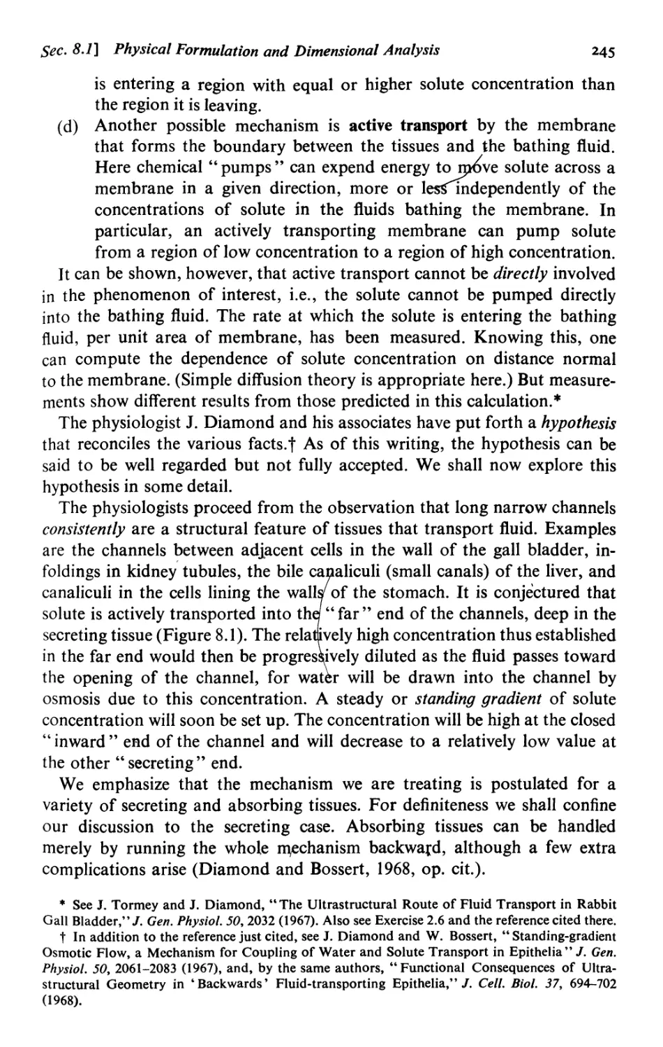
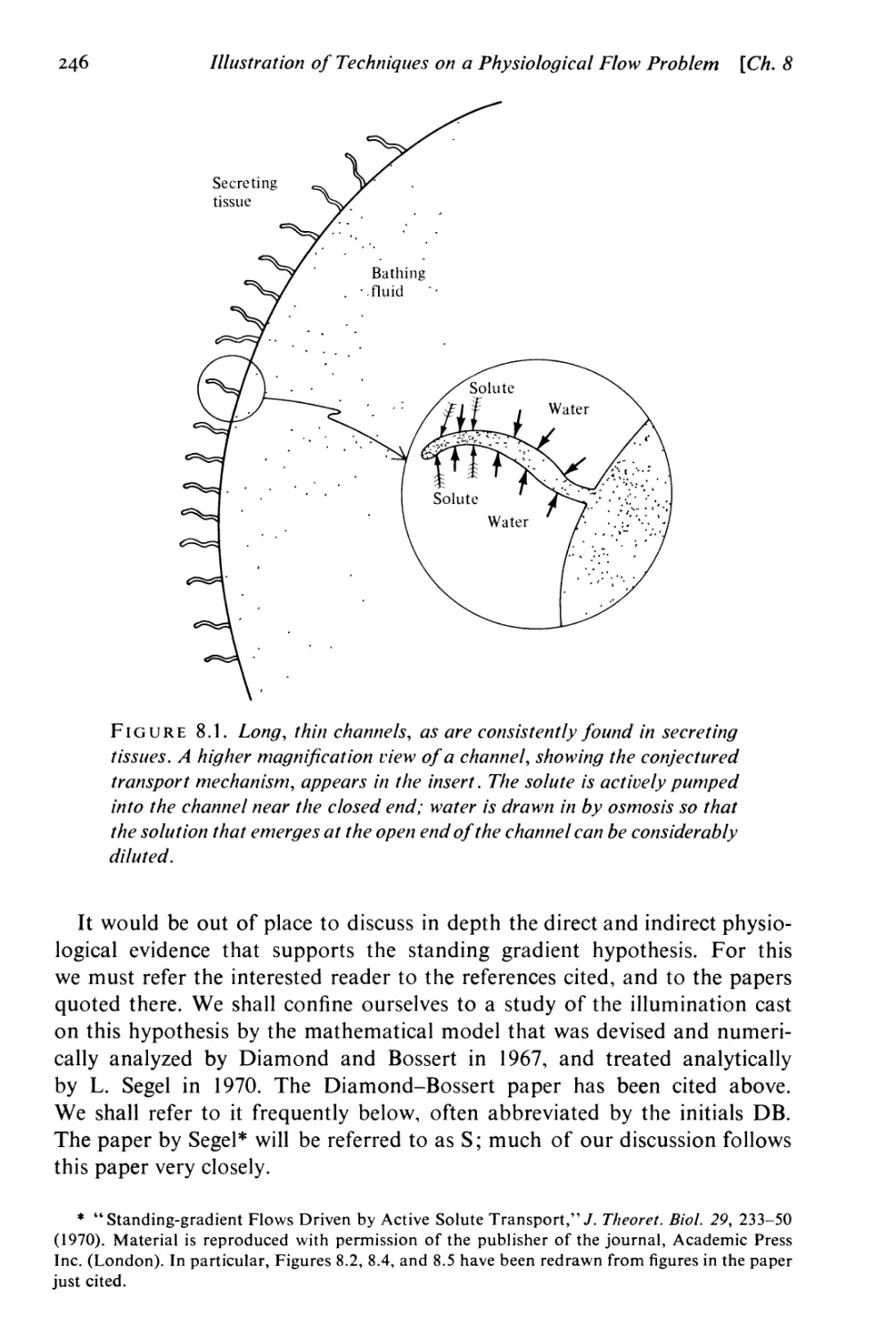
regarded but not yet fully accepted (as in the physiological flow problem
discussed in Chapter 8).
(g)	Some rather lengthy examples are worked out in detail, e.g., the
perturbation calculations in Section 7.2, in response to student objections
that they are often asked in exercises and in examinations to solve much harder
problems than they have ever seen done in the text.
(h)	We have provided a number of exercises to reinforce, test, and extend
the reader’s understanding. Noteworthy are multipart exercises, often based
on a relatively recent journal article, which develop a major point in a step-
by-step manner. (An example is Exercise 15.2.10.) Even if a student cannot do
one part of the exercise, he can take its result for granted and proceed. Such
exercises have been successfully used as the central part of final examinations.
PREREQUISITES
We have assumed that the potential reader has had an introductory college
course in physics and is familiar with calculus and differential equations.
Only a few exercises require knowledge of complex analysis. We make
considerable use of such topics as directional derivatives, change of variables
in multiple integrals, line and surface integrals, and the divergence theorem.
Often mathematics majors will have taken an advanced calculus course that
omits some of these topics, but we have found that such students are suffi-
ciently sophisticated mathematically to be able readily to pick up by them-
selves what is required. [Potential readers who feel inadequacies in vector
calculus and physical reasoning would profit from studying Div, Grad, Curl,
and All That by H. M. Schey (N.Y., Norton, 1973).]
RELATIONSHIPS BETWEEN THIS TEXT AND VARIOUS COURSES
Historically, this book grew out of the union of two courses. The first
was Foundations of Applied Mathematics introduced by G. H. Handelman
at Rensselaer around 1957. (A precursor of this course was taught by A. Schild
and Handelman at Carnegie Institute of Technology, now Carnegie-Mellon
Preface	xi
University.) A second course, Introduction to Applied Mathematics, was
introduced by С. C. Lin at Massachusetts Institute of Technology around
1960. These courses have been taught annually, many times, by the present
authors in their respective institutions. In recent years preliminary drafts
of the present work have been used as text material. Such drafts have also
been used in applied mathematics courses taught by P. Davis at Worcester
Polytechnic Institute, D. Drew at New York University, and D. Wollkind
at Washington State University. Considerable improvements in the draft
text have resulted; the authors welcome further suggestions from users of the
printed work.
ACKNOWLEDGMENTS
The work was jointly planned. One of us (C.C.L.) wrote the initial draft
of Part A, with the exception of Section 1.3, and also Chapter 16. The other
of us (L.A.S.) drafted the remainder of the book, with the exception of
Chapter 12, written by G. H. Handelman. There was considerable consulta-
tion on revisions. L.A.S. was responsible for the final editorial work.
In writing this book, we have drawn on a background for which we are
deeply indebted to our families, colleagues, teachers, and students, and to the
writers of numerous other books. We are grateful to G. H. Handelman for
showing, from classroom experience, that an introduction to continuum
mechanics is probably best made by starting with one-dimensional problems—
and for writing out his approach as Chapter 12. Among many who have made
useful suggestions concerning this volume, we must single out Roy Caplan,
Paul Davis, Donald Drew, William Ling, Robert O’Malley, Jr., Edward
Rothstein, Terry Scribner, Hendrick Van Ness, and especially Edith Luchins.
Numbers of secretaries have performed yeoman service. The publishers have
also been most helpful, particularly our editors Everett Smethurst and Elaine
Wetterau.
The work of one of us (L.A.S) was partially supported in 1968-1969
by a Leave of Absence Grant from Rensselaer. Further support was received
during 1971-1972 from the National Science Foundation Grant GP33679X
to Rensselaer, and from a John Simon Guggenheim Foundation Fellowship.
That year was spent as a visitor to the Department of Applied Mathematics,
Weizmann Institute, Rehovot, Israel. The hospitality and technical assis-
tance afforded there are gratefully acknowledged.
С. C. L.
L. A. S.
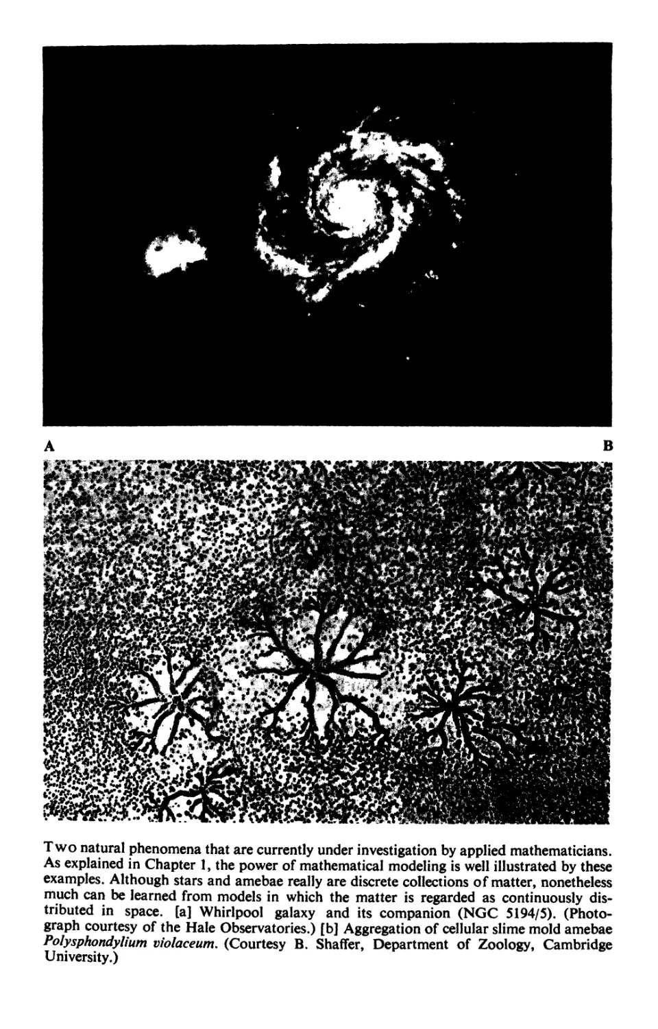
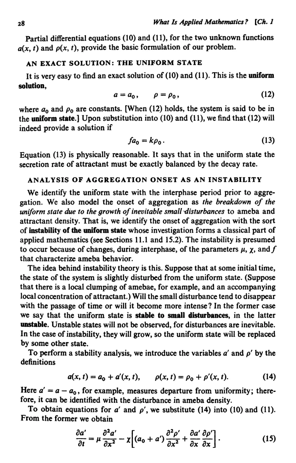
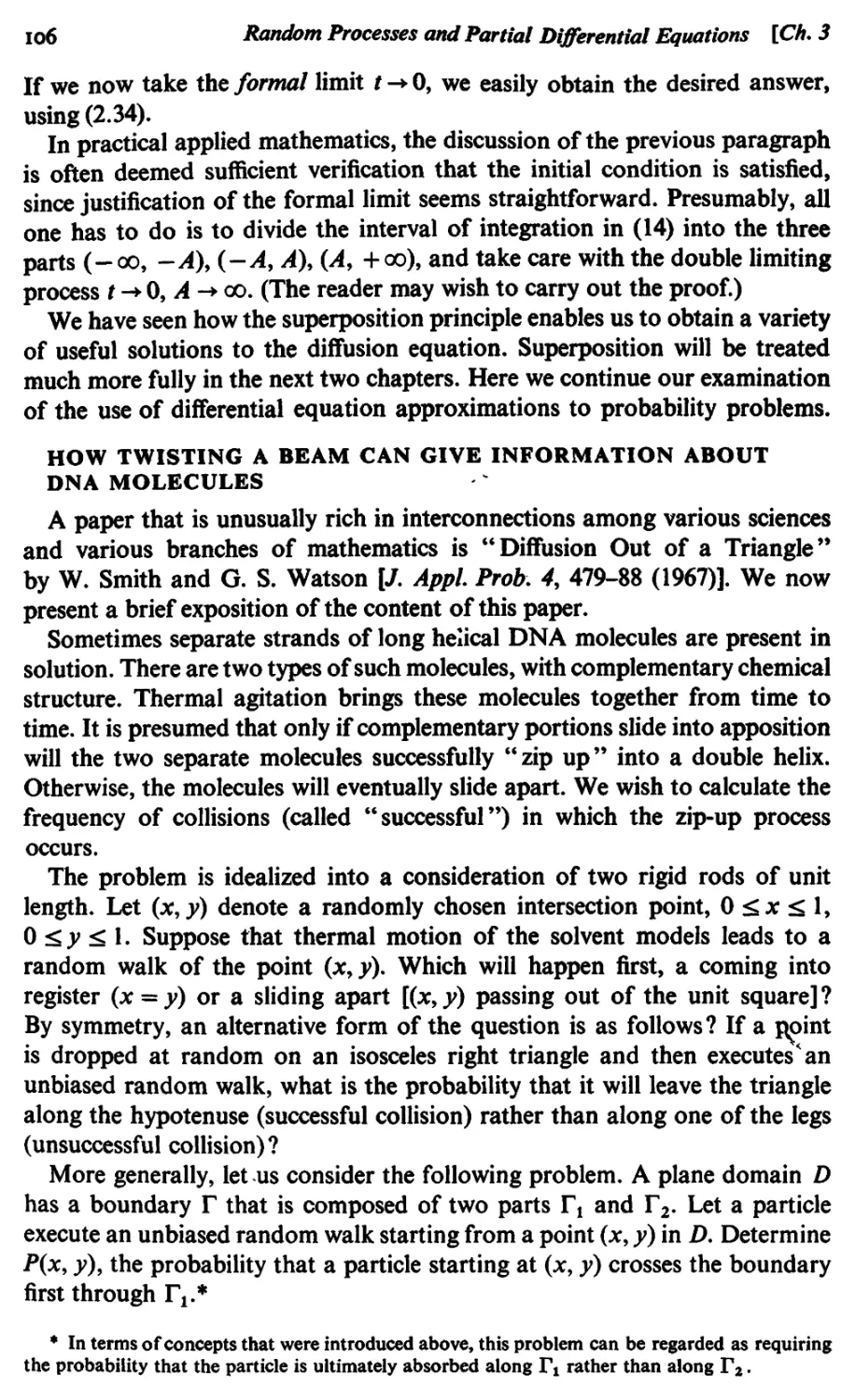
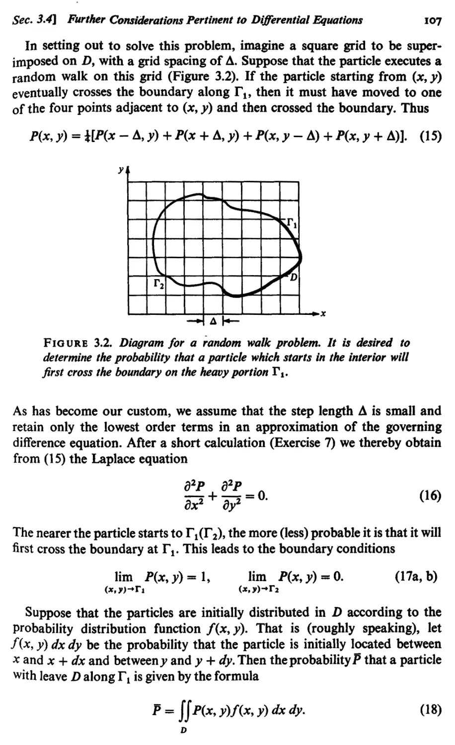
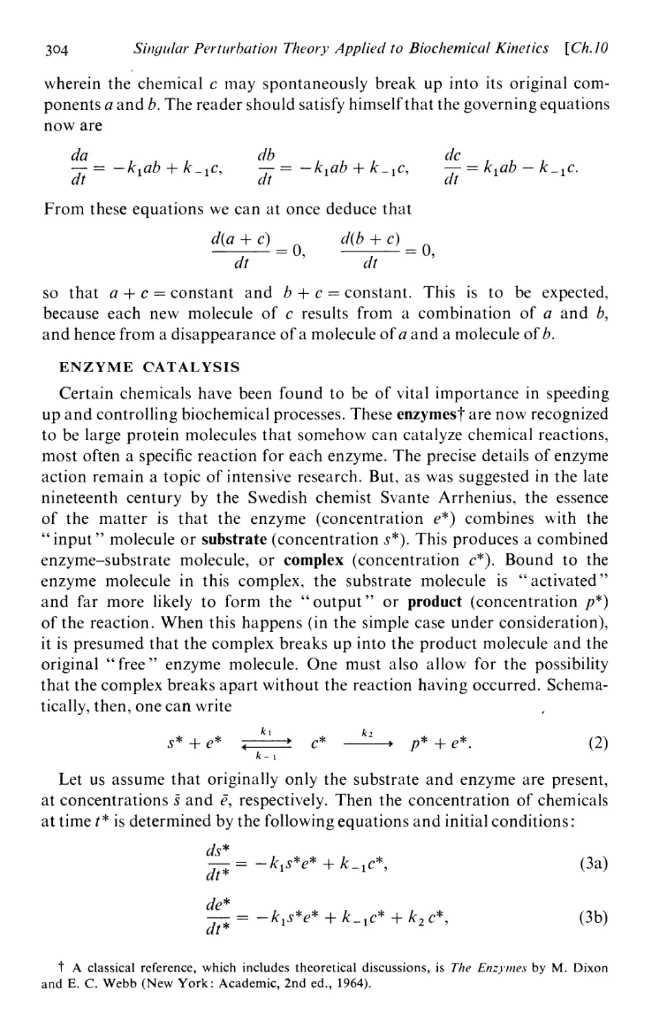
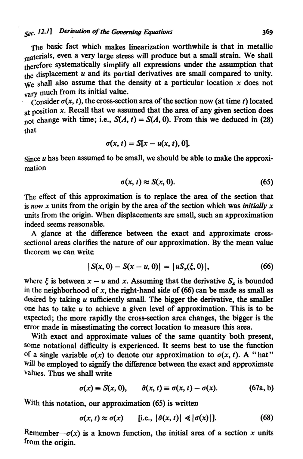
Two natural phenomena that are currently under investigation by applied mathematicians.
As explained in Chapter 1, the power of mathematical modeling is well illustrated by these
examples. Although stars and amebae really are discrete collections of matter, nonetheless
much can be learned from models in which the matter is regarded as continuously dis-
tributed in space, [a] Whirlpool galaxy and its companion (NGC 5194/5). (Photo-
graph courtesy of the Hale Observatories.) [b] Aggregation of cellular slime mold amebae
Polysphondylium violaceum. (Courtesy B. Shaffer, Department of Zoology, Cambridge
University.)
Contents
PART A
AN OVERVIEW OF THE INTERACTION OF
MATHEMATICS AND NATURAL SCIENCE
Chapter 1
What Is Applied Mathematics?
3
1.1	. On the nature of applied mathematics 4
The scope, purpose, and practice of applied mathematics 5 / Applied
mathematics contrasted with pure mathematics 61 Applied mathematics
contrasted with theoretical science 7 / Applied mathematics in engineering 8 /
The plan of the present volume 8 / A preview of the following volume g /
Concepts that unify applied mathematics 10
1.2	Introduction to the analysis of galactic structure 10
Physical laws governing galactic behavior 10 / Building blocks of the
universe 11 / Classification of galaxies 111 Composition of galaxies 13 /
Dynamics of stellar systems 14 / Distribution of stars across a galactic disk 16 /
Density wave theory of galactic spirals ig
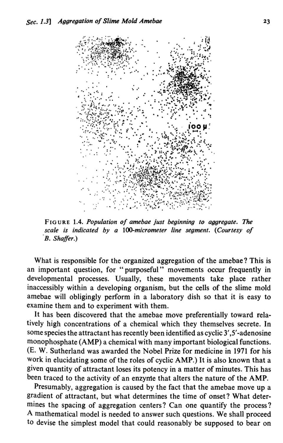
1.3	Aggregation of slime mold amebae 22
Some facts about slime mold amebae 22 I Formulation of a mathematical
model 241 An exact solution: The uniform state 28 I Analysis of aggregation
onset as an instability 28 / Interpretation of the analysis 30
Appendix 1.1 Some views on applied mathematics 31
On the nature of applied mathematics 311 On the relationships among pure
mathematics, applied mathematics, and theoretical science 32 / On the teaching
and practice of applied mathematics 33
Chapter 2
Deterministic Systems and Ordinary
Differential Equations	36
2.1	Planetary orbits 36
Kepler's laws 37 / Law of universal gravitation 3g / The inverse problem:
Orbits of planets and comets 3g / Planetary orbits according to the general
theory of relativity 41 / Comments on choice of methods 411 N particles: A
deterministic system 42 I Linearity 43
xiii
xiv
Contents
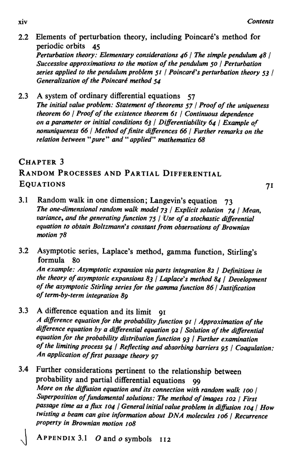
2.2	Elements of perturbation theory, including Poincare’s method for
periodic orbits 45
Perturbation theory: Elementary considerations 461 The simple pendulum 48 I
Successive approximations to the motion of the pendulum 50 I Perturbation
series applied to the pendulum problem 51 / Poincares perturbation theory 53 /
Generalization of the Poincart method 54
2.3	A system of ordinary differential equations 57
The initial value problem: Statement of theorems 57 I Proof of the uniqueness
theorem 60 I Proof of the existence theorem 61 I Continuous dependence
on a parameter or initial conditions 63 I Differentiability 64 I Example of
nonuniqueness 661 Method of finite differences 66 / Further remarks on the
relation between “pure” and “applied” mathematics 68
Chapter 3
Random Processes and Partial Differential
Equations	71
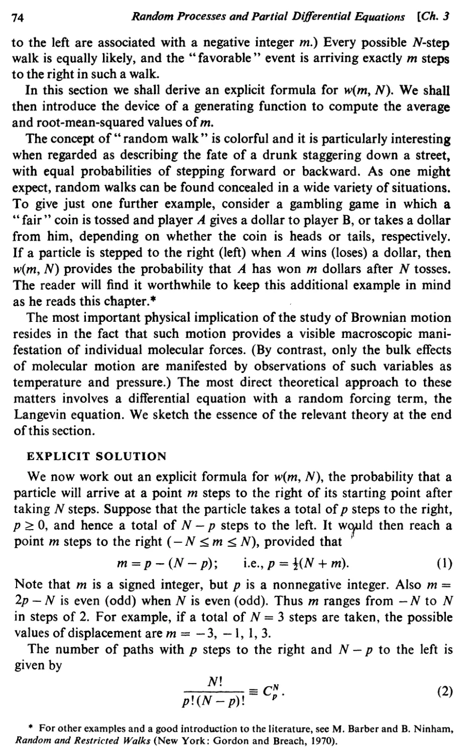
3.1	Random walk in one dimension; Langevin’s equation 73
The one-dimensional random walk model 73 I Explicit solution 74 / Mean,
variance, and the generating function 75 / Use of a stochastic differential
equation to obtain Boltzmann's constant from observations of Brownian
motion 78
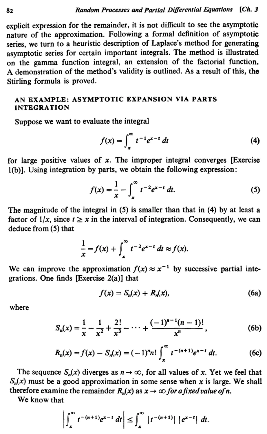
3.2	Asymptotic series, Laplace’s method, gamma function, Stirling’s
formula 80
An example: Asymptotic expansion via parts integration 82 I Definitions in
the theory of asymptotic expansions 83 I Laplace's method 84 I Development
of the asymptotic Stirling series for the gamma function 861 Justification
of term-by-term integration 89
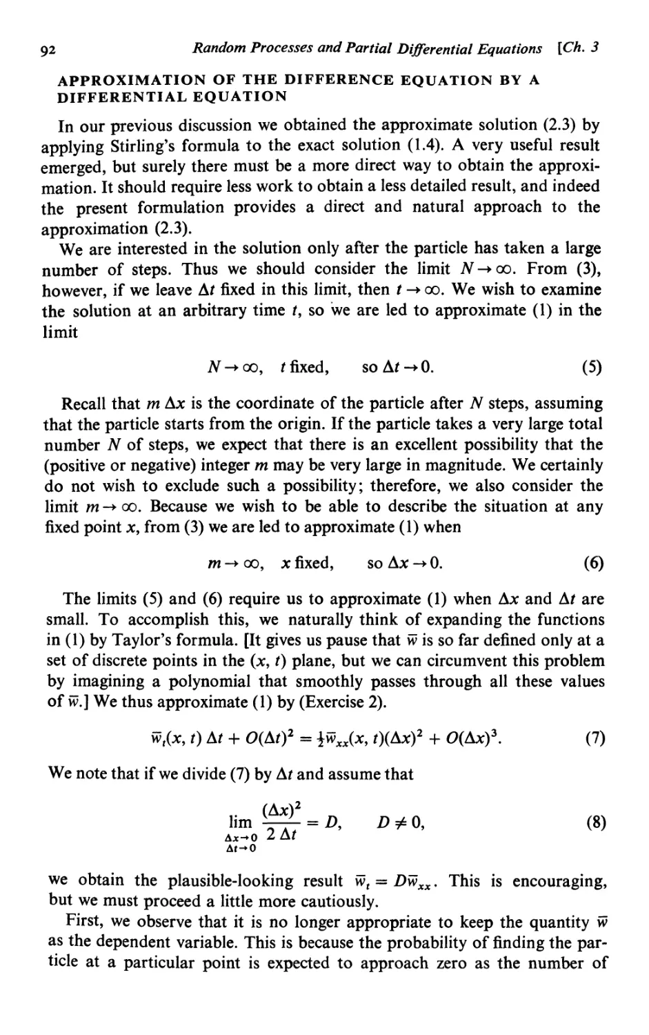
3.3	A difference equation and its limit 91
A difference equation for the probability function 91 / Approximation of the
difference equation by a differential equation 92 I Solution of the differential
equation for the probability distribution function 93 / Further examination
of the limiting process 94 I Reflecting and absorbing barriers 95 / Coagulation:
An application of first passage theory 97
3.4	Further considerations pertinent to the relationship between
probability and partial differential equations 99
More on the diffusion equation and its connection with random walk 100 /
Superposition of fundamental solutions: The method of images 102 / First
passage time as a flux 104 I General initial value problem in diffusion 1041 How
twisting a beam can give information about DNA molecules 106 / Recurrence
property in Brownian motion 108
I Appendix 3.1 О and о symbols 112
Contents
XV
Chapter 4
Superposition, Heat Flow, and Fourier Analysis 114
4.1	Conduction of heat 115
Steady state heat conduction 116 / Differential equation for one-dimensional
heat conduction 117 I Initial boundary value problem for one-dimensional
heat conduction 118 / Past, present, and future 119 / Heat conduction in
three-dimensional space 120 / Proof of the uniqueness theorem 122 I The
maximum principle 123 I Solution by the method of separation of variables 1231
Interpretation; dimensionless representation 127 / Estimate of the time required
to diffuse a given distance 129
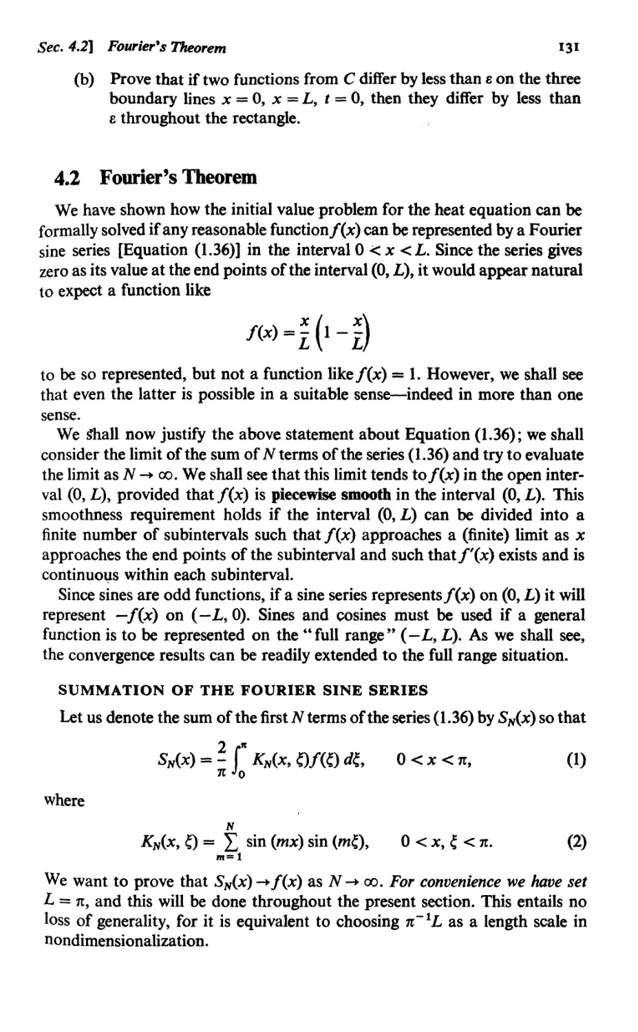
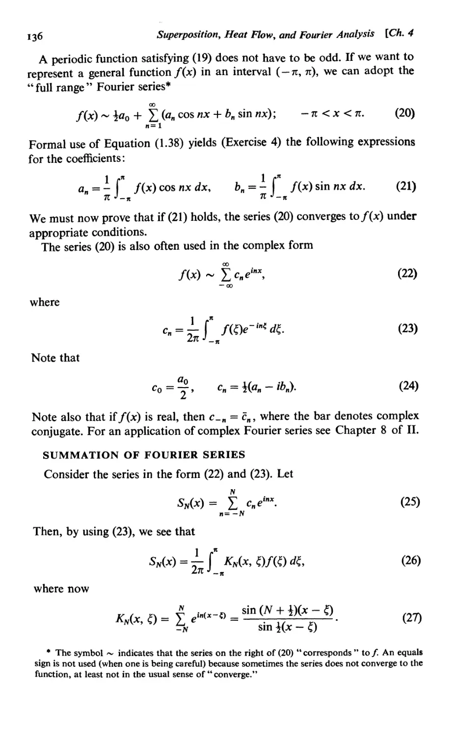
4.2	Fourier’s theorem 131
Summation of the Fourier sine series 1311 Proof of the lemmas 134 I A formal
transformation 135 / Fourier series in the full range 135 / Summation of Fourier
series 136 / Half-range series 137
4.3	On the nature of Fourier series 137
Fourier series for the constant function 138 / Fourier series for the linear
function 139 / Fourier series for the quadratic function 139 / Integration and
differentiation of Fourier series 139 I Gibbs phenomenon 141 / Approximation
with least squared error 144 I Bessel's inequality and Parseval's theorem 146 /
Riesz-Fischer theorem 147 / Applications of Parseval's theorem 147
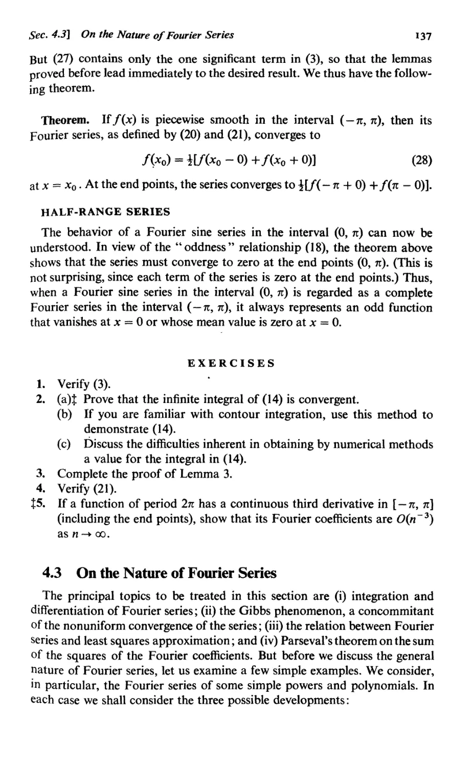
Chapter 5
Further Developments in Fourier Analysis	150
5.1	Other aspects of heat conduction 150
Variation of temperature underground 150 / Numerical integration of the heat
equation 153 I Heat conduction in a nonuniform medium 155
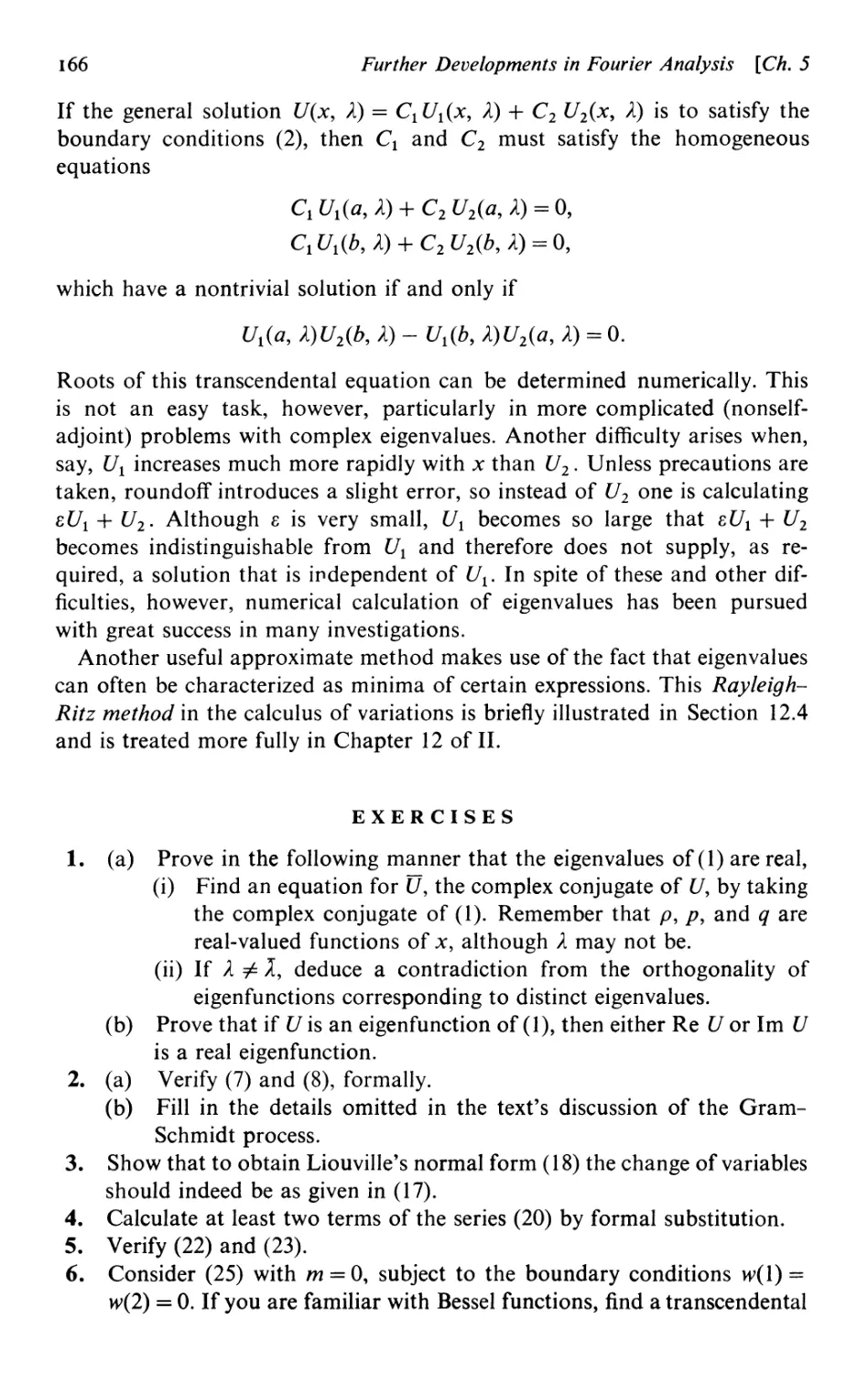
5.2	Sturm-Liouville systems 159
Properties of eigenvalues and eigenfunctions 160 / Orthogonality and
normalization 161 / Expansion in terms of eigenfunctions 162 / Asymptotic
approximations to eigenfunctions and eigenvalues 163 / Other methods of
calculating eigenfunctions and eigenvalues 165
5.3	Brief introduction to Fourier transform 167
Fourier transform formulas and the Fourier identity 167 I Solution of the heat
equation by Fourier transform 170
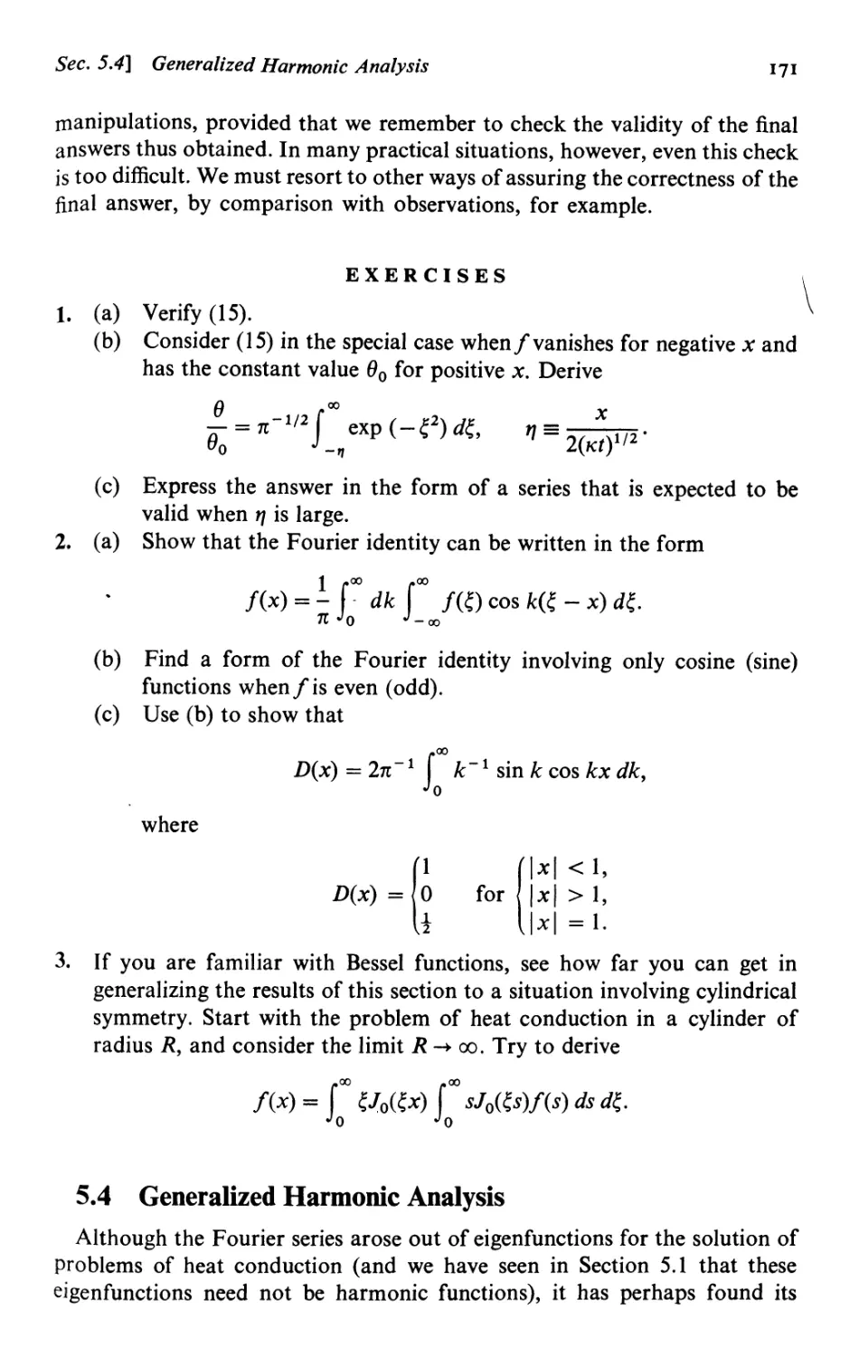
5.4	Generalized harmonic analysis 171
Remarks on functions that cannot be analyzed by standard Fourier
methods 172 / Fourier series analysis of a truncated sinusoidal function 173 I
Fourier integral analysis of a truncated sinusoidal function 174 I
Generalization to stationary time sequences 1761 Autocorrelation function and
the power spectrum 178 / Verification of the cosine transform relation
between the power spectrum and the autocorrelation 179 I Application 180
xvi
Contents
PART В
SOME FUNDAMENTAL PROCEDURES
ILLUSTRATED ON ORDINARY DIFFERENTIAL
EQUATIONS
Chapter 6
Simplification, Dimensional Analysis, and Scaling 185
6.1	The basic simplification procedure 186
Illustrations of the procedure 1861 Two chastening examples 187 I Conditioning
and sensitivity 189 / Zeros of a function 190 I Second order differential
equations 1911 Recommendations 194
6.2	Dimensional analysis 195
Putting a differential equation into dimensionless form 195 /
Nondimensionalization of a functional relationship 198 / Use of scale models
200 I Summary 203
6.3	Scaling 209
Definition of scaling 211 I Scaling the projectile problem 211 I Order of
magnitude 213 I Scaling known functions 214 I Orthodoxy 2181 Scaling and
perturbation theory 2211 Scaling unknown functions 222
Chapter 7
Regular Perturbation Theory	225
7.1	The series method applied to the simple pendulum 225
Preliminaries 226 I Series method 227 / Discussion of results so far 230 /
Higher order terms 231
7.2	Projectile problem solved by perturbation theory 233
Series method 233 I Parametric differentiation 2361 Successive approximations
(method of iteration) 238 I General remarks on regular perturbation theory 240
Chapter 8
Illustration of Techniques on a Physiological Flow
Problem	244
8.1	Physical formulation and dimensional analysis of a model for
“standing gradient” osmotically driven flow 244
Some physiological facts 244 / Osmosis and the osmol 247 I Factors that affect
standing gradient flow 248 I Dimensional analysis of a functional relationship
249 I Possibility of a scale model for standing gradient flow 253
8.2	A mathematical model and its dimensional analysis 253
Conservation of fluid mass 254 I Conservation of solute mass 254 / Boundary
conditions 255 I Introduction of dimensionless variables 2571 Comparison of
physical and mathematical approaches to dimensional analysis 259
Contents	xvii
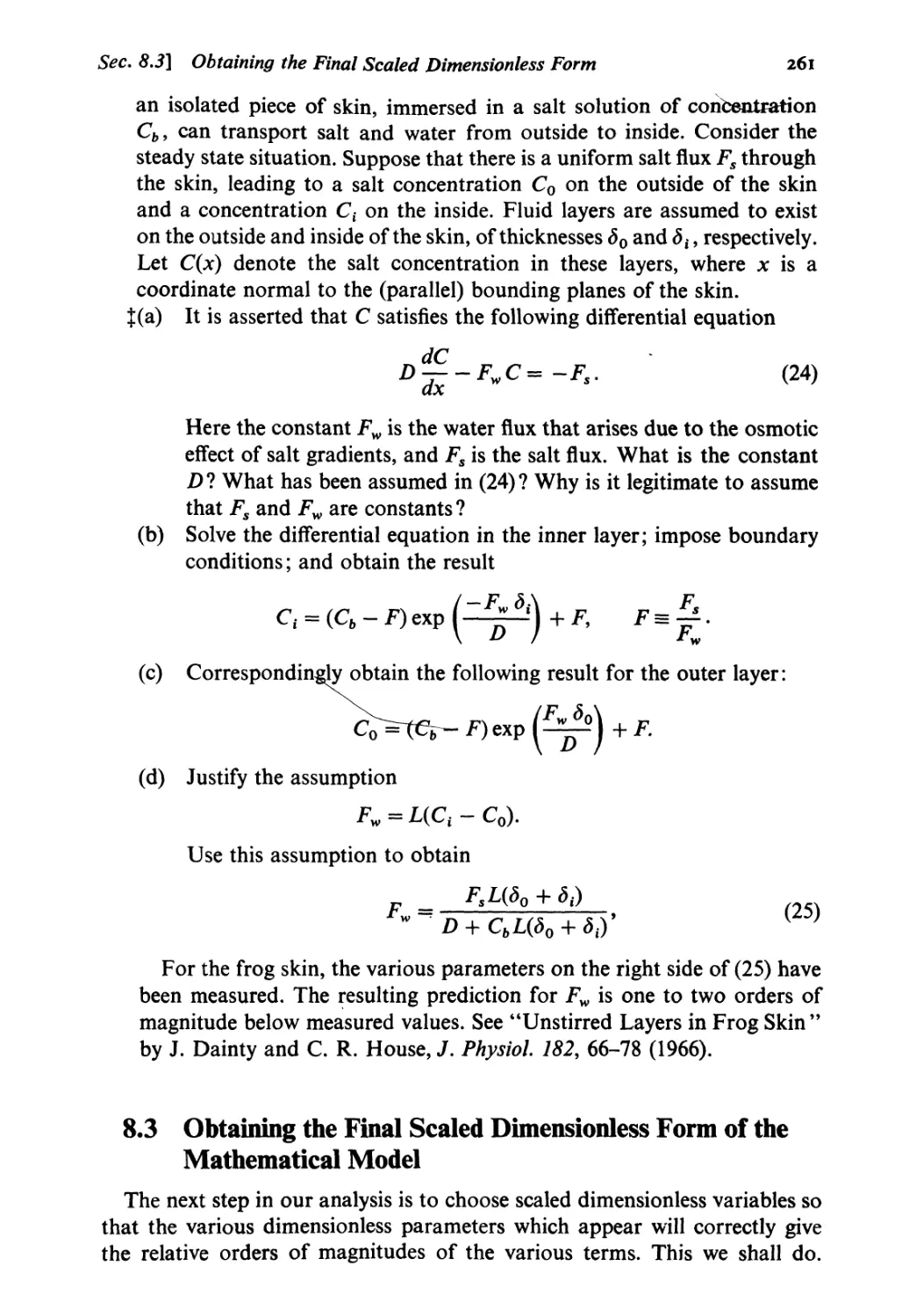
8.3	Obtaining the final scaled dimensionless form of the mathematical
model 261
Scaling 262 / Estimating the size of the dimensionless parameters 264 I An
unsuccessful regular perturbation calculation 2631 Relation between
parameters 2651 Final formulation 267
8.4	Solution and interpretation 268
A first approximation to the solution 2681 Comparison with numerical
calculations 269 I Interpretation: Physical meaning of the dimensionless
parameters 272 / Final remarks 274
Chapter 9
Introduction to Singular Perturbation Theory 277
9.1	Roots of polynomial equations 278
A simple problem 278 / A more complicated problem 2811 The use of scaling 284
9.2	Boundary value problems for ordinary differential equations 28 5
Examination of the exact solution to a model problem 285 I Finding an
approximate solution by singular perturbation methods 291 / Matching 293 I
Further examples 295
Chapter 10
Singular Perturbation Theory Applied to a Problem
in Biochemical Kinetics	302
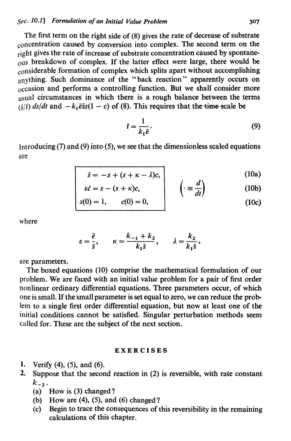
10.1	Formulation of an initial value problem for a one enzyme-one
substrate chemical reaction 302
The law of mass action 302 I Enzyme catalysis 304 I Scaling and final
formulation 306
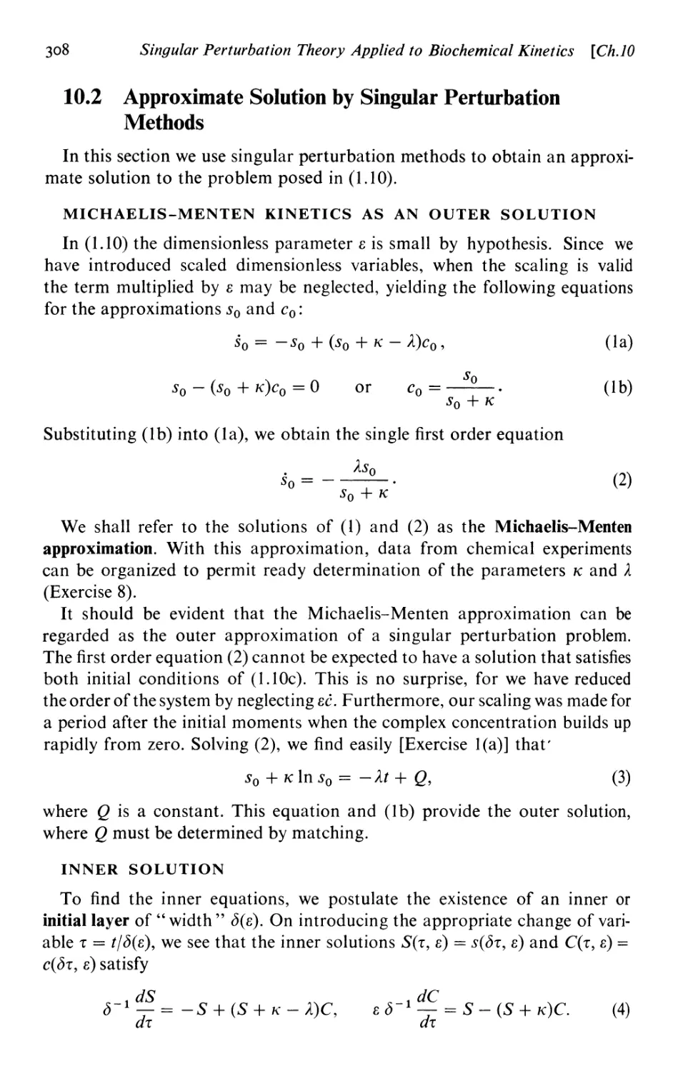
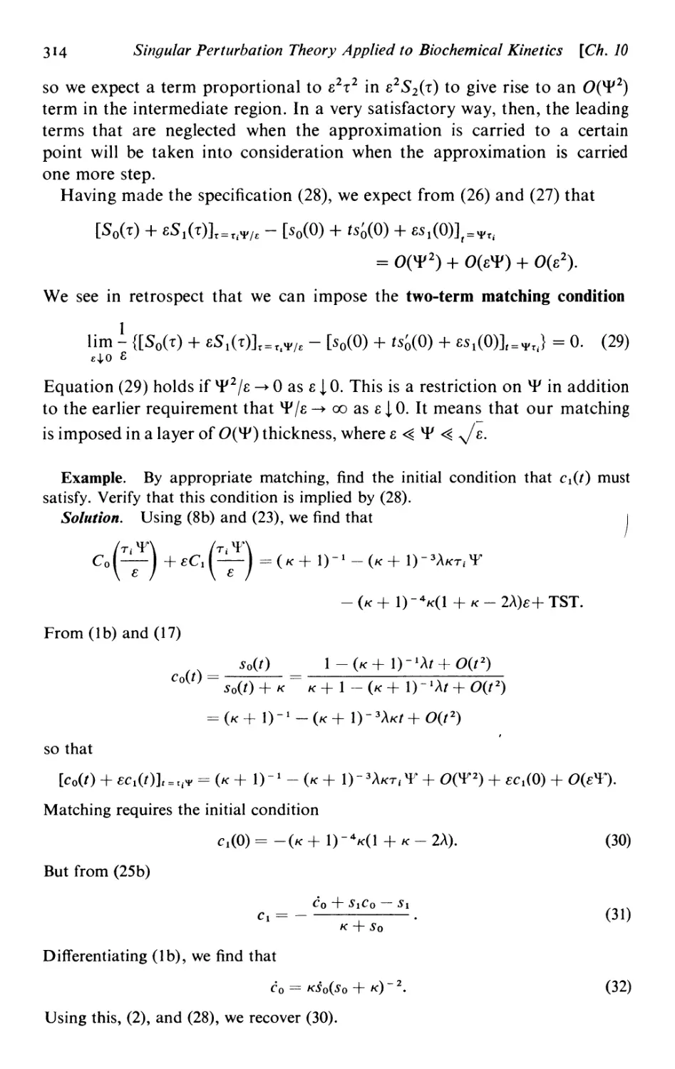
10.2	Approximate solution by singular perturbation methods 308
Michaelis-Menten kinetics as an outer solution 308 / Inner solution 308 I A
uniform approximation 310 / Comments on results so far 311 / Higher
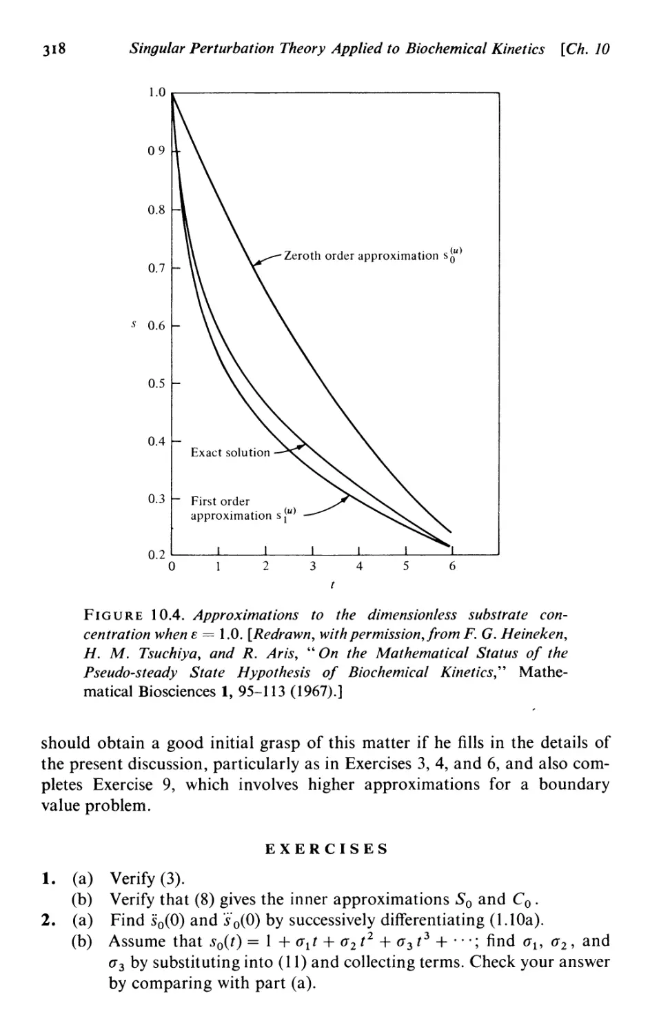
approximations 3111 Further analysis for large times 315 / Further discussion
of the approximate solutions 317
Chapter 11
Three Techniques Applied to the Simple Pendulum 321
11	.1 Stability of normal and inverted equilibrium of the pendulum 321
Determining stability of equilibrium 322 / Discussion of results 323
1	l.M A multiple scale expansion 325
Substitution of a two-scale series into the pendulum equation 327 I Solving
lowest order equations 328 I Higher approximations; removing resonant
terms 328 I Summary and discussion 330
11	.3 The phase plane 334
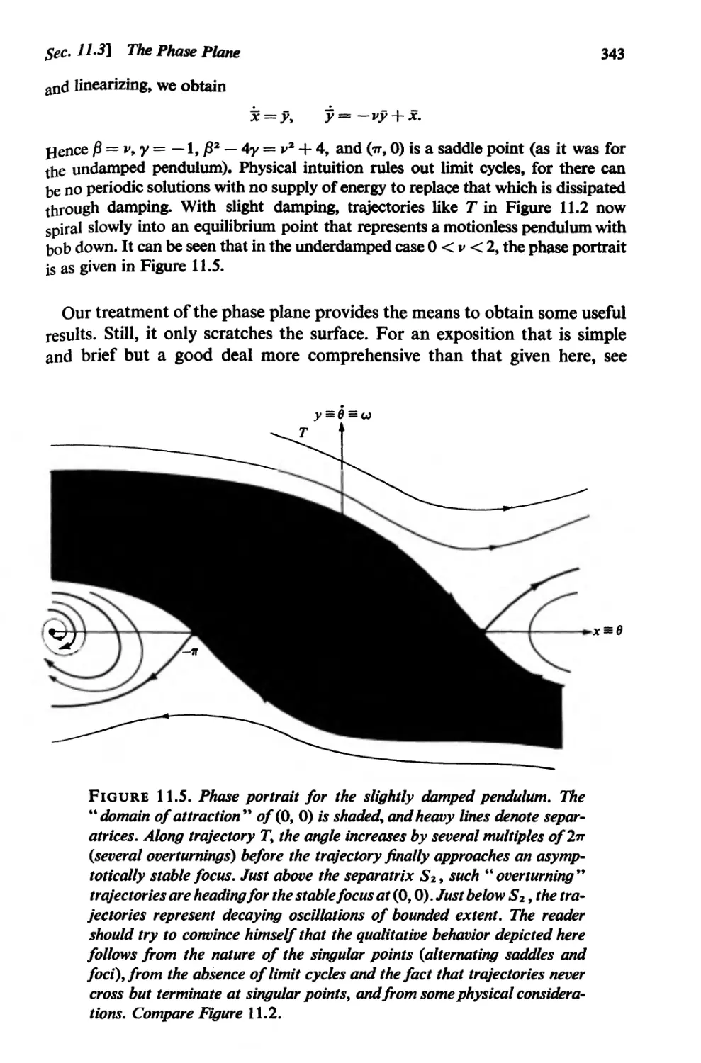
The phase portrait of an undamped simple pendulum 335 I Separatrices 3371
Critical points 338 I Limit cycles 339 / Behavior of trajectories near critical
points 339
xviii
Contents
PART C
INTRODUCTION TO THEORIES OF CONTINUOUS
FIELDS
Chapter 12
Longitudinal Motion of a Bar	349
12.1	Derivation of the governing equations 349
Geometry 349 I The material derivative and the Jacobian 352 I Conservation
of mass 355 I Force and stress 3581 Balance of linear momentum 360 / Strain
and stress-strain relations 362 I Initial and boundary conditions 366 /
Linearization 368
12.2	One-dimensional elastic wave propagation 376
The wave equation 377 / General solution of the wave equation 377 / Physical
significance of the solution 3781 Solutions in complex form 379 / Analysis of
sinusoidal waves 380 / Effects of a discontinuity in properties 381
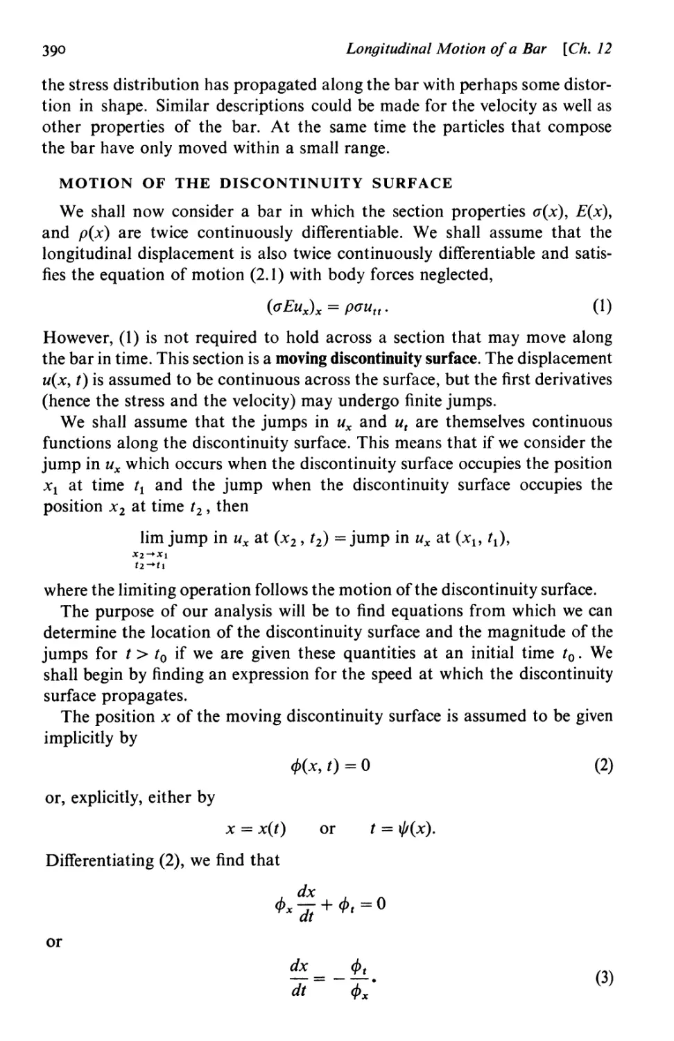
12.3	Discontinuous solutions 388
Motion of the discontinuity surface 390 / Behavior of the discontinuity 396
12.4	Work, energy, and vibrations 401
Work and energy 4011 A vibration problem 403 / The Rayleigh quotient 404 /
Properties of eigenvalues and eigenfunctions 405 I An exact solution when
properties are constant 406 I Characterization of the lowest eigenvalue as the
minimum of the Rayleigh quotient 4061 Estimate of the lowest eigenvalue for
a wedge 407
Chapter 13
The Continuous Medium	412
13.1	The continuum model 413
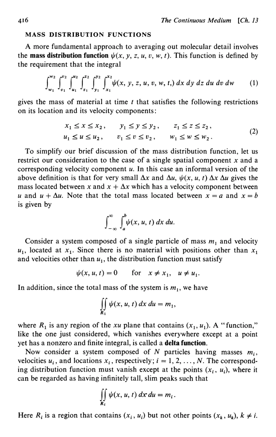
Molecular averages 414 I Mass distribution functions 416 / The continuum as
an independent model 417
13.2	Kinematics of deformable media 418
Points and particles 419 I Material and spatial descriptions 420 I Streamlines
and particle paths 422 / A simple kinematic boundary condition 425
13.3	The material derivative 426
13.4	The Jacobian and its material derivative 429
Appendix 13.1	On the chain rule of partial differentiation 433
Appendix 13.2	The integral mean value theorem 435
Appendix 13.3	Similar regions 436
Contents	xix
Chapter 14
Field Equations of Continuum Mechanics	440
14.1	Conservation of mass 440
Integral method: Arbitrary material region 441 I Integral method: Arbitrary
spatial region 444 / Small box method 444 I Large box method 446
14.2	Balance of linear momentum 454
An integral form of Newton's second law 454 I Local stress equilibrium 456 /
Action and reaction 457 / The stress tensor 458 I Newton's second law in
differential equation form 461
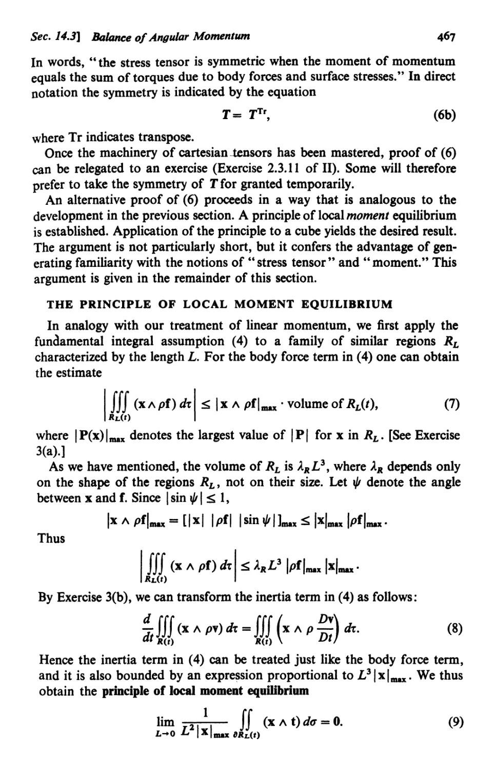
14.3	Balance of angular momentum 465
Torque and angular momentum 465 / Polar fluids 4661 Symmetry of the stress
tensor 4661 The principle of local moment equilibrium 4671 Local moment
equilibrium for a cube 468
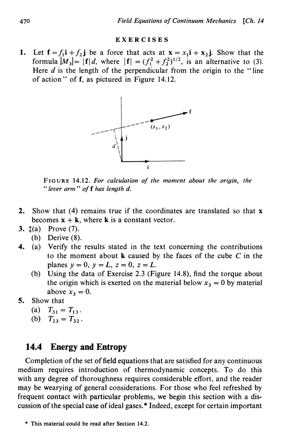
14.4	Energy and entropy 470
Ideal gases 4711 Equilibrium thermodynamics 474 I Effects of inhomogeneity
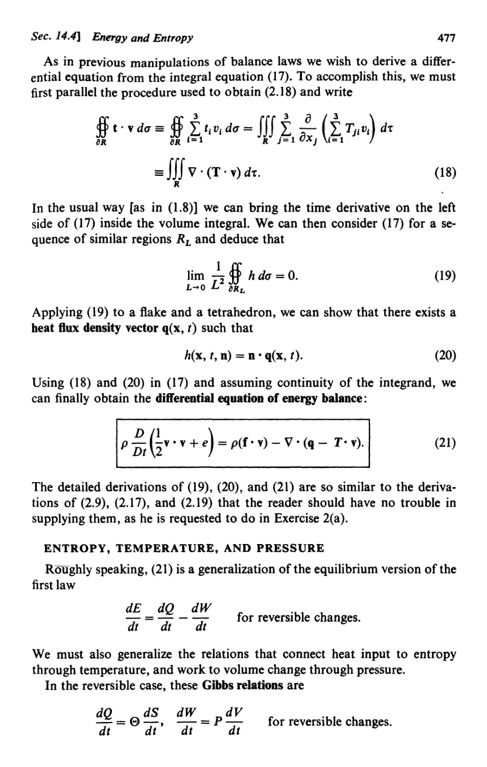
and motion 4751 Energy balance 476 / Entropy, temperature, and pressure 4771
Internal energy and deformation rate 479 I Energy and entropy in fluids 480
14.5	On constitutive equations, covariance, and the continuum model 485
Recapitulation of field equations 485 / Introduction to constitutive
equations 4861 The principle of covariance 4871 Validity of classical continuum
mechanics 490
Appendix 14	.1 Thermodynamics of spatially homogeneous
substances 491
Experiments with a piston 492 / First law of equilibrium thermodynamics 494 /
Entropy 4961 Second law of equilibrium thermodynamics 500
Appendix 14	.2 Some historical remarks 501
Chapter 15
Inviscid Fluid Flow	505
15.1	Stress in motionless and inviscid fluids 505
Molecular point of view 506 / Continuum point of view 506 / Hydrostatics 5081
Inviscid fluids 510
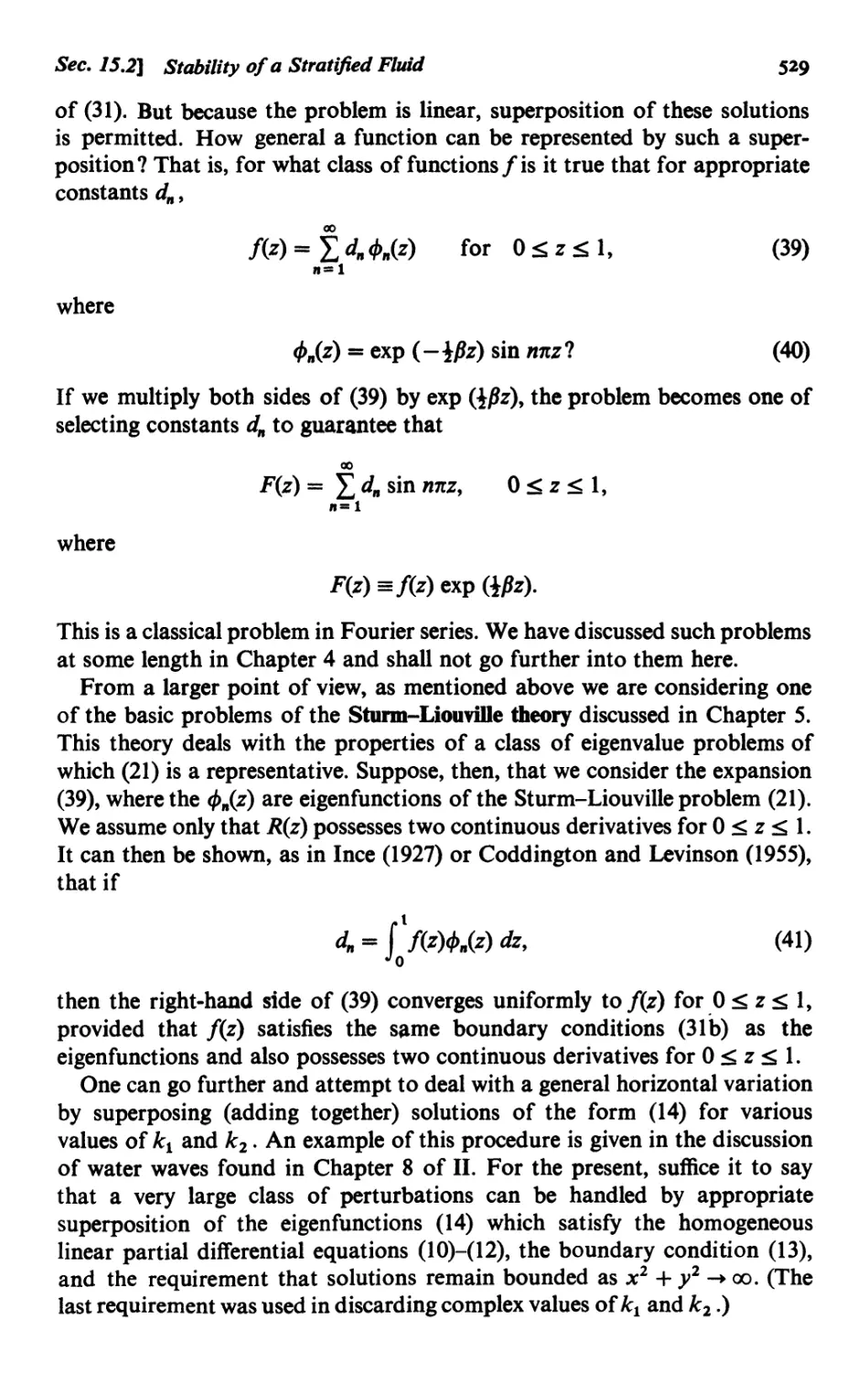
15.2	Stability of a stratified fluid 515
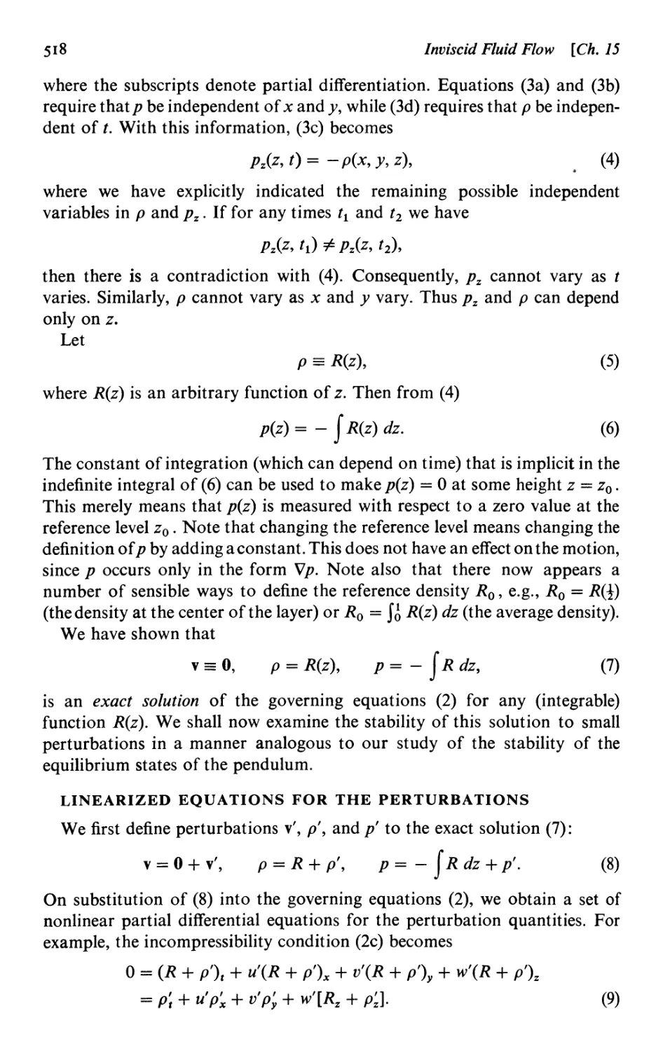
Governing equations and their exact equilibrium solution 5161 Linearized
equations for the perturbations 518 / Characterization of the growth rate о
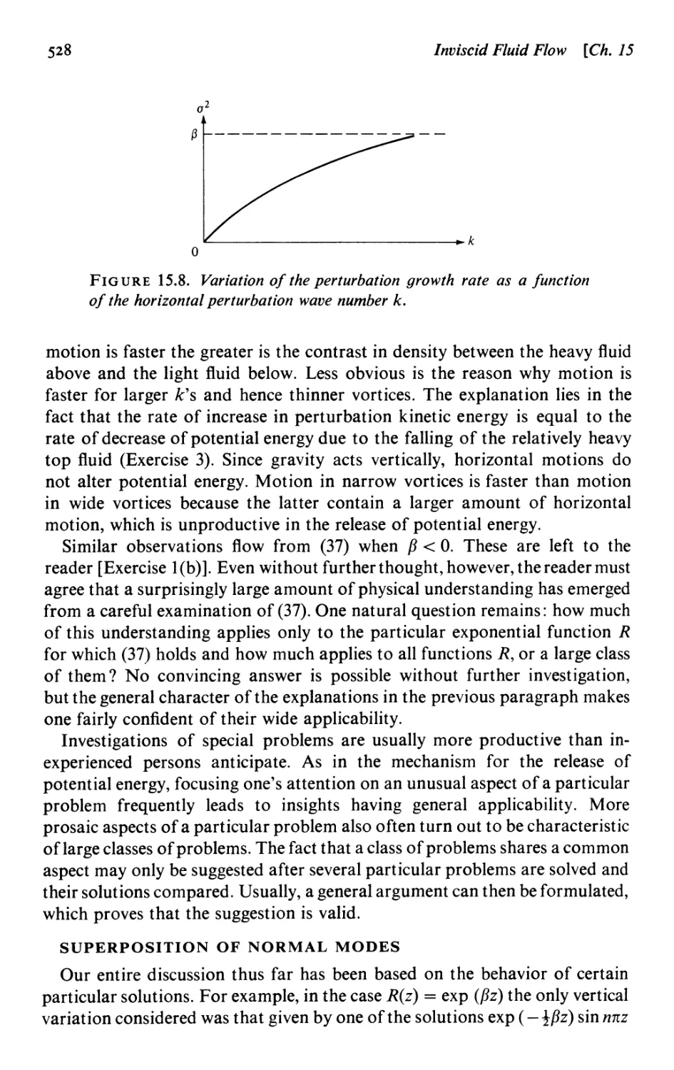
as an eigenvalue 521 / Qualitative general deductions 523 I Detailed results for
a particular stratification 5251 Superposition of normal modes 5281 Nonlinear
effects 530 I Worked example: A model of viscous flow instability 531
15.3	Compression waves in gases 539
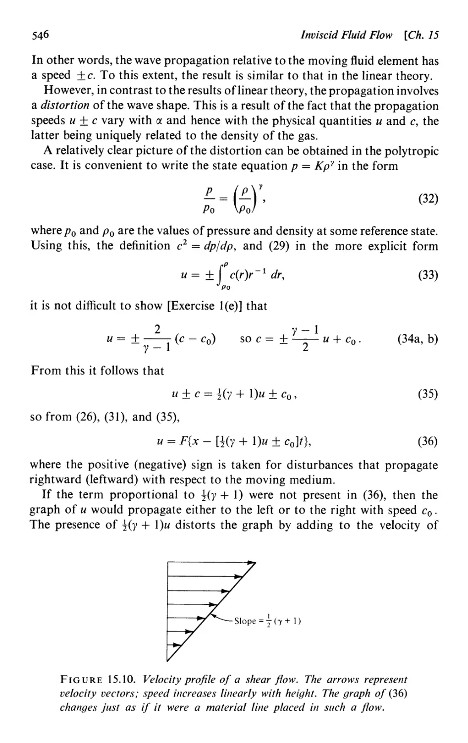
Inviscid isentropic flow of a perfect gas 540 / Waves of small amplitudes 5411
The speed of sound 542 I Spherical waves 543 I Nonlinear waves in one
dimension 544 / Shock waves 547
XX
Contents
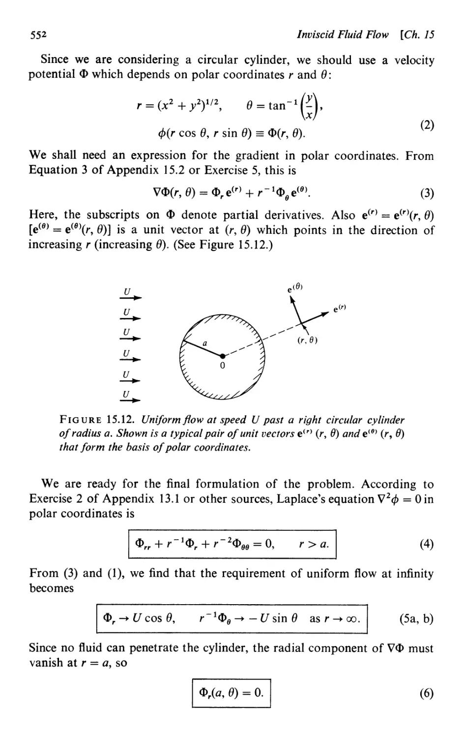
15.4	Uniform flow past a circular cylinder 551
Formulation 551 / Solution by separation of variables 553 I Interpretation of
solution 555
Appendix 15	.1 A proof of D’Alembert’s paradox in the
three-dimensional case 560
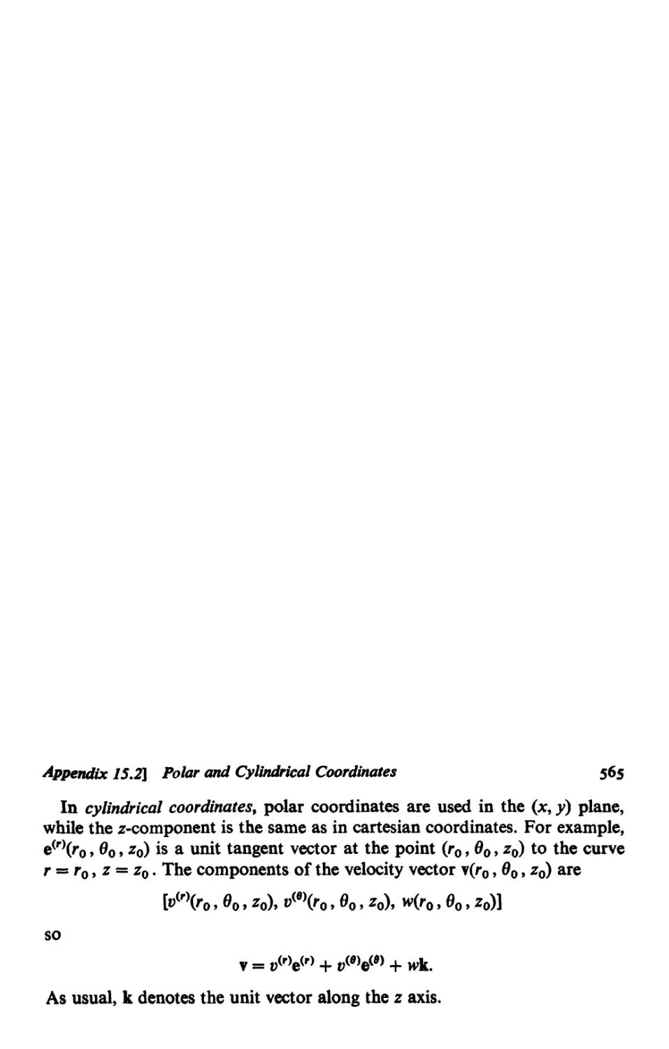
Appendix 15	.2 Polar and cylindrical coordinates 563
Chapter 16
Potential Theory	566
16.1	Equations of Laplace and Poisson 566
Gravitational potential of discrete mass distributions 566 / Gravitational
potential of continuous mass distributions 567 / Theorems concerning harmonic
functions 570 I Integral representation for the solution to Poisson's equation
572 I Uniqueness 573
16.2	Green’s functions 574
Green's function for the Dirichlet problem 574 I Representation of a harmonic
function using Green's function 575 I Symmetry of the Green's function 575 I
Explicit formulas for simple regions 575 I Widespread utility of source, image,
and reciprocity concepts 5771 Green's function for the Neumann problem 5781
Green's function for the Helmholtz equation 579
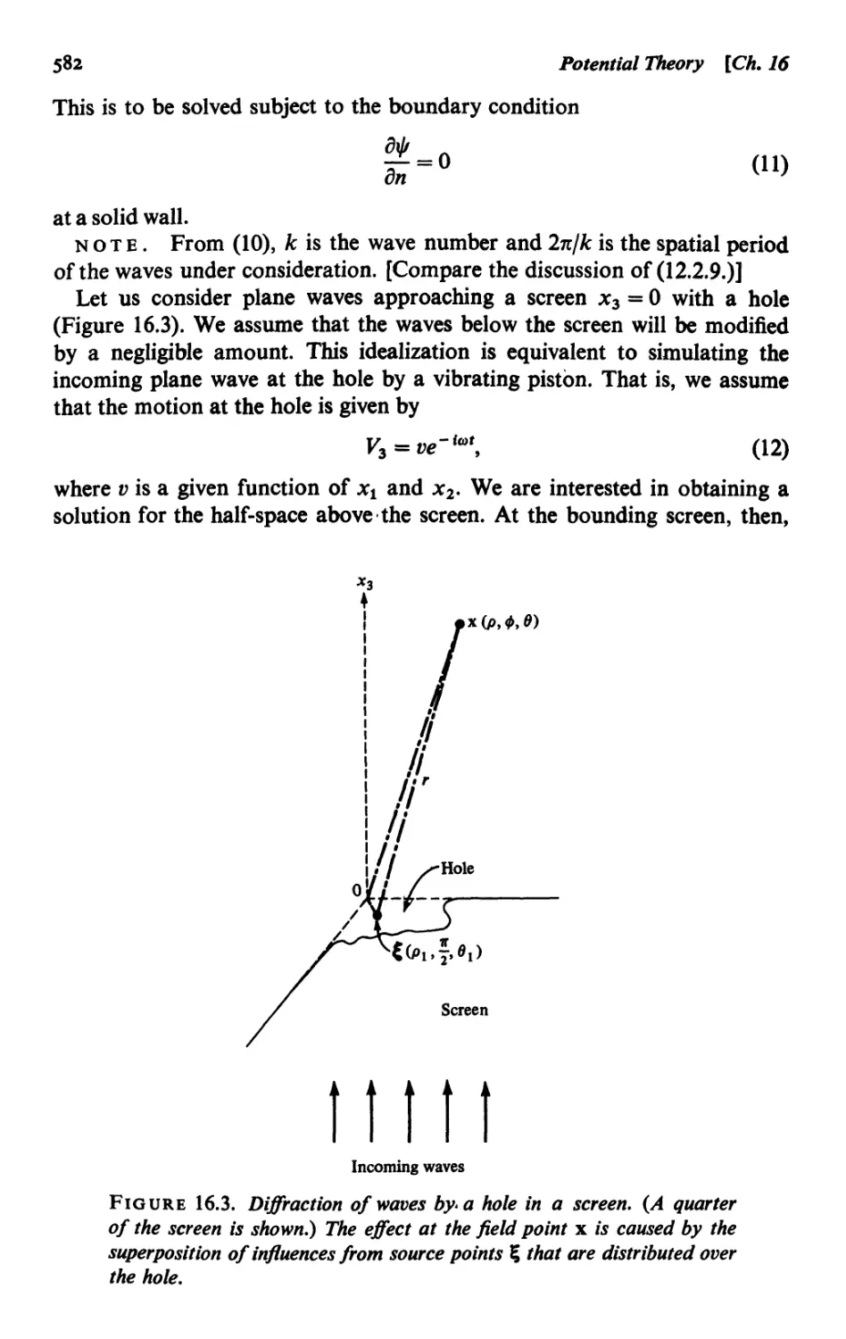
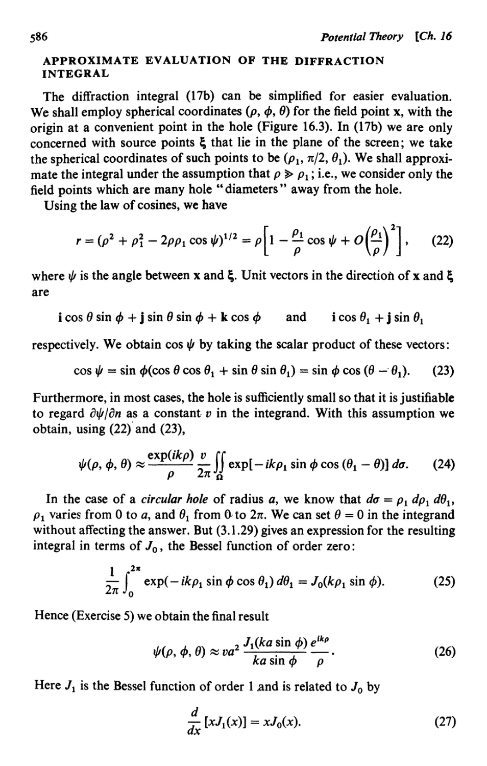
16.3	Diffraction of acoustic waves by a hole 580
Formulation 580 / Selection of the appropriate Green's function 583 I
Derivation of the diffraction integral 584 I Approximate evaluation of the
diffraction integral 586
Bibliography
Supplementary Bibliography	595
Updated Material	597
Hints and Answers (for exercises marked with $)	599
Index	605
Conventions
Each chapter is divided into several sections (e.g., Section 5.2 is the second
section of Chapter 5). Equations are numbered consecutively within each
section. Figures and tables are numbered consecutively within each chapter.
When an equation outside a given section is referred to, the section num-
ber precedes the equation number. Thus “ Equation (6.3.2)” [or (6.3.2)] refers
to the second numbered equation of Section 6.3. But if this equation were
referred to within Section 1 of Chapter 6, then the chapter number would be
assumed and the reference would be to “Equation (3.2)” [or (3.2)]. The
fourth numbered equation in Appendix 3.1 is denoted by (A3.1.4).
A double dagger^ preceding an Exercise, or a part thereof, signifies that a
hint or an answer will be found in the back of this volume.
The symbol 0 signifies that the proof of a theorem has concluded.
The succeeding volume is referred to as “II.”
A brief bibliography of books useful to beginning applied mathematicians
can be found at the end of this volume. When reference is made to one of
these books, the style “Smith (1970)” is employed.
PART A
An Overview of the
Interaction of Mathematics and
Natural Science
Chapter 1
What Is Applied Mathematics?
The purpose of this book is to foster an appreciation of the nature
of applied mathematics. We attempt to explain the essential processes involved
and to provide experience in applied mathematics as it is used in a variety
of physical problems.
The book is not intended as a compilation of methods—which cannot be
complete in any case. Rather, it is believed that an appreciation of the
applied mathematician’s approach will provide the student with a clear
framework on which to fit his knowledge, and with a creative attitude. These
are much more valuable than an encyclopedia of methods.
Section 1.1 begins with some fairly detailed remarks on the nature of
applied mathematics. Then follows an outline of the applied mathematical
topics that are to be presented in this work. Section 1.2 consists of an intro-
duction to the study of galactic structure, and Section 1.3 analyzes the sudden
aggregation of a population of amebae. The main purpose of Sections 1.2
and 1.3 is to provide an early feeling for the type of problem now under
investigation by applied mathematicians. (The authors selected the topics
from among their own current interests.) On first perusal at least, the reader
should not concern himself unduly with detail but should concentrate on
getting a general impression.
The behavior of stars and the behavior of amebae might seem to have little
in common. It is an excellent illustration of the power of applied mathematics,
however, to realize that this is not the case. For example, we shall see that
both stars and amebae behave as if their mass were continuously distributed—
notwithstanding the fact that one can see (using a microscope) gaps between
amebae, while the nearest stars are light-years apart. But it is of little relevance
that an idealized mathematical model such as the continuum is “wrong.”
The real question is : Do the errors have a significant effect upon predictions
concerning the phenomena under investigation?
For stars and amebae the idealization implied in the continuum model is
particularly striking, since it is the particulate aspect of the phenomena
that first makes itself evident. Water and air seem like continua—for most
people the existence of molecules is hearsay—but the continuum model is,
of course, also very useful for investigating phenomena involving these
media.
Another similarity between the examples of Sections 1.2 and 1.3 is that
both require an explanation of organized structure. The spiral galactic
pattern demands an investigation for reasons of aesthetics alone, but a more
basic reason is that the pattern offers an important clue to the nature of the
3
4
What Is Applied Mathematics ? [Ch. 1
forces involved. The morphogenetic (form-producing) motion of the amebae
is studied because of the clues it can provide to the organized cellular move-
ment that is a basic element of developmental biology. In both areas
understanding is far from complete.
1.1 On the Nature of Applied Mathematics
Mathematics began with simple practical problems such as division of a
flock of animals among family members (number theory) and the measure-
ment of land area (geometry). Gradually, elementary ideas were organized,
and they evolved into logical structures. A monumental example of early
achievements is Euclid’s geometry. The Greeks realized that the study of
mathematical theorems can be based on certain axioms. Only much later,
however, did it become clear that the axioms (such as the parallel postulate)
cannot be completely and decisively verified by experience. Indeed, it was
through a change in the parallel postulate that non-Euclidean geometry was
created; this led to many important ramifications. There is no doubt that
these pure mathematical developments are extremely important in appli-
cations.
As an increasing portion of mathematics was developed in a manner
independent of theoretical sciences, the term pure mathematics emerged. The
creative efforts of pure mathematicians are certainly impressive, but it would
be unfortunate to restrict our study of mathematics in any manner. Joint
study of mathematics and its applications can provide richer content and
greater intellectual challenge. Moreover, such study can stimulate the
development of new mathematical methods and theory. Some of these
developments will in turn find applications in the sciences.
Applied mathematics is guided by the spirit of and belief in the interdepen-
dence of mathematics and the sciences. It would be incorrect to claim that
all parts of mathematics involve such interdependence, but in the study of
applied mathematics one must give priority to such parts. This policy is
based on the assumption that the areas of mathematics that grew directly out
of the study of scientific problems have a greater likelihood of again being
applicable to other scientific problems. To give one example, later in this
chapter we see an application to a current problem in developmental biology
of stability theory for partial differential equations. This theory was developed
primarily in the classical fields of fluid mechanics and elasticity.
Historically, the development of mathematics and physics had a very close
connection. Classical examples may be found in the work of Newton (see
Chapter 2), Gauss, Euler, Cauchy, and others. More modern examples
appear throughout the study of relativity theory, Brownian motion, statistical
mechanics, and the associated theories of covariance, probability, and general-
ized harmonic analysis. Why is there such an intimate relationship between
mathematics and the physical sciences ?
Sec. 1-1} On the Nature of Applied Mathematics	5
An answer often given* to this philosophical question is that
GOD IS A MATHEMATICIAN.
In other words, it is believed that there is a basic harmony and order in nature.
Consequently, the description of natural phenomena can be organized by the
logical discipline of mathematics. In social and economic contexts, by
contrast, perhaps it is the logic imposed by man in his quest for optimality
that allows so large a role for mathematics.
THE SCOPE, PURPOSE, AND PRACTICE OF APPLIED
MATHEMATICS
The scope of applied mathematics is very broad and can be well described
by borrowing the following words of Albert Einstein:
Its realm is accordingly defined as that part of the sum total of our knowledge
which is capable of being expressed in mathematical terms, f
These words were used by Einstein to define physics. Taken literally, this
definition would certainly include mathematical theories of biology, econom-
ics, communication engineering, etc., and it is therefore a more adequate
description of applied mathematics.
We shall now attempt to give a brief description of the objectives and the
methodology of applied mathematics, and to contrast them with those of
pure mathematics and of theoretical science.
The purpose of applied mathematics is to elucidate scientific concepts and
describe scientific phenomena through the use of mathematics, and to
stimulate the development of new mathematics through such studies. The
process of using mathematics for increasing scientific understanding can be
conveniently divided into the following three steps:
(i)	The formulation of the scientific problem in mathematical terms.
(ii)	The solution of the mathematical problems thus created.
(iii)	The interpretation of the solution and its empirical verification in
scientific terms.
There is widespread misunderstanding that the second step is the most
important and that manipulative skill is the most valued asset of an applied
mathematician. Generally speaking, however, all three steps are equally
important. In a given class of problems, one step might stand out as more
important or more difficult than another.
A knowledge of methods and a proficiency in manipulative skill are
obviously necessary. A person with an encyclopedic knowledge of methods
* “ God is number”—Pythagoras; “ God ever geometrizes”—Plato; “ God ever arithmetizes”
—Jacobi; “The Great Architect of the Universe now begins to appear as a mathematician”—
Jeans. Quotes given (without much approval) by E. T. Bell, Men of Mathematics (London :
Penguin, 1953), p. 21.
t Out of My Later Years (New York: Philosophical Library, 1950), p. 98.
6
What Is Applied Mathematics ? [Ch. 1
alone can provide valuable aid to other scientists using mathematics. But it is
essential to realize that this knowledge is not sufficient for an applied mathe-
matician working as an independent scientist. He must also be able to
exercise judgment in the formulation of a problem, in decisions on which
problems to attack, and in choices of what idealizations and approximations
to adopt in order to simplify the problem without losing its essentials. An
aspiring applied mathematician must try even harder to cultivate sound
judgment than manipulative skill.
Finally, it is most important to extract, from the mathematical theory, the
proper scientific conclusions and implications for empirical verification. As far
as is feasible, conclusions must be reduced to the simplest form and expressed
in the most specific terms. This step serves as a culmination of the whole
effort and as a basis for future progress. A new understanding obtained, an
insight gained, a new perspective attained—these are much more important
and satisfying than the mere derivation of certain formulas and the compila-
tion of certain useful numerical tables. The accumulation of specific quanti-
tative information must be regarded as a means to an end.
It should now be apparent that an understanding of the scientific motivation
of the problem and the ability to use heuristic reasoning, as well as mani-
pulative skill, are essential to the practice of applied mathematics. Indeed,
these elements stand out as being more important than the ability to carry
out a rigorous proof. In many cases the rigorous formulation of a mathe-
matical theory may take many years. In the meantime, the applied mathe-
matician must proceed despite the incompleteness of the logical structure.
However, he must strive to be correct and to be as careful as possible in his
reasoning.
APPLIED MATHEMATICS CONTRASTED WITH PURE
MATHEMATICS
The differences in motivation and objectives between pure and applied
mathematics—and the consequent differences in emphasis and attitude—
must be fully recognized. In pure mathematics, one is often dealing with
such abstract concepts that logic remains the only tool permitting judgment
of the correctness of a theory. In applied mathematics, empirical verification
is a necessary and powerful judge.
However, there is still a close relationship between the two disciplines.
In some cases (e.g., celestial mechanics), rigorous theorems can be proved
that are also valuable for practical purposes. On the other hand, there are
many instances in which new mathematical ideas and new mathematical
theories are stimulated by applied mathematicians or theoretical scientists.
The theory of distributions is a fairly recent example.
If a scientific problem cannot be adequately formulated in terms of existing
mathematical concepts, new concepts have to be generated, such as the
abstract “game” of von Neumann. If the mathematical problem formulated
Sec. 1.Л On the Nature of Applied Mathematics
7
cannot be solved in terms of existing methods, or the nature of its solution
cannot be adequately understood in terms of existing theory, new methods
and new theory must be developed. (Many nonlinear problems are in this
category.) We therefore record a fourth part of applied mathematics:*
(iv)	The generation of scientifically relevant new mathematics through
creation, generalization, abstraction, and axiomatic formulation.
It should be recognized that as the mathematical theory is being developed,
the first few theorems proved may not produce an impact in pure mathematics
but must be appreciated as an accomplishment that is useful for the purposes
of applied mathematics. On the other hand, much second-rate pure mathe-
matics is concealed beneath the trappings of applied mathematics (and vice
versa). As always, knowledge and taste are needed if quality is to be assured.
APPLIED MATHEMATICS CONTRASTED WITH
THEORETICAL SCIENCE
The distinction between a theoretical scientist and an applied mathematician
is often blurred, because each may work in the spirit of the other. A theoretical
physicist, when his problem cannot be solved by frontal attack, sometimes
engages in the study of related mathematical model problems—even to the
extent of following the practices of pure mathematicians—in order to build
up confidence and judgment in understanding the mathematical aspects of
the real physical problem. This type of work is often also done by applied
mathematicians for their own problems. At the same time, an applied
mathematician draws scientific conclusions from his theory in order to
compare with empirical evidence. To do this effectively, he must command
considerable scientific knowledge of the problem he is studying.
It is often the case that a theoretical scientist, from long study of his
particular subject, has a deeper knowledge of a certain discipline. An applied
mathematician, by contrast, may work in more than one discipline and
cross-fertilize each. Indeed, in these times of increasing specialization, cross
fertilization is one of the most useful and satisfying activities of an applied
mathematician.
By and large, a theoretical physicist (for example) is more attracted to the
discovery of new physical laws and principles, and therefore has more
appreciation for studies related to these, even when the attempt is only
partially successful. His work often tends to be more inductive and more
speculative in nature. The applied mathematician is more interested in the
proper mathematical descriptions of phenomena. He tends to derive the
consequences of known laws and principles.
* There are those who regard this fourth part as the only applied mathematics and consider
the first three parts as science, not mathematics. Others find most of the work that is classifiable
under this fourth part to be of little genuine scientific relevance (so that it should be judged
primarily on its mathematical merit). The authors are not doctrinaire, but they lean more toward
the latter view. And with the exception of some material in Chapter 2, this book concentrates on
parts (i)-(iii), for it is here that there is a gap in the literature.
8
What Is Applied Mathematics ? [Ch. 1
To give an illustration, the origin of hurricanes would not be a subject of
central interest to a modern physicist, for hurricane genesis can probably be
fully described in terms of the principles of classical mechanics and thermo-
dynamics. Yet it is a very attractive subject for the applied mathematician,
who appreciates the challenge of the nonlinear problems involved as well as
the inherent scientific interest of the phenomenon.
APPLIED MATHEMATICS IN ENGINEERING
Understanding of basic concepts is as useful to the engineer as it is to the
scientist. But for the engineer such understanding is just a means to the end
of designing structures, machines, and processes to accomplish certain tasks
with efficiency and reliability. The requirement to develop detailed design
criteria often makes extensive large scale numerical calculations indispensable.
At the very least, however, the engineer should be able to appreciate the more
qualitative model-making activities described in this work, so that he can take
advantage of relevant theoretical results. And as a lofty goal, the engineer can
aspire to combine applied mathematical and scientific insight with practicality,
as have the masters of his profession.*
THE PLAN OF THE PRESENT VOLUME
The reader will find some others’ views concerning the nature, teaching,
and practice of applied mathematics in Appendix 1.1. The authors’ views have
been outlined above; in a sense, the remainder of this work is an elaboration
of that outline.
This volume is divided into three parts. In contrast to the rest of the work,
which is rather detailed, Part A provides an overview of applied mathematics.
As above, it begins with an essay on the nature of applied mathematics.
This chapter continues by presenting an introduction to two examples
of current research in applied mathematics. Chapters 2 and 3 contrast
deterministic processes, as exemplified in the equations of particle dy-
namics, and probabilistic processes, as exemplified in the study of random
walk. Part A concludes with two chapters on Fourier series, a classical topic
that is not only still useful but continues to develop. The main concept
illustrated here is the principle of superposition.
In Part В an attempt is made to convey the essence of certain important
applied mathematical methods and ways of thinking. Particularly in the
discussion of the basic simplification procedure and of scaling in Chapter 6,
this involves an attempt to make explicit certain approaches that “everyone
knows” after a while, but which are rarely treated in print. The procedures
♦ An entertaining and informative biography of one such master is The Wind and Beyond by
Theodore von Karman (the subject of the book) and Lee Edson (Boston: Little, Brown, 1967).
Von Karman used fundamental applied mathematical investigations to estimate the behavior of
engineering systems and thereby to play a major role in airplane design (from the earliest days
through jets) and the design of turbines, pumps, tunnels, dams, and bridges.
Sec. 1.1] On the Nature of Applied Mathematics
9
in question have a large intuitive element, but still there is something to be
learned by a detailed examination of their content.
Both regular and singular perturbation theory are discussed in Part B,
as is the phase plane method. Two chapters are devoted to careful discussions
of nontrivial examples that involve the various techniques and show some
processes of applied mathematics at work. One example involves an osmoti-
cally driven flow that is of interest in physiology: the other considers some
important aspects of biochemical kinetics. Throughout Part В only ordinary
differential equations are considered so that the basic ideas are illustrated in
relatively simple contexts.
Part C provides an introduction to continuum mechanics. Training in this
classical theory is important to the applied mathematician for two main
reasons: (a) Continuum mechanics remains an important subject in its own
right, and its methods (as we shall see several times in this volume) are
continually being applied in new areas; and (b) the depth that is possible in
theoretical analysis must be illustrated in a well-developed field of study.
Continuum mechanics is such a field and (unlike quantum mechanics for
example) deals with relatively familiar physical phenomena.
Part C begins with a simple but revealing study in continuum mechanics,
concerned with one-dimensional problems that arise when investigating
longitudinal motions of an elastic bar. Two chapters then present careful
derivations of the principal field equations that govern the behavior of
general continuous media (e.g., conservation of mass, balance of linear
momentum). Additional constitutive equations are added to the field equa-
tions, so “ inviscid ” fluids are given full mathematical description. Chapter 15
treats various examples that involve inviscid flow (stability of a stratified
fluid, sound waves, flow past an obstacle). The final chapter, a study of
potential theory, concludes with the use of Green’s functions in an analysis
of the diffraction of sound waves by a hole in a screen. Partial differential
equations form the mathematical core of this part.
A PREVIEW OF THE FOLLOWING VOLUME
Many important applied mathematical ideas are illustrated only briefly
in the present volume. They are deserving of much more study. Some of this
is provided in a following volume (designated here as II).
The following volume begins with some prerequisites to an efficient study
of three-dimensional continuum mechanics, particularly cartesian tensors.
Then follows a considerable amount of material on viscous fluid flow and on
elasticity. There is also a detailed discussion of dispersive waves, particularly
surface waves on water. This provides the most penetrating analysis of the
present work and brings the reader through much brilliant theory by classical
authors to the frontiers of present-day research. The last part of II is con-
cerned with variational methods. The more advanced theory is given a setting
that involves basic ideas of functional analysis.
10
What Is Applied Mathematics ? [Ch. 1
CONCEPTS THAT UNIFY APPLIED MATHEMATICS
Our presentation is not tightly organized like a handbook but is built
(somewhat like a symphony) around certain major themes. We shall not list
all the themes and their relations; it should be part of the reader’s training
and enjoyment to discover them for himself. To give just one illustration of
what we mean, however, we note that pure mathematicians classify partial
differential equations into
и. .	/	,	д2и	д2и	A
elliptic I such as -r-г +	= 01,
F	\	dx2	dy2	/
...	/	Л
parabolic |such as ~	= 0 j,
v 1- / к d2” Л
hyperbolic |such as — ^2 =	‘
Applied mathematicians often prefer the complementary viewpoint of regard-
ing natural phenomena as illustrating equilibrium, diffusion, or wave
propagation. We shall see how these themes—and others, such as stability,
randomness, and optimization—help to unify applied mathematics by
revealing common features of superficially disparate problems.
1.2 Introduction to the Analysis of Galactic Structure
In this section we indicate how theoretical analysis can begin to explain
aspects of galactic structure. As with all mathematical theories of natural
phenomena, we require (i) the basic physical laws that are relevant, and (ii) the
particular characteristics of the system under investigation.
Requirement (i) can be briefly disposed of, for the required laws are those
of classical physics. To satisfy requirement (ii), we shall carry the reader
on a brief quantitative survey of the universe. We then present in some detail
the formulation and solution of a problem that provides prediction of the
distribution of stars across a galactic disk. We conclude with a very brief
sketch of some current ideas about the cause of the spiral structure that is
a feature of many galaxies.
PHYSICAL LAWS GOVERNING GALACTIC BEHAVIOR
In studying galaxies, the basic physical laws that one uses are those of
classical physics: (i) Newton’s laws of motion and his law of universal
gravitation, which govern all classical mechanics; (ii) the laws of electro-
dynamics according to the formulation of Maxwell; and (iii) the laws of
thermodynamics.
The reader should notice that there are very few fundamental empirically
based laws. However, we frequently have to introduce new mathematical
concepts that are essential for the study of certain physical problems. In the
Sec. 1>2] Introduction to the Analysis of Galactic Structure	n
particular example that concludes this section, for instance, only physical laws
known to Newton are used. But we require mathematical concepts of much
more recent vintage, such as phase space and density in phase space.
We turn now to a survey of certain facts about our universe. It should
be remembered that the qualitative and quantitative information that we
cite is the fruit of an enormous amount of scientific effort, over centuries of
time.
BUILDING BLOCKS OF THE UNIVERSE
Our expanding universe is about 10 billion (IO10) years of age. At the
present time, it is composed of about 10 billion galaxies as the building
blocks. These galaxies, rather well-defined collections of gas and stars, are
approximately uniformly distributed in the universe (which appears to have
no border in space). There is a degree of nonuniformity: galaxies form clusters
through mutual gravitational attraction. Our own galaxy—the Milky Way
system—is a member of a cluster of 17 galaxies.
To convey a general impression of the nature of the galaxies, let us cite a
few characteristics of the Milky Way system. Its shape is that of a thin disk
with a roughly spherical nucleus at its center. (The sun is situated toward the
outer edge of the system, about 10,000 parsecs* from the galactic center.)
At a distance of about 15,000 parsecs from the center, the mass density of
the galaxy becomes quite small. The galaxy is in rotation; the linear velocity
is about 250 km/sec in the solar vicinity.
The nearest star is about 4 light years (1.3 pc) away. By contrast, the orbit
of Pluto is about 40 A.U. (2 x 10“4 pc). Thus the solar system may be
likened to an atom of a monatomic gas. This gas is relatively rarefied, at
least in our vicinity.
CLASSIFICATION OF GALAXIES
By their appearance, galaxies are classified into four categories: (i) ellip-
ticals (including sphericals), (ii) normal spirals (disk-shaped), (iii) barred
spirals, and (iv) irregulars. Examples of these galaxies are shown in Figure 1.1.
Another example is shown in the frontispiece.
The galaxies can be classified according to an ordered scheme, such as
that shown in Figure 1.2. Galactic classification was originally based on geo-
metrical appearance alone, and detailed study shows that the geometrical
characteristics are related to other physical parameters, for example, the gas
content. This indicates that there is a dynamical basis for the differences in
galactic appearance, a difference that persists over considerable periods of
time (a few billion years).
* A parsec (pc) = 3 x 1018 cm is the distance at which the radius of the orbit of the earth
around the sun (called the astronomical unit, A.U.) subtends an angle of 1 second of arc. It is thus
about 2 x 105 A.U. A light-year is about 0.3 pc. An object traveling at the speed of 1 km/sec
covers a distance of 1 parsec in about 1 million years.

Sec, 1.21 Introduction to the Analysis of Galactic Structure
В
Figure 1.2. Composite of Hubble and de Vaucouleurs galaxy classi-
fication systems. (Photograph courtesy of the Hale Observatories.)
The disk-shaped galaxies must be in sufficiently rapid rotation to maintain
their shape. Spherical galaxies presumably have no net rotation. Elliptical
galaxies with different degrees of flatness have different degrees of rotation.
Bar-shaped galaxies are in uniform rotation but not about an axis of sym-
metry. Classical examples of such rotating systems held together by gravitation
were discovered by the mathematician Jacobi (1804-1851).
COMPOSITION OF GALAXIES
Each galaxy is composed of about 10 billion stars (109- 10n stars, to be
more exact). Our galaxy is among the largest. The sun is an average star,
about 5 billion years of age. Massive stars, e.g., those of 40 solar masses,
are brilliant, and they bum out their nuclear fuel very quickly. They must
therefore have been formed comparatively recently (say, within the past 10
million years). The evolution of the sun is quite slow; its nuclear energy will
not be exhausted for another 10 billion years.
There is also a substantial amount of gas in the galaxies—up to more than
20 per cent in the irregular galaxies, somewhat less in the Sc spirals, down to
1 or 2 per cent in the Sa spirals, and practically none in the giant ellipticals.
Our galaxy has a gaseous content of about 3-4 per cent.
Figure 1.1. Examples of galaxies of various types: (upper left) elliptical
galaxy EO pec. NGC 4486; (upper right) normal spiral SC NGC 5364;
(center) barred galaxy SBb(s), NGC 1300; (lower) irregular galaxy
Irr /, the Large Magellanic Cloud. (Photographs courtesy of the Hale
Observatories.)
14
What Is Applied Mathematics ? \Ch. 1
On such a large scale, the gas behaves practically as a perfect electric
conductor, even though it is only slightly ionized and the conductivity is
small by terrestrial standards. The cosmic magnetic field produced by the
electric current in interstellar gas is a few microgauss (10“6 gauss, the gauss
being the cgs unit of magnetic field).
Permeating the interstellar space are cosmic ray particles and electro-
magnetic radiation of various wavelengths (ranging from alpha rays, to X
rays, to optical radiation, to radio waves). These may exert an influence on the
gas and the magnetic field. We therefore use the term “interstellar medium”
to describe the whole system, which interacts only weakly with the systems
of stars. Indeed, the principal dynamical interaction between the stars and
the gas is gravitational.
DYNAMICS OF STELLAR SYSTEMS
To analyze the structure of the galaxy (e.g., to explain the spiral structure),
one must first place it in a proper mathematical context. How does one begin
to tackle such a complicated system?
As explained earlier, the first essential step is to construct an idealized model.
This step can be taken only after we have ascertained the relevant empirical
facts and the general laws governing our system.
An important set of facts about the galaxy is given in Table 1.1. We see
Table 1.1. Energy densities in our galaxy*.
Source	Energy density (Units: 10"12 erg cm"3)
Total radiation (star light)	0.7
Turbulent gas motion	0.5
Total energy of galactic rotation	1300
Cosmic rays	1
Magnetic field (10"5 gauss)	4
* From P. Morrison, Rev. Mod. Phys. 29, 235 (1957).
that the following constituents make successively smaller contributions to the
energy density: (i) the stellar system (by far the most prominent), (ii) the gas,
(iii) the magnetic field, and (iv) the cosmic ray particles and other forms of
radiation. Thus we should begin by formulating the dynamics of the most
energetic component, the stellar system. This formulation will now be
described.*
A collection of stars, separated by distances of the order of 106-107 times
their radii (distances that are many times the radii of their outermost planets)
* A full system of equations governing the dynamics of a galaxy can be found in a survey by
С. C. Lin, J. Appl. Math. 14, 876-921 (1966).
Sec. 1-2} Introduction to the Analysis of Galactic Structure	15
may be treated as a set of masses subject to gravitational attraction. It is
possible to write down the system of dynamical equations governing their
behavior according to Newton’s laws of motion and universal gravitation.
Such systems will be discussed in detail in Chapter 2. However, this is clearly
not a suitable way to describe the galactic system, for we cannot hope to
follow the motion of each of the billions of stars. We must consider them in
some sort of collective manner, in the so-called statistical description.
For simplicity, we shall consider the idealized situation of stars of uniform
mass. (A discussion of the validity of this idealization must be left to more
specialized treatments of the topic.) Since the motion of a star is specified by
its position and velocity, we consider the number of stars within a given
range of position and velocity. For precise mathematical formulation, we
introduce the phase space of six dimensions (x, y, z;u, v, w), combining
positional coordinates and velocity coordinates. The phase space number
density or distribution function *P(x, y, z; u, v, w; t) of the stars in this phase
space at time t is defined so that *P(x, y, z; w, r, w; t) dx dy dzdudvdw gives
the number of stars whose three spatial coordinates are, respectively, in the
ranges (x, x + dx), (у, у + dy), (z, z + dz), and whose three velocity compon-
ents are in the ranges (и, и + du), (v, v + dv), and (w, w 4- dw). The distri-
bution function T then gives a complete description of the stellar system at
any instant.* To describe the dynamical process, we must consider the change
of this distribution function in the course of time.
In terms of the distribution function % the mass density p(x, y, z, t) of the
stars is given by
00
p(x, y, z, t) = JJJ ^(x, y, z; u,v,w,t) du dv dw,	(1)
— 00
where m* is the mass of an individual star. This equation merely states that
to get the total mass density, we must sum up the mass of all the stars with
various velocities.
Each of the stars is moving in the combined gravitational field of all the
others. Except for stars coming into close encounter! with a given star, the
motion of an individual star will be essentially influenced only by the gravita-
tional field due to the smeared-out distribution of matter with density
z,t) given by (1). This gravitational field is given by the negative
gradient of the gravitational potential K(x, y, z, t), which is related to the
density p by
V(x,y,z,t) =—G fff	_	(2)
J(x- x0)2 + (y - JO)2 + (z - z0)2
* From material in Sections 13.1 and 14.5 one can understand that we work with the distribu-
tion function V because interstellar distances are small on a galactic scale, but typical distances
traveled between collisions are not.
t Close encounters require specialized treatment, but their net effect is negligible in the present
problem. See S. Chandrasekhar, Principles of Stellar Dynamics (New York: Dover, 1960).
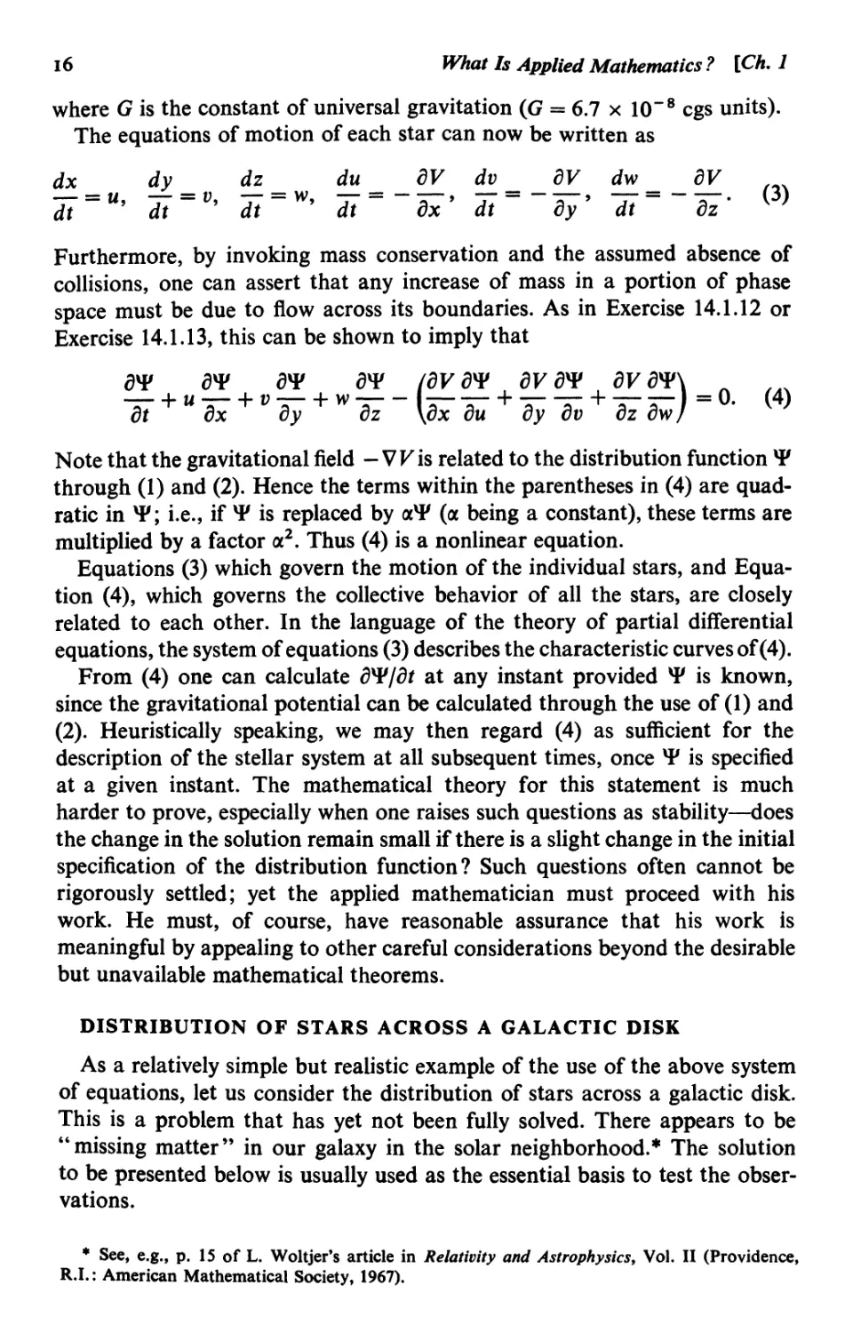
16	What Is Applied Mathematics? [Ch. 1
where G is the constant of universal gravitation (G = 6.7 x IO""8 cgs units).
The equations of motion of each star can now be written as
dx	dy	dz	_ du _	dV	dv __	dV	dw _	dV
dt~U’	dt	dt W’ dt	dx 9	dt	dy 9	dt	dz *
Furthermore, by invoking mass conservation and the assumed absence of
collisions, one can assert that any increase of mass in a portion of phase
space must be due to flow across its boundaries. As in Exercise 14.1.12 or
Exercise 14.1.13, this can be shown to imply that
ат	ат	ат	ат	/агат	агат	ауат\	л
dt	dx	dy	dz	\ax du	dy dv	dz dw/ 1 7
Note that the gravitational field - VKis related to the distribution function T
through (1) and (2). Hence the terms within the parentheses in (4) are quad-
ratic in T; i.e., if T is replaced by aT (a being a constant), these terms are
multiplied by a factor a2. Thus (4) is a nonlinear equation.
Equations (3) which govern the motion of the individual stars, and Equa-
tion (4), which governs the collective behavior of all the stars, are closely
related to each other. In the language of the theory of partial differential
equations, the system of equations (3) describes the characteristic curves of (4).
From (4) one can calculate ST/dt at any instant provided T is known,
since the gravitational potential can be calculated through the use of (1) and
(2). Heuristically speaking, we may then regard (4) as sufficient for the
description of the stellar system at all subsequent times, once T is specified
at a given instant. The mathematical theory for this statement is much
harder to prove, especially when one raises such questions as stability—does
the change in the solution remain small if there is a slight change in the initial
specification of the distribution function? Such questions often cannot be
rigorously settled; yet the applied mathematician must proceed with his
work. He must, of course, have reasonable assurance that his work is
meaningful by appealing to other careful considerations beyond the desirable
but unavailable mathematical theorems.
DISTRIBUTION OF STARS ACROSS A GALACTIC DISK
As a relatively simple but realistic example of the use of the above system
of equations, let us consider the distribution of stars across a galactic disk.
This is a problem that has yet not been fully solved. There appears to be
“missing matter” in our galaxy in the solar neighborhood.* The solution
to be presented below is usually used as the essential basis to test the obser-
vations.
* See, e.g., p. 15 of L. Woltjer’s article in Relativity and Astrophysics, Vol. II (Providence,
R.I.: American Mathematical Society, 1967).
Sec. 1.2] Introduction to the Analysis of Galactic Structure	17
The galactic disk is 10 kpc ( = 104 pc) in radius but only 600 pc in thickness.
Thus, to a good approximation, we should be able to consider the galaxy to
vary locally only in the direction perpendicular to the disk. We shall take this
to be the direction of the z axis with z = 0 at the center of the disk. Then, in
the stationary state, T = V^z, w) and (4) becomes
54х dV ат л
w--------------= 0.
dz dz dw
(5a)
It can be shown (Section 16.1) that the potential V(z) satisfies the Poisson
differential equation
d2V
—2 = 4nGp(z).
oz
(5b)
Our considerations now focus on a definite mathematical problem, that
posed by (5a) and (5b). (Certain additional requirements on the solution
will also be invoked later.) We shall treat these equations in two steps.
Equation (5a) can be solved by the standard method of Lagrange for
integrating partial differential equations of the first order. Let us briefly recall
the salient features of this method.
For a partial differential equation of the form
ач	ат
P(z, w, T) -—F Q(z, w, T) — = R(z, w, T),
dz	dw
(6a)
(6b)
Lagrange’s method of characteristics is based on the characteristic equations
dz dw JT
P “ Q ” R
Let/i(*, w, T) = Ci and/2(z, w, T) = c2 be solutions of any two independent
ordinary differential equations implied by (6b). (Here and c2 are constants.)
Then /j and f2 can be shown to define functions T that satisfy (6a). Thus
fi and/2 provide constants or integrals of the phenomenon described by (6a).
The intersections of the surfaces = cl9f2 = c2 give the characteristic curves.*
The general solution to (6a) is given by
ЛЛ,Л) = о.
In the present case, R = 0, so that one integral relation is T = ct [which
obviously provides a solution of (5a)]. A second characteristic equation is
dz dw
w	— dV/dz9
(7)
A slight extension of these remarks shows that (3) gives the characteristics of (4), as stated
aoove.
i8
What Is Applied Mathematics? [Ch. 1
which leads at once to the integral
+ V(z) = £,	(8)
where £ is a constant, that gives the total energy per unit mass of the star.
Thus the general solution of (5a) is
^=/(^=/[1^ + ^)].	(9)
A special case of (9) is compatible with the observed Gaussian distribution
of velocities. We take
f(E) = Aoe~fiE,	(10)
where Ao and 0 are suitable constants. The constant 0 is prescribed by the
distribution of velocities. Furthermore, by the one-dimensional version of (1),
Ao must be related to the local density by
4dw.	(11)
Indeed, we find the density distribution to be of the form
p(z) = poe-™	(12)
P = j
where p0 is the density where K(z) = 0, which we shall take to be at z = 0,
the middle of the galactic plane.* The quantity p0 is related to Ao and 0 by
(13)
The observational determination of p0 is based on (12), which follows
from (5a), without the use of the Poisson equation (5b). From (12) one can
determine K(z), and hence its second derivative, as
d2F	1 d2
dz2	0 dz2 П \p0/ ’
(14)
One can determine 0 from the distribution of stellar velocities, by using
(10), and one can observe the number of stars per unit volume, which is
proportional to p. Evaluation of the expression in (14) is then possible.
Furthermore, this can be done for any species of stars.f Thus we have the
possibility of determining the total stellar mass by combining (14) with (5b).
As mentioned before, existing knowledge reveals a considerable descrepancy.
The mass determined by this dynamical procedure is about 1.7 times larger
than that obtained by direct observational determination.
* A potential is defined only up to an additive constant, since just its gradient is significant.
t From observations of their spectral lines, stars are classified into a number of different
species. These species basically correspond to stars of different properties such as mass, composi-
tion, and age.
Sec. 1-2] Introduction to the Analysis of Galactic Structure
19
Equation (5b) has yet to be satisfied. Thus, to complete the analysis, one
must solve the equation
d2V
d-^^^Gpoe-^\	(15)
dz
To do this, multiply both sides by dVjdz and integrate, with the specification
that
dV
V = — = 0 atz = 0,	(16)
dz
since the gravitational force also vanishes at the middle of the galactic plane.
Then (Exercise 1) there is little difficulty in showing that the distribution of
density finally takes on the form
— = sech2—,	(17)
Po	zo
where z0 is given by
z2=(27iGPoj?)-1.	(18)
What have we gained from our theoretical analysis? Of most importance
is the discrepancy between theory and observation concerning the value of p0.
A naive person might think that this discrepancy proves our analysis to be of
little worth, but just the opposite is true. Rough agreement between experi-
ment and a plausible theory could be largely a coincidence, but disagreement
means that there is more to the phenomenon than meets the eye. The italicized
phrase is doubly relevant here, for there must be some invisible mass present
to account for the excess of the predicted mass compared to that observed.
The two principal conjectures are that the excess mass is due either to mole-
cular hydrogen or to dark stars. The matter has not been resolved at the
time of writing.
DENSITY WAVE THEORY OF GALACTIC SPIRALS
It is beyond the scope of this book to carry out much further analysis of
stellar systems beyond that given above. We shall, however, report here
briefly some recent developments in the theory of galactic spirals, based on
stellar dynamics and gas dynamics, as another example of the power of
mathematical analysis.
The bright spiral arms of galaxies are marked by massive young stars.
These stars are known to be rotating faster in the interior parts of a galaxy
than in the outer parts. If a spiral arm is “ material,” i.e., if it always consists
of the same stars, we must then have what is known as the “ winding dilemma.”
For trailing spiral patterns,* the spiral arms would tend to wind into a
* A spiral pattern is called “ trailing ” if it opens up in the direction behind that of the rotation
of the stars; “leading,” if in the opposite sense. A leading material spiral pattern would loosen
up under the effect of differential rotation.
20
What Is Applied Mathematics ? \Ch. 1
tighter structure. However, the Hubble classification is based not only on the
tightness of winding, but on other physical parameters as well. Furthermore,
these physical parameters cannot change as rapidly as the geometry of a
material spiral arm. Thus we must accept the hypothesis that the spiral
pattern remains quasi-permanent.
In the 1920s the Swedish astronomer Bertil Lindblad suggested that there
are “ density waves ” in the stellar system which underlie the observed spiral
structure. These are periodic temporary concentrations of stars caused by
their self-gravitation. Qualitatively, they are similar to acoustic waves, but
the physical mechanisms involved are different in the two cases. Lindblad
did not carry out any detailed mathematical analysis of the collective behavior
of these stars. He was therefore able to make only general conjectures about
these waves, and some of them were inevitably incorrect. Thus his ideas
remained unaccepted for a long time.
In the 1960s the density wave theory was revived by С. C. Lin and Frank
H. Shu when they succeeded in calculating a spiral structure for the Milky
Way system, in reasonable agreement with observations. The method was
also applied to other galaxies, and a number of other observable consequences
were deduced and checked against astronomical data. (See Figure 1.3.)
For a summary report of the status of the theory, see the general discourses
of B. J. Bok and С. C. Lin at the 14th General Assembly of the International
Astronomical Union.* Suffice it to note here that the theoretical studies of
these density waves offer very challenging mathematical problems. Indeed,
the problems are similar to those encountered in the study of waves in
electromagnetic plasmas. (By analogy, a stellar system may be called a
“ gravitational plasma.”) Thus the understanding of galactic systems requires
extensive mathematical analysis of a rather subtle kind. At the same time,
it stimulates the study of certain mathematical methods and theories that are
applicable to other important problems.
EXERCISES
1. (a) Deduce the relation (17) for the density distribution of stars across
a galactic disk. Sketch.
(b) Obtain the distribution of gravitational potential
K(z) = 4л(7р0 Zq In cosh —.	(19)
zo
(c) Find the gravitational field at “large” distances from the galactic
plane. Discuss what is meant by “large.”
* Published in Highlights of Astronomy, Vol. II (Dordrecht, Holland: D. Reidel Publishing
Company, 1971). For general information on spiral structure, including a description of the
density wave theory, see the article “ Updating Galactic Spiral Structure ” by B. J. Bok in Amer.
Scientist 60, 708-22 (1972).
Sec. 1.2] Introduction to the Analysis of Galactic Structure
Figure 1.3. The same photograph as in the frontispiece with added
curves indicating the location of the peak of synchrotron emission as
observed by D. S. Mathewson, P. C. van der Kruit, and W. N. Brouw.
Coincidence of this curve with the dust lane is strong evidence in favor of
the density wave theory of galactic spirals. Reprinted with permission
from Astron, and Astrophys. 17, 468 (1972).
22
What Is Applied Mathematics ? [Ch. 1
1.3 Aggregation of Slime Mold Amebae
In this section we shall formulate a mathematical model to describe the
aggregation of slime mold amebae. We shall thereby gain some understanding
of a phenomenon of considerable current interest in developmental biology.
{Developmental biology includes embryology, the study of how a single cell
develops into a complicated embryo, but also encompasses the development
of simpler organisms that cannot be said to have an embryo.) We begin with
some facts about slime mold amebae that provide a basis for our mathematical
model.
SOME FACTS ABOUT SLIME MOLD AMEBAE*
One can begin a description of the life cycle of the slime mold amebae at
the spore stage, where each ameba is dormant within a protective covering.
When conditions are favorable, an ameba emerges from its spore. Of the
order of 10 micrometers (10”3 cm) across, the amebae are rather shapeless
one-celled organisms that move by extending contractile portions of them-
selves (pseudopods).
The natural habitat of the amebae is soil or dung. An important element
of the food chain on earth, they feed on bacteria by engulfing them. If food
is plentiful, the amebae continually feed and multiply by mitosis (dividing
in two). If the food supply becomes exhausted there is an interphase period of
random and somewhat feeble movement, where the amebae are more or less
evenly distributed over the area available to them. During this period, the
disappearance of the food supply triggers certain changes in the amebae.
The details of these internal changes are not known, but there is no difficulty
in observing the striking external phenomenon that results. After a few hours,
the amebae begin to aggregate into a number of collection points. Typically,!
these are more or less regularly distributed, with a spacing of a few hundred
micrometers. (See the frontispiece. Figure 1.4 gives an idea of what the be-
ginnings of aggregation look like under conditions of lower cell density.)
After aggregation has been completed, the amebae that have collected at a
given point (ranging in numbers from a few in laboratory experiments, up to
200,000) form a multicelled slug. This moves as a unit, although the formerly
free living amebae retain their cell walls within the slug. Then the slug stops
and erects a stalk, on top of which is a roundish container of spores. The
cycle is thus completed.
♦ “There is no philosophy which is not founded upon knowledge of the phenomena, but to get
any profit from this knowledge it is absolutely necessary to be a mathematician.”—Daniel
Bernoulli. Quoted by C. Truesdell on p. 318 of Essays in the History of Mechanics (New York:
Springer, 1968).
t There are several species of cellular slime mold, with various corresponding differences in
behavior. [See J. T. Bonner, The Cellular Slime Molds (Princeton, N. J.: Princeton U.P., 1967).]
Our description is appropriate for the most studied species, Dictyostelium discoideum.
Sec. 1.3] Aggregation of Slime Mold Amebae
23
Figure 1.4. Population of amebae just beginning to aggregate. The
scale is indicated by a 100-micrometer line segment. (Courtesy of
B. Shaffer.)
What is responsible for the organized aggregation of the amebae? This is
an important question, for “purposeful” movements occur frequently in
developmental processes. Usually, these movements take place rather
inaccessibly within a developing organism, but the cells of the slime mold
amebae will obligingly perform in a laboratory dish so that it is easy to
examine them and to experiment with them.
It has been discovered that the amebae move preferentially toward rela-
tively high concentrations of a chemical which they themselves secrete. In
some species the attractant has recently been identified as cyclic 3',5'-adenosine
monophosphate (AMP) a chemical with many important biological functions.
(E. W. Sutherland was awarded the Nobel Prize for medicine in 1971 for his
work in elucidating some of the roles of cyclic AMP.) It is also known that a
given quantity of attractant loses its potency in a matter of minutes. This has
been traced to the activity of an enzyirie that alters the nature of the AMP.
Presumably, aggregation is caused by the fact that the amebae move up a
gradient of attractant, but what determines the time of onset? What deter-
mines the spacing of aggregation centers? Can one quantify the process?
A mathematical model is needed to answer such questions. We shall proceed
to devise the simplest model that could reasonably be supposed to bear on
24	What Is Applied Mathematics ? [Ch. 1
the circumstances.* If analysis of this model is encouraging, one can add
detail later. For this, the reader is referred to the paper just cited and to
subsequent papers by various authors in the same journal.
FORMULATION OF A MATHEMATICAL MODEL
Since the distance between amebae is small compared to the typical
distance between aggregation centers, we shall employ a continuum model.
Suppose that the aggregation takes place in the (x, y) plane. For simplicity
we shall assume that no quantities Change with y, so that only x variation
need be considered. Exercise 3 shows that this assumption of unidimension-
ality is not at all essential, but it makes exposition easier.
Let a(x, t) denote the number of amebae per unit area at position x and
time t. Consider the amebae located in the region x0 < x < x0 + Ax, where
Ax is an arbitrary number (not necessarily small). We shall now write a
general balance law for this region; this states that the rate of change of the
net amount of a in the region equals the rate at which a flows across the
boundary, plus the net rate of creation of a within the region. In the present
case, a stands for amebae, and the net creation of amebae is equal to the
excess of births over deaths. But the balance law is “general” because it
applies to any substance whatever. For how else can a substance appear in
the region except by creation or by flow across its boundaries?
To proceed, we must define the flux density J(x1? t). This gives the net
rate per unit length at which a crosses the line x = xP Also, J is defined to be
positive if there are more amebae crossing in the direction of x increasing
than in the opposite direction. The term Q(x, t) is the net rate per unit area
at which a is being created. The desired balance law can now be written.
Considering the rectangle of Figure 1.5, we obtain
Q -xo + Ax	-xo+Ax ,
— a(x, 0 dx = J(x0, t) - J(x0 + Ax, t) + Q(x, t) dx. (1)
JXQ	JXQ
It is convenient to use the integral mean value theorem (Appendix 13.2) to
write
о
— [^(xp t) Ax] = J(x0, t) - J(x0 + Ax, t) + Q(x2 , t) Ax;
x0 < Xi < x0 + Ax, x0 < x2 < x0 + Ax. (2)
We divide by Ax and then take the limit as Ax -► 0, to obtain the general
balance law in differential equation form,
da z	dJ
(*o > 0 = “ 7^ (*o , 0 + Q(*o > 0, *o arbitrary. (3)
♦ We adapt material in a paper by E. F. Keller and L. A. Segel, Л Theoret. Biol. 26, 399-415
(1970).
Sec. 1.3} Aggregation of Slime Mold Amebae
25
1
Ax
_L_
*0
x0 + Ax
Figure 1.5. The balance law (3) considers the rate of change of mass
in a rectangle of length Дх and unit width, in the case where у variation
is absent.
In the case of the amebae, reproduction can be ignored because there is
little or none of it in the absence of food. Deaths can also be ignored, since
there are few during the time interval of interest. Thus we take
e^O.	(4)
To obtain an expression for the flux J, let us first consider a situation when
attractant is absent. Then the amebae appear to move about randomly.
Owing to such “ diffusionlike ” movement, a concentration of amebae tends
to disperse. Thus there is a random flux Jr from regions of high ameba
concentration to regions of low concentration. The magnitude of the flux at x
seems to depend on the concentration difference between x and nearby points.
We characterize this difference by dafdx (the simplest choice) and make the
hypothesis that
L ox J
(5)
for some function F. Now when a = constant, J — 0—for in random motion
there will be as many amebae moving to the left as to the right. In this case
dajdx s 0. Therefore, given (5), it is only sensible to assume that
F(0) = 0.
(6)
Thus the graph of F must have an appearance such as that depicted in
Figure 1.6. For sufficiently small values of s, we can approximate the graph
by a straight line. Calling the slope of the line —д, we obtain F(s) = —дл as
the simplest reasonable assumption concerning F; i.e.,
_. ч 3a(x, t)
P)
2б
What Is Applied Mathematics ? [Ch. 1
Figure 1.6. Possible plot of the function F defined in (5). The graph
provides negative values for s>Q because there should be a leftward
{negative) flux if amebae density is higher at larger values of x. Similar
reasoning explains the positivity for s < 0.
Combining (3), (4), and (7), we obtain
да _ d / da\
St dx \ dx) *
(8)
Equation (8) is the diffusion equation, which will be studied at length
beginning in Chapter 3. This equation is used to model the concentration
variation of any kind of randomly moving set of particles, for example smoke
particles in air (see Chapter 3). The constant p, which governs the vigor of
the random movement, is generally called the diffusivity. Here we call p the
motility, giving precise meaning to a biological term that is often used only in
a qualitative manner.
Equation (8) was obtained under the assumption that no attractant was
present. To account for chemotaxis, which is directional motion induced by
variations in chemical concentration, we add to Jr of (7) an additional
contribution Jc. Let p(x, t) be the density of the attractant. Arguing as
before, we pass from an initial assumption that Jc is a function of the attract-
ant gradient dp/dx to the assumption that Jc is proportional to the attractant
gradient, at least for small values of the gradient. For a given gradient, if
the amebae density is twice as great, the net flux should be twice as great.
The proportionality factor should thus be a multiple of a. We are led to the
hypothesis that
г dp
(9>
Sec. 1»3] Aggregation of Slime Mold Amebae
The factor % measures the strength of chemotaxis. Note that in contrast to (7),
there is no negative sign in (9). This is because amebae tend to move toward
attractant concentrations (and away from ameba concentrations).
Assuming that the total flux J in (3) is the sum of the random contribution
J and the chemotactic contribution Jc, we are led to our final equation for
the change in ameba density:
We shall take p, and / to be positive constants. It is not difficult to take into
account a variation with p which is probably present, but this would only
change some details of the analysis to come [Exercise 2(a)]. Note that even
with constant p and %, (10) contains a (quadratic) nonlinear term /a(dp/dx),
because this term is proportional to the product of two unknown functions,
a and dpjdx. [Such a quadratic nonlinearity was also found in our study of
galactic structure—compare the remarks following Equation (2.4.)] Nonlinear
terms generally make mathematical analysis more difficult, and hence more
challenging and more rewarding.
We also need an equation for the attractant density p. This will be of the
general form (3):
dt dx
(The subscript “ a ” refers to attractant.) The random motion of the attractant
molecules will be modeled by a proportionality of flux to gradient, as in (7):
The net creation term 0a has a positive contribution fa as a result of the
secretion of attractant by the amebae. Here f is the rate of secretion per unit
amebae density. What of the decay in attractant activity? We take the rate
of decay (as in radioactivity or some other spontaneous process) to be
proportional to the amount of attractant present,* via the constant k.
Thus QA =fa — kp, and the desired equation for dpjdt is
(H)
We shall take /, k. and D to be positive constants.
♦ As we stated above, decay is actually due to the action of an enzyme. If Michaelis-Menten
kinetics (Chapter 10) are assumed, this can be modeled by making к a certain function of p.
But the essentials of the analysis are unchanged [Exercise 2(b)].
28
What Is Applied Mathematics ? [Ch, 1
Partial differential equations (10) and (11), for the two unknown functions
a(x, t) and p(x, f), provide the basic formulation of our problem.
AN EXACT SOLUTION: THE UNIFORM STATE
It is very easy to find an exact solution of (10) and (11). This is the uniform
solution,
u = a0, P = PO,	(12)
where aQ and p0 are constants. [When (12) holds, the system is said to be in
the uniform state.] Upon substitution into (10) and (11), we find that (12) will
indeed provide a solution if
/u0 = fcp0-	(13)
Equation (13) is physically reasonable. It says that in the uniform state the
secretion rate of attractant must be exactly balanced by the decay rate.
ANALYSIS OF AGGREGATION ONSET AS AN INSTABILITY
We identify the uniform state with the interphase period prior to aggre-
gation. We also model the onset of aggregation as the breakdown of the
uniform state due to the growth of inevitable small 'disturbances to ameba and
attractant density. That is, we identify the onset of aggregation with the sort
of instability of the uniform state whose investigation forms a classical part of
applied mathematics (see Sections 11.1 and 15.2). The instability is presumed
to occur because of changes, during interphase, of the parameters д, /, and f
that characterize ameba behavior.
The idea behind instability theory is this. Suppose that at some initial time,
the state of the system is slightly disturbed from the uniform state. (Suppose
that there is a local clumping of amebae, for example, and an accompanying
local concentration of attractant.) Will the small disturbance tend to disappear
with the passage of time or will it become more intense? In the former case
we say that the uniform state is stable to small disturbances, in the latter
unstable. Unstable states will not be observed, for disturbances are inevitable.
In the case of instability, they will grow, so the uniform state will be replaced
by some other state.
To perform a stability analysis, we introduce the variables a' and p' by the
definitions
a(x, 0 = a0 + <*'(x, t), p(x, t) = pQ + p'(x, t).	(14)
Here a' = a — a0, for example, measures departure from uniformity; there-
fore, it can be identified with the disturbance in ameba density.
To obtain equations for a' and p', we substitute (14) into (10) and (11).
From the former we obtain
да' д2а' Г d2p' da'dp']	z._4
dt “M^-z[(ao + a)for + arRr (15)
Sec. 1-3] Aggregation of Slime Mold Amebae
29
This equation is nonlinear, owing to the presence of the quadratic terms
я'(32р75х2) and (da'ldx)(dp'ldx). We shall assume that the disturbances
(and their derivatives) are small, in which case we call a' and pf perturbations.
The perturbations are involved quadratically in some terms and linearly in
others. Products of two small terms should be negligible in comparison with
the other terms of (15), which contain but a single perturbation function.
We thus linearize the equation by deleting all nonlinear terms. We obtain
da' d2a' d2p'
~8t=li~dxT~Xao'dxT
(16)
as the linearized version of (10). As for (11), upon substituting (14) and em-
ploying (13), we obtain
dp'	d2p'
±=fa'-kp' + D-£,	(17)
which is already linear.
We are faced with a pair of linear partial differential equations with
constant coefficients. We guess that there are solutions of the form
a' — Cj sin qx eot, p' = C2 sin qx efft,	(18)
where C\ and C2 are constants.* It is easily seen [Exercise 1(a)] that there are
indeed solutions of the form (18), provided that
(<r + W2)Cj - xao<H2C2 = °’	(19a)
-fCt +(a + k + Dq2)C2 = 0.	(19b)
This system of algebraic equations has the trivial solution Cj = C2 = 0.
[From (18) we see that we have merely verified that it is possible to have an
identically zero perturbation of an exact solution.] For a nontrivial solution,
the determinant of the coefficients must vanish. We thus obtain the following
quadratic equation for a:
a2 + bo 4- c = 0; b = к 4- (д 4- D)q29 c = pq2(k 4- Dq2) - xaQfq2.
(20)
The quadratic equation can be shown to have real roots [Exercise 1(b)].
To ensure stability, both roots must be negative, so that the exponential
factor exp {at) brings about decay of the perturbations. It is not difficult to
show (Exercise 1) that a necessary and sufficient condition for stability is
c > 0, which requires that
Х^о/ <	+ Tty2), <1 # 0.	(21)
* The reasons that lie behind such an assumption as (18) are more fully discussed in Section
15.2. We mention here that a cosine dependence in (18) will yield exactly the same results. (Com-
pare Exercise 3.) Also, more general disturbances can be obtained by the superposition of sinu-
soidal solutions, using Fourier analysis (as discussed in Chapters 4 and 5).
30
What Is Applied Mathematics ? \Ch. 1
From (18), 2n/q is the wavelength of the perturbation under investigation.
Since д and к are positive, the right side of (21) decreases monotonically as q
decreases, toward a greatest lower bound of pk. Therefore, the longer the
wavelength 2n/q, the more “dangerous” the perturbation [for (21) is more
easily violated]. We conclude that instability is possible whenever
(22)
pk
for then (21) is violated for a range of sufficiently small values of q\
INTERPRETATION OF THE ANALYSIS
The view of aggregation that emerges is this. During the beginning of the
interphase period, inequality (22) does not hold and the uniform state is stable.
Triggered by the stimulus of starvation, the various parameters gradually
change. Eventually, (22) is satisfied, and aggregation commences. We identify
the size of the “aggregation territory” with the instability wavelength; our
analysis predicts that the territory size is “ very large ” in some sense.
The instability criterion (22) has the following interpretation. Suppose
that there is a concentration of amebae and attractant at some point. Random
“diffusion” of amebae with motility p tends to disperse this concentration,
as does the attractant decay, whose strength is measured by k. Larger p and к
means larger stabilizing effects. It is therefore appropriate that increases in
p and к mean that the instability criterion (22) is more difficult to satisfy.
By contrast, a local concentration of attractant tends to draw amebae
toward it by chemotaxis (strength /). Also, a concentration of amebae will
provide a corresponding increase of attractant concentration because of the
higher local concentration of secretion sources. The strength of this effect is
measured by aof. This explains the appearance of the destabilizing factors
aof and x in the numerator of (22). Instability ensues if destabilizing effects
outweigh stabilizing.
The explanation of aggregation provided in the previous paragraph could
perhaps have been provided without doing a mathematical analysis. But, as
is typical, only after carrying through some calculations does one seem able
to discern the physical essence of a situation. Also, the criterion (22) is a
quantitative one, capable of experimental test. No full quantitative tests have
been performed as yet, but it has been discovered that both the chemotactic
sensitivity % and the attractant secretion rate f go up by about 100-fold at the
time aggregation commences. As illustrated in our discussion of galactic
structure, future quantitative tests might reveal defects in understanding that
would never emerge from qualitative considerations.
The above analysis is based on a paper (op. cit.) that appeared in 1970
in the Journal of Theoretical Biology. Since that time, several other papers
on slime mold aggregation, by various authors, have appeared in that journal
and elsewhere. They deal with such matters as (i) a more accurate modeling of
Appendix 1.1] Some Views on Applied Mathematics	31
the chemical kinetics and hence (among other things) a possible refinement of
the “ very large territory size ” prediction mentioned above; (ii) the streaming
type of aggregation, as in the frontispiece; and (iii) the influence of pulsatile
attractant secretion and refractory periods. Future work will doubtless
examine the effects of nonlinearity. Two survey articles on slime mold aggrega-
tion and other collective chemotactic motions, written for a mathematical
audience, can be found in Some Mathematical Questions in Biology, Vol. Ill
(Providence, R.I.: American Mathematical Society, 1972).
EXERCISES
1.	(a) Verify (19).
(b)	Show that the roots of the quadratic equation (20) are real.
(c)	Show that both roots are negative if and only if both b and c are
positive.
(d)	Show that since/, D, and x are positive, if c > 0, then b > 0. Thereby
deduce (21).
2.	Investigate the changes in the analysis that would occur under the follow-
ing conditions.
(a)	If p and x were functions of p.
(b)	If к and f were functions of p.
3.	If two-dimensional variation is considered, the governing equations (10)
and (11) are replaced by
77 = V • (AiVa - %aVp), =fa - kp + DV2p.
ot	ot
Assume disturbances with spatial dependence sin (q^x + q2y + 0), where
ft, q2, and в are constants. Show that if q2 = q2 + q2, then 2n/q remains
the disturbance period and the instability condition remains (22).
4.	Define A by xanfll& = 1 + A and suppose that A is small and positive.
[Compare (22).] Ignoring higher order terms in A, find an approximation
for the larger root of the quadratic. Deduce that the wavelength of the
fastest growing disturbance is approximately 2n(2D/kA)1/2.
Appendix 1.1 Some Views on Applied Mathematics
ON THE NATURE OF APPLIED MATHEMATICS
I . . . describe applied mathematics as the bridge connecting pure mathematics
with science and technology. I have deliberately described this bridge as connecting
two areas of activity rather than leading from one to the other, because the bridge
carries two-way traffic. Its importance to science and technology is obvious, but it
is not less important to pure mathematics, which would be poorer without the
stimuli coming from the applications.
W. Prager, “Introductory Remarks” in the special issue, “Sympo-
sium on the Future of Applied Mathematics,” Quart, Appl, Math, 30,
1-9 (1972).
32
What Is Applied Mathematics ? [Ch. 1
One should not judge applied mathematicians by their contribution to mathe-
matics any more than one judges historians by their contributions to history.
Much creative effort goes into interpretation. To try to use mathematical ideas on
problems which at first sight seem too complex or obscurely stated to fit any pattern
is, for many people, an exciting challenge and it is this which I feel to be the essence
of applied mathematics.
R. W. Brockett, “The Synthesis of Dynamical Systems,” ibid., pp.
41-50.
Here then are three topics on computation—algorithmic complexity, operating
system modeling, and data structuring—which could use much heavier mathematical
participation than they now receive. Their requirements are far from the kind of
approximative analysis that has been so successful in the physical sciences. But they
will be large areas of endeavor with many people engaged in their engineering
development and in their use—larger than most of the uses of mathematics we now
have. I think we shall have to broaden our idea of what applied mathematics is to
include these subjects.
H. Cohen, “ Mathematical Applications, Computation, and Complex-
ity,” ibid., pp. 109-121.
I feel that * applied mathematics ’ should be defined * dynamically ’ and operation-
ally as the process—and the study of the process—of application of mathematics to
the other disciplines. 'Applied Mathematics’ is what 'applied mathematicians’ do,
while ' applied mathematicians ’ are people who go out and talk to those in other
disciplines who are attempting to use mathematics, and who know enough about
the discipline itself to understand the problems on a deeper level.
P. Herman, “ Comments on the COSRIMS Report,” Amer. Math.
Monthly, 517-21 (May 1970).
ON THE RELATIONSHIPS AMONG PURE MATHEMATICS,
APPLIED MATHEMATICS, AND THEORETICAL SCIENCE
I think that it is a relatively good approximation to truth—which is much too
complicated to allow anything but approximations—that mathematical ideas
originate in empirics .... But, once they are so conceived, the subject begins to live
a peculiar life of its own and is better compared to a creative one, governed by
almost entirely aesthetical motivations .... As a mathematical discipline travels far
from its empirical source [however].... there is a grave danger that the subject will
develop along the line of least resistance, that the stream, so far from its source,
will separate into a multitude of insignificant branches, and that the discipline will
become a disorganized mass of details and complexities.
John von Neumann, “The Mathematician,” reprinted in the World
of Mathematics (New York: Simon & Schuster, 1956), p. 2063.
‘Applied Mathematics’ is an insult, directed by those who consider themselves
‘pure’ mathematicians, at those whom they take for impure. Mathematics is,
always has been, and always will be pure mathematics. The adjective ‘pure’ is
redundant. The very essence of mathematics is abstraction, created by fancy and
tempered by rigor, but ‘pure mathematics’ as a parricide tantrum denying growth
Appendix 1.1} Some Views on Applied Mathematics	33
from human sensation, as a shibboleth to cast out the impure, is a disease invented
in the last century ....
C. Truesdell, “The Modem Spirit in Applied Mathematics,” 1CSU
Rev. World Sci. 6, 195-205 (1964).
The miracle of the appropriateness of the language of mathematics for the formu-
lation of the laws of physics is a wonderful gift which we neither understand nor
deserve. We should be grateful for it, and hope that it will remain valid in future
research and that it will extend, for better or for worse, to our pleasure even though
perhaps also to our bafflement, to wide branches of learning.
E. P. Wigner, “The Unreasonable Effectiveness of Mathematics
in the Natural Sciences,” Commun. Pure Appl. Math. 13,1-14 (1960).
ON THE TEACHING AND PRACTICE OF APPLIED
MATHEMATICS
It has always been a temptation for mathematicians to present the crystallized
product of their thoughts as a deductive general theory and to relegate the individual
mathematical phenomenon into the role of an example. The reader who submits to
the dogmatic form will be easily indoctrinated. Enlightenment, however, must come
from an understanding of motives: live mathematical development springs from
specific natural problems which can be easily understood, but whose solutions are
difficult and demand new methods of more general significance.
R. Courant, Remarks from the preface of Dirichlet's Principle
(New York: Wiley-Interscience, 1950).
There was complete unanimity on the point that presently mathematics majors
do not learn enough about applications .... There was also agreement that every
mathematician should become acquainted with at least one area of application.
Joint Report of the Committee on Graduate and Postdoctoral
Education and of the Committee on Undergraduate Education,
1970-71 Annual Report, Division of Mathematical Sciences, National
Research Council, p. 78.
The world is becoming more and more complicated. We are rapidly approaching
an unbearable and even dangerous situation .... Mathematics is the only subject
broad enough to prevent this. Not the mathematics actually taught but a new
mathematics inspired by all fields of applications. It must be taught as fundamental
science which provides indispensable modes of thinking and tools to cope with the
real world: the physical world, and the man-made world.
A. Engel, “ The Relevance of Modem Fields of Applied Mathematics
for Mathematical Education,” Educ. Studies Math. 2,257-69 (1969).
In mathematics courses the talk is usually about problems. Not much is said
about where the problems come from or about what is done with the answers.
It seems to us that this missing part of the story is worth telling. It is particularly
important to those who intend to be mathematicians, since it explains why the
electronic computer is not going to put them on the unemployment rolls. It is also
important to those who are going into the mathematically oriented sciences, since
34
What Is Applied Mathematics ? [Ch. 1
it explains why the electronic computer is not going to remove their privilege
(or duty, as it may be regarded) of learning a great deal of mathematics.
R. Hooke and D. Shaffer, Math and Aftermath (New York: Walker
and Co., 1965), p. 4.
I think we need some discipline as mathematicians trying to get into applied
fields. The discipline you need is to be able to turn off the mathematics as soon as
you’ve discovered what the really relevant physical phenomena are that go on, and
then go on for the new physical phenomena.
Remarks by H. B. Keller, “Symposium on Mathematical Pro-
fessional Societies and Their Present Role,” reported on pp. 50-51 of
the 1970-71 Annual Report, Division of Mathematical Sciences,
National Research Council.
Rigor that just polishes the mathematical surface, but does not penetrate essen-
tials of the subject matter in question, is not indispensable in applications.
U. Grenander, “Computational Probability and Statistics,” SIAM
Rev. 15, 134-91 (1973).
Too much of the attitude of many young mathematicians is that of always finding
out what is wrong with what is being said [by scientists] rather than what is right;
and I think one of the important things in the game of applied mathematics is to try
to understand a bit of what is right.
E. W. Montroll, “ Education in Applied Mathematics ” (Proceedings
of a conference sponsored by SIAM), SIAM Rev. 9, 326 (1967).
To a large extent, the community of core mathematicians has decided that it is
not its responsibility to provide instruction related to the application of mathematics;
to the same large extent, much of the instruction in methodology has become the
responsibility of the applied mathematics community. The important question is:
Will this community include in the instruction it offers illustrations of the heuristic,
inventive, reasoning so necessary to progress in science, in technology, and ultimately
in our whole society or will it retreat into a cloistered preoccupation with abstrac-
tions both in its research and its instruction? If it does retreat, then the present
generation and possibly a few future generations of students will receive little
instruction of this sort and those that enter the worlds of technology, of science,
of environmental repair and of medical advancement, will do so severely handicapped
by a grotesquely distorted education.
Our symposium is labeled ‘The future of applied mathematics.’ It is my view
that if, in answer to the foregoing questions, we make the latter choice, applied
mathematics has no viable future whatever—it could only become a small, rather
sterile corner of mathematics, a discipline which despite its moments of greatness,
already is populous enough to contain more sterility than it wants. But if we make
the former choice, i.e., if among all of its other activities, the applied mathematics
community provides innovative contributions to the mathematization of disciplines
which are just becoming quantitative, if it concerns itself with finding approximate
models for complicated phenomena (thereby sacrificing accuracy of detail for ease
of interpretability), if it seeks to develop techniques whereby the implications of
Appendix 1.1} Some Views on Applied Mathematics	35
given mathematical models can more easily be inferred, then applied mathematicians
will have inherited much of today’s continuation of the challenges, the intellectual
achievements, the contributions to society, and the fun which, before they abdicated,
was largely the property of the mathematicians and the physicists.
G. F. Carrier, “Heuristic Reasoning in Applied Mathematics,” in
the special issue, “Symposium on the Future of Applied Mathe-
matics,” Quart. Appl. Math. 30, 11-15 (1972).
Chapter 2
Deterministic Systems and Ordinary
Differential Equations
In this chapter we shall illustrate something of the range of applied mathe-
matics using particle dynamics as our central example. The principal purpose
of our discussion will be to analyze the process of applied mathematics.
We are not primarily interested at this point in enlarging the reader’s facility,
so a thorough exposition of certain methods will be deferred.
We first examine the relation between Kepler’s laws, which describe the
motion of the planets, and Newton’s formulation of the theoretical law of
universal gravitation. The orbits of planets and comets are deduced by the
rather ingenious classical solution of the governing equations. When
relativistic effects are considered, however, attempting to find an exact
solution no longer is an optimal procedure. A perturbation method should
be used. The same method is called for when one wishes to calculate the rela-
tively small effect of other planets upon a given planet’s orbit about the sun.
As an illustration of practical calculational procedures that have been
devised to fill a definite need, we discuss perturbation theory in a certain
amount of detail. Roughly speaking, this theory permits one to calculate
the effects of small disturbances on otherwise known situations. Remarkably
valuable information can be obtained by sophisticated variants of perturba-
tion theory—one cannot expect its content to be summarized in a few pages.
Thus our discussion is a foretaste of what is to come in the remainder of
this volume.
Particle dynamics is an example of a deterministic process wherein the
future is completely determined, given sufficient knowledge of the present.
Whether the outcome of such processes is to be calculated in detail or just
contemplated philosophically, certain purely mathematical questions arise.
We conclude this chapter by stating and proving some relevant theorems.
These involve existence, uniqueness, and continuous dependence on a
parameter of systems of ordinary differential equations.
2.1 Planetary Orbits
People of all eras have been moved by the grandeur and the beauty of
Nature when watching stars in the darkness of night. As they made careful
observations, they discovered that some of the “stars” are wanderers—the
planets (TtAav^nys = wanderer in Greek). Indeed, records of planetary paths
formed one of the earliest important collections of scientific data.
36
Sec. 2.1] Planetary Orbits
37
In the first comprehensive history of China “Shihchi” {Records of the
Grand Historian of China), written about the second century b.c., there is
one volume devoted to celestial observations. Five planets were recognized,
and it was known that the period of Jupiter is almost exactly 12 years. This
is a special case of Bode's law*
In the West, accurate observations of planetary motions were made by
Copernicus (1473-1543), Tycho Brahe (1546-1601), and Galileo (1564-1642).
The great amount of observational data collected by Tycho Brahe formed
the basis of the famous laws of Kepler (1571-1630). These laws then led
Newton (1642-1727) to the discovery of the law of universal gravitation,
with the help of the then newly invented differential calculus. The study of
these developments provides an excellent classical case study of applied
mathematics.
KEPLER’S LAWS
In their original form, Kepler’s laws may be stated as follows:
I.	The planets describe ellipses about the sun as a focus.
II.	The areas swept over by the radius vector drawn from the sun to a
planet in equal times are equal.
III.	The squares of the times of describing the orbits (periods) are propor-
tional to the cubes of the major axes.f
To accomplish a mathematical formulation, we adopt a polar coordinate
system (r, 0) with the sun as the origin. We treat all the planets and even the
sun itself as mass points. (Note that this is an approximation or idealization
in the formulation. It is appropriate because the radius of the sun is small
compared to the distance between the sun and a given planet.) The second
law of Kepler then states that, following the orbit (r(t), 0(t)) of a planet,
r20 = h9 ha constant,	(1)
* The radii of the planets of the Sun are fairly accurately given by the formula 0.4 4-0.3 X 2я
in astronomical units. The values of n are — oo, 0, 1, 2,... 7, 8 for Mercury, Venus, Earth, Mars,
minor planets, etc. Neptune and Pluto do not follow this law accurately. This fact probably
implies that Pluto was originally a satellite of Neptune.
t “ Newton later wrote: ‘ Kepler knew ye Orb to be not circular but oval, and guessed it to be
Elliptical.’ This is correct, but Kepler’s guess was no idle guess; it came out of a hunch actively
pursued, in confrontation with all previous theories and with Tycho’s new data.”
This quotation is from an interesting account by Curtis Wilson, in the March 1972 Scientific
American (Vol. 227, p. 92), of how Kepler discovered the first two of his laws. Wilson’s summary
of his findings includes these further remarks.
“ At the root of all his [Kepler’s] theorizing, however, was that initial sense of the significance
of the inverse relation between velocity and distance—an anticipatory glimmer of what would
one day be the law of the conservation of angular momentum. It was in the light of that hunch
that he was guided through 900 pages of calculation to a planetary theory better than any that
had been proposed before .... What was . . . important through all the accident and luck was
Kepler’s belief in the possibility of understanding, his devotion to his task that carried him through
four years of reasoning and calculation, and finally, the rightness of his initial hunch and his
ability to disentangle the confused state of things before him in the light of it.”
38	Deterministic Systems and Ordinary Differential Equations [Ch.2
since [Exercise 1(a)] h is twice the area swept over by the radius vector in
unit time. (It is appropriate to use the notation • for d/dt, as introduced by
Newton.) To obtain a useful simple interpretation of this result, we introduce
the cartesian coordinates (x, y). Then (1) can be written as
xy — ух = Л,	(2)
which yields, upon differentiation with respect to /,
xy — yx = 0.	(3)
If we define vectors r and s by
r = xi 4- yj, s = -yi 4- xj,	(4)
then г • s = 0, so s is perpendicular to the position vector r. But according to
(3), f • s = 0 so that f is in the direction of r. That is, if the “equal areas"
result holds, then the acceleration of the planet is always directed toward the
sun (or away from it). Reversal of the steps in our reasoning shows that the
converse of this result is also true.
The lesson to be learned here is that the interpretation of mathematical
results may depend very much on the form in which they are stated. The
equivalent equations (1) and (3) enable us to see quite different aspects of
the same phenomenon, with completely different interpretation and insight.
Note the importance of manipulative skill.
The first law of Kepler states that the orbit can be described by the simple
formula
where p > 0 and 0 < e < 1. This is a standard form of an equation for the
ellipse whose semimajor axis is given by p/(l — e2). With a little manipulation
[Exercise 2(a)], one can show that the acceleration in the radial direction is
h2
ar = r-r62^ ~—2.	(6)
Thus the acceleration is inversely proportional to the square of the radial
distance. Note that nothing has been said about the forces between the
celestial objects. [A statement, such as (6), which describes the geometric
character of motion, or which follows from this character, is said to be
kinematical.]
The quantities h and p are characteristics of the individual planets. It is
by the use of the third law of Kepler that one can show that the ratio h2/p
is the same for all the planets [Exercise 2(b)]. Thus, for planetary motion,
where К is a universal constant.
Sec. 2.1} Planetary Orbits
39
law of universal gravitation
The laws of Kepler have led us to the inverse square law for the accelera-
tion of all the planets, with the same constant of proportionality. Newton,
by combining the above results with his second law of motion and assuming
the principle of superposition (i.e., that the effect of two suns is double that
of a single one), was led to formulate the present form of the law of universal
gravitation,
„ GMm
Рг=—^-.
r2
(8)
Here Ff is the magnitude of the force acting between two point masses of
amounts M and m separated by a distance r; G is a universal constant. The
force is attractive.
The simple elegance of the mathematical manipulations is striking, especi-
ally when one compares the theory with the tedious observations. But can
this powerful law be dreamed up without these observations? The answer is
obviously no. Neither can the required calculations be made without the
use of the then newly invented discipline of calculus.
The law of universal gravitation is indeed one of the most remarkable
of the laws of nature. Why is it universal ? Why is the power exactly equal to 2 ?
Even more remarkable is that, according to the general theory of relativity,
such an elegant principle can be replaced by another, which has even more
penetration and breadth and is at least equally elegant, if not more so. It
hardly seems frivolous to say that God is a mathematician!
On the working level, we observe that in order to arrive at our conclusions
it is necessary to keep the physical interpretation of the results in mind all the
time and to be quite skillful with the manipulations.
There is another lesson to be learned from the history of the law of universal
gravitation, giving further evidence of the need for adequate notation and
of proficiency with analytical manipulations. Newton tried to test his law by
applying it to the motion of the moon about the earth and comparing the
moon’s acceleration with that of a body at the surface of the earth, as directly
observed. This comparison cannot be made without knowing the gravitational
potential of a continuous distribution of matter over a sphere. It is now well
known that the gravitational attraction due to such a distribution of mass is
equivalent to that due to a concentrated mass at the center. Newton was at
first not able to prove this and consequently delayed his publication of the
comparison for about 20 years.
THE INVERSE PROBLEM: ORBITS OF PLANETS AND COMETS
We start now with Newton’s law (8) or the kinematical law (6), and ask
how the planets would move. We find that (i) we have to be able to solve
differential equations to provide a satisfactory answer, and (ii) not all the
40
Deterministic Systems and Ordinary Differential Equations [Ch, 2
orbits are ellipses. Some orbits are hyperbolas and others are parabolas—
and nature has provided these examples in the cometary orbits. The solution
of the relevant differential equations, as we shall now see, requires consider-
able skill in manipulation.
The formulation of the mathematical problem consists of asking for
periodic orbits for the following system of two differential equations of the
second order:
dt2 \dt) r2
(9a)
1 d / 2 dO\ л
--|r—I = 0.
rdt\ dt
(9b)
where the expressions on the left-hand side are the components of accelera-
tion (ar, ae) in the polar coordinate system. To follow the motion of the
planets, one has to integrate (9) for the pair of functions r(t), 0(t). There
seems to be no direct way to accomplish this analytically. (Numerical integra-
tion methods can be applied, but understanding and insight would tend to
be lost.) The ingenious way out of the difficulty is to look for the orbit in the
form r = r(ff). Even here, as we shall see below, a clever transformation is
needed to solve the resultant differential equation.
Equation (9b) can be integrated once to yield r2d ~ h, h a constant. (The
quantity r26 is called a constant or integral of the motion.) Thus the law of
uniform area (1) is recovered. We can now use (1) to replace the time deriva-
tives in (9a) with differentiation with respect to the angular variable в. The
resultant equation is still very complicated, but it can be simplified by intro-
ducing the variable
и = r'1.
With this we obtain
d2u GM
<№ + u~ h2 ‘
(10)
The general solution of (10) is [Exercise 3(b)]
и = /T2GM[1 + e cos (0 - 0O)],	(11)
where e and 0O are constants of integration.
The solution (11) is periodic in 0, but not all the orbits are periodic. When
e < 1, (11) yields the observed elliptical orbits. But when e> 1, и may
vanish for some value of 0, and the planet would then be infinitely far away;
the orbits are hyperbolas. Parabolic orbits are obtained in the marginal case
e = 1. The integration constant 0O is unimportant as it merely assigns the
value 0O to an axis of symmetry.
Sec. 2.1} Planetary Orbits
41
PLANETARY ORBITS ACCORDING TO THE GENERAL THEORY
OF RELATIVITY
When modification of Newtonian mechanics is considered in the light of
the general theory of relativity, it can be shown that equation (10) for the
planetary orbit is changed to the form
d2u GM Z1 .
(12)
where £ is a small parameter (and where the influence of the other planets
still has not been taken into account). The integration of this equation is
more difficult, since it is nonlinear in u. However, it can still be done in terms
of elliptic functions. To obtain the solution in a more convenient form, the
problem should be treated by “perturbation theory,” which is based on
the fact that the solution of a differential equation depends continuously
on a parameter that enters continuously in the differential equation. (We
shall soon discuss these matters further.) In the present case, when e = 0,
the solution is known. Because of the continuous dependence of и upon £,
the solution for small £ can be obtained by an appropriate small modification
of the solution for £ = 0.
The result obtained by the use of the perturbation theory shows that the
orbit is still very close to an ellipse, but there is an advance of the perihelion
(nearest point to sun) by the amount 2nea2 over one period. (A method for
obtaining this result is given in Section 2.2.) The observation of this advance
yields one of the principal experimental tests of the general theory of
relativity.*
COMMENTS ON CHOICE OF METHODS
The advance of the perihelion can also be established by detailed numerical
integration, or by examination of the solution of (12) in terms of elliptic
functions. However, neither method gives the results in as transparent a
form as perturbation theory, which is also extremely accurate in this case.
In other instances, analysis of a well-formulated problem with the aid of
modern computing machines can often yield more accurate numerical
results than those obtained by the use of approximate analytical methods.
It is, however, often difficult to extract useful general information from a
large amount of numerical data unless one has already gained insight into
the problem through general analytical studies. On the other hand, exploratory
* Equation (12) has been derived by K. Schwarzschild. The present situation on the relativistic
Perihelion advance with regard to the comparison of experiment with theory is as follows. For
Mercury, where the effect is largest (43 seconds of arc in a century) observations are in accord
with Einstein’s theory. But some controversy remains, for there is a possible flattening of the
sun that could perhaps leave room for alternatives to Einstein’s theory. See K. Nordtvedt,
‘Gravitation Theory: Empirical Status from Solar System Experiments,” Science 178, 1157-1164
(1972).
42	Deterministic Systems and Ordinary Differential Equations [Ch. 2
numerical studies sometimes are an invaluable preliminary to successful
analytical work. The judicious balance in the use of all types of methods is
indeed most important.
N PARTICLES: A DETERMINISTIC SYSTEM
Consider now a system of N particles in gravitational interaction; e.g.,
the solar system comprising the sun and the nine major planets. Let us denote
the position vector and the velocity vector of the particle a by ra and va,
respectively (a = 1, 2, ..., N). Then the equation governing the motion of
the ath particle is
wara = Fa, a = l,2,...,N,	(13)
where
F. = I Fe, ;	(14)
P*a
i.e., the resultant force acting on the ath particle is due to the contribution
of all the other particles. We have, according to Newton’s law,
f«, = -	(r‘ ~ = -*'•>	(15)
lra“r/H
which depends only on the positional coordinates of the particles. In other
physical situations, there may be an external force field and the forces may
also depend on the velocities of the particles (e.g., when the particles are
electrically charged and there is a prevailing magnetic field). But, in general,
there are no true forces dependent on the acceleration of the particle.
Thus we have
Fa = Fa(t, r^, vy); a,/?,y = l,2,...,N.	(16)
In this most general case, we may still write the equations of motion (13)
as a system of differential equations of the first order*.
mt^ = Fa(t,rfi,vy), ^ = ^', a,fi,y = l,2,...,N. (17a, b)
We have 6N variables (ra, va); a = 1, ..., N. We expect that the subsequent
behavior of the system would be determined if we were given the instantaneous
positions and velocities of all the particles at any instant. Mathematically,
this means that (17) should have a well-defined solution if it is solved under
the conditions
ra = r<0), va = v<0) at/ = t0; a = 1,2, ...,N.	(18)
These conditions are called initial conditions, and the problem we have just
posed is called an initial value problem for a system of ordinary differential
equations.
Sec. 2.1} Planetary Orbits	43
That the initial value problem has a unique solution can in fact be proved,
as we shall see in Section 2.3. This proof has wide ranging consequences,
for it has led some philosophers to a deterministic view of the universe. For
what can be the place of “free will,” it can be argued, if the evolution of the
cosmos can be uniquely determined by examining the configuration at any
arbitrary instant?*
But nowadays existence and uniqueness theory is also important from a
practical (rather than philosophical) point of view. The advent of computing
machines has made it desirable to ensure that a problem is precisely formu-
lated before expensive calculations are attempted. At least at the present
stage of development of computers, one cannot expect the machine to detect
difficulties in the original formulation and then to suggest suitable modifica-
tions. In practice, trial-and-error approaches are often used, for it has certainly
not been possible to prove all the required theorems. But experienced opinion
is superior to guesswork, and the ability to exercise sound judgments in the
absence of rigorous guidelines is perhaps one of the most valuable assets of
an applied mathematician from the practical standpoint.
LINEARITY
To make sure that an important concept is understood, we close this
section with a brief review of linearity. The concept will be illustrated in
connection with systems of differential equations.
If f(x) = ax + b, a and b constants, the graph of у = /(x) is a straight
line. For this reason, f is called a linear function. When b = 0, the function
is called homogeneous; otherwise, it is inhomogeneous.
The linear homogeneous function (often just called linear) has strikingly
simple properties. If L(x) = ax, then
L(xr 4- x2) = L(xx) 4- Цх2), Цсх^ = c£(xx);	(19a, b)
or, equivalently,
£(qxt 4- c2x2) = qL(xx) 4- c2L(x2),	(20)
Here q and c2 are any constants; xx and x2 are arbitrary values of x.
Let x(r) be an n-element column vector (n by 1 matrix) that depends on
the scalar t. Define a vector-valued function L(x) by
L(x) = ^ - A • x,	(21)
at
where the derivative is (as usual) taken component by component, and where
A = A(r) is an n by n matrix that multiplies x. Note that A does not depend
on x.
* Needless to say, we are only scratching the surface of the philosophical position, and we
shall not pursue the matter further.
44	Deterministic Systems and Ordinary Differential Equations [Ch. 2
The function L also possesses the linearity properties. For if x and у are
any (differentiable) vector functions and a is a scalar (usually a real number),
then
L(x + y) = L(x) + L(y), L(ax) = aL(x). (22а, b)
We also have the analogue of (20), which treats of what is called the linear
combination ax + fty of x and у (where /? is another scalar):
L(ax +/?y) = aL(x) +/?L(y).	(23)
The reader has probably met some of the many consequences of the very
important linearity properties (22) or (23). It is relevant here to give an
example involving systems of ordinary differential equations. Using the
definition (21),
L(x) = 0
is a linear (homogeneous) system of first order differential equations. Property
(22a) implies that the sum of two solutions is a solution for
L(x) = 0, L(y) = 0,
implies
L(x + y) == L(x) + L(y) == 0.	(24)
Property (22b) implies that the scalar multiple of a solution is a solution, for
L(x) = 0 implies that L(ax) = aL(x) = 0.	(25)
Similarly, a linear combination of two solutions {or of many solutions) is a
solution.
EXERCISES
1.	(a) Equation (1) is often derived in elementary treatments of polar
coordinates. If the derivation is unfamiliar to you, work it out for
yourself.
(b)	Verify (2).
(c)	Show that (1) follows from (3).
2.	(a) Verify (6).
(b) Prove (7).
3.	(a) Verify (10).
(b) Derive (11).
4.	In the text’s theoretical discussion of Kepler’s laws, the sun and the
planets were treated as mass points. Write a brief essay that provides
justification for such a treatment.
5.	(a) Verify (22) and (23) when L is defined by (21).
(b)	Prove in general that (22) holds if and only if (23) holds.
(c)	Prove that a linear combination of solutions to a linear system of
equations such as (21) is also a solution.
Sec. 2.2] Elements of Perturbation Theory
45
6.	Eliminate 0 from the equations of (9) to obtain a differential equation
for radial motion. Integrate to derive Kepler’s representation of radial
motion:
r = a(l — e cos E), n(t — Г) = E — e sin E.
Here a is the semimajor axis of the ellipse, e is the eccentricity, n is the
frequency of the orbit, T is the time of perihelion passage, and E (called
the eccentric anomaly) is a parameter that runs over the range (0, 2л)
for a complete orbit. (The position angle 0 is known as the true anomaly;
the quantity M = E — e sin E, which varies linearly in time, is known as
the mean anomaly.)
To do this, first obtain the energy equation in the form
/dr\2 _ 2 a2e2 - (r - a)2
\Л/ r2a2(l — e2)
by noting that the radial velocity is zero at the perihelion and aphelion
(the points which are nearest and farthest from the sun, respectively).
2.2 Elements of Perturbation Theory, Including Poincare’s
Method for Periodic Orbits
At the beginning of this chapter we considered a single planet moving
around a fixed sun. The subsequent discussion of A-particle interactions re-
minds us that our earlier considerations neglected the interaction among the
planets.* We can build on our previous work by “ approximating ” the force
Fa on the ath planet by a basic force field F<0) (due to the sun), and regard-
ing the effect of the other planets as “ small perturbations.” To formalize this
process, we can replace the right-hand side of (1.13) or (1.17a) by
Fa(2) = F<°> + 2[Fe - F<°>]
and allow the parameter Л to vary in the interval (0, l).f The effect of the
perturbation is then obtained by comparing the solutions for 2 = 0 and
= 1, respectively.
In practice, determination of the effect of small perturbations on the
motion of planets involves special difficulties. This is because the perturbation
effects accumulate over many periods of time, yet we do not expect the shape
of an individual orbit to be greatly changed. The difficulty was overcome by
Poincare, whose ideas will be discussed briefly after a presentation of the
theory in the ordinary form.
* Also neglected was the solar motion, whose effect can be studied only by introducing another
set of dependent variables.
t Although not necessary, it is instructive to imagine that as Л varies continuously from 0 to 1,
the solar system varies from one with but a single planet, through intermediate systems with
other planets of small mass, to the actual system of which we are a part.
46
Deterministic Systems and Ordinary Differential Equations [Ch, 2
PERTURBATION THEORY: ELEMENTARY CONSIDERATIONS
To clarify the ideas just discussed, let us consider the simplest example
of a single ordinary differential equation
4^ = f(x, у, e)	(1)
dx
to be solved under the initial conditions
У = y0 when x = x0.	(2)
We wish to examine the dependence of the solution y(x, e) on the parameter s
that occurs in (1).
Suppose that the solution y(x9 s) is known for e = 0.* Assume that y(x9 e)
can be expanded into a Taylor series in 8, when the latter is sufficiently small
in magnitude:
y(x, e) = j>(0)(x, 0) + 8j(1)(x, 0) + • • • + eny(n)(x9 0) + • • •.	(3)
1 / d ”v\
/>fc0).-M)	.	(4)
И. \u8 / £ = o
If we now substitute (3) into (1) and regard the equation as an identity in 8,
we shall find that we can obtain a sequence of linear differential equations
in j(n). For example, disregarding all terms of order 82 or higher, we have
+ e + • • • = /(x,/0) + ey(1) + • • •, e)
dx dx
—f(x, y(0\ 0) + efy(x, y(0\ 0)/n + efe(x, ym, 0) + • • •,
where we have used Taylor’s theorem to expand f. Equating equal powers
of 8, we find
Jv(0)
-L_ = /(x,/°>,0),	(5a)
dx
dv(i)
= fy(x, y<°\ 0)У1 > + fe(x, y{0\ 0), etc.	(5b)
The solution for (5a) has been presumed to be known. Upon substitution
of this solution into (5b), one obtains a definite equation for the correction
/и
The initial conditions to be imposed on the successive correction terms are
J(1)(x0,0) = 0, /2>(x0,0) = 0,..., yM(x0,0) = 0,	(6)
since the original condition (2) does not depend on 8.
* This entails no loss of generality. If the solution is known for e — £0, define a new parameter
ё = £ — £0.
Sec. 2.2] Elements of Perturbation Theory
47
Note that (5b) can be explicitly solved in terms of quadratures under the
appropriate initial condition of (6). Indeed, calculations will show that all
the terms y(n)(x, 0) satisfy an equation of the form
dv^
-1— = Ay™ + B(n\ n = 1, 2,...,	(7)
dx
where A is /y(x, y(0), 0) for all и, and В(л) depends on x and all the y(k)’s
preceding у(л). Thus, once y(0) is found, the problem of obtaining the higher
approximations is relatively simple in principle, since explicit solution of
(7) is possible in terms of quadratures.
A simplifying feature of this type will be found in all other cases of the
perturbation method, including those involving partial differential equations.
Example 1. The solution of the differential equation
dy
dTi+y2>	<8>
subject to the initial condition
У(0) = 0,	(9)
is
у = /°> = tan x.	(10)
Find a first approximation to the solution, subject to the same initial condition, of
dy
£ = l+(l + e)y\	(11)
ax
when |e[ <1. Compare with the exact solution.
Outline of solution. The exact solution to the perturbed problem is
Xx, £) = (1 + €)"1/2 tan [(1 + e)1/2x].
A Taylor series expansion of this solution in powers of e gives
y(x, e) = tan x 4- e(4x sec2 x — I tan x) + • • •.
Forgetting the exact solution for the moment, we assume that
y(x, e) = y(0)(x) 4- ey(1)(x) 4- • • *.
On substitution into (11), we find
rfy<0)	dy(iy
^_ + £^4_...=1+(1+ £)[(X<»)* + 2£/oy ° +•••],
ax	dx
so that
dv(1)
= (>,(0))2 + 2X°>(1).
48	Deterministic Systems and Ordinary Differential Equations [Ch. 2
[It is frequently the case, as here, that direct substitution provides the desired
perturbation equations more easily than substitution into a general formula such as
(5b).] Rearranging the differential equation for y(1) into standard form and using
the fact that y(0)(x) = tan x, we obtain
—— 2y(1) tan x = tan2 x.	(12)
This equation has an integrating factor of
exp (—2 J tan x dx) = cos2 x.
Indeed, (12) can be written
It is now easily seen that the solution for y(1) is precisely as given above.
The reader should fill in the details of the above calculation (Exercise 2).
Hopefully, a good idea of how straightforward perturbation calculations
are accomplished has already emerged. But detailed “training” and further
discussion is provided in Chapter 7.
THE SIMPLE PENDULUM
Theoreticians often find it helpful to consider the operation of an idealized
device that displays interesting properties in a readily visualized form. One
such device is the spring-mass-dashpot system. As most readers will have
seen, in the simplest instance this system is governed by a second order
ordinary differential equation with constant coefficients; it therefore provides
a concrete illustration of the properties of that ubiquitous equation. Here,
for the first of several times in this book, we shall consider another example
of such an idealized device, the simple pendulum. In the present context,
consideration of the pendulum will provide an illustration (i) of the fact that
perturbation theory is often used implicitly wh$m we formulate simplified
physical models, and (ii) of the large cumulative effect of small perturbations
and the method Poincare devised to describe this effect. The same effect
as that of (ii), and the same calculational method but in a less transparent
form, are relevant to planetary orbits.
A standard discussion in elementary physics texts is a reduction of the pen-
dulum problem to that of simple harmonic motion when the amplitude is
small, and we vaguely feel we can improve the approximation when needed.
The discussion deals with a simple pendulum as an idealized object which, by
definition, consists of a rigid, straight, weightless rod of fixed length L, with
point mass m at one end. The rod is free to rotate about a horizontal axis
at the point of suspension.
Sec. 2.2] Elements of Perturbation Theory
49
Fig ure 2.1. Forces on a simple pendulum of mass m are represented by
the dark arrows. Magnitudes of the forces are indicated. The tension T
in the string is equal to mg cos 0. The unbalanced tangential force of
magnitude mg sin 0 causes acceleration of the bob.
The italicized words above represent the idealizations involved in the
formulation of the model. Estimation of the error introduced by these idealiza-
tions might be very difficult. (For example, if the rod is slightly elastic it
becomes capable of undergoing torsional, longitudinal, and bending vibra-
tions.) But we shall consider an approximation whose consequences can
be more easily analyzed. Denote by 0(t) the inclination of the rod to the
vertical at time t. If s(t) denotes the distance the bob has moved from the
vertical in a counterclockwise direction, then OL = s. Equating m(d2sldt2) to
the force component which is tangential to the path of the bob, we obtain
the following equation of motion:
mL§ = — mg sin в.	(13)
Here g is the acceleration due to gravity. The tension along the string does
not enter, because it acts normally to the path of the bob. (See Figure 2.1.)
The equation of motion may also be written in the following slightly
different form:
/^\1/2
0 4- cdq sin в = 0 for t > 0, where co0 =1-1
(14)
50	Deterministic Systems and Ordinary Differential Equations [Ch. 2
To obtain a definite solution, we may impose the initial conditions
0 = a, 0 = Q at t = 0.	(15)
Equations (14) and (15) comprise the formulation of our mathematical
problem.
SUCCESSIVE APPROXIMATIONS TO THE MOTION OF THE
PENDULUM
In the usual treatment of the problem, the approximation sin в « 0 is
introduced. Then (14) becomes
0 +co2 0 = 0,	(16)
whose solution [subject to condition (15)] is given by
Q
0O = a cos o)Q t H-sin cd0 t.	(17)
An obvious inference from the solution is that, irrespective of the initial
conditions, the motion is periodic with the period
/>0 = — = 2л/~у/2.	(18)
"о \9J
This approximate solution is not adequate, however, if we are interested
in following the motion of the mass point over many periods, for the period
given by (18) is not exactly right. According to the “exact” equation (14),
the motion is indeed periodic, but the correct period is
2 r*/2
P = P0 - \ (1 — k2 sin2 ^) 1/2 d^	(19)
7Г Jo
where k2 — sin2 (0m/2) and 0m is the amplitude of the oscillation [i.e., the
maximum value of 16(t) | ]:
0wEmax 10(t) |.	(20)
t
With every swing of the pendulum, the approximate solution misestimates
the time of maximum amplitude by a further increment of P — Po. [The
error in period is about 0.2 per cent for an amplitude 0m = 10° = л/18 radians
(Exercise 4).] Thus the solution to the approximate equation (16) can be
expected to be nearly the same as the solution to (14) only for a number of
periods N such that N(P — PQ) is small compared to P.
To improve on the approximation, one might write (14) in the form
6 + col в = (Oq(6 — sin 0)	(21)
Sec. 2.2] Elements of Perturbation Theory	51
and then obtain a reasonably accurate value of the right-hand side of (21)
by using the first approximation 0O of (17), writing 0 — sin 0 « 0O “ sin #o •
This is justified by the argument that the right-hand side of (21), namely,
(дЗ д5 \	дЗ
&~в + 3!~5!+) =W°3!-	’
is of the order of 03, while the left-hand side is of the order of 0. Thus the
smaller right-hand side can be ignored altogether to obtain an initial approxi-
mation 0o(O- A better approximation should be obtained if the substitution
0 = 0O is made on the right side, etc. Thus the first attempt at an improved
approximation, 0x(t), might be expected to satisfy
0t + mJ 0i = mj(0o - sin 0O);	0X(O) = a, 0X(O) = O. (23a, b, c)
But to make an exact evaluation of the right side of (23a) with the rough
approximation 0O gives rise to a problem that is needlessly difficult to solve.
As one might suspect, no accuracy is lost if one makes the approximation
indicated in (22) and therewith replaces (23) by
03
+	0t(O) = a, ^(0) = П.	(24)
In principle, repetition of the process will provide successively more
accurate approximations. Hence the method is known as iteration (Latin
iterare, to do again), or successive approximations.
Problem (24) also arises in another approach to the improvement of the
basic approximation 0O, to be discussed now. We therefore defer considera-
tion of the solution to (24).
note. Chapter 7 contains a more thorough treatment of the method
of iteration.
PERTURBATION SERIES APPLIED TO THE PENDULUM
PROBLEM
In a perturbation series approach, it is convenient to introduce a new
variable,

(25)
where 0m is the maximum amplitude defined in (20). Intuitively, 0W seems
to provide a natural standard of comparison for the angular displacement.
The new variable 0 satisfies |0| < 1, and this proves useful in estimating
the size of various terms. Considerable further justification for this type of
variable change is given in Section 6.3.
With (25), the governing equation (21) becomes
03
ё + cog О = cog(0 - em 1 sin 0m 0) = cog 0% — + • • •.	(26)
О
52	Deterministic Systems and Ordinary Differential Equations [Ch. 2
We note that since |0| < 1, the right-hand side of (26) is of the order* of
0* , a quantity that we assume to be very small compared to unity.
For simplicity, let us consider the case where the pendulum is released from
rest (Q = 0). It is physically clear that 0m — a, so that our problem becomes
Й + <»o 0 = a>o(® — a “1 sin a&)
oo	02n+l
=	г,.	(27а)
n=l	{Zn + 1)!
0(0) = 1,	6(0) = 0.	(27b, c)
To find a solution of (27), we write
© = 0(r, a) = 0(O)(t) + a0(1)(O + a20(2)(O + • • •	(28)
and substitute it into (27a) to obtain an infinite sequence of equations, in
the spirit of our earlier discussion of perturbation theory. The initial conditions
for the various approximations are
0(O)(O)= 1, 6(O)(0) = 0;	(29a)
0<")(O) = 0, 6(я)(0) = 0, for n > 1.	(29b)
In this formulation, the dependence of the solution on the amplitude a is
explicitly demonstrated. Note that if all the higher powers of the amplitude
a are neglected, we have the usual simple harmonic motion.
To ensure that our method works, we might wish to satisfy ourselves
that the series (28) converges. But this turns out to be an incorrect stipulation,
for it is neither necessary nor sufficient. Even when such a series is divergent,
it can still be useful as an asymptotic series (see Chapter 3). On the other hand,
convergence does not assure its usefulness. An inordinately large number
of terms might have to be summed to obtain reasonable accuracy.
As a matter of fact, it can be shown that the series (28) is in general con-
vergent in any finite interval 0 < t < T, provided that a is sufficiently small.f
However, this does not assure us of the usefulness of the solution for many
periods. One way to see this is actually to carry out the calculations^ which
show that
0(°>(O = cos <d0 /,	0(1)(O = 0.	(30)
* “ Of the order of,” roughly speaking, means “ about the same size as,” but it is useful to
give a precise meaning to “order” in this sense. See Appendix 3.1.
t This can be inferred from the analytic dependence of the right-hand side of (27a) on the
complex variable a. This general theory is beyond the scope of the present discussion. See
Coddington and Levinson (1955).
§ Some readers may have fully grasped the idea of straightforward perturbation theory from
the single example that has been worked out. They can attempt to verify (30), (31), and (33) by
themselves. Other readers may prefer, either now or later, to peruse Section 7.1, where the required
calculations are carried out in detail.
Sec. 2.2} Elements of Perturbation Theory	53
Thus ®(2) satisfies
®(2)+ o>o ®<2) = "7^ cos3 co0 t.	(31)
6
Using a trigonometric identity, we can rewrite (31) as
«(2)	_ (2) CO?
0 + a>o ® = 24 (COS + 3 cos wo 0-	(32)
This is a nonhomogeneous linear equation with constant coefficients. The
right-hand side is of the simple type that invites the use of the method of
undetermined coefficients. The presence of the “ resonant ” cos (co0 t) term
leads us to anticipate a contribution to the solution with a factor of t. And
indeed, the solution of (32) and the initial conditions (29b) turns out to be
®(2)(0 = tH cos % * “ fir cos 3coo* + I sin t. (33)
Noteworthy in (33) is the term proportional to cos 3co0 t. This appearance
of more rapidly oscillating “higher harmonics” is a typical nonlinear
phenomenon.
But the term proportional to t sin coo t holds the center of our interest.
Alone among the contributions to the correction term a2®(2), this term is
not uniformly small for all time. Rather, for long times t « (Dq la~2 we must
contemplate a secular* term which, far from being a small correction, has
become of the same size as 0(O). When this happens, the whole basis of the
approximation is invalidated. Thus the approximation 0(O) 4- a20(2) is an
improvement over 0(O) only for the time interval that 0(O) itself offers a
reasonable approximation (Exercise 5). We have not yet penetrated to the
core of the problem.
POINCARE’S PERTURBATION THEORY
The failure of the unmodified perturbation method occurs in all cases of
periodic motions. In connection with the study of the perturbation of plane-
tary orbits, Poincaref developed a modified perturbation theory to overcome
the difficulty. The key to his theory is the introduction of a parametric
representation that recognizes the change of period indicated by (19).
This permits the removal of any secular term that might arise in the calcula-
tions.
The Poincare representation of the solution 0(7, a) is
0 = 0<O)(t) 4- а0(1)(т) 4- а20(2)(т) 4- • • •,	(34a)
t = т 4- af(l)(r) 4- a2t(2)(r) 4- • • •,	(34b)
* Saeculum means “generation” or “age” in Latin; hence the word “secular” applies to
processes of slow change.
t Poincare (1854-1912) was one of the world’s leading mathematicians around the turn of
the century.
54	Deterministic Systems and Ordinary Differential Equations [Ch, 2
where т is a parameter. The idea is to let the solution ®(0)(t) take on the
simple form (34a) in the variable t, but to distort the time scale so that the
defects in the solution are removed. We expect to eliminate all secular terms
and to get the correct period (19) to a good approximation. The calculation
is fairly complicated but can be simplified by noting that the series (34) should
really be in a2. It also turns out that one may take all the correction terms
to be a constant multiple of t, thus
t = t(1 + a2h2 + •• •), h2 a constant.	(35)
The equation for ®(2) is then found (Exercise 6) to be
d20(2)	,	d2&(Q) cog
 ---3- + cog ®(2) - 2h2	" = -7 (cos Зсо0т + 3 cos coot), (36)
ат	d'r 24
or, using (30),
d2®(2) 2лГП 2z1	.	cog
-—5- + cog ®(J = cog(| - 2h2) cos coo т + — cos 3coot.
ат	24
As in (33), the cos coo т term on the right side would lead to an undesirable
secular term proportional to т sin coot. But now we can avoid this by taking
h2 = й.	(37)
The period in т is thus 2л/соо to this approximation, but is (2л/соо)(1 + а2Л2)
in t. This should be compared with (19).
The reader can better appreciate the need to change the time scale by
obtaining the pendulum period using exact integration (Exercise 9). A more
interesting example involves the advance of the perihelion of Mercury’s
orbit (Exercise 10). The reader may find it easier to do Exercise 10 after
having carefully studied the detailed discussion in Section 7.1 of perturbation
theory for the simple pendulum.
GENERALIZATION OF THE POINCARE METHOD
The solution of specific problems is only a prelude to understanding—a
means to an end. In particular, the lessons learned from attacking a specific
problem can often be formulated in terms of general principles and developed
into general theory in order to deepen our understanding. But this cannot
always be done in a formal manner. The Poincare theory is a case in point.
The success of the parametric representation introduced by Poincare has
led to its application to other types of ordinary differential equations, for
the removal of a variety of difficulties of a similar nature. Basically, there is
a need to shift the solution surface by a mapping or distortion in the domain
of the independent variables. But it is not fruitful to try to classify all
the problems that can be solved by this approach.
We have not mentioned any theorems that rigorously justify the use of
the Poincare method. Such theorems are, in fact, available in a number of
Sec. 2.2} Elements of Perturbation Theory
55
instances. Nevertheless, many situations in which the value of the Poincare
approach can scarcely be doubted are not subsumed under present rigorous
treatments. One reason why final formalization of valuable ideas in the form
of theorems is often impracticable is that theorems of desirable generality
are very difficult to prove. A more subtle reason is that a listing of definitive
theorems seems to close a subject, whereas an applied mathematician is
always struggling to open new areas of application by suitable modification
and generalization of known results.
EXERCISES
1.	Demonstrate the validity of (7).
2.	Fill in the details of the solution to Example 1.
3.	Prove the validity of (19). Begin by multiplying (14) by &.
4.	Demonstrate the correctness of the statement under (20) concerning
the error in period. Assume that Q = 0.
5.	Consider the time interval in which a2®(2\ as given in (33), is a small
correction to 0(O). Show that this interval is essentially the same as
the number of periods N mentioned under (20).
6.	Carry the Poincare method through the derivation of (36). [The principal
result (37) then follows at once.]
7.	Show that the more general assumption (34b) reduces to (35) when the
Poincare method is carried through.
8.	A grandfather’s clock is to be designed. It is to be 5 feet long and to have
a maximum swing of | foot at the tip of the pendulum. Show that the
linear approximation for the period T = 2n(L/g)l/2 is not good enough
[H. O. Pollack, Educ. Stud. Math. 2, 393-404 (1969)]. To do this,
derive and use the inequality
(a2 — 02)a~1 sin a < 2 cos 0 — 2 cos a < (a2 — 02)^1 — | sin2
and apply it to a form of the integral giving the exact period. Obtain
1 — cos a T — To / a \1/2
---------<--------^<1------1 -1,
12 To \sin a/
where T is the exact period and a is the maximum angular displacement.
Hint: Use the fact that (sin x)/x has a local maximum at x = 0 to show
that
fa .	, sin a ra	. .	n
sin x dx >----- x dx, x < a < -.
a	11	2
Also show that
. Лх\2 • 2 a
1 — cos x > 21 -1 sin -.
\a/	2
Integrate from 0 to x and then from 0 to a.
56	Deterministic Systems and Ordinary Differential Equations [СЛ. 2
9. Show that a first integral of
d20	, . n л
-r-т + ci)q sin t) = 0
dt2
is
1 /d0\2	2	,/ . ,a . 2 0\
- I— I = a>o(cos 0 — cos a) = 2ci>ol sin - — sin -I,
where a is the maximum amplitude. Verify that a further transformation
0	a
sin - = sin - sin ф
2	2
brings the solution of the problem into the form
t = — I (1 - sin2 ^)“1/2 d^\
w0 Jn/2
WO) = a)
where k2 = sin2 (a/2). Obtain the period of oscillation as a power series
in k2.
10. An experimental test of the general theory of relativity is the advance
of the perihelion of Mercury. According to this theory, the equation
of the orbit is (1.12):
+ и = a(l 4- ew2), a = GMh~2.
аф
This differs from the classical form by the term eu2. In the Newtonian
case (e = 0), the solution is
и = uQ = a[l 4- e cos (ф — ф0)],
where e is the eccentricity and ф0 determines the position of the peri-
helion. Show that the angle between two succeeding perihelions is
2na2e to a first approximation. One method is the following.
If the solution of the relativistic equation is given in the form
и = aQ 4- cos рф 4- a2 cos 2рф 4- • • •
and we assume
p = 1 4- ep(1) 4- e2p<2) + • • •,
ak^a^ + 8a^ + 82a^ + ---9
then
Sec. 2.5] A System of Ordinary Differential Equations
57
2.3 A System of Ordinary Differential Equations
The purpose of this section is to demonstrate the fourth part of applied
mathematics that we listed in Chapter 1: how the desire to solve scientific
problems motivates the development of a mathematical theory, and the
manner in which such theories aid us in the solution of scientific problems.
We shall begin the discussion with a statement of certain theorems related
to the initial value problem for mechanics. The proofs will follow. (As far
as it is feasible, the proofs presented here will be those actually useful for
constructing the solutions.) At the end of the section we shall briefly discuss
the general question of the value of such proofs to the applied mathematician.
THE INITIAL VALUE PROBLEM: STATEMENT OF THEOREMS
For a given (initial) point P0(T, G, G , • • • > G) in the (n + 1)-dimensional
space of the points P(f, z2, .... z„), the initial value problem for a system
of ordinary differential equations
^ = fk(f,zi,z2,...,zn); k = l,2,...,n	(1)
at
is to find functions
zm = ^m(0, m = l,2, ...,n	(2)
such that (1) is satisfied, and
^m(O = Cm at/ = T, m= 1,2, ...,n.	(3)
We now state and subsequently prove certain theorems that are valid
for the initial value problem. In the statement of these theorems and in
subsequent discussions we shall frequently use z and £ to denote collectively
the set of variables (z1? z2, ..., z„) and (G, G, ..., Q.
Theorem 1 (Existence). Suppose that the functions* fk(t, z) are continuous
in a rectangular parallelepiped defined by
R:\t-T\^a9 \zk-£k\<b; к = 1, 2,..., n. (4)
This implies that there exists an upper bound M such that
\fk\^M9	fc=l,2,...,n,	(5)
for P(t, z19 z2,..., zn) in R. Suppose further that each/t satisfies the following
Lipschitz condition in R:
l/(t,z1,...,z„)-/(l,z1,z2,...,za)l < ЛЦЙ! -zx| + ••• + |zB-z„|]. (6)
* Some mathematicians are always careful to distinguish the function f from /(*), the value
of this function at x. We do not find it profitable to emphasize this distinction.
58	Deterministic Systems and Ordinary Differential Equations [Ch. 2
(The Lipschitz condition is implied if each of the functions fk has continuous
partial derivatives.) Then there exists a solution of the initial value problem
in an interval 11 — т | < a, where
a = min la, — I.	(7)
The solution functions [the functions gm of (2)] have continuous first deriva-
tives.
Theorem 2 (Uniqueness). The solution of the initial value problem is
unique.
The significance of Theorem 2 can be appreciated only when we can pro-
duce an example in which there is more than one set of functions satisfying
the same equation and initial conditions, when (of course) the conditions
in Theorem 1 are not all fulfilled. This will be done below.
Next we generalize the initial value problem to
dzv
-J- = z, A), Zk = at t = t.	(8)
dt
Now the right-hand side of the equation depends on the parameter 2.
Theorem 3 (Continuous dependence on parameters). Let the functions
fk(t, z, 2) (k = 1, 2, ..., n) satisfy the requirements prescribed in Theorem 1.
Further let these functions depend continuously on the parameter 2 in a
certain neighborhood 12 — 201 < c, where 20 and c are constants. Then the
solution functions are also continuous functions of 2 in some neighborhood
of 20.
Theorem 3 can be used to prove that the solutions are continuous functions
of the initial values (t, 0. This continuous dependence can be regarded as
demonstrating the stability of the solution with respect to changes in initial
values, in the sense of the following theorem.
Theorem 3' (Stability). Let zm = gm(t; £m) denote the /nth solution func-
tion (2) with the dependence on the initial condition explicitly noted. Then
given any e > 0 and fixed time T, T > t, there exists a 6 = S(e9 T) such that
l&.(G L) - gm{f, Q| < e for т < t < T whenever | - CJ < 6.
Theorem 3 is an expression of our intuitive feeling that when the functions
fk(t, z, 2) are changed slightly (through the parameter 2), the solutions should
also be changed slightly. Our corresponding expectation for the initial
conditions is expressed in Theorem 3'. Let us now look more carefully at
the nature of the dependence on a parameter.
Sec. 2.3] A System of Ordinary Differential Equations
59
We shall take the initial conditions to be fixed and consider the dependence
of the solutions zm = gm(t, 2) on 2. One might expect the nature of this
dependence to be the same as that of the functions /fc(z, z, 2) in (8). Thus, if
the fk are analytic in 2 in the neighborhood of 2 = 20 (i.e., if they have a
convergent Taylor series when 0 < 12 — 201 < r for some r), then the solution
functions gm should have the same property. For linear differential equations,
this is generally true. That is, the solution of the equation*
-j- = A(t, 2)z 4- b(t, 2)
(9)
is analytic in 2, provided that A(t, 2) and b(t, 2) are analytic in 2, even though
they may merely be continuous in t. (Note that the Lipschitz condition is
automatically satisfied for linear equations when the coefficients are con-
tinuous.) In the nonlinear case, the situation is a little more complicated,
as we can see from our experience with the development of a perturbation
solution for (2.1),
T- = Ж y>«)•
dx
In present terms, the formalf calculations there depended on the fact that
the functions fk(t, z, 2) were analytic in z as well as in 2. To keep the dis-
cussion relatively simple, we shall therefore restrict our attention to the
first derivative with respect to 2.
If formal differentiation is justified, we would expect the functions
d
um{t, A) = — zm(t, 2)
(10)
to satisfy the differential equation obtainable formally from the differentiation
with respect to 2 of the original equation (8), remembering that fk and zm
both depend on 2.§ Carrying out this differentiation, we obtain
dt ^tdzm т + дГ
(ii)
We note that (11) is a linear system in {uk} whose coefficient functions are
known functions of t, since the set {zm(t, 2)} is known. If the initial values
are independent of the parameter 2, then the initial ccnditions on the {ut} are
uk = 0.	(12)
* This may be regarded as a single equation or a system of linear equations. In the latter case,
A is a matrix, and z and b are vectors.
t A formal calculation is one that is presumably valid under suitable but unspecified conditions.
§ Successive parametric differentiation of an equation forms the basis of an excellent way to
perform perturbation calculations. See Section 7.2.
6о
Deterministic Systems and Ordinary Differential Equations [Ch. 2
In view of the above discussions, we expect to have
Theorem 4. If the n(n + 1) functions
dfk Sfk
k,m = \,2, ...9n;
dzm дЛ
are continuous in the variables t and {zm} and in the parameter Л, then the
solution functions zm(t9 Л) of Theorem 3 are differentiable with respect to Л,
and the partial derivatives (10) satisfy the differential equations (11) and the
initial conditions (12).
Since generalization is almost immediate, the proofs of all the theorems
stated above will now be presented in the case of a single dependent variable.
PROOF OF THE UNIQUENESS THEOREM
The uniqueness theorem is usually the easiest to prove. In the present
case, the ideas used will also be found to be useful for the proof of the
existence theorem.
We consider the equation
d/ = f(x,y)	(13)
dx
and seek a solution satisfying the initial condition у = y0 when x — xQ. Let
g(x) be one such solution. Then
9\x) =/[x, g(x)],	(14)
and hence
g(x) = y0+ C	(15)
Jxo
If there were another solution G(x) satisfying the same initial conditions,
then
-X	/
<?(*)= Jo + I f[t<G(t)]dt.	(16)
JX0
If we now subtract (15) from (16), we obtain
G(x) - g(x) = Г [/(I, G) -f{t9 £)] dt.	(17)
JXQ
The magnitude of the integral on the right-hand side can be appraised with
the help of the Lipschitz condition:
|/(r, G) -/(r, g)| < G(0 - g(t) |.	(18)
Thus
| G(x) - g(x) | < К Г | G(t) - g(t) | dt.	(19)
JXQ
Sec. 2.3] A System of Ordinary Differential Equations	61
In the interval [x0, x], |G(x) - ff(x) | has a maximum value that we shall
denote by ||G(x) - ^(x)||. It then follows from (19) that
|G(x)-0(x)| <l|G(x)-^(x)|| -X|x-x0|,	(20)
and hence
\\G(x) — g(x)\\ <; \\G(x)-g(x)\\ -X|x-x0|,	(21)
or
[l~X(x-xo)]4|G(x)-^)||^0.
If we now take the length |x — x0| sufficiently small, equal to (2Л)"1 for
example, we can make the first factor positive. Hence (21) requires that
HG(x)-^(x)||=0,
from which the desired result follows at once. 0
PROOF OF THE EXISTENCE THEOREM
We have seen that the solution of the initial value problem for the differential
equation (13) satisfies the integral equation (15). Conversely, if we have a
solution of the integral equation (15), we have a solution for the differential
equation, with the initial conditions implied. This can be verified by direct
calculation (Exercise 1). Thus it is sufficient to prove the existence theorem
for the integral equation.
To prove that (15) has a solution, we adopt the method of successive
approximations. We start with a crude approximation у = y0, which at least
satisfies the initial condition.* We then calculate the sequence of functions
У1(х) = ?’о+( f(t,yo)dt,
y2(x) = y0 + Г f[t, я(0] <*.
JX9
(22)
л(х) = Уо + Г f[t, Уп-At)] dt,
JXO
We shall prove that this sequence converges uniformly to a continuous
function in a suitably restricted interval |x — x0| ^a, which may be
specified as in Theorem 1; i.e., a = min (a, bjM). [Here M is the upper bound
on |/| that was introduced in (5).] The restriction to the range b}M is needed
* It is certainly not necessary to make this particular initial approximation. For example,
the same final result will obviously be obtained if уДх), defined in (22), is used as the initial
approximation.
62	Deterministic Systems and Ordinary Differential Equations [Ch. 2
only because we wish to keep the successive approximations (22) within the
bound |y — y0| <6, wherein the continuity of /is assured. Otherwise,
there is no further restriction on the range of x.
To prove that the sequence of functions defined by (22) uniformly
approaches a limit in the interval | x — x01 < a, let us consider the differences
between successive functions. For j>i(x) — y0 we have
1/(*>Уо)1 dt<. A/|x -XO|,	(23)
JX0
where M is the upper bound on/first mentioned in (5).
In general, we have
1л(х) - Л-1(*)I £ Г I/['.	-fit, J„-2(0]I dt. (24)
We need to relate the difference in the right-hand side to the difference
y„-i(0 — У»-1(0- This relation is supplied by the Lipschitz condition:
l/U Л-1(0] -fit, K-2(0] I K\yn-&)-yn_2(f)\.	(25)
We are thus able to establish the recurrence relation
W*) - K-i(*)| К [ |y„-i(t) - J„-2(OI dt.	(26)
JXQ
By combining (23) and (26), we obtain [Exercise 3(c)]
I	- y„-i(x) |	.	(27)
n\
But the right-hand side of (27) is M/К times the nth term in the series for
exp (X| x — x01). Thus let us adopt the device of introducing a series expression
for the limit as n -► oo of y„(x), namely,
Уо + £ brW - Л-1(х)]-	(	(28)
r= 1	>
This series is absolutely and uniformly convergent, since its terms are bounded
by the corresponding terms of another series with that property. We thus
have lim„_>00 yn(x) = y(x) for some function y. Further, y(x) can be shown to
satisfy the integral equation (15) by examining the limiting form of the
sequence of equations (22). Here it is only necessary to justify the inversion
of the processes of integration and taking the limit; but since the integral
is over a finite range, this follows from well-known theorems. Q
The key process in the proof is the conversion of the differential equation
into an integral equation and then the application of the method of successive
approximations. The integral formulation has two advantages: (i) the initial
values are automatically incorporated; and (ii) the integration process makes
Sec. 2.3] A System of Ordinary Differential Equations	63
the functions smoother, and questions about the existence of a derivative
are avoided.
The proof required many technical steps. Since similar steps often occur
in other problems, it is convenient to summarize them in some form so that
they need not be continually repeated. This is one reason for developing
the theory of function spaces, in which an important concept is the norm
suitably defined (in various ways) to replace the concept of distance in ordinary
Euclidean space. Another reason is that ordinary geometric ideas can be
used to give intuitions about abstract distance properties.
In the present case, one possible norm is the quantity ||^(x) — G(x)||
first used in (20). Another possible measure of “distance” is the quantity
D defined by
n2 = —L- Г [G(x) - g(x)]2 dx.	(29)
b “ a J a
In words, D is the root-mean-squared difference between G and g. This
norm does not occur naturally here, but it will be used in Chapters 4 and 5.
Appendix 12.1 of II provides certain details concerning function spaces
and related concepts. [In particular, Equation (59) of that Appendix gives
an abstract characterization of distance that is exemplified by both of the
norms just defined.] Material in Chapter 12 of II on variational methods
furnishes examples of the unity and clarity that can be achieved with such
concepts.
CONTINUOUS DEPENDENCE ON A PARAMETER OR INITIAL
CONDITIONS
Before we proceed to prove Theorems 3 and 3', let us note that if the solution
of the differential equation
^- — f{x,y,X),	(30)
OX ,
under the initial condition у = y0 for x = x0 > depends continuously on 2,
then it depends continuously on (x0, j>0)- For we can introduce the new
variables (£, rj) = (x — x0, у — y0) and solve the equation
^ = /« + хо,»/+УоД)	(31)
under the initial condition rj = 0 for £ = 0. The function on the right-hand
side of (31) is continuous in (x0, Jo)-
Return now to (30). Let us treat the equation in the integral formulation
y(x, X) = y0 + f f[x9 y(x9 X), 2] dx.	(32)
JXq
64	Deterministic Systems and Ordinary Differential Equations [Ch, 2
Consider two solutions y(x, A) and y(x, Ao) and their difference. We have
y(x, A) - y(x, Ao) = [ {/[x, y(x, X), 1] - f[x, y(x, Ao), A]} dx
Jxo
+ Г {fix, У(Х9 Ao), 2] -/[x, y(x, Ao), Ao]} dx. (33)
JX0
The first integral on the right-hand side can be appraised with the help of
the Lipschitz condition and the second integral by simple continuity in A.
Thus, by using an argument similar to that used in the proof of the unique-
ness theorem, we have [Exercise 3(a)]
||y(x, X) - y(x, Ao)|| < K|X - x01 • ||y(x, A) - y(x, Ao)|| + <51 x - x01,
(34)
where
| /(x, y(x, Ao), A) -/(x, y(x, Ao), Ao) | < 8.	(35)
For | x — x01 < (2Л?)-1, one can show [Exercise 3(b)] that (34) implies that
|y(x, A) - y(x, Ao)| < 2<51 x - x01.	(36)
The quantity 8 can be made as small as desired by decreasing | A — Ao |.
The restriction on | x — x01 is not crucial, since one can cover any finite
interval | x — x01 < a by a finite number of intervals of the above type.
Upon passing from one interval to another, one would have to allow for a
difference in the initial condition y0, but this difference is of the order of 8.
Since we have only a finite number of such intervals, the cumulative difference
is still of the order of 8 and does not influence the essentials of our arguments.
□
DIFFERENTIABILITY
We consider the pair of differential equations
dy
/ = f(x,y,X)	(37)
ax
and
= fy(x, у, X)u +/д(х, у, X),	(38)
where /(x, y, A), fy(x, y, A), and /л(х, у, A) are continuous functions. Note
that (38) is obtained by formally differentiating (37) with respect to A and
writing и for dy/dX.
We consider a solution y(x, A) of (37). We also consider, for у = y(x, A), a
solution of (38) satisfying the initial condition u(x0, A) = 0. The existence of
Sec. 2.3] A System of Ordinary Differential Equations	65
these solutions is assured by the continuity of the functions involved.* We
wish to prove that
и(х,А) = ^-Л	(39)
The difficult part of the proof is to establish the existence of the partial
derivative dy/8X. This will be done by direct evaluation of the limit of
Ду/ДА as ДА -> 0.
Let
Ду = У(*> A) ~ У(х, Ao), Д/=f[x, y(x, Ao), A] -f[x, y(x, Aq), Ao].
From (33)
~ = ff,(x, y, X&dx + f %-dx,	(40)
ДЛ •'xo	XQ
where у is a value intermediate between y(x, 20) and y(x, A). We have used
the continuity of the partial derivative fy(xy y, 2) so that the mean value
theorem can be applied. We also have
u(x, 20) = f fy[x, y(x, 20), 20]u(x, 20) dx + Г /А[х, y(x, 20), ^0] dx. (41)
Jxo	JXo
By combining (40) and (41), we obtain for the difference
, , ч У(х, A) -y(x, Ao)	....
и> = u(x, Ao)------—---------- (42)
the integral equation
w = I" f/x, y, X)w dx + D,	(43)
where
J A(x, y(x, A0),A0) - dx.
D = f \fy(x, y(x, Ao), A) -f/x, y, A0)]w dx +
JXO	•'xoL
Because of the continuity of the functions fy and /A, the quantity D can be
made as small as we wish by reducing A2. Since |/J,(x, y, 2)| is bounded by
one can prove, from (43), that
lim w = 0	(44)
дл->о
by the same sort of reasoning as that previously used. The reader should
complete the proof (Exercise 4).
* The Lipschitz condition is satisfied for (38), because the right-hand side is linear in the
dependent variable u.
66	Deterministic Systems and Ordinary Differential Equations [Ch, 2
EXAMPLE OF NONUNIQUENESS
One can better appreciate the usefulness of the uniqueness theorem under
the Lipschitz condition when one sees some examples of the lack of unique-
ness when the condition is not satisfied. Consider the differential equation
dy
(45)
where
f(x,y) =	2 when (x, y) ^(0,0),	(46a)
/(0,0) = 0.	(46b)
It is easy to verify that f(x,y) is continuous at (x, y) = (0, 0) but does not
satisfy the Lipschitz condition. Equation (45) admits the solution
у = с2 - ^/x4 + c4	(47)
for all finite real values of c. Thus there is an infinity of solutions satisfying
the initial condition (x, y) — (0, 0). All the integral curves have zero slope
at the origin.
The lack of uniqueness can easily be understood from a heuristic point
of view, since (45) does not give a unique value for the curvature of the
integral curve at (x, y) = (0, 0). Indeed, the curvature of the solution curve
at this point is undefined. For the derivative of the slope of the solution curve
is given by the limit as (x, y) -► (0, 0) of
y\x,y)-^(0,0) f, .	2
dx dx _ У) 4x2j
x — 0	x x4 4- y2
An existence theorem can still be proved in this case by ^the method of
finite differences, to be outlined in a moment. Since there is lack of uniqueness,
an initial value for d2yldx2 must be prescribed (implicitly or explicitly) for
each solution.
METHOD OF FINITE DIFFERENCES
The method of finite differences is the natural approach to the solution of
differential equations from the point of view of numerical integration. It
yields at the same time a practical way of calculating the solutions, especially
with the aid of modern computing machines, and a way for proving an
existence theorem. To obtain a glimpse of this method, we may start again
with the integral formulation
У = Уо+ Г	(48)
JXQ
Sec. 2.3] A System of Ordinary Differential Equations	67
Let us divide the interval (x0, x) into n subintervals (each of length h) and
write
У = Уо + Г* fli, XO] ^ + • • • + Г f[i, J(O] di. (49)
JX0	JXn-i
This is still exact, but we shall now evaluate each of the integrals in (49)
approximately by writing
Г* f[i,y(i)]di = hf(xk,yk).	(50)
Jxk
Here yk is the value of у obtained by using the approximation (50) in (49)
up to the point xk; i.e., we have
CXI
А=Го +	f(x0,y0)di,
JX0
rx2
У2=У1+| ftx^yjdi,	(51)
У(х) = yn = y„-i + [	/(x„-i, y„-i) di.
The solution is then the broken line CL in Figure 2.2. This is taken as an
approximation to the true integral curve C. Since there is an error in у at
each approximation, the accumulation of errors would, in general, make the
approximating curve CL deviate farther and farther from the true curve C
Figure 2.2. The simplest finite difference method provides the broken
line CL as an approximation to the actual solution C of a differential
equation.
68	Deterministic Systems and Ordinary Differential Equations [Ch, 2
as the calculation process goes on according to (51). One might think at
first sight that this would be intolerable. Actually, since the error in у is of
the order of h2 in each step [local formula error is О(й2)], it can be shown that
the cumulative error is of the order of h [cumulative formula error is 0(h)].
Indeed, one can prove the convergence of the approximate solution to a
unique true solution when the Lipschitz condition is satisfied. Even when the
Lipschitz condition is not satisfied, a partial sequence can always be chosen
to converge to a solution; but there is no longer any assurance of uniqueness.
An 0(h) cumulative formula error can be made as small as desired by taking
h small enough. But then many calculations will be required to find the
solution in a given x interval, and the cumulative roundoff error may be
unacceptably large. To gain better accuracy, one can adopt higher order
approximations when evaluating the integrals in (49). But then, calculations
for a given interval are longer, so that they take more time and possibly
introduce more roundoff error. The reader will find extensive discussions of
such issues in books on numerical methods.
FURTHER REMARKS ON THE RELATION BETWEEN “PURE”
AND “APPLIED” MATHEMATICS
In this section we have gone into mathematical theory that generally would
be regarded as being of a “pure” nature. We conclude with some remarks
on the interaction between the pure and the applied aspects of mathematics.
(Also see Chapter 1.)
That most pure mathematicians would benefit from studying works in
applied mathematics seems fairly clear, for in their quest for scientific
knowledge, applied mathematicians (and other theoretical scientists) leave
unanswered many questions of a mathematical character. An applied mathe-
matician may, for example, construct a formal perturbation method which
provides a solution to a problem that agrees very closely with experiment.
The pure mathematician will often find it worthwhile to determine conditions
under which these calculations are guaranteed to be valid. Sujfh justifications
may require proofs that certain general theorems apply in a particular case.
Or they may best be accomplished by expanding and recasting a whole seg-
ment of mathematics. An example of such a recasting is Laurent Schwarz’s
relatively recent generalization of the concept of function to that of distribu-
tion, so that Dirac’s virtuoso child, the delta function, could at last be
legitimatized.* Of course, much of pure mathematics is internally motivated
—but it seems unwise to neglect a rich source of meaningful problems.
What help is pure mathematics to an applied mathematician? Certainly,
it is a contribution to science to have a body of theory incontrovertibly
♦ A good reference is M. J. Lighthill’s Fourier Analysis and Generalized Functions (New
York: Cambridge U.P., 1962). The dedication of this work is a capsule history: “To Paul Dirac
who saw that it must be true, Laurent Schwartz who proved it, and George Temple who showed
how simple it could be made?’
Sec. 2.3} A System of Ordinary Differential Equations	69
established. The magnitude of the contribution is an increasing function of
existing doubt in the theory. Indeed, if the doubt is serious, the applied
mathematician himself will try to resolve the controversy by fashioning
appropriate proofs.
At the educational level, the future applied mathematician should be
exposed to a considerable body of mathematical theory and proof (although
care must be taken not to overemphasize this aspect). He should learn typical
conditions under which the operations he may have to perform are valid.
Moreover, he should become aware of additional mathematical concepts
that may someday form a suitable framework for his theories or calculations.
For example, some applied mathematicians find use for the unifying geometric
character of the function space concepts, developed in recent decades. To
give a more classical example, the Gibbs phenomenon, which can arise in
practical calculations, cannot be appreciated without a knowledge of the
distinction between pointwise and uniform convergence. (See Section 4.3.)
And, to cite another possibility, it could be that a student will first become
aware of the calculational usefulness of an integral equation formulation, or
of a successive approximations approach, by virtue of having studied certain
constructive existence theorems.
Examples of the relation between pure and applied mathematics are
provided by our discussion of theorems for differential equations. Thus it
is a beautiful theoretical result that under suitable conditions solutions
depend continuously on parameters. But this result misses a very important
scientific issue, for it merely shows that the solution is changed by an arbitrarily
small amount over a fixed time interval by a sufficiently small change in the
parameter. Left untouched is the question of the ultimate effect of a given
small change in a parameter, a question that could well be missed entirely
by one who accepts an impressive theorem as the last word. Poincare began
the study of long term and “ ultimate ” effects. Much more has since been
accomplished, both formally and rigorously, but the issues are by no means
resolved. [See Moser (1973).]
Another example of the relation between pure and applied mathematics
stems from the fact that standard existence and analyticity theorems for
systems of ordinary differential equations are valid only for a sufficiently
short interval of time. But if these equations describe the trajectories of
interacting particles, it seems likely that the theorems should usually hold
for arbitrarily long time intervals. For a discussion of classical results on
such matters see Chapter 16 of E. T. Whittaker’s Analytical Dynamics
(New York: Cambridge U.P., 1927).
To achieve a degree of balance, we presented a few formal proofs in this
chapter. But such proofs can be found in many fine books. Hence proofs are
mainly omitted in the remainder of the present work, since we concentrate
on the relatively unexplored interaction between science and mathematics
that is the core of an applied mathematician’s profession.
70	Deterministic Systems and Ordinary Differential Equations [Ch. 2
EXERCISES
1.	Show that a solution of (15) satisfies (13) and the initial condition
X*o) = J2 о • Carefully justify all your steps.
2.	Prove that j(x), the sum of the series (28), satisfies the integral equation
(15).
3.	(a) Verify (34).
(b) Verify (36).
. (c) Verify (27).
4.	Complete the proof of (39).
5.	(a) Verify the statement under (46b).
(b)	Verify (47).
(c)	Feigning ignorance of (47), see if you can derive it.
Chapter 3
Random Processes and Partial
Differential Equations
In Chapter 2 we considered the dynamics of individual particles, and
we showed that interaction of the particles can be modeled by a system of
ordinary differential equations. Existence of a solution to these equations
under prescribed conditions (usually specified values of the initial position
and velocity of each particle) is assured by a classical mathematical theory.
Actual determination of an adequate approximation to the solution can be
carried out, if necessary, by numerical integration. Study of the algorithms
used in numerical analysis is necessary to provide assurance that a given
approximation is accurate. Nevertheless, mathematical theory assures us
of the unique existence of the solution. The future of the particles is completely
determined by their past, so our model is deterministic.
We shall now study examples of models in which there is uncertainty in
the predicted outcome of a process. In such situations we shall refer to
random processes; the corresponding models will be termed probabilistic.
For example, we shall see that when many particles interact, it is often useful
to adopt a model in which each particle’s motion is described by certain
probabilities.
Although we shall give some consideration to random processes for their
own sake, our primary goal is to investigate the connection between proba-
bilistic and deterministic models of the same phenomenon. The key fact
here is that even though a process is regarded as random, nevertheless in
many circumstances we can write down deterministic problems in partial
differential equations that yield a definite distribution function for the
probabilities associated with the process. The partial differential equation
for the distribution function is identical with the equation one would write
down in a deterministic characterization of the phenomenon.
It might appear paradoxical that a random process can be characterized
by a definite equation. But we know from experience that when individually
unpredictable events are repeated a large number of times, there usually
emerges a definite regularity. For example, when a “fair” coin is tossed
once, we have no idea whether head or tail will turn up. But after a large
number of tosses we can be almost certain that the proportion of heads will
differ only a little from |.* With this example and others like it in mind, it is
perhaps not so surprising that there is a determinable distribution of prob-
abilities which characterizes a random process.
* Precise statements of this nature fall under the heading “ laws of large numbers.”
72
Random Processes and Partial Differential Equations [Ch. 3
The characterization of situations in which probabilistic models are appro-
priate is rather a subtle matter, but typically there is an element of incom-
pleteness of information. Let us once again consider the example of coin
tossing. Once a coin is tossed, its motion is determined. The process of tossing,
however, involves many parameters, such as the coin’s initial orientation,
velocity, and spin; the properties of the surface on which it bounces; etc.
Usually, we have no precise knowledge of these parameters.
An even more important characteristic of situations where probabilistic
models are useful is illustrated by the fact that a slight change of the para-
meters could shift the final configuration of a coin from “head” to “tail,”
or vice versa. Another familiar example of this extreme sensitivity is found in
the kinetic theory of gases. Here each molecule can be regarded as following
exact mechanical laws of motion and exact laws of interaction (if the hard
sphere model is adopted, for instance). But a slight change in the initial con-
ditions would probably result in a tremendous change in the condition after
many collisions.
An averaging of the solutions of a number of problems with varying initial
conditions and a consequent blurring of the sensitivity of a single problem
can be regarded as underlying the successful modeling of sensitive systems
by random processes.
In Section 3.1 we formulate a model in which Brownian motion is regarded
as being caused by an assemblage of particles that move randomly on a line,
taking steps of equal length with equal probability of moving right and left.
An explicit expression is obtained for the probability w(w, N) that such a
particle has moved m steps to the right after taking a total of N steps. The
section concludes with a sketch of how theory enables one to determine
molecular properties from observations of Brownian motion.
The important concept of an asymptotic approximation is developed in
Section 3.2. This is necessary in order to understand the sense in which a
certain simplified expression approximates w(m9 N) when N is large, but
the methods introduced in Section 3.2 are of far wider applicability.
In Section 3.3 we introduce a difference equation for w(m9 N) and then
approximate this difference equation by a limiting differential equation.
This equation is none other than the diffusion equation commonly used in
macroscopic descriptions of the motion of many particles. We show that the
“unit source” or “fundamental” solution of the diffusion equation provides
the same approximation to w as that mentioned in the previous paragraph.
The usefulness of the differential equation approach is illustrated by con-
sideration of random walk in the presence of reflecting or absorbing barriers.
Further explorations of the connection between probability and differ-
ential equations are made in Section 3.4. For example, it is shown how the
method of images, used in differential equations, leads to the solutions of
some probability problems. The fundamental solution, first met in a prob-
ability context, is shown to provide the key to a solution of the general
Sec. 3.1] Random Walk in One Dimension; Langevin's Equation	73
initial value problem for the diffusion equation. Section 3.4 concludes with
a discussion that links (among other things) the collision of DNA molecules,
the twisting of a beam, the probability that a randomly walking drunk will
some day return to his starting point, and the irreversible character of an
assemblage of particles in quasi-periodic motion.
3.1 Random Walk in One Dimension; Langevin’s Equation
In Brownian motion, small particles move about irregularly in a liquid or
gas. Perhaps the most common manifestation of this phenomenon is the
dancing of dust particles in a beam of sunlight.
The relatively large dust particles move because of myriads of impacts
by the molecules that comprise the surrounding medium. In making a
mathematical model of this situation, we should without doubt regard the
impacts as occurring randomly. There is no possibility of computing the tra-
jectory of each molecule, and no interest in doing so, if one wishes to under-
stand the broad outlines of the phenomenon.
THE ONE-DIMENSIONAL RANDOM WALK MODEL
Let us try to construct the simplest possible model that bears on the
situation. Thus, although the motion is three-dimensional, let us consider a
projection of the particle, which moves randomly along a line. A reasonable
idealization of the motion consists of a sequence of steps, with randomly
determined lengths and durations. We shall simplify the picture still further
by considering steps of a fixed length Ax that occur at a fixed time interval
А/. We are thus led to the classical one-dimensional model of Brownian
motion, in which a particle moves according to the following rules:
(i) During the passage of a certain fixed interval of time Ar, a particle
takes one step of a certain fixed length Ax along the x axis.
(ii) It is equally probable that the step is to the right or to the left.
We shall study the characteristics of a'particle that executes the unbiased*
random walk described by (i) and (ii). To do this we need only the rudiments
of probability theory since a very simple type of probability problem is involved.
In a given situation a certain set of possible events is selected for attention.
These events are often labeled “favorable.” Because all events are regarded
as “equally likely,” the probability of a selected “favorable” event is given
by the ratio
number of favorable events
total number of events
We wish to determine the probability w(w, N) that a particle will arrive at
a point m steps to the right of its starting point after taking N steps. (Points
* The walk is biased unless steps in all permitted directions are equally probable.
74	Random Processes and Partial Differential Equations [Ch. 3
to the left are associated with a negative integer m.) Every possible 7V-step
walk is equally likely, and the “favorable” event is arriving exactly m steps
to the right in such a walk.
In this section we shall derive an explicit formula for w(m, TV). We shall
then introduce the device of a generating function to compute the average
and root-mean-squared values of m.
The concept of “random walk” is colorful and it is particularly interesting
when regarded as describing the fate of a drunk staggering down a street,
with equal probabilities of stepping forward or backward. As one might
expect, random walks can be found concealed in a wide variety of situations.
To give just one further example, consider a gambling game in which a
“ fair ” coin is tossed and player A gives a dollar to player B, or takes a dollar
from him, depending on whether the coin is heads or tails, respectively.
If a particle is stepped to the right (left) when A wins (loses) a dollar, then
w(m, TV) provides the probability that A has won m dollars after N tosses.
The reader will find it worthwhile to keep this additional example in mind
as he reads this chapter.*
The most important physical implication of the study of Brownian motion
resides in the fact that such motion provides a visible macroscopic mani-
festation of individual molecular forces. (By contrast, only the bulk effects
of molecular motion are manifested by observations of such variables as
temperature and pressure.) The most direct theoretical approach to these
matters involves a differential equation with a random forcing term, the
Langevin equation. We sketch the essence of the relevant theory at the end
of this section.
EXPLICIT SOLUTION
We now work out an explicit formula for w(m, TV), the probability that a
particle will arrive at a point m steps to the right of its starting point after
taking N steps. Suppose that the particle takes a total of p steps to the right,
p > 0, and hence a total of N — p steps to the left. It wtyild then reach a
point m steps to the right (- N < m < N), provided that F
m=p — (N — p)\	i.e., p = |(TV + m).	(1)
Note that m is a signed integer, but p is a nonnegative integer. Also m =
2p — TV is even (odd) when N is even (odd). Thus m ranges from — N to N
in steps of 2. For example, if a total of N = 3 steps are taken, the possible
values of displacement are m = -3, —1,1,3.
The number of paths with p steps to the right and N — p to the left is
given by
TV*
Vfv1"	(2)
p\(N — p)\ p
♦ For other examples and a good introduction to the literature, see M. Barber and B. Ninham,
Random and Restricted Walks (New York: Gordon and Breach, 1970).
Sec. 3.1] Random Walk in One Dimension; Langevin's Equation	75
Recall that C* is called the binomial coefficient, because of its role in the
binomial expansion
N
(X + ^)N=	(3)
p = 0
The total number of different N-step paths is 2N. Dividing by the number
of favorable events, we obtain the result
CN
w(m, W) =	, where p = |(2V + m).	(4)
The number desired for (2) is the same as the number of full box-empty box
patterns formed by p balls in N boxes, one ball per box. (A ball in the fcth box is
analogous to the Ath step being to the right.) We start by considering p distinguish-
able balls. The first ball, pi9 can be placed in any of N boxes; the second, p2, in
any of JV — 1 boxes; etc. Thus p distinguishable balls can be placed in N boxes in
the following number of ways:
N!
!)] = __.	(5)
Interchanging distinguishable , balls permutes the order in which they appear but
does not change the pattern of full and empty boxes. There are pl permutations of
p balls. Summing up:
number of ways p
distinguishable b
can be placed in
boxes
number of full
= box-empty box
patterns
number of
permutations of
distinguishable
balls within a
pattern
or
N!
(N-pY
CNP-p\>
yielding (2).
Let us check that the sum of all probabilities is unity. Using (3), we find
that indeed
N	NN
L" w(m, N) = C?(i)N =	(*(№/ = (1 + i)N = 1. (6)
m=-N	p=0	p-Q
note. The double prime on the sum is used to indicate that the summa-
tion index takes every other value.
MEAN, VARIANCE, AND THE GENERATING FUNCTION
Suppose that f is a function whose domain is the possible outcomes m
of the random walk. Then the expected value of /is defined by
N
<f>N = I" /(^)w(AH, N).	(7)
m= -N
76
Random Processes and Partial Differential Equations [Ch. 3
The term “expe-cted value” or average value is used, because in a large
number A of W-step walks, one would expect the particle to arrive m steps
to the right of its- starting point Aw(m, 2V) times. The average value of f(m)
would be expected to be
N
А-1 Г /(т)И»Кт,ЛГ)] = </>м.	(8)
m= -N
It is customary to omit the subscript N in (7). Also, customary usage
employs </(w)> instead of </>. For example, iff(m) = mk, (J) is replaced
by To giv-e another example, the average value of p(m) =	+ ли),
the number of steps to the right, can be written in the following equivalent
ways:
N	N
<P> = L" P(m)w(m, N) = £ pCNp(i)N.
m=-N	p=0
Here we have used formula (4) for w(m9 N). Passage from the first sum to
the second has been made by changing variables from m to p.
The most im]>ortant cases of </> are the average or mean displacement
<аи) and the mean square displacement or variance <w2>. The expected value
of f(m) = mk is called the fcth moment.
In order to ewaluate the various moments, we introduce the generating
function
N
G(u) = I C*G)V.	(9)
p = 0
This function is formed by attaching a power of a newly introduced variable
и to the probability w(m, N) and summing over all permissible ranges of the
parameter p (which is preferable to m because p goes in steps of unity).*
Alternatively, (93 can be viewed as a Fourier series of form
p(O = L«₽ei₽'.	(!°)
p
with и = e'* and ap = 0 for p> N. The generating function method is
therefore related to the Fourier transform method to be considered later.
* It is not difficult to follow manipulations using the generating function, but it is amazing
that anyone would Have thought of this device. Amazement is lessened upon learning that the
first person to make use of the generating function was the genius Euler. In Vol. 1, Chapter VI,
of his splendid book: Induction and Analogy in Mathematics (New York: Oxford U.P., 1954),
G. Polya discusses tHe motivation for using a generating function. He states that “ a generating
function is a device s-omewhat similar to a bag. Instead of carrying many little objects detachedly,
which could be emb-arrassing, we put them all in a bag, and then we have only one object to
carry, the bag. Quite similarly, instead of handling each term of the sequence a0, an ...»
a„, ... individually, wve put them all in a power series ax", and then we have only one mathe-
matical object to handle, the power series.” And to deal with power series, we can use the extra-
ordinarily powerful t heory of analytic functions. For a guide to the extensive literature on genera-
ting functions see E_ B. McBride, Obtaining Generating Functions (New York: Springer, 1971)
and the review of thds monograph by J. Wimp in SIAM Rev. 14, 663-67 (1972).
Sec. 3.J] Random Walk in One Dimension; Langevin's Equation	jq
To demonstrate the use of the generating function, we note that
N	N
G'(l) = L PCp(i)N = Z" pw(m,n) = <p>.	(11)
p =1	m =— N
But since p = |(W 4- th),
<P> = E' H»»» AT) + i £" mw(m, N) = ±N + |</и>.	(12)
m=— N	m= —N
If G(u) can be written in a simple form, we shall therefore have no difficulty
in evaluating G'( 1) = <p> and hence the desired average value <m>. But
another use of the binomial expansion (3) gives
G(u) = (1 + u)*(i)N,	(13)
which is a closed form for G, in contrast to the series form (9). Equation (13)
allows us to conclude at once that <741) = N/2. From (11) and (12), then, we
see that
<P>=p	<m> = 0.	(14a, b)
It is to be expected that the average displacement <ти> is zero, for motions
to the left and to the right are equally probable.
Example. Find <m2>1/2 and interpret the result.
Solution. From (9)
G"(D = i p(p - 1 )C?(4)N = <p(p- 1)> = <P2> - <p>.
p = 0
But, from (13),
(1\N N(N —
G"(u) = N(N - 1)(1 + u)N-2 - , G"(l) =	-.
\2/	4
Using the result <p> = N/2 of (14a),
<P2> - <P> = IN2 - iN, <P2> = iN2 4- IN.
However,
m = 2p — N so that <m2> = 4<p2> — 47V<p> 4-2V2.
That is,
<m2> = N2 4- N— 2N2 4- N2 = N.
The root-mean-squared displacement from the origin, i.e., the standard deviation, is
</h2>,,2 = 7V1/2,	(15)
which is much less than the number of steps N. This is a consequence of the can-
cellation of efforts due to the random leftward and rightward motion of the
particle.
78	Random Processes and Partial Differential Equations [Ch. 3
USE OF A STOCHASTIC DIFFERENTIAL EQUATION TO OBTAIN
BOLTZMANN’S CONSTANT FROM OBSERVATIONS OF
BROWNIAN MOTION
We now turn to a very brief exposition of how observations of Brownian
particles can lead to a determination of molecular properties. This possibility
was provided by Einstein, and the experiments were carried out by Perrin.
An outline of their approach follows.
Assume that the macroscopic resistance on the particle is proportional
to the velocity—as is predicted by classical hydrodynamics (see Section 3.6
of II). Introduce the ensemble average, < >, a mean calculated from many
repetitions of the same experiment. Observe the particle for a period t to
obtain either (i) the net displacement projected along a line (denoted by x),
or (ii) the net displacement itself (denoted by r). Einstein showed that these
observations of diffusion should obey the statistical law
<x2> = |<r2> = 2Dt,	(16)
where the diffusion coefficient D is given by
Here 0 is the absolute temperature, and f is the coefficient of resistance such
that the force acting on a particle moving at velocity v is —/v. For spherical
particles of radius a moving in a medium with viscosity coefficient д, f is
determined by Stokes’ law [Equation (3.6.10) of II]:
/=6яда.	(18)
In (17), к stands for Boltzmann’s constant. (It is a fundamental physical
result that the average kinetic energy of a gas molecule is equal to %k®.)
Perrin was able to verify (16) and thus to determine the Boltzmann con-
stant к over wide ranges of 0, д, and a. Since к equals the previously known
universal gas constant R, divided by Avogadro’s number No, the determina-
tion of к led at once to a value for No.
Result (16) is essentially found in Equations (3.8) and (3.28) by examining
random walk in an appropriate limit, but a fuller description requires another
approach. The modern theory of the Brownian motion of a free particle
generally starts with Langevin's equation,
dy
+	(19)
dt
where v denotes the velocity of the particle and m its mass. The influence of
the surrounding medium is split up into two parts, the macroscopic dynamical
friction -fy and a random force F(t). It is assumed that F(/) is independent
of the position and the velocity of the moving particle, and that it varies
extremely rapidly compared to the variation of v.
Sec. 5.7] Random Walk in One Dimension; Langevin's Equation
79
It would take us too far afield to reproduce the required theory of the Lange-
vin equation in this volume. The reader must be referred to references such
aS pp. 22-27 of Chandrasekhar’s article in Wax (1954). But in the next two
paragraphs we shall provide a very sketchy treatment in an attempt to convey
the essence of the relationship one finds between macroscopic and micro-
scopic processes.
If we multiply (19) scalarly with x, the displacement of the particle from
the mean position of a group of particles, and consider the ensemble average
over the group, we obtain
m (1 <x ‘ v> “ <y2>) = ~/<x ’ v> - <x ’ F>-	(2°)
We now assume that <x • F> = 0 and that (\dxjdt) • (rfx/A)> becomes
stationary. We can then solve (20) for the quantity <x • v>. This quantity
is proportional to the diffusion coefficient; for, from (16),
<x.v> = |(/^^\) = 3D.	(21)
2 \\ at //
The solution for (x • v) shows that eventually (x • v) also becomes stationary
and takes on the value
Unfortunately, we have no way of evaluating the right-hand side of (22)
in this simple derivation. We may argue, however, that the random motion
of the macroscopic particle will attain an energy which is equal to that of
the molecular motion. Thus we postulate that
><v2> = fW.	(23)
Combining (21), (22), and (23), we obtain (17).
EXERCISES
(a) Show that w(m, N) is an even function of m and interpret this result,
(b) Verify (13).
2.	Given w(m, N) as in (4):
(a)	Find <p3> and <m3>.
(b)	Find <p4> and <m4>.
3.	Consider a random walk where the probability p of taking a step to the
right is not necessarily the same as the probability Л = 1 — p of taking a
step to the left.
(a)	Show that now
w(m, N) = C%ppAN~p.
8о
Random Processes and Partial Differential Equations [Ch. 3
(b)	Introduce a generating function and use it to find the mean and
variance of the displacement m.
(c)	Repeat Exercise 2 in this case.
4.	(a) The Bessel function of the first kind, of order p, is defined as follows:
/,(*) = f
fc = O
(- l)‘(x/2)2‘+p
k\(k+p)\
(24)
Show (formally) that this series provides a solution to Bessel’s
equation,
л2^4 + х^ + (х2-р2)у = 0.	(25)
dx dx
(b)	If p is an integer n, show that
J_„(x) = (-l)Vw(x).	(26)
(c)	Demonstrate that
eXrl2e-x/2r=Y E V...	rJ~* = r”Jn(X), (27)
j = Ok = O	n=-oo
which provides the generating function for the Bessel functions of
integer index n.
(d)	In (27), replace r by exp (iO) and deduce the following integral repre-
sentation:
J„(x) = r- f" ei(xsine-"<’)d0; n = 0, ±1, ±2,....	(28)
2я _я
(e)	By a change of variable, obtain the alternative formula
iw(n/2) 2л
Jn(x) = ——	e-KxcosOt+nOt) dg	(29)
2л
(We shall need the formula for n = 0 in Section 16.3.)
3.2 Asymptotic Series, Laplace’s Method, Gamma
Function, Stirling’s Formula
We have seen that the probability w(m, N) that a Brownian particle will
arrive m steps to the right of its starting point after taking a total of N steps
is given by
N\
—N, where p = j(N + m).	(1)
P • P) •
Sec. 3.2] Asymptotic Series, Laplace's Method, Gamma Function
81
We wish to approximate this result when N, p, and N — p are large; we are
thus led to the problem of approximating the factorial of a large number.
This is a general problem that occurs in many other situations. Years ago,
Stirling showed* that the natural logarithm of a factorial can be represented
by the series
i .	1 i	Ц i	1	1
In и! ~ - In (2л) + I n + -I In n - n + — - ——5 + • • •.
2	\	2/	12л 360>r
(2a)
The dominant terms give Stirling’s formula or Stirling’s approximation,
n\ ~ (2ял)1/2Л"и.	(2b)
By applying (2) to the factorials in (1) [Exercise 1(a)], we obtain the approx-
imation
w(m, N) ~
/ 2 \1/2	(-m2\
Ы exphvr
(3)
Table 3.1 shows that this approximation is an excellent one, even for such
seemingly moderate values as m = 4, n = 10. Nevertheless, the series of which
the first terms are given in (2) is known to be divergent for all values of n.
In what rigorous sense, then, is (2) a valid mathematical expression?
Table 3.1. w(in, N) for N = 10.
m	Exact formula (1)	Asymptotic formula (3)
0	0.24609	0.252
2	0.20508	0.207
4	0.11715	0.113
6	0.04374	0.042
8	0.00977	0.010
10	0.00098	0.002
To understand the nature of the Stirling approximation (2), and to handle
many other problems, we must consider the concept of an asymptotic
series. We begin our discussion with a relatively simple example, in which
an approximating series is generated by parts integration. As there is an
* James Stirling (1692—1770) was an English mathematician of the period after Newton.
Stirling actually derived a series that has smaller coefficients than those in (2), but the coefficients
are more difficult to obtain. “The ingenuity needed to obtain the series with the mathematical
resources then available, not even the general definition of z! being known, is astonishing. The
usual form is most accurately described as de Moivre’s form of Stirling's series, since all the
principles used in finding it were given by Stirling” in a letter to de Moivre (Jeffreys and Jeffreys,
1962, p. 467).
82
Random Processes and Partial Differential Equations [СЛ. 3
explicit expression for the remainder, it is not difficult to see the asymptotic
nature of the approximation. Following a formal definition of asymptotic
series, we turn to a heuristic description of Laplace’s method for generating
asymptotic series for certain important integrals. The method is illustrated
on the gamma function integral, an extension of the factorial function.
A demonstration of the method’s validity is outlined. As a result of this, the
Stirling formula is proved.
AN EXAMPLE: ASYMPTOTIC EXPANSION VIA PARTS
INTEGRATION
Suppose we want to evaluate the integral
f(x) = f° r^-dt	(4)
for large positive values of x. The improper integral converges [Exercise
1(b)]. Using integration by parts, we obtain the following expression:
f(x) = - - f dt.	(5)
x Jx
The magnitude of the integral in (5) is smaller than that in (4) by at least a
factor of 1/x, since t > x in the interval of integration. Consequently, we can
deduce from (5) that
- =/(x) + f t 2ex ‘ dt &f(x).
x	J x
We can improve the approximation /(x)«x-1 by successive partial inte-
grations. One finds [Exercise 2(a)] that
/(x) = S„(x) + R„(x),	(6a)
where
_ 1	1	2!
S„(x) — %	^2	x3	' ’ ‘ +
x"
R„(x) =f(x) - Sn(x) = (-!)"«! J*	dt.
(6b)
(6c)
The sequence Sn(x) diverges as n -* oo, for all values of x. Yet we feel that
S„(x) must be a good approximation in some sense when x is large. We shall
therefore examine the remainder Rn(x) as x -> oo for a fixed value of n.
We know that
<jJ°° |Г<"+1)| dt.
Sec. 3.2] Asymptotic Series, Laplace*s Method, Gamma Function	83
Since t > x, I/”("+1)| < x“("+1), so that we can write
|Ля(х)| <n!x”("+1) f dt = n!x~("+1).	(7a)
•'.x
Thus, if x -* oo, R„(x) -» 0 for any fixed value of n. In fact, as long as x 2л,
one can show [Exercise 2(b)] that
|Яи(х)1 <2-("+1)n’2,	(7b)
which is small even for moderate values of n. When n = 3, for example,
Rn < TT4 « 0.007 provided that x > 6.
Equation (7a) shows that the remainder in our series is less than the first
term neglected. This is not always the case, however. The generalizable
property of (7a) is that for fixed n, the ratio of the remainder to the last term
retained approaches zero as x~* co. Let us formalize this statement in a defin-
ition.
definitions in the theory of asymptotic expansions
Consider
^41	An	. An4.«	.
ло + — + ^2 + ‘ ’ ’ + -^ + ^s+t + ‘ ’  s»(*) + ^+t + • • • •	(8)
The expression S„(x) is said to provide an asymptotic expansion of f(x)
(as x -► oo) if
lim x"[/(x) - 5я(х)] = 0 (n fixed).	(9a)
x->00
In other notation, requirement (9a) can be written
f(x) — S„(x) = o(x_") as x -* oo (л fixed).	(9b)
In case (9) holds we write
f(x)~ Y^iX~‘, x-»oo.	(10)
i=0
The symbol “ ~ ” is read “is asymptotic to.” If (10) holds for every л, we
write
Л*)~	x-»oo,	(11)
i = 0
and we speak of the asymptotic power series development of f (as x	oo).
In practice, the series in (11) is usually divergent for any fixed large
On the other hand, if this series does converge to f for x sufficiently
Random Processes and Partial Differential Equations {Ch, 3
84
large, i.e., if
lim f(x) - Y.AiX 1 =0
n-+oo	i = O
for x large and fixed,
(12)
then (11) is asymptotic as x -> oo (Exercise 3).
As we have seen, in
ex~* dt ~ X(-1)”"1('I~ l)!x“
we have an example of a series that diverges for all x but is asymptotic as
x -> oo. The distinction between a convergent series and an asymptotic
series must be kept clearly in mind. To prove that a series expansion is asymptotic
as x-> oo, we examine the remainder /(x) — 5n(x), after a fixed number n of
terms, when x becomes very large. By contrast, a convergence proof requires
examination of the remainder at a fixed value of the independent variable when
n becomes very large.
The definition of asymptotic series can be extended to include x-+ — oo.
Moreover, one often wishes to consider |z| -> oo, where z is complex.
(In the latter case, there is usually a restriction on the range of values of arg z.)
Asymptotic expansions as z approaches an arbitrary point z0 may also arise,
but it is often convenient to reduce to the case where the variable approaches
oo by introducing l/(z — z0) as a new variable.
To give one more definition,
N
f(x) ~g(x) YAnx~n> x oo,	(13)
n= 0
means
f(x} N
-Т\~ Ё4.Х "> x-»oo.	(14)
g(x) „=o
Asymptotic expansions can often be obtained by judicious use of parts
integration. (See Exercise 7.) We shall now describe a different approach,
which is of wider applicability and which provides a relatively straightforward
derivation of Stirling’s series.
LAPLACE’S METHOD
We present a method, due to Laplace, for obtaining the asymptotic
expansion of certain integrals containing a large parameter. Suitably general-
ized, this method is one of the most frequently used in applied mathematics.
In its standard form, Laplace’s method is used for integrals which can be
placed in the form
F(A)= g(t)e~Wt)dt, 2 > 0.	(15)
gec. 5.2] Asymptotic Series, Laplace's Method, Gamma Function
85
An approximation is sought in the case in which the positive constant A
is large. The idea used in the whole class of methods of which Laplace’s
method is a paradigm is this: transform the integral if necessary until, for
large 2, the dominant contribution to the result comes from a small portion
of the path of integration. Suppose that portion is in the neighborhood of
a point t0. Then simplify the integrand in that neighborhood by using a
Taylor expansion about t0.
In carrying out explicit calculations on (15), we shall assume that f(t)
has an absolute minimum at an interior point tQ of the interval [a, p], with
ff(t0) =	Approximating f(t) by the first two nonvanishing
terms in its Taylor series, we see that exp [-A/(r)] behaves like Q(t) exp
[-	0)], where
Q(t) = exp
-WoX* - /о)2
2
Figure 3.1 depicts graphs of Q(t) when
Wo) t m
—-— = 1, 10, and 100.
2
For large A, Q(t) is seen to be appreciable only within a very small dis-
tance of tQ. Within a narrow band about t0 it should be permissible to
Figure 3.1. Illustration of the fact that exp[—A(z —z0)2] decays
rapidly from its maximum value when A is positive and large.
86
Random Processes and Partial Differential Equations [Ch. 3
approximate g(t) of (15) by g(tQ). We are thus led to the conjecture that
F(A) = J g(t)e-^dt
~ g(tQ) exp [ - Л/(/о)] f 2(0 dt-
But since only a narrow interval about t0 makes a substantial contribution
to the integral, we can obtain a further simplification at little cost in accuracy
by replacing the limits of integration by — oo and oo. With the change in
variable
1/2
w = (t - to)
74U1
. 2 J
our result becomes [Exercise 8(a)]
exp [- 2/(f0)]
' 2 ]1/2
Ж).
| exp(-2u2)du.
(16a)
Evaluating the integral by (34) below, we finally obtain*
ЛЛ)~0('о)ехр[-Л/(/о)]
’ 2тс I1/2
_F(^J
as 2 -* oo.
(16b)
Rather than provide a proof for (16b), we pass at once to the development
of Stirling’s series. We shall perform manipulations that are similar in spirit
to those just completed.
DEVELOPMENT OF THE ASYMPTOTIC STIRLING SERIES FOR
THE GAMMA FUNCTION
Our first step, by no means an easy one, is to find an integral representation
for n!. This is accomplished by introducing! the gamma function Г(^), where
Г(5)= xrle~xdx.	(17)
It takes only a straightforward application of parts integration [Exercise 2(c)]
to verify that when s is a positive integer n, then
Г(и) = (и-1)!.	(18)
But the integral in (17) is defined for more than positive integral values of s.
An important special case is
Г(1) = 7я,	(19)
* Formula (16b) can be generalized so that it applies to complex integrals by choosing an
integration path of “ steepest descent ” near “ saddle points ” that are complex analogues of the
stationary points of f. In the present case, the path of integration is fixed, but it happens to be
the path of steepest descent.
f Given our earlier remarks on the origin of the generating function, the reader will not be
surprised to learn that it was Euler who obtained the integral representation (17).
Sec. 3.2] Asymptotic Series, Laplace4s Method, Gamma Function	87
a formula with a trick proof [Exercise 2(d)]. Indeed, (17) remains meaningful
even if s assumes complex values, as long as Re(^) > 0.
We are interested in the behavior of Г(У) for large positive s. To obtain an
integrand containing an exponential with s as a factor, we write (17) as
T(s) = Г xs~ Xe'xdx= [°°e(s’1)lnxe"x Jx,
•'o	^0
which shows that
r00
r(.s) = e sF dx, where F(x, s) = -In x + s"1 In x + s'1*.
Considered as a function of x, F(x, s) is stationary at the point x0, where
dF
— = 0,	i.e., x0=s— 1.	(20)
In contrast to the fixed location of tQ in our treatment of (15), the point
xQ “ moves ” as s 00. To fix its location, we make x = s — 1 correspond
to the fixed point t = 1 by the change of variable
	X	(21)
With this (17) becomes		
where	Г(5) = (5-l)V,	(22)
J= ехр[-(5-1)/(0]Л,	/(/>Z-lnZ.	(23)
The minimum off(t) occurs for
/'(Zo) = O or Z0 = l-	(24)
At the minimum,/has the value/(1) = 1. The integrand of (23), therefore,
has a maximum at t = 1 and drops off extremely rapidly as t goes away from
this point.
To bring out the dominant features of the integrand, we write
Л s 5 - 1, /(/) =/(Z0) + [/W	(25)
with which our integral becomes
3(2) = fdt.	(26)
(We have assumed that s — 1 = Л is positive, but since we are interested in
large s, this is not an additional restriction.) To emphasize the key fact that
(27)
(28)
88	Random Processes and Partial Differential Equations [Ch. 3
[/(0%- is a nonnegative function with a single maximum, we introduce
a new variable w that satisfies
w2 =f(t)
We specify w completely by
w = -	-/Go). t t0-,
w = y/f(t)-f(t0),	t>t0.
Using the fact that w increases continuously and monotonically from — oo
to co as t increases from 0 to oo [Exercise 4(a)], we rewrite (26) as
r00	dt
J(2) = e-V(«o) f e-^ dw	(29)
J-„о	dw
The next task is to expand dt/dw as a power series in w. Now
и-2 =f(t)	= t - 1 - In t,	(30)
SO
w* = i(>-i)2-ia-i)3 + --.	(3i)
Consequently [Exercise 4(b)], we may write
t - 1 = y[l w(l + arw 4- a2 w2 + • • •)•	(32)
The coefficients a15 a2, ... may be determined by substituting (32) into (31)
and comparing terms [Exercise 4(c)].
From (32) we can easily calculate a power series for dtfdw. Assuming that
term-by-term integration is permitted, we find that the evaluation of (29)
reduces to computation of integrals of the form
4(A) = [°° e~^\Fdw, m = 0, 1,2,....	(33)
An elementary substitution shows that Zo is a multiple of Г(|). Therefore,
using the expression for Г(|) in (19), we find
/0(Л) =	(34)
Similar substitutions reduce determination of Im to computation of Г integrals.
Alternatively, one can formally differentiate (34) with respect to A (Exercise 5).
The result is
4(X) = 0, m odd;
1- 3 - 5 - - - (jtz — 1)ЛЛ1/2	меч
W-----------2m/2Xm/2------' (jj ’	™ eVen-	(35)
$ес. 3.2} Asymptotic Series, Laplace's Method, Gamma Function	89
Putting all our results together (Exercise 5), we obtain
/2л\1/2
/= v) e-A[l + <?(2-1)],	(36)
so that
In T(s) = (s - I) In (5 - 1) - (s - 1) + I In 2n + o(—Ц) •	(37)
In particular, when s = n + 1, n an integer, we recover the leading terms of
Stirling’s series (2a).
JUSTIFICATION OF TERM-BY-TERM INTEGRATION
Series like (32), in general, have a finite radius of convergence, and thus
our termwise integration is not justifiable if one insists on working with
convergent series. Yet, for large 2, the only important contribution to the
integral is near w = 0, and here the series is expected to converge. We have
a strong intuition that all is well. Indeed, the result (35) can be justified (and
even extended, as in Exercise 6) in the asymptotic sense. To do this, instead
of using the series (32) we make a slight change of viewpoint and write t — 1
as a finite sum plus a remainder:
t - 1 s Jlw [1 + • • • + a2„ w2" + а2л+1и’2"+1 + ®2„+2(w)w2"+2]. (38)
Coefficients with odd subscripts provide no contribution to the integral
in (29), since the corresponding integrand is an odd function. Thus the last
nonvanishing contribution from the polynomial in (38) is proportional to
/2я(2) and this is О(Г"'1/2), by (35). The remainder makes a contribution
proportional to
Г ®2n+2(w)w2,,+2e-2w2 dw = A"""3/2 Г #2л+2 (-4=) Г2л+2е"'2 dt. (39)
For (39) to be 0(2“"“3/2), as desired, all we need is that the integral on the
right side converges. This will certainly be the case if ^2л+2(*/\Д) is bounded
for large t, or even if it becomes infinite as long as this is not in any way
comparable with the growth of exp (t2).
The literature contains a number of theorems that give sufficient conditions
for the validity of various manipulations which yield asymptotic expansions.
As usual, however, we stress here the spirit of the approach, since in any case
published theorems must often be extended before they apply to a case met in
practice. The extension may be very difficult. If so, many applied mathemati-
cians may not make the effort to carry it out.
This is quite typical of many manipulations in applied mathematics.
The formal steps can be justified, but perhaps the usual rule is to accept the
plausible, unless there is reasonable doubt to the contrary, i.e., unless a
serious issue can be raised. If you wish, you may imagine that the following
90	Random Processes and Partial Differential Equations \Ch. 3
qualifying statement is often implied in work in applied mathematics:
“The result obtained is plausible and tentative; but we have as yet no reason
to doubt its validity.” In many cases of extreme complexity, the mathematical
justification, even of a general process, may take years to accomplish. It is
obvious that one cannot wait for it before going ahead. The attitudes and
practices that we adopt are consequently fundamentally different from those
adopted by pure mathematicians.
EXERCISES
1.	(a) Verify (3).
(b) Show that the improper integral in (4) is convergent.
2.	(a) Verify (6b) and (6c).
(b)	Verify (7b).
(c)	Verify (18).
(d)	Show that
I = [ e~x2 dx = f e~y2 dy = yfn
by considering I2 and introducing polar coordinates in the (x, y)
plane. Thereby verify (19).
3.	Show that if (8) converges for x sufficiently large, then (8) is an asymptotic
series as x -> oo.
4.	(a) Verify (29) and (31).
(b)	Provide a formal proof that justifies the inversion necessary to
obtain (32).
(c)	Determine the coefficients and a2 ’n (32).
5.	(a) Verify (34) and (36).
(b)	Derive the formulas in (35) by reducing the integrals to gamma
functions.
(c)	Derive (35), for even w, by formal differentiation of (34).
(d)	Justify the formal procedure of part (c).
6.	Extend the text’s derivation of (37), and obtain more terms of Stirling’s
series (2a).	\
7.	Use integration by parts to obtain asymptotic expansions as x oo of the
following integrals:
r00
(a)	The complementary error function 2я“1/2 e~t2 dt.
J X
(b)	The Fresnel integrals
C(x) = [ cos	t A dt,	S(x) = [ sin	f A dt.
J о \2 /	Jq \2 /
8.	(a) Verify (16a) and (16b).
(b) Provide a formal proof that (16b) is valid if suitable restrictions are
made on f and g.
Sec. 5.5] A Difference Equation and Its Limit
91
33 A Difference Equation and Its Limit
One of the essential elements that underlies the success of theoretical
analyses is the practice of approaching the same problem in a variety of ways.
The strength of the various methods will then supplement each other and
enable one to reach a deeper understanding. So far we have attempted to
follow the motion of a particle as it started out from the origin. We have
obtained exact and approximate expressions for w(m, N), the probability
that a particle will arrive m steps to the right after taking a total of N steps.
If we now turn our attention to the particle’s immediate behavior after it
has reached the point i steps to the right of the origin, we shall be enlightened
in an entirely different manner. We shall find that random walk can be de-
scribed by a certain difference equation. This equation can be approximated
by a differential equation, which turns out to be the diffusion equation.
Various solutions of the diffusion equation will be shown to provide solutions
for probability problems of considerable interest.
A DIFFERENCE EQUATION FOR THE PROBABILITY FUNCTION
We assert that the following difference equation,
vv(x, t 4- At) = |w(x — Ax, t) 4- |w(x 4- Ax, t),	(1)
governs the change of
vv(x, /) =	(2)
\Ax A//
in finite steps of time At In (1) and (2) we have defined
x = m(Ax), t = V(Ar).	(3)
Thus w(x, t) is the probability that the particle which starts at the origin at
time t = 0 is located at point x at time t. Our difference equation (1) merely
states that to reach the point x at the time t 4- Af, at time t the particle must
either reach the point x — Ax [probability w(x — Ax, /)] and then take a step
to the right [probability |], or it must reach the point x 4- Ax and then take
a step to the left.
Equation (1) governs the evolution of w. To complete the formulation of
the problem in these terms, we must add the condition that the particle
begins at the origin:
w(0,0) = l; w(x, 0) = О, X96O.	(4)
We expect to be able to recover the exact solution (1.4) for w by solving the
difference equation (1) subject to the initial conditions (4). Readers may not
be able to provide the solution from first principles, but they can easily
verify that (1.4) satisfies (1) and (4) (Exercise 1).
92
Random Processes and Partial Differential Equations {Ch. 3
APPROXIMATION OF THE DIFFERENCE EQUATION BY A
DIFFERENTIAL EQUATION
In our previous discussion we obtained the approximate solution (2.3) by
applying Stirling’s formula to the exact solution (1.4). A very useful result
emerged, but surely there must be a more direct way to obtain the approxi-
mation. It should require less work to obtain a less detailed result, and indeed
the present formulation provides a direct and natural approach to the
approximation (2.3).
We are interested in the solution only after the particle has taken a large
number of steps. Thus we should consider the limit 7V->oo. From (3),
however, if we leave Az fixed in this limit, then t oo. We wish to examine
the solution at an arbitrary time t, so we are led to approximate (1) in the
limit
N -> oo, t fixed, so At 0.	(5)
Recall that m Ax is the coordinate of the particle after N steps, assuming
that the particle starts from the origin. If the particle takes a very large total
number N of steps, we expect that there is an excellent possibility that the
(positive or negative) integer m may be very large in magnitude. We certainly
do not wish to exclude such a possibility; therefore, we also consider the
limit m -> oo. Because we wish to be able to describe the situation at any
fixed point x, from (3) we are led to approximate (1) when
th —> oo, x fixed, soAx->0.	(6)
The limits (5) and (6) require us to approximate (1) when Ax and Az are
small. To accomplish this, we naturally think of expanding the functions
in (1) by Taylor’s formula. [It gives us pause that w is so far defined only at a
set of discrete points in the (x, t) plane, but we can circumvent this problem
by imagining a polynomial that smoothly passes through all these values
of w.] We thus approximate (1) by (Exercise 2).
wr(x, t) At + O(Az)2 = |wxx(x, z)(Ax)2 4- 0(Ax)3.	(7)
We note that if we divide (7) by Az and assume that
(Ax)2
lim^ = Z),	P/0,	(8)
лх-о 2 Az
we obtain the plausible-looking result wt = Dwxx. This is encouraging,
but we must proceed a little more cautiously.
First, we observe that it is no longer appropriate to keep the quantity vv
as the dependent variable. This is because the probability of finding the par-
ticle at a particular point is expected to approach zero as the number of
Sec. 3.5] A Difference Equation and Its Limit	93
points becomes infinite. Since only every other point on the x axis can be
occupied at any instant, we introduce the quantity
In terms of u, the probability at time t of finding a particle on or between
a = i &x and b = к Ax can be expressed by
к
p u(m t) • 2 Ax.	(10)
m = i
[Remember that the sum takes in every other value of m from i to k. We
take both i and к to be even (odd) if N is even (odd).]
We must also take note of the fact that assumption (8) seems at first to
have little intuitive appeal. But if this assumption is not made, then our
limiting process does not seem to yield a sensible result. Let us therefore
accept (8) for the moment. If further examination of our limiting results
confirms our impression that we are making progress, we can return to the
justification of (8). On the other hand, if our formalism proves unedifying,
there is no point in convincing ourselves of its legitimacy.
Using (9) and (8), then, the leading approximation to (7) for small Ax
and А/ is
du	d2u
dt	dx2
(И)
Taking the limit of (10) as Ax -> 0, we find that u(x, z) is related to the prob-
ability U(a, b;t) of finding the particle in the interval (a, b) at time Z by
U(a,b;t)=\ u(x,t)dx.	(12)
J a
More informally, the probability density function и is such that u(x, t) dx is
the probability that at time Z the particle is located between x and x + б7х.*
SOLUTION OF THE DIFFERENTIAL EQUATION FOR THE
PROBABILITY DISTRIBUTION FUNCTION
What if a particle starts at the origin and takes a large number of steps
at random? We would expect that the distribution of probabilities would
satisfy (11). Certainly,
I* w(x, Z)t7x=l,	(13)
J - 00
* Note the analogy with the mass density function p(x, /), which can be regarded as providing
the mass of material located at time t between x and x + dx.
94
Random Processes and Partial Differential Equations [Ch, 3
for the particle must be somewhere along the x axis. Moreover, since the
particle started at the origin we must require that*
lim u(x, t) = 0,	x/0.	(14)
tj.0
If we could solve the differential equation (11) subject to the conditions
(13) and (14), we would expect to achieve our goal of proceeding directly
to an approximation for large N, without first obtaining the exact solution.
Those reasonably familiar with partial differential equations can find the
desired solution by looking for a function и of self-similar form. But to see
whether our program is sensible, we can work backward. In present terms,
the approximate solution (2.3) is [Exercise 3(a)]
/ x2 \
uxu0(x,t), u0(x, 0 = (4тг£>0“1/2ехр Ij •	(15)
And it is not difficult to verify that uQ satisfies the differential equation (11),
the normalization condition (13), and the initial condition (14) [Exercise
3(b)]. It can also be shown that the solution is unique.
We have uncovered a method for directly obtaining an approximate
solution to random walk problems: set up a difference equation, perform
appropriate limiting operations, and then solve the resulting problem in
partial differential equations.
Since our approach seems successful, we shall want to examine it more
carefully and also to try it out on some new problems. This will be done
in the remainder of this chapter. For the moment, let us look a little more
closely at the solution u0. We note that the area under the curve и = w0(x, t)
is always unity, but that u0 becomes more sharply peaked as Z10. The maxi-
mum value of uQ (at x = 0) increases as Z|0 like Z"1/2, but the “width”
decreases like Z1/2.f Thus, as ZjO, w0 approaches a limiting “delta function”
that has unit area even though it is zero at every point except the origin.
As t increases, the width of uQ increases from its initial zero value like Z1/2,
a fact already indicated by Equation (1.14a).
FURTHER EXAMINATION OF THE LIMITING PROCESS
We have seen that the approximation (15) can be obtained in two ways,
by applying Stirling’s formula to the exact solution and by solving the limiting
differential equation (11) under appropriate conditions. But for accurate
approximation via Stirling’s formula, we had to require not only that the
total number of steps N was large but also that p and N — p were large.
Recall from Section 3.1 that the latter two numbers are the total number of
steps taken to the right and left, respectively. Thus if p or N — p is small,
* The downward arrow in (14) means that t approaches zero through positive values.
t The width may be defined by setting x2 = 4 Dr, for instance, to obtain the position where the
exponential factor in (15) is 1/e of its maximum.
Sec. 5.5] A Difference Equation and Its Limit
95
most of the steps are either taken to the left or to the right, and the displace-
ment m is comparable either to -TV or to N. As a consequence, we may inter-
pret the above-mentioned requirement on the use of Stirling’s formula
as excluding those rare cases where the displacement is comparable to the
total distance traveled. This requirement was not mentioned in our derivation
of the limiting differential equation. Why not?
To see the answer, let us write out in full the limiting process we used.
This was
Дх->0, Ar ->0, rw-*oo, TV-*oo, /и(Дх)->х, TV(Ar)-»r,
(Ax)2 D	<16)
2(A/)	'
With this
so that the speed with which the tiny steps are taken is infinite in the limit.
Also, and more importantly,
m __ m Ax At _ x kt
TV = TV At Ax = ? A^“* *	( )
Thus, our limiting process does, in fact, implicitly use the assumption that the
displacement from the origin, m Ax s x, is small compared to the total
distance traveled, TV Ax.
The previous discussion provides some insight into the reason why our
limit must be such that (Ax)2/Ar remains finite. From (18) the requirement
that m be small compared to N means that Ax/Ar must approach infinity.
This makes our requirement of finite (Ax)2/Ar a little less mysterious. But
a better reason for this requirement is that the ratio of the net displacement m
to the standard deviation TV1/2 is x[Ar/r(Ax)2]1/2 [Exercise 3(c)]. Equation
(3.3) shows that most net displacements have magnitudes less than a small
multiple of N112, which provides good motivation for considering a limit
wherein m/N112 is fixed.
REFLECTING AND ABSORBING BARRIERS
To give an indication of the power afforded by the limiting differential
equation, let us consider a random walk problem in which a particle starts
from the origin, as before, but in the presence of a perfectly reflecting barrier
at x = L + | Ax, L > 0. The presence of this barrier means that a particle
that reaches x = L at time t and then moves to the right will again be found
at x = L at time t 4- Ar. A particle also can attain the position x = L by
moving to the right from x = L ~ Ax. Consequently,
w(L, Г + Ar) = iw(L - Ax, Г) + |vv(L, r).	(19)
9б
Random Processes and Partial Differential Equations [Ch. 3
Upon introducing the probability distribution function и = w/(2 Дх) via (9)
and letting Дх -> 0, this condition becomes
ux(L,t) = 0.	(20)
All other conditions remain the same, except that (13) must be replaced by
f u[x,t)dx—\,	(13a)
~ 00
since all particles remain to the left of x = £.
Finding a solution и = uR(x, t) to the differential equation (11) that
satisfies (13a), (14), and (20) is—as we shall see in Section 3.4—not too much
more difficult than finding a solution to (11) when the last condition is
omitted. The result is that the distribution function in the presence of a barrier
at x = L is given by
и = uR(x, t); uR(x, t) = u0(x, t) + u0(x — 2£, t).	(21)
It is possible to find an exact solution to the random walk problem with a
reflecting barrier and then to obtain (21) by using Stirling’s approximation.
But, given some familiarity with differential equations at least, a smaller
amount of ingenuity is perhaps necessary to obtain (21) from an appropriate
solution to the differential equation (11). For both the exact and the approxi-
mate problems, a reflection idea is generally used to obtain a solution.
Let us now consider the situation when there is a perfect absorber just
to the right of x = L. By this we mean that the particle is removed if it moves
to the right from x = L. Thus the only way that a particle can arrive at x = L
is first to arrive at x = £ — Ax and then move to the right. In this situation,
then, the governing difference equation holds for x < L — Ax, and there is
the further condition that
w(£, t + At) = jw(L — Ax, t).
Upon introducing и = w/(2 Ax) and neglecting higher order terms in Ax, \\e
obtain the boundary condition
w(£, t) = 0.	(22)
The solution of (11), (14), and (22) is (for — oo < x < L)
w = uA(x, t), uA(x, t) = u0(x, t) - Uq{x - 2£, t).	(23)
Equation (23) gives the approximate probability that a particle, having
started from the origin at time zero, is located between x and x + dx at
time t. Also of interest is the probability £(£, t) dt that a particle is absorbed
at x = £ in the time interval (Z, t + dt), given that it started at the origin
when t = 0. Another interpretation of F is that it represents the probability
Sec. 3.3] A Difference Equation and Its Limit
97
that a particle makes its first passage to L in the time interval (r, t + dt).
As we shall demonstrate in Section 3.4, the required formula is remarkably
simple. It is
F(L, t) =
(24)
Thus the first passage time is proportional to the gradient in the probability
distribution function for random walk in the presence of an absorbing
barrier.
COAGULATION: AN APPLICATION OF FIRST PASSAGE
THEORY
We shall indicate one of the numerous applications of first passage time
calculations by considering the coagulation exhibited by colloidal particles
when an electrolyte is added to the solvent. [Our discussion will be very
sketchy. For more details see pp. 60ff. of Chandrasekhar’s article in Wax
(1954).] The theory, due to Smulchowski, begins by assuming that the elec-
trolyte causes a sphere of influence of radius R to appear around each particle,
and that particles stick when they approach within a distance R. Suppose
that the sphere of influence of a single particle is centered on the origin and
that a sea of other particles, of concentration v, moves randomly around it.
Regarding the sphere as an absorbing barrier and the random sea as associated
with a diffusivity Dl9 the rate at which particles arrive at p = R (p the radial
polar coordinate) is
/p2 8w\
4nDA^—\	,	(25)
\ UP /p=R
where we have used the formula for the gradient in spherical coordinates.
In (25), w is the solution of
wt = DiV2^,
w = v at t = 0,
w = 0 at p = R,
p> R.
p> R\
t > 0.
(26)
If the particle, assumed stationary in the first instance, is itself undergoing
Brownian motion with diffusivity D2, it can be shown that Dx in (25) and (26)
should be replaced by Dt + D2. Knowing the coalescence rate, one can then
write down a set of kinetic equations that describe the rate of formation of
£-fold particles by coalescence of i- and j-fold (i + j = k), and the •disappear-
ance of к-fold particles due to their coalescence with other particles. Some
simplifying assumptions allow solution of the equations, and the results are
in reasonable accord with experiment.
98
Random Processes and Partial Differential Equations [Ch. 3
EXERCISES
2.
3.
4.
5.
Verify that (1) and (4) are satisfied by the function w(m, N) defined in
(1.4).
Verify (7).
(a)	Verify that (2.3) implies (15).
(b)	Show that the function u0 defined in (15) satisfies (11), (13), and
(14).
(c)	Show that (1.15) can be interpreted as showing that the mean
squared displacement in time t is /(Дх)У(Д0. Use (3) to verify that
mN"112 = х[Д///(Дх)2]1/2.
(d)	If, by chance, you are already familiar with similarity methods [see
Section 3.4 of II], use them to derive (15).
Using (15), evaluate the first four moments for diffusion from a point
source. Compare them with those obtained in (1.14), (1.15), and
Exercise 1.2.
(a)	Consider a particle executing an unbiased random walk on a cubic
lattice, between points a distance Дх apart. Let Д/ be the duration
of a step. By generalizing the text’s discussion of the one-dimension-
al problem, show that
du _ /32u d2u d2u\
dt \5x2 + dy2 + dz2)9
where
Ax-0 6(At)
(27)
(28)
and и is suitably defined to represent a probability density.
(b)	Comment on the difference between (28) and the corresponding
one-dimensional formula (8).
(c)	What do you think that the two-dimensional version of (28) and
(8) is? Test your conjecture.
6.	Consider one-dimensional random walk in which the particle moves a
step to the left, a step to the right, or stays where it is, with equal prob-
ability. Show that the limiting probability distribution again satisfies
the diffusion equation. Why is the change in definition of the diffusivity
D plausible?
7.	Consider the random walk of a particle along the x axis. Suppose that
the particle moves a distance Д to the left or right with probability
q or 1 — q, respectively. One step takes т time units.
(a) Write a difference equation for w(m, N), the probability that the
particle is a distance тиД from the origin at time Nt (m and N
are integers).
I(b) Find the limiting differential equation as A -► 0, т -► О, Д2/2т = D,
mA -► x, Nt -> t. Show that q must approach i in a certain way
if there is to be a limit of the type sought.
Sec. 3.4] Further Considerations Pertinent to Differential Equations
99
8.	Consider random walk along the x axis in a field of constant force.
In time т a particle moves a distance A to the right or left with prob-
ability i — /?A or J + /?Л, where 0 is a constant. Write a difference
equation for the probability that the particle is a distance mA from
the origin at time Nt, m and N integers. Find the limiting differential
equation as A -► 0, т -► 0, Д2/2т = D, mb -*x, Nt-> t.
9.	An elastically bound particle moves to the right or left, if it is at АД,
-R^K^R (R a fixed integer), with probability |(1 ~AA-1) or
|(1 + AA”1). The duration of each step is t. Convince yourself that
“elastically bound” is a sensible description. If A->0, t->0,
A~> oo, Д2/2т = D, (At)-1 etc., derive the limiting equation
du 5(xu)
dt ? dx
(29)
for an appropriate probability density u.
10.	It is not easy to derive honestly, but it is straightforward to verify, that
w(x, 0 = ,	0 - e~2y,)~112 exp Г - л J (30)
v ' \l2nDx 7 r |2D[1-exp(-2yr)]J
satisfies (29) and the auxiliary conditions u^0; u(x,t)dx = 1;
limt_0 u(x, t) = 0, x 0.
(a)	Verify this.
(b)	Compare this result with that of the free particle. In particular,
show that (30) approaches the free particle result as у ->0.
(c)	Comment on the behavior of the two results as t -► oo for x fixed.
11.	(a) Suppose that a particle moves in an unbiased random fashion
in the plane, taking a step of length A every т seconds. Justify
the equation
1 f2*
ф(х, у, t + т) = —	4- A cos в, у + A sin 0, f) d0.	(31)
2n Jq
In doing so, define ф. Start by explaining why a particle should
step in a direction between 0 = 0O and 0 = 0O + J0 with prob-
ability dOjlit.
(b) Introduce a probability density function. By approximating (31),
show that this function satisfies the diffusion equation.
3.4 Further Considerations Pertinent to the Relationship
Between Probability and Partial Differential Equations
It is quite remarkable that the process of Brownian motion is governed
in the limit by a partial differential equation of a fairly simple form. It is
even more remarkable that this equation is common to many other physical
processes such as heat conduction or diffusion of one gas through another,
for these are quite different physical processes, at least superficially. The fact
100
Random Processes and Partial Differential Equations [Ch. 3
that many natural processes can be described by similar or even identical
equations is essential to the very existence of applied mathematics as a scien-
tific discipline. For, if there were no such natural unifying tendency, the
mathematical study of various phenomena would be hopelessly fragmented.
In the present section we continue to study the relations between random
walk and partial differential equations. We begin by reviewing the derivation
of the diffusion equation from a macroscopic or continuum viewpoint.
We stress that different microscopic models can give rise to this same macro-
scopic equation. The blurring of inessential microscopic detail is one reason
why the theory of a number of rather different phenomena is subsumed in a
study of a few differential equations.
We shall examine various solution techniques for the diffusion equation.
The interplay between probability and differential equation theory is illus-
trated in the process. For example, a probability problem gives rise to the
source solution, which is the key to solving the general initial value problem
for the diffusion equation. On the other hand, certain special solutions for
the diffusion equation provide answers to probability questions.
We close with an examination of a remarkable set of relationships between
various probability problems on the one hand, and Laplace’s equation and
the inhomogeneous Laplace equation (Poisson’s equation) on the other.
MORE ON THE DIFFUSION EQUATION AND ITS CONNECTION
WITH RANDOM WALK
We shall examine the limiting partial differential equation
(1)
more carefully. We have already encountered this equation in Chapter 1.
Let us review the main points of its derivation from a macroscopic perspective.
Let u(x, t) be the amount per unit length of some quantity. Let J(x, t)
denote they/wx of this quantity, the net rate at which the quantity is passing
from the left of x to the right of x, at time Л* If the quantity is conserved, the
rate at which it accumulates in an interval must equal the rate at which it
passes into the interval through its boundaries. Thus, for arbitrary Ax,
d rx+Ax
— u(x, t) dx = J(x, t) — J(x 4- Ax, t).
dt
In the limit as Ax -> 0, this yields
du._
dt dx
(2)
* It is often useful to regard и as the amount per unit volume of a quantity whose distribution
only depends on a single coordinate x. Then J is a flux density, the flux per unit area placed
perpendiculary to the x coordinate line.
Sec, 3.4} Further Considerations Pertinent to Differential Equations	ioi
We suppose that there is a tendency for relatively high concentrations
of и to disperse, i.e., there is a flow from high concentrations to low concen-
trations. The simplest reasonable hypothesis one can think of to describe a
process in which flow is “caused” by differences in и is to assume that the
magnitude of J is proportional to duldx. Denoting the proportionality
constant by — D, we therefore write
With D positive, (3) correctly shows a flow of и to the left if и increases with
x (8u/dx > 0) and a flow to the right if и decreases with x.
Combining (2) and (3), we obtain (1) (assuming that D is a constant).
This diffusion equation is the one we obtained as our limiting description of
random motion. As mentioned in the first paragraph of this section, (1) is
known to provide an excellent description of many physical phenomena.
For example, if и denotes the concentration of solute particles immersed in
solvent [in which case (3) is called Fick’s Law], then (1) describes the diffusion
of solute. If и denotes temperature [in which case (3) is called the Newton-
Fourier law of cooling], then (1) describes the diffusion of heat. And in Chapter
1 we have mentioned the application of (1) to the random motion of motile
microorganisms.
When dust particles move in air they are subjected, as a result of collisions
with surrounding air molecules, to a vast number of tiny nudges. Paint part-
icles in water receive similar nudges from water molecules. When we speak
of the diffusion of dust particles or paint, we have in mind a spreading over
times that are very long compared with the typical time interval between
nudges and a spreading over distances that are very long compared with the
typical amount that a particle moves between nudges. Thus, in retrospect,
we can agree with the reasonableness of our finding that the diffusion equation
results from a random walk in which step size Ax and step interval Az are
regarded as small.
Heat diffusion is harder to perceive clearly. Molecular collisions should
certainly cause some sort of random change in the local kinetic energy, but
it is not obvious that heat “walks” in the same way that dust particles do.
It is helpful in this connection to consider Exercise 3.6, where the reader is
asked to show that the diffusion equation (1) results from a random walk
wherein with equal probability the particle moves to the left, moves to the
right, or stays where it is. This provides one illustration of a general feature:
the same limiting or macroscopic equation is obtained for a number of different
microscopic models. There is a blurring of microscopic detail. Thus a theoreti-
cal unity is obtained by ignoring differences (say between molecular details
of heat and solute diffusion), which are in any case irrelevant for many pur-
poses.
102
Random Processes and Partial Differential Equations [Ch. 3
We wish to emphasize that a random walk model of Brownian motion is
appropriate because of the vast disparity between the two scales involved.
To fix ideas, imagine that one is examining a randomly moving dust particle
through a certain magnifying glass Only sufficiently large motions can
be resolved by Mt; so, too frequent observation of the particle is pointless.
With this in mind, suppose that one finds that it is sensible to plot the course
of the particle by determining its position every seconds. A more powerful
magnifying glass M2 might be utilized. Now one can profitably measure the
position of the particle every t2 seconds, t2 < tv A yet more powerful glass
M3 reveals yet more detail and makes it appropriate to determine particle
position every t3 seconds, t3 < t2.
All these “macroscopic” time scales are very large compared with the
typical time т between molecule-particle collisions. Thus one can pick an
intermediate time Д/ such that т < Д/ < t{\ j = 1, 2,.... Based on Д/, one can
construct a random walk model of the dust particle motion in which a “ step ”
is defined as the typical displacement after a time interval of length Д/. Two
salient features of the random walk model are that successive steps are
regarded as independent and analysis proceeds via the diffusion limit. Succes-
sive steps can safely be treated as independent, since there is effectively no
correlation between events separated in time by Дг seconds. (By contrast, the
effects of successive nudges are not necessarily independent.) The diffusion
limit is appropriate, because many steps are required to produce a typical
displacement.
To reiterate, diffusion limits (or, equivalently, Stirling’s approximation)
can be employed, because one can define a “ step time ” Д/ that is small com-
pared with the macroscopic scales And the hypothesis of independent
steps can be used because At is large compared with the typical time т between
individual molecular nudges.
A final point should be made. Ever increasing detail* will become manifest
as one selects successive magnifying glasses The particle path will be
revealed as increasingly long and distorted, and hence the speed as in-
creasingly great. This is the reason why one can accept the infinite particle
velocity that is a formal concomitant of the Brownian model in the diffusi^p
limit.
SUPERPOSITION OF FUNDAMENTAL SOLUTIONS: THE
METHOD OF IMAGES
Equation (1), interpreted as describing the flow of heat, will be discussed
at some length in Chapters 4 and 5. Here we wish to illustrate the interplay
between probability and differential equations by considering the solution
w0(x, 0 given in (3.15) (and repeated here for reference),
♦ If the “magnifying glass” is powerful enough to resolve the effect of a single nudge, then no
further detail is revealed by taking an even more powerful glass. But at this stage there is no longer
a separation of macroscopic and molecular scales, and the entire basis for the standard random
walk model has disappeared.
Sec. 3.4} Further Considerations Pertinent to Differential Equations	103
/__
u0(x, 0 = (4w.D0~1/2exp|j^j.	(4)
Remember that this solution satisfied the “delta function” initial condition
(3.14) and also that the integral of uQ over the entire x axis was unity. We
can thus interpret u0(x, 0 as a unit source solution, which gives the amount of
mass that diffuses out at time t to a location between x and x 4- dx, assuming
that a unit amount of mass was initially concentrated at the origin. This
interpretation matches the random walk interpretation if we imagine the unit
mass as composed of a large number M of tiny particles. Then the probability
that a single particle is between x and x + dx gives the percentage of the M
particles that have this location.
The function u0 is also called the elementary or fundamental solution
to (1), since more general solutions can be built up from suitable combina-
tions of solutions like u0. To see this, we first observe that the diffusion
equation (1) is invariant when x and t are changed into x — £ and t — t. This
translation invariance is easily verified by direct substitution (Exercise 1).
Also, it is physically obvious, since the diffusion process is the same no
matter where we fix our origin of space measurement and no matter when
we start our clock.
Because of the translation invariance, u0(x — t — t) is also a solution.
This new solution represents the effect at point x and time t (t > t) of a source
introduced at point £ at time t.
Next, we take account of the fact that the diffusion equation (1) is linear
so that the principle of superposition holds. That is, if ur(x, t) and u2(x, t) are
two solutions of (1), then
u(x, t) = с^щЦх, t) 4- c2 u2(x, t)	(5)
is also a solution. So is any finite linear combination of solutions. As an
example, for (1) we may consider the solution
u(x, t) = qu0(x - <J19t) 4- c2 uQ(x - £2,0,	(6)
which is a superposition of the effects of two sources, one located at f x and
one located at . The strengths of the two sources, i.e., the amount of mass
concentrated at and £2, have the values q and c2, respectively.
At the end of the previous section we sought a solution to (1) with a
vanishing x derivative at x = L. We can now solve this problem by super-
position, using the method of images. For if one unit source is placed at
x = 0 and another image source of equal strength is placed at x = 2L,
then the resulting mass distribution will always be symmetric about x = L*
A function symmetric about x = L must have a zero derivative there, and
* Note that the symmetry implies that exactly half the total mass will always remain to the
left of x — L. Thus the total “probability mass ” in x < L is unity, as is required by (3.13a).
104	Random Processes and Partial Differential Equations [Ch. 3
this is the required boundary condition. We thus obtain the required solution
t/0(x, 0 + wo(* ~	0 of Equation (3.21).
We leave to the reader the demonstration that the solution (3.23), where и
is required to vanish at x = L9 can also be readily found by the method of
images. But we wish to point out how one can obtain the result (3.24) for the
first passage time F(L, t).
FIRST PASSAGE TIME AS A FLUX
The function F(L9 t) was defined so that F(L, t) dt is the probability that a
particle which starts from the origin at time zero is absorbed at x = L in
the time interval (r, t + dt). An alternative interpretation of F can be given
in terms of a situation involving a unit amount of mass that is initially
concentrated at the origin, which is diffusing in the presence of a mass sink
at x = L. In this situation F provides the rate at which mass is leaving the
system at x = L, by being absorbed in the sink there. In other words, F is
the flux of mass at x = L, in the direction of increasing x:
F(L9t) =J(L,t).	(7)
But we know that the flux is proportional to the gradient of the appropriate
distribution, which in this case is the absorbing-barrier function uA(x9t)
of Equation (3.23). We at once obtain the desired result of Equation (3.24),
F(L,z)=.
\^/x = L
More ingenuity would have been required to obtain this result from purely
probabilistic considerations [see Chandrasekhar’s article in Wax (1954).]
GENERAL INITIAL VALUE PROBLEM IN DIFFUSION
To see further use of the source solution, let us consider the general one-
dimensional problem of solute diffusion. Imagine an infinite region in which
the solute is initially distributed in some manner:
u(x91) = g(x) at t = 0,	— oo < x < oo.	(8)
How does the solute distribute itself? What is desired is a solution to the
diffusion equation (1) subject to the initial condition (8). We can obtain
quite a general distribution of mass by considering a large number of sources
of strength /(<^f) A£ located at points = i Д£, i = 0, ±1, ..., ±M. Now
w0(x — %i91) gives the mass that diffuses x — units, in time t9 from a unit
initial concentration. The total mass at x from all the sources is thus given by
м
I	(9)
i=-M
l/(x, t) = j
Sec. 3.4} Further Considerations Pertinent to Differential Equations	105
In the limit as M -> 00, Д£ -♦ 0, this would become*
Г «0(х-е,о/ю<	(io)
J — 00
Roughly speaking, in (10), /({) dt is the strength of the source located at
x = t- For the initial condition (8), then, we should take g =f. We therefore
conjecture that the solution to the initial value problem is
“ u0(x-^t)g^)d^.	(11)
— 00
Formula (9) can also be obtained from a probabilistic point of view.
We know that u0(x - & , 0 provides the probability that a particle is found
x - units to the right of where it starts (at time /), given that the particle
has taken many random steps. If/({f) Д£ particles started at , then of these
u0(x - £i, Д{ are expected at point x. Thus (9) sums the individual
contributions to the particles at x from the various initial concentrations at
= i Д£. We are again led to the conjecture that (11) provides the solution
we see£.
To verify that the function defined in (11) does in fact solve our problem,
we should first substitute it into the equation (1). There is no difficulty if
vanishes outside a finite interval, for then differentiation under the
sign of integration is justified. Even for the infinite interval, the process of
formal differentiation is not difficult to justify. One merely has to show that
the infinite integrals, obtained after the formal differentiation process, are
convergent.
A more urgent problem is to verify that (11) satisfies the initial condition
lim f w0(x - t z)^(0 dt = g(x).	(12)
гфО J -co
To accomplish this, let us introduce the variable у by
which is suggested by the exponential function in w0(x - f). [Compare (4).]
Our solution (11) then becomes
u(x, z) = — f	e ~41 g(x + r/у/4Dt) dq.	(14)
yj7lJ-oo
* The strength of each individual source is made to approach zero in the limit. Otherwise,
an infinite number of sources would give rise to an infinite amount of mass. As it is, we have
adjusted the relation between source strength and number of sources so that the total amount of
mass remains finite as the number of sources become infinite.
io6	Random Processes and Partial Differential Equations [Ch. 3
If we now take the formal limit t -► 0, we easily obtain the desired answer,
using (2.34).
In practical applied mathematics, the discussion of the previous paragraph
is often deemed sufficient verification that the initial condition is satisfied,
since justification of the formal limit seems straightforward. Presumably, all
one has to do is to divide the interval of integration in (14) into the three
parts (—oo, - A), (- A, A), (A, + oo), and take care with the double limiting
process t -+ 0, A -> oo. (The reader may wish to carry out the proof.)
We have seen how the superposition principle enables us to obtain a variety
of useful solutions to the diffusion equation. Superposition will be treated
much more fully in the next two chapters. Here we continue our examination
of the use of differential equation approximations to probability problems.
HOW TWISTING A BEAM CAN GIVE INFORMATION ABOUT
DNA MOLECULES
A paper that is unusually rich in interconnections among various sciences
and various branches of mathematics is “Diffusion Out of a Triangle”
by W. Smith and G. S. Watson [J. Appl. Prob. 4, 479-88 (1967)]. We now
present a brief exposition of the content of this paper.
Sometimes separate strands of long helical DNA molecules are present in
solution. There are two types of such molecules, with complementary chemical
structure. Thermal agitation brings these molecules together from time to
time. It is presumed that only if complementary portions slide into apposition
will the two separate molecules successfully “zip up” into a double helix.
Otherwise, the molecules will eventually slide apart. We wish to calculate the
frequency of collisions (called “successful”) in which the zip-up process
occurs.
The problem is idealized into a consideration of two rigid rods of unit
length. Let (x, y) denote a randomly chosen intersection point, 0 < x <; 1,
0 < у < 1. Suppose that thermal motion of the solvent models leads to a
random walk of the point (x,y). Which will happen first, a coming into
register (x = y) or a sliding apart [(x, y) passing out of the unit square] ?
By symmetry, an alternative form of the question is as follows? If a point
is dropped at random on an isosceles right triangle and then executes "an
unbiased random walk, what is the probability that it will leave the triangle
along the hypotenuse (successful collision) rather than along one of the legs
(unsuccessful collision) ?
More generally, let us consider the following problem. A plane domain D
has a boundary Г that is composed of two parts Ti and Г2. Let a particle
execute an unbiased random walk starting from a point (x, y) in D. Determine
P(x, y), the probability that a particle starting at (x, y) crosses the boundary
first through ГР*
* In terms of concepts that were introduced above, this problem can be regarded as requiring
the probability that the particle is ultimately absorbed along I\ rather than along Г?•
Sec. 3.4] Further Considerations Pertinent to Differential Equations
107
In setting out to solve this problem, imagine a square grid to be super-
imposed on D, with a grid spacing of A. Suppose that the particle executes a
random walk on this grid (Figure 3.2). If the particle starting from (x, y)
eventually crosses the boundary along Г15 then it must have moved to one
of the four points adjacent to (x, y) and then crossed the boundary. Thus
P(x, у) = |[P(x - А, у) + P(x + А, у) + P(x, у — A) + P(x, у + A)]. (15)
Figure 3.2. Diagram for a random walk problem. It is desired to
determine the probability that a particle which starts in the interior will
first cross the boundary on the heavy portion Г,.
As has become our custom, we assume that the step length A is small and
retain only the lowest order terms in an approximation of the governing
difference equation. After a short calculation (Exercise 7) we thereby obtain
from (15) the Laplace equation
d2P d2P
dx2 + dy2
(16)
The nearer the particle starts to Г1(Г2), the more (less) probable it is that it will
first cross the boundary at Г,. This leads to the boundary conditions
lim P(x, y) = 1
lim P(x, y) — 0.
(дс,у)-»Г2
(17a, b)
Suppose that the particles are initially distributed in D according to the
probability distribution function f(x, y). That is (roughly speaking), let
f(x, y) dx dy be the probability that the particle is initially located between
x and x + dx and between у and у 4- dy. Then the probability P that a particle
with leave D along Гt is given by the formula
P = ffP(x’ y)f(x, y) dx dy.
(18)
ю8	Random Processes and Partial Differential Equations [Ch. 3
We have reduced the DNA collision question to the solution of (16)
subject to the boundary conditions of (17), and then a substitution of the
result P(x, y) into the integral of (18). A transformation of the problem will
render its solution more tractable—as it is, the discontinuous boundary
conditions of (17) make the solution awkward.
The basis for the transformation is the symmetric Green's formula
]J (qv2p - pv2g) do=- p	(19)
D
in which d/dn denotes exterior normal derivative. In (19) we take P to be
the function defined above, while Q is required to satisfy
V20=/,	0 = 0 on Г.	(20)
With this, a short calculation [Exercise 7(b)] shows that
P=f	(21)
*Ti	/
If Q can be determined, our problem is solved by (21). But the problem
for Q is not only relatively simple compared to the problem for P, it is a
problem that appears in many physical contexts. For example, it arises in the
flow of viscous fluid down a pipe with cross section D (Exercise 3.2.14 of II)
and (when /is constant) in the torsion of a prismatical bar(Section5.2ofII).
Using published solutions of (20) for constant /, Smith and Watson cal-
culated P = 0.41062 for the case when the particle is initially dropped at
random on an isosceles right triangle (the biologically interesting situation).
The details need not concern us. What we wish to emphasize is how classical
ideas of potential theory, and classical solutions in the theory of elasticity,
illumine considerations in the seemingly distant matter of a probability
calculation in biochemistry.
RECURRENCE PROPERTY IN BROWNIAN MOTION
We can now solve some elementary differential equations to answer an
interesting question in probability theory. The question is, if a particle starts
executing a random walk from a given point x, what is the probability that
it will eventually touch another given point yl The answer depends on the
dimension of the space in which the walk is executed. We shall treat the one-
dimensional case, but our discussion can be readily generalized to higher
dimensions.
Suppose that the particle starts at a point x in the set D described by
D: e < | x | < R.
By the one-dimensional version of the argument used to obtain (16) and
(17), the probability that a particle which starts at x will hit the boundary
Sec. 3.4] Further Considerations Pertinent to Differential Equations	109
I x I = £ before the boundary | x| = К is the solution P(x) of the following
problem:
d2P
-—5 = 0, x m D ;	(22a)
dx2
P = 1 when |x| = £, P = 0 when |x| = R. (22b, c)
We seek a linear function that satisfies the boundary conditions. The result is
P(x) = ^-^-	(23)
R — £
As R -> 00 (for x and £ fixed), P —► 1. This means that the particle is virtually
certain to touch the interval |x| = £ before it “escapes.” Since the starting
point is arbitrary, we can conclude that a particle is virtually certain to
pass arbitrarily close to any given point on the line. And, by repeating the
argument, we conclude that the particle is virtually certain to do this arbi-
trarily often. We say that one-dimensional random walk has the recurrence
property. With the tools at our disposal, we can show (Exercise 9) that the
recurrence property also holds in two dimensions, but not in three.
The more “directed” character of diffusion in lower dimensions is a phe-
nomenon of importance in applications. To give an example, G. Adam and
M. Delbruck* have provided quantitative results along the lines we have dis-
cussed in an effort “to propose and develop the idea that organisms handle
some of the problems of timing and efficiency, in which small numbers of
molecules and their diffusion are involved, by reducing the dimensionality
in which diffusion takes place from three-dimensional space to two-dimen-
sional surface diffusion.”
The recurrence property seems to threaten theoreticians, however, as well
as help them. It appears that random walk possesses a quasi-cyclic character,
and this seems entirely out of keeping with its use as a model for such ir-
reversible processes as diffusion. In fact, Poincare proved that there is a
stronger property of the recurrence type. A collection of interacting particles,
making up a dynamical system, will return arbitrarily closely to its initial
state with probability 1. (A few initial states must be excluded—the excluded
states forming a set of Lebesgue measure zero.) How, asked Zermelo, can
one reconcile the recurrence property of dynamical systems with the irreversi-
bility of continuum theories?
The resolution of the “Zermelo paradox” is based on the fact that the
mean time to recurrence is very long in situations that we regard as irreversible.
For example, it is true that if you lower a spoonful of cream into a cup of
coffee that the cream particles should eventually return to form a spoon shape,
* In A. Rich and N. Davidson (eds.), Structural Chemistry and Molecular Biology (San
Francisco: Freeman, 1968).
110	Random Processes and Partial Differential Equations [Ch. 3
but the expected time to do this is very large compared to the age of the uni-
verse. Thus there is no real contradiction with a continuum model for diffusion,
which predicts that the cream will spread more or less evenly throughout
the coffee in a matter of minutes. [For a more detailed exposition, see Kac’s
article in Wax (1954).]
The discussion of the previous paragraph returns us to our original derivation
of the connection between random walk and diffusion. Both the approaches
from random walk to a diffusionlike result—whether by Stirling’s formula
or by passage from a difference equation to a limiting differential equation—
both approaches gave approximations that were inaccurate for those rare
particles which almost always went to the right or almost always went to
the left. Misestimating the effects of very rare events will not have a perceptible
effect on over-all results, and this is why the diffusion model is so successful.
But as responsible thinkers, we must not lose sight of the limitations of our
models.
EXERCISES
1.	Provide a formal verification of the fact that (1) remains the same if the
variables (x, 0 are replaced by (x — J, у — t), where J and t are
constants.
2.	(a) Verify that the function uR of (3.21) has the properties claimed for
it in the text.
(b) Use the method of images to derive Equation (3.23). Verify directly
that uA has the desired properties.
3.	Provide a formal proof that (11) provides a solution to (1), providing
g is suitably restricted.
4.	Complete the demonstration that taking the limit of (14) as t -► 0 indeed
provides a proof that the initial condition (12) is satisfied by the function
и defined in (11). Assume that g(x) is a continuous function of x that
is bounded for all values of x (including | x | —> oo).
5.	Show that if g(x) has a discontinuity at a point x0, the limiting value
of the integral in (14) is
ItoUo - 0) + g(x0 + 0)],
the average of the values obtained when approaching x0 from the left
and right.
6.	Using (11), write down the density w(x, t) of a solute if initially
и = 1	for 0 < x < 1,
и = 0	for x < 0 and x > 1.
Express the answer in terms of the error function,
л
erf £ == 2л 1/2 Г exp (—s2) ds.
Sec. 3.4] Further Considerations Pertinent to Differential Equations
in
Then verify directly that the equations and boundary conditions are
satisfied.
7.	(a) Expand (15) in powers of A and obtain (16). [Usually, in numerical
analysis, the difference equation (15) is used as an approximation
to (16). Here we work backward and approximate (15) by the
differential equation (16).]
(b) Verify (21).
8.	Derive (19) from the divergence theorem JJD V • у do = jr n • v ds.
Begin by considering the two special cases v = QVP and v = PVQ.
9.	$(a) The two-dimensional analogue of (22) requires finding a function
P of the polar coordinate r that satisfies
d2P
dr2
£-0.
8 <Г <R,
P(e) = 1, P(R) = 0.
Find this function and use it to show that the recurrence property
holds in two dimensions.
t(b) Extend the above calculations to the three-dimensional case by
finding a suitable function P of the spherical coordinate p. Show
that e/p is the probability that a particle that starts a distance p
from the origin will ever approach to within e of the origin,
e < p. Deduce that the recurrence property does not hold in three
dimensions.
10.	(This exercise presents an alternative approach to the diffusion limit
of random walk.) Suppose that a large number of particles are executing
a one-dimensional random walk, with step length Ax and a time
interval Ar per step. Let
V(x, t) = number of particles at point x, time Г;
v(x, t) = net number of particles that move from x to x + Ax in
the time interval (r, t + Ar).
Furthermore, define p and J by
p(x, t) =
N(x, t)
Ax
y(x,t)
At
J(x,t) =
(a)	What is the interpretation of p and J?
(b)	Show that to first approximation dpjdt = — dJ/dx.
(c)	Justify the following assumption in unbiased random walk:
v(x, t) = %N(x, t) — iN(x + Ax, t).
(d)	By taking an appropriate limit, derive a relation between J and p,
and thereby show that p satisfies the diffusion equation.
112	Random Processes and Partial Differential Equations [Ch. 3
11.	Repeat Exercise 10 for the case of biased random walk, where the
particle moves to the right with probability p and to the left with
probability q, q p, p + q — 1. (Compare Exercise 3.7.)
12.	The motion of certain amebae is known to be affected by the concen-
tration c of certain chemical attractants. Let us idealize the ameba as an
organism that takes a step Д to the right or to the left with an average
frequency f=f(c). Suppose that the organism has a chemical receptor
at each end and that the distance between receptors is aA. Finally, let
a(x) be the density of amebae centered at x. (There is also a depend-
ence on time r, but we do not indicate this in our notation.)
(a)	What is implied by the assumption that the flux J is given by
J = [ f[c(s 4- |aA)]a(^) ds — f f[c{s — |aA)]a(s) ds.
Jx-S	Jx
(b)	From the equation above, show that to lowest order in A,
where
д(с) =/(c)A2> z(c) = (a -
(c)	Try to explain why / changes sign with a — 1.
(d)	Discuss the case a = 0. [Chapter 1 gives some idea of the significance
of the “chemotaxis” phenomenon modeled here. For further de-
velopment along the lines just outlined, see E. F. Keller and
L. A. Segel, J. Theoret. Biol. 30, 225 (1971).]
13.	How might the random walk concept be used in a quantatitive dis-
cussion of polymer molecules? (These molecules are composed of a
long chain of identical submolecules.)
Appendix 3.1 О and о Symbols
Definition 1. ф(х) = О[ф(х)] as x -► x0 if there exists a positive Constant M
such that | ф(х) | < M\ ф(х) | whenever x is sufficiently close to x0.
remarks. “</> = ОСД)” is read “ф is big-oh of ф.” Most often x0 is
either zero or infinity. Reference to x0 is frequently omitted if the x0 is
clear from the context. Sometimes the phrase “</> is of the order of 1Д” is
used instead of ф = О(ф). If ф(х0) 0, ф = О(ф) if and only if ф/ф is bounded
in a sufficiently small neighborhood of x0 •
Examples, (i) </>(x) = 0(1) as x xQ means that ф is bounded in the neighbor-
hood of x0. (ii) x2 sin x = O(x3) as x -> 0. (iii) x2 tanh x = O(x2) as x oo.
(iv) The O(x5) term in the Maclaurin expansion for 1/(1 — 2x) is (2x)5 (x->0 is
understood).
Appendix 3.1] О and о Symbols
ИЗ
Definition 1 is extended in various ways. Thus, for vectors, ф(х) =
О[ф(х)] as x->x0 requires that | ф(х)| < M\ ф(х)| for |x —x0| small.
Moreover, ф(х) = О[ф(х)] for x in the region R means that there exists a
positive constant M such that | ф(х) | < M | ф(х) | for all x in R. Also,/(x, s) =
0[#(x, e)] as x -► x0 means that there exists a positive quantity M, which can
depend on e but not on x, such that |/(x, e)| < Af(e)|#(x, s)| whenever x
is sufficiently close to x0. If an Л/ can be found that is independent of e,
then we say that f = 0(g) as x -► x0, uniformly in e.
Definition 2. ф(х) = oftA(x)] as x -> xQ if for every positive constant M
we have | ф(х) | < M\ ф(х) | whenever x is sufficiently close to x0. In words,
“ф is small-oh of ф.”
Particularly when x0 = oo, the above definition is often altered so that there
is no requirement on ф and ф when x = x0 . Then ф = о(ф) if and only
if limx_xo ф/ф = 0.
Examples, (i) x2 In x = o(x) as x-* 0. (ii) e~x = #(1) as x-► oo.
EXERCISES
1.	Interpret and prove the following (Erdelyi, 1956, p. 8).
(а)	О[О(Ф)] = О(Ф).
(b)	О(Ф)ОСР) = 0(ФТ).
(с)	О(Ф) + О(Ф) = О(Ф) + о(Ф) = О(Ф).
2.	Make up and prove some more lemmas like those in Exercise 1.
Chapter 4
Superposition, Heat Flow, and
Fourier Analysis
The majority of scientific problems that can be treated by standard
mathematical methods are linear. For linear homogeneous problems, the
principle of superposition holds; i.e., if special solutions to the problem are
known, then a linear combination of such solutions yields new solutions.
Furthermore, the solution in the inhomogeneous case can be obtained by
linear combination of solutions to the homogeneous problem and a special
solution of the inhomogeneous problem.
Perhaps the most important landmark in the development of the basic
theory for solving linear problems is the publication in 1822 of Fourier’s
Theorie Analytique de la Chaleur (Mathematical Theory of Heat). Not only
does this book provide an exemplary formal treatment of a general class ot
“boundary value problems,” but it also serves to initiate the theory of a
mathematical approach possessing great generality. In its original and general-
ized forms, Fourier’s approach is indispensable to modern science and engi-
neering. It is one of the most important landmarks in the development of
applied mathematics.
The early history of Fourier analysis is typical in its demonstration of
differences in emphasis between pure and applied mathematicians. E. T. Bell
sums up the situation this way.*
It was while at Grenoble that Fourier composed the immortal Theorie Analytique
de la Chaleur (Mathematical Theory of Heat), a landmark in mathematical physics.
His first memoir on the conduction of heat was submitted in 1807. This was so
promising that the Academy encouraged Fourier to continue by setting a contri-
bution to the mathematical theory of heat as its problem for the Grand Pi^ize in 1812.
Fourier won the prize, but not without some criticism which he resented 'deeply but
which was well taken.
Laplace, Lagrange, and Legendre were the referees. While admitting the novelty
and importance of Fourier’s work they pointed out that the mathematical treatment
was faulty, leaving much to be desired in the way of rigor. Lagrange himself had
discovered special cases of Fourier’s main theorem but had been deterred from
proceeding to the general result by the difficulties which he now pointed out. These
subtle difficulties were of such a nature that their removal at the time would probably
have been impossible. More than a century was to elapse before they were satis-
factorily met.
* In E. T. Bell, Men of Mathematics (N .YSimon and Schuster, 196 l),pp. 197-98. Copyright©
1937 by E. T. Bell. Reprinted by permission of Simon and Schuster, Inc.
114
Sec. 4.1} Conduction of Heat	115
In passing it is interesting to observe that this dispute typifies a radical distinction
between pure mathematicians and mathematical physicists. The only weapon at the
disposal of pure mathematicians is sharp and rigid proof, and unless an alleged
theorem can withstand the severest criticism of which its epoch is capable, pure
mathematicians have but little use for it.
The applied mathematician and the mathematical physicist, on the other hand,
are seldom so optimistic as to imagine that the infinite complexity of the physical
universe can be described fully by any mathematical theory simple enough to be
understood by human beings. Nor do they greatly regret that Airy’s beautiful
(or absurd) picture of the universe as a sort of interminable, self-solving system of
differential equations has turned out to be an illusion born of mathematical bigotry
and Newtonian determinism; they have something more real to appeal to at their
own back door—the physical universe itself. They can experiment and check the
deductions of their purposely imperfect mathematics against the verdict of exper-
ience—which, by the very nature of mathematics, is impossible for a pure mathe-
matician. If the mathematical predictions are contradicted by experiment they do
not, as a mathematician might, turn their backs on the physical evidence, but
throw their mathematical tools away and look for a better kit.
This indifference of scientists to mathematics for its own sake is as enraging to
one type of pure mathematician as the omission of a doubtful iota subscript is to
another'type of pedant. The result is that but few pure mathematicians have ever
made a significant contribution to science—apart, of course, from inventing many
of the tools which scientists find useful (perhaps indispensable). And the curious
part of it all is that the very purists who object to the boldly imaginative attack of
the scientists are the loudest in their insistence that mathematics, contrary to a
widely diffused belief, is not all an affair of grubbing, meticulous accuracy, but is as
creatively imaginative, and sometimes as loose, as great poetry or music can be on
occasion. Sometimes the physicists beat the mathematicians at their own game in
this respect: ignoring the glaring lack of rigor in Fourier’s classic on the analytical
theory of heat, Lord Kelvin called it “a great mathematical poem.”
As Bell points out, Fourier’s work was at first criticized for its lack of rigor.
Yet its importance as a new approach and a powerful method was undeniable
even from its very beginning, and it sparked developments in pure mathematics.
The solution of specific problems, and the subsequent stimulation to more
general developments, cannot be more clearly exemplified than in the study
of Fourier analysis, a subject that should be familiar to every student of
applied mathematics.
4.1 Conduction of Heat
Let us begin by considering a simple problem of heat conduction, involving
a metal rod, insulated on the sides, with one end in a bath at temperature
and the other end in a bath at temperature 02- We shall formulate a
mathematical representation for this problem and for its three-dimensional
generalization. Next we discuss some of the mathematical issues that arise.
Il6	Superposition, Heat Flow, and Fourier Analysis [Ch. 4
In particular, we prove a uniqueness theorem. We solve the one-dimensional
problem by the method of separation of variables, and we show how the use
of dimensionless variables facilitates interpretation of the solution.
STEADY STATE HEAT CONDUCTION
In the steady state, the temperature в in the rod will be found to have a
uniform gradient, and the rate of flow of heat will be proportional to this
gradient. Thus, suppose that the end point of the rod located at x = 0 is at
temperature and the end located at x = L is at temperature 02 (see Figure
4.1). Then the temperature at a distance x from one end is
(1)
x
0 = 0s(x) = 01+(02-01)-.
Area A
I________I—I___________L
0	x x + Дх	L
Figure 4.1. One-dimensional heat conduction along a rod.
(The subscript s is added to denote the steady state.) The temperature
gradient is
d0s _ @2 ~
dx L
(2)
The heat flux density J (the rate of heat flow per unit area per unit time, in the
direction of increasing x) is found to be proportional to the temperature
gradient. We write
-A
dx
(3)
where к is the coefficient of heat conductivity. The negative sign is introduced
so that к will be positive if (as expected) heat flows in the direction of de-
creasing temperature. Thus, with к > 0, J is positive in (3) when d0/dx is
negative.*
* An enormous amount of work has gone into measuring various “phenomenological co-
efficients” like k. For a summary of a nearly one thousand page compilation of results on pure
substances alone, see “Thermal Conductivities of the Elements” by R. W. Powell and Y. S.
Touloukian, Science 181, 999-1008 (1973).
Sec. 4.1] Conduction of Heat
nq
DIFFERENTIAL EQUATION FOR ONE-DIMENSIONAL HEAT
CONDUCTION
Now consider the adjustment of the temperature distribution before the
steady state is reached. The temperature at any point x at any instant t is now
denoted by 0(x, t). Can we find an equation governing the function 0(x, t) ?
We assume that (3) still holds for each instant, so that the instantaneous
heat flux density is given by*
-Л.
dx
(4)
Consider a section of a cylindrical rod between x and x + Ax (Figure 4.1).
The heat flow across the surface at x into this section is at the rate
(5)
where A is the (constant) cross-sectional area. The subscript x indicates that
the expression within the parentheses is to be evaluated at x.
The'heat flow across the surface at x + Ax out of the section has the same
form as (5) except that the expression is evaluated at x 4- Ax. Thus the net gain
of heat is at the rate q, where
q=A (к — I	•
L\ их/x+Ax \ dx) x\
(6)
If no sources or sinks of heat are present, then the net gain of heat per unit
mass is proportional to the rise of the temperature 0. Thus
Ic0p(a Ml,
Ct
(7)
where p is the density of the material and c is its specific heat. (A unit increase
of temperature increases the amount of heat in a unit mass of material by
c units.) If we equate (6) and (7), divide by Ax, and take the limit as Ax ->0,
we obtain
88 d / d0\
?C dt dx \ dx/
(8)
It has been implied that the rod is composed of a homogeneous material and
therefore p, c, and к are constants; but since (8) is a local equation, it holds
* Equation (4) is an example of a constitutive equation. Such equations describe the behavior
of a particular material, in contrast with universal physical laws, such as conservation of mass,
which describe the behavior of all materials. To see that (4) is not universally valid, note that if
we were dealing with a liquid, we would have to add to the heat flux density J a contribution
due to convection. It is not an easy matter to establish constitutive equations. We shall discuss
many such equations in the course of this work.
118	Superposition, Heat Flow, and Fourier Analysis [Ch.
even for an inhomogeneous cylindrical rod (when p, c, and к are function
of x).
In the case of a homogeneous material we may write (8) as
Here к = к/pc is usually called the coefficient of thermal diffusivity in order t
recognize the similarity of (9) with the equation of diffusion of matter. Typica
values of к are 1.14 cm2/sec for copper and 0.011 cm2/sec for granite.
INITIAL BOUNDARY VALUE PROBLEM FOR ONE-DIMENSIONAI
HEAT CONDUCTION
Having found the equation governing 0(x, t), we now turn to the complete
formulation of the problem.
We are dealing with the solution of (9) in a domain D in the (x, t) plan
(see Figure 4.2) defined by
D:0<x<L,	0<t<oo.
Figure 4.2. Mathematical formulation of the problem of heat^conduc-
tion: the domain, its boundary, and the boundary conditions. 4
The boundary of this unbounded domain is a (heavily drawn) curve C that is
concave (upward). From physical considerations, it is clear that the initial
temperature of the rod must be known in order to define the problem. Let
this be
0(x, 0) = #(x).	(10)
The ends of the rod are kept at fixed temperatures for all t > 0 so that
0(O,t) = 0i, 0(L,O = 02, forr>0.	(11)
The rod may have been exposed to the baths beginning only at t = 0; therefore
#(0) and g(L) need not be equal to and 02, respectively.
Sec. 4.1} Conduction of Heat	IJ9
Our mathematical problem is now formulated. To emphasize this, let us
repeat the equations [(9), (10), and (11)]; find 0(x, t) for 0 < x < L, 0 < t < oo,
where
de	d20	r л	л
=	forO<x<L, 0 < t < oo.
dt	dx2
Q(x, 0) = g(x) (g given) for 0 < x < L.
0(0, 0 = 0b 0(L, r) = в2	for t > 0.
__________t—	___  -__
In deference to the physical interpretation of the problem, the conditions
(11) are often referred to as the boundary conditions (being imposed at the
boundary of the rod), and condition (10) is referred to as the initial condition
(being imposed at the initial instant). Mathematically, they are both conditions
prescribed on the concave boundary C of the domain D. A close look at theory
(not presented here) is required to clarify this confusion in terminology.
PAST, PRESENT, AND FUTURE
Suppose that after the evolution of heat distribution in the bar has been
allowed to go on for some time, the temperature at the left end is changed to
at the instant tl9 tt > 0. Physical experience indicates that the temperature
distribution in the rod will be influenced in the future (t > tf) but not in the
past (t<ti). Thus the equation must have a “sense of time,” physically
speaking. Indeed, it is physically clear that the solution in the domain
Di = {(x, t) 10 < x < L, 0 < t < tx}
is entirely determined by the conditions specified on the heavily marked curve
Cj of Figure 4.3. Changes in the specification of 0(0, t) and 0(L, t) for t > tt
can have no influence.
t
e = e\ d2
o = e'2
Figure 4.3. Difference between past and future illustrated by a
change of boundary conditions. For t<ti the solution is only affected by
changes along Ci, the heavily marked portion of the boundary.
120
Superposition, Heat Flow, and Fourier Analysis [Ch. 4
The solution in the domain D2 is defined by a similar specification of
conditions on a concave curve. Thus we may make the conjecture that the
solution of the equation (8) in a domain D bounded by a concave curve C and
a line t = constant (see Figure 4.4) is determined by specifying the value of
6 on C. This is indeed a correct result: The unique existence of the solution
can be proved for a sufficiently smooth curve C and continuous prescribed
values.
----------------------------► x
Figure 4.4. General mathematical formulation of the problem of heat
conduction: the domain and its boundary.
HEAT CONDUCTION IN THREE-DIMENSIONAL SPACE
It is not difficult to generalize the formulation of the heat conduction
problem to cover the case of three spatial dimensions. As we shall show
in a moment, the final equation governing the change of the temperature
0(x, y, z, t) at the point (x, y, z) and time t is
de __ id2e d2e d2e\
dt \dx2 + dy2 + dz2 /
or = kV20,
dt
(12)
in the case of a homogeneous material. [Equation (12) generalizes (9).] In
the case of an inhomogeneous medium, we have the following generalization
of(8):
de d
dt dx
к I 4” ~ I к — I “Ь I к ~
dx/ dy \ dy/ dz \ dz,
(13a)
In vector notation, (13a) is
de
рс-=У-(кМ).
(13b)
If the temperature over a surface enclosing a given volume is prescribed for
all time and the temperature inside is given at the initial instant, we would
Sec. 4.1] Conduction of Heat
121
expect the solution to be completely specified. Again, this is true, but the
proof of the existence theorem is not easy.*
The derivation of (13) can be accomplished by considering a rectangular
box with two of its corners at (x, y, z) and (x + Дх, у + Ay, z + Az) and using
substantially the same reasoning as before.! [See Exercise 2(b).] The deriva-
tion can also be accomplished by applying the divergence theorem to the
following equation for the rate of heat increase in a region R bounded by an
arbitrary smooth closed surface 8R:
hSSIcp0dx=SkZdff=^kn'veda- (14)
R	dR	SR
In (14) n is the unit outward normal. This equation uses the assumption that
the heat flux through an element of surface in the direction of n is — k(dO/dri)
where d/dn denotes the normal derivative [compare (4)]. From (14),
JJJ[cp^-v(W0)]a = °.	(15)
R
Since R is arbitrary, the integrand must be zero if it is continuous.^ Otherwise,
near a point Po, where the integrand does not vanish, we must be able to
find a small region RQ in which the integrand has the same sign as its value at
PQ. The integral (15) cannot vanish when R = RQ, leading to an absurdity.
The complete formulation of a problem depends not only on the derivation
of the equation but also on the specification of initial and boundary condi-
tions. One common boundary condition is
(a)	The temperature is specified for all time at each point on the bound-
ary. (It may vary from point to point.)
Another possible boundary condition is
(b)	The boundary is insulated, so that dOfdn = 0 at every point on the
boundary.
A third and more general condition is
(c)	The heat loss from the boundary is proportional to the amount by
which the surface temperature is higher than the ambient tempera-
ture. * * * §
* Particularly noteworthy existence proofs, for the wave and Laplace equations as well as
the heat equation, are supplied in a remarkable paper by R. Courant, K. Friedrichs, and H. Lewy
[“On the Partial Differential Equations of Mathematical Physics,” translated by P. Fox in
IBM Journal //, 215-34 (1967); the original paper appeared in the German journal Math. Ann.
100, 32-74 (1928)]. Existence emerges automatically from proofs that the solutions to appropriate
hnite difference schemes approach limiting values, as the mesh size decreases, which satisfy given
partial differential equations and initial boundary conditions. Connections with Green’s functions
and random walk are also explored.
t In keeping with the “broad-brush” approach of the first three chapters, derivations are
merely outlined here. For a more careful treatment of the required ideas, see Chapter 14,
particularly Section 14.1.
§ This is the Dubois Reymond lemma, a result that we shall use many times.
122
Superposition, Heat Flow, and Fourier Analysis [Ch. 4
There are many other possibilities such as the prescription of the time vari-
ation of the temperature over the bounding surface or a portion thereof. It is
difficult to cite all the possible cases, and it is much harder to prove all the
necessary existence theorems, as required by the approach of the pure math-
ematician. For the applied mathematician it is sufficient to adopt as a working
hypothesis that one condition analogous to (a), (b), or (c) may be specified on the
boundary. The validity of this hypothesis will be accepted unless a reasonable
doubt can be demonstrated. Indeed, this hypothesis will be accepted for
an inhomogeneous medium as well, and even for cases where the specific heat
(say) is a function of temperature.
In general, it would be satisfying to have the unique existence of the
solutions proved under prescribed conditions; but this is not always possible.
Often, the applied mathematician obtains the conditions to be prescribed from
consideration of the scientific problem. He sometimes checks the appropriate-
ness of his equations by proving that they have at most one solution (unique-
ness). (If more conditions are prescribed than are necessary for uniqueness,
either these extra conditions are redundant or they cannot be fulfilled.)
Although the existence of solutions cannot be taken for granted, proofs are
surprisingly difficult. Applied mathematicians often do not consider the gain
in confidence that these proofs furnish to be worth the effort.
Since uniqueness is easy to demonstrate, we now present the proof. Then
we state and comment upon another general result, the maximum principle.
PROOF OF THE UNIQUENESS THEOREM
Consider the problem of heat conduction in a region R with prescribed
temperature on the bounding surface S. Let O^x, y, z, t) be a solution
satisfying the initial condition 0X = g(x, y, z) at t = 0. To prove uniqueness,
let us assume that there is another solution 02(л, у, z, t) satisfying the same
condition. Then their difference 0 = 02 - 0X would also satisfy the heat
equation (13), but with the following boundary condition and initial
condition:
0 = 0 on 5,	(16a)
0 = 0 at t = 0.	(16b)
Uniqueness is proved if 0 can be shown to be identically equal to zero. To
show this, we first multiply (13) by 0 and integrate over the region R. We find
[Exercise 5(a)] that
j Шpc dT=_£+§ke da'
R	SR
where
E = JjJ fc(V0)2 dt.
R
Sec. 4.1] Conduction of Heat	123
The surface integral vanishes because of (16a). Since pc is independent of /,
we may integrate (17) with respect to t in the interval (0, rt) and obtain
JJJ pee2 Jt) - 0 = - E dt	(18)
R	П
if we recall the initial condition (16b). The left-hand side of (18) is non-
negative and its right-hand side is nonpositive, if tY > 0. Thus both sides must
be equal to zero. Since tx is arbitrary we must have
8 = 0, at all times.	(19)
Thus V0 = 0 at all times, and hence 0(x, y, z, t) can only be a function of time.
The vanishing of the left-hand side of (18) then shows that [0(^)]2 = 0, and
hence 0 = 0. 0
THE MAXIMUM PRINCIPLE
An important result in the theory of partial differential equations can be
conjectured from the intuitive feeling that heat is never intensified as a result
of diffusion. That is, we expect temperature in the interior of a domain never
to exceed the largest of the temperatures that occur on the boundary or are
assigned initially. With some ingenuity, one can indeed prove the following
result. If 0(x, t) is defined and continuous for 0 x L, 0 t T, and if в
satisfies the heat equation (9) in the interior of this rectangular region, then в
assumes its maximum and minimum when t = 0 or when x = 0 or when x = L.
(We state our results in one dimension for simplicity, but they are valid for
higher dimensions, too.) For a proof, see texts on differential equations, e.g.,
Tychonov and Samarski (1964, pp. 165-67).
With the aid of the maximum principle, proofs of uniqueness and con-
tinuous dependence on initial and boundary conditions are easily con-
structed (Exercise 11). Bear in mind, however, that the maximum principle
has been stated only for solutions that are continuous in the closed rectangle,
so one is permitted to make deductions from this principle only for the class
of solutions that are so restricted. This restriction does not apply to the
uniqueness proof that was given above, which employed the energy method.
As has been illustrated to some extent, a major task in the theory of partial
differential equations is to prove that the solutions to various problems exist,
are unique, and depend continuously on initial and boundary data. Such
problems are said to be well posed.
SOLUTION BY THE METHOD OF SEPARATION OF VARIABLES
There is no obvious way to approach the basic heat conduction problem
posed above, namely, solution of the heat conduction equation (9), the
initial condition (10), and the boundary conditions (11). The ingenious method
used by Fourier is based on the idea of superposing an infinite number of
124
Superposition, Heat Flow, and Fourier Analysis [Ch. 4
appropriate simple solutions to the linear equation (9). The key to his method
is the determination of an infinite number of such solutions by the technique
of separation of variables.
For reasons that we shall give below, in problems of the type we are
investigating, the Fourier method applies directly only to the part of the
solution that decays to zero, leaving the steady state solution 0s. Let us denote
this decaying transient by v(x, t) ; i.e.,
r(x, t) = 0(x, t) — 0s(x).	(20)
Since 0S is a steady solution of the heat equation (9), the transient satisfies the
same equation:
dv d2v
dt K dx2
(21)
The initial condition is now
for 0 < x < L, v(x, 0) = f(x);	f(x) = g(x) - 0s(x).	(22)
The boundary conditions (11) become
t;(0, t) = v(L, t) — 0 for all t > 0.
(23)
Note that, unlike (11), these boundary conditions are homogeneous, in the
sense that they are satisfied by the zero function.
We follow a step-by-step procedure to solve the problem posed by (21), (22),
and (23). (Exactly the same procedure is used to solve a related problem in
Section 15.4. Taken together, the two illustrations should provide an adequate
exposition of the method.)
Step a . Assume a product solution:
v(x, t) = X(x)T(f).	(24)
Step b. Substitute into the governing differential equation. From (24) and
(21),
XT' = kX"T (x'^,T' = ^}.	(25)
\ dx dt)
Step c. Separate variables. We write (25) in the form
rw T\t)
X(x) KT(t)
(26)
The variables are now separated, so that the left side is a function only of the
independent variable x and the right side is a function only of the independent
variable t. It appears that each side of (26) can be varied more or less at will,
by altering the independent variables x and t. If this were truly the case, a
Sec. 4.1} Conduction of Heat
125
contradiction would arise. Thus both sides of (26) must equal a separation
constant k9 so that we obtain the separation equations
X" = kX9 Г = ккТ.	(27a, b)
Step d. Determine permissible values of the separation constant from a
problem consisting of a separated equation and suitable homogeneous boundary
conditions. The homogeneous boundary conditions are provided by (23).
They give
X(0)T(0 = 0, X(L)T(t) = 0 for all t > 0,
or (excluding T = 0)
ДО) = Д£) = 0.	(28)
These conditions must be applied to the solution of (27a). As is usually the
case, it is helpful to give separate consideration to the possibilities к > 09 к = 09
fc<0.
If к > 0, we write к = p29 p > 0. The general solution of the resulting
equation’ X" = Xp2 is
X = Cr cosh px + C2 sinh px.
The boundary conditions (28) require that = C2 = 0, so that X = 0.
If к = 0, we must solve X" = 0 subject to (28). In this case, too, there is only
the trivial solution X = 0.
If к < 0, we write к = —a2, a > 0. The general solution of the resulting
equation X” = — a2X is
X = Ci cos ax + C2 sin ax.	(29)
The requirement Д0) = 0 is only satisfied if Ct = 0. The requirement X(L) =
0 gives
C2 sin aL = 0.	(30)
One possible deduction from (30) is C2 = 0. But since Ct = 0, this would
again provide a trivial solution. Nontrivial solutions result only if the separa-
tion constant к = —a2 takes on certain special values. Such solutions are
permitted, in the light of (30) and since a > 0, only if
With (31) we indeed obtain nontrivial solutions (29) of the form
mtix
X(x) = Bm sin ——,	Bm arbitrary constants.	(32)
126	Superposition, Heat Flow, and Fourier Analysis [Ch. 4
Step e. Solve the remaining separated equation when the separation
constant takes on the values determined in (d). With (31), since к = —a2, (27b)
becomes
r=_^\r.	(33)
l
Every solution of this equation is a constant multiple of
m It \
---(34)
L 1
Step f. Superpose all possible product solutions and attempt to satisfy
the remaining initial or boundary conditions. “Superpose” means (roughly
speaking) “ add together.” Thus we assume for v the infinite series
z x £ ~ . mnx	/	™2n2 \
sin-—expl--------VTKt)-	(35)
m=l	Ь	\ L	/
Since the heat equation (21) is linear, a finite series of the form (35) would
certainly provide a solution (since each term is a solution). Under “ suitable
conditions” infinite series have the same properties as finite sums; we proceed
under the assumption that such conditions will hold here, at least in some
interesting instances.
The boundary conditions (23) are homogeneous so that the series (35)
should satisfy (23), since each term does separately.*
The initial condition (22) is not satisfied, but we have all the constants Bm
at our disposal. If we attempt to satisfy this condition, we have
00	mux
f(x) =YB>n sin ~T~»	0 < X <L>	(36)
m=l	L
as a necessary condition. From this we can proceed formally to find the value
taken by a typical coefficient, say Bn, if we multiply by sin (иях/L) and
integrate from 0 to L. It can be shown (Exercise 8) that Bt( is given by
«	2 X • ППХ J
B" = 7J /(x)sin~7”dx’	(3?)
L jq	L
* It is now evident why we chose to apply the Fourier method to the transient solution v; for
v satisfies the homogeneous boundary conditions (23), but the full solution 0 satisfies the inhomo-
geneous boundary conditions (11). The latter conditions do not have the linearity property of
being satisfied by the sum of functions that individually satisfy them. Note that the homogeneity
of the X equation (27a) and the accompanying boundary conditions (28) meant that the trivial
solution was always a possibility. Our efforts to obtain a nontrivial solution led to the deter-
mination of a discrete infinite set of permissible separation constants and thus to the infinite
series (35)—another illustration of the key role played by homogeneity. Beginners often forget
that before standard application of the Fourier separation of variables procedure (a)-(f) can be
made, it must be arranged that (with two independent variables) one of the separated equations
has homogeneous boundary conditions. (The general rule is that “all but one” of the separated
equations must have homogeneous boundary conditions.)
Sec. 4.1} Conduction of Heat
This follows from
127
/ . mnx . nnx'
I sm ——, sm —-
mux птсх
cos —cos—-
к	la	la J
L/2
0
if m = n,
if m n,
(38a)
(38b)
rL	mnx . nnx ,	4
cos —— sm —- dx = 0,	(38c)
1 -l L L
where we use the notation*
Uj)-J f(x)g(x)dx.
(39)
With this notation, (37) takes the following form (where tn is used instead of n)
^m = 2L 4/(x), sin—).
\ 1^1
(40)
We have thus found a tentative solution to our problem as
0(x, t) = 0/x) + £ В J sm —— )e
1	\ b /
(mn!L)2Kt
(41)
where the Bm are determined from the initial condition (22) by means of
Equation (40). Is (41) really a solution? To give a positive answer we must be
sure that it is possible to express the function /(x) in the form (36). This
would certainly be true if /(x) were the sum of a finite number of sinusoidal
terms. Indeed, one can express any “ reasonable ” function in such a form,
but the proof is not easy. In overcoming this difficulty to a specific problem,
we shall open the door to a general mathematical theory. But before we go
into this matter, let us examine some implications of the solution obtained.
INTERPRETATION; DIMENSIONLESS REPRESENTATION
Our solution (41) approaches the steady state temperature distribution
6s(x) given by (1), as expected. Of the various terms in the infinite series, the
fundamental (m = 1) decays much more slowly than the harmonics (m > 2).
Thus the deviation from the equilibrium distribution soon has a nearly
sinusoidal form, no matter what the initial temperature distribution may be.
The amplitude of this sinusoidal term decreases exponentially in time. The
* Later we shall see how ( , ) can be regarded as a generalization of the scalar product of two
vectors, but this need not concern us at present. Only (38a) is needed to demonstrate (37), but
(38b) and (38c) are needed below.
128
Superposition, Heat Flow, and Fourier Analysis [Ch. 4
exponent к(я/£)2 depends only on the length of the rod L and the thermal
diffusivity к of the material.*
For this problem, times should be compared to the time scale
L2
t0 = -,	(42)
К
during which significant temporal change in the solution occurs. Significant
spatial changes take place in a fraction of the length scale L. Measuring
according to these scales is equivalent to introducing the variables
f = 7 and т = - = -5 •	(43)
jL	Iq Lt
These variables are dimensionless in that their value is independent of the
unit of measurement. (For example, if x = 10 cm and L = 100 cm, then
£ = as it is if x = 0.1 m and L = 1 m.) Using these variables, we may take
our tentative solution (41) to be ®(^, t), where
©G, T) = t0 ?) = 0sCU) +£вт sin mU	(44)
1
an equation that shows no explicit dependence on L and к. As a matter of fact,
this introduction of dimensionless parameters can be done from the beginning.
Then (9) becomes [Exercise 8(b)]
The equation is to be solved in the domain D' defined by
Z>':O<£<1,	0<t<oo.	(46)
The initial and boundary conditions for the homogeneous problem are
0(0, 0 = 0(1, z) = 0,
0(e, 0) = G(0, where G(0 = g(L®.
In the original formulation, the temperature at a point with coordinates
(x, 0 seemingly could depend in an arbitrary way on the two parameters к and
L. The dimensionless formulation shows that explicit dependence on к and L
disappears if £ and т are used as independent variables. Such a reduction of
the number of parameters on which a solution explicitly depends generally
follows from the use of dimensionless variables.
The dimensionless formulation can be used for making predictions via the
use of experimental models. Thus, if we construct a scale model for testing
* The most slowly decaying harmonic (m = 2) decays like exp (—4тт2кГ/£2), a factor that
decreases to a fraction e“4 (i.e., less than 2 per cent) of its initial value in LPIiPk ~ 0.1 L2/k time
units. For a copper bar 10 cm long, this would be less than 10 sec.
Sec. 4.1} Conduction of Heat
[29
a practical problem of heat conduction, using the same material, the time
scale in the actual case would be N2 times as long if the model were 1/N of
the actual size. The reason is that the time t occurs only in the combination
т = Kt IL2. A given value of т is reached in a model experiment, where L is
replaced by L/7V, only if t is replaced by N2t. (See Section 6.2 for further
discussion concerning the use of models.)
These arguments can be applied straightforwardly to the three-dimensional
equation (12) and appropriate boundary conditions and initial conditions.
Consequently, for example, if we throw hot copper spheres into icy water,
it would take four times as long to cool down a sphere that is twice as large
in diameter (Exercise 4).
We emphasize that in dimensionless form the results are independent of the
units used for our measurements. The dimensionless formulation, therefore,
gives the true mathematical essence of the problem. For a fuller discussion of
dimensional analysis, see Seation 6.2.
ESTIMATE OF THE TIME REQUIRED TO DIFFUSE A GIVEN
DISTANCE
To conclude, we deduce a fundamental fact concerning diffusion. This is a
consequence of the result that the slowest decaying mode, with spatial
dependence sin (тгх/Т), decays like exp (— tc2k7/L2). Since the heat in this mode
is concentrated in the middle of the bar, we can regard the decay of the initial
heat distribution, roughly, as the passage of heat out of the bar through a
distance d = L/2. In terms of J, the decay factor is exp (—7c2KZ/4d2). In a time
t = d2jK the sinusoidal temperature distribution decays to exp (—tt2/4) « 8
per cent of its initial value. That is, diffusion through a distance d takes
roughly d2/K time units. An alternative statement is in time t a substance
diffuses approximately (kZ)1/2 distance units.
EXERCISES
1.	The general initial value problem for heat conduction is formulated for a
domain D bounded by a concave curve C and a line parallel to the x axis
(a characteristic curve), with the value of temperature specified on the
initial curve C (Figure 4.4). Explain why this formulation is reasonable,
using physical arguments.
2.	(a) Check that the one-dimensional heat equation (8) holds for an
inhomogeneous rod.
(b) The equation of heat conduction in three dimensions may be derived
by using the same arguments employed in the text for deriving
the equation for the one-dimensional problem. One considers the
amount of heat flowing into a rectangular box through the six
sides. Carry out this derivation.
<30
Superposition, Heat Flow, and Fourier Analysis [Ch. 4
3.	By using the method used in the text for proving the uniqueness theorem,
carry out the proof when the boundary condition is
+ he = 0, h > 0,
dn
on the surface 5 enclosing the volume occupied by the conductor. Let
the initial temperature distribution be specified as in the text.
4.	Formulate the problem of the cooling of a copper sphere thrown into
icy water. Show that it takes four times as long to cool down a sphere
that is twice as large in diameter.
5.	(a) Verify (17).
(b) The expression in (34) could be preceded by the arbitrary constant
C. Show that this would introduce no new generality into the series
solution (35).
6.	Solve the one-dimensional heat conduction problem by Fourier series
when the right end of the bar is insulated so that the second boundary
condition of (11) is replaced by the condition that dO/dx vanishes at
x — L.
7.	Suppose that both ends of the bar are insulated. Then there is no longer
a unique steady state solution. Discuss this fact.
8.	(a) Verify (37) and (38).
(b) Verify (45).
9.	Consider the temperature в in a semi-infinite slab z > 0. Suppose that
0 = 0 for time t < 0, but that there is an impulsive change in temperature
so that when z = 0, в = U (a positive constant) for t > 0. Find 0(z, t).
Write the answer in terms of erf rj = 2л”1/2 J g exp (—s2) ds (so that
erf oo = 1).
One expects the temperature to diffuse outward a distance (k/)1/2 in
time t. Furthermore, (kz)1/2 is the only other combination of variables
and parameters other than z, which has the dimension of a length. For
both these reasons, look for a solution to the diffusion equation of the
form
OM-fWKtY1'2}.
10.	Make a change of variable of the form v =f(x, that transforms the
differential equation
vt = avxx 4- fivx 4- yv\ a, ft, у constants
into the standard form (9).
11.	Consider the class C of functions that are continuous in the closed
rectangle x g [0, L], t g [0, T] and satisfy the heat equation (9) in the
interior of this rectangle.
(a)	Using the maximum principle, prove uniqueness in this class for the
usual initial boundary value problem.
Sec. 4.2\ Fourier's Theorem
Bi
(b)	Prove that if two functions from C differ by less than e on the three
boundary lines x = 0, x = L, t = 0, then they differ by less than
e throughout the rectangle.
4.2 Fourier’s Theorem
x\
l)
We have shown how the initial value problem for the heat equation can be
formally solved if any reasonable function f(x) can be represented by a Fourier
sine series [Equation (1.36)] in the interval 0 < x <L. Since the series gives
zero as its value at the end points of the interval (0, £), it would appear natural
to expect a function like
/W = y(l-
to be so represented, but not a function like f(x) = 1. However, we shall see
that even the latter is possible in a suitable sense—indeed in more than one
sense.
We Shall now justify the above statement about Equation (1.36); we shall
consider the limit of the sum of N terms of the series (1.36) and try to evaluate
the limit as N 00. We shall see that this limit tends to f(x) in the open inter-
val (0, L), provided that f(x) is piecewise smooth in the interval (0, L). This
smoothness requirement holds if the interval (0, £) can be divided into a
finite number of subintervals such that f(x) approaches a (finite) limit as x
approaches the end points of the subinterval and such that f'(x) exists and is
continuous within each subinterval.
Since sines are odd functions, if a sine series represents f(x) on (0, L) it will
represent —f(x) on (—L, 0). Sines and cosines must be used if a general
function is to be represented on the “full range” (—L, L). As we shall see,
the convergence results can be readily extended to the full range situation.
SUMMATION OF THE FOURIER SINE SERIES
Let us denote the sum of the first N terms of the series (1.36) by SN(x) so that
2 cn
SN(x) = -J
71 J0
where
0 < x < я,	(1)
N
kn(x, 0 = X s*n (wx) s*n (w0>
m= 1
o<x, е<л. (2)
We want to prove that SN(x) f(x) as N 00. For convenience w have set
L = n9 and this will be done throughout the present section. This entails no
loss of generality, for it is equivalent to choosing rc~lL as a length scale in
nondimensionalization.
132
Superposition, Heat Flow, and Fourier Analysis [Ch. <
The summation of (2) can be carried out with reasonable ease if we use the
complex representation
sin w =------------•
2i
The answer (Exercise 1) is
1 (sin [^ + |)(x-Q] _ sin [^ + l)(x + Qb
2\ 2sin[l(x-0] 2sin[i(x + 0] f
If x is a fixed point inside the interval (0, я), the first term within the curly
brackets on the right-hand side of (3) is well defined for 0	< л except when
£ = x; but even here, this term has a definite limit N 4-|. The graph of this
term is shown schematically in Figure 4.5. In a very narrow interval | x — £ | <
л/(# +1), the function has a very high peak. Outside this interval, it shows a
highly oscillatory behavior.
The second term on the right-hand side of (3) also shows a highly oscil-
latory behavior for large N but no strong peak. Keeping the behavior of the
two terms making up KN in mind, we now consider SN(x), where
S„(x) = Stf>(x) + Stf >(x),	0 < x < л,	(4)
Figure 4.5. Schematic graph of the function
sin [(N+ J)(x - £)]/2 sin [J(x - £)].
133
Sec. 4.2] Fourier's Theorem
with
n JQ 2 sin i(x — Q)	(5)
7t J0	2 sin ^(x + 0	(6)
Because of the highly oscillatory nature of the integrand in (6), we can expect
the integral to approach zero as N -> 00. For when N is large, over each period
of the sinusoidal function in the numerator the other factors are practically
constant, and hence there is essentially no contribution to the integral from
each period. In (5) a similar argument holds except when £ is near x, where
(roughly speaking) the large factor N + J is “ neutralized ” by the small
factor x — %. Thus the behavior of /(0 is important only when £ is near
x. We state these conclusions in the form of the following lemmas, which
we shall subsequently prove.
Lemma 1. If ф(£) is piecewise smooth in the closed interval [a, b\9 then
f <№) К dt = O(rl) as 2 oo.	(7)
Lemma 2. If 0(0 is piecewise smooth in the closed interval \a, Z>], then at
a point x0 where ф is continuous,
lim f 0(0 S- - - d£ = пф(х0), a <x <b.	(8)
A->oo	Xq
Lemma 3. At a point x0 where 0(x) has a jump discontinuity, (8) holds,
provided that we define ф(х0) to be the average of the left- and right-hand
limits of 0(0 as £ x0:
Ф(х0) = 4[ф(%0 - 0) + ф(х0 + 0)].	(9)
Here, by definition,
0(xo ± 0) = lim 0(xo ± e),
£10
where the downward-pointing arrow means that e decreases to zero; i.e., e
approaches zero through positive values.
According to Lemma 1, S^2)(x)-»0. Also S^n(x) -+f(x), according to
Lemma 2, if we define
0(0 =Л0 э л
2 sin |(x — 0
(10)
134	Superposition, Heat Flow, and Fourier Analysis [Ch. 4
Furthermore, if there is a discontinuity of f(x) at x = x0, the sum of the sine
series at x0 would be
/(xo) = i(/(x0 + 0) + f(xQ - 0)],	(11)
in accordance with (9). This completes the process of summing the Fourier
sine series—except for proving the lemmas.
PROOF OF THE LEMMAS
Td prove Lemma 1, we break the integral into a finite number of simila
integrals over intervals in each of which the function ф'(х) is continuous. Take
a typical interval (c, d); we integrate by parts, obtaining
Г# = [(ii)’	~ (iA)"1 fW'A{ d£.
Jc	J c
Since all the functions involved are bounded, Lemma 1 follows immediately. [
(We have used a complex exponential function in the integrand for con*
venience. Because the real and imaginary parts in an equation must be sepa-
rately equal to each other, both cosine and sine terms are included.)
To prove Lemma 2, let (c, d) denote an interval, containing x0, in which ф
is smooth. We need only consider the integral (8) over this interval, since the
remaining contribution approaches zero as 2-» oo, according to Lemma lr
Using the identity
Ф(х) = ФМ + [ф(х) - ф(х0)],
and the definition
(12)
X ~ Xq
we write the integral in question as
7(2) = ф(х0) Г S-n	—— dx + f F(x, x0) sin 2(x — x0) dx. (13)
Jc x — xQ Jc V
When 2 -> oo, the first term approaches пф(х0), since
----dv = n.	(14)
J-oo V
Formula (14) can be proved most easily by the method of contour integration
in the complex plane. Alternatively, it is not difficult to prove the convergence
of the integral, and the calculations in this section would assure us that the
value of the integral is n.
The second term in (13) can be shown to approach zero as 2 -> oo with the
help of Lemma 1. Given any preassigned positive number e, we can choose a
number 5(e) such that
Sec. 4.2] Fourier's Theorem
135
J.*o + <5	g
F(x, x0) sin 2(x — x0) dx < -,
xo-d	2
since the integrand is bounded. In the intervals (c, x0 — 8) and (x0 + 3, J), the
contributions to the integral can be made as small as we wish by choosing 2
sufficiently large, according to Lemma 1: hence the desired result. Q
To prove Lemma 3, we break the interval (a, b) into the intervals (a, x0)
and (x0, *), and repeat the arguments for Lemma 2. We are led to the inte-
grals
r00 sin v , r° sin v ,
---------dv =	-----dv,
Jo v J-oo V
whose values are я/2, according to (14). The rest of the derivation is easy
(Exercise 3). 0
A FORMAL TRANSFORMATION
A formal method that is useful for quickly obtaining the right answer, but
which is not convenient for proving its correctness, proceeds as follows.
If we introduce into (8) the new variable и by the relation
2(e-x0) = w,	(15)
we obtain an integral of the form
лЛ(Ь —xo) /	«Д cir» 11
/(2)=f dx0 + - --------------du.	(16)
•'Л(а-хо)	\	Л/ U
From a formal point of view it is clear that
lim 1(2) = f Ф(х0) du = яф(х0).	(17)
Л-* oo	J — oo	U
To justify the formal limiting process, however, we have to write
</>(x0) +
and use essentially the same arguments as above.
FOURIER SERIES IN THE FULL RANGE
Each term of the sine series is an odd function in x and hence the series
defines an odd function/(x). That is, iff(x) is given by the series in (0, я), then
the series defines /(x) in the interval ( —я, 0) by the identity
/(x)=-/(-x),	— я<х<0.	(18)
Beyond the interval ( — я, я), the function defined by the Fourier series is
periodic:
f(x + 2л) =/(x).
(19)
136	Superposition, Heat Flow, and Fourier Analysis {Ch. 4
A periodic function satisfying (19) does not have to be odd. If we want to
represent a general function f(x) in an interval ( — л, л), we can adopt the
“full range” Fourier series*
f(x) ~ |я0 + E (an cos nx + sin их); - л < x < л. (20)
л = 1
Formal use of Equation (1.38) yields (Exercise 4) the following expressions
for the coefficients:
If”	If”
a„ = -	/(x) cos nx dx, b„ = -l /(x) sin nx dx. (21)
Л •'-я	Л •'-я
We must now prove that if (21) holds, the series (20) converges to f(x) under
appropriate conditions.
The series (20) is also often used in the complex form
/(x) ~ £си?"*,	(22)
— oo
where
c„ = 4-Г	(23)
2л J
Note that
Co = у, c„ = i(a„ - ibn).	(24)
Note also that if/(x) is real, then c_„ = cn, where the bar denotes complex
conjugate. For an application of complex Fourier series see Chapter 8 of II.
SUMMATION OF FOURIER SERIES
Consider the series in the form (22) and (23). Let
W= Z cneinx.	(25)
n= -N
Then, by using (23), we see that
Sn(x) = 4- f KN(x,W(t)d{,	(26)
27C J _n
where now
KN(X, 0 = I	.	(27)
-N	sin |(x - <)
* The symbol ~ indicates that the series on the right of (20) “ corresponds ” to f An equals
sign is not used (when one is being careful) because sometimes the series does not converge to the
function, at least not in the usual sense of “ converge.”
Sec. 4.3] On the Nature of Fourier Series
137
But (27) contains only the one significant term in (3), so that the lemmas
proved before lead immediately to the desired result. We thus have the follow-
ing theorem.
Theorem. If f(x) is piecewise smooth in the interval ( — л, л), then its
Fourier series, as defined by (20) and (21), converges to
Л*о) = l[/(x0 - 0) +f(xQ + 0)]	(28)
at x = Xq . At the end points, the series converges to |[/(- л + 0) + /(л - 0)].
HALF-RANGE SERIES
The behavior of a Fourier sine series in the interval (0, л) can now be
understood. In view of the “oddness” relationship (18), the theorem above
shows that the series must converge to zero at the end points (0, л). (This is
not surprising, since each term of the series is zero at the end points.) Thus,
when a Fourier sine series in the interval (0, л) is regarded as a complete
Fourier series in the interval (—л, л), it always represents an odd function
that vanishes at x = 0 or whose mean value is zero at x — 0.
EXERCISES
1.	Verify (3).
2.	(a)t Prove that the infinite integral of (14) is convergent.
(b)	If you are familiar with contour integration, use this method to
demonstrate (14).
(c)	Discuss the difficulties inherent in obtaining by numerical methods
a value for the integral in (14).
3.	Complete the proof of Lemma 3.
4.	Verify (21).
J5. If a function of period 2л has a continuous third derivative in [ — л, л]
(including the end points), show that its Fourier coefficients are O(n~3)
as n —► 00.
4.3 On the Nature of Fourier Series
The principal topics to be treated in this section are (i) integration and
differentiation of Fourier series; (ii) the Gibbs phenomenon, a concommitant
of the nonuniform convergence of the series; (iii) the relation between Fourier
series and least squares approximation; and (iv) Parseval’s theorem on the sum
of the squares of the Fourier coefficients. But before we discuss the general
nature of Fourier series, let us examine a few simple examples. We consider,
in particular, the Fourier series of some simple powers and polynomials. In
each case we shall consider the three possible developments:
138
Superposition, Heat Flow, and Fourier Analysis [СЛ. 4
(i)	The full range series in the complete interval (—я, я).
(ii)	The sine series in the interval (0, л).
(iii)	The cosine series in the interval (0, я).
The reader should verify all the necessary calculations that yield (1), (2), (4),
(5), (7), (8), and (9) below (Exercise 1).
FOURIER SERIES FOR THE CONSTANT FUNCTION
For the complete interval, the series for the constant function f(x) = 1 has
only one term, the constant term. All the higher terms vanish:
a» = *» = 0; n^l.	(1)
The cosine series takes on the same form, since f(x) is even.
The sine series is much more interesting. It is
4(11	1
1 = - {sinx + -sin 3x + -sin 5x + •••},	0<х<я.	(2)
it \	3	5	j
Because the sines are odd, the above series represents — 1 for the interval
(—л, 0). We shall designate by S(x) the square wavefunction represented by the
series (2). Thus
S(x>
—л <x <0,
0 <x <я;
(3)
and S is periodic with period 2л. The function takes a step 2 upward at x = 0
and a step downward at x = я [Figure 4.6(a)].
S(x)
-------------- !-------------------------
I------------1___________________________I____________L.
-2ir	—я	0	ir	2ir
(a)
Figure 4.6. The functions S(x) and C(x).
Sec. 4.3] On the Nature of Fourier Series	139
FOURIER SERIES FOR THE LINEAR FUNCTION
For the complete interval, the Fourier series for /(x) = x is
x = 2{sin x — | sin 2x +1 sin 3x---------},	— n<x<n.	(4)
For the interval (0, n), the sine series is obviously still given by (4); but the
cosine series, which represents the function |x| in [—л, я], is
Let us designate the function represented by the series (5) by C(x). We note
that C(x) is continuous and has corners at x = 0, ± 2n,... [Figure 4.6(b)]. We
also note that
C'(x) = S(x).	(6)
This follows by comparing (2) with (5), or by a direct examination of the
functions C and S. Using (6), if we integrate the series in (2) from 0 to x, we
obtain
л	11
- C(x) = (1 — cos x) + -5 (1 — cos 3x) + 75 (1 — cos 5x) + • • •.	(7)
4	3	5
At x = я, this gives
я2 ,	1	1
8’=1+Зг+55+"	(8)
The reader should verify that one can obtain the same answer by formally
calculating the average of the square of the series (2) over the interval (0, n).
This is a special case of Parseval’s theorem (to be considered below).
FOURIER SERIES FOR THE QUADRATIC FUNCTION
We can discuss f(x) = x2 in the same spirit, but we know from our experi-
ence that its sine series is of primary interest. We proceed indirectly by formal
integration of (5), obtaining, not x2, but the polynomial
(nx — x2) = sin x+ sin 3x + sin 5x + ♦ ♦ •.	(9)
о	3	5
The sine series for x2 can now be obtained by (4) and (9). By putting x « n/2
into this series, we can obtain a series for n3 [Exercise 8(b)]. This series con-
verges faster than series (8) for n2 and can be used as a fairly practical way to
compute л.
INTEGRATION AND DIFFERENTIATION OF FOURIER SERIES
Let f(x) be a piecewise smooth function with the Fourier series
/(x)= —+ У (a„ cos nx + b„ sin их),	(10)
2	Л=1
140	Superposition, Heat Flow, and Fourier Analysis [Ch. 4
convergent in the interval (—я, я). Since the convergence is not uniform,
standard theorems give no assurance that the series can be integrated term
by term. Term-by-term integration is nevertheless permissible, as we shall
see. There is little reason to expect that (10) can be differentiated term by
term; indeed, series (2) and (4) are obvious cases in which the differentiated
series do not converge.*
Let us examine these questions a little more closely. The formal integration
of (10) from 0 to x leads to
F(x) —	~ У [— sin nx + — [1 — cos nx]|,	(11)
2	И=1 \n	n	)
where
(12)
Formal differentiation of (10) yields
oo
f'(x) ~ 0 4- У (—nan sin nx 4- nbn cos nx).	(13)
n= 1
We shall now verify (11) and (13) directly by (i) calculating the Fourier series
of the relevant functions, and then (ii) by examining their convergence. For
(11), the calculation is straightforward, and the reader can easily verify
(Exercise 3) that if we write
F(x) — x =	+ У (A„ cos nx 4- B„ sin nx),	(14)
2	2 n~ i
then
A„=—, B„=—,	n*0.	(15)
n	n
The convergence of the series (14) is assured, since Fis continuous (because
it is the integral of a piecewise smooth function). In particular, F(x) is con-
tinuous at x = 0, and F(0) = 0, so that
0 = iAo+£A„.	(16)
n = 1
Equation (11) then follows from (14) and (16).
Direct verification of (13) constitutes much more of a problem. There is no
assurance that the series converges at all, much less that it converges to
f'(x). To see what happens, let
a'	®
— 4- У (a'n cos nx 4- b'n sin nx)	(17)
2	И=1
* The differentiated series can be “summed” in an appropriate manner, but this matter is
beyond the present discussion.
Sec. 4.3} On the Nature of Fourier Series	141
denote the Fourier series for f'(x). Upon partial integration of the defining
integrals of a'n and b'n and comparison with the corresponding integrals for an
and bn , we find (Exercise 3) that
ла' = лпЬп + (- 1)"[/(я) -Л-я)],	(18)
лЬ'п=-лпап.	(19)
Reference to the formal series (13) shows that if
Л-я)=/(л),	(20)
i.e., if the function is periodic and has no discontinuity anywhere, including
-л or + л, then formal differentiation is justified if the resultant series
converges. An example is afforded by the function C(x) with Fourier series
(5). Note that С( — л) = C( + л) = л. In this example, C'(x) can be shown to
have a convergent Fourier series (Exercise 4).
Considerations similar to the above may be made for sine expansions and
cosine expansions in the range (0, л). Referring to equations analogous to
(18) and (19), one can see that iff'(x) has a sine expansion in (0, л), it can be
obtained by differentiating the cosine expansion of f(x). On the other hand,
if we start out with a sine expansion of f(x), formal differentiation is in
general not justified.
GIBBS PHENOMENON
Just before the turn of the century, the American physicist A. Michelson
constructed a machine by which the first 80 Fourier components of a graph-
ically given function could be determined. This analysis could be checked
by adding up the components obtained and verifying that the function so
synthesized was close to the original function. In most cases it was, but when
the square wave function S(x) was analyzed, at its point of discontinuity
“a peculiar protuberance appeared which was not present in the original
function. Michelson was puzzled and thought that perhaps a hidden mechan-
ical defect of the machine might cause the trouble. He wrote about his observa-
tion to Josiah Gibbs, the eminent mathematical physicist, asking for his
opinion. Gibbs investigated the phenomenon and explained it (in a letter to
Nature in 1899).”*
The unusual behavior of the partial sum near a discontinuity is called the
Gibbs phenomenon. Some such behavior should perhaps have been anticipated
from the outset, in view of the fact that the trigonometric functions are
infinitely differentiable, yet the Fourier series may converge to a discontinuous
function.
♦ The quotation is from a book that is an excellent source of further reading on Fourier
series. The spirit is similar to that we have tried to convey, but much more material is presented.
The book is C. Lanczos, Discourse on Fourier Series (Edinburgh: Oliver & Boyd, 1966).
142
Superposition, Heat Flow, and Fourier Analysis [Ch. 4
As a simple example of the Gibbs phenomenon, consider the square wave
function S(x) of (3) and the behavior of its Fourier series (2) near x = 0. The
series converges, partly as a result of the decrease in size of the successive
terms and partly as a result of the change of sign associated with the sine
function. However, for very small values of x, this oscillatory behavior is not
evident in the first к terms if (2k + l)x < n. All these terms are positive.
Indeed, we shall now show that as long as (2k 4- l)x is finite, there will
be a deviation from the final value. One would therefore expect the partial
sum of (2) to approach the limiting value only when (2k 4- l)x -* oo.
Using formulas (2.26) and (2.27) for SN(x), particularized for the square
wave function S(x) of (3), we see that
CM 1 i f° , f’\ sin + IXx -
SN(x) = — I -	+1------^7-------(21)
2n\ J-n J о/ sin|(x-£)
In the intervals (—n, 0) and (0, л), we introduce the transformations 0 = x — £
and 0 = £ — x, respectively. Then (21) becomes
$n(x) —
sin (N 4- 1)0
----:—гт---U(7.
sin |0
(22)
[The reader is asked in Exercise 6(a) to verify the above equation and also
equations (23), (25), (26), and (27) below.] Equation (22) may also be written
as
sin (N +1)0
----:—-----U(7<
Sin 10
(23)
One of the discontinuities of S(x) is at x = 0. Let us focus on the behavior
of the partial sum SN(x) in the neighborhood of this point, for positive values
of x. When x is small, the effect of the second term is small, since the de-
nominator in the integrand is near 1. For the first term, we write
N 4-1 = m, mO = t],	(24)
with which
1 rmx sin n
SN(x) ~ - f - . Д—. dtl = IN(x).	(25)
л Jo m sin (ri/2m)
By writing
2 rmx sin t] 0f/2m)
we see that for any fixed positive value of x, no matter how small, we have
lim IN(x) = - f —drj = 1.	(26)
N-*oo	It Ц
On the other hand, for у = mx = (N 4- l)x fixed, we have
2
lim IN(x) = - Si[(N 4- l)x],
N-+oo	It
(27a)
143
>ес. 4.3} On the Nature of Fourier Series
vnere the sine integral function Si is defined by*
„ . ry sin q ,
$»(>) = --------dr],
Jo 4
The first maximum of Si(y) occurs at у = n [Exercise 5(a)]. Therefore
. w(x) and SN(x) reach approximately the peak value
2 ('’'sin
— _ I -----dn ~ 1.179
л Jo *7
C —
° max
(27b)
(28)
it x » rc/(W 4- i), or Nx « n. This means that the maximum value of the
martial sum SN of the series (2) is reached if we include only the first set of
jositive terms, in agreement with our general expectations.
remark. This comparison between the sum SN and the integral allows
is to deduce (27) by the following heuristic reasoning. If we denote 2x by Л,
md introduce у = (N + |)x as before, we may write ^(x) as a sum approxi-
mating to the integral in (27). The reader is asked to carry out this reasoning
_n Exercise 6(b).
Formula (27a) shows that, for N large, the values of x for which there is
leviation of lN(x) from its limiting value unity [for x > 0, (N + $)x -юо] is
restricted to x = O(N~1). The maximum error remains finite at about 18 per
ent as N -► oo, but the range over which there is an appreciable error is squeezed
iown to zero as TV-* oo. This is typical of Gibbs phenomenon. It is a splendid
ilustration of a series that converges but does not converge uniformly (Figure
J-7).
Figure 4.7. Qualitative graphs of Zw(x). The values of N are taken
successively larger in (a), (b) and (c), respectively. As N increases, the
peak continually narrows and passes to the left of any fixed x. Conse-
quently, IN(x)-+l as N-+<x>9 for any fixed x such that 0<x<l. But
the peak is always present; so for any N there are always small positive
values of x for which | ZN(x) — 11 is not small, and thus convergence is
nonuniform for 0 < x < 1.
For formulas, graphs, and tables of 57, see Abramovitz and Stegun (1964, pp. 231 ff.).
М4
Superposition, Heat Flow, and Fourier Analysis [Ch. 4
APPROXIMATION WITH LEAST SQUARED ERROR
While the study of the pointwise convergence of the Fourier series is
extremely interesting, one cannot help wishing for a simpler perspective of
the approximation procedure. A simple approach, which has much greater
generality, is the method of least squares, due originally to Gauss.
Consider a finite sum of trigonometric functions
SN(x) = £ упе-Л У-П = У„.	(29)
n= — N
If we want this sum to approximate a given function f(x), we would like to
make the difference
=f(x) - SN(x)	(30)
as small as possible in some sense. This may be accomplished by minimizing
the mean square error:
m = F[ £^dx	(3i)
2тгЗ
by a proper choice of the undetermined coefficients yn.
The quantity M defined by (31) is a quadratic function of the coefficients
yn9 and hence a necessary condition for it to be a minimum is to require the
simultaneous linear equations
dM
— =0
ду„
(32)
to be satisfied. Equation (32) yields the condition
If”	.	.
-f [/(x) - SN(x)]e'nx dx = 0,
2л-'_я
or the conditions
Уп =
Tj f(x)e~ 'nx dx, я = 0, 1, 2,..../V,
(33)
as the reader can easily verify [Exercise 7(a)]. The quantities yn are thus the
Fourier coefficients defined by (2.23) and denoted by cn. In fact, a little calcula-
tion shows that
w = </2>- E kl2 + E k-y„l2,	(34)
n=— N	n=-N
where </2> denotes the mean value off2 (over the interval [ — я, я]):
</2>=5~[ f2(x)dx.
Sec. 4.3] On the Nature of Fourier Series
145
If we note that only the last term is at our disposal when y„ is varied, it is
clear that we must necessarily have y„ — c„ in order to minimize the error, and
that this condition is also sufficient.
Note that the coefficients are finally decided by (33), in that they are not
to be changed if we choose to include more terms in the approximating sum
(29).
The method of least squares can be generalized in various ways. For
example, suppose that .we have an infinite set of functions ф0(*), • • •, Ф„(х),....
which satisfy the following condition involving some given nonnegative
function w:
J я	dx = 6nn.	(35)
Before indicating the uses of such a set of functions, let us mention some
terminology that is very often employed. Condition (35) when m # n is by
definition a property of functions that are orthogonal on the interval [—я, я]
with respect to the weighting function w. Condition (35) with m = n is said to
provide a normalization of the set of functions, for it specifies an otherwise
arbitrary constant multiple of the фп. Mutually orthogonal and normalized
functions are said to be orthonormal. (Subsequent discussion will justify the
use of the term “ orthogonal.”)
Given a set of functions that satisfy the orthonormality condition (35),
we may attempt to approximate an arbitrary function f(x) in the interval
(- я, я) by a finite sum
N
Sn(x)= E УпФ„(х)	(36)
л-0
by minimizing the weighted mean square error
= j-,efcx)w(x)dx
w w(x) dx
(37)
Here eN(x) is defined by (30). Note that errors at values of x where w is relatively
large are weighted more heavily in the computation of Mw; hence the term
“weighted” error.
Let < >w denote a weighted mean value so that
CfKxMx)dx
= --------------•
J' w(x) dx
We now have the following generalization of (34) [Exercise 7(a)]:
Mw = </2>w- £ |c.|2 + £ k-7.12.	(38)
n—-N	n~-N
ГС
f-«/(x)^B(x)w(x)dx
"" f-_,w(x)dx
146	Superposition, Heat Flow, and Fourier Analysis [Ch. 4
The error is minimized when the y/s are chosen to be the same as the cn’s
defined by (39).
The method for constructing the set of functions фп(х) for a given w(x) is
essentially that of the Gram-Schmidt process, to be discussed in Section 5.2.
We shall not go into this process here. Suffice it to say that it is possible to
proceed in a step-by-step fashion, even if we accept the restriction that the
фп(х) are polynomials of degree n. As an illustration, we shall merely mention
the Legendre polynomials
1 dn
-|<-Y<1' <4°)
These can be regarded as polynomials defined on the interval (—1, 1), which
are mutually orthogonal in an unweighted sense (w = 1). The conventional
normalization requirement imposed on Legendre polynomials is not
f1 Л2Л=1
J -1
but rather is Рл(1) = 1.
BESSEL’S INEQUALITY AND PARSEVAL’S THEOREM
If we put yn = cn in (34), we obtain the Bessel inequality
x |c„|2 < </2>,	(41a)
n= -N
since M — 0. In terms of the real coefficients [compare (2.24)] this reads
4ao + i L (an + b2) < </2>.	(41b)
n = 1
If the Fourier series converges in a pointwise manner, with the exception
of a finite number of points of discontinuity, then
lim M = 0,
N-> 00
and hence
Ш=</2>	(42a)
n= — OO
or
+ i f + b„2) = </2>-	(42b)
n= 1
Either of these identities is known as Parseval’s theorem. They can be formally
obtained from the Fourier series (2.20) or (2.22).
Even when the mean square error M does not approach zero, the inequalities
(41) guarantee the convergence of the infinite series in (42).
Sec. 4.3} On the Nature of Fourier Series	147
RIESZ-FISCHER THEOREM
Suppose that we now pose the following problem, which can be regarded
as a converse to Parseval’s theorem. Given a set of real numbers aQ, am, bm,
fn = 1, 2, ..., oo such that the series
i«0 + L + bm>
1
is convergent, is there a function f(x) such that the series
00
iao + E cos nx + b„ sin nx)	(43)
Л=1
is its Fourier series?
An affirmative answer to this question depends on the introduction of the
concepts of Lebesgue measure and Lebesgue integration. With these notions
introduced, we have the Riesz-Fischer theorem,* which states that (i) the
series (43) is indeed the Fourier series of a function f which is square integrable^
and that (ii) the partial sums of the series converge in the mean to f
The problem we posed is a very natural one from a mathematical point of
view,. It appears that it might have a simple solution, but it is here that new
mathematical concepts and theories emerge. On the other hand, for physical
applications, such a mathematical question does not arise naturally.
APPLICATIONS OF PARSEVAL’S THEOREM
Let us now consider, in contrast to the above theoretical discussions, some
elementary applications of Parseval’s theorem, which are useful for practical
purposes. In particular, we shall show how one can evaluate the integral that
occurs when one wants to calculate Stefan’s radiation constant from Planck’s
law of radiation. As indicated in Exercise 9, this integral is
First, we observe that from (2), by an application of the theorem of
Parseval, we obtain another derivation of (8). Second, if we apply Parseval’s
theorem to (5), we obtain [Exercise 7(b)]
1 + 3* + 5*+	=96‘
To evaluate (44), as requested in Exercise 9, one expands the denominator
of the integrand as a power series in e~x and integrates term by term. One
thereby obtains a constant multiple of
„ 1 1 I
5* = I* + 2* + 3* +
• See Б. C. Titchmarsh, Theory of Functions (Oxford: Oxford University Press, 2nd ed.,
1949), p. 423.
148	Superposition, Heat Flow, and Fourier Analysis [Ch. 4
which differs from (45) in that all the integers, instead of just the odd ones,
are present. But S4 can be related to the series (45) by noting that the even
terms themselves make up 2-4 S4, so that [Exercise 7(b)]
If presented with the problem of summing , few would have the ability
to obtain the answer (47) by making a seemingly roundabout detour through
Fourier series. Consequently, our calculations can be regarded as an illus-
tration of possible unexpected applicability of mathematical analysis.
EXERCISES
(a)
(b)
(c)
(d)
9. (a)
(b)
1.	Verify the following Fourier series calculations: (1), (2), (4), (5), (7),
(8) [two ways—see the remark under (8)], (9).
2.	Carry out the calculations outlined under (9).
3.	Verify (15), (18), and (19).
4.	Show that C'(x) has a convergent Fourier series.
5.	(a) Verify that the first maximum of the sine integral function occurs
at у — n.
(b) (Project) Without consulting the literature, derive as many prop-
erties as you can of the sine integral function.
6.	(a) Verify (22), (23), (25), (26), and (27).
(b) Carry out the program of heuristic reasoning that is outlined
under (28).
7.	(a) Verify (33), (34), and (38).
(b)	Verify (45) and (47).
(c)	Why would mean cubed error not be a useful concept?
8.	With the aid of the results proved in this section show that
n 111
43 + 5 “ 7+”’’
1 ! 1
32“ “ З5 + 53 “ 7s + ’ ” ’
7Г4 _	111
96“ 1 +3* +5*+ Г+'"'
Use series (c) to calculate an approximation to n.
Using hints given in the text, show that
r00 № dx 7t4
Jo = 15’
The integral of (a) occurs in the theory of thermal radiation. As
discussed in physics texts, according to Planck’s law the density
Sec. 4.3} On the Nature of Fourier Series	149
of radiation w(v) [per unit volume, per unit range of frequency v] at
temperature T is given by
%nhv*lc3
exp (hvjkT) — 1
Here h is Planck’s constant and к is Boltzmann’s constant.
Show that the total radiation density in a cavity at temperature
T is
8n5fc4 4
15AV ’
giving the famous proportionality to the fourth power of the
temperature of Stefan’s law.
10.	Calculate numerically the sum of a number of terms of series (2) to
observe the Gibbs phenomenon in practice. Graph your results. (Project.)
11.	Calculate numerically the sum of a number of terms of the solution of
the heat equation when the initial temperature of the rod is uniform at
the beginning and the ends are suddenly brought to zero temperature.
Notice that there is, in general, no Gibbs phenomenon. Can you imagine
a situation in which the Gibbs phenomenon would be present ? (Project.)
12.	This exercise concerns the inhomogeneous boundary value problem
d2y
^+ky=f, 0<х<я;	X0)=X*) = 0.	(48)
dx
Here к is regarded as a given fixed constant, and /is a given function of
x.
(a)	Using integration by parts, show that if (48) is to have a solution,
then it is necessary that /be orthogonal [on the interval (0, n) with
weighting function unity] to all solutions ф of
(12ф
+ кф = 0, 0 < x < л; ф(0) = ф(п) = 0.
dx
(This necessary condition will be used in Exercise 7.2.11, which is
concerned with the application of perturbation theory to determine
eigenvalues.)
(b)	Assume that
00	00
/ = £ cn sin nx,	sin nx.
n=1	n= 1
Since/is known, the cn will be known coefficients of a Fourier sine
series. The problem is to determine the kn. Do this by substituting
into (48). Show that there are zero, one, or an infinite number of
solutions, depending on the nature of /. (This is a special case of
the “Fredholm alternative.”) Are the results compatible with
part (a)?
Chapter 5
Further Developments in
Fourier Analysis
In Chapter 4 we examined simpleforms ofthe problem of heat conduction
and we presented some of the mathematical theory of Fourier series that was
inspired by attempts to solve this problem. Our treatment followed historical
developments closely and serves as a case study to illustrate the role of ap-
plied mathematics.
In this chapter we shall again make a study in this spirit but at a somewhat
deeper level. Once more starting with specific problems, we shall outline
theory and methods of wide-ranging applicability and implications.
We begin by considering some specific problems of heat conduction. A
study of the problem of heat conduction in inhomogeneous media will lead
to the discussion of eigenfunctions more general than the harmonic functions.
The case of an infinite homogeneous medium will introduce the topic of
Fourier integral. It will then be pointed out that the analysis of a time se-
quence, such as a weather record, may often be conveniently made in terms of
Fourier series or integral but that this is not sufficient. There exist time se-
quences that cannot be so represented. The theory of generalized harmonic
analysis is required, and this will be briefly described.
5.1 Other Aspects of Heat Conduction
This section begins by reducing the study of annual temperature variation
in the earth to a relatively simple heat conduction problem for a homogeneous
medium. A brief calculation brings out the main features of the solution.
The discussion then turns to numerical analysis of the heat equation. Finally,
advantages of a mixed numerical and analytical approach are illustrated
with reference to heat conduction in a nonuniform medium.
VARIATION OF TEMPERATURE UNDERGROUND
On the surface of the earth, the daily average temperature at time
may be regarded as varying with a period of one year. We may represent this
variation by
/(0 = £ C„e2KintlT, where C„ = C_„, T= 1 year. (1)
n = — 00
We want to know the consequent variation of temperature underground (say,
in a cellar). We shall neglect the curvature of the surface of the earth, since we
150
Sec. 5.7] Other Aspects of Heat Conduction	151
shall be concerned with depths of the order of only a few meters. These two
approximations—the neglect of diurnal (daily) variation and the neglect of
curvature—are introduced to formulate a simplified model. Such approxi-
mations could in principle be justified by analyzing a model that contains
curvature and diurnal variation effects. Yet this may be quite complicated,
and is indeed hardly worthwhile, at least at this stage. But plausible argu-
ments to simplify the problem can be given in terms of the smallness of cer-
tain parameters. Adopting a procedure that we recommend for general use,
we shall sketch these arguments at once, before we attempt to carry out
the detailed calculations.
In the simplified model the equation governing the distribution of tem-
perature 0(x, t) at a depth x and at time t is the usual equation of heat
conduction,
Here к is the thermometric diffusivity of soil whose value is approximately
к = 2 x 10“3 cm2/sec.	(3)
The relevant time scale Tis a year:
T = 3.15 x 107 sec.	(4)
It is a fundamental fact about diffusion (see the end of Section 4.1) that in
time T a substance diffusing with diffusivity к will spread a distance of order
of magnitude y/xT. In the present case this length scale is
,/кГ~ 250 cm «8ft.	(5)
For diurnal variation the time scale is T/365 so that the length scale would be
smaller than (5) by a factor of ^/365 « 19. Thus neglect of diurnal variation
would be expected to produce errors of the order of 5 or 10 per cent, while the
curvature of the earth would produce entirely negligible effects on phenomena
limited to a few meters depth.
To find the temperature underground according to our simplified model,
we first take note of the boundary condition 0(0, t) = /(/), where f(t) is given
by (1). We try solutions of the form
0(X,O= £ Cnwn(x)e2nin,IT,	(6)
n= — oo
where C„ = C_„ so that 0 is real. (The bar denotes a complex conjugate.) We
make the following stipulations:
(i)	Each of the terms will satisfy (2).
(ii)	w„(0) = 1 so that (1) will be satisfied.
(iii)	w„(x) remains bounded and presumably approaches zero as x oo
(for n 0), since the temperature at great depths is not expected to be
sensitive to the variations of surface temperature.
152
Further Developments in Fourier Analysis [Ch. 5
Can all these stipulations be satisfied? We must carry out the calculations
to find out.
The first stipulation yields the following ordinary differential equation for
ифс):
The possible values of pn are
(I П I 7Г\ 1/2
>0	(8)
kT /
and the + sign is to be taken accordingly as n 0 (Exercise 1). The general
solution of (7) is then
w„(x) = A„e(1± i)qnX + Bne~{1± i)q”x.	(9)
Because of condition (iii), we must have An = 0. To satisfy condition (ii), we
must have Bn = 1. Thus the final form of solution (6) becomes
0(x,O = £ Cne-(i±i)qnxe2nintiT	(Ю)
n = — OO
To emphasize that 0 is real, we write the complex coefficients in polar form,
putting
CB=|C„|e‘>- so that C_„ = C„ = |C„|e-4	(11)
Equation (10) then becomes
0(x,t)= |C0| +2 X |C„|e-,"xcos (2nn!- + yn-qnx\. (12)
Л=1	\	1	J
To interpret the solution, we first note that the cosine factor represents a
wave of frequency InnIT and wave number qn. (If these matters are not
familiar, see Section 12.2.) Thus the nth “partial wave” propagates with
a speed
Inn /4лк|и|\1/2
qnT \ T )	'	{ ’
In addition, there is exponential damping in the direction of propagation.
From (8) the damping coefficient qn increases like | n |1/2.
The constants | Cn | and yn give the amplitudes and phases of the various
damped waves. These can be determined from initial conditions, but this
would add little to the general understanding we seek.
Since damping increases with n, the most important contribution to the
solution comes from the term with n= 1. With the numerical values cited
above, for which -JkT « 250 cm, we find from (8) that
qt «0.71 m"1.	(14)
Sec, 5.1] Other Aspects of Heat Conduction	153
Thus, at the point xt = 4.4 m, where q^ = n, the temperature is opposite in
phase to the surface condition, but the amplitude is down by a factor of e~n =
0.0432. It is winter at a depth of 4.4 meters when it is summer on the surface.
The temperature variation, however, is only about 4 per cent of the surface
variation. This shows the usefulness of a deep cellar for wine and vegetable
storage.
As noted above, the diurnal variation has a much thinner penetration; all
the variations take place in a thin surface layer. This phenomenon is well
known in many processes, e.g., the skin effect in electromagnetism. Exercise
3.2.1 of II deals with the entirely analogous effect produced in a viscous fluid
by an oscillating plane boundary.
In all these cases the basic elements are the periodic variations in time of a
quantity whose distribution is governed by a diffusive process, with basic
terms exhibited by (2).
NUMERICAL INTEGRATION OF THE HEAT EQUATION
With the advent of large computers, there is a new balance between the
advantages of analytical methods versus numerical methods. So far, we have
concentrated on the use of analytical methods. We have nevertheless inadver-
tently discussed the basis for the numerical integration of the heat equation,
because the natural equation to be used for finding an approximate solution to
the heat equation by the method of finite differences is the difference equation
(3.3.1), which was the basis for our discussion of random walk.
Indeed, consider the difference equation
0(x, t + k) - 0(x, t) = |[0(x - Л, t) + 0(x + Л, /)] - 0(x, 0,	(15)
[which is equivalent to (3.3.1)]. Approximating for small h and k, we find that
1 Г	h2
ket(x, t) 4- O(k2) = - 0(x, t) - Л0х(х, t) + у 0xx(x, t) + О(Л3)
+ 0(x, t) + hOx(x, 0 + — 0xx(x, t) + О(Л3)
- 0(x, t)
or
h2	/h3\
et=^-exx + o(k) + o(-\.
In the formal limit as й->0, k ^0, with h2fk fixed, we obtain the diffusion
equation
h2
et = DOxx, D=—.	(16a, b)
Now if we start with the differential equation (16) and consider (15) as an
“approximation” to it, we must insist that Л = Ax and k = 1st are related by
154
Further Developments in Fourier Analysis [Ch. 5
\t =
(Ax)2
2D
Thus the increment in t is smaller by an order of magnitude when compared
with the subdivisions in x. Indeed, books on numerical analysis prove an
extremely important related result, namely, that if
Ar
(Ax)2
2D ’
(17)
then the difference equation method of analysis is stable. This means that if the
initial values are changed by a small amount, the solution is changed by an
amount of the same order. On the other hand, if the interval Ar is so large that
(17) is reversed, then the method is unstable. In that case any small error in
the initial condition (or inevitable small roundoff errors) would eventually
cause large errors in the subsequently calculated values.
If we refer to Figure 5.1, we see that (15) allows us to calculate the value of
м(х, Г) at an interior point P' from the values at P and its neighboring points
PY and P2. The same condition obtains for Q'. For boundary points R' and
S', the situation is different, but if и is given along the boundaries AAt and
BBt, the process of numerical integration can be carried on. [If the boundary
condition is that of insulation, then we take u(R') = u(Q') to conform to
du/dx = 0.] Thus the solution in the whole domain А{АВВ{ can be found.*
Figure 5.1. Grid points involved in a numerical analysis of the heat
equation. In particular, to obtain the temperature 0 at P'(x, t + k), we
need to know 0 at P(x, t), Pi(x — h, t), and P2(x + h, t).
* Confidence that our problem is well posed is generated by verification that a straightforward
numerical scheme, in principle at least, can provide a solution to the partial differential equation
plus associated boundary and initial conditions. Another verification of such a fact, with a
numerical scheme for a more complicated problem, will be found in Appendix 3.1 of II.
Sec. 5.7] Other Aspects of Heat Conduction
155
In the problem of heat conduction along an infinite rod (— 00 < x < + 00),
we would expect the temperature distribution to approach constant values
with vanishing derivatives at infinity. If we take a sufficiently large interval
- A < x < A and impose a suitable condition at the end points, the method of
finite differences can be carried through.
A comparison of the analytical versus numerical methods shows clearly
that the former can give better insight into the nature of the problem. For
example, it is no doubt possible to discover by numerical methods the fact
that the deviation of the distribution of temperature from the steady state will
eventually become sinusoidal, but the analytical solution (Equation 4.1.41)
shows this immediately and clearly. Also, the source solution considered in
Chapter 3 is obviously very difficult to describe numerically.
The chief advantage of the numerical solution is its greater generality, when
the differential equation does not have a simple form. The analytical method
works beautifully, largely because the differential equation is linear and the
coefficients are constants. Indeed, the geometry has to be simple, too. Suppose
that we are dealing with a problem involving inhomogeneous material. We
shall see, in the next section, that analytical methods begin to run into com-
plications. Moreover, for nonlinear problems, analytical methods are often
very clumsy, if not impossible. But even for such problems, there are certain
situations where analytical methods have advantages over a purely numerical
approach, chiefly when singularities and other rapid variations are involved.
In general, a mixed approach, using both kinds of methods, is the most
sensible.
A mixed approach might begin with the analysis of a crude model to find
the most important effects and to determine interesting parameter ranges.
Then numerical analysis of a more complete model might provide needed
detail. In a problem area where understanding is minimal, it might be wise to
start with a few numerical experiments to gain a general understanding of the
phenomenon. Armed with such an understanding, one can often isolate the
central aspects of the phenomenon for analytical study. A return to the com-
puter may then be useful to obtain a detailed picture.
A three-dimensional problem containing a number of parameters will
probably continue to defy complete numerical analysis for a long time. And
even if such an analysis were available, the resulting surfeit of data would be
of little use to a person unless he had some analytically generated understand-
ing of the problem.
HEAT CONDUCTION IN A NONUNIFORM MEDIUM
We shall now study an example that illustrates some advantages of a mixed
approach and introduces an important subject called Sturm-Liouville theory.
Suppose that we are dealing with heat conduction in an alloy whose
composition is not homogeneous. The density p, specific heat c, and heat
156
Further Developments in Fourier Analysis \Ch. 5
conductivity к are then functions of position. As stated in Section 4.1, the
equation for heat conduction then becomes
de d ( do\ d / de\ d / de\
pc — = — \k — I + — к — I + — I к — I
dt dx \ dx/ dy \ dy/ dz \ dz/
(18)
or
pc- = V-(kV0).
This equation still allows simple solutions with the variable t separated
out:
0(x, y, z, t) = U(x, y, z)e~At.	(19)
In the one-dimensional case, U satisfies an ordinary differential equation
(k 4- XpcU = 0,	(20)
dx \ dx/
where k, p, and c are functions of the variable x.
In general, (20) cannot be solved explicitly in simple analytical form, but
we can still gain insight into the nature of its solutions by analogy with the
case of a uniform medium. For definiteness let us consider the specific prob-
lem where the end points of a rod lying along (0, L) are kept at temperature
zero, so that
1/(0) = U(L) = 0.	(21)
Let us recapitulate our work on the homogeneous case. When k, p, and c
are constants, (20) has nontrivial solutions satisfying (21) only if 2 = ^л,
where
kn2ti2
P„ = —Г2-’	«=1,2, ....	(22)
pcL
The corresponding solutions are constant multiples of
Un(x) = sin .	(23)
A solution corresponding to particular initial values is obtained by super-
position.
In the present case, by analogy with the development just presented and
with (6), we would expect a solution of the form
м = f U„(x)e~^.	(24)
n = 1
Sec. 5.7] Other Aspects of Heat Conduction	157
Here each t/n(x) is defined by the differential equation (20) (with Л = A„)
d I dUX
— U -7-1 + *„pcUn = 0.	(25a)
dx \ dx /
The boundary conditions are
С7и(0) = 0, Un(L) = 0.	(25b)
The problem afforded by (25) has the trivial solution (7 = 0. Nontrivial solu-
tion functions Un(x) generally exist only for certain constants An, n = 1,2,....
The Un are termed eigenfunctions belonging to the eigenvalues A„. We note
that if Un(x) is a solution, so is C„(7n(x), for any constant Cn. If we now impose
the initial condition w(x, 0) = /(x) on the series solution (24), we see that we
must have
/«= f ед(х)	(26)
n= 1
for some choice of the constants C„.
The solution of the heat conduction problem is now seen to depend on the
possibility of expressing (in an appropriate sense) an arbitrary function as an
infinite series of the form (26). The required body of theorems and tech-
niques is known as the Sturm-Liouville theory.* We shall not pursue it in
detail here, but in the next section we shall develop a few facts that can be
obtained from some relatively simple arguments. We shall show how these can
be useful for the explicit solution of our problem.
At this point, let us briefly compare the present approach and a purely
numerical approach to the solution of (18). If the domain in question is very
complicated, one might well decide to use a numerical approach right from
the beginning. However, even here, it might be simpler to use superpositions
of solutions of the form (19). Let us examine this in the one-dimensional case;
the remarks also hold in higher dimensions.
In the case of the one-dimensional medium, we know that for the homo-
geneous case,
п2п2к	к
An = “7F“, n = l,2,...; k = —.	(27)
L	pc
Since the corresponding nth spatial eigenfunction фп is multiplied by the
factor exp (—Ant), only the terms for low values of n are important in the
series solution (24), except for a very short initial period wherein Ktn2IL2 is
not yet of magnitude unity. It is reasonable to expect that this qualitative
feature will not be changed by the introduction of inhomogeneity, with the
possible exception of cases where the inhomogeneity is “very large.” Thus
the practical solution of most inhomogeneous problems should reduce to
See Courant and Hilbert (1953, Vol. 1, Chap. 5).
158	Further Developments in Fourier Analysis [Ch. 5
finding a few of the lower eigenfunctions and eigenvalues. These can be
determined by numerical integration of some ordinary differential equations,
in contrast to the partial differential equation (18). Thus we continue to expect
that the qualitative behavior of the solution is one in which various “modes”
are damped out at quite different rates. In the highly inhomogeneous case,
however, the mode shapes might be far from sinusoidal.
There is a further advantage to an analytic approach. The eigenfunctions
and eigenvalues thus found can be shown to be associated with other physical
problems. Consider an attempt to solve the equation
d2w d	/ dw\	d	/ dw\	d	/	dw\
pc TT = 7-	и — I	+	—	I к — I	+	—	(Zc — I	(28)
dt2 дх	\ dx/	dy	\ dy/	dz	\	dz/
(which occurs for vibrations of a continuous medium),	by a simple normal
mode solution of the form
iv = W(x, y, z)eia)t.	(29)
If co2 = 2, then the equation satisfied by W(x, y9 z) is the same as that for
U(x, y, z). If the boundary conditions are also identical, we would be led to
the same eigenvalue problem with the same set of eigenfunctions. Two seem-
ingly unrelated problems, one involving diffusion and the other vibration,
are thus brought together by mathematical considerations.
EXERCISES
1.	Verify (7) and (8).
2.	For what physical reason do we expect all the eigenvalues of (25) to be
positive?
3.	(Project.) Perform a numerical analysis of the problem of finding annual
temperature variation in the earth. Assume that the surface temperature
has only two values, a “summer” value for half the year and a
“winter” value for the other half. Compare your results with the
appropriate special case of (12).
4.	Using Bessel functions, determine the eigenfunctions of (25) when к =
ахш, pc = pxn; a, /3, m, and n are constants. Discuss.
5.	Formulate the annual temperature variation problem for a spherical
earth. If w(r, t) is the temperature as a function of the radius r and the
time Z, introduce a new dependent variable ru(r, t). Without actually
solving any equations, discuss the correction due to sphericity.
{6. The solution (12) shows that the annual temperature oscillates with an
amplitude that depends on depth. At one observation station in the
Soviet Union, the amplitude was measured at 11.5, 6.8, 4.2, and 2.6°C
at 1,2, 3, and 4 m. Use these data to determine a value for the thermo-
metric diffusivity к of the earth.
Sec. 5.2] Sturm-Liouville Systems
159
|7. Measurements 2 or 3 km below the surface of the earth have revealed
an increase in temperature with depth of about 3°C every 100 m. As we
have seen, annual variations are insensible at these depths. A reasonable
explanation for the observations, however, is that the temperature grad-
ient is a result of the earth’s cooling. Show that this is an unsatisfactory
hypothesis on the basis of the following data. Rocks melt at about 1200°C,
the average thermometric diffusivity of granite and basalt is 6 x 10"3
cm2/sec, and the age of the earth is about 109 years.*
5.2 Sturm-Liouville Systems
We now consider a slight generalization of a mathematical problem that
arose in the previous section, the problem of determining certain solutions of
the second order Sturm-Liouville differential equation
d Г	dUA
i— p(x)— + [Ap(x)-^(x)]t/ = 0.
dx	dx\
(1)
Here 2 is a parameter;p, p, and q are real-valued functions of x; and the func-
tions p and p are positive. (The function q was identically zero in the pre-
ceding example. For ordinary Fourier series,/? = p = 1, q = 0.) We shall again
take the boundary conditions to be
U(a) = 0, U(b) = 0.
(2)
It will become clear as we progress, however, that the gist of the discussion
will not be greatly changed when other homogeneousf boundary conditions
are introduced in place of (1). (See Exercise 7.)
We shall now show that
(i) Nontrivial solutions t/f can exist only for certain real discrete values
2f of 2.
(ii) These solutions are orthogonal to each other with weighting function
p(x) in the sense that
p(x)Ui(x)Uj(x) dx = 0, if 2f 2;.
J a
(3)
* This problem and the preceding are adapted from an excellent discussion by Tychonov and
Samarski (1964, pp. 215-55) of geophysical applications of heat diffusion theory.
t The word “ homogeneous ” is overworked, but its various usages have become traditional.
Here are four of them: (a) A homogeneous condition on a function is one that is certainly satisfied
by the zero function. Thus (1) is a homogeneous equation but t/'(0) — 5 = 0 is not a homogeneous
boundary condition, (b) A homogeneous material is one whose composition is uniform, (c) The
special differential equation dyfdx = f(yfx) is termed “ homogeneous.” (d) A function f of n
variables is said to be homogeneous of degree m if
f(txlt tx2, ...,txn) = tmf{xux2i..., x„).
1бо
Further Developments in Fourier Analysis [Ch. 5
By analogy with our experience with Fourier series, we would also expect (iii)
to have an infinite number of eigenfunctions and (iv) to be able to express a
broad class of functions, in a suitable sense, as infinite series of eigenfunctions.
As mentioned before, these last two propositions are not easy to prove, and
we shall not attempt proofs here. However, we shall show (v) how the
higher eigenfunctions and eigenvalues can be approximately calculated, even
though we cannot give a rigorous proof of their existence. We shall also show
(vi) how the lower eigenfunctions can be calculated by mixed numerical and
analytical methods, or directly by numerical methods. [The higher (lower)
eigenvalues are the larger (smaller) ones. The corresponding eigenfunctions
are also called “higher” and “lower.”]
PROPERTIES OF EIGENVALUES AND EIGENFUNCTIONS
We wish to show that the boundary conditions (2) can be satisfied only for
a discrete set of values of 2. By this we mean that each eigenvalue 2 can be
made the center of a small circle which encloses no other eigenvalues.
Let Ua and Up form a fundamental set of solutions of (1). By definition this
means that any solution of (1) can be expressed in the form
U(x, 2) = caUa(x; 2) + cpUp(x; 2)	(4)
for certain constants ca and cp. (Note that the explicit dependence of Ua and
Up on 2 has been exhibited.) The boundary conditions (2) require that
caUa(a; 2) + cpUp(a; 2) = 0,
caL/a(Z>;2) + ^^(Z>;2) = 0.
The solution to this pair of homogeneous equations for ca and cp is nontrivial
only if
t/a(«;2)	Up^X) „
Ua(b- 2)	^(Z>;2) U-
We assert that this secular or characteristic equation (5) will yield a de-
numerable set of eigenvalues. (This gives the discrete spectrum, in contrast to
the continuous spectrum case where there is a continuum of eigenvalues.)
A proof can be constructed by showing that Ua(x, 2) and Up(x, 2) can be
chosen to be analytic functions of the parameter 2, regarded as a complex
variable. Those familiar with complex variable theory will recognize that the
conclusion follows from the fact that the zeros of an analytic function are
isolated.
It is not hard to show (once the idea of the proof is born—see Exercise 1)
that the eigenvalues must be real numbers. [Also, the eigenfunctions can al-
ways be taken to be real. See Exercise 1(b).] By analogy with the case of the
Fourier functions, furthermore, we would anticipate that the sequence of
i6i
Sec. 5.2] Sturm-Liouville Systems
eigenvalues has no upper bound. We also expect the higher eigenfunctions (those
corresponding to larger values of Л) to oscillate rapidly. These expectations
turn out to be correct. They form the basis of the asymptotic evaluation of
the eigenvalues and of their corresponding eigenfunctions.
ORTHOGONALITY AND NORMALIZATION
We shall now show that a pair of eigenfunctions corresponding to different
eigenvalues satisfy the orthogonality condition (3). Consider the two equations
d I dUX
Tx\P^)+^p-q}U^
(6a)

(6b)
If we multiply (6a) by Uj and (6b) by C/f, and subtract, we obtain
+ (2,- - IJpUi Uj = 0.
If we integrate this equation between the limits (a, b)9 and impose the bound-
ary conditions (2), we find using parts integration [Exercise 2(a)] that
so
{.1U4X
, dx /	1 dx \ dx /
dx = 0,
(7)
(Xt-Aj) f pUiUjdx = 0.
(8)
be-
Thus, unless 2, = ^, the orthogonality condition (3) must be satisfied.
If there are a finite number .y of linearly independent eigenfunctions
longing to the same eigenvalue, we can construct (by the Gram-Schmidt
process) a set of p mutually orthogonal eigenfunctions belonging to this
eigenvalue. To accomplish this, let us assume that U„i9 Unl9...9 Uns are
linearly independent eigenfunctions all belonging to the eigenvalue Л„. We
shall now specify, one by one, mutually orthogonal eigenfunctions F\,..., Vs.
For we shall take Unl. For we shall take
Ffc — Ckl^l + *’* + cktk-l^k-l + Unk> \<k<,S.	(9)
We assume that all the previous F’s have been chosen, and impose the re-
quirement that Vk shall be orthogonal to mutually orthogonal V\9 ..., Vk-t-
We then find [Exercise 2(b)] that
Vm) + (Uak, Vm) = 0,
(10)
1б2
Further Developments in Fourier Analysis [Ch. 5
where*
(C7, r)= p(x)U(x)V(x) dx.	(11)
J a
Not all the are zero, unless Unk is already orthogonal to all the Km’s.
We shall standardize our notation by adopting a set of eigenfunctions
{фп(х)} that are orthogonal to each other and normalized so that (фп, фп) = 1.
Thus
(Фт > Фп) $mn •>
(12)
where
<5m„ = 0, m ф n, 5mm = 1.
We should remember, however, that some of the eigenvalues may be the
same. If there are two linearly independent eigenfunctions with the same
eigenvalue, we speak of this eigenvalue as having a multiplicity of two, or
being a doublet, etc. An example of multiple eigenvalues is furnished by the
harmonic functions in the interval ( — л, л):
= \/'in
</>j(x) = —- sin x, v71	ф2(х) = —у COS x,	(13)
Фгп-Ах) = -/ sin их,	ф2п(х) = —у COS ПХ- У 71
The functions {^2n-i(x), Ф1п(х)} form a doublet with common eigenvalue
M2-t
EXPANSION IN TERMS OF EIGENFUNCTIONS
If we try to express an arbitrary function /in a series using the set of func-
tions {фп}, as was done with Fourier series, we may evaluate the coefficients in
a similar manner. Indeed, if
/(x) = £ cn ф„(х),
n = 0
(14)
* The notation ( , ) emphasizes the connection with the scalar product of vectors. Indeed,
the Gram-Schmidt process is often first met in the purely algebraic task of converting a linearly
independent set of vectors to a mutually orthogonal set. As some readers may already know, the
connection hinted at here is one of basically identical formal structure. This is exploited in
Appendix 12.1 of II, where the ideas of Sturm-Liouville theory are generalized to self-adjoint
operators.
f The </>’s can be regarded as eigenfunctions of the problem
ф" Х2ф — 0, ф(— 7т) — ф(тг), Ф'(~ гг) = ф'(тт)
On comparing with the Sturm-Liouville equation (1), we confirm that the weighting function p{x)
is identically equal to unity. Orthonormality has already been asserted in (4.1.38).
Sec. 5.2] Sturm-Liouville Systems	163
we have (formally)
= L Сп(ф{’ Фп) = E cn$in = ci>
n = 0	n — 0
i.e.,
c„ = (Фп,Л= ( Ф„(х)р(х)Дх) dx.	(15)
Ja
It is an exceptional function that requires only a finite number of terms in
(14). Thus we must have an infinite number of eigenfunctions before we can
hope that (14) will be valid for a general class of functions. Certainly, this
requirement alone is not sufficient. If by some accident we did not include
ф0(х) in the list, for example, we could not expect to be successful. We thus
have the need to prove the completeness of the eigenfunctions with respect to
some class of functions—in the sense that a suitable series of eigenfunctions
will converge to any function of the class. This is by no means easy. We shall
therefore restrict ourselves to the statement that the set of eigenfunctions of
a Sturifi-Liouville problem (with weak conditions on the coefficient functions)
is indeed complete with respect to a broad class of functions.
To enumerate the eigenfunctions, we may depend on the number of zeros
that a function has in the interval in question. For example, for the harmonic
functions (13), фт(х) has m zeros in the open interval ( — л, л). Such behavior
of the eigenfunctions is guaranteed by certain oscillation theorems. The
reader is referred to books on differential equations for proofs of com-
pleteness theorems and oscillation theorems.
ASYMPTOTIC APPROXIMATIONS TO EIGENFUNCTIONS AND
EIGENVALUES
One can gain an insight into the nature of the eigenfunctions фп and their
associated eigenvalues An by an analysis of their behavior when n and An are
large. For this purpose, it is convenient first to transform the original differ-
ential equation (1) into the normal form of Liouville by introducing a new
independent variable t = t(x), and a new dependent variable w, where
U = y(x)w.	(16)
We have two functions at our disposal, and we may aim at imposing two
desirable conditions on the equations. If we choose these conditions as (i) the
coefficient of dwfdt should be zero, and (ii) the coefficient of A should be unity,
we must (Exercise 3) take the functions w and t so that
U(x) =-------^-й74> t(x) = f	dx. (17a, b)
v ' [p(x)p(x)]1/4	J L>(x)J
164	Further Developments in Fourier Analysis [Ch, 5
We then obtain Liouville’s normal form,
d2w
+ R-$(')> = o,	(18)
where
a	d2
4=^ + (ррГ^^2[(ррП	(19)
For an equation in the form (1) it is difficult to get any idea of how the
solution behaves when A is large. For (18), however, this is an easy matter.*
Assuming that A is large compared to we at once guess that (18) has the
approximate solutions exp ( + iA1/2t). Thus it is “ natural ” to try to solve (18),
when A is large, by the series
w(t) = exp (±zA1/20ko(0 + A~1/2wY(t) + •••].	(20)
The reader should calculate a few terms of this series by direct substitution
(Exercise 4). He will see, for example, that w0 must be a constant.
Let us now impose the boundary conditions w = 0 at the end points,
(ta, *ь)- We must make these points correspond to the original end points
x = a and x = b. This can be accomplished by writing (17b) in the form
and taking
rb Гр(01 1/2
'-°' Hra * m
We find (Exercise 5) that for large n the eigenvalues and eigenfunctions satisfy
A„1/2 = nn-
b [/>(*)]1/2
U„(x) - [p(X)p(x)] sin	dxj [I + J
(22)
(23)
These results are very useful for practical purposes. Surprisingly perhaps, but
typically, they are very accurate even for fairly small values of n.
As an example, consider the Bessel equation
(24)
♦ We thus learn from Liouville that if an equation contains a large parameter, we will probably
accomplish something useful if we introduce new variables so that certain terms are definitely
small relative to this parameter. These terms can be omitted to obtain a first approximation.
Sec. 5.2] Sturm-Liouville Systems
165
This is a special case of (1) with p = p = x, q = m2jx. The Liouville trans-
formation (17) is U = w~1/2 and x = t, and the resultant equation (18) is
d 2w l12 m
\k2-----x-^w = 0.
dx2 \ x2 /
(25)
When к is large (and x is not near zero), the first approximation to the general
solution is
w(x) = q cos kx + c2 sin kx.
If the boundary conditions w(a) = w(b) = 0 are imposed, we are led to the
approximate eigenfunctions
H>„(X) = sin kn(x - a),	(26)
with
*„ = ^;n = l,2, 3,....
b — a
If a = 1 and b = 2, the lowest approximate eigenvalue is kt = n. When
m = 0 (a favorable case to be sure) the actual lowest eigenvalue is between
3.1 and 3.2 (Exercise 6). Of course, when m = our “approximation” gives
the exact solution.
Once the form of an approximate solution is known, it can often be obtained
by a more direct method than that originally used. In the present case the
calculations can be made after a simpler transformation U = vp~112 followed
by the formal substitution v = е'л'/2ф {vQ + A1/2vt + •••}. With this, ф will
automatically turn out to be the function t(x) defined by (17b) (Exercise 10).
The series does not converge, but it is asymptotic—and very useful. An asymp-
totic series of such a form is used to bridge classical mechanics with quantum
mechanics in the Schrodinger formulation. This same form had been used long
before in the theory of water waves. The procedure is also found to be useful
even when p(x) changes sign. In that case the “JWKB theory” has to be in-
voked to resolve the difficulties occurring near a zero of p(x). It is, however,
beyond our scope to go further into these matters. The reader is referred to
such references as Cole (1968, Section 3.7).
OTHER METHODS OF CALCULATING EIGENFUNCTIONS AND
EIGENVALUES
Numerical techniques can often be used advantageously to calculate eigen-
values and eigenfunctions. One way to do this is to solve initial value problems
for the two linearly independent functions Ut(x9 A) and U2(x, A), where, in
addition to the differential equation (1), these functions respectively satisfy
the initial conditions
Ut(a, A) = 0, U^b, A) = 1,
U2(u,A)= 1,	U2(b,A) = 0.
166
Further Developments in Fourier Analysis [Ch. 5
If the general solution U(x, 2) =	2) 4- C2 U2(x, 2) is to satisfy the
boundary conditions (2), then and C2 must satisfy the homogeneous
equations
Q Ur(a, 2) 4- C2 U2(a, 2) = 0,
X) + C2U2(b, 2) = 0,
which have a nontrivial solution if and only if
U^a, X)U2(b, 2) - Ut(b, X)U2(a, 2) = 0.
Roots of this transcendental equation can be determined numerically. This
is not an easy task, however, particularly in more complicated (nonself-
adjoint) problems with complex eigenvalues. Another difficulty arises when,
say, increases much more rapidly with x than U2. Unless precautions are
taken, roundoff introduces a slight error, so instead of U2 one is calculating
8Ur 4- U2. Although e is very small, Ur becomes so large that sU1 4- U2
becomes indistinguishable from and therefore does not supply, as re-
quired, a solution that is independent of Ц. In spite of these and other dif-
ficulties, however, numerical calculation of eigenvalues has been pursued
with great success in many investigations.
Another useful approximate method makes use of the fact that eigenvalues
can often be characterized as minima of certain expressions. This Rayleigh-
Ritz method in the calculus of variations is briefly illustrated in Section 12.4
and is treated more fully in Chapter 12 of II.
EXERCISES
1.	(a) Prove in the following manner that the eigenvalues of (1) are real,
(i) Find an equation for I/, the complex conjugate of (/, by taking
the complex conjugate of (1). Remember that p, p, and q are
real-valued functions of x, although 2 may not be.
(ii)	If 2/2, deduce a contradiction from the orthogonality of
eigenfunctions corresponding to distinct eigenvalues.
(b) Prove that if U is an eigenfunction of (1), then either Re U or Im U
is a real eigenfunction.
2.	(a) Verify (7) and (8), formally.
(b) Fill in the details omitted in the text’s discussion of the Gram-
Schmidt process.
3.	Show that to obtain Liouville’s normal form (18) the change of variables
should indeed be as given in (17).
4.	Calculate at least two terms of the series (20) by formal substitution.
5.	Verify (22) and (23).
6.	Consider (25) with zn = 0, subject to the boundary conditions w(l) =
w(2) = 0. If you are familiar with Bessel functions, find a transcendental
Sec. 5.3] Brief Introduction to Fourier Transform
167
equation for the eigenvalues kn. By use of a table of Bessel functions,
show that lies between 3.1 and 3.2.
7.	(a) Verify (3) when the boundary conditions (2) are replaced by
U'(a) = U\b) = Q.
(b) Are there more general boundary conditions that will still permit
the derivation of (3) ?
8.	Verify (3) for the fourth order Sturm-Liouville problem
d2 sd2U]
dx2 [/(X) dx2.
dU'
dx
+ [W)-<7(x)]t/=0;
Ufa) = U'(a) = U(b) = U'(b) = 0.
9.	(a) Show that the general second order equation
d2U	dU
a(x) TT +	-7- + Ш	A d(x)]U =	0
dx	dx
can be put into Sturm-Liouville form by an appropriate change of
. variables.
(b) Can the general fourth order eigenvalue problem be put into the
form of Exercise 8 ?
10.	Carry out the alternative approach to (17b) that is outlined below
(26).
11.	Generalize the results of Exercise 4.3.12 so that they apply to the second
order Sturm-Liouville problem (1) and (2).
5.3 Brief Introduction to Fourier Transform
This brief treatment of a large topic is motivated by a desire to find the
limit as 00 of the solution to a heat conduction problem in a rod of
length L. We are led from Fourier series to Fourier transform formulas. As a
check, we recover an earlier result for heat flow in the infinite rod. Further
application of the Fourier transform can be found in the treatment of dis-
persive waves in Chapter 8 of II.
FOURIER TRANSFORM FORMULAS AND THE FOURIER
IDENTITY
In Section 4.1 we considered the solution of the problem of heat conduction
along a rod of length L. In the limit when L-> 00, we should be able to re-
trieve the solution of the infinite interval heat conduction problem that we
obtained in Chapter 3 with the help of the source solution. Crucial here is
generalizing the representation of an arbitrary function
f(x) = £ Bm sin —
m= 1	-U
168
Further Developments in Fourier Analysis [Ch. 5
in the limit L->oo. (Compare Equation 4.1.36.) More generally, we shall
discuss the limit as L -> oo of the complete Fourier series in complex form
f(x) = f Cnein*x'L,	(1)
— 00
where
1 rL
c„=—f f^)e-in^Ldf	(2)
Zb J _L
There seems no obvious way to simplify (1) and (2) when L is large. It is
true that for fixed L the integrand in Cn becomes highly oscillatory when
«-►oo. Consequently, the variation in f during a single oscillation of
exp( — inn^/L) is hardly noticeable, so the positive contributions will almost
cancel the negative. On the other hand, this whole idea is invalid for those
values of n which are of the same magnitude as L.
From the study of the Liouville transformation we learned to attempt to
clarify the role of a large parameter by changing from the given variables in
the problem, in this case n and L. The previous paragraph suggests the im-
portance of л/L; therefore, we shall introduce a multiple of this quantity as
one variable:
k =	(3a)
(The added factor n just makes the resulting formulas a little simpler.) It
turns out that the second variable (which we call A£) should be taken as the
difference between adjacent values of к (as n increases by unity):
Sk — --	(3b)
Li
With these, (2) becomes
A& rL ...
Cn = C(k) = — Л()е-лЧС	(4)
2л J _L
We now introduce (4) into (1) and obtain
o°	\k	rL
f(x) = £ effcx— f f(£)e-ik*d^k= ...,-2M, -A£,0,A£,... (5)
k=-oo 2л
The behavior of the integral in (5) as L -► oo depends crucially on the
behavior of/(0 for | £| large. We have enough on our hands at the moment;
so let us bypass this matter by considering a function f(x) that vanishes iden-
tically outside an interval ( — A, A). If we take L> A, the integral in (5) may
be taken between the limits ( — oo, oo) and represents a definite function
g(k)= Г f(6)
J -oo
Sec. 5.3] Brief Introduction to Fourier Transform
With this (5) becomes
169
0°	Mr
f(x)= Y e>kx9(k) — -	(7)
*=-00	271
The limit of the sum as L -+ 00 and A*-+0 is
fix) = y~[ g(k)eikxdk
271-1
:»)
if the integral converges.*
In (6), the function g is known as the Fourier transform of the function f.
Note that the inversion formula (8) from g back to /has substantially the same
form as the Fourier transform formula (6), the main differences being the
factor in and the change of sign of i. The numerical factor is sometimes redis-
tributed to give more symmetry to the formulas. It is convenient to combine
(6) and (8) into the Fourier identity
2ТГ * — oo * — oo
(9)
So far we have proved (9) only for the case wherein f(x) = 0 when | x | > A.
We shall now verify (9) for a far more general class of functions by a limiting
process.
Consider the function f(x, K) defined by the integral
/(x,K) = -J dkf	(10)
J-ao
If J-oo 1/(01 exists, then the order of integration may be interchanged, and
we obtain
ct 1 f°° 2i sin	лл	nn
Ж K) = J. /«> i(« - O ' di-	(11)
We now break up tho^ interval of integration in (11) into the subintervals
(-oo, a), (a, 6), (b, oo); a < x <b. It can be shown that if / is of bounded
variation, then the contributions from the first and last of these subintervals
approach zero as К -► oo.f If / is piecewise smooth, the treatment of the
* Nontrivial limits involve such expressions as the quotient of two small terms, say, or (as
here) a sum of very many very small terms. We have succeeded in evaluating the present limit,
because by a change of variable we have cast our problem into a sum of many small terms whose
limit is readily recognized as a definite integral.
t See Jeffreys and Jeffreys (1962, p. 454). Recall that f(x) is of bounded variation if Sf.o
/(*1+1) — /(*/)! <M for some M and for every possible subdivision — oo < x0< xi < •••
XN < XN+ 1 < -|~00.
170	Further Developments in Fourier Analysis [Ch. 5
middle subinterval is precisely covered by the lemmas proved in Section 4.2.
In particular, according to (4.2.8),
lim^^/Cx, K) = f(x).
Thus the identity (9) is established, subject to the same interpretations as before
at a discontinuity.
SOLUTION OF THE HEAT EQUATION BY FOURIER
TRANSFORM
Having established the Fourier transform relation, we can readily solve the
problem of heat conduction over an infinite rod. Again we look for solu-
tions to Ot = kOxx that have the form X(x)T(t). We require X(x) to remain
finite as |x| -► oo. The most general solutions of this form are multiples of
exp (ikx — k2Kt\ where к is any real number. From these simple solutions
we construct by superposition the general solution
0(x, t) = f A(k) exp (ikx — k2Kt) dk.	(12)
- oo
Boundary conditions at x = 0 and L previously required us to select only a
denumerable family of wave numbers к (discrete spectrum), but now к can
be any real number (continuous spectrum). Previously, we took a weighted
sum of permissible eigenfunctions; now, with a continuous spectrum, this
sum becomes an integral weighted by the function A.
We can satisfy an arbitrary initial condition
0(x,V)=f(x\	(13)
by (6) and (8), if A(k) — g(k)f2n. If we introduce the form (6) into (12), the
solution is directly expressed in terms of the initial distribution f(x) by
1 fCO	-00
0(x, t) = - f dk |	/(0 exp [ik(x -П- k2Kt] d£.	(14)
If we invert the order of integration and then carry out the integration with
respect to k, we find [Exercise 1(a)] the solution in the form
1	r00
O(x,/) = -=f	(15)
AtlKt * - 00
This was obtained before by the method of source solution in Section 3.4. We
note that (15) is a valid solution of the problem even when the infinite integral
of | f(x) | is not convergent, as the solution (15) can be directly verified.*
Here is an example that makes a strong case for heuristic reasoning and formal
* Rigorous verification that a formal solution actually satisfies all the conditions of a problem
of course provides a (constructive) existence theorem. For such an approach to the heat equation
see Lecture 8 of S. L. Sobolev, Partial Differential Equations of Mathematical Physics (New York:
Pergamon, 1964).
Sec. 5.4} Generalized Harmonic Analysis
171
manipulations, provided that we remember to check the validity of the final
answers thus obtained. In many practical situations, however, even this check
is too difficult. We must resort to other ways of assuring the correctness of the
final answer, by comparison with observations, for example.
EXERCISES	\
1.	(a) Verify (15).
(b)	Consider (15) in the special case when f vanishes for negative x and
has the constant value 0O for positive x. Derive
0	-00	x
(c)	Express the answer in the form of a series that is expected to be
valid when rj is large.
2.	(a) Show that the Fourier identity can be written in the form
/(*) = -[ dk f ДО cos k(£ - x)
(b)	Find a form of the Fourier identity involving only cosine (sine)
functions when f is even (odd).
(c)	Use (b) to show that
- f00 -	.
Z)(x) = 2n~1	A:-1 sin A: cos kx dk,
where
(1	Лx| < 1,
D(x) = (0 for I I x I > 1,
U	lkl=l.
3.	If you are familiar with Bessel functions, see how far you can get in
generalizing the results of this section to a situation involving cylindrical
symmetry. Start with the problem of heat conduction in a cylinder of
radius R, and consider the limit R 00. Try to derive
/(X) = Г £70(£x) f °0 Ц>(Ж) dS d£.
Jo	Jo
5.4 Generalized Harmonic Analysis
Although the Fourier series arose out of eigenfunctions for the solution of
problems of heat conduction (and we have seen in Section 5.1 that these
eigenfunctions need not be harmonic functions), it has perhaps found its
Further Developments in Fourier Analysis [Ch. 5
172
greatest application for the analysis of time-dependent signals and periodic
structures. To glimpse the range of these applications, just consider a few
instances of periodic phenomena. The different colors perceived by man are
due to electromagnetic waves of different frequencies. The ear can detect
different notes when stimulated by mechanical waves of different frequencies.
Periodic structures occur in inanimate crystal lattices as well as in animate
millipedes. Periodic motions of planets, double stars, and variable stars are
well known. The diurnal and annual variation of weather is a consequence
of the periodic motion of the earth.
In spite of the prevalence of periodicity, however, once we decide to analyze
time-dependent signals (such as temperature records) into harmonic compon-
ents, we are introducing something artificial, since such sequences need not
really be periodic. To be sure, we can try to extract the periodic components
such as the diurnal and annual variations in weather, and the 11 year cycle in
sunspot activity. Yet there may still be a great deal of the signal left over. One
must therefore be prepared to deal with those nonperiodic time variations
that continue indefinitely with unabated (though bounded) amplitude. Such
problems fall outside the method of Fourier analysis discussed thus far. They
require what is known as generalized harmonic analysis.
REMARKS ON FUNCTIONS THAT CANNOT BE ANALYZED BY
STANDARD FOURIER METHODS
Although the general theory is too complicated to be presented here, one
can get some feeling for the nature of the problem by considering a function
that is the sum of a few periodic functions whose periods are not commen-
surable. An example is
/(/) =	+ A2eiv32t + А3ё^\	(1)
where for all integers m and n
mcDi / па)/,	i,J=l,2,3; i ф j.
One may add to /(/) a function of the type
0(0 = e'w°2'2, w0 > 0.	(2)
But this function decays sufficiently rapidly as |/| -> 00 so that it can be
resolved into harmonic components by the Fourier transform method, even
though it shows no resemblance to harmonic functions. On the other hand,
the function /(/) of (1) does not show a singly periodic behavior and cannot
be represented by a Fourier series. Neither does it die off at infinity. It can
therefore not be represented by a proper Fourier integral. Of course, it is
already resolved into periodic components—but how shall we analyze more
general functions that do not have such simplicity?
Sec. 5.4} Generalized Harmonic Analysis
173
The first step is to take a sufficiently long record, hopefully lasting over
many of the periods of any significant periodic component that may be pres-
ent. For example, in the case of a meteorological record we need at least 10
years’ observations. To see how each truly periodic component would show up
in a Fourier analysis based on such a record, let us examine the Fourier anal-
ysis of a single periodic component lasting over a finite period of time:
A(0 =
Uoei<00',
[0,
Id <r,
Id >t.
(3)
We shall refer to fT, as a truncated sinusoidal function.
We shall now analyze the truncated sinusoidal function defined by (3),
using both Fourier series and Fourier integral. When we consider the limit as
T -> 00, using the first method, we get discrete harmonic components. We may
even reproduce the function exactly if the interval 2T happens to be an exact
integral multiple of the period 2л/т0. In the second method, we get a con-
tinuous spectrum, but with a peak presumably at = a>0. Let us examine the
details.
FOURIER SERIES ANALYSIS OF A TRUNCATED SINUSOIDAL
FUNCTION
Let Q = 2n/2T = n/Tbe the fundamental frequency. We wish to represent
(3) in the form
AQei(OQt = f CneinQt, for — T< t < T.	(4)
— 00
Then [Exercise 1(a)]
_ sin(ct>0 - nCl)T	<o0
" “ 0 (coo - ntyT ’	" * П '
(5)
The important components are associated with small values of (coo — n£t)T.
If o)Q happens to be an integral multiple of Q, say a>Q = &Q, then we have
only one nonvanishing coefficient Ck in the Fourier series. If к < coo/Q < к 4- 1,
then both Ck and Cfc + 1 would be important. In the worst situation, with
co0/Q = к 4-1, i.e., when the interval 2T happens to be a half-integral multiple
of the basic period 2nl(oQ9 we have [Exercise 1(b)]
-r
k n
(6)
These are the dominant coefficients, each having an amplitude of about 0.64Л 0.
Their frequencies do not differ greatly from a>0, the fractional error being
only %k, which is just 5 per cent if the record covers a time interval of about
10 periods.
174
Further Developments in Fourier Analysis [Ch. 5
It might be puzzling that we have two fairly large components, the sum of
whose amplitudes exceeds Ao . Actually, we should really consider the measure
of “energy” £, where
E= £ KJ2-
n = — 00
Then Parseval’s theorem (4.3.42) guarantees that
£=|Л|2.	(7)
Further, Bessel’s inequality (4.3.41) gives assurance that a finite number of
components contains only a fraction of the energy. In the case just considered,
the two dominant components contain about 80 per cent of the energy.
FOURIER INTEGRAL ANALYSIS OF A TRUNCATED
SINUSOIDAL FUNCTION
The Fourier series approach just discussed has the somewhat disconcerting
feature of splitting one sinusoidal component into two. We shall show that
the method of Fourier integral yields only a “ broadening of the spectral
line”—to borrow an expression from the experimental physicist. The general
Fourier transform relation
1 r00
= - I	dt
and its inverse give for the truncated sinusoid (3)
A0Tsin (coo - a>)T
aT(<i>) =-------------—	(8)
n (a>0 — co)T
and
f(t)=C e^ar(co)dco	(9)
J - 00
as the reader is asked to verify in Exercise 2. The square of the function
aT(a)) of (8) is plotted in Figure 5.2. The ratio of the central maximum to the
first subsidiary maximum is about (Зтг/2)2 « 22.2. Thus the energy is practically
all contained in the shaded central band, which has a spread in frequency of
Aco = 2nfT = 2Q. The fraction of energy contained is given by
no)
2 sm2 ц dt)
which is about 90 per cent of the total energy (Exercise 3)—
The advantage of the Fourier integral approach is the reproduction of the
original signal as a single component, with a broadening of its line spectrum
Sec. 5.4] Generalized Harmonic Analysis
175
[дг(со)]2
Figure 5.2. Broadening of a spectral line of frequency cu0, in the
Fourier integral representation of the truncated sinusoid (3).
but without a distortion of its frequency. This approach is also convenient for
considering the case oo. If we consider the limiting value of (8), we obtain
fl^co) = Нт aT(co) = (°0’	co - co° ,	(Ц)
(indeterminate, co/coo.
To obtain definite limiting values, we introduce the definition
fl л^1 Qin И
Лг(со) = I aT(co) dco= — f ----------- dt],	(12)
J-oo	J-oo
where q = (co — co^T. When T-> oo, AT(co) -> A^co), where
A f \ (Aq	for CO > COq ,	zi
ЛооСсо)^ nu	r	(13)
00 7	(0 for co < coo.
Following standard notation, we shall write (13) as
Л00(т) = Л0Я(т-со0),	(14)
where H(x) is the Heaviside function defined by
ад = (1	Ior x > J	(15)
v 7	(0	for x < 0.	v 7
We can interpret our result? adequately at this point. From (9) we see that
aT(cd) is essentially the amplitude (per unit frequency) of the harmonic of
frequency co. Definition (12) shows that AT(co) gives the cumulative amplitude.
In the limit, AT(co) suffers a jump as shown in (13) or (14). The entire contri-
bution to A^co) comes at the single frequency coo. Thus the Fourier integral
approach comes arbitrarily close to an exact reproduction of a signal of
period coo if the length of time over which this signal is observed increases
without bound.
176
Further Developments in Fourier Analysis {Ch. 5
More precise and usable results can be obtained upon introduction of the
Stieltjes integral.* With this, (9) can be written
J,co = oo
ei0>> dAT(<»)
m = — on
(16)
to = — 00
and the formal limit T -> oo has meaning, since the Stieltjes integral can be
defined for functions AT with discontinuities. Indeed, in the limit form with
Лоо(со) given by (14), Equation (16) yields the original function Л0е“°оГ, for
— oo<Z<oo.To obtain this result from (9), we should write
ar(co) -> ae(®) = Ao3(co - <oo)
(17)
in the limit oo. Here <5(x) is the Dirac delta function that satisfies
f(x)d(x - a)dx = f(d).
(18)
Since the relation Л^(со) = aT(co) is implied by the definition of Яг(со) in
(12), (14) and (17) imply that
<5(x) = H'(x).
(19)
This is a valid and useful formal result.
The reader will find it worthwhile to justify all the formalism by referring
to the lemmas in Section 4.2.
GENERALIZATION TO STATIONARY TIME SEQUENCES
The discussion above can be formalized in the general case of a function
f(t) called a stationary time sequence.f To this end, consider a truncated func-
tion fT(t) where
/r(0 =/('),	\t\ <T;
= o,	\t\ > T.
♦ Let F be continuous. The Riemann integral F(a>) da> is defined by a familiar limit of
2^(со*)(со/+1 — cuf), a)i < co* < co/ + 1. If A is a monotonically increasing function, the Stieltjes
integral IA = F(co) dA is defined by a similar limit of SiF(co*)[>4(col + 1) — Л(со,)]. If A is a step
function [which we express in terms of the Heaviside function of (15)] then the integral reduces
to a sum:
Л(со) = S c„ H(w — con)
n= 1
Ia= S cnF(wn).
n= 1
(We assume that cn is a convergent series of nonnegative constants.) If A is continuously
differentiable, we obtain an ordinary Riemann integral:
IA = Г(со)Л'(со) Jto.
For proofs and further information, see texts on analysis, e.g., Chapter 5 of D. Widder’s Advanced
Calculus (Englewood Cliffs, N.J.: Prentice-Hall, 1947).
f We shall not attempt a precise definition here. The nature of a stationary time sequence is
described at the beginning of the section, with the weather record as a typical example. Also see
the remark below (24).
Sec. 5.4} Generalized Harmonic Analysis
If we define in analogy to (8)
177
аг(<о)==^Г fAOe-^dt,	(20)
then the cumulative contribution of ur(co) in the interval (co, co + Aco) is
.со + Дю	1	.00 e~i<Ot —	+
AAAa>) = ]	aj{a)) da> = — l /АО-----------г-------dt, (21)
*co	Zlt J — oo	1t
where we have interchanged the order of integration. [Convergence difficulties
prevent introduction of an integral from — oo to co, as in the corresponding
formula (12).] The appearance of the factor t in the denominator then facili-
tates the convergence of the integral in (21) as Т-» oo. If the limiting integral
does exist, one may then expect to be able to introduce a function A(co) such
that /(/) may be expressed as the Stieltjes’ integral
/(0=Г °° elmt dA{oi).	(22)
•'(0 = — 00
Theorem 1. Equation (22) holds if A(co) is defined by
1 f«o J _ g-i“«
Ж®) = -] /(0------------— dt.	(23)
2n J-oo — it
Proof. We divide the infinite line — oo < co < oo into intervals of length
Дсо (with zero at one point of subdivision), and consider the sum
SN(t)= t eimn,[A((o„ + Aco) - Л(<оп)],
n= — N
where N(Aco) = Q, a fixed number. It is expected that in the limit Aco -► 0,
Q -> oo, SN(t) will approach f(t), as indicated by (22). In the above expression,
co'n may be taken to be any value in the interval (con, con 4- Aco); it is convenient
to take it to be con 4- Aco/2.
A little manipulation shows that
=	/(02sin-K^/2)-'] I e^-^dt’.
2,71 J-ao	t	n=-N
Using (4.2.27), we see that the sum within the above integral is
ei(Ao/2)(, - r> + DO ~ OOM].
sin [|(r - t')(Acw)]
Thus, for fixed Q, the limit of as N -+ oo is
1 f°° /./ /X Sin ~ О 1 ,
S(Q) = — J f(t )	- — dt.
П •'-oo	t — t
The limiting process Q -> oo is already familiar to us (Lemma 2, Section 4.2).Q
178
Further Developments in Fourier Analysis [Ch. 5
For a time sequence that combines the oscillatory behavior of (1) with an
additional contribution exhibiting the rapid decay of (2) with increasing 111,
the function А(ы) would have three discontinuities, at co = co b co2, co3, re-
spectively, with a smooth variation in between, to take care of (2).
AUTOCORRELATION FUNCTION AND THE POWER SPECTRUM
It is clear that A (co) could be very complicated if there were an infinite
number of discrete components of the type (1) such that the infinite series
composed of the squares of the amplitude still converges. Moreover, a func-
tion representing noise or turbulence is generally not representable by a com-
bination of such an infinite sum together with a function that has a Fourier
transform. This is best seen by the following considerations.
We introduce the autocorrelation function A(t), which is employed for
analyzing noisy signals (using a bar for complex conjugate):
1	f'o+r --- ------------------
R(r) = lim — f	+ t) dt =	+ t)>,.	(24)
T-»oo	Jto~T
(By definition, for a stationary time sequence, the autocorrelation function is
independent of the reference time t0.) In the case of the function given in (1),
the autocorrelation function is (Exercise 5)
A(t) = |t!i |Vt91T + | A2\2eia)2X + | A3 |2е,ЪзТ,	(25)
which shows anharmonic periodic behavior. However, for noisy or turbulent
signals,
R(t) -> 0	as т —> oo,
since the random nature of the signal annihilates the autocorrelation for
large distances.
The theory of generalized harmonic analysis has been rigorously developed
by Norbert Wiener and other mathematicians. We cannot go into further
details here except to mention one principal result. The theory shows that
there exists a power spectrum defined by
|f(co)= lim 1^1 	(26)
2	Aco-»o t\a>
Furthermore, it can be shown that this power spectrum stands in Fourier
cosine transform relation to A(t):
A(t) = f F(gj) cos сот <7co,	(27a)
J о
2 f°°
F(aA = - cos cot c/t.	(27b)
7U0
179
Sec. 5.4] Generalized Harmonic Analysis
For т = 0, (27a) and (24) combined yield the relation
< |/(0 |2>Г= Гад rfw.	(28)
Equation (28) is the equivalent of Parseval’s theorem, which justifies the term
“power spectrum” [since F(co) da> provides the contribution from the fre-
quency interval (co, co + rfco) to the “energy” given by the mean off2].
VERIFICATION OF THE COSINE TRANSFORM RELATION
BETWEEN THE POWER SPECTRUM AND THE
AUTOCORRELATION
The derivation of (27) is quite difficult. However, in a statistical sense, where
the correlation function R(r) is defined by the ensemble average (an average
over many repetitions of a phenomenon)
*(t) =	+ t)>,	(29)
then the result is relatively easy to obtain. We take f(t) to be real.
We start with (21) and consider its limiting form (as T-* oo):
1 r00 e~io)t —
AA(<») = -J /(Г)--------------------------dt.	(30)
2л J-oo	It
We form | АЛ(со) |2 by multiplying (30) with its complex conjugate, using t' as
the variable of integration in the expression for АЛ. The double integral in
(Z, t') may then be transformed into one using the variables (z, т), where
т = t' - t.	(31)
We then obtain
-OO	X.QO
(2л)2|А4(со)|2 = f eia>T dr f dt
J —	* — on

t(t + t)
Let us take the statistical average. Then
(2я)2<|ДЛ(о))|!>= f <“*«(.)[
* — on	* -
dt
+ t)
and hence
Дсо->0 ACO	J-oo	(2л)
|1 — eix\2 J
-----5----dx,
X
where the variable x = (Aco)Z is a new integration variable. It can be shown
(Exercise 7) that
|l_eix|2	oo 1 — COS X
-----2----dx = 2 I ---------2---ax = 2л.	(32)
J — oo X	* — oo X
i8o	Further Developments in Fourier Analysis [Ch. 5
Hence
2	2nJ_„
Now R(f) must be an even function of t, since
Л(т) =	+ t)> = </(/ - t)/(z)> = R(-T).
Thus the cosine transform relationship is established.
APPLICATION
Experimental verification of the Fourier transform relation (27) for turbulent
signals was first accomplished by G. I. Taylor. (See Figure 5.3.)
Frequency
(b)
Figure 5.3. One-dimensional spectra: o, direct measurement; x,
transformed double correlation. [Reproduced with permission from
R. W. Stewart and A. A. Townsend. Phil. Trans. Roy. Soc. (London),
A234, 359 (1951).]
Sec. 5.4] Generalized Harmonic Analysis
181
In modern radio astronomical observatories, the spectral analysis of the
incoming radiation is done by the use of (27). The correlation function R(x) of
the incoming signal is first computed, and the spectral function F(co) is then
obtained as its Fourier cosine transform. All this is done with automated
equipment. Knowledge of F gives clues to the nature of the signaling source.
EXERCISES	j
1.	(a)	Verify	(5).	/
(b)	Verify	(6).
2.	Verify (8).
3.	Show that the fraction Ф defined in (10) is about
4.	(Project.) Justify various formal results of this section, as suggested under
(19).
5.	Show that the autocorrelation function for the function given in (1) is
supplied in (25).
6.	Fill in the details of the proof of Theorem 1.
7.. If you are familiar with contour integration methods, use them to estab-
lish (32).

PART В
Some Fundamental Procedures
Illustrated on Ordinary Differential
Equations

Chapter 6
Simplification, Dimensional Analysis,
and Scaling	1
number of procedures that are of value to the applied mathematical^
will be described and illustrated in Part В of this volume. This chapter, the
first of six that comprise Part B, is concerned with steps that should be taken
to modify a preliminary formulation of a mathematical problem so that it
assumes a more manageable character. Section 6.1 deals with the advan-
tages and possible pitfalls of modifying a problem by deleting certain
terms, terms which seem to be relatively small and whose deletion makes the
problem easier to solve. In Section 2 we show that the use of dimensionless
variables reduces the number of parameters which determine the solution of a
problem. This is an aspect of dimensional analysis, a straightforward pro-
cedure but one that is more subtle and more useful than one first expects.
We demonstrate in Section 6.2 that dimensionless variables can be selected
in a number of ways, with the same relatively few dimensionless parameters
appearing in each case. In Section 6.3 we discuss a particular selection process
that gives rise to what are called “scaled” dimensionless variables. When
these variables are used in the dimensionless formulation of a problem, the
dimensionless parameters that appear acquire added significance: they provide
the relative magnitudes of various terms. Consequently, if correctly Scaled
variables can be chosen (and this is not an easy matter), the problem is often
ripe for certain perturbation methods. There are two classes of such methods:
the simpler regular perturbation methods (the subject of Chapter 8) or the
more complicated singular perturbation methods (Chapter 9). Perturbation
methods provide one of the most useful sets of applied mathematical tools.
Thus it is well worth devoting some effort to understanding the procedure
discussed in Section 6.3, which sets up a problem so that perturbation
calculations become somewhat “ natural.”
Our pedagogical strategy in this chapter* is to present the various ideas
in the context of a particular problem, that of a point mass radially projected
from the earth’s surface and subjected only to a gravitational force that
varies with distance. (All damping effects are neglected.) Since this “projectile
problem” is a very simple one, the reader should be able to focus all his
* Sections 6.1 and 6.3 follow in outline, and in many cases word for word, the article “ Simpli-
fication and Scaling” by L. A. Segel [SIAM Rev. 14, 547-71 (1972)]. These are reprinted with
permission from SIAM Review (1972). Copyright 1972 by the Society for Industrial and Applied
Mathematics.
185
i86
Simplification, Dimensional Analysis, and Scaling [Ch. 6
energies on mastering the new concepts and techniques. These, and the
material of the next chapter, are given nontrivial application in the treatment
of a physiological flow problem in Chapter 8. Mathematically, what is
required here is the solution of a boundary value problem for a pair of
nonlinear ordinary differential equations. Many of the ideas are used later
in the analysis of more complicated problems, involving partial differential
equations.
6.1 The Basic Simplification Procedure
Simplification of a given set of equations may make it possible to avoid
large machine calculations or massive analytic work and still to obtain useful
answers. Even if the equations can be solved exactly without undue effort,
simplified equations may yield a sufficiently accurate solution whose features
are more readily apparent than those of the exact solution. Drastic simplifi-
cation may allow rapid solution and immediate determination of whether one
is on the right track.
The following basic simplification procedure is used time and again by
applied mathematicians:
Step a. Somehow identify terms that are relatively small. In practice the
smallness of a given term is generally gauged in relation to other terms in the
same equation.
Step в. Delete relatively small terms and solve the resulting simplified
problem.
Step c. Check for consistency. That is, use the approximate solution
just obtained to evaluate the neglected terms, to ensure that they are indeed
relatively small.
We shall now present some examples of the procedure. In doing so, we
shall use the symbol ~ to mean “seems to be approximately equal to” and
to mean “is approximately equal to.”
ILLUSTRATIONS OF THE PROCEDURE
Example 1.	Suppose that the problem
10^ = 21, 5x + y = 7,	(la, b)
is nontrivial. In (la) the coefficient of the x term is small compared to the coefficient
of the у term, so it is tempting to assume that the x term may be neglected to first
approximation. Omitting this term, we obtain
T~2.1, x ~ 1(7 — 2.1) 0.98.	(2)
Approximating the unknowns by means of the values given in (2), we estimate that
the ratio of the first term on the left side of (la) to the second has magnitude
0.98/21 « 0.05. This number is small compared to unity, so that our approximation
appears consistent. Also, our approximate values of x and у are close to the true
values x = 1, у = 2.
Sec. 6.1} The Basic Simplification Procedure
187
Example 2.	(The projectile problem). Consider a body of constant mass m that
is radially projected upward from the earth’s surface with initial speed V. Let R
denote the radius of the earth and let x*(r*) denote radial distance from the earth’s
surface at time t*. (We use starred variables here so that in later discussions of this
example we can introduce unstarred dimensionless variables.) If we neglect air
resistance, the governing equations and initial conditions are
d2x* gR2	dx*	I
(We have merely equated acceleration with force per unit mass, using the inverse
square law in a form that correctly gives acceleration — g when x* = 0.)
If V is small in some sense, the displacement x* should be small compared to R.
Instead of (3) we can then consider the simplified problem
d2x*	dx*
=	x*(0) = 0,	^j(0)=K	(4)
with solution
dx*
= ~gt* + V, x* = - igt*2 + Vt*.	(5)
*	at*
At the time t* = Vg~l, when the speed vanishes, we find from (5) that x* reaches
a maximum of IV2/g. Thus x*/R is at most lV2lgRy and our approximation is
consistent when V2 is small compared to gR. ( e ,
ч z
There is a feeling of general well-being attached" to the property of being
consistent, but precisely what does consistency imply in the present context?
To generate interest in the answer to this question, we now present some
examples that illustrate some possibly disturbing aspects of the basic simplifi-
cation procedure.
TWO CHASTENING EXAMPLES*
Example 3.	Consider the equations
O.Olx + j = 0.1,	x+101y=ll.	(6a, b)
In (6a) the coefficient of the x term is small compared to the coefficient of the у
term; so let us neglect the former term to obtain
у -0.1, x-11 - 101(0.1) = 0.9.	(7)
Using (7), we estimate that the ratio of the first term on the left side of (6a) to the
second has magnitude (0.01)(0.9)/0.1 = 0.09. Because this number is small compared
to unity, our approximation appears to be consistent. But the exact answer is
y— 1, x= — 90; therefore, our “approximation” for у is off by a factor of 10,
while our “approximation” for x is off by a factor of 100 and has the wrong sign
also.
♦ See C.Lanczos, Applied Analysis (London: Pitman, 1957), pp. 198ff. and p. 276 for other
examples.
188
Simplification, Dimensional Analysis, and Scaling [Ch. 6
To see what went wrong, let us generalize (6) and consider the following
equations for x(fi) and Xе):
£x±j> = 0.1, x+101^=11.	(8)
Equations (8) reduce to (6) when e = 0.01. The approximation (7) corresponds
to taking c = 0. But is it true that x(fi) ж x(0), Xе) ~ j(0) when £ = 0.01 ?
As soon as we ask this question, it becomes clear that we shall be in trouble
if x(fi) and Xfi) change rapidly as £ varies near £ = 0. That this is indeed the
case can be seen from the exact solution to (8):
0.9	0.1-Ik
1 - 101e’	1 - lOle ’
e/ 1/101.
(9)
Example 3 illustrates the fact that an approximation which appears
consistent may not actually be so. In approximating x(0.01) and j>(0.01) by
x(0) and X0), we simplified the equations by neglecting the £X(fi) term. This
is a consistent procedure if 10.01x(0.01) | is small compared to |j(0.01)|.
Assuming that we only knew the approximate solutions x(0) and X0), we
checked for consistency as best we could by examining |0.01x(0)/X0)|.
This ratio has the satisfactorily small value 0.09 so that the approximation
appeared consistent. We were deceived, however, since the exact result is
0.01X0.01) =09
xo.oi)
We thus distinguish apparent consistency (the approximation to the neglected
term is small) from genuine consistency (the term neglected is truly small).
The third step in the basic simplification procedure should really be called
checking for apparent consistency.
It is not surprising that our approximation in Example 3 was a poor one,
because it was apparently consistent but not genuinely consistent. But it is
disheartening that an approximation can be apparently consistent but not
genuinely so. Even more disheartening is the fact that an approximation
that seems genuinely consistent may be very inaccurate, as is illustrated in
the next example.
Example 4.	(Wilkinson, 1963, p. 41). The polynomial
(x - l)(x - 2)(x - 3) •••(*- 20) = x20 - 210x19 ± • • •	(10)
has as zeros the first 20 positive integers. If the coefficient of x19 is changed by the
addition of ex19, where e= —2~23« —1.19 x 10”8, then the smaller zeros are
almost unaltered. But the larger zeros are so radically altered that the changed
equation has five pairs of complex conjugate roots, given roughly by 10 ± 0.64/,
12 ±1.7/, 14 ±2.5/, 17 ±2.8/, and 20 ±1.9/. Whether the added term ex19 is
evaluated using the “approximate” zeros or the exact zeros, it is still small in
magnitude compared to the retained term — 210x19. Both apparent and genuine
consistency seem verified, but the approximation is again a poor one.
Sec. 6.1] The Basic Simplification Procedure	189
CONDITIONING AND SENSITIVITY
We have established the existence of wretched consistent approximations.
It is clearly necessary to examine matters with more care. We shall find that
certain general remarks can be made, but that further understanding requires
a somewhat detailed analysis of various problem classes.
As was illustrated in Example 3, knowledge that a problem has been
altered by a small amount is significant only if the problem is well conditioned
in the sense that small changes in its statement are accompanied by snyill
changes in its solution. The problem is termed ill conditioned if this is not/the
case. It will also be convenient here to use the terminology that the solution
to a problem is sensitive to neglect of a term T if such neglect cannot be ex-
pected to result in a small change in the solution even when the neglected term
is genuinely small. Thus Wilkinson (1963) reports that the smaller zeros of
(10) are not sensitive to alterations in any of the coefficients (these alterations
can be regarded as the neglect of certain terms in an obvious way), and even
the larger zeros are not sensitive to small changes in certain coefficients. But
the larger zeros are sensitive to small changes in some of the coefficients,
namely, those multiplying the higher powered terms in the polynomial.
The only blanket statement that it seems possible to make concerning the
value of consistency checks is that the lack of apparent consistency is almost
certainly associated with poor approximation. To show this, let x symbolize the
true solution to a problem and let x denote the approximate solution that
one obtains when the term T is neglected. Neglect of T is apparently or
genuinely consistent, respectively, if T(x) or T(x) is small. (The notation used
here is symbolic, x could be a vector function, for example, and T could
depend on the components of x and several of their derivatives.) If the
solution is sensitive to the neglect of Г, then, by definition, such neglect
cannot be expected to lead to a good approximation. If the solution is not
sensitive to the neglect of T, then
[T(x) small] implies [x x x] implies [T(x) small],
assuming that T varies continuously. The finding of a large apparent error
T(x) is therefore logically inconsistent with the supposition that the term
neglected is genuinely small, and neglect of a genuinely large term cannot be
expected to lead to a good approximation.
The imprecise words “small” and “large” appear again and again,
but these words can only be given a definite meaning in the context of a
particular problem. Thus the numerical magnitude of an acceleration (say)
can be changed by altering the time scale, but this change can have no effect
on the question of whether the acceleration is negligible or not. To mention
a slightly different example, if a certain temperature should be ГС but was
calculated as 1.1 °C, the error is 10 per cent. If the Fahrenheit scale is employed,
the percentage error is only about 0.5 per cent, but it is without significance
190
Simplification, Dimensional Analysis, and Scaling [Ch. 6
that the latter percentage is much smaller than the former. Whatever temper-
ature scale is used, the decision as to whether an error is acceptable or not
rests on scientific grounds and must be independent of the units employed.
note. The difference between the alterations of the time scale and the
temperature scale is that the former involves only the choice of a unit, while
the latter also involves the choice of a zero.
To make further progress, it is necessary to consider particular types of
problems. We shall discuss the determination of the zeros of a function,
and second order ordinary differential equations. See Segel (1972, op. cit.)
for similar remarks on linear algebraic equations.
ZEROS OF A FUNCTION
Let a zero of f(x, s) be x(fi) so that
/Ш, £] = 0.	(11)
Suppose that £ is a small parameter, and let an approximation x(0) to the zero
x(fi) be found by setting £ = 0, so that /[x(0), 0] = O.The equation error in
equating/(x, 0) to zero rather than f(x, e) is f(x, e) — f(x, 0). The error is
apparent or genuine, depending on whether this expression is evaluated when
x = x(0) or x = x(fi). Thus, for the genuine equation error g, we have
g =/[x(e), £] -/[%(£), 0] = -£/<°>x'(0) + О(г2).
(We continue to use a superscript zero to indicate that £ has been set equal to
zero.) The apparent equation error or residual satisfies
r =/[x(0), £] -/[X(0), 0] = /[x(0), £] = £/£(0) + O(£2).
We wish to relate r to = x(fi) — x(0), the error in the solution. We shall
be retaining only the lowest powers of £. To the lowest order,
A(fi) — £x'(0).
But
0 = /[х(в), £]	0] = £{/<O)x'(0) +	+ O(£2).
The vanishing of the expression within the curly brackets implies two things,
(i) The genuine error and the apparent error are equal to first approximation,
(ii) To first order, the error is given by
h=-f^-	<12>
As is generally true, the error depends not only on the residual r but also
on a measure of the condition of the problem. In this case the “condition”
depends on /^0). In particular, if /*0) is small, then a small change in f is
associated with an 0(1) change in x; in other words, a small change in the
Sec. 6.1] The Basic Simplification Procedure	191
equation is associated with a nonsmall change in the solution. If such ill con-
ditioning is present, one expects a large error in spite of a small residual.
By contrast, for well-conditioned problems [/l0) of order of magnitude unity],
(12) shows that a large residual r precludes a small error h.
If we write (12) in the form
we see that when relative error h/x is to be estimated, it is the relative residual
r/x that is relevant, where x is the solution. Except for cases of ill conditioning,
r can be compared to the approximate solution. Consequently, in Example 4
one should not examine the ratio of the neglected term to a term retained but
the ratio of the neglected term to the estimated solution. The latter ratio is
£X19/x. For s = — 2“23, this ratio is small for x close to unity but becomes
large for x much bigger than 2. There is a clear warning of difficulty for the
larger roots. Actually, the warning is somewhat premature, for here the
conditioning factor acts to keep the errors reasonable for zeros up to about
10. [See Wilkinson (1963) for a full discussion of sensitivity in this problem.]
Normally, the various terms in a polynomial might be expected to be of the
same size with coefficients of unit magnitude; in such a case, comparison with
any term retained will give the magnitude of the desired ratio between the
residual and the solution. The present polynomial is not “ normal,” however.
Many of its coefficients are very large, but the terms nearly cancel because of
sign alternations. “ Abnormal ” equations with such large but nearly canceling
terms afe not a rarity; this must be kept in mind when comparing a term
neglected with an allegedly “typical” term retained.
SECOND ORDER DIFFERENTIAL EQUATIONS
Consider an initial value problem for x(t, e):
d
f(t,x,x,x,e) = 0;	x(0) = A, x(0) = B, lei < 1, •= — .	(13)
dt
The following reasoning closely parallels that just used in the discussion of
the equation/[x(fi), fi] = 0.
An approximate solution x(o)(0 is found by setting s = 0:
/(?, x(0), x((y), x(0), 0) = 0.
In setting e = 0, one makes an equation error of
f (t, x, x, x, s) — f (t, x, x, x, 0).
To find the residual, one evaluates the equation error when x = x(0):
Г =f(t, X(0), X<°>, X(0), fi) = £[/5L=o + <?(£2).
192	Simplification, Dimensional Analysis, and Scaling [Ch. 6
The genuine equation error g satisfies
9 = ~f(t, x, X, x, 0) = -£[f2xe +f3xe + /4a:£]£=0 + O(e2).
(Subscripts denote partial derivatives.) But
0 =f(t, x, x, x, 8) — f(t, x(0), x(0), x(0), 0)
= £[/1Хе +/з Xe +	+/5L=0 + O(82).
Thus, as before, using a superscript to remind us that all terms are evaluated
at e = 0, we have
Л0)х<0) +Л0)*<0) +Л0,х<0) = -Л°>.	(14)
We conclude from (14) that the residual and the genuine equation error are
the same to lowest order. Also, we can now obtain an expression for the error
in terms of the residual. To do this, we make the definitions
Е(0^(ЛО),ЛО),ЛО)),	(15)
h(z) = (x — x(0), x - x(0), x - x(0)).
We note that
h(z) = e(x<0), x<0), x<0)) + O(e2).
Thus to lowest order, (14) implies that
Fh=- r.	(16)
Now
|r| = |F||h||cos (F, h)| < |F||h|
so that
We again see that a large residual precludes a small error unless the problem
is ill conditioned.
Note that both the error vector h and the condition vector F involve not
only the behavior of the solution, but also of its first two derivatives. Thus,
even if a small change in the equation is associated with a small change in
the solution itself, ill conditioning arises if, for example, the solution’s
second derivative is markedly affected.
It is difficult to make any general statements from (16) about whether a
small residual implies a small error. Ill conditioning must certainly be ex-
cluded. Further, one must somehow satisfy oneself that the smallness of r
does not arise from cancellation of nonsmall errors in x^0), x<0), and x<0).
In particular cases one can often make stronger statements. To illustrate this,
consider
x + (1 + £x)~2 =0;	x(0) = 0,	x(0)=l.	(17)
Sec. 6.Д The Basic Simplification Procedure	193
As is demonstrated in Section 6.3, (17) is the governing equation of the
appropriately nondimensionalized version of the projectile problem of
Example 2 when the parameter e s V2IRg is small. In this case F = (0,0,1)
and г к -2ex(O)(0, so one can immediately deduce from (16) that
|«x<0)| 2e max |x<0>(t)| + O(e2).	(18)
To first order in e, the above relation shows that the error in the acceleration
is small. Two integrations permit estimates of the error in x itself (Exercise 1).
An important point can be introduced via consideration of small vibrations
of a simple nonlinear pendulum. As is indicated in Section 7.1 the proper
formulation of this problem is
0 + £’1/2 sin (e,/20) = 0;	0(0) = 1, 0(0) = 0, 0<e«l. (19)
Here 0(0 is a measure of angular displacement at time t, and e is a measure
of the initial displacement, which is assumed to be small. The zeroth approxi-
mation is 0(O) = cos t. Using (16) to express the error, we find that
e[0<o> + 0<o>] = r = e(i)[0<o>]3.	(20)
We see illustrated here why it is difficult to bound the error from a knowledge
of the residual, for (20) is nothing less than a differential equation for 0*O).
We are faced with the problem of obtaining an estimate of the solution
to a linear differential equation from a knowledge of the magnitude of its
forcing term. There is no universal formula here, but the following simple
calculation is typical of what can be done. Using the method of variation of
parameters and observing that the initial conditions 0*O)(O) = d*0)(0) = 0
hold, we write
e0<O)(O= fsin(t-£)r«M.
Since |r| £7,
О
еТ
|80<o>(O| £ - for
О
As is well known, there is indeed an increase of error with T.
From another point of view, the current example illustrates the fact that
perhaps the best way to obtain information about the validity of the first
approximation is to compute the second approximation. After all, 0jO) is
nothing more than the O(e) coefficient in the power series expansion of
0(r, e). Equation (20), which gbvems 0*O), was obtained by what can be
regarded as the parametric differentiation approach to perturbation theory.*
♦ See General Sensitivity Theory by R. Tomovic and M. Vukobratovic (N.Y.: Elsevier, 1972)
for a detailed discussion of the calculation of functions like and of the role of such functions
in understanding the sensitivity of various systems to parameter variation.
194
Simplification, Dimensional Analysis, and Scaling [Ch. 6
RECOMMENDATIONS
In our analysis of the basic simplification procedure, we began a probe
into the relation between the residual and the error. In one sense, we only
scratched the surface of the subject, for an important part of numerical
analysis concerns itself with how to obtain successively better approximate
solutions to various problems by successively decreasing residuals.* Our
main concern, however, is with problems which are so formidable that
successive approximations are out of the question—one can barely obtain
the first approximation. For such problems, which are frequently encountered
by the applied mathematician, our discussion leads us to make the following
recommendations.
(i)	Use the basic simplification procedure in difficult problems. Not
much extra work is required to estimate the magnitude of neglected
terms, and you will at least learn where your simplification is almost
certainly invalid (when the residual is large).
(ii)	Although it is difficult to bound the error associated with a given
residual, it may be helpful to regard the residual as an extraneous
forcing and to use physical intuition to estimate its effect. Another
possibility is to replace the residual by its mean or maximum value
and to evaluate the effect of this constant forcing. To spot hidden
ill conditioning, make small random modifications in the problem
and solve again (Lanczos, 1957, op. cit., p. 170).
(iii)	Beware of comparing a term neglected with a term retained. To
estimate relative error, it is best to compare the neglected term with
your approximate solution.
(iv)	An applied mathematician studies simplified models to gain an
understanding of complicated situations. In this spirit, regard a
deep study of the simpler classical problems of numerical analysis
and perturbation theory as not only of value in itself, but also of
value in its indication of what to expect in more complicated prob-
lems.
(v)	If possible, compute an “extra” term and use it to estimate the error
in the first approximation. [For an illustration of this recommenda-
tion, see the discussion centered around Equation (7.1.25).]
EXERCISES
1.	Use (18) to provide a bound for I e-v'°’(01 •
2.	A slab is in a steady state with temperature To at x = 0 and 7\ at x = 1.
The thermal conductivity is given by к = k0 exp (ex), where |e| < 1,
* With the aid of Green’s functions and Lipschitz conditions, the presence of a small residual
can often be used to demonstrate the excellence of approximations. For example, see N. Ferguson
and B. Finlayson’s discussion of a mixed analytic-numerical attack on problems involving heat
and mass transfer of a multicomponent system undergoing chemical reaction in catalyst pellets
[Amer. Inst. Chem. Eng. J. 18, 1053-1059 (1972)]. In one case, 13-digit accuracy is proved.
Sec. 6.2] Dimensional Analysis	195
Obtain an approximation to the temperature distribution by replacing
к by its average value. Check for consistency.
3.	Water flowing from a small circular hole in a container has a speed v
which is approximately given by v == 0.6y/2gh9 where g is the gravitational
acceleration and h is the height of the water above the hole. Let A(h)
be the area of the cross section at height h.	I
(a)	Derive	J
at	A(h)
(b)	Suppose that the actual shape of the container is approximated by
A(h) = hc9 c a constant. Solve the initial value problem. Discuss the
apparent consistency of the approximation. Are there circumstances
where the approximation could be both apparently consistent and
wretched ?
6.2 Dimensional Analysis
Dimensional analysis occupies an unusual place among the techniques
available to a theoretical scientist. The formal manipulations required are
easy, but the ideas involved are seen on close inspection to be rather deep.
(See Bridgman, 1931.) It is now known that dimensional analysis shares
with the theory of similarity solutions to partial differential equations a
common foundation in the theory of continuous groups. (See Birkhoff, 1960.)
It would take us too far afield to cover thoroughly the more theoretical
aspects of dimensional analysis. For these the reader is referred to the
literature. Rather, we shall introduce the practical aspect of the subject,
largely by illustrating general ideas using the simple projectile problem
formulated in Section 6.1. (At the end of Section 4.1 we discussed some
aspects of dimensional analysis, in connection with heat flow.)
We shall show how to nondimensionalize a differential equation. In
addition, we shall illustrate how nondimensionalization can be used even if
the equations governing a phenomenon are unknown, provided that the
relevant parameters can be listed. Included in our remarks on the advantages
of dimensional analysis is a brief discussion of the use of scale models. We
assume a rudimentary familiarity with the notion of physical dimension,
e.g., in the statement “acceleration, as indicated by its typical units cm/sec2,
has dimension length/time2.”
PUTTING A DIFFERENTIAL EQUATION INTO DIMENSIONLESS
FORM
We can illustrate the main ideas of dimensional analysis very simply on the
projectile problem, which was already referred to in Example 2 of Section
6.1. We repeat the equations that govern the displacement x*(t*) at time r* of
196
Simplification, Dimensional Analysis, and Scaling [Ch. 6
a particle which is radially projected at initial speed V'.
d2x* aR2	dx*
Here R is the radius of the earth, g is the gravitational acceleration, and x*
is taken to be zero when the particle rests on the surface of the earth.
To put (1) into dimensionless form, we follow a two-step procedure for
nondimensionalization, which can be used for a large class of problems.
Step a . List all parameters and variables, together with their dimensions
(in terms of fundamental units such as mass Л, length , time У). In the
present instance, we have the following list:
Variables	Dimension
Dependent variable x* Independent variable t*	&
Parameters	
Gravitational acceleration g Initial speed V Earth radius R	
Step b. Let v* be a variable. Form a combination of parameters p* with
the same dimensions as v*. Introduce v*lp* as a new dimensionless variable.
Here R has the same dimensions as x* and RV'X has the same dimensions
as t*. Thus we introduce the new variables у and т defined by
*	t *
У = И’ T = RV~l
(2a, b)
These variables are dimensionless, because their numerical value is the same
whatever standard of measurement is used. For example, if R = 4000 miles
and x* = 8000 miles, then у = 2. If the kilometer is used as our standard
length, we have R = 6436 km, x* = 12,872 km, and still у = 2.
Substitution of the new variables of (2) into (1) requires the chain rule.
Thus (writing everything out in full)
d2x* d2(yR) d /dy\ d /dy dz\ d /dy V\
d(t*)2	d(t*)2 dt*\dt*) dt*\di:dt*/ & dt* \dz R/
У d fdy\ у d fdy\ dr V2 d2y
dt* ydz) dzydz/dt* R dz2'
A little further calculation (Exercise la) gives the final result:
(3)
(4)
197
Sec. 6.2] Dimensional Analysis
where
Note that the dimensions of the parameter e are
x)2 _^2-2^--2+2 =eg>o^-o	/
‘	у
That is, e is dimensionless.
remarks, (i) In (2), R is called an intrinsic reference length; R/ V is an
intrinsic reference time. Generally speaking, intrinsic reference quantities are
defined to be standards of measurement formed from the parameters of a
given problem, (ii) It can be shown that only dimensionless combinations of
parameters (like a), sometimes called dimensionless groups, appear in a
properly nondimensionalized problem, (iii) We have used starred quantities
for dimensional variables so that we could use more convenient unstarred
variables for the final dimensionless quantities, (iv) Computations like (3) are
continually required in nondimensionalization. The calculations are equi-
valent to a formal removal of constants so that they precede the derivative,
like this:
d2x* _ d2(yR) _ R d2y V2 d2y
d(t*)2 = d(RV~4)2 = R2V~2	( '
(v) The temperature ® often has to be included as a fundamental unit, in
addition to mass length and time Moreover, it can be of advantage
in certain special problems to assume the existence of additional fundamental
units. (See Exercise 7.)
Explicitly noting parameter dependence, we observe that (1) has a solution
of the form
x* = **(/♦; 0, Я, Ю,	(7)
while the solution to (4) can be written
у = у(т; e).
(8)
The solution (7) depends on the three parameters g, R, and K, but in (8) only
the single dimensionless parameter a appears.
As an alternative to (2b), we could base our reference time on the accelera-
tion g, writing
x* °	/*
Z~R'
with which (1) becomes
(9)
d2z 1
dz2~ (г+1)2’
z(0) = 0, — (0) = e1/2.	(10)
“Ti
198	Simplification, Dimensional Analysis, and Scaling [Ch. 6
Now we expect a solution of the form
Z = z(T!,fi).	(11)
There are innumerable reference times, since h(e)RV~1 will serve, for any
function h. Whichever of these reference times is employed, it will still be the
case, as in (8) and (11), that the dimensionless distance from the earth
depends only on a dimensionless time and the single dimensionless parameter
£.
A priori it would seem advantageous in a given problem to compare
lengths, for example, with an intrinsic reference length rather than with an
arbitrary length such as the distance between two scratches on a certain metal
bar. As our example illustrates, this is the case—and the advantage is that
the number of parameters which appear in a problem is reduced when dimension-
less variables are employed. (To be more precise, no parameters disappear,
but they occur only in certain dimensionless combinations.) Our example
also illustrates the fact that in all but the simplest problems, nondimensional-
ization can be carried out in a variety of ways, each of which confers the same
reduction in the number of parameters that appear.
We stress that since all parameters appear in the dimensionless version of
the projectile problem only in the combination e, any dimensionless result
to be gleaned from the projectile problem depends only on the parameter e.
For example, suppose that we are interested in’the dimensionless time tm
when the projectile achieves its maximum height. Using the dimensionless
formulation (4), we see that this time can be determined as the solution of
the equation
T -°-
But since у = у(т, c), the above equation shows that tm = /(e) for some
function /. In terms of the original variables we have that the dimensional
time to maximum height, t£, is given by
NONDIMENSIONALIZATION OF A FUNCTIONAL
RELATIONSHIP
We shall now show that (12) can be deduced even if the governing differen-
tial equation of the problem is unknown, as long as all variables and para-
meters that should appear in such an equation are known. Again, we illustrate
a general procedure on the projectile problem. (We shall give the particular
example immediately below each of the six required steps.) The procedure is
based on the idea that since the parameters of the problem have dimensions
of the form Ma&b£Tc, one should attempt to find dimensionless parameter
combinations by taking products of parameters raised to a power.
$ес. 6.2] Dimensional Analysis
199
Step a . Assume that a dimensionless quantity of interest is a function Ф
of the dimensional parameters of the problem*
^А_ = Ф(Г,^Л).	(13)
Step b. Consider a term 71 made up of a product of powers of the quan-
tities in the argument of Ф.	1
n = Faiga2Ra3; a19 a2, a3 constants. J (14)
Step c. Insert the dimensions of the various quantities
Dimension of n = (tf^-1)*^#’-2)*2#*3
S т e P d . To obtain a dimensionless parameter л, require each exponent of
f£9 etc., to vanish, and thereby obtain a system of linear algebraic
equations
ai + a2 + a3 = 0,	— oq — 2a2 = 0.
Step e. Find the general solution to the system of algebraic equations,
in terms of arbitrary constants q, c2, ..., etc.
а.2 = съ q arbitrary;
oc1 = — 2q, a3 = — ( — 2q + q) = q.
Step f. Substitute back into it to obtain an expression of the form
7ici7ic22 • • •. Any dimensionless combination of the original arguments of Ф can
be expressed as a function of the щ. Thus Ф can be replaced by a function of
the iti.
In the present case, from (14) and (15) we have
. IqR\Cl
it = V~2cigC1RC1 = I рг I .
Since n is dimensionless for an arbitrary choice of q, in particular we obtain
a dimensionless parameter gRfV2 = itv when q — 1. Any other dimensionless
combination of V9 g9 and R must be a function of itv Since the left side of (13)
is dimensionless, the right side must be also. [Otherwise we could reach a
contradiction by evaluating Ф(К,^, R) for two different sets of measurement
standards.] Thus it must be that
^i/2^-i/2 -Фууг)	(16)
for some function ф. The above result can be written
^ = Rll2g-1/24>^.	(17)
* A parameter should be included if it would appear in a mathematical problem that would
lead in principle to the determination of a single-valued function Ф.
200
Simplification, Dimensional Analysis, and Scaling [Ch. 6
It is perhaps not obvious that this is equivalent to
/K2\
& = RV-'f — ,	(18)
\9K/
a form of (12) that we derived from the differential equation formulation of
the problem. But (16) can be written
t^ = RV-1R-1,2Vg-1^^.	(19)
If we can choose a function ф such that (19) is true, we can choose a function
/(e) =	to make (18) hold, and conversely.
We have validated our assertion that even without knowing the governing
equation and initial conditions, one is able to show that the quotient of
the time and RV"1 can depend only on the single combination V2jgR of
the three parameters V, g, and R. To see the value of this ability, imagine that
someone was collecting data on t^ from a number of experiments on various
planets. An ignorant person might try to organize the data by plotting
versus V for fixed values of R and g. He would then choose several other
values of R and obtain several corresponding curves on the same page
(Exercise 2). He would repeat his plotting on another page, choosing another
value of g. The complete presentation of his data would require a book.
But if he knew about dimensional analysis, he could plot all his data on a
single curve of t^/RV-1 versus V2jgR.
Taking a slightly different point of view, we remark that it is a considerable
advance in understanding to know that, purely on dimensional grounds,
the dimensionless time to reach maximum height can only depend on V2/gR.
To give another simple example, one can deduce by dimensional analysis
alone that the period during which a simple pendulum executes a small-
amplitude oscillation is independent of the mass of the bob, and in fact is a
constant multiple of ^/E^. (See Exercise 3.) A less trivial illustration of the use
of dimensional analysis (which we shall merely mention) is provided by its
role in the universal equilibrium hypothesis put forward in 1941 by the
Soviet scientist Kolmogorov. This relatively simple hypothesis is a landmark
in the still elusive quest to understand turbulent fluid flow. See G. K.
Batchelor’s Homogeneous Turbulence (New York: Cambridge U.P., 1960),
pp. 114ff.
USE OF SCALE MODELS
We have illustrated the fact that dimensional analysis is useful to an
experimenter because to determine the behavior of the system, he or she
need only make measurements of the relatively few dimensionless parameters
that characterize the system. There is another reason for the usefulness of
dimensional analysis to scientists and engineers. With it, one can show that
Sec. 6.2} Dimensional Analysis
201
scale models* will duplicate the behavior of the original system provided
that the governing dimensionless parameters have the same values in the two
systems. Since theoreticians must have an appreciation of the nature and
limitation of experiment, we shall devote a few paragraphs to a discussion
of scale models.
A scale model has the same shape as the device of primary interest but is
of a more convenient size. The object of the present remarks is to stress /that
model performance which closely mimics that of the given device can only be
expected if not only size, but also other attributes, are proportioned^) that
the important dimensionless parameters are identical in both device and
model.
Ship design provides a good example of the use of models. Suppose that
one is interested in the amount of work per unit time P (for power) which
must be applied to keep a certain ship of length L moving in a straight line
at constant speed U. Work must be supplied primarily to replace energy
that is either wasted in making waves on the water surface or that is dissipa-
ted because of the viscosity of the water. A hydrodynamicist would thus
expect that
P =/(£/, L, <7, p,v),	(20)
where g is the acceleration due to gravity, p is the density of the water, and v
is the kinematic viscosity of water. [Material in II on water waves and on
viscous fluid motion gives the background required to make the assumption
(20) with confidence, but for present purposes it will do no harm to accept (20)
without scepticism.] By dimensional analysis (Exercise 4) one can deduce that
(2»
where Fr = UI(Lg)xl2 is called the Froude number and Re = UL/v is called the
Reynolds number. These two dimensionless parameters are associated with
wave resistance and viscous resistance, respectively. This should not be
surprising, since, only the first contains a measure of the force of gravity that
is overcome by the waves and only the second contains a measure of fluid
viscosity.
Suppose that one constructs a scale model of the ship m^ question, of
exactly the same shape but one-hundredth the size. (If primes are used for
model parameters, this means that L' = 10“ 2L.) In order that the model
experiment be associated with the same Froude number as the full scale ship,
one would have to move the model one-tenth as fast as the speed U. For then
_ 10“^
Fr - (L'g)'* (10~2Lg)112 ~ Fr
* We emphasize that in this discussion the word “model** does not refer to a mathematical
model but is used in the familiar sense, which applies, for example, to a small replica of an airplane.
202
Simplification, Dimensional Analysis, and Scaling \Ch. 6
To obtain the same Reynolds number, one would have to use a fluid whose
kinematic viscosity v is one-thousandth that of water. No such fluid exists.
(Air, for example, has a kinematic viscosity which is about 15 times greater
than that of water.) It thus seems that one cannot make a model that
reproduces the dimensionless parameters of the full scale ship.
Contrary, perhaps, to expectation, the fact that the Reynolds number for
the full scale ship motion is apt to be enormous does not save the situation.
[If a ship 100 m long moves 10 m/sec (about 20 miles/hr), since v = 10“2
cm2/sec for water, the Reynolds number is about 109.] It is reasonable to
expect that if one knows how P behaves for Re = 107 and 108, say, that a
simple extrapolation will give the behavior for Re = 109. It is a central fact
of fluid mechanics, however, that “the flow characteristics do not simply
flatten out when Re becomes large or small. They continue to vary and for
many geometries give big and unexpected ‘kicks’ as R passes through values
which are quite surprisingly high.” (Lighthill, 1963) (The “kicks” arise from
phenomena such as the sudden transition from smooth laminar to eddying
turbulent flow or from other qualitative changes in the flow pattern.) In
assessing ship resistance, one finds “ kicks ” as the Froude number varies also.
An important reason for this is the sensitivity of the resistance to the nature
of the interaction between bow and stern waves.
Ship design, then, serves as an example of an area in which model experi-
ments cannot provide easy answers. Thus ship design remains more of an
art than a science, although a considerable contribution to the subject has
been made by workers in theoretical fluid mechanics.*
A possible source of error in model experiments is that the correctness of
deductions made by dimensional analysis obviously requires the correctness
of the basic assumption that the quantities of interest depend in essence only
on the parameters listed. If an important parameter is ignored, model
experiments cannot be expected to give accurate results. Waves from a
sufficiently small ship model, for example, may be strongly influenced by
surface tension T. The corresponding dimensionless parameter here can be
taken to be the Bond number Bo = pgL2jT. If the model does not have the
same Bond number as the full scale object, then errors will result if surface
tension is important in either experiment.
Excellent physical understanding is clearly required to ascertain all the
important parameters in complicated situations. The difficulties that arise
when such understanding is lacking are illustrated by the scale-up problems
which arise in chemical engineering. New chemical plants, although geo-
metrically similar to pilot plants and appropriately similar in many other
ways as well, sometimes do not work properly because the pilot plant did not
* A good review article is G. Gadd, “Understanding Ship Resistance Mathematically,”
J. Inst. Math. Appl. 4, 43-57 (1968). Also see D. H. Peregrine, “A Ship’s Waves and Its Wake,”
J. Fluid Meeh. 49, 353-60 (1971).
Sec. 6.2] Dimensional Analysis	2°3
reproduce correctly some dimensionless parameter which unexpectedly has a
major influence on plant operation. Chemical plants typically involve such
complicated interplay between flow and chemical reaction that it is no
surprise that model experiments are difficult to design.*
To cite another area of great current interest, physiological problems are
similar in many ways to the problems that face chemical engineers, but are
even more complicated, so that model experiments must be regarded/with
even greater caution. Nevertheless, such experiments can be useful (See
Section 8.2.)	/
SUMMARY
We have illustrated the fact that it is a routine matter to nondimensionalize
the governing equations of a problem. Furthermore, we have discussed the
use of dimensional analysis in situations where understanding is not sufficient
to allow formulation of the governing equations. What is necessary is enough
physical intuition to list the parameters that would appear in the governing
equations if these were known. From this list, a straightforward procedure
automatically yields a set of dimensionless parameters that characterize the
problem in question.
We have used physical intuition and specific examples in our discussion.
Our assertions and conclusions certainly bear further investigation. For
example, one should be able to prove in some sense that it is sufficient to
consider dimensionless grbups which are formed by taking the products of
the various parameters, each raised to a power. Similarly, one should not
have to rely on “intuition” when one asserts that a dimensionless parameter
can only depend on dimensionless combinations of other parameters. One
approach to the required proofs is outlined in Exercises 9-12.
A detailed use of dimensional analysis on a nontrivial example will be found
in Chapter 8. For the use of dimensionless variables in a complicated system
of partial differential equations, initial conditions, and boundary conditions,
see the treatment of water waves in Chapter 7 of II. Nondimensionalization
of a less complicated system of partial differential equations is carried out
in Section 15.2.
It is important to remember that there are fewer, often very significantly
fewer, dimensionless parameters than dimensional (three as opposed to eight
in the example of Chapter 8). Whether they are obtained experimentally,
* Although not easy, model experiments are essential in chemical engineering. This is summar-
]zed in a famous phrase of L. H. Baekeland, “Commit your blunders on a small scale and make
your profits on a large scale.” For an interesting treatment of the problems involved in predicting
large scale plant performance from small scale experiments, see the book by R. E. Johnstone
and M. W. Thring, Pilot Plants and Scale-up Methods in Chemical Engineering (New York:
McGraw-Hill, 1957). This book begins with the quotation, “Vitruvius says that small models are
°f no avail for ascertaining the effects of large ones; and I here propose to prove that this con-
clusion is a false one”—From the Notebooks of Leonardo da Vinci.
204
Simplification, Dimensional Analysis, and Scaling [Ch. 6
numerically, or analytically, results can thus be found with less effort and can
be displayed in a more compact and meaningful form. Nondimensionalization
should generally be employed on all but the simplest problems.
EXERCISES
1.	(a) Complete the derivation of (4).
(b) Exhibit explicitly the type of contradiction that is mentioned
in the sentence in square brackets above (16).
2.	Use your qualitative feeling for the answer and plot t^ versus V for
several values of R. Imagine that g is fixed. Refer all your plots to a
single set of axes.
3.	(a) A pendulum is executing small vibrations. Show that it is impossible
on dimensional grounds that the period T depends only on the
length L of the pendulum and the mass m of the bob.
(b) Show by dimensional analysis that the assumption that T depends
on m, L, and g, the acceleration due to gravity, leads to the relation
T = £(L/#)1/2, к a constant. [As in (2.2.18), by solving a simple
differential equation, one can show that к = 2л.]
f(c) Suppose that the pendulum is pulled out farther, so that its ampli-
tude of oscillation is no longer small. What can you conclude by
dimensional analysis?
4.	Show that (20) implies (21). (The dimensions of v are !.)
5.	The thrust T developed by a ship propeller in deep water (dimensions
of T —	depends on the radius a of the propeller, the number
of revolutions per minute n, the velocity V with which the ship advances,
the gravitational constant g, the density p, and the kinematic viscosity v
of the water (dimensions of v =^2У’-1). Show by using the formal
approach of the text that
T i(an ae\
[See E. G. Keller and R. E. Doherty, Mathematics of Modern Engi-
neering, Vol. I (New York: Dover, 1961).]
6.	Consider D, the diffusion constant for spherical particles of radius a
in Brownian motion. Here D depends on a, on the temperature T and
the viscosity p of the surrounding gas, and on the Boltzmann constant
к = 1.38 x 10"6 erg/degree. Show by dimensional analysis that D is a
constant multiple of kTfap. (The dimensions of D and p are J^2^”1
and	respectively.)
7.	For a small sphere falling under gravity in a viscous fluid, it is observed
that the speed of fall is (after a short time) a constant v. Let a, pr, p2, p,
and g represent the radius and density of the sphere, the density and
viscosity of the liquid, and the gravitational acceleration, respectively.
Sec. 6.2] Dimensional Analysis	2°5
(a)	Using dimensional analysis with fundamental units of mass,
length, and time, show that v = (p/Pi«)/[PiP~2«V Pi/P\\- Use
the fact that viscous stress (force/unit area) equals the product of д
and the velocity gradient (derivative of velocity with respect to
length).
(b)	Since motion here is unaccelerated, we need not make use of the pro-
portionality of acceleration to force, and force can be treated As a
separate fundamental unit. Hence show that v = а2Р1др~1ф(р2/Р1)-
[Stokes derived the formula ф(х) = (f)(l — x), a result of great
utility. For example, it was used in the Millikan oil drop experiment.
Stokes’s result is obtained in Exercise 3.6.6 of IL]
8.	Consider steady nonturbulent incompressible flow of a liquid in
a circular pipe. The pressure difference Др between the two ends
of the pipe should depend only on its length £, radius Л, and the
maximum speed U of the fluid of viscosity p and density p. Show
that according to dimensional analysis the situation can be des-
cribed equally well by either of the following equations:
Др _f(PUR PUL\ bp __f(PUR L\
yu2~f\~'~r ipU2~f\ p 9r)'
[It is reasonable to suppose that when L/R is large—say L/R > 20
—changing L/R should have little effect on the answer. In this case
the relation Др/|рС72 = f(pUR/p) should hold to good accuracy.
This illustrates the fact that physical reasoning sometimes shows
how to choose the dimensionless parameters so that one of them
can be neglected. For more examples of this type of reasoning, see
the valuable book of Kline (1965), from which the present problem
was adapted. See Exercise 6 for dimensions of p.]
Exercises 9—12 guide the reader through proofs of some of the principal
results of dimensional analysis. The approach is analytic, as in Bridgman
(1931). For an algebraic approach see Birkhoff (1960).
9. Given a fundamental unit of length like the meter, we know how to
measure the length between two given marks. Length satisfies the
change of units rule: If a new fundamental unit is chosen, 1/x times as
large as the old, then the new measurement gives a number that is x times
as large as the old. (Example: A centimeter is times as large as the
meter; so, to change meter measurements to centimeter measurements,
multiply by 100.) Quantities that satisfy the change of units rule, such as
length, mass, and time, are called primary quantities.
(a) Derive the requirement of absolute significance of relative magni-
tude (ASRM): The ratio of two measurements of a primary quantity
is independent of the fundamental unit of measurement chosen.
206
Simplification, Dimensional Analysis, and Scaling [Ch, 6
(Example: Mass of hydrogen atom MH equals 1.67 x 10 24 g.
Mass of electron Me equals 9.11 x 10"28 g, MHfMe — 1800. Or
MH = 3.69 x IO"27 lb, Me = 2.01 x 10"зо1Ь,апаЛ/я/Л/в = 1800.)
(b) Give another example of ASRM.
10.	Secondary quantities are measured by combining the measurements of
primary quantities in a prescribed way. (Example: Measurement of the
secondary quantity speed equals measurement of length divided by
measurement of time.)
(a) Let (p19 p2,..., p„) and q2,..., qn) denote two sets of measure-
ments of primary quantities. (Example: pt and qt are distances
transversed by cars p and q in times p2 and q2.) Let/(p19 p2,..., pn)
and /(#i,#2> •••»#«) denote corresponding measurements of a
certain secondary quantity. (Example: For average car speed,
f(Pi,Pi) = PdPi •) Explain why we should postulate
/(X1P1, . .XnPn) =^’;••,/>.) /(д.	(22)
7Wi> •••>?»)
for any Xi, pi, qt; i = 1,..., n, (Note that the distinction between
primary and secondary quantities is somewhat arbitrary.)
}(b) Differentiate (22) with respect to xt—keeping x2,..., xn fixed—and
then set xf = 1; i = 1,..., n, Show that
f(Pl, P2,---,Pn) = ff(P2...PnM*.
where at is a constant and g is an arbitrary function. Deduce
/(Pl> P2 > • • • , Pn) = Ql'P?   • Pn",
where C is a constant. Usually, we take C = 1. Thus the measure-
ment of a secondary quantity is expressible as a product of powers
of measurements of primary quantities. The secondary quantity
is said to have dimensions paxlp22.. ,p„n, (We use the same symbol
for a primary quantity and its measurement.) [Example: Speed has
dimensions (length)1 • (time)"1.] A secondary quantity is dimension-
less if all its dimensional exponents at are zero.
(c) Show that if the fundamental units of measurement for primary
quantities are decreased by the factors yl9..., y„, then S' and S,
the new and old measurements of a secondary quantity, are related
by
S' = ft ••• ftS.
11.	Let M be the net mass of water that has leaked out of a certain container,
since the container was opened at time t = 0. Suppose that if M is
carefully measured in grams and the time t in minutes, the results fit the
following law:
M = 5 - 5 exp (-Z).
(23)
Sec. 6.2] Dimensional Analysis	207
(a)	How will (23) be altered if kilograms are used as a mass scale and
seconds as a time scale ?
If, like (23), an equation is a true description of a situation for
some given system of fundamental units, the equation is said to be
correct (in that system of units).
(b)	Show that no matter what mass and length scales are used, the
measurements will be described by the formula	/
CVM = 5 - 5 exp ( - C21\	/(24)
where the constants and C2 have the dimensions (mass)”1 and
(time)”1, respectively.
Equation (24) is called complete because it is true whatever
fundamental units are used (as long as the dimensional constants
Q and C2 are chosen correctly). Although not complete, (23) is a
correct description of the facts. As in the transition from (23) to
(24), any correct equation can be made complete by introducing a
dimensional constant in front of each observed quantity.
12.	This problem outlines a proof of the Buckingham pi theorem, which
states (roughly speaking) that any complete equation implies an equation
in which all variables appear in dimensionless combinations.
(a)	Let R19 ...,Rm be measurements of m (primary or secondary)
quantities. Suppose that there is one and only one functional
relationship
Rm) = 0	(25)
connecting these measurements and that (25) is complete. Suppose
further that there are n fundamental units and that each is decreased
by a factor xt, i = 1,..., n. Show that there must be a relationship
of the form
<Mllxa212 • • • xan"Ri,..., хаГ • • • xa”nRm) = 0.	(26)
(As the proof unfolds, it may be helpful to work a particular
example that illustrates the general results for which the exercise
calls.)
(b)	Deduce from (26) that
S aki.^k Фк(&1> •*-9 ^m) =
k=l
where a subscript i on ф denotes the partial derivative with respect
to the zth argument.
(c)	Assuming that akl Ф 0, introduce the new independent variables Tk ,
Tk = R^9 k =	(27)
so that
Ф(Т1,...,Тт) = 0,
208
Simplification, Dimensional Analysis, and Scaling [Ch. 6
where
Ф(т1,...,тт) = Ф(Л‘ n-).
Show that
m
Z ЛФ* = 0,
k = 1
where the subscript к on Ф denotes a derivative with respect to the
£th argument. Show also that all quantities Tk have dimensional
exponent unity with respect to the first primary quantity.
(d)	Introduce another new set of independent variables Uk\
T
Uk=—, к = 1,	— 1, Um = Tm,
* m
so that
X(Ul,...,Um) = 0,	(28)
where
Xtth,..., ит) = Ф(и1и„„ U2Um,..., Um).
Show that dyJdUm = Q. Show also that the quantities Uk are
dimensionless with respect to the first primary quantity. Thus (25)
implies (28), a relation involving m — 1 quantities that have a
dimensional exponent zero with respect to the first primary
quantity.
(e)	Show that the above conclusion remains valid even if some or all
of the quantities akl are zero.
(f)	Deduce finally the relation
F(n1? n2, ...) = 0,
where the quantities nk are dimensionless. Noting the change of
variables involved, show also that the nk are products of powers of
R1? R2 , ..., Rm, Show that “ usually ” there will be m — n such
dimensionless products.
remark. Suppose that F = 0 can be solved for щ and that
the expression for actually contains Rr. If one solves for Rt,
then each term in the resulting expression must be of the same
dimension. This result is called the principle of dimensional homo-
geneity.
13.	Some cookbooks say that a roast should be cooked x minutes per
pound; others say minutes per pound for small roasts and x2 minutes
per pound for large roasts. Discuss. [See M. S. Klamkin, “On Cooking
a Roast,” SIAM Review 3, 167-69 (1961).]
Sec. 6.3] Scaling
209
6.3 Scaling
Many mathematical problems contain small or large parameters. We need
only concern ourselves with small parameters, for if Л is a large parameter,
then we can introduce a small parameter с = 1/A.	,
Taking advantage of the smallness of a parameter is not as simple as iymay
seem. We saw some instances of this in Section 6.1; these were connected
with ill conditioning and insensitivity.
To see another sort of difficulty that one has to contend with, consider a
function of a single independent variable and a single small parameter e.
Presumably, a first approximation to the function can be obtained by letting
e tend to zero with the independent variable fixed. But the results depend on
how the independent variable is chosen. As an illustration consider
u(x, e) = x + e“*/e forO<x<l, e > 0.	(la)
Here
lim u(x, e) = x.	(lb)
£->o
If we switch to the new independent variable = x/e, we have
v(£, e) == u(e^, £) = ££ + lim r(£, s) = e~*.	(2)
£-»0
On the other hand, if we introduce ц = x/e2, we obtain
e) = u(e2ij, e) = 82rj + e~e,,9 lim kv(iy, e) = 1.	(3)
«-0
Which of the three limits
x, exp( — £) = exp I—-), or 1,	(4a, b, c)
\ s /
if any, gives the correct first approximation to u? This is not too difficult a
question, but let us proceed slowly.
Section 6.2 revealed an important class of situations where there is a
choice of independent variable. These stem from a degree of arbitrariness in
selecting the intrinsic reference quantities that are used as denominators
when defining dimensionless variables. This was illustrated using the projectile
problem (Equation 2.1):
d2x* gR2 4/лч л dx* /лч
5(г*р - ~(х* + к)2’ х()-0’	•	()
Employing a reference length R and a reference time RV'1, we introduced
the dimensionless variables
x*	r*
’"If	(6)
210
Simplification, Dimensional Analysis, and Scaling [Ch. 6
and obtained (2.4):
d2v 1	dv
Another choice,
X*
Z = ~R’
t*
(8)
y/fy 1
led to (2.10):
d2z
dz2 (z 4- I)2 ’
z(0) = 0,
^-(0) = ^2.
Jr,
(9)
1
Here
V2
£ = -
gR
(10)
If £ is known to be very small compared to unity, then a naive person might
merely delete terms preceded by £. But this cannot be right, for from (7) one
would obtain
-(^+1)-2 = O, X0) = 0,	~-(0)=i,	(11)
dx
while from (9) one would obtain
d2z	1	dz
*(°) = 0,	T“(0) = 0.	<12)
dz{ (z + 1)	drt
These “approximate” problems are different; so at least one is inappro-
priate. In fact, both are inappropriate. Problem (11) has no solution, while
problem (12) has a negative solution (Exercise 1) and can therefore only apply
beneath the surface of the earth. It is apparent that a term cannot be neglected
merely because it is preceded by a small parameter.
Enough seeds of doubt have been sown. It is time to weed out false ideas
and to reveal flourishing techniques.
In the last section we showed how to choose dimensionless variables, and
we pointed out that this generally can be done in a number of ways. In this
section we propose that dimensionless variables should be selected so that
if a term is preceded by a small dimensionless parameter, then that term
should be negligible to a first approximation.*
The process of choosing this particular set of dimensionless variables is
called “scaling.” We shall demonstrate that scaling is far from a routine
matter, but it is nevertheless helpful to be clearly aware of the goal of this
process and of the pitfalls that remain even if the goal can be attained.
* It does little good to know that a dimensional parameter is small, for such a parameter can
be made to take an arbitrary value by an appropriate choice of units.
Sec. 6.3] Scaling
211
definition of scaling
Since dimensionless variables can be chosen in a variety of ways, one
cannot expect that the appearance of a small dimensionless parameter will
inevitably signify the presence of a relatively small term. Scaling amounts to
nondimensionalizing so that the relative magnitude of each term is indicated
by a dimensionless factor preceding that term. More formally, in theoracess
of scaling one attempts to select intrinsic reference quantities so that each term
in the dimensional equations transforms into the product of a constant dimen-
sional factor which closely estimates the term's cyder of magnitude and a
dimensionless factor of unit order of magnitude. (For the time being we shall
use the phrase “ order of magnitude ” in the sense of “ approximate size.” We
shall shortly specify the meaning of this phrase more precisely.) Intrinsic
reference quantities that are selected by this process are called scales. Gener-
ally, scales differ for different parameter ranges. Also, we shall see that for
a given range of parameters, it may be necessary to choose different scales
for different ranges of independent variables.
SCALING THE PROJECTILE PROBLEM
To illustrate the scaling procedure, let us consider the projectile problem (5)
in situations where the projectile’s distance from the earth’s surface x* is
always small compared to the earth’s radius R. Such limited motion occurs
only when the initial speed V is “ sufficiently small.” On dimensional grounds
we can assert that V must be small compared to a multiple of (Я#)1/2, the
only combination of parameters other than V with dimension length/time.
When x* < R, it is clear that the acceleration has order of magnitude g,
the gravitational acceleration at the earth’s surface. Now if a projectile is
launched with initial speed V and is then acted on by a uniform deceleration
of magnitude g9 the projectile will momentarily come to rest (at its maximum
elevation) in time V/g. Taking the average of its initial and final speeds, we
estimate that in time V/g it will move a distance equal to (iV)(V/g) = \ V2/g.
To keep the factor | in this expression might imply more accuracy than we
can legitimately claim—remember that we have replaced the continuously
changing speed of the projectile by the average of its initial and final values,
and we have ignored the change of the force of gravity with distance. We
thus take V2/g as our estimate of the order of magnitude of x*.
remark. Our initial assumption that the parameters are such that x*
is always small compared to R is now seen to require that V2/g be small
compared to R. Because we have thdught more deeply about the problem,
it is not surprising that this is a more precise statement than the requirement
“V must be small compared to a multiple of (Rg)1/2” which is all that one
can deduce on dimensional grounds.
We have completed the most difficult part of the scaling procedure, esti-
mation of the size of various terms in the special circumstances under con-
sideration. We now show how to take formal advantage of the above
212
Simplification, Dimensional Analysis, and Scaling [Ch. 6
estimates, which show (i) that the displacement x* has order of magnitude
V2fg and (ii) that the acceleration d2x*ldt*2 has order of magnitude g.
Using (i), we assert that the dimensionless displacement x should be defined
by
With this change of variable, x* will be replaced according to the equation
V2
x* = — x.	(14)
9
The first factor on the right side of (14), (И2/#), correctly and explicitly shows
the order of magnitude of x*. As x* is of order of magnitude V2lg, (13) shows
that the dimensionless factor x must have order of magnitude unity, as
required by the scaling procedure.
Because of estimate (ii) we must choose a time scale T such that if the
dimensionless time t, defined by
t = ->
is introduced, then the term d2x*!dt*2 is transformed into the product of a
dimensionless term and the constant g. But, from (13) and (15),
d2x* V2 d2x
d(t*)2 = gT2 dt2'
The requirement V2/(gT2) = g gives T = V/g as an equation defining the time
scale.
With the appropriate scaled dimensionless variables
x*	.	....
the governing equation (5) becomes
✓V 2	& R 2
>	( TZ2 il PA2 > *(0) = 0,	(0) = 1.	(17a, b, c)
C dr (xVg + Rfi	dt
To simplify, we divide both sides of (17a) by g and divide the numerator and
denominator of its right side by R2. This gives
x=-(l+8x)“2,	x(0) = 0,	x(0)=l.	(18)
(Note that because of this division, it is relative orders of magnitude that are
now explicitly displayed. In particular, the factor e gives the order of magni-
tude of x* divided by R.)
Sec. 6.3] Scaling
213
Since the projectile problem (5) has been nondimensionalized in the
particular way called for by the scaling procedure, we are confident that when
g is small compared to unity, the term ex is small compared to 1. If the lowest
approximation to x(t) is denoted by x(0)(f), we have, from (18),
x(0)=-l, x(O)(0) = 0,	x(0)(0)= 1.	___--(19)
Thus
x(0) = f —|f2 and 0<x(0)<l	forO</<2.
Particularly in its dimensional form,
6?2X*	Jx*
^--g, x-<0)-0,	_(0).И,
everyone knows that (19) provides the zeroth approximation to the solution
of the projectile problem. But few inexperienced individuals can without
hesitation arrive at (18), a form of the problem that permits ready deter-
mination of higher approximations. (See Section 7.2.)
The inappropriateness of the previously obtained “ approximate ” problems
(11) and (12) when £ < 1 can now be ascribed to the fact that in both (6)
and (8) the choice of dimensionless variables was not in accordance with the
scaling procedure. That these incorrect “approximate” problems do not
have a sensible solution is comforting and typical but, unfortunately, not
inevitable. (Recall Examples 3 and 4 of Section 6.1.)
We must emphasize that the choice of scales depends on the parameter range
under consideration. As an illustration of this, observe that we have scaled the
projectile problem when £ < 1, but if £-1 is a small parameter, then new
scaling is required. To mention one facet of the new situation, when £-1 is
small the initial speed is so large that the particle soon passes many earth
radii from the earth’s surface, and it becomes wrong to estimate that J2x*/J/*2
has magnitude g.
Another point can now be illustrated. Full understanding of a problem
requires one to have in mind a physical interpretation of each dimensionless
parameter which appears in its dimensionless formulation. In the present case,
the only such parameter is £ = V2fgR. As was mentioned under (18), £ can be
interpreted as the ratio of two lengths. In the denominator is the earth radius
R- In the numerator is V2jg, an estimate of the maximum height achieved
by a projectile shot from the surface/of the earth with a nonlarge initial
speed V.
ORDER OF MAGNITUDE
It is helpful to make a precise definition of the phrase “ order of magni-
tude.” A number A will be said to have order of magnitude 10”, n an integer, if
3-10”’1 < \AI < 3-10”.
214
Simplification, Dimensional Analysis, and Scaling [Ch, 6
Since logi0 3 # a virtually equivalent characterization of a number A with
order of magnitude 10" is
n - i < log10 | A | <n + |.
By the order of magnitude of a function f defined over a certain region, we mean
the order of magnitude of the number M, where M is the maximum (or
perhaps the least upper bound) of |/| over the given region. Note the distinc-
tion between the order of a function defined over a certain domain, denoted
by the .О symbol (Appendix 3.1), and the numerical order of magnitude of a
function as defined above.
SCALING KNOWN FUNCTIONS
The scaling of known functions is now a straightforward matter. Considera-
tion of a few examples will generate some intuition.
Let us at first consider a phenomenon that is governed by the first order
ordinary differential equation
(20)
Suppose that the independent variable x* is restricted to an interval Z* (which
may be infinite). It will be convenient to refer to w* as a velocity component
and to imagine that x* is a spatial variable, although our discussion applies
to any dimensional dependent and independent variables u* and x*.
Let L be the length scale and U the velocity scale. Introduce dimensionless
variables by
We have
du*	U du(x)
dx	L dx
u*
u= и
(21)
(22)
x
L
If U and L are indeed appropriate scales, then the combinations of U and L
that appear on the right side of the equations in (22) must be reasonable
estimates for the maximum absolute values of the terms on the left. Now
ordinary scales can usefully be regarded as estimates of exact scales in which
U and UjL actually equal these maximum absolute values. For exact scales
U = max |i/*(x*)|
x* in I*
and
U	du*
— = max ——
L x- in !• dx*
(23)
(24)
*15
Sec. 6.3] Scaling
-rom (24), using (23),
I u* I
T =	max
“ | du*ldx*\m^
(25)
Equations (23) and (25) give explicit expressions for the exactvelocity and
ength scales in problems governed by (20). Note from Figure 6.1 that L can
je interpreted as the base of a right triangle whose altitude is | w* | max and
vnose hypotenuse has the slope | du*jdx* | max. Moreover, Figure 6.1
supports the qualitative statement that the length scale is an estimate of the
nnrtest distance over which the function undergoes a significant change in
л* (x*)
Example 1.	Find velocity and length scales U and L when
w*(x*) = A sin Ax*, — oo < x* < oo,
vnere A and A are positive constants.
Solution. Obviously, U = A. Since
du*
~dx*
I^Acos Ax* | max = AX,
25) implies that L = A ~ 4
Example 2.	Find U and L when
w*(x*) = A x* 4” exp
0^x*^l,
vhere A and e are positive constants, e << 1.
2l6
Simplification, Dimensional Analysis, and Scaling [Ch. 6
Solution
U=\u*\ma^A,
du*
dx*
max
so L = £. See Figure 6. 2.
Figure 6.2. The length scale is approximately £ for the function u*,
where u*(x*) = A[x* + exp (—x*/e)]; A and £ are positive constants,
0 < x* < 1, and £ < 1.
Suppose that the problem is governed by
w*----,
k dx*
dNu*\
dx*N)
= 0,
(26)
generalizing (20).f Equation (23) is still an appropriate definition of the
velocity scale U, but in choosing the length scale L we have to consider each
of the derivatives
d‘u*(x*)
dx*1
U rd'u(x)
Ll L dx1
x = x*/L
i = 1,2, ...,N.
We must choose L so that
dlu*
dx*1
i = 1,2, ...,7V.
(27)
t Generalization to problems in which there is more than one independent variable or more
than one dependent variable is also possible. See Exercises 3 and 4.
Sec. 6.3] Scaling
217
To make our estimate as sharp as possible, we must select the largest value of
L such that (27) is satisfied. It follows that L is the largest constant such that
г и lVi
Ll
for i = 1, 2,N; or
и Г U 11/2	U 11/N
L - smallest of ।	|majt’ [| d2u*ldx*21 roaxJ ’'"’Ll dNu*!dx*N | ma J
Example 3.	If (26) is the governing equation, find the length scale L for the
sinusoid of Example 1.
Solution
U	Г Л
“ [ла*
so that L = A"1, regardless of how many derivatives are involved in (26). (See
Figure 6.3.)
Figure 6.3. The length scale A"1 of a sinusoid is approximately
one-sixth of its period 2?rA” \
Note that x* does not explicitly appear in the governing equation
F(u*, du*fdx*) = 0 of (26). This is characteristic of a wide class of spatially
homogeneous problems. For such problems “ one place is just as good as an-
other.” Formally, spatial homogeneity manifests itself in the fact that the gov-
erning equation, having no explicit appearance of the independent variable
x*, retains its form when subject to the axis translation x* -► x* + constant.
As would be expected, length scales for problems not characterized by
spatial homogeneity must take into account the variations of the inhomo-
geneity. For example, even if the magnitudes of и* and du*jdx* are correctly
assessed, without further thought one cannot be sure of the magnitudes of
such terms as a* exp (x*) and (l/x*)(Ju*/Jx*).
The function considered in Example 3 has a length scale that is independent
of N, the number of derivatives that must be taken into account. Here is an
example of a function whose length scale does depend on N.
218
Simplification, Dimensional Analysis, and Scaling [Ch. 6
Example 4.	If (26) is the governing equation, find U and L if
w*(x*) = M4- A sin Ax*, — oo < x* < oo,
where M, A, and A are positive constants.
Solution
Г U l1/z 1Г M]1"	If M]1/N
+	, ф<| -	1+T	, soL=- 1 + —
[ I d 'u*ldx*' I maxj	AL А]	А[
The dependence on N is weak providing M/A is not large compared to unity.
When M is large, the length scale is large.
ORTHODOXY
Two matters of concern remain even after the process of scaling enables
one to put a problem into a form that explicitly reveals the presence of terms
(if any) having relatively small orders of magnitude. The first matter is that
neglect of relatively small terms may have a large effect. This has been dis-
cussed in Section 6.1. In what follows, we shall assume that relatively small
terms are negligible.
The second matter of concern stems from the fact that the order of magni-
tude of a term estimates that term’s maximum magnitude. If the magnitudes
of the various terms in an equation stray too far from their maximum values,
then the order of magnitude estimates may give misleading impressions of
their relative sizes over much of their domain of definition. We say that a
term in an equation satisfies the orthodoxy requirement in a given domain if
the term’s absolute value does not differ drastically from its maximum
absolute value except, perhaps for a negligible portion of the domain in
question. Suppose that in a certain equation the order of magnitude of a
term 7\ is much greater than that of a second term T2 . If the first term fails
to satisfy the orthodoxy requirement, then it may be smaller in absolute value
than the second term for much of the domain in question, even though its
maximum absolute value is much greater than the maximum absolute value
of the second term. (See Figure 6.4.)
Both unorthodoxy and difficulties due to it are less widespread than one
might think. Unorthodoxy might seem almost inevitable, e.g., when the same
length scale must serve to characterize the change of several dependent
variables; but this is not the case. The reason seems to be that the dependent
variables are bound to combine so that certain differential equations are
satisfied. It is difficult to imagine how such variables can differ wildly in
behavior. Presumably, this is why it commonly occurs in practice that a
length scale selected by concentrating on just one of several dependent
variables frequently serves well for all of them.
“Harmless” unorthodox functions occur in the study of small amplitude
water waves. (See Section 8.1 of II.) According to linear theory the velocity
components and the (dynamic) pressure, and their derivatives, are unorthodox
Sec. 6.3] Scaling
219
Figure 6.4. Two terms Ti and T2 are defined on the interval I.
Their orders of magnitude are 10 and 1, respectively, (a) Ti satisfies
the orthodoxy requirement; T2 is small compared to Ti throughout I.
(b) Ti does not satisfy the orthodoxy requirement; T2 appears to be
negligible only in the subinterval h, Ti appears to be negligible in I3,
and both functions are of about the same size in the intermediate
subinterval I2.
functions because they decay rapidly with depth. But all decay at exactly the
same exponential rate so that the relative orders of magnitude of the various
terms are correctly estimated by examining what goes on near the water
surface. Such behavior is to be expected whenever the problem can be re-
garded as being governed by a system of linear equations with constant
coefficients.
Another common situation in which a degree of unorthodoxy is tolerable
involves oscillatory terms of relatively large maximum amplitude. Thus one
would say that terms of unit order of magnitude in an equation can probably
be neglected to first approximation if other terms are known to behave like
sinusoids of large amplitude. This is so in spite of the fact that the sinusoidal
terms are small near their zeros. Because there is almost no room for inter-
esting behavior in a function that mi^st pass smoothly from values specified
on one side of a narrow region to nearby values which are specified on the
other side, it would appear that these small regions of unorthodoxy can be
ignored. (Compare Exercise 6.)
An important failure of orthodoxy occurs when dependent variables behave
like the function
[/—x*\ 1
x* + exp I--1 ,	0<x*<l, 0<£<l,	(28)
\ e / J
220
Simplification, Dimensional Analysis, and Scaling [Ch. 6
whose graph appears in Figure 6.2. Suppose that the term du*[dx* must be
assessed. Because г is small, the rapid change of the exponential in (28) means
that an estimate of | du*jdx* | in an interval containing points near x* = 0 is
a gross overestimate for an interval not containing such points. For example,
when 3e < x* < 1,
du*
dx*
~ Аг *e 3.
max
Consequently L я е3г, a length scale more than 10 times as large as £, the
length scale appropriate for 0 < x* < 1. To satisfy the orthodoxy requirement,
we must split [0, 1] into two parts and choose a different length scale in each
part. In the outer region, more than a few multiples of e from x* = 0, we have
I «* I max ~ A and
du*
dx*
xA,
max
so U = A and L = 1.
Introducing these scales, we obtain
и
и = —, x = x*, so u(x, £) = A~ru*(x, г) = x 4- e~x/\
A
In the inner region, within a few multiples of £ from x* = 0, we find that
PLax-Л and
du*
dx*
Аг S
max
so U = A and L = г.
Using £ and v for scaled variables in the inner region, we have
v — —, £ = —, so v(f, г) = A~1 и*(г^, г) = г£, + e~^.
А г
To obtain a first approximation in the two regions, we let г -► 0, keeping the
respective independent variables fixed. We obtain in the outer region
u(x, г) x,	(29)
and in the inner region
и(£,г)хе~^, so u(x, г) я e~x/E.	(30)
Our simple example illustrates that lack of orthodoxy in a given domain
can be remedied by introducing subdomains in each of which orthodoxy is
present. Different scales will be required in the different subdomains. Thus,
in the presence of unorthodoxy, one must not seek a first approximation with a
single scale but rather must seek different approximations in different sub-
domains. An approximation that is valid throughout the domain can actually
be found, but it must vary on two or more scales at the same time.
By our last point, as illustrated in (29) and (30), we have essentially answered
the question posed at the beginning of the section, as to which of the three
Sec. 6.3] Scaling
221
expressions in (4) is the correct first approximation to u. It remains only to
state that the approximation и к 1 of (4c) is only valid very near x = 0. This
is to be expected, for lengths are measured with respect to e2, a quantity that
is small, even compared to the width of the inner region. The liprif e -► 0,
q = e~2x fixed, gives an approximation that is valid only withifia few multi-
ples of e2 from x = 0; и я 1 is clearly the appropriate form for such an
approximation. Nothing of interest is gained here by considering an “ inner-
inner” region of width O(e2).
In the present instance we have advocated the introduction of different
scales in different regions to overcome unorthodoxy, while in our earlier
discussion of large amplitude sinusoids we suggested that the unorthodoxy be
ignored. The region of unorthodoxy is narrow in both cases, but only in the
present case does the function change rapidly and so accumulate considerable
alteration.
An example of a situation in which more than one scale must be introduced
is provided by the projectile problem when e”1 is large. The scaling of (16) is
still appropriate when the projectile is near the earth, but another scaling is
required when the projectile is far from the earth. As above, there is an inner
region (thickness a V2!g) and a much larger outer region (projectile more
than a few radii from the earth’s surface).
It can happen that two scales coexist. An example is е~ъх sin x which
oscillates on an 0(1) scale with an amplitude which varies on a relatively
long O(e~1) scale. Under some circumstances it is profitable to recognize the
simultaneous existence of more than one scale, e.g., in the slow change in
the frequency of a pendulum. (Compare Section 2.2.) Under other circum-
stances, it may be best to ignore the rapid variation or to average it out, even
though this means that large errors will be made in approximating the
derivatives of the answer. Averaging small scale irregularities in order to
reveal major trends is the strategy of many successful phenomenological
theories.*
SCALING AND PERTURBATION THEORY
Once a problem has been correctly scaled, one can in principle derive
arbitrarily accurate approximations by systematic exploitation, via pertur-
bation theory, of the presence in the equations of a small parameter. From the
present point of view, “regular” perturbation theory deals with orthodox
situations where one set of scales suffices. “ Singular” perturbation theory has
been developed to handle unorthodox situations in which more than one scale
must be introduced in order to obtain an approximation that is uniformly
valid throughout the domain. The elements of regular and singular pertur-
bation theory will be discussed in Chapters 7 and 9, respectively.
♦ For an example see D. Drew’s use of averaging methods to obtain field equations for two-
phase problems in mechanics [Stud. Appl. Math. 50, 133-66 (1971).]
222	Simplification, Dimensional Analysis, and Scaling [Ch. 6
SCALING UNKNOWN FUNCTIONS
Order of magnitude estimation and scaling require a knowledge of the main
features of the solution to the very problem one is trying to solve. How can one
obtain the information necessary for the required order of magnitude esti-
mates? We list six possibilities.
(i)	Utilize experimental or observational evidence concerning the pheno-
menon in question. Often this indicates that a phenomenon is
primarily due to a balancing of two effects, and a scaling can be
obtained by balancing the terms that correspond to these effects.
(The derivation of the boundary layer equations in Section 3.3 of II
provides a good example of such balancing.)
(ii)	Obtain hints from experience of related problems.
(iii)	Solve highly simplified versions of the given problem. (This was
illustrated in our discussion of the projectile problem, where we used
knowledge of the answer obtained when variation of gravitational
force with distance is neglected. Knowing the zeroth approximation,
we employed scaling to adapt the problem for efficient determination
of higher approximations.)
(iv)	(Inverse procedure.) Make certain order of magnitude assumptions
merely because the concomitant neglect of terms renders the problem
tractable. (For example, assume that nonlinear terms are negligible.)
Evaluate the neglected terms, perhaps using the approximate solution
to do so. If possible, select parameter ranges so that these terms do
indeed appear to be negligible. Hope that these parameter ranges are
characteristic of interesting phenomena and that the demonstrated
lack of inconsistency signals a justified neglect of small terms.
(This is illustrated in the discussion of linearized water wave theory,
in Section 7.3 of II.)
(v)	Use a trial and error approach. Assume a certain scaling; solve the
resulting simplified dimensionless problem; and then check to see
whether the dimensionless terms are of unit order of magnitude.
(vi)	Employ the results of computer calculations for particular but repre-
sentative values of the various parameters involved in the problem.
The last item forms the basis for a joint computational analytical inves-
tigation. For problems involving ordinary differential equations, analog
computers* are an invaluable tool; parameter variation is accomplished
merely by twisting a dial. The use of such a computer often provides enough
“ feel ” for the problem so that a simple and revealing analytic approximation
can be determined.
* A form of scaling is required in analog computation. Units must be chosen so that various
magnitudes do not exceed the capacity of the machine. Here too, one must somehow obtain
information about the solution to the problem one is trying to solve. See, for example M. L. James,
G M. Smith, and J. C. Wolford, Analog Computer Simulation of Engineering Systems (New York:
International Textbook, 1966).
Sec. 6.3] Scaling
223
Models for natural phenomena often embody a system of partial differential
equations containing many parameters and involving two or three spatial
dimensions. To follow the temporal evolution of the solution even once by
numerical methods may be extremely demanding of computer time. There
may thus be no possibility of thoroughly understanding the effect of para-
meter variation by using a direct numerical attack. BuMf a few numerical
solutions are available, order of magnitude estimates can often be made
which provide the key to the simplifications required in an analytic investi-
gation. If successful, such an investigation will exhibit the dependence of the
solution on the various parameters and will also reveal the general features
of the solution that form the basis for physical understanding.
EXERCISES
1. Show that the solution to (12) is negative for > 0. (It is not necessary
tp solve the problem in order to do this.)
{2. Find the “velocity scale” U and the “length scale” L for the function
u* = A exp ( — ax*), b < x* < 00, wheii the governing equation is of
the form (20). Comment on the fact that L is independent of b.
3.	Generalize the text’s characterization of the length scale to the case
where the governing equation is F(u*, 3u*/3x*, du*jdy*) = 0.
4.	Generalize the characterization of the length scale to the case where
the problem requires determination of two dependent variables u* and
v*. Suppose that the governing equations are
/ * * du* du* dv* dv*\ л
Fl и*, V*, —r , —5 , —5 , —г I = 0.
\ dx* dy* dx* dy*J
5.	Concoct a specific example that shows an effect of spatial inhomogeneity
on the length scale.
6.	Solve for y(x',fy
d2y
+ п2У = sin x + e, y(0) = 1, y'(O) = 0.
Compare y(x, 0) with y(x, e) when e < 1. Sketch. Thereby verify the
text’s remarks (concerning harmless unorthodox functions) in the
paragraph preceding (28).
7.	Why is the “harmless unorthodoxy” of small amplitude water waves
typical of problems governed by a system of linear equations with
constant coefficients?
224	Simplification, Dimensional Analysis, and Scaling \Ch. 6
8.	This exercise concerns the projectile problem when air resistance is
considered but changing gravitational attraction is not taken into account.
The equation and initial conditions are
d2x* 1 dx*	.	dx* zz44
m -1^2 + к~1Л = ~m9, x*(0) = 0, -TJ (0) = V-
dt* dt*	dt*
(a)	When V is sufficiently small, scaled variables are still given by (16).
Why?
(b)	Introduce the variables of (16) and show that the problem becomes
one in which the only parameter is = kV[mg. Give a physical
interpretation of /3.
9.	(a) Oscillations of a pendulum released from rest are governed by
Equation (7.1.1) (with Q = 0). Show that (7.1.3) defines properly
scaled dimensionless variables, assuming that the initial amplitude
a is not too large.
f(b) What choice of scaled variables should be made if a = 0 and Q is
small ?
f(c) Discuss scaling when both a and Q are nonzero and small.
10.	Show that the limits in (lb), (2), and (3) are not uniform for, respectively,
xe(0, 1] £e(0, oo), ^e(0, oo).
Chapter 7
Regular Perturbation Theory
(jTivEN the solution to a certain mathematical ргб1э1ет^ how is the
solution determined when the conditions of the problem are slightly altered ?
The systematic answer to this question forms the subject of perturbation
theory.
Section 2.2 contains some discussion of perturbation theory. In keeping
with the broad viewpoint of Part A, the treatment there is not detailed. Its
principal purpose is to illustrate how the approach of Poincare can remove
bothersome secular terms that appear in a naive approach to including the
effects of other planets upon the motion of a selected planet about the
sun. This is done indirectly, by discussing the effect of small nonlinearity
upon the motion of a simple pendulum.
We are now in a more favorable situation regarding the study of perturba-
tion theory. This arises through the discussion in Chapter 6 of ways to
formulate a mathematical model so that a meaningful small parameter ap-
peared in it (if this is permitted by the conditions of the problem). In the
present short chapter, our object is to provide some detailed examination
of regular perturbation theory. Roughly speaking, this theory is appropriate
when a reasonable initial approximation is obtained by means of a straight-
forward attempt at simplifying a problem that involves a small parameter.
Section 7.1 provides details that were omitted in the treatment of the
pendulum problem given in Chapter 2. Section 7.2 illustrates various
aspects of regular perturbation calculations on the projectile problem.
(The mathematical formulation of this problem was the subject of much
detailed discussion in the previous chapter.) In all, three approaches to the
calculations will be presented: series, parametric differentiation, and suc-
cessive approximation.
Further application of regular perturbation theory, this time on a more
difficult problem involving a pair of ordinary differential equations, is made
in Chapter 8. Moreover, Chapter 10 in II contains a lengthy analysis of the
use of this theory (with some modifications) in a water wave problem gov-
erned by a system of nonlinear partial differential equations. Taken together,
all these examples provide a foundation for the use of an important technique.
7.1 The Series Method Applied to the Simple Pendulum
In this section we discuss the power series approach to perturbation calcu-
lations. The calculations are illustrated on the problem of the simple pendu-
lum. Except toward the end of the discussion, we have avoided essential
225
226
Regular Perturbation Theory \Ch. 7
reference to Chapter 6. Thus the material to be presented here could well be
read in conjunction with Section 2.2, where we presented an introduction
to perturbation calculations for the pendulum.
PRELIMINARIES
In Section 2.2 we introduced the simple pendulum, a weightless rigid rod
of fixed length L with a point of mass m at one end; the mass is free to rotate
about a, horizontal axis at the point of suspension. There, or in introductory
physics texts, the governing mathematical problem is shown to consist of
the following equations of motion and initial conditions for the angular
displacement 0* as a function of time t*:
б/20*	- . _ /ч / ?	9\
sin 0* = 0	/*>0.
(,)
at t * = 0,	0* = a and —- = Q.
dt*
(2)
(Here 0* = 0 when the pendulum hangs vertically downward.) With the
“ usual ” assumption of small displacement, one replaces sin 0* by 0* and
obtains (Section 2.2)
0*(Z*) = a cos coo t* 4- Qcoo 1 sin coo t*.
We wish to improve this approximation in a systematic manner. For sim-
plicity we shall restrict our discussion to the case Q = 0 (pendulum released
from rest).
The first step is to introduce dimensionless variables 0 and t:
0*
t = coot*, 0 = —
a
The problem now takes the form
J20 sin(a0) л
-ЗЛ- + —— =0, 0(0) =1,
dt a
(3)
(4)

The new dependent variable 0 measures angular displacement in units of
the initial angular displacement a. The new independent variable t measures
time in units of coq 1, where 2tccoq 1 is the period of small oscillations. The
introduction of these dimensionless variables has provided us with a problem
in which there appears a single parameter a, and we wish to develop an
approximate solution under the assumption that a is small compared to
unity.*
♦ Those who have studied Section 6.3 should recognize that the new variables are scaled.
The reference angle a is the largest value of 0*(r*). The reference time is 1fin accord with
Example 3 of Section 6.3.
Sec. 7.1\ The Series Method Applied to the Simple Pendulum
227
A basic tool in our analysis is the Maclaurin expansion
ptn\	r-^0)/^
Fw = X Cia , Ci = —-—
i = 0	П
(5a, b)
Assuming convergence, the successive partial sums of the above4eries provide
ever more accurate approximations to F for small a. Eventowrite down the
series, however, it is necessary that the function in question be infinitely
differentiable at the origin. On the other hand, if only a few derivatives are
known to exist, we can use the Maclaurin formula in the form of a finite
sum plus remainder:
£ between 0 and a. (6)
No convergence questions arise here, and bounds on the (n + l)st derivative
permit estimates of the error.
In the material to follow, for definiteness we shall proceed under the
assumption that various functions have infinite series of the Maclaurin type.
If'these functions have only a finite number of derivatives, however, there
is a tacit understanding that the series is appropriately terminated.
To make sure that there is no confusion on the matter, we note that if a
function F depends on variables other than a, partial derivatives must be
used in the Maclaurin expansion, and the coefficients are no longer constant.
Thus, if F = F(t9 a), then (5) becomes
00	1 d'F
F(t, a) = £ C^-, Ct{t) = -.^1(1,0).
i = Q	ll UU
(7a, b)
It is usually only feasible to obtain the first few terms in the various series.
To make sure this is done systematically, we must keep track of the terms
we have neglected. To do this we use the О notation, where by O(gf) we
mean a collection of terms containing jth or higher powers of a. For example,
sina = a-^ + O(a5), cos a = 1 + O(a2).
Assuming that our formal calculations are valid, this is consistent with the
precise use of the О symbol as defined in Appendix 3.1.
We now outline the series approach to perturbation theory as it is applied
to a differential equation. The approach is broken down into five steps. Each
step i$ immediately illustrated as it applies to the pendulum problem (4).
SERIES METHOD
Perturbation Method I. Assume that the dependent variable can be expanded
in a series of powers of the small parameter.
228
Regular Perturbation Theory [Ch. 7
Step a. Substitute the power series into the differential equation. Here
we assume
Q(t, a) = £ 0,(?)4.	(8)
i = 0
The substitution gives
00	/ °°	\	/	d \
£ Cfa1 + a~1 sinla £ 0f u'j = 0	(• = —-),	(9)
i = 0	\ i = 0	/	\	dt/
where the validity of term-by-term differentiation has been taken for granted.
Step в . Expand all quantities so that each term is written as a power series.
There is nothing further to do at present with the first term in (9); it is already
written as a power series. Treatment of the second term requires that we use
the Maclaurin series for the sine function to write
a”1 sin I a £ 0f a11
\ i = 0	/
We aim to retain terms only through O(a2f but during intermediate calcu-
lations we retain some smaller terms, to make sure that nothing crucial has
been neglected. We find
(°0	Л	a2
67^ 0/tz1) = 0O + «01 + «202 + O(a3) —- [0o + <9(«)] + 0(«4)
i = 0	/	6
Step c. Collect all terms in the equation and equate to zero the success-
ive coefficients in the series. Using (11), we write (9) as
(®o + 0O) + 40! + 0J + a2(02 + O2 - 102) + O(a3) = 0.	(12)
Equation (12) has the form of (7a) with F=Q. From (7b), this implies
that Ci = 0 for all i. Assuming the necessary convergence, we are led to
require the vanishing of each coefficient in (12):
®o + ®o = 0’
0! +0i =o,	(13)
02 +02 =10^.
Our original nonlinear differential equation has been replaced by a sequence
of linear differential equations. This is a characteristic feature of the per-
turbation method.
Sec. 7.1} The Series Method Applied to the Simple Pendulum	229
S т E P D. Substitute the power series into the original initial (or boundary)
conditions, expand, equate the coefficients to zero, and obtain a set of initial
(or boundary) conditions to supplement the sequence of differential equations
obtained in Step (c). In the present case, 0(0) = 1 implies that
1 = £ 0i(O)a‘ or 0 = [0o(O) — 1 ] 4- a0/O) + a2Q2(M+ O(a3). (14)
i = 0	/
Hence we require that
©o(0) = 1,	©i(0) = 0, 02(O) = O, etc.	(15)
Similarly, we require that
(=>o(0) = 0,	0/0) = 0, 0/0) = 0, etc.	(16)
Step	e.	Successively solve	the sequence of differential	equations	and
boundary	conditions obtained by	Steps (a)-(d). In the present	case,	we	first
have to solve
6o + 0o = O, 0o(O) = 1,	0o(O) = 0.	(17)
The differential equation has the general solution
0O = A cos t + В sin t\ A, В constants.	(18)
The particular solution satisfying the initial conditions is
0O = cos t.	(19)
This is the usual approximation, in dimensionless form.
Froin (13), (15), and (16), 0/Z) satisfies
0j + 0j = 0,	0/0) = 0,	6/0) = 0.
The solution is	\
(20)
There is no correction at this stage.
Similarly, ©2(z) satisfies
62 + 02 = i©o = 1 cos31,	®2(0) = 0, 62(0) = 0.	(21)
Since the solution of the homogeneous equation is known, we could use the
method of variation of parameters to obtain a particular solution of the
inhomogeneous equation.* The jnethpd of undetermined coefficients is
frequently easier if it is applicable. It can be used here if we perform the
often helpful step of using a trigonometric identity to transform an expression
involving powers of cos t and sin t into an expression involving linear combinations
of these trigonometric functions. In the present case, the appropriate identity is
cos31 = i (cos 3/4-3 cos t).
This is a general feature of regular perturbation calculations for ordinary differential equations.
230	Regular Perturbation Theory [Ch. 7
Using this to transform the differential equation of (21) into
02 + ®2 = У4 COS 3/ + I cos t,	(22)
we can now apply the method of undetermined coefficients. In doing so,
we must take note of the fact that the forcing term | cos t is a solution of
the homogeneous equation. Consequently, the usual form of the correspond-
ing particular solution must be multiplied by the independent variable t.
We find (Exercise 1) for the general solution to (22),
02(f) — A cos t + В sin t — cos 3/ + f^t sin t.	(23)
Imposing the initial conditions, we obtain A = В = 0.*
From (19), (20), and (23), we see that the complete approximate solution,
taking terms of O(g2) or lower into account, is
0(/, a) « cos t + cos t — cos 3f + те? s^n 0-	(24)
Noteworthy is the higher frequency term cos 3/.
DISCUSSION OF RESULTS SO FAR
Knowing a correction to the usual approximation cos t, we can now de-
termine when this correction is small. We see that the terms proportional to
the bounded quantities cos t and cos 3t in the correction are small for all
time provided only that a is small. It is otherwise with the term proportional
to Zsin f. the latter is small compared to unity if and only if < 1.
It is becoming clear that we have different situations, depending upon whether
or not we examine the approximation (i) for a fixed finite time interval
[0, T], or (ii) for the unbounded interval [0, oo). Let us consider case (i) first.
For the time interval [0, T], the correction is small and the approximation
0(t, a) & cos t appears to be consistent! provided that	1. We
would expect, in fact, that the approximation is asymptotically valid as a 10,
uniformly for t e [0, Т]. By this we mean that we anticipate that the exact
solution and the approximation can be made to differ by an arbitrarily small
amount for the entire range of the independent variable provided the parameter
is taken sufficiently small. Symbolically, in the present case uniform asymptotic
validity of the approximation cos t requires that, given any e > 0, there
exists a positive constant aQ, which may depend on e and T but must be
independent of t, such that
10(a, t) — cos 11 < £ whenever 0 < t < T, 0 < | a | < aQ.
♦ Note that a multiple of the homogeneous solution, cos r, appears in the final answer (23).
Beginners sometimes write down just a particular solution to equations analogous to (22),
forgetting that they have no justification for discarding the homogeneous solution, which in any
case is needed to satisfy the initial conditions.
t We are using the terminology of Section 6.1.
Sec. 7.1} The Series Method Applied to the Simple Pendulum
231
Now consider the unbounded interval [0, 00). For a given initial angular
displacement a, the term -^a2t sin t oscillates with ever-increasing amplitude.
Such behavior can be rejected on physical grounds. Thus our perturbation
scheme has apparently not provided an approximation that is asymptotically
valid for t e [0, 00). Methods for obtaining improved expansions will be
discussed in Section 9.2. For now, let us be content with the fact that all
appears well in [0, Т].	'
Let us look at our approximations from a slightly different point of view.
At the beginning of our discussion we estimated the validity of the usual
approximation cos t by examining the next term in the perturbation ex-
pansion. It is important to realize the advantage of this approach compared
to the basic simplification procedure of Section 6.1. For the pendulum prob-
lem, that procedure would entail making the approximation a~* sin a® « 0,
finding the approximate solution 0O = cos t, and checking for consistency by
determining whether a-1 sin a@Q » ©0. Now
a 1 sin a®Q .	, .
lim -----—------= 1 uniformly in t,	(25)
e->0
since 10OI <1 for all t, so that the approximation is apparently consistent
when a is small. But the true solution also satisfies | ®{t) | < 1. (This is obvious
physically—a proof is requested in Exercise 4.) Thus (25) remains true when 0
is substituted for ©0 and the approximation is genuinely consistent. In the
terminology of Section 6.1 the approximation cos t is nevertheless “ wretched ”
in that after sufficient time has elapsed its misestimate of the period of oscilla-
tion Will bring about grave errors in its prediction of the true angular dis-
placement 0. The deficiency in the approximation was not signaledfiy the basic
simplification procedure but it was revealed by the appearances^the next term
in the perturbation expansion. This fact serves as an antidote to the examples
of wretched consistent approximations given in Sectional and given again
here in our discussion of the pendulum.
It is hard to think of an instance in which the failure of an approximation
is not indicated by the appearance of the next term. Be that as it may, the
antidote is not universal because in complicated problems a forbidding amount
of additional work may be required to compute one more term. The simple
substitution required by the consistency check in the basic simplification pro-
cedure may be all that it is feasible to do. In spite of its hazards, a check for
consistency is well worth carrying out in such instances, for reasons that have
been mentioned in Section 6.1.
HIGHER ORDER TERMS
We can obtain higher terms in our perturbation series by continuing our
calculations. No new questions of principle arise, but the computations
eventually appear forbiddingly difficult.
232
Regular Perturbation Theory [Ch. 7
It is helpful to take advantage of the fact that the identical vanishing of
0j(Z) is not accidental. Indeed 0t(z) = 0 for all odd i. To see this, observe
that the governing differential equation (4) is unchanged if —a is substituted
for a. Assuming that (4) has a unique solution, this means that 0(Z, a) =
0(z, — a). In other words, 0 is an even function of its second argument.
(What is the physical reason behind this fact?) From this it is not difficult
to show (Exercise 2) that all odd-ordered derivatives of 0(Z, a) with respect
to a vanish when a = 0. Thus coefficients in the series (8) satisfy
1
0/0 = 77
i\
7T0(z, af
i odd.
We conclude that there are no odd powers of a in the series for 0(z, a).
To obtain higher corrections, it is best to take advantage of this and assume
from the outset that 0(Z, a) has an expansion in powers of a2.
remark. The considerations of the previous paragraph show that
before starting perturbation calculations, you should see if symmetry arguments
can be used to prove that the proper expansion variable is the square of the
naturally occurring small parameter. If you miss such symmetry you will not
blunder because of your error of omission; you will only have to work
harder to obtain a given degree of accuracy.
By calculating more terms, we expect to improve the validity of our approx-
imation. This is true for the bounded interval [0, Т]. In fact, it can be shown
that the series (8) is convergent when |a| < aQ, for some sufficiently small
aQ. The convergence is uniform for Z in [0, Т]. That is, given any £ > 0
there exists a nonnegative integer No (which is independent of Z) such that
N
i = 0
< £
(26)
whenever N > No, | a | < a0, t e [0, Т].
Implied by this convergence (see Section 3.2) is the fact that the series (8)
is asymptotic as a 0, uniformly in Z for Z e [0, Т]. This means that for
any £ > 0 and any fixed N, there exists a positive number aY (which is inde-
pendent of Z) such that
a~N Of, a)
N
X 0iU)a' < s
i = 0
(21)
whenever |a| < ar, t e [0, Т]. In terms of the notation of asymptotic analysis
(Appendix 3.1),
v
0(Z, a) = £ 0»(O^r + o(aN) uniformly for z e [0, T].*	(28)
i = 0
* In our formal calculations we assumed that the remainder in (28) was <?(aN+1), a stronger
requirement than o{aN).
Sec. 7.2] Projectile Problem Solved by Perturbation Theory
233
Since it is difficult to calculate very many terms of the series, the asymptotic
result is apt to be more useful than the convergence proof. But remember
the distinction. In a convergent approximation one considers the parameter
as fixed and thinks of improving accuracy by taking more terms. In an asymp-
totic approximation one considers a fixed number of terms and/ thinks of
improving accuracy by letting the parameter approach a “favoj^ole” value.
Taking more terms does not improve the situation as far asTne unbounded
interval is concerned. The O(an) terms contain contributions proportional
to tn, so all “correction” terms are 0(1) when t = O(a~l). In Section 2.2
we briefly considered Poincare’s method of obtaining an improved approxi-
mation. Another approach to this matter will be discussed in Chapter 11.
EXERCISES
1.	Use the method of undetermined coefficients to derive (23).
2.	J(a) Show that the derivative of an even function is an odd function and
that the derivative of an odd function is an even function.
(b)	Show that the second derivative of an even function is an even
function.
(c)	Show that all odd-ordered derivatives of an even function vanish
at the origin.
3.	(Lengthy.) Assume that (4) has the series solution
0 = 0O +	+ ai®2 + • • •, ax = a2,
and calculate 02.	/
{4. Prove that (4) implies that 10(t) | <1. /
5. Calculate a correction to the lowest order approximation when the
initial conditions of (1) are taken with a(= 0, Q “small.”
7.2 Projectile Problem Solved by Perturbation Theory
In this section we treat by three different perturbation methods the pro-
jectile problem that was finally formulated in Equation (6.3.18). First, we
employ the series method that was introduced in the previous section.
By means of worked examples, we show how the somewhat lengthy calcula-
tions proceed. The student should not read these examples, of course, but
should use them as a check on his own work.
The remainder of the section illustrated, on the same problem, the method
of parametric differentiation and the method of successive approximation.
SERIES METHOD
The dimensionless distance x of a projectile from the earth at dimension-
less time t is governed by the following equations and initial conditions:
x= — (l+£x)“2,	x(0) = 0, x(0)=l. (la, b, c)
234
Regular Perturbation Theory [Ch. 7
This was shown in Section 6.3 (compare 6.3.18). Recall that £ = V2lgR,
where V is the initial speed upward, g is the gravitational acceleration, and
R is the earth’s radius. We are interested in the effect of the variation of
gravitational attraction with distance in situations where the projectile does
not stray too far from earth. As discussed in Section 6.3, we should therefore
examine the solution to (1) when s is small. Following the perturbation
procedure outlined above, we assume a power series expansion
x(t, e) = x0(t) +	+ e2x2(t) + • • •	(2)
and substitute it into the governing equation. Next, we use (2) to write the
term (1 + 8x)~2 as a power series in s. In principle this could be done by
employing the Taylor series formula but experience teaches that in con-
structing power series one should use the binomial expansion whenever possible.
It is best to perform preliminary manipulations if necessary so that the first
term in the binomial is unity, in which case the expansion takes the simple
form
+ И < 1. (3)
In the present case we have
(1 + ex)-2 = 1 — 2ex + |( —2)( —3)e2x2 + 6?(e3)
= 1 - 2e[x0 + £Xj + 6?(e2)] + 3e2[x0 + О(б)]2 + O(83)
= 1 + e(-2x0) + s2(-2x1 + 3x§) + 6?(e3).
Equating the coefficients of various powers of 8 to zero, we find the following
sequence of problems.
x0 = -1,	xo(0) = 0,	xo(0) = 1.	(4a)
Xj = 2x0,	Xj(0) = 0,	Xi(0) = 0.	(4b)
x2 = 2xt — 3xq ,	x2(0) = 0,	x2(0) = 0.	(4c)
Example 1. Solve the system (4).
Solution. Equation (4a) yields upon integration
Xo(0=-^+l, xQ(t) = t -y2.	(5)
With this (4b) becomes
xx(r) - It - t\ x^O) = 0,	Xi(0) = 0,
so
XiO) = t2 — |/3, Xi(z) = у3 — Л-z4.	(6)
Sec. 7.2] Projectile Problem Solved by Perturbation Theory	235
From (4c)
Mt) =	- it* - 3(t2 -t3 + it*)
= -3r2 + Yr’-H<\
so that	J
x2(0=-t3 + Ht4-HtJ, X2(0=-it4 + Ut5-iW6.	(7)
Thus, the solution is
x = t - it2 + e(it3 - Az4) + e2(-it* + iits - Met6) + • • •.	(8)
Of interest is the time tm at which the projectile reaches its maximum height.
At this time the speed vanishes; i.e.,
/	- J - . [ , ^x(tm) = 0.	(9)
We can find a first approximation to tm by solving x0(f) = 0. From (5), this
gives tm » 1. To do better, we shall utilize the solution to the accuracy we
have obtained. Combining (9) and (8), we thus derive the following equation
for/m:
1 - tm + 8[d -	+ e2[- d+H4 -	+ O(83) = 0.	(10)
This is a quintic equation, neglecting O(e3) terms. But we are only interested
in the root that is approximately unity. Furthermore, we expect that this
root, like all the other quantities we have been seeking, has a series expansion
in s. Since Equation (10) for tm is correct onjy through O(e2), we assume an
expansion correct to the same order:	/
tm = 1 + s + a2 Г + O(e3).	(11)
It is now a straightforward calculation to obtain the coefficients in this
expansion.
Example 2. Calculate tfi and a2 in (11).
Solution. Inserting (11) into (10), we obtain
0 = -a1£ - a2 £2 + 41 +	+ O(e2) - 4(1 + З^е + O(e2))]
+ e2[-1 + H - ii + 0(e)]
= e(—ai + 1 — i) + e2(— a2 + 2ai —	— Л) 4- d(e3).
Upon equating each power of e to zero, we find
ai = I, a2 = ai — Л = t,
so
/m=l+^+te2 + O(e3).
(12)
236
Regular Perturbation Theory [Ch. 7
Example 3. Determine the maximum height xm = x{tm}.
Solution
Xm = X(tm) = tm —	— Лбп] + £ 2[—+ eotm — зУо^т] + O(e3)
= 1 + У + le2 - Ml + *e + IE2 + oo3)]2
+ Mid + ie + oo2))3 - Л(1 + У + oo2))*]
+ £2[— I + »o — зУо + D(e)] + D(e3)
= 1 + h + И2 - Ml + te2 + + f£2 + O(£3)]
+ 4(1(1 + 2£ + o(£2)) - A(1 + + О(г2))]
- he2 + <9(e3),
so
xm<f) — I + %e +|£2 + D(e3).	(13)
The answers that we have obtained on carrying through the exercise of
treating the trajectory problem by perturbation theory are, in retrospect,
easy to understand qualitatively. The correction terms to tm and xm are posi-
tive. This is to be expected. When the weakening of gravitational attraction
with distance is taken into account, the computed time for the projectile to
reach its maximum distance from the earth will be longer, and the farthest
excursion achieved will be larger, compared to the case when gravitational
attraction is deemed invariant with distance.
In the present problem the solution is of interest only during the finite time
interval [0, 2tm]. Unlike the pendulum problem, there is no difficulty caused
by the inevitable buildup of small effects over a sufficiently long interval.
We expect our approximations to be uniformly valid for 0 < t < 2tm. In-
deed, using the exact solution, one can see that, for example, the series (13)
converges to the correct value of xm(f) provided that 0 < e < 2. (See Exercise
2.)
Recall that in Section 6.3 we showed that only if dimensionless variables
were chosen correctly (by scaling) did the “naive approximation” of neglect-
ing terms multiplied by a small parameter yield an appropriate mathematical
problem. From the present point of view, the “naive approximation” is
the first term in a series expansion of the solution. We draw the conclusion
that correct scaling is a prerequisite to successful use of the regular perturbation
method.
Until now, we have confined our discussion to a single method, that of
series. We now treat briefly two closely related methods: parametric differ-
entiation and successive approximations.
PARAMETRIC DIFFERENTIATION
The idea of the parametric differentiation method is that equations for the
coefficients xf(0 in the expansion
00
X(t,£)= £%,(/)£''	(14)
i= 0
$ес. 7.2] Projectile Problem Solved by Perturbation Theory
237
can be obtained by successively differentiating the problem for x(t, e) with
respect to e. After differentiating, one sets e = 0. The reason that this method
works is simply that the coefficients xz satisfy

d'x(t9 e)“
de'
e-Q
(Г5)
In the series method, of course, equations for the xf(t) are obtained by sub-
stitution and collecting. The two methods are equivalent in essence, but
sometimes the differentiation method yields slightly easier calculations.
We now present the method, illustrating it on the projectile problem.
Perturbation Method П
Step a . Differentiate equations and boundary conditions with respect to
the small parameter. Consider the projectile problem of (6.3.18):
x(r, e) = — [1 + ex{t, e)]“2,	x(0, e) = 0, x(0, e) = 1.	(16)
We obtain the following upon differentiating the differential equation with
respect to e\
— = 2(1 + ex) |e — + x .	(17)
08	\ 08	/
Note that we have had to keep in mind that x depends on 8. It is convenient
to introduce the notation
x(i)(t, e) = d £); / z = 0,1,....	(18a)
08	/
In particular,	I
x(0)(I, g) = х(Д g).	(18b)
With this (17) can be written
x(1) = 2[1 + sx(0)]~3[gx(1) + x(0)],	(19)
and a second differentiation (Exercise 3a) gives
x(2) = 2[1 + gx(0)]“3[ex<2) 4- 2x(1)] - 6[1 + gx(0)]"4[ex(1) 4- x(0)]2. (20)
Step b. Set the parameter equal to zero in the various equations. We
introduce another notation:
/0(0 = x(0(Z, 0).	(21)
[Comparison with (15) shows that the/f)differ only by a constant factor z!
from the Xi that are used in the series approach to regular perturbations.]
Using (21), we obtain from (16), (19), and (20),
y(0) = — 1, y^ = 2y(0\ y(2) = 4y(1) — 6[УО)]2.	(22a, b, c)
238	Regular Perturbation Theory [Ch. 7
If we repeat Steps (a) and (в) for the boundary conditions, we obtain
/O)(0) = 0,	y(O)(0)=l.	(23a)	1
Уп(0) = 0,	y(1)(0) = 0.	(23b)
У2)(0) = 0,	y(2)(0) = 0.	(23c)
As the reader can easily verify, the equations for the yt differ only by the
appearance of appropriate constants from the corresponding equations |
for the Xi, which were obtained above (Exercise 4). The same final result t
is attained by a different route.
SUCCESSIVE APPROXIMATIONS (METHOD OF ITERATION)
Another approach to perturbation theory can be motivated in the following
way. Suppose that some problem has the form
F(z) = G(z).	(24)
(One can think of both F and G as polynomials for definiteness.) Suppose
further that the equation F = 0 provides a rough approximation z0 to the
desired solution z. To obtain a second approximation, rather than ignore
G(z) entirely, we can approximate it by G(z0). We can then solve for a new
approximation z1? which satisfies
F(zJ = G(z0).	I
The procedure can be repeated by means of
F(zn) = G(zn_xY /7 = 2,3,....	(25)
Example. If
z-2 = 0.01z3,	I
then an initial approximation to a solution is z0 = 2. A better approximation is ,
z = 2 +0.01(8) = 2.08.	t
The iteration method was briefly mentioned in Section 2.2, as a way to
improve upon an initial approximation in the pendulum problem. We now
present a more general description of this method, using the projectile
problem as an illustration.
Perturbation Method III. (For a problem involving a single ordinary
differential equation for an unknown function x.)
Step a. Write the differential equation in the form F(x, x, x, ..., z) =
(7(x, x, x, ..., z), where F = 0 will provide an initial approximation to the
desired solution. The initial approximation to the projectile problem (1)
comes from solving x = — 1. We therefore write (la) in the form
x + 1 = — (1 + ex)-2 + 1
Sec. 7.2] Projectile Problem Solved by Perturbation Theory
239
or
fi(2x + ex2)
(1 4- £x)2
(26)
remark. In proceeding, we shall use the notation zt for the /th approx-
imation. This is to distinguish the present approximation from x^and^),
which were introduced in our discussions of Methods I and II.
Step в. Successively solve the equations
F(zO9zO9zO9 ..., Г) = 0;
F(zn9 zn9 zn9... 9 f) = G(zn_p zn_ 15 zn_j,..., t)9	(27)
«=1,2,....
Usually, each approximation zf is made to satisfy the full initial conditions or
boundary conditions, but this requirement may sometimes be relaxed with
advantage. For the projectile problem we have the iteration scheme
zo + l=0,	zo(0) = 0,	zo(0) = 1.	(28)
Zb(0) = 0,	f„(0) = l. (29)
(1 4-ez^J
An example will show a useful consideration in problems that explicitly
involve a small parameter. Consider the quadratic equation
- ex2 + x- 1=0,	(30)
The iteration scheme for approximations to the root near 1 is
<^0
x0 — 1 = 0,	(31a)
хл~1=ех2_1 or x„ = 1 4-fix2-!, «=1,2,... .	(31b)
Thus	< >	-	1 1 '
Xx = 1 4- fi, x2 = 1 4- 8(1 4- e)2 = 1 4- 8 4- 2e2 4- e3,
x3 = 1 4- 8(1 4- 8 4- 2e2 4- 83)2 = 1 4- e 4- 2e2 4- 5e3 4- • • •.	(32)
What is noteworthy here is that the coefficient of 83 in x3 is not the same as
the corresponding coefficient in x2 • The latter coefficient is wrong. This is
because xx is correct only through terms pf order 8, so that x2 is only correct
through terms of order e2. We can take account of this fact and save much
Profitless calculation of higher order terms if we replace (31) by
x0=l, хя = 1 4-£X2_1 4-О(£л+1)	(33)
and do not calculate the О(ел+1) terms.
* The symbol < means “ much less than.”
1а
240	Regular Perturbation Theory [Ch. 7
i
Exactly the same type of considerations can be used in the analysis of (28)
and (29). From (28) we find that z0 = t — |z2. Substitution into (29) yields
2a(z - |/2) + s2(z - j/2)2 v ,
Z1 [1+^-4^ Y ’
With no ultimate loss of accuracy, we write this complicated equation as
z\ + 1 = 2e(/-|/2) + O(e2).	(35)
Together with the initial conditions of (29) this yields
Z1 = t - i?2 + £(|Z3 -rL/4) + O(£2).	(36)
It is not difficult to show [Exercise 7(a)] that the next approximant z2 satisfies
z2 + 1 = 2s(r - |r2) + е2[|/3 -	- 3(z - lr2)2] + (9(a3).	(37)
Solving this equation, we find on comparison with (8) that the second
approximation z2 is correct through terms of order e2 as anticipated [Exercise
7(b)].
An advantage of the successive approximation method is that it does not
require identification of a small parameter. As the method is iterative, a
minor mistake in calculation may only delay, not destroy, close approxi-
mation to the correct answer. Moreover, there are times when the form of the
answer cannot readily be guessed, but yet it emerges from several iterations
of the successive approximation method. Finally, this method sometimes
leads to relatively easy proofs of convergence, using induction.
The chief disadvantage of the successive approximation method is that gen-
erally many hard-won terms in a new iterate only give the illusion of providing
better accuracy. As we have seen, however, sometimes this disadvantage
can be circumvented by a modification of the procedure.
GENERAL REMARKS ON REGULAR PERTURBATION THEORY
We have in essence been considering determination of a function f which
depends on a parameter e as well as on an independent variable /, and which
satisfies a differential equation with appropriate initial or boundary condi-
tions. When we set e = 0, we obtained a solvable problem whose solution
was a function /0. We can categorize regular perturbation theory more pre-
cisely than we have, but still somewhat roughly, by saying that it consists
of methods for systematically improving on the approximation/0, when that
approximation seems to be uniformly valid in the entire domain of the inde-
pendent variable t. An equation lies in the province of singular perturbation
theory (the subject of Chapter 9) when setting s = 0 yields a problem that
(i) has no solution, or (ii) has a solution that does not provide a uniformly
valid approximation over the entire domain of interest, or (iii) has many
solutions.
We have considered here only the case when f satisfies a single ordinary
Sec. 7.2] Projectile Problem Solved by Perturbation Theory
241
differential equation, but the method of perturbation is substantially the
same when f satisfies an algebraic equation, a difference equation, a partial
differential equation, an integral equation, systems of such equations, etc.
Any of the three methods—series, differentiation, or successive approxima-
tions—can be used. Each yields a sequence of problems^to be solved. The
nature of the individual problems and the techniques-rgquired to solve them
will be peculiar to the type of equations one works with, but the perturbation
method provides a common framework.
The calculations we have employed are formal in that various limit opera-
tions have been interchanged without justification. For example, upon sub-
stituting an infinite series into a differential equation, we have interchanged
the operations of summation and differentiation. In the differentiation
approach, we exchanged the order of differentiation with respect to the pa-
rameter and differentiation with respect to the independent variable. In
all cases we assumed, without rigorous justification, the existence of solutions
having suitable dependence on a parameter.
The theoretically inclined mathematician might have acquired motivation
for the study of theorems justifying our formal manipulations and motivation
for the invention of further-reaching theorems than are currently available.
Others will be content to proceed formally, knowing that the class of problems
for which formal calculations can be justified is considerably narrower than
the class for which it is imperative that such calculations be performed if
progress is to be made.
A difficulty with perturbation methods is that the complexity of the cal-
culations increases rapidly with the number of terms retained. Often, however,
one or two terms suffices. (We see an example of this in Chapter 8.) In other
cases, a computer can be used to perfirm the required manipulation. See,
for example, “ Viscous Incompressible (Flow Between Concentric Rotating
Spheres, Part 1, Basic Flow” by B. R. Munson and D. D. Joseph, J. Fluid
Meeh. 49, 289-303 (1971). Here terms through the seventh power of an
appropriate small parameter are retained, which requires calculation of
about 1000 coefficients.
EXERCISES
tl. Find the exact solution for x, in the projectile problem (1).
2.	Use Exercise 1 to show that xm = |/(1 — je). Use.this to check (13).
3.	Verify the following equations.
(a)	Equation (20).
(b)	Equations (35) and (36).
4.	Show that the equations of (4) are compatible with those of (22) and (23).
5.	Construct an example for Perturbation Method III in which it is
advantageous not to make all iterates satisfy the original initial con-
ditions.
242
Regular Perturbation Theory [Ch. 7
6.	(a) Verify (32).
(b) Show that the scheme (33) also yields (32).
7.	(a) Verify (37).
(b) Solve (37) and thereby demonstrate agreement with (8).
8.	Treat the pendulum problem of Section 1 according to the following
methods.
(a)	By parametric differentiation.
(b)	By successive approximations.
9.	Consider the quadratic equation m2 + em — 4 = 0, 0 < £ <£ 1.
(a)	Solve by the quadratic formula and expand the results as series
in £. Then, pretending that the problem m2 — 4 = 0 is solvable but
the original problem is not, develop approximate solutions.
(b)	Solve by the series method.
(c)	Solve by parametric differentiation.
(d)	Solve by successive approximations.
10.	In the projectile problem, when air resistance is taken into account but
changing gravitational attraction is neglected, the equations are
d2x* 1 dx*	^ZZ4X	dx* zzA4
+k^M = ~m0’ *(0)=0’	^-(0)=К
dt* dt*	dt*
For small damping, the change of variables
x*	t*
X = W7T’ t = yT1’
is still appropriate. (Compare Exercise 6.3.8.) Assume the power series
expansion
kV
x(t, P) = xo(O + fixdJ) + • • •, P = — •
mg
Proceed as in the corresponding problem treated in the text to show that
fm = 1 ~ iP + iP2 + ” ’ > xm = 2 — iP + iP2 + ’' ’ •
11.	Consider the eigenvalue problem
y" + 2(1 + sx)y = 0, 0 < x < n;	X0) = X71) = 0, 0 < £ < 1.
J(a) By perturbation theory, using the result of Exercise 4.3.12(a),
determine a first correction e2(1w) to the eigenvalues 2&0 = n2
which correspond to 8 = 0; n = 1, 2,... .
(b) Use Exercise 4.3.12(b) to find a series expansion for the first
correction to the corresponding eigenfunctions Xn). To obtain a
unique answer, impose the normalization
f [Хл)]2б/х= 1.
Jo
Sec. 7.2] Projectile Problem Solved by Perturbation Theory
243
12.	Find approximate solutions to
36x3 + (162 + 4e)x2 — 24ex — 9e = 0
that are valid for small | e |.
13.	Of interest in a certain calculation are the two roots oj
e + V =	+1)3
that are near x = a root for e = 0. Find the first term or two in series
expansions for these roots.
Chapter 8
Illustration of Techniques on a
Physiological Flow Problem
ГAhis chapter is concerned with an analysis of “standing gradient flow.”
The flow is osmotic in nature, being driven by solute concentration differences.
The problem will be treated on a sufficiently simple level so that our dis-
cussion can be self-contained.
In our analysis we shall put to good use a number of the ideas we have
studied in simpler contexts—dimensional analysis, scaling, and regular
perturbation theory. We shall see how dimensional analysis reduces the
number of relevant parameters from eight to three. Part of the scaling is
rather challenging. Moreover, the perturbation theory is not entirely straight-
forward, for there are two important parameters in the problem whose
relative magnitudes must be ascertained. In summary, while only involving
a pair of first order ordinary differential equations, the model for standing
gradient flow that we shall consider is sophisticated enough to require a
panoply of our methods for its thorough analysis.
8.1 Physical Formulation and Dimensional Analysis of a
Model for 66Standing Gradient” Osmotically Driven
Flow
In this section we outline the various physiological and biophysical con-
siderations that are relevant to the problem we wish to investigate. We then
use dimensional analysis to draw a few preliminary conclusions about the
phenomenon under consideration.
SOME PHYSIOLOGICAL FACTS
The relevant physiological facts are these.
(a)	Solute is secreted by various tissues into the fluid that is adjacent
to them, or “bathes” them. For example, several different salts are
secreted by the tissues of the kidney into the fluid that flows in
kidney tubules.
(b)	In the cases of interest, the solute concentration in the bathing fluid
is approximately equal to, or perhaps somewhat greater than, the
average concentration of solute in the secreting tissue.
(c)	One possible mechanism for solute secretion is diffusion, but this
cannot be the principal mechanism here. The reason is that solute
244
Sec. 8.1} Physical Formulation and Dimensional Analysis
245
is entering a region with equal or higher solute concentration than
the region it is leaving.
(d)	Another possible mechanism is active transport by the membrane
that forms the boundary between the tissues and the bathing fluid.
Here chemical “pumps” can expend energy to move solute across a
membrane in a given direction, more or lestfmdependently of the
concentrations of solute in the fluids bathing the membrane. In
particular, an actively transporting membrane can pump solute
from a region of low concentration to a region of high concentration.
It can be shown, however, that active transport cannot be directly involved
in the phenomenon of interest, i.e., the solute cannot be pumped directly
into the bathing fluid. The rate at which the solute is entering the bathing
fluid, per unit area of membrane, has been measured. Knowing this, one
can compute the dependence of solute concentration on distance normal
to the membrane. (Simple diffusion theory is appropriate here.) But measure-
ments show different results from those predicted in this calculation.*
The physiologist J. Diamond and his associates have put forth a hypothesis
that reconciles the various facts.f As of this writing, the hypothesis can be
said to be well regarded but not fully accepted. We shall now explore this
hypothesis in some detail.
The physiologists proceed from the observation that long narrow channels
consistently are a structural feature of tissues that transport fluid. Examples
are the channels between adjacent cells in the wall of the gall bladder, in-
foldings in kidney tubules, the bile canaliculi (small canals) of the liver, and
canaliculi in the cells lining the walls' of the stomach. It is conjectured that
solute is actively transported into the “far” end of the channels, deep in the
secreting tissue (Figure 8.1). The relatively high concentration thus established
in the far end would then be progressively diluted as the fluid passes toward
the opening of the channel, for water will be drawn into the channel by
osmosis due to this concentration. A steady or standing gradient of solute
concentration will soon be set up. The concentration will be high at the closed
“inward” end of the channel and will decrease to a relatively low value at
the other “secreting” end.
We emphasize that the mechanism we are treating is postulated for a
variety of secreting and absorbing tissues. For definiteness we shall confine
our discussion to the secreting case. Absorbing tissues can be handled
merely by running the whole ipechanism backward, although a few extra
complications arise (Diamond and Bossert, 1968, op. cit.).
* See J. Tormey and J. Diamond, “The Ultrastructural Route of Fluid Transport in Rabbit
Gall Bladder,” J. Gen. Physiol. 50, 2032 (1967). Also see Exercise 2.6 and the reference cited there.
t In addition to the reference just cited, see J. Diamond and W. Bossert, “ Standing-gradient
Osmotic Flow, a Mechanism for Coupling of Water and Solute Transport in Epithelia” J. Gen.
Physiol. 50, 2061-2083 (1967), and, by the same authors, “Functional Consequences of Ultra-
structural Geometry in ‘Backwards’ Fluid-transporting Epithelia,” J. Cell. Biol. 37, 694-702
(1968).
246
Illustration of Techniques on a Physiological Flow Problem [Ch. 8
Figure 8.1. Long, thin channels, as are consistently found in secreting
tissues. A higher magnification view of a channel, showing the conjectured
transport mechanism, appears in the insert. The solute is actively pumped
into the channel near the closed end; water is drawn in by osmosis so that
the solution that emerges at the open end of the channel can be considerably
diluted.
It would be out of place to discuss in depth the direct and indirect physio-
logical evidence that supports the standing gradient hypothesis. For this
we must refer the interested reader to the references cited, and to the papers
quoted there. We shall confine ourselves to a study of the illumination cast
on this hypothesis by the mathematical model that was devised and numeri-
cally analyzed by Diamond and Bossert in 1967, and treated analytically
by L. Segel in 1970. The Diamond-Bossert paper has been cited above.
We shall refer to it frequently below, often abbreviated by the initials DB.
The paper by Segel* will be referred to as S; much of our discussion follows
this paper very closely.
♦ “Standing-gradient Flows Driven by Active Solute Transport,”/. Theoret. Biol. 29, 233-50
(1970). Material is reproduced with permission of the publisher of the journal, Academic Press
Inc. (London). In particular, Figures 8.2, 8.4, and 8.5 have been redrawn from figures in the paper
just cited.
Sec. &7] Physical Formulation and Dimensional Analysis	247
OSMOSIS AND THE OSMOL
To make sure that readers feel secure about the biophysical prerequisites
necessary to an understanding of the subsequent discussion, let us briefly
state some important facts about osmosis.	/
The boundary of the tissue under consideration can be regarded as a semi-
permeable membrane, through which water but not salt can flow. Thus
solute (e.g., salt) cannot flow through the membrane but solvent (e.g.,
water) can. If the number of solute particles per unit volume is different
on the two sides of such a membrane, then water flows across the membrane
to equalize the solute concentration. The water thus flows from a region of
relatively high water concentration to a region of relatively low concentration,
which is not surprising.
The rate of osmotic flow across a unit area of a semipermeable membrane
turns out to depend primarily on the ratio of the number of solute particles
per unit volume on the two sides of the membrane. In discussions of phe-
nomena involving osmosis, it is therefore natural to use as a measure of
concentration the number of particles present in a given volume of fluid.
A unit of such a measure is the osmol* which we now define.
Recall that a gram molecular weight or mole of a substance is an amount
of that substance whose mass in grams is numerically equal to its molecular
weight. A mole contains Avogadro’s number 6.06 x 1023 molecules.
Certain molecules break apart or dissociate when put into solution; others
do not. If a mole of a nondissociating substance like glucose is put into
water, we say that the water contains 1 osmol of solute. A milliosmol is one-
thousandth of an osmol. /
A salt molecule in water dissociates into a sodium ion and a chloride ion.
If a mole of salt is placed in an\effectively infinite amount of water, the water
is said to contain 2 osmols of\olute. (“Effectively infinite” means “large
enough to permit essentially complete dissociation.”)
Because of “ interference ” effects, doubling the number of solute particles
in a finite volume does not double the osmotic effect. Similarly, to give an ex-
ample, adding 1 mole of salt to a solution having the concentration of
human body fluid is found to increase the effective concentration of salt in
that fluid by 1.85 osmols.f Note that the correction is only a few per cent.
We need not concern ourselves with such a small factor; therefore we shall
* Introduction of this term is not strictly necessary, but it points up the lesson that an applied
mathematician must learn the terminology of a new field when he starts to work in it, so that he
can communicate easily with the experts. Once one has decided to make the effort, it is surprisingly
easy to master a new technical vocabulary and thereby to have large areas of a new field revealed
as aspects of science with which one is more or less familiar. Some further effort, also illustrated
to some extent by the following discussion, shows other areas of the new field to be understandable
with the aid of new but relatively simple scientific principles.
t See Chapter II of R. F. Pitts, Physiology of the Kidney and Body Fluids (Chicago: Yearbook
Medical, 1963).
248	Illustration of Techniques on a Physiological Flow Problem [Ch. 8
assume that the rate of solvent flow across a unit area of semi-permeable
membrane is proportional to the difference of solute concentrations (mass
per unit volume) across the membrane.
FACTORS THAT AFFECT STANDING GRADIENT FLOW
As a preliminary to setting up the mathematical model, let us list the
physical factors that are presumed to govern the phenomenon. We must
emphasize that the model building has already started, for a number of factors
will be entirely ignored, their influence being considered secondary. Examples
of such factors are the changing cross-sectional shape of the channel, radial
effects, and the permeability of channel wall to solute. Similarly, factors that
are considered will be taken into account in a way which is more or less
approximate. For example, a linear relation will be assumed to connect
osmotic flow of water across the channel wall and solute concentration
difference across the wall, so that the permeability of the wall to water can
be characterized by a single, constant, parameter. As we have mentioned,
such a linear relation is probably adequate, but it should be kept in mind
that a possible source of error has been introduced.
Here, then, are the assumptions we shall make.
(i)	The channel will be idealized as a right cylinder with cross-sectional
area a, circumference c, and length L.
(ii)	Suppose there is a solute concentration difference across the wall
of the channel. Then the rate of flow of water across a unit area of
channel wall will be assumed to be directly proportional to this
concentration difference. The constant of proportionality is the
permeability and is denoted by the letter P.
(iii)	The concentration of solute in the “bathing fluid” outside the chan-
nel is assumed to have the constant value Co. Not only will this be
assumed to be true along the sides of the channel, but contrary
tendencies at the open end will be neglected so that there, too, the
concentration will be required to have the value Co.
(iv)	In the channel, the solute will be carried along by a varying fluid
velocity which depends only on the distance along the channel.
In addition to this convection of solute, solute diffusion will take place.
The diffusion constant will be denoted by D.
(v)	The active solute transport will be assumed to take place only in a
portion of the tube wall extending a distance <5 from the closed end.
The rate of solute transport per unit area of channel wall will be
assumed to have the constant value Ao. The assumptions and no-
menclature are summarized in Figure 8.2.
The quantity that is of primary physiological interest is the rate at which
solute emerges from the open end of the channel. It is useful to think in
terms of the emergent osmolarity Os*, which is defined as that concentration
of solute which, when multiplied by the volume of solvent that leaves the
Sec. 8.1] Physical Formulation and Dimensional Analysis
249
Side View
End View
Figure 8.2. The simplified standing gradient flow system.
tube per unit time, gives the rate at which solute leaves the end of the tube
per unit time.
The definition of Os* will be clearer if we introduce some notation. Let
us select an x* axis that is parallel to the generators of the tube so that the
closed end of the tube corresponds to x* = 0 and the open end to x* = L.
Let r*(x*) denote the speed of the fluid at position x*, in the direction of
increasing x*. Then the volume of fluid that emerges from the open end of
the tube per unit time is av*(L), since a is the cross-section area. We denote
the flux density of solute at x* by F*(x*).f By definition, the flux density
F*(xJ) is the rate at which solute crosses a unit area of the plane x* = x*
in the direction of increasing x*. Thus solute emerges from the open end of the
tube at a rate aF*(E). By definition, the emergent osmolarity Os* satisfies
av*(E)Os* = aF*(L\ so	\
Os* =-------
u*(L)
(1)
We now turn to a discussion of what one can learn from dimensional
analysis at this point. The reader can pass at once to Section 8.2 if he wishes,
for results obtained in the remainder of the present section will not be used
in what follows.
DIMENSIONAL ANALYSIS OF A FUNCTIONAL RELATIONSHIP
If assumptions (i)-(v) above are correct, then a standing gradient flow is
completely determined by the eight parameters 8, L, c, D, Co, P, NQ, and a.
Once these parameters are given, the idealized problem is completely specified,
assuming that we have not left out anything essential. This is a dangerous
assumption, for unerring characterization of a physical problem requires
t We are making an exception to our usual practice of employing J to denote flux density.
250	Illustration of Techniques on a Physiological Flow Problem [Ch. 8
well-developed intuition. Granting this assumption, however, let us see what
the methods of dimensional analysis can tell us.
If the above-mentioned eight parameters completely characterize the stand-
ing gradient flow system, then, in particular, they must uniquely determine
the quantity Os*. Symbolically, we write
Os*
—- =f(8, L, c, D, Co , P, Nq , a).	(2)
co
Note that we have written (2) so that its left side is dimensionless, being the
quotient of two concentrations.
To proceed with a dimensional analysis, we must know the dimensions of
each of the various parameters. The required material is given in Table 8.1.
Table 8.1. Parameters and their dimensions
= length, = mass, = time).
Parameter	Dimension
8, L, c D Co, Os* P No a	<ег
The most difficult entry, that for the permeability P, is obtained from the
following considerations. To measure P, one must set up a known solwfe
concentration difference across a membrane and measure the volume of
solpe^Z that crosses a given area in a given time. This volume is proportional
to the concentration difference via the permeability constant, so that
,	solvent volume/(area x time)
permeability = ——---------:----------------------------,
difference in solute mass per unit volume
giving the dimensions Л~хof Table 8.1.
Since Os*ICq is dimensionless, the value of the function on the right
side of (2) must also be independent of units, so that f must depend on dimen-
sionless combinations of its arguments. Since Л, and appear as powers,
only powers of the arguments will permit their cancellation. Thus f must
involve its variables in combinations of the form
<5aiLa2ca3Dfl4Og5Pa67Vg7«fl8,	(3a)
where the are constants. This combination has dimensions
~	~1	~	-^f£2a* (3 b)
Sec. 8. J] Physical Formulation and Dimensional Analysis
251
or
+02 + 03 + 204 —Зв5 + 4об_207 +2oe ^^05-06+07^-04 “O6-O7
and will be dimensionless if and only if
di 4“ o2 4“ O3 4* 2a4 — 3o, 4* 4o^ ~~	4~	= 0,
o5 - o6 4- a7 = 0,
-«♦ - a6 - a7 = 0.
The solution to the above equations can be written (Exercise 1)
a6 = a, a7 = P, a4 = -(a 4- P), as = a - p,
a2 — y, аз —	a8 = ®> at = a 4- P — у — в — 2e,
where a, P, y, 0, and £ are arbitrary. With this, (3a) becomes
sa+f-y-t-2tLyctD-a-fc,-fpaN^
(3c)
(4a)
(4b)
or
(4c)
\ Juz / \x/Lq/ \C/ / \C7/ \(7 /
Thus, as discussed in Section 6.2, we see that the only dimensionless groupings
of the eight parameters are
6PCq 5No L c a
n2~DC0’ Пз~6’ П*~д' П5~Р>

or some combination thereof. Consequently,
7Г=/(А.л2, jt3, л4,л5).
co
From the assumption that the emergent osmolarity depends on the eight
parameters of Table 8.1, we have deduced that the ratio of emergent to
ambient osmolarity depends on the five dimensionless groups of (5). With
further thought we can do better. It is possible to convince oneself that the
permeability P must always occur in the combination cP, for with one-
dimensional flow (or even just axisymmetric flow) only the permeability
per unit length matters. Similarly, No and D must occur only in the combina-
tions cNo and aD. Moreover, the area a and the circumference c do not enter
the problem except in the above combinations. (This last assertion is not
easy to justify at the present stage, but let us accept it for the moment.)
With the definitions
Pt = cP, Nt = cNq ,	= aD,
we have, for some function g,
O*
-^- = g(S,L, D^Co^NJ.
C0
(5)
(6)
252
Illustration of Techniques on a Physiological Flow Problem [Ch. 8
As above, we can therefore assert that the dimensionless emergent osmo-
larity must depend on dimensionless combinations of the form

(7)
This term has the dimensions
+ Ьг + 4Ьз — 3b4 + 5bs — be~ bs + bf>OJ— b^ — bs — be
which (Exercise 2) can be shown to be dimensionless if and only if, for arbi-
trary a, and y,
bY = 2a + 2p — y, b2 = y, b3 = — a — /?,	= a — /?, b5 = a, b6 = f.
(8)
With this, (7) becomes
/b2C0PAap2NAp/LV
\	) \D^C~0) W
Returning to our original notation, we deduce that for some function/],
O*
-y =ft(Tt6, я7, я8),
co
(9)
where
_cd2CQP _cS2N0 _L
(10)
Instead of the eight dimensional parameters listed on the right side of (2)
we need only consider the three combinations of (9)!
Other combinations than those in (9) can be used. For example, a function
of 7T6, 7t7, and 7t8 is also a (different) function of	1/л7, and л8.
Making the abbreviations
_ tt-j_ Nq	_ 1 ___ ciCqD _ ~L
n6 PCq’	я7 cN0d2’ П8 d’
we can therefore write, for some function f2,
<?*
7^=/2(v, rj, 2).
co
(И)
(12)
The same basic result, that Os*ICQ depends only on three dimensionless
parameters, will be deduced below from the governing differential equations
of the problem. There we shall see some theoretical consequences that can
be drawn from this result. Now let us examine some possible consequences
for experimenters.
Sec. 8.2} A Mathematical Model and Its Dimensional Analysis
253
POSSIBILITY OF A SCALE MODEL FOR STANDING GRADIENT
FLOW
Our dimensional analysis reveals the possibility of making scaleTnbdels
for standing gradient flows. In contrast with airplane and ship models, here
the model would be much larger than the true system, for the tubes in which
standing gradient flow would actually take place are so tiny that it is only
with great difficulty and ingenuity that measurements can be made.
Suppose that it was deemed worthwhile to construct a model secreting
tube that was 100 times as long as the genuine tube. Using primes to denote
the parameters for the model system, this means that L' = 100£. If we also
make the region of solute pumping 100 times as long (<5Z = 100<5), then
я'8 L'/6' = L/8 = so that one of the three parameters governing the
original system remains the same in the model system. If we make the area
to circumference ratio 104 times as large (a'/c' = lO^/c) and retain the
same values of the remaining dimensional parameters (Co = Co, P' = P,
Nq = NQ, D' = Z>), then the other two governing dimensionless parameters
in (9) retain their values (n6 = nf6, л7 = я7). If (6) is valid, then (9) is valid
and the ratio of emergent to ambient osmolarity will be the same in the two
systems (Os*'ICq = Os*/C0). Measurements in the model system will yield
information about behavior of the original system, but only if we have not
omitted any important parameters. When dealing with living organisms,
it is very difficult to be sure that all essential factors are included in a model.
Further progress requires formulation of a definite mathematical problem.
To this we now turn.	\
EXERCISES
1. Use the theory of linear equations to verify that the solution to (4a)
contains five arbitrary parameters. (Students often feel that systems of
linear equations containing fewer unknowns than equations are “ex-
ceptional,” but dimensional analysis is an area where such equations
occur all the time.)
2. Verify that (7) is dimensionless if and only if (8) holds.
8.2 A Mathematical Model and its Dimensional Analysis
In this section we formulate a mathematical model for standing gradient
flow and then subject it to a dimensional analysis. The required equations
could be obtained by specializing general results obtained elsewhere, but
we shall proceed essentially from first principles, if only in order to make the
present discussion nearly self-contained. There are two governing equations,
one for conservation of fluid mass and one for conservation of solute mass.
254	Illustration of Techniques on a Physiological Flow Problem [Ch. 8
CONSERVATION OF FLUID MASS
We can assume that water has a uniform density so that it will suffice
to require conservation of fluid volume. Consider a test cylinder extending
from x* to x* + Ax*. Here Ax* stands for a positive number, not necessarily
a small one. Let r*(x*) denote the fluid velocity at x*, taken positive in the
direction x* increasing. Then the rate at which fluid enters the test cylinder
through its ends is
a[r*(x*) — r*(x* + Ax*)],	(1)
since a is the cross-section area of the cylinder. By the assumption of propor-
tionality between rate of water flow through the lateral walls and concentra-
tion difference, the rate at which water enters the test cylinder through its
lateral walls is
.хЧДл*
Pc [C*(s) — Co] ds.	(2)
Jx*
[As a check on signs, if C* > Co, so solute concentration is higher inside
the tube, then the term (2) is positive, corresponding correctly to the fact
that water will enter the tube to dilute the relatively high solute concentration
there.]
Since no water is created inside the test cylinder, the terms in (1) and (2)
must add to zero. Thus, using the integral mean value theorem on the second
term,
ф*(х*) - r*(x* + Ax*)] + Pc[C*(x* + 0 Ax*) - Co] Ax* = 0,
where 0 < 0 < 1. Dividing by Ax* and taking the limit as Ax* -► 0, we obtain
the first equation:
— = Рш'1(С*-С0).	(3)
CONSERVATION OF SOLUTE MASS
Let A*(x*) denote the rate at which solute is actively transported inward
across a unit area of lateral boundary located at x*.f As above, let F*(x*)
be the amount of solute per unit time that crosses a unit area which is located
at x*, and which is oriented normally to the generators of the cylinder.
Recall that F* is positive if solute flows in the direction x* increasing. Setting
to zero the net rate at which solute flows into the test cylinder, we obtain
fx* + Ax*
c N*(s) ds + a[F*(x*) - F*(x* + Ax*)] = 0.	(4)
'x*
t For the moment we consider the general case. Later we return to the special assumption
that N* is constant for 0 < x* < 8 and zero elsewhere.
Sec. 8.2] A Mathematical Model and Its Dimensional Analysis	255
As in the previous equation, by using the integral mean value theorem,
dividing by Ax*, and then letting Ax* -► 0, we obtain
dF*
cN*(x*)-a— = Q.	(5)
ax*
The solute flux per unit area F* is the sum of two parts, (a) flux due to
convection Fc*nv and (b) flux due to diffusion Fd*ff. First, let us ascertain the
convective contribution, that due to the bodily transport of the solute by fluid
motion. We observe that if the fluid at x* has speed r*(x*) then, per unit time,
the volume of fluid which crosses a unit area at x* (in the direction of increas-
ing x*) is t>*(x*). (Here the area is assumed to be oriented normally to the
generators of the cylinder.) The mass of solute that crosses this unit area in
a unit time is therefore C*(x*)r*(x*), since C* is the mass of solute per unit
fluid volume. Hence
^onv = C*r*.	(6)
The diffusive flux is given by
(7)
where D, a constant, is the solute diffusivity. Equation (7) is sometimes
called Fick’s law; it states the solute flux is proportional to the spatial deri-
vative in solute concentration, just as the Newton-Fourier Law of cooling
says that heat flux (or temperature flux) is proportional to the spatial
derivate of temperature. With the negative sign in (7) the constant D will be
positive, since solute flows away fromsregions of relatively high concentration.
A justification of assumption (7) canbe provided by an argument identical
with that used to justify Equation (1.3.7). Or the analogy with heat flux can
be accepted, in which case (7) is essentially the same as Equation (4.1.4).
At any rate, combining (6) and (7) we have
/rfc*\
F* = r*C*-Z> —(8)
\ax*/
BOUNDARY CONDITIONS
The differential equations necessary for our problem are supplied by (3),
(5), and (8). It remains to state boundary conditions. These follow.
No fluid is to flow across the closed end of the channel, so that
at x* =0, r* = 0.	(9)
No solute is to flow across the closed end of the channel so that F* = 0
at x* = 0. Using (8) and (9), we can write this condition as
dC*
at x* = 0,	— = 0.	(10)
ax*
256	Illustration of Techniques on a Physiological Flow Problem [Ch. 8
As stated earlier, we assume that the solute concentration at the open end
of the channel equals Co, the assumed concentration of bathing fluid. Thus
at x* = L, C* = C0.	(11)
To determine as simply as possible the effect of a solute “pumping”
confined to the closed end of the tube, we take A* to have the constant value
No near the closed end of the channel and to be zero elsewhere:
N*=N0 for0<x*<<5; A* = 0 for 3 < x* < L. (12)
Since A* has been assumed to be discontinuous at x* = <5, our problem
has now been effectively split up into two problems, one for 0 < x* < 3,
the other for <5 < x* < L. We must assume further conditions to “link”
these problems together appropriately. We shall derive the conditions from
naive physical considerations. Other derivations are requested in the exercises.
No solute is being created at x* = 3; therefore the solute that enters from
the left must equal the solute leaving from the right. In symbols,
F*(3~) = F*(3+), where F*(3±) = lim F*(3 ± e).f (13)
£JO
Similarly, no fluid is being created at x* = 3, so the fluid volume entering
from the left must equal the fluid volume leaving from the right. Thus
r*(<T) = v*(3+).	(14)
We adopt as an additional physical hypothesis, because its denial is contrary
to our intuition concerning molecular behavior, that the solute concentration
itself is a continuous function of x* at x* = 3. If C* and F* are continuous
at 3, then dC*)dx* must be continuous at x* = 3, or
dC* e JC*	+
= )• <15>
uX*	dx*
With the form of active solute transport assumed in (12), the solute mass
conservation equation (5) can easily be integrated once. We find
aF* = cNox* + 2i, 0<x*<(5; aF* = Q2, 3 < x* < L. (16)
F*(0) = 0 implies that Qr = 0. The continuity of F* at x* = 3 implies that
Q2 = cN0 3. Thus
aF* = cNox*, 0<x*<3; aF* = cN0 3, 3 < x* < L. (17)
Since the lateral walls have been assumed impermeable to solute, (17)
could almost have been written down at once. It merely states that solute
flux increases linearly with x* in the region of the channel where there is
uniform active transport per unit length, and that the flux remains constant
in the region of the channel where no further transport takes place.
t lim/(e) = lim /(c).
ej.0	c —► 0
e>0
Sec. 8.2] A Mathematical Model and Its Dimensional Analysis	257
Of central interest is the emergent osmolarity Os*, which was defined
in Equation (1.1). Summarizing our previous discussion, we see that Os* is
determined by the following mathematical problem:
= PccT^C* — Co) for 0 < x* < 8 and 8 < x* < L.
dx*	°
(a-1c7Vox* for0<x*<<5,
v*C* - D-----=	,
dx* \a 1cN0 8 for <5 < x* < L.
v*(0) = 0, C*(L) = Co, v* and C* continuous at x* = <5.
Determine
# F*(L) cN08
v*(L) av*(L)
[In obtaining the last line, we have used (17).]
In the above, we have eliminated the condition that dC*fdx* must vanish
at x* = 0 and the condition that dC*ldx* must be continuous at x* = 8.
These are implied by the conditions already required. This conforms to our
expectation that having integrated an equation once, fewer boundary con-
ditions are necessary.
As a check on the above equations we/can test for dimensional homogeneity :
in a given equation each term must have the same dimension; otherwise,
one could render an equation false bv changing one of the fundamental
units of measurement. (For a formal discussion of this matter, see Exercise
6.2.12.) To give an example, in the first equation the dimensions of the left
side are those of velocity/length or, &’~1. From Table 8.1 the dimensions of
the right side are
(^"1«^4^'‘1)(^)(^2)"1(jr^’3) =
so that the equation is indeed dimensionally homogeneous.
The boxed equations (18) comprise the mathematical formulation of the
standing gradient problem. We are faced with a system of two first order
nonlinear differential equations for the two unknown functions v*(x*) and
C*(x*). As expected, there are two boundary conditions. There is also a
pair of continuity conditions, to “stitch together” the variables at the point
x* = 8, where the specification of the problem changes.
INTRODUCTION OF DIMENSIONLESS VARIABLES
The next step is to switch to dimensionless variables. In doing so, we shall
refer distance x* to the length 8 and concentration C* to the reference con-
centration Co. There is no obvious choice for a velocity scale. We can find
one by trial and error, but the following procedure is a little more rational.
258
Illustration of Techniques on a Physiological Flow Problem [Ch. 8
From (6) the convective flux density equals the product of velocity and
concentration. Thus velocity must have the dimensions of flux density
divided by concentration. From (17) the combination of parameters cN0 b/a
has the dimensions of flux density, for this is the total solute flux density
at the open end of the tube. A typical concentration is Co. Thus we take
cNqSUciCq) as our reference velocity. To check, we consult Table 8.1,
which shows that
..	r cNob
dimensions of-----
aC0
~lr'
This is, of course, the correct dimension for a velocity.
We thus introduce the dimensionless variables x, r, and C, defined by
X* X = T’	c4- co	- v* V ~ cN03/(aC0)	(19)
We obtain [Exercise 5(a)]			
C- 1 =vv’	for 0 < x < 2,	(20a)
vC - tjC = {*	for 0 < x < 1, for 1 < x < Я,	(20b)
KO) = o,	C(2) = 1,	(20c, d)
C and v continuous at x = 1.		(20e)
The dimensionless emergent osmolarity Os is given by
		Os* 1 Os =	=	, Co KA)		(21)
Here	N<> V = 	 PC о	_aC0D '	t,~cN0d2’		(22)
just as in (1.11).
In the original dimensional problem (18), the eight parameters b, L, c, D, Co,
P, No, a appear so that any feature of the “answer,” e.g., the value of Os*,
can only depend on these eight parameters. In the dimensionless problem (20),
only the three parameters v, ц, and 2 appear. Any feature of the answer to
the dimensionless problem, e.g., the value of Os = Os*/C0 = l/f(A), can de-
pend only on these three parameters.
Suppose that we had used L as a reference length rather than b. What then?
With у = x*/£ replacing x = x*jb, we would have obtained [Exercise 5(b)]
/ d\
C — 1 = v< v', for 0 < у < 1 г = — I;	(23a)
\ dy)
Sec. 8.2] A Mathematical Model and Its Dimensional Analysis
259
vC-niC' = {^
for 0 <y < A~*,
for A-1 <y < 1-
(23b)
v(0) = 0,	(23c, d)
C and v continuous at у = A"1,	Os = ——.	(23e)
v(l)
Here a bar indicates that the dependent variables are a function of y, and
aC0D	N0S
41 cN06L* V‘ PC%L
Again, only three parameters are involved, this time ift, vn and Л. As expected,
the new parameters are functions of the old, for = A”1^,
This illustrates the fact that although the form of the equations and boundary
conditions is changed when different nondimensionalizations are used (the
dimensionless parameters are different and are located in different places),
this inessential change does not alter the number of dimensionless parameters
on which the answer depends.
COMPARISON OF PHYSICAL AND MATHEMATICAL
APPROACHES TO DIMENSIONAL ANALYSIS
The same result, that only three dimensionless parameters govern the
standing gradient problem, was obtained from a rather general physical
formulation of the problem in Section 8.1, and a precise mathematical
formulation here. (The same sort of resultwas obtained in Section 6.2, for the
relatively trivial projectile problem.) Let uK compare the two approaches.
It would appear that formulating the equations which govern a phenomenon
has great value, even if the equations appear entirely intractable. Thus,
murky depths of physical intuition must seemingly be plumbed if the para-
metric dependence of Os* given in (1.2) is to be “intuited.” Deriving the
governing equations required a comparatively less difficult selection and
simplification of known physical laws. And once the equations are derived,
the relevant dimensional parameters appear automatically. Again, rather
considerable physical intuition is required to be sure of our earlier statement
[leading to (1.6)] that the parameters a, c, No, P, and D enter our stand-
ing gradient flow problem only in the combinations cP, cNQ, and aD.
From the governing equations (18), one sees at once that NQ, P, and D
are always coupled with a and c as in the just-mentioned combinations.
The fact that a and c appear in no other combinations is not obvious but
becomes so if one replaces the speed v* by the volume flux w*, where w* = av*
(Exercise 4). Thus introduction of dimensionless variables into a set of equations
isolates the dimensionless parameters in a way that is computationally easy
and does not require the somewhat deep justification of the pi theorem.
2бО
Illustration of Techniques on a Physiological Flow Problem [Ch. 8
Knowing dimensionless parameters on which the solution to a problem
must depend, one can often obtain without further effort some significant
aspects of the phenomenon under investigation. For example, we see from
the parameter list in (22) that the shape of the cross section affects standing
gradient flow only through the parameter ale. It is natural to define an effec-
tive radius r by a/c = r/2. If the cross section is circular, then the effective
radius equals the actual radius. Since r and D occur only in the parameter q,
we can be certain that halving the effective radius (say by squeezing a
channel of given circumference) has precisely the same effect as halving the
diffusivity D. To give another example, the flow is unaffected if No, P, and r
are all doubled.
EXERCISES
1.	(a) Deduce (13) by integrating (5) from x* — £ to x* + e, using (12),
and then letting e approach zero.
(b) Using the same process, deduce (14) from (3). [As pointed out, e.g.,
by Friedman (1956, p. 176), for this formal process for finding
jump conditions in the presence of discontinuities to be valid, it is
necessary that the differential equations be written in a form that
holds for an inhomogeneous medium, where all “parameters” are
functions of the independent variables. For example, the heat
equation must be written in the form (4.1.13) rather than (4.1.12).
Another approach to the derivation of jump conditions, is given in
Exercise 2.]
2.	(a) Deduce from (4) that if N* is bounded, then F* is continuous,
(b) Similarly, deduce from the fact that (1) and (2) add to zero that v*
is continuous if C* is bounded. (This use of the fundamental integral
equations of conservation is the best way to derive jump conditions.
For more complicated examples, see Section 12.3 and Exercises
14.4.6-9.)
3.	Check all the equations of (18) for dimensional homogeneity.
4.	Show that if iv* = av* is introduced into (18), then a and c appear only
in the combinations cP, cN0, and aD, thereby verifying the assumptions
leading up to (1.6). Can you see why w*, not v*, is the appropriate depen-
dent variable ?
5.	(a) Derive (20), the dimensionless version of (18).
(b) Use у = х*Щ instead of x = x*/<5, to derive (23).
6.	The purpose of this exercise is to guide the reader through certain cal-
culations that led to the realization that a simple view of solute transport
in membranes had to be abandoned. As pointed out at the beginning of
Section 8.1, the standing gradient hypothesis is an attempt to remedy
the situation.
For definiteness, let us focus our attention on frog skin. It is known that
Sec. 5.3] Obtaining the Final Scaled Dimensionless Form	261
an isolated piece of skin, immersed in a salt solution of concentration
Cb9 can transport salt and water from outside to inside. Consider the
steady state situation. Suppose that there is a uniform salt flux Fs through
the skin, leading to a salt concentration Co on the outside of the skin
and a concentration Ct on the inside. Fluid layers are assumed to exist
on the outside and inside of the skin, of thicknesses <50 and , respectively.
Let C(x) denote the salt concentration in these layers, where x is a
coordinate normal to the (parallel) bounding planes of the skin.
J(a) It is asserted that C satisfies the following differential equation
D^-FWC=-FS.	(24)
ax
Here the constant Fw is the water flux that arises due to the osmotic
effect of salt gradients, and Fs is the salt flux. What is the constant
D? What has been assumed in (24)? Why is it legitimate to assume
that Fs and Fw are constants ?
(b)	Solve the differential equation in the inner layer; impose boundary
conditions; and obtain the result
/-F d\	F
Ct = (Cb - F)exp (—^-j + F,
(c)	Correspondingly obtain the following result for the outer layer :
Co = ГСь - F) exp j + F.
(d)	Justify the assumption
Fw=L(Ci — C0).
Use this assumption to obtain
FsL(80 + 8t)
w D + CbU80 + 8tY	' '
For the frog skin, the various parameters on the right side of (25) have
been measured. The resulting prediction for Fw is one to two orders of
magnitude below measured values. See “Unstirred Layers in Frog Skin”
by J. Dainty and C. R. House, J. Physiol. 182, 66-78 (1966).
8.3 Obtaining the Final Scaled Dimensionless Form of the
Mathematical Model
The next step in our analysis is to choose scaled dimensionless variables so
that the various dimensionless parameters which appear will correctly give
the relative orders of magnitudes of the various terms. This we shall do.
262	Illustration of Techniques on a Physiological Flow Problem [Ch. 8
We then show that there exists a small parameter v in the problem. It appears
that straightforward application of the regular perturbation method can be
made, but difficulty arises when this is attempted. To avoid the difficulty,
the relation between a second dimensionless parameter, q, and v must be estab-
lished. When this is done (in the second half of the section), at last the problem
is in final form.
SCALING
As was mentioned in the discussion of scaling in Section 6.3, we are faced
with estimating the size of various terms that will only be known when
the problem is solved. But we are not operating in a vacuum—we have
computer calculations for some typical values of the various parameters
(Figure 8.3).
Determining a scale for the concentration C*(x*) is easy. The obvious
guess that C*(x*) is always about the magnitude of the concentration Co
of bathing fluid is reinforced by the results displayed in Figure 8.3. We
Figure 8.3. Examples of concentration variation in a standing gradient
flow system, from Figure 3 of DB (reproduced with permission}. In the
numerical calculations, whose results are given here, the parameters had
the following values: L = 100/x — 10“2 cm, 3 = 10/x, r — 0.05p, Co — 0.3
mOsm/cm3, D = 10“5 cm2/sec, No = 10"5 (curve 1), 5 x 10 "6 (curve 3),
or 10 "6 (curves 2 and 4) mOsm/cm2 sec, P = 10“5 (curves 1, 3, and 4)
or 10"6 (curve 2) cm4/sec mOsm. The calculated values of Os* for curves
1-4 were 0.342, 0.803, 0.318, and 0.304.
Sec. <?.5] Obtaining the Final Scaled Dimensionless Form
263
therefore take Co as the concentration scale and introduce a dimensionless
concentration C by
co
(1)
Direct estimate of the magnitude of r* seems difficult. After some thought,
however, an indirect approach suggests itself, based on the fact that it is
concentration differences that drive the flow. We first note that the maximum
velocity (which the scaling procedure requires us to estimate) is expected to
be at the open end of the tube. This is because the cumulative amount of
water drawn in by osmosis increases with x*. We therefore focus our attention
on x* = L.
From (2.8), the flux density at x* = L satisfies
rfC*
F*(L) = t;*(L)C*(£)-P —(£).
ax*
(2)
The two terms on the right side reflect the effects of convection and diffusion,
respectively, in discharging solute from the tube. We expect that dC*ldx*
will be negative at x* = L so that we can write
F*(L)5:P*(b)C*(« or t>*(£)<	(3)
Using the boundary condition C*(i)^C0, and the expression in (2.17)
for F*(L), we can write the last inequality as
(4)
aC0
We anticipate that diffusion effects at their most intense will still not
greatly outweigh convection in discharging solute.* The two sides of the
inequalities in (3) should therefore not differ by an enormous amount.
Consequently, the right side of (4) can serve as an estimate of the largest
value of r*, and this is precisely what a velocity scale should do.
In determining a scale for the independent variable x*, we should focus
our attention on the region where the dependent variables C* and r* are
changing most rapidly. The scale should be a constant that estimates the
distance over which a significant part of that change takes place. From
Figure 8.3 it appears that the dependent variables change appreciably over
distances considerably smaller than the channel length, and that 3 is the
appropriate length scale.
♦ Using (2.18), we see that F*(L)/[Cov*(L)]== Os*/C0. In the DB calculations this ratio of
total to convective flux ranged from around unity in three cases to about t in one case. This bears
out our contention that diffusive flux will never greatly exceed convective flux.
2б4
Illustration of Techniques on a Physiological Flow Problem [Ch. 8
To summarize, concentration, velocity, and length scales are estimated to
be Co, cN0 3/aC0, and 3, respectively. Thus we should introduce the scaled
dimensionless variables
С*	r*	x*
Co ’ cN0 3/aC0’	3
But this choice of variables is one of those considered [in (2.19)] when our
only concern was to put the problem in dimensionless form. The resulting
equations are given in (2.20).
ESTIMATING THE SIZE OF THE DIMENSIONLESS PARAMETERS
The equations of (2.20) form a nonlinear system; there is no apparent way
to solve them exactly. It is natural in such circumstances to look for a sim-
plification. Because scaled variables were employed, the dimensionless para-
meters v and q that appear in (2.20) should provide good estimates for
the relative magnitudes of the various terms. If one of these parameters is
relatively small, the corresponding term should be negligible to a first approx-
imation. In such a case, perturbation theory might provide a method of
treating the problem.
To estimate the parameters, we must turn to the physiologists for quanti-
tative information. Using data compiled and analyzed by DB, we find the
estimates for minimum, typical, and maximum values of the various di-
mensional and dimensionless parameters listed in Table 8.2. This table
Table 8. 2. Estimated values of the various parameters.
Parameter	Units	Minimum value	Typical value	Maximum value
r	cm	io-6	5 x 10~6	10"4
L	cm	4 X 10“4	10"2	2 X 10’2
8	cm	4 X 10"5	10~3	2 x IO"3
D	cm2/sec	10"6	io-5	5 x IO"5
No	mOsm/cm2 sec	IO’10	IO’7	io-5
P	cm4/sec mOsm	IO’6	2 X IO"5	2 x 10-4
Co	mOsm/cm3	—	3 X 10-1	—
V	Dimensionless	IO"5	5 x 10"2	102
V	Dimensionless	4 x 10-3	75	IO10
к	Dimensionless*	4 x IO’3	5	200
* к will be defined below.
shows that v is typically small and can be very small. (The maximum and
minimum values of the dimensionless parameters are exaggerated because
all the constituent dimensional parameters are unlikely to be of extreme size
in a single system.)
Sec. 5.5] Obtaining the Final Scaled Dimensionless Form	265
AN UNSUCCESSFUL REGULAR PERTURBATION CALCULATION
Since we have employed scaled dimensionless variables, we can deduce
from (2.20a) that C(x) « 1; i.e., C*(x*) « Co. To obtain more information,
we assume that the dependent variables can be expanded as a power series
in the small parameter v:
C(x) = C(0)(x) 4- vC(1)(x) 4- v2C(2)(x) 4- • • •,	(6a)
r(x) = r(0)(x) 4- vy(1)(x) 4- v2r(2)(x) 4- • • •.	(6b)
We now substitute into (2.20). From (2.20b), for example, we obtain
[t/0) + w(1) + • • -][C(0) + vC(1) + •••]- jf[C<0) + vC(1) + • • •]'= (1).
(Here we introduce a two-element column vector, with the convention that
the upper element is to be used for 0 < x < 1 and the lower for 1 < x < Л.)
The next step is to equate to zero the coefficients of each power of v. In do-
ing so, we must decide on the role of rj. A natural assumption is that rj
is independent of v, in which case we find
v°: C(0) = 1,	r<0)C^’ - r/C(0)' = ф.	(7a, b)
v: C(1) = r<0)',	W’+W’-^^O.	(8a, b)
It is readily seen that the solutions to (7) and (8) which satisfy the boundary
conditions (2.20c, d) are (Exercise 1)
C(0) = l, =	C(1)=(i)> г<1)=-(о)-	(9)
The functions r(1) and C(1) are not continuous at x = l, which violates
(2.20e). There appear to be no solutions of the type sought.
RELATION BETWEEN PARAMETERS
The difficulty arises from inadequate handling of the two parameters
v and rj that appear in the differential equations of the problem.* (It turns
out that the parameter 2 in the boundary conditions does not play a crucial
role.) Our basic simplification of (2.20a, b) for small v was to omit the term
vv' in (2.20a). We retained all the terms in (2.20b). But we may set rj =
where, from the definitions of rj and v in (2.22),	= v/rj = cNq S2/aPCo D.
♦ In Segel’s work, the assumption that rj is independent of v was rejected on the grounds that
a discontinuous solution is unacceptable. But the discontinuity can be “ fixed up ” by the methods
of singular perturbation theory (Exercise 9.2.9). This type of solution can be ruled out, however,
on the grounds that no trace of such behavior is found in the numerical results provided by DB.
That is, although a solution with a rapidly varying part near x = 1 is certainly possible in principle,
it does not appear to be appropriate in the parameter domain of biological interest.
266	Illustration of Techniques on a Physiological Flow Problem [Ch. 8
If it is assumed that гц remains fixed as v approaches zero, then the term
proportional to C' would be omitted in the basic simplification of (2.20b).
Still another possibility is to write
rj2 ,	aD
4 = —, Where >?2 = w? =		(10)
V	Ji CzQ CO
Suppose that q2 remains fixed as v goes to zero. Making the substitution
q — >h/v> multiplying by v, and then letting v -► 0, we see that the leading
term in (2.20b) is now C' = 0. It has become clear that the presence of two
parameters allows contemplation of a number of different limits. Which one
is appropriate to our problem?
From (9) we know that
lim C(x; v, q, A)
v-»0
И, A fixed
has the acceptable value unity. We run into trouble, however, in looking at
the next approximation, since
lim v-1[C(x; v, >/, Л) - 1] = C(1) = (4	(11)
v-*0	\0/
у, A fixed
is not continuous. It turns out, as we shall see, that the appropriate limit
keeps fixed the quantity rj2 defined in (10). For
lim C(x; v, t], X) = 1, and lim v"1[C(x; v, q, A) — 1] (12)
v-*0	v-*0
>/2» A fixed	П2» A fixed
is continuous.
Before proceeding, it is worth noting that the limit used in (12) can be
written more fully as
lim C(x; v, q, A).	(13)
v->0, n~*oo
riv = ri2
x, П2» A fixed
An example of a function of tj, A, and v that does not permit the limit
(11) but does permit the limit (13) is Aev sin For
lim Aey sin
v-o	V/v/
fl, A fixed
does not exist but
1-	1 V • /Ц 2 • /Ц
lim ле sm I — I = A sin | — I.
v-0	\r]V/	\ri2J
A, nv = H2 fixed
There is no automatic procedure that will lead inevitably to success in
problems, such as the present one, which involve several parameters. Try
various possibilities is one bit of advice. Many a confident invitation to the
Sec. 5.3] Obtaining the Final Scaled Dimensionless Form
267
reader to “consider the following dimensionless variables” leaves unmen-
tioned the trial and error leading to the correct choice. Somewhat better
advice is: Use your physical intuition. Because one of the authors provided
the analysis of the present problem it can be stated that the correct approach
here was originally arrived at (after a time) by a combination of trial and
error and the following physical reasoning.
When v is small, we see from the volume conservation equation (2.20a)
that the dimensionless solute concentration C is approximately unity. In
dimensional terms, this means that the solute concentration C* is approxi-
mately equal to the ambient solute concentration Co. If C= 1, then of
course C' = 0, but making the approximation C = 0 and eliminating the
term rfC' in (2.20b) is dangerous. One reason for this is that although C
may remain nearly equal to unity, it may fluctuate rapidly around unity,
so C' could be rather large. Even if C' is not too large, it is multiplied by a
parameter which might very well be large (see Table 8.2) so that the term
qC' could be important.
On the other hand, to use the fact that C « 1 to justify the approximation
vC » v seems very sensible. The term vC represents the convection of solute.
To assume that vC « v is tantamount to replacing/convection of solute at
the actual spatially varying concentration C(x) by convection of solute at
the approximate (dimensionless) concentration imity. This should be appro-
priate either if the actual concentration C*(x*) does not stray too far from
Co or if solute convection is not too important. '
FINAL FORMULATION
Just a little directed trial and error now leads to the final answer. If the sub-
stitution (10) is made, the lowest order approximation gives C(0) = 1, while
the next approximation gives an O(y) correction C(1) to C and an 0(1)
velocity r(0).* The quantities C(1) and r(0) satisfy a (linear) conservation of
solute equation in which vC is replaced by v(0)9 i.e., in which fluid carries
along solute of concentration unity.
One other consideration enters the final formulation of the problem,
but it is a trivial one. Formulas look a little simpler if one writes the pa-
rameter Ц2 of (10) in the form
22
^ = -5-	(14)
rv
Although the argument leading to it may have seemed circuitous, the pro-
cedure now is straightforward. Using (10) and (14), we replace the parameter
by means of
* It is encouraging at this point to note, using Table 8.2, that т]2, unlike r^, is not typically
large. It has a typical value of about 4.
268
Illustration of Techniques on a Physiological Flow Problem [Ch. 8
The problem of (2.20) now becomes
C — 1 = vv',
v(0) = 0, C(2) = 1, C and v continuous at x = 1.
(16a, b)
(16c, d, e)
0 < v < 1,
к, 2 = 0(1).
Determine
This is the final scaled dimensionless form of the problem. It was quite a
struggle to obtain the proper formulation. But it is a straightforward matter
now, as we shall see in the next section, to solve the problem by the methods
of regular perturbation theory.
We stated in Section 1.1 that the solution of a mathematical problem
may not be the hardest job facing an applied mathematician. Our discussion
here provides a good illustration of this point.
EXERCISES
1. Verify (7) and (8), and obtain the solutions of (9). Also, verify (16).
8.4 Solution and Interpretation
We are now ready to solve our problem by a regular perturbation. We
shall find that the very first approximation to Os, the dimensionless quantity
of primary interest, is adequate for our purposes. The analytic expressions
obtained in our approximate solution are used to provide a deeper under-
standing of standing gradient flow. A noteworthy point here is the physical
interpretation of the dimensionless parameters.
A FIRST APPROXIMATION TO THE SOLUTION
Upon substituting the series (3.6a) and (3.6b) into (3.16a, b), we obtain
the following equations on collecting powers of v (Exercise 1):
v°:C(0) = 1,	A2C(0)' =0;	(la, b)
vi.C(i) = f,<°P;	Л2С(1)' = к2 _Q+r(0)C(0’	;	(2a, b)
V2.C<2) = 1,<1);	A2C(2)' = к2[г(0)С(1) + г(1)С(0)].	(За, b)	
Sec. 8.4} Solution and Interpretation	269
Equations (la) and (lb) hold if and only if C(0) = 1. Using this, on com-
bining (2a) and (2b) we find that
A2r<°>" - к2г<0) = -к2
(4)
The solution to this equation and the relevant boundary conditions can be
found by standard methods (Exercise 2). Thus, for 0 < x < 1,
r(0) = x — Kt sinh kX~1x9 C(1) = 1 — cosh кЛ~1х; (5)
and for 1 < x < A,
r(0) = 1 — K2 cosh к(1 — A"1*),	C(1) = K2 kA"1 sinh k(1 — X~1x). (6)
Here
A cosh k(1 — A"1)	„ A sinh kA-1
Kr =---------4 >	K2 =--------;----•	(7)
к cosh к	к cosh к
The first approximation to the emergent osmolarity is
Os*
Os = — = [v(A)]-1 « [^(A)]"1 = (1 -K2yl.	(8)
co
Since A typically has the value 10, kA"1 will often not exceed unity. In this
case we can make the approximation sinh (кА"1) « kA-1, which enables
us to write the strikingly simple formula
cosh к
cosh к — 1
(9)
COMPARISON WITH NUMERICAL CALCULATIONS
Let us compare our approximate results with numerical calculations done
for a number of particular cases by DB. Figure 8.4 gives a plot of Os as
determined by (9). Almost all of DB’s numerical results, displayed by them
in five graphs, fall on this single curve. To show the extent of agreement and
disagreement we have also plotted a number of points from their Figure 7,
a graph of emergent osmolarity as a function of permeability in which L =
100 дш, 8 = 10 дт, г = 0.05 дт, Со = 0.3 mOsm/cm3, D = 10"5 cm2/sec,
and No = 10"5(C), 10"6(O), 10"7(V), Ю"8(+), or 10"9(П) mOsm/cm2 sec.
W? have used a semilog plot of Os versus 5k2/6 to facilitate the comparison.
It will be seen that agreement ranges from good to excellent except for the
largest values of No. For such values the parameter v is no longer small
enough to permit neglect of the higher order terms in (6). The O(v2) terms
in the series expansions are given in Exercise 3. As will be discussed further,
these terms improve the agreement at large v.
A clearer presentation of our approximate results is obtained by plotting
Os versus к as in Figure 8.5. We use (9) and do not employ a logarithmic
270
Illustration of Techniques on a Physiological Flow Problem [Ch. 8
Figure 8.4. A plot of Os, the ratio of the concentration of fluid emerg-
ing from the open end of the channel (Os*) to the ambient concentration
(Co). According to (9), the approximate theoretical expression used, Os
depends only on the parameter к that was defined in (3.15). The various
points were obtained numerically from the “exact” solution by DB,
using various parameter values as detailed in the text.
scale on the abscissa as we did in Figure 8.4. To see the effect of solute trans-
port site, we also specialize (8) to plot Os versus к when 2 = 2, i.e., when solute
is actively transported over the first half of the channel.
We shall discuss our results further in a moment. First, let us pause to
make explicit what we have achieved from the point of view of perturbation
theory. Our problem was a second-order nonlinear inhomogeneous system
of ordinary differential equations. There was in addition one boundary
condition at each end of the interval. The inhomogeneous terms were differ-
ent in each of two different subintervals. Continuity conditions linked the
solutions appropriate for each of the subintervals. Thus the problem was not
a particularly simple one.
Diamond and Bossert treated the problem numerically for a number of
cases. Their analysis involved setting an extra boundary condition at x = 0,
“shooting” the solution toward x = 2, and adjusting the extra boundary
Sec. 8.4] Solution and Interpretation
271
Figure 8.5. Plots of the dimensionless emergent concentration Os
versus к. (The parameter к measures the relative importance of convection
and diffusion; it is independent of the rate at which the solute is actively
pumped into the tube.) Bottom curve: theoretical prediction when A -> 00,
where A is the ratio of the channel length L to the length 8 of the region of
solute pumping. The results for A = 10 are indistinguishable from those
plotted here. Top curve: theoretical prediction for A = 2.
condition at x = 0 again and again (according to a certain scheme) until
the solution behaved properly at x = Л.
By a regular perturbation method we were able to fit virtually all the
results of DB with the simple expression (9). The straightforward calculations
necessary to derive this expression could be repeated in an hour or two.
But the reader should not lose sight of what was required to set up these
calculations. In particular, he should recall the intuitive thinking (which
was aided by perusal of some numerical solutions) that went into the process
of scaling. By this process we were assured that the size of the dimensional
parameters represented the relative magnitudes of the various terms. The
reader should also remember that experimental information (borrowed from
the compilation of DB) enabled us to assert that one of these parameters was
small for many problems of physiological interest and that the other was
rather large. Finally, we should keep in mind that physical intuition coupled
with some trial and error was required to exploit the information on pa-
rameter size by means of the perturbation method.
Perhaps it appears discouraging at first that straightforward perturbation
calculations must be supplemented by considerable additional reasoning in
some problems. In the authors’ view, although there are many problems that
Sec. 8.4\ Solution and Interpretation	^13
This is an exact result, which can be obtained from the defining relationship
for Os* in (2.18). Combining (11) and (12), we obtain
+ 2k~2.	(13)
Thus, when the solution (9) is expanded for small values of к, we find that
Os « 2k”2, in agreement with the corresponding expansion of (13).
We have seen that the parameter к provides an estimate of the relative
importance of convection and diffusion that is closely related to Os. When
к is small, diffusion is dominant so that the graph of concentration vs.
distance very nearly represents the constant gradient, which is typical of
diffusion problems. (Compare curve 2 of Figure 8.3.) It is no wonder that
(13) is nearly exact in this case—for C*(£/2) is almost exactly the average
concentration in the tube, and [C*(L/2) — CQ]/[L/2] is an excellent estimate
for the concentration gradient.
When к becomes large, then the interpretation (11) of 2k“2 loses its quan-
titative accuracy, but still (13) provides a rough approximation. As we shall
now show, the approximate interpretation (11) of Equation (10) for к2 can
be exploited in order to understand a fundamental aspect of the phenomenon
under investigation.
A striking feature of flow from the salt glands of birds and the kidney tu-
bules of crocodiles is that the concentration of the secretion seems virtually
unaffected by changes in the rate of active transport into the tubule. DB’s
numerical calculations showed that the standing gradient system is able to
reproduce this feature. In present terms we are speaking of the fact that
Os is independent of v unless v is large. How can this be? Formula (10)
gives the answer. If NQ d decreases, then the typical solute concentration C
decreases, less water is drawn into the channel, and the importance of con-
vection in sweeping out solute is lessened. According to (10), however, the
decrease of C results in a decrease of the concentration gradient at the open
end. This restores the balance between convection and diffusion, and thereby
keeps the emergent osmolarity at its original value. It appears that only when
the solute concentration in the fluid that issues from the active region is
rather large do changes in this concentration affect the proportions of solute
removed from the open end of the channel by convection and diffusion.
Determination of the next term in the perturbation series (Exercise 3) gives
the expected qualitative result^ originally illustrated in DB’s numerical work,
that when v is large, (9) provides an underestimate of the emergent osmo-
larity
Note that it is essentially the first term in the series that provides almost all
the interesting information. This occurs frequently.
To get an idea of what values of v signal the inappropriateness of the lowest
order approximation (9) in physiological situations, we observe from Figure
8.4 that agreement with (9) is good for the point О when 5k2/6 = 20 but poor
when 5k2/6 = 2. In the former case v = 5 but in the latter v = 50. From Table
274	Illustration of Techniques on a Physiological Flow Problem [Ch. 8
8.2, even values of v as high as 5 would be unusual. We conclude that the
lowest order approximation is expected to furnish an adequate description
of standing gradient flows in all but highly exceptional physiological situa-
tions.
It is apparent from its definition (2.22), with No in the numerator, that v
is a dimensionless measure of the importance of active transport. If desired,
a more accurate interpretation of v can be obtained by writing
v =
Nocd
C*(l)
LPrf(c2-c0)c*(i)c0JL
(14)
where C2 is a typical concentration toward the closed end of the tube. (Again
it facilitates interpretation to introduce the same factor into the numerator
and the denominator.) From (14) one obtains

v
/7*
л conv
C*(l)
C2 ~ Cq
. Co
(15)
where F*iff and Fc*nv are evaluated at x = 1, the end of the active transport
region.
The last of the three parameters governing Os is 2 = L/д, which obviously
measures the degree of concentration of the actively transporting sites at the
closed end of the tube. Also, 2 does not enter the simplified formula (9), while
Figure 8.5 shows that use of (9) makes very little change even when 2 is as
small as 2. (When 2 is decreased, the pumping rate No must be decreased
if the total solute transported is to remain the same, but for the range of
parameters of primary interest such a decrease in No has no effect on Os.)
This very weak dependence of Os on 2 gives confidence in the model; it
shows that the features of standing gradient flow will be found as long as
active transport is confined “to a reasonable extent” toward the closed end
of the tube. To give one more observation on the effect of 2, we note from
Exercise 3 that the larger 2 is, the higher v must be before effects of high trans-
port rate becomes evident. It is in accord with intuition that even high trans-
port rates have little effect when the active site only occupies a very small
fraction of the tube length.
FINAL REMARKS
In closing this chapter let us recall that the problem of standing gradient
osmotic flow has served to illustrate a number of basic techniques in applied
mathematics such as nondimensionalization, scaling, and perturbation theory.
More important, the problem serves as a paradigm of how theory can be
used to take a step forward in scientific understanding.
As we have seen, the standing gradient problem was originally formulated
to make precise a suggested answer to a physiological riddle. The numerical
Sec. ЯЛ] Solution and Interpretation
275
calculations of DB showed that the suggestion was a feasible one: active
solute pumping at the far end of a channel was demonstrated to be capable
of doing the job required of it for reasonable values of the various parameters
involved. The numerical calculations also helped in ascertaining the typical
values of various terms, as was required in the present analytic treatment
of the problem. The analytic treatment yielded a simple formula (9), which
summed up the operation of the standing gradient model.
There is some value in being able to consult this formula rather than a
number of tables or graphs for the “ answer,” given a particular set of para-
meters. A more important result of the analysis is the understanding of the
flow process, for the model is doubtless oversimplified so that precise pre-
dictions cannot be trusted. The understanding resides (i) in the isolation, from
eight dimensional parameters, of the dimensionless parameter к as the govern-
ing parameter of the flow, (ii) in the physical interpretation of к, (iii) in the
prediction that the independence of emergent osmolarity Os* on the solute
pumping rate No is to be expected in physiological systems, and (iv) in the
analysis of why this prediction emerges. To see the virtue of theoretical work,
compare what you now know of standing gradient flow to the ingenious
but unsupported idea that started the whole train of reasoning: “secreting
tissues may work by active pumping deep in their ubiquitous infoldings.”*
EXERCISES
1.	Derive (1), (2), and (3).
2.	Solve (4), subject to appropriate boundary conditions. Thereby obtain
(5) and (6).
3.	(a) Use (5) and (6) to show that v(1) satisfies the following equations:
0 < x < 1: Q2 v<-»№ -	sinh 2kX-1x
— KiX sinh kX^x — KikX^x cosh kX^x + x.
1 < X < X: 0}2v(1)' - v(1) = - 1^2 к/х Sinh 2<1 - X">x)
/	+ K2 кХ-i sinh <1 - X-Jx).
* Refinements and extensions of the standing gradient model have been made and analyzed.
See, for example, S. Weinbaum and J. R. Goldgraben, “On the Movement of Water and Solute
in Extracellular Channels with Filtration, Osmosis, and Active Transport,’’J. Fluid Meeh. 53,
481-512 (1972). Weinbaum and Goldgraben stress that C*(L) can take values other than Co,
depending on conditions at the exit. They draw interesting conclusions from considering a
one-parameter family of solutions wherein C*(L) = С, C arbitrary. Another important part of
their paper concerns effects of an imposed pressure gradient.
276	Illustration of Techniques on a Physiological Flow Problem [Ch. 8
(b) Show that solutions are
0 < x < 1: v(1) = Ai sinh kX~1x + Bi cosh кХ~гх
+	sinh 2кХ-1л — cosh kX^x
sinh kX-'x - x, C<2> =
1 < x < X: v(1) = A2 sinh k(1 — X-1x) + B2 cosh k(1 — X”1*)
— ^K2k2X~2x cosh k(1 — X-1x)
sinh 2к(1 - X-1x), C<2> = v^',
where the four constants B{, A2, and B2 are to be determined
by the requirements r(1)(0) = 0, r(1)'(2) = 0, and r(1) and r(1)'
continuous at x = 1.
(c) Simplify otherwise unwieldy expressions by neglecting terms of
order unity compared to terms of order 2. Obtain
.nzxx —5 sinh 2k — 4 sinh к — 6k cosh2 к
V< >(X) =-----------12k-1X cosh3 к------------
(d) Make a further simplification by expanding the hyperbolic functions
in powers of к and retain the first nonvanishing term. Obtain
7 k6
V(1W=- ЖЖ
The correction is thus seen to decrease the dimensionless exit speed
r(2) (at least when Л-1 and к are not too large) and therefore to
increase Os.
Chapter 9
Introduction to Singular
Perturbation Theory
Singular perturbation theory has grown out of attempts to deal with
physical problems, the most important of which involves the boundary
layer phenomenon in fluid mechanics. The classical instance of this phenom-
enon occurs in the flow past an object such as an airplane wing. As will be
discussed with some care in Chapter 3 of II, the appropriately scaled equations
in this case contain the effects of viscosity only in terms multiplied by an
extremely small parameter. Yet if these terms are neglected, computations
show that the air exerts no drag on the wing. This is D’Alembert’s paradox
(see Section 15.4). The paradox was resolved early in this century when
Ludwig Prandtl showed experimentally and theoretically that however small
the viscosity or “stickiness” of the fluid, viscous effects are important in a
thin layer near the wing. Prandtl’s discovery not only was a breakthrough in
the understanding of aerodynamics, but it opened up the investigation, via
singular perturbation theory, of how small causes (e.g., small fluid viscosity)
can lead to large effects (appreciable drag).
It might seem that the practitioner of singular perturbation theory would
find relatively few important problems to work on, but this is not at all the
case. The abundance of such problems is at least partially explained by the
fact that singular perturbation techniques seem to be appropriate for examin-
ing the behavior of solutions near their “worst” singularities. “Taking the
bull by the horns” and examining functions near their worst* singularities is
the best way to obtain information about qualitative behavior, and it is
elucidation of this behavior that is very often the goal of a theoretician.!
In this lies the point of a remark once made about a distinguished applied
mathematician, “All he can do is singular perturbation problems. But of
course he can turn all problems into singular perturbation problems!”
Our introduction to singular perturbation theory begins with a discussion
of/algebraic equations having a small parameter multiplying the term of
highest degree. First, introductory concepts of singular perturbation theory
are used to find the behavior of certain roots which are “ missed ” by regular
perturbation theory. Then successive approximation procedures are applied
to find better approximations to these roots, or to suggest appropriate series
♦ In the language of complex variable theory, the worst singularities are essential.
f See L. A. Segel, “The Importance of Asymptotic Analysis in Applied Mathematics,’’
Amer. Math. Monthly 73, 7-14 (1966).
277
278	Introduction to Singular Perturbation Theory [Ch. 9
assumptions. After this we turn to an extensive treatment of a particular
ordinary differential equation which serves as a model equation for singular
perturbation phenomena. With it we illustrate a goodly amount of the analysis
required in applying singular perturbation theory to simple boundary value
problems.
We are using the word “ model ” here in a somewhat different sense than
we have heretofore. Most of the time we use descriptive models, which are
designed to caricature definite natural phenomena. Now we are speaking of a
conceptual model, which is “constructed to elucidate delicate and difficult
points of a theory. Not always is it easy (or even desirable) to draw a sharp
dividing line between the two types, but the extremes on both sides are clearly
recognizable.”*
The model equation that we shall study is a linear second order equation
with constant coefficients and a small parameter multiplying the highest
derivative. We carefully examine the exact solution to this equation and its
associated boundary conditions. This enables us to develop the main lines of a
singular perturbation procedure that works for a large class of problems in
which a small parameter multiplies the highest derivative in a differential
equation. The variety of singular perturbation problems that one is likely to
meet is so large as to preclude the hope of a comprehensive recipe. Certainly,
none is offered here; indeed, none is available. Instead, stress is laid on the
“spirit of singular perturbations” with the hope that the reader will be
spurred to further study of this fascinating and valuable subject.
Opportunity for further study is offered in the next chapter, where singular
perturbation theory is used to analyze enzyme-catalyzed chemical reactions.
Then in Section 11.2 we employ the powerful “multiple-scale” approach to
singular perturbation calculations on the now-familiar pendulum problem.
All these illustrations concern problems that are governed by ordinary
differential equations. In Chapter 3 of II we discuss the application of
singular perturbation techniques to viscous flow at high Reynolds number.
This is the boundary layer problem which, as mentioned above, provided
the primary stimulus to the development of singular perturbation methods.
9.1 Roots of Polynomial Equations
A SIMPLE PROBLEM
A very simple problem which gives insight into singular perturbation theory
is the quadratic equation
&m2 4- 2m + 1 = 0, where 0 < e < 1.	(1)
See “Some Mathematical Models in Science” by M. Kac, Science 166, 695-99 (1969).
Sec. 9.1] Roots of Polynomial Equations	279
To obtain an approximate solution, we neglect the seemingly small term ew2
and find
2m + 1 « 0, m « —
We can improve this “naive” approximation by any of the three methods
discussed in Chapter 7 (Exercise 1). For example, if we assume a series
solution
m = —| + ЫП1 + z2m2 + • • •,	(2)
we find that
w =-1-<£-т^е2 +	(3)
We can thus obtain an arbitrarily accurate approximation to one solution of
the quadratic (1). But according to the fundamental theorem of algebra,
there are two such solutions. Here, then, is a perturbation problem in which
a straightforward approach does not produce a completely satisfactory
answer. Thisjs4fieTind of problem in which the singular perturbation method
can be used with advantage.
The sirigular nature of (1) is connected with the fact that the full equation
is of second degree (and therefore has two roots), while the approximate
equation 2m + 1 = 0 has but a single root. By comparison, the equation
m1 + em — 4 = 0 (treated in Exercise 7.2.9) is second degree, and so is the
approximate equation m2 — 4 == 0; this is an example of a regular pertur-
bation problem. It is a characteristic feature of singular perturbations that the
naively approximated problem has a different qualitative character from the
original problem.
In searching for an approximation to the second root m of the quadratic,
we begin with the knowledge that neglect of the term em2 is not justified.
We have already found the root to the first degree equation that results when
this term is neglected.
If m were (7(1), i.e., if in approached a (finite) limit as a->0, then the
neglect of the term em2 presumably would be justified for small e—because
then this term would be small compared to the term 1. We are presumably
dealing with a root that becomes very large when e 0 (or, possibly, with a
root that does not approach a limit when e -► 0).
As £ -► 0, each of the terms cm2, 2m, and 1 has a certain magnitude. If all
thTee terms have the same magnitude, the task of obtaining in is not lightened
by the fact that e is small: all three terms in (1) are important and we are back
to the original equation. Perhaps two of the terms are of the same magnitude
and the third is relatively small. We have agreed that em2 must be retained,
so the possibilities are em2 and 1 of the same magnitude, 2m relatively small;
em2 and 2m of the same magnitude, 1 relatively small. If the first possibility
obtains, then from (1) we see that sin2 -I- 1 « 0 or in « ie~i/2. In this case,
however, 2m » 2i&~1/2 and the “relatively small” term is in fact of relatively
28о
Introduction to Singular Perturbation Theory [Ch. 9
large magnitude (|2m| > 1). The second possibility is that ш1 + 2m & 0.
If we discard the alternative rn & 0 for the moment, we find that m «-2c-1.
Here the term omitted is, indeed, relatively small compared to the terms
retained:
1 < | cm21 «4с-1, 1 < 12m | «4с-1.
Thus our approximation appears to be consistent. The discarded alternative
should be ignored, for if m « 0, then the neglected term is not small compared
to the terms retained, which is an inconsistency.
To improve on our first estimate of m, let us employ the successive approxi-
mations procedure. As discussed in Section 7.2, the idea is to write the equa-
tion in the form f(m) = g(m), where the initial approximation m(0) is provided
by the solution to/(W0)) = 0 and higher approximations by the solutions to
f(m(l)) = #(W,-1)), i — 1, 2, ....
It might appear that the way to do this is to choose f(m) = cm2 + 2w, but
then setting/ = 0 yields the spurious first approximation m(0) « 0 as well as
the true first approximation m(0) « — 2e-1. To avoid this, we divide (1) by m.
Thus a scheme to obtain successive approximations w(,) to m is given by
m(0) = — 2e-1 and
em(,) 4- 2 =
____1
772(I-1)
or
(4)
With this
and
Note that if we expand the second term in powers of e, we obtain
m « 772(2) = — 2c 1 + I + |c 4- • • •.
Inspection of (4) shows that a similar series can be obtained for m(3), m(4), etc.
Here, as in other problems, it is probably best to abandon the successive
approximations method once the form of the solution becomes clear. We have
seen from the above calculations that the root m can be written in the form
m = — 2c 1 4- m0 +	4- m2£2 4- • • •.
(5)
Sec. 9.7] Roots of Polynomial Equations
281
The coefficients mi can be obtained with less labor by the series method^
starting with the assumption (5), than by successive approximation [Exercise
2(a)]. Alternatively, one can begin with the assumption that wn can be expanded
in powers of г and use the parametric differentiation procedure [Exercise 2(b)].
Let us summarize. From (3) and (5) we see that the quadratic equation
gm2 + 2m + 1 = 0 has the roots
m =—! + •••,	m = — 2e 14’".	(6)
An arbitrarily accurate expression for the first root can be obtained by the
methods of regular perturbation theory, since that root has a power series
expansion. The second root becomes infinite as e -* 0. The leading term in its
approximate expression can be determined by finding and equating to zero
a pair of terms with matching and relatively large magnitudes. One of these
must be the term em2 whose neglect, on the “naive” grounds that it has a
small parameter as a factor, led to an approximation only for the 0(1) root
m = — 1 + -4.
Our first example (1) is readily solved by the quadratic formula. The
expressions for the two roots may be expanded to provide a check on our
calculations (Exercise 3). It should already be apparent, however, that the
approach just illustratecfcan be used on any algebraic equation with a small
parameter multiplying the term of highest power.
A MORE COMPLICATED PROBLEM
Consider the quartic equation f |
ex4 4- ex3 — x2 4- 2x — 1 = 0,
(7)
0 < 8 < 1.
Roots that approach a nonzero limit as e 0 can be approximated by neglect-
ing the terms ex4 and гх3. This gives the quadratic x2 — 2x 4- 1 = 0 with the
double root of unity.
Example 1. Find Higher approximations to the roots of (7) that are approxi-
mately equal to unity.
Partial Solution. We assume
x = 1 4- Xi8 + O(82).
Upon substitution into (7) we obtain
e[2 4- 0(e)] - xU2 + O(e3) = 0.
Collecting terms of O(e), we obtain 2 = 0, a contradiction. The form we assumed
for the solution must be incorrect. To find the correct form, we set up a successive
approximations scheme. Putting the dominant portion of (7) on the left, we consider
(x — I)2 = ex4 4- ex3.
282
Introduction to Singular Perturbation Theory [Ch. 9
This leads to the scheme
Xo = 1; xn = 1 + y/exi-1 + exj-i, «=1,2,...,
for one of the two roots and
x0 = 1; xn = 1 — Vex*-i + Ex3n_i, «=1,2,...,
for the other. A couple of iterations indicate that the roots can be expanded in
powers of e1/2. Let us introduce a == e1/2 so that (7) becomes
a2x* + a2x3 — (x — I)2 = 0.
Then the problem reduces to a straightforward determination of the coefficients in
the expansion
x = 1 + xra + x2 a2 + • • •.
The reader is asked to carry out the calculations [Exercise 4(a).]
To obtain first approximations for the two remaining roots, we again
employ the very frequently useful balancing procedure which supposes a pair
of terms to be of the same magnitude and the remaining terms to be negligible.
We have already considered the case in which the first two terms of (7) are
negligible. Thus the alternatives that remain for balancing terms are (a) ex4 «
— ex3, (b) ex4 ~ x2, (c) ex4 ~ — 2x, (d) £X4 » 1, (e) £X3 « x2, (f) £X3 « — 2x,
(g) fix3 « 1, with the remaining terms negligible.
The zero roots that arise from alternative (a) can be excluded, as above.
The remaining root x « — 1 also leads to an inconsistency, for the “large”
terms fix4 and —ex3 are in fact O(e).
Alternative (b) gives the nonzero roots
/°> = -L	(8)
Vе	Vs
[In (8) we have denoted the positive and negative roots by p and «.] Using the
approximations (8) to x, we see that ex4 and x2 are x), while the remaining
terms behave as follows:
ex3 = O(e"1/2), 2x = O(e”1/2),	1 = 0(1).	(9)
These are indeed relatively small so that (8) gives initial approximations to
the two roots we are investigating. It can be shown, as expected, that
alternatives (c)-(g) are all inconsistent [Exercise 4(b)].
To obtain more accurate expressions for the O(e-1/2) roots by successive
approximations, we mimic our earlier procedure and, dividing through by x2,
rewrite (7) as
ex2 — 1 = x-2 — 2x-1 — ex,
p(0) = -L
n<°> = —
XA
Sec, 9,1] Roots of Polynomial Equations	283
where the left side is the binomial whose two roots are the zeroth approxima-
tions (8). The iterates therefore satisfy
£[x<0)]2 — 1=0, £[x(k)]2 - 1 = [x*-1*]-2 - 2[x<k-1)]"1 - ex(k"1>;
Jt= 1,2,....
Solving for x(k), we obtain the final iteration scheme
ум =	+	_ Ze-1!/*-1*]-1 - p<k~l\
(10a)
Л(к) = -^Д-1 + е-1[л(*-1)Г2 _	_ n(k-l)
(10b)
Here p(k) denotes the fcth approximation to the positive root, p, of magnitude
c"1/2 and и(к) is4he Ath approximation to the negative root, n, of this
magnitude. Note that each of the two roots p and n is associated with a
uniquely determined sequence of iterates. Beginners often make the mistake
of sprinkling ± signs throughout formulas that correspond to (10). This
results in a proliferation of4‘approximations ” that cannot be correct, since
the total number of roots must, of course, equal the degree of the equation.
For each root there must be an iteration scheme that yields a unique answer at
every stage.
Fronr(lO) we find
p™ = уе-1-ЗГ1/2 + 1,	и(1) =	+	+ к (11)
We can expand these expressions about e = 0. As is common in successive
approximation schemes, only the leading term in the correction is trustworthy,
so we obtain finally
Determination of the next approximation confirms what is already indicated
by (11) and (12): p and n have series expansions in powers of ^/e.
The reader should fill in the details of the above example and carry out
some exercises to gain facility in exploiting the presence of a small parameter
in algebraic equations. Our discussion has illustrated the only relatively
difficult features: (i) the need to be careful of multivalued roots, and (ii) the
possible occurrence of fractional powers of £ in series expansions for the roots.
The appearance of fractional powers can be anticipated by application of the
successive approximations procedure.
284
Introduction to Singular Perturbation Theory \Ch. 9
THE USE OF SCALING
Those who are familiar with the scaling ideas of Section 6.3 might find it
worthwhile to apply those ideas here. Thus, in (1) only one of the two roots
is 0(1), and only for this root is the w2 term expected to have a small effect
on the answer. The other root is 0(e-1), so that the change of variable
m = 8~1m is necessary to obtain a problem with a correctly scaled 0(1)
variable m. In terms of m, (1) becomes
e(£_1m)2 + 2£-1m + 1=0 or m2 + 2m + £ = 0,
which yields the approximation m « —2 in accord with earlier results. Note
that in this example, and in the other example of this section, no single scale
can be used to characterize the complete solution of the problem. This will be
found to be a distinctive property of singular perturbation problems.
EXERCISES
1.	(a) Assume a solution to (1) of the form (2) and thereby verify (3).
(b) Obtain (3) by the parametric differentiation procedure.
(c) Obtain (3) by successive approximations.
2.	(a) Find a series expansion to the second root m of (1) by assuming (5).
At the least, find mQ and mx.
J(b) Verify the above calculations by using the parametric differentiation
method.
J3. Solve (1) by the quadratic formula; expand the expressions for the two
roots in series; and compare with the results of Exercises 1 and 2.
4.	(a) To a first approximation, as the text showed, (7) has a pair of
equal roots. Find a three-term approximation to these roots by
completing Example 1. In particular, show that the roots are not
equal.
(b)	Show that alternatives (c)-(g) that were proposed in the discussion
of (7) are inconsistent.
(c)	Graph the four roots of (7) as a function of £, for small £.
(d)	Verify (12) and find one more term in the series using successive
approximations.
(e)	Obtain the result of (d) by using series.
J(f) Obtain the result of (d) by a modified parametric differentiation
approach.
5.	Find a first approximation, valid for small positive £, to all roots of the
following equations.
(a)	£x4 — x2 + 3x — 2 = 0.
(b)	£x5 + x3 - 1 = 0.
(c)	X + £X3 = 2.
(d)	£X3 + £X2 + x — 1 = 0.
Sec. 9.2] Boundary Value Problems for Ordinary Differential Equations
285
6.
7.
8.
Find a second approximation to the roots estimated in Exercise 4.
Discuss in detail the character of the roots of
ep„(x) + pm(x) = 0, n > tn,
where pt denotes a polynomial of degree i.
This problem outlines a more deductive approach to the estimate of the
root m of (1). Let m(e) = E(e) + R(s). Because we wish the remainder R
to be small compared to the estimate E, we require that lime_0WE) = 0.
From (1),
(13)
e(£+Д)2 + 2(£ + Я)+ 1 =0.
$(a) Suppose that |e£| -> oo. Obtain a contradiction.
{(b) Suppose that \гЕ\ ->0. Obtain a contradiction.
(c) । From (a) and (b), if гЕ has a limit, then it must approach a non-
zero constant. Determine this constant.
9.2 Boundary Value Problems for Ordinary Differential
Equations
In this section we shallstudyfhe use of singular perturbation methods to
obtain approximate solutions for second order ordinary differential equations
with a small parameter multiplying the highest derivative. Most of the
discussion concerns a simple “model” problem. Some of the results found in
the previous section will prove useful here.
EXAMINATION OF THE EXACT SOLUTION TO A MODEL
PROBLEM
Consider the following equation for >>(*):	'
+ 2	4-у = 0;	0<X< 1, 0 < e < 1,
dx dx
(1)
with the boundary conditions
y(0) = 0,
Я1) = I-
(2a, b)
Note that £ is positive.
"Since 8 is very small, we naively suppose that the first term in (1) may be
neglected. This gives the equation
2$ + y = 0	(3)
with the general solution
у = К exp (-lx),
286
Introduction to Singular Perturbation Theory [Ch. 9
where К is an arbitrary constant. A dilemma at once appears, for if К is
determined by (2a) the “approximation”
У = 0	(4)
results, while if К is determined by (2b), the “approximation” is
У = exp G - |x).	(5)
Neither “approximation” can satisfy both boundary conditions, so that
as e -► 0, neither can approach the true solution for all x in the closed interval
[0, 1]. Is either of the two “approximations” ever a good one? If so, in what
part of the interval? How does the solution behave in the remainder of the
interval? Can one obtain an approximation that is good throughout the
interval?
To answer these questions, we shall solve (1) and (2) exactly and then
approximate the answer for small positive £. Then we shall reconsider the
problem, pretending that we do not know the exact solution but keeping in
mind its qualitative behavior. We shall be able to develop an approximation
procedure that will work for a large class of problems whose exact solutions
are impossible to attain.
Before embarking on this program, let us note that the present problem
possesses “singular” features that are similar to those of the algebraic
equations discussed above. For the second degree polynomial equation (1.1),
the approximate equation was of first degree and had a single root. Here the
approximate equation (3) is first order, so the two boundary conditions (2)
cannot both be satisfied. In Equation (1.1) the term &m2 could not be negligible
for all roots. Here the term sd2yldx2 must be important at least for portions
of (0, 1). It must be that d2yfdx2 is large in those portions; otherwise &(d2yldx2)
would indeed be negligible for small enough £.
Returning to the analysis of (1), we first observe that since this equation
is linear and has constant coefficients, it has the general solution
у = Q exp (mvx) + C2 exp (m2x),	(6)
where and m2 are the two roots of
&m2 + 2m +1=0.	(7)
When the boundary conditions of (2) are imposed, we obtain the final
solution,
exp (пцх) - exp (m2 x)
? exp (mi) — exp (m2)
Equation (7) is the same as Equation (1.1), so that when £ is small, we may
employ our earlier analysis, as summarized in (1.6), and approximate mr
and m2 by
1	2
mi = -m2 =	(9)
2	£
Sec. 9.2} Boundary Value Problems for Ordinary Differential Equations 287
Using (9), since e is positive, we see that we can neglect exp (w2) compared
with exp (mf) in the denominator of (8). We thus write the approximate
solution to our problem as
y(x, e) « e1/2[e x/2 — e 2x/E]>—0 < e < 1.
(10)
What is the qualitative behavior of the approximate solution (10)? As
required by boundary condition (2a), this approximation has the value zero
at x = 0, since the second term in the square bracket has exactly the same
magnitude as the first and is of opposite sign. As x increases, however, the
second term decreases rapidly. When x = e this term is only — e”2, about
one-seventh of its value at x = 0. When x = 2e it is less than 2 per cent of
this value. Thus, except when x is within a few times 8 of x = 0, the second
term is negligible and (10) may be further approximated to yield
by = e1/2e’x/2 = e(1/2)(1"x).	(11)
lay then be drawn, as in the solid line of Figure 9.1. We
n changes rapidly in a layer near x = 0 whose thickness
is O(e). Such a region of rapid change near a boundary is called a boundary
layer.
Notice that (11) is the same as (5). Thus, for small positive e, the solution
to the differential equation(l)and the boundary conditions (2) rises rapidly
from its assigned value of zero at x = 0 until it merges with (5), the solution
Figure 9.1. The graph of (10), a good approximation to the solution
of (1) and (2) when e is small and positive (solid line). The “ outer ap-
proximation ” [(11), (14), or (5)] is depicted by a dashed line.
288
Introduction to Singular Perturbation Theory \Ch. 9
to the naive equation (3) that satisfies boundary condition (2b) at x = 1.
This “naive” solution is depicted by a dashed line in Figure 9.1.
It is instructive to consider the case when £ is small and negative. Approxi-
mate roots of (7) are still given by (9), but now it is the first term of the
denominator of the exact solution (8) that is negligible. We have
y(x, e) « — e2/£[e-x/2 — e-2x/£],	|e| < 1, £ < 0.	(12)
Moreover, the first term of this expression is exponentially small for all x in
[0, 1] so that we can write, with negligible loss of accuracy,
y(x, £) « е(2/«)(1-х), |fi| < 1, £ < 0.	(13)
The sole term remaining in (13) is virtually zero except in a boundary layer
where x is within a few times £ of x = 1. (See Figure 9.2.) For small negative £,
Figure 9.2. The solution to (1) and (2) when e is small and negative.
the solution of (1) and (2) is thus well approximated by the (identically zero)
solution of the naive equation that satisfies boundary condition (2a). The
boundary layer still has a thickness that is <?(£), but in contrast to the case
where £ is small and positive, it is now located near x = 1.
If this example is typical of a class of second order boundary value problems
(and it is), it appears that an appropriate “naive” equation serves to
furnish a good approximation to the solution of the full equation except near
one of the boundaries. There, the solution changes rapidly to conform with
the boundary condition that cannot be satisfied by the solution to the naive
equation. Which boundary condition should be applied to the naive equation,
and which left to be satisfied with the aid of a boundary layer, depends on the
relative signs of the various terms. (It is not merely the sign of £ that determines
this, for the equation can always be multiplied by — 1 if necessary, to make
Sec. 9.2] Boundary Value Problems for Ordinary Differential Equations
289
the small parameter positive.) If we assume that the boundary layer will
either be near x = 0 or x = 1, its location can presumably be ascertained
fairly efficiently by trial and error.
So that the reader will not entertain false notions, we must warn him that
although the generalizations of the previous paragraph apply ^iraTarge class
of important problems, they do not, for example, apply to all boundary
value problems for linear second order ordinary differential equations with
a small parameter multiplying the highest derivative. We shall return to the
matter of delineating the problems for which singular perturbation methods
are appropriate. For the present, a mood of cautious optimism is appropriate.
It is profitable to examine more carefully the relation between the solution
to the approximate equation (3) and the solution to the full problem (1).
Because the solution to (3) and the appropriate boundary condition provides
an approximation that is valid outside a boundary layer, it is customary to
associate the word outer with that approximation. Until further nptice we
shall consider the case a > 0; therefore the appropriate outer appfoximation
will be thabofTl 1). We use О for outer and write
Уо(х) = exp [1(1 - x)].	(14)
We know that yo(x) is a good approximation to the exact solution y(x, e)
except near x = 0. Indeed, it is not difficult to show [Exercise 1(a)] that
lim y(x, a) = yo(x) for x in (0, 1].*	(15)
ejo
The limit is uniform for a<x< 1, a positive. That is, given any £>0,
there exists a positive number D that depends on E but not on x, such
that \y(x, a) — yo(x)| < E whenever 0 < a < D for all x in [a,1].
Equation (15) contains the first of several limits in this section that
involve a function of more than one variable. Whenever we take a limit with
respect to one of the stated variables, it will be tacitly understood that the
remaining variables are fixed during the limiting process. Thus, in (15) the
dependence of у on x and a is explicitly stated. In the limit, x is considered to
be fixed as a decreases toward zero.
Returning to our discussion of yo(x), we note that, using (10) and (14),
lim lim y(x, a)
хфО Le|O
But
= yo(0) = e1/2.	(16)
lim lim y(x, e) = lim 0 = 0,	(17)
ефО 1_хф0	J ефО
so that the operations lime4r0 and limx4,0 cannot be interchanged. Such an
interchange would be permitted if the limit of (15) were uniform over (0, b)
♦ The downward arrow in (15) signifies that e approaches zero through positive values.
290	Introduction to Singular Perturbation Theory [Ch. 9
for some positive b* Thus y(x, e) does not approach y0(x) uniformly on such
an interval, as can also be deduced directly.
To sum up, the outer solution y0(x) does not satisfy the boundary condition
at x = 0. However, y0(x) is the limit as Ц0 of y(x, e) in (0, 1], but the limit
is not uniform. We say that the approximation y0(x) is not uniformly valid
in (0, 1].
However close a fixed x is to the origin, that x becomes farther and
farther outside the boundary layer as £ 10. Thus, from (15) the outer solution
y0(x) is aptly named, for it approximates the true solution only outside the
boundary layer. But what is an appropriate approximation for small £ inside
the boundary layer? We now turn to this question.
It turns out that there is little to be gained in arbitrarily pinpointing a
precise “edge” to the boundary layer. On the other hand, it seems clear, for
example, that x = 0.1£ is well inside the boundary layer, while x = 4fi is far
toward the edge of the boundary layer. This is true regardless of the value of e,
as long as £ is small. To find a typical value of the solution well inside and far
toward the edge of the boundary layer, then, one could consider, respectively,
lim[y(x, e)|x=o.1£] and lim [y(x, e)|x=4J.
More generally,
lim e)|x={£] = .vXO, t fixed,	(18)
e|0
will provide an approximation yfi^) to the solution at an unchanging pro-
portional distance £ into a boundary layer whose absolute thickness shrinks
continually as £ 10. We call this the inner or boundary layer approximation,
where / stands for “inner.” Using alternative notation, we define the function
У by
Y(f,£) = y(fs,£)	(19)
with which
Y^8).	(20)
ElO
We emphasize that £ is held fixed in the limits of (18) and (20).
In our present example, from (8),
,<x. C) - W - exP х». К s exp(mi)2exp(„,2).
SO
e) = A'fexp (w,eO - exp (w2e^)].
See, e.g., Franklin (1964), p. 395.
Sec. 9.2] Boundary Value Problems for Ordinary Differential Equations 291
From (9), or more fully, from our earlier discussion concerning the roots of
the quadratic equation (7),
lim smfz) — 0,	lim em2(e) = — 2.
£10	«10
Hence
У&) = lim F(e, e) = el'2(l - e~ 2<).	(21)
£10
Figure 9.3 shows that y$) does indeed provide a good approximation to the
exact solution within the boundary layer.
Figure 9.3. Comparison between the exact solution to (1) and (2) for
small positive e {dashed line) and the “ inner ” boundary layer approxima-
tion (21) {solid line). Agreement is good near x = 0.
FINDING AN APPROXIMATE SOLUTION BY SINGULAR \ /
PERTURBATION METHODS	V
Let us return to the original problem of (1) and (2):
d2y	dy
/	£-;4 + 2-/- + y = 0;	y(0) = 0,	=	0<e«l.	(22)
dx	dx
We shall now derive an approximate solution to this problem, pretending that
we do not know its exact solution. We shall take from our previous discussion
the supposition that the solution to the outer equation well approximates the
exact solution except in a thin layer near one of the boundaries. For the
moment we shall also take as given that the boundary layer is located near
x = 0.
292
Introduction to Singular Perturbation Theory [Ch. 9
The outer approximation does not vary rapidly, so it should be permissible
to neglect the term &d2yjdx2. Using the advance knowledge that the boundary
layer is near x = 0, we require the outer approximation yo to satisfy the
boundary condition at x = 1. Thus
2^+>’o = 0,	№(1)=1,	(23a, b)
dx
so
yo(x) = exp [1(1 - x)],	(24)
in agreement with (14).
Let the boundary layer near x = 0 have a thickness whose order of magni-
tude is given by <5(e). The layer thickness approaches zero as e|0, so we
require that <5J,0 as ej,O. To ascertain how the solution behaves in the
boundary layer, we introduce

(25)
which permits us to measure proportional distance into the layer. [We know
from (18) that <5(e) = £, but we are temporarily “forgetting” this.]
Strong motivation for the change of variable (25) is provided by the
scaling concept (Section 6.3). The length scale (x scale) of the outer solution
(24) is of order unity. This scale is not appropriate in the boundary layer,
however, for there the solution changes rapidly in a distance of magnitude b.
Thus (25) can be regarded as a rescaling appropriate for the boundary layer
region. Two scales, <5 inside the boundary layer and unity outside, must
thus be used to specify the variation of the solution to (22). Such double
scales are a telltale sign of a singular perturbation problem, as we have
mentioned in the discussion of “unorthodoxy” in Section 6.3.
Let us introduce the change of variable (25) into the differential equation
of (22). Replacing the function у by У as in (19), we obtain
£ d2Y
2dY
+ -— + Y=0.
о dQ
(26)
We now balance terms pairwise, just as we did in determining the magnitude
of the second root m of the quadratic equation (1.1). Since b is the length
scale in the boundary layer, the expressions d2 Y/d^2, dY/d£, and Y are all 0(1)
there. The orders of magnitudes of the various terms are
8
b2’
1
b'
1.
(27)
Hopefully, two of these balance and the third is negligible (for then the
problem can be simplified by neglecting a term). One term of the balancing
Sec- 92] Boundary Value Problems for Ordinary Differential Equations 293
pair must be e/52, since we have already seen that an approximation wbjch
js valid throughout [0, 1] cannot be obtained if the second derivative term is
never taken into account.
If the first expression in (27) balances the third, then 5 = e1/2. Hence 1/5
is large compared to the other expressions (1/5 = g~1/2 > 1), not negligible.
If the first expression in (27) balances the second, then
al	/
= 1 or 5 = 8 (so£ = - .	(28)
о о	у е/
Now the remaining expression is negligible (1 < e *), so (28) provides the
scaling that we seek. With (28), (26) becomes
d2Y 2dY
~df+~d£
(29)
This is h\i 1 ner equation; it has been obtained with a scaling appropriate to
the inner c\boundary layer. As a first approximation, we neglect the last
term and takefc^an approximate equation describing behavior in the bound-
ary layer

И0А
[In passing from (29) to (30), we have let e j 0 with £ fixed so that the repx .,<>
ment of Y by yf is called for, by (20).] This second order equation requires
two boundary conditions. One stems from ^p(O) = 0. In the present variables
this is
b(0) = 0.	(31)
The second boundary condition on y, y(l) = 1, will not supply a second
restriction on yt, since x = 1 is far outside the boundary layer, while all the
above discussion has been aimed at approximating a function that describes
the solution inside this layer of rapid change. For the moment, then, let us
put aside the question of the second boundary condition and solve (30) and
(31). We obtain
= C(1 - e~2<),	(32)
where C is a constant.
MATCHING
It turns out, not surprisingly with hindsight, that to specify C we must
match the inner solution at its “farthest extremity” with the outer solution
at its “ nearest extremity,” for both these extremities correspond to the same
“edge” of the boundary layer. One hopes for the existence in some sense of
such an “edge” (or, better, an overlap or intermediate region), where both
294
Introduction to Singular Perturbation Theory [Ch. 9
the inner and outer solutions are reasonable approximations to the true
solution. The two approximations may reasonably be required to agree in an
overlap region.
The matching is a subtler matter than it might seem at first and is an
object of continuing intensive study at this writing. It appears that the best
way to proceed begins by recognizing that when x = 0(6), then x is within
the boundary layer, whereas when x = 0(1), then x is outside the boundary
layer. For x to be in the intermediate region, we should let x = О [0(e)]
where 0(0) lies between 0(6) and 0(1); i.e.,
lim y=°o, lim 0 = 0.	(33a, b)
Now, when x was within the boundary layer [x = 0(<5)], it was appropriate to
introduce the variable £ = x)6 and to let e|0 with £ fixed. Analogously,
when x is in the intermediate region it is appropriate to introduce q, where
1 = (x = >/©,	(34)
0	\	о /
and to let e|0 with q fixed. Thus the inner and outer approximations are
said to match if they have a common limit when the new variable q is
introduced and held fixed as e tends to zero. Hence matching requires that
. lim[y0(x)|x=,e] =iim[y/(0|?=4e/J.	>/fixed. (35)
In the present case, the left side of (35) is, from (24) and (33b),
lim [e(1/2)(1-x)|x=ne] = lim e(1/2)(1-,,e) = e1/2.	(36)
The right side of (35) is, from (32) and (33a),
lim C(1 -e~2"0/<5) = C.	(37)
£10
Thus (35) requires that C = e1/2 so, from (32),
^(O = e1/2(1 -e"2*),	(38)
and this agrees with (21).
For our particular problem, both from the exact solution and from a
fairly comprehensive-seeming approximation method, we have derived an
inner approximation y^) and an outer approximation y0(x). It would be
useful to have a uniform approximation yv, which would be valid throughout
[О, 1]. This can be obtained by addingyt and^0 and subtracting their common
part. Thus
Уи(х) = y0(x) + j'/R) - lim j’o(z/0).	(39)
\O/ £io
г
Sec. 9.2] Boundary Value Problems for Ordinary Differential Equations 295
In the inner region the sum of the first and third terms on the right is negligible,
leaving the inner approximation. In the outer region the sum of the second and
third terms is negligible, as can be seen from (35), which leaves the outer
approximation. Thus yv reduces to the appropriate approximation in each
region. For the example under study we have, from (24), (38), and (36),
№(x) = e(V2)(i-x) + e1/2(l - e“2x/c) - e1/2 = ?/2(e'x/2 - e"2x/e),
which agrees with (10), our initial approximation to the exact solution.
further examples
In our study of the illustrative problem (22) we took as given that the
boundary layer was located near x = 0. We know that this is the ca\e when
fi|0, but the boundary layer is near x = 1 when e f 0. Fortunately, if we make
an incorrect assumption concerning the location of the boundary layer, it
shows dp, since it leads to a breakdown in our procedure. We illustrate this
and, at the same time, provide more familiarity with the singular perturbation
procedure пЦЬе following examples.
' Example 1. Show that the boundary/layer procedure breaks down when e f 0
if a boundary layer is assumed to exist near x = 0.
Solution. All steps of the analysis go through just as before except that at the
very last stage, (37) is replaced by
lim C(1 - e'2™*) = 00
etO
and no matching is possible.
Example 2.	Carry through the calculations assuming that a boundary layer is
present near x = 1.
Solution. We should now require the outer approximation to satisfy the
boundary condition at x = 0. The outer approximation still satisfies (23a) then,
but (23b) is replaced by yo(0) = 0, giving yo(x) = 0.
For x to be within the boundary layer, it is necessary that 1 — x be O(b) so that
the appropriate boundary layer variable is (1 — x)/8 = £ (Note that £ is positive.)
Introducing £, we find that
e d2Y 2dY
S5 d$2 ~ 8	+ Y ~ °'
(40)
Since (40) differs from (26) only in a sign change, term balancing is accomplished
just as before and again 8(e) = e. Neglecting the last term in (40) and requiring Y to
have the value unity at £ = 0 (corresponding to x = 1), we find
п(Й = С(е2<-1)+1.
To specify the constant C, we introduce the intermediate variable tj — (1 — x)/0,
where 0 is subject to the restrictions (33) as before. We then impose the matching
requirement (35) (with appropriate small modifications):
lim у i
40
7J0\
lim уо(Д — 0?j) = 0.
4o
296
Introduction to Singular Perturbation Theory [Ch. 9
If e approaches zero through positive values, the limit of yi does not exist (as
expected), but if it approaches zero through negative values, the limit is — C + 1.
In the latter case C = I, y^) = exp (2£), and
yv(x) = 0 + e2(1 -x)/e — 0 = e2(1 -x)/c,
in agreement with (13).
Generalizing, we propose the following basic procedure for singular
perturbation boundary value problems for second order ordinary differential
equations. This procedure will not always work. However, it will work for a
large class of problems, and will work for a still larger class of problems with
modifications that should be within reach of the reader.
Consider the boundary value problem
d
ey" +f(x,y,y') = 0, y(a) = A, y(b) = B;	.	(41)
dx
Suppose (with no loss of generality) that e is positive. Suppose also that the
problem has a unique solution* with a boundary layer at x = a. This supposi-
tion does not commit us to whether the boundary layer is to the right or to
the left, for we have not specified which of a or b is the larger.
(a)	Determine the outer approximation yo by solving
f(x, у о , Уо) = о, y0(b) = В.	(42)
(b)	Introduce into (41) the boundary layer variable
where the sign is chosen to make £ positive in the interior of the
interval over which the differential equation holds. (Note that
x = a ± With the notation У(£, e) = y(a +	e), (41) can be
written
^^F+/(fl±^’y’±^)=0-	(44)
Suppose that for small e (and fixed 0 the dominant contribution to
the second term in (44) has the form
(45)
\ du
♦ The reader should be aware of the fact that even if (41) is linear, it may have an infinite
number of solutions or it may have no solutions at all. See, for example, Section 1.5 of I. Stakgold’s
у Boundary Value Problems of Mathematical Physics (N.Y.: Macmillan, 1967).
Sec. 9.2] Boundary Value Problems for Ordinary Differencial Equations 297
for some function Fand some constant 5. [Note that F(£, У, dY]d£) is
independent of <5.] Balance the second derivative term with (45) by
choosing
= or й=е1/(2+Ч	(46)
The problem must be such that s> —2 if 6 is to approach zero with &
as required.
(c)	Determine ^z(f) by solving
d2yf / dyr\
d^ + FV’yi ’ dU = °’	b(0) = A'
(d)	To find the arbitrary constant in the solution to (47), introduce the
intermediate variable
Lx — a
’“±ад’	(48>
function that is unspecified except for the requirements
*	0(b)
lim 0(e) = 0 and	lim ——- = 00.	(49)
e|0	£10 0(e)
Impose the matching requirement
lim [)’o(x) |I=e±eJ = lim [y/0, tj fixed. (50)
remarks, (a) Further restrictions on 0 may be imposed to obtain
matching, (b) The above procedure should not be slavishly “ plugged into ”
but should rather be regarded as a summary and a guide. This will result
in a more efficient attack on easier problems and will increase the reader’s
chance of developing the “feeling” for singular perturbations which is
necessary for generalizing the method to harder problems, (c) Nonlinear
problems frequently require considerable adaptation of the above procedure.
Typically, the nonlinear reduced equation (42) will have more than one
solution. Different solutions serve as the outer approximation in different
regions. The choice of outer solution is governed by the possibility of matching
with “boundary layers” located near the boundaries and in the interior.
[See Cole (1968), Chap. IL]
Example 3.	Find outer and inner approximations for small positive e to the
solution of \
s^ + a(x)^ + /W = °;	X0) = 0, Я1)=1, a(0)^ao>0, /3(0) finite.
dx2 dx
To save trial and error, the information that the boundary layer is near x = 0 is
given.
298
Introduction to Singular Perturbation Theory [Ch. 9
Solution. The outer approximation satisfies ay' + fly = О, XI) = 1, and so is
given by
j'o(x) = exp
IY .
---ds
Ух “CO
We introduce £ = x/8, where 8(e) -+ 0 as e 10. We obtain
e d2Y
82 dt2 +
a(8$<Zr
8 dt
+ p(8t)Y = 0.
Since a(3£) a0 when e 0 for fixed £, the magnitudes of the various terms again
are as in (27); hence, by the same argument as was used there, 3 = e. The inner
approximation satisfies d2ydd^2 + aodyT’d^ = 0, y2(0) = 0, so y;(£) = C(1 — e~aQi).
Matching gives C = exp {J* [^O/a^)] cZv}.
Other interesting features of singular perturbation problems are illustrated
in the exercises, e.g., problems
(a)	of higher order than second (Exercise 7),
(b)	where it is not true that 3(e) = e [Exercise 2(c)], and
(c)	where the outer solution in a second order equation does not satisfy
either boundary condition (Exercise 6).
As we have mentioned, singular perturbation theory is very much an art at
present. The procedures have been rigorously justified only on a fraction of
the problems upon which they have been used. As is illustrated in the books
of Van Dyke (1964), Cole (1968), and Nayfeh (1973), ingenuity in applying
singular perturbation techniques, particularly to nonlinear ordinary differen-
tial equations and to partial differential equations, leads to elegant and satisfy-
ing results. Traps threaten the unwary, but as has been remarked,* “the
inalienable right to think while using any technique provides a very real
degree of protection against the acceptance of ... spurious constructions.”
EXERCISES
1. (a) Verify (15).
(b) Verify that the limit of (15) is uniform in [a, 1] as stated in the text.
,	(c) Show directly that the limit is not uniform in (0, 1].
2.1 Find inner, outer, and uniform approximations to the solutions of the
following problems. Assume that e is small and positive and that there
is a boundary layer at x = 0. Proceed from first principles in each case;
do not “plug” into formulas. (' = dfdx.)
(a) еУ" + (1 + x)yf + у = 0; j/(0) = 0, y(1) = 1.
+ у + / = 0; yo) = i, yi) = i.
t(c)' ey" + x1/3y' + у = 0; j(0) = 0, y(’) = e~3/2-
* G. F. Carrier, “Singular Perturbation Theory and Geophysics,” SIAM Rev. 12, 175-93
(1970).
Sec. 9.2] Boundary Value Problems for Ordinary Differential Equations	299
3.	Show that contradictions result in the problems of Exercise 2 if lhe
boundary layer is assumed to be near x = 1.
4.	A “ small ” mass m hangs from a weightless spring with internal damping
proportional to speed. A vertical impulse I (instantaneous momentum
change) is imparted to the mass by striking it with a hammer. Initial
conditions on the vertical deflection y* at time r* can thus be taken as
rfy*
at /* =0: y* = 0, m = I.
dt*
The governing equation is
/J2y*\	(dy*\	. .	_
v)+" W+ky	°'
where д and к are the damping and spring constants, respectively. Since
the Inass is small, we have a strongly “overdamped” situation wherein
the mass will quickly return to rest after the impulse is expended in
stretching4he spring. This exercise requests a perturbation analysis of
the situation.
(a)	Show that a certain choice oCdimensionless variables reduces the
problem to	/
в/+У + у-0,	y(0) = 0, e/(0) = l. (51)
(b)	Solve the problem by singular perturbation techniques, using the
following hints. Do not impose an initial condition on the outer
approximation. Find an inner approximation that satisfies both
initial conditions. Then complete determination of the outer
approximation.
t(c) Is your answer plausible? Discuss briefly. In particular, explain
why (51) is correctly scaled, provided that t is not too small.
(d) Find a composite solution valid for the entire range t > 0.
(e) Check your answer by examining the exact solution when £ < 1.
J5. Use singular perturbation theory to obtain outer, inner, and composite
expansions to the solution of the problem (Carrier, op. cit.)
eu” — (2 - x2)u = -1,	u(-1) = m(1) = 0.
remark. It is sufficient to solve the differential equation on (0,1)
subject to the boundary conditions «'(0) = 0, u(l) = 0. Why?
6л (a) Use singular perturbation techniques to approximate the solution
> to \
ey_y = 0,	y(0) = l, j(l) = 2, 0 <e « 1.
Show that singular perturbation techniques fail on the problem
ey + y = 0;	j(0) = l, /(0 = 2, 0<e<U. C
Use the exact solution to show why things go wrong.
300	Introduction to Singular Perturbation Theory [Ch. 9
7. For a slightly stiff string with fixed ends, the modes of vibration have a
shape y(x) given by the eigenvalue problem
Z = Ayf	J(O) = /(0) = X1) = /(1) = 0
Here e is a measure of the stiffness; 0 < 8 < 1. The eigenvalue 2 is a
dimensionless frequency of vibration. Find outer and inner approxima-
tions, assuming that 2 is 0(1),and conclude that the stiffness has no effect
on the eigenvalues to lowest order. [For a discussion of corrections due
to stiffness see Sec. 3 of R. E. O’Malley’s “ Topics in Singular Pertur-
bations,” Advan. Math. 2, 365-40 (1968). Reprinted in Lectures on
Ordinary Differential Equations (New York: Academic, 1970).]
{8. Find the exact solution to
у" — 82y = 0; XO) == L У'СХ) -> 0 as x -> oo,
and take its limit as 8 j 0. Show that there are three different types of
limits, depending on the range of x under consideration. Thereby
demonstrate that this problem has a singular perturbation character for
small e in spite of the fact that the order of the equation does not change
when 8 is set equal to zero.*
9.	The object of this exercise is to show how the “unacceptable” dis-
continuity that appeared in (8.3.9) can be “fixed” with the aid/of
singular perturbation theory.
(a)	In (8.4.5), (8.4.6), and (8.4.7), reintroduce the parameter rj9 using
к = 2(i/v)~1/2. Show that when qv < 1,
C- 1 -|e(x"1)/(,?v)1/2, x< 1,
v Uie"(x"1)/(,?v)1/2, x> 1.
Sketch. Also sketch the discontinuous function
if fixed
(b)	It should now be apparent that (8.3.6) provides an outer expansion
for the problem of (8.2.20). Pretend that you do not know the
results of part (a) and “fix” the discontinuity obtained in (8.3.9)
with a boundary layer.
10.	In studying viscous fluid flow past an infinite plane, one is led to the
following problem for y(x; £)on0<x<oo,0<£:
e(ym + УУ") + 1 - (y')2 = 0, у (0) = /(0) = 0, lim y’(x) = 1.
x-»oo
This exercise is taken from Sec. 1 of the O’Malley paper cited in Exercise 7.
9.2} Boundary Value Problems for Ordinary Differential Equations	301
We are interested in the case e j 0, and you may assume that there is a
boundary layer at x = 0. Determine the first term in the outer solution.
Also determine the boundary layer equation, boundary conditions,
and matching conditions. Do not solve. [To do this, you will have to
introduce boundary layer variables for both x and y, and also make use
of the requirement that in passing from the inner to the outer region
y'(x) must be continuous as £ 10.]
$ес. 10.1} Formulation of an Initial Value Problem
303
Figure 10.1. Schematic illustration of molecular collisions. The heavily
bordered portions of the “ molecules ” M and N must join for a successful
reaction, (a) An effective collision, (b) An ineffective collision.
may lead to interference effects.) Using the same symbols for the chemicals
and for their concentrations (number of molecules per unit volume), we
may write dc)dt ~ a. By the same token, dc)dt ~ b. This leads us to the
equation
=krab,
dt
where kt is the rate constant. Chemists use the symbolism
, fci
a + b -----------► c
to denote the reaction in question. As should be apparent, the equations
governing the concentrations of a and b in this case are
dia , , db , ,
— = — kxab, — = —kxab.
dt	dt
An important special case is the situation where a and b are identical,
and combine to form the two element chain or dimer a2. We then have
— = А: л2
dt K ’
ki
a + a --------> a2,
This illustrates the fact that when just two molecules of a substance are
involved in a reaction, the rate is proportional to the square of the corres-
ponding concentration.
The above discussion, while plausible, is speculative. The acceptability
of the ideas we have put forth dates from 1867 when their validity was
experimentally established by the Norwegians Guldberg and Waage.
It is only a slight extension of our basic ideas to consider a reversible
reaction
1 kl
a + b
c,
k-i
(1)
Chapter 10
Singular Perturbation Theory Applied to
a Problem in Biochemical Kinetics
As an example of a relatively simple but important application of the
techniques introduced in Chapter 9, we shall now examine a problem in
biochemical kinetics. We shall be led to consider singular perturbation
theory for an initial value problem involving a certain system of ordinary
differential equations. Some details of the discussion of boundary value
problems in Chapter 9 are inapplicable, but the arguments are the same in
spirit. The reader’s understanding should thus be reinforced.
In Section 10.1 we formulate a mathematical problem that describes the
course of a chemical reaction catalyzed by an enzyme. We shall consider the
frequently occurring case when the initial enzyme concentration is small
(in a sense to be made more precise). The problem can then be profitably
analyzed with the techniques of singular perturbation theory. This we do
in Section 10.2. In particular, we make a technical advance over Chapter 9
by indicating how higher approximations can be obtained.
10.1 Formulation of an Initial Value Problem for a
One Enzyme-One Substrate Chemical Reaction
THE LAW OF MASS ACTION
We shall be mainly interested in the time course of reactions that are cata-
lyzed by enzymes, but first we must consider some simple cases of the law
of mass action, which forms the foundation for quantitative studies of chemical
reactions.
For definiteness let us start by considering a situation wherein molecules
a and b combine to give molecule c. If a and b are to react, they must undergo
an effective collision. Not every collision may be effective because juxta-
position of active or important parts of the molecules is probably required
for the reaction (Figure 10.1).
If we hold external factors (such as temperature) fixed, and also keep the
concentration of b fixed, then it is natural to suppose that the frequency
of effective collisions (and hence the rate of reaction) is proportional to the
concentration of a. For if we double the amount of a involved, there should
be twice as many effective collisions per unit time. (This assumes that the
concentration of a is not too high; otherwise doubling this concentration
302
304	Singular Perturbation Theory Applied to Biochemical Kinetics [Ch. 10
wherein the chemical c may spontaneously break up into its original com-
ponents a and b. The reader should satisfy himself that the governing equations
now are
da	,	db	f	de 1 1	1
— =	— kxab +	K_iC,	— =	— kxab + Lx	— = kxab	— k<c.
dt	dt	dt
From these equations we can at once deduce that
d(a + c) _ d(b + c) _ q
dt ' dt '
so that a + c = constant and b + c = constant. This is to be expected,
because each new molecule of c results from a combination of a and b,
and hence from a disappearance of a molecule of a and a molecule of b.
ENZYME CATALYSIS
Certain chemicals have been found to be of vital importance in speeding
up and controlling biochemical processes. These enzymesf are now recognized
to be large protein molecules that somehow can catalyze chemical reactions,
most often a specific reaction for each enzyme. The precise details of enzyme
action remain a topic of intensive research. But, as was suggested in the late
nineteenth century by the Swedish chemist Svante Arrhenius, the essence
of the matter is that the enzyme (concentration e*) combines with the
“input” molecule or substrate (concentration $*). This produces a combined
enzyme-substrate molecule, or complex (concentration c*). Bound to the
enzyme molecule in this complex, the substrate molecule is “activated”
and far more likely to form the “output” or product (concentration p*)
of the reaction. When this happens (in the simple case under consideration),
it is presumed that the complex breaks up into the product molecule and the
original “free” enzyme molecule. One must also allow for the possibility
that the complex breaks apart without the reaction having occurred. Schema-
tically, then, one can write
5* + e* .....c* ———► p* + e*.	(2)
к - i
Let us assume that originally only the substrate and enzyme are present,
at concentrations s and e, respectively. Then the concentration of chemicals
at time Z* is determined by the following equations and initial conditions:
ds*
— = — krs*e* + k_rc*,	(3a)
de*
— = —krs*e* + k_xc* + k2 c*,	(3b)
t A classical reference, which includes theoretical discussions, is The Enzymes by M. Dixon
and E. C. Webb (New York: Academic, 2nd ed., 1964).
Sec- 10.1} Formulation of an Initial Value Problem
305
de* — = kYs*e* — k_iC* — k2 c*, at*	(3c)
dp* _	* d^ 2c ’	(3d)
at Z* = 0: s* = s, e* = e, c* = 0, p* = 0.	(3e)
Adding (3b) and (3c), and using (3e), we conclude that
e*(Z*) + c*(f*) = constant = e.	(4)
We can thus eliminate e* and consider the problem
Js*
— = -k,es* + (kis* + Л-jk*,	(5a)
rfc*
— = k,es* - fas* + k_, + fc2)c*,	(5b)
at*
s*(O) = s, c*(0) = 0.	(5c)
Once $*(/*) and c*(r*) have been determined by the above equations, e*(t*)
and p*(Z*) can be determined from the easily deduced equation
(s*4-c*+p* = s.	(6)
Setting up the equations for the time course or kinetics of the reaction is
not an idle exercise, for one cannot merely take a snapshot of the molecular
interaction to check on whether or not Arrhenius’ speculations are correct.
But experimenters have been able to follow the time course of reactions, for
example by taking advantage of certain changes in light absorption properties.
Comparison of such observations with theoretical kinetic results form the
classical evidence for the existence of the enzyme-complex mechanism.
Certain simplifying assumptions have enabled clear comparison with
experiment. A number of different people are given credit here. The names
most often mentioned are those of the Berlin scientists Leonor Michaelis
and Maude Menten, but others prefer to cite the Frenchman Henri or the
Englishmen Briggs and Haldane, f Be that as it may, the main idea is as
follows.
It often occurs, or can be arranged, that the initial concentration of sub-
strate is much larger than that of enzyme. (“Concentration’’means number
of molecules per unit volume.) In such a case there will be a short initial
t Later analyses from a singular perturbation point of view occur in articles by J. R. Bowen,
A. Acrivos, and A. K. Oppenheim, “ Singular Perturbation Refinement to Quasi-steady State
Approximation in Chemical Kinetics,** Chem. Eng. Set. 18, 177-88 (1963); and F. G. Heineken,
H. M. Tsuchiya, and R. Aris, “ On the Mathematical Status of the Pseudo-steady State Hypoth-
esis of Biochemical Kinetics,” Math. Biosci. 1, 95-113 (1967).
Зоб	Singular Perturbation Theory Applied to Biochemical Kinetics [Ch. 10
period when the enzyme will quickly “load up” with substrate so that the
concentration of complex increases rapidly. During most of the reaction time,
however, the concentration of complex will remain approximately constant.
The reason for this is that as long as there are many substrate molecules
around for each enzyme molecule, the speed of the reaction will only be limited
by how fast the enzyme can work, not by the availability of substrate to work
on. The time for an enzyme molecule that becomes “free” to bind to a new
substrate molecule is always about the same. Of course, when most of the
substrate is used up, this time will become longer and longer. In the final
stage of the reaction, therefore, complex concentration should noticeably
decrease. Ultimately, all the substrate will have been converted to product by
reaction (2), the enzyme will be entirely in its “ free ” form once again, and no
complex will be present.
In comparing their observations with theory, biochemists therefore make
the hypothesis that complex concentration can be regarded as constant to
first approximation. Equation (5b) with dc*)dt* = 0 can then be used to
express c* in terms of 5*. Upon substitution of this result into (5a), the prob-
lem reduces to a single ordinary differential equation for ds*)dt* in terms of
5*. This gives the “ Michaelis-Menten kinetics.” In this chapter we shall
give a detailed treatment of the problem by singular perturbation methods.
In particular, we shall show that the Michaelis-Menten kinetic equation
corresponds to the “outer” equation in the terminology of the previous
chapter. Our analysis follows rather closely that of Heineken et al. (op. cit.).
SCALING AND FINAL FORMULATION
The first step is to introduce dimensionless variables in such a way that the
maximum magnitude of each term is correctly estimated by the parameter
that precedes it (scaling). In doing this, we focus our attention on the situation
after the initial “loading-up” phase and before the final stage. For the
period in question, s is an excellent estimate for $*, since our entire approach
is based on the fact that will not decrease much from its initial value s.
Further, in the presence of an abundance of substrate, most of the enzyme
initially present should soon join with substrate to form complex. We thus
take e as an estimate for c*. The choice of time scale is perhaps not immediately
obvious; therefore, let us simply denote it by t. We thus introduce dimension-
less substrate and complex concentrations and a dimensionless time by
5*	c*	z*
s = —, c = —, t = —.
s	e	t
Upon substituting into (5a), we obtain
s ds
- — — —kless(\ — c) + k_xec.
t dt
(8)
Sec. 10.1} Formulation of an Initial Value Problem
307
The first term on the right side of (8) gives the rate of decrease of substrate
concentration caused by conversion into complex. The second term on the
right gives the rate of increase of substrate concentration caused by spontane-
ous breakdown of complex. If the latter effect were large, there would be
considerable formation of complex which splits apart without accomplishing
anything. Such dominance of the “back reaction” apparently occurs on
occasion and performs a controlling function. But we shall consider more
usual circumstances in which there is a rough balance between the terms
(s/f) dsjdt and — ktess(l — c) of (8). This requires that the timescale be
1
kre
(9)
Introducing (7) and (9) into (5), we see that the dimensionless scaled equations
are
s = — s 4- (5 4- к — 2)c,
ec = 5 — (5 4- k)c,
(10a)
(10b)
(10c)
where
ё	fc_i 4- k7	„ k2
z, к = —l—^9 Я = -4
s	kjS	kts
are parameters.
The boxed equations (10) comprise the mathematical formulation of our
problem. We are faced with an initial value problem for a pair of first order
nonlinear ordinary differential equations. Three parameters occur, of which
one is small. If the small parameter is set equal to zero, we can reduce the prob-
lem to a single first order differential equation, but now at least one of the
initial conditions cannot be satisfied. Singular perturbation methods seem
called for. These are the subject of the next section.
EXERCISES
1.	Verify (4), (5), and (6).
2.	Suppose that the second reaction in (2) is reversible, with rate constant
k-2 •
(a)	How is (3) changed?
(b)	How are (4), (5), and (6) changed?
(c)	Begin to trace the consequences of this reversibility in the remaining
calculations of this chapter.
Singular Perturbation Theory Applied to Biochemical Kinetics [Ch.10
308
10.2 Approximate Solution by Singular Perturbation
Methods
In this section we use singular perturbation methods to obtain an approxi-
mate solution to the problem posed in (1.10).
MICHAELIS-MENTEN KINETICS AS AN OUTER SOLUTION
In (1.10) the dimensionless parameter e is small by hypothesis. Since we
have introduced scaled dimensionless variables, when the scaling is valid
the term multiplied by e may be neglected, yielding the following equations
for the approximations 50 and c0:
So = -s0 + (s0 + к - 2)c0,	(la)
50 - ($0 + K)C(> = 0 or C0=		(lb)
s0 + к
Substituting (lb) into (la), we obtain the single first order equation
We shall refer to the solutions of (1) and (2) as the Michaelis-Menten
approximation. With this approximation, data from chemical experiments
can be organized to permit ready determination of the parameters к and 2
(Exercise 8).
It should be evident that the Michaelis-Menten approximation can be
regarded as the outer approximation of a singular perturbation problem.
The first order equation (2) cannot be expected to have a solution that satisfies
both initial conditions of (1.10c). This is no surprise, for we have reduced
the order of the system by neglecting ec. Furthermore, our scaling was made for
a period after the initial moments when the complex concentration builds up
rapidly from zero. Solving (2), we find easily [Exercise 1(a)] that'
s0 + к In 50 = — At + Q,	(3)
where Q is a constant. This equation and (lb) provide the outer solution,
where Q must be determined by matching.
INNER SOLUTION
To find the inner equations, we postulate the existence of an inner or
initial layer of “width” <5(e). On introducing the appropriate change of vari-
able т = t/d(£), we see that the inner solutions S(r, e) = s(3t, e) and C(t, e) =
c(<5t, e) satisfy
= -S + (S + K-X)C, cd~'~ = S-(S + K)C. (4)
ат	ат
gee. 10.2] Approximate Solution by Singular Perturbation Methods	309
order to retain the term involving dCjdx, we must take
5(e) = e so т = r/e.*	(5)
'fhus the inner equations are
S' = e[-S + (S + K-A)C], C = S - (S + k)C,	(6)
dx
Because we want the inner solutions to be appropriate to the first few mo-
ments of the reaction, the original initial conditions must be satisfied. Thus
S(0,e) = l, C(0,e) = 0.	(7)
Let 50(т) and Q(T) denote the first approximation to the inner solutions.
From (6) and (7) these satisfy
S{> = 0, C'=50-(504-k)C0;	So(0)=l, Co(0) = 0.
Hence [Exercise 1(b)]
So(t) = 1,	C0(t) = (к +	(8a, b)
and the inner approximations are completely determined.
To match, we introduce an intermediate variable Tf such that
t	'Pfc)
limT/(e) = 0, lim—= oo, (9a, b, c)
4r(£) ефО	ефО 0(e)
in parallel with (9.2.49). Recall from (5) that 5(e) = e. (Note also that
т =	/5.) In parallel with (9.2.50), the matching condition on the sub-
strate concentration is that, for fixed rf,
lim[s0(t)|,=4,ti] = lim [S0(t)|i=T(W] or so(0) = l, (10)
ефО	ефО
since So = 1. Hence Q = 1 in (3), so that
sQ + Kln$o =	+ 1-	(11)
This completes the (implicit) determination of the outer approximation to the
substrate concentration.
The corresponding matching condition on the concentration of the com-
plex requires that
co(0) = lim {(к + 1)-1[1 - e“(K+1)t<,FM]} = (к + I)"1,	(12)
ефО
♦ We can regard the introduction of r rather than t as a required rescaling in an initial layer
where, far from being negligible compared to s and (s 4- *)c, c is comparable to these terms as
complex concentration rapidly builds. Here, then, is another instance of an unorthodox function
whose proper description requires the introduction of more than one scale. (Compare Section 6.3.)
ЗЮ	Singular Perturbation Theory Applied to Biochemical Kinetics [Ch. 10
using (8b). There are no remaining constants which can be chosen so that
this condition will be satisfied. From (lb) and (10), however, we have
/АЛ 5<>(0)	1	,ir.
Co(°) = -77^— =	(13)
so that the condition is automatically satisfied. This state of affairs is not a
coincidence. It comes about because of our correct approach to the problem.
A UNIFORM APPROXIMATION
The procedure for obtaining a uniform approximation is always the same:
add the inner and outer approximations and subtract their common part. The
justification given for this procedure after its first introduction in (9.2.39),
is not restricted to the particular context in which it appeared. In the present
case the initial term ^u) in the uniform approximation 5(u) to 5 is given by
4“)(0 = 5O(0 + 5o(-) -1 or	= 50(0.	(14)
Here we have used (10) and the fact that SQ = 1. Correspondingly, for the
complex concentration we have, using (12),
/t\	1	SzJfl	-(K+l)t/£
4“’(0 = Co(0 + Co - -	so 4“>(0 =	—e——(15)
\£/ К + 1	S0(t) + К К + 1
All our various results are expressed in terms of s0(t), which is given
implicitly by the transcendental equation (11). For fixed values of the para-
meters к and 2, s0 can be plotted as a function of t using various numerical
methods [e.g., see Ralston (1965)]. Furthermore, as we shall now show,
useful analytic approximations can be obtained for small and large values
of t.
For small t a power series expansion is appropriate. To obtain this ex-
pansion, we require the derivatives of s0(t) evaluated at t = 0. But the initial
condition on sQ is so(0) = 1- Also, from the differential equation (1.10a) and
the initial condition (13), we find at once that
so(0) = -1 + 1	= -(* + 1)-1A.	(16)
1 । к
Higher order terms can be found either by successively differentiating
(1.10a) or by substituting a power series into (11) and equating coefficients
(Exercise 2).
For our purposes it will be sufficient to record the result
s0(t)= 1 -(k+ l)-12t +O(t2).	(17)
When t > Я-1, (11) can be approximated by
s0 + к In 50 « -At.	(18)
gee. 10.2} Approximate Solution by Singular Perturbation Methods	311
Since s0 is positive, the right side equals a large negative number when t is
large. The only way the left side of (18) can yield such a number is for 50
to approach zero as t -+ oo.* When is small and positive, we have | In s01 >
5o. Hence (18) can be approximated by к 1п50 л giving
/-ЛЛ
s0(t) «exp I---1,	t large.	(19)
\ К J
Using the above result, our approximation |ln s0| seems consistent
when At/к > exp(—Af/к). Since exp (—2) «0.14, we can probably regard
this requirement as fulfilled when At/к > 2. Another requirement, made at
the beginning, is that t > A"1. Since A and к are typically of order unity,
we can thus expect the exponential substrate decay of (19) after a few units
of dimensionless time r, i.e., when the dimensional time r* is a few multiples
of(&ie)“1.
COMMENTS ON RESULTS SO FAR
Until fairly recently, biochemists have been content with an informal
derivation of the Michaelis-Menten relation (lb) between complex and sub-
strate. Interpreted as in Exercise 8, this relation has proved very useful in
understanding the action of enzymes in biological systems. As one would
expect, however, eventually problems arise in which deeper analytically based
understanding is required in order that the fundamental ideas can be applied
to more complicated situations. One example that shows this is some work of
S. Rubinow and J. Lebowitzf concerning the interaction with a substrate
and an inhibitor of the enzyme L-asparagine amidohydrolase. (This chemical
shows promise in cancer therapy.)
From our detailed analysis we can obtain a quantitative estimate of how
long an initial interval must pass before the Michaelis-Menten approximation
can be used. From (15) we see that the approximation s0/(s0 4- к) to cQ
[see (lb)] will be accurate only after an initial interval of dimensionless
duration equal to a few multiples of е(к + I)”1. During this interval, the
complex concentration c(ou\t) increases rapidly from its initial value of zero
to a value approximately equal to (к 4- I)"1. In practice the duration of the
initial interval is typically a second or less.
HIGHER APPROXIMATIONS
Until now we have found only the simplest kinds of inner, outer, and
uniform approximations to the solutions of singular perturbation problems.
It is possible to improve on these approximations in a systematic manner,
as we now illustrate. The main idea is to posit series expansions for the
♦ We certainly expect on physical grounds that the substrate will all be used up eventually.
f “ Time-dependent Michaelis-Menten Kinetics for an Enzyme-Inhibitor-Substrate System,”
J. Amer. Chem. Soc. 92, 3888-3893 (1970).
312	Singular Perturbation Theory Applied to Biochemical Kinetics [Ch. 10
solutions to the inner and outer equations. (The approximations obtained
thus far are the first terms in these expansions.) Additional conditions neces-
sary for the unique specification of higher approximations can be obtained
by introducing an intermediate variable as before, but requiring a more accur-
ate match.
To illustrate the procedure for finding higher approximations, we return
to the enzyme kinetics problem. We now deal with the inner and outer
equations by assuming series expansions. For the inner equations (6) this
requires the assumption
5(t, e) = 50(t) + еЭД + ’ ’ * , С(т, e) = C0(t) + eC^t) + • • • . (20)
Upon the usual substitution and collection of terms (Exercise 3), we find,
of course, that the lowest approximations 50 and Q are given as before by (8).
The next higher order approximations satisfy
= — 50 + (к — A + 50)C0 , Ci = — (к + 5q)Q + (1 — C0)5i. (21)
Upon substitution of the series into the boundary conditions (7), we find that
the higher approximations satisfy the homogeneous boundary conditions
ЭД = 0, C^O) = 0.	(22)
By elementary but somewhat lengthy calculations, the solutions of (21) and
(22) are found to be
= — (к + 1)-2[Лт! + (1 + к - 2)(1 - e’T1)],	= (к + 1)т,
ct = -(к + 1)~4{2к,т1 + к(1 + к - 22) + (1 + к - 2)e"2T1	(23)
+ [12т2 + (1 + к - 2)(1 — к)тг — (1 + 2к + к2 — 2 - 2к2)]е”Т1}.
For the outer solutions we also assume expansions in powers of e:
5(z, e) = 5o(O + ^i(0 + • • • , c(t, e) = co(O +	+ • • • •	(24)
Note that here the independent variable is the outer variable t. In (20) we
used the inner variable t. Again, the lowest order approximations s0 and c0
are given, as before, by (lb) and (11). Exercise 4(a) shows that the next
approximations satisfy the equations
= (^0 -	+ (к - 2 + Joki, cQ = ^(1 - c0) - (к + Sokp (25a, b)
We lack initial conditions. These must be determined by matching.
For higher order matching, the reader will do well if he introduces the
intermediate variable and matches “ as accurately as is reasonable.” To know
what is “reasonable” requires experience (some of which will now be pro-
vided) and varying degrees of ingenuity.
In the present initial value problem the inner solution is completely
determined. Let us construct an intermediate expansion for the inner substrate
concentration. To do this, we express the inner variable in terms of the inter-
gee. 10.2} Approximate Solution by Singular Perturbation Methods
313
mediate variable = //*P of (9). We find from the expressions for S0(t)
and (t) in (8) and (23) that
= 1 -(к +	1)"2(1 +K-2)fi+TST + •••. (26)
Following Cole (1968), we use the abbreviation TST for transcendentally
small terms. In Si(ri'l'le) such a term is
(Т.Ф
-(k + 1)~—
€
which decreases exponentially to zero as e 10 with fixed, since 'P/e -♦ + 00
by (9c). This is to be contrasted with the algebraic decrease of a term such as
-(к +	which is explicitly written in (26).
The above expression must be matched with the outer solution s(t) when
t is expressed in terms of the intermediate variable . But how can the term
proportional to *P in (26) be matched? With the insight provided by the early
masters of singular perturbation theory, we observe that at lowest order a
match was afforded by proper choice of so(0), the “innermost” value of
the outer approximation sQ(t). Now we must examine this approximation
more closely near t = 0. In fact we utilize not just so(0) but the first two
terms of the expansion of s0(t) about t = 0. From (17)
sQ(t) = 1 -(* + l)“xAr + O(t2) so = !-(*+ l)'1^ V + OOP2).
Upon introduction of the intermediate variable, the O(t) term in 50(z) pro-
vides just what is necessary to match the 0(4') term in (26).
Not only must our more accurate match take account of two terms in
Sq, but it must also introduce one term from 5^ Thus we should match (26)
with
^(t^W) + e^T) + O(a2) = 1 - (к + 1)’^T + OOP2)
+ as^O) + O(eT) + O(e2). (27)
This requires that
5X(O) = -(* + 1)"2(1 + к - Л),	(28)
which is the desired initial condition for st.
Let us discuss the matching a little further. We ask: What will match the
OQP2) term in (27)—which came from the O(t2) term in s0(t)2 The matching
term must come from the neglected 82S2 term in (26). Just as a term pro-
portional to ат in aSi(T) gave rise to an OOP) term in the intermediate region,
314	Singular Perturbation Theory Applied to Biochemical Kinetics [Ch. 10
so we expect a term proportional to £2t2 in £2S2(T) to giye rise to an C^T2)
term in the intermediate region. In a very satisfactory way, then, the leading
terms that are neglected when the approximation is carried to a certain
point will be taken into consideration when the approximation is carried
one more step.
Having made the specification (28), we expect from (26) and (27) that
[S0(t) +	- [so(O) + tSo(O) + es/O)]^,.
= O(T2) + O(eT) + O(s2).
We see in retrospect that we can impose the two-term matching condition
lim - {[S0(t) + £5|(т)]т=Г1>Р/£ - [so(0) + (Sq(0) + es,(())],=у,.} = 0. (29)
Ефо £
Equation (29) holds if T2/£ -> 0 as £ 10. This is a restriction on T in addition
to the earlier requirement that T/fi -> oo as £ 10. It means that our matching
is imposed in a layer of O(4/) thickness, where £ << T <<
Example. By appropriate matching, find the initial condition that Ci(t) must
satisfy. Verify that this condition is implied by (28).
Solution. Using (8b) and (23), we find that	I
Co f| + ECi I--------I = ( к -h I)-1 — (к + 1)" 3XKTi T
\ E /	\ E /
-(к-h 1)-4k(1 -h к - 2A)e-h TST.
From (lb) and (17)
_ 5o(z) _ 1 ~(^+ D^Ar + OG2)
C° 1 So(t) + К к + 1 — (к + 1) “ lXt + O(t2)
= (к+ V)~1-(k + 1)-3Ak/+ O(t2)
so that
[co(O + ECi(t)]t =	= (к + 1) -1 - (к + 1)" 3Axrf T + O(T2) + £C1(0) + O(£T).
Matching requires the initial condition
с2(0) = — (x + l)-*x(l 4- x — 2A).
But from (25b)
Co + S1C0 — Si
Ci = - --------------- .
к + So
Differentiating (lb), we find that
Co = KSo(so ~h k)~2.
Using this, (2), and (28), we recover (30).
(30)
(31)
(32)
Sec, 10,2} Approximate Solution by Singular Perturbation Methods
315
We can now complete the determination of the second approximation.
From (25b) we can derive (31), which, upon substitution into (25a), gives
an equation for sx(t). After some computation (Exercise 5), it is seen that
this equation, together with initial condition (28), has the solution
S1=-^-
s0 + к
In
' к + s0 ’
XI + k)s0.
к — A + s0‘
k + s0 .
so that from (31) and (32)
1
(к + s0)3
2ks02
k + s0
— ks0 + s0(k — 2) In
/ k + s0 \1
\(1 + Фо/J
(33)
(34)
к — A
к
As in the case of the lowest approximation, the uniform solution equals
the inner solution plus the outer solution minus the common part, but now
the solutions are taken to higher order. For example, let be the approxi-
mation to s(u) in which O(s) terms are retained. Then
e) = [s0(t) + fiSi(t)] +
[s°G)+eSiG)]
- [1 - (к + l)-‘At - e(K + 1)'2(1 + к - Я)]
= -So(0 +
^o(0
so(0 + к
к — А,
-----In
к
/ к + s0(t) ) _ к — Л + s0(t)~
\(к + l)s0(t)/ к + so(t) .
е(1 + к - Л)е-(к+1)‘/е
(^+"гр
(35)
FURTHER ANALYSIS FOR LARGE TIMES
We have investigated a problem in enzyme kinetics by developing and
explaining principles that are of wide application in singular perturbation
theory. The present problem, however, is one of the widening (but by no means
all-inclusive) class that can be treated by a rigorously based “ prescription.”
As applied by Heineken et al. (op. cit.), the prescription comes from work by
the Soviet mathematician A. B. Vasil’eva.* This work proves, for example,
that the above expression for e) is an asymptotic approximation to the
exact solution s(e\t, e) in the sense that
| s(e\t, e) — s<?\t, e) | < ae2 when 0 < t < T,	(36)
for sufficient small e. The quantity a is independent of e and t but it may
depend on the constant T, In other words the error is uniformly O(s2)
throughout a time interval of fixed length T,
In contemplating a result such as the one just stated, one naturally is
curious as to whether the restriction to a fixed time interval is made because
♦ Russ. Math. Surv. 18, 13 (1963).
316
Singular Perturbation Theory Applied to Biochemical Kinetics [Ch. 10
of technical difficulties in constructing the proof or whether the restriction
is required by the nature of the problem. That the former is likely is seen
by calculating the ratio zs^tys^t), using the “large time” approximation
5o(0 ~exp ( —Az/к) of (19). We find
51(0 ~ 1 Г К- X In______к____________к - Л ~	- A)t
s0(t) к L к (1 + к) ехр ( —Ат/к) к J к3
For our approximation to be apparently consistent (in the terminology
of Section 6.1), the correction £St(t) should be small compared with s0(t).
From the above calculation we see that this is the case (if 2 / к) unless et =
(9(1), t = (9(l/e). But when t = (9(l/e) then, by (19), s0 « exp (— А/кв), a trans-
cendentally small quantity. Thus the inconsistency affects the solution only
when it is completely negligible. Indeed, direct calculation of the solution for
very large times produces results that are the same as those of (19) and
(lb). (See Exercise 7.)
Our remarks lead to the conjecture that inequality (36) holds for all non-
negative t. Proofs of this type of conjecture have in fact been given. [See
F. C. Hoppensteadt, “Singular Perturbations on the Infinite Interval,”
Trans. Amer. Math. Soc. 123, 521-35 (1966).]
Figure 10.2. Approximations to the dimensionless substrate con-
centration when e = 0.1. The “ exact ” solution was obtained numerically.
[Redrawn with permission, from F. G. Heineken, H. M. Tsuchiya, and
R. Aris, “ On the Mathematical Status of the Pseudo-steady State Hypo-
thesis of Biochemical Kinetics,'1' Mathematical Biosciences 1, 95-113
(1967).]
Sec. 10.2} Approximate Solution by Singular Perturbation Methods	317
FURTHER DISCUSSION OF THE APPROXIMATE SOLUTIONS
To gauge the accuracy of the approximations they obtained, Heineken
et al. (op. cit.) found by numerical calculations some “exact” solutions to
the governing equations (1.10). Employing data relevant to the hydrolysis
of benzoyl-L-arginine ethyl ester catalyzed by the enzyme trypsin, they took
к = 1,2 = 0.375. Their results are shown in Figures 10.2-10.4. These figures
show excellent agreement with e = 0.1, “a value that the biochemist would
regard as quite large,” and good agreement even when e = 1.0.
The more analytic information that is available concerning the time course
of the chemical reaction, the easier it is to deduce the values of the various
parameters from concentration measurements. Analytic solutions lend
themselves readily to investigations of parameter variation. But perhaps the
largest recompense for an investigation such as the one just concluded is the
thorough understanding it gives of the scientific phenomenon.
From the point of view of presenting important ideas in applied mathe-
matics, the present example has served to illustrate the technique for finding
higher order approximations in singular perturbation theory. The reader
Figure 10.3. Approximations to the dimensionless complex concen-
tration when e = 0.1. [Redrawn, with permission, from F. G. Heineken,
H. M. Tsuchiya, and R. Aris, “ On the Mathematical Status of the
Pseudo-steady State Hypothesis of Biochemical Kinetics,” Mathematical
Biosciences 1, 95-113 (1967).]
318
Singular Perturbation Theory Applied to Biochemical Kinetics [Ch. 10
Figure 10.4. Approximations to the dimensionless substrate con-
centration when e = 1.0. [Redrawn, with permission, from F. G. Heineken,
H. M. Tsuchiya, and R. Aris, “ On the Mathematical Status of the
Pseudo-steady State Hypothesis of Biochemical Kinetics,” Mathe-
matical Biosciences 1, 95-113 (1967).]
should obtain a good initial grasp of this matter if he fills in the details of
the present discussion, particularly as in Exercises 3, 4, and 6, and also com-
pletes Exercise 9, which involves higher approximations for a boundary
value problem.
EXERCISES
1.	(a) Verify (3).
(b) Verify that (8) gives the inner approximations SQ and Co .
2.	(a) Find 5o(0) and so(O) by successively differentiating (1.10a).
(b) Assume that s0(z) = 1 4- ott 4- cr2t2 4- cr3 t3 4- • • •; find ot, o2 9 and
a3 by substituting into (11) and collecting terms. Check your answer
by comparing with part (a).
Sec. 10.2] Approximate Solution by Singular Perturbation Methods
319
3.	(a) Show that and Cx, the O(e) coefficients in the inner expansions,
satisfy (21) and (22).
(b) Find the equations that are satisfied by S2 and C2.
t(c) Obtain and Cb as in (23).
4.	(a) Show that q and q, the 0(e) coefficients in the outer expansions,
satisfy (25).
(b) Find the equations that are satisfied by s2 and c2.
5.	J(a) Use (31) to obtain a nonhomogeneous first order differential
equation for q. Show that this equation and the initial condition
(28) has the solution (33).
(b) Find the solution for q, and thereby verify (34).
6.	Find in a manner similar to that used in (35), the uniform approximation
V-
7.	For very large times we expect that s = s*ls< 1 and c = c*/c< 1.
Subject to this expectation, find an approximate solution to (1.10).Show
that retention of the dominant term in the solution permits a match with
(19) and (lb), and thereby show that s0 and c0 continue to give first
.approximations to 5- and Zreveriibr very large times.
8.	The object of this exercise is to indicate the way that biochemists utilize
the Michaelis-Menten approximation.
(a)	Define the rate of product formation V by V = dp*jdt*. Let Vmax
be the maximum rate of product formation at any time for any
initial substrate concentration s. Use (1.4) to show that Rmax = k2 e.
(b)	Using the Michaelis-Menten equation (lb), show that when 5 = к,
then V = |Fmax. Equivalently, show that V = |Fmax when 5* = Km,
where Am = (^_1 + kf)fki. (This gives an interpretation of к or,
as biochemists prefer, of Km, the Michaelis constant.)
(c)	Show that the results can be presented as shown in Figure 10.5.
This double-reciprocal plot is deservedly popular with biochemists
because (if applicable) one can fit data with a straight line.
Figure 10.5. Lineweaver-Burk double reciprocal plot relating velocity
V (rate of product formation) with substrate concentration s*.
320 Singular Perturbation Theory Applied to Biochemical Kinetics [Ch. 10
t(d) Part (b) gives an interpretation of к. Rather than use the other
dimensionless constant, A, it is perhaps preferable to present the
results in terms of P = k_Jk2 [А = k/(1 + P)]. The quantity P
is the rate at which the complex dissociates back into substrate
and enzyme, divided by the rate at which it yields enzyme plus pro-
duct. But 2, or other combinations of к and A, are also directly
interpretable. What is the interpretation of A? Of some other
combinations?
9.	Consider
£/ + (1 + x)y' + y = 0,	X0) = 0, X0=h 0<£«l.
This is a special case of an illustrative problem discussed by Cole (1968).
(a)	Show that an outer approximation is yo(x) = 2/(1 4- x) and an inner
approximation is У/(£) = 2 — 2 exp (-£), where £ = x/г. Show that
a uniform approximation is 2/(1 + x) - 2 exp (—x/e).
(b)	Show that the О (г) contribution to the outer solution is
+i(*) = -1(1 +X)"1 +2(1 +x)~3,
while the 0(e) contribution to the inner solution is
Y^) = C(1 - e~<) - 2(eJ + £ - ±-tf2e-<).
(c)	Verify that to determine the constant C, one should set rj(e) = x/0(a)
and match
3g
J'oC®’/) +	= 2 — 2&Г] + O(Q2tj2) + — + O(£0>?)
and
y0(—) + £У1 (—) = 2 - 2&f] + O(02n2) + 2e + Ce + TST,
\ £ / \ £ /
giving C = — |. (Recall that TST indicates transcendentally small
terms.)
(d)	Find the uniform approximation that retains terms through 0(e).
Chapter 11
Three Techniques Applied to the
Simple Pendulum
Th,S chapter contains some brief discussions of certain useful techniques
and concepts. All the discussions are centered on the pendulum problem. We
have already treated this problem in some detail, but nevertheless, as will
be seen, much can be learned from further investigation. From this we draw
the general moral that a surprising amount of scientific understanding can be
gleaned from an intensive study of a properly selected special problem.
In Section 11.1, we investigate the fate of small perturbations to the two
possible equilibrium positions of the pendulum, bob upward and bob down-
ward. This provides a simple illustration of the concept of stability, which was
briefly introduced in our earlier investigation of ameba aggregation (Section
1.3) and which is taken up again in more detail when we study the stability of
density-stratified fluids (Section 15.2).
Section 11.2 illustrates the power of the “multiple scale” perturbation
method. For the pendulum this method recognizes that there are two time
scales, one during which the pendulum executes an oscillation, and a much
longer one during which the period of the oscillation changes significantly.
The multiple scale or “two-timing” method has recently found application
in many contexts.
Section 11.3 shows how qualitative understanding of all possible motions
of a simple pendulum can be obtained by an analysis of the displacement-
angular velocity plane. The damped and undamped pendulum are contrasted.
Another method of wide applicability is thereby illustrated, phase plane
analysis.
The three sections are mutually independent and can be read in any order.
11.1 Stability of Normal and Inverted Equilibrium of the
Pendulum
Very often, in subjects ranging from mechanics to economics, the equations
that govern a phenomenon have time-independent steady state or equilibrium
solutions. A simple pendulum, for example, has two such solutions—one
with the bob downward (normal equilibrium) and one with the bob upward
(inverted equilibrium).
Why is it that we never see a pendulum in inverted equilibrium? It is
because the equilibrium is unstable, in the sense that the slightest disturbance
321
322
Three Techniques Applied to the Simple Pendulum [Ch. 11
will result in a radically different situation. This rather simple problem
will be examined here, to provide an elementary example of a general tech-
nique that will be developed further in Section 15.2.
DETERMINING STABILITY OF EQUILIBRIUM
The equation governing the motion of the pendulum contains the time
variable t only in t derivatives. This occurs in many problems, indeed in all
problems in which the choice of a time origin is immaterial. Using the pen-
dulum as an example for such time-translation-invariant situations, we shall
outline a procedure for investigating the stability of equilibrium. We shall
restrict ourselves to small departures from equilibrium or perturbations.
As a consequence we need only consider linear equations. Nevertheless, much
useful information can be obtained.
Step a . Determine all equilibrium solutions. For the pendulum it is con-
venient to write the equation for the angular displacement 0* in the form
d20*
-—y- + sin 0* = 0.	(1)
dt2
[Here t is time, measured in units (Lfgf12. The derivation of (1) was given
in Section 2.2.]
By definition an equilibrium state does not change with time; hence we
search for a constant 0 such that 0* = 0. Thus sin 0 = 0 and we have two
cases.
Case (i): 0=0, normal equilibrium.
Case (ii): 0 = n, inverted equilibrium.
Step в. Introduce a variable that measures departure from equilibrium.
For the pendulum, such a variable is O', where
0' = 0*- 0.	(2)
In terms of O', the governing equation is
d20'
+ sin (0 + O') = 0.	(3)
dt
Step c. Assume that the departure from equilibrium is just a small pertur-
bation and retain only linear terms in the governing equations. To obtain an
approximate equation for O', we use the Taylor formula
(0j2
Ж) =/(0) +/w +/"(£)
where £ is between 0 and O'. We neglect the remainder term, since it is
proportional to (O')2, a nonlinear expression composed of the square of a
small quantity. This gives the linear approximation
sin (0 + O') = sin 0 + 0' cos 0.
Sec. 11.1] Stability of Normal and Inverted Equilibrium of the Pendulum
Substituting for 0, we find in case (i) that
323
J20'
-^- + 0' = o,	(4a)
and in case (ii) that
J20' nf
Sir-e'-o-	(4b>
Step d . Determine the behavior of the perturbations as functions of time.
We find that (4a) has the solution
0' = 0O cos t 4- 0X sin /,	(5)
where the constants 0O and 0X are determined by the initial conditions
0'(O)=0O,	?(0)=ep	(6)
According to (5), if one slightly perturbs a pendulum hanging in normal
equilibrium, small oscillations result. The smaller the initial perturbation
displacement 0O and velocity 01? the smaller the amplitude of the resulting
oscillations.
To investigate the stability of the inverted pendulum, we solve (4b) and
find, using the initial conditions (6),
O' = l(0o + OJe’ 4- 1(0O - OJe"',	(7a)
or equivalently,
0' = 0O cosh t 4- sinh t.	(7b)
DISCUSSION OF RESULTS
The inverted pendulum is an example of an equilibrium state wherein
small perturbations almost certainly increase with time. Since slight disturb-
ances are inevitable, such unstable equilibrium points should not be observed
in practice.*
An exceptional situation occurs when 0X = — 0o. Here (7a) shows that
0'(O decays exponentially to zero. Evidently, for an initial angular displace-
ment from equilibrium 0O, an Initial angular velocity of — 0O is just exactly
enough to restore the pendulum, finally, to the inverted equilibrium position.
While theoretically interesting, this exceptional situation is of little practical
significance.
♦ The pendulum can persist in an inverted position if the pivot oscillates appropriately.
See, for example, J. P. Den Hartog, Mechanical Vibrations (New York: McGraw-Hill, 4th ed.,
1956), pp. 348-50.
324	Three Techniques Applied to the Simple Pendulum [Ch. 11
Equilibrium with bob upward is said to be unstable because there exists
a small perturbation that grows with time. This definition takes into account
the fact that only unusual initial conditions would be such as to exclude this
growing solution.
Equilibrium with bob downward is termed neutrally stable to the class of
perturbations considered, because these small disturbances neither grow
nor decay. Another term is also used to describe this situation, Liapunov
stable. This term is applicable if (as here) the perturbed solution will remain
arbitrarily close to the equilibrium solution, provided that the initial dis-
turbance is sufficiently small.
The effect of damping is considered in Section 11.3. There we see (from
a somewhat wider point of view) that small perturbations from normal
equilibrium eventually die out completely, so that the equilibrium is again
attained. In such a case we speak of asymptotic stability. As a matter of fact
the pendulum eventually comes to rest in the bob-down position, whatever
the initial condition, when damping is present. This position is therefore
said to be globally asymptotically stable. The large number of definitions,
and there are more, give a hint of the subtleties involved in stability theory.
We remind the reader that we have deleted all nonlinear terms, a procedure
that is reasonable in a study of small perturbations, but one that has not been
rigorously justified. On this matter we comment that our results are expected
to be correct except perhaps for the borderline case of neutral stability, where
a tiny change in the problem could nudge the state of the system either way.
A more extensive study of stability theory will be found in Section 15.2.
There, the stability of a layer of fluid whose density varies is analyzed. As
one would expect, there are close parallels between the behavior of a top-heavy
pendulum and a top-heavy fluid layer. But the latter situation is considerably
more complicated; its description involves partial differential equations.
EXERCISES
1.	In biological applications the population P of certain organisms at time t
is sometimes assumed to obey the logistic or Verhulst-Pearl equation
dP
— = aP(l — PE J), t = time, E a constant.	(8)
dt
(a)	Determine the equilibrium population levels.
(b)	Examine their stability.
(c)	With the information obtained from (a) and (b), discuss the quali-
tative behavior of the population. Reinforce your assertions by
examining the levels of P at which P is decreasing and increasing,
respectively.
(d)	Solve (8) exactly and compare the results with (a), (b), and (c).
Sec. 11.2] A Multiple Scale Expansion
325
2.	Another population equation in common use, associated with the name
of Gompertz, is
= aP(ln £ - In P).
Carry out the instructions of Exercise 1(a), (b), (c) for this model.
3.	Still another population model is
^ = aP(E1P~c-E2),
at
where the “competition constant” c satisfies 0 < c < 1. Carry out the
instructions of Exercise 1(a), (b), (c) for this model.
11.2 A Multiple Scale Expansion
The stability analysis of Section 11.1 revealed important distinctions
between equilibrium points, and, by virtue of linearization, this was easily
accomplished. But our approach is of limited validity. The limitations are
most manifest in our treatment of the inverted pendulum. The solution (1.7)
predicts a displacement that continues to increase exponentially, but if we
tap an inverted pendulum we do not expect it to whirl with ever-increasing
speed. After a time, however, (1.7) cannot be expected to hold, because there
is an inconsistency between the large predicted values of в' and “small
perturbation theory.” There are no apparent inconsistencies connected with
(1.5) but, as we have discussed in Section 7.1, this solution, too, has defici-
encies that become more and more pronounced as time passes. In Chapter 2
we have briefly indicated one method of remedying the deficiency. This is
Poincare’s introduction of a perturbed independent variable designed to
take into account the fact that small oscillations have a period that depends
mildly on the amplitude of oscillation. We now discuss another approach.
In our discussion of singular perturbation theory we pointed out that the
solutions to a number of problems possessed more than one scale. For ex-
ample, in the illustrative boundary value problem (Equation 9.2.1)
d2y	dy
fiT4 + 2-f- + j = 0;	j(0) = 0, Xl) = h 0 < a < 1,
dx	dx
the solution varied rapidly with scale 1/e in the boundary layer near x = 0
and then varied more slowly with an 0(1) scale in the rest of the interval.
Similar variation occurred in the enzyme kinetics problem of Chapter 10.
In the pendulum problem, we saw in Section 7.1 that the regular perturbation
solution fails because on a long 0(1 la2) time scale there is a significant devia-
tion in the pendulum’s position compared to the prediction made by linearized
theory, with its slightly erroneous amplitude-independent 0(1) period.
326
Three Techniques Applied to the Simple Pendulum [Ch. 11
It has become increasingly evident in recent years that explicit formal
recognition of the presence of multiple scales leads to approximation methods
of great power. For example, consider the simple problem
„	/ d\
у + 2sy + (1 + s2)y = 0, j<0) = 0, j>(0) = 1 I = — ) .	(1)
\ dt/
i ’'	4 1
The exact solution is
y(t, s) = exp ( —£/) sin t.	(2)
Suppose that one applied regular perturbation theory to obtain an expansion
in powers of s, assuming that
y(.f, £) = J'oCO + eMO +	+ • • • •	(3)
One would then obtain the following expansion of (2):
y(t, e) = sin t — st sin t + |s2r2 sin t + • • • .	(4)
As expected, terms containing powers of t appear and limit the usefulness
of the expansion. On the other hand, suppose that a solution of the form
у —f(t, st, e) were sought, where
/(/, T, e) =/t0,(r, т) + е/(1)(л т) + с2/(2)(/, t) + • • •.	(5)
Here the existence of two scales is explicitly recognized. By comparing with
the exact answer, we know that f(l\t, t) = 0, i > 1, and that
f^\t, r) = e~T sin t, so f(t, st, s) = e~Lt sin t.	(6)
The first term of the expansion would yield the exact solution in this specially
designed problem.
We shall now illustrate the multiple scale method on the'pendulum prob-
lem written in the scaled form of (7.1.4):
d2O sin (#0)	dO
-—= +—-— =0; at / = 0, 0 = 1, — = 0.	(7a)
dt2 a	dt
We shall show that if an expansion like (5) is assumed, then the successive
terms in the series can be systematically obtained. Approximations result
that are valid for successively longer time intervals.
The solution 0 of (7a) is actually a function of a2 (see Section 7.1). To
bring this out, we introduce a2 = s and expand sin (aO) = sin (e1/20) in a
Taylor series. Equation (7a) is thus replaced by
<720	4
— + 0_ie03 + ...=O.	(7b)
Sec. 11.2] A Multiple Scale Expansion	327
SUBSTITUTION OF A TWO-SCALE SERIES INTO THE
PENDULUM EQUATION
To obtain an approximate solution to (7b) we assume that ®(z, e) =
f(t, st, e) and that an expansion of the form (5) is valid in some sense. In
computing derivatives, we must use the chain rule to find, for example,
that iff^\t9 t) s exp (—t) sin t, then
d ч d . _T . . dt d . _T . . dx
—fl°Xt,et) = -(e 'suit) - + -(e'sint) —
dt	ut	z=Et dt OX	x—Et dt
= cos t — sin t.
More generally, it is convenient to write
«0 =/,<”> £+/!"’ £ -Г + =/!">.
dt	dt dt
where the subscript i indicates partial differentiation with respect to the ith
argument. Thus if we assume that
f(t, st, s) = /(0)(f, st) 4- bf{l\t, st) 4- s2f(2\t, st) + • • •,	(8)
then
Ъ(/, £t, s) =/<°> + e[/r> +/!<*>] + s2[/P +/1(2)] + • • •	(9)
dt
and
d2
e) =Л<?> +	+№ +ЛТ]
+ eW+/H)+/2(})+/1T] + --,	(10)
where all functions on the right side of (9) and (10) are to be evaluated at
(t, st). Assuming continuity of second partial derivatives,	, so that
we can write (10) as
<,‘лу) =/!!’ +	+/.4’1 + «“(/S’ + 2fll> +/Щ +   . (ii)
We are now ready for the standard step of substituting the assumed series
into the governing equation. Using (11), we thus find that if ® is given by the
series f of (8), then (7b) implies that
0 = [/li)(t»8t)+/<0)(t, st)]
+	«0 et) + 2/<°>(t, st) - |(/0>(t, st))3] + • • •.
Since the terms in the square brackets depend on e, we have here a situation
which is not that of a power series identically equal to zero. It is not necessary
328
Three Techniques Applied to the Simple Pendulum [Ch. 11
to set equal to zero the factors multiplying successive powers of e. It is, how-
ever, sufficient and convenient, so we impose the conditions
/(O)+/(O) = 0>	(12)
/iT+/(1) = |[/(O>]3-2/^>.	(13)
The initial conditions of (7) require, using (9), that
/<O)(0, 0) = 1,	/‘O)(0, 0) =	0;	(14)
/(1)(0, 0) = 0,	/1(1>(0,0)=	-/Л0,0).	(15)
SOLVING LOWEST ORDER EQUATIONS
We are faced with the partial differential equation (12). If we regard f
as a function of the variables t and t, this equation can be written
We see that т appears only as a parameter; so the partial differential equation
is, in fact, no more difficult to solve than the simple ordinary differential
equation one meets in finding an approximate solution to the pendulum prob-
lem by regular perturbation theory. Thus
t) = A(t) cos t + B(t) sin t,	(16)
where the “ arbitrary constants ” A and В must be regarded as functions of t.
The initial conditions (14) lead to the requirement
Л(0)=1,	B(0) = 0.	(17)
At this stage we have reached essentially the same conclusions as we did
in our regular perturbation calculation, where the lowest approximation was
0^1- cos t + 0 • sin t.	(18)
We do not know what A(t) and B(r) are, but we do know that they are
initially unity and zero, respectively. We also know that it is A(£t) and
B(zt) which appear in the solution so that these quantities will remain close
to their initial values until t becomes comparable with 1/e. Equation (18)
gives no fuller information than (16) and (17), for we know that (18) becomes
a poor approximation just when t = O(l/e).
HIGHER APPROXIMATIONS; REMOVING RESONANT TERMS
To proceed with the calculation, we substitute the results we have obtained
so far into (13), obtaining
av(1)	1
	+ f(1) = ~(A cos t + В sin t)3 — 2( — A' sin t + B’ cos r),
where ' = d/dx. Using trigonometric identities [as in Exercise 2(a)], we can
rewrite this equation in the form
gec. A Multiple Scale Expansion
329
Л2Г(П	1
-^2- +/<П = [-2В’ + А(Л3 + АВ2)] cos t
+ [2 А' + КВ3 + А2 В)] sin t
+ AC*3 - ЗАВ2) cos 3t - т&В2 - ЗА2 В) sin 3t.	(19)
Since (19) is “essentially” an ordinary differential equation, we can employ
the method of undetermined coefficients. According to this method, since
cos t and sin t are solutions of the homogeneous equation, the corresponding
particular solutions will contain terms proportional to t cos t and t sin /,
respectively.
The presence of cos t and sin t on the right side of (19) will thus force
the term c/(1) in the series (8) to contain terms proportional to er cos t and
et sin t. However small c is, these terms will eventually cease to become
negligible, compared to the lowest order approximation /(0). We wish to
avoid this. Indeed we shall require that the successive approximations
are of order eN uniformly in time. To this end we require that each
f(i\t, is bounded for 0 < t <oo. Methodical application of this boundedness
requirement forms the heart of multiple scale methods.
In the present instance the boundedness requirement demands the deletion
of the “resonant” forcing terms proportional to cos / and sin / in (19);
therefore we must have
-2B’ + |(Л3 + АВг) = О, 2A' + |(B3 + A2B) = 0. (20a, b)
At first this nonlinear system might seem formidable, but soon we notice
that since A(t) 0, at least near т = 0 [since Л(0) = 1], we can use (20a)
to find A2 + B2 = 16B'/A. Substitution into (20b) then gives
2A' +	= 0 or (Л2 + B2)' = 0.
A
Using the initial condition (17), we at once infer that A2 + B2 = 1. Substitut-
ing back into (20), we find that — 16B' + A = 0, 16Л' + В = 0. Again
employing (17), we find that [Exercise 2(b)]
Л(т) = cos ~, B(x) = sin .	(21)
10	10
We use (16) and recall that e = a2, and so we conclude that the pendulum
amplitude can be approximated to lowest order by
7 x °2t	. a2/ .
f' a*t) = cos — cos t + sm — sm t
16	16
in agreement with the result of (2.2.35) and (2.2.37).
330
Three Techniques Applied to the Simple Pendulum [Ch. 11
With (20), (19) becomes [Exercise 2(c)]
aV(1)	1
-^5- + /(1) = — (A3 - ЗАВ2) cos 3t -	- ЗЯ2Л) sin 3t.	(23)
This has the solution [Exercise 2(d)]
/(1) = C(r) cos t 4- D(t) sin t — т^у(Я3 — ЗАВ2) cos 3t
4-	тЬС^3 ~ ЗЯ2В) sin 3t.	(24)
At this stage, all that is known about C and D are the initial conditions
required by (15). The calculations can in principle be continued. We shall not
carry them further, however, for the main ideas have already been illustrated.
We note the appearance in (24) of higher frequency harmonics proportional
to cos 3t and sin 3t. It should be apparent that other harmonics will continue
to appear if the calculations are continued. This harmonic generation is a
characteristic nonlinear phenomenon.
The simple linearized theory of the pendulum makes an O(a2) error in its
prediction of the period. This means, as we have seen, that predictions become
unreliable when t = O(a~2). The improved result (22) provides an O(a2)
correction to the period so that predictions are expected to be reliable until t
becomes О(а~4). Exercises 4 and 5 show that the next approximation should
hold until t = O(a~6). It is typical of a class of solution methods for nonlinear
problems defined on unbounded intervals that successive approximations
adequately cover successively larger portions of these intervals.
SUMMARY AND DISCUSSION
Let us sum up the basic elements of the procedure. Consider an ordinary
differential equation for f(t, e), where £ is a small parameter. Suppose that
failure of a regular perturbation expansion to be uniformly valid, or some
other reason, leads to the supposition that f varies on two scales, one 0(1)
and the other 0(e). Calculations can then proceed as follows.
(a)	Assume the expansion
/(/, £) = f^\t, r, e) 4- e/( 1 \t, t, £) 4- £2f(2)(t, t, s) 4- • • • , т = et.
(b)	Substitute into the original equation and obtain a sequence of equa-
tions for the /(l) by equating to zero the coefficients of successively
higher powers of £.
(c)	Remove indeterminancy by requiring that the /(,) remain bounded
for all time.
(d)	Solve the equations for the /(l), successively.
remarks, (i) Higher approximations often require that the variables
t and т = £t be supplemented by t2 = Ъ = etc. (See Exercises 5 and 6.)
(ii) The equations for the/(I) are partial differential equations, but they involve
both variables only in the nonhomogeneous terms. Thus there is little added
gec. 11.2] A Multiple Scale Expansion	331
difficulty on this score, since “extra” variables in many respects behave like
parameters.
We have provided a guide to the use of multiple scale techniques in a
class of problems, but this is certainly not a universal recipe. As usual, a
flexible attitude will help the reader to widen the class of problems with
which he can deal. So will practice, as encouraged by the exercises.
We can now usefully characterize, more precisely than we have heretofore,
problems for which singular perturbation methods are appropriate. These
problems have the property that an expansion in powers of a suitable small
parameter, with coefficients depending only on the independent variable,
is not uniformly valid for all relevant values of the independent variable.
We have seen three types of singular perturbation methods that can be used
advantageously on such problems. These involve (i) introduction of a slightly
distorted independent variable (Chapter 2), (ii) use of differently scaled
variables in different domains, with the separate expansions joined by the
matching technique (Section 9.2), and (in) application of multiple scale
assumptions (this section). For a given simple problem it is often possible to
decide which of these methods is “ best.” More often than not, however, even
on simple problems this decision involves value judgments such as whether or
not it is “better” to sacrifice some brevity in calculation to gain a more
automatic approach.
EXERCISES
1.	Assume a solution of (1) of the form (5). Verify that (6) is obtained by
substituting into the equation.
2.	(a) Verify that/(1) satisfies (19).
(b)	Verify (21).
(c)	Verify (23).
(d)	Verify (24).
t3. Consider
У + sy3 + у = 0;	X°) = °, У(0) = t
Assume that
y(f, e) =/tO)0, t) + t) + • • •, where t = et,
and obtain the approximate solution
/	ЗвЛ"1'2
у « 11 +—I sin 1 + 0(c)-
Give a physical interpretation of the problem and of the solution.
4.	Ротсагё noticed that introduction of a slightly distorted time scale c,
where
t = t(1 + h2a2 + h4a4 + •••),
(25)
332
Three Techniques Applied to the Simple Pendulum {Ch. 11
will lead to a uniformly valid perturbation solution of the pendulum
problem. (Do not confuse this т with the abbreviation for £/ used
elsewhere.) In Section 2.2 the successive coefficients were chosen
to remove “resonant” terms in the various differential equations.
M. Pritulo* suggested that in such problems, one should carry out a
regular perturbation calculation and then introduce the new time
scale chosen in such a way that secular (growing) terms are eliminated.
This exercise applies Pritulo’s approach to the pendulum problem.
(a)	To find a first correction to the period in the pendulum problem,
replace t by t(1 + h2 a2 4- ♦••) in (7.1.24) and show that no secular
terms remain when h2 = In doing so, prove and use the
approximation cos (t 4- h2 а2т) « cos т — h2 та2 sin t.
(b)	As a start toward finding the coefficient A4, show that if (25)
holds, then
cos t = cos т — (h2 т sin т)а2
— %(h2 t2 cos т + 2A4t sin т)а4 + • • • .
(c)	Given (25), show that the secular terms in the regular perturbation
solution 0o(r) + a2O2(t) + a404(Z) of (7.1.24) and Exercise 7.1.3
are
1 \ 2 •	(h2 h2 1 \ 4 2
cost
. hi h2\ 4	/h2	1 \ 4 .
i4 4- :------la т sin т + I----------la т sin 3т.
4	192	16/	\64	1024/
Show that these terms vanish if
t = 41 + T6fl2 + зтНтД4 + •••]•
(That a single choice of h2 makes three expressions vanish at first
seems miraculous but is merely a consequence of the fact that we
have picked the correct form for the solution, so that everything
must work out.)
(d)	With (c) the solution
/ a2 \
cos т 4- I — (cos т - cos 3т) 4- • • •
has period 2л in т and
2л[1 + Тб^2 +	+ ‘ ”]
in t. Verify this answer by expanding the integrand of (2.2.19) in
powers of a2.
J. Appl. Math. Meeh. 26, 661-67 (1962).
11,2} A Multiple Scale Expansion
333
remark. Pritulo’s approach offers an easy way to get the first
correction. It seems to offer no advantage at higher orders, however.
Then, in contrast to Poincare’s original method, one must actually com-
pute the secular terms, which are later discarded.
From Exercise 4 it should be apparent that determination of higher
corrections to the period of the pendulum by the mutyple scale method
would require an assumption of the form
0 = /(0)(t, et, e2t) + c/(1)(Z, et, e2t) -I- e2/(2)(f, с/, e2r) + O(c3) (e = a2).
It turns out that the calculations are very formidable.
(a)	To get some idea of how things go, show that the method fails if
(8) is assumed and the calculations are carried to O(e2).
(b)	Assume that the /(i) are also a function of e2t and carry the calcula-
tions at least through 0(c).
For a relatively simple calculation involving three scales consider
у + 2ey + у = 0;	y(0) = 0, y(0) = l.
Assume that
У =/(0)(Л Ч, *2) +	?15 т2) + e2fm(t, *i.h) + О(«3),
where тх = et, т2 = e2t.
(a)	Show that
foo* +/<0) = 0,
-/<?> - 2/<0) - 2/0<}> - 2/0<1>,
where subscripts 0, 1, 2 denote partial derivatives with respect to
t, and t2 . What are the initial conditions?
(b)	Show that/(0) = A(t19 t2) cos t + B(t19 t2) sin t.
(c)	Show that
-4^, тг) = e"Т1а(72), В{тъ т2) = е’^(т2),
/(1) = С(тп т2) cos t + Z>(Ti, т2) sin t.
(d)	Find a(r2) and /?(т2) and compare /(0) with the exact solution.
To show that boundary layer problems can be treated by the multiple
scale method, consider again the example [Equation (9.2.1)]
d2v	dy
et4 + 2/ + j = 0;	t(0) = 0, y(l) = l, 0<c<l.
dx	dx
334
Three Techniques Applied to the Simple Pendulum [Ch. 11
Assume that
У —	^0 + e/(1)(*> X) 4- • • • 4- transcendentally small terms,
where X = x/e.
(a) Show that on substituting the series into the differential equation,
the vanishing of O(e-1) terms leads to
/(0)(х, X) = Ct(x) 4- C2(x) exp (- 2X).
f(b) Show that the vanishing of 0(1) terms requires
fW + 2/Г = -[2C1 + CJ + [2Q - C2] exp (-2X).
Why must we require that 2C[ +	= 0? Why is it not necessary
to require that 2C2 — C2 = 0? Show that
С/х) = exp [|(1 - x)],
while C2(x) is unspecified except for the condition C2(0) = — ei/2.
Compare your answer with that obtained by other approaches
to the problem.
(c) What happens when г is small and negative ?
11.3 The Phase Plane
Our previous discussions of the pendulum have all been concerned with
what happens when it is slightly deflected from an equilibrium position.
All the perturbation methods we employed in these discussions are useful
in a wide variety of problems, e.g., problems governed by systems of non-
linear partial differential equations. (The methods must be extended, but
their principles remain the same.)
The pendulum problem can, in fact, be solved in closed form with the
aid of elliptic integrals. We have not followed this approach because it is
rarely the case that solutions can be expressed exactly in terms of known
functions, so that discussion of the exact solution would not lead to ideas
with the desired breadth of applicability. We now take a point of view midway
between those of perturbation theory and exact solution. This will enable us
to illustrate the important phase plane approach to nonlinear problems.
We wish to consider in one “glance” all possible initial conditions; there-
fore, precise scaling is not helpful. Nondimensionalizing merely to reduce the
number of parameters that appear, we thus start with the pendulum equation
in the standard dimensional form [Equation (7.1.1)]:
d26* q	d&*
—24sin0*=O,	0*(O) = a, -(0) = П. (1)
gee- The Phase Plane	335
^/e introduce the variables
Here time is referred to the scale (L/^)1/2 and angular displacement to the
radian. With (2) our problem becomes
ZL\1/2
0 + sin 0 = 0,	0(0) = а, 0(О) = П|-|	=b.	(3)
\9)
We now take advantage of the fact that (3) is a second order differential
equation in which the independent variable does not appear explicitly.
Using a “ trick ” that has become part of the elementary literature of differ-
ential equations (Boyce and DiPrima, 1969, p. 89), we make the abbreviation
о = 6 and regard to as a function of 0. Thus
d26 _da> _ da> dO da>
'di2 = ~di==dOdi = WdO’
and our equation becomes
dco
coco’ + sin 0 = 0, co' = — .	(4)
du
This can be integrated once, yielding
|co2 — cos в = constant = |fe2 — cos a	(5)
or
co2 = 2 cos в — 2 cos a + b2.	(6)
We have used the fact that co — b when в = a, from (3).
THE PHASE PORTRAIT OF AN UNDAMPED SIMPLE
PENDULUM
Let us sketch the family of curves given by (6) when all possible values
of a and b are considered. To do this, we make the following observations,
(i) Both co and 0 can be replaced by their negatives without altering (6)
so that the curves are symmetric in both the 0 and co axes. It is therefore
sufficient to restrict our attention to the first quadrant, (ii) The right side of
(6) has period 2л in 0 so that we can further restrict attention to the strip
60 0, 0 < в < 2л. (iii) If co is positive, it follows from (4) that co’ = 0 at
0 = 0 (horizontal tangent), co’ < 0 for 0 < 0 < л (co decreasing), co’ = 0 at
0 = л (horizontal tangent), and to' > 0 for л < в < 2л (co increasing), (iv) If
0 7* 0, л, then | co' | -► oo as co 0 (vertical tangent on 0 axis). We have de-
duced the qualitative behavior shown in Figure 11.1.
336
Three Techniques Applied to the Simple Pendulum \Ch. 11
Figure 11.1. Portion of the phase plane for the undamped pendulum:
schematic drawing.
Of particular interest are the points (0, 0) and (л, 0). Here a tangential
slope co' is undefined by (4). But for 0 near zero, (4) gives approximately
о do + в dd = 0,	(7)
so that co2 + 02 = constant, and in the neighborhood of (0, 0) the curves are
circles. For 0 near n we write 0 = л + В and assume that S is small. We
obtain
о do — В dB = 0, о2 — B2 = constant.	(8)
Near (л, 0) the curves are thus hyperbolas, of which the degenerate hyperbola
о = ±0,	i.e., о = ±(0 — л),
passes through (л, 0).
One more observation will be useful. From о = 6 it follows that 0 increases
with time if and only if о is positive. This enables us to indicate with an
arrow how the curves are traced as time passes. Combining all this, we obtain
Figure 11.2.
To each initial condition 0(0) = a, 0(0) = b, there corresponds a point
(a, b) in Figure 11.2. With the exception of the points («л, 0), n = 0, ±1, ...,
from each initial point one can follow in the direction of the arrow a unique
curve that traces out the subsequent angular displacement 0 and angular
speed В = co of the pendulum. These curves are called trajectories, and the
plane itself is called the phase plane. The collection of trajectories in the phase
plane is aptly said to comprise the phase portrait of the system, for this
collection depicts the behavior of which the system is capable.
It must be kept in mind that values of 0 that differ by 2л correspond to
the same position. One way to take account of this fact is to imagine that
the phase plane strip 0 < 0 < 2л is wound on a right circular cylinder with
0 = 0 identified with 0 = 2л. Thus all trajectories correspond to periodic
motions.
gec, /Ь31 The Phase Plane
337
Figure 11.2. Schematic phase portrait for the undamped pendulum. The
separatrices Si and S2 (heavy lines) bound a domain consisting of closed
trajectories about the center (0, 0). These trajectories represent periodic
oscillations of bounded extent—i.e., the pendulum never overturns. A
trajectory such as T represents a continually overturning motion.
SEPARATRICES
Trajectories that start near (0,0) satisfy |0| < n (pendulum never over-
turns). By contrast, on all trajectories starting at (n, b) for nonzero b, the
angle в periodically passes through n. (An inverted pendulum, given a non-
zero initial speed, will continually circle its support.)
Consider now the special trajectories passing through odd integer multiples
of n. These separate the trajectories that correspond to paths circling the
support from trajectories that correspond to nonoverturning paths. Such a
special curve, which separates regions of different qualitative behavior,
is called a separatrix.
Let the separatrix passing through (л, 0) intersect the to axis at (0, bQ).
Then co2 = 2 cos 0 — 2 + Z>o, from (0- In order that to -♦ 0 as 0 -♦ л, we must
’lave b^ = 4 or b0 = ±2. Hence a pendulum at bob-down equilibrium will
circle its support if and only if its initial angular speed has magnitude greater
than 2.
Example. Give a physical explanation of the condition just obtained.
Solution. An initial dimensionless angular speed of 2 corresponds by (3) to an
initial dimensional angular speed of D = 2(b/p)~1/2. Let the bob have mass zn, and
ЗЗЗ	Three Techniques Applied to the Simple Pendulum [Ch. 11
take the zero of potential energy at the bob-down position. Then the initial energy
is all kinetic and has the magnitude |/n(QL)2 = ZmLg, since the bob has linear speed
if the pendulum is of length L. Energy is conserved so that this initial kinetic
energy is just enough to elevate the bob a distance 2L to a motionless inverted
position. If the initial energy is any larger, the bob will reach the inverted position
with nonzero speed and will continue to rotate.
CRITICAL POINTS
Consider the points at which co = 6 = 0. From (4), at such points we also
have sin 0 = 0. These points play an important dual role. From the point
of view of the original differential equation (3), these are the equilibrium
points that represent solutions which can persist through time without
change. When the problem is cast in the form (4), these points represent
the critical points.
To see the role of critical points, consider first a point P which is not
such a point. Then, from (4), one has
This gives a unique value to the slope of the trajectory co = co(0) that
passes through P. By contrast, the above equation cannot be used as it stands
at a critical point (coo,0O). The only way to obtain a slope at such a point is
to consider
sin 0
lim —--------»
W-+CO0
e-+e0
and this limit generally has different values depending on how the approach
to (co0,0o) is made. (See Exercise 1.)
Because trajectories have a unique tangent except at critical points, it
follows that curves composed of trajectories cannot cross except at critical
points. Consequently, examination of trajectories in the neighborhood of
critical points is particularly revealing. But since critical points and equi-
librium points are identical, such an examination is equivalent to a study of
the stability of equilibrium. Thus the small perturbation solutions given in
(1.5) and (1.7) describe behavior in the neighborhood of normal and inverted
equilibrium. Equivalent descriptions are provided by (7) and (8). In particular,
the exceptional perturbation of the inverted pendulum that decays to zero
[see the material below (1.7)] is represented in the phase plane as a perturb-
ation along a separatrix. A solution starting precisely along the appropriate
separatrix will follow that trajectory into equilibrium at (л, 0).
The wide applicability of our approach can be appreciated if it is realized
that for any dynamical system whose position can be described by a single
coordinate, say x, Newton’s second law takes the form x = g(x, x, t). Most
gee. 11.3] The Phase Plane	339
important are autonomous systems in which time does not explicitly appear;
i e., g = g(x, x). For these, if we introduce the speed v s x, we have v(dvldx) =
д(х, v), and consideration of the v-x phase plane is again appropriate.
More generally, one can consider the first order equation for X*):
dy
= (9)
The slope dyfdx is uniquely defined except at critical points where /(x, y) — 0,
g(xt y) = 0. Let trajectories in the x-y (phase) plane be parametrized by t, so
dy/dx = (dyldt)l(dxldt). Then the trajectory through (x0, y0) can be described
by x = x(t), у = X0> where
^ = 9(x,y)-,	x(/0) = x0, X^o) = JPo- 00)
LIMIT CYCLES
By the relevant existence and uniqueness theorems (assuming sufficient
smoothness—see Chapter 2), precisely one trajectory passes through each
point. The further fact that the slope is uniquely defined except at critical
points makes plausible the following classification of possible trajectories
emerging from a point (x0, y0)-*
(i)	The trajectory through (x0, >o) consists entirely of the point (x0, y0).
Then this point is an equilibrium point (i.e., a critical point).
(ii)	The trajectory through (x0,y0) returns to (x0,y0)- The resulting
simple closed curve is called a limit cycle and is the phase plane path
of a periodic solution.
(iii)	The trajectory through (x0,y0) neither remains at this point nor
returns to it, but either passes to infinity, or approaches some other
equilibrium point, or approaches a closed curve. Although the closed
curve could pass through several critical points, in practice it is
usually a limit cycle (and therefore passes through no critical points).
The location of limit cycles is generally not a simple matter and will not
be discussed further. It is frequently easy, however, and is always valuable,
to determine behavior in the neighborhood of critical points.
BEHAVIOR OF TRAJECTORIES NEAR CRITICAL POINTS
If (X, Y) is a critical point of (9) or (10), then by definition
f(X, У) = 0, p(XD = 0.	(11)
Introducing deviations from equilibrium x and у by
x(o=r+x(o, xo=r+m
* S. Lefschetz, Differential Equations: Geometric Theory (New York: Wiley-Interscience,
1957), Chap. 10.
340
Three Techniques Applied to the Simple Pendulum [Ch. 11
we have by formal application of the two-variable Taylor formula
dx _	dy
— = ax + by, — = ex 4- dy,
dt	dt
(12)
where the constants a, b, c, and d are given by
a =fx(X, Y), b =fy(X, Y), c = gx(X, Y), d = gy(X, Y),
and where remainder terms have been neglected. The linear system (12) has
solutions of the form
xl _ Г*
jd_ 1л
emt
if
b
d — m у
a — m
c
O'
0
For a nontrivial solution the determinant of the coefficient matrix must
vanish so that
m2 4- {hn 4- у = 0 where P = —(a id), у = ad — be. (13)
We assume that у ф 0 and p2 — Ay / 0. There are then these possibilities.
I : P2 — 4y > 0.
Equation (13) has the real roots and m2, where
2mt = -fi +Jp2 - 4y, 2m2 = ~P - Jp2 - 4y.
1(a): у < 0, so > 0, m2 < 0. Equilibrium is unstable and trajectories
near (X, Y) appear like the level lines near a mountain
pass. Hence (X, Y) is called a saddle point or col. An
example is the equilibrium point (я, 0) in Figure 11.2.
1(b): у > 0. Both roots are positive (negative) and equilibrium is
unstable (asymptotically stable) if P is negative (positive).
The trajectories can be shown to form a node as illustrated
in Figure 11.3.
II: p2 — Ay <0.
Now (13) has the complex conjugate roots ~iP + ii^/Ay — p2 and (12) has
solutions proportional to
e (i/2)/?r cos _ p2\ e a/2)/** sin y/Ay — p2
Sec. 11-3] The Phase Plane
341
Figure 11.3. Some trajectories near a typical stable node. The arrows
are reversed when the node is unstable.
П(а): P = 0. Perturbations are periodic and trajectories near the equi-
librium point are thus closed. Such an equilibrium point is
called a center. Equilibrium is Liapunov stable and neu-
trally stable. An example of a center is the point (0, 0) in
Figure 11.2.
11(b): p 0. The equilibrium point is a focus for spirals. If p < 0, as
time passes the phase point spirals farther and farther
from the focus, which is unstable. If p > 0, on the other
hand, the focus is asymptotically stable.
The different types of qualitative behavior exhibited by solutions to (12)
in the various situations can be quickly ascertained from Figure 11.4. But is
this behavior appropriate for the nonlinear equations (10) in the neighbor-
hood of the equilibrium point (I, У)? That is, can one justify the linearization
leading to (12)? It turns out that a sufficient condition for an affirmative
answer is the continuity of f and g and their first partial derivatives in a
neighborhood of (X, У). An exception, not surprisingly, is the center, for the
slightest inaccuracy can prevent the perfect return of the state point to a
given position that is required fora periodic solution.
The case of the center, and the cases у = 0, p2 — 4y = 0, which were not
included in the possibilities discussed above, certainly require more dis-
cussion. This is not within our scope here.
As a worked example, we now consider the damped pendulum. The device
used above to obtain an explicit expression for the trajectories no longer can
be employed. Thus general phase plane methods are essential in this case.
342
Three Techniques Applied to the Simple Pendulum [Ch. 11
7 < 0: saddle
/3 < 0, 7 > 0
Unstable node
Figure 11.4. Qualitative behavior of the solutions to (12): dxfdt =
ax + by, dyjdt = ex + dy. Abbreviations: ft = —(a + d), у = ad — be.
Example. Analyze phase plane behavior for the equation
0 + v0 + sin 0 = 0,	(14)
governing a damped pendulum.
Solution, We write
x = 0, x = y,
so that
x = у, у = — vy — sin x.
Linearizing about the equilibrium point (0, 0), we have
x = у, У = —vy — x,
so that, from (12) and (13),
a = 0,	b=\,	c=— 1, d=—v;
P—v, y=l, /?2 — 4y = v2 — 4.
Therefore (0, 0) is a stable node if v2 — 4 > 0 and a stable focus if v2 — 4 < 0.
The two possibilities are identical with the over- and under-damped situations
encountered in elementary treatments of the (linearized) pendulum problem.
Consider the equilibrium point x = it, у = 0. Introducing perturbations x and у by
$ес. Н-З) The Phase Plane
343
and linearizing, we obtain
x = y* y=—vy + x.
Hence ft = v, у = — 1, ft2 — 4y = v2 4- 4, and (rr, 0) is a saddle point (as it was for
the undamped pendulum). Physical intuition rules out limit cycles, for there can
be no periodic solutions with no supply of energy to replace that which is dissipated
through damping. With slight damping, trajectories like T in Figure 11.2 now
spiral slowly into an equilibrium point that represents a motionless pendulum with
bob down. It can be seen that in the underdamped case 0 < v < 2, the phase portrait
is as given in Figure 11.5.
Our treatment of the phase plane provides the means to obtain some useful
results. Still, it only scratches the surface. For an exposition that is simple
and brief but a good deal more comprehensive than that given here, see
Figure 11.5. Phase portrait for the slightly damped pendulum. The
“ domain of attraction” of (0, 0) is shaded* and heavy lines denote separ-
atrices. Along trajectory T* the angle increases by several multiples of 2tt
(several overturnings) before the trajectory finally approaches an asymp-
totically stable focus. Just above the separatrix S2* such “ overturning”
trajectories are heading for the stable focus at (0,0). Just below S2, the tra-
jectories represent decaying oscillations of bounded extent. The reader
should try to convince himself that the qualitative behavior depicted here
follows from the nature of the singular points (alternating saddles and
foci)* from the absence of limit cycles and the fact that trajectories never
cross but terminate at singular points* and from some physical considera-
tions. Compare Figure 11.2.
344
Three Techniques Applied to the Simple Pendulum [Ch. 11
Chapter 9 of Boyce and DiPrima (1969). Much richer treatment with an
eye to applications can be found, for example, in books by J. Stoker* and by
A. Andronov, A. Vitt, and S. Khaikin.f For theoretical results, start with the
classical text of Coddington and Levinson (1955).
The phase plane concept is capable of wide generalization. For example,
consider a system of N particles. Initial conditions require specification of
three position components and three velocity components for each particle.
Instead of the phase plane, we must consider a phase space of 6N dimensions,
half for the position coordinates and half for the velocity coordinates. One
speaks of a system of 67V degrees of freedom. In continuum mechanics, par-
ticles lose their identity, but it has proved useful to introduce infinite dimen-
sional phase spaces, with a single dimension being identified with a Fourier
component of some variable.
Observe that what is of interest in phase plane analysis is the qualitative
behavior of trajectories, not their precise course. Modern research on differ-
ential equations is largely concerned with elucidating such qualitative be-
havior, and this is just what often concerns the applied mathematician.
EXERCISES
1.	(a) Use (7) to show that if one approaches the origin along the line
cd = Кв, then the trajectories one crosses have the slope —K~r.
(Thus the limiting slope depends on the mode of approach.) Interpret
geometrically.
(b) Harmonize (1.5) and (1.7) with (7) and (8).
2.	(a) Eliminate e* and c* from (10.1.3) to obtain a pair of equations for
5* and p*.
(b)	Show that there is only one physically significant equilibrium point,
and determine its stability.
(c)	Find the four regions in the first quadrant of the 5* —/?* plane where
ds*jdt* and dp*jdt* are both positive, both negative, or have the
two combinations of opposite signs. Use this information to sketch
the possible trajectories.
(d)	Compare the present approach to the problem with that of Chapter
10. [See I. G. Darvey and R. F. Matlak, “An Investigation of a
Basic Assumption in Enzyme Kinetics Using Results of the Geo-
metric Theory of Differential Equations,” Bull. Math. Biophys.
29, 335-41 (1967).]
3.	(a) The equations
dx	,	,	4	dy
—• = (a - bx - cy)x,	— = (e - fx - gy)y,
dt	dt
♦	Nonlinear Vibrations (New York: Wiley-Interscience, 1950).
t Theory of Oscillations (Elmsford, N.Y.: Pergamon, 1966).
Sec. 11-3] The Phase Plane	345
are a simple model for the competition between two species of
organisms. (Here a, b, c, e, f, and g are constants.) Write a brief
essay on what is assumed in this model, and on what some of its
limitations are expected to be.
(b)	By examining the phase plane, show that if (a/c) > (e/g) and (a/h) >
(e]f), then species x wins. Is this reasonable?
(c)	Discuss the case (a/c) < (e/g), (e/f) < (a/b). (See Section 3D of
J. M. Smith, Mathematical Ideas in Biology, Cambridge: Cambridge
U.P., 1968.)
4.	Use the phase plane approach on Exercise 15.2.7 (which is self-contained).

PART С
Introduction to Theories of
Continuous Fields

Chapter 12
Longitudinal Motion of a Bar
Wenow begin the third part of the present volume, a part devoted to the
study of basic continuum mechanics. This chapter will be devoted to a
discussion of the one-dimensional longitudinal motion of a bar, a physical
problem that arises in many different contexts. As we shall see, it is possible
to elucidate a number of significant aspects of the phenomena involved, with
relatively elementary mathematical techniques. To give one example, an in-
coming elastic wave doubles its force at a plane where it is reflected (Exercise
12.2.9). There could be dire consequences if this were not anticipated.
We have based the development of the basic equations on the same ap-
proach that is used in deriving similar results for the three-dimensional
continuum. We feel that the general approach is clearer if it is first presented
without the complications of three-dimensional geometry. Thus we rec-
ommend that at least Section 12.1 be studied before the general material,
which begins in Chapter 13. (On the other hand, some will prefer to regard the
present chapter as providing a particular illustration of the general theory
of continuum mechanics, and this is certainly a feasible procedure.) Many of
the specific questions that will be considered are prototypes of similar
problems which will be tackled later with more complicated geometries.
Such items as wave propagation, reflection and transmission, dispersion,
propagation of discontinuities, and free vibrations arise in a natural manner.
The mathematical techniques used in studying these can be generalized,
although with difficulties at times, so that they apply in two and three dimen-
sions.
Our general strategy will be to adopt an optimistic attitude toward ob-
taining a simple but meaningful one-dimensional formulation of elastic*
motion. Certain subtleties that a deep discussion would require are not
treated here.
12.1 Derivation of the Governing Equations
GEOMETRY
The bar shown in Figure 12.1 is assumed to be slender. That is, the average
diameter of a cross section must be small when compared with the length of
the bar. Although the cross section may be variable, we shall require that its
♦ “The property of recovery of an original size and shape is the property that is termed
elasticity’’(Love, 1944).
349
350
Longitudinal Motion of a Bar [Ch. 12
Figure 12.1. A bar that probably can be regarded as “slender.”
Cross sections normal to the unit vector i are assumed to remain plane
and to retain their shape as they move.
variation along the bar be small. Because of these geometrical restrictions it
is not unreasonable to assume (as we shall) that each cross section remains plane
throughout the motion and moves longitudinally without distortion. It is this
assumption, that the only variation is longitudinal, which gives the problem
its one-dimensional character.
Throughout this chapter we assume that the bar can be regarded as
composed of continuously distributed matter in smooth motion (with possible
exceptions at special locations). This is perfectly natural, but some discussions
of the deeper implications of the continuum assumption will be found in
Section 13.1.
We shall switch back and forth between two independent variables. The
spatial coordinate x picks out a particular location in space, while the
material coordinate A picks out a particular cross section. We shall always
specify a cross section by stating its distance A from a reference point (the
origin). This measurement will be made at some fixed reference time (usually
time t = 0). Distance to the right (left) of the origin will be taken positive
(negative), as usual.
In our one-dimensional problem, complete information about the motion
of the bar requires knowledge of the position of every section at all times. We
shall write the required functional description of the cross-section paths as
follows:
x = x(A, t),	x(A,0) = A.	(la, b)
In words, these equations state “x is the position now (at time t) of the
section that was initially (at time zero) located at A; A is the position at time
zero of the section initially located at A.”
We shall assume that (1) is uniquely invertible so that we can write
A = A(x, t) [with A(A, 0) = А].	(2)
In words, “Л is the initial position of the particle now at x.” Using common
language, (2) is obtained from (1) by solving for A in terms of x. By definition,
this implies the identities
x[A(x, t), /] = x, A[x(A, t), /] = A.	(3a, b)
Example 1. If x = A + /, then A = x — t and, indeed, (x — /) + / = x, (A + t)
— t = A.
Sec. 12.1} Derivation of the Governing Equations
351
As stated, sometimes we use A as the independent variable [in (1)] and
sometimes x [in (2)]. But note that we also sometimes use A as a dependent
variable [in (2)] and we sometimes use x in this role [in (1)].
Usually, we shall use lowercase letters for functions of the spatial variable
and uppercase letters for functions of the material variable. Thus we shall
write
f[x(A9 0, t] = F(A9 0,	/(x, 0 = F[A(x9 0, t].	(4a, b)
Example 2. Let 0(x,1) denote the temperature at time t at position x. Let
0(Л, t) denote the temperature at time t of the section which was initially located
at A. Then
0[x(A, t)9 t] = 0(A, t)9	0(x, 0 = Q[A(x, t\ /].	(5a, b)
Note that (5a) can be converted into (5b) by substituting for A in terms of x and t
and then using (3a). Similarly, (3b) can be used to convert (5b) into (5a).
We s^iall frequently have to convert from spatial to material variables.
Rather than use the somewhat bulky notation of (4a), or the even bulkier
/(%, 0 |x=x(A, O’
we shall sometimes make the abbreviation
/[х(л,0,г]=/(х>0|л or /MA/VWU- (6)
This should be read “/ evaluated at A” Similarly, we write
Г[Л(х,0,*]^к	(7)
To see this notation displayed in useful formulas, consider the differ-
entiation of (4a) by means of the chain rule.* We find [Exercise 1(a)]
3x
8A dx A 8A9
dF_df^ 8x df
dt dx A dt dt
dt
(8a, b)
Focus attention on a section that is initially located at A and now, at time t9
is to be found at position x. The vector joining the initial position to the
current position is called the displacement vector and is denoted by
и(Л, 0 = U(A9 r)i.
♦ A detailed discussion of the chain rule will be found in Appendix 13.1. We note here only
that it might be helpful to think of x and t as spatial variables, and A and Г as material variables,
with t' = t. Then chain rule applied to (4a) gives
I
\л^ st
ел ах|лал + аНлал’ ar ex
I 4-
These equations reduce to (8) when f is identified with t.
352
Longitudinal Motion of a Bar [Ch. 12
Here i is a unit vector in the positive A direction. The component function
U(A, t) will be known as the displacement (in material coordinates). We see
from Figure 12.2 that
x(A, f) = A + U(A, t).	(9)
Figure 12.2. The displacement U(A, t) takes place when a section
moves from initial position A to final position x(A, t) = AU(A, t).
We define the displacement in spatial coordinates, u(x, t), by
u(x, t) = U[A(x, tf Z].
(10)
If we substitute for A in terms of x, we find from (9) that
x = A(x, t) + u(x, t).
(11)
This has the interpretation “the initial position of the section now at x plus
that section’s displacement equals its present position.”
A section’s longitudinal velocity component, or velocity for short, is
defined in material coordinates by
x dx(A, t)
V(A, t) =
ot
(12)
From (9) we also have
. dU(A, t)
V(A, t) = —
ot
(13)
The spatial velocity component v is related to V by
v(x, t) = V[A(x, t), Z], v[x(A, t), /] = Г(Л, t).
(14a, b)
The velocity vector is then given by v(x, t)i = v(x, t) and V(A, Z)i = У (A, t) in
spatial and material coordinates, respectively.
THE MATERIAL DERIVATIVE AND THE JACOBIAN
In present notation the chain rule result (8b) can be written
dt dt
df
+
dx
(15)
Sec. 12.1] Derivation of the Governing Equations
353
We shall define the material derivative DflDt of the function /(x, t) by the
important equation
р/(х, о	о Dt	dt	A=A(x, t)
(16)
By making the substitution A = A{x, t) in (15), we thereupon find
Df(x,t)_df(x,t) Zf(x,t)
~~Dt
(17)
The material derivative Df(x, t)/Dt represents the rate of change of the
function f following a material section. It can be thought of as giving the
change with time of f9 as seen by an observer who is riding with the section
now located at x.
Example 3. Consider a motionless bar (y = 0) of uneven temperature 0(x,t).
Here
D0(x,O M(x9t)
Dt ~ bt ’
for the only reason that the temperature can change at x is because of local heating
or cooling processes which occur at that fixed point. But if the bar moves, we have
do oe ье
Dt bt^ bx
(18)
There is an additional term because material is being bodily carried or connected
past the position x at velocity v.
Example 4. Consider the case of an infinite bar that steadily moves through a
roller which thins it. (See Figure 12.3.) Let some time be designated t = 0, and
label with the coordinate A some section far to the left of the roller. The velocity
of this section will be approximately constant until the section reaches the roller.
Then it will speed up to the faster velocity that is required to move the thinner bar
out of the way. Thus V(A, t) will have a graph like that in Figure 12.4. On the other
hand, if one fixes one’s gaze at a particular point x, the velocity there will never
Figure 12.3. A very long bar moving steadily through a roller. The
thinner material moves faster than the thicker.
354
Longitudinal Motion of a Bar [Ch. 12
Figure 12.4. The velocity V of a fixed section of the bar of Figure 12.3
increases as the bar is stretched because of passage under the roller.
change, for the process has been assumed to proceed steadily. Thus at any fixed
value of x, r(x, t) is constant; i.e., dv/dt = 0.
For the velocity, (17) generally takes the form
Dv(x, t) dv(x, t) .	4 dr(x, t)
Dt dt	17
The left side of this equation is the rate of change with time of the velocity of a
certain cross section, namely, that cross section now located at x. In other words,
(19) is an expression for the acceleration of the cross section now located at x.
As we have seen, in the present example the first term on the right side of (19) is
zero, for the velocity at a given position is always the same. But we expect from
Figure 12.4 that the acceleration of any given section is nonzero. And indeed, the
second term in (19) gives a nonzero contribution to the acceleration. This arises
from the fact that the section which is at x at time t is not the section that was at x at
time t — Al
It is hard for some people to believe that du(x, t)jdt is not the acceleration of the
section located at x. But note that
dv(x, t) r(x, 14- Az) — r(x, t)
—-— = lim -------------------------.
dt дг->о	^t
The numerator gives the difference in velocities of sections located at x at times
t + Az and z, respectively. Generally, these are different sections, but to find the
acceleration we must compute the time rate of change of a single section’s velocity.
We have derived some extremely useful results by manipulating (8b).
Somewhat less useful formulas, but still worthwhile ones, can be derived from
(8a). Indeed, (8a) and (9) imply that
dF I dU\ df
— =114----|	—
dA \ dA) dx
A
Sec. 12.1} Derivation of the Governing Equations
355
or
df _ dFjdA
dx A ~ 1 + dUjdA ’
Moreover [Exercise 1(b)], one can show that
8F SflSx
8 A x 1 — dujdx'
(20)
(21)
The derivative dxfiA that appears in the preceding calculations is the
Jacobian of the one-dimensional transformation between the x coordinates
and the A coordinates. With this in mind, let us write SxfdA = J(A, t). We
shall have need in the near future for a simple expression for 8Jf8t. Applying
the chain rule, we see that
ы_8/8х\	fa
dt 8t\8A/ 8A\8t/ 8 A 8x Л8А
We thus obtain the Euler expansion formula in material coordinates,
8J(A,t)_	8v(x, t)
dt	dx
(22)
In spatial coordinates, (22) becomes
Dt	v 7 dx
(23)
The extension of this expansion formula to higher dimensions is found in
Section 13.4, where it will be seen that the results are essentially the same as
(22) and (23), but the calculations are more elaborate.
CONSERVATION OF MASS
As will be the case for the three-dimensional continuum, we shall take as
basic assumptions generalizations of the various fundamental laws that are
postulated in the study of the mechanics of systems of particles.
We shall begin by considering the conservation of mass, by which we mean
that the mass of an arbitrary material portion of the bar is unchanged
throughout the motion. In order to see the analytic implications of this
statement, let us designate the mass per unit volume of the bar at a section
occupying, the position x at time t by p(x, t). The mass density, or simply
density, S(A, t) in material coordinates is therefore given by
d(A91) = p[x(A91)91].	(24)
356
Longitudinal Motion of a Bar [Ch. 12
Similarly, the area of a cross section occupying the position x at the time t
will be denoted by cr(x, /). In material coordinates the cross-section area is
denoted by S, where
5(Л, t) = a[x(A, t), /].	(25)
Recall that we have assumed that each cross section moves as a whole in
the longitudinal direction only. Consequently, the area of a given cross
section will not change in time; i.e.,
S(A, t) = S(A, 0).	(26)
Thus
a(x, t) = S[A(x, Г), 0].	(27)
Furthermore, since A(x, t) = x — u(x, z), we may write
<t(x, t) = 5[x - u(x, tf 0].	(28)
Since the distribution of area at time t = 0, S(A, 0), is assumed known, we
observe that cr(x, t) is a known function of x — w(x, tf although the dis-
placement w(x, t) must itself be found.
We shall follow an arbitrary portion of the bar in time. At t = 0, this
portion is designated by the interval
M < A < A,
while at t it is given by
m(Z) < x < fl(z),
where
х(Л/, Z) = m(z), x(A, t) = n(t).	(29)
The assumption of mass conservation can now be written in the form
d rn(t)
— p(x, t)a(x, t) dx = 0.	(30)
dtlm(t)
In order to avoid differentiating the limits of integration, we change the
variable of integration to material coordinates with the result
d rn	d rN	dx
— p(x, t)a(x, t)dx = —	<5(A, t)S(X, t) — dA.
dtJm	dtJM	dA
Taking the derivative of the integrand, and replacing dxjdA by J, we obtain
Nfc’
л г a	a ]
- (SS)J + 3S - J dA.
jm Lar	at
(31)
Sec. 12.1} Derivation of the Governing Equations	357
Using the Euler expansion formula (22), we may write the last integral as
f* P
dv
(<5S) + <5S-
dx
JdA.
Returning this last result to spatial coordinates, we find that the conservation
of mass requirement takes the form
r" fD(pa) dv
I Hr4 s|
dx = 0.
(32)
Since the interval m < x < n is taken over an arbitrary portion of the bar,
the integrand in the above equation must itself vanish if (as we assume) it is
continuous.* We thus obtain the differential equation of mass conservation
D(p°)
Dt
dv
4- pa — = 0.
dx
(33)
This equation is frequently known as the continuity equation. A form that may
look more familiar to some can be written if we define the mass per unit length
p = pa with which (33) becomes
Dp _ dv
Ы+Рд~Х = ^
(34)
The continuity equation can be simplified in the one-dimensional situation
we have been considering. To see this, recall that S(A, t) — S(A, 0). Thus
dS
— = o
dt
Da л
so — = 0
Dt
and (33) becomes
Dp	dv
a — 4- pa — = 0.
Dt	dx
In the event that the material is incompressible,
<5(Л, t) = 8(A, 0).
This implies that
dd л	Dp	л
— = 0,	so —	=	0,
dt	Dt
(35)
(36)
(37)
(38)
♦ Formally, we have used the Dubois-Reymond lemma. [See the remarks following Equation
(4.1.15).] It might be preferable to use this lemma before making the final change to spatial coordi-
nate^ for then the arbitrary nature of the integration interval is clearer.
358
Longitudinal Motion of a Bar [Ch. 12
and the continuity equation reduces to
Consequently, the bar does not deform as it moves (Exercise 11).
FORCE AND STRESS
In order to consider the hypothesis of balance of linear momentum, we
shall have to say a word or two about the types of forces that will be con-
sidered. These will be divided into two classes, body forces and surface
tractions. Body forces (like gravity) will be defined as forces acting on a portion
of the bar which are functions of the volume or the mass of that portion.
Surface forces are forces that are transmitted across a cross section from one
portion of the bar to the other. It is assumed that they depend only on the
position of the section, and whether the portion of the bar being acted upon
lies on the left or the right of the section. (For the corresponding analysis in
three dimensions, the reader is referred to Section 14.2.)
The forces and other vectors we shall be considering are all parallel to the
i direction, and hence the distinction between the vector and its one component
is not too significant. Nevertheless, it will be useful for the moment at least
to preserve this difference. The body force per unit mass will be denoted in
spatial coordinates by f(x, t). In material coordinates the body force is
F(^4, /), where
F[^(x, o, d = f(%, 0-
We shall also write
f(x, t) —f(x, /)i.
The surface traction or stress vector will be denoted by t(x, t; + ). This
designates the force per unit area across a section located at x at time t.
The force is exerted by material on the positive side on material on the negative
side.* Similarly, t(x, Z; —) is the force per unit area across a section at x
at time t exerted by material on the negative side acting on material on the
positive side.
We emphasize that if we consider a section of area a at the location x at
time t [Figure 12.5(a)], we cannot specify the traction until we agree which
portion of the bar is considered to exert the stress. Thus, in Figure 12.5(b), we
consider the stress produced by the material to the right of the section. The
force so produced is a(x, t)t(x,1; +). Similarly, in Figure 12.5(c) we have
* Remember, by convention the positive side is the right side. Another notation, which is
more cumbersome but which is required in Section 14.2, uses t(x, /; i) instead of t(x, /; +).
Here i is the unit normal pointing outward from the material on which the stress is acting.
Similarly, t(x, /, — i) is used instead of t(x, /, —). Again, the indicated vector (—i in this case)
points outward from the material on which the stress is acting.
Sec. 12.1] Derivation of the Governing Equations
359
(b)	(c)
Figure 12.5. (a) The stress in the bar at the section x is undefined.
(b) The product of the stress vector t(x, t, +) and the cross-section area
a(x9t) gives the surface force exerted by the unshaded portion of the bar
on the shaded portion, (c) In contrast to (b), here the surface force repre-
sents the effect exerted by the shaded portion on the unshaded.
indicated the force a(x, Z)t(x, t; —) produced by the material to the left of the
section on the material on the right. We have drawn the vectors t(x, /; +)
and t(x, t; —) oppositely directed in anticipation of some type of law of
“action and reaction. ” Such a law will be proved below.
We must point out that it is not known at this stage whether the force in
Figure 12.5(b) points to the right (as drawn) or to the left, i.e., whether the
material to the right of the section pulls or pushes on the remainder of the
bar. When a problem is completely analyzed, this question can be settled.
In the absence of this analysis the direction of the arrow is arbitrarily chosen,
and the lack of significance of this direction must not be overlooked.
By contrast, if we know that a portion of the bar is in a state of tension,
then the forces applied at the end sections will be as shown in Figure 12.6(a).
If the section of the bar is in a state of compression, the forces are as shown
in Figure 12.6(b).
A state of tension is sometimes referred to as one of “positive” stress,
whereas a state of compression is considered to be one of “ negative ” stress.
If we use this nomenclature, we see that there are two sign conventions at
work. Considering tension as positive means that we are using a sign con-
vention intrinsic to the body with positive stresses pointing outward and
(a)	(b)
Figure 12.6. (a) A bar under tension (positive stress), (b) A bar under
compression (negative stress).
360	Longitudinal Motion of a Bar [Ch. 12
negative stresses pointing inward. On the other hand, there is a sign con-
vention for the components induced by the orientation of the A axis. Thus
we see from Figure 12.6(a) that in a state of tension, of “positive” stress, the
stress t(m, Z; —) has a negative component, whereas t(n, /; +) has a positive
component. The opposite is, of course, true for a state of compression. Both
types of sign conventions are useful and can be effective, provided that one
is careful to state which is being employed.
BALANCE OF LINEAR MOMENTUM
As in our discussion of the conservation of mass, let us follow an arbitrary
portion of the bar described in spatial coordinates by m(t) < x < n(t). In
mechanics, (linear) momentum is the product of mass and velocity. Thus the
linear momentum of this section is defined by the integral
rn(t)
pay dx.	(40)
•'m(t)
The hypothesis of balance of linear momentum* states that the time rate of
change of linear momentum of any portion of the bar is equal to the sum of
all the external forces acting on it. Thus
d rn	rn
— pay dx = paf dx + t(m, t; —)a(m, t) + t(n, t; + )<т(и, tf (41)
dt	m
The calculation of the left-hand side of (41) can be handled in exactly the
same manner as that used in our discussion of mass conservation. One shifts
to material coordinates, carries out the differentiation using the Euler expansion
formula, and then returns to spatial coordinates. After observing that certain
terms vanish because of the mass conservation formula (33), one obtains
[Exercise 1(c)] the result
d rn	rn Dy
— ] pay dx= \ p<7 — dx.	(42)
dt Jm	Dt
With this, our expression (41) for the balance of linear momentum becomes
rn Г I Dy	\1 ,
pal------fl dx = t(m, Г; — }a(m, t) + t(n, t; +)a(n, t).	(43)
m L	/ J
The right-hand side of (43) is in somewhat awkward form, since it does
not appear as an integral and thus precludes use of the Dubois-Reymond
lemma. This difficulty can be alleviated by the following procedure. Let us
consider a generic section x = x0, in the arbitrary portion of the bar, which
divides it into two pieces I and II, satisfying
I: m < x < х0, II: x0 < x < n.
* If the linear momentum of the bar were truly conserved, then the time derivative of (40)
would be zero.
Sec. 12.1} Derivation of the Governing Equations
36i
Figure 12.7. Section x = x0 divides the bar into pieces I and П.
(See Figure 12.7.) We shall now apply formula (43) to each of these parts,
with the results
XQ	/Dv	\
pal--— f I dx = t(x0, t; +)a(x0,0 + фи, Z; — )a(m, t\ (44a)
m	K-Lsl	/
r	/ JJV	\
pal •—— f J dx = t(x0, t; —)a(x0, t) + t(w, t; +)a(n, t).	(44b)
J xn	\Dt	/
Adding (44a) and (44b) and subtracting (43), we find that
t(x0, G +)<r(x0, 0 + t(*o, C ,0 = 0.
Since x = xQ is a generic section, we may then conclude* for any section
t(x, /;—)= — t(x, t; +).
(45)
It should be noted that the result derived in (45) can be considered as a form
of Newton’s third law in ordinary particle mechanics (action equals reaction),
although in this case it is found as a consequence of the conservation of linear
momentum. Equation (45) also tells us that we predicted correctly in drawing
the oppositely directed vectors t(x, t, +) and t(x, t, —) in Figures 12.5(b)
and 12.5(c).
We are now in a position to simplify (43) through the use of the action-
reaction result (45). To this end, we introduce the following definition: the
stress component, T(x, /), is defined! by
t(x, +) = T(x, r)i.	(46)
* The derivation just completed, save for notation, is precisely the same as one that can be
applied in three dimensions. See Exercise 14.2.1.
t The reader will note that we have been inconsistent in our notation in using a capital letter
to refer to a quantity evaluated in spatial coordinates. We shall find it convenient, however, to
make this deviation to match more closely with the symbolism conventionally used in three
dimensions.
362	Longitudinal Motion of a Bar [Ch. 12
We thus see from this definition and (45) that
t(x,/; -)= -T(x,/)i.	(47)
In a few instances, we shall want to refer to the stress component in material
coordinates and shall use the notation t) for this purpose; i.e.,
^(Л, t) = Г[х(Л, Z), /] or T(x, t) = ^[Л(х, Z), Z].
We are now in a position to write the right-hand side of (43) in the form of
an integral, for
t(m, t\ t) 4- t(n, Z; +)<т(л, t) = i[T(n, t)cr(n, t) — T(m, t)cr(m, z)]
(«)
Jm
Dropping the vector form of (43), since there is only one component present,
we can then write the balance of linear momentum as
dx
dx = 0.
(49)
Since the portion of the bar has been arbitrarily chosen, if the above integrand
is continuous, then the Dubois-Reymond lemma allows us to conclude the
following final form for the law of balance of linear momentum:
Dv
Pa~j^t = p°f+
d(To)
dx
(50)
STRAIN AND STRESS-STRAIN RELATIONS
In analyzing the motion of a bar, we normally consider as known (i) the
cross-section area a, (ii) the body force /, and (iii) appropriate initial data on
all the other variables. We have three unknown functions, the density p,
the displacement и (or equally well the velocity v = Du/Dt), and the stress
component T. On the other hand, we have developed but two basic differential
equations (33) and (50). Thus it would appear that our mathematical descrip-
tion of the motion is incomplete.
At the same time, our discussion of the physics of the situation is also
deficient. We have derived field equations that describe the universal physical
requirements of mass conservation and momentum balance. But we have in no
way incorporated any properties of the particular material from which the bar
has been made. Common experience shows us that two bars which are
identical in geometry and subject to the same loadings can vary considerably
in their subsequent motion if they are composed of different materials. This
Sec. 12.1} Derivation of the Governing Equations	363
deficiency in our analysis can be repaired through the introduction of a
constitutive relation, which in this case describes the particular nature of the
material by relating a measure of the distortion of the bar to the amount of
stress required to produce this distortion.
We must first assign a precise meaning to the notion of “ distortion.” To do
this, consider two sections that originally (at t = 0) were located at the nearby
locations A and A + ДЛ. At time t these sections occupy the positions x(A, t)
and x(A + ДЛ, t). The sections in question originally enclosed an element of
material having length ДЛ. At time t this material has a new length
x(A + АЛ, t) — x(A, f),
which can be approximated by
[We have used the relationship x(A, t) = A + U(A, t) of (9).]
A reasonable measure of distortion is
new length — original length
original length
In the present instance, to lowest approximation this measure is
_ (1 + 8UI8A) IsA-tsA _8U
e~ ДА ~ 8A'
Thus the axial strain, or simply the strain (as e is called), is given by
(51)
(52)
Since higher powers of ДА have been neglected in approximating our
measure of distortion, one often speaks of the strain as a change in infinitesimal
length per unit original infinitesimal length. It will be observed later that the
task of defining an appropriate measure of strain in three dimensions is
more elaborate.
In forming a constitutive equation, we shall assume that the stress compo-
nent ST (A, t) is a function of the strain e(A, t). This makes concrete our
feeling that the more one wants the bar to elongate, the harder one has to pull
it. We shall limit ourselves to situations in which the initial state of the bar is
free of stress. Thus the graph of stress component versus strain might have
the appearance of the heavy line in Figure 12.8. In particular, the graph must
go through the origin.
364
Longitudinal Motion of a Bar [Ch. 12
Figure 12.8. Plot of a “typical” relation between stress 2Г and
strain e.
We can make some progress without reference to experiments.* We reason
that for sufficiently small strain £, the graph of Figure 12.8 can be approxi-
mated by its tangent line at the origin. If the slope of this line is denoted by
we thereby hypothesize that
^(Л, t) = <^(Л, /) • е(Л, /).	(53a)
More simply, we find that
8U
dA
(53b)
In Hooke’s law (53b), the proportionality factor is called Young’s modulus.
By the way, Robert Hooke (a seventeenth-century contemporary of Newton)
postulated the proportionality of stress and strain only for large scale or
global situations. In our pointwise or local version of Hooke’s law, Young’s
modulus may be a function of A and t—for the nature of the bar may vary
with these variables. We shall assume, however, that
<Г(Л, t) = <?(A, 0),
(54)
where the initial composition of the bar, and hence the initial distribution
of the stiffness factor <f, is known.f
* This is a dangerous procedure, but it is sometimes a necessary one. Perhaps only by guessing
a reasonable constitutive equation and then making some plausible and interesting theoretical
deductions can one convince an experimenter that it is worth his while to investigate certain
phenomena.
t Aging effects could be included by allowing £ to be a known function of t as well as of A.
gee. 12.1] Derivation of the Governing Equations
365
In spatial variables, Young’s modulus is designated by E. That is, E(x, t) =
$[A(x, 0, *]• Typically, E = 3 x 107 lb/in.2 (2 x 1011 dynes/cm2) for steel and
Ю8 lb/in.2 (7 x 1012 dynes/cm2) for aluminum.
We note that, by (21) with F = U and f =u, in spatial coordinates our
constitutive assumption is
T(x, t) = E(x, t)
du/dx
1 — duldx
(55)
There is no doubt that it is a good approximation to replace the actual
stress-strain curve by its tangent line at the origin, provided that strains are
sufficiently small. The question is: Are there significant problems in which
such small strains are found? It turns out that there is a wide range of such
problems. To give one indication of this, consider the change in length of a
standard 39-ft railroad track. During the temperature change from winter to
summer an expansion of | in. could easily occur. The corresponding strain
is 0.00053. [If no provision were made by a gap between rails to allow for
this expansion, the resultant axial stress (approximately 16,000 lb/in.2) would
be more than sufficient to cause the rail to buckle out of its straight position.]
The above remarks should provide sufficient motivation to pursue the
consequences of our constitutive assumption. Using Hooke’s law, we can
write the momentum balance requirement (50) as
(56)
Alternatively, using (55) and the result v = Du/Dt, we have
D2u	д Eg du)dx
Dt2	dx 1 — duldx
(57)
At this point, there are no obvious omissions in our basic equations.
Let us therefore review the situation to see whether the number of equations
appears sufficient.
In the momentum equation (57) we regard a, E, and f as known, while
и and p are unknown. Thus from the initial area distribution, one can
determine a as a function of и from (28). Similarly, from (54), Young’s
modulus is a function of и determined from the original distribution of <?:
E(x, t) = <?[x — u(x, t)9 0].
(58)
Finally, the body force F(A, t) (typically gravity) will be regarded as equal
to its given initial distribution F(A, 0) so that
f(x, t) = F[x - u(x, 0,0]
(59)
can be regarded as known.
366	Longitudinal Motion of a Bar [Ch, 12
Again recalling that v = Du/ Dt, we see that the mass conservation equation
(33),
also contains the two unknown functions и and p. We are thus faced with two
equations in as many unknowns. Even for linear algebraic equations, one can
draw no definitive conclusions from the fact that there are as many equations
as unknowns. Nevertheless, we can draw the tentative conclusion that we have
done a satisfactory job in formulating the governing differential equations.
INITIAL AND BOUNDARY CONDITIONS
One expects that a properly formulated problem will have a unique
solution. But in the simplest problems of mechanics, and here, too, uniqueness
cannot be expected unless initial conditions are prescribed. Different dis-
placements and density variations must certainly be expected from bars that
have different initial configurations. Thus we make the stipulation
u(x, 0) = w0W, »(x, 0) = v0(x), p(x, 0) = p0(x),	(60)
where u0, v0, and p0 are given functions.
We must also make some statement about what happens at the ends of the
bar. This is certainly reasonable in the case of a bar of finite length or at
the finite end of a semiinfinite bar. The situation is perhaps not as clear in the
case of an infinite bar; but we have an intuitive feeling that if nothing is
said about what happens at “infinity,” there may be serious difficulties in
trying to find a unique solution. We shall make no attempt to discuss this
uniqueness question at this time. Rather, the case of the finite end will be
examined in a few examples. We shall formulate boundary conditions in
material coordinates and shall leave to the reader the task of translation into
spatial coordinates.
Let us assume that the bar has a finite terminus at A = L. First consider
the case in which the bar is built in at the end, so that it is constrained from
movement. In such a case we refer to the boundary as a fixed end. The
boundary condition can then be stated as
U(L, z) = 0.	(61)
[It is understood that (61) must hold for all positive /.] In contrast with the
case just treated, we can have the situation where no constraint whatsoever
is applied, a free end. Under these conditions, no force is applied at the end
to restrict the motion. At the end A = L, this requirement can be written,
using Hooke’s law (53), as
<T(L, Z)S(L, t)UA(L, Z) = 0,	(62a)
where we have used subscript A to denote partial differentiation.
Sec. 12.1] Derivation of the Governing Equations	367
In most cases neither 8 nor S will vanish at A =^L, and (62a) can be
replaced by the simpler form
^,0 = 0.	(62b)
But S will vanish if the bar comes to a point at A = L. It must not be con-
cluded, however, that (62a) is vacuous in such an instance. We find frequently,
when S vanishes at A = L, that possible solutions of the equation of motion
can have singularities at that point. Equation (62a) then tells us that the
singularity cannot be so strong that the indicated product will not vanish.
For example, if S behaves like (A — L) near A = L, a purported solution U
that behaves like log (A — L) is ruled out by (62a).
The fixed end and the free end are, by all odds, the most common end
conditions met in practice. There are, however, a number of others that do
arise; and we shall consider two of them. These boundary conditions are a bit
more subtle in derivation, primarily because one must be careful with the
algebraic signs.
Let us consider a rigid mass fixed to the free end of the bar at A = £, as
shown in Figure 12.9. The mass M will undergo the same displacement U(L,1)
Figure 12.9. A semiinfinite bar joined to a mass M.
as the end of the bar. Now let us isolate the mass itself. If we ignore the
effect of gravity, the force acting on the mass due to the bar is S(L, t)t[x(L91),
t; — ]. In terms of the stress component,
t[x(L9 t)9 G -] = -iT[x(L9 Г), /].
Applying Newton’s second law to the mass M and replacing the stress com-
ponent through Hooke’s law, we obtain the following boundary condition:
- S(L, r)<?(L, t)UA(L9 t) = MUtt(L9t).	(63)
As it should be, (62a) is recovered in the limit M 0.
As our final example, we shall consider a linear spring attached to the free
end of the bar on one side and rigidly fixed at the other end (Figure 12.10).
As the bar undergoes various displacements, the spring will follow. But there
will be a lag, due to the inertia of the spring. In general, one would be faced
with a separate, difficult, problem for the spring. One would have to find a
368
Longitudinal Motion of a Bar [Ch. 12
Figure 12.10. Bar with one end built in and one end constrained by
a linear spring.
solution that matches the solution of the bar at the bar-spring junction.
To avoid this difficulty, we shall assume that the spring is so light that its
inertia is negligible. Under such circumstances, a displacement of the bar will
instantly cause a corresponding uniform stretching of the spring.
Consider a slice at the end of the bar, corresponding to initial coordinates
between L — A and L. There is a surface stress t[x(L — A, /), t; — ] acting on
the left face of this slice. In obtaining the force on the right face, we assume
that the spring is initially in an unstretched position. We denote the spring
constant by k2. Then the magnitude of the spring force is |k2U(L, t)\. We
assert that the actual force on the bar due to the spring is — k2U(L,t)L
Indeed, if U(L, t) is positive, this force is leftward—which is the appropriate
direction for the force due to a compressed spring. On the other hand, if
U(L, t) is negative, the force on the end of the bar is rightward—which is
appropriate when the spring is extended.
The final step is to equate the rate of change of the slice’s momentum with
the sum of the surface forces just discussed and the body force. Upon taking
the limit as A -> 0, one sees that the inertia terms and the body force are
negligible. Thus the boundary condition
S(L, t)£(L, t)Ua(L, t)= -к2U(L, t)	(64)
emerges as the required balance between surface stress and spring force
(Exercise 15). Boundary conditions, such as (64), that involve a linear com-
bination of the unknown function and its first derivative are frequently
referred to as impedance boundary conditions.
LINEARIZATION
A well-formulated problem seems to be offered by the governing equations
(57) and (33), the initial conditions (60), and a pair of boundary conditions
of the type we have just derived. But the equations are nonlinear, so that, in
general, numerical or advanced analytical techniques are required to obtain
useful exact or approximate solutions. Such techniques are out of place in
this chapter, which is supposed to serve as a relatively simple introduction
to continuum mechanics. Without further ado, therefore, we shall linearize
the equations and boundary conditions.
gee»	Derivation of the Governing Equations	369
The basic fact which makes linearization worthwhile is that in metallic
materials, even a very large stress will produce but a small strain. We shall
therefore systematically simplify all expressions under the assumption that
the displacement и and its partial derivatives are small compared to unity.
We shall also assume that the density at a particular location x does not
vary much from its initial value.
Consider <r(x, t), the cross-section area of the section now (at time t) located
at position x. Recall that we assumed that the area of any given section does
not change with time; i.e., S(A91) = S(A, 0). From this we deduced in (28)
that
<r(x, t) = Six — u(x, /), 0].
Since и has been assumed to be small, we should be able to make the approxi-
mation
o(x,0«S(x,0).	(65)
The effect of this approximation is to replace the area of the section that
is now x units from the origin by the area of the section which was initially x
units from the origin. When displacements are small, such an approximation
indeed seems reasonable.
A glance at the difference between the exact and approximate cross-
sectional areas clarifies the nature of our approximation. By the mean value
theorem we can write
|S(x, 0) - S(x - u, 0)| = IuSx& 0)|,	(66)
where £ is between x — w and x. Assuming that the derivative is bounded
in the neighborhood of x, the right-hand side of (66) can be made as small as
desired by taking и sufficiently small. The bigger the derivative, the smaller
one has to take и to achieve a given level of approximation. This is to be
expected; the more rapidly the cross-section area changes, the bigger is the
error made in misestimating the correct location to measure this area.
With exact and approximate values of the same quantity both present,
some notational difficulty is experienced. It seems best to use the function
of a single variable o(x) to denote our approximation to <r(x, f). A “hat”
will be employed to signify the difference between the exact and approximate
values. Thus we shall write
a(x) = S(x, 0), d(x, 0 s <r(x, t) — a(x).	(67a, b)
With this notation, our approximation (65) is written
ff(x, t) « <r(x)	[i.e., | d(x, t) | < | a(x) | ].	(68)
Remember—<r(x) is a known function, the initial area of a section x units
from the origin.
370	Longitudinal Motion of a Bar [Ch. 12
In (58) and (59) we have exact analogues of (28) so that we can treat the
Young’s modulus E(x91) and the body force /(x, t) in exactly the same way
as we treated cr(x, t). We approximate the present value of each quantity at x
by the known initial value of that quantity at x* Thus we define
E(x) s /(x, 0), Ё(х, t) s E(x, t) - E(x);	(69)
f(x) = F(x,0),	j(x,t)=f(x,t)-f(x).	(70)
We assume that
| Ё(х, 01 < IE(x, 01,	|/(x, 01 < \fix, 0|,	(71)
so that
£(x,0«£(x),	/(x,/)«/(x).	(72)
We have said all along that a(x91), E(x91)9 and f(x91) were regarded as
known functions, although (before approximation) the argument of the
functions contained the unknown displacement u. Previously, p(x91) was
regarded as unknown, but this function, too, must be approximated by its
known initial value. Otherwise, the term p(x, t)o(x91) D2u/Dt2 in the momen-
tum equation (57) will remain nonlinear. Approximation of the density
requires extra care, because the assumption
5(Л, t) = b(A9 0)
is inappropriate. If this assumption holds, the material is incompressible
and the only one-dimensional motions are uninteresting rigid motions
(Exercise 11).
Although 5(Л, t) <5(Л, 0), we still write
p(x) = S(x, 0), p(x, I) = p(x, t) - p(x),	(73)
and assume that
I Kx, t) I « I p(x) |	SO p(x, t) « p(x).	(74)
If we approximate the difference p by the lowest order terms in the appro-
priate Taylor series, we find [Exercise 18(a)] that
1Л(х,Г)| x	(75)
Knowledge that the displacement и is small, then, is not sufficient to guarantee
that \p\ is small. It could be that the action of small displacements produces
continual compression or rarefaction that would eventually lead to a significant
Roughly speaking, we ignore the difference between material and spatial coordinates.
gee. 12.1} Derivation of the Governing Equations	371
deviation of the density of a section from its initial value. As we see from
05), this will not happen if the motion has been proceeding for a sufficiently
short time (t sufficiently small).
As the final link in our chain of approximations, we recall that the velocity v
is given by
Du
V=Dt = "’ + Wi*'
Solving for v, we find that
1 — ux
(76)
Since we are assuming that u and its derivatives are small compared to unity,
we can make the approximation
5u(x, t)
v(x, t) № —-—
' dt
(77)
Note that the assumed smallness of ut implies
|v(x, t)| «£ 1.
(78)
As is easily verified (Exercise 19), if we; retain only lowest order terms we
obtain the following linearized version of the momentum balance equation
(57):
t X , \^U	Z X Z XZV X	3 I p(x)o(x) ^5- = p(x)a(x)f(x) + —	Г	•
(79)
v
The continuity equation (33) can be written in the form
[p(x, t)<r(x, 01 + »	[P(x, tXx, t)] + P(x, tMx, 0^ = 0-
The first term can be rewritten as follows:
[p(*.	01 = {[PCO + P(x, 0]k(x) + d(x, 0B-
Again retaining the lowest order terms, we obtain the following linearized
version of the continuity equation:
^[о(хЖ*>0 + Х*Ж*>0] + »^[р(хМх)] + р(хМх)^ = 0. (80)
ot	ox	ox
372
Longitudinal Motion of a Bar [Ch. 12
Equation (79) contains but a single unknown function, the displacement
w(x, z). Appropriate boundary conditions are linearized versions of (61)-(64).
These versions are as follows [Exercise 16(b)]:
Fixed end:	и = 0.
Free end:	oEux = 0.
Mass-loaded end:	Mutt -1- oEux = 0.
End constrained by light spring:	aEux 4- k2u = 0.
(81a)
(81b)
(81c)
(81d)
Each boundary condition is to be imposed at the (known) initial position of
the appropriate end.
note. In the above equations, and in the remaining equations of this
chapter, if a, E, and f are written without arguments, the known functions
<t(x), E(x), and f(x) are implied.
It would appear that a self-contained linearized mathematical model for
one-dimensional deflection of a bar is composed of the differential equation
(79), a boundary condition such as those of (81) at each end of the bar, and
the initial conditions
u(x, 0) = u0(x), ut(x9 0) = v0(x).	(82)
What, then, is the role of the continuity equation (80)? The answer to this
question is a little easier to see if we introduce the mass per unit length
p(x9 t) and its approximation p(x):
p(x91) = p(x, t)a(x9 t)9 p(x) = p(x)a(x).	(83)
To lowest order
p(x, t) - p(x) = [p(x) + p(x, Z)][<r(x) + &(x, Z)] - p(x)a(x)
» p(x)a(x91) + p(x9 t)a(x)
so that the linearized continuity equation (80) can be regarded as stating
a _ d
— [p(x91) - p(x)] « - — [v(x9 t)p(x)a(x)].	(84)
ot	ox
We see, then, that in linear theory the continuity equation provides a first
correction to the difference between the actual and initial values of the mass
per unit length. This correction is easily computed once the velocity v « ut is
found. The correction is not of major interest in most applications, however,
and the continuity equation is usually ignored in linear theory. Nevertheless,
a careful worker would at least check to see that the predicted correction
is indeed small, so that the approximate analysis has the appearance of
consistency.
373
gee. 12.1] Derivation of the Governing Equations
EXERCISES
1.	(a) Verify (8).
(b)	Verify (21).
(c)	Verify (42).
2.	Consider a motion described by
x = A + t(A -1),	0 £ A 1, 0 < t £ tt.
(a)	Describe the motion in qualitative terms.
(b)	Find U(A, t). Find u(x, t) from the formula и — x — A. Verify
that u\A = U.
(c)	Find
И(Л(),	«*!>.
dt	dt
(d)	Make the substitution x = x(A9 t) in the second and fourth
expressions. Compare the first pair; the second pair. Discuss fully
in terms of the material derivative.
3.	Consider a motion described by
(a)	Find the material variable A as a function of x and t.
(b)	Calculate (7(Л, t) and u(x, t).
(c)	Find the velocity V(A,1) in material coordinates and v(x9 t) in
spatial coordinates.
(d)	Check the Euler expansion formula for this case by direct compu-
tation.
4.	Establish the following differentiation formulas:
(a)	D(f±g)IDt^DflDt±DglDt.
(b)	D{fg)IDt^f{DglDt) + g{DflDtY
(c)	Does the analogue of the usual formula for the derivative of a
quotient hold?
5.	Consider a bar in the form of a truncated right circular cone. It is of
length 1 and has radius at one end and r2 at the other. The bar is
assumed tb undergo the motion described in Exercise 2.
(a)	Find the cross-section area S(A> 0) at time t = 0.
(b)	Let a(x, t) denote the cross-section area at the position x9 at time t.
Find a(x91) and calculate DojDt. How does this compare with
dS(A9 ty/dtl
£6. Derive the equation for mass conservation by a direct attack on the
integral
d
p(x9 t) dx9 p = pa.
dxJX(M, t)
374
Longitudinal Motion of a Bar [Ch. 12
7.	(a) Show by use of the procedure and notation of the text’s discussion
of mass conservation that
j рл(о	^i(o vj)g
— I g dx = I — + 9 —
dt Jm(t)	L Dt dx.
dx.
(b)	Use integration by parts to derive the one-dimensional version
of the Reynolds transport theorem:
j ^(o	f^dg	n(t)
T, ffdx = ~z7dx + 9v
at	Jm(0 Ot	m(t)
(c)	Interpret the result of (b). (In three dimensions the interpretation
is the same; see Section 14.1.)
8.	If v(x, t) is independent of t, the motion is called steady.
(a)	If you are familiar with first order partial differential equations,
show that the most general steady motion has a displacement that
can be written in the form u(x, t) = x —	— g(x)\ for some
functions F and g.
(b)	What can be said about the other quantities of interest ?
9.	Show that the mass conservation equation in material coordinates can
be quickly obtained in the form
t)S(A,t)J(A,t)\ = Q.
ot
Deduce the alternative form
b(A, t)S(A, t)J(A, t) = 6(A, 0)S(A, 0).
[Since S(A, t) = S(A, 0) the cross-section area factor can be canceled.]
10. In the text’s discussion of mass conservation, it is M and N, not m(t)
and n(t)9 which are arbitrary. Nevertheless, (33) can be concluded
directly from (32). Show this.
11.	Show that (39) implies that x(A, t) = A + f(t) for some function f
Interpret this result. Is it reasonable?
J12. Find the “action-reaction” equation by the “thin-slice” approach.
Consider a section of the bar of width Ax with the end forces as
indicated in Figure 12.11. Apply the momentum conservation equation
and then let Ax 0.
Figure 12.11. Surface forces on a thin slice of bar with cross-
section area cr.
Sec» 12.1] Derivation of the Governing Equations
375
13.	If we wish to be cavalier in our derivation of the approximate equation
of motion (79), we can use a “ thin-slice ” approach and linearize as we
go along. Carry out this procedure in the following manner. The forces
acting on a small slice of the bar of width Ax are as shown in Figure
12.12.
(a)	Apply Newton’s second law of motion to the slice.
(b)	Find the limiting form of the equation when Ax 0.
(c)	Use Hooke’s law.
f pa bx
dx
Figure 12.12. Body and surface forces on a thin slice of bar.
14.	The Eulerian strain* is defined as the lowest order approximation to the
quotient
present length — original length
present length
Find an expression for the Eulerian strain in spatial coordinates. Use
two different approaches.
(a)	Consider a section of bar that is now (at time f) located between
x and x + Ax.
(b)	Consider a section of bar that was initially located between A and
A + АЛ. Approximate the quotient; then change to spatial
coordinates.
15.	Complete the derivation of (64).
16.	(a) Transform the boundary conditions (62a), (63), and (64) into
conditions on u.
(b) Linearize to obtain (81b-d).
17.	Gravity was neglected in obtaining boundary condition (63). Under
what circumstances is this justified?
18.	(a) Verify (75).
(b) What is the relation between the function p0(*) of (60) and the
function p(x) of (73)?
* Euler’s name is associated with spatial coordinates, Lagrange’s with material. Consequently,
Euler’s name is invoked when the change in length is compared to the present length, and Lagrange’s
when comparison is made with the original length.
376	Longitudinal Motion of a Bar [Ch. 12
19.	Show that our various assumptions give (79) as a first approximation
to the momentum balance equation (57).
20.	Show that (84) has a very reasonable physical interpretation. You may
find this easier if you integrate between fixed limits x = a and x = b.
21.	Show that a |-in. elongation of a 39-ft steel rail is equivalent to a
strain of 0.00053. Show that the corresponding stress is about 16,000
lb/in.2 (This verifies a statement in the text.)
22.	For a certain spatial region, and in a certain time interval (0, tff the
one-dimensional motion of a bar is described by x = (A — r)/(l + At).
(a) Find A(x, t) and verify that A[x(A, t), t) = A.
(b)	Find a formula for the velocity, as a function of time, of the cross
section that was initially located 3 units to the right of the origin.
(c)	The density is given in material coordinates by the formula
b(A, t) = A2. Find an expression for the density that would be
measured at a fixed point located one unit to the right of the origin.
23.	Let us employ /(Л, t) and j(x, t) to denote the Jacobian in material
and spatial coordinates, respectively. Recall that
dJ(A, t)
dt
dv
dx
Dj _ . /М
Dt J \dx/
= J
The goal here is to find a formula for D2jlDt2. Do this in two ways,
and show that the answers are the same.
(a)	Proceed in spatial coordinates and use the “ natural ” formula for
the material derivative of a product.
(b)	Find d2Jldt2 in material coordinates and then switch to spatial
coordinates at the end. Use very careful and explicit notation.
12.2 One-dimensional Elastic Wave Propagation
In this section and the following, we shall exclusively treat the linearized
momentum balance equation (1.79). We shall consider, primarily, the case of
constant physical properties. Consequently, the governing equation is the
one-dimensional wave equation. Many of our conclusions concerning this
special problem will be generalized to more complicated situations throughout
the course of the text. It should be recalled that the linearization process
told us essentially that to the order of magnitude that has been retained,
there is no distinction between material coordinates and spatial coordinates.
Furthermore, the density p, cross-section area a, and Young’s modulus E
can be taken as known functions of position only. For reference, we repeat
the linearized momentum equation (1.79):
[o(x)E(x)ux(x, z)L - p(x)a(x')utl(x, t) + p(x)<s(x)f(x, t) = 0.
(1)
Sec. 12.2] One-dimensional Elastic Wave Propagation
377
THE WAVE EQUATION
We shall begin by considering the important case that occurs when the
material and geometric properties, a, £, and p, are independent of x and
the body force, /, vanishes. Equation (1) then reduces to
uxx = 0.	(2a)
Jd
It is frequently convenient to introduce the constant c, the speed of sound, given
by
Equation (2a) can then be written as
M„-C-2«„ = O or utt = c2uxx,	(2b)
a differential equation that is normally called the wave equation. We shall see
shortly that these descriptions of c and (2a) or (2b) are indeed apt.
GENERAL SOLUTION OF THE WAVE EQUATION
In order to find the solutions of (2b), we shall try to ascertain an appropriate
change of variables. Let us examine what we can do with what is perhaps
the simplest such change, namely, a linear transformation of x and t. We
shall set
£ = ax + pt and tj = yx 4- 5t,
where the constants, a, /?, y, and 3 will be determined so as to simplify the
resulting differential equation. Direct application of the chain rule of partial
differentiation then yields (Exercise 1)
(a2 - fi2c~2)u(( + 2(ay - <5j?c~2)u{, + (у2 - <52c-2)u„ = 0.	(3)
As we shall see, the most helpful selection of the constants in the linear
transformation is one for which the coefficients of the terms containing
and vanish. One such selection is to set
a = pc"1 and у = —Sc"1.
(There are other choices that will accomplish the same end, but the examination
of them is left as an exercise.) The transformation of variables now becomes
£ = a(x 4- ct), tj = y(x — ct).
We note that neither a nor у can vanish if the transformation is to be non-
degenerate. The coefficient of the term can now be simplified, since
- о	(xyc2
ay — 3Pc 2 = ay 4---= 2ay.
Longitudinal Motion of a Bar [Ch, 12
378
Thus (3) can be reduced to
= 0,
or, more simply, to*
^ = 0.	(4)
The general solution to (4) can now be readily obtained, for the equation
states that is independent of rj. Consequently, we may integrate directly
with respect to ry, with the result
where F is an arbitrary function. Integrating once more, we find
M = pCM + GOO,
where G is an arbitrary function.
We have tacitly assumed that F is integrable. In fact, for future purposes
the arbitrary functions that appear in the solution should be twice differenti-
able but otherwise arbitrary. Since F can be chosen at liberty, subject to
these restrictions, we can equally well write
и = Я(£) 4-	(5)
In terms of the original variables, x and t9 (5) becomes
u(x, t) = H[a(x 4- ct)] + (7[y(x — c/)].
Since H and G are arbitrary, we may write finally
u(x, t) =f(x - ct) 4- g(x 4- ct)9	(6)
where f and g are arbitrary functions. Equation (6) is the general solution
of (2b).
PHYSICAL SIGNIFICANCE OF THE SOLUTION
Before considering special forms of f and g9 let us examine the physical
significance of (6), concentrating on the first term f(x — ct). Figure 12.13 is
a typical plot of/(x — ct) as a function of x with t considered as a parameter.
The solid curve corresponds to t = t0 and the dashed curve to t = (Only a
portion of the curves are graphed.) We see that the second curve is obtained
from the first simply by translation to the right through a distance c(tx — tQ).
Thus f can be considered as a fixed pattern or wave that moves to the right
a distance c(Zr — r0) in a time interval — t0. In other words, the wave moves
to the right with the fixed speed c.
♦ The reader who has some acquaintance with the theory of partial differential equations will
recognize that what we have just done is to reduce the original equation to canonical form by
introducing the characteristic coordinates £ and ту.
Sec. 12.2} One-dimensional Elastic Wave Propagation
379
f
Figure 12.13 A wave traveling to the right with speed c.
An important and useful special case occurs when the functions f and g
are taken to be sine and cosine functions. With such a choice, a solution could
be written in the form
u(x, t) = A sin a(x — cf) + В cos a(x — ci)
+ £ sin a(x + ct) + F cos a(x + cl). (7)
SOLUTIONS IN COMPLEX FORM
It is frequently more convenient to replace the trigonometric expression
by the complex exponential through the use of the relation
exp (rr) = cos т + i sin t,
where i — (—1)1/2. Equation (7) can then be rewritten as
u(x, t) = sd exp [ia(x — cl)] + Л exp [ia(x + cf)],	(8)
where the coefficients sd and St are generally complex (Exercise 4).
We shall digress for a moment to discuss complex solutions. First of all,
note that any linear partial differential equation in x and t, say
du du d2u
Ци) — a0 + — + a2 — + a3 + •••=()	(a, are real constants)
has solutions of the form
и =Дх, t),	f(x, t) = sd exp (ax) exp (fit).
(Here any of the constants sd and a and fi may be complex.) For
L{f} = sd exp (ax) exp (fif)[a0 + t^a + a2fi + a3a2 + • • •]
and a solution will result if the polynomial in the square brackets vanishes.
Second, since L is linear and has real coefficients,
L(Re f) = Re L(f) = 0,	£(Im/) = Im L(f) = 0.
(In the above equation, Re denotes “ real part of” and Im “ imaginary part
of,” as usual.) We therefore see that both Re f and Im f provide real-valued
solutions of Ци) = 0.
38о
Longitudinal Motion of a Bar [Ch. 12
Not all constant coefficient linear equations have solutions that are purely
sines or purely cosines, but all have solutions of exponential form. One can
always work with linear combinations of sines and cosines (or sinh and
cosh) instead of exponentials, but the latter often provide more compact
calculations.
ANALYSIS OF SINUSOIDAL WAVES
Let us consider one of the terms in the solution (7) in some detail. In
particular, let
2я(х - ct)
w(x, t) = a cos-------
a > 0.
(9)
Since the cosine is bounded between +1 and —1, the coefficient a is the
maximum of the absolute value of w(x, t) and is called the amplitude. Further-
more,
u(x + 2, /) = a cos
2n(x 4- A — ct)
~A
[2л(х — ct) 1	2л(х — ct)
= a cos -------------1- 2n } = a cos----------
I A	J	A
= u(x, t).
We can interpret this result in the following manner. If we regard t as fixed,
then u(x, t) as a function of x repeats itself in a distance A. In other words,
w(x, t) is a periodic function of x of period A. This “ spatial period,” A, is
called the wavelength; and its reciprocal, к = 2-1, measures the number of
waves in a unit distance and is known as the wave number.
Similarly, we can regard x as fixed and ask for the time т at which the wave
will repeat itself. This requires that
u(x, t + t) = a cos
'2n z ч 2яст-
— (x - ct) - —-
Z	A
= w(x, t);
from which it follows that
2ясг
—— = 2n
A
or
(10)
We call т the period and its reciprocal n,n = с/A, the frequency. The frequency
thus measures the number of waves passing a given point x in a unit time.
Sec. 12.2} One-dimensional Elastic Wave Propagation	381
Now let us consider two solutions, ur and u2, given by
ur = a cos 2it(kx — nt\
u2= a cos [2rc(fcx — nt) 4- c]
- Г, / e \
= a cos 2л m 4- —71 — nt .
L \ 2nk)
It is seen that u2 is the same as ut except for a shift in x in the amount of
е/2пк = e2/2n. The parameter e is known as the phase of u2 relative to ut.
In the particular case in which e = n, u2 = — we refer to this situation
by saying that and u2 are n radians (or 180 degrees) out of phase.
We would like to point out finally that solutions of the form
u(x, t) = exp [2пЦкх — nZ)]
= exp (2nikx) exp (—2nint)
are not as particular as it might first appear. More general time dependence
can be synthesized as a series or integral through Fourier methods. For
example, consider the sum of sinusoidal waves which are congruent but
which travel in opposite directions
sin 2tt(kx — nt) 4- sin 2n{kx 4- nt) = 2 sin (2nkx) cos (2imt).
The result is a pattern that rises and falls between fixed nodes at x=m/k9
m = 0, ±1,.... This is a standing wave. Rather general functions of x can
be similarly expressed in terms of complex exponential functions. Although
the general line of attack is rather straightforward, there are numerous
situations where the resulting mathematical problems can be both intriguing
and challenging. See Chapter 4.
EFFECTS OF A DISCONTINUITY IN PROPERTIES
Let us now consider a very simple example that makes use only of expo-
nential-type solutions and yet has some interesting conclusions. We take as
our configuration two semiinfinite bars, I (— 00 < x < 0) and II (0 < x < 00).
Both have constant Young’s modulus and density, the first with values
and pt and the second with values E2 and p2. Both parts have the same shape
and cross-section area. The velocity of sound in I will be denoted by q and
in II by c2. The two semiinfinite bars are assumed to be welded together at
x = 0 (Figure 12.14).
Considering a right-moving incident wave
exp [i(x - q/)]
in bar I, we shall try to determine both the ensuing transmitted wave in bar
II and any additional reflected wave that might be produced by the presence
of the interface.
382
Longitudinal Motion of a Bar [Ch. 12
’ Pi»ci
Figure 12.14. Two bars welded together. The bars differ in their
values of Young's modulus E and density p, and therefore in their sound
speed c = (E/p)1 /2.
In order to carry out the required calculations, we must first translate the
conditions at the interface into analytic terms. Let us denote the displacement
in I by uffx, t) and in II by w2(x, t). Since the two bars are welded together,
the displacement must be continuous across x = 0. Thus
0 = w2(0 + , t),
(11)
where 0— implies a limit where x approaches the origin but always remains
to its left, whereas 0+ implies a limit where x approaches the origin but
always remains to the right.
In addition, the force must be continuous across the interface (Exercise 13).
Noting that the cross-section area of the two portions are the same, this
requirement implies that
We shall look for a solution in which щ is composed of the incoming wave
together with a reflected left-moving wave and u2 is a right-moving wave.*
In other words, we try for solutions
«i = exp [z(x — qf)] + A exp [za(x + qf)],
w2 = В exp [ifi(x — c2 0L
The constants Л, B, a, and P will now be determined from the interface
conditions (11) and (12).
We derive from (11) the requirement that
exp ( — iclt) + A exp (zaqf) = В exp ( — iflc2t)
for all values of t. In order for this to be true, the arguments of all the ex-
ponentials must be the same. Thus
a = — 1 and P = —
c2
♦ An effective way of solving simple problems is, as here, to guess the form of the answer.
Expertise in this solution method, as with others, comes with practice.
Sec. 12.2} One-dimensional Elastic Wave Propagation
38З
In addition, the coefficients must satisfy
1+ A = B.
(13a)
Taking into account the conditions on the exponentials, we may write
iq = exp [i(x — q/)] + A exp [—i(x + ql)],
«2 = В exp
7q(x — c21)'
C2
Introducing these results into boundary condition (12), we find that
E.
— EtA
E2c2B
Cl
(13b)
Equations (13a) and (13b) can now be solved for the amplitudes with the
result [Exercise 5(a)]:
, i-K „	2
“1+Я’	-1+K’
£2^1 _ I Pl
E1C2
(14)
The expression for the amplitude A of the reflected wave shows us that there
will be a phase shift in this wave of n if R is greater than unity.* As should be,
the case when R = 1 (uniform bar), the transmitted wave is identical with
the incident and there is no reflection.
The contemplation of limiting cases almost always increases one’s under-
standing of a solution’s implications. Often one can view the general case as
some sort of compromise between comparatively understandable extremes.
In the present instance we note first that as R -> oo, A -► — 1 and В -► 0.
For R > 1, the situation is that of a wave in a relatively light flexible bar
impinging on a relatively heavy stiff bar. In the limit, the latter bar remains
motionless. Taking the real part of the limiting incident solution
Ui = exp [i(x - qr)] - exp [-i(x + qf)],	(15)
we obtain
cos (x — ctt) — cos (x + cvt) = 2 sin x sin ctt.	(16)
This is a standing wave. The displacement vanishes at the discontinuity x = 0
just as if the light flexible bar were rigidly fixed at that point. Indeed, the
limiting solution for x < 0 is identical to that for a wave in a semiinfinite bar
* Since A and В are always real, there is no advantage in using complex notation. Cosine
solutions or sine solutions could have been assumed from the outset. See Exercise 16 for an
instance when this is not the case.
384	Longitudinal Motion of a Bar [Ch. 12
which is built in at one end [Exercise 7(a)]. This is no surprise, at least in
retrospect.
Note that the imaginary part of (15) is
sin (x —	+ sin (x + cYt) = 2 sin x cos qf,	(17)
which differs from (16) only in phase.
In the other limiting case R -+ 0, the reflected wave is the same as would
be obtained if the bar along x < 0 had a free end at x = 0. The transmitted
wave has the maximum possible amplitude. Details of the discussion are left
to the reader [Exercise 7(c)].
It is illuminating to consider the distribution of energy in this problem.
The required generalizations of energy concepts from particle mechanics
are provided in Section 12.4. With these one can compute the energy per unit
length in the various waves. Since no dissipative mechanisms are present,
one expects that the energy in the incoming wave will just balance the sum of
the energies in the transmitted and reflected waves. This is, in fact, the case
(Exercise 4.6).
One more observation is required. In Section 12.1 we referred several
times to a mathematical problem in which the governing equation (or
equations) was supplemented by appropriate initial conditions (at time t = 0)
and boundary conditions (at the two ends of the bar). The problem we have
just solved, however, was not of this initial-boundary type. Rather, it was of
the scattering type, which is commonly encountered in wave motion problems.
Here an incoming signal is prescribed for all time, and the resultant effect is
sought. To make sure that only the prescribed incoming signal is “causing”
the phenomenon, one must (as here) require a radiation condition. Roughly
speaking, this is
total solution minus prescribed incoming solution is entirely outgoing.
(18)
EXERCISES
1.	Carry out the detailed calculations required to derive (3).
2.	In the discussion below (3), we made one selection for the parameters a
and y. Consider all the other choices that would make the appropriate
coefficients in (3) vanish and determine which ones will lead to meaning-
ful solutions. Do any of these additional choices yield essentially new
solutions?
3.	In the text we analyzed the geometrical significance of the solution
/(x — ct). Carry out a similar analysis for g{x + ct). What would have
happened if we had chosen the solution f(ct — x) ?
4.	(a) Writing jaZ = M + iN, = P + iQ, determine M, N, P, and Q in
terms of А, В, E, and F so that (7) and (8) are equivalent.
Sec. 12.2} One-dimensional Elastic Wave Propagation	385
(b) Also show that a solution of the form
u(x, t) = A sin a(x — ct) + В cos a(x — ct)
can be written in the form
w(x, t) = H sin a(x — ct + e)
as well as
w(x, t) = К cos a(x — ct + 8).
What is the corresponding exponential form?
5.	(a) Derive the expressions for the coefficients A and В given in (14).
(b) Redo the problem, using dimensionless variables from the outset.
6.	In imposing the displacement continuity requirement (11), we asserted
that all the exponentials must have the same argument if the appropriate
equation was to be valid for all t. Supply a formal proof for this asser-
tion.
7.	(a) Suppose that a semiinfinite uniform bar occupying — 00 < x < 0 is
subject to the incident wave exp [i(x — cf)]. Find the reflected wave
when the bar has a fixed end at x = 0.
(b)	Repeat part (a) in the case when the bar has a free end at x = 0.
(c)	Provide a full discussion of the solution given by (14) when К 1.
8.	In the case of the bar composed of two media, suppose that an incoming
wave is given by the known function
/W - x).
Find the reflected wave gfat + x) and the transmitted wave h(c21 — x).
How does the behavior depend on the parameter R2
9.	Consider a semiinfinite uniform bar occupying — 00 < x < 0, carrying
a mass M at the finite end x = 0. It is subject to a right-moving incident
wave f(ct — x), which has the property that
f(z) = 0 whenever z < 0.
Writing the displacement in the form
w(x, Г) = f(ct — x) + g(ct + x),
find the reflected wave g(ct + x). After obtaining the general solution,
examine the special cases that occur when M is allowed to approach
zero and when M is allowed to approach infinity. In the latter case,
calculate the force at x = 0 that would be produced by the incident wave
f(ct — x) alone, and compare it with the force produced at this location
by the complete solution. (You will find that the force is doubled.
Failure to anticipate this effect could lead to structural failure.)
Longitudinal Motion of a Bar [СЛ. 12
386
10.	If a bar of uniform properties is immersed in a viscous medium that
imparts a resisting force proportional to the velocity ut, the equation
of longitudinal motion of the bar is
=	+ kut).	(19)
Derive (19), using the approach of Exercise 1.13. Explain the constant
к and determine its units.
11.	Show that if we look for a solution of (19) of the form
u(x, t) = exp (—^kt)v(x9 t)9
then v(x, t) will satisfy
vxx = ^2 (vti - I*2”)-	(20)
Furthermore, if k2 < 1 in (20), approximate solutions can be found by
dropping the last term. Show that such approximate solutions can be
written in the form
u(x, t) = exp ( — %kt)[f(x - ct) 4- g(x 4- er)].	(21)
Solution (21) is known as an attenuated wave.
12.	Study the appropriateness of the approximation described in Exercise 11
by solving the following specific initial value problem
u(x, 0) = 0, ut(x, 0) = cos
c
first using (20) as it stands and, second, approximating (20) by
vxx = ±2Vtt.	(22)
How do the two solutions compare? Proceed by using separation of
variables (Sections 4.1 and 15.4); i.e., write
v(x, t) = h(x)m(t)9
from which
c2h” m" — %k2m 2
h m
where Л is a constant. Use the same technique on (22).
13.	The derivation of boundary condition (12) was omitted. Supply an
argument for this condition based on a “thin-slice” analysis similar
to that used in the Exercise 1.12.
Sec. 12.2] One-dimensional Elastic Wave Propagation
387
14.	Consider the longitudinal motion of a uniform bar governed by
w«-c2«xx = 0,
и(х,О)=Дх),	u,(x, 0) = ^(x),	0<x<£,
u(0, t) = u(L, 0 = 0, t > 0.
(a) Describe the physical meaning of these initial and boundary
conditions.
J(b) Derive the solution
u(x, 0 = 1 [/(* + Ct) + f(x - CO] + (Д f 9{s) ds
2	\2.CJ •'x-ct
of the wave equation subject to these boundary conditions.
(c) The functions Дх) and g(x) are defined only for 0 < x < L. How-
ever, using/and g in the solution written above requires that / and
g be defined for all values of their arguments. Use the boundary
conditions to argue that/and g should be extended as odd functions
of period 2L.
15.	(a) Use the results of Exercise 14 to examine the following case. The
initial velocity g(x) = 0 and the initial displacement is given by the
graph shown in Figure 12.15. That is, /=0 except for a small
neighborhood about x0. Examine how this “bump” propagates.
Draw a sketch in the (r, x) plane of the regions where the bump in /
has an effect. For example, what is the significance of the line
x — ct — x0 ?
(b) Perform a similar analysis when the material in a small region
around some point x0 is given an initial velocity, but no point of
the bar is given an initial displacement.
Figure 12.15. Graph of a bump in displacement.
Longitudinal Motion of a Bar [Ch. 12
388
16.	Consider a semiinfinite uniform bar occupying — 00 < x < 0. Suppose
that a light spring, with spring constant k2, attaches the bar to x = 0.
We wish to examine the reflection of an incoming sinusoidal wave and
thereby to explore the possible advantages of complex notation. We note
that our problem is to determine a solution of the wave equation which
satisfies
k2
и + ku = 0 at x = 0, к = —.
aE
J(a) Look for a solution of the form
U = ei(ct-X) + Qei(ct + X)
and determine Q. Take the real part of the final answer, and write
it in the two ways
и = cos (ct — x) + a cos (ct + x) + ft sin (ct 4- x) (23)
and
и = cos (ct — x) + В cos (ct + x + <5).
(b) Look for a solution of the form (23) and compare the amount of
work with that required in (a) to obtain such a solution indirectly.
17.	Show that a particular solution of the forced wave equation
«xx - (“2)"» = F(X’ 0
is given by
I u fx + c(r-0
u(x, t) = —	F(x, t) dx dt.
2C Jx-c(t-l)
18.	(a) Use the concepts discussed in Chapter 6 to provide a more careful
treatment of Exercise 11.
(b) Use perturbation theory to compute a correction to the approximate
solution found in Exercise 11.
12.3 Discontinuous Solutions*
We have tacitly assumed in our discussion of particular examples in the
preceding section that the solutions under study had all the analytic prop-
erties—continuity, differentiability, and the like—that one might desire.
We shall now briefly consider what can be said if some of these restrictions
♦ Sections 12.3 and 12.4 can be read in either order.
Sec. 12.3] Discontinuous Solutions	389
are removed. In particular, we shall look at “mild” discontinuities, which
will be characterized more explicitly in the course of the discussion. It should
be noted at the very outset that the displacement, w(x, t), will be assumed to be
continuous, for we shall rule out motions that characterize tearing or folding
of the material. Discontinuities of certain types will be allowed in the deriv-
atives, however.
Investigations of discontinuous solutions arise naturally in the study of
the motion of a bar. For example, one can ask what happens when the bar is
suddenly struck at one end. This will no doubt produce a jump in the stress
in the bar and very likely a jump in the velocity. Will an impulse imparted at
one section be felt over the entire length of the bar? If so, will this occur
instantaneously or will it take a finite length of time for the section at a
particular location to “ hear ” the disturbance ? Can the disturbance propagate
at any speed and how will the properties of the bar affect the disturbance as
it moves along? We shall see that it is possible to answer some of these
questions with rather elementary methods.
The reader who is familiar with the elements of the theory of second order
partial differential equations will recognize that what we shall be doing is,
in disguised form, analyzing the characteristics and the equations that hold
along them. The language to be used, however, is somewhat different from
that normally employed in purely mathematical discussions.
It should be noted that we have already studied one example that can be
thought of as having a form of discontinuous solution. We were concerned
in Section 12.2 with two semiinfinite bars, with different properties, welded
together at a fixed position, x = 0. This situation may also be interpreted as
one infinite bar having a jump in section properties at x = 0. Boundary
condition (2.12) states that the stress is continuous across the fixed material
discontinuity. Since E jumps from Et to E2 across the section x = 0, it
follows that the displacement u(x91) has a jump in the derivative ux(x, t).
Consequently, this problem may be considered as one in which the solution
displays some form of discontinuity. We shall be concerned in the following,
however, with somewhat more general situations in which the location of the
discontinuity is not fixed in space and the material properties can vary from
point to point.
One final remark should be made before proceeding with the specific
analysis. We have blithely talked about waves and discontinuities propagating
along the bar; and yet we have taken, as a paramount assumption, that the
motions of the sections, or particles, are small. There is no inconsistency,
however, for it is not the particles constituting the cross sections that propa-
gate along the bar but rather certain properties, or functions of space and
time, which do so. For example, if we note the distribution of stress in the
bar at one instant of time and then at a later instant, we may find that the
graph at the later instant appears to be more or less the same as that at
the earlier time save for a shift in position. Thus we would conclude that
390
Longitudinal Motion of a Bar [Ch. 12
the stress distribution has propagated along the bar with perhaps some distor-
tion in shape. Similar descriptions could be made for the velocity as well as
other properties of the bar. At the same time the particles that compose
the bar have only moved within a small range.
MOTION OF THE DISCONTINUITY SURFACE
We shall now consider a bar in which the section properties cr(x), E(x),
and p(x) are twice continuously differentiable. We shall assume that the
longitudinal displacement is also twice continuously differentiable and satis-
fies the equation of motion (2.1) with body forces neglected,
(<jEux)x = poutt.	(1)
However, (1) is not required to hold across a section that may move along
the bar in time. This section is a moving discontinuity surface. The displacement
u(x91) is assumed to be continuous across the surface, but the first derivatives
(hence the stress and the velocity) may undergo finite jumps.
We shall assume that the jumps in ux and ut are themselves continuous
functions along the discontinuity surface. This means that if we consider the
jump in ux which occurs when the discontinuity surface occupies the position
x{ at time and the jump when the discontinuity surface occupies the
position x2 at time t2, then
lim jump in ux at (x2 ,12) = jump in ux at (x1? rj,
X2-*Xi
Г2-*Г1
where the limiting operation follows the motion of the discontinuity surface.
The purpose of our analysis will be to find equations from which we can
determine the location of the discontinuity surface and the magnitude of the
jumps for t > tQ if we are given these quantities at an initial time tQ. We
shall begin by finding an expression for the speed at which the discontinuity
surface propagates.
The position x of the moving discontinuity surface is assumed to be given
implicitly by
Ж 0 = 0	(2)
or, explicitly, either by
x = x(t) or t = \^(x).
Differentiating (2), we find that
, dx
Фх~т+
dt
or
gee. 12.3] Discontinuous Solutions
391
Equation (3) relates the speed of the discontinuity surface, dxjdt, to the
partial derivatives of the function ф(х9 t). One of the questions that we shall
study is whether there are any restrictions on this speed.
We shall denote the jump in a function f(x9 t) across such a discontinuity
surface by the operator [/(x, r)], which is defined by
lftx9 0] =f(x t) -/(x+, 0,
where
f(x -, 0 = I™ /(£, t)9	£ < x,
and
/(x+,1) = lim/(f, Г),	< > x.
Recalling that the displacement u(x91) has been assumed to be continuous
across the discontinuity surface, we may write
M=0.	(4)
Rather than regard the discontinuity surface as a moving section in
one-dimensional x space, it will be more convenient to consider the surface
as being represented by a fixed curve in an (x, r) space, as indicated in Figure
12.16. We shall designate the arc length along the curve ф(х9 0 = 0 by s.
Integrating along the curve between two arbitrary points (x0, t0) and (xn rt),
we have
u„{x-,t) ds = u(xt -, G) - u(xo~> to)-
•4x0-, ro)
Similarly,
p(Xl+,tl)
U,(x+, t) ds = Ufa +, G) - u(x0+, t0).
^(Xo + .to)
Fig ure 12.16. Path of the discontinuity surface plotted in the xt plane.
392
Longitudinal Motion of a Bar [Ch. 12
Subtracting the two integrals and using (4), we can then conclude that
Г [Ms(x, /)] ds = 0.	(5)
J(xo,to)
From the chain rule
/ x / dx / x dt
ufx, t) = ux(x, t) — + ufx, t) —,
ds	ds
and
_ z	. dx	dt
[«5(x, 01 = K(x, 017- + [«,(*, 0] v •
ds	ds
Thus [ws(x, /)] is continuous along the discontinuity surface. Since the
points (x0,/0) and (xn tf) have been arbitrarily chosen along the curve,
the Dubois-Reymond lemma may be applied to (5), yielding
hs(x,r)]=0.	(6)
Equation (6) states that the tangential derivative of и is also continuous
across the discontinuity surface.
We may exploit (6) by rewriting it in terms of the derivatives ux and
with the result that
dx
W 77 +	= °-
dt
Therefore,
dx_ _ _Ф± _ M
dt фх W ’
or
(Ь
[«Л = М?-	(7)
Equation (7) shows that the jumps in the first derivatives are related to one
another, and to the shape of the discontinuity surface.
We have yet to examine the implications that и is the solution of (1) on
either side of the discontinuity surface. Let C be an arbitrary closed curve in
the (x, t) plane bounding an interior G. The unit exterior normal n will be
written in component form as
n = nr\ + H2j,
where the unit vectors i and j are shown in Figure 12.17. The boundary curve
C ranges from t = tx to t = t2, the right-hand side of C is denoted by x = n(t),
Sec. 12.3} Discontinuous Solutions
393
Figure 12.17. The curve C is the boundary of a region G with unit
exterior normal n.
and the left-hand side by x = m(t), as indicated. For a given value of t, let
us consider a portion of the bar given by (but see p. 411)
m(0 < x < n(t).
We apply the integrated balance of linear momentum equation, in linearized
form, to this portion of the bar. Combining (1.43), (1.46), and (1.47), we
obtain
f"(O
pcrutt dx = Т(л, t)a(n, t) — T(m, t).
Jm(t)
Integrating this relation over < t < t2, we have
42	42
pautt dx dt = T(n, t)cr(n, t)dt — T(m. t)a(mb t) dt
Jti
= f T(n, t)o(n, t)dt + f T(m, t)(r(m, f) dt.
Jt2
It should be noted that we have assumed that the integrals involving the
acceleration, utt, and the stress, T, exist.
394
Longitudinal Motion of a Bar [Ch. 12
Let us introduce as a parameter the arc length, s, along the curve C.
Referring to Figure 12.17, we see that on x = n(t)
dt = cos в ds = nt ds.
Similarly, on x = m(t), we have
dt = —cos 6 ds — nr ds.
Consequently, our integral relation may now be written as
JJ pcrutt dx dt = Tonr ds = <6 Eaux nr ds.
g	J c	J c
Applying Green’s theorem to the left-hand side, we obtain
(b (Eaux nr — paut n2) ds = 0.	(8)
J c
We now consider the region shown in Figure 12.18, where Г is an arbitrary
trajectory of the discontinuity surface. We see that u G2 is bounded by
Гх u Г2, Gi is bounded by rt u Г, and G2 is bounded by Г2 u Г. Applying (8)
to each of these three regions in turn, we obtain
[Eouxnt — pautn2\ ds = 0,
Jr1ur2
[Eauxnt — pautn2\ ds — 0,
кТ1иГ(-)
and
(Eau^ — pvutn2) ds — {Eouxnv — poutn2) ds = 0,
Jr2	Jr( + )
where Г( —) indicates that the discontinuous functions are evaluated as
limits from the Gt side of Г. Similarly, Г( + ) indicates that the limit is taken
Figure 12.18. Trajectory Г of the discontinuity surface divides an arbi-
trary region into two portions, Gi and G2.
Sec. 12.3} Discontinuous Solutions
395
from the G2 side of Г. Furthermore, the normal n = nxi + n2j appearing in
the integrals over Г is taken as directed from into G2. Consequently, the
second integral in the last equation must be prefixed by a minus sign, as
indicated.
Subtracting the first integral from the sum of the remaining integrals, we
then obtain
(Effuxnt — pautn2) ds —	— paut n2) ds = 0.
JH-)	JH + )
Since E, a, and p are continuous across Г, the last equation may be written
in the form
(Eff- pa[ut]n2) ds = 0.	(9)
Jr
We recall that the jumps [uj and [i/J have been assumed to be continuous
along the curve Г. Since the arc Г has been arbitrarily chosen along ф(х, t) = 0,
the Dubois-Reymond lemma may be applied to (9) with the result
Eofwjrti - pa[ф2 = 0
along </>(*, t) = 0. Now the unit normal vector n is proportional to фх\ + j.
Consequently, we may conclude that
- pMh = o.	(10)
Equations (7) and (10) constitute a pair of linear, algebraic, homogeneous
equations in the unknowns [i/J and [uj. These will possess a nontrivial
solution provided the determinant of the coefficients vanishes. Thus
+ рф? = 0,
or
/Фх\2 = P
\Фг) E'
Applying (3), we may then conclude that
or
Thus we see that the discontinuity surface or wave front moves either to the
left or to the right at a determined speed. We recall that in the case of constant
properties this speed, (E/p)1/2, was designated by c. We shall use the same
396	Longitudinal Motion of a Bar [Ch. 12
notation for variable properties, noting that c now depends upon x. Thus (11)
can be written as
dx z s
— = +c(x).
dt
We see that weak discontinuities propagate at the local speed of sound.
(The discontinuities must be small or “weak”; otherwise the basic lineariza-
tion would be invalid.) This result is a generalization of that found in the
previous section, where we showed that in a uniform bar all smooth small
longitudinal disturbances propagate with the speed of sound. The generaliza-
tion might have been anticipated if we had realized that a discontinuity can
be regarded as a local disturbance which can only sense the local properties
of the bar.
note. Propagation of disturbances at the local sound speed is also dis-
cussed in the treatment of one-dimensional gas dynamics found in Section
15.3. In contrast to a solid, however, a gas generally possesses bulk convective
motion. Consequently, disturbance propagation must be measured with
respect to the bulk motion.
BEHAVIOR OF THE DISCONTINUITY
Now that we have determined the behavior of the moving discontinuity
surface, let us see whether something can be said about the growth of the
jump itself as time progresses. We have written the equation of the dis-
continuity surface in implicit form, ф(х, t) = 0. Solving this equation for t,
we can write
t = <Д(х),
i.e.,
ф(х, t) = ф(х) — t = 0.
The function ф(х) is known as the wave function. Since
it is seen that
or
<A'2 = ^>	(12)
which is known as the eiconal equation. There is a three-dimensional counter-
part to (12), but the corresponding derivation is much more tedious.
Sec. 12.3] Discontinuous Solutions	।	397
Let us now return to the question of how the discontinuity itself behaves
as the wave front propagates. Knowing the jump in stress or velocity at a
section x0 at time *o , we would like to find out whether one can determine,
from the properties of the bar, the subsequent jumps that will occur when
the wave front has reached the position x at the time t. In particular, we shall
consider a wave front propagating to the right with the material to the right
of the front being undisturbed. The case in which the material to the right of
the front is not quiescent will be left as an exercise.
We shall designate the velocity by
«,(*, 0 = V(x, 0.
It is convenient to introduce a special notation for the jumps in displacement
and velocity at the discontinuity. (Of course, the first of these is identically
zero.) Thus we make the definitions
C7(x) s [м(х,
and
=*(x) *
Taking into account the quiescent state to the right of the wave front, we have
I7(x) = «(x,^(x))	(13)
and
И(х) = р(х,1Д(х)).	(14)
Since the displacement is assumed to be continuous across the front,
0 = t/(x).	(15)
Differentiating (15), we then find that
0 = U'(x) = ux[x, <A(x)] + ut[x, ф(х)]
which can be rewritten through the use of (14) and the wave function ф as
0 = ux[x, ^(x)] + F(x)^'(x).
Thus
«x[x,»A(x)]=-И(х)<А'(х).	(16)
Since U"(x) also vanishes, we can carry out a similar calculation with the
result
«U*.	- (W	(17)
Performing a similar computation on V(x), we find
V(x) = vx + v,il/'(x),
398
Longitudinal Motion of a Bar [Ch. 12
which can be transformed to yield
vt = с2(У'ф' -	(18)
Finally, we evaluate the equation of motion (1) on the left-hand side of the
front. Thus
povt = (Eaux)x = (Eo)'ux + Eauxx,
or
Before continuing with the calculations, let us review the situation briefly.
Our aim is to find an equation for V = [wj and for in terms of the
material properties of the bar. Equations (16), (17), and (18) express the
pertinent derivatives in terms of V; these expressions can then be used in (19).
The only possible complication appears to be terms containing vx, which will
have to be eliminated to carry out the program.
Introducing (18) into (19), we can show that
V ф - ихф = —— ux + uxx.
Ea
Inserting (16) and (17), we find that
(Eof
У’Ф' -рхф' = - -7г- Уф' -»хф’ - (УФУ-
П(У
We observe that the terms containing vx cancel and the resulting expression
can be reduced to
Г _	1 (Еаф')'
~V~ ~2 Еоф'
Let us denote by x0 the location of the discontinuity surface at time t = t0.
Then (20) may be integrated to yield
У(х) = [E(-x0)g(x0)iA'(x0)]1/2
V(x0)	[Е(х)а(х)ф'(х)]112
Since ф’ = 1/c and E = c2p, we may rewrite this as
K(x) = K(x0)
[р(х0)<т(х0)с(х0)]1/2
[р(х)<т(х)с(х)]1/2
(21)
Equation (21) then states that the jump in velocity satisfies
it / .An _irr , n ГР(^оМ^оШо)11/2
Kx,	Mx0,/o)]r0=«xo)[	J •	(22)
j2t3\ Discontinuous Solutions
399
3iaceT = Eux, (16) yields
[T(x, 01=*(x) = -Е(х)Г(х)ф'(х).
(21), we can then show that
IT-Г/ .Y1	rP(*M*M*o)]1/2	„к
[T(x, OJ,-Wx) - [Г(х0, 'o)]to=«(xo) Lp(x0)c(x0)<t(x)J	’	(23)
Equations (22) and (23) are the propagation equations we have been seeking.
Consider, for example, a bar of uniform material; i.e., p(x) = p(x0),
r(X) s c(x0). Suppose that the bar has the shape of a truncated wedge
of unit thickness, and of half-height a at x = 0 and half-height b at x = L. Since
c(x) = c(xq) = c9 a constant, we reach the conclusion that the eiconal equa-
tion (12)
can be immediately integrated to yield
, z x x
1 = ф(х) = -,
c
where we have agreed that x = 0 when t = 0. In addition,
/ ч (л-£)х|
a(x) = 2 a--———I .
I	«Lz I
Thus the jump in velocity will satisfy
Г 1	1 1/2
01- MO, 0)1 [i _ (1 _
and the jump in stress obeys
Г 1	11/2
PU 0]»-«/c - 0Ж °)]	_ tyajx/L]
We observe that in this special case, the jump in velocity increases as the
area decreases and the jump in stress behaves similarly. This is not un-
reasonable, since one would expect the stress to increase as the cross-section
area diminishes and the corresponding jump in velocity to increase as well.*
For varying density p and local sound speed c, the situation is somewhat
more complicated. We note from (22) and (23) that the jump in velocity will
increase if p(x)c(x)a(x) < p(x0)c(x0)a(x0); whereas the jump in stress will
increase if p(x)c(x)/a(x) > p(x0)c(x0)/a(x0).
* The fact that the intensity of the jump in stress produced by a hammer blow would increase
as the area diminished could be of practical importance, for a high stress level can lead to failure
°Г the material.
400
Longitudinal Motion of a Bar [Ch. 12
EXERCISES
1.	In the analysis just concluded, we have assumed that the jumps were
continuous along the discontinuity surface. Reexamine the arguments
to determine what could be said if this requirement were lightened to
piecewise continuity.
2.	Carry out an analysis of the propagation of a discontinuity for the
following equations:
(a)	The heat equation, uxx = cut, where c is constant.
(b)	Laplace’s equation, uxx + utt = 0.*
3.	The preceding analysis has been carried out under the hypothesis that the
material properties £, a, and p are continuous. A different form of dis-
continuity was considered in the previous section. The purpose of this
exercise will be to show that the approach just used can be applied to the
previously considered problem. Assume that we have a discontinuity sur-
face in the bar which is fixed for all time. Furthermore, E, <7, and p may
have jump discontinuities across this fixed surface. Apply the method of
analysis of this section to the new problem. In particular, show that the
result equivalent to (7) states that the velocity is continuous across the
discontinuity surface, and that the equivalent to (10) yields the fact that
the force is also continuous across the surface.
4.	The detailed calculations that yield (17) through (23) have not been
included in the text. Verify these equations.
5.	Carry out the same analysis as that of the example at the end of the
chapter, with the bar reversed.
6.	Modify the discussion under (23) so that it applies to a truncated cone
of basic radii a and b (see Figure 12.19). What is the difference in the
behavior of the jumps?
7.	Define an appropriate “difference displacement” so as to remove the
text’s restriction to wave fronts moving into undisturbed material.
Figure 12.19. Side view of a truncated cone whose ends are circular
disks of radii a and b.
♦ Imaginary propagation velocities should be rejected, as they have no direct physical meaning.
Yet extensions into the complex domain have proved of considerable value. See Garabedian
(1964), especially Chap. 16.
Sec. 12.4] Work, Energy, and Vibrations
401
12.4 Work, Energy, and Vibrations
We shall consider briefly in this section the relation between work and
energy. In addition, we shall examine some special solutions of the wave
equation known as free vibrations. In the course of our discussion, we shall
see how the balance between work and energy plays a role in the vibration
problem that is both physically interesting and computationally valuable.
WORK AND ENERGY
Let us consider a bar of length L which has varying sectional properties
and which is subject to end forces F(L, t) and F(0, t) only. (See Figure 12.20.)
Using Hooke’s law, we observe that
f(L,t)=E(E)o(L)ux(L,t)i
and
F(0, t) = -£(0)a(0)u,(0, t)i-
Figure 12.20. Bar subject to end forces.
In analogy with ordinary particle mechanics, we define the kinetic energy
density (per unit length) of the bar as
ip(x)a(x)u,2(x, t)	(1)
and the total kinetic energy of the bar at time t by
£(0 = 1 f P(x)c(x)u*(x, t) dx.	(2)
Assuming that there are no distributed forces along the length of the bar,
we define the work of the external forces, We, in the time interval 0 < t <;	as*
We = f1 [F(L, t) • ut(L, t)i + F(0, 0 • uf(0, Ofl	(3)
•'o
Thus
We = f1 [E(L)a(L)ux(L, t)ut(L, t) - £(0>(0>x(0, />,(0, /)] dt (4)
Jo
♦ Recall that work is done at a rate equal to the scalar product of the force and velocity
vectors. We are extending this definition of point mechanics with the goal of obtaining some
meaningful generalizations of classical results.
402
Longitudinal Motion of a Bar [Ch. 12
If т denotes the internal force per unit length, the internal work, Wt, will
be given by
Wi = f f uit dx dt.
•'o ^0
To evaluate t, consider an arbitrary portion of the bar defined by
£<%<£ + /.
The force exerted on this portion by the remaining parts of the bar is given by
ле + /, о<т(е + /) - ж = f	[t(X, t)a(X)]x dx.
Thus the internal force, t, per unit length at £ is given by
t(£, t) = lim (/) 1	[T(x, I)cr(x)]x dx
i->o
=	(5)
Therefore,
Wi = f f (Ta)xut dx dt = f f (Eaux)xut dx dt.	(6)
Jo Jo	^0 ^0
We shall define the change in potential energy in the time interval 0 < t < tA
as the difference between the work of the external forces and the internal
forces in that time interval. In order to find an analytic expression for the
change in potential energy, let us return to the formula for Wt. Integrating
by parts, we find that
Wi = f Eaux ut
Jq
= J Eauxut
dt — I Ea I uxuxt dt dx
0	^0	^0
L	-L
dt — jEaux
о	Jo
dx
о
= We-i f E(x)<7(x)ux(x, t)
J0	0
dx.
Thus we see that the change in potential energy in the time interval 0 < t < tr
is given by
«Г	.L
| E(x)a(x)ux(x9 tf) dx — | E(x)cr(x)ux(x, 0) dx.
Consequently, the potential energy P at time t is given by
P(t) = | fLE(x)o(x)ux(x, t) dx + C.	(7)
Jq
gee. 12.4] Work, Energy, and Vibrations
403
We shall take C = 0 so that the arbitrary zero of potential energy is identified
with the strain-free state (ux = 0).
Let us return now to the equation of motion
(E<7Wx)x = P<7«tt.
If we multiply by ut and integrate over both x and t, we then have
f f (Eauf)xut dx dt = f f p<ruttutdt dx.
Jq Jq	Jq Jq
Integrating, we obtain
L	ft 1	11
dt — I I Eouxutx dx dt = I pouf dx.
0 JQ JQ	J0 0
^Eouxut
The second integral on the left-hand side can be simplified as
f Eg f uxuxtdtdx — i ( E(x)<r(x)ux(x, t) dx.
0 J0	JQ	0
Thus we may conclude that
£e<twxu,
dt = if PffUt
0 Jo
dx + £ E<ru%
0	JQ
dx.
0
(8)
We note that (8) states that the work done by the external forces equals the
change in kinetic energy plus the change in potential energy. This result is
referred to as the work-energy principle.
A VIBRATION PROBLEM
We now turn our attention to a special problem that can serve as a prototype
for a whole class of questions that appear frequently in this text. Let us
consider a bar of length L, fixed at the end x = 0, and attached to a linear
spring at the other end. We assume that there are no external forces. Thus the
displacement satisfies the following differential equation and boundary
conditions:
(Eoux)x = pGutt,	Q < x <L,
u(0, 0 = 0,	(9)
E(L)a(L)ux(L, t) + k2u(L, t) = 0.
We ask whether it is possible to obtain standing wave solutions with harmonic
time dependence} i.e., are there solutions to (9) of the form
u(x, t) = w(x) exp (ia>t) 1
404
Longitudinal Motion of a Bar [Ch. 12
Substituting this assumed solution into the boundary value problem (9) and
dropping the exponential factor that is common to every term, we find
(Eaw')' = — co2 paw,	0 < x <L,
w(0) = 0,
E(L)a(L)w'(L) + k2w(L) = 0,
(10)
where ' denotes differentiation with respect to x.
Equations (10) define a Sturm-Liouville problem, which, in general, has
only the trivial solution w = 0, corresponding to the uninteresting case of
no motion. There are, however, certain values of the frequency co for which
there are nontrivial solutions. Such values of co are eigenvalues and the corre-
sponding solutions are eigenfunctions. A number of general results for Sturm-
Liouville problems have been given in Section 5.2. Our discussion here is
largely independent. We concentrate on a particular method for practical
estimation of the eigenvalues.
THE RAYLEIGH QUOTIENT
Let us examine some of the properties enjoyed by the eigenvalue and the
corresponding eigenfunction w(x). We begin by multiplying the differential
equation in the system (10) by w(x) and integrating from 0 to L, with the
result
«L	»L
(Eaw')'w dx + co2 paw2 dx = 0.
•'o	JQ
Integrating the first integral by parts, we obtain
Eaw'w
Eaw'2 dx + co2 I paw2 dx = 0.
Now
E(0)a(0)w'(0)w(0) = 0
from the first of the boundary conditions in (10) and
E(L)a(L)w'(L)w(L) = -k2w2(L)
from the second of the boundary conditions. Thus
— k2w2(L) — f Eaw'2 dx + co2 paw2 dx = 0,
co2 = R(w),
(П)
Sec. 12.4} Work, Energy, and Vibrations
405
where
Eaw'2 dx + k2w2(E)
R(w) =-------cl----ГЗ-------
jo pew2 dx
is known as the Rayleigh quotient. Equation (11) will be seen to be a very
useful relation connecting the eigenfunction and the eigenvalue.
The Rayleigh quotient R(w) has an interesting physical interpretation.
To see this, multiply both the numerator and the denominator of R by |.
Then upon substitution of и = w exp (icot), one can see at once that R is
equal to the potential energy of internal strain (7) plus a potential energy
equal to one-half the force* k2w(L) on the stretched spring times the distance
w(L) stretched, all divided by the kinetic energy (2). In short, the Rayleigh
quotient is the ratio of total potential to kinetic energy for a given mode of
vibration.
PROPERTIES OF EIGENVALUES AND EIGENFUNCTIONS
Let us return to the eigenvalue problem (10) and assume that we have a
second eigenvalue д, corresponding to the eigenfunction y(x). We also
assume that co2 and p2 are distinct from one another. Thus p and y(x)
satisfy
(Еоу'У + p2 pay = 0,
X0) = 0,	(12)
E(L)o(L)yf(L)=-k2y(L).
By an argument virtually the same as that used to prove (5.2.3), one can show
that eigenfunctions corresponding to distinct eigenvalues are orthogonal, in
the sense that
I powy dx = 0.	(13)
Also by reasoning which differs only in detail from that used in Chapter 5,
one can show that the eigenvalues co2 of (10) are necessarily real and that the
eigenfunctions can always be taken to be real. But is it possible for co2 to be
negative, in which event co would be purely imaginary? Should this prove
to be the case, the temporal behavior would no longer be oscillatory but
would rather exhibit exponential growth or decay. [If co = io, then exp (icot) =
exp (—ot) grows (decays) if о is negative (positive).] This question can be
settled by noting that the expression (11), which equates co2 to the Rayleigh
quotient, demonstrates that since the eigenfunction corresponding to the
eigenvalue co2 is real, then co2 is positive.
Finally, we note that the eigenfunctions corresponding to a single eigenvalue
are unique to within a multiplicative constant (see Exercise 1).
♦ For a spring, the potential energy can be regarded as the average force required to stretch it
a given amount, times the amount stretched. See Exercise 5.
406
Longitudinal Motion of a Bar [Ch. 12
AN EXACT SOLUTION WHEN PROPERTIES ARE CONSTANT
Next, we shall consider the very simple example that arises when one
considers a bar with constant properties which is built in at x = 0 and free
at x = L. Here £, a, and p are constant and k2 = 0. Boundary value problem
(10) becomes
/co\2
w" + I -1 w = 0,
\c /
w(0) = w'(L) = 0,
where, as usual, c2 = E/p. The general solution of the differential equation is
(co \	/co \
— x I + N cos I — x I •
C J	\c /
The first boundary condition implies that N = 0, and the second boundary
condition then requires that
co
— cos
c
= 0.
Noting that co = 0 yields a trivial solution, we see that
co (2n + 1)я
c 2	’
where n = 0, 1, 2, .... Thus there are a denumerable number of eigenvalues
con and a denumerable number of corresponding eigenfunctions w„(x) given by
(2n + l)7tC*
co„ =------------,
n 2L
wn(x) = sin
(2n + 1)ях’
2L
n = 0, 1,2, ....
CHARACTERIZATION OF THE LOWEST EIGENVALUE
AS THE MINIMUM OF THE RAYLEIGH QUOTIENT
The preceding example illustrates the fact that the exact calculation of the
eigenvalues and eigenfunctions depends on finding explicit solutions to the
governing differential equation, a task that is not always easily accomplished.
A number of techniques have been developed for finding eigenvalues approxi-
mately, and we shall close this chapter by considering one of these methods
briefly.
In Chapter 12 of II we shall consider a number of minimum properties
that are related to eigenvalue problem (10). One result, which we shall state
without proof, is the following. Let U be the class of functions u(x) that are
Sec. 12.4} Work, Energy, and Vibrations	407
twice differentiable and vanish at x = 0. Designate the lowest eigenvalue of
(10) by co}. Let
д = min R(u)	(14)
ueU
and let w(x) denote the corresponding minimizing function. Then д = co}
and w(x) is the corresponding eigenfunction.
The minimum principle has the following physical interpretation. Functions
in class U are called virtual displacements (perhaps “ conceivable displace*
ments” would be a better phrase). They are smooth and satisfy the boundary
condition at x = 0. The corresponding Rayleigh quotient gives the ratio of
virtual potential energy to virtual kinetic energy. The lowest eigenvalue is the
minimum of this ratio.
It is interesting to note that the functions which belong to the class U are
not required to satisfy the second of the boundary conditions in (10). But it
can be shown that the minimizing function will automatically satisfy this
boundary condition. Such a boundary condition is termed natural and
appears in a wide variety of problems associated with minimum principles.
Further discussion, which includes a proof of the characterization of co2,
as the minimum of the Rayleigh quotient (if it has one), will be found in
Section 12.2 of II.
The minimum principle stated above, as well as the similar theorems for
the higher eigenvalues, gives rise to a very effective technique, the Rayleigh-
Ritz method, for obtaining approximate values for the eigenvalues. Here we
shall only give an indication of the power of the technique by finding an
estimate for the lowest eigenvalue in a particular problem. The idea is
simple. If the lowest eigenvalue co} is the smallest value of R(u) among all
и e U, then an upper bound for co} can be computed by evaluating R for any
function u whatever which belongs to U. Presumably, the cleverer we are in
guessing a u that approximates the correct eigenfunction co, the closer our
upper bound will be to the exact eigenvalue.
ESTIMATE OF THE LOWEST EIGENVALUE FOR A WEDGE
We now consider the special example of a bar that is of unit thickness but
wedge-shaped in plan form, as shown in Figure 12.21. The bar is free at the
pointed end and clamped at its base. The area a is given by
bx
ff-—.
The eigenvalue problem for this configuration is
(Ebxw'V	to2pbxw	. л
------1 =	iy—	for 0 < x < L,
Li /-------------------Lt
w(L) = 0,	xw' -> 0 as x -> 0.
408
Longitudinal Motion of a Bar [Ch. 12
Figure 12.21. A wedge that is built in at its broad end and is free at
its pointed end.
The second boundary condition is by no means a trivial one, for it states
that the solution w cannot be as singular as log x in the neighborhood of
the origin. Since £, b, p, and L are constants, the boundary value problem
reduces to
/ / w P
(xw ) + —— xw = 0 for 0 < x < L,
w(L) = 0,	xw' —> 0 as x -> 0.
The solution to the differential equation satisfying the second boundary
condition is
w = Jo
where Jo is the Bessel function of zero order. The first boundary condition
requires that
Jo
co
= 0.
There are a denumerable infinity of solutions co to the above equation, one
for each zero of the Bessel function Jo. Taking the smallest zero from a
table in one of the various collections, we find that
/£\1/2
Wi = -	2.4048 A’1.
\p!
Let us pretend that we do not know the above solution and try to estimate
a»! by means of the minimum principle. The Rayleigh quotient corresponding
to this eigenvalue problem is found to be

Jo Exu'2 dx
Jo pxu2 dx ’
Sec. 12.4} Work, Energy, and Vibrations	409
with the required boundary condition that u(L) = 0. If we take as our trial
function
й = L — x
and denote the corresponding value of the Rayleigh quotient by Л2, a simple
calculation shows that
or
We thus see that our very simple approximation provides an upper bound
which is in erfor by less than two per cent.
It should be quickly pointed out that the example just cited is somewhat
too successful. It will be found, in practice» that such simple trial functions
rarely lead to such close estimates. Nevertheless, it is hoped that this case
will convince the reader that the minimum characterization is an extremely
valuable one and that comparatively elementary calculations can lead to
quite decent estimates of the eigenvalues. Experience shows that if the trial
function reflects a physically reasonable displacement, the estimated eigenvalue
will be much closer than one resulting from an arbitrarily chosen function.
There is an art in using the Rayleigh-Ritz method efficiently, and prior
reflection frequently produces rewards in accuracy and ease of computation.
EXERCISES
1.	Establish the fact that the eigenfunctions of (10) corresponding to a
given eigenvalue are unique to within a multiplicative constant by the
following argument. Suppose that there are two linearly independent
eigenfunctions corresponding to the same eigenvalue. Show that there
is a linear combination, u(x), with the property n(0) = w'(0) = 0. Apply
the uniqueness theorem for second order equations (see, e.g., Boyce and
DiPrima, 1969, p. 99).
2.	The eigenvalue problem for a bar fixed at x = 0 and carrying a mass M
at x = L is given by
(Eov'y + <o2pav = 0,	0 < x < L,
r(0)=0,
E(L)a(L)t/(L) = co2Mv(L).
What is the Rayleigh quotient for this problem? What is the orthog-
onality relation that eigenfunctions corresponding to distinct eigenvalues
satisfy?
4Ю
Longitudinal Motion of a Bar [Ch. 12
3.	Consider the eigenvalue problem discussed in the text for a bar of con-
stant properties. The eigenvalue problem takes the form
v" + A2v = 0,	0 < x <
v(0) = 0,
+ а2г(|л) = 0.
(a)	Find the transcendental equation satisfied by A. What is the lowest
nontrivial eigenvalue if a2 = j ?
(b)	Find an approximate eigenvalue by taking
v = x.
(c)	Find an improved eigenvalue by taking
v = x + ax3,
where a is determined so that R[v] is as small as possible. What are
the percentage errors when compared with the previous exact calcu-
lation? (The calculations here are somewhat lengthy. Excellent re-
sults can frequently be obtained by the Rayleigh-Ritz method if a
number of parameters are employed, but then use of a computer
is essential.)
4.	The transverse vibrations of a simply supported beam of length L are
governed by the eigenvalue problem
[E(x)/(x)w"]" = a>2pa(x)w,
w(0) = w"(0) = W(L) = w”(L) = 0.
(The boundary conditions correspond to simply supported ends.)
(a)	Show that the corresponding Rayleigh quotient is
Jo E(x)I(x)w"(x)2 dx
Jo P<?(x)w(x)2 dx
Begin, as in the text, by multiplying the governing differential
equation by w.
(b)	What is the orthogonality relation that eigenfunctions corresponding
to distinct eigenvalues satisfy?
5.	The displacement x(r) of a mass m restrained by an undamped spring
satisfies md2xjdt2 = —k2x. [Here x = 0 when the spring is unstretched.]
Multiply the equation by dxjdt and integrate. Interpret in terms of a
kinetic energy ^m{dx)dt)2 and a potential energy ^k2x2. Compare these
definitions of energy with the continuum versions of kinetic and potential
energy defined in the text. [Note that the potential energy can be inter-
preted as stored work, where this work is the product of the distance the
spring is extended times the average of the initial force (zero) and the
final force in the extension process.]
Sec. 12,4] Work, Energy, and Vibrations
411
6.	At the end of Section 12.2 we obtained a complex solution to a wave
reflection problem. The real part of this solution was
и = cos (x - qr) + A cos (x + c^), x < 0;
и — В cos [fi(x — c2 01	x > 0.
[The constants A and В are given in (2.14).] Provide a full discussion of
the distribution of energy.
(a)	In particular, find the total energy per period for x < 0 and for x > 0.
(b)	Your results in (a) should be independent of time; show from general
considerations that this must be so.
(c)	Making allowances for the fact that the transmitted wave does not
have the same period as the incident and the reflected waves, show
that the energy in the incoming wave balances the sum of the energies
in the transmitted and reflected waves.
Correction to pp. 393-94:
The region G in Figure 12.17 should be a slightly distorted rectangle,
corresponding to a bar that at time is located between x = a and x = b and
whose points never deviate significantly from x = a and x = b. (This is the
general case, given our assumption of small deformation, and invoking a
rigid translation if necessary.) The same remark holds for Figure 12.18; in
addition the curve Г should be a slight perturbation from a vertical line.
Equation (8) cannot be derived from Green’s theorem, since ut is dis-
continuous. One can obtain this equation as follows. Define
v = (oT, — paut) = (Eaux, — ptrut).
Note that on the top and bottom of C = Г\ u Г2, n = (0, 1) and (1, 0)
respectively. The left and right sides of C are nearly vertical lines so that n2 is
negligible and the normals can be approximated by ( — 1, 0) and (1, 0) respec-
tively. If one now integrates the appropriate linearized version of (41) with
respect to t, one obtains
(	d	]
0=1 {T(n, t)o(n, t) - T(m, t)a(m, t) — — pout dx\ dt.
Jn (	dtJm(t)	J
This yields = 0, which is equivalent to (8).
Chapter 13
The Continuous Medium
Historic moments usually culminate one long series of events and
begin another. One such moment came in 1687 with the publication of
Newton’s Principia. Dramatically positioned at the head of Book 1 were the
three laws.
I.	Every body continues in its state of rest, or of uniform motion straight
ahead, unless it be compelled to change that state by forces impressed
upon it.
II.	The change of motion is proportional to the motive force impressed,
and it takes place along the right line in which that force is impressed.
III.	To an action there is always a contrary and equal reaction, or, the
mutual actions of two bodies upon each other are always equal and
directed to contrary parts.
By taut and clear deductions from these laws Newton summed up a
century’s work on the motion of one or two bodies in a vacuum. “What
Newton writes is correct, clear, and short. In earlier works the brilliant
diamonds of discovery lie concealed in an opaque matrix of wordy special
cases, laborious details, metaphysics, confusion, and error; while Newton
follows a vein of pure gold.”*
Unlike his work on the one and two body problems, Newton’s work on
the three body problem was not centered on the formulation and solution of
the governing differential equations. Indeed “ he shows no sign of an attempt
to set up equations of motion. That he obtained some correct inequalities
and groped his way to the major approximate results under this handicap
is one more tribute to his peerless grasp of the physical essence of mechanics
and to the might of his brain. It does not show, however, that his formulation
of the general laws of mechanics was adequate. History proves the contrary.”!
Further progress on the three body problem required formulation of the
general equations of celestial mechanics and these equations were not pub-
lished until 1749 (by Euler).
Newton’s definitive and lasting work concerned bodies that could be ideal-
ized as rigid bodies or as point masses. In Book II Newton struggled with
motion in a resisting medium, but most of his work has since been discarded.
There is no disgrace in this. It took at least a century to achieve even a
general understanding of the problems Newton grappled with, and many
important questions remain to this day.
♦ C. Truesdell, “A Program Toward Rediscovering the Rational Mechanics of the Age of
Reason,” Arch. Hist. Exact Sci. 7:1,5 (1960).
t Ibid., p. 7.
412
Sec, 13.1} The Continuum Model
413
Motion in a resisting medium is a major problem in the subject that is
now termed continuum mechanics. A turning point in the history of contin-
uum mechanics occurred in 1776, nearly a century after the publication of
Principia, with the publication of Euler’s laws of mechanics. These state that
for every body or system of bodies, and for every part of every body, whether
the bodies are conceived of as points or as filling space, whether deformable
or rigid:
1. The total force acting upon the body equals the rate of change of the total
momentum.
2. The total torque acting upon the body equals the rate of change of the total
moment of momentum, where both the torque and the moment are taken with
respect to the same fixed point.*
Euler’s laws form the core of the restrictions governing the motion of
continuous media, but they are not the only ones. It is the purpose of this
chapter and the next to present a mathematical formulation of all such
restrictions that need to be considered, whatever the constitution of the
medium, if one ignores electric, magnetic, chemical, and certain other effects.
The few historical remarks we have made indicate that formulation of these
restrictions, or laws, required more than a century of endeavor by some of
the most brilliant men of their age. Further evidence for this assertion is
provided in the historical discussion of Appendix 14.2.
As this book is being written, the equations of continuum mechanics are
an active subject for research. Older equations are being clarified and unified
by the invention of deeper and further-reaching concepts, while new equa-
tions are being formulated to encompass ever-widening classes of important
scientific phenomena. Thus, it is our hope that from the discussion to follow
the reader will not only gain a good understanding of “laws of nature”
that have great historic importance and great present importance, but that
he will also gain an understanding of the process of formulating the equations
that embody such laws which may aid him in a future attempt to formulate
new equations.
We begin the present chapter with a discussion of the continuum model.
We then introduce the material and spatial descriptions of the motion of a
continuous medium and some related mathematical concepts and formulas.
With this background, the equations that embody the basic laws can be effi-
ciently presented. This is done in Chapter 14.
13.1 The Continuum Model
In earlier discussions we have used models of nature in which a substance
or quality is regarded as continuously distributed in space. For example,
temperature and mass have been regarded as smoothly varying functions
♦ Ibid., p. 31.
414
The Continuous Medium [Ch. 13
of position. In this section we shall subject the concept of a continuum to
closer scrutiny, particularly as it is used in mechanics.
Particle mechanics deals with the equilibrium and motion of systems of
point masses. In continuum mechanics one deals with a continuous medium
wherein smoothly varying properties like density and velocity are assigned
to each point in space that is instantaneously occupied by the body under
consideration.
Most of us probably view materials like water or steel as being composed
of assemblages of molecules. This corpuscular (corpus = body) viewpoint
and the continuum viewpoint are both illuminated by considering how de-
pendent variables in the second can be regarded as a suitable average of
corresponding variables in the first. To fix ideas, let us start by considering
how the density of a fluid is related to its molecular structure.
MOLECULAR AVERAGES
At time t consider a cube C, centered about the point (x0, y0, z0), whose
sides have length h.
C: |x - x0| <P,	|z-z0| <|Л.
Within C there is a certain amount of mass Mh and hence a mean density
ph = Mhlh?. In order to define a density p(xQ, y0, z0, t) at the point
(x0 , Уо > zo) and at the time /, we examine what happens as h becomes smaller
and smaller. We obtain the graph of ph as a function of h that is depicted
in Figure 13.1. This graph does not record the results of actual experiments;
it is impossible to make a sequence of measurements at a fixed time t. Rather,
Figure 13.1. Graph of mean density in a box of side A, versus h.
The box is centered on a fixed point (%0, y0, ^o), and in a “thought experi-
ment" all measurements are made at a certain time t. The scale on the
abscissa is logarithmic.
Sec. 13.7] The Continuum Model
415
the figure presents the conclusions of a “ thought experiment ” based on the
following general considerations.
The density varies in region III because of the nonuniform nature of the
fluid. For example, suppose that (x0,	, z0) were a point in the Gulf Stream.
If C were very large, it would contain some relatively warm Gulf Stream
water and some relatively cool ordinary ocean water, and would have a higher
density than a smaller cube containing only Gulf Stream water. But one
would anticipate only very small density fluctuations as h decreased from 10
to 1 cm. The transition between regions III and II might be expected to
occur when h is of the order of magnitude of hundreds of meters.*
In region II the graph of ph is horizontal because one would certainly not
expect fluctuations in ph as h decreased, say, from about 10 cm to about
10"5 cm.
If h were so small that there were only a few molecules in the cube C,
then a small decrease in h might well cause a large change in the mean density
ph. This change would occur when a previously counted molecule was ex-
cluded by a slight shrinkage of the box. To gain an idea of when this effect
is significant, note that 1 cm3 of water contains about 3 x 1022 molecules.
Consequently, when h is approximately 10"7 cm one expects about 30
molecules in C. For values of h less than about 10"7 cm, one therefore
expects the rapid variations of region I.
Thus, as h decreases from large values, fluctuations in ph will only become
negligible at values of h small compared to L, the length scale of density
nonuniformities. (This scale is a typical distance over which significant
changes in density take place. Compare Section 6.3.) Rapid fluctuations
again appear when h is of the order of a length scale I describing the typical
distance between molecules. Region II will exist providing that < L.
The quantity p(x0 > Jo, *0,0 should be taken to be the value of ph in region II.
From the present molecular average point of view, it thus seems possible to
consider mass to be continuously distributed if the scale of distance between
molecules is small compared to the scale of density nonuniformities.
Similar considerations lead to the identification of the continuum velocity
v(x0, Jo, *0,0 with the average velocity of the molecules that at time t are
located in a small cube centered about (x0, Jo, *o)- The cube should contain
many molecules, |>ut it should be small compared to the scale of velocity
nonuniformities. (Incidentally, “the” scale of nonuniformity actually de-
pends on what types of changes are of interest in a particular problem.
For example, the scale of velocity variation in the study of global air circu-
lation would be far different than the scale that is relevant to an analysis
of insect flight.)
* We have in mind the grossest density variations. Certain small variations would be masked
by coarse averaging. If these are of interest, the transition between regions II and III would occur
at a much smaller value of h.
416	The Continuous Medium [Ch. 13
MASS DISTRIBUTION FUNCTIONS
A more fundamental approach to averaging out molecular detail involves
the mass distribution function ф(х, у, z, и, v, w, t). This function is defined by
the requirement that the integral
pV2 М2 pZ2 рУ2 f*2
ф(х, у, z, и, v, w, t,) dx dy dz du dv dw (1)
JWi JV1 JU1 JZ1 Jyt JX1
gives the mass of material at time t that satisfies the following restrictions
on its location and its velocity components:
Xr < X < x2, yt < у < y2, Zj < z < z2,
щ < и < u2, vr < V < v2 ,	< w < w2 .
To simplify our brief discussion of the mass distribution function, let us
restrict our consideration to the case of a single spatial component x and a
corresponding velocity component u. In this case an informal version of the
above definition is that for very small Ax and Aw, ф(х, и, t) Ax Aw gives the
mass located between x and x + Ax which has a velocity component between
w and w + Aw. Note that the total mass located between x — a and x = b
is given by
i^(x, w, t) dx du.
J - 00
Consider a system composed of a single particle of mass mx and velocity
w1? located at xP Since there is no material with positions other than xt
and velocities other than w1? the distribution function must satisfy
i/a(x, w, z)=0 for x/x1? w / wP
In addition, since the total mass of the system is we have
JJ ф(х, и, t) dx du = тъ
Ri
where Rt is any region of the xw plane that contains (x1? wt). A “function,”
like the one just considered, which vanishes everywhere except at a point
yet has a nonzero and finite integral, is called a delta function.
Now consider a system composed of N particles having masses
velocities wf, and locations xf, respectively; i = 1, 2, ..., N. The correspond-
ing distribution function must vanish except at the points (xf, w£), where it
can be regarded as having infinitely tall, slim peaks such that
JJ ф(х, и, t) dxdu =	.
Ri
Here Ri is a region that contains (xt-, wt) but not other points (xfc, wfc), к / i.
Sec. 13.1} The Continuum Model
417
In many situations N is very large, but there is a distance increment Ax
and a velocity increment Aw such that the following two requirements are
satisfied: (i) Each rectangle of dimension Ax by Aw in xw space contains
many peaks of ф; and (ii) the increments Ax and Aw are small compared to
interesting length and velocity changes. Since details are not of interest,
it is appropriate to define an average mass distribution function T(x, w, /). One
way to do this is to require that the mass corresponding to T is correct in an
appropriate Ax by Aw region:
/,m + (1/2)Au rx+(l/2)Ax
*P(x, w, t) Ax Aw = I I	(3)
So defined, the function T no longer has infinite peaks, but it does have
small discontinuities when the boundary of the Ax by Aw rectangle about
(x, w) crosses one of the (xf, wf). Since the integral of a piecewise continuous
function is continuous, however, another averaging would remove these
discontinuities. The first derivative of the new averaged function would still be
discontinuous, but this defect can be removed by another averaging, etc.
The details are not important here. What should be realized is that for large
scale phenomena one can achieve considerable simplification by focusing
attention on a smooth averaged distribution function. In Chapter 1 we dis-
cussed the use of such an average, T, in stellar dynamics. Also see Exercises
14.1.12 and 14.1.13.
Further simplification results if it is also true that the distance that a particle
travels before it is sensibly deflected by another is small compared to the scale
of interesting phenomena. Then, for example, one can write equations for
p(x, y, z, t) and v(x, y, z, r)» rather than ^(x, y, z, w, r, w, t). This matter
will be discussed further in Section 14.5.
THE CONTINUUM AS AN INDEPENDENT MODEL
Another approach to the continuum, although superficially naive, is no
less valid than the molecular-average approach just discussed. This approach
starts by questioning the assumptions underlying the justification of a con-
tinuum model by reference to the “real” molecular structure of nature.
Indeed, are molecules “real”? Are those assemblages of spheres and rods
which the chemists use “real”? Do not the physicists tell us that molecules
are “really” complicated structures of atoms, which are themselves tiny
solar systems of electrons in orbit about a nucleus? When pressed a little,
physicists in fact caution us that the tiny solar system is a model for what is
more accurately described by certain clouds of probability densities which
give the statistical behavior of fundamental particles. When pressed still
further, they aver that there may be something more fundamental than
fundamental particles but urge that the questioner return in a few years
when the present stimulating confusion may have given way to a clearer
understanding of the foundations of physics.
4i8
The Continuous Medium [Ch. 13
From this point of view the continuum is that one of a number of models used
in science which should obviously be the first employed in attempting to explain
what “ appear to be” macroscopic phenomena. This model is neither inferior
nor superior to other models of nature. Like all of them, it is to be judged
by experimental examination of the deductions made from it. In particular,
there is no necessity to refer to the molecular model in developing the con-
tinuum model. The latter can stand on its own.
Nevertheless, one might assert that the molecular model is superior to the
continuum model in the same way that quantum mechanics or relativistic
mechanics is superior to classical mechanics, because the latter can be derived
as an average or a special case of the former. This is partially true. By taking
appropriate averages of the equations used in the kinetic theory of perfect
gases, for example, one can derive the corresponding continuum equations.
“In theory” one could also do this for all materials, but in practice this is
not at present possible; the molecular details of the liquid and solid states
are imperfectly understood and the required mathematical techniques are not
fully developed. Indeed, a great part of the utility of the continuum model
lies in its ability to disregard molecular details.
A more subtle point is this. The measurements needed for quantum me-
chanics and molecular mechanics are made with instruments. To interpret
the needle deflections or oscilloscope traces, one must use the laws of contin-
uum mechanics. From this point of view the roles of “superior” and “in-
ferior” in the previous paragraph are reversed. It appears that the various
models of nature are probably better conceived as lying on a circle, equally
near and far from “reality,” than as being linearly ordered by their degree
of reality.
Most scientists on most occasions do not concern themselves with the
thorny philosophical questions that emerge from a searching examination
of what lies at the foundation of their endeavors. Our brief look at the founda-
tions of continuum mechanics has revealed that they are no less secure than
the foundations of other branches of science. The reader is probably ready
to cover over what defects there are in the foundations and, hoping for the
best, to commence building.
EXERCISE
1. Demonstrate that the value for p(x0, j0,20, t) would be unchanged if
spheres, rather than cubes, were used in the computation of ph. Gener-
alize.
13.2 Kinematics of Deformable Media
We turn to the study of the motion of a continuum without regard to the
forces that produce the motion. This is called kinematics as opposed to
dynamics, the study of the influence of forces on motion.
Sec. 13.2} Kinematics of Deformable Media	419
POINTS AND PARTICLES
As a continuum moves, it is natural to try to specify the position of each
point as a function of the time t. To identify a given point, we specify its
position A at a certain initial time tQ. If x is the position vector of this point
at Z, we describe the motion of the medium by the equations
x = x(A, z), x(A, Zo) - A.	(la, b)
In words, x is the position at time t of a point that was initially (at t = Zo)
located at A. The word particle is used to denote the point that starts at a
fixed initial position A and moves according to (1). For fixed A the curve
x = x(A, t), t> tQ,
is called a particle path.
We emphasize that in the continuum model a particle is not a molecule.
An example gives an idea of the magnitudes involved. Recall from the
conclusion of Section 4.1 that in time t a substance diffuses roughly (Z)z)1/2
units, where D is the diffusivity. The observed value of D for carbon dioxide
diffusing in air is 0.14cm2/sec at 0°C. Thus molecules of carbon dioxide
that were initially confined to a very small volume in 1 min would diffuse
so as to be located mainly within a sphere of radius about 3 cm. Diffusion
into a sphere of radius 1 cm would take place in just 7 sec.
Let A(x, t) be the function of x and t obtained by solving (1) for A. The
result
A = A(x, Z)
states that A is the initial position of the particle now (at time t) located at x.
Since A(x, t) and x(A, t) are a pair of inverse functions,
A[x(A, t), z] = A, x[A(x, t), t] = x.	(2a, b)
We shall postulate impenetrability of matter: A(x, t) and x(A, t) will be
assumed to be single-valued invertible functions so that, at time Z, for each A
there exists a unique x and vice versa. We shall also postulate smoothness of
motion: A(x, t) and x(A, t) will be assumed to have as many continuous
partial derivatives as required for the various operations we shall perform
on these functions.
In some contexts it is necessary to relax these assumptions on certain
curves and surfaces to allow for the splitting or coalescence of material.
Moreover, consideration of discontinuous shock waves or the formation
and collapse of bubbles require that the invertibility assumption be dropped
for certain domains.
As one example of the many dependent variables that will enter our dis-
cussion, consider the density. Let <5(A, t) denote the mass per unit volume at
time t of the particle initially located at A. Let p(x, t) denote the mass per
unit volume at time Z, at the fixed point x. We assert that at time t the value
420
The Continuous Medium [Ch. 13
of a dependent variable at the point x equals the value of the same dependent
variable for the particle located at x at time t. This assertion could be called
point-particle interchangeability. It is really part of the definition of “ particle.”
In the case of density, point-particle interchangeability gives
p(x, z) = <5[A(x, tf z].	(3)
To see this, observe that, by the definition of b, the expression <5[A(x, Z), Z]
describes the density now associated with a particle that was initially located
at the initial location of the particle now at x. (“Now” means “at time t”)
This is the same as saying that <5[A(x, z), z] is the density associated with a
particle now at x.
MATERIAL AND SPATIAL DESCRIPTIONS
Substituting x = x(A, t) into (3) and using (2a), we find
p[x(A, tf Z] = <5(A, t).	(4)
Equations (3) and (4) illustrate the transformation between the spatial
description and material description, where these terms* are defined as
follows.
Spatial description: x, t independent variables.
Material description: A, t independent variables.
To obtain a spatial description of air motion, one would measure (as time
progresses) velocity, pressure, temperature, etc., at various fixed stations
on the ground and in towers. To obtain a material description, one would
make such measurements in various freely traveling balloons.
Let us consider the relation between material and spatial descriptions of
velocity. In analogy with elementary point mechanics, we define the velocity
of a particle by the rate of change of that particle’s position with time:
To preserve point-particle interchangeability, we must define v(x, Z), the
velocity in spatial coordinates, by
v(x, z) = V[A(x, z), z].f	(6a)
* Instead of “ spatial ” and “ material ” description the terms Eulerian and Lagrangian descrip-
tion are often used. Both descriptions were originated by Euler, but Lagrange’s contributions to
the development of particle mechanics were sufficient to justify his name being used.
t Equation (6a) must hold for the same reasons as those used to confirm Equation (3). Because
the argument is involved, we repeat it in somewhat different terms. (The required verbalization
deepens understanding of material and spatial variables.) Note first that V(A, t) is the velocity at
time t of the particle initially located at A. Also, in the equation A = A(x, r), the expression
A(x, r) denotes the initial position of the particle that now (at time t) is located at x. Therefore,
V[A(x, r), r] is the velocity at time t of the particle whose initial position is that of the particle now
at x. In other words, V[A(x, t), r] is the velocity at time t of the particle that is located at x at time t.
By point-particle interchangeability, this must be the velocity at time t at the fixed spatial point x.
Sec. 13.2] Kinematics of Deformable Media	421
Equations (6a) and (2a) imply that
v[x(A, t), П = V(A, t).	(6b)
When all dependent variables, like v(x, t) and p(x, t), are independent of t,
the flow is called steady.* Note that the term “steady” implies time inde-
pendence in the spatial description. Thus in steady flow of water through a
pipe of varying cross section, the velocity measured by a fixed probe will
always be the same. But the velocity of a given fluid particle will vary as the
particle speeds up through constrictions and slows down at wide sections
of the pipe.
Throughout this chapter (and most of this book) we shall determine the
components of vectors by referring to a fixed right-handed cartesian co-
ordinate system. For theoretical purposes numerical subscripts are best,
but for particular problems it is often convenient to adopt a simpler notation.
The two notations that we shall use are summarized in Table. 13.1.
Table 13.1. Two notations.
	Theoretical discussions	Particular problems
Unit vectors along coordinate axes	e(1) e<2) e<3)	i, j, к
Position vector components Material Spatial	/41, A2 , Л3 Xi, x2, x3	А, В, C x, у9 z
Velocity vector components Material Spatial	K, V2, V3 V19 v2, V3	U, V, w U, V9 w
Theorem 1. If the particle paths are known, the spatial velocity field
v(x, t) can be determined, and vice versa.
Proof, Given x(A, t), we can find V(A, t) from (5). If we express A in
terms of x and t and substitute into V(A, 0, then we obtain v(x, t), by (6a).
On the other hand, suppose that v(x, t) is known. Combining (5) and (6b),
we obtain
—77^ = v[x(A, 0, tl	(7)
ct
* The notion of a steady flow is used mainly in fluid mechanics. Displacement rather
than velocity is the central dependent variable in solid mechanics, and the displacement generally
depends on time even when the velocity is steady. Compare Exercise 12.1.8.
422
The Continuous Medium [Ch. 13
If we no longer explicitly indicate the dependence of x on its initial position
A and on the time t, we can rewrite (7) more simply as
dx
= Y(x, /).	(8)
ct
Since v(x, t) is assumed known, (8) can be regarded as a first order nonlinear
differential equation for x (or as a system of three equations for the three
components of x). The required initial conditions are simply
at t = t0, x = A.	(9)
Provided these equations have a solution (as we shall assume), we can find x. □
In dealing with differential equations, one usually does not explicitly
indicate the dependence of the unknown function on the initial conditions.
For this reason, in many texts (8) is written
Here x is regarded as a function of t only, with “fixed” initial point A.
The partial derivative notation of (8), which says “keep A constant,” is
therefore not deemed necessary.
STREAMLINES AND PARTICLE PATHS
At time t a streamline is defined as a curve whose tangent vector at each
point is parallel to the instantaneous velocity vector at that point. Let s
be the arc length of the streamline x = x(s, t), which emanates from a point
x0 at time t. Choose the sign of 5 so that dx/ds points in the same direction as
the velocity vector, not in the opposite direction. Let 5 = 0 at x0. Then x(s, t)
is determined by the following equation and initial condition:*
dx(s)	v[x(s), r]
ds	|v[x(j), /]] ’
x(0) = x0
(|v| /0).
(H)
(We have used the fact that dxjds is a unit tangent vector.) If written in
subscript notation, the differential equations of (11) become
dXi vL
ds |v|’
з
i = 1, 2, 3; | v|2 = £ vj.
i= 1
If Vi /0,
v2 dx2/ds dx2 v3 dx3
dxjds dxr	dxr
* As above, we shall often use t = 0, rather than t = tQ, for the initial time.
423
Sec. 13.2] Kinematics of Deformable Media
Similarly, if v2 # 0 or v3 / 0, one can write
vt dxt v3 dx3
v2 dx2 v2 dx2
_ dxt v2 _ dx2
v3 dx3’ »3 dx3
Such equations are often compactly summarized by
dx1 _ dx2 dx3
V1	v3
(12)
It can be shown that in steady flow, streamlines and particle paths coincide
(Exercise 5).
Example 1. Suppose the material description of a certain two-dimensional
motion is given by
x1 = Axet, x2 = A2e~f, t>0.	(13)
Find the spatial description of the motion and show that the motion is steady.
Reverse the process, and find the material description from the spatial. Find
particle paths and streamlines.
Solution
- = A1eti~A2e-tj = V(A, t).
Inverting (13) is trivial:
А1=Х!е~т, A2 = x2ef, t>0.
Substitution of (15) into (14) yields the spatial description
V[A(x, t), z] = v(x, t) = (xie"*)eri — (x2 er>“rj = xj — x2 j.
Since v is independent of t, the motion is a steady one.
Working backward, given the spatial description
v = Xii —x2j,
we find that
(14)
(15)
(16)
(17)
(18)
dx	dxt	dx2
dt	dt	dt
Solving (18) subject to the initial condition x(0) = A, we obtain
Xi = Л1вг, x2 = A2e f.
(19)
We thereby recover (13). As t increases from 0 to 00, one can thus determine from
(19) the path of the particle that was located at x = A when t = 0. In this case the
parameter t can easily be eliminated giving for the particle path a portion of the
hyperbola
XiX2 = AVA2.
(20)
424
The Continuous Medium [Ch. 13
Suppose that >0, A2 <0. Then, for />0, xr = Агег implies that Xi > Ai,
while x2 = A2e~T implies that Л2<х2<0; therefore the particle path is the
“upper” portion of that part of XiX2 = ArA2 which lies in the fourth quadrant.
See Figure 13.2. (This example illustrates the care that must always be taken in
passing from a parametric representation of a curve to a nonparametric represen-
tation.)
Figure 13.2. The particle path determined in Example 1. As t in-
creases, Xi increases, so the arrow indicates the direction of motion.
The streamlines are found by using (12). Thus
dXi	dx2
Xi	x2 '
Hence
In | Xi | = — In | x21 + constant or XiX2 = constant. (21)
Comparison of (21) and (20) shows that the coincidence of particle paths and
streamlines for steady flows is verified in this particular case.
The passage from particle paths to spatial velocity field requires as a key
step the inversion
x = x(A, t) -> A = A(x, t).
In the very simple example just discussed, this was easily accomplished; but
can it be accomplished in general? Another difficult mathematical question
arises in attempting to compute particle paths from spatial velocity fields.
Under what conditions is there a solution to the differential equation (8)
subject to the initial conditions (9)? We cannot delve into these matters
here, but we refer the reader to Chapter 2, where a start was made on presenting
some of the mathematics involved.
There are concrete problems that are easier to solve if the material descrip-
tion is employed. Examples can be found in the nonlinear theory of one-
dimensional compressible flow phenomena. (See Courant and Friedrichs,
Sec, 13,2} Kinematics of Deformable Media
425
1948.) Such problems are the exception, however, since there is usually not
sufficient compensation for the extra effort required to ascertain the fate of
each particle. But although the spatial description is generally more conve-
nient than the material* when it comes to investigating specific phenomena,
the material description offers the more natural framework for the formula-
tion of the basic physical laws. It is therefore necessary to transform certain
expressions from material to spatial coordinates. Consideration of such
transformations begins in the next section.
A SIMPLE KINEMATIC BOUNDARY CONDITION
Materials are often subject to exterior constraints of a kinematic nature.
A simple but important example occurs when the material is in contact
with an impermeable boundary (wall). Since no material can penetrate such
a boundary, the velocity component normal to the wall must be zero. (No
penetration is caused by relative tangential velocity.) If n(x, t) is a unit normal
to the wall, the boundary condition for x on the wall is
v(x, t) • n(x, t) = prescribed normal velocity of wall. (22)
When the wall is stationary, of course, v • n = 0. Other kinematic boundary
conditions arise (e.g., at the interface between two media), but at this point
it is sufficient to indicate the existence of this type of constraint.
EXERCISES
JI. Suppose that the spatial coordinates xt of a particle at time t are given by
+ x2 = A2ef, x3 = A3 + tA1.
Find the velocity vector v(x, t) \ i.e., transform from the material to the
spatial description.
2.	In a two-dimensional steady flow the velocity components are given by
и = у, v = x.
(a)	Show that the streamline passing through (x0, >>o) is a hyperbola.
t(b) Find the particle path that commences at (x0, y0)- Note the coinci-
dence of the particle path and the streamline.
{3. In a two-dimensional unsteady flow the velocity components are given by
и = t, v = x 4- 1 (t is the time).
(a)	Find the streamline passing through (x0, y0),
(b)	Find the particle path that commences at (x0, Jo)-
* For certain classes of models, notably those of linear elasticity, the difference between
material and spatial variables is of the order of terms already neglected. Consequently, the
distinction between these variables is essentially negligible.
426	The Continuous Medium {Ch. 13
{4. In a two-dimensional flow, the x and у velocity components are given by
и = e~y cos t, v = 1.
(a)	Find the streamlines at time t.
(b)	Find the particle paths, expressing the constants of integration in
terms of the initial coordinates A and B.
5.	Give a physical argument showing that particle paths and streamlines
coincide in steady flow.
6.	Interpret (6b) in the manner of the text’s interpretation of (6a).
13.3 The Material Derivative
To provide physical motivation for the mathematical content of this sec-
tion, consider the fact that fishing boats in Norwegian fjords sometimes act
sluggishly because they generate internal waves on the underwater interface
between fresh fjord water and heavier sea water beneath. The time in which
significant diffusion of salt takes place is very large compared to the period
of the waves generated. As a consequence, one can assume that each packet
of fluid maintains its density as it moves. Formally, this incompressibility
assumption is
a<5(A, z)
4r-=0’	(1)
where <5(A, t) is the density at time t of a water particle that was initially at A.
The reader should contrast (1) with the assumption of uniform density
<5(A, Z) = constant,	(2)
which is not appropriate for this problem.
In Section 15.2 we discuss waves in layers of incompressible fluid whose
density varies with height. Here we wish only to examine how equations like
(1) can be transformed from material to spatial variables. We shall obtain a
formula that is fundamental not only for the problem of internal density
waves but for the entire formulation of continuum mechanics.
Before proceeding, the reader should review the chain rule (Appendix
13.1). Use of the careful notation discussed in this Appendix is essential for
secure understanding of what follows.
Recall that in spatial variables, we denote the density by p(x, t) so that
p(x, t) = <5[A(x, r), z],	<5(A, t) = p[x(A, z), z],	(3)
as in (2.3) and (2.4). In material variables the density is described by
<5(A, t). When we compute a partial derivative of 3 with respect to Z, we
regard the initial position A as fixed. On the other hand, when we compute
Sec. 13.3] The Material Derivative
427
such a partial derivative of p(x, t), the density described in spatial variables,
we regard the spatial position x as fixed. Since A and x are related, we can
relate the two derivatives by the chain rule [compare (5), Appendix 13.1]:
5<5(A, 0 _ dp dxi	dp dx2
dt dxi x=x(A,t) dt	dx2 x=x(A,t) dt
dp	dx3 dp
dx3 x-x(A,o dt dt
. (4)
x=x(A, t)
As in (2.5), dxjdt evaluated at (A, t) is simply Ц(А, /), the ith velocity
component expressed in material variables; i = 1, 2, 3. Our goal is an expres-
sion for the left-hand side of (4) in spatial coordinates. To obtain this, we
must make the substitution A = A(x, t), which yields
3<5(A, 0
dt
A = A(x, t) i=l	OXi	Ot
(5)
where we have used the relation
K(A, 01 a=a(x, t) =	0-
(6)
The notation DfDt is frequently employed for the material or substantial
derivative which appears on the left-hand side of (5). With this we have
dd(A, t)	s Dp(x, t)
dt	A = A(x, t)	Dt
Dp(x, C	1	5p(x, t)	. „ . x
Dt	 =	+ v(x, r) • Vp(x, r). ot
(7)
(8)
It is important that the reader fully understand the meaning of (7) and
(8). Remember that the function 5<5(A, t)/dt gives the rate of change with
time of the density of the particle whose initial position was A. If the substitu-
tion A = A(x, f) is made in the afore-mentioned function of A and t, then a
function of x and t results. This gives the rate of change with respect to time
of the density of the particle now located at x. With (8) the right side of (7)
is a calculable function of x and t. Thus (7) and (8) allow computation of the
rate of change of particle density when all variables are referred to spatial
coordinates. We see that this computation requires knowledge of the spatial
description of density p(x, t) and of the spatial description of velocity v(x, t).
We remark that in spatial variables, the condition for incompressibility is
DpiDt = 0. A motion satisfying this condition is sometimes called isochoric.
We have used the density throughout our discussion only for concreteness.
For any quantity, the material derivative tells the time rate of change of that
quantity for a fixed particle. Thus, to give an important example, if v(x, t)
428
The Continuous Medium {Ch, 13
denotes the velocity of the particle at position x and time t, then Z>v(x, t))Dt
denotes the acceleration of the particle located at position x at time t. That is,
5V(A, 0	__ Dv(x, t) Dy _dy
dt a=a(x,o Dt Dt dt
The zth component of DyfDt is given by the formula
DVi dVi з dv,
Dt dt + dx/
(9)
We have derived the important formulas (7) and (8) by a careful application of
rather standard mathematics. Having accomplished this, we shall reexamine the
material derivative in a way that is less careful but which perhaps sheds more
light on its physical meaning.
The time rate of change of the density of a particle is the result of the following
two effects:
(a)	At the spatial position x the density changes with time.
(b)	The particle at x at time t arrived there from another part of the material,
so there may be a density change even in a steady motion for which
0 =0
'dt
Effect (a) is clearly given by the first term of (8). We now show that effect (b) is
given by the second term of this equation.
In the very short time interval (/, t + Дг), the particle located at x at time t moves
a distance approximately given by | v(x, t) | Дл This motion is (approximately) in
the direction of the unit vector v(x, /)/1 v(x, t) |. The change of p per unit length in
this direction (at a fixed time) is (v/|v|) • Vp.* The change of p due to motion
through the distance | v | Д/ is the product of the distance traveled and the change
per unit distance, i.e.,
(|v|	=(v.Vp) ДЛ
This is the change in time Дл To find the change per unit time, we must divide by Д/,
which gives the desired result.
EXERCISES
JI. Suppose that p(x, t) =	4- x2 sin /; xt = Ax + /, x2 = A2 + t2, x3 = 0.
Verify (8) in this case by explicitly computing both sides of the equations.
[Find <5(A, t); compute d<5(A, t)fdt\ etc.]
2.	(a) Show that the flow given by
x — A 4- £ sin tot, у = В (e and co constants)
is not a steady one. Describe it.
(b) If the density is given by p(x, t) = p0/(l 4- x2), calculate Dp!Dt.
* Recall that the directional derivative of a function is obtained by taking the scalar product
of the gradient of the function with a unit vector in the appropriate direction.
Sec. 13.4} The Jacobian and Its Material Derivative	429
3.	Consider the two-dimensional motion whose material description is,
for some constant a>,
Xi = Ax cos (ot — A2 sin cot, x2 = At sin cot + A2 cos (ot.
(a)	Show that in spatial coordinates, the velocity v(x, t) is given by
v = — &>x2i + coxtj
so that the flow is steady.
(b)	Show that the particle paths are circles about the origin.
(c)	Calculate the streamlines at time t and thus show that they coincide
with the particle paths.
(d)	Find V(A, t) and verify (9).
4.	In the Eulerian description, a flow is given by the steady velocity
field
= 2Xi 4- 3x2,	»2 = Xi - x2, v3 = 0.
(a)	Find the corresponding Lagrangian description.
(b)	Plot the path of particles that pass through the point xt = 2,
x2 = 0, sometime during the motion. Note that all such particles
have the same path, since the motion is steady.
(c)	Find the acceleration of the particle that is instantaneously located
at (3, 4). Comment on the fact that the answer is nonzero, although
the flow is steady.
5.	Let Xi=Aiexpt, x2 = Л2ехр(—r) (as in Example 1 of Section
13.2). Show that p(x, t) = хгх2 is the density of an incompressible
motion in two ways:
(a)	By computing Dp(x, t)!Dt.
(b)	By computing d<5(A, t)!dt.
13.4 The Jacobian and Its Material Derivative
Having introduced via x = x(A, t) the material description of a moving
continuum, we can make precise the notion that a specified portion of material
occupies the region R(t) at time t. We specify the portion of material by giving
its location at some instant of time, say t = 0. Denote by Я(0) the region
occupied at t = 0 by the designated portion of material. Let the subsequent
motion of any point x be described by x = x(A, t). Then the region R(t) occu-
pied by the designated material at time t is in mathematical language the
image of A(0) at time t under the mapping x = x(A, t). More informally,
a point x is in R(t) if, at time r, x = x(A, t) for a point A in /?(0).
Let i^(t) denote the volume of R(t). Then
lT(0) = JJpA dA2dA3
Л(О)
and 'TK(t) = JJJ dXi dx2 dx3. (la, b)
«(0
430
The Continuous Medium [Ch. 13
Although any letters could have been used for the three dummy variables of
integration in (1), it is suggestive to use the “initial” variables A19 A2, and
A3 in (la) and to use in (lb) the variables x2, and x3 associated with the
time t. In (lb) we can change the variables of integration to Ai9 Л2, and A3,
where A = A(x, /). According to the Jacobian rule

1,
A2 , A3, t) dAx dA2 dA3,
(2)
K(0)
where the Jacobian is defined by the following determinant:
ЛЛ,Я2,
^(xt,X2,X3)
i, A2 , A3)
dxt	dx{	dxi
dA~{	dT2	dA3
dx2	dx2	dx2
dAl	dA2	dA3
^3	dx3	dx3
dAr	dA2	dA3
No absolute value sign is needed on J, since the components of x and A
are both determined in right-handed coordinate systems.
Using the integral mean value theorem (Appendix 13.2), we see that (2)
implies that
f~(t) = J(Al, A2, A3, t) JJJdAi dA2dA3 =J(At, A2, A3, r)-T(O) (3)
K(0)
for some point (Л1? A29 A3) in R(0).
We now wish to consider (3) as R continues to “shrink” about a fixed
point (Л1? Л2, A3). To make this idea precise, let us apply (3) to each of a
sequence of similar regions Rn(fi) whose volume ^„(0) approaches zero as
h-*oo. (Roughly speaking, “similar” means “having the same shape,”
but the idea of similarity, one that we shall use several times, is made precise
in Appendix 13.3.) Every region Rn is required to contain the fixed point
(Ai9 A2, A3). According to (3),
У\(0 = J(A\n\ A(2\ Л(3П)) • У\(0); A(n) e Rn; n = 1, 2, 3, ....
But, since the Rn are similar and have ever-decreasing volume,
lim (A("y, A(2\ A<">) = (A„ A2, Л3),
n-* 00
as is proved in Appendix 13.3. Thus, if J is continuous at (Alf A2, A3),
y' (/)
lim	=-/(ai^A2,A3, t).	(4)
Sec. 13.4] The Jacobian and Its Material Derivative
431
More geometrically but less precisely, one can say that the Jacobian at
point A and time t represents the dilatation of an infinitesimal volume initially
at A, where the dilatation is the ratio of volume occupied by the infinitesimal
material region at time t to its initial volume. The importance of the Jacobian
is confirmed by our ability to describe it, as in (4), in a manner that does not
depend on the use of a particular coordinate system.
In later work we shall frequently need an expression for dJ(A, f)/3f, the
rate of change of the dilatation.* We shall now find this expression in a
straightforward manner for the two-dimensional case. The three-dimensional
case will be left as an exercise. A compact and elegant derivation is afforded
by the machinery of cartesian tensors (Example 3 in Section 1.2 of II).
We shall employ the following formula for the derivative of a determinant:
£ ^(0 B(t)
dt C(t) D(t)
dA
dt
C
dB A
D dt
В
dD >
dt
(5)
which the reader can easily verify. Using (5), we have the following expression
for the partial derivative of the Jacobian with respect to time, keeping the
initial coordinates At and A2 fixed:
	dxi	dxi		dvt	dVt		dxi	8x1
dJ(AlfA2,t) 3	dAt	dA2			dAi	dA2	4-	dAl	dA2
dt	~ dt	dx2	dx2		dx2	dx2		dV2	dV2
	dAt	dA2		dAt	dA2		dAt	dA2
(6)
We have employed the result 8x/8t = V of (2.5). We have also assumed xt and
x2 to be twice continuously differentiable so that orders of differentiation
can be interchanged. For example,
8 8xr _ 8 dXi _ 8V1
8t8A1 8AX dt 8А/
By the chain rule, the first of the two determinants on the right-hand side
of (6) can be written
dvi		8vi	dx2	dvi		dvi	dx2
dxi	dAt	8x2	dAt	8x1	dA2	8x2	dA2
	dx2 dA^				dx2 dT2		
♦ Some authors define the dilatation as the limit of [T^H(t)—	Whether this
definition or (4) is used, dJ/dt still gives the rate of change of the dilatation.
(7)
432
The Continuous Medium [Ch. 13
In (7) we have indicated by a vertical line that x must be expressed in terms
of A and t in dvjdx^ and dv1/dx2 .
To obtain the final simplification in a generalizable way, we notice that
(7) can be written as the sum of two determinants:
dv\ dxY
dxr dAx
~dAr
dvY	dx{		dvt	dx2
dxt	8A2	+	dx2	dAr
dx	'2		dy	C2
8A2			d^	
dvt dx2
dx2 dA2
dx2
dZ2
(8)
The second determinant in (8) is zero, since it equals dvjdx2 times a deter-
minant with two identical rows. The first determinant on the right side of (6)
thus reduces to (dvJdx^J. Similarly, the second determinant on the right
side of (6) reduces to (dv2ldx2}J, giving
dJ(A^ A2,t)
dt
(dvy	dv2
— + —
dxr dx2
}(АЬА2,().
x = x(A, t)
(9a)
Analogous calculations (Exercise 3) yield the three-dimensional result
dJ(A^ A2, A3, t)
dt
(dv<	dv2	dv3
—- + —- + —-
dxr	dx2	dx3
7(А1,Л2,А3,0. (9b)
x = x(A, t)
If we make the substitution A = A(x, t) [i.e., if we write (9) in spatial variables]
and use the definition of V • v, we have the Euler expansion formula,
,),<). (1»)
Equations (9) and (10) look simpler when written as follows.
dJ
In material variables: — = [(V • v) |x=x(A> r)]J.	(11)
In spatial variables:	DJ — = (V • v)J Dt	(12)
We emphasize that the derivatives required by the divergence V • are with
respect to spatial variables.
The reader may choose to remember the Euler expansion formula as (11)
or as (12) or as: “The derivative of the Jacobian is the divergence of the
velocity times the Jacobian.” When actually using the Euler formula, how-
ever, he risks trouble unless he keeps the independent variables straight, as
in (9) and (10).
Appendix 13.1} On the Chain Rule of Partial Differentiation
433
EXERCISES
1.	Give an example of a sequence of regions (An) with the following prop-
erties:
(i)	A and В are distinct fixed points (independent of ri) interior
to each region Rn, n = 1, 2,....
(ii)	The volume of Rn approaches zero as n oo.
2.	Use induction to generalize (5) to a result for an n x n determinant.
3.	Generalize the proof given in the text so that (10) holds for the three-
dimensional case J = J (A t, A2, A3, /).
J4. Calculate the Jacobian of the two-dimensional motion and verify (12)
in the following cases:
(a)	xt= А^ехр t, x2 = A2 exp (-Г), x3 = A3.
(b)	Xi=A\/2expt9 x2 = A2 exp (—r), x3 = A3.
5. By direct calculation show that d(xi9 x2)ld(Ai9 A2) = 1 for the motion
of Exercise 3.3. What is the significance of this result ?
Appendix 13.1 On the Chain Rule of Partial Differentiation
By means of an example we illustrate the careful notation that is essential
if confusion is to be avoided in all but simple applications of the chain rule.
Suppose that a certain quantity is given as a function of the Cartesian
coordinates x and y. For definiteness let us consider the temperature of a cer-
tain body B. In the present discussion we shall use the notation T = T(x9 y).
Suppose that polar coordinates (r, 0) are introduced so that
x = r cos 0, у = r sin 0.
Denoting the temperature of В as described in polar coordinates by т(г, 0),
we have
т(г, 0) = T[x(r, 0), y(r, 0)], T(x, y) = т[г(х, y\ 0(x, y)].	(1)
For example, if
T(x, y) = x2 4- sin y,	(2)
then on introducing polar coordinates, we find
т(г, 0) = r2 cos2 0 + sin (r sin 0).	(3)
Note that
T(r, 0) = r2 + sin 0 ф т(г9 в).	(4)
If we wished to find 5t/50, the chain rule could be used as follows:
dx dT dy
dd dx x=rcose d0^ dy x=rcose d6
y—rsinO	y—rsinO
434
The Continuous Medium [Ch. 13
The notation is unambiguous. For example, since T is a function of x and y,
у is held constant in computing dTfdx. The equations associated with the
vertical line indicate that after computing dT/dx, one should substitute r cos в
for x and r sin 3 for y. Thus (5) becomes
dr
— = 2x
33
(— r sin в) + cos у (r cos 3)
x = rcosO	x = rcos0
y = rsin0	y = rsinO
= — 2r2 sin в cos в + cos (r sin 3) • r cos в.
The same result can, of course, be obtained directly from (3).
A proof of the chain rule is given in calculus books, but sometimes care
is not taken to distinguish between expressions such as T(r, 0) and r(r, 0).
In these books an implicit change in the usual functional notation is made in
discussing certain topics such as the chain rule. When r and 3 are used
as arguments of T, then T refers to the function in (3) that we call r. When
x and у are used as arguments, the original function (2) is meant. Thus the
symbol Tis ambiguous. In our work such ambiguity would lead to confusion.
EXERCISES
1. Derivation of the following equation is requested in Exercise 2 of
Appendix 14.1:
a© 3P a©
+ Q-- P— = Q	(E,E independent). (6)
3 V 3E 3E
Here V is the volume of a system, © is its temperature, E its internal
energy, and P its pressure. Any two of these variables can be regarded
as dependent and the other two as independent. Show that for the five
other choices of independent variables the above relation implies that
0	+ 8(v,p) 0	(V, P independent), (V, © independent),	(7) (8)
dE „ dP ай-0а® + Р = о		
dE	dV	dE — + 0	p p — = o 8p	a®	sp	(©, P independent),	(9)
^d(P,V)	dE ® тттг— -Р-л	1=0 d(@, E)	dE	(©, E independent),	(10)
d@	dV	d(E,Q) 	©	p __—' = о dP	dE	д(Е, P)	(P, E independent).	(H)
Appendix 13.2] The Integral Mean Value Theorem
435
A good way to proceed is as follows. First consider a general variable
change and specialize later to all the particular cases. To rewrite (6)
using new independent variables x and j, define ®(x, y) by
O[£(x, y), V(x,y)] = S(x, y).
Recall the chain rule results
= qeex + &y vx, = ®ee„ + ®rv,.
Express ®E as the following quotient of Jacobians:
<?(0, V)ld(x,y)
E d(E, V)!d{x,y) '
Find similar expressions for ®K and PE. Proceed by successively identi-
fying (x, y) with the various independent variable pairs of (7)—(11).
note. Equations (7)-(l 1) have been written in the “ usual ” nota-
tion in which, to give an example, no distinction is made between
the internal energy regarded as a function of P and K, or as a function
of P and ®.
%2. Usmg the notation of (1), by chain rule express
д2Т d2T
dx2 + dy2 ~
x = rcos в, y — r sin 0
in terms of т(г, 0) and its derivatives.
3. Exercise 2 requested the transformation of the Laplacian into polar
coordinates. Make the transformation into spherical coordinates by
expressing
ra2r + a2r + d2r
|_0X dy dz _ x = p sin <>cos 0, у = p sin ф sin 0, z = pcos ф
in terms of т(р, ф, в) and its derivatives, using one of the following
possibilities.
t (a) Do the problem in full generality (a rather long calculation).
(b) Assume that d^ s 0.
(c) Assume that д/дф = d/dO = 0.
Appendix 13.2 The Integral Mean Value Theorem
Theorem. Let R be a connected closed bounded region of three-dimen-
sional space with volume V, 0 < V < oo. Let/be continuous on R and denote
by M and m the maximum and minimum values of /(x) for x in R. Then
there exists a point x in R such that
(1)
436	The Continuous Medium [Ch. 13
Proof. From the definition of the triple integral as a limit of sums, it
follows that
fffmch * IffMdx'
R	R	R
SO
mVjjj f(x) dx < MV or m < V1 JJJ/(x) dx < M. (2a, b)
R	R
Since a continuous function defined over a closed bounded region is bounded
and takes on its upper and lower bounds, there exist points x(w) and x(M)
in R that satisfy
/(x(m)) = m, f( x(M)) = M.
The hypothesis of connectedness assures the existence of a space curve
x = x(z) that joins x(w) and x(M) and lies within R :
x(t(w)) = x(w), x(t(M)) = x(M); x(t) in R for t(m) < t < t(M).
Since/[x(z)] is a continuous function of the parameter t, it must take on every
value between m and M, by the intermediate value theorem. In particular,
from (2b), there exists a parameter value 7 between t(w) and such that
Дх(7)]=И-1	(3)
R
The conclusion (1) follows immediately from (3) and the definition x = x(7). □
remarks. The integral mean value theorem holds for «-dimensional
connected closed bounded regions R in «/-dimensional space; n<m,
«7 = 1,2,.... Only slight changes in the wording of the proof are necessary.
If F(x) is a vector function of x, then (1) obviously holds for each compo-
nent Ft of F. There will generally be a different point x for each component.
Appendix 13.3 Similar Regions
In this appendix we shall sketch the derivation of certain useful properties
of “star-shaped” regions. We then generalize to unions of such regions.
Definition 1. A closed region of space R is called star-shaped if there exists
an interior point of R (called O) that can be connected to each point of R
by a straight line lying within R. Figure 13.3 illustrates a planar star-shaped
region and a possible point O.
Appendix 13.3} Similar Regions
437
Figure 13.3. Planar star shaped region. The inner region is similar
to the outer.
If we choose О as the origin, then R can be described using spherical
coordinates (p, ф, 0) by the relations
0 < p </(ф, 0),	0 < ф < л, 0 < в < 2n.
(The coordinate p merely provides the distance from point О to a given point
in R, along the line joining the two points.) We shall assume that f is con-
tinuous and piecewise continuously differentiable with /(ф, 0) = /(ф, 2я).
Definition 2. Two star-shaped regions R(1) and R(2) are called similar
ij, after possible rotation and translation, they can be described by the equa-
tions
0 < p ^/<‘>(ф, 0), i= 1,2,	(1)
where/(2) = Lf(1) for a positive constant L (Figure 13.3).
We now show that the volumes К[Я(1)] and the surface areas 5[Я(0] of
the similar star-shaped regions R{i) are in the ratios L3 and L2, respectively.
Theorem 1.	К[Д(2)] = L3 V[R<1 >].
Proof. Using the formula for volume in spherical coordinates, we have
Г/<2>(Ф,0)
F[K(2)]= Г Г I p2ыъфdpdфdO
•'O ^0 •'O
= i Г Г[/(2)(Ф,0)]3 sin ф <1ф de.	(2)
The result follows at once from the relation /(2) = Z/(1). □
438
The Continuous Medium [Ch. 13
Theorem 2.	S[A(2)] = L2S[A(1)].
Proof. Using (1), if a point x = (x15 x2, x3) is on the boundary of R{l\
it can be described by the relation x = x(I), where
} = /(‘M #) sin Ф cos
x(2° =	0) sin ф sin 0,	(3)
x(3} = /(1\ф, 0) cos ф.
We regard (3) as a parametric representation of the bounding surfaces and
use the appropriate formula for surface area to write*
r2n
S[A">] = f f
Jo Jo
dx(,) dx(l)
~8ф л ~дё~
d<f>dO.
(4)
The result follows from the relation x(2) = Lx(1). □
Another result that will prove useful involves a sequence of mutually
similar star-shaped regions R(n\
R(n): p </(п\ф, 0), /(л)=Д,/(1); n= 1,2, 3, ... .	(5a, b)
Let Dn be the maximum distance between two points in R(n\
Theorem 3
As n oo, И[А(л)] —► 0 if and only if Dn -+ 0.	(6)
Proof. Using Theorem 1, Г[Д(л)] = L3E[tf(1)], so Е[Я(л)]->0 if and
only if Ln -+ 0. By (5b), Ln -+ 0 if and only if/(л) -> 0. This implies that
И[Д(л)] -> 0 if and only if -+ 0,	(7)
where
Pma’x= max	0).
0 < ф < л
О<0<2л
[The existence of p^x is guaranteed, since/(пЧф, 0) is continuous in the closed
bounded region 0 < ф <n, 0 < 0 < 2л.] It is not difficult to show (Exercise 2)
that
p«<A and Dn<2p^.	(8a, b)
The result follows from (7) and (8). □
Theorem 4. The three previous theorems remain true for regions that are
the union of a finite number of star-shaped regions.
Proof. Left to the reader.
* The letter x is employed so frequently that, to avoid confusion, we use a wedge to denote
the cross product.
Appendix 13.3} Similar Regions	439
EXERCISES
1. (a) Use polar coordinates to define planar star-shaped regions.
(b) Show that “ similar triangles ” are similar in the sense used here.
(c) State and prove versions of the above theorems which are appro-
priate for planar star-shaped regions.
J2. (a) Prove (8b).
(b) Prove (8a).
3.	Show that for the family of mutually similar regions jR(n),
ия(и)]=4ьлз, sm=pR^,
where ar and pR are independent of n. (This result is used in Section
14.2.)
4.	Formulate and prove for regions that are the unions of star-shaped
regions:
(a)	Theorem 1.
(b)	Theorem 2 (note that corresponding regions must be “similarly
located,” in a sense that should be explained).
(c)	Theorem 3.
Chapter 14
Field Equations of Continuum Mechanics
In this chapter we shall provide careful derivations of the field equations
that restrict the behavior of any continuous medium. These equations
express conservation of mass, and balance of linear momentum, of angular
momentum, and of energy. In addition there are Gibbs relations, which
couple heat flow with entropy and temperature, and couple work done with
pressure and volume. Finally, there is an entropy inequality.
Only “ordinary” mechanical effects will be considered—electrical, mag-
netic, and chemical effects will be ignored.
In the concluding section of the chapter we give a short discussion of a
topic to be taken up much more fully in the remainder of the book, the differ-
ent constitutive equations that distinguish different media. It is important
to bear in mind that such equations (indeed, all physically meaningful
equations) must not differ essentially if a new coordinate system is employed.
This matter is discussed briefly, although it is only taken up fully in II. We
conclude with a few additional remarks on the validity of the continuum
model.
14.1 Conservation of Mass
Derivation of the equations governing continuum mechanics is not an
easy matter. Hard study is necessary before real understanding is gained.
Although it may initially be confusing to contemplate more than one approach
to a topic, nevertheless we shall present four ways to derive the equation of
mass conservation. Consideration of the advantages and deficiencies of all
four approaches will lead the reader to a deeper understanding of the issues
involved in formulating equations that describe natural processes. We aim
not to give an excuse for using a “well-known” equation but rather to
attempt a derivation that will satisfy a critical person. We hope thereby to
aid those readers who, sometime in the future, might attempt to derive
equations governing phenomena not previously formulated in mathematical
terms.
The first method begins with a statement of mass conservation for an arbi-
trary material region. The central technical content of the derivation is a
computation of the time derivative of an integral over a moving material
region. Ultimately, a volume integral over an arbitrary region is shown to
vanish. The desired differential equation follows by the Dubois-Reymond
lemma.
440
Sec, 14,1] Conservation of Mass	441
The second method, an application of the divergence theorem, is based
on a statement of mass conservation for an arbitrary spatial region. Both
the third and fourth methods are based on invoking mass conservation for a
fixed rectangular box. In the third approach the box is infinitesimal; in the
fourth, suggestive but dangerous manipulation of infinitesimals is avoided
by means of the integral mean value theorem.
INTEGRAL METHOD: ARBITRARY MATERIAL REGION
Section 13.4 gave a precise characterization of the idea that a specified
portion of material occupies the region R(t) at time t. That the mass of a
portion of material does not vary as time increases is one way to state what is
meant by conservation of mass. Thus we hypothesize that
~ J/Jp(*i, *2, , 0	<&з = О, Л(0 arbitrary, (1)
where p(x, t) denotes the density at point x, time t.
Since (1) holds over an arbitrary material region R(t), we shall be able to
transform it into the more tractable form of a differential equation by means
of the Dubois-Reymond lemma, which follows.
Suppose that
$f(x)dxL<ix2dx3~0	(2)
R
for every region R contained in a domain D. Iff(*) is continuous for x in D, then
/(x) he 0 for x in D.
The simple proof is given in Section 4.1.
To take the derivative inside the integral in (1), as required for (2), we
shall transform to initial coordinates A via the material description x =
x(A, t). The region of integration will thereby no longer depend on time.
Thus, denoting the integral in (1) by I(t) (the integral is a function only of
time), we have
7.=	^x’ 0 dxt dx2 dx3 = ilSSI P^A’dA1 dAi dA* •
ai ai R(t)	ai K(0)
(3)
Here R(0) is the region occupied by the material when t = 0. We have changed
the element of volume by using the Jacobian rule.
We can write (3) more simply as
7Г7,Я?'А',)ЛА’,)А
by employing the material density <5(A, t) s p[x(A, f), z] of (13.3.3). We now
take the time differential inside the integral and use partial derivative notation
442
Field Equations of Continuum Mechanics [Ch. 14
to indicate that A is held constant during the differentiations with respect
to t:
Yt=JJJ J<A’dAi dA> dA>- (4)
dt id, _ dt	dt _
Using the Euler expansion formula (13.4.11), we obtain
Т/ = KJ + 5(A, 0(V • v) b(A, t) dAt dA2 dA3.
Ut R(0) I Ot	x = xlA,l>)
Making the variable change A = A(x, r) and using (13.3.7), (13.3.3), and the
relation between x and A given in (13.2.2b), we then obtain
= JJJ I’nT (X’ + p(x' ’ v<x-')]( dxY dx2 dx3.	(5)
dt R(t) I)
But dljdt = 0, by (1). From (5) we thereby conclude that
— + pV • v = 0,	(6)
where we have assumed that the integrand in (5) is continuous and therefore
have used the Dubois-Reymond lemma. Equation (6), often called the
continuity equation, is the desired differential equation form of mass con-
servation. Since Dp! Dt = dp jet + v • Vp, an alternative form of (6) is
+ V • (pv) = 0.	(7)
ct
We have seen how the time derivative of an integral over the moving
material region R(t) can be calculated by the device of shifting from R(t)
to R(0) and back. It is appropriate here to present two useful formulas
that essentially record the results of using this device in commonly encoun-
tered contexts. Proofs are left to the reader (Exercise 1).
For a sufficiently smooth function F and material region R(t), assuming
conservation of mass, it is not difficult to show that
R(t)	R(t)
(8)
From a formal point of view the above result can be regarded as permitting one to
take d[dt inside the integral provided that one recognizes the “moving” variables
of integration by changing this operator to the material derivative DfDt. If this
were permitted, we would have
w K(t)	«(')	K(t)
Sec. 14.1] Conservation of Mass	443
Comparison of (8) with (9) shows that the validity of the well-established former
equation requires Z)(p dr)IDt = 0. But this is reasonable, as D(p dr)/Dt can be
interpreted as giving the change with time of the mass of a moving material element.
A result closely related to (8) is the following. For any sufficiently smooth
function G and material region R(t),
Jt№Gdt=:№d-£dz+ §GN-nda*	(10)
R(t)	R(t)	dR(t)
Here, as usual, n is the unit exterior normal to R, dz is a volume element,
do is a surface element, and dR denotes the boundary of R. Both (8) and
(10) are valid if Fand G are replaced by vector fields F and G [Exercise 1(d)].
Equation (10) is the Reynolds transport theorem. Its interpretation is
illuminating. Let Rt be a region fixed in space that coincides with R(t) at
time t. Certainly,
Rt	Rt	R(f)
(A partial derivative notation must be used under the integral sign, to show
that the integration variables are held constant during the t differentiation.)
But in computing the left side of (10), the contribution of (11) must be
supplemented by
Gv • n do = Jf}> Gy • n do.	(12)
dK(t)	QRt
We assert that the surface integral (12) can be regarded as giving the rate
at which a substance of concentration G units per unit volume is being
carried by the material as it flows through the boundary of Rt. To see this,
observe that v • n provides the component of the velocity v that points
outward from the boundary. Suppose, for the moment, that v is independent
of time. In U units of time, a column of material Uy • n units long and do
in cross-sectional area passes through surface element of area do. (Tangential
flow does not cause material to pass through the element.) As a consequence,
material passes through the element at the rate v • n do volume units per
unit time. Even if v depends on time, v • n gives the instantaneous volume
flux density through the surface element. (Flux density means flow rate per
unit area.) If the material contains a substance of concentration G units per
unit volume, then the flux of this substance through the surface element is
Gy • n do. The total flux of G is given by (12), a result that we shall often use.
Putting the pieces of our discussion of (10) together, we see that the
derivative with respect to time of J J JK(f) G dz is equal to the derivative with
* As in (10), we frequently employ the traditional notation to indicate that an integral is taken
over a closed surface. But we have not attempted to be completely consistent in this practice.
444
Field Equations of Continuum Mechanics [Ch. 14
respect to time of the integral of G over the stationary region Rt that instanta-
neously coincides with the material region R(tf plus the flux of G through the
boundary of Rt.
INTEGRAL METHOD: ARBITRARY SPATIAL REGION
We start with the statement that conservation of mass requires that for
a region fixed in space the rate of increase of the mass contained in this region
must equal the net mass flux into the region. Only flow of mass across the bound-
ary can cause a change in the mass of the material contained in a fixed region,
since mass is neither created nor destroyed. In mathematical terms, then,
the italicized statement is
Т Ш0 A = - § n(x, t) • v(x, Op(x, t) dff.	(13)
“I R	dR
Here R is an arbitrary region, fixed in space; dR is its boundary; and n
is a unit exterior normal to dR. Using the divergence theorem, we can write
(13) as
Ш + v ‘ ^x’ M*’dx = °-	(14)
(Partial derivative notation is used in the first term, because the variable of
integration, x, must be kept fixed during the time differentiation.) Since R
is arbitrary, if the integrand is continuous, then (7) follows by the Dubois-
Reymond lemma.
SMALL BOX METHOD
The ideas we wish to illustrate are more clearly seen if we confine ourselves
to two-dimensional situations, with velocity components и and v in the direc-
tions of increasing x and increasing y, respectively. We shall assume that
there is no velocity component in the z direction, and that u, r, and the den-
sity p are independent of z.
We again apply the idea that the rate at which mass in a region increases
must equal the mass influx across its boundary. In contrast to the previous
method, here we consider a special region. This is a “small box” of unit
thickness in the z direction but of small dimensions Ax and \y in the x and у
directions (Figure 14.1). The box is an imaginary one; fluid freely passes
through faces F2, F3, and F4 shown in Fig. 14.1. Because of the assump-
tion of two-dimensionality, no fluid passes through the faces that are parallel
to the xy plane.
We shall reason informally. The reader is asked to abandon skepticism
for the moment. The mass flux across face Fr into the box is (pu)0 Ay, where
the subscript indicates that pu is to be evaluated at (x0, j>0). (The z coordinate
can be ignored, since there is no variation in the z direction.) Since \y is
Sec. 14.1} Conservation of Mass
445
Figure 14.1. Imaginary box used for the derivation of the continuity
equation in cartesian coordinates.
very small, we can probably ignore the fact that pu is not strictly constant
over Ft.
The mass flux into the box across F3 is
-|(p«)o+ -7-^ Ax|a_f.	(15)
I L dx Jo J
The second term in the square brackets is a correction to account for the
fact that pu is to be evaluated on F3, not Ft. Since d{pu)jdx gives the change
in pu per unit length, we should get the required correction by multiplying
by Ax, the actual distance between and F3. As Ax is small, it is probably
permissible to evaluate d(pu)fdx at x = x0. The negative sign in (15) comes
from the fact that at F3 a positive и velocity component means net outward
mass flux.
Adding the contributions from Ft and F3, we find a net mass influx of
-m	de)
L vx J о
Similarly, or by symmetry, the net mass influx across F2 and is
fd(pv)
- Hr-	<17)
L Jo
The sum of (16) and (17) must equal the net rate of mass increase as expressed
by means of a change in density, i.e.,
(-M	(|\ Д,
I L Sx Jo	L Sy Joi \St/0
446	Field Equations of Continuum Mechanics [Ch. 14
Since (x0, yQ) was arbitrary, we have at any point
dp	d	d
’ + у (pu) + — (pv) = 0.	(19)
dt	dx	dy
Equation (19) is the two-dimensional version of the continuity equation (7).
Extension of the argument just given to three dimensions should present no
difficulty.
This type of derivation was used by the early masters of continuum mech-
anics, yet a critical person cannot be satisfied with it. These early masters
were certainly geniuses, and a genius might be defined as a person who gets
the right answer for inadequate reasons, or the wrong reasons. Not having a
genius’s almost unerring instinct for truth, and the self-confidence that goes
with it, the ordinary person is filled with doubt. Why can we ignore the
variation of pu across Fr when it is essential to take into account the variation
of pu as one passes from to F3? How can we be sure that we are not
neglecting something important when we evaluate dp/dt at (x0,jr0)? What
confidence can we have in our ability to discern negligible terms after learning
that in polar coordinates one cannot neglect Дг in the expression (r0 + Дг) Д0
for the length of one side of the appropriate box? (See Exercise 10.) Our final
derivation retains the spirit of the previous method but overcomes our doubts
by a more rigorous procedure.
LARGE BOX METHOD
We still consider two-dimensional motion through a box such as that in
Figure 14.1, but we no longer require Ax and by to be “very small.” In fact,
to avoid unwarranted simplifications, it is best to think of Дх and by as
large.
Consider again the mass flux inward through Fr. At time t this is
рУо + Ay
p(x0, y, t)u(x0 ,y,t) dy,	(20)
Jyo
where we have used the fact that x = x0 on FP Similarly, the mass flux
inward through F3 is
рУо + Ay
— p(xo + Ax, У, t)u(xo + Ax, y, t) dy.
Jyo
The net inward mass flux contribution from F{ and F3 is, using the integral
mean value theorem,
рУо + Ay	-yo + Ay
M(y) dy = M(yt) dy = SyM(yt).	(21)
Jyo	Jyo
Here
M(y) = p(xo, У, t)u(x0 P(xo + Ax, y, t)u(x0 + Дх, у, t), (22)
Sec. 14.1} Conservation of Mass
447
and is a constant that satisfies y0 <	<> yQ 4- Ay. In employing the nota-
tion M(y) above, we have not explicitly indicated the dependence on x0 and t
in order to emphasize the у dependence relevant to application of the integral
mean value theorem.
In like manner, the mass flux inward through faces F4 and F2 is
xo + Ax
\p(x, У о, t)v(x, y0, t) - p(x, y0 + by, t)v(x, y0 + Ду, 0] dx
•'xo
= Дх[р(хх, y0, t)v(Xi, y0, t) - p(x1, y0 + Ду, t)v(xi, y0 + Ду, t)]. (23)
On the other hand, the rate of change of mass contained in the “ big box” is
Л ryo + Ay fx0 + Ax
T. |	J	P(x> У> 0 dx dy
dt ^yo	JXQ
fyo + Ayrxo + Ax3p	So
= f	f	4-(x, У, 0dxdy = -£(x2,y2,t) Дх Ду.	(24)
*Уо	^XO	dt	dt
The second equality in (24) follows from the integral mean value theorem
for areas, so x2 and y2 are constants that satisfy
x0 < x2 < x0 + Дх, уо < у 2 < у о + Ду.	(25)
Contemplation of the factor Дх Ду in (24) makes one wish that there
were a similar factor in (22) and (23). This can be arranged by applying the
derivative mean value theorem, which states that if f' exists in an interval
containing [j0, y0 4- Ду], then
/(Уо + Ду) -/(Уо) =f(i) Ду,	(26)
for some Z satisfying
Уо < £ < Уо + ДУ-
То apply this to (23), we identify/(y0) with p(xt, y0, t)v(xlt y0, t). The right
hand side of (23) can then be written
(27)
dy
where y0 < y3 < y0 + Ду. Similarly, from (22) the contribution from
and F3 can be written
- Дх Ду------------------------->	(28)
дх
where x0 < x3 < x0 4- Дх. Conservation of mass requires that the sum of the
expressions in (27) and (28) equals the right-hand side of (24). Canceling
Дх Ду, we find that for any Дх and Ду, however large or small,
d(pu) d(pv) _ dp
dx~ y=y^ dy~ yZy^dt
(29)
448	Field Equations of Continuum Mechanics [Ch. 14
for some and satisfying
x0 < xz < x0 + Ax, yQ<yi<yQ + ky, /=1,2,3.
The desired equation (19) now follows for continuous u, r, and p by taking
equations (29) in the limit as Ax -► 0, Ay -► 0.
In performing our derivations, we require differing degrees of smoothness
in order that we can be guaranteed that various theorems hold. It is inappro-
priate to ask whether the velocity components, density, etc., “really” have
the required number of derivatives. What we actually would like to know
is whether a model in which, say, thrice-differentiable velocity components
are assumed can accurately describe the phenomena in which we are interested.
Only experience in solving problems can give the answer, so for the present,
we merely need to keep in mind that our derivations require “sufficient”
smoothness. Looking ahead, we can remark that experience indicates that
no smoothness difficulties arise for most solutions, but that in certain very
important problems discontinuous solutions definitely must be allowed
and appropriate modifications made in our derivations.
EXERCISES
1.	(a) Derive (8) from first principles.
(b)	Derive (10) from first principles.
(c)	Show that (8) follows from (10) and vice versa (assuming mass
conservation).
(d)	Show that (8) and (10) remain true if F and G are replaced by
vector fields F and G.
2.	Carry through the following alternative approach to the manipulations
of the large box method. Show that (21) can be written as
-уо+Ду -xo + Ax 3[p(x? t)u(x, y, 0] ,	,
----------л---------dx dy-
^yo *O	OX
Combine with a similar expression for the first line of (23), and with the
left-hand side of (24), to obtain a double integral that vanishes over the
arbitrary rectangle of Figure 14.1. Deduce (19).
3.	Here is another approach to conservation of mass that is analytically
neat but somewhat unsatisfying physically.
(a)	Show that in one dimension mass conservation requires that
fXo + f
O)(*o, Уо ,t) - (pu)(x0 + yf), Z) = p, dx.
Jxo
Differentiate with respect to Obtain the final equation by
setting £ = 0 or by noting that x0 + £ and y0 are arbitrary.
(b)	Repeat for the two-dimensional case.
Sec. 14.1} Conservation of Mass	449
4.	Derive the three-dimensional version of (19) using the following methods.
(a)	The small box method.
(b)	The large box method.
5.	According to a certain cosmological theory, matter is continually being
created in the universe. Assuming that the material in the universe
can be taken as a continuum, write a modified mass conservation equa-
tion.
6.	(a) Interpret
Ш 5(A, 0) dA3 dA2 dA3 = JJJ p(x, t)	dx2 dx3 (30)
a<0)	жо
as a form of the mass conservation requirement. Deduce the
mass conservation equation in material coordinates.
p[x(A,0,t]/(A,t) = a(A,0) or <5(A,/)J(A,Z) = <5(A,0).
(31)
(b)	Show that for an incompressible motion J(A, t) = 1.
(c)	Show that J(A, 0) s 1.
7.	Derive the spatial continuity equation from the material, and vice
versa, by direct change of variables. Start with
^[<5(A,OJ(A,0] = O.
Cartesian tensors, the subject of Chapter 2 of П, provide an efficient
framework for formulating physical laws that must be invariant in some
sense, regardless of which cartesian coordinate system is used. Rules for
changing from one cartesian system to another are formulated in this
subject. General tensors permit manipulation of general coordinate
changes. The next four exercises give a hint of what is involved.
8.	Show by direct calculation that the two-dimensional mass conservation
equation (19) has the same form in variables appropriate to new axes
rotated counterclockwise through an angle в with respect to the original
axes. Follow these steps.
(a)	Denote the original unit vectors by i and j and the new unit vectors
by 1' and j'. Show that
1-1' = cos 0, 1 • j' = — sin 0, j • i' = sin 0, j • j' = cos 0.
(32)
(b)	Let
v(x, у) - и(х, y)i + v(x, y)j = u'(x, y)Y + v'(x, y)j'.	(33)
450
Field Equations of Continuum Mechanics [Ch. 14
Thus u(x, y) and u'(x, y) are the velocity components at (x, y)
in the directions of i and i', respectively. Show that
u(x, y) = u'(x, y) cos 0	— v'(x, y) sin 0,	(34a)
v(x, y) = u'(x, y) sin 0	+ v'(x, y) cos 0,	(34b)
u'(x, y) = u(x, y) cos в	+ v(x, y) sin 6,	(34c)
v'(x, y) = — w(x, y) sin	0 + v(x, y) cos 0.	(34d)
(c)	Let (x', y’) be the coordinates in the primed system of a point
whose coordinates in the unprimed system are (x, y). Show that
x = x cos О — у' sin 0,	у = x sin в + у' cos 0,	(35a, b)
x' = x cos 0 + у sin 0,	y’ = — x sin 0 + у cos 0. (35c, d)
(d)	Use a bar to denote the use of primed coordinates so that, for
example,
w(x, у) = й[х'(х, у), y’(x, jOL
u(x’, y') = u[x(x', y'), y(x', /)].
Employ the chain rule to establish that (19) implies
sp	S(pu)	d(pv) =
dt	dx' dy'
(36)
where p(x', y') gives the density in primed coordinates.
9.	Consider a two-dimensional flow (iv = d/dz = 0) of a compressible
fluid of density p(x, y). By passing from the known cartesian equation,
using changes of variables and the chain rule, show that in polar co-
ordinates
dR 1 d ч 1 d z
—+ --(rUK) + --(KK) = 0.
dt r dr	r dd
(37)
Here
x = r cos 0, у = r sin 0, R(r, 0) = p(r cos 0, r sin 0),
and U(r, 0) and K(r, 0) are the velocities in the directions of r increasing
and 0 increasing, respectively. If you need a hint, refer to Appendix 15.2.
10.	Derive (37) by direct application of the box argument to the element
of area pictured in Figure 14.2. (After the derivation has been completed,
note that the difference in length between the outer and inner curved
boundaries can be ignored in taking the area of the box but not in
computing the flux across these boundaries.)
See. 14.1} Conservation of Mass
451
Figure 14.2. Front view of an imaginary box used for the derivation
of the continuity equation in polar coordinates. (The box should be
regarded as extending a unit distance into the paper.)
11.	By considering a moving point to have coordinates [x(0,X0] or
alternatively [r(t), 0(0], derive (34a) and (34b) from x = rcos0,
у = r sin 0.
12.	The object of this exercise is to explore how the concepts of continuum
and conservation can be applied to stellar dynamics. These concepts
are applied to the average mass distribution function ¥. (See the dis-
cussion in Section 13.1.) What we wish to do is to derive the funda-
mental conservation equation (1.2.4). No knowledge of Section 1.2
is required to do the exercise.
For simplicity we shall restrict consideration to a function that
depends on spatial coordinate x, the corresponding velocity component
w, and the time t. Thus *P(x, w, t) is a smooth function with the property
that to sufficient accuracy
fM2 »X2
J J *P(x, u, 0 dx du
JU1 JXi
gives the mass of material which is located between Xi and x2, and
which has a velocity between ut and u2.
(a)	Consider the “big box” in (x, u) space pictured in Figure 14.3.
Explain fully what is meant by “ the mass of the fluid occupying
the box.” That is, what can one say about the position and velocity
of such fluid? This is an easy question.
(b)	Write a double integral giving the mass of fluid in the box at time t.
(c) Show that the time rate of change of (b) is Tf(x*, w*, t) Lx Lu,
where
x0 x* < x0 + Lx, uQ<u* <uQ + Lu.
Remember that и is an independent variable.
452
Field Equations of Continuum Mechanics [СЛ. 14
T
Ди
1
(x0,Uq)
Si
53
Figure 14.3. Imaginary box used to derive an equation for the
distribution function Т(х, u,t).
(d)	What is meant by “ the net amount of fluid mass passing inward
through the side labeled in the time interval (/, t + Ar)”?
(e)	Explain why (d) is given by
.mo + Дм
^«0
,Xo
f T(x, u, t) dx du.
^XQ-uSt
Xo
(f)	From (e) show that the rate of mass flow inward through side
at time t is
fM0 +Дм
uT(x0 , и, t) du.
^UQ
(g)	Derive a similar expression valid for side S2 .
(h)	Combine (f) and (g) to form an expression proportional to Ax Au.
(i)	Same as (d), only substitute S3 for
(j)	Explain why (i) is given by
•Uo
'x0 L	5)ds
Ф(х, и, Г) du
dx,
where u(x, r) is the acceleration in the direction of x increasing.
As only gravitational forces need be considered, the acceleration
(force per unit mass) is independent of u.
(k)	Use the methods of (f )-(h) to find an expression for the mass flux
inward through S3 and S4.
(1)	Since collisions between stars can be ignored, the final answer is
obtained by equating (c) with (h) + (k) and taking the appropriate
limit.
Sec. 14.1} Conservation of Mass
453
13. The object of this problem is to derive the same final differential equation
(1.2.4) that was obtained in Exercise 12, but in a different manner. Here
we shall imitate the first method that was used above for deriving the
ordinary mass conservation equation.
We shall use the notation
x = x(X, U9 /), и = u(X, U91)9	(38a, b)
to describe motion in xu space. We shall assume that (38a) and (38b)
can be inverted to yield
X = X(x9 u91)9 U = U(x9 u9t).	(39a, b)
(a)	What is the physical meaning of (38a) and (39b)?
(b)	We make the definition
dt
What is the physical meaning of A ? How should we define a(x, u, t),
the “ spatial ” version of A1
(c)	Let
4(X, U, t) =Ч[х(Х, U, t), u(X, U, t), t].	(40)
Define the generalized material derivative 2f2t by
0T(x,u,Q d4(X,U,t)
2t ~ dt
X>X(x,o, о
U = l/(x, и, О
(41)
Show (using careful and explicit notation) that
_ ЭТ 3T 5*
®t dt U dx + du'
(42)
(d) Define
S(X,U,t) =
dx
dX
dx
dU
du
dX
du
dU
(43)
Using careful and explicit notation, derive
у • —
dt ' du
x=x(X, U, 0
к=м(Х, I/, t)
(44)
454
Field Equations of Continuum Mechanics [Ch. 14
(e) In the absence of “collisions,” a final differential equation can
now be obtained by using the procedure that we followed in deriv-
ing the usual equation for mass conservation. That is, we define
a suitably generalized “material region” 7?(r) and assume that
— JJ T(x, u, t)dxdu = 0.	(45)
dt R(t)
The final differential equation is obtained by manipulating (45).
Perform this manipulation.
14.2 Balance of Linear Momentum
We shall now apply a version of Newton’s second law to the motion of a
continuum.
AN INTEGRAL FORM OF NEWTON’S SECOND LAW
In particle mechanics a particle P that has mass m and moves with velocity v
is said to possess (linear) momentum mv. According to Newton’s second law,
the rate of change of the linear momentum of P is equal to the net force
acting on P. To generalize this law to continuum mechanics, we define the
linear momentum at time t possessed by material of density p(x, r) that occu-
pies a region /?(/) as
JJJ p(x, z)v(x,/) Й?Т,	(1)
where v is the velocity vector. Again, the time rate of change of the integral
in (1) is hypothesized to be equal to the net forces acting on the material in R.
What kind of forces are expected? The force of gravity is the most familiar
example of body forces, which in particle mechanics are proportional to the
mass of a point particle. In continuum mechanics it is natural to pass from
points to regions by means of an integral. We thus consider body forces on
the material in R that are of the form
JJJ p(x’ z)f(x> 0 dT’	(2)
R(f)
where f(x, t) is the body force vector per unit mass. We also consider surface
forces. These have the form
JJ t(x, t,n)da,	(3)
«««)
where x is the position vector of the surface element, 1 is the time, and n
is the unit exterior normal to dR at x. The dependent variable t is called the
stress vector.
Sec. 14.2] Balance of Linear Momentum	455
In writing (3), we have implicitly assumed that force per unit area (stress)
approaches a limit as area approaches zero. To see this, let Sk (k = 1,2, 3,...)
denote a sequence of smooth similar surfaces of decreasing area, each a por-
tion of dR and each containing the point x(0). Let n(0) be the unit exterior
normal to dR at x(0). Then if Ak is the area of Sk, the zth component of the
force per unit area on Sk is
// Zf(x, t, n) da = ti(x(k\ n(k)); i = 1, 2, 3,
AkSk
where we have used the integral mean value theorem. Here n(k) is the unit
exterior normal at x(k), a point of Sk. If tt is a continuous function of its
variables,
lim 4- JJ ti(x, t, n) da = f f(x(0), Z, n(0)),	(4)
лк-ю AkJsJk
x<°> in Sfc
since x must approach x(0) as Ak -> 0. [Note that n is determined at every
point x on a given surface so that in this situation t(x, Z, n) is actually a function
only ofx and z.]
Why ought one to assume the existence of a stress? Historically, this
assumption emerged as a generalization of what were originally special
assumptions concerning special materials. In stretching a metal bar, for
example, it has been assumed since Hooke that the relative elongation is
proportional to the applied force per unit area. The randomly colliding
elastic spheres model of a perfect gas leads to the introduction of a normal
force per unit area (pressure), as the reader doubtless recalls from his intro-
ductory physics course. Some historical remarks can be found in Appendix
14.2, but an adequate appreciation of the long and interesting history of
continuum mechanics requires further reading.
The definitions of f and t are given fully by the assumptions that forces
of the form (2) and (3) act on R. But it may be useful to provide more verbal
descriptions of these important quantities.
Body force. At time Z, a force per unit mass f(x, t) is assumed to act
at each point x of R.
Surface stress. At time Z, consider a point x on the boundary dR of
region R. Let n be the unit exterior normal* to R at x. Then t(x, Z, n) is the
force per unit area exerted at the point x of dR by the material exterior to R
on the material interior to R.
* Whenever we employ the unit exterior normal n, it virtually goes without saying that we
assume that n exists. That is, we assume that the boundary dR of R divides space into two regions,
a bounded connected set of points called the interior of J?, and the complement of this region
called the exterior. We generally assume that n varies smoothly as x moves about the surface.
456
Field Equations of Continuum Mechanics [Ch. 14
Combining our speculations thus far, we put forth the hypothesis that the
rate of change of linear momentum in a material region R{t) equals the con-
tribution of the body forces plus the contribution of the surface forces:
^/Я*п'</т=Ш^т+	(5)
Ul R(t)	R(t)	dR(t)
This fundamental equation, due to Cauchy, can be viewed in the following
way. The effect of the rest of the universe on the linear momentum of material
occupying R(t) can be replaced, it is hypothesized, by the effect of a long
range body force per unit mass f, acting throughout /?(/), plus the effect of
stresses t, acting on the boundary of /?(/) and representing the additional
effect {contact force) of material adjacent to R{t). In other words, as far as
linear momentum is concerned, our assumption is that we can replace the
effect of the universe outside R(t) by appropriate body forces f and stresses t.
Alternatively, (5) simply states that linear momentum increases because
of a momentum source per unit volume pf and a momentum influx per unit
area t. Such a lofty point of view has a certain appeal, but a descent is prob-
ably necessary when one wishes to identify momentum sources and fluxes
with the pushes and pulls of everyday experience.
To attain an appropriate degree of respect for (5), the reader might (a) mull
it over until he is convinced that it is obviously correct, and then (b) consult
Section 7.1 in II which shows that (5) is incorrect under certain circumstances
(when surface tension must be taken into account).
LOCAL STRESS EQUILIBRIUM
By the vector version of (1.8) we can take the time derivative in (5) inside
the integral:
(6)
(7)
With this, (5) can be rewritten as
R(t) \ul/	R(t)	dR(t)
Important consequences can be derived from (7) even without a clear idea
of the forces involved. To do this, consider a family of similar regions RL
characterized by the length L. (An example is provided by the family of
rectangular parallelepipeds with sides of lengths aL, bL, and cL.) As men-
tioned in Exercise 3 of Appendix 13.3, such regions have the same shape and
their volume У*L and area ffL satisfy
Sec. 14.2} Balance of Linear Momentum
457
for some constants kR and , which depend only on the shape of the regions.
Hence for any continuous function G, the integral mean value theorem
implies that
Я/ G(x) dt = ARL3G(x), x in Rl .	(8)
Kt.
Let us apply (8) to the right side of (7), component by component. Since all
volume integrals are proportional to L3, by dividing by L2 and then letting
L -♦ 0, we find that
Iim7i Я =	(9)
Equation (9) is an important one. Insight into its meaning can be acquired
by recognizing that if the material in the region RL were subject to surface
stresses and to no other forces, and if this material were in equilibrium, then
necessarily the total force on the material would have to vanish. That is,
Я t(/<r = O.
dRL
Actually, each region RL is moving and is subject to body forces. But as
L -► 0, the effect of the surface stress term becomes more and more dominant
compared to the volume integrals
№pSdr and
Rl	Rl
which represent the effects of motion (inertia) and body forces. In the limit
one obtains (9), which states, roughly speaking, that the surface force on an
infinitesimal region, divided by its area дя£2, vanishes—just as if the region
were in equilibrium. Equation (9) is thus known as the principle of local
stress equilibrium.
ACTION AND REACTION
We shall derive consequences of the principle of local stress equilibrium
by applying it to various regions. We first consider a rectangular paralleli-
piped Ft, containing a fixed point x on one corner and having dimensions
sL by L by L, c < 1 (Figure 14.4). Let n, — n, nT, — nT, nRi, and — nR, be the
unit exterior normals to the front, rear, top, bottom, right, and left faces of
this “flake,” respectively. (See Figure 14.4.) By the integral mean value
theorem, the /th component of the surface integral in (9) can be written as
L2[ti(xF, t9 n) + ti(xR, t9 —n) + sQi]; i = 1, 2, 3,	(10)
where
Qi = ti(xT9t9 nT) + ti(xB919 -nT) + ti(xRi919 nRi) + ti(xL919 -nR/).
458
Field Equations of Continuum Mechanics [Ch. 14
Figure 14.4. The “flake” FL. Application of the principle of local
stress equilibrium to this family of regions gives the “action-reaction”
law (12).
Here xF, xB, xF, xB, xBf-, and xL are points in the front, rear, top, bottom,
right, and left faces of the flake, respectively. Equation (10) comes from
multiplying ti at some point on each face by the area of that face. The area
is L2 for the front and rear faces, e£2 for the remaining faces.
Combining (9) and (10), we obtain
rz(x, /, n) + £(x, /, —n) + &Qi = 0; i = 1, 2, 3.
The first argument in each t-t is x, since xF, xB, etc., all approach x as L -> 0,
and since we assume that tt is continuous in a domain containing x. Using
the continuity and hence the boundedness of Qt, we observe that can
be made arbitrarily small so that
£(x, r, n) + rt(x, t, — n)'= 0; i = 1, 2, 3;	(11)
or, suppressing the dependence on x and Л
t(-n)= -t(n).	(12)
We have thus deduced the counterpart of Newton’s third (action-reaction)
law for continua.
Consider Figure 14.5. At time t the stress at x representing the action of
adjacent material exterior to Rx on Rx is t(x, /, n). We have shown that this
stress is equal in magnitude and opposite in direction to t(x, t, — n), which
represents the effect at x on R2 of adjacent material exterior to R2 .
THE STRESS TENSOR
We now show that t(n) can be expressed as a linear combination of t(e(1)),
t(e(2)), and t(e(3)). To do this, we apply (9) to the tetrahedron of Figure
14.6. The mutually perpendicular faces of area S, are normal to the ortho-
Sec. 14.2} Balance of Linear Momentum
459
Figure 14.5. At x the stress on Rl9 due to the material of R2, is equal
and opposite to the stress on R2, due to the material of Ri.
Figure 14.6. A tetrahedron whose slanting face has area S=L2.
Application of the principle of local stress equilibrium as L-+0 gives the
relation (17) between the stress vector and the stress tensor.
normal basis vectors e(<). These faces meet at x. The “slanting” face has
area S'. We define L by L = S1/2.
The jth component of the force acting on the face of area is, by the
integral mean value theorem,
Sitjfx^t, ~e(i)); U= 1,2,3,
where x(<) is a point in this face. Let us denote by n the unit exterior normal
to the slanting face of area S. Then, for some point x(0) in the slanting face,
Stj(x(0\ t, n) is the jth component of the force acting on this face. Since
is the projection of S on the /th coordinate plane,
S'i = [n-e(0]S’ = niS,	(13)
where is the ith component of n. Applying (9), with L2 = S, we obtain
з
Ё л( r/x, t, - e(i)) + tj(x, t, n) = 0.	(14)
1
4бо
Field Equations of Continuum Mechanics [Ch. 14
We have used the fact that all points selected by the mean value theorem
must approach x; q = 0, 1,2, 3. Using (12), we can rewrite (14) as
We define by
з
G(x, t, n) = £ п^(х, t, e(i)), J = 1, 2, 3.
i= 1
T0(x, t) = tj(x, t, e(i>),
i,j = 1,2, 3.
(15)
(16)
(See Figure 14.7.) Now we rewrite (15) finally as
з
tj(x, t,n)= £ Ttj(x, t),
i= 1
j= 1,2, 3.
(17)
Using what can be regarded as a generalization of dot-product notation, we
sometimes write (17) as
t(x, t, n) = n • T(x, t).
(This direct notation will be used extensively for tensors in II.)
Time t
Figure 14.7. Some components of the stress tensor. The shaded area
represents a surface element at point x with unit normal e(3). The effect
at time t of material above the element on material below it is given by
the stress vector t(x, /, e(3)). The three components of this vector are
T31, T32, and T33.
The very important relation (17) shows that the dependence of the stress
vector t on the exterior unit normal vector n is necessarily of a special linear
form. This dependence is a consequence of the principle of local stress equi-
librium. The nine quantities T/y; i,j =1,2,3 are called components of the
stress tensor T. The significance of the term tensor will be discussed in detail
in Chapter 2 of II. It will, however, be worth remembering that the first
component of Ти refers to the unit vector that is normal to the face on which
Sec. 14.2] Balance of Linear Momentum	461
the stress, denoted by the second component of TtJ, is acting. [Refer to defini-
tion (16).] A good mnemonic is
First	Qecond
ace	Otress .
For example, Tl3 is the third component of the stress vector acting on the
face (area element) whose exterior normal points in the direction of
increasing
NEWTON’S SECOND LAW IN DIFFERENTIAL EQUATION FORM
As a first consequence of (17) we observe that the /th component of the
surface term in the momentum conservation equation (7) can be written
Я^* = Я £п,Тм4<7 = Я/£ ^(Tv)dt, (18)
where in the last equation we have used the divergence theorem. With this
(7) can be written in component form as
Since R(f) is arbitrary, if we assume that the integrand is continuous we can
write
7=1,2,3.	(19)
JLH	i=i OXi
In direct notation, (19) is written
Dv
Py- = pf+V'T.	(20)
Relations (19) or (20) are Cauchy’s differential equations expressing for
any continuum the balance* of linear momentum. The only hypotheses used in
obtaining these equations were sufficient smoothness, of the functions in-
volved and mass conservation [employed to obtain (6)].
EXERCISES
1. Let S denote the common material boundary of the regions Rt and R2
depicted in Figure 14.5. Write the integral equations of linear momen-
tum balance for Ru for R2, and for Rt + R2. Infer that
Я (t(*> *.—) +1(*, t,»)] Л = ®>
* If momentum were conserved, a particle’s momentum would change only as a result of
momentum flux across its boundary. The body force term in (19) provides an additional source of
momentum. Hence it has become customary to speak of “balance” rather than “conservation.”
4б2
Field Equations of Continuum Mechanics [Ch. 14
and hence obtain an alternative derivation of (11). [Compare the deri-
vation of Equation (12.1.45).]
$2. In a certain two-dimensional problem, the stress tensor has four non-
zero components: Tn, T12, T21, and T22. In terms of these four quanti-
ties, find the force exerted by the material in the direction of the vector
i — j on the surface element of area dA whose exterior normal has the
direction of the vector 2i + j.
3.	(a) Show that if no body forces are acting, then
= T22 = T33 = T12 = T21 = 0,	T13 = T31 = x2(xY — 1),
and
^32 = T23 = |(*i + 2xx — x2)
can be the components of the stress tensor for a material at rest.
(b) Consider an infinite equilateral triangular cylinder whose cross
section is depicted in Figure 14.8. Show that the net force on each
of the bounding planes is zero, if the stress tensor is that of part (a).
Figure 14.8. Cross section of a triangular cylinder.
$(c) Find the net force (per unit length in the x3 direction) exerted by
the lower shaded region on the upper unshaded region.
4.	(a) Using conservation of mass, show that the /th component of
pD^IDt is
у 3(VjPVj) ! S(pVj)
j=i dXj	dt
Deduce from (19) the linear momentum transfer equation
4 J/pvdT = /J/pf^ + §[t-pv(v-n)]tZ<T.	(21)
R	R	dR
Here R is a region fixed in space.
Sec. 14.2] Balance of Linear Momentum	463
(b) The ith component of pv(v • n) is £)= ^PViVjnj- The nine quantities
P»iVj (i9j = 1,2, 3) are called the components of the momentum
flux tensor. Why is this an appropriate name? (Concentrate on
the words “momentum flux.” The significance of “tensor”
will be discussed later. Also see Exercise 4.5.)
5.	Suppose that fluid is in steady motion past a bounded obstacle. Let S
be an imaginary surface enclosing the obstacle (Figure 14.9). Suppose
that f s 0. Let К be the force acting on the obstacle. Use the linear
momentum transfer equation to deduce К = $$ [t — pv(v • n)] da. (The
force on an obstacle immersed in a steady flow can thus be deduced
from a knowledge of what is happening far from the obstacle. See
Exercise 6.)
Figure 14.9. Knowledge of the stress and velocity on the control
surface S allows computation of the force on the obstacle.
Consider a uniform steady flow past an obstacle. Suppose that the fluid
is inviscid so that (Section 15.1) t = —pn, wherep is the pressure. Suppose
further that
t = t0O + O(|x|'3),	/>=/>«, + O(| x|-3),	(22)
where the constants and px represent the constant velocity and pres-
sure at Ix| =00. [As stated in Appendix 3.1, g(x) = O(|x|"") (with
“ |x| —♦ 00 ” understood) means that lim|xHa0 |x|"|g(x)| = constant.]
Use the momentum transfer equation to prove that the force on the
obstacle is zero. This result is essential in the proof of the D’Alembert
paradox. (See Appendix 15.1.)
7. (a) For various purposes it is worthwhile writing the Cauchy equations
(19) in material variables. We obtain
Г 3 3	1
(23)
Ot	ii^iOXi Jx=x(A, t)
464
Field Equations of Continuum Mechanics [Ch. 14
The body force and stress tensor terms on the right side of (23)
are defined by
F/A, t) = /Дх(А, г), Г],	^l7(A, r) = T0[x(A, r), /].
(b)
(c)
What equations justify the transformation of the left side of (19)
to the left side of (23) ?
A weakness in (23) is that it contains a differentiation with respect
to the dependent variables , while the independent variables are
Make the necessary adjustment using the chain rule. To do
this, use the chain rule to deduce expressions for the quantities
dAjldXi from the result dAJdAj =
For inviscid fluids
I-
i=i dXi
where p is the pressure, and (23) becomes
d2X:	dp
d
OX:
becomes
k = 1,2,3.	(24)
rotated by an angle в
Deduce
V (^2xJ p\dXj dp
j=i\dt2 / dAk dAk
8. Suppose that a primed coordinate system is
compared to an unprimed system so that
X1 = x'i cos 0 — x2 sin в	xi = xi cos ® + x2 sin
x2 = x'i sin 0 + x'2 cos в	x2 = — Xi sin в + x2 cos в.
(a)	To obtain a relation between components of the two-dimensional
stress tensor in the primed and unprimed coordinates, verify
the following reasoning.
T22 = stress component in 2' direction on face
with normal in 2' direction.
The zth component of stress of face with exterior normal in 2'
direction is given (in unprimed system) by
tt = — sin в Tu + cos в T2i.
Therefore
T22 = ^11 sin2 0 — (T12 + T21) sin в cos 9 + T22 cos2 0.
(b)	Similarly, show that
T[2 = —Tn sin в cos в + T12 cos2 в — T2i sin2 в + T22 sin в cos 0,
and find expressions for T21 and T[Y.
Sec. 14.3} Balance of Angular Momentum
465
14.3 Balance of Angular Momentum
In this section we shall establish an equation for the balance of angular
momentum. To begin, let us review some material studied in elementary
particle mechanics.
TORQUE AND ANGULAR MOMENTUM
The torque M (or moment of force) about the origin О due to a force f
acting at point x is defined by the equation
M = XAf,	(1)
where л denotes vector product. If
f =/i> +/2!	x = Xji 4- X2j + *зк>
M = MJ + M2i + M3k,	(2)
then, in particular,
M3 = xlf2-x2f1.	(3)
The third component of M (the moment about the x3 axis) can thus be
computed by multiplying the force components ft and f2 by their respective
“lever arms” x2 and xlf and adopting the convention that counterclockwise
and clockwise contributions are positive and negative, respectively. (See
Figure 14.10.*) Analogous results hold for and M2.
Figure 14.10. The lever arms of the force components fi and f2 are
x2 and Xi. Counterclockwise contributions to torque about the origin
are regarded as positive.
* The sign can also be remembered by the right-hand rule. Point your thumb along the
x3 axis (out of the paper). Then the fingers of your right hand will point in the direction of a
positive contribution to the moment about this axis.
466
Field Equations of Continuum Mechanics [Ch. 14
If a mass point at x possesses momentum P, its moment of momentum or
angular momentum about О is defined to be x л P. Suppose a system of mass
points is subject to mutual central forces (like gravity) which are directed
along the lines joining the interacting particles. It is then a theorem of point
mechanics that the rate of change of each particle’s moment of momentum
is equal to the sum of the torques acting on the particle.
In continuum mechanics we deal not only with central acting body forces
like gravity, but also with contact forces that differ greatly from material to
material. Now we must make the assumption that in any “nonmoving”
or inertial coordinate system, the rate of change of moment of momentum is
equal to the torques exerted by body forces and surface stresses. To formulate
this assumption more precisely, we must generalize the concepts of moment of
momentum and torque used in point mechanics, but this is straightforward.
We thus postulate
4JJJ (xapv) dx=Ш (xAPf)dx + К (хло d°-	<4)
at R(t)	R(t)	dR(t)
POLAR FLUIDS
Assumption (4) is not obviously true. In fact, it is sometimes not true at all.
For polar fluids, which typically contain long molecules, it is necessary to introduce
an internal angular momentum per unit mass 1. Thus the total angular momentum
contains a contribution from internal angular momentum in addition to the usual
contribution from the moment of linear momentum. We assumed in (4) that the
moment of momentum was changed only by the same body forces and surface
stresses which change linear momentum. Now we allow the presence of a body
torque per unit mass g and a couple stress per unit area c. Instead of (4), then, for
polar fluids one assumes that
(5)
Manipulation of (5) is not difficult once cartesian tensors can be used (see Exercise
2.3.12 of II). It was introduced here to counteract complacent acceptance of (4).
We shall therefore not consider (5) further in this section. References that show
the possible usefulness of (5), to analyze experiments involving liquid crystals, are
articles by H. Gasparoux and J. Proust [J. Phys. 32, 953 (1971)] and by H. Tseng,
D. Silver, and B. Finlayson [Phys. Fluids 15, 1213 (1972)].
SYMMETRY OF THE STRESS TENSOR
In our studies of mass conservation and linear momentum balance, we
started with an integral statement of the appropriate law and derived a differ-
ential equation as a consequence. From the angular momentum balance
relation (4), an even more striking consequence can be derived, namely,
Ту(х,О = ТЛ(х,О.	(6a)
Sec. 14.3} Balance of Angular Momentum
467
In words, “the stress tensor is symmetric when the moment of momentum
equals the sum of torques due to body forces and surface stresses.” In direct
notation the symmetry is indicated by the equation
Г= ГТг,	(6b)
where Tr indicates transpose.
Once the machinery of cartesian-tensors has been mastered, proof of (6)
can be relegated to an exercise (Exercise 2.3.11 of II). Some will therefore
prefer to take the symmetry of T for granted temporarily.
An alternative proof of (6) proceeds in a way that is analogous to the
development in the previous section. A principle of local moment equilibrium
is established. Application of the principle to a cube yields the desired result.
The argument is not particularly short, but it confers the advantage of gen-
erating familiarity with the notions of “stress tensor” and “moment.” This
argument is given in the remainder of this section.
THE PRINCIPLE OF LOCAL MOMENT EQUILIBRIUM
In analogy with our treatment of linear momentum, we first apply the
fundamental integral assumption (4) to a family of similar regions RL
characterized by the length L. For the body force term in (4) one can obtain
the estimate
fff (XApf)dt ^|XApf|
RHO
m»x • volume of RL(t),	(7)
where |P(x)L„ denotes the largest value of |P| for x in RL. [See Exercise
3(a).]
As we have mentioned, the volume of RL is ARL3, where depends only
on the shape of the regions RL, not on their size. Let ф denote the angle
between x and f. Since | sin ф |	1,
|x л pt|
max [|x| |pf| I sin I Jnuut |x|
max HImax *
Thus
fff (x л pt) dt £ zRL3 |pf Ix^.
RM
By Exercise 3(b), we can transform the inertia term in (4) as follows:
^/(хл^Л-^хлр^Л.	(8)
Hence the inertia term in (4) can be treated just like the body force term,
and it is also bounded by an expression proportional to L’lxlm». We thus
obtain the principle of local moment equilibrium
lim
l-*o
rai*. Я (хлОЛ-в.
1х1тахеЯь(0
(9)
468	Field Equations of Continuum Mechanics [Ch. 14
LOCAL MOMENT EQUILIBRIUM FOR A CUBE
Let us now apply (9) to a cube C of side L. We choose our cartesian co-
ordinate system so that the origin is at one corner of the cube and the axes
point along its edges (Figure 14.11). The faces of the cube have exterior nor-
mals ±i, +j, +k so that the components of the stress vectors acting on these
Figure 14.11. A cube for application of the principle of local moment
equilibrium. The three components of the force on the front face are
equal in magnitude to the indicated components of the stress tensor.
forces are appropriately signed components of the stress tensor . For C,
|x|max = J1L, so the principle of local moment equilibrium (9) becomes
lim JJ (x л t) do = 0.	(10)
l-»o L ec
We shall discuss the moment about the x3 axis in detail, but we shall leave
the analogous treatment of the moments about the other axes to the reader
(Exercise 5). Since we consider the situation at time t throughout, we shall not
explicitly indicate the time dependence of the various quantities until we
obtain our final result.
On the face of C in the plane x = L, the stress vector t(L, y, z) has the
components TU(L, y, z), z = 1, 2, 3. Because of (3) the contributions to the
moment about к of these three components are
-f f T^L, y, z)y dy dz,	f T12(L, y, z) dy dz, 0, (11)
Jq ^0	•'O
respectively. Of course, T13 makes no contribution to the moment about the
Sec. 14.3} Balance of Angular Momentum	469
к axis. The contributions due to stresses acting on the face in the plane
x = 0 are
[L [LT11(O,y,z)ydydz, 0,	0.	(12)
•'O •'o
The T12 contribution to (12) is zero because its lever arm has zero length.
The sign of the Tn contribution requires careful consideration. Since t(i) =
-t(-i), z) has the components -Тн(0,у, z), /=1,2,3. The first
component, — Tu, points in the direction of i, so the product of — Tn and
its lever arm у must be preceded by a minus sign.
Adding (11) and (12) and then applying the integral mean value theorem,
we find a net contribution of
- [Тц(£, Л, zt) - Ти(0, л, *1)]Я£2 + T12(£,y2, z2)L\	(13)
where
0<^,^<£,	/=1,2.	(14)
Using the mean value theorem for derivatives, we find that
5Tn
Tii(£> У19 zi)	^ii(0> Уii zi) =	(xi> У19 zi)L;	0 < ^ < £.
Hence the absolute value of the first term in (13) is less than
L4.
Vх	max
When the limit of (10) is applied, this 0(£4) term will vanish. (We assume
that dTnfdx and similar quantities are bounded.)
Let us now consider the contributions to the moment about к caused by
the stresses acting on the faces in у = 0 and у =L. Arguments of the kind
we have just presented show that the T2j contributions are
— T21(x3,£, z3)£3, 0(£4), 0;	0<x3,z3<£.	(15)
In like manner the contributions from the faces in z = 0 and z = £ are all
O(£4). Applying (10) to the cube C, we find that
T12(0,0,0) = T21(0,0,0).	(16)
Similarly (Exercise 5),
T31(0,0,0) = T13(0,0,0) and T23(0,0,0) = T32(0,0,0). (17)
Since the origin was taken at the arbitrary point that we initially selected
for consideration, (16) and (17) hold for any point. Thus (6) has been
demonstrated.
470
Field Equations of Continuum Mechanics [Ch. 14
EXERCISES
1.	Let f =/ii +/2 j be a force that acts at x = jqi + x2j. Show that the
formula |M3|= |f|rf, where |f| = (/2+/22)1/2» is an alternative to (3).
Here d is the length of the perpendicular from the origin to the “line
of action” of f, as pictured in Figure 14.12.
(*! ,*2)
Figure 14.12. For calculation of the moment about the origin, the
“ lever arm ” of f has length d.
2.	Show that (4) remains true if the coordinates are translated so that x
becomes x + k, where к is a constant vector.
3.	J(a) Prove (7).
(b) Derive (8).
4.	(a) Verify the results stated in the text concerning the contributions
to the moment about к caused by the faces of the cube C in the
planes у = 0, у = L, z = 0, z = L.
(b) Using the data of Exercise 2.3 (Figure 14.8), find the torque about
the origin which is exerted on the material below x3 = 0 by material
above x3 = 0.
5.	Show that
(a)	T31 = T13.
(b)	T23 = T32.
14.4 Energy and Entropy
Completion of the set of field equations that are satisfied for any continuous
medium requires introduction of thermodynamic concepts. To do this
with any degree of thoroughness requires considerable effort, and the reader
may be wearying of general considerations. For those who feel refreshed by
frequent contact with particular problems, we begin this section with a dis-
cussion of the special case of ideal gases.* Indeed, except for certain important
♦ This material could be read after Section 14.2.
Sec. 14.4] Energy and Entropy
471
general results that are the subject of exercises, the material on perfect fluids
is the only thermodynamical material that is used subsequently (in discussions
of sound waves, Sections 15.3 and 16.3).
Energy and entropy considerations must be included for completeness,
and such considerations play a major role in many areas of applied mathe-
matics. Those who wish to have a strong foundation in continuum mechanics
must at some time return to the main part of this section, beginning with the
portion labeled “Equilibrium Thermodynamics.” There they will find dis-
cussions of the general differential equation of energy balance, Gibb’s
relations, the Clausius-Duhem law of entropy increase, etc.
IDEAL GASES
It is an experimental fact that at low pressures the product of the pressure
P and volume Vn of n moles* of a gas is equal to the product of n, the
temperature ®, and a constant & whose value is the same for all gases.
Moreover, at low pressures the internal energy E is almost completely deter-
mined by the temperature. With support from a simple kinetic theory model
to which the reader probably has been exposed, one is thereby led to define
an ideal gas, a “ model ” material with the equations of state
PVn = n&&9 E = E(0)	(0 = 8.3143 J/mole deg), (la, b)
Common gases can be regarded as ideal at pressures below about 2 atm if
errors of a few per cent are tolerable.
In particular problems (la) takes a more convenient form if it is divided
by Mn, the mass of n moles of gas. We may therefore write
M
(2a)
where R = nStfMn is a constant for any particular gas. We also note that it
can be shown that (lb) can be replaced by the relation
E = Cr 0 + constant,	(2b)
where Cy is the specific heat at constant volume [Exercise 1(a)].
As is usual in elementary treatments of thermodynamics, our discussion
thus far has concerned a container filled with gas under uniform conditions.
We are aiming at a theory for a gas wherein conditions vary, but we shall
proceed in the simplest way possible by assuming that (2a) and (2b) still
hold locally. Thus we write
p = pRQ, e = cv0 + constant,	(3a, b)
* Recall that a mole of a gas has a mass in grams that is numerically equal to the molecular
weight of the gas. It contains a number of molecules equal to Avogadro’s number: 6.0225 x 1023.
472
Field Equations of Continuum Mechanics [Ch. 14
where p = p(x, z) is the local mass per unit volume, 0 = 0(x, t) is the local
temperature, p = p(x, t) is the local pressure, e = e(x, t) is the local internal
energy per unit mass, and cv is the local specific heat.*
Elementary physics texts give arguments which show that the assumption
t(x, r, n) = —p(x, f)n	(4)
for the stress vector t is a reasonable one for an ideal gas. We shall accept
this assumption here. It is discussed at some length in Section 15.1.
With (4), the equation of momentum balance (2.20) plus the equation of
mass conservation (1.6) provide four equations for five unknowns: three
components of velocity, the density, and the pressure. The introduction of
the equation of state (3a) introduces one more relation, but also one more
variable, the temperature. According to (3b), the temperature is related to
the internal energy of the system. Hence we need to introduce a new physical
law: the principle of energy balance, or the first law of thermodynamics.f
Consider a unit mass of gas of volume V. The first law states that
dQ = dE + P dV,	(5)
where dQ is the heat introduced to the unit mass and E is its internal energy.
Before we attempt to transform (5) into a partial differential equation,
let us note an important relationship. If we consider the ratio dQ/О, we have
(using dE = Cv dO and P = RO/ V)
dQ dO dV
ё-^ё^ё
(6)
Assume that Cv is constant. Then the right-hand side of (6) equals
d(Cv log 0 + 7? log V). Thus dQ/О is a total differential in terms of the state
variables 0 and V. (Q itself is not a state variable.) Equation (6) can be
regarded as a very special case of the second law of thermodynamics, which
states that the quantity dQ/О is a total differential of the state variables for
all reversible (infinitesimally slow) exchanges of heat. Thus, if we follow a
reversible process and restore a medium to its original state, we have
J 0
(7)
where the integral is taken, for example, along a closed curve in the (K, 0)-
state plane. For reversible processes we may consequently define a new func-
tion 5 of any state Z, the entropy, by
Jo
(8)
♦ Often the specific heats can be considered constants, so there is no difference between
Cv and cv.
t In many cases the density of a fluid particle, or even of the whole fluid, can be regarded as
constant. (See Section 15.2 for an example.) Then there is no need to introduce thermodynamic
concepts.
Sec. 14.4} Energy and Entropy
473
where the integral is taken along any path in a state plane, starting from a
reference state 0 and ending at E. In particular, for an ideal gas, (8) yields
S = Cv log О + К log V + constant	(9)
if the specific heat at constant volume is independent of temperature. From (9)
it follows that the equation of state P = R&jV may be rewritten in the form
p =	(10)
Here
is the ratio of specific heats (at constant pressure and constant volume,
respectively), and К is a constant characteristic of the gas. (See Exercise 1.)
We now turn to the reformulation of (5) as a partial differential equation
for the flow field. We regard (5) as referring to a given fluid particle, and we
invoke the substantial derivative. Since K, the volume of a unit mass, is the
reciprocal of the density, we are led to write
De D /1\ Dq
----F p— |-| = —.
Dt p Dt \p/ Dt
(12)
Here we have used local variables. In particular, e is the internal energy
per unit mass. Also DqfDt is the rate at which heat is introduced to the gas
per unit mass. From our previous experience with heat conduction, we expect
that (in the absence of radiation effects)
(14)
(15)
Dq 1
-^ = -V(kV0).	(13)
Dt p
If we introduce the entropy per unit mass s, and if we assume that local
processes are reversible, we may also reformulate (8) as
= 0-i£?
Dt Dt'
Moreover, (10) becomes
p = KeSICvp*.
Since e is a function of the state variables, a combination of (12) and (13),
£+/>£^>=lv(*ve),	Об)
Dt Dt p
together with the equations of continuity and motion, form a system of
five differential equations for the three components of velocity and two of
the state variables. The three equations (3a), (3b), and (15) relate the five
state variables p, p, e, and 5.
474
Field Equations of Continuum Mechanics [Ch. 14
Hopefully, the above discussion will make it easier for the reader to under-
stand the situation for a general medium. The energy equation and, conse-
quently, other thermodynamic relations must be introduced to complete the
formulation of the basic equations. To show that we can put the full set of
equations to practical use, we point out (as mentioned above) that they
can be used to study acoustic waves, to give just one example. If we consider
small disturbances in a homogeneous gas originally at density p0 so that
p = Po(l + °)
and
a < 1,
then one can show that a satisfies, in the linear approximation, the partial
differential equation of wave motion
d2a 2 d2a
dt2 C° dx2
Here c0 is the wave speed, a constant in the medium. The detailed discussions,
which the reader may wish to study at this point, are given in Section 15.3.
Having completed our treatment of an important special case, we now turn
to a general discussion of thermodynamical considerations in mechanics.
Some of the points made above will be repeated, but in a fuller and more
general context.
EQUILIBRIUM THERMODYNAMICS
Elementary treatments of thermodynamics normally consider only materials
whose properties are uniform in space and time. The term thermostatics has
been introduced to emphasize that only infinitesimally slow changes can be
directly handled by the elementary theory. We shall retain the older termin-
ology equilibrium thermodynamics.
We wish to study materials whose properties change from moment to
moment and from point to point, so we cannot restrict ourselves to equi-
librium concepts. On the other hand, these simpler concepts must provide the
foundation of our discussion. Although we have generally assumed a know-
ledge of basic physical principles, it is our experience that thermodynamic
concepts such as entropy are far less familiar than corresponding mechanical
concepts such as force, work and kinetic energy. Consequently, equilibrium
thermodynamics is briefly reviewed in Appendix 14.1.*
Some salient ideas of equilibrium thermodynamics are these: (i) Energy
is conserved in the sense that an increase in a system’s internal energy E
is equal to the heat added to the system minus the work done by the system.
♦ Energy and entropy considerations must be included for completeness, but further use of
the results we obtain is restricted to our discussion of compression waves and to various exercises.
Sec. 14.4] Energy and Entropy
475
(ii) For a reversible process, excluding electrical and chemical effects (as we
shall throughout), an element of work dW done by the system on a unit
area can be computed by forming the product of the pressure P and the
element of distance ds moved by the substance on which the pressure acts.
(Summing such contributions, one obtains the formula dW = P dV, where
dV is a change in volume.) (iii) If heat Q is reversibly added to a system,
the corresponding entropy change S2 — is given by the integral f 0-1 dQ,
where О is the absolute temperature. If the change in entropy is irreversible,
then S2 — Si exceeds f ®-1 dQ. (iv) The entropy of an isolated system does
not decrease, and only in reversible processes does it remain the same.
EFFECTS OF INHOMOGENEITY AND MOTION
Situations in which properties change from point to point are handled
in a familiar manner. One defines point functions (intensive variables) whose
integral provides the corresponding overall (extensive) quantities. Thus, if
Я is a region with boundary dR, at some point x in R or on dR, and at a
time t, e(x, t) = internal energy density per unit mass, at point x and time t,
and Л(х, t, n) = heat efflux defined as follows. At time t, consider a point x
on the boundary dR of region R. Let n be the unit exterior normal to R at x.
Then Л(х, t, n) is the rate of heat flow per unit area through dR at x,from
the interior to the exterior.
The net internal energy in R at time t is jjjRe(x,/)pA; the net heat efflux
is given by the surface integral §eR Л(х, t, n) da.
In contrast to equilibrium thermodynamics we must consider the effects
of motion. One effect is that the internal energy must be supplemented by
an energy of motion. This is the familiar kinetic energy with a density per
unit mass of |vv, where v is the velocity vector. Motion must also be
considered when net work is computed. Extending (ii) above, we assume
that the rate of doing work at a point is the product of the force at that point
times the local velocity. There will thus be contributions to the net work
from an integral over R of the body force pt times the velocity, and an integral
over the boundary dR of the stress t times the velocity.
We cannot limit ourselves to the homogeneous states of equilibrium thermo-
dynamics, where, for example, a single temperature characterizes the entire
domain under consideration. But we shall assume that the various dependent
variables have a sufficiently weak dependence on both space and time that we
can regard our domain as composed of a number of volume elements, each
in equilibrium but changing reversibly due to slight property differences
between adjacent elements. If this local equilibrium assumption is justified, we
can postulate with some confidence that the various classical equilibrium
relations hold for a material particle. Presumably, our results will be valid
if elements that are small compared to length scales of interest will reach
equilibrium in times that are short compared to time scales of interest.
Deeper study is certainly needed to build confidence in the equations, but
476
Field Equations of Continuum Mechanics \Ch. 14
the reader can be assured that they have been successfully used in very many
instances. On the other hand, the search for a further-ranging thermodyna-
mics continues to the present day, spurred particularly by the “far-from
equilibrium” behavior that occurs in biology.
ENERGY BALANCE
Taking into account nonhomogeneity and motion, then, we postulate
the following extension of the energy balance* condition (i), for any material
region R(t):
v + <’)p^=JJJ(f-v)p^+ § (~h + t-v)da. (17)
The heat efflux h is preceded by a negative sign because inward flow of heat
increases the energy in R.
It is instructive to contemplate the analogy between (17) and the angular momen-
tum balance equation for polar fluids (3.5):
7JK(xAv + 1)prfT
K(t)
= JJj (x л f + g)p dr + (x л t + c) da.
R(t)	SR(t)
Both equations have the form of a general law of balance, namely,
rate of change of quantity
= rate of volume creation + rate of flux through surface.
But further, each termf is composed of a macroscopic part and a microscopic part.
For example, the energy is divided into kinetic and internal. Kinetic energy can be
thought of as being due to the gross macroscopic motion of the material, while
internal energy can be regarded as being due to microscopic internal degrees of
freedom. The distinction between macroscopic and microscopic seems to blur on
more intense scrutiny, however, for is it not true that all continuum quantities are
macroscopic manifestations of microscopic behavior ? A deeper view of the distinc-
tion we seek seems to involve the notion of observer invariance. For example,
internal energy looks the same to two observers moving with constant velocity
relative to one another; kinetic energy does not. We shall not pursue these matters
further, except to note the remarkable fact that all the fundamental balance laws of
mechanics can be deduced from the energy balance postulate and suitable require-
ments of observer invariance. (See Exercise 2.3.13 of II.)
♦ We assume a nonpolar fluid; otherwise there would have to be additional terms to represent,
e.g., the rate of working of the couple stresses c.
f In (17) f v could be supplemented by a heat generation contribution r. Such contributions,
however, will not considered here.
Sec, 14.4} Energy and Entropy	477
As in previous manipulations of balance laws we wish to derive a differ-
ential equation from the integral equation (17). To accomplish this, we must
first parallel the procedure used to obtain (2.18) and write
§ t • V da = § ft, vt do =	dt
dR	dR i=1	R J=lGXj \i=l /
sJJJv-(T-v)dr.
R
(18)
In the usual way [as in (1.8)] we can bring the time derivative on the left
side of (17) inside the volume integral. We can then consider (17) for a se-
quence of similar regions RL and deduce that
lim h do = 0.	(19)
Applying (19) to a flake and a tetrahedron, we can show that there exists a
heat flux density vector q(x, t) such that
Л(х, t9 n) = n • q(x, t).
(20)
Using (18) and (20) in (17) and assuming continuity of the integrand, we
can finally obtain the differential equation of energy balance:
(21)
The detailed derivations of (19), (20), and (21) are so similar to the deriva-
tions of (2.9), (2.17), and (2.19) that the reader should have no trouble in
supplying them, as he is requested to do in Exercise 2(a).
ENTROPY, TEMPERATURE, AND PRESSURE
Roughly speaking, (21) is a generalization of the equilibrium version of the
first law
dE dQ	dW
— = —---------r	for reversible changes.
dt dt	dt
We must also generalize the relations that connect heat input to entropy
through temperature, and work to volume change through pressure.
In the reversible case, these Gibbs relations are
dQ	dS	dW	dV	r ,V1 v
— = 0—, —— = P—- for reversible changes.
dt	dt	dt	dt
478
Field Equations of Continuum Mechanics [Ch. 14
(22)
Thus the first law can be written
J£ _ dS n dV
= Q -P
dt dt dt
Temperature 0 and pressure P were regarded as known concepts in the
informal discussion from which (22) was generated as (9b) of Appendix 14.1.
(Other notation: £ = internal energy, S = entropy, V = volume.) An alternate
approach is to arrive at (22) by starting with the definitions
(23)
0
\(70 / у	\<7 г / g
where the subscripts indicate the variable that is held constant in the partial
differentiation. (It is not without intuitive appeal, for example, that the partial
derivative of internal energy with respect to volume V is the negative of the
pressure.) Now two state functions determine any third state function. In
particular, if E = E(S, 7), then
(24)
s
III \U&/у *
and (22) follows with the aid of (23).
To generalize, let us now use capital letters to denote quantities that are
regarded as functions of material variables A and t. Functions of thermo-
dynamic variables will be written with an overbar. For example, £(A, t)
gives the internal energy at time t of the particle which was initially at A.
On the other hand, Ё(5, К) provides the internal energy of a particle whose
entropy and specific volume are 5 and K, respectively. We assume that if
two state variables are known for a particle, then any third state variable is
uniquely determined. In particular,
£(A, t) = E[S(A, t), K(A, Z)].
Paralleling (24), we have by chain rule that*
dE _dEdS dEdV
Tt ~UsTt +arIt'
We can use the following counterpart of (23) to define temperature 0 and
pressure P:
(25)
0-—,
dE
SV
With this, (25) becomes
dE dS dV
— = 0 — -P —.
dt dt dt
(26)
(27)
* Since the dependence on 5, K, A, and t has been exhibited, there is no need to make explicit
the variables that are held constant in the partial differentiations.
Sec. 14.4] Energy and Entropy
479
Let us return to spatial coordinates, making a corresponding shift to small
letters for the various variables. Entropy per unit mass, for example, satisfies
s(x, t) = S[A(x, /), ']•
A partial derivative with respect to time keeping A constant becomes a
material derivative. In spatial coordinates, then, (27) is
De Ds D(p"1)
--= Q-----n ------.
Dt	Dt P Dt
(28)
In (28), p denotes density as usual. Mass per unit volume turns out to be a
more natural variable in continuum mechanics than its reciprocal, the volume
per unit mass.
The energy balance requirement (21) and the Gibbs relation (28) complete
the list of field equations that express fundamental physical laws that are
valid for any continuum for which chemical, electrical, and relativistic
effects are negligible. There is another fundamental law, however, an in-
equality which ^generalizes the thermostatic idea that entropy increase equals
or exceeds heat addition divided by absolute temperature. This is,
(29)
ai R(t)	0R(O
where as usual n is a unit exterior normal to the material region R(t). In
differential equation form, assuming appropriate continuity, we have [Exer-
cise 2(c)]
p ^-V-flHq).	(30)
Equations (29) and (30) are two versions of what is sometimes referred to
as the Clausius-Duhem inequality.
INTERNAL ENERGY AND DEFORMATION RATE
Some manipulations of the basic energy and thermodynamic equations
provide insight into their implications and also provide alternative and often
more convenient forms. These manipulations give rise to expressions that
contain quantities Dtj defined by the following combination of derivatives
of velocity components:
The quantities D^ are called the components of the rate of deformation tensor
D. As their name indicates, these components give information on how and
48о
Field Equations of Continuum Mechanics [Ch. 14
at what rate the material is being deformed. Our later study of cartesian ten-
sors provides a background against which the meaning of the Dtj is more
clearly seen. This meaning is discussed in detail in Section 3.1. of II. The
exercises for that section request proofs of several results which elucidate
the relation between rate of deformation and energy charges. One of these
results will be noted in the next paragraph.
A relation involving kinetic energy is implied by the momentum balance
requirement (2.19)
Dv} „ з d
By taking the scalar product of this equation with the velocity vector v
and integrating over a material volume R, one finds that
• yP dx = KJf • VP dr + § t • у do - JJj T.D dx,
ai R 2	R	dR	R
T:D = f ТиИи.	(32)
i,j=l
(A proof is requested in Exercise 3.1.7 of II). Thus the kinetic energy in a given
piece of material is increased by the rate of working of body forces and
surface stresses and decreased by a term involving the interaction of stress
and deformation. This result can be converted into the following differential
equation by a process used several times:
^(bbf-v+v-(r<v)- t'd (зз)
Upon subtracting (33) from the energy balance law (21), one obtains
p — = —N • q + T:D.
Dt
(34)
This equation shows how internal energy results from heat flux and from the
stress-deformation term T:D that appeared in (33). This term is thus seen
to represent the conversion of kinetic to internal energy.
ENERGY AND ENTROPY IN FLUIDS
Thermodynamic relations are particularly important in fluid mechanics,
so it will be worthwhile to abandon complete generality and derive a few more
relations concerning energy and entropy in fluids. This will require antici-
pation of the characterization of fluids to be given later, but this should not
cause difficulty.
We split the components of the stress tensor into a part proportional
to the Kronecker delta and a “leftover” part with components
TiJ= -р^.+ Уи.	(35)
Sec. 14.4} Energy and Entropy	481
For compressible fluids, p can be identified with the pressure. When viscous
effects are ignored, = 0. Substitution of (35) into (34) yields
De
p-j^ = -pV-v-V-q + Ф, Ф= V.D,	(36)
From this, one can deduce [Exercise 3(b)]
р^=-0-1у’ + 0-1ф,	(37)
which shows how the entropy of a material particle changes. Both terms on
the right side presumably represent entropy change due to heat flow divided
by temperature. In the second Ф must therefore represent heat generation
by deformation. Indeed, the dissipation function Ф represents the rate per unit
volume at which mechanical energy is dissipated into heat.
Comparison of (37) with the second law of thermodynamics in the differ-
ential equation form (30) leads to the requirement
0-1ф — 0-2q • V0 ;> 0.	(38)
Sufficient conditions for satisfaction of this requirement, and therefore
sufficient conditions for the validity of the second law, are
-q-V0^O,	Ф>0.	(39)
The first condition states that heat always flows against a temperature gradi-
ent, the second that deformation never converts heat into mechanical energy.
EXERCISES
1.	(a) In general, the specific heats Cv and CP are defined as the rate of
change of heat with temperature at constant volume and pressure,
respectively. That is,
/ac\ c = (SQ\
\д@)у’ r \зе)Р’
where we use subscripted parentheses to remind us of the variable
held constant in the partial differentiation. Use the first law to
justify Cv = (dEfd&)v. Deduce that an ideal gas satisfies (2b).
(b) Show that consideration of changing temperature at constant
pressure gives the result dQ = CPd&; hence CP = Cv + R.
[Use (a).]
2.	(a) Supply detailed derivations of equations (19), (20), and (21).
(b)	Verify (33) and (34).
(c)	Derive (30) by extending the Dubois-Reymond lemma.
482	Field Equations of Continuum Mechanics [Ch. 14
3.	(a) Verify (36).
(b)	Use the continuity equation and (28) to derive (37).
(c)	Verify (38).
$4. If the velocity v of a motion satisfies v = V0 for a scalar function ф,
then the motion is said to be irrotational. Suppose that a material has
constant density and occupies a simply connected region R. Let К be
the kinetic energy of the irrotational motion of such a material and K*
the kinetic energy of any other motion having the same normal velocity
at the boundary. Prove that K< K*.
5.	Note that in their differential equation versions the law of mass con-
servation, and the laws of momentum and energy balance, all have the
form
DF
p— = pQ - V • J.	(40a)
(a)	What is the general interpretation of equations with this form?
In particular, why is the Q term missing in the mass conservation
equation but not in the other two balance equations?
(b)	Why can v be interpreted as a mass flux vector, and — T • v as
an energy flux vector? (The flux of a scalar is a vector. The flux
of the momentum vector must be a “higher” quantity in some
sense, and analogy with the other equations shows this flux to be
given by the negative stress tensor — T.)
(c)	Explain why
~Г,Ш PFdt = Ш PQdz + JJ J(n) (40b)
at R(t)	R(t)	dR(t)
is the integral form of a general balance law; in particular, what is
j(n) = j(x, t, n)? Show that j(-n) = — j(n), and hence that j(x, t, n)
= n • J(x, t) for some vector J. Deduce that a continuity assumption
allows one to derive (40a) from (40b). [Exercise 8 shows what
happens in the presence of discontinuities.]
The field equations were initially formulated as integral equations
involving arbitrary material regions. When the integrands are continuous,
differential equations can be deduced. When the integrands are dis-
continuous (as may be the case), one can derive relations between the
various discontinuities. This is done in the next four exercises.
6.	Let Q(t) be the set of points x that were in a given region Q(r0) at
time t0 and whose movements are governed by a certain function y.
That is,
Q(t) = {x I x = y( Y, t) for every Y in 0(ro), where y(Y, z0) = Y}.
Sec. 14.4} Energy and Entropy	483
Show that if F and p are smooth functions of space and time, and if
/is defined by
/(r) = J/JrpA,
Q(t)
then
?=/Я dx + Яda’ (41)
at e«)01 «ao>
where w = Sy/St, wn = w • n, and n is the unit exterior normal to SQ.
This result is similar to the Reynolds transport theorem (1.10). The
present problem deals with the change of a quantity that is integrated
over a region moving according to a context-free rule given by the
abstract function y, whereas (1.10) deals with the case ysx, Y = A,
so that the region moves according to the transformation x=x(A, f).
Recall that when this particular notation is used we speak of Q as
a material'region and think of the motion of a continuum with velocity
v s (hL/St.
The interpretation of (41) is as follows. The instantaneous rate of
change at time t of a quantity obtained by integrating Fp over a moving
region Q(t) is caused by two factors:
(a)	The change of Fp with time at all points that are included in the
region Q at time t.
(b)	The net distortion of Q due to the motion of its boundaries with
velocity dy/dt = w. Locally tangential motion of the boundary
adds no new points to the region of integration; hence the appear-
ance of the normal component % in (41).
7.	Let R be a material region that is divided into subregions R~ and R+
by an arbitrarily moving surface E. Dependent variables, including
density and velocity, may be discontinuous across E. Let S~(S+)
be the_portion of SR, the boundary of R, which is also a boundary of
R~(R+). Thus
8R = S~+S+,	SR~=S~+Z,	SR+=S++Z.
Let n be the exterior normal to R and let n£ be the normal to £ which
points into R+. Let’ n_(n+) be the exterior normal to R~(R+). (See
Figure 14.13.)
If a is a point on E, we define for any scalar or vector quantity E
E+(a) = lim E(x),	E“(a) = lim E(x), [E(a)J s E+(a) — E”(a).
x-»a	x-*a
x in R+	x in R-
484
Field Equations of Continuum Mechanics [Ch. 14
Figure 14.13. Diagram for the calculation of relations between discon-
tinuities across the surface 2.
(a)	Apply the result of Exercise 6 to and R , then add. (Be careful
of the normals.) Derive
i JJj FP dx = Я1 i (FP № + § FPV* da - Я ГрЛ % da. (42)
ai R(t)	R(t) Gl	dR	E
Here vn = v • n where v is the velocity of a particle, wn = w • n2.
(b)	Let v^=v-n±. For a on E, define ^(a) = [w(a) — v±(a)] • n2,
the relative normal speeds of the discontinuity surface. Derive
z Я/fp dT = Я1 i w dx + § F+p+v- da + § F~p~^ da
R(t)	R(J)	dR +	dR~
- jj[s„pF№-	(43)
s
(c)	Assume that there are no discontinuities except across E. Derive
finally, now identifying p with the density, that
Я/ Fp dt = {{f^Pdt~ Я	da- <44)
ai R(t)	R(t) Ul	L
8.	(a) Define [j] by
Q(x, t, n)] = j+(x, t, nE) - j”(x, t, nE),	(45)
where we have used notation from Exercise 7. Deduce that
IpFsA + DI = 0	(46)
at each point of a surface of discontinuity.
(b)	Deduce the following “jump conditions.”
Conservation of mass:	fps J = 0.	(47a)
Balance of linear momentum:	[pvsn + t] = 0.	(47b)
Balance of energy: [p(e +	• v)jJ 4- [t • v — Л] = 0.	(47c)
Sec. 14.5} Constitutive Equations, Covariance, and Continuum Model	485
(c)	Show that for a nonpolar material, balance of moment of mo-
mentum adds no new restrictions.
9.	(a) Suppose that the discontinuity surface is actually a material surface.
Show that the jump condition derived from the mass conservation
equation in the previous exercise is no longer a restriction and that
an arbitrary discontinuity in density is allowable.
(b) Suppose that a material surface divides two inviscid fluids, where
t = — pn. (Here p is the pressure; see Section 15.1.) Show that the
momentum balance jump condition leads to the requirement that
the pressure be continuous across the discontinuity surface.
For more applications of the jump conditions, see the exercises for Section
15.3.
14.5 On Constitutive Equations, Covariance, and the
Continuum Model
A wide view pf continuum mechanics is provided in this section. We begin
by recapitulating the field equations so far derived. We see that there are
many fewer equations than unknowns, and we give a few simple examples
of the constitutive equations that are needed to fill out the picture by pro-
viding the nature of a particular material’s behavior.
When formulating constitutive equations, perhaps the only general re-
striction is the requirement that the equations not depend essentially on the
choice of a number of possible, equivalent, coordinate systems. This is an
instance of the principle of covariance. In a brief discussion of this principle,
we give as a primary example the “ derivation ” of the Lorentz transformation
from the postulate that the velocity of light be the same in systems that display
uniform relative motion.
It is appropriate to conclude the chapter by reviewing the appropriateness
of the continuum model. We shall see that this model is only applicable
if the typical distance between molecular collisions is small compared to
length scales ofrnterest.
RECAPITULATION OF FIELD EQUATIONS
Let us recapitulate the equations we have obtained for a nonpolar single-
phase continuous medium, which does not exhibit electric, magnetic, or
chemical effects.
Conservation of mass:
Dp
-^ + pV-v = 0.	(1.6)
486	Field Equations of Continuum Mechanics [Ch. 14
Balance of linear momentum :
Dn
p — = pi + V ’ T.
Dt
Balance of moment of momentum:
T= TTr.
Balance of energy:
D
P ~Dt
Gibbs relations:
= p(f • v) — V • (q — T • v).
De л Ds Dv
— = 0----p — ;
Dt Dt *Dt
л de(s, v)	— de(s, v)
0 =---------: p =----------------
ds	dv
Second law of thermodynamics:
Ds	.
p57-"v’(0 q)*
(2.20)
(3.6)
(4.21)
(4.28)
(4.30)
• v + e
Kinematic boundary condition:
v • n prescribed on boundary.
(13.2.22)
The unknowns are density p, velocity vector v, pressurep, specific volume v,
heat flux vector q, temperature в, specific internal energy e, specific entropy
5, and stress tensor T. Regarded as given is the specific body force f.
There are 21 unknown scalar functions, counting three components for
the vectors v and q and nine components for the stress tensor T. There are
the equivalent of 12 scalar equations, one inequality, and one boundary
condition. We must reconcile the disparity between the number of equations
and the number of unknowns with our feeling that if the initial state of a
medium is known, then normally the laws of mechanics should uniquely
determine how the medium moves and changes.
Predictions of existence and uniqueness of solutions from tallys of the
number of equations and unknowns is dangerous, even for systems of linear
algebraic equations. Our system is vastly more complicated—but an explana-
tion of the excess number of unknowns does not lie in this direction.
INTRODUCTION TO CONSTITUTIVE EQUATIONS
It is as obvious as any statement about the material world ever is that
additional equations are necessary to describe fully the restrictions on the
motion of a given material. The deformation of a railroad bridge as a train
Sec. 14.5] Constitutive Equations, Covariance, and Continuum Model
487
passes over it and the meandering of the Gulf Stream are both limited by
the common necessity to conserve mass, balance momentum and energy, etc.
But there must be further different constraints which describe the fact that
throughout the deformation steel remains steel and water remains water.
Constitutive equations is the term given to the mathematical descriptions of
the various kinds of solidity of solids, fluidity of fluids, and the exotic quality
of exotic materials.
Here are some examples of constitutive equations. In a rigid body, the
distance between any two particles remains constant. In an incompressible
medium the density of each particle is constant, so DpIDt = 0. For a perfect
gas (with constant specific heats), the pressure p and the density are related
by p = Kpy, where К and у are constants for a given gas. For ordinary
materials the heat flux vector q is related to the temperature в by the Newton-
Fourier law of cooling q = — kV0, where the scalar thermal conductivity к
depends on в, and to a small extent (usually) on the pressure p. In Chapter 15
we consider an inviscid fluid for which the stress vector t, the normal vector n,
and the pressure p are related by t = — pn.
Some constitutiye equations, such as those for rigid bodies and incom-
pressible materials, are reasonably obvious idealizations. Others, such as
Newton’s law of cooling, are generally regarded as obtained by experiment.*
But to obtain the constitutive equations such as those for ordinary elastic
solids and viscous fluids, one starts with assumptions that hardly seem obvious
even in retrospect, and then simplifies by means of some reasonably so-
phisticated mathematical manipulations. These manipulations are most easily
performed with the apparatus of tensors. That this apparatus is not necessary
is demonstrated by the fact that it was not used by the men who originally
formulated the constitutive equations for elastic solids and viscous fluids.
Tensors do seem a necessary conceptual tool, however, in modem attempts
to find constitutive equations for more exotic materials. We therefore post-
pone our major discussions of constitutive equations until II, after tensors
have been introduced.
THE PRINCIPLE OF COVARIANCE
The study of constitutive equations perhaps brings into the sharpest focus
the need to stress the principle of coVariance. Indeed, many of the modem
attempts to find constitutive equations for more exotic materials are based
on this principle.
The principle of covariance is most conveniently formulated in terms of
tensor calculus. A detailed discussion of covariance and its relation to car-
tesian tensors is provided in II. At this point, let us explain the principle only
briefly.
♦ This is often an oversimplified view. For example, see J. A. Ruffner’s article, “ Reinterpre-
tation of the Genesis of Newton’s Law of Cooling.” Arch. Hist. Exact Sci. 2, 138-52 (1964).
(Note that, as above, the name Fourier is often also associated with this cooling law.)
488	Field Equations of Continuum Mechanics [Ch. 14
Basically, the principle of covariance (or invariance) states that all physical
laws must take on the same form when stated in “equivalent” frames of
reference of the observers. Thus two observers who choose two different sets
of coordinate axes, stationary relative to each other, should certainly find the
same physical laws stated in the same form. Examples are provided in Exer-
cises 1.8 through 1.11. To give another example, consider the equation of
heat conduction in two spatial dimensions:
If a second observer employs another Cartesian coordinate system, he will
find the equation
dT	ld2T	d2T'\
-7" =	+ т-Т *	(2)
dt	\дх	ду /
However, there is also a mathematical connection x = x(x') and x' = x'(x)
between the coordinate systems (x, y) and (х',У). Since к-1 dT/dt is inde-
pendent of the coordinate system chosen, it must follow that
d2T d2T _ \d2T' d2T'~]
dx2 + dy2 Ux'2+ dy2_L'=X'(x) ’
as can indeed be verified (Exercise 1).
When vectorial quantities are involved, the situation becomes much more
complicated. The formalism of vector analysis avoids this issue. However,
this is only superficial. One must make sure that a certain quantity, such as a
velocity, is a vector. Not every quantity with a direction and a magnitude
is a vector. For example, an infinitesimal rotation or an angular velocity
is a vector, but a finite rotation is not. (It is a tensor, as we shall see later.)
Besides tensor analysis, the principle of covariance can underly other
theories. Thus the variational formulation of mechanics provides an illus-
tration of an extensive branch of applied mathematics that is developed in a
manner independent of a particular choice of coordinates. This leads to the
development of the subject in terms of generalized and canonical coordinates.
The classical developments of the theories of Lagrange, Hamilton, Jacobi,
and others may be found in treatises of mechanics.
As an example of the usefulness of the principle of covariance, consider
the Michelson-Morley experiment, which shows that light propagates at a
constant speed whether the frame of reference is moving with constant velo-
city or not. We shall now demonstrate that the Lorentz transformation is
the only linear transformation which leaves the propagation speed of waves
invariant in two (relativistically equivalent) frames of reference that are in
uniform relative motion.
Sec. 14.5] Constitutive Equations, Covariance, and Continuum Model
489
The wave equation
d2u
d?
~ d2u
c di?
(4)
= 0
describes light propagation in the frame of reference of the observer (x, t).
Now, if another observer, moving at a speed v relative to the first, attempts
to describe the same phenomenon with his own frame of reference (xz, f),
he finds that the light waves are also propagating with the same speed c
(not c ± v). We wish to show that this can be true if the two frames (x', t')
and (x, t) are related by the Lorentz transformation
x — vt
y/1 - v2/c2
t — vxjc2
J1 - v2!c2
(5a)
(5b)
We observe that in the new frame of reference, the equation of wave pro-
pagation for u'(x', t') = u[x(x', t'), t(x', t’)] takes on the standard form
d2u' 2 d2u'
di^~c d^
0.
(6)
One can readily verify that the linear transformation (5) does transform (4)
into (6) (Exercise 2). However, we wish to “discover” (5).
Let us recall, as we just mentioned above in connection with the heat equa-
tion, that the Laplace operator remains invariant under a rotation of axes.
Thus, if we define
у = ict, y' = id',	(7)
(4) and (6) would transform into each other if the variables are related by a
rotation between the (x, y) system and the (xz, y') system; i.e., if for some angle
0,
x' — x cos в + у sin 0,	(8a)
y' = —x sin в + у cos 0.	(8b)
If the equations of (8) are to represent real relations between (x, t) and (xz, f),
then 0 must be complex. Indeed, if 0 = /</>, where ф is real, we derive from
(8) the real relationships
x' = x cosh ф — ct sinh ф,	(9a)
ct' = —x sinh ф + ct cosh ф.	(9b)
To obtain a physical interpretation for ф, we note that to an observer using
the (x, t) system, a point xz = constant fixed in the (xz, f) system satisfies
dx
— = c tanh ф.
dt
490
Field Equations of Continuum Mechanics [Ch. 14
Thus
v
tanh ф =
c
where v is the velocity of the frame (x', t') as measured in the frame (x, t).
Conversely, for x fixed, we can verify from (9) that
rfx'	, ,
—— = — c tanh ф — —v.
dt
which confirms the symmetry of the two systems. Equations (9) can now be
easily rewritten into the form (5) (Exercise 3).
We are all well informed of the revolutionary changes of our fundamental
concepts caused by the special theory of relativity, whose essential mathe-
matical basis is the Lorentz transformation. Here is a powerful demonstration
that physical issues must be examined and appreciated beyond pure mathe-
matical formalism. At the same time, it is a demonstration that the seemingly
innocuous principle of covariance can lead to important consequences.
VALIDITY OF CLASSICAL CONTINUUM MECHANICS
Now that the foundations of continuum mechanics have been laid, it is
appropriate to reconsider the relationship between the continuum and the
particulate models of a material. Complete understanding of this relationship
is still an unattained goal; here we confine ourselves to some qualitative
remarks.
As we pointed out in Section 13.1, continuum variables such as density
and velocity can be defined, a priori or by an averaging process, providing
that a typical interparticle distance is small compared to a typical length scale
of the phenomenon under investigation. Other continuum variables can be
defined in the same fashion. For example, the components of the stress tensor
at a point can be related to average values of momentum flux. But for a con-
tinuum description to be of use, not only must continuum variables be
definable, but it must be possible to relate these variables by equations that
determine them completely.
In classical continuum theories the values of the various variables at a given
point of space and time are determined by a set of partial differential equa-
tions. These equations relate the values of the unknowns and their derivatives
at each of the various points of the spatial and temporal domain of interest.
Implicit in these equations, then, is the assumption that the average variables
are locally determined. For if the change in average quantities at a point
were influenced by faroff configurations, then no set of equations at that
point could completely determine these quantities.
Local determinism requires that particles do not “remember” their past
for long. To be more precise, the “forgetting time” must be short compared
Appendix 14.1} Thermodynamics of Spatially Homogeneous Substances
491
to time scales of interest if ordinary continuum theories are to be employed.
An example illustrating a situation when this is not the case is provided by the
very high frequency waves which make up ultrasonic phenomena.*
The process of effectively “forgetting” the details of past configurations
is accomplished by the interactions between particles. One can imagine a
group of people who are blindfolded and set out into a crowded room.
After a few bumps into others, each blindfolded person will become dis-
oriented. Similarly, after a few interparticle interactions (which are usually
called collisions), the fate of a given set of particles will scarcely be predictable
from their initial configuration.!
The term mean free path is used to denote a typical distance between
collisions. Another way of saying that “forgetting time” must be short
compared to time scales of interest is that the mean free path must be short
compared to distance scales of interest.
To summarize our all-too-brief discussion, for classical continuum theories
to be applicable both the typical interparticle distance and the mean free path
must be small compared to length scales of interest. When the first of these
conditions holds, but not the second, a modified continuum approach can
be used—as in'the treatment of stellar dynamics in Section 1.2.
EXERCISES
1.	Use (8) to verify (3).
2.	Verify that if a change of variables is described by (5), then (4) trans-
forms into (6).
3.	Show that (5) is an equivalent form of (9).
Appendix 14.1 Thermodynamics of Spatially Homogeneous
Substances
We discuss here the thermodynamics of continuous substances that are
spatially homogeneous. § By a spatially homogeneous substance we mean one
that can be regarded as characterized by a single value of such variables as
temperature, pressure, etc. (Thus we can speak of the temperature of the * * * §
* Considerable effort is being devoted to formulating generalizations of classical continuum
theories that will provide improved predictions in situations such as those found in ultrasonics. A
good illustration is provided by the papers of Ph. Selwyn and I. Oppenheim, Physica 54, 161-94,
195-222(1971).
t “ In principle ” the future configuration of a set of particles may be completely determined by
initial conditions. After a few collisions, however, inevitable slight errors in specification of the
initial conditions will have brought about such a large cumulative error that further calculation
would be meaningless.
§ Our presentation has been considerably influenced by H. C. Van Ness’s excellent elementary
explanation of thermodynamic concepts in the slim paperback Understanding Thermodynamics
(New York: McGraw-Hill, 1969).
492	Field Equations of Continuum Mechanics [Ch. 14
substance and the pressure.) In the present context, homogeneity will also
be regarded as implying lack of a preferred direction of molecular motion—
thus only motionless substances will be discussed. A substance that remains
in the same homogeneous state is said to be at equilibrium.
An example of the type of system to be considered is provided in Figure
14.14. There a motionless quantity of gas is contained between thermally
insulating walls and an insulated piston. With the gas can be associated various
quantities, such as its volume F, the pressure P it exerts, its temperature 0
(we reserve the letter T for stress), and its internal energy E. It is an experi-
mental fact that substances having the same values of any pair of these
state variables will always have the same value of the remaining variables. By
contrast, there are measurable quantities, such as the heat Q, which are not
determined by the values of a pair of state variables. These quantities depend
on the history of the manipulations to which the material was subjected.
Figure 14.14. Gas contained by a piston that is weighted down by a
container filled with sand. The system is regarded as perfectly insulated
so that no heat can flow into or out of the gas.
EXPERIMENTS WITH A PISTON
Consider some thought experiments on the configuration of Figure 14.14.
There the weight pushing down on the piston is partly composed of fine sand
located in the container pictured in the figure. Suppose that a single speck
of sand is removed. (We do not wish to complicate our discussion by con-
siderations of work against gravity, so we imagine that the sand is trans-
ferred, without changing its height, to a shelf.) On removal of the speck, the
piston would move upward a very small amount (assuming a frictionless
piston). There would only be a tiny amount of nonuniformity introduced
into the system, and that for a very short time. If the remaining grains of
Appendix 14.1} Thermodynamics of Spatially Homogeneous Substances 493
sand are removed, one at a time, the piston would gradually become elevated.
This elevation is a result of the work W done by the gas on the piston and the
sand. Now W — J dW, where, by definition, dW = Fds. Here F is the force
and ds is the element of distance moved against that force. Because each
tiny step of the process barely disturbs the uniformity of the system, with
little error we can continue to speak of the pressure P in the system at each
volume V. It is this pressure that is responsible for the force on the piston.
If the area of the piston is Л, the magnitude of the force is PA. Suppose that
the initial gas volume was and the final volume V2. Now F ds = PA ds
and A ds = dV, the element of volume. Therefore,
work done by the gas on the piston in slowly _ rV1 (yx ,	.
expanding from volume to volume V2 ” JKl '	' '
If the specks of sand were placed back on the piston, one by one, we assert
that the piston would be found to return to a position that would be indis-
tinguishable from its original position. Although the temperature of the gas
would be found to drop as it expanded, the temperature would also return
to its original value when the sand specks were replaced.
Suppose, in contrast, that all the sand were suddenly removed. The
piston would shoot upward, fall back, rebound upward a little, oscillate a
bit more perhaps, and finally settle to a new level. During the course of this
process the pressure and temperature would not remain uniform throughout
the gas. (Remember, heat flow is prevented by insulation.) In particular,
since one could not speak of the pressure P at a given volume V, one could
not use (1) to evaluate the work done. One would observe in addition the
qualitative result that the piston would not rise as far as it did in the very slow
process considered in the previous paragraph. Also, the temperature would
not decrease as much. If the sand were suddenly dumped back onto the piston,
the apparatus would not return to the position it was in before the experiment
started. Neither would the temperature return to its initial value. It would,
in fact, be higher.
We shall return later to a discussion of the irreversible processes, such as
that which occurs when all the sand is suddenly removed. For the present
it is sufficient to note that the course of such processes cannot be described
by a formalism restricted to homogeneous states. On the other hand, the
final result obtained by carrying out an irreversible process and then waiting
a time of sufficient duration is a homogeneous state and can be described.
Furthermore, we have seen that a very slow process virtually does preserve
homogeneity at all times, and that such processes are virtually reversible.
We shall be able to describe the course of limiting infinitely slow reversible
processes. “Limiting” here is used essentially in its mathematical sense,
so there should be no cavils that an infinitely slow process will never achieve
a change. The slower an actual process is, the more nearly it will be approxi-
mated by the limiting reversible case.
494
Field Equations of Continuum Mechanics [Ch. 14
For simplicity we considered an insulated cylinder and hence an adiabatic
process in which no heat was added to the system or removed from it. But
one can also consider essentially reversible processes in which heat is slowly
added by means of tiny temperature differences between the inside of the
container and the outside.
We shall now formulate the first of the two main postulates of equilibrium
thermodynamics. Like all physical laws, these postulates cannot be “ proved ”
by experiment. Rather, they conjecture that a certain amount of experiment
and experience has revealed results of a universal character. The validity
of the conjectures is established by comparing deductions from them with
experiment. Consequently, it is not profitable to engage in exacting scrutiny
of the heuristic reasoning that leads to the conjectures. Some feeling for the
heurism must be acquired, however, if only because “ laws ” that are posited
without supporting discussion have little psychological appeal.
Two versions will be given for each of the thermodynamic “laws.” The
first will be a comparison of two homogeneous states, the second a statement
about the behavior of slowly varying systems.
FIRST LAW OF EQUILIBRIUM THERMODYNAMICS
First Form. Let two homogeneous states of a system have internal
energies E{ and E2, respectively. Then if AE = E2 — Ex,
\E = Q - W,
where Q is the heat added to the system and W is the work done by the system
in passing from state 1 to state 2. (Note that nothing is said about the process
by which state 2 is attained from state 1. This process may be irreversible,
so that nonhomogeneities are present in the course of the process.)
Second Form. For reversible processes, a shorthand* for the computa-
tion required to compute changes in internal energy from the amount of heat
transferred and work done is
dE = dQ- dW.	(2)
Equation (2) reminds one of the line integral that is required for calculation
of the change in E. In the present discussion, let us regard P and V as in-
dependent state variables. Suppose that a system passes from a state
with internal energy En pressure Px, and volume to a state £2 internal
energy E2, pressure P2, and volume V2. Suppose that £2 is reached from
* The “ shorthand ” is analogous to the formula ds2 = dx2 + dy2 for the arc length of a plane
curve. If the curve is given by x = x(t), y = y(t), tr < t < t2 , then of course the “long-hand”
formula is 5 = f ds = J [(dxjdt)1 + (dyldt)2}*12 dt.
Appendix 14.1] Thermodynamics of Spatially Homogeneous Substances 493
£1 along a state curve £ that specifies the P-V values traversed. (See Figure
14.15.) The first law (2) tells us that
f dQ dQ r dW dW
£j-£‘ = J WdP + WdV~ 7pdP + ~avdV- <3>
As usual, a line integral can be converted to an ordinary single integral
if a parametrization of the curve £ is available. Suppose that such a para-
metrization is given by
P = P(t), V = 7(0, where t is time, <, t t2.	(4)
Then
„	„ P* IdQ dP , dQ dV\ J И’ IdW dP dW dV\ J
2	1 \dP dt + dV dt) dt Jt) (dP dt + d? dt) dt' (5)
[In (5), F(0 and 7(0 are substituted for P and V, the arguments in the deriva-
tives of Q(P, V) and W(P, 7).]
Figure 14.15. The P-V state plane. The passage of the system from
state Si to state St is fully described by specification of the state curve S.
Since, for example,
d w „ dQdP dQdV
— QLP(t), 7(01 = —---------------------Ь — —,
dPdt^dVdt’
in (5) we can replace t2 by a variable upper limit t, differentiate with respect
to t, and obtain the first law as the differential equation
</£ dQ dW
<6)
This equation is valid only in the limit of very slow changes.
In the piston system of Figure 14.14 we have seen that dW = PdV. Gen-
eralization of our earlier argument establishes the same expression for the
496
Field Equations of Continuum Mechanics \Ch. 14
work of expansion in such systems as balloons of gas. More general systems
can accomplish chemical and electrical work, but we shall not introduce
such generality here.
A very important point is that neither the heat Q nor the work PF is a
state variable. As can be verified by experiment, Q and PF in a reversible
process depend on the process, not just on the initial and final states. In
particular, it is profitless to try to ascertain “the heat content” of a piece
of material; for, suppose that to establish a reference point the material were
regarded as having zero heat at some moment. A later value of the material’s
“heat content” would presumably be equal to the measurable quantity
“ net heat added.” But if the exact details of the entire history were ever lost,
then the value of its heat content could not be checked—since the present
state of a system gives no clue to the way heat was added to it in the past.
The same argument shows that it is profitless to try to assign “ work content”
to a piece of material.
Since W and Q are not state variables, the line integrals fz dW and fz dQ
would give different values for different state curves [But the first law
guarantees that the difference of these two integrals, fz (dW — dQ) = jz dE,
depends only on the initial and final points of for E is a state variable.]
In other words, neither dW nor dQ is an exact differential. Note, however,
that (in a reversible process) multiplication of dW by the integrating factor
P-1 provides an exact differential, for P-1 dW — dV* Empirical establish-
ment of the fact that P-1 dW is the differential of a state function might be
accomplished by forcing some substance to pass in various ways from state
to state by doing work very slowly. Suppose that the pressure was
measured frequently so that plots of P-1 versus W could be constructed, as
in Figure 14.16. Then the area under these curves would all be the same, for
f P"1 dW= [ dV=V2- K,	(7)
and the difference between volumes does not depend on the process by which
the system passes from its initial state to its final state.
ENTROPY
An important observation is not yet reflected in our theoretical construc-
tion, namely that there is a “natural” direction to processes. For example,
if a cold metal bar is brought into a room, heat always flows into the metal
until the temperature of the bar and the room are equalized. No energy has
been lost, it has just been spread uniformly around. But uniformly distributed
energy is not available to flow and do useful work. Indeed work has to be
done (say by means of a refrigerator) to restore the original nonuniform
state. The Nobel physicist Richard Feynman sums up the observations in a
* Since dW = P dV for a reversible process, only a change in V causes an alteration in W.
Thus dWjdP = 0 in (3) and (5).
Appendix 14.1] Thermodynamics of Spatially Homogeneous Substances
497
Figure 14.16. Results from two hypothetical reversible experiments
plotted as curves of 1/P versus W. Although two different values of W
are found at the same state , the area under the two curves is the same
(up to their respective termination points). But if^P~YdW depends only
on the initial and final points of S, then P“1 dW is an exact differential of a
state function (the volume V).
picturesque way* by comparing energy with water that initially is located
all over a man who has just emerged from a bath. Two handy but tiny towels
are dry. The man pats himself first with one towel and then the other, but
after awhile no further transfer of water can take place (in this idealized
model). The man and the towels are all equally damp. All the water (energy)
is still there, but no further natural “flow” will take place.
None of the state functions that we have discussed changes in a “one-
way” fashion. With hindsight, at least, it is natural to speculate that there
is a missing state function, and that this function will indeed change in a
directional manner. We have pointed the way toward discovery of this func-
tion in an earlier paragraph. Multiplication of dW by the integrating factor
P'1 converted it into an exact differential, the differential of the state function
volume. In addition to dW, the first law contains another nonexact differ-
ential, dQ. And indeed, experiments for reversible processes show that an
exact differential results if dQ is multiplied by an integrating factor, in this
case 0"1 (Figure 14.17). The state function whose differential is given by
0""1 dQ is called the entropy S. Thus
dS = 0”1 dQ (reversible process).	(8)
note. For (8) to hold, temperature must be measured with respect to
a zero value at the lowest possible temperature. Thus in all calculations in-
volving thermodynamics an absolute scale (such as the Kelvin scale) is used
in ascribing a value to 0. We emphasize that only for reversible processes
does (8) provide a shorthand for a method to calculate entropy changes by a line
integral.
In The Character of Physical Law (Cambridge, Mass.: MIT Press, 1967).
498
Field Equations of Continuum Mechanics [Ch. 14
Figure 14.17. Results from two hypothetical reversible experiments
plotted as curves of 0-1 versus Q, The area under the two curves is the
same. Thus 0 “1 dQ is an exact differential of a state function (the
entropy 5).
With (8) and the expression dW = P dV, which holds for reversible ex-
pansion and compression processes, the first law can be written
dE = 0 dS - P dV,
(9a)
or for slow changes,
dE dS dV
- = Q — -P — .
dt dt dt
(9b)
Is there a directionality to the change of SI To obtain some insight, con-
sider two experiments with the insulated piston of Figure 14.14. In both
cases we remove the sand from the piston so that the gas expands from its
initial state to its final state £2 • Since the piston is insulated, the expansion
is adiabatic.
Case 1. Slow reversible adiabatic process. Here
The system is insulated; so, certainly, no heat is added. Thus S2 = Sl:
the entropy does not change. (Consequently, the process is called isentropic.)
Case 2. Irreversible adiabatic process. Consider the P-0 diagram
of Figure 14.18. For reference, the reversible expansion from to some
state , caused by slow removal of the sand, is represented by a solid curve.
The course of the irreversible process cannot be wholly characterized on the
diagram, because at a given time no single values of P and 0 characterize
the system. It is helpful to consider average values of P and 0, represented
by the dotted curve, but only the end point £2 is of importance. The P
coordinate of this point is the same as the corresponding coordinate in the
reversible case, because the same amount of sand has been removed. But
Appendix 14.1} Thermodynamics of Spatially Homogeneous Substances
499
Figure 14.18. The curve from Si to S3 represents a reversible expan-
sion of a piston. The dashed curve represents the average course of an
irreversible expansion that ultimately results in a gas state S3 with the
same pressure as S3 • Properties of%2 can be deduced by imagining the
effect of the reversible cooling necessary to bring the system from £3
to S3 (dotted curve).
experiment shows that there is a “wasteful” extra heating in the fast ir-
reversible expansion, hence the higher temperature coordinate at point £2 •
To determine information about the state of the system at £2 >we adopt the
frequently used stratagem of imagining a reversible process that would
bring the system to a state with known properties. The state of the system
could be brought from £2 to Ез by a slow reversible cooling. Since heat
would have to be removed from the system, dQ is negative in the formula
dS = dQ/® and the cooling would result in a decrease in entropy relative
to the uniform value of the entropy which is characteristic of the states along
the reversible curve between and £3. This reasoning shows that the
entropy increases in the irreversible adiabatic expansion from to £2 •
The same reasoning applies adiabatic compression. If it is reversible
it is isentropic, but irreversible adiabatic compression increases entropy
(Exercise 1). Similar results are obtained in other experiments and thought
experiments with systems, like the piston, which are insulated from their
surroundings so that there is no heat transfer across their boundaries.
Indeed, presumably one must exclude the transfer of anything at all across the
boundaries. In isolated systems, then, one is led to the hypothesis that the
entropy never decreases, and only stays the same in reversible processes.
A related hypothesis is that the entropy in the universe never decreases,
for the universe is “isolated” in the sense that nothing can enter it from
“elsewhere.” But we must beware of generalizing too far from our mundane
experiences. In most heat transfer experiments, it is hard to trace any in-
fluence of surroundings farther away than the building, or perhaps the city
500
Field Equations of Continuum Mechanics [Ch, 14
in which the experiment is being conducted. It is perhaps not surprising,
therefore, that there are unanswered questions involved in truly cosmological
thermodynamics.* To evade such questions, let us hypothesize that the
entropy of a system plus its surroundings never decreases, and leave somewhat
vague the definition of “ surroundings.”
A useful property of entropy is implied by the statement in italics that
concludes the last paragraph. This property applies to systems that change
irreversibly but slowly enough so that they can still be characterized by a
single temperature ®. (An example is provided by a system composed of two
constituents which are allowed to mix, or by a system containing a slowly
moving but “nonfrictionless” piston.) We know that if the change were
reversible, then the entropy change would be given by f 0"1 dQ. We assert
that in the irreversible case the entropy change exceeds this quantity.
To back up our assertion, we begin with the observation that the heat flow
into the system should have an effect that is independent of the type of
surrounding. We therefore imagine surroundings that have a uniform tem-
perature 0 which is equal at any time to the temperature of the system.f
No irreversible aspects will be allowed in our imagined surroundings, so the
slow temperature change of the surroundings will be reversible.
Let and S2 denote the values of entropy in the initial and final states of
the system, and let and S2 denote the corresponding entropies of the
surroundings. Using the fact that the heat flowing into the system is flowing
reversibly out of the surroundings, we have
S2-Sj =
But by the italicized statement above
S2 И- S2 — (Si + Sj) > 0.
Consequently, since ® = (5,
S2 - St > J0-1 dQ.
Our discussion can be summarized by the postulation of another law of
nature.
SECOND LAW OF EQUILIBRIUM THERMODYNAMICS
First Version. Suppose that an isolated system changes from a homo-
geneous state with entropy to a homogeneous state with entropy S2.
Then S2 > S19 with equality holding only for a reversible change.
♦ See, for example, B. Gal-or, “The Crisis About the Origin of Irreversibility and Time
Anisotropy,** Science 176> 11-17 (1972).
t No heat flows in the absence of a temperature difference. Thus it would be more accurate
to speak of the limit as the heat conductivity of the surroundings increases without bound, so that
a vanishingly small temperature difference between system and surroundings is required to
generate dQ.
Appendix 14.2} Some Historical Remarks	501
Second Version. Suppose that a nonisolated system changes slowly from a
homogeneous state with entropy to a homogeneous state with entropy S2 •
(The change must be slow enough so that at any moment the system is
characterized by a single temperature 0.) Then
S2 - Si > J©-1 dQ,
with equality holding only for a reversible change.
As for the connection between entropy and the availability of energy for
work, we mention a revealing deduction by Lord Kelvin. Kelvin considered
processes that operate among various heat reservoirs at temperatures 0O,
01? 02,..., where 0O < 0X < 02 • * • • He showed that such a process
causes an amount of energy to become unavailable for further work that is
equal in magnitude to 0O times the change in entropy brought about by
the process.
EXERCISES
1. The text discusses entropy changes in reversible and irreversible expansion
experiments tfiat use the insulated piston apparatus depicted in Figure
14.14. Provide a similar discussion for the corresponding compression
experiments.
2. If 5 = 5(£, К), deduce the following equation from the facts (i) that
dS = 0-1P dV + 0-1 dE is an exact differential, and (ii) that the order
of second partial derivatives is immaterial (if these derivatives are con-
tinuous) :
d&	dP	d&
+	= O £ independent).
о V	oE	oE
(Similar relations are valid when other variables are regarded as inde-
pendent. Derivation of some of these provides good practice in the
technique of partial differentiation. See Exercise 1 of Appendix 13.1.)
Appendix 14.2 Some Historical Remarks
In the next paragraphs we shall sketch very briefly some points in the early
historical development of continuum mechanics so that the reader may begin
to see that it was developed only after years of effort by brilliant men. In
doing so, we lean heavily on a characteristically penetrating and eloquent
article by Clifford Truesdell,* to which we refer the reader for much more
detail and also for assessment of the role of experiment in the development
of mechanics.
♦	“A Program Toward Rediscovering the Rational Mechanics of the Age of Reason,’
Arch. Hist. Exact Sci. /(1), 3-36 (I960).
502
Field Equations of Continuum Mechanics [Ch. 14
That Newton’s laws are only the vital first step in the development of
continuum mechanics is apparent from the fact that Newton himself could
not solve a number of the major problems of the subject. Indeed, many of
these problems are not solved today.
For example, Newton tried to find the force on a body immersed in flowing
air by considering the motion of an elastic solid moving through a lattice of
equally spaced elastic particles. The resulting theory gave a resistance pro-
portional to the density of the air, the cross-section area of the body, and
the square of the speed. It accounts poorly for the force on the front of the
body and not at all for the relatively low pressures at the rear that are re-
sponsible for the major part of the resistance. Late in the nineteenth century,
Newton’s theory was used to “prove” that airplane flight was impossible
because of the large resistance that would be encountered. Its influence
lingered into the twentieth century in wind pressure calculations required
by building codes.* This is not surprising, since it was work at the beginning
of the twentieth century by Prandtl that opened the way for the good under-
standing of the resistance of streamlined bodies that we have today. Even
this understanding is incomplete, while bluff body resistance remains largely
an unsolved problem. (See Chapter 3 in II.)
Newton did not try to ascertain the resistance of a body by attempting
to find an approximate solution to certain partial differential equations that
followed from his laws. Instead he tried to solve the problem by means of
various particular assumptions and special insights. This is typical. Only
after years of experience with particular problems did it become clear which
assumptions were valid and which invalid. More study was necessary before
it was possible to say which of the valid assumptions were fundamental
and which could be deduced from fundamental assumptions. Most difficult
of all was the distillation of “ ways of looking at things ” into clearly defined
principles.
An instance of a “ failure ” to recognize what later turned out to be a vital
general principle is provided by some work on the vibrating string by the
English mathematician Brook Taylor. In 1713 Taylor applied Newton’s
law to a differential element of the string, but he did not see that equations
of motion can be derived by applying Newton’s second law to each infini-
tesimal part of a body. “He did not recognize the result as a differential
equation of motion, and his (further) work rests on confusing and partially
erroneous assumptions ” (Truesdell).
The first explicit derivation of an equation of motion by application of
Newton’s laws to an infinitesimal element appeared in John Bernoulli’s
Hydraulics (1739). In this treatment of the one-dimensional motion of in-
compressible inviscid fluid, Bernoulli introduced as a dependent variable
♦	P. F. Nemenyi, “The Main Concepts and Ideas of Fluid Dynamics in Their Historical
Development,” Arch. Hist. Exact Sci., 2(1), 52-86 (1960).
Appendix 14.2} Some Historical Remarks
503
what he called internal force and what we would now call pressure. The pres-
sure exerted by a wall or by a column of liquid in hydrostatics had been used
before. Nevertheless, although he explained it badly and hardly exploited it,
John Bernoulli made a major conceptual advance by introducing the unknown
internal force.
We come now to the titan Leonard Euler (1707-1783), who “calculated
without apparent effort, as men breathe, or as eagles sustain themselves in
the wind” (Arago). Euler’s works, comprising numerous volumes, codified
great quantities of earlier material and made profound contributions to
every kind of mathematics known in his time. “His notation is almost
modern—or perhaps we had better say that our notation is almost Euler’s”
(Struik). Even total blindness during the last 17 years of his life seemed only
to heighten the quality of Euler’s work.*
We can only touch upon a few of Euler’s most important discoveries.
Two vital contributions appeared during the 1750s. First, a sharpened
appreciation of the difference between kinematics and dynamics led Euler
to an understanding of mass conservation. Second, he applied John Ber-
noulli’s barely exploited concept of internal force for one-dimensional flows
to flow in pumps and turbines, and then generalized to our modem notion
of the internal normal pressure in three-dimensional flow of inviscid fluid.
For years Euler tried to reconcile the theory of flexible lines with that of
elastic bands. The former uses equilibrium of forces, the latter equilibrium
of moments. In 1771 he saw that a shear as well as a tension is necessary to
account for the force exerted on an isolated element of an elastic line. This
was the first use of a general stress vector.
It appears that Euler was led to the postulation of the conservation of
moment of momentum by the work just mentioned and by work in 1744 on
many linked bars in a plane. Thus decades of effort culminated in 1776 with
the publication of Euler’s laws of mechanics.
Although Euler introduced an unknown stress vector in his study of
elasticity, the vital general concept of stress vector was not introduced for
56 more years. This was accomplished by no less a person than Cauchy, who
also did fundamental work in the theory of complex functions, formulated
the calculus as we now learn it, and made a number of important early
investigations of finite groups.
Even the few paragraphs we have devoted to some historical points suffice
to show that the development of continuum mechanics required years of
work by men of the highest ability. One more point remains to be made.
It is that although the principles of continuum mechanics can now be reduced
to a few lines, thanks to a distillation by men of genius, nevertheless, secure
understanding requires much study.
♦	But even geniuses are not flawless. For example, Newton and Euler made an incorrect
physical assumption when they tried to calculate the speed of sound. See Section 15.3.
504	Field Equations of Continuum Mechanics [Ch. 14
By contrast, calculational methods are an example of ingenious discoveries
that are readily appreciated. For instance, consider Euler’s discovery that
linear ordinary differential equations with constant coefficients have expo-
nential solutions. In a few hours an able college sophomore can learn all
there is to know about this matter. It is usually otherwise with a new physical
concept. To a student, at first the new way of looking at things often seems
simple and natural. Experience indicates, however, that if an individual is to
gain a thorough understanding of a hard-won concept he must personally
experience some of the painful intellectual struggle that led to it. A lecture
or a text can do no more than point the way.
The phrase “ intuitively obvious ” therefore does not belong in a discussion
of the basic principles of continuum mechanics, or in a discussion of the basic
principles of any branch of modern science. A more appropriate watchword
is that found on one of the humorous cards that are sometimes displayed in
offices and laboratories: “Anyone who remains calm amidst all this confusion
simply does not understand what is going on.”
Chapter 15
Inviscid Fluid Flow
As was discussed in Section 14.5, the field equations describe properties,
such as conservation of mass, which are common to all continua, whereas
constitutive equations describe the qualities that distinguish one particular
kind of continuum from another. We begin this chapter with a discussion
of one of the simplest constitutive equations, the one for an inviscid or
perfect fluid. (As we shall see, this equation holds for all fluids when there
is no motion.) We then turn to the formulation and solution of some specific
problems and thus begin to understand the power and defects of the inviscid
fluid model.
The first specific class of problems treated deals with the fate of small
disturbances to a quiescent horizontal fluid layer whose density varies with
height. The «important concept of stability is introduced, the technique of
linearization is used, and the resulting eigenvalue problems are examined for
qualitative behavior or are solved in special cases. We see that the inviscid
model provides reasonable predictions for situations of physical interest.
We next consider compression waves in gases. Our discussion touches on
small-amplitude sound waves and large-amplitude shock waves. We encounter
solutions to the linearized wave equation which propagate without changing
shape, and we examine deforming simple wave solutions to the appropriate
system of nonlinear partial differential equations. Solutions of the latter type
develop such rapid variation that virtually discontinuous shock waves result.
All these predicted flows are well verified experimentally.
Finally, we employ separation of variables to find a two-dimensional flow
of a uniform stream past a circular cylinder. This flow does not seem in accord
with experience, for a calculation indicates that the net drag force on the
cylinder is zero. Further investigation shows that the same result holds for
the flow of a uniform stream past quite general bodies. For this problem, then,
the inviscid model does not seem satisfactory. A discussion of how viscous
forces cause drag is a central motif of Chapter 3 in II.
15.1 Stress in Motionless and Inviscid Fluids
The central object of the present section is to characterize the stress vector
in a motionless fluid and to give evidence that the result obtained could also
be useful for a class of fluids in motion. A molecular model will provide the
basis for our initial inference.
505
506
Inviscid Fluid Flow [Ch. 15
MOLECULAR POINT OF VIEW
Consider an assemblage of many tiny mass points moving rapidly about
with no preferred direction and colliding elastically. This is a reasonable and
familiar “perfect gas” molecular model of a gas at rest. (Molecules have a
preferred direction in a moving gas.) From this model, as in elementary
physics texts, we deduce that the molecular bombardment of a surface element
is responsible for a purely normal stress on that element. The tangential force
components add to zero because there is no preferred direction. For the same
reason, the magnitude of the pressure (normal force per unit area) on an
element should be independent of the element’s orientation. Thus we assume
that the stress vector t satisfies
t(x, t, n) = -p(x» 0n»	(0
where p is the pressure.
The elastic mass point molecular model of the previous paragraph is
obviously inappropriate for liquids. A summary of progress in the study of
more appropriate molecular models can be found, for example, in Seeger
and Temple (1965). But without delving into the kinetic theory of liquids,
we can guess that some sort of jostling will replace the elastic collisions of
the perfect gas. There will still be no preferred direction so that (1) can be
expected to hold in a motionless liquid.
Although solids are not the object of our present investigation, we should
perhaps mention the very different behavior enforced by their molecular struc-
ture. Molecules that are normally constrained to more or less preferred
locations can generally adjust to any time-independent force by a fixed dis-
placement, with a concommitant alteration of the various molecular inter-
actions. Consequently, just because the solid is motionless, there is no reason
to expect a simple stress distribution within it.
It is also appropriate here to recall that many materials are not easily
classified as “solids,” “liquids,” or “gases.” An example is the children’s
toy Silly Putty, which bounces if a ball of it is thrown on the floor but slowly
flows into the shape of its container if it is left undisturbed. We shall not
concern ourselves here with such borderline cases. We shall use the words
“solid, liquid, gas” according to their meaning in ordinary discourse. (Thus
a “fluid” is either a liquid or a gas.) Our constitutive relations will apply to
typical representatives of each class of material: the solid steel, the liquid
water, and the gas air.
CONTINUUM POINT OF VIEW
Let us reconsider stress in a motionless fluid, this time using common
experience of fluid as a continuum. In doing so, we shall find it useful to
distinguish between shear stresses that act on an element in a direction
perpendicular to its normal n and normal stresses that act along n.
Sec. 15.1] Stress in Motionless and Inviscid Fluids	507
It is noteworthy that shear stresses are particularly apparent in liquids like
cold molasses, which we call ** very viscous.” As an illustration, think of how
difficult it is to slice through cold molasses with a knife. The edge of the knife
blade is so thin that this resistance must be due to shear stresses acting on the
flat part of the blade (Figure 15.1). The faster you try to slice, the harder it is.
Figure 15.1. Knife К slicing downward through cold molasses.
(a) 5 denotes the resisting shear stress exerted on the knife by the fluid.
(b) Arrows indicate typical fluid velocities.
If you turn the knife sideways and try to “ spread ” the molasses, the faster you
want to make one layer of molasses flow over another, the harder you have to
push (Figure 15.2). These observations could be summed up in the qualitative
graph of Figure 15.3. Note that small relative speeds are associated with small
shear stresses. One expects that the shear stresses will vanish for a motionless
fluid, wherein relative velocities of adjacent material are always zero.
We are led to assume that for a motionless fluid, stresses are purely normal.
That is, t must be in the direction of n, so
t(x, t, n) = -p(x, n)n,	(2)
for a scalar function p. The present continuum argjnnent thus leads to an as-
sumption that is the same as (1) except that at the inoment we cannot rule out
Figure 15.2. Knife К moving to the right and spreading molasses.
Arrows in the fluid indicate typical velocity vectors.
508
Inviscid Fluid Flow [Ch. 15
Figure 15.3. Qualitative plot, deduced from ordinary experience, of
the shear stress т versus dv, the relative velocity of adjacent layers offluid.
a dependence of p on n. But from the relation between the stress vector and
the stress tensor	Z/x, t, n) = X nt Ttj(x, t) i= 1
we find using (2) that	-p(x, t, n)nj = Yni Tij(X’ 0, i= 1
which implies that	^(x, Z) =-p(x, z, n)<5;;,	(3)
where is the Kronecker delta. Since the left side of (3) is independent of n,
it must be that p(x, t, n) is actually independent of n. Thus we find from a
continuum viewpoint that the pressure p on an element of area located at
point x must be independent of the normal vector n—just as we inferred
above from the lack of a preferred direction of molecular motion.
note. Tiny gas bubbles in carbonated beverages are spherical. This
confirms our view that the magnitude of the pressure in a motionless fluid
is independent of the orientation of the surface element over which the stress
acts.
HYDROSTATICS
Since p does not depend on n, the constitutive equation for a motionless
fluid takes the final form
Tv(x,z)=-p(x,Z)5v.	(4)
For a motionless fluid we, of course, have
v = 0.	(5)
Sec. 15.1] Stress in Motionless and Inviscid Fluids	509
With (4) and (5), Equation (14.2.19) for linear momentum conservation
becomes simply
pf—Vp = 0,	(6)
which is the hydrostatic equation. It is easily seen that unless there are heat
effects, all the other field equations are automatically satisfied.
As a simple application of hydrostatics let us check that our results are
compatible with the fact that one never sees a block of fluid resting motionless
on a solid surface. Suppose that there were such a motionless block of fluid, of
height H and width W, and with a coordinate origin located in the center of
its base (Figure 15.4). We attempt to solve (6), where the body force is due to
gravity,
(7)
and the fluid is subject to a uniform atmospheric pressure pe:
P — Pa when 0 £ z < Я, x = (on the sides); (8a)
P — Pa	— I FT x < I FT (on the t op).	(8b)
Figure 15.4. Postulated stationary block of fluid resting on a solid.
As is customary, when solving specific problems we use x, y, and z as spatial
coordinates rather than the more cumbersome xls x2, and x3.
If we use (7), (6) becomes
~Px = 0, -py = 0, -pg - pz = 0-	(9)
Equations (9) and (8b) require that
p= -pg(z- H) + pa,
but we are unable to satisfy (8a) with this pressure. As expected, our equations
show that Figure 15.4 cannot depict a fluid at rest. On the other hand, the
hydrostatic equations and boundary conditions would be satisfied if a wall
Were present at x = in which case (8a) should be deleted.
5Ю
Inviscid Fluid Flow [Ch. 15
Suppose that a block of material is placed on a table and does not deform.
Our argument would seem to allow us to rule out the hypothesis that the
block is a fluid. But it could be that the block would undergo fluid-like
deformation if observed for a longer period. We should say that “the block
does not behave like a fluid when subjected to gravity-like forces over a
period of hours.” The more precise terminology reminds us that the ab-
straction “fluid” is useful for understanding a certain range of phenomena.
It diminishes our surprise on learning that “solid rock” can usefully be
regarded as fluid in the study of deformations that occur over geological time
scales.*
INVISCID FLUIDS
Our discussion of slicing cold molasses associated large shear stresses with
what are commonly called “fluids of high viscosity.” On the other hand, it is
easy to slice a knife through water or air. It therefore appears reasonable to
assume, as a first approximation at any rate, that shear stresses are always
zero in these important fluids. Thus we define a class of inviscid fluids, for
which, even when they are in motion, the stress tensor satisfies the constitutive
equation (4). The equation for conservation of linear momentum (14.2.19) now
becomes the famous Euler momentum equation for inviscid flow:
p —=-V/> + pf.	(10)
The remainder of this chapter contains some examples that show successes
and failures of the inviscidf assumption. We shall use as governing equations
the Euler momentum equation just derived, an equation for conservation of
mass, and (in our study of compression waves) appropriate equations of
♦ In a note in Physics Today (Vol. 17, p. 62, 1964) M. Reiner ascribes the knowledge that
rock flows to the Prophetess Deborah. “ In her famous song after the victory over the Philistines,
she sang, ‘The mountains flowed before the Lord.’ When, over 300 years ago, the Bible was
translated into English, the translators . . . translated the passage as ‘The mountains melted
before the Lord’—and so it stands in the authorized version. But Deborah knew two things.
First, that the mountains flow, as everthing flows. But second, that they flowed before the
Lord, and not before man, for the simple reason that man in his short lifetime cannot see them
flowing, while the time of observation of God is infinite. We may therefore well define as a
nondimensional number the Deborah number
_ time of relaxation
time of observation ’
The difference between solids and fluids is then defined by the magnitude of Z>.”
From a scientific point of view, then, one should not ask whether a given piece of material is a
solid or a fluid. If the Deborah number is large, the material should be regarded as a solid. Other-
wise it should be regarded as a fluid.
t The term “perfect” used to be applied to fluids that satisfy (10). This term perhaps reflects
an optimistic nineteenth-century view that only failures of its Maker could cause nature to
deviate from behavior that is relatively accessible to mathematical analysis.
Sec. 15.1] Stress in Motionless and Inviscid Fluids
5li
state. We shall require that no fluid penetrate the boundary. But in the
absence of shear stresses, we have no reason to postulate any restriction on
how our inviscid fluid can slip along the boundary.
EXERCISES
41. Show that the magnitude of the net pressure force on a body that is
completely submerged in a liquid is equal to the weight of the liquid
displaced by the body. Show that the direction of the force is upward
(i.e., opposite to the direction of gravity).
2. Assuming that gravity acts in the direction opposite to that of the
z axis, derive in detail from first principles the hydrostatic equation
dp
— + pg = 0.
az
Do this by equating to zero the net vertical forces on a horizontal fluid
slice.
The next two exercises deal with the useful concept of the stream
function.
3. (a) Consider two-dimensional steady fluid flow. Show that the
continuity equation implies that V л (—pvi + puj) = 0. Thus there
exists a function ф such that ри = фу, pv= —фх- Why? Show
that the same relations hold for unsteady flow when p = constant.
(b) Justify the name “stream function” for ф by showing that the
curves ф = constant are streamlines. (Thus determination of ф is
tantamount to obtaining streamlines for the flow: also pu and pv
can be found merely by differentiation.)
}4. (a) Let C be a curve joining a pair of streamlines ф = ф0 and ф =
of a two-dimensional flow. (See Figure 15.5.). Let the arc length s
Figure 15.5. Two streamlines ф~ф1 and ф = фо. Computation of
an integral along an arbitrary curve C (with unit normal n) provides a
physical interpretation for the difference ф1 — ф0.
512	Inviscid Fluid Flow [Ch. 15
of C have the values .s0 and when C intersects these two curves,
5,1 > sQ. Show that
f pv • n ds = фг — ф0,
s0
where v is the velocity vector and
dy. dx
n = 7“ 1 “ 7" J
ds ds
Interpret physically.
(b) Consider two-dimensional motion of an inviscid fluid of constant
density. Let a conservative body force f be given in terms of a
potential Ф by f = VO. By taking the curl of the momentum
equation, show that
d(v2<A) a(W, ф) ^2 = — + —
dt d(x, y) ’	dx2 dy2
(The three components of a vector equation are thus replaced
by a single scalar equation.)
{5. A barotropic fluid is defined to be a fluid in which the pressurep depends
only on the density: p = p(p). (An example is provided by an ideal gas in
isentropic flow.) In such a fluid show that V л (p-1Vp) = 0. If V л q =
0, then q = Vr for some r. Advanced calculus books give methods for
determining r. Use such a method to determine the scalar function
of which p-1Vp is the gradient in a barotropic fluid.
6. This exercise shows that a velocity potential continues to exist for a
portion of inviscid barotropic fluid subject to a conservative body force
if it exists initially for that portion of fluid. This justifies the assumed
existence of the velocity potential in many problems, in particular
those in which the motion can be regarded as commencing from a
motionless state. (Another derivation of this important result, using
tensor calculus, is requested in Exercise 2.3.10 in II.)
(a)	The starting point is the following equation of motion for an
inviscid fluid in material variables that was obtained in Exercise
14.2.7:
Suppose that external forces are conservative, so that the force
vector is the gradient of some scalar potential Q (^ = — ЗО/5Л7).
Suppose further that the fluid is barotropic [p = p(p)]. By inte-
Sec. 15.Ц Stress in Motionless and Inviscid Fluids
513
grating the above equations with respect to time between zero
and Z, show that they can be written
у dxi dxi __ y(0) _ _	.
A dt 8Ak * dAk
к = 1,2, 3,
where

ук =
8xk
dt ’
To do this, use integration by parts and show that
dxk
8Ak
= 1
t = 0
directly from the definition of the partial derivative.
(b)	Suppose a velocity potential exists at t = 0 for a finite portion of
the fluid:
3
Лф0= '£ViWdX(-, ^0)=К(|,=0.
i = 1
Derive
3 dxu	3
H~dXk-YVi0)dAk=-dX
fc=l Ot	i=i
and thereby show that a velocity potential exists for the same
portion of fluid at all other times.
7.	This exercise shows that under certain circumstances the momentum
equation (10) for inviscid flows can be integrated, yielding the Bernoulli
equation. As later exercises indicate, the Bernoulli equation provides
a very useful relation between flow speed and pressure.
(a)	Verify the identity
v-Vv = |V(|v|2) - v л (V л v)
by comparing the components of each side of the equation.
(This result is Theorem 7 of Section 2.3 in II. There a more elegant
proof is furnished by the methods of tensor calculus.)
(b)	A fluid motion satisfying V л v = 0 is termed irrotational. (A
discussion at the beginning of Section 3.1 of II shows why the
term is appropriate.) For irrotational fluids, v = V</> for some
velocity potential ф. Also, if the force field F is conservative,
then F = — 7Ф for a force potential Ф.
514
Inviscid Fluid Flow [Ch. 15
For the irrotational motion of an inviscid barotropic fluid
subject to a conservative body force, deduce the unsteady Bernoulli
equation:
дф	1	9 r _i
— + - I v I2 + p 1 dp + Ф = a function of time.
dt	2 J
note. An important special case is steady flow of fluid
with uniform density, in which case the Bernoulli equation clearly
becomes
1 I 12 P
- v 2 4-----H Ф = constant.
21 1 p
$8. An inviscid fluid of uniform density is in steady irrotational flow along
a horizontal pipe of variable cross section. Assume that the speed is
uniform across any given cross section. If Ap is the pressure difference
indicated by a differential pressure gauge connected at two locations
having cross sections and s2, find a formula for the mass m of liquid
flowing per second. The answer is the square root of a certain quantity.
Can this quantity be negative so that the mass flux is imaginary?
9. Consider some water in a tin can (right circular cylinder) rotating with
constant angular velocity co. The velocity field for a fluid rotating as a
solid body is
и = — coy, v = cox, w = 0.
(This is in ordinary cartesian coordinates—not polar coordinates.)
The above velocity field satisfies the boundary conditions on the tin
у
Figure 15.6. Vessel in the form of a figure of revolution. At each
value of y, the cross section is a circle of radius r and area S = ттг 2. Liquid
flows out through a small hole in the bottom. The vessel is to be designed
so that its surface descends at a constant speed V.
Sec. 15.2] Stability of a Stratified Fluid
515
can. Show that the inviscid incompressible equations of motion, with
gravity, are also satisfied. Find the form of the free surface, assuming
that the pressure at the fluid surface equals the air pressure A (A a
constant).
J10. An axisymmetric hourglass is to be designed so that the surface of the
incompressible inviscid liquid it contains descends at a constant rate V.
(See Figure 15.6.) Show that and find the proportionality
constant.
15.2 Stability of a Stratified Fluid
Slime mold amebae, after exhaustion of their food supply, suddenly begin
to aggregate into more or less regularly spaced collection points. Fluid flowing
smoothly through a pipe develops violent random eddies if the driving
pressure gradient is increased too far. A metallic structure collapses if a slight
additional load is placed on it. All these phenomena and many more can be
regarded as exemplifying an instability of equilibrium. By a state of eqpdUMuni
we mean a steady state that is permitted by the governing equations of the
problem. We say that a system is perturbed from equilibrium if it is put in a
state that differs somewhat from the equilibrium state. The perturbation is
what must be added to the equilibrium state to achieve the perturbed state.
If an initial perturbation of equilibrium becomes larger in some sense as the
system evolves, we say that the equilibrium state is unstable to that perturbation.
An instability problem of biological interest was briefly discussed in
Section 1.3. It will help in motivation if that discussion has at least been
skimmed. More important, before proceeding the reader should be familiar
with the pendulum instability calculations presented (independently of
surrounding material) in Section 11.1, for here we shall examine material
that is related to, but is more complicated than, stability theory for the
pendulum—namely, the study of the stability of bottom-heavy and top-heavy
layers of fluid.
The simple pendulum is a mechanical system with but a single degree of
freedom. Its state can be described in terms of a single variable, the angular
deviation of the rod from a reference value. Thus the evolution of the pen-
dulum in time is governed by a single ordinary differential equation. By
contrast, a layer of fluid can be said to have an infinite number of degrees of
freedom. In the present case, description of the state of the fluid at a given
moment requires specification at every point in the layer of three velocity
components, a pressure, and a density. The evolution of the system in time
is governed by a set of partial differential equations. But in spite of these
profound differences, one suspects (correctly) that there are many similarities
in the behavior of a top-heavy fluid and an inverted pendulum, and in the
behavior of a bottom-heavy fluid and a pendulum in “ normal” position.
5i6	Inviscid Fluid Flow {Ch. 15
The motion of a pendulum is studied so carefully not because of its direct
technical importance, but because it provides a relatively familiar and readily
understandable prototype of many physical situations. Similarly, the inviscid
fluid motion to be studied below, although of no small interest in itself,
acquires considerable added importance when it is regarded as a prototype
of the natural phenomena that are manifestations of instability in continuously
distributed systems.
An extreme case of the sort of problem that we shall consider is a situation
that involves two immiscible fluids, say oil and water. Each of the two fluids
separately can be regarded as possessing a uniform density, but this is not
true of the combination of fluids. During the course of motion, the density
at a particular point in space might first be that of water, then later that of
oil, again that of water, etc. In spite of this, the density associated with a given
small packet of fluid particles remains constant as that packet moves about.
Generalizing, we shall consider in this section a fluid that is incompressible
but not of uniform density.
We shall see that if gravity acts vertically downward, then in principle it is
possible for a horizontal layer of incompressible fluid to remain motionless
for any distribution of density that depends solely on the vertical coordinate z.
Hence we speak in the title of this section of a stratified fluid, a fluid “ formed
in layers” (of different densities). Assuming that the fluid is inviscid, we
turn to an investigation of the stability of a stratified horizontal layer. We
shall obtain some general results for classes of stratified layers and some
particular results for special cases. The first goal of our analysis is to obtain
a set of linear partial differential equations for the perturbations in velocity
and density. Since the equilibrium solution depends only on the vertical
coordinate z, we can then reduce the problem to a single ordinary differential
equation of a function of z.
GOVERNING EQUATIONS AND THEIR EXACT EQUILIBRIUM
SOLUTION
Consider, then, an incompressible inviscid fluid of varying density that is
contained between two rigid horizontal planes located at z* = 0 and z* = d.
(Here z* is the vertical coordinate; x* and y* will be the horizontal coordi-
nates.) The governing equations are the following:
Conservation of mass:
Dp*
__ + p*V-v* = 0.	(la)
Balance of linear momentum for inviscid fluid:
Z>v*
P* 7777 = ~VP* ~ P*Pk-	Ob)
Sec. 15.2} Stability of a Stratified Fluid	5П
Incompressibility:
No penetration of horizontal planes:
v* • к = 0 for z* = 0, d.	(Id)
All variables have their conventional meaning, except that an asterisk has
been added to emphasize that variables are not dimensionless. As usual, к is
the “vertical” coordinate vector and g is the acceleration due to gravity,
so — p*pk is the correct term to represent a constant gravitational force that
acts vertically downward.
We introduce dimensionless variables in order to reduce the numbers of
parameters that occur explicitly. (See Section 6.2 for a discussion of dimen-
sional analysis.) At our disposal we have the length d and the gravitational
acceleration g (dimension: length/time2). In order to be able to obtain a
quantity with the dimensions of mass, we employ a “typical” density RQ
(dimension: mass/length3). As there is as yet no obvious way to assign a
definite value to the constant Ло>we shall leave it unspecified for the present.
We select combinations of d, g, and Ro so that variables without asterisks,
defined as follows, are dimensionlessf:
x*	t* _ p*	v*	p*
X = 7’ t = <digT2’ P~~R0'	P~R^Tg-
If we introduce these variables and also use (1c) to modify (la), we obtain
Dn
V • v = 0, p — = — Vp - pk,	(2a, b)
Dp
— = 0; w = 0 for z = 0, 1.	(2c, d)
Dt
Here w is the vertical component of velocity, and the operators V and D/Dt
are to be interpreted using the new (unstarred) variables. The equations of (2)
are essentially the same as those of (1), except that in the nondimensional
variables of (2) the distance between the bounding planes and the gravita-
tional acceleration both have the value unity.
Does a motionless layer correspond to a possible solution of (2)? With
v = 0, (2a) and (2d) are identically satisfied, while the remaining equations
become
px = 0, py = 0, pz=-p, pt = 0,	(3a, b, c, d)
t Distances are compared to the width d of the layer. A factor of 21/2 is omitted because it
clutters the equations, but otherwise times are compared to the time (2d/^)1/2 that it takes a freely
falling particle to traverse the layer, starting from rest. Similarly, velocities are essentially referred
(to the terminal speed (2d^)1/2 attained by a particle falling a distance d, starting from rest.
518
Inviscid Fluid Flow [Ch. 15
where the subscripts denote partial differentiation. Equations (3a) and (3b)
require that p be independent of x and y, while (3d) requires that p be indepen-
dent of t. With this information, (3c) becomes
Pz(z, 0= -p(x,y,z),	,	(4)
where we have explicitly indicated the remaining possible independent
variables in p and pz. If for any times tY and t2 we have
Pz(z, tt) * pz(z, t2),
then there is a contradiction with (4). Consequently, pz cannot vary as t
varies. Similarly, p cannot vary as x and у vary. Thus pz and p can depend
only on z.
Let
P = R(z),	(5)
where R(z) is an arbitrary function of z. Then from (4)
P(z) = - J R(z) dz.	(6)
The constant of integration (which can depend on time) that is implicit in the
indefinite integral of (6) can be used to make p(z) = 0 at some height z = z0.
This merely means that p(z) is measured with respect to a zero value at the
reference level z0. Note that changing the reference level means changing the
definition ofp by adding a constant. This does not have an effect on the motion,
since p occurs only in the form Vp. Note also that there now appears a
number of sensible ways to define the reference density RQ, e.g., RQ = Л(|)
(the density at the center of the layer) or RQ = Jo ^(z) dz (the average density).
We have shown that
v = 0, p = R(z), p = — J R dz,	(7)
is an exact solution of the governing equations (2) for any (integrable)
function R(z). We shall now examine the stability of this solution to small
perturbations in a manner analogous to our study of the stability of the
equilibrium states of the pendulum.
LINEARIZED EQUATIONS FOR THE PERTURBATIONS
We first define perturbations v', p', and p' to the exact solution (7):
v = 0 + v', p = R + p', p = — dz + p'.	(8)
On substitution of (8) into the governing equations (2), we obtain a set of
nonlinear partial differential equations for the perturbation quantities. For
example, the incompressibility condition (2c) becomes
0 = (R 4- p )t + u'(R + p')x 4- v'(R 4- p')y 4- w'(R 4- p')z
= Pt + “'Pt + V'Py + W'[Rz + Pzl-	(9)
Sec. 15.2] Stability of a Stratified Fluid
519
As with the pendulum, we should get significant information even if we
limit ourselves to perturbations so small that an expression containing the
product of two perturbation terms can be neglected as insignificant compared
with expressions containing as a factor only one perturbation term. It should
be clearly understood that we restrict ourselves to small perturbations not
because only these perturbations are physically significant, but because only
with this restriction can we obtain a relatively simple linear problem to solve.
Application of the linearization procedure* (deletion of nonlinear terms)
to (9) yields
dR	,-лх
+	=0.	(10)
az
while application to the momentum balance condition (2b) gives the three
scalar equations
M = -Px, Rv't = Rw', = -Pi ~ p'- (Ha, b, c)
The continuity equation (2a), without approximation, implies the linear
equation
u’x +	+ w' = 0,	(12)
and boundary condition (2d) requires
w' = 0	for z = 0,1.	(13)
Equations (10)-(13) comprise a linear problem for the perturbations. There
are five partial differential equations for the five unknown functions u', v', w’,
p', and p'.
In the set of linear partial differential equations (10), (11), and (12), the
independent variables x, y, and t appear only in the form of derivatives. To
put it another way, as far as these variables are concerned, the partial
differential equations have constant coefficients. Extending the procedure
* Those familiar with scaling (Section 6.3) can better appreciate the linearization. In (9), for
example, terms like u'p£ and can be neglected while a term like p't is retained if all dimension-
less perturbation terms are small compared to unity. But the nondimensionalization process we
used was based on scales comparable to those which describe free fall of a particle. Thus, for
example, the dimensionless vertical velocity component o' will be small compared to unity if the
actual velocity in the perturbed flow is small compared to the terminal velocity in free fall. This
and similar arguments give an idea of what is meant by a “ small perturbation.**
If we wished to utilize the scaling technique in full, we should (for example) have chosen
(ф)1/2е for a velocity scale, 0< e < 1. This would explicitly indicate that we are considering a
situation in which the maximum expected speed is small compared to the terminal speed of free
fall. Similar introduction of a small parameter e into the scales for the other dependent variables
would lead to the appearance of e before all nonlinear terms in the governing equations. The
stage would then be set for a perturbation analysis, the first equations of which would form the
linearized problem that we derived less formally in the main body of the text.
520
Inviscid Fluid Flow {Ch. 15
used for linear ordinary differential equations with constant coefficients, we
can find solutions in which the dependence on each of the variables x, y, and t
is exponential—again, on substitution each term will have an exponential
factor that can ultimately be canceled.
The previous paragraph partially motivates our search for solutions of the
form
”w'(x, У у z-> 0 " v'(x, y, z, t) w'(x, y, z, t)			'w(z)  C(z) w(z)	ei(klx+k2y) + at
p\x, y, z, t) .p'(x, y, z, t)_		p(z)	
(14)
At this point it may seem that we are only considering a very small class of
perturbations. Even if true, however, for these perturbations our equations
reduce to ordinary differential equations, which makes their solution relatively
easy.* A more telling point, which we shall discuss below, is that our
special perturbations can be “added” to give a rather general perturbation.
We remark that as is always the case for linear problems, we can satisfy
the requirement that velocity, pressure, and density be real by taking as our
final solutions either the real or the imaginary part of the complex solution
(14).
In (14), a may be complex, but we take kr and k2 to be real. If either kr or k2
has a nonzero imaginary part, then the perturbations will grow without
bound as x -> ± oo or as у ± oo. For example, if
kr = k^+ik^ kV^O,
then
| exp iktx | = exp( — k[l)x) -► oo <
las
if k(p < 0,
X -> + oo
x -> — oo
ifk^0 >0.
The restriction to real values of kr and k2 limits the set of perturbations
under discussion, but this set seems to contain enough elements to synthesize
all perturbations of interest. It might be helpful to think of the contrasting
case of disturbances generated at the entrance region of a long pipe. Here
“interesting perturbations” are bounded in time but grow in space.f
Having established the form of perturbation to be considered we can
proceed with the calculations. Upon substituting (14) into (10), (11), and (12),
* Investing a great deal of work to obtain a special solution might be unwise, but if only a
relatively small amount of work is necessary, then consideration of a special case is probably
worthwhile. This is a general rule of procedure in applied mathematics.
t In the last analysis, only complete specification of an initial boundary value problem can
determine the class of perturbations that should be considered—but a more informal approach
is appropriate in preliminary investigations such as the present one.
Sec. 15.2} Stability of a Stratified Fluid
521
and canceling the common exponential factor, we obtain the linear ordinary
differential equations
* dR . л	ж-ч
<rp + —w = 0,	(15)
dz
dp
Rau = — ik^P, Rob = — ik2 P, Rofi = — -— p, (16a, b, c)
dz
dfi
iktu + ik2 b + — = 0,	(17)
dz
and the boundary conditions
w(0) = й>(1) = 0.
(18)
CHARACTERIZATION OF THE GROWTH RATE a AS AN
EIGENVALUE
Since the boundary conditions apply to fi(z), we try to eliminate the other
variables. This can.be done as follows.* Solving (16a) and (16b) for and
ik2b in terms of P and then substituting into (17), one obtains
*	» 1-2 d^
p = —Rak 2 —
dz
(19)
where
k2 = k2 4- k2.
(20)
One can then use (15) and (19) to write (16c) entirely in terms of To
simplify our notation, we write W=w. We finally obtainf
d idW\	_,dR	л — |Л —) +Л2(<7 2 — dz \ dz J	\ dz J	(21a)
»P(0) = W(l) = 0.	(21b)
We note at once from (21) that kr and k2 appear only in the combination
k2 = k2 + k2. Now the perturbations that we are considering are pro-
portional to
exp [i(fcxx 4- k2y)] = exp (ik • r) where r = xi + yj, к = kJ 4- L
♦ In a given problem, considerable trial and error might precede the discovery of an efficient
elimination scheme.
f The equations of (21) form a Sturm-Liouville problem. We shall repeat some of the general
discussion of this problem in Section 5.2. The repetition serves the dual purposes of illustrating
general ideas in a particular context, and of making this section self-contained.
522
Inviscid Fluid Flow [Ch. 15
But [Exercise 1(a)]
2n k\
exp ik • I г + — -1
L \ к kJ
= exp (ik • r).
Thus the perturbations are constant along the lines к • г = constant (lines
that are perpendicular to the wave number vector k). They have a spatial
period of 2n/k9 where к = (к2 + kty12 = | к |. The fact that only к enters (21)
means that the stability behavior depends only on the spatial period of the
perturbations; it does not depend on their orientation. This is to be expected,
because there is no preferred direction in the problem—but keep in mind
that nonlinear interactions, not considered here, may act preferentially
among modes with certain combinations of wave-number vectors.
note. The terms overall wave number or horizontal wave number are
sometimes used for k, the magnitude of k.
There seems little possibility that we can find an explicit formula for the
solution of (21) in terms of the function R(z). We do know, however, that
the linear second order ordinary differential equation (21) has a general
solution of the form
W= G W(i)(z; k\ a2) + C2 W(2)(z; k\ a2),
(22)
where PF(1) and JV(2) are linearly independent solutions of (21). (We have
explicitly indicated the dependence of the solution on the parameters k2 and
Application of the boundary conditions (18) gives a pair of homogeneous
linear algebraic equations for the constants Q and C2:
IF(1)(0; k\ a2) + C2 PT(2)(0; k2, a2) = 0,
Ci IF(1)(1; F, a2) + C2 I02)(1; k2, a2) = 0.
(23)
These equations have the trivial solution Ct = C2 = 0 corresponding to
W = 0. This must be the case, for W = 0 implies that u=v=p=p=0 and
an identically zero perturbation to an exact solution is certainly permissible.
In order that there be nontrivial solutions to (23), we must have
IF(1)(0; k2, a2)
W(l\l;k2, a2)
JF2)(0; F, a2)
I02)(1; k2, a2)
= 0,
(24)
or, defining the function F,
F(k2, a2) = 0.
(25)
The (homogeneous) equation and boundary conditions (21) thus constitute an
eigenvalue problem that possesses nontrivial solutions if and only if there is a
relation between the parameters k2 and a2. If к is regarded as given, (25)
implicitly determines a2. Generally, there are many permitted values of a that
correspond to each k.
Sec, 15,2} Stability of a Stratified Fluid
523
The consequences for stability are these. Given kt and k2, the x and у wave
numbers of the perturbation, we determine к by (20). For a given value of k9
values of a2 can in principle be obtained from (25). Suppose that for some
value of к there exists a corresponding a with positive real part:
a = o-(r) 4- ia(i), a(r) > 0.
Since
I exp ar I = exp (a(r)r),	(26)
the perturbation velocity, pressure, and density will increase exponentially
with time. If we can find at least one such growing perturbation to the
motionless layer, then we term the motionless state unstable. If all possible
values of a(r) are negative for a certain class of perturbations, we term the
motionless state stable to that class of perturbations. If, for a certain class of
perturbations, all values of a(r) satisfy a(r) < 0 and at least one value satisfies
a(r) = 0, then we term the motionless state neutrally stable to that class of
perturbations. *
Let us return to the particular problem under study. This will enable us to
illustrate the general discussion of the last four paragraphs and will prepare
the ground for a somewhat more comprehensive discussion at the end of
tnis section.
QUALITATIVE GENERAL DEDUCTIONS
Given the eigenvalue problem (21), there are two ways of proceeding. The
first is to try to make some general deductions about the behavior of the
eigenvalue a, for classes of initial density distributions R(z\ without actually
solving the equation. The second is to choose a particular function R, solve
the problem in detail, and thereby to obtain a complete analysis of the
behavior of a for a particular problem. Let us start with the first approach.
Equation (21a) may have complex solutions. We are going to take as final
answers only the real and imaginary parts of (14) so that there is no physical
reason to require that IV itself be real. With the possibility of complex
solutions in mind, then, we multiply (21a) by its complex conjugate W and
integrate from zero to 1:
r1	d /	dW\	r1	dR	r1
f W— IR— } dz + k2a~2 Г \W\2 — dz — k2{ R\W\2dz = 0. (27)
•'o	dz \	dz /	•'o	dz
♦ Unstable perturbations will eventually grow so large that linear theory becomes inconsistent.
Even when disturbance growth is predicted, however, it presumably is always possible to select
for examination initial perturbations which are so small that linearization is valid for a certain
time interval. Thus an instability result derived from linear theory should be meaningful in its
prediction of instability for the motionless state, in spite of the fact that the ultimate condition
of the flow cannot be ascertained by linear theory in this case.
524
Inviscid Fluid Flow [Ch. 15
This is not an obvious thing to do, but, as we shall see, it yields some interesting
information. The manipulations that we are in the process of relating are but
the simplest example of a number of ways which have been developed over
the years for obtaining qualitative information about the solutions to eigen-
value problems such as (21) without actually solving them explicitly.
If we integrate the first term in (27) by parts, we obtain
WRd-^
dz
The boundary conditions (21b) imply that IT(0) = PF(1) = 0, so we can
deduce from (27) the equation
/•i dR	/*i
a"2 I — I W I2 dz = f Rl W I2 dz + k~2 [ R
•'o dz
dW 2
(28)
Deduction 1. If dR/dz > 0 for 0 < z < 1 (density continually increasing
with height), then every value of a2 satisfies о2 = P for some positive quantity
P. Hence
а=±Ул	(29)
This follows at once from (28), since к is real, once we make explicit the
physical requirement that density be a positive quantity:
tf(z)>0,	0<z<l.	(30)
From (29) we see that eigenvalues of (21), if they exist, occur in pairs, one
positive and one negative. In treatises on ordinary differential equations it is
shown that an infinite number of eigenvalues do, in fact, exist provided that R
satisfies certain conditions. It is sufficient, for example, that R satisfy (30) and
also possess two continuous derivatives for 0<z< 1. Equilibrium states
corresponding to such functions R are thus definitely unstable, owing to the
presence of the positive root in (29). The reason for the negative root in (29)
is entirely analogous to the corresponding reason in the case of the inverted
pendulum. Whatever the initial density perturbation, the initial velocity
perturbation can be chosen in exactly the right way so that the fluid finally
ends up in its (unstable) equilibrium state wherein heavy fluid strata are at
the top of the layer.
Deduction 2. If dR/dz <0 for 0<z<l, then we obtain a = + iy/P
for some positive quantity P. The motionless state is neutrally stable to the
class of perturbations corresponding to eigenfunctions of (21). [Again, this
follows at once from (28).] When the density continually decreases with
height, velocity, density, and pressure oscillate in time, in analogy with the
ordinary pendulum’s periodic oscillation about equilibrium. Wave motion
must thus be expected when a stably stratified fluid is disturbed. Such “ inter-
Sec. 15.2] Stability of a Stratified Fluid
525
nal waves” are frequent and important in various atmospheric and oceano-
graphic phenomena.
We conclude our illustration of the qualitative deductions that can be
made from (21) by stating the following noteworthy result (Ince, 1927,
p. 237). If
dR л	,
— > 0 for z0 < z < z19 where 0 < z0 < zY < 1,
dz
then there are an infinite number of positive eigenvalues a2. Thus a motionless
layer of stratified inviscid fluid is unstable if it contains any sublayer whatever,
no matter how thin, wherein the density increases with height.
DETAILED RESULTS FOR A PARTICULAR STRATIFICATION
We shall now consider (21) for a particular function R, If our interest in
stratified fluids were directly motivated by a particular application, then the
function R would be selected to represent some experimental measurements.
Such a function would probably be rather complicated. Sophisticated analysis
might yield a solution of the resulting version of (21), but it is quite possible
that a numerical approach would be a more appropriate way to obtain the
details that are often desired when one attempts to deal with a practical
problem. Our interests here are more general. As a first step we therefore
seek a particular function R which makes (21) as simple as possible. The
reader might like to cover up the next paragraph and spend a few moments
trying to select such a function.
As Lord Rayleigh was the first to observe, it turns out that if for some
constant /?
R(z) = exp (j?z),
then (21a) reduces to the following equation with constant coefficients:
d2W	dW
-ГТ + Д — + k2(fia-2 - 1)W = 0.	(31a)
dz	dz
We still have the same boundary conditions
W(p) = W(l) = 0.	(31b)
The constant coefficient linear equation (31a) has solutions of the form
exp (rz), provided that the constant r is a root of the quadratic equation
r2 + 0r + F(^“2-l) = 0.	(32)
Thus
r =	± Vc.	(33)
where
Q = ft2 - 4k2(fta~2 - 1).
(34)
526
Inviscid Fluid Flow [Ch. 15
It is convenient to consider separately the cases where the roots and r2
of (32) are (1) real and unequal, (2) real and equal, and (3) complex conjugates.
Case (1): Q > 0. The general solution to (31a) is
W = Cr exp (rrz) + C2 (exp r2 z),
where
n = -w + Me, r2 =
In order that there be a nontrivial solution satisfying PF(0) = PF(1) = 0,
direct calculation or application of (24) yields the requirement exp (rt) =
exp (r2), which is not satisfied for positive Q.
Case (2): Q = 0. The general solution to (31) is
W = exp ( —|/?z) + C2z exp ( —
The boundary conditions of (31b) imply that = C2 = 0. As in case (1),
there is no nontrivial solution.
Case(3): Q < 0. We write Q= — /z2 so that the general solution to
(31a) is
W = exp (-l/teXCj cos (|/zz) + C2 sin (|/zz)].	(35)
The requirements W(0) = IF(1) = 0 imply that
Cx = 0, C2 sin (|/z) = 0,
so for a nontrivial solution,
|/z = ил, n = ± 1, ±2, ±3, ... .	(36)
Since Q = — /z2, from (36) and (34) we deduce that if a2 = a2, where
a2 = 4k2ft(4k2 + ft2 + 4и2я2)-1,	(37)
then (31) has the nontrivial solutions (eigenfunctions)
W = exp ( —|/?z) sin (z?7iz), n = 1, 2, 3, ... .	(38)
Since sin ( — nnz) = — sin (nnz), no new eigenfunctions are obtained by
allowing the possibilities n = — 1, —2, —3 in (38).
note. Equation (37) is an example of the general relation (25), which
we asserted must connect a2 and k2 if the eigenvalue problem is to have
nontrivial solutions.
From (37), if fi < 0 (density decreases exponentially with height), then a is
a purely imaginary number. The equilibrium state is neutrally stable with
respect to the class of perturbations for which W is given by (38); and p, w,
and v are found from (19) and (16). (Remember, W = w.)
In considering (37) for fi > 0 (density increases exponentially with height)
we note first that <72 is positive (instability) in accordance with deduction 1.
Next, let us explore the effect of varying n. Remember that for fixed horizontal
Sec. 15.2] Stability of a Stratified Fluid
527
disturbance period 2n]k there is a disturbance mode of vertical period 2/w for
every positive integer n. Each such disturbance is multiplied by a different time
factor exp (an f), where <7Я is given by (37). The growth rate an is largest when
n = 1, and it approaches zero monotonically as n -> 00.
The explanation for the variation of growth rate with n lies in the different
streamline patterns for different values of n. Figure 15.7 shows these lines,
(b)
(c)
Figure 15.7. Schematic streamline patterns for perturbation modes
of various vertical periodicities. The perturbations are superimposed on
a motionless layer of fluid whose density variation with height is given by
exp (flz), where ft is small and positive. The overturning or vortical motion
is viewed along the axes of the vortices.
along which the flow circulates with ever-increasing speed. (In this figure the
density stratification exponent ft has been taken to be small, to simplify the
calculations required to obtain the streamlines. These calculations are re-
quested in Exercise 2.) Evidentally, the motion accelerates faster when the
heavy fluid falls in a single overturning vortex which fills the whole layer
[Figure 15.7(a)] than it does when there is a double vortex [Figure 15.7(b)], etc.
For fixed n and Д, a2 increases monotonically from zero to fl as к increases
from zero to infinity (Fig. 15.8). It is as expected that the maximum value of
a2 increases as fi increases. This means that, other things being equal, the
528
Inviscid Fluid Flow [Ch. 15
Figure 15.8. Variation of the perturbation growth rate as a function
of the horizontal perturbation wave number k.
motion is faster the greater is the contrast in density between the heavy fluid
above and the light fluid below. Less obvious is the reason why motion is
faster for larger k's and hence thinner vortices. The explanation lies in the
fact that the rate of increase in perturbation kinetic energy is equal to the
rate of decrease of potential energy due to the falling of the relatively heavy
top fluid (Exercise 3). Since gravity acts vertically, horizontal motions do
not alter potential energy. Motion in narrow vortices is faster than motion
in wide vortices because the latter contain a larger amount of horizontal
motion, which is unproductive in the release of potential energy.
Similar observations flow from (37) when ft < 0. These are left to the
reader [Exercise 1(b)]. Even without further thought, however, the reader must
agree that a surprisingly large amount of physical understanding has emerged
from a careful examination of (37). One natural question remains: how much
of this understanding applies only to the particular exponential function R
for which (37) holds and how much applies to all functions R, or a large class
of them? No convincing answer is possible without further investigation,
but the general character of the explanations in the previous paragraph makes
one fairly confident of their wide applicability.
Investigations of special problems are usually more productive than in-
experienced persons anticipate. As in the mechanism for the release of
potential energy, focusing one’s attention on an unusual aspect of a particular
problem frequently leads to insights having general applicability. More
prosaic aspects of a particular problem also often turn out to be characteristic
of large classes of problems. The fact that a class of problems shares a common
aspect may only be suggested after several particular problems are solved and
their solutions compared. Usually, a general argument can then be formulated,
which proves that the suggestion is valid.
SUPERPOSITION OF NORMAL MODES
Our entire discussion thus far has been based on the behavior of certain
particular solutions. For example, in the case R(z) = exp (ftz) the only vertical
variation considered was that given by one of the solutions exp ( — %ftz) s\nnnz
Sec. 15.2] Stability of a Stratified Fluid
529
of (31). But because the problem is linear, superposition of these solutions
is permitted. How general a function can be represented by such a super-
position? That is, for what class of functions /is it true that for appropriate
constants dn ,
for O^z^l,	(39)
л= 1
where
ф„(г) = exp (—|/?z) sin nnzl	(40)
If we multiply both sides of (39) by exp Q0z), the problem becomes one of
selecting constants dn to guarantee that
F(z) = £ 4> s*n nnz’ 0 z < 1,
n— 1
where
F(z) =f(z) exp (jflz).
This is a classical problem in Fourier series. We have discussed such problems
at some length in Chapter 4 and shall not go further into them here.
From a larger point of view, as mentioned above we are considering one
of the basic problems of the Sturm-Liouville theory discussed in Chapter 5.
This theory deals with the properties of a class of eigenvalue problems of
which (21) is a representative. Suppose, then, that we consider the expansion
(39), where the фп(г) are eigenfunctions of the Sturm-Liouville problem (21).
We assume only that R(z) possesses two continuous derivatives for 0 < z <> 1.
It can then be shown, as in Ince (1927) or Coddington and Levinson (1955),
that if
d. = /‘/(^(z) dz,	(41)
then the right-hand side of (39) converges uniformly to /(z) for 0 < z 1,
provided that /(z) satisfies the same boundary conditions (31b) as the
eigenfunctions and also possesses two continuous derivatives for 0 z 1.
One can go further and attempt to deal with a general horizontal variation
by superposing (adding together) solutions of the form (14) for various
values of kY and k2. An example of this procedure is given in the discussion
of water waves found in Chapter 8 of II. For the present, suffice it to say
that a very large class of perturbations can be handled by appropriate
superposition of the eigenfunctions (14) which satisfy the homogeneous
linear partial differential equations (10)—(12), the boundary condition (13),
and the requirement that solutions remain bounded as x2 + y2 -> oo. (The
last requirement was used in discarding complex values of kt and k2.)
530
Inviscid Fluid Flow [Ch. 15
Looking for eigenfunctions like those of (14) and hoping to be able to
handle a general initial value problem by superposition is called the normal
mode approach to stability. The eigenfunctions found by this approach are
the normal modes. We observe that a rigorous normal mode treatment of the
linearized problem requires not only a proof that a given class of initial
conditions can be synthesized from the normal modes, but also that the
corresponding infinite series satisfies the equations and boundary conditions.
Remark. When the normal mode approach fails, as it sometimes does,
the use of Laplace transforms usually saves the day. For an example, see G.
F. Carrier and С. T. Chang, “On an Initial Value Problem Concerning
Taylor Instability of Incompressible Fluids,” Q. Appl. Math. 16, 436-39
(1959). [Some might find it helpful to view the situation in the following terms.
Normal modes correspond to isolated eigenvalues (point spectrum). In many
instances, a continuous spectrum is also present and the normal modes do not
form a complete set. Integral superpositions are required to solve the initial
value problem.]
NONLINEAR EFFECTS
We have treated a set of perturbations which are so small that nonlinear
effects can be ignored. But is this set nonempty? That is, can one show that
the behavior of perturbations of sufficiently small amplitude is given by the
linearized theory? In many cases, recent work allows an affirmative answer
to be given to this question. (We speak here and below of stability theory in
general.)
If linear theory reveals even one perturbation that grows, we feel quite
confident that the equilibrium state is unstable. Nonlinear terms might act
to restrict the growth of a disturbance to very small amplitudes. Nevertheless,
the resulting flow will differ from the equilibrium state, so the latter can
properly be said to be unstable.
By contrast, if all disturbances die out according to linear theory, this is
only evidence that sufficiently small disturbances ultimately will leave no
effect upon the equilibrium state. This is a useful result, for it means that if
one is sufficiently careful in isolating the equilibrium flow from disturbances
then the flow should persist. But how careful does one have to be? Might it
not be the case that the equilibrium flow will be destabilized by disturbances
which are physically “ moderate ” but which are sufficiently large so that linear
theory is not applicable? Such questions form the matter studied in nonlinear
stability theory whose development “took off” in the 1960s. In a sentence
one can report that some flows are extremely sensitive to large-amplitude
perturbations, while for others increasing the amplitude of the perturbation
does not hasten the onset of instability.
The computer is indispensable in studying large perturbations. As an
example of the results achieved, consider a numerical study by B. J. Daly
[(Phys. Fluids 10, 297 (1967)] of the stability of a heavy layer of fluid
Sec. 15.2] Stability of a Stratified Fluid
531
placed above a lighter layer. Daly reports that “at a density ratio of 10:1,
the heavy fluid falls through the lighter fluid in the form of a sharp narrow
spike whose amplitude accelerates with time. At density ratios of 2:1 or less,
however, the tip of the spike is broadened ... so that its late time velocity . ..
is constant.” A later calculation by the same author [Phys. Fluids 12,
1340 (1969)] examines the effect of surface tension upon the breaking up of
the spike into separated drops.
Calculations of the initial development of the flow, when perturbations
are small, agree with linear stability theory. Throughout, the calculations
are in agreement with relevant experiments.
WORKED EXAMPLE: A MODEL OF VISCOUS FLOW
INSTABILITY
A feature of linear stability theory has not yet been illustrated, namely,
the prediction that at the onset of instability growing disturbances will have
a particular finite wavelength. We have seen that for a stratified inviscid fluid,
disturbances of all wavelengths are unstable when the fluid is top-heavy.
Our study of the particular case R(z) = exp (fiz) showed that growth speed
decreased with wavelength, because thinner vortices are more efficient at
using up the available potential energy. When viscosity is considered, how-
ever, very small wavelengths are inefficient because the resulting large
velocity gradients dissipate a great deal of energy. A “compromise” leads
to a “most dangerous disturbance” of intermediate wavelength.
Thus, when viscous fluid layers become sufficiently top-heavy, they begin
a circulatory motion with a well-defined wavelength. Sufficient top-heaviness
is required because the stabilizing nature of viscosity will otherwise prevent
motion.
It is beyond our scope here to pursue the investigation of stability in top-
heavy fluids. [For further information see S. Chandrasekhar’s book Hydro-
dynamic and Hydromagnetic Instability (New York: Oxford U.P., 1961).]
We do wish to point out, however, that there are many instances where in-
stability sets in at a specific wavelength, when the destabilizing influence
is sufficiently large. One such instance is illustrated in Exercise 10, a study of
chemical reaction in the presence of diffusion. Another will now be outlined.
Simple viscous flows become unstable if they are sufficiently speeded up.
This fact can be appreciated without studying viscous fluid motion, by an
analysis of a model equation. This equation is contrived so that the analysis
preserves the essential features of the full calculations but does not share
their complication.
Example. Consider viscous flow (viscosity = v) between parallel plates a distance
d apart. Let the bottom plate be stationary and the top plate move with speed U.
Pretend that the dimensionless tangential speed u(x, y, t) satisfies the following
equation and boundary conditions:
R ~1 [uxx 4- wyy] - uxxxx -ut = uxx uy,	u(x, 0, t) = 0, u(x, 1,0 = 1. (42)
532
Inviscid Fluid Flow [Ch. 15
The true equations have the same general structure as (42). In particular, the
dimensionless speed parameter or “ Reynolds number ” R = Ud/v appears in a very
similar fashion.
It is easy to verify that (42) has the exact solution u(x, y, t) = y.f Consider small
perturbations to this solution of the form f(y) cos kx exp (ст/). Show that the (R, k)
plane is divided into regions of stability and instability as shown in Figure 15.9.
Find Rc and kc. If the speed of the flow is slowly increased from a small value,
instability will set in when R = Rc at a wave number of kc. Why ?
Figure 15.9. The neutral curve in the plane of Reynolds number R
versus wave number к divides the stability region from the instability
region.
Solution. If w(x, y, t) = у 4- u'(x, y, t), the linearized equation for u' is
R 1 [^xx + Wyy]	Uxxxx Ut Uxx — 0*
If u'(x, y, t) = f(y) cos (kx) exp (ст/), then f satisfies
f" 4- A/= 0, /(0) = /(1) = 0, where A = Rp - Ro - Rp2 - p.
The only nontrivial solutions of the eigenvalue problem for f occur when A = n2ir\
n = 1,2.......[The solutions are constant multiples of sin (mrz).] Thus
Rp — Ro — Rp2 — p = n2n2
and ст < 0 (stability) if and only if
p 4- n2?r2
R < R(p, n) where R(p, n) =----------------—.
t The dimensional speed u* and vertical coordinate y* are related to и and у by u*fU = u,
y*/d = y. Thus the solution и = у corresponds to u* = Uy*Id. This is a flow whose speed increases
linearly from zero at the motionless plate y* = 0 to U at the moving plate y* = d.
Sec. 15.2] Stability of a Stratified Fluid
533
Instability will set in as R increases when the above inequality is reversed, at the
smallest value Re of R(p, ri). By inspection the smallest value occurs when n = 1.
Minimization with respect to p then gives
Me + 7T2	/-----
Re =------;, where pc = kl = —тг2 + Vtt2 H- 1.
pc~pl
For R < Re, a < 0 no matter what the wave number к of the perturbation. When
R is just barely bigger than Rc, perturbations can grow, namely, those with wave
numbers at or near kc.
EXERCISES
1.	(a) Remarks on the geometric significance of the wave number vector к
were made under (21). Verify these remarks.
(b) Discuss in physical terms the variation of the oscillation frequencies
that are given by (37), when fi < 0.
2.	This problem requests verification of the qualitative streamline picture
of Figure 15.7. With no loss of generality the у axis can be aligned
along the axis of the perturbation overturnings, so v' = 0, k2 = 0. For
simplicity restrict your consideration to the case of small p. It is virtually
sufficient to determine the lines x = constant and z = constant along
which the flow is vertical or horizontal.
3.	From (11) deduce that if the flow pattern consists of the periodic
repetition of flow in a domain D (e.g., a rectangle or a hexagon), then
J Ш 'v dt=~ Шwp’dt s p ’w
(In the linear approximation the left side of the above equation is the
rate of change of the perturbation kinetic energy; the right side is the
rate at which work is done by the buoyancy force.)
4.	An alternative to assuming (14) and taking the real part of the final
answer is to assume that
u' = [ut cos (fax + fay) + u2 sin (fax + fa y)]e**9
with similar assumptions for the other dependent variables. Convince
yourself that this is a bad alternative by attempting to carry through the
required calculations. (If you complete the calculations, you should
obtain the same result as that obtained using the complex notation, but
with much more effort.)
£5. In biology, the number of individuals p in a given population at time t
is often approximately governed by the equation dp/dt — kp, where
к = fat) is the reproduction rate. Consider the possibility
к = a — Pp (a, P positive constants) so — = ap — Pp2.
534
Inviscid Fluid Flow [Ch. 15
(The Pp term in к represents the decline in population growth rate due
to overcrowding and the concomitant decrease in the food supply,
increase in level of toxins, etc.) Clearly, there are two exact steady
solutions to the governing equation:
P — Pq
a
wherepo =0 or p0 =-•
Investigate the stability of these solutions to small disturbances.
6.	This problem concerns inviscid fluid of unit uniform density (p = 1)
contained between two infinite rigid parallel plates у — 0 and у = 1.
Gravity will be ignored and only two-dimensional motions will be
considered (w = djdz = 0). The governing equations and boundary
conditions
— = — Vp,	Vv = 0; v = 0 on у = 0,1,
Dt
have the solution
u=U(y), v = 0,	p=p0,
where U is an arbitrary differentiable function and pQ is a constant.
(a)	Determine a set of linear partial differential equations that govern
small perturbations to the above solution.
(b)	Assume solutions proportional to exp [za(x - cr)] with a real. In
particular, take v = L(y) exp [za(x — ct)]. Eliminate pressure and
horizontal velocity. Thereby show that the problem can be reduced
to
(t/-c)(K"-a2K)-t/"K=0;	K(0) = K(l) = 0. (43)
Why does the existence of nontrivial solutions to (43) imply a
functional relation between c and a2 ?
(c)	Let c = cr + iCi and assume that ct- / 0. Divide (43) by U - c.
Multiply by Ц the complex conjugate of V, and integrate between
zero and 1. Perform an integration by parts. Take the imaginary
part of the resulting equation. Obtain
Ci Cu"\V\2\U - c|"2 dy = 0.
Jo
Deduce that U must have at least one inflection point if / 0 and
comment on the significance of the result.
7.	As a model of fluid motion, J. M. Burgers considered the following
system of equations for u(t) and U(t)\
dU n 2 rr dU rr
_ — p — u2 — vU — = JJU _ vu.
dt	dt
Here P and v are positive constants.
Sec, 15,2] Stability of a Stratified Fluid	535
(a)	Show that there is a solution U = P/v, и = 0, which is stable if and
only if P < v2.
(b)	Show that when P > v2, there is another pair of stable solutions
with constant values for U and w. [It is reminiscent of real fluids
that a relatively simple flow (with и = 0) becomes unstable at a
critical value P = v2 of the driving “ pressure gradient ” P and that
a new type of flow emerges which is stable but more complicated.]
8.	In this problem we consider the stability of an inviscid incompressible
fluid layer of uniform density R19 moving horizontally with uniform
speed over a layer of uniform density R2 and uniform horizontal
speed U2. Gravity acts vertically downward. We restrict ourselves
throughout this problem to two-dimensional motions (v = 8/Sy = 0.)
It is reasonable to conjecture that our results will have something to do
with the generation of water waves by wind.
(a)	Find pt(z) and p2(z) so that if U19 U2, Ri9 and R2 are constants,
then the following provides a solution to the inviscid incompressible
flow equations (la-c).
For 0 < z < 00: w* = Ul9 w* = 0, p* = Rl9 p* = Pi(z).
For — 00 < z < 0: u* = U2, w* = 0, p* = R2, p* = p2(z).
Also insure the continuity of pressure at the interface z = 0
between the two immiscible fluids [Exercise 14.4.8(b) with sn = 0,
t = -pn].
Account must be taken of the kinematic boundary condition
w* = + wCx on z = £(x, f), where z = C(x, t) is the equation of
the interface. (This condition is derived in Section 7.1 of II.) For
the present simple solution, z = 0 is the equation of the interface
and the kinematic boundary condition is clearly satisfied.
(b)	In the upper layer, write
и* =	+ u{, w* = w[, p* = Ki + p[, p* = Pi(z) + Pl. (44)
Derive a linearized set of partial differential equations for the
perturbations [the primed quantities in (44)]. Do the same for the
lower layer perturbations. (Use the subscript 2 for these.)
(c)	Write
w[(x, z, t) = w>i(z) exp [ia(x — ct)} (a real, c complex),
plus similar expressions for w'f, p'f, p'f; i = 1, 2. Reduce each set of
partial equations in (b) to an ordinary differential equation, one
for and one for 
(d)	Let the perturbed interface between the two layers be written
z = C(x, t) = £ exp [ra(x - ct)],	£ a constant.
536
Inviscid Fluid Flow [Ch. 15
From the kinematic boundary condition derive
(e)	We are neglecting surface tension, so the pressure (not the pertur-
bation pressure) must be continuous at z = £. Deduce
WiM - c)'1 +	- c)
dz
= R2 w2(U2 - c)-1 + R2(U2 -c)^ at z = c-
dz
(f)	It is consistent with our small perturbation assumption to apply
the boundary conditions of (d) and (e) at z = 0. (Why?) It simplifies
the algebra a little to consider the case Ur = — U2 = К (Why
does this involve no real loss of generality?) Use these two remarks
to solve for vvx and w2 (impose sensible conditions as |z| -> oo)
and hence to deduce
C = Cm + (cd + cv)1/2.
Here cm is a weighted average velocity of the two layers
+ R2 U2
,
m Rr + r2
and cd and cv result from the density and velocity discontinuities,
respectively:
_9R.-R1	_	- Ul)2
Cd a Rl + R2' C° (Л, + R2)2
(g)	Show that there is always instability when heavy fluid is above
lighter (Taylor instability).
(h)	Compare the result for V = 0 with the text’s results for exponential
variation of density with height. As predicted here, an oil-water
interface oscillates much more slowly than an air-water interface.
This was noticed by Benjamin Franklin (Lamb, 1932, p. 371).
(i)	Demonstrate the existence of instability when Rr = R2 (Kelvin-
Helmholtz instability). Show that sufficiently short wavelengths
are still unstable when RY < R2 so that, contrary to experience,
the slightest zephyr should cause the appearance of short waves
in water. [When the approach of this exercise is modified by the
inclusion of surface tension effects, theory predicts that a wind
speed well in excess of 10 miles per hour is required before water
waves are generated. This speed is much greater than the observed
Sec. 15.2] Stability of a Stratified Fluid
537
value so that a more subtle mechanism of wave generation must
be sought. Much research has been devoted to this problem.
See, e.g., A. Gupta, M. Landahi, and E. Mollo-Christensen, J.
Fluid Meeh. 33, 673-91 (1968).]
$9. In the case R = constant, the term involving the growth rate a dis-
appears from (21a). Reconsider this case. Since the assumption of ex-
ponential time dependence leads to difficulty, instead of (14) start with
the assumption
u' = u(z, t) exp [/(^x 4- k2 j)]; etc.
(a)	Show that for some functions а, д0, vQ, and w0,
u = ifc1fc"2a,(z)t + u0(z),	6 = ik2 k~2a'(z)t 4- vQ(z),
й> = a(z)t 4- w0(z),	/5 = R[fc~2a"(z) - a(z)], P = -M“2a'(z).
(b)	Interpret the results (i) when the problem is regarded as examining
the stirring up of a layer of uniform density (so p = 0); (ii) when
the problem is regarded as examining the fate of a layer whose
initial density is nearly uniform (so P is some given function of z).
10. Publication of a paper* by the mathematician A. Turing (better known
for his fundamental work in logic) has sparked interest in the possibility
that chemical instabilities play important roles in biology. A contribution
to this matter was made by I. Prigogine and R. Lefever,f who studied
the (artificial) reaction scheme
A-^X,	2X+Y-^3X, B + X-^Y+D,	X-^E.
(45)
To obtain governing equations, diffusion terms are added to terms that
are required by the law of mass action (Section 10.1). For simplicity, we
consider only a single cartesian spatial coordinate r. The reader may
wish to verify that one can obtain the following equations for X and Y.
d-^- = k1A + k2X2Y-k3BX-k4X+ Dx^, (46)
dY ,	d2Y
— =-k2X2Y + k3BX+DY^T.	(47)
Since the same number of molecules of X and Y are represented on
the left of the expressions in (45) as on the right, (45) gives the over-all
reaction scheme A 4- В -► E 4- D. We shall regard the initial constituents
as having essentially fixed uniform concentrations A and B, so A and В
* Proc. Roy. Soc. (London) B237, 37 (1952).
t J. Chem. Phys. 48, 1695 (1968).
538
Inviscid Fluid Flow [Ch. 15
will be taken as constants in all that follows. The purpose of this
problem is to show that there is a critical value of concentration at
which an instability sets in.
(a)	To make the calculations slightly easier, we shall assume that Dx
and Dy are equal and shall take Dx = DY = D. What is the physical
meaning of this assumption? When might it be expected to be
valid, or nearly so?
(b)	Show that (46) and (47) have a unique uniform solution X = Xo,
Y = Yo, where the constants Xo and Уо are given by
X = — A
° k4 ’
k3k4B
kik2 A
(c)	Show that upon introduction of the change of variables
л	У	r
x = —, у = —, т = kxt9 s = .______________— у (49)
У Yo	JD/kl	J
(46)	and (47) become
dx	d2x
— = к + fix2 у - fix - KX + —у,	(50)
ст	ds
Sy
8т
2	S2y
-yx2y + yx + -^,
(51)
with
A: 4	Bk3 k1k2A2
If you have studied the material on dimensional analysis and
scaling, describe fully why this change of variables is a good idea.
In doing so, mention what conclusions you can draw from (50)
and (51) without further work, and state what simplifications could
now be employed (if necessary) in a further study of these equations.
(d)	Show that by writing x = 1 + x, у = 1 + у, with the further
assumption
x = Jc cos ps ea\ У = У cos ps eax9
the stability of the uniform solution to small perturbations can be
ascertained from a study of the equations
0 = Jc( — ст — Я) + Py, 0 — — y& — (B + c)£,
where
A = к + p2 - P, B = y +
Sec. 15.3] Compression Waves in Gases	539
(e)	Show that 0 must satisfy an equation of the form a2 + bo + c = 0.
Demonstrate that disturbances die out if and only if b > 0 and
c > 0. In this part and the next we consider the possibility that
instability arises due to a change of c from positive to negative.
Under these circumstances demonstrate that a necessary and
sufficient condition for stability to a perturbation of wave number
p is AB + Py > 0, or
P < Pc(m) where Pc(m) = (m + к^упТ1 + 1), m = p2.
J(f) Continuing part (e), find the value of Д at which instability will
first set in as p is slowly increased, and find the expected wavelength
of this instability.
J(g) Now consider the possibility of instability due to a change in the
sign of b. Find the value of p at which this type of instability will
first set in as P is slowly increased. Show that this value is less than
the corresponding value of (f) and thereby deduce that instability
will actually commence in the oscillatory manner described here
in part (g). [If the assumption Dx = DY is dropped, then there are
parameter ranges such that instability begins in the fashion des-
cribed in parts (e) and (f).]
15.3 Compression Waves in Gases
Compression waves in gases abound in nature. In everyday life we ex-
perience acoustic waves of human communication, noise and music. Ex-
plosions produce “ shock waves, ” which are compression waves of high
intensity. During the late stages of stellar evolution, a star explodes and
sends out shock waves that eject much of its mass. In the solar atmosphere,
acoustic waves are believed to be responsible for keeping the sun’s corona
region at a temperature of 1 or 2 million degrees, whereas the surface of the
sun remains relatively cool at a temperature of about 6000°K.
In the present section we shall briefly describe the elementary theory of
compression waves in ideal gases, beginning with the basic equations and
the theory at small amplitudes.
A general discussion of compression waves leads to the development of the
theory of partial differential equations of the “hyperbolic” type. We cannot
go at all deeply into the general theory here, but we shall reproduce some of
the early work of Riemann for one-dimensional compression waves of finite
amplitude. We shall thereby afford one of the few glimpses at nonlinear
effects which are offered in the present volume.* At present, fuller treatment
of nonlinearity belongs in advanced courses. Moreover, new approaches to
♦ The perturbation methods of Part В are used on some nonlinear problems, but the non-
linearity does not play such a large role there.
54°	Inviscid Fluid Flow [Ch, 15
nonlinearity are a central concern of contemporary research. Older books
sometimes inculcated the attitude that the appearance of nonlinearity was a
matter to be viewed with near despair, but we would like to leave the correct
modern impression. Nonlinearity today offers a challenge to be viewed with
enthusiasm. Perhaps existing numerical and analytical methods will work,
at least after some adaptation; or perhaps a reputation can be made by invent-
ing a new method.
INVISCID ISENTROPIC FLOW OF A PERFECT GAS
We shall employ the following basic equations of inviscid hydrodynamics:
the equation of mass conservation (14.1.7),
др Д d
(1>
the Euler equations of momentum balance (1.10), in the absence of body force,
SVi	V	8V‘	1 8P
-z: + L VJT~ =	;
Ot	j=i OXj	p OXi
and the thermodynamic equation (14.4.14),
Here p is density, the are velocity components, p is pressure, 0 is temperature,
and s is entropy per unit mass.
In (3) we have omitted the term DqlDt, i.e., we have assumed that the heat
flow into a given piece of gas is negligible during any time that this piece
undergoes significant distortion. Thus the distortion process can be regarded
as adiabatic. Moreover, we neglect the dissipation of mechanical energy into
heat, an assumption that is consonant with the neglect of viscosity. (Compare
Exercise 3.1.8 of II.) According to (3), the flow is isentropic.
The equations above are to be solved together with an equation of state.
From Section 14.4 or from previous knowledge of elementary thermo-
dynamics, we recall that we can use either
p = RpQ or p = Ko es/Cvp7, Ko a constant, (4a, b)
for either one of these equations can be derived if the other is regarded as
known (and specific heats can be regarded as constant). Here Cv, the specific
heat at constant volume, satisfies
CY = Rl(y-\),	(5)
where у = CPICV is the ratio of specific heats and R is a constant for a given
gas.
Sec. 15.3] Compression Waves in Gases
541
Equation (3) states that the entropy of a fluid particle is constant. We shall
only consider cases (such as flow started from rest) where the entropy is
uniform throughout the flow. In such cases s s constant and we can take as
an equation of state (4b) in the form
p = Kpy, К a constant.	(6)
This is frequently called the polytropic state equation. It is sometimes replaced
by the more general barotropic relation p = p(p), since the theory is not
greatly complicated thereby.
If we regard the pressure as a known function of density, then the phenom-
ena are governed by (1) and (2), the equivalent of four scalar equations for the
three velocity components and the density. The initial distribution of density
and velocity must be prescribed, and the normal component of velocity must
vanish on any fixed solid boundaries. On moving solid boundaries, the normal
velocity of the gas must be the same as that of the boundary.
WAVES OF SMALL AMPLITUDES
We wish to consider small disturbances to a homogeneous motionless
atmosphere. Let the undisturbed atmosphere have uniform density p0. To
consider a small disturbance, we write
= 1 + a.
Po
(7)
The quantity <r, sometimes called the condensation, measures the departure of
the dimensionless density ratio p/p0 from its unperturbed value of unity.
We look for a solution where the condensation о is small compared to
unity and where the magnitudes of the velocity components are also small.
The product of two small factors should thus be negligible, so our strategy
will be to delete all nonlinear terms.
Substituting (7) into (1), we find that
да Д 8v(	2, d
37 + I Г + £ г = °-
dt i dxi	&i dxt
We neglect the third term compared with the second to obtain the linear
equation
(8)
0.
(9)
5a * dvt
dt Д dxt
The linearization is valid if not only the condensation a but also its spatial
derivatives are small compared to unity. If we also linearize (2), we obtain
[Exercise 1(a)]
2 da
dt Cq dxi
(10)
542
Inviscid Fluid Flow [Ch. 15
We have written
P(p) = P(Po) + co(P — Po) +	’	00
where
c2o=p'(Po)-	(12)
What has been implied in the linearization that resulted in (10)? To see,
let U and S be typical magnitudes of the velocity components and con-
densation. Let spatial derivatives multiply the magnitude of a quantity by
about L1 and temporal derivatives by about t-1. Then (9) and (10) imply
that
Et"1 « UL~\	(13)
On elimination of E the above equations yield
(14)
(This is a dimensionally correct result, for c0 does have the dimensions of a
speed.) Thus the convective acceleration rVv is, as assumed, small compared
to the local acceleration d^dt if
U2L~X < С/т"1,	i.e., if U<c0.
The ratio U/cQ is called a Mach number. Our linearization appears to be
valid if this ratio of fluid speed to sound speed is sufficiently small.
From (9) and (10) we derive the wave equation for the condensation a:
д2а 9 з д2а	d2a 7 ~
or = <15)
In general the velocity components will not satisfy the wave equation
but both dvijdt and ^vk!^xk do [Exercise 1(f)].
(16)
THE SPEED OF SOUND
If a = a(x1, /), at a given time the density is constant on the planes xr =
constant. The development of such plane waves is governed by
d2o 2 d2a
dt2	C° dxj
Solutions in unbounded space of this one-dimensional wave equation have
been discussed in Section 12.2. There the equations governed small displace-
ments in an elastic medium. The formal nature of the solutions is of course
independent of their physical interpretation (and the discussion of the wave
equation in Section 12.2 is independent of the rest of Chapter 12.)
Plane wave solutions of (16) propagate with unchanged shape at speed c0.
Thus c0 is the speed of sound at the density p0. This speed is not unequivocally
Sec. 15.3] Compression Waves in Gases
543
specified by our analysis, for the assumed barotropic relation p = p(p) can
be obtained in more than one way (as we now discuss).
In his study of acoustic waves, Newton made the seemingly plausible
assumption that the gas temperature does not change as it expands and con-
tracts. Thus he regarded the equation of state as having the form p « p(p, 0)
with 0 = constant. For a perfect gas this would amount to using the equation
(4a) with 0 = constant, i.e., pp~l = constant. With this,
\Sp/e P
(It was actually Euler who derived the above result by appeal to the wave
equation, thereby improving on Newton’s less formal argument.)
Observation shows that the Newton-Euler isothermal sound speed is not
correct. It was Laplace who pointed out that the expansion and compression
in sound waves should be regarded as an adiabatic and hence isentropic
process. [See the discussion of (3).] The state equation p = Kpy is thus the
correct one for perfect gases, and
c2
(17)
SPHERICAL WAVES
If the wave has spherical symmetry, the Laplace operator becomes
dr2 dr
where r = (x2 + x2 + x2)1/2 is the distance of (х1э x2, x3) from the origin.
The wave equation takes the form
_2 d2o d2a _ . da
dt2 dr2 dr
To solve this equation, we introduce the transformation of variable
(18)
(19)
Then P satisfies the equation of plane waves
_2cPp_d^P
c° dt2~dr2’
(20)
whose solutions we have studied. Thus the general solution for spherical
waves has the form
a = r~xf(r - ct) + r~xg(r + ct).	(21)
The two terms represent outgoing and incoming waves, respectively.
544
Inviscid Fluid Flow [Ch. 15
The amplitude of the spherical waves decreases with distance according to
the factor 1/r. This could have been anticipated [and hence the change of
variable (19) could have been motivated] by the following considerations.
The energy in the wave is proportional to the square of its amplitude. No
mechanisms for energy dissipation have been included in our model, so
energy on a spherical shell will propagate outward on a surface whose area
increases like r2. Conservation of energy requires that the energy be pro-
portional to r~2, so the disturbance amplitude itself must be proportional to
r”1.
The solution (21) generally has a singularity at r = 0. This singularity
usually does not appear in the solution to a physical problem however. For
example, if we consider a pulsating sphere that sends out spherical waves,
we exclude small values of r.
A solution of the form (21) that has special interest is found by taking
f(r — ct) = sin k(r — ct), g(r + ct) = sin k(r + ct), (22)
where к is a constant. With (22), (21) becomes
о = 2r “1 sin kr cos kct.	(23)
This standing wave solution is finite throughout infinite space. Many other
interesting solutions can be obtained by superimposing such standing spherical
waves.
NONLINEAR WAVES IN ONE DIMENSION
In the linear theory of wave propagation, the wave shape is preserved.
When the full nonlinear equations of hydrodynamics are used, as is ap-
propriate when the amplitudes of the waves are no longer small, we do not
expect the general nature of the propagation to be changed. We do expect,
however, that the wave form may be distorted. We also expect that the
waves propagating to the right and to the left may interact with each other.
To demonstrate these effects, we consider the nonlinear problem following
the method of Riemann.
We begin our investigation by looking for solutions that propagate in
only one direction. In the linearized case, such waves are a function of a
combination of x and t, either x + ctor x — ct. Let us see if there are solutions
in the nonlinear case that depend on some such combination. We seek simple
wave solutions in which the density and velocity are functions of a single
quantity, a(x, t).
For flows that depend on a single spatial coordinate x and have velocity
u(x, t), the continuity and momentum equations (1) and (2) can be written
dp
dt
du
di
dp	du
w + p — =0,
dx	dx
du c2 dp
u — + -	= 0,
dx p dx
(24)
(25)
Sec. 15.5] Compression Waves in Gases	545
where c2 = dp/dp. Upon introducing
«= “(“)» P = P(«),	(26)
we obtain
da
й-°,	(27a)
(3a	3a\ c2 da
_+,_)+(27b)
These equations are compatible if and only if

or
и = ± I c(p)p~1 dp.	(29)
The equation for a becomes
да	da
^ + («±c)- = 0.	(30)
Equation (30) is quasi-linear; i.e., it is linear in the derivatives. (It is not
linear in the general sense, since the “coefficients” depend on the dependent
variables и and c.) Such an equation can be treated by the “method of
characteristics,” which we shall not discuss in detail here. Instead we shall
write down the solution of (30) and verify it by direct substitution.
We assert that a general solution of (30) is
a = Г(д), д = x - (и ± c)r,	(31)
which is obtained from (30) as if и ± c were a constant. To verify that (31) is
indeed a solution, we note that
da	Г	3al
- = Г(д) 1-Ki/'±c')t;L
dx	L	5xj
— = Г(д)|^-(м±с)-Г(и ±c)— j.
From this it follows that dafdx and dafdt are in the ratio — (u ± c), and (30)
is satisfied.
The interpretation of (31) can be accomplished in a manner similar to that
for linear waves. Given values of a, and hence given values of и and c, displace
to the right at the speed и ± c. That is, the particular state corresponding to a
given a propagates at a speed и 4- c for one simple wave and и — c for another.
546
Inviscid Fluid Flow [Ch. 15
In other words, the wave propagation relative to the moving fluid element has
a speed + c. To this extent, the result is similar to that in the linear theory.
However, in contrast to the results of linear theory, the propagation involves
a distortion of the wave shape. This is a result of the fact that the propagation
speeds и + c vary with a and hence with the physical quantities и and c, the
latter being uniquely related to the density of the gas.
A relatively clear picture of the distortion can be obtained in the polytropic
case. It is convenient to write the state equation p = Kpy in the form
p / P \7
— = — ,	(32)
Po Vo/
where p0 and p0 are the values of pressure and density at some reference state.
Using this, the definition c2 = dpldp, and (29) in the more explicit form
и = ± c(r)r 1 dr,	(33)
Jpo
it is not difficult to show [Exercise 1(e)] that
2	у — 1
и = +-------(с — c0) so c = + —-— и + c0 .	(34a, b)
у — 1	2
From this it follows that
и ± c = |(y + l)w + c0,	(35)
so from (26), (31), and (35),
u = F{x- [i(y + 1> ± c0]t},	(36)
where the positive (negative) sign is taken for disturbances that propagate
rightward (leftward) with respect to the moving medium.
If the term proportional to |(y + 1) were not present in (36), then the
graph of и would propagate either to the left or to the right with speed c0.
The presence of |(y + l)w distorts the graph by adding to the velocity of
Figure 15.10. Velocity profile of a shear flow. The arrows represent
velocity vectors; speed increases linearly with height. The graph of (36)
changes just as if it were a material line placed in such a flow.
Sec. 15.3] Compression Waves in Gases
547
propagation a term proportional to the ordinate. The graph distorts just as if
it were composed of dye particles placed in a stream whose speed increased
linearly with height, as in Figure 15.10.
It can be shown that as long as the speed of sound increases in some fashion
with density, the same qualitative features hold as in the polytropic case.
Although we have found two simple waves, it is not possible to solve the
nonlinear initial value problem by superposition of these solutions. There is a
well-developed theory for this problem, but we shall not pursue it further.
Example. (Details are requested of the reader in Exercise 4.) Consider a piston
gradually started from rest and pushed into an infinitely long tube at a speed
substantially lower than the speed of sound. Let the tube be filled with an ideal gas
at density p0.
We shall consider the early stages of the solution, during which the leading part
of the disturbance should be of very small magnitude. Thus the leading edge of the
disturbance should travel forward with the sound speed, so we expect
for x > Co t, P = Po and и s u0.
Let the position f of the piston at time т be described by £ = f(r). Then it can be
shown that the appropriate simple wave solution can be parametrically described by
u=f'(r), x - /(r) = (u + c)(t - r); f(r)< x< cot.	(37)
Here c is related to и by (34b), taking the positive sign.
SHOCK WAVES
As the distortion of shape progresses, a point will be reached when the
solution becomes three-valued (Figure 15.11). To have three values of density
at a point is unphysical, and some spectacular phenomenon must occur that
can no longer be described without refinement of the theory. Indeed, a shock
wave is formed whose description by inviscid theory requires acceptance of
discontinuous solutions.
The formation of a shock must involve some physical processes hitherto
ignored. These are the diffusive processes of viscosity and heat conduction.
However small the coefficients of viscosity and heat conduction are, just
before the solution develops an infinite gradient [Figure 15.11(b)], derivatives
are so large that diffusive processes are no longer negligible. If one assumes
that the distortion process continues outside this diffusive region, it appears
that a discontinuity would tend to form; this is the shock wave.
One can visualize the formation of the shock in another manner. Consider
the piston problem mentioned in the example above. The disturbances have
a front progressing at speed c0. The gas behind the front, being compressed,
has a higher local sound speed. Thus the later disturbances tend to catch up
with the earlier ones and produce stronger compressions.
548
Inviscid Fluid Flow [Ch. 15
(a)
(b)
Figure 15.11. Three stages in the spatial variation of the density p
according to simple wave theory.
Analysis of the detailed propagation of compression waves, including
shocks in general, requires a numerical procedure. But we shall confine
ourselves to a brief examination of conditions at the discontinuity.
To see how variables “jump” across shock discontinuities, consider an
observer moving with the shock. This observer sees a shock with a fixed
location. Let flow conditions ahead of the shock be designated with a
subscript a and those behind by a subscript b. Thus the flow into the shock
has a speed ua, and the flow leaving the shock has a speed ub. It is easy to see
[Exercise 5(a)] that conservation of mass requires that
Pa «a = Pb Ub = m.	(38)
Other exercises show that the momentum relation requires that
~Pa 4 Pa U2a = ~Рь 4- pb ul,	(39)
Sec. 75.5] Compression Waves in Gases	549
while the energy equation requires that
Pa »a + "»(!«« +	= pb ub + mQug + e„),	(40)
where e is the internal energy per unit mass.
It is a remarkable fact that the detailed events within the thin shock
region can be ignored, and that various compressible flows can be well
described by treating shocks as discontinuities in the solutions. Values of the
dependent variables on either side of the discontinuity are related by “jump
conditions” like (38), (39), and (40).
The successful use of discontinuous solutions in compressible flow theory
emphasizes the fact that theoreticians always deal with models of natural
phenomena. One might even grant the assertion “nature really changes
continuously” but this would not bar the use of discontinuous solutions,
for (as in compressible flow) such solutions might provide excellent models
when regions of rapid change are anticipated.
The use of discontinuous solutions in one-dimensional elasticity has been
treated in Section 12.3. Exercises on deducing general jump conditions
across discontinuities have been given in Section 14.4. Specialization of the
general results to shocks is requested in Exercises 8 and 9. The most important
result is this. As a consequence of the Clausius-Duhem integral inequality
(14.4.29), when an inviscid fluid passes through a shock its entropy cannot
decrease* [Exercise 9(d)].
EXERCISES
1.	Verify the following equations:
Va) (10).
(b)	(20).
(c)	(27).
(d)	(28), (29), and (30)
(e)	(34) and (35).
(f)	Verify the statement after (15).
2.	Formulate and solve a problem concerned with the radiation of sound
waves from a pulsating sphere.
3.	If you have studied the material on nondimensionalization and scaling,
apply these ideas to the derivation of the wave equation for the conden-
sation. Your answer should take the form of a brief essay.
4.	(a) Derive (37).
(b) Discuss the solution given by (37) in the special case f(r) = ат2,
where a is a constant.
♦ According to the energy equation (3), a particle’s entropy remains constant. But the essence
of the treatment of shocks as discontinuity surfaces is to regard all dissipative processes [which
were neglected in (3)] as present but only in narrow shock regions. In particular, (3) cannot be
used to determine jumps across the shock.
550
Inviscid Fluid Flow [Ch. 15
J(c) Comment on the statement: “This problem is without physical
significance because there is no such thing as an infinite tube.”
5.	(a) Derive (38) by equating the rate at which mass flows into and out
of a unit area of shock surface.
(b)	Derive (39) by equating force to rate of increase of momentum.
(c)	Derive (40) by equating the rate of working of pressure to a rate of
energy change.
6.	Suppose that a gas in an unbounded medium is initially at rest but has a
perturbation in condensation with a nonuniform distribution a=F(x).
Verify that the solution is
a — i[F(x — ct) + F(x 4- cr)].
Sketch when F(x) is given by a triangular “bump” at the origin.
7.	Consider gas in an infinite tube with one end closed. If the boundary at
the closed end moves back and forth according to the law £ = G(t), show
that the induced motion in the gas is given according to linearized theory
by
U1 =G'(t-—
\ co/
Find the corresponding density distribution.
8.	Consider an inviscid fluid with no heat flux (h = r = 0). This exercise and
the next one apply the results of Exercise 14.4.8 to shocks, thereby
obtaining a number of results concerning the jumps of various quantities.
Since fluid crosses a shock, in the notation of Exercise 14.4.7, s„ / 0,
s~ / 0. Let vt denote the vector obtained by projecting the velocity
vector v onto the shock surface. Manipulate the formulas of Exercise
14.4.8(b) to obtain
[p5B]| = 0, [ps* + p] = 0, [vj = 0,	+ Д = 0, (41a, b, c, d)
where I = e + px is the specific enthalpy and т = p~ \ the specific volume.
(The letter v, normally used to denote volume, is already associated with
velocity.) Also
P——=	(42)
p -p
To do this, write v = p„n + rtT, where T is in the tangent plane to the
shock surface. Take the T and n components of the momentum jump
condition, remembering to use the constitutive equation for an inviscid
fluid. Use the mass jump condition to show that vt must be continuous;
etc.
9.	f(a) Show that for any shock s„ and must have the same sign.
(b)	Show that the common sign of s„ and s~ must be negative if fluid
flows across the shock from — to +. (See definitions and figure for
Exercise 14.4.7.) The region R — is then called the front of the shock.
Sec. 15.4] Uniform Flow Past a Circular Cylinder
551
(c)	Extend Exercise 14.4.8 to show that for an inviscid fluid with no
heat flux [pjr„ 5] ;> 0, where s is specific entropy.
(d)	Deduce [jr] > 0.
$(e) The quantity t“ — t+ is called the shock strength. It can be shown
that this quantity is positive and that
— s-- = K(x~ _t+)3 + ---,
where К is a constant and • • • indicates omitted higher order terms.
Show that the speed at which an infinitely weak shock moves
relative to the fluid is the sound speed (3p/3p)1/2. Start with the fact
that there is an equation of state p = p(p, s). Use (42).
10.	Use Lagrange’s method of characteristics (see Section 1.2) to derive (31).
15.	4 Uniform Flow Past a Circular Cylinder
Determination of the force on an obstacle in a moving fluid has been a
leading problem in the study of fluid motion for centuries. Although much
progress has been made, major aspects of the problem remain unexplained.
In this section we start a discussion of flow past obstacles by examining a two-
dimensional inviscid flow past an infinite circular cylinder.
FORMULATION
We are trying to start with the simplest particular problem that might bear
on the general phenomenon in question. Let us then consider a circular
cylinder
x2 + y2 = a2,	— 00 < z < 00,
immersed in a steady two-dimensional flow of a uniform-density fluid.
Suppose that the fluid moves with uniform velocity Uy far from the cylinder,
so that the velocity vector v satisfies
v(x, У) -► Ui as x2 4- y2 -► oo-	(1)
Making an assumption that will be justified toward the end of the section,
we shall write the velocity as the gradient of a potential function ф. The
assumption of uniform density requires that ф be harmonic if mass is to be
conserved. For p = constant and DpjDt + pV-v = 0 implies that V-v =
V20 = 0.
We shall employ the method of separation of variables to determine a
harmonic function ф that satisfies appropriate boundary conditions. Once
this velocity potential ф is determined, we can find the pressure p—for the
inviscid version of momentum conservation links velocity and pressure. The
( integrated effect of pressure gives the total force on the body.
552
Inviscid Fluid Flow [Ch. 15
Since we are considering a circular cylinder, we should use a velocity
potential Ф which depends on polar coordinates r and в:
r = (x2 + j>2)1/2,	0 = tan-1	,
W
ф(г cos в, r sin 0) = Ф(г, в).	(2)
We shall need an expression for the gradient in polar coordinates. From
Equation 3 of Appendix 15.2 or Exercise 5, this is
УФ(г, 0) = Фге(г) + г-1Фве(0).	(3)
Here, the subscripts on Ф denote partial derivatives. Also e(r) = e(r)(r, в)
[e(0) = e(0)(r, 0)] is a unit vector at (r, 0) which points in the direction of
increasing r (increasing 0). (See Figure 15.12.)
e(0)
Figure 15.12. Uniform flow at speed U past a right circular cylinder
of radius a. Shown is a typical pair of unit vectors e(r) (г, в) and e(0) (r, 6)
that form the basis of polar coordinates.
We are ready for the final formulation of the problem. According to
Exercise 2 of Appendix 13.1 or other sources, Laplace’s equation V2</> = Oin
polar coordinates is
Ф„ + г ]Фг + г 2Ф00 = 0, r > a.
(4)
From (3) and (1), we find that the requirement of uniform flow at infinity
becomes
Фг U cos 0, r -► — U sin в as r -► oo. (5a, b)
Since no fluid can penetrate the cylinder, the radial component of УФ must
vanish at r = fl, so
Фг(а, 0) = 0.
(6)
Sec. 15.4] Uniform Flow Past a Circular Cylinder	553
One more condition must be imposed, because the point with polar coordi-
nates (r0, 0O) also has the coordinates (r0,0O + 2nn), n = ± 1, ±2,.... We
must certainly require that the velocity be the same whether we consider it
at (r, 0) or at (r, 0 + 2n). Thus ¥Ф must have period 2n in 0, or
Фг(г, 0 + 2я) = Фг(г, 0), Фв(г, 0 + 2п) = Фв(г, 0).	(7а, Ь)
The boxed equations provide a definite mathematical problem. In solving
it, we shall see that another condition must be prescribed if a unique solution
is desired.
SOLUTION BY SEPARATION OF VARIABLES
Although a solution to (4)-(7) can almost be guessed, we shall solve these
equations by the method of separation of variables. Those who have not had
previous experience with this procedure should note that the six steps (a)-(f)
that we apply to this particular separation of variables problem apply with
little or no modification to any such problems. (Compare Section 4.1; see
also Exercise 7.) •
Step a . Assume a product solution:
Ф(г, 0) = R{r)®{6).
Step b. Substitute into the governing differential equation: From (4),
1	,	/ dR d&\
R"& + r~lR'& + r~2RO" = 0	= —, 0' = — I.	(8)
\ dr dv J
Step c. Separate variables. We write (8) in the form
R" + r~iR' ®"
r~2R ~	0	W
The variables are now separated so that the left side is a function only of the
independent variable r and the right side is a function only of the independent
variable 0. Reasoning just as under (2.4), we deduce that both sides of (9)
must equal a separation constant к so that we obtain the separated equations
R" + r"1*' = kr~2R, 0" = -k®.	(10a, b)
Step d . Determine permissible values of the separation constant from an
eigenvalue problem consisting of a separated equation and suitable homogeneous
boundary conditions. The equations of (10) are both second order, so we
seek a pair of homogeneous boundary conditions. Trial and error indicates
that of the various possibilities, only the conditions stemming from (7) are
appropriate. From (7a)
Я'(г)0(0 + 2л) = K'(r)O(0),
554
Inviscid Fluid Flow [Ch. 15
so either
A' = 0	(11)
or
0(0 + 2л) = 0(0).	(12)
From (7b)
0'(0 4- 2 л) = 0'(0).	(13)
Since К == 0 gives the trivial solution, there is no alternative to (13). As an
eigenvalue problem to determine k, we therefore take (10b), (12), and (13).
[We shall consider the possibility (11) separately.]
If к > 0, we write к = /z2, /z / 0. The general solution to (10b) can then be
written
0 = cos pO 4- C2 sin /z0.	(14)
From (12) and (13)
Ci[cos ц(0 4- 2л) — cos pO] 4- C2[sin /z(0 4- 2л) — sin /z0] = 0,	(15)
СД — /z sin /z(0 4- 2л) 4- /z sin /z0] 4- C2[/z cos /z(0 4- 2л) — /z cos /z0] = 0.
(16)
Equations (15) and (16) have only the trivial solution = C2 = 0 unless we
require that the determinant of the coefficients vanishes. By the use of simple
trigonometric identities, this requirement gives
/z[cos /z(0 4- 2л) — cos /z0]2 4- /z[sin /z(0 4- 2л) — sin /z0]2 = 0,
or
2 — 2[cos /z(0 + 2л) cos /z0 4- sin /z(0 4- 2л) sin /z0] = 0,
or
cos 2л/1 =1 so /z = ± 1, ±2, ±3, ... .	(17)
When /z is an integer, (15) and (16) are indeed satisfied for arbitrary constants
Q and C2•
If к = 0, the only nontrivial solution of (10b), (12), (13) is 0 = 0O, where 0o
is a nonzero constant. If к < 0, there are no nontrivial solutions of (10b), (12),
and (13) [Exercise 1(a)].
Step e. Solve the remaining separated equation when the separation
constant takes on the values determined in step (d). When к = n2 the equidimen-
sional or Euler equation (10a) has as a general solution a linear combination
of rn and r~n, n > 0. When к = 0 the general solution is a linear combination
of 1 and In r (Boyce and DiPrima, 1963, Sec. 4.4).
Sec. 15.4] Uniform Flow Past a Circular Cylinder
555
Step f . Superpose all possible product solutions and attempt to satisfy the
remaining boundary conditions. By “superpose” we mean “form a linear
combination of.” To include all possible product solutions in this combi-
nation, we must consider the possibility (11). Equations (11) and (8) imply that
Q” = 0 and lead to the conclusion that an arbitrary multiple of в is a product
solution of (8) and (7), which must be added to the list of such solutions al-
ready obtained. From this conclusion and the results of steps (d) and (e) we
are led to assume for Ф the infinite series
Ф(г, в) = Ав + BQ + Bt In r
+ E KCZ + e.r-) cos (nff) + (D„r" + 4,r-’) sin (л0)]. (18)
The condition at infinity (5) is satisfied if
Ct = U; Z)1=0; СЛ = ВЯ = О; л = 2, 3,4,....
Boundary condition (6) then requires that
Bx = 0; c1 = L7a2; rfx=0; c„ = rfn = 0; л = 2, 3,4,....
A solution to all equations and boundary conditions is thus
Ф = Ав + U(r + a2r~r) cos 0,	(19)
as can easily be checked by direct substitution.
INTERPRETATION OF SOLUTION
The presence of the term Ав in (19) is noteworthy. This term is independent
of U but depends on the arbitrary constant A, so there are an infinite number
of uniform flows past the cylinder. The velocity vector corresponding to Ав is,
using the polar coordinate gradient formula (3),
V(A0) = Аг"1*™	(20)
The corresponding flow is purely circumferential. Its speed approaches zero
as r oo, so the uniform flow at infinity is unaffected by this circulatory
motion.
As a measure of over-all rotation in a flow, Kelvin in 1869 introduced the
concept of the circulation K(C) around a simple closed curve C, which he
defined in terms of a line integral as follows:
X(C) = <£ v • dr.	(21)
J c
When v = 7Ф one can show without difficulty [as in Exercise 1(e)] that
circulation around C _ change of Ф when C is traversed once
in a given direction ~ in the given direction.
556
Inviscid Fluid Flow [Ch. 15
When Ф is given by (19), K(C) = 2лA for any curve C circling the cylinder
once in the counterclockwise direction [and K(C) = 0 for any curve C that
does not enclose the cylinder].
Our separation of variables approach would thus have given a unique
answer if we had required as r -> oo not only that the velocity approach a
constant U but also that the circulation approach a constant 2лA.
Let us return to the question that motivated our investigation: What is the
force on the cylinder? To find the force we must compute the pressure from
the momentum equation for steady motion. From (1.10) with f = 0* we
obtain
(v V)v= -P~^P or (V</> • V)V</> =-v(-)	(22a, b)
\p/
The left side of (22) is known, so p can be computed by direct calculation.
Even using polar coordinates, however, this is somewhat unpleasant. A
simpler approach stems from the observation that (22) can be written
V^V</>-V</> + -1 =0,
\2	pj
so
- | V012 + - = constant.	(23)
2	p
By considering (23) in the limit r -> oo, we can determine the constant. Our
final result is
11V12 + - = I u2 + — (A^limp).	(24)
2	p 2	p	r-»oo
(This is a special case of Bernoulli’s equation, proved in Exercise 1.7.) The
force F on the cylinder of radius a is given in terms of the exterior normal
n and arc length s by
F = J t	pn ds = — J (cos + sin 0j) pa dO. (25)
By using (24) and (19), a little calculation shows [Exercise 1(c)] that
F = —pUK} (К — 2лA = counterclockwise circulation). (26)
With flow at infinity in the direction of increasing x, lift and drag are
defined as the force components in the j and — i directions. We have found
a lift proportional to the circulation, and no drag. To put it dramatically,
♦ If the effect of gravity were taken into account, there would merely be an additional lifting
force due to buoyancy (Exercise 9).
Sec. 15.4} Uniform Flow Past a Circular Cylinder
557
the lack of drag can be interpreted as predicting that there would be no down-
ward force exerted on your arm if you held it under Niagara Falls. Something
is wrong somewhere.
Suspicion first falls on the assumption v = V</>. But it is a central result of
inviscid flow theory that V л v = 0, and hence that this assumption is
inevitable, for flow starting from rest—even if gravity is introduced and even
if a varying density is considered, provided that the equation of state is of the
form p = p(p) (Exercise 1.6).
Perhaps there is another uniform flow past a circle that is not revealed
by separation of variables. Perhaps the no-drag paradox holds only for the
completely symmetric circular shape, and more sensible results emerge for
more general shapes. But it can be shown that for two-dimensional uniform
inviscid incompressible flow past any rigid bounded object,
v = Ui + Лг-1е(в) + O(r~2) asr->oo,	(27)
and (26) continues to give the force (Kutta-Joukowsky theorem).
The three-dimensional counterpart of (27) is
v= Ui+ 6(r~3)
and F = 0, in some ways an even more striking result.
In Section 15.1 we stated that it appears reasonable to assume that shear
stresses are always zero in water and air. This inviscid fluid assumption led
to good results when used in our discussions of the stability of a stratified
layer of an incompressible liquid, and of compression waves in gases. But we
cannot accep {the result that drag is absent in the flow past two- and three-
dimensional obstacles. There are two valuable lessons here: (i) that a “ reason-
able” assumption may or may not turn out to be a good one; and (ii) that a
given mathematical model may be perfectly adequate in some contexts and
yet inadequate in others.
The predicted absence of drag is called D’Alembert’s paradox.* One’s first
reaction on hearing such a counterintuitive result is that it was derived as a
consequence of an error in reasoning. Only a mathematical proof can fully
convince one that it is the basic assumptions which are at fault. A proof for
the three-dimensional case is outlined in Appendix 15.1.
Resolution of D’Alembert’s paradox requires the study of viscous fluids,
wherein the possibility of shear stresses is considered. This is done in Chapter
3 of II. It is found that however small the viscosity, shear stresses are always
important in thin layers located near solid boundaries and perhaps elsewhere.
The thickness of these layers approaches zero as the viscosity tends to zero,
but for “blunt” bodies there is an effect on drag that does not tend to zero.
♦ A proof for the two-dimensional case was given by Euler in 1745. D’Alembert “ rediscovered
or appropriated” it in 1752. Later (1768) “he reasserted it in sensational terms” (Truesdell and
Toupin, 1960, p. 541.)
558
Inviscid Fluid Flow [Ch. 15
For streamlined bodies such as airfoils, on the other hand, the thin layers
have little effect on the flow; the drag approaches zero as the viscosity goes
to zero. For streamlined bodies, then, the D’Alembert “paradox” is virtually
a correct result, for the drag on such bodies is very small. Furthermore, the
two-dimensional force formula (26) is the basis for an explanation of the lift
provided by an airfoil.
In summary, the inviscid model provides a good first approximation to the
study of flow past streamlined bodies, but the flow past blunt bodies is grossly
different from the simple predictions of classical inviscid flow theory. The
most important elements in the theory of flow past streamlined bodies are
discussed in Chapter 3 of II. The reader will search in vain, however, for a
definitive treatment of flow past blunt bodies; the main questions here
remain open.
EXERCISES
1.	(a) Show that there are no nontrivial solutions of (10b), (12), and (13)
if к is negative.
(b)	Verify by direct substitution that (19) satisfies all required equations
and boundary conditions.
(c)	Verify (26).
(d)	Use the relation between pressure and speed given by the Bernoulli
equation (24) to show that (26) is plausible.
(e)	Verify the relation between circulation and the change of ф that is
stated below (21).
2.	(a) We have found that the velocity potential, Ф(г, 0), describing the
uniform flow around a circular cylinder, is given by (19). Determine
the corresponding stagnation points, i.e., the points at which v = 0.
Be sure to distinguish the cases 2aU > A, 2aU = A, and 2aU < A.
Indicate the positions of the stagnation points relative to the
cylinder in each of these instances.
(b) Assume that v(x, t) is differentiable and show that streamlines have
a well-defined tangent except at stagnation points. Conclude that
streamlines can cross only at such points.
3.	Noting that the flow at infinity is uniform, that the circle must be part
of a streamline, and that a streamline can branch at a stagnation point,
one can make a surprisingly accurate sketch of the streamlines for this
problem. Do so.
4.	Suppose that a velocity potential ф exists. Show that ф(Р]) — ф(Ро)
equals the line integral of the velocity along any curve joining the points
Po and Pp A meaning is thus ascribed to the potential function.
5.	(a) Suppose that a velocity potential ф(х, у) exists for the velocity field
v(x, y). Consider the transformation into polar coordinates. Show
that the relation between the radial velocity component Vr(r, 0)
Sec. 15.4] Uniform Flow Past a Circular Cylinder
559
and the velocity potential in polar coordinates Ф(г, в) is Vr = ЭФ/
dr. Do this by direct calculation in the following way. Since e(r> =
cos 01 + sin 0j is a unit vector making angle 0 with positive x axis
and Vr = v • e(r), then
9ф	дф
Vr = T~ cos 9 + sin 9.
9x	9y
Change 9ф/9х and 9ф/9у into polar coordinates via the chain rule,
(b) Show that the azimuthal velocity component Ve can be expressed
as Кв = г-1(йФ/30) by justifying and completing the following
steps:
... Лф 9Ф d9
Ув = Уф- e(9) =	= — — = •••.
ds 99 ds
Here dф/ds is the directional derivative in the direction of increas-
ing 9.
|6. Derive (26) by using the momentum transfer equation. (See Exercise
14.2.5.)
|7. Consider potential flow (v = 7Ф), past a sphere of radius a, of an
inviscid fluid of uniform density. Orient axes so that far from the
sphere p = a there is uniform flow of velocity — Uk, U a constant. Use
spherical coordinates. (See Figure 15.13.) Look for axisymmetric flow
Figure 15.13. Diagram of the situation discussed in Exercise 7.
(9/99 = 0), and show that the problem reduces to the following set of
equations for Ф(р, ф):
. ±9 / г9Ф\ 9 / . , 5Ф\ л
дФ
ф -> ~ Up cos ф as р -* oo, — = 0 at р = а.
др
5бо
Inviscid Fluid Flow [Ch. 15
Find the most general solution that emerges from a separation of
variables approach. You will need the following facts: the Legendre
equation for у(ф) is
1 d I . . dy\
-r—; H lsin 37) + кУ = °-
sm ф d(p \ аф/
Solutions to this equation remain finite for all ф only if к = n(n 4- 1),
n = 0, 1, 2,... . The corresponding solutions are multiples of Pn(cos </>),
where the Pn are (Legendre) polynomials of degree n, for example,
P0(x) = 1, Л(%) = X, P2(x) = i(3x2 - 1).
8. Find the net force exerted on the sphere by the flow of Exercise 7. Do
this by integrating the local effects of pressure.
9. (a) Show hov’ (23) would be altered if a body force term f = — gy were
added to the right side of (22a).
(b) Show that the effect considered in (a) would add a buoyancy term
to the formula for F in (26).
Appendix 15.1 A Proof of D’Alembert’s Paradox in the
Three-dimensional Case
Consider three-dimensional irrotational inviscid fluid flow generated by the
motion of a bounded object and suppose that the fluid is motionless at
infinity. Let v = V</>, where ф is the velocity potential. If the fluid is of uniform
density, V • v = 0, ф is harmonic, and (16.1.18) can be applied. This equation
represents a harmonic function at a point P in terms of an integral over the
boundary dR of a region R that surrounds P. If P is the origin, the equation
reads
1 дф~
r dn
do
(djdn = exterior normal derivative).
With a slight reinterpretation we can write
1 дф~
r' dn
do,
(1)
where rf is the distance from x to the variable of integration that runs over dR.
Let К be a region that contains x and is bounded within by S, a surface
containing the obstacle mentioned above; and is bounded without by S,
a large sphere of radius p centered on x (Figure 15.14).
Appendix 15.1] A Proof of D'Alembert's Paradox
56i
Figure 15.14. Region R used in representing the velocity potential
at x for flow past obstacle O. The vectors n are typical unit exterior
normals to R.
It is not difficult to show (Exercise 1) that (1) implies that
ф(х) = —Щ/ ф do + 2“ JJ [Уф * n] do + 7- Д Ф (V)
4np2J£ 4npJ^ J 4я $ [ dn\r'J
r' dn.
do.
(2)
In (2) and below, the time t is not explicitly designated, since it is regarded
as fixed throughout our discussion.
The first integral in (2) is the mean value of ф over a sphere of radius p
centered at x. For the moment, let us take for granted the plausible assertion
that this value is independent of x in the limit p -> 00. We shall sketch a proof
of this assertion below.
That the second integral in (2) vanishes in the limit can be deduced from the
fact that V</> -► 0 at large distances from the origin, because of the assumption
that the fluid is motionless at infinity.
Suppose now that the obstacle moves with a uniform velocity — U. Take
new coordinate axes that move with velocity — U relative to the old ones.
(In the new coordinate system, of course, the obstacle is stationary and fluid
5б2
Inviscid Fluid Flow [Ch. 15
far from the obstacle moves with velocity U.) By using the deductions made
so far, we see that the velocity potential satisfies

>t	1 ffL 5 0\	1
= U • x + constant + — ф — —------—
4 я L on \r ) rcn
da.
(3)
Exercise 2 shows that as r = | x| -> oo, we can deduce from (3) that
d(x) -► U • x + constant — ---h O(r 2).	(4)
4яг
Here
da=Я v</,’n d°=Я v*n da
is the net outflow of fluid through S. As there are no sources, we must have
F = 0.	'	(5)
To prove this, note that the divergence theorem shows that
F- JJ V<£-n</<r = 0.	(6)
obstacle
But the second integral in (6) is zero, since v • n = 0 on the stationary obstacle.
From (4), (5), and Bernoulli’s equation (4.24) we can conclude [Exercise
2(b)] that
as r -► oo, v = U + 0(r-3), p = p-f + 0(r~3).	(7)
Since we know that the speed and pressure approach their values at infinity
in this fashion, it follows from Exercise 14.2.6 that there is no force on the
obstacle.
note. For a two-dimensional body, the estimate of behavior at infinity
cannot be obtained by the argument used above: the velocity potential may
be multiple-valued. One can utilize the Poisson integral representation of the
solution,* or one can proceed from analytic function theory.
It remains to prove the lemma that the mean value of ф on a sphere
Sx of radius p is independent of the position x of its center. Denote this
mean value by Mp(x), and let u denote a unit vector. Then
Mp(x + au) - M (x) = —Ц ff ф da - —Ц ff ф da
4тср	4лp
r эх + au	r Sx
= ^-2\\{ф*-ф)^,	(8)
4яр2
* The Poisson integral representation is the two-dimensional version of (16.2.13), with a
logarithmic singularity.
Appendix 15.2} Polar and Cylindrical Coordinates	563
where </>* is ф evaluated according to the change of variables necessary to
shift the domain of integration in the first integral from Sx+<m to Sx. By the
integral mean value theorem, we can deduce from (8) that
Mp(x + au) - Mp(x) = ф* - ф = V</> • (vector of magnitude a),	(9)
where ф* — ф and V</> are evaluated at some point on S'. Since |V</>| -►0 as
p -► 00, we conclude that
MX(x + au) -	= 0
for arbitrary a and u. Hence M00(x) is a constant.
EXERCISES
1.	Verify equations (2) (3), and (6).
2.	(a) Verify (4).
(b) Verify (7).
3.	Explicitly «carry out the change of variables required in (8) and thereby
obtain an expression for the “vector of magnitude a" mentioned in (9).
Appendix 15.2 Polar and Cylindrical Coordinates
Let e(r)(r0,0O) be a unit tangent vector at the point (r0,0O) to the “ r-
varying” coordinate curve 0 = 0O. Let e(e)(r0,0O) be a unit tangent vector at
the same point to the “0-varying” coordinate curve r = r0. e(r) and e(0) are
to point in the directions of increasing r and 0, respectively (Figure 15.15).
In polar coordinates the components of a vector v(r, 0) are defined to be t>(r)
and v(e\ where
v(r, 0) = v<r\r, 0)e(r)(r, 0) + v<e\r, 0)ew(r, 0).	(1)
Figure 15.15. Fixed cartesian unit vectors i and j, and a typical pair
of varying polar unit vectors e(r) and e(e).
564	Inviscid Fluid Flow [Ch. 15
Since e(r) and e(e) are orthogonal unit vectors,
v(r) = v • e(r),	r(0) = v • e(0).	(2)
In particular, when v = УФ the relations
дФ	дФ
(3)
follow almost immediately from the following formula for the directional
derivative of Ф in the direction of the unit vector e:
<7Ф „
— = УФ*е.
ds
The following formulas relate polar coordinates with cartesian (unit
vectors i and j, velocity components и and v). If
i= Cie(r) + C2e(0),
then
e(r)ei = C1, Cx=cos0; e(e)*i = C2, C2 = cos ^0 +	•
Thus
i = cos 0 e(r) — sin 0 e(0).	(4)
Similarly,
j — sin 0 e(r) + cos 0 e(0),	(5)
and
e(r) = cos 0 i + sin 0 j,	(6)
e(e) = — sin 0 i + cos 0 j.	(7)
From (1), (6), and (7), since v = u\ + vj,
i/r) = и cos 0 + v	sin 0,	(8)
= — и sin 0 +	v	cos	0.	(9)
In like manner, using (4) and (9),
и = t/r) cos 0 -	sin	0,	(10)
v = r(r) sin 0 + t?(e)	cos	0.	(11)
Appendix 15.2} Polar and Cylindrical Coordinates	565
In cylindrical coordinates, polar coordinates are used in the (x, y) plane,
while the z-component is the same as in cartesian coordinates. For example,
e(r)(r0, Oq , zQ) is a unit tangent vector at the point (r0, Oo , *0) to the curve
r = r0, z = z0. The components of the velocity vector v(r0, >2o) are
[v(,)(r0 > 0o > zo)> ’ 0o»zo), »v(r0,0O, z0)]
so
v = u(r)e<r> + »(e)e<e) + и»к.
As usual, к denotes the unit vector along the z axis.
Chapter 16
Potential Theory
Ihe theory of gravitational potential, and its extension to the theory
of electrostatics and to electromagnetic and sound waves, provides fine
examples of the power of mathematical analysis. It also gives rise to a
number of very subtle and challenging problems. In this chapter we shall
discuss a few of the highlights of this subject to give a reader a feeling of the
breadth of its implications and ramifications.
In Section 16.1, using the gravitational potential for motivation, we derive
various results for the equations of Laplace and Poisson. Section 16.2 deals
primarily with the construction and use of Green’s functions; electrostatics
provides physical background. The final section treats an inviscid flow prob-
lem that reduces to Helmholtz’s equation: the problem of the diffraction
of planar sound waves impinging on a hole in a screen.
16.1 Equations of Laplace and Poisson
The first major formula in this section, equation (7), gives the gravitational
potential K(x) due to mass that is distributed in various regions throughout
space. We show that if x is outside the mass distributions, then K(x) satisfies
Laplace’s equation (3), while if x is within a mass distribution, then K(x)
satisfies Poisson’s equation (8). We then turn to a brief study of functions
that satisfy these equations within bounded regions JR, with the object of
representing the functions by formulas which involve integrals over the boun-
dary dR of R. For Laplace’s equation, the representation leads to the mean
value theorem and to the maximum principle for harmonic functions. We also
conclude that (7) must be satisfied by a function which satisfies Poisson’s
equation provided that its behavior at infinity is specified in a certain way.
This section closes with some remarks on uniqueness. A theorem-proof
style seems appropriate.
GRAVITATIONAL POTENTIAL OF DISCRETE MASS
DISTRIBUTIONS
As is discussed in introductory physics courses, the gravitational potential
К at a field point x, due to a point mass m located at the source point is
given by
566
Sec. 16.1] Equations of Laplace and Poisson
(Here G is the universal gravitational constant 6.67 x 10“8 dyne cm2/g2.)
By definition, the potential is a scalar quantity whose negative gradient gives
the gravitational force g. Thus from (1) we obtain the inverse square force due
to a point mass m:
|x-£|3 ’	(2)
It is easy to verify [Exercise 1(b)] that, except when x = £, the gravitational
potential satisfies the Laplace equation
3 d2V
’•’'-йй'1’-	(3)
In complicated problems, e.g., in the presence of boundaries of all but the
simplest shapes, it is not possible to guess an exact expression for the potential.
It is usually best, in such cases, to work from the differential equation that
the potential satisfies. Preparing ourselves for these cases, we observe that
we can obtain (1) by seeking a solution of the partial differential equation (3)
with a singularity at the point Such a specification is really quite vague,
since there are other solutions [e.g., the partial derivatives of (1)] that satisfy
the same general requirement. One must be more precise in specifying the
nature of the singularity. In fact, to recover (1), one should impose the re-
striction that
lim rV = —Gm.
r-*0
(4)
The gravitational potential due to a number of mass points mlt m2,... ,ms
located at ,..., £s is
(5)
This function V also satisfies the differential equation (3) (when x / £*).
To recover (5) from (3), we have to stipulate
lim |x — %k\V= — Gmk, к = 1, 2,..., s.	(6)
As we shall see later, there is also a condition at infinity to be specified.
GRAVITATIONAL POTENTIAL OF CONTINUOUS MASS
DISTRIBUTIONS
If there is a mass distribution of density p(£), the gravitational potential
is given by
568
Potential Theory [Ch. 16
Here dx is the element of volume; integration is with respect to £. It is
convenient to take infinite space as the region of integration, with the under-
standing that p = 0 in regions devoid of mass. For x within such regions,
the Laplace equation is again satisfied. What about a point that lies within
a mass-filled region?
First, there is a question of the convergence of the integral, but this can
be proved without difficulty. Second, if we wish to calculate the force vector
by formally calculating the gradient of (7), the problem becomes more serious,
but formal differentiation of (7) can still be justified. However, when we at-
tempt to calculate the second derivatives of (7), the formal procedure is
no longer justifiable. Indeed, we find that the gravitational potential (7)
does not satisfy the Laplace equation (3), but satisfies the Poisson equation:
V2K = 4nGp.	(8)
Although the formal derivation of this relationship is quite easy—as we shall
see immediately—the proof of the existence of the second derivatives (for
sufficiently smooth density distributions) is more complicated. [See Jeffreys
and Jeffreys (1962), Sec. 6.04.] We begin the discussion with a famous formula
that relates gravitational flux to mass.
Theorem 1 (Gauss). The flux F of the gravitational force field g = — VK
is defined by
F = g • n do.	(9a)
dR
Here n is a unit exterior normal to dR, a surface (assumed to be smooth
enough to permit various manipulations) that encloses a region R. The flux F
is related to the total mass M enclosed within dR by the relationship
F=-4nGM.	(9b)
A mass point on the surface is considered half inside and half outside.
Proof Consider first a single point mass. If the surface dR does not en-
close it, then by the divergence theorem we have
§ g •	= JJJ V • g	=	(10)
dR	R	R
If there is a mass point inside R, say at point P, the above theorem cannot be
applied. But let us draw a spherical surface 5 of small radius e, centered at
the mass point P (Figure 16.1).*
♦ The use of a small sphere to exclude a singularity is a very useful device. We shall use it
again subsequently.
Sec. 16.1] Equations of Laplace and Poisson
569
Figure 16.1. Use of a sphere S of small radius e to exclude a singular-
ity point P. The vectors n are unit exterior normals to the region enclosed
by S and dR.
Since (10) holds if it is applied to the region between S and dR we have
Jfg-n<*7 = 0.
ак	s
In this equation, the unit normals n to the surfaces dR and S are both directed
outward from the region between these surfaces; in particular, the normal
on S' points toward the mass point. On the surface S, the law of inverse
squares enables us to calculate the flux [Exercise 3(a)], and we immediately
obtain the desired result (9b) for a single mass point. By the principle of
superposition, it also holds in general. 0
Theorem 2.	If x is in a domain that contains continuously distributed
mass of density p, then the potential K(x) of (7) satisfies Poisson’s equation
(8).
Proof. We write (9) as
g • n<ir = —4xG JJJ p dt.
»я	я
If the divergence theorem may be applied to the left-hand side of this equation,
we have
JJJ (V • g + 4nGp) dt = 0,	(11)
R
for an arbitrary region R. Thus, for any point with a neighborhood in which
the integrand is continuous, we arrive at the desired result,
-V-g = V2K = 4nGp,	(12)
by using the Dubois-Reymond lemma (Section 4.1). Q
570
Potential Theory [Ch. 16
THEOREMS CONCERNING HARMONIC FUNCTIONS
Functions satisfying the Laplace equation in a domain 9) are said to be
harmonic in 9. For example, as stated in (3), the function
r-1 = |x -	-1	(13)
is harmonic in the variable x, with § fixed, in any domain not containing
the point This function is also harmonic in the variable with x fixed,
in any domain not containing x.
We shall now prove three theorems about harmonic functions. The second
and perhaps most important of these asserts that the value of a harmonic
function ф at x is the mean value of the same function over any spherical surface
centered around x (and within the domain of the function). If ф is interpreted
as steady state temperature (Section 4.1) this theorem is physically reasonable
—for if the temperature at x were not equal to its average, one would expect
heat to flow, in order to “smooth out” the heat distribution. If ф is given the
probabilistic interpretation of Section 3.3, then the theorem states the highly
plausible result that for a particle starting at x the probability of leaving a
specified portion of the boundary is equal to the average of the correspond-
ing probabilities for particles starting on a sphere around x (and within the
domain of the function).
Theorem 3.	A harmonic function ф(х) is determined within a region R
by its values and those of its normal derivative on the boundary dR of R.
The formula is given in (18). (We assume sufficient smoothness to carry out
the steps of the proof.)
Proof We start with the symmetric Green’s formula
Я ^2v ~dx=$ (m _ y
r	$ \ Sn dn,
(14)
where d/dn denotes a derivative in the direction of the exterior normal. For-
mula (14) is an immediate consequence of the divergence theorem. (See
Exercise 3.4.8.) In (14) we set
и = ф, v = r f
(15)
and regard as the variable of integration. There is a singularity of v =
| x — | “1 at the point P with coordinates x. To exclude it, we again surround
P with a sphere 5 of small radius e (Figure 16.1). We then apply (14) to the
region between R and S. Since the left-hand side of (14) vanishes identically,
dR
\d_f
r dn
]^ф"
r dn
da = 0.
(16)
s
Sec. 16.1] Equations of Laplace and Poisson
571
On S, the normal derivative satisfies d/dn = — d/dr, and hence the second
integral becomes
e2 e Sr .
p2* p« ф 1 дф 2 .
da =	-7 + - — e2 sin f dn,
Jo Jo e2 e dr
(17)
where and q are the polar and azimuthal angles of spherical coordinates.
If we now let the radius e of the sphere S approach zero, we obtain, from
(16),
1 дф'
r dn
da + 4пф(х) = 0,
or
^x)= ° (18)
4Я SR L UH У/ r
The representation (18) is quite useful—indeed, we have already used it
in the proof of D’Alembert’s paradox (Appendix 15.1).
Theorem 4	(Mean value theorem for harmonic functions). Let x be the
center of a sphere R of radius p. Suppose that ф is harmonic in a domain
containing R. Then
Ф<Х) = 4^§
Proof. Applying (18) and using the fact that djdn = d/dr on dR, we obtain
ф(х) = —L $ Ф da + -L $ da.
dnp2 ti. 4”P 8R dn
Employing the divergence theorem, we see at once that the integral in the
second term vanishes, for it equals
JJ (n • Уф) da = JJJ У2ф dx = 0. 0
SR	R
The mean value theorem will now be used to show that a nontrivial har-
monic function cannot have an interior maximum or minimum. (Compare
the remarks in Section 4.1 concerning the maximum principle for the heat
equation.)
Theorem 5	(Maximum principle for harmonic functions). Let ф be a function
that is harmonic within a region R. Then either ф is identically constant,
or the maximum and minimum values of ф occur on the boundary of R.
572
Potential Theory \Ch. 16
Proof. Suppose that ф has an interior local maximum M at a point
so that | </>(x) | < M for |x — £| < e, £ sufficiently small. Apply Theorem 4,
taking £> as the center of a sphere of radius £1?	< £. This gives
But ф(£) = M, so the equality sign must be used in the above equation. Thus
[Exercise 4(a)]
</>(x) = M, |x-^|<£.	(19)
Now take new circles, centered on |x —	= £, and repeat the argument.
The desired result follows. The proof ruling out internal minima is essentially
the same. 0
INTEGRAL REPRESENTATION FOR THE SOLUTION TO
POISSON’S EQUATION
Again let us employ Green’s identity (14). As before, we set r = r“1,
but now we put и = И, a function satisfying Poisson’s equation (8). We
obtain the following integral representation for a function V that satisfies
Poisson’s equation within a bounded region R [Exercise 4(b)]:
(го)
4л $ L дп \г/ г dn J r г
The last term in (20) is the volume integral (7), giving the gravitational
potential due to the density distribution p. The other term represents con-
tributions from the surface S, which can also be given physical interpreta-
tions. Such interpretations are quite real when we consider problems in
electrostatics but are rather artificial for the gravitational problem. In the
latter case the surface integral should really be regarded as giving contribu-
tions from mass distributions outside of R. We shall therefore consider the
case where the surface dR -> oo. In the limit we are dealing with mass distri-
buted in an unbounded region, so it is expected that (7) would follow.
If (7) holds, we can make formal appraisals of the magnitudes of V and
VK at infinity, and obtain
K-r"1, VK~r"2, as r->oo.	(21)
The conditions (21) should be regarded as stipulations on the solutions we
seek. Otherwise, there is no assurance of uniqueness; in fact, harmonic
functions such as rn cos n0 could be added to V. With conditions (21) imposed,
it is a matter of simple calculation to show that indeed the surface integral
in (20) approaches zero as the surface dR recedes to infinity [Exercise 5(b)].
We thus obtain the following result.
Sec. 16.1] Equations of Laplace and Poisson
573
Theorem 6 (A partial converse of Theorem 2). Let V satisfy Poisson’s
equation within a region R. If R is bounded and has a sufficiently smooth
boundary, then the representation (20) applies. If R is unbounded and V
has behavior (21) for large r, then (7) holds.
UNIQUENESS
Formula (18) suggests that a harmonic function is completely specified
in a domain once the value of the function and its normal derivative are given
on the enclosing surface. This is certainly true, but the function is actually
uniquely determined by either the value of the function or its normal derivative.
(In the latter case, there is still the freedom of an arbitrary additive constant.)
If a harmonic function is sought with prescribed boundary values, it is
customary to speak of the Dirichlet problem or the first boundary value
problem for harmonic functions. If the normal derivative of the function is
prescribed on the boundary, the literature refers to the Neumann problem
or the second boundary value problem.
For both Dirichlet and Neumann problems (or a combination of them)
uniqueness can be proved by following an argument similar to that used to
prove uniqueness for heat conduction (Exercise 6). Alternatively, the maxi-
mum principle can be employed (Exercise 7). Extension of the proofs to the
Poisson equation is very simple (Exercise 8).
EXERCISES
1.	(a) Verify (2).
(b) Verify that the function V defined in (1) satisfies (3) except when
x = §.
2.	Supply sufficient conditions to permit two differentiations to be taken
under the integral sign in (7) and thereby prove that K(x) satisfies La-
place’s equation when x is in a domain that is devoid of mass.
3.	(a) Complete formal verification of Theorem 1.
(b) Fill in the details that are required to complete the proof.
4.	(a) Verify (19) by an argument similar to that used under (4.1.15).
(b) Verify (20).
5.	(a) Provide formal calculations which indicate that (7) implies (21).
(b) Show that if the conditions of (21) are satisfied, then the surface
integral in (20) approaches zero as the surface approaches infinity.
6.	(a) Prove a uniqueness theorem for the Dirichlet problem by following
the general approach that leads to (4.1.17). (The proof in the
present case is actually easier.)
(b)	For the Neumann problem, show that two solutions can differ
at most by a constant. Give a physical argument which shows that
this is a reasonable result.
574
Potential Theory [Ch. 16
(c)	Prove a uniqueness theorem for the problem wherein a harmonic
function is sought with prescribed values on part of the boundary
and a prescribed normal derivative on the rest of the boundary.
7.	(a) Use the maximum principle to prove that the Dirichlet problem
has at most one solution.
(b) Use the maximum principle to prove that a solution to the Dirichlet
problem depends continuously on the boundary data.
8.	Extend the various proofs so that they apply to the Poisson equation.
16.2 Green’s Functions
In this section we construct a variety of Green’s functions. Roughly
speaking, these give the effect at a field point x of a unit source (of heat,
electrostatic potential, gravitational potential, etc.) that is concentrated at
Explicit formulas for Green’s functions are given for free space and for
situations in which a planar or spherical boundary is present. We show
how the corresponding general boundary value problems can be solved,
once these functions are determined.
GREEN’S FUNCTION FOR THE DIRICHLET PROBLEM
To deepen our understanding of harmonic functions and to provide a
useful method for solving specific problems, we should introduce the concept
of Green’s function. This is best done in the context of electrostatics.
Consider a cavity inside a perfect conductor, at potential zero (“ grounded ”).
If there is a positive point charge e at an internal point £ (the source point),
there would be induced negative charges on the surface. These would be
distributed in such> a manner that the potential on the surface remains
zero. The potential at any other internal point x (a field point) is then a
well-defined quantity, and we shall denote it by eG(x, £). G is a Green’s
function. As is typical, it can be regarded as the “ effect ” (potential) at x due
to a unit “ cause” (charge) located at Near the point £ we would expect the
potential directly due to the charge e to dominate effects of surface charges,
and therefore we anticipate that
G(x,^)~r-1 as r=|x —£|-*0.	(1)
Moreover, the potential (up to a factor e)
(2)
must be due to the induced surface charges only. Thus G\(x, £) can have no
contributions from interior singularities; this function must be harmonic
everywhere inside the cavity.
The Green's function G(x, £) for a domain D is thus mathematically defined
as a solution of the Laplace equation for x / £ which (i) vanishes on the boundary
of D and (ii) satisfies the condition (1). This function is also known as the
Sec. 16.2\ Green's Functions
575
fundamental solution (of the Laplace equation) for the domain D and repre-
sents a generalization of the function 1/r, which is the fundamental solution
for infinite space.
The existence of the Green’s function is not easy to prove. Clearly, its
existence proof is equivalent to that for the function Gx(x, which is har-
monic in D and satisfies the boundary condition Gt(x, £) = —Цг. This
special boundary condition does not make matters any better, so the existence
proof for G is in general no easier than the existence proof for the Dirichlet
problem itself.
REPRESENTATION OF A HARMONIC FUNCTION USING
GREEN’S FUNCTION
We now show that the Green’s function provides a representation for a
harmonic function which, in contrast to (1.18), does not use values of both
the function and its normal derivative on the boundary. We assert that the
value of a harmonic function at any interior point of a region R may be
expressed by
♦s*'	<3)
To prove this relationship, we simply follow the same steps as in the proof
of Theorem 1.3, with 1/r replaced by G. Since G vanishes on the boundary,
the second term on the right-hand side of (1.18) is now replaced by zero.
Equati n (3) thus defines the harmonic function in terms of its values on
the boundary, in agreement with the uniqueness theorem.
SYMMETRY OF THE GREEN’S FUNCTION
In free space the potential at a point x due to a unit charge placed at the
point % is the same as the potential at £ due to a unit charge at x, for the
function 1/r is symmetric in (x, £). This is true also for potentials inside a
cavity in a conductor, so we expect that
G(x1,x2) = G(x2,x1).	(4)
To prove this reciprocity property, we again follow the same steps as in the
proof of Theorem 1.3. In Green’s identity (1.14) we use the functions
u = G(Xi,^), v = G(x2,£),
where is the variable of integration. The detailed calculations are left to
the reader (Exercise 1).
EXPLICIT FORMULAS FOR SIMPLE REGIONS
Green’s function provides a key to the solution of the boundary value
problem for the harmonic function. Unfortunately, it is not possible to write
down the Green’s function except for the simplest kind of regions. We shall
576
Potential Theory [Ch. 16
now consider a pair of related cases in which such a function is known:
(i) the semiinfinite space bounded by an infinite plane, and (ii) the region
inside or outside a sphere. The geometry in these two cases is related by an
inversion process.
Infinite plane. If there are two electrical charges of opposite sign situated
in the position of mirror images relative to a plane x{ = 0, the potential on the
plane is zero. Thus the Green’s function for x{ > 0 is
where % is related to £ by
(G,G,e;) = (-G,e2,e3).	(6)
(The points £ and are mirror images with respect to the plane xr = 0.)
The solution of the Dirichlet problem for the right half-space, according to
(3), is then found to be (Exercise 2)
<j>(xiy x2,x3) = ^ Д</>(0,£2,£з)|х-^| 3dff,	(7)
where the integration (with respect to is taken over the infinite plane
£i=0.
Sphere. Consider a sphere with center О and radius a. In this case the
“image” % of a source point £ turns out to be defined by the relationship
|^Г1^|=а2,
(8)
plus the requirement that point and image lie on the same radial line. If
the field point x is on the sphere, then the potential at x must be zero, by the
definition of the Green’s function. In this case, the geometric situation is
depicted in Figure 16.2. The triangles OQ'P and OPQ are similar so that
|x-£'| a
|x-^|	|^|
(9)
To obtain the zero boundary condition, then, the charge placed at Q' must be
opposite in sign, but smaller by a factor a/|£|, compared with the charge
placed at Q. Thus, for a point x outside the sphere, the Green’s function is

g/IEI
(10)
while for a point x inside the sphere it is

[x-^l ’
(11)
Sec. 16.2] Green's Functions
577
Figure 16.2. Source point Q and image point Q' for a conducting
sphere of radius a. The field point x is on the sphere, so the potential there
must be zero.
From these functions it can be shown after some calculation (Exercise 4)
that the solution for a point x outside the sphere is
ф(х) =
|x|2-*2
4яа
and (Exercise 5) for a point x inside the sphere is
ф(х) =
(a2 - |x|2)
4na
IVI = a
(12)
(13)
Я
|x-!-'|3'
Equations (12) and (13) are referred to as Poisson integral formulas.
WIDESPREAD UTILITY OF SOURCE, IMAGE, AND
RECIPROCITY CONCEPTS
The general concepts that we have been discussing for the Dirichlet
problem are widely applicable. We already have used them, in Chapter 3,
for the diffusion equation. There, as here, we solved general problems with
integrals involving source solutions. We also used the method of images.
In particular, we mention that the reciprocity property (4) also holds for the
fundamental solution u0(x - <J, 0 of the heat equation. [Recall from Section
3.4 that this solution is the temperature at point x, time /, which is present
due to a unit amount of heat that is released at time zero from point f.
As can be seen from the explicit formula (3.4.4), the value of u0(x - t)
remains the same if x and £ are interchanged.]
In Chapter 3 and the present chapter, then, we have seen reciprocity
relationships that are inherent in heat flow, gravitational attraction, and
electrostatics. But this is far from a complete picture. To mention one other
example, the Nobel Prize in chemistry was awarded to L. Onsager in 1968
for his contributions to irreversible thermodynamics, especially for his
discovery of certain reciprocity relationships in the transfer coefficients.
578
Potential Theory [Ch. 16
We now extend our present discussion of Green’s functions by taking into
account different boundary conditions for Laplace’s equation and by dealing
with a new equation,
V2w 4- k2u = 0, к > 0.	(14)
This Helmholtz equation, as we shall see, arises in wave propagation problems.
Thus we will have presented examples of the use of source solutions in the
three great areas of classical mathematical physics—wave propagation,
equilibrium (governed by Laplace’s equation), and diffusion.
GREEN’S FUNCTION FOR THE NEUMANN PROBLEM
The boundary condition on the Green’s function for the Dirichlet problem
enabled us to obtain the solution (3), which depends only on the boundary
values of ф, not on its normal derivative. There is an alternative to the
choice of the boundary condition. We may choose to define a Green’s
function of the second kind Я(х, £) satisfying the boundary condition
dH
— = 0 on the boundary.	(15)
dn
To be more precise, besides the condition (15), the function H(x, %) with %
fixed and x the running variable is a solution of the Laplace equation in an infinite
domain D, except at the point £, in whose neighborhood we have
Я(х, ^W1,	r=\x-^\.	(16)
If we follow through the reasoning of Section 16.1 (Exercise 6), we shall find,
instead of (3), that
<£(x)=3- Д HT~da-	<17)
4л: yR on
A minor observation should be made here. If H is a Green’s function of
the second kind, then H + constant is another. However, formula (17) is
not influenced by this change, since the extra term is zero (as in the proof of
Theorem 1.4). We thus have a formal solution of the boundary value problem
of the second kind. We see that the harmonic function ф is completely speci-
fied by its normal derivative on the boundary. Bear in mind, however, that
two functions which differ by a constant have the same normal derivative.
The physical interpretation of the Green’s function of the second kind
best emerges in the context of fluid dynamical examples. In Section 16.3
we shall discuss such an example in some detail.
The explicit construction of the Green’s function of the second kind is also
possible in the presence of simple boundaries like a plane or a sphere. In the
Sec, 16.2] Green's Functions
579
case of a plane x± = 0, the method of images may again be applied (Exercise
7) to obtain the solution
Я(хЛ) |x-£| + |x-£'| ’
(18)
where and % are image points related by (6). Here, unlike in the Dirichlet
case (5), one has two terms of the same sign. The reader should work out the
Green’s function for the case of the sphere.
GREEN’S FUNCTION FOR THE HELMHOLTZ EQUATION
The concept of the Green’s function can be extended to other partial differ-
ential equations. Consider the Helmholtz equation (14). In spherical co-
ordinates (p, ф, в) it is
A Fir (p2	« + fc2“ = °>	(19)
P \PP \ op) J
where
1 5 / . ± d \	1	a2
& = ~---7 — I Sin ф — I + ~ о	. -Гт, .	(20)
sm ф дф\ * дф/ sm2	ф дв2
If the solution has spherical symmetry, then & = 0 and we may rewrite
(19) as
^(р«) + Л2(ри) = 0.	(21)
dp
This constant coefficient equation for pu yields the solutions
M = p-1e±i4	(22)
Either of the solutions (22) corresponds to the fundamental solution r-1
in the case of potential theory (fc~>0). We may therefore construct two
Green’s functions,
e**|x-U
^1>(хД,Л)~т—77	(23a)
Iх 51
and
е-«|ж-51
(^(хДЛ)--!—g| •	(23b)
Iх
These are spherically symmetric solutions of the Helmholtz equation (14),
except at the point %, and they satisfy the appropriate boundary condition
G -» 0 as r -> oo.
53о
Potential Theory [Ch. 16
EXERCISES
1.	(a) Prove (4).
2.	(a) Verify that (5) has the required properties of a Green’s function.
(b) Derive (7), by showing that an integral over an infinite hemisphere
is negligible.
3.	(a) Verify (9).
(b) Show that (10) and (11) are the appropriate Green’s functions.
4.	Derive (12).
5.	Derive (13).
6.	Derive (17).
7.	(a) Verify that (18) gives the Green’s function for the Neumann prob-
lem in a half-space.
(b) Generalize to the spherical case.
16.3 Diffraction of Acoustic Waves by a Hole
Light waves can propagate through a hole in a wall only as a narrow
beam, whereas sound waves can propagate rather freely. The latter case is
said to involve the diffraction of waves with wavelength much longer than the
size of the hole. We shall now consider this phenomenon with the aid of a
Green’s function for a wave of arbitrary length. We shall see that the phenom-
enon of diffraction is most interesting when we are dealing with wavelengths
comparable to the size of the hole. For waves of such lengths we derive the
characteristic diffraction pattern, alternating rings of sound and silence.
FORMULATION
Consider acoustic waves governed by the following linearized equations
of inviscid hydrodynamics, (15.3.9) and (15.3.10):
da з dVi
dt + i= i dX'
0,
(la)
dVi	2 da
dt	C° dXi
(lb)
Here c0 is the speed of sound for the medium at rest, and v(x, t) is the velocity
of the medium at point x, time t. The condensation a(x, t) (dimensionless
density perturbation) is related to the density* a(x, r) by the formula
a = a0(l + a),
(2)
♦ We are reserving the letter p, usually used to denote density, for a spherical coordinate.
Sec. J 6.3] Diffraction of Acoustic Waves by a Hole
581
where a0 *s the density of the unperturbed medium. If we eliminate from
(la) and (lb), we obtain the wave equation for the condensation s\
d2s 2 * d2s
At a solid boundary the normal component of velocity vanishes. Hence,
using (lb), we have
(3)
л	2	_	, Sff
That is,
on
(4)
Equations (3) and (4) may be used as the basis for the study of acoustic
waves.
Alternatively, if we introduce the velocity potential ф such that
Зф
Vi ~ dxt’
we may derive, using (lb) and absorbing a function of t into ф,
-2дф
a=~c° ТС
(5)
(6)
Hence (la) leads to the wave equation for ф:
dt2 ~ ° Л dx2 '
The condition
8ф
— = 0 at a solid boundary
on
(7)
(8)
then follows easily from the definition of ф. We shall use (7) and (8) as the
basic equations instead of (3) and (4).
To consider waves at a particular frequency co, we study solutions of (7)
that have the form
ф = е~,ш,ф(х).	(9)
The spatial function ф satisfies the Helmholtz equation
Ч2ф + к2ф = 0, k2 = ^.	(10)
CQ
582	Potential Theory {Ch. 16
This is to be solved subject to the boundary condition
at a solid wall.
note. From (10), к is the wave number and lit/k is the spatial period
of the waves under consideration. [Compare the discussion of (12.2.9.)]
Let us consider plane waves approaching a screen x3 = 0 with a hole
(Figure 16.3). We assume that the waves below the screen will be modified
by a negligible amount. This idealization is equivalent to simulating the
incoming plane wave at the hole by a vibrating piston. That is, we assume
that the motion at the hole is given by
F3 = re-'“‘,	(12)
where v is a given function of and x2. We are interested in obtaining a
solution for the half-space above the screen. At the bounding screen, then,
Incoming waves
Figure 16.3. Diffraction of waves by* a hole in a screen, (A quarter
of the screen is shown,) The effect at the field point x is caused by the
superposition of influences from source points £ that are distributed over
the hole.
Sec. 16.3] Diffraction of Acoustic Waves by I a Hole
583
the exterior normal points in the direction of the negative x3 axis. Thus, over
the hole we have the boundary condition
and hence, by (9),
30 _ _ дф _
dn
— = -v3 = — ve~itat,
8x3
8ф
dn
—v.
(13)
(14)
One other physical consideration must be introduced. We are interested
in effects caused by the waves arriving at the screen from below and from no
other cause. Such effects must be a superposition of outward traveling waves
only. We thus impose the condition that the above italicized phrase holds.
(Such a radiation condition has already been encountered in the discussion
of longitudinal elastic waves in Section 12.2.)
Recapitulating, we present the final formulation of a mathematical prob-
lem that represents diffraction of plane acoustic waves by a hole in a screen.*
We shall designate by fi the set of (x19 x2) coordinates that correspond to
the hole.
V2^ + к2ф = 0,	x3 > 0.	(10)
дф	л — =-y;	x3=0, dn	(*i, x2) e Q.	(14)
дф	_ = 0; x3 = 0, dn	(Xi, x2) Ф O.	(H)
Solution must be a synthesis of outward-moving waves.
k2 and v(xi, x2) are given.
SELECTION OF THE APPROPRIATE GREEN’S FUNCTION
In (2.23) we have recorded solutions to Helmholtz’s equation (10) that
possess spherical symmetry. Using (9), we are led to the following basic
source solutions for the velocity potential ф:
p”1 exp(-icot + ikp) = p 1 exp[ifc(p - c/)],	(15a)
p 1 exp(-mtf - ikp) = p 1 exp[-z&(p 4- ct)].	(15b)
Here p is the spherical coordinate, which measures distance from some
origin, and c = co/k.
* Incorporation of the various subtleties connected with this problem remains a matter for
continuing study. A recent paper, with references to earlier work, is A. V. Chinnaswamy and
R. P. KanwaFs “ Uniform Asymptotic Theory of Diffraction by a Plane Screen by the Method
of Boundary Layers,” SIAM J. Appl. Math. 23, 339-55 (1972).
584	Potential Theory \Ch. 16
The first of the above solutions corresponds to outgoing waves, the second
to incoming. Both sets of waves move with speed c, and in both cases the
effect can be regarded as due to a “cause” concentrated at the origin.
We wish to consider “causes” that are located at any point £ in the hole,
and we have stipulated that only outgoing waves should be considered. Thus
we make use of the Green’s function having the singularity
|х-$Г
Since the problem involves given values of the normal derivatives, we choose
the Green’s function of the second kind,
<«
Here is the reflection of % in the wall, so if xw is a point on the wall, xw —!; =
— (xw — %). By choosing the positive sign in (16), then, we have used the
method of images to construct a Green’s function whose normal derivative
vanishes on the wall.
DERIVATION OF THE DIFFRACTION INTEGRAL
We shall now show that the solution is given by the “diffraction integral”
(17a)
where the variable of integration is % and integration is carried out over the
hole in the screen. Here дф{дп is assumed known. On the wall, Я(1) = 2elkrjr,
where r = |x — £|. Thus the integral (17a) can also be written in the form
—Ж1-
The physical interpretation of this formula is not difficult to discern. The
amplitude of the wave at any point x is obtained by a superposition of waves
generated from a “smear” of sources at the hole, of strength per unit area
(2л)"1 дф/дп. Each source point % is associated with its own r = |x —
so each effect acquires an appropriate phase delay during its propagation
to the field point x. The fact that complicated wave phenomena can be re-
garded as resulting from the superposition of waves from point sources, with
appropriate phase differences and concomitant cancellation and reinforce-
ment, is known as Huygen’s principle.
The form of the solution (17) may be anticipated from (2.17), the solution
of the boundary value problem of the second kind for the harmonic function.
Derivation of (17) requires a more subtle discussion, however, because of
conditions at infinity.
If we consider a domain bounded by the wall and a hemisphere S centered
Sec. 16.3} Diffraction of Acoustic Waves by a Hole
5»5
at some point on the hole in the screen [Exercise 3(b)], we may readily derive
the following representation of the solution:
^х) = 4"ЯЯ<1)Т’</<т + 7"	)	da- (18)
4л ft дп 4л ft \ dn dn J
When the radius of the hemisphere S is made infinitely large, it is expected—
^and it must be verified—that the integral over the hemisphere approaches
zero. Equation (17a) then follows.
To verify that the contribution from S vanishes in the limit, let us note
that the largest terms in Я(1) and ф have the following behavior:
ikr'
Я(1)~ —,	—•	(19a,b)
Here r is the distance from a point £ on the hemisphere S to a point x at a
finite distance from the screen, and r' is the distance from x to the image
point (see Figure 16.4). Thus, in the integrand H^Xd^/dn) — ^(dH^ldri)
that occurs in (18), the largest term arises from the differentiation of the ex-
ponential factor and is of the form
eikr eikr'
r r'
(20)
other terms being O(r 3) as r-+ oo.* Some calculation (Exercise 4) shows
that
Sr
Sn
dn \rj
(21)
and hence the integrand over the spherical surface is O(r 3). Since the area
of the hemisphere is O(r2), the desired result holds.
Figure 16.4. Source point £ and its image
See Appendix 3.1 for the definition of the О symbol.
586
Potential Theory [Ch. 16
APPROXIMATE EVALUATION OF THE DIFFRACTION
INTEGRAL
The diffraction integral (17b) can be simplified for easier evaluation.
We shall employ spherical coordinates (p, ф9 в) for the field point x, with the
origin at a convenient point in the hole (Figure 16.3). In (17b) we are only
concerned with source points that lie in the plane of the screen; we take
the spherical coordinates of such points to be (рь л/2, 0J. We shall approxi-
mate the integral under the assumption that p >	; i.e., we consider only the
field points which are many hole “diameters” away from the hole.
Using the law of cosines, we have
r = (p2 4- p2 - 2ppi cos ^)1/2
= p 1 _ £1 cos ф -J. of—\
L P	\p J J
(22)
where ф is the angle between x and £. Unit vectors in the direction of x and £
are
i cos в sin ф + j sin в sin ф 4- к cos ф and i cos 0X + j sin 0t
respectively. We obtain cos ф by taking the scalar product of these vectors:
cos ф = sin </>(cos 0 cos 0i 4- sin 0 sin 0J = sin ф cos (0 — 0X).	(23)
Furthermore, in most cases, the hole is sufficiently small so that it is justifiable
to regard дф/дп as a constant v in the integrand. With this assumption we
obtain, using (22) and (23),
ф(р9 ф9 0) «	ff exp[—ikpi sin ф cos (0t — 0)] do. (24)
p 2n
In the case of a circular hole of radius a, we know that da = px dpr d0l9
pt varies from 0 to a9 and 0t from 0 to 2я. We can set 0 = 0 in the integrand
without affecting the answer. But (3.1.29) gives an expression for the resulting
integral in terms of Jo, the Bessel function of order zero:
1 c2n
— exp(— ikpi sin ф cos 0J d0r = J0(^Pi sin Ф)-	(25)
2ft Jq
Hence (Exercise 5) we obtain the final result
. .	...	, Jr(ka sin ф) eikp
ф(р, ф, в) « va2 " ; J7 — •	26)
ka sin ф p
Here is the Bessel function of order 1 and is related to Jo by
— [xJi (x)] = xJ0(x).
(27)
Sec. 16.3] Diffraction of Acoustic Waves by a Hole	587
We see from (26) that the wave amplitude vanishes on those directions ф
for which Jt(ka sin ф) = 0. The direction ф = 0 is an exception, since
Jt(ka sin ф) 1
lim ——:—— = -.
Ф-о ka sin ф 2
Consequently, “silent rings” are defined by the positive zeros of
ka sin ф = 3.832, 7.016,10.173, 13.324, etc.	(28)
It is readily shown that the intensity is a maximum at ф = 0, as one would
expect from physical considerations.
Note that for there to be a real angle ф satisfying any of the equations (28),
ka 3.832. That is, the wavelength 2n/k must be smaller than 2ла/3.832 «
0.8(2a). There are no “silent rings” unless the wavelength is somewhat less
than the diameter of the hole. On the other hand, if the wavelength is too small,
the rings will be too close together for satisfactory resolution.
Many kinds of waves are governed by the wave equation (7) with the con-
dition of vanishing normal derivative (8), and the above calculations apply
with little or no modification. To demonstrate the wave nature of matter,
G. P. Thompson sent electron beams through a small hole and obtained
diffraction patterns of the kind just calculated.
EXERCISES
1.	Shew that introduction of a velocity potential [as in (5)] is justified in a
problem governed by (1).
2.	Write a paragraph or two on the advantages and limitations of the
assumption (12). Can less restrictive assumptions be made without
entailing too much additional effort ?
3.	(a) Verify that the normal derivative of Я*0 vanishes on the wall.
(b) Derive (18).
4.	Verify (19), (20), and (21).
5.	(a) From the series definition of the Bessel functions in Exercise 3.1.21,
prove that (27) holds.
(b) Obtain (26).
6.	Discuss the location and magnitudes of the various maximum intensities
given by (26).
7.	Show that the image point % is just one of the possible choices in (19b);
any point behind the screen may be used to accomplish our purpose.

Bibliography
General Applied Mathematics
Courant, R., and D. Hilbert. (1953) Methods of Mathematical Physics. Vol. 1. New
York: Interscience Publishers, a division of John Wiley & Sons, Inc. 561 pp.
“ Mathematical methods originating in problems of physics are developed and
the attempt is made to shape results into unified mathematical theories.” (Volume
2 does not have the classical style of Vol. 1 but is a compendium of important
results in the theory of partial differential equations.)
Friedman, B. (1956) Principles and Techniques of Applied Mathematics. New York:
John Wiley & Sons, Inc. 315 pp.
“This book was written in an attempt to show how the powerful methods
developed by... abstract studies can be used to systematize the methods and
techniques for solving problems in applied mathematics.”
Genin, J., and J. S. Maybee. (1970) Introduction to Applied Mathematics, Vol. 1.
New York: Holt, Rinehart and Winston, Inc. 289 pp.
“ We have tried to present the material in a unified way, motivated by more or
less realistic problems drawn from a variety of fields. Moreover, we have tried to
give a clear description of the nature and extent of the practical information that
can be obtained with the techniques presented.” Junior-senior level.
Jeffreys,. H., and B. Jeffreys. (1962) Methods of Mathematical Physics. New York:
Cambridge University Press. 716 pp.
“ This book is intended to provide an account of those parts of pure mathe-
matics that are most frequently needed in physics .... Abundant applications to
special problems are given as illustrations.”
KArmAn, T. von, and M. A. Biot. (1940) Mathematical Methods in Engineering.
New York: McGraw-Hill Book Company. 505 pp.
“ There are two ways of teaching the art of applying mathematics to engineering
problems. One consists of a systematic course comprising selected branches of
mathematics including a choice of appropriate examples for applications. The
other chooses certain representative groups of engineering problems and demon-
strates the mathematical approach to their solution.... This book might be
considered an experiment in the second method.”
Pollard, H. (1972) Applied Mathematics: An Introduction. Reading, Mass.:
Addison-Wesley Publishing Co., Inc. 99 pp.
“I wish to convince the advanced undergraduate, or beginning graduate
student... that applied mathematics is interesting... by presenting a small
selection of problems of major importance... and calling the attention of the
student to failure as well as success.”
Sagan, H. (1961) Boundary and Eigenvalue Problems in Mathematical Physics.
New York: John Wiley & Sons, Inc. 381 pp.
A senior-graduate text that provides a good alternative reference for much of
the material in Part A.
589
590
Bibliography
Advanced Calculus
Franklin, P. (1940) A Treatise on Advanced Calculus. New York: John Wiley &
Sons, Inc., 1940. Reprinted by Dover Publications, Inc., New York, 1964. 595 pp.
Hildebrand, F. B. (1962) Advanced Calculus for Applications. Englewood Cliffs,
N.J.: Prentice-Hall, Inc. 646 pp.
Kaplan, W. (1952.) Advanced Calculus. Reading, Mass.: Addison-Wesley Publish-
ing Co., Inc. 678 pp.
Differential Equations
Boyce, W., and R. Diprima. (1969) Elementary Differential Equations and Boundary
Value Problems, 2nd ed. New York: John Wiley & Sons, Inc. 583 pp.
“ This book is written from the ... viewpoint of the applied mathematician,
whose interests in differential equations may at the same time be quite theoretical
as well as intensely practical.”
Coddington, E., and N. Levinson. (1955) Theory of Ordinary Differential Equations.
New York: McGraw-Hill Book Company. 429 pp. .
Authoritative advanced work.
Garabedian, P. (1964) Partial Differential Equations. New York: John Wiley J?
Sons, Inc. 672 pp.
A graduate text “ written for engineers and physicists as well as mathemati-
cians.”
Ince, E. (1927) Ordinary Differential Equations. Essex, England; Longman Group
Ltd. Reprinted by Dover Publications, Inc., New York, in 1956. 558 pp.
An excellent source for the classical theory.
Kellogg, O. (1929) Potential Theory. Reprinted by Dover Publications, Inc.,
New York, 1953. 384 pp.
“ It is inherent in the nature of the subject that physical intuition and illus-
tration be appealed to freely, and this has been done. However, in order that the
book may present sound ideals to the student, and also serve the mathematician,
both for purposes of reference and as a basis for further developments, the
proofs have been given by rigorous methods.”
Moser, J. (1973) Stable and Random Motions in Dynamical Systems, with Special
Emphasis on Celestial Mechanics. Princeton, N.J.: Princeton University Press.
198 pp.
A modern and deep study.
Tychonov, A., and A. Samarski. (1964) Partial Differential Equations of Mathe-
matical Physics, Vol. I. San Francisco: Holden-Day, Inc. 390 pp. Vol. II, 1967,
250 pp.
Representative of a large class of books, this is relatively brief and has good
illustrations of how the mathematics is used.
Dimensional Analysis
Birkhoff, G. (1960) Hydrodynamics—A Study in Logic, Fact, and Similitude,
2nd ed. Princeton, N.J.: Princeton University Press. Also reprinted by Dover
Publications, Inc., New York, 1955. 186 pp.
Bibliography	591
Noteworthy for the use of group theory in unifying ideas of dimensional
analysis and similarity theory.
Bridgman, P. W. (1931) Dimensional Analysis, rev. ed. New Haven, Conn.: Yale
University Press. (Paperback edition, 1963.) 113 pp.
Discusses fundamental aspects of the subject with clarity and profundity.
Huntley, H. E. (1967) Dimensional Analysis. New York: Dover Publications, Inc.
158 pp.
A good, inexpensive general reference.
Kline, S. J. (1965) Similitude and Approximation Theory. New York; McGraw-Hill
Book Company. 229 pp.
A useful discussion of dimensional analysis and scaling.
Lighthill, M. J. (1963) Laminar Boundary Layers, Chap. 1, L. Rosenhead (ed.).
New York: Oxford University Press.
Part 3 of this chapter, in just 11 pages, contains an excellent discussion of
dimensional reasoning and its application to the simplification of problems in
fluid mechanics.
Perturbation Methods
Cole, J. (1968) .Perturbation Methods in Applied Mathematics. Waltham, Mass.:
Ginn/Blaisdell. 260 pp.
“This text is written very much from the point of view of the applied mathe-
matician; much less attention is paid to mathematical rigor than to rooting out
the underlying ideas, using all means at our disposal.”
Lagerstrom, P. A., and R. G. Casten. (1972) “Basic Concepts Underlying
Singula TPerturbation Techniques.” Society for Industrial and Applied Mathematics
(SIAM) Review 14, 63-120.
A readable and up-to-date survey.
Nayfeh, A. H. (1973) Perturbation Methods. John Wiley & Sons, Inc. 425 pp.
The latest and most comprehensive book on its subject.
Van Dyke, M. (1964) Perturbation Methods in Fluid Mechanics. New York:
Academic Press, Inc. 229 pp.
The first modem book on the subject of perturbation methods, it contains
many insights.
Probability and Its Relation to Differential Equations
Feller, W. (1968) An Introduction to Probability Theory and Its Applications, Vol. I.
New York: John Wiley & Sons, Inc. 509 pp.
“ It is the purpose of this book to treat probability theory as a self-contained
mathematical subject rigorously, avoiding nonmathematical concepts. At the
same time, the book tries to describe the empirical background and to develop
a feeling for the great variety of practical applications.
Wax, N. (ed.) (1954) Selected Papers on Noise and Stochastic Processes. New York:
Dover Publications, Inc. 337 pp.
A collection of six important papers. The text refers to S. Chandrasekhar’s
“Stochastic Problems in Physics and Astronomy” and M. Kac’s “Random
Walk and the Theory of Brownian Motion.”
592
Bibliography
Foundations of Continuum Mechanics
Aris, R. (1962) Vectors, Tensors, and the Basic Equations of Fluid Mechanics.
Englewood Cliffs, N.J.: Prentice-Hall, Inc. 286 pp.
“ Sets out to show that the calculus of tensors is the language most appropriate
to the rational examination of physical field theories.” The argument is illustrated
by detailed consideration of fluid mechanical equations.
Jaunzemis, W. (1967) Continuum Mechanics. New York: Macmillan Publishing
Co., Inc. 604 pp.
A graduate text that takes a “modern” rigorous approach to the subject.
Emphasizes elasticity.
Sommerfeld, A. (1950) “ Mechanics of Deformable Bodies,” in Lectures on Theoret-
ical Physics, Vol. II. New York: Academic Press, Inc. 396 pp.
“ My aim is to give the reader a vivid picture of the vast and varied material
that comes within the scope of theory when a reasonably elevated vantage point
is chosen.” Unlike the other references, this requires no knowledge of tensors.
Truesdell, C., and W. Noll. (1965) “ The Non-linear Field Theories of Mechanics,”
in Encyclopedia of Physics, S. Flugge (ed.), Vol. III/3. New York: Springer-Verlag
New York, Inc. 602 pp.
“The maximum mathematical generality consistent with concrete, definite
physical interpretation is sought.”
Truesdell, C., and R.Toupin. (1960) “The Classical Field Theories,” in Encyclo-
pedia of Physics, S. Flugge (ed.), Vol. III/l, pp. 226-790. New York: Springer-
Verlag New York, Inc.
“We present the common foundation of the field viewpoint. We aim to
provide the reader with a full panoply of tools of research, whereby he himself,
put into possession not only of the latest discoveries but also of the profound but
all too often forgotten achievements of previous generations, may set to work
as a theorist. This treatise is intended for the specialist, not the beginner.”
Elasticity
Green, A. E., and W. Zerna. (1954) Theoretical Elasticity. New York: Oxford
University Press, Inc. 442 pp.
“This book is mainly concerned with three aspects of elasticity theory which
have attracted attention in recent years... finite elastic deformations, complex
variable methods for two-dimensional problems ... and shell theory.”
Love, A. E. H. (1944) A Treatise on the Mathematical Theory of Elasticity, 4th ed.
New York: Dover Publications, Inc. 643 pp.
“ It is hoped ... to present a fair picture of the subject in its various aspects,
as a mathematical theory, having important relations to general physics, and
valuable applications to engineering.” Although not easy to read, this is the
classical reference work.
Prescott, J. (1924) Applied Elasticity. Essex, England: Longman Group Ltd.
666 pp. Reissued by Dover Publications, Inc., New York, 1946.
“ In writing this book I have tried to see the subject from the point of view of
the engineer rather [than] from that of the mathematician.”
Bibliography	593
Sokolnikoff, I. S. (1956) Mathematical Theory of Elasticity. New York: McGraw-
Hill Book Company. 476 pp.
Perhaps the best single reference. “ This book represents an attempt to present
several aspects of the theory of elasticity from a unified point of view and to
indicate, along with the familiar methods of solution of the field equations of
elasticity, some newer general methods of solution of the two-dimensional
problems.”
Timoshenko, S. P., and J. M. Goodier. (1970) Theory of Elasticity, 3rd ed. New
York: McGraw-Hill Book Company. 567 pp.
“ The primary intention ... [is] to provide for engineers, in as simple a form
as the subject allows, the essential fundamental knowledge of the theory of
elasticity together with a compilation of solutions of special problems that are
important in engineering practice and design.”
A leading journal is the Journal of Applied Mechanics.
Fluid Mechanics
Batchelor, G..K. (1967) An Introduction to Fluid Dynamics. New York: Cambridge
University Press. 615 pp.
“ A textbook which can be used by students of applied mathematics and which
incorporates the physical understanding and information provided by past
research.”
Lamb, H. (1932) Hydrodynamics, 6th ed. New York: Cambridge University Press.
738 pp.
Also available from Dover Publications. An encyclopedic collection of classical
results.
Landau, L. D., and E. H. Lifschitz. (1959) Fluid Mechanics. Elmsford, N.Y.:
Pergamon Press, Inc. 536 pp.
“The nature of the book is largely determined by the fact that it describes
fluid mechanics as a branch of theoretical physics.” Translated from the Russian
by J. B. Sykes and W. H. Reid.
Prandtl, L., and O. G. Tietjens. (1934) Applied Hydro- and Aeromechanics.
New York: McGraw-Hill Book Company. 270 pp. Also available from Dover
Publications, Inc., New York, 1957, as Fundamentals of Hydro- and Aero
Mechanics.
Brief and inexpensive, with considerable physical insight.
Seeger, R. J., and G. Temple (eds.). (1965) Research Frontiers in Fluid Dynamics.
New York: Interscience Publishers, a division of John Wiley & Sons, Inc.
738 pp.
A collection of useful survey articles.
Serrin, J. B. (1959) “Mathematical Principles of Classical Fluid Mechanics,”
in Encyclopedia of Physics, S. Fliigge (ed.), Vol. VIII/1, pp. 125-263. New York:
Springer-Verlag New York, Inc.
“ Our intent... is to present in a mathematically correct way, in concise form,
and with more than passing attention to the foundations, the principles of
classical fluid mechanics.”
594
Bibliography
The two principal journals are Journal of Fluid Mechanics and Physics of Fluids.
Beginning in 1969, Annual Reviews of Fluid Mechanics, a collection of authori-
tative summaries of research progress, has been published by Annual Reviews,
Inc., Palo Alto, Calif.
Numerical Analysis
Ralston, A. (1965) A First Course in Numerical Analysis. New York: McGraw-Hill
Book Company. 578 pp.
A standard introductory text.
Wilkinson, J. (1963) Rounding Errors in Algebraic Processes. London: Her Majesty’s
Stationery Office. 161 pp.
A thin book, with many ideas.
Handbooks and Tables
Abramowitz, M., and I. Stegun. (1964) “ Handbook of Mathematical Functions,”
National Bureau of Standards Applied Mathematics Series 55, 1046 pp. Reprinted
by Dover Publications, Inc., New York, 1965.
An invaluable collection of formulas, graphs, and tables.
Freiberger, W. (ed.) (1960) The International Dictionary of Applied Mathematics.
New York: Van Nostrand Reinhold Company. 1173 pp.
Defines the terms and describes the methods in the applications of mathematics
to 31 fields of science and engineering. Includes French, Gentian, Russian, and
Spanish equivalents of the terms defined in the book.
Murphy, G. (1960) Ordinary Differential Equations and Their Solution. New York:
Van Nostrand Reinhold Company. 451 pp.
Contains a tabulation of 2315 equations and their solutions.
Supplementary Bibliography (1988)
Companion Volume
A “following volume”, designated as 11, was mentioned on p. 9. This is
Segel, L. (1977) Mathematics Applied to Continuum Mechanics (with material on
elasticity by G. H. Handelman). New York: Macmillan Publishing Company. Cor-
rected edition reprinted by Dover Publications, 1987.
General Applied Mathematics
In the last decade, a number of books have been published whose purpose is to
teach the art of constructing mathematical models. Some representative publications
are listed below.
Aris, R. (1978) Mathematical Modelling Techniques. London: Pitman Publishing
Ltd. 191 pp.
The original title (was)... “Notes toward the definition of the craft of mathematical
iriodelling.”
Bender, E. A. (1978) An Introduction to Mathematical Modeling. New York: John
Wiley & Sons, Inc. 256 pp.
“This book is designed to teach students how to apply mathematics by formulating,
ana i zing, and criticizing models.”
Burghes, D. N., Huntley, I., and McDonald, J. (1982) Applying Mathematics: A
Course in Mathematical Modelling. Chichester Ellis Horwood Ltd. 194 pp.
“We regard mastery of model formulation as a crucial step, and much of this
book is devoted to attempting to make you more proficient in this process/’
Cross, M., and Moscardini, A. O. (1985) Learning the Art of Mathematical Mod-
elling. Chichester. Ellis Horwood Ltd. 155 pp.
“The primary aim of this book is to provide a framework which allows the ‘novice’
modeller to ‘catch’ the ability to build mathematical models to analyse real world
problems arising from an industrial or commercial context”
Haberman, R. (1977) Mathematical Models: Mechanical Vibrations, Population Dy-
namics, and Traffic Flow. Englewood Clifts, N.J.: Prentice-Hall, Inc. 402 pp.
“By studying three diverse areas in which mathematics has been applied ...
mechanical vibrations, population dynamics, and traffic flow... this text attempts
to introduce to the reader some of the fundamental concepts and techniques of
applied mathematics.”
Mathematical Methods
Bender, С. M., and Orszag, S. A. (1978) Advanced Mathematical Methods for
Scientists and Engineers. New York: McGraw-Hill Book Company. 593 0p.
595
596
Supplementary Bibliography
“The main purpose ... is to present and explain mathematical methods for ob-
taining approximate analytical solutions to differential and difference equations...
(by) asymptotic and perturbative analysis .... We stress care but not rigor.”
Cole, J. D., and Kervorkian, J. (1981) Perturbation Methods in Applied Mathe-
matics. New York: Springer-Verlag, Inc. 558 pp.
A major revision of Cole (1968).
Strang, G. (1986) Introduction to Applied Mathematics. Wellesley, Mass.: Wellesley-
Cambridge Press. 758 pp.
“The central topics are differential equations and matrix equations—the contin-
uous and discrete.... We intend to try—working always with specific examples—
to combine the algorithms with the theory.”
Numerical Analysis
Lapidus, L., and Pinder, G. F. (1982) Numerical Solution of Partial Differential
Equations in Science and Engineering. New York: John Wiley & Sons, Inc. 677 pp.
“... Incorporates the essential elements of all the numerical methods currently
used extensively in the solution of partial differential equations encountered regular^?
in science and engineering.”
Ralston, A., and Rabinowitz, P. (1978) A First Course in Numerical Analysis, 2nd
ed. New York: McGraw-Hill Book Company. 556 pp.
A major revision of Ralston (1965).
Differential Equations and Dynamical Systems
Arnold, V. 1. (1973) Ordinary Differential Equations. Cambridge, Mass.: MIT Press.
200 pp.
“I have tried to emphasize the geometric and qualitative aspect... The applications
... to mechanics are considered in more than customary detail.”
Guckenheimer, J., and Holmes, P. (1983). Nonlinear Oscillations, Dynamical Sys-
tems, and Bifurcations of Vector Fields. New York: Springer-Verlag, Inc. 453 pp.
“There is now widespread interest in the engineering and applied science com-
munities in strange attractors, chaos, and dynamical systems theory. We have written
this book primarily for members of this community.”
Hirsch, M. W., and Smale, S. (1974) Differential Equations, Dynamical Systems,
and Linear Algebra. New York: Academic Press. 358 pp.
“This book is about dynamical aspects of ordinary differential equations and the
relations between dynamical systems and certain fields outside pure mathematics
... The importance of the ordinary differential equations vis d vis other areas of
science lies in its power to motivate, unify, and give force to those areas. Our four
chapters on “applications” have been written to do exactly this.”
John, F. (1978) Partial Differential Equations. New York: Springer-Verlag, Inc. 198
PP.
“Emphasis is put on discovering significant features of a differential equation,
and on exploring them as far as possible with a limited amount of machinery from
mathematical analysis.”
Updated Material
Much of the material in this book is classical, but some concerns newer fields of
application. Largely by means of references, we here update the newer material.
Section 1.2
In recent years, especially in the 19804, there have been extensive studies of the
dynamics of galactic disks, aimed at determining the mechanisms for the formation
and maintenance of the spiral structure in galaxies and at following the evolution of
such spiral structures in the course of time. Naturally, the details of these processes
depend on the basic model adopted for the galaxy. A variety of dynamical scenarios
have been described for different basic models. In particular, there is now a successful
theory for the global structures of all Hubble morphological types in terms of linear
modes calculated for a family of physically plausible basic states. Work is continuing
on the application of the theory to observational data in order to establish the physical
reality of these* models. Advanced mathematical methods, both analytical and com-
putational, are used in such research work. A recent reference is
Bertin, G. and Lin, С. C. (1985) “Formation and maintenance of spiral structure
in galaxies'*, in The Milky Way Galaxy, International Astronomical Union Sym-
posium 106 (H. van Woerden et al., eds.). Dordrecht: D. Riedel, pp. 513-532.
Section 1.3
Aggregation of slime mold amoebae is an example of biological pattern formation.
A discussion of advances in both the particular and the general area of application
can be found in
Levin, S. A., and Segel, L. A. (1985) “Pattern Generation in Space and Aspect,”
SIAM Review, Vol. 27, No. 1, pp. 45-67.
A major application of the motility-chemotaxis equation (1.3.10) has been to the
modelling of the chemotactic response of white blood cells to bacterial invasion.
See for example
Lauffenburger, D. A., and Kennedy, C. R. (1983) “Localized Bacterial Infection
in a Distributed Model for Tissue Inflammation,*' J. Math. Biology, Vol. 16, pp.
141-163.
Chapter 6 An illuminating example of scaling, simplification, and a “wretched
consistent approximation” is given by
Riley, N. (1976) “A Note on 'Simplification and Scaling,"' Proc. Edinburgh Math.
Soc., Vol. 20, pp. 63-67.
Chapter 8 Interest has continued both in standing gradient flows, and in the ap-
proach discussed here to find approximate solutions. For example see
McLaughlin, S., and Mathias, R. T. (1985) “Electro-osmosis pnd the Reabsorption
of Fluid in Renal Proximal Tubules,” J. Gen. Physiol., Vol. 85, pp. 699-728.
597
598	Updated Material
Chapter 10 This chapter is based on the “traditional” dimensionless variables
(10.1.7) for the enzyme-complex equations (10.1.5). These variables lead to a singular
perturbation development in termsofa small parameter e = ё/s that reflects the assumed
small ratio of the initial enzyme concentration £ to the initial substrate concentration
f. Recent research has provided a good rationale for a different choice of dimensionless
variables. It turns out that the “correct” small parameter is e*  e/(s + Km) where
Km « (^-i + k2)/ki. Note that if e is small then e* is small, and indeed all results
obtained for small c are valid. But even if c is not small, e* may be small and the
various approximations may still be valid. See the following references.
Segel, L. A., and Slemrod, M. (1988) “The Quasi-Steady State Assumption: A Case
Study in Perturbation,” SIAM Review, in press.
Segel, L. A. (1988) “On the Validity of the Steady State Assumption of Enzyme
Kinetics,” Bull Math, Biology, in press.
Hints and Answers
(for exercises marked with t)
Section 3.3
7(b). Hint: Separate off the terms q[w(m 4-1, N — 1) — 2w(m, N — 1) 4- w(m — 1,
N-l)].
Section 3.4
9(a). Р(г) = (1пЛ-1пг)/(1пЯ-1п£). (b) P(p) = (R"1 — p'O/CR-1 — e”1).
Section 4.2
2(a). Hint: Reduce the problem to one in alternating series.
5. Hint: Use integration by parts.
Section 5.	1
6.	к = 0.004 cm2/sec.
7.	According to the given data, the cooling process would take about 3 x 10®
years. It is now believed that heat given off by radioactive substances is the major
source of the observed temperature gradient.
Section 6.	2
3(c). T/(L/gy/2 = f(A!L)y where A is the initial linear displacement of the bob.
When AIL is small, ДЛ/L) can be replaced by Д0), so the result of this part reduces
to the result of part (b).
10(b). Hint: You must solve an equation of the form [yi>df(yi9..., уя)/ЗУ1]/
f(yi9 • • • > У*) = constant.
Section 6.	3
2.	и = Л exp(-u/>),L = a-1.
9(b). From the zeroth order solution (7.1.2) with a = 0, the time scale should
again be wj1; the scale for 0* should be Ошо1. (c) The angle scale should be a
(or £W) if a is considerably larger (or smaller) than l. If both quantities are
about the same size, then either scale or their average or geometric mean can be
used.
Section 7.	1
2(a). Hint: Use the definition of derivative.
4.	Hint: Derive an equation expressing conservation of energy, and consider its
consequences.
Section 7.	2
1.	Hint: If x = v, dv/dt = (dvldx)(dxldt) = v(dvldx).
11(a). Ai"> = — (2n2/w)Jo x sin2 nx dx = — (2л2/тгХЬг2 4- In ~ 2).
599
боо
Hints and Answers
Section 8.2
6(a). Partial answer. The steady state mass conservation requirement is F3(x) — Fs
(x + Дх) = 0 for arbitrary Дх so that Fs is constant.
Section 9.	1
2(b). As the text indicates, begin by introducing s = em into (1), where 5 can be
safely assumed to have a Maclaurin expansion in powers of e.
3.	Hint: In expanding the square root, it is helpful to write (4 — 4 e)1/2 =
2(1 —c)1/2 and then to use the binomial theorem.
4(f). Hint: Introduce a new variable у = xe1/2.
8(a). Divide (13) by eE2. (b) Divide (13) by E and remember that m and hence E
does not approach a nonzero limit as e->0.
Section 9.	2
2(c). jo(x) = exp (- ix2/3), yf(£) = к ft exp (- is413) ds; к -1 = J* exp (- is4'3) ds.
4(c). Partial answer. By balancing the first two terms in the differential equation,
one sees that the time scale for t small is pk~'. From the second initial condition
it then follows that Ip"1 is the correct scale for the displacement.
5.	Hint: There are boundary layers of O(e1/2) thickness near x = 1 and x =
8.	The limit is 1 if ex = o(l), e~k if ex = к + o(l), and 0 if 1/x = o(e).
Section 10.2
3(c). Hint: Use the method of undetermined coefficients.
5(a). Hint: Using (2), show that the equation for si has a relatively simple inte-
grating factor and can be written
/к 4- £ о	\	Г — * кА
dt \ Sq	J	|_$о(*Уо + к) Sq(Sq + к)2
So.
Completion of the solution thus requires computing
— к kX
r — К	КЛ
J u(u 4- k) + p(u 4- k)2
du,
which can be accomplished by employing partial fractions.
8(d). Hint: It is often helpful to multiply the numerator and denominator by the
same parameter.
Section 11.2
3. Hint: A system quite similar to (20) appears. Again, the approach is to find an
equation for the analogue of Л24-В2. When this is done, one of the functions
involved will be found to be identically zero.
7(b). In establishing boundary conditions, ignore TST terms.
Section 12.1
6. Hint: First use Leibniz’s rule to perform the differentiation. Then employ the
integral mean value theorem to transform the integral. Finally, consider the limit
N-+M.
12. Hint: Use the integral mean value theorem.
Hints and Answers
601
Section 12.2
14(b). Hint: First consider two special cases, where /=0 and g — 0, respectively.
16(a). Q = (1 - к2 + 2/k)/(l + №), В = 1, 8 = tan *1 [2к/(1 - к2)].
Section 13	.2
1.	v = i + X2 j 4- (xi — f)k.
2(b). Hint: The particle paths are given by x = x(t), у = y(t), where dx/dt = y,
dy/dt = x. The solution of these equations can be obtained by eliminating either
x or y.
3(a). |x2 4- x = t(y - y0) +	+ Xq). (b) x= ±t2 +XQ,y = It3 + (Ab + l)f
+ yo.
4(a). x = -exp (-y) cos t 4- constant, (b) x = | exp (-r + - BXsin t - cos t) +
A - | exp (-BXsin t0 - cos Го), у = t - to + B.
Section 13	.3
1.	Partial answer. 8(A, t) = (Ai + t) + (A2 + t2)sin t.
Section 13	.4
4(a). J=l.(b)J=Hr1/2.
Appendix 13.1
2. d2r/dr2 4- r~1 дт/dr + r~2 82т/дв2.
д / дт\	д / дт\	д2т
Хя)- Р'2 Тр V2 Тр) + (pI Sin (Sin Ф8ф)+(р2 Si“2 № •
Appendix 13.3
2. Hints: (a) Use the triangle inequality, (b) Use the fact that zero is an interior
point of R™.
Section 14.2
2. (10)-1/2(2T11 + T21-2T12-T22)d4.
Me). Zero.
6. Hint: Integrate over a sphere of radius R. Use the fact that the absolute value
of the integral is no greater than 4nR2 times the absolute value of the integrand.
Section 14.3
3(a). Hint: Use the integral mean value theorem.
Section 14.4
4. Hint: Write v =	4- w. Show that К* = К 4- a nonnegative term.
Section 15.1
1. Hint: Transform ff pn da to a volume integral and use the hydrostatic expression
for p.
4 and 5. Hint: Use the identity curl (grad g) = 0.
5. p"1Vp= V Jp”1 ф.
8.	Hint: Use Bernoulli’s equation and a simple form of the continuity requirement.
10. Hint: Use a simple form of the continuity equation.
602
Hints and Answers
Section 15	.2
5.	The first steady solution is unstable, the second is stable.
9(a). Hint: If Q = д2и>/д/2, show that d2Q/dz2 = k2Q. (b). In case (i) the pertur-
bation velocity maintains its initial value. There is neither growth nor decay, since
there is no mechanism for altering the initial perturbation. (The perturbation would
disappear in this situation if the slightest viscosity were present.) In case (ii) the
slight variation in pressure, and the resulting pressure gradient, drive a flow that
increases with time until linearization ceases to be valid.
10(f). Instability sets in at the minimum value of £c(m), namely, (V у + Vк)2.
This minimum occurs when m = mc = (y*)1/2, so the expected wavelength of the
instability is 2тг/(ук)1/4.
10(g). According to the possibility investigated here, instability would set in when
fl first exceeds the value у + к.
Section 15	.3
4(c). The solution should be appropriate at a given point Of an actual tube until
the disturbance reaches the end of the tube and some reflected disturbance travels
back to the point in question.
9(a). Hint: Use (41b) and introduce m, the common value of p*st and p*i;
whose existence is guaranteed by (41a). (e). Hint: Employ Taylor’s formula to
approximatep* —p~ = p(p*, s*)~p(p~, s~).
Section 15	.4
6.	Hint: Use as a control surface the cylinder x2 +y2 = A2, z = ± 1. Let oo.
7. Ф= - t/p[l-Ka/p)3]cos^.
Authors Cited
Citations from the bibliography are not indexed.
Acrivos, A., 305
Adam, G., 109
Andronov, A., 344
Aris, R., 305
Barber, M., 74
Batchelor, G. K., 200
Bell, E. T., 5,114
Bok, B. J., 20
Bonner, J. T., 22
Bossert, W., 245
Bowen, J. R., 305
Brockett, R. W., 32
Carrier, G. F., 35, 298, 530
Chandrasekhar, S., 15, 531
Chang, С. T., 530
Chinnaswamy, A. V., 583
Cohen, H., 32
Courant, R., 33, 121
Dainty, J., 261
Daly, B. J., 530
Darvey, I. G., 344
Delbruck, M., 109
Den Hartog, J. P., 323
Diamond, J., 245
Doherty, R. E., 204
Drew, D., 221
Edson, L., 8
Einstein, A., 5
Engel, A., 33
Ferguson, N., 194
Feynman, R., 496
Finlayson, B., 194, 466
Friedrichs, K., 121
Gadd, G., 202
Gal-or, B., 500
Gasparoux, H., 466
Goldgraben, J. R., 275
Grenander, U., 34
Gupta, A., 537
Heineken, F. G., 305
Herman, P., 32
Hooke, R., 34
Hoppenstead, F. C., 316
House, C. R., 261
James, M. L., 222
Johnstone, R. E., 203
Joseph, D., 241
Kac, M., 278
Kanwal, R. P., 583
Keller, E. F., 24,112
Keller, E. G., 204
Keller, H. B., 34
Khaikin, S., 344
Klamkin, M. S., 208
Lanczos, C., 141,187
Landahi, M., 537
Lebowitz, J., 311
Lefever, R., 537
Lefschetz, S., 339
Lewy, H., 121
Lighthill, M. J., 68
Lin, С. C., 14, 20
McBride, E. B., 76
Matlak, R. F., 344
Mollo-Christensen, E., 537
Montroll, E. W., 34
Morrison, P., 14
Munson, Z. Z., 241
Nemenyi, P. F., 502
Ninham, B., 74
Nordtvedt, K., 41
O’Malley, R. E., 300
Oppenheim, A. K., 305
Oppenheim, I., 491
Pitts, R. F. 247
Pollack, H. O., 55
Polya, G., 76
Prager, W., 31
Prigogine, I., 537
Proust, J., 466
Reiner, M., 510
Rubinow, S., 311
Ruffner, J. A., 487
Schey, H. M., viii
Segel, L., 24, 112, 185, 246,
277
Selwyn, Ph., 491
Shaffer, D., 34
Silver, D., 466
Smith, G. M., 222
Smith, J. M., 345
Smith, W., 106
Sobolev, S. L., 170
Stakgold, I., 296
Stoker, J., 344
Thring, M. W., 203
Titchmarsh, E. C., 147
Tormey, J., 245
Truesdell, C., 22, 33,412, 501
Tseng, H., 466
Tsuchiya, H. M., 305
Turing, A., 537
Van Ness, H. C., 491
Vasil’eva, A. B., 315
Vitt, A., 344
von Karm&n, T., 8
von Neumann, J., 32
Watson, G. S., 106
Weinbaum, S., 275
Whittaker, E. T., 69
Widder, D., 176
Wigner, E. P., 33
Wilson, C., 37
Wimp, J., 76
Wolford, J. C., 222
Woltjer, L., 16
603

Subject Index
Absorbing barrier, 96
Action and reaction, 361, 457-58
Active transport, 245
Adiabatic process, 494
AMP, 23
Analyticity, 59
Angular momentum, 466
conservation of, 37
Anharmonic periodic behavior, 178
Anomaly, 45
Aphelion, 45
Applied mathematics, 4-8, 31-33
Astronomical unit, 11
Asymptotic approximations, 81-89, 230, 232
to eigenfunctions and eigenvalues, 163-65
Asymptotic series, 230, 232
Asymptotic stability, 324
Attenuated wave, 386
Autocorrelation function, 178
Autonomous systems, 339
Availability of energy, 501
Average value, 76
Axial strain, 363
Balance law, 24; see also Linear momentum
balance, Energy balance
Balancing procedure, 282
Barotropic fluid, 512, 541
Basic simplification procedure, 186-94
Bernoulli equation, 513-14, 556
Bessel equation, 164-65
Bessel function, 80
Bessel inequality, 146
Binomial coefficient, 75
Binomial expansion
use in perturbation theory, 234
Birds, salt glands of, 273
Bode’s law, 37
Body force, 358, 454
Boltzmann’s constant, 78
Bond number, 202
Boundary conditions, 119, 121
elastic bar, 366-68, 372
homogeneous, 124, 126
Boundary layer, 288
Brownian motion, 73-74, 78-79
recurrence property in, 108-110
Buckingham pi theorem, 207
Buoyancy, 556
Cauchy’s differential equations, 461
Center, 341
Chain rule, 433-34
Change of units rule, 205
Characteristic curves, 17
Characteristic equations, 17,160
Characteristics, Lagrange’s method of, 17
Chemical engineering, scale models in,
202-203
Chemotaxis, 26
Circular cylinder, flow past, 551-58
Circulation, 555
Clausius-Duhem inequality, 479
Coagulation, 97
Coin tossing, 72, 74
Col, 340
Collisions, 491
Completeness, 163
dimensional, 207
Complex, 304
Complex representation, 379-80
Compression waves, 539-49
Computation, 32
Condensation, 541
Conservation laws; See Mass conservation,
Linear momentum balance
Consistency, 188, 189
Constitutive equations, 363, 487; see also
entries for specific substances, such as
Motionless fluid, Inviscid fluid
heat flux, 117
Contact force, 456
Continuity equation, 357, 442
Continuous dependence, 63
Continuous medium, 414
Continuum, 3, 24, 417-18
Continuum mechanics, validity of, 490-91
Convection, 353
Convergence, 52
absolute, 62
of perturbation series, 232-33
uniform, 62
Convergent series, compared to asymptotic, 84
Cosine series; see Fourier series
Covariance, 487
Critical points, 338
behavior of trajectories near, 339-41
Crocodiles, kidney tubules of, 273
Cross-section paths, 350
Cylindrical coordinates, 565
D’Alembert’s paradox, 557, 560-63
Deborah number, 510
Deformation rate, 479-80
Degree of freedom, 344
Delta function, 416
Density, 355; see also Phase space number
density
Deterministic system, 42
Difference equation, 91, 153
Differentiability, 60, 64-65
Differential equations; see also Laplace
equation, Wave equation
nondimensionalization of, 195-98
residuals for, 191-93
system of, 42
Diffraction
of acoustic waves, 580-87
integral, 584-86
Diffusion coefficient, 78
Diffusion equation, 26, 93,100,118, 120-29,
151, 156
fundamental facts concerning, 129
numerical integration of, 153
solution by Fourier transform, 170-71
Diffusivity, 26,255
Dilatation, 431
Dimensional analysis, 195-204
comparison of physical and mathematical
approaches, 259
of functional relationship, 249-52
practical examples of, 204-205
Dimensional homogeneity, 208, 257
Dimensionless groups, 197
Dimensionless parameters
estimating the size of, 264
physical interpretation of, 272-74
Dimensionless variables, 128, 196, 517
Dirac delta function, 176
Direct notation, 460
605
боб
Subject Inde
Dirichlet problem, 573
Discontinuous solutions, 549
for elastic bars, 381-84, 388-99
for general media, 482-85
Discrete spectrum, 160
Displacement, 352
Dissipation function, 481
Dissociation, 247
Distortion, measure of, 363
Distribution function, 15-16
DNA molecules, collision of, 106
Drag, 556
Dubois-Reymond lemma, 121,441
Dynamics, 418
Effective radius, 260
Eiconal equation, 396
Eigenfunctions, 157
asymptotic approximation, 163-65
completeness, 163
linear independence, 161
orthogonality, 161
properties, 405
Eigenvalue problem, 522
perturbation theory for, 242
Eigenvalues, 157
asymptotic approximations to, 163-65
multiplicity of, 162
numerical determination of, 165-66
properties of, 405
Elasticity, 349
Emergent osmolarity, 248
Energy, 45, 480
Energy balance, 476
Engineering, applied mathematics in, 8
Ensemble average, 78,179
Entropy, 478-81, 496-501
Enzymes, 304-306
Equations, heat; see Heat equation
Equilibrium, 321, 515
stability of, 322-24
Equilibrium thermodynamics, 474
Error
formula, 68
least squared, 144
weighted, 145
Euler expansion formula, 355,432
Euler momentum equation, 510
Eulerian strain, 375
Eulerian variables, 357,420
Euler’s contributions to mechanics, 413,
503-504
Euler’s laws of mechanics, 413,503-504
Existence, 57,61
Exotic materials, 487
Expected value, 75
Falling sphere, dimensional analysis
of flow, 205
Fick’s law, 101,255
Field equations, 365,440,485-86
Field point, 574
Finite differences, 66-68
First passage time, 97,104
Flux, 24,100,104
Focus, 341
Formal calculation, 59
Fourier identity, 169
Fourier series, 77,131-39
Fourier theorems, 137
Fourier transform, 167-72
Fourier’s book on mathematical theory
of heat, 114-15
Free will, 43
Frequency, 380
Fresnel integrals, 90
Frog skin, 260-61
Froude number, 201
Function space, 63
Functional relationship,
nondimensionalization of, 198—200
Fundamental solution, 103-106,160
of Laplace equation, 575
Fundamental term, 127
Fundamental units, 196
Galactic spirals, 19-20
Galaxies, 10-14
Gamma function, 86-89
Gauss* theorem, 568
Generating function, 76-77,80
Gibbs phenomenon, 141-43
Gibbs relations, 477
Gompertz equation, 325
Gram molecular weight, 247
Gram-Schmidt process, 161-62
Gravitation, 39
Gravitational potential, 15,566
Green’s formula, 108
Green’s functions, 574-79
Ground, temperature in, 151-53
Harmonic analysis, generalized, 172-80
Harmonic functions, 570-72
Harmonics, 127
Heat conduction, 115-29
geophysical, 158-59
m ground, 151
in nonuniform medium, 156
three-dimensional, 120
Heat conductivity, Ц6
Heat content, 496
Heat equation; see Diffusion equation
Heat flux density, 116,477
Heaviside function, 175
Helmholtz equation, 578-81
Heurism, 34
Higher harmonics, 53
Homogeneity, 159
dimensional, 208
spatial, 217
Homogeneous boundary condition, 124,
126
Homogeneous function, 43
Hooke’s law, 364
Horizontal wave number, 522
Hourglass, 515
Huygen’s principle, 584
Hydrostatic equation, 509
Ideal gas, 471
Ill-conditioned problem, 189
Images, method of, 103, 576-77
Impedance boundary conditions, 368
Impenetrability of matter, 419
Incompressibility, 357,426
Infinite plane, Green’s function for, 576
Inhomogeneous function, 43
Initial conditions, 119
Initial layer, 308
Initial value problem, 42,46,57,104
singular perturbation approximation to,
308-16
Inner approximation, 290
Inner equation, 293
Inner solution, 308
Instability, 28; see also Stability
Kelvin-Helmholtz, 536
of stratified fluid, 515-30
Taylor, 536
Subject Index
607
Integral
of differential equations, 17,40, 56
Integral equation, 61
Integral mean value theorem, 435-36
Integrals, asymptotic approximation of, 84
Intermediate expansion, 312—13
region, 293-94
Internal energy, 476
Interphase, 22
Intrinsic reference quantities, 197-98
Inviscid fluid, constitutive equation for, 510
Irreversible processes, 493
Irrotational motion, 482, 513
Isentropic processes, 498
Isochoric motion, 427
Iteration, 50-51, 61
for perturbation calculations, 238-40
for polynomial roots, 280
Jacobian, 355
material derivative of, 429-32
Jump conditions, 391-95,484, 548-49
Kelvin-Helmholtz instability, 536
Kepler’s laws, 37
Kinematic boundary condition, 425
Kinematics, 38
of deformable media, 418-25
Kinetic energy
in elastic bars, 401
Kinetics, reaction, 305
Kutta-Joukowsky theorem, 557
Lagrangian strain, 375
Lagrangian variables, 420
Langevin’s equation, 78
Laplace equation, 107, 552, 567
Laplace method, 84
Large box method, 446-48
Large numbers, laws of, 71
Least squared error; see Error
Legendre equation, 560
Length scale, 128, 215
Liapunov stability, 324
Lift, 556
Limit cycles, 339
Line integrals, in thermodynamics, 494-95
Linear combination, 44, 59
Linearity, 43
Linearization, 29, 322, 368-71, 519
Lineweaver-Burke plot, 319
Liouville’s normal form, 164
Lipschitz condition, 57
Local determinism, 490
Local equilibrium assumption, 475
Local moment equilibrium, 467
Local stress equilibrium, 456-57
Logistic equation, 324
Lorentz transformation, 488-90
Mach number, 542
Mass action, law of, 302-304
Mass conservation, 16, 254-55, 356-58,
440-49
Mass distribution function, 416-17,451-52
Matching, 293-94, 297, 312-15
Material derivative, 353, 426-28
Material description, 420
Material region, 429
Material variables, 357
Mathematical model
Brownian motion, 73-74, 78-79
chemotactic amoebae, 24-27
conceptual versus descriptive, 278
diffraction of acoustic waves, 583
Mathematical model (cont.)
DNA collision, 106
enzyme-substrate chemical reaction,
302-307
one-dimensional elastic bar, 371-72
planetary motion, 37-40
simple pendulum, 48
standing gradient flow, 244-68
stellar system, 14
Maximum principle, 123, 571-72
Mean displacement, 76
Mean free path, 491
Mean square displacement, 76
Mean value theorem, 571
Michaelis constant, 319
Michaelis-Menten approximation, 308
Michelson Fourier analyzer, 141
Model, mathematical; see Mathematical
model
Model equation, 278
Models, scale, 200-203
Mole, 247
Molecular average, 414-15
Molecular model, 506
Moment, 76
force, 465
momentum, 466
Momentum balance
angular, 465-69
linear, 360-62, 454-61
Momentum flux tensor, 463
Momentum transfer equation, 462
Morphogenetic motion, 4
Motility, 26
Motionless fluid, constitutive equation
for, 506-508
Multiple scale expansions, 325-31
Naive approximations, 279
Natural boundary conditions, 407
Neumann problem, 573
Neutral stability, 324, 523
Newton’s contributions to mechanics, 412,
502-503
Newton’s laws, 412
Newton-Euler sound speed, 543
Newton-Fourier law of cooling, 101
Node, 340
Nonlinearity, 16, 27, 53, 539-40
in stability theory, 530
in waves, 544-47
Nonuniqueness, 66
Norm, 63
Normal modes, 158, 530
Normal stress, 506
Normalization, 145
Notation, theoretical vs. particular, 421
Numerical analysis, 41
compared with analytical approach,
155, 157
for eigenvalues, 165-66
of stratified fluid layer, 531
О and о symbols, 112-113, 227
Observer invariance, 476
Orbits, planetary and cometary, 40
Order, 52
Order of magnitude, 213-14
Order symbols, 112-13
Orthodoxy, 218-21
Orthogonal functions, 145
Orthogonality, 161
Oscillation theorems, 163
Osmol, 247
Osmosis, 247
6о8
Subject Index
Outer approximation, 289
solution, 308
Over-all wave number, 522
Parameter dependence, continuity of, 58
Parametric differentiation, 59,236
Parsec, 11
Parseval’s theorem, 146
Partial differential equations
classification of, 10
first order, 17
Particle, 419
Particle path, 419,423-24
Pendulum problem, 48, 55
dimensional analysis applied to, 204
multiple scale method applied to, 326-30
phase plane behavior for, 335-38, 342-43
residuals for, 193
series method for, 226-33
stability of, 322-24
Perihelion, 45
advance of, 41, 56
Period, 380
Permeability, 248
Perturbation, 29, 515
Perturbation theory, 41, 45-55
multiple scale methods, 325-31
Poincare’s, 53-55
series method, 225-36
two-parameter, 265-67
unsuccessful use of, 265
Phase, 381
Phase plane, 334-44
Phase space number density, 15
Pi theorem, 207
Piecewise smoothness, 131
Pipe flow, 205
Piston, 492-93
Plane waves, 542
Planets, 36
Point-particle interchangeability, 420
Poisson equation, 18, 568
Poisson integral formulas, 577
Polar coordinates, 563-64
Polar fluids, 466
Polynomial, zeros of, 188
Polynomial equations, singular perturbations
applied to, 278-84
Polytropic state equation, 541
Potential energy, in elastic bars, 402-403
Potential theory, gravitational, 566-69
Power spectrum, 179-80
Pressure, 478, 506
Primary quantities, 205
Pritulo method, 332
Probability, 73
Probability density function, 93
Projectile problem
air resistance in, 224
basic simplification procedures for, 187,193
iteration method in, 239
nondimensionalization of, 195-98
parametric differentiation in, 237-38
perturbation theory in, 233-40
scaling of, 211-13
Propeller thrust, 204
Pure mathematics, relation to applied
mathematics, 68-69,115
Quasi-linear equation, 545
Radiation, 147
Radiation condition, 384, 583
Railroad track, strain in, 365
Random motion, 25
Random processes, 71
Random walk, 73-77, 91-97, 100-101
Rate constant, 303
Rate of deformation tensor, 479
Rayleigh quotient, 404-409
Rayleigh-Ritz method, 407-409
Reciprocity property, 575
Recurrence property, 108-10
Reflected wave. 381
Reflecting barrier, 95-96
Regular perturbation theory, 240
Relative error, 191
Relativity, 41
Residual, 190-94
Resonant term, 53
Reversible processes, 493
Reynolds number, 201
Reynolds transport theorem, 374, 443
Riemann method, 544
Riesz-Fischer theorem, 147
Rigid body, 487
Rigor, 34
Saddle point, 340
Scale models, 200-203,253
Scale-up problems, 202
Scaling, 209-23, 226, 284
in chemical kinetics, 306-307
regular perturbation theory and, 236
in standing gradient flow problem, 262^64
Scattering, 384
Secondary quantities, 206
Secular equation; see Characteristic equation
Secular term, 53
Semipermeable membrane, 247
Sensitivity, 71, 189, 193
Separation constant,' 125
Separation of variables, 123-27, 553-55
Separatrix, 337
Shear stress, 506
Ship design, 201-202
Shock strength, 551
Shock waves, 547-^49
Silent rings, 587
Silly Putty, 506
Similar regions, 436-39
Simple waves, 544
Sine integral function, 143
Sine series; see Fourier series
Singular perturbation theory, 277-301
applied to biochemical kinetics, 302-20
higher approximations in, 311-16
Singularity, excluded by small sphere, 568-69
Skin effect, 153
Slime mold amebae, aggregation of, 22-31
Small box method, 444-46
Small terms, neglect of, 210
Smoothness, piecewise, 131
Sound speed, 377, 542
Source point, 574
Source solution, 103
Spatial description, 420
Spatial variables, 357,420
Specific heat, 481
Sphere
cooling of, 129
flow past, 559-60
Green’s function for, 576-77
Spherical waves, 543
Stability, 16, 28, 58, 322-24
in numerical analysis, 154
in population dynamics, 533-34
of reaction-diffusion equations, 537-39
of two-layer inviscid flow, 535-36
of viscous flow model, 531, 534-35
Subject Index
Stagnation points» 558 Standing gradient flow, 245 Standing wave, 381,403,544 Star-shaped regions, 436 State variables, 492 Stationary time sequence, 176-78 Steady flows, 421,423 Stefan’s law, 149 Stieltjes integral, 176 Stirling’s approximation, 81,86-89,102 Stokes* law, 78,204-5 Strain, 363 Stratified fluid, 516 Stream function, 511 Streamlines, 422-24 Stress, 358-60,454 component, 361 in motionless fluids, 505-10 in one-dimensional elastic bar, 364 tensor, 458-61 Stress-strain relation, 364 Stumf-Liouville theory, 15SL 167,404-405, 521,529 Substantial derivative; see Material derivative Substrate, 304 Successive approximations; see Iteration Superposition, 39,103,114 Surface traction, 358 Symmetry, in perturbation calculations, 232 Systems of ordinary differential equations, theorems for, 57-65 Taylor instability, 536 Taylor series, 46,47 Tensors, 449 Term-by-term integration, 89 Theoretical science, contrasted with applied mathematics. 7 TMrmal diffusivity, 118 Thermodynamics, 491-501 Thermostatics, 474 Time scale, 128 Torque, 465 Trajectories, 336	Transient, 124 Translation invariance, 103 Transmitted wave, 381 Trial and error, 222 Triangle, diffusion from, 106-108 Trigonometric identities, 229 Trivial solution, 125,157 Truncated sinusoid, Fourier analysis of, 173-76 Uniform approximation, 294-95,310 Uniform validity, 289-90 Uniqueness, 58,60,122-23 Unorthodoxy, 218-21 Unstable equilibrium, 515 Unstirred layers, 261 Variance, 76-77 Vector, 488 product, 465 Velocity, 352,420 Velocity potential, 512-13,558 Velocity scale, 214 Verhulst-Pearl equation, 324 Virtual displacement, 407 Wave equation, 377-78,542 Wave function, 396 Wave number, 380 Wave number vector, 522 Wavelength, 380 Wedged?ropagation of discontinuities in, Weighting function, 145 Well-posed problem, 123 Work, 401-402,493 Work-energy principle, 403 Wretched consistent approximations, 189 Young’s modulus, 364-65 Zermelo paradox, 109 Zero of a function, 190-91