SCRIPTA SERIES IN MATHEMATICS
Tikhonov and Arsenin . Solutions of lll-Posed Problems, 1977
Rozanov · Innovation Processes, 1977
{OLUTIONS OF
ILL-POSED PROBLEMSJ
ANDREY N. TIKHONOV
Moscow State University
and
VASlllY Y. ARSENIN
Moscow Institute of Engineering Physics
Translation Editor
FRITZ JOHN
New York University-Courant
Institute of Mathematical Sciences
@
1977
v. H. WINSTON &
Washington,
8/9489
A HALSTED PRESS BOOK
JOHN WILEY & SONS
York
Toronto
London
Sydney

Copyright @ 1977, by V. H. Winston & Sons, a Division of
Scripta Technica, Inc.
CONTENTS
All rights reserved. Printed in the United States of Americ.
No part of this publication may be reproduced, stored ina
retrieval system, or transmitted, in any form or by any means,
electronic, mechanical, photocopying, recording, or otherwise,
without prior written permission of the publisher.
TRANSLATION EDITOR'S PREFACE ix
PREFACE TO THE ENGLISH EDITION xi
V. H. Winston & Sons, a Division of Scripta Technica, Inc.,
Publishers
1511 K Street, N.W., Washington, D.C. 20005
INTRODUCTION 1
 1. Remarks on the formulation of mathematical problems 1
 2. The concepts of well-posed and ill-posed problems ... 7
3. Examples of ill-posed problems ............... 9
Distributed solely by Halsted Press, a Division of John Wiley
& Sons, Inc.
library of Congress Cataloging in Publication Data
CHAPTER 1 THE SELECTION METHOD. QUASISOLUTIONS 27
 1. The selection method of solving ill-posed problems . .. 28
 2. Quasisolutions . . . . . . . . . . . . . . . . . . . . . . . . . .. 32
 3. Approximate determination of quasisolutions 37
4. Replacement of the question Az = u with an equation
close to it ............................. 40
5. The method of quasiinversion . . . . . . . . . . . . . . . .. 42
Tikhonov, AndreI Nikolaevich, 1906-
Solutions of ill-posed problems.
(Scripta series in mathematics)
An English-language translation of MerOJI,bl pemeHMSI HeKOp
peKTHblX 3aJI,aQ, published by HaYKa in the USSR.
Bibliography: p.
Includes index.
1. N1ll11ericl al1a.lyi-Improperly posed problems.
I. Arsenfn, Vasilir IAkovlevich, joint author. II. Title.
III. Series.
QA297.T5413 1977 519.4 77-3422
ISBN 0-470-99124-0
CHAPTER II. THE REGULARIZATION METHOD 45
 1. The concept of a regularizing operator ........... 45
 2. Methods of constructing regularizing operators ..... 50
3. The construction of regularizing operators by
minimization of a smoothing funcational ......... 63
4. Application of the regularization method to the ap-
proximate solution of integral equations of the first
kind ................................. 73
 5. Examples of application of the regularization method. 78
6. Determination of the regularization parameter 87
Composition by Marie A. Maddalena, Scripta Technica, Inc.
v

CHAPTER III. SOLUTION OF SINGULAR AND ILL-CONDI-
TIONED SYSTEMS OF LINEAR ALGEBRAIC
EQUATIONS
 1. The regularization method of finding the normal
solution ...............................
 2. Supplementary remarks . . . . . . . . . . . . . . . . . . . . .
CHAPTER VII. STABLE METHODS OF MINIMIZING
FUNCTIONALS AND SOLVING OPTIMAL
CONTROL PROBLEMS
 1. A stable method of minimizing functionals .......
2. A stable method of solving optimal-control problems .
95
99
107
CHAPTER IV. APPROXIMATE SOLUTIONS OF INTEGRAL
EQUATIONS OF THE FIRST KIND OF TI/IE
CONVOLUTION TYPE
 1. Classes of regularizing operators for equations of t4e
convolution type .........................
 2. Deviation of the regularized solution from the exact
one .................................
 3. Asymptotic estimates of the deviation of a regularized
solution from the exact solution for an equation of
the convolution type as a --+ 0 ................
CHAPTER VIII. STABLE METHODS OF SOLVING OPTIMAL-
PLANNING (LINEAR-PROGRAMMING)
PROBLEMS
 1. The formulation of optimal-planning and mathemati-
cal-programming problems . . . . . . . . . . . . . . . . . . .
2. Optimal-planning problems. Existence and uniqueness
of solutions. ............................
 3. The regularization method of solving optimal-
planning problems ........................
109
110
124
BIBLIOGRAPHY
129
SUBJECT INDEX
CHAPTER V. CERTAIN OPTIMAL REGULARIZING
OPERATORS FOR INTEGRAL EQUATIONS
OF THE CONVOLUTION TYPE 147
 1. The optimal regularized solution. The connection
between the regularization method and optimal Wiener
filtering. ............................... 149
2. Properties of the function 1/J(P) for equations with
kernels of types I-IV. ..................... 155
3. Determination of the high-frequency characteristics of
a signal and noise and of the optimal value of the
regularization parameter. ................... 164
CHAPTER VI. STABLE METHODS OF SUMMING FOURIER
SERIES WITH COEFFICIENTS THAT ARE
APPROXIMATE IN THE 1 2 METRIC 175
 1. Classes of stable methods of summing Fourier series 177
 2. Optimal methods of summing Fourier series ....... 187
vii
vi
191
194
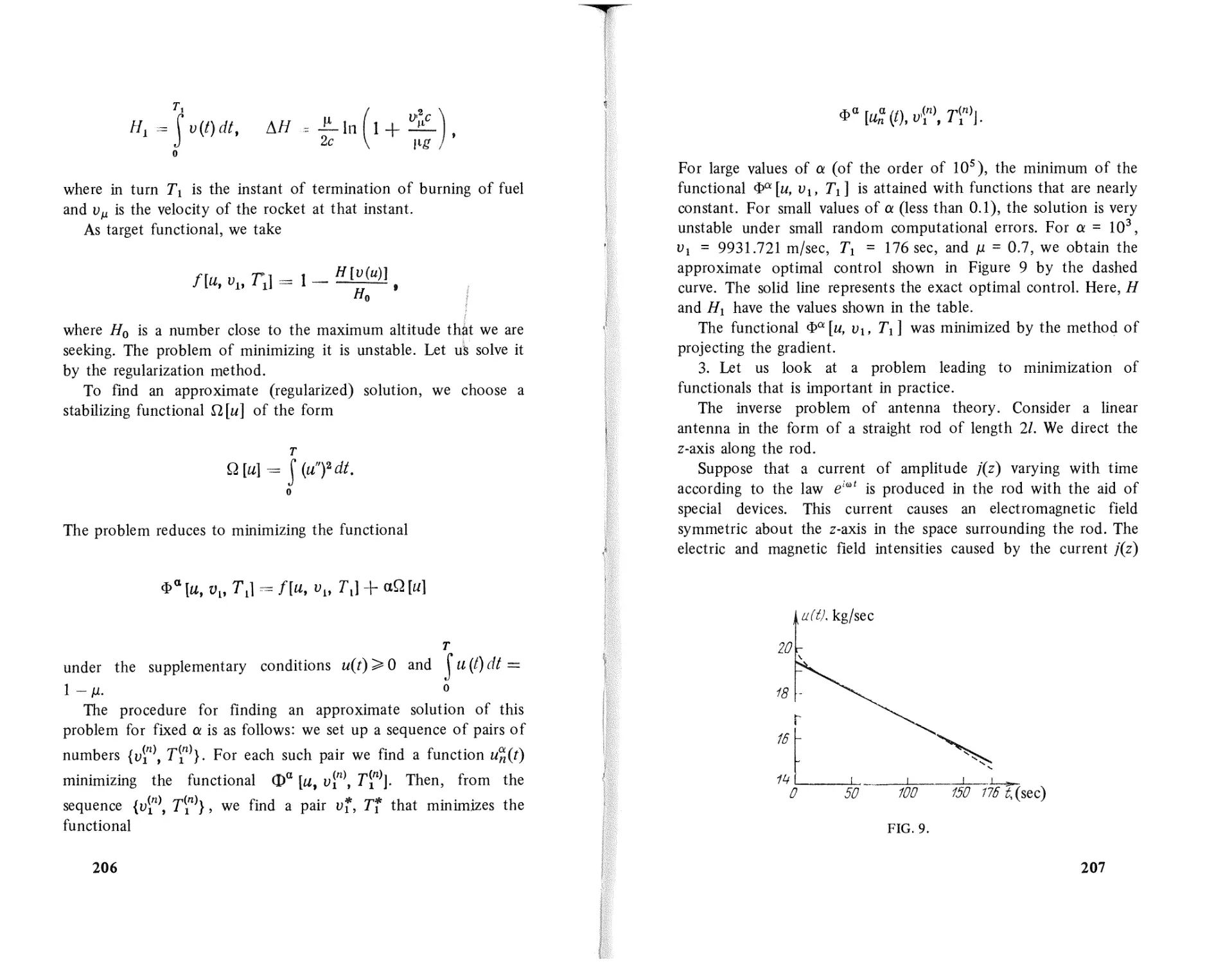
202
211
212
216
222
236
256

TRANSLATION EDITOR'S PREFACE
The notion of a well-posed ("correctly set") mathematical
problem makes its debut with the discussions in Chapter I of J.
Hadamard's Lectures on Cauchy's Problem in Linear Partial
Differential Equations (Yale University Press, 1923). It represented
a significant step forward in the classification of the multitude of
problems associated with differential equations, singling out those
with sufficiently general properties of existence, uniqueness and
(by implication) stability of solutions. Hadamard observes:
"But it is remarkable, on the other hand, that a sure guide is
found in physical interpretation: an analytic problem always being
correctly set, in our use of the phrase, when it is the translation of
some mechanical or physical question."
From the point of view of the present volume, Hadamard's
notion of a mechanical or physical question appears as too narrow.
It applies when the problem is that of determining the effects
("solutions") of a complete set of independent causes ("data").
But in many applied problems we have to get along without a
precise knowledge of the causes, and in others we are really trying
to find "causes" that will produce a desired effect. We are then
led to "ill-posed" problems. One might say that the majority of
applied problems are, and always have been, ill-posed, particularly
when they require numerical answers.
ix

The general methods of mathematical analysis were best
adapted to the solution of well-posed problems; moreover, it was
not clear in what sense ill-posed problems could have solutions
that would be meaningful in applications. A. N. Tikhonov was one
of the earliest workers in the field of ill-posed problems who
succeeded in giving a precise mathematical definition of
"approximate solutions" for general classes of such problems, and
in constructing "optimal" solutions. The book by A. N. Tikhonov
and V. Ya. Arsenin gives a general theory of ill-posed problems
and introduces the reader to a wide variety of applications ranging
from heat flow to the design of optical systems and the utomatic
processing of observational data. The present translationhould be
of special interest to mathematicians and scientists concerned with
the numerical solution of applied problems, but are unfamiliar
with Russian language literature on the subject. But not only to
those. Past experience suggests that the concepts and methods
used in the discussion of ill-posed problems will in turn stimulate
advances in "pure" mathematical analysis.
PREFACE TO ENGLISH EDITION
Fritz John
The advent of the computer had forced the application of
mathematics to all branches of human endeavor. This broadening
of the range of influence of mathematics is one of the most
import signs of scientific and technological progress, and has
produced a need to take a new look at the potential applications
of this science.
One important property of mathematical problems is the
stability of their solutions to small changes in the initial data.
Problems that fail to satisfy this stability condition are called,
following Hadamard, ill-posed. * For a long time mathematicians
felt that ill-posed problems cannot describe real phenomena and
objects. However, we shall show in the present book that the class
of ill-posed problems includes many classical mathematical
problems and, most significantly, that such problems have
important applications.
If the initial data in such problems are known only
approximately and contain a random error, then the above-
mentioned instability of their solutions leads to nonuniqueness of
the classically-derived approximate solutions and to serious
difficulties in their physical interpretation. Also, in many cases
*Also called improperly posed or incorrectly posed by some authors
(Editor).
xi
x

there simply is no classical solution of problems with approximate
initial data. In solving such problems, one must first define the
concept of an approximate solution that is stable to small changes
in the initial data, and to use special methods for deriving this
solution.
Ill-posed problems include such classical problems of analysis
and algebra as differentiation of functions known only approxi-
mately, solution of integral equations of the first kind, summation
of Fourier series with approximate coefficients, analytical
continuation of functions, finding the inverse Laplace trnsform,
the Cauchy problem for the Laplace equation, solution off singular
or ill-conditioned systems of linear algebraic equations, af? many
others, some of which are of great practical significance... We can
divide all such problems into two subclasses, namely, those of
recognition and those of design. The first subclass includes, among
others, problems of mathematical processing and interpretation of
data, as in nuclear-, plasma-, or radiophysics, electronics,
interpretation of geophysical observations, mineral (including
petroleum) prospecting, rocketry, nuclear reactor engineering, etc.
The second subclass includes many optimization problems, for
example, design of antenna or optical systems, optimal control,
and optimal economic planning.
Our book deals with solutions of problems of this nature. It
defines the concept of an approximate solution of such problems
that is stable to small changes in the initial data and it examines in
detail methods of constructing solutions that are easily processed
on a computer.
As we have already said, the initial data underlying ill-posed
problems (generally measurements) contain random errors. De-
pending on the nature of this initial information, one can take
either a deterministic or a probabilistic approach to derivation of
the approximate solutions or in evaluating the error of the data.
We have generally (except for Chapters IV and V) confined
ourselves to the deterministic approach. The interested reader will
find the probabilistic approach discussed, among others, in
references 63, 64, 87, 100, 105, 124, 128, 129, 179-181, 184
and 217.
One feature of the book is the development of the
regularization method in construction of approximate solutions of
ill-posed problems that was first expounded in [156-161].
We have not attempted a survey of the literature on ill-posed
problems. Therefore, the bibliography at the end does not pretend
to be complete. However, one recommended survey of the
literature is that of Morozov [122].*
The book is designed for a broad range of scientists, teachers,
engineers and students interested in mathematical processing of
information and prediction of experiments.
We thank A. V. Lukshin for many valuable comments.
A. N. Tikhonov and V. Ya. Arsenin
*See also L. Payne: Improperly Posed Problems (to appear shortly)
[Editor] .
xii
xiii

INTRODUCTION
 1. Remarks on the formulation of mathematical problems.
1. The rapidly increasing use of computational technology
requires the development of computational algorithms for solving
broad classes of problems. But just what do we mean by the
"solution" of a problem? What requirements must the algorithms
for finding a "solution" satisfy?
Many features of problems encountered in practice are not
reflected by the classical conceptions and formulation of problems.
Let us illustrate this with some examples.
2. Example 1. Consider the Fredholm integral equation of the
first kind with kernel K(x, s):
b
 K (x, s) z (s) ds = u (x). c <: x  d,
a
(1.1.1 )
where z(s) is the unknown function in a space F and u(x) is a
known function in a space U. Let us assume that the kernel K(x, s)
is continuous with respect to the variable x and that it has a
continuous partial derivative aKjax. For brevity, we shall denote
by A the operator defined by

b
AZ=S K(x,s)z(s)ds
a
This means that we cannot take for the "solution" of equation
(1.1.1) approximating Z1(S) the exact solution of that equation
with the approximately known right-hand member u(x) =1= U1 (x)
since such a solution may not exist. The fundamental question
then arises as to what we should mean by an approximate solution
of equation (1.1.1) with approximately known right-hand member.
Obviously, equation (1.1.1) has a solution (in the classical sense)
only for right-hand members u(x) that belong to the image AF of
the set F of functions z(s) under the mapping
..
We shall seek a solution z(s) in the class C of functions that are
continuous on the interval [a, b] . We shall measure changes in the
right-hand member of the equation with the L 2 -metric defined by
f } 1/ 2
Pu (llu u 2 )= l [U l (x) - U 2 (X)J2 dx
while we measure changes in the solution z(s) in
defined by
C-metric
b
U = Az ==  K (x, s) 2 (s) ds, 2 (s) E F.
a
P F (2 1 , 2 2 ) = max 121 (S) - 2 2 (s) I
sE[a,b]
4. Furthermore, the solution of equation (1.1.1), understood in
the classical sense, that is, obtained according to the rule
3. Suppose that for some u = U1 (x) the function Z1 (s) is a
solution of equation (1.1.1):
2 = A-lu,
b
 K (x, s) 2ds) ds == ud x ).
a
where A -1 is the inverse of the operator A, does not possess the
property of stability under small changes in the "initial data" (the
right-hand member u(x».
To see this, note that the function Z2(S) = Z1(S) + Nsin ws is a
solution of equation (1.1.1) with right-hand member
If instead of the function U1 (x) we know only an approximation
u(x) that differs slightly (in the Lrmetric) from U1 (x), we can
speak only of finding an approximate solution of equation (1.1.1),
that is, a function close to Z1 (s).
Here, the right-hand member u(x) can be obtained experi-
mentally, for example, with the aid of a recording device, and it
may have "corners" at which the function u(x) does not have a
derivative. With such a right-hand member, equation (1.1.1) does
not have a solution (in the classical sense) since the kernel K(x, s)
has a continuous derivative with respect to x and hence the
right-hand member must also have a continuous derivative with
respect to x.
b
u 2 (x) -= udx) + N  K (x, s) sin (Os ds.
a
Obviously, for any number N, if the values of ware sufficiently
great, we can make the change
fd [ b ] 2 } t/2
fJ U (U h u,) = I N It}  K (x, s) sin (0 s ds dx
2
3

P F (Z1' zz) = max I Z2 (S) - Z1 (s) 1= max I N sin (Us I = I N I
sEra b] sE[a,b]
(1.1.2)
Thus, we need not only to answer the question as to what is
meant by an approximate solution of equation (1.1.1) but also to
give an algorithm for constructing one that will be stable under
small changes in the initial data u(x).
The situation encountered in this example is typical of ill-posed
problems.
5. We have considered a case in which it is known in advance
that equation (1.1.1) has an exact solution (in the classical sense)
zr(s) corresponding to the right-hand member ur(x) and we are
required to find an approximation for it if, instead of the function
ur(x), we know only an approximation u(x) of it such that
pu(u r , u) 8.
If we have no information regarding the existence of an exact
solution of equation (1.1.1) but do have information regarding the
class of possible right-hand members U, we can also pose the
problem of finding an approximate solution of equation (1.1.1).
To do this, we define the concept of a generalized solution
(quasisolution) of equation (1.1.1) on the set F as an element z of
F at which the distance pu(Az, u) attains its greatest lower
bound [71, 72]; that is,
arbitrarily small without preventing the change in the correspond-
ing solutions Zl (s) and Z2(S), namely,
from ..the- being arbitrarily great. Here, we measured the difference
between the functions Zl (s}>and Z2 (s) in the C-metric.
If the difference between the solutions is estimatt1!d in the
L 2 -metric, the solution of equation (1.1.1) is again unstble under
small changes in u(x). Specifically,
P F (z., z,) = {  I z.(s) - z, (s) I' <is} 'I, = I N I { si n' ros ds f"
= IN 1"1 J b - a -  sin (0 (b - a) cos (0 (b + a). (1.1.3)
V 2 2(0
One can easily see that the numbers wand N can be chosen in
such a way that, for arbitrarily small discrepancies between Ul (x)
and U2 (x), the discrepancy between the corresponding solutions as
calculated according to formula (1.1.3) can be arbitrary.
However, the requirement of stability of the solution of
equation (1.1.1) has to be satisfied since it is associated with the
physical determinacy of the phenomenon (relationship) described
by that equation.
The problem of solving the integral equation (1.1.1) is not
completely settled by taking as an approximate solution a function
z(s) for which
Pu (Az, u) = inf Pu(Az, u),
ZEF
Az = S K (x, s)z(s)ds.
a
Obviously, if equation (1.1.1) has a solution zr EF in the usual
sense for u = ur, it coincides with the generalized solution of the
equation Az = Ur.
The problem then arises of finding algorithms for constructing
generalized solutions that are stable under small changes in the
right-hapd member u(x).
Example 2. Consider the system of linear algebraic equations
Pu (Az, u)  6,
Az -= u,
(1.1 .4)
where u approximates the right-hand member of the equation
with accuracy 8: pu(u, u 1 ) 8.
4
where Z is an unknown vector, u is a known vector, and A = {a ij }
is a square matrix with elements aij.
5

If the system (1.1.4) is nonsingular, that is, if det A*,O, it has
a unique solution, which we can find by Cramer's rule or by some
other method. *
If the system (1.1.4) is singular, it will have a solution (not
unique) only when the condition for existence of a solution
(vanishing of the relevant determinants) is satisfied.
Thus, before solving the system (1.1.4), we need to check
whether it is singular or not. To do this, we need to evaluate the
determinant of the system det A.
If n is the order of the system, evaluation of det A !requires
approximately n 3 operations. No matter how accurtely we
perform the calculations, the value that we obtain for dt A will
differ from the true value as a result of the accumulation of
computational errors, and this discrepancy will be arbitrarily great
for sufficiently large n. This circumstance necessitates construction
of algorithms for solving the system (1.1.4) that do not involve
preliminary determination as to whether the system is singular or
not.
Furthermore, in practical problems, we often know only
approximately the right-hand member U and the elements of the
matrix A, that is, the coefficients in the system (1.1.4). In such
cases, we are ",dealing not with the system (1.1.4) but with some
other system Az = u such that II A -A II  0 and II u-u II  0, where
the meaning of the norm is usually determined by the nature of
the problem. Having the matrix A instead of the matrix A, we are
even less able than before to draw a definite conclusion as to
whether the system (1.1.4) is singular or not.
In such a case, all we know regarding the exact system Az = u
is that IIA-AIIo and Ilu-ull6. But there are infinitely
many systems with such initial data (A, u), and we cannot
distinguish between them within the framework of the level of
error known to us. Such possible exact systems may include
singular ones.
Since we have the approximate system k = u rather than the
exact one (1.1.4), we can speak only of finding an approximate
solution. But the approximate system may be unsolvable. The
question then arises as to what we are to understand by an
approximate solution of the system (1.1.4). It must also be stable
under small changes in the initial data (A, u).
 2. The concepts of well-posed and ill-posed problems.
1. Well-posed and ill-posed problems are distinguished. The con-
cept of a well-posed problem of mathematical physics was introduced
by J. Hadamard [201, 202] in the attempt to clarify what types of
boundary conditions are most natural for various types of
differential equation (for example, the Dirichlet and analogous
problems for elliptic equations and the Cauchy problem for
hyperbolic equations).
The solution of any quantitative problem usually ends in
finding the "solution" z from given "initial data" u: z = R(u). We
shall consider u z as elements of metric spaces U and F with
metrics Pu(Ul, U2) for Ul, U2 E U and Pp(Zl, Z2) for Zl, Z2 E F.
The metric is usually determined by the formulation of the problem.
2. Suppose that 'the concept of solution is defined and that to
every element u E U there corresponds a unique solution z = R(u)
in the space F.
The problem of determining the solution z = R(u) in the space
F from the initial data u E U is said to be stable on the spaces (F, U)
if, for every positive number E, there exists a positive number
O(E) such that the inequality PU(Ul, U2)  O(E) implies Pp(Zl, Z2)
 E, where Zl = R(ud and Z2 = R(U2) with Ul and U2 in U and Zl
and Z2 in F.
The problem of determining the solution Z in the space F from
the "initial data" u in the space U is said to be well-posed on the
pair of metric spaces (F, U) if the following three conditions are
satisfied:
1) for every element u E U there exists a solution Z in the space
*Kurosh, A. G., Kurs vysshey algebry (Course of higher algebra), 10th
ed., Moscow, Nauka, 1971.
F;
2) the solution is unique;
7
6

3) the problem is stable on the spaces (F, U).
For a long time, it was the accepted point of view in
mathematical literature that every mathematical problem has to
satisfy these conditions [93].
Problems that do not satisfy them are said to be ill-posed.
It should be pointed out that the definition of an ill-posed
problem is with respect to a given pair of metric spaces (F, U)
since the same problem may 'be well-posed in other metrics (see
examples 2 and 3 of 3 of this introduction).
Remark. The fact that the spaces F and U are metric paces is
used here to express the closeness of elements as a tbeans of
describing neighborhoods in the spaces F and U. The bas'iC results
to be given below remain valid for topological spaces F and U (see
[73] ).
If the class U of initial data is chosen in a "natural" manner for
the problem in question, conditions 1) and 2) characterize its
mathematical determinacy. Condition 3) is connected with the
physical determinacy of the problem and also with the possibility
of applying numerical methods to solve it on the basis of
approximate initial data.
When we get right down to it, what physical interpretation can
we give to the solution of a problem if arbitrarily small
disturbances in the initial data can cause great changes in the
solution?
3. That a problem be well-posed has often been treated as a
condition that any mathematical problem corresponding to any
physical or technological problem must satisfy. This generated
doubt as to the usefulness of studying ill-posed problems.
However, this point of view, while perfectly natural as applied to
certain phenomena that have been studied over the years, is not
valid for all problems. In 3, we shall give some examples of
ill-posed problems relating both to the basic mathematical
apparatus and also to a broad class of applied problems.
4. The problem of finding an approximate solution of an
ill-posed problem in a natural class F is in practice ambiguous.
Thus, suppose that the problem of solving the equation
Az=u
(1.2.1)
in the class F is ill-posed. *
Let us suppose that the right-hand member of equation (1.2.1)
is known to us with accuracy 0; that is, we know not its exact
value UT but an element 'it such that PU(UT, u) <; 0.
It is natural to seek an approximate solution of equation (1.2.1)
in the class Q{j of elements z for which Pu{Az, 'if) <; O.
However, in a number of cases, this class of elements is too
broad. As was shown in example 1 of  1, these elements
(functions z(s)) include elements that can differ greatly from each
other (in the metric of the space F). Therefore, not every element
of the class Q{j can be taken as an approximate solution of
equation (1.2.1).
A rule for selecting possible solutions is necessary. For this, we
need to use supplementary information (generally available)
concerning the solution. Such information may be of a
quantitative or qualitative nature. The attempt to use supplemen-
tary information of a quantitative nature leads to the concept of a
quasisolution [71, 72], of which we shall speak in greater detail in
Chapter I.
The use of supplementary information of a qualitative nature
(for example, smoothness of the solution) necessitates a different
approach to the construction of approximate solutions of equation
(1.2.1). This approach is followed in [156-161] and will be
described in Chapter II.
3. Examples of ill-posed problems.
1. Example 1. The problem of solving an integral equation of
the first kind
b
S K (x, s) z (s) ds = u (x).
a
*This will be the case, for example, if A is a completely continuous
operator. Then, the inverse operator A -1 will not in general be continuous
on U and the solution of equation (1.2.1) will not be stable under small
changes in the right-hand member u (in the metric of the space U).
8
9

We looked at this example in detail in  1, where it was pointed
out that its solution is unstable under small changes in the
right-member u(x).
Example 2. The problem of differentiating a function u(t) that
is known only approximately.
Suppose that Z1 (t) is the derivative of the function U1 (t). The
function U2 (t) = U1 (t) + N sin wt differs from U1 (t) in the metric
of C by an amount Pe(U1, U2) = INI for arbitrary values of w.
However, the derivative Z2tt) = U2 '(t) differs from Z1 (t) in the
C-metric by an amount INw I, which can be arbitrarily great for
sufficiently large values of Iw I.
We note that the problem of finding the nth derivatiy of the
function u(t) reduces to solving the integral equation o{the firs
kind
However, in practical problems, these requirements on the
functions u(t) often cannot be verified. Therefore, the metric used
above for estimating the difference between functions u(t) in U is
not a natural one for the differentiation problem.
Example 3. Numerical summation of Fourier series when the
coefficients are known approximately in the metric of 1 2 .
00
Suppose that !I (t) =  an cos nt. If instead of an we take
n=o
the coefficients c n = an + €In for n  1 and Co = ao, we obtain
00
the series 12 (t) -= 2j C n cos nt. The coefficients in these series
n=o
differ (in the metric of 1 2 ) by an amount
t
r 1 (t - t)n-lz (t) dt -_= II (t).
J (n -1)1
o
{ 00 J ilt { 00 1 J ilt '1 j3t2
€ 1 = !lo (C n - an)?' = € 1 -;;; = € r  ,
Thus, this problem does not possess the property of stability, a
fact that leads to great difficulties in approximate evaluation of
derivatives.
Remark 1. If we take other metrics on the sets F and U (or on
one of them), then the problem of differentiating u(t), which is
known only approximately, may be well-posed on the pair of
metric spaces (F, U).
Thus, if U is the set of continuously differentiable functions on
the interval [a, b] and the distance between two functions U1 (t)
and U2 (t) in U is measured in the metric defined by
which we can make arbitrarily small by choosing € sufficiently
small. At the same time, the difference
00
12 (t) - 11 (t)= € 2j  cos nt
n=l
Pu (U h U 2 ) = sup { I U 1 (t) - U 2 (t) I + I U; (t) -- U; (t) I},
tE[a.b]
may be arbitrarily large (for t = 0, the last series diverges).
Thus, if we take the deviation of the sum of the series in the
metric of C, summation of the Fourier series is not stable.
Remark 2. If the difference between functions I(t) in F is
estimated in the metric of L 2 , the problem of summation of
Fourier series with coefficients given approximately (in the metric
of 1 2 ) will be well-posed on such a pair of metric spaces (F, U).
Specifically, from Parseval's theorem, we have
but the distance between two functions Z1 (t) and Z2 (t) in F is
measured in the C-metric, then the problem of differentiation
obviously is well posed in that pair of metric spaces (F, U).
10
11

1t 1/ 00 1/ '11 rn
is [f,(I) - f,(I)J'dl} , = {  (en - an)'} , =', V % .
o n-l
u (x, 0) = f (x), au I = 'P (x), - 00 < x <
a y y=o
can be made arbitrarily large for sufficiently large values of a.
Thus, this problem is not stable and hence is ill-posed.
However, the Cauchy problem for Laplace's equation is
encountered in applications [68-70, 75, 84, 94, 96, 209, 211,
212]. As an example, we may cite the problem of continuation of
the gravitational potential observed on the surface of the earth
(y = 0) in the direction away from the gravitational field sources. *
Example 5. The problem of analytic continuation of a function
known on part of a region to the entire region.
Let D denote a bounded region and let E denote an arc of a
curve contained in D. Then, the problem of analytic continuation
of the function represented by the arc E to the entire region D is
unstable.
To see this, let Zo denote a point on the boundary of the
region D at a positive distance d from E and let 11 (z) denote a
function that is analytic in D. The function 12 (z) = 11 (z) + €/(z -
zo), where € is a given positive number, is also analytic in D. On
the curve E, these functions differ by €/(z - zo), which does not
exceed in absolute value the ratio €/d; that is, lf2 (z) - 11 (z)1  €/d
everywhere) on E. The ratio €/d can be made arbitrarily small by
choosing .(3.. sufficiently great. However, the difference 12 (z) - 11 (z)
= €/(z - zo) is unbounded in absolute value on the region D as a
whole (see also [78, 192, 194, 196]).
Example 6. The inverse gravimetry problem. Suppose that the
density of a body is different from that of the surrounding
medium. The problem is to determine the shape of the body from
the anomalies in the gravitational field strength caused by it on
the surface of the earth (see [36-38,40,41, 148, 165]).
Let us suppose that the medium under the surface of the earth
(z = 0) consists of masses with known densities PI and P2
separated by a boundary z(x) (see Fig. 1).
Suppose that z(x) = -H everywhere except on an interval
a  x  b, on which z(x) = -H + z(x).
Example 4. The Cauchy problem for the two-dimensional
Laplace's equation (Hadamard's example [202]). This problem
consists in finding a solution of the equation b.u(x, y) = 0 from
the initial data, that is, in finding a solution satisfying the
conditions
where I(x) and 'P(x) are given functions.
If we set 11 (x) == 0 and 'PI (x) = a-I sin ax, then the solution of
the Cauchy problem will be the function Ul (x, y) = a- 2 sin ax sinh ay,
where a > O.
If we set 12 (x) = 'P2 (x) == 0, then the solution of this Cauchy
problem is U2(X, y) == O.
If we estimate the differences in initial data and solutions in
the metric of C, we have
PC(fl' '2) = sup I II (x) - 12 (x) 1=0,
x
1
Pc ('P 1J 'P 2 ) -= sup I 'Pd x ) - 'P:.l (x) I =-= -.
x a
The second of these can be made arbitrarily small by taking a
sufficiently large. However, for any fixed y > 0, the difference
between the solutions
Pc(U 1 , u 2 ) -= sup I u 1 (x, y) - u 2 (x, U) I ==
x
/ 1. . h \ 1' h
= sup -stnaxsm ay = -Sill ay
x  
*The potential of the gravitational field of the earth satisfies Laplace's equa-
tion 6u = O.
12
13

Thus, the problem of determining the function z{x) reduces to
solving the nonlinear integral equation of the first kind
:'J.
X
b
Az = \; in (x - £)2 + H2 ds = u ( x)
 (x-£)2+(H-z())2 '
a
C!.
b X
where u(x) = (21T/p). Here, A is a nonlinear integral operator.
It is easy to show that the solution of this equation is unstable
under small changes in the right-hand member u(x).
A vast literature [42,95, 125, 126, 131-140] has been written
on questions of uniqueness of the solution of the inverse
gravimetry problem.
Let us mention some other classes of mathematical problems
that include ill-posed problems: the solution of systems of linear
algebraic equations with vanishing determinant (see Chapter III),
certain problems in linear programming (see Chapter VIII),
problems of minimizing functionals such that convergence of a
sequence of values of the functional being minimized to its
smallest value does not imply convergence of the minimizing
sequence (see Chapter VII), certain optimal control problems (see
Chapter VII), and many others [104].
2. An important class of ill-posed problems of great practical
value is constituted by problems of planning optimal systems and
constructions. We present one of these problems below.
Let us look at a problem of designing physical systems. This
class includes problems of designing optical systems with given
transmittances (or reflectances). Such systems can be obtained, for
example, with the aid of laminated coatings deposited in the form
of thin fIlms on the surface of the "backing".
Consider a flat nonhomogeneous plate of infinite extent and
thickness H. Let us set up a z-axis perpendicular to the plate with
zero point chosen so that, within the plate, O<z<H. Let n(z)
denote the index of refraction at the point z. Suppose that a
monochromatic plane light wave of length A = 21TC/W is incident
normally to the plate. Let us suppose
FIG. 1.
Such a configuration of masses causes on the surface of the
earth an anomaly in the gravitational field strength
I1g = -- oV I '
OZ 2=0
where V is the potential due to masses of density p = P 2 - Pi
filling the region S shown in Figure 1.
Since
v = j ;: In ( : ) ds d11, where r = V (x - S)2 + (z - '11)2,
S
we have
b -H+Z(£)
6.g = - L S r -  in.!. ds d'l1l - -=
2n J 011 r 2-0
a -H
b
=  r in (x - £)2 + H2 ds
2n J (x - £)2 + (H - z (;))2
a .
An anomaly in the gravitational field strength on the surface of
the earth can be measured.
14
15

a) that the half-spaces {z<O} and {z>H} outside the plate are
each homogeneous with indices of refraction no and nH'
b) that there is no absorption in the plate or in the half-spaces
outside it.
Suppose that the electric field of the incident wave in the
half-space {z < O} has the form Ein = 0 0 (z) i rot , where
-l.!!!..noz
(go(z) = Eoe C is the amplitude of the wave. Under these
conditions, the amplitude o{ the electric field (g (z) the
equation (see [35])
2
(g" -+ n5(g =0.
c 2
In this half-space {z < O}, the total electric field is the
resultant of the fields of the incident and reflected waves. The
amplitude (&-:0 (2) of the total field in this half-space is
.W
 l cnoz
(go (z) = (go () +c1e
The amplitude of the electric field of the wave passing through the
plate is 0H (z)=c 2 (g0(z).
Inside the plate, the amplitude of the field [ff (z) is a solution
of the boundary-value problem (see [35])
(E"
(02
-n 2 (z) <8 =0, O<z< H,
c 2
(1.3.1 )
0' (0) -- i.!!!.. no [(8 (0) -2Eo] = 0,
c
(g' (H) + i no  (H) =0.
c
(1.3.2)
(1.3.3)
If n(z) is piecewise-continuous on the interval (0, H), we have,
at points of discontinuity Zi,
(S (Zi -0) = (S (Zi + 0), (S' (Zi - 0) = (S' (Zi + 0).
16
The transmission capacity of such a system (the plate) is
characterized by the transmittance
J
T = n (H) I <jfj (H) 1 2 .
no <jfj 0 (0)
(1.3 .4 )
Obviously, for such a system, this quantity is a function of the
length A of the wave incident to the plate*: T =: T(A).
The direct problem consists in finding the transmittance T(A)
from given 00, n(z), and H, and it reduces to solving the
boundary-value problem (1.3.1)-(1.3.3) for [ff (z).
Frequently, we need to solve the problem inverse to this one. It
consists in determining from a given function T(A) the system
(n(z), H), that is, in finding the index of refraction n(z) of points
in the plate and the thickness H of the plate. This problem is
called the synthesis problem.
It is not well-posed because .there may not exist a system (n(z), H)
(a plate of thickness H with index of refraction n(z)) having
the prescribed transmittance T(A). It is also possible that more
than one system will have' that transmittance.
In addition, not every system is realizable in practice.
It is of interest to consider the synthesis problem for laminated
systems in which the unknown function n(z) is piecewise-constant.
In this case, the index of refraction n(z) has a constant value nj in
the jth layer (for j = 1, 2, . . . , N), the thicknesses of the layers dj
are arbitrary, and the number of layers N is not given. A problem
of this kind that is important in practice is that of designing
laminated coatings. Let us look in greater detail at the
mathematical formulation of this problem, which is the discrete
analogue of the problem examined above of designing optical
systems.
We shall describe a system consisting of N layers by a
2N-dimensional vector x = {d 1 , d 2 , . . . , d N ; nl, n2, . . . , nN}, the
components of which are the thicknesses dj and the indices of
*In some cases, one deals not with T("A) but with the reflectance R ("A) =
1 - T("A).
17

. . f the layers. The solution of problem (1.3.1 )-(1.3.3)
refraction nJ 0 ) 2N dimensional vector x a
assigns, by formula (1.3.4, to any -
unique transmittance T(A).
Thus, a nonlinear operator
A (x, A) If (A)
(1.3.6)
A (x, A) = T (A),
Al -< A <: A 2
(1.3.5)
N
minimizing N and d =  d l such that" A (x, A) - T (A) ilL! < 0,
1=1
where 8 is a given number at least equal to 8 0 . This problem
can be solved in the following way: By increasing successively
by one the number of layers N, we find the smallest value N
= No for which D 2 N o includes a vector XN for which
 0
1/ A (XN o ' A) -- T (A) /lL! < o.
When we have thus determined the number No, we seek, in the
class of vectors x in D 2No satisfying the condition
No
11.4 (x, A) - T (A) IL  6, a vector x minimizing d =  d 1' . A
1'=1
solution of this problem obviously exists since D 2No is a closed
convex set contained in a finite-dimensional Euclidean space.
Examples for the numerical solution of such problems are given in
[35J.
3. The problem of designing optical systems that we have just
considered is the problem of determining the coefficients n(z) in
equation (1.3.1) from a known fURctional T(A) of the solution of
that equation. It is one of the inverse problems of mathematical
physics.
Many other physical problems lead to problems of determining
the coefficients in differential equations (ordinary or partial) from
certain known functionals of their solutions. An example is the
inverse kinematic problem of seismology. Its physical formulation
is the following: Let D denote a region bounded by a surface S. A
wave process (that is, a process described by the wave equation)
generated by Sources acting at points of the surface S is considered
in D. At points of S different from the wave Source points, the
time of passage of waves through that region is recorded. We are
required to find from these data the speed a = a(M) of
propagation of waves within the region as a function of the point
M. One can exhibit yet other physical problems leading to inverse
problems of this kind. An examination of such problems may be
found in [20,101-103,111, 141-143J.
. t f 2N-dimensional vectors x.
is defmed on some se 0 f 2N-dimensional vectors
Let R 2N denote the Euclidean spae .0
d t th e closed region m It defined by
and let D 2 N eno e
D 2N = {xER2N; d 1' :> 0, nmin  n1' n max ; j= 1, 2, t ., N}.
We shall estimate the diffrence between funtion.s T(A) in the
. "\"\ ) * Le t T('A ) denote a function m L 2 (AI, A2)
metnc L 2 (/\1, 1\2 . \
defined on the interval [AI, A2] .
Let us find
6 N = inf 1\ A (x, A) n -- T (Iv) \lL.'
XED 2 N
......... () ......... ... :> O. We shall call the
Obviously, ()1:> ()2:> ... ?" m?".
 - 11 ' m  t he limiting attamable accuracy.
number Uo - Urn
m-+oo . fi d' N-layer system with
The design problep consists m In mg an. ed to find a system
'tt e 'Fi C A) Here we are requlf
given transmi anc . , N and with smallest overall
with the smallest number of layers 0
N
 d 1 entary requirements are
thickness d = LJ j. These supp em
1=1
. t of stability under external
dT ed by the requlfemen )
con I Ion '1' 1 t d hen the number of layers is large ,
disturbances (easl y VlO a e w be dusty when the
by the possibility that the apparatus may
coatings are deposited, etc. . bl consists in
The mathematical formulation of thIS. pro em
finding an approximate solution of the equation
*Instead of the Lrmetric, we could take the C-metric.
18
19

4. One important problem is the construction of systems. of
automatic mathematical processing of the results of a physIcal
eXDeriment. One stage in the processing is the solution of inverse
prblems of the form Az = u for z. ..,
Many modern experimental devices for investlgatm. g physIcal
phenomena and objects of various kinds are complIcated and
expensive complexes (accelerators of elementary particles, evices
for obtaining and investigating high-temperature plasma, devIces for
investigating the properties of.matter at very low temperatures, etc.).
The desire for reliable information regarding the pheomenon
under investigation or the study of "rare" and "weak'l' effects
frequently necessitates many repetitions of a sinle exeriment.
Automation of the performance of an expenment", and of
registration of its results enables us to obtain in a short time a
large volume of necessary information (tens and hundreds of
thousands of photographs, oscillograms, readings of detec.tos,
etc.). To obtain from this information the necessary charactenstlcs
of the phenomenon or object being studied, we subsequently hae
to process the results of its observations. In many caes, thIS
processing must be done almost simultaneously wIt ,the
performance of the experiment or with nly a sall permIssIble
lag. In such a case, the processing necessItates gomg over a large
amount of information and can be done only with a computer.
For a large class of experimental set-ups, we can single out the
following steps in the processing of observational resuts [66]:
First step. Information is taken from the recordmg d.evice or
from a constant carrier (for example, a photographIc cell),
converted to a numerical code, and entered in the memory of the
computer. . .
Second step. The results of observation are statlstlIlY
processed with an estimate of the degree of relia?ility: NormalIzmg
measurements (background, calibrational, dosunetnc, etc.) are
allowed for.
Third step. The results obtained at the second step of the
processing are interpreted. Usually, this interpretation consists in
estimating the sought characteristics of the model of the
phenomenon or object being studied.
What is usually recorded in a physical experiment is not the
parameters z of interest to us but certain of their manifestations u
= Az. Therefore, the interpretation problem usually reduces to
solving an equation Az = u. In many cases, this problem is
ill-posed.
A program for carrying out the entire processing complex (from
the first through the third step) is usually called a complete
system of mathematical processing of observational results or,
more briefly, a processing system. A processing system can operate
both in a "dialogue regime" and automatically, without the
intervention of a human being in the intermediate stages. This
procedure for automatic mathematical processing of observational
results requires the use, in the processing system, of algorithms for
solving the equation Az = u (including ill-posed problems) that are
easily realized on a computer.
A description is given in [33, 176] of a system of automatic
mathematical processing of the results of a physical experiment on
the interaction of r-quanta with neutrons and protons.
5. Inverse problems constitute a broad class of ill-posed
problems arising in physics, technology, and other branches of
learning.
Suppose that the object or phenomenon in question is
characterized by an element ZT (a function or vector) belonging to
a set F. Frequently, ZT does not lend itself to direct study and
some manifestation of it AZ T = uT is investigated (here, UTEAF,
where AF is the image of the set F under the mapping executed
by the operator A). Obviously, the equation
Az= u
(1.3.7)
has a solution on F only for those elements u that belong to the
set AF. The element uT is usually obtained from measurements
and hence we know it only approximately. Let u denote its
approximate value. In such cases, we can speak only of finding an
approximate solution (that is, close to ZT) of the equation
Az = u.
(1.3.8)
20
21

Here, u generally does not belong to the set AF. Frequently, the
operator A is such that the inverse operator A -1 is not continuous
(for example, when A is a completely continuous operator, in
particular, the integral operator of Example 1). Under these
conditions, we cannot take for the approximate solution the exact
solution of equation (1.3.7) with approximate right-hand member;
that is, we cannot take for the approximate solution the element
z=A -1ff for two reasons: First, such a solution may not exist on
the set F since u may not belong to the set AF, so that
requirement 1) of a well-posed problem is not satisfied. ,Second,
even if such a solution does exist, it will not possess the property
of stability since the inverse operator A -1 is not cntinuous
whereas stability of a solution of the problem (1.3.7) is usually a
consequence of its physical determinacy and hence an approximate
solution must possess this property. Thus, requirement 3) of a
well-posed problem is not satisfied. Consequently, the problem
(1.3.7) is ill-posed.
In many cases, the absence of stability makes difficult a
physical interpretation of the measurement results. Satisfying this
condition is also necessary 'for the use of numerical methods of
solution on the basis of approximate initial data. Thus, in the case
of inverse problems we are confronted with the basic question:
what do we mean by "approximate solution" of such problems? If
an answer is given to this question, the problem then arises of
finding algorithms for constructing approximate solutions that will
possess the property of stability with respect to small changes in
the initial data.
6. In what follows, our basic attention will be given to
methods of solving ill-posed problems of the form (1.3.7). These
include systems of linear algebraic equations and Fredholm integral
equations of the first kind. In the first case, the operator A is a
matrix whose elements are the coefficients in the system; in the
second, the operator A is the integral operator
7. Suppose that the elements z and u in equation (1.3.7) are
functions (scalar or vector) of the point M and the time t and that
the operator A is a linear operator determined by the nature of
the transformation from z to u. If we know the reaction
(response) of the transformer to the Dirac delta function, which
becomes infinite when M P and t = T, that is, the function
A8(M, P; t, T) = K(M, P; t, T), then, for an arbitrary function
z(M, t) in F, we have
Az =  K (M, P; t, t) Z (P, t) dVpdt,
where the integral is over the entire domain of definition of the
function z(P, t). The function K(M, P; t, T) is called the impulse
transfer function or, more briefly, the impulse function of the
transformer (system). It is also often called the apparatus function
of the system. In this case, equation (1.3.7) reduces to an integral
equation of the first kind.
Let us consider, for example, the problem of studying the
spectral composition of a beam of light (the spectroscopy
problem). Suppose that the observed radiation is nonhomogeneous
and that the distribution of the energy density over the spectrum
is characterized by a function z(s), where s is the frequency (or
energy). If we pass the beam through a measuring apparatus, we
obtain an experimental spectrum u(x). Here, x may be the
frequency and it may also be expressed in terms of voltage or
current of the measuring device. If the measuring device is linear,
then the functional relationship between z(s) and u(x) is given by
b
1z =  K (x, s) z (s) ds = u (x),
a
b
Az ;:::::  K (x, s) Z (5) cis.
a
where K(x, s) is the apparatus function, assumed to be known. It
represents the experimental spectrum (as a function of x) when a
monochromatic beam of frequency s and unit intensity (this is the
22
23

delta function 8(s - x)) hits the device. The numbers a and bare
the ends of the spectrum.
8. .If z depends only on the time and if the transformer
(apparatus) is homogeneous with respect to time, then the
function K(M, P; t, 7) depends only on the difference t - 7:
t
S K (t - -r) z ('r) d,; = u (t),
o
K (M, P; t, -r) == K (t -- -r).
where K(t) is the impulse function of the cable (see Chapter II).
c) Calculation of the derivatives of a function that is known
only approximately. For the nth derivative z(x) of a function u(x)
we have the equation
In this case, the operator Az has the form
00
Az = S K (t - -r) z (-r) d-r,
-00
x
S (x -- t(-lZ (t) Lit = u (x).
(n 1)1
Xo
and equation (1.3.7) becomes
d) Automatic control problems, for example, the determination
of the transfer functions k(t) of linear transformers from the input
and output signals x(t) and yet):
00
S K (t - -r) z (-r) d-r = u (t).
(1.3.9)
t
Ak = S x (t - ,;) k (-r) d-r = y (t).
o
-00
This is an integral equation of the first kind of the convolution
type. Examples of problems leading to equation (1.3.9) are the
following:
a) the problem of determining the form of a radio impulse z(t)
emitted by a source from the results of its reception at great
distances from the source u(t) when we know the impulse
function of the trace of the distribution K(t). The equation for
z(t) has the form
There are also many others (see [148, 164]).
t
Az =  K (t - -r) z (-r) d-r = u (t).
o
b) the problem of determining the form of an electrical
impulse at the input of a cable z(t) from measurements of it at
the output of the cable u(t):
24
2S

CHAPTER I
THE SELECTION METHOD.
QUASISOLUTIONS
The possibility of determining approximate solutions of ill-posed
problems that are stable under small changes in the initial data is
based on the use of supplementary information regarding the
solution. Various kinds of supplementary information are possible.
In the first category of cases, the supplementary information,
which is of a quantitative nature, enables us to narrow the class of
possible solutions, for example, to a compact set, and the problem
becomes stable under small changes in the initial data. In the
second category of cases, to fmd approximate solutions that are
stable under small changes in the initial data, we use only
qualitative information regarding the solution (for example,
information regarding its smoothness (see [156-161,175]).
In the present chapter, we shall look at the selection method,
which has broad practical application, the quasisolution method,
the method of replacement of the original equation with an
equation close to it, and the quasiinversion method. As an
ill-posed problem, we shall consider the problem of solving the
equation
Az= u
(1.0.1)
27

for z, where u belongs to a metric space U and z belongs to a
metric space F. The operator A maps F onto U. It is assumed that
A has an inverse operator A -1 though the latter is not in general
continuous. When the operator A possesses these properties, we
shall call equation (1.0.1) an operator equation of the first kind
or, more briefly, an equation of the first kind.
eu (Azo, u) = inf eu(Az, u).
ZEM
the class M of possible solutions for which the selection method is
stable and zn -+ zT [155]. These requirements consist in
compactness of the set M and are based on the following
topological lemma:
Lemma. Suppose that a compact (in itself) subset F of a metric
space Fo is mapped onto a subset U of a metric space U o . If the
mapping F -+ U is continuous and one-to-one, the inverse mapping
U -+ F is also continuous.
Proof. Let <(J denote the function that maps any element z of F
into an element u of U and let 1/; denote the inverse mapping from
U onto F.
Let us take an arbitrary element Uo of U. Let us show that the
function 1/;(u) is continuous at Uo. Suppose that this is not the
case. Then, there exists a positive number €1 such that, for every
position number 0, there exists an element u of U such that PuUl,
uo) < 0 though pp(z, zo)  €1 . Here, z = 1/;(u) and Zo = ljJ(uo).
Let us take a sequence {on} of values of 0 that converges to 0
as n -+ 00. For every On, there exists an element Un such that
 1. The selection method of solving ill-posed problems.
1. A method of solving equation (1.0.1) approximately that is
widely used in computational work is the selection mthod. It
consists in calculating the operator Az for elements z bel@nging to
some given subclass Me F of possible solutions; that is, ''We solve
the direct problem. As an approximate solution, we, take an
element Zo belonging to the set M for which the difference Pu(Az,
u) attains its minimum:
Suppose that we know the right-hand member of equation
(1.0.1) exactly: u = u T, and that we are required to find its
solution ZT. Usually, we take for M a set of elements z depending
a finite number of parameters varying within finite limits in
such a way that M is a closed set contained in a finite-dimensional
space. If the desired exact solution ZT of equation (1.0.1) belongs
to the set M, then inf Pu(Az, u) =0 and this infimum is
ZEM
attained with the exact solution ZT. If equation (1.0.1) has a
unique solution, the element Zo minimizing Pu(Az, u) is uniquely
defined.
In practice, minimization of pu(Az, u) is done only
approximately, and our first fundamental question about the
selection method is as follows: If {zn} is a sequence of elements of
M such that Pu(Azn, u) --+ 0 as n -+ 00, can we assert that pp(zn,
Z T) -+ 0 as n -+ 00, that is, that {z n} converges to z T?
2. The attempt to find a basis for the success of the selection
method has led to some general functional requirements restricting
Pu (un, u o ) < 6n and Pp(in, zo) > €It where Zn = 1/; (Un).
Obviously, the sequence {un} converges to the element uo. Since
all the elements zn belong to the compact set F, the sequence {zn}
has a subsequence that converges to an element Zo of F:
- -
{znk}  ZOo
Here, Zo =1= Zo since PP(znk' zo)  €1' Corresponding to this
subsequence is a sequence of elements
u nk <{J (Znk)
of U that converges (in the sense of continuity of the mapping «J)
to the element iio = «J(zo) and is a subsequence of the sequence
{un}. Since this last sequence converges to Uo = «J(zo), we have
U o = <{J (20) = U o = <{J (zo).
28
29

Since the mapping F --+ U is one-to-one, it follows that Zo = zo.
Since we showed above that Zo =1= Zo, we have reached a
contradiction. This completes the proof of the lemma.
Thus, the minimizing sequence {zn} in the selection method
converges to zT as n --+ 00 if zT belongs to a compact class M of
possible solutions.
Suppose that, instead of the exact right-hand member UT, we
have an element U o such that pu(u o ' u T )  o. If ufj belongs to the
set AM (the image of the set M under the operator A) a.nd M is
compact, we can use the selection method to find an apP¥oximate
solution z of the equation Az = u o ' It will als\f> be an
approximation of the solution ZT of the equation Az =v.1T since
the inverse operator A -1 is continuous on AM. In finding z as
an approximation of zT, we I1eed to keep in mind the level of
error in the right-hand member since
can be used successfully to solve the problem. Thus, we have given
a definitive answer to the first question.
Let us look at the problem of solving the Fredholm integral
equation of the first kind
b
Alz = J l( (x, s) z (s) d8 = U (x), U (x) E La
a
(1.1.1)
on a set M 1 of decreasing (or increasing) uniformly bounded
functions; that is, for some B, we have Iz(s) I  B. This problem is
well-posed in the sence of Tikhonov since the set M 1 is compact
in the space L 2 [43].
To see this, let us take an arbitrary sequence E = {ZI (s), Z2(S),
. . ., zn(s),.. .} of functions in MI. According to Helly's choice
theorem, * there exists a subseqence
Pu (Az, u T ) < Pu (Az, u{j) + Pu (u{j, uTJ.
El = {zn 1 (8), zna (8), ..., znk (8), ...}
3. On the basis of what has been said, M. M. Lavrent'yev
formulated [99] the concept of a well-posed problem in the sense
of Tikhonov. As applied to equation (1.0.1), a proplem is said to
be well-posed in the sense of Tikhonov if we know that,
corresponding to the exact solution U = uT, there exists a unique
solution zT of equation (1.0.1) (so that AZT = UT) belonging to a
given compact set M. In this case, the operator A -1 is continuous
on the set N = AM and, if we know not the element UT but an
element Ufj such that PU(UT, Ufj)  0 and U o EN, then for an
approximate solution of equation (1.0.1) with right-hand member
U = U o we can take the element Zo = A-I u o ' Since U o EN, this
Zo approaches ZT as 0 --+ O. A set F 1 (contained in F) on which
the problem of finding a solution of equation (1.0.1) is well posed
is called a well-posedness class. Thus, if the operator A is
continuous and one-to-one, the compact set M to which zT is
restricted is a well-posedness class for equation (1.0.1). Hence, if
the problem (1.0.1) is well-posed in the sense of Tikhonov and the
right-hand member U belongs to AM, then the selection method
of the sequence E and a function z(s) in M 1 C L 2 such that
lirn znk (8) = Z (8)
nk
except possibly at a denumerable set of points of discontinuity of
the function z(s). As we know, ** pointwise convergence of the
subsequence E 1 to the function z(s) everywhere except possibly at
a denumerable set of points implies convergence of the
subsequence E 1 to the function z(s) in the metric of L 2 .
Thus, as an approximate solution of equation (1.1.1) on the set
M 1 with only approximately known right-hand member uEAM 1 ,
*E. C. Titchmarch, Eigenfunction Expansions Associated with Second-
Order Differential Equations, Oxford University Press, part 2, 1958.
**M. A. Krasnosel'skiy, P. P. Zabreyko, Ye. I. Pustyl'nik, and P. Ye.
Sobolevskiy, Integral'nyye operatory v prostranstvakh summiruyemykh
funktsiy (Integral operators in spaces of summable functions), Moscow,
Nauka, 1966.
30
31

we can take the exact solution of that equation with right-hand
member U = U. As we know, this last -pr.oblem is equivalent to the
problem of finding on the set M 1 the function minimizing the
functional
z = A-1u
(1.2.1)
1\ A 1 z 6 - U II!  6 2 .
! (1.1.2)
to construct a solution of equation (1.0.1) that is stable with
respect to small changes in the right-hand member u of the
approximate equation.
Most of the time, we do not have an effective criterion for
determining whether the element u belongs to the set N or not.
This needs to be assumed known in advance. In practical
problems, we often know not the exact value of the right-hand
member UT but an approximate value of it 'ii, which may not
belong to the set N = AM. In these cases, we cannot use formula
(1.2.1) to construct an approximate solution of equation (1.0.1)
since the symbol A -1 U may be meaningless.
2. The attempt to avoid the difficulties associated with the
absence of a solution of equation (1.0.1) in the case of an inexact
right-hand member u led V. K. Ivanov [71, 72] to the concept of
a quasi solution of equation (1.0.1), which is a generalization of
the concept of a solution of that equation.
An element of z EM minimizing, for given u, the functional
Pu(Az, u) on the set M is called a quasisolution of equation
(1.0.1) on M:
'-' -2
N [Z u} = 1\ Alz - U IILa'
Suppose that PU(UT, u)  o. Then, as approximate solution 'of
equation (1.1.1), we can take 'the function z 0 for which
If we replace the integral operator A 1 with an operator
representing summation over a fixed grid with n nodes and if we
denote by Zi the values of the unknown function at the nodes, the
problem of constructing an approximate solution of equation
(1.1.1) reduces to the problem of finding a finite-dimensional
vector minimizing the functional N[z, u] and satisfying equation
(1.1.2). This is a linear programming problem.
In certain cases, we can actually exhibit compact well-posedness
classes. This makes it possible to construct stable approximate
solutions.
4. Because of error in the initial data, the element U may fail
to belong to the set AM. Under these conditions, equation (1.0.1)
does not have a (classical) solution and the question arises as to
what we mean by an approximate solution of equation (1.0.1).
In this case, we introduce the concept of a quasisolution. If the
set M is compact, the selection method enables us to find an
approximation to the quasisolution.
In the following section, we shall treat quasisolutions in detail.
Pu (Az, u) = inf Pu (Az, u).
ZEM
 2. Quasisolutions.
1. Suppose that the operator A in equation (1.0.1) is
completely continuous. In those cases, mentioned in  1, in which
we are seeking a solution on a compact subset M of F and the
right-handed member u of the equation belongs to the set N =
AM, it is possible to use the formula
If M is a compact set, a quasisolution obviously exists for every
u E U. If in addition u EAM, then the quasisolution z coincides
with the usual (exact) solution of equation (1.0.1). There may be
more than one quasisolution. In such a case, by a quasisolution we
shall mean any element of the set D of quasisolutions.
It is possible to exhibit sufficient conditions for a quasisolution
to be unique and to depend continuously on the right-hand
member u.
Let us recall the definition. Let y denote an element and Q a
subset of the space U. An element q of the set Q is called a
projection of the element y onto the set Q (and we write q = Py) if
32
33

Pu (y, q) = Pu (y, Q),
concepts and we shall not stop' for thts. For the case in which
equation (1.0.1) is linear, we can easily obtain more general results
contained in the following theorem [72]:
Theorem 2. Suppose that equation (1.0.1) is linear, that the
homogeneous equation Az = 0 has only the zero solution, that the
set M is convex, and that every sphere in the space U is strictly
convex. Then, a quasisolution of equation (1.0.1) on the compact
set M is unique and it depends continuously on the right-hand
member u.
Proof. Let z denote a quasisolution and suppose that u = Az.
Since the set M is convex, the set N = AM is also convex by virtue
of the linearity of the operator A. Obviously, 'it is the projection
of the element u onto the set N. Since every sphere in the space U
is assumed to be strictly convex, the projection u is unique. The
remainder of the proof is the same as for Theorem 1.
3. Suppose that F and U are Hilbert spaces, that M == S R is the
ball (11 z II  R) in the space F, and that A is a completely
continuous operator.
In this case, a quasisolution of equation (1.0.1) can be
represented in the form of a series of eigenfunctions or
eigenvectors <{In of the operator A * A, where the asterisk denotes
the adjoint operator.
We know that A *A is a self-adjoint positive completely
continuous operator from F into F. Let q  A2  . . . An  . . .
denote the complete system of its eigenvalues and let <{Jl , <{J2, . . . ,
<{In, . .. denote the corresponding complete orthonormalized
system of its eigenfunctions or eigenvectors. The element A *u can
be represented by a series of the form
where
Pu (y, Q) = inf Pu (y, h).
hEQ
Theorem 1. If the equation Az = u can have more than one
solution on a compact set M '(lnd if the projection of each element
u of U onto the set N = AM is unique, then the quasisoltion of
equation (2.0.1) is unique and depends continuously! on the
right-hand member u.
Proof. Suppose that z is a quasisolution and that li = Az.
Obviously, u is a projection of the element u onto the set N =
AM. By the hypothesis of the theorem, it is unique. This fact and
the fact that the mapping of the set M onto the set N is
one-to-one imply uniqueness of the quasisolution z.
Obviously, z = A-I U = A-I Pu. By virtue of the lemma on the
continuity of the inverse mapping of a compact set (see  1), the
operator A-I) is continuous on N. The projection operator P is
continuous* on U. Therefore, A-I P is a continuous operator on U
and hence the quasisolution z depends continuously on the
right-hand member u.
Thus, all the conditions for well-posedness are restored when
we shift to the quasisolution; that is, the problem of finding the
quasisolution of equation (1.0.1) on the compact set M is
well-posed.
If the solution of equation (1.0.1) is not unique, then the
quasisolutions constitute a set D of elements of the compact set
M. In this case, without the restrictions listed in Theorem 1 on the
set N, we have continuous dependence of the set of quasisolutions
D on u in the sense of continuity of multiple-valued mappings. It
is not difficult to prove this assertion (see [72, 106]) though its
proof would require the introduction of a number of new
00
A*u = 2] bn<{Jn.
n=l
(1.2.2)
*L. A. Lyusternik and V. I. Sobolev, Elements of Functional Analysis,
Ungar, New York, 1961 (translation of Elementy funktsional'nogo analiza).
Under these conditions, we have [72]:
Theorem 3. The quasisolution of equation (1.0.1) on the set SR
is expressed by
34
35

 00 h n
z =  T:" <{In
n=l n
(1.2.3)
We seek the solution of this equation in the form of a series of
the <{In:
if
00
z = 2i Cn<{Jn.
n=l
(1.2.9)
00 bZ
)1 .!:- < R 2
,,--J 'A Z
n=l n
(1.2.4)
Substituting this series into equation (1.2.8) and using the
expansion (1.2.2), we find C n = bn/An. Consequently, inequality
(1.2.4) means that IIzll <R and it is a question of finding the
unconditional extremum of the functional (1.2.7). The series
(1.2.3) is then the solution of the problem.
On the other hand, if inequality (1.2.5) holds, this means that
IIzll R and we need to solve the problem for a conditional
extremum of the functional (1.2.7) under the condition that
IlzIl2=R 2 . By using the method of undetermined Lagrangian
multipliers, we can reduce the problem to that of finding the
unconditional extremum of the functional
but by
DO
Z -
- J
n=l
b n
<{In
 + 'An
zf
00 bZ
 .-!!:..:> R 2 .
n=l 'A
(1.2.5)
(Az-u, Az-u) + a(z, z).
00 b2
:3 n = R 2 .
('An + )2
n=l
(1.2.6)
and we can then reduce this problem to that of finding the
corresponding solution of the Euler equation A * Az + az = A *u.
Substituting for z the expression given by (1.2.9) and using the
expansion (1.2.2), we find
Here, {3 is a root of the equation
Proof. The quasisolution minimizes the functional
b n
c n = -.
a+An
p (Az, u) (Az - u, Az -- u),
(1.2.7)
We determine the parameter a from the condition IIzllz=Rz,
which is equivalent to (1.2.6).
for which the Euler equation has the form*
A*Az = A*u.
(1.2.8)
 3. Approximate determination of quasisolutions.
In the preceding section, we saw that finding a quasi solution
involves finding an element in an infinite-dimensional space. For
approximate determination of a quasisolution, it is natural to shift
*V. I. Smirnov, Course of Higher Mathematics, Vol. V, Addison-Wesley,
Reading, Mass., 1964 (translation of Kurs vysshey matematiki).
36
37

to a finite-dimensional space. There is a fairly general approach to
approximate determination of quasisolutions of equations (1.0.1)
[60, 72], in which A is a completely continuous operator.
We shall assume that the sufficient conditions listed in section 2
for existence of a unique quasi solution on a given set M are satisfied;
that is, we shall assume that the set M is convex and compact and
that a sphere in the space U is strictly convex.
Let M 1 , M 2 , . . . denote a sequence of closed compact sets M n
such that
Hrn Pu (u, N n) = Pu (u, N).
noo
(1.3.3)
Since
Pu(u, N n ) = Pu(u, Bn),
we have
M 1 C M 2 C
CMnC
Hrn Pu (u, Bn) = Pu (u, Az).
nco
(1.3.4)
00
and the closure of their union U M n coincides with M. A
n=l
quasisolution of equation (1.0.1) exists on each set M n , but it may
not be unique. We denote by Tn the set of all quasisolutions on
the set M n .
Let us show that we can take for an approximation of the
quasisolution z on the set M any element 'in in Tn. Here,
Each set Bn is compact since it is a closed subset of the compact
set N n . Therefore, there exists in Bn an element Yn such that
Pu(Yn, u) = inf Pu(Y, u).
YEB n
Hrn P F (Zn, z) = O.
n-+oo
The sequence {Yn} has at least one cluster point belonging to N
since N is a compact set. Let Yo denote a cluster point of the set
{Yn} and let {Ynk} denote a subsequence that converges to Yo; that
is,
Define N n = AM n and let Bn denote the set of projections of
the element u onto the set Nn' Obviously, Bn = ATn and
N 1 £N a £ . . . c. N n' Then,
tirn Pu (Ynk' Yo) = O.
n k-'>OO
It follows from (1.3.3) and (1.3.4) that
Pu(u, N 1 ) '> ... '> Pu(u, N n ) '> ... '> Pu(u, N) =
= Pu (u, AZ). (1.3.1)
Pu (u, Yo) = Hrn P u u, Ynk) =.
n kOO
= lirn Pu (u, B nk ) = Pu (u, .42) = Pu (u, N).
nkoo
00
Since the set U N n is everywhere dense in N, for every positive
n=l
e there exists a number no (e) such that, for every n > no (e),
Thus,
Pu (u, N n) < P u (u, N) + e.
(1.3.2)
Pu (u, Yo) = Pu (u, N).
It follows from (1.3.1) and (1.3.2) that
This fact and the uniqueness of the quasisolution on the set M
imply that
38
39

Yo = AZ.
Since Yo is an arbitrary cluster point of the set {y n}, the sequence
{Yn} converges to Az. This means that we can take as
approximation of the quasisolution any element zn in the set Tn
since, by virtue of the lemma of  1, zn -+ Z as n -+ 00.
If we take for M n an n-dimensional set, the problem of finding
an approximate quasisolution on the compact set M reduces to
minimizing the functional Pb(Az, u) on the set M n , is, to
finding the minimum of a function of n variables.
Quasisolutions have also been studied in [52, 53,
74, 106, 109].
4. Replacement of the equation Az = u with an equation
close to it.
Equations of the form (1.0.1) in which the right-hand member
u does not belong to the set N = AM have been studied by M. M.
Lavrent'yev [97-99]. To him belongs the idea of replacing the
original equation (1.0.1) with an equation that in some sense is
close to it and for which the problem of finding the solution is
stable under small changes in the right-hand member and solvable
for an aribtrary right-hand member u belonging to U. In the
simplest case, this is done in the following way:
Suppose that F = U = H are Hilbert spaces, that A is a
bounded, positive, self-adjoint linear operator, that SR == {x,
!I xII R, xEF} is the ball of radius R in the space F, and
that B is a completely continuous operator defined, for every
R > 0, on SR. As well-posedness class M, we take the set DR =
BS R , that is, the image of the sphere SR under the operator B. It
is assumed that the sought exact solution ZT of equation (1.0.1)
with right-hand member u = u T exists and belongs to the set DR.
Equation (1.0.1) is replaced with the equation
(A + aE) Z = Az + az = u,
(1.4.1 )
where a is a positive numerical parameter. With appropriate choice
40
of the parameter a, the solution of equation (1.4.1)
Za = (A + aE) -lU,
(1.4.2)
is taken for the approximate solution of equation (1.0.1). Here, E
is the identity operator.
Remark. To estimate the deviation PF(zT' zs) of the
approximate solution from the exact one, we can use the modulus
of continuity w of the inverse operator on N.
Suppose that U1 and U2 belong to N and that PU(U1, U2)  o.
Then,
oo(, N) = sup PP(A-1U 1 , A- 1 U 2 ).
u 1 ,ua EN
Obviously, if PU(UT, us)  0 and Zs = A -1 Us, then
Pp (z T' Z6) < ro (6, N).
Let us return to equation (1.4.1). If IIAzll  and
00(6, DR)=sup IIzlI, we can easily obtain an estimate of the
DR
deviation of Zev. from zT' Obviously,
IJza -z'TIIIIZa-ZTII + II za -iall,
(1.4.3)
where
Za = (A + aErlur.
Consequently,
/3
!!Za - zT11  00 (0, DR) + - .
a
(1.4.4)
If we know the modulus of continuity w(o, DR) or a majorant of
it, we can use (1.4.4) to find the value of the parameter a as a
function of 0 that will minimize the right-hand member of
inequality (1.4.4).
41

 5. The method of quasiinversion.
1. We know that the Cauchy problem for the heat flow
equation with negative values of the time is unstale nder smll
changes in the initial values. The instability remams m cas m
which the solution is subject to certain extra boundary condItIOns.
The method of quasiinversion [104] has been developed for a
stable solution of such problems. Let us describe the essential
features of that method for a very simple heat-flow equation
without justifying our steps. A detailed treatment, applicale to a
broader class of problems, is contained in [104].
2. Let us look at the direct problem. Let D denote ja finite
region in n-dimensional Euclidean space Rn of points »< = (Xl,
X2, . . . , x n ). Suppose that D is bounded by a piecewise-smooth
surface S. Let SO(x) denote a given continuous function defined on
D. With t denoting the time, the direct problem consists in finding
a solution u = u(x, t), in the region G = {XED, t> O}, of the
equation
au __ /J.u = 0
at
(1.5.1)
that satisfies the boundary condition
U lX, t) = 0 for
XES
(1.5.2)
and the initial condition
u (x, 0) = SO (x).
(1.5.3)
Here,
n
t::.u = '" a 2 u .
LJ ax 2
k==l k
We know that this problem has a solution. To every function
42
'P(x)EC there corresponds a solution of the problem
(1.5.1)-(1.5.3). Let us denote it by u(x, t; SO).
The inverse problem consists in finding the function I?(x) when
we know the function u(x, t; SO). In actual problems, the function
u(x, t; SO) is usually found empirically and hence known only
approximately. Let us assume that uEL 2 . Such a function may
fail to correspond to any "initial" function SO(x). Thus, there may
not be a solution of the inverse problem in the class of functions C.
Therefore, let us look at the problem of finding a generalized
solution of the inverse problem.
Suppose that we are given a positive number T and a function
1/; (x) belonging to L 2 and defined on D. The functional
f (SO) = S I u (x, T; SO) -1/; (x) 1 2 dx
D
is defined on the set of functions SO (x) in the class C. We shall
refer to a function SO(x) for which
f 0 = i nf f ( SO)
If) EC
as a generalized solution of the inverse problem.
Remark. A "natural" approach to solution of this problem is to
choose the function SO(x) in such a way that [(SO) = O. To do this,
it is sufficient to find the solution of the direct problem
au _ t::.u = O.
at '
u (x, t) = 0 for XES, 0 < t < T;
u (x, T) = 1/; (x)
and then set SO' (x) = u (x, 0). But this problem is not in general
solvable for a given function 1/; (x) in L 2 . Furthermore, it is
unstable under small changes in the function I/J (x).
43

On a certain class of generalized functions SO(x), we have fo = 0
(see [104]). Therefore, we shall examine the problem of finding
an approximate value of fo with a given error level:
For given e > 0, find a function SOe(x) for which f(soe)  e.
This problem is solved by the method of quasiinversion.
The idea of the method of quasiinversion consists in finding an
operator BOt. close to the heat-flow operator a/at - such that,
when it is substituted for the heat-flow operator, the problem is
stable for t < T:
Baua = 0, XE D, t< T, a >0;
U a (x, T) = 1/; (x);
U a (x, t) = 0 for XES, t < T
When we solve this problem, we get
so (x) = U a (x, 0).
Usually, for the operator BOt. we take the operator
!... -i -- af),2
at
and solve the direct problem
aU a
lit - Ua - o.f), 2u a = 0, XED, t < T, a > 0;
u a (x, T) = 1/; (x);
u a (x, t) = 0 for XES, 0 < t  T,
!J.U a = 0 for XES, ° < t < T.
We then set
so (x) = U a (x, 0).
It should be pointed out that UOt. does not converge in the usual
sense as a -+ O.
This quasiinversion method can be applied to a broader class of
problems dealing with evolution equations (see [104]).
44
CHAPTER II
THE REGULARIZATION METHOD
In Chapter I, we examined the situation in which the class of
possible solutions of equation (1.0.1) is a compact set. However,
for a number of applied problems, this class F is not compact and
the changes in the right-hand member of the equation
Az=u
(2.0.1)
that are associated with its approximate nature can take u outside
the set AF. We shall call such problems genuinely ill-posed
problems. A new approach to the solution of ill-posed problems
that was developed in [156-161] enables us, in the case of
genuinely ill-posed problems, to construct approximate solutions
of equation (2.0.1) that are stable under small changes in the
initial data. This approach is based on the fundamental concept of
a regularizing operator [157].
 1. The concept of a regularizing operator.
1. Suppose that the operator A in equation (2.0.1) is such that
its inverse A -1 is not continuous on the set AF and the set F of
possible solutions is not compact.
45

If the right-hand member of the equation is an element U(j E U
that differs from the exact right-hand member UT by no more
than 0, that is, if pu(u(j, UT)  0, it is obvious that the
approximate solution Z(j of equation (2.0.1) cannot be defined as
the exact solution of this equation with approximate right-hand
member U = U(j, that is, according to the formula
Z{) = A- 1 u{).
The numerical parameter 0 characterizes the error In the
right-hand member of equation (2.0.1). Therefore, it is nailural to
define Z(j with the aid of an operator depending on a p*ameter
having a value chosen in accordance with the error 0 in the initial
data U(j. Specifically, as 0 -+ 0, that is, as the right-hand member
U(j of equation (2.0.1) approaches (in the metric of the space U)
the exact value UT, the approximate solution Z(j must approach (in
the metric of the space F) the exact solution ZT that we are
seeking for the equation
Az = u T .
Suppose that the elements ZT EF and uTE U are connected
by AZ T = uT'
Definition 1. An operator R(u, 0) is said to be a regularizing
operator for the equation Az = U in a neighborhood of U = UT if
1) there exists a positive number 01 such that the operator
R(u, 0) is defined for every 0 in 0  0  oland every U(j E U
such that
Pu (U T , u)  6;
and
2) for every e>O, there exists a 00 = oo(e, UT)Ol such that
the ineq uality
Pu(U{), UT)  6  6 0
46
implies the inequality
Pp (z{), ZT)  e,
where Z(j = R(u(j , 0).
Remark 1. This definition does not assume uniqueness of the
operator R, and Z(j denotes any element in the set {R(u(j, o)}.
In many cases, it is more convenient to use another definition
of a regularizing operator, one that subsumes the definition just
given.
Definition 2. An operator R(u, a) depending on a parameter a
is called a regularizing operator for the equation Az = U in a
neighborhood of u = UT if
1) there exists a positive number 01 such that the operator
R(u, a) is defined for every a> 0 and every U in U for which
Pu (u, u T )  6  6 1
and
2) there exists a function a = a(o) of 0 such that, for every
e > 0, there exists a number o(e)  01 such that the inclusion
U(j E U and the inequality
PU(U T , u{»  6 (e)
imply
Pp(ZT' za) e,
where Zex = R(u(j, a(o».
Again, there is no assumption of uniqueness of the operator
R(u(j, a(o». We should point out that here the function a = a(o)
also depends on U(j. *
*Dependence of the parameter ex on U(j implies that it is also dependent
on UT and hence on zT since AZT = uT.
47

2. If Pu(UT, Ub)<:O, we know from [156, 157] that we can
take for an approximate solution of equation (2.0.1) with
approximately known right-hand member Ub the element Za =
R(Ub, a) obtained with the aid of the regularizing operator R(u,
a), where a = a(o, Ub) in accordance with the error in the initial
data Ub. This solution is called a regularized solution of equation
(2.0.1). The numerical parameter a is called the regularization
parameter. Obviously, every regularizing operator defines a stable
method of approximate contruction of the solution of equations
(2.0.1) provided the choice for a is consistent with th acturacy 0
of the initial data (a = a(o)). If we know that PU(UT, ubj<:O, we
can, by the definition of a regularizing operator, * chpose the
value of the regularization parameter a = a(o) in such a way that,
as 0 --+ 0, the regularized solution Za = R(Ub, a(o)) approaches (in
the metric of F) the sought exact solution ZT, that is, PF(ZT,
Za(6») --+ O. This justifies taking as approximate solution of equation
(2.0.1) the regularized solution.
Thus, the problem of finding an approximate solution of
equation (2.0.1) that is stable under small changes in the
right-hand member reduces
a) to finding regularizing operators,
b) to determining the regularization parameter a from
supplementary information pertaining to the problem, for
example, pertaining to the size of the error in the right-hand
member Ub.
This method of constructing approximate solutions is called the
regularization method.
3. Out of all the operators R(u, a) from U into F that depend
on the parameter a and that are defined for every U E U and every
positive a, we need to single out the operators that are continuous
*In this definition, U T is assumed to be fixed and for this reason the
dependence of R on uT is not explicitly emphasized. The only information
assumed regarding uT appears in the definition of b. When we have
supplementary information regarding uT, we naturally use other definitions
of a regularizing operator that take this information into account.
48
with respect to u. For these, we can give sufficient conditions for
belonging to the set of regularizing operators of equation (2.0.1).
This is an immediate consequence of the
_ Theorem. Let A denote an operator from F into U and let
R(u, a) denote an operator from U into F that is defined for every
element U of U and every positive a and that is continuous with
respect to u. If
lim R. (Az, a) = Z
a-lO
for every element Z of F, then the operator R(u, a) is a
regularizing operator for the equation
Az=u.
Proof. It will be sufficient to show that the operator R(u, a)
possesses property 2) of definition 2 (see p. 46).
Let ZT and U T denote fixed elements of F and U respectively
such that AZ T = UT. Let 0 denote a fixed positive number. Then,
for every element Ub of U such that
Pu (u, U T)  6,
we have
PF (T< (u{), a)'ZT)  P F (R (u{), a), R CUT, a)) f- P F (R (UT, a), ZT)'
(2.1.1)
Since the operator R(u, a) is continuous with respect to U at the
"point" uT, it follows that, for sufficiently small positive 0 <: 0
the inequality 1 ,
Pu (u, UT)  6
(2.1.2)
implies the inequality
PF(R (u, a), R (UT ,a))  (0 (6),
(2.1.3)
49

where w(o) --+ 0 as 0 -+ O.
Since
lirnR(AzT,a) = lirn R(uT,a) = Z'!',
a-.O
a->o
- (0 Z ) such that, for
there exists for every positive 0 an al - a l , T
a :::;;;;al,
P F (& (UT' a), zT)  ro (6).
It follows from inequalities (2.1.1)" (2.1.3), and (2.1
for every 0 :::;;;; 0 I and a :::;;;; al ,
(2.1.4)
that,
(2.1.5)
PF (R (U6, a)'ZT)2ro(6).
o -+ 0 there exists for every e > 0 a o(e) such
Since w(o) --+ 0 as , _ ( 0 z ) the inequalities (2.1.2)
that, for o:::;;;;o(e):::;;;;ol and a - al , T,
and (2.1.5) imply
PF (R (U6, a), ZT)  e.
h f f the theorem.
This completes t e proo 0 (u a) which depend on the numericl
Remark 2. Operators R '" d " mathematical literature m
have been examme m
parameter a f C' solutl " o ns of various problems
. "th "stence proo s lor
connectlOn WI eXl ) d 1 in generalizations of conver-
(i;:dgse:;;hep::'toras :e continuous with respect o 6 u
hey define, with a suitable correspndence between a an ,
methods for finding approximate solutlOns.
 2. Methods of constructing regularizing operators.
d" [156-161] for constructing
A method is presente l hich is based on a
" " erators for equatlOns (2.0.1), w
regulanzmg op d " b " t l " n th e P resent section (see
" "1 We shall escn e I
variational pnnclp e. h t the equation Az = UT has a
also [211 D. We shall assume t a
unique solution ZT'
50
1. Let n [z] denote a continuous nonnegative functional
defined on a subset FI of F that is everywhere dense in F.
Suppose that
a) ZT belongs to the domain of definition of n [z] ,
b) for every positive number d, the set of elements z of FI for
which n [z] :::;;;; d is a compact subset of FI .
We shall refer to functionals n[z] possessing these properties as
stabilizing functionals.
Suppose that we know that the deviation of the right-hand
member U a from the exact value UT does not exceed 0, that is,
P u( U a , uT):::;;;; o. It then is natural to seek an approximate solution
in the class Qa of elements z such that pu(Az, u a ):::;;;; O. This Qa is
the set of possible solutions. However, we cannot take an arbitrary
element Za of Qa as the approximate solution of equation (2.0.1)
with approximate right-hand member U = U a because such a
"solu tion" will not in general be continuous with respect to O.
Thus, the set Qa is too broad. We need a principle for selecting
the possible solutions that ensures that we obtain as approximate
solution an element (or possibly more than one element) of Qa
that depends continuously on O. For such a principle we may take
the above-mentioned variational principle, which is also applicable
to the construction of approximations to a quasisolution if one
exists.
Suppose that n [z] is a stabilizing functional defined on a
subset (proper or otherwise) FI of the set F. We shall consider
only" those elements of Qa on which the functional n [z] is
defined; that is, we shall consider only elements of the set
FI 0 = QonFi" Among the elements of this set, let us find the one
(or' ones) that will minimize the functional n[z] on Fi,o. Let Za
denote such an element. * It can be regarded as the result of
applying to the right-hand member U = U a of equation (2.0.1) an
operator if. depending on the parameter 0:
Z = R (u, 6).
*The existence of such an element will be proven below.
51

2. We shall show that the operator R(u, 0) is a regularizing
operator for equation (2.0.1) and hence that the element
Zr, = R (U6, 6)
can be taken as approximate solution of equation (2.0.1).
Let us show first of all that the operator R(u, 0) is defined for
every 0 > 0 and every U o E U such that
Pu (ur" u r ) < 6.
Since n[z] is a nonnegative functional, there exists
inf Q [zl = Qo'
zeF l.r,
Let {zn} denote a minimizing sequence for n [z] , that is, one such
that
lirn Q [znl = Qo.
n-foOO
We may assume without loss of generality that, for every n> 1,
Q[Zn]<Q[Zn-I]< ... Q[ZI]'
Thus, the sequence {zn} belongs to the compact (in itself) set of
elements z of F 1 such that
Q [z}  Q [zII.
Consequently, this sequence has a convergent subsequence {Zn,J.
Let us define
Hrn Znk = Zr,.
nk-foOO
The compactness of the sequence {Zn,J on F I implies that Zo
52
belongs to the set F I , so that the functional n [z J i defined on
it. *
The continuity of the functional n [z] at the element z
implies that 0
Pu (AZr,nk' U6nk) < 6nk'
But since
lirn Q [Znk] = Qo'
n k-+OO
we have
Q [Z6] = Qo = inf Q [z].
ZEF 1 ,6
Thus, propeE.,ty 1) of the definition of a regularizing operator is
proven for R(u, 0). Let us now show that it possesses property 2)
of the definition.
Since the element Zo minimizes the functional n [z] on the set
F 1,0 and ZT EF 1,11, it is obvious that
Q [z]  Q [Z'T ].
Thus, the element Zo belongs to the set
Fr = {z; Q [z] < Q [ZT]}'
which is compact on Fl'
Suppose that we are given a sequence { u } such that () ( u U )
 0 h { } . n vU r, n
"'" n, were 0 n IS a sequence of positive numbers that converges
to 0; that is on -+ 0 as n --+ 00. For every On, the set QOn is
defined. Let us now define
F1,r,n = Qr,n n Fl'
*One can easily see that zijEFi,o.
53

Each of the sets F I,t)n has, by virtue of what we have just proven,
an element Zr, minimizing the functional n [z] on that set. Thus,
corresponding nto the sequence of numbers {on} is a sequence of
elements {zon} belonging to the set F T , which is compact on Fl'
Consequently, the sequence {zr,n} has a convergent (in the metric
of F) subsequence
{ZOnk}'
Remark. If the equation Az = UT has more than one solution,
this method can still be used to construct a regularizing operator.
In this case, every convergent subsequence {Zi\n} converges to some
solution of equation (2.0.1) with right-hand member U = UT
although different subsequences may converge to different
solutions.
3. Thus, with this approach, the problem of finding an
approximate solution of equation (2.0.1) with approximate
right-hand member consists in minimizing the functional n [z] on
the set
Let us define
z = lirn ZOIl .
nk->oo k
F I . o = Qo nFl,
Since zr,n E F I.On C Qf:J n , it follows that, for every element
zOnk of this subsequence,
Pu (Az onk , uo nk )  onk"
Taking the limit as nk --+ 00 and using the continuity of the
operator A, we obtain
where
Qr, = {z; Pu(Az, uo)  o}.
It should be pointed out that numerical solution of this last
problem on a computer is often difficult.
Define
Pu (Ai; u T ) = O.
Qo = inf Q {Z]
:lEFt
Consequently, Ai = uT' The uniqueness of the solution of
equation (2.0.1) with right-hand member U = uT implies that z =
zT' Thus,
lim zOn = ZT.
n k->OO k
and let Mo denote the set of all elements z of FI such that n [z]
= no.
Let us assume for simplicity that M 0 consists of a single
element Zo. * There are two possibilities:
1) The sets Mo and Ft,i\ have one or more members in
common;
2) the sets Mo and Ft,i\ are disjoint.
In the first case, we take the element Zo as the solution of the
variational problem of minimizing the functional n [z] on the set
This will be the case for every convergent subsequence of the
sequence {Zi\n}' It follows that, for every squence {on} of positive
numbers On that converges to zero, the corresponding sequence
{Zi\ } converges (in the metric of the space F) to the element ZT'
This proves that R(u, 0) possesses pro]?erty 2) of the definition
of a regularizing operator, so that it is a regularizing operator for
equation (2.0.1).
*If the set M has more than one element, stability of the solution
should be understood in the sense of continuity of multiple-valued
mappings.
54
55

F 1 O' This solution is stable under small changes in u o ' To see
thi, note that, for every e > 0, the solution, belongs to the set De
(compact on Fd of elements z such that n[z]  no + e. The
operator A is continuous and one-to-one. The lemma of  1 of
chapter I then tells us that the inverse mapping is also continuous.
In the second case, Pu(u o , AMo) > 0 and, for a broad class of
cases, we can reduce the problem of minimizing the functional
n [z] on the set F i , 0 to the classical problem of finding a
conditional extremum of the functional n [z]. This problem is
much more amenable to numerical solution on a compuFer. The
reduction can be made with the aid of the lemma to pe given
below.
We shall say that the functional n [z] is quasimonotonib* if, for
every element Zo of F I that does not belong to the set Mo,
every neighborhood of it includes an element z I of F I such that
n[zd <n[zo]'
Lemma. The greatest lower bound of a quasimonotonic
functional n[z] on a set F i ,o for which MonF1,0 is empty is
attained for an element Zo for which Pu(Azo, u o ) = O.
Proof. Let us suppose that
For every z in that neighborhood, we have
Pu (Az, ur,) < (),
since
Pu (Az, ur,)  Pu (Az, Az 6 ) + Pu (AZ6, ur,) <
<  2  +  =  t  < 6.
Consequently,
o (z, Zr,) C Qr,.
The quasimonotonicity of the stabilizing functional n [z] implies
that the neighborhood O(z, zo) includes an element ZO,1 of F I
such that
Q [Zr"l] < Q [zr,].
(2.2.1)
inf Q [z]
ZEF1.lJ
Since the element ZO,1 belongs to the sets Qo and F I and hence to
the set F 1,0, inequality (2.2.1) is in contradiction with the
assumption that the functional n [z] attains its greatest lower
bound on the set F 1 ,0 at Zo' This completes the proof of the
lemma.
We can use this lemma to solve the problem of minimizing the
functional n [z] not on the set F 1 . 0 but on the set F I under the
condition that the element z that we are seeking satisfies the
equation
is attained at an element Zo of F 1,0 for which
Pu(Az lJ , ur,) =  < 6.
By virtue of the restriction imposed on the size of the error 0,
we have zo$Mo. The continuity of the operator A on F implies
the existence of a neighborhood O(z, zo) of the element Zo all
elements of which satisfy the inequality
Pu (Az, u() = 6.
-
Pu (Az, Azr,) < -.
2
This is a conditional extremum problem. Let us solve it by the
method of undetermined Lagrange multipliers; that is, let us
minimize the functional
*M. M. Lavrent'yev and other authors have used this term but with a
different meaning.
 (Z" U6] = P (Az. Ur,) + aQ (Z],
(2.2.2)
56
57

where the numerical parameter a is determined from the condition
pu(Azex.' u o ) = &, where Zex. is an element at which the functional
M'" [z, Ui\] attains its greatest lower bound.
If Lagrange's method is realizable, that is, if there exists an a
such that Pu(Azex., u a ) = &, then the original variational problem is
equivalent to the problem of minimizing the functional M'"[z, uo].
Specifically, if a is chosen in such a way that Pu(Azex., u o ) = &,
then the solution Zo of the original variational problem also
minimizes th functional Me.\;. [z, us], Conversely, if z ex. minimizes
the functional Mex. [z, us] under the condition P u(Az, uk) = &,
then the minimum of the functional n [z] is attained at #he same
element Zex.' The question of sufficient conditions for reaizability
of Lagrange's method is examined in greater detail in section 6 of
the present chapter. *
The element Zex. can be regarded as the result of applying to the
right-hand member u = Us of equation (2.0.1) some operator R I
depending.. on the parameter a:
Za = Rl (u, a (6)),
Za = Rl (U6, a),
will be a regularizing operator for equation (2.0.1). Under certain
conditions, such a function exists and can be found, for example,
from the relationship Pu(Azex., us) = &. We shall see in 3 that a
set of such functions a(&) exists. The possibility of using different
functions a(&) in the regularizing operator R I (u, a(&)) is
connected with the nonuniqueness of regularizing operators for
equation (2.0.1). We shall look in greater detail in   3 and 6 at
ways of determining the regularization parameter.
In connection with what has been said, the problem of finding
the optimal value (in a sense determined in advance) of the
regularization parameter a = a(&) is a natural one. For certain
operators A of the convolution type, this problem will be
examined in Chapter V.
5. It should be pointed out that, whereas the original problem
(2.0.1) does not have the property of stability, we shall show in
3 that the problem of minimizing the functional Mex. [z, u] is
stable under small changes in the right-hand member u. This
stability has been attained by narrowing the class of possible
solutions through the introduction of the functional n [z] with
the properties described above. Thus, n plays a stabilizing role.
For this reason, it is called the stabilizing functional for the
problem (2.0.1) or simply the stabilizer.
The choice of stabilizing functional n [z] is often prompted by
the nature of the problem. However, in a number of cases, more
than one choice is possible. We shan call the functional Mex. [z, u] a
smoothing functional.
6. We have described a method for constructing regularizing
operators that is based on a variational principle. In what follows,
we shall call it the variational method of constructing regularizing
operators. There are other ways of doing this. A method based on
the use of the spectrum of the operator A is described, for
example, in [16, 18, 19] (see also [104, 185-187]). For
operators A of convolution type, a method is given in Chapter IV
for constructing a regularizing operator by using Fourier, Laplace,
Mellin, and other integral transformations. Regularizing operators
where a = a(&) depends on the discrepancy (see section 6).
Thus, as approximate solution of equation (2.0.1), we take the
solution of a different problem (the problem of minimizing the
functional Mex. [z, u]) that is close to the original one for small
values of the error in the right-hand member U o . **
4. It should be mentioned that it is possible to consider the
functional Mex. [z, u] without connecting it with the question of a
conditional extremum of the functional n [z] and to seek an
element Zex. minimizing it on the set Fl' The problem then arises
of finding the regularization parameter a in the form of a function
depending on & and on the other parameters of the problem (a =
a(&)) such that the operation R I (u, a(&») defining the element
*It is possible to construct an example in which Lagrange's method for
solving conditional extremum problems is not realizable; that is, ex. may not
be defined by the condition PV(Azex., us) = s.
**See Theorem 2 of g 3 of the present chapter.
58
59

are also examined in [5-7] and [149] for equations of
convolution type.
7. Approximate solutions of the equation Az = u that are
stable under small changes in the initial data can also be
constructed by the method of iterations (see [17, 91, 92, 99, 112,
117,151,153]), taking zn =R(u,zn_l,...,Zn_k),where k<n.
For these solutions to be stable under small changes in the initial
data, the iteration number n = n(o) yielding Zn (taken as the
approximate solution) must.. be compatible with the size of the
error in the initial data.
Sometimes, we can obtain an a priori estimate of the
of Zn from zT (see [99, 117])
Let n [z] denote a quasimonotonic stabilizing functional
defined on a subset F 1 of F. Let us suppose that the numbers 0
and h characterize the approximate nature of the initial data {Ah,
Ub} in the following sense:
pu(Az, Ahz)
PU(u T , U)  6, h = sup 1/ ' h < 00.
{ ZEFt {Q [z)} 2
Q[z]¥=o
Let us suppose that, for arbitrary h  0, the operator Ah maps
F continuously and one-to-one onto U and that A 0 = A.
Following the idea of the method of regularization expounded in
 2, we can formulate the above-mentioned problem of finding an
approximate solution of equation (2.2.3) that is stable under small
changes in the initial information as follows: Out of all elements z
belonging to F I such that
PF (zn, ZT) B (6, n)
and then, by minimizing B(o, n), find n(o). In some cases, n(o)
can be found from the discrepancy.
8. We have examined in detail methods for constructing
approximate solutions of ill-posed problems of the form (2.0.1)
that are stable under small changes in the initial information when
the right-hand member of (2.0.1) is inexactly given but the
operator A is assumed to be known exactly. Let us look at the
problem of constructing a solution of equation (2.0.1) in cases in
which both the right-hand member of the equation and the
operator A are given approximately [46, 47] .
Let ZT denote the exact solution of the ill-posed problem
(2.0.1) with right-hand member U = UT. Suppose that zTEF and
uT E U. Let A denote a continuous one-to-one operator from F
into U. Suppose that we are given not the exact initial data {A,
UT} of the problem (2.0.1) but a two-parameter family of
approximate initial data {Ah, Ub}, the closeness of which to the
exact data is characterized by a pair 'Y = (h, 0) of nonnegative
numbers h and o. Then, it is only a question of finding an
approximate solution (Le., one close to ZT) of the equation
P (Ahz, u)  6 z +h2Q[Z],
find an element z'Y giving the functional n [z] its greatest lower
bound on the set F 1 .
Lemma. The greatest lower bound of the functional n[z] is
attained with an element z'Y of F I for which
p- (AhZ'Y' (6) = 2 + h 2 Q [z'Y J.
Proof. We proceed in the same manner as in 2. Let us suppose
that inf Q [z] is attained with an element Zo of F I for which
ZEFt
Ahz = U6.
(2.2.3)
p (Ahz o , u) = 6 < 6 2 + h 2 Q [zo] = t.\.
The continuity of the operator Ah (from F into U) implies that,
for every number 01 such that 00 < 0 I < £\0, there exists a
neighborhood 0 1 (z, zo) of the element Zo any element z in which
satisfies the inequality Pu(AhZ, Ub) < 01' Since the functional
n [z] is continuous, there exists a neighborhood O 2 (z, zo) of the
element Zo in which every element z satisfies the inequality
60
61

or <0 2 + h 2 n[z]. Consequently, for all elements z belonging to
the intersection of the neighborhoods 0 1 (z, zo) and O 2 (z, zo), we
have
P (Ahz, u{)) < 0 2 + h 2 Q [z].
(2.2.4)
Since the functional n [z] is quasimonotonic, every neighbor-
hood 03(Z, zo) of the element Zo that is contained in the
intersection Odz, zo) noz (z, zo) includes an element jZl for
which n[zd < n[zo]. Since inequality (2.2.4) is satisfied/for the
element ZI, this means that inf Q[z] is not attained \fith the
ZEFt
element Zo. This contradiction with the assumption proves the
lemma.
According to this lemma, the problem of minimizing the
functional n[z] on the set F 1 under the condition Pi, (Ah Z ,
Ub)02 + h 2 n[z} reduv's to the problem of minimizing n[z]
under the condition P (AhZ, uo) =6 2 +h2Q[Z] and is solved in
accordance with the method described in  2 by minimizing the
corresponding smoothing functional
M' [z, u{), A h ] = P (Ahz, U6) + (a - h 2 ) Q [z].
Here, the parameter a can be determined from the discrepancy by
the condition
P (Ahz, u{)) - h 2 Q [z] = 0 2 .
The operator R 2 (Ub, Ah' h, 0) which assigns to the initial data
of the problem {Ah, Ub} an element z'Y' where 'Y = (h, 0),
minimizing the functional n [z] on the set of elements of F 1 for
which p (Ahz, uo) = 6 2 +h2Q[Z] is a regularizing operator for
the problem (2.2.3).
It should be pointed out that the element z'Y is not necessarily
unique.
62
3. The construction of regularizing operators by minimization
of a smoothing functional.
We can construct the regularizing operator for equation (2.0.1)
by minimizing the smoothing functional MOi. [z, u]. The para-
meter a is then determined from the discrepancy by the condi-
tion
Pu (Az a , u{)) = o.
This method of constructing the regularizing operator is, as we saw
in  2, equivalent to the method of constructing it by minimizing
the functional n [z] on the set of elements z for which
Pu (Az, U6)  o.
As we noted in 2, the smoothing functional MOi. [z, u] can be
defined formally without connecting it with the variational
problem of finding a conditional extremum of the functional n [z]
and the regularizing operator can be constructed by solving the
problem of minimizing the functional MOi. [z, u]. Here, we need to
take for a the corresponding function of 0 in accordance with
definition 2 of a regularizing operator. In the present section, we
shall show that it is possible to obtain in this way a broad class of
regularizing operators.
We point out here that the regularization method described
below for finding an approximate solution of equation (2.0.1) and
its justification can be applied without any change to the
approximate determination of a quasisolution of the same
equation.
1. Suppose that the set F of possible solutions of equation
(2.0.1) is a metric space and that n [z] is a stabilizing functional
defined on a set F 1 C F. Then, we have
Theorem 1. Let A denote a continuous operator from F into
U. For every element u of U and every positive parameter a, there
exists an element ZOi. E F 1 for which the functional
M a [z, u] = P (Az, u) + aQ [2]
63

attains its greatest lower bound:
inf M a [z, u] = M a [Za, U].
ZEFt
Proof. Since Mcx  0 for every ZE F I , the quantity inf Mcx =
M 0 cx exists, the infimum being over all admissible elements of Fl'
There exists a minimizing sequence {zn cx } of elements of FI such
that lim JYf,; = Mg, where M = M a [z, u]. Obviously, we may
n->-oo
assume that, for every n,
M+l  M  1\1.
Then, for every n and every fixed a> 0,
Q [z] M = Q.
a
Thus, the sequence {z} belongs to the set of elements Z of F I for
which n [z ]  Q. Since this set is a com pact sub set 0 f F I' the
sequence {z} has a subsequence {Zk} that converges (with respect
to the metric of F) to some element Za of F I . The continuity of
the operator A implies
inf  [z, u] = lim M a [z, u] = lim M a [Zk' u] =
ZEF 1 n-+::xJ n k->-OO
= lim {P (Azk' u) + aQ [Zk]} = p (Aza, U) + aQ [Za].
n k->-OQ
This completes the proof of the theorem.
Thus, an operator RI (u, a) into F I is defined on the set of
pairs (u, a), where u E U and a> 0, so that the element
Za = Rl (u, a)
minimizes the functional Mcx [z, u].
Sufficient conditions for uniqueness of the element Za can be
exhibited. This will be the case, for example, if the operator A is
64
linear, the set F is a Hilbert space, and n [z] is a quadratic
stabilizing functional.
To see this, let us suppose that there exist two elements zg)
and z) for which the functional MCX [z, u] attains its greatest
lower bound. Consider elements of the space FI located on the
line segment (in the space F) connecting z) and z) :
Z = Zl) +  (Z2) __ Zl»).
On the elements of this line, the functional Mcx [z, u] is a
nonnegative quadratic function of 13. Consequently, it cannot
attain its least value at two distinct values of 13. For a nonlinear
operator A, the element Za may not be unique.
2. We need to show that the operator R I (u, a) is a regularizing
operator for equation (2.0.1).
Let us denote by T ill the class of functions that are
nonnegative, nondecreasing, and continuous on an interval [0, 0 I] .
Theorem 2. Let zT denote a solution of equation (2.0.1) with
right-hand member u = uT; that is, AZ T = UT' Then, for any
positive number e and any functions 131 (0) and 132 (0) in the class
Till such that 132(0) = 0 and 02/131(0)132(0), there exists a
number 00 = oo(e, 131, 132)01 such that for tiE U and 0 oo
the inequality p u(u, uT)  0 implies the inequality P F(ZT, za)  e,
where za = R I (ii, a) for all a satisfying the inequalities
6 2
1 (0)  a 2 (6).
Proof. Since the functional Ma [z, 'il] attains its minimum when
Z = zcx, we have
a --  
M [Za, U]  M a [ZT'U],
Therefore,
-- a a 
aQ[Za] < M [Za, U]  M [ZT' U] =
2 -- 2--
= Pu (Az T , U) + aQ [2 T ] = Pu (U T , U) + aQ [ZT] 
62 + aQ[zT] = a{  + Q(ZT]}.
65

The inequality 0 2 /{31 (0)  a implies that  <l ()<l«\) and
0 2 a
- + Q [ZT] < 1 (l) + Q [ z T l = Ho. Thus,
a
Q [ZaJ < Ho and Q I Z T l  Ho.
Consequently, the elements zT and zQ belong to the set F Ho of
elements Z of FI such that
Q[Z] < Ho.
This set is compact in Fl, Let U Ho denote the image of \the set
F Ho under the mapping u = Az. Since the operator A is
continuous, the mapping F HoU Ho is continuous and hence the
solution of the equation Az = u is unique for every UE U Ho and
the set F Ho is compact. Therefore, by the lemma of Chapter I, the
inverse mapping U HoF Ho is also continuous (in the metric of F).
This means that for arbitrary e > 0 there exists a number 'Y(e) > 0
such that the inequality
Pu (u 1 , u 2 ) < 'Y(e), u 1 , U 2 E UHo
implies the inequality
P F(Zl' Z2)  e
if UI = AZ 1 and U2 = Az 2 .
Furthermore, for u and u a = A, we have
2-- 2 -- -- a -
Pu (U a , U) = Pu (Az a , U) < 1\;1 2 [Za, U]  M [ZT' U] =
2 ""
= PU (NT' U) + aQ [zTJ=
= P(lIT'U) + aQ [ZT]  0 2 + aQ [Zr]'
Using the inequality a  {32 (0), we obtain
- "" 1/
Pu (u a , U) < {2 + 2 () Q [ZT]} J = tp (),
(2.3.1)
66
where tp(o) is a continuous monotonically increasing function on
[0, 0 I] and tp(0) = O. Obviously,
Pu (u a , u T )  Pu (U a , u) + Pu (u, U T ).
Using inequality (2.3.1) and the inequality
(2.3.2)
Pu (il, u T ) < 0,
we obtain
P u (U'a, U T )   + tp (0) = 1/; (0),
(2.3.3)
where 1/;(0) is a continuous monotonically increasing function on
[O,od for which 1/;(0) = O. Setting 00 = 1/;-1 ('Y(e), where 1/;-I(y)
is the inverse of the function y = 1/;(0), and using the continuity
of the mapping U Ho-'?-F Ho, we see that, for all a in the closed
interval
0 2
 <a2(0),
1 (0)
the inequality
Pu (U,tty) <   o
implies the inequality
P F (ZT' Za)  e.
This completes the proof of the theorem. Estimates of the
errors in the approximate solutions are examined in [26, 27, 77,
80, 85, 86, 117].
This theorem shows that, when we construct regularizing
operators by minimizing the smoothing functional Ma [z" u], the
regularization parameter a is a multiple-valued function of the
error in the right-hand member o. This function can be defined
67

not only in terms of the discrepancy, that is, from the condition
Pu(Az, Ul) = D, as was done in 2, but also in other ways (see
6).
Remark 1. Frequently, restrictions of the form 'PI (x) 
ZT(X)'P2(X), where 'PI (x) and 'P2(X) are given functions, are
imposed by the nature of the problem on the solution zT(X)
that we are seeking. For example, the solution must be
nonnegative ('PI (x) == 0). In such cases, we need to take as the
space of possible solutions F .the space of functions z(x) satisfying
those inequalities. Theorems 1 and 2 of the present section} remain
valid in these cases.
3. Suppose that a subset CP of a metric space F apmits a
metrization P <t> (z 1, Z 2) that maj orizes the metric P F( Z 1 , Z 2) 0 f the
space F; that is, for every pair of elements ZI and Z2 in CP,
P F(Zl, Z2) < P<c> (Zl, Z2)'
If the sphere
P<c> (z, Zo) -< d
(with center at Z 0) is compact in F (in the metric of F), then
Theorem 1 is valid; that is, there exists an element Zo: E CP
minimizing the functional
M a [z, u] = pf; (Az, it) + aQ [z],
(2.3.4)
where
Q [z] = P (z; 0).
If the exact solution zT of equation (2.0.1) that we are seeking
belongs to the set CP, then the operator R 2 (li, a) which provides,
for every a> 0 and U E U, an element 20: minimizing the
functional (2.3.4) is a regularizing element. The proofs of these
assertions are analogous to those given in sections 1 and 2.
Thus if F is the set of continuous functions z(x) on the
,
68
interval [a, b] with metric
P F (Zl, Z2) = sup I Zl (x) - Z2 (x) I,
xE[a,b]
then we can take for the set CP the set C I of continuously
differentiable functions on that interval with metric
P<c> (Zh Z2) = sup {I Z1 (x) - Z2 (x) I + I z; (x) - z (x) I}.
a::;;;;xb
By Arzela's theorem, any sequence {zn(x)} of continuous func-
tions zn(x) that satisfy the inequality
P<c> (zn, zo) < d
contains a subsequence {znk (x)} that converges uniformly to a
continuous function zo(x)EF, that is, that converges to zo(x) in
the sense of the metric of F. Consequently, the sphere {z; P<t>(z,
Z 0)  d} is compact in C.
As a second example,- consider the case in which F is the space
of continuous functions z(x) on the interval [a, b] with the
C-metric
P F (Zh Z2) = sup I Zd X ) - Z2 (x) I,
ax<b
and CP is the space of functions that have square-integrable
generalized derivatives up to pth order; that is, CP is the Sobolev
space W. The metric in W is defined by
{ b p ( d r z ) 2 } t/2
P." (z" Z2) = f o q, (x) dx' dx ,
Z = Z1 - Z2'
where qo(x), qI (x), . . . , qp -1 (x) are given nonnegative continuous
functions and qp(x) is a given positive continuous function. It is
well known that, for every p, the space W is a Hilbert space and
69

that a closed ball in it is compact in C. Consequently, if we seek
regularized solutions of equation (2.0.1) in the space W  ,
Theorems 1 and 2 are also valid for them.
Remark 2. Since in this case a regularized solution za(x)
minimizes the stabilizing functional
S b p ( dr ) 2
Q [z] =  q, (x) -;- dx
a '=0 dx
(2.3.5)
(under the condition pu{u, Az) = 8), it will obviouslt be a
"smoothest" function (up to order p) for which Pu(Az, ) = 8.
Thus, in this case, we approximate the sought solution zT with the
aid of the "smoothest" functions (up to order p).
Stabilizers of the form (2.3.5), where qr(x)  0 for r = 0,
1, . . . , p - 1 and qp(x) > 0 will be called stabilizers of pth order.
If all the functions qr(x) are constants, they will be called
stabilizers of pth order with constant coefficients. *
Conditions under which regularizing operators exist are
examined in [25].
Remark 3. The results of  1-3 were obtained for equations
(2.0.1), in which the operator A is continuous. However, these
results can be carried over to equations in which the operator A is
closed (see [61, 106-108, 114]).
Remark 4. The regularization method that we have described
can also be used to solve well-posed problems of the form Az = u,
for example, to solve Fredholm integral equations of the' second
kind.
Various questions associated with ill-posed problems are
examined in the following papers [1,4,8,21,22,54,81,88,89,
110, 113, 123, 147, 150, 152, 154, 163, 169, 174, 191, 193,
197-200,204-206,208,213,215,216,218,219] .
4. The concepts of quasisolutions and of regularized solutions
of the equation Az = u were defined in Chapters I and II. We shall
*In mathematical literature, they are sometimes called Tikhonov
stabilizers (see, for example, [144-146]).
70
now show the connection (established in [74]) between these two
concepts.
Suppose that
Az = u,
(2.3.6)
where z and u belong to Banach spaces F and U respectively and
A is a linear operator from F into U, and suppose that the range
R(A) of the operator A is everywhere dense in U and that the
inverse A -1 of A exists but it is not continuous. Let n [z] denote
a continuous nonnegative convex functional defined on a linear
manifold F I that is everywhere dense in F. Suppose that n [z ]
satisfies the following conditions:
a) n[O] = 0;
b) for every fixed nonzero element z of F I , the function 'PC(3)
= n [{3z] is a strictly increasing function of the variable {3 such that
Iirn 'P () = + 00;
(3-++00
c) for every d  0, the set
FJ == {z, zEFt, Q [z] d}
is compact.
Obviously, n[z] is a stabilizing functional for equation (2.3.6)
and
F 1 = U F.
d>o
We note that pth-order stabilizing functionals (see subsection 3)
have the three properties listed.
Suppose that zd is a quasisolution of equation (2.3.6) on a
compact set F ; that is, zd is an element minimizing the
functional II Az - u 11 2 on the compact set F. It is shown in
[79] that n[Zd] = d. Consequently, for given d > 0, the problem
of finding the quasisolution Zd on the compact set F"j reduces
to minimizing the functional
71

pt (Azt u) =11 Az - u 11 2
under the condition n [z] = d, that is, to the problem of finding
the unconditional minimum of the functional
M a [Zt uJ = pt (Az, u) aQ [.2]
on the set FJ.
Suppose that an element Zc1 minimizes the functional Mcx [z, u].
By 3, the element Zcx is a regularized solution of equation fl.3.6)
on the set F . Thus, a quasisolution of equation (2.3.6) ion the
compact set F J is a regularized solution of that equation (When
we substitute the element Zcx into equation (2.3.6), we obtain the
discrepancy pu(Azcx, u) = Scx.
The three conditional parameters d, a, and Scx are connected by
two relationships:
Q [za] = d, Pu (Az a , u)= 0"
(2.3.7)
If we know one of them, we can find the other two by using
(2.3.7). With the regularization method, we are usually given the
parameter Scx, that is, the value of the error in the right-hand
member of equation (2.3.6).
Since FJ. C Fi1 z for d 1 < d 2 , a regularized solution of equation
(2.3.6) on the set F 1,6 = Fl. n Q() (see 2, Chapter II) belongs to
the set FI -= U FJ.
d;?;o
Thus, the family of regularized approximate solutions of
equation (2.3.6) consists of quasisolutions on the family of
extended compact sets F J.
5. A regularized solution of the equation Az = u can also be
constructed in the form of a series. Suppose that F and U are
Hilbert spaces and that A is a completely continuous operator
from F into U. Let F 1 denote a Hilbert subspace of the space F
with a majorant norm such that, for every d> 0, the set of
elements z of F 1 for which II z II  d is compact in F. Then, we
can take for the stabilizer the functional n [z] = 11 z W. In this case
72
Euler's equatiop for the smoothing functional Mcx [z, u] has the
form
A*Az + az = A*u.
(2.3.8)
Here, A * A is a self-adjoint operator. Let {'P n} denote the complete
system of its eigenfunctions and let {An} denote the corresponding
eigenvalues.
As we know, A *u can be represented in the form of a series
00
A*u = :zj cn'Pn.
n=l
If we seek a solution in the form
00
z= 2j bn'Pn,
n=l
we obtain for its coefficients the formula
C n
b n = - .
'An + a
The parameter a is determined from the discrepancy (cf. Theorem
3 of section 2 of Chapter I).
Variational methods of solving ill-posed problems are also
examined in [23].
4. Application of the regularization method to the approximate
solution of integral equations of the first kind.
1. As was shown in 3, to find an approximate (regularized)
solution of equation (2.0.1), it is sufficient to find an element
Zcx EF minimizing the functional Mcx [z, u]. This last problem can
be solved either by direct methods for minimizing the functional
73

(for example, by the method of steepest descent) or by solving the
Euler equation corresponding to the functional Mcx [z, u]. This
equation has the form
A*Az aQ' [z] = A*u,
where A * is the adjoint of the operator A and [2' [z] is the
Frechet derivative of the functional [2[z].
2. Suppose that we are retjuired to find a regularized solution
of a Fredholm integral equation of the first kind on finite
interval [a, b] (see [156])
b
S K (x, s) z (s) ds = u (x),
a
(2.4.1 )
where e X d and u(x)EL2 [e, d].
Let us use a first-order stabilizer. Thus, we seek a regularized
solution zcx(s) in the space W . It minimizes the functional
d { b 2
Marz, u] = f J K(x, S)Z(S)dS-U(X)} dx+
b
a S {% (s) Z2 (s) - ql (s) ( :: r} ds.
a
(2.4.2)
A condition for a minimum of this functional is vanishing of its
first variation. This last condition is written in the form
 (-a { :, [q, (5) :: ] - qo (5) Z (5) } +
+ J K. (5, f) z (f) df - b (5)) V (5) ds + aq, (5) z' (5) V (5) i:
(2.4.3)
74
Here, v(s) is an arbitrary variation of the function z(s) such that
both z(s) and z(s) + v(s) belong to the class of admissible
functions,
and
d
R (s, t) = J K n;, s) K (, t) d,
c
d
b (s) = S I( (, s) u (G) d£.
c
Condition (2.4.3) will be satisfied if
b
5 R (s, t) z (t) dt -- a { d [ql (s) ; ] -- qo (s) z} = b (s)
a (2.4.4)
and
ql (s) z' (s) v (s) I = o.
(2.4.5)
Thus, if we know the values of the desired solution z(s) of
equation (2.4.1) at both ends of the interval [a, b], then we can
take as admissible functions in minimizing the functional (2.4.2)
only functions z(s) in. W that assume the prescribed values at those
end-points. In this case, the functions v(s) must vanish at s = a and
s = b and condition (2.4.5) will be satisfied.
In the case that we have described, the problem of finding a
regularized solution zcx(s) thus reduces to finding a solution of the
integrodifferential equation (2.4.4) satisfying the conditions
z (a) = z;., z (b) = 2;,
(2.4.6)
where Zt and Z2 are known numbers.
If the values of the solution z(s) that we are seeking are not
known at the end-points s = a and s = b, we can satisfy condition
(2.4.5) by taking
7S

z' (a) = z' ( b) = 0.
(2.4.7)
In this case, we need to take as regularized solution of equation
(2.0.1) a solution of equation (2.4.4) satisfying conditions (2.4.7).
Other boundary conditions that the solution of equation (2.4.4)
must satisfy are obviously possible. For example, there might b'e
conditions of the form
z (a) = ii, z' (b) = °
(2.4.8)
or
z' (a) = 0, z (b) = 2;.
(2.4.9)
Remark 1. When we do not know the values of the sought
solution at the end-points of the interval, we set
z' (a) = 0, z' (b) = 0.
But the solution of (2.4.1) that we are seeking may not satisfy
these conditions. If, for example, we know that the derivative of
the solution that we are seeking has the value g at s = a, then, by
setting z(s) = z(s) + g.s in equation (2.4.1), we obtain an equation
of the same form (with the same kernel) but with a different
right-hand member for the function z(s). The solution that we are
seeking will satisfy the condition z'(a) = O.
3. If in solving equation (2.4.1), we use pth-order stabilizers,
then Euler's equation for the functional Mcx [z, u] will have the
form [157]
b P d r [ drz ]
S R (s, I) z (I) dl + a o (-I)' ds' q, (s) ds' = b (s).
a
We can easily write boundary conditions that are possible for the
solution sought for this equation. For example,
76
z (a) = z' (a) =
z (b) = z' (b) =
= Z(P-l) (a) = 0;
= Z(P-l) (b) = 0.
We shall not write other possible boundary conditions.
4. The problem (2.4.4), (2.4.6) or the problem (2.4.4), (2.4.7)
and others can be solved numerically on a computer. In such a
case, equation (2.4.4) is replaced with its finite-difference
approximation on a given grid. If we take a uniform grid with step
h, equation (2.4.4) is replaced with a system of finite-difference
equations of the form
-  { q i k-l . Zk-l + Ql.k . Zk+1 -- (Ql.k + Ql.k-l) . Zk-
h 2 '
n
- h 2 qo.k . Zk} + 2j Kk.r . zr . h = b k ; k = 1,2, . . . , n - 1-
r=o
(2.4.10)
Here, Ql,lt=ql(S,J, qo,It=QO(Sh)' Zft=z(Sft), bk=b(Sk)' 8ft
= kh + a, sn  b, and the K ft . r are the coefficients in the
quadrature formula used to replace the integral in (2.4.4) with a
finite sum. If the solution of equation (2.4.4) that we are seeking
must satisfy the boundary conditions (2.4.6), then, in the system
(2.4.10), we set
Zo = Zh Zn = Z2'
On the other hand, if this solution satisfies conditions (2.4.7), the
number k in the system (2.4.10) must assume the values
k = 0, 1, 2, ..., n.
We then take
Z-1 = zo' zn+1 == Zn.
77

Sometimes, it is more expedient to seek a solution on a
nonuniform grid with mesh points sit not necessarily equally
spaced:
h k = Sku - Sk, h k =F h k +1.
In these cases, equation (2.4.4) is approximated by a system of
linear algebraic equations of the form
{ 1 1
-- a - QI,kZk+1 +  ql,k-lzk-I -
hkh k _ I hk_I
( ) n
qI k qt> k-l -
- hh + h2 Zk ) + aqo,kzk +  Kk,r' zr .
k k-I k-l r=O
=b k .
(2.4.11)
The boundary conditions for the solution of this system are
written just as in the case of a uniform grid (see also [48, 182,
183, 188,210]).
Remark 2. An approximate solution of the integral equation
(2.4.1) can also be constructed by replacing the integral with the
corresponding approximating sum on the grid and replacing
equation (2.4.1) with a system of linear algebraic equations. The
system obtained is then solved by the regularization method
described in Chapter III.
 5. Examples of application of the regularization method.
We next give some examples of the application of the
regularization method to the solution of integral equations of the
first kind.
Example 1. Consider the problem of numerical differentiation
(see also [24, 51, 56, 57]). The nth derivative z(t) of the function
u(t) is a solution of the integral equation
t
S 1 (t - 1')n-I Z (1') d1' = u (t).
(n -1)1
o
(2.5.1)
78
If the right-hand member (u = u(t» is given only approxi-
mately, we can speak only of an approximate expression for the
derivative.
t
Suppose that u(t) = S exp(-y4)dy. Then, u'(t) = exp(-t 4 )
o
and u"'(t) = -12t 2 exp (_t 4 ) + 16t 6 exp (_t 4 ).
The graphs of the functions u'(t) and u"'(t) are shown by the
solid curves in Figures 2 and 3.
Suppose that, instead of u(t), we have U(ti) = u(t)(1 + ()i€),
where the () i are random numbers in the interval [-1, 1].
Calculation of the first and third derivatives of the function u(t)
for one of the sequences of random numbers {() i} by the
regularization method yields the results shown by the dashed
curves in Figures 2 and 3. Here, with u'(t) we took h = 0.1, € =
0.1, and a = 0.0055; with u'''(t), we took h = 0.05, € = 0.01, and
a = 0.55.10- 6 . The parameter a was determined from the
discrepancy.
Let us look at two more examples, which are typical of
problems associated with the processing of experimental observa-
tions.
f/r i)
1,0
0,5
o
1 2
FIG. 2.
3
If t
79

u"'(t}
o
-1.0
-2,0-
-3.0 -
FIG. 3.
...
,.
I
,
I
I
,
I
I
I
Example 2. Let us look at the problem of determining the
spectral composition of radiation (electromagnetic radiation of the
gamma ray type, X-rays, or corpuscular radiation) [162, 164,
175] .
Suppose that the radiation that we are concerned with is
nonhomogeneous and that the distribution of the density of the
particles (photons) is characterized by a function z(s), where s is
either frequency or energy. When we test this radiation through a
measuring device, we obtain an experimental spectrum u(x) (where
x may be frequency or energy). If the measuring device is linear,
the connection between z(s) and u(x) is given by
80
,
b
Az = J K (x, s)z(s)ds = u(x),
a
(2.5.2)
where a and b are the ends of the spectrum and K(x, s) reflects a
property of the device (assumed to be known) and is an
experimental spectrum (with respect to x) if monochromatic
radiation of frequency (or energy) s and of unit intensity falls on
the device. This function can also be regarded as the response of
the measuring device to the delta function z = S(x - s).
The problem consists in determining the true spectrum of the
radiation z(s) from the experimental spectrum u(x) and it reduces
to solving equation (2.5.2) for z(s).
Let us look at a mathematical model, taking z(s) close to the
function zT(s) and a device function K(x, s) close to the device
function in the corresponding practical problems.
Solving the direct problem, let us calculate the experimental
spectrum
b
u(x)c =  K(x, s)z(s)ds
a
on a grid with respect to x: {Xl, X2, . . . , x n }. Simulating the
process of bringing out random errors in the measurement of the
experimental spectrum u(x), we replace u(xa with U(Xi) according
to the formulas
U (Xl) -= U (Xl) ( 1 + 6, V 3 (b - a) 0 ) ,
b 3  as
where the () i are random numbers in the interval (-1, 1) with
uniform distribution law. Obviously, the mean value of u(xa is
U(Xi) and the variance of U(Xi) is a 2 . The mean square deviation
11[7 (x) - u (x) II =
b 1/
= {S [u(x) - U (x) J2 dx} 2  [ 3a2  2} 8; J l/2 = (J
ani
81

is a characteristic of the accuracy of the initial data.
Let us take for z(s) the function shown by the solid curve in
Figure 4 and let us take K(x, s) =( 1- ;) 'f)(x-s), where 'f)(x
-s) is a unit function. Let us take a = 0 and b = 11. We calculate
11
ii (x) = S K (x, s) z (s) ds.
o

Then we solve the equation
2,96 2,83 2,48
2.20 3,24 2,36 2,28
I I I I I I !
" I . . . _ 
'I ,I II " II " 'I
"I 'I 1\ ,I '1
,I ,I 'I 1\ " , I
,I ,I 'I 'I ,I "
,I " 'I
,I I II I'
,I I II I I I
,I ", I I I I
,I I I I I \I, 'I , ,
I ,I' I I I I, I' I
I ,I I I I I , 1/ I' I I I
I I , , I , II I' I' I , I
I I II I , I , II I' I I I I
I, I I , , " II I' ,I I ,
I' II I , "" ' I
I' I I I I'  II I, I ,
II II I i II I 1/ I, "
II , I II II I, II
I' :' I: I: :  : i
I' I' I' I II
I' I' I' I' II
 j:: II
I I' 
!
for z(s).
I(S)
2,0
1,5
1,0
0,5
11
S K (x, s) z (s) ds = it (x)
o
1 2 J 'f 5 5 7 8 9 10 11 s
FIG. 4.
82
Z(S)
60
30
s
50
40
20
10
1
J
it
, I , I
5 Ii 7 8
FIG. 5.
2
3
We replace the last equation with the system of linear algebraic
equations
n
2j KijZjdsj = U (Xi),
j=l
approximating the integral with a sum by means of Simpson's
formula. The results are shown by the dashed broken line in
Figure 4. The saw-toothed broken line has nothing in common
with z(s). The circles in the same drawing show the values of Zj
obtained by applying the regularization method. Here, the
calculations were performed with machine accuracy. Figure 5
shows the results of applying the regularization method to the
solution of the equation with right-hand member U(Xi) with
relative errors at the nodal points xi equal to 5% and 10% of the
measured value of U(Xi) (curves 2 and 3, curve 1 being the graph
of z(x».
83

This example is a model for the problem of reproducing the
true spectrum of a flow of fast neutrons caused by a
polonium-berillium source. This spectrum is similar to the curve
z(s). As recording device, we use a scintillation sensor [162].
For different levels of error in the right-hand member u(x), we
can, by solving the problem under consideration, estimate the
corresponding errors in the function z(s). In this way, we can
predict the outcome of the experiment by determining z(s) and
thus plan the experiment.
This is a typical problem of mathematical planning! of an
experiment.
Example 3. Let us look at the problem of reproducng the
shape of a time-dependent electrical impulse signal zT(t) applied at
the input of a coaxial cable of length 1 from the output signal
u(t). The connection between ZT(t) and u(t) is given by
z(t)
1,5
1,0
0,5
i
J K (t - 't') ZT('t') d't' = II (t),
o
o 2 4- 5 8
15
22 t
FIG. 6.
in which K(t) is a known impulse function
u
0,1
t
K (t) = 11 (t) III exp ( _ 1l 2 J2 ) ,
11 41£t 3 4t
(2.5.3)
o
where J1 is a constant characterizing the type of cable and rj(t) is a
unit function.
For zT(t) we choose the function represented by the solid
curve in Figure 6 and we take its convolution with the kernel
(2.5.3), in which J1 = 3.05.10- 4 and 1= 10 4 . We obtain the
function u(t) shown in Figure 7. At the nodal points of the grid
il
{ti}, we introduce into the values of U(ti) = J K (t iT) ZT(-t) d't
()
disturbances according to the formulas u(ta = u(ta(1 + ()i€), where
the ()i are random numbers in [-1, 1]. If we set € = O.OI.p, then
FIG. 7.
the relative error of U(ti) in comparison with u(ta does not exceed
p%. We took p = 5.
From the given values of u(ta, we are required to find a
solution of the equation
t
J K (t - t) z ('t') dt = u (t)
o
that approximates ZT(t).
84
8S

This problem was solved by the regularization method on a grid
of step h = 0.4 for 0  T  23. For the stabilizing functional n[z]
we took
23
Q[z] = S {(Z')2+ Z 2}dt.
o
The inverse heat-flow problem consists in finding the
temperature vet) on the boundary x = 0 from the results of
measuring the temperature u(xo, t) at a distance Xo > 0 from the
boundary. This problem reduces to solving the integral equation
For the boundary conditions we took z(O) = z(23) = O. With a
= 0.00156, we obtained the results shown by the dashed curve in
Figure 6. The parameter a was determined from the discrpancy.
Let us look at some inverse heat-flow problems. THere are
several kinds of these. We shall confine ourselves to two f them.
The inverse heat-flow problem of solving the Cauchy prot)1em for
the heat-flow equation for negative time is well known. For
example, we are required to solve the equation
t
r Xo v(-t) eXD [ - Xo J d-r = U (x o ' t)
J -V 4Jta 2 (I _ t)3 i 4a 2 (1- t)
o
for VeT), that is, to solving the equation examined in Example 3.
The heat-flow problem for negative time values are examined in
[104, 203]. Similar questions are examined in [20, 34, 39, 55,
65] .
 6. Determination of the regularization parameter.
a 2 u XX = Ut
1. The question of determination of the regularization
parameter will be treated here only for regularizing operators
Rl (u, a) obtained by the variational method (see   1-3).
In the study of particular problems, it is usually difficult to
actually find the regularization parameter a as a function a(o)
(where 0 is the error in the initial data) for which the operator
Rl (u, a(o» is a regularizing operator. In many cases, we know a
number 0 characterizing the inaccuracy of the initial information.
The problem consists in finding the corresponding value of the
regularization parameter a out of all admissible values, that is,
values that are equal to the value of one of the functions a = a(o)
for which the operator Rl (u, a(o» is a regularizing operator. The
choice of the admissible value of the regularization parameter
depends essentially on the information available regarding the
approximate initial information. Various ways of finding such a
val ue a are described in the Ii tera ture. Below, we shall look at
some of these.
First method. Suppose that the right-hand member Us of
equation (2.0.1) is known with an error 0; that is, Pu(us, uT)o.
Then, under certain restrictions, the regularization parameter a
can be determined from the discrepancy, that is, from
for t < T if u(x, T) is a known function [(x). This problem is un-
stable under small changes in the function [(x). Besides the above-
described regularization method, another stable method of solving
such problems is the method of quasireversibility (see [104 D. A
representative of the other kind of inverse heat-flow problem is the
following, which is of great practical importance and leads to the
integral equation examined in example 3:
Consider a homogeneous half-space x > 0 bounded by the plae
x = O. Suppose that the initial temperature is zero throughout this
half-space and that the temperature on its boundary is a function
vet) of time alone. In this case, the direct heat-flow problem
consists in solving the equation a 2 u xx = Ut in the region (x> 0,
t> 0) subject to the initial conditions u(x, 0) = 0, u(O, t) = vet).
Its solution is
t
u(x, t) = S xv (t) exp [ - Xl ] d'C.
V 4Jta 2 (t - t)3 4a 2 (/- t)
o
86
87

Pu (Aza' UO) = 6.
(2.6.1)
Let us show that the functions mea), 'P(a), and 1/1(a) are lower-
and upper-semicontinuous. In the following lemmas, {an} will
denote a sequence of positive numbers that converges to a positive
number ao and {za} will denote the sequence of the
n an
corresponding elements za n of the sets F .
Lemma 2. If the sequence {zu n } converges, then
Let us denote Ma [Za, U], P  (Aza, u), and Q [Za] by mea),
l,O(a), and 1/1(a) respectively. If the set of elements fiti :::::{za} for
which inf Ma [z, u] is attained consists of more than a single
element, then l,O(a) and 1/1(a) will be multiple-valued functions. Let
us look at certain properties of the functions mea), 'P(a), and
1/1(a).
Lemma 1. The functions mea) and 'P(a) are nondecreasing
functions; 1/1(a) is a nonincresing function.
Proof. Suppose that al < a2 and
1 . - c::: F ao
1m Za = Z I:.::.:; .
n
n-oo
(2.6.3)
2 ) - a.
I{J I = Pu (Az ai , tl , 1/1 i = Q [ZaJ, mi = Ai t [Zai' u]
Proof. Obviously,
(i
1, 2),
an M a [ - ]
lim .M [Zan' U] = 0 Z, U
n-><:JO
m 2 = 'P2 + a 2 1/1/2:> 'P2 + a 1 1/.l1 2 :> 'PI + a l 1/1 1 = ml' (2.6F.2)
since the terms of the functional Ma [z, u] are continuous with
respect to Z and a. Let us suppose that the element z does not
belong to the set Fao, that is, that it does not minimize the
functional Mao Iz, u]. Then, there exists zQ E Fao such that
a.
where the zal are arbitrary elements in the set F '. We have
from which the mono tonicity of mea) follows. Also,
l\1 aO [zo' u] = Mao If, u] -, where  > O.
'PI + al'I/J l -< 'P2 -+ all/.l'J, and 'P 2 + a 2 1/1 2 -< 'PI + azl/.l I .
This leads to a contradiction since
F rom this we get
Hm Man {Zao' U] = Mao {Zao' U] = Mao {z, U] -  ,
n-oo
(a l - a 2 ) 1/1 I -< (a l - a 2 ) 1/.1'2'
so that, beginning with some n(I3), we have for all n ;?; n(l3)
Since al < a 2 , we have 1/.11 ;?; 1/12' It follows from this result and
the second of inequalities (2.6.2) that 'P2 ;?; 'Pl. This completes the
proof of the lemma.
Remark. By its definition, the function mea) is single-valued. In
contrast, if the set fiti::::: {za} consists of more than element, the
functions l,O(a) and 1/1(a) may be multiple-valued since these may
have different values for different elements Za of fiti although the
sum l,O(a) + a 1/1 (a) is the single-valued function mea). The
monotonicity proven in the lemma applies to any choice of values
of l,O(a) and 1/1(a).
an ] < M ao [ - ] 
.M {zao'u Z'u -"2'
On the other hand,
  - 
M [Zan' U] > M [Z, U] - 2" .
Consequently,
88
89

an an
M [Zan' U] >M [Zao' U],
the corresponding subsequence {l(J (an)} converges to 'P. This
means that the entire sequence {l(J (an)} converges to \p. This
proves the lower-semi continuity .
Remembering that
which contradicts the definition of the element za n . This
completes the proof of the lemma.
Lemma 3. The functions mea), l(J(a), and 1/1(a) are 10wer- and
upper-semicontinuous at every a> O.
We shall confine ourselves to proving that l(J(a) is lower-semi-
continuous since the proofs for the other two functions and for
upper-semicontinuity are the s,ame.
Proof. Suppose that {an} is an increasing sequence of positive
numbers that converges to a positive number ao. Correspoqding to
it is the sequence {pan} of sets of elements za n that minupize the
functional Man [z, u]. Let {la n } denote an arbitrary sequence of
elements za n of pan,. Beginning with some n, the terms of this
sequence belong to the compact set
m (a) = A-1 a [Za, u]
is, by its definition, a single-valued function of a, we immediately
obtain the
Corollary. The function mea) is a continuous nondecreasing
function of a.
We note that, if the set AF is everywhere dense in U, then
m( a) --+ 0 as a --+ 0 (and m(O) = 0). This follows from the fact that,
for every e > 0, there exists an element Zl and an a = aCe) such
that
{Z; Q [z] -< Q [zao-e, e > O}.
Af1 [z1, u] = pb (Azl, u) + aQ [z1] < e
Consequently, it has a convergent subsequence. Without loss of
generality, we may assume that {Zan} is that subsequence. We
write lim za n = Z. It follows frm Lemma 2 that Z E pa o . Then,
n-+'X>
the sequence of values of
for a = aCe). For this, we need to choose ZI so that
p (AzI, u) < !... and a (e) < e .
2 2Q[Zl]
Pu (AZa n , u)
The possibility of doing this follows from the fact that AF is
everywhere dense in U.
We note also that l(J(0) ,; O. This is true because
converges to
Pu (Az ao ' u),
l(J(a)+a1/1(a)=m(a)O as aO.
By Lemma 1, the sequence {l(J (an)} is nondecreasing and thus
converges to a number l(J, which is the greatest lower bound of the
set of values of {l(J (ao) }. If this were not the case, there would
exist a' value  a o ) less than \p. Then, for sufficiently large n, there
would exist elements Za of pan for which l(J(a n ) is also less than
_ n
l(J, which violates the mono tonicity of the function l(J( a). It follows
that, for an arbitrary subsequence of the original sequence {za n },
From these lemmas, we immediately get the
Theorem. If l(J(a) is a single-valued function, then, for every
positive number
0< Pu (Azo, u), where Zo E {z; Q [z] = inf Q [Y]},
YEF t
there exists an a(S) such that
90
91

Pu (AZ a (6h u) = {,.

which differs from Euler's equation (2.6.4) only in the right-hand
member.
The problem [120] of finding, out of all elements of the set
FI that satisfy the condition Q[z] R2, an element that provides
inf p U 2 (Az, U8) also leads to the problem of minimizing the
functional MO'. [z, U8]. Therefore, if we know the number R, we
can determine the regularization parameter a from the condition
Q[zO'.] = R 2 . This is the second method of determining a.
In a manner analogous to the proof of the solvability of the
equation Pu(AzO'., u) = 0, we can show that the equation Q[zO'.] =
R 2 is solvable. In computational practice, this value of a can be
found approximately either by a sorting from a given set of values
aI, a2,"', an or by Newton's method [115,116], which (as is
shown in the two articles mentioned) converges for an arbitrary
initial approximation ao > O.
We note that the derivative YO'. = dzO'.lda, which is involved
here, is a solution of equation (2.6.5).
The third method consists in finding a quasioptimal value of
the regularization parameter a = a q o'
Let us assume the space F to be equipped with a norm. By
definition (see [67]),
Remark. The function Ip(a) is single-valued, for example, if the
element ZO'. is unique (see p. 63).
In computational practice, one way of determining a from the
discrepancy is as follows:
Let 0 denote the error in the right-hand member U8 of
equation (2.0.1). We take a finite section of the monotonic
sequence ao, aI, a2, ., , an. For example, the a's may
constitute a geometric progression: ak = aoqk for k = 0, It 2, . . . ,
n, where q > O. For every value of ak, one finds an !element
(function) zUk minimizing the functional
ak
M [z, Ul)]
and one calculates the discrepancy Pu (Azak' Ul»). One chooses for
a a number f1k for which, with the required accuracy,
o
Pu (AZako' uo) = 6.
An approximate solution of the equation l(J (a) = P u(Aza, U6) = 6
for a can also be found by Newton's method. We need only
note that the function l(J1 (r) = l(J(1 h) is a decreasing convex
function [115, 120]. Therefore, for an arbitrary initial approxi-
mation ro = l/a o > 0, Newton's method converges. The deri-
vative of l(J1 (r), which we need when using this method, will
be expressed in terms of the derivative YO'. = dzO'.lda of the
regularized solution ZO'. with respect to a. The element ZO'. is a
solution of Euler's equation for the functional MO'. [z, U8] :
. II dZa II
a qo = mf sup a -
a P U (uf:"uT)<,6 da F'
(A*A + aB) Z = A*U6,
(2.6.4)
where the supremum is over all the right-hand members U8 of
equation (2.0.1) that satisfy the inequality Pu(U8, UT)O. To
find a qO approximately, we need to find the regularized solutions
ZO'. corresponding to a large number of possible right-hand
members U8. Frequently, we have only one specific right-hand
member U8. In such cases, we can find only
where B = Q'[z].
When we differentiate the identity (A * A
respect to a, we find that yO'. = dzO'.lda
equation
+ aB)zO'. == A *U8 with
is a solution of the
(A*A -t- aB) y = - aBz a ,
(2.6.5)
inf II a dZ a I I .
a da IF
92
93

The efficiency of this method of determining the parmeter a for
certain classes of problems has been shown with representative
examples (see [67, 160, 165]). We note that the function Ya =
adza/da is a solution of the equation
(A*A + aB) y = A*Az a - A*u,
which differs from Euler's equation for the functional Ma [z, U8]
only in the right-hand membet.
The fourth method consists in taking, as a suitable valu of the
regularization parameter, a value a = ao that maximizes the ratio
CHAPTER III
Pu (A (a :za )t AZa - u)
V (a) = a
Pu (Az a , uo)
SOLUTION OF SINGULAR AND
ILL-CONDITIONED SYSTEMS OF
LINEAR ALGEBRAIC EQUATIONS
The efficiency of this method of choosing a has been shown [67]
for sample problems with the aid of computational experiments.
Depending on the supplementary information that we may have
regarding the right-hand member, there are yet other methods of
choosing the parameter a. For example, in Chapter IV, 2 we
shall give a method of finding a (c, f)-optimal value of the
regularization parameter, which makes use of similar information.
The efficiency of the different methods of determining the
parameter a for different classes of problems is established by
performing a computational experiment. Analogous questions are
examined in [28, 49, 50] .
1. We know the difficulties involved in solving so-called
ill-conditioned * systems of linear algebraic equations. Large
changes (beyond what is acceptable) in the solution may result
from small changes in the right-hand members of such systems.
Consider the system of equations
Az = u,
(3.0.1)
where A = {aij} is a matrix with elements aij, z = {Zj} is the
unknow vector :vith coordinates Zj, and u = {Ui} is a known
vector wIth coordmates ui. In these definitions, i, j = 1, 2, . . . , n.
The system (3.0.1) is said to be singular if the determinant of
A is zero. In this case, the matrix A has zero eigenvalues.
If we consider systems with fixed norming of the elements of
the matrix A, then the determinant det A is close to zero for
ill-conditioned systems of this kind.
*It should be pointed out that this term does not have a fully
established definition.
94
95

If the calculations are only approximate, it is impossible in
some cases to determine whether a given system of equations is
singular or ill-conditioned. Thus, ill-conditioned and singular
systems can be indistinguishable within the framework of a given
accuracy. Obviously, such a situation may arise when the matrix A
has eigenvalues sufficiently close to zero.
In practical problems, we often know only approximately the
right-hand member u of the system and the elements of the matrix
A, that is, the coefficients in the system (3.0.1). In such cases, we
are dealing not with the system (3.0.1) but with somel other
system Az = 11 such that IIX - A II 6 and lifi - ull  6 J where
the particular norm chosen usually depends on the nature( of the
problem. Since we have the matrix A rather than the matrix' A, we
cannot make a definite judgment as to the singularity or
nonsingularity of the system (3.0.1).
In such cases, all we know about the exact system Az = u
whose solution we need to find is that II X - A II and II fi u II
are each no greater than O. But there are infinitely many systems
with such initial data (A, u), and, within the framework of the
error level known to us, they are indistinguishable. Since we have
the approximate system Az = ii instead of the exact system
(3.0.1), we can speak only of finding an approximate solution. But
the approximate system Az = u may not be solvable. The question
then arises as to what we should understand by an approximate
solution of the system (3.0.1).
Among the "possible exact systems" there may be singular
systems. If a singular system has any solution at all, it has
infinitely many. In such a case, when we speak of an
approximation of the solution, which solution do we mean?
Thus, we often have to consider a whole class of systems of
equations that are indistinguishable from each other (on the basis
of a given error level) that may include both singular and
unsolvable systems. The methods of constructing approximate
solutions of systems of this class must be generally applicable.
These solutions must be stable under small changes in the initial
data in (3.0.1).
The construction of such methods is based on the idea of
"selection" expounded in Chapter II in the discussion of the
regularization method.
2. Thus, suppose that the system (3.0.1) is singular and that
the vector u constituting the right-hand member satisfies the
conditions of solvability of the system. The solution of such a
system is not unique. Let FA denote the set of its solutions. We
then pose the problem of finding a normal solution of the system.
Following [166, 167], we define the normal solution of the
system (3.0.1) for the vector ZI as the solution ZO for which
II ZO - ZI II = inf II z - zlll,
ZEFA
where ZI is a fixed element (vector) determined by the
formulation of the problem and II z II, the norm of the vector z, is
defined by
n 1/.
Ilzll = {zi} .
}=1
In what follows, we shall assume for simplicity that Zl = o.
Obviously, the normal solution is unique.
Remark 1. The normal solution ZO of the system (3.0.1) can be
defined as the solution minimizing a given positive-definite
quadratic form in the coordinates of the vector z - ZI. All the
results to be given below remain valid with this definition.
Remark 2. Suppose that the rank of the matrix A of a singular
system (3.0.1) is r < n. Let Zr+h Zr+2, . . . , zn constitute a basis of
the vector space N A consisting of elements z for which Az = 0;
that is, N A ={z;Az = O}."The solutionzO of the system (3.0.1)
that satisfies the n - r orthogonality conditions
(2 0 -Z1, zs) = 0, .5 = r + 1, r + 2, ... ,n, (3.0.2)
is unique and, as one can easily see, it coincides with the normal
solution.
96
97

Remark 3. In linear algebra, a vector z mInImIzmg the
discrepancy IIAz - ull 2 is called a pseudo solution of the system
(3.0.1). A normal pseudo solution is defined analogously to our
definition of a normal solution. The method described below for
constructing approximate normal solutions of the system (3.0.1)
can also be used to find approximate normal pseudo solutions (see
[121]).
3. One can easily see that the problem of finding the normal
solution of the system (3.0,,"1) is ill-posed. Suppose that A is a
symmetric matrix. If it is nonsingular, an orthogonal traqsforma-
tion
!lAII = { Lj aij } l/\ Ilull = { Li U7l1/2.
. . i J
t,]
(3.0.3)
Suppose that i are the eigenvalues of the matrix A. We know
that they depend continuously on A in the norm (3.0.3).
Consequently, the eigenvalues X r + b r+2"'" X n can be made
arbitrarily small for sufficiently small O.
If they are not equal to zero, then
 tI 1 I\<
Zi = -:::::- Ui .
Ai
Z = V z*, U = V u*
'Aiz; = U;
(i
1,2, . . . ,n),
Thus, there exist disturbances of the system within the limits of
any sufficiently small tolerance 0 for which certain Zi* will assume
arbitrary prenamed values. This means that the problem of finding
the normal solution of the system (3.0.1) is unstable.
Below, we shall describe a method, developed in [166, 167],
for finding the normal solution of the system (3.0.1) that is stable
under small disturbances (in the norm (3.0.3» of the right-hand
member u and of the matrix A. It is based on the regularization
method.
will put it in diagonal form, and the resulting system will have the
form
where the 'Iv are the eigenvalues of the matrix A.
If the symmetric matrix A is singular of rank r, then n - r of
its eigenvalues will be equal to zero. Suppose that
'Ai =!= 0 for i c= 1, 2, . . . , r
1. The regularization method of finding the
normal solution.
and
'Ai = 0 for i = r + 1, r + 2" . . . , n.
1. Suppose that, instead of the exact singular system Az = 'ii,
we have the system with approximate right-hand member
Suppose that the "initial data" (A and u) of the system are given
with an error; that is, instead of A and u we are given
o-approximations A and 11 of them:
Az=u,
(3.1.1)
IIA-AII<6, Ilu -ul/<o.
where II fi - u II  {) and the vector 11 may fail to satisfy the
solvability condition.
It is natural to seek an approximate normal solution of the
system (3.1.1) among the vectors z such that IIA z - fi II  {). By
the definition of normal solution, this solution will minimize the
functional Q [ z] = II Z_Z1 II 2 .
Here
98
99

Thus, the problem reduces to mlmmlzmg the functional
II Z_Z1 II 2 on the set of vectors satisfying the inequality
IIAz-uli<5. Since the functional Q[z] =llz-z 1 11 2 is obvious-
ly a stabilizing and quasimon9tonic functional (see Chapter II,
2), the latter problem is equivalent to the problem of minimizing
that functional on the set of vectors z satisfying the condition
IIAz- u II = <5. It reduces to finding the vector za minimizing the
smoothing functional
With an eye to broadening the field of applicability of the
regularization method later on, let us again prove some theorems
on the asymptotic behavior of za() as 0 --+ 0.
We denote by U A the vector subspace of the vectors z (for
z ERn):
VA = {U; U = Az, ZE R n }.
M a [z, u A] = II Az -- ul1 2 + a II z - z1112,
Let VA denote the projection of the vector it onto VA' Obviously,
The value of the parameter a is then determined the
condition IIAza - U II = <5, that is, from the discrepancy.
Obviously, there exists only one such vector za. It can be
determined from the system of linear equations
Ilu - vA 1\ -< Ilu- Azil.
n
az + Lj ak,jzj = 6;,
j=1
k = 1, 2,.. . , n
Theorem 1. As a --+ 0, the vectors za minimizing the functional
Ma [z, ii, A] converge to the normal solution 20 of the system Az
=vA' 
Proof. Let FA denote the set of all solutions of the system Az
= vA' As we know, the vector v = it - vA is orthogonal to the
subspace VA. Consequently,
where
IIAz -u11 2 = IIAz - VA \\2 +\\u - 1[2
n
n
and
ak,j = Lj aikalj and b k = Lj aikUi,
1=1 i=1
a  ,...., 
M [z, u, A] =  Az - VA 112+ II U - v A 11 2 + aQ [z] =
= M a [z,, A] + II ii-VA 1\2. (3.1.2)
or with the aid of some other algorithm for minimizing the
functional (form)
 [z, u, A].
Since VA E U A , the system
The vector za can be regarded as the result of applying to u some
operator za = R(u, a) depending on the parameter a. Since the
conditions for applicability of the regularization method hold in
the present case, it follows from what was said in Chapter II. 2
that the operator R(fi, a) is a regularizing operator. Hence, the
vector za = R(u, a) can be used as approximate normal solution of
the system (3.1.1).
Az=
(3.1.3)
is solvable. The vector za minimizing the functional Ma [z, U, A]
also minimizes the functional Ma[z, VA, A] since, by (3.1.2),
these func!ionals differ by lIu-v A 11 2 , which is independent of z.
Since Az 0 = VA, we have
aQ[za] <M a [za,VA' A] -< M a [2O,, A] = aQ [201
100
101

or
Q [za] -< Q [iOI = d.
(3.1.4)
At the end of 2 of Chapter II, we proved the applicability of
the variational principle to the construction of regularized
approximate solutions of such problems. This principle reduces to
minimization of the corresponding smoothing functional MO'. [z, 'ii,
1]. The regularization parameter can be determined with the use
of this method from the generalized discrepancy [47]. Below, we
shall give a theorem on the asymptotic behavior of the regularized
solution za(6) as 0 --+ O. The possibility of determining the
regularization parameter by other methods follows.
Thus, instead of looking at this problem, we shall follow [166,
167] and look at the problem of minimizing the functional (form)
Since Rn is an n-dimensional Euclidean space and zE Rn, the set
of vectors z such that
Q [z] = II Z 11 2 -< d
is compact for arbitrary d> O.
Thus, zO'. belongs to a compact set. From this set it is possible
to construct a sequence {za k } that converges to some eletitent z
as ak --+ O. The vector z? minimizes the functional IIAz VA 11 2 .
Since the minimum of this functional is 0, we have
M a [z, u, A] = II Az - ull 2 aQ [z],
where
o 
Az 1 = VA;
that is, the vector z is a solution of equation (3.1.3). It follows
from (3.1.4) that
Q l z] = II z If.
II z II < 1/ Zo II.
(3.1.5)
There exists a unique element zO'. minimizing the functional MO'. [z,
11, 1'J.
Let us suppose that the vector u satisfies the conditions for
solvability and that ZO is the normal solution of the equation Az =
u.
Theorem 2. Suppose that i and 'ii are o-approximations of the
matrix A and the vector u. Let (3(o) and ao(o) denote continuous
positive functions that approach 0 monotonically as 0 --+ 0 and
that satisfy the inequality
o "
Q [Zl] -< Q [Zo]
or
Since the normal solution 2° of equation (3.1.3) minimizes the
norm 112'°1\, it follows from (3.1.5) that z = zO. This completes
the proof of the theorem.
2. Let us now look at the case in which both the right-hand
member of the equation and the matrix A are inexactly given; that
is, let us look at an equation of the form
0 2
-<ao(o).
 (0)
Az = u,
Then, for every e > 0, there exists a oo(e, II ZO II) > 0 such that the
inequality
where
(3.1.6)
II;a -- ZO 11-< e
II;; - u II -< 0, II A - A 11< o.
holds for every a satisfying the inequalities
102
103

0 2
-<a<aO()'
f3 (0)
(3.1. 7)
Then, using inequality (3.1.7) and the equation Az o = u, we find
where 0 < 0  00'
Proof. Define U X = {u; u = Az, z ERn} md let v A denote
the projection of the vector u onto the subspace U;. Then, the
vector v = u - vi" is orthogonal to UA'. We know that
IIAzO- ;AII = Ilu- ;AIIllu-ull+ lIu- vA 11<llu - I+
+ Ilu-Azoll<llu - iill + Ilu --ull+ Ilu-AzOI\ = 21Iu- u ll+
+ II Az°--.. AzOll < 21I u -- ull + II A - A II 1\ ZO II -< () (2 + 11 ZO II).
II u     II ii - Az II
Thus,
and
11 AzO - vAil -< () (2 + Ilzo ID.
(3.1.10)
a....,    
M [z, u, A] = Ilu - V ;11 2 + M a [z, VA' A].
Inequality (3.1.8) then follows from (3.1.9) and (3.1.10).
Furthermore,
Consequently, the vector za minimizing the functional
aQ [za]-<M a [za, vi' AJ-<M a [ZO, vA' A1 = II A z o-;A:11 2 +aQ [ZO].
a  
M [z,u, A]
Using inequality (3.1.8), we obtain
also minimizes the functional
a  -
M [z, vx' A].
 a - - 
aQ [za]'<M [za, vA' AJ 
< C2{)2 + aQ [ZO]
[ C 2 0 2 1 (3.1.11)
a  + \\zOI12 J'
Obviously,
or
 iZa'A' A] <Ma[zO, ;;, A] = lI.4zo--I; A I1 2 + aQ[zO].
II'2a112 < C 2 02 + l\z O I12.
a
(3.1.12)
One can easily see that
For arbitrary a satisfying conditions (3.1.7), we find from (3.1.12)
IIAzo - I;A 11-<11 Az()- Azoll + II Azo-A II  C6, (3.1.8)
112 a 11'< II ZO 1\ + €1 (6),
(3.1.13)
where
C = 2 (I + II ZO II).
where €1 (0) --+ 0 as 0 --+ O.
Let {on}, {an}, {An}, and {un} denote sequences, respectively, of
positive numbers, positive numbers, matrices, and right-hand
members of equation (3.1.1) such that
Specifically,
II Azo -- Azo II -< II A -- A II . II ZO II -< 611 ZO II.
(3.1.9)
o n --+ 0 as n --+ 00 ,
104
105

II An - A 11-< 6n, II Un - U 11-< 6n ,
II Alan - Azo II = 1\ Azan - u II -< b n ,
and
we obtain
6 2
 <- an  a o (6n).
f3 (On) ---
(3.1.14)
Az = u.
Corresponding to these sequences is a sequence of vectors za n
minimizing respectively the furtctionals
Thus, z? is a solution of the equation Az = u. It coincides with
the normal solution ZO by virtue of the normal solution's
minimality and the inequality
an -
M [z, Un, An].
II z II < 1\ ZO II,
Since the numbers an satisfy inequalities (3.1.14), they also satisfy
inequalities (3.1.13); that is, for every n,
IIzan II -< II ZO II + €l (6n).
(3.1.15)
which is obtained by taking the limit in inequality (3.1.15). This
completes the proof of the theorem.
This theorem justifies our taking za as approximate normal
solution of the system.
Remark 1. Theorem 2 holds for a broad class of equations of
the form Az = 11 with disturbed initial data (1: 11). Its proof
remains virtually unchanged.
Remark 2. If the matrix A is ill-conditioned and its
o-neighborhood contains a singular matrix A, the conditions are
then equivalent to the conditions of Theorem 2 and, in this case,
it is natural to solve the system by the regularization method as
described above.
Questions of stable methods of solving systems of algebraic
equations have also been examined in [29, 30, 62-64, 118, 121].
This means that the sequence {za n } is bounded (with respect to
the norm) and hence compact. Therefore, it has a convergent
subsequence. Without changing the notation, we obtain
lim za n = z.
n-OQ
For vectors in this subsequence, we have
IIA;a n '- Azoll-<
-< 11 AZan - An 2a nll +-11 An zan - vA' 11 + II i- Azoll-<
-< 6n Ilz an 11-+ V.,t n [z an,  An' An] + 6n (2 -t- 112° II) -<
-< 6n {2 211 ZO II + € 1 (6n)} + V C6; + a O (6n) II ZO 11 2 = b n .
 2. Supplementary remarks.
Remark 1. Since the exposition of  1 is not essentially
connected with the finite dimensionality of the spaces F and U to
which the elements z and u belong, that exposition remains valid
for arbitrary continuous linear operators Az (the proofs are
repeated word for word) if U is a Hilbert space and F belongs to a
normed space in which F is s-compactly embedded [161]. This
enables us to use the regularization method for Fredholm integral
equations of the second kind (see [2, 3]).
Here, we used the following inequalities: (3.1.10) for an estimate of
the norm II vi - AzO II, (3.1.15) for an estimate of IIzan II, and
11 . an ....a n"" ""
(3.1.11) for an estImate of 1'\1 [2 , V An' An]' Obviously, b n --+ 0
as n --+ 00. Taking the limit in
106
107

Remark 2. The method described is also suitable for solving
ill-posed linear programming problems (see Chapter VIII) in which
one seeks a solution of a system that satisfies supplementary
constraints (the solution must belong to a closed convex set).
Remark 3. The stabilizer n [z] can also be taken in the form
n
Q [z] =  PdZi - Zli)2,
i,.l
CHAPTER IV
where Pi>O and Zl =(ZI h Z12, ..., ZI n)'
This change of stbilizr does ot change
formulations of the theorems of  1 or their proofs.
the
APPROXIMATE SOLUTIONS OF
INTEGRAL EQUATIONS OF THE
FIRST KIND OF THE
CONVOLUTION TYPE
Among integral equations of the first kind, one often
encounters equations of the convolution type K(t)*z(t) = u(t), for
example, an equation of the form
00
J K (t - 't) Z ('t) d't = u (t).
-00
(4.0.1)
Obviously, the regularization method can be applied to the
construction of approximate solutions of. equations of the
convolution type. For this it is sufficient to indicate methods of
constructing regularizing operators. In Chapter II, we examined a
variational method for constructing such operators. In the present
chapter, we shall, following [11, 14, 15], use integral transforma-
tions for equations of the convolution type to construct a broad
family of regularizing operators that are easily realized on a
computer. For one subclass of this class, we shall indicate the
connection with the regularizing operators obtained by the
variational method.
108
109

II An - All < On, lIun-ull <On,
1\ Alan - AzO II = \1 Azan - u" -< b n ,
and
we obtain
fJ2
--!!:- <. an -< a o (an).
f3 (fJ n )
(3.1.14)
Az = u.
Corresponding to these sequences is a sequence of vectors za n
minimizing respectively the furfctionals
Thus, z? is a solution of the equation Az = u. It coincides with
the normal solution ZO by virtue of the normal solution's
minimality and the inequality
an ----
M [Z, Un, An].
\\z11 -< IIZOII,
Since the numbers an satisfy inequalities (3.1.14), they also satisfy
inequalities (3.1.13); that is, for every n,
II'za n 11-< II ZO II + €1 (On).
(3.1.15)
which is obtained by taking the limit in inequality (3.1.15). This
completes the proof of the theorem.
This theorem justifies our taking zCY. as approximate normal
solution of the system.
Remark 1. Theorem 2 holds for a broad class of equations of
the form Az = u with disturbed initial data (1: u). Its proof
remains virtually unchanged.
Remark 2. If the matrix A is ill-conditioned and its
a-neighborhood contains a singular matrix A, the conditions are
then equivalent to the conditions of Theorem 2 and, in this case,
it is natural to solve the system by the regularization method as
described above.
Questions of stable methods of solving systems of algebraic
equations have also been examined in [29, 30, 62-64, 118, 121].
This means that the sequence {z\I n } is bounded (with respect to
the norm) and hence compact. Therefore, it has a convergent
subsequence. Without changing the notation, we obtain
lirn za n = z.
n-..oo
For vectors in this subsequence, we have
II Azan -- Azoll <:
<: IIAza n - An za nll +-IIAn zan -V Al! + I!A- Azoll <:
< 6n l!za n I\-t V.J\1a n (za,\ VAn' An] + an (2 -t-II ZO[() -<
< an {2 + 21I z 0\\ + €1 (on)} + V C6 + a o (6n}lIz0112= b n .
 2. Supplementary remarks.
Remark 1. Since the exposition of  1 is not essentially
connected with the finite dimensionality of the spaces F and U to
which the elements z and u belong, that exposition remains valid
for arbitrary continuous linear operators Az (the proofs are
repeated word for word) if U is a Hilbert space and F belongs to a
normed space in which F is s-compactly embedded [161]. This
enables us to use the regularization method for Fredholm integral
equations of the second kind (see [2, 3]).
Here, we used the following inequalities: (3.1.10) for an estimate of
the norm \1 VA - AzO /I, (3.1.15) for an estimate of II'za n /I, and
n . an ",a n '" .....
(3.1.11) for an estImate of iV1 [z ,vAn' An]' Obviously, bn--+O
as n --+ 00. Taking the limit in
106
107


We shall- look in detail at the construction of a regularizing
operator for equation (4.0.1) with the use of the Fourier
transformation. However, all the results obtained (and their
proofs) will be analogous for equations of the convolution type
that require use of the Laplace transformation, Mellin's transfor-
mation, and others. Therefore, we shall not give the reasoning or
the calculations here for the corresponding equations.
It is shown in  1 that the error vet) in the right-hand member
u(t) is additive; that is, u(t) = lJT(t) + vet).
The class of regularizing operators mentioned above qan be
constructed under very weak requirements on the riglit-hand
member u(t) of the equation and on the error vet) (u and vlbelong
to L 2 ) and without allowance for the random nature*of the
function v (t).
In examining the deviation (see 2) of the regularized solution
from the exact one, we assume in addition that the error vet)
(interference, noise) is the sample function of a stationary random
process that is uncorrelated with the solution zT(t) that we are
see king. This devi ation is estimated in the probabilistic metric
SUp[za (t) - Zr(t)]2, where the vinculum denotes the mathe-
t
matical expectation. Below, we shall examine regularized solutions
obtained with the aid of very simple pth-order stabilizers.
According to the nature of the asymptotic behavior (as w --+ 00)
of the Fourier transform of the kernel of the equation, we can
distinguish four classes of integral equations of the convolution
type encountered in practice for which, under supplementary
assumptions regarding the asymptotic behavior (as w --+ 00) of the
spectral density of the error v (t), asymptotic estimates with
respect to a (as a --+ 0) for the deviation of the regularized solution
from the exact one [9-11, 13] are given both for the part due to
the influence of the regularization method and for the part due to
the error in the right-hand member.
 1. Classes of regularizing operators for equations of
the convolution type.
1. Consider an equation of the convolution type
110
Z (t) * K (t) = u (t),
(4.1.1)
in which K(t) and u(t) are given functions and z(t) is the unknown
function. Here, Z belongs to a metric space F and u belongs to a
metric space U.
Let us suppose that, for u(t) = uT(t), this equation has a
unique solution zT(t) belonging to F, that is,
ZT(t) * K (t) = llT(t).
The problem consists in finding the function zT(t). If the
right-hand member is known with an error, that is, if, instead of
uT(t), we have a function u(t) such that
Pu (u T , u) -< 0,
then, instead of finding zT, we can pose only the problem of
finding an approximate solution. As approximate solution, let us
take the regularized solution
Za (t) -= R (u, a),
where R(u, a) is a regularizing operator.
2. Let us look at the broad class of regularizing operators
obtained with the aid of classical integral transformations. We shall
describe this class.
Suppose that F is a set of functions belonging to L 1 and that U
is a set of functions belonging to L 2 . Let A denote a continuous
linear operator with domain of definition D A containing F.
Consider the equation
Az = u, U E U.
(4.1.2)
Let us suppose that this equation has a unique solution on F. Let
1" denote a linear integral transformation, for example, the Fourier
transformation (or it could be the Laplace or Mellin transforma-
tion). Application of 1" to (4.1.2) yields
111

:/ [Az] -= :/ [u] = u (ro).
(4.1.3)
if we use the Mellin transformation.
3. For definiteness, let us look at an equation of the form
Suppose that the operator A is such that we can use (4.1.3) to
determine :/ [z] = z( w) in the form
2 (ro) = 1/1 (U (ro), ro).
00
Az == S 1( (t -- 1:) 2 (1:) dt = u (t)
-00
(4.1.5)
If Az is the convolution z(t)*K(t) of the function z(t) with some
given function K(t) (the kernl) and if the convolution formula
and let us apply the Fourier transformation. Here,
:/[2 * 1(] -= :/ [z] . :/ [K]
u(t)EL 2 (-00,00),
1((t)E:Jtc L d- oo ,oo),
holds for the transformation :/, then
and
1/1 (u (ro), ro) =  () '
(4.1.4)
2 (t) E F C L 1 ( - 00, (0).
where K(w) is the JI-transform of the function K(t). Formula
(4.1.4) is valid as applied, for example, to convolutions of the
form
If the right-hand member of equation (4.1.5) is known only
approximately, that is, if u(t) = ur(t) + vet), where vet) is an
interference (noise), then
a)
cd
2 (t) * 1( (t) = S 1( (t - 1:) 2 (1:) d-r
-00
2 (ro) = U (w) = Ur(w) + v (w) .
K. (w) K. (w) K (w)
if we use the Fourier transformation or of the form
Since uT(w) = K(w)zr{w), we have
b)
t
2 (t) * 1( (t) = J 1( (t - -r) 2 (1:) d-r
o
2 (ro)
ZV(ro) + v(w) .
r K. (w)
c)
r f ( t ) d't
z (t) * 1( (t) = J 1(  2 (1:) "7
o
This formula gives us the Fourier transform of the exact solution
of equation (4.1.5) with approximate right-hand member u(t). As
approximate solution of equation (4.1.5) with approximate
right-hand member u(t), it would seem natural to take the
function obtained with the aid of the inverse Fourier transfor-
mation, that is, the function
(here K(t) == z(t) == 0 for t < 0) if we use the one-sided Laplace
transformation or of the form
112
113

00
Z (t) =  5 Z (co) exp (- icot) dco =
21&
-00
by a suitable multiplier f(w, a) (depending on the parameter a in
accordance with  1 of Chapter II) [11, 14, 15].
4. Returning to equation (4.1.2), let us look at an operator of
the form
00 00
=  5 Zr(CO) exp (+ icot) dco +  5 v (ro) eXD (+icot) dco =
2 1& 21& K. (ro) · I
-00 -00
00
Rf(u, a) :/-1 [1/1 (u (co), co) . f (co, a)],
= z,r(t) +  r v (ro) exp
21& J K. (ro)
-00
icot) dco.
where 71- 1 is the inverse of the transformation 71 and few, a) is a
given function defined for all nonnegative values of the parameter
a and arbitrary w that occur in forming the operator :/-1. Under
suitable conditions on the function f(w, a), the operator Rlu, a)
is a regularizing operator for equation (4.l.2).
For definiteness, we shall examine in what follows an equation
of convolution type of the form (4.1.5) and shall take for :/ the
Fourier transformation. In this case,
However, this function may not exist since the last integrl may
diverge. Specifically, by the properties of the Fourier tranMorma-
tion, the functions K(w) and v(w) approach 0 as w --+ 00, ut this
approach to zero is not coordinated since the function vet) (hence
v(w)) is usually of a random nature. Therefore, the ratio
v (co)! K (co)
00
Rf(u, a) =  r f(ro,a) u(co)eXp(-iwt)dco. (4.1.6)
2n J K (ro )
-00
may, as a result of the influence of high frequencies w of the
random function v( w), fail to have an inverse Fourier transform.
But even if this ratio has an inverse Fourier transform wet), the
deviation of the function wet) from zero (in the C- or L 2 -metric)
can be arbitrarily large.
Thus, we cannot take the exact solution of equation (4.1.5) as
approximate solution of that equation with approximate right-
hand member. Such a solution may not exist and, even if it does,
it may not be stable under small deviations in the right-hand
member u(t). The reason for the instability' of such an algorithm
for constructing the "solutions" is the influence of high
frequencies w of the Fourier transform v( w) of the interference
vet). Therefore, if we wish to construct approximate solutions of
equation (4.1.5) that are stable under small deviations in the
right-hand member u(t) with the aid of the inverse Fourier
transformation, we need to "suppress" the influence of the high
frequencies w, multiplying, for example, the function
Suppose that the function few, a) satisfies the following
conditions:
u (co) / K (co)
If) f(w, a) is defined on the region (a  0, _00 < w < 00);
2f) 0 f(w, a)  1 for all a  0 and w;
3f) f(w, 0)= 1;
4f) for every a> 0, the function few, a) is an even function
with respect to wand it belongs to L 2 (_00, 00);
Sf) for every a> 0, we have f( w, a) --+ 0 as w --+ :too;
6f) few, a) --+ 1 nondecreasingly as a -+ 0 and this convergence
is uniform on every interval Iwl  WI;
7f) few, a)/K(w)EL 2 (-00, 00) for every a>O;
8f) for every w =1= 0, we have f(w, a) -+ 0 as a --+ 00, and this
convergence is uniform on every interval of the form [WI, W2],
where 0 < WI < W2 .
Thus, a function f( w, a) satisfying these eight conditions
defines a one-parameter operator Rj{u, a) of the form (4.1.6).
114
115

r-
5. If the deviation of the right-hand member of equation
(4.1.5) is estimated in the metric of L 2 (_00, 00) but the deviation
of the solution z(t) is estimated in the C-metric and if we assume
that Z(W)ELt (_00,00), then we have the
Theorem. If the function few, a) satisfies conditions 1 r8f, the
corresponding operator Rlu, a) of the form (4.1.6) is a regulariz-
ing operator for equation (4.1.5) that is continuous with respect
to u.
Proof. Let us show that the operator Rj{u, a) is continuous
with respect to u. We estimate the difference
l:1Rf = Rfj,l' a) - R/(u 2 , a) =
00
=  5 f{w, a) [U l (ro) - U 2 (ro)] exp (- irot) dro.
2Jt K (w)
We have
00
\l:1Rfl  r , f(w, a) l lu l (ro)-ll2(ro)ldro.
2Jt J l K (w)
-00
Applying the Cauchy-Bunyakovskiy inequality, we obtain
I Mil <; 2: {II : j' dCiJ i 'I. (I u. (CiJ) - U. (CiJ) l'dlO r- ·
By property 7 f, the integral
1,0 (a) = 5 00 , f(w, a) t 2drol
l K(w)
-00
exists and hence the value of Ip(a) is finite. The deviation of Ut (t)
from U2(t) in the L 2 -metric, that is, PL 2 (Ut, U2) is, by
116
Plancherel's theorem, * equal to
1 foo ) '/2
2Jt l S I U 1 (ro) -u 2 (ro) 121ro .
-00
If PL 2 (Ut, U2) o, then IMfl o Vl{J(a). The continuity of the
operator' Rj{u, a) follows.
If the operator R(u, a) is continuous with respect to u and if
lim R (Az, ex) =z for every zEF, then this operator is, by the
a-+o
theorem of Chapter II,  l, a regularizing operator. Therefore, to
prove the theorem, it will be sufficient to show that, for every
function z(t) in F such that z( W)E L t , we have
lirn Rf(Az, a) z (t),
ao
where
00
Az = S l( (t -- 1') Z ('r) d1'.
-00
Since u( w) = K( W )z( w), we have
I L\zl = I Rf(u, a) - z (t) 1=
1
2Jt
00
.r z(ro){f(ro,a)---l}exp(-irot)dro .
Consequently,
*For every function u(t) in L 2 ,
00 00
S I u (w) \2 dw=2Jt S I u (I) 1 2 dt.
-00 -00
117

00
I L\zl < 5 1 z(ro) 11/(ro, a) -- II dro =
2n
I L\z I == I Rf(Az, a) - z (t) I <e.
-00
This means that
1 -  ffi 1 1 j o:;
= - 1 z (ro)ll/(ro, a) --lldro+ - Iz (ro)ll/(ro, a)-II dro +
2n 2n
ffi 1
lirn Rf(Az, a) = z (t).
a-o
ffi 1
+ 5 Iz{ro)ll/(ro,a)-I/dro.
 2n
-ffi 1
This completes the proof of the theorem.
Thus, the function zQ(t) = Rj{u, a) obtained with the aid of
the operator (4.1.6) is a regularized solution of equation (4.1.5). If
the function of two variables j( w, a) of the operator (4.1.6)
possesses properties If-8f, we shall refer to it as a stabilizing
factor.
Remark 1. In the article [75] on solution of the Cauchy
problem for Laplace's equation in a strip, a stabilizing factor of
the form
Since 0 /(w, a)  l, it follows that
1 - j <?l 1 00 5
/ L\z I < - I z (ro) I dro + - I z (ro) / dro +
2n 2n
-00 ffi 1
ffi 1
+  5 Iz(ro)ll/(ro,a) -lldw.
2n
-ffi 1
1 (ro, a) = e- a 2 ffi2
is used.
Remark 2. If we take
Sinc z(w)EL I (_00, 00), for every € > 0 there exists an WI(€»O
such that the inequality
1 (ro, a)
( 1,
0,
I ro I -< l/h;
I ro I > l/h;
(a = h),
-WI 00
 5 I z (ro) I dro +  S I z (ro) I dro < 
2n 2n 2
-00 ffi 1
where h is the step of the grid on which we are seeking a solution
of equation (4.1.5), we obtain the familiar method of constructing
an approximate solution of that equation.
6. Suppose that M( w) is a given even function with the
following properties:
holds for every WI  WI (€). By property 6f of the function j(w,
a), there exists an ao(€) such that the inequality
1 ffi S 1 (€) €
- / z (ro) II I(ro, a) - 1/ dro < - .
2n 2
-ffi 1 (F)
a) It is piecewise-continuous on every finite interval;
b) it is nonnegative and M(w) > 0 for w *- 0;
c) M(w)C>O for sufficiently large Iwl;
d) for every a>O, the ratio K(-w)/[L(w) + a:JI.1(w)] belongs
to L 2 (_00,00), where L(w) =K(w)K(-w) = IKwI 2 .
holds for every a  ao(€). Thus, for given € > 0, there exists an
a o (€) such that, for a  ao(€),
118
119

L (ro)
[(ro, a) = L (ro) + aM (ro)
00
<1>" (a) =;- 5
-00
aL (ro) M2 (ro) I u (ro) 1 2 dw
>0.
{L (w) + aM (ro)}3
If we set
we obtain classes of regularizing operators for equation (4.1.5).
Each such class is determined by the function M( w).
7. For a particular function M(w), the regularization parameter
a can be found from the resulting discrepancy. If the discrepancy
in the right-hand member u(t) is estimated in the L 2 -metric, the
square of the discrepancy for the regularized solution 4cx(t) is
calculated from the formula
Thus, the discrepancy resulting from the regularized solution is a
strictly increasing function of the variable a and it ranges from 0 to
lIu(t) ilL 2' Consequently, if the error () in the right-hand. membe: U o
of equation (4.1.5) is less than lIu o (t) ilL 2' then there eXIsts a umque
solution a for which <I>(a) = ()2 . On the other hand, if ()  lIu o (t) ilL 2'
the equation <I>(a) = ()2 does not have a solution.
8. Obviously, <I>(a) depends on the choice of the function
M( w); that is,
<I> (a) = <I> M (a).
00
PI. (Az a , u) = S [Az a - u (t)]2 dt =
00
= -.!. r I K (ro) Za (ro) - u (ro) 1 2 dro = <I> (a).
2n J
-00
For small values of a, the basic contribution to <l>M(a) is made by
large frequencies. Therefore, if M I (w)  M 2 (w) for sufficiently
large w, then, for sufficiently small a,
-00
<I> M 1 (a) > <I> .'11 2 (a).
Since
In particular, if we take MI(w) = ro 2P1 and M2(w) = ro 2pt , then,
for PI > P2,
K (- w) u (w)
Za (ro) =
L (ro) + aM (ro)
<I> PI (a) > <I> P2 (a).
we have
1
<I> (a) = -
2n
00
5 a2M2 (ro) I u (ro) 1 2 dro
{L (ro) + aM (ro)}2
The solution a of the equation <l>p(a) = ()2 obviously depends on
p: a = a(p). Also, for PI > P2, we have -a(pd < a(P2)' Thus, with
increase in the order of regularization P, the value of a(p)
decreases.
What was said in 6 of Chapter II applies here to the
determining of a from the discrepancy.
9. One easily sees that the regularized solution of equation
(4.1.5) defined by
-'00
Obviously, <1>(0) = 0 and
00
<I> (a) -< -.!. (' I u (ro) 1 2 dro = II u (I) I.
2n J
-00
00
Za (t) :::=  5 K (- ro) u (ro) exp (- irot) dro
2n L(w)+aM(ro)
-00
(4.1.7)
Also, <I>(a) approaches Ilu(t)/lt as a --+ 00. In addition,
121
120

minimizes the functional
00
M a [z,u] = J (AZ-U)2dt + aQ[z]
-00
with stabilizing functional of the form
00
Q {z] = S M (0)) / Z (0)) 1 2d O).
-00
Here,
00
Az = S K (t - T) Z (T) dT.
-00
If we take
p
M (0)) 2j qn0)2n,
n=o

.8)
where the qn are given nonnegative constants and, in particular,
qp > 0, we obtain from formula (4.1.8) pth-order stabilizers. If we
take M( w) = w 2r , where r is any positive number, we obtain
stabilizers of the form
00
Q {z] = B J I z(r) (t) /2 dt,
-()O
where
z(r) (t) = r (m + 1)
r(m+ 1-r)
t
5 d m+t
(t - T)m-r  dT .
d't m +1
-00
122
(The function z(r)(t) can be regarded as the derivative of
nonintegral order r.) Here, m is an integer at least equal to the
integral part of r (that is, m  [r]) and B is a positive number.
We may take for M( w) a function with arbitrary rate of growth
as w --+ 00. Obviously, proceeding as we did with the examples
given, we can obtain other stabilizers n [z] on the basis of formula
(4.1.8).
10. The reason for considering different families of regularizing
operators is that we might choose for each particular problem (or
class of problems) the best operator. This might be, for example,
an operator minimizing the discrepancy (in the sense defined
above) between the regularized solution za(t) and the exact
solution zr(t) that we are seeking, or it might be n operator that
is more convenient for machine realization.
Let <I>(z 1, Z2) denote a given nonnegative functional defined on
a set of the form S X S, where S is a set of functions to which
both the regularized solutions zaJt) of equation (4.1.5) and the
exact solution zr(t) belong. (For example, <I>(Zl' Z2) might be the
norm of the difference between Z2 and zd.
Whatever the functional <I>(z 1, Z2) might be, let us look at the
following problems:
Problem 1. For a fixed stabilizing factor few, a), find a value
a o of the regularization parameter a such that
<I> (za o ' zr) = inf <I> (za, z r)'
a
Problem 2. Let g:- f= {f( 0), ex)} denote a given family of
stabilizing factors. From this family, find a functionfo(w, a) and
a value of the regularization parameter a = a op that minimizes the
functional <I>(zco zr):
<I> (Zop, ZT) = inf <I> (Za, Z7').
{ FE$' f
a>o
123

Here,
00 U (00)
Za (I) - Z, T (t) =  S {[(w, a) - I} -L- exp (- iwt) dw +
2n K (00)
-00
Zop= RIo (u, aop).
We shall say that the regularizing operator RIo (u, a op )
corresponding to the function [o(w, a) and to the value of the
regularization parameter a = a op is optimal on the family, f!F j
and that a op is the optimal value of the regularization parameter
on that family. The regularized solution of equation (4.1.5)
obtained with the aid of the optimal regularizing operator will be
called the optimal regularized solution.,
Sometimes, it is impossible to find the optimal stabilizin factor
(algorithm) in the family f!F j but possible to find a factorplose to
it (in some specified sense). For this reason, we are interested in
Problem 3. Estimate <I> ( za j Za j ) under the condition
J, I' 2, 2
Pg-(f't. [2) o, where Zal.fl=Rf1(u, ad, za2.f2=Rf2(u, (2)'
and p$ (It, [2) is a metric for f!Fj'
These problems and modifications of them will be examined in
the present and later chapters.
00
+  5 [(00, a) v(w) exp (-iwt) dw.
2n K (00)
-OCI
(4.2.1)
The first term in the right-hand member of this equation
characterizes the influence of the regularization (when the
right-hand member is exact); the second characterizes the influence
of the noise in the right-hand member of equation (4.1.5).
Let us define
1 5 00 UT(W)
I:1 r (t, a) = - {[(w, a) - I} - exp (-- iwt)dw =
2Jt' K (00)
-00
00
=  5 {[(w, a) - I} ZT(w) exp ( - iwt) dw, (4.2.2)
2n
-00
 2. Deviation of the regularized solution from the
exact one.
00
!J. n (t, a) = -.!.. S [(00, a) v (w) exp (- iwt) dw, (4.2.3)
2n K (00)
-00
1. Let us return to equation (4.1.5). Suppose that u(t) = uT(t)
+ vet), where vet) is an interference (noise). Let us suppose that
vet) is a random function uncorrelated with the solution ZT(t) that
wee seeking and that its mathematical expectation is equal to
0: vet) = O.
The regularized solution can be written in the form
so that (4.2.1) becomes
Za (t) - ZT(t) = !J. r (t, a) + !J. n (t, a).
00
+ J... 5 [(00, a) v (w) exp (-iwt) dw.
2n K (00)
-00
It was shown in  1 (see theorem in subsection 5) that t:,.r(t, a)
approaches zero as a --+ 0 and that the convergence is uniform with
respect to t. Since vet) is a random fun'ction, t:,.n(t, a) is a lso a
random function and its mathematical expectation is zero: t:,.n(t,
a) = O.
Remark. If j(t) is a random function (a random process), then
the function
00
za (t) =  5 [(00, a) UT(W) exp (- iwt) dw-t-
2n K (00)
-00
Consequently,
R (t h t 2 ) = [(t 1 ) [(t 2 )
124
125

is called the autocorrelation function of the process f(t). For
stationary random processes, the autocorrelation function depends
only on the difference t 2 -t 1 , so that we may write
then a 2 (0:) -+ 00 as 0: -+ O. It immediately follows from the
properties of the function few, 0:) that a 2 (0:) -+ 0 as 0: -+ 00.
3. The metric in which we estimate the deviation of z(t) from
zT(t) is chosen on the basis of the nature of the information
available regarding the noise in the right-hand member of the
equation. If vet) is a random function, it is natural to use a
probabilistic metric.
Let us estimate the deviation between z(t) and zT(t) from the
formula
R(t) = f(7)f(t + 7).
The Fourier transform of the autocorrelation function of a
stationary random process f(t) is called its spectral density S( w). It
is well known * that, for  real w, the function S( w) is a
nonnegative even function such that Sew) S(O) and Sew) -+ 0 as
W --+ 00.
p (za, zT)= sup [Za (t) - zT(t)F.
t
2. In what follows, we shall assume that vet) is thet sample
function of a stationary random process with spectral ['"density
S( w). Under these assumptions, the variance of the random
function 6. n (t, a) (the variance of the influence of the noise) is
Suppose that
00
, (f, a) = a 2 (a) =  S f 2 (w, a) S (00) dw, (4.2.4)
431 2 L (w)
-00
 (a) = sup  (t, a).
t
Then
where
Tf (a) = sup [Za (I) - ZT(t)]2 =  (a) + a 2 (a). (4.2. 'i)
t
L (00) = K (00) K (- (0).
S(w) ( )
- $. L 1 - 00, 00 ,
L (w)
As 0: -+ 0, 6.;(0:) -+ 0 (see p. 116) and a 2 (0:) increases monotoni-
cally. Consequently, Tj{o:) attains its smallest value at some value
0: 0 of 0:. (If this value is not unique, let us take the smallest such
value.) We shall call 0: 0 the (C, f)-optimal value of the
regularization parameter. The regularized solution obtained for 0: =
0: 0 is the asymptotically (as 0: -+ 0) best in the s.ense of min Tj{o:)

in the class of regularized solutions corresponding to a given
function few, 0:).
It will be of interest to ascertain the classes of equations of the
form (4.1.5) for which we can, by using the corresponding
information regarding the solution sought and the noise, determine
the (c, f)-optimal value of the regularization parameter 0: or a
value close to it. The very definition of 0:0 indicates that, to find
it, we need to calculate 6.;(0:) and a 2 (0:) for small values of a; that
is, we need to find asymptotic representations of the functions
It is obvious from property 6f of the function few, 0:) that
a 2 (a) increases as a -+ 00. If
S (w)
 ELI (- OC, (0),
L(w)
then a 2 (a) approaches a finite value a 2 (0) as a --+ O. On the other
hand, if
* A. A. Sveshnikov, Prikladnyye metody teorU sluchaynykh funktsiy (Ap-
plied methods in the theory of random functions), Moscow, Nauka press, 1968.
126
127

!Ji(t, a), b,.;(a), and a 2 (a) as a -+ O. Thus, the problem arises of
asymptotic estimation, as a -+ 0, of f1; (t, a), f1; (a), and a 2 (a).
Such estimates will be given in  3 for certain classes of equations.
4. At first glance, we might expect to have to find these
estimates for each stabilizing factor I(w, a). However, it is possible
to exhibit classes of stabilizing factors (see [14, 15]) such that the
asymptotic estimates for f1;(t, a), f1;(a), and a 2 (a) as a -+ 0 will
be the same for stabilizing factors in the same class. Therefore, it
will be sufficient to obtain. these estimates for the simplest
stabilizing factors in the class in question.
Definition. We shall say that two stabilizing factors 11 al )
and 12 (w, a2) are asymptotically €-c1ose if, for some € > there
exists an a o (€) such that the inequality*
M 1 (ro) = ro 2P ,
M 2 (ro) = ro 2p -t qp_l ro2P - 2 + . . . + qo,
(4.2.6)
(4.2.7)
where
qo, qlP ... , qp-l> 0,
are asymptotically €-close for every € > O.
5. Let us estimate the difference between the regularized
solutions of equation (4.1.5) obtained with the aid of asymptot-
ically €-close stabilizing factors 11 (w, ad and 12 (w, (2)'
Obviously,
1 1 /1 (w, al) _ 12(W, (2 ) II  €
l( (w) l( (W) La
Za lo f. (I) - Zalda (I) I 
holds for all a1 and a2 less than ao(€) such that
I  -- 1 [ < min {a, a:}. If we take
a 2
00
...!- S I Idw, al) - h (w, cx 2 ) I I u (ro) I dw 
2n l( (w) l( (w)
-00
  II 11 (w, al) _ /2 (w, (2) II . 1\ u (t) 1/  € II u (I) II .
2n l( (w) l( (W) La La
La
L(w)
I ( w , a) = L (w) + aM (w) ,
Since the stabilizing factors defined by the functions (4.2.6)
and (4.2.7) are asymptotically €-close for every € > 0, it will be
sufficient, in the examination, for example, of regularized
solutions obtained with the aid of pth-order stabilizers with
constant coefficients, to obtain asymptotic estimates of the
functions f1;(t, a), f1;(a), and a 2 (a) as a -+ 0 for regularized
solutions obtained with the simplest pth order stabilizers, that is,
for M(w) = w 2P .
then the stabilizing factors
L(w)
11 (ro,a l ) = L (00) + aIM! (w) ,
L (w)
1,(0), a 2 ) =
L (w) + a2M2 (w)
defined by the functions
 3. Asymptotic estimates of the deviation of a regularized
solution from the exact solution for an equation of
the convolution type as a --+ O.
*\\'Pl (w) -'P2 (w) IlL! is the distance between the functions 'PI (w) and
1.{J2 (w) in the metric for L 2 (- 00, (0).
1. Following [9, 10], we shall obtain below asymptotic
formulas for f1,(t, a) and a 2 (a) for various types of equation of
128
129

A
-.
w n
2. Various problems reduce to equations with kernels of these
types. As examples, the problem of calculating the nth derivative,
the problem of automatic control, and the problem of restoring
electromagnetic signals distorted by a filter with concentrated
parameters (capacitance, inductance, resistance) lead to kernels of
the first type; problems of restoring electromagnetic signals
distorted by a long line with losses (a cable or a conducting
medium) lead to the second type (with m = 2); problems of
restoring electromagnetic signals propagated over a spherical
surface received in a region of geometric shadow also lead to the
second type; problems of restoring acoustic signals propagated
through a viscous medium lead to the third type. There are many
others.
3. We shall assume that the spectral density of the noise Sew),
for real w, is such that, as Iwl -+ 00,
the form (4.1.5). These types are determined by the asymptotic
nature of the Fourier transform of the kernel K(w) as Iwl--+ 00.
Here, we shall look at four types of equation.
Type I. K( w) is a rational function that has no zeros on the
real axis but that approaches zero as w -+ 00 at the same rate as
where n is a positive integer. .
Type II. All finite singular points of the function Kqw) are
located in a bounded region. For every positive number{ B, the
integral
B
S dw
L (w)
o
S(ro)=,
w a
converges. As w -+ 00,
!..
K(ro)  H exp[-(iAw)m],
where a is a nonnegative and So a positive constant. If a = 0 and
Sew) = So, we have a "white" noise. Here, So is a characteristic of
the noise level.
In what follows, we shall examine the asymptotic behavior of
the functions f1y(t, 0:) and a 2 (0:) only for stabilizers with constant
coefficients: qi(S) = qi = const. In this case,
where m> 1 and A> o.
Type III. As w -+ 00,
K (ro)  If exp (- Aro 2 ).
K (ro)  A ,
w n (In In . . . In I w I)k

s times
M (ro) = ro 2p -1-- qp_ 1 w 2P - 2 + . . . + qo
(for a pth-order stabilizer).
Since the stabilizing factors L(w)j[L(w) + aM(w)] defined by
the functions
M 1 (w) = ro 2P + qp_l ro2P - 2 + . . . -t- qo,
M 2 (ro) = ro 2P ,
are asymptotically €-c1ose for every € > 0, it will, by virtue of 2
of the present chapter, be sufficient to get asymptotic estimates of
the functions tJ.,(t, 0:) and a 2 (0:) for the functionsM(w) = w 2P .
where H and A are positive.
Type IV. As Iwl-+ 00,
where A is a positive number, and nand S are nonnegative
integers. If n > 0, there is no restriction on k except that it be an
integer, but if n = 0, both k and S are positive.
130
131

4. Estimation of f1 r (t, ex) for equations with kernel of the first
type. For a pth-order stabilizer for which M( w) = (()2 p , the
regularized solution of equation (4.1.5) with exact right-hand
member UT(t) has the form
For zeros of the first kind, (()ta-+(()t as ex -+ O. If WI is a simple
zero of the function L( w), we have
ex:: 00
za (t) = J La (t - 1') ZT(1') d1' = S La (s) . ZT(t -
-00 -
res{ L(w)exp(-irot) } = L(rota)exp(-iwlat) =
L (ro) + aro 2P 00=00 ( dL )
Ia 2pa.W2P-I + _
ta dw
OO=OOla
(w la - rol) . ( )
( dL ) 00=001 exp (- iwi) + 0 [(Wla - (()1)21 =
2pa,ro;P-l + -
dw 00=00 t
= «(()Ia - ro 1 ) exp (- i(()l t )[ 1 + 0 (a)] + 0 [(rola - ro 1 )2].
00
1 5 L (ro) ZT (w)
Za (t) = - . exp (- irot) d(()
2n L (w) + a,w 2P
-00
or
(4.3.1)
Since
00
La(t) =  S L (w) exp (- iwt) d(()
231 L (w) + a,w'!.p
-00
(4.3.2)
[(ro) = L (ro) + aro 2p =
= [«(()1) + «(() -- (()1) (-L:!:.) + 0 [«(()l - (())2J,
00=001
[(rota) = ° and L «(()1) = 0,
where
is an even function. Therefore,
it follows that
00
Za (t) = S La (s) {ZT(t - s) -t- ZT(t + s)} ds. (4.3.3)
o
o = aro: P + [(  Lw, + 2p a ro :P-' ] (ro a- ro.) +
+ 0 [«(()w - (()1)2].
The integral in (4.3.2) is equal to the sum of the residues of the
integrand at its poles (multiplied by 21Ti) located in the upper
half-plane for t < 0 and in the lower half-plane for t > O. The
poles of the integrand are the zeros of the denominator L(w) +
(X,(()2 P , which are of one or the other of two kinds:
1) zeros rota that approach the zeros of the function L( w) as
ex --+ 0,
2) zeros (()2a that become infinite as ex -+ O. Let us look at the
contribution of each of these to Lcx(t).
Therefore,
roUt - ro 1 =
- aro;P
(  Lw, {I + 0 (a) + 0 [(ro la - rot)']}.
Consequently,
132
133

Wta - WI =
- aroP
{I -t- 0 (a)},
(  Loo,
L 2a (t) = _ 2J I A /2 iro 2a exp (- iro 2a t) ,
2qaroZ
res { L (ro) exp (- irot) }
L (ro) + aro 2P ro=h>la
- aro i P
x
where the summation is over all roots of the second kind of the
equation L( w) + a; w 2p = 0 that lie in the upper half-plane. For
small ex, these roots can be replaced with the roots w) of the
equation
so that
( Loo.
X exp (- iw 1 t) [1 + 0 (a)} = 0 (a) exp t!- iw 1 t).
1 +  w 2 q = 0
I A 1 2 ·
(4.3.4)
If WI is a zero of multiplicity 'Y, we find by analogous
reasoning (under the assumption that L(w) is 'Y - 1 times
differentiable) that
Therefore,
iro) exp (-irok) t)
L 2a (t) = - 2J 2q
k
(4.3.5)
res { L (co) exp (- lrot) } = 0 (alII') exp (- iw 1 t).
L (ro) + aro 2p ro=ro 1a
for t  O. Analogously,
The number of zeros of the first kind is finite and independent
of a. Therefore, the contribution of poles of the first kind Wta to
the function Lcx(t) is O( a;i/'Y o ), where 'Yo is the highest multiplicity
of any of the zeros of the function L( w).
5. Let us now look at the contribution of poles of the second
kind W2a. Since W2aoo as ex --+ 0, we can, for sufficiently small ex,
use the asymptotic representation of the function L( w); that is,
we can set L(w) = IA 12/W 2n . Therefore,
L 2a (t) = 
k
irok) exp (- irok)t)
2q
(4.3.6)
for t  O. Here, the summations are over all roots of equation
(4.3.4) that are located in the upper (resp . lower) half-plane for
t  0 (resp. t  0). As ex -+ 0, the roots 00 k) approach infinity
along the rays
{ L (ro) exp (-irot) } I A 1 2 exp (- iro 2a t) . ro 2a
res = ,
L (ro) + aro 2P ro=ro 2a 2qaro:Z
q = n + p.
arg r.... = 2k + 1 "'" (k ../ )
UI 0111  n .
2q
Also,
Thus, the contribution L 2a (t) of poles of the second kind to
Lcx(t) is, for t  0,
k) (L A 1 2 ) 2Q .
I w I =
\ a
134
135

We note that n + p roots of equation (4.3.4) lie in the upper
half-plane and n + p in the lower.
If in formula (4.3.3) we replace Lcx(t) with L za (t), we obtain
from formula (4.3.6), for t  0,
we have *
00 ' q + iw(k)exp( -iw(k)£)
Za (t) = Lj a a {Zr(t + 6) + ZT(t - 6)} d
'0 k=o 2q
-1
Za (t) = zT(I)+ J.- ( '  iT Z( [1 + 0 (a )].
q sin ( 2q )
Here, we used the relationships
(4.3.7)
or
q ( 2k + 1 ) 1T
eoCOS  n = __0 cos 2Q'
 . ( 2k + 1 ..... ) cos2(rq)
L.J SIn - _II = .
k=o 2q sin (i 1T q )
Q 00
za (t) = -1-  r {- i(J)k)exp (- i(J)k)£)[ZT(t +6)+ZT(t -6)]}d6.
q k=O.t
(43.8)
Thus, we have the asymptotic (as ex -+ 0) formula
00
 t (t :t )  exp (- ) d = t (t) + + t' (I) + 0 ( ;, ) .
1
/),; (I, a) = .i.- sin- 2 ( ..::. ) (  ) q I dZT I 2[ 1 + 0 (a ; ) ].
q2 2q" A 1 2 dt
(4.3.9)
To estimate these integrals, we use the asymptotic formula
1 q 2'
za (t) = -  {2z T (t) +  z(t)}+ 0 ([(J)k)]-2).
2q i::o w k)
Therefore, we have
Theorem 1. The asymptotic (as ex --+ 0) formula (4.3.9) is valid
in the use of pth-order regularization for equation (4.1.5) with a
kernel of the first kind [10].
In particular, this formula is valid for stabilizers of zeroth
order, that is, for p = o. ,
We know [185] that, in the use of zeroth-order stabilizers, the
regularized solution zcx(t) of an equation with right-hand member
uT(t) will not in general approximate the exact solution zT(t)
uniformly on (_00, 00) as ex -+ O. From formula (4.3.9) with p = 0,
we obtain the
Corollary. If the derivative of the solution zT(t) of equation
(4.1.5) with a kernel of the first kind and with right-hand member
which is valid for large values of Re {3 > 0, as can be established
by twice integrating by parts. Let us set (3 = iw k). Since the
summation in formula (4.3.7) is over only those Toots of equation
(4.3.4) in the lower half-plane, we have Re (iw») > O. If we set
f(t) = ZT(t), we obtain
Since
1
(J)k) = ( I  12 ) 2q e
I zk+1
-j'(
2q
*We assume that 'Yo < 2q.
136
137

u = ur(t) is bounded on (_00, 00), then the regularized solution
zcx(t) of equation (4.1.5) obtained with the aid of a pth-order
stabilizer (where p = 0, 1, 2, . . .) approximates uniformly on (_00,
00) the exact solution zr(t) as ex -+ O.
6. An estimate of A,(t, ex) for equations with kernels of types
II-IV.
Theorem 2. In the use of pth-order stabilizers with constant
coefficients for otaining a regularized solution of equation (4.1.5)
with type-II kernel, the follo.wing asymptotic (as ex --+ 0) formulas
are valid [10]:
where
[ 2 P APH2 ]
3 = In .
a
Theorem 4. In the use of pth-order stabilizers with constant
coefficients for obtaining a regularized solution of equation (4.1.5)
with type IV kerrzel, the following asymptotic (as ex -+ 0) formulas
are valid [1 0] :
1'>, (t, a)= V  A( : r z(t) [Ii- 0 (1, )).
(4.3.10)
1
1 ( ) 2i dz [ ( 1 )1
!!:J.ta- 2k -II 0-
, (, ) - q sin (  ) A'' d/ + . ·
(4.3.14)
A 2 ptl  ( Cm ) (zPt!>m d2p+1 zr [ ( 1 )]
!!:J. ( ta ) -- -- - 1+0-
r, - 2p + 1 :rt 2 dt2P+1 2'
(4.3.11)
1 2; 1 d 2p +1 z r ( 1 )]
1'>, (t. a) = . (2 P + 1 ) ( ;, :k) d/,p+1 T L I + 0 Ii: '
qsm -:rt
2q
where
( :rt ) ( H2A2P )
C m = 2 cos 2m '2 = In  .
(4.3.15)
where
Theorem 3. In the use of pth-order stabilizers with constant
coefficients for obtaining a regularized solution of equation (4.1.5)
with type-III kernel, the following asymptotic (as ex -+ 0) formulas
are valid [10]:
1
4 = ln[( 2 rq].
s times
... 12 ( 2A ) 1/2 dZr [ ( 1 ) ]
r (t, a) = V -;- (3; di 1 + 0 (3; ,(4.3.12)
The formulas for t!.,-(t, a) in Theorems II-IV are proven, in a
manner analogous to the proof of Theorem 1, by evaluating the
corresponding integrals with the aid of residues though the
calculations are more laborious (see [10, 13]), and for this reason
we shall not give the proofs here.
7. An estimate of a 2 (ex) for equations with kernels of types
1- IV. For
 1 ( 2A ) 2P;1 d2P+1 zr [ ( 1 )]
 t a - -- - - 1 O-
r (, ) - n 2p + 1 3 dtZp+1 + 3 
4.3.13)
138
139

f (00, a) = L (wt+ aM (w)
Here, Sas(w) and Las(w) are the values of the functions Sew) and
L(w) calculated from their asymptotic formulas. Consequently,
formula (4.2.4) takes the form
0'2 (a) = So . 0 (1) + 11
(4.3.17)
00
0'2 (a) =  s L (w) S (w) dw
2n 2 {L (w) + aM (w)}2
o
(4.3.16)
and the problem reduces to estimating the limit (as a -+ 0) of the
integral
It follows immediately from this formula that a 2 (a) -+ 00 s a -+ 0
for equations with kernels of types I-N (for types I anQ N, we
set n > max (a, )). On the other hand, for any fixed a i > 0, the
integral (4.3.16) converges. Consequently, for sufficiently small
values of the parameter a, the basic contribution to the integral
(4.3.16) is provided by large frequencies w. Keeping this in mind,
let us represent the integral (4.3.16) as the sum of two integrals:
1 C Las' 5:as dw
11 = 2n 2  (L as +W2P)2 .
(4.3.18)
For equations with type-I kernels, the integral II has the form
1 S ro o 1 oo J '
0'2 (a) = - .., + - ....
2n 2 2n 2
o roo,
1 J <x; Soww-2adw
11 == -
2n 2 a \
o I A 12 ( 1 + - w 2Q ) 2
I A 1 2
and, when we make the change of variable x = (alIA 21)002 q , it can
be evaluated exactly. We obtain
Let us take Wo sufficiently large that, for w  wo, the functions
L( w) and S( w) can be replaced with their asymptotic representa-
tions. Then, for M( w) = W 2p , we have
11 _  ( I A 1 2 )
4qn 2 I A 1 2 a
2fl-2a t-1
2q
2p + 2a - 1
. ( 2 P + 2a - 1 ) .
2q Sin --n
2q
(4.3.19)
roo
2 () 1 51 L.S
(1 a-- -
2n 2 (L + aw 2P )2
o
L as S as )
\dw +
(Las + aw 2p )2 J
1 r Lar,,' Sas dw
+-\
2n 2 J (L L aw 2P ) 2
o as 1-
Thus, we have
Theorem 5. For equations with type-I kernel, the variance of
the influence of the noise in a regularized solution a 2 (a) is
calculated from formulas (4.3.17) and (4.3.19) and it approaches
infinity as a -+ O.
8. For equations with type-II kernels, we have
Taking S(O) = D. So, where D > 0, and remembering that
S( w)  S(O) for every w, we immediately find that, as a -+ 0,
1 S w o 1 L . S LasS as )
- --'- doo = so' 0(1).
2n 2 0 (L + aw 2P )2 (L as + aw 2P )2
roo 00
(12 (a) =  {" L. S dw +  \ Las . Sasdw
2n 2 j (L + aw 2P )2 2n2.) (Las + aw 2P )2 '
o (Uo
140
141

where Wo is chosen as in subsection 1.
Obviously, as ex  0,
Wo
{ L.Sdw -::=So.()(l).
J (L+a(I)2 P )2
Thus,
(}'2 (a) So .0 (1) + /2'
where
00
/2 ::::  \ . Las Sas LIlt) .
2:rt 2 ,-, (L + aCJ)'?P ) 2
w as
o
We can write the integrand in the expression for 1 2 in the form
m- 2a P(m, ex). The function F(w, ex) has a sharply expressed
maximum whose position Wi approaches infinity as ex  O. We can
use the method of steepest descent to estimate 1 2 , We find Wi
from the equation aF(w, ex)/aw = 0, which can be written in the
form
am2PK (m) -l( (m) K (m) -- 2pm'2 P -IK t (m) 0,
(4.3.21)
where
I
Kt (m) H exp [-- 0.5 C m (Am )m J {L (m)P/2.
Since, for large values of w,
mKi (fi)) Kt_ (m),
we can replace equation (4.3.21) with the equation
142
L (m) := am?p.
(4.3.22)
One can easily see that the formula
mt =  ( h.. ) m [ 1 -t- 0 (  ) l
A C m 2 J
(4.3.23)
holds when equation (4.3.22) has a unique positive root Wi'
Applying the method of steepest descent to evaluate the
integral 1 2 , we obtain
/2 =
1-2p-2a
mS o . WI
I '
411 :rt 3 C m a(ACUI)m
which, together with formula (4.3.23), yields
/2
1
'lpf-za-1+ -
mSo _ A 2 ptza-l ( Cm ) m [ 1 -t- 0 (  )] . (4.3.24)
4C m -V:rt 3 rx 2 2
Thus, we have
Theorem 6. For equations of the form (4.1.5) with type-II
kernel, the variance of the influence of the noise a 2 (ex) in a
regularized solution obtained with the aid of the simplest
pth-order stabilizer (M( w) = w 2 p) is calculated from formulas
(4.3.20) and (4.3.24) and it approaches infinity at the same rate as
1 2 as a  O.
9. In an analogous manner, we can establish the following
theorems:
Theorem 7. For equations of the form (4.1.5) with type-III
kernel, the variance of the influence of the noise a 2 (ex) in a
regularized solution obtained by means of the simplest pth-order
stabilizer is calculated according to the formula
(}'2 (a) = So . 0 (1) + /3'
(4.3.25)
where
143

/3
So (22P+2a ;2P-2a-l r 1 + 0 (  )J .
BV n 3 . a l 3
(4.3.26)
Remark 1. If we have in advance some information regarding
the least upper bound of the absolute value of the first derivative
of the exact solution IZy(t)l, then, to determine a,ao, we should
use formulas (4.3.9), (4.3.10), (4.3.12), and (4.3.14) and
accordingly formulas (4.3.19), (4.3.24), (4.3.26), and (4.3.28). If
we have some information regarding the absolute value of the (2po
+ 1 )st derivative, to solve the problem we need to use a Po th-order
stabilizer, and to determine aao, we need to use relationships
obtained from the formula
Theorem 8. For equations of the form (4.1.5) with type-IV
kernel, the variance of the influence of the noise a 2 (a) in a
regularized solution obtained with the aid of the simplest
pth-order stabilizer is calculated according to the formula
(}'2(a) o.O(1) /4' (4.3.27)
where
a
(1 - 21q ) SoA Q 2n-2aH k 2p+2a-l
( : ) 2q 2q [1+0( : )J
/4 = (2 P - 1 )  4
2q sin :rc
(4.3.28)
(}'2(a) _= ;(cx)
10. Using formulas (4.3.9)-(4.3.15), (4.3.17), (4.3.19),
(4.3.20), (4.3.24)-(4.3.28), we can find from the condition
by using the relationships (4.3.9), (4.3.11), (4.3.13), and (4.3.15)
and accordingly (4.3.19), (4.3.24), (4.3.26), and (4.3.28).
Remark 2. For some of the cases examined in this chapter,
other estimates of the deviation of the regularized solution from
the exact one when M( w) = w 2 are given in [4].
An examination is made in [79] of the asymptotic estimates of
the deviation of the regularized solution from the exact one for a
one-dimensional integral equation of the form (1.1.1) that is not of
the convolution type.
L\ (a) = (}'2 (a)
a value of a that is close to the (c, f)-optimal value. We shall call
this value almost optimal and shall denote it b y a To find a
ao' ao'
we need to know the least upper bound of IZ r '(t)1 or
IcP P +1zr/ dt 'l,P+1I.
Suppose, for example that sup Izr(t)1 = Bo. Then, from
t
formulas (4.3.9) and (4.3.19), we find
aao= I A 1 2 1  2p+2a-1
4:rc 2 B 2 I A 1 2
o
sin 2 (fq)
. ( 2p + 2a - 1
510
2q

n) r....
144
145

CHAPTER V
CERTAIN OPTIMAL REGULARIZING
OPERATORS FOR INTEGRAL
EQUATIONS OF THE
CONVOLUTION TYPE
1. Suppose that the right-hand member u(t) of the equation
00
Az = S K (t - 1:) Z (1:) d1: = u (t)
-00
(5.0.1 )
contains a random interference (noise) vet) and hence is a random
function. The regularized solutions of equation (5.0.1)
Za (t) = Rf(ll, a)
are also random functions. Just as in Chapter N, we shall estimate
their deviations from the exact solution zr(t) (or each other) in a
probabilistic metric:
Pp(Za,Zr) = (za -zr)2,
(5.0.2)
where the vinculum denotes the mathematical expectation.
147

Having thus defined a metric in F, let us look at the regularized
solutions obtained with the aid of stabilizing factors of the form
In the present chapter, the above-mentioned optimal regularized
solution and the estimates of the deviation of a nonoptimal
regularized solution from the optimal one will be treated as
applied to the second formulation of the problem in the use of a
priori information of type a). This will be done under the
assumption that vet) and the solution sought are sample functions
of two uncorrelated random processes. We shall denote by S( w)
and N( w) respectively the spectral densities of these processes.
We shall indicate a method of finding approximate asymptotic
representations of S( w) and N( w) as w --+ 00.
Considerations associated with the use of a priori information
of type b) may be found in [179-181].
L (00)
f(ro, a) = L «(I) + aM (ffi) .
2. In the present chapter, we shall find, out of all such
regularized solutions, the one that is optimal in the sense of the
metric (5.0.2). It. will be sl10wn that the <?£I!()r represeIlUng
!i!na.!Wiel11!!!E!l1B- is a reg l,E!iIlg<?pr tor of tihe class
described in Chapter IV. For equations with kernels of tyqes I and
II (see Chapter IV, 3), we shall find the optimal reularized
solution in the class of solutions obtained with the aid of the
simplest pth-order stabilizers (M( w) = w ZP ) and we shall study the
deviations of nonoptimal solutions from the optimal one [11, 14].
3. It should be mentioned that in the examination of equations
of the form Az = u, where z is the unknown function depending
on the variable t, two formulations of the problem are possible.
With the first formulation, the function U = ur(t) is
deterministic and we are required to find a deterministic solution
zr(t). If instead of the functi0n ur(t); we know only a
a-approximation u(t) = ur(t) + vet) of it such that Pu(u, ur)  a,
we can speak only of finding a solution that approximates zr(t).
The interferellce vet) is usually a random varIable.
With the seCQfld formulation, ur(t) is the sample function of a
random process and we, need to find the sample function of
another random process zr(t) connected with the first by AZ r =
ur. If instead of ur(t), we have u(t) = ur(t) + vet), where vet) is
an interference (noise) in the form of a random process, then we
seek a "solution" close to zr(t).
In solving this problem, the use of supplementary information
regarding the solution sought and the noise is significant. Cases are
possible in which
a) we know the spectral densities of the solution and of the
noise,
b) we know the probability distributions of the solution and of
the noise.
 1. The optimal regularized solution. The connection between
the regularization method and optimal Wiener filtering.
1. Suppose that zr(t) is the exact solution of equation (5.0.1)
with right-hand member U =: ur(t); that is, Az r == ur(t). Let us
suppose that u(t) = ur(t) + vet). Let us look at regularized
solutions of equation (5.0.1) of the form
00
Za (t) = ..!.. S K (- (0) U (ffi) exp (- irot) dro = RM (u, a),
2n L (00) + aM (00)
-00
(5.1.1)
K(-oo)
where the function belongs to L 2 (_00, (0) for
L (00) + aM (00)
every a> O. The operator RM(U, a) is defined in terms of the
function M( w). It can be written in the form of a convolution
00
RM(u, a) = J La(t-T:)uCr)dT:,
-00
where
148
149

00
La (t) =  \ K (- w) exp (- irot) dro.
2n J L (w) + aM (w)
-00
since v(w) = v(w') = O. For stationary random processes,
ZT( ro) . zr( ro ') = N ( ro ) 8 ( (I) + ro 1 )
2. Among operators of this kind, o ne can find an operator
RM 0 (u, a) minimizing [Za (t) - ZT(t»)2. Obviously,
and
v «u) v (ro / ) =8(ro)6(ro+ro / ),
00
za ( t)-Z T( t)  \ { K(-cp)u(w) -zT(ro»)exp(--irot)dro=
2n J L «(t) + aM (w) J
-00
1 OO s { K (- w) [uT(w) + v(w» }
= _ 2 ""' -ZT(ro) exp(-
JO L (w) + aM (w)
where o(w + w") is Dirac's delta function. Performing the
integration in the expression on the right with respect to w' and
using the properties of the delta function and the fact that M( w)
and L( w) are even functions, we obtain the value of the deviation
-00
IZa (t) - ZT(t)]2 = T (aM)
00
=  S { L (ro) zT( ro) + K (- w) v ( ro )
2n L (w) + aM (w)
-00
ZT(ro)} exp(-irot)dro=
00
T (aM) = ..!. S a2M2 (co) N (w) + L (ro) S (w) dro. (5.1.2)
4n 2 [L (w) + aM (W)]2
-00
00
1 ) { -aM (00) zT(ro) K (- ro) v (ro) } ( . t) d
_= - + exp - tro w
2n t L (ro) + aM (ro) L (w).+ wM (ro).
-00
From the condition that this functional be minimized on 'the
set of functions M( w), we find by eiementary calculations that the
minimum is attained with the function
since uTe w) = K( W )ZT( w). Therefore,
(Za (I) '- ZT(t)]2 =
1 S (ro)
M(ro) = Mo(ro) =--
a N (w)
and
00
1 j ' - aM (w) zT(w) + K(- w) v (w) ( . t) d
= - exp - tro ro x
2n L (ro) + aM (w)
-00
00
. [ (I) (/)] 2- 1 S S2(w)+L(w)N(w)S(w) d
mm za -ZT - - (R).
{M(ro)} 4n 2 N (w) [L (w) + aM o (W)]2
-00
1 S OO - aM (w') zT(w') + K (- w') v (w') ( . ' t) d '
x - exp - ero ro-
2n L (d) + aM (ro')
-00
  5 °O\ a2M (w) M (w') zT(ro) zT(w')+K (-w) K (-w')v (w)v(ro') X
4n 2 J [L (w) + aM (w)] [L (w') + aM (ro')]
-00
x exp [- i (ro -+- ro') t] dro dro'
Thus, an operator RM(u, a) of the form (5.1.1) minimizing the
deviation (5.0.2) of the regularized solution za(t) from the exact
one zT(t) and corresponding to the function
/W (ro) = Mo «0) =  S (w)
a N (w)
150
151

is independent of a and has the form
00
RM ( u) =  S K (- (0) U (w) exp (- ioot) doo. (5.1.3 )
o 2n S (00)
-00 L (00) + N (00)
The approximate (regularized) solution zop(t) of equation (5.0.1)
obtained with the aid of this bperator is independent of para
meter a and it is represented by the formula
00
zop (t) =  S K (- w) U (00) exp ( - iwt) doo. (5.1.4)
2n S «(t)
-00 L (w) + --
N «(0)
We shall call it the optimal regularized solution of equation
(5.0.1). It coincides with the result of applying the optimal Wiener
filtering to find z(t) from u(t) = uT(t) + vet). [220] . Therefore, we
shall also call the operator RM 0 (u) the optimal Wiener filtering
operator.
Remark. To obtain the optimal regularized solution, we need to
know the spectral densities of the noise and the solution that we
are seeking. In practical problems leading to equation (5.0.1), we
often have information enabling us to find S( 61 ) (at least
approximately). We usually make some sort of assumptions
regarding the spectral density of the solution N( 61) and then check
to see if they are valid. In  3 of the present chapter, we shall give
a method for determining approximately the asymptotic behavior
of the functions S( 61) and N( 61) as 61 --+ 00 under the
supplementary assumption that the random processes in question
are ergodic.
3. Formula (5.1.1) defines one-parameter families (classes) of
linear regularizing operators. Each such family is defined in terms
of the function M(w) satisfying conditions a)-d) of Chapter IV,
 1. Thus, we have proven
152
Theorem 1. Among the functions M( 61) possessing properties
a)-d) of Chapter IV,  1, there exists a function Mo( 61) such that
the one-parameter family of regularizing operators RMo (u, a)
includes the optimal Wiener filtering operator.
The significance of Theorem 1 lies, first of all, in the fact that
the optimal filtering operator belongs to the family of stable
operators that depend continuously on the right-hand member u(t)
of equation (5.0.1). Consequently, the optimal filtering operator is
stable, that is, continuous with respect to u at every fixed exact
right-hand member. Second, it follows from this theorem and  3
of Chapter IV that small deviations of the function M( 61) from
S(w)/N(w) (in the sense of asymptotic €-closeness of the
corresponding factors I( 61, a)) cause small deviations in the
regularized solution from the optimal one. This reveals the
possibility of obtaining approximate solutions of equation (5.0.1)
that are close to the optimal one by using simpler algorithms for
constructing the regularized solution.
In many cases, it is possible to calculate (most often
approximately) the spectral density of the noise S( 61) by using
information regarding the noise but the spectral density of the
solution N( 61) that we are seeking is unknown. Therefore, it is
usually impossible to use the optimal filtration operator to
construct an approximate solution. In this connection, the
possibility of replacing the optimal regularizing operator (the
optimal filtering operator) with an operator close to it, one using
less a priori information for its construction, is of interest. In  3
of the present chapter, we shall, for equations of types I and II,
demonstrate the possibility of finding, to any desired degree of
accuracy, the asymptotic behaviors of Sew) and N(w) from the
family of regularized solutions under the assumption that the
stationary random processes in question are ergodic. Here, we shall
use the simplest pth-order regularizing operators (M( 61) = w 2P ).
4. If M(w) = w 2p , where p is a nonnegative number, not
necessarily an integer, then T(aM) is a function of the parameters
a and p. Let us denote it by T(a, p).
If we take M(w) = w 2p in formula (5.1.2), we obtain
153

00 00 a,2ro4P N . dw
T (a, ) =  5 L. S . dw +  S . ' (5.1.5)
P 21'[2 (L + aw2p)2 2n z (L + aw 2P )Z
o 0
For any p > 0, when we let a approach zero, the second integral
in (5.1.5), namely,
1 CIIO s a,2W4P . N. dw
!J.2 a - -
( ) -- 2n'2 (L + aw 2P )Z
o
approaches zero monotonically* and the integral
00
cr' (a) cc 2:'  ( :;o';'
o
decreases monotonically.
Furthermore, 2(00) = 00 and a 2 (00) = O. Therefore, for every
fixed value of p, the function
T (a, p) = 0 2 (a) + !J.2 (a)
has a mlllllltUm at some** value a = a p ' We shall call this value
the p-optimal value of the regularization parameter a. It is
determined from the condtion aTjaa = 0, which has the form
00 00
S a. L . N . w 4P d 5 S. L . w 2P d(t)
(L + aw 2P )S (0 = (L + aw2Pp
o 0
(5.1.6)
Obviously, a p is a function of p. Consequently,
T (ap, p) = 1/1 (p).
(5.1.7)
*This can be proven just as for !1 r (t, a) in Chapter IV.
**If this value is not unique, let us take the smallest possible value.
154
5. Let us examine some of the properties of the function tfJ(P).
We shall do this for equations with kernels K(t) whose Fourier
transforms on the real axis have an asymptotic behavior, as w --+ 00,
of one of the following types:
1) K «(0) =  , n > 0
(On
(type I);
2) K (w) ::::: Hw" exp [-(iwA)f11], A>O, v>O, ff ;>0, m>O
(type II);
3) K «(0) H exp (- A( 2 ), A> 0, H > 0 (type III);
A
4) K «(0) , Il :> 0, k > 0, n -1-k=l=O
wI! (Ill If! . . . In (1)/'
'--------
s times
(type N).
We shall also assume that the spectral densities of N( w) and S( w)
have asymptotic representations as w --+ 00 on the real axis of the
form
N ((0) = No , b > 0;
(!)2b
s «(0) = , a> O.
(U2a
Let us look at asymptotic estimates of the integrals
00 00
!J.2 (a) =  S a2w4PN dw and (12 (a) =  5 S. L dw .
2n 2 (L + aw 2P )2 2n 2 (L +- aw 2P p
o 0
 2. Properties of the function tfJ(P) for equations
with kernels of types I-N.
1. Kernels of type I. Repeating the reasoning of Chapter N,
3, we fmd
155

('0 fJ, 2 W 4fJ N as dw
{).2 (a) 22 5 \- 0 (a),
(Las + fJ,W 2fJ )2
0
00 SasLas dw
1 '. o (So),
(}'2 (a) 2n 2 j (Las + fJ,W 2P )2
0
where, as before, the symbol fas means that f( w) is calculated for
all values of w from the asymptotic formula. Thus,
1 5 00 fJ,2W4PNas
2n 2 (Las + fJ,W 2p )2
o
00
No S
2n 2 1 A4\ ( fJ, )
o 1 + _ W 2q 2
\ I A \2
a2w1P-2b dw
, q==p+n.
This integral can be evaluated * by making the change of variable x
= (a/IAI 2 )w 2Q . Proceeding in this way, we obtain
N 1 ( a ) 'Y
{).2 (a) -= --!L- (l -- ')') -:-- - + 0 (a 2 ),
4Jtq sm ')'n I A \2
(5.2.1)
where')' = (2b - 1 )/2q.
In an analogous manner, we calculate a 2 (a):
1 ) -t
(}'2 ( a) So (1-- 1-1) -:-- (  -1- 0 (So),
= 4Jtq 1 A 1 2 SIn!ln 1 A \2
(5.2.2)
*1. S. Gradshteyn and I. M. Ryzhik, Table of Integrals, Series and
Products, New York and London, Academic Press, 1965, 4th ed. (translation
of TabUtsy integralov, summ, ryadov i proizvedeniy), p. 293.
156
where
1-1=
2n -2£1
2q
Consequently, for type I kernels, we have
T (a, p) C , ( I: l C. c  [, r So 1- 0 (a')+ 0 (So)
(5.2.3)
as a --+ 0, where
C - No 1- ')' .
1 -- ,
4nq sin ')'n
1 1- /l
C 2 =
4Jtq I A 1 2 sin /In
Let us suppose that nonnegative numbers p, n, b, and a satisfy
the conditions
o < ')' < 1, 0 < 1-1 < Land u > 2a,
(5.2.4)
from which it follows that
1) 2b> 1; 2b < 2n --1-2p -1-1;
2) 2a< 2n + 1; 2p> 1--2a.
It follows from these requirements, in particular, that, in the
case of a white noise (a = 0), we need to use a regularizing
algorithm of order p > .
The numbers b and n characterize the order of smoothness of
the solution sought and of the kernel K(t). The inequality 2b < 2n
+ 2p + 1 indicates that, when n < b, the order p of the
regularization cannot be chosen arbitrarily. We mention that the
numbers p, n, b, and a are not necessarily integers.
157

Using formula (5.2.3) and keeping only the principal terms, we
fmd from the condition aTjaex = 0 the p-optimal value* of ex:
1
a p IAI2(  : So)1t
(5.2.5)
or
a p
1
( S 1 . )  + t
A 2 0 1: -  sin ')'n .
I I No 111. 1 2 ')' 1- ')' sin n
(5.2.6)
Substituting this value of a p into formula (5.2.3), we obtain

(  C ) t!-t ( ')' )
t/J (p) == T (a p , p) -= -::; c: So . 1 t- -; C 1
(5.2.7)
or

= ( 1 _ 2.. ) No 1- ')' {  (1- It) sin')'n So } +!-t.
t/J{p) -\  4qn sin')'n ')'(1-')') sinn N o IAI2
(5.2.8)
Of course, ')' and J..L are functions of p. Here, t/J(p) is the smallest
of the possible mean values (for different values of the
regularization parameter a) of the square of the deviation of the
regularized solution za(t) from the exact solution zT(t) in the use
of the simplest pth-order regularization. How will this minimum
deviation vary with change in p? The answer is given by
*We can obtain the same value of a from equation (5.1.6) by evaluating
the integrals in it with the same change of variable x = (alIA 1 2 )w 2Q .
158
Theorem 2. For type- I kernels, the function
following properties:
1) it has a unique minimum at p = Po = b - a;
2) it increases monotonically in the interval
p --+ 00, it approaches a finite limit
t/J(p) has the
p >Po and, as
( ) _ .,. ( ) sin (')'on) .
1/1 00 - If' Po ,
11:1'0 (1- 'Yo)
(5.2.9)
3)
t/J"(po) = y(1-y) { n2y2 -1- y2 } , (5.2.10)
t/J (Po) (2b -1)2 sin 2 (ny) (1- y)2
where
y = ')' 0 ')' 0 = ')' (Po), 1-10 = 1-1 (Po)'
f10
Proof. Taking the logarithmic derivative of t/J(p), we find
t/J' (p) = 1/1 (p) q (')''': f1) . 'P (')', l1),
where
'fJ ')' L -=  - .!. +  - .!. -l- n sin [n (r + f1») .
( ,) 1- ')' ')' 1- f1 f1 sin (')'n). sin (f1n)
Since 0 < ')' < 1 and 0 < J..L < 1, the function 1/1(p) is positive for all
values of p. Under the restrictions on ')' and J..L mentioned, the
function 'P(,)" J..L) vanishes only when ')'(P) + J..L(P) = 1, that is, when
p = Po = b - a. This proves property 1).
The function 'f}{')', J..L) remains positive in the interval p > Po.
Consequently, in this interval, t/J(p) increases monotonically.
Using formula (5.2.8) and taking the limit directly, we find
1 No { So } O
t/J (00) = f10 2n 2 (2b -1) No I A pi .
159

J 'Yo (1- 'Yo) { So } 'Yt! No
t/J(p = 2nsin(n'Y o ) N o IAI2 l-to(2b-1)
We shall call the simplest stabilizer of order Po the best
simplest stabilizer. Consequently, for a strongly smoothing operator
Az, one can in computational work use the simplest stabilizer of
any sufficiently large order P > Po, not necessarily the best.
Remark 1. The ratio t/J (p) - 1/1 (Po) can also be estimated by
t/J (Po)
using property ) of the function 1/1(P) in Theorem 2. We obtain
On the other hand,
Equation (5.2.9) follows from these formulas. Property 3) is
established by a straightforward calculation beginning with formula
(5.2.8),
Corollary 1. For arbitrary p. > Po ,
o <: t/J(p) -1/1 (Po) < 2L
tJ; (Po) 1- 'Yo
1/1 (p) -1/1 (Po) ____ (p - PO)2 Y (1- y) { n2y2 -1-- yo, } .
t/Jo (Po) ---- 2 (2b -1)2 sin 2 (ny) (1- y)2
We shall call the value cx.p(P) of cx. corresponding to
regularization of order P = Po the optimal value of the
regularization parameter and we shall denote it by a opt :
Thus, the smallest square deviation t/J(P), corresponding to
regularization of arbitrary order P > Po, differs only slightly from
the smallest square deviation 1/1(Po) corresponding to regularization
of optimal order Po. Consequently, for sufficiently small values of
'Yo, we can use a regularization of arbitrary sufficiently large order
P > Po. We note that we then need to take the regularization
parameter a equal to a p .
We shall say that the operator
a opt = a p (Po)'
Obviously, for equations with type I kernels,
a'oPt = Sol No.
GO
Az = .f K (t --1') z (1') d1'
-00
The regularized solution z opt (t) obtained by regularization of
order P = Po with a = a opt coincides with the function zo.f. (t)
obtained by optimal Wiener filtering; that is,
is strongly smoothing [10, 11] if n is considerably greater than b
and a, that is, if n » max {b, a}.
Corollary 2. For a strongly smoothing operator Az, the
minimum of the mean value of the square deviation of the
regularized solution from the exact one, that is, the function t/J(P),
is weakly dependent on the order p of the regularization.
This is true because, in such a case, the number
.z:opt (I) = zo.f. (t).
Remark 2. It follows from formulas (5.2.1) and (5.2.2) that,
for p = Po and a = a opt '
(J2 (Pt)
6,2 (aopi')
2b -1
= y.
2n -2a +1
2h -1
'Yo = 2n +2b -2a
Consequently, for strongly smoothing operators (n  a, b),
when one is using regularization of optimal order Po with the
optimal value of the regularization parameter (a ::: cx.opt), the chief
is small.
160
161

contribution to the size of the deviation T( a opt , Po) is that of the
regularization, not that of the noise.
2. Kernels of types II and III. By virtue of what was shown at
the beginning of subsection 1, we can replace equation (5.1.6) for
determining a p with the equation
00 W4p-2bL (0) dO)
aN (' ,as
o o {Las(w) + aw 2p }3
00
= So 5
W2P-2aLa (w) dw
{ Las ( w) + aoo 2p p
(5.2.11)
The integral
00 W 2P - 2a L
I 5 as
1 = dO)
(L + aoo 2P ) 3
o as
is evaluated by the method of steepest descent and is equal to
(!)p-'1aLas (u)d
/1 =
{L as (W1) + awPp
[ 3 _
n + 0 (a 2) t
V 1(.(001. 0 ) I J
where
U)2p-2aLas (w)
f 1 (rot a) --= a In
{l. as «(!) + aoo 2P }3
and the double prime denotes the second derivative with respect
to w. Here, WI is a root of the equation
( -2L + aro2P ) dLas _ 4p +2a a. ro 2P . L as + 2p -2a L 2 as =O.
as doo 00 00
Obviously, WI is a function of a and it approaches 00 as a --+ O.
Since
oo 4p - 2b L as (w) [ 1 ]
= ro 2P-2b+2Q exp -; f 1 (rot a) t
{L (u) + aw 2P }3
as
162
t
the integral
co (1)4p-2b L dw
I, = S (L +o;:P)'
o as
is also evaluated by the method of steepest descent and is equal to
/2 = oop-2aLas (WI) [ 1 / i" n rop-2b+2a -1-_ 0 (a+) ] .
{L as ((Ul) + awiPp V If 1 (w1' a)\
Substituting the values found for /1 and /2 into formula (5.2.11)
and keeping only the principal terms, we obtain the following
equation for determining a p :
a =  {ro l (an -2 P -2b+2a.
No
For P = Po, we obtain a opt = So/No.
In subsection 1, we saw that the greater n is, that is, the higher
the order of decrease in K( w) as W --+ 00, the smaller will the
difference 1/1(P) - 1/1 (Po ) be for P > Po, that is, the weaker will the
influence of the order of regularization P on the function tfJ(P) be.
Consequently, we can quite justifiably replace the optimal order of
regularization Po with an arbitrary order P > Po.
In the case of equations with kernels of types II and III, the
order of decrease of the function K( w) as W --+ 00 is greater than
that of any power with negative exponent w- n . Therefore, we can
regard an operator Az with kernel of type II or III as strongly
smoothing. Consequently, Corollary 2 of Theorem 2 of the present
section is applicable to it.
In the case of an equation with type-IV kernel, everything is
determined by the value of the exponent n rather than by the
numbers s and k. We shall not carry out the corresponding
calcuations [13].
163

Remark 3. Results analogous to those of  1 and 2 remain
valid for multidimensional integral equations of the first kind of
the convolution type (see [144, 145]).
3. Let us define
-:an 00
F (a)--: aMP J {A* ia (t) -- AZa (t)]}2 dt,
-00
 3. Determination of the high-frequency characteristics of
a signal and noise and of the optimal value of the
regularization parameter.
where A * is the adjoint of the operator A in L 2 . Obviously,
F(a) > 0 for all a> O.
Let us look at equations with type-I kernels.
Theorem. For small noises (that is, for small So), the function
F( a) has a local minimum at a P oint a = a ' and a local
mm
maximum at a point a = a max ' Here, a m < a .
ax mm'
Proof: Using Planche reI's theorem and the expression for the
spectral density U(w) of the right-hand member of equation
(5.0.1)
1. Let us return to the question of finding the pptimal
regularization order Po and the optimal value of the regulrization
parameter aopt. As was shown for type-I equations, Po (= b - a
and a opt = So/No. Thus, to find Po and aopt (and also the
p-optimal value a p of a), we need to know the high-frequency
characteristics of the signal and noise, namely, No, b, So, and a. In
many practical problems, the characteristics of the noise So and a
can be determined (approximately) from observational results. This
is not true of the high-frequey characteristics of the signal No
and b. Our assumption regarding the nature of the dependence of
the spectral density of the signal on the frequency, that is, N( w),
is valid for a broad class of problems. However, the numbers No
and b, which determine this dependence for large values of w, are
usually unknown and it is not possible to determine them directly
from observational results.
2. In the present section, we shall show that these parameters
can be uniquely determined from the family of regularized
solutions {za(t)} corresponding to different values of a and
constructed with the aid of the simplest regularizing operator
M(w) = w 2p , the order p of which can be chosen rather arbitrarily.
This can be done in an especially simple manner for ergodic
processes [11].
Thus, application of the regularization method to ergodic
processes enables us to find the optimal approximate solution of
equation (5.0.1) (or one close to it), using much less a priori
information regarding the solution sought and the noise than with
the method of optimal filtering.
U (00) c-_-= L (00) N (00) + S (00),
we find
F (a)
2p , r
-= a. q )
-00
L (LN + S) w 4P dw
(L + aw 2P )2
or
F (a) =2 a 2; J,_O L (LN + S) w 4P doo + 5 00 L (LN + S) w 4P doo l '
lJ (L + aw 2P )2 (L + aw 2P )2
o ffio
We choose Wo so that, for w > wo, the function L( w), N( w), and
S( w) can be calculated from asymptotic formulas.
For small a,
j ffi_O L2Nw4P dw ffio
=B1 (' Nw 4P dm=O(1), where 0.25<8 1 < I'
(L + aw 2P )2  '
o 0
ffio ffio
5 Lsu)4{J Litt) j - 4
= 8 2 S. L -1 00 P dm =0 (1), where O.25<B g < 1;
(L + aw 2P p
o
164
165

00 L2 N(t)'tp d(t) 00 (U-l p - 2b d(t)
II =  No I
(L + aw 2P )2 (11  w2Qr
W o W O TIA 12
4P-2bu -4P+2b-l
CO --1 zq
= ; J1 X 2q dx . C :1 2 )
(1 + X)2
Xo
no
I - S LSW4P dw
2 -- (L _L aW2p ) 2
W o I
:--= C 2 (a) (  )
I A 1 2
-4p+2n-2a+1
2q
So
'TA\2'
where
C 2 (a) ---+ C1.0
Jt 2p -2a +1
(2q)2 sin ( 2 P - +1 n)
as a -+ O.
where
a 2q
Xo = - 000 .
1 A 1 2
Consequently, for small a,
As a -+ 0, the last integral approaches the value of the same
integral with lower end-point 0, which is easily evaluated and is
found to be equal to
( a ) 'Y ( ) -J.L S 2p
F (a) = 0 3 (a) 1 A 1 2 + C 4 (a) I  1 2 . I A  1 -t- 0 (a 11),
(5.3.1)
where
2p .-2n -2b + 1
J't
2q
1
sin ( 4n +b -1 n)
:!.E.
C s (a) =2Cd a ) I AI q , C 4 (a)

2C 2 (a) I A I q .
Thus,
Since 'Y and J1 are positive, it follows that F( a) -+ 00 as a -+ O.
For a  1, the integral
II = C 1 ( a) (  )
1 AI2
-4p+2b-l
2q
S W4P L . U dw
"'. (L +u'u'p),
where
lies between the integrals
nN 2p -2n -2b +1
C 1 (a) -- C 10 = ---.!!..
(2q)2 sin ( 4n + :: -1 n)
as a --7 O.
S (LU)maxw4Pdw S
"'. (Lm;n + am 'P)' and "'.
o 0
(LU)minw4Pdw
(L max + aw 2P )2
In an analogous manner, we find
But
166
167

w
r (i) 4p d(i)
.J ' (+ aw'P)'
o l
2p
1 awo l+
1 -2- -- f 2p d
_ . a 2p x x
2p . ( + X)2 '
o
( :> 0).
2P 00 -2n
q  L2 N(i) 4P d(i)
a = 0 (a q ).
(L + a(i)2 P )2
W.
As a -+ 00, the last integral approaches infinity at the same rate as
a 1 / 2 p. Consequently,
In an analogous manner, we find
j (J) 
-= 0 (a -2)
( -I- a(i)2 P )2
(i) 4p dw
2p 00
all 
W.
LS (i) 4p d (i)
- 0 ( a q )
(L + (}(i)2P)2 -. .
-2n
o
Thus, as a -+ 00,
and
'-2n
2P w.
- 5 (i)4p. L. U d(i)
a q --=O(a
(L + a(i)2 P )2
o
2ft
F(a) = O(a q).
q ).
Let us estimate the derivative F'(a) for small values of a.
Obviously,
Let us look at the integrals over the interval (wo, 00):
00
r L2N (i) 4P d(i)
J (L+a(i)2P)2
W o
00
r (i)4P-2b d(i)
= No.J ( 1 + a (i)2 q ) 2
w. JAi2
 [In F (a)] .::  .  [ill F i (a)],
da aq da
where
00
-4P+2b-l 5
No 2q
=-a
2q 2q
awo
4P-2b + 1
--1
X 2q dx
(1 + X)2
00
FI (a) = 5
o
L (LN -I- S) (u 4P d(j)
(L + a(i)2 P )2
As a --+ 00, the last integral approaches zero at the same rate as
-4n-2b+ 1
a 2q . Consequently,
The condition F'(a) = 0 is equivalent to the condition
, 2p
aFda) + -Fda) = 0
q
00
5 L2Nro4Pdro
= 0 (a- 2 )
(L + aro 2P )2
w.
or
and
2p
q+l, 2p
a FI (a) + - F (a) = O.
q
(5.3.2)
168
169

Repeating the reasoning followed in the estimation of F(a) for
large values of a, we find that, for small values of a, the left-hand
member of equation (5.3.1) has the form
 ( a ) 'Y  ( a ) -J.L S 2p
Cda.)-y IAI2 - C 2 (a)  IAI2 /Ai 2 + ° (aq),
(5.3.3)
where
C 1 (a)  21 A 1-4 P / Q C IO ' C 2 (a) -+ 2IAI-4 P / Q C 20 as a o.
We can write the sum (5.3.3) in the form
( - 2p }
C ( a ) 'Ya-J.L a'Y+J.L + L 2(a)  + O ( a q+J.L ) a
I 1 1 'Y C 1 (a) IAI2 1 , 1
a
IAI2
Since the numbers 'Y and fJ., the sum 2pjq + fJ., and the ratio
(;2 JC I are all positive, it follows that, for small values of So, the
function
 2p +
f ( ) 'Y+JA. fl So C 2 q J.L )
2 a 1 =a l ----=-+0(a 1
'Y IA/2 C 1
vanishes at a point al = a l , min such that amin = ai, min . IA 1 2
lies in the region of applicability of the representation (5.3.1) for
the function F(a) (see Fig. 8). The point a = amin can only be a
local minimum of the function F(a). Obviously,
am in = amin (So)
and
lim aml n (So) = O.
SO -» 0
From the estimate of the function F(a) for large a, we see that,
170
F(cc)
ctmin a max
a
FIG. 8.
in an interval of values of a much greater than 1, the function
F(a) approaches 0 monotonically as a -+ 00. This fact and the fact
that a = amin F( a) has a local minimum imply the existence of a
point a = 0' max > a min at which F( a) has a local maximum.
Obviously, a max is a function of So. This completes the proof of
the theorem.
4. It should be pointed out that the ratio amin ja max
approaches 0 as So --+ O. The condition
ct .
<1
ct max
may be regarded as a criterion of smallness of the noise and hence
as a criterion of applicability of the above-obtained results to the
analysis of experimental curves u(t).
For values of p satisfying the inequality
4p > 2b - 1,
the first term in the formula for f2(al) can be neglected. In this
case, we find from the condition f2 (ad = 0
1
a = (   ) 'Y+I' .
min C 1 'Y IAI2
171

In the case of ergodic processes, the function F(a) is
determined without a priori knowledge of the high-frequency
characteristics of the solution sought and the noise from the
formula
-2n T
F (a) = a q lim  5 {A* (Aza - U)}2 dt.
->00 T
o
We can then determine unambiguously the values of the
parameters No, b, So, and a.
Specifically, on the interval (0, amin) the curve y F(a) is
determined only by the parameters a, So, p, and n since term
C 4 (a) I ( IA2 r
is the predominant term in the formula for F(a) for small values
of a, where

C 4 (a) = 2C 2 (a) I A I q
and
n
C (a)->-
2 (2q)2
2p - 2a + 1
. ( 2 p  2a + 1 )
sm n
2q
as a  O.
On the interval (amin, a max ), the curve y = F( a) is determined
only by the parameters No, b, p, and n since on this interval the
predominant term in the formula for F(a) is
C a (a) (\;\2 ) ,
where
-4P
C:} (a) = 2 I A I q C 1 (a)
172
and
C ( ) nN 0 2{J -- 2n -- 21J -1- 'I as a - O.
1 a-
(2q)2 . ( 2 P - 2n - 2b + 1 )
sIn n
2q
Since, for ergodic processes, F(a) is determined without a priori
information regarding the high-frequency characteristics of the
signal and noise, we can in these cases determine the parameters
So, a, No, and b from the regularized solutions.
For arbitrary stationary processes, these parameters are
determined (for example, by the method of least squares) from
the family of regularized solutions {za(t)}, which contains a rather
large number of functions za(t).
5. We have examined in detail the question of determination of
the high-frequency characteristics of the signal and noise in the
case of equations of type-I kernels. If the kernel is strongly
smoothing (n '5J> b, a), we can also take n '5J> p. Then, the factor
a- 2n /(n+p) in the function F(a) can be written in the form
-z( 1-  + : -...) -2( 1-  )
a a,
where pin 4:.. 1.
Keeping in mind both this fact and the fact that kernels of
types II and III are strongly smoothing, we can determine the
function F(a) for them:
00
F (a) = a- 2 + e - p S {A* [Az a - U]}2 dt,
-00
where € . P 4:.. 1.
With the function F( a) determined in this way, if we repeat the
reasoning followed for kernels of type I, we get the same results
regarding the possibility of determining the high-frequency
characteristics of the signal and noise.
Estimates of the convergence of regularized solutions are also
contained in [44, 45, 130]. Conditions under which equations of
the convolution type are well posed are examined in [83].
173

CHAPTER VI
STABLE METHODS OF SUMMING
FOURIER SERIES WITH COEFFICIENTS
THAT ARE APPROXIMATE
IN THE /2 METRIC
1. The problem of summing a Fourier series with respect to a
given orthonormal system of functions {n(t)} consists in finding a
function f(t) from its Fourier coefficients.
In practice, one sometimes determines a function f(t)
characterizing a process or phenomenon being studied by
measuring the coefficients an in its Fourier expansion with respect
to an orthonormal system of functions {n(t)}. Such measure-
ments are always approximate. Thus, instead of the true values an,
we obtain approximate values C n of the Fourier coefficients. The
problem arises of summing the Fourier series with approximate
coefficients.
It was mentioned in the introduction (see Example 3) that the
problem of summing Fourier series does not have the property of
stability under small changes (in the 1 2 -metric) in the Fourier
coefficients if the deviation of the sum of the series is estimated in
the C-metric. Hence, this is an ill-posed problem.
A method of summing Fourier series with approximate
coefficients that has been used for a long time consists in taking
for the approximate value of the sum f(t) of such a series the SUIT,
175

of a finite (and not too large) number of its initial terms; that is,
one takes
k
I (t) z 2} C n l(Jn (t).
n=l
regularization. The problem of summing the Fourier series of a
function f(t) can be regarded as the problem of solving an
operator equation in the function f(t). Specificially, if to every
function in the set F we assign an element u of the space 1 2 ,
namely, the sequence {an} of its Fourier coefficients an with
respect to the system {l(Jn(t)} with weight pet) (thus, u = {an}), we
may write
A summation method based on the idea of regularization, one
that is stable under small changes in the coefficients in the 1 2 -metric,
was proposed in [158].
Following [158], we shall say that a method of summfng the
Fourier series of functions f(t)E F with coefficients C n trat are
approximate in the 1 2 -metric is stable in the sense of the metric of
the space F if, for every positive number E, there exists a positive
number a(E) such that the inequality
AI = u.
(6.0.1 )
Obviously, this operator from CD into 1 2 is continuous on CD'
Consequently, the problem of summing a Fourier series, which
consists in finding the function f(t) from the given sequence of its
Fourier coefficients u = {an}, reduces to solving equation (6.0.1)
for f(t). We know from analysis that, in the class CD, this problem
has a unique solution.
00
2j (C n - )2  6 2 (E)
n=l
00
011
 1. Classes of stable methods of summing Fourier series.
1. If we know only approximate values of the Fourier
coefficients of the function that we are seeking, that is, of the
right-hand member u of equation (6.0.1), we can speak only of
finding an approximate solution of the problem. Since this
problem is ill-posed, it is natural to use the regularization method
to find an approximate solution of it.
Following [12], we take as stabilizing functional nlf] a
functional of the form
implies the inequality
PF(f,j)E,
where I and 1 are the results of summing the two series
 cn"P n (t) and  Cnl(J n (t)
n=l
n=l
00
Q [I] =  I . Sn,
n=l
(6.1.1)
respectively by the method in question.
2. We denote by CD the space of functions that are contiE.uous
(with respect to the C-metric) in a closed bounded region D. We
shall examine Fourier series of functions I(t) in CD with respect to
a system {l(Jn(t)}.
Following [158] and [12], we shall construct in  1 a class of
stable methods of summing Fourier series based on the idea of
which is defined by the sequence {n}' Here, the In are the Fourier
coefficients of the function I(t) with respect to a complete
orthonormal system {l(Jn(t)} of functions (with weight pet) > 0) and
{n} is a sequence of positive numbers whose order of growth as
n -+ 00 is no less than n2+E, where E  O. One can easily see that,
176
177

for an arbitrary positive number d, the set of functions l(t)E. CD
for which n [t]  d is compact in CD' (This remains true even if
the sequence {n} has order of growth no less than nUt, where
€ > 0, as n -+ 00.)
Stabilizing functions of this kind constitute a natural
generalization of the functionals n [t] that we used in Chapter II.
To see this, suppose that {'Pn(t)} is a complete orthonormal
sxstem of eigenfunctions of a boundary-value problem of the form
function f(t) in the right-hand member of this formula its Fourier
00
series  In . ',On (t) , we obtain
n=l
!!.. [k (t) lfJ" (t)] - q (t) ',0 (t) + 'A'P (t) -= 0, °  t 
dt
',0 (0) -= ° -= ',0 (l),
l ( 00 ) 00
Q rfl = f m, 1m '<Pm (I) /n {q<Pn (I) - :1 [k . <P]} dl =
00 I
 Inlm 5 ',0 m (t) {q . ',On - d (k'P)} dt.
n,m=l 0
where k(t) > 0 and q(t)  0 on the interval [0, 1] and {An} is the
set of eigenvalues of that problem. Then, the stabilizing functional
d ' (
Since q'Pn - - (k'Pn) = 'An'Pn and since the functions ',On t) and
dt
'Pm(t) are orthogonal for n =1= m, we have
I
Q [11 -= J {k (/)2 1- qf2} dt,
o
00 I OJ
Q (fl =  Inlm'An S 'Pm'Pn dt -=  1A.n.
n=l 0 n=l
m=l
which we used in Chapter II, 4 for the functions f(t) satisfying
the conditions 1(0) = f(1) = 0, can be written in the form
00
2. Let us formulate the problem more precisely. We denote by
9Jl the set of all the above-mentioned sequences {n} corresponding
to all nonnegative values of € [12].
Let {',On (t)}, where t = (tl, t 2 . . ., t N ), denote a complete
orthonormal system (with weight pet) > 0) of functions defined on
a closed bounded region 15 of RN (the N-dimensional Euclidean
space), and let l(t) denote a continuous function on 15 that can be
represented by its Fourier expansion in the system {'Pn(t)}:
Q[f]= 2j fA,n' where the In are the coefficients in the Fourier
n=l
expansion of f(t) in functions of the system {',On (t)}. Specifically,
integrating the first part of the integral expression for n [t] by
parts, we get
I I I
\ k (f')2 dt = if' k I - 5 I  (kf') dt = - 5 1!!:... (kf') dt.
 dt dt
o 0 0
00
j (t) =  an'Pn (t),
n=l
I
Consequently, Q [f] = 5 f {qf - d (kf')} dt. Substituting for the
o
where
an = S p (t)1 (I) ',On (t) dl.
D
178
179

Suppose that, instead of the Fourier coefficients an, we know
only approximate values of them C n = an + "In. Suppose that the
errors "In are small (in the 1 2 -metric) and, in particular,
00
 "I 6 2 .
n=l
Thus, instead of the s2quence u = {an}, we have the sequence U8 =
{cn} such that P l 2 (u, uo)  o. Consequently, instead of the
Fourier series with exact coefficients
00
Lj an'Pn (t),
n=l
we have the series with approximate coefficients
00
2j Cn'Pn (t).
n=l
( 6.1.2)
Our aim is to seek, in the class CD' a function /(t)
approximating the function let) for which the sequence {cn} of
coefficients is close (in the 1 2 -metric) to tl.!.e sequence {an} 0 f the
coefficients in the Fourier expansion of f(t), that is, a function
with Fourier coefficients C n such that
00
2j (cn--an)202.
n=l
The approximation must e such that Pc(f, h -+ 0 as 0 --+ O.
We cannot take for I(t) the limit Set) of the series (6.1.2)
calculated according to the rule
180
k
S (t) -= lim  Cn'Pn (t),
k->oo
n=l
.-f
because, as was shown in the introduction, this summation is not
stable under small changes (in the 1 2 -metric) in the coefficients C n .
Obviously, we need to seek the solution in the class Q8 of
functions in CD for which
Pla (At, U6)  fJ.
But this class is not compact. It is too broad. We need to narrow it
down. To do this, let us take some fixed functional n 1 [tJ of the
form (6.1.1) described in subsection 1:
00
Ql [fl =  fSn,
n=l
where {£n} E9Jl.
Let F denote the set of functions in CD on which the
functional n 1 [tJ is defined and let us then write
F 6 ,s -= Q6 n F.
We shall seek an approximation of At) on the set FO,c:.CD'
For definiteness, in what follows we shall examine the
one-dimensional problem. In this case, t is the coordinate of a
point on the real line and the region D is a finite interval (a, b).
Since the problem of finding a function from its Fourier
coefficients reduces to solving the operator equation (6.0.1), it is
natural to seek an approximation of the function itt) by the
regularization method. To do this, let us look at the functional
iW a [U6, f] pTs (A.t, U6) + aQl rfl,
which contains a numerical parameter a (the regularization
181

parameter). We can also write it in the form
00 00
00
Ql [f] = 2j f A.n,
n=l
,H a [u, 11 =  (fn - C n )2 + a 2} ISn,
n=l n=l
(6.1.3)
where the A. n ,!-re the eigenvalues of the boundary-value problem
mentioned and the In are the coefficients in the Fourier expansion
of I(t) with respect to the system {'Pn(t)} with weight pet). '"
3. We find the coefficients in the Fourier expansion of la(t)
wifh respect to the system {'Pn(t)} from the condition that the
partial derivatives of the functional (6.1.3) with respect to the
variables In (for n = 1, 2, . . .) vanish. We obtain
where the In are the Fourier coefficients of the function I(t) in
th expansion with respect to the system {'Pn(t)} with weight
pet) > 0, that is,
fn = J 1(/) p (t)'Pn (t) dt.
D
.4)
Theorems 1 and 2 of 3 of Chapter II are v"lid for the
smoothing functional Ma [f, u{j] . The proof of their validity in this
case can be carried out just as in Chapter II.
Thus, there exists the function fcx(t) in F M minimizing the
functional Ma [f, u{j] on the set F (\ . We shall use this function as
approximation of itf). '
We shall call the functional [21 [tJ the stabilizing functional for
the problem of stable summation of series of the form (6.1.2).
Remark 1. If we take as the system {'Pn(t)} the set of
eigenfunctions of the boundary-value problem
la.n =
1 + a6n
C n
Thus the approximation that we are seeking for the function
Jtt) can be written in the form
00
fa (t) =  r (n, a) C n ',On (t),
n=l
(6.1.5)
where
div (kV 1,0) - q2 (I) 1,0 + A.P (t) 1,0 = 0, tED,
1,0 Is -= ° ( or a'P I -= 0 ) ,
, an s
1
r (n, a) = -,
1 + a6n
where S is the boundary of the region D in which we are seeking
the solution, then the functional [21 [tJ can be taken in the form
'"
and we can calculate la(t) from
Ql [f) =  (k (Vf)2 +- q2f2} dt
D
k
--- \ .
la (t, -= hm  r (n, a) cn'Pn (t).
k.-oo
n=l
(6.1.6)
or in the equivalent form
4. Formulas (6.1.5) and (6.1.6) define a method of summing
the series
182
183

00
 Cn\{Jn (t)
n=1
that is stable in the sense of the C-metric under small changes (in
the lrmetric) in the coefficients c n . In fact, the procedure
described for obtaining the function h(t) can be written in the
form of an operator R(u, a):
j: (t) = R (uo, a).
This operator is a regularizing operator for equation (6.0. and
hence is stable.
We note that the value of the parameter a must be chosen so as
to be compatible with the error in the initial data 0; that is, a =
a(o). Jt can be found, for example, from the condition
P l 2 (/1 fa, Ur,) = l5, which can also be written in the form
00 !l2f: 2
"" 2 ':, n _ 6 2
L.i Cn (1 +!l£ )2 - .
n=l n
This is justified in exactly the same way as was described in
Chapter II.
00
For 6 2 < 2j C , the parameter a is uniquely determined since
n=1
the function
00 2 1l2£
If; (a.) -= 2j Cn (1 + ll£n)2
n=1
is a continuous increasing function for a> 0 and its value at a =: 0
is O. To see the monotonicity, note that
184
, ()  2 { 2!l£ !l2£ . 26 n }
1/1 a = ':;:1 C n (1 + <I£n)2 - (1 + !l6n) 3 =
= 2a.  C £ > 0
(1 + !l6n)3 .
n=1
00
Since 1/1 (a.) < 2j c, the equation 1/1(a) = 0 2 has no solution for
00 n= 1
6 2 >  C.
71=1
Remark 2. The sum of the original series
00
 Cn\{Jn (t),
1l=
understood as the limit
k
lim "" Cn\{Jn (t),
k-'>oo 
n=l
cannot serve as an approximation of the sum of the series
00
 en \{In (I)
n=l
because of its instability under small changes (in the 1 2 -metric) in
the coefficients Cn. On the other hand, the sum of the series
00
1
 cn\{Jn (t),
1 + !l6n
n=1
185

k
lirn 
k-oo
n=l
1
Cn'Pn (t),
1 + aS n
Remark 2. If the function l{t) is piecewise-continuous, the
method described is a stable summation method at every point of
continuity of jet).
understood again as the limit
1
r (n, a) -=
1 + CXS n
2. Optimal methods of summing Fourier series.
1. Since there is a large class of stable methods of summing
Fourier series, it is natural to consider the problem of finding the
one that is optimal in some respect or other. In the present
section, we shall solve this problem in various formulations [12].
Approximately known coefficients in a Fourier series can
contain uncontrollable random errors. Therefore, we can treat
them as random numbers and use probabilistic methods in solving
the problem of approximate summation of the series.
2. Let us assume that the errors in the Fourier coefficients,
that is, the numbers 'Yn, are random numbers satisfying the
following two requirements:
1) {'Yn} is a sequence of pairwise uncorrelated random numbers;
2) the mathematical expectations of these numbers are equal to
0; that is, ;Yn = 0 for all values of n.
Under these conditions, the approximate values of the Fourier
coefficients C n are also random numbers. The mathematical
expectations of the random numbers c and 'Y are connected by
is stable under small changes (in the 1 2 -metric) in the coefficients
C n , and, for a value aCeS) of a compatible ith the error in the
coefficients Cn, it approximat6'S the function fit) uniformly.
Thus, the factors
playa stabilizing role. We shall call them stabilizing factors.
If we set
r(k, a)= J 1 for k n,
l 0 for k > n,
we obtain the commonly used summation method mentioned on
page 179. In this case, we need to take the sequence {k} in the
form
 < 00 for k  n,  = 00 for k > n,
-2 2 -2
Cn = an + 'Y n.
and then set a = O.
Remark 1. If in the classical method of summing a Fourier
series by taking the limit as n -* 00 of the sequence of partial sums
n
The variances of the random variables C n and 'Yn are the same and
2 -2
are equal to an =rn. We shall assume them to be known.
The functions faCt) minimizing the functional MCY. for a fixed
sequence {n} EIDl is therefore a random function.
Let us define
 Ck'Pk (t)
k=l
(fa) = fa (t> - j (t),
we take the number n compatible with the error eS in the sequence
{cn}, this way of summing will be stable.
where
186
187

00
j (t) =  an'P n (t).
n=l
For a measure of the deviation of faCt) from f(t), we can take the
mathematical expectation of the square of (dfah, that is, the
quantity *
A)
(L\fa)

or the integral
B)
S P (t ) (L\faH dt.
D
3. Thus, suppose that we have a Fourier series with
approximate coefficients C n . As we saw in  2, an approximate
sum of it that is stable under small changes (in the 1 2 -metric) in
the sequence {c n } depends on a and on the choice of sequence {n}
in 9)1. Let us pose the problem of finding the approximate sum
that deviates least (for fixed a) from ](t) in the sense of
inf S (L\fa) P (t) dt and inf (L\fa).
{n}Eim D gn}E
What supplementary information regarding the coefficients C n and
the noise must we have for this? To answer this question, we find
the approximate sums that are optimal in the senses indicated. For
a deviation of type B), we have
*If we know the probability distribution density p(x) of the quantity
(Af)! == x, then the mathematical expectation (L\j)!) is ca1culatedfrom the
formula (for a<, x <, b)
b
(f) = S (f)p (x) dx.
a
188
- 00 0 2 + a 2 £2 (;2 _ 0 2 )
S (L\fa)P (t) dt =  n n n n = <f> (6h ..., 6n, .. .).
D n=l (1 + a£n)2
The deviation will be mInImUm for those values of n =  at
which the derivatives a<f>/an vanish. From these conditions, we
easily find that
, o
6n =
a (C - o)
Consequently,
1 0 2
" (n, a) = = 1 - -!:!...
1 + a£ c '
Thus, the sum that is optimal in the sense of the minimum of B)
has the form
_ 00 ( 02 )
f oPt (t) =  1 - _; Cn'Pn (t).
n=l C n
(6.2.1)
Analogously, for a deviation of type A) we find that the sum that
is optimal at a fixed point t = to has the form
00 ( 02 )
f opt (to) =  1 - _: Cn'Pn (to)'
n=l C n
(6.2.2)
Thus, to obtain sums of series with approximate coefficients C n
that are optimal in the senses indicated, we need to know the
values of c and a for all values of n. This means that we need
to know the exact Fourier coefficients an since* c = a + a.
*Compare with Wiener's optimal filtering in Chapter V,  2.
189

But only the ratios aMc appear in formulas (6.2.1) and
(6.2.2). In a number of specific problems, we can find
approximate values of these ratios. How do the sums (6.2.1) and
(6.2.2) then change?
Suppose that
( a2 ) (12
n = n (1 -I- n),
c2 2
n approx C n
where
00
   €.
n=l
From these values, we obtain, the sum
ToPt, appmx(t) =  [ 1 - ( :: ) ] Cn'Pn (t).
n-l n approx
If we also know that, for all n,
Ip (t)  Q,
then
17 0 p!, appmx (t) - fit) I ,;:;; V Q, € . 1 c.
Thus, the optimal summation with stabilizing factors
" (n, a) = 1 - ()'/c
is stable under small changes in the numbers a/c in the sense
indicated.
Another method of stable summat i 0n of Fourier series is
treated in [90].
190
CHAPTER VII
STABLE METHODS OF MINIMIZING
FUNCTIONALS AND SOLVING
OPTIMAL CONTROL PROBLEMS
1. A number of problems that are important in practice lead to
mathematical problems of minimizing functionals f[z] . We need to
distinguish between two kinds of such problems. The first kind
includes problems in which we need to find the minimum (or
maximum) value of a functional. Various problems of planning
optimal systems or constructions are examples. With them, it is
not important which elements z provide the sought minimum.
Therefore, as approximate solutions we can take the values of the
functional for any minimizing sequence {zn}, that is, a sequence
such that f[zn] -* inf f[z] as n -* 00.
The other kind includes problems in which we need to find the
elements z that minimize the functional f[z]. We shall refer to
these as problems of minimization with respect to the argument.
Such problems include those in which the minimizing sequences
may be divergent. In such cases, it is obvious that we cannot take
as approximate solution the elements of the minimizing sequence.
It is natural to call such problems unstable or ill-posed. Whole
classes of optimal control problems that are important in practice
are ill-posed in this sense. Examples are problems in which the
functional to be optimized depends only on the phase variables
[ 168] .
191

In the present chapter, we shall look at stable methods of
solving problems of the second kind.
2. Suppose that a continuous functional f[z] is defined on a
metric space F. The problem of minimizing f[z] on F consists in
finding an element z 0 E F that provides f[ z ] with its smallest
value fo:
inf I[z] = f[zo] = fo.
ze.F
(7.0.1 )
Let us suppose that this problem has a unique solutio Zo. Let
{zn} denote a minimizing sequence, that is, one such that 1
lirn f[zn] = foe
n-+oo
We shall say that the minimization of the functional f[z] on
the set F is stable (see [171]) if every minimizing sequence {zn}
converges (in the metric of the space F) to an element Zo of F.
We shall say that the problem (7.0.1) of minimizing f[z] on F
is well-posed if it has a solution and is stable. Otherwise, we shall
say that it is ill-posed.
Methods of direct minimization of the functional f[z] are
extensively used for finding the element Zo. With these methods,
one constructs a minimizing sequence {zn} with the aid of some
algorithm. Here, the elements Zn for which f[zn] are sufficiently
close to fo are treated as approximate values of the element Zo
that one is seeking.
In their idea, direct minimization methods have great
universality. Suppose, for example, that F is a set of functions z(t)
of a single variable t. Taking for the function z(t) its grid
approximation zi = Z(ti) for i = 1, 2,. . . , n, we arrive at the
problem of minimizing a function of n variables. The methods of
solving such a problem are rather universal and not connected with
any particular functional f[z] .
However, such an approach to the finding of an approximate
olution is justifiable only when the minimizing sequence {zn} that
IS constructed converges to the element Zo.
192
We pointed out above that some functional-minimization
problems do not have this property of stability. There exist
minimizing sequences that do not converge to Zo.
To obtain approximate ,solutions of unstable problems of
minimizing functionals f[ z] , it is sufficient to give algorithms for
constructing minimizing sequences {zn} that converge to an
element Zo.
3. Let us consider solutions of differential equations of the
form
dxjdt = F (t, x, u),
(7.0.2)
that satisfy the initial condition
x (to) = x o '
(7.0.3)
where x(t) = (Xl (t), x 2 (t), . . ., xn(t)} is an n-dimensional-
vector-valued function defined on an interval to  t  T, Xo is a
give vetor, and u(t) = {u l (t), u 2 (t), . . ., u m (t)} is an
m-dimensional-vector-valued function (the control) with range in
an m-dimensional metric space U.
Let f[x(t)] denote a given nonnegative functional (the target
functional) defined on the set of solutions of the system (7.0.2).
Obviously, the solutions of the system (7.0.2) depend on the
chosen control u(t); that is, x(t) = xu(t). Therefore, the value of
the functional f[x(t)] for each solution of the system (7.0.2) is a
functional of the controlling function u(t). It is defined on the set
U; that is, f[xu(t)] = <p[u] .
The problem of optimal control can be formulated, for
example, as the problem of finding, in some class U I of functions
in the space U, a controlling function uo(t) that minimizes (or
maximizes) the functional <p[u] = f[xu(t)] .
Like the problem of minimizing the functional f[z] , which was
described in subsection 1, this problem also can be unstable.
Consider the case in which the class of admissible controls U I is
the space of functions of a single variable t with the uniform
metric and f[x(t)] is a continuous functional. Then, for any
193

€ > 0, there exists a control Ut (t) such that
1)
f[x ul (t)] fi[xuo (t)] + €,
and
2) the difference Ut (t) - uo(t) may assume arbitrarily large
values allowed by membership of the functions Ut (t) and uo(t) in
the class U t .
Let us take a function Ut (t) that coincides with uo(t)
everywhere except in the interval (tt - r, tt + r) in wJ;1ich the
difference Ut (t) - uo(t) exceeds a fixed number B allqwed by
membership of the functions Ut (t) and uo(t) in the qlass U t .
Obviously, for any 8 > 0, there exists a r = r(8) such It,hat the
inequality IX ut (t) xuo(t)1 < 8 holds for solutions XUt (t) and
xuo(t) of the system (7.0.2), (7.0.3) correspond,ing to the controls
Ut (t) and uo(t). By choosing 8 and hence r = r(8) sufficiently
small, we can get /[xu(t)] /[xuo (t)] + € whereas syp IUt (t) -
uo(t)1 ?i:: B. This establishes the existence of unstable optimal
control problems.
Remark. As target functional we can take a functional
depending both on the phase variables and on the controlling
functions.
In the present chapter, we shall look at algorithms for
constructing minimizing sequences that converge to an element for
which the functional in question attains its smallest. value.
 1. A stable method of minimizing functionals.
1. Suppose that we are required to find an element Zo of F at
which a given functional /[ z] attains its smallest value on the set
F:
inf I[z] = I (zo] = 10'
ZEF
(7.1.1 )
In this section, we shall, following [171], examine ways of
194
constructing minimizing sequences {z n} that converge to the
element Zo.
We shall say that a minimizing sequene {zn} of the functional
/[z] is regularized if there exists a set F which is compact in F
and to which all the Z n belong [171].
Obviously, a regularized minimizing sequence converges to the
element Zo if the problem of minimizing the functional /[z] has a
unique solution Zo. If the functional /[ z] is bounded below, then
the functional /[ z] attains its greatest lower bound at any limit
point z of the regularized minimizing sequence {zn}; that is,
I[z] = fo.
Having these mlmmlzing sequence {zn}, we can take, as
approximate values of the element Zo that we are seeking,
elements Zn corresponding to those values of n for which /[zn]
coincides with /0 within the prescribed accuracy.
Thus, it is sufficient for us to give algorithms for constructing
regularized minimizing sequences. This can be done by using the
stabilizing functionals n [z] described in Chapter II. Let us give
some definitions that we shall need [171].
2. Let F denote a subset of F and suppose that n [z] is a
stabiliing functional. Let us introduce a metric p(z t , Z2) for z t ,
Z2 EF c F which majorizes the metric of F' (that is, p(Zt,
Z2)?i::PF(Zt, Z2) for all Zt and Z2 in F) and for hich the balls
s, = {z; Z E F, P (z, 2;;)  r}
in the space F with arbitrary center Zo are compact in F (in the
metric of the space F). We shall say in this case, that F is
s-compactly embedded in F.
If the metric p(Zt, Z2) defines an s-compact embedding of Fin
F and if I{)( q) is a nonnegative increasing function, then the
functional
Q [z] = 'P (P (z, 2;;))
is obviously a stabilizing functional.
195

3. In calculating the functionals f[ z], one often uses
approximate values of them. Approximate calculation of a
functional f[ z] can be regarded as the calculation of another
functional J1z] the norm of whose deviation from f[z] is small.
We shall refer to the smallest number 0 for which the
inequality
17[z] - [[z] I  6Q [zJ
holds for all elements z o( F as the norm of the deviatjon, with
respect to the stabilizing functional n [z] , between the Nnctionals
[[z] and f[z] defined on the set Ii. '
4. Let us turn to the construction of regularized I1\linimizing
sequences of a functional f[z]. Let us suppose that
inf I[z] = l[ z 0 1 = 10'
ZEF
Suppose that n [z] is a stabilizing functional and that fo [z] is a
parametric family of functionals (defined for all 0  0) that
approximate the functional f[ z] on the set F in such a way that
116 [z] - I[z] I  6Q [z].
Let us assume that the element Zo minimizing the functional
f[z] belongs to the set F.
For every a> 0, consider the functional
M a [z,/6] =/6[Z] + aQ[z],
defined for every zEF. Obviously, if 0 < a, then M<X [z, fo] is
bounded below (on F) since
M a [z, 16] :> I[z] - 6Q [z] + aQ [z] >= 1 0 -
Consequently, it has a greatest lower bound
196
M a ,6 = inf M a [z, 16].
ZEF
We shall say that an element za, 1\ almost minimizes the
functional M<X [z, fo] if
AfX [Za.6, I 0]  M a .6 + a,
where  = Ha) and 0  Ha)  o = const.
Theorem 1. For every € > 0, there exists an a o = ao(€) such
that the inequality
P p (Za.6, zo)  €
is satisfied for every element za, 1\ that almost minimizes the
function1 <Xlz, fo) with parameters a  ao(€) and ofa  q < 1 if
the metrzc m F ma]orizes the metric of the space F.
Proof. To prove the theorem, it will be sufficient to show that
for any two sequences {an} and {on} that converge to 0 and hav
the property that, for every n,
6n/an q < 1,
the sequence {Za n .6 n } of elements Za n .6n that almost minimize the
f . 1 an
unctlOna s M [z, 16 n J converges to the element Zo. Obviously,
Man
I Z a n .6 n ,/6 n ] -= 16n [Za n .6 n J + anQ [Za n .6 n ] 
 M an ,6n + an£o  16n [zoJ + anQ [zo] an£o.
Using the inequalities
IOn [z] :> I [z] - 6nQ [z],
16n [z]  I[z] + 6nQ [z],
we obtain
197

fI1afl'fl] - 6n Q [la/P6n] -\- anQ r Z a n .6 n ] <
 f[zo] + (an + 6n) Q [101 + afl' (7.1.2)
Since
f[Za n .6 n ] >= fIz o ].
we obtain from (7.1.2)
(an - 6n) Q [Zan.6n]  (an --1- 6n) Q [zo] + ant
Since On <.qa n , if we now replace On with qa n , we obtaih
1 + q o d
Qlza 6 ]-Qlzo] + - = O'
n. n 1  q 1 _ q
Thus, all elements of the sequence {Za n ,6,j belong to the compact
set
F do _ {z; Z E F, 2 [z]  do}.
Also, it follows from (7.1.2) that
o  f{zan.6n] - f rl01 <- (an -1- 6n) Q [zo] -\- an (7.1.3)
because
6n--ananq--an = an(q-l)<O.
Since an and On approach 0 as n -* 00, it follows from (7.1.3). that
the sequence {zan. 6n} is a minimizing se<I2ence for the functIOnal
f[ z]. Since it belongs to the com pact set F do' it is regularized and
consequently it converges to Zo. This completes the proof of the
theorem. _
5. Let us look at the case in which F is a Hilbert space. We
shall say that F is s-compactly and continuously convexly
embedded in F if
198
a) the balls
Sr = {z; ZE F, Ilzl\'}
are compact in F and
b) for any two sequences {11)} and {Z2)} of points in F such
that P p (ZAl), Z2» _ 0 as n -* 00, we have Pp (Zl), n)O and
\ ( (I) + (2»
pp(z2" n) -)0- 0 as n -* 00, where n = 0.5 Zn Zn.
If F is s-compactly embedded in F and ",(q) is a nonnegative
increasing continuous function, then, as was pointed out in
subsection 2, a functional of the form
Ql [z] = '" (II Z 112)
is a stabilizing functional.
Suppose that fo [z] is a 0 -approximation of the functional f[ z]
with respect to the stabilizing functional
Ql [l] = '" (II 2 112).
For 0 < a, the functional
M [2, f6] = f6 [z] + aQl [z]
has a greatest lower bound M.6 on the set F:
M.6 = inf M [z, f,,].
zEF
Theorem 2. If F is a Hilbert space s-compactly and continl}gusly
convexly embedded in F, there exists an element Za, of F that
minimizes the functional
M [z, fo}
if 0 fa <. q < 1.
199

Proof. Suppose that {zn} is a sequence minimizing a functional
M [z, 16] such that the sequence {M [Zn, f6]} converges to M,6.
Without loss of generality, we may assume that it is a decreasing
sequence, so that, for every n,
M [Z1» 10] > 10 [zn] + aQl [znJ >10 [znl 1- (a -- 0) Ql [zn].
Therefore,
QdznJ = Ip (II Zlllj2)  (1 { [ZI' 1 0 ] -- I [Z' _, /]}.
a 1 - q) t
Since [[zn] [[zo], where Zo is an element minimizing the
functional [[ z] , we have
Ip (II Zn IF)  (1 {M [ZI' [6] - l[zoD = C 1 ,
a 1 - q)
where the constant C 1 is independent of n. It follows that, for
every n,
IIZn II  Cz"
where C 2 is a constant independent of n. Thus, {Zn} CST for r =
C 2 . Since the balls Sr are assumed to be compact in F, the
sequence {zn} is also compact in F. Without changing the notation,
let us assume that this last sequence converges (in the metric of F)
to an element z of F.
Let us show that it converges strongly to an element z of F. To
do this, let us show that it is fundamental in F that is, that, for
every e > 0, there exists an n( e) such that the inequality
IIZn+p -znlle
holds for n  nee) and p > O. Let us suppose that this is not the
case. Then, there exist an eo and numerical sequences {nk} and
{mk}, where mk = nk + p, for which
200
II zmk - znk II:> eo.
Let us define
Sk = 0.5 (zmk - znk).
Then,
k = 0.5 (zmk + Znk) = ink £k = Zmk - .
Since znk and zmk are elements of a minimizing sequence {zn}
of the functional M [z, [6] and since the sequence
{iY [Zn, J o]}
is decreasing, it is obvious that, for sufficiently large k,
[dk] + alp (II k 112) - {[6 [Znk] + alp (II Znk \(2)} > - e
and
[6 [k] + al.{J (II k 1\2) - {[6 [Zmk] + alp (II Zmk \1 2 )} > e;,
where t5k and e k approach 0 as k --+ 00. .....
By virtue of the continuous convexity of the embedding of F
in F,
lirn [6 [Znk] = lirn [6 [Zmk] = lirn [6 [k]
k_oo k-'>oo k-oo
and
Ip (II k 112) - Ip (11 znk 112) > - €,
Ip (\\ k 112) - Ip (11 Zmk IF) > €;,
(7.1.4)
where 'i and € approach 0 as k -* 00.
201

Since I{J( IIz 11 2 ) is an increasing function that is uniformly
continuous in the region IIz II  C 2 , we obtain from (7.1.4)
{II Znk 11 2 + 2 (znk' ) II  112} -II Znk 11 2 >= - 
with range in a complete m-dimensional metric space U. Let us
look at solutions of the system (7.2.1) that satisfy the initial
condition
and
x (to) = x o ,
(7.2.2)
2\IkI12-2(zmk-Znk' Sk) = -211kIl2>=-(
where Xo is a given vector.
Below, we shall look at the class of optimal-control problems in
which the target functional depends only on the phase variables.
Let f[x] denote a given nonnegative continuous functional
defined on the solutions of the problem (7.2.1), (7.2.2). Since
these solutions depend on u (so that we might write x = xu(t),
the functional f[xu(t)] = <p[u] is defined on U. Let us look at the
problem (problem U) of finding a control uo(t) minimizing the
functional <P [z]. We shall call this control the optimal control. It
was pointed out above that this problem is ill-posed. Let us
suppose that there is an optimal control uo(t) in the space U.
A stable method for determining Uo (t) approximately is
described in the present section. Following [172], we shall do this
by a regularization method. To obtain such a method, it is, as was
mentioned above, sufficient to find an algorithm for constructing
minimizing sequences {un(t)} that converge to the function uo(t).
2. Consider the smoothing functional
{ II Zmk \\2 - 2 (Zmk' ) + \I  112} -II Zmk 11 2 >= - ;,
where  and ; approach 0  as k -* 00. It follows that
or
II Gk W -< 0.5 (; + ;) -- 0 as k  00,
which contradicts the assumption according to which
II II = 0.511 zm k - znk II > 0.5 . Bo.
Thus, {zn} is a fundameEtal sequence in F QIat converges
strongly to a.'1 element z of F. Since the metric in F majorizes the
metric in F, it follows that z = z. Obviously, the element Za,6 = Z
= z is the element that we are seeking, the one that minimizes the
functional FI [z, fo] . This completes the proof of te theorem.
B a [u] = <P [u] + aQ [u],
 2. A stable method of solving optimal-control
problems.
1. Suppose that we are given a system of equations
where Q[u] is a stabilizing functional. The functional BeY. [u] is
nonnegative. Therefore, it has a greatest lower bound B% on U:
B = inf B a [u].
UEU
dxjdt = F (t, x, u),
(7.2.1 )
Let U I denote a subset of U that admits a metrization PI (UI ,
U2) majorizing the metric of the space U.
Let us define Q1[U]=P (u, uo), B{u]=<p [u]+aQ., and
Bl -= inf B {u], where Uo is a fixed element of U I . Let {an}
UEU
where x(t) = {Xl (t), x 2 (t), . . . , xn(t)} is an n-dimensional-vector-
valued function defined on an interval to  t  T and u(t) =
{u l (t), u 2 (t), . . ., u m (t)} is a controlling vector-valued function
202
203

denote a decreasing sequence of positive numbers that converges
to 0 and let {U ak (t)} denote a sequence of controls in U I . Then
we have
Theorem 1. If problem U has a unique optimal control uo(t)
belonging to the set U I , then the sequence of functions {u a k (t)}
satisfying the inequalities
ak ak
B [u ak (t)]  B 01 + akC,
where C is a constant independent of a, converges in the fnetric of
U to Uo (t).
If U I is a Hilbert space, we have
Theorem 2. If U I (with metric pdUI, U2)) is s-compactly and
continuously convexly embedded in U, then there exists an
element ucx(t) in U I that minimizes the functional B [u].
The proofs of these theorems are completely analogous to the
proofs of Theorems 1 and 2 of  1 and for this reason we omit
them.
Obviously, these theorems lead directly to a stable method for
determining the optimal control approximately.
Example. Let us look at the problem of the vertical ascent of a
sounding rocket in a homogeneous atmosphere to its maximum
altitude [31, 32]. For this we know the exact solution [127].
The vertical motion of a body of variable mass met) in a
homogeneous atmosphere is described by the system of equations
dv 1 2
- = - [au(t) -cv (t)]-g
& men ·
dm
- = ._-u(t)
dt
with initial conditions m(O) = mo, v(O) = Vo. Here, met) is the
variable mass of the body (mo ;;;?; met)  j.t, where j.t is the mass of
the rocket body), v{t) is the velocity of the rocket, u(t) is the
controlling function (equal to the consumption of fuel per second
during the time of flight), and a, c, and g are constants;
specifically, a = 2500 m/sec is the velocity (relative to the rocket)
204
at which the gases are ejected, c = 0.2 . 10- 7 kg-sec/m is the
generalized ballistic coefficient of air resistance and g =
9.81 m/sec 2 is the acceleration due to gravity.
Even comparatively crude approximate solutions of this
problem have a sharp burst at the initial instant (t = 0); that is,
they have a o-form nature. Therefore, it is natural to seek a
solution in the form UI = Ao(t) + u(t), where A is a constant and
o(t) is Dirac's delta function. The function u(t) that we are
seeking is a continuous and sufficiently smooth function. It will be
much simpler to find the function u(t) numerically than to find a
function with a o-form singularity. Such a representation of the
solution means that, to attain the maximum altitude, it is most
convenient to burn up a certain amount of fuel instantaneously,
and, after a certain velocity vr is attained, to begin a gradual
consumption of the fuel. Obviously, the optimal controlling
function £let) must be positive on some interval 0 < t < Tf and
equal to zero for t> Tf. We need to determine u(t) and the
parameters v f and Tf.
Thus, we need to examine the two-parameter target functional
f[u, VI, T I ] and, to do this, we need (using the condition that it
be minimal) to find u(t) and the parameters vf and Tf.
According to Tsiolkovsky's formula, the mass m I of the fuel
that must be consumed instantaneously to obtain a velocity VI is
calculated from the equation
V'I = v'o + a 11 n ( 1 - :; ) I.
Then, A is determined from mI' For what follows, let us take Vo
= 0 and mo = 1.
The altitude to which the rocket is lifted H = H[v(u)] is equal
T
to the integral S V (t) dt, where T is the instant at which the
o
velocity becomes equal to zero: veT) = O. It can be represented in
the form H = HI + Ml, where
205

T 1
HI c= S v(t)dt,
o
I1H  In ( 1 + VItC ) ,
2c Ilg
where in turn TI is the instant of termination of burning of fuel
and v J.L is the velocity of the rocket at that instant.
As target functional, we take
f [ u v r, ] - 1 _ H [v (u)]
, l' 1 - Ho'
we are
solve it
where Ho is a number close to the maximum altitude
seeking. The problem of minimizing it is unstable. Let
by the regularization method.
To find an approximate (regularized) solution, we choose a
stabilizing functional .Q [u] of the form
T
Q [u] -= S (U")2 dt.
o
The problem reduces to minimizing the functional
<l>o.{u, Vi' Ttl == flu, Vi' Td -I- aQ[u]
T
under the supplementary conditions u(t)  0 and S II (I) dt =
1 - J.1. 0
The procedure for finding an approximate solution of this
problem for fixed a is as follows: we set up a sequence of pairs of
numbers {vi n ), Tin)}. For each such pair we find a function u(t)
minimizing the functional <Do. [u, vi n ), rr)J. Then, from the
sequence {vi n ), Tin)}, we find a pair vi, Ti that minimizes the
functional
206
<l>o. [u (t), V'i n ), Tin)].
For large values of a (of the order of 10 5 ), the minimum of the
functional <l>a: [u, VI, T I ] is attained with functions that are nearly
constant. For small values of a (less than 0.1), the solution is very
unstable under small random computational errors. For a = 10 3 ,
VI = 9931.721 m/sec, TI = 176 sec, and J.1 = 0.7, we obtain the
approximate optimal control shown in Figure 9 by the dashed
curve. The solid line represents the exact optimal control. Here, H
and HI have the values shown in the table.
The functional <l>a: [u, VI, T I ] was minimized by the method of
projecting the gradient.
3. Let us look at a problem leading to minimization of
functionals that is important in practice.
The inverse problem of antenna theory. Consider a linear
antenna in the form of a straight rod of length 2/. We direct the
z-axis along the rod.
Suppose that a current of amplitude j(z) varying with time
according to the law e iwt is produced in the rod with the aid of
special devices. This current causes an electromagnetic field
symmetric about the z-axis in the space surrounding the rod. The
electric and magnetic field intensities caused by the current j(z)
Ldf), kg/sec
20
18 -
r-
15 L 
14 I ......L-.... 
o 50 100 150 175 t, (sec)
FIG. 9.
207

Exact s01ution
Approximation solution
1
A r . J . 0 S . ( ) -ikz cas e d P ( 0 )
1 :::::::: SIn \J ! z e z -= \J ,
-1
(7.2.3)
HI =0. 16507.10 7 m
H =0.51496.10 7 m
H 1 =0.16514.10 7 m
H =0.51497.10 7 m
where k = w/c is the wave number, c being the speed of light.
The direct problem in antenna theory consists in determining
the directivity pattern P(O, 'f) from a given current 7(M), that is, in
calculating the function P( 0 , 'f) = Am.
What is usually meant by the inverse problem in antenna theory
is the problem of finding the current distribution J(M) generating a
given directivity pattern P(O, 'f). For a linear antenna, this problem
consists in solving a Fredholm integral equation of the first kind
(7.2.3) for j(z). As we know, this problem is ill-posed. It should be
mentioned that equation (7.2.3) has a solution only for a very
restricted class of right-hand members P(O), that is, only for
realizable directivity patterns. The given patterns usually do not
belong to that class. Furthermore, a number of conditions (for
example, boundedness of the current and of its derivative,
minimum reactive power, etc.) are usually imposed in practice on
the current distribution J(M), and it is not possible to allow for
these in solving equation (7.2.3). Additional conditions are
imposed on the directivity pattern. These include, for example, the
requirement that it be close to a given directivity pattern, that it
be nonzero in a fixed interval of angles but zero outside that
interval (this corresponds to the case of strictly directed radio
transmission), that it have its maximum value in the principal lobe,
that the energy in the lateral lobes be minimum, etc. Therefore, it
is expedient to formulate the inverse problem in a different
manner. _
Suppose that 1> i[ P (8, 'f))], for i = 1, 2, . . . , n, are functi0.!lals
such that the ith of them is defined on the set of functions P(O,
'f) satisfying the ith condition imposed on the directivity patterns.
Suppose that '¥ krf(M)], for k = 1, 2, . . . , m, are functionals
defined on the set of functions /(M) satisfying the condition
imposed on the current distribution. These functionals characterize
the complexity of the construction.
and the intensity of the radiation of the antenna are determined
by that current; that is, they are functionals A E fj] , AU fj], and
AM fj] . '
Let Q denote a plane in which the axis of the rod lis. Let us
draw a circle in Q of radius R much greater than both 'the wave
length A and the rod length 21 with center at the midpoint of the
rod. Then, at every point of that circle the magnetic field vector
will be dire cted perpendicularly to the plane Q. Its magnitude will
be a function of the radius R and the angle 0 between the z-axis
and the direction from the midpoint of the rod to the point of
reception. Its relative value (relative, for example, to its value at
some point on the circle) is a function only of the angle 0:
A[j]=P(8).
The function P(O) is called the directivity pattern (with respect
to the magnetic field intensity-the directivity pattern with respect
to the electric field intensity or radiation flux is defined
analogously).
In the case of a complicated configuration of the antenna, the
directivity pattern A [7] will be in general be a vector-valued
function of the two spherical coordinates 0 and 'f) of the reception
point:
A [71 = P (8, 'f)).
In the case of a linear antenna of length 2/, the connection
between the current j(z) and the directivity pattern P(O) is
expressed by the formula (see [177])
208
209

Consider the functionals
m -+ n -+
\¥ fiJ =  '¥k\¥k Oi and <P [P] = L1 i'<Pl[P],
k=1 1=1
where the "Ik and the (3i are positive weighting coefficients chosen
on the basis of the significance and influence of the corresponding
conditions imposed on the  current -+ distribution and on the
directivity patterns. The functional <P [P] is defined on thel set of
functions satisfying all the conditions imposed on the dirpctivity
patterns. The functional \¥ [1] is defined on the set of fnctions
7{M) satisfying all the conditions imposed on the current
distributions.
Therefore, following [177], what we shall consider as an
approximate solution of the inverse problem of antenna theory is
a current ](M) minimizing the functional <P under the condition
\¥  \¥ 0 or the functional
CHAPTER VIII
STABLE METHODS OF SOLVING
OPTIMAL-PLANNING (LINEAR-
PROGRAMMING) PROBLEMS
<P [A r/n + \¥ U],
Numerous optimal-planning and mathematical-programming
problems (linear and nonlinear) are unstable: small changes in the
initial data can lead to large (sometimes arbitrarily large) changes
in the solution. In such problems, we are actually dealing with
incomplete determinacy of the solution. This points to incomplete-
ness in the formulation of the problem. Precision in formulating a
problem is of great applied significance since the application of a
mathematical tool to planning questions (to the development of
optimal plans) is based on the solution of such problems.
Of special importance is the development of methods for
finding "solutions" of such problems that are stable under small
changes in the initial data.
The present chapter is devoted to these questions. In  1, we
shall treat the formulation of optimal-planning and mathematical-
programming problems (including linear-programming problems)
and shall show how they are unstable. We shall introduce the
concept of a normal solution. In the remaining sections, we shall
look at the questions of existence and uniqueness of a solution
and at methods, based on regularization (see Chapter II), for
finding approximate solutions that are stable under small changes
in the initial data.
where 0 is a numerical factor characterizing the influence of the
restrictions on the current distribution. Problems of minimizing
such functionals have been examined above.
The definition of the optimal set of parameters is usually
controlled by making a computational experiment.
This problem is a typical problem in the planning of optimal
solutions (constructions).
210
211

 1. The formulation of optimal-planning and mathematical-
programming problems.
1. Let us give the classical formulation of a typical
optimal-planning problem. Let Zj, for 1 j  n, denote the
number of objects of the jth kind that are produced, let aj denote
the maximum possible number of objects of the jth kind, and let
Cj denote the total labor expended on the jth object at all the
basic divisions of the plant. Then, the scalar product 'PI (z) = (c, z)
of the vectors C = {CI, C2 ..., cn} and Z = {Zl, Z2,' '1" zn}
characterizes the load of the plant in the plan for prodcing Z
objects. Let bi, for 1  i  m, denote the reserve of time! of the
ith division of the plant. Let aU denote the labor expended!1 0n the
jth object in the ith division.
We denote by G the set of vectors Z (plans) satisfying the
conditions b - Az  0 and 0  Z  a, where a and b are the
vectors a = {aI' a2, ..., an} and b = {bl, b 2 ,..., b m } and A =
{aij} is the matrix with elements aij.
The problem of determining the optimal plan z can consist in
finding a vector z out of the set of vectors (plans) G for which the
load of the plant is maximum, that is,
max 1/1 1 (z) = 1/1 1 (z).
ZEG
The function 'PCz) is called the target function of the problem.
The well-known simplex method was used to calculate from the
data of one of the factories the optimal quarterly plans
corresponding to some set of initial data with varying accuracy
[178]. The results of the calculations are shown in Table 1, where
the Roman numbers represent the variants of the solutions
(corresponding to different initial data) and the Arabic numbers
represent the components of the solutions (the vectors z). It is
obvious from the table that, for comparatively close optimal values
of the target function Ip(z) (for differences of the order of 1%),
the number of objects to be produced according to these optimal
plans fluctuates from one kind of object to the other over a range
of several hundreds. Thus, this problem is unstable.
212
w


f-;
x cY;) <oM 0':> 00 t- oo C'\I a
00 00 t- cY':! cY':! t- e- t-
cY':! I.1j  C'\I C'\I cY':!
C'\I
C'\I  0':> C'\I t.O 00 <oM
X  '1" I- cY;) 00 <:.0 1-
<:.0   C'\I C'\I cY;)
C'\I
:::i cY':! cY;) 0':> <:.0 I.1j 00  cY;)
r- OO l- a I.1j <:.0 I.1j l-
ef,) I.1j -.:j1 <oM C'\I cY':!
C'\I
<:.0 00 0':> <:.0 I.1j ..... 0':> <:.0
:; -.:j1 -.:j1 t- <:.0 a 0':> <:.0 l-
-.:j1 I.1j -.:j1 ..... C'\I cY;)
C'\I
...... 0':>  I.1j 0':> a l..":) 0':> a
:; <:.0 a I.1j  <:.0 0':> I.1j 00
-::t' <:.0 I.1j C'\I cY;)
C'\I
:; t- .,... <:.0 0':> I.1j cY':! ..... C'1
a .,... ...-::t'  a c. <:.0 00
I.1j <:.0 ''j'I ..... C'\I cY;)
C'\I
>- 00 ...-::t' C'\I 00 t- l-
M ...-::t' ..... 0':>  00
<:.0 <:.0 ...-::t' C'\I cY':!
C'\I
 I.1j ...-::t' <:.0 <:.0  00
<:.0 00 t- cY:> .,... 
t- <:.0 cY:> cY':!
C'\I
- ...D  C'? <:.0  a a
0':> cY':! C'\I I.1j 0':> I.1j 0':>
- I.1j <:.0  C'\I cY;)
C'\I
a  ...-::t' <:.0 e- O':> a
- 0':> cY':! C'\I cY:> 0':>  0':>
- I.1j <:.0  C'\I cY:>
C'\I
 00 00 <:.0 <:.0 a .....
...... - cY) .,... <:.0 0':> I.1j 0':>
<:.0 <:.0  C'\I cY':!
C'\I
-
,-..
a)
:0
..... ;::3
\"1 ..... C'\I cY;) ...-::t' I.1j <:.0 t- o .'-; C'\I cY;)  "I ....
<oM ..... ..,... ..,... ..,... ;:8
a
Q
213

2. Optimal-planning problems constitute a special case of
linear-programming problems, which in turn constitute a special
case of mathematical-programming problems.
Let Rn denote the n-dimensional space of vectors z = (z 1,
Z2, . . ., zn) and let g(z) and h(z) denote given vector-valued
functions defined on Rn:
II 'P6 (z) - 'P (z; II < 6, Ilg (z) - g6 (z) 1\ < b,
II h6 (z) - h (z) II < ().
The choice of the functions 'P6(Z), g6(Z), and h6(Z) from the set
g (z) = {gl (z), g2 (z), ..., gp (z)},
h (z) = {h pH (z), hp+2 (z), ..., h m (z)} (p < m),
Q6 ('P, g, h) = {('P6, g6, h 6 ) : II 'P'li - 'P II < 6,
\\g6- gll<{), Il h 6- h ll <()}
where gi(Z) and hj{z) are scalar functions.
We denote by G the set of vectors z in the space Rn
g(z)  0 and h(z) = 0:
which
is usually of a random nature.
Thus, we can make a judgment regarding the solution of the
original problem (8.1.1) only from the solution of the
approximate problem
G = {z; g (z) > 0, h (z) =O}.
min 'P'lI (z),
. , eG 6
(8.1.2)
'P(Z} = min 'P (z).
ZEG
(8.1.1)
where G 6 = {z; g6(Z)  0, h 6 (z) = O}, which is randomly chosen
from the class of approximate problems defined by Q6.
4. Let H6 ('P, g, h) denote the set of solutions Z6 of problems
of the form (8.1.2) for all ('P6, g6, h6) in Q6' The problem (8.1.1)
is said to be stable if
Let )O(z) denote a given scalar function.
The mathematical-programming problem consists in finding a
vector z in Rn that minimizes the function 'P(z) on the set G:
The function )O(z) is called the target function of the problem
(8.1.1).
If in this problem the functions )O(z), g(z), and h(z) are linear,
the problem is called a linear-programming problem. As a rule,
optimal-planning problems fall in this class.
3. In practice, information regarding the functions )O(z), g(z),
and h(z) is approximate. For example, these functions are known
with an error; hence, instead of them we can take any functions
'P6 (z), g6 (z), and h6 (z) for which *
lI = sup II z - z 11---+ 0 as 6 -)- O.
z.zeH6
On the other hand if there exists a number B > 0 such that, for
every 0 > 0, there xists two triples ('P, g, h) and ('P, g, h) in
Q6 and solutions z& and zs of the problem (8.1.2) corresponding
to them such that
I\z- z\I>B,
*For simplicity of notation, we took 0 to be the same for all three
functions. In practice, an estimate of the error is determined by vectors
,  " " , fJ" " "
l) = (u I ' 6 2 , ... , 6 p ' 6 ptl ' . . . , 6m) and 6" = ( 1,6 2 ' . . . , 6n) on
the basis of an appropriate choice of norms for them.
then the problem (8.1.1) is said to be unstable.
It is also natural to call unstable optimal-planning and
mathematical-programming problems ill-posed. Obviously, the
exact solutions z& and Zs of the ill-posed problem (8.1.1) with
214
215

approximate initial data ('P;, h, g) and ('P, h, g) do not
provide sufficient information regarding the solution of the
original problem.
Thus, finding the exact solutions of problems of this kind
cannot serve as a reliable method of solving optimal-planning
problems with approximate initial data.
Such a situation often arises in computational work when one
is using several methods of solving mathematical-programming
problems. We mention that!> despite the great differences in the
solutions zi> and zi>', the values of the target functions 'P /(z) and
'P (z) may differ only slightly from each other. Wh;t as been
said is reflected in the results shown in Table 1.
Obviously, this is a linear-programming problem. Here g(z) = z and
h( z) = Az - u.
2. If the condition (system of equations) Az = u has linearly
dependent rows, the problem (8.2.1)-(8.2.3) is in general
ill-posed. One usually assumes that the rows of the given
conditions are linearly independent. However, this assumption
cannot be checked in practice when the initial data are given
approximately. Therefore, we shall not assume linear independence
of the given conditions and shall deal with ill-posed problems of
the form (8.2.4).
Let us prove the existence of a solution to such problems.
Theorem 1. If conditions (8.2.1) and (8.2.2) are consistent, the
problem (8.2.1 )-(8.2.3) has at least one solution.
Proof. Suppose that Cj > 0 for 1 j jo and Cj = 0 for jo <j  n.
We denote by Rl the set of vectors in the space Rn for which
condition (8.2.2) holds:
 2. Optimal-planning problems.
Existence and uniqueness of solutions.
1. Suppose that we are given a matrix A = {aij} with elements
aij and vectors ii = {Ui}, for i = 1, 2, . . . , m, and C = {Cj}, where
Cj  0, for j = 1, 2,..., n. Let us look at the following
optimal-planning problem.
In the set G of elements (vectors) z = {Zj} in n-dimensional
space Rn that satisfy the conditions
R1={z; z/>O for j = 1,2, ..., n}.
Let R 2 denote the set of vectors in Rn satisfying conditions
(8.2.1) and (8.2.2):
R 2 = {z; zER 1 , Az = u}.
Az = u,
zJ> 0 (j 1, 2, ..., n),
(8.2.1 )
(8.2.2)
The assumed consistency of conditions (8.2.1) and (8.2.2) implies
that R 2 is nonempty.
Let 'Po denote the greatest lower bound of the set of values
assumed on the set R 2 by the target function Ip(z) defined by
(8.2.3) and let {Z(k)} denote a minimizing sequence of points in
R 2 , that is, a sequence such that 'P(Z(k»---+-'Po as k--+r:x>.
Obviously, we can assume that 'P (Z(k» 'P (Z(k":'1» for k> 1.
Since
find an element (vector) z = {if} minimizing the function
n
'P (z) = (c, z) = 2J CjZj,
j=1
(8.2.3)
that is, an element z such that
'P (Z(k»  'P (Z(k-1»),
'P (Z) = min 'P (z).
ZEG
(8.2.4)
it follows that, for 1  j  j 0,
216
217

CIZJk)  l{J (Z\(k») l{J (Z(1.
Z'={Zj}, ljjo' z"={Zj}, jo<jn,
A' = {ail}, 1 jjo, A' = {aij}, io< in, i = 1,2, ..., m.
Consequently, for 1 :;;;:.i .jo, the coordinates Zk) of the vector Z(k)
are bounded:
Since the system
i k )  l{J (Z(l»
I -..;;::
ci
A"z" = it - A;Z(k)
For all positive numbers dj, the set of points in the
for which
Rio
is consistent (suppose that zit = Z k) is its solution) and since the
vector u = u - A'z(k) satisfies all the linear relationships that the
rows of the matrix A" satisfy, the system (8.2.5) is also
consistent. It has a nonzero solution for which Zj  0 (where
io <in).
To see this, suppose that it is not the case. Then, a linear
manifold of elements z" for which A" z" = u is at a finite positive
distance from the set R;' :::: {zIt; Zj  0, io <i  n}. In this case, the
manifolds defined by
Oz/dl'
1  j  jo'
is compact in Rio. The sequence {Z(h)} of vectors
i(k) = {Zk)}, 1  j  jo, k.= 1, 2,
in the space Rio j  contained in the parallelepiped with edges
A" z" = u - A'z(k)
(k = 1, 2, ...)
l{J (z(I) )
d l = -'---.
Cj
for suffiiently large k are also at finite distances from R;'. But
this contradicts the membership of Z(h) in Rl'
Taking any nonzero solution zit ER; of the system (8.2.5)
such that zJ'  0 (for io <i  n), we see that the vector
Consequently, it has a subsequence that converges to a vector
zERfo Without changing the notation, let us suppose that
. (k) - -
hm Z = Z = {Zj}, 1  i  io.
k......oo
z' = (;, , ... , Z/o' Z/o+19 ..., z)
A"z" = - A'z' + it,
(8.2.5)
satisfies conditions (8.2.1) and (8.2.2) and that l{J (z) = l{Jo. This
completes the proof of the theorem.
The following example shows that the solution of the problem
(8.2.1 )-(8.2.3) may fail to be unique.
Example 1. Suppose that l{J(z) = Z3 and that condition (8.2.1)
has the form
Since l{J(z) depends only on the first io coordinates of the vector Z
(Cj = 0 for i > i 0)' it follows that l{J(z) = l{Jo.
Consider the system of equations in zIt
where
ZI - Z2 = O.
218
219

Obviously, the minimum of the function 'P(z) = Z3 on the set Rl
= {z; Zj  0; j = 1, 2, 3} is equal to 0 and it is attained at points of
the ray Z 1  0 defined by
sets
22=21' 2 3 =0.
{z; Az = u}, Rl = {z; Z, > 0, j = 1, 2, ..., n},
{z; 'P (z) = 'P o}
3. When we have a set of solutions, to make the problem
definite we need to impose supplementary conditions on the
solution sought.
Suppose that it is a question of optimal-planning problems. Let
us suppose that work is being performed in accordance wit a plan
z(O) and that it is necessary to modify this plan with change in the
initial data. Different optimal plans correspond to the ne\\r initial
data. It is natural to choose whichever plan deviates the least
from the original plan z(O). A similar choice criterion is connected
with the minimum expenditure on organizational readjustments
that were not taken into account in the formulation of the
problem. We take for measure of deviation between the new and
old plans :l(0) and z(O) the weighted square deviation
and is hence itself closed.
Theorem 2. The normal solution of the problem (8.2.1 )-(8.2.3)
is unique.
Proof. Let us suppose that there exist two distinct normal
solutions Z(1) and Z(2). Then, for any positive number a, the vector
z = ail) + Z(2),  = 1- a
satisfies condition (8.2.1) (by virtue of its linearity) and (8.2.2).
Furthermore,
'P (z) = a'P (z(1)) + 'P (Z(2») = a'Po + 'Po = 'Po.
Since z(1) and Z(2) are normal solutions, we have
 z(O) - iO)  = {1 pdzjO) - zjOJ). } '/',
II Z(l) - i O ) II = II z<2) - z<0) II.
On the other hand, for a = 0.5 we have
or, in general, some positive-definite quadratic form. With this in
mind, we give the
Definition. Let z(O) denote a vector in Rn. We shall say that :l(0)
is a normal solution of the problem (8.2.1)-(8.2.3) (with respect
to z(O» if
z = 0.5 (i l ) + Z(2»)
and
II; - z(O) 11 2 \I z(l) - z(o) 11 2 -II 0.5 (z(1) - Z(2) )[[2.
II ;(0) - Z<0) [I  II z -- Z(o) II,
Thus,
where Z is any solution of that problem. If the solution of the
problem (8.2.1 )-(8.2.3) is unique, it obviously coincides with the
normal solution. If the problem has more than one solution, the
existence of a normal solution is obvious since the set H of vectors
minimizing the function <p(z) is the intersection of the three closed
II z - z(o) 11 2 < II Z(l) - Z<0) 11 2 ,
which contradicts the fact that Z(1) is a normal solution if
Z(1) =l=Z(2). This completes the proof of the theorem.
220
221

It was mentioned above that the solution of the problem
(8.2.1 )-(8.2.3) is in general unstable under small changes in the
original information. The following section is devoted to a stable
method of solving such problems, namely, the regularization
method.
present section is devoted to an exposition of a stable method of
approximate determination of a normal solution to the exact
problem.
2. The optimal-planning problem thus becomes a variational
problem: Find the minimum of the function 'P(z) for 'PCz)  0) or,
what amounts to the same thing, of the function 'P 2 (z) on the set
 3. The regularization method of solving optimal-planning
problems.
1. Usually, the initial data in optimal-planning prblems are
only approximate. In what follows, we shall distingui$h between
the solvable problem (the exact problem) and the problrm actually
assigned (given in a form approximating the exact one).
The assigned problem does not enable us to draw any
conclusion either as to the stability of the solvable problem or as
to the uniqueness of its solution even though that problem has
these properties. As we saw, the exact solution of the given
problem is ineffective for investigating the problem to be solved.
From the point of view of the information available to us, any set
of initial data {'P, h, g} satisfying the conditions
G = {z; Z E R,l' Az = u}.
If 'P 2 (z) is a stabilizing functional for that set, that is, if the set
Gd of elements z of G for which 'P 2 (z)  d is compact, then the
existence of an element Zo minimizing 'P(z) is obvious. However, as
the example given above shows, 'P 2 (z) is not always a stabilizing
functional.
Let us look in greater detail at the definition of the measure of
error in prescribing 'PCz). Suppose that a stabilizing functional
II'P 0 (z) -- 'P (2) 1\ < <\ 1\ ho (z) - h (z) II  6,
II g( (z)- g (z) II  6. (8.3.1)
n
n[z] (for example, n[z] might be 2i Pi (Zi- z n 2 ) and target
1=1
functions 'PCz) and z) are defined on Rn. We define the measure
of deviation between 'P 2 (z) and 2(Z) as the smallest number a
such that
I 'P 2 (z) - ;2 (z) I   (1 + Q [z]).
can serve as initial data of the (exact) problem to be solved.
It should be noted that if in addition to the conditions Az = u
we add on some linearly dependent equations, this makes the
problem unstable (even if it was stable beforehand) although it
remains equivalent to that problem in the practical sense. For
linear-programming (optimal-planning) problems with a sufficiently
great number of conditions Az = u, we cannot as a rule actually
test whether the condition of linear independence is satisfied or
not.
Thus, an approach to the solution of linear-programming
(optimal-planning) problems that does not require an assumption
of linear independence of the conditions Az = u is necessary. The
For linear-programming problems, where 'P 2 (z) and '4'2 (z) are
quadratic functionals, such a definition is natural. The presence of
the 1 in the right-hand member is necessary since n[zo] can be
equal to zero without having 'P 2 (zo) equal to zero.
3. Suppose that, in an optimal-planning problem, we are given
not the exact initial data {A, ii, c} but a-approximations of them
{A, 'ii, c} such that
Ilu-ull6 and 1'P2(z)-2(z)I(1 +Q[z]),
where Ip(z) = (c, z), z) = (c: z), and n[z] is a stabilizing
functional on Rn (a positive-definite quadratic form).
222
223

<1> 2 (Z) =  (Z) + A, (1 + Q [z]), (A > 0)
<1>2 (z) can be regarded as a correction for the influence of factors
not taken into account in the target function 2 (z), and X can be
regarded as the value of an expert estimate of their influence.
Analogous motivation (see Chapter II, 2, subsection 8, where
the problem Az = u with approximately known operator A and
right-hand member u is examined) leads to the construction of an
approximate solution of the problem of optimal planning with
approximate initial data {A', 'ii, c} as the solution of the problem of
minimizing the smoothing functional
Let us take the auxiliary target function
and let us solve approximately the optimal planning problem with
target function <1>2 (z). This substitution is admissible from the
point of view of accuracy of giving of the target function if X  0,
since
>
I <1>2(Z) _;2 (z) 1= A{l + Q[z])  () (1 + Q[z]).J
a ,....,,....,,...., 2 ,....,
M;. [z, u, c, A] = II PI + a {'P 2 (z) + A (1 + Q [z])},
Thus, among the vectors z belonging to the set R 1 stich that
IlAz - u/l  0, we are required to find the vector Zl) mihimizing
the function <1>2 (z). Obviously, the auxiliary target function <1>2(Z)
is a quasimonotonic stabilizing functional on the set R 1 (where
<1>2 (z) is a quadratic functional).
Consequently, the conditions of the lemma of  2 of Chapter II
are satisfied. According to that lemma, the greatest lower bound
of the functional (function) <1>2(Z) is attained with that vector Zl)
in R 1 for which IlAzl) u II = O. This problem is equivalent to the
problem of minimizing the quadratic form
where a is defined on the basis of the discrepancy by
2 2 """ '""
PI = Pu (Az a , u) - h 2 <1>2 (Z) = (}2.
Here, h characterizes the error in assigning the operator A (see 2
of Chapter II).
5. Let us look again at the linear-programming problem of
fmding an element 2 0 minimizing the function 'P(z) = (c, z) on the
set
 [z, u, c: A] = II Az - ul1 2 -1- a [;2 (z) + A (1 + Q [z])]
R 2 = {z; Az = ii, Z E R 1 },
with determination of the parameter a from the condition
1lAza ull = 0, where za is a vector minimizing M[z, u, c, A].
Since 1lAza - ull 2 is a quadratic form, the discrepancy 'P(a) =
1lAza - ull 2 is a continuous increasing function, so that the
parameter a is uniquely determined from the condition 'P(a) = 0 2 .
4. In the mathematical formulation of optimal-planning prob-
lems, one usually does not take into account all the factors in
choosing the target function 'PCz) = (c, z). Such factors may
include, for example, the requirement of only small deviation of
the optimal plan sought, corresponding to new (and only slightly
different from the original) initial data, from the preceding plan
(the requirement of minimum organizational readjustment). The
introduction of the term X(1 + Q [z]) into the new target function
where A is a linear operator.
Let Zo denote an element relative to which we seek a normal
solution. Consider the auxiliary problem hI.: Find an element z
. . .. A
mmlmIzmg the functional
<1> 1 (z) = 'P 2 (z) + AQ [z]
on the set R 2 . Here, Q [z] is a positive-definite quadratic form.
The existence of an element ZA is obvious if the conditions
defining R 2 are compatible. One can easily show that the element
ZA i unique. Specifically, for linear-programming problems, the set
R 2 IS convex. Suppose that there exist two elements Zl and Z2
minimizing the quadratic functional <1>2(Z). On that segmet of th
224
225

line
Z = zL + (zK-z), - 00 < < 00,
belonging to R 2 , the values of the function <I>2(Z) represent a
quadratic function of (3 and thus cannot have two minimum
values.
Above, we examined the optimal-planning problem in which the
functional 2(Z) was replaced ith
<I>2 (z) = 2 (z) + Iv (1 + Q [z]).
Let us show that the solution Z"A of the problem with fuilCtional
<I>2(Z) approaches the normal solution of the original problem as
A --+ O.
Let z(O) denote the normal solution of the problem
(8.2.1 )-(8.2.3).
Theorem 1. For every € > 0, there exists a AO(€) such that
II Zl. -- 2"(0) II  €
for A < AO(€); that is, z"A approaches the normal solution of the
problem (8.2.1)-(8.2.3) as A --+ O.
Proof. Let us suppose that this is not the case. Then, there
exists an €o > 0 and a sequence {Ak} converging to zero such that
II Z"k - z(O) /I  €o for all k. Since Z"k minimizes the functional
1{J2(Z) + AkQ[Z], we have
1{J2 (Zf) + IvkQ [z"k 1  1{J2 (i(O» + Ivk Q [:2(01.
Therefore,
1{J2 fiCO» - 1{J2 (z?)
Q [Z"k 1  Q [2<0)] +
Ak
Since I{J (2"(0»  I{J (z) for all Z in the set R 2 = {z; Az = ii, zE R 1}'
226

it follows that I{J (2(0»  I{J (Z"k)' Consequently,
-(0)
Q [z"k 1  Q [z 1.
Thus, the sequence {Z"'k} belongs to the compact set of elements z
for which
Q [z]  Q [2(0)].
Consequently, it has a convergence subsequence {Zk}' Let us write
z = Hrn Zk' Obviously, II z - :2(0) II'> € o. Since Zk E R 2 , we have
k-oo
Az = it and :2 E Rl
Obviously,
I{J (2) = I{J (2(0»
and
\I z -- ZO 11 2 = Q (z]  Q [z(O)] =  z(O) - zor.
These conditions define a unique normal solution of the problem
(8.2.1)-(8.2.3). Consequently, z = z(O). But this contradicts the
inequality IIz - z(O) II €o. This completes the proof of the
theorem.
Remark. If conditions (8.2.1) and (8.2.2) are not satisfied (or if
their satisfaction is difficult to determine), we can seek a
quasisolution of the linear programming problem. To find it, we
use the regularization method described above.
6. Suppose that the initial data A, ii, and c of the problem
(8.2.4) are known only approximately. Instead of A, ii, and c, we
have 1: u, and c such that
11A-AII6, Ilu -ull6, Ilc-cll6.
227

In this case, we can speak only of finding a .solution that is close
to the normal solution of the problem (8.2.4). In this subsection,
we shall show that for suitable choice of the parameters a and A
compatible with the error 0 in the initial data A, 'ii, and c, a
regularized solution of the problem za..'- that minimizes the
functional
M [z; A, ti, c]
approximates with prenamed accuracy the sought normal sotion
£(0) of the problem (8.2.4) with exact initial data A, "ii, c and
that it is stable under small changes in A, u, and c.
We note first of all that the system of equations
Az=u
is consistent if and only if
  A R n }
UEU = {u; u= z,zE .
A
If u f/= U A' then, when we denote by v the orthogonal projection
of'ii onto Vi, we have
IIAz- ul1 2 = IIAz -v 11 2 + Ill; -u 11 2 .
It follows that
M [z; A, U, CJ =Mf [z; A,v, c] + II v - u11 2 . (8.3.2)
The second term in the right-hand member of (8.3.2) is
independent of a and A. Consequently, the element Za/A
minimizing the functional M [z; A, li, Cj also minimizes the
functional  [z; A,u, '0] and vice versa. Since both these
functionals are positive quadratic forms in the Zj for j = 1, 2, . . . ,
n, the existence of an element za.A minimizing them on R 1 is
obvious.
228
7. Let us estimate the deviation of the regularized solution
from the exact normal one.
Theorem 2. In the problem (8.2.1)-(8.2.3), suppose that,
instead of the exact initial data, A, 11 and c, we know approximate
data A, 'ii, and c such that
II A - AII-< 6, ru-ull6, IIc-cll 6.
Suppose that za.,'J.. is an element minimizing the functional
a -  
M A [z; A, u, c]
on the set R 1 and that z(O) is a normal solution of the problem
(8.2.1 )-(8.2.3) with exact initial data. Suppose that a o (0) and
/30(0) are given nonnegative continuous increasing functions that
vanish at 0 = 0 and satisfy the condition
6 2  a o (6) o (6).
Then, for any € > 0, there exist AO(€) and oo(€, AO) (depending
also on A, 11, c, ao(o), and /30(0» such that the inequality
IIza..,.-z(O) II::::;; €
holds for all A  AO(€) and all 0  0o(€, AO) and a that satisfy the
double inequality
6 2
-a<ao(6).
o (l3)
Proof. Theorem 1 of 3 tells us that, for every € > 0, there
exists a AO( €/2) such that
Ilz,- - 2(0) II  €/2
for arbitrary A  Ao(€/2) and any element z"A minimizing the
functional
229

:;;2 (Z) + AQ [Z)
= {) (1 + 1/ z(O) 1\) + II u - it II + II AZ"<°) - I1z(O) II <
 6 (1 + l/z(O) II) + 6 + II A -- A IIllz(O) II  26 (1 + 112"<°)11).
on the set R 2 . Therefore, it will be sufficient for us to show that,
under the conditions of Theorem 2 of the present section, for any
fixed }...>O there exists a 0o(€,}...) such that, for all ooo(€,}...)
and a satisfying the double inequality
Thus,
II A ;<0) - v II  B 6,
(8.3.7)
6 2
-a<ao(6),
o (6)
(8.3.3)
where B = 2(1 + IIz(O) II). Using this estimate, we obtain from
(8.3.5)
Za.1. - z", U< €/2.
(8.3.4)
aA.g [za,tJ  aA. { B0 2 + 2 (i(O» + Q (Z(O) ) } .
at. t.
we have
To prove the validity of the estimate (8.3.4), let us first estimate
Q[Za,'] and IIAza,,,-Az(O) II. Obviously,
Consequently.
""" """ """ -- --- a -(0) ,....- -- ,....-
aAQ [Za.:;,]  M [Za, A; A, u, c]  M", [z ; A, u, c) =
= II Az(O) ,- V 11 2 + a {;2 (2<0») + A.g [z(O)j}. (8.3.5)
Here, z) = (c, z). Also,
g IZa.A]  80 2 + -:P2 (Z(O» + g [2(0)].
at. t.
Using (8.3.3), we obtain
g [Za,A)  B . O (6} + -;;;2 reO» + g (Z(O)} = N (6, A.).
II Az(O) -v \\ 
 II A2(0) - Az(O) 11-4- 1\ k(O) - u II + II u -; II =
= II Az(O) - Az(O) II + Iin - ull + Ilu -vII).
Since N(o, }...) is an increasing function of 0, it follows that
Q[za,,,]::::;;N (, Iv), where 50 is a fixed number.
Let us estimate IIAza,,,-Az(O) II. Obviously,
Using the estimates ItA - A II  0 and lIil - Ii II  0, we obtain
1\ 112(0) -v II  611 z(O) 11 + 6 + Ilu -v II.
(8.3.6)
II AZa.1. - Az(O) II 
 II A,1. - AZa.A II + IIAza,A -v II + Ilv - Az(O) II 
 II AZa.A - AZa,A  + {M [za,A; A, u, en tl, + 11-;'- Az(O) II.
Since llti vII  lIu - Az II for an arbitrary element z, we obtain
from (8.3.6)
Using (8.3.5), (8.3.7), and (8.3.3), we obtain
II fli(O) -; II < 6 (1 + '1\ zeO) 1\) + II u .- 112(0) II 
 6 (1 + II z(O) II) + II u - it II + II it - 71;(0) 11 =
II AZ a ,1. - Az(O) 1\  61/ za.1.11 +
+ V B6 2 + a o (6) {;P2 (2<0» + A.g [z(O)]} + Ilv - k(O) II.
230
231

II V - Az(O)II \\u- vii + Ilu - u\\
 Ilu - JiZ<0) II + 6  11ii: -- ull + IIAz(O) - 1fZ<0) II + 6 
 26 + II A -- A II \\ ;(0) II  6 (2 + 11"2(0) 1\).
hence has a convergent subsequence {Zk.J. Let us define
z = Hrn Z'k''''
koo
Since A:z(O)=u and lIu-vll::;:;;;lIu-Azll for every z, we have
Obviously, z E R I . Since
Using this estimate, we obtain
 AZk'" - Az(O) II < 11 (6k)
and Tj(o k)  0 as k --+ 00, passage to the limit yields
1\ AZa, - Az(O) 1\  6 (2 + II ;(0) II + Irza, \1) +
+ 11 B6 2 + U o (6) {2 (z(O» + AQ [z(O)}} = 11 (6).
II Az - &(0) II = 0,
Obviously, Tj(o) --+ 00 as 0 --+ O.
Let us now show that, for arbitrary € > 0, there exists a 00 =
0o(€, A) such that the inequality
so that Az = Az(O) = U. This means that z E R .
,..." _, 2
__ Let JIs estimate 1p2 (zak.,,)+tvQ [zak.l. If we write
Ipk(Z) = (Ck, z), we have
\1 Za. - z II  € /2
Uk {1p2 (Z'a,,,) + tvQ [Z:k''']} 
 Uk {lp2 (Zk''') - : (Zk''') + : (Zk''') + AQ lZk''']} 
 Uk {: (Zk''') + AQ fZk''']} + Uk 111p2 (l;;k''') -: (Zk''') II =
--2 ".."..,. -,
= Uk {Ip k (Zak''') + AQ [Zak''']} +
+ U/ IIIp (zd k .,,) - ;k k''') 11 . II <P (Zk''') + k (Zk''') 11 <
""'2 , ,
 Uk {Ip k (Zak') + 1.,Q [Zak''']} +
+ Uk II (, Zk''') - (c, Zk''') II (II (c, Zk') II + \I (Ck' Zk''') II) 
-2 , ,..""
 Uk {lpk (Zak') + 1.,Q [Zak']} +
+ Uk liCk - c 1111 Zk' II (II c \\ + II  II) Irzk' 11 
--'2 ,.."", ......"
<; Uk {lpk (Zak''') + 1.,Q [Zak,A]} + uk6k IIZk'A 11 2 (IICII + !!ckll) 
ak "" - .-
 MIv [Z", Ak, Uk, Ck] +. 0 (Uk' 6 k ).
holds for 0 :< 0o(€, A) and all a satisfying (8.3.3). Let us suppose
that no such 0o(€, A) exists. This means that there exist an €o > 0
and sequences {Ak}, {Uk}, {Ck}' and {o k} that converge (with respect
to the corresponding norms) to A, li, c, and 0 respectively such
that the inequality
1\ Zak,1v - Z)., II >= € 0/ 2
holds for all ak satisfying the conditions
6 2
ukuo(6k).
o (6 k )
However,
Q [Zak'''}  N (6 0 , tv).
,..."
Consequently, the sequence {zak'} belongs to a compact set and
Thus,
232
233

ak {1p,2 (Zk') + ]..,g [Zk.n 
a -- -' --
 .Mk [Z, Ak' Uk, Ck] + 0 (ak . {)k). (8.3.8)
have Zl\. = Zl\.. Consequently, for sufficiently large k, say for
k  ko(€o), we have IIZk' i\l -zAII <€o/2, which contradicts the
assumption. This completes the proof of the theorem.
Remark. We took n[z] = IIz - Zo 11 2 but actually used only the
fact that the set of elements z for which n [z]  d is compact for
arbitrary d> o. All the results remain valid if we take for n [z]
any positive-definite quadratic form
Here, Zk is an element minimizing the functional 1,02 (z) + An [z]
on the set R 2 .
In a completely analogous manner, we obtain
2
ak {lpk (z) + ]..,g [zn 
_ ak {1p,2 (z) + ]..,Q [ZA]} -t- ak6k II ZA 11 2 (II ell + III Ck ID. (8.3.9)
Q [z] =  Pij (ZI- z1) (Zj - z/),
1,/
Let us estimate
modifying appropriately the definition of a normal solution.
a k ,.." -' -- , -'2
M [Z,,; Ak' Uk, ckl = II AkZ - Uk 11 2 + ak {lpk (Zi\) + ivQ zn.
Since Azl\. = 11 and IIz,JI::::;; II:Z(O) II, we have
AkZ" - Uk II  III AkZ - Az 11-+ II Uk - U II 
 II Ak - A II Ilz \1 + 6k  6k (1 + IlzAII)  6k (1 + II z(OI).
Using (8.3.9), we obtain
ak ,..",..",.." 2 -(0) 2
M [z, Ak' Uk, ckl  6k (1 + Ilz ll) +
+ ak {1p2 (z) + ]..,Q [z]} + ak . 6k (\l c 11 + lick ID Ilz 11 2 .
It follows from this estimate and (8.3.8) that
1,02 [Zk') + ]..,Q [Zk']  1,0,2 (Z) + ]..,g [zl + 0 (6 k ) + 0 (6:/ak)'
Taking the limit as k --+ 00, we obtain
1,02 (Z) + ]..,Q [ZA] <: 1,0,2 (Zi\) + A,Q [Zi\l.
Since the element Zl\. minimizes the functional 1,02 (z) + An [z] , we
234
235

BIBLIOGRAPHY
8. V. Ya. Arsenin, Discontinuous solutions of equations of the
first kind, Zhurnal vychislitel 'noy matematiki i matematiche-
skoy [iziki, 5, 5 (1965).
9. V. Ya. Arsenin and V. V. Ivanov, Solution of certain integral
equations of the first kind of the convolution type by the
regularization method. Zhurnal vychislitel'noy matematiki i
mLltematicheskoy [iziki, 8, 2 (1968).
10. V. Ya. Arsenin and V. V. Ivanov, The influence of pth-order
regularization, Zhurnal vychislitel'noy matematiki i mate-
mLlticheskoy [iziki, 8, 3 (1968).
11. V. Ya. Arsenin and V. V. Ivanov, Optimal regularization,
Doklady Akad. nauk SSSR, 182, 1 (1968).
12. V. Ya. Arsenin, Optimal summation of Fourier series with
approximate coefficients, Doklady Akad. Nauk SSSR" 183,
2 (1968).
13. V. Ya. Arsenin and T. I. Savelova, Application of the
regularization method to integral equations of the first kind
of the convolution type, Zhurnal vychislitel 'noy matematiki i
mLltematicheskoy [iziki, 9, 6 (1969).
14. V. Ya. Arsenin, A method of approximate solution of
integral equations of the first kind of the convolution type
Trudy (Proceedings) Mat. Inst. Akad. Nauk SSSR, 133
(1973).
15. V. Ya. Arsenin, 0 Metodakh resheniya nekorrektno postav-
lennykh zadach (Methods of solving ill-posed problems),
Rotoprint, Moscow Institute of Engineering Physics (MIFI),
Moscow, 1973.
16. A. B. Bakushinskiy, A general procedure for constructing
regularizing algorithms for a linear ill-posed equation in a
Hilbert space, Zhurnal vychislitel'noy matematiki i mate-
mLlticheskoy [iziki, 7, 3 (1968).
17. A. B. Bakushinskiy and V. N. Strakhov, The solution of
certain integral equations of the first kind by the method of
approximations, Zhurnal vychislitel 'noy matematiki i mate-
mLlticheskoy /iziki, 8, 1 (1968).
18. A. B. Bakushinskiy, Algorithms for regularization in the case
1. L. Aleksandrov, A regularizational computational process
for analyzing exponential dependence, Zhurnal vychis-
litel'noy matematiki i matematicheskoy [iziki, 10, 5
(1970).
2. B. Aliyev, Two approaches to the difference method of
solving Neumann's problem in a rectangular region. Zhurnal
vychislitel'noy matematiki i matematicheskoy [iziki, 12, 1
(1972).
3. B. Aliyev, Regularizing algorithms for a stable normal
solution of an equation of the second kind on a spectrum,
Zhumal vychislitel'noy matematiki i matematicheskoy [iziki,
10, 3 (1970).
4. Yu. B. Anikonov, Operator equations of the first kind,
Doklady Akad. nauk SSSR, 207,2, (1972).
5. Yu. T. Antokhin, An analytical approach to the problem of
equations of the first kind, Doklady Akad. nauk SSSR, 167,
4 (1966).
6. Yu. T. Antokhin, Ill-posed problems in a Hilbert space and
stable methods of solving them, Di[[erentsial'nyye Uravne-
niya, 3, 7 (1967).
7. Yu. T. Antokhin, Ill-posed problems for equations of the
convolution type, Di[[erentisial'nyye Uravnen iya, 4, 9
(1968).
236
237

of linear equations with unbounded operators, Doklady
Akad. Nauk SSSR, 183, 1 (1968).
19. A. B. Baku shin skiy , The problem of constructing linear
regularizing algorithms in Banach spaces, Zhurnal vychislitel'-
noy mLltemLltiki i matematicheskoy fiziki, 13, 1 (1973).
20. B. M. Budak and V. N. Vasil'yeva, The solution of the
inverse Stefan problem, Zhurnal vychislitel'noy matematiki i
mLltemLlticheskoy fiziki, 13, 1, 4 (1973).
21. V. V. Vasin, Regularization of nonlinear partial difrferential
equations, Differentsial'nyye Uravneniya, 4, 12 (196$).
22. V. V. Vasin and V. P. Tanana, Approximate s01btion of
operator equations of the first kind, Matematicheskiye
zapiski, Gorky University of the Urals, 4, 6 (1968).
23. V. V. Vasin, The connection between different variational
methods of approximate solution of ill-posed problems,
Matematicheskiye zametki, 7, 3 (1970).
24. V. V. Vasin, Stable computation of a derivative, Zhurnal
vichislitel'noy mLl tema tiki i matematicheskoy fiziki, 13, 6
(1973).
25. V. A. Vinokurov, The concept of regularizability of
discontinuous mappings, Zhurnal vychislitel'noy matematiki i
matematicheskoy fiziki, 11, 5 (1971).
26. V. A. Vinokurov, The error in approximate solution of linear
problems, Zhurnal vychislitel'noy matematiki i matematiche-
skoy fiziki, 12, 3 (1972).
27. V. A. Vinokurov, General properties of the error of
approximation of the solution of linear functional equations,
Zhurnal vychislitel'noy matematiki i matematicheskoy fiziki,
11, 1 (1971).
28. V. A. Vinokurov, Two notes regarding the choice of
regularization parameter, Zhurnal vychislitel'noy matematiki i
mLltemLlticheskoy fiziki, 12, 2 (1972).
29. V. V. Voyevodin, A regularization method, Zhurnal
vychislitel'noy mLltematiki i matematicheskoy fiziki, 9, 3
(1969).
30. M. K. Gavurin and V. M. Ryabov, Application of Chebyshev
polynomials to regularization of ill-posed and poorly
conditioned equations in a Hilbert space, Zhurnal vychislitel'-
noy mLltematiki i matematicheskoy fiziki, 13, 6 (1973).
31. V. Ya. Galkin, Calculation of the controlling function upon
the lifting of a rocket probe to the maximum altitude, in the
collection Vychislitel'naya matematika i programmirovaniye
(Computational mathematics and programming), XII,
Moscow State Univ. Press, 1969.
32. V. Ya. Galkin, The problem of relay control in vertical
lifting of a rocket, in the collection Vychislitel'naya
matematika i programmirovaniye (Computational mathe-
matics and programming), XII, Moscow State University
Press, 1969.
33. V. Ya. Galkin, Problems of processing and interpretation of
the results of certain experiments in nuclear physics, author's
abstract of candidate's dissertation, Moscow State University,
1972.
34. T. M. Geyman, P. N. Zaikin, V. A. Maslennikov, and N. N.
Sedov, Problems in quantitative electronic microscopy, in the
collection Vychislitel'naya matematika i programmirovaniye
(Computational mathematics and programming), XIV,
Moscow State University Press, 1970.
35. V. B. Glasko, A. N. Tikhonov, and A. V. Tikhonravov,
Synthesis of multilayer coverings, Zhurnal vychislitel'noy
mLltematiki i matematicheskoy fiziki, 14, 1 (1974).
36. V. B. Glasko, V. V. Kravtsov, and G. N. Kravtsova, A reverse
gravimetry problem Vestnik (Herald), Moscow State Univer-
sity, 2 (1970).
37. V. B. Glasko, Uniqueness of soLution of certain inverse
seismology problems, Zhurnal vychislitel'noy matematiki i
mLltematicheskoy fiziki, 10, 6 (1970).
38. V. B. Glasko, A. Kh. Ostromogil'skiy, and V. G. Filatov,
Restoration of the depth and form of a contact surface by
regularization, Zhurnal vychislitel'noy matematiki i mate-
maticheskoy fiziki, 10, 5 (1970).
39. V. B. Glasko, Use of the regularization method to solve the
problem of thermal probing of the atmosphere, Fizika
atmosfery i okeana, IV, 3 (1968).
238
239

40. V. B. Glasko, B. A. Volodin, Ye. A. Mudretsov, and N. Yu.
Nefedova, Solution of the inverse gravitational prospecting
problem for a contact surface by the regularization method,
Fizika Zemli, 5 (1972).
41. V. B. Glasko, Uniqueness of determination of the structure
of the crust of the earth from Rayleigh surface waves,
Zhurnal 11Ultematiki i matematicheskoy /iziki, 11, 6 (1971).
42. V. B. Glasko, Some mathematical questions of interpreting
geophysical observations, author's abstract of doctor's
dissertation, Moscow State University, 1972.
43. A. V. Goncharskiy and A. G. Yagola, Uniform a,pproxi-
mation of monotonic solutions of ill-posed pr9blems,
Doklady Akad. Nauk SSSR, 184, 4 (1969).
44. A. V. Goncharskiy, A. S. Leonov, and A. G. Yagola,
Estimates of the speed of convergence of regularized
approximations for equations of the convolution type,
Zhurnal vychislitel'noy matematiki i matematicheskoy /iziki,
12,3(1972).
45. A. V. Goncharskiy, A. S. Leonov, and A. G. Yagola,
Solution of two-dimensional integral equations of the first
kind with kernel depending on the difference between its
arguments, Zhurnal vychislitel'noy matematiki i matemati-
cheskoy /iziki, 11,5 (1971).
46. A. V. Goncharskiy, A. S. Leonov, and A. G. Yagola, A
regularizing algorithm for ill-posed problems with approxi-
mately given operator, Zhurnal vychislitel'noy matematiki i
11Ulte11Ulticheskoy /iziki, 12, 6 (1972).
47. A. V. Goncharskiy, A. S. Leonov, and A. G. Yagola, A
generalized discrepancy principle, Zhurnal vychislitel'noy
11Ulte11Ultiki i matematicheskoy /iziki, 13, 2 (1973).
48. A. V. Goncharskiy, A. S. Leonov, and A. G. Yagola, A
finite-difference approximation of linear ill-posed problems,
Zhurnal vychislitel'noy matematiki i matematicheskoy /iziki,
14, 1 (1974).
49. A. V. Goncharskiy, A. S. Leonov, and A. G. Yagola, A
discrepancy Principle in the solution of nonlinear ill-posed
problems, Doklady Akad. Nauk USSR, 214,3 (1974).
50. V. I. Gordonova and V. A. Morozov, Numerical Algorithms
for choosing a parameter in the regularization method,
Zhurnal vychislitel'noy matematiki i matematicheskoy /iziki,
13, 3 (1973).
51. V. B. Demidovich, Restoration of a function and its
derivatives from experimental information, in the collection
Vychislitel'naya matematika i programmirovaniye, VIII,
Moscow State University Press, 1967.
52. A. M. Denisov, Approximations of quasisolutions of a
Fredholm equation of the first kind with kernel of a special
form, Zhurnal vychislitel'noy matematiki i matematicheskoy
/iziki, 11, 5 (1971) and 12,6 (1972).
53. A. M. Denisov, Approximation of quasisolutions of certain
integral equations of the first kind, Zhurnal vychislitel'noy
mate11Ultiki i 11Ultematicheskoy /iziki, 14, 1 (1974).
54. R. Denchev, Tikhonov's regularization method for weak
solutions of boundary-value problems, Zhurnal vychislitel'noy
11Ultematiki i 11Ultematicheskoy /iziki, 9, 2 (1969).
55. V. P. Didenko and N. N. Kozlov, Regularization of certain
ill-posed problems in engineering cybernetics, Doklady Akad.
Nauk SSSR, 214, 3 (1974).
56. T. F. Dolgopolova, Finite-dimensional regularization in the
case of numerical differentiation of periodic functions, Matema-
ticheskiye zapiski, Gorky University of the Urals, 7, 4(1970).
57. T. F. Dolgopolova and V. K. Ivanov, Numerical differentia-
tion, Zhurnal vychislitel'noy matematiki i matematicheskoy
/iziki, 6, 3 (1966).
58. I. N. Dombrovskaya, Linear operator equations of the first
kind, Izvestiya vuzov, Matematika, 2 (1964).
59. I. N. Dombrovskaya, Solution of ill-posed problems in a
Hilbert space, Mate11Ulticheskiye zapiski, Gorky University of
the Urals, 4, 4 (1964).
60. I. N. Dombrovskaya and V. K. Ivanov, The theory of certain
linear equations in abstract spaces, Sibirskiy matematicheskiy
zhurnal, VI, 3 (1965).
61. I. N. Dombrovskaya, Equations of the first kind with closed
operator, Izvestiya vuzov, Matematika, 6 (1967).
240
241

62. Ye. L. Zhukovskiy and R. Sh. Liptser, A recursion method
of calculating normal solutions of linear algebraic systems of
equations, Zhurnal vychislitel'noy matematiki i matemati-
cheskoy fiziki, 12, 4 (1972).
63. Ye. L. Zhukovskiy and V. A. Morozov, Successive Bayesian
regularization of algebraic systems of equations, Zhurnal
vychislitel'noy matematiki i matematicheskoy fiziki, 12, 2
(1972).
64. Ye. L. Zhukovskiy, Statistical regularization of algebraic
systems of equations, Zhurnal vychislitel'noy mate1/1aiiki i
matematicheskoy fiziki, 12, 1 (1972).
65. P. N. Zaikin, Numerical solution of the inverse pniblem of
operational calculus in the real domain, Zhurnal vychislitel'-
noy matematiki i matematicheskoy fiziki, 8, 2 (1968).
66. P. N. Zaikin, A system of continuous automatic processing
of experimental results from investigation of sections of
photonuclear reactions, Author's abstract of candidate's
dissertation, Moscow State University, 1968.
67. P. N. Zaikin and A. S. Mechenov, Questions regarding
numerical solution of integral equations of the first kind by
the regularization method, Otchet vychislitel'nogo tsentra
(Report of the computational center), Moscow State
University, No. 144-TZ, 1971 (rotaprint).
68. V. K. Ivanov, Unstable linear problems with multiple-valued
operators, Sibirskiy matematicheskiy zhurnal, XI, 5 (1970).
69. V. K. Ivanov, The inverse potential problem for a body close
to a given one, Izvestiya Akad. Nauk SSSR, Ser. matem., 20,
6 (1956).
70. V. K. Ivanov, Stability of the inverse logarithmic potential
problem, Izvestiya vuzov, Matematika, 4 (1958).
71. V. K. Ivanov, lll-posed linear problem, Doklady Akad. Nauk
SSSR, 145, 2 (1962).
72. V. K. Ivanov, On ill-posed problems, Matematicheskiy
sbornik, 61,2 (1963).
73. V. K. Ivanov, Ill-posed problems in topological spaces,
Sibirskiy matematicheskiy zhurnal, X, 5 (1969).
74. V. K. Ivanov, A type of ill-posed linear equation in topo-
logical vector spaces, Sibirskiy matematicheskiy zhurnal, VI,
4 (1965).
75. V. K. Ivanov, The Cauchy problem for Laplace's problem in
an infinite strip, Differentsial'nyye Uravneniya, 1, 1 (1965).
76. V. K. Ivanov, Regularization of unstable problems, Sibirskiy
matematicheskiy zhurnal, VII, 3 (1966).
77. V. K. Ivanov, Approximate solution of operator equations of
the first kind, Zhurnal vychislitel'noy matematikii i mate-
maticheskoy fiziki, 6, 6 (1966).
78. V. K. Ivanov and T. I. Korolyuk, A problem of numerical
analytic continuation of harmonic functions, Matematiches-
kiye zapiski, Gorky University of the Urals, 5, 4 (1966).
79. V. K. Ivanov, Fredholm integral equations of the first kind,
Differentsial'nyye Uravneniya, 3, 3 (1967).
80. V. K. Ivanov and T. I. Korolyuk, Estimation of the error in
the solution of ill-posed linear problems, Zhurnal vychislitel'-
noy matematiki i matematicheskoy fiziki, 9, 1 (1969).
81. I. I. Iyevlev, Approximate solution of equations of the first
kind, Zhurnal vychislitel'noy matematiki i matematicheskoy
fiziki, 13, 4 (1973).
82. V. G. Karmanov, Estimates of the convergence of iterational
minimization methods, Zhurnal vychislitel'noy matematiki i
matematicheskoy fizikl: 14, 1 (1974).
83. A. V. Knyazev, Conditions for proper posing of nonlinear
integral equations with kernel dependent on the difference
between the variables, Zhurnal vychislitel'noy matematiki i
matematicheskoy fiziki, 10, 4 (1970).
84. T. I. Korolyuk, The Cauchy problem for Laplace's equation,
Izvestiya vuzov, Matematika, 3 (1973).
85. L. F. Korkina, The solution of operator equations of the
first kind in Hilbert spaces, Izvestiya vuzov, Matematika, 7
(1967).
86. L. F. Korkina, Regularization of operator equations of the
first kind, Izvestiya vuzov, Matematika, 8 (1969).
87. Ye. L. Kosarev, Numerical solution of Abel's integral
242
243

equation, Zhurnal vychislitel'noy matematiki i matemati-
cheskoy fiziki, 13, 6 (1973).
88. S. G. Kreyn and O. I. Prozorovskaya, Approximate methods
of solving ill-posed problems, Zhurnal vychislitel'noy mate-
matiki i matematicheskoy fiziki, 3, 1 (1963).
89. S. G. Kreyn, Classes of proper posing for certain boundary-
value problems, Doklady Akad. Nauk SSSR, 114, 6 (1957).
90. N. M. Krukovskiy, On Tikhonov-stfble summation of Fourier
series with disturbed oefficients by certain regular methods,
Vestnik, Moscow State University, Ser. I. Mematika,
mekhanika, 3 (1973).
91. A. V. Kryanev, Solution of ill-posed problems by d{e method
of successive approximations, Doklady Akad. Nauk USSR,
210, 1 (1973).
92. A. V. Kryanev, An iterational method of solving ill-posed
problems, Zhurnal vychislitel'noy matematiki i matematiches-
koy fiziki, 14, 1 (1974).
93. R. Courant and D. Hilbert, Methods of Mathematical Physics,
II, Partial Differential Equations, New York, Interscience,
1962.
94. M. M. Lavrent'yev, The Cauchy problem for Laplace's
equation, Izvestiya Akad. Nauk SSSR, Ser. matem., 20, (1956).
95. M. M. Lavrent'yev, The inverse problem in potential theory,
Doklady Akad. Nauk SSSR, 106, 3 (1956).
96. M. M. Lavrent'yev, The Cauchy problem for linear elliptic
equations, Doklady Akad. Nauk SSSR, 112, 2 (1957).
97. M. M. Lavrent'yev, Integral equations of the first kind,
Doklady Akad. Nauk SSSR, 127, 1 (1959).
98. M. M. Lavrent'yev, Integral equations of the first kind,
Doklady Akad. Nauk SSSR, 133, 2 (1960).
99. M. M. Lavrent'yev, Some Improperly Posed Problems of
Mathematical Physics, Springer-Verlag, Berlin, Heidelberg,
and New York, 1967 (translation of 0 nekotorykh
nekorrektnykh zadachakh matematicheskoy fiziki).
100. M. M. Lavrent'yev and V. G. Vasil'yev, Certain ill-posed
problems of mathematical physics, Sibirskiy matematicheskiy
zhurnal, VII, 3 (1966).
101. M. M. Lavrent'yev, An inverse problem for the wave
equation, Doklady Akad. Nauk SSSR, 157, 3, 1964.
102. M. M. Lavrent'yev, A class of inverse problems for
differential equations, Doklady Akad. Nauk SSSR, 160, 1
(1965).
103. M. M. Lavrent'yev, V. G. Romanov, and V. G. Vasil'yev,
Mnogomernyye obratnyye zadachi dlya differentsial'nykh
uravneniy (Multidimensional inverse problems for differential
equations), Novosibirsk, Nauka press, 1969.
104. R. Lattes and J.-L. Lions, Methods of QuasireversibWty:
Applications to Partial Differential Equations, American
Elsevier, New York, 1969 (translation of Methode de quasi-
reversibWte et applications).
105. V. L. Lebedev, On the solution of compact sets of certain
restoration problems, Zhurnal vychislitel'noy matematiki i
matematicheskoy fiziki, 6, 6 (1966).
106. O. A. Liskovets, lll-posed problems with a closed irreversible
operator, Differentsial'nyye Uravnen iya, 3,4(1967).
107. O. A. Liskovets, Regularization of linear equations in Banach
spaces, Differentsial'nyye Uravneniya, 4, 6 (1968).
108. O. A. Liskovets, A regularization method for nonlinear
problems with a closed operator, Sibirskiy matematicheskiy
zhurnal, XII, 6 (1971).
109. O. A. Liskovets, The method of €-quasisolutions for
equations of the first kind, Differentsial'nyye Uravneniya, 9,
10 (1973).
110. G. I. Marchuk and S. A. Atanbayev, Certain questions of
global regularization, Doklady Akad. Nauk SSSR, 190, 3
(1970).
111. G. I. Marchuk, The posing of certain inverse problems,
Doklady Akad. Nauk SSSR, 156, 3 (1964).
112. G. I. Marchuk and V. G. Vasiliyev, Approximate solution of
operator equations of the first kind, Doklady Akad. Nauk
SSSR, 195, 4 (1970).
113. V. P. Maslov, Regularization of ill-posed problems for
singular integral equations, Doklady Akad. Nauk SSSR, 176,
5 (1967).
244
245

114. I. V. Mel'nikova, The solution of equations of the first kind
with closed multiple-valued operator, Izvestiya vuzov,
Matematika, 12 (1971).
115. V. A. Morozov, Regularization of ill-posed problems and the
choice of regularization parameter, Zhurnal vychislitel'noy
matematiki i matematicheskoy Jiziki, 6, 1 (1966).
116. V. A. Morozov, The choice of parameter in solving
functional equations by the regularization method, Doklady
Akad. Nauk SSSR, 175,6 (1967).
117. V. A. Morozov, Regularization families of operators, in the
collection Vychislitel'naya matematika i programrrjirovaniye
(Computational mathematics and programming), VIII,
Moscow University Press, 1967.
118. V. A. Morozov, The principle of discrepancy in the solution
of inconsistent equations by Tikhonov's regularization
method, Zhurnal vychislitel'noy matematiki i matematiches-
koy Jiziki, 13, 5 (1973).
119. V. A. Morozov, Calculation of lower bounds of functionals
from approximate information, Zhurnal vychislitel'noy mate-
matiki i matematicheskoy Jiziki, 13,4(1973).
120. V. A. Morozov, The principle of optimal discrepancy with
approximate solution of equations involving nonlinear
operators, Zhurnal vychislitel 'noy matematiki i matematiches-
koy Jiziki, 14, 2 (1974).
121. V. A. Morozov, Pseudo solutions, Zhurnal vychislitel'noy
matematiki i matematicheskoy Jiziki, 9, 6 (1969).
122. V. A. Morozov, Lineynyye i nelineynyye nekorrektnyye
zadachi. Itogi nauki i tekhniki. Matematicheskiy analiz
(Linear and nonlinear ill-posed problems, contributions to
science and technology, mathematical analysis), 11, Moscow,
VINITI Press, 1973.
123. V. A. Morozov, Solution of ill-posed problems with nonlinear
unbounded operator by the regularization method, DiJ-
Jerentisial'nyye Uravneniya, 6, 8 (1970).
124. M. V. Murav'eva. Optimality and limiting properties of a
Bayesian solution of a system of linear algebraic equations,
Zhurnal vychislitel'noy matematiki i matematicheskoy Jiziki,
13, 4 (1973).
125. P. S. Novikov, Uniqueness of the inverse potential theory
problem, Doklady Akad. Nauk SSSR, 18, 3 (1938).
126. A. Kh. Ostromogil'skiy, Uniqueness of the solution of certain
inverse problems, Zhurnal vychislitel'noy matematiki i
matematicheskoy Jiziki, 11, 1 (1971).
127. D. Ye. Okhotsimskiy, The theory of motion of rockets,
Prikladnaya matematika i mekhanika, 10,2(1946).
128. A. P. Petrov and A. V. Khovanskiy, Estimation of the
error in solution of linear problems when there are errors
in the operators and right-hand members, Zhurnal
vychislitel'noy matematiki i matematicheskoy Jiziki, 14, 2
(1974).
129. V. V. Petrov and A. S. Uskov, Informational aspects of the
regularization problem, Doklady Akad. Nauk SSSR, 195, 4
(1970).
130. A. Ya. Perel'man and V. A. Punina, Application of Mellin's
convolution to the solution of integral equations of the first
kind with kernel depending on a product, Zhurnal
vychislitel'noy matematiki i matematicheskoy Jiziki, 9, 3
(1969).
131. A. I. Prilepko, The external inverse problem of the
volumetric potential of variable density for a body close to a
given one, Doklady Akad. Nauk SSSR, 185, 1 (1969).
132. A. I. Prilepko, Interior inverse problems in potential theory,
Doklady Akad. Nauk SSSR, 182, 3 (1968).
133. A. I. Prilepko, Inverse contact problems of generalized
magnetic potentials, Doklady Akad. Nauk SSSR, 181, 5
(1968).
134. A. I. Prilepko, Uniqueness of determination of the form and
density of a body in inverse potential theory problems,
Doklady Akad. Nauk SSSR, 193, 2 (1970).
135. A. I. Prilepko, Uniqueness of determination of the form of a
body from the values of the external potential, Doklady
Akad Nauk SSSR, 160, 1 (1965).
246
247

136. A. I. Prilepko, Uniqueness of the solution of an inverse
problem in the form of an integral equation of the first kind,
Doklady Akad. Nauk SSSR, 167,4(1966).
137. A. I. Prilepko, Existence of solutions of inverse problems in
potential theory, Doklady Akad. Nauk SSSR, 199, 1 (1971).
138. A. I. Prilepko, Interior inverse problems regarding generalized
potentials, Sibirskiy matematicheskiy zhurnal, 12, 3 (1971).
139. A. I. Prilepko, Inverse problem in potential theory,
Differentsil'nyye Uravn<!niya, 3, 1 (1967).
140. A. I. Prilepko, The interior inverse problem of metahrmonic
potential for a body close to a given one, Different1ial'nyye
Uravneniya, 8, 1 (1972).
141. V. G. Romanov, Nekotoryye obratnyye zadachi dlya
uravneniy giperbolicheskogo tipa (Some inverse problems for
hyperbolic equations), Novosibirsk, Nauka Press, 1972.
142. V. G. Romanov, Obratnyye zadachi dlya differentsial'nykh
uravneniy (Inverse problems for differential equations),
Novosibirsk State University Press, 1973.
143. V. G. Romanov, The abstract inverse problem and questions
regarding its posing, Funktsional'nyy ana liz, 7, 3 (1973).
144. T. I. Savelova and V. V. Tikhomirov, The solution of integral
equations of the first kind of the convolution type in the
multidimensional case, Zhurnal vychislitel'noy matematiki i
motematicheskoy fiziki, 13, 3 (1973).
145. T. I. Savelova, Solutions of the convolution type with
inexactly given kernel by the regularization method, Zhurnal
vychisUtel'noy matematiki i matematicheskoy fiziki, 12, 1
(1972).
146. T. I. Savelova, Application of a class of regularizing
algorithms to the solution of integral equations of the first
kind of the convolution type in a Banach space, Zhurnal
vychislitel'noy matematiki i matematicheskoy fiziki, 14, 2
(1974).
147. T. I. Savelova, Projection methods of solving linear ill-posed
problems, Zhurnal vychislitel'noy matematiki i matematiche-
skoy fiziki, 14,4(1974).
148. V. N. Strakhov, The solution of ill-posed problems of
magnetometry and gravimetry in the form of integral
equations of the convolution type, Izvestiya Akad. Nauk
SSSR, Ser. Fizika Zemli, 4, 5 (1967).
149. V. N. Strakhov, Numerical solution of ill-posed problems
represented by integral equations of the convolution type
(Doklady Akad. Nauk SSSR), 178, 2 (1968).
150. V. N. Strakhov, Linear ill-posed problems in a Hilbert space,
Differentsial'nyye Uravneniya, 6, 8 (1970).
151. V. N. Strakhov, A method of successive approximations for
linear equations in a Hilbert space, Zhurnal vychislitel'noy
matematiki i matematicheskoy fiziki, 13, 4 (1973).
152. V. N. Strakhov, The construction of approximate solutions,
optimal with respect to order, of linear conditionally
well-posed problems, Differentsial'nyye Uravneniya, 11, 10
(1973).
153. V. N. Strakhov, The speed of convergence in the method of
simple iteration, Zhurnal vychislitel'noy matematiki i mate-
maticheskoy fiziki, 13, 6 (1973).
154. V. P. Tanana, Approximate solution of operator equations of
the first kind in locally convex spaces, Izvestiya vuzov,
matematika, 9 (1973).
155. A. N. Tikhonov, The stability of inverse problems, Doklady
Akad Nauk SSSR, 39, 5 (1943).
156. A. N. Tikhonov, The solution of ill-posed problems, Doklady
Akad Nauk SSSR, 151,3 (1963).
157. A. N. Tikhonov, Regularization of ill-posed problems,
Doklady Akad Nauk SSSR, 153; 1 (1963).
158. A. N. Tikhonov, Stable methods of summing Fourier series,
Doklady Akad. Nauk SSSR, 156, 1 (1964).
159. A. N. Tikhonov, Solution of nonlinear integral equations,
Doklady Akad. Nauk SSSR, 156, 6 (1964).
160. A. N. Tikhonov and V. B. Glasko, Approximate solution of
Fredholm integral equations of the first kind, Zhurnal
vychislitel'noy matematiki i matematicheskoy fiziki, 4, 3
(1964).
248
249

161. A. N. Tikhonov, Nonlinear equations of the first kind,
Doklady Akad. Nauk SSSR, 161, 5 (1965).
162., A. N. Tikhonov, V. Ya. Arsenin, L. A. Vladimirov, G. G.
Doroshenko, and A. A. Dumova, The processing of apparatus
spectra of gamma-quanta and fast neutrons measured with
the aid of single'-crystal scintillation spectrometers, Izvestiya
Akad. Nauk SSSR, Ser. Fizicheskaya, XXIX, 5 (1965).
163. A. N. Tikhonov, Methods of regularizing optimal control
problems, Doklady Akud. Nauk SSSR, 162,4 (1965).
164. A. N. Tikhonov, V. Ya. Arsenin, A. A. Dumoa, L. V.
Mayorov, and V. I. Mostovoy, A new method of! restoring
true spectra, Atomnaya energiya, 18,6(1965). !.
165. A. N. Tikhonov and V. B. Glasko, Application of
regularization methods in nonlinear problems, Zhurnal
vychislitel'noy matematiki i matematicheskoy [iziki, 5, 3
(1965).
166. A. N. Tikhonov, lll-posed problems of linear algebra and a
stable method of solving them, Doklady Akad. Nauk SSSR,
163, 6 (1965).
167. A. N. Tikhonov, The stability of algorithms for solving
singular systems of linear algebraic equations, Zhurnal
vychislitel'noy matematiki i matematicheskoy fiziki, 5, 4(1965).
168. A. N. Tikhonov, lll-posed optimal planning problems and
stable methods for solving them, Doklady Akad. Nauk SSSR,
164, 3 (1965).
169. A. N. Tikhonov, Methods for solving ill-posed problems,
Theses of addresses at the International Congress of
Mathematicians, Moscow, 1966.
170. A. N. Tikhonov, Ill-posed optimal planning problems,
Zhurnal vychislitel'noy matematiki i matematicheskoy [iziki,
6, 1 (1966).
171. A. N. Tikhonov, Stability of the problem of minimizing
functionals, Zhurnal vychislitel'noy matematiki i mate-
moticheskoy fiziki, 6, 4 (1966).
172. A. N. Tikhonov, V. Ya. Galkin, and P. N. Zaikin, Direct
methods of solving optimal control problems, Zhurnal
vychislitel'noy matematiki i matematicheskoy [iziki, 7, 2
(1967).
173. A. N. Tikhonov and V. B. Glasko, Methods of determining
the temperature of the surface of bodies, Zhurnal vychislitel'-
noy matematiki i matematicheskoy [iziki, 7, 4 (1967).
174. A. N. Tikhonov, lll-posed problems, in the collection
Vychislitel'naya matematika i programmirovaniye (Computa-
tional mathematics and programming), VIII, Moscow State
University Press, 1967.
175. A. N. Tikhonov, V. V. Alikayev, V. Ya. Arsenin, and A. A.
Dumova, Determination of the distribution function of the
electrons of a plasma from the spectrum of Bremsstrah-
lungen, Zhurnal eksperimental'noy i teoreticheskoy [iziki, 55,
5 (1968).
176. A. N. Tikhonov, V. G. Shevchenko, V. Ya. Galkin, P. N.
Zaikin, B. I. Goryachev, B. S. Ishkhanov, and I. M.
Kapitonov, A system of continuous automatic processing of
the results of an experiment from investigation of the
sections of photonuclear reactions, in the collection
Vychislitel'naya matematika i programmirovaniye (Computa-
tional mathematics and programming), XIV, Moscow State
University Press, 1970.
177. A. N. Tikhonov and V. I. Dmitriyev, Methods of solving the
inverse antenna theory problem, in the collection Vychis-
litel'naya motematika i programmirovaniye (Computational
mathematics and programming), XIII, Moscow State Univer-
sity Press (1969).
178. A. N. Tikhonov, V. G. Karmanov, and T. L. Rudneva,
Stability of linear programming problems, in the collection
Vychislitel'naya matematika i programmirovaniye (Computa-
tional mathematics and programming), XII, Moscow State
University Press, 1969.
179. V. F. Turchin, Solution of a Fredholm equation of the first
kind in the statistical aggregate of smooth functions, Zhurnal
vychislitel'noy matematiki i matematicheskoy [iziki, 7, 6
(1967).
251
250

180. V. F. Turchin, Choice of the aggregate of smooth functions
in the solution of the inverse problem, Zhurnal vychislitel'-
noy matematiki i matematicheskoy fiziki, 8, 1 (1968).
181. V. F. Turchin, V. P. Kozlov, and M. S. Malkevich, Use of the
methods of mathematical statistics to solve ill-posed
problems, Uspekhi fizicheskikh nauk, 102, 3 (1970).
182. L. S. Frank and L. A. Chudov, Difference methods for
solving an ill-posed Cauchy problem, in the Collection
Vychislitel'naya matematika i programmirovaniye (Computa-
tional mathematics and programming), XIV, Moscow State
University Press, 1965.
183. L. S. Frank, Difference methods for solving th Cauchy
problem for first-order ill-posed systems, Vestnik,t\Moscow
State University, Matematika, 1 (1966).
184. L. A. Khalfin and V. N. Sudakov, A statistical approach to
correctness of posing of the problems of mathematical
physics, Doklady Akad. Nauk SSSR, 157, 5 (1964).
185. Yu. I. Khudak, Regularization of the solutions of integral
equations of the first kind, Zhurnal vychislitel'noy mate-
matiki i matematicheskoy fiziki, 6, 4 (1966).
186. Yu. I. Khudak, Convergence of a family of regularizing
operators, Zhurnal vychislitel 'noy matematiki i mate-
maticheskoy fiziki, 12, 2 (1972).
187. Yu. I. Khudak, Convergence of regularizing algorithms,
Zhurnal vychislitel'noy matematiki i matematicheskoy fiziki,
11, 1 (1971).
188. L. A. Chudov, Difference schemes and ill-posed problems for
partial differential equations, in the collection Vychislitel'-
naya matematika i programmirovaniye, VIII, Moscow State
University Press, 1967.
189. R. Arcangeli, Pseudosolution de l'equation Ax = y, Comptes
Ren. A cad. Sci., 263, 8 (1966).
190. R. Bellman, R. Kalaba, and J. Lochett, Dynamic program-
ming and ill-conditioned linear systems, J. Math. Anal. and
Appl., 10 (1965).
191. A. Bensonssan and P. Kenneth, Sur l'analogue entre des
methodes de regularisation et de penalisation, Rev. franc.
inform. et rech. oper. 2, 13 (1968).
192. H. S. Cavayan and G. G. Belford, On computing a stable
least squares solution to the inverse problem for a planar
Newtonian potential, SIAM, J. Appl. Math., 20, 1 (1971).
193. S. Cruceanu, Regularisation pour les probltmes a operateurs
monotones et la methode de Galerkine, Comment. Math.
Univ. Carol., 12, 1 (1971).
194. J. Douglas, A numerical method for analytic continuation,
Boundary Problems Different. Equat. Univ. Wisconsin Press,
Madison, 1960.
195. J. Douglas, Mathematical programming and integral equa-
tions, Sympos. Numerical Treatm. Ordinary Differential
Equations, Integral and Integro-different. Equat. Birkhauser,
1960.
196. J. Douglas, Approximate continuation of harmonic and
parabolic functions, Numerical Solution of Partial Different-
ial Equations, Acad. Press, New York, 1966.
197. J. Douglas and T. Callie, An approximate solution of an
improper boundary value problem, Duke Math. J., 26, 3
(1959).
198. D. W. Fox and C. Pucci, The Dirichlet problem for the wave
equation, Annali di Math., 46 (1958).
199. G. Fichera, Sul Concetto di problemi "ben posti" per una
equazione differentiale, Rendiconti di Matematica e delle sue
applicazioni, 19, 1 (1960).
200. M. Furi and A. Vignoli, On the regularization of nonlinear
ill-posed problem in Banach spaces, J. Optimiz. Theory and
Appl., 4, 3 (1969).
201. J. Hadamard, Sur les problemes aux derivees partielles et leur
signification physique, Bull. Princeton Univ., 13 (1902).
202. J. Hadamard, Le probleme de Cauchy et les equations aux
derivees partielles lineaires hyperboliques, Hermann, Paris,
1932.
203. F. John, Numerical solution of the equation of heat conduction
for preceding times, Ann. Mat. Pura ed Appli., 40, (1955).
252
253

204. F. John, A note on "improper" problems in partial
differential equations, Comm. Pure and Appl. Math., 8
(1955).
205. F. John, Continuous dependence on data for solutions with a
prescribed bound, Comm. Pure and Appl. Math., 13, 4
(1960).
206. F. John, Numerical solution of problems which are not
well-posed in the sense of Hadamard, Symposium on
Numerical Treatment of Partial Differential Equations with
Real Characterictics, Rome, 1959.
207. K. Marton and L. Varga, Regularization of certain operator
equations by filters, Stud. Sci. Math. Hung., 6, 3 (19V 1); 6,
4 (1971).
208. I. P. Nedyalkov, An approach in the theory of incorrect
problems, Dokl. Bolg. AN, 23 (1970).
209. D. J. Newman, Numerical method for solution of an elliptic
Cauchy problem, J. Math. and Phys., 39, 1 (1960).
210. L. E. Payne, Bounds in the Cauchy problem for the Laplace
equation, Arch. Rational Mech. Anal,S, 1 (1960).
211. D. L. Phillips, A technique for the numerical solution of
certain integral equations of the first kind, J. Assoc. Comput.
Mach., 9, 1 (1962).
212. C. Pucci, Sui problemi Cauchy non "ben posti", Atti Acad.
Naz. Lincei, Rend. Cl. Sc. fis. mat. et natur., 18, 5 (1955).
213: C. Pucci, Discussione del problema di Cauchy pur Ie
equazioni di tipo ellittico, Ann. mat. pur ed appl., 46
(1958).
214. C. Pucci, On the improperly posed Cauchy problems for
parabolic equations, Symposium on Numerical Treatment of
Partial Differential Equations with Real Characteristics,
Rome, 1959.
215. J. Replogle and B. D. Holcomb, The use of mathematical
programming for solving singular and poorly conditioned
systems of equations, J. Math Anal., 20, 2 (1967).
216. G. Ribitre, Regularisation des operateurs, Rev. frans. inform.
etrech. oper., 1,11 (1967).
217. C. B. Shaw, Improvement of the resolution of an instrument
by numerical solution of an integral equation., J. Math. Anal.
and Appl, 37, 1 (1972).
218. O. N. Strand and E. R. Westwater, Statistical estimation of
the numerical solution of Fredholm integral equations of
the first kind, J. Assoc. Comput. Math., 15, 1 (1968).
219. S. Twomey, On the numerical solution of Fredholm integral
equations of the first kind by the inversion of the linear
system produced by quadrature, J. Assoc. Comput. Mach.,
10, 1 (1963).
220. S. Twomey, The application of numerical filtering to the
solution of integral equations encountered in indirect sensing
measurements, J. Franklin Inst., 1965.
221. N. Wiener, Extrapolation, Interpolation and Smoothing of
Stationary Time Series with Engineering Applications, New
York, Wiley, 1950.
254
255

SUBJECT INDEX
almost optimal value, 143
analytic continuation, 13
anomalies in gravitational field
strength, 13
antenna theory, inverse problem of,
205
apparatus function, 23
Arzel:i's theorem, 68
asymptotic behavior of regularized
solution, 102
asymptotic estimates, 128
asymptotic €-closeness, 127, 151
autocorrelation function, 125
automatic mathematical processing,
20
Banach spaces, 70
best simplest stabilizer, 159
C-metric, 2
compact sets, lemma on, 28
(C, f)-optimality, 126
cable, 24, 83
Cauchy problem, 12, 118
completely continuous operator, 9, :n,
34, 39
computer solution, 76
continuous convex embedding, 196
convolution type, integral equations
of, 24,59, 108, 128, 145
delta function, 23, 80, 149, 203
derivatives of approximately known
functions, 10, 25
256
differentiation of aproximatelY
known function, 10, 25
Dirac delta function, 23, 80, 149, 203
directivity pattern, 206
embedding, 196
ergodic processes, 170
Euler's equation, 35, 72, 73, 75, 91
existence of solution of optimal-
planning problems, 214
finite-difference equations, 76
first kind, operator equation of, 27
Fourier series, summation of, 11, 173
Fourier transform(ation), 109-113,
129,153
FHfchet derivative, 73
Fredholm integral equation, 1, 22,
30,69,73,106,207
generalized solution, 5,42
genuinely ill-posed problems, 44
gravitational potential, continuation
of, 13
grids, 77
Hadamard, J., 7
heat-flow problems, 41,85
Helly's choice theorem, 30
high-frequency characteristics, 162
ill-conditioned systems, 94
ill-posed problems (definition), 8
impulse (transfer) function, 23
indistinguishable systems, 95
integral equations, 72, 77,86,108
of convolution type, 24, 59, 108,
128,145
integrodifferential equation, 74
inverse gravimetry problem, 13
inverse heat-flow problems, 85
inverse kinematic problem of seis-
mology, 19
inverse operators, 29, 40, 44
inverse problems, 21
kernel type, 129
L 2 -metric, 2
Lagrange's method, 57
Laplace's equation, 12, 118
Lavrent'yev, M. M., 39
linear algebraic equations, systems of,
94
linear-programming problems, 209
manifestations of parameters, 21
minimization of functionals, 189,
195
modulus of continuity, 40
nonsingular systems, 6
norm of deviation, 194
normal solution
of optimal-planning problem, 218
of system of linear equations, 96
numerical differentiation, 77
operator equation of first kind, 27
optical systems, 15
optimal control problems, 189, 200
optimal methods of summing Fourier
series, 185
optimal-planning problems, 209
optimalregularized solution, 123,150
optimal regularizing operators, 145
optimal value of regularizing para-
meter, 159
optimal Wiener filtering, 147, 150
optimality on a family, 123
order of a stabilizer, 69
probability distribution, 146
processing of results of experiments,
20
processing systems, 21
projection, 32
pseudo solutions, 97
pth-order stabilizers, 137,138,146
quasiinversion,4l
quasimonotonic functionals, 55, 99
quasioptimal values, 92
quasireversibility method, 85
quasisolutions, 5, 9, 31,36
radiation, composition of, 79
radio impulse, 24
reflectances, 15
regularization method, 44, 72
regularization parameter, 47, 86
regularized minimizing sequence, 193
regularized solution, 47
regularizing operator
construction, 49
definition, 45, 46
replacement of one equation with
another, 39
rocket, 202
s-compactly embedded spaces, 106, 193
seismology, inverse kinematic pro blem
of, 19
selection method, 27
self-adjoint operators, 34
semicontinuity, 88, 89
singular sytems, 6, 94
smoothing functionals, 58, 99
minimization of, 61
sounding rocket, 202
spectral density, 125, 146
spectrum, 79
stabilizing factors, 118, 184
stabilizing functionals (stabilizers),
50,58,99,180
order of, 69, 70
stable problems, 7
strongly smoothing operators, 158
synthesis problem, 17
257

target function, 210, 212
Tikhonov, well-posed problem in the
sense of, 29
Tikhonov stabilizers, 69
topological spaces, 8
transfer functions, 25
transformations (Fourier, Laplace,
Mellin), 109-113
(see also under Fourier)
transmittance, 15, 17
Tsiolkovsky's formula, 203
uniqueness of solution of optimal-
planning problem, 214
variational methods, 72
well-posed problems
definition, 7
in the sense of Tikhonov, 29
well-posedness class, 29
Wiener filtering 147, 187
258
1"