/


Текст
1
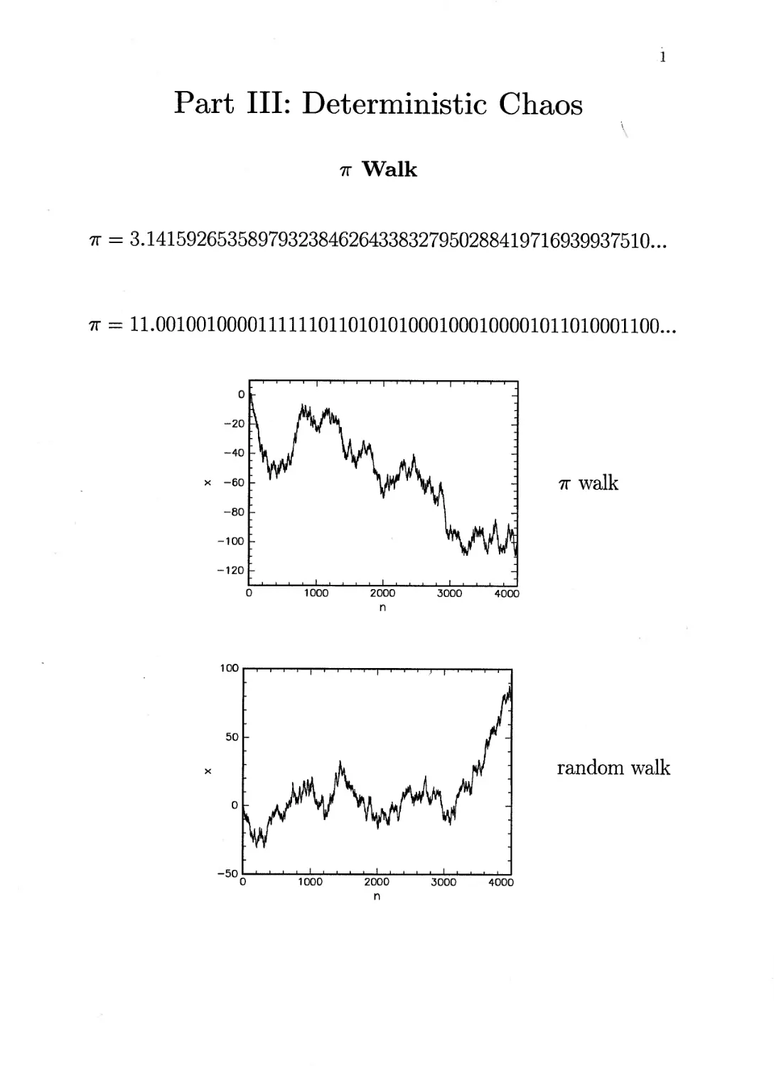
Part III: Deterministic Chaos
7Г Walk
7Г = 3.14159265358979323846264338327950288419716939937510...
7Г = 11.00100100001111110110101010001000100001011010001100...
7Г walk
random walk
2
Henon-Heiles System
1: U = 0.01
2: U = 0.04
3: U = 0.125
triangle: U = 1/6
Equation of motion
dH
Oxi
x = px
У = Py
px = -x- 2xy
Py = -y-X2 + y2
4 — d phase space: x, y,px,py
3
The Trajectory in the Phase Space
4
Projection into XY plane (E = 0.166)
5
Poincare Sections
Fig. 6: Qualitatively different trajectories can be distinguished by their Poincare sections:
a) chaotic motion; b) approach of a fixed point; c) cycle; d) cycle of period two.
x(ti) = 0
Three Body Problem
Typical orbit in a three body problem of celestial mechanics.
The upper part shows the beginning, the lower part the sequel of
the chaotic motion of a small planet around two suns of equal mass.
Driven Pendulum
в' + yO + sin 0 = A cos(cu£)
Fig. 2: Transition to chaos in a driven pendulum, a) Regular motion at small values of the
amplitude A of the driving torque, b) Chaotic motion at A = A e (note the different scales for 6).
c) and d) Regular and irregular trajectories in phase space {6, 6) which correspond to a) and b).
e) Phase diagram of the driven pendulum (у = 0.2. 0(0) = 0, 0(0) = 0). Black points denote
parameter values (A, co) for which the motion is chaotic. (After Bauer, priv. comm.)
Double Pendulum
Demo version:
http: //www.scruffy.phast.umass.edu/all4/dpendulum.html
9
Ueda Attractor
x + 0.05a; + x3 = 4.1 cos(0.7t)
Poincare section
X
10
Chaos in Dissipative Systems
Lorenz Attractor
X = (т[у — x)
у = px — у — xz
z = xy — /3z
a = 10, p = 28, P = 8/3, ж(0) = 2/(0) = г(0) = 1
Sensitivity to Initial Conditions
D(t) = D(0)ehi,
n
12
2-d Lorentz Gas
13
14
Billiards
FIG. 1. Stadium boundary for the Helmholtz equation. The
boundary shape is governed by the parameter y=a/2? with the
restriction that the area remain constant (=ir).
FIG. 3. Typical example of a single trajectory in the /=1
stadium boundary.
15
Systems With Deterministic Chaos
Forced pendulum
Fluids near the onset of turbulence
Lasers
Nonlinear optical devices
Josephson junctions
Chemical reactions
Classical many-body systems (three-body problem)
Particle accelerators
Plasmas with interacting nonlinear waves
Biological models for population dynamics
Stimulated heart cells
16
The Periodically Kicked Rotator
Rotator kicked by a force E
oo
Ф + IV = F = Kf(<p) E 6(t - nT),
n=0
n integer
Г is the damping constant, T is the period between two kicks.
Two variables x = 92 and у = ф
(xn, yn) = lim[a?(nT - e), y(nT - e)]
Two-dimensional map
1 - e-rT
^n+l
?/n+l
17
Logistic Map
жп+1 = rxn(l - xn), (0 < X < 1, 0 < r < 4)
Henon Map
«^n+l — 1 + Уп
Уп+l ~ bxn
Chirikov or Standart Map
Г —> 0, /(ж) = — sin x
4~ 3/n+l
2/n+i = Уп ~ К sin xn
18
The Bernoulli Shift
(mod 1) =
if xn < 0.5,
жп+1 = Frac (2®n)
n
£o = 1/3, x2 = 2/3, £3 = 1/3 = £0
£o — 0.2, xi = 0.4, X2 = 0.8, £3 = 0.6, x^ = 0.2 = xq.
xq = 0.21, xi = 0.42, X2 = 0.84, x% = 0.68, x± = 0.36, x$ = 0.72,
xq = 0.44, xy = 0.88, x% = 0.76, xg = 0.52, ®ю = 0.04, хц =
0.08, a?i2 = 0.16, а?1з = 0.32, «и = 0.64, x15 = 0.28, Ж16 = 0.56,
£17 = 0.12, £18 = 0.24, £19 = 0.48, £20 = 0.96, £21 = 0.92,
£22 = 0.84 = £2!
19
X
20
Unstable periodic orbits
Xk PC exact abs error rel. error in %
Xq 0.21 0.21 0 0
Xi 0.4200000 0.42 0 0
X2 0.8400000 0.84 0 0
£3 0.6799999 0.68 0.1192093E-06 0.00001753078
Ж4 0.3599999 0.36 0.1192093E-06 0.00003311369
X5 0.7199998 0.72 0.2384186E-06 0.00003311369
x6 0.4399996 0.44 0.3874302E-06 0.00008805231
x7 0.8799992 0.88 0.7748604E-06 0.00008805231
x8 0.7599983 0.76 0.1668930E-05 0.0002195961
x9 0.5199966 0.52 0.3397465E-05 0.0006533586
£10 0.03999329 0.04 0.6709248E-05 0.01677312
Xn 0.07998657 0.08 0.1342595E-04 0.01678243
£12 0.1599731 0.16 0.2689660E-04 0.01681037
£13 0.3199463 0.32 0.5370378E-04 0.01678243
£14 0.6398926 0.64 0.1074076E-03 0.01678243
£15 0.2797852 0.28 0.2148151E-03 0.07671969
£16 0.5595703 0.56 0.4296899E-03 0.07673033
£17 0.1191406 0.12 0.8593947E-03 0.7161623
£18 0.2382812 0.24 0.1718789E-02 0.7161623
£19 0.4765625 0.48 0.3437489E-02 0.7161436
£20 0.9531250 0.96 0.6874979E-02 0.7161436
£21 0.9062500 0.92 0.1375002E-01 1.494567
£22 0.8125000 0.84 0.2749997E-01 3.273807
£23 0.6250000 0.68 0.550000E-01 8.088236
21
Binary representation
0 < жо < 1
_ <7,1 a2 a3 oo
жо — ~ = z2 «t/2 = O.aia2a3...
•Z Tt O l/=l
where аг = 0 or 1.
Examples:
0.5 = 0.1, 0.25 = 0.01, 3/4 = 0.11, etc
o.2 = o.gon^onoon... = 0.0011
1/3 = 0.01, 1/7 = 0.001
0.21 = 0.0011010111000010100011
How to find binary representation?
let xq = x = O.aoaia2«3, and we compute
xn+i = 2жп (modi); n = 0,1,2...
then
a _ f 0, if xk < 1/2,
1 1, otherwise
22
The Shift Operator
Xi = <т(жо) = 0.O2«3«4-”
X2 = Сг(Ж1) = 0.«304615...
x3 = a(x2) = O.a4a5a6...
An Infinite Number of Unstable Periodic Orbits
Xq = 0.010203—O>k
Уо = 0.O1O2O3...Ofc.-
Initial Point Difference |x0 - 1/чг| Period
Binary Fraction
0.0101000101111100110000011... 1/тг 0.000- 2° aperiodic
O.01010 10/31 0.137- 2~5 5
0.0101000101 325/1023 0.632- 2-io 10
0.010100010111110 10430/32767 0.060- 2-is 15
0.01010001011111001100 333772/1048575 0.211- 2-20 20
0.O1010001O1111100110000011 10680707/334554431 0.113- 2-25 25
Periodic points are dense!
23
Properties of Chaos
• Sensitivity to initial conditions
• Periodic points are dense
• Mixing or ergodicity
Sensitivity:
xq = O.aia2«3---anbi&2^3---, Vo = O.aia2a^...anciC2C2...
Xn = O.616263... , yn = O.C1C2C3...
Mixing: Choose any two arbitrarily small interval I and J. For
mixing, one requres that one can find a starting point xq in I,
whose orbit will enter the other interval at some iteration.
Figure 10.40 : Mixing requires that any given interval J can be reached from
any other interval. Here two examples are shown how we can reach a small
Interval at 0.0110.
24
Ergodicity: means that if we pick a number Xq in the unit interval
at random, then almost surely (with probability equal to one) the
results of the shift operation will produce numbers which will get
arbitrarily close to any number in the unit interval. Numbers Xq
with a periodic pattern in their binary expansion do not show such
behavior and in some way they are extremly scarely populated in
the unit interval.
Almost all irrational numbers in [0,1] (with the
exception of a set of measure zero) in their binary
representation contain any finite sequence of digits
infinitely often.
У = 0.616263...bk..., xG = O.a1a2a3...anb1b2b3...bkan+k...
\xn - y\ < 2 k
An important property of the Bernoulli shift
For random Xq G [0,1] the sequence of iterates crn(a?o) (where
сг2(ж) = сг(сг(ж))) has the same random properties as successive
tosses of a coin.
xG = (0. 1 0 0 1
25
Liapunov Exponent for the Bernoulli Shift
xn+i = Frac (2xn), Xk = Frac (2^0)
C-, _ _ гЛ1п2 _ ( ln2\^
£k — So — e Sq — j so
Л = In 2 — Liapunov exponent for the Bernoulli shift
26
The two basic ingredients of chaos
Stretch-Cut-and-Paste
Uniform kneading by stretch-cut-
and-paste.
Stretch-and-cut-and-paste: Stretch to twice the length. Cut in
half. Move the right half up, slide it
over the left half, and paste it down.
Figure 10.30
stretch
move up
slide left
Kneading with a Rolling Pin
Kneading as a feedback process:
stretch, fold, stretch, and so on.
Stretch
Fold
Stretch
Figure 10.26
27
Tent Map
жп+1 = T(xn) = 1 — 2
nt
if xn < 0.5,
if xn > 0.5
Unstable fixed point x$ = 2/3.
28
Unstable fixed point x0 = 2/3
x = T(x), x = 2/3
X
29
Periodic Orbits for the Tent Map
T(T(0.4)) = T2
(0.4) = 0.4, T(T(0.8)) = T2(0.8) = 0.8
X
30
How to find periodic orbits for the tent map?
One can easily check that
T(T(x)) = Т(ф))
Therefore
T(T(T(x))) = T(<r(a(x)))
Tn(x) = Tan~l(x)
The theorem
Let wq be a periodic point of the Bernoulli shift with period n
Wq = (Tn[wQ).
Then xq = T(wq) is the periodic point of the tent map with the
same period.
Proof:
П*о) = T\T(w0)) = T"+1(w0) = Z(a"(w0)) = T(w0) = x0
31
The Triangular Map Д(ж)
For r = 1 the triangular map is equivalent to the tent map
Liapunov exponent
A = In 2r,
rc = 1/2
r < rc, A < 0 (order), r > rc, A > 0 (chaos)
32
1/2
Transition from Order to Chaos at r
r < 1/2
order
r > 1/2
chaos
X
33
0.70
0.65
0.60
xc 0.55
0.50
0.45
0.40
0 200 400 600 800 1000
Example of chaotic behavior for r = 0.7
0.70
0.65
0.60
xc 0.55
0.50
0.45
0.40
0 50 100 150 200
П
П
34
Deterministic Diffusion
Piecewise linear periodic map
~b ffan))
*^n+l — —
f(x ± 1) = /(a:)
•^n
(xn) = 0, (aty oc n
35
X
n
36
37
Logistic Map
(0 < x < 1, 0 < A < 4)
Two Fixed Points
, a?0 — 0, xi =
xq is stable for 0 < A < 1, x± is stable for 1
38
xq = 0 is the only attractor for 0 < Л < 1
X
39
xi = (A — 1)/A is the only attractor for 1 < A < 3
40
41
Spiraling to the fixed point, 2 < Л < 3.
42
X
43
Period Doubling — Route to Chaos
44
1.0
0.8
0.6
с
X
0.4
0.2
0.0
0 10 20 30 40 50
45
Period Two Orbit, 3 < A < 1 + у/б
xn+i = f(xn), f(x) = A®(1 - x)
Period two orbit:
/(Xi) = Ж2, /(Ж2) = => /(Ж)) = Xi
—А3#4 + 2А3ж3 - Л2(1 + А)ж2 + (А2 — 1)ж = О
х = 0 and ж = (А — 1)/А are roots of this equation.
= 0,
+ 1 ± ~ 3)(A + 1)
46
47
region of stability
[/(№))]' = /'(ж2)/'(й1) = -A2 + 2A + 4
—A2 + 2A + 4 = —1 =>• A = 1 + V6 « 3.449
48
Period Four Orbit
П
49
/(/(/(/(*)))) = f\x) = х
X
50
Period Eight Orbit
51
Chaos
X
52
1.0
0.8
0.6
с
X
0.4
0.2
0.0
0 200 400 600 800 1000
П
53
The Bifurcation Diagramm
0 12 3 4
X
54
The Infinite Sequence of Period-Doublings
Ai =3, A2 = 3.449, A3 = 3.544, A4 = 3.564,
ATO = 3.5699456...
55
The Feigenbaum Constants and Universality
5 = lim —^-1 = 4.6692...
k^°° A^+i — Xk
a = lim = 2.5029...
k-+oo dk
Fig. 24: Distances d„ of the fixed points
closest to x = 1/2 for superstable
2"-cycles (schematically).
= 0.543
56
Universality of the
Feigenbaum Constant
Results from experiments wherein
period-doubling plays a role. The
numbers in the third column are to
be compared with the Feigenbaum
constant 6 = 4.669... Table adapted
from P. Cvitanovid, Universality in
Chaos, Adam Hilger, Bristol, 1984.
Table 11.24
Experimental Measurements of Period-Doublings
Experiment Number of period doublings 6
Hydrodynamic: water 4 4.3 ±0.8
helium 4 3.5 ±0.15
mercury 4 4.4 ±0.1
Electronic: diode 5 4.3 ±0.1
transistor 4 4.7 ±0.3
Josephson 4 4.4 ±0.3
Laser: laser feedback 3 4.3 ±0.3
Acoustic: helium 3 4.8 ±0.6
57
Self- Similarity
Self-Similarity in the
Feigenbaum Diagram
A close-up sequence of the final-
state diagram of the quadratic iter-
ator reveals its self-similarity. Note
that the vertical values in the first
and third magnifications have been
reversed to reflect the fact that the
previous diagram has been inverted.
The second magnification is. of
course, also a vertical inversion of
the first; the values, however, are in
their ‘normal* relationship.
Figure 11.3
58
59
3.840 3.845 3.850 3.855
60
The Period Three Window
61
1.0
0.8
0.6
0.4
0.2
0.0
0 20 40 60 80 100
X
62
X
63
Лс = 1 + Ve = 3.8284271...
X
64
The Intermittency Route to Chaos
X=3.8284
0 500 1000 1500 2000
П
65
Figure IX.2 Iteration of и I—► u'(u) when two fixed points u± exist.
The point и_ is locally stable: iterations starting near it converge towards it. However
u+ is unstable: iterations diverge from it.
Figure 1X3 Iteration of и —► и' = и + s + и2 for в > 0.
Unlike that of Figure IX.2 (s < 0), this mapping has no fixed point For s small and
positive, iterations beginning at negative values of и spend a long time in the narrow
channel separating the graphs of u' and the identity map.
66
Chaos
1.0
0.8
0.6
c
X
0.4
0.2
0.0
хц = 0.9
П
67
л=4 х0 = 0.900001
п
68
Lyapunov Exponent for Logistic Map
Lyapunov exponent