The PowerPC Compiler Writer's Guide - Hoxey S., Karim F., Hay B., Warren H.

Автор: Hoxey S. Karim F. Hay B. Warren H.

Теги: programming computer science

ISBN: 0-9649654-0-2

Год: 1996

Похожие

Engineering a Compiler

Beginning C++ Compilers: An Introductory Guide to Microsoft C/C++ and MinGW Compilers

Compilers Pearson New International Edition Principles, Techniques, and Tools

Embedded Systems Architecture. A Comprehensive Guide for Engineers and Programmers. (Embedded Technology)

Текст

The PowerPC
Compiler Writer’s Guide

Edited by:

Steve Hoxey
Faraydon Karim
Bill Hay
Hank Warren

Warthman
Associates

© International Business Machines Corporation 1996. All rights reserved.
1-96. Printed in the United State of America.
This notice applies to The PowerPC Compiler Writer’s Guide, dated January 1996. The following paragraphs do not apply
in any country or state where such provisions are inconsistent with local law: The specifications in this publication are
subject to change without notice. The publication is provided “AS IS.” International Business Machines Corporation
(hereafter “IBM”) does not make any warranty of any kind, either expressed or implied, including, but not limited to, the
implied warranties of merchantability and fitness for a particular purpose. Information in this document is provided solely
to enable system and software implementers to use PowerPC microprocessors. Unless specifically set forth herein, there
are no express or implied patent, copyright or any other intellectual property rights or licenses granted hereunder to design
or fabricate PowerPC integrated circuits or integrated circuits based on the information in this document. Permission is
hereby granted to the owner of this publication to copy and distribute only the code examples contained in this publication
for the sole purpose of enabling system and software implementers to use PowerPC microprocessors, and for no other
purpose. IBM does not warrant that the contents of this publication or the accompanying code examples, whether
individually or as one or more groups, will meet your requirements or that the publication or the accompanying code
examples are error-free. This publication could include technical inaccuracies or typographical errors. Changes may be
made to the information herein; these changes may be incorporated in new editions of the publication.
Notice to U.S. Government Users—Documentation Related to Restricted Rights—Use, duplication or disclosure is subject
to restrictions set forth in GSA ADP Schedule Contract with IBM Corporation.
The following are registered trademarks of the IBM Corporation: IBM and the IBM logo.
The following are trademarks of the IBM Corporation: IBM Microelectronics, POWER, RISC System/6000, PowerPC,
PowerPC logo, PowerPC 601, PowerPC 603, PowerPC 604. PowerPC™ microprocessors are hereinafter sometimes
referred to as “PowerPC”.
The following are trademarks of other companies:
SPECfp92, SPECint92, SPECfp95, and SPECint95 are trademarks of Standard Performance Evaluation Corporation.
Requests for copies of this publication should be made to the office shown below. IBM may use, disclose or distribute
whatever information you supply in any way it believes appropriate without incurring any obligation to you.
IBM Microelectronics Division
1580 Route 52, Bldg. 504
Hopewell Junction, NY 12533-6531
Tel: (800) POWERPC
Fax Service 415-855-4121
The IBM home page can be found at: http://www.ibm.com
The IBM Microelectronics Division PowerPC home page can be found at: http://www.chips.ibm.com/products/ppc
Library of Congress Catalog Card Number: 95-62115
ISBN 0-9649654-0-2
Published for IBM by:
Warthman Associates
240 Hamilton Avenue
Palo Alto, California 94301
(415) 322-4555
writers@warthman.com

Foreword

By
Fredrick R. Sporck
Director
IBM Microelectronics Division—PowerPC Products

IBM’s reputation for commitment to technology and innovation is legendary in the computer
industry. Over the past two decades, IBM has followed this tradition with its dedication to
the development and enhancement of RISC architecture.
With the introduction of the PowerPC architecture, IBM has again recognized the need for
supporting its products. In response, IBM has prepared The PowerPC Compiler Writer’s
Guide. Some of the brightest minds from many companies in the fields of compiler and processor development have combined their efforts in this work. A balanced, insightful examination of the PowerPC architecture and the pipelines implemented by PowerPC processors
has yielded a guide giving compiler developers valuable insight into the generation of highperformance code for PowerPC processors.
By taking this step, IBM is equipping readers of The PowerPC Compiler Writer’s Guide with
the power to harness the potential of the PowerPC revolution. Once again, IBM is stepping
forward with dedication to its customers and the powerful backing of its cutting-edge architecture.

Contents

Introduction

1.1

RISC Technologies........................................................................................................ 1

1.2

Compilers and Optimization .......................................................................................... 3

1.3

Assumptions ................................................................................................................. 4

Overview of the PowerPC Architecture

2.1
2.1.1
2.1.2
2.1.2.1
2.1.2.2
2.1.2.3
2.1.3
2.1.3.1
2.1.3.2
2.1.3.3
2.1.4

Application Environment ............................................................................................... 5
32-Bit and 64-Bit Implementations and Modes......................................................... 5
Register Resources................................................................................................... 7
Branch .................................................................................................................. 7
Fixed-Point ........................................................................................................... 7
Floating-Point ....................................................................................................... 8
Memory Models........................................................................................................ 8
Memory Addressing ............................................................................................. 8
Endian Orientation .............................................................................................. 10
Alignment ........................................................................................................... 10
Floating-Point ......................................................................................................... 11

2.2
2.2.1
2.2.2
2.2.3
2.2.3.1
2.2.3.2
2.2.3.3

Instruction Set ............................................................................................................ 13
Optional Instructions .............................................................................................. 13
Preferred Instruction Forms.................................................................................... 14
Communication Between Functional Classes .......................................................... 14
Fixed-Point and Branch Resources..................................................................... 14
Fixed-Point and Floating-Point Resources.......................................................... 15
Floating-Point and Branch Resources ................................................................ 15

Code Selection

3.1
3.1.1
3.1.1.1
3.1.1.2
3.1.1.3
3.1.2
3.1.2.1
3.1.2.2
3.1.2.3
3.1.3
3.1.3.1

Control Flow................................................................................................................ 17
Architectural Summary ........................................................................................... 19
Link Register ...................................................................................................... 19
Count Register.................................................................................................... 20
Condition Register.............................................................................................. 21
Branch Instruction Performance............................................................................. 22
Fall-Through Path ............................................................................................... 23
Needless Branch Register and Recording Activity .............................................. 23
Condition Register Contention............................................................................ 23
Uses of Branching .................................................................................................. 23
Unconditional Branches...................................................................................... 23

3.1.3.2
3.1.3.3
3.1.3.4
3.1.3.5
3.1.3.6
3.1.4
3.1.4.1
3.1.4.2
3.1.4.3
3.1.5
3.1.5.1
3.1.5.2
3.1.5.3

Conditional Branches.......................................................................................... 24
Multi-Way Conditional Branches......................................................................... 25
Iteration .............................................................................................................. 28
Procedure Calls and Returns .............................................................................. 32
Traps and System Calls ...................................................................................... 34
Branch Prediction ................................................................................................... 35
Default Prediction and Rationale......................................................................... 35
Overriding Default Prediction.............................................................................. 36
Dynamic Branch Prediction ................................................................................ 37
Avoiding Branches .................................................................................................. 37
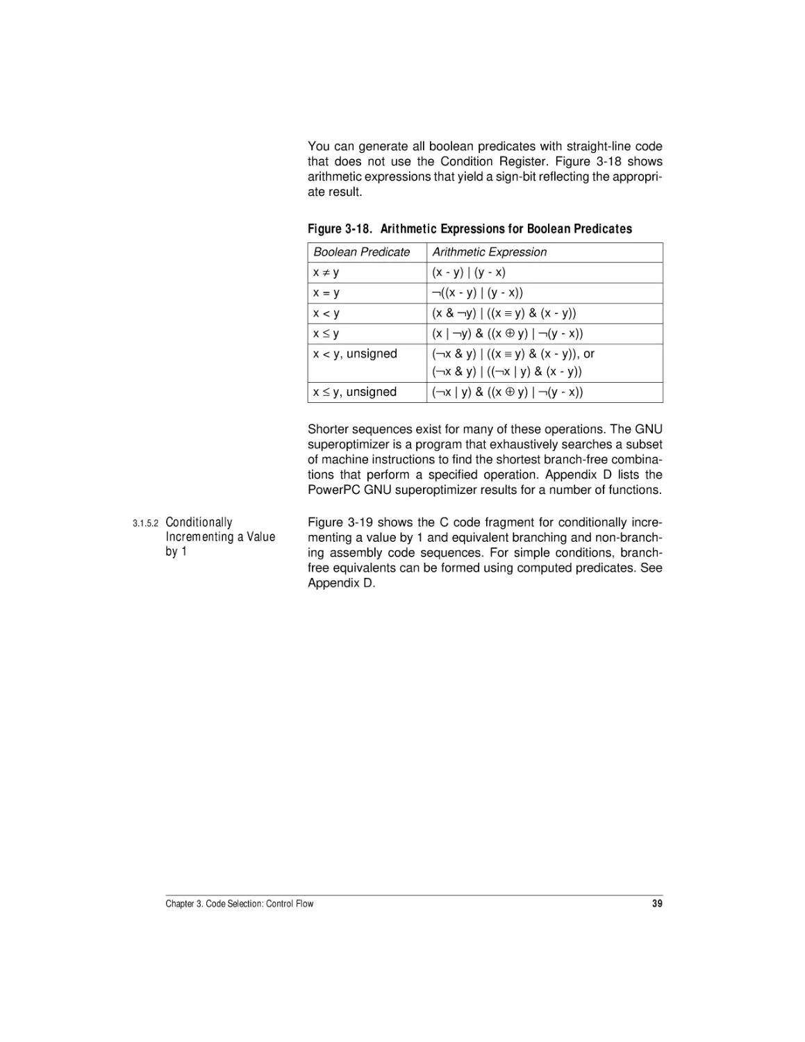
Computing Predicates ........................................................................................ 38
Conditionally Incrementing a Value by 1............................................................. 39
Condition Register Logical.................................................................................. 40

3.2
3.2.1
3.2.1.1
3.2.1.2
3.2.1.3
3.2.1.4
3.2.1.5
3.2.2
3.2.2.1
3.2.2.2
3.2.2.3
3.2.2.4
3.2.2.5
3.2.2.6
3.2.3
3.2.3.1
3.2.3.2
3.2.3.3
3.2.3.4
3.2.3.5
3.2.3.6
3.2.3.7
3.2.3.8
3.2.3.9
3.2.3.10

Integer and String Operations ..................................................................................... 43
Memory Access ...................................................................................................... 43
Single Scalar Load or Store ................................................................................ 43
Load and Reserve/ Store Conditional.................................................................. 44
Multiple Scalar Load or Store ............................................................................. 45
Byte-Reversal Load or Store............................................................................... 45
Cache Touch Instructions ................................................................................... 45
Computation ........................................................................................................... 45
Setting Status ..................................................................................................... 46
Arithmetic Instructions ....................................................................................... 47
Logical Instructions ............................................................................................ 47
Rotate and Shift Instructions .............................................................................. 47
Compare Instructions ......................................................................................... 48
Move To/From XER............................................................................................. 48
Uses of Integer Operations ..................................................................................... 48
Loading a Constant into a Register ..................................................................... 48
Endian Reversal .................................................................................................. 49
Absolute Value.................................................................................................... 50
Minimum and Maximum..................................................................................... 51
Division by Integer Constants ............................................................................. 51
Remainder .......................................................................................................... 61
32-Bit Implementation of a 64-Bit Unsigned Divide ............................................ 62
Bit Manipulation.................................................................................................. 65
Multiple-Precision Shifts .................................................................................... 66
String and Memory Functions ............................................................................ 68

3.3
3.3.1
3.3.2
3.3.2.1
3.3.2.2
3.3.2.3
3.3.2.4
3.3.3
3.3.4
3.3.4.1
3.3.4.2
3.3.4.3

Floating-Point Operations............................................................................................ 72
Typing, Conversions and Rounding ........................................................................ 72
Memory Access ...................................................................................................... 74
Single-Precision Loads and Stores..................................................................... 74
Double-Precision Loads and Stores.................................................................... 74
Endian Conversion.............................................................................................. 75
Touch Instructions.............................................................................................. 75
Floating-Point Move Instructions ............................................................................ 75
Computation ........................................................................................................... 75
Setting Status Bits .............................................................................................. 75
Arithmetic ........................................................................................................... 75
Floating-Point Comparison ................................................................................. 76

3.3.5
3.3.6
3.3.6.1
3.3.6.2
3.3.6.3
3.3.6.4
3.3.6.5
3.3.7
3.3.7.1
3.3.8
3.3.8.1
3.3.8.2
3.3.8.3
3.3.9
3.3.10
3.3.11
3.3.12

FPSCR Instructions................................................................................................. 76
Optional Floating-Point Instructions ....................................................................... 77
Square Root ....................................................................................................... 77
Storage Access................................................................................................... 77
Reciprocal Estimate............................................................................................ 77
Reciprocal Square Root Estimate ....................................................................... 77
Selection............................................................................................................. 78
IEEE 754 Considerations......................................................................................... 78
Relaxations......................................................................................................... 79
Data Format Conversion ......................................................................................... 79
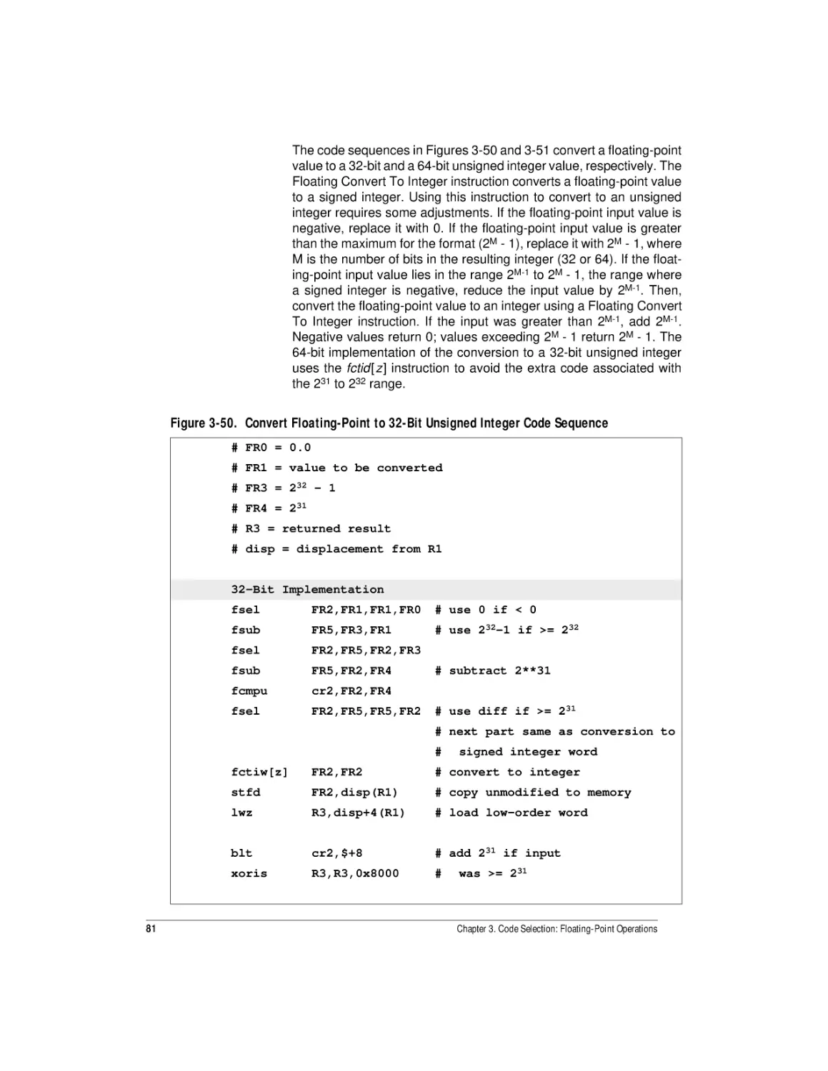
Floating-Point to Integer..................................................................................... 80
Integer to Floating-Point..................................................................................... 83
Rounding to Floating-Point Integer .................................................................... 85
Floating-Point Branch Elimination........................................................................... 86
DSP Filters.............................................................................................................. 92
Replace Division with Multiplication by Reciprocal................................................. 92
Floating-Point Exceptions ....................................................................................... 93

Implementation Issues

4.1

Hardware Implementation Overview ........................................................................... 98

4.2
4.2.1
4.2.2
4.2.3
4.2.4

Hazards ..................................................................................................................... 100
Data Hazards......................................................................................................... 100
Control Hazards .................................................................................................... 102
Structural Hazards ................................................................................................ 103
Serialization .......................................................................................................... 104

4.3
4.3.1
4.3.2
4.3.3
4.3.4
4.3.5
4.3.6
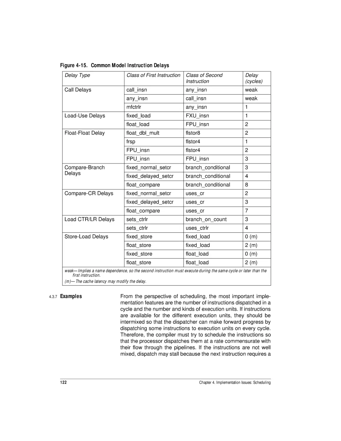
4.3.7

Scheduling ................................................................................................................ 104
Fixed-Point Instructions........................................................................................ 104
Floating-Point Instructions ................................................................................... 105
Load and Store Instructions ................................................................................. 106
Branch Instructions .............................................................................................. 110
List Scheduling Algorithm .................................................................................... 112
Common Model .................................................................................................... 117
Examples .............................................................................................................. 122

4.4
4.4.1
4.4.2
4.4.3

Alignment.................................................................................................................. 133
Loads and Stores.................................................................................................. 133
Fetch Buffer .......................................................................................................... 134
TLB and Cache...................................................................................................... 134

Clever Examples

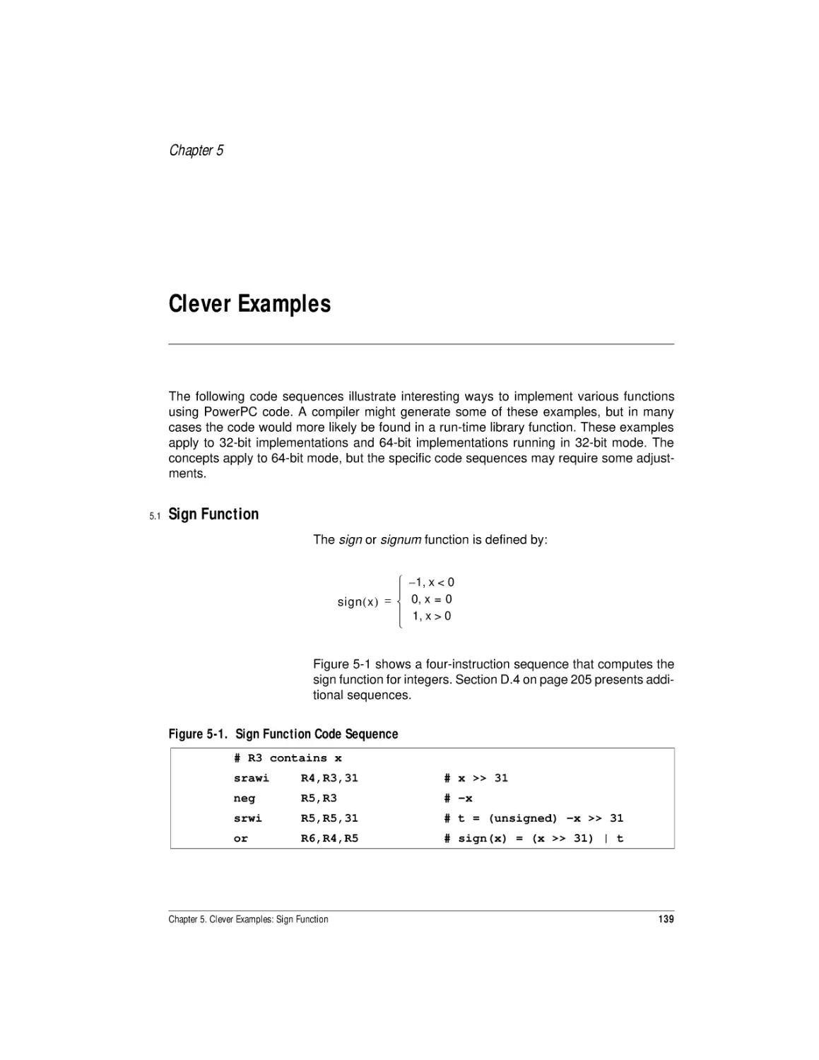
5.1

Sign Function ............................................................................................................ 139

5.2

Transfer of Sign ........................................................................................................ 140

5.3

Register Exchange .................................................................................................... 140

5.4

x = y Predicate .......................................................................................................... 141

5.5

Clear Least-Significant Nonzero Bit........................................................................... 141

139

vii

5.6

Round to a Multiple of a Given Power of 2 ................................................................ 142

5.7

Round Up or Down to Next Power of 2 ..................................................................... 142

5.8

Bounds Checking ...................................................................................................... 144

5.9

Power of 2 Crossing.................................................................................................. 144

5.10

Count Trailing Zeros.................................................................................................. 145

5.11

Population Count....................................................................................................... 146

5.12

Find First String of 1-Bits of a Given Length.............................................................. 150

5.13

Incrementing a Reversed Integer .............................................................................. 152

5.14

Decoding a “Zero Means 2n” Field............................................................................. 153

5.15

2n in Fortran .............................................................................................................. 154

5.16

Integer Log Base 10 .................................................................................................. 154

Appendices
A.

ABI Considerations

A.1
A.1.1
A.1.2
A.1.3

Procedure Interfaces ................................................................................................. 157
Register Conventions............................................................................................ 158
Run-Time Stack .................................................................................................... 160
Leaf Procedures.................................................................................................... 163

A.2
A.2.1
A.2.2
A.2.3

Procedure Calling Sequence...................................................................................... 163
Argument Passing Rules....................................................................................... 163
Function Return Values......................................................................................... 165
Procedure Prologs and Epilogs............................................................................. 165

A.3
A.3.1
A.3.2
A.3.3

Dynamic Linking........................................................................................................ 167
Table Of Contents.................................................................................................. 167
Function Descriptors............................................................................................. 168
Out-of-Module Function Calls ............................................................................... 168

Summary of PowerPC 6xx Implementations

B.1

Feature Summary ...................................................................................................... 171

B.2
B.2.1
B.2.2

Serialization............................................................................................................... 174
PowerPC 603e Processor Classifications.............................................................. 174
PowerPC 604 Processor Classifications ............................................................... 174

B.3

Instruction Timing..................................................................................................... 175

B.4

Misalignment Handling.............................................................................................. 184

viii

157

171

PowerPC Instruction Usage Statistics

C.1

By Instruction Category............................................................................................. 187

C.2

By Instruction............................................................................................................ 188

C.3

General Information .................................................................................................. 195

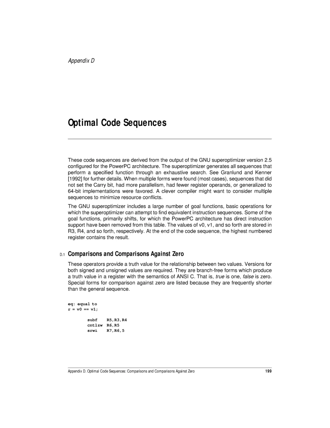
Optimal Code Sequences

D.1

Comparisons and Comparisons Against Zero ........................................................... 199

D.2

Negated Comparisons and Negated Comparisons Against Zero ............................... 202

D.3

Comparison Operators .............................................................................................. 204

D.4

Sign Manipulation ..................................................................................................... 205

D.5

Comparisons with Addition ....................................................................................... 206

D.6

Bit Manipulation ........................................................................................................ 208

Glossary

209

Bibliography and References

235

F.1

Bibliography .............................................................................................................. 235

F.2

References ................................................................................................................ 235

Index

187

199

237

Figures

Figure 2-1.
Figure 2-2.
Figure 3-1.
Figure 3-2.
Figure 3-3.
Figure 3-4.
Figure 3-5.
Figure 3-6.
Figure 3-7.
Figure 3-8.
Figure 3-9.
Figure 3-10.
Figure 3-11.
Figure 3-12.
Figure 3-13.
Figure 3-14.
Figure 3-15.
Figure 3-16.
Figure 3-17.
Figure 3-18.
Figure 3-19.
Figure 3-20.
Figure 3-21.
Figure 3-22.
Figure 3-23.
Figure 3-24.
Figure 3-25.
Figure 3-26.
Figure 3-27.
Figure 3-28.
Figure 3-29.
Figure 3-30.
Figure 3-31.
Figure 3-32.
Figure 3-33.
Figure 3-34.
Figure 3-35.
Figure 3-36.
Figure 3-37.
Figure 3-38.
Figure 3-39.

Application Register Sizes..................................................................................... 6
Floating-Point Application Control Fields ............................................................ 12
if-else Code Example........................................................................................... 25
C Switch: if-else Code Sequence......................................................................... 26
C Switch: Range Test Code Sequence................................................................. 27
C Switch: Table Lookup Code Sequence ............................................................. 28
strlen Code Example ........................................................................................... 29
Branch-On-Count Loop: Simple Code Example................................................... 30
Branch-On-Count Loop: Variable Number of Iterations Code Example ............... 30
Branch-On-Count Loop: Variable Range and Stride Code Example..................... 31
Compound Latch Point Code Example................................................................ 32
Function Call Code Example—C Source ............................................................. 33
Relative Call to foo Code Sequence..................................................................... 33
Call to foo Via Pointer Code Sequence................................................................ 34
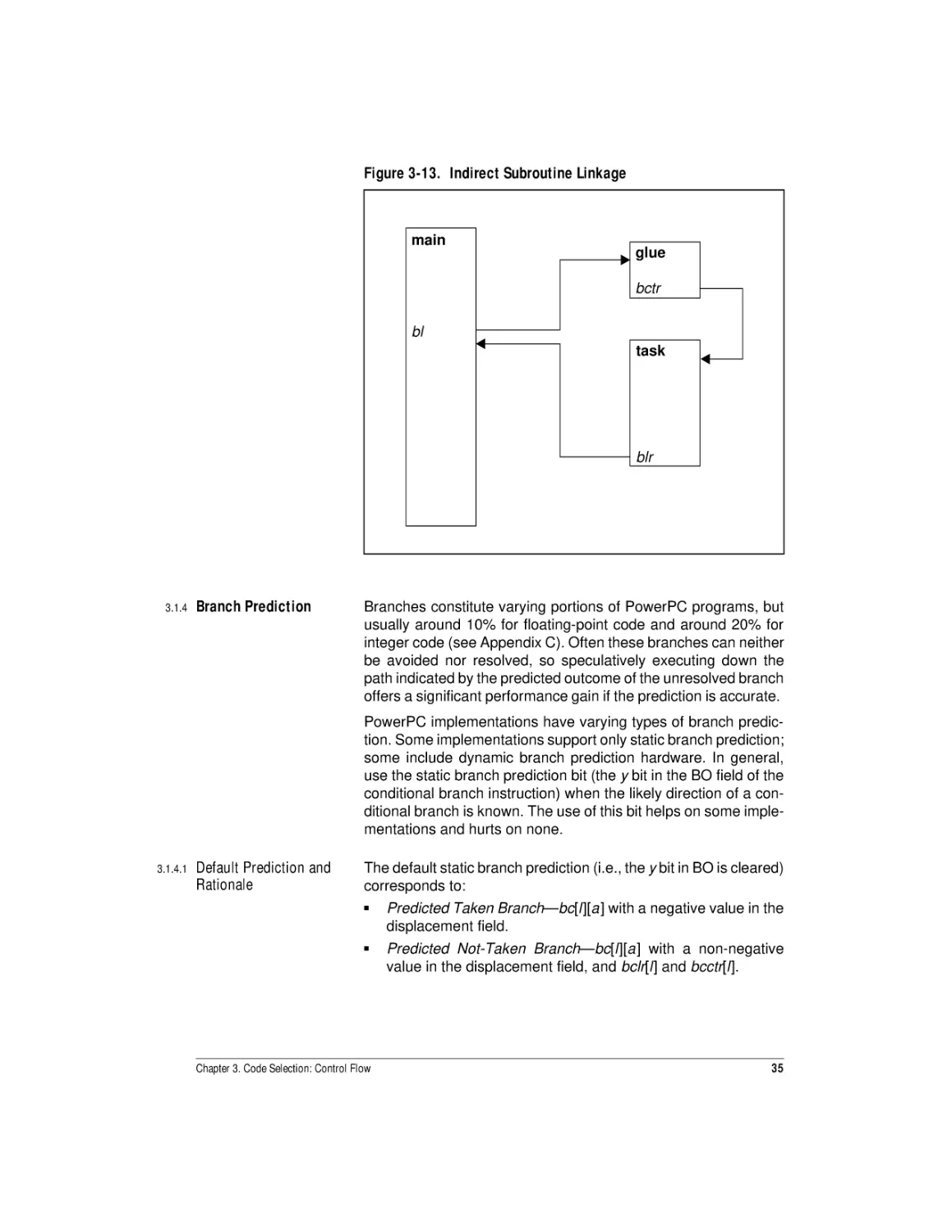
Indirect Subroutine Linkage ................................................................................ 35
Conditional Return Code Example....................................................................... 37
Predicate Calculation: Branching Code Sequence ............................................... 38
Predicate Calculation: Condition-Register Logical Code Sequence ..................... 38
Predicate Calculation: Fixed-Point-Operation Code Sequence............................. 38
Arithmetic Expressions for Boolean Predicates................................................... 39
Conditionally Incrementing a Value by 1 Code Example...................................... 40
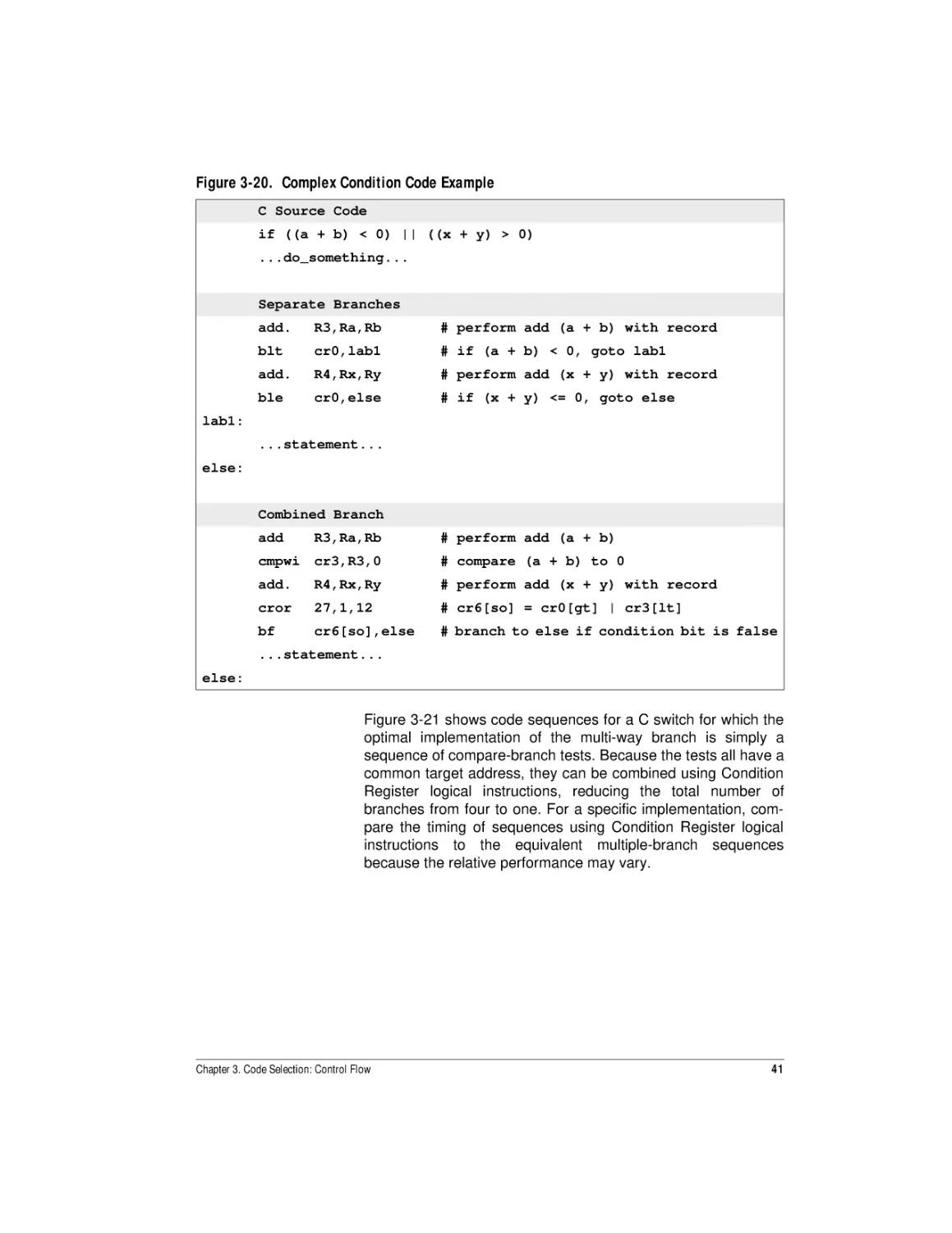
Complex Condition Code Example ...................................................................... 41
C Switch: Condition Register Logical Code Example........................................... 42
Scalar Load Instructions ..................................................................................... 44
Scalar Store Instructions .................................................................................... 44
Endian Reversal of a 4KB Block of Data Code Sequence..................................... 50
Absolute Value Code Sequence........................................................................... 50
Unsigned Maximum of a and b Code Sequence.................................................. 51
Signed Maximum of a and b Code Sequence...................................................... 52
Signed Divide by 3 Code Sequence..................................................................... 53
Signed Divide by 5 Code Sequence..................................................................... 53
Signed Divide by 7 Code Sequence..................................................................... 54
Signed Divide by -7 Code Sequence ................................................................... 55
Unsigned Divide by 3 Code Sequence................................................................. 55
Unsigned Divide by 7 Code Sequence................................................................. 56
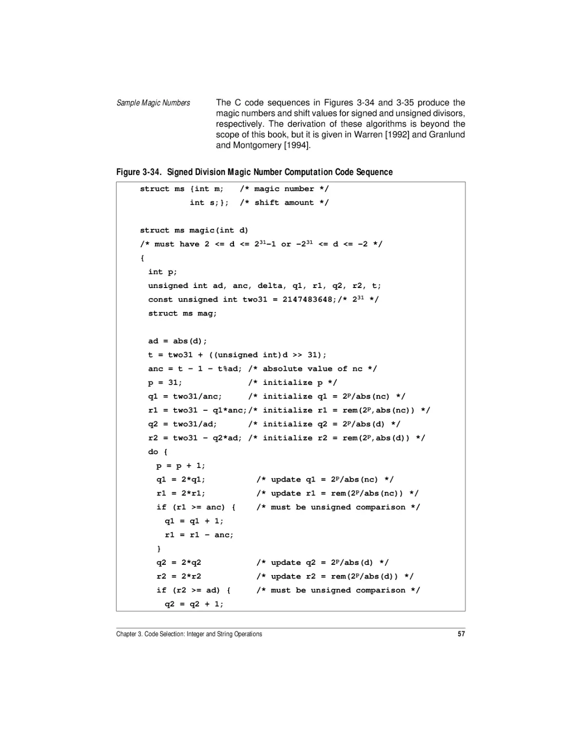
Signed Division Magic Number Computation Code Sequence ............................ 57
Unsigned Division Magic Number Computation Code Sequence ........................ 58
Some Magic Numbers for 32-Bit Operations ...................................................... 60
Some Magic Numbers for 64-Bit Operations ...................................................... 60
32-Bit Signed Remainder Code Sequence........................................................... 61
32-Bit Unsigned Remainder Code Sequence....................................................... 61
xi

Figure 3-40.
Figure 3-41.
Figure 3-42.
Figure 3-43.
Figure 3-44.
Figure 3-45.
Figure 3-46.
Figure 3-47.
Figure 3-48.
Figure 3-49.
Figure 3-50.
Figure 3-51.
Figure 3-52.
Figure 3-53.
Figure 3-54.
Figure 3-55.
Figure 3-56.
Figure 3-57.
Figure 3-58.
Figure 3-59.
Figure 3-60.
Figure 3-61.
Figure 3-62.
Figure 3-63.
Figure 3-64.
Figure 3-65.
Figure 4-1.
Figure 4-2.
Figure 4-3.
Figure 4-4.
Figure 4-5.
Figure 4-6.
Figure 4-7.
Figure 4-8.
Figure 4-9.
Figure 4-10.
Figure 4-11.
Figure 4-12.
Figure 4-13.
Figure 4-14.
Figure 4-15.
Figure 4-16.
Figure 4-17.
Figure 4-18.
Figure 4-19.
Figure 4-20.

xii

32-Bit Implementation of 64-Bit Unsigned Division Code Sequence ................... 62
Structure x .......................................................................................................... 66
Code sequences to Extract Bit Fields................................................................... 66
Code Sequences to Insert Bit Fields .................................................................... 66
Left Shift of a 3-Word Value................................................................................ 67
Code Sequence to Shift 3 Words Left When sh < 64........................................... 67
Find Leftmost 0-Byte: Non-Branching Code Sequence........................................ 69
Memset Code Sequence with Scalar Store Instructions ...................................... 70
Convert Floating-Point to 32-Bit Signed Integer Code Sequence ........................ 80
Convert Floating-Point to 64-Bit Signed Integer Code Sequence ........................ 80
Convert Floating-Point to 32-Bit Unsigned Integer Code Sequence .................... 81
Convert Floating-Point to 64-Bit Unsigned Integer Code Sequence .................... 82
Convert 32-Bit Signed Integer to Floating-Point Code Sequence ........................ 83
Convert 64-Bit Signed Integer to Floating-Point Code Sequence ........................ 84
Convert 32-Bit Unsigned Integer to Floating-Point Code Sequence .................... 84
Convert 64-Bit Unsigned Integer to Floating-Point Code Sequence .................... 85
Round to Floating-Point Integer Code Sequence................................................. 86
Greater Than or Equal to 0.0 Code Example........................................................ 87
Greater Than 0.0 Code Example .......................................................................... 88
Equal to 0.0 Code Example.................................................................................. 89
Minimum Code Example ..................................................................................... 90
a Equal To b Code Example ................................................................................. 91
Matrix Product: C Source Code........................................................................... 92
Double-Precision Matrix Product: Assembly Code.............................................. 92
Convert Division to Multiplication by Reciprocal Code Example.......................... 93
Precise Interrupt in Software Code Example ....................................................... 94
Processor Implementations ................................................................................ 98
2-Bit Branch History Table Algorithm................................................................ 103
Integer Instruction Pipeline ............................................................................... 105
Floating-Point Instruction Pipeline .................................................................... 106
Load-Store Instruction Pipeline......................................................................... 107
Pointer Chasing—Load-Use Delay .................................................................... 108
Integer-to-Float Conversion: Load-Store Contention Code Example ................. 109
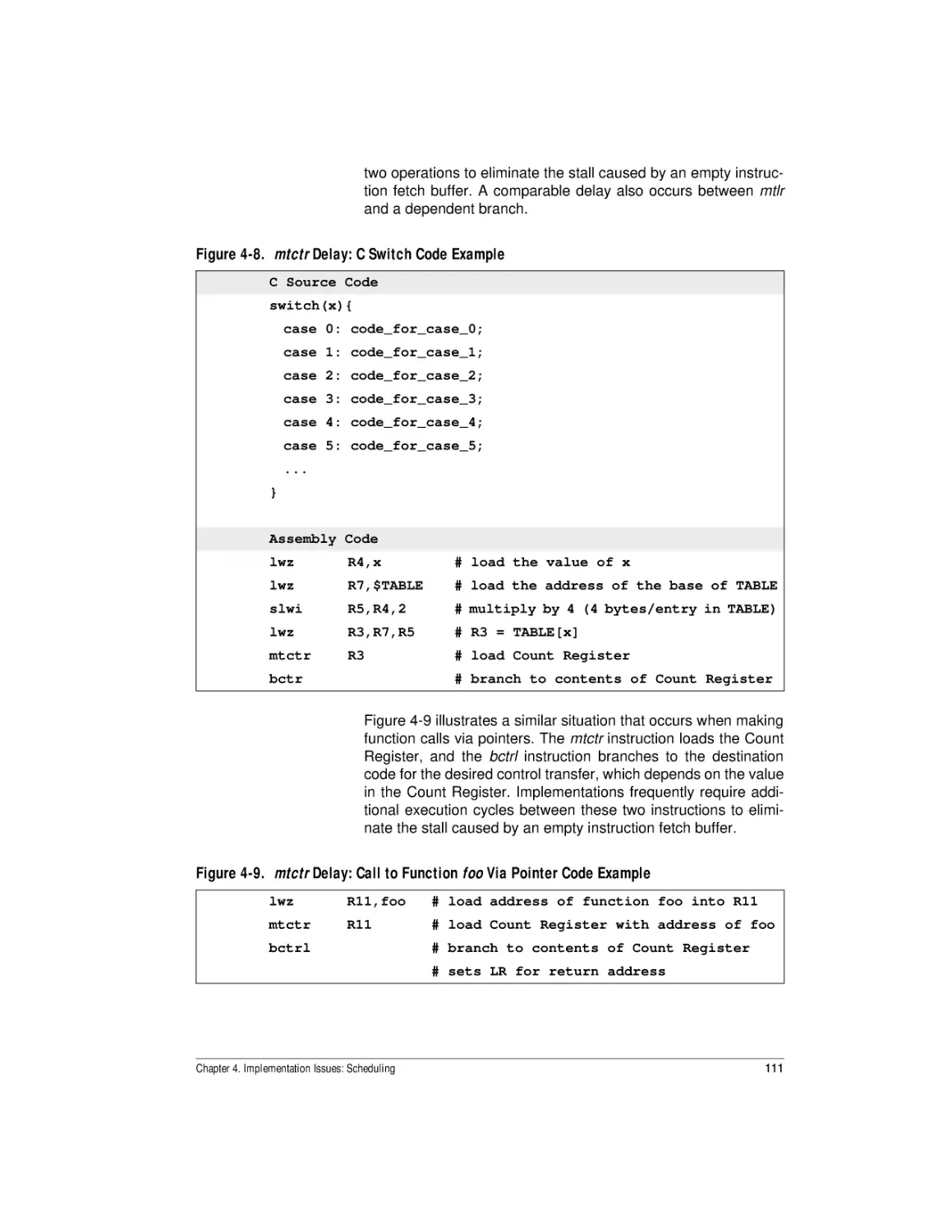
mtctr Delay: C Switch Code Example ................................................................ 111
mtctr Delay: Call to Function foo Via Pointer Code Example ............................. 111
Basic Block Code Example ................................................................................ 113
Basic Block Dependence Graph......................................................................... 113
Values for Scheduling Example......................................................................... 115
Scheduled Basic Block Code Example............................................................... 118
Common Model Instruction Classes ................................................................. 119
Common Model Instruction Delays................................................................... 122
Simple Scheduling Example with Load-Use Delay Slot ..................................... 123
Multi-Part Expression Evaluation Scheduling Example ..................................... 124
Basic Block Code Example: C Code ................................................................... 125
Basic Block Code Example: Scheduled for Common Model .............................. 126
Basic Block Code Example: Scheduled for PowerPC 604 Processor ................. 127

Figure 4-21.
Figure 4-22.
Figure 4-23.
Figure 4-24.
Figure 4-25.
Figure 5-1.
Figure 5-2.
Figure 5-3.
Figure 5-4.
Figure 5-5.
Figure 5-6.
Figure 5-7.
Figure 5-8.
Figure 5-9.
Figure 5-10.
Figure 5-11.
Figure 5-12.
Figure 5-13.
Figure 5-14.
Figure 5-15.
Figure 5-16.
Figure 5-17.
Figure 5-18.
Figure 5-19.
Figure 5-20.
Figure A-1.
Figure A-2.
Figure A-3.
Figure A-4.
Figure A-5.
Figure A-6.
Figure A-7.
Figure A-8.
Figure B-1.
Figure B-2.
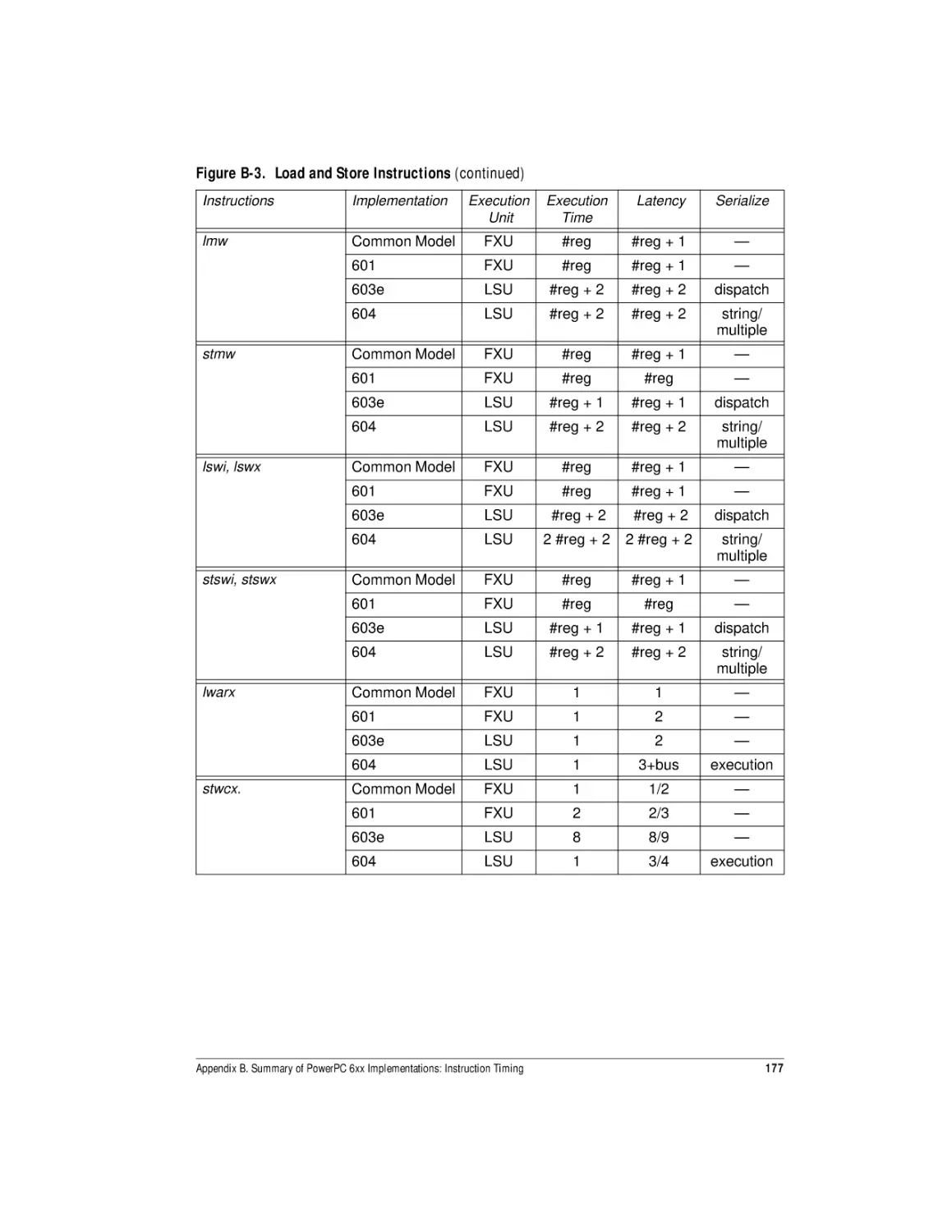
Figure B-3.
Figure B-4.
Figure B-5.
Figure B-6.
Figure B-7.
Figure B-8.
Figure C-1.
Figure C-2.
Figure C-3.
Figure C-4.
Figure C-5.

Dependent Arithmetic-Conditional Assignments Example ................................
Rescheduled Dependent Arithmetic-Conditional Assignments Example ...........
Basic Matrix Multiply Kernel Code Example ......................................................
Matrix Multiply Code Example—Scheduled for PowerPC 604 Processor .........
Nested Loops: Touch Instruction Example........................................................
Sign Function Code Sequence ..........................................................................
Fortran ISIGN Function Code Sequence ............................................................
Register Exchange Code Sequence ...................................................................
“x = y” Predicate Code Sequence......................................................................
Clear Least-Significant Nonzero Bit Code Sequence .........................................
Test for 0 or a Power of 2 Code Sequence........................................................
Round Up to a Multiple of 8 Code Sequence.....................................................
Values of flp2(x) and clp2(x).............................................................................
flp2(x) Code Sequence......................................................................................
clp2(x) Code Sequence .....................................................................................
Detect Page Boundary Crossing Code Sequence ..............................................
Count Trailing Zeros Code Sequence ................................................................
Number of Powers of 2 Code Sequence ...........................................................
Branch-Free Population Count Code Sequence.................................................
Branching Population Count Code Sequence....................................................
Alternative Population Count Code Sequence ...................................................
Detect First String of n 1-Bits Code Sequence ..................................................
Incrementing a Reversed Integer Code Sequence.............................................
2n in Fortran Code Sequence ............................................................................
Integer Log Base 10 Code Sequence ................................................................
AIX ABI Register Usage Conventions ................................................................
Relevant Parts of the Run-Time Stack for Subprogram ccc ..............................
Argument Passing for foo1 ...............................................................................
Argument Passing for foo2 ...............................................................................
Function Descriptor ..........................................................................................
main: Function-Calling Code Example...............................................................
ptrgl Routine Code Sequence............................................................................
glink_printf Code Sequence ..............................................................................
PowerPC 6xx Processor Features .....................................................................
Branch Instructions ..........................................................................................
Load and Store Instructions..............................................................................
Cache Control Instructions ...............................................................................
Fixed-Point Computational Instructions ............................................................
Floating-Point Instructions................................................................................
Optional Instructions ........................................................................................
Number of Accesses for Misaligned Operands .................................................
Instruction Frequency in Integer SPEC92 Benchmarks .....................................
Instruction Frequency in Floating-Point SPEC92 Benchmarks ..........................
Most Frequently Used Instructions in Integer SPEC92 Benchmarks .................
Most Frequently Used Instructions in Floating-Point SPEC92 Benchmarks ......
PowerPC Instruction Usage in SPEC92 Benchmarks ........................................

129
130
131
132
135
139
140
141
141
141
142
142
143
143
144
145
145
146
146
148
148
152
153
154
155
159
162
164
164
168
169
170
170
172
176
176
178
178
181
182
184
188
188
189
190
191

xiii

xiv

Preface

Purpose and Audience
This book describes, mainly by coding examples, the code patterns that perform well on
PowerPC processors. The book will be particularly helpful to compiler developers and application-code specialists who are already familiar with optimizing compiler technology and
are looking for ways to exploit the PowerPC architecture. It will also be helpful to application
programmers who need to understand and tune the output of PowerPC compilers and to
faculty members and graduate students specializing in the study of compilers. We assume
that compiler developers have already developed a compiler front-end and are seeking to
develop a PowerPC back-end.
The book does not attempt to teach the average programmer how to write a compiler or the
accompanying library routines. Readers seeking this kind of information may wish to
acquire some of the publications listed in the references.
The book is a companion to Book I of The PowerPC Architecture. Detailed descriptions from
The PowerPC Architecture are not repeated except in summary form, although we include
several references to sections in the specification. The material and instructions described
in Books II and III of The PowerPC Architecture are, in general, not included because they
are primarily of interest to operating-system developers.

Code Examples
Where possible and useful, the book includes code examples, generalizations of coding
approach, and general advice on issues affecting coding decisions. The examples are primarily in PowerPC assembler code, but they may also show related source code (typically
C or Fortran). Most of the code examples are chosen to perform well on a generic PowerPC
processor, called a Common Model, although advice on coding for specific PowerPC-processor implementations is sometimes included.
Most code examples are from IBM. A few code examples in Chapter 5, “Clever Examples”,
have been contributed by non-IBM programmers. A few examples are taken from The PowerPC Architecture or IBM technical papers. The PowerPC extended mnemonics that are
used in the code examples are listed in a table at the end of this preface.

Contributors
Writers and Editors:
■
IBM Editor: Steve Hoxey, IBM Toronto Laboratory
■
IBM Editor: Faraydon Karim, IBM Microelectronics Division
■
IBM Editor: Bill Hay, IBM Toronto Laboratory
■
IBM Editor: Hank Warren, IBM Thomas J. Watson Research Center
■
Writer: Philip Dickinson, Warthman Associates
■
Independent Editor: Dennis Allison, Stanford University
■
Managing Editor: Forrest Warthman, Warthman Associates
Review Comments and/or Code Examples:
■
Steve Barnett, Absoft Corporation
■
Bob Blainey, IBM Toronto Laboratory
■
Patrick Bohrer, IBM Microelectronics Division
■
Gary Davidian, Power Computing Corporation
■
Kaivalya Dixit, IBM RISC System/6000 Division
■
Bill Hay, IBM Toronto Laboratory
■
Richard Hooker, IBM Microelectronics Division
■
Steve Hoxey, IBM Toronto Laboratory
■
Steve Jasik, Jasik Designs
■
Faraydon Karim, IBM Microelectronics Division
■
Lena Lau, IBM Toronto Laboratory
■
Cathy May, IBM Thomas J. Watson Research Center
■
John McEnerney, Metrowerks, Inc.
■
Dave Murrell, IBM Microelectronics Division
■
Tim Olson, Apple Computer, Inc.
■
Brett Olsson, IBM System Technology and Architecture Division
■
Tom Pennello, MetaWare, Inc.
■
Mike Peters, IBM PowerPC Performance Group
■
Brian Peterson, IBM Microelectronics Division
■
Nam H. Pham, IBM Microelectronics Division
■
Warren Ristow, Apogee Software, Inc.
■
Alex Rosenberg, Apple Computer, Inc.
■
Tim Saunders, IBM Microelectronics Division
■
Ed Silha, IBM System Technology and Architecture Division
■
Fred Strietelmeier, IBM System Technology and Architecture Division
■
S. Surya, IBM PowerPC Performance Group
■
Maureen Teodorovich, IBM Microelectronics Division
■
Hank Warren, IBM Thomas J. Watson Research Center
■
Pete Wilson, Groupe Bull

xvi

Notation
0:31

Bits 0 through 31 of a big-endian word.

General-purpose register a, where a is a number or letter other
than A.

General-purpose register indicated by the field 11:15 in the
instruction encoding for load/store instructions that do not update
and addi and addis instructions. If this field indicates R0, the
value 0 is used.

FRa0:36

Floating-point register a, big-endian bits 0:36.

crn

Condition Register field n.

crn [lt ]

The lt bit in Condition Register field n. The following table summarizes the names of the bits in the Condition Register fields used
in this book.

Condition Register Field Bits
Bit Name

Bit Position in
Field

0 in CR1

fex

1 in CR1

2 in CR1

3 in CR1

Description

The result of a recording fixedpoint operation or a fixed-point
compare.

The result of a recording floatingpoint operation.

The result of a floating-point
compare operation.

(x)

The contents of x, where x indicates some register or field.

(RA|0)

The contents of general-purpose register A, or the value 0 if RA
indicates R0.

0xFFFF

Decimal 65535 (64K) in hexadecimal notation.

0b0011

Decimal 3 in binary notation.

xvii

x || y

The concatenation of x and y.

x repeated n times.

∈

Is a member of.

Logical AND.



Logical OR.

⊕

Logical XOR.

Logical NOT.

≡

Logical equivalence.

instruction

A PowerPC instruction mnemonic.

[.]

An optional period at the end of a PowerPC instruction mnemonic. It causes condition codes for the result to be stored in the
Condition Register (CR).

[o]

An optional “o” at the end of a PowerPC instruction mnemonic. It
causes the SO (summary overflow) and OV (overflow) bits of the
fixed-point exception register (XER) to reflect the result.

Acronyms, words, and phrases are defined in the Glossary at the back of the book. The following table gives the equivalent mnemonic for extended mnemonics used in this book:

Extended Mnemonics Used in This Book
Extended Mnemonic

Equivalent Mnemonic

Name

bctr

bcctr 20,bi

Branch Unconditionally to CTR

bctrl

bcctrl 20,bi

Branch Unconditionally to CTR
Setting LR

bdnz target

bc 16,bi,target

Decrement CTR,
Branch If CTR ≠ 0

bdnzf target

bc 8,bi,target

Decrement CTR, Branch If CTR ≠
0 and Condition False

bdz target

bc 18,bi,target

Decrement CTR, Branch If
CTR = 0

beq crn,target

bc 12,4*n+2,target

Branch If Equal To

LR—Link Register
CTR—Count Register
crn—Condition Register field n
xx—Alphabetic code for bit in Condition Register field (see previous table)
UI—Unsigned 14-bit intermediate
SI—Signed 14-bit intermediate
bi—Bit in Condition Register

xviii

Extended Mnemonics Used in This Book (continued)
Extended Mnemonic

Equivalent Mnemonic

Name

bf crn[xx],target bc 4,bi,target

Branch If Condition False

bge crn,target

bc 4,4*n,target

Branch If Greater Than Or Equal
To

bgt crn,target

bc 12,4*n+1,target

Branch If Greater Than

bgtlr crn

bclr 12,4*n+1

Branch If Greater Than to LR

ble crn, target

bc 4,4*n+1,target

Branch If Less Than Or Equal To

blr

bclr 20,bi

Branch Unconditionally to LR

blt crn,target

bc 12,4*n,target

Branch If Less Than

bne crn,target

bc 4,4*n+2,target

Branch If Not Equal To

bt crn[xx],target bc 12,bi,target

Branch If True

cmplw crn,Ra,Rb

cmpl crn,0,Ra,Rb

Compare Logical Word

cmplwi crn,Ra,UI

cmpli crn,0,Ra,UI

Compare Logical Word Immediate

cmpw crn,Ra,Rb

cmp crn,0,Ra,Rb

Compare Word

cmpwi crn,Ra,SI

cmpi crn,0,Ra,SI

Compare Word Immediate

li Rx,value

addi Rx,0,value

Load Immediate

lis Rx,value

addis Rx,0,value

Load Immediate Shifted

mfctr Rx

mfspr Rx,9

Move From CTR

mflr Rx

mfspr Rx,8

Move From LR

mfxer Rx

mfspr Rx,1

Move From XER

mr Rx,Ry

or Rx,Ry,Ry
(ori Rx,Ry,0)

Move Register

mtctr Rx

mtspr 9,Rx

Move To CTR

mtlr Rx

mtspr 8,Rx

Move To LR

mtxer Rx

mtspr 1,Rx

Move To XER

not Rx,Ry

nor Rx,Ry,Ry

Logical NOT

slwi Rx,Ry,n

rlwinm Rx,Ry,n,0,31-n

Shift Left Immediate

srwi Rx,Ry,n

rlwinm Rx,Ry,32-n,n,31

Shift Right Immediate

sub Rx,Ry,Rz

subf Rx,Rz,Ry

Subtract

subi Rx,Ry,value

addi Rx,Ry,-value

Subtract Immediate

xix

Chapter 1

Introduction

High-performance computer systems depend on good hardware design coupled with powerful compilers and operating systems. Although announced in 1991, the PowerPC architecture represents the end product of nearly 20 years of evolution starting with work on the
801 system at IBM. From the beginning, advanced hardware and software techniques were
intermingled to develop first RISC and then superscalar computer systems. This guide
describes how a compiler may select and schedule code that performs to the potential of
the architecture.
1.1

RISC Technologies
The time required to execute a program is the product of the path
length (the number of instructions), the number of cycles per
instruction, and the cycle time. These three variables interact with
one another. For example, reducing the cycle time reduces the
window of time in which useful work can be performed, so the
execution of a complex instruction may be unable to finish. Then,
the function of the complex instruction must be separated into
multiple simpler instructions, increasing the path length. Identifying the optimal combination of these variables in the form of an
instruction set architecture, therefore, represents a challenging
problem whose solution depends on the hardware technology
and the software requirements.
Historically, CISC architectures evolved in response to the limited
availability of memory because complex instructions result in
smaller programs. As technology improved, memory cost
dropped and access times decreased, so the decode and execution of the instructions became the limiting steps in instruction
processing. Work at IBM, Berkeley, and Stanford demonstrated
that performance improved if the instruction set was simple and
instructions required a small number of cycles to execute, preferably one cycle. The reduction in cycle time and number of cycles

Chapter 1. Introduction: RISC Technologies

needed to process an instruction were a good trade-off against
the increased path length. Development along these RISC lines
continued at IBM and elsewhere. The physical design of the computer was simplified in exchange for increased hardware management by compilers and operating systems.
The work at IBM led to the development of the POWER™ architecture, which implemented parallel instruction (superscalar) processing, introduced some compound instructions to reduce
instruction path lengths in critical areas, incorporated floatingpoint as a first-class data type, and simplified the architecture as
a compiler target. Multiple pipelines permitted the simultaneous
execution of different instructions, effectively reducing the number of cycles required to execute each instruction. The POWER
architecture refined the original RISC approach by improving the
mapping of the hardware architecture to the needs of programming languages. The functionality of key instructions was
increased by combining multiple operations in the same instruction: the load and store with update instructions, which perform
the access and load the effective address into the base register;
the floating-point multiply-add instructions; the branch-on-count
instructions, which decrement the Count Register and test the
contents for zero; or the rotate-mask instructions. This increased
functionality significantly reduced the path length for critical areas
of code, such as loops, at the expense of moderately longer pipeline stages.
The POWER instruction set architecture and the hardware implementation were developed together so that they share a common
partitioning based on function, minimizing the interaction
between different functions. By arranging the instruction set in
this way, the compiler could better arrange the code so that there
were fewer inter-instruction dependencies impeding superscalar
dispatch. The role of the compiler became more important
because it generated code that could extract the performance
potential of this superscalar hardware.
IBM, Motorola, and Apple jointly defined the PowerPC architecture as an evolution of the POWER architecture. The modifications to the POWER architecture include:

■

Clearer distinctions between the architecture and implementations.

■

Simplifications and specifications to improve high-speed
superscalar and single-chip performance.

■

32-bit and 64-bit architectures.

■

Memory-consistency model for symmetric multiprocessing.

Chapter 1. Introduction: RISC Technologies

1.2

Compilers and Optimization
The quality of code generated by a compiler is measured in terms
of its size and execution speed. The compiler must balance these
factors for the particular programming environment. The quality is
most profoundly affected by the choice of algorithm and data
structures, choices which are the province of the individual programmer. Given the algorithm and data structures, quality
depends upon a collusion between the compiler, the processor
architecture, and the specific implementation to best exploit the
resources of the computer system. Modern processors rely upon
statistical properties of the programs and upon the ability of the
compiler to transform and schedule the specification of the algorithm in a semantically equivalent way so as to improve the performance of individual programs. Today, most programming is
done in a high-level language. The compilers for these languages
are free to generate the best possible machine code within the
constraint that the semantics of the language are preserved. This
book concentrates on compilers for procedure-oriented languages, such as C or Fortran.
Optimizations are traditionally classified as machine-independent
or machine-dependent. Compilers usually perform machine-independent optimizations by transforming an intermediate language
version of the program into an equivalent optimized program, also
expressed in the intermediate language. The choice of optimizations normally considered machine-independent and their order
of application, however, may actually be machine-dependent.
Most classical compiler issues, including the front-end syntactic
and semantic checks, intermediate language, and most machineindependent optimizations are not covered here; they are
described elsewhere in the literature. This book focuses principally on implementation-dependent optimizations specific to the
PowerPC architecture.
Machine-dependent optimizations require detailed knowledge of
the processor architecture, the Application Binary Interface (ABI)
and the processor implementation. Detailed issues of code
choice depend mostly on the architecture. Typical compilers
examine the intermediate representation of the program and
select semantically equivalent machine instructions. The ABI is a
convention that allows programs to function in a particular programming environment, but restricts the type of code that a compiler can emit in many contexts. Two PowerPC compilers that
target different operating environments may generate quite different optimized code for the same program. Machine-dependent
optimizations, such as program layout, scheduling, and alignment considerations, depend on the implementation of the archi-

Chapter 1. Introduction: Compilers and Optimization

tecture. In the case of the PowerPC architecture, there are a
number of implementations, each with different constraints on
these optimizations.
1.3

Assumptions
The assumptions made in this book include:
■

■

Familiarity with the PowerPC Architecture—We assume that
you know the PowerPC architecture as described in The PowerPC Architecture: A Specification for a New Family of RISC
Processors (hereafter known as The PowerPC Architecture ).
We make frequent references to sections in this book.
Common Model—Unless otherwise stated, we assume that
you are generating code for the PowerPC Common Model
implementation, which is described in Section 4.3.6 on page
117. The Common Model is a fictional PowerPC implementation whose scheduled code should perform well, though perhaps not optimally, on all PowerPC implementations.
Optimizations for particular processors are mentioned where
appropriate. We consider only uniprocessor systems. Multiprocessing systems lie beyond the scope of this work.
Compiler Environment—We assume that you have already
developed a compiler front-end with an intermediate language
connection to an optimizing and code-emitting back-end, or
that you are directly optimizing application programs in an
assembler. This book discusses only the optimizing and codeemitting back-end that creates PowerPC object files.

Chapter 1. Introduction: Assumptions

Chapter 2

Overview of the PowerPC Architecture

Books I through III of The PowerPC Architecture describe the instruction set, virtual environment, and operating environment, respectively. The user manual for each processor
specifies the implementation features of that processor. In this book, the term PowerPC
architecture refers to the contents of Books I through III. The compiler writer is concerned
principally with the contents of Book I: PowerPC User Instruction Set Architecture.
2.1

Application Environment
The application environment consists of resources accessible
from the problem state, which is the user mode (the PR bit in the
Machine State Register is set). The PowerPC architecture is a
load-store architecture that defines specifications for both 32-bit
and 64-bit implementations. The instruction set is partitioned into
three functional classes: branch, fixed-point and floating-point.
The registers are also partitioned into groups corresponding to
these classes; that is, there are condition code and branch target
registers for branches, Floating-Point Registers for floating-point
operations, and General-Purpose Registers for fixed-point operations. This partition benefits superscalar implementations by
reducing the interlocking necessary for dependency checking.
The explicit indication of all operands in the instructions, combined with the partitioning of the PowerPC architecture into functional classes, exposes dependences to the compiler. Although
instructions must be word (32-bit) aligned, data can be misaligned within certain implementation-dependent constraints.
The floating-point facilities support compliance to the IEEE 754
Standard for Binary Floating-Point Arithmetic (IEEE 754).

2.1.1

32-Bit and 64-Bit
Implementations and
Modes

The PowerPC architecture includes specifications for both 32and 64-bit implementations. In 32-bit implementations, all application registers have 32 bits, except for the 64-bit Floating-Point
Registers, and effective addresses have 32 bits. In 64-bit imple-

Chapter 2. Overview of the PowerPC Architecture: Application Environment

mentations, all application registers are 64-bits long—except for
the 32-bit Condition Register, FPSCR, and XER—and effective
addresses have 64 bits. Figure 2-1 shows the application register
sizes in 32-bit and 64-bit implementations.

Figure 2-1. Application Register Sizes
Registers

32-Bit Implementation
Size (Bits)

64-Bit Implementation
Size (Bits)

Condition Register

Link Register and Count Register

General-Purpose Registers

fixed-point Exception Register

Floating-Point Registers

Floating-Point Status and Control
Register

Both 32-bit and 64-bit implementations support most of the
instructions defined by the PowerPC architecture. The 64-bit
implementations support all the application instructions supported 32-bit implementations as well as the following application
instructions: load doubleword, store doubleword, load word algebraic, multiply doubleword, divide doubleword, rotate doubleword, shift doubleword, count leading zeros doubleword, sign
extend word, and convert doubleword integer to a floating-point
value.
The 64-bit implementations have two modes of operation determined by the 64-bit mode (SF) bit in the Machine State Register:
64-bit mode (SF set to 1) and 32-bit mode (SF cleared to 0), for
compatibility with 32-bit implementations. Application code for
32-bit implementations executes without modification on 64-bit
implementations running in 32-bit mode, yielding identical results.
All 64-bit implementation instructions are available in both
modes. Identical instructions, however, may produce different
results in 32-bit and 64-bit modes:
■

■

Addressing—Although effective addresses in 64-bit implementations have 64 bits, in 32-bit mode, the high-order 32 bits
are ignored during data access and set to zero during instruction fetching. This modification of the high-order bits of the
address might produce an unexpected jump following the
transition from 64-bit mode to 32-bit mode.
Status Bits—The register result of arithmetic and logical
instructions is independent of mode, but setting of status bits
depends on the mode. In particular, recording, carry-bit–setting, or overflow-bit–setting instruction forms write the status
Chapter 2. Overview of the PowerPC Architecture: Application Environment

bits relative to the mode. Changing the mode in the middle of
a code sequence that depends on one of these status bits can
lead to unexpected results.
■

2.1.2

2.1.2.1

The PowerPC architecture identifies each register with a functional class, and most instructions within a class use only the registers identified with that class. Only a small number of
instructions transfer data between functional classes. This separation of processor functionality reduces the hardware interlocking needed for parallel execution and exposes register
dependences to the compiler.

Branch

The Branch-Processing Unit includes the Condition Register,
Link Register (LR) and Count Register (CTR):
■

■

2.1.2.2

Count Register—The entire 64-bit value in the Count Register
of a 64-bit implementation is decremented, even though conditional branches in 32-bit mode only test the low-order 32 bits
for zero.

Fixed-Point

Condition Register—Conditional comparisons are performed
by first setting a condition code in the Condition Register with
a compare instruction or with a recording instruction. The condition code is then available as a value or can be tested by a
branch instruction to control program flow. The 32-bit Condition Register consists of eight independent 4-bit fields
grouped together for convenient save or restore during a context switch. Each field may hold status information from a
comparison, arithmetic, or logical operation. The compiler can
schedule Condition Register fields to avoid data hazards in
the same way that it schedules General-Purpose Registers.
Writes to the Condition Register occur only for instructions
that explicitly request them; most operations have recording
and non-recording instruction forms.
Link Register—The Link Register may be used to hold the
effective address of a branch target. Branch instructions with
the link bit (LK) set to one copy the next instruction address
into the Link Register. A Move To Special-Purpose Register
instruction can copy the contents of a General-Purpose Register into the Link Register.
Count Register—The Count Register may be used to hold
either a loop counter or the effective address of a branch target. Some conditional-branch instruction forms decrement the
Count Register and test it for a zero value. A Move To SpecialPurpose Register instruction can copy the contents of a General-Purpose Register into the Count Register.

The Fixed-Point Unit includes the General-Purpose Register file
and the Fixed-Point Exception Register (XER):

Chapter 2. Overview of the PowerPC Architecture: Application Environment

2.1.2.3

Floating-Point

■

General-Purpose Registers—Fixed-point instructions operate
on the full width of the 32 General-Purpose Registers. In 64bit implementations, the instructions are mode-independent,
except that in 32-bit mode, the processor uses only the loworder 32 bits for determination of a memory address and the
carry, overflow, and record status bits.

■

XER—The XER contains the carry and overflow bits and the
byte count for the move-assist instructions. Most arithmetic
operations have carry-bit–setting and overflow-bit–setting
instruction forms.

The Floating-Point Unit includes the Floating-Point Register file
and the Floating-Point Status and Control Register (FPSCR):
■

■

2.1.3

2.1.3.1

Floating-Point Registers—The Floating-Point Register file
contains thirty-two 64-bit registers. The internal format of
floating-point data is the IEEE 754 double-precision format.
Single-precision results are maintained internally in the double-precision format.
FPSCR—The processor updates the 32-bit FPSCR after
every floating-point operation to record information about the
result and any associated exceptions. The status information
required by IEEE 754 is included, plus some additional information to expedite exception handling.

Memory Models

Memory is considered to be a linear array of bytes indexed from
0 to 232 - 1 in 32-bit implementations, and from 0 to 264 - 1 in 64bit implementations. Each byte is identified by its index, called an
address, and each byte contains a value. For the uniprocessor
systems considered in this book, one storage access occurs at a
time and all accesses appear to occur in program order. The main
considerations for the compiler writer are the addressing modes,
alignment, and endian orientation. Although these considerations
alone suffice for the correct execution of a program, code modifications that better utilize the caches and translation-lookaside
buffers may improve performance (see Section 4.4 on page 133).

Memory Addressing

The PowerPC architecture implements three addressing modes
for instructions and three for data. The address of either an
instruction or a multiple-byte data value is its lowest-numbered
byte. This address points to the most-significant end in big-endian
mode, and the least-significant end in little-endian mode.

Instructions

Branches are the only instructions that specify the address of the
next instruction; all others rely on incrementing a program
counter. A branch instruction indicates the effective address of
the target in one of the following ways:

Chapter 2. Overview of the PowerPC Architecture: Application Environment

■

Branch Not Taken—The byte address of the next instruction
is the byte address of the current instruction plus 4.

■

Absolute—Branch instructions to absolute addresses (indicated by setting the AA bit in the instruction encoding) transfer
control to the word address given in an immediate field of the
branch instruction. The sign-extended value in the 24-bit or
14-bit immediate field is scaled by 4 to become the byte
address of the next instruction. The high-order 32 bits of the
address are cleared in the 32-bit mode of a 64-bit implementation. An unconditional branch to an absolute address, which
has a 24-bit immediate field, transfers control to a byte
address in the range 0x0 to 0x01FF_FFFC or 0xFE00_8000
to 0xFFFF_FFFC. A conditional branch to an absolute
address, which has a 14-bit immediate field, transfers control
to a byte address in the range 0x0 to 0x7FFC or
0xFFFF_8000 to 0xFFFF_FFFC.
Relative—Branch instructions to relative addresses (indicated
by clearing the AA bit in the instruction encoding) transfer control to the word address given by the sum of the immediate
field of the branch instruction and the word address of the
branch instruction itself. The sign-extended value in the 24-bit
or 14-bit immediate field is scaled by 4 and then added to the
current byte instruction address to become the byte address
of the next instruction. The high-order 32 bits of the address
are cleared in the 32-bit mode of a 64-bit implementation.
Link Register or Count Register—The Branch Conditional to
Link Register and Branch Conditional to Count Register
instructions transfer control to the effective byte address of the
branch target specified in the Link Register or Count Register,
respectively. The low-order two bits are ignored because all
PowerPC instructions must be word aligned. In a 64-bit implementation, the high-order 32 bits of the target address are
cleared in 32-bit mode. The Link Register and Count Registers are written or read using the mtspr and mfspr instructions,
respectively.

■

Data

All PowerPC load and store instructions specify an address register, which is indicated in the RA field of the instruction. If RA is
0, the value zero is used instead of the contents of R0. The effective byte address in memory for a data value is calculated relative
to the base register in one of three ways:
■

Register + Displacement—The displacement forms of the
load and store instructions add a displacement specified by
the sign-extended 16-bit immediate field of the instruction to
the contents of RA (or 0 for R0).

Chapter 2. Overview of the PowerPC Architecture: Application Environment

■

Register + Register—The indexed forms of the load and store
instructions add the contents of the index register, which is a
General-Purpose Register, to the contents of RA (or 0 for R0).

■

Register—The Load String Immediate and Store String Immediate instructions directly use the contents of RA (or 0 for R0).

The update forms reload the register with the computed address,
unless RA is 0 or RA is the target register of the load.
Arithmetic for address computation is unsigned and ignores any
carry out of bit 0. In 32-bit mode of a 64-bit implementation, the
processor ignores the high-order 32-bits, but includes them when
the address is loaded into a General-Purpose Register, such as
during a load or store with update.
2.1.3.2

Endian Orientation

The address of a multi-byte value in memory can refer to the
most-significant end (big-endian) or the least-significant end (little-endian). By default, the PowerPC architecture assumes that
multi-byte values have a big-endian orientation in memory, but
values stored in little-endian orientation may be accessed by setting the Little-Endian (LE) bit in the Machine State Register. In
PowerPC Little-Endian mode, the memory image is not true littleendian, but rather the ordering obtained by the address modification scheme specified in Appendix D of Book I of The PowerPC
Architecture. In Little-Endian mode, load multiple, store multiple,
load string, and store string operations generate an Alignment
interrupt. Other little-endian misaligned load and store operations
may also generate an Alignment interrupt, depending on the
implementation. In most cases, the load and store with byte
reversal instructions offer the simplest way to convert data from
one endian orientation to the other in either endian mode.

2.1.3.3

Alignment

The alignment of instruction and storage operands affects the
result and performance of instruction fetching and storage
accesses, respectively.

Instructions

PowerPC instructions must be aligned on word (32-bit) boundaries. There is no way to generate an instruction address that is
not divisible by 4.

Data

Although the best performance results from the use of aligned
accesses, the PowerPC architecture is unusual among RISC
architectures in that it permits misaligned data accesses. Different PowerPC implementations respond differently to misaligned
accesses. The processor hardware may handle the access or
may generate an Alignment interrupt. The Alignment interrupt
handler may handle the access or indicate that a program error
has occurred. Load-and-reserve and store-conditional instruc-

Chapter 2. Overview of the PowerPC Architecture: Application Environment

tions to misaligned effective addresses are considered program
errors. Alignment interrupt handling may require on the order of
hundreds of cycles, so every effort should be made to avoid misaligned memory values.
In Big-Endian mode, the PowerPC architecture requires implementations to handle automatically misaligned integer halfword
and word accesses, word-aligned integer doubleword accesses,
and word-aligned floating-point accesses. Other accesses may
or may not generate an Alignment interrupt depending on the
implementation.
In Little-Endian mode, the PowerPC architecture does not require
implementation hardware to handle any misaligned accesses
automatically, so any misaligned access may generate an Alignment interrupt. Load multiple, store multiple, load string, and store
string instructions always generate an Alignment interrupt in Little-Endian mode.
A misaligned access, a load multiple access, store multiple
access, a load string access, or a store string access that crosses
a page, Block Address Translation (BAT) block, or segment
boundary in an ordinary segment may be restarted by the implementation or the operating system. Restarting the operation may
load or store some bytes at the target location for a second time.
To ensure that the access is not restarted, the data should be
placed in either a BAT or a direct-store segment, both of which do
not permit a restarted access.
2.1.4

Floating-Point

The PowerPC floating-point formats, operations, interrupts, and
special-value handling conform to IEEE 754. The remainder
operation and some conversion operations required by IEEE 754
must be implemented in software (in the run-time library).
A Floating-Point Register may contain four different data types:
single-precision floating-point, double-precision floating-point,
32-bit integer, and 64-bit integer. The integer data types can be
stored to memory or converted to a floating-point value for computation. The frsp instruction rounds double-precision values to
single-precision. The precision of the result of an operation is
encoded in the instruction. Single-precision operations should act
only on single-precision operands.
The floating-point operating environment for applications is determined by bit settings in the Floating-Point Status and Control
Register (FPSCR) and the Machine State Register (MSR). Figure
2-2 shows the bit fields and their functions. Floating-point interrupts may be disabled by clearing FE0 and FE1. If either FE0 or
FE1 is set, individual IEEE 754 exception types are enabled with
the bits in the FPSCR indicated in Figure 2-2.

Chapter 2. Overview of the PowerPC Architecture: Application Environment

The non-IEEE mode implemented by some implementations may
be used to obtain deterministic performance (avoiding traps and
interrupts) in certain applications. See Section 3.3.7.1 on page 79
for further details.

Figure 2-2. Floating-Point Application Control Fields
Register

Field *

Name

Function

FPSCR

Floating-Point Invalid Operation Exception Enable
0 Invalid operation exception handled with the IEEE
754 default response.
1 Invalid operation exception causes a Program interrupt.

Floating-Point Overflow Exception Enable
0 Overflow exception handled with the IEEE 754
default response.
1 Overflow exception causes a Program interrupt.

Floating-Point Underflow Exception Enable
0 Underflow exception handled with the IEEE 754
default response.
1 Underflow exception causes a Program interrupt.

Floating-Point Zero-Divide Exception Enable
0 Zero divide exception handled with the IEEE 754
default response.
1 Zero divide exception causes a Program interrupt.

Floating-Point Inexact Exception Enable
0 Inexact exception handled with the IEEE 754
default response.
1 Inexact exception causes a Program interrupt.

Floating-Point Non-IEEE Mode
0 The processor executes in an IEEE 754 compatible
manner.
1 The processor produces some results that do not
conform with IEEE 754.

* 64-bit and 32-bit refer to the type of implementation.

Chapter 2. Overview of the PowerPC Architecture: Application Environment

Figure 2-2. Floating-Point Application Control Fields (continued)
Register

MSR

Field *

Name

Function

30:31

Floating-Point Rounding Control
00 Round to Nearest
01 Round toward 0
10 Round toward +∞
11 Round toward -∞

64-bit: 52
32-bit: 20

FE0

64-bit: 55
32-bit: 23

FE1

Floating-Point Exception Modes 0 and 1
00 Ignore exceptions mode. Floating-point exceptions
do not cause interrupts.
01 Imprecise nonrecoverable mode. The processor
interrupts the program at some point beyond the
instruction that caused the enabled exception, and
the interrupt handler may not be able to identify this
instruction.
10 Imprecise recoverable mode. The processor interrupts the program at some point beyond the instruction that caused the enabled exception, but the
interrupt handler can identify this instruction.
11 Precise mode. The program interrupt is generated
precisely at the floating-point instruction that caused
the enabled exception.

* 64-bit and 32-bit refer to the type of implementation.

2.2

Instruction Set
All instructions are 32 bits in length. Most computational instructions specify two source register operands and a destination register operand. Only load and store instructions access memory.
Furthermore, most instructions access only the registers of the
same functional class. Branch instructions permit control transfers either unconditionally, or conditionally based on the test of a
bit in the Condition Register. The branch targets can be immediate values given in the branches or the contents of the Link or
Count Register. The fixed-point instructions include the storage
access, arithmetic, compare, logical, rotate and shift, and move
to/from system register instructions. The floating-point instructions include storage access, move, arithmetic, rounding and
conversion, compare, and FPSCR instructions.

2.2.1

Optional Instructions

The PowerPC architecture includes a set of optional instructions:
■
■

General-Purpose Group—fsqrt and fsqrts.
Graphics Group—stfiwx, fres, frsqrte, and fsel.

Chapter 2. Overview of the PowerPC Architecture: Instruction Set

If an implementation supports any instruction in a group, it must
support all of the instructions in the group. Check the documentation for a specific implementation to determine which, if any, of
the groups are supported.
2.2.2

2.2.3

2.2.3.1

Preferred Instruction
Forms

Some instructions have a preferred form, which may execute significantly faster than other forms. Instructions having preferred
forms include:
■

Load and Store Multiple—Load multiple and store multiple
instructions load or store the sequence of successive registers from the first target or source register through R31. In the
preferred form, the combination of the effective address and
the first target or source register should align the low-order
byte of R31 to a 128-bit (quadword) boundary.

■

Load and Store String—Load string and store string instructions load or store the sequence of bytes from the first target
or source register through successive registers until all the
bytes are transferred. In the preferred form, the target or
source register is R5 and the last accessed register is R12 or
lower.

■

No-Op—The preferred form of the no-op is ori 0,0,0.

Communication
Between Functional
Classes

A special group of instructions manage the communication
between the resources of different functional classes. No branch
instructions can use resources of the non-branch classes. The
communication always occurs through an fixed-point or floatingpoint instruction. The execution of these instructions may cause
substantial implementation-dependent delays because both execution units must be available simultaneously as both are
involved in the execution of the instruction.

Fixed-Point and
Branch Resources

The fixed-point instructions manage the following transfers
between fixed-point and branch registers:
■

General-Purpose Register to Condition Register—Move To
Condition Register Fields (mtcrf)

■

Condition Register to General-Purpose Register—Move
From Condition Register (mfcr)
General-Purpose Register to Link Register—Move To Link
Register (mtlr)
Link Register to General-Purpose Register—Move From Link
Register (mflr)
General-Purpose Register to Count Register—Move To
Count Register (mtctr)
Count Register to General-Purpose Register—Move From
Count Register (mfctr)

■

Chapter 2. Overview of the PowerPC Architecture: Instruction Set

■

XER to Condition Register—Move to Condition Register Field
from XER (mcrxr)
Fixed-Point Record Instruction to CR0—An fixed-point arithmetic or logical instruction with the record bit set loads CR0
with condition codes representing the comparison of the result
to 0 and the Summary Overflow bit.
Fixed-point Comparison Instruction to CRx—An fixed-point
comparison instruction loads the CR field specified in the
instruction with condition codes representing the result of the
comparison and the Summary Overflow bit.

2.2.3.2

Fixed-Point and
Floating-Point
Resources

No direct connection exists between General-Purpose Registers
and Floating-Point Registers. A transfer between these registers
must be done by storing the register value in memory from one
functional class and then loading the value into a register of the
other class.

2.2.3.3

Floating-Point and
Branch Resources

The floating-point instructions manage the following transfers
between Floating-Point Registers and Branch Unit registers:
■

FPSCR to CR—Move to Condition Register field from FPSCR
(mcrfs)

■

Floating-Point Record Instruction to CR1—A floating-point
arithmetic instruction with the record bit enabled loads CR1
with condition codes indicating whether an exception
occurred.

■

Floating-Point Comparison to CRx—A floating-point comparison instruction loads the CR field specified in the instruction
with condition codes representing the result of the comparison.

Chapter 2. Overview of the PowerPC Architecture: Instruction Set

Chapter 3

Code Selection

An effective compiler must select machine language representations that perform best for
the operations and structures of the high-level language being compiled. This selection
does not necessarily occur at a single step in the compilation process, but rather may be
distributed among several steps. Some of the selection may occur during the transformation
of the source code to an intermediate language, during various optimization transformations, or during the final generation of the assembly or machine language code.
An important consideration for code selection is the relationship between instructions. A
dependence is a relationship between two instructions that requires them to execute in program order. A control dependence requires an instruction to execute in program order with
respect to a branch instruction. An instruction has a data dependence on a preceding
instruction when its source operand is the result of the preceding instruction. This result may
be an indirect input through a data dependence on one or more intermediate instructions.
Two instructions have a name dependence when, although not data dependent, both
access a particular register or memory location as an operand, so they must be executed
in program order. If the register or memory location for one of the instructions is renamed,
the name dependence is removed. An output dependence is a name dependence for which
the instruction’s destination register or memory location is the preceding instruction’s destination register or memory location. An antidependence is a name dependence for which the
instruction’s destination register or memory location is the preceding instruction’s source
register or memory location.
This chapter shows how to compile certain common operations and structures in high-level
languages, such as C or Fortran, into PowerPC instructions. For the purpose of clarity, the
examples illustrate simple sequences that generally do not include full scheduling optimizations.
3.1

Control Flow
The performance of modern processors is extremely sensitive to
branches and program branching behavior. Branches fall into one
of three categories: unconditional branches, conditional branches
that select one of two potential successor addresses (one of
Chapter 3. Code Selection: Control Flow

which is the next sequential address, sometimes called the fallthrough successor), and unconstrained branches whose target
address is computed.
Programs decompose into basic blocks, which are single-entry,
multiple-exit units with no internal branch targets. Basic blocks
form the simplest unit of optimization because, within a basic
block, only local data dependencies need be considered. Optimizations that span multiple basic blocks require more complicated
analysis of data flow within the program. Thus, minimizing the use
of branches increases the size of the basic blocks and simplifies
optimization.
A branch is unresolved when either the condition or the target
address is unavailable when the branch is processed. If the processor delays execution until a branch is resolved, the pipeline
usually stalls. As an alternative, the processor may execute a predicted path of the unresolved branch. When the branch is
resolved, if the prediction was correct, execution simply continues. If the prediction was incorrect, the processor must back up,
cancel speculative instructions subsequent to the branch, and
begin execution from the correct instruction, a potentially large
penalty in pipelined and superscalar processors. By using branch
instructions that are always resolved (unconditional branches or
branch-on-count instructions) or by ensuring that the condition
and target address are available before the branch is processed,
the unused cycles and possible mispredict penalties of an unresolved branch may be avoided. If a branch, taken or not, is
resolved early enough, prefetching along the target path may permit the execution of the branch in parallel with other instructions
preventing stalls in the pipeline. Therefore, a highly desirable
optimization is to compute the condition or to load the Link or
Count Register as early as possible in the basic block so that the
dependent branch is resolved when it is encountered.
Because most PowerPC processors are pipelined and superscalar, many clock cycles may go unused during branch-resolution
delays. Therefore, most PowerPC processors have the ability to
execute speculatively. The branch prediction may be derived
from the static prediction ( y ) bit in the conditional branch instruction or from dynamic branch-prediction hardware. Accurate predictions can dramatically improve performance.
The PowerPC architecture allows a variety of features that can
reduce the number of branches, enable the early resolution of
conditional branches, and permit the accurate prediction of unresolved branches. These features include:
■

Multiple branch-instruction formats:
- Conditional based on the test of a bit in the Condition Register.

Chapter 3. Code Selection: Control Flow

- Conditional based on the comparison of the value in the
Count Register to zero after decrementing it (resolved).
- Conditional based on the test of a bit in the Condition Register and the comparison of the value in the Count Register
to zero after decrementing it.
- Unconditional (always resolved).
■

The ability of any branch instruction to save the address of the
following instruction in the Link Register as a return address.

■

Eight Condition Register fields and the associated Condition
Register logical instructions, which can combine multiple condition results to reduce the number of branches.

■

Implementation-specific branch prediction mechanisms:
- Static branch prediction bit in the conditional branch instruction encoding.
- Dynamic branch prediction hardware.

3.1.1

3.1.1.1

Architectural
Summary

The PowerPC architecture supports many flow-control options.
The Link Register can be used to save the return address during
subroutine linkage. The Count Register can be used to maintain
the loop counter for loops with a fixed number of iterations. The
result of compare and record operations are first-class values, so
all the traditional optimizations can be applied (e.g., common subexpression and dead code elimination). Book I: Chapter 2 of the
The PowerPC Architecture includes complete details regarding
the control-flow resources and instructions.

Link Register

The Link Register is loaded either directly from a General-Purpose Register (using the mtlr instruction) or by executing a
branch instruction with the link bit (LK) in the instruction set to
one. All branch instructions permit setting LK to one to save the
address of the next instruction in the Link Register. A subsequent
branch to the Link Register using the bclr[l ] instruction initiates a
transfer of control to the instruction following the branch that last
wrote the Link Register. This mechanism permits subroutine linkage because a branch to a function may automatically write its
return address in the Link Register. In fact, a branch instruction
with LK set to one writes the address of the next instruction in the
Link Register whether the branch is actually taken or not. Optimizations that attempt to minimize the saving and restoring of the
Link Register need to be aware of this feature.

Chapter 3. Code Selection: Control Flow

The address of the next instruction is given by:
bcl

20,31,$+4

The value 20 in the BO field means branch always, so the result
of the test of bit 31 in the Condition Register is ignored. This
instruction is an unconditional branch to the relative address 4
bytes forward (the next instruction) with LK set to one so that the
address of the next instruction is written to the Link Register.
During a control transfer to a computed target address, depending on the local context and ABI constraints, either the Link Register or the Count Register may hold the target address in order
to preserve some ongoing use of the other. The Link Register,
however, typically maintains the return address for function linkage, so control transfer to a computed address normally uses the
Count Register. The PowerPC architecture does not require this
division of labor.
In most ABIs, the Link Register is volatile and used for subroutine
linkage. A function may save the Link Register value in its stack
frame or leave it in a General-Purpose Register. If the intent is to
return via a branch to the address in the Link Register, the value
must be restored to the Link Register before the return.
3.1.1.2

Count Register

If a loop has a predetermined number of iterations, this number
may be written to the Count Register so that a branch-on-count
instruction (a conditional branch with bit 2 of the BO field cleared)
can automatically decrement the Count Register and test it for
zero. Branch-on-count operations are always resolved, except
perhaps for the first iteration if the value in the Count Register is
not yet valid. In 64-bit implementations, whether in 64-bit or 32-bit
mode, the processor decrements the entire 64-bit Count Register,
but tests only the low-order 32 bits in 32-bit mode.
To transfer control to a computed address, the Count Register
may be loaded with a target address from a General-Purpose
Register using the mtctr instruction, followed by a branch to the
Count Register. When possible, independent instructions should
separate the load of the Count Register from the branch to prevent pipeline stalls.
In most implementations, saving and restoring the Count Register introduces delays that cancel the performance advantage of
the branch-on-count operation over the equivalent add, compare
and branch sequence. In particular, the branch-on-count operation should be used only on a single loop in a set of nested loops
(usually the innermost loop that can be implemented using it) and
should not be used if the loop body contains a call to a subprogram that may alter the Count Register.

Chapter 3. Code Selection: Control Flow

3.1.1.3

Condition Register

The 32-bit Condition Register reflects certain properties of computations and their results, either implicitly through recording
operations or explicitly through comparison operations and direct
transfers. Condition Register logical instructions can manipulate
individual Condition Register bits. Conditional branch instructions
may test these computational properties.
The Condition Register has various interpretations. The mfcr
instruction treats it as a 32-bit register. Recording instructions,
compare instructions, mcrf, mcrxr, and mcrfs treat it as eight 4-bit
registers. Conditional branch and Condition Register logical
instructions treat it as 32 1-bit registers. The meaning associated
with each bit is managed by the compiler.

Recording Instructions

Most fixed-point operations have recording instruction forms, that
is, forms that write a 4-bit value to Condition Register field 0 that
includes three bits denoting whether the result is less than,
greater than, or equal to zero, and the summary overflow (SO) bit.
This implicit recording may eliminate the need for an additional
comparison before a conditional branch. Conditional branch
instructions can test SO for fixed-point exception support.
Most floating-point operations have recording instruction forms,
that is, forms that write a 4-bit value to Condition Register field 1
that includes floating-point exception summary information. This
implicit recording allows conditional branches to test for floatingpoint exceptions generated by the recording instruction or a previous instruction.

Compare Instructions

The result of an fixed-point or floating-point comparison can be
written to any of the Condition Register fields. Compare instructions treat the Condition Register as eight 4-bit fields. Condition
Register logical instructions may combine several of the results
from such comparisons, potentially eliminating branches.
Fixed-point comparisons may be signed or unsigned, and 32-bit
or 64-bit (for 64-bit implementations). Floating-point comparisons
may be ordered, which cause an exception if either operand is a
NaN, or unordered, which cause an exception only if either operand is an SNaN.

mcrf Instruction

The mcrf instruction copies the contents of one Condition Register field to another, treating the Condition Register as eight 4-bit
fields. In particular, this instruction can copy the result of one
recording instruction out of Condition Register field 0 or 1 so that
a second recording instruction will not overwrite the previous
record.

Chapter 3. Code Selection: Control Flow

If the linkage conventions require certain Condition Register
fields to be preserved across call boundaries and the cost of saving the Condition Register in memory is prohibitive, the mcrf
instruction can move data from volatile to nonvolatile Condition
Register fields. This use of the Condition Register is limited by the
aggressiveness of optimizers and assembly programmers.

3.1.2

mtcrf and mfcr Instructions

The mtcrf instruction loads 4-bit fields of the Condition Register
from a General-Purpose Register. The mfcr instruction copies the
contents of the Condition Register to a General-Purpose Register. The most common use for these instructions is saving and
restoring fields of the Condition Register across subroutine
boundaries. Depending on ABI requirements, the contents of the
Condition Register may remain in a General-Purpose Register or
be stored in memory.

mcrxr Instruction

The mcrxr instruction moves bits 0:3 of the XER to one of the
Condition Register fields. This field of the XER contains the Summary Overflow (SO), Overflow (OV), and Carry (CA) bits. Their
presence in the Condition Register allows conditional branching
on these bits for fixed-point exception support. This instruction
clears bits 0:3 of the XER.

mcrfs Instruction

The mcrfs instruction copies the contents of a 4-bit field of the
FPSCR to a 4-bit field of the Condition Register. The FPSCR contains the floating-point exception summary bits, the floating-point
exception bits, the Floating-Point Fraction Rounded bit, the Floating-Point Fraction Inexact bit, and the Floating-Point Result
Flags. One way to interrogate these bits is to load them into the
Condition Register. Then, conditional branching can determine
the presence and nature of an exception and the class of a floating-point result.

Condition Register Logical
Instructions

The Condition Register logical instructions (crand, cror, crxor,
crnand, crnor, creqv, crandc, and crorc) allow direct manipulation
of bits in the Condition Register. These eight instructions can
combine the results of multiple conditions into a single condition
for test by a conditional branch. Condition Register logical instructions treat the Condition Register as 32 1-bit fields.

Branch Instruction
Performance

Implementation details affect the manner in which the control flow
instructions are selected. The dispatch and cache access behavior favor the fall-through path of branches. Using some branch
unit or recording instructions unnecessarily can degrade performance.

Chapter 3. Code Selection: Control Flow

3.1.2.1

Fall-Through Path

When possible, the most likely outcome of a branch should lie on
the fall-through (not-taken) path. Consider a PowerPC processor
that can dispatch four instructions per cycle. If an unresolved
branch is the first instruction, the remaining three instructions,
those lying on the fall-through path, may be dispatched speculatively in the same cycle as the branch, even if the branch is predicted taken. No fetch is needed to access instructions on the fallthrough path. If the unresolved branch is the last instruction and
it is predicted taken, the next group of fetched instructions will
come from the branch target. It is also likely, however, that the
instructions on the fall-through path are available in the cache.

3.1.2.2

Needless Branch
Register and
Recording Activity

On some PowerPC implementations, the execution of the mtlr,
mflr, mtctr, mfctr or Condition Register instructions causes serialized execution, when they could otherwise have executed in parallel. If a branch instruction has the LK bit set to one, it loads the
Link Register with the address of the following instruction,
whether the branch is taken or not. Therefore, do not enable LK
unless you need the address of the next instruction for some purpose, such as function linkage. Setting the record bit of instructions needlessly can prevent parallel execution by introducing
resource dependencies.

3.1.2.3

Condition Register
Contention

Conditional branch instructions and Condition Register logical
instructions treat the Condition Register as 32 1-bit fields. Most
implementations, however, treat the Condition Register as a set
of eight 4-bit fields, so better timing characteristics result if the
destination bit is in a different field than either of the source fields,
thereby avoiding a delay due to contention. For example, on
some implementations,
cror

11,0,2 # cr2[so] = cr0[lt] | cr0[eq]

will execute faster than
cror

3.1.3

3.1.3.1

3,0,2

# cr0[so] = cr0[lt] | cr0[eq].

Uses of Branching

High-level language flow control features map to unconditional
branches, conditional branches, multi-way conditional branches,
counting loops, and function calls and returns. The following sections describe PowerPC code to implement these features.

Unconditional
Branches

Unconditional flow control statements in C include unconditional
goto, break, continue, and return. The unconditional goto, break,
and continue statements may be implemented using unconditional branches to relative immediate addresses (b) or using

Chapter 3. Code Selection: Control Flow

unconditional branches to the Link or Count Register (bclr or
bcctr). The return statement is implemented using a branch to the
Link Register (see Section 3.1.3.5 on page 32).
Branching to an absolute address transfers control to the signextended word address given in the immediate field of the branch
instruction. Some ABIs use the linking forms of this instruction
(bla or bcla) to call special functions.
3.1.3.2

Conditional Branches

Conditional branching statements in C include if and if-else,
which are most often implemented using conditional branch
instructions and perhaps some unconditional branches. The conditional expression, which, depending on the source language,
can take various forms, is evaluated, and the result is placed in a
bit of the Condition Register. The most common way to write the
result of a conditional expression to the Condition Register for
testing by conditional branch instructions involves compare
instructions or recording instructions, both of which set a 4-bit
field in the Condition Register. These bits may be further manipulated using Condition Register logical instructions. Figure 3-1
shows C and assembly code for an if-else sequence. This simple
example uses a recording instruction form to provide the conditions for both conditional branches.
Some simple sequences that involve fixed-point comparisons
can be replaced with branch-free code, as shown in
Section 3.1.5.1 on page 38 and Appendix D. For floating-point
comparisons, the optional Floating Select ( fsel ) instruction can
sometimes replace this type of conditional structure when IEEE
754 compatibility is not required. See Section 3.3.9 on page 86.

Chapter 3. Code Selection: Control Flow

Figure 3-1. if-else Code Example
C Source Code
a = b + c;
if (a > 0)
...action 1...
else if (a < 0)
...action 2...
else
...action 3...

Assembly Code
add.

Ra,Rb,Rc

# recording form generates conditions
# for both conditional branches

ble

cr0,lab1

# if a > 0, do action 1

...action 1...
b

out

# exit

bge

cr0,lab2

# else if a < 0, do action 2

lab1:

...action 2...
b

out

# exit

lab2:

# else do action 3
...action 3...

out:
3.1.3.3

Multi-Way Conditional
Branches

The multi-way branch construction, as represented by the C
switch or the Fortran computed goto, can be implemented in several different ways. These include if-else sequences, branch
tables, hash tables, arithmetic progressions, search algorithms
over binary or ternary trees, range testing, or combinations of
these and others. The choice of the best implementation depends
on problem specifics, including the number and distribution of test
conditions and the instruction timings and latencies.
Figure 3-2 shows the example of a C Switch and assembly code
that implements it as a series of if-else constructions.

Chapter 3. Code Selection: Control Flow

Figure 3-2. C Switch: if-else Code Sequence
C Source Code
switch (x) {
case 10: case 11: case 12: case 13: case 14: case 15:
...do_something...
}

Assembly Code
lwz

R3,x

cmpwi

cr0,R3,10

beq

cr0,lab10

cmpwi

cr1,R3,11

beq

cr1,lab11

cmpwi

cr5,R3,12

beq

cr5,lab12

cmpwi

cr6,R3,13

beq

cr6,lab13

cmpwi

cr7,R3,14

beq

cr7,lab14

cmpwi

cr0,R3,15

beq

cr0,lab15

# load x into R3

# if (x == 10) goto lab10

# else if (x == 11) goto lab11

# else if (x == 12) goto lab12

# else if (x == 13) goto lab13

# else if (x == 14) goto lab14

# else if (x == 15) goto lab15

...
lab10:
lab11:
lab12:
lab13:
lab14:
lab15:
...do_something...

The same example can be coded as a range test as shown in Figure 3-3. Multiple compares and combining branch conditions
facilitate this approach.

Chapter 3. Code Selection: Control Flow

Figure 3-3. C Switch: Range Test Code Sequence
lwz

R3,x

# load x into R3

subic

R4,R3,10

# tmp = (x - min)

cmplwi

cr3,R4,5

# logically compare (tmp, max-min)

bgt

cr3,out

# if tmp < 0 or tmp > 5,
#

x is outside the range [min,max]

...do_something...
out:

Another example involves the use of a branch table. Figure 3-4
shows a C switch. Assume that TABLE contains the 32-bit
addresses of code corresponding to the various case n: labels. To
branch to a computable address, load that address (after computation) into either the Count Register or the Link Register, and
then branch to the contents of the register. The local context and
ABI conventions determine which of the special registers to use
for this purpose. For example, within the body of an iterative loop
based on the value in the Count Register, you might choose the
Link Register. If the Link Register is required for other purposes
such as subroutine linkage, its contents can be saved in another
register or memory temporarily while the Link Register is being
used for this purpose. Figure 3-4 shows how to implement the C
switch by using the Count Register to hold the branch target.
The cases of a switch are frequently decomposed into clusters,
which are a group of cases handled as a unit for the purpose of
selecting the implementation. Some guidelines that are useful for
selecting the implementation of a switch statement in the PowerPC architecture include:
■

The average cycle time to traverse a linked list is 4 cycles per
node (i.e., cycles per element for an if-else form, or cycles per
node if the values are arranged in a balanced binary tree).

■

The average cycle time to perform a range test is 5 cycles.

■

The average cycle time to perform a table lookup is 17 cycles
(includes a range test to verify table bounds).

■

The typical density at which table lookup becomes feasible is
33% with a minimum of 5 entries. For example, if the table has
a total of 100 elements, 60 of which lead to labeled clauses,
the table is said to have a density of 60%.

Chapter 3. Code Selection: Control Flow

Figure 3-4. C Switch: Table Lookup Code Sequence
C Source Code
switch(x){
case 0: code_for_case_0;
case 1: code_for_case_1;
case 2: code_for_case_2;
case 3: code_for_case_3;
case 4: code_for_case_4;
case 5: code_for_case_5;
...
}

Assembly Code
lwz

R4,x

# load x into R4

lwz

R7,$TABLE

# R7 = address of TABLE

slwi

R5,R4,2

# multiply by 4 (4 bytes/entry in TABLE)

lwzx

R3,R7,R5

# R3 = TABLE[x]

mtctr

# load Count Register

bctr
3.1.3.4

Iteration

# branch to contents of Count Register

A do group is any kind of iterative construct, such as a C for loop
or a Fortran do loop. The latch point of an iterative construct is the
branch that transfers control from the bottom of the loop back to
the top. It is a back edge in the program flow graph. The following
instructions may serve as latch points:
■
■

■
■

Unconditional Branch.
Conditional Branch—Test a specified bit in the Condition Register.
Branch-On-Count—Test the Count Register for zero.
Complex Form (conditional branch and branch-on-count)—
Test a specified bit in the Condition Register and test the
Count Register for zero.

A do group has the general form:
loop:
...body of code...
latch_to_loop

Chapter 3. Code Selection: Control Flow

The C language while, do, and for statements are examples of do
groups. Figure 3-5 shows a simple implementation of the C strlen
function that uses the while statement.

Figure 3-5. strlen Code Example
C Source Code
i = 0;
while(s[i] != ‘\0’)
++i;
/* i is the length of the string s */
Assembly Code
addi

R4,R3,-1

# initialize

lbzu

R5,1(R4)

# read s[i] and increment

cmpwi

cr3,R5,0

# compare s[i] to ‘\0’

bne

cr3,loop

# if (s[i] != ‘\0’) goto loop

subf

R3,R3,R4

# R3 is the length of the string s

loop:

out:

Loops for which the number of iterations can be computed at
compile time or at execution time represent a special case of do
groups. In this case, you may use the branch-on-count form of
conditional branch (extended mnemonics bdnz and bdz) for loop
control, rather than some form of add, compare, and branch on a
Condition Register bit. Branch-on-count operations are almost
always resolved, so they may execute in parallel with other
instructions, preventing stalls in the fixed-point and floating-point
pipelines. Fortran do loops and many of the C for loops represent
opportunities to exploit the branch-on-count feature.
Figure 3-6 shows a simple Fortran do loop and the corresponding
assembly code. If the program uses the loop index in computations, increment a separate value because of delays associated
with access of the Count Register.

Chapter 3. Code Selection: Control Flow

Figure 3-6. Branch-On-Count Loop: Simple Code Example
Fortran Source Code
do 10 i=1,10
...loop body...
10

continue

Assembly Code
li

R3,10

# number of iterations = 10

R4,1

# set up induction variable i

mtctr

# load CTR with the number of iterations

loop:
...loop body...
addi

R4,R4,1

# i = i + 1 (needed if program uses i)

bdnz

loop

# decrement and branch to loop if (CTR) ≠ 0

Figure 3-7 shows an example where the number of iterations is
not known until execution time. The program must confirm that
the number of iterations is at least one. If not, branch around the
loop.

Figure 3-7. Branch-On-Count Loop: Variable Number of Iterations Code Example
Fortran Source Code
do 10 i=1,N
...loop body...
10

continue

Assembly Code
lwz

R3,n

# load number of iterations = n

cmpwi

cr0,R3,1

# compare the number of iterations to 1

R4,1

# setup induction variable i

blt

cr0,out

# goto out if n < 1

mtctr

# load CTR with the number of iterations

loop:
...loop body...
addi

R4,R4,1

# i = i + 1 (needed if program uses i)

bdnz

loop

# decrement and branch to loop if (CTR) ≠ 0

out:

Chapter 3. Code Selection: Control Flow

Figure 3-8 shows the example of a loop where the initial and final
values of the loop index, as well as the stride, are determined at
execution time. You must calculate the number of iterations and
confirm that it is at least one. If not, as in the preceding example,
branch around the loop.

Figure 3-8. Branch-On-Count Loop: Variable Range and Stride Code Example
Fortran Source Code
do 10 i=ns,nf,nstep
...loop body...
10

continue

Assembly Code
lwz

R3,ns

# load starting value of i

lwz

R4,nf

# load final value of i

subf

R6,R3,R4

# nf - ns

lwz

R5,nstep

# load stepping increment

divw

R6,R6,R5

# (nf - ns)/nstep

addi

R6,R6,1

# (nf-ns)/nstep + 1 = number of iterations

cmpwi

cr0,R6,1

# compare the number of iterations to 1

R7,R3

# set up induction variable i

blt

cr0,out

# goto out if number of iterations < 1

mtctr

# load CTR with the number of iterations

loop:
...loop body...
add

R7,R7,R5

# i = i + nstep (needed if program uses i)

bdnz

loop

# decrement and branch to loop if (CTR) ≠ 0

out:

Figure 3-9 shows a Fortran example with a compound branch
form of latch point. The do loop and the if inside the loop combine
to form a single latch point. Although this form of branch-on-count
is not resolved, it combines the two conditional branches into one.

Chapter 3. Code Selection: Control Flow

Figure 3-9. Compound Latch Point Code Example
Fortran Source Code
do 10 i=1,100
...loop body...
if(a .eq. b) goto 20
10

continue

Assembly Code
# R3 contains a
# R4 contains b
li

R5,100

# i = 100

mtctr

# CTR = 100

loop:
...loop body...
cmpw

cr3,R3,R4

# compare a and b

bdnzf

cr3[eq],loop

# decrement and branch to loop
#

if (CTR) ≠ 0 and a ≠ b

lab20:
3.1.3.5

Procedure Calls and
Returns

Procedure calls usually use the Link Register to hold the return
address. Details of the linkage conventions, such as parameter
passing, stack format, and specifics of indirect procedure calling,
are ABI-specific. The examples in this section use the Link Register to hold the return address for procedure linkage.
A procedure call can be a relative branch to another procedure or
an indirect call through a pointer. For a call through a pointer, the
address of the procedure is loaded from memory into a GeneralPurpose Register. The simplest case is a direct call through a
pointer, which copies the procedure address to the Count Register and then branches to the Count Register with LK set to one.
Figure 3-10 shows the C source for two calls that illustrate:
■

Relative branch to a procedure (within range of branch displacement).

■

Simple call via pointer to a procedure.

Some system libraries provide stub routines with special linkage
conventions to handle transfers via pointers to arbitrary procedure addresses. The examples in Figures 3-10 through 3-12 do
not assume such a routine.

Chapter 3. Code Selection: Control Flow

Figure 3-10. Function Call Code Example—C Source
#include <stdio.h>

int foo(int i)
{
printf("I'm in function foo\n");
return(i);
}

main()
{ int (*foo_bar)(int i);

foo_bar = foo;
foo(1);

/* call foo directly */

foo_bar(2);

/* call foo via pointer foo_bar */

}

Figures 3-11 shows the relative call in assembly language. The
procedure parameter is loaded into R3, and the code branches
unconditionally to the address of the procedure with LK set to
one.

Figure 3-11. Relative Call to foo Code Sequence
li

R3,1

# function argument R3 = 1

foo

# branch relative to foo sets Link Register

Figure 3-12 shows the call via pointer in assembly language. The
address of the procedure is loaded from memory into a GeneralPurpose Register, and then copied to the Count Register. The
procedure parameter is loaded into R3, and the code branches to
the Count Register with LK set to one. In both cases, the return
will occur by branching to the Link Register, perhaps first having
to load it (using mtlr) if it was stored. The Link Register can be
used instead of the Count Register in this example.

Chapter 3. Code Selection: Control Flow

Figure 3-12. Call to foo Via Pointer Code Sequence
lwz

R11,foo

# copy address of function foo into R11

R3,2

# function argument R3 = 2

mtctr

R11

bctrl

# load Count Register
# branch to contents of Count Register
# copies return address to Link Register

Another possibility involves calling a procedure through an intermediate routine in order to support some type of global subroutine linkage. The details of this subject depend strongly on linkage
conventions established in the ABI. Figure 3-13 shows an example of this process. The procedure main executes until it encounters a procedure call through a pointer, represented in this
example by the bl instruction. Some identifier of the desired procedure is written to a register that is passed as a parameter.
Then, a branch to the intermediate routine, glue, is executed with
LK set to one so that the desired procedure, task, will return to the
original procedure, main. In glue, the address of task is loaded
from memory into a General-Purpose Register and then copied
to the Count Register. The glue procedure executes a branch to
the Count Register with LK disabled, transferring control to task.
When ready to return from task, a branch to the Link Register,
which contains the address of the next instruction in main, is executed. For details regarding ABI linkage conventions, see Appendix A.
3.1.3.6

Traps and System Calls

Trap and system call instructions generate conditional and
unconditional interrupts, respectively. They are seldom used by
compilers. Section 3.3.12 on page 93 describes an example
which uses trap instructions to handle floating-point interrupts
precisely using software. Another possible use involves bounds
checking (see Section 5.8 on page 144).

Chapter 3. Code Selection: Control Flow

Figure 3-13. Indirect Subroutine Linkage

main

glue

bctr
bl
task

blr

3.1.4

Branch Prediction

Branches constitute varying portions of PowerPC programs, but
usually around 10% for floating-point code and around 20% for
integer code (see Appendix C). Often these branches can neither
be avoided nor resolved, so speculatively executing down the
path indicated by the predicted outcome of the unresolved branch
offers a significant performance gain if the prediction is accurate.
PowerPC implementations have varying types of branch prediction. Some implementations support only static branch prediction;
some include dynamic branch prediction hardware. In general,
use the static branch prediction bit (the y bit in the BO field of the
conditional branch instruction) when the likely direction of a conditional branch is known. The use of this bit helps on some implementations and hurts on none.

3.1.4.1

Default Prediction and
Rationale

The default static branch prediction (i.e., the y bit in BO is cleared)
corresponds to:
■

Predicted Taken Branch—bc[l ][a ] with a negative value in the
displacement field.

■

Predicted Not-Taken Branch—bc[l ][a ] with a non-negative
value in the displacement field, and bclr[l ] and bcctr[l ].

Chapter 3. Code Selection: Control Flow

Conditional branches to either the Link Register or the Count
Register are assumed to be not taken by default. Conditional
branching with a negative displacement (a backward branch)
defaults as taken, but with a positive displacement (a forward
branch) defaults as not taken. In general, branches tend to be not
taken, with the exception of loops, in which they are almost
always taken. Loops involve backward branches, so the default
for this case is taken. These considerations lead to a Backward
Taken/Forward Not-Taken branch prediction algorithm. The rules
apply to absolute as well as relative displacements, although the
sign of the displacement for absolute branches does not necessarily indicate forward or backward. Branch prediction does not
apply to unconditional branches, including the case of a Branch
Conditional with the BO field indicating branch always.
3.1.4.2

Overriding Default
Prediction

Use conditional branching with the override of the static branch
prediction (i.e., the y bit in BO is set to one) when the branch will
most likely behave in contradiction to the default prediction. The
assembly mnemonic indicates this override by the addition of a
suffix: “+” for predicted taken and “-” for predicted not taken. Overriding static branch prediction is useful when:
■

■

Testing for Error Conditions—If an unlikely call to an error handler lies on the fall-through path, override the default prediction.
Testing Known Distributions—Sometimes a program has
been profiled for branching. The default might be overridden
on the basis of this information.
Conditional Subroutine Return—Figure 3-14 shows a conditional return. In this case, it is known that a is likely to be positive. Thus, the “+” sign added to the mnemonic overrides the
default static branch prediction.

Ball and Larus [1993] describe heuristics that enable correct
static branch prediction more than 80% of the time. Even better
prediction is possible if the code is profiled, that is, executed to
collect information on branch outcomes for subsequent compilation.
It is preferable to reverse the direction of a branch, rather than
override the default branch prediction because branch reversal
makes more effective use of the instruction cache. To reverse the
direction of a branch, exchange the instructions on the taken path
with those on the fall-through path and adjust the condition calculation and program layout appropriately. In some cases, however,
it is not convenient to reverse a branch’s direction, so overriding
the default branch prediction remains an important option.

Chapter 3. Code Selection: Control Flow

Figure 3-14. Conditional Return Code Example
C Source Code
int condret(int a)
{
if(a>0) return(a);
else return(a+1);
}

Assembly Code
# R3 contains the input and return value
# the compiler knows that most likely a > 0
cmpwi

cr0,R3,0

bgtlr+

# set cr0 with comparison a > 0
# conditional branch to the link register
# determined by cr0[gt], R3 = a
# “+” indicates branch is predicted taken

addi

R3,R3,1

blr
3.1.4.3

3.1.5

# R3 = a + 1
# normal return

Dynamic Branch
Prediction

PowerPC processors have implementation-dependent dynamic
branch-prediction capabilities. Although software does not
directly control these mechanisms, knowledge of their behavior
can help software estimate the costs of misprediction for those
processors that implement dynamic prediction. See Section 4.2.2
on page 102 for details.

Avoiding Branches

Branching, both conditional and unconditional, slows most implementations. Even an unconditional branch or a correctly predicted taken branch may cause a delay if the target instruction is
not in the fetch buffer or the cache. It is therefore best to use
branch instructions carefully and to devise algorithms that reduce
branching. Many operations that normally use branches may be
performed either with fewer or no branches.
Reducing the number of branches:
■

Increases the size of the basic blocks, and therefore
increases opportunities for scheduling within a basic block.

■

Decreases the number of basic blocks.

Chapter 3. Code Selection: Control Flow

3.1.5.1

Computing Predicates

Predicates utilize a boolean expression as an integer value. For
example, in C:
ne = ((x != y) ? 1 : 0);

Figure 3-15 shows how to calculate this expression using an ordinary control flow translation.

Figure 3-15. Predicate Calculation: Branching Code Sequence
cmpw

cr0,Rx,Ry

# place compare result in cr0

R3,1

# R3 = 1

bne

cr0,lab

# x != y

R3,0

# R3 = 0

lab:

You can avoid the branch by using Condition Register logical
instructions, as shown in Figure 3-16. In this case, the result of
the comparison is directly transferred from the Condition Register
to a General-Purpose Register, from which the bit is extracted
and then flipped.

Figure 3-16. Predicate Calculation: Condition-Register Logical Code Sequence
cmpw

cr0,Rx,Ry

# place compare result in cr0

mfcr

# R4 = condition register

rlwinm

R5,R4,3,31,31

# extract the cr0[eq] bit

xori

R3,R5,1

# flip the bit to obtain 0/1

Some implementations have delays associated with accessing
the Condition Register using the mfcr instruction. An alternative
that uses only fixed-point operations is shown in Figure 3-17.

Figure 3-17. Predicate Calculation: Fixed-Point-Operation Code Sequence
subf

R0,Rx,Ry

# R0 = y - x

subf

R3,Ry,Rx

# R3 = x - y

R3,R3,R0

# R3 = R3 | R0
# sign bit holds desired result

rlwinm

R3,R3,1,31,31

# extract the sign bit

Chapter 3. Code Selection: Control Flow

You can generate all boolean predicates with straight-line code
that does not use the Condition Register. Figure 3-18 shows
arithmetic expressions that yield a sign-bit reflecting the appropriate result.

Figure 3-18. Arithmetic Expressions for Boolean Predicates
Boolean Predicate

Arithmetic Expression

x≠y

(x - y) | (y - x)

x=y

¬((x - y) | (y - x))

x<y

(x & ¬y) | ((x ≡ y) & (x - y))

x≤y

(x | ¬y) & ((x ⊕ y) | ¬(y - x))

x < y, unsigned

(¬x & y) | ((x ≡ y) & (x - y)), or
(¬x & y) | ((¬x | y) & (x - y))

x ≤ y, unsigned

(¬x | y) & ((x ⊕ y) | ¬(y - x))

Shorter sequences exist for many of these operations. The GNU
superoptimizer is a program that exhaustively searches a subset
of machine instructions to find the shortest branch-free combinations that perform a specified operation. Appendix D lists the
PowerPC GNU superoptimizer results for a number of functions.
3.1.5.2

Conditionally
Incrementing a Value
by 1

Figure 3-19 shows the C code fragment for conditionally incrementing a value by 1 and equivalent branching and non-branching assembly code sequences. For simple conditions, branchfree equivalents can be formed using computed predicates. See
Appendix D.

Chapter 3. Code Selection: Control Flow

Figure 3-19. Conditionally Incrementing a Value by 1 Code Example
C Source Code
if (a < b) ++b;

Branching Code
# R3 contains a
# R4 contains b
cmpw

cr0,R3,R4

# compare a and b

bge

cr0,lab

# branch if a >= b

addi

R4,R4,1

# b = b + 1

lab:
# R4 contains the desired result

Branch-Free Code
# R3 contains a
# R4 contains b

3.1.5.3

subf

R0,R4,R3

# a - b

eqv

R2,R3,R4

# a ≡ b

and

R2,R0,R2

# (a ≡ b) & (a - b)

andc

R0,R3,R4

# a & ~b

R0,R0,R2

# (a & ~b) | ((a ≡ b) & (a - b))

rlwinm

R0,R0,1,31,31

# extract predicate

add

R4,R4,R0

# if (a < b) then b++

Condition Register
Logical

The Condition Register logical instructions can be used to combine several branch conditions, thus reducing the number of
branches. For example, Figure 3-20 shows the C code fragment
for a complex conditional expression and two equivalent assembly code sequences: one that has a comparison and branch for
each side of the OR, and another that uses a Condition Register
logical OR to combine the results of the compare and recording
operations for a single test by a conditional branch. This form may
present itself in situations where a common sub-expression
exists between this and other code, thus offering opportunities for
multiple compare and recording instructions within a single basic
block.

Chapter 3. Code Selection: Control Flow

Figure 3-20. Complex Condition Code Example
C Source Code
if ((a + b) < 0) || ((x + y) > 0)
...do_something...

Separate Branches
add.

R3,Ra,Rb

# perform add (a + b) with record

blt

cr0,lab1

# if (a + b) < 0, goto lab1

add.

R4,Rx,Ry

# perform add (x + y) with record

ble

cr0,else

# if (x + y) <= 0, goto else

lab1:
...statement...
else:

Combined Branch
add

R3,Ra,Rb

# perform add (a + b)

cmpwi

cr3,R3,0

# compare (a + b) to 0

add.

R4,Rx,Ry

# perform add (x + y) with record

cror

27,1,12

# cr6[so] = cr0[gt] | cr3[lt]

cr6[so],else

# branch to else if condition bit is false

...statement...
else:

Figure 3-21 shows code sequences for a C switch for which the
optimal implementation of the multi-way branch is simply a
sequence of compare-branch tests. Because the tests all have a
common target address, they can be combined using Condition
Register logical instructions, reducing the total number of
branches from four to one. For a specific implementation, compare the timing of sequences using Condition Register logical
instructions to the equivalent multiple-branch sequences
because the relative performance may vary.

Chapter 3. Code Selection: Control Flow

Figure 3-21. C Switch: Condition Register Logical Code Example
C Source Code
switch(i){
case 0: case 20: case 30: case 40:
i+=10; break;
}

Assembly Code
lwz

R3,i

# load i into R3

cmpwi

cr0,R3,0

# compare R3 to 0 -> cr0

cmpwi

cr1,R3,20

# compare R3 to 20 -> cr1

cmpwi

cr6,R3,30

# compare R3 to 30 -> cr6

cmpwi

cr7,R3,40

# compare R3 to 40 -> cr7

cror

cr5[eq],cr0[eq],cr1[eq]

# cr5[eq] = cr0[eq] | cr1[eq]

cror

cr0[eq],cr7[eq],cr6[eq]

# cr0[eq] = cr7[eq] | cr6[eq]

cror

cr1[eq],cr5[eq],cr0[eq]

# cr1[eq] = cr5[eq] | cr0[eq]

bne

cr1,out

# i != 0, 20, 30, 40, goto out

addi

R3,R3,10

# i += 10

stw

R3,i

# store new i

out:

Chapter 3. Code Selection: Control Flow

Chapter 3
3. Code Selection

3.2

Integer and String Operations
Optimal code selection generally depends on the surrounding
code. The total number of instructions should be minimized, but
scheduling considerations may give longer code sequences a
performance advantage. Where possible, branches and long
latency instructions (multiplies, divides, loads, and stores) should
be avoided. Because of the pipelined, superscalar nature of many
PowerPC implementations, the minimization of dependences
introduces flexibility in scheduling and opportunities for parallel
computation.
Dependences, particularly the so-called false dependences (antidependences and output dependences) may cause the processor to stall, even when it can be avoided. (Renaming mechanisms
are frequently provided in advanced implementations to eliminate
false dependences.) The PowerPC instruction forms explicitly
indicate all operands, facilitating the determination of dependence. Moreover, most operations have instruction forms that do
not record, set the carry bit, or set the overflow bit, thereby reducing the potential for conflicts over these resources.
The PowerPC integer instruction set architecture includes:
■

Load and store instructions
- Byte, halfword, word scalar accesses. 64-bit implementations also have doubleword scalar accesses.
- Update forms, which write the calculated address to the
base register.
- Halfword and word byte-reversal forms.
- Multi-word and multi-byte forms.

3.2.1

3.2.1.1

■

Cache touch instructions.

■

Addition, subtraction, multiplication and division operations.

■

Comparison operations.

■

A complete set of bit-parallel logical operations.

■

Sign extend and count leading zeros operations.

■

Rotate and shift instructions with masking capabilities, which
permit flexible manipulation of bit fields.

Memory Access

The PowerPC architecture is a load-store architecture; that is,
only load and store instructions can move values between registers and memory. These instructions introduce delays due to
memory latencies, so their use should generally be minimized.

Single Scalar Load or
Store

Figures 3-22 and 3-23 show the PowerPC scalar load and store
instructions. The update form of the load or store writes the calculated address to the base register, simplifying the iterative load

Chapter 3. Code Selection: Integer and String Operations

or store of data structures, such as strings or arrays. The update
load or store instructions execute as fast or faster than the equivalent non-update load or store instruction and the associated add.
If the RA field of a non-updating load or store is R0, the value 0 is
used instead of the contents of R0.

Figure 3-22. Scalar Load Instructions
Scalar Type

Basic
Form

Indexed
Form

Update
Form

Update
Indexed
Form

logical byte

lbz

lbzx

lbzu

lbzux

logical halfword

lhz

lhzx

lhzu

lhzux

logical word

lwz

lwzx

lwzu

lwzux

logical doubleword (ld)

(ldx)

(ldu)

(ldux)

algebraic halfword

lha

lhax

lhau

lhaux

algebraic word

(lwa)

(lwax)

—

(lwaux)

Instructions in parentheses are available only in 64-bit implementations.

Figure 3-23. Scalar Store Instructions
Scalar Size

Basic
Form

Indexed
Form

Update
Form

Update
Indexed
Form

byte

stb

stbx

stbu

stbux

halfword

sth

sthx

sthu

sthux

word

stw

stwx

stwu

stwux

doubleword

(std)

(stdx)

(stdu)

(stdux)

Instructions in parentheses are available only in 64-bit implementations.
3.2.1.2

Load and Reserve/
Store Conditional

The load and reserve instructions load the addressed value from
memory and then set a reservation on an aligned unit of real storage (called a reservation granule ) containing the address. The
size of a reservation granule is implementation dependent. It
must be a multiple of 4 bytes for lwarx and a multiple of 8 bytes
for ldarx. In most implementations, it equals the size of a cache
line. A subsequent store conditional instruction to this address
verifies that the reservation is still set on the granule before carrying out the store. If the reservation does not exist, the instruction completes without altering storage. If the store is performed,
bit 2 of CR0 is set; otherwise, it is cleared. The processor may
clear the reservation by setting another reservation or by executing a conditional store to any address. Another processor may
clear the reservation by accessing the same reservation granule.
Chapter 3. Code Selection: Integer and String Operations

A pair of load-and-reserve and store-conditional instructions permit the atomic update of a single aligned word or doubleword
(only in 64-bit implementations) in memory.
A compiler that directly manages threads may use these instructions for in-line locks and to implement wait-free updates using
primitives similar to compare and swap. Because locked or synchronized operations in multi-processor systems are complex,
these operations are usually exposed only through calls to appropriate run-time library functions.
Further details about the use of these instructions may be found
in Book I Section 3.3.7 and Book II Section 1.8.2 of The PowerPC
Architecture.
3.2.1.3

Multiple Scalar Load or
Store

The load and store multiple and move assist instructions access
a sequence of words or bytes in memory. In PowerPC LittleEndian mode, the execution of these instructions generates an
interrupt.
Some implementations may not execute these instructions as
efficiently as the equivalent sequence of scalar loads and stores.
If the output of the compiler targets a generic PowerPC implementation, the use of an equivalent sequence of scalar loads or
stores may be preferable. For a particular implementation, check
Appendix B and relevant implementation-specific documentation
for the latency and timing of these instructions.

3.2.1.4

Byte-Reversal Load or
Store

The byte-reversal loads and stores reverse the order of the bytes
in the accessed halfword or word, regardless of the processor’s
endian mode. With knowledge of the data structure, data types,
and endian orientation, these instructions may be used for endian
conversion. Some implementations may have a longer latency for
byte reversing loads and stores than for ordinary loads and
stores.

3.2.1.5

Cache Touch
Instructions

The data cache touch instructions may improve performance by
providing the processor with a hint that the cache line containing
the addressed byte will soon be fetched into the data cache. The
processor is not required to act on this hint. Successful use of the
touch instructions requires knowledge of the cache geometry and
a non-blocking cache. See Section 4.4.3 on page 134 for further
details.

3.2.2

Computation

All integer computational instructions have operands that are
stored in registers or appear as intermediate fields in the instruction. With the exception of multiplies and divides, they usually
execute in a single cycle.

Chapter 3. Code Selection: Integer and String Operations

3.2.2.1

Setting Status

Integer operations may write the status of the result to either the
Condition Register or the XER, depending on the opcode (some
cause the Carry bit to be written) and the Rc and OE fields (if
present) in the instruction. Unnecessarily setting status bits can
reduce instruction-level parallelism by increasing instruction
interdependence. The addi, addis, add, and subf instructions do
not access status bits.

Recording

Most integer instructions have a Record (Rc) field. When the Rc
field in an instruction is set, CR0 is written reflecting both a comparison of the result to zero and the Summary Overflow bit. The
andi., andis., and addic. instructions also record, even though
they do not have an Rc field. For 64-bit implementations operating in 64-bit mode, the full 64-bit register value is compared to
zero. For 64-bit implementations operating in 32-bit mode, only
the low-order 32 bits are compared to zero. Even unsigned
instructions with the Rc field set, such as the logical and rotation
instructions, set CR0 based on signed comparison of the result to
zero.

Carry

Carrying and extended arithmetic operations may set the Carry
(CA) bit. In addition, the Shift Right Algebraic instruction sets CA
when the argument is negative and a 1-bit has been shifted out;
CA is cleared otherwise. In 64-bit implementations, the value of
CA depends on whether the processor is in 32-bit or 64-bit mode.
During a sequence of instructions using CA, changing modes can
lead to unexpected results.

Overflow

XER contains two overflow bits: overflow (OV) and summary
overflow (SO). OV indicates whether an overflow occurred during
the execution of an integer arithmetic instruction with the OE field
set. Add, subtract from, and negate instructions may set OV if the
carry into the most-significant bit is not the same as the carry out
of it. Multiply low and divide instructions may set OV if the result
cannot be represented in 64 bits for doubleword forms and 32 bits
for word forms.
The processor sets SO whenever setting OV. SO remains set,
however, until explicitly cleared by an mtxer or mcrxr instruction.
Remaining set allows the check for overflow to occur at the end
of a sequence of integer arithmetic instructions, rather than
immediately after each instruction.
In 64-bit implementations, the OV and SO values depend on
whether the processor is in 32-bit or 64-bit mode. During a
sequence of instructions using OV, changing modes can lead to
unexpected results.

Chapter 3. Code Selection: Integer and String Operations

3.2.2.2

Arithmetic Instructions

The PowerPC arithmetic operations include:
■

Add and subtract from

■

Add and subtract from carrying

■

Add and subtract from extended

■

High and low multiplies

■

Signed and unsigned multiplies

■

Signed and unsigned divides

addi, addis, add, and subf are the preferred forms for addition and
subtraction because they set no status bits. If the source register
is R0 for addi and addis, the value 0 is used instead of the contents of R0.
In the most general case, the multiplication of two n-bit operands
yields a 2n-bit product. Multiply low and multiply high return the
low-order and high-order n-bits of the product, respectively. For
mulli and mullw, the low-order 32 bits of the product are the correct 32-bit product for 32-bit mode. The low-order 32 bits of the
product are independent of whether the operands are regarded
as signed or unsigned 32-bit integers. For mulli and mulld, the
low-order 64 bits of the product are independent of whether the
operands are regarded as signed or unsigned 64-bit integers. In
some implementations, multiply instructions, with the exception
of mulli, may execute faster if the second argument is smaller in
absolute value than the first.
3.2.2.3

Logical Instructions

The PowerPC architecture provides a large number of Boolean
instructions ( and, or, nand, nor, xor, eqv, andc and orc ) so that
any 2-argument Boolean function can be calculated with only a
single instruction. These instructions can easily implement the
bit-parallel operators in higher-level languages. Logical expressions can be calculated as predicates as described in Section
3.1.5.1 on page 38.
The AND Immediate instruction has only a recording form. If the
immediate value is of the form 2n - 2m with n greater than m (i.e.,
an unbroken series of 1s), the AND Immediate instruction may be
replaced with a non-recording rlwinm instruction.
The Count Leading Zeros operation is useful in many algorithms.
To implement this function with other operations requires at least
10 instructions. If the cntlzw instruction’s record bit is set, the LT
bit in CR0 is cleared.

3.2.2.4

Rotate and Shift
Instructions

The PowerPC architecture implements instructions that can shift,
rotate, extract, clear and insert bit fields in a general way. The
shift instructions have analogous word and doubleword forms.
The rotate instructions, however, do not have analogous word
and doubleword forms because the 32-bit instruction size pre-

Chapter 3. Code Selection: Integer and String Operations

vents an equivalent specification of the mask. In a 64-bit implementation, the rotate and shift word instructions operate on the
low-order 32 bits; the high-order 32 bits are cleared.
3.2.2.5

Compare Instructions

The compare instructions write the condition code resulting from
the comparison of two operands to the specified field in the Condition Register, whose 4 bits hold the result of the comparison and
a copy of the Summary Overflow bit from the XER. The L field in
the instruction determines whether the operands are treated as
32-bit (L = 0) or 64-bit (L = 1) quantities. In a 64-bit implementation, bit 32 is the sign bit in 32-bit mode. In 32-bit implementations, L must be cleared.

3.2.2.6

Move To/From XER

mtxer may be used to clear the SO bit or to write bits 25:31 of the
XER, which specify the number of bytes a Move Assist instruction
transfers. mfxer may be used to save the value of the XER during
a function call.

Uses of Integer
Operations

Many high-level language operations and functions have a
straightforward, but not necessarily unique translation into PowerPC assembly. The following sections examine code sequences
for important or non-obvious operations and consider some of the
trade-offs among possible sequences.

Loading a Constant
into a Register

Loading an integer constant into a register (either an address or
a datum) is a common operation. The optimum way to handle this
operation depends on the size of the constant and the availability
of registers and cache lines to hold a constant pool.

3.2.3

3.2.3.1

The Load Immediate extended mnemonic (li Rd,value, which is
equivalent to addi Rd,R0,value) loads a 16-bit sign-extended
value into the destination register. The large number of immediate
instruction forms, however, can handle most operations involving
constants smaller than 16 bits without the need for a separate
load. Immediate arithmetic and signed-compare instructions sign
extend their 16-bit immediate value to allow negative intermediates. Add Immediate and Add Immediate Shifted instructions with
source register R0 use the value of zero instead of the contents
of R0.
The method of loading an arbitrary 32-bit or 64-bit value into a
destination register involves either constructing it in a register or
loading it from memory. The following code sequence builds a 32bit value in a register provided bit 16 of value is 0 and Rd is not
R0:
li
addis

Rd,(value & 0xFFFF)
Rd,Rd,((value >> 16) & 0xFFFF)

Chapter 3. Code Selection: Integer and String Operations

If bit 16 of value is 1, use the following code sequence:
li
addis

Rd,(value & 0xFFFF)
Rd,Rd,((value >> 16) & 0xFFFF) + 1

If the destination register is R0, use an intermediate register other
than R0. An alternative to the preceding sequence involves the
OR Immediate instruction (lis Rd,value is equivalent to addis
Rd,R0,value):
lis
ori

Rd,((value >> 16) & 0xffff)
Rd,Rd,(value & 0xffff)

The add instructions are preferred to logical instructions because
future PowerPC implementations may have a three-input adder,
which permits executing the preceding two instructions (and
other forms of add-feeding-add) in parallel, even though they are
not independent. Do not use andi. to load a constant because it
needlessly sets CR0.
The construction of a general 64-bit constant may use the rldimi
instruction to combine two 32-bit constants formed as indicated
above. If the implementation has multiple integer units, the formation of the two 32-bit constants may proceed in parallel so that the
entire 64-bit constant requires 3 cycles. Special 64-bit values or
special circumstances, such as the availability of the needed 32bit components in registers, might reduce the number of required
cycles.
If a register is dedicated to contain the base address of a constant
pool in memory, the cost of loading a constant is the single load
cost plus the associated cache or memory access delay. Loading
the constant from memory is preferred to constructing the constant if the load is likely to hit in the cache and addressing code
is unnecessary, or if too many constants are required to be kept
in registers. It is almost always better to load 64-bit values from a
constant pool in memory. The ABI can affect this trade-off. For
example, in the AIX ABI, constants may be placed in the Table Of
Contents (TOC), whose base address resides in R2. Accessing
these constants, therefore, requires no addressing code and
most likely the access will hit in the cache.
3.2.3.2

Endian Reversal

Byte-reversal load and store instructions allow block transfers of
data between applications with different endian orientations. For
example, assume a 4KB block of data is known to be a sequence
of 32-bit quantities. Figure 3-24 shows a loop that reverses the

Chapter 3. Code Selection: Integer and String Operations

endian orientation of the data block. This loop correctly reverses
the endian orientation of the data independent of the endian
mode of the processor.

Figure 3-24. Endian Reversal of a 4KB Block of Data Code Sequence
# R3 = base address of the source buffer
# R4 = base address of the destination buffer
li

R5,1024

# 1024 words to transfer

mtctr

# load count register

addi

R4,R4,-4

# adjust the destination for the loop

subf

R6,R4,R3

# difference between source and destination

lwbrx

R5,R4,R6

# load byte-reverse at (dest + diff)

stwu

R5,4(R4)

# store with update to destination

bdnz

loop

# branch to loop if ctr != 0

loop:

This example illustrates the use of byte-reversal instructions and
how store update can subsume address computation. Because
the byte-reversal instructions do not have an update form, this
example calculates the difference between the source and destination buffer addresses outside of the loop. Then, the load
address is given by the destination address indexed by the difference, allowing the byte-reversal load to use the address updated
by the store.
3.2.3.3

Absolute Value

The absolute value of an integer may be expressed in C as:
(a >= 0) ? a : (0 - a)

Figure 3-25 shows a non-branching instruction sequence to compute this function.

Figure 3-25. Absolute Value Code Sequence
# R3 = argument a
srawi

R4,R3,31

# R4 = (a < 0) ? -1 : 0

xor

R5,R4,R3

# R5 = (a < 0) ? ~a : a

subf

R6,R4,R5

# R6 = (a < 0) ? (~a + 1) : a

# R6 = result

Chapter 3. Code Selection: Integer and String Operations

3.2.3.4

Minimum and
Maximum

The integer minimum or maximum can be expressed, assuming
a and b have the same type:
min(a,b):
max(a,b):

(a <= b) ? a : b
(a >= b) ? a : b

Figure 3-26 shows a code sequence computing max(a,b ) for
unsigned values. This approach is based on the fact that subtraction of unsigned values generates a carry if the subtrahend is
greater than or equal to the minuend. By replacing andc with and,
the code in Figure 3-26 produces min(a,b ).

Figure 3-26. Unsigned Maximum of a and b Code Sequence
# R3 = a
# R4 = b
subfc

R5,R3,R4

# R5 = b - a with carry
# CA = (b >= a) ? 1 : 0

subfe

R6,R4,R4

# R6 = (b >= a) ? 0 : -1

andc

R5,R5,R6

# R5 = (b >= a) ? (Rb - Ra) : 0

add

R7,R3,R5

# R3 = (b >= a) ? Rb : Ra

# R7 = result

Figure 3-27 shows a code sequence computing max(a,b ) for
signed values. The first two lines shift the unsigned values so that
the problem becomes finding the maximum of unsigned values.
By replacing andc with and, the code in Figure 3-27 produces
min(a,b ).
3.2.3.5

Division by Integer
Constants

On many implementations, integer division is rather slow compared to integer multiplication or other integer arithmetic and logical operations. When the divisor is a constant, integer division
instructions can be replaced by shifts to the right for divisors that
are powers of 2 or by multiplication by a magic number for other
divisors. The following describes techniques for 32-bit code, but
everything extends in a straightforward way to 64-bit code.

Chapter 3. Code Selection: Integer and String Operations

Figure 3-27. Signed Maximum of a and b Code Sequence
# R3 = a
# R4 = b
xoris

R5,R4,0x8000

# flip sign b

xoris

R6,R3,0x8000

# flip sign a

# the problem is now analogous to that of the unsigned maximum
subfc

R6,R6,R5

# R6 = R5 - R6 = b - a with carry

subfe

R5,R5,R5

# R5 = (b >= a) ? 0 : -1

andc

R6,R6,R5

# R6 = (b >= a) ? (Rb - Ra) : 0

add

R6,R6,R3

# R6 = (b >= a) ? Rb : Ra

# CA = (b >= a) ? 1 : 0

# R6 = result

Signed Division

Most computers and high-level languages use a truncating type
of signed-integer division in which the quotient q is defined as the
integer part of n/d with the fraction discarded. The remainder is
defined as the integer r that satisfies
n=q×d+r
where 0 ≤ r < |d| if n ≥ 0, and −|d| < r ≤ 0 if n < 0. If n = -231 and
d = -1, the quotient is undefined. Most computers implement this
definition, including PowerPC processor-based computers. Consider the following examples of truncating division:
7/3 = 2 remainder 1
(-7)/3 = -2 remainder -1
7/(-3) = -2 remainder 1
(-7)/(-3) = 2 remainder -1

Signed Division by a Power
of 2

If the divisor is a power of 2, that is 2k for 1 ≤ k ≤ 31, integer division may be computed using two elementary instructions:
srawi
addze

Rq,Rn,Rk
Rq,Rq

Rn contains the dividend, and after executing the preceding
instructions, Rq contains the quotient of n divided by 2k. This code
uses the fact that, in the PowerPC architecture, the shift right
algebraic instructions set the Carry bit if the source register contains a negative number and one or more 1-bits are shifted out.
52

Chapter 3. Code Selection: Integer and String Operations

Otherwise, the carry bit is cleared. The addze instruction corrects
the quotient, if necessary, when the dividend is negative. For
example, if n = -13, (0xFFFF_FFF3), and k = 2, after executing
the srawi instruction, q = -4 (0xFFFF_FFFC) and CA = 1. After
executing the addze instruction, q = -3, the correct quotient.

Signed Division by NonPowers of 2

For any divisor d other than 0, division by d can be computed by
a multiplication and a few elementary instructions such as adds
and shifts. The basic idea is to multiply the dividend n by a magic
number, a sort of reciprocal of d that is approximately equal to
232/d. The high-order 32 bits of the product represent the quotient. This algorithm uses the PowerPC multiply high instructions.
The details, however, are complicated, particularly for certain divisors such as 7. Figures 3-28, 3-29, and 3-30 show the code for
divisors of 3, 5, and 7, respectively. The examples include steps
for obtaining the remainder by simply subtracting q × d from the
dividend n.

Figure 3-28. Signed Divide by 3 Code Sequence
lis

Rm,0x5555

# load magic number = m

addi

Rm,Rm,0x5556

# m = 0x55555556 = (232 + 2)/3

mulhw

Rq,Rm,Rn

# q = floor(m*n/232)

srwi

Rt,Rn,31

# add 1 to q if

add

Rq,Rq,Rt

# n is negative
#

mulli

Rt,Rq,3

# compute remainder from

sub

Rr,Rn,Rt

# r = n - q*3

Figure 3-29. Signed Divide by 5 Code Sequence
lis

Rm,0x6666

# load magic number = m

addi

Rm,Rm,0x6667

# m = 0x66666667 = (233 + 3)/5

mulhw

Rq,Rm,Rn

# q = floor(m*n/232)

srawi

Rq,Rq,1

srwi

Rt,Rn,31

# add 1 to q if

add

Rq,Rq,Rt

# n is negative

mulli

Rt,Rq,5

# compute remainder from

sub

Rr,Rn,Rt

# r = n - q*5

Chapter 3. Code Selection: Integer and String Operations

Figure 3-30. Signed Divide by 7 Code Sequence
lis

Rm,0x9249

# load magic number = m

addi

Rm,Rm,0x2493

# m = 0x92492493 = (234 + 5)/7 - 232

mulhw

Rq,Rm,Rn

# q = floor(m*n/232)

add

Rq,Rq,Rn

# q = floor(m*n/232) + n

srawi

Rq,Rq,2

# q = floor(q/4)

srwi

Rt,Rn,31

# add 1 to q if

add

Rq,Rq,Rt

# n is negative
#

mulli

Rt,Rq,7

# compute remainder from

sub

Rr,Rn,Rt

# r = n - q*7

The general method is:
1. Multiply n by a certain magic number.
2. Obtain the high-order half of the product and shift it right some
number of positions from 0 to 31.
3. Add 1 if n is negative.
The general method always reduces to one of the cases illustrated by divisors of 3, 5, and 7. In the case of division by 3, the
multiplier is representable in 32 bits, and the shift amount is 0. In
the case of division by 5, the multiplier is again representable in
32 bits, but the shift amount is 1. In the case of 7, the multiplier is
not representable in 32 bits, but the multiplier less 232 is representable in 32 bits. Therefore, the code multiplies by the multiplier
less 232, and then corrects the product by adding n × 232, that is
by adding n to the high-order half of the product. For d = 7, the
shift amount is 2.
For most divisors, there exists more than one multiplier that gives
the correct result with this method. It is generally desirable, however, to use the minimum multiplier because this sometimes
results in a zero shift amount and the saving of an instruction.
The corresponding procedure for dividing by a negative constant
is analogous. Because signed integer division satisfies the equality n/(-d) = -(n/d), one method involves the generation of code for
division by the absolute value of d followed by negation. It is possible, however, to avoid the negation, as illustrated by the code in
Figure 3-31 for the case of d = -7. This approach does not give
the correct result for d = -231, but for this case and other divisors
that are negative powers of 2, you may use the code described
previously for division by a positive power of 2, followed by negation.

Chapter 3. Code Selection: Integer and String Operations

Figure 3-31. Signed Divide by -7 Code Sequence
lis

Rm,0x6DB7

# load magic number = m

addi

Rm,Rm,0xDB6D

# m = 0x6DB6DB6D = -(234 + 5)/7 +232

mulhw

Rq,Rm,Rn

# q = floor(m*n/232)

sub

Rq,Rq,Rn

# q = floor(m*n/232) - n

srawi

Rq,Rq,2

# q = floor(q/4)

srwi

Rt,Rq,31

# add 1 to q if

add

Rq,Rq,Rt

# q is negative (n is positive)
#

mulli

Rt,Rq,-7

# compute remainder from

sub

Rr,Rn,Rt

# r = n - q*(-7)

The code in Figure 3-31 is the same as that for division by +7,
except that it uses the multiplier of the opposite sign, subtracts
rather than adds following the multiply, and shifts q rather than n
to the right by 31. (The case of d = +7 could also shift q to the right
by 31, but there would be less parallelism in the code.)
The multiplier for -d is nearly always the negative of the multiplier
for d. For 32-bit operations, the only exceptions to this rule are
d = 3 and 715,827,883.

Unsigned Division

Perform unsigned division by a power of 2 using a srwi instruction
(a form of rlwinm). For other divisors, except 0 and 1, Figures 332 and 3-33 illustrate the two cases that arise.

Figure 3-32. Unsigned Divide by 3 Code Sequence
lis

Rm,0xAAAB

# load magic number = m

addi

Rm,Rm,0xAAAB

# m = 0xAAAAAAAB = (233 + 1)/3

mulhwu

Rq,Rm,Rn

# q = floor(m*n/232)

srwi

Rq,Rq,1

# q = q/2
#

mulli

Rt,Rq,3

# compute remainder from

sub

Rr,Rn,Rt

# r = n - q*3

Chapter 3. Code Selection: Integer and String Operations

Figure 3-33. Unsigned Divide by 7 Code Sequence
lis

Rm,0x2492

# load magic number = m

addi

Rm,Rm,0x4925

# m = 0x24924925 = (235 + 3)/7 - 232

mulhwu

Rq,Rm,Rn

# q = floor(m*n/232)

sub

Rt,Rn,Rq

# t = n - q

srwi

Rt,Rt,1

# t = (n - q)/2

add

Rt,Rt,Rq

# t = (n - q)/2 + q = (n + q)/2

srwi

Rq,Rt,2

# q = (n + m*n/232)/8 = floor(n/7)
#

mulli

Rt,Rq,7

# compute remainder from

sub

Rr,Rn,Rt

# r = n - q*7

The quotient is
(m × n)/2p,
where m is the magic number (e.g., (235 + 3)/7 in the case of division by 7), n is the dividend, p ≥ 32, and the “/” denotes unsigned
integer (truncating) division. The multiply high of c and n yields
(c × n)/232, so we can rewrite the quotient as
[(m × n)/232]/2s,
where s ≥ 0.
In many cases, m is too large to represent in 32 bits, but m is
always less than 233. For those cases in which m ≥ 232, we may
rewrite the computation as
[((m - 232) × n)/232 + n]/2s,
which is of the form (x + n)/2s, and the addition may cause an
overflow. If the PowerPC architecture had a Shift Right instruction
in which the Carry bit participated, that would be useful here. This
instruction is not available, but the computation may be done
without causing an overflow by rearranging it:
[(n - x)/2 + x]/2s-1,
where x = [(m - 232)n]/232. This expression does not overflow, and
s > 0 when c ≥ 232. The code for division by 7 in Figure 3-33 uses
this rearrangement.
If the shift amount is zero, the srwi instruction can be omitted, but
a shift amount of zero occurs only rarely. For 32-bit operations,
the code illustrated in the divide by 3 example has a shift amount
of zero only for d = 641 and 6,700,417. For 64-bit operations, the
analogous code has a shift amount of zero only for d = 274,177
and 67,280,421,310,721.

Chapter 3. Code Selection: Integer and String Operations

Sample Magic Numbers

The C code sequences in Figures 3-34 and 3-35 produce the
magic numbers and shift values for signed and unsigned divisors,
respectively. The derivation of these algorithms is beyond the
scope of this book, but it is given in Warren [1992] and Granlund
and Montgomery [1994].

Figure 3-34. Signed Division Magic Number Computation Code Sequence
struct ms {int m;
int s;};

/* magic number */
/* shift amount */

struct ms magic(int d)
/* must have 2 <= d <= 231-1 or -231 <= d <= -2 */
{
int p;
unsigned int ad, anc, delta, q1, r1, q2, r2, t;
const unsigned int two31 = 2147483648;/* 231 */
struct ms mag;

ad = abs(d);
t = two31 + ((unsigned int)d >> 31);
anc = t - 1 - t%ad; /* absolute value of nc */
p = 31;

/* initialize p */

q1 = two31/anc;

/* initialize q1 = 2p/abs(nc) */

r1 = two31 - q1*anc;/* initialize r1 = rem(2p,abs(nc)) */
q2 = two31/ad;

/* initialize q2 = 2p/abs(d) */

r2 = two31 - q2*ad; /* initialize r2 = rem(2p,abs(d)) */
do {
p = p + 1;
q1 = 2*q1;

/* update q1 = 2p/abs(nc) */

r1 = 2*r1;

/* update r1 = rem(2p/abs(nc)) */

if (r1 >= anc) {

/* must be unsigned comparison */

q1 = q1 + 1;
r1 = r1 - anc;
}
q2 = 2*q2

/* update q2 = 2p/abs(d) */

r2 = 2*r2

/* update r2 = rem(2p/abs(d)) */

if (r2 >= ad) {

/* must be unsigned comparison */

q2 = q2 + 1;

Chapter 3. Code Selection: Integer and String Operations

Figure 3-34. Signed Division Magic Number Computation Code Sequence (continued)
r2 = r2 - ad;
}
delta = ad - r2;
} while (q1 < delta || (q1 == delta && r1 == 0));

mag.m = q2 + 1;
if (d < 0) mag.m = -mag.m; /* resulting magic number */
mag.s = p - 32;

/* resulting shift */

return mag;
}

Figure 3-35. Unsigned Division Magic Number Computation Code Sequence
struct mu {unsigned int m;/* magic number */
int a;

/* “add” indicator */

int s;}

/* shift amount */

struct mu magicu(unsigned int d)
/* must have 1 <= d <= 232-1 */
{
int p;
unsigned int nc, delta, q1, r1, q2, r2;
struct mu magu;

magu.a = 0;

/* initialize “add” indicator */

nc = - 1 - (-d)%d;
p = 31;

/* initialize p */

q1 = 0x80000000/nc;

/* initialize q1 = 2p/nc */

r1 = 0x80000000 - q1*nc;/* initialize r1 = rem(2p,nc) */
q2 = 0x7FFFFFFF/d;

/* initialize q2 = (2p-1)/d */

r2 = 0x7FFFFFFF - q2*d; /* initialize r2 = rem((2p-1),d) */
do {
p = p + 1;
if (r1 >= nc - r1 ) {

q1 = 2*q1 + 1;

/* update q1 */

r1 = 2*r1 - nc;

/* update r1 */

Chapter 3. Code Selection: Integer and String Operations

Figure 3-35. Unsigned Division Magic Number Computation Code Sequence (continued)
}
else {
q1 = 2*q1;

/* update q1 */

r1 = 2*r1;

/* update r1 */

}
if (r2 + 1 >= d - r2) {
if (q2 >= 0x7FFFFFFF) magu.a = 1;
q2 = 2*q2 + 1;

/* update q2 */

r2 = 2*r2 + 1 - d;

/* update r2 */

}
else {
if (q2 >= 0x80000000) magu.a = 1;
q2 = 2*q2;

/* update q2 */

r2 = 2*r2 + 1;

/* update r2 */

}
delta = d - 1 - r2;
} while (p < 64 && (q1 < delta || (q1 == delta && r1 == 0)));

magu.m = q2 + 1;

/* resulting magic number */

mag.s = p - 32;

/* resulting shift */

return magu;
}

Even if a compiler includes these functions to calculate the magic
numbers, it may also incorporate a table of magic numbers for a
few small divisors. Figure 3-36 shows an example of such a table.
Magic numbers and shift amounts for divisors that are negative or
are powers of 2 are shown just as a matter of general interest; a
compiler would probably not include them in its tables. Figure 337 shows the analogous table for 64-bit operations.
The tables need not include even divisors because other techniques handle them better. If the divisor d is of the form b × 2k,
where b is odd, the magic number for d is the same as that for b,
and the shift amount is the shift for b increased by k. This procedure does not always give the minimum magic number, but it
nearly always does. For example, the magic number for 10 is the
same as that for 5, and the shift amount for 10 is 1 plus the shift
amount for 5.

Chapter 3. Code Selection: Integer and String Operations

Figure 3-36. Some Magic Numbers for 32-Bit Operations
d

signed

unsigned

m (hex)

-5

99999999

m (hex)

-3

55555555

-2k

7FFFFFFF

k-1

—

80000001

k-1

232-k

55555556

AAAAAAAB

66666667

CCCCCCCD

2AAAAAAB

AAAAAAAB

92492493

24924925

38E38E39

66666667

CCCCCCCD

2E8BA2E9

BA2E8BA3

2AAAAAAB

AAAAAAAB

51EB851F

125

10624DD3

Figure 3-37. Some Magic Numbers for 64-Bit Operations
d

signed

unsigned

m (hex)

-5

9999999999999999

-3

5555555555555555

-2k

7FFFFFFFFFFFFFFF

k-1

m (hex)

—

8000000000000001

k-1

264-k

5555555555555556

AAAAAAAAAAAAAAAB

6666666666666667

CCCCCCCCCCCCCCCD

2AAAAAAAAAAAAAAB

AAAAAAAAAAAAAAAB

4924924924924925

2492492492492493

1C71C71C71C71C72

E38E38E38E38E38F

6666666666666667

CCCCCCCCCCCCCCCD

2E8BA2E8BA2E8BA3

2AAAAAAAAAAAAAAB

AAAAAAAAAAAAAAAB

A3D70A3D70A3D70B

47AE147AE147AE15

125

20C49BA5E353F7CF

0624DD2F1A9FBE77

Chapter 3. Code Selection: Integer and String Operations

In the special case when the magic number is even, divide the
magic number by 2 and reduce the shift amount by 1. The resulting shift might be 0 (as in the case of signed division by 6), saving
an instruction.
To use the values in Figure 3-36 to replace signed division:
1. Load the magic value.
2. Multiply the numerator by the magic value with the mulhw
instruction.
3. If d > 0 and m < 0, add n.
If d < 0 and m > 0, subtract n.
4. Shift s places to the right with the srawi instruction.
5. Add the sign bit extracted with the srwi instruction.
To use the values in Figure 3-37 to replace unsigned division:
1. Load the magic value.
2. Multiply the numerator by the magic value with the mulhwu
instruction.
3. If a = 0, shift s places to the right with the srwi instruction.
4. If a = 1,
- Subtract q from n.
- Shift to the right 1 place with the srwi instruction.
- Add q.
- Shift s - 1 places to the right with the srwi instruction.
It can be shown that s - 1 ≥ 0, except in the degenerate case
d = 1, for which this technique is not recommended.
3.2.3.6

Remainder

Figure 3-38 shows a code sequence that computes the 32-bit
signed remainder assuming that the quotient is well-defined. The
code in Figure 3-39 shows the computation of the 32-bit unsigned
remainder.

Figure 3-38. 32-Bit Signed Remainder Code Sequence
divw

Rt,Ra,Rb

# quotient = (int)(Ra / Rb)

mullw

Rt,Rt,Rb

# quotient * Rb

subf

Rt,Rt,Ra

# remainder = Ra - quotient * Rb

Figure 3-39. 32-Bit Unsigned Remainder Code Sequence
divwu

Rt,Ra,Rb

# quotient = (int)(Ra / Rb)

mullw

Rt,Rt,Rb

# quotient * Rb

subf

Rt,Rt,Ra

# remainder = Ra - quotient * Rb

Chapter 3. Code Selection: Integer and String Operations

The corresponding code sequences for the signed and unsigned
64-bit remainders appears the same, except that the doubleword
forms of the multiply and divide are used.
3.2.3.7

32-Bit Implementation
of a 64-Bit Unsigned
Divide

With the exception of division, 32-bit implementations of 64-bit
arithmetic operations are straightforward exercises in multi-precision arithmetic. This section presents a 32-bit code sequence that
performs 64-bit unsigned division. Signed division may use the
same routine for the magnitudes followed by appropriate correction of the quotient and remainder (and preceded by trapping for
the -263/(-1) case).
Figure 3-40 shows a 32-bit implementation of a 64-bit unsigned
division routine, which uses a restoring shift and subtract algorithm. The dividend (dvd) is placed in the low-order half of a 4-register combination (tmp:dvd). Each iteration includes the following
steps:
1. Shift the tmp:dvd combination 1 bit to the left.
2. Subtract the divisor from tmp.
3. If the result is negative, do not modify tmp and clear the loworder bit of dvd.
4. If the result is positive, place the result in tmp and set the loworder bit of dvd.
5. If the number of iterations is less than the width of dvd, goto
step 1.
This implementation of the algorithm shifts the original dividend
value in tmp:dvd so that the minimum number of iterations is
required.

Figure 3-40. 32-Bit Implementation of 64-Bit Unsigned Division Code Sequence
#
#

(R3:R4) = (R3:R4) / (R5:R6)
quo

dvd

(64b) = (64b / 64b)

dvs

#
# Remainder is returned in R5:R6.
#
# Code comment notation:
# msw = most-significant (high-order) word, i.e. bits 0..31
# lsw = least-significant (low-order) word, i.e. bits 32..63
# LZ = Leading Zeroes
# SD = Significant Digits
#
# R3:R4 = dvd (input dividend); quo (output quotient)

Chapter 3. Code Selection: Integer and String Operations

Figure 3-40. 32-Bit Implementation of 64-Bit Unsigned Division Code Sequence (continued)
# R5:R6 = dvs (input divisor); rem (output remainder)
#
# R7:R8 = tmp

# count the number of leading 0s in the dividend
cmpwi

cr0,R3,0

# dvd.msw == 0?

cntlzw

R0,R3

# R0 = dvd.msw.LZ

cntlzw

R9,R4

# R9 = dvd.lsw.LZ

bne

cr0,lab1

# if(dvd.msw == 0) dvd.LZ = dvd.msw.LZ

addi

R0,R9,32

# dvd.LZ = dvd.lsw.LZ + 32

lab1:
# count the number of leading 0s in the divisor
cmpwi

cr0,R5,0

# dvd.msw == 0?

cntlzw

R9,R5

# R9 = dvs.msw.LZ

cntlzw

R10,R6

# R10 = dvs.lsw.LZ

bne

cr0,lab2

# if(dvs.msw == 0) dvs.LZ = dvs.msw.LZ

addi

R9,R10,32

# dvs.LZ = dvs.lsw.LZ + 32

lab2:
# determine shift amounts to minimize the number of iterations
cmpw

cr0,R0,R9

# compare dvd.LZ to dvs.LZ

subfic

R10,R0,64

# R10 = dvd.SD

bgt

cr0,lab9

# if(dvs > dvd) quotient = 0

addi

R9,R9,1

# ++dvs.LZ (or --dvs.SD)

subfic

R9,R9,64

# R9 = dvs.SD

add

R0,R0,R9

# (dvd.LZ + dvs.SD) = left shift of dvd for
#

subf

R9,R9,R10

# (dvd.SD - dvs.SD) = right shift of dvd for
#

mtctr

initial dvd

initial tmp

# number of iterations = dvd.SD - dvs.SD

# R7:R8 = R3:R4 >> R9
cmpwi

cr0,R9,32

addi

R7,R9,-32

blt

cr0,lab3

# compare R9 to 32

# if(R9 < 32) jump to lab3

Chapter 3. Code Selection: Integer and String Operations

Figure 3-40. 32-Bit Implementation of 64-Bit Unsigned Division Code Sequence (continued)
srw

R8,R3,R7

# tmp.lsw = dvd.msw >> (R9 - 32)

R7,0

# tmp.msw = 0

lab4

srw

R8,R4,R9

subfic

R7,R9,32

slw

R7,R3,R7

# R7 = dvd.msw << 32 - R9

R8,R8,R7

# tmp.lsw = R8 | R7

srw

R7,R3,R9

# tmp.msw = dvd.msw >> R9

lab3:
# R8 = dvd.lsw >> R9

lab4:
# R3:R4 = R3:R4 << R0
cmpwi

cr0,R0,32

addic

R9,R0,-32

# compare R0 to 32

blt

cr0,lab5

# if(R0 < 32) jump to lab5

slw

R3,R4,R9

# dvd.msw = dvd.lsw << R9

R4,0

# dvd.lsw = 0

lab6

slw

R3,R3,R0

lab5:
# R3 = dvd.msw << R0

subfic

R9,R0,32

srw

R9,R4,R9

# R9 = dvd.lsw >> 32 - R0

R3,R3,R9

# dvd.msw = R3 | R9

slw

R4,R4,R0

# dvd.lsw = dvd.lsw << R0

lab6:
# restoring division shift and subtract loop
li

R10,-1

# R10 = -1

addic

R7,R7,0

# clear carry bit before loop starts

lab7:
# tmp:dvd is considered one large register
# each portion is shifted left 1 bit by adding it to itself
# adde sums the carry from the previous and creates a new carry

adde

R4,R4,R4

# shift dvd.lsw left 1 bit

adde

R3,R3,R3

# shift dvd.msw to left 1 bit

adde

R8,R8,R8

# shift tmp.lsw to left 1 bit

Chapter 3. Code Selection: Integer and String Operations

Figure 3-40. 32-Bit Implementation of 64-Bit Unsigned Division Code Sequence (continued)
adde

R7,R7,R7

# shift tmp.msw to left 1 bit

subfc

R0,R6,R8

# tmp.lsw - dvs.lsw

subfe.

R9,R5,R7

# tmp.msw - dvs.msw

blt

cr0,lab8

# if(result < 0) clear carry bit

R8,R0

# move lsw

R7,R9

# move msw

addic

R0,R10,1

# set carry bit

bdnz

lab7

lab8:

# write quotient and remainder
adde

R4,R4,R4

# quo.lsw (lsb = CA)

adde

R3,R3,R3

# quo.msw (lsb from lsw)

R6,R8

# rem.lsw

R5,R7

# rem.msw

blr

# return

lab9:
# Quotient is 0 (dvs > dvd)
mr

R6,R4

# rmd.lsw = dvd.lsw

R5,R3

# rmd.msw = dvd.msw

R4,0

# dvd.lsw = 0

R3,0

# dvd.msw = 0

blr
3.2.3.8

Bit Manipulation

# return

Extracting and inserting bit fields in register sized quantities are
common operations. For example, consider the following C structure declaration:
struct {
unsigned
unsigned
unsigned
unsigned
} x;

f1
f3
f4
f8

:1;
:3;
:4;
:8;

This structure can be packed into a 32-bit word from left-to-right,
consistent with a big-endian system, as shown in Figure 3-41.
Figure 3-42 presents instructions to extract these bit fields. Figure
3-43 presents instructions to insert into these bit fields.

Chapter 3. Code Selection: Integer and String Operations

Figure 3-41. Structure x

1 3 3 3 4 4 4 4 8 8 8 8 8 8 8 8 - - - - - - - - - - - - - - - msb

Bit Number

lsb

Figure 3-42. Code sequences to Extract Bit Fields
rlwinm

Rt,Rx,1,31,31

# Rt = f1 from Rx

rlwinm

Rt,Rx,4,29,31

# Rt = f3 from Rx

rlwinm

Rt,Rx,8,28,31

# Rt = f4 from Rx

rlwinm

Rt,Rx,16,24,31

# Rt = f8 from Rx

Figure 3-43. Code Sequences to Insert Bit Fields

3.2.3.9

rlwimi

Rt,Rx,31,0,0

# insert f1 into Rt from Rx

rlwimi

Rt,Rx,28,1,3

# insert f3 into Rt from Rx

rlwimi

Rt,Rx,24,4,7

# insert f4 into Rt from Rx

rlwimi

Rt,Rx,16,8,15

# insert f8 into Rt from Rx

Multiple-Precision
Shifts

A multiple-precision shift is the shift of an N-doubleword quantity
(64-bit mode) or an N-word quantity (32-bit mode). The quantity
to be shifted is contained in N consecutive registers. For further
details, including immediate and algebraic shifts, see Appendix E
of Book I of The PowerPC Architecture and Kacmarcik [1995].
For a general reference, see Lamport [1975].
Figure 3-44 shows the example of the left shift of a 3-word quantity stored in R2 through R4. The size of the shift obviously affects
the algorithm, as indicated in the figure. Figure 3-45 shows
assembly code that executes this shift. The shift instructions in
the code function in such a way that those which are nonzero
when the shift is less than 32 bits, are zero for shifts greater than
or equal to 32 bits and vice versa.

Chapter 3. Code Selection: Integer and String Operations

Figure 3-44. Left Shift of a 3-Word Value

sh ≤ 32
sh
32 < sh < 64

Figure 3-45. Code Sequence to Shift 3 Words Left When sh < 64
# R6 = shift amount, sh
# R2 (msw) to R4 (lsw) = multi-word
# R0 = temporary

# introductory assignments
subfic

R31,R6,32

# R31 = 32 - sh

addi

R30,R6,-32

# R30 = sh - 32

subfic

R29,R6,64

# R29 = 64 - sh

# register 2
slw

R2,R2,R6

# R2 << sh (nonzero if sh < 32)

srw

R0,R3,R31

# (unsigned) R3 >> 32 - sh

R2,R2,R0

# combine results in R2

slw

R0,R3,R30

# R3 << sh - 32 (nonzero if sh > 31)

R2,R2,R0

# combine results in R2

srw

R0,R4,R29

# (unsigned) R4 >> 64 - sh

R2,R2,R0

# (nonzero if sh < 32)

# (nonzero if sh > 31)
# combine results in R2

Chapter 3. Code Selection: Integer and String Operations

Figure 3-45. Code Sequence to Shift 3 Words Left When sh < 64 (continued)
# register 3
slw

R3,R3,R6

# R3 << sh (nonzero if sh < 32)

srw

R0,R4,R31

# (unsigned) R4 >> 32 - sh

R3,R3,R0

# combine results in R3

slw

R0,R4,R30

# R4 << sh - 32 (nonzero if sh > 31)

R3,R3,R0

# combine results in R3

# (nonzero if sh < 32)

# register 4
slw
3.2.3.10

String and Memory
Functions

R4,R4,R6

Library functions such as those that perform block moves or pattern searching may perform better by:
■

■

# R4 = r4 << sh (nonzero if sh < 32)

Aligning Accesses—Whenever possible, perform only aligned
accesses.
Aligning Loads—In situations where choice exists to align
loads or stores but not both, preference should be given to
aligning the loads.
Using Floating-Point Registers—In situations where data is
simply copied without being modified or examined, consider
using floating point registers (i.e., lfd and stfd ) to transfer data.
In a 32-bit implementation, the float double loads and stores
can effectively double the available bandwidth. Because they
have 64-bit General-Purpose Registers, 64-bit implementations do not benefit from an increase in bandwidth, but transferring data with the Floating-Point Registers does preserve
the General-Purpose Registers for other uses. Some implementations do not support double-precision loads and stores
and attempting this type of transfer would cause interrupts.
The FP bit in the Machine State Register must be set to avoid
a Floating-Point Unavailable interrupt.
Using Scalar Load and Store Instructions—Consider replacing load multiple, store multiple, load string, or store string
instructions with the equivalent series of scalar load or store
instructions. Load multiple, store multiple, load string, and
store string instructions perform poorly on some implementations in comparison to the equivalent series of scalar load and
store instructions.

Chapter 3. Code Selection: Integer and String Operations

Searching for the First
Occurrence of a Specified
Byte Value

The end of a string in the C language is denoted by an all-0 byte
or null character. Therefore, the length of a string is determined
by searching the string with increasing address for the 0-byte,
and returning the number of bytes scanned, not counting the
0-byte. A string length function might load and test single bytes
until reaching a word boundary, and then load a word at a time
into a register and test the register for the presence of the 0-byte.
In the big-endian case, the index of the first 0-byte from the highorder end of the register is desired. A convenient encoding is values from 0 to 3, denoting bytes 0 to 3, and a value of 4 denoting
there is no 0-byte in the word. Therefore, a value of 0 through 4
is returned. This value is added to the string length as successive
words are searched. The little-endian case functions analogously.
Figure 3-46 shows a branch-free implementation of this function,
which uses the cntlzw instruction.

Figure 3-46. Find Leftmost 0-Byte: Non-Branching Code Sequence
lis

Rc,0x7F7F

addi

Rc,Rc,0x7F7F

# c = 0x7F7F7F7F

and

Ry,Rx,Rc

# x & 0x7F7F7F7F

Rt,Rx,Rc

# x | 0x7F7F7F7F

add

Ry,Ry,Rc

# (x & 0x7F7F7F7F) + 0x7F7F7F7F

nor

Ry,Ry,Rt

# ∼(y | t)
# nonzero bytes = 0x00
# zero bytes = 0x80

cntlzw Rn,Ry

# n = 0, 8, 16, 24, or 32

srwi

# divide by 8 to get result

Rn,Rn,3

The same branch-free algorithm can be used to search for any
particular byte value by first XORing the word to be searched with
a word consisting of the desired byte value replicated in each byte
position. For example, to search x for an ASCII blank (0x20),
search x ^ 0x20202020 for a 0-byte. Two words can be compared
for matching bytes by searching for a 0-byte in the word resulting
from the XOR of the two words. If all that is required is a test for
a 0-byte, use the preceding code sequence up to the nor instruction. If the word contains a 0-byte, the result of the nor instruction
is nonzero. By using the recording form of the nor instruction, the
EQ bit in CR0 can be tested by a subsequent conditional branch.

Memset

Figure 3-47 shows a version of the C memset function, which
copies a specified byte value into a range of bytes beginning at
some destination address. The Move Assist instructions may be
used to implement this function, but not all implementations exe-

Chapter 3. Code Selection: Integer and String Operations

cute them well, and little-endian systems must trap and emulate
them. This memset function employs scalar store instructions.
This code sequence loads a register with four copies of the byte
value. The sequence begins by storing a byte and/or halfword
until it reaches a word boundary, at which point it can use alignedword stores. If any bytes remain after the final aligned-word store,
byte stores manage these.

Figure 3-47. Memset Code Sequence with Scalar Store Instructions
# R3 = address of the start of the block of memory
# LSB of R4 = value to be copied
# R5 = size of the block in bytes
mr

R0,R5

R31,R3

cmplwi cr1,R0,3

# total vs. 3

rlwimi R5,R4,8,16,23 # low-order of R5 = 2 copies of byte
rlwimi R5,R5,16,0,15 # R5 = 4 copies of byte
ble

cr1,done

# if (total <= 3) goto done

andi.

R6,R3,3

# low-order 2 bits of dest. address

cmpwi

cr1,R6,2

beq

cr0,W_align

subf

R0,R6,R0

beq

cr1,H_align

# block is halfword aligned

stb

R5,0(R31)

# store 1 byte

addi

R31,R31,1

blt

cr1,W_align

# if (2 low-order bits == 0)
# block is word aligned

H_align:
sth

R5,0(R31)

addi

R31,R31,2

cmpwi

cr0,R0,0

# set cr0 comparing R0 to 0

srwi

R6,R0,3

# total bytes/8

W_align:

# remainder of block is word aligned
# halfword aligned

# remainder of block is word aligned

cmplwi cr2,R0,8

# total vs. 8

mtctr

# CTR = number of 8 byte blocks

addi

R31,R31,-4

# R31 = R3 - 4

blt

cr2,done

# total < 8 goto done

Chapter 3. Code Selection: Integer and String Operations

Figure 3-47. Memset Code Sequence with Scalar Store Instructions (continued)
andi.

R0,R0,7

# R0 = total % 8

stw

R5,4(R31)

stwu

R5,8(R31)

# issue 2 aligned stores per iteration

bdnz

loop

# loop till no more 8-byte blocks

beqlr

cr0

# return if zero bytes left

mtctr

# CTR = number of bytes left

addi

R31,R31,-1

stbu

R5,1(R31)

bdnz

bloop

loop:

done:

bloop:

blr

Chapter 3. Code Selection: Integer and String Operations

# return, R3 = destination address

Chapter 3
3. Code Selection

3.3

Floating-Point Operations
The principles underlying floating-point instruction selection parallel
those for fixed-point instruction selection: The total number of instructions should be reduced, especially the number of long-latency
instructions (divides, loads and stores). Dependences should be minimized to increase flexibility of scheduling and opportunities for parallel computation.
An important difference between floating-point and fixed-point instruction selection, however, involves the inherent rounding of floatingpoint calculations. In general, the finite floating-point format is an
imperfect representation of a real number, hence the need for rounding. The error introduced during rounding can be analyzed, and various approaches have been developed to reproducibly control this
error. The IEEE 754 Standard for Binary Floating-Point Arithmetic
(IEEE 754) specifies the most common approach. The PowerPC
architecture includes the features needed to conform to IEEE 754.
The requirements of IEEE 754, however, restrict the optimizations
available during code selection.
The PowerPC architecture’s floating-point support includes:

3.3.1

Typing,
Conversions and
Rounding

■

Load and store instructions.

■

Elementary arithmetic (addition, subtraction, multiplication and
division) instructions.

■

Fused multiply-add instructions. The processor maintains the
intermediate product at full precision, an attribute that offers considerable advantage to a clever numerical programmer.

■

Support for both single-precision and double-precision.

■

Rounding and conversion instructions.

■

Comparison instructions.

■

Instructions to control the Floating-Point Unit and to test floatingpoint conditions.

■

Hardware support for the IEEE 754 standard, including conforming formats, rounding modes, operations, special values and
exceptions.

The PowerPC architecture includes 32 64-bit Floating-Point Registers. These Floating-Point Registers contain the values of all source
and destination operands for all floating-point operations (except for
floating-point loads and stores). The floating-point data types supported by the PowerPC architecture include the IEEE 754 double and
single formats and a 32-bit two’s complement integer format. 64-bit
implementations also support a 64-bit two’s complement integer format.

Chapter 3. Code Selection: Floating-Point Operations

During a load into a Floating-Point Register, the processor converts
32-bit single-precision values to the 64-bit double-precision format. A
full complement of single-precision arithmetic operations accept single-precision values as input and round their results to single-precision. Maintaining the single-precision values in double-precision
format in the Floating-Point Registers removes the need for these values to undergo conversion to double-precision. In addition, a doubleprecision operation can trivially perform the multiplication of two single-precision values to produce a double-precision result.
Some implementations perform all floating-point operations (except
division) in double-precision format, rounding the final result to the target precision. Some implementations perform single-precision operations with less latency than the comparable double-precision
operations. In summary, there may be timing differences between single-precision and double-precision operations, so consult Appendix B
and specific implementation documentation for further information.
The 64-bit integer format fills the entire Floating-Point Register, while
the 32-bit integer format resides in the low-order half of the register.
These integer values result from a direct load into the Floating-Point
Register, a conversion from a floating-point value, or the transferal of
the contents of the FPSCR by mffs. The PowerPC architecture
includes several instructions to support conversion between integer
and floating-point formats in the Floating-Point Registers. Detailed
algorithms describing their behavior can be found in Appendix B of
Book I of The PowerPC Architecture. Code examples that perform
these conversions appear in Section 3.3.8 of this book and Appendix
E.3 of Book I of The PowerPC Architecture.
An important optimization involves avoiding the conversion of integer
induction variables to floating-point values in floating-point computational loops if the integer values take part in floating-point computations. Integer-to-float conversions are time-consuming. One way to
avoid this is to create a floating-point value that increments in lock
step with the induction variable. Using this floating-point value in the
calculation avoids the conversion.
The Floating Round to Single-Precision ( frsp ) instruction explicitly
rounds the value in a Floating-Point Register to single-precision, with
all applicable IEEE 754 exceptions. PowerPC single-precision arithmetic operations automatically round their results to single-precision.

Chapter 3. Code Selection: Floating-Point Operations

The value of the RN field in the Floating-Point Status and Control
Register (FPSCR) determines the rounding mode as follows:
■

00—Round to nearest

■

01—Round toward 0

■

10—Round toward +∞

■

11—Round toward -∞

The FPSCR instructions, mtfsb0, mtfsb1, mtfsfi, and mtfsf, can write
this field.
3.3.2

3.3.2.1

Memory Access

The floating-point instruction set architecture includes load and store
functionality analogous to that provided for fixed-point operations.
This includes load, store, load with update, store with update, load
indexed, store indexed, load with update indexed, and store with
update indexed. No floating-point exceptions occur during the execution of these instructions, although the processor may generate Data
Storage or Alignment interrupts.

Single-Precision
Loads and Stores

The single-precision floating-point load copies the addressed word
from memory and interprets it as a 32-bit single-precision value, which
is reformatted as a 64-bit double-precision value and written to a
Floating-Point Register. The single-precision store functions in
reverse, reformatting the double-precision contents of a FloatingPoint Register to a single-precision format and writing the result to the
addressed word in memory. The detailed algorithms for the singleprecision floating-point loads and stores are found in Sections 4.6.2
and 4.6.3 of Book I of The PowerPC Architecture, respectively.
A single-precision store operation does not round the register value to
single-precision, but merely performs a format conversion when copying the data. This format conversion may involve denormalizing the
value, but does not include rounding. For the storage of a properly
rounded single-precision result, it is the compiler’s responsibility
either to round the result to single-precision with the frsp instruction
prior to the store or to ensure that the value in the register falls in the
range of the single-precision format. Storing a double-precision value
that is not rounded to single-precision can produce unexpected
results when the operand is out of range.

3.3.2.2

Double-Precision
Loads and Stores

The double-precision load copies the addressed doubleword from
memory to a Floating-Point Register without modification. Similarly,
the double-precision store copies the contents of a Floating-Point
Register to the addressed doubleword in memory without modification.

Chapter 3. Code Selection: Floating-Point Operations

3.3.2.3

Endian
Conversion

The fixed-point load with byte reversal and store with byte reversal
instructions enable the endian reversal of floating-point values. The
procedure for a single-precision floating-point value involves loading
it into a General-Purpose Register using the Load Word with Byte
Reversal instruction, and then storing it normally. The procedure for a
double-precision floating-point value involves loading both of its 32-bit
halves into General-Purpose Registers using Load Word with Byte
Reversal instructions, followed by storing the two halves normally but
reversing their order (upper to lower and lower to upper). Alternatively, the preceding procedures may also use normal loads and bytereversal stores.

3.3.2.4

Touch
Instructions

High-performance compilers and carefully crafted library code may
use the touch instructions to give the processor a hint regarding which
data to load into the cache. See the discussion in Section 4.4.3 on
page 134 for details.

3.3.3

Floating-Point
Move
Instructions

The floating-point move instructions copy data from one FloatingPoint Register to another, altering the sign bit in some cases. These
instructions do not alter the FPSCR.

3.3.4

Computation

All floating-point arithmetic operations use only Floating-Point Register values as source and destination operands. Floating-point comparison operations use only Floating-Point Register values as source
operands and a Condition Register field as a destination operand.
Floating-point operands or results that are NaNs or infinities may
increase execution time.

3.3.4.1

Setting Status Bits

All arithmetic, rounding and conversion floating-point instructions
have a recording form, which copies bits 0:3 of the FPSCR to field 1
of the Condition Register, reflecting possible exceptions that occurred
during calculation of the result. In addition, all floating-point operations
update the FPSCR to characterize the result and associated exceptions.

3.3.4.2

Arithmetic

Arithmetic instructions have two forms: single- and double-precision.
The processor does not round the source operands of a single-precision operation to single-precision, and for this reason and others,
using double-precision valued operands leads to undefined results.
All operands for single-precision operations should either be the result
of a single-precision operation or should be previously rounded to single-precision. Use single-precision operators on single-precision values, and double-precision operators on single- or double-precision
values.
Multiplication followed by a dependent addition is the most common
idiom in floating-point code, so the PowerPC architecture includes a
set of fused multiply-add instructions. The multiply-add instructions do

Chapter 3. Code Selection: Floating-Point Operations

not round the multiplication result before performing the addition. This
property is useful for many algorithms, some of which appear in subsequent sections. On the other hand, this property does not conform
to IEEE 754, which requires rounding after every operation, but the
results of the fused multiply-add instructions always differ from IEEE
754 results in a way that would be considered more accurate.
Many PowerPC implementations have floating-point units designed
around the fused multiply-add functionality. Regardless of the arithmetic operation, the actual execution involves both a multiplication
and an addition. Addition operations include an effective multiply by
1. Multiplication operations include an effective add to 0. In these
implementations, the multiply-add operations are faster than separate
multiply and add steps.
For the negative multiply-add or multiply-subtract instructions, the
rounding occurs prior to the sign inversion. Therefore, when the
rounding mode is round toward ±∞, the fnmadd instruction, defined as
-[A × C + B], is not the same as -A × C - B, and the compiler cannot
substitute fnmadd for -A × C - B if IEEE 754 compatibility is required.
Similar concerns apply to fnmsub and -A × C + B.
On all existing designs, the division operation requires a large number
of cycles to execute. In the special case that the divisor is a power of
2, you may replace the division with multiplication by the reciprocal,
which can be represented precisely, unless the divisor is a denormal
other than 2-127 (for single-precision) or 2-1023 (for double-precision).
3.3.4.3

Floating-Point
Comparison

The processor writes the 4-bit result of floating-point compare instructions to both the specified field of the Condition Register and the
FPCC field of the FPSCR. This result indicates the relation between
the two values: less than, greater than, equal to, or unordered. If
either of the operands is a SNaN, VXSNAN in FPSCR is set. If interrupts on Invalid Operations are enabled, the processor generates the
corresponding interrupt.
If either operand is a NaN, the Floating Compare Ordered ( fcmpo )
instruction sets VXVC in FPSCR. If interrupts on Invalid Operations
are enabled, the processor generates the corresponding interrupt.

3.3.5

FPSCR
Instructions

FPSCR instructions appear to synchronize the effects of all floatingpoint instructions. In fact, an FPSCR instruction may not execute until:
■

All floating-point exceptions caused by previous instructions are
recorded in the FPSCR.

■

All floating-point interrupts generated by previous instructions
have been processed.

Chapter 3. Code Selection: Floating-Point Operations

No subsequent instruction that depends on or alters the FPSCR may
execute until the FPSCR instruction has completed. Therefore, avoid
unnecessary use of FPSCR instructions.
FPSCR instructions do not set the FEX and VX bits in FPSCR explicitly, but rather these bits represent the logical OR of the exception bits
and the Invalid Operation exception bits, respectively. On some
implementations, updating fewer than all eight fields of the FPSCR
may result in substantially poorer performance than updating all the
fields.

Optional
Floating-Point
Instructions

The PowerPC architecture includes some optional instructions, which
are divided into two groups: general-purpose (fsqrt and fsqrts) and
graphics (stfiwx, fres, frsqrte, and fsel). An implementation must support all instructions in a given group if it supports any of them. If good
performance is required for all implementations, avoid the optional
instructions. On some implementations, they cause interrupts and
hence take on the order of 100 cycles or more to execute. If higher
performance on some set of implementations that directly support
these instructions is desired, their use should be restricted to library
code for reasons of portability. See Appendix B and implementationspecific documentation for availability and performance of these
instructions.

3.3.6.1

Square Root

The fsqrt [ s ] instruction computes the square root, accurate to the
indicated precision. With the exception of -0, if the operand is negative, the operation produces a QNaN for a result and causes an
Invalid Square Root Invalid Operation exception. The square root of 0 is -0.

3.3.6.2

Storage Access

The stfiwx instruction stores the lower 32 bits of a Floating-Point Register to a word in memory without modification. If the source operand
was produced by a single-precision instruction, the value stored in
memory is undefined.

3.3.6.3

Reciprocal
Estimate

The fres instruction generates an estimate of a reciprocal, accurate to
1 part in 256. If greater accuracy is required, this result can serve as
the seed for a Newton-Raphson approximation algorithm.

3.3.6.4

Reciprocal Square
Root Estimate

The frsqrte instruction generates an estimate of the reciprocal square
root, accurate to 1 part in 32. If greater accuracy is required, this result
can serve as the initial seed for a Newton-Raphson approximation
algorithm.

3.3.6

Chapter 3. Code Selection: Floating-Point Operations

3.3.6.5

3.3.7

Selection

The optional fsel instruction conditionally copies one of two values to
the target register on the basis of comparison of a third value to zero.
This instruction can implement comparison to zero, minimum or maximum calculations, and simple if-then-else constructions. Examples of
its use appear in Section 3.3.9. This instruction does not cause an
exception if one of the operands is an SNaN. Therefore, using it to
replace comparison-branch combinations does not comply with IEEE
754.

IEEE 754
Considerations

IEEE 754 places requirements on the whole system, including the
processor, run-time libraries, operating system, and compiler. The
division of responsibility for complying with IEEE 754 varies among
systems, but those parts handled by the hardware do not have to be
emulated by the software.
The PowerPC architecture’s hardware support for the IEEE 754 standard includes:
■

Formats—32-bit single-precision and 64-bit double-precision.

■

Rounding—All four rounding modes: Round to Nearest, Round
toward +∞, Round toward -∞, and Round toward 0.

■

Operations—Add, subtract, multiply, divide, square root (optionally supported by PowerPC architecture), round to single-precision, convert floating-point value to integer word or doubleword,
convert integer doubleword to floating-point value, and compare
(result is delivered as a condition code).

■

Special values—Infinity, signed zero, QNaN and SNaN.

■

Exceptions—Invalid Operation, Divide by Zero, Overflow, Underflow, Inexact. The sub-categories of Invalid Operation include:
SNaN, ∞ - ∞, ∞ ÷ ∞, 0 ÷ 0, ∞ × 0, Invalid Compare, Software
Request, Invalid Square Root, and Invalid Integer Convert.

■

Traps—If the IEEE 754 default response to one of the preceding
exceptions is not acceptable to the programmer, an interrupt can
be enabled.

Given the hardware support, the run-time libraries are expected to
provide functions to perform the following:
■

Square root (if not directly supported in hardware).

■

IEEE 754 remainder.

■

Conversion between floating-point and integer formats.

■

Rounding of a floating-point value to a floating-point integer.

■

Conversions between binary and decimal.

■

IEEE 754 recommended functions.

■

Support for extended formats (IEEE 754 recommended).

Chapter 3. Code Selection: Floating-Point Operations

These functions are available in run-time libraries, such as those
specified in the AIX API.
The operating system must provide:
■

A floating-point state that is consistent through context changes.

■

Compatible interrupt handling.

The compiler must generate code in a predictable manner consistent
with the source language definition. The influence of IEEE 754 occurs
principally during optimization. The integer optimizations, such as
strength reduction, common subexpression elimination, and even
evaluation of constants at compile time, are greatly restricted in their
use. Some optimizations such as scheduling, inlining of code, and
certain algebraic identities remain legitimate. Farnum [1988] and
Goldberg [1991] examine many of these issues.
3.3.7.1

3.3.8

Relaxations

Certain PowerPC floating-point extensions do not comply with IEEE
754. These include the multiply-add instructions and non-IEEE mode.

Multiply-Add

IEEE 754 requires the rounding of results that do not fit in the destination format. Because the multiply-add operation maintains the full
precision of the multiplication result, rather than rounding before the
addition, the final result may differ from the IEEE 754 result in a manner considered to be more accurate. Compilers should incorporate a
mode that handles multiplications and additions separately for strict
compatibility with IEEE 754.

Non-IEEE Mode

Setting the NI bit in the FPSCR places the processor in Non-IEEE
mode. In this mode, all implementations convert denormalized results
to zero with the appropriate sign. An implementation may demonstrate other modified behaviors in this mode. See the relevant implementation-specific documentation for more information. Non-IEEE
mode makes the performance of floating-point arithmetic deterministic, but the results obtained in this mode may differ from those of the
same calculations in IEEE mode.

Data Format
Conversion

High-level languages define rules specifying various implicit conversions or coercions, in addition to the explicit conversion requests in
the source code. Compilers may execute these conversions between
different types using calls to functions in the run-time library. For simple cases, the compiler may emit the code directly.
The code examples in this section often use the optional fsel instruction. If IEEE 754 compatibility is required or if the instruction is not
supported on the target processor, replace this instruction with the
equivalent comparison-branch sequence.

Chapter 3. Code Selection: Floating-Point Operations

3.3.8.1

Floating-Point to
Integer

These examples convert a floating-point value in FR1 to an integer in
R3. The processor always transfers values between the floating-point
unit and the fixed-point unit through memory.
In general, floating-point to integer conversions require rounding. The
rounding mode is that indicated in the RN field of the FPSCR unless
the “z” form of the convert to integer instruction is used. Then, regardless of the rounding mode, the value is rounded toward zero, effectively truncating the fractional part of the floating-point value.
The code sequences in Figures 3-48 and 3-49 convert a floating-point
value to a 32-bit and a 64-bit signed integer value, respectively. The
Floating Convert To Integer instructions convert the floating-point
value to an integer in the Floating-Point Register. The Store FloatPoint Double instructions directly copy the bit pattern of this integer to
memory. Then, the integer is loaded into a General-Purpose Register.

Figure 3-48. Convert Floating-Point to 32-Bit Signed Integer Code Sequence
32-Bit Implementation
fctiw[z]

FR2,FR1

# convert to integer

stfd

FR2,disp(R1)

# copy unmodified to memory

lwz

R3,disp+4(R1)

# load the low-order 32 bits

64-Bit Implementation
fctiw[z]

FR2,FR1

# convert to integer

stfd

FR2,disp(R1)

# copy unmodified to memory

lwa

R3,disp+4(R1)

# load low-order 32 bits with sign
#

extension

Figure 3-49. Convert Floating-Point to 64-Bit Signed Integer Code Sequence
64-Bit Implementation Only
fctid[z]

FR2,FR1

# convert to doubleword integer

stfd

FR2,disp(R1)

# store float double

R3,disp(R1)

# load double word

Chapter 3. Code Selection: Floating-Point Operations

The code sequences in Figures 3-50 and 3-51 convert a floating-point
value to a 32-bit and a 64-bit unsigned integer value, respectively. The
Floating Convert To Integer instruction converts a floating-point value
to a signed integer. Using this instruction to convert to an unsigned
integer requires some adjustments. If the floating-point input value is
negative, replace it with 0. If the floating-point input value is greater
than the maximum for the format (2M - 1), replace it with 2M - 1, where
M is the number of bits in the resulting integer (32 or 64). If the floating-point input value lies in the range 2M-1 to 2M - 1, the range where
a signed integer is negative, reduce the input value by 2M-1. Then,
convert the floating-point value to an integer using a Floating Convert
To Integer instruction. If the input was greater than 2M-1, add 2M-1.
Negative values return 0; values exceeding 2M - 1 return 2M - 1. The
64-bit implementation of the conversion to a 32-bit unsigned integer
uses the fctid [ z ] instruction to avoid the extra code associated with
the 231 to 232 range.

Figure 3-50. Convert Floating-Point to 32-Bit Unsigned Integer Code Sequence
# FR0 = 0.0
# FR1 = value to be converted
# FR3 = 232 - 1
# FR4 = 231
# R3 = returned result
# disp = displacement from R1

32-Bit Implementation
fsel

FR2,FR1,FR1,FR0

# use 0 if < 0

fsub

FR5,FR3,FR1

# use 232-1 if >= 232

fsel

FR2,FR5,FR2,FR3

fsub

FR5,FR2,FR4

fcmpu

cr2,FR2,FR4

fsel

FR2,FR5,FR5,FR2

# subtract 2**31
# use diff if >= 231
# next part same as conversion to
#

fctiw[z]

FR2,FR2

signed integer word

# convert to integer

stfd

FR2,disp(R1)

# copy unmodified to memory

lwz

R3,disp+4(R1)

# load low-order word

blt

cr2,$+8

# add 231 if input

xoris

R3,R3,0x8000

was >= 231

Chapter 3. Code Selection: Floating-Point Operations

Figure 3-50. Convert Floating-Point to 32-Bit Unsigned Integer Code Sequence (continued)
64-Bit Implementation
fsel

FR2,FR1,FR1,FR0

# use 0 if < 0

fsub

FR4,FR3,FR1

# use 232-1 if >= 232

fsel

FR2,FR4,FR2,FR3
# next part same as conversion to
#

signed integer word except

convert to double

fctid[z]

FR2,FR2

# convert to doubleword integer

stfd

FR2,disp(R1)

# copy unmodified to memory

lwz

R3,disp+4(R1)

# load low-order word, zero extend

Figure 3-51. Convert Floating-Point to 64-Bit Unsigned Integer Code Sequence
64-Bit Implementation Only
# FR0 = 0.0
# FR1 = value to be converted
# FR3 = 264 - 2048
# FR4 = 263
# R4 = 263
# R3 = returned result
# disp = displacement from R1
fsel

FR2,FR1,FR1,FR0

# use 0 if < 0

fsub

FR5,FR3,FR1

# use max if > max

fsel

FR2,FR5,FR2,FR3

fsub

FR5,FR2,FR4

# subtract 263

fcmpu

cr2,FR2,FR4

# use diff if >= 263

fsel

FR2,FR5,FR5,FR2
# next part same as conversion to
#

signed integer doubleword

fctid[z]

FR2,FR2

# convert to integer

stfd

FR2,disp(R1)

# copy unmodified to memory

R3,disp(R1)

# load doubleword integer value

blt

cr2,$+8

# add 263 if input

add

R3,R3,R4

Chapter 3. Code Selection: Floating-Point Operations

was >= 263

3.3.8.2

Integer to
Floating-Point

The code sequences in Figures 3-52 and 3-53 convert an integer in
R3 to a floating-point value in FR1. 64-bit implementations include an
instruction that simplifies this task.
In a 32-bit implementation, you may convert a 32-bit integer to a floating-point value as follows. Flip the integer sign bit and place the result
in the low-order part of a doubleword in memory. Create the highorder part with sign and exponent fields such that the resulting doubleword value interpreted as a hexadecimal floating-point value is
0x1.00000dddddddd×10D, where 0xdddddddd is the hexadecimal
sign-flipped integer value. Then, load the doubleword as a floatingpoint value. Subtract the hexadecimal floating-point value
0x1.0000080000000×10D from the previous value to generate the
result.
The 64-bit implementations possess the Floating Convert From Integer Doubleword (fcfid) instruction, which converts an integer to a floating-point value. Both 64-bit implementation examples transfer the
value to the floating-point unit, where the fcfid instruction is used.
The conversion of a 32-bit integer to a floating-point value is always
exact. The conversion of a 64-bit integer to a floating-point value may
require rounding, which conforms to the mode indicated in the RN
field of the FPSCR.

Figure 3-52. Convert 32-Bit Signed Integer to Floating-Point Code Sequence
32-Bit Implementation
# FR2 = 0x4330000080000000
addis

R0,R0,0x4330

# R0 = 0x43300000

stw

R0,disp(R1)

# store upper half

xoris

R3,R3,0x8000

# flip sign bit

stw

R3,disp+4(R1)

# store lower half

lfd

FR1,disp(R1)

# float load double of value

fsub

FR1,FR1,FR2

# subtract 0x4330000080000000

64-Bit Implementation

extsw

R3,R3

# extend sign

std

R3,disp(R1)

# store doubleword integer

lfd

FR1,disp(R1)

# load integer into FPR

fcfid

FR1,FR1

# convert to floating-point value

Chapter 3. Code Selection: Floating-Point Operations

Figure 3-53. Convert 64-Bit Signed Integer to Floating-Point Code Sequence
64-Bit Implementation Only
std

R3,disp(R1)

# store doubleword

lfd

FR1,disp(R1)

# load float double

fcfid

FR1,FR1

# convert to floating-point integer

The code sequences in Figure 3-54 convert an unsigned 32-bit integer to a floating-point value. These code examples parallel those
given for the signed case in Figure 3-52.
In a 32-bit implementation, construct the floating-point value in memory, as before, but do not flip the sign bit. Subtract the hexadecimal
floating-point value 0x1.0000080000000×10D from the loaded value
to produce the result.
In a 64-bit implementation, replace the sign extension in the signed
version with a zero extension performed by the rldicl instruction.

Figure 3-54. Convert 32-Bit Unsigned Integer to Floating-Point Code Sequence
32-Bit Implementation
# FR2 = 0x4330000000000000
addis

R0,R0,0x4330

# R0 = 0x43300000

stw

R0,disp(R1)

# store high half

stw

R3,disp+4(R1)

# store low half

lfd

FR1,disp(R1)

# float load double of value

fsub

FR1,FR1,FR2

# subtract 0x4330000000000000

64-Bit Implementation
rldicl

R0,R3,0,32

# zero extend value

std

R0,disp(R1)

# store doubleword value to memory

lfd

FR1,disp(R1)

# load value to FPU

fcfid

FR1,FR1

# convert to floating-point integer

The code sequence in Figure 3-55 converts a 64-bit unsigned integer
value to a floating-point value in a 64-bit implementation. The first
example converts the two 32-bit halves separately and combines the
results at the end with a multiply-add instruction.
The second example presents an alternative, shorter sequence that
can be used if the rounding mode is Round toward ±∞, or if the rounding mode does not matter. This example converts the entire integer

Chapter 3. Code Selection: Floating-Point Operations

doubleword in a single step with a subsequent addition to correct for
negative values. The addition operation may cause inaccuracy in certain rounding modes.

Figure 3-55. Convert 64-Bit Unsigned Integer to Floating-Point Code Sequence
64-Bit Implementation (All Rounding Modes)
# FR4 = 232
rldicl

R2,R3,32,32

# isolate high half

rldicl

R0,R3,0,32

# isolate low half

std

R2,disp(R1)

# store high half

std

R0,disp+8(R1)

# store low half

lfd

FR2,disp(R1)

# load high half

lfd

FR1,disp+8(R1)

# load low half

fcfid

FR2,FR2

# convert each half to floating-

fcfid

FR1,FR1

fmadd

FR1,FR4,FR2,FR1

# (232)*high + low
#

point integer (no round)

(only add can round)

Alternate Version (Only for Round toward ±∞)
# FR2 = 264

3.3.8.3

std

R3,disp(R1)

# store doubleword

lfd

FR1,disp(R1)

# load float double

fcfid

FR1,FR1

# convert to floating-point integer

fadd

FR4,FR1,FR2

# add 264

fsel

FR1,FR1,FR1,FR4

Rounding to
Floating-Point
Integer

if R3 < 0

The code sequences in Figure 3-56 round a floating-point value in
FR1 to a floating-point integer in FR3. The RN field in the FPSCR
determines the rounding mode, unless you use the “z” form of the
convert to integer instruction. Regardless of the rounding mode, the
“z” form rounds the value toward zero, effectively truncating the fractional part of the floating-point value.
You may round a floating-point value to a 32-bit integer as follows. For
non-negative values, add 252 and then subtract it, allowing the floating-point hardware to perform the rounding using the rounding mode
given by the RN field. For negative values, add -252 and then subtract
it. If you require a rounding mode different from that specified in the
RN field, this technique would require modification of RN.

Chapter 3. Code Selection: Floating-Point Operations

In a 64-bit implementation, you may round a floating-point value to a
64-bit floating-point integer by converting to a 64-bit integer and then
converting back to a floating-point value. If VXCVI is set, indicating an
invalid integer conversion, the value does not fit into the 64-bit integer
format (i.e., the value is greater than or equal to 264). These large values have no fractional part.

Figure 3-56. Round to Floating-Point Integer Code Sequence
32-Bit Implementation
# FR0 = 0.0
# FR2 = 0x43300000 = 252
# FR3 = 0xC3300000 = -252
fcmpu

cr6,FR1,FR0

cr6[lt],lab

fcmpu

cr7,FR1,FR2

cr7[gt],exit

# input was floating-point integer

fadd

FR4,FR1,FR2

# add 252

fsub

FR1,FR4,FR2

# subtract 252

exit

fcmpu

cr7,FR1,FR3

cr7[lt],exit

# input was floating-point integer

fadd

FR4,FR1,FR3

# add -252

fsub

FR1,FR4,FR3

# subtract -252

# branch if value < 0.0

lab:

exit:

64-Bit Implementation

3.3.9

mtfsb0

# clear VXCVI

fctid[z]

FR3,FR1

# convert to fixed-point integer

fcfid

FR3,FR3

# convert back again

mcrfs

7,5

# transfer VXCVI to CR

31,$+8

# skip if VXCVI was 0

fmr

FR3,FR1

# input was floating-point integer

Floating-Point
Branch
Elimination

When IEEE 754 conformance is not required, the optional Floating
Select ( fsel ) instruction can eliminate branches in certain floatingpoint constructions that involve comparisons. The fsel instruction has
4 operands. The first is the target register. The second operand is
compared to 0.0. If it is greater than or equal to 0.0, the contents of

Chapter 3. Code Selection: Floating-Point Operations

the third operand are copied to the target register. Otherwise, the contents of the fourth operand are copied to the target register. fsel does
not cause an exception if any of the operands are SNaNs. It may also
generate results different from what the equivalent comparisonbranch code yields in some special cases. The floating-point compare
and select instructions ignore the sign of 0.0 (i.e., +0.0 is equal to 0.0).
The code examples in Figure 3-57 perform a greater than or equal to
0.0 comparison for both comparison-branch and fsel object code. The
fsel code does not cause an exception for a NaN, unlike the comparison-branch code.
The use of the Condition Register Logical instruction reduces the
number of branches from two to one. Unlike the integer case, greater
than or equal to is not equivalent to not less than because the result
of the comparison could be unordered.

Figure 3-57. Greater Than or Equal to 0.0 Code Example
Fortran Source Code
if (a .ge. 0.0) then x = y
else x = z

Branching Assembly Code
# (FR0) = 0.0
fcmpo

cr7,FRa,FR0

# causes exception if a is NaN

cror

cr5[fe],cr7[fe],cr7[fg]

# temp = (a .gt. 0.0)
#

.or. (a .eq. 0.0)

cr5[fe],lab1

# if (.not.temp) then branch

fmr

FRx,FRy

# x = y

lab2

fmr

FRx,FRz

lab1:
# x = z

lab2:

fsel Assembly Code
fsel

FRx,FRa,FRy,FRz

# if (a .ge. 0.0) then x = y
# else x = z
# no exception if a is NaN

Chapter 3. Code Selection: Floating-Point Operations

The code examples in Figure 3-58 perform a greater than 0.0 comparison. The fsel code uses the comparison (-a ≥ 0), while reversing the
assignments. If a is a NaN, the result of the assignment is reversed
from the branch case. Again, an SNaN or a QNaN does not cause an
exception in the fsel case.

Figure 3-58. Greater Than 0.0 Code Example
Fortran Source Code
if (a .gt. 0.0) then x = y
else x = z

Branching Assembly Code
# (FR0) = 0.0
fcmpo

cr7,FRa,FR0

# causes exception if a is NaN

cr7[fg],lab1

# if .not.(a .gt. 0.0) then branch

fmr

FRx,FRy

# x = y

lab2

fmr

FRx,FRz

lab1:
# x = z
# if (a is NaN) then x = z
lab2:

fsel Assembly Code
fneg

FRs,FRa

# s = -a

fsel

FRx,FRs,FRz,FRy

# if (s .ge. 0.0) then x = z
# else x = y
# if (a is NaN) then x = y
# no exception if a is NaN

Chapter 3. Code Selection: Floating-Point Operations

The code examples in Figure 3-59 perform an equal to 0.0 comparison. Two fsel instructions are used in series so that x is set to y only
if a ≥ 0.0 and a ≤ 0.0. Otherwise, x is set to z. Again, a NaN does not
cause an exception.

Figure 3-59. Equal to 0.0 Code Example
Fortran Source Code
if (a .eq. 0.0) then x = y
else x = z

Branching Assembly Code
# (FR0) = 0.0
fcmpo

cr7,FRa,FR0

# causes exception if a is NaN

cr7[fe],lab1

# if (a .ne. 0) then branch

fmr

FRx,FRy

# x = y

lab2

fmr

FRx,FRz

lab1:
# x = z

lab2:

fsel Assembly Code
fsel

FRx,FRa,FRy,FRz

# if (a .ge. 0.0) then x = y

fneg

FRs,FRa

# s = -a

fsel

FRx,FRs,FRx,FRz

# if (s .ge. 0.0) then x = x

# else x = z

# else x = z
# no exception if a is NaN

Chapter 3. Code Selection: Floating-Point Operations

The code examples in Figure 3-60 perform the min( a,b ) function. You
may compute this function by comparing 0.0 to the difference
between a and b, and using the result to select a or b conditionally. If
either a or b is a NaN, a different result from the comparison-branch
version may occur. Moreover, the subtraction operation may cause
exceptions that do not occur for the comparison-branch case. The
code for the maximum function is analogous.

Figure 3-60. Minimum Code Example
Fortran Source Code
x = min(a,b)

Branching Assembly Code
fcmpo

cr7,FRa,FRb

# causes exception if a or b is NaN

cr7[fl],lab1

# if (.not.(a .lt. b)) then branch

fmr

FRx,FRa

# min = a

lab2

fmr

FRx,FRb

lab1:
# min = b
# if (a or b is NaN) then min = b
lab2:

fsel Assembly Code
fsub

FRs,FRa,FRb

# s = a - b
# causes exception if
#

fsel

FRx,FRs,FRb,FRa

a or b is SNaN

# if (s .ge. 0.0) then min = b
# else min = a
# if (a or b is NaN) then min = a
# no exception if a or b is QNaN

Chapter 3. Code Selection: Floating-Point Operations

The code examples in Figure 3-61 compare a and b for equality. Two
fsel instructions are used in series so that x is set to y only if ( a b ) ≥ 0.0 and ( a - b ) ≤ 0.0. Otherwise, x is set to z. This comparison
between two values is similar to the minimum function, having similar
incompatibilities with the comparison-branch approach.

Figure 3-61. a Equal To b Code Example
Fortran Source Code
if (a .eq. b) then x = y
else x = z

Branching Assembly Code
fcmpo

cr7,FRa,FRb

# causes exception if a or b is NaN

cr6[fe],lab1

# if (a .eq. b) then branch

fmr

FRx,FRy

# x = y

lab2

fmr

FRx,FRz

lab1:
# x = z

lab2:

fesl Assembly Code
fsub

FRs,FRa,FRb

# s = a - b
# causes exception if
#

fsel

FRx,FRs,FRy,FRz

a or b is SNaN

# if (s .ge. 0.0) then x = y
# else x = z

fneg

FRs,FRs

# s = -s

fsel

FRx,FRs,FRx,FRz

# if (s .ge. 0.0) then x = z
# else x = z
# no exception if a or b is QNaN

Chapter 3. Code Selection: Floating-Point Operations

3.3.10

DSP Filters

The dot product represents the core of DSP algorithms. In fact, matrix
multiplication forms the basis of much scientific programming. Figure
3-62 shows the C source for the example of a matrix product.

Figure 3-62. Matrix Product: C Source Code
for(i=0;i<10;i++){
for(j=0;j<10;j++){
c[i][j]=0;
for(k=0;k<10;k++){
c[i][j] = c[i][j] + a[i][k] * b[k][j];
}}}

The central fragment/inner loop code is:
c[i][j] = c[i][j] + a[i][k] × b[k][j];
assume:
Ra -> points to array a - 8
Rb-> points to array b - 80
Rc-> points to array c - 8
Figure 3-63 shows the object code for the double-precision floatingpoint case. The multiply-add instructions and update forms of the load
and store instructions combine to form a tight loop. This example represents an extremely naive compilation that neglects loop transformations.

Figure 3-63. Double-Precision Matrix Product: Assembly Code
dloop:

3.3.11

lfdu

FR0,8(Ra)

lfdu

FR1,80(Rb)

# load b[k][j], bump to next element

fmadd

FR2,FR0,FR1,FR2

# c[i][j] + a[i][k] * b[k][j]

bdnz

dloop

stfdu

FR2,8(Rc)

Replace Division
with
Multiplication by
Reciprocal

# load a[i][k], bump to next element

# store c[i][j] element

Because a floating-point division operation requires significantly more
cycles to execute than a floating-point multiplication operation, you
might replace repeated division by a loop invariant with calculation of
the reciprocal prior to entering the loop and multiplication by the reciprocal inside the loop. The combined rounding error from the calculation of the reciprocal and from multiplication of the reciprocal by the
dividend may differ from the rounding error of simple division. Hence,
this procedure may yield a result different from that required by IEEE

Chapter 3. Code Selection: Floating-Point Operations

754. The code example in Figure 3-64 includes a Newton-Raphson
iteration to correct for this error. This transformation requires the full
precision of the intermediate result during the multiply-add operation.
The correction generates the IEEE 754 result so long as the divisor is
a non-zero normal number and the dividend is not infinite. If the divisor is a denormal, multiplying by the reciprocal may give a different
result than division (the reciprocal of a denormalized number may be
infinite). Adding the special cases to the code complicates the use of
this method by the compiler. If it is known that the special cases do
not occur, this technique simplifies.

Figure 3-64. Convert Division to Multiplication by Reciprocal Code Example
Fortran Source Code
do 10 j = 1,n
10

x(j) = x(j)/y

Assembly Code
# FR1 = 1.0
# FR5 = y
# R3 = address of x(j) - 8
# CTR = n
fdiv

FR2,FR1,FR5

# calculate the reciprocal
# FR2 = rec = 1/y

loop:
lfd

FR3,8(R3)

# load x(j)

fmul

FR4,FR3,FR2

# multiply by the reciprocal
# FR4 = q = x(j)*rec

fneg

FR6,FR4

fmadd

FR7,FR6,FR5,FR3

# calculate residual
# FR5 = res = x(j) - q*y

fmadd

FR8,FR7,FR2,FR4

# correct x(j)*rec
# x(j)/y = x(j)*rec + (res * rec)

3.3.12

Floating-Point
Exceptions

stfdu

FR8,8(R3)

bdnz

loop

# store x(j)/y with update

The default responses defined by IEEE 754 for floating-point exception conditions are satisfactory for many cases, but certain situations
require the additional software control offered by a trap. The PowerPC
architecture provides four floating-point exception modes: Ignore
Exceptions, Imprecise Nonrecoverable, Imprecise Recoverable, and

Chapter 3. Code Selection: Floating-Point Operations

Precise. Many implementations, however, support only the Ignore
Exceptions and Precise modes. Depending on the implementation,
Precise mode may substantially degrade the performance of the processor. Therefore, software alternatives to Precise mode that enable
trapping on floating-point exceptions, but maintain performance
become important. The choice of using an alternative depends sensitively on the way floating-point operations are handled in the compiler
and the performance of Precise mode on the target implementations.
These software alternatives involve placing the processor into Ignore
Exceptions mode, but enabling the desired exceptions through the
Floating-Point Status and Control Register (FPSCR). Interrogation of
the FEX bit in the FPSCR reveals whether an enabled exception has
occurred. This interrogation may be carried out using run-time library
functions, such as those described in the AIX API. Another approach
uses a recording floating-point instruction form followed by a conditional branch to test the copy of FEX placed in CR1. If FEX is set indicating that an enabled exception has occurred, control is transferred
to the appropriate trap handling routine. This control transfer can be
managed with an unconditional trap instruction that generates an
interrupt, which transfers control to the usual floating-point interrupt
handler or with a simple call to a service routine. Figure 3-65 shows
an example that uses a recording floating-point instruction, a conditional branch to interrogate FEX, and an unconditional trap to transfer
control to the interrupt handler. The interrupt handler must fully diagnose the cause of the interrupt, which involves interrogating the
FPSCR register.

Figure 3-65. Precise Interrupt in Software Code Example
fma.

FR1,FR1,FR2,FR3

# recording floating-point operation

cr1[fex],lab2

# branch if there is an exception

lab1:
...
lab2:
trap
b

# unconditional trap to handler
lab1

Chapter 3. Code Selection: Floating-Point Operations

# return

Depending on the frequency of floating-point operations and the cost
of running in Precise mode for the implementation under consideration, the overhead associated with the application of software-controlled trapping to all floating-point instructions may degrade
performance more than running in Precise mode. The potential benefit of these approaches may occur only when a single test for exceptions at the end of a series of floating-point operations suffices. In this
case, if an exception occurs during the execution of the series, you
may not be able identify the operation that caused it.

Chapter 3. Code Selection: Floating-Point Operations

Chapter 4

Implementation Issues

Performance depends on the implementation of an architecture: code optimized for one
implementation or system may function poorly on another. This section describes implementation-specific features and the effects they have on performance. Although optimal
performance on different implementations may involve code selection issues, this chapter
focuses on the following implementation-specific optimization methods:
■

■

Scheduling—Arranging the instruction stream to minimize stalls caused by maintaining
a processor and memory state consistent with scalar execution.
Alignment—Arranging data and instructions with respect to hardware boundaries in
order to minimize the interchange between successively less-efficient layers in the
memory hierarchy.

These optimization methods are sensitive to the detailed layout and code selection of the
program, but the specific optimizations that are most beneficial for general-purpose code
include:
■

Scheduling independent instructions between a comparison and its dependent branch
to fill a possible mispredict delay.

■

Separating a load from the instruction which uses the result of the load.

■

Using a mixture of instruction types designed to allow the maximum use of the multiple
execution units.

■

Aligning loads and stores.

■

Although not an optimization in the traditional sense, avoiding the use of POWER-only
instructions on implementations that do not support them prevents time-consuming trap
handing.

The trade-offs of scheduling and alignment choices are described and, when possible, the
best choices for the full range of PowerPC implementations are identified.

Chapter 4. Implementation Issues:

4.1

Hardware Implementation Overview
The PowerPC architecture requires a sequential execution model
in which each instruction appears to complete before the next
instruction starts from the perspective of the programmer.
Because only the appearance of sequential execution is required,
implementations are free to process instructions using any technique so long as the programmer can observe only sequential
execution. Figure 4-1 shows a series of progressively more complex processor implementations.

Figure 4-1. Processor Implementations

Sequential Execution

FDE

Pipelined

FP
E1

Superscalar

FP
E2

FX
E

FP
E3

B
E

Instruction Path
Forwarding Data Path

F—Fetch
D—Decode
E(n)—Execute (Stage n)
C—Complete
FP—Floating-Point
FX—Fixed-Point
B—Branch

Chapter 4. Implementation Issues: Hardware Implementation Overview

The sequential execution implementation fetches, decodes, and
executes one instruction at a time in program order so that a program modifies the processor and memory state one instruction at
a time in program order. This implementation represents the
sequential execution model that a programmer expects.
The pipelined implementation divides the instruction processing
into a series of pipeline stages to overlap the processing of multiple instructions. In principle, pipelining can increase the average
number of instructions executed per unit time by nearly the number of pipeline stages. An instruction often starts before the previous one completes, so certain situations that could violate the
sequential execution model, called hazards, may develop. In
order to eliminate these hazards, the processor must implement
various checking mechanisms, which reduce the average number of instructions executed per cycle in practice.
The superscalar implementation introduces parallel pipelines in
the execution stage to take advantage of instruction parallelism in
the instruction sequence. The fetch and decode stages are modified to handle multiple instructions in parallel. A completion stage
following the finish of execution updates the processor and memory state in program order. Parallel execution can increase the
average number of instructions executed per cycle beyond that
possible in a pipelined model, but hazards again reduce the benefits of parallel execution in practice.
The superscalar implementation also illustrates forwarding (feedback). The General-Purpose Register result calculated by a
fixed-point operation is forwarded to the input latches of the fixedpoint execution stage, where the result is available for a subsequent instruction during update of the General-Purpose Register.
For fixed-point compares and recording instructions, the Condition Register result is forwarded to the input latches of the branch
execution stage, where the result is available for a subsequent
conditional branch during the update of the Condition Register.
Section 4.2.1 on page 100 describes forwarding in greater detail.
The PowerPC instruction set architecture has been designed to
facilitate pipelined and superscalar (or other parallel) implementations. All PowerPC implementations incorporate multiple execution units and some out-of-order execution capability.
For descriptive purposes, the generic pipeline stages of instruction processing are given as follows:
■

■
■

Fetch—One or more instructions are copied from the instruction cache or memory into the fetch buffer.
Decode—Instructions in the fetch buffer are interpreted.
Dispatch—Instructions are sent to the appropriate execution
units.

Chapter 4. Implementation Issues: Hardware Implementation Overview

■

Execute—The operations indicated by the instructions are
carried out in the execution units.

■

Complete—At the end of execution, the result of instructions
can be forwarded to other pending instructions while the result
awaits write back.
Write Back—The results of execution are written to the architected register, cache or memory in program order, and any
exceptions are recognized.

■

The user manual for each implementation describes its particular
pipeline stages.
4.2

Hazards
The PowerPC architecture requires any implementation to contain enough interlocks so that the sequential execution model is
maintained. This section examines the various mechanisms that
PowerPC implementations use to maintain the sequential execution model in the face of potential data hazards, control hazards,
and structural hazards.

4.2.1

Data Hazards

100

A data hazard is a situation in which an instruction has a data
dependence or a name dependence on a prior instruction, and
they occur close enough together in the instruction sequence that
the processor could generate a result inconsistent with the
sequential execution model. There are three ways for a data hazard to occur:
■

Write After Read (WAR)—An instruction attempts to write an
operand before a prior instruction has read it, causing the prior
instruction to read the wrong data. This hazard is caused by
an antidependence in the instruction stream and can be
removed by renaming either operand.

■

Write After Write (WAW)—An instruction attempts to write an
operand before a prior instruction has written it, leaving the
wrong value written. This hazard is caused by an output
dependence in the instruction stream and can be removed by
renaming either operand.

■

Read After Write (RAW)—An instruction attempts to read a
source operand before a prior instruction has written it, causing the instruction to read an incorrect value. This hazard is
caused by a data dependence in the instruction stream. A
data dependence represents the flow of data through the program and is the only genuine restriction to parallel and out-oforder execution. That is, you cannot remove it by renaming
the operands.

Chapter 4. Implementation Issues: Hazards

The simplest means to eliminate a data hazard is for the processor to execute the instructions sequentially and, if necessary, to
stall the instruction that occurs later in program order until the first
instruction completes its use of a mutually required operand. Forwarding (feedback or bypassing) represents a performance
improvement for handling true dependences. In a simple model
of instruction execution, an instruction writes its result to a register from which a subsequent dependent instruction reads its
source operand. Forwarding can improve performance by providing the results of the first instruction to a subsequent instruction
simultaneous with the write to the register file. For example, the
final stage of processing an integer instruction consists of writing
the result to a General-Purpose Register for access by subsequent instructions, but this write back may require an extra cycle.
PowerPC implementations usually include forwarding logic that
provides the result to subsequent instructions during the completion stage and thereby permits dependent integer instructions to
execute in consecutive cycles. Forwarding may apply to results
within an execution unit for a subsequent execution in that unit, or
to results of one unit required in some other unit. During execution of an integer comparison, for instance, the processor may
directly forward a Condition Register field result to the Branch
Processing Unit for use by a subsequent branch instruction. Forwarding is reflected in the instruction timing for a given implementation.
To avoid RAW hazards, the processor must sequentially execute
the relevant instructions. Renaming of operands, however, may
be used to eliminate WAR and WAW hazards. Dynamic register
renaming capability varies among PowerPC implementations
from none to full renaming of General-Purpose Registers, Floating-Point Registers, and Condition Register fields.
On some implementations, certain registers may have associated shadow registers. These registers are most often associated
with Branch-Unit registers, like the Link Register and the Count
Register. For example, a shadow register stack for the Link Register may allow speculative execution of function calls.
Full register renaming defines a new renamed register for every
result. High-performance implementations include a large
rename register file. When the rename register file is full, the processor stalls at dispatch until slots in the file become available.
The string instructions tend to serialize the processor because of
the difficulty associated with renaming the multiple destination
registers. The update instructions represent two results, which
most implementations can handle unless a large number of the
update instructions appear consecutively. Knowledge of the processor’s dynamic register renaming capability is important during
register allocation. Register allocation produces many antidepenChapter 4. Implementation Issues: Hazards

101

dences as it tries to optimize register reuse. If the implementation
has minimal or no dynamic register renaming, the compiler
should statically rename the registers to improve performance.
4.2.2

Control Hazards

Control hazards result when an unresolved branch makes the
correct path of execution uncertain. When a processor encounters an unresolved conditional branch, it has these options to prevent the control hazard:
■

Stall until the branch is resolved, thus identifying the correct
path.

■

Execute speculatively down one of the paths (prediction algorithms decide which path).

■

Execute speculatively down both paths until the branch is
resolved. Execution down the incorrect path is cancelled.

Stalling until the branch is resolved is the simplest alternative, but
this alternative idles some of the execution units. Speculative
execution down multiple branch paths may require a substantial
increase in hardware. All current PowerPC implementations predict how the branch will be resolved and speculatively continue
execution down the predicted path. Accurate branch prediction
algorithms may allow speculatively computed results to be used
more than 90% of the time, depending on the program, the prediction algorithm, and hardware support for prediction.
Conditional branch instructions include a static prediction bit that
allows a compiler to specify how the processor predicts the
branch, although some implementations ignore this bit. Section
3.1.4 on page 35 describes the static branch prediction mechanism.
Dynamic branch prediction uses hardware to track the history of
specific branches. Although software does not directly control
these mechanisms, they can significantly affect code performance. Knowledge of their behavior can help software to estimate the costs of misprediction for those processors that
implement dynamic prediction. The main dynamic prediction
mechanisms used in current implementations include branch target address caches and branch history tables.
A Branch Target Address Cache (BTAC) stores the targetaddresses of taken branches as a function of the address of the
branch instruction. If this branch instruction is fetched again, the
fetch logic will automatically fetch the cached target address on
the next cycle, even without decoding the fetched instructions.
Correctly predicted branches may effectively execute in zero
cycles. This approach saves a cycle, but if the branch was
resolved and mispredicted, a delay associated with this misprediction may occur. The size of this delay depends on the stage in
the pipeline at which the misprediction is identified. Some imple102

Chapter 4. Implementation Issues: Hazards

mentations may store target addresses in the BTAC as a function
of an address that references two or more instructions. In such
implementations, branches should be separated to avoid the
interference caused by a taken branch writing its target address
over the target address of another branch.
A Branch History Table (BHT) maintains a record of recent outcomes for conditional branches (taken or not taken). Many implementations have branch history tables that associate 2 bits with
each conditional branch in the table. The four states of the 2-bit
code stand for strongly taken, weakly taken, weakly not taken,
and strongly not taken. Figure 4-2 shows the relationship
between these four states. A conditional branch whose BHT entry
is taken, either strongly or weakly, is predicted taken. Likewise,
any branch whose entry is not taken, is predicted not taken. If a
branch is strongly taken, for example, and is mispredicted once,
the state becomes weakly taken. On the next encounter of the
branch, it is still predicted taken. Requiring two mispredictions to
reverse the prediction for a branch prevents a single anomalous
event from modifying the prediction. If the branch is mispredicted
twice, however, the prediction reverses.

Figure 4-2. 2-Bit Branch History Table Algorithm

T
NT

Strongly
Not Taken

Weakly
Not Taken
NT

T
Weakly
Taken

Strongly
Taken

T—Taken
NT—Not Taken

The PowerPC architecture offers no means for the operating system to communicate a context switch to the dynamic branch prediction hardware, so the saved history may represent another
context. The processor will correctly execute the code, but additional misprediction and the associated degradation of performance may be introduced.
4.2.3

Structural Hazards

Structural hazards occur when different instructions simultaneously access the same hardware resources, which can be execution units, dispatch or reservation slots, register file ports, store
queue slots, and so forth. The processor handles this hazard by
stalling the later instruction in program order until the resource

Chapter 4. Implementation Issues: Hazards

103

becomes available. Hardware designers can reduce this conflict
by duplicating the resource in contention while adding the necessary logic for its correct integration into the processor.
4.2.4

4.3

Serialization

To maintain a processor and memory state consistent with the
sequential execution model, in certain situations, implementations may serialize the execution of a whole class of instructions
or even all instructions. These situations may involve hazards or
modifications of the processor state. For example, if there is more
than one Fixed-Point Unit, additional precautions may be
required to ensure that common resources, such as the XER
fields, are correctly maintained in program order. If the floatingpoint rounding mode is changed, the processor must ensure that
all subsequent floating-point operations execute in the new
mode. If Precise mode is enabled requiring precise floating-point
exceptions, floating-point instructions may need to execute in
program order. Serialization might involve placing an interlock on
the dispatch of certain instructions; preventing a certain instruction from executing until it is the oldest uncompleted instruction in
the pipeline; or flushing the instruction pipeline, refetching and reexecuting the instructions following a particular instruction.
Appendix B and the user manuals for specific implementations
contain further details regarding serializing instructions and the
processor’s response.

Scheduling
Scheduling is a machine-dependent optimization that reorders
the instruction sequence subject to data and control flow restrictions so as to minimize the execution time for a given processor
hardware. To do effective scheduling, the compiler must possess
a model for the processor that reflects instruction timing and serialization properties, mispredict penalties for branches, and hardware resources available. Instruction scheduling is an area of
code generation that is sensitive to small perturbations of the
algorithm parameters.

4.3.1

Fixed-Point
Instructions

104

The availability of the result of a fixed-point instruction depends
on the length of the pipeline in the Fixed-Point Unit and whether
forwarding is supported. Figure 4-3 shows the instruction pipeline
for most fixed-point instructions. Each stage requires a single
cycle. The completion and write back stages usually occur concurrently. The result is forwarded from the execution stage to the
input latches of the execution stage for use by a subsequent integer instruction, which can execute concurrently with the write
back stage of the first. Therefore, two dependent, single-execution-cycle fixed-point instructions can execute in consecutive
cycles.
Chapter 4. Implementation Issues: Scheduling

Figure 4-3. Integer Instruction Pipeline

Fetch

Decode

Dispatch

Execute

Complete
Writeback

Forwarding

The fixed-point multiply and divide instructions generally require
multiple cycles of execution. The instruction pipeline has the
same form as for single-cycle instructions, but these instructions
remain in the execution stage for several cycles, the number of
which is implementation-dependent (see Appendix B for the specific timing values). In most PowerPC implementations, the number of cycles may also depend on the values of the operands. For
example, if a sufficient number of the high-order bits of the multiplier are sign-extension bits, the number of cycles may be
reduced.
Although most implementations forward the General-Purpose
Register result of a recording instruction from the execution stage
to the input latches of the fixed-point execute unit for the next
fixed-point instruction, the condition code result may not be available in the Branch Processing Unit until after the write back stage.
Similar restrictions may also apply to the Carry (CA) and Overflow
(OV) fields in the Fixed-Point Exception Register (XER).
4.3.2

Floating-Point
Instructions

Figure 4-4 shows the floating-point pipeline. The execute stages
have a multiply-add structure: 1 cycle for multiply, 1 cycle for add,
and one cycle for normalization. Some implementations combine
these stages in different ways. Each stage of the pipeline requires
1 cycle, but the Floating-Point Unit displays more variation in timing than the Fixed-Point Unit. Implementations that have only a
single-precision multiplier or adder increase the latency of some
double-precision operations by 1 cycle; for example, a doubleprecision multiply instruction would occupy a single-precision
multiply stage for 2 cycles. Divide, square root, and floating reciprocal estimate are instructions that require multiple cycles to execute. Floating-point operations whose source or destination
operands are IEEE 754 special values (NaNs or infinity) may
require additional cycles. With these exceptions, independent
floating-point instructions can be dispatched on successive
cycles. Higher-performance PowerPC processors forward the
result from the normalize execute stage to the input latches of the

Chapter 4. Implementation Issues: Scheduling

105

multiply execute stage for use by a subsequent dependent floating-point instruction. This forwarding reduces the stall between
consecutive dependent floating-point instructions by 1 cycle.

Figure 4-4. Floating-Point Instruction Pipeline
Execute
Fetch

Decode

Dispatch

Multiply

Add

Normalize

Complete
Writeback

Forwarding

4.3.3

Load and Store
Instructions

Load and store instructions have complex timing and reordering
properties because they access cache and memory. Organizing
code to minimize cache misses is a difficult implementation-specific task that is normally attempted only in research compilers,
but code that minimizes cache misses may realize significant performance gains. If a data-cache access misses, several cycles
are required to retrieve the data from memory. This section
assumes that all accesses hit in the cache.
Figure 4-5 shows the instruction pipeline for load and store
instructions. The execution of load and store operations is composed of two stages. The first stage calculates the address. The
second stage performs the cache access and either loads or
stores the value when the data is available. Floating-point loads
and stores differ from fixed-point loads and stores, even though
both execute in the same Fixed-Point Unit or Load-Store Unit,
due to differences in operand availability, conversions, and alignment. In most implementations, load instructions forward their
result to the input latches of either the fixed-point or floating-point
execute stages. The load of a General-Purpose Register should
be separated from the instruction which uses it by the cache
access delay, which is usually 1 cycle. The cache access delay
for the load of a Floating-Point Register is usually 2 cycles.

106

Chapter 4. Implementation Issues: Scheduling

Figure 4-5. Load-Store Instruction Pipeline
Execute
Fetch

Decode

Dispatch

Calculate
Address

Access
Cache

Complete
Writeback

Forwarding

The example in Figure 4-6 uses pointer chasing to illustrate how
execution pipelines can stall because of the latency for cache
access. This latency stalls dispatch of the dependent compare,
creating an idle execution cycle in the pipeline. Moving an independent instruction between the compare and the branch can
hide the stall, that is, perform useful work during the delay. The
delay is referred to as the load-use delay. The same principle
applies to any instruction which follows the load and has operands that depend on the result of the load.
To enhance performance, some PowerPC implementations may
dynamically reorder the execution of memory accessing instructions, executing loads prior to stores with the intent of preventing
processor starvation. Processor starvation occurs when an execution unit is stalled waiting for operand data. This reordering
could violate program semantics if a reordered load is executed
prior to a store that modifies an overlapping area in memory. This
situation is called a load-following-store contention. PowerPC
implementations must correct this situation in order to maintain
correct program behavior, but the mechanism of correction varies
among implementations. The correction, however, must result in
re-executing the load in program order. This serialization of the
load may involve redispatching or even refetching the load and
subsequent instructions, thus significantly adding to the effective
latency of the load instruction. This situation can arise in implementations with a single Load-Store Unit that dynamically reorder
the loads and stores, or in implementations with multiple LoadStore Units, which can execute a load instruction and a store
instruction during the same cycle in different units.

Chapter 4. Implementation Issues: Scheduling

107

Figure 4-6. Pointer Chasing—Load-Use Delay
C Source Code
typedef struct ss {
struct ss *p_prev,*p_nxt;
int field;
} SS,*P_SS;

P_SS p_s;

void t001(int i,P_SS x)
{ P_SS p;

for(p = p_s; ; p = p->p_nxt){
if(p->p_nxt == x) break;
}
p->field = i;
}

Assembly Code for Loop Body
# R4 contains x
CL.40:
mr

R5,R0

# p = p->p_nxt

lwz

R0,4(R5)

# load p->p_nxt

cmplw

cr0,R0,R4

# compare p->p_nxt and x

bne

cr0,CL.40

# if p->p_nxt != x, branch back

CL.4:

The example in Figure 4-7 uses an integer to floating-point conversion to illustrate the load-following-store contention. The code
fragment sums two integer vectors (a and b ) into a double-precision floating-point vector (d ), converting an integer value to a
floating-point value. This example uses consecutive storage locations to perform the in-line conversion. The instructions indicated
by asterisks at the left margin consecutively access the same
memory location so that the loaded value is data-dependent on
the preceding store value. Some implementations require additional cycles to perform this sequence because of the special
serialization of the cache accesses. Where possible, compilers
should avoid such load-following-store contentions by separating
the memory-dependent instructions.
108

Chapter 4. Implementation Issues: Scheduling

Figure 4-7. Integer-to-Float Conversion: Load-Store Contention Code Example
C Source Code
void t011(int *a, int *b, double *d)
{ int i;

for(i=0;i<100;++i){
d[i] = (double)(a[i] + b[i]);
}
}

Assembly Code
# R3 points to int array a
# R4 points to int array b
# R5 points to double array d
# SP is reference address for temporary location
lfs

FR1,0(R6)

# float short constant 0x59800004

addis

R0,R0,0x4330

# R0 = 0x4330000

stw

R0,-8(SP)

# prepare floating-point double
# temporary location containing the

...

# value 0x4330 0000 0000 0000

loop:

lwzu

R0,4(R3)

# load a[i]

lwzu

R6,4(R4)

# load b[i]

add

R0,R0,R6

# a[i] + b[i]

xoris

R0,R0,0x8000

# flip sign bit

stw

R0,-4(SP)

# store into the low-order part of the

*
*

# floating-point temporary location
lfd

FR0,-8(SP)

# floating-point load double of value

fsub

FR0,FR0,FR1

# perform the conversion

stfdu

FR0,8(R5)

# d[i] = converted value

bdnz

loop

If load and store queues are present, they may perform some of
the following functions:
■

Hold a pending store that was executed out-of-order and is
waiting for the in-order completion signal to access cache or
memory.

Chapter 4. Implementation Issues: Scheduling

109

■

Hold stores while the data bus is busy.

■

Hold loads that are executed prior to stores.

■

Act like a faster cache. Because programs generally reuse a
variable soon after updating it, keeping it around may avoid a
cache access.

■

Allow multiple stores to the same location to be folded into a
single store to memory.

■

Allow store gathering, which is the grouping of storage to
sequential addresses into a single transaction (e.g., multiple
consecutive store byte instructions).

The implementation-dependent depth of the store queue affects
the number of outstanding loads and stores that the processor
can support. A filled store queue may stall instruction dispatch.
In most implementations, a delay should be scheduled following
an instruction that computes the value for a subsequent store. For
example, consider a floating-point add and dependent store of
the result. If the store immediately follows the add, the store will
likely complete execution and wait several cycles for completion
of the add. On the other hand, a dependent store should immediately follow a floating-point arithmetic operation in implementations that have dynamic store forwarding, which synchronizes the
store with the completion of the arithmetic operation. The User
Manual for each processor specifies the specific behavior.
4.3.4

Branch Instructions

Branch prediction in PowerPC implementations uses a combination of static and dynamic branch prediction. In order to hide any
delay due to a mispredicted branch, independent instructions
should be scheduled between the instruction generating the
branch condition or the target address and the dependent branch
that tests the condition or transfers control to the address. The
length of the delay depends on when the condition is available to
the Branch Processing Unit and whether the branch was predicted correctly. A move to the Link Register or move to the Count
Register instruction that generates the target address for a
dependent branch behaves similarly to the compare instruction
case, but the dependence is through the target address rather
than the condition code.
The example in Figure 4-8 illustrates the use of mtctr in a switch
statement implemented as a branch table. In this example,
assume TABLE contains the 32-bit instruction addresses of code
corresponding to the various case n: labels. The mtctr instruction
loads the Count Register, and the bctr instruction branches to the
destination code for the desired case, which depends on the
value in the Count Register. For most implementations, you
should schedule several independent instructions between these

110

Chapter 4. Implementation Issues: Scheduling

two operations to eliminate the stall caused by an empty instruction fetch buffer. A comparable delay also occurs between mtlr
and a dependent branch.

Figure 4-8. mtctr Delay: C Switch Code Example
C Source Code
switch(x){
case 0: code_for_case_0;
case 1: code_for_case_1;
case 2: code_for_case_2;
case 3: code_for_case_3;
case 4: code_for_case_4;
case 5: code_for_case_5;
...
}

Assembly Code
lwz

R4,x

# load the value of x

lwz

R7,$TABLE

# load the address of the base of TABLE

slwi

R5,R4,2

# multiply by 4 (4 bytes/entry in TABLE)

lwz

R3,R7,R5

# R3 = TABLE[x]

mtctr

# load Count Register

bctr

# branch to contents of Count Register

Figure 4-9 illustrates a similar situation that occurs when making
function calls via pointers. The mtctr instruction loads the Count
Register, and the bctrl instruction branches to the destination
code for the desired control transfer, which depends on the value
in the Count Register. Implementations frequently require additional execution cycles between these two instructions to eliminate the stall caused by an empty instruction fetch buffer.

Figure 4-9. mtctr Delay: Call to Function foo Via Pointer Code Example
lwz

R11,foo

# load address of function foo into R11

mtctr

R11

# load Count Register with address of foo

bctrl

# branch to contents of Count Register
# sets LR for return address

Chapter 4. Implementation Issues: Scheduling

111

4.3.5

List Scheduling
Algorithm

List scheduling attempts to reorder instructions in a basic block,
subject to data dependence constraints, to yield the minimum
execution time for a given processor. This section presents the
list scheduling algorithm used in the IBM XL family of compilers,
which evolved from many years of extensive empirical testing at
IBM. Because the scheduler is required to support a wide variety
of processor implementations, it isolates processor-specific information in tables, so scheduling for a different processor merely
requires a different set of tables. The algorithm is processor-independent. Section 4.3.6 presents the tables for the PowerPC Common Model. For further description of the list scheduling algorithm
as well as global scheduling issues and techniques, see Blainey
[1994] and references contained therein.
The list scheduling algorithm reorders the instructions in a window that contains straight-line code. This window is determined
by reaching a maximum allowed size (chosen to limit compile
time), a basic block boundary, or an instruction that restricts code
motion. If the windows are smaller than the basic block, they are
overlapped to ensure that instructions near the boundaries are
well scheduled.
The dependence graph for the scheduling window is computed to
map the data and name dependences. Each node of the dependence graph represents an instruction, which is marked with the
execution unit and execution time (in cycles) required to process
the instruction. The directed edges that connect the nodes represent the dependences. A data dependence edge, marked with
the number representing the delay (in cycles) between the connected instructions, points to the instruction node that has a data
dependence on the source of the edge. A name dependence
edge, marked weak, points to the instruction node that has a
name dependence on the source of the edge. Figure 4-10 shows
a Fortran code sequence and a simple translation to an assembly
code sequence. Figure 4-11 shows the corresponding dependence graph for this example. The indicated execution times,
execution units, and delays are those of the Common Model (see
Section 4.3.6).

112

Chapter 4. Implementation Issues: Scheduling

Figure 4-10. Basic Block Code Example
Fortran Source Code
t5 = (a(i) + b(i))
t0 = (a(i) - b(i))
t0 = t0*c(i)
e(i) = t5/t0

Assembly Code

lwz

R0,-1596(R3)

# load b(i)

lwz

R4,-1196(R3)

# load a(i)

add

R5,R0,R4

# t5 = (a(i) + b(i))

subf

R0,R0,R4

# t0 = (a(i) - b(i))

lwz

R6,-796(R3)

# load c(i)

mullw

R0,R0,R6

# t0 = t0*c(i)

divw

R0,R5,R0

# e(i) = t5/t0

stw

R0,4(R3)

# store e(i)

* Instruction labels to which Figure 4-11 refers.

Figure 4-11. Basic Block Dependence Graph

[fxu,1]

1
1
1

[fxu,1]

weak

[fxu,1]

0
1
0

[fxu,5]

0
7

[fxu,36]
0

Chapter 4. Implementation Issues: Scheduling

[fxu,1]

113

Before describing the algorithm, some preliminary concepts need
to be defined. The instructions at the beginning of the window
include:
■

The first instruction in program order.

■

Any subsequent instruction that has no dependence on a previous instruction in the window.

■

Any instruction that has only a weak dependence on an
instruction in one of the preceding two classes.

The sum-delay for instruction v, Sv, is the maximum delay over all
execution paths from the instruction to the end of the window:


 max i ∈ Succ(v) ( W vi + S i ), if ( Succ(v) ≠ ∅ )
Sv = 

0, otherwise


where Wvi is the delay between a successor instruction i that is
data dependent on instruction v, and Succ(v) represents the set
of successor instructions to instruction v in the dependence
graph. The critical path for instruction v, Cv , is the maximum execution time over all execution paths from the instruction to the end
of the window:


 max i ∈ Succ(v) ( W vi + Ci ), if ( Succ(v) ≠ ∅ )
Cv = Ev + 
0, otherwise



where Ev is the CPI for the instruction v. The expected execution
time for a window, T, is the maximum of the longest critical path
for the instructions in the window or the longest execution time
required from an execution unit for the window:


Ei 
∑

T = max max v C v, max k ∈ { execution unit types }  i ∈ { k-type instructions }


-------------------------------------------------------------- ( number of k-type units ) 



The earliest time for instruction v, Dv , is the longest of the execution paths from the beginning of the window to the instruction.

114

Chapter 4. Implementation Issues: Scheduling

 max
i ∈ Pred(v) ( W vi + E i + D i ), if ( Pred(v) ≠ ∅ )

Dv = 
0, otherwise



where Pred(v) is the set of predecessor instructions of the instruction v in the dependence graph. The latest time for instruction v,
Fv , is
Fv = T – C v .

Figure 4-12 shows the values of the sum delay, critical path, earliest time, and latest time for the instructions in Figures 4-10 and
4-11.

Figure 4-12. Values for Scheduling Example
Instruction

Sum Delay

Critical Path

Earliest Time

Latest Time

The list scheduling algorithm executes a time-driven simulation
that dispatches instructions in each cycle that are expected to dispatch on the target processor during the equivalent cycle. Given
the instruction window, the list scheduling algorithm proceeds as
follows:
1. Generate the dependence graph and compute the expected
time to complete the window and the sum delay, critical path,
earliest time, and latest time for each instruction.
2. Initialize the ready list of instructions. For each cycle, a ready
list is generated that includes all instructions that have no
incoming edges from undispatched nodes or weak incoming
edges from nodes that are currently in the ready list. The
instructions at the beginning of the window comprise the initial
ready list.
Chapter 4. Implementation Issues: Scheduling

115

3. Clear the machine cycle counter.
4. Clear the tentatively scheduled set. The tentatively scheduled
set is a working set of instructions considered for commitment
during this cycle.
5. Select the next instruction v from the ready list. If all the
instructions in the ready list have been considered, goto step
8.
6. Determine if instruction v meets the criteria to be eligible for
dispatch this cycle:
- The machine cycle counter must have reached the earliest
time for instruction v.
- If instruction v has any weak incoming edges, the weak predecessors must have been dispatched in a previous cycle or
tentatively scheduled to dispatch this cycle.
- The execution synchronization counter must not exceed the
processor’s tolerance. The synchronization counter keeps
track of the relative number of fixed-point and floating-point
instructions by adding 1 during the dispatch of a fixed-point
instruction and by subtracting 1 during the dispatch of a
floating-point instruction. If the counter exceeds a processor-specific value, fixed-point instructions will not be dispatched. If the counter is below some negative value,
floating-point instructions are not dispatched.
If ineligible, goto step 5.
If eligible, goto step 7.
7. Attempt to allocate resources for instruction v.
If the resources are available, enter the instruction in the tentatively scheduled list. Goto step 5.
If the resources are not available, identify the instructions in
the tentatively scheduled set that compete for the needed
resources. Calculate the preference function, defined below,
for instruction v and each of the competing instructions. If the
preference function prefers the instruction v over a competing
instruction, replace this instruction in the tentatively scheduled
set by instruction v. Attempt to allocate resources for the displaced instruction and calculate the preference function for
the displaced instruction with competing members of the tentatively scheduled set, except for instruction v. If the initially
displaced instruction can displace another instruction, do it.
Goto step 5.
8. Commit the tentatively scheduled instructions for this cycle.
Add any uncovered instructions to the ready list. Increment
the time counter. If there are additional instructions in the window to dispatch, goto step 3; otherwise, the algorithm has
completed.

116

Chapter 4. Implementation Issues: Scheduling

The preference function takes two instructions as arguments and
returns the instruction that is heuristically preferred for dispatch in
this cycle. The function involves making the following sequence
of steps until one instruction is preferred to the other.
1. If the store queue is filled, prefer a non-store instruction.
2. If the number of stores remaining to be dispatched in the window is greater than the critical store count, qr/(q+1), where q
is the size of the store queue and r is the number of instructions that remain to be dispatched in the window, prefer a
store instruction.
3. If the number of required registers is greater than the number
of available registers for a given register file, prefer the
instruction that minimizes the use of registers. This check
involves lifetime analysis.
4. If dispatching one instruction of the pair causes the other to
dispatch after its latest time, prefer the other instruction.
5. Prefer the instruction with the larger uncover count. The
uncover count is the number of new instructions that enter the
ready list following the dispatch of an instruction.
6. Prefer the instruction with the larger sum delay.
7. Prefer the instruction with the larger critical path.
8. Prefer the instruction that appears first in program order.
Figure 4-13 compares the example from Figure 4-10 to the same
basic block scheduled for the Common Model. The difference is
the upward movement of instruction 5, the load of c(i), because
its sum delay was greater than that of instruction 3 or 4.
4.3.6

Common Model

In order for the compiler to schedule instructions, it requires a
model of the target processor. This section describes the tables
of timing values and resources for the Common Model, which
closely resembles the PowerPC 601 processor. The scheduler
has similar tables for each target processor.
The parameters in the tables do not necessarily reflect the timing
of an actual processor, but rather they lead to the generation of
well scheduled code when used in the scheduler. For example,
following a fixed-point compare, there is a delay of 3 cycles
before a conditional branch can use the result. In most current
implementations, there is no delay. The 3 cycle delay parameter
causes the scheduling algorithm to insert independent operations
between the compare and branch to fill the stall that occurs in the
event of a misprediction.

Chapter 4. Implementation Issues: Scheduling

117

Figure 4-13. Scheduled Basic Block Code Example
Unscheduled Assembly Code
1

lwz

R0,-1596(R3)

# load b(i)

lwz

R4,-1196(R3)

# load a(i)

add

R5,R0,R4

# t5 = (a(i) + b(i))

subf

R0,R0,R4

# t0 = (a(i) - b(i))

lwz

R6,-796(R3)

# load c(i)

mullw

R0,R0,R6

# t0 = t0*c(i)

divw

R0,R5,R0

# e(i) = t5/t0

stw

R0,4(R3)

# store e(i)

Scheduled Assembly Code for Common Model
1

lwz

R0,-1596(R3)

# load b(i)

lwz

R4,-1196(R3)

# load a(i)

lwz

R6,-796(R3)

# load c(i)

add

R5,R0,R4

# t5 = (a(i) + b(i))

subf

R0,R0,R4

# t0 = (a(i) - b(i))

mullw

R0,R0,R6

# t0 = t0*c(i)

divw

R0,R5,R0

# e(i) = t5/t0

stw

R0,4(R3)

# store e(i)

The Common Model is a fictional processor whose properties
serve as a compiler target. Code developed for this target executes well on all PowerPC processors, although probably not
optimally for any given processor.
The implementation of the Common Model consists of a 32-bit
processor that has three execution units: Branch (BPU), FixedPoint (FXU), and Floating-Point (FPU). It has a store queue of
size 1, and the synchronization can vary between +6 and -2.
The instructions are divided into a series of classes that share
certain timing or delay properties.
The unit-restricted instruction classes are denoted as follows:
■
■
■
■

118

BPU-insn—Branch-Unit instruction.
FXU-insn—Fixed-Point-Unit instruction.
FPU-insn—Floating-Point-Unit instruction.
any-insn—Any instruction.

Chapter 4. Implementation Issues: Scheduling

Figure 4-14 shows further classification of the instruction set
along with the unit(s) required to execute the class of instruction
and the execution time in cycles. The execution units and execution times label the nodes in the dependence graph.

Figure 4-14. Common Model Instruction Classes
Class

Description

Execution Time (cycles)
BPU

FXU

FPU

call_insn

Branch instructions with LK = 1.

branch_unconditional

Unconditional branch instructions.

—

branch_on_count

Branch-on-count instructions.

—

branch_conditional

Conditional branch instructions.

—

cr_logic

Condition Register logical instructions.

—

mcrf

Move Condition Register fields instruction.

—

uses_cr

Branch_on_count, branch_conditional,
cr_logic, and mcrf classes

—

fixed_load

Fixed-point load (except multiple and
string).

—

fixed_store

Fixed-point store (except multiple and
string).

—

multiple_string

Load multiple, store multiple, load
string, and store string instructions.

—

#reg

—

touch

Data cache touch instructions.

—

fixed

Integer arithmetic instructions (except
multiplication and division.

—

fixed_mul

Integer multiply instructions (when the
magnitude of the multiplier has 16 or
fewer bits).

—

long_mul

Integer multiply instructions (when the
magnitude of the multiplier has more
than 16 bits).

—

fixed_div

Integer divide instructions.

—

fixed_compare

Integer compare instructions.

—

trap_insn

Trap instructions.

—

fixed_logic

Logic instructions.

—

fixed_rot_shift

Rotate and shift instructions.

—

mtfspr

Move to/from SPRs instructions.

—

#reg—The number of registers accessed.
Rc=0—Non-recording instruction forms.

Chapter 4. Implementation Issues: Scheduling

119

Figure 4-14. Common Model Instruction Classes (continued)
Class

Description

Execution Time (cycles)
BPU

FXU

FPU

mfctrlr

Move from CTR or LR instructions.

—

mtctrlr

Move to CTR or LR instructions.

—

fixed_normal_setcr

Integer compare and recording operations (except multiply and divide).

—

fixed_delayed_setcr

Integer multiply and divide recording
operations.

same
as
Rc=0

—

uses_ctrlr

Instructions that read the Link Register
or Count Register.

float_load

Floating-point load instructions.

—

float_store

Floating-point store instructions.

—

flstor8

Double-precision floating-point store
instructions.

—

flstor4

Single-precision floating-point store
instructions.

—

float_sngl

Single-precision floating-point arithmetic instructions.

—

float_dbl_mult

Double-precision floating-point operations that include a multiply.

—

float_dbl_nomult

Double-precision floating-point operations that do not include a multiply.

—

float_ds

Single-precision floating-point division.

—

float_dl

Double-precision floating-point divide
instructions.

—

float_compare

Floating-point compare instructions.

—

frsp

Floating-point round to single instructions.

—

convert_to_integer

Convert to integer instructions.

—

mffs

mffs instruction.

—

mcrfs

mcrfs instruction.

—

mtfsf

mtfsf, mtfsfi, mtfsb1, mtfsb0 instructions.

—

Varies with instruction.

#reg—The number of registers accessed.
Rc=0—Non-recording instruction forms.

120

Chapter 4. Implementation Issues: Scheduling

The call_insn class uses all three units for one cycle. From a
scheduling perspective, this establishes a resource dependence
on all units (typically calls pass parameters in registers and place
results into General-Purpose Registers or Floating-Point Registers).
Figure 4-15 shows the delay between dependent instructions of
the indicated classes. These delays label the directed edges in
the dependence graph. Adding the execution time and the delay
yields the instruction latency in most cases. Where a data dependence exists but a delay is not specified, the delay is zero. A
name dependence leads to a weak delay, which means that the
weak predecessor must dispatch before or concurrently with dispatch of the name dependent instruction. The weak delay (i.e., in
call_insn) means that the instruction order is preserved between
a call instruction and any subsequent instruction, even though
they may be dispatched and/or executed in the same cycle. This
name dependance prevents the scheduler from hoisting instructions around call points because the hoisted code might cause
register save/restore code to be emitted. (The nature of
save/restore code and rules governing it are ABI issues.) The
delay time should be added to the earlier throughput number to
yield the latency. The (m) on some delays indicates that cache
latency may modify the delay.
The examples in the next section compare scheduling for the
Common Model to scheduling for the PowerPC 604 processor.
Although the full scheduling model of the PowerPC 604 processor is not presented here, its most significant differences from the
Common Model include:
■

The ability to dispatch four instructions every cycle.

■

A different set of execution units:
- two Simple Fixed-Point Units (for most integer operations).
- a Complex Fixed-Point Unit (for multiply, divide, and move
to/from system register operations).
- a Floating-Point Unit.
- a Load-Store Unit.
- a Branch Processing Unit.

■

Many serializing instructions are serializing and require special handling.

See Appendix B for a summary of the PowerPC 604 implementation.

Chapter 4. Implementation Issues: Scheduling

121

Figure 4-15. Common Model Instruction Delays
Delay Type

Call Delays

Load-Use Delays
Float-Float Delay

Compare-Branch
Delays

Compare-CR Delays

Load CTR/LR Delays
Store-Load Delays

Class of First Instruction

Class of Second
Instruction

Delay
(cycles)

call_insn

any_insn

weak

any_insn

call_insn

weak

mfctrlr

any_insn

fixed_load

FXU_insn

float_load

FPU_insn

float_dbl_mult

flstor8

frsp

flstor4

FPU_insn

flstor4

FPU_insn

fixed_normal_setcr

branch_conditional

fixed_delayed_setcr

branch_conditional

float_compare

branch_conditional

fixed_normal_setcr

uses_cr

fixed_delayed_setcr

uses_cr

float_compare

uses_cr

sets_ctrlr

branch_on_count

sets_ctrlr

uses_ctrlr

fixed_store

fixed_load

0 (m)

float_store

fixed_load

2 (m)

fixed_store

float_load

0 (m)

float_store

float_load

2 (m)

weak—Implies a name dependence, so the second instruction must execute during the same cycle or later than the
first instruction.
(m)—The cache latency may modify the delay.
4.3.7

Examples

122

From the perspective of scheduling, the most important implementation features are the number of instructions dispatched in a
cycle and the number and kinds of execution units. If instructions
are available for the different execution units, they should be
intermixed so that the dispatcher can make forward progress by
dispatching some instructions to execution units on every cycle.
Therefore, the compiler must try to schedule the instructions so
that the processor dispatches them at a rate commensurate with
their flow through the pipelines. If the instructions are not well
mixed, dispatch may stall because the next instruction requires a

Chapter 4. Implementation Issues: Scheduling

particular execution unit that is busy. Scheduling can affect code
selections for a given operation. Code that is sub-optimal in isolation may execute faster than optimal code in a specific context.
The code sequence in Figure 4-16 shows a simple example with
a load-use delay slot that has been scheduled for the Common
Model and the PowerPC 604 processor. The cycle column on the
left indicates the clock cycle in which the instruction begins execution. The difference between these sequences is the location of
the subtract instruction. The Common Model executes the subtraction in the load-use delay slot, but the PowerPC 604 processor executes the subtraction early because it has multiple FixedPoint Units.

Figure 4-16. Simple Scheduling Example with Load-Use Delay Slot
C Code
int foo(int a[], int i, int j, int k) {
a[i] = a[i] + (k - j);
}

Cycle

PowerPC 601 Processor Schedule

slwi

R4,R4,2

# i * 4

lwzx

R0,R3,R4

# load a[i]

subf

R5,R5,R6

# k - j

add

R5,R0,R5

# a[i] = a[i] + (k - j)

stwx

R5,R3,R4

# store a[i]

Cycle

PowerPC 604 Processor Schedule

subf

R0,R5,R6

# k - j

slwi

R5,R4,2

# i * 4

lwzx

R4,R3,R5

# load a[i]

add

R0,R4,R0

# a[i] = a[i] + (k - j)

stwx

R0,R3,R5

# store a[i]

Figure 4-17 shows a related example that uses the evaluation of
an expression with many independent parts to illustrate the differences between various PowerPC implementations with respect
to number and type of execution units. Each iteration involves the
loading and summing of ten elements of an array.

Chapter 4. Implementation Issues: Scheduling

123

Figure 4-17. Multi-Part Expression Evaluation Scheduling Example
C Source Code
int t008i(int *a)
{ int i; int r;

r = 0;
for(i=0;i<100;i+=10){
r = r + a[i+0] + a[i+1] + a[i+2] + a[i+3] + a[i+4]
+ a[i+5] + a[i+6] + a[i+7] + a[i+8] + a[i+9];
}
return(r);
}

Cycle

Unscheduled Assembly Fragment

lwz

R0,4(R3)

# load a[i+1]

add

R5,R5,R0

# r = r + a[i+1]

lwz

R6,8(R3)

# load a[i+2]

add

R5,R5,R6

# r = r + a[i+2]

...

Cycle

Assembly Fragment Scheduled to Account for Cache Latency

lwz

R0,4(R3)

# load a[i+1]

lwz

R6,8(R3)

# load a[i+2]

add

R5,R5,R0

# r = r + a[i+1]

add

R5,R5,R6

# r = r + a[i+2]

...

Cycle

Assembly Fragment Scheduled for a PowerPC 604 Processor

lwz

R0,4(R3)

# load a[i+1]

lwz

R6,8(R3)

# load a[i+2]

add

R5,R5,R0

# r = r + a[i+1]

lwz

R0,12(R3)

# load a[i+3]

add

R5,R5,R6

# r = r + a[i+2]

lwz

R0,16(R3)

# load a[i+4]

...

124

Chapter 4. Implementation Issues: Scheduling

The unscheduled assembly fragment consists of alternating
loads and dependent adds, whose sum accumulates in R0.
Because of the load-use delay, each load-add combination
requires 3 cycles to execute. The fragment that has been scheduled to account for cache latency pairs the loads and adds to fill
the load-use delay slot. This code motion reduces the number of
cycles to execute each load-add combination to 2 cycles. The
schedule for the Common Model would consist of a larger group
of loads followed by a group of adds because the load and add
operations require the same execution unit, and the sum delay
associated with the loads is larger. On the PowerPC 604 processor or other implementations with a separate Load-Store Unit,
after some initial setup, the schedule will consist of alternating
independent loads and adds. The optimal arrangement of the 20
operations varies among implementations due to variations in the
maximum number of instructions dispatched per cycle and the
types of execution units.
Figure 4-18 shows the C code for a basic block that contains a
mix of floating-point, load, store, and other fixed-point instructions. Figures 4-19 and 4-20 show the corresponding assembly
code when scheduled for the Common Model and for the PowerPC 604 processor. It shows that the primary scheduling differences arise from the fact that the PowerPC 604 processor can
execute loads and stores in parallel with fixed-point arithmetic.

Figure 4-18. Basic Block Code Example: C Code
#include <stdlib.h>
double compute (double a[], double b[], double c[], double d[],
int i, int j, int k) {
double asq, bsq, csq, dsq;

asq = a[i+j] * a[i+j+1];
bsq = b[i+k] * b[i+k+1];
csq = c[j+k] * c[j+k+1];
dsq = d[i+j+k] * d[i+j+k+1];
a[i+j] = bsq;
b[i+k] = asq;
c[j+k] = dsq;
d[i+j+k] = csq;

return asq + bsq + csq + dsq;
}

Chapter 4. Implementation Issues: Scheduling

125

Figure 4-19. Basic Block Code Example: Scheduled for Common Model
Cycle

126

Instruction

add

R10,R8,R9

# j + k

add

R0,R7,R9

# i + k

addi

R11,R0,1

# i + k + 1

slwi

R11,R11,3

# (i + k + 1) * 8

addi

R12,R10,1

# j + k + 1

slwi

R12,R12,3

# (j + k + 1) * 8

lfdx

FR3,R5,R12

# load c[j+k+1]

add

R8,R7,R8

# i + j

add

R9,R8,R9

# i + j + k

addi

R7,R9,1

# i + j + k + 1

slwi

R7,R7,3

# (i + j + k + 1) * 8

lfdx

FR1,R6,R7

# load d[i+j+k+1]

slwi

R7,R0,3

# (i + k)*8

addi

R0,R8,1

# i + j + 1

lfdx

FR5,R4,R11

# load b[i+k+1]

slwi

R11,R10,3

# (j + k) * 8

slwi

R10,R0,3

# (i + j + 1) * 8

slwi

R8,R8,3

# (i + j) * 8

lfdx

FR0,R3,R10

# load a[i+j+1]

lfdx

FR4,R4,R7

# load b[i+k]

lfdx

FR2,R3,R8

# load a[i+j]

fmul

FR5,FR4,FR5

# bsq = b[i+k] * b[i+k+1]

fmul

FR2,FR2,FR0

# asq = a[i+j] * a[i+j+1]

lfdx

FR0,R5,R11

# load c[j+k]

slwi

R9,R9,3

# (i + j + k) * 8

fmul

FR3,FR0,FR3

# csq = c[j+k] * c[j+k+1]

lfdx

FR4,R6,R9

# load d[i+j+k]

fadd

FR0,FR5,FR2

# asq + bsq

stfdx

FR5,R3,R8

# store a[i+j] = bsq

stfdx

FR2,R4,R7

# store b[i+k] = asq

fmul

FR1,FR4,FR1

# dsq = d[i+j+k] * d[i+j+k+1]

fadd

FR0,FR3,FR0

# (asq + bsq) + csq

stfdx

FR1,R5,R11

# store c[j+k] = dsq

stfdx

FR3,R6,R9

# store d[i+j+k] = csq

fadd

FR1,FR1,FR0

# (asq + bsq + csq) + dsq

Chapter 4. Implementation Issues: Scheduling

Figure 4-20. Basic Block Code Example: Scheduled for PowerPC 604 Processor
Cycle

Instruction

add

R10,R7,R9

# i + k

add

R0,R8,R9

# j + k

add

R7,R7,R8

# i + j

addi

R11,R10,1

# i + k + 1

slwi

R8,R11,3

# (i + k + 1) * 8

addi

R12,R0,1

# j + k + 1

slwi

R11,R12,3

# (j + k + 1) * 8

lfdx

FR2,R4,R8

# load b[i+k+1]

addi

R8,R7,1

# i + j + 1

slwi

R8,R8,3

# (i + j + 1) * 8

lfdx

FR3,R5,R11

# load c[j+k+1]

add

R9,R7,R9

# i + j + k

slwi

R7,R7,3

# (i + j) * 8

lfdx

FR0,R3,R8

# load a[i+j+1]

slwi

R8,R0,3

# (j + k) * 8

addi

R0,R9,1

# i + j + k + 1

lfdx

FR1,R3,R7

# load a[i+j]

slwi

R9,R9,3

# (i + j + k) * 8

slwi

R11,R0,3

# (i + j + k + 1) * 8

fmul

FR5,FR1,FR0

# asq = a[i+j] * a[i+j+1]

lfdx

FR4,R6,R9

# load d[i+j+k]

slwi

R10,R10,3

# (i + k) * 8

lfdx

FR1,R4,R10

# load b[i+k]

fmul

FR1,FR1,FR2

# bsq = b[i+k] * b[i+k+1]

lfdx

FR0,R5,R8

# load c[j+k]

fmul

FR0,FR0,FR3

# csq = c[j+k] * c[j+k+1]

lfdx

FR2,R6,R11

# load d[i+j+k+1]

stfdx

FR1,R3,R7

# store a[i+j] = bsq

fadd

FR1,FR1,FR5

# asq + bsq

fmul

FR2,FR4,FR2

# dsq = d[i+j+k] * d[i+j+k+1]

stfdx

FR5,R4,R10

# store b[i+k] = asq

fadd

FR1,FR0,FR1

# (asq + bsq) + csq

stfdx

FR2,R5,R8

# store c[j+k] = dsq

stfdx

FR0,R6,R9

# store d[i+j+k] = csq

fadd

FR1,FR2,FR1

# (asq + bsq + csq) + dsq

Chapter 4. Implementation Issues: Scheduling

127

The decision to dispatch instructions may be dependent on:
1. Data pending due to a memory (cache) latency or an instruction currently executing.
2. Required execution resource busy.
3. Insufficient execution units of a desired type.
4. Synchronization events.
The following rules summarize an effective means to manage the
instruction scheduling process:
■

Attempt to hide the data-pending stalls because they are the
easiest to detect and can be removed using relatively simple
list-scheduling techniques. (In this case, the data pending stall
is caused by the cache delay created by the load instructions.)

■

The order of items (1) through (4) indicates their relative
importance. This priority order generates the most improvement for the least effort to do the transformation.

Thus far, the examples have involved code motion within a basic
block. The average size of a basic block in a typical program is
between five and ten instructions, so restricting scheduling to
basic blocks may substantially reduce opportunities for performance enhancement. Figure 4-21 shows an example that uses
serially dependent arithmetic and a conditional assignment. In
the C code, each statement in the body of the loop has a data
dependence on the statement immediately preceding it, so the
statements themselves cannot be rearranged. That is, each addition to r feeds data to a compare which, if true, resets the variable
r used by the next sum.
The basic blocks of the assembly code fragment are indicated by
the letters A through D on the left margin. Consider the first basic
block, which is marked with A. Scheduling within the basic block
has placed the load at the top of the block because of the loaduse delay, which is covered by the add. The compare is data
dependent on both the load and the add, and the branch is data
dependent on the compare. Assuming the branch is predicted
correctly, this block requires at least 3 cycles to execute.

128

Chapter 4. Implementation Issues: Scheduling

Figure 4-21. Dependent Arithmetic-Conditional Assignments Example
C Source Code
/* dependent integer ops */
int t009i(int *a)
{ int i; int r;
int r0,r1,r2,r3,r4,r5,r6,r7,r8,r9;

r = 0;
r0 = a[0]; r1 = a[1]; r2 = a[2]; r3 = a[3]; r4 = a[4];
for(i=0;i<100;i+=10){
r = r + r0; if(r >= a[i+0]) r = 0;
r = r + r1; if(r >= a[i+1]) r = 0;
r = r + r2; if(r >= a[i+2]) r = 0;
r = r + r3; if(r >= a[i+3]) r = 0;
r = r + r4; if(r >= a[i+4]) r = 0;
}
return(r);
}

Assembly Code
# R29 contains the address of a[i]
# R12 contains r0
# R13 contains r1
A

lwz

R10,0(R29)

# get next a[i+0]

add

R9,R9,R12

# r = r + r0

cmpw

cr0,R9,R10

# r >= a[i+0]

blt

cr0,lab1

R9,0

# r = 0

lwz

R10,4(R29)

# get next a[i+1]

add

R9,R9,R13

# r = r + r1

cmpw

cr0,R9,R10

# r >= a[i+1]

blt

cr0,lab2

R9,0

B
lab1:

lab2:

# r = 0

....

Chapter 4. Implementation Issues: Scheduling

129

Figure 4-22 shows a version of this code that has been scheduled
using global scheduling to move code between basic blocks. The
load in the first basic block has been hoisted (moved up in program order) from the third basic block, which lies deeper (later) in
the flow graph. This hoist of the load is legal because every
thread of control entering the third basic block includes the first
basic block. This code motion removes the load-use delay. The
compare retains its data dependence on the add, but the compare, load, and branch can execute simultaneously on a processor with a Load-Store Unit that is separate from the Fixed-Point
Unit, such as the PowerPC 604 processor. If the branch is predicted correctly, the basic block can execute in 2 cycles.

Figure 4-22. Rescheduled Dependent Arithmetic-Conditional Assignments Example
# This sequence is the same as in Figure 4-22,
#

except as indicated

add

R9,R9,R12

cmpw

cr0,R9,R10

lwz

R10,4(R29)

A
A
A

# This load is hoisted from the
#

blt

cr0,lab1

R9,0

add

R9,R9,R13

cmpw

cr0,R9,R10

lwz

R30,8(R29)

following basic block.

lab1:

C
C
C

# This load is hoisted from the
#

blt

cr0,lab2

R9,0

lab2:

following basic block.

....

Figure 4-23 shows the Fortran code for a basic matrix multiply
kernel before and after loop optimizations have been applied. The
optimizations include interchanging the i and j loops, unrolling the
i loop five times, and fusing the resulting five copies of the k loop.
Figure 4-24 shows the assembly code for the innermost loop. In
addition to the previously mentioned optimizations, the loop has
been software pipelined to cover the latency of the loads.

130

Chapter 4. Implementation Issues: Scheduling

Figure 4-23. Basic Matrix Multiply Kernel Code Example
Fortran Source Code
subroutine multiply (a, b, c, n, m)
integer*4 i, j, k, n;
real*8 a(n,m), b(m,n), c(n,n)
do 30 i = 1, n
do 20 j = 1, n
c(i,j) = 0.0d0
do 10 k = 1, m
c(i,j) = c(i,j) + a(i,k) * b(k,j)
10

continue

20
30

continue
continue
end

Fortran Code Following Loop Transformations
subroutine multiply (a, b, c, n, m)
integer*4 i, j, k, n;
real*8 a(n,m), b(m,n), c(n,n)

do 20 j= 1, n
do 30 i= 1, n/5
c(i,j) = 0.0d0
do 10 k = 1, m
c(i,j) = c(i,j) + a(i,k) * b(k,j)
c(i+1,j) = c(i+1,j) + a(i+1,k) * b(k,j)
c(i+2,j) = c(i+2,j) + a(i+2,k) * b(k,j)
c(i+3,j) = c(i+3,j) + a(i+3,k) * b(k,j)
c(i+4,j) = c(i+4,j) + a(i+4,k) * b(k,j)
10

continue

continue
...clean-up code for mod(n,5) iterations of i loop...

continue
end

Chapter 4. Implementation Issues: Scheduling

131

Figure 4-24. Matrix Multiply Code Example—Scheduled for PowerPC 604 Processor
mtctr

R30

# load m-1 into the Count Register

lfdux

FR8,R7,R14

# load a(i,1)

R6,R8

# put address b(1,j) - 8 in R6

addi

R3,R3,40

lfd

FR6,16(R4)

# load c(i+1,j)

lfd

FR2,24(R4)

# load c(i+2,j)

lfd

FR0,32(R4)

# load c(i+3,j)

lfd

FR4,8(R7)

# load a(i+1,1)

lfd

FR1,40(R4)

# load c(i+4,j)

bdz

CL.18

lfdu

FR3,8(R6)

# load b(k,j)

lfd

FR5,16(R7)

# load a(i+2,k)

lfd

FR7,24(R7)

# load a(i+3,k)

fmadd

FR10,FR8,FR3,FR10

# c(i,j)=c(i,j)+a(i,k)*b(k,j)

lfd

FR9,32(R7)

# load a(i+4,k)

fmadd

FR6,FR4,FR3,FR6

# c(i+1,j)=c(i+1,j)+a(i+1,k)*b(k,j)

fmadd

FR2,FR5,FR3,FR2

# c(i+2,j)=c(i+2,j)+a(i+2,k)*b(k,j)

lfdux

FR8,R7,R14

# load a(i,k)

fmadd

FR0,FR7,FR3,FR0

# c(i+3,j)=c(i+3,j)+a(i+3,k)*b(k,j)

lfd

FR4,8(R7)

# load a(i+1,k+1)

fmadd

FR1,FR9,FR3,FR1

# c(i+4,j)=c(i+4,j)+a(i+4,k)*b(k,j)

bdnz

CL.27

# latch to CL.27

lfdu

FR7,8(R6)

# load b(m,j)

lfd

FR3,16(R7)

# load a(i+2,m)

lfd

FR5,24(R7)

# load a(i+3,m)

fmadd

FR9,FR8,FR7,FR10

# c(i+4,j)=c(i+4,j)+a(i+4,m)*b(m,j)

fmadd

FR4,FR4,FR7,FR6

# c(i+4,j)=c(i+4,j)+a(i+4,m)*b(m,j)

fmadd

FR2,FR3,FR7,FR2

# c(i+4,j)=c(i+4,j)+a(i+4,m)*b(m,j)

stfd

FR9,8(R4)

# store c(i,j)

lfd

FR8,32(R7)

# load a(i+4,m)

fmadd

FR0,FR5,FR7,FR0

# c(i+4,j)=c(i+4,j)+a(i+4,m)*b(m,j)

stfd

FR4,16(R4)

# store c(i+1,j)

fmadd

FR1,FR8,FR7,FR1

# c(i+4,j)=c(i+4,j)+a(i+4,m)*b(m,j)

stfd

FR2,24(R4)

# store c(i+2,j)

stfd

FR0,32(R4)

# store c(i+3,j)

stfdu

FR1,40(R4)

# store c(i+4,j)

CL.27:

CL.18:

132

Chapter 4. Implementation Issues: Scheduling

The overall observations are:
■

Before applying the loop optimizations, each iteration of the
innermost loop requires one floating-point multiply-add
instruction and two loads. On any of the current PowerPC
implementations, this calculation is significantly load-store
bound.

■

For the transformed loop, each iteration of the innermost loop
requires five floating-point multiply-add instructions and six
loads. This calculation shows a good mix of floating-point and
load instructions that exploit the separate Floating-Point Unit
and Load-Store Unit of the PowerPC 604 processor.

Although loop transformations are performed in a different part of
the compilation process than instruction scheduling, they may
play an important role in balancing the instruction mix for effective
use of the processor’s resources.
4.4

Alignment
The alignment of data and instructions relative to various implementation- and system-defined boundaries can result in
increased throughput. Detailed knowledge of these boundaries
and sufficiently regular algorithms and data structures to take
advantage of this knowledge generally occur only in high-performance situations such as numerically intensive computing or performance-optimized library routines. Alignment of scalar load and
store instructions, however, is important in PowerPC implementations.

4.4.1

Loads and Stores

A value is aligned in memory if its address is a multiple of its size.
Aligned memory references almost always execute in fewer
cycles than misaligned references, which usually require two
sequential accesses to transfer the data. More importantly, most
implementations may not handle the misaligned access within
the hardware. Instead, these implementations generate an interrupt and the associated overhead (~100 cycles). The use of interrupts to handle misaligned references is especially common in
Little-endian mode. Therefore, compilers should search carefully
for misaligned or potentially misaligned storage references at
compile time and generate appropriate equivalent code to avoid
the misaligned references.
For the purpose of high-speed transfers, like memory-to-memory
copies, if the hardware manages misaligned accesses with a sufficiently small penalty, the most efficient way to perform the fixedlength loads and stores may be to execute misaligned loads and
stores and let the hardware handle the alignment corrections.
The specific trade-offs are highly implementation-specific.

Chapter 4. Implementation Issues: Alignment

133

4.4.2

Fetch Buffer

The fetch rate of PowerPC implementations ranges from 1 to 8
instructions per cycle. This number is generally determined by the
cache interface and width of the data bus between the CPU and
the cache. To make most effective use of the fetch buffer, all
fetched instructions should be executed. Branches complicate
matters because they may redirect program flow so as to cancel
the execution of instructions loaded into the fetch buffer. It is possible to arrange the code or introduce no-ops such that branches
reside in the last position in the buffer, and branch targets reside
in the first position. In this way, instructions loaded into the fetch
buffer are not needlessly cancelled. Perhaps the most useful
application of fetch buffer alignment is small loops. Small loops
that can be condensed (perhaps with the assistance of branchon-count and load-with-update instructions) and aligned to fit in
one or two widths of the fetch buffer can substantially increase
the efficiency of code fetching.

4.4.3

TLB and Cache

TLB size, cache size, and cache geometry can have an important
effect on the performance of code. The example in Figure 4-25
shows the Fortran source code for some nested loops and the
corresponding optimized assembly code for the body of the innermost loop. The principal optimizations include loop unrolling, software pipelining, scheduling, and the use of data cache touch
instructions.
The inner loop in this code sequence has been unrolled eight
times, and the copies are indicated in the figure. Software pipelining separates the execution of the loop body into two stages:
■

Load c( i , j +1) and a( i , j +2).

■

Load b(i , j +3), calculate the sum, and store the result.

The code motion among the multiple copies in the inner loop
reveals the scheduling of the code.
Data cache touch instructions prefetch the parts of the arrays that
will be needed in a few iterations. This prefetching prevents
cache misses and associated stalls. This example does a 100byte forward touch to ensure that the touch prefetches data from
the next cache block. This code was compiled for a PowerPC 601
processor, which has a 32KB unified 8-way set associative cache
with a block size of 64 bytes.
The techniques, such as array blocking, that make the most efficient use of the cache and TLB resources are beyond the scope
of this book and are not specific to the PowerPC architecture. For
further reading on this topic, see IBM Corporation [1993b].

134

Chapter 4. Implementation Issues: Alignment

Figure 4-25. Nested Loops: Touch Instruction Example
Fortran Source Code
program main

integer i,j,n
real*4 a(1000,1000), b(1000,1000)
real*4 c(1000,1000)

n=1000
do 20 j=1,n
do 10 i = 1,n
c(i,j) = c(i,j+1) + a(i,j+2) + b(i,j+3)
10
20

continue
continue
end

Assembly Code for Innermost Loop Body
# index for touching a is (R31) = 100
# index for touching b is (R4) = 100
# index for touching the next column in c is (R3) = 4100
CL.2:
lfsu

FR2,4(R5)

# load b(i,j+3)

copy 1

fadds

FR0,FR1,FR0

# tmp = c(i,j+1) + a(i,j+2)

copy 1

lfsu

FR3,4(R29)

# load a(i,j+2)

copy 2

lfs

FR4,4008(R30)

# load c(i,j+1)

copy 2

lfsu

FR5,4(R5)

# load b(i,j+3)

copy 2

fadds

FR0,FR0,FR2

# c(i,j) = tmp + b(i,j+3),

copy 1

stfsu

FR0,4(R30)

# store c(i,j)

copy 1

dcbt

R30,R3

# touch c

fadds

FR1,FR4,FR3

# tmp = c(i,j+1) + a(i,j+2)

copy 2

lfs

FR6,4008(R30)

# load c(i,j+1)

copy 3

lfsu

FR2,4(R29)

# load a(i,j+2)

copy 3

lfsu

FR4,4(R29)

# load a(i,j+2)

copy 4

fadds

FR0,FR1,FR5

# c(i,j) = tmp + b(i,j+3)

copy 2

stfsu

FR0,4(R30)

# store c(i,j)

copy 2

lfs

FR3,4008(R30)

# load c(i,j+1)

copy 4

Chapter 4. Implementation Issues: Alignment

135

Figure 4-25. Nested Loops: Touch Instruction Example (continued)

136

lfsu

FR0,4(R5)

# load b(i,j+3)

copy 3

fadds

FR1,FR6,FR2

# tmp = c(i,j+1) + a(i,j+2)

copy 3

lfsu

FR5,4(R5)

# load b(i,j+3)

copy 4

lfsu

FR2,4(R29)

# load a(i,j+2)

copy 5

fadds

FR0,FR1,FR0

# c(i,j) = tmp + b(i,j+3)

copy 3

stfsu

FR0,4(R30)

# store c(i,j)

copy 3

lfs

FR6,4008(R30)

# load c(i,j+1)

copy 5

fadds

FR1,FR3,FR4

# tmp = c(i,j+1) + a(i,j+2)

copy 4

lfsu

FR4,4(R29)

# load a(i,j+2)

copy 6

fadds

FR0,FR1,FR5

# c(i,j) = tmp + b(i,j+3)

copy 4

stfsu

FR0,4(R30)

# store c(i,j)

copy 4

lfs

FR3,4008(R30)

# load c(i,j+1)

copy 6

lfsu

FR0,4(R5)

# load b(i,j+3)

copy 5

fadds

FR1,FR6,FR2

# tmp = c(i,j+1) + a(i,j+2)

copy 5

dcbt

R5,R4

# touch b

lfsu

FR5,4(R5)

# load b(i,j+3)

copy 6

lfsu

FR2,4(R29)

# load a(i,j+2)

copy 7

fadds

FR0,FR1,FR0

# c(i,j) = tmp + b(i,j+3)

copy 5

stfsu

FR0,4(R30)

# store c(i,j)

copy 5

lfs

FR6,4008(R30)

# load c(i,j+1)

copy 7

fadds

FR1,FR3,FR4

# tmp = c(i,j+1) + a(i,j+2)

copy 6

lfsu

FR4,4(R29)

# load a(i,j+2)

copy 8

fadds

FR0,FR1,FR5

# c(i,j) = tmp + b(i,j+3)

copy 6

stfsu

FR0,4(R30)

# store c(i,j)

copy 6

lfs

FR3,4008(R30)

# load c(i,j+1)

copy 8

dcbt

R29,R31

# touch a

lfsu

FR0,4(R5)

# load b(i,j+3)

copy 7

fadds

FR1,FR6,FR2

# tmp = c(i,j+1) + a(i,j+2)

copy 7

Chapter 4. Implementation Issues: Alignment

Figure 4-25. Nested Loops: Touch Instruction Example (continued)
lfsu

FR5,4(R5)

# load b(i,j+3)

copy 8

fadds

FR2,FR3,FR4

# tmp = c(i,j+1) + a(i,j+2)

copy 8

fadds

FR1,FR1,FR0

# c(i,j) = tmp + b(i,j+3)

copy 7

stfsu

FR1,4(R30)

# store c(i,j)

copy 7

fadds

FR2,FR2,FR5

# c(i,j) = tmp + b(i,j+3)

copy 8

lfsu

FR0,4(R29)

# load a(i,j+2)

copy 1

lfs

FR1,4008(R30)

# load c(i,j+1)

copy 1

stfsu

FR2,4(R30)

# store c(i,j)

copy 8

bdnz

CL.2

# latch to CL.2

CL.40:

Chapter 4. Implementation Issues: Alignment

137

138

Chapter 4. Implementation Issues: Alignment

Chapter 5

Clever Examples

The following code sequences illustrate interesting ways to implement various functions
using PowerPC code. A compiler might generate some of these examples, but in many
cases the code would more likely be found in a run-time library function. These examples
apply to 32-bit implementations and 64-bit implementations running in 32-bit mode. The
concepts apply to 64-bit mode, but the specific code sequences may require some adjustments.
5.1

Sign Function
The sign or signum function is defined by:
 – 1, x < 0

=
sign ( x )
 0, x = 0
 1, x > 0


Figure 5-1 shows a four-instruction sequence that computes the
sign function for integers. Section D.4 on page 205 presents additional sequences.

Figure 5-1. Sign Function Code Sequence
# R3 contains x
srawi

R4,R3,31

# x >> 31

neg

R5,R3

# -x

srwi

R5,R5,31

# t = (unsigned) -x >> 31

R6,R4,R5

# sign(x) = (x >> 31) | t

Chapter 5. Clever Examples: Sign Function

139

5.2

Transfer of Sign
The function that transfers the sign of one argument to another,
the integer version of which is called ISIGN in FORTRAN, is
defined by:

 abs ( x ), y ≥ 0
ISIGN ( x, y ) =  – a bs ( x ), y < 0



Figure 5-2 shows a four-instruction sequence that calculates the
ISIGN function (mod 232).

Figure 5-2. Fortran ISIGN Function Code Sequence
# R3 contains x
# R4 contains y

5.3

xor

R5,R4,R3

# x ^ y

srawi

R5,R5,31

# t = (x ^ y) >> 31

xor

R6,R3,R5

# x ^ t

sub

R6,R6,R5

# ISIGN(x,y) = x ^ t - t

Register Exchange
Figure 5-3 shows two code sequences that exchange the contents of two registers without the need of a temporary register.
The approach of the first sequence, which uses XOR operations,
derives from the fact that a ^ b ^ a = b. The EQV operation can
substitute for XOR operation. The second sequence uses an
addition and two subtractions. The large number of registers in
the PowerPC architecture, however, makes the need for such
exchanges unlikely.

140

Chapter 5. Clever Examples: Transfer of Sign

Figure 5-3. Register Exchange Code Sequence
Using XOR
# R3 = a
# R4 = b
xor

R3,R3,R4

# R3 = a ^ b

xor

R4,R4,R3

# R4 = b ^ (a ^ b) = a

xor

R3,R3,R4

# R3 = (a ^ b) ^ a = b

Using Arithmetic
# R3 = a
# R4 = b

5.4

add

R3,R3,R4

# R3 = a + b

sub

R4,R3,R4

# R4 = (a + b) - b = a

sub

R3,R3,R4

# R3 = (a + b) - a = b

x = y Predicate
The x = y predicate has the value 1 if x = y, and 0 if x ≠ y. The
three-instruction code sequence in Figure 5-4 computes this
predicate. The x = 0 special case requires only two instructions
because the subtraction is not necessary.

Figure 5-4. “x = y” Predicate Code Sequence
# R3 contains x
# R4 contains y

5.5

sub

R5,R4,R3

# x - y

cntlzw

R5,R5

# nlz(x - y)

srwi

R5,R5,5

# (unsigned) nlz(x - y) >> 5

Clear Least-Significant Nonzero Bit
The code in Figure 5-5 illustrates how to clear the least significant
non-zero bit of an integer x by ANDing the value with its value
decremented by 1.

Figure 5-5. Clear Least-Significant Nonzero Bit Code Sequence
# R3 contains x
subi

R4,R3,1

# tmp = x - 1

and

R3,R3,R4

# x = x & (x - 1)

Chapter 5. Clever Examples: x = y Predicate

141

The code in Figure 5-6 uses this idea to test for 0 or a power of 2.
If the result following the clearing of the least-significant bit is 0,
the original value was either 0 or a power of 2.

Figure 5-6. Test for 0 or a Power of 2 Code Sequence
# R3 contains x
subi

R4,R3,1

# tmp = x - 1

and.

R4,R4,R3

# tmp = x & (x - 1)

beq

cr0,ZeroOrPowerOfTwo

# branch if x = 0 or
#

5.6

if x = power of 2

Round to a Multiple of a Given Power of 2
Figure 5-7 illustrates how to round a value up to a multiple of a
given power of 2.

Figure 5-7. Round Up to a Multiple of 8 Code Sequence
# R3 contains x

5.7

addi

R4,R3,7

# x + 7

rlwinm

R4,R4,0,0,28

# (x + 7) & -8

Round Up or Down to Next Power of 2
The floor power of 2 (flp2 ) and ceiling power of 2 (clp2 ) functions
are similar to the floor and ceiling functions, respectively, but they
round to an integral power of 2, rather than to an integer. Figure
5-8 tabulates some sample values of these functions.

142

Chapter 5. Clever Examples: Round to a Multiple of a Given Power of 2

Figure 5-8. Values of flp2(x) and clp2(x)
x

flp2(x)

clp2(x)

...

231-1

230

231

231+1

231

...

232-1

231

For x > 231, clp2(x) is defined to be 0 because 0 is the mathematically correct result modulo 232, following the usual computer
arithmetic convention. Defining these functions to be 0 for x = 0 is
arbitrary.
Figures 5-9 and 5-10 show code sequences that calculate flp2(x)
and clp2(x), respectively. The notation nlz(x) denotes the number
of leading zeros function (evaluated using the cntlzw instruction).
Because PowerPC shifts in 32-bit mode are mod 64, these
instructions give a zero result if the shift amount is in the range 32
to 63.

Figure 5-9. flp2(x) Code Sequence
# R3 contains x
lis

R0,0x8000

# load constant 0x8000_0000

cntlzw

R4,R3

# nlz(x)

srw

R4,R0,R4

# flp2(x) = 0x8000_0000 >> nlz(x)

Chapter 5. Clever Examples: Round Up or Down to Next Power of 2

143

Figure 5-10. clp2(x) Code Sequence
# R3 contains x

5.8

R1,1

# load constant 1

addi

R4,R3,-1

# x - 1

cntlzw

R4,R4

# nlz(x - 1)

subfic

R4,R4,32

# 32 - nlz(x - 1)

slw

R4,R1,R4

# clp2(x) = 1 << (32 - nlz(x - 1))

Bounds Checking
Bounds checking refers to verification that an integer x lies
between two bounds a and b; that is, a ≤ x ≤ b. If the integers are
signed and a ≤ b, a ≤ x ≤ b is equivalent to (x - a) u≤ (b - a),
where the notation ≤ denotes a signed comparison, and u≤
denotes an unsigned comparison. Similarly, if the integers are
unsigned and a u≤ b, a u≤ x u≤ b is equivalent to (x - a) u≤ (b - a).
Thus, for both signed and unsigned integers, a single comparison
can perform a check that seems to require two comparisons.
An important application of bounds checking is to ensure that
array indices fall in the proper range. For example, suppose values from 1 to 10 index a one-dimensional array A. For a reference
A(i), a compiler might generate code to check that 1 ≤ i ≤ 10 and
trap if this condition is not satisfied. The compiler can do this
check by evaluating the inequality (i - 1) u≤ 9. In this example,
there is a good chance that the quantity (i - 1) is needed to do
array indexing, so only one additional instruction (trap on
unsigned greater than 9, using the twi instruction) effectively
accomplishes the check.
These transformations are correct only if a ≤ b (or a u≤ b). Computer languages that do not allow arrays to have a zero or negative number of elements may use these transformations even
when the array bounds are variables.

5.9

Power of 2 Crossing
Given an address A and a length L that address memory, we wish
to determine whether the referenced bytes cross a power of 2
boundary of some particular size. The four-instruction sequence
in Figure 5-11 illustrates this operation for a page boundary (4096
bytes).

144

Chapter 5. Clever Examples: Bounds Checking

Figure 5-11. Detect Page Boundary Crossing Code Sequence
# R3 contains address A
# R4 contains length L
rlwinm

R5,R3,0,20,31

# A & 4095

subfic

R5,R5,0x1000

# t = 4096 - (A & 4095)

cmplw

cr3,R5,R4

# unsigned compare of t and L

blt

cr3,boundary_cross

# branch if t

If a boundary crossing occurs,
L - (4096 - (A & 4095))

gives the length that extends beyond the block boundary and may
be calculated with one additional instruction ( subf).
5.10

Count Trailing Zeros
The four instruction sequence in Figure 5-12 calculates the number of trailing zeros (ntz) of a word x. The first two instructions
form a mask identifying the trailing zeros. Then, the number of
leading zeros is subtracted from 32 to yield the result.

Figure 5-12. Count Trailing Zeros Code Sequence
# R3 contains x
addi

R4,R3,-1

# x - 1

andc

R4,R4,R3

# ∼x & (x - 1)

cntlzw

R4,R4

# t = nlz(∼x & (x - 1))

subfic

R4,R4,32

# ntz(x) = 32 - t

The “number of powers of 2" (npow2) function might be defined
as follows:
 ntz ( x ), x ≠ 0
npow2 ( x ) = 
– 1, x = 0


This variation of the count trailing zeros function treats a 0 argument as a special case, returning -1. Figure 5-13 shows a code
sequence that calculates npow2(x). The first two instructions
form a mask identifying the least-significant 1-bit. Then, the num-

Chapter 5. Clever Examples: Count Trailing Zeros

145

ber of leading zeros is subtracted from 31 to yield the result. An
argument of 0 generates an all-0 mask, which has 32 leading
zeros. Subtracting 32 from 31, the function returns -1.

Figure 5-13. Number of Powers of 2 Code Sequence
# R3 contains x

5.11

neg

R4,R3

# -x

and

R4,R4,R3

# x & -x

cntlzw

R4,R4

# t = nlz(x & -x)

subfic

R4,R4,31

# npow2(x) = 31 - t

Population Count
The population count is the number of 1-bits in a 32-bit word. Figure 5-14 shows a branch-free function for population count. The
algorithm involves summing the 1-bits in 2-bit, 4-bit, 8-bit, 16-bit
and 32-bit fields sequentially. This function requires 18 instructions, counting one for a load of each of the large immediate values (but neglecting the function prolog and epilog). The
advantage of this algorithm is its relatively short worst-case execution time and the lack of branches.

Figure 5-14. Branch-Free Population Count Code Sequence
C Source Code
int nbits(unsigned int x)
{
unsigned long int t;

x = x - ((x >> 1) & 0x55555555);
t = ((x >> 2) & 0x33333333);
x = (x & 0x33333333) + t;
x = (x + (x >> 4)) & 0x0F0F0F0F;
x = x + (x << 8);
x = x + (x << 16);
return(x >> 24);
}

146

Chapter 5. Clever Examples: Population Count

Figure 5-14. Branch-Free Population Count Code Sequence (continued)
Assembly Code
# R3 contains x
lwz

# load R4 with 0x33333333

lwz

# load R5 with 0x55555555

lwz

# load R6 with 0x0F0F0F0F

srwi

R7,R3,1

# x >> 1

and

R7,R7,R5

# t = (x >> 1) & 0x55555555

sub

R3,R3,R7

# x = x - t

srwi

R7,R3,2

# x >> 2

and

R7,R7,R4

# t1 = (x >> 2) & 0x33333333

and

R8,R3,R4

# t2 = x & 0x33333333

add

R3,R7,R8

# x = t1 + t2

srwi

R7,R3,4

# x >> 4

add

R7,R7,R3

# t = x + x >> 4

and

R3,R7,R6

# x = t & 0x0F0F0F0F

slwi

R7,R3,8

# x << 8

add

R3,R7,R3

# x = x + x << 8

slwi

R7,R3,16

# x << 16

add

R3,R7,R3

# x = x + x << 16

srwi

R3,R3,24

# return x >> 24

Other algorithms that employ loops have smaller code volume
and execute faster for some values of x. For example, if you
expect that x contains only a few 1-bits, construct a loop that
counts the number of times a bit in x is turned off. The code in Figure 5-15 uses x = x & (x - 1) to clear the least-significant 1-bit.

Chapter 5. Clever Examples: Population Count

147

Figure 5-15. Branching Population Count Code Sequence
# R3 contains x
cmplwi

cr0,R3,0

# test for no bits set

R4,0

# initialize the counter

beq

Done

# exit if x = 0

subi

R5,R3,1

# tmp = x - 1

and.

R3,R5,R3

# x = x & (x - 1)

addi

R4,R4,1

# increment the counter

bne

Loop

# next iteration

Loop:

Done:

# R4 contains population count

Figure 5-16 shows an alternative approach employing table
lookup. This code will probably execute faster than that of Figures
5-14 and 5-15 on many implementations, and for many values of
the argument x, particularly on implementations with a large number of functional units.

Figure 5-16. Alternative Population Count Code Sequence
C Source Code
int nbits(unsigned int x)
{
static unsigned char popcnt[256] =
{0, 1, 1, 2, 1, 2, 2, 3, 1, 2, 2, 3, 2, 3, 3, 4,
1, 2, 2, 3, 2, 3, 3, 4, 2, 3, 3, 4, 3, 4, 4, 5,
1, 2, 2, 3, 2, 3, 3, 4, 2, 3, 3, 4, 3, 4, 4, 5,
2, 3, 3, 4, 3, 4, 4, 5, 3, 4, 4, 5, 4, 5, 5, 6,
1, 2, 2, 3, 2, 3, 3, 4, 2, 3, 3, 4, 3, 4, 4, 5,
2, 3, 3, 4, 3, 4, 4, 5, 3, 4, 4, 5, 4, 5, 5, 6,
2, 3, 3, 4, 3, 4, 4, 5, 3, 4, 4, 5, 4, 5, 5, 6,
3, 4, 4, 5, 4, 5, 5, 6, 4, 5, 5, 6, 5, 6, 6, 7,
1, 2, 2, 3, 2, 3, 3, 4, 2, 3, 3, 4, 3, 4, 4, 5,
2, 3, 3, 4, 3, 4, 4, 5, 3, 4, 4, 5, 4, 5, 5, 6,
2, 3, 3, 4, 3, 4, 4, 5, 3, 4, 4, 5, 4, 5, 5, 6,
3, 4, 4, 5, 4, 5, 5, 6, 4, 5, 5, 6, 5, 6, 6, 7,
2, 3, 3, 4, 3, 4, 4, 5, 3, 4, 4, 5, 4, 5, 5, 6,
3, 4, 4, 5, 4, 5, 5, 6, 4, 5, 5, 6, 5, 6, 6, 7,

148

Chapter 5. Clever Examples: Population Count

Figure 5-16. Alternative Population Count Code Sequence (continued)
3, 4, 4, 5, 4, 5, 5, 6, 4, 5, 5, 6, 5, 6, 6, 7,
4, 5, 5, 6, 5, 6, 6, 7, 5, 6, 6, 7, 6, 7, 7, 8};
int count0, count1, count2, count3;

count0 = popcnt[(x & 0x000000FF)];
count1 = popcnt[((x >> 8) & 0x000000FF)];
count2 = popcnt[((x >> 16) & 0x000000FF)];
count3 = popcnt[((x >> 24) & 0x000000FF)];
return(count0 + count1 + count2 + count3);
}

Assembly Code
# R3 contains x
lwz

# load R2 with address of POPCNT array

andi

R4,R3,0x00FF

# extract & right-justify byte 3

rlwinm

R5,R3,24,24,31

# extract & right-justify byte 2

lbzx

R4,R2,R4

# popcnt[byte 3]

rlwinm

R6,R3,16,24,31

# extract & right-justify byte 1

lbzx

R5,R2,R5

# popcnt[byte 2]

rlwinm

R7,R3, 8,24,31

# extract & right-justify byte 0

lbzx

R6,R2,R6

# popcnt[byte 1]

lbzx

R7,R2,R7

# popcnt[byte 0]

add

R3,R4,R5

add

R4,R6,R7

# accumulate result into R3 and return

add

R3,R3,R4

You may also code a novel algorithm from the following rather
surprising formula (Morton [1990]):
31

nbits ( x ) = –

∑ rotatel( x, i ) ,
i=0

where rotatel( x , i ) rotates x to the left i places.

Chapter 5. Clever Examples: Population Count

149

5.12

Find First String of 1-Bits of a Given Length
The problem of finding the first occurrence of a string of 1-bits of
a given length has application in disk allocation algorithms. For
example, if x = 0b001110001111100011...1 and you are searching
for 4 consecutive 1-bits, this function should return 8 (which is the
position of the leftmost bit in the leftmost string of 4 or more consecutive 1-bits, where the bits are numbered from the left starting
with 0).
One algorithm for this operation uses a series of cntlzw instructions. The function first counts the number of leading 0s in x, and
shifts x left by that amount. The shift amounts are summed to a
variable to keep track of the total amount shifted. Then, the function counts the number of leading 1s in x (by counting the number
of leading 0s in ∼x). If this number is sufficiently large, it returns,
with the return value equal to the total amount shifted. Otherwise,
it shifts left by the value that “count leading zeros” returned to discard the too-short sequence of 1s just encountered, and
increases the total shift by this shift amount. This process repeats
until either the function returns, or x is 0, indicating that no
sequence of sufficient length was found.
This algorithm is fast if the argument x consists of a small number
of groups of consecutive 0s and 1s, or if the desired sequence is
found quickly, which may be common situations. On the other
hand, this algorithm has a worst-case execution time of about 180
instructions for x = 0b0101...01 and n ≥ 2.
An algorithm based on a sequence of Shift Left and AND instructions has a shorter worst-case execution time. To see how this
algorithm works, consider searching for a string of eight or more
consecutive 1-bits in a 32-bit word x. This search might proceed
as follows:
x = x & (x << 1);
x = x & (x << 2);
x = x & (x << 4);

After the first assignment, the 1s in x indicate the starting positions of strings of length two. After the second assignment, the 1s
in x indicate the starting positions of strings of length four (a string
of length two followed by another string of length two). After the
third assignment, the 1s in x indicate the starting positions of
strings of length eight. Executing “count leading zeros” on this
word generates the position of the first string of length eight (or
more) or the value 32 if none exists.

150

Chapter 5. Clever Examples: Find First String of 1-Bits of a Given Length

Observe that the above three assignments may occur in any
order. To develop an algorithm that works for any length n from 1
to 32, the reverse order is more convenient. The case n = 10 illustrates the general method:
x1
x2
x3
x4

=
=
=
=

x & (x << 5);
x1 & (x1 << 2);
x2 & (x2 << 1);
x3 & (x3 << 1);

The first statement uses an n/2 shift, which reduces the problem
to that of finding a string of five 1-bits in x1. The next statement
shifts x1 left by floor(5/2) = 2 and ANDs it with x1, which reduces
the problem to that of finding a string of length 3 (5 - 2). The last
two statements identify the location of length-3 strings in x2. The
sum of the shift amounts is always n - 1.
Figure 5-17 shows this algorithm for a general n. The execution
requires from 3 to 38 instructions, as n ranges from 1 to 32.
If n is often moderately large, unroll this loop by repeating the loop
body five times. This unrolled loop gives a branch-free algorithm
that executes in a constant 20 instructions. The unrolled version
requires fewer instructions than the looping version for n ≥ 5. (For
a 64-bit version of this algorithm, the unrolled code would repeat
the loop six times).

Chapter 5. Clever Examples: Find First String of 1-Bits of a Given Length

151

Figure 5-17. Detect First String of n 1-Bits Code Sequence
C Source Code
int ffstr(int x, int n)
/* Must have 1 ≤ n ≤ 32 */
{
int s;

while(n > 1) {
s = n >> 1;
x = x & (x << s);
n = n - s;
}
return(nlz(x));

/* (Returns 32 if not found) */

}

Assembly Code
# R3 contains x
# R4 contains n
loop:
cmpwi

cr3,R4,1

# compare n and 1

ble

done

# branch if n ≤ 1

srwi

R5,R4,1

# s = n/2

slw

R6,R3,R5

# x << s

and

R3,R3,R6

# x = x & x << s

sub

R4,R4,R5

# n = n - s

loop

# next iteration of loop

cntlzw

R3,R3

# return nlz(x)

done:

5.13

Incrementing a Reversed Integer
The problem of incrementing a reversed integer has application
to the Fast Fourier Transform (FFT) algorithm, which employs an
integer and its bitwise reversal to index an array in memory. The
integer and its reversal have the same length, almost certainly
less than 32 bits, and they are both right-justified in a register.
Here, we assume that the reversed integer is 32 bits in length. For
the FFT application, it is necessary to shift the result right a cer152

Chapter 5. Clever Examples: Incrementing a Reversed Integer

tain number of bits before using it to index an array in memory.
Thus, the incrementing proceeds as follows, in hexadecimal:
00000000, 80000000, 40000000, C0000000, 20000000,
A0000000,....
The five instructions in Figure 5-18 increment a reversed integer.
When n = 32, the algebraic shift yields all 1s as a result, so this
code sequence properly steps from 0xFFFFFFFF to 0.

Figure 5-18. Incrementing a Reversed Integer Code Sequence
# R3 contains x

5.14

lis

R4,0x8000

# load R8 with 0x80000000

not

R5,R3

# ∼x

cntlzw

R5,R5

# n = nlz(∼x)

sraw

R5,R4,R5

# m = 0x80000000 >> n

xor

R3,R3,R5

# x = x ^ m

Decoding a “Zero Means 2n” Field
Sometimes a zero or negative value for a quantity does not make
sense, so the quantity is encoded in an n-bit field with a zero
value indicating 2n and a nonzero value having its normal binary
interpretation. The 5-bit length field of Load String Word Immediate (lswi) instruction is a good example. An instruction that loads
zero bytes is not useful, but it is definitely useful to be able to load
32 bytes. Values of 0 to 31 for the length field could denote
lengths from 1 to 32, but the zero means 32 convention results in
simpler logic when the processor must also support a corresponding instruction with a variable (in-register) length that
employs straight binary encoding (e.g., PowerPC's lswx instruction). To encode an integer in the range 1 to 2n into the zero
means 2n encoding, simply mask the integer with 2n - 1. The following 3-instruction sequences perform the decoding operation
without a test-and-branch:
((x - 1) & 7) + 1
((x + 7) | 8) - 7
((x - 1) & 8) + x

There are many other similar and equivalent expressions.

Chapter 5. Clever Examples: Decoding a “Zero Means 2n” Field

153

5.15

2n in Fortran
The IBM XL Fortran compiler defines the 2n function as:
n

2 , 0 ≤ n ≤ 30


31
pow2 ( n ) = 
– 2 , n = 31

 0, ( n < 0 )or ( n ≥ 32 )


The exponent n and the result are interpreted as signed integers.
This definition satisfies the ANSI/ISO Fortran standard, but is
more restrictive than necessary to meet that standard. The definition is reasonable for n ≥ 31, because it generates the mathematically correct result, modulo 232, and the result agrees with the
result of repeated multiplication.
The standard way to compute 2n involves putting the integer 1 in
a register and shifting it left n places. The difficulty with this procedure is that shift amounts are treated modulo 64, giving incorrect results for large or negative shift amounts.
The code sequence in Figure 5-19 computes the function correctly using four instructions.

Figure 5-19. 2n in Fortran Code Sequence

5.16

addi

R4,R3,-32

# n - 32

andc

R4,R4,R3

# tmp = ¬n & (n - 32)

srw

R4,R4,31

# tmp = (unsigned) tmp >> 31

slw

R5,R4,R3

# pow2(n) = tmp << n

Integer Log Base 10
We define of integer log base 10 to be:
 undefined, x < 0

– 1, x = 0
i log 10 ( x ) = 
 floor ( log 10 ( x ) ), x > 0


where log10(x) is the ordinary (real) base-10 logarithm. This function has application to the conversion of a binary number to decimal for inclusion into a line with leading zeros suppressed. The
conversion process successively divides by 10, producing the
least significant digit first. It would be convenient to know where
to place the least significant digit so that putting the converted

154

Chapter 5. Clever Examples: 2n in Fortran

number in a temporary area and then moving it can be avoided.
For this application, it would be even more convenient to define
ilog10(0) to be 0; this is considered in the following.
The code sequence in Figure 5-20 computes the integer log base
10. This sequence assumes x is an unsigned number, extending
its range of application and avoiding the undefined cases. It computes ilog10(x) with two table lookups, executing in 11 branchfree instructions as coded, or 10 instructions if the values in
table1 are multiplied by 4, to save a shift when accessing table2.
You can modify this procedure to return the value 0, rather than
-1, for x = 0 (which is preferable for the decimal conversion problem) by changing the last entry in table1 to 1 (i.e., change the final
0 in table1 to a 1).

Figure 5-20. Integer Log Base 10 Code Sequence
C Source Code
int ilog10(unsigned int x)

{
static unsigned char table1[33] = { 10, 9, 9, 8, 8, 8,
7, 7, 7, 6, 6, 6, 6, 5, 5, 5, 4, 4, 4,
3, 3, 3, 3, 2, 2, 2, 1, 1, 1, 0, 0, 0, 0 };
static int table2[11] = { 1, 10, 100, 1000,
10000, 100000, 1000000, 10000000,
100000000, 1000000000, 0 };

int y;
y = table1[nlz(x)];
y = y - ((unsigned) (x - table2[y]) >> 31);
return(y);
}

Chapter 5. Clever Examples: Integer Log Base 10

155

Figure 5-20. Integer Log Base 10 Code Sequence (continued)
Assembly Code
# R3 contains x
lwz

R4,.table1

# load table1’s base address

lwz

R5,.table2

# load table2’s base address

cntlzw

R6,R3

# nlz(x)

lbzx

R6,R4,R6

# load table1(nlz(x))

slwi

R7,R6,2

# times 4 for offset into table2

lwzx

R7,R5,R7

# load table2(y)

subf

R7,R7,R3

# t = x - table2(y)

srwi

R7,R7,31

# t = (unsigned) t >> 31

subf

R3,R7,R6

# ilog10(x) = y - t

blr

156

# return

Chapter 5. Clever Examples: Integer Log Base 10

Appendix A

ABI Considerations

A compiler converts the source code into an object module. The linker resolves cross-references between one or more object modules to form an executable module. The loader
converts an executable module into an executable memory image.
An Application Binary Interface (ABI) includes a set of conventions that allows a linker to
combine separately compiled and assembled elements of a program so that they can be
treated as a unit. The ABI defines the binary interfaces between compiled units and the
overall layout of application components comprising a single task within an operating system. Therefore, most compilers target an ABI. The requirements and constraints of the ABI
relevant to the compiler extend only to the interfaces between shared system elements. For
those interfaces totally under the control of the compiler, the compiler writer is free to choose
any convention desired, and the proper choice can significantly improve performance.
IBM has defined three ABIs for the PowerPC architecture: the AIX ABI for big-endian 32-bit
PowerPC processors and the Windows NT and Workplace ABIs for little-endian 32-bit PowerPC processors. Other PowerPC users have defined other ABIs. As a practical matter,
ABIs tend to be associated with a particular operating system or family of operating systems. Programs compiled for one ABI are frequently incompatible with programs compiled
for another ABI because of the low-level strategic decisions required by an ABI. As a framework for the description of ABI issues in this book, we describe the AIX ABI for big-endian,
32-bit systems. For further details, check relevant AIX documentation, especially the
Assembler Language Reference manual (IBM Corporation [1993a]). The AIX ABI is nearly
identical to what was previously published as the PowerOpen ABI.
The AIX ABI supports dynamic linking in order to provide efficient support for shared libraries. Dynamic linking permits an executable module to link functions in a shared library module during loading.
A.1

Procedure Interfaces
Compiled code exposes interfaces to procedures and global
data. The program model for the AIX ABI consists of a code segment, a global data segment, and a stack segment for every
active thread. A thread is a binding of an executing program, its
Appendix A. ABI Considerations: Procedure Interfaces

157

code segment, and a stack segment that contains the state information corresponding to the execution of the thread. Global variables are shared.
The procedure (or subroutine) is the fundamental element of execution and, with the exception of references to globally defined
data and external procedures, represents a closed unit. Many
compilers make the procedure the fundamental unit of compilation and do not attempt any interprocedural optimization. An ABI
specifies conventions for the interprocedure interfaces.
The interface between two procedures is defined in terms of the
caller and the callee. The caller computes parameters to the procedure, binds them to arguments, and then transfers control to
the callee. The callee uses the arguments, computes a value
(possibly null), and then returns control to the statement following
the call. The details of this interface constitute much of the content of the ABI.
When a procedure is called, some prolog code may be executed
to create an a block of storage for the procedure on the run-time
stack, called an activation record, before the procedure body is
executed. When the procedure returns, some epilog code may be
executed to clean up the state of the run-time stack.
A.1.1

158

At the interface, the ABI defines the use of registers. Registers
are classified as dedicated, volatile, or non-volatile. Dedicated
registers have assigned uses and generally should not be modified by the compiler. Volatile registers are available for use at all
times. Volatile registers are frequently called caller-save registers. Non-volatile registers are available for use, but they must be
saved before being used in the local context and restored prior to
return. These registers are frequently called callee-save registers. Figure A-1 describes the AIX register conventions for management of specific registers at the procedure call interface.

Appendix A. ABI Considerations: Procedure Interfaces

Figure A-1. AIX ABI Register Usage Conventions
Register Type Register

Status

Use

GeneralPurpose

GPR0

Volatile

Used in function prologs.

GPR1

Dedicated

Stack Pointer.

GPR2

Dedicated

Table of Contents (TOC) Pointer.

GPR3

Volatile

First argument word;
first word of function return value.

GPR4

Volatile

Second argument word;
second word function return value.

GPR5

Volatile

Third argument word.

GPR6

Volatile

Fourth argument word.

GPR7

Volatile

Fifth argument word.

GPR8

Volatile

Sixth argument word.

GPR9

Volatile

Seventh argument word.

GPR10

Volatile

Eighth argument word.

GPR11

Volatile

Used in calls by pointer and as an environment pointer.

GPR12

Volatile

Used for special exception handling
and in glink code.

GPR13:31

Non-volatile

Values are preserved across procedure
calls.

FPR0

Volatile

Scratch register.

FPR1

Volatile

First floating-point parameter;
first floating-point scalar return value.

FPR2

Volatile

Second floating-point parameter;
second floating-point scalar return
value.

FPR3

Volatile

Third floating-point parameter;
third floating-point scalar return value.

FPR4

Volatile

Fourth floating-point parameter;
fourth floating-point scalar return value.

FPR5

Volatile

Fifth floating-point parameter.

FPR6

Volatile

Sixth floating-point parameter.

FPR7

Volatile

Seventh floating-point parameter.

FPR8

Volatile

Eighth floating-point parameter.

FPR9

Volatile

Ninth floating-point parameter.

FloatingPoint

Appendix A. ABI Considerations: Procedure Interfaces

159

Figure A-1. AIX ABI Register Usage Conventions (continued)
Register Type Register

Special-Purpose

Condition
Register

A.1.2

Run-Time Stack

Status

Use

FPR10

Volatile

Tenth floating-point parameter.

FPR11

Volatile

Eleventh floating-point parameter.

FPR12

Volatile

Twelfth floating-point parameter.

FPR13

Volatile

Thirteenth floating-point parameter.

FPR14:31

Non-volatile

Values are preserved across procedure
calls.

Volatile

Branch target address;
procedure return address.

CTR

Volatile

Branch target address;
loop count value.

XER

Volatile

Fixed point exception register.

FPSCR

Volatile

Floating-point status and control register.

CR0, CR1

Volatile

Condition codes.

CR2, CR3, CR4

Non-volatile

Condition codes.

CR5, CR6, CR7

Volatile

Condition codes.

The stack provides storage for local variables. A single dedicated
register, GPR1 (also called SP), maintains the stack pointer,
which is used to address data in the stack. The stack grows from
high addresses toward lower addresses. To ensure optimal alignment, the stack pointer is quadword aligned (i.e., its address is a
multiple of 16).
To examine the structure of the run-time stack, consider the following sequence of procedure calls: aaa calls bbb calls ccc calls
ddd. Figure A-2 on page 162 shows the relevant areas of the runtime stack for procedure ccc. These areas include:

160

■

bbb’s Argument Build Area—ccc recognizes this area as its
input parameter area. It is at least eight words long and must
be doubleword aligned. It defines the home location of the
subprogram arguments. The size of this area must be equal
to or greater than the space required for the argument list
used by any subprogram called by bbb. Ownership of this
area of the stack is yielded to the called subprogram (in this
case ccc) at the point of the call and hence must be regarded
as volatile across call boundaries.

■

bbb’s Link Area—The six words contain (offsets are relative to
the stack pointer before calling ccc):

Appendix A. ABI Considerations: Procedure Interfaces

- Offset 0 —Back chain to aaa (i.e., the stack pointer before
calling bbb).
- Offset 4 — ccc saves the Condition Register here if it modifies any of its nonvolatile fields.
- Offset 8 — ccc saves the Link Register here if it calls another
function or uses the Link Register for another purpose.
- Offset 12 —Reserved for compiler use.
- Offset 16 —Reserved for binder use.
- Offset 20 —The glink or ptrgl routines save the address of
the TOC from GPR2 here if bbb executes an out-of-module
call.
■

ccc’s FPR Save Area—Save area for any non-volatile Floating-Point Registers used by ccc. This area must be doubleword aligned. The non-volatile Floating-Point Registers that
the procedure uses are saved immediately adjacent to bbb’s
link area. The space required ranges from 0 to 144 bytes.

■

ccc’s GPR Save Area—Save area for any non-volatile general-purpose registers used by ccc. The non-volatile GeneralPurpose Registers that the procedure uses are saved immediately adjacent to ccc’s FPR save area at a negative displacement from the stack pointer before calling ccc. The
required space ranges from 0 to 76 bytes.
Alignment Padding —Space inserted in order to quadwordalign the stack pointer.
ccc’s Local Stack Area—Local variables and temporary space
for the owner that addresses this region by offset from the
stack pointer.
ccc’s Argument Build Area—The description of this area is
analogous to the for bbb’s argument build area. This area is
at least eight words long and must be doubleword aligned. It
defines the home location of the subprogram arguments. The
size of this area must be equal to or greater than the space for
argument storage used by any subprogram called by ccc.
ccc’s Link Area—The six words contain (offsets are relative to
the stack pointer after the ccc prolog):
- Offset 0 —Back chain to bbb (i.e., the previous stack
pointer).
- Offset 4 — ddd saves the Condition Register here if it modifies any nonvolatile fields.
- Offset 8 — ddd saves the Link Register here if it calls another
function or uses the Link Register for another purpose.
- Offset 12 —Reserved for compiler use.
- Offset 16 —Reserved for binder use.

■

Appendix A. ABI Considerations: Procedure Interfaces

161

- Offset 20 —The glink or ptrgl routines save the address of
the TOC from GPR2 here if ccc executes an out-of-module
call.

Figure A-2. Relevant Parts of the Run-Time Stack for Subprogram ccc
Offset from Stack Pointer

Stack Pointer after
Prolog of ccc

0
4
8
12
16
20
24

Back Chain to bbb
CR Saved by ddd
LR Saved by ddd
Reserved for Compilers
Reserved for Binders
Saved TOC
Argument. Word 0
.
.
Argument Word n

ccc’s Link Area

ccc’s Argument Build Area

24 + 4*(# Argument Words)

aaa
Local Variables and
Temporary Storage

bbb
calls

Increasing
Address

Alignment Padding

-8*(# FPRs) - 4*(# GPRs)

-8*(# FPRs)

Stack Pointer before
Call to ccc

162

calls

ccc’s Local Stack Area

0
4
8
12
16
20
24

GPRx.Value
.
.
GPR31 Value

ccc’s GPR Save Area

FPRy .Value
.
.
FPR31 Value

ccc’s FPR Save Area

Back Chain to aaa
CR Saved by ccc
LR Saved by ccc
Reserved for Compilers
Reserved for Binders
Saved TOC
Parameter
. Word 0
.
.
Parameter Word m

ccc
calls

ddd

bbb’s Link Area

bbb’s Argument Build Area
(ccc’s Input Parameter Area)

Appendix A. ABI Considerations: Procedure Interfaces

A.1.3

A.2
A.2.1

Leaf Procedures

A leaf procedure is a procedure that does not call another procedure. During the normal procedure calling process, the non-volatile registers are saved on the stack with a negative offset to the
stack pointer. If an interrupt occurs, a handler that uses the stack
must avoid modifying a 220-byte area (the size of a full save of all
non-volatile registers) at a negative offset to the stack pointer to
ensure that program execution will continue properly following
the interrupt handling. Therefore, a leaf procedure can use this
220-byte area for saving non-volatile registers or as a local stack
area. If the procedure either calls another procedure or requires
more than 220 bytes of space on the stack, it should establish a
new activation record.

Procedure Calling Sequence
Argument Passing
Rules

Where possible, the actual parameters to subprogram arguments
are passed in registers. The procedure’s argument list maps to
the argument build area on the stack, even if the actual parameters are not stored on the stack. The storage location on the stack
reserved for a parameter that has been passed in a register is
called its home location. Only the first 8 words of the argument list
need not be stored on the stack; the remaining portion of the
argument list is always stored on the stack.
The argument-passing rules provide the maximum level of support for inter-language calls and facilitate consistent handling of
calls between mismatched or incorrectly prototyped C function
definitions. Compilers may discover and exploit the properties of
individual calls (e.g., through the use of prototypes), and thereby
modify various parts of the following description; however, the
program behavior must appear as if the rules were applied uniformly. The argument-passing rules are:
■

All parameters to a subprogram, regardless of type, are
mapped into the argument build area such that the home location of each subprogram argument is appropriately defined for
its type. That is, if an actual parameter were stored to the
home location, the value obtained by a corresponding load
instruction referencing the argument's home location is the
same as the actual parameter.

■

The values corresponding to the first eight words of the input
parameter area are passed in General-Purpose Registers
GPR3:10, inclusive.

■

Up to 13 floating-point parameters, if they exist, are passed in
the Floating-Point Registers FPR1:13, inclusive. Any floatingpoint values that extend beyond the first 8 words of the argument list must also be stored at the corresponding location on
the stack.

Appendix A. ABI Considerations: Procedure Calling Sequence

163

■

If the called subprogram requires addressability to its parameter area, it is sufficient to store GPR3:10 to their corresponding locations on the stack, thus initializing the home locations
of any parameters passed in registers.

Figure A-3 shows how the arguments are passed for the following
function:
void foo1(long a, short b, char c);

Figure A-3. Argument Passing for foo1
Argument

Type

Argument Words in
Build Area

General-Purpose

Registers
Floating-Point

long

(0)

GPR3

—

short

(1)

GPR4

—

char

(2)

GPR5

—

() indicate that the resource is reserved on the stack or in the register, but the value may not be present.

Figure A-4 shows how the arguments are passed for another
function that has both integer and floating-point values:
void foo2(long a, double b, float c, char d,
double e, double f, short g, float h);

Figure A-4. Argument Passing for foo2
Argument

Type

Argument Words in
Build Area

General-Purpose

Registers
Floating-Point

long

(0)

GPR3

—

double

(1:2)

(GPR4:5)

FPR1

float

(3)

(GPR6)

FPR2

char

(4)

GPR7

—

double

(5:6)

(GPR8:9)

FPR3

double

(7),8
(The word at 32
contains the loworder half of f)

(GPR10)
(high-order
part of f)

FPR4

short

—

float

—

FPR5

() indicate that the resource is reserved on the stack or in the register, but the value may not be present.

164

Appendix A. ABI Considerations: Procedure Calling Sequence

The first 8 words of the argument list are passed in registers. This
example assumes that the function prototype is visible at the
point of the call; hence, floating-point parameters need not be
copied to the General-Purpose Registers.
A.2.2

A.2.3

Function Return
Values

Procedure Prologs
and Epilogs

Where a function returns its value depends upon the type of the
value being returned. The rules are:
■

Values of type int, long, short, pointer, and char (length less
than or equal to four bytes), as well as bit values of lengths
less than or equal to 32 bits, are returned right-justified in
GPR3, sign-extended or not as appropriate.

■

If the called subprogram returns an aggregate, there exists an
implicit first argument, whose value is the address of a callerallocated buffer into which the callee is assumed to store its
return value. All explicit parameters are appropriately relabeled.

■

Eight-byte non-floating-point scalar values must be returned
in GPR3:GPR4.

■

Scalar floating-point values are returned in FPR1 for float or
double, and in FPR1:FPR2 for quadword precision. Fortran
complex*8 and complex*16 are returned in FPR1:FPR2, and
complex*32 is returned in FPR1:FPR4.

A procedure prolog sets up the execution environment for a procedure; a procedure epilog unwinds the execution environment
and re-establishes the old environment so that execution can
continue following the call. The AIX ABI does not specify a prescribed code sequence for prologs and epilogs, but it does stipulate that certain actions be performed. Any update of the SP must
be performed atomically by a single instruction to ensure that
there is no timing window during which an interrupt can occur and
the stack is in a partially updated state.
Prolog code is responsible for establishing a new activation
record and saving on the stack any state that must be preserved:
■

If the Link Register will be used (for another call or for a computed jump), save it at offset 8 from the stack pointer.

■

If any of the non-volatile Condition Register fields will be used,
save the Condition Register at offset 4 from the stack pointer.

■

If any non-volatile Floating-Point Registers will be used, save
them in the FPR save area.

■

If any non-volatile General-Purpose Registers will be used,
save them in the GPR save area.

■

If a new activation record is required, sum the following items
to determine the new stack pointer’s displacement from the
current stack pointer:

Appendix A. ABI Considerations: Procedure Calling Sequence

165

- 8*(number of non-volatile Floating-Point Registers saved)
- 4*(number of General-Purpose Registers saved)
- size in bytes of the local stack area
- 4*(maximum number of argument words for any called procedure)
- 24 (the fixed size of the link area)
- the number of bytes required to align the stack frame
Subtracting this displacement from the current stack pointer to
form the new stack pointer and saving the previous stack
pointer at offset 0 from the new stack pointer must be performed atomically so that an interrupt cannot perturb the creation of a new activation record. If the magnitude of the
displacement is less than 215, use:
stwu

R1,-offset(R1).

If the displacement is greater than or equal to 215, load the offset
into R3 and use:
stwux

R1,R1,R3.

Epilog code is responsible for unwinding and deallocating the
activation record:
■

If a new activation record was acquired, restore the old stack
pointer. If the relative displacement between the current and
previous stack pointers is less than 215, simply add the displacement to the current stack pointer. For procedures that
call alloca() to dynamically increase the size of the local storage area or that have a displacement between the current and
previous stack pointers greater than 215, load the previous
stack pointer from the stack.

■

If any non-volatile General-Purpose Registers were altered,
restore them.

■

If any non-volatile Floating-Point Registers were altered,
restore them.

■

If any non-volatile Condition Register fields were altered,
restore them (mtcrf instruction).

■

If the Link Register was altered, restore it.

■

Return to the caller using the value in the Link Register.

The prolog and epilog sequences support a number of variations,
depending upon the properties of the procedure being compiled.
For example, a stackless leaf procedure (that is, a procedure
which makes no calls and requires no local variables to be allo-

166

Appendix A. ABI Considerations: Procedure Calling Sequence

cated in its stack frame) can save its caller’s registers at a negative offset from the caller’s stack pointer and does not actually
need to acquire an activation record for its own execution.
The content of the prolog and epilog code involves a number of
trade-offs. For example, if the number of General-Purpose Registers and Floating-Point Registers that need to be saved is small,
the saves should be generated in-line. If there are many registers
to be saved, the save and restore could be done with a system
routine at the cost of a branch and link and return. For a high performance machine, the branch penalty may be substantial and
needs to be traded-off against the additional code (and instruction
cache penalties) associated with doing the saves and restores inline. Although load and store multiple instructions could be used,
scalar loads and stores offer better performance for some implementations. Also, they do not function in Little-Endian mode.
A.3

Dynamic Linking
The AIX ABI supports the dynamic linking of procedures. In
effect, all symbols need not be resolved during linking and the
execution module can bind to routines in other modules at load
time or dynamically during program execution. This dynamic linking permits different applications to share library routines and
modification of these routines without the requirement of statically
relinking the applications, reducing the size of a program. On the
other hand, there is a performance cost associated with out-ofmodule references of approximately eight machine cycles per
call.

A.3.1

Table Of Contents

The Table Of Contents (TOC) is a common storage area that may
contain address constants and external scalars for a given object
module. Each object module has its own unique TOC. The calling
conventions between object modules involve multiple TOCs. The
TOC contains addresses of data objects and load-time bound
procedure addresses. The General-Purpose Register GPR2
(also called RTOC) contains the address of the current TOC.
Variables that are visible outside of the module are accessed
using the TOC. The address of the variable is stored in the TOC
at a compiler-known offset. The value may be accessed as follows:
lwz
lwz

Appendix A. ABI Considerations: Dynamic Linking

R3,offset_&value(RTOC)
R4,0(R3)

167

To optimize the access of a number of variables, a single reference address may be stored in the TOC, and the different variables may be indexed from this address. Another optimization is
to directly store the value of the variable in the TOC:
lwz

A.3.2

Function Descriptors

R3,offset_value(RTOC)

Figure A-5 shows the three-word structure defining a function
descriptor. Every function that is externally visible has a function
descriptor. The first word contains the address of the function.
The second word contains the function’s TOC pointer. The third
word contains an optional environment pointer, which is useful for
some programming languages. The loader initializes the function
descriptors when a module is loaded for execution.

Figure A-5. Function Descriptor
struct {
void *(func_ptr)(); /* the address of the function */
void *toc_value;

/* RTOC value for the function */

void *env;

/* environment pointer */

}
A.3.3

Out-of-Module
Function Calls

168

Figure A-6 shows a C fragment and the assembly code generated by a compiler for a function call by pointer and a function call
by name. The instructions indicated by asterisks on the left in the
assembly listing represent the function calls.

Appendix A. ABI Considerations: Dynamic Linking

Figure A-6. main: Function-Calling Code Example
C Source Code
extern int printf(char *,...);
main()
{
int (*foo_bar)(char *,...);
foo_bar = printf;
foo_bar("Via pointer\n");
printf("Direct\n");
}

Assembly Code
mflr

# get value of LR

stw

R31,-4(SP)

# save old R31 in stack

lwz

R31,.CONSTANT(RTOC)

# get address of strings

stw

R0,8(SP)

# save LR in callers stack frame

stwu

SP,-80(SP)

# create activation record

lwz

R11,.printf(RTOC)

# get &(function descriptor)

R3,R31

# string address to parameter 1

.ptrgl

# call pointer glue

lwz

RTOC,20(SP)

# reload RTOC from stack frame

addi

R3,R31,16

# string address to parameter 1

.printf

# call printf via glink code

ori

R0,R0,0

# reload RTOC from stack frame

lwz

R12,88(SP)

# reload old LR

lwz

R31,76(SP)

# restore R31

mtlr

R12

# load LR

addi

SP,SP,80

blr

# remove activation record
# return via LR

The function call by pointer uses a system routine, ptrgl, shown in
Figure A-7. The “.” immediately preceding the function name in
the assembly listing is a linker convention indicating that the
address of the function is represented by the symbol. The ptrgl
routine performs a control transfer to an external function whose
address is unknown at compile-link time. On entry, it assumes
that GPR11 contains the address of the function descriptor for the

Appendix A. ABI Considerations: Dynamic Linking

169

function being called. The ptrgl routine acts as a springboard to
the external function, which will return directly to the call point and
not to ptrgl. A compiler may inline the code for ptrgl.

Figure A-7. ptrgl Routine Code Sequence
lwz

R0,0(R11)

# load function’s address

stw

RTOC,20(SP)

# save RTOC in stack frame

mtctr

# CTR = function address

lwz

RTOC,4(R11)

# RTOC = callee's RTOC

lwz

R11,8(R11)

bctr

# R11 = environment of callee
# transfer to function

When an external function is called by name, the linker injects a
call to a global linkage (glink) routine and replaces the no-op with
code to restore the caller’s TOC address in RTOC on return:
bl
lwz

.glink_printf # call glink for printf
RTOC,20(SP) # restore TOC pointer

Figure A-8 shows the glink routine, which intercepts the call to the
out-of-module function, obtains the location of the callee’s function descriptor from the TOC, saves the caller’s RTOC value, load
RTOC with the callee’s TOC address, and transfers control to the
function as in the case of call by pointer. This springboard code is
unique for each procedure and is generated at link time.

Figure A-8. glink_printf Code Sequence
lwz

R12,.printf(RTOC)

# get address of descriptor

stw

RTOC,20(SP)

# save RTOC in stack frame

lwz

R0,0(R12)

# load function address

lwz

RTOC,4(R12)

# RTOC = callee's RTOC

mtctr

# CTR = function address

bctr

# transfer to function

Statically (compiler-time) bound procedures do not need springboard code and can be compiled without the no-op following the
branch and link. The linker introduces the springboard code only
when necessary. If the called routine is linked to the same module
as its caller, then the compiled code sequence is unchanged; that
is, the branch and link target is not directed to the springboard
code and the no-op remains (control transfers directly to the
called function).

170

Appendix A. ABI Considerations: Dynamic Linking

Appendix B

Summary of PowerPC 6xx Implementations

This appendix summarizes the implementation features of currently available PowerPC 6xx
processors that are potentially of interest to compiler writers. These features principally
involve the performance of the programmer interface outlined in Book I of The PowerPC
Architecture. The abbreviations used for the execution units in this section include:

B.1

■

BPU—Branch Processing Unit.

■

FXU—Fixed-Point Unit (also called Integer Unit or IU in the user manuals for the PowerPC 601, 603e, and 604 implementations).

■

FPU—Floating-Point Unit.

■

LSU—Load-Store Unit.

■

SRU—System Register Unit.

■

SFX—Simple Integer Unit (also called Single-Cycle Integer Unit or SCIU in the user
manual for the PowerPC 604 implementation).

■

CFX—Complex Integer Unit (also called the Multi-Cycle Integer Unit or MCIU in the user
manuals for the PowerPC 604 implementation).

Feature Summary
Figure B-1 compares the currently available processors and the
Common Model described in Section 4.3.6 on page 117. The following features are summarized:
■

■
■

■

Implementation Type—The PowerPC Architecture allows for
32-bit and 64-bit implementations. All currently available
implementations are 32-bit.
Maximum Number of Instructions Fetched per Cycle
Instruction Queue—The depth of the buffer that holds fetched
instructions until they are issued to either the execution units
or the reservation stations.
Maximum Number of Instructions Issued per Cycle

Appendix B. Summary of PowerPC 6xx Implementations: Feature Summary

171

■

■
■

■

■
■

Number of Rename Registers—The number and type of registers available to remove data hazards caused by name
dependences.
Execution Units—The number and types of execution units.
Reservation Stations—If present, the size of each execution
unit’s buffer that holds the pending instructions for that unit
until they initiate execution.
Maximum Number of Instructions Completed per Cycle
Completion Unit—If present, the buffer that holds instructions
that have completed execution until they update the processor state and memory in program order with their results.
Caches—The types and sizes of caches on the processor
chip.
TLBs—The types and sizes of translation-lookaside buffers.
Reorder Loads and Stores—The step during which the processor first permits reordering of loads and stores, usually to
promote data loads before stores or in the context of a nonblocking cache.
Load and Store Queues—Type and size.
Branch Prediction—Static or dynamic and description of hardware for dynamic case.

Figure B-1. PowerPC 6xx Processor Features
Feature

Common Model PowerPC 601
Processor

PowerPC 603e
Processor

PowerPC 604
Processor

Implementation
Type

32-Bit

Maximum Number
of Instructions
Fetched per Cycle

—

Instruction Queue

—

8-Entry

6-Entry

8-Entry

Maximum Number
of Instructions
Issued per Cycle

Number of Rename
Registers

(implied)

LR—2

GPR—5
FPR—4
LR—1
CTR—1
CR—1

GPR—12
FPR—8
LR—1
CTR—1
CR—8

GPR—General-Purpose Register
FPR—Floating-Point Register
LR—Link Register
CTR—Count Register

172

CR—Condition Register
BTAC—Branch Target Address Cache
BHT—Branch History Table

Appendix B. Summary of PowerPC 6xx Implementations: Feature Summary

Figure B-1. PowerPC 6xx Processor Features (continued)
Feature

Common Model PowerPC 601
Processor

PowerPC 603e
Processor

PowerPC 604
Processor

Execution Units

BPU
FXU
FPU

BPU
FXU
LSU
SRU
FPU

BPU
2 SFXs
CFX
LSU
FPU

none

FXU—1
LSU—1
SRU—1
FPU—1

BPU—2
SFX—
2 each
CFX—2
LSU—2
FPU—2

none

5-Entry

16-Entry

Reservation
Stations

Maximum Number
of Instructions
Completed per
Cycle

Completion Unit
Caches

(implied)

8-Way 32KB
Unified
64-Byte
Cache Block

4-Way 16KB Iand D-Caches
32-Byte
Cache Block

TLBs

—

256-Entry
Unified TLB

2-Way 64entry ITLB and
DTLB

2-Way 128Entry ITLB and
DTLB

Reorder Loads and
Stores

—

during bus
transactions

during cache
access

Load and Store
Queues

—

2-Entry Read
3-Entry Write

1-Entry Store
Queue

4-Entry Finish
Load Queue
6-Entry Store
Queue

Branch Prediction

Static

Static
1 Level of
Prediction

Dynamic
64-Entry BTAC
512-Entry
BHT (2 bits per
entry)
2 Levels of
Prediction

GPR—General-Purpose Register
FPR—Floating-Point Register
LR—Link Register
CTR—Count Register

CR—Condition Register
BTAC—Branch Target Address Cache
BHT—Branch History Table

Appendix B. Summary of PowerPC 6xx Implementations: Feature Summary

173

B.2

Serialization
In order to maintain the appearance of execution in program
order, the processor must occasionally enforce varying degrees
of sequential execution in the processor. The degree depends on
both the implementation and the instruction. The PowerPC 601
implementation uses a system of tags that flow through the fixedpoint pipeline; therefore, only instructions that the PowerPC
architecture defines as synchronizing demonstrate serializing
behavior. The PowerPC 603 and 604 implementations permit the
instructions to move through the pipelines more independently,
so certain instructions incorporate the degrees of serialization as
indicated in the following sections.

B.2.1

PowerPC 603e
Processor
Classifications

The PowerPC 603 processor uses the following categories for its
serializing instructions:
■

■

B.2.2

PowerPC 604
Processor
Classifications

The PowerPC 604 processor uses the following categories for its
serializing instructions:
■

■

174

Completion—The processor holds the serializing instruction
in the execution unit until all prior instructions in the completion unit have been retired.
Dispatch—Until retiring the serializing instruction from the
completion unit, the processor inhibits the dispatch of subsequent instructions.
Refetch—Until retiring the serializing instruction from the
completion unit, the processor inhibits the dispatch of subsequent instructions. Then, the processor forces the refetching
of all subsequent instructions.

Dispatch—Following mtlr, mtctr, or mtcrf, no other such
instructions, branch instructions, or CR-logical instructions
can dispatch until the original instruction executes.
Execution—The serializing instruction cannot be executed
until it is the oldest uncompleted instruction in the processor.
Postdispatch—All instructions following the serializing
instruction are flushed, refetched, and re-executed.
String/Multiple—The processor divides string and multiple
storage accesses into a series of scalar accesses that are dispatched one word per cycle.

Appendix B. Summary of PowerPC 6xx Implementations: Serialization

B.3

Instruction Timing
The following cycle counts assume that:
■

Data and instruction accesses hit in the cache.

■

Branch target addresses hit in the cache.

■

Out-of-order loads do not access the same address as a store
which precedes it in program order but follows it in machine
execution.

■

Page translation hits in the TLB.

■

References to memory are aligned.

■

No exceptions are detected during execution.

■

All operands are available for execution.

■

Hardware resources are available to permit execution.

■

Floating-point operations do not involve special case operands or results.

■

If the instruction updates the floating-point overflow exception
enable (OE) bit or the carry (CA) bit, its execution is not
delayed by any other instruction that updates these bits.

The columns in the table are:
■
■

■

Instructions —The PowerPC instruction mnemonics.
Execution Unit—The execution unit on the processor that carries out the operation.
Execution Time (cycles)—The number of execution cycles
required per instruction for a series of independent instructions. This number of cycles normally equals the length of the
longest execution stage. For the compiler, it represents the
number of cycles to allow before scheduling another independent instruction to that execution unit.
Latency (cycles )—The effective number of cycles required to
generate the result starting from the beginning of execution.
For the compiler, this number of cycles indicates when the
result is ready for use by another instruction. If two results are
given separated by a forward slash, the first value represents
the latency of the General-Purpose Register result or the
Floating-Point Register result, as appropriate for the instruction. The second value represents latency for the Condition
Register field result for the recording form of the instruction.
Serialize—Indicates the type of serialization caused by execution of the instruction, if any. Serializing instructions reduce
performance and should be avoided when possible.
#reg—The number of registers accessed during multiple and
string instructions.
bus—Refers to an additional system-dependent time associated with the system bus.

Appendix B. Summary of PowerPC 6xx Implementations: Instruction Timing

175

Figure B-2. Branch Instructions
Instructions

Implementation

Execution
Unit

Execution
Time

Latency

Serialize

b[l][a], bc[l][a], bcctr[l],
bclr[l]

Common Model

BRU

—

601

BPU

—

603e

BPU

—

604

BPU

—

Common Model

BRU

—

601

FXU

—

603e

SRU

completion

604

BPU

execution

Common Model

BRU

—

601

FXU

—

603e

SRU

completion

604

BPU

execution

crand, cror, crnand,
crnor, crxor, creqv,
crandc, crorc

mcrf

Figure B-3. Load and Store Instructions
Instructions

Implementation

Execution
Unit

Execution
Time

Latency

Serialize

lbz, lbzu, lbzux, lbzx,
lha, lhau, lhaux, lhax,
lhz, lhzu, lhzux, lhzx,
lwz, lwzu, lwzux, lwzx,
lhbrx, lwbrx

Common Model

FXU

—

601

FXU

—

603e

LSU

—

604

LSU

—

stb, stbu, stbux, stbx,
sth, sthu, sthux, sthx,
stw, stwu, stwux, stwx,
sthbrx, stwbrx

Common Model

FXU

—

601

FXU

—

603e

LSU

—

604

LSU

execution

Common Model

FXU

—

601

FXU

—

603e

LSU

—

604

LSU

—

Common Model

FXU

—

601

FXU

—

603e

LSU

—

604

LSU

execution

lfd, lfdu, lfdux, lfdx, lfs,
lfsu, lfsux, lfsx

stfd, stfdu, stfdux,
stfdx, stfs, stfsu,
stfsux, stfsx

176

Appendix B. Summary of PowerPC 6xx Implementations: Instruction Timing

Figure B-3. Load and Store Instructions (continued)
Instructions

Implementation

Execution
Unit

Execution
Time

Latency

Serialize

lmw

Common Model

FXU

#reg

#reg + 1

—

601

FXU

#reg

#reg + 1

—

603e

LSU

#reg + 2

dispatch

604

LSU

#reg + 2

string/
multiple

Common Model

FXU

#reg

#reg + 1

—

601

FXU

#reg

—

603e

LSU

#reg + 1

dispatch

604

LSU

#reg + 2

string/
multiple

Common Model

FXU

#reg

#reg + 1

—

601

FXU

#reg

#reg + 1

—

603e

LSU

#reg + 2

dispatch

604

LSU

2 #reg + 2

string/
multiple

Common Model

FXU

#reg

#reg + 1

—

601

FXU

#reg

—

603e

LSU

#reg + 1

dispatch

604

LSU

#reg + 2

string/
multiple

Common Model

FXU

—

601

FXU

—

603e

LSU

—

604

LSU

3+bus

execution

Common Model

FXU

1/2

—

601

FXU

2/3

—

603e

LSU

8/9

—

604

LSU

3/4

execution

stmw

lswi, lswx

stswi, stswx

lwarx

stwcx.

Appendix B. Summary of PowerPC 6xx Implementations: Instruction Timing

177

Figure B-4. Cache Control Instructions
Instructions

Implementation

Execution
Unit

Execution
Time

Latency

Serialize

dcbf, dcbst

Common Model

—

601

FXU

—

603e

LSU

2 (miss)
5 (hit)

complete

604

LSU

execution

—

601

FXU

—

603e

LSU

completion

dcbi

dcbt, dcbtst

dcbz

Common Model

604

LSU

execution

Common Model

FXU

—

601

FXU

—

603e

LSU

completion

604

LSU

execution

—

601

FXU

—

603e

LSU

completion

604

LSU

execution

Common Model

Figure B-5. Fixed-Point Computational Instructions
Instructions

Implementation

Execution
Unit

Execution
Time

Latency

Serialize

addi, addis, add[o][.],
subf[o][.], addic[.],
subfic, addc[o][.],
subfc[o][.], neg[o][.]

Common Model

FXU

1/3

—

601

FXU

1/1

—

603e

FXU,
SRU

1/2

—

604

SFX

1/1

—

Common Model

FXU

1/3

—

601

FXU

1/1

—

603e

FXU,
SRU

1/2

—

604

SFX

1/1

execution

adde[o][.], subfe[o][.],
addme[o][.],
subfme[o][.],
addze[o][.],
subfze[o][.]

Setting the Overflow bit causes postdispatch serialization in the PowerPC 604 processor.

178

Appendix B. Summary of PowerPC 6xx Implementations: Instruction Timing

Figure B-5. Fixed-Point Computational Instructions (continued)
Instructions

Implementation

Execution
Unit

Execution
Time

Latency

Serialize

mulli

Common Model

FXU

3-5

—

601

FXU

—

603e

FXU

2-3

—

604

CFX

—

Common Model

FXU

5/8

—

601

FXU

5-9

5-9/5-9

—

603e

FXU

2-5

2-5/3-6

—

604

CFX

3-4

3-4/4-5

—

Common Model

FXU

5/8

—

601

FXU

5-10

5-10/5-10

—

603e

FXU

2-6

2-6/3-7

—

604

CFX

1-2

3-4/4-5

—

Common Model

FXU

19/21

—

601

FXU

36/36

—

603e

FXU

37/38

—

604

CFX

20/21

—

Common Model

FXU

—

601

FXU

—

603e

FXU,
SRU

—

604

SFX

—

and[.], or[.], nand[.],
nor[.], xor[.], eqv[.],
andc[.], orc[.], andi.,
andis., ori, oris, xori,
xoris, extsb[.], extsh[.]

Common Model

FXU

1/3

—

601

FXU

1/1

—

603e

FXU

1/2

—

604

SFX

1/2

—

cntlzw[.]

Common Model

FXU

1/3

—

601

FXU

1/1

—

603e

FXU

1/2

—

604

SFX

1/2

—

mulhw[.], mullw[o][.]

mulhwu[.]

divw[o][.], divwu[o][.]

cmp, cmpi, cmpl,
cmpli

Setting the Overflow bit causes postdispatch serialization in the PowerPC 604 processor.

Appendix B. Summary of PowerPC 6xx Implementations: Instruction Timing

179

Figure B-5. Fixed-Point Computational Instructions (continued)
Instructions

Implementation

Execution
Unit

Execution
Time

Latency

Serialize

rlwimi[.], rlwinm[.],
rlwnm[.], slw[.],
sraw[.], srawi[.], srw[.]

Common Model

FXU

1/3

—

601

FXU

1/1

—

603e

FXU

1/2

—

604

SFX

1/2

—

Common Model

FXU

—

601

FXU

—

603e

SRU

—

604

CFX

dispatch

Common Model

FXU

—

601

FXU

—

603e

SRU

completion

604

CFX

execution

Common Model

FXU

—

601

FXU

603e

SRU

dispatch

604

CFX

completion

Common Model

FXU

—

601

FXU

—

603e

SRU

completion

604

CFX

execution

Common Model

FXU

—

601

FXU

—

603e

SRU

completion

604

SFX
CFX

1
1

—
dispatch/
execution

mtlr, mtctr

mflr, mfctr

mtxer

mfxer

mtcrf

Setting the Overflow bit causes postdispatch serialization in the PowerPC 604 processor.

180

Appendix B. Summary of PowerPC 6xx Implementations: Instruction Timing

Figure B-5. Fixed-Point Computational Instructions (continued)
Instructions

Implementation

Execution
Unit

Execution
Time

Latency

Serialize

mcrxr

Common Model

FXU

—

601

FXU

—

603e

SRU

dispatch

604

CFX

execution

Common Model

FXU

—

601

FXU

—

603e

SRU

completion

604

CFX

execution

mfcr

Setting the Overflow bit causes postdispatch serialization in the PowerPC 604 processor.

Figure B-6. Floating-Point Instructions
Instructions

Implementation

Execution
Unit

Execution
Time

Latency

Serialize

fmr[.], fabs[.], fnabs[.],
fneg[.]

Common Model

FPU

3/10

—

601

FPU

4/4

—

603e

FPU

3/3

—

604

FPU

3/4

—

Common Model

FPU

3/10

—

601

FPU

4/4

—

603e

FPU

3/3

—

604

FPU

3/4

—

Common Model

FPU

3/10

—

601

FPU

5/5

—

603e

FPU

4/4

—

604

FPU

3/4

—

Common Model

FPU

3/10

—

601

FPU

4/4

—

603e

FPU

3/3

—

604

FPU

3/4

—

Common Model

FPU

21/28

—

601

FPU

31/31

—

603e

FPU

33/33

—

604

FPU

32/33

—

fadd[.], fsub[.]

fmul[.], fmadd[.],
fmsub[.], fnmadd[.],
fnsub[.]

fadds[.], fsubs[.],
fmuls[.], fmadds[.],
fmsubs[.], fnmadds[.],
fnsubs[.]
fdiv[.]

Appendix B. Summary of PowerPC 6xx Implementations: Instruction Timing

181

Figure B-6. Floating-Point Instructions (continued)
Instructions

Implementation

Execution
Unit

Execution
Time

Latency

Serialize

fdivs[.]

Common Model

FPU

21/28

—

601

FPU

17/17

—

603e

FPU

18/18

—

604

FPU

18/19

—

fctiw[.], fctiwz[.], frsp[.] Common Model

fcmpo, fcmpu

mffs[.]

mcrfs

mtfsf[.], mtfsfi[.],
mtfsb0[.], mtfsb1[.]

FPU

3/10

—

601

FPU

4/4

—

603e

FPU

3/3

—

604

FPU

3/4

—

Common Model

FPU

—

601

FPU

—

603e

FPU

—

604

FPU

—

Common Model

FPU

1/8

—

601

FPU

4/4

—

603e

FPU

3/3

completion

604

FPU

3/4

—

Common Model

BPU,
FPU

—

601

FXU

—

603e

FPU

completion

604

FPU

—

Common Model

FPU

1/8

—

601

FXU

4/4

—

603e

FPU

3/3

completion

604

FPU

3/4

—

Figure B-7. Optional Instructions
Instructions

Implementation

Execution
Unit

Execution
Time

Latency

Serialize

stfiwx

Common Model

—

601

—

603e

LSU

—

604

LSU

execution

182

Appendix B. Summary of PowerPC 6xx Implementations: Instruction Timing

Figure B-7. Optional Instructions (continued)
Instructions

Implementation

Execution
Unit

Execution
Time

Latency

Serialize

fres[.]

Common Model

—

601

—

603e

FPU

18/18

—

604

FPU

18/19

—

Common Model

—

601

—

603e

FPU

3/3

—

604

FPU

3/4

—

Common Model

—

601

—

603e

FPU

3/3

—

604

FPU

3/4

—

frsqrte[.]

fsel[.]

Appendix B. Summary of PowerPC 6xx Implementations: Instruction Timing

183

B.4

Misalignment Handling
PowerPC processors can automatically handle some misaligned
accesses. Figure B-8 shows the number of transfers required to
access various misaligned operands, or indicates that the processor generates an alignment interrupt. For the indicated processors, all misaligned accesses in Little-Endian mode cause
alignment interrupts. Moreover, the use of any load multiple, store
multiple, load string, or store string operation in Little-Endian
mode causes an alignment interrupt.

Figure B-8. Number of Accesses for Misaligned Operands
Misalignment Type

601

603e

604

Halfword

cross 2B boundary

cross 4B boundary

cross 8B boundary

cross 4KB boundary

interrupt 1

cross 256MB boundary

interrupt

cross 4B boundary

cross 8B boundary

Word

load/
store
multiple

2
1

interrupt

cross 4KB boundary

interrupt

cross 256MB boundary

interrupt

2
1

interrupt 1
interrupt

not word-aligned

≈

interrupt

word-aligned, but cross 4KB
boundary

#reg

—2

word-aligned, but cross
256MB boundary

interrupt

interrupt 3

1.5#reg 4

— means not applicable.
interrupt refers to an alignment interrupt.
T refers to the T bit in the Segment Register.
DR refers to the Data Relocation bit in the Machine State Register.
1 If T = 0 and DR = 1.
2 If miss in TLB, get PTE and restart instruction.
3 If T changes.
4 The number of cycles depends on the position of the access relative to the doubleword boundaries.

184

Appendix B. Summary of PowerPC 6xx Implementations: Misalignment Handling

Figure B-8. Number of Accesses for Misaligned Operands (continued)
Misalignment Type

601

603e

604

load/
store
string

cross 256MB boundary

interrupt

interrupt 3

lwarx,
stwcx.

not word-aligned

interrupt

singleprecision
floatingpoint

cross 4B boundary

interrupt

cross 8B boundary

interrupt

doubleprecision
floatingpoint

cross 4KB boundary

interrupt

cross 256MB boundary

interrupt

odd-word-aligned

not-word-aligned

interrupt

cross 4KB boundary

interrupt 1

interrupt

cross 256MB boundary

interrupt

interrupt
3

interrupt

Appendix B. Summary of PowerPC 6xx Implementations: Misalignment Handling

185

186

Appendix B. Summary of PowerPC 6xx Implementations: Misalignment Handling

Appendix C

PowerPC Instruction Usage Statistics

The statistical properties of programs are often an important consideration for a compiler
writer who faces difficult trade-offs among different optimizations. This section presents
PowerPC instruction frequency statistics derived from traces of the SPEC92 benchmark
suite. The traces recorded the number of times each type of instruction was executed during
each of the benchmarks.
C.1

By Instruction Category
Figures C-1 and C-2 show the instruction frequency in each of the
benchmarks of the SPEC92 suite for the following categories of
instructions:
■

Branch—Branch, branch conditional, branch conditional to
Link Register, and branch conditional to Count Register
instructions.

■

Integer—Fixed-point arithmetic, compare, logical, rotate, and
shift instructions.

■

Load—Fixed-point load, load with byte reversal, load multiple,
load string, load-and-reserve, and floating-point load instructions.

■

Store—Fixed-point store, store with byte reversal, store multiple, store string, store conditional, and floating-point store
instructions.
Floating-Point—Floating-point arithmetic, rounding, conversion, and compare instructions.

■

The percentages represent the fraction of the total number of
instructions executed in that benchmark program (or in the entire
set of integer or floating-point programs in the case of average)
for the specified category.

Appendix C. PowerPC Instruction Usage Statistics: By Instruction Category

187

Figure C-1. Instruction Frequency in Integer SPEC92 Benchmarks
Benchmark

Branch

Integer

Load

Store

FloatingPoint

008.espresso

22.9%

46.8%

21.1%

5.3%

0.0%

022.li

20.7%

34.2%

25.6%

15.5%

0.0%

023.eqntott

27.9%

42.8%

27.0%

0.9%

—

026.compress

19.5%

53.8%

17.6%

9.0%

—

072.sc

23.5%

40.1%

20.1%

10.7%

1.2%

085.gcc

21.1%

42.0%

21.7%

11.1%

0.0%

average

22.1%

39.7%

23.8%

10.7%

0.1%

Figure C-2. Instruction Frequency in Floating-Point SPEC92 Benchmarks
Benchmark

Branch

Integer

Load

Store

013.spice2g6

16.0%

39.2%

33.0%

4.7%

6.6%

9.7%

15.2%

28.6%

9.2%

34.9%

13.9%

7.4%

17.5%

11.4%

49.6%

039.wave5

7.0%

12.7%

28.3%

18.7%

31.5%

047.tomcatv

4.7%

1.4%

28.9%

11.6%

51.4%

11.2%

20.8%

13.1%

8.5%

41.3%

052.alvinn

5.1%

1.1%

52.1%

14.0%

27.5%

056.ear

7.8%

3.3%

26.8%

19.9%

41.4%

077.mdljsp2

14.7%

7.5%

16.7%

10.7%

50.3%

078.swm256

1.3%

0.3%

28.7%

15.1

54.5%

089.su2cor

5.1%

10.4%

31.7%

14.9%

35.7%

14.2%

3.6%

26.9%

10.4%

44.4%

093.nasa7

4.3%

4.4%

38.0%

16.1%

35.9%

094.fpppp

3.5%

8.4%

37.9%

15.3%

33.9%

average

9.2%

13.9%

29.6%

12.3%

34.0%

015.doduc
034.mdljdp2

048.ora

090.hydro2d

C.2

FloatingPoint

By Instruction
Figures C-3, C-4, and C-5 shows the frequency of PowerPC
instruction execution by instruction averaged over either the integer or floating-point programs in SPEC92. The number of executions for each instruction is divided by the total number of
executions in all of the integer or floating-point programs to give
the percent. Figures C-3 and C-4 show the 20 most frequently

188

Appendix C. PowerPC Instruction Usage Statistics: By Instruction

used instructions in the integer and floating-point parts of
SPEC92 arranged in decreasing order of frequency. Figure C-5
shows the frequency of all instructions in the integer and floatingpoint parts of SPEC92 arranged alphabetically by mnemonic.

Figure C-3. Most Frequently Used Instructions in Integer SPEC92 Benchmarks
Instruction

Number of Executions

Percent of Total

1508917705

18.139%

lwz

1229199616

14.777%

addic

598626049

7.196%

stw

588953694

7.080%

cmpi

520487282

6.257%

addi

486856037

5.853%

rlwinm

317849202

3.821%

addic.

276509061

3.324%

addc

221924567

2.668%

lwzu

199764606

2.401%

cmp

179553516

2.158%

lhau

174867658

2.102%

171011479

2.056%

lbz

163250603

1.963%

cmpl

157763383

1.897%

cmpli

155353285

1.868%

stwu

112130839

1.348%

mtcrf

99774741

1.199%

lwzx

97825934

1.176%

stb

73789744

0.887%

7334409001

88.170%

Appendix C. PowerPC Instruction Usage Statistics: By Instruction

189

Figure C-4. Most Frequently Used Instructions in Floating-Point SPEC92 Benchmarks
Instruction

Number of Executions

Percent of Total

4632759740

8.201%

lfd

4541238554

8.039%

lfs

4027314472

7.129%

rlwinm

2622073529

4.642%

fmadd

2552767648

4.519%

lwzx

2550409671

4.515%

fmadds

2226101857

3.941%

stfd

2212288366

3.916%

fmul

2040451730

3.612%

stfs

1829710486

3.239%

fadds

1753192121

3.104%

fcmpu

1643620521

2.910%

lwz

1611894060

2.853%

lfsu

1579616198

2.796%

fmuls

1388578318

2.458%

fnmsub

1365945195

2.418%

stfsu

1299232823

2.300%

cmp

1263727046

2.237%

fsub

1172654396

2.076%

addc

190

1084453453

1.920%

43398030184

76.825%

Appendix C. PowerPC Instruction Usage Statistics: By Instruction

Figure C-5. PowerPC Instruction Usage in SPEC92 Benchmarks
Instruction

Integer Programs

Floating-Point Programs

Number of
Executions

Percent of Total

Number of
Executions

Percent of Total

221924567

2.668%

1084453453

1.920%

1429791

0.017%

2049288

0.004%

adde

—

39184

0.000%

addi

486856037

5.853%

320521990

0.567%

addic

598626049

7.196%

782613603

1.385%

addic.

276509061

3.324%

330571846

0.585%

addis

5168608

0.062%

314271092

0.556%

addme

—

25240

0.000%

addze

4671144

0.056%

13936494

0.025%

109633

0.001%

13597934

0.024%

and

41115820

0.494%

9797567

0.017%

and.

53685924

0.645%

—

andc

23867739

0.287%

7820006

0.014%

andc.

18230312

0.219%

498

0.000%

andi.

5951436

0.072%

18704

0.000%

171011479

2.056%

304118306

0.538%

1508917705

18.139%

4632759740

8.201%

19000179

0.228%

3015888

0.005%

182674

0.002%

1054

0.000%

73175784

0.880%

139117978

0.246%

3681108

0.044%

—

addc
addc.

addze.

bcctr
bcl
bclr
bclrl
bl

62473955

0.751%

130018248

0.230%

bla

215842

0.003%

55948

0.000%

cmp

179553516

2.158%

1263727046

2.237%

cmpi

520487282

6.257%

309750854

0.548%

cmpl

157763383

1.897%

1279258

0.002%

cmpli

155353285

1.868%

13328060

0.024%

4971137

0.060%

1167422

0.002%

—

76952

0.000%

cntlzw
crand
crandc

0.000%

60966972

0.108%

creqv

3421939

0.041%

134551

0.000%

crnand

1466272

0.018%

26273

0.000%

crnor

2702659

0.032%

77116

0.000%

Appendix C. PowerPC Instruction Usage Statistics: By Instruction

191

Figure C-5. PowerPC Instruction Usage in SPEC92 Benchmarks (continued)
Instruction

cror

Integer Programs

Floating-Point Programs

Number of
Executions

Percent of Total

Number of
Executions

Percent of Total

7976555

0.096%

71760372

0.127%

crorc

298252

0.004%

38873

0.000%

crxor

6672859

0.080%

104980

0.000%

231212

0.003%

1530368

0.003%

divw.

0.000%

1360208

0.002%

divwu

1399

0.000%

—

extsh

325088

0.004%

37319

0.000%

16589

0.000%

—

fabs

39522

0.000%

399163534

0.707%

fadd

1014834

0.012%

959230838

1.698%

fadds

—

1753192121

3.104%

fcmpo

1348

0.000%

2274252

0.004%

fcmpu

997654

0.012%

1643620521

2.910%

28436

0.000%

30243292

0.054%

140573

0.002%

228519745

0.405%

fdivs

—

125692567

0.223%

fmadd

518559

0.006%

2552767648

4.519%

divw

extsh.

fctiwz
fdiv

fmadds
fmr
fmsub
fmsubs
fmul

—

2226101857

3.941%

1303749

0.016%

673731204

1.193%

126198

0.002%

343716277

0.608%

—

197597953

0.350%

689836

0.008%

2040451730

3.612%

fmuls

—

1388578318

2.458%

fnabs

—

4296

0.000%

573

0.000%

31327405

0.055%

fnmadd

—

777075

0.001%

fnmadds

—

690006

0.001%

82974

0.001%

1365945195

2.418%

—

571824561

1.012%

fneg

fnmsub
fnmsubs
frsp

—

692609710

1.226%

fsub

398869

0.005%

1172654396

2.076%

—

779069473

1.379%

163250603

1.963%

993619

0.002%

fsubs
lbz

192

Appendix C. PowerPC Instruction Usage Statistics: By Instruction

Figure C-5. PowerPC Instruction Usage in SPEC92 Benchmarks (continued)
Instruction

Integer Programs

Floating-Point Programs

Number of
Executions

Percent of Total

Number of
Executions

Percent of Total

30006762

0.361%

319549

0.001%

28228

0.000%

—

7070049

0.085%

109943

0.000%

10279862

0.124%

4541238554

8.039%

lfdu

—

1024217155

1.813%

lfdux

—

149148931

0.264%

183171

0.002%

801456823

1.419%

1507240

0.018%

4027314472

7.129%

lfsu

—

1579616198

2.796%

lfsux

—

49660136

0.088%

lfsx

—

132365011

0.234%

13485592

0.162%

40598

0.000%

lhau

174867658

2.102%

224

0.000%

lhax

1371004

0.016%

2059234

0.004%

242417

0.003%

325458

0.001%

lhzu

—

1332

0.000%

lhzx

1631257

0.020%

62096671

0.110%

lbzu
lbzux
lbzx
lfd

lfdx
lfs

lha

lhz

lmw

45073238

0.542%

14666169

0.026%

lscbx

114286

0.001%

0.000%

lscbx.

383371

0.005%

5815

0.000%

lswi

235197

0.003%

11141

0.000%

lswx

657508

0.008%

3139420

0.006%

1229199616

14.777%

1611894060

2.853%

199764606

2.401%

170131767

0.301%

459875

0.006%

—

lwzx

97825934

1.176%

2550409671

4.515%

mcrf

10890080

0.131%

10400503

0.018%

0.000%

7257

0.000%

6261353

0.075%

5312019

0.009%

mffs

103575

0.001%

95918930

0.170%

mflr

52188006

0.627%

13662190

0.024%

mfxer

335199

0.004%

2246

0.000%

mtcrf

99774741

1.199%

53633362

0.095%

lwz
lwzu
lwzux

mcrfs
mfcr

Appendix C. PowerPC Instruction Usage Statistics: By Instruction

193

Figure C-5. PowerPC Instruction Usage in SPEC92 Benchmarks (continued)
Instruction

Integer Programs
Number of
Executions

mtctr

Floating-Point Programs

Percent of Total

Number of
Executions

Percent of Total

61223320

0.736%

54319408

0.096%

mtfsb0

220

0.000%

1250786

0.002%

mtfsb1

11960

0.000%

941288

0.002%

201208

0.002%

191042591

0.338%

mtfsf
mtlr

53821802

0.647%

17820085

0.032%

mtxer

730895

0.009%

206687

0.000%

mulhw

21619

0.000%

569101

0.001%

mulli

491379

0.006%

2345111

0.004%

mullw

714641

0.009%

38414428

0.068%

mullw.

271070

0.003%

235758

0.000%

nand

529971

0.006%

—

17016242

0.205%

10007001

0.018%

neg
neg.

4744

0.000%

8200

0.000%

nor

28890495

0.347%

—

26593457

0.320%

131473

0.000%

or.

263127

0.003%

92782

0.000%

orc

14434

0.000%

—

ori

45094423

0.542%

114268060

0.202%

94877

0.001%

18520054

0.033%

rlwimi

4907005

0.059%

122049076

0.216%

rlwinm

317849202

3.821%

2622073529

4.642%

rlwinm.

23266792

0.280%

43556696

0.077%

7624612

0.092%

0.000%

slw.

219

0.000%

sraw

250893

0.003%

66308

0.000%

10066915

0.121%

30465201

0.054%

4536

0.000%

17840

0.000%

srw

1527328

0.018%

—

stb

73789744

0.887%

188058

0.000%

stbu

3253185

0.039%

166728

0.000%

stbx

885848

0.011%

19779

0.000%

stfd

17578444

0.211%

2212288366

3.916%

—

603686337

1.069%

oris

slw

srawi
srawi.

stfdu

194

Appendix C. PowerPC Instruction Usage Statistics: By Instruction

Figure C-5. PowerPC Instruction Usage in SPEC92 Benchmarks (continued)
Instruction

Integer Programs
Percent of Total

stfdux

—

372

0.000%

stfdx

—

189224250

0.335%

stfs

—

1829710486

3.239%

stfsu

—

1299232823

2.300%

stfsux

—

26694600

0.047%

stfsx

—

27155759

0.048%

sth

3328726

0.040%

9883

0.000%

sthu

3741612

0.045%

18600

0.000%

sthx

1110650

0.013%

0.000%

stmw

50087129

0.602%

14868701

0.026%

stswi

1435842

0.017%

13953336

0.025%

stswx

972972

0.012%

3161671

0.006%

stw

588953694

7.080%

686158051

1.215%

stwu

112130839

1.348%

26753711

0.047%

244822

0.003%

23581

0.000%

stwx

31902458

0.384%

4742094

0.008%

subfc

16985159

0.204%

120372027

0.213%

subfc.

3935482

0.047%

152880700

0.271%

subfe

18628277

0.224%

9718627

0.017%

subfe.

13262

0.000%

—

subfic

8357256

0.100%

44722143

0.079%

xor

1181036

0.014%

73418

0.000%

206756

0.002%

125858

0.000%

7662292

0.092%

60957499

0.108%

8318452722

100.000%

56489422213

100.000%

stwux

xori
xoris

C.3

Floating-Point Programs

Number of
Executions

Percent of Total

General Information
All benchmarks are compiled under the AIX version 4.1 operating
system.
The C language benchmarks were compiled using:
■

C Compiler: IBM C Set ++ for AIX C/C++ Compiler Version
3.01.

■

KAP C Preprocessor Version 1.4 (as indicated).

Appendix C. PowerPC Instruction Usage Statistics: General Information

195

The Fortran language benchmarks were compiled using:
■

Fortran Compiler: AIX XL Fortran Compiler Version 3.02.

■

KAP Fortran Preprocesor Version 3.1 (as indicated).

■

VAST Preprocessor Version 4.03 (as indicated).

The compiler flags for each specific benchmark are:
■

008.espresso—C Compiler
-O3 -qro -Q=5000 -qunroll=1 -qproto -qupconv -qinlglue\
-qonce -qproclocal -qassert=ALLP -qipa
/usr/ccs/lib/bmalloc.o -bnso -bI:/lib/syscalls.exp

■

022.li—C Compiler, KAP C Preprocessor
-O3 -qarch=ppc -Q -qcompact -qunroll=2 -qdatalocal\
-Dlongjmp=_longjmp -Dsetjmp=_setjmp
+K4 +Kargs=-ur2=100:-arl=3:-inll=5:-ind=10:\
-inline=newnode, xlgetvalue,xlygetvalue,xlxgetvalue, \
xlobgetvalue,getivcnt,consa,consd,cons,evform,\
xlevlist,mark,sweep,xlframe,xlabind,xlbind, \
xlevarg,xlarg,xllastarg,binary,cxr:-inff=xlobj.kapin.c,\
xlsy.kapin.c,xldmem.kapin.c,xlsubr.kapin.c
-bnso -bI:/lib/syscalls.exp

■

023.eqntott—C Compiler, KAP C Preprocessor
-O3 -Q+cmppt:cmppth -qinlglue -qonce -qassert=typeptr\
-qunroll=1
+K4 +Kargs=-ur2=1:-inline=cmppt,cmppth,cmpptx,cmpv
/usr/ccs/lib/bmalloc.o -bnso -bI:/lib/syscalls.exp

■

026.compress—C Compiler, KAP C Preprocessor
-O3 -qarch=ppc -qro -qlibansi -qproclocal -Q=1000\
-qassert=typeptr -qassert=addr
+K4 +Kargs=-inline=output:-inll=4:-ind=4:-ur=2:-arl=3
/usr/ccs/lib/bmalloc.o -bnso -bI:/lib/syscalls.exp

■

072.sc—C Compiler, KAP C Preprocessor
-O3 -qarch=ppc -Q=1000 -DSYSV3 -DSIGVOID\
-DSIMPLE -Dlongjmp=_longjmp -Dsetjmp=_setjmp\
-qdatalocal -qdataimported=stdscr:COLS:LINES:errno\
-qassert=typeptr -qassert=addr -qproclocal
+K4 +Kargs=-ur2=1:-arl=3:-inline=eval,RealEvalOne,\
RealEvalAll,dosum
/usr/ccs/lib/bmalloc.o -bnso -bI:/lib/syscalls.exp
-lcurses -lm -lPW -L/local/spec92/cint92/benchspec/072.sc\
-lc

196

Appendix C. PowerPC Instruction Usage Statistics: General Information

■

085.gcc—C Compiler, KAP C Preprocessor
-O -qarch=ppc -qignerrno -qroconst -ma -Dsetjmp=_setjmp\
-Dlongjmp=_longjmp -qassert=typeptr
+K4 +Kargs=-ur2=1
-lm -bnso -bI:/lib/syscalls.exp

■

013.spice2g6—Fortran Compiler, VAST Preprocessor
-O3 -qarch=ppc -qhsflt -qnofold -qhot
-Pv -Wp,-ea78,-Iindxx:dcsol,-Sv01.f:v06.f
-bnso -bI:/lib/syscalls.exp

■

015.doduc—Fortran Compiler, VAST Preprocessor
-O3 -qarch=ppc -qtune=601 -qhsflt -qnosave
-Pv -Wp,-ea7,-Isi:coeray,-Ssi.f:coeray.f
-bnso -bI:/lib/syscalls.exp -L/local/sharma/lib -lm

■

034.mdljdp2—Fortran Compiler, KAP Fortran Preprocessor
-O3 -qarch=ppc -qhsflt -qnofold
-Pk -Wp,-inline,-r=3,-ur=2
-bnso -bI:/lib/syscalls.exp -L/local/sharma/lib -lm

■

039.wave5—Fortran Compiler, KAP Fortran Preprocessor
-O3 -qarch=ppc -qhsflt -qnoflod
-Pk -Wp,-r=3,-inline,-ur=2
-bnso -bI:/lib/syscalls.exp -L/local/sharma/lib -lm

■

047.tomcatv—Fortran Compiler, KAP Fortran Preprocessor
-O3 -qstrict -qarch=ppc -qhsflt
-Pk -Wp,-r=3,-inline,-ur=4,-ag=a
-bnso -bI:/lib/syscalls.exp -L/local/sharma/lib -lm

■

048.ora—Fortran Compiler, KAP Fortran Preprocessor
-O -qarch=ppc -qhsflt -qrndsngl
-Pk -Wp,-inline,-r=3,-ur=2,-ur2=105,-ag=a,-ind=2,-inll=2
-bnso -bI:/lib/syscalls.exp -L/local/sharma/lib -lm

■

052.alvinn—C Compiler, KAP C Preprocessor
-O3 -Q=1000 -qarch=ppc -qhsflt -qassert=typeptr\
-qassert=addr
+K4 +Kargs=-ur2=5000:-arl=1
-bnso -bI:/lib/syscalls.exp

■

056.ear—C Compiler, KAP C Preprocessor
-O3 -qarch=ppc -qproclocal -qhsflt -Q -qunroll=2
+K4 +Kargs=-arl=3:-ur2=5000
-bnso -bI:/lib/syscalls.exp -L/u/lu/tmp -lm

Appendix C. PowerPC Instruction Usage Statistics: General Information

197

■

077.mdljsp2—Fortran Compiler, KAP Fortran Preprocessor
-O3 -qarch=ppc -qhsflt -qnosave -qunroll=2
-Pk -Wp,-inline,-r=3,-ur2=159,-ag=a
-bnso -bI:/lib/syscalls.exp

■

078.swm256—Fortran Compiler, KAP Fortran Preprocessor
-O3 -qarch=ppc -qhot -qfloat=hssngl -qnofold
-Pk -Wp,-r=3,-ur2=135,-ur=4,-ag=a
-bnso -bI:/lib/syscalls.exp -L/local/sharma/lib -lm

■

089.su2cor—Fortran Compiler, KAP Fortran Preprocessor
-O3 -qarch=ppc -qstrict -qhssngl -qnosave -qnofold
-Pk -Wp,-f,-inline=trngv:sweep:adjmat:matmat,-ind=2,-inll=2,\
-ur=4,-ur2=398,-r=3,-ag=a
-bnso -bI:/lib/syscalls.exp -L/local/sharma/lib -lm

■

090.hydro2d—Fortran Compiler, VAST Preprocessor
-O3 -qarch=ppc -qhsflt -qnofold -qunroll=8
-Pv -Wp,-eq,-f,-me
-bnso -bI:/lib/syscalls.exp -L/local/sharma/lib -lm

■

093.nasa7—Fortran Compiler, KAP Fortran Preprocessor
-O3 -qarch=ppc -qhsflt
-DTIMES
-Pk -Wp,-inline=vpetst:vpenta:ffttst,-ind=2,-inll=2,-ur=2,\
-f,-ur2=200,-r=3,-ag=a
-bnso -bI:/lib/syscalls.exp -L/local/sharma/lib -lm

■

094.fpppp—Fortran Compiler, VAST Preprocessor
-O3 -qarch=ppc -qnofold -qstrict
-Pv -Wp,-ea278,-me
-bnso -bI:/lib/syscalls.exp -L/local/sharma/lib -lm

198

Appendix C. PowerPC Instruction Usage Statistics: General Information

Appendix D

Optimal Code Sequences

These code sequences are derived from the output of the GNU superoptimizer version 2.5
configured for the PowerPC architecture. The superoptimizer generates all sequences that
perform a specified function through an exhaustive search. See Granlund and Kenner
[1992] for further details. When multiple forms were found (most cases), sequences that did
not set the Carry bit, had more parallelism, had fewer register operands, or generalized to
64-bit implementations were favored. A clever compiler might want to consider multiple
sequences to minimize resource conflicts.
The GNU superoptimizer includes a large number of goal functions, basic operations for
which the superoptimizer can attempt to find equivalent instruction sequences. Some of the
goal functions, primarily shifts, for which the PowerPC architecture has direct instruction
support have been removed from this table. The values of v0, v1, and so forth are stored in
R3, R4, and so forth, respectively. At the end of the code sequence, the highest numbered
register contains the result.
D.1

Comparisons and Comparisons Against Zero
These operators provide a truth value for the relationship between two values. Versions for
both signed and unsigned values are required. They are branch-free forms which produce
a truth value in a register with the semantics of ANSI C. That is, true is one, false is zero.
Special forms for comparison against zero are listed because they are frequently shorter
than the general sequence.
eq: equal to
r = v0 == v1;
subf
R5,R3,R4
cntlzw R6,R5
srwi
R7,R6,5

Appendix D. Optimal Code Sequences: Comparisons and Comparisons Against Zero

199

______________________________________________________________________
ne: not equal to
r = v0 != v1;
subf
addic
subfe

R5,R3,R4
R6,R5,-1
R7,R6,R5

subf
R5,R3,R4
subf
R6,R4,R3
or
R7,R6,R5
srwi
R8,R7,31
______________________________________________________________________
les: less than or equal to (signed)
r = (signed_word) v0 <= (signed_word) v1;
ges: greater than or equal to (signed)
r = (signed_word) v1 >= (signed_word) v0;
srwi
R5,R3,31
srawi
R6,R4,31
subfc
R7,R3,R4
adde
R8,R6,R5
______________________________________________________________________
leu: less than or equal to (unsigned)
r = (unsigned_word) v0 <= (unsigned_word) v1;
geu: greater than or equal to (unsigned)
r = (unsigned_word) v1 >= (unsigned_word) v0;
li
R6,-1
subfc
R5,R3,R4
subfze R7,R6
______________________________________________________________________
lts: less than (signed)
r = (signed_word) v0 < (signed_word) v1;
gts: greater than (signed)
r = (signed_word) v1 > (signed_word) v0;
subfc
eqv
srwi
addze
rlwinm

200

R5,R4,R3
R6,R4,R3
R7,R6,31
R8,R7
R9,R8,0,31,31

Appendix D. Optimal Code Sequences: Comparisons and Comparisons Against Zero

______________________________________________________________________
ltu: less than or equal to (unsigned)
r = (unsigned_word) v0 < (unsigned_word) v1;
gtu: greater than or equal to (unsigned)
r = (unsigned_word) v1 > (unsigned_word) v0;
subfc
R5,R4,R3
subfe
R6,R6,R6
neg
R7,R6
______________________________________________________________________
eq0: equal to 0
r = v0 == 0;
subfic R4,R3,0
cntlzw R4,R3
adde
R5,R4,R3
srwi
R5,R4,5
______________________________________________________________________
ne0: not equal to 0
r = v0 != 0;
addic
R4,R3,-1
subfe
R5,R4,R3
______________________________________________________________________
les0: less than or equal to 0 (signed)
r = (signed_word) v0 <= 0;
neg
R4,R3
orc
R5,R3,R4
srwi
R6,R5,31
______________________________________________________________________
ges0: greater than or equal to 0 (signed)
r = (signed_word) v0 >= 0;
srwi
R4,R3,31
xori
R5,R4,1
______________________________________________________________________
lts0: less than 0 (signed)
r = (signed_word) v0 < 0;
srwi

R4,R3,31

Appendix D. Optimal Code Sequences: Comparisons and Comparisons Against Zero

201

______________________________________________________________________
gts0: greater than 0 (signed)
r = (signed_word) v0 > 0;
neg
R4,R3
andc
R5,R4,R3
srwi
R6,R5,31
______________________________________________________________________

D.2

Negated Comparisons and Negated Comparisons Against Zero
These are branch-free forms that place a full word truth value into a register. Negated comparisons return 0 if the condition is false and -1 (0xFFFF_FFFF on a 32-bit machine) if it is
true. That is, each bit in the word reflects the truth value of the comparison. In general, these
sequences are building blocks for specialized sequences, but may be constructed by a
compiler during optimization. Compare to zero is a special case because shorter forms are
frequently available.
neq: negative equal to
r = -(v0 == v1);
subf
R5,R4,R3
addic
R6,R5,-1
subfe
R7,R7,R7
______________________________________________________________________
nne: negative not equal to
r = -(v0 != v1);
subf
R5,R4,R3
subfic R6,R5,0
subfe
R7,R7,R7
______________________________________________________________________
nles: negative less than or equal to (signed)
r = -((signed_word) v0 <= (signed_word) v1);
nges: negative greater than or equal to (signed)
r = -((signed_word) v1 >= (signed_word) v0);
xoris
subf
addc
subfe

202

R5,R3,0x8000
R6,R3,R4
R7,R6,R5
R8,R8,R8

Appendix D. Optimal Code Sequences: Negated Comparisons and Negated Comparisons Against Zero

______________________________________________________________________
nleu: negative less than or equal to (unsigned)
r = -((unsigned_word) v0 <= (unsigned_word) v1);
ngeu: negative greater than or equal to (unsigned)
r = -((unsigned_word) v1 >= (unsigned_word) v0);
subfc
R5,R3,R4
addze
R6,R3
subf
R7,R6,R3
______________________________________________________________________
nlts: negative less than (signed)
r = -((signed_word) v0 < (signed_word) v1);
ngts: negative greater than (signed)
r = -((signed_word) v1 > (signed_word) v0);
subfc
R5,R4,R3
srwi
R6,R4,31
srwi
R7,R3,31
subfe
R8,R7,R6
______________________________________________________________________
nltu: negative less than (unsigned)
r = -((unsigned_word) v0 < (unsigned_word) v1);
ngtu: negative greater than (unsigned)
r = -((unsigned_word) v1 > (unsigned_word) v0);
subfc
R5,R4,R3
subfe
R6,R6,R6
______________________________________________________________________
neq0: negative equal to 0
r = -(v0 == 0);
addic
subfe

R4,R3,-1
R5,R5,R5

______________________________________________________________________
nne0: negative not equal to 0
r = -(v0 != 0);
subfic R4,R3,0
subfe
R5,R5,R5

Appendix D. Optimal Code Sequences: Negated Comparisons and Negated Comparisons Against Zero

203

______________________________________________________________________
nles0: negative less than or equal to 0 (signed)
r = -((signed_word) v0 <= 0);
addic
R4,R3,-1
srwi
R5,R3,31
subfze R6,R5
______________________________________________________________________
nges0: negative greater than or equal to 0 (signed)
r = -((signed_word) v0 >= 0);
srwi
R4,R3,31
addi
R5,R4,-1
______________________________________________________________________
nlts0: negative less than 0 (signed)
r = -((signed_word) v0 < 0);
srawi
R4,R3,31
______________________________________________________________________
ngts0: negative greater than 0 (signed)
r = -((signed_word) v0 > 0);
subfic R4,R3,0
srwi
R5,R3,31
addme
R6,R5
______________________________________________________________________

D.3

Comparison Operators
This operation provides an index value that captures the full relationship between two values: -1 if less than, 0 if equal, and 1 if greater than. Comparisons occur frequently in sorting
and searching. Frequently the value computed is used as an index rather than tested with
branch instructions.
cmpu: compare (unsigned)
r = (unsigned_word) v0 > (unsigned_word) v1? 1 : ((unsigned_word) v0 <
(unsigned_word) v1 ? -1 : 0);
subf
R5,R4,R3
subfc
R6,R3,R4
subfe
R7,R4,R3
subfe
R8,R7,R5
______________________________________________________________________

204

Appendix D. Optimal Code Sequences: Comparison Operators

D.4

Sign Manipulation
These operations manipulate the sign of a value. The sign function sgn returns zero if the
value of its argument is zero, 1 if it is greater than zero, and -1 if it is less than zero. The
absolute value and negated absolute values return the input value made either a positive
or negative, respectively.
sgn:
r = (signed_word) v0 > 0 ? 1 : ((signed_word) v0 < 0 ? -1 : 0);
xoris
R4,R3,0x8000
addc
R4,R3,R3
srawi
R5,R4,31
subfe
R5,R3,R4
subfze R6,R5
subfe
R6,R5,R3
______________________________________________________________________
abs:
r = (signed_word) v0 < 0 ? -v0 : v0;
srawi
R4,R3,31
add
R5,R4,R3
xor
R6,R5,R4
______________________________________________________________________
nabs
r = (signed_word) v0 > 0 ? -v0 : v0;
srawi
R4,R3,31
subf
R5,R3,R4
xor
R6,R5,R4
______________________________________________________________________

Appendix D. Optimal Code Sequences: Sign Manipulation

205

D.5

Comparisons with Addition
These sequences all handle the sum or difference of a value with the result of a relational
operator: a conditional increment or decrement. As with other relational expressions, both
signed and unsigned forms are necessary. Likewise, the case of one of the relation operands having the value of zero is specialized as there are shorter code sequences. These
sequences are for optimizing common C constructs like:
if(cond) a++;
if(cond)a=someval;
else a=someval+1;

eq+: if equal to, increment
r = (v0 == v1) + v2;
subf
R6,R3,R4
subfic R7,R6,0
addze
R8,R5
______________________________________________________________________
ne+: if not equal to, increment
r = (v0 != v1) + v2;
subf
R6,R3,R4
addic
R7,R6,-1
addze
R8,R5
______________________________________________________________________
les+: if less than or equal to (signed), increment
r = ((signed_word) v0 <= (signed_word) v1) + v2;
ges+: if greater than or equal to (signed), increment
r = ((signed_word) v1 >= (signed_word) v0) + v2;
xoris
R6,R3,0x8000
xoris
R7,R4,0x8000
subfc
R8,R6,R7
addze
R9,R5
______________________________________________________________________
leu+: if less than or equal to (unsigned), increment
r = ((unsigned_word) v0 <= (unsigned_word) v1) + v2;
geu+: if greater than or equal to (unsigned), increment
r = ((unsigned_word) v1 >= (unsigned_word) v0) + v2;
subfc
R6,R3,R4
addze
R7,R5
______________________________________________________________________
lts+: if less than (signed), increment
r = ((signed_word) v0 < (signed_word) v1) + v2;

206

Appendix D. Optimal Code Sequences: Comparisons with Addition

gts+: if greater than (signed), increment
r = ((signed_word) v1 > (signed_word) v0) + v2;
subf
R6,R4,R3
xoris
R7,R4,0x8000
addc
R8,R7,R6
addze
R9,R5
______________________________________________________________________
ltu+: if less than (unsigned), increment
r = ((unsigned_word) v0 < (unsigned_word) v1) + v2;
gtu+: if greater than (unsigned), increment
r = ((unsigned_word) v1 > (unsigned_word) v0) + v2;
subfc
R6,R4,R3
subfze R7,R5
neg
R8,R7
______________________________________________________________________
eq0+: if equal to 0, increment
r = (v0 == 0) + v1;
subfic R5,R3,0
addze
R6,R4
______________________________________________________________________
ne0+: if not equal to 0, increment
r = (v0 != 0) + v1;
addic
R5,R3,-1
addze
R6,R4
______________________________________________________________________
les0+: if less than or equal to 0 (signed), increment
r = ((signed_word) v0 <= 0) + v1;
subfic R5,R3,0
srwi
R6,R3,31
adde
R7,R6,R4

Appendix D. Optimal Code Sequences: Comparisons with Addition

207

______________________________________________________________________
ges0+: if greater than or equal to 0 (signed), increment
r = ((signed_word) v0 >= 0) + v1;
addi
R5,R4,1
srwi
R6,R3,31
subf
R7,R6,R5
______________________________________________________________________
lts0+: if less than 0 (signed), increment
r = ((signed_word) v0 < 0) + v1;
srwi
R5,R3,31
add
R6,R5,R4
______________________________________________________________________
gts0+: if greater than 0 (signed), increment
r = ((signed_word) v0 > 0) + v1;
neg
R5,R3
srawi
R6,R5,31
addze
R7,R4
______________________________________________________________________

D.6

Bit Manipulation
The clear_lsb(a) function clears the least-significant 1-bit. The clear_lsb2(a,b) function
clears the bit in b corresponding to the least-significant 1-bit of a.
clear_lsb:
r = v0 & ~(v0 & -v0);
neg
R4,R3
andc
R5,R3,R4
______________________________________________________________________
clear_lsb2:
r = v1 & ~(v0 & -v0);
neg
R5,R3
and
R6,R5,R3
andc
R7,R4,R6
______________________________________________________________________

208

Appendix D. Optimal Code Sequences: Bit Manipulation

Appendix E

Glossary

This glossary defines terms used in this book. Italicized terms within definitions are themselves defined elsewhere in the glossary. The terms are defined with respect to a 32-bit
PowerPC implementation. For more information on the terms defined here, see the Index
at the end of the book.

Bit 30 of certain branch instructions. It differentiates between relative (displacement from current instruction address) and absolute addressing modes.

ABI

Application Binary Interface.

activation record

A block of storage in the run-time stack used to hold information
for a procedure.

address

A 32-bit or 64-bit effective address generated by a program.

algebraic

A type of load instruction that places the sign-extended memory
value in the destination register.

alias

The relationship between two data entities or a data entity and a
pointer that denote a single area in memory.

alignment

The positioning in memory of operand values at addresses relative to their size or length. Thus, a properly aligned value is positioned at an address equal to an integral multiple of its size.

antidependence

A type of name dependence for which the instruction’s destination register or memory location is the preceding instruction’s
source register or memory location. Compare write after read.

API

Application Program Interface.

Appendix E. Glossary:

209

argument

A parameter passed between a calling procedure and the called
procedure.

atomic

Performed as a single indivisible unit, without interference or
interruption.

Bytes.

Bits.

base

A value in a register that is added to an immediate value or to the
value in an index register to form the effective address for a load
or store instruction.

base address

The reference address of a data structure in memory. Parts of the
data structure are accessed relative to this address.

basic block

Single-entry, single-exit unit of program code with no internal
branch targets.

big-endian

An ordering of bytes and bits in which the lowest-address byte
and lowest-numbered bit are the most-significant (high) byte and
bit, respectively. Compare endian orientation and little-endian.

Big-Endian mode

When the Little-Endian (LE) bit in the Machine State Register is
clear, the processor is said to run in Big-Endian mode. This mode
handles data as if it were big-endian. Compare Little-Endian
mode.

binary point

A radix point in the binary representation of a floating-point number.

Block Address
Translation (BAT)

A hardware mechanism in which effective addresses are translated directly to real addresses, bypassing the segmentation and
paging mechanisms. The BAT mechanism is typically used to
store large numeric arrays, display buffers or other large data
structures, and it has higher priority than segmented address
translations. Compare Segmented Address Translation.

blocking

An optimization that transforms a loop nest into an iteration over
blocks that are designed to improve the locality of memory
access for better use of the cache and TLB.

branch

An instruction that conditionally or unconditionally transfers control.

branch-and-link

A branch instruction that writes the current instruction address
plus 4 into the Link Register.

210

Appendix E. Glossary:

branch folding

The execution of a resolved or correctly predicted branch instruction in parallel with other instructions so as to prevent a stall due
to a control transfer in the non-branch pipelines.

branch-on-count

A conditional branch instruction that has bit 2 of the BO field
cleared. These instructions decrement the Count Register and
test it for zero.

branch prediction

Selecting an outcome for an unresolved conditional branch so
that execution can continue. Misprediction requires the processor
to back up, cancel instructions executed subsequent to the
branch, and begin execution along the correct direction (taken or
not taken).

Branch-Processing
Unit

A logic block that executes control transfer instructions and, in
some implementations and in the Common Model, the Condition
Register logical instructions.

branch resolution

The correct determination of the direction (taken or not taken) of
a conditional branch instruction.

branch target
address cache

A cache used in branch prediction. It stores the target addresses
of taken branches as a function of the branch address. When the
branch instruction is fetched, the fetch unit will fetch the target
address on the next cycle unless a fetch address of higher priority
exists.

BTAC

See branch target address cache.

bubble

An unused stage in the pipeline during a cycle. Compare stall.

bypass

See forward.

See Carry bit.

cache block

An aligned unit of storage operated on by a cache management
instruction. The maximum block size is one page.

cache hit

A cache access for which the cache block is valid.

cache miss

A cache access in which the cache block is either not present or
not valid.

cache touch

Compiler-directed method of prefetch in which the processor is
informed of cache blocks that will be required in the near future.
If the processor has available cycles on the bus, it may load the
requested blocks so that the subsequent accesses hit in the
cache.

Appendix E. Glossary:

211

Carry bit

Bit 2 in the Fixed-Point Exception Register (XER). Fixed-point
carrying and extended arithmetic instructions set CA if there is a
carry out of the most-significant bit. Shift Right Algebraic instructions set CA if any 1-bits are shifted out of a negative operand.

CIA

Current Instruction Address.

clean-up code

In loops that have been unrolled or blocked, an additional code
sequence that ensures that all iterations of the original code are
executed in the unrolled or blocked code.

clear

To write a zero (0) in a bit location. Compare set.

coherence

The ordering of writes to a single location, such as shared memory. Atomic stores to a given location are coherent if they are serialized in some order, and no processor is able to observe any
subset of those stores as occurring in a conflicting order.

coherence block

The block size used in managing memory coherence.

committed

With respect to an instruction, when the process writing back its
result has begun and cannot be prevented by an exception. Compare write back.

Common Model

A fictional PowerPC implementation whose resources and timing
represent a compiler target when scheduling code that is
expected to perform well on all PowerPC implementations.

compiler

A program that translates a source program into machine language output in an object module.

complete

With respect to an instruction, when its result is both available to
another instruction and can be retired, and it is past the point
where the it can cause an exception. Compare retire.

completion unit

In some implementations, a buffer where instructions reside following the finish of execution until the program-order write back
of the results.

condition code

The properties of operation results, as reflected in bit settings in
status registers. The Condition Register has eight 4-bit condition
code fields. Compare Condition Register.

Condition Register

The 32-bit register that indicates the outcome of certain operations and provides a means for testing them as branch conditions.

context

The privilege, protection and address-translation environment of
instruction execution.

context switch

A process or task switch.

212

Appendix E. Glossary:

context
synchronization

The halting of instruction dispatch from the fetch buffer, clearing
of the fetch buffer, and completion of all instructions currently in
execution (i.e., past the point where they can produce an exception) in the context in which they began execution. The first
instruction after a context-synchronizing event is fetched and
executed in the context established by that instruction. Context
synchronization occurs when certain instructions are executed
(such as isync or rfi) or when certain events occur (such as an
exception). All context-synchronizing events are also executionsynchronizing. Compare execution synchronization.

control dependence

The relationship of an instruction with a branch instruction that
requires them to execute in program order.

control hazard

A situation in which a control dependence occurs in the instruction sequence, so the processor could generate a result inconsistent with execution in program order.

Count Register

The 32- or 64-bit register that holds a loop count, which can be
decremented during certain branch instructions, or provides the
branch target address for the bcctr[l ] instructions.

CPU time

The time required to complete an instruction sequence. It is equal
to the (cycle time) * (number of instructions) * (cycles per instruction).

See Condition Register.

CRn

One of eight 4-bit fields (n = 0,...,7) in the Condition Register (CR)
that reflect the results of certain operations.

CTR

See Count Register.

cycle

The internal processor clock cycle.

data dependence

The relationship of a given instruction with a preceding instruction
in which an input for the given instruction is the result of the preceding instruction. This result may be an indirect input through a
data dependence on one or more intermediate instructions. Also
known as a flow dependence, a true dependence, or a def-use
dependence.

data hazard

A situation in which an instruction has a data dependence or a
name dependence on a prior instruction, and they occur close
enough together in the instruction sequence that the processor
could generate a result inconsistent with execution in program
order.

dedicated register

A register designated by an ABI for a specific use.

def-def dependence

See output dependence.

Appendix E. Glossary:

213

def-use dependence

See data dependence.

denormal

See denormalized number.

denormalized
number

A nonzero floating-point number whose exponent is the format’s
minimum, but represented as all zeros, and whose implicit
leading significand bit is zero.

dependence

A relationship between two instructions that requires them to execute in program order. Dependence is a property of a program.
See control dependence, data dependence, and name dependence.

direct-store segment

A memory segment, typically used for I/O, in which effective
addresses are mapped onto an external address space, usually
an I/O bus.

displacement

An offset or index from a base address.

double-precision
format

An IEEE 754 floating-point data type. The common 64-bit implementation includes a 52-bit significand, an 11-bit biased exponent, an implicit binary point, and a 1-bit sign. Also called double
format.

doubleword

8 bytes.

dynamic branch
prediction

Methods in which hardware records the resolution of branches
and uses this information to predict the resolution of a branch
when it is encountered again.

dynamic linking

Linking of a program in which library procedures are not incorporated into the load module, but are dynamically loaded from their
library each time the program is loaded.

dynamic store
forwarding

A feature of the PowerPC 601 processor that allows the floatingpoint to collapse a floating-point arithmetic operation followed by
a floating-point store operation that depends on the result of the
arithmetic operation into a single operation through the pipeline.

endian orientation

A view of bits and bytes in which either the little end (least-significant or low end) or the big end (most-significant or high end) is
assigned the lowest value or address. Thus, there are two types
of endian orientation—little-endian and big-endian. Endian orientation applies to bits, in the context of register-value interpretation, and to bytes, in the context of memory accesses. See Danny
Cohen[1981]. Compare low and high.

exception

An error, unusual condition, or external signal that may alter a status bit and will cause a corresponding interrupt, if the interrupt is
enabled.

214

Appendix E. Glossary:

execution
synchronization

The halting of instruction dispatch and the completion of all
instructions currently in execution (i.e., past the point where they
can produce an exception) in the context in which they began
execution. Unlike context synchronization, the fetch buffer is not
cleared and the execution-synchronizing event need not be executed in a context established by that event (it can be executed in
the context of prior instructions). Compare context synchronization.

execution time

The number of cycles that an instruction occupies an execution
unit preventing another independent instruction from being
issued to the same unit. The execution time is normally equal to
the length of the longest execution stage in cycles.

exponent

The component of a binary floating-point number that signifies the
integer power of two by which the significand is multiplied in
determining the value of the represented number. Occasionally
the exponent is called the signed or unbiased exponent.

extended mnemonic

A simplified instruction mnemonic defined (and required) by the
PowerPC architecture.

external cache

Optional cache external to the processor, often called level-2 (L2)
cache.

fall-through path

The path of execution following a not-taken conditional branch.

FE0, FE1

See Floating-Point Exception Mode bits.

fetch

To load instructions (as opposed to data) from storage. Compare
read.

FEX

See Floating-Point Enabled Exception Summary bit.

See Floating-Point Fraction Inexact bit.

first-class value

A value for which the architecture explicitly supports operations.

fixed-point

The PowerPC architecture’s term for integer. Compare floatingpoint.

Fixed-Point
Exception Register

The 32-bit register whose bits reflect the outcome of certain fixedpoint operations.

Fixed-Point Unit

A logic block that executes integer arithmetic and logical instructions and, in some implementations and in the Common Model,
loads and stores.

flat memory

Memory in which all segments overlap the same linear address
range.

Appendix E. Glossary:

215

floating-point

A fixed-length binary form of the familiar scientific notation, in
which a real number is represented by a pair of numerals. The
real number is the product of one of the numerals (a fixed-point
part called the significand ), and a value obtained by raising the
implicit base to a power denoted by the other numeral (called the
exponent ). Compare integer.

Floating-Point
Available bit

Bit 18 (FP) in the Machine State Register. It controls access to
and execution of floating-point instructions.

Floating-Point
Enabled Exception
Summary bit

Bit 1 (FEX) in the Floating-Point Status and Control Register
(FPSCR), and in field 1 of the Condition Register (CR1). It indicates that an enabled exception bit is currently set.

Floating-Point
Exception Mode bits

Bit 20 (FE0) and bit 23 (FE1) in the Machine State Register. They
specify the enabling, recoverability and precision of interrupts
caused by floating-point instructions.

Floating-Point
Exception Summary
bit

Bit 0 (FX) in the Floating-Point Status and Control Register
(FPSCR) and in field 1 of the Condition Register. It indicates that
an exception bit in the FPSCR has changed from 0 to 1.

Floating-point
Fraction Inexact bit

Bit 14 (FI) in the Floating-Point Status and Control Register
(FPSCR). It indicates that an instruction either produced an inexact significand during rounding or caused a disabled overflow
exception. This bit is a non-sticky version of the XX bit in the
FPSCR register.

Floating-Point
Fraction Rounded bit

Bit 13 (FR) in the Floating-Point Status and Control Register
(FPSCR). It indicates that the instruction that rounded the intermediate result incremented the fraction.

Floating-Point
Inexact Exception bit

Bit 6 (XX) in the Floating-Point Status and Control Register
(FPSCR). It indicates that an Inexact exception has occurred.
This is a sticky version of the FI bit in the FPSCR register.

Floating-Point
Inexact Exception
Enable bit

Bit 28 (XE) in the Floating-Point Status and Control Register
(FPSCR). It causes the processor to generate a Program interrupt when an Inexact exception occurs.

Floating-Point Invalid
Operation Exception
Enable bit

Bit 24 (VE) in the Floating-Point Status and Control Register
(FPSCR). It causes the processor to generate a Program interrupt when an Invalid Operation exception occurs.

Floating-Point Invalid
Operation Exception
(0 ÷ 0 ) bit

Bit 10 (VXZDZ) in the Floating-Point Status and Control Register
(FPSCR). It indicates that a division of zero by zero has occurred.

Floating-Point Invalid
Operation Exception
(∞ ÷ ∞) bit

Bit 9 (VXIDI) in the Floating-Point Status and Control Register
(FPSCR). It indicates that a division of infinity by infinity has
occurred.

216

Appendix E. Glossary:

Floating-Point Invalid
Operation Exception
(∞ − ∞) bit

Bit 8 (VXISI) in the Floating-Point Status and Control Register
(FPSCR). It indicates that a magnitude subtraction of infinities
has occurred.

Floating-Point Invalid
Operation Exception
(∞ × 0 ) bit

Bit 11 (VXIMZ) in the Floating-Point Status and Control Register
(FPSCR). It indicates that a multiplication of infinity by zero has
occurred.

Floating-Point Invalid
Operation Exception
(Invalid Compare ) bit

Bit 12 (VXVC) in the Floating-Point Status and Control Register
(FPSCR). It indicates that an ordered comparison involving a
NaN has occurred.

Floating-Point Invalid
Operation Exception
(Invalid Integer
Convert ) bit

Bit 23 (VXCVI) in the Floating-Point Status and Control Register
(FPSCR). It indicates that the result of a floating-point-to-integer
conversion is invalid.

Floating-Point Invalid
Operation Exception
(Invalid Square Root )
bit

Bit 22 (VXSQRT) in the Floating-Point Status and Control Register (FPSCR). It indicates that an invalid square root exception has
occurred.

Floating-Point Invalid
Operation Exception
( SNaN ) bit

Bit 7 (VXSNAN) in the Floating-Point Status and Control Register
(FPSCR). It indicates that a signaling NaN was an input operand
to a floating-point operation.

Floating-Point Invalid
Operation Exception
(Software Request )
bit

Bit 21 (VXSOFT) in the Floating-Point Status and Control Register (FPSCR). It indicates that an mcrfs, mtfsfi, mtfsf, mtfsb0 or
mtfsb1 instruction was executed setting VXSOFT in order to generate an exception.

Floating-Point Invalid
Operation Exception
Summary bit

Bit 2 (VX) in the Floating-Point Status and Control Register
(FPSCR) and bit 2 in field 1 of the Condition Register (CR1). It
indicates that an Invalid Operation Exception bit is set.

Floating-Point NonIEEE mode bit

Bit 29 (NI) in the Floating-Point Status and Control Register
(FPSCR). Setting the bit enables Non-IEEE mode. See NonIEEE mode.

Floating-Point
Overflow Exception
bit

Bit 3 (OX) in the Floating-Point Status and Control Register
(FPSCR), and in field 1 of the Condition Register (CR1). It indicates that a floating-point Overflow exception has occurred.

Floating-Point
Overflow Exception
Enable bit

Bit 25 (OE) in the Floating-Point Status and Control Register
(FPSCR). It causes the processor to generate a Program interrupt when an Overflow exception occurs.

Floating-Point
Register

One of the 32 64-bit registers that are used for the source and
destination operands in floating-point arithmetic operations.

Appendix E. Glossary:

217

Floating-Point Result
Flags

The field located at 15:19 in the Floating-Point Status and Control
Register (FPSCR), which includes the Floating-Point Result
Class Descriptor (C, bit 15) and the Floating-point Condition
Code (FPCC, bits 16:19). Various combinations of the flags identify a result as a positive or negative normalized, denormalized,
zero or infinite number, or a quiet NaN.

Floating-Point
Rounding Control

Bits 30:31 (RN) in the Floating-Point Status and Control Register
(FPSCR). They specify the processor’s rounding mode (Round to
Nearest, Round toward 0, Round toward +∞, or Round toward
-∞).

Floating-Point Status
and Control Register

The 32-bit register that controls the handling of floating-point
exceptions and records status resulting from floating point operations.

Floating-Point
Underflow Exception
bit

Bit 4 (UX) in the Floating-Point Status and Control Register
(FPSCR). It indicates that an Underflow exception has occurred.

Floating-Point
Underflow Exception
Enable

Bit 26 (UE) in the Floating-Point Status and Control Register
(FPSCR). It causes the processor to generate a Program interrupt when an Underflow exception occurs.

Floating-Point Unit

A logic block that executes floating-point arithmetic, conversion,
rounding instructions.

floating-point value

A fractional number determined by the signed product of a significand and base raised to the power of a signed exponent. Also
called a real number.

Floating-Point Zero
Divide Exception bit

Bit 5 (ZX) in the Floating-Point Status and Control Register
(FPSCR). It indicates that a Zero-Divide exception has occurred.

Floating-Point ZeroDivide Exception
Enable bit

Bit 27 (ZE) in the Floating-Point Status and Control Register
(FPSCR). It causes the processor to generate a Program interrupt when a Zero-Divide exception occurs.

forward

To immediately provide the result of the previous instruction to the
current instruction, at the same time that the result is written to the
register file. Also called bypass.

See Floating-Point Available bit.

FPRF

See Floating-Point Result Flags.

FPR0:31

The 32 64-bit Floating-Point Registers. They are used for source
and destination operands in floating-point operations.

FPSCR

See Floating-Point Status and Control Register.

218

Appendix E. Glossary:

FPU

Floating-Point Unit.

See Floating-Point Fraction Rounded bit.

fraction

The 23- or 52-bit field of a significand that lies to the right of its
implied binary point.

FRx

A Floating-Point Register, where “x” is any number or letter.

function

A procedure that returns a value.

functional class

One of the divisions of the PowerPC architectural resources:
branch, fixed-point, and floating-point. This separation simplifies
superscalar operation.

See Floating-Point Exception Summary bit.

General-Purpose
Register

Any of the 32 registers used for integer, logical, comparison, load,
and store operations.

halfword

2 bytes.

hazard

A situation in which the overlapped or out-of-order execution of a
pair of instructions could generate a result inconsistent with execution of the instructions in program order. A hazard is a property
of a program running on a specific implementation. See control
hazard, data hazard, and structural hazard. Compare dependence.

high

The most-significant bit or byte numbers in a field, register or
memory. Compare low.

hoist

To move an instruction to an earlier point in the program execution order.

home location

The storage location, typically in the local stack frame of the
called procedure, reserved for an actual parameter that has been
passed in a register.

IEEE 754

The IEEE Standard for Binary Floating-Point Arithmetic 7541985.

IEEE mode

The operating mode in which floating-point operations generally
conform to IEEE 754. The mode is enabled by clearing the NI bit
(bit 29) of the FPSCR. Compare Non-IEEE mode.

immediate operand

An operand included in an instruction. Also called immediate constant or immediate value.

implicit bit

An implied value of 1 or 0 located immediately to the left of an
implied binary point in the significand of single- and double-precision floating-point data types.

Appendix E. Glossary:

219

imprecise

A non-restartable event occurring at a point other than an instruction boundary. Compare precise.

imprecise interrupt

An instruction-caused interrupt in which the pipeline state, including intermediate data of partially executed instructions, is frozen
and saved. Imprecise interrupts occur one or more instructions
after execution of the instruction causing the interrupt. They are
not restartable. The PowerPC architecture defines one imprecise
interrupt: the imprecise-mode floating-point enabled exception.
Compare precise interrupt.

index

An offset from a base address.

indirect

An access is said to be “indirect” when a register holds its target.
For example, an indirect branch is one whose target is specified
in a register.

Inexact exception

A floating-point exception, defined by the IEEE 754 standard, that
is generated when the result of a calculation is not exact. Most
programs mask this exception by having XE = 0.

inline expansion

An optimization in which the reference to a procedure is replaced
with the code of the procedure itself to eliminate calling overhead.

instruction queue

A holding place for fetched instructions that are awaiting decode.

instruction restart

The re-execution of an instruction that has generated an exception.

integer bit position

The first bit-position in the significand to the left of the binary point
in a floating-point data-type format.

interlock

A hardware mechanism that enforces program-order execution of
operations under certain dependency circumstances.

interprocedural
analysis

The process of inspecting referenced procedures for information
on relationships between arguments, returned values, and global
data.

interrupt

A change in the machine state in response to an exception.

210 (as in KB for 1,024 bytes).

latch point

The branch in an iterative construct that transfers control from the
bottom of the loop back to the top. Also known as the back edge
of the flow graph.

latency

The number of cycles required to complete an instruction. Compare throughput.

See Little-Endian Mode bit.

220

Appendix E. Glossary:

least-significant

The bits or bytes having the least weight in the number representation.

lifetime analysis

The process of inspecting references to variables to determine
whether the final assignment to a variable needs to be stored or
can be discarded.

Link Register

The 32- or 64-bit register used to provide the branch target
address for the bclr instruction and to hold the return address
after the bl instruction.

linkage convention

A set of conventions that determines how control transfers to
other procedures occur. Also called calling conventions. Compare run-time environment.

linkage editor

A program that resolves cross-references between separately
compiled or assembled object modules and then assigns final
addresses to create a single relocatable load module. If a single
object module is linked, the linkage editor simply makes it relocatable. Also known as the linker.

little-endian

An ordering of bytes and bits in which the lowest-address byte
and lowest-numbered bit are the least-significant (low) byte and
bit, respectively. Compare endian orientation, big-endian, low and
high.

Little-Endian Mode
bit

Bit 31 (LE) in the Machine State Register. It specifies the current
operating mode as Little-Endian (LE = 1) or Big-Endian (LE = 0).

Bit 31 of certain branch instructions. When set to 1, it causes the
Link Register (LR) to be loaded with the current instruction
address plus 4.

load

To read data (but not instructions) from storage. Compare fetch.

loader

A program that reads the load module into memory, performing all
necessary dynamic linking, so that the module can execute.

load-following-store
contention

In implementations that can dynamically reorder the execution of
memory-accessing instructions, a situation in which the reordering could violate program semantics because a reordered load is
executed prior to a store that modifies an overlapping area in
memory. PowerPC processors automatically maintain correct
program behavior, but this situation degrades performance.

load module

The executable output file produced by the linkage editor.

load-store bound

Where the delay in a series of computations is caused by the
amount of data that must be loaded into registers or stored back
into memory.

Appendix E. Glossary:

221

load and store
queues

On some implementations, buffers that are used to hold pending
memory accesses.

Load-Store Unit

In some implementations, a logic block that executes memory
accessing instructions.

load-use delay

The time between when a value is requested from cache or memory and when it is available to a subsequent instruction.

locality

See spatial locality and temporal locality.

local variable

A symbol defined in one program module or procedure that can
be used only in that program module or procedure.

loop fusion

An optimization that takes the bodies of loops with identical iteration counts and combines them into a single loop.

loop interchange

An optimization that changes the order of loops within a loop nest
to achieve stride minimization or to eliminate data dependencies.

loop unrolling

A transformation of a loop that copies the loop body a specified
number of times and adjusts the loop control appropriately. The
resulting larger loop body minimizes the loop control overhead
and presents improved opportunities for other optimizations.

low

The least-significant bit or byte numbers in a field, register or
memory. Compare high. Also, the highest-numbered bits or bytes
in a data structure.

See Link Register.

LSB

Least-significant (low) byte.

lsb

Least-significant (low) bit.

machine-dependent
optimization

A code-improving transformation for a particular implementation,
architecture or ABI.

machineindependent
optimization

A code-improving transformation that does not depend on the
implementation, architecture, or ABI.

Machine State
Register

A 32- or 64-bit register that defines certain states of the processor.

mask

A pattern of bits used to keep, delete, or test another pattern of
bits.

memory

Unless otherwise stated, main (virtual) memory. The term is not
normally used for cache, ROM or other memory structures without specific qualification.

222

Appendix E. Glossary:

memory coherence

See coherence.

misaligned

Not in alignment.

miss penalty

The time required to fill a cache block after a cache miss. Also,
for loads, the additional latency due to a cache miss as compared
to a cache hit.

MMU

Memory management unit, which controls address translation
and protection.

most-significant

The bits or bytes having greatest weight in the number representation.

MSB

Most-significant (high) byte.

msb

Most-significant (high) bit.

MSR

See Machine State Register.

name dependence

The relationship between two instructions that, although not data
dependent, both access a particular register or memory location
as an operand, so they must be executed in program order. If the
register or memory location for one of the instructions is changed
either statically by the compiler or dynamically by the processor,
the name dependence is removed. See antidependence and output dependence.

NaN

An abbreviation for Not a Number; a symbolic entity encoded in
floating-point format. See signaling NaN and quiet NaN.

See Floating-Point Non-IEEE-Mode Enable bit.

NIA

Next Instruction Address. For taken branch instructions, it is the
branch target address. For instructions that do not branch or otherwise cause non-sequential instruction fetching, it is the current
instruction address (CIA) plus 4 bytes.

Non-IEEE mode

An implementation-dependent floating-point mode in which the
processor produces some floating-point results that do not conform with IEEE 754. Trapping is suppressed by forcing arithmetically reasonable values, rather than trapping to produce IEEEspecified results, such as using zeros for denormalized values.
Non-IEEE mode makes performance deterministic, which is critical for certain applications. See Floating-Point Non-IEEE Enable
Mode bit.

non-volatile register

A register designated by an ABI whose value must be preserved
across procedure calls. Also called a callee-save register.

Appendix E. Glossary:

223

no-op

No-operation. A single-cycle operation that does not affect registers or generate bus activity.

normal

See normalized number.

normalize

To shift the intermediate result’s significand to the left while decrementing the exponent for each bit shifted until the most significant bit is a 1.

normalized number

A nonzero floating-point number whose leading implicit significand bit is 1 and whose exponent bits are not all 1s, nor all 0s.

object module

The output file of a compiler or other language translator. It
includes the machine language translation and other information
for symbolic binding and relocation.

See Floating-Point Overflow Exception Enable bit.

offset

A value that is added to a base address.

optimization

The process of achieving improved run-time performance or
reduced code size of an application. Optimization can be performed by a compiler, by a preprocessor, or through hand-tuning
of the source code or the assembly language output of a compiler.

ordinary segment

A general-use segment in memory or memory-mapped I/O that
can hold references to code and data, or a mixture thereof. There
can be up to 16M such segments. Each segment is exactly
256MB in size and the segments may not overlap.

out-of-order

Not in program order. Out-of-order applies to instruction processing stages, but the final write back stage must be in program
order.

output dependence

A type of name dependence for which the instruction’s destination register or memory location is the preceding instruction’s
destination register or memory location. Compare Write After
Write.

See Overflow bit.

overflow

A signed integer arithmetic error in which the result cannot be
represented in the destination register. An floating-point arithmetic error in which the exponent of the result exceeds the largest
exponent representable in the destination format.

Overflow bit

Bit 1 (OV) in the Fixed-Point Exception Register (XER). It indicates an overflow result.

See Floating-Point Overflow Exception bit.

224

Appendix E. Glossary:

page

A 4KB storage unit aligned on a 4KB boundary. Each page can
have independent protection and control attributes, and change
and reference status can be independently recorded.

path length

The number of instructions in an instruction sequence. See CPU
time.

pipeline

The sequence of stages in instruction processing. For each
instruction passing through the pipeline, some stages are
skipped and some are repeated. Pipelining makes it possible to
overlap instruction processing so that throughput (the number of
instructions completed per cycle) is greater than latency (the
number of cycles required to complete an instruction).

pointer

In the many programming languages, a variable that contains the
address of another variable.

pointer chasing

Processing a series of pointers to other pointers in a computer
program.

POWER

Performance Optimized With Enhanced RISC, the predecessor
architecture on which the PowerPC architecture is based. The
POWER architecture is used in RS/6000 systems.

The problem state bit in the Machine State Register (bit 17). In
page translation, the PR bit is used in conjunction with the PP, N,
Ks and Kp bits to determine access privilege. In the PowerPC
architecture, the user (non-privileged) mode is called the problem
state. Compare supervisor state.

precise

A restartable event occurring at an instruction boundary. Compare precise interrupt.

precise interrupt

An instruction-caused interrupt in which dispatching of new
instructions to the pipeline is halted, instructions currently in the
pipeline are completed to the extent possible, and the state of the
processor is changed so as to match the sequential order of execution. Instructions following the one causing the interrupt can be
restarted. Compare imprecise interrupt.

precision

The number of bits in the significand of a floating-point data format.

predicate

A logical relationship.

prefetch

To fetch instructions ahead of the processor’s ability to dispatch
them.

preprocessor

A program that modifies, and possibly optimizes, source programs before they are processed by a compiler.

Appendix E. Glossary:

225

privilege level

One of two access-permission levels: supervisor (PR=0) or problem (PR=1). See PR.

privilege mechanism

A resource-protection mechanism controlled by operating-system parameters in the Segment Registers, page table entries and
Machine State Register.

privileged instruction

An instruction that can be executed only in the supervisor state.
See privilege level.

problem state

The less privileged of the processor’s two operating states (the
other is supervisor state, which is the more privileged state).
Problem state is enabled when the problem state (PR) bit in the
Machine State Register is 1. In problem state, software cannot
access most control registers or the supervisor memory space,
and cannot execute privileged operations.

procedure

A subprogram invoked by a branch-and-link instruction. Procedures, unlike tasks, can be re-entrant because each call
(entrance) pushes processor state and parameters onto the
stack, allowing nested returns. Compare task, process and
thread.

process

A unit of resource ownership created and managed by the operating system. Processes correspond to user jobs or applications.
They own resources such as memory segments, open files and
threads. Unlike the threads that can be created within a process,
a process is not itself dispatched for execution. Also called task.
Compare thread and procedure.

processor starvation

A situation in which an execution unit or processor is stalled waiting for operand data. Compare stall.

profile

To collect information from an executing program that can be fed
back into a compiler to improve performance. Profiling is often
used to improve branch prediction.

program order

The order in which instructions occur for execution in the program. When some instruction sequence executes in program
order, the processing of one instruction appears to complete
before the processing of the next instruction appears to begin.
Pipelined and superscalar processors attempt to maintain the
appearance of execution in program order. Compare sequential
order.

protection

The mechanisms, implemented by means of privilege levels or
states, that limit software access to other software and hardware
resources.

quadword

16 bytes.

226

Appendix E. Glossary:

quiet NaN

A floating-point Not a Number (NaN) that propagates through
every arithmetic operation, except ordered comparisons, without
signaling exceptions. It is used to represent the results of certain
invalid operations, such as some arithmetic operations involving
infinities or NaNs. In the PowerPC architecture, a quiet NaN is
denoted by its most significant fraction bit being 1 and all of its
exponent bits being 1. Compare signaling NaN.

R0:32

Any of the 32 General-Purpose Registers. They are used for integer, logical, and string operations.

RAW

See read after write.

See record.

read

To load data (as opposed to instructions) from storage. Compare
fetch.

read after write

A data hazard in which an instruction attempts to read a source
operand before a prior instruction has written it, causing the
instruction to read an incorrect value. Compare data dependence.

record

To set or clear bits in the Condition Register (CR) to reflect characteristics of an executed instruction’s result. The recording is
caused by instruction mnemonics that end in a period (.); such
instructions have the Rc bit (bit 31) of the instruction set to 1.

re-entrant

The ability of a program to be executed simultaneously by two or
more processes or threads.

The process of selecting which variables will reside in registers at
any point in the program.

rename register

In some implementations, an additional register that, along with
some control logic, permits the elimination of a WAW or WAR
hazard.

reservation

An exclusive right to access a storage location. Reservations are
set with the lwarx instruction and cleared with the stwcx. instruction and other instructions that store into the reservation granule
in which the reservation is set. Compare reservation granule.

reservation granule

The storage block size corresponding to the number of low-order
bits ignored when a store to a real address is compared with a
reservation at that address.

Appendix E. Glossary:

227

reservation station

In some implementations, an instruction buffer associated with an
execution unit that holds issued instructions until the execution
unit and required source operands are ready. The reservation
station allows subsequent instructions to issue and execute in
other execution units even though a prior instruction is stalled.

resolved

Describes a branch whose condition and target address are
known.

restart

See instruction restart.

retire

To write the results of a completed instruction back to memory. An
instruction can be retired after it completes. Compare complete.

See Floating-Point Rounding Control Field.

run-time environment

A set of conventions that determines how instructions and data
are loaded into memory, how they are addressed, and how functions and system services are called (linkage or calling conventions). To obtain usable code, a compiler and its target operating
system must observe the same run-time environment model.

A General-Purpose Register, where “x” is any number or letter.

scheduling

A compiler optimization that reorders the instruction sequence
subject to data and control flow restrictions so as to maximize use
of the processor’s hardware.

segment

A fixed 256-MB unit of address space that can hold code, data, or
any mixture thereof. The PowerPC architecture specifies two
types of segments, ordinary and direct-store (for POWER architecture compatibility). In 32-bit implementations, up to sixteen
segment registers can be loaded with entries that select segments. The 52-bit virtual address space supports up to 16M fixedlength (256MB), non-overlapping segments.

sequential execution
model

The model of program execution in which each instruction
appears to complete before the next instruction starts.

sequential order

The order in which the compiler output of a program appears in
storage. Compare program order.

serialization

A implementation-dependent, hardware-enforced alteration of
the processor state so as to match the sequential ordering of
instructions. The types of serialization are Compare synchronization. See also sequential order, program order, context synchronization, and execution synchronization.

set

To write a value of one (1) into a bit location. Compare clear.

See Sixty-Four-Bit Mode bit.

228

Appendix E. Glossary:

shadow register

A register that can be updated by instructions that are executed
out-of-order without destroying machine state information.

sign extension

The filling of an operand into a wider register or format in which
the additional bits are copied from the sign bit. Compare zero
extension.

signaling NaN

A floating-point Not a Number (NaN) that causes an invalid-operation exception when used. In the PowerPC architecture, a signaling NaN is denoted by its most significant fraction bit being 0
and all of its exponent bits being 1. Compare quiet NaN.

significand

The component of a binary floating-point number that consists of
an implicit leading bit to the left of its implied binary point and a
fraction field to the right.

single-precision
format

The narrowest precision IEEE 754 floating point data type. The
common 32-bit floating-point data type that includes a 23-bit fraction, an 8-bit biased exponent, and a sign bit. Also called single
format.

Sixty-Four-Bit Mode
bit

The bit (bit 0) in the Machine State Register that specifies
whether the processor runs in 32- or 64-bit mode on 64-bit implementations.

SNaN

See signaling NaN.

See Summary Overflow bit.

software pipelining

A loop optimization in which the body of the loop in divided into a
series of stages that are executed in parallel in a manner analogous to hardware pipelining.

spatial locality

The principle that memory references in a time interval tend to be
clustered in the address space. Compare temporal locality.

Special-Purpose
Register

A register with a specific function, including an implementationspecific function, that is not fulfilled by a General-Purpose Register (GPR) or a Floating-Point Register (FPR).

speculation

Execution of an instruction before it is known whether the instruction should be executed. Speculative execution may avoid a stall
caused by a control hazard. The results of speculative execution
must be specially maintained so that the results of mispredicted
execution can be eliminated.

SPR

See Special-Purpose Register.

stale

A value older than what should have been obtained.

Appendix E. Glossary:

229

stall

An instruction in a pipeline cannot proceed. Possible causes of
the stall include occupation of the next stage by another instruction, waiting for operands, or serialization. Compare bubble.

static branch
prediction

A method in which software (for example, compilers) gives a hint
to the processor about the direction the branch is likely to take.
See static branch prediction bit.

static branch
prediction bit

Bit 4 (y) in the BO field of conditional branch instructions. It provides a hint to the processor about whether the branch is likely to
be taken.

static linking

The linking of procedures at compile time, rather than at link time
or at load time.

sticky bit

A bit that is set by hardware and remains so until cleared by software.

stride

The relationship between the layout of an array’s elements in
memory and the order in which those elements are accessed. A
stride of length N means that for each array element accessed,
N-1 adjacent memory elements are skipped over before the next
accessed element.

string

A sequence of characters.

structural hazard

A situation in which the overlapped or out-of-order execution of a
pair of instructions generates a conflict between them for a
hardware resource.

subroutine

A procedure that does not return a value.

Summary Overflow
bit

Bit 0 in the Fixed-Point Exception Register (XER). It indicates an
overflow has occurred since this bit was last cleared. When set,
bit 3 in a field of the Condition Register (CRn) that is specified in
an integer compare instruction is a copy of the SO bit in XER.

supervisor state

The more privileged of the processor’s two operating states (the
other is problem state, which is the less-privileged user state).
Supervisor state is enabled when the problem state (PR) bit in the
Machine State Register is 0. In supervisor state, software can
access all control registers and the supervisor memory space, as
well as execute privileged operations.

synchronization

A software-enforced alteration of the processor state so as to
match the program order of instructions. Compare serialization.
See also sequential order, program order, context synchronization, and execution synchronization.

system

A combination of processors, storage, and associated mechanisms that is capable of executing programs.

230

Appendix E. Glossary:

system register

A register accessible only to supervisor (highest-privilege) software.

taken

Conditional branches are “taken” when the condition they are
testing is “true”.

task

A process (unit of resource ownership) in a multiprogramming
(multitasking) environment. A task owns a virtual address space
in which it stores processor state, and it may own other resources
such as protected access to other processes, I/O devices and
files. Compare process, thread and procedure.

temporal locality

The principle that references to a block of memory tend to be
clustered in time. Compare spatial locality.

thread

A unit of operating-system scheduling and dispatching that executes sequentially and can be interrupted. Threads are created
by processes (tasks), which may own one or more of them, and
threads use the resources of the creating process. A thread can
be running or waiting to be run. Compare process, procedure and
task.

throughput

The number of instructions completed per unit time. Compare
latency.

tiny

A floating-point nonzero intermediate result that is less in magnitude than the smallest normalized number of the destination data
type.

TLB

See translation-lookaside buffer.

translation-lookaside
buffer

An on-chip cache that translates addresses in the virtual address
space to addresses in physical memory. The TLB caches the
page-table entries for the most recently accessed pages, thereby
eliminating the necessity to access the page table from memory
during most load/store operations.

trap

An instruction that tests for a specified set of conditions. If any of
the tested conditions are met, the system trap handler is invoked.

Trap interrupt

An interrupt that results from the execution of a trap instruction.

See Floating-Point Underflow Exception Enable bit.

update

The action, by a load/store instruction, of automatically copying
the target address computed by the instruction into the base register used for the address computation. Update instructions are
useful for moving repetitively through data structures.

use-def dependence

See antidependence.

Appendix E. Glossary:

231

user mode

The least-privileged operating mode. Compare supervisor state.
See problem state.

See Floating-Point Underflow Exception bit.

See Floating-Point Invalid Operation Exception Enable bit.

virtual memory

An address space that is larger than its associated physical memory space, but which maps completely to the physical space. The
mapping is implemented with a paging mechanism. In paging,
unused parts of the virtual memory space are kept in storage (typically disk) that is external to the physical memory, and swapped
into physical memory as needed.

volatile register

A register designated by an ABI as unnecessary to save across
procedure calls. Also called a caller-save register.

See Floating-Point Invalid Operation Exception Summary bit.

VXCVI

See Floating-Point Invalid Operation Exception ( Invalid Integer
Convert ) bit.

VXIDI

See Floating-Point Invalid Operation Exception (∞ ÷ ∞) bit.

VXIMZ

See Floating-Point Invalid Operation Exception (∞ × 0 ) bit.

VXISI

See Floating-Point Invalid Operation Exception (∞ - ∞) bit.

VXSNAN

See Floating-Point Invalid Operation Exception (SNaN ) bit.

VXSOFT

See Floating-Point Invalid Operation Exception (Software
Request ) bit.

VXSQRT

See Floating-Point Invalid Operation Exception (Invalid Square
Root) bit.

VXVC

See Floating-Point
Compare ) bit.

VXZDZ

See Floating-Point Invalid Operation Exception (0 ÷ 0 ) bit.

WAR

See write after read.

WAW

See write after write.

word

4 bytes.

write after read

A data hazard in which an instruction attempts to write an operand before a prior instruction has read it, causing the prior instruction to read the wrong data. Compare antidependence.

232

Invalid

Operation

Exception

(Invalid

Appendix E. Glossary:

write after write

A data hazard in which an instruction attempts to write an operand before a prior instruction has written it, leaving the wrong
value written. Compare output dependence.

write back

A pipeline stage for the process of writing the result of an instruction back to a register. Compare committed.

See Floating-Point Inexact Exception Enable bit.

XER

See Fixed-Point Exception Register.

See Floating-Point Inexact Exception bit.

y bit

See static branch prediction bit.

See Floating-Point Zero-Divide Exception Enable bit.

zero extension

The filling of an operand into a wider register or format in which
the additional bits are zeros. The resulting destination loses any
sign and is typically an unsigned integer. Compare sign extension.

See Floating-Point Zero-Divide Exception bit.

Appendix E. Glossary:

233

234

Appendix E. Glossary:

Appendix F

Bibliography and References

F.1

Bibliography
The origin of RISC is described in Hennessy et al [1981], Patterson and Ditzel [1980], and Radin [1982].
Hennessey and Patterson provide an excellent overview of computer architecture. Aho, Sethi, and Ullman [1988] explore the
development of compilers in general. Auslander and Hopkins
[1982] outline the classic methods of compiler optimization.
The PowerPC Tools Catalog lists development tools for PowerPC
systems. It can be found on the Internet at:
http://www.chips.ibm.com:80/products/ppc/
Developers/toolbox.html

F.2

References
■

Aho, Alfred V., Sethi, Ravi, and Ullman, Jeffery D. [1988]. Compilers: Principles, Techniques, and Tools, Addison-Wesley, Reading Massachusetts, ISBN 0-201-10088-6.

■

Auslander, M. and Hopkins, M. [1982]. “An overview of the PL.8 compiler,” Proceedings
of the ACM SIGPLAN ‘82 Conference on Programming Language Design and Implementation, Boston, Massachusetts.
Ball T. and Larus J. [1993]. “Branch prediction for free,” Proceedings of the ACM SIGPLAN ‘93 Conference on Programming Language Design and Implementation (June),
Albuquerque, NM.
Blainey, R. J. [1994]. “Instruction scheduling in the TOBEY compiler,” IBM J. Res.
Develop 38:5 (September), 577.
Farnum, Charles [1988]. “Compiler support for floating-point computation,” Software
Practice and Experience, 18:7 (July), 701.

■

Appendix F. Bibliography and References: Bibliography

235

■

Goldberg, David [1991]. “What every computer scientist should know about floatingpoint arithmetic,” ACM Computing Surveys, 23:1 (March), 5.

■

Granlund, Torbjorn and Montgomery, Peter L. [1994]. SIGPLAN Notices, 29 (June), 61.

■

Granlund, T. and Kenner, R. [1992]. “Eliminating branches using a superoptimizer and
the GNU C compiler,” Proceedings of the SIGPLAN Conference on Programming Language Design and Implementation (June), San Francisco, CA. In SIGPLAN Not. 27:7
(July), 341.

■

Hennessy, J., Jouppi, N., Baskett, F. and Gill, J. [1981]. “MIPS: A VLSI processor architecture,” Proc. CMU Conf. on VLSI Systems and Computations (October), Computer
Science Press, Rockville, MD, 189.

■

Hennessey, John L. and Patterson, David A. [1996]. Computer Architecture A Quantitative Approach, Second Edition, Morgan Kaufmann Publishers, San Francisco, ISBN 155860-329-8.
IBM Corporation [1994]. The PowerPC™ Architecture, Morgan Kaufmann Publishers,
San Francisco, ISBN 1-55860-316-6.
IBM Corporation [1993a], AIX Version 3.2 Assembler Language Reference, IBM Order
Number SC09-1705-00.
IBM Corporation [1993b], Optimization and Tuning Guide for Fortran, C, and C++, IBM
Order Number SC23-2197-02.
IBM Microelectronics and Motorola[1993]. PowerPC 601: RISC Microprocessor User’s
Manual, IBM Order Number 52G7484.
IBM Microelectronics and Motorola[1994]. PowerPC 603: RISC Microprocessor User’s
Manual, IBM Order Number MPR603UMU-01.
IBM Microelectronics and Motorola[1994]. PowerPC 604: RISC Microprocessor User’s
Manual, IBM Order Number MPR604UMU-01.
IBM Microelectronics and Motorola[1994]. PowerPC Microprocessor Family: The Programming Environments, IBM Order Number MPRPPCFPE-01.
Institute of Electrical and Electronics Engineers [1985]. IEEE Standard for Binary Floating-Point Arithmetic, ANSI/IEEE Std 754-1985.
Institute of Electrical and Electronics Engineers, IEEE Standard Glossary of Mathematics of Computing Terminology, ANSI/IEEE Std 1084-1986 (out of print).
Kacmarcik, Gary [1995]. Optimizing PowerPC Code, Addison-Wesley, Reading Massachusetts, ISBN 0-201-40839-2.
Lamport, Leslie [1975]. Comm. ACM 18:8 (August), 471.
Morton, Mike [1990]. “Quibbles & Bits,” Computer Language 7:12 (December), 45.
Patterson, D. A. and D. R. Ditzel [1980]. “The case for the reduced instruction set computer,” Computer Architecture News 8:6 (October), 25.
Radin, G. [1982]. “The 801 minicomputer,” Proc. Symposium Architectural Support for
Programming Languages and Operating Systems (March), Palo Alto, CA, 39.
Warren, Henry S., Jr., IBM Research Report RC 18601 [1992]. Changing Division by a
Constant to Multiplication in Two’s Complement Arithmetic, (December 21).

■

■
■
■

■

236

Appendix F. Bibliography and References: References

Appendix G

Index

Numerics
2n in Fortran, 154
32-bit implementation, 5
32-bit mode, 5
64-bit implementation, 5
64-bit mode, 5
A
AA, 9, 209
ABI, 157, 209
absolute value, 50, 205
activation record, 209
add, 46
addi, 46
addic., 46
addis, 46
address, 6, 209
addressing modes, 8
addze, 53
AIX
argument passing rules, 163
function descriptors, 168
function return values, 165
out-of-module function calls, 168
procedure calling sequence, 163
procedure interfaces, 157
procedure prologs and epilogs, 165
Register Conventions, 158
run-time stack, 160
Table Of Contents, 167
algebraic, 209
Appendix G. Index:

alias, 209
alignment, 10, 68, 133, 184, 209
load and store, 133
Alignment interrupt, 10, 74, 184
andi., 46, 49
andis., 46
API, 209
argument, 210
atomic, 165, 210
B
B, 210
b, 210
base, 210
base address, 210
basic block, 112, 210
bclr, 19
big-endian, 10, 210
Big-Endian mode, 210
binary point, 210
bit manipulation, 65, 208
Block Address Translation, 210
blocking, 210
bounds checking, 144
branch, 210
absolute, 9, 24
branch-and-link, 210
branch-on-count, 29, 211
conditional, 24
conditional to Count Register, 9
conditional to Link Register, 9
237

dynamic prediction, 35, 102
folding, 211
instruction performance, 22
multi-way conditional, 25
needless activity, 23
prediction, 18, 35, 102, 172, 211, 214,
230
registers, 7
relative, 9
resolution, 211, 228
scheduling, 110
static prediction, 35, 230
unconditional, 23
unresolved, 18
branch history table, 103
branch target address cache, 102, 211
Branch-Processing Unit, 7, 211
BTAC (see branch target address cache)
bubble, 211
bypass, 101, 211
C
CA (see Carry bit)
cache, 134, 172
block, 211
hit, 211
miss, 106, 211
touch, 134, 211
touch instructions, 45, 75
Carry bit, 46, 212
CIA, 212
clean-up code, 131, 212
clear, 212
clear least-significant nonzero bit, 141
cntlzw, 47
coherence, 212
coherence block, 212
committed, 212
Common Model, 117, 212
compare instructions, 21
compiler, 157, 212
complete, 100, 212
completion unit, 172
computing predicates, 38
condition code, 212
Condition Register, xix, 6, 7, 21, 160, 212
Condition Register contention, 23
Condition Register logical, 40
238

conditional increment, 39
context, 212
context switch, 103, 212
context synchronization, 213
control flow, 17
conversions, 72
Count Register, 6, 7, 20, 213
count trailing zeros, 145
CPU time, 213
CR (see Condition Register)
CR0:7, 213
CTR (see Count Register)
cycle, 213
D
data
addressing, 9
alignment, 10
decode, 99
decoding a “zero means 2n” field, 153
delay, 112
denormal, 214
denormalized number, 214
dependence, 17, 214
antidependence, 17, 209
control, 17, 213
data, 17, 213
def-def, 213
def-use, 214
name, 17, 223
output, 17, 224
use-def, 231
direct-store segment, 214
dispatch, 99
displacement, 214
division
64-bit unsigned fixed-point, 62
by a power of 2, 52
by integer constants, 51
magic number, 53
replace with multiplication by reciprocal,
92
do loop, 29
double-precision format, 72, 214
doubleword, 214
DSP filters, 92
dynamic branch prediction, 35, 102, 214
dynamic linking, 167, 214
dynamic store forwarding, 214
Appendix G. Index:

E
effective address, 214
endian conversion, 75
endian orientation, 10, 214
endian reversal, 49
exception, 214
executable module, 157
execute, 100
execution synchronization, 215
execution time, 112, 175, 215
exponent, 215
extended mnemonic, xx, 215
external cache, 215
F
fall-through path, 23, 215
FE0, FE1 (see Floating-Point Exception
mode bits)
fetch, 99, 215
fetch buffer alignment, 134
FEX (see Floating-Point Enabled Exception
Summary bit)
FI (see Floating-Point Fraction Inexact bit)
find first string of 1-bits of a given length,
150
first-class value, 215
fixed-point, 215
Fixed-Point Exception Register, 6, 8, 46,
215
Fixed-Point Unit, 7, 104, 215
flat memory, 215
floating-point, 216
Available bit, 216
branch elimination, 86–91
double-precision load and store, 74
Enabled Exception Summary bit, 94, 216
environment controls, 11
Exception Mode bits, 13, 216
Exception Summary bit, 216
exceptions, 93
Floating-Point Status and Control
Register, 6, 8, 11, 94, 218
Fraction Inexact bit, 216
Fraction Rounded bit, 216
Inexact Exception bit, 216
Inexact Exception Enable bit, 12, 216
Invalid Operation Exception (∞ − ∞) bit,
217
Appendix G. Index:

Invalid Operation Exception (∞ × 0) bit,
217
Invalid Operation Exception (∞ ÷ ∞) bit,
216
Invalid Operation Exception (0 ÷ 0) bit,
216
Invalid Operation Exception (Invalid
Compare) bit, 217
Invalid Operation Exception (Invalid
Integer Convert) bit, 217
Invalid Operation Exception (Invalid
Square Root) bit, 217
Invalid Operation Exception (SNaN) bit,
217
Invalid Operation Exception (Software
Request) bit, 217
Invalid Operation Exception Enable bit,
12, 216
Invalid Operation Exception Summary bit,
217
move instructions, 75
multiply-add, 79
Non-IEEE Mode bit, 12, 217
operand, 218
Overflow Exception Bit, 217
Overflow Exception Enable bit, 12, 217
Register, 6, 8, 68, 72, 159, 217
Result Flags, 218
Rounding Control, 13, 74, 218
scheduling, 105
single-precision load and store, 74
Underflow Exception bit, 218
Underflow Exception Enable bit, 12, 218
Zero-Divide Exception bit, 218
Zero-Divide Exception Enable bit, 12,
218
Floating-Point Unit, 8, 105, 218
format conversion, 79–86
floating-point to integer, 80
integer to floating-point, 83
rounding to floating-point integer, 85
forwarding, 99, 101, 218
FP (see Floating-Point Available bit)
FPR0:32, 218
FPRF (see Floating-Point Result Flags)
FPSCR (see Floating-Point Status and
Control Register)
FPU, 219

239

FR (see Floating-Point Fraction Rounded
bit)
fraction, 219
fres, 77
frsp, 74
frsp, 11, 73
frsqrte, 77
FRx, 219
fsel, 78, 86
fsqrt, 77
function, 219
functional class, 5, 219
inter-communication, 14
FX (see Floating-Point Exception Summary
bit)
G
General-Purpose Register, 6, 8, 159, 219
H
halfword, 219
hardware overview, 98
hazard, 100, 219
control, 102, 213
data, 100, 213
read after write, 100, 227
structural, 103, 230
write after read, 100, 232
write after write, 100, 233
high, 219
hoist, 219
home location, 219
I
IEEE 754, 5, 11, 78–79, 86, 92, 219
IEEE mode, 219
if-else, 24
immediate operand, 219
implementations, 171
implicit integer bit, 219
imprecise, 220
imprecise interrupt, 220
incrementing a reversed integer, 152
index, 220
indirect, 220
Inexact Exception, 220
inline expansion, 220

240

instruction, 13
addressing, 8
alignment, 10
arithmetic, 47
compare, 48
Condition Register logical, 22
floating-point arithmetic, 75
floating-point compare, 76
floating-point selection, 78
FPSCR, 76
load, 9
logical, 47
optional, 13, 77
preferred form, 14
queue, 171, 220
reciprocal estimate, 77
reciprocal square root estimate, 77
record, 21
restart, 11, 220
rotate, 47
shift, 47
square root, 77
store, 9
instruction usage statistics, 187
integer
bit position, 220
integer log base 10, 154
interlock, 100, 220
interprocedural analysis, 158, 220
iteration, 28
K
K, 220
L
latch point, 28
latency, 175, 220
LE (see Little-Endian Mode bit)
leaf procedures, 163
least-significant, 221
lifetime analysis, 221
link bit, 7, 19
Link Register, 6, 7, 19, 221
linkage convention, 157, 221
linkage editor, 157, 221
little-endian, 221
Little-Endian Mode bit, 221
LK, 221
Appendix G. Index:

load, 43, 221
and reserve, 44
multiple, 45
scheduling, 106
string, 45
with byte-reversal, 45
load and store queue, 109, 172, 173, 222
loader, 157, 221
load-following-store contention, 107, 221
loading a constant into a register, 48
load-store bound, 133, 221
Load-Store Unit, 106, 130, 222
load-use delay, 107, 222
locality, 222
loop
optimization, 130, 222
low, 222
LR, 222
LSB, 222
lsb, 222
M
Machine State Register, 6, 11, 222
machine-dependent optimization, 3, 222
machine-independent optimization, 3, 222
magic number, 51
algorithm, 57
mask, 48, 222
maximum, 51
mcrf, 21
mcrfs, 21, 22
mcrxr, 21, 22, 46
memory, 8, 222
access, 43
addressing, 8
coherence (see coherence)
functions, 68
models, 8
memset, 69
mfcr, 22, 38
mfctr, 23
mffs, 73
mflr, 23
mfspr, 9
minimum, 51
misaligned, 223
miss penalty, 223
MMU, 223
Appendix G. Index:

most-significant, 223
MSB, 223
msb, 223
MSR (see Machine State Register)
mtcrf, 22
mtctr, 20, 23
mtlr, 19
mtspr, 9
mtxer, 46, 48
mulld, 47
mulli, 47
mullw, 47
multiple-precision shifts, 66
N
NaN, 223
NI (see Floating-Point Non-IEEE-Mode
Enable bit)
NIA, 223
Non-IEEE mode, 12, 79, 223
no-op, 14, 224
normal, 224
normalize, 224
normalized number, 224
Notation, xviii
O
object module, 157, 224
OE (see Floating-Point Overflow Exception
Enable bit)
offset, 224
optimization, 3, 224
ordinary segment, 224
out-of-order, 224
OV (see Overflow bit)
overflow, 46, 224
Overflow bit, 46, 224
OX (see Floating-Point Overflow Exception
bit)
P
page, 225
path length, 225
pipeline, 99, 225
pipeline stages, 99
pointer, 225
pointer chasing, 107, 225

241

population count, 146
POWER, 225
power of 2 crossing, 144
PowerPC Little-Endian mode, 10
PR, 225
precise, 225
precise interrupt, 93, 225
precision, 72, 225
predicate, 38, 225
prefetch, 225
preprocessor, 195, 225
privilege level, 226
privilege mechanism, 226
privileged instruction, 226
problem state, 5, 226
procedure, 32, 157, 226
process, 226
processor starvation, 107, 226
profile, 36, 226
program order, 99, 226
protection, 226
Q
quadword, 226
quiet NaN, 227
R
R0:32, 227
range test, 26
RAW (see read after write)
Rc, 227
read, 227
read after write, 100, 227
record, 21, 46, 227
re-entrant, 227
register
allocation, 101, 227
dedicated, 158, 213
exchange, 140
non-volatile, 158, 223
renaming, 101, 172
volatile, 158, 232
registers, 7
remainder, 61
reservation, 44, 227
reservation granule, 44, 227
reservation station, 172, 228
resolution, 18
242

retire, 228
RISC, 1
rlwinm, 47
RN (see Floating-Point Rounding Control
Field)
round to a multiple of a given power of 2,
142
round up or down to next power of 2, 142
rounding, 72
run-time environment, 228
Rx, 228
S
scheduling, 104, 228
searching for the specified byte value, 69
segment, 228
sequential execution model, 99, 228
sequential order, 228
serialization, 104, 174, 228
set, 228
SF (see Sixty-Four Bit Mode bit)
shadow register, 101, 229
sign extension, 229
sign function, 139, 205
signaling NaN, 229
significand, 229
single-precision format, 72, 229
Sixty-Four-Bit mode, 6, 229
SNaN (see signaling NaN)
SO (see Summary Overflow bit)
software pipelining, 229
spatial locality, 229
Special-Purpose Register, 160, 229
speculation, 18, 229
SPR (see Special-Purpose Register)
srawi, 53
stale, 229
stall, 102, 230
static branch prediction, 35, 230
static linking, 170, 230
status bits, 6, 46
floating-point, 75
stfiwx, 77
sticky bit, 230
store, 43
conditional, 44
multiple, 45
scheduling, 106
Appendix G. Index:

string, 45
with byte reversal, 45
stride, 31, 230
string, 230
functions, 68
strlen, 29
subf, 46
subroutine, 230
Summary Overflow bit, 230
superscalar, 99
supervisor state, 230
switch, 25
synchronization, 230
system, 230
system register, 231
T
taken, 18, 231
task, 231
temporal locality, 231
thread, 158, 231
throughput, 231
tiny, 231
TLB (see translation-lookaside buffer)
transfer of sign, 140
translation-lookaside buffer, 134, 172, 231
trap, 94, 144, 231
trap interrupt, 94, 231
typing, 72
U
UE (see Floating-Point Underflow
Exception Enable bit)
update, 231
user mode, 232
UX (see Floating-Point Underflow
Exception bit)
V
VE (see Floating-Point Invalid Operation
Exception Enable bit)
virtual memory, 232
VX (see Floating-Point Invalid Operation
Exception Summary bit)
VXCVI (see Floating-Point Invalid
Operation Exception (Invalid Integer
Convert) bit)

Appendix G. Index:

VXIDI (see Floating-Point Invalid Operation
Exception (∞ ÷ ∞) bit)
VXIMZ (see Floating-Point Invalid
Operation Exception (∞ × 0) bit)
VXISI (see Floating-Point Invalid Operation
Exception (∞ − ∞) bit)
VXSNAN (see Floating-Point Invalid
Operation Exception (SNaN) bit)
VXSOFT (see Floating-Point Invalid
Operation Exception (Software Request)
bit)
VXSQRT (see Floating-Point Invalid
Operation Exception (Invalid Square
Root) bit)
VXVC (see Floating-Point Invalid Operation
Exception (Invalid Compare) bit)
VXZDZ (see Floating-Point Invalid
Operation Exception (0 ÷ 0) bit)
W
WAR (see write after read)
WAW (see write after write)
while, 29
word, 232
write after read, 100, 232
write after write, 100, 233
write back, 100, 233
X
x = y predicate, 141
XE (see Floating-Point Inexact Exception
Enable bit)
XER (see Fixed-Point Exception Register)
XX (see Floating-Point Inexact Exception
bit)
Y
y bit (see static branch prediction bit)
Z
ZE (see Floating-Point Zero-Divide
Exception Enable bit)
zero extension, 233
ZX (see Floating-Point Zero-Divide
Exception bit)

243

244

Appendix G. Index: