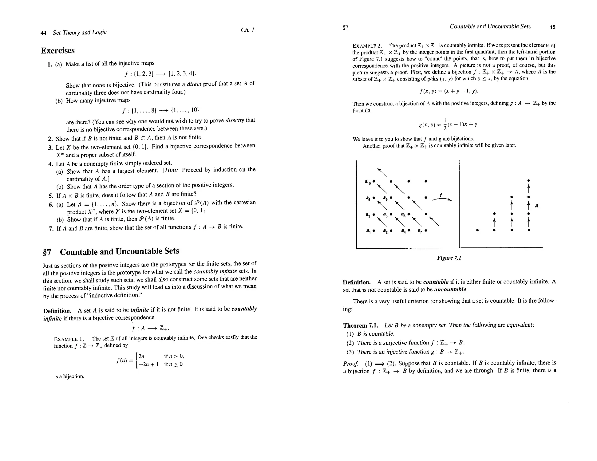
/


Текст
Topology
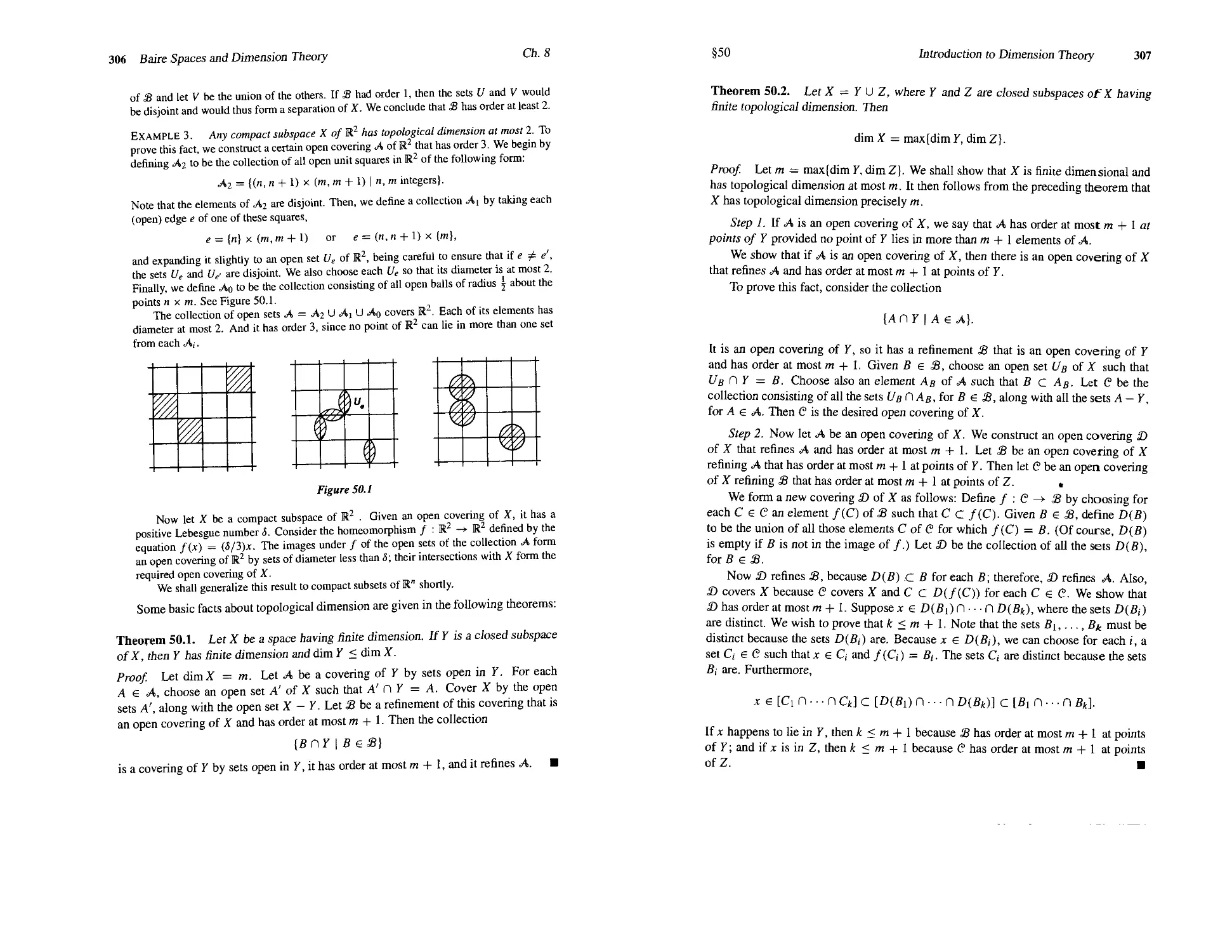
Second Edition
James R. Munkres
Massachusetts Institute of Technology
Prentice Hall, Upper Saddle River, NJ 07458
Library of Congress Cataloging-in-Publication Data
Munkres, James R.
Topology/James Raymond Munkres.—2nd ed.
p. cm.
Includes bibliographical references and index.
ISBN 0-13-181629-2
1. Topology. I. Title.
QA611.M82 2000
514—dc21 99-052942
CIP
Acquisitions Editor: George Lobell
Assistant Vice President of Production and Manufacturing: David W. Riccardi
Executive Managing Editor: Kathleen Schiaparelli
Senior Managing Editor: Linda Mihatov Behrens
Production Editor: Lynn M. Savino
Manufacturing Buyer: Alan Fischer
Manufacturing Manager: Trudy Pisciotti
Marketing Manager: Melody Marcus
Marketing Assistant: Wince Jansen
Director of Marketing: John Tweeddale
Editorial Assistant: Gale Epps
Art Director: Jayne Conte
Cover Designer: Bruce Kenselaar
Composition: MacroTeX Services
© 2000,1975 by Prentice Hall, Inc.
Upper Saddle River, NJ 07458
Ail rights reserved. No part of this book may
be reproduced, in any form or by any means,
without permission in writing from the publisher.
Printed in the United States of America
10 9 8 7
isbn o-ia-
Prentice-Hall International (UK) Limited, London
Prentice-Hall of Australia Pty. Limited, Sydney
Prentice-Hall Canada, Inc., Toronto
Prentice-Hall Hispanoamericana, S.A., Mexico
Prentice-Hall of India Private Limited, New Delhi
Prentice-Hall of Japan, Inc., Tokyo
Pearson Education Asia Рте. Ltd.
Editora Prentice-Hall do Brasil, Ltda., Rio de Janeiro
For Barbara
Contents
Preface xi
A Note to the Reader xv
Part I GENERAL TOPOLOGY
Chapter 1 Set Theory and Logic 3
1 Fundamental Concepts 4
2 Functions 15
3 Relations 21
4 The Integers and the Real Numbers 30
5 Cartesian Products 36
6 Finite Sets 39
7 Countable and Uncountable Sets 44
*8 The Principle of Recursive Definition 52
9 Infinite Sets and the Axiom of Choice 57
10 Well-Ordered Sets 62
*11 The Maximum Principle 68
* Supplementary Exercises: Well-Ordering 72
viii Contents
Chapter 2 Topological Spaces and Continuous Functions 75
12 Topological Spaces 75
13 Basis for a Topology 78
14 The Order Topology 84
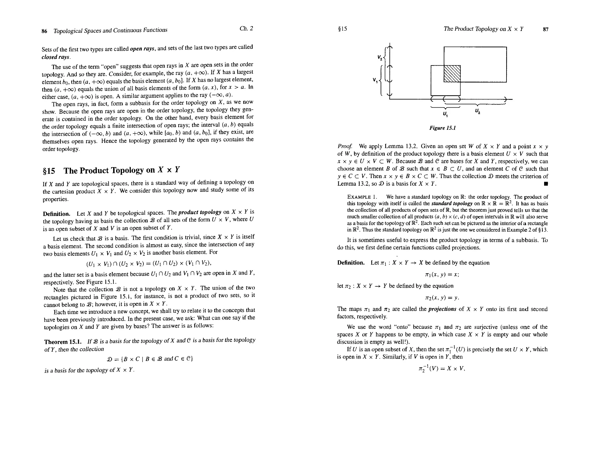
15 The Product Topology on X x Y 86
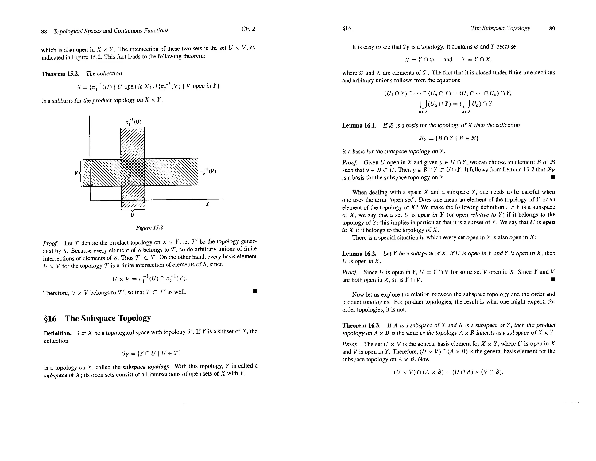
16 The Subspace Topology 88
17 Closed Sets and Limit Points 92
18 Continuous Functions 102
19 The Product Topology 112
20 The Metric Topology 119
21 The Metric Topology (continued) 129
*22 The Quotient Topology 136
'Supplementary Exercises: Topological Groups 145
Chapter 3 Connectedness and Compactness 147
23 Connected Spaces 148
24 Connected Subspaces of the Real Line 153
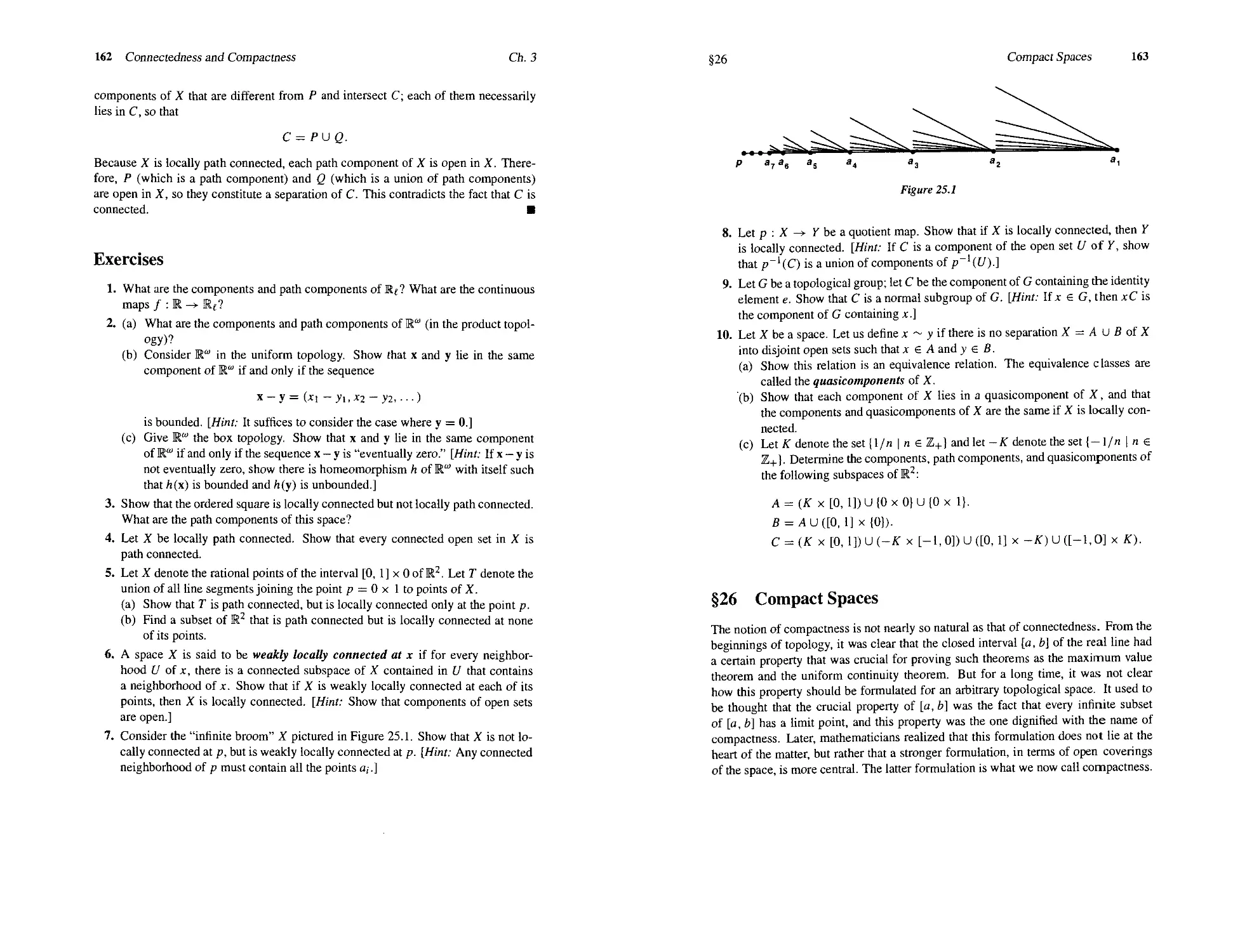
*25 Components and Local Connectedness 159
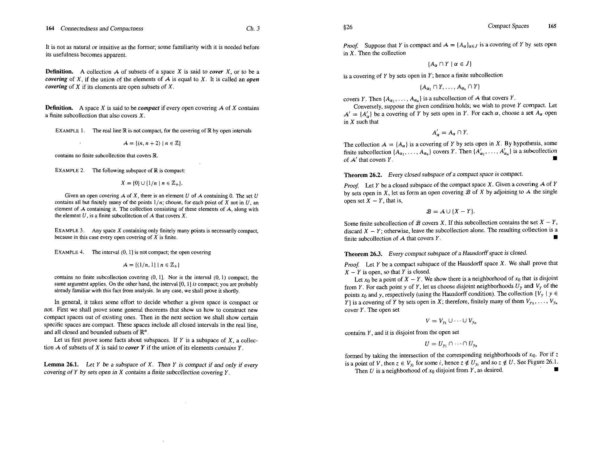
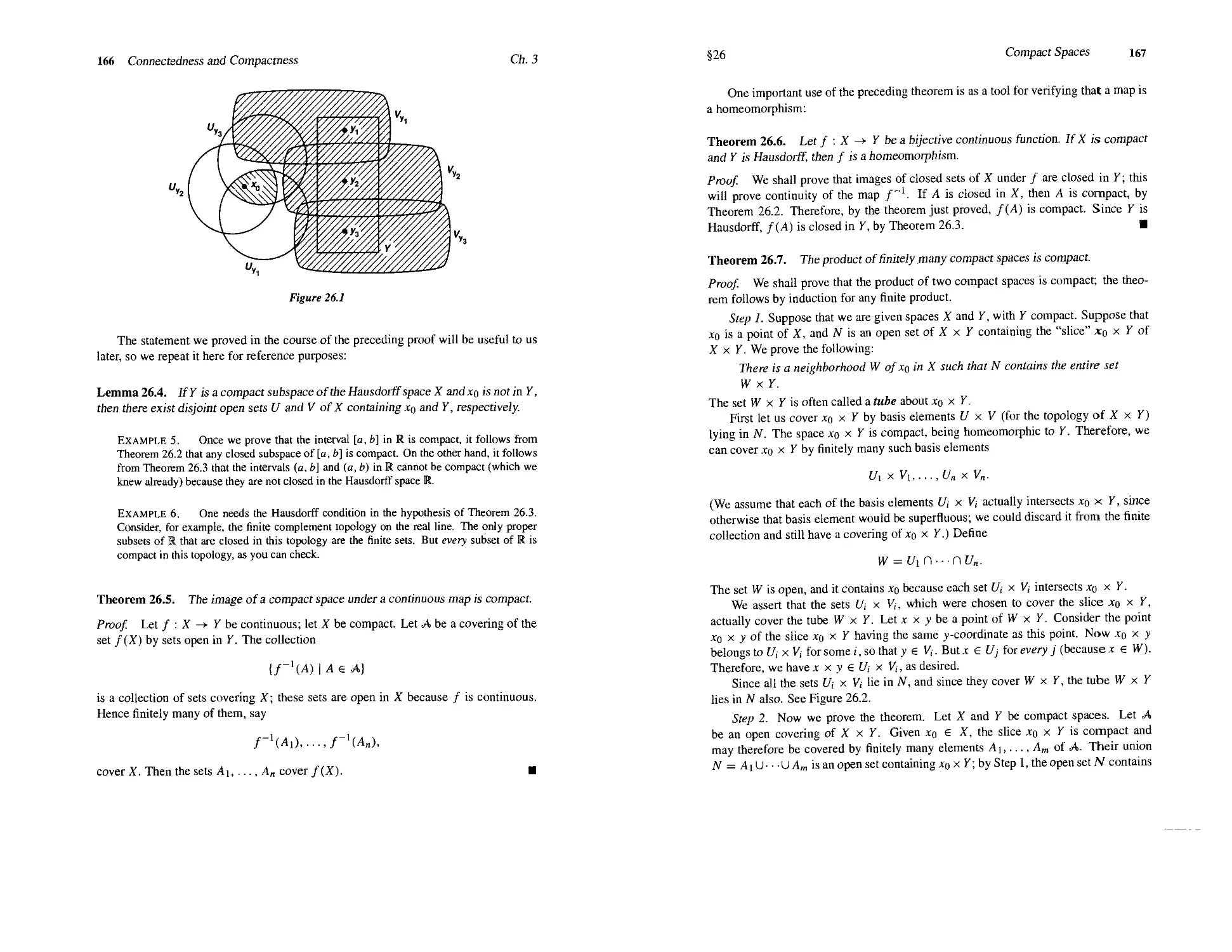
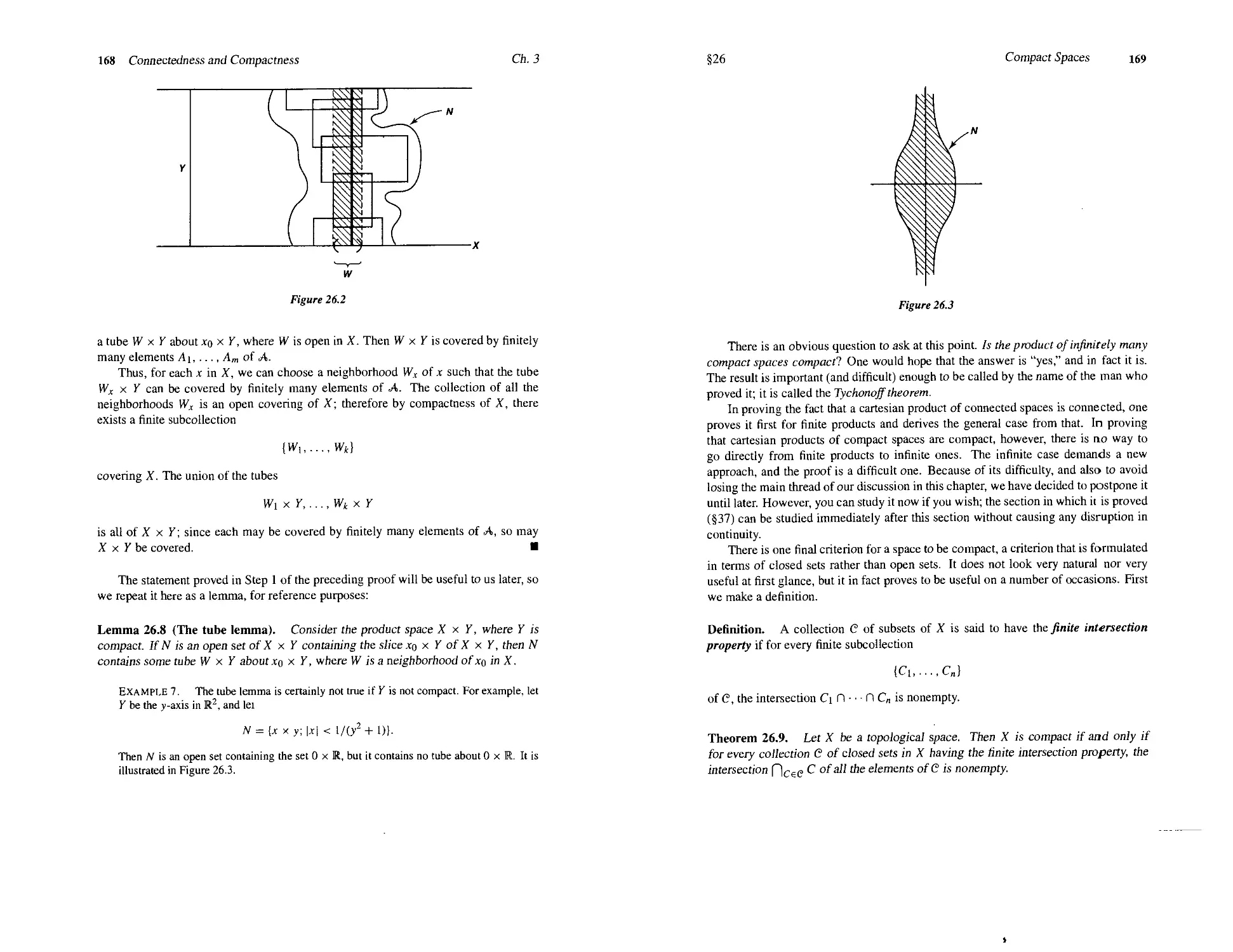
26 Compact Spaces 163
27 Compact Subspaces of the Real Line 172
28 Limit Point Compactness 178
29 Local Compactness 182
* Supplementary Exercises: Nets 187
Chapter 4 Countability and Separation Axioms 189
30 The Countability Axioms 190
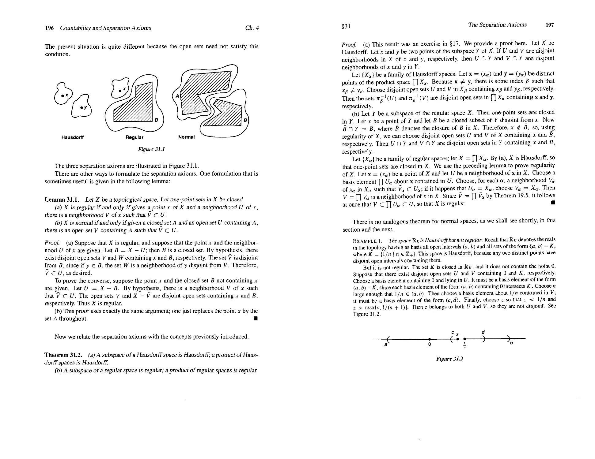
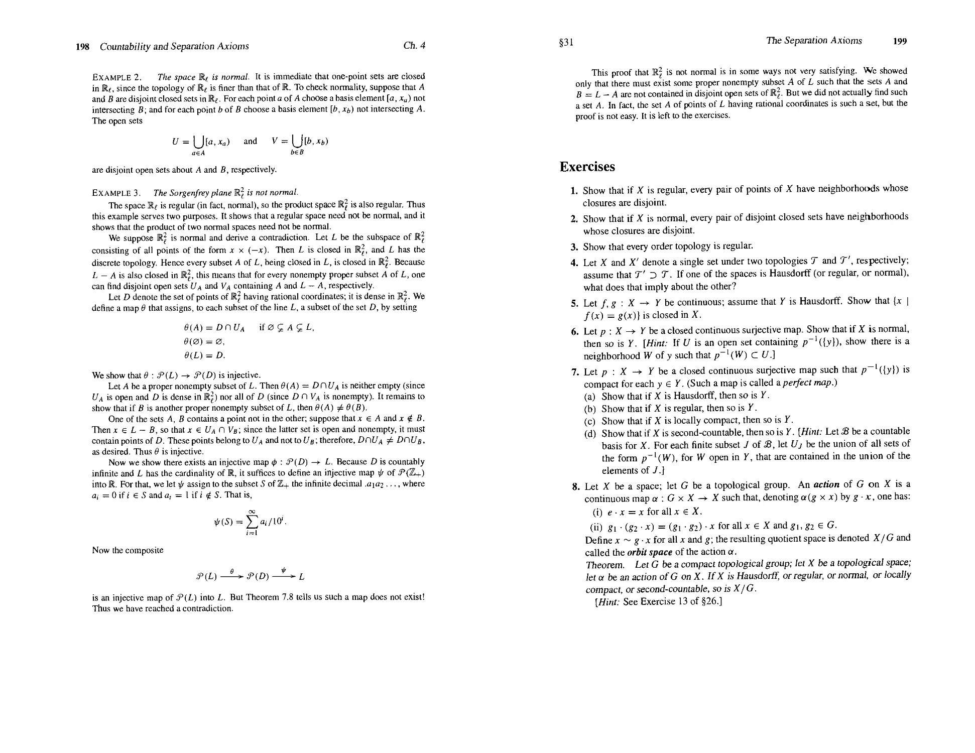
31 The Separation Axioms 195
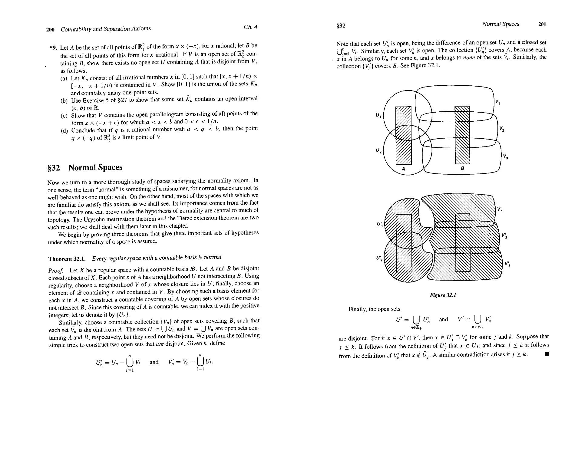
32 Normal Spaces 200
33 The Urysohn Lemma 207
34 The Urysohn Metrization Theorem 214
*35 The Tietze Extension Theorem 219
*36 Imbeddings of Manifolds 224
'Supplementary Exercises: Review of the Basics '228
Chapter 5 The Tychonoff Theorem 230
37 The Tychonoff Theorem 230
38 The Stone-Cech Compactification 237
Chapter 6 Metrization Theorems and Paracompactness 243
39 Local Finiteness 244
40 The Nagata-Smirnov Metrization Theorem 248
41 Paracompactness 252
42 The Smirnov Metrization Theorem 261
Contents ix
Chapter 7 Complete Metric Spaces and Function Spaces 263
43 Complete Metric Spaces 264
*44 A Space-Filling Curve 271
45 Compactness in Metric Spaces 275
46 Pointwise and Compact Convergence 281
47 Ascoli's Theorem 290
Chapter 8 Baire Spaces and Dimension Theory 294
48 Baire Spaces 295
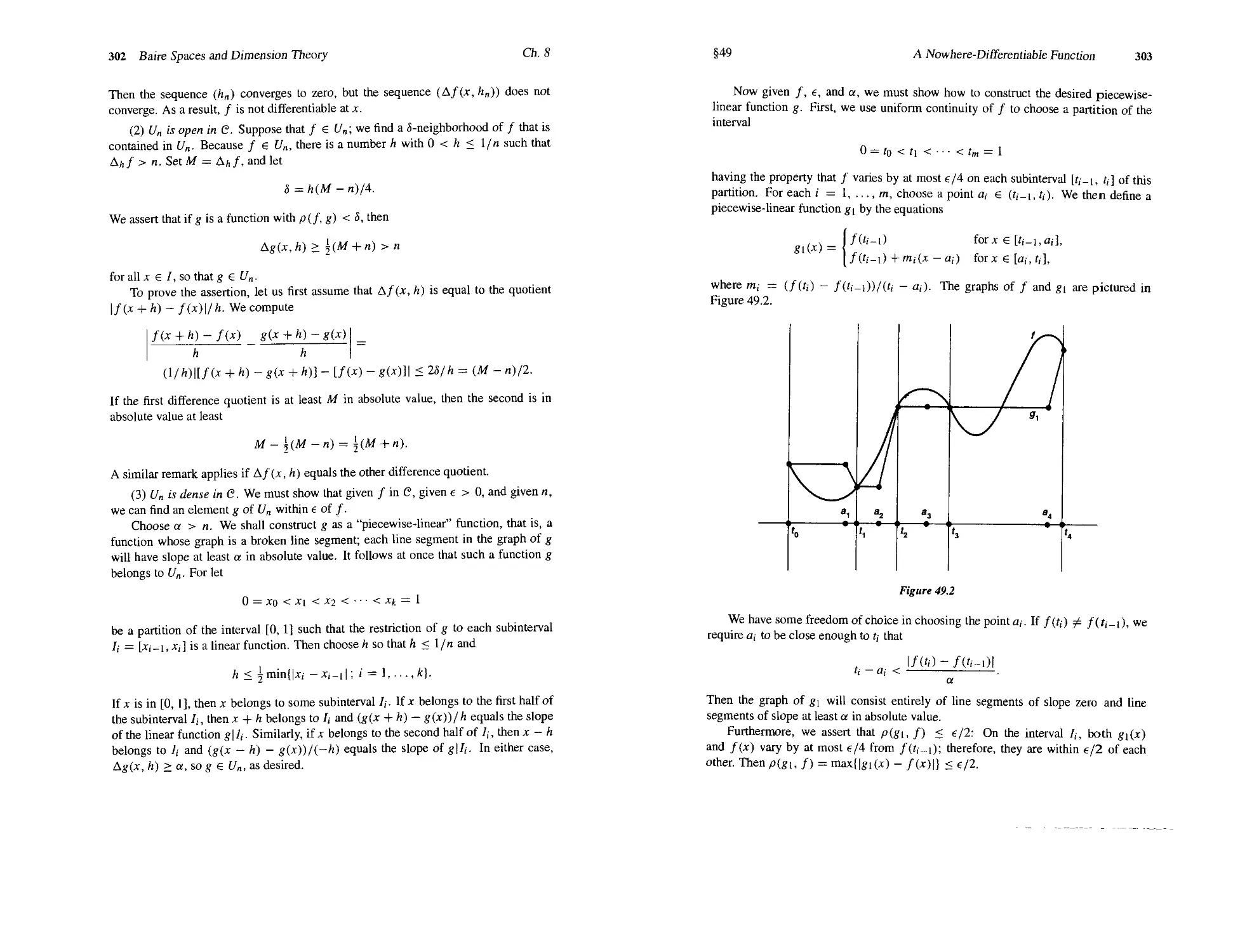
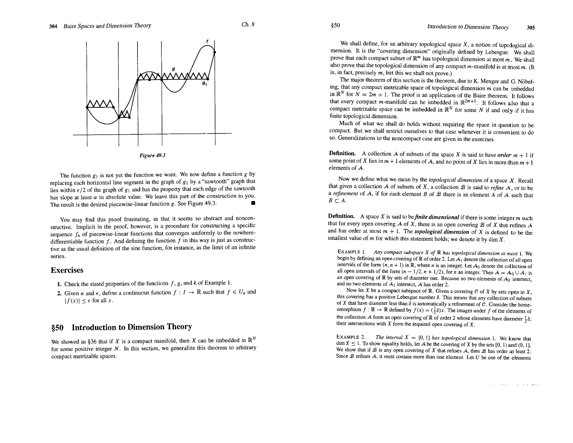
*49 A Nowhere-Differentiable Function 300
50 Introduction to Dimension Theory 304
'Supplementary Exercises: Locally Euclidean Spaces 316
Part II ALGEBRAIC TOPOLOGY
Chapter 9 The Fundamental Group 321
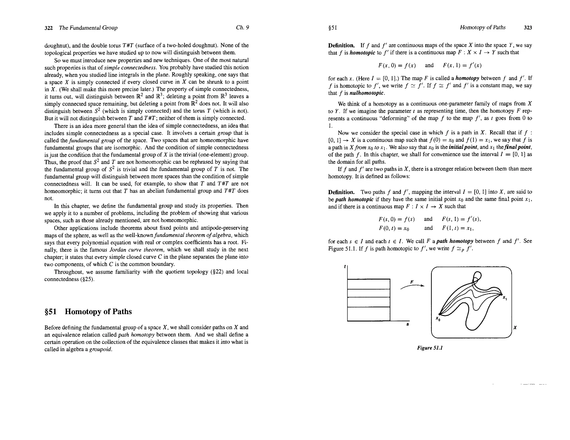
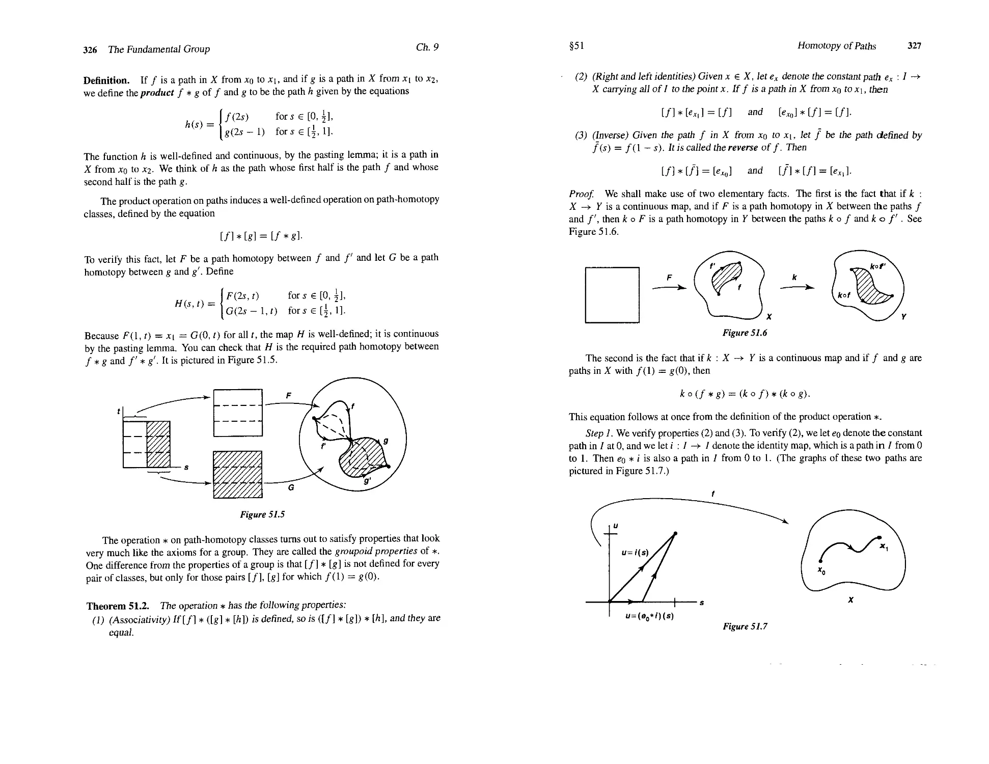
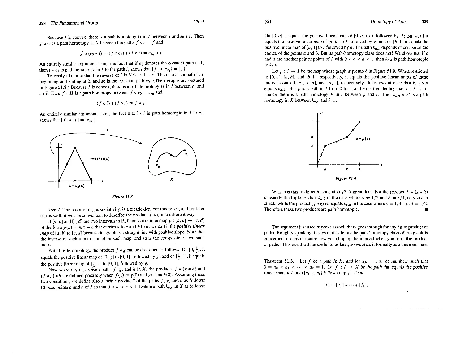
51 Homotopy of Paths 322
52 The Fundamental Group 330
53 Covering Spaces 335
54 The Fundamental Group of the Circle 341
55 Retractions and Fixed Points 348
*56 The Fundamental Theorem of Algebra 353
*57 The Borsuk-Ulam Theorem 356
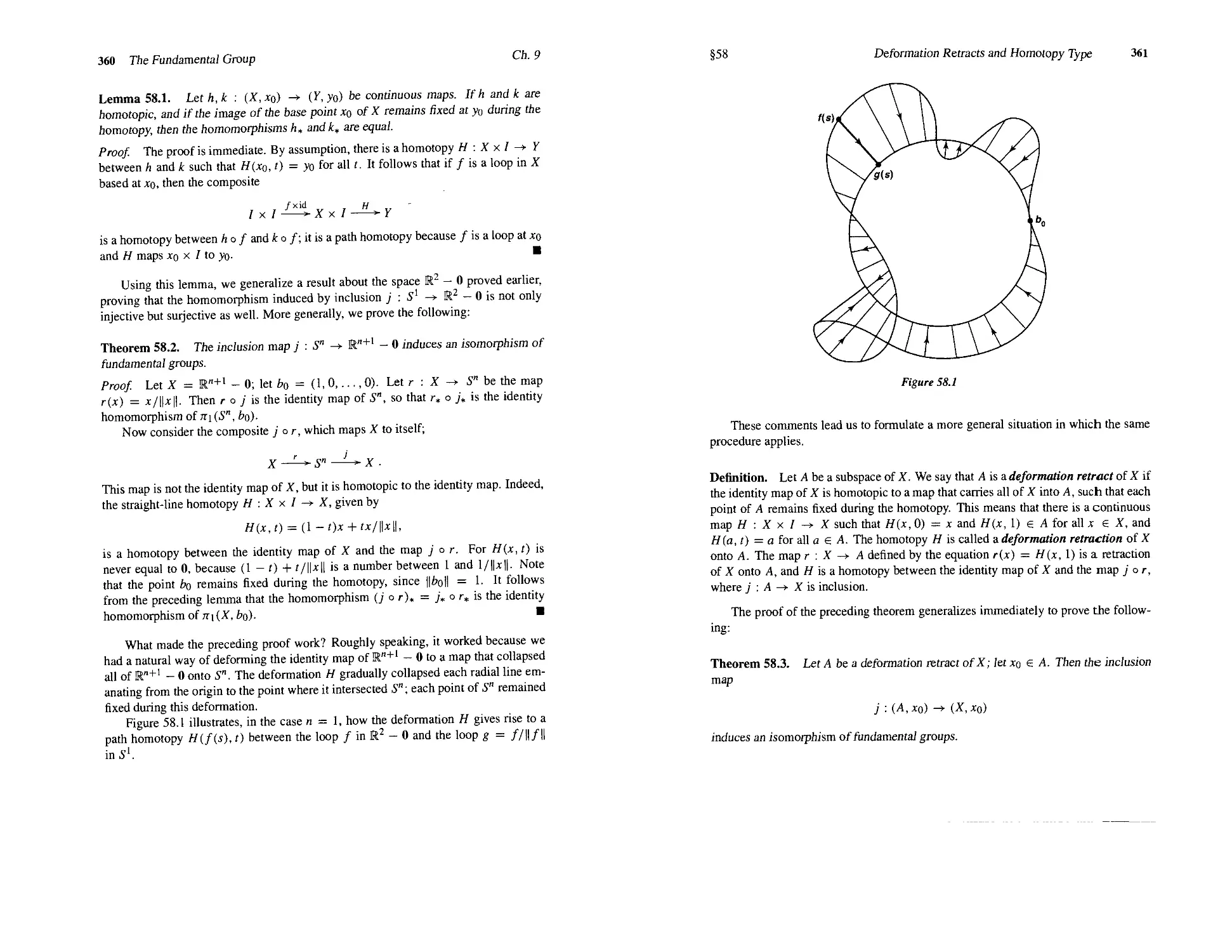
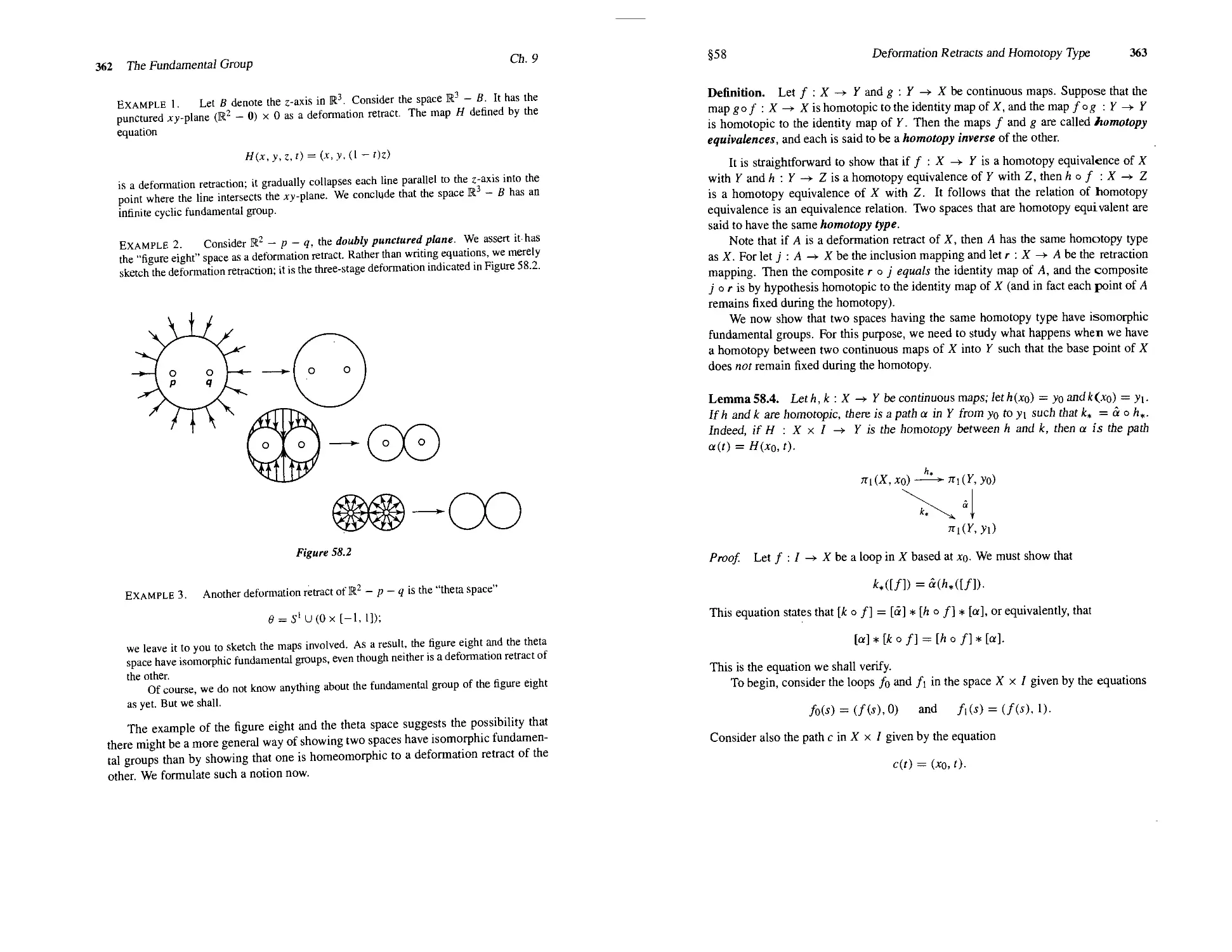
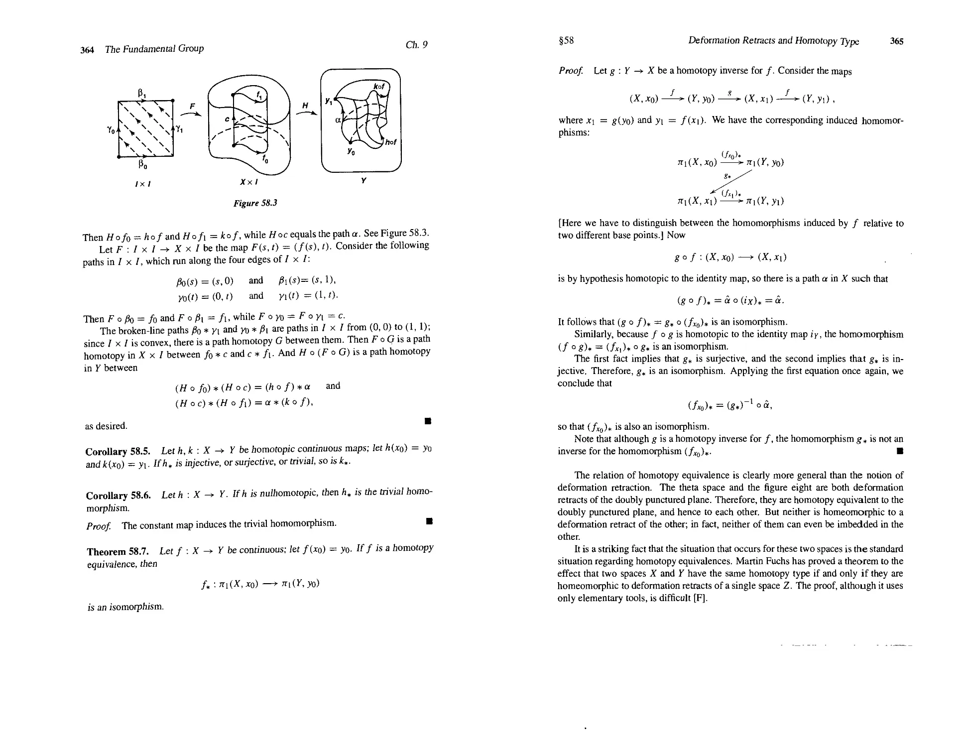
58 Deformation Retracts and Homotopy Type 359
59 The Fundamental Group of 5" 368
60 Fundamental Groups of Some Surfaces 370
Chapter 10 Separation Theorems in the Plane 376
61 The Jordan Separation Theorem 376
*62 Invariance of Domain 381
63 The Jordan Curve Theorem 385
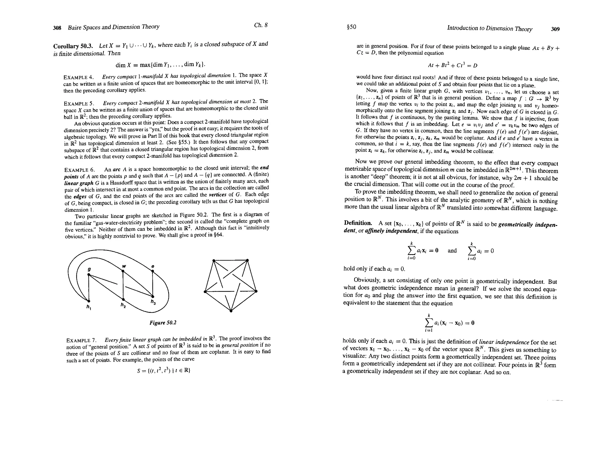
64 Imbedding Graphs in the Plane 394
65 The Winding Number of a Simple Closed Curve 398
66 The Cauchy Integral Formula 403
Chapter 11 The Seifert-van Kampen Theorem 407
67 Direct Sums of Abelian Groups 407
68 Free Products of Groups 412
69 Free Groups 421
70 The Seifert-van Kampen Theorem 426
71 The Fundamental Group of a Wedge of Circles 434
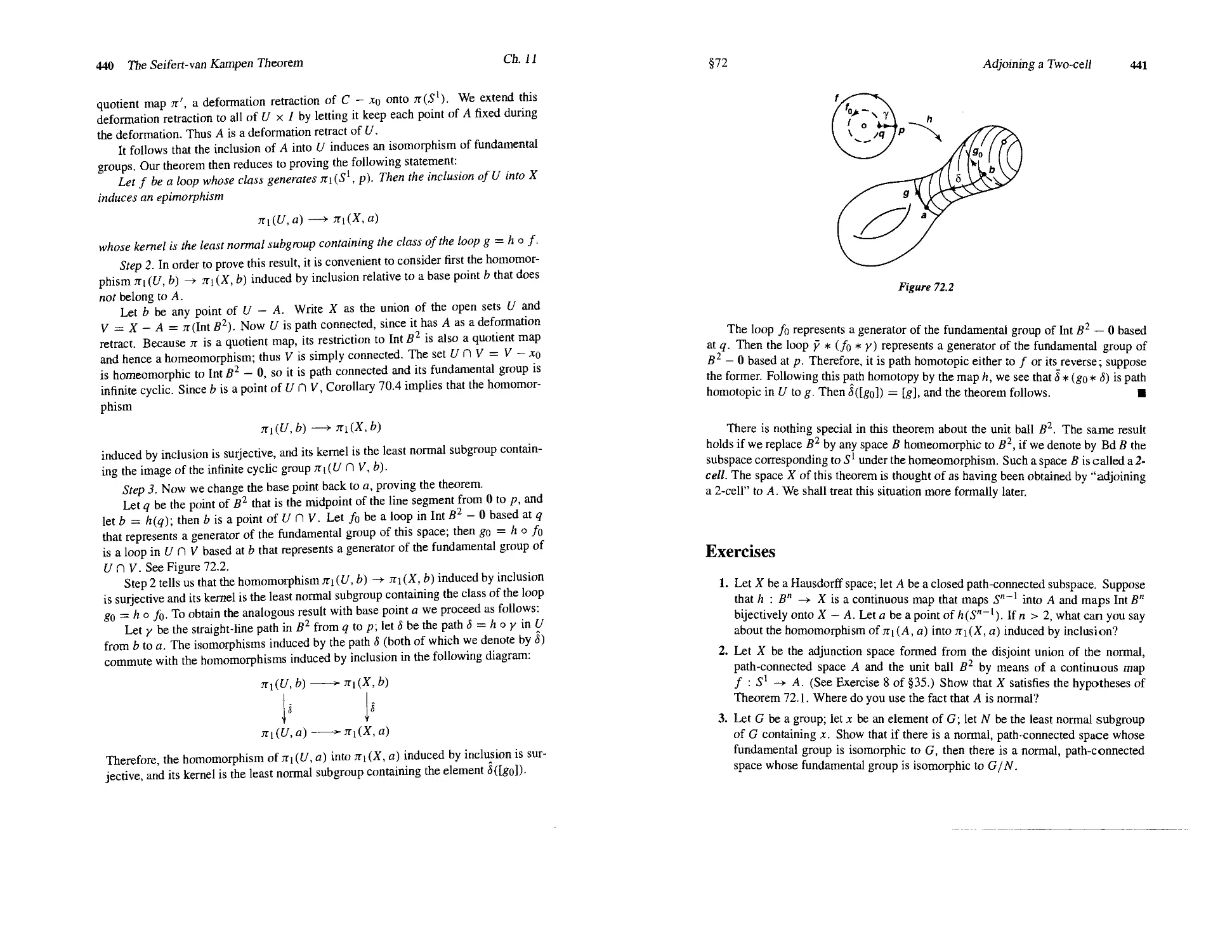
72 Adjoining a Two-cell 438
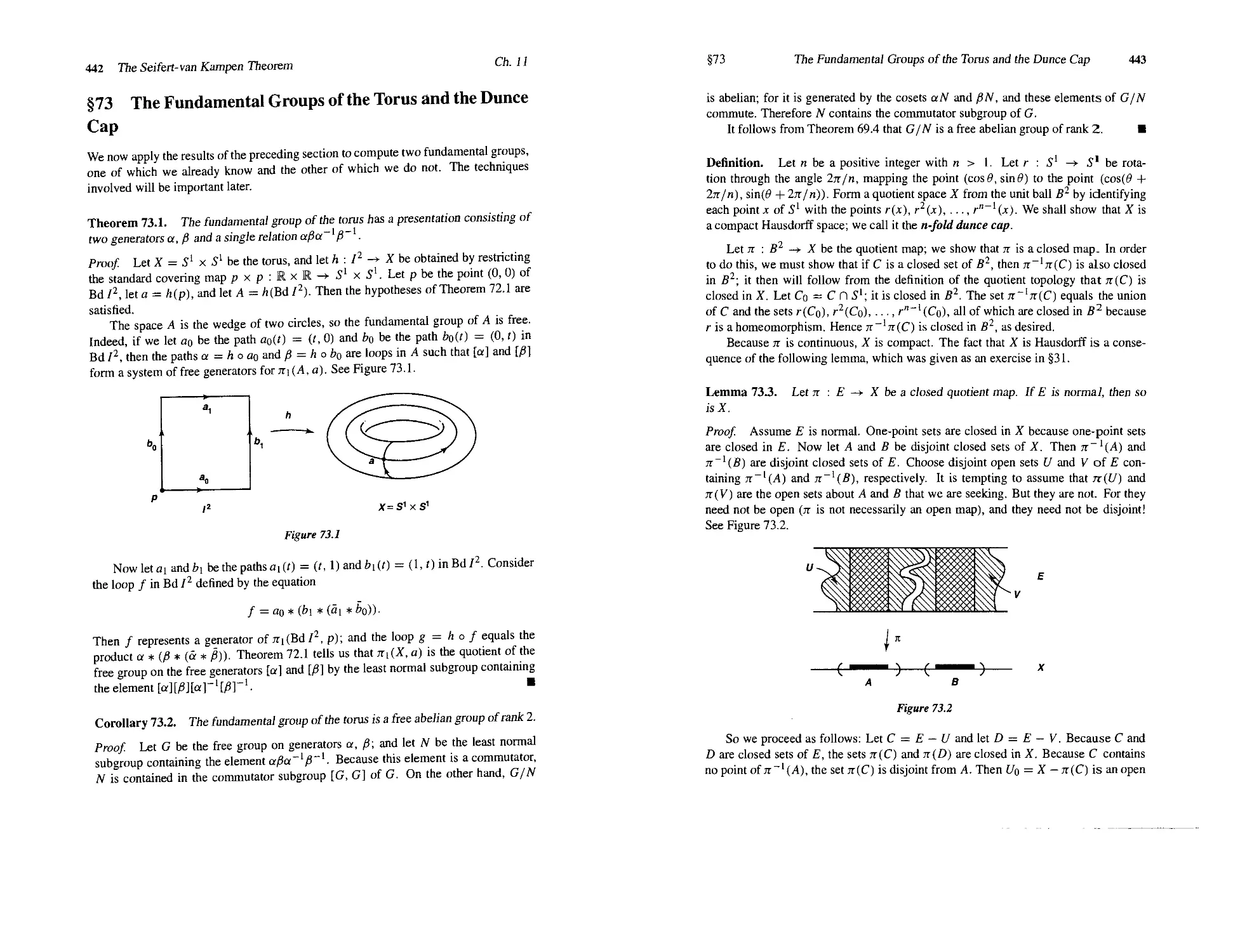
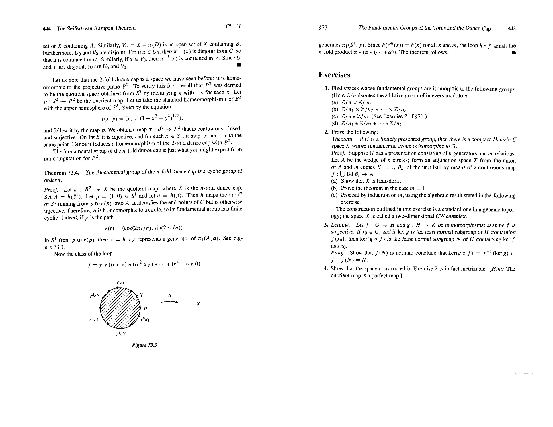
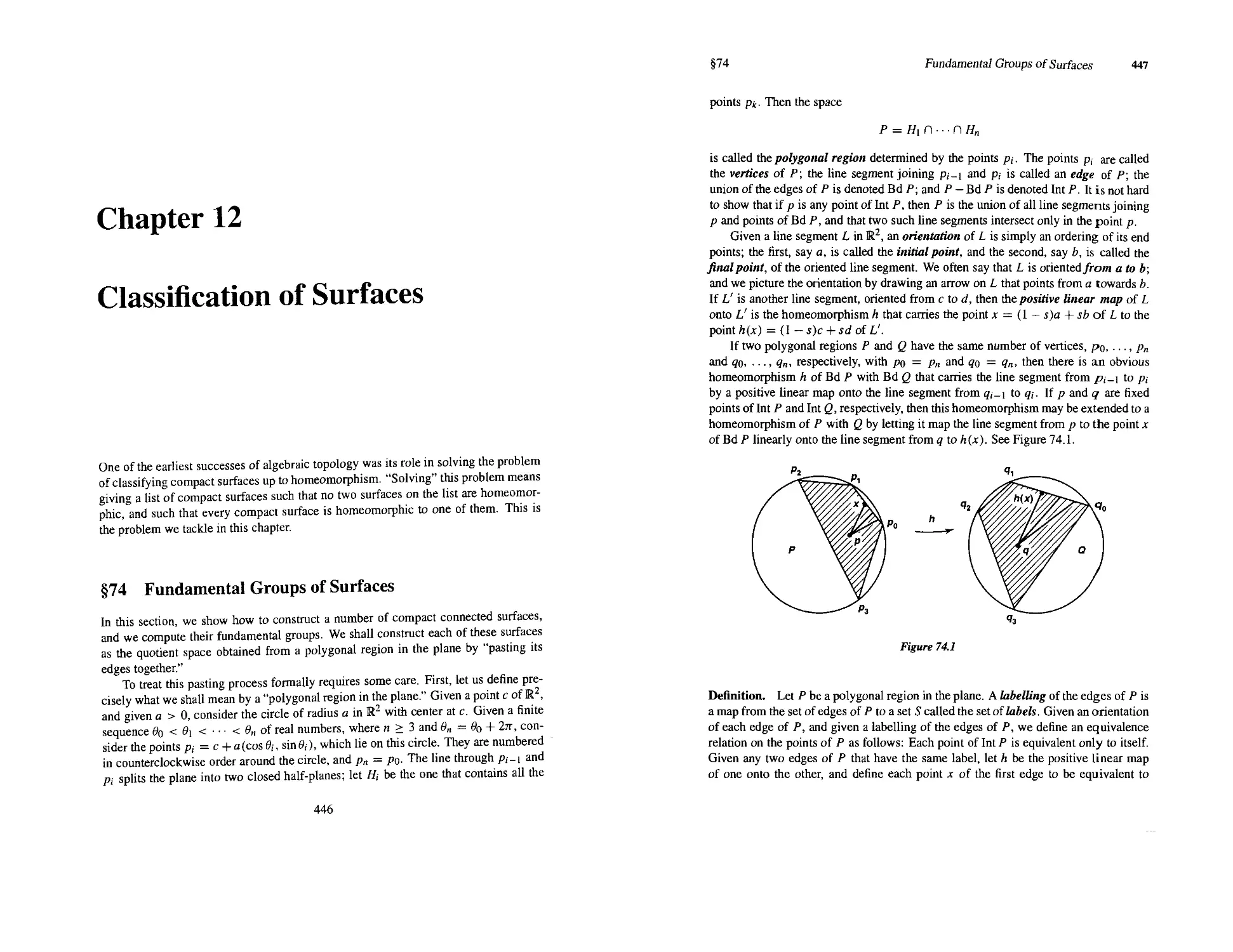
73 The Fundamental Groups of the Torus and the Dunce Cap 442
Contents
Chapter 12 Classification of Surfaces 446
74 Fundamental Groups of Surfaces 446
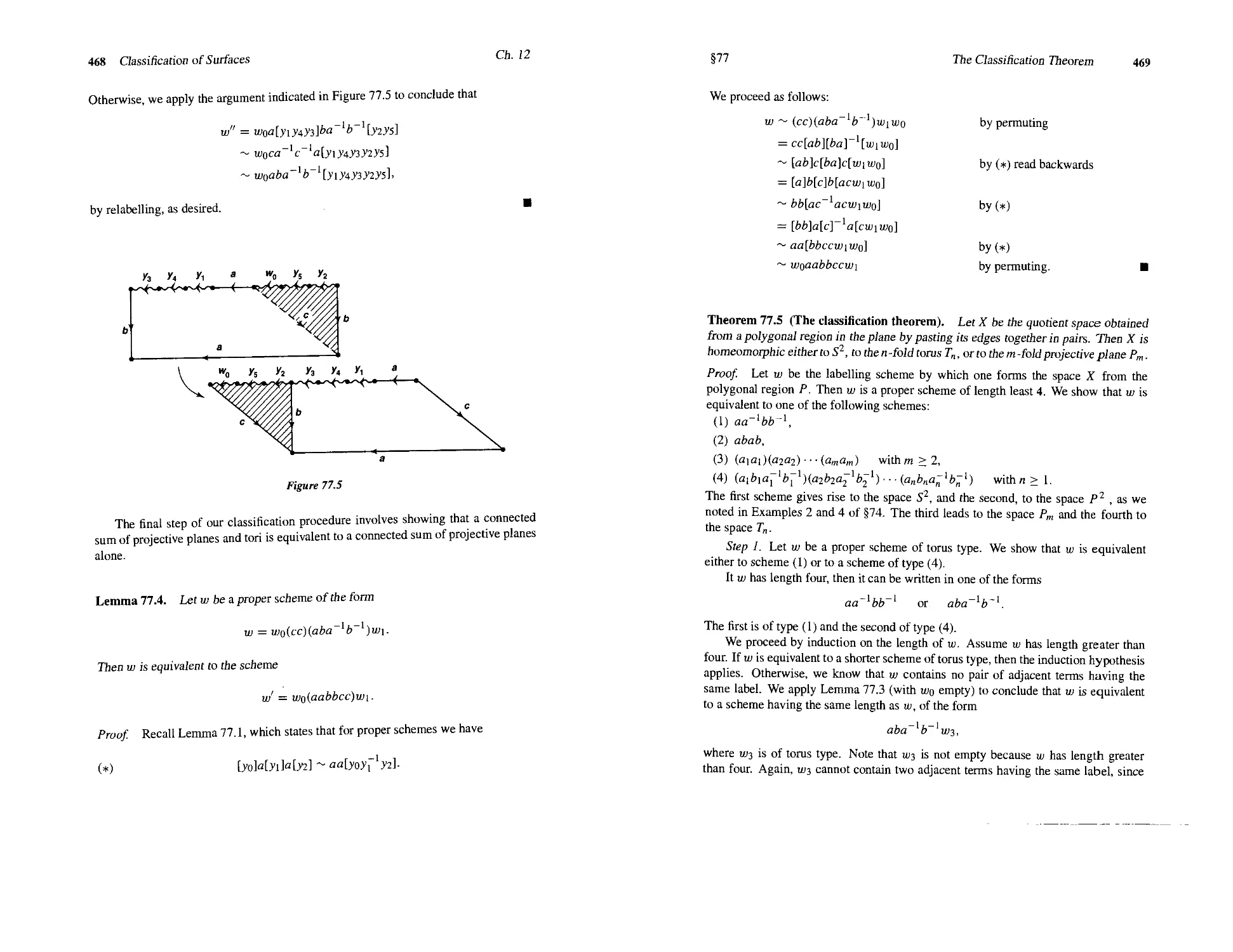
75 Homology of Surfaces 454
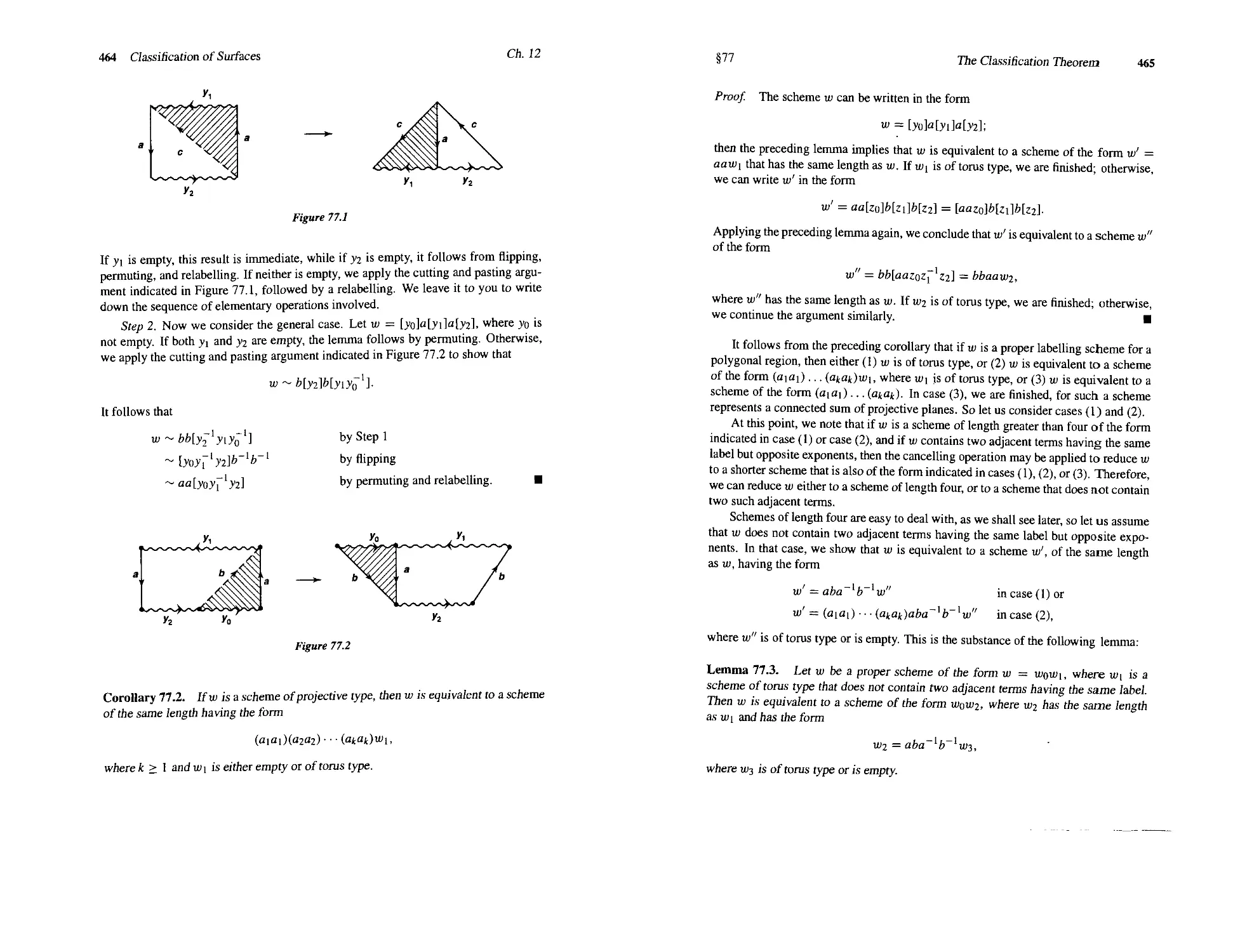
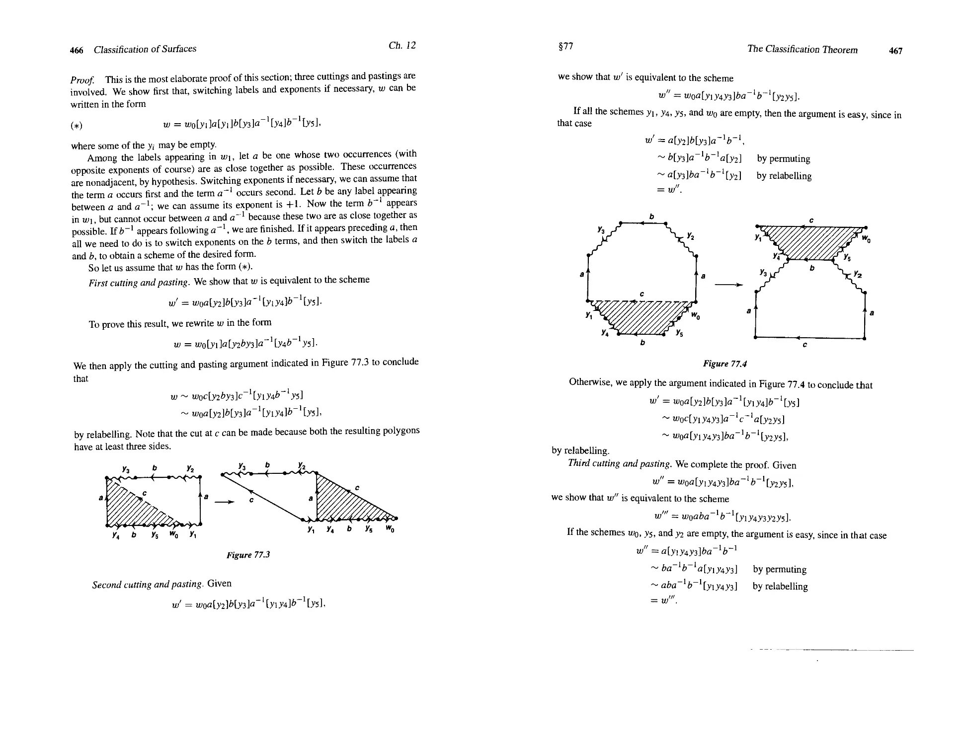
76 Cutting and Pasting 457
77 The Classification Theorem 462
78 Constructing Compact Surfaces 471
Chapter 13 Classification of Covering Spaces 477
79 Equivalence of Covering Spaces 478
80 The Universal Covering Space 484
*81 Covering Transformations 487
82 Existence of Covering Spaces 494
'Supplementary Exercises: Topological Properties and л\ 499
Chapter 14 Applications to Group Theory 501
83 Covering Spaces of a Graph 501
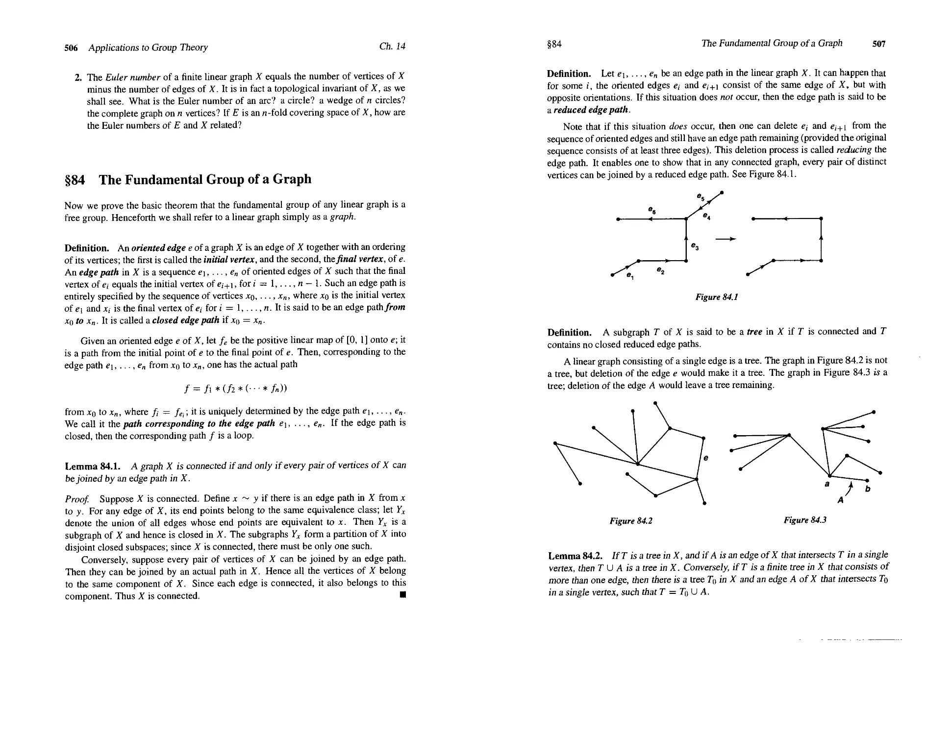
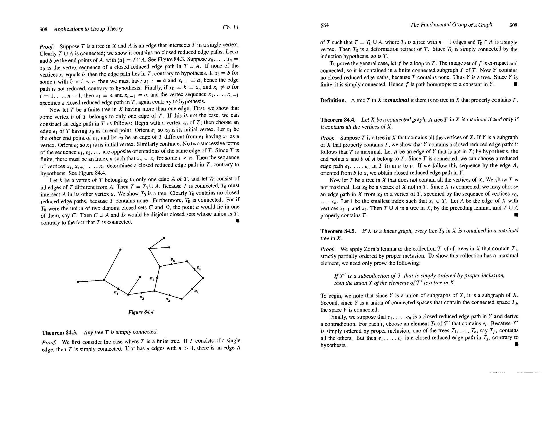
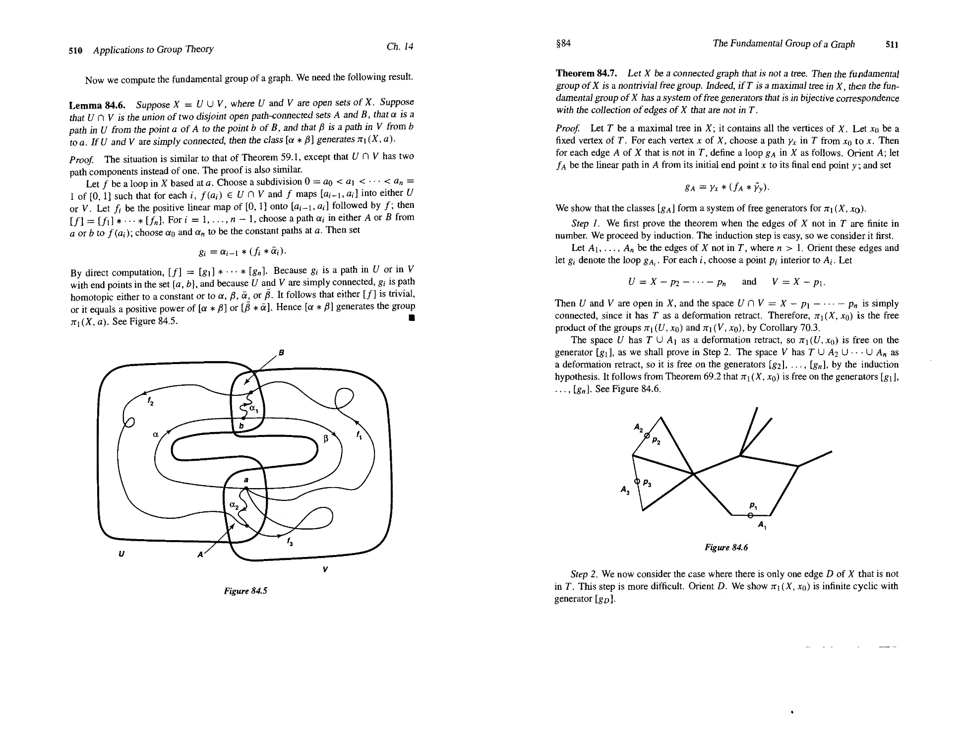
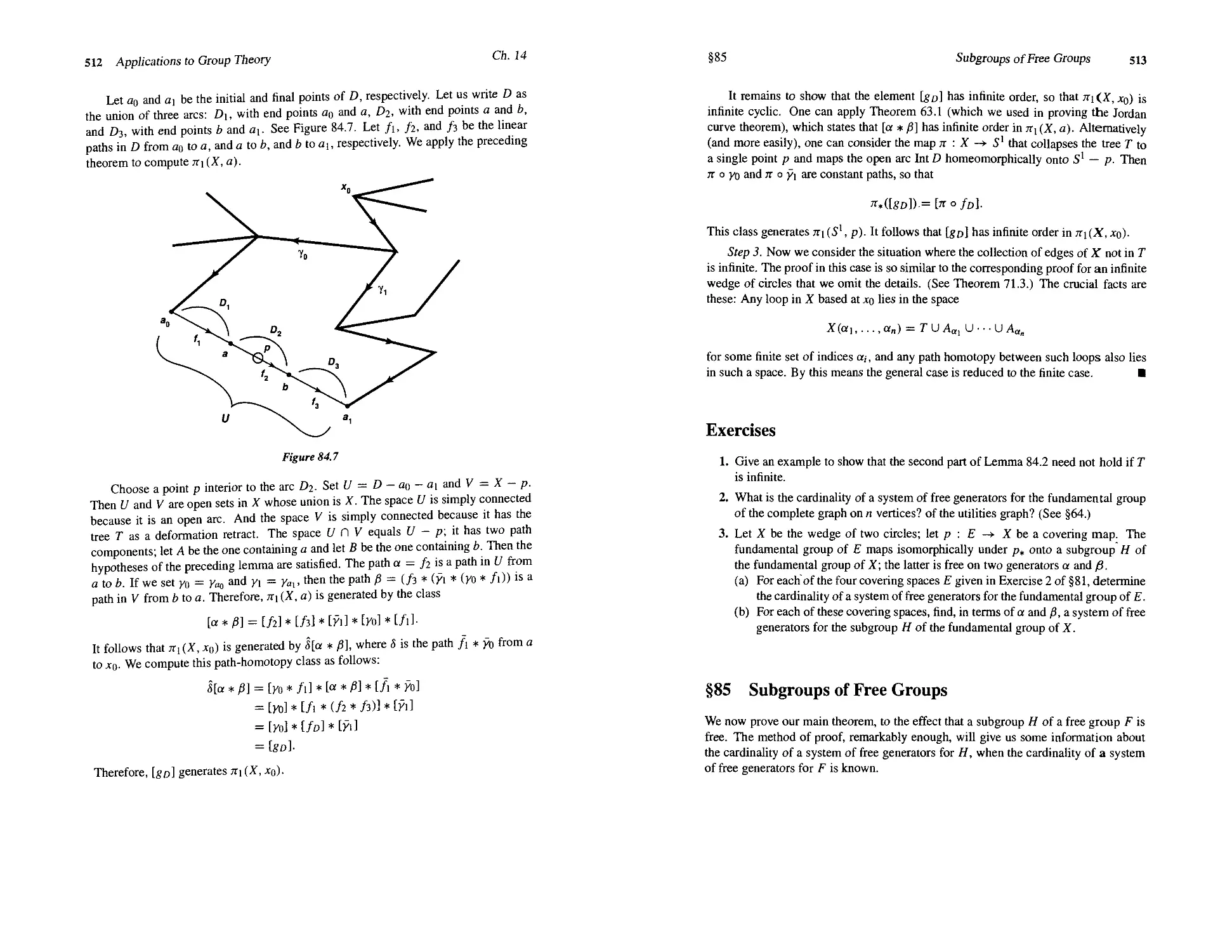
84 The Fundamental Group of a Graph 506
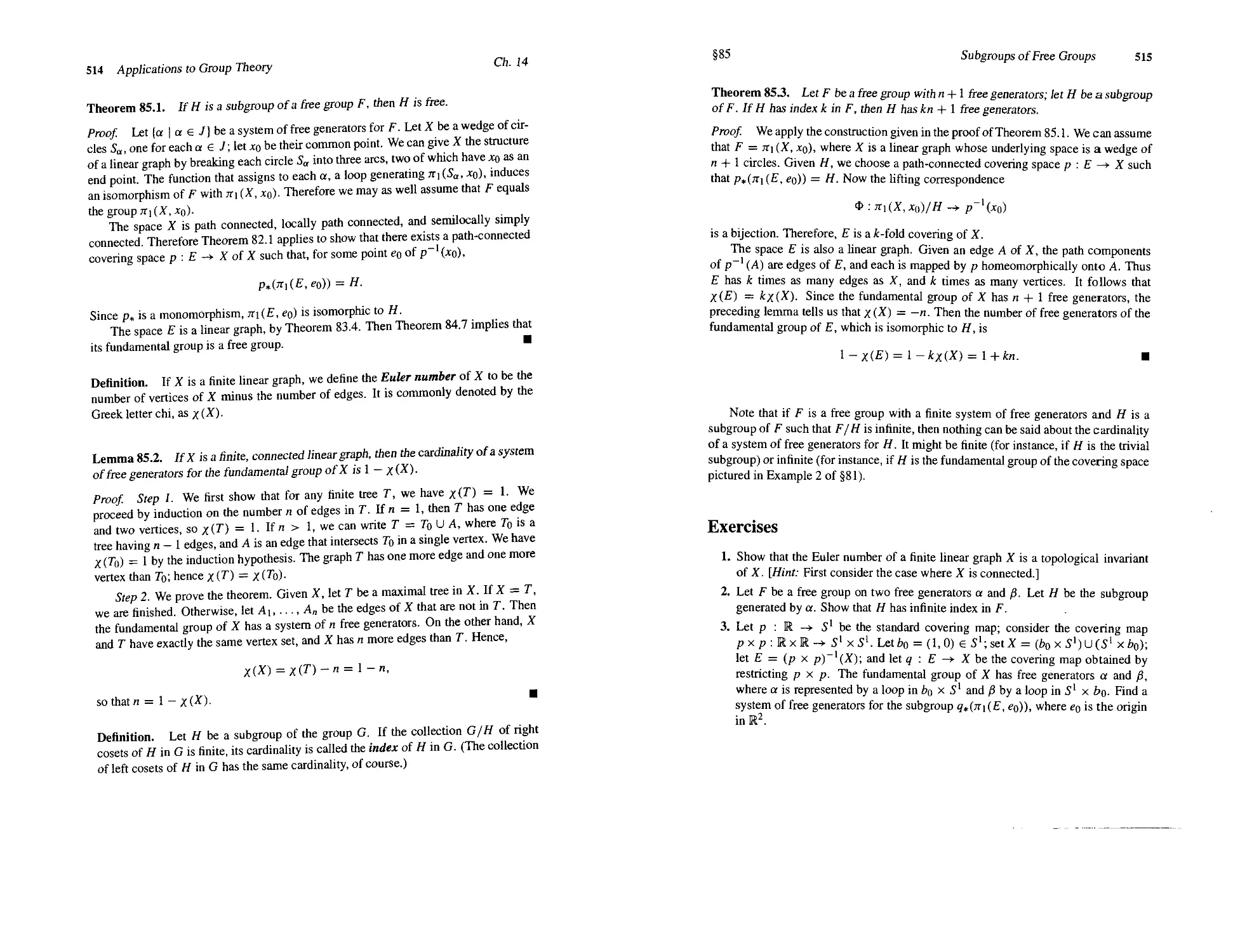
85 Subgroups of Free Groups 513
Bibliography 517
Index 519
Preface
This book is intended as a text for a one- or two-semester introduction to topology, at
the senior or first-year graduate level.
The subject of topology is of interest in its own right, and it also serves to lay the
foundations for future study in analysis, in geometry, and in algebraic topology. There
is no universal agreement among mathematicians as to what a first course in topology
should include; there are many topics that are appropriate to such a course, and not all
are equally relevant to these differing purposes. In the choice of material to be treated,
I have tried to strike a balance among the various points of view.
Prerequisites. There are no formal subject matter prerequisites for studying most of
this book. I do not even assume the reader knows much set theory. Having said that,
I must hasten to add that unless the reader has studied a bit of analysis or "rigorous
calculus," much of the motivation for the concepts introduced in the first part of the
book will be missing. Things will go more smoothly if he or she already has had some
experience with continuous functions, open and closed sets, metric spaces, and the
like, although none of these is actually assumed. In Part II, we do assume familiarity
with the elements of group theory.
Most students in a topology course have, in my experience, some knowledge of
the foundations of mathematics. But the amount varies a great deal from one student
to another. Therefore, I begin with a fairly thorough chapter on set theory and logic. It
starts at an elementary level and works up to a level that might be described as "semi-
sophisticated." It treats those topics (and only those) that will be needed later in the
book. Most students will already be familiar with the material of the first few sections,
but many of them will find their expertise disappearing somewhere about the middle
xii Preface
of the chapter. How much time and effort the instructor will need to spend on this
chapter will thus depend largely on the mathematical sophistication and experience of
the students. Ability to do the exercises fairly readily (and correctly!) should serve as
a reasonable criterion for determining whether the student's mastery of set theory is
sufficient for the student to begin the study of topology.
Many students (and instructors!) would prefer to skip the foundational material
of Chapter 1 and jump right in to the study of topology. One ignores the foundations,
however, only at the risk of later confusion and error. What one can do is to treat
initially only those sections that are needed at once, postponing the remainder until
they are needed. The first seven sections (through countability) are needed throughout
the book; I usually assign some of them as reading and lecture on the rest. Sections 9
and 10, on the axiom of choice and well-ordering, are not needed until the discussion
of compactness in Chapter 3. Section 11, on the maximum principle, can be postponed
even longer; it is needed only for the Tychonoff theorem (Chapter 5) and the theorem
on the fundamental group of a linear graph (Chapter 14).
How the book is organized. This book can be used for a number of different courses.
I have attempted to organize it as flexibly as possible, so as to enable the instructor to
follow his or her own preferences in the matter.
Part I, consisting of the first eight chapters, is devoted to the subject commonly
called general topology. The first four chapters deal with the body of material that,
in my opinion, should be included in any introductory topology course worthy of the
name. This may be considered the "irreducible core" of the subject, treating as it does
set theory, topological spaces, connectedness, compactness (through compactness of
finite products), and the countability and separation axioms (through the Urysohn
metrization theorem). The remaining four chapters of Part I explore additional topics;
they are essentially independent of one another, depending on only the core material
of Chapters 1-4. The instructor may take them up in any order he or she chooses.
Part II constitutes an introduction to the subject of Algebraic Topology. It depends
on only the core material of Chapters 1-4. This part of the book treats with some
thoroughness the notions of fundamental group and covering space, along with their
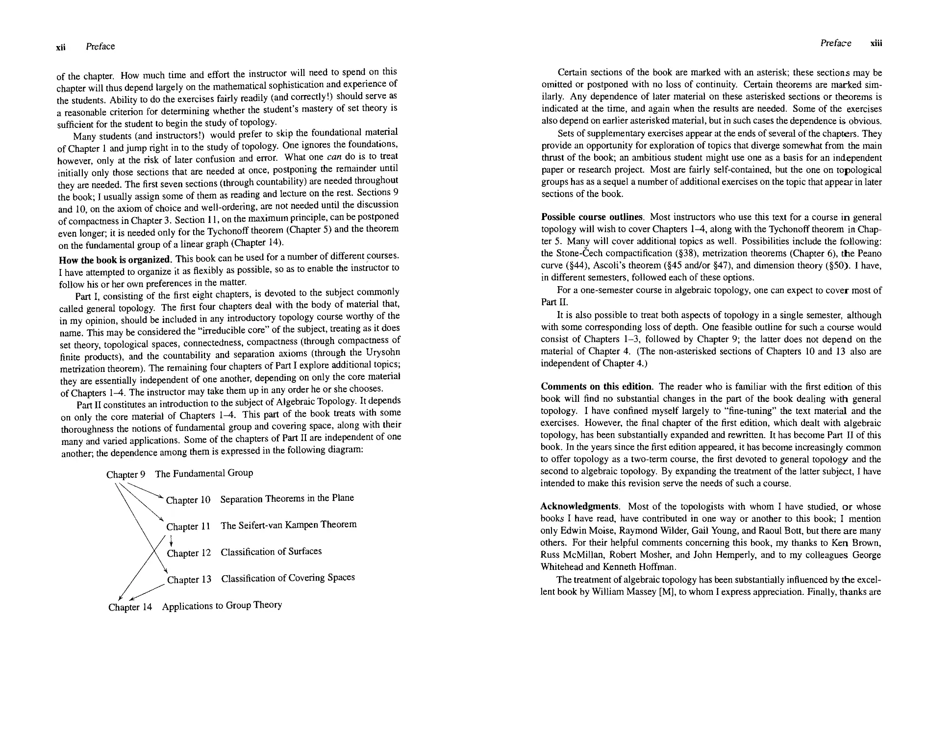
many and varied applications. Some of the chapters of Part II are independent of one
another, the dependence among them is expressed in the following diagram:
Chapter 9 The Fundamental Group
Chapter 10 Separation Theorems in the Plane
Chapter 11 The Seifert-van Kampen Theorem
I
Chapter 12 Classification of Surfaces
Chapter 13 Classification of Covering Spaces
Chapter 14 Applications to Group Theory
Preface xiii
Certain sections of the book are marked with an asterisk; these sections may be
omitted or postponed with no loss of continuity. Certain theorems are marked sim-
similarly. Any dependence of later material on these asterisked sections or theorems is
indicated at the time, and again when the results are needed. Some of the exercises
also depend on earlier asterisked material, but in such cases the dependence is obvious.
Sets of supplementary exercises appear at the ends of several of the chapters. They
provide an opportunity for exploration of topics that diverge somewhat from the main
thrust of the book; an ambitious student might use one as a basis for an independent
paper or research project. Most are fairly self-contained, but the one on topological
groups has as a sequel a number of additional exercises on the topic that appear in later
sections of the book.
Possible course outlines. Most instructors who use this text for a course in general
topology will wish to cover Chapters 1—4, along with the Tychonoff theorem in Chap-
Chapter 5. Many will cover additional topics as well. Possibilities include the following:
the Stone-Cech compactification (§38), metrization theorems (Chapter 6), the Peano
curve (§44), Ascoli's theorem (§45 and/or §47), and dimension theory (§50). I have,
in different semesters, followed each of these options.
For a one-semester course in algebraic topology, one can expect to cover most of
Part II.
It is also possible to treat both aspects of topology in a single semester, although
with some corresponding loss of depth. One feasible outline for such a course would
consist of Chapters 1-3, followed by Chapter 9; the latter does not depend on the
material of Chapter 4. (The non-asterisked sections of Chapters 10 and 13 also are
independent of Chapter 4.)
Comments on this edition. The reader who is familiar with the first edition of this
book will find no substantial changes in the part of the book dealing with general
topology. I have confined myself largely to "fine-tuning" the text material and the
exercises. However, the final chapter of the first edition, which dealt with algebraic
topology, has been substantially expanded and rewritten. It has become Part II of this
book. In the years since the first edition appeared, it has become increasingly common
to offer topology as a two-term course, the first devoted to general topology and the
second to algebraic topology. By expanding the treatment of the latter subject, I have
intended to make this revision serve the needs of such a course.
Acknowledgments. Most of the topologists with whom I have studied, or whose
books I have read, have contributed in one way or another to this book; I mention
only Edwin Moise, Raymond Wilder, Gail Young, and Raoul Bott, but there are many
others. For their helpful comments concerning this book, my thanks to Ken Brown,
Russ McMillan, Robert Mosher, and John Hemperly, and to my colleagues George
Whitehead and Kenneth Hoffman.
The treatment of algebraic topology has been substantially influenced by the excel-
excellent book by William Massey [M], to whom I express appreciation. Finally, thanks are
Preface
due Adam Lewenberg of MacroTeX for his extraordinary skill and patience in setting
text and juggling figures.
But most of all, to my students go my most heartfelt thanks. From them I learned
at least as much as they did from me; without them this book would be very different.
J.R.M.
A Note to the Reader
Two matters require comment—the exercises and the examples.
Working problems is a crucial part of learning mathematics. No one can learn
topology merely by poring over the definitions, theorems, and examples that are worked
out in the text. One must work part of it out for oneself. To provide that opportunity is
the purpose of the exercises.
They vary in difficulty, with the easier ones usually given first. Some are routine
verifications designed to test whether you have understood the definitions or examples
of the preceding section. Others are less routine. You may, for instance, be asked to
generalize a theorem of the text. Although the result obtained may be interesting in its
own right, the main purpose of such an exercise is to encourage you to work carefully
through the proof in question, mastering its ideas thoroughly—more thoroughly (I
hope!) than mere memorization would demand.
Some exercises are phrased in an "open-ended" fashion. Students often find this
practice frustrating. When faced with an exercise that asks, "Is every regular Lindelof
space normal?" they respond in exasperation, "I don't know what I'm supposed to do!
Am I suppose to prove it or find a counterexample or what?" But mathematics (outside
textbooks) is usually like this. More often than not, all a mathematician has to work
with is a conjecture or question, and he or she doesn't know what the correct answer
is. You should have some experience with this situation.
A few exercises that are more difficult than the rest are marked with asterisks. But
none are so difficult but that the best student in my class can usually solve them.
A Note to the Reader
Another important part of mastering any mathematical subject is acquiring a reper-
repertoire of useful examples. One should, of course, come to know those major examples
from whose study the theory itself derives, and to which the important applications
are made. But one should also have a few counterexamples at hand with which to test
plausible conjectures.
Now it is all too easy in studying topology to spend too much time dealing with
"weird counterexamples." Constructing them requires ingenuity and is often great
fun. But they are not really what topology is about. Fortunately, one does not need
too many such counterexamples for a first course; there is a fairly short list that will
suffice for most purposes. Let me give it here:
RJ the product of the real line with itself, in the product, uniform, and box topolo-
topologies.
Rt the real line in the topology having the intervals [a, b) as a basis.
5д the minimal uncountable well-ordered set.
Ig the closed unit square in the dictionary order topology.
These are the examples you should master and remember; they will be exploited
again and again.
Parti
GENERAL TOPOLOGY
Chapter 1
Set Theory and Logic
We adopt, as most mathematicians do, the naive point of view regarding set theory.
We shall assume that what is meant by a set of objects is intuitively clear, and we shall
proceed on that basis without analyzing the concept further. Such an analysis properly
belongs to the foundations of mathematics and to mathematical logic, and it is not our
purpose to initiate the study of those fields.
Logicians have analyzed set theory in great detail, and they have formulated ax-
axioms for the subject. Each of their axioms expresses a property of sets that mathe-
mathematicians commonly accept, and collectively the axioms provide a foundation broad
enough and strong enough that the rest of mathematics can be built on them.
It is unfortunately true that careless use of set theory, relying on intuition alone,
can lead to contradictions. Indeed, one of the reasons for the axiomatization of set
theory was to formulate rules for dealing with sets that would avoid these contradic-
contradictions. Although we shall not deal with the axioms explicitly, the rules we follow in
dealing with sets derive from them. In this book, you will learn how to deal with sets
in an "apprentice" fashion, by observing how we handle them and by working with
them yourself. At some point of your studies, you may wish to study set theory more
carefully and in greater detail; then a course in logic or foundations will be in order.
4 Set Theory and Logic Ch. 1
§1 Fundamental Concepts
Here we introduce the ideas of set theory, and establish the basic terminology and
notation. We also discuss some points of elementary logic that, in our experience, are
apt to cause confusion.
Basic Notation
Commonly we shall use capital letters A, B, ... to denote sets, and lowercase letters
a, b, ... to denote the objects or elements belonging to these sets. If an object a
belongs to a set Л, we express this fact by the notation
a € A.
If a does not belong to A, we express this fact by writing
a i A.
The equality symbol = is used throughout this book to mean logical identity. Thus,
when we write a = b,we mean that "a" and "b" are symbols for the same object. This
is what one means in arithmetic, for example, when one writes | = f ¦ Similarly, the
equation A — В states that "A" and "B" are symbols for the same set; that is, A and В
consist of precisely the same objects.
If a and b are different objects, we write а ф b; and if A and В are different sets,
we write А ф В. For example, if A is the set of all nonnegative real numbers, and В
is the set of all positive real numbers, then А ф В, because the number 0 belongs to A
and not to B.
We say that A is a subset of В if every element of A is also an element of B; and
we express this fact by writing
A CB.
Nothing in this definition requires A to be different from B; in fact, if A = B, it is true
that both ЛсВ and В С A. If А С В and A is different from B, we say that A is a
proper subset of B, and we write
AC B.
If
The relations С and Q are called inclusion and proper inclusion, respectively.
А с В, we also write В Э A, which is read "B contains A."
How does one go about specifying a set? If the set has only a few elements, one
can simply list the objects in the set, writing "A is the set consisting of the elements a,
b, and c." In symbols, this statement becomes
A = {a, b, c),
where braces are used to enclose the list of elements.
§1
Fundamental Concepts
The usual way to specify a set, however, is to take some set A of objects and some
property that elements of A may or may not possess, and to form the set consisting
of all elements of A having that property. For instance, one might take the set of
real numbers and form the subset В consisting of all even integers. In symbols, this
statement becomes
В = {x | x is an even integer}.
Here the braces stand for the words "the set of," and the vertical bar stands for the
words "such that." The equation is read "B is the set of all x such that x is an even
integer."
The Union of Sets and the Meaning of "or"
Given two sets A and B, one can form a set from them that consists of all the elements
of A together with all the elements of B. This set is called the union of A and В and
is denoted by A U B. Formally, we define
AUB = {x | x e A or* e B].
But we must pause at this point and make sure exactly what we mean by the statement
"x e A or л е В."
In ordinary everyday English, the word "or" is ambiguous. Sometimes the state-
statement "P or Q" means "P or Q, or both" and sometimes it means "P or Q, but not
both." Usually one decides from the context which meaning is intended. For example,
suppose I spoke to two students as follows:
"Miss Smith, every student registered for this course has taken either a course in
linear algebra or a course in analysis."
"Mr. Jones, either you get a grade of at least 70 on the final exam or you will flunk
this course."
In the context, Miss Smith knows perfectly well that I mean "everyone has had linear
algebra or analysis, or both," and Mr. Jones knows I mean "either he gets at least 70
or he flunks, but not both." Indeed, Mr. Jones would be exceedingly unhappy if both
statements turned out to be true!
In mathematics, one cannot tolerate such ambiguity. One has to pick just one
meaning and stick with it, or confusion will reign. Accordingly, mathematicians have
agreed that they will use the word "or" in the first sense, so that the statement "P or Q"
always means "P or Q, or both." If one means "P or Q, but not both," then one has to
include the phrase "but not both" explicitly.
With this understanding, the equation defining Л U В is unambiguous; it states that
Л U В is the set consisting of all elements x that belong to Л or to В or to both.
6 Set Theory and Logic
Ch.l
The Intersection of Sets, the Empty Set, and the Meaning of "If... Then"
Given sets A and B, another way one can form a set is to take the common part of A
and В. This set is called the intersection of A and В and is denoted by А П В. Formally,
we define
А П В = {x \ x e A and x e B}.
But just as with the definition of A U B, there is a difficulty. The difficulty is not in the
meaning of the word "and"; it is of a different sort. It arises when the sets A and В
happen to have no elements in common. What meaning does the symbol А Л В have
in such a case?
To take care of this eventuality, we make a special convention. We introduce a
special set that we call the empty set, denoted by 0, which we think of as "the set
having no elements."
Using this convention, we express the statement that A and В have no elements in
common by the equation
АГ\ В = 0.
We also express this fact by saying that A and В are disjoint.
Now some students are bothered by the notion of an "empty set." "How," they say,
"can you have a set with nothing in it?" The problem is similar to that which arose
many years ago when the number 0 was first introduced.
The empty set is only a convention, and mathematics could very well get along
without it. But it is a very convenient convention, for it saves us a good deal of
awkwardness in stating theorems and in proving them. Without this convention, for
instance, one would have to prove that the two sets A and В do have elements in
common before one could use the notation Л n В. Similarly, the notation
С = {* | x 6 A and x has a certain property)
could not be used if it happened that no element x of A had the given property. It is
much more convenient to agree that А П В and С equal the empty set in such cases.
Since the empty set 0 is merely a convention, we must make conventions relating
it to the concepts already introduced. Because 0 is thought of as "the set with no
elements," it is clear we should make the convention that for each object x, the relation
x € 0 does not hold. Similarly, the definitions of union and intersection show that for
every set A we should have the equations
A U 0 = A and А П 0 = 0.
The inclusion relation is a bit more tricky. Given a set A, should we agree that
0 С Л? Once more, we must be careful about the way mathematicians use the English
language. The expression 0 С A is a shorthand way of writing the sentence, "Every
element that belongs to the empty set also belongs to the set A." Or to put it more
§1
Fundamental Concepts
formally, "For every object x, if x belongs to the empty set, then x also belongs to the
set A."
Is this statement true or not? Some might say "yes" and others say "no." You
will never settle the question by argument, only by agreement. This is a statement of
the form "If P, then Q," and in everyday English the meaning of the "if ... then"
construction is ambiguous. It always means that if P is true, then Q is true also.
Sometimes that is all it means; other times it means something more: that if P is false,
Q must be false. Usually one decides from the context which interpretation is correct.
The situation is similar to the ambiguity in the use of the word "or." One can refor-
reformulate the examples involving Miss Smith and Mr. Jones to illustrate the ambiguity.
Suppose I said the following:
"Miss Smith, if any student registered for this course has not taken a course in
linear algebra, then he has taken a course in analysis."
"Mr. Jones, if you get a grade below 70 on the final, you are going to flunk this
course."
In the context, Miss Smith understands that if a student in the course has not had linear
algebra, then he has taken analysis, but if he has had linear algebra, he may or may not
have taken analysis as well. And Mr. Jones knows that if he gets a grade below 70, he
will flunk the course, but if he gets a grade of at least 70, he will pass.
Again, mathematics cannot tolerate ambiguity, so a choice of meanings must be
made. Mathematicians have agreed always to use "if ... then" in the first sense, so
that a statement of the form "If P, then Q" means that if P is true, Q is true also, but
if P is false, Q may be either true or false.
As an example, consider the following statement about real numbers:
Ifx > 0, then хъ ф 0.
It is a statement of the form, "If P, then Q," where P is the phrase "x > 0" (called
the hypothesis of the statement) and Q is the phrase "x3 ф 0" (called the conclusion
of the statement). This is a true statement, for in every case for which the hypothesis
x > 0 holds, the conclusion x3 ф 0 holds as well.
Another true statement about real numbers is the following:
Ifx2 < 0, then x = 23;
in every case for which the hypothesis holds, the conclusion holds as well. Of course,
it happens in this example that there are no cases for which the hypothesis holds. A
statement of this sort is sometimes said to be vacuously true.
To return now to the empty set and inclusion, we see that the inclusion 0 с А
does hold for every set A. Writing 0 с A is the same as saying, "If x e 0, then
x e A," and this statement is vacuously true.
8 Set Theory and Logic
Ch.l
Contrapositive and Converse
Our discussion of the "if ... then" construction leads us to consider another point of
elementary logic that sometimes causes difficulty. It concerns the relation between a
statement, its contrapositive, and its converse.
Given a statement of the form "If P, then Q" its contrapositive is defined to be
the statement "If Q is not true, then P is not true." For example, the contrapositive of
the statement
Ifx > 0, then x3 Ф 0,
is the statement
Ifx3 = 0, then it is not true that x > 0.
Note that both the statement and its contrapositive are true. Similarly, the statement
Ifx2 < 0, then x = 23,
has as its contrapositive the statement
Ifx ф 23, then it is not true that x2 < 0.
Again, both are true statements about real numbers.
These examples may make you suspect that there is some relation between a state-
statement and its contrapositive. And indeed there is; they are two ways of saying precisely
the same thing. Each is true if and only if the other is true; they are logically equiva-
equivalent.
This fact is not hard to demonstrate. Let us introduce some notation first. As a
shorthand for the statement "If P, then Q," we write
which is read "P implies g." The contrapositive can then be expressed in the form
(not Q) =» (not P),
where "not Q" stands for the phrase "Q is not true."
Now the only way in which the statement "P =>¦ Q" can fail to be correct is if the
hypothesis P is true and the conclusion Q is false. Otherwise it is correct. Similarly,
the only way in which the statement (not Q) =>¦ (not P) can fail to be correct is if
the hypothesis "not Q" is true and the conclusion "not P" is false. This is the same
as saying that Q is false and P is true. And this, in turn, is precisely the situation in
which P => Q fails to be correct. Thus, we see that the two statements are either both
correct or both incorrect; they are logically equivalent. Therefore, we shall accept a
proof of the statement "not Q =>¦ not P" as a proof of the statement "P =>¦ QV
There is another statement that can be formed from the statement P =>. Q. It is
the statement
Q
P,
§ 1 Fundamental Concepts 9
which is called the converse of P =>¦ Q. One must be careful to distinguish between a
statement's converse and its contrapositive. Whereas a statement and its contrapositive
are logically equivalent, the truth of a statement says nothing at all about the truth or
falsity of its converse. For example, the true statement
//* > 0, then x3 ф 0,
has as its converse the statement
Ifx3 ф 0, then x>0,
which is false. Similarly, the true statement
Ifx2 < 0, then x = 23,
has as its converse the statement
Ifx = 23, then x2 < 0,
which is false.
If it should happen that both the statement P =>. Q and its converse Q =*¦ P are
true, we express this fact by the notation
which is read "P holds if and only if Q holds."
Negation
If one wishes to form the contrapositive of the statement P =$ Q, one has to know
how to form the statement "not P," which is called the negation of P. In many cases,
this causes no difficulty; but sometimes confusion occurs with statements involving the
phrases "for every" and "for at least one." These phrases are called logical quantifiers.
To illustrate, suppose that X is a set, Л is a subset of X, and P is a statement about
the general element of X. Consider the following statement:
(*)
For every x € A, statement P holds.
How does one form the negation of this statement? Let us translate the problem into
the language of sets. Suppose that we let В denote the set of all those elements x
of X for which P holds. Then statement (*) is just the statement that Л is a subset
of B. What is its negation? Obviously, the statement that A is not a subset of B; that
is, the statement that there exists at least one element of A that does not belong to B.
Translating back into ordinary language, this becomes
For at least one x € A, statement P does not hold.
Therefore, to form the negation of statement (*), one replaces the quantifier "for every"
by the quantifier "for at least one," and one replaces statement P by its negation.
10 Set Theory and Logic
Ch.l
The process works in reverse just as well; the negation of the statement
For at least one x e A, statement Q holds,
is the statement
For every x € A, statement Q does not hold.
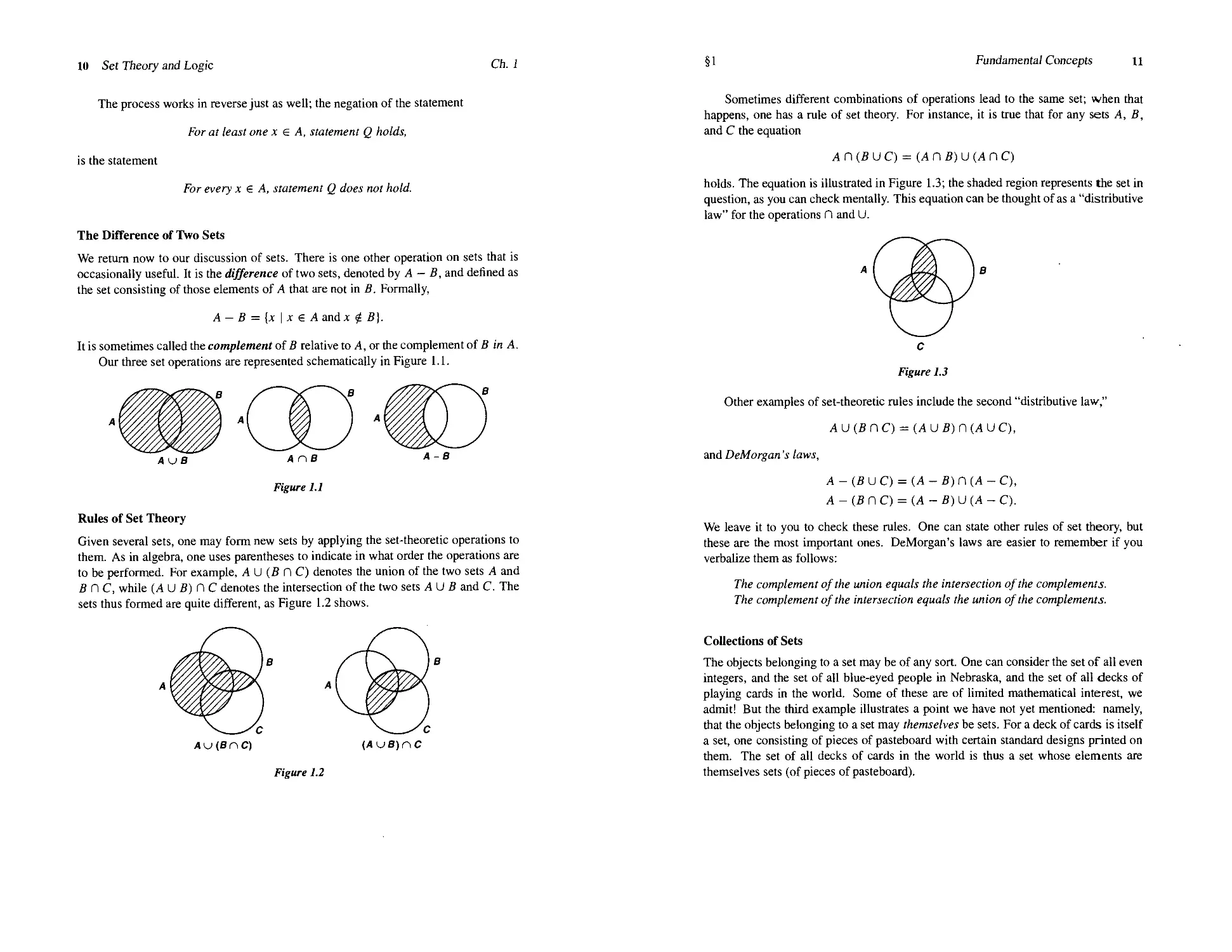
The Difference of Two Sets
We return now to our discussion of sets. There is one other operation on sets that is
occasionally useful. It is the difference of two sets, denoted by A — B, and defined as
the set consisting of those elements of A that are not in B. Formally,
A - В = {x \ x e A and x <? B}.
It is sometimes called the complement of В relative to A, or the complement of В in A.
Our three set operations are represented schematically in Figure 1.1.
A-B
Rules of Set Theory
Given several sets, one may form new sets by applying the set-theoretic operations to
them. As in algebra, one uses parentheses to indicate in what order the operations are
to be performed. For example, A U (В П C) denotes the union of the two sets A and
В DC, while (A U В) П С denotes the intersection of the two sets A U В and С The
sets thus formed are quite different, as Figure 1.2 shows.
AU(BnC)
Figure 1.2
§1
Fundamental Concepts
11
Sometimes different combinations of operations lead to the same set; when that
happens, one has a rule of set theory. For instance, it is true that for any sets A, B,
and С the equation
А П (S U С) = (А П В) U (А П С)
holds. The equation is illustrated in Figure 1.3; the shaded region represents the set in
question, as you can check mentally. This equation can be thought of as a "distributive
law" for the operations П and U.
С
Figure 1.3
Other examples of set-theoretic rules include the second "distributive law,"
A U (В П С) = (A U В) П (A U С),
and DeMorgan 's laws,
A - (В U С) = (А - В) П (А - С),
А - (В П С) = (А - В) U (А - С).
We leave it to you to check these rules. One can state other rules of set theory, but
these are the most important ones. DeMorgan's laws are easier to remember if you
verbalize them as follows:
The complement of the union equals the intersection of the complements.
The complement of the intersection equals the union of the complements.
Collections of Sets
The objects belonging to a set may be of any sort. One can consider the set of all even
integers, and the set of all blue-eyed people in Nebraska, and the set of all decks of
playing cards in the world. Some of these are of limited mathematical interest, we
admit! But the third example illustrates a point we have not yet mentioned: namely,
that the objects belonging to a set may themselves be sets. For a deck of cards is itself
a set, one consisting of pieces of pasteboard with certain standard designs printed on
them. The set of all decks of cards in the world is thus a set whose elements are
themselves sets (of pieces of pasteboard).
12 Set Theory and Logic
Ch. I
We now have another way to form new sets from old ones. Given a set A, we can
consider sets whose elements are subsets of A. In particular, we can consider the set
of all subsets of A. This set is sometimes denoted by the symbol !P{A) and is called
the power set of A (for reasons to be explained later).
When we have a set whose elements are sets, we shall often refer to it as a collec-
collection of sets and denote it by a script letter such as Л or ?. This device will help us
in keeping things straight in arguments where we have to consider objects, and sets of
objects, and collections of sets of objects, all at the same time. For example, we might
use Л to denote the collection of all decks of cards in the world, letting an ordinary
capital letter A denote a deck of cards and a lowercase letter a denote a single playing
card.
A certain amount of care with notation is needed at this point. We make a distinc-
distinction between the object a, which is an element of a set A, and the one-element set [a],
which is a subset of A. To illustrate, if A is the set {a, b, c), then the statements
a e А, {а} С A, and {a} e IP (A)
are all correct, but the statements [a] s A and а С Л are not.
Arbitrary Unions and Intersections
We have already defined what we mean by the union and the intersection of two sets.
There is no reason to limit ourselves to just two sets, for we can just as well form the
union and intersection of arbitrarily many sets.
Given a collection Л of sets, the union of the elements of Л is defined by the
equation
[J A = {* | x 6 A for at least one A e A].
AaA
The intersection of the elements of Л is defined by the equation
О A = {x I x 6 A for every A e A).
AaA
There is no problem with these definitions if one of the elements of A happens to be
the empty set. But it is a bit tricky to decide what (if anything) these definitions mean
if we allow A to be the empty collection. Applying the definitions literally, we see that
no element x satisfies the defining property for the union of the elements of A. So it is
reasonable to say that
if A is empty. On the other hand, every x satisfies (vacuously) the defining property for
the intersection of the elements of A. The question is, every x in what set? If one has a
given large set X that is specified at the outset of the discussion to be one's "universe of
discourse," and one considers only subsets of X throughout, it is reasonable to let
§1
Fundamental Concepts
13
when A is empty. Not all mathematicians follow this convention, however. To avoid
difficulty, we shall not define the intersection when A is empty.
Cartesian Products
There is yet another way of forming new sets from old ones; it involves the notion of an
"ordered pair" of objects. When you studied analytic geometry, the first thing you did
was to convince yourself that after one has chosen an л:-axis and a y-axis in the plane,
every point in the plane can be made to correspond to a unique ordered pair (x, y) of
real numbers. (In a more sophisticated treatment of geometry, the plane is more likely
to be defined as the set of all ordered pairs of real numbers!)
The notion of ordered pair carries over to general sets. Given sets A and B, we
define their cartesian product A x В to be the set of all ordered pairs (a, b) for which a
is an element of A and b is an element of B. Formally,
A x В = ((я, b) | a € A and b 6 S).
This definition assumes that the concept of "ordered pair" is already given. It can be
taken as a primitive concept, as was the notion of "set"; or it can be given a definition in
terms of the set operations already introduced. One definition in terms of set operations is
expressed by the equation
it defines the ordered pair (a, b) as a collection of sets. If а ф b, this definition says that
(a, b) is a collection containing two sets, one of which is a one-element set and the other
a two-element set. The first coordinate of the ordered pair is defined to be the element
belonging to both sets, and the second coordinate is the element belonging to only one of
the sets. If a = b, then (a, b) is a collection containing only one set {a), since {a, b) =
{a, a] = (a) in this case. Its first coordinate and second coordinate both equal the element
in this single set.
I think it is fair to say that most mathematicians think of an ordered pair as a primitive
concept rather than thinking of it as a collection of sets!
Let us make a comment on notation. It is an unfortunate fact that the notation (a, b)
is firmly established in mathematics with two entirely different meanings. One mean-
meaning, as an ordered pair of objects, we have just discussed. The other meaning is the
one you are familiar with from analysis; if a and b are real numbers, the symbol (a, b)
is used to denote the interval consisting of all numbers x such that a < x <b. Most of
the time, this conflict in notation will cause no difficulty because the meaning will be
clear from the context. Whenever a situation occurs where confusion is possible, we
shall adopt a different notation for the ordered pair (a, b), denoting it by the symbol
a x b
instead.
14 Set Theory and Logic Ch. 1
Exercises
1. Check the distributive laws for U and П and DeMorgan's laws.
2. Determine which of the following statements are true for all sets A, B,C, and D.
If a double implication fails, determine whether one or the other of the possible
implications holds. If an equality fails, determine whether the statement be-
becomes true if the "equals" symbol is replaced by one or the other of the inclusion
symbols С or 3.
(a) А С В and А С С <3> А С (В U С).
(b) А С В or А С С <3> А С (В U С).
(c) А С В and А С С <3> А С (В П С).
(d) Л С В or Л С С <3> Л С (В П С).
(e) А-(А- В) = В.
(f) Д-(В -Л) = А- В.
(g) Л П (В - С) = (А П В) - (Л П С),
(h) A U (В - С) = (A U В) - (A U С),
(i) (ADB)U(A-В) = А.
0) А С С and В С О => {А х В) С (С х D).
(к) The converse of (j).
A) The converse of (j), assuming that A and В are nonempty.
(m) (A x B) U (С x D) = (A U C) x (B U D).
(n) (A x В) П (C x D) = (А П С) х (В П ?>).
(o) A x (S - C) = (A x S) - (A x C).
(p) (il-i)x(C-D) = HxC-fixC)-AxO.
(q) (Ax fl) - (C x ?>) = (A - С) х (В - D).
3. (a) Write the contrapositive and converse of the following statement: "If x < 0,
then x2 — x > 0," and determine which (if any) of the three statements are
true,
(b) Do the same for the statement "If x > 0, then x2 - x > 0."
4. Let A and В be sets of real numbers. Write the negation of each of the following
statements:
(a) For every a € A, it is true that а2 е В.
(b) For at least one a 6 A, it is true that a2 € B.
(c) For every a € A, it is true that a2 ? B.
(d) For at least one a <? A, it is true that a2 e B.
5. Let A be a nonempty collection of sets. Determine the truth of each of the
following statements and of their converses:
(a) x e Ua€,a A =>¦ * € A for at least one A e A.
(b) x € LUe,A A => j: € A for every A e A.
(c) x € Плел A => x e A for at least one A € A.
(d) x e С\АеЛ A =>¦ x € A for every A € A
6. Write the contrapositive of each of the statements of Exercise 5.
§2
Functions
15
7. Given sets A, B, and C, express each of the following sets in terms of A, B,
and C, using the symbols U, П, and —.
D = {x | x € A and (x e В or x e C)},
? = {* | (* € A and* € B)or;c € C},
F = [x | л: € A and (* € В => л: € С)}.
8. If a set A has two elements, show that P(A) has four elements. How many
elements does !P (A) have if A has one element? Three elements? No elements?
Why is P(A) called the power set of A?
9. Formulate and prove DeMorgan's laws for arbitrary unions and intersections.
10. Let R denote the set of real numbers. For each of the following subsets of К х К,
determine whether it is equal to the cartesian product of two subsets of R.
(a) {(x,y) \x is an integer}.
(b) ((*, y) | 0 < у < 1).
(c) ((*, у) I У > x).
(d) ((*,>') | x is not an integer and у is an integer).
(e) {(x,y)\x2 + y2< 1}.
§2 Functions
The concept of function is one you have seen many times already, so it is hardly nec-
necessary to remind you how central it is to all mathematics. In this section, we give the
precise mathematical definition, and we explore some of the associated concepts.
A function is usually thought of as a rule that assigns to each element of a set A,
an element of a set В. In calculus, a function is often given by a simple formula such
as f(x) = 3x2 + 2 or perhaps by a more complicated formula such as
One often does not even mention the sets A and В explicitly, agreeing to take A to be
the set of all real numbers for which the rule makes sense and В to be the set of all real
numbers.
As one goes further in mathematics, however, one needs to be more precise about
what a function is. Mathematicians think of functions in the way we just described,
but the definition they use is more exact. First, we define the following:
Definition. A rule of assignment is a subset r of the cartesian product С х D of two
sets, having the property that each element of С appears as the first coordinate of at
most one ordered pair belonging to r.
16 Set Theory and Logic
Ch.l
Thus, a subset r of С x D is a rule of assignment if
[(c, d) e r and (c, d') € r] ==» [d = d'].
We think of r as a way of assigning, to the element с of C, the element d of D for
which (c, d) e r.
Given a rule of assignment r, the domain of г is defined to be the subset of С
consisting of all first coordinates of elements of r, and the image set of r is defined as
the subset of D consisting of all second coordinates of elements of r. Formally,
domain r = (c | there exists d e D such that (c, d) € r},
image r = {d | there exists с е С such that (c,d) e r].
Note that given a rule of assignment r, its domain and image are entirely determined.
Now we can say what a function is.
Definition. A function f is a rule of assignment r, together with a set В that contains
the image set of r. The domain A of the rule r is also called the domain of the
function /; the image set of r is also called the image set of /; and the set В is called
the range of /.t
If / is a function having domain A and range S, we express this fact by writing
/'¦A
B,
which is read "/ is a function from A to B," or "/ is a mapping from A into S," or
simply "/ maps A into S." One sometimes visualizes / as a geometric transformation
physically carrying the points of A to points of B.
If / : A —»¦ В and if a is an element of A, we denote by f(a) the unique element
of В that the rule determining / assigns to a; it is called the value of / at a, or
sometimes the image of a under /. Formally, if r is the rule of the function /, then
f(a) denotes the unique element of В such that (a, /(a)) € r.
Using this notation, one can go back to defining functions almost as one did before,
with no lack of rigor. For instance, one can write (letting R denote the real numbers)
"Let / be the function whose rule is [(x,x3 + 1) | x e R} and whose
range is R,"
or one can equally well write
"Let / : R -> R be the function such that f(x) = хг + 1."
Both sentences specify precisely the same function. But the sentence "Let / be the
function f(x) = хъ + 1" is no longer adequate for specifying a function because it
specifies neither the domain nor the range of /.
t Analysts are apt to use the word "range" to denote what we have called the "image set" of /.
They avoid giving the set В a name.
§2
Functions
17
Definition. If / : A -> В and if Ao is a subset of A, we define the restriction of /
to Ao to be the function mapping Ao into В whose rule is
{(a, f(a)) | a 6 Ao}.
It is denoted by /|Ao, which is read "/ restricted to Ao"
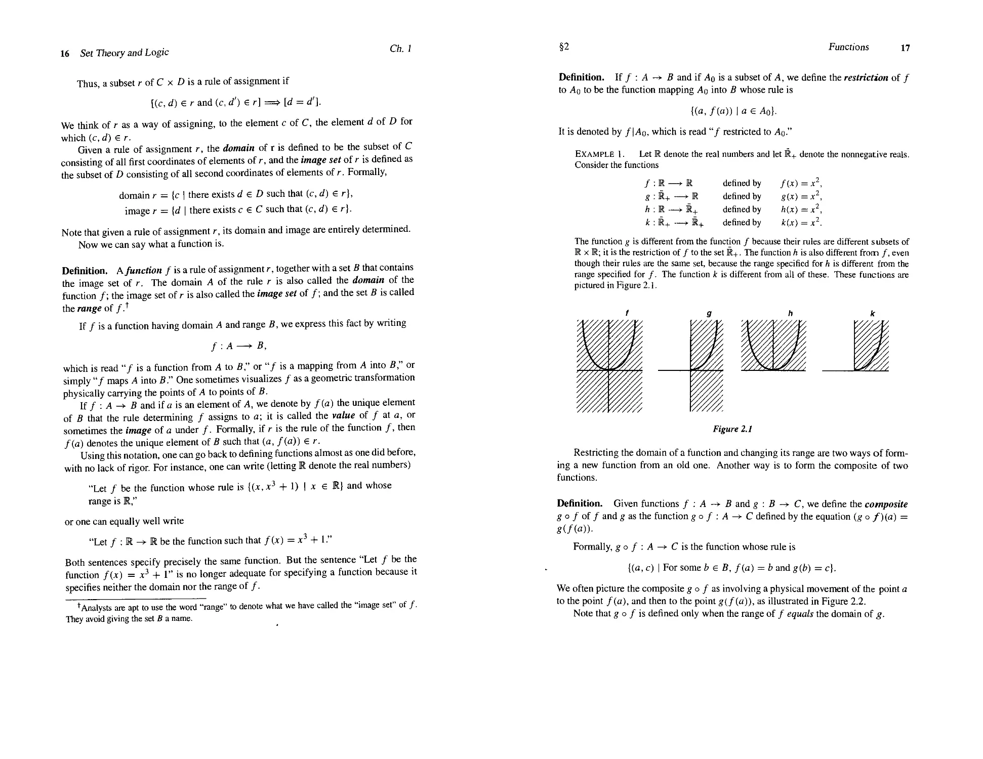
Example 1. Let R denote the real numbers and let R+ denote the nonnegative reals.
Consider the functions
/:R —
g:&+-
h :M —
к :R+ -
¦ Ш
-»R
+ K+
-* K+
defined by
defined by
defined by
defined by
f(x)=x\
g(x)=x2,
h(x)=x2,
k(x) = x2.
The function g is different from the function / because their rules are different subsets of
R x R; it is the restriction of / to the set R+. The function A is also different from /, even
though their rules are the same set, because the range specified for A is different from the
range specified for /. The function к is different from all of these. These functions are
pictured in Figure 2.1.
Figure 2.1
Restricting the domain of a function and changing its range are two ways of form-
forming a new function from an old one. Another way is to form the composite of two
functions.
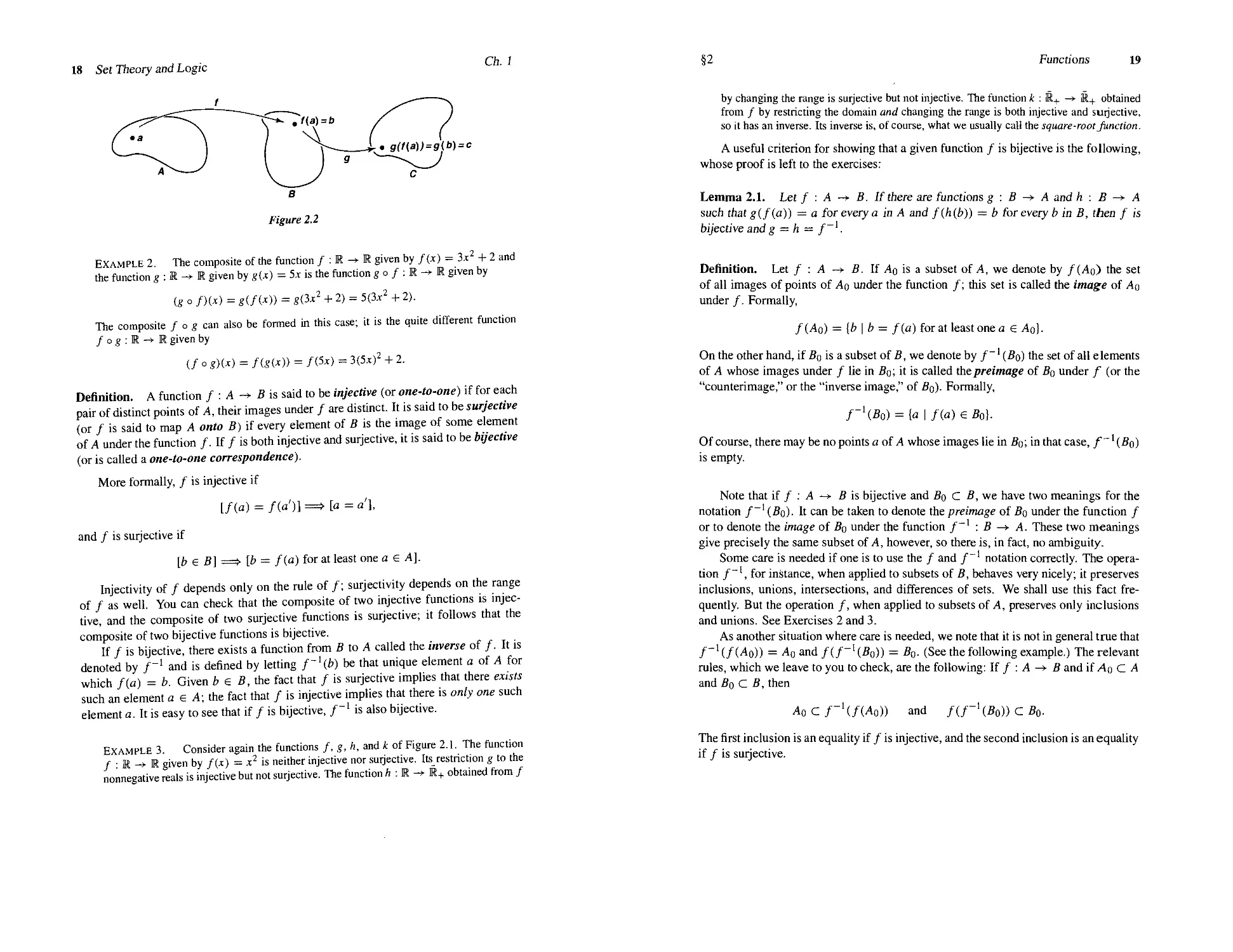
Definition. Given functions / : A —> В and g : В —> С, we define the composite
g о f of / and g as the function g о f : A —>¦ С defined by the equation (g о f)(a) =
g(f(a)).
Formally, g о / : A —>• С is the function whose rule is
{(a, c) | For some b e B, f(a) = b and g(b) = c).
We often picture the composite g о / as involving a physical movement of the point a
to the point /(a), and then to the point g(f(a)), as illustrated in Figure 2.2.
Note that g о / is defined only when the range of / equals the domain of g.
18 Set Theory and Logic
Ch. 1
Example 2. The composite of the function / : R -> R given by f(x) = 3*2 + 2 and
the function g : Ш —> R given by g(x) = 5x is the function g о / : R —> R given by
(g о
= «(/(*)) = gC.t2 + 2) = 5C*2 + 2).
The composite fog can also be formed in this case; it is the quite different function
/ о g : R -> R given by
(/ о
= fEx) = 3E*J + 2.
Definition. A function / : A -> S is said to be injective (or one-to-one) if for each
pair of distinct points of A, their images under / are distinct. It is said to be surjective
(or / is said to map A onto B) if every element of Й is the image of some element
of A under the function /. If / is both injective and surjective, it is said to be bijective
(or is called a one-to-one correspondence).
More formally, / is injective if
¦ [a = a'],
and / is surjective if
[b e B] => [b = f(a) for at least one a e A].
Injectivity of / depends only on the rule of /; surjectivity depends on the range
of / as well. You can check that the composite of two injective functions is injec-
injective, and the composite of two surjective functions is surjective; it follows that the
composite of two bijective functions is bijective.
If / is bijective, there exists a function from S to A called the inverse of /. It is
denoted by /~' and is defined by letting f~l{b) be that unique element a of Л for
which /(a) = b. Given be S, the fact that / is surjective implies that there exists
such an element a e A; the fact that / is injective implies that there is only one such
element a. It is easy to see that if / is bijective, /~' is also bijective.
EXAMPLE 3. Consider again the functions /, g, h, and к of Figure 2.1. The function
/ : R —* R given by f(x) = x2 is neither injective nor surjective. Its restriction g to the
nonnegative reals is injective but not surjective. The function A : R —* R+ obtained from /
§2
Functions
19
by changing the range is surjective but not injective. The function к : Ш+ —>• R+ obtained
from / by restricting the domain and changing the range is both injective and surjective,
so it has an inverse. Its inverse is, of course, what we usually call the square-root function.
A useful criterion for showing that a given function / is bijective is the following,
whose proof is left to the exercises:
Lemma 2.1. Let f : A -> B. If there are functions g : В -> A and h : В —у А
such that g(f(a)) = a for every a in A and f(h(b)) = b for every b in B, then f is
bijective and g = h — f~l.
Definition. Let f : A -> B. If Ao'is a subset of A, we denote by /(Ao) the set
of all images of points of Aq under the function /; this set is called the image of Aq
under /. Formally,
f(Ao) — {b | b = f(a) for at least one a 6 Aol-
On the other hand, if So is a subset of B, we denote by /"' (So) the set of all elements
of A whose images under / lie in So; it is called thepreimage of So under f (or the
"counterimage," or the "inverse image," of So). Formally,
f-l(B0) = {a | f{a) 6 So).
Of course, there may be no points a of Л whose images lie in So; in that case, f~l(Bo)
is empty.
Note that if / : A —>¦ В is bijective and So С S, we have two meanings for the
notation /~' (So). It can be taken to denote the preimage of So under the function /
or to denote the image of So under the function /"' : В —*¦ A. These two meanings
give precisely the same subset of A, however, so there is, in fact, no ambiguity.
Some care is needed if one is to use the / and /~' notation correctly. The opera-
operation /"', for instance, when applied to subsets of S, behaves very nicely; it preserves
inclusions, unions, intersections, and differences of sets. We shall use this fact fre-
frequently. But the operation /, when applied to subsets of A, preserves only inclusions
and unions. See Exercises 2 and 3.
As another situation where care is needed, we note that it is not in general true that
f'l(f(A0)) = Ao and f(f~l(B0)) = So. (See the following example.) The relevant
rules, which we leave to you to check, are the following: If / : A -*¦ В and if Ao С А
and So С S, then
AoCf-l(f(Ao)) and /(/"'(йо))С5о.
The first inclusion is an equality if / is injective, and the second inclusion is an equality
if / is surjective.
20 Set Theory and Logic
Ch.l
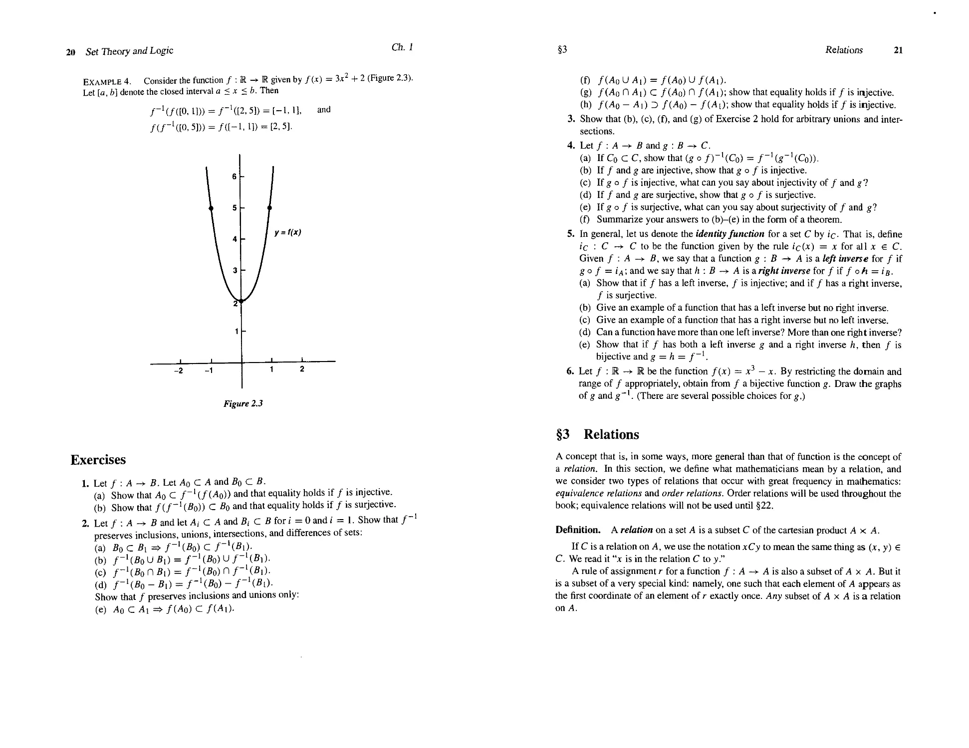
EXAMPLE 4. Consider the function / : К -»• R given by /(*) = 3*2 + 2 (Figure 2.3).
Let [a, b] denote the closed interval a <x <b. Then
/-'(/([0,1])) = /-'([2,5]) = [-1,1],
/(/"'([0,5])) = /([-1,1]) = [2, 5].
and
-2
I
\
\
-1
6
5
4
i 3
?
1
- I
-
l/
1
m
1
2
Figure 2.3
Exercises
1. Let / : A -> S. Let Ao С A and So С S.
(a) Show that Ao С /"' (/(Ao)) and that equality holds if / is injective.
(b) Show that /(/"' (Bo)) С Bo and that equality holds if / is surjective.
2. Let / : A -> S and let Л, С A and Я, С S for i = 0 and / = 1. Show that /~'
preserves inclusions, unions, intersections, and differences of sets:
(a) BoCfli =>/-'(йо)С/-1(Й1).
(b) / '1
(c) /
(d) /(йоЙ1) /(йо)/A)
Show that / preserves inclusions and unions only:
(e) A0CA| => /(Ao) С /(Ai).
§3
Relations
21
(f)
(g) /(Ao П A{) С /(Ao) П /(Ai); show that equality holds if / is injective.
(h) /(Ao - Ai) 3 /(Ao) - /(Ai); show that equality holds if / is injective.
3. Show that (b), (c), (f), and (g) of Exercise 2 hold for arbitrary unions and inter-
intersections.
4. Let / : A -> В and g : В -> С.
(a) If Co С С, show that (g о /г'(Со) = /"'(«"'(Со)).
(b) If / and g are injective, show that g о / is injective.
(c) If g о / is injective, what can you say about injectivity of / and g?
(d) If / and g are surjective, show that g о / is surjective.
(e) If g о / is surjective, what can you say about surjectivity of / and g?
(f) Summarize your answers to (b)-(e) in the form of a theorem.
5. In general, let us denote the identity function for a set С by ic- That is, define
ic '¦ С -> С to be the function given by the rule ic(x) = x for all x € C.
Given / : A —>¦ B, we say that a function g : В -> A is a /e/if inverse for / if
go / = iA; and we say that h : В -> A is aright inverse lor f if f oh = /3.
(a) Show that if / has a left inverse, / is injective; and if / has a right inverse,
/ is surjective.
(b) Give an example of a function that has a left inverse but no right inverse.
(c) Give an example of a function that has a right inverse but no left inverse.
(d) Can a function have more than one left inverse? More than one right inverse?
(e) Show that if / has both a left inverse g and a right inverse h, then / is
bijective and g = h = f~l.
6. Let / : R -> R be the function f(x) = x3 — x. By restricting the domain and
range of / appropriately, obtain from / a bijective function g. Draw the graphs
of g and g~l. (There are several possible choices for g.)
§3 Relations
A concept that is, in some ways, more general than that of function is the concept of
a relation. In this section, we define what mathematicians mean by a relation, and
we consider two types of relations that occur with great frequency in mathematics:
equivalence relations and order relations. Order relations will be used throughout the
book; equivalence relations will not be used until §22.
Definition. A relation on a set A is a subset С of the cartesian product A x. A.
If С is a relation on A, we use the notation xCy to mean the same thing as (*, y) €
C. We read it "x is in the relation С to y."
A rule of assignment r for a function / : A —>¦ A is also a subset of A x A. But it
is a subset of a very special kind: namely, one such that each element of A appears as
the first coordinate of an element of r exactly once. Any subset of A x A is a relation
on A.
22 Set Theory and Logic
Ch. 1
Example 1. Let P denote the set of all people in the world, and define D С P x P by
the equation
D = {(x, У) I x is a descendant of y).
Then D is a relation on the set P. The statements "x is in the relation D to y" and "* is
a descendant of v" mean precisely the same thing, namely, that (x,y) 6 D. Two other
relations on P are the following:
В = |(.t, у) | x has an ancestor who is also an ancestor of y),
S = {(x, y) | the parents of л: are the parents of у).
We can call В the "blood relation" (pun intended), and we can call S the "sibling relation."
These three relations have quite different properties. The blood relationship is symmetric,
for instance (if x is a blood relative of y, then у is a blood relative of x), whereas the
descendant relation is not. We shall consider these relations again shortly.
Equivalence Relations and Partitions
An equivalence relation on a set Л is a relation С on Л having the following three
properties:
A) (Refiexivity) xCx for every x in A.
B) (Symmetry) If xCy, then yd.
C) (Transitivity) If xCy and yCz, then xCz.
Example 2. Among the relations defined in Example 1, the descendant relation D is
neither reflexive nor symmetric, while the blood relation В is not transitive (I am not a
blood relation to my wife, although my children are!) The sibling relation S is, however,
an equivalence relation, as you may check.
There is no reason one must use a capital letter—or indeed a letter of any sort—
to denote a relation, even though it is a set. Another symbol will do just as well.
One symbol that is frequently used to denote an equivalence relation is the "tilde"
symbol ~. Stated in this notation, the properties of an equivalence relation become
A) x ~ x for every x in A.
B) If x ~ y, then у ~х.
C) If x ~ у and у ~ z, then x ~ z.
There are many other symbols that have been devised to stand for particular equiva-
equivalence relations; we shall meet some of them in the pages of this book.
Given an equivalence relation ~ on a set A and an element x of A, we define a
certain subset ? of A, called the equivalence class determined by x, by the equation
E = {y\y~x].
Note that the equivalence class E determined by x contains x, since x
lence classes have the following property:
x. Equiva-
Equiva§3
Relations
23
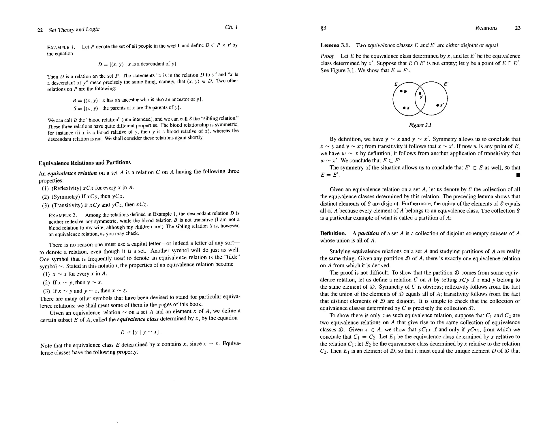
Lemma 3.1. Two equivalence classes E and ?' are either disjoint or equal.
Proof. Let E be the equivalence class determined by x, and let ?' be the equivalence
class determined by x'. Suppose that E П ?' is not empty; let у be a point of E П ?'.
See Figure 3.1. We show that E = ?'.
Figure 3.1
By definition, we have у ~ х and у ~ x'. Symmetry allows us to conclude that
x ~ у and у ~ x'; from transitivity it follows that x ~ x'. If now w is any point of E,
we have uj ~ x by definition; it follows from another application of transitivity that
w ~ л'. We conclude that E с ?'.
The symmetry of the situation allows us to conclude that ?' С ? as well, So that
? = ?'. ¦
Given an equivalence relation on a set A, let us denote by S the collection of all
the equivalence classes determined by this relation. The preceding lemma shows that
distinct elements of 8 are disjoint. Furthermore, the union of the elements of S equals
all of A because every element of A belongs to an equivalence class. The collection S
is a particular example of what is called a partition of A:
Definition. A partition of a set A is a collection of disjoint nonempty subsets of A
whose union is all of A.
Studying equivalence relations on a set A and studying partitions of A are really
the same thing. Given any partition ?) of A, there is exactly one equivalence relation
on A from which it is derived.
The proof is not difficult. To show that the partition X) comes from some equiv-
equivalence relation, let us define a relation С on A by setting xCy if x and у belong to
the same element of D. Symmetry of С is obvious; refiexivity follows from the fact
that the union of the elements of S) equals all of A; transitivity follows from the fact
that distinct elements of X) are disjoint. It is simple to check that the collection of
equivalence classes determined by С is precisely the collection ?).
To show there is only one such equivalence relation, suppose that C\ and C2 are
two equivalence relations on A that give rise to the same collection of equivalence
classes ?). Given x e A, we show that yCix if and only if yCjx, from which we
conclude that C\ = Сг- Let E\ be the equivalence class determined by x relative to
the relation C\; let ?2 be the equivalence class determined by x relative to the relation
Ci. Then E\ is an element of ?), so that it must equal the unique element D of S) that
24 Set Theory and Logic
Ch.l
contains x. Similarly, ?2 must equal D. Now by definition, E\ consists of all у such
that yC\x; and ?2 consists of all у such that уСгх. Since Ey = D = ?2, our result is
proved.
Example 3. Define two points in the plane to be equivalent if they lie at the same
distance from the origin. Reflexivity, symmetry, and transitivity hold trivially. The collec-
collection g of equivalence classes consists of all circles centered at the origin, along with the set
consisting of the origin alone.
EXAMPLE 4. Define two points of the plane to be equivalent if they have the same
y-coordinate. The collection of equivalence classes is the collection of all straight lines in
the plane parallel to the x-axis.
Example 5. Let X be the collection of all straight lines in the plane parallel to the line
у — —x. Then X is a partition of the plane, since each point lies on exactly one such line.
The partition X comes from the equivalence relation on the plane that declares the points
(xo, Уо) and (xi, y\) to be equivalent if xq + yo = xi + y\.
EXAMPLE 6. Let X' be the collection of all straight lines in the plane. Then X' is not
a partition of the plane, for distinct elements of X' are not necessarily disjoint; two lines
may intersect without being equal.
Order Relations
A relation С on a set Л is called an order relation (or a simple order, or a linear order)
if it has the following properties:
A) (Comparability) For every x and у in A for which x ф у, either xCy or yCx.
B) (Nonreflexivity) For no x in A does the relation xCx hold.
C) (Transitivity) If xCy and yCz, then xCz.
Note that property A) does not by itself exclude the possibility that for some pair of
elements x and у of A, both the relations xCy and yCx hold (since "or" means "one
or the other, or both"). But properties B) and C) combined do exclude this possibil-
possibility; for if both xCy and yCx held, transitivity would imply that xCx, contradicting
nonreflexivity.
Example 7. Consider the relation on the real line consisting of all pairs (x, y) of real
numbers such that x < y. It is an order relation, called the "usual order relation," on the
real line. A less familiar order relation on the real line is the following: Define xCy if
x2 < y2,or if л:2 = у2 andx < у. You can check that this is an order relation.
EXAMPLE 8. Consider again the relationships among people given in Example 1. The
blood relation В satisfies none of the properties of an order relation, and the sibling rela-
relation S satisfies only C). The descendant relation D does somewhat better, for it satisfies
both B) and C); however, comparability still fails. Relations that satisfy B) and C) occur
often enough in mathematics to be given a special name. They are called strict partial
order relations; we shall consider them later (see §11).
§3
Relations 25
As the tilde, ~, is the generic symbol for an equivalence relation, the "less than"
symbol, <, is commonly used to denote an order relation. Stated in this notation, the
properties of an order relation become
A) If x ф y, then either x < у or v < x.
B) If x < y, thenx ф у.
C) If x < у and у < 1, then x < z.
We shall use the notation x < у to stand for the statement "either x < у or x = y";
and we shall use the notation у > x to stand for the statement "x < y." We write
x < у < z to mean "* < у and у < z."
Definition. If X is a set and < is an order relation on X, and if a < b, we use the
notation (a, b) to denote the set
(x \a < x < b};
it is called an open interval in X. If this set is empty, we call a the immediate prede-
predecessor of b, and we call b the immediate successor of a.
Definition. Suppose that A and В are two sets with order relations <A and <s
respectively. We say that A and В have the same order type if there is a bijective
correspondence between them that preserves order; that is, if there exists a bijective
function / : A -> В such that
ai <л a2 =*• /(ai) <s f(a2).
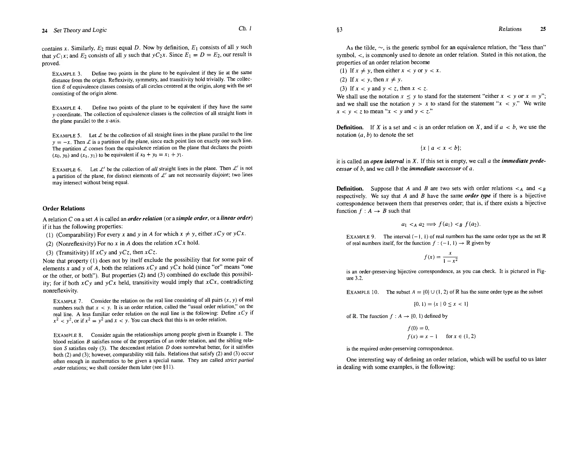
Exam ple 9. The interval (-1, 1) of real numbers has the same order type as the set R
of real numbers itself, for the function / : (— 1, 1) —> R given by
fix) =
\-x2
is an order-preserving bijective correspondence, as you can check. It is pictured in Fig-
Figure 3.2.
Example 10. The subset A = |0) U A, 2) of R has the same order type as the subset
[0, 1) = {* I 0<* < 1]
of R. The function / : A -*¦ [0, 1) defined by
/@) = 0,
f(x)=x-\ for* e A,2)
is the required order-preserving correspondence.
One interesting way of defining an order relation, which will be useful to us later
in dealing with some examples, is the following:
26 Set Theory and Logic
Ch. 1
y=x/A-x2
Figure 3.2
Definition. Suppose that A and В are two sets with order relations <A and <fl
respectively. Define an order relation < on A x В by defining
a\ x b\ < 02 x fo
if ai <д иг, or if ai = O2 and b\ <в Ьг. It is called the dictionary order relation on
Ax B.
Checking that this is an order relation involves looking at several separate cases;
we leave it to you.
The reason for the choice of terminology is fairly evident. The rule defining < is
the same as the rule used to order the words in the dictionary. Given two words, one
compares their first letters and orders the words according to the order in which their
first letters appear in the alphabet. If the first letters are the same, one compares their
second letters and orders accordingly. And so on.
EXAMPLE 11. Consider the dictionary order on the plane ixR. In this order, the
point p is less than every point lying above it on the vertical line through p, and p is less
than every point to the right of this vertical line.
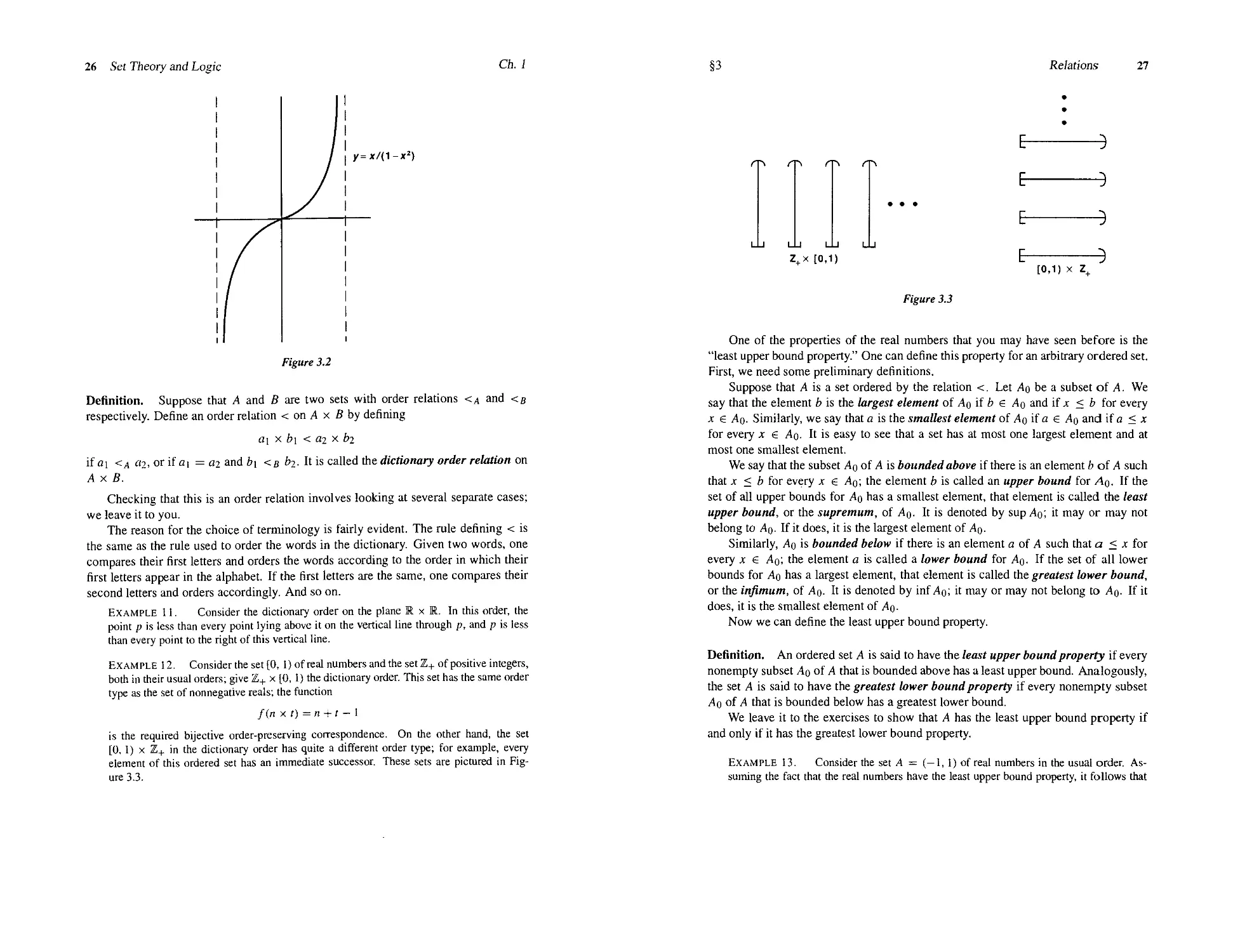
Ex AM PLE 12. Consider the set [0, 1) of real numbers and the set Z+ of positive integers,
both in their usual orders; give 2,+ x [0, 1) the dictionary order. This set has the same order
type as the set of nonnegative reals; the function
f(n x t) = n + r - 1
is the required bijective order-preserving correspondence. On the other hand, the set
[0, 1) x Z+ in the dictionary order has quite a different order type; for example, every
element of this ordered set has an immediate successor. These sets are pictured in Fig-
Figure 3.3.
Relations
27
Z+x[0,1)
[0,1) x Z+
Figure 3.3
One of the properties of the real numbers that you may have seen before is the
"least upper bound property." One can define this property for an arbitrary ordered set.
First, we need some preliminary definitions.
Suppose that A is a set ordered by the relation <. Let До be a subset of A. We
say that the element b is the largest element of Ao if b e До and if x < b for every
x € До. Similarly, we say that a is the smallest element of До if a e До and if a < x
for every x € До. It is easy to see that a set has at most one largest element and at
most one smallest element.
We say that the subset До of A is bounded above if there is an element b of A such
that x < b for every x € До; the element b is called an upper bound for До- If the
set of all upper bounds for До has a smallest element, that element is called the least
upper bound, or the supremum, of До. It is denoted by sup До; it may or may not
belong to До- If it does, it is the largest element of До.
Similarly, До is bounded below if there is an element a of A such that a < x for
every x e До; the element a is called a lower bound for До. If the set of all lower
bounds for До has a largest element, that element is called the greatest lower bound,
or the infimum, of До. It is denoted by inf До; it may or may not belong to До- If it
does, it is the smallest element of До.
Now we can define the least upper bound property.
Definition. An ordered set A is said to have the least upper bound property if every
nonempty subset Ao of A that is bounded above has a least upper bound. Analogously,
the set A is said to have the greatest lower bound property if every nonempty subset
До of A that is bounded below has a greatest lower bound.
We leave it to the exercises to show that A has the least upper bound property if
and only if it has the greatest lower bound property.
EXAMPLE 13. Consider the set A = (-1, 1) of real numbers in the usual order. As-
Assuming the fact that the real numbers have the least upper bound property, it follows that
28 Set Theory and Logic
Ch. 1
the set A has the least upper bound property. For, given any subset of A having an upper
bound in A, it follows that its least upper bound (in the real numbers) must be in A. For
example, the subset {—l/2n | n € Z+) of A, though it has no largest element, does have a
least upper bound in A, the number 0.
On the other hand, the set В = (-1, 0) U @, 1) does not have the least upper bound
property. The subset {—l/2n | n e Z+) of В is bounded above by any element of @, 1),
but it has no least upper bound in B.
Exercises
Equivalence Relations
1. Define two points (xq, yo) and (x\. y\) of the plane to be equivalent if yo — x\ =
y\ — x\. Check that this is an equivalence relation and describe the equivalence
classes.
2. Let С be a relation on a set A. If Aq С A, define the restriction of С to Aq to be
the relation С Л (До х ^о)- Show that the restriction of an equivalence relation
is an equivalence relation.
3. Here is a "proof that every relation С that is both symmetric and transitive is
also reflexive: "Since С is symmetric, aCb implies bCa. Since С is transitive,
aCb and bCa together imply aCa, as desired." Find the flaw in this argument.
4. Let / : A -> В be a surjective function. Let us define a relation on A by setting
qq ~ oi if
(a) Show that this is an equivalence relation.
(b) Let A* be the set of equivalence classes. Show there is a bijective correspon-
correspondence of A* with B.
5. Let S and S' be the following subsets of the plane:
S - {(x, y) | у = x + 1 and 0 < x < 2),
S' = {(x, y) | у - x is an integer}.
(a) Show that S' is an equivalence relation on the real line and S' э S. Describe
the equivalence classes of S'.
(b) Show that given any collection of equivalence relations on a set A, their
intersection is an equivalence relation on A.
(c) Describe the equivalence relation T on the real line that is the intersection
of all equivalence relations on the real line that contain S. Describe the
equivalence classes of T.
§3
Relations
29
Order Relations
6. Define a relation on the plane by setting
(xo,yo) < (x\,yi)
if either yo — x^ < y\ — xf, or yo — x^ = y\ — x\ and xq < x\. Show that this
is an order relation on the plane, and describe it geometrically.
7. Show that the restriction of an order relation is an order relation.
8. Check that the relation defined in Example 7 is an order relation.
9. Check that the dictionary order is an order relation.
10. (a) Show that the map / : (-1, 1) -> R of Example 9 is order preserving.
(b) Show that the equation g(y) = 2y/[l + A + 4y2I/2] defines a function
g : R —>• (—1,1) that is both a left and a right inverse for /.
11. Show that an element in an ordered set has at most one immediate successor and
at most one immediate predecessor. Show that a subset of an ordered set has at
most one smallest element and at most one largest element.
12. Let Z+ denote the set of positive integers. Consider the following order relations
on Z+ x Z+:
(i) The dictionary order,
(ii) (x0, yo) < (x\, y\) if either x0 - yo < xx - yu or x0 - y0 - x\ - y\ and
yo < yi-
(iii) (x0, yo) < (x\, yi) if either x0 + yo < x\ + y\, or xo + yo=x\ + yi and
У0 < У1-
In these order relations, which elements have immediate predecessors? Does the
set have a smallest element? Show that all three order types are different.
13. Prove the following:
Theorem. If an ordered set A has the least upper bound property, then it has the
greatest lower bound property.
14. If С is a relation on a set A, define a new relation D on A by letting (b, a) € D
if (a, b)€C.
(a) Show that С is symmetric if and only if С = D.
(b) Show that if С is an order relation, D is also an order relation.
(c) Prove the converse of the theorem in Exercise 13.
15. Assume that the real line has the least upper bound property,
(a) Show that the sets
[0, 1] = {x | 0 <x < I],
[0, 1) = {x | 0 < x < 1}
have the least upper bound property.
(b) Does [0, 1] x [0, 1] in the dictionary order have the least upper bound prop-
property? What about [0, 1] x [0, 1)? What about [0, 1) x [0, 1]?
30 Set Theory and Logic
Ch. 1
§4 The Integers and the Real Numbers
Up to now we have been discussing what might be called the logical foundations for
our study of topology—the elementary concepts of set theory. Now we turn to what
we might call the mathematical foundations for our study—the integers and the real
number system. We have already used them in an informal way in the examples and
exercises of the preceding sections. Now we wish to deal with them more formally.
One way of establishing these foundations is to construct the real number system,
using only the axioms of set theory—to build them with one's bare hands, so to speak.
This way of approaching the subject takes a good deal of time and effort and is of
greater logical than mathematical interest.
A second way is simply to assume a set of axioms for the real numbers and work
from these axioms. In the present section, we shall sketch this approach to the real
numbers. Specifically, we shall give a set of axioms for the real numbers and shall
indicate how the familiar properties of real numbers and the integers are derived from
them. But we shall leave most of the proofs to the exercises. If you have seen all
this before, our description should refresh your memory. If not, you may want to
work through the exercises in detail in order to make sure of your knowledge of the
mathematical foundations.
First we need a definition from set theory.
Definition. A binary operation on a set A is a function / mapping A x A into A.
When dealing with a binary operation / on a set A, we usually use a notation
different from the standard functional notation introduced in §2. Instead of denoting
the value of the function / at the point (a, a') by f(a, a'), we usually write the symbol
for the function between the two coordinates of the point in question, writing the value
of the function at (a, a') as afa'. Furthermore (just as was the case with relations),
it is more common to use some symbol other than a letter to denote an operation.
Symbols often used are the plus symbol +, the multiplication symbols ¦ and o, and the
asterisk *; however, there are many others.
Assumption
We assume there exists a set R, called the set of real numbers, two binary operations +
and ¦ on R, called the addition and multiplication operations, respectively, and an order
relation < on K, such that the following properties hold:
Algebraic Properties
A) (x + y) + z = x + (y + z),
(x ¦ y) ¦ z = x ¦ (y ¦ z) for all x, y, z in R.
¦ (y ¦
B) x + у = у + x,
x ¦ у = у ¦ х for all x, у in R.
§4
The Integers and the Real Numbers
31
C) There exists a unique element of R called zero, denoted by 0, such that x + 0 = x
for all x e R.
There exists a unique element of R called one, different from 0 and denoted by 1,
such that x ¦ 1 = x for all x e K.
D) For each x in R, there exists a unique у in К such that x + у = 0.
For each x in R different from 0, there exists a unique у in R such that x ¦ у = 1.
E) x ¦ (у + z) = (x ¦ y) + (x ¦ z) for alU, y, z e R.
A Mixed Algebraic and Order Property
F) If x > y, then* + z > у + z.
If x > у and z > 0, then* • z > у ¦ z.
Order Properties
G) The order relation < has the least upper bound property.
(8) If x < y, there exists an element z such that x < z and z < y.
From properties (l)-E) follow the familiar "laws of algebra." Given x, one de-
denotes by —x that number у such that x + у = 0; it is called the negative of x. One
defines the subtraction operation by the formula z — x = z + (—x). Similarly, given
x ф 0, one denotes by l/x that number у such that x ¦ у = 1; it is called the reciprocal
of x. One defines the quotient z/x by the formula z/x = z ¦ (l/x). The usual laws of
signs, and the rules for adding and multiplying fractions, follow as theorems. These
laws of algebra are listed in Exercise 1 at the end of the section. We often denote x ¦ у
simply by xy.
When one adjoins property F) to properties (l)-E), one can prove the usual "laws
of inequalities," such as the following:
If x > у and z < 0, then x ¦ z < у ¦ z.
-1 <0 and 0 < 1.
The laws of inequalities are listed in Exercise 2.
We define a number x to be positive if x > 0, and to be negative if x < 0. We
denote the_positive reals by K+ and the nonnegative reals (for reasons to be explained
later) by R+. Properties (l)-F) are familiar properties in modern algebra. Any set
with two binary operations satisfying (l)-E) is called by algebraists afield; if the field
has an order relation satisfying F), it is called an ordered field.
Properties G) and (8), on the other hand, are familiar properties in topology. They
involve only the order relation; any set with an order relation satisfying G) and (8) is
called by topologists a linear continuum.
Now it happens that when one adjoins to the axioms for an ordered field [proper-
[properties (l)-F)] the axioms for a linear continuum [properties G) and (8)], the resulting
list contains some redundancies. Property (8), in particular, can be proved as a conse-
consequence of the others; given x < у one can show that z = (x + y)/(l + 1) satisfies
the requirements of (8). Therefore, in the standard treatment of the real numbers,
properties (l)-G) are taken as axioms, and property (8) becomes a theorem. We have
32 Set Theory and Logic
Ch. 1
included (8) in our list merely to emphasize the fact that it and the least upper bound
property are the two crucial properties of the order relation for K. From these two
properties many of the topological properties of К may be derived, as we shall see in
Chapter 3.
Now there is nothing in this list as it stands to tell us what an integer is. We now
define the integers, using only properties (l)-F).
Definition. A subset A of the real numbers is said to be inductive if it contains the
number 1, and if for every x in A, the number x+1 is also in A. Let A be the collection
of all inductive subsets of K. Then the set Z+ of positive integers is defined by the
equation
= f| A.
Note that the set K+ of positive real numbers is inductive, for it contains 1 and
the statement x > 0 implies the statement x + 1 > 0. Therefore, Z+ С К+, so the
elements of Z+ are indeed positive, as the choice of terminology suggests. Indeed, one
sees readily that 1 is the smallest element of Z+, because the set of all real numbers x
for which x > 1 is inductive.
The basic properties of Z+, which follow readily from the definition, are the fol-
following:
A) Z+ is inductive.
B) (Principle of induction). If A is an inductive set of positive integers, then A =
Z+.
We define the set Z of integers to be the set consisting of the positive integers Z+,
the number 0, and the negatives of the elements of Z+. One proves that the sum,
difference, and product of two integers are integers, but the quotient is not necessarily
an integer. The set Q of quotients of integers is called the set of rational numbers.
One proves also that, given the integer n, there is no integer a such that n < a <
n + \.
If n is a positive integer, we use the symbol Sn to denote the set of all positive
integers less than n; we call it a section of the positive integers. The set Si is empty,
and Sn+i denotes the set of positive integers between 1 and n, inclusive. We also use
the notation
for the latter set.
Now we prove two properties of the positive integers that may not be quite so
familiar, but are quite useful. They may be thought of as alternative versions of the
induction principle.
Theorem 4.1 (Well-ordering property). Every nonempty subset of Z+ has a small-
smallest element.
§4
The Integers and the. Real Numbers 33
Proof. We first prove that, for each n € Z+, the following statement holds: Every
nonempty subset of {I, ..., n} has a smallest element.
Let A be the set of all positive integers n for which this statement holds. Then A
contains 1, since if n = 1, the only nonempty subset of {1,..., n] is the set {1} itself.
Then, supposing A contains n, we show that it contains n + 1. So let С be a nonempty
subset of the set {1,..., n + 1(. If С consists of the single element n + 1, then that
element is the smallest element of С Otherwise, consider the set СП A,..., л(, which
is nonempty. Because n € A, this set has a smallest element, which will automatically
be the smallest element of С also. Thus A is inductive, so we conclude that A = Z+;
hence the statement is true for all n eZ+.
Now we prove the theorem. Suppose that D is a nonempty subset of Z+_. Choose
an element n of D. Then the set A = D Л A,..., n] is nonempty, so that A has a
smallest element k. The element к is automatically the smallest element of D as well.
Theorem 4.2 (Strong induction principle). Let A be a set of positive integers.
Suppose that for each positive integer n, the statement Sn С A implies the statement
n e A. Then A = Z+.
Proof. If A does not equal all of Z+, let n be the smallest positive integer that is not
in A. Then every positive integer less than n is in A, so that Sn С A. Our hypothesis
implies that n € A, contrary to assumption. ¦
Everything we have done up to now has used only the axioms for an ordered field,
properties (l)-F) of the real numbers. At what point do you need G), the least upper
bound axiom?
For one thing, you need the least upper bound axiom to prove that the set Z+ of
positive integers has no upper bound in K. This is the Archimedean ordering property
of the real line. To prove it, we assume that Z+ has an upper bound and derive a
contradiction. If Z+ has an upper bound, it has a least upper bound b. There exists
n e Z+ such that n > b — 1; for otherwise, b — 1 would be an upper bound for Z+
smaller than b. Then n + 1 > b, contrary to the fact that b is an upper bound for Z+.
The least upper bound axiom is also used to prove a number of other things
about K. It is used for instance to show that К has the greatest lower bound prop-
property. It is also used to prove the existence of a unique positive square root ^fx for
every positive real number. This fact, in turn, can be used to demonstrate the existence
of real numbers that are not rational numbers; the number ~J2 is an easy example.
We use the symbol 2 to denote 1 + 1, the symbol 3 to denote 2+1, and so on
through the standard symbols for the positive integers. It is a fact that this procedure
assigns to each positive integer a unique symbol, but we never need this fact and shall
not prove it.
Proofs of these properties of the integers and real numbers, along with a. few other
properties we shall need later, are outlined in the exercises that follow.
34 Set Theory and Logic
Ch. 1
Exercises
, using only axioms (l)-E):
1. Prove the following "laws of algebra"
(a) If x + у = x, then у = 0.
(b) 0 ¦ x = 0. [Hint: Compute (x + 0) • x.]
(c) -0 = 0.
(d) -(-x)=x.
(e) x(-y) = -(xy) = (-x)y.
(f) (-l)x = -x.
(g) x(y - z)= xy - xz.
(h) ~{x + y) = -x-y; -(x -y) = -x + y.
(i) If x ф 0 and x ¦ у = x, then у = 1.
(j) x/x = 1 ifx /0.
(k) x/1 =x.
A) x ф 0 and у ^ 0 => xy ^ 0.
(m) (l/y)(l/z) = l/(yz)ify,z/0.
(n) (x/y)(w/z) = (xw)/{yz) if y, Z / 0.
@) (x/y) + (w/z) = (xz + wy)/(yz) if y, z / 0.
(p) x/0=> 1/x ^0.
(q) l/(w/z)=z/wiiw,z^0.
(r) (x/y)/(w/z) = (xz)/(yw) if y, w, z ^ 0.
(s) (ax)/y = a(x/y) if у ф 0.
(t) (-x)/y=x/(-y) = -(x/y)ify ф0.
2. Prove the following "laws of inequalities" for R, using axioms A )-F) along with
the results of Exercise 1:
(a) x > у and w>z=>x + w>y + z.
(b) x > 0 and y>0=>x + y>0 and x ¦ у > 0.
(c) х > 0 о -х < 0.
(d) x > у -о- -х < -у.
(e) х > у and z < 0 => xz < yz.
(f) x / 0 => x2 > 0, where x2 = x ¦ x.
(g) -1 <0< 1.
(h) xy > 0 -o- x and у are both positive or both negative.
A) x > 0 =^. 1/x > 0.
(j) x > у > 0 =^. 1/x < 1/y.
(k) x < у =^. x < (x + y)/2 < y.
3. (a) Show that if Л is a collection of inductive sets, then the intersection of the
elements of Л is an inductive set.
(b) Prove the basic properties A) and B) of Z+.
4. (a) Prove by induction that given n € Z+, every nonempty subset of {1,..., n]
has a largest element.
(b) Explain why you cannot conclude from (a) that every nonempty subset of Z+
has a largest element.
§4
The Integers and the Real Numbers 35
5. Prove the following properties of Z and Z+:
(a) a,b € Z+ =Ф a + b € Z+. [Hint: Show that given a € Z^_, the set
X = [x | x € К and a + x € Z+1 is inductive.]
(b) a, b € Z+ =^> a ¦ b € Z+.
(c) Show that aeZ+=>a-leZ+U {0}. [Hint: Let X = {x | x e R and
x - 1 6 Z+ U {0(; show that X is inductive.]
(d) c, d € Z =^> с + d 6 Z and с - d € Z. [йш/; Prove it first for d = 1.]
(e) c, d € Z =^> с • d € Z.
6. Let a e R. Define inductively
for n € Z+. (See §7 for a discussion of the process of inductive definition.)
Show that for n, m e Z+ and a,kR,
amfem = (ab)m.
These are called the laws of exponents. [Hint: For fixed n, prove the formulas
by induction on т.]
7. Let a e R and а ф 0. Define a0 = 1, and for л e Z+, a~" = I/a". Show that
the laws of exponents hold for a, b ф0 and n, m € Z.
8. (a) Show that R has the greatest lower bound property.
(b) Show that inf{l/n | n € Z+} = 0.
(c) Show that given a with 0 < a < 1, inf{a" \ n e Z+( = 0. [Hint: Let
h = A - a)/a, and show that A + h)" > 1 + лЛ.]
9. (a) Show that every nonempty subset of Z that is bounded above has a largest
element.
(b) If x ? Z, show there is exactly one л e Z such that л < x < л 4-1.
(c) If x — у > 1, show there is at least one л e Z such that у < n < x.
(d) If у < x, show there is a rational number z such that у < z < x.
10. Show that every positive number a has exactly one positive square root, as fol-
follows:
(a) Show that if x > 0 and 0 < h < 1, then
(x + hI < x2 + hBx + 1),
(x -hJ >x2 -ЛBх).
(b) Letx > 0. Show that if x2 < a, then (x + hJ < a for some h > 0; and if
x2 > a, then (x - hJ > a for some h > 0.
36 Set Theory and Logic
Ch. 1
(c) Given а > 0, let В be the set of all real numbers x such that x2 < a.
Show that В is bounded above and contains at least one positive number.
Let b = sup B; show that b2 = a.
(d) Show that if b and с are positive and b2 = c2, then b = с
11. Given m € Z, we say that m is even if m/2 6 Z, and m is odd otherwise.
(a) Show that if m is odd, m = 2л + 1 for some л e Z. [tfmf: Choose л so that
n < m/2 < n + 1.]
(b) Show that if p and <jr are odd, so are p ¦ q and p", for any л € Z+.
(c) Show that if a > 0 is rational, then a = m/л for some m, л € Z+ where
not both m and л are even. [#mf: Let л be the smallest element of the set
[x | x € Z+ and* -a e Z+}.]
(d) Theorem. V2 to irrational.
§5 Cartesian Products
We have already defined what we mean by the cartesian product A x fi of two sets.
Now we introduce more general cartesian products.
Definition. Let A be a nonempty collection of sets. An indexing function for Л is
a surjective function / from some set J, called the index set, to A. The collection A,
together with the indexing function /, is called an indexed family of sets. Given
a 6 У, we shall denote the set /(a) by the symbol Aa. And we shall denote the
indexed family itself by the symbol
which is read "the family of all Aa, as a ranges over J." Sometimes we write merely
{Aa}, if it is clear what the index set is.
Note that although an indexing function is required to be surjective, it is not re-
required to be injective. It is entirely possible for Aa and Ap to be the same set of A,
even though а ф fi.
One way in which indexing functions are used is to give a new notation for arbi-
arbitrary unions and intersections of sets. Suppose that / : J —> A is an indexing function
for A; let Aa denote /(a). Then we define
Aa = {x | for at least one a e J,x e Aa],
aeJ
and
I) Aa = {x | for every a e J, x e Aa].
asJ
Cartesian Products
37
These are simply new notations for previously defined concepts; one sees at once
(using the surjectivity of the index function) that the first equals the union of all the
elements of A and the second equals the intersection of all the elements of A.
Two especially useful index sets are the set A,..., л} of positive integers from 1
to n, and the set Z+ of all positive integers. For these index sets, we introduce some
special notation. If a collection of sets is indexed by the set {1,..., л(, we denote the
indexed family by the symbol {A\,..., An(,and we denote the union and intersection,
respectively, of the members of this family by the symbols
A[U---UAn and А\П---ПАп.
In the case where the index set is the set Z+, we denote the indexed family by the
symbol [Ai, Аг,...}, and the union and intersection by the respective symbols
U A2U-
and AiHA2n-
Definition. Let m be a positive integer. Given a set X, we define an m-tuple of
elements of X to be a function
x: {l,...,m}->- X.
If x is an m-tuple, we often denote the value of x at i by the symbol xi rather than x(i)
and call it the ith coordinate of x. And we often denote the function x itself by the
symbol
Now let {Ai,..., Am] be a family of sets indexed with the set {1,..., m(. Let X
A i U • ¦ • U Am. We define the cartesian product of this indexed family, denoted by
m
Y\Ai or A\ x ¦¦¦ x Am,
to be the set of all m-tuples (x\,..., xm) of elements of X such that x-t € A, for each i.
Example 1. We now have two definitions for the symbol Ax B. One definition is,
of course, the one given earlier, under which A x В denotes the set of all ordered pairs
(a, b) such that a e A and b s. B. The second definition, just given, defines A x В as
the set of all functions x : {1,2) -> A U В such that x(l) 6 A and xB) € B. There
is an obvious bijective correspondence between these two sets, under which the ordered
pair (a,b) corresponds to the function x defined by x(l) = a and xB) = b. Since we
commonly denote this function x in "tuple notation" by the symbol (a, b), the notation
itself suggests the correspondence. Thus for the cartesian product of two sets, the general
definition of cartesian product reduces essentially to the earlier one.
Example 2. How does the cartesian product AxBxC differ from the cartesian products
A x (B x C) and (Ax В) х С? Very little. There are obvious bijective correspondences
between these sets, indicated as follows:
(a, b, c) ^ (a, (b, c)) ^-> ((a, b), c).
38 Set Theory and Logic
Ch. 1
Definition. Given a set X, we define an ш-tuple of elements of X to be a function
x : Z+ —» X;
we also call such a function a sequence, or an infinite sequence, of elements of X. If
x is anw-tuple, we often denote the value of x at i by Xj rather than x(i), and call it the
i th coordinate of x. We denote x itself by the symbol
(x\,x2,...) or (xn)nez+-
Now let [A\, Аг,...} be a family of sets, indexed with the positive integers; let X be
the union of the sets in this family. The cartesian product of this indexed family of
sets, denoted by
J| At or A[ x A-i x • ¦ • ,
is defined to be the set of all w-tuples (x\, x2, ¦ ¦ ¦) of elements of X such that x, € A;
for each i.
Nothing in these definitions requires the sets A, to be different from one another.
Indeed, they may all equal the same set X. In that case, the cartesian product A\ x
• • ¦ x Am is just the set of all m-tuples of elements of X, which we denote by Xm.
Similarly, the product A\ x A2 x • • • is just the set of all w-tuples of elements of X,
which we denote by Xе".
Later we will define the cartesian product of an arbitrary indexed family of sets.
Example 3. If К is the set of real numbers, then R'" denotes the set of all m-tuples of
real numbers; ii is often called euclidean m-space (although Euclid would never recognize
it). Analogously, W is sometimes called "infinite-dimensional euclidean space"; it is the
set of allw-tuples(Xi,;\:2, •¦.) of real numbers, that is, the set of all functions x : Z+ ->• R.
Exercises
1. Show there is a bijective correspondence of A x В with В х A.
2. (a) Show that if n > 1 there is bijective correspondence of
A\ x ¦ ¦ ¦ x An with (A\ x • ¦ • x An-\) x А„.
(b) Given the indexed family {Ai, Аг,...}, let B, = A21-1 x A2; for each
positive integer i. Show there is bijective correspondence of A\ x A2 x ¦ ¦ ¦
with Bi x B2 x ¦ • •.
3. Let A = A\ x A2 x • ¦ • and В = B\ x Вг x ¦ • •.
(a) Show that if В, с A, for all 1, then В С A. (Strictly speaking, if we are
given a function mapping the index set Z+ into the union of the sets B,, we
must change its range before it can be considered as a function mapping Z+
into the union of the sets A,. We shall ignore this technicality when dealing
with cartesian products).
6 Finite Sets 39
(b) Show the converse of (a) holds if В is nonempty.
(c) Show that if A is nonempty, each A, is nonempty. Does the converse hold?
(We will return to this question in the exercises of §19.)
(d) What is the relation between the set A U В and the cartesian product of the
sets A, U В, ? What is the relation between the set A n В and the cartesian
product of the sets А; Л B, ?
4. Let m, n € Z+. Let X ф 0.
(a) If m < n, find an injective map / : Xm —>¦ X".
(b) Find a bijective map gj'xl"^ Xm+".
(c) Find an injective map Л : X" -> Хш.
(d) Find a bijective map 1:Х"хГ->Х"
(e) Find a bijective map/ : Хш x Хш -> Хш.
(f) If А С В, find an injective map m : (Аш)" -* Вш.
5. Which of the following subsets of Кш can be expressed as the cartesian product
of subsets of K?
(a) {x I Xj is an integer for all i}.
(b) {x I jc,- > i for alii}-
(c) {x I xi is an integer for all i > 100}.
(d) {x I x2 =xi].
§6 Finite Sets
Finite sets and infinite sets, countable sets and uncountable sets, these are types of sets
that you may have encountered before. Nevertheless, we shall discuss them in this
section and the next, not only to make sure you understand them thoroughly, but also
to elucidate some particular points of logic that will arise later on. First we consider
finite sets.
Recall that if л is a positive integer, we use Sn to denote the set of positive integers
less than л; it is called a section of the positive integers. The sets Sn are the prototypes
for what we call the finite sets.
Definition. A set is said to be finite if there is a bijective correspondence of A with
some section of the positive integers. That is, A is finite if it is empty or if there is a
bijection
f:A
1,...,л}
for some positive integer л. In the former case, we say that A has cardinality 0; in the
latter case, we say that A has cardinality n.
For instance, the set {1,..., л} itself has cardinality n, for it is in bijective corre-
correspondence with itself under the identity function.
40 Set Theory and Logic
Ch.l
Now note carefully: We have not yet shown that the cardinality of a finite set is
uniquely determined by the set. It is of course clear that the empty set must have
cardinality zero. But as far as we know, there might exist bijective correspondences
of a given nonempty set A with two different sets {1,..., л} and {1,..., m}. The
possibility may seem ridiculous, for it is like saying that it is possible for two people
to count the marbles in a box and come out with two different answers, both correct.
Our experience with counting in everyday life suggests that such is impossible, and in
fact this is easy to prove when л is a small number such as 1, 2, or 3. But a direct proof
when л is 5 million would be impossibly demanding.
Even empirical demonstration would be difficult for such a large value of л. One
might, for instance, construct an experiment by taking a freight car full of marbles and
hiring 10 different people to count them independently. If one thinks of the physical
problems involved, it seems likely that the counters would not all arrive at the same
answer. Of course, the conclusion one could draw is that at least one person made a
mistake. But that would mean assuming the correctness of the result one was trying
to demonstrate empirically. An alternative explanation could be that there do exist
bijective correspondences between the given set of marbles and two different sections
of the positive integers.
In real life, we accept the first explanation. We simply take it on faith that our
experience in counting comparatively small sets of objects demonstrates a truth that
holds for arbitrarily large sets as well.
However, in mathematics (as opposed to real life), one does not have to take this
statement on faith. If it is formulated in terms of the existence of bijective correspon-
correspondences rather than in terms of the physical act of counting, it is capable of mathemat-
mathematical proof. We shall prove shortly that if л ф m, there do not exist bijective functions
mapping a given set A onto both the sets {1,..., л) and {1,..., m(.
There are a number of other "intuitively obvious" facts about finite sets that are
capable of mathematical proof; we shall prove some of them in this section and leave
the rest to the exercises. Here is an easy fact to start with:
Lemma 6.1. Let n be a positive integer. Let A be a set; let an be an element of A.
Then there exists a bijective correspondence f of the set A with the set {1,..., л + 1}
if and only if there exists a bijective correspondence g of the set A — {oq} with the set
{1,...,«}.
Proof. There are two implications to be proved. Let us first assume that there is a
bijective correspondence
g: A-{a0}^ {l,...,n}.
We then define a function / : A —>• {1,..., л + 1) by setting
f(x) = g(x) forx e A-{aQ],
/(ao) = n + l.
One checks at once that / is bijective.
Finite Sets
41
To prove the converse, assume there is a bijective correspondence
/: A—* {1,...,л + 1|.
If / maps ao to the number л + 1, things are especially easy; in that case, the restric-
restriction /|A — {oq} is the desired bijective correspondence of A — {ao} with {1,..., л(.
Otherwise, let /(ao) = m, and let ai be the point of A such that f(a\) = n +- 1. Then
a\ ф oq. Define a new function
h: A
by setting
h{a\) = m,
h(x) = f(x) forxe A-{aQ}-{ai}.
See Figure 6.1. It is easy to check that л is a bijection.
Now we are back in the easy case; the restriction h | A — {ад} is the desired bijection
of A — {an} with {1,..., л}. ¦
• • ) A • • а„ • • a.
•X
1,...,m,...,n
1 m
n + 1 J
Figure 6.1
From this lemma a number of useful consequences follow:
Theorem 6.2. Let A be a set; suppose that there exists a bijection f : A —>• {1,..., л}
for some л e Z+. Let В be a proper subset of A. Then there exists no bijection
g : В -> {1,..., n}; but (provided В ф 0) there does exist a bijection h : В —>
{1, ..., m} for some m < n.
Proof. The case in which В = 0 is trivial, for there cannot exist a bijection of the
empty set В with the nonempty set {1,..., л}.
We prove the theorem "by induction." Let С be the subset of Z+ consisting of
those integers n for which the theorem holds. We shall show that С is inductive. From
this we conclude that С = Z+, so the theorem is true for all positive integers n.
First we show the theorem is true for л = 1. In this case A consists of a single
element {a}, and its only proper subset В is the empty set.
42 Set Theory and Logic
Ch.l
Now assume that the theorem is true for n\ we prove it true for n + 1. Suppose
that /:A->{l,...,n + l}isa bijection, and В is a nonempty proper subset of A.
Choose an element ад of В and an element a\ of A - B. We apply the preceding
lemma to conclude there is a bijection
g: A-{a0}^ {l,...,n}.
Now В — {ao} is a proper subset of A — {ao}, for a\ belongs to A — {ao} and not to
В — {ao}. Because the theorem has been assumed to hold for the integer n, we conclude
the following:
A) There exists no bijection h : В — {ao} -* {1,..., n}.
B) Either В - {uq} = 0, or there exists a bijection
к : В - [ao]—>-{l,...,p} for some p < n.
The preceding lemma, combined with A), implies that there is no bijection of В with
{1,..., n + 1}. This is the first half of what we wanted to proved. To prove the second
half, note that if В - {ao} = 0, there is a bijection of В with the set {1}; while if
В — {ao} Ф 0, we can apply the preceding lemma, along with B), to conclude that
there is a bijection of В with {1,..., p + 1(. In either case, there is a bijection of В
with {1,..., m( for some m < n + 1, as desired. The induction principle now shows
that the theorem is true for all n 6 Z+. ¦
Corollary 6.3. IIA is unite, there is no bijection of A with a proper subset of itself.
Proof. Assume that В is a proper subset of A and that / : A -> В is a bijection. By
assumption, there is a bijection g : A -»¦ {1,..., n] for some n. The composite go/
is then a bijection of В with {1,..., n}. This contradicts the preceding theorem. ¦
Corollary 6.4. Z+ is not finite.
Proof. The function / : Z+ -> Z+ - {1( defined by /(л) = n + 1 is a bijection
of Z+ with a proper subset of itself. ¦
Corollary 6.5. The cardinality of a finite set A is uniquely determined by A.
Proof. Let m < n. Suppose there are bijections
Then the composite
is a bijection of the finite set {1,..., n} with a proper subset of itself, contradicting the
corollary just proved. ¦
§6
Finite Sets 43
Corollary 6.6. If В is a subset of the finite set A, then В is finite. If В is a proper
subset of A, then the cardinality of В is less than the cardinality of A.
Corollary 6.7. Let В be a nonempty set. Then the following are equivalent:
A) В is finite.
B) There is a surjective function from a section of the positive integers onto B.
C) There is an injective function from В into a section of the positive integers.
Proof. A) => B). Since В is nonempty, there is, for some n, a bijective function
/:{1 «}-*B.
B) => C). If / : {1,..., n] ->¦ В is surjective, define g : В -» {1,. .., n) by
the equation
g(b) = smallest element of f~\{b\).
Because / is surjective, the set f~l {(b)} is nonempty; then the well-ordering property
of Z+ tells us that g(b) is uniquely defined. The map g is injective, for if b ф b',
then the sets f~l({b}) and f~l({b'}) are disjoint, so their smallest elements must be
different.
C) ==» (l).Ifg : В —> {1,..., n) is injective, then changing the range of g gives
a bijection of В with a subset of {1,..., n\. It follows from the preceding corollary
that В is finite. ¦
Corollary 6.8. Finite unions and finite cartesian products of finite sets are finite.
Proof. We first show that if A and В are finite, so is A U B. The result is trivial
if A or В is empty. Otherwise, there are bijections / : {l,...,m( -> A and g :
{1,..., n] —>¦ В for some choice of m and n. Define a function h : {1, ..., m +
n] -» A U В by setting h(i) = f(i) for i = 1, 2, ..., m and h(i) - g(i - m) for
i = m + 1, ..., m + n. It is easy to check that h is surjective, from which it follows
that A U В is finite.
Now we show by induction that finiteness of the sets A\,..., An implies finiteness
of their union. This result is trivial for n = 1. Assuming it true for n - 1, we note that
A\ U • • • U А„ is the union of the two finite sets Ai U ¦ ¦ • U An-\ and А„, so the result
of the preceding paragraph applies.
Now we show that the cartesian product of two finite sets A and В is finite. Given
a 6 A, the set {а} х В is finite, being in bijective correspondence with B. The set
A x В is the union of these sets; since there are only finitely many of them, A x В is
a finite union of finite sets and thus finite.
To prove that the product A\ x • • • x А„ is finite if each A, is finite, one proceeds
by induction. ¦
44 Set Theory and Logic
Exercises
1. (a) Make a list of all the injective maps
/: {1,2,3}
Ch. 1
{1,2,3,4}.
Show that none is bijective. (This constitutes a direct proof that a set A of
cardinality three does not have cardinality four.)
(b) How many injective maps
are there? (You can see why one would not wish to try to prove directly that
there is no bijective correspondence between these sets.)
2. Show that if В is not finite and 8 С A, then A is not finite.
3. Let X be the two-element set {0, 1}. Find a bijective correspondence between
Xе" and a proper subset of itself.
4. Let A be a nonempty finite simply ordered set.
(a) Show that A has a largest element. [Hint: Proceed by induction on the
cardinality of A.]
(b) Show that A has the order type of a section of the positive integers.
5. If A x В is finite, does it follow that A and В are finite?
6. (a) Let A = {1,..., n]. Show there is a bijection of P(A) with the cartesian
product X", where X is the two-element set X = {0, 1).
(b) Show that if A is finite, then IP (A) is finite.
7. If A and В are finite, show that the set of all functions / : A -> В is finite.
§7 Countable and Uncountable Sets
Just as sections of the positive integers are the prototypes for the finite sets, the set of
all the positive integers is the prototype for what we call the countably infinite sets. In
this section, we shall study such sets; we shall also construct some sets that are neither
finite nor countably infinite. This study will lead us into a discussion of what we mean
by the process of "inductive definition."
Definition. A set A is said to be infinite if it is not finite. It is said to be countably
infinite if there is a bijective correspondence
/:/!—>• Z+.
Example 1. The set Z of all integers is countably infinite. One checks easily that the
function / : Z -* Z+ denned by
/(«) =
2л if л > О,
-2л+1 ifn<0
is a bijection.
Countable and Uncountable Sets
45
Example 2. The product Z+ x Z+ is countably infinite. If we represent the elements of
the product Z+ x Z+ by the integer points in the first quadrant, then the left-hand portion
of Figure 7.1 suggests how to "count" the points, that is, how to put them in bijective
correspondence with the positive integers. A picture is not a proof, of course, but this
picture suggests a proof. First, we define a bijection / : Z+ x Z+ -» A, where A is the
subset of Z+ x Z+ consisting of pairs (x, y) for which у < х, by the equation
Then we construct a bijection of A with the positive integers, defining g : A
formula
. by the
We leave it to you to show that / and g are bijections.
Another proof that Z+ x Z+ is countably infinite will be given later.
aio
\ \ \
Зг>
t t t
Figure 7.1
Definition. A set is said to be countable if it is either finite or countably infinite. A
set that is not countable is said to be uncountable.
There is a very useful criterion for showing that a set is countable. It is the follow-
following:
Theorem 7.1. Let В be a nonempty set. Then the following are equivalent;
A) В is countable.
B) There is a surjective function / : Z+ —>• B.
C) There is an injective function g : В -> Z+.
Proof. A) ==> B). Suppose that В is countable. If В is countably infinite, there is
a bijection / : Z+ -> В by definition, and we are through. If В is finite, there is a
46 Set Theory and Logic
Ch. I
bijection h : A, ..., n]
to a surjection / : Z+ -
¦+ В for some n > 1. (Recall that В ф 0.) We can extend A
В by defining
/@ =
A(i) for 1 < i < n,
/j(l) for i > n.
C). Let / : Z+ -> В be a surjection. Define g : В -+ Z+ by the equation
= smallest element of f~l({b}).
B)
Because / is surjective, /~'({fc}) is nonempty; thus g is well defined. The map g is
injective, for if b ф b\ the sets f~l([b\) and /"'(C7')) are disjoint, so their smallest
elements are different.
C) —i A). Let g : В -> Z+ be an injection; we wish to prove В is countable.
By changing the range of g, we can obtain a bijection of В with a subset of Z+. Thus
to prove our result, it suffices to show that every subset of Z+ is countable. So let С
be a subset of Z+.
If С is finite, it is countable by definition. So what we need to prove is that every
infinite subset С of Z+ is countably infinite. This statement is certainly plausible. For
the elements of С can easily be arranged in an infinite sequence; one simply takes the
set Z+ in its usual order and "erases" all the elements of Z+ that are not in С!
The plausibility of this argument may make one overlook its informality. Provid-
Providing a formal proof requires a certain amount of care. We state this result as a separate
lemma, which follows. ¦
Lemma 7.2. If С is an infinite subset of Z+, then С is countably infinite.
Proof. We define a bijection h : Z+ -> C. We proceed by induction. Define A(l) to
be the smallest element of C; it exists because every nonempty subset С of Z+ has a
smallest element. Then assuming that A(l) h(n - 1) are defined, define
h(n) = smallest element of [C - h({\, ..., n - 1))].
The set С - A({ 1, ..., n - 1}) is not empty; for if it were empty, then h : A n -
1} -> С would be surjective, so that С would be finite (by Corollary 6.7). Thus h(n)
is well defined. By induction, we have defined h(n) for all n e Z+.
To show that A is injective is easy. Given m < n, note that A(m) belongs to the set
/i((l n - 1)), whereas h(n), by definition, does not. Hence h(n) ф h(m).
To show that A is surjective, let с be any element of C; we show that с lies in the
image set of h. First note that /i(Z+) cannot be contained in the finite set A, ..., c),
because A(Z+) is infinite (since A is injective). Therefore, there is an n in Z+, such
that h(n) > с Let m be the smallest element of Z+, such that h(m) > с Then for all
i < m, we must have h(i) < с Thus, с does not belong to the set A((l, ..., m - 1}).
Since h(m) is defined as the smallest element of the set С - h{{\ m— 1}), we
must have h(m) < с Putting the two inequalities together, we have him) = c, as
desired. "
Countable and Uncountable Sets
47
There is a point in the preceding proof where we stretched the principles of logic
a bit. It occurred at the point where we said that "using the induction principle" we
had defined the function h for all positive integers n. You may have seen arguments
like this used before, with no questions raised concerning their legitimacy. We have
already used such an argument ourselves, in the exercises of §4, when we defined a".
But there is a problem here. After all, the induction principle states only that if A
is an inductive set of positive integers, then A = Z+. To use the principle to prove a
theorem "by induction," one begins the proof with the statement "Let A be the set of
all positive integers n for which the theorem is true," and then one goes ahead to prove
that A is inductive, so that A must be all of Z+.
In the preceding theorem, however, we were not really proving a theorem by in-
induction, but defining something by induction. How then should we start the proof?
Can we start by saying, "Let A be the set of all integers n for which the function h is
defined"? But that's silly; the symbol h has no meaning at the outset of the proof. It
only takes on meaning in the course of the proof. So something more is needed.
What is needed is another principle, which we call the principle of recursive defi-
definition. In the proof of the preceding theorem, we wished to assert the following:
Given the infinite subset С of Z+, there is a unique function h : Z+ -> С
satisfying the formula:
(*)
/jA) = smallest element of C,
/i(i) = smallest element of [C - A((l, ..., i - 1})] for all i > 1.
The formula (*) is called a. recursion formula for h; it defines the function h in
terms of itself. A definition given by such a formula is called a recursive definition.
Now one can get into logical difficulties when one tries to define something recur-
recursively. Not all recursive formulas make sense. The recursive formula
h(i) = smallest element of [C-/j({1, ..., i + 1})],
for example, is self-contradictory; although h(i) necessarily is an element of the set
A ({1, ..., i + 1}), this formula says that it does not belong to the set. Another example
is the classic paradox:
Let the barber of Seville shave every man of Seville who does not shave himself.
Who shall shave the barber?
In this statement, the barber appears twice, once in the phrase "the barber of Seville"
and once as an element of the set "men of Seville"; this definition of whom the barber
shall shave is a recursive one. It also happens to be self-contradictory.
Some recursive formulas do make sense, however. Specifically, one has the fol-
following principle:
Principle of recursive definition. Let A be a set. Given a formuia that defines A(l)
as a unique element of A, and for i > 1 defines h(i) uniquely as an eiement of Л
in terms of the values ofh for positive integers less than i, this formula determines a
unique function h : Z+ —>¦ A.
48 Set Theory and Logic
Ch. 1
This principle is the one we actually used in the proof of Lemma 7.2. You can
simply accept it on faith if you like. It may however be proved rigorously, using the
principle of induction. We shall formulate it more precisely in the next section and
indicate how it is proved. Mathematicians seldom refer to this principle specifically.
They are much more likely to write a proof like our proof of Lemma 7.2 above, a proof
in which they invoke the "induction principle" to define a function when what they are
really using is the principle of recursive definition. We shall avoid undue pedantry in
this book by following their example.
Corollary 7.3. A subset of a countable set is countable.
Proof. Suppose А с В, where В is countable. There is an injection f of В into Z+;
the restriction of / to A is an injection of A into Z+. ¦
Corollary 7.4. The set Z+ x Z+ is countabiy infinite.
Proof. In view of Theorem 7.1, it suffices to construct an injective map / : Z+ x
Z+ -> Z+. We define / by the equation
It is easy to check that / is injective. For suppose that 2m = 2Р3Я. If n < p, then
3m = 2'J-4, contradicting the fact that 3m is odd for all m. Therefore, n = p. As
a result, 3ra = У>, Then if m < q, it follows that 1 = y<-my another contradiction.
Hence m = q. Ш
Example 3. The sei Q+ of positive rational numbers is countabiy infinite. For we can
define a surjection g : Z+ x Z+ —>¦ Q+ by the equation
g(n, m) = m/n.
Because Z+ x Z+ is countable, there is a surjection / : Z+ -> Z+ x Z+. Then the
composite g о / : Z+ —>¦ Q+ is a surjection, so that Q+ is countable. And, of course, Q+
is infinite because it contains Z+.
We leave it as an exercise to show the set Q of all rational numbers is countabiy infinite.
Theorem 7.5. A countable union of countable sets is countable.
Proof. Let (А„)„еу be an indexed family of countable sets, where the index set J is
either A, ..., N] or Z+. Assume that each set An is nonempty, for convenience; this
assumption does not change anything.
Because each An is countable, we can choose, for each n, a surjective function
/„ : Z+ -> А„. Similarly, we can choose a surjective function g : Z+ -» J. Now
define
h : Z+ x Z+ -> I J A,,
§7
Countable and Uncountable Sets
49
by the equation
h(k,m) = fg(k)(m).
It is easy to check that h is surjective. Since Z+ x Z+ is in bijective correspondence
with Z+, the countability of the union follows from Theorem 7.1. ¦
Theorem 7.6. A finite product of countable sets is countable.
Proof. First let us show that the product of two countable sets A and В is с ountable.
The result is trivial if Л or В is empty. Otherwise, choose surjective functions / :
Z+ ->¦ A and g : Z+ -> B. Then the function h : Z+ x Z+ -> A x В defined by the
equation h(n, m) — (/(n), g(m)) is surjective, so that A x В is countable.
In general, we proceed by induction. Assuming that Ai x ¦ • ¦ x An-\ is countable
if each A; is countable, we prove the same thing for the product A\ x ¦ • • x An. First,
note that there is a bijective correspondence
g :
defined by the equation
x An
(A[ x ¦ ¦ • x An-i) x An
g(x\ xn) = ((jci xn-\),xn).
Because the set Ai x ¦ • • x An-\ is countable by the induction assumption and А„ is
countable by hypothesis, the product of these two sets is countable, as proved in the
preceding paragraph. We conclude that A\ x ¦ ¦ ¦ x А„ is countable as well. ¦
It is very tempting to assert that countable products of countable sets should be
countable; but this assertion is in fact not true:
Theorem 7.7. Let X denote the two element set @, 1). Then the set Хш is uncount-
uncountable.
Proof. We show that, given any function
g : Z+ —+ Xм,
g is not surjective. For this purpose, let us denote g(n) as follows :
g(n) = {хп\,хпг,х„ъ, ...*„,„,...),
where each X{j is either 0 or 1. Then we define an element у = (y\, yi, ..., yn, ...)
of Хш by letting
Уп =
0 if*™ = 1,
1 if xnn = 0.
50 Set Theory and Logic
Ch. 1
(If we write the numbers xnx in a rectangular array, the particular elements xnn appear
as the diagonal entries in this array; we choose у so that its nth coordinate differs from
the diagonal entry xnn.)
Now у is an element of Хш, and у does not lie in the image of g; given n, the
point g(n) and the point у differ in at least one coordinate, namely, the nth. Thus, g is
not surjective. ¦
The cartesian product (О, \}Ш is one example of an uncountable set. Another is the
set 3>(Z+), as the following theorem implies:
Theorem 7.8. Let A be a set. There is no injective map / : .Я(А) -> A, and there is
no surjective map g : A —>¦ P(A).
Proof. In general, if В is a nonempty set, the existence of an injective map f : В -*
С implies the existence of a surjective map g : С -> В; one defines g(c) = /~'(c)
for each с in the image set of /, and defines g arbitrarily on the rest of C.
Therefore, it suffices to prove that given a map g : A -> 1P{A), the map g is not
surjective. For each а е A, the image g(u) of a is a subset of A, which may or may
not contain the point a itself. Let В be the subset of A consisting of all those points а
such that g(a) does not contain a;
B = {a\aeA-g(a)}-
Now, В may be empty, or it may be all of A, but that does not matter. We assert that В
is a subset of A that does not lie in the image of g. For suppose that В = g(ao) for
some ao e A. We ask the question: Does oq belong to В or not? By definition of B,
ao е В <=*• ao 6 A - g(ao)
In either case, we have a contradiction.
e A — B.
Now we have proved the existence of uncountable sets. But we have not yet men-
mentioned the most familiar uncountable set of all—the set of real numbers. You have
probably seen the uncountability of R demonstrated already. If one assumes that every
real number can be represented uniquely by an infinite decimal (with the proviso that a
representation ending in an infinite string of 9's is forbidden), then the uncountability
of the reals can be proved by a variant of the diagonal procedure used in the proof of
Theorem 7.7. But this proof is in some ways not very satisfying. One reason is that
the infinite decimal representation of a real number is not at all an elementary conse-
consequence of the axioms but requires a good deal of labor to prove. Another reason is
that the uncountability of R does not, in fact, depend on the infinite decimal expansion
of R or indeed on any of the algebraic properties of R; it depends on only the order
properties of R. We shall demonstrate the uncountability of R, using only its order
properties, in a later chapter.
§7
Countable and Uncountable Sets 51
Exercises
1. Show that Q is countably infinite.
2. Show that the maps / and g of Examples 1 and 2 are bijections.
3. Let X be the two-element set @, 1). Show there is a bijective correspondence
between the set ,P(Z+) and the cartesian product Хш.
4. (a) A real number x is said to be algebraic (over the rationals) if it satisfies some
polynomial equation of positive degree
x" + а„-]х"~1 -i h a\x + «о = О
with rational coefficients щ. Assuming that each polynomial equation has
only finitely many roots, show that the set of algebraic numbers is countable,
(b) A real number is said to be transcendental if it is not algebraic. Assuming
the reals are uncountable, show that the transcendental numbers are uncount-
uncountable. (It is a somewhat surprising fact that only two transcendental numbers
are familiar to us: e and it. Even proving these two numbers transcendental
is highly nontrivial.)
5. Determine, for each of the following sets, whether or not it is countable. Justify
your answers.
(a) The set A of all functions / : {0, 1} -> Z+.
(b) The set Bn of all functions / : A, ..., n) -> Z+.
(c) ThesetC = LLz+B"-
(d) The set D of all functions / : Z+ -> Z+.
(e) The set E of all functions / : Z+ -> {0, 1).
(f) The set F of all functions / : Z+ -> @, 1) that are "eventually zero."
[We say that / is eventually zero if there is a positive integer N such that
/(n) = 0foralln >N.]
(g) The set G of all functions / : Z+ —>¦ Z+ that are eventually 1.
(h) The set H of all functions / : Z+ —>¦ Z+ that are eventually constant,
(i) The set / of all two-element subsets of Z+.
(j) The set J of all finite subsets of Z+.
6. We say that two sets A and В have the same cardinality if there is a bijection
of Л with B.
(a) Show that if В С A and if there is an injection
f-A
B,
then A and В have the same cardinality. [Hint: Define A\ = A, B\ = B,
and for n > 1, An = /(An_i) and В„ = /(Bn_i). (Recursive definition
again!) Note that А, Э B\ D Aj D Вг D A3 Э • ¦ ¦. Define a bijection
h : A -> В by the rule
h(x) =
f(x) if x e А„ — В„ for some n,
x otherwise.]
52 Set Theory and Logic
Ch. 1
(b) Theorem (Schroeder-Bemstein theorem). If there are injections f : A—>¦
С and g : С -> A, then A and С have the same cardinality.
7. Show that the sets D and E of Exercise 5 have the same cardinality.
8. Let X denote the two-element set @, 1); let iS be the set of countable subsets of
Хш. Show that Хш and IB have the same cardinality.
9. (a) The formula
(*)
/iB) = 2,
h(n) = [h(n + I)]2 - [ft(n - I)]2
for n > 2
is not one to which the principle of recursive definition applies. Show that
nevertheless there does exist a function h : Z+ -> R satisfying this formula.
[Hint: Reformulate (*) so that the principle will apply and require h to be
positive.]
(b) Show that the formula (*) of part (a) does not determine h uniquely. [Hint:
If h is a positive function satisfying (*), let f(i) = h(i) for i ф 3, and let
/C) = -AC)J
(c) Show that there is no function h : Z+ -> R satisfying the formula
() =1,
/iB) = 2,
ft(n) = [A(n + I)]2 + [h{n - I)]2 for n > 2.
* §8 The Principle of Recursive Definition
Before considering the general form of the principle of recursive definition, let us first
prove it in a specific case, that of Lemma 7.2. That should make the underlying idea
of the proof much clearer when we consider the general case.
So, given the infinite subset С of Z+, let us consider the following recursion for-
formula for a function h : Z+ —>¦ C:
(*)
/i(l) = smallest element of C,
h(i) = smallest element of [C - ft({ 1 i - 1))] for i > 1.
We shall prove that there exists a unique function h : Z+ —>¦ С satisfying this recursion
formula.
The first step is to prove that there exist functions defined on sections A,..., n)
of Z+ that satisfy (*):
Lemma 8.1. Given n e Z+, there exists a function
that satisfies (*) for all i in its domain.
The Principle of Recursive Definition
S3
Proof. The point of this lemma is that it is a statement that depends on n; therefore, it
is capable of being proved by induction. Let A be the set of all n for which the lemma
holds. We show that A is inductive. It then follows that A = Z+.
The lemma is true for n = 1, since the function / : {1} -> С defined by the
equation
/A) = smallest element of С
satisfies (*).
Supposing the lemma to be true for n — 1, we prove it true for n. By hypothesis,
there is a function /' : A, ..., n — 1} -> С satisfying (*) for all i in its domain.
Define / : A,..., n] -> С by the equations
/(i) = /'(/) fori€{l,...,n-l},
f'n) = smallest element of [C - /'({1, ..., n - 1})].
Since С is infinite, /' is not surjective; hence the set С — /'(A, ... ,n— 1}) is not
empty, and f(n) is well defined. Note that this definition is an acceptable one; it does
not define / in terms of itself but in terms of the given function /'.
It is easy to check that / satisfies (#) for all i in its domain. The function /
satisfies (*) for i < n — 1 because it equals /' there. And / satisfies (*) for i = n
because, by definition,
f'n) = smallest element of [C - /'(A n- 1})]
and/'({l,...,n-l}) = /({!,..., n-1}). ¦
Lemma 8.2. Suppose that f : (l,...,n) -> С and g : A m) ->¦ С both
satisfy (*) for all i in their respective domains. Then f(i) = g(i) for all i in both
domains.
Proof. Suppose not. Let i be the smallest integer for which f'i) ф g(i). The inte-
integer i is not 1, because
/A) = smallest element of С =
by (*). Now for all j < i, we have f(j) = g(j)- Because / and g satisfy (*),
/(i) = smallest element of [C - /(A i - 1})],
g(i) = smallest element of [C -g((l, ...,i - 1})].
Since /(A i — 1}) = g(jl,..., i — 1}), we have f(i) = g(i), contrary to the
choice of i. ¦
54 Set Theory and Logic
Ch. 1
Theorem 8.3. There exists a unique function h : Z+ -> С satisfying (*) for all
i e Z+.
Proof. By Lemma 8.1, there exists for each n a function that maps A,..., n] into С
and satisfies (*) for all i in its domain. Given n, Lemma 8.2 shows that this func-
function is unique; two such functions having the same domain must be equal. Let /„ :
{1, ..., n} -> С denote this unique function.
Now comes the crucial step. We define a function h : Z+ -> С by defining its
rule to be the union U of the rules of the functions /„. The rule for /„ is a subset of
A,..., n] x C; therefore, U is a subset of Z+ x C. We must show that U is the rule
for a function h : Z+ -> C.
That is, we must show that each element i of Z+ appears as the first coordinate of
exactly one element of V. This is easy. The integer i lies in the domain of /„ if and
only if n > i. Therefore, the set of elements of U of which i is the first coordinate is
precisely the set of all pairs of the form (i, /n@). for n >i. Now Lemma 8.2 tells us
that /n(i) = fm(i) if n, m > i. Therefore, all these elements of U are equal; that is,
there is only one element of U that has i as its first coordinate.
To show that h satisfies (*) is also easy; it is a consequence of the following facts:
Л@ = /«(') fori<n,
/„ satisfies (*) for all i in its domain.
The proof of uniqueness is a copy of the proof of Lemma 8.2. ¦
Now we formulate the general principle of recursive definition. There are no new
ideas involved in its proof, so we leave it as an exercise.
Theorem 8.4 (Principle of recursive definition). Let A be a set; let uq be an el-
element of A. Suppose p is a function that assigns, to each function f mapping a
nonempty section of the positive integers into A, an element of A. Then there exists a
unique function
h : Z+ -> A
such that
41) = ao,
i — 1}) fori>l.
The formula (*) is called a recursion formula for h. It specifies h{\), and it
expresses the value of h at i > 1 in terms of the values of h for positive integers less
than i.
Example 1. Let us show that Theorem 8.3 is a special case of this theorem. Given the
infinite subset С of Z+, let ao be the smallest element of C, and define p by the equation
p(f) = smallest element of [C - (image set of /)].
The Principle of Recursive Definition
55
Because С is infinite and / is a function mapping a finite set into C, the image set of / is
not all of C; therefore, p is well defined. By Theorem 8.4 there exists a function h : Z+ ->•
С such that A A) = uo, and for i > 1,
as desired.
= smallest element of [C — (image set of h | {1,..., i — 11)]
= smallest element of [C - h({\ ...,i- 1})],
Example 2. Given a e R, we "defined" a", in the exercises of §4, by the recursion
formula
a"=a"-'-a.
We wish to apply Theorem 8.4 to define a function h : Z+ —> R rigorously such that
h(n) = a". To apply this theorem, let ao denote the element a of R, and define p by the
equation p(f) = f(m)-a, where / : A,... ,m| —> R. Then there exists a unique function
h : Z+ -»¦ R such that
1 =10,
i - 11) for i > 1.
This means that AA) = a, and h(i) — h(i — 1) • a for i > 1. If we denote h(i) by a', we
have
a = a -a.
as desired.
Exercises
1. Let (b\, &2. • • •) be an infinite sequence of real numbers. The sum X)*=i ** is
defined by induction as follows :
n n— 1
f or n = 1,
for n > 1.
Let A be the set of real numbers; choose p so that Theorem 8.4 applies to define
this sum rigorously. We sometimes denote the sum Хл!=1 ^к by the symbol
b[ +b2 -i \-bn.
56 Set Theory and Logic
Ch. 1
2. Let {Ь\,Ьг, ...) be an infinite sequence of real numbers. We define the product
П"=1 bk by the equations
Л-1
П bk = (fl Ьк} ' Ь" f0rn>1-
Use Theorem 8.4 to define this product rigorously. We sometimes denote the
product П"=1 bk by the symbol Ь\Ьг---Ъп.
3. Obtain the definitions of a" and n! for n € Z+ as special cases of Exercise 2.
4. The Fibonacci numbers of number theory are defined recursively by the formula
\n=K-\+K-i forn>2.
Define them rigorously by use of Theorem 8.4.
5. Show that there is a unique function h : Z+ -> R+ satisfying the formula
= 3,
fori > 1.
+ satisfying the formula
6. (a) Show that there is no function h : Z+
A(l) = 3,
A(i) = [A(i-l)-l]1/2 for i > 1.
Explain why this example does not violate the principle of recursive defini-
definition,
(b) Consider the recursion formula
= 3,
Л(°-
if Л0" — 1) < 1
R+ satisfying this for-
forShow that there exists a unique function h : Z+
mula.
7. Prove Theorem 8.4.
8. Verify the following version of the principle of recursive definition: Let A be
a set. Let p be a function assigning, to every function / mapping a section Sn
ofZ+into A, an element p(/) of A. Then there is a unique function A : Z+ -> A
such that h(n) = p(h\Sn) for each n € Z+.
Infinite Sets and the Axiom of Choice
57
§9 Infinite Sets and the Axiom of Choice
We have already obtained several criteria for a set to be infinite. We know, for instance,
that a set A is infinite if it has a countably infinite subset, or if there is a bijection of A
with a proper subset of itself. It turns out that either of these properties is sufficient
to characterize infinite sets. This we shall now prove. The proof will lead us into a
discussion of a point of logic we have not yet mentioned—the axiom of choice.
Theorem 9.1. Let A be a set. The following statements about A are equivalent:
A) There exists an injective function f : Z+ —>¦ A.
B) There exists a bijection of A with a proper subset of itself.
C) A is infinite.
Proof. We prove the implications A) =>¦ B) =>¦ C) => A). To prove that A) => B),
we assume there is an injective function / : Z+ —>¦ A. Let the image set _/(Z+) be
denoted by B; and let f(n) be denoted by an. Because / is injective, an ф ат if
n ф m. Define
by the equations
¦ : A
g(x) = x
foran e B,
for* e A - B.
The map g is indicated schematically in Figure 9.1; one checks easily that it is a
bijection.
A-B
Figure 9.1
The implication B) => C) is just the contrapositive of Corollary 6.3, so it has
already been proved. To prove that C) => A), we assume that A is infinite and
construct "by induction" an injective function / : Z+ —>¦ A.
First, since the set A is not empty, we can choose a point a\ of A; define /A) to
be the point so chosen.
Then, assuming that we have defined /A) fin — 1), we wish to define fin).
The set A — /(A, ..., n — 1)) is not empty; for if it were empty, the map/ : A, ..., n—
1} —> A would be a surjection and A would be finite. Hence, we can choose an
58 Set Theory and Logic
Ch.l
element of the set Л - /(A, ..., n — 1}) and define f(n) to be this element. "Using
the induction principle", we have defined / for all n e Z+.
It is easy to see that / is injective. For suppose that m < n. Then f(m) belongs to
the set /(A,..., n — 1}), whereas f(n), by definition, does not. Therefore, f(n) Ф
f{m). ¦
Let us try to reformulate this "induction" proof more carefully, so as to make
explicit our use of the principle of recursive definition.
Given the infinite set A, we attempt to define / : Z+ —> A recursively by the
formula
(*)
f(i) = an arbitrary element of [A — /({1, ..., i — 1))] for i > 1.
But this is not an acceptable recursion formula at all! For it does not define f(i)
uniquely in terms of/|jl, ..., i — 1).
In this respect this formula differs notably from the recursion formula we consid-
considered in proving Lemma 7.2. There we had an infinite subset С of Z+, and we defined h
by the formula
h{i) = smallest element of C,
h(i) = smallest element of [C - h{{ 1,..., i - 1})]
for i > 1.
This formula does define h(i) uniquely in terms of A|{1,..., i — 1).
Another way of seeing that (*) is not an acceptable recursion formula is to note
that if it were, the principle of recursive definition would imply that there is a unique
function / : Z+ -> A satisfying (*). But by no stretch of the imagination does (*)
specify / uniquely. In fact, this "definition" of / involves infinitely many arbitrary
choices.
What we are saying is that the proof we have given for Theorem 9.1 is not actually
a proof. Indeed, on the basis of the properties of set theory we have discussed up to
now, it is not possible to prove this theorem. Something more is needed.
Previously, we described certain definite allowable methods for specifying sets:
A) Defining a set by listing its elements, or by taking a given set A and specifying a
subset В of it by giving a property that the elements of В are to satisfy.
B) Taking unions or intersections of the elements of a given collection of sets, or
taking the difference of two sets.
C) Taking the set of all subsets of a given set.
D) Taking cartesian products of sets.
Now the rule for the function / is really a set: a subset of Z+ x A. Therefore, to prove
the existence of the function /, we must construct the appropriate subset of Z+ x A,
using the allowed methods for forming sets. The methods already given simply are not
adequate for this purpose. We need a new way of asserting the existence of a set. So,
we add to the list of allowed methods of forming sets the following:
Infinite Sets and the Axiom of Choice 59
Axiom of choice. Given a collection A of disjoint nonempty sets, there exists a set С
consisting of exactly one element from each element of A; that is, a set С such that С
is contained in the union of the elements of A, and for each A € A, the set С П A
contains a single element.
The set С can be thought of as having been obtained by choosing one element
from each of the sets in A.
The axiom of choice certainly seems an innocent-enough assertion. And, in fact,
most mathematicians today accept it as part of the set theory on which they base their
mathematics. But in years past a good deal of controversy raged around this particular
assertion concerning set theory, for there are theorems one can prove with its aid that
some mathematicians were reluctant to accept. One such is the well-ordering theorem,
which we shall discuss shortly. For the present we shall simply use the choice axiom
to clear up the difficulty we mentioned in the preceding proof. First, we prove an easy
consequence of the axiom of choice:
Lemma 9.2 (Existence of a choice function). Given a collection iS of nonempty
sets (not necessarily disjoint), there exists a function
c-.m^ U в
BeS
such thatc(B) is an eiement of В, for each В е 3S.
The function с is called a choice function for the collection B.
The difference between this lemma and the axiom of choice is that in this lemma
the sets of the collection iS are not required to be disjoint. For example, one can
allow iS to be the collection of all nonempty subsets of a given set.
Proof of the lemma. Given an element В of B, we define a set B' as follows:
B' =
\xeB).
That is, B' is the collection of all ordered pairs, where the first coordinate of the ordered
pair is the set B, and the second coordinate is an element of B. The set B' is a subset
of the cartesian product
? x у В.
BeS
Because В contains at least one element x, the set B' contains at least the element
(B, x), so it is nonempty.
Now we claim that if B\ and Bi are two different sets in B, then the corresponding
sets B[ and B'2 are disjoint. For the typical element of B[ is a pair of the form (B\, x 1)
and the typical element of B'2 is a pair of the form (В?, *г)- No two such elements can
be equal, for their first coordinates are different. Now let us form the collection
С = (B' I В е ?};
60 Set Theory and Logic
Ch. 1
it is a collection of disjoint nonempty subsets of
Bx (J fi.
BeS
By the choice axiom, there exists a set с consisting of exactly one element from each
element of G. Our claim is that с is the rule for the desired choice function.
In the first place, с is a subset of
В x (J fi.
BsS
In the second place, с contains exactly one element from each set B'; therefore, for
each В € В, the set с contains exactly one ordered pair (B, x) whose first coordinate
is B. Thus с is indeed the rule for a function from the collection В to the set Uses &¦
Finally, if (B, x) € c, then x belongs to B, so that c(B) € B, as desired. ¦
A second proof of Theorem 9.1. Using this lemma, one can make the proof of
Theorem 9.1 more precise. Given the infinite set A, we wish to construct an injective
function / : Z+ -*¦ A. Let us form the collection В of all nonempty subsets of A. The
lemma just proved asserts the existence of a choice function for В; that is, a function
с: В ¦
BeS
such that c(B) € fi for each В € B. Let us now define a function / : '.
recursion formula
(*)
A by the
/(i) = c(A-/({!,..., i-1})) for i >
Because A is infinite, the set A - /(A i - 1)) is nonempty; therefore, the right
side of this equation makes sense. Since this formula defines /(i) uniquely in terms of
/1A, ..., i — 1), the principle of recursive definition applies. We conclude that there
exists a unique function / : Z+ -> A satisfying (*) for all i € Z+. Injectivity of /
follows as before. ¦
Having emphasized that in order to construct a proof of Theorem 9.1 that is logi-
logically correct, one must make specific use of a choice function, we now backtrack and
admit that in practice most mathematicians do no such thing. They go on with no
qualms giving proofs like our first version, proofs that involve an infinite number of
arbitrary choices. They know that they are really using the choice axiom; and they
know that if it were necessary, they could put their proofs into a logically more sat-
satisfactory form by introducing a choice function specifically. But usually they do not
bother.
And neither will we. You will find few further specific uses of a choice function
in this book; we shall introduce a choice function only when the proof would become
§9
Infinite Sets and the Axiom of Choice-
61
confusing without it. But there will be many proofs in which we make an infinite
number of arbitrary choices, and in each such case we will actually be using the choice
axiom implicitly.
Now we must confess that in an earlier section of this book there is a proof in
which we constructed a certain function by making an infinite number of arbitrary
choices. And we slipped that proof in without even mentioning the choice axiom. Our
apologies for the deception. We leave it to you to ferret out which proof it was!
Let us make one final comment on the choice axiom. There are two forms of
this axiom. One can be called toe finite axiom of choice; it asserts that given a finite
collection A of disjoint nonempty sets, there exists a set С consisting of exactly one
element from each element of A. One needs this weak form of the choice axiom
all the time; we have used it freely in the preceding sections with no comment. No
mathematician has any qualms about the finite choice axiom; it is part of everyone's
set theory. Said differently, no one has qualms about a proof that involves only finitely
many arbitrary choices.
The stronger form of the axiom of choice, the one that applies to an arbitrary col-
collection A of nonempty sets, is the one that is properly called "the axiom of choice."
When a mathematician writes, "This proof depends on the choice axiom," it is invari-
invariably this stronger form of the axiom that is meant.
Exercises
Хш, where X is the two-element set @, 1),
1. Define an injective map / : Z+
without using the choice axiom.
2. Find if possible a choice function for each of the following collections, without
using the choice axiom:
(a) The collection A of nonempty subsets of Z+.
(b) The collection В of nonempty subsets of Z.
(c) The collection G of nonempty subsets of the rational numbers Q.
(d) The collection Ю of nonempty subsets of Хш, where X = @, I).
3. Suppose that Л is a set and (/„ }nez+ is a given indexed family of injective func-
functions
fn :{!.....«}¦
A.
Show that A is infinite. Can you define an injective function / : Z+ -*¦ A
without using the choice axiom?
4. There was a theorem in §7 whose proof involved an infinite number of arbitrary
choices. Which one was it? Rewrite the proof so as to make explicit the use of
the choice axiom. (Several of the earlier exercises have used the choice axiom
also.)
62 Set Theory and Logic
Ch. I
5. (a) Use the choice axiom to show that if / : A -> В is surjective, then / has a
right inverse h : В -> A.
(b) Show that if / : A -> В is injective and A is not empty, then / has a left
inverse. Is the axiom of choice needed?
6. Most of the famous paradoxes of naive set theory are associated in some way or
other with the concept of the "set of all sets." None of the rules we have given for
forming sets allows us to consider such a set. And for good reason—the concept
itself is self-contradictory. For suppose that A denotes the "set of all sets."
(a) Show that Р(А) С A; derive a contradiction.
(b) (Russell's paradox.) Let ? be the subset of A consisting of all sets that are
not elements of themselves;
¦S = {A | A € A and Л <$. A].
(Of course, there may be no set A such that A € A; if such is the case, then
IB = A.) Is IB an element of itself or not?
7. Let A and В be two nonempty sets. If there is an injection of В into A, but no
injection of A into B, we say that A has greater cardinality than B.
(a) Conclude from Theorem 9.1 that every uncountable set has greater cardinal-
cardinality than Z+.
(b) Show that if A has greater cardinality than B, and В has greater cardinality
than C, then A has greater cardinality than С
(c) Find a sequence Ai, Аг, ... of infinite sets, such that for each n 6 Z+, the
set An+i has greater cardinality than An.
(d) Find a set that for every n has cardinality greater than An.
*8. Show that !Р(Ъ+) and R have the same cardinality. [Hint: You may use the fact
that every real number has a decimal expansion, which is unique if expansions
that end in an infinite string of 9's are forbidden.]
A famous conjecture of set theory, called the continuum hypothesis, asserts
that there exists no set having greater cardinality than Z+ and lesser cardinality
than R. The generalized continuum hypothesis asserts that, given the infinite
set A, there is no set having greater cardinality than A and lesser cardinality
than !P(A). Surprisingly enough, both of these assertions have been shown to
be independent of the usual axioms for set theory. For a readable expository
account, see [Sm].
§10 Well-Ordered Sets
One of the useful properties of the set Z+ of positive integers is the fact that each of
its nonempty subsets has a smallest element. Generalizing this property leads to the
concept of a well-ordered set.
§10
Weil-Ordered Sets
63
Definition. A set A with an order relation
nonempty subset of A has a smallest element.
is said to be well-ordered if every
Example 1. Consider the set {1, 2} x Z+ in the dictionary ordering. Schematically, it
can be represented as one infinite sequence followed by another infinite sequence:
ai, a2, аз, • ¦¦; ^i, b2, ^з,¦¦ ¦
with the understanding that each element is less than every element to the right of it. It is
not difficult to see that every nonempty subset С of this ordered set has a smallest element:
If С contains any one of the elements а„, we simply take the smallest element of the
intersection of С with the sequence а\,аг,...; while if С contains no а„, then it is a
subset of the sequence b\, Ьг, ¦ ¦ ¦ and as such has a smallest element.
Example 2. Consider the set Z+ x Z+ in the dictionary order. Schematically, itcan be
represented as an infinite sequence of infinite sequences. We show that it is well-ordered.
Let X be a nonempty subset of Z+ x Z+. Let Л be the subset of Z+ consisting of all first
coordinates of elements of X. Now A has a smallest element; call it a0- Then the collection
[b I a0 x b e XI
pty subset of Z+; let bo be its smallest element. By definition of the dictionary
bo is the smallest element of X. See Figure 10.1.
is a nonempty subset of Z.
order, ao x
Figure 10.1
Example 3. The set of integers is not well-ordered in the usual order; the subset
consisting of the negative integers has no smallest element. Nor is the set of real numbers in
the interval 0 < x < 1 well-ordered; the subset consisting of those x for which 0 < x < 1
has no smallest element (although it has a greatest lower bound, of course).
There are several ways of constructing well-ordered sets. Two of them are the
following:
A) If A is a well-ordered set, then any subset of A is well-ordered in the restricted
order relation.
64 Set Theory and Logic
Ch. 1
B) If A and В are well-ordered sets, then A x В is well-ordered in the dictionary
order.
The proof of A) is trivial; the proof of B) follows the pattern given in Example 2.
It follows that the set Z+ x (Z+ x Z+) is well-ordered in the dictionary order; it
can be represented as an infinite sequence of infinite sequences of infinite sequences.
Similarly, (Z+L is well-ordered in the dictionary order. And so on. But if you try to
generalize to an infinite product of Z+ with itself, you will run into trouble. We shall
examine this situation shortly.
Now, given a set A without an order relation, it is natural to ask whether there
exists an order relation for A that makes it into a well-ordered set. If A is finite, any
bijection
/:A—>{!,...,n}
can be used to define an order relation on A; under this relation, A has the same order
type as the ordered set A, ..., n). In fact, every order relation on a finite set can be
obtained in this way:
Theorem 10.1. Every nonempty finite ordered set has the order type of a section
j 1,..., n\ of Z+, so it is well-ordered.
Proof. This was given as an exercise in §6; we prove it here. First, we show that
every finite ordered set A has a largest element. If A has one element, this is trivial.
Supposing it true for sets having n — 1 elements, let A have n elements and let uq € A.
Then A — jao) has a largest element a\, and the larger of (ao> "i) is the largest element
of A.
Second, we show there is an order-preserving bijection of A with A, ..., n] for
some n. HA has one element, this fact is trivial. Suppose that it is true for sets
having n — 1 elements. Let b be the largest element of A. By hypothesis, there is an
order-preserving bijection
Define an order-preserving bijection / : A
f(x) = f'(x)
fib) = n.
- {1, ..., n} by setting
for хфЬ,
Thus, a finite ordered set has only one possible order type. For an infinite set,
things are quite different. The well-ordered sets
;i,...,n} x z+,
l+ x Z+,
l+ x (Z+ x Z+)
§10
Well-Ordered Sets
65
are all countably infinite, but they all have different order types, as you can check.
All the examples we have given of well-ordered sets are orderings of countable
sets. It is natural to ask whether one can find a well-ordered uncountable set.
The obvious uncountable set to try is the countably infinite product
X = Z+ x Z+ x • ¦ ¦ :
of Z+ with itself. One can generalize the dictionary order to this set in a natural way,
by defining
if for some n > 1,
(aba2, ...) < (bub2,...)
щ = b(, for i < n and an < bn.
This is, in fact, an order relation on the set X; but unfortunately it is not a well-ordering.
Consider the set A of all elements x of X of the form
x = (l,...,l,2, 1,1,...),
where exactly one coordinate of x equals 2, and the others are all equal to 1. The set A
clearly has no smallest element.
Thus, the dictionary order at least does not give a well-ordering of the set (Z+)M.
Is there some other order relation on this set that is a well-ordering? No one has ever
constructed a specific well-ordering of (Z+)a). Nevertheless, there is a famous theorem
that says such a well-ordering exists:
If A is a set, there exists an order reiation on
Theorem (Well-ordering theorem).
A that is a well-ordering.
This theorem was proved by Zermelo in 1904, and it startled the mathematical
world. There was considerable debate as to the correctness of the proof; the lack of
any constructive procedure for well-ordering an arbitrary uncountable set led many to
be skeptical. When the proof was analyzed closely, the only point at which it was found
that there might be some question was a construction involving an infinite number of
arbitrary choices, that is, a construction involving—the choice axiom.
Some mathematicians rejected the choice axiom as a result, and for many years a
legitimate question about a new theorem was: Does its proof involve the choice axiom
or not? A theorem was considered to be on somewhat shaky ground if one had to use
the choice axiom in its proof. Present-day mathematicians, by and large, do not have
such qualms. They accept the axiom of choice as a reasonable assumption about set
theory, and they accept the well-ordering theorem along with it.
The proof that the choice axiom implies the well-ordering theorem is rather long
(although not exceedingly difficult) and primarily of interest to logicians; we shall omit
it. If you are interested, a proof is outlined in the supplementary exercises at the end
66 Set Theory and Logic
Ch. I
of the chapter. Instead, we shall simply assume the well-ordering theorem whenever
we need it. Consider it to be an additional axiom of set theory if you like!
We shall in fact need the full strength of this assumption only occasionally. Most
of the time, all we need is the following weaker result:
Corollary. There exists an uncountable well-ordered set.
We now use this result to construct a particular well-ordered set that will prove to
be very useful.
Definition. Let X be a well-ordered set. Given а e X, let Sa denote the set
Sa = {x | x € X and x < a].
It is called the section of X by a.
Lemma 10.2. There exists a well-ordered set A having a largest element Q, such that
the section Sq of A by Q is uncountable but every other section of A is countable.
Proof. We begin with an uncountable well-ordered set B. Let С be the well-ordered
set {1, 2} x В in the dictionary order; then some section of С is uncountable. (Indeed,
the section of С by any element of the form 2 x b is uncountable.) Let Ci be the
smallest element of С for which the section of С by Ci is uncountable. Then let A
consist of this section along with the element п. Ш
Note that Sq is an uncountable well-ordered set every section of which is count-
countable. Its order type is in fact uniquely determined by this condition. We shall call it a
minimal uncountable well-ordered set. Furthermore, we shall denote the well-ordered
set A = Sq U {Q} by the symbol Sq (for reasons to be seen later).
The most useful property of the set Sq for our purposes is expressed in the follow-
following theorem:
Theorem 10.3. If A is a countable subset ofSa, then A has an upper bound in Sq.
Proof. Let A be a countable subset of Sq. For each а € A, the section Sa is count-
countable. Therefore, the union В = (JaeA Sa is also countable. Since Sq is uncountable,
the set В is not all of Sq; let a: be a point of Sq that is not in B. Then x is an upper
bound for A. For if x < a for some a in A, then x belongs to Sa and hence to B,
contrary to choice. ¦
Exercises
1. Show that every well-ordered set has the least upper bound property.
§10
Weil-Ordered Sets
67
2. (a) Show that in a well-ordered set, every element except the largest (if one
exists) has an immediate successor.
(b) Find a set in which every element has an immediate successor that is not
well-ordered.
3. Both A,2) x Z+ and Z+ x {1,2} are well-ordered in the dictionary order. Do
they have the same order type?
4. (a) Let Z_ denote the set of negative integers in the usual order. Show that
a simply ordered set A fails to be well-ordered if and only if it с ontains a
subset having the same order type as Z_.
(b) Show that if A is simply ordered and every countable subset of Л is well-
ordered, then A is well-ordered.
5. Show the well-ordering theorem implies the choice axiom.
6. Let Sq be the minimal uncountable well-ordered set.
(a) Show that Sq has no largest element.
(b) Show that for every a € Sq, the subset {x \ a < x) is uncountable.
(c) Let Xo be the subset of Sq consisting of all elements x such that x has no
immediate predecessor. Show that Xo is uncountable.
7. Let У be a well-ordered set. A subset Уо of У is said to be inductive if for every
a € У,
Ea С Уо) ==> a € Уо.
Theorem (The principle of transunite induction). If J is a well-ordered set
and Уо is an inductive subset of У, (hen Уо = У.
8. (a) Let Ai and A 2 be disjoint sets, well-ordered by <i and <2, respectively.
Define an order relation on Ai U At by letting а < b either if a, b e A\ and
a <i b, or if a,b e Ai and a <2 b, or if a e Ai andfo € Аг. Show that this
is a well-ordering.
(b) Generalize (a) to an arbitrary family of disjoint well-ordered sets, indexed
by a well-ordered set.
9. Consider the subset A of (Ъ+)ш consisting of all infinite sequences of positive in-
integers x = (x\, X2,...) that end in an infinite string of 1 's. Give A the following
order: x < у if xn < yn and xi = y,- for i > n. We call this the "antidictionary
order" on A.
(a) Show that for every n, there is a section of A that has the same order type as
(Z-)_)" in the dictionary order.
(b) Show A is well-ordered.
10. Theorem. Let J and С be well-ordered sets; assume that there is no surjective
function mapping a section of J onto C. Then there exists a unique function
h : J —>¦ С satisfying the equation
(*)
h(x) = smallest [C - h(Sx)]
68 Set Theory and Logic
Ch.l
11
for each x e J, where Sx is the section of J by x.
Proof.
(a) If h and к map sections of J, or all of J, into С and satisfy (*) for all x in
their respective domains, show that h(x) = k{x) for all x in both domains.
(b) If there exists a function h : Sa -> С satisfying (*), show that there exists a
function к : Sa U [a] ->• С satisfying (*).
(c) If К С J and for all a € A" there exists a function ha : Sa -* С satisfying
(*), show that there exists a function
к : (J Sa —* С
aeK
satisfying (*).
(d) Show by transfinite induction that for every /3 e J, there exists a function
hjj : Sfi -> С satisfying (*). [Hint: If p has an immediate predecessor a,
then 5g = Sa U (a). If not, 5g is the union of all Sa with a < /3.]
(e) Prove the theorem.
Let A and В be two sets. Using the well-ordering theorem, prove that either they
have the same cardinality, or one has cardinality greater than the other. [Hint: If
there is no surjection / : A -* B, apply the preceding exercise.]
* § 11 The Maximum Principlef
We have already indicated that the axiom of choice leads to the deep theorem that ev-
every set can be well-ordered. The axiom of choice has other consequences that are even
more important in mathematics. Collectively referred to as "maximum principles,"
they come in many versions. Formulated independently by a number of mathemati-
mathematicians, including F. Hausdorff, K. Kuratowski, S. Bochner, and M. Zorn, during the
years 1914-1935, they were typically proved as consequences of the well-ordering
theorem. Later, it was realized that they were in fact equivalent to the well-ordering
theorem. We consider several of them here.
First, we make a definition. Given a set A, a relation ч on A is called a strict
partial order on A if it has the following two properties:
A) (Nonreflexivity) The relation a -< a never holds.
B) (Transitivity) If a -< b and b -< c, then a -< c.
These are just the second and third of the properties of a simple order (see §3); the
comparability property is the one that is omitted. In other words, a strict partial order
behaves just like a simple order except that it need not be true that for every pair of
distinct points x and у in the set, either x < у от у < x.
If ч is a strict partial order on a set A, it can easily happen that some subset В
of A is simply ordered by the relation; all that is needed is for every pair of elements
of В to be comparable under -<.
^This section will be assumed in Chapters 5 and 14.
§11
The Maximum Principle
69
Now we can state the following principle, which was first formulated by Hausdorff
in 1914.
Theorem (The maximum principle). Let A be a set; let < be a strict partial order
on A. Then there exists a maximal simply ordered subset В of A.
Said differently, there exists a subset В of A such that В is simply ordered by -<
and such that no subset of A that properly contains В is simply ordered by -<.
EXAMPLE 1. If Л is any collection of sets, the relation "is a proper subset of" is a
strict partial order on A, Suppose that A is the collection of all circular regions (interiors
of circles) in the plane. One maximal simply ordered subcollection of A consists of all
circular regions with centers at the origin. Another maximal simply ordered subcollection
consists of all circular regions bounded by circles tangent from the right to the y-axis at the
origin. See Figure 11.1.
Figure 11.1
Example 2. If (xo, yo) and (x\, y\) are two points of the plane K2, define
(-co, yo) -< (jci.yi)
if y0 = yj and xo < x\. This is a partial ordering of K2 under which two points are
comparable only if they lie on the same horizontal line. The maximal simply ordered sets
are the horizontal lines in K2.
One can give an intuitive "proof" of the maximum principle that is rather appeal-
appealing. It involves a step-by-step procedure, which one can describe in physical terms as
follows. Suppose we take a box, and put into it some of the elements of A according
to the following plan: First we pick an arbitrary element of A and put it in the box.
Then we pick another element of A. If it is comparable with the element in the box,
we put it in the box too; otherwise, we throw it away. At the general step, we will have
a collection of elements in the box and a collection of elements that have been tossed
away. Take one of the remaining elements of A. If it is comparable with everything
in the box, toss it in the box, too; otherwise, throw it away. Similarly continue. After
70 Set Theory and Logic
Ch.l
you have checked all the elements of A, the elements you have in the box will be com-
comparable with one another, and thus they will form a simply ordered set. Every element
not in the box will be noncomparable with at least one element in the box, for that was
why it was tossed away. Hence, the simply ordered set in the box is maximal, for no
larger subset of A can satisfy the comparability condition.
Now of course the weak point in the preceding "proof" comes when we said,
"After you have checked all the elements of A." How do you know you ever "get
through" checking all the elements of A? If A should happen to be countable, it is not
hard to make this intuitive proof into a real proof. Let us take the countably infinite
case; the finite case is even easier. Index the elements of A bijectively with the positive
integers, so that A = {ai, 02 ...}. This indexing gives a way of deciding what order
to test the elements of A in, and how to know when one has tested them all.
Now we define a function ft : Z+ ->• {0, 1}, by letting it assign the value 0 to
1 if we "put a\ in the box," and the value 1 if we "throw a, away." This means that
ft(l) = 0, and for 1 > 1, we have ft(i') = 0 if and only if a,- is comparable with every
element of the set
{cij \j < 1 and A(./) = 0}.
By the principle of recursive definition, this formula determines a unique function
A : Z+ -* {0, 1). It is easy to check that the set of those aj for which h(j) = 0 is a
maximal simply ordered subset of A.
If A is not countable, a variant of this procedure will work, if we allow ourselves to
use the well-ordering theorem. Instead of indexing the elements of A with the set Z+,
we index them (in a bijective fashion) with the elements of some well-ordered set J, so
that A = {aa | or € J}. For this we need the well-ordering theorem, so that we know
there is a bijection between A and some well-ordered set J. Then we can proceed as
in the previous paragraph, letting a replace 1 in the argument. Strictly speaking, you
need to generalize the principle of recursive definition to well-ordered sets as well, but
that is not particularly difficult. (See the Supplementary Exercises.)
Thus, the well-ordering theorem implies the maximum principle.
Although the maximum principle of Hausdorff was the first to be formulated and
is probably the simplest to understand, there is another such principle that is nowadays
the one most frequently quoted. It is popularly called "Zorn's Lemma," although Ku-
ratowski A922) and Bochner A922) preceded Zorn A935) in enunciating and proving
versions of it. For a history and discussion of the tangled history of these ideas, see [C]
or [Mo]. To state this principle, we need some terminology.
Definition. Let A be a set and let ч be a strict partial order on A. If В is a subset
of A, an upper bound on В is an element с of A such that for every b in B, either
b = с or b -< c. A maximal element of A is an element m of A such that for no
element a of A does the relation m < a hold.
Zorn's Lemma. Let A be a set that is strictly partially ordered. If every simply
ordered subset of A has an upper bound in A, then A has a maximal element.
§11
The Maximum Principle 71
Zorn's lemma is an easy consequence of the maximum principle: Given. A, the
maximum principle implies that A has a maximal simply ordered subset B. The hy-
hypothesis of Zorn's lemma tells us that В has an upper bound с in A. The element с is
then automatically a maximal element of A. For if с -< d for some element d of A,
then the set В U {d}, which properly contains B, is simply ordered because b -< d for
every b e B. This fact contradicts maximality of B.
It is also true that the maximum principle is an easy consequence of Zorn's lemma.
See Exercises 5-7.
One final remark. We have defined what we mean by a strict partial order on a set,
but we have not said what a partial order itself is. Let ч be a strict partial order on a
set A. Suppose that we define а < b if either а < b or а = b. Then the relation ;< is
called a partial order on A. For example, the inclusion relation С on a collection of
sets is a partial order, whereas proper inclusion is a strict partial order.
Many authors prefer to deal with partial orderings rather than strict partial order-
ings; the maximum principle and Zorn's lemma are often expressed in these terms.
Which formulation is used is simply a matter of taste and convenience.
Exercises
1. If a and b are real numbers, define a < b if b — a is positive and rational. Show
this is a strict partial order on R. What are the maximal simply ordered subsets?
2. (a) Let ч be a strict partial order on the set A. Define a relation on A by letting
a < b if either a ¦< b or a = b. Show that this relation has the following
properties, which are called the partial order axioms:
(i) a < a for all a € A.
(ii) a <b and b ¦< a => a = b.
(iii) a <b and b < с ==> a <c.
(b) Let P be a relation on A that satisfies properties (i)-(iii). Define a relation S
on A by letting aSb iiaPb and а ф b. Show that 5 is a strict partial order
on A.
3. Let A be a set with a strict partial order -<; let я: е A. Suppose that we wish to
find a maximal simply ordered subset В of A that contains x. One plausible way
of attempting to define В is to let В equal the set of all those elements of A that
are comparable with x;
В = [у | у е A and either я: < у or у < x].
But this will not always work. In which of Examples 1 and 2 will this procedure
succeed and in which will it not?
4. Given two points (*o, yo) and (x\, y\) of M2, define
(xo,yo) -< (xi,yi)
72 Set Theory and Logic
Ch. I
if xq < x\ and yo < y\. Show that the curves у = л:3 and у = 2 are maximal
simply ordered subsets of R2, and the curve у = x2 is not. Find all maximal
simply ordered subsets.
5. Show that Zorn's lemma implies the following:
Lemma (Kuratowski). Let Л be a collection of sets. Suppose that for every
subcoUection В of Л that is simply ordered by proper inclusion, the union of the
elements of ? belongs to Л. Then Л has an element that is properly contained
in no other element of Л.
6. A collection Л of subsets of a set X is said to be of finite type provided that a
subset В of X belongs to Л if and only if every finite subset of В belongs to Л.
Show that the Kuratowski lemma implies the following:
Lemma (Tukey, 1940). Let Л be a collection of sets. If Л is of finite type, then
Л has an element that is properly contained in no other element of Л.
7. Show that the Tukey lemma implies the Hausdorff maximum principle. [Hint:
If -< is a strict partial order on A, let Л be the collection of all subsets of A that
are simply ordered by <. Show that Л is of finite type.]
8. A typical use of Zorn's lemma in algebra is the proof that every vector space
has a basis. Recall that if A is a subset of the vector space V, we say a vector
belongs to the span of A if it equals a finite linear combination of elements of A.
The set A is independent if the only finite linear combination of elements of A
that equals the zero vector is the trivial one having all coefficients zero. If A is
independent and if every vector in V belongs to the span of A, then A is a basis
iorV.
(a) If A is independent and v e V does not belong to thespan of A, show AU{u)
is independent.
(b) Show the collection of all independent sets in V has a maximal element.
(c) Show that V has a basis.
*Supplementary Exercises: Well-Ordering
In the following exercises, we ask you to prove the equivalence of the choice axiom,
the well-ordering theorem, and the maximum principle. We comment that of these
exercises, only Exercise 7 uses the choice axiom.
1. Theorem (General principle of recursive definition). Let J be a well-ordered
set; let С be a set. Let 7 be the set of all functions mapping sections of J into C.
Given a function p : T -> C, there exists a unique function h : J ->• С such
thath(ct) - p(h\Sa)foreachct e J.
[Hint: Follow the pattern outlined in Exercise 10 of §10.]
2. (a) Let J and ? be well-ordered sets; let h : J -* ?. Show the following two
statements are equivalent:
(i) h is order preserving and its image is ? or a section of E.
§11
* Supplementary Exercises: Well-Ordering 73
(ii) h(a) = smallest [E - h(Sa)] for all a.
[Hint: Show that each of these conditions implies that h(Sa) is a section of
?; conclude that it must be the section by h(a).]
(b) If ? is a well-ordered set, show that no section of ? has the order type of ?,
nor do two different sections of ? have the same order type. [Hint: Given J,
there is at most one order-preserving map of J into ? whose image is ? or
a section of ?.]
3. Let J and ? be well-ordered sets; suppose there is an order-preserving map
к : J -> ?. Using Exercises 1 and 2, show that J has the order type of ? or
a section of ?. [Hint: Choose eo € E. Define h : J -* ? by the recursion
formula
h(a) = smallest [E - h(Sa)] if h(Sa)j^E,
and h(a) = eo otherwise. Show that h(a) < k{a) for all a; conclude that
h(Sa) ф ? for all a.]
4. Use Exercises 1-3 to prove the following:
(a) If A and В are well-ordered sets, then exactly one of the following three
conditions holds: A and В have the same order type, or A has the order type
of a section of B, or В has the order type of a section of A. [Hint: Form
a well-ordered set containing both A and B, as in Exercise 8 of §10; then
apply the preceding exercise.]
(b) Suppose that A and В are well-ordered sets that are uncountable, such that
every section of A and of В is countable. Show A and В have the same order
type.
5. Let X be a set; let Л be the collection of all pairs (A, <), where A is a subset
of X and < is a well-ordering of A. Define
if (A, <) equals a section of (A', <')¦
(a) Show that ч is a strict partial order on A.
(b) Let ? be a subcoUection of Л that is simply ordered by -<. Define B' to be
the union of the sets B, for all (B, <) e S; and define <' to be the union
of the relations <, for all (B, <) € S. Show that (B\ <') is a well-ordered
set.
6. Use Exercises 1 and 5 to prove the following:
Theorem. The maximum principle is equivalent to the well-ordering theorem.
7. Use Exercises 1-5 to prove the following:
Theorem. The choice axiom is equivalent to the well-ordering theorem.
Proof. Let X be a set; let с be a fixed choice function for the nonempty subsets
of X. If T is a subset of X and < is a relation on 7", we say that (T, <) is a tower
in X if < is a well-ordering of T and if for each x e T,
x = c(X- SX(T)),
74 Set Theory and Logic
Ch. 1
where SX(T) is the section of T by x.
(a) Let (Ti, <i) and (Гг. <г) be two towers in X. Show that either these two
ordered sets are the same, or one equals a section of the other. [Hint: Switch-
Switching indices if necessary, we can assume that h : T\ —>¦ Tj is order preserving
and h(T[) equals either 7*2 °r a section of Ti. Use Exercise 2 to show that
h(x) = x for all x.]
(b) If (T, <) is a tower in X and T ф X, show there is a tower in X of which
(T, <) is a section.
(c) Let {№, <t)\k € A") be the collection of all towers in X. Let
T = (J 7* and
/ts/f
= u«*>-
Show that (T, <) is a tower in X. Conclude that T = X.
8. Using Exercises 1-4, construct an uncountable well-ordered set, as follows. Let
Л be the collection of all pairs (A, <), where A is a subset of Z+ and < is a well-
ordering of A. (We allow A to be empty.) Define (A, <) ~ (A', <') if (A, <)
and (A', <') have the same order type. It is trivial to show this is an equivalence
relation. Let [(A, <)] denote the equivalence class of (A, <); let E denote the
collection of these equivalence classes. Define
if (A, <) has the order type of a section of (A', <').
(a) Show that the relation <K is well defined and is a simple order on E. Note
that the equivalence class [@, 0)] is the smallest element of E.
(b) Show that if a = [(A, <)] is an element of ?, then (A, <) has the same
order type as the section Sa(E) of E by a. [Hint: Define a map f : A —> E
by setting fix) — [(SX(A), restriction of <)] for each x e A.]
(c) Conclude that E is well-ordered by <K.
(d) Show that E is uncountable. [Hint: If h : E -> Z+ is a bijection, then h
gives rise to a well-ordering of Z+J
This same argument, with Z+ replaced by an arbitrary well-ordered set X,
proves (without use of the choice axiom) the existence of a well-ordered set E
whose cardinality is greater than that of X.
This exercise shows that one can construct an uncountable well-ordered set,
and hence the minimal uncountable well-ordered set, by an explicit construction
that does not use the choice axiom. However, this result is less interesting than it
might appear. The crucial property of Sq, the one we use repeatedly, is the fact
that every countable subset of Sq has an upper bound in Sq. That fact depends,
in turn, on the fact that a countable union of countable sets is countable. And the
proof of that result (if you examine it carefully) involves an infinite number of
arbitrary choices—that is, it depends on the choice axiom.
Said differently, without the choice axiom we may be able to construct the
minimal uncountable well-ordered set, but we can't use it for anything!
Chapter 2
Topological Spaces
and Continuous Functions
The concept of topological space grew out of the study of the real line and euclidean
space and the study of continuous functions on these spaces. In this chapter, we de-
define what a topological space is, and we study a number of ways of constructing a
topology on a set so as to make it into a topological space. We also consider some
of the elementary concepts associated with topological spaces. Open and closed sets,
limit points, and continuous functions are introduced as natural generalizations of the
corresponding ideas for the real line and euclidean space.
§12 Topological Spaces
The definition of a topological space that is now standard was a long time in being
formulated. Various mathematicians—Frechet, Hausdorff, and others—proposed dif-
different definitions over a period of years during the first decades of the twentieth cen-
century, but it took quite a while before mathematicians settled on the one that seemed
most suitable. They wanted, of course, a definition that was as broad as possible,
so that it would include as special cases all the various examples that were useful
in mathematics—euclidean space, infinite-dimensional euclidean space, and function
spaces among them—but they also wanted the definition to be narrow enough that the
standard theorems about these familiar spaces would hold for topological spaces in
75
76 Topological Spaces and Continuous Functions
Ch.2
general. This is always the problem when one is trying to formulate a new mathe-
mathematical concept, to decide how general its definition should be. The definition finally
settled on may seem a bit abstract, but as you work through the various ways of con-
constructing topological spaces, you will get a better feeling for what the concept means.
Definition. A topology on a set X is a collection 3" of subsets of X having the
following properties:
A) 0 and X are in 7.
B) The union of the elements of any subcollection of 3" is in 3".
C) The intersection of the elements of any finite subcollection of 3~ is in T.
A set X for which a topology T has been specified is called a topological space.
Properly speaking, a topological space is an ordered pair (X, 3~) consisting of a
set X and a topology 3" on X, but we often omit specific mention of 3" if no confusion
will arise.
If X is a topological space with topology 3", we say that a subset U of X is an
open set of X if U belongs to the collection 3". Using this terminology, one can say
that a topological space is a set X together with a collection of subsets of X, called
open sets, such that 0 and X are both open, and such that arbitrary unions and finite
intersections of open sets are open.
EXAMPLE 1. Let X be a three-element set, X = {a,b,c}. There are many possible
topologies on X, some of which are indicated schematically in Figure 12.1. The diagram
in the upper right-hand corner indicates the topology in which the open sets are X, 0,
{a, b), {b), and {b, c). The topology in the upper left-hand corner contains only X and 0,
while the topology in the lower right-hand corner contains every subset of X. You can get
other topologies on X by permuting a, b, and c.
Figure 12.1
From this example, you can see that even a three-element set has many different
topologies. But not every collection of subsets of X is a topology on X. Neither of the
collections indicated in Figure 12.2 is a topology, for instance.
§12
Topological Spaces
77
Figure 12.2
Example 2. If X is any set, the collection of all subsets of X is a topology on X; it is
called the discrete topology. The collection consisting of X and 0 only is also a topology
on X; we shall call it the indiscrete topology, or the trivial topology.
EXAMPLE 3. Let X be a set; let Tj be the collection of all subsets V of X such that X-V
either is finite or is all of X. Then Tj is a topology on X, called the finite complement
topology. Both X and 0 are in Tj, since X - X is finite and X - 0 is all of X. \i{Va] is
an indexed family of nonempty elements of Tj, to show that (J Ua is in Tj, we compute
X-\Jlla = f}(X-Ua).
The latter set is finite because each set X - Ua is finite.
elements of Tj, to show that (~) ?/, is in Tj, we compute
If V\, ..., Un are nonempty
The latter set is a finite union of finite sets and, therefore, finite.
EXAMPLE 4. Let X be a set; let Tc be the collection of all subsets U of X such that
X — U either is countable or is all of X. Then Tc is a topology on X, as you can check.
Definition. Suppose that 3" and 3"' are two topologies on a given set X. If 3"' Э 3",
we say that 3"' is finer than 3"; if 3"' properly contains 3", we say that T is strictly
finer than 3". We also say that 3" is coarser than 3"', or strictly coarser, in these two
respective situations. We say 3" is comparable with 3"' if either T'dTotTd 3"'.
This terminology is suggested by thinking of a topological space as being some-
something like a truckload full of gravel—the pebbles and all unions of collections of peb-
pebbles being the open sets. If now we smash the pebbles into smaller ones, the collection
of open sets has been enlarged, and the topology, like the gravel, is said to liave been
made finer by the operation.
Two topologies on X need not be comparable, of course. In Figure 12.1 preced-
preceding, the topology in the upper right-hand corner is strictly finer than each of the three
topologies in the first column and strictly coarser than each of the other topologies in
the third column. But it is not comparable with any of the topologies in the second
column.
Other terminology is sometimes used for this concept. If 3"' D 3", some math-
mathematicians would say that 3"' is larger than 3", and 3" is smaller than 3"'. This is
certainly acceptable terminology, if not as vivid as the words "finer" and "coarser."
78 Topological Spaces and Continuous Functions
Ch.2
Many mathematicians use the words "weaker" and "stronger" in this context. Un-
Unfortunately, some of them (particularly analysts) are apt to say that T' is stronger
than 3~ if 3~' D 3", while others (particularly topologists) are apt to say that T' is
weaker than 3" in the same situation! If you run across the terms "strong topology"
or "weak topology" in some book, you will have to decide from the context which
inclusion is meant. We shall not use these terms in this book.
§13 Basis for a Topology
For each of the examples in the preceding section, we were able to specify the topology
by describing the entire collection T of open sets. Usually this is too difficult. In
most cases, one specifies instead a smaller collection of subsets of X and defines the
topology in terms of that.
Definition. If X is a set, a basis for a topology on X is a collection ? of subsets of X
(called basis elements) such that
A) For each x e X, there is at least one basis element В containing x.
B) If x belongs to the intersection of two basis elements B\ and B2, then there is a
basis element Вт, containing x such that B3 С В\ П Bi-
If ? satisfies these two conditions, then we define the topology T generated by ? as
follows: A subset U of X is said to be open in X (that is, to be an element of T) if for
each x e U, there is a basis element В € ? such that x e В and В с U. Note that
each basis element is itself an element of T.
We will check shortly that the collection T is indeed a topology on X. But first let
us consider some examples.
EXAMPLE 1. Let ? be the collection of all circular regions (interiors of circles) in the
plane. Then ? satisfies both conditions for a basis. The second condition is illustrated in
Figure 13.1. In the topology generated by S, a subset V of the plane is open if every x
in U lies in some circular region contained in U.
m
X
Figure 13.2
§13
Basis for a Topology
79
EXAMPLE 2. Let ?' be the collection of all rectangular regions (interiors of rectangles)
in the plane, where the rectangles have sides parallel to the coordinate axes. Then ?'
satisfies both conditions for a basis. The second condition is illustrated in Figure 13.2; in
this case, the condition is trivial, because the intersection of any two basis elements is itself
a basis element (or empty). As we shall see later, the basis ?' generates the same topology
on the plane as the basis ? given in the preceding example.
EXAMPLE 3. If X is any set, the collection of all one-point subsets of X is a basis for
the discrete topology on X.
Let us check now that the collection T generated by the basis ? is, in fact, a
topology on X. If U is the empty set, it satisfies the defining condition of openness
vacuously. Likewise, X is in T, since for each x e X there is some basis element
В containing x and contained in X. Now let us take an indexed family {Ua}a€j, of
elements of T and show that
u = \Jua
belongs to T. Given x e U, there is an index a such that x e Ua. Since Ua is open,
there is a basis element В such that x e В с Ua. Then x e В and В с U, so that U
is open, by definition.
Now let us take two elements U\ and U2 of T and show that U\ Л 11г belongs to T.
Given x e U\t~)U2, choose a basis element B[ containing x such that B\ с U\; choose
also a basis element B2 containing x such that Bi с Иг- The second condition for a
basis enables us to choose a basis element Вт, containing x such that Вт, с В\ П Bi.
See Figure 13.3. Then x e B3 and Bj, с U\ П U2, so U[ П V2 belongs to T, by
definition.
Figure 13.3
Finally, we show by induction that any finite intersection U\ П • ¦ ¦ П Un of elements
of T is in T. This fact is trivial for n = 1; we suppose it true for n — 1 and prove it
for/1. Now
(L/i П ¦ ¦ ¦ П Un) = (Ui П • • • П ?/„_,) П Un.
80 Topological Spaces and Continuous Functions
Ch.2
By hypothesis, U\ П ¦ ¦ • П Un-\ belongs to 3"; by the result just proved, the inter-
intersection of V\ П • ¦ • П Un-i and Un also belongs to 3".
Thus we have checked that collection of open sets generated by a basis ? is, in
fact, a topology.
Another way of describing the topology generated by a basis is given in the fol-
following lemma:
Lemma 13.1. Let X be a set; let ? be a basis for a topology T onX. Then T equals
the collection of all unions of elements of ?.
Proof. Given a collection of elements of ?, they are also elements of T. Because 3~
is a topology, their union is in T. Conversely, given U e 3~, choose for each x € U
an element Bx of ? such that x e Bx с U. Then U = Цсе?/ B*> so u e4uals a "nion
of elements of ?. ¦
This lemma states that every open set U in X can be expressed as a union of
basis elements. This expression for U is not, however, unique. Thus the use of the
term "basis" in topology differs drastically from its use in linear algebra, where the
equation expressing a given vector as a linear combination of basis vectors is unique.
We have described in two different ways how to go from a basis to the topology
it generates. Sometimes we need to go in the reverse direction, from a topology to a
basis generating it. Here is one way of obtaining a basis for a given topology; we shall
use it frequently.
Lemma 13.2. Let X be a topological space. Suppose that С is a collection of open
sets ofX such that for each open set U of X and each x in U, there is an element С
of С such thatx e С С U. Then в is a basis for the topology ofX.
Proof. We must show that С is a basis. The first condition for a basis is easy. Given
x € X, since X is itself an open set, there is by hypothesis an element С of С such
that x e С С X. To check the second condition, let x belong to C\ П Сг, where C\
and Сг are elements of C. Since C\ and Сг are open, so is Cx П Сг. Therefore, there
exists by hypothesis an element Cj, in С such that x e C3 С Су П Сг-
Let 3" be the collection of open sets of X; we must show that the topology 3"'
generated by С equals the topology 3". First, note that if U belongs to 3" and ifxeU,
then there is by hypothesis an element С of С such that x e С cU.lt follows that U
belongs to the topology 3"', by definition. Conversely, if W belongs to the topology 3"',
then W equals a union of elements of C, by the preceding lemma. Since each element
of С belongs to 3" and 3" is a topology, W also belongs to 3". ¦
When topologies are given by bases, it is useful to have a criterion in terms of the
bases for determining whether one topology is finer than another. One such criterion
is the following:
113
Basis for a Topology
81
Lemma 13.3. Let ? and ?' be bases for the topologies T and T', respectively, on
X. Then the following are equivalent:
A) 3"' is finer than T.
B) For each x e X and each basis element В е ? containing x, there is a basis
element B' e ?' such thatx e В' С В.
Proof B) => A). Given an element U of 3", we wish to show that U e 3"'. Let
x e U. Since ? generates T, there is an element В € ? such that x € В с U.
Condition B) tells us there exists an element B' e ?' such that x € В' с В. Then
x € В' с U, so U € Г', by definition.
A) => B). We are given x e X and В e ?, with x € B. Now В belongs to 3"
by definition and T С 3"' by condition A); therefore, В e T'. Since T' is generated
by ?', there is an element B' € ?' such that x € В' с В. ш
Some students find this condition hard to remember. "Which way does the inclu-
inclusion go?" they ask. It may be easier to remember if you recall the analogy between
a topological space and a truckload full of gravel. Think of the pebbles as the basis
elements of the topology; after the pebbles are smashed to dust, the dust particles are
the basis elements of the new topology. The new topology is finer than the old one,
and each dust particle was contained inside a pebble, as the criterion states.
EXAMPLE 4. One can now see that the collection $ of all circular regions in the plane
generates the same topology as the collection S' of all rectangular regions; Figure 13.4
illustrates the proof. We shall treat this example more formally when we study metric
spaces.
Figure 13.4
We now define three topologies on the real line R, all of which are of interest.
Definition. If ? is the collection of all open intervals in the real line,
(a,b) = {x | a <x <b),
the topology generated by ? is called the standard topology on the real line. Whenever
we consider R, we shall suppose it is given this topology unless we specifically state
otherwise. If ?' is the collection of all half-open intervals of the form
[a, b) = [x | a < x < b],
82 Topological Spaces and Continuous Functions
Ch.2
where а < b, the topology generated by ?' is called the lower limit topology on R.
When R is given the lower limit topology, we denote it by Же. Finally let К denote the
set of all numbers of the form 1/n, for/i € Z+, and let S" be the collection of all open
intervals (a, b), along with all sets of the form (a, b) - K. The topology generated
by S" will be called the K-topology on R. When R is given this topology, we denote
it by M.K ¦
It is easy to see that all three of these collections are bases; in each case, the
intersection of two basis elements is either another basis element or is empty. The
relation between these topologies is the following:
Lemma 13.4. The topologies of Же and Ra- are strictly finer than the standard topol-
topology on R, but are not comparable with one another.
Proof. Let 3", 3~', and T" be the topologies of R, Re, and Ra-, respectively. Given
a basis element (a, b) for T and a point x of (a, b), the basis element [x, b) for T'
contains x and lies in (a, b). On the other hand, given the basis element [x, d) for 3~',
there is no open interval (a, b) that contains x and lies in [x, d). Thus 3~' is strictly
finer than 3".
A similar argument applies to M.g. Given a basis element (a, b) for 5" and a
point x of (a, b), this same interval is a basis element for 3~" that contains x. On the
other hand, given the basis element В = (—1, I) — К for T" and the point 0 of B,
there is no open interval that contains 0 and lies in B.
We leave it to you to show that the topologies of Rj and №.% are not comparable.
A question may occur to you at this point. Since the topology generated by a
basis & may be described as the collection of arbitrary unions of elements of S, what
happens if you start with a given collection of sets and take finite intersections of
them as well as arbitrary unions? This question leads to the notion of a subbasis for a
topology.
Definition. A subbasis S for a topology on X is a collection of subsets of X whose
union equals X. The topology generated by the subbasis S is defined to be the collec-
collection T of all unions of finite intersections of elements of S.
We must of course check that 3" is a topology. For this purpose it will suffice to
show that the collection & of all finite intersections of elements of S is a basis, for
then the collection 3" of all unions of elements of ? is a topology, by Lemma 13.1.
Given x € X, it belongs to an element of S and hence to an element of S; this is the
first condition for a basis. To check the second condition, let
fil = Si П ¦ ¦ • П Sm and B2 = S[ П • • • П S'n
be two elements of S. Their intersection
fit П B2 = (Si П • • • П S,n) П (SJ П • • • П S'n)
§ 13 Basis for a Topology 83
is also a finite intersection of elements of S, so it belongs to S.
Exercises
1. Let X be a topological space; let A be a subset of X. Suppose that for each я: е А
there is an open set U containing x such that U С A. Show that A is open in X.
2. Consider the nine topologies on the set X = {a, b, c) indicated in Example 1
of §12. Compare them; that is, for each pair of topologies, determine whether
they are comparable, and if so, which is the finer.
3. Show that the collection Tc given in Example 4 of § 12 is a topology on the set X.
Is the collection
Too = {U \ X — U is infinite or empty or all of X)
a topology on XI
4. (a) If {Ta} is a family of topologies on X, show that (~) Ta is a topology on X.
Is U Та a topology on XI
(b) Let {Та} be a family of topologies on X. Show that there is a unique small-
smallest topology on X containing all the collections Ta, and a unique largest
topology contained in all Ta.
(c) lfX = {a,b,c), let
Ti = {0,X,[a],{a,b]} and T2 = {0, X, {a}, {b, c}}.
Find the smallest topology containing 3"i and T2, and the largest topology
contained in 3~i and T2.
5. Show that if A is a basis for a topology on X, then the topology generated by A
equals the intersection of all topologies on X that contain A. Prove the same if
A is a subbasis.
6. Show that the topologies of Re and Ra- are not comparable.
7. Consider the following topologies on R:
3~i = the standard topology,
32 = the topology of Ra- ,
33 = the finite complement topology,
34 = the upper limit topology, having all sets (a, b] as basis,
35 = the topology having all sets (-00, a) = {x | x < a] as basis.
Determine, for each of these topologies, which of the others it contains.
8. (a) Apply Lemma 13.2 to show that the countable collection
? = {(a, b) I a < b,a and b rational)
84 Topological Spaces and Continuous Functions
Ch.2
is a basis that generates the standard topology on R.
(b) Show that the collection
С = {[a, b) | а < b, a and b rational)
is a basis that generates a topology different from the lower limit topology
§14 The Order Topology
If X is a simply ordered set, there is a standard topology for X, defined using the order
relation. It is called the order topology; in this section, we consider it and study some
of its properties.
Suppose that X is a set having a simple order relation <. Given elements a and b
of X such that а < b, there are four subsets of X that are called the intervals deter-
determined by a and b. They are the following :
(a,b) = lx | a <x <b),
(a,b] = {x | a < x <b],
[a,b) = {x | a < x < b],
[a,b] = {x | a <x <b}.
The notation used here is familiar to you already in the case where X is the real line,
but these are intervals in an arbitrary ordered set. A set of the first type is called an
open interval in X, a set of the last type is called a closed interval in X, and sets of the
second and third types are called half-open intervals. The use of the term "open" in
this connection suggests that open intervals in X should turn out to be open sets when
we put a topology on X. And so they will.
Definition. Let X be a set with a simple order relation; assume X has more than one
element. Let ? be the collection of all sets of the following types:
A) All open intervals (a, b) in X.
B) All intervals of the form [ao, b), where ao is the smallest element (if any) of X.
C) All intervals of the form (a, bo], where bo is the largest element (if any) of X.
The collection ? is a basis for a topology on X, which is called the order topology.
If X has no smallest element, there are no sets of type B), and if X has no largest
element, there are no sets of type C).
One has to check that В satisfies the requirements for a basis. First, note that every
element x of X lies in at least one element of S: The smallest element (if any) lies
in all sets of type B), the largest element (if any) lies in all sets of type C), and every
other element lies in a set of type A). Second, note that the intersection of any two sets
of the preceding types is again a set of one of these types, or is empty. Several cases
need to be checked; we leave it to you.
§14
The Order Topology
85
Example 1. The standard topology on K, as defined in the preceding section, is just lhe
order topology derived from the usual order on K.
Example 2. Consider the set К x R in the dictionary order; we shall denote Lhe general
element of M x К by x x y, to avoid difficulty with notation. The set К х М has neither a
largest nor a smallest element, so the order topology onlxR has as basis the collection
of all open intervals of the form (a x b, с x d) for a < c, and for a = с and b < d. These
two types of intervals are indicated in Figure 14.1. The subcollection consisting of only
intervals of the second type is also a basis for the order topology on R x I, as you can
check.
a xd
axb
cxd
a x b
Figure 14.1
Example 3. The positive integers Z+ form an ordered set with a smallest element. The
order topology on 2,+ is the discrete topology, for every one-point set is open: If n > 1,
then the one-point set (л) = (n — 1, n + 1) is a basis element; and if n = 1, the one-point
set A) = [ 1,2) is a basis element.
EXAMPLE 4. The set X = A, 2) x Z+ in the dictionary order is another example of
an ordered set with a smallest element. Denoting 1 x n by а„ and 2 x n by bn, we can
represent X by
The order topology on X is not the discrete topology. Most one-point sets are open, but
there is an exception—the one-point set (fci). Any open set containing b\ must contain a
basis element about b\ (by definition), and any basis element containing b\ contains points
of the a, sequence.
Definition. If X is an ordered set, and a is an element of X, there are four subsets
of X that are called the rays determined by a. They are the following:
(a, +oo) = [x | x > a],
(—00, a) = [x | x < a),
[a, +oo) = [x | x > a},
(—00, a] = {x | x < a].
86 Topological Spaces and Continuous Functions
Ch.2
Sets of the first two types are called open rays, and sets of the last two types are called
closed rays.
The use of the term "open" suggests that open rays in X are open sets in the order
topology. And so they are. Consider, for example, the ray (a, +00). If X has a largest
element bo, then (a, +00) equals the basis element (a, bo]. If X has no largest element,
then (a, +00) equals the union of all basis elements of the form (a, x), for x > a. In
either case, (a, +00) is open. A similar argument applies to the ray (—00, a).
The open rays, in fact, form a subbasis for the order topology on X, as we now
show. Because the open rays are open in the order topology, the topology they gen-
generate is contained in the order topology. On the other hand, every basis element for
the order topology equals a finite intersection of open rays; the interval (a, b) equals
the intersection of (—00, b) and (a, +00), while [ao, b) and (a, bo], if they exist, are
themselves open rays. Hence the topology generated by the open rays contains the
order topology.
§15 The Product Topology on X x Y
If X and Y are topological spaces, there is a standard way of defining a topology on
the cartesian product X x Y. We consider this topology now and study some of its
properties.
Definition. Let X and Y be topological spaces. The product topology on X x Y is
the topology having as basis the collection ? of all sets of the form U x V, where U
is an open subset of X and V is an open subset of Y.
Let us check that ? is a basis. The first condition is trivial, since X x Y is itself
a basis element. The second condition is almost as easy, since the intersection of any
two basis elements U\ x V\ and (/2 x V2 is another basis element. For
((/, x Vi) П (U2 x V2) = (f/i П U2) x (Vi П V2),
and the latter set is a basis element because U\ П U2 and Vi П V2 are open in X and Y,
respectively. See Figure 15.1.
Note that the collection ? is not a topology on X x Y. The union of the two
rectangles pictured in Figure 15.1, for instance, is not a product of two sets, so it
cannot belong to ?; however, it is open in X x Y.
Each time we introduce a new concept, we shall try to relate it to the concepts that
have been previously introduced. In the present case, we ask: What can one say if the
topologies on X and Y are given by bases? The answer is as follows:
Theorem 15.1. If? is a basis for the topology ofX and С is a basis for the topology
ofY, then the collection
?> = [B x С \ В 6 ? and С e C]
is a basis for the topology ofX x Y.
§15
The Product Topology on X x У
87
Figure 15.1
Proof. We apply Lemma 13.2. Given an open set W of X x Y and a point x x у
of W, by definition of the product topology there is a basis element U x V such that
xxyeUxVcW. Because ? and С are bases for X and Y, respectively, we can
choose an element В of ? such that x б В С U, and an element С of С such that
у б С С V. Then ixyeJxCclf. Thus the collection Ю meets the criterion of
Lemma 13.2, so X) is a basis for X x Y. ¦
Example 1. We have a standard topology on R: the order topology. The product of
this topology with itself is called the standard topology on R x R = R2. It has as basis
the collection of all products of open sets of R, but the theorem just proved tells us that the
much smaller collection of all products (a,b)x(c, d) of open intervals in R will also serve
as a basis for the topology of R2. Each such set can be pictured as the interior of a rectangle
in R2. Thus the standard topology on R2 is just the one we considered in Example 2 of § 13.
It is sometimes useful to express the product topology in terms of a subbasis. To
do this, we first define certain functions called projections.
Definition. Let n\ : X x Y -*¦ X be defined by the equation
л\(х,у) =х;
let 7Г2 : X x Y -* У be defined by the equation
The maps л\ and 712 are called the projections of X x Y onto its first and second
factors, respectively.
We use the word "onto" because ж\ and 7Г2 are surjective (unless one of the
spaces X от Y happens to be empty, in which case X x Y is empty and our whole
discussion is empty as well!).
If U is an open subset of X, then the set n^x (U) is precisely the set U x Y, which
is open in X x Y. Similarly, if V is open in Y, then
n~\V) = X x V,
88 Topological Spaces and Continuous Functions
Ch.2
which is also open in X x Y. The intersection of these two sets is the set U x V, as
indicated in Figure 15.2. This fact leads to the following theorem:
Theorem 15.2. The collection
S = {jrf'({/) | U open in X] U {jrf'(V) | V open in У)
is a subbasis for the product topology on X x У.
Figure 15.2
Proof. Let T denote the product topology on X x У; let T' be the topology gener-
generated by S. Because every element of S belongs to 7", so do arbitrary unions of finite
intersections of elements of S. Thus T С 3". On the other hand, every basis element
U x V for the topology T is a finite intersection of elements of S, since
U x V = nll
Therefore, U x V belongs to T', so that T С Т' as well.
§16 The Subspace Topology
Definition. Let X be a topological space with topology T. If Y is a subset of X, the
collection
Ту = {Y П U | U € T)
is a topology on Y, called the subspace topology. With this topology, Y is called a
subspace of X; its open sets consist of all intersections of open sets of X with Y.
§16
The Subspace Topology
89
It is easy to see that Ту is a topology. It contains 0 and Y because
0 = Y П 0 and У = У П X,
where 0 and X are elements of T. The fact that it is closed under finite intersections
and arbitrary unions follows from the equations
(f/i П Y) П ¦ ¦ • П ((/„ П Y) = (Ui П ¦ ¦ • П Un) П У,
Lemma 16.1. If Si is a basis for the topology ofX then the collection
is a basis for the subspace topology on Y.
Proof. Given U open in X and given у € U П У, we can choose an element В of ?
such that у € S с I/. Then у е BC\Y cUnY. It follows from Lemma 13.2 that JBy
is a basis for the subspace topology on У. щ
When dealing with a space X and a subspace У, one needs to be careful when
one uses the term "open set". Does one mean an element of the topology of У or an
element of the topology of XI We make the following definition : If У is a subspace
of X, we say that a set U is open in Y (or open relative to Y) if it belongs to the
topology of У; this implies in particular that it is a subset of У. We say that U is open
in X if it belongs to the topology of X.
There is a special situation in which every set open in У is also open in X:
Lemma 16.2. Let Y be a subspace ofX. lfU is open in У and Y is open in X, then
U is open in X.
Proof. Since U is open in У, U = Y П V for some set V open in X. Since У and V
are both open in X, so is У П V. щ
Now let us explore the relation between the subspace topology and the order and
product topologies. For product topologies, the result is what one might expect; for
order topologies, it is not.
Theorem 16.3. If A is a subspace of X and В is a subspace ofY, then the product
topology on Ax В is the same as the topology Ax В inherits as a subspace ofX x Y.
Proof. The set U x V is the general basis element for X x Y, where U is open in X
and V is open in У. Therefore, (U x V) П (A x B) is the general basis element for the
subspace topology on A x B. Now
(U x V) П (A x B) = (U П A) x (V П B).
90 Topological Spaces and Continuous Functions
Ch.2
Since U П A and V П В are the general open sets for the subspace topologies on A
and B, respectively, the set (U П A) x (V П B) is the general basis element for the
product topology on A x B.
The conclusion we draw is that the bases for the subspace topology on A x В and
for the product topology on A x В are the same. Hence the topologies are the same. ¦
Now let X be an ordered set in the order topology, and let У be a subset of X. The
order relation on X, when restricted to У, makes У into an ordered set. However, the
resulting order topology on Y need not be the same as the topology that Y inherits as
a subspace ofX. We give one example where the subspace and order topologies on У
agree, and two examples where they do not.
Example 1. Consider the subset Y = [0,1] of the real line R, in the subspace topology.
The subspace topology has as basis all sets of the form (a,b) П У, where (a, b) is an open
interval in R. Such a set is of one of the following types:
(a,b)DY =
(a ,b) if a and b are in Y,
[0,b) if only b is in Y,
(a, 1] if only a is in У,
К or 0 if neither a nor b is in У.
By definition, each of these sets is open in Y. But sets of the second and third types are not
open in the larger space R.
Note that these sets form a basis for the order topology on У. Thus, we see that in the
case of the set У = [0, 1], its subspace topology (as a subspace of R) and its order topology
are the same.
Example 2. Let У be the subset [0, 1) U B) of R. In the subspace topology on Y the
one-point set B) is open, because it is the intersection of the open set (|, |) with Y. But in
the order topology on У, the set B) is not open. Any basis element for the order topology
on Y that contains 2 is of the form
[x | x € Y and a < x < 2)
for some a € Y; such a set necessarily contains points of Y less than 2.
Example 3. Let / = [0, 1]. The dictionary order on / x / is just the restriction to
/ x / of the dictionary order on the plane R x R. However, the dictionary order topology
on / x / is not the same as the subspace topology on / x / obtained from the dictionary
order topology on R x R! For example, the set A/2) x A/2, 1] is open in / x / in the
subspace topology, but not in the order topology, as you can check. See Figure 16.1.
The set / x / in the dictionary order topology will be called the ordered square, and
denoted by /„.
The anomaly illustrated in Examples 2 and 3 does not occur for intervals or rays
in an ordered set X. This we now prove.
Given an ordered set X, let us say that a subset У of X is convex in X if for each
pair of points a < b of У, the entire interval (a, b) of points of X lies in У. Note that
intervals and rays in X are convex in X.
The Subspace Topology
91
/
\
ч
/
4
Subspace
Order
Figure 16.1
Theorem 16.4. Let X be an ordered set in the order topology; let Y be a subset
ofX that is convex in X. Then the order topology on У is the same as the topology У
inherits as a subspace ofX.
Proof.
then
Consider the ray (a, +oo) in X. What is its intersection with У? If a € У,
(a, +oo) П У = {x | x € У and x > a);
this is an open ray of the ordered set У. If а ? У, then a is either a lower bound on У
or an upper bound on У, since У is convex. In the former case, the set (a, +oo) П У
equals all of У; in the latter case, it is empty.
A similar remark shows that the intersection of the ray (—oo, a) with Y is either
an open ray of У, or У itself, or empty. Since the sets (a, +oo) n У and (-oo, а) П У
form a subbasis for the subspace topology on У, and since each is open in the order
topology, the order topology contains the subspace topology.
To prove the reverse, note that any open ray of У equals the intersection of an open
ray of X with У, so it is open in the subspace topology on У. Since the open rays of У
are a subbasis for the order topology on У, this topology is contained in the subspace
topology. ¦
To avoid ambiguity, let us agree that whenever X is an ordered set in the order
topology and У is a subset of X, we shall assume that У is given the subspace topology
unless we specifically state otherwise. If У is convex in X, this is the same as the order
topology on У; otherwise, it may not be.
Exercises
1. Show that if У is a subspace of X, and A is a subset of У, then the topology A
92 Topological Spaces and Continuous Functions
Ch.2
inherits as a subspace of У is the same as the topology it inherits as a subspace
oiX.
2. If T and T' are topologies on X and T' is strictly finer than T, what can you
say about the corresponding subspace topologies on the subset У of XI
3. Consider the set Y = [—1, 1] as a subspace of R. Which of the following sets
are open in У? Which are open in K?
A = [x\ i < |jc| < 1),
B = {x\\<\x\< 1),
C = {x\\<\x\ < 1),
D = {x\ А<И<1),
E = {x |0< \x\ < landl/x?Z+).
4. A map / : X -*¦ Y is said to be an open map if for every open set U of X, the
set /((/) is open in Y. Show that л\ : X x Y -+ X and тгг : X x Y -+ У are
open maps.
5. Let X and X' denote a single set in the topologies T and T', respectively; let Y
and Y' denote a single set in the topologies V. and W, respectively. Assume
these sets are nonempty.
(a) Show that if T' D T and W D U, then the product topology on X' x Y' is
finer than the product topology on X x Y.
(b) Does the converse of (a) hold? Justify your answer.
6. Show that the countable collection
{(a, b) x (c, d) | a < b and с < d, and a, fc, c, d are rational)
is a basis for R2.
7. Let X be an ordered set. If У is a proper subset of X that is convex in X, does it
follow that Y is an interval or a ray in X?
8. If L is a straight line in the plane, describe the topology L inherits as a subspace
of Ri xR and as a subspace of Rt xRi. In each case it is a familiar topology.
9. Show that the dictionary order topology on the set R x R is the same as the
product topology Rrf x R, where K^ denotes R in the discrete topology. Compare
this topology with the standard topology on R2.
10. Let / = [0, 1]. Compare the product topology on I x I, the dictionary order
topology on / x /, and the topology I x I inherits as a subspace of R x R in the
dictionary order topology.
§ 17 Closed Sets and Limit Points
Now that we have a few examples at hand, we can introduce some of the basic concepts
associated with topological spaces. In this section, we treat the notions of closed set,
§17
Closed Sets and Limit Points 93
closure of a set, and limit point. These lead naturally to consideration of a certain
axiom for topological spaces called the Hausdorff axiom.
Closed Sets
A subset A of a topological space X is said to be closed if the set X — A is open.
Example 1. The subset [a, b] of R is closed because its complement
R - [a, b] = (-oo, a) U (b, +oo),
is open. Similarly, [a, +oo) is closed, because its complement (—oo, a) is open. These
facts justify our use of the terms "closed interval" and "closed ray." The subset [a, b) of R
is neither open nor closed.
Example 2. In the plane R2, the set
(x x у | x > 0 and у > 0)
is closed, because its complement is the union of the two sets
(-oo, 0) x R and R x (-oo, 0),
each of which is a product of open sets of R and is, therefore, open in R2.
Example 3. In the finite complement topology on a set X, the closed sets consist of X
itself and all finite subsets of X.
Example 4. In the discrete topology on the set X, every set is open; it follows that
every set is closed as well.
Example 5. Consider the following subset of the real line:
У = [0,1] U B,3),
in the subspace topology. In this space, the set [0, 1] is open, since it is the intersection of
the open set (—j, \) of R with Y. Similarly, B, 3) is open as a subset of У; it is even open
as a subset of R. Since [0, 1] and B, 3) are complements in У of each other, we conclude
that both [0, 1] and B, 3) are closed as subsets of Y.
These examples suggest that an answer to the mathematician's riddle: "How is
a set different from a door?" should be: "A door must be either open or closed, and
cannot be both, while a set can be open, or closed, or both, or neither!"
The collection of closed subsets of a space X has properties similar to those satis-
satisfied by the collection of open subsets of X:
94 Topological Spaces and Continuous Functions
Ch.2
Theorem 17.1. Let X be a topological space. Then the following conditions hold:
AH and X are closed.
B) Arbitrary intersections of closed sets ore closed.
C) Finite unions of closed sets are closed.
Proof. AH and X are closed because they are the complements of the open sets X
and 0, respectively.
B) Given a collection of closed sets {Aa)ae./, we apply DeMorgan's law,
X- f]Aa = \J(X-Aa).
aeJ cteJ
Since the sets X — Aa are open by definition, the right side of this equation represents
an arbitrary union of open sets, and is thus open. Therefore, f~) Aa is closed.
C) Similarly, if A, is closed for i = 1,..., n, consider the equation
The set on the right side of this equation is a finite intersection of open sets and is
therefore open. Hence (J A* is closed. ¦
Instead of using open sets, one could just as well specify a topology on a space by
giving a collection of sets (to be called "closed sets") satisfying the three properties of
this theorem. One could then define open sets as the complements of closed sets and
proceed just as before. This procedure has no particular advantage over the one we
have adopted, and most mathematicians prefer to use open sets to define topologies.
Now when dealing with subspaces, one needs to be careful in using the term
"closed set." If У .is a subspace of X, we say that a set A is closed in Y if A is a
subset of Y and if A is closed in the subspace topology of Y (that is, if Y — A is open
in Y). We have the following theorem:
Theorem 17.2. Let Y be a subspace ofX. Then a set A is closed in Y if and only if
it equals the intersection of a closed set ofX with Y.
Proof. Assume that A = С П Y, where С is closed in X. (See Figure 17.1.) Then
X — С is open in X, so that (X — С) П Y is open in Y, by definition of the subspace
topology. But (X — C)I~\Y = Y — A. Hence У — A is open in Y, so that A is closed in
Y. Conversely, assume that A is closed in Y. (See Figure 17.2.) Then У — A is open
in У, so that by definition it equals the intersection of an open set U of X with У. The
set A: - U is closed in X, and A = У П {X - U), so that A equals the intersection of
a closed set of X with У, as desired. ¦
A set A that is closed in the subspace У may or may not be closed in the larger
space X. As was the case with open sets, there is a criterion for A to be closed in X;
we leave the proof to you:
§17
Closed Sets and Limit Points 95
V//.
ш
У///////
'Ж.
ж.
Ш
Ш////////.
i
А
шт.
'//////у
Ш
Figure 17.1
Figure 17.2
Theorem 17.3. Let У be a subspace ofX. If A is closed in Y and Y is closed in X,
then A is closed in X.
Closure and Interior of a Set
Given a subset A of a topological space X, the interior of A is denned as the union of
all open sets contained in A, and the closure of A is denned as the intersection of all
closed sets containing A.
The interior of A is denoted by Int A and the closure of A is denoted by Cl A or
by A. Obviously Int A is an open set and A is a closed set; furthermore,
Int А с А с А.
If A is open, A = Int A; while if A is closed, A = A.
We shall not make much use of the interior of a set, but the closure of a set will be
quite important.
When dealing with a topological space X and a subspace У, one needs to exercise
care in taking closures of sets. If A is a subset of У, the closure of A in У and the
closure of A in X will in general be different. In such a situation, we reserve the
notation A to stand for the closure of A in X. The closure of A in У can be expressed
in terms of A, as the following theorem shows:
Theorem 17.4. Let Y be a subspace ofX; let A be a subset ofY; let A denote the
closure of A in X. Then the closure of A in Y equals А П Y.
Proof. Let В denote the closure of A in У. The set A is closed in X, so А П У is
closed in У by Theorem 17.2. Since А ПУ contains A, and since by definition В equals
the intersection of all closed subsets of У containing A, we must have В с (А П У).
On the other hand, we know that В is closed in У. Hence by Theorem 17.2,
В = С П У for some set С closed in X. Then С is a closed set of X containing A;
because A is the intersection of all such closed sets, we conclude that А с С Then
(АПУ) С (СПУ) = S. ¦
96 Topological Spaces and Continuous Functions
Ch.2
The definition of the closure of a set does not give us a convenient way for actually
finding the closures of specific sets, since the collection of all closed sets in X, like
the collection of all open sets, is usually much too big to work with. Another way of
describing the closure of a set, useful because it involves only a basis for the topology
of X, is given in the following theorem.
First let us introduce some convenient terminology. We shall say that a set A
intersects a set В if the intersection А П В is not empty.
Theorem 17.5. Let A be a subset of the topological space X.
(a) Then x € A if and only if every open set U containing x intersects A.
(b) Supposing the topology of X is given by a basis, then x € A if and only if every
basis element В containing x intersects A.
Proof. Consider the statement in (a). It is a statement of the form P 4Ф- Q. Let
us transform each implication to its contrapositive, thereby obtaining the logically
equivalent statement (not P) 4» (not Q). Written out, it is the following:
x ? А Ф=> there exists an open set U containing л: that does not intersect A.
In this form, our theorem is easy to prove. If л: is not in A, the set U = X — A is an
open set containing x that does not intersect A, as desired. Conversely, if there exists
an open set U containing x which does not intersect A, then X — U is a closed set
containing A. By definition of the closure A, the set X - U must contain A; therefore,
x cannot be in A.
Statement (b) follows readily. If every open set containing x intersects A, so does
every basis element В containing x, because В is an open set. Conversely, if every
basis element containing x intersects A, so does every open set U containing x, be-
because U contains a basis element that contains x. ¦
Mathematicians often use some special terminology here. They shorten the state-
statement "{/ is an open set containing x" to the phrase
"(/ is a neighborhood of x."
Using this terminology, one can write the first half of the preceding theorem as follows:
If A is a subset of the topological space X, then x e A if and only if every
neighborhood of x intersects A.
Example 6. Let X be the real line R. If A = @, 1], then A = [0, 1], for every
neighborhood of 0 intersects A, while every point outside [0, 1 ] has a neighborhood disjoint
from A. Similar arguments apply to the following subsets of X:
If В = (l/п |n eZ+),thenB = @[UB. If C = @} U A, 2), then С = j0)U[l,2].
If Q is the set of rational numbers, then Q = R. If Z+ is the set of positive integers, then
Z+ = Z+. If R+ is the set of positive reals, then the closure of R+ is the set R+ U @).
(This is the reason we introduced the notation R+ for the set R+ U @), back in §2.)
§17
Closed Sets and Limit Points 97
Example 7. Consider the subspace Y = @, 1] of the real line R. The set A = @, i) is
a subset of У; its closure in R is the set [0, j], and its closure in Y is the set [0, \] П Y =
@, |].
Some mathematicians use the term "neighborhood" differently. They say that A
is a neighborhood of x if A merely contains an open set containing x. We shall not
follow this practice.
Limit Points
There is yet another way of describing the closure of a set, a way that involves the
important concept of limit point, which we consider now.
If A is a subset of the topological space X and if x is a point of X, we say that x is a
limit point (or "cluster point," or "point of accumulation") of A if every neighborhood
of x intersects A in some point other than x itself. Said differently, x is a limit point
of A if it belongs to the closure of A — {*). The point x may lie in A or not; for this
definition it does not matter.
Example 8. Consider the real line R. If A = @, 1], then the point 0 is a limit point
of A and so is the point j. In fact, every point of the interval [0, 1] is a limit point of A, but
no other point of К is a limit point of A.
If В = A/n | n e Z+),then0is the only limit point of B. Every other point x of R has
a neighborhood that either does not intersect В at all, or it intersects В only in the point x
itself. If С = @) U A, 2), then the limit points of С are the points of the interval [1,2]. If
Q is the set of rational numbers, every point of R is a limit point of Q. If Z+ is the set of
positive integers, no point of R is a limit point of Z+. If R+ is the set of positive reals, then
every point of @) U R+ is a limit point of R+.
Comparison of Examples 6 and 8 suggests a relationship between the closure of a
set and the limit points of a set. That relationship is given in the following theorem:
Theorem 17.6. Let A be a subset of the topological space X; let A' be the set of all
limit points of A. Then
A = ADA'.
Proof. If x is in A', every neighborhood of x intersects A (in a point different from x).
Therefore, by Theorem 17.5, x belongs to A. Hence А' С A. Since by definition
А с A, it follows that A U А' С A.
To demonstrate the reverse inclusion, we let x be a point of A and show that
x € A U A'. If x happens to lie in A, it is trivial that x s A U A'; suppose that x
does not lie in A. Since x € A, we know that every neighborhood U of x intersects A;
because x ? A, the set U must intersect A in a point different from x. Then x € A',
so that x € A U A', as desired. ¦
98 Topological Spaces and Continuous Functions
Ch.2
Corollary 17.7. A subset of a topological space is closed if and only if it contains all
its limit points.
Proof. The set A is closed if and only if A = A, and the latter holds if and only if
А' С А. Ш
Hausdorff Spaces
One's experience with open and closed sets and limit points in the real line and the
plane can be misleading when one considers more general topological spaces. For
example, in the spaces К and K2, each one-point set {xo} is closed. This fact is easily
proved; every point different from xo has a neighborhood not intersecting {xoi, so
that (*o) is its own closure. But this fact is not true for arbitrary topological spaces.
Consider the topology on the three-point set [a, b, c] indicated in Figure 17.3. In this
space, the one-point set {b} is not closed, for its complement is not open.
Figure 17.3
Similarly, one's experience with the properties of convergent sequences in К and
K2 can be misleading when one deals with more general topological spaces. In an
arbitrary topological space, one says that a sequence х\,хг, ... of points of the space
X converges to the point x of X provided that, corresponding to each neighborhood U
of x, there is a positive integer N such that х„ e U for all n > N. In К and К2, а
sequence cannot converge to more than one point, but in an arbitrary space, it can. In
the space indicated in Figure 17.3, for example, the sequence denned by setting х„ = b
for all n converges not only to the point b, but also to the point a and to the point c!
Topologies in which one-point sets are not closed, or in which sequences can con-
converge to more than one point, are considered by many mathematicians to be somewhat
strange. They are not really very interesting, for they seldom occur in other branches
of mathematics. And the theorems that one can prove about topological spaces are
rather limited if such examples are allowed. Therefore, one often imposes an addi-
additional condition that will rule out examples like this one, bringing the class of spaces
under consideration closer to those to which one's geometric intuition applies. The
condition was suggested by the mathematician Felix Hausdorff, so mathematicians
have come to call it by his name.
Definition. A topological space X is called a Hausdorff space if for each pair x\, хг
of distinct points of X, there exist neighborhoods U\, and Ui oix\ and X2, respectively,
that are disjoint.
§17
Closed Sets and Limit Points
99
Theorem 17.8. Every finite point set in a Hausdorff space X is closed.
Proof. It suffices to show that every one-point set {xo} is closed. If x is a point of X
different from xo, then x and xo have disjoint neighborhoods U and V, respectively.
Since U does not intersect {xo), the point x cannot belong to the closure of the set {xo}.
As a result, the closure of the set {.to) is {xo} itself, so that it is closed. ¦
The condition that finite point sets be closed is in fact weaker than the Hausdorff
condition. For example, the real line К in the finite complement topology is not a
Hausdorff space, but it is a space in which finite point sets are closed. The condition
that finite point sets be closed has been given a name of its own: it is called the T\ ax-
axiom. (We shall explain the reason for this strange terminology in Chapter 4.) The
T\ axiom will appear in this book in a few exercises, and in just one theorem, which is
the following:
Theorem 17.9. Let X be a space satisfying the T\ axiom; let A be a subset of X.
Then the point x is a limit point of A if and only if every neighborhood ofx contains
infinitely many points of A.
Proof. If every neighborhood ofx intersects A in infinitely many points, it certainly
intersects A in some point other than x itself, so that x is a limit point of A.
Conversely, suppose that x is a limit point of A, and suppose some neighbor-
neighborhood U of x intersects A in only finitely many points. Then U also intersects A — {x}
in finitely many points; let {x\, ...,xm] be the points of U П (A — {x}). The set
X — {x\,... ,xm) is an open set of X, since the finite point set {x\, ...,xm\ is closed;
then
Un(X-{xl,...,xm})
is a neighborhood ofx that intersects the set A — {x} not at all. This contradicts the
assumption that x is a limit point of A. ¦
One reason for our lack of interest in the T\ axiom is the fact that many of the
interesting theorems of topology require not just that axiom, but the full strength of
the Hausdorff axiom. Furthermore, most of the spaces that are important to mathe-
mathematicians are Hausdorff spaces. The following two theorems give some substance to
these remarks.
Theorem 17.10. IfX is a Hausdorff space, then a sequence of points ofX converges
to at most one point ofX.
Proof. Suppose that xn is a sequence of points of X that converges to x. If у ф х,
let U and V be disjoint neighborhoods of x and y, respectively. Since U contains xn
for all but finitely many values of n, the set V cannot. Therefore, xn cannot converge
to y. ¦
100 Topological Spaces and Continuous Functions
Ch.2
If the sequence xn of points of the Hausdorff space X converges to the point x
of X, we often write х„ —»• x, and we say that x is the limit of the sequence xn.
The proof of the following result is left to the exercises.
Theorem 17.11. Every simply ordered set is a Hausdorff space in the order topology.
The product of two Hausdorff spaces is a Hausdorff space. A subspace of a Hausdorff
space is a Hausdorff space.
The Hausdorff condition is generally considered to be a very mild extra condition
to impose on a topological space. Indeed, in a first course in topology some mathe-
mathematicians go so far as to impose this condition at the outset, refusing to consider spaces
that are not Hausdorff spaces. We shall not go this far, but we shall certainly assume
the Hausdorff condition whenever it is needed in a proof without having any qualms
about limiting seriously the range of applications of the results.
The Hausdorff condition is one of a number of extra conditions one can impose on
a topological space. Each time one imposes such a condition, one can prove stronger
theorems, but one limits the class of spaces to which the theorems apply. Much of the
research that has been done in topology since its beginnings has centered on the prob-
problem of finding conditions that will be strong enough to enable one to prove interesting
theorems about spaces satisfying those conditions, and yet not so strong that they limit
severely the range of applications of the results.
We shall study a number of such conditions in the next two chapters. The Haus-
Hausdorff condition and the T\ axiom are but two of a collection of conditions similar to one
another that are called collectively the separation axioms. Other conditions include the
countability axioms, and various compactness and connectedness conditions. Some of
these are quite stringent requirements, as you will see.
Exercises
1. Let G be a collection of subsets of the set X. Suppose that 0 and X are in C,
and that finite unions and arbitrary intersections of elements of С are in С Show
that the collection
T = {X-C\C ев)
is a topology on X.
2. Show that if A is closed in Y and Y is closed in X, then A is closed in X.
3. Show that if A is closed in X and В is closed in Y, then Ax В is closed in X x Y.
4. Show that if U is open in X and A is closed in X, then U — A is open in X, and
A — U is closed in X.
5. Let X be an ordered set in the order topology. Show that (a, b) С [a, b]. Under
what conditions does equality hold?
§17
Closed Sets and Limit Points
101
6. Let A, B, and Aa denote subsets of a space X. Prove the following:
(a) If Л с В, then Ac В.
(b) AU В = A U Д.
(c) [_}Aa d[J4; give an example where equality fails.
7. Criticize the following "proof" that U Aa С (J Aa: if {Aa) is a collection of
sets in X and if x 6 [jAa, then every neighborhood U of x intersects (J Aa.
Thus U must intersect some Aa, so that x must belong to the closure of some Aa.
Therefore, x € 1J Aa.
8. Let A, B, and Aa denote subsets of a space X. Determine whether the following
equations hold; if an equality fails, determine whether one of the inclusions э
or с holds.
(a) АПВ = А П B.
(b) ГЙ?=ГИа-
(c) А - В = А - В.
9. Let Л С X and В С Y. Show that in the space X x Y,
i under each of these
A x В = A x B.
10. Show that every order topology is Hausdorff.
11. Show that the product of two Hausdorff spaces is Hausdorff.
12. Show that a subspace of a Hausdorff space is Hausdorff.
13. Show that X is Hausdorff if and only if the diagonal A = {x x x \ x e X] is
closed in X x X.
14. In the finite complement topology on K, to what point or points does the se-
sequence xn = \/n converge?
15. Show the T\ axiom is equivalent to the condition that for each pair of points of X,
each has a neighborhood not containing the other.
16. Consider the five topologies on К given in Exercise 7 of § 13.
(a) Determine the closure of the set К = {l/n \ n s
topologies.
(b) Which of these topologies satisfy the Hausdorff axiom? the T\ axiom?
17. Consider the lower limit topology on К and the topology given by the basis G
of Exercise 8 of § 13. Determine the closures of the intervals A = @, V2) and
В = (V% 3) in these two topologies.
18. Determine the closures of the following subsets of the ordered square:
A = {(l/n) x0| n € Z+),
fi = {(l-l/n) x \ | л eZ+),
С = [x x 0 | 0 < x < 1},
D = {x x \ | 0 < x < 1},
? = {i xy | 0 < у < 1).
102 Topological Spaces and Continuous Functions
Ch.2
19. If А с X, we define the boundary of A by the equation
BdA = А П(Д- A).
(a) Show that Int A and Bd Л are disjoint, and A = Int A U Bd A.
(b) Show that Bd A = 0 4Ф- A is both open and closed.
(c) Show that U is open 4» Bd U = U - U.
(d) If U is open, is it true that U = Int(t/)? Justify your answer.
20. Find the boundary and the interior of each of the following subsets of R2:
(a) A = {x x у | у = 0}
(b) В = {x x у | x > 0 and у ф 0)
(c) С = A U В
(d) D = {* х у | * is rational)
*21
| 0 < х2 - у2 < 1)
(e) Е = {* х у
(f) F = {* х у | * ^ 0 and у < 1/х)
(Kuratowski) Consider the collection of all subsets A of the topological space X.
The operations of closure A -* A and complementation A —> X — A are func-
functions from this collection to itself.
(a) Show that starting with a given set A, one can form no more than 14 distinct
sets by applying these two operations successively.
(b) Find a subset A of К (in its usual topology) for which the maximum of 14 is
obtained.
§18 Continuous Functions
The concept of continuous function is basic to much of mathematics. Continuous
functions on the real line appear in the first pages of any calculus book, and continuous
functions in the plane and in space follow not far behind. More general kinds of
continuous functions arise as one goes further in mathematics. In this section, we shall
formulate a definition of continuity that will include all these as special cases, and we
shall study various properties of continuous functions. Many of these properties are
direct generalizations of things you learned about continuous functions in calculus and
analysis.
Continuity of a Function
Let X and Y be topological spaces. A function / : X -* Y is said to be continuous if
for each open subset V of Y, the set /~' (V) is an open subset of X.
Recall that/"'(^) is the set of all points x of X for which/(л) € V; it is empty
if V does not intersect the image set f(X) of /.
Continuity of a function depends not only upon the function / itself, but also on
the topologies specified for its domain and range. If we wish to emphasize this fact,
we can say that / is continuous relative to specific topologies on X and Y.
Continuous Functions
103
Let us note that if the topology of the range space Y is given by a basis B, then to
prove continuity of / it suffices to show that the inverse image of every basis element
is open: The arbitrary open set V of Y can be written as a union of basis elements
Then
V = U Ba.
aeJ
f~l(V)=\Jrl(Ba),
so that f~l(V)is open if each set / x(Ba) is open.
If the topology on Y is given by a subbasis S, to prove continuity of / it will even
suffice to show that the inverse image of each subbasis element is open: The arbitrary
basis element В {от Y can be written as a finite intersection Si П • • ¦ П Sn of subbasis
elements; it follows from the equation
that the inverse image of every basis element is open.
Example 1. Let us consider a function like those studied in analysis, a "real-valued
function of a real variable,"
¦ R.
In analysis, one defines continuity of / via the "c-5 definition," a bugaboo over the years
for every student of mathematics. As one would expect, the €-8 definition and ours are
equivalent. To prove that our definition implies the €-8 definition, for instance, we proceed
as follows:
Given ад in R, and given e > 0, the interval V = (/(ад) -e, f{xo) + c) is an open set
of the range space R. Therefore, /~' (V) is an open set in the domain space R. Because
/"' (V) contains the point xo, it contains some basis element (a, b) about xq. We choose 8
to be the smaller of the two numbers xo — a and b — xq. Then if \x — ад I < 8, the point x
must be in (a, b), so that f(x) e V, and \f(x) - /(дго)| < с, as desired.
Proving that the €-8 definition implies our definition is no harder; we leave it to you.
We shall return to this example when we study metric spaces.
Example 2. In calculus one considers the property of continuity for many kinds of
functions. For example, one studies functions of the following types:
:R
:R
:R2
:R3
:R2
—>¦ RA
-^R3
—>¦ R
—>¦ R
,. M2
(curves m the plane)
(curves in space)
(functions f(x, y) of two real variables)
(functions fix, y, z) of three real variables)
(vector fields v(x, v) in the plane).
Each of them has a notion of continuity defined for it. Our general definition of continuity
includes all these as special cases; this fact will be a consequence of general theorems we
shall prove concerning continuous functions on product spaces and on metric spaces.
104 Topological Spaces and Continuous Functions
Ch.2
Example 3. Let R denote the set of real numbers in its usual topology, and let R<
denote the same set in the lower limit topology. Let
be the identity function; f(x) = x for every real number.*. Then / is not a continuous
function; the inverse image of the open set [a, b) of Ш( equals itself, which is not open
in R. On the other hand, the identity function
g : Ш.1 —> R
is continuous, because the inverse image of (a, b) is itself, which is open in Rg.
In analysis, one studies several different but equivalent ways of formulating the
definition of continuity. Some of these generalize to arbitrary spaces, and they are
considered in the theorems that follow. The familiar "€-5" definition and the "con-
"convergent sequence definition" do not generalize to arbitrary spaces; they will be treated
when we study metric spaces.
Theorem 18.1. Let X and Y be topological spaces; let f : X -+ Y. Then the
following ore equivalent:
A) / is continuous.
B) For every subset A ofX, one has /(А) с /(А).
C) For every closed set BofY, the set /"' (B) is closed in X.
D) For each x € X and each neighborhood V of fix), there is a neighborhood U
ofx such that fill) С V.
If the condition in D) holds for the point x of X, we say that / is continuous at
the point x.
Proof. We show that A) => B) => C) => A) and that A) => D) => A).
A) => B). Assume that / is continuous. Let A be a subset of X. We show that if
x 6 A, then fix) 6 /(A). Let V be a neighborhood of fix). Then/ (V) is an open
set of X containing x\ it must intersect A in some point y. Then V intersects /(A) in
the point /(y), so that fix) e /(A), as desired.
B) => C). Let В be closed in Y and let A = f~\B). We wish to prove that A
is closed in X; we show that A = A. By elementary set theory, we have /(A) =
fif~\B)) с В. Therefore, if x € A,
fix) € /(А) с /(A) CB = B,
so that x € /"' (S) = A. Thus А с A, so that A = A, as desired.
C) => A). Let V be an open set of Y. Set 5 = Г - V. Then
f~\B) =
= X- f~\V).
Now В is a closed set of Y. Then f~liB) is closed in X by hypothesis, so that /"' (VO
is open in X, as desired.
§18
Continuous Functions
105
A) => D). Let jc € X and let V be a neighborhood of fix). Then the set
(/ = /-'(V) is a neighborhood of x such that/((/) с V.
D) => A). Let V be an open set of Y; let jt be a point of/ (V). Then/(.r) s V,
so that by hypothesis there is a neighborhood ?4 of x such that f(Ux) с V. Then
(/с с f~liV). It follows that /"' (V) can be written as the union of the open sets Ux,
so that it is open. ¦
Homeomorphisms
Let X and Y be topological spaces; let / : X —>¦ Y be a bijection. If both the function /
and the inverse function
/"' : Y -+ X
are continuous, then / is called a homeomorphism.
The condition that /"' be continuous says that for each open set U of X, the
inverse image of U under the map /"' : Y —>¦ X is open in Y. But the inverse
image of U under the map /"' is the same as the image of U under the map /. See
Figure 18.1. So another way to define a homeomorphism is to say that it is a bijective
correspondence / : X ->¦ Y such that f{U) is open if and only if U is open.
Figure 18.1
This remark shows that a homeomorphism / : X -*¦ Y gives us a bijective cor-
correspondence not only between X and Y but between the collections of open sets of X
and of Y. As a result, any property of X that is entirely expressed in terms of the topol-
topology of X (that is, in terms of the open sets of X) yields, via the correspondence /, the
corresponding property for the space Y. Such a property of X is called a topological
property of X.
You may have studied in modem algebra the notion of an isomorphism between al-
algebraic objects such as groups or nngs. An isomorphism is a bijective correspondence
that preserves the algebraic structure involved. The analogous concept in topology is
that of homeomorphism; it is a bijective correspondence that preserves the topological
structure involved.
Now suppose that / ; X -*¦ Y is an injective continuous map, where X and Y
are topological spaces. Let Z be the image set fiX), considered as a subspace of Y;
then the function f':X—>-Z obtained by restricting the range of / is bijective. If /'
happens to be a homeomorphism of X with Z, we say that the map / : X —>¦ Y is a
topological imbedding, or simply an imbedding, of X in Y.
106 Topological Spaces and Continuous Functions
Ch.2
Example 4. The function / : R
See Figure 18.2. If we define g : R -
-* R given by f(x) = Ъх + 1 is a homeomorphism.
R by the equation
then one can check easily that f(g(y)) = у and g(f(x)) = x for all real numbers x and y.
It follows that / is bijective and that g = f~l; the continuity of / and g is a familiar result
from calculus.
Example 5. The function F : (-1, 1) -»¦ R defined by
is a homeomorphism. See Figure 18.3. We have already noted in Example 9 of §3 that F
is a bijective order-preserving correspondence; its inverse is the function G defined by
GOO =
2v
The fact that F is a homeomorphism can be proved in two ways. One way is to note that
because F is order preserving and bijective, F carries a basis element for the order topology
in (—1, 1) onto a basis element for the order topology inR and vice versa. As a result, F is
automatically a homeomorphism of (—1, 1) with R (both in the order topology). Since the
order topology on (—1, 1) and the usual (subspace) topology agree, F is a homeomorphism
of (-1, l)withR.
7
t(x) = Zx + 1
Figure 18.2
F(x) =
1-х2
Figure 18.3
A second way to show F a homeomorphism is to use the continuity of the algebraic
functions and the square-root function to show that both F and G are continuous. These
are familiar facts from calculus.
Example 6. A bijective function f : X -*¦ Y can be continuous without being a home-
homeomorphism. One such function is the identity map g : R< -» R considered in Example 3.
Another is the following: Let S] denote the unit circle,
Sl = {x xj \
= 1),
§18
Continuous Functions
107
considered as a subspace of the plane R2, and let
F : [0, 1) —> S[
be the map defined by f(t) = (cos 2л?, sin2л?). The fact that / is bijective and continu-
continuous follows from familiar properties of the trigonometric functions. But the function /~'
is not continuous. The image under / of the open set U = [0, \) of the domain, for in-
instance, is not open in Sl, for the point p = /@) lies in no open set V of R2 such that
VnS1 С /(С/). See Figure 18.4.
U
Е-Э-
0 1
Figure 18.4
Example 7. Consider the function
g : [0,1) —>- R2
obtained from the function / of the preceding example by expanding the range. The map g
is an example of a continuous injective map that is not an imbedding.
Constructing Continuous Functions
How does one go about constructing continuous functions from one topological space
to another? There are a number of methods used in analysis, of which some generalize
to arbitrary topological spaces and others do not. We study first some constructions
that do hold for general topological spaces, deferring consideration of the others until
later.
Theorem 18.2 (Rules for constructing continuous functions). Let X, Y, and Z be
topological spaces.
(a) (Constant function) If f : X -> Y maps all of X into the single point yo of Y,
then f is continuous.
(b) (Inclusion) If A is a subspace ofX, the inclusion function j : A —* X is contin-
continuous.
(c) (Composites) If f : X —> Y and g : Y —* Z are continuous, then the map
g о f : X -> 2 is continuous.
108 Topological Spaces and Continuous Functions
Ch.2
(d) (Restricting the domain) If f : X ~* Y is continuous, and if A is a subspace
ofX, then the restricted function f\ A : A -> Y is continuous.
(e) (Restricting or expanding the range) Let f : X —* Y be continuous. If Z is a
subspace of Y containing the image set f(X), then the function g : X -> Z
obtained by restricting the range of f is continuous. If Z is a space having Y as
a subspace, then the function h : X -* Z obtained by expanding the range of f
is continuous.
@ (Local formulation of continuity) The map f : X -> Y is continuous ifX can be
written as the union of open sets Ua such that f\Ua is continuous for each a.
Proof, (a) Let f(x) = yo for every x in X. Let V be open in Y. The set f~l(V)
equals X or 0, depending on whether V contains yo or not. In either case, it is open.
(b) If U is open in X, then j~l(U) = U П A, which is open in A by definition of
the subspace topology.
(c) If U is open in Z, then g~l(U) is open in Y and f~l(g~l(U)) is open in X.
But
by elementary set theory.
(d) The function f\A equals the composite of the inclusion map j : A -* X and
the map / : X -* Y, both of which are continuous.
(e) Let / : X -> Y be continuous. If f(X) С Z с Y, we show that the function
g : X -> Z obtained from / is continuous. Let В be open in Z. Then В = Z П U for
some open set U of Y. Because Z contains the entire image set f{X),
f-l(U)=g-[(B),
by elementary set theory. Since f~l(U) is open, so is g~l(B).
To show h : X -* Z is continuous if Z has У as a subspace, note that h is the
composite of the map f : X -*¦ Y and the inclusion map j : Y -> Z.
(f) By hypothesis, we can write X as a union of open sets Ua, such that f\Ua is
continuous for each a. Let V be an open set in Y. Then
because both expressions represent the set of those points x lying in Ua for which
f(x) s V. Since f\Ua is continuous, this set is open in Ua, and hence open in X. But
so that f~l(V) is also open in X. Ш
Theorem 18.3 (The pasting lemma). Let X = A U В, where A and В are closed
in X. Let f : A -> Y and g : В -*¦ Y be continuous. If f(x) = g(x) for every
x & АП B, then f and g combine to give a continuous function h : X -> Y, defined
by setting h(x) = f(x) ifx s A, andh{x) = g(x) ifx s B.
§18
Continuous Functions
109
Proof. Let С be a closed subset of Y. Now
by elementary set theory. Since / is continuous, f~l (C) is closed in A and, therefore,
closed in X. Similarly, g~l(C) is closed in В and therefore closed in X. Their union
h ~' (C) is thus closed in X. Ш
This theorem also holds if A and В are open sets in X; this is just a special case of
the "local formulation of continuity" rule given in preceding theorem.
Example 8. Let us define a function h : R -» R by setting
h(x) =
x for* < 0,
x/2 for x > 0.
Each of the "pieces" of this definition is a continuous function, and they agree on the
overlapping part of their domains, which is the one-point set @). Since their domains are
closed in R, the function h is continuous. One needs the "pieces" of the function to agree
on the overlapping part of their domains in order to have a function at all. The equations
x-2 forjc <0,
,+2 for,>0.
for instance, do not define a function. On the other hand, one needs some limitations on
the sets A and В to guarantee continuity. The equations
x - 2 for x < 0,
x+2 forx>0,
for instance, do define a function / mapping R into R, and both of the pieces are continuous.
But / is not continuous; the inverse image of the open set A, 3), for instance, is the nonopen
set[0, 1). See Figure 18.5.
Figure 18.5
110 Topological Spaces and Continuous Functions
Ch.2
Theorem 18.4 (Maps into products). Let f : A -> X x Y be given by the equation
/(a) = (/1@),/2@)).
Then f is continuous if and only if the functions
f:A—*X and f2:A^Y
are continuous.
The maps /1 and /2 are called the coordinate functions of /.
Proof. Let ki : X x Y —>¦ X and ni : X x Y -> Y be projections onto the first and
second factors, respectively. These maps are continuous. For ir^l(U) = U x Y and
л^~'(V) = X x V, and these sets are open if U and V are open. Note that for each
a € A,
fl(a) = ni(f(a)) and f2(a) = n2(f(a)).
If the function / is continuous, then /1 and /2 are composites of continuous func-
functions and therefore continuous. Conversely, suppose that /1 and f2 are continuous. We
show that for each basis element U x V for the topology of X x Y, its inverse image
f~\U x V) is open. A point a is in f~l(U x V) if and only if /(a) e U x V, that
is, if and only if /1 (a) s U and /2(a) s V. Therefore,
Since both of the sets
( '(?/) and /2 '(V) are open, so is their intersection.
There is no useful criterion for the continuity of a map / : A x В —* X whose
domain is a product space. One might conjecture that / is continuous if it is continuous
"in each variable separately," but this conjecture is not true. (See Exercise 12.)
Example 9. In calculus, a parametrized curve in the plane is defined to be a continuous
map / : [a,b] -> R2. It is often expressed in the form f(t) = (x(t), y(t)); and one
frequently uses the fact that / is a continuous function of / if both x and у are. Similarly,
a vector field in the plane
\(x,y) = P(x,y)i+Q(x,y)j
= (.P(x,y),Q(x,y))
is said to be continuous if both P and Q are continuous functions, or equivalently, if v is
continuous as a map of R2 into R2. Both of these statements are simply special cases of
the preceding theorem.
One way of forming continuous functions that is used a great deal in analysis is to
take sums, differences, products, or quotients of continuous real-valued functions. It
is a standard theorem that if /, g : X -*¦ R are continuous, then f + g, f — g, and
/ ¦ g are continuous, and f/g is continuous if g(x) Ф 0 for all x. We shall consider
this theorem in §21.
§18
Continuous Functions
111
Yet another method for constructing continuous functions that is familiar from
analysis is to take the limit of an infinite sequence of functions. There is a theorem to
the effect that if a sequence of continuous real-valued functions of a real variable con-
converges uniformly to a limit function, then the limit function is necessarily continuous.
This theorem is called the Uniform Limit Theorem. It is used, for instance, to demon-
demonstrate the continuity of the trigonometric functions, when one defines these functions
rigorously using the infinite series definitions of the sine and cosine. This theorem
generalizes to a theorem about maps of an arbitrary topological space X into a metric
space Y. We shall prove it in §21.
Exercises
R, the e-S definition of continuity implies the
1. Prove that for functions / : '.
open set definition.
2. Suppose that / : X -> Y is continuous. If * is a limit point of the subset A of X,
is it necessarily true that f(x) is a limit point of f(AO
3. Let X and X' denote a single set in the two topologies T and T\ respectively.
Let (' : X' -> X be the identity function.
(a) Show that i is continuous о Т' is finer than T.
(b) Show that 1 is a homeomorphism о T' = T.
4. Given xq s X and yo 6 Y, show that the maps / : X -> X x Y and g : Y ->
X x Y defined by
f(x) = x x
and g(y) =хоху
are imbeddings.
5. Show that the subspace (a, b) of R is homeomorphic with @,1) and the subspace
[a, b] of R is homeomorphic with [0, 1].
6. Find a function / : R -*¦ R that is continuous at precisely one point.
7. (a) Suppose that / : R ->• R is "continuous from the right," that is,
lim f(x) = /(a),
Show that / is continuous when considered as a function
for each a s
from E{ to R.
(b) Can you conjecture what functions / : К —>
sidered as maps from R to R< ? As maps from
this question in Chapter 3.
8. Let Y be an ordered set in the order topology. Let f,g : X
(a) Show that the set {x | f(x) < g(x)} is closed in X.
are continuous when con-
: to R«? We shall return to
Y be continuous.
112 Topological Spaces and Continuous Functions
Ch.2
(b) Let h : X ->¦ Y be the function
h(x) = min{f(x),g(x)}.
Show that h is continuous. [Hint: Use the pasting lemma.]
9. Let {Aa} be a collection of subsets of X; let X = Ц, <V Let / : X -»¦ У;
suppose that f\ Aa, is continuous for each a.
(a) Show that if the collection {Aaj is finite and each set Aa is closed, then / is
continuous.
(b) Find an example where the collection [Aa] is countable and each Aa is
closed, but / is not continuous.
(c) An indexed family of sets [Aa] is said to be locally finite if each point x
of X has a neighborhood that intersects Aa for only finitely many values of
a. Show that if the family [Aa] is locally finite and each Aa is closed, then
/ is continuous.
10. Let f : A -*¦ В and g : С -* D be continuous functions. Let us define a map
/xg:AxC-*BxDbythe equation
(/ x g)(a x c) = f(a) x g(c).
Show that / x g is continuous.
11. Let F : X xY -*¦ Z. We say that F is continuous in each variable separately if
for each yo in Y, me map h : X -* Z defined by h(x) = F(x x yo) is continuous,
and for each x0 in X, the map к : Y -+ Z defined by k(y) = F(xo x y) is
continuous. Show that if F is continuous, then F is continuous in each variable
separately.
12. Let F : R x К -> R be defined by the equation
F(x x y) =
ху/(хг
О
if x x у = 0 x 0.
(a) Show that F is continuous in each variable separately.
(b) Compute the function g : К -> R defined by g(x) = F(x x x).
(c) Show that F is not continuous.
13. Let А С X; let / : A -*¦ Y be continuous; let Y be Hausdorff. Show that
if / may be extended to a continuous function g : A -> Y, then g is uniquely
determined by /.
§19 The Product Topology
We now return, for the remainder of the chapter, to the consideration of various meth-
methods for imposing topologies on sets.
319
The Product Topology
113
Previously, we defined a topology on the product X x Y of two topological spaces.
In the present section, we generalize this definition to more general cartesian products.
So let us consider the cartesian products
Xi x ¦ • • x Х„ and Xi x X2 x • • • ,
where each X; is a topological space. There are two possible ways to proceed. One
way is to take as basis all sets of the form U\ x • • ¦ x Un in the first case, and of the
form U\ x U2 x ¦ • • in the second case, where Ui is an open set of X,- for each i. This
procedure does indeed define a topology on the cartesian product; we shall call it the
box topology.
Another way to proceed is to generalize the subbasis formulation of the definition,
given in § 15. In this case, we take as a subbasis all sets of the form ж~l(Uj), where j' is
any index and [/, is an open set of X,-. We shall call this topology the product topology.
How do these topologies differ? Consider the typical basis element В for the
second topology. It is a finite intersection of subbasis elements jt~'([/,), say for j =
i'i, ..., ik- Then a point x belongs to В if and only if jr,-(x) belongs to U; for j =
i'i,..., ik\ there is no restriction on n-t(x) for other values of i.
It follows that these two topologies agree for the finite cartesian product and differ
for the infinite product. What is not clear is why we seem to prefer the second topology.
This is the question we shall explore in this section.
Before proceeding, however, we shall introduce a more general notion of cartesian
product. So far, we have defined the cartesian product of an indexed family of sets
only in the cases where the index set was the set A,..., n) or the set Z+. Now we
consider the case where the index set is completely arbitrary.
Definition. Let / be an index set. Given a set X, we define a J-tuple of elements
of X to be a function x : / —> X. If a is an element of /, we often denote the value
of x at a by xa rather than x(a); we call it the ath coordinate of x. And we often
denote the function x itself by the symbol
which is as close as we can come to a "tuple notation" for an arbitrary index set /. We
denote the set of all /-tuples of elements of X by XJ.
Definition. Let {Aa)a<Ej be an indexed family of sets; let X = (JaeJ Aa. The
cartesian product of this indexed family, denoted by
is defined to be the set of all /-tuples (xa)a<Ej of elements of X such that xa s Aa for
each a e /. That is, it is the set of all functions
x : / -> I J Aa
such that x(a) 6 Aa for each a 6 /.
114 Topological Spaces and Continuous Functions
Ch.2
Occasionally we denote the product simply by \\Aa, and its general element
by (*a), ifme index set is understood.
If all the sets Aa are equal to one set X, then the cartesian product f[a6y Aa is just
the set X1 of all ./-tuples of elements of X. We sometimes use "tuple notation" for
the elements of XJ, and sometimes we use functional notation, depending on which is
more convenient.
Definition. Let (Xa}aeJ be an indexed family of topological spaces. Let us take as
a basis for a topology on the product space
aeJ
the collection of all sets of the form
ГК
aeJ
where Ua is open in Xa, for each a s J. The topology generated by this basis is called
foe, box topology.
This collection satisfies the first condition for a basis because f[ xa is itself a basis
element; and it satisfies the second condition because the intersection of any two basis
elements is another basis element:
aeJ аеУ аеУ
Now we generalize the subbasis formulation of the definition. Let
be the function assigning to each element of the product space its 0th coordinate,
it is called the projection mapping associated with the index /j.
Definition. Let Sp denote the collection
Sp = {n~j;\Up) | Up open in Xp],
and let S denote the union of these collections,
The topology generated by the subbasis S is called the product topology. In this topol-
topology Пае у x" 's called a product space.
§19
The Product Topology
us
To compare these topologies, we consider the basis ? that S generates. The col-
collection ? consists of all finite intersections of elements of S. If we intersect elements
belonging to the same one of the sets Sp, we do not get anything new, because
nj\Up) n^-'(V^) = nj\Up Л Vp);
the intersection of two elements of Sp, or of finitely many such elements, is again an
element of Sp. We get something new only when we intersect elements from different
sets Sp. The typical element of the basis ? can thus be described as follows: Let /Ji,
..., pn be a finite set of distinct indices from the index set J, and let Up, be an open
set in Xpi for ( = 1,..., n. Then
B =
П л? (Up2) Л ¦ • • Л л^1 (Up,)
is the typical element of ?.
Now a point x = (xa) is in В if and only if its /Jith coordinate is in Upt, its /j2th
coordinate is in Up2, and so on. There is no restriction whatever on the ath coordinate
of x if a is not one of the indices /Ji Д,. As a result, we can write В as the product
where Ua denotes the entire space Xa if a ф P\ fSn.
All this is summarized in the following theorem:
Theorem 19.1 (Comparison of the box and product topologies). The box topol-
topology on {"I Xa has as basis all sets of the form J~[ Ua, where Ua is open in Xa for
each a. The product topology on J~[ Xa has as basis all sets of the form J~[ Ua, where
Ua is open in Xa for each a and Ua equals Xa except for finitely many values of a.
Two things are immediately clear. First, for finite products Па=1 Х" ^e two
topologies are precisely the same. Second, the box topology is in general finer than
the product topology.
What is not so clear is why we prefer the product topology to the box topology. The
answer will appear as we continue our study of topology. We shall find that a number
of important theorems about finite products will also hold for arbitrary products if we
use the product topology, but not if we use the box topology. As a result, the product
topology is extremely important in mathematics. The box topology is not so important;
we shall use it primarily for constructing counterexamples. Therefore, we make the
following convention:
Whenever we consider the product J~[ Xa, we shall assume it is given the
product topology unless we specifically state otherwise.
Some of the theorems we proved for the product X x Y hold for the product Ц Xa
no matter which topology we use. We list them here; most of the proofs are left to the
exercises.
116 Topological Spaces and Continuous Functions
Ch.2
Theorem 19.2. Suppose the topology on each space Xa is given by a basis ?a. The
collection of all sets of the form
aeJ
where Ba s tBa for each a, will serve as a basis for the box topology on П«€У %<*¦
The collection of all sets of the same form, where Ba s Ba for finitely many
indices a and Ba = Xa for all the remaining indices, will serve as a basis for the
product topology nasy Xa.
Example 1. Consider euclidean n-space R". A basis for R consists of all open intervals
in R; hence a basis for the topology of R" consists of all products of the form
(a\.,bi) x (e2, Ъг) x ¦ • ¦ x (a,,, ba).
Since K" is a finite product, the box and product topologies agree. Whenever we con-
consider R", we will assume that it is given this topology, unless we specifically state other-
Theorem 19.3. Let Aa be a subspace of Xa, for each a s J. Then \\Aa is a
subspace of J~[ Xa if both products are given the box topology, or if both products are
given the product topology.
Theorem 19.4. If each space Xa is a Hausdorff space, then Г] Xa is a Hausdorff
space in both the box and product topologies.
Theorem 19.5. Let {Xa} be an indexed family of spaces; let Aa с Xa for each a. If
Y[ Xa is given either the product or the box topology, then
Proof. Let x = (xa) be a point of Г] Aa; we show that x s f] Aa. Let U = f] Ua be
a basis element for either the box or product topology that contains x. Since xa s Aa,
we can choose a point ya e Ua П Aa for each a. Then у = (ya) belongs to both U
and I~[ Aa . Since U is arbitrary, it follows that x belongs to the closure of Г] Aa.
Conversely, suppose x = (xa) lies in the closure of Y[ Aa< *n either topology. We
show that for any given index /i, we have xp 6 Ap. Let Vp be an arbitrary open set
of Xp containing xp. Since 7i7l(Vp) is open in fj Xa in either topology, it contains a
point у = (ya) of f] Aa. Then yp belongs to Vp П Ap. It follows that xp e Ар. Ш
So far, no reason has appeared for preferring the product to the box topology. It is
when we try to generalize our previous theorem about continuity of maps into product
spaces that a difference first arises. Here is a theorem that does not hold if f] Xa is
given the box topology:
§19 The Product Topology 117
Theorem 19.6. Let f : A -> flasy xa be given by the equation
where fa '¦ A -> Xa for each a. Let Y[Xa ^ave the product topology. Then the
function f is continuous if and only if each function fa is continuous.
Proof. Let кр be the projection of the product onto its /Jth factor. The function np
is continuous, for if Up is open in Xp, the set n^{Up) is a subbasis element for the
product topology on Xa. Now suppose that / : A -*¦ \\Xa is continuous. The
function fp equals the composite лр о /; being the composite of two continuous
functions, it is continuous.
Conversely, suppose that each coordinate function fa is continuous. To prove
that / is continuous, it suffices to prove that the inverse image under / of each subbasis
element is open in A; we remarked on this fact when we defined continuous functions.
A typical subbasis element for the product topology on Г] Xa is a set of the form
Kg (Up), where /J is some index and Up is open in Xp. Now
because fp = лр о /. Since fp is continuous, this set is open in A, as desired. ¦
Why does this theorem fail if we use the box topology? Probably the most con-
convincing thing to do is to look at an example.
Example 2. Consider R", the countably infinite product of R with itself. Recall that
where Xn = R for each n. Let us define a function / : R
/(?) = ('¦ t,t,...);
by the equation
the nth coordinate function of / is the function /„ (;) = t. Each of the coordinate functions
fn '¦ R —* R is continuous; therefore, the function / is continuous if Кш is given the
product topology. But / is not continuous if R"" is given the box topology. Consider, for
example, the basis element
11 11
B = (-[, 1) x (--, -) x (-j.j) x---
for the box topology. We assert that f~l(B) is not open in R. If /~'(B) were open
in R, it would contain some interval (—$, S) about the point 0. This would mean that
f((—S, $)) С В, so that, applying п„ to both sides of the inclusion,
/ЛЫ, &)) = {-6, 8) С (-1/л, 1/л)
for all n, a contradiction.
118 Topological Spaces and Continuous Functions
Ch. 2
Exercises
1. Prove Theorem 19.2.
2. Prove Theorem 19.3.
3. Prove Theorem 19.4.
4. Show that (X\ x • • ¦ x Xn-i) x Xn is homeomorphic with X\ x • • ¦ x Х„.
5. One of the implications stated in Theorem 19.6 holds for the box topology.
Which one?
6. Let x i, x2,... be a sequence of the points of the product space f[ x<* • show that
this sequence converges to the point x if and only if the sequence na (x i), na (\2),
... converges to na{x) for each a. Is this fact true if one uses the box topology
instead of the product topology?
7. Let R°° be the subset of Шш consisting of all sequences that are "eventually zero,"
that is, all sequences (xi,x2, ¦¦¦) such that jc,- ф 0 for only finitely many values
of ( What is the closure of R°° in W in the box and product topologies? Justify
your answer.
8. Given sequences @1,02, • • ¦) and (bu b2, ¦ ¦ ¦) of real numbers with a, > 0 for
all (', define h : W° -> Rw by the equation
h((xi,x2, ...)) = (oi*i +b\,a2x2 +b2,...).
Show that if W is given the product topology, h is a homeomorphism of W with
itself. What happens if Шш is given the box topology?
9. Show that the choice axiom is equivalent to the statement that for any indexed
family {Aa}aeJ of nonempty sets, with J фО, the cartesian product
is not empty.
10. Let A be a set; let {Xa}aeJ be an indexed family of spaces; and let {fa}asj be
an indexed family of functions fa : A -»• Xa.
(a) Show there is a unique coarsest topology T on A relative to which each of
the functions fa is continuous.
(b) Let
S/, = {fpl(Uf)) I Up is open in Xp],
and let S = \J Sp. Show that S is a subbasis for T.
(c) Show that a map g : Y -* A is continuous relative to T if and only if each
map fa ° g is continuous.
(d) Let / : A -»• f[ %<* be defined by the equation
f(a) = (fa(a))aeJ;
let Z denote the subspace /(A) of the product space f[ Xa. Show that the
image under / of each element of T is an open set of Z.
§20
The Metric Topology 119
§20 The Metric Topology
One of the most important and frequently used ways of imposing a topology on a set is
to define the topology in terms of a metric on the set. Topologies given in this way lie
at the heart of modern analysis, for example. In this section, we shall define the metric
topology and shall give a number of examples. In the next section, we shall consider
some of the properties that metric topologies satisfy.
Definition. A metric on a set X is a function
d-.XxX
R
having the following properties:
A) d(x, y) > 0 for all*, у s X; equality holds if and only if x = y.
B) d(x,y) = d(y,jc)foralljc,y 6 X.
C) (Triangle inequality) d (x, y) + d (у, г) > d (x, z), for all *, у, z S X.
Given a metric d on X, the number d(x, y) is often called the distance between x
and у in the metric d. Given € > 0, consider the set
Bd(x,e) = [y \d(x,y)<€]
of all points у whose distance from * is less than s. It is called the (-ball centered
at x. Sometimes we omit the metric d from the notation and write this ball simply as
B(x, e), when no confusion will arise.
Definition. If d is a metric on the set X, then the collection of all e-balls Bj(x, e), for
x e X and € > 0, is a basis for a topology on X, called the metric topology induced
byd.
The first condition for a basis is trivial, since * e B(x, e) for any € > 0. Before
checking the second condition for a basis, we show that if у is a point of the basis
element B(x, e), then there is a basis element B(y, S) centered at у that is contained
in B(x, e). Define S to be the positive number e — d(x, y). Then B(y, S) С В(х, e),
for if г 6 B(y, 5), then d{y, z) < e — d(x, y), from which we conclude that
d(x,z) <d{x,y)+d{y,z) <€.
See Figure 20.1.
Now to check the second condition for a basis, let B[ and B2 be two basis elements
andlety 6 BinB2. We have just shown that we can choose positive numbers <$i and<52
so that B(y, &i) с B\ and B(y, &2) с В2. Letting S be the smaller of Si and S2, we
conclude that B(y, j) с Bi П B2.
Using what we have just proved, we can rephrase the definition of the metric topol-
topology as follows:
120 Topological Spaces and Continuous Functions
Ch.2
Figure 20.1
A set U is open in the metric topology induced by d if and only if for each
у eU, there is a 8 > 0 such that Bd(y, S) С U.
Clearly this condition implies that U is open. Conversely, if U is open, it contains
a basis element В = Bd(x, e) containing y, and В in turn contains a basis element
Bd(y, 8) centered at y.
Example 1. Given a set X, define
d{x,y) = \ ilx^y,
d(x,y) = 0 ifx = y.
It is trivial to check that d is a metric. The topology it induces is the discrete topology; the
basis element B(x, 1), for example, consists of the point* alone.
Example 2. The standard metric on the real numbers R is defined by the equation
d(x,y) = \x-y\.
It is easy to check that d is a metric. The topology it induces is the same as the order
topology: Each basis element (a, b) for the order topology is a basis element for the metric
topology;indeed,
(a,b) = B(x,e),
where x = (a + b)/2 and e = (b - a) 12. And conversely, each e-ball B(x, e) equals an
open interval: the interval (x — e, x + e).
Definition. If X is a topological space, X is said to be metrizable if there exists a
metric d on the set X that induces the topology of X. A metric space is a metrizable
space X together with a specific metric d that gives the topology of X.
Many of the spaces important for mathematics are metrizable, but some are not.
Metrizability is always a highly desirable attribute for a space to possess, for the exis-
existence of a metric gives one a valuable tool for proving theorems about the space.
§20
The Metric Topology 121
It is, therefore, a problem of fundamental importance in topology to find condi-
conditions on a topological space that will guarantee it is metrizable. One of our goals in
Chapter 4 will be to find such conditions; they are expressed there in the famous the-
theorem called Urysohn 's metrization theorem. Further metrization theorems appear in
Chapter 6. In the present section we shall content ourselves with proving merely that
R" and W are metrizable.
Although the metrizability problem is an important problem in topology, the study
of metric spaces as such does not properly belong to topology as much as it does
to analysis. Metrizability of a space depends only on the topology of the space in
question, but properties that involve a specific metric for X in general do not. For
instance, one can make the following definition in a metric space:
Definition. Let X be a metric space with metric d. A subset A of X is said to be
bounded if there is some number M such that
d{a\,a2) < M
for every pair a\,aioi points of A. If A is bounded and nonempty, the diameter of A
is defined to be the number
diam A = sup{d(ai, aj)
s A).
Boundedness of a set is not a topological property, for it depends on the particular
metric d that is used for X. For instance, if X is a metric space with metric d, then
there exists a metric d that gives the topology of X, relative to which every subset of X
is bounded. It is defined as follows:
Theorem 20.1. Let X be a metric space with metric d. Define d : X x X -*¦ R by
the equation
d(x, y) = min{d(x, y), 1).
Then d is a metric that induces the same topology as d.
The metric d is called the standard bounded metric corresponding to d.
Proof. Checking the first two conditions for a metric is trivial. Let us check the
triangle inequality:
d(x,z) < d(x,y) + d(y,z).
Now if either d(x, y) > 1 or d(y, z) > 1, then the right side of this inequality is at
least 1; since the left side is (by definition) at most 1, the inequality holds. It remains
to consider the case in which d(x, y) < 1 and d(y,z) < 1. In this case, we have
d(x. z) < d(x, y) + d(y, z) = d(x, У) + d(y, z).
Since d(x, z) < d(x, z) by definition, the triangle inequality holds for d.
122 Topological Spaces and Continuous Functions
Ch.2
Now we note that in any metric space, the collection of €-balls with e < 1 forms
a basis for the metric topology , for every basis element containing x contains such an
e-ball centered at x. It follows that d and d induce the same topology on X, because
the collections of s-balls with e < 1 under these two metrics are the same collection.
Now we consider some familiar spaces and show they are metrizable.
Definition. Given x = (x{,..., xn) in R", we define the norm of x by the equation
and we define the euclidean metric d on R" by the equation
d(x, y) = ||x - y|| = [(*i - yif + ¦ ¦ ¦ + (xn - ynJ]l/2-
We define the square metric p by the equation
p(x, y) = max{|jr, - y,| \xn - у„\].
The proof that d is a metric requires some work; it is probably already familiar to
you. If not, a proof is outlined in the exercises. We shall seldom have occasion to use
this metric onR".
To show that p is a metric is easier. Only the triangle inequality is nontrivial. From
the triangle inequality for R it follows that for each positive integer i,
Then by definition of p,
Ui ~Zi\ < \Xi - V;| + |y; -Zi\.
xi -zi\ <p(x, y) + p(y, z).
As a result
p(x, z) =
!*,- - г,-1) < p(x, y) + p(y, z),
as desired.
On the real line К = R1, these two metrics coincide with the standard metric
for R. In the plane K2, the basis elements under d can be pictured as circular regions,
while the basis elements under p can be pictured as square regions.
We now show that each of these metrics induces the usual topology on R". We
need the following lemma:
Lemma 20.2. Let d and d' be two metrics on the set X; let T and T' be the topologies
they induce, respectively. Then T' is liner than T if and only if for each x in X and
each e > 0, there exists a S > 0 such that
Bd,(x,8)CBd(x,e).
§20
The Metric Topology 123
Proof. Suppose that T' is finer than T. Given the basis element Bd{x, e) for T, there
is by Lemma 13.3 a basis element B' for the topology T' such that* б В' с Bd(x, e).
Within B' we can find a ball В#(х, S) centered at x.
Conversely, suppose the S-e condition holds. Given a basis element В for T con-
containing x, we can find within В a ball Bjlx, e) centered at x. By the given condition,
there is a S such that B<f (*, ^) С Bd(x, e). Then Lemma 13.3 applies to show T' is
finer than T. Ш
Theorem 20.3. The topologies on R" induced by the euclidean metric d and the
square metric p are the same as the product topology on R".
Proof. Let x = (xi,... ,xn) and у = (yi у„) be two points of R". It is simple
algebra to check that
x,y) < d(\, y) < V"p(x,y).
The first inequality shows that
Bd(x,e)CBp(x,e)
for all x and e, since if d(\, y) < e, then p(x, у) < е also. Similarly, the second
inequality shows that
for all x and e. It follows from the preceding lemma that the two metric topologies are
the same.
Now we show that the product topology is the same as that given by the metric p.
First, let
В = (ai,bi) x ¦¦¦ x (an,bn)
be a basis element for the product topology, and let x = (jq,..., xn) be an element
of B. For each i, there is an e, such that
(х> -fi.xi +€,) С (aj.bi);
choose € = min{ei,..., е„). Then Bp(x, e) С В, as you can readily check. As a
result, the p-topology is finer than the product topology.
Conversely, let Bp(x, e) be a basis element for the p-topology. Given the element
у s Bp(\, e), we need to find a basis element В for the product topology such that
But this is trivial, for
Bp(\, e) = (xi - e, x\ + e) x • • ¦ x (xn -e,xn + e)
is itself a basis element for the product topology.
124 Topological Spaces and Continuous Functions
Ch.2
Now we consider the infinite cartesian product Еш. It is natural to try to generalize
the metrics d and p to this space. For instance, one can attempt to define a metric d
on W by the equation
rf(x,y) =
ytY
1/2
But this equation does not always make sense, for the series in question need not
converge. (This equation does define a metric on a certain important subset of R"\
however; see the exercises.)
Similarly, one can attempt to generalize the square metric p to Кш by defining
p(x, y) = sup{|j:4 -yn\).
Again, this formula does not always make sense. If however we replace the usual
metric d(x, y) = \x — y\ on R by its bounded counterpart d(x, y) = min{|;t — y\, 1),
then this definition does make sense; it gives a metric on W0 called the uniform metric.
The uniform metric can be defined more generally on the cartesian product Ry for
arbitrary J, as follows:
Definition. Given an index set J, and given points x = (xa)aej and у = (ya)aej
of RJ, let us define a metric p on Ry by the equation
p(x, y) = sup{d(xa, ya) | a s J),
where d is the standard bounded metric on R. It is easy to check that p is indeed a
metric; it is called the uniform metric on Ry, and the topology it induces is called the
uniform topology.
The relation between this topology and the product and box topologies is the fol-
following:
Theorem 20.4. The uniform topology on RJ is finer than the product topology and
coarser than the box topology; these three topologies are all different if J is infinite.
Proof. Suppose that we are given a point x = (xa)aej and a product topology basis
element |~[ Ua about x. Let <*i,..., an be the indices for which Ua Ф R. Then for
each i, choose e,- > 0 so that the e,- -ball centered at хщ in the d metric is contained
in Uai\ this we can do because Uai is open in R. Let e = min(ei, ...,€„); then the
e-ball centered at x in the p metric is contained in J~[ Ua. For if г is a point of Ry such
that p(x, z) < e, then d(xa, za) < e for all a, so that г 6 f] Ua. It follows that the
uniform topology is finer than the product topology.
On the other hand, let В be the e-ball centered at x in the p metric. Then the box
neighborhood
§20
The Metric Topology
125
of x is contained in B. For if у s U, then d(xa, ya) < \( for all a, so that /5(x, y) <
Showing these three topologies are different if J is infinite is a task we leave to
the exercises. ¦
In the case where J is infinite, we still have not determined whether Ry is metriz-
able in either the box or the product topology. It turns out that the only one of these
cases where RJ is metrizable is the case where J is countable and Ry has the product
topology. As we shall see.
Theorem 20.5. Letd(a, b) = min{|a — b\, 1) be the standard bounded metric on R.
Ifx and у are two points ofW°, define
Then D is a metric that induces the product topology on Шш.
Proof. The properties of a metric are satisfied trivially except for the triangle inequal-
inequality, which is proved by noting that for all (',
d(xj,Zi)
so that
sup
d(yitzi) „,.„,.
H : < D(x, y) + D(y, z),
i
< z)(x, y) + D(y, г).
The fact that D gives the product topology requires a little more work. First, let U
be open in the metric topology and let x 6 U; we'find an open set V in the product
topology such that x s V с U. Choose an e-ball Sd(x, e) lying in U. Then choose Af
large enough that l/N < e. Finally, let V be the basis element for the product topology
V = (xi - €, X[ + e) x • • • x (xx - €, xn + e) x R x R x • • • .
We assert that V С Bd(x, e): Given any у in R"\
xi,yi) 1 .
: < — fon > N.
Therefore,
D(x,y)<maxH(JCl-yi),-
"~ \ 1 ' '
N ' N]
If у is in V, this expression is less than e, so that V С Bd(x, e), as desired.
126 Topological Spaces and Continuous Functions
Conversely, consider a basis element
Ch. 2
for the product topology, where Ui is open in R for i = e*i,..., а„ and Ui = R for all
other indices i. Given x e V, we find an open set V of the metric topology such that
xeVcl/. Choose an interval (x, - e,-, x-t + e,-) in К centered about x, and lying
in U, for i = ai,..., an; choose each et < 1. Then define
6 = min{e,7/ | t = ofi,..., а„).
We assert that
x e BD(\,e) С У.
Let у be a point of Bd(x, e). Then for all i.
Now if ;' = ai, ..., an, then i < ei/i, so that d(xi, y,-) < e, < 1; it follows that
\xi — yi\ < ii¦ Therefore, у e П U,:. asdesired. ¦
Exercises
1. (a) In R", define
\х„ - yn\
Show that d' is a metric that induces the usual topology of R". Sketch the
basis elements under d' when n = 2.
(b) More generally, given p > 1, define
Г: - V; \P
for x, у е К". Assume that d' is a metric. Show that it induces the usual
topology on R".
2. Show that К х К in the dictionary order topology is metrizable.
3. Let X be a metric space with metric d.
(a) Show that d : X x X -*¦ R is continuous.
(b) Let X' denote a space having the same underlying set as X. Show that if
d : X' x X' -*¦ E is continuous, then the topology of X' is finer than the
topology of X.
§20
The Metric Topology
127
One can summarize the result of this exercise as follows: If X has a metric d,
then the topology induced by d is the coarsest topology relative to which the
function d is continuous.
4. Consider the product, uniform, and box topologies on R™.
(a) In which topologies are the following functions from R to R™ continuous?
f(t) = (t,2t,3t,...),
h(t) = (t,\t,\t,...).
(b) In which topologies do the following sequences converge?
w, = A, 1, 1, 1,...), x, = A,1, 1, 1,...),
w2 = @,2,2,2,...), x2 = @, i,i,i,...),
W3 = (O,0,3,3,...), x3 = @,0,i,i...),
yi = (l,0,0,0,...),
= A, 1,0,0,...),
5. Let R°° be the subset of W" consisting of all sequences that are eventually zero.
What is the closure of M°° in Шш in the uniform topology? Justify your answer.
6. Let p be the uniform metric on Ш.ш. Given x = (x\, X2,. ¦ ¦) € K™ and given
0 < t < 1, let
t/(x, e) = (xi - e, x\ + e) x ¦ • • x (х„ - e, xn + e) x ¦ ¦ ¦ .
(a) Show that t/(x, e) is not equal to the e-ball Bp(x, e).
(b) Show that (/(x, e) is not even open in the uniform topology.
(c) Show that
7. Consider the map h : Шш -> Ш.ш defined in Exercise 8 of §19; give Ш°* the uni-
uniform topology. Under what conditions on the numbers a, and b\ is h continuous?
a homeomorphism?
8. Let X be the subset of Шш consisting of all sequences x such that ? xf converges.
Then the formula
128 Topological Spaces and Continuous Functions
Ch.2
defines a metric on X. (See Exercise 10.) On X we have the three topologies it
inherits from the box, uniform, and product topologies on Шш. We have also the
topology given by the metric d, which we call the ('¦-topology. (Read "little ell
two")
(a) Show that on X, we have the inclusions
box topology D ? -topology D uniform topology.
(b) The set R°° of all sequences that are eventually zero is contained in X. Show
that the four topologies that R°° inherits as a subspace of X are all distinct.
(c) The set
Я = f] [0, \/n]
is contained in X; it is called the Hubert cube. Compare the four topologies
that H inherits as a subspace of X.
9. Show that the euclidean metric d on R" is a metric, as follows: If x, у е R" and
с € R, define
x + y = (x\+y\,...,xn +yn),
cx = (ex,, ...,«„),
x-y = x\yi -I \-xnyn.
(a) Show that x • (y + z) = (x • y) + (x ¦ z).
(b) Show that |x-y| < ||x||||y||. [Him: If x, у ^O.leta = l/||x|| and* = l/||y||,
and use the fact that \\ax ±by\\ > 0.]
(c) Show that ||x + y|| < ||x|| + ||y||. [Hint: Compute (x + y) • (x + y) and
apply (b).]
(d) Verify that d is a metric.
10. Let X denote the subset of Шш consisting of all sequences (x\, хг, ¦..) such that
? xf converges. (You may assume the standard facts about infinite series. In
case they are not familiar to you, we shall give them in Exercise 11 of the next
section.)
(a) Show that if x, у e X, then ? \xi У; I converges. [Hint: Use (b) of Exercise 9
to show that the partial sums are bounded.]
(b) Let с e R. Show that if x, у e X, then so are x + у and ex.
(c) Show that
1/2
=i
is a well-defined metric on X.
§21
The Metric Topology (continued)
129
*11. Show that if d is a metric for X, then
d'(x,y)=d{x,y)/(l+d(x,y))
is a bounded metric that gives the topology of X. [Hint: If f(x) = x/( 1 + x) for
x > 0, use the mean-value theorem to show that f(a + b) - f(b) < f(a).]
§21 The Metric Topology (continued)
In this section, we discuss the relation of the metric topology to the concepts we have
previously introduced.
Subspaces of metric spaces behave the way one would wish them to; if A is a
subspace of the topological space X and d is a metric for X, then the restriction of d
to Л x Л is a metric for the topology of A. This we leave to you to check.
About order topologies there is nothing to be said; some are metrizable (for in-
instance, Z+ and R), and others are not, as we shall see.
The Hausdorff axiom is satisfied by every metric topology. If x and у are distinct
points of the metric space (X, d), we let e = ^d(x, y); then the triangle inequality
implies that Bj(x, e) and Bj(y, e) are disjoint.
The product topology we have already considered in special cases; we have proved
that the products R" and Шш are metrizable. It is true in general that countable products
of metrizable spaces are metrizable; the proof follows a pattern similar to the proof
for Кш, so we leave it to the exercises.
About continuous functions there is a good deal to be said. Consideration of this
topic will occupy the remainder of the section.
When we study continuous functions on metric spaces, we are about as close to
the study of calculus and analysis as we shall come in this book. There are two things
we want to do at this point.
First, we want to show that the familiar "e-S definition" of continuity carries over
to general metric spaces, and so does the "convergent sequence definition" of continu-
continuity.
Second, we want to consider two additional methods for constructing continuous
functions, besides those discussed in §18. One is the process of taking sums, differ-
differences, products, and quotients of continuous real-valued functions. The other is the
process of taking limits of uniformly convergent sequences of continuous functions.
Theorem 21.1. Let f : X -> Y; let X and Y be metrizable with metrics dx anddy,
respectively. Then continuity of f is equivalent to the requirement that given x e X
and given e > 0, there exists S > 0 such that
dx(x, y)<8=* dr(f(x), f(y)) < e.
Proof. Suppose that / is continuous. Given x and e, consider the set
Г\В(/(Х),€)),
130 Topological Spaces and Continuous Functions
Ch.2
which is open in X and contains the point x. It contains some S-ball B(x, S) centered
at x. If у is in this S-ball, then f(y) is in the e-ball centered at f(x), as desired.
Conversely, suppose that the e-S condition is satisfied. Let V be open in Y; we
show that /~'(V) is open in X. Let x be a point of the set f~l(V). Since f(x) €
V, there is an e-ball B(f(x), e) centered at f(x) and contained in V. By the e-
S condition, there is a S-ball B(x, 8) centered at x such that f(B(x, $)) с B(f(x), e).
Then B(x, 8) is a neighborhood of x contained in f~l(V), so that /~'(V) is open, as
desired. ¦
Now we turn to the convergent sequence definition of continuity. We begin by
considering the relation between convergent sequences and closures of sets. It is cer-
certainly believable, from one's experience in analysis, that if x lies in the closure of a
subset A of the space X, then there should exist a sequence of points of A converging
to x. This is not true in general, but it is true for metrizable spaces.
Lemma 21.2 (The sequence lemma). Let X be a topological space; let А с X. If
there is a sequence of points of A converging to x, then x € A; the converse holds ifX
is metrizable.
Proof. Suppose that xn ->¦ x, where xn € A. Then every neighborhood U of x
contains a point of A, so x e A by Theorem 17.5. Conversely, suppose that X is
metrizable and x e A. Let d be a metric for the topology of X. For each positive
integer n, take the neighborhood Bd(x, 1/n) of radius 1/n of x, and choose х„ to be
a point of its intersection with A. We assert that the sequence xn converges to x: Any
open set U containing x contains an e-ball Bj(x, e) centered at x\ if we choose N so
that l/N < e, then U contains xt for all i > N. Ш
Theorem 21.3. Let f : X -> Y. If the function f is continuous, then for every con-
convergent sequencexn ->¦ x in X, the sequence f(xn) converges to f(x). The converse
holds ifX is metrizable.
Proof. Assume that / is continuous. Given xn ->¦ x, we wish to show that f(xn) ->¦
f(x). Let V be a neighborhood of f(x). Then f~l(V) is a neighborhood of x, and so
there is an N such that xn e f'l(V) forn > N. Then f(xn) € V forn > N.
To prove the converse, assume that the convergent sequence condition is satisfied.
Let Л be a subset of X; we show that /(А) с f(A). If x e A, then there is a
sequence xn of points of A converging to x (by the preceding lemma). By assumption,
the sequence f(xn) converges to f(x). Since /(*„) e f(A), the preceding lemma
implies that f(x) e /(A). (Note that metrizability of Y is not needed.) Hence f(A) с
/(A), as desired. ¦
Incidentally, in proving Lemma 21.2 and Theorem 21.3 we did not use the full strength
of the hypothesis that the space X is metrizable. All we really needed was the countable
collection Вд(х, 1/n) of balls about x. This fact leads us to make a new definition.
A space X is said to have a countable basis at the point x if there is a countable
collection {[/„}nez+ of neighborhoods of x such that any neighborhood U of x contains at
§21
The Metric Topology (continued)
13X
least one of the sets Un. A space X that has a countable basis at each of its points is said to
satisfy the first countability axiom.
If X has a countable basis {Un) at x, then the proof of Lemma 21.2 goes through; one
simply replaces the ball Bjix, 1/n) throughout by the set
The proof of Theorem 21.3 goes through unchanged.
A metrizable space always satisfies the first countability axiom, but the converse is not
true, as we shall see. Like the Hausdorff axiom, the first countability axiom is a requirement
that we sometimes impose on a topological space in order to prove stronger theorems about
the space. We shall study it in more detail in Chapter 4.
Now we consider additional methods for constructing continuous functions. We
need the following lemma:
Lemma 21.4. The addition, subtraction, and multiplication operations are continu-
continuous functions from RxK into K; and the quotient operation is a continuous function
from Rx(8- @)) intoK.
You have probably seen this lemma proved before; it is a standard "e-S argument."
If not, a proof is outlined in Exercise 12 below; you should have no trouble filling in
the details.
Theorem 21.5. // X is a topologicul space, and if f, g : X -> К are continuous
functions, then f + g, f - g, and f ¦ g are continuous. Ifg(x) ^Qforallx, then f/g
is continuous.
Proof. The map h : X -»• К х К defined by
h(x) = f(x) x g(x)
is continuous, by Theorem 18.4. The function f + g equals the composite of h and
the addition operation
+ : R x К -> R;
therefore / + g is continuous. Similar arguments apply to / — g, f ¦ g, and f/g. ¦
Finally, we come to the notion of uniform convergence.
Definition. Let /„ : X -*¦ Y be a sequence of functions from the set X to the metric
space Y. Let d be the metric for Y. We say that the sequence (/„) converges uniformly
to the function / : X -*¦ Y if given e > 0, there exists an integer N such that
d(fn(x), f(x)) < e
(or all n > N and all x in X.
Uniformity of convergence depends not only on the topology of Y but also on its
metric. We have the following theorem about uniformly convergent sequences:
132 Topological Spaces and Continuous Functions
Ch.2
Theorem 21.6 (Uniform limit theorem). Let /„ : X -> Y be a sequence of contin-
continuous functions from the topological space X to the metric space Y. If(fn) converges
uniformly to f, then f is continuous.
Proof. Let V be open in Y\ let xq be a point of /~' (V). We wish to find a neighbor-
neighborhood U of x0 such that f(U) С V.
Let >>o = /(*o)- First choose e so that the e-ball B(yo, e) is contained in V. Then,
using uniform convergence, choose N so that for all n > N and all x € X,
d(fn(x), f(x)) < e/3.
Finally, using continuity of fn, choose a neighborhood U of xq such that /# carries U
into the e/3 ball in Y centered at /n(xo).
We claim that / carries U into B(yo> e) and hence into V, as desired. For this
purpose, note that if x e U, then
d(f(x), /n(x)) < e/3 (by choice of iV),
<*(/*(*). /лг(*о)) < e/3 (by choice of U),
d(fN(xo), f(xo)) < e/3 (by choice of N).
Adding and using the triangle inequality, we see that d(f(x), f(xo)) < e, as
desired. ¦
Let us remark that the notion of uniform convergence is related to the definition of
the uniform metric, which we gave in the preceding section. Consider, for example,
the space Шх of all functions / : X -у К, in the uniform metric p. It is not difficult to
see that a sequence of functions /„ : X -у К converges uniformly to / if and only if
the sequence (/„) converges to / when they are considered as elements of the metric
space (R*, p). We leave the proof to the exercises.
We conclude the section with some examples of spaces that are not metrizable.
Example I. R™ In the box topology is not metrizable.
We shall show that the sequence lemma does not hold for R". Let A be the subset of
Л10 consisting of those points all of whose coordinates are positive:
A = ((*,, *2, ¦ ¦ •) I xi > 0 for all i € Z+}.
Let 0 be the "origin" in R<°, that is, the point @,0,...) each of whose coordinates is zero.
In the box topology, 0 belongs to A; for if
В = (oi.bi) x (a2,b2) x •••
is any basis element containing 0, then В intersects A. For instance, the point
belongs to В П A.
But we assert that there is no sequence of points of A converging to 0. For let (a,,) be
a sequence of points of A, where
a,, = (x\n,X2n, ...,xln,...).
§21
The Metric Topology (continued) 133
Every coordinate хш is positive, so we can construct a basis element B' for the box topol-
topology on R by setting
В' = (-хц,хц) X (-*22,*22) X ••• .
Then B' contains the origin 0, but it contains no member of the sequence (а„); the
point а„ cannot belong to B' because its nth coordinate xnn does not belong to the interval
(—х„„, х„„). Hence the sequence (а„) cannot converge to 0 in the box topology.
EXAMPLE 2. An uncountable product of Л with itself is not metrizable.
Let J be an uncountable index set; we show that RJ does not satisfy the sequence
lemma (in the product topology).
Let A be the subset of R7 consisting of all points (xa) such that xa = 1 for all but
finitely many values of a. Let 0 be the "origin" inR-7, the point each of whose coordinates
isO.
We assert that 0 belongs to the closure of A. Let J~[ Ua be a basis element containing 0.
Then Ua ф R for only finitely many values of a, say for a = a i,..., an. Let (xa) be the
point of A defined by letting xa = 0 for a = a i,..., а„ and xa = 1 for all other values of
a; then (xa) € А П f[ Ua, as desired.
But there is no sequence of points of A converging to 0. For let а„ be a sequence of
points of A. Given n, let Jn denote the subset of J consisting of those indices oe for which
the ath coordinate of а„ is different from 1. The union of all the sets Jn is a countable
union of finite sets and therefore countable. Because J itself is uncountable, there is an
index in J, say f}, that does not lie in any of the sets Jn. This means that for each of the
points а„, its /Jth coordinate equals 1.
Now let Up be the open interval (—1, 1) in R, and let U be the open set яГ'(У^)
in Ry. The set U is a neighborhood of 0 that contains none of the points а„; therefore, the
sequence а„ cannot converge to 0.
Exercises
1. Let А С X. If d is a metric for the topology of X, show that d\A x A is a metric
for the subspace topology on A.
2. Let X and Y be metric spaces with metrics dx and dy, respectively. Let / :
X -y Y have the property that for every pair of points x\, xj of X,
dY(f(x\), f(x2))=dx(x\,x2).
Show that / is an imbedding. It is called an isometric imbedding of X in Y.
3. Let Х„ be a metric space with metric dn, for n € Z+.
(a) Show that
P(x, У) = max{rfi(*i, yi) dn(xn, yn)\
is a metric for the product space X\ x ¦ ¦ • x Xn.
134 Topological Spaces and Continuous Functions
Ch.2
(b) Let dt = min{di, 1}. Show that
D(x,y) = sup{dj(xi,y()/i}
is a metric for the product space f\ %i ¦
4. Show that Re and the ordered square satisfy the first countability axiom. (This
result does not, of course, imply that they are metrizable.)
5. Theorem. Letxn —* x and yn —> у in the space K. Then
xn + yn
¦ x + у,
х - У,
ХпУп -> Xy,
and provided that each у„ ф 0 and у ф О,
Хп/Уп -> х/у
х and
[Hint: Apply Lemma 21.4; recall from the exercises of §19 that if xn
yn ->¦ y, then xn x yn ->¦ x x y.]
6. Define /„ : [0, 1] ->¦ К by the equation fn(x) = x". Show that the sequence
(/„(*)) converges for each x € [0, 1], but that the sequence (/„) does not con-
converge uniformly.
7. Let X be a set, and let /„ : X -у К be a sequence of functions. Let p be
the uniform metric on the space Шх. Show that the sequence (/„) converges
uniformly to the function / : X -> К if and only if the sequence (/„) converges
to / as elements of the metric space (Шх, p).
8. Let X be a topological space and let У be a metric space. Let /„ : X -> Y
be a sequence of continuous functions. Let xn be a sequence of points of X
converging to x. Show that if the sequence (/„) converges uniformly to /, then
(fn(xn)) converges to f(x).
9. Let /„ : К ->¦ К be the function
See Figure 21.1. Let / : К -> К be the zero function.
(a) Show that /„(*) ->¦ f(x) for each x e K.
(b) Show that /„ does not converge uniformly to /. (This shows that the con-
converse of Theorem 21.6 does not hold; the limit function / may be continuous
even though the convergence is not uniform.)
10. Using the closed set formulation of continuity (Theorem 18.1), show that the
following are closed subsets of K2:
A = [x x у | xy = 1),
S1 = [x xy \x2 + y2 = 1),
B2 = {xxy\x2 + y2 < 1).
§21
The Metric Topology (continued)
135
Figure 21.1
The set B2 is called the (closed) unit ball in K2.
11. Prove the following standard facts about infinite series:
(a) Show that if (sn) is a bounded sequence of real numbers and sn < sn+\ for
each n, then (sn) converges.
(b) Let (an) be a sequence of real numbers; define
If in -> s, we say that the infinite series
?
converges to s also. Show that if ? ai converges to s and ? b, converges
to t, then XXca; + bi) converges to cs + t.
(c) Prove the comparison test for infinite series: If |a,-| < b, for each i, and if
the series ? h converges, then the series ? ai converges. [Hint: Show that
the series ? |a, | and ? ci converge, where с; = \щ \ + a,-.]
(d) Given a sequence of functions /„ : X -> K, let
Prove the Weierstrass M-test for uniform convergence: If\fi(x)\ < M, for
all x € X and all i, and if the series ? W,- converges, then the sequence (sn)
converges uniformly to a function s. [Hint: Let rn = Х^л+i W. Show
that if к > n, then \sk(x) - sn(x)\ < rn; conclude that \s(x) - sn(x)\ < rn.]
12. Prove continuity of the algebraic operations on K, as follows: Use the metric
d(a, b) = \a — b\ on К and the metric on R2 given by the equation
P((x, y), (x0, yo)) =
- xo\, \y - yolb
136 Topological Spaces and Continuous Functions
Ch.2
(a) Show that addition is continuous. [Hint: Given e, let S = e/2 and note that
d(x + y, x0 + yo) <\x- xo\ + \y- yol-1
(b) Show that multiplication is continuous. [Hint: Given (xo, yo) and 0 < e <
1, let
|yol
and note that
d(xy,xoyo) < \xo\\y - yol
-xo\\y — yol-1
(c) Show that the operation of taking reciprocals is a continuous map from
К — @) to K. [Hint: Show the inverse image of the interval (a, b) is open.
Consider five cases, according as a and b are positive, negative, or zero.]
(d) Show that the subtraction and quotient operations are continuous.
*§22 The Quotient Topologyf
Unlike the topologies we have already considered in this chapter, the quotient topology
is not a natural generalization of something you have already studied in analysis. Nev-
Nevertheless, it is easy enough to motivate. One motivation comes from geometry, where
one often has occasion to use "cut-and-paste" techniques to construct such geometric
objects as surfaces. The torus (surface of a doughnut), for example, can be constructed
by taking a rectangle and "pasting" its edges together appropriately, as in Figure 22.1.
And the sphere (surface of a ball) can be constructed by taking a disc and collapsing
its entire boundary to a single point; see Figure 22.2. Formalizing these constructions
involves the concept of quotient topology.
ь,
Figure 22.1
^This section will be used throughout Part II of the book. It also is referred to in a number of
exercises of Part 1.
§22
The Quotient Topology
137
Figure 22.2
Definition. Let X and Y be topological spaces; let p : X —> У be a surjective map.
The map p is said to be a quotient map provided a subset U of Y is open in Y if and
only if p~l(U) is open in X.
This condition is stronger than continuity; some mathematicians call it "strong
continuity." An equivalent condition is to require that a subset Л of У be closed in Y
if and only if p~' (A) is closed in X. Equivalence of the two conditions follows from
equation
f-l(Y-B) = X-f~1(B).
Another way of describing a quotient map is as follows: We say that a subset С
of X is saturated (with respect to the surjective map p : X —> Y) if С contains every
set p~\{y\) that it intersects. Thus С is saturated if it equals the complete inverse
image of a subset of Y. To say that p is a quotient map is equivalent to saying that p is
continuous and p maps saturated open sets of X to open sets of Y (or saturated closed
sets of X to closed sets of Y).
Two special kinds of quotient maps are the open maps and the closed maps. Recall
that a map / : X -* Y is said to be an open map if for each open set U of X, the
set f(U) is open in Y. It is said to be a closed map if for each closed set A of X, the
set /(A) is closed in Y. It follows immediately from the definition that if p : X ->¦ Y
is a surjective continuous map that is either open or closed, then p is a quotient map.
There are quotient maps that are neither open nor closed. (See Exercise 3.)
Example 1. Let A" be the subspace [0, 1] U [2, 3] of R, and let Y be the subspace [0, 2]
of R. The map p : X -* Y denned by
p(x) =
x for* e [0,1],
лг-l for* e [2,3]
is readily seen to be surjective, continuous, and closed. Therefore it is a quotient map. It is
not, however, an open map; the image of the open set [0, 1] of X is not open in Y.
Note that if A is the subspace [0, 1) U [2, 3] of X, then the map q : A -»¦ Y obtained
by restricting p is continuous and surjective, but it is not a quotient map. For the set [2, 3]
is open in A and is saturated with respect to q, but its image is not open in Y.
138 Topological Spaces and Continuous Functions
Ch.2
EXAMPLE 2. Let n\ : R x R -»¦ R be projection onto the first coordinate; then щ is
continuous and surjective. Furthermore, n\ is an open map. For if U x V is a nonempty
basis element for R x R, then ni(U xV) = U is open in R; it follows that n\ carries open
sets of R x R to open sets of R. However, n\ is not a closed map. The subset
С = [x x у | xy = 1}
of R x R is closed, but ni (C) = R - {0}, which is not closed in R.
Note that if A is the subspace of R x R that is the union of С and the origin {0}, then
the map q : A —> К obtained by restricting n\ is continuous and surjective, but it is not a
quotient map. For the one-point set @) is open in A and is saturated with respect to q, but
its image is not open in R.
Now we show how the notion of quotient map can be used to construct a topology
on a set.
Definition. If X is a space and A is a set and if p : X ->¦ A is a surjective map, then
there exists exactly one topology 5" on A relative to which p is a quotient map; it is
called the quotient topology induced by p.
The topology 5" is of course denned by letting it consist of those subsets U of A
such that p~x(U) is open in X. It is easy to check that 5" is a topology. The sets 0
and A are open because p~'@) = 0 and p~l(A) = X. The other two conditions
follow from the equations
asJ
Example 3. Let p be the map of the real line R onto the three-point set A = (a, b, c)
defined by
/>(*) =
a if* > 0,
b ifx<0,
с ifx=0.
You can check that the quotient topology on A induced by p is the one indicated in Fig-
Figure 22.3.
Figure 22.3
There is a special situation in which the quotient topology occurs particularly fre-
frequently. It is the following:
§22
The Quotient Topology
139
Definition. Let X be a topological space, and let X* be a partition of X into disjoint
subsets whose union is X. Let p : X -> X* be the surjective map that carries each
point of X to the element of X* containing it. In the quotient topology induced by p,
the space X* is called a quotient space of X.
Given X*, there is an equivalence relation on X of which the elements of X* are
the equivalence classes. One can think of X* as having been obtained by "identifying"
each pair of equivalent points. For this reason, the quotient space X* is often called an
identification space, от a decomposition space, of the space X.
We can describe the topology of X* in another way. A subset U of X* is a col-
collection of equivalence classes, and the set p~' (U) is just the union of the equivalence
classes belonging to U. Thus the typical open set of X* is a collection of equivalence
classes whose union is an open set of X.
Ex AMPLE 4. Let X be the closed Unit ball
{xxy\x2+y2< 1}
in R2, and let X* be the partition of X consisting of all the one-point sets {r x y) for
which x2 + y2 < 1, along with the set S1 = [x x y) \ x2 + y2 = 1). Typical saturated
open sets in X are pictured by the shaded regions in Figure 22.4. One can show that X* is
homeomorphic with the subspace of K3 called the unit 2-sphere, defined by
= {(x,y,z)
x2+y2
P(U)
Figure 22.4
Example 5. Let X be the rectangle [0, 1] x [0, 1]. Define a partition X* of X as follows:
It consists of all the one-point sets [x x y) where 0 < x < 1 and 0 < у < 1, the following
types of two-point sets:
and the four-point set
{x x0,i x 1} where 0 < x < 1,
{0 x y, I x y) where 0 < у < 1,
@x0,0 x 1, 1 xO, 1 x 1).
Typical saturated open sets in X are pictured by the shaded regions in Figure 22.5; each is
an open Set of X that equals a union of elements of X*.
140 Topological Spaces and Continuous Functions
Ch.2
The image of each of these sets under p is an open set of X', as indicated in Fig-
Figure 22.6. This description of X* is just the mathematical way of saying what we expressed
in pictures when we pasted the edges of a rectangle together to form a torus.
0x0
xx 1
xx 0
Figure 22.5
P(V)
P(W)
Figure 22.6
Now we explore the relationship between the notions of quotient map and quo-
quotient space and the concepts introduced previously. It is interesting to note that this
relationship is not as simple as one might wish.
We have already noted that subspaces do not behave well; if p : X ->¦ Y is a
quotient map and Л is a subspace of X, then the map q : A ->¦ p(A) obtained by
restricting p need not be a quotient map. One has, however, the following theorem:
Theorem 22.1. Let p : X ->¦ Y be a quotient map; let A be a subspace. of X that is
saturated with respect to p; letq : A -»¦ p(A) be the map obtained by restricting p.
A) If A is either open or closed in X, thenq is a quotient map.
*B) Ifp is either an open map or a closed map, then q is a quotient map.
Proof. Step 1. We verify first the following two equations:
= p(U)r\p(A)
if V С p(A);
if U С X.
§22
The Quotient Topology
141
To check the first equation, we note that since V с р(А) and A is saturated, p~l(V)
is contained in A. It follows that both p~l(V) and<7~'(V) equal all points of A that
are mapped by p into V. To check the second equation, we note that for any two
subsets U and Л of X, we have the inclusion
p(U ПА) с p(U) l~\p(A).
To prove the reverse inclusion, suppose у = p(u) = p(a), for и e U and a e A.
Since A is saturated, A contains the set p~l(p(a)), so that in particular A contains u.
Then у = p(u), where и е U !~\ A.
Step 2. Now suppose A is open or p is open. Given the subset V of p(A), we
assume that q~x (V) is open in A and show that V is open in p(A).
Suppose first that A is open. Since q~l(V) is open in A and A is open in X, the
set q~l(V) is open in X. Since q~l(V) = p~x(V), the latter set is open in X, so that
V is open in Y because p is a quotient map. In particular, V is open in p(A).
Now suppose p is open. Since ^"'(V) = p~[(V) and<7~'(T) is open in A, we
have p~*(V) = U П A for some set U open in X. Now p(p~l(V)) = V because p is
surjective; then
V = p(p~l(V)) = p(U П A) = p(U) П p(A).
The set p(U) is open in Y because p is an open map; hence V is open in p(A).
Step 3. The proof when A or p is closed is obtained by replacing the word "open"
by the word "closed" throughout Step 2. ¦
Now we consider other concepts introduced previously. Composites of maps be-
behave nicely; it is easy to check that the composite of two quotient maps is a quotient
map; this fact follows from the equation
On the other hand, products of maps do not behave well; the cartesian product of
two quotient maps need not be a quotient map. See Example 7 following. One needs
further conditions on either the maps or the spaces in order for this statement to be
true. One such, a condition on the spaces, is called local compactness; we shall study
it later. Another, a condition on the maps, is the condition that both the maps p and q
be open maps. In that case, it is easy to see that p x q is also an open map, so it is a
quotient map.
Finally, the Hausdorff condition does not behave well; even if X is Hausdorff,
there is no reason that the quotient space X* needs to be Hausdorff. There is a simple
condition for X* to satisfy the T\ axiom; one simply requires that each element of the
partition X* be a closed subset of X. Conditions that will ensure X* is Hausdorff are
harder to find. This is one of the more delicate questions concerning quotient spaces;
we shall return to it several times later in the book.
Perhaps the most important result in the study of quotient spaces has to do with the
problem of constructing continuous functions on a quotient space. We consider that
142 Topological Spaces and Continuous Functions
Ch.2
problem now. When we studied product spaces, we had a criterion for determining
whether a map / : Z ->¦ П Xa into a product space was continuous. Its counterpart in
the theory of quotient spaces is a criterion for determining when a map f : X* —>¦ Z
out of a quotient space is continuous. One has the following theorem:
Theorem 22.2. Let p : X
Y be a quotient map. Let Z be a space and let
g : X ->¦ Z be a map that is constant on each set p ' ({y}), for у е Y. Then g induces
a map f : Y -> Z such that f о р = g. The induced map f is continuous if and only
ifg is continuous; f is a quotient map if and only if g is a quotient map.
>Z
Proof For each у e Y, the set g(p~l({y})) is a one-point set in Z (since g is constant
on p~l ({y})). If we let /(y) denote this point, then we have denned a map / : Y -> Z
such that for each л: 6 X, f(p(x)) = g(x). If / is continuous, then g = f о р is
continuous. Conversely, suppose g is continuous. Given an open set V of Z, g~ (V)
is open in X. But g~l(V) = p~l(f~l(V)Y, because p is a quotient map, it follows
that f~l(V) is open in Y. Hence / is continuous.
If / is a quotient map, then g is the composite of two quotient maps and is thus a
quotient map. Conversely, suppose that g is a quotient map. Since g is surjective, so
is /. Let V be a subset of Z; we show that V is open in Z if /""'(V) is open in Y.
Now the set p~l(f~l(V)) is open in X because p is continuous. Since this set equals
g~l(V), the latter is open in X. Then because g is a quotient map, V is open in Z. ¦
Corollary 22.3. Let g : X -> Z be a surjective continuous map. Let X* be the
following collection of subsets ofX:
X* = {g-1({z})\zeZ).
Give X* the quotient topology.
(a) The map g induces a bijective continuous map f : X* ->¦ Z, which is a homeo-
homeomorphism if and only ifg is a quotient map.
Y* >¦ 7
X f L
(b) If Z is Hausdorff, so is X*.
Proof. By the preceding theorem, g induces a continuous map / : X* -> Z; it is
clear that / is bijective. Suppose that / is a homeomorphism. Then both / and the
§22
The Quotient Topology
143
projection map p : X -> X* are quotient maps, so that their composite q is a quotient
map. Conversely, suppose that g is a quotient map. Then it follows from the preceding
theorem that / is a quotient map. Being bijective, / is thus a homeomorphism.
Suppose Z is Hausdorff. Given distinct points of X*, their images under / are
distinct and thus possess disjoint neighborhoods U and V. Then /"'([/) and f~l(V)
are disjoint neighborhoods of the two given points of X*. ¦
EXAMPLE 6. Let X be the subspace of R2 that is the union of the line segments [0, 1] x
{«}, for n € Z+, and let Z be the subspace of R2 consisting of all points of the form
x x (x/n) for x e [0, 1] and n € Z+. Then X is the union of countably many disjoint
line segments, and Z is the union of countably many line segments having an ead point in
common. See Figure 22.7.
Define a map g : X -»¦ Z by the equation g(x x n) = x x (x/n); then g is surjective
and continuous. The quotient space X* whose elements are the sets g~'({z)) is simply the
space obtained from X by identifying the subset {0j x Z+ to a point. The map g induces a
bijective continuous map / : X* —* Z. But / is not a homeomorphism.
To verify this fact, it suffices to show that g is not a quotient map. Consider the
sequence of points х„ = (l/я) x n of X. The set A = [xn] is a closed subset of X because
it has no limit points. Also, it is saturated with respect to g. On the other hand, the set g(A)
is not closed in Z, for it consists of the points zn = A/n) x (l/n2); this set has the origin
as a limit point.
Figure 22.7
EXAMPLE 7. The product of Two quotient maps need not be a quotient map.
We give an example that involves non-Hausdorff spaces in the exercises. Here is an-
another involving spaces that are nicer.
Let X = R and let X* be the quotient space obtained from X by identifying the
subset Z+ to a point b; let p : X -» X* be the quotient map. Let Q be the subspace of R
consisting of the rational numbers; let i : Q -» Q be the identity map. We show that
p x i : X x i
TxQ
is not a quotient map.
For each n, letcn = V2/n, and consider the straight lines in R2 with slopes 1 and —1,
respectively, through the point nxc,,. Let Vn consist of all points of X x Q that lie above
both of these lines or beneath both of them, and also between the vertical lines x = n — 1 /4
and* = л + 1/4. Then Un is open in X x Q; it contains the set \n) x Q because cn is not
rational. See Figure 22.8.
144 Topoiogicai Spaces and Continuous Functions
Ch.2
Let U be the union of the sets ?/„; then U is open in X x Q. It is saturated with respect
to p x i because it contains the entire set Z+ x [q] for each q € Q. We assume that
U' = (p x i)(U) is open in X* x Q and derive a contradiction.
Because U contains, in particular, the set Z+ x 0, the set V contains the point b x (X
Hence U' contains an open set of the form W x Is, where W is a neighborhood of b in A"*
and Is consists of all rational numbers у with \y\ < 8. Then
p-\W) x 1SCU.
Choose n large enough that cn < S. Then since p'x (W) is open in A" and contains Z+,
we can choose 6 < 1/4 so that the interval (n - e, n + e) is contained in р"'(Ю- Then
?/ contains the subset V = (n - 6, n + e) x Is of A" x Q. But the figure makes clear that
there are many points x x у of V that do not lie in U\ (One such is the point x x y, where
л: = n + ^e andy is a rational number with \y - с„\ < je.)
Figure 22.»
Exercises
1. Check the details of Example 3.
2. (a) Let p : X ->¦ У be a continuous map. Show that if there is a continuous map
/ : Y ->¦ X such that p о / equals the identity map of Y, then p is a quotient
map.
(b) If Л С X, a retraction of X onto Л is a continuous map r : X -> A such
that r(a) = a for each a e A. Show that a retraction is a quotient map.
§22
* Supplementary Exercises: Topoiogicai Groups
145
3. Let jti : К х К -> К be projection on the first coordinate. Let A be the subspace
of К x К consisting of all points x x у for which either x > 0 or у = 0 (or both);
let ^ : Л ->¦ К be obtained by restricting л\. Show that ^ is a quotient map that
is neither open nor closed.
4. (a) Define an equivalence relation on the plane X = K2 as follows:
xq Х- Уо ~ xi x y\ if xq
Let X* be the corresponding quotient space. It is homeomorphic to a familiar
space; what is it? [Hint: Set g(x x y) = x + y2.]
(b) Repeat (a) for the equivalence relation
x0 x y0
x y.
if 4 + у1 = A + У?-
5. Let p : X —> У be an open map. Show that if A is open in X, then the map
<7 : A -> p(A) obtained by restricting p is an open map.
6. Recall that Шк denotes the real line in the ^-topology. (See §13.) Let Y be
the quotient space obtained from Rk by collapsing the set A" to a point; let
p : Шк -> Y be the quotient map.
(a) Show that Y satisfies the T\ axiom, but is not Hausdorff.
(b) Show that p x p ; Ш.ц х Ш.ц —> Y x Y is not a quotient map. [Hint: The
diagonal is not closed in Y x Y, but its inverse image is closed in K^ x Rk ¦]
*SuppIementary Exercises: Topoiogicai Groups
In these exercises we consider topoiogicai groups and some of their properties. The
quotient topology gets its name from the special case that arises when one forms the
quotient of a topoiogicai group by a subgroup.
A topoiogicai group G is a group that is also a topoiogicai space satisfying the
Ti axiom, such that the map of G x G into G sending x x у into x ¦ y, and the
map of G into G sending x into x~[, are continuous maps. Throughout the following
exercises, let G denote a topoiogicai group.
1. Let H denote a group that is also a topoiogicai space satisfying the T\ axiom.
Show that Я is a topoiogicai group if and only if the map of H x H into H
sending x x у into x ¦ y~l is continuous.
2. Show that the following are topoiogicai groups:
(a) (Z,+)
(b) (K,+)
(c) (K+,0
(d) (S1, •), where we take 5' to be the space of all complex numbers г for which
|z| = l.
146 Topological Spaces and Continuous Functions
Ch.2
(e) The general linear group GL(n), under the operation of matrix multiplica-
multiplication. (GL(n) is the set of all nonsingular n by n matrices, topologized by
considering it as a subset of euclidean space of dimension n2 in the obvious
way.)
3. Let Я be a subspace of G. Show that if Я is also a subgroup of G, then both Я
and Я axe topological groups.
4. Let a be an element of G. Show that the maps fa,ga : G -* G defined by
fa(x) = a-x and ga(x) = x ¦ a
are homeomorphisms of G. Conclude that G is a homogeneous space. (This
means that for every pair x, у of points of G, there exists a homeomorphism
of G onto itself that carries x to y.)
5. Let Я be a subgroup of G. If x e G, define ,хЯ = {* • ft | h б Я); this set is
called a left coset of Я in G. Let G/H denote the collection of left cosets of Я
in G; it is a partition of G. Give G/H the quotient topology.
(a) Show that if a e G, the map fa of the preceding exercise induces a home-
homeomorphism of G/H carrying xH to (a ¦ x)H. Conclude that G/H is a
homogeneous space.
(b) Show that if Я is a closed set in the topology of G, then one-point sets are
closed in G/H.
(c) Show that the quotient map p : G -*¦ G/H is open.
(d) Show that if Я is closed in the topology of G and is a normal subgroup of G,
then G/H is a topological group.
6. The integers Z are a normal subgroup of (R, +). The quotient R/Z is a familiar
topological group; what is it?
7. If Л and В are subsets of G, let Л ¦ В denote the set of all points a ¦ b for a e Л
and b e B. Let A denote the set of all points a~l, fora e A.
(a) A neighborhood V of the identity element e is said to be symmetric if V =
V~l. If U is a neighborhood of e, show there is a symmetric neighborhood
V of e such that V • V С f/. [Яшл- If W is a neighborhood of e, then
W • W~l is symmetric]
(b) Show that G is Hausdorff. In fact, show that if x фу, there is a neighbor-
neighborhood V of e such that V ¦ x and V ¦ у are disjoint.
(c) Show that G satisfies the following separation axiom, which is called the
regularity axiom: Given a closed set A and a point x not in A, there ex-
exist disjoint open sets containing A and x, respectively. [Hint: There is a
neighborhood V of e such that V ¦ x and V ¦ A are disjoint.]
(d) Let Я be a subgroup of G that is closed in the topology of G; let p : G -+
G/H be the quotient map. Show that G/H satisfies the regularity axiom.
[Hint: Examine the proof of (c) when A is saturated.]
Chapter 3
Connectedness
and Compactness
In the study of calculus, there are three basic theorems about continuous functions,
and on these theorems the rest of calculus depends. They are the following:
Intermediate value theorem. If / : [a, b] -> R is continuous and if л is a real
number between f(a) and f(b), then there exists an element с е [a, b] such that
f(c) = r.
Maximum value theorem. If / : [a, b] -*¦ R is continuous, then there exists an
element с e [a, b] such that f(x) < f(c) for every x e [a, b].
Uniform continuity theorem. If / : [a, b] —> R is continuous, then given € > 0,
there exists S > 0 such that \f(xi) — f(x2)\ < e for every pair of numbers x\, x-i
of [a, b] for which \x\ — хг\ < S.
These theorems are used in a number of places. The intermediate value theorem is
used for instance in constructing inverse functions, such as ifx and arcsin;t; and the
maximum value theorem is used for proving the mean value theorem for derivatives,
upon which the two fundamental theorems of calculus depend. The uniform continuity
theorem is used, among other things, for proving that every continuous function is
integrable.
We have spoken of these three theorems as theorems about continuous functions.
But they can also be considered as theorems about the closed interval [a, b] of real
numbers. The theorems depend not only on the continuity of / but also on properties
of the topological space [a. b].
The property of the space [a, b] on which the intermediate value theorem depends
147
148 Connectedness and Compactness
Ch.3
is the property called connectedness, and the property on which the other two depend
is the property called compactness. In this chapter, we shall define these properties for
arbitrary topological spaces, and shall prove the appropriate generalized versions of
these theorems.
As the three quoted theorems are fundamental for the theory of calculus, so are the
notions of connectedness and compactness fundamental in higher analysis, geometry,
and topology—indeed, in almost any subject for which the notion of topological space
itself is relevant.
§23 Connected Spaces
The definition of connectedness for a topological space is a quite natural one. One says
that a space can be "separated" if it can be broken up into two "globs"—disjoint open
sets. Otherwise, one says that it is connected. From this simple idea much follows.
Definition. Let X be a topological space. A separation of X is a pair U, V of disjoint
nonempty open subsets of X whose union is X. The space X is said to be connected
if there does not exist a separation of X.
Connectedness is obviously a topological property, since it is formulated entirely
in terms of the collection of open sets of X. Said differently, if X is connected, so is
any space homeomorphic to X.
Another way of formulating the definition of connectedness is the following:
A space X is connected if and only if the only subsets of X that are both
open and closed in X are the empty set and X itself.
For if Л is a nonempty proper subset of X that is both open and closed in X, then the
sets U = A and V = X — A constitute a separation of X, for they are open, disjoint,
and nonempty, and their union is X. Conversely, if U and V form a separation of X,
then U is nonempty and different from X, and it is both open and closed in X.
For a subspace У of a topological space X, there is another useful way of formu-
formulating the definition of connectedness:
Lemma 23.1. IfY is a subspace of X, a separation ofY is a pair of disjoint nonempty
sets A and В whose union is Y, neither of which contains a limit point of the other.
The space Y is connected if there exists no separation ofY.
Proof. Suppose first that A and В form a separation of Y. Then A is both open and
closed in Y. The closure of A in У is the set А П Y (where A as usual denotes the
closure of A in X). Since A is closed in Y, A = А П У; or to say the same thing,
А П В = 0. Since A is the union of A and its limit points, В contains no limit points
of A. A similar argument shows that A contains no limit points of B.
Conversely, suppose that A and В are disjoint nonempty sets whose union is Y,
neither of which contains a limit point of the other. Then АП В = 0 and АП В = 0;
§23
Connected Spaces 149
therefore, we conclude that А П Y = A and ВПУ = B. Thus both A and В are closed
in Y, and since A = Y — В and В = Y — A, they are open in Y as well. ¦
Example 1. Let X denote a two-point space in the indiscrete topology. Obviously there
is no separation of X, so X is connected.
Example 2. Let У denote the subspace [-1, 0) U @,1 ] of the real line R. Each of the
sets [-1,0) and @, 1] is nonempty and open in Y (although not in R); therefore, they form
a separation of Y. Alternatively, note that neither of these sets contains a limit point of the
other. (They do have a limit point 0 in common, but that does not matter.)
Example 3. Let X be the subspace [-1, 1] of the real line. The sets [-1, 0] and @, 1]
are disjoint and nonempty, but they do not form a separation of X, because the first set is
not open in X. Alternatively, noie that the first set contains a limit point, 0, of the second.
Indeed, there exists no separation of the space [— 1, 1]. We shall prove this fact shortly.
Example 4. The rationals Q are not connected. Indeed, the only connected subspaces
of Q are the one-point sets: If У is a subspace of Q containing two points p and q, one can
choose an irrational number a lying between p and q, and write Y as the union of the open
sets
У П (-oo, a) and УП(а,+оо).
Ex AMPLE 5. Consider the following subset of the plane R2:
X = {jcxy|y = O}U{jcxy|jc>Oandy = l/x].
Then X is not connected; indeed, the two indicated sets form a separation of X because
neither contains a limit point of the other. See Figure 23.1.
Figure 23.1
We have given several examples of spaces that are not connected. How can one
construct spaces that are connected? We shall now prove several theorems that tell
how to form new connected spaces from given ones. In the next section we shall apply
these theorems to show that some specific spaces, such as intervals in R, and balls and
cubes in R", are connected. First, a lemma:
Lemma 23.2. If the sets С and D form a separation of X, and if Y is a connected
subspace ofX, then Y lies entirely within either С or D.
Proof. Since С and D are both open in X, the sets С П У and D П У are open in У.
These two sets are disjoint and their union is У; if they were both nonempty, they
would constitute a separation of У. Therefore, one of them is empty. Hence У must
lie entirely in С or in D. Ш
150 Connectedness and Compactness
Ch.3
Theorem 23.3. The union of a collection of connected subspaces of X that have a
point in common is connected.
Proof. Let {Aa} be a collection of connected subspaces of a space X; let p be a point
of П K- We prove that the space Y = |J Aa is connected. Suppose that Y = С U D
is a separation of Y. The point p is in one of the sets С or D; suppose p e C.
Since Л„ is connected, it must lie entirely in either С or D, and it cannot lie in D
because it contains the point p of С Hence Aa С С for every a, so that |J Aa С С,
contradicting the fact that D is nonempty. ¦
Theorem 23.4. Let A be a connected subspace ofX. If А С В С A, then В is also
connected.
Said differently: If В is formed by adjoining to the connected subspace A some or
all of its limit points, then В is connected.
Proof. Let Л be connected and let А С В С A. Suppose that В = С U D is a
separation of B. By Lemma 23.2, the set A must lie entirely in С or in D\ suppose
that А С С. Then А С С; since С and D are disjoint, В cannot intersect D. This
contradicts the fact that D is a nonempty subset of В. Ш
Theorem 23.5. The image of a connected space under a continuous map is con-
connected.
Proof. Let / : X -> У be a continuous map; let X be connected. We wish to
prove the image space Z = f(X) is connected. Since the map obtained from / by
restricting its range to the space Z is also continuous, it suffices to consider the case
of a continuous surjective map
g : X -+ Z.
Suppose that Z = A U В is a separation of Z into two disjoint nonempty sets open
in Z. Then g (A) and g (B) are disjoint sets whose union is X; they are open in X
because g is continuous, and nonempty because g is surjective. Therefore, they form
a separation of X, contradicting the assumption that X is connected. ¦
Theorem 23.6. A finite cartesian product of connected spaces is connected.
Proof. We prove the theorem first for the product of two connected spaces X and Y.
This proof is easy to visualize. Choose a "base point" a x b in the product X x Y.
Note that the "horizontal slice" X x bis connected, being homeomorphic with X, and
each "vertical slice" x x Y is connected, being homeomorphic with Y. As a result,
each 'T-shaped" space
TX=(X xb)U(xx Y)
is connected, being the union of two connected spaces that have the point x x b in
common. See Figure 23.2. Now form the union [JxeX Tx of all these T-shaped spaces.
§23
Connected Spaces
151
This union is connected because it is the union of a collection of connected spaces that
have the point a x bin common. Since this union equals X x Y, the space X x Y is
connected.
Y
X >
< Y
ах Ь
Xx b
x a
Figure 23.2
The proof for any finite product of connected spaces follows by induction, using
the fact (easily proved) that X\ x ¦ ¦ ¦ x Xn is homeomorphic with (X\ x ¦ ¦ • x Xn-\) x
Xn. m
It is natural to ask whether this theorem extends to arbitrary products of connected
spaces. The answer depends on which topology is used for the product, as the follow-
following examples show.
Example 6. Consider the cartesian product R" in the box topology. We can write Нш
as the union of the set A consisting of all bounded sequences of real numbers, and the set В
of all unbounded sequences. These sets are disjoint, and each is open in the box topology.
For if a is a point of R1", the open set
U = (ai - 1, a\ + 1) x (O2 - 1, a2 + 1) x ¦ • •
consists entirely of bounded sequences if a is bounded, and of unbounded sequences if a if
unbounded. Thus, even though R is connected (as we shall prove in the next section), R™
is not connected in the box topology.
EXAMPLE 7. Now consider R" in the product topology. Assuming that R is con-
connected, we show that R" is connected. Let R" denote the subspace of R" consisting of
all sequences x = (х\,хг,...) such that x; = 0 for ; > n. The space R" is clearly
homeomorphic toR", so that it is connected, by the preceding theorem. It follows that the
space R°° that is the union of the spaces R" is connected, for these spaces have the point
0 = @, 0,...) in common. We show that the closure of R°° equals all of Rw, from which
it follows that R1" is connected as well.
Let a = (ai, 02,...) be a point of R1". Let V = \~[ G,- be a basis element for the
product topology that contains a. We show that U intersects R°° . There is an integer N
such that Ui = R for i > N. Then the point
of R°° belongs to U, since a; s U-, for all i, and 0 s Ui for i > N.
152 Connectedness and Compactness
Ch.3
The argument just given generalizes to show that an arbitrary product of connected
spaces is connected in the product topology. Since we shall not need this result, we
leave the proof to the exercises.
Exercises
1. Let T and T be two topologies on X. If T Э 3", what does connectedness
of X in one topology imply about connectedness in the other?
2. Let (А„) be a sequence of connected subspaces of X, such that А„ П An+\ ф 0
for all n. Show that (J А„ is connected.
3. Let [Aa] be a collection of connected subspaces of X; let Л be a connected
subspaceof X. Show that if А П Аа Ф 0for alia, thenAU(|jAa) is connected.
4. Show that if X is an infinite set, it is connected in the finite complement topology.
5. A space is totally disconnected if its only connected subspaces are one-point
sets. Show that if X has the discrete topology, then X is totally disconnected.
Does the converse hold?
6. Let А С X. Show that if С is a connected subspace of X that intersects both A
and X - A, then С intersects Bd A.
7. Is the space R^ connected? Justify your answer.
8. Determine whether or not R'" is connected in the uniform topology.
9. Let A be a proper subset of X, and let В be a proper subset of Y. If X and Y are
connected, show that
(X x Y) - (A x B)
is connected.
10. Let {Xa}a?j be an indexed family of connected spaces; let X be the product
space
x = f]xa.
aeJ
Let a = (aa) be a fixed point of X.
(a) Given any finite subset К of J, let Хк denote the subspace of X consisting
of all points x = (xa) such that xa = aa for a $ K. Show that Хк is
connected.
(b) Show that the union Y of the spaces Xa: is connected.
(c) Show that X equals the closure of Y; conclude that X is connected.
11. Let p : X -* Y be a quotient map. Show that if each set p~l({y}) is connected,
and if Y is connected, then X is connected.
12. Let У С X; let X and Y be connected. Show that if A and В form a separation
of X - Y, then У U A and Y U В are connected.
§24
Connected Subspaces of the Real Line 153
§24 Connected Subspaces of the Real Line
The theorems of the preceding section show us how to construct new connected spaces
out of given ones. But where can we find some connected spaces to start with? The
best place to begin is the real line. We shall prove that К is connected, and so are the
intervals and rays in R.
One application is the intermediate value theorem of calculus, suitably general-
generalized. Another is the result that such familiar spaces as balls and spheres in euclidean
space are connected; the proof involves a new notion, called path connectedness,
which we also discuss.
The fact that intervals and rays in R are connected may be familiar to you from
analysis. We prove it again here, in generalized form. It turns out that this fact does
not depend on the algebraic properties of R, but only on its order properties. To make
this clear, we shall prove the theorem for an arbitrary ordered set that has the order
properties of E. Such a set is called a linear continuum.
Definition. A simply ordered set L having more than one element is called a linear
continuum if the following hold:
A) L has the least upper bound property.
B) If x < y, there exists z such that x < z < y.
Theorem 24.1. If L is a linear continuum in the order topology, then L is connected,
and so are intervals and rays in L.
Proof. Recall that a subspace Y of L is said to be convex if for every pair of points
a, b of Y with a < b, the entire interval [a, b] of points of L lies in Y. We prove that
if У is a convex subspace of L, then Y is connected.
So suppose that Y is the union of the disjoint nonempty sets A and B, each of
which is open in Y. Choose a & A and b e B; suppose for convenience that a < b.
The interval [a, b] of points of L is contained in Y. Hence [a, b] is the union of the
disjoint sets
= АП[а,Ь] and
= ВП[а,Ь],
each of which is open in [a, b] in the subspace topology, which is the same as the order
topology. The sets Ao and Bo are nonempty because a e Ao and b e Bo. Thus, Ao
and Bo constitute a separation of [a, b].
Let с = sup Ao- We show that с belongs neither to Ao nor to Bo, which contradicts
the fact that [a, b] is the union of Ao and Bo.
Case 1. Suppose that с e Bo- Then с ф a, so either с = b or a < с < b. In
either case, it follows from the fact that Bo is open in [a, b] that there is some interval
of the form (d, c] contained in Bo. If с = b, we have a contradiction at once, for d is a
smaller upper bound on Ao than c. If с < b, we note that (c, b] does not intersect Ao
154 Connectedness and Compactness
Ch.3
(because с is an upper bound on Ao). Then
(d, b] = (d, c] U (с, b]
does not intersect Ao. Again, d is a smaller upper bound on Ao than c, contrary to
construction. See Figure 24.1.
d с
с е
d с
E—*-*—3
Figure 24.1
a ' b
с е
E t;) ]
а Ь
figure 24.2
2. Suppose that с e Aq. Then с ф b, so either с = a or a <c <6.
Because Ao is open in [a, b], there must be some interval of the form [c, e) contained
in Ao- See Figure 24.2. Because of order property B) of the linear continuum L, we
can choose a point z of L such that с < z < e. Then z € Ao, contrary to the fact that
с is an upper bound for Ao. ¦
Corollary 24.2. The real line Ш is connected and so are intervals and rays in R.
As an application, we prove the intermediate value theorem of calculus, suitably
generalized.
Theorem 24.3 (Intermediate value theorem). Let f : X -*¦ Y be a continuous
map, where X is a connected space and Y is an ordered set in the order topology. If а
and b are two points of X and ifr is a point of Y lying between /(a) and f{b), then
there exists a point cofX such that f(c) = r.
The intermediate value theorem of calculus is the special case of this theorem that
occurs when we take X to be a closed interval in R and Y to be R.
Proof. Assume the hypotheses of the theorem. The sets
A = f(X) П (-oo, r) and В = f(X) П (r, +oo)
are disjoint, and they are nonempty because one contains /(a) and the other con-
contains f(b). Each is open in f(X), being the intersection of an open ray in Y with f(X).
If there were no point с of X such that f(c) = r, then /(X) would be the union of the
sets A and B. Then A and В would constitute a separation of /(X), contradicting the
fact that the image of a connected space under a continuous map is connected. ¦
Connected Subspaces of the Real Line
155
Example 1. One example of a linear continuum different from R is the ordered square.
We check the least upper bound property. (The second property of a linear continuum is
trivial to check.) Let Л be a subset of / x /; let тг| : I x I —>¦ /be projection on the first
coordinate; let ft = supTri(A). If b s ni(A), then A intersects the subset ft x I of I x I.
Because b x I has the order type of /, the set А Л (b x I) will have a least upper bound
b x c, which will be the least upper bound of A. See Figure 24.3. If b $ Л[(А), thenb x 0
is the least upper bound of A; no element of the form У х с with У < b can be an upper
bound for A, for then У would be an upper bound for ni (A).
it,^) x 0
K,(A) x О У
Figure 24.3
Example 2. If X is a well-ordered set, then X x [0,1) is a linear continuum in the
dictionary order; this we leave to you to check. This set can be thought of as having been
constructed by "fitting in" a set of the order type of @, 1) immediately following each
element of X.
Connectedness of intervals in R gives rise to an especially useful criterion for
showing that a space X is connected; namely, the condition that every pair of points
of X can be joined by a path in X;
Definition. Given points x and у of the space X, a path in X from x to у is a
continuous map / : [a, b] -> X of some closed interval in the real line into X, such
that f{a) — x and f(b) = y. A space X is said to be path connected if every pair of
points of X can be joined by a path in X.
It is easy to see that a path-connected space X is connected. Suppose X = A U В
is a separation of X. Let / ; [a, b] -> X be any path in X. Being the continuous
image of a connected set, the set f([a, b]) is connected, so that it lies entirely in either
A or B. Therefore, there is no path in X joining a point of A to a point of B, contrary
to the assumption that X is path connected.
The converse does not hold; a connected space need not be path connected. See
Examples 6 and 7 following.
156 Connectedness and Compactness
Ch.3
Example 3. Define the unit ball B" in R" by the equation
B" = {x | ||x|| < 1),
where
The unit ball is path connected; given any two points x and у of B", the straight-line path
/ : [0, 1]-»- «"definedby
f(t) = (\-t)x + ty
lies in B". For if x and у are in B" and t is in [0, 1],
11/@11 <A-0||х||-И||у||<1.
A similar argument shows that every open ball Bd(x, e) and every closed ball Bd(x, e)
in R" is path connected.
EXAMPLE 4. Define punctured euclidean space to be the space R" - {0}, where 0 is
the origin in R". If n > 1, this space is path connected: Given x and у different from 0,
we can join x and у by the straight-line path between them if that path does not go through
the origin. Otherwise, we can choose a point z not on the line joining x and y, and take the
broken-line path from x to z, and then from z to y.
EXAMPLE 5. Define the unit sphere S"~[ inR" by the equation
S" = {x | ||x|| = 1).
If n > 1, it is path connected. For the map g : Ш" - @} ->• S"~l defined by g(x) = x/||x||
is continuous and surjective; and it is easy to show that the continuous image of a path-
connected space is path connected.
EXAMPLE 6. The ordered square 1% is connected but not path connected.
Being a linear continuum, the ordered square is connected. Let у = 0x0 and q =
1 x 1. We suppose there is a path / : [a, b] -»¦ /„ joining p and q and derive a contradiction.
The image set f([a, b]) must contain every point x x у of Q, by the intermediate value
theorem. Therefore, for each x s /, the set
Ux =/-'(хх@, 1))
is a nonempty subset of [a, b]; by continuity, it is open in [a, b]. See Figure 24.4. Choose,
for each iel,a rational number qx belonging to Ux. Since the sets Ux are disjoint, the
map x -> qx is an injective mapping of / into Q. This contradicts the fact that the interval /
is uncountable (which we shall prove later).
Example 7. Let 5 denote the following subset of the plane.
S = [x x sin(l/jc) | 0 <x < 1).
Because S is the image of the connected set @,1] under a continuous map, S is connected.
Therefore, its closure S in R2 is also connected. The set S is a classical example in topology
§24
Connected Subspaces of the Real Line 157
xx @, 1)
P
Figure 24.4
called the topologist's sine curve. It is illustrated in Figure 24.5; it equals the union of S
and the vertical interval 0 x [-1, 1]. We show that S is not path connected.
Suppose there is a path / : [а, с] —* S beginning at the origin and ending at a point
of S. The set of those (for which /(/) s Ox [—1, 1] is closed, so it has a largest element/;.
Then / : [b, c] -> I is a path that maps b into the vertical interval 0 x [-1, 1] and maps
the other points of [b, c] to points of 5.
Replace [b, c] by {0,1] for convenience; let f(t) = (x(t), y(t)). Then _t@) = 0,
while x(t) > 0 and y(r) = sm(l/.*(r)) for/ > 0. We show there is a sequence of points
/„ -»¦ 0 such that у(/„) = (-1)". Then the sequence y(tn) does not converge, contradicting
continuity of/.
To find tn, we proceed as follows: Given n, choose и with 0 < и < x(l/n) such that
sin(l/«) = (-1)". Then use the intermediate value theorem to find tn with 0 <z tn < 1/n
such that x(tn) = u.
Figure 24.5
Exercises
1. (a) Show that no two of the spaces @, 1), @,1], and [0, 1] are homeomorphic.
[Hint: What happens if you remove a point from each of these spaces?)]
(b) Suppose that there exist imbeddings / : X -> Y and g : Y -y X. Show by
means of an example that X and Y need not be homeomorphic.
(c) Show R" and R are not homeomorphic if n > 1.
158 Connectedness and Compactness
Ch.3
2. Let / : S1 -*¦ R be a continuous map. Show there exists a point x of Sl such
that f(x) = f(-x).
3. Let / : X -> X be continuous. Show that if X = [0, 1], there is a point x such
that f(x) = x. The point л: is called a fixed point of /. What happens if X
equals [0, l)or@, 1)?
4. Let X be an ordered set in the order topology. Show that if X is connected, then
X is a linear continuum.
5. Consider the following sets in the dictionary order. Which are linear continua?
(a) Z+ x [0, 1)
(b) [0, 1) x Z+
(c) [0, 1) x [0, 1]
(d) [0, 1] x [0, 1)
6. Show that if X is a well-ordered set, then X x [0, 1) in the dictionary order is a
linear continuum.
7. (a) Let X and Y be ordered sets in the order topology. Show that if / : X -* Y
is order preserving and surjective, then / is a homeomorphism.
(b) Let X = Y = R+. Given a positive integer n, show that the function f(x) =
x" is order preserving and surjective. Conclude that its inverse, the nth root
function, is continuous.
(c) Let X be the subspace (—oo, — 1) U [0, oo) of R. Show that the function
/ : X -> R defined by setting f(x) = x + 1 if x < -1, and f(x) = x if
x > 0, is order preserving and surjective. Is / a homeomorphism? Compare
with (a).
8. (a) Is a product of path-connected spaces necessarily path connected?
(b) If Л С X and Л is path connected, is A necessarily path connected?
(c) If / : X -*¦ Y is continuous and X is path connected, is f(X) necessarily
path connected?
(d) If {Ac} is a collection of path-connected subspaces of X and if |~| Аа ф 0,
is U Aa necessarily path connected?
9. Assume that R is uncountable. Show that if A is a countable subset of R2, then
R2 — A is path connected. [Hint: How many lines are there passing through a
given point of R2?]
10. Show that if U is an open connected subspace of R2, then U is path connected.
[Hint: Show that given xq e U, the set of points that can be joined to x0 by a
path in U is both open and closed in U.]
11. If A is a connected subspace of X, does it follow that Int A and Bd A are con-
connected? Does the converse hold? Justify your answers.
*12. Recall that Sq denotes the minimal uncountable well-ordered set. Let L denote
the ordered set Sq x [0, 1) in the dictionary order, with its smallest element
deleted. The set L is a classical example in topology called the long line.
§25
Components and Local Connectedness 159
Theorem. The long line is path connected and locally homeomorphic to Ш, but
it cannot be imbedded in R.
(a) Let X be an ordered set; let a < b < с be points of X. Show that [a, c) has
the order type of [0, 1) if and only if both [a, b) and [b, c) have the order
type of [0, 1).
(b) Let X be an ordered set. Let xq < x\ < • • • be an increasing sequence of
points of X; suppose b = sup{;t,). Show that [xq, b) has the order type of
[0, 1) if and only if each interval [xj , jc,-+1) has the order type of [O, I).
(c) Let ao denote the smallest element of S&. For each element a of S^ different
from ao, show that the interval [ao x 0, a x 0) of S& x [0, 1) has the order
type of [0, 1). [Hint: Proceed by transfinite induction. Either a has an
immediate predecessor in S&, от there is an increasing sequence a, in Sq
with a = sup{a,}.]
(d) Show that L is path connected.
(e) Show that every point of L has a neighborhood homeomorphic with an open
interval in R.
(f) Show that L cannot be imbedded in R, or indeed in R" for any n. [Hint:
Any subspace of R" has a countable basis for its topology.]
*§25 Components and Local Connectedness1^
Given an arbitrary space X, there is a natural way to break it up into pieces that are
connected (or path connected). We consider that process now.
Definition. Given X, define an equivalence relation on X by setting x ~ у if there
is a connected subspace of X containing both x and y. The equivalence classes are
called the components (or the "connected components") of X.
Symmetry and reflexivity of the relation are obvious. Transitivity follows by not-
noting that if A is a connected subspace containing x and y, and if В is a connected
subspace containing у and z, then A U В is a subspace containing x and z that is
connected because A and В have the point у in common.
The components of X can also be described as follows:
Theorem 25.1. The components ofX are connected disjoint subspaces ofX whose
union is X, such that each nonempty connected subspace of X intersects only one of
them.
Proof. Being equivalence classes, the components of X are disjoint and their union
is X. Each connected subspace A of X intersects only one of them. For if A intersects
the components C\ and C2 of X, say in points x\ and xt_, respectively, then x\ ~ xj
by definition; this cannot happen unless C\ = Сг-
^This section will be assumed in Part II of the book.
160 Connectedness and Compactness
Ch.3
To show the component С is connected, choose a point xq of C. For each point x
of C, we know that xq ~ x, so there is a connected subspace Ax containing xq and x.
By the result just proved, Ax С С. Therefore,
Since the subspaces A* are connected and have the point xq in common, their union is
connected. ¦
Definition. We define another equivalence relation on the space X by defining x ~ у
if there is a path in X from x to y. The equivalence classes are called the path compo-
components of X.
Let us show this is an equivalence relation. First we note that if there exists a path
/ : [a, b] —>¦ X from x to у whose domain is the interval [a, b], then there is also
a path g from x to у having the closed interval [c, d] as its domain. (This follows
from the fact that any two closed intervals in E are homeomorphic.) Now the fact that
x ~ x for each x in X follows from the existence of the constant path / : [a, b] -* X
defined by the equation /(/) = x for all t. Symmetry follows from the fact that if
/ : [0, I] -> X is a path from x to y, then the "reverse path" g : [0, 1] —>¦ X defined
by g(r) = /A — () is a path from у tox. Finally, transitivity is proved as follows: Let
/ : [0, 1] -> X be a path from x to y, and let g : [1, 2] -> X be a path from у to z.
We can "paste / and g together" to get a path h : [0,2] -» X from x to z; the path h
will be continuous by the "pasting lemma," Theorem 18.3.
One has the following theorem, whose proof is similar to that of the theorem pre-
preceding:
Theorem 25.2. The path components of X are path-connected disjoint subspaces
ofX whose union is X, such that each nonempty path-connected subspace ofX inter-
intersects only one of them.
Note that each component of a space X is closed in X, since the closure of a
connected subspace of X is connected. If X has only finitely many components, then
each component is also open in X, since its complement is a finite union of closed sets.
But in general the components of X need not be open in X.
One can say even less about the path components of X, for they need be neither
open nor closed in X. Consider the following examples:
Example 1. If Q is the subspace of R consisting of the rational numbers, then each
component of Q consists of a single point. None of the components of Q are open in Q.
Example 2. The "topologist's sine curve" S of the preceding section is a space that has
a single component (since it is connected) and two path components. One path component
is the curve S and the other is the vertical interval V = 0 x [-1, 1]. Note that S is open
in S but not closed, while V is closed but not open.
If one forms a space from 5 by deleting all points of V having rational second co-
coordinate, one obtains a space that has only one component but uncountably many path
components.
§25
Components and Local Connectedness 161
Connectedness is a useful property for a space to possess. But for some purposes,
it is more important that the space satisfy a connectedness condition locally. Roughly
speaking, local connectedness means that each point has "arbitrarily small" neighbor-
neighborhoods that are connected. More precisely, one has the following definition:
Definition. A space X is said to be locally connected at x if for every neighbor-
neighborhood U of x, there is a connected neighborhood V of x contained in U. If X is locally
connected at each of its points, it is said simply to be locally connected. Similarly, a
space X is said to be locally path connected at x if for every neighborhood U of x,
there is a path-connected neighborhood V of x contained in U. If X is locally path
connected at each of its points, then it is said to be locally path connected.
Example 3. Each interval and each ray in the real line is both connected and locally
connected. The subspace [— 1,0) U @, 1] of R is not connected, but it is locally connected.
The topologist's sine curve is connected but not locally connected. The rationale Q are
neither connected nor locally connected.
Theorem 25.3. A space X is locally connected if and only if for every open set U
ofX, each component ofU is open in X.
Proof. Suppose that X is locally connected; let U be an open set in X; let С be a
component of U. If x is a point of C, we can choose a connected neighborhood V of x
such that V с U. Since V is connected, it must lie entirely in the component С of U.
Therefore, С is open in X.
Conversely, suppose that components of open sets in X are open. Given a point x
of X and a neighborhood U of x, let С be the component of U containing x. Now С
is connected; since it is open in X by hypothesis, X is locally connected at x. Ш
A similar proof holds for the following theorem:
Theorem 25.4. A space X is locally path connected if and only if for every open
set UofX, each path component ofU is open in X.
The relation between path components and components is given in the following
theorem:
Theorem 25.5. If X is a topological space, each path component of X lies in a
component of X. If X is locally path connected, then the components and the path
components ofX are the same.
Proof. Let С be a component of X; let x be a point of C; let P be the path component
of X containing x. Since P is connected, P с С We wish to show that if X is locally
path connected, P = C. Suppose that P Q C. Let Q denote the union of all the path
162 Connectedness and Compactness
Ch.3
components of X that are different from P and intersect C; each of them necessarily
lies in C, so that
С = PUQ.
Because X is locally path connected, each path component of X is open in X. There-
Therefore, P (which is a path component) and Q (which is a union of path components)
are open in X, so they constitute a separation of C. This contradicts the fact that С is
connected. ¦
Exercises
1. What are the components and path components of R^? What are the continuous
maps / : R -> Ег?
2. (a) What are the components and path components of Шш (in the product topol-
topology)?
(b) Consider R1" in the uniform topology. Show that x and у lie in the same
component of R1" if and only if the sequence
is bounded. [Hint: It suffices to consider the case where у = 0.]
(с) Give RM the box topology. Show that x and у lie in the same component
of R"" if and only if the sequence x - у is "eventually zero." [Hint: If x - у is
not eventually zero, show there is homeomorphism h of W° with itself such
that h(x) is bounded and ft(y) is unbounded.]
3. Show that the ordered square is locally connected but not locally path connected.
What are the path components of this space?
4. Let X be locally path connected. Show that every connected open set in X is
path connected.
5. Let X denote the rational points of the interval [0, 1] x 0 of R2. Let T denote the
union of all line segments joining the point p = 0 x 1 to points of X.
(a) Show that T is path connected, but is locally connected only at the point p.
(b) Find a subset of R2 that is path connected but is locally connected at none
of its points.
6. A space X is said to be weakly locally connected at x if for every neighbor-
neighborhood U of x, there is a connected subspace of X contained in U that contains
a neighborhood of x. Show that if X is weakly locally connected at each of its
points, then X is locally connected. [Hint: Show that components of open sets
are open.]
7. Consider the "infinite broom" X pictured in Figure 25.1. Show that X is not lo-
locally connected at p, but is weakly locally connected at p. [Hint: Any connected
neighborhood of p must contain all the points a,-.]
§26
Compact Spaces
163
Figure 25.1
8. Let p : X -> Y be a quotient map. Show that if X is locally connected, then Y
is locally connected. [Hint: If С is a component of the open set U of Y, show
that p~l(C) is a union of components of p~l(U).]
9. Let G be a topological group; let С be the component of G containing the identity
element e. Show that С is a normal subgroup of G. [Hint: If x e G, then xC is
the component of G containing x.]
10. Let X be a space. Let us define x ~ у if there is no separation X = А и В of X
into disjoint open sets such that x e Л and у е В.
(a) Show this relation is an equivalence relation. The equivalence classes are
called the quasicomponents of X.
(b) Show that each component of X lies in a quasicomponent of X, and that
the components and quasicomponents of X are the same if X is locally con-
connected.
(c) Let К denote the set {l/n\n e Z+] and let -K denote the set {- 1/л | п е
Z+]. Determine the components, path components, and quasicomponents of
the following subspaces of R2:
A = (K x [0,1]) U @x0) U {Ox 1}.
В = Л U ([0,1] х{0)).
С = (ЛГ х [0, 1]) U (-K х [-1, 0]) U ([0, 1] х -К) U ([-1,0] х К).
§26 Compact Spaces
The notion of compactness is not nearly so natural as that of connectedness. From the
beginnings of topology, it was clear that the closed interval [a, b] of the real line had
a certain property that was crucial for proving such theorems as the maximum value
theorem and the uniform continuity theorem. But for a long time, it was not clear
how this property should be formulated for an arbitrary topological space. It used to
be thought that the crucial property of [a, b] was the fact that every infinite subset
of [a, b] has a limit point, and this property was the one dignified with the name of
compactness. Later, mathematicians realized that this formulation does not lie at the
heart of the matter, but rather that a stronger formulation, in terms of open coverings
of the space, is more central. The latter formulation is what we now call compactness.
164 Connectedness and Compactness
Ch.3
It is not as natural or intuitive as the former; some familiarity with it is needed before
its usefulness becomes apparent.
Definition. A collection A of subsets of a space X is said to cover X, or to be a
covering of X, if the union of the elements of A is equal to X. It is called an open
covering of X if its elements are open subsets of X.
Definition. A space X is said to be compact if every open covering A of X contains
a finite subcollection that also covers X.
Example 1. The real line R is not compact, for the covering of R by open intervals
А = {(л, л+ 2) | л s Z)
contains no finite subcollection that covers R.
Example 2. The following subspace of R is compact:
X = [0\U{l/n | л sZ+}.
Given an open covering A of X, there is an element U of A containing 0. The set U
contains all but finitely many of the points l/л; choose, for each point of X not in U, an
element of A containing it. The collection consisting of these elements of A, along with
the element V, is a finite subcollection of A that covers X.
EXAMPLE 3. Any space X containing only finitely many points is necessarily compact,
because in this case every open covering of X is finite.
EXAMPLE 4. The interval @, 1] is not compact; the open covering
A = {A/л, 1] | л sZ+)
contains no finite subcollection covering @, 1]. Nor is the interval @, 1) compact; the
same argument applies. On the other hand, the interval [0, 1 ] is compact; you are probably
already familiar with this fact from analysis. In any case, we shall prove it shortly.
In general, it takes some effort to decide whether a given space is compact or
not. First we shall prove some general theorems that show us how to construct new
compact spaces out of existing ones. Then in the next section we shall show certain
specific spaces are compact. These spaces include all closed intervals in the real line,
and all closed and bounded subsets of R".
Let us first prove some facts about subspaces. If У is a subspace of X, a collec-
collection A of subsets of X is said to cover Y if the union of its elements contains Y.
Lemma 26.1. Let Y be a subspace of X. Then Y is compact if and only if every
covering ofY by sets open in X contains a finite subcollection covering Y.
§26
Compact Spaces
165
Proof. Suppose that Y is compact and A = {Aa)a?y is a covering of Y by sets open
in X. Then the collection
{Аа П Y | a e J]
is a covering of Y by sets open in У; hence a finite subcollection
{Aa, П Y, ..., Аа„ П Y]
covers Y. Then [Aai,..., AaJ is a subcollection of A that covers Y.
Conversely, suppose the given condition holds; we wish to prove Y compact. Let
A' = {A'a} be a covering of Y by sets open in Y. For each a, choose a set Aa open
in X such that
A'a = Aa П Y.
The collection A = {Aa} is a covering of Y by sets open in X. By hypothesis, some
finite subcollection {Aap ..., Аа„] covers Y. Then {A^,..., A'aJ is a subcollection
of A' that covers Y. ¦
Theorem 26.2. Every ciosed subspace of a compact space is compact.
Proof. Let У be a closed subspace of the compact space X. Given a covering A of Y
by sets open in X, let us form an open covering ? of X by adjoining to A the single
open set X - Y, that is,
S = AU{X-Y).
Some finite subcollection of <S covers X. If this subcollection contains the set X - Y,
discard X - У; otherwise, leave the subcollection alone. The resulting collection is a
finite subcollection of A that covers Y. ¦
Theorem 26.3. Every compact subspace of a Hausdorff space is closed.
Proof. Let У be a compact subspace of the Hausdorff space X. We shall prove that
X - Y is open, so that Y is closed.
Let xq be a point of X - Y. We show there is a neighborhood of xq that is disjoint
from Y. For each point у of У, let us choose disjoint neighborhoods Uy and Vy of the
points xq and y, respectively (using the Hausdorff condition). The collection {Vy \ у €
У) is a covering of Y by sets open in X; therefore, finitely many of them Vyi,..., Vyn
cover У. The open set
contains У, and it is disjoint from the open set
U = Uyi П • ¦ • П Uyn
formed by taking the intersection of the corresponding neighborhoods of xq. For if z
is a point of V, then г € Vyi for some i, hence г $. Uyi and so z $. U. See Figure 26.1.
Then U is a neighborhood of xq disjoint from У, as desired. ¦
166 Connectedness and Compactness
Ch.3
Figure 26.1
The statement we proved in the course of the preceding proof will be useful to us
later, so we repeat it here for reference purposes:
Lemma 26.4. IfY is a compact subspace of the Hausdorff space X andxo is not in Y,
then there exist disjoint open sets U and V of X containing xq and Y, respectively.
Example 5. Once we prove that the interval [a,b] in R is compact, it follows from
Theorem 26.2 that any closed subspace of [a, b] is compact. On the other hand, it follows
from Theorem 26.3 that the intervals (a, b] and (a, b) in R cannot be compact (which we
knew already) because they are not closed in the Hausdorff space R.
EXAMPLE 6. One needs the Hausdorff condition in the hypothesis of Theorem 26.3.
Consider, for example, the finite complement lopology on the real line. The only proper
subsets of Ж that are closed in this topology are the finite sets. But every subset of R is
compact in this topology, as you can check.
Theorem 26.5. The image of a compact space under a continuous map is compact.
Proof. Let / : X -> Y be continuous; let X be compact. Let Л be a covering of the
set f(X) by sets open in Y. The collection
{/"'(A) | А€Л]
is a collection of sets covering X; these sets are open in X because / is continuous.
Hence finitely many of them, say
cover X. Then the sets A\, ..., An cover f(X).
§26
Compact Spaces
167
One important use of the preceding theorem is as a tool for verifying that a map is
a homeomorphism:
Theorem 26.6. Let f : X ->¦ Y be a bijective continuous function. If X is compact
and Y is Hausdorff, then f is a homeomorphism.
Proof. We shall prove that images of closed sets of X under / are closed in Y; this
will prove continuity of the map /""'. If A is closed in X, then A is compact, by
Theorem 26.2. Therefore, by the theorem just proved, /(A) is compact. Since Y is
Hausdorff, /(A) is closed in Y, by Theorem 26.3. ¦
Theorem 26.7. The product of finitely many compact spaces is compact.
Proof. We shall prove that the product of two compact spaces is compact; the theo-
theorem follows by induction for any finite product.
Step 1. Suppose that we are given spaces X and Y, with Y compact. Suppose that
xo is a point of X, and N is an open set of X x Y containing the "slice" xq x Y of
X x Y. We prove the following:
There is a neighborhood W of хц in X such that N contains the entire set
W xY.
The set W x Y is often called a tube about xo x Y.
First let us cover xo x Y by basis elements U x V (for the topology of X x Y)
lying in N. The space xo x Y is compact, being homeomorphic to Y. Therefore, we
can cover xo x Y by finitely many such basis elements
UlxVu...,UnxVn.
(We assume that each of the basis elements Ui x V, actually intersects xo x Y, since
otherwise that basis element would be superfluous; we could discard it from the finite
collection and still have a covering of Xo x Y.) Define
W = Ui n---r\Un.
The set W is open, and it contains xo because each set Ui x V; intersects xq x Y.
We assert that the sets C/, x V/, which were chosen to cover the slice xq x Y,
actually cover the tube W x Y. Let x x у be a point of W x Y. Consider the point
xo x у of the slice Xq x Y having the same ^-coordinate as this point. Now xq x у
belongs to Ut x Vj for some i, so that у € V;. But x 6 Uj for every j (because x € W).
Therefore, we have x x у € Ui x V;, as desired.
Since all the sets Ui x Vi lie in N, and since they cover W x Y, the tube W x Y
lies in N also. See Figure 26.2.
Step 2. Now we prove the theorem. Let X and Y be compact spaces. Let Л
be an open covering of X x Y. Given xo € X, the slice хц х Y is compact and
may therefore be covered by finitely many elements A\ Am of A. Their union
N = AiU- • -UAm is an open set containing xo x Y\ by Step 1, the open set N contains
168 Connectedness and Compactness
Ch.3
Figure 26.2
a tube W x ? about xq x Y, where W is open in X. Then W xY is covered by finitely
many elements A\, ..., Am of A.
Thus, for each x in X, we can choose a neighborhood Wv of x such that the tube
Wx x Y can be covered by finitely many elements of A. The collection of all the
neighborhoods Wx is an open covering of X; therefore by compactness of X, there
exists a finite subcollection
[Wu...,Wk]
covering X. The union of the tubes
WixY,...,WkxY
is all of X x Y; since each may be covered by finitely many elements of A, so may
X x Y be covered. ¦
The statement proved in Step 1 of the preceding proof will be useful to us later, so
we repeat it here as a lemma, for reference purposes:
Lemma 26.8 (The tube lemma). Consider the product space X x Y, where Y is
compact. If N is an open set of X x Y containing the slice XQxYofXxY, then N
contains some tube W x Y about xq x Y, where W is a neighborhood ofxo in X.
EXAMPLE 7. The tube lemma is certainly not true if Y is not compact. For example, let
Y be the y-axis in R2, and lei
N = {xxy;\x\<l/(y2 + l)}.
Then N is an open set containing the set OxR, but it contains no tube about 0 x R. It is
illustrated in Figure 26.3.
§26
Compact Spaces 169
Figure 26.3
There is an obvious question to ask at this point. Is the product of infinitely many
compact spaces compact? One would hope that the answer is "yes," and in fact it is.
The result is important (and difficult) enough to be called by the name of the man who
proved it; it is called the Tychonoff theorem.
In proving the fact that a cartesian product of connected spaces is connected, one
proves it first for finite products and derives the general case from that. In proving
that cartesian products of compact spaces are compact, however, there is no way to
go directly from finite products to infinite ones. The infinite case demands a new
approach, and the proof is a difficult one. Because of its difficulty, and also to avoid
losing the main thread of our discussion in this chapter, we have decided to postpone it
until later. However, you can study it now if you wish; the section in which it is proved
(§37) can be studied immediately after this section without causing any disruption in
continuity.
There is one final criterion for a space to be compact, a criterion that is formulated
in terms of closed sets rather than open sets. It does not look very natural nor very
useful at first glance, but it in fact proves to be useful on a number of occasions. First
we make a definition.
Definition. A collection G of subsets of X is said to have the finite intersection
property if for every finite subcollection
{Ci Cn)
of (?, the intersection C\ П ¦ ¦ ¦ П С„ is nonempty.
Theorem 26.9. Let X be a topological space. Then X is compact if and only if
for every collection G of closed sets in X having the unite intersection property, the
intersection ПсеС ^- °^a" tne elements ofG is nonempty.
170 Connectedness and Compactness
Ch.3
Proof. Given a collection Л of subsets of X, let
C = {X - A | A € Л)
be the collection of their complements. Then the following statements hold:
A) Л is a collection of open sets if and only if С is a collection of closed sets.
B) The collection Л covers X if and only if the intersection ПсеС *- °f a" me
elements of G is empty.
C) The finite subcollection {Ab ..., А„) of Л covers X if and only if the intersec-
intersection of the corresponding elements C,¦ = X — A, of G is empty.
The first statement is trivial, while the second and third follow from DeMorgan's law:
X-([JAa) = f)(X-Aa).
The proof of the theorem now proceeds in two easy steps: taking the contrapositive
(of the theorem), and then the complement (of the sets)!
The statement that X is compact is equivalent to saying: "Given any collection Л
of open subsets of X, if Л covers X, then some finite subcollection of Л covers X."
This statement is equivalent to its contrapositive, which is the following: "Given any
collection Л of open sets, if no finite subcollection of A covers X, then A does not
cover X." Letting G be, as earlier, the collection {A" - A | A € A\ and applying
(l)-C), we see that this statement is in turn equivalent to the following: "Given any
collection G of closed sets, if every finite intersection of elements of G is nonempty,
then the intersection of all the elements of G is nonempty." This is just the condition
of our theorem. ¦
A special case of this theorem occurs when we have a nested sequence C\ D Cj D
¦ ¦ ¦ D Cn D Cn+i 3 ... of closed sets in a compact space X. If each of the sets Cn is
nonempty, then the collection G = {Cn)n(=z+ automatically has the finite intersection
property. Then the intersection
is nonempty.
We shall use the closed set criterion for compactness in the next section to prove
the uncountability of the set of real numbers, in Chapter 5 when we prove the Ty-
chonoff theorem, and again in Chapter 8 when we prove the Baire category theorem.
Exercises
1. (a) Let T and T' be two topologies on the set X; suppose that ГэТ. What
does compactness of X under one of these topologies imply about compact-
compactness under the other?
(b) Show that if X is compact Hausdorff under both T and T', then either T
and T are equal or they are not comparable.
§26
Compact Spaces
171
2. (a) Show that in the finite complement topology on R, every subspace is com-
compact.
(b) If R has the topology consisting of all sets A such that R - A is either
countable or all of R, is [0, 1] a compact subspace?
3. Show that a finite union of compact subspaces of X is compact.
4. Show that every compact subspace of a metric space is bounded in that metric
and is closed. Find a metric space in which not every closed bounded subspace
is compact.
5. Let A and В be disjoint compact subspaces of the Hausdorff space X. Show that
there exist disjoint open sets U and V containing A and B, respectively.
6. Show that if / : X -> К is continuous, where X is compact and Y is Hausdorff,
then / is a closed map (that is, / carries closed sets to closed sets).
7. Show that if Y is compact, then the projection 7Г] : X x Y -> X is a closed map.
8. Theorem. Let f : X —>¦ Y; let Y be compact Hausdorff. Then f is continuous
if and only ifthegraph of f,
Gf = {xx f(x) | x € X),
is closed in X x Y. [Hint: If G f is closed and V is a neighborhood of /(xo),
then the intersection of G/ and X x (Y — V) is closed. Apply Exercise 7.]
9. Generalize the tube lemma as follows:
Theorem. Let A and В be subspaces ofX and Y, respectively; let N bean open
set in X x Y containing A x B. If A and В are compact, then there exist open
sets U and V in X and Y, respectively, such that
Ax В cU xV с N.
10. (a) Prove the following partial converse to the uniform limit theorem:
Theorem. Let /„ : X -> R be a sequence of continuous functions, with
fn (x) -»¦ f(x) for each xeX.Iff is continuous, and if the sequence /„ is
monotone increasing, and ifX is compact, then the convergence is uniform.
[We say that /„ is monotone increasing if /„ (x) < /n+1 (x) for all n and x.]
(b) Give examples to show that this theorem fails if you delete the requirement
that X be compact, or if you delete the requirement that the sequence be
monotone. [Hint: See the exercises of §21.]
11. Theorem. Let X be a compact Hausdorff space. Let Л be a collection of closed
connected subsets ofX that is simply ordered by proper inclusion. Then
Y=f]A
АеЛ
is connected. [Hint: If С U D is a separation of Y, choose disjoint open sets U
and V of X containing С and D, respectively, and show that
f)(A-(UUV))
172 Connectedness and Compactness
Ch.3
is not empty.]
12. Let p : X —>¦ К be a closed continuous surjective map such that p~l({y}) is
compact, for each у € Y. (Such a map is called aperfect map.) Show that if Y
is compact, then X is compact. [Hint: If U is an open set containing p~l([y}),
there is a neighborhood W of у such that p~l(W) is contained in U.]
13. Let G be a topological group.
(a) Let A and В be subspaces of G. If A is closed and В is compact, show A ¦ В
is closed. [Hint: If с is not in A • B, find a neighborhood W of с such that
W ¦ B is disjoint from A.]
(b) Let Я be a subgroup of G; let p : G -> G/H be the quotient map. If Я is
compact, show that p is a closed map.
(c) Let Я be a compact subgroup of G. Show that if G/H is compact, then G
is compact.
§27 Compact Subspaces of the Real Line
The theorems of the preceding section enable us to construct new compact spaces from
existing ones, but in order to get very far we have to find some compact spaces to start
with. The natural place to begin is the real line; we shall prove that every closed inter-
interval in R is compact. Applications include the extreme value theorem and the uniform
continuity theorem of calculus, suitably generalized. We also give a characterization
of all compact subspaces of R", and a proof of the uncountability of the set of real
numbers.
It turns out that in order to prove every closed interval in R is compact, we need
only one of the order properties of the real line—the least upper bound property. We
shall prove the theorem using only this hypothesis; then it will apply not only to the
real line, but to well-ordered sets and other ordered sets as well.
Theorem 27.1. Let X be a simply ordered set having the least upper bound property.
In the order topology, each closed interval in X is compact.
Prvof. Step I. Given а < b, let A be a covering of [a, b] by sets open in [a, b] in the
subspace topology (which is the same as the order topology). We wish to prove the
existence of a finite subcollection of A covering [a, b]. First we prove the following:
If x is a point of [a, b] different from b, then there is a point у > x of [a, b] such that
the interval [x, y] can be covered by at most two elements of A.
If x has an immediate successor in X, let у be this immediate successor. Then
[x, y] consists of the two points x and y, "so that it can be covered by at most two
elements of A. If x has no immediate successor in X, choose an element A of Л
containing x. Because x ф b and A is open, A contains an interval of the form [x,c),
for some с in [a, b]. Choose a point у in (x, c); then the interval [x, y] is covered by
the single element A of A.
§27
Compact Subspaces of the Real Line
173
Step 2. Let С be the set of all points у > a of [a, b] such that the interval [a, y]
can be covered by finitely many elements of A. Applying Step 1 to the case x = a,
we see that there exists at least one such y, so С is not empty. Let с be the least upper
bound of the set C; then a < с < b.
Step 3. We show that с belongs to C; that is, we show that the interval [a, c] can
be covered by finitely many elements of A. Choose an element A of A containing c;
since A is open, it contains an interval of the form (d, c] for some d in [a, b]. If с is
not in C, there must be a point г of С lying in the interval (d, c), because otherwise d
would be a smaller upper bound on С than c. See Figure 27.1. Since г is in C, the
interval [a, z] can be covered by finitely many, say n, elements of A. Now [z, с] lies
in the single element A of A, hence [a, c] = [a, z] U [г, с] can be covered by n + 1
elements of A. Thus с is in C, contrary to assumption.
z у or у
d с
Figure 27.1
Figure 27.2
Step 4. Finally, we show that с = b, and our theorem is proved. Suppose that
с < b. Applying Step 1 to the case x = c, we conclude that there exists a point у > с
of [a, b] such that the interval [с, у] can be covered by finitely many elements of A.
See Figure 27.2. We proved in Step 3 that с is in C, so [a, c] can be covered by finitely
many elements of A. Therefore, the interval
[a, y] = [a, c] U [с, у]
can also be covered by finitely many elements of A. This means that у is in C, con-
contradicting the fact that с is an upper bound on C. ¦
Corollary 27.2. Every closed interval in R is compact.
Now we characterize the compact subspaces of R":
Theorem 27.3. A subspace A of R" is compact if and only if it is closed and is
bounded in the euclidean metric d or the square metric p.
Proof. It will suffice to consider only the metric p; the inequalities
P(x, y) < d(x, y) < y/np{x, y)
imply that A is bounded under d if and only if it is bounded under p.
Suppose that A is compact. Then, by Theorem 26.3, it is closed. Consider the
collection of open sets
{Bp@,m) |m€Z+),
174 Connectedness and Compactness
Ch.3
whose union is all of R". Some finite subcollection covers A. It follows that А с
Bp@, M) for some M. Therefore, for any two points x and у of A, wehave/)(x, y) <
2M. Thus A is bounded under p.
Conversely, suppose that A is closed and bounded under p; suppose that p(x, y) <
N for every pair x, у of points of A. Choose a point xo of A, and let p(xo, 0) = b.
The triangle inequality implies that p(x, 0) < N + b for every x in A. If P = N + b,
then A is a subset of the cube [-P, P]n, which is compact. Being closed, A is also
compact. ¦
Students often remember this theorem as stating that the collection of compact
sets in a metric space equals the collection of closed and bounded sets. This statement
is clearly ridiculous as it stands, because the question as to which sets are bounded
depends for its answer on the metric, whereas which sets are compact depends only on
the topology of the space.
EXAMPLE 1. The unit sphere S" and the closed unit ball B" in W are compact
because they are closed and bounded. The set
| 0<x < 1)
is closed in R2, but it is not compact because it is not bounded. The set
S = [x x (sin(l/jc)) | 0 < x < 1)
is bounded in R2, but it is not compact because it is not closed.
Now we prove the extreme value theorem of calculus, in suitably generalized form.
Theorem 27.4 (Extreme value theorem). Let f : X -*¦ ? be continuous, where Y
is an ordered set in the order topology. IfX is compact, then there exist points с andd
in X such that f(c) < /(x) < f(d) for every x € X.
The extreme value theorem of calculus is the special case of this theorem that
occurs when we take X to be a closed interval in R and Y to be R.
Proof. Since / is continuous and X is compact, the set A = f{X) is compact. We
show that A has a largest element M and a smallest element m. Then since m and M
belong to A, we must have m — f(c) and M = f(d) for some points с and d of X.
If A has no largest element, then the collection
{(-oo, a) | a 6 A)
forms an open covering of A. Since A is compact, some finite subcollection
{(-00,01), ...,(-oo,an)}
covers A. If a,- is the largest of the elements aj, .. .an, then a; belongs to none of these
sets, contrary to the fact that they cover A.
A similar argument shows that A has a smallest element. ¦
§27
Compact Subspaces of the Real Line
175
Now we prove the uniform continuity theorem of calculus. In the process, we
are led to introduce a new notion that will prove to be surprisingly useful, that of a
Lebesgue number for an open covering of a metric space. First, a preliminary notion:
Definition. Let (X, d) be a metric space; let A be a nonempty subset of X. For each
x € X, we define the distance from x to A by the equation
d(x,A) =mi{d(x,a) \ a € A).
It is easy to show that for fixed A, the function d(x. A) is a continuous function
of x: Given x, у е X, one has the inequalities
d(x, A) < d{x, a) < d(x, y) + d{y, a),
for each a € A. It follows that
d(x, A) - d(x, y) < inf d(y, a) = d(y, A),
so that
d(x,A) -d(y,A) < d{x,y).
The same inequality holds with x and у interchanged; continuity of the function
d(x, A) follows.
Now we introduce the notion of Lebesgue number. Recall that the diameter of a
bounded subset A of a metric space {X, d) is the number
sup{d(alta2) I ai,a2 € A).
Lemma 27.5 (The Lebesgue number lemma). Let A be an open covering of the
metric space (X, d). If X is compact, there is а 8 > 0 such that for each subset of X
having diameter less than S, there exists an element of Л containing it.
The number & is called a Lebesgue number for the covering Л.
Proof. Let Л be an open covering of X. If X itself is an element of Л, then any
positive number is a Lebesgue number for A. So assume X is not an element of A.
Choose a finite subcollection {Aj An) of A that covers X. For each i, set
C, = X — Aj, and define / : X -*¦ R by letting f(x) be the average of the numbers
d(x,Ci). That is,
d(x,d).
We show that/(x) > Oforallx. Givenx € X,choosei sothatx € A,-. Then choosee
so the e-neighborhood of x lies in A,-. Then d(x, C/) > e, so that f(x) > e/n.
176 Connectedness and Compactness
Ch.3
Since / is continuous, it has a minimum value 5; we show that 5 is our required
Lebesgue number. Let В be a subset of X of diameter less than S. Choose a point xo
of B; then В lies in the ^-neighborhood of xq. Now
& < /(xo) < d(x0, Cm),
where d(xo, Cm) is the largest of the numbers d(xo, C,). Then the ^-neighborhood
of xo is contained in the element Am = X - Cm of the covering Л. ¦
Definition. A function / from the metric space (X, dx) to the metric space (Y, dy)
is said to be uniformly continuous if given e > 0, there is a S > 0 such that for every
pair of points xo, xi of X,
dx(x0,xi) < S=>dY(f(x0),f(xi)) < €.
Theorem 27.6 (Uniform continuity theorem). Let f : X -> У be a continuous
map of the compact metric space (X, dx) to the metric space (?, dy). Then f is
uniformly continuous.
Proof. Given e > 0, take the open covering of Y by balls B(y, e/2) of radius e/2.
Let Л be the open covering of X by the inverse images of these balls under /. Choose S
to be a Lebesgue number for the covering Л. Then if x\ and xj are two points of X
such that dx{x\, хг) < <5, the two-point set {xi, хг} has diameter less than S, so that
its image {/(xi), /(хг)) lies in some ball B(_v, e/2). Then dy(f(x[), f(xj)) < e, as
desired. ¦
Finally, we prove that the real numbers are uncountable. The interesting thing
about this proof is that it involves no algebra at all—no decimal or binary expansions
of real numbers or the like—just the order properties of R.
Definition. If X is a space, a point x of X is said to be an isolated point of X if the
one-point set (x) is open in X.
Theorem 27.7. Let X be a nonempty compact Hausdorff space. IfX has no isolated
points, then X is uncountable.
Proof. Step I. We show first that given any nonempty open set U of X and any
point x of X, there exists a nonempty open set V contained in U such that x ? V.
Choose a point у of U different from x; this is possible if x is in U because x is not
an isolated point of X and it is possible if л: is not in U simply because U is nonempty.
Now choose disjoint open sets W\ and W2 about x and y, respectively. Then the set
V = W9 П U is the desired open set; it is contained in U, it is nonempty because it
contains y, and its closure does not contain x. See Figure 27.3.
Step 2. We show that given / : Z+ —>• X, the function / is not surjective. It
follows that X is uncountable.
§27
Compact Subspaces of the Real Line 177
Figure 27.3
Let х„ = f(n). Apply Step 1 to the nonempty open set U = X to choose a
nonempty open set V\ С X such that V\ does not contain x\. In general, given Vn-\
open and nonempty, choose Vn to be a nonempty open set such that Vn с Vn—i and Vn
does not contain х„. Consider the nested sequence
Vi Э V2 Э ¦ ¦ ¦
of nonempty closed sets of X. Because X is compact, there is a point x e f]Vn, by
Theorem 26.9. Now x cannot equal х„ for any n, since x belongs to Vn and х„ does
not. ¦
Corollary 27.8. Every closed interval in R is uncountable.
Exercises
1. Prove that if X is an ordered set in which every closed interval is compact, then X
has the least upper bound property.
2. Let X be a metric space with metric d; let А С X be nonempty.
(a) Show that d(x, A) = 0 if and only if x € A.
(b) Show that if A is compact, d(x, A) = d(x, a) for some a e. A.
(c) Define the e-neighborhood of A in X to be the set
U(A,e) = {x I d{x, A) < e].
Show that U(A, e) equals the union of the open balls Bj(a, e) tor a e A.
(d) Assume that A is compact; let U be an open set containing A. Show that
some e-neighborhood of A is contained in U.
(e) Show the result in (d) need not hold if A is closed but not compact.
3. Recall that Rk denotes R in the К -topology.
(a) Show that [0, 1] is not compact as a subspace
178 Connectedness and Compactness
Ch.3
(b) Show that RK is connected. [Hint: (-00, 0) and @, 00) inherit their usual
topologies as subspaces of Rk-]
(c) Show that Rk is not path connected.
4. Show that a connected metric space having more than one point is uncountable.
5. Let X be a compact Hausdorff space; let [An] be a countable collection of closed
sets of X. Show that if each set A,, has empty interior in X, then the union IJ An
has empty interior in X. [Hint: Imitate the proof of Theorem 27.7.]
This is a special case of the Baire category theorem, which we shall study in
Chapter 8.
6. Let Ao be the closed interval [0, 1] in JR. Let A\ be the set obtained from Ao by
deleting its "middle third" (\, \). Let A2 be the set obtained from A\ by deleting
its "middle thirds" E, §) and E, §). In general, define А„ by the equation
i°
An = An_i - (J
J
->
The intersection
C= П
is called the Cantor set; it is a subspace of [0,1].
(a) Show that С is totally disconnected.
(b) Show that С is compact.
(c) Show that each set А„ is a union of finitely many disjoint closed intervals of
length 1/3"; and show that the end points of these intervals lie in С
(d) Show that С has no isolated points.
(e) Conclude that С is uncountable.
§28 Limit Point Compactness
As indicated when we first mentioned compact sets, there are other formulations of
the notion of compactness that are frequently useful. In this section we introduce
one of them. Weaker in general than compactness, it coincides with compactness for
metrizable spaces.
Definition. A space X is said to be limit point compact if every infinite subset of X
has a limit point.
In some ways this property is more natural and intuitive than that of compactness.
In the early days of topology, it was given the name "compactness," while the open
covering formulation was called "bicompactness." Later, the word "compact" was
shifted to apply to the open covering definition, leaving this one to search for a new
§28
Limit Point Compactness
179
name. It still has not found a name on which everyone agrees. On historical grounds,
some call it "Frechet compactness"; others call it the "Bolzano-Weierstrass property."
We have invented the term "limit point compactness." It seems as good a term as any;
at least it describes what the property is about.
Theorem 28.1. Compactness implies limit point compactness, but not con versely.
Proof. Let X be a compact space. Given a subset A of X, we wish to prove that if A
is infinite, then A has a limit point. We prove the contrapositive—if A has no limit
point, then A must be finite.
So suppose A has no limit point. Then A contains all its limit points, so that A is
closed. Furthermore, for each a 6 A we can choose a neighborhood Ua of a such that
Ua intersects A in the point a alone. The space X is covered by the open set X — A
and the open sets Ua; being compact, it can be covered by finitely many of these sets.
Since X — A does not intersect A, and each set Ua contains only one point of A, the
set A must be finite. ¦
EXAMPLE 1. Let Y consist of two points; give Y the topology consisting of ? and
the empty set. Then the space X — Z+ x Y is limit point compact, for every nonempty
subset of X has a limit point. It is not compact, for the covering of X by the open sets
Vn = (л) x Y has no finite subcollection covering X.
EXAMPLE 2. Here is a less trivial example. Consider the minimal uncountable well-
ordered set Sa, in the order topology. The space Sa is not compact, since it has no largest
element. However, it is limit point compact: Let A be an infinite subset of Sa- Choose a
subset В of A that is countably infinite. Being countable, the set В has an upper bound b
in Sn', then В is a subset of the interval [ao, b] of Sa, where ao is the smallest element
of Sa- Since Sq has the least upper bound property, the interval [ao, b] is compact. By the
preceding theorem, В has a limit point x in [ao, b]. The point x is also a limit point of A.
Thus Sa is limit point compact.
We now show these two versions of compactness coincide for metrizable spaces;
for this purpose, we introduce yet another version of compactness called sequential
compactness. This result will be used in Chapter 7.
Definition. Let X be a topological space. If (х„) is a sequence of points of X, and if
ni < «2 < • • ¦ < л,- < • • ¦
is an increasing sequence of positive integers, then the sequence (>,-) defined by setting
y\ — х„, is called a subsequence of the sequence (х„). The space X is said to be
sequentially compact if every sequence of points of X has a convergent subsequence.
'Theorem 28.2. Let X be a metrizable space. Then the following are equivalent:
A) X is compact.
B) X is limit point compact.
C) X is sequentially compact.
180 Connectedness and Compactness
Ch.3
Proof. We have already proved that A) => B). To show that B) =» C), assume
that X is limit point compact. Given a sequence (х„) of points of X, consider the set
A = {xn | л € Z+). If the set A is finite, then there is a point x such that x = xn for
infinitely many values of n. In this case, the sequence (xn) has a subsequence that is
constant, and therefore converges trivially. On the other hand, if A is infinite, then A
has a limit point x. We define a subsequence of (х„) converging to x as follows: First
choose л i so that
*„, € B(x, 1).
Then suppose that the positive integer n,-i is given. Because the ball B(x, \/i) inter-
intersects A in infinitely many points, we can choose an index л, > n,_i such that
Then the subsequence х„,, х„2, ... converges to x.
Finally, we show that C) =^ A). This is the hardest part of the proof.
First, we show that if X is sequentially compact, then the Lebesgue number lemma
holds for X. (This would follow from compactness, but compactness is what we are
trying to prove!) Let Л be an open covering of X. We assume that there is no <5 > 0
such that each set of diameter less than <5 has an element of Л containing it, and derive
a contradiction.
Our assumption implies in particular that for each positive integer л, there exists a
set of diameter less than 1 / n that is not contained in any element of Л; let С„ be such a
set. Choose a point х„ € С„, for each n. By hypothesis, some subsequence (xnj) of the
sequence (xn) converges, say to the point a. Now a belongs to some element A of the
collection A; because A is open, we may choose an € > 0 such that B{a, e) С A. If i
is large enough that 1 /л, < e/2, then the set Cn, lies in the e/2-neighborhood of xn.; if
i is also chosen large enough that d(xni, a) < e/2, then Cnj lies in the «-neighborhood
of a. But this means that Cni с A, contrary to hypothesis.
Second, we show that if X is sequentially compact, then given € > 0, there exists
a finite covering of X by open e-balls. Once again, we proceed by contradiction.
Assume that there exists an € > 0 such that X cannot be covered by finitely many
e-balls. Construct a sequence of points xn of X as follows: First, choose x\ to be any
point of X. Noting that the ball B(x\, e) is not all of X (otherwise X could be covered
by a single e-ball), choose xz to be a point of X not in B(xi, e). In general, given
x\ xn, choose xn+i to be a point not in the union
B(xi,e)U---UB(xn,e),
using the fact that these balls do not cover X. Note that by construction d{xnJr\ ,xt) >
6 for i — 1,..., л. Therefore, the sequence (xn) can have no convergent subsequence;
in fact, any ball of radius e/2 can contain xn for at most one value of n.
Finally, we show that if X is sequentially compact, then X is compact. Let Л be
an open covering of X. Because X is sequentially compact, the open covering Л has
a Lebesgue number <5. Let e = 8/3; use sequential compactness of X to find a finite
§28
Limit Point Compactness 181
covering of X by open e-balls. Each of these balls has diameter at most 28/3, so it
lies in an element of Л. Choosing one such element of Л for each of these e -balls, we
obtain a finite subcollection of Л that covers X. Ш
Example 3. Recall that Sq denotes the minimal uncountable well-ordered set Sa with
the point SI adjoined. (In the order topology, Л is a limit point of Sn, which is why we
introduced the notation Sq for Sq U (?2), back in §10.) It is easy to see that the space Sn
is not metrizable, for it does not satisfy the sequence lemma: The point Л is a limit point
of Sn; but it is not the limit of a sequence of points of Sq, for any sequence of points of Sq
has an upper bound in Sq. The space Sq, on the other hand, does satisfy the sequence
lemma, as you can readily check. Nevertheless, Sq is not metrizable, for it is limit point
compact but not compact.
Exercises
1. Give [0, 1]ш the uniform topology. Find an infinite subset of this space that has
no limit point.
2. Show that [0, 1] is not limit point compact as a subspace of Rj.
3. Let X be limit point compact.
(a) If / : X -> Y is continuous, does it follow that f(X) is limit point compact?
(b) If A is a closed subset of X, does it follow that A is limit point compact?
(c) If X is a subspace of the Hausdorff space Z, does it follow that X is closed
inZ?
We comment that it is not in general true that the product of two limit point com-
compact spaces is limit point compact, even if the Hausdorff condition is assumed.
But the examples are fairly sophisticated. See [S-S], Example 112.
4. A space X is said to be countably compact if every countable open covering
of X contains a finite subcollection that covers X. Show that for a T\ space X,
countable compactness is equivalent to limit point compactness. [Hint: If no
finite subcollection of Un covers X, choose xn ? U\ U ¦ • • U Un, for each л.]
5. Show that X is countably compact if and only if every nested sequence Ci Э
C2D ¦ ¦ ¦ of closed nonempty sets of X has a nonempty intersection.
6. Let (X, d) be a metric space. If / : X -> X satisfies the condition
d(f(x),f(y)) = d(x,y)
for all x, у € X, then / is called an isometry of X. Show that if / is an isometry
and X is compact, then / is bijective and hence a homeomorphism. [Hint: If
a ? f(X), choose e so that the e-neighborhood of a is disjoint from J(X). Set
x\ = a , and xn+i = f(xn) in general. Show that d(xn,xm) > e for л ф т.]
7. Let (X, d) be a metric space. If / satisfies the condition
d(f(x),f{y))<d(x,y)
182 Connectedness and Compactness
Ch.3
for all x, у € X with x ф у, then / is called a shrinking map. If there is a
number a < 1 such that
d(f(x),f(y))<ad{x,y)
for all x, > € X, then / is called a contraction, A fixed point of / is a point x
such that /(x) = x.
(a) If / is a contraction and X is compact, show / has a unique fixed point.
[Hint: Define /' = / and fn+i = f о /". Consider the intersection A of
the sets А„ =/"(X).]
(b) Show more generally that if / is a shrinking map and X is compact, then /
has a unique fixed point. [Hint: Let A be as before. Given x € A, choose х„
so that x = /n+1 (.*„). If a is the limit of some subsequence of the sequence
yn = /"(х„), show that a e A and /(a) = x. Conclude that A = /(A), so
that diam A = 0.]
(c) Let X = [0,1]. Show that /(x) = x - x2/2 maps X into X and is a
shrinking map that is not a contraction. [Ямг: Use the mean-value theorem
of calculus.]
(d) The result in (a) holds if X is a complete metric space, such as R; see the
exercises of §43. The result in (b) does not: Show that the map / : R -»•
R given by f{x) = [x + (x2 + l)'/2]/2 is a shrinking map that is not a
contraction and has no fixed point.
§29 Local Compactness
In this section we study the notion of local compactness, and we prove the basic the-
theorem that any locally compact Hausdorff space can be imbedded in a certain compact
Hausdorff space that is called its one-point compactification.
Definition. A space X is said to be locally compact at x if there is some compact
subspace С of X that contains a neighborhood of x. If X is locally compact at each of
its points, X is said simply to be locally compact.
Note that a compact space is automatically locally compact.
EXAMPLE 1. The real line R is locally compact. The point x lies in some interval (a,b),
which in turn is contained in the compact subspace [a,b]. The subspace Q of rational
numbers is not locally compact, as you can check.
EXAMPLE 2. The space Ж" is locally compact; the point x lies in some basis element
(a\,b\)x ¦ ¦ -x(an,bn), which in turn lies in the compact subspace [ai, i>i] x ¦ ¦ ¦ x [ап,Ь„].
The space Ж" is not locally compact; none of its basis elements are contained in compact
subspaces. For if
В =
x ¦•¦ x (а„,Ь„) х Ж x •
§29
Local Compactness
183
were contained in a compact subspace, then its closure
В = [а\,Ь\] x ¦ ¦ • x [а„, Ь„] x R x • ¦ ¦
would be compact, which it is not.
EXAMPLE 3. Every simply ordered set X having the least upper bound property is
locally compact: Given a basis element for X, it is contained in a closed interval in X,
which is compact.
Two of the most well-behaved classes of spaces to deal with in mathematics are the
metrizable spaces and the compact Hausdorff spaces. Such spaces have many useful
properties, which one can use in proving theorems and making constructions and the
like. If a given space is not of one of these types, the next best thing one can hope for is
that it is a subspace of one of these spaces. Of course, a subspace of a metrizable space
is itself metrizable, so one does not get any new spaces in this way. But a subspace of a
compact Hausdorff space need not be compact. Thus arises the question: Under what
conditions is a space homeomorphic with a subspace of a compact Hausdorff space?
We give one answer here. We shall return to this question in Chapter 5 when we study
compactifications in general.
Theorem 29.1. Let X be a space. Then X is locally compact Hausdorff if and only
if there exists a space Y satisfying the following conditions:
A) X is a subspace of Y.
B) The set ? — X consists of a single point.
C) Y h a compact Hausdorff space.
IfY and Y' are two spaces satisfying these conditions, then there is a homeomorphism
of Y with Y' that equals the identity map on X.
Proof. Step 1. We first verify uniqueness. Let Y and Y' be two spaces satisfying
these conditions. Define h : Y -* Y' by letting h map the single point p of Y — X to
the point q of Y' — X, and letting h equal the identity on X. We show that if U is open
in Y, then /i(C/) is open in Y'. Symmetry then implies that h is a homeomorphism.
First, consider the case where U does not contain p. Then hill) = U. Since U is
open in Y and is contained in X, it is open in X. Because X is open in 1", the set U is
also open in 1", as desired.
Second, suppose that U contains p. Since С = Y — U is closed in Y, it is compact
as a subspace of Y. Because С is contained in X, it is a compact subspace of X.
Then because X is a subspace of Y', the space С is also a compact subspace of 1".
Because Y' is Hausdorff, С is closed in Y', so that /i([/) = Y' - С is open in Y', as
desired.
Step 2. Now we suppose X is locally compact Hausdorff and construct the space Y.
Step 1 gives us an idea how to proceed. Let us take some object that is not a point
of X, denote it by the symbol oo for convenience, and adjoin it to X, forming the set
Y = X U {oo}. Topologize Y by defining the collection of open sets of Y to consist
184 Connectedness and Compactness
Ch.3
of A) all sets U that are open in X, and B) all sets of the form ? - C, where С is a
compact subspace of X.
We need to check that this collection is, in fact, a topology on Y. The empty set is
a set of type A), and the space У is a set of type B). Checking that the intersection of
two open sets is open involves three cases:
UiDUo is of type A).
(Y - C\) П (Y - C2) = Y - (Ci U Сг) is of type B).
Ui D(Y -Ci) = Ui n(X-Ci) is of type A),
because C\ is closed in X. Similarly, one checks that the union of any collection of
open sets is open:
\Jua = U is of type A).
\J(Y-Cp) = Y-(f]Cp) = Y-C is of type B).
(U Ua) U (U(y " CP)) = UU{Y-C) = Y-{C-U),
which is of type B) because С — U is a closed subspace of С and therefore compact.
Now we show that X is a subspace of Y. Given any open set of Y, we show its
intersection with X is open in X. If U is of type A), then U Л X = U; if Y - С is of
type B), then (Y - С) Л X = X - С; both of these sets are open in X. Conversely,
any set open in X is a set of type A) and therefore open in Y by definition.
To show that Y is compact, let Л be an open covering of Y. The collection Л must
contain an open set of type B), say Y - C, since none of the open sets of type A) con-
contain the point oo. Take all the members of Л different from Y — С and intersect them
with X; they form a collection of open sets of X covering C. Because С is compact,
finitely many of them cover C; the corresponding finite collection of elements of Л
will, along with the element Y - C, cover all of Y.
To show that Y is Hausdorff, let x and у be two points of Y. If both of them lie
in X, there are disjoint sets U and V open in X containing them, respectively. On the
other hand, if x 6 X and у = oo, we can choose a compact set С in X containing
a neighborhood U of x. Then U and Y - С are disjoint neighborhoods of x and oo,
respectively, in Y.
Step 3. Finally, we prove the converse. Suppose a space Y satisfying conditions
A )-C) exists. Then A" is Hausdorff because it is a subspace of the Hausdorff space Y.
Given x € X, we show X is locally compact at x. Choose disjoint open sets U and V
of Y containing x and the single point of Y - X, respectively. Then the set С = Y - V
is closed in Y, so it is a compact subspace of Y. Since С lies in X, it is also compact
as a subspace of X; it contains the neighborhood if of x. ¦
If X itself should happen to be compact, then the space Y of the preceding theorem
is not very interesting, for it is obtained from X by adjoining a single isolated point.
However, if X is not compact, then the point of Y — X is a limit point of X, so that
X = Y.
§29
Local Compactness
185
Definition. If Y is a compact Hausdorff space and X is a proper subspace of Y whose
closure equals Y, then Y is said to be a compactification of X. If Y - X equals a single
point, then Y is called the one-point compactification of X.
We have shown that X has a one-point compactification Y if and only if X is
a locally compact Hausdorff space that is not itself compact. We speak of У as "the"
one-point compactification because Y is uniquely determined up to a homeomorphism.
EXAMPLE 4. The one-point compactification of the real line R is homeomorphic with
the circle, as you may readily check. Similarly, the one-point compactification of M2 is
homeomorphic to the sphere S2. If RJ is looked at as the space С of complex numbers,
then С U {oo) is called the Riemann sphere, or the extended complex plane.
In some ways our definition of local compactness is not very satisfying. Usually
one says that a space X satisfies a given property "locally" if every x € X has "arbi-
"arbitrarily small" neighborhoods having the given property. Our definition of local com-
compactness has nothing to do with "arbitrarily small" neighborhoods, so there is some
question whether we should call it local compactness at all.
Here is another formulation of local compactness, one more truly "local" in nature;
it is equivalent to our definition when X is Hausdorff.
Theorem 29.2. Let X be a Hausdorff space. Then X is locally compact if and only
if given x in X, and given a neighborhood U ofx, there is a neighborhood V ofx such
that V is compact and V с U.
Proof. Clearly this new formulation implies local compactness; the set С = V is the
desired compact set containing a neighborhood ofx. To prove the converse, suppose X
is locally compact; let x be a point of X and let U be a neighborhood of x. Take the
one-point compactification Y of X, and let С be the set Y — U. Then С is closed
in Y, so that С is a compact subspace of Y. Apply Lemma 26.4 to choose disjoint
open sets V and W containing x and C, respectively. Then the closure V of V in Y is
compact; furthermore, V is disjoint from C, so that V С U, as desired. ¦
Corollary 29.3. Let X be locally compact Hausdorff; let A be a subspace ofX. If A
is closed in X or open in X, then A is locally compact.
Proof. Suppose that A is closed in X. Given x 6 A, let С be a compact subspace
of X containing the neighborhood U of x in X. Then С П A is closed in С and thus
compact, and it contains the neighborhood U Л A of x in A. (We have not used the
Hausdorff condition here.)
Suppose now that A is open in X. Given x € A, we apply the preceding theorem
to choose a neighborhood V of x in X such that V is compact and V С A. Then
С = V is a compact subspace of A containing the neighborhood V of x in A. Ш
Corollary 29.4. A space X is homeomorphic to an open subspace of a compact
Hausdorff space if and only ifX is locally compact Hausdorff.
Proof. This follows from Theorem 29.1 and Corollary 29.3. ¦
186 Connectedness and Compactness
Exercises
Ch.3
1. Show that the rationale Q are not locally compact.
2. Let {Xa} be an indexed family of nonempty spaces.
(a) Show that if fj Xa is locally compact, then each Xa is locally compact and
Xa is compact for all but finitely many values of or.
(b) Prove the converse, assuming the Tychonoff theorem.
3. Let X be a locally compact space. If / : X -*¦ Y is continuous, does it follow
that f(X) is locally compact? What if / is both continuous and open? Justify
your answer.
4. Show that [О, 1]Ш is not locally compact in the uniform topology.
5. If / : Xi —>¦ X2 is a homeomorphism of locally compact Hausdorff spaces,
show / extends to a homeomorphism of their one-point compactifications.
6. Show that the one-point compactification of К is homeomorphic with the cir-
circle S1.
7. Show that the one-point compactification of Sn is homeomorphic with Sq.
8. Show that the one-point compactification of Z+ is homeomorphic with the sub-
space {0} U {1/n I n e Z+] of R.
9. Show that if G is a locally compact topological group and Я is a subgroup, then
G/H is locally compact.
10. Show that if X is a Hausdorff space that is locally compact at the point x, then
for each neighborhood U of x, there is a neighborhood V of x such that V is
compact and V С U.
*11. Prove the following:
(a) Lemma. If p : X -*¦ Y is a quotient map and if Z is a locally compact
Hausdorff space, then the map
л = p x i'z : X x Z
Y x Z
is a quotient map.
[Hint: If л~1(А) is open and contains x x y, choose open sets U\ and V
with V compact, such that x x у e U\ x V and U\ x V С л~1(А). Given
UjxV с л~1(А), use the tube lemma to choose an open set Uj+y containing
p-1(p(t/,))suchthatC/i+ixV' с 7t~l(A).LelU = \J Ut; show that U x V
is a saturated neighborhood of x x у that is contained in л~1 (А).]
An entirely different proof of this result will be outlined in the exercises
of §46.
(b) Theorem. Let p : A -*¦ В and q : С —> D be quotient maps. If В and С
are locally compact Hausdorff spaces, then p x q : A x С —* В x D is a
quotient map.
§29
'Supplementary Exercises: Nets 187
* Supplementary Exercises: Nets
We have already seen that sequences are "adequate" to detect limit points, continuous
functions, and compact sets in metrizable spaces. There is a generalization of the
notion of sequence, called a net, that will do the same thing for an arbitrary topological
space. We give the relevant definitions here, and leave the proofs as exercises. Recall
that a relation < on a set A is called a partial order relation if the following conditions
hold:
A) a < a for all a.
B) If a 3 p and p < a, then a = p.
C) If a ¦< p and p < y, then a ¦< y.
Now we make the following definition:
A directed set У is a set with a partial order <. such that for each pair a, p of
elements of У, there exists an element у of У having the property that a < у and
1. Show that the following are directed sets:
(a) Any simply ordered set, under the relation <.
(b) The collection of all subsets of a set S, partially ordered by inclusion (that
is, A < В if А С В).
(c) A collection Л of subsets of S that is closed under finite intersections, par-
partially ordered by reverse inclusion (that is A ¦< В if A 3 B).
(d) The collection of all closed subsets of a space X, partially ordered by inclu-
inclusion.
2. A subset К of У is said to be cofinal in У if for each a e У, there exists p e К
such that a < p. Show that if У is a directed set and К is cofinal in У, then К is
a directed set.
3. Let X be a topological space. A net in X is a function / from a directed set У
into X. If a e У, we usually denote f(a) by xa. We denote the net / itself by
the symbol (xa)aej, or merely by (xa) if the index set is understood.
The net (xa) is said to converge to the point x of X (written xa -*¦ x) if for
each neighborhood U of x, there exists a e У such that
a ¦<
U.
Show that these definitions reduce to familiar ones when J = Z+.
4. Suppose that
(•*«)«€./ —> x in x and (ya)a6y —> у in Y.
Show that (xa x ya) —> * x у in X x У.
5. Show that if X is Hausdorff, a net in X converges to at most one point.
6. Theorem. Let A € X. Thenx e A if and only if there is a net of points of A
converging tox.
[Hint: To prove the implication =>, take as index set the collection of all neigh-
neighborhoods of x, partially ordered by reverse inclusion.]
188 Connectedness and Compactness
Ch.3
7. Theorem. Let f : X —>• Y. Then f is continuous if and only if foe every con-
convergent net (xa) in X, converging to x, say, the net (f(xa)) converges to f(x).
8. Let / : J -*• X be a net in X; let f(a) — xa. If К is a directed set and
g : К —>• J is a function such that
(i) iii=> g(i) ¦< g(j),
(ii) g(K) is cofinal in J,
then the composite function / о g : К —>¦ X is called a subnet of (xa). Show
that if the net (xa) converges to x, so does any subnet.
9. Let (xa)aej be a net in X. We say that x is an accumulation point of the net (xa)
if for each neighborhood U of x, the set of those a for which д:а е U is cofinal
in 7.
Lemma. The net (xa) has the point x as an accumulation point if and only if
some subnet of(xa) converges tox.
[Hint: To prove the implication =>, let К be the set of all pairs (a, U) where
a ? J and U is a neighborhood of x containing xa. Define (a, U) < (ft, V) if
a < fi and V С U. Show that AT is a directed set and use it to define the subnet.]
10. Theorem. X is compact if and only if every net in X has a convergent subnet.
[Hint: To prove the implication =>, let Ba = {xp | ar ;< j8} and show that
[Ba] has the finite intersection property. To prove <=, let Л be a collection of
closed sets having the finite intersection property, and let <S be the collection of
all finite intersections of elements of Л, partially ordered by reverse inclusion.]
11. CoroiJary. Let G be a topological group; let A and В be subsets ofG. If A is
closed in G and В is compact, then A ¦ В is closed in G.
[Hint: First give a proof using sequences, assuming that G is metrizable.]
12. Check that the preceding exercises remain correct if condition B) is omitted from
the definition of directed set. Many mathematicians use the term "directed set"
in this more general sense.
Chapter 4
Countability and Separation
Axioms
The concepts we are going to introduce now, unlike compactness and connectedness,
do not arise naturally from the study of calculus and analysis. They arise instead from a
deeper study of topology itself. Such problems as imbedding a given space in a metric
space or in a compact Hausdorff space are basically problems of topology rather than
analysis. These particular problems have solutions that involve the countability and
separation axioms.
We have already introduced the first countability axiom; it arose in connection with
our study of convergent sequences in §21. We have also studied one of the separation
axioms—the Hausdorff axiom, and mentioned another—the T\ axiom. In this chapter
we shall introduce other, and stronger, axioms like these and explore some of their
consequences. Our basic goal is to prove the Urysohn metrization theorem. It says
that if a topological space X satisfies a certain countability axiom (the second) and a
certain separation axiom (the regularity axiom), then X can be imbedded in a metric
space and is thus metrizable.
Another imbedding theorem, important to geometers, appears in the last section
of the chapter. Given a space that is a compact manifold (the higher-dimensional
analogue of a surface), we show that it can be imbedded in some finite-dimensional
euclidean space.
189
190 Countabilky and Separation Axioms
Ch.4
§30 The Countability Axioms
Recall the definition we gave in §21.
Definition. A space X is said to have a countable basis at x if there is a countable
collection ? of neighborhoods of x such that each neighborhood of x contains at least
one of the elements of B. A space that has a countable basis at each of its points is
said to satisfy ihefirst countability axiom, or to be first-countable.
We have already noted that every metrizable space satisfies this axiom; see §21.
The most useful fact concerning spaces that satisfy this axiom is the fact that in
such a space, convergent sequences are adequate to detect limit points of sets and to
check continuity of functions. We have noted this before; now we state it formally as
a theorem:
Theorem 30.1. Let X be a topological space.
(a) Let A be a subset of X. If there is a sequence of points of A converging to x,
then x e A; the converse holds ifX is first-countable.
(b) Let f : X ->• Y. If f is continuous, then for every convergent sequence xn -*¦ x
in X, the sequence f(xn) converges to f(x). The converse holds if X is first-
countable.
The proof is a direct generalization of the proof given in §21 under the hypothesis
of metrizability, so it will not be repeated here.
Of much greater importance than the first countability axiom is the following:
Definition. If a space X has a countable basis for its topology, then X is said to
satisfy the second countability axiom, or to be second-countable.
Obviously, the second axiom implies the first: if ? is a countable basis for the
topology of X, then the subset of <S consisting of those basis elements containing the
point x is a countable basis at x. The second axiom is, in fact, much stronger than the
first; it is so strong that not even every metric space satisfies it.
Why then is this second axiom interesting? Well, for one thing, many familiar
spaces do satisfy it. For another, it is a crucial hypothesis used in proving such theo-
theorems as the Urysohn metrization theorem, as we shall see.
Example 1. The real line IK has a countable basis—the collection of all open inter-
intervals (a, b) with rational end points. Likewise, Ш" has a countable basis—the collection of
all products of intervals having rational end points. Even R" has a countable basis—the
collection of all products П„<е2+ "«. where Un is an open interval with rational end points
for finitely many values ofn, and Un = R for all other values of n.
Example 2. In the uniform topology, Uf" satisfies the first countability axiom (being
metrizable). However, it does not satisfy the second. To verify this fact, we first show that
if X is a space having a countable basis &, then any discrete subspace A of X must be
countable. Choose, for each a e A, a basis element Ba that intersects A in the point a
§30
The Countability Axioms
191
alone. If a and b are distinct points of A, the sets Ba and Вь are different, since the first
contains a and the second does not. It follows that the map a ->¦ Ba is an injection of A
into S, so A must be countable.
Now we note that the subspace A of R" consisting of all sequences of 0's and l's is
uncountable; and it has the discrete topology because p(a, b) = 1 for any two distinct
points a and b of A. Therefore, in the uniform topology Rw does not have a countable
basis.
Both countability axioms are well behaved with respect to the operations of taking
subspaces or countable products:
Theorem 30.2. A subspace of a first-countable space is first-countable, and a count-
countable product of first-countable spaces is first-countable. A subspace of a second-
countable space is second-countable, and a countable product of second-countable
spaces is second-countable.
Proof. Consider the second countability axiom. If <S is a countable basis for X, then
{BDA|Be<S}isa countable basis for the subspace A of X. If ?,¦ is a countable
basis for the space X,, then the collection of all products fj ?/,, where ?/,- б ?,¦ for
finitely many values of i and (/, = X, for all other values of i, is a countable basis for
The proof for the first countability axiom is similar. ¦
Two consequences of the second countability axiom that will be useful to us later
are given in the following theorem. First, a definition:
Definition. A subset A of a space X is said to be dense in X if A = X.
Theorem 30.3. Suppose that X has a countable basis. Then:
(a) Every open covering ofX contains a countabie subcollection covering X.
(b) There exists a countable subset ofX that is dense in X.
Proof. Let {Bn} be a countable basis for X.
( (a) Let A be an open covering of X. For each positive integer n for which it is pos-
possible, choose an element A,, of A containing the basis element Bn. The collection A'
of the sets А„ is countable, since it is indexed with a subset J of the positive integers.
Furthermore, it covers X: Given a point x e X, we can choose an element A of Л
containing x. Since A is open, there is a basis element В„ such that x e В„ с А.
Because В„ lies in an element of Л, the index n belongs to the set J, so A,, is defined;
since А„ contains Bn, it contains x. Thus A' is a countable subcollection of A that
covers X.
(b) From each nonempty basis element В„, choose a point xn. Let D be the set
consisting of the points xn. Then D is dense in X: Given any point x of X, every basis
element containing x intersects D, so x belongs to D. Ш
192 Countability and Separation Axioms
Ch.4
The two properties listed in Theorem 30.3 are sometimes taken as alternative
countability axioms. A space for which every open covering contains a countable
subcovering is called a Lindelof space. A space having a countable dense subset is
often said to be separable (an unfortunate choice of terminology).* Weaker in general
than the second countability axiom, each of these properties is equivalent to the second
countability axiom when the space is metrizable (see Exercise 5). They are less impor-
important than the second countability axiom, but you should be aware of their existence, for
they are sometimes useful. It is often easier, for instance, to show that a space X has a
countable dense subset than it is to show that X has a countable basis. If the space is
metrizable (as it usually is in analysis), it follows that X is second-countable as well.
We shall not use these properties to prove any theorems, but one of them—the
Lindelof condition—will be useful in dealing with some examples. They are not as
well behaved as one might wish under the operations of taking subspaces and cartesian
products, as we shall see in the examples and exercises that follow.
EXAMPLE 3. The space Ri satisfies all the countability axioms but the second.
Given x € R[, the set of all basis elements of the form [x, х + \/n) is a countable
basis at x. And it is easy to see that the rational numbers are dense in R[.
To see that Ri has no countable basis, let S be a basis for Re- Choose for each x, an
element Bx of ? such that a: € Bx С [x,x + 1). If x ф у, then Bx ф By, since x = inf Bx
and у = ЫВУ. Therefore, В must be uncountable.
To show that Re is Lindelof requires more work. It will suffice to show that every open
covering of Rf by basis elements contains a countable subcollection covering Rj. (You can
check this.) So let
A= l[aa,ba)}aeJ
be a covering of R by basis elements for the lower limit topology. We wish to find a
countable subcollection that covers R.
Let С be the set
C={J(aa,ba),
aeJ
which is a subset of R. We show the set R — С is countable.
Let x be a point of R — C. We know that x belongs to no open interval (aa, ba);
therefore x = ap for some index fi. Choose such a /3 and then choose qx to be a rational
number belonging to the interval (ap, bp). Because (ap, bp) is contained in C, so is the
interval (ap, qx) = (x,qx). It follows that if x and у are two points of R — С with x < y,
then qx < qy. (For otherwise, we would have x < у < qy < qx, so that у would lie in the
interval (x, qx) and hence in C.) Therefore the map x —>¦ qx of R — С into <Q is injective,
so that R - С is countable.
Now we show that some countable subcollection of A covers R . To begin, choose for
each element of R — С an element of A containing it; one obtains a countable subcollec-
subcollection A' of A that covers R — С Now take the set С and topologize it as a subspace of R;
in this topology, С satisfies the second countability axiom. Now С is covered by the sets
(aa, ba), which are open in R and hence open in C. Then some countable subcollection
^This is a good example of how a word can be overused. We have already denned what we mean
by a separation of a space; and we shall discuss the separation axioms shortly.
§30
The Countability Axioms
193
covers С Suppose this subcollection consists of the elements (аа,Ьа) for а = <*i, cc2,
Then the collection
А" = {[аа,Ьа) |a = ai,a2,...)
is a countable subcollection of A that covers the set C, and A' U A" is a countable subcol-
subcollection of A that covers R[.
Example 4. The product of two Lindelof spaces need not be Lindelof. Although the
space R[ is Lindelof, we shall show that the product space R(xR, = R^ is not. The space
R^ is an extremely useful example in topology called the Sorgenfrey plane.
The space Rj has as basis all sets of the form [a, b) x [c, d). To show it is not Lindelof,
consider the subspace
L = [x x (-x) | x e R[).
It is easy to check that L is closed in R^. Let us cover R^ by the open set Rj — L and by
all basis elements of the form
[a,b) x [-a,d).
Each of these open sets intersects L in at most one point. Since L is uncountable, no
countable subcollection covers Rj. See Figure 30.1.
[a,b) x l-a
Figure 30.1
Example 5. A subspace of a Lindelof space need not be Lindelof. The ordered square /-
is compact; therefore it is Lindelof, trivially. However, the subspace A - I x @, 1) is not
Lindelof. For A is the union of the disjoint sets Ux = [x] x @, 1), each of which is open
in A. This collection of sets is uncountable, and no proper subcollection covers A.
194 Countability and Separation Axioms
Exercises
Ch.4
1. (a) A Gs set in a space X is a set A that equals a countable intersection of open
sets of X. Show that in a first-countable T\ space, every one-point set is a
Gj set.
(b) There is a familiar space in which every one-point set is a Gg set, which
nevertheless does not satisfy the first countability axiom. What is it?
The terminology here comes from the German. The "G" stands for "Gebiet,"
which means "open set," and the "<5" for "Durchschnitt," which means "intersec-
"intersection."
2. Show that if X has a countable basis {В„}, then every basis С for X contains
a countable basis for X. [Hint: For every pair of indices n, m for which it is
possible, choose Cn,m € С such that В„ с Cnm С Bm.}
3. Let ^ have a countable basis; let A be an uncountable subset of X. Show that
uncountably many points of A are limit points of A.
4. Show that every compact metrizable space X has a countable basis. [Hint:
Let Л„ be a finite covering of X by 1/n-balls.]
5. (a) Show that every metrizable space with a countable dense subset has a count-
countable basis,
(b) Show that every metrizable Lindelof space has a countable basis.
6. Show that Ri and /^ are not metrizable.
7. Which of our four countability axioms does Sn satisfy? What about Sn?
8. Which of our four countability axioms does Жш in the uniform topology satisfy?
9. Let A be a closed subspace of X. Show that if X is Lindelof, then A is Lindelof.
Show by example that if X has a countable dense subset, A need not have a
countable dense subset.
10. Show that if X is a countable product of spaces having countable dense subsets,
then X has a countable dense subset.
11. Let / : X —>¦ У be continuous. Show that if X is Lindelof, or if X has a
countable dense subset, then f(X) satisfies the same condition.
12. Let / : X —>¦ Y be a continuous open map. Show that if X satisfies the first or
the second countability axiom, then f{X) satisfies the same axiom.
13. Show that if X has a countable dense subset, every collection of disjoint open
sets in X is countable.
14. Show that if X is Lindelof and Y is compact, then X x Y is Lindelof.
15. Give R' the uniform metric, where / = [0, 1]. Let <?(/, R) be the subspace con-
consisting of continuous functions. Show that C{1, R) has a countable dense subset,
and therefore a countable basis. [Hint: Consider those continuous functions
whose graphs consist of finitely many line segments with rational end points.]
§31
The Separation Axioms
195
16. (a) Show that the product space R', where / = [0, 1], has a countable dense
subset,
(b) Show that if J has cardinality greater than !PB,+)% then the product space RJ
does not have a countable dense subset. [Hint: If D is dense in RJ, define
/ : J -»• P(D) by the equation f(ct) = D П л~\(а, b)), where (a, b) is а
fixed interval in R.]
*17. Give W" the box topology. Let Q°° denote the subspace consisting of sequences
of rationals that end in an infinite string of 0's. Which of our four countability
axioms does this space satisfy?
*18. Let G be a first-countable topological group. Show that if G has a countable
dense subset, or is Lindelof, then G has a countable basis. [Hint: Let {Bn} be a
countable basis at e. If D is a countable dense subset of G, show the sets dBn,
for d e D, form a basis for G. If G is Lindelof, choose for each n a countable set
С„ such that the sets cBn, for с e Cn, cover G. Show that as n ranges over Z+,
these sets form a basis for G.]
§31 The Separation Axioms
In this section, we introduce three separation axioms and explore some of their prop-
properties. One you have already seen—the Hausdorff axiom. The others are similar but
stronger. As always when we introduce new concepts, we shall examine the relation-
relationship between these axioms and the concepts introduced earlier in the book.
Recall that a space X is said to be Hausdorff if for each pair x, у of distinct points
of X, there exist disjoint open sets containing x and y, respectively.
Definition. Suppose that one-point sets are closed in X. Then X is said to be reg-
regular if for each pair consisting of a point x and a closed set В disjoint from x, there
exist disjoint open sets containing x and B, respectively. The space X is said to be
normal if for each pair A, В of disjoint closed sets of X, there exist disjoint open sets
containing A and B, respectively.
It is clear that a regular space is Hausdorff, and that a normal space is regular.
(We need to include the condition that one-point sets be closed as part of the definition
of regularity and normality in order for this to be the case. A two-point space in the
indiscrete topology satisfies the other part of the definitions of regularity and normality,
even though it is not Hausdorff.) For examples showing the regularity axiom stronger
than the Hausdorff axiom, and normality stronger than regularity, see Examples 1
and3.
These axioms are called separation axioms for the reason that they involve "sepa-
"separating" certain kinds of sets from one another by disjoint open sets. We have used the
word "separation" before, of course, when we studied connected spaces. But in that
case, we were trying to find disjoint open sets whose union was the entire space.
196 Countability and Separation Axioms
Ch.4
The present situation is quite different because the open sets need not satisfy this
condition.
Hausdorff
The three separation axioms are illustrated in Figure 31.1.
There are other ways to formulate the separation axioms. One formulation that is
sometimes useful is given in the following lemma:
Lemma 31.1. Let X be a topological space. Let one-point sets in X be closed.
(a) X is regular if and only if given a point x of X and a neighborhood U of x,
there is a neighborhood V ofx such that V С U.
(b) X is normal if and only if given a closed set A and an open set U containing A,
there is an open set V containing A such that V С U.
Proof, (a) Suppose that X is regular, and suppose that the point x and the neighbor-
neighborhood U of x are given. Let В = X — U; then В is a closed set. By hypothesis, there
exist disjoint open sets V and W containing x and B, respectively. The set V is disjoint
from B, since if у e B, the set W is a neighborhood of у disjoint from V. Therefore,
V С U, as desired.
To prove the converse, suppose the point x and the closed set В not containing x
are given. Let U = X — B. By hypothesis, there is a neighborhood V of x such
that V С U. The open sets V and X — V are disjoint open sets containing x and B,
respectively. Thus X is regular.
(b) This proof uses exactly the same argument; one just replaces the point x by the
set A throughout. ¦
Now we relate the separation axioms with the concepts previously introduced.
Theorem 31.2. (a) A subspace of a Hausdorffspace is Hausdorff; a product of Haus-
Hausdorff spaces is Hausdorff.
(b) A subspace of a regular space is regular; a product of regular spaces is regular.
§31
The Separation Axioms
197
Proof, (a) This result was an exercise in §17. We provide a proof here. Let X be
Hausdorff. Let x and у be two points of the subspace У of X. If U and V are disjoint
neighborhoods in X of x and y, respectively, then U П У and V П Y are disjoint
neighborhoods of x and у in Y.
Let [Xa] be a family of Hausdorff spaces. Let x = (xa) and у = (ya) be distinct
points of the product space П-^а- Because x ф у, there is some index /3 such that
xp фур. Choose disjoint open sets U and V in Xp containing xp and yp, respectively.
Then the sets 7r^'([/) and 7r^'(V) are disjoint open sets in J"| Xa containing x and y,
respectively.
(b) Let У be a subspace of the regular space X. Then one-point sets are closed
in У. Let x be a point of У and let В be a closed subset of У disjoint from x. Now
В П У = В, where В denotes the closure of В in X. Therefore, x ^ B, so, using
regularity of X, we can choose disjoint open sets U and V of X containing x and B,
respectively. Then U П У and V П У are disjoint open sets in У containing x and B,
respectively.
Let {Xa} be a family of regular spaces; let X = f]Xa. By (a), X is Hausdorff, so
that one-point sets are closed in X. We use the preceding lemma to prove regularity
of X. Let x = (xa) be a point of X and let U be a neighborhood of x in X. Choose a
basis element \\ Ua about x contained in U. Choose, for each a, a neighborhood Va
of xa in Xa such that Va С Ua; if it happens that Ua = Xa, choose Va = Xa. Then
V = Y\ Va is a neighborhood of x in X. Since V = П Va by Theorem 19.5, it follows
at once that j/c[]f« С U,so that X is regular. ¦
There is no analogous theorem for normal spaces, as we shall see shortly, in this
section and the next.
Example 1. The space Rxis Hausdorff but not regular. Recall that Rjc denotes the reals
in the topology having as basis all open intervals (a, b) and all sets of the form (a,b) — K,
where К = [l/n \ n € Z+}. This space is Hausdorff, because any two distinct points have
disjoint open intervals containing them.
But it is not regular. The set К is closed in Rk, and it does not contain the point 0.
Suppose that there exist disjoint open sets U and V containing 0 and K, respectively.
Choose a basis element containing 0 and lying in t/. It must be a basis element of the form
(a,b)~ K, since each basis element of the form (a, b) containing 0 intersects К. Choose n
large enough that l/n e (a, b). Then choose a basis element about l/n contained in V;
it must be a basis element of the form (c, d). Finally, choose z so that z <. l/n and
z > maxfc, l/(n + 1)). Then z belongs to both U and V, so they are not disjoint. See
Figure 31.2.
cz
Figure 31.2
198 Countability and Separation Axioms
Ch.4
Example 2. The space R( is normal. It is immediate that one-point sets are closed
in Ri, since the topology of R[ is finer than that of R. To check normality, suppose that A
and В are disjoint closed sets in R?. For each point a of A choose a basis element [a, xa) not
intersecting B; and for each point b of В choose a basis element [b, хь) not intersecting A.
The open sets
U = {J[a,xa) and V=\J[b,xb)
are disjoint open sets about A and B, respectively.
Example 3. The Sorgenfrey plane Ш2 is not normal.
The space Mi is regular (in fact, normal), so the product space Rj is also regular. Thus
this example serves two purposes. It shows that a regular space need not be normal, and it
shows that the product of two normal spaces need not be normal.
We suppose R2 is normal and derive a contradiction. Let L be the subspace of R2
consisting of all points of the form x x (—x). Then L is closed in R2, and L has the
discrete topology. Hence every subset A of L, being closed in L, is closed in R2. Because
L — A is also closed in R^, this means that for every nonempty proper subset A of L, one
can find disjoint open sets Ua and Va containing A and L — A, respectively.
Let D denote the set of points of R2 having rational coordinates; it is dense in R^. We
define a map в that assigns, to each subset of the line L, a subset of the set D, by setting
B(A) = DnUA if0?A?L,
6@) = 0,
6(L) = D.
We show that в : P(L) ->¦ S>(D) is injective.
Let Л be a proper nonempty subset of L. Then в (A) — D П Ua is neither empty (since
Ua is open and D is dense in Rj!) nor all of D (since D П Va is nonempty). It remains to
show that if В is another proper nonempty subset of L, then в(А) ф в(В).
One of the sets А, В contains a point not in the other; suppose that x € A and x $ B.
Then x e L — B, so that x € Ua П Vb\ since the latter set is open and nonempty, it must
contain points of D. These points belong to Ua and not to Us \ therefore, DCiUa ф DnUe,
as desired. Thus в is injective.
Now we show there exists an injective map ф : ¦'P(D) —>¦ L. Because D is countably
infinite and L has the cardinality of R, it suffices to define an injective map ijt of РA*+)
intoR. For that, we let ф assign to the subset 5 of Z+ the infinite decimal ,a\a%..., where
at = 0 if i € 5 and a, = 1 if i <? S. That is,
Now the composite
3>(L)
¦3>(D)
is an injective map of S'(L) into L. But Theorem 7.8 tells us such a map does not exist!
Thus we have reached a contradiction.
§31
The Separation Axioms
199
This proof that Ш2 is not normal is in some ways not very satisfying. We showed
only that there must exist some proper nonempty subset A of L such that the sets A and
В = L — A are not contained in disjoint open sets of R2. But we did not actually find such
a set A. In fact, the set A of points of L having rational coordinates is such a set, but the
proof is not easy. It is left to the exercises.
Exercises
1. Show that if X is regular, every pair of points of X have neighborhoods whose
closures are disjoint.
2. Show that if X is normal, every pair of disjoint closed sets have neighborhoods
whose closures are disjoint.
3. Show that every order topology is regular.
4. Let X and X' denote a single set under two topologies 7 and T', respectively;
assume that T' D T. If one of the spaces is Hausdorff (or regular, or normal),
what does that imply about the other?
5. Let f,g:X-* Y be continuous; assume that Y is Hausdorff. Show that {x \
f(x) = g(x)} is closed in X.
6. Let p : X -* Y be a closed continuous surjective map. Show that if X is normal,
then so is Y. [Hint: If U is an open set containing p ({>"}), show there is a
neighborhood W of у such that p~l(W)cU.]
7. Let p : X -»• У be a closed continuous surjective map such that p~l({y}) is
compact for each у & Y. (Such a map is called a.perfect map.)
(a) Show that if X is Hausdorff, then so is Y.
(b) Show that if X is regular, then so is Y.
(c) Show that if X is locally compact, then so is Y.
(d) Show that if X is second-countable, then so is Y. [Hint: Let ? be a countable
basis for X. For each finite subset J of <S, let Uj be the union of all sets of
the form p~l(W), for W open in У, that are contained in the union of the
elements of J.]
8. Let X be a space; let G be a topological group. An action of G on X is a
continuous map a : G x X —>¦ X such that, denoting a (g x л;) by g ¦ x, one has:
(t) e ¦ x = x for all x € X.
(ii) Si ¦ {gi ¦ x) = {gi -gi)-x for all x 6 X and gi, g2 6 G.
Define x ~ g ¦ x for all x and g; the resulting quotient space is denoted X/G and
called the orbit space of the action a.
Theorem. Let G be a compact topological group; let X be a topological space;
let a be an action ofGonX.IfX is Hausdorff, or regular, or normal, or locally
compact, or second-countable, so is X/G.
[Hint: See Exercise 13 of §26.]
200 Countability and Separation Axioms
Ch.4
*9. Let A be the set of all points of Щ of the form x x (—x), for x rational; let В be
the set of all points of this form for x irrational. If V is an open set of R| con-
containing B, show there exists no open set U containing A that is disjoint from V,
as follows:
(a) Let Kn consist of all irrational numbers x in [0, 1] such that [x, x + 1/n) x
[—x, —x + 1/n) is contained in V. Show [0, 1] is the union of the sets Kn
and countably many one-point sets.
(b) Use Exercise 5 of §27 to show that some set Kn contains an open interval
(c) Show that V contains the open parallelogram consisting of all points of the
form x x (—x + e) for which a < x <b and 0 < e < 1/n.
(d) Conclude that if q is a rational number with a < q < b, then the point
q x {—q) of R^ is a limit point of V.
§32 Normal Spaces
Now we turn to a more thorough study of spaces satisfying the normality axiom. In
one sense, the term "normal" is something of a misnomer, for normal spaces are not as
well-behaved as one might wish. On the other hand, most of the spaces with which we
are familiar do satisfy this axiom, as we shall see. Its importance comes from the fact
that the results one can prove under the hypothesis of normality are central to much of
topology. The Urysohn metrization theorem and the Tietze extension theorem are two
such results; we shall deal with them later in this chapter.
We begin by proving three theorems that give three important sets of hypotheses
under which normality of a space is assured.
Theorem 32.1. Every regular space with a countable basis is normal.
Proof. Let X be a regular space with a countable basis SS. Let A and В be disjoint
closed subsets of X. Each point x of A has a neighborhood U not intersecting В. Using
regularity, choose a neighborhood V of x whose closure lies in U; finally, choose an
element of SS containing x and contained in V. By choosing such a basis element for
each x in A, we construct a countable covering of A by open sets whose closures do
not intersect B. Since this covering of A is countable, we can index it with the positive
integers; let us denote it by (?/„).
Similarly, choose a countable collection {Vn] of open sets covering B, such that
each set Vn is disjoint from A. The sets U = (J Un and V = (J Vn are open sets con-
containing A and B, respectively, but they need not be disjoint. We perform the following
simple trick to construct two open sets that are disjoint. Given n, define
К = Un -
and
§32
Normal Spaces
201
Note that each set U'n is open, being the difference of an open set Un and a closed set
U;=i Vi. Similarly, each set V'n is open. The collection {U'n} covers A, because each
x in A belongs to Un for some n, and x belongs to none of the sets V,. Similarly, the
collection {V^} covers B. See Figure 32.1.
Figure 32.1
Finally, the open sets
are disjoint. For if x € U' П V', then x 6 l/j¦ П V/ for some j and k. Suppose that
j < k. It follows from the definition of U' that x e (/,; and since j < к it follows
Uj. A similar contradiction arises if j > к. Ш
from the definition of V[ that x
202 Countability and Separation Axioms
Ch.4
Theorem 32.2. Every metrizable space is normal.
Proof. Let X be a metrizable space with metric d. Let A and В be disjoint closed
subsets of X. For each а е A, choose ea so that the ball B(a, ea) does not intersect B.
Similarly, for each b in B, choose еь so that the ball B(b, еь) does not intersect A.
Define
U = (J B(a, ea/2) and V = (J B(b, eb/2).
asA befl
Then U and V are open sets containing A and B, respectively; we assert they are
disjoint. For if z e U n V, then
z € В(а,еа/2)ПВ(Ь,еь/2)
for some a € A and some b e B. The triangle inequality applies to show that
d(a,b) < (ea + eb)/2. If e0 < еь, then d(a,b) < еь, so that the ball В(Ь,еь)
contains the point a. If еь < ea, then d(a, b) < ea, so that the ball В (a, fa) contains
the point b. Neither situation is possible. ¦
Theorem 32.3. Every compact Hausdorff space is normal.
Proof. Let X be a compact Hausdorff space. We have already essentially proved
that X is regular. For if x is a point of X and В is a closed set in X not containing x,
then В is compact, so that Lemma 26.4 applies to show there exist disjoint open sets
about x and B, respectively.
Essentially the same argument as given in that lemma can be used to show that X
is normal: Given disjoint closed sets A and В in X, choose, for each point a of A,
disjoint open sets Ua and Va containing a and B, respectively. (Here we use regularity
of X.) The collection {Ua} covers A; because A is compact, A may be covered by
finitely many sets ?/<,,,..., Uam. Then
U = UUI U • • • U UUm and V = Vai П ¦ • • П Vum
are disjoint open sets containing A and В, respectively. ¦
Here is a further result about normality that we shall find useful in dealing with
some examples.
Theorem 32.4. Every well-ordered set X is normal in the order topology.
It is, in fact, true that every order topology is normal (see Example 39 of [S-S]);
but we shall not have occasion to use this stronger result.
Proof. Let X be a well-ordered set. We assert that every interval of the form (x, y]
is open in X: If X has a largest element and у is that element, (x, y\ is just a basis
element about y. If у is not the largest element of X, then (x, y] equals the open set
(x, y'), where y' is the immediate successor of y.
§32
Normal Spaces
203
Now let A and В be disjoint closed sets in X; assume for the moment that neither A
nor В contains the smallest element ao of X. For each a ? A, there exists a basis
element about a disjoint from B; it contains some interval of the form (x, a]. (Here
is where we use the fact that a is not the smallest element of X.) Choose, for each
a € A, such an interval (xa, a] disjoint from B. Similarly, for each b e B, choose an
interval (уь, b] disjoint from A. The sets
U = \J(xa,a) and V=\J(yb,b]
are open sets containing A and B, respectively; we assert they are disjoint. For suppose
that z e U П V. Then z e {xa, а] П (уь, b] for some a e A and some b e В. Assume
that a < b. Then if a < уь, the two intervals are disjoint, while if a > уь, we have
a e (уь, b], contrary to the fact that (уь, b] is disjoint from A. A similar contradiction
occurs if b < a.
Finally, assume that A and В are disjoint closed sets in X, and A contains the
smallest element ao of X. The set {ao} is both open and closed in X. By the result of
the preceding paragraph, there exist disjoint open sets U and V containing the closed
sets A — (oq } and В, respectively. Then U U {ao) and V are disjoint open sets containing
A and В, respectively. ¦
EXAMPLE 1. If J is uncountable, the product space RJ is not normal. The proof is
fairly difficult; we leave it as a challenging exercise (see Exercise 9).
This example serves three purposes. It shows that a regular space RJ need not be
normal. It shows that a subspace of a normal space need not be normal, for R-' is home-
omorphic to the subspace @, l)y of [0, l]J, which (assuming the Tychonoff theorem) is
compact Hausdorff and therefore normal. And it shows that an uncountable product of
normal spaces need not be normal. It leaves unsettled the question as to whether a finite or
a countable product of normal spaces might be normal.
Example 2. The product space Sa x Sa is not normal.^
Consider the well-ordered set 5n, in the order topology, and consider the subset Sa, in
the subspace topology (which is the same as the order topology). Both spaces are normal,
by Theorem 32.4. We shall show that the product space Sa x 5д is not normal.
This example serves three purposes. First, it shows that a regular space need not be
normal, for Sa x 5n is a product of regular spaces and therefore regular. Second, it shows
that a subspace of a normal space need not be normal, for Sa x Sa is a subspace of Sa x Sa,
which is a compact Hausdorff space and therefore normal. Third, it shows that the product
of two normal spaces need not be normal.
First, we consider the space Sa x Sq, and its "diagonal" Д = [x x x | x e Sq).
Because Sa is Hausdorff, Д is closed in Sa x Sn: If t/ and V are disjoint neighborhoods
of x and y, respectively, then U x V is a neighborhood of x x у that does not intersect Д.
Therefore, in the subspace 5jj x Sa, the set
A = A n (Sa x Sa) = A - {Я x Я)
^Kelley [K] attributes this example to J. Dieudonne and A. P. Morse independently.
204 Countability and Separation Axioms
Ch.4
xx Q
Figure 32.2
is closed. Likewise, the set
В = Sa x {Я)
is closed in 5n xSg, being a "slice" of this product space. The sets A and В are disjoint.
We shall assume there exist disjoint open sets U and V of Sa x Sa containing A and S,
respectively, and derive a contradiction. See Figure 32.2.
Given x e Sa, consider the vertical slice x x Sa- We assert that there is some point p
with x < p < Q such that x x p lies outside U. For if U contained all points x x p for
л < p < ?2, then the top point x x Q. of the slice would be a limit point of U, which it is
not because V is an open set disjoint from U containing this top point.
Choose P(x) to be such a point; just to be definite, let fl(x) be the smallest element
of Sn such that x < p(x) < п and x x fi(x) lies outside U. Define a sequence of points
of Sa as follows: Let;q be any point of Sa¦ Let^2 = P(xi), and in general, х„+\ = f}(xn).
We have
X\ < X2 < . . . ,
because p(x) > x for all x. The set [xn] is countable and therefore has an upper bound
in Sa', let b € Sa be its least upper bound. Because the sequence is increasing, it must
converge to its least upper bound; thus х„ -> b. But р(х„) = xn+\, so that fi(xn) —> b
also. Then
р(х„)
¦ b x b
in the product space. See Figure 32.3. Now we have a contradiction, for the point b x b
lies in the set A, which is contained in the open set U; and U contains none of the points
xn x p(xn).
§32
Normai Spaces 205
x, x |3(x,
bxb
Figure 32.3
Exercises
1. Show that a closed subspace of a normal space is normal.
2. Show that if f] Xa is Hausdorff, or regular, or normal, then so is Xa. (Assume
that each Xa is nonempty.)
3. Show that every locally compact Hausdorff space is regular.
4. Show that every regular Lindelof space is normal.
5. Is Rw normal in the product topology? In the uniform topology?
It is not known whether Kw is normal in the box topology. Mary-Ellen Rudin
has shown that the answer is affirmative if one assumes the continuum hypothe-
hypothesis [RM]. In fact, she shows it satisfies a stronger condition called paracompact-
ness.
6. A space X is said to be completely normal if every subspace of X is normal.
Show that X is completely normal if and only if for every pair А, В of separated
sets in X (that is, sets such that А П В — 0 and А П В = 0), there exist
disjoint open sets containing them. [Hint: If X is completely normal, consider
Х-(АПВ).]
7. Which of the following spaces are completely normal? Justify your answers.
(a) A subspace of a completely normal space.
(b) The product of two completely normal spaces.
(c) A well-ordered set in the order topology.
(d) A metrizable space.
206 Countability and Separation Axioms
Ch.4
(e) A compact Hausdorff space.
(f) A regular space with a countable basis.
(g) The space Re.
*8. Prove the following:
Theorem. Every linear continuum X is normal
(a) Let С be a nonempty closed subset of X. If U is a component of X — C, show
that U is a set of the form (c, c') or (c, oo) or (—00, c), where c, c' € C.
(b) Let A and В be closed disjoint subsets of X. For each component W of
X — A U В that is an open interval with one end point in A and the other
in B, choose a point c\v of W. Show that the set С of the points c\v is closed.
(c) Show that if V is a component of X - C, then V does not intersect both A
and B.
*9. Prove the following:
Theorem. If J is uncountable, then Ey is not normal.
Proo/ (This proof is due to A. H. Stone, as adapted in [S-S].) Let X = (Z+)y; it
will suffice to show that X is not normal, since X is a closed subspace of RJ. We
use functional notation for the elements of X, so that the typical element of X is
a function x : J -*¦ Z+.
(a) If x € A" and if В is a finite subset of J, let l/(x, B) denote the set consisting
of all those elements у of A" such that у (a) = x(a) for а e В. Show the sets
t/(x, B) are a basis for X.
(b) Define Pn to be the subset of X consisting of those x such that on the set
J — x~l(n), the map x is injective. Show that Pi and Рг are closed and
disjoint.
(c) Suppose U and V are open sets containing Pi and Pi, respectively. Given a
sequence a i, 012, ... of distinct elements of J, and a sequence
0 =
< ti2 <
of integers, for each i > 1 let us set
B; ={«!,••• ,<*„,)
and define x, € A" by the equations
x;(«j) = J for 1<У5 "i-i.
X,- (a) = 1 for all other values of a.
Show that one can choose the sequences a;- and ns so that for each 1, one
has the inclusion
U(Xi,Bi)cU.
[Hint: To begin, note that Xi(a) = 1 for all a; now choose Bi so that
§33
The [Jrysohn Lemma 207
(d) Let A be the set [011,012, ..¦} constructed in (c). Define у : J ->¦ Z+ by the
equations
y(dj) = j foray € A,
y(a) = 2 for all other values of a.
Choose В so that U(y, В) С V. Then choose 1 so that В П A is contained
in the set B,. Show that
is not empty.
10. Is every topological group normal?
, B)
§33 The Urysohn Lemma
Now we come to the first deep theorem of the book, a theorem that is commonly
called the "Urysohn lemma." It asserts the existence of certain real-valued continuous
functions on a normal space X. It is the crucial tool used in proving a number of
important theorems. We shall prove three of them—the Urysohn metrization theorem,
the Tietze extension theorem, and an imbedding theorem for manifolds—in succeeding
sections of this chapter.
Why do we call the Urysohn lemma a "deep" theorem? Because its proof involves
a really original idea, which the previous proofs did not. Perhaps we can explain
what we mean this way: By and large, one would expect that if one went through this
book and deleted all the proofs we have given up to now and then handed the book
to a bright student who had not studied topology, that student ought to be able to go
through the book and work out the proofs independently. (It would take a good deal of
time and effort, of course; and one would not expect the student to handle the trickier
examples.) But the Urysohn lemma is on a different level. It would take considerably
more originality than most of us possess to prove this lemma unless we were given
copious hints!
Theorem 33.1 (Urysohn lemma). Let Xbea normal space; let A and В be disjoint
closed subsets ofX. Let [a, b] be a closed interval in the real line. Then there exists a
continuous map
f:X-+[a,b]
such that f(x)=afor every x in A, and f(x) — b for every x in B.
Proof. We need consider only the case where the interval in question is the interval
[0, 1]; the general case follows from that one. The first step of the proof is to con-
construct, using normality, a certain family Up of open sets of X, indexed by the rational
numbers. Then one uses these sets to define the continuous function /.
208 Countabitity and Separation Axioms
Ch.4
Step 1. Let P be the set of all rational numbers in the interval [0, 1].^ We shall
define, for each p in P, an open set Up of X, in such a way that whenever p < g, we
have
Up С Uq.
Thus, the sets Up will be simply ordered by inclusion in the same way their subscripts
are ordered by the usual ordering in the real line.
Because P is countable, we can use induction to define the sets U p (or rather, the
principle of recursive definition). Arrange the elements of P in an infinite sequence in
some way; for convenience, let us suppose that the numbers 1 and 0 are the first two
elements of the sequence.
Now define the sets U p, as follows: First, define U\ = X - B. Second, because A
is a closed set contained in the open set U\, we may by normality of X choose an open
set C/o such that
А С Uq and Uq cUi.
In general, let Pn denote the set consisting of the first n rational numbers in the
sequence. Suppose that Up is defined for all rational numbers p belonging to the
set Pn, satisfying the condition
(*)
p <q
UnCUa
Let r denote the next rational number in the sequence; we wish to define Ur-
Consider the set Pn+i = Pn U [r]. It is a finite subset of the interval [0, 1], and, as
such, it has a simple ordering derived from the usual order relation < on the real line.
In a finite simply ordered set, every element (other than the smallest and the largest)
has an immediate predecessor and an immediate successor. (See Theorem 10.1.) The
number 0 is the smallest element, and 1 is the largest element, of the simply ordered
set Рп-и, ап^r 's neither 0 nor 1. So r has an immediate predecessor p in Pn+i and an
immediate successor q in Pn+i. The sets Up and Uq are already defined, and Up с Uq
by the induction hypothesis. Using normality of X, we can find an open set Ur of X
such that
Up С Ur and Ur С Uq.
We assert that (*) now holds for every pair of elements of Pn+\. If both elements lie
in Pn, (*) holds by the induction hypothesis. If one of them is r and the other is a point
s of Pn, then either i < p, in which case
or s > q, in which case
Us С Up CUr,
Ur С Uq С Us.
t Actually, any countable dense subset of [0, 1] will do, providing it contains the points 0 and 1.
§33
The Urysohn Lemma
209
Thus, for every pair of elements of P,,+i, relation (*) holds.
By induction, we have Up defined for all p e P.
To illustrate, let us suppose we started with the standard way of arranging the elements
of P in an infinite sequence:
¦J. 5-3-4
3 i
4- 5-
5' 5-
After defining C/o and U{, we would define Ui/г so that Ua С C/i/2 and U1/2 С U\. Then
we would fit in t/1/3 between Go and U1/2; and ?/2/3 between U1/2 and U\. And so on. At
the eighth step of the proof we would have the situation pictured in Figure 33.1. And the
ninth step would consist of choosing an open set U2/5 to fit in between t/1/3 and U[/2- And
so on.
Figure 33.1
Step 2. Now we have defined Up for all rational numbers p in the interval [0, 1].
We extend this definition to all rational numbers p in E by defining
Up =
if p < 0,
Up = X if p > 1.
It is still true (as you can check) that for any pair of rational numbers p and q,
P<q=*UpCUq.
Step 3. Given a point x of X, let us define Q(x) to be the set of those rational
numbers p such that the corresponding open sets Up contain x:
Q(x) = [p | x € Up].
210 Countability and Separation Axioms
Ch.4
This set contains no number less than 0, since no x is in Up for p < 0. And it contains
every number greater than 1, since every x is in Up for p > 1. Therefore, Q(x) is
bounded below, and its greatest lower bound is a point of the interval [0,1]. Define
f{x) = inf Q(jc) = inf{p | x s Up].
Step 4. We show that / is the desired function. If x e A, then x e Up for every
p > 0 so that Q(x) equals the set of all normegative rationale, and fix) = inf Q(x) =
0. Similarly, ifxeB, then x e Up for no p < 1, so that QW consists of all rational
numbers greater than 1, and fix) = 1.
All this is easy. The only hard part is to show that / is continuous. For this
purpose, we first prove the following elementary facts:
A) x € Ur => fix) < r.
B) x?Ur=> fix) > r.
To prove A), note that if x e Ur, then x e Us for every s > r. Therefore, Q(jc)
contains all rational numbers greater than r, so that by definition we have
fix) = infQ(jc) < r.
To prove B), note that if x $ Ur, then x is not in Us for any s < r. Therefore,
contains no rational numbers less than r, so that
fix) = infQ(;c) > r.
Now we prove continuity of /. Given a point xq of X and an open interval (c, d)
in R containing the point /(jco), we wish to find a neighborhood I/ of x0 such that
/(?/) С (с, rf). Choose rational numbers p and g such that
с < p < fixo) <q <d.
We assert that the open set
U = Uq-Up
is the desired neighborhood of xq. See Figure 33.2.
f
-i E-
Figure 33.2
First, we note that xq eU. For the fact that /(jcn) <q implies by condition B)
that xq € Uq, while the fact that /(jcn) > P implies by A) that xo<?Up.
Second, we show that fiU) С (c,d). Let x e U. Then л € I/, C I/,, so
that /(*) < 9, by A). And x ? Up, so that x i Up and /(л) > p, by B). Thus,
fix) S [p, ?] С (с, d), as desired. ¦
§33
The Urysohn Lemma 211
Definition. If A and В are two subsets of the topological space X, and if there is a
continuous function / : X -» [0, 1] such that /(A) = @) and /(B) = A), we say
that A and В сап be separated by a continuous function.
The Urysohn lemma says that if every pair of disjoint closed sets in X can be
separated by disjoint open sets, then each such pair can be separated by a continuous
function. The converse is trivial, for if / : X -*¦ [0, 1] is the function, then /~' ([0, i))
and f~l({j, 1]) are disjoint open sets containing A and B, respectively.
This fact leads to a question that may already have occurred to you: Why cannot
the proof of the Urysohn lemma be generalized to show that in a regular space, where
you can separate points from closed sets by disjoint open sets, you can also separate
points from closed sets by continuous functions?
At first glance, it seems that the proof of the Urysohn lemma should go through.
You take a point a and a closed set В not containing a, and you begin the proof
just as before by defining U\ = X — В and choosing Uq to be an open set about a
whose closure is contained in U\ (using regularity of X). But at the very next step
of the proof, you run into difficulty. Suppose that p is the next rational number in
the sequence after 0 and 1. You want to find an open set Up such that Uq с Up and
Up С Uу. For this, regularity is not enough.
Requiring that one be able to separate a point from a closed set by a continuous
function is, in fact, a stronger condition than requiring that one can separate them by
disjoint open sets. We make this requirement into a new separation axiom:
Definition. A space X is completely regular if one-point sets are closed in X and
if for each point xq and each closed set A not containing xq, there is a continuous
function / : X -» [0, 1] such that /(jcn) = 1 and /(A) = {0}.
A normal space is completely regular, by the Urysohn lemma, and a completely
regular space is regular, since given /, the sets f~l([0, j)) and f~li(j, 1]) are dis-
disjoint open sets about A and xq, respectively. As a result, this new axiom fits in between
regularity and normality in the list of separation axioms. Note that in the definition one
could just as well require the function to map xq toO, and A to {l},forg(.t) = I —fix)
satisfies this condition. But our definition is at times a bit more convenient.
In the early years of topology, the separation axioms, listed in order of increasing
strength, were labelled 7\, Tj (Hausdorff), Тъ (regular), T4 (normal), and Г5 (com-
(completely normal), respectively. The letter "T" comes from the German "Trennungsax-
iom," which means "separation axiom." Later, when the notion of complete regular-
regularity was introduced, someone suggested facetiously that it should be called the "Т-З5
axiom," since it lies between regularity and normality. This terminology is in fact
sometimes used in the literature!
Unlike normality, this new separation axiom is nicely behaved with regard to sub-
spaces and products:
Theorem 33.2. A subspace of a completely regular space is completely regular. A
product of completely regular spaces is completely regular.
212 Countability and Separation Axioms
Ch.4
Proof. Let X be completely regular; let У be a subspace of X. Let xq be a point of Y,
and let A be a closed set of Y disjoint from xq. Now A = А П Y, where A denotes the
closure of A in X. Therefore, xq ? A. Since X is completely regular, we can choose
a continuous function / : X -»• [0, 1] such that f(xo) = 1 and /(A) = {0}. The
restriction of / to Y is the desired continuous function on Y.
Let X = PI Xa be a product of completely regular spaces. Let b = (ba) be a point
of X and let A be a closed set of X disjoint from b. Choose a basis element PJ Ua
containing b that does not intersect A; then Ua = Xa except for finitely many a, say
a = a\,..., an. Given i = 1,..., n, choose a continuous function
fi : Xai ->¦ [0, 1]
such that fi {bai) = 1 and /; (X - Uai) = {0). Let 0; (x) = fi (ль, (x)); then 0,- maps X
continuously into E and vanishes outside 7г~Ч^а()- The product
is the desired continuous function on X, for it equals 1 at b and vanishes outside PI Ua.
¦
EXAMPLE 1. The spaces Щ and So x Sq are completely regular but not normal. For
they are products of spaces that are completely regular (in fact, normal).
A space that is regular but not completely regular is much harder to find. Most of
the examples that have been constructed for this purpose are difficult, and require consid-
considerable familiarity with cardinal numbers. Fairly recently, however, John Thomas [T] has
constructed a much more elementary example, which we outline in Exercise 11.
Exercises
1. Examine the proof of the Urysohn lemma, and show that for given r,
p>r q<r
p, q rational.
2. (a) Show that a connected normal space having more than one point is uncount-
uncountable.
(b) Show that a connected regular space having more than one point is uncount-
uncountable, t [Hint: Any countable space is Lindelof.]
3. Give a direct proof of the Urysohn lemma for a metric space (X, d) by setting
d(x, A)
d(x,A) + d(x, B)'
t Surprisingly enough, there does exist a connected Hausdorff space that is countably infinite. See
Example 75 of [S-S].
§33
The Urysohn Lemma 213
4. Recall that A is a "Gj set" in X if A is the intersection of a countable collection
of open sets of X.
Theorem. Let X be normal. There exists a continuous function f : X -» [0,1]
such that f(x) = 0 for x e A, and f(x) > 0 for x ? A, if and only if A is a
closed G$ set in X.
A function satisfying the requirements of this theorem is said to vanish pre-
precisely on A.
5. Prove:
Theorem (Strong form of the Urysohn lemma). Let X be a normal space. There
is a continuous function f : X -*¦ [0, 1] such that f(x) = 0 for x e A, and
f(x) — \forxeB, and 0 < f(x) < 1 otherwise, if and only if A and В are
disjoint closed G$ sets in X.
6. A space X is said to be perfectly normal if X is normal and if every closed set
in X is a G$ set in X.
(a) Show that every metrizable space is perfectly normal.
(b) Show that a perfectly normal space is completely normal. For this reason the
condition of perfect normality is sometimes called the "Tj axiom." [Hint:
Let A and В be separated sets in X. Choose continuous functions /, g :
X ->¦ [0, 1] that vanish precisely on A and B, respectively. Consider the
function f — g.]
(c) There is a familiar space that is completely normal but not perfectly normal.
What is it?
7. Show that every locally compact Hausdorff space is completely regular.
8. Let X be completely regular; let A and В be disjoint closed subsets of X. Show
that if A is compact, there is a continuous function / : X ->¦ [0, 1] such that
/(A) = {0)and/(B) = {l).
9. Show that RJ in the box topology is completely regular. [Hint: Show that it
suffices to consider the case where the box neighborhood (—1, l)J is disjoint
from A and the point is the origin. Then use the fact that a function continuous
in the uniform topology is also continuous in the box topology.]
*10. Prove the following:
Theorem. Every topological group is completely regular.
Proof. Let Vo be a neighborhood of the identity element e, in the topological
group G. In general, choose Vn to be a neighborhood of e such that Vn ¦ Vn С
Vn-\. Consider the set of all dyadic rationale p, that is, all rational numbers of
the form k/2n, with к and n integers. For each dyadic rational p in @, 1 ], define
an open set U(p) inductively as follows: C/(l) = Vo and U{\) = V\. Given n,
if U(k/2n) is denned for 0 < k/2" < 1, define
= Vn+i,
= Vn+i-U(k/2n)
214 Countabilky and Separation Axioms
Ch.4
for 0 < к < 2". For p < 0, let U(p) = 0; and for p > 1, let U(p) = G. Show
that
VnU(k/2n)cU((k + \)/2n)
for all it and n. Proceed as in the Urysohn lemma.
This exercise is adapted from [M-Z], to which the reader is referred for further
results on topological groups.
¦11. Define a set A" as follows: For each even integer m, let Lm denote the line seg-
segment m x [-1, 0] in the plane. For each odd integer n and each integer к > 2,
let Cn,k denote the union of the line segments (n + 1 - l/k) x [-1,0] and
(„ _ i + i//t) x [—1, 0] and the semicircle
[x x у | (jc - nJ + y2 = A - l/kJ and у > 0}
in the plane. Let pn.k denote the topmost point n x A - l/k) of this semicircle.
Let X be the union of all the sets Lm and С„д, along with two extra points а
and b. Topologize X by taking sets of the following four types as basis elements:
(i) The intersection of X with a horizontal open line segment that contains
none of the points pn.k-
(ii) A set formed from one of the sets Cn,k by deleting finitely many points,
(iii) For each even integer m, the union of {a\ and the set of points x x у of
X for which x < m.
(iv) For each even integer m, the union of {b} and the set of points x x у of
X for which x > m.
(a) Sketch X; show that these sets form a basis for a topology on X.
(b) Let / be a continuous real-valued function on X. Show that for any c, the
set f~l(c) is a G$ set in A". (This is true for any space X.) Conclude that
the set Sntk consisting of those points p of Cn,k for which f(p) ф f{Pn,k)
is countable. Choose d s [-1, 0] so that the line у = d intersects none of
the sets Sn.*. Show that for n odd,
f((n - 1) x d) - lim f(pn,k) = f((" + 1)
к-юа
Conclude that f(a) = f(b).
(c) Show that X is regular but not completely regular.
d).
§34 The Urysohn Metrization Theorem
Now we come to the major goal of this chapter, a theorem that gives us conditions
under which a topological space is metrizable. The proof weaves together a number
of strands from previous parts of the book; it uses results on metric topologies from
Chapter 2 as well as facts concerning the countability and separation axioms proved in
§34
The Urysohn Metrization Theorem 215
the present chapter. The basic construction used in the proof is a simple one, but very
useful. You will see it several times more in this book, in various guises.
There are two versions of the proof, and since each has useful generalizations that
will appear subsequently, we present both of them here. The first version generalizes
to give an imbedding theorem for completely regular spaces. The second version will
be generalized in Chapter 6 when we prove the Nagata-Smirnov metrization theorem.
Theorem 34.1 (Urysohn metrization theorem). Every regular space X with a
countable basis is metrizable.
Proof. We shall prove that X is metrizable by imbedding A" in a metrizable space Y;
that is, by showing X homeomorphic with a subspace of Y. The two versions of
the proof differ in the choice of the metrizable space Y. In the first version, Y is
the space W" in the product topology, a space that we have previously proved to be
metrizable (Theorem 20.5). In the second version, the space Y is also Еш, but this
time in the topology given by the uniform metric p (see §20). In each case, it turns out
that our construction actually imbeds X in the subspace [0, 1]ш of R"\
Step L We prove the following: There exists a countable collection of continuous
functions fn : X -* [0, 1] having the property that given any point xq of X and
any neighborhood U of xq, there exists an index n such that fn is positive at xq and
vanishes outside U.
It is a consequence of the Urysohn lemma that, given xq and U', there exists such a
function. However, if we choose one such function for each pair (xq, U), the resulting
collection will not in general be countable. Our task is to cut the collection down to
size. Here is one way to proceed:
Let [Bn\ be a countable basis for X. For each pair n, m of indices for which
В„ С Bm, apply the Urysohn lemma to choose a continuous function gnm : X ->¦
[0, 1] such that gn,m(Bn) = A) and gn,m(X - Bm) = {0}. Then the collection {gn,m}
satisfies our requirement: Given xq and given a neighborhood U of xq, one can choose
a basis element Bm containing xq that is contained in U. Using regularity, one can then
choose Bn so that *o ? Bn and Bn С Bm. Then n, m is a pair of indices for which the
function gnm is defined; and it is positive at xq and vanishes outside U. Because the
collection {gn.m} is indexed with a subset of Z+ x Z+, it is countable; therefore it can
be reindexed with the positive integers, giving us the desired collection {/„}.
Step 2 (First version of the proof). Given the functions /„ of Step 1, take Ж" in the
product topology and define a map F : X -»¦ Еш by the rule
We assert that F is an imbedding.
First, F is continuous because Еш has the product topology and each /„ is contin-
continuous. Second, F is injective because given x ф у, we know there is an index n such
that /„(*) > 0 and /„(y) = 0; therefore, F(x) ф F(y).
Finally, we must prove that F is a homeomorphism of X onto its image, the sub-
subspace Z = F(X) of Rw. We know that F defines a continuous bijection of X with Z,
216 Countability and Separation Axioms
Ch.4
so we need only show that for each open set U in X, the set F(U) is open in Z. Let zo
be a point of F(U). We shall find an open set W of Z such that
zo
W С F(C/).
Let *о be the point of U such that F(^o) = zo- Choose an index N for which
fy(x0) >0andfN(X-U) = @). Take the open ray @, +oo) in R, and let V be the
open set
V =тг~'(@,+оо))
of Кш. Let W = V П Z; then W is open in Z, by definition of the subspace topology.
See Figure 34.1. We assert that zo e W С F(U). First, zo 6 W because
/wUo) > 0.
Second, W С F(?/). For if z e W, then z = F(jc) for some x e X, and 7r;v(z) S
@,+oo). Since nN{z) = nN{F(x)) = fN(x), and /n vanishes outside U, the points
must be in I/. Then z = F(x) is in F(t/), as desired.
Thus F is an imbedding of X in R«\
Figure 34.7
Srep 5 (Second version of the proof). In this version, we imbed A" in the metric
space (W°, p). Actually, we imbed X in the subspace [0, If, on which p equals the
metric
/0(x, y) = sup{|*i -y,|).
§34
The Urysohn Metrization Theorem
217
We use the countable collection of functions /„ : X -> [0, 1] constructed in Step 1.
But now we impose the additional condition that fn(x) < \/n for all jc. (This condi-
condition is easy to satisfy; we can just divide each function /„ by n.)
Define F : X -+ [0, If by the equation
as before. We assert that F is now an imbedding relative to the metric p on [0, If. We
know from Step 2 that F is injective. Furthermore, we know that if we use the product
topology on [0, \f, the map F carries open sets of X onto open sets of the subspace
Z = F(X). This statement remains true if one passes to the finer (larger) topology on
[0, 1]ш induced by the metric p.
The one thing left to do is to prove that F is continuous. This does not follow from
the fact that each component function is continuous, for we are not using the product
topology on W now. Here is where the assumption fn(x) < l/n comes in.
Let xq be a point of X, and let e > 0. To prove continuity, we need to find a
neighborhood U of xq such that
xeU =*p(F(x),F(xo))<e.
First choose N large enough that \/N < e/2. Then for each n = 1, ..., N use the
continuity of /„ to choose a neighborhood Un of xq such that
\fn(x)-fn(X0)\<€/2
for x € Un. Let U = U\ П ¦ ¦ ¦ Л 11ц\ we show that U is the desired neighborhood
ofxo. Let* eU.Un <N,
\fn(*) ~ fn(xo)\ <e/2
by choice of U. And if n > N, then
\fn(x)-fn(xo)\ < l/N <e/2
because /„ maps X into [0, l/n]. Therefore for allx € U,
p(F(x), F(x0)) < e/2 < e,
as desired. ¦
In Step 2 of the preceding proof, we actually proved something stronger than the
result stated there. For later use, we state it here:
Theorem 34.2 (Imbedding theorem). Let X be a space in which one-point sets are
closed. Suppose that (fa)aeJ IS an indexed family of continuous functions fa:X-+
R satisfying the requirement that for each point xq of X and each neighborhood U
ofxo, there is an index a such that fa is positive at xq and vanishes outside U. Then
the function F : X -> RJ defined by
F(x) = (fM))*eJ
is an imbedding of X in RJ. If fa maps X into [0, 1 ] for each a, then F imbeds X in
[0, l]J.
218 Countability and Separation Axioms
Ch.4
The proof is almost a copy of Step 2 of the preceding proof; one merely replaces n
by a, and Rw by Ry, throughout. One needs one-point sets in X to be closed in order
to be sure that, given x ф у, there is an index a such that fa(x) ф fa(y).
A family of continuous functions that satisfies the hypotheses of this theorem is
said to separate points from closed sets in X. The existence of such a family is readily
seen to be equivalent, for a space X in which one-point sets are closed, to the re-
requirement that X be completely regular. Therefore one has the following immediate
corollary:
Theorem 34.3. A space X is completely regular if and only if it is homeomorphic to
a subspace of [0, l]y for some J.
Exercises
1. Give an example showing that a Hausdorff space with a countable basis need not
be metrizable.
2. Give an example showing that a space can be completely normal, and satisfy
the first countability axiom, the Lindelof condition, and have a countable dense
subset, and still not be metrizable.
3. Let X be a compact Hausdorff space. Show that X is metrizable if and only if X
has a countable basis.
4. Let X be a locally compact Hausdorff space. Is it true that if X has a countable
basis, then X is metrizable? Is it true that if X is metrizable, then X has a
countable basis?
5. Let X be a locally compact Hausdorff space. Let Y be the one-point compactifi-
cation of X. Is it true that if X has a countable basis, then Y is metrizable? Is it
true that if Y is metrizable, then X has a countable basis?
6. Check the details of the proof of Theorem 34.2.
7. A space X is locally metrizable if each point x of X has a neighborhood that is
metrizable in the subspace topology. Show that a compact Hausdorff space X is
metrizable if it is locally metrizable. [Hint: Show that X is a finite union of open
subspaces, each of which has a countable basis.]
8. Show that a regular Lindelof space is metrizable if it is locally metrizable. [Hint:
A closed subspace of a Lindelof space is Lindelof.] Regularity is essential; where
do you use it in the proof?
9. Let X be a compact Hausdorff space that is the union of the closed subspaces X\
and Хг ¦ If X \ and Xi_ are metrizable, show that X is metrizable. [Hint: Construct
a countable collection Л of open sets of X whose intersections with Xi form a
basis for Xj, for i = 1, 2. Assume Xi — Xi_ and X-i - X\ belong to Л. Let В
consist of finite intersections of elements of A.]
§35
The Tietze Extension Theorem
219
* §35 The Tietze Extension Theorem1
One immediate consequence of the Urysohn lemma is the useful theorem called the
Tietze extension theorem. It deals with the problem of extending a continuous real-
valued function that is defined on a subspace of a space X to a continuous function
defined on all of X. This theorem is important in many of the applications of topology.
Theorem 35.1 (Tietze extension theorem). Let X be a normal space; let A be a
closed subspace ofX.
(a) Any continuous map of A into the closed interval [a, b] of R may be extended
to a continuous map of all ofX into [a, b].
(b) Any continuous map of A into R may be extended to a continuous map of all
ofX intoR.
Proof. The idea of the proof is to construct a sequence of continuous functions sn
defined on the entire space X, such that the sequence sn converges uniformly, and such
that the restriction of sn to A approximates / more and more closely as n becomes
large. Then the limit function will be continuous, and its restriction to A will equal /.
Step 1. The first step is to construct a particular function g defined on all of X such
that g is not too large, and such that g approximates / on the set A to a fair degree of
accuracy. To be more precise, let us take the case / : A -* [—r, r]. We assert that
there exists a continuous function g : X -> R such that
\g(x)\ < jr forallxeX,
\g(a) - f(a)\ < \r foralUeA.
The function g is constructed as follows:
Divide the interval [—r, r] into three equal intervals of length \r:
Let В and С be the subsets
and С = f\h)
of A. Because / is continuous, В and С are closed disjoint subsets of A. Therefore,
they are closed in X. By the Urysohn lemma, there exists a continuous function
having the property that g(x) = — ^r for each x in B, and g(x) = ^r for each x in C.
Then \g(x)\ < jr for all jc. We assert that for each a in A,
\g(a) - f{a)\ < \r.
^This section will be assumed in §62. It is also used in a number of exercises.
220 Countability and Separation Axioms
Ch.4
Figure 35.1
There are three cases. If a e В, then both /(a) and g(a) belong to /]. If a € C, then
/(a) and g(a) are in /3. And if a ? В U C, then /(a) and g(a) are in /2. In each case,
\g(a) - f(a)\ < \r. See Figure 35.1.
Step 2. We now prove part (a) of the Tietze theorem. Without loss of generality,
we can replace the arbitrary closed interval [a, b] of E by the interval [-1, 1].
Let / : X -> [-1, 1] be a continuous map. Then / satisfies the hypotheses
of Step 1, with г = 1. Therefore, there exists a continuous real-valued function g,,
defined on all of X, such that
\g\(x)\<l/3
|/(fl)-gl(a)|<2/3
forjceX,
fora € A.
Now consider the function / - gi • This function maps A into the interval [-2/3,2/3],
so we can apply Step 1 again, letting r = 2/3. We obtain a real-valued function gi
§35
Тле Tietze Extension Theorem 221
<- - for*eX,
defined on all of X such that
\f(a)-gi(a)~g2(a)\< 1-1 fora € A.
Then we apply Step 1 to the function f — gi — g2- And so on.
At the general step, we have real-valued functions g\, ..., gn defined on all of X
such that
B
\f(a) - 8l(a) gn{a)\ < -
\3/
for a s A. Applying Step 1 to the function f — g\ — ¦ ¦ ¦ — gn, with r = (|)n, we
obtain a real-valued function gn+\ defined on all of X such that
for x € X,
\f(a)-gi(a) gn+i(a)\ < (- ) fora S A.
By induction, the functions gn are defined for all n.
We now define
for all x in X. Of course, we have to know that this infinite series converges. But that
follows from the comparison theorem of calculus; it converges by comparison with the
geometric series
To show that g is continuous, we must show that the sequence sn converges to g
uniformly. This fact follows at once from the "Weierstrass M-test" of analysis. With-
Without assuming this result, one can simply note that if к > п, then
-sn(x)\ =
222 Countability and Separation Axioms
Ch.4
Holding n fixed and letting к -» oo, we see that
/2
\g(x) - sn(x)\ < f-
for all .t s X. Therefore, sn converges to g uniformly.
We show that g(a) = f(a) for a s A. Let jnU) = ?"=i g,U), the nth partial
sum of the series. Then g(x) is by definition the limit of the infinite sequence sn(x) of
partial sums. Since
for all a in A, it follows that sn(a) -> /(a) for all a s A. Therefore, we have
Finally, we show that g maps X into the interval [-1, 1]. This condition is in fact
satisfied automatically, since the series A/3) ?B/3)" converges to 1. However, this
is just a lucky accident rather than an essential part of the proof. If all we knew was
that g mapped X into R, then the map г о g, where r : R -> [-1, 1] is the map
r(y) = у if |y| < 1,
r(y) = y/\y\ if \y\ > 1,
would be an extension of / mapping X into [-1, 1].
Step 3. We now prove part (b) of the theorem, in which / maps A into R. We can
replace R by the open interval (— 1, 1), since this interval is homeomorphic to R.
So let / be a continuous map from A into (-1,1). The half of the Tietze theorem
already proved shows that we can extend / to a continuous map g : X -*¦ [—1,1]
mapping X into the closed interval. How can we find a map h carrying X into the
open interval?
Given g, let us define a subset D of X by the equation
Since g is continuous, О is a closed subset of X. Because g(A) = /(A), which is
contained in (-1, 1), the set A is disjoint from D. By the Urysohn lemma, there is a
continuous function ф : X -+ [0, 1] such that 0(D) = @) and ф(А) = A). Define
h(x) = 4>(x)g{x).
Then h is continuous, being the product of two continuous functions. Also, h is an
extension of /, since for a in A,
h(a) = ф{a)g(a) = 1 ¦ g(a) = f(a).
Finally, h maps all of X into the open interval (-1, 1). For if x s D, then h(x) =
0-g(x) = 0. And if* ? D,then|g(jc)| < 1; it follows that | А (л) | < 1 -\g(x)\ < 1. ¦
§35
Exercises
The Tietze Extension Theorem
223
1. Show that the Tietze extension theorem implies the Urysohn lemma.
2. In the proof of the Tietze theorem, how essential was the clever decision in Step 1
to divide the interval [—r, r] into three equal pieces? Suppose instead that one
divides this interval into the three intervals
h = [—r, —a
h = [—or, ar], /3 = [ar, r],
for some a with 0 < a < 1. For what values of a other than a = 1 / 3 (if any)
does the proof go through?
3. Let X be metrizable. Show that the following are equivalent:
(i) X is bounded under every metric that gives the topology of X.
(ii) Every continuous function ф : X -» R is bounded,
(iii) X is limit point compact.
[Hint: If ф : X -*¦ R is a continuous function, then F(x) — x x ф(х) is an
imbedding of X in X x R. If A is an infinite subset of X having no limit point,
let 0 be a surjection of A onto Z+.]
4. Let Z be a topological space. If У is a subspace of Z, we say that У is a retract
of Z if there is a continuous map r : Z -» Y such that r(y) = у for each у е Y.
(a) Show that if Z is Hausdorff and У is a retract of Z, then Y is closed in Z.
(b) Let A be a two-point set in K2. Show that A is not a retract of R2.
(c) Let S1 be the unit circle in R2; show that S1 is a retract of R2 - {0}, where 0
is the origin. Can you conjecture whether or not S1 is a retract of M2?
5. A space Y is said to have the universal extension property if for each triple
consisting of a normal space X, a closed subset A of X, and a continuous function
/ : A -» Y, there exists an extension of / to a continuous map of X into Y.
(a) Show that RJ has the universal extension property.
(b) Show that if Y is homeomorphic to a retract of RJ, then Y has the universal
extension property.
6. Let У be a normal space. Then Y is said to be an absolute retract if for every
pair of spaces (Yq, Z) such that Z is normal and Yq is a closed subspace of Z
homeomorphic to Y, the space Yq is a retract of Z.
(a) Show that if Y has the universal extension property, then У is an absolute
retract.
(b) Show that if Y is an absolute retract and Y is compact, then Y has the univer-
universal extension property. [Hint: Assume the Tychonoff theorem, so you know
[0, l]J is normal. Imbed Y in [0, l]J.]
7. (a) Show the logarithmic spiral
С = {0 x 0) U [e' cos / x e' sin / | ( s R)
is a retract of R2. Can you define a specific retraction r : R2 -» C?
224 Countability and Separation Axioms
Ch.4
Figure 35.2
(b) Show that the "knotted x-axis" К of Figure 35.2 is a retract of R3.
*8. Prove the following:
Theorem. Let Y be a normal space. Then Y is an absolute retract if and only
ifY has the universal extension property.
[Hint: If X and Y are disjoint normal spaces, Л is closed in X, and / : A -* Y
is a continuous map, define the adjunction space Z/ to be the quotient space ob-
obtained from X U Y by identifying each point a of Л with the point f(a) and with
all the points of /"' ((/(a))). Using the Tietze theorem, show that Z/ is normal.
If p : X U Y -* Z/ is the quotient map, show that p\Y is ahomeomorphism of
Y with a closed subspace of Z/.]
9. Let X\ с Хг с • • • be a sequence of spaces, where X, is a closed subspace
of Xl+1 for each i. Let X be the union of the Xt; let us topologize X by declaring
a set U to be open in X if f/ П X, is open in X for each i.
(a) Show that this is a topology on X and that each space X, is a subspace (in
fact, a closed subspace) of X in this topology. This topology is called the
topology coherent with the subspaces X,.
(b) Show that / : X -* У is continuous if /|X, is continuous for each i.
(c) Show that if each space X,- is normal, then X is normal. [Hint: Given disjoint
closed sets A and В in X, set / equal to 0 on Л and 1 on B, and extend /
successively to A U В U X, for i = 1, 2 ]
*§36 Imbeddings of Manifolds1^
We have shown that every regular space with a countable basis can be imbedded in the
"infinite-dimensional" euclidean space Кш. It is natural to ask under what conditions a
space X can be imbedded in some finite-dimensional euclidean space M.N. One answer
to this question is given in this section. A more general answer will be obtained in
Chapter 8, when we study dimension theory.
^This section will be assumed when we study paraqompactness in §41 and when we study dimen-
dimension theory in §50.
§36
Imbedding^ of Manifolds
225
Definition. An m-manifold is a Hausdorff space X with a countable basis such that
each point x of X has a neighborhood that is homeomorphic with an open subset
ofRm.
A 1-manifold is often called a curve, and a 2-manifold is called a surface. Man-
Manifolds form a very important class of spaces; they are much studied in differential
geometry and algebraic topology.
We shall prove that if X is a compact manifold, then X can be imbedded in a finite-
dimensional euclidean space. The theorem holds without the assumption of compact-
compactness, but the proof is a good deal harder.
First, we need some terminology.
If ф : X -» R, then the support of ф is defined to be the closure of the set
ф~' (R — {0}). Thus if x lies outside the support of ф, there is some neighborhood of x
on which ф vanishes.
Definition. Let {U\ ,...,{/„} be a finite indexed open covering of the space X. An
indexed family of continuous functions
ф,¦ : X —> [0, 1] for i = 1, ..., n,
is said to be a partition of unity dominated by {Ui) if:
A) (support 0,) С Uj for each i.
B) ELi&W = 1 for each x.
Theorem 36.1 (Existence of finite partitions of unity). Let {U\,..., Un) be a finite
open covering of the normal space X. Thtn there exists a partition of unity dominated
by{Ui).
Proof. Step 1. First, we prove that one can "shrink" the covering {?/,-} to an open
covering {Vi,..., Vn} of X such that Vi С f/, for each i.
We proceed by induction. First, note that the set
A = X - (U2 U ¦ ¦ • U Un)
is a closed subset of X. Because [U\,... ,Un) covers X, the set A is contained in the
open set U\. Using normality, choose an open set Vi containing A such that V\ С U\.
Then the collection {V|, Щ, ¦ ¦ ¦, Un] covers X.
In general, given open sets V\, ...,Vk-\ such that the collection
covers X, let
A = X - (V, U ¦ ¦ ¦ U Vk-i) - (Uk+l U.-иЩ.
Then A is a closed subset of X which is contained in the open set Uk. Choose Vi to be
an open set containing A such that Vk С Uk. Then {Vi, ..., Vk-\, Vk, Uk+i,... ,Un)
covers X. At the nth step of the induction, our result is proved.
226 Countability and Separation Axioms
Ch.4
Step 2. Now we prove the theorem. Given the open covering {U\ ,...,?/„} of X,
choose an open covering {V\,..., Vn) of X suchjhat V, с Ui for each i. Then choose
an open covering {W\ Wn) of X such that W, С V, for each i .Using the Ury sohn
lemma, choose for each i a continuous function
in-.x
[0,1]
such that ifi(Wi) = {1} and V;(X- V/) = @). Since фГ1(Я-[0)) is contained in V,,
we have
(support fi) С V; С t/,-.
Because the collection {W,} covers X, the sum *(jc) = ?"_, i^OO is positive for
each д:. Therefore, we may define, for each j.
Pj(x) =
It is easy to check that the functions ф\ ф„ form the desired partition of unity. ¦
There is a comparable notion oi partition of unity when the open covering and the
collection of functions are not finite, nor even countable. We shall consider this matter
in Chapter 6, when we study paracompactness.
/or
Theorem 36.2. If X is a compact m-manifold, then X can be imbedded in RN
some positive integer N.
Proof. Cover X by finitely many open sets {U\ Un], each of which may be
imbedded in Mm. Choose imbeddings g,- : Uj -> Rm for each i. Being compact and
Hausdorff, X is normal. Let ф\, ...,</>„ be a partition of unity dominated by {Uj}; let
A,- = support 0;. For each i = 1, ..., n, define a function /г; : X -* Mm by the rule
Ф\(х) ¦ gi(x) for jc € Ui,
0 = @ 0) forjc€X-A;.
[Here ф1 (jc) is a real number с and g,- (jc) is a point у = (y\,..., ym) of Mm; the product
с ¦ у denotes of course the point (cy\,..., cym) of M'".] The function h, is well defined
because the two definitions of /г, agree on the intersection of their domains, and /г, is
continuous because its restrictions to the open sets Ui and X — A; are continuous.
Now define
F : X —> (M x • ¦ ¦ x M x Em x ¦ ¦ • x Mm)
by the rule
F(x) =
), ..., ф„{х),к\{х),..., hn(x)).
§36
Imbeddings of Manifolds
227
Clearly, F is continuous. To prove that F is an imbedding we need only to show that
F is injective (because X is compact). Suppose that F(x) = F(y). Then ф{{х) =
0;(.y) and Л,-(jc) = hi(y) for all i. Now 0;(jc) > 0 for some i [since ?<?; (jc) = 1].
Therefore, ф^у) > 0 also, so that jc, у € Ut. Then
(pdx) ¦ gdx) = hi(x) = hi(y) = ф{{у) ¦ gi(y).
Because ф^х) = (pi(y) > 0, we conclude that gi(x) = g;(y). But g,- : C,- -* R'n is
injective, so that jc = y, as desired. ¦
In many applications of partitions of unity, such as the one just given, all one needs
to know is that the sum J2 0;(jc) is positive for each jc. In others, however, one needs
the stronger condition that that J]0,(jc) = 1. See §50.
Exercises
1. Prove that every manifold is regular and hence metrizable. Where do you use the
Hausdorff condition?
2. Let X be a compact Hausdorff space. Suppose that for each jc 6 X, there is a
neighborhood U of jc and a positive integer к such that U can be imbedded in Rk.
Show that X can be imbedded in RN for some positive integer N.
3. Let X be a Hausdorff space such that each point of X has a neighborhood that is
homeomorphic with an open subset of Mm. Show that if X is compact, then X is
an m-manifold.
4. An indexed family {Aa} of subsets of X is said to be a point-finite indexed family
if each jc € X belongs to Aa for only finitely many values of a.
Lemma (The shrinking lemma). Let X be a norma] space; let {U\, 112, ¦ ¦ ¦} be
a point-finite indexed open covering of X. Then there exists an indexed open
covering {V\, Vi,...} of X such that Vn С Un for each n.
5. The Hausdorff condition is an essential part of the definition of a manifold; it is
not implied by the other parts of the definition. Consider the following space:
Let X be the union of the set M - @) and the two-point set {p, q). Topologize X
by taking as basis the collection of all open intervals in M that do not contain 0,
along with all sets of the form (-a, 0) U {p} U @, a) and all sets of the form
(-a,0) U {q} U @, a), for a > 0. The space X is called the line with two
origins.
(a) Check that this is a basis for a topology.
(b) Show that each of the spaces X — {p} and X — {q} is homeomorphic to M.
(c) Show that X satisfies the T\ axiom, but is not Hausdorff.
(d) Show that X satisfies all the conditions for a 1 -manifold except for the Haus-
Hausdorff condition.
228 Countability and Separation Axioms
Ch.4
* Supplementary Exercises: Review of the Basics
Consider the following properties a space may satisfy:
A) connected
B) path connected
C) locally connected
D) locally path connected
E) compact
F) limit point compact
G) locally compact Hausdorff
(8) Hausdorff
(9) regular
A0) completely regular
A1) normal
A2) first-countable
A3) second-countable
A4) Lindel6f
A5) has a countable dense subset
A6) locally metrizable
A7) metrizable
1. For each of the following spaces, determine (if you can) which of these properties
it satisfies. (Assume the Tychonoff theorem if you need it.)
(a) 5q
(b) Sn
(c) Sn x Sn
(d) The ordered square
(e) Rt
(f)
(g)
(h)
(i)
(j)
(k)
' in the product topology
' in the uniform topology
' in the box topology
in the product topology, where / = [0, 1 ]
2. Which of these properties does a metric space necessarily have?
3. Which of these properties does a compact Hausdorff space have?
4. Which of these properties are preserved when one passes to a subspace? To a
closed subspace? To an open subspace?
5. Which of these properties are preserved under finite products? Countable prod-
products? Arbitrary products?
§36
* Supplementary Exercises: Review of the Basics
229
6. Which of these properties are preserved by continuous maps?
7. After studying Chapters 6 and 7, repeat Exercises 1-6 for the following proper-
properties:
A8) paracompact
A9) topologically complete
You should be able to answer all but one of the 340 questions involved in Exer-
Exercises 1-6, and all but one of the 40 questions involved in Exercise 7. These two are
unsolved; see the remark in Exercise 5 of §32.
Chapter 5
The Tychonoff Theorem
We now return to a problem we left unresolved in Chapter 3. We shall prove the
Tychonoff theorem, to the effect that arbitrary products of compact spaces are compact.
The proof makes use of Zorn's Lemma (see § 11). An alternate proof, which relies
instead on the well-ordering theorem, is outlined in the exercises.
The Tychonoff theorem is of great usefulness to analysts (less so to geometers).
We apply it in §38 to construct the Stone-Cech compactification of a completely regu-
regular space, and in §47 in proving the general version of Ascoli's theorem.
§37 The Tychonoff Theorem
Like the Urysohn lemma, the Tychonoff theorem is what we call a "deep" theorem. Its
proof involves not one but several original ideas; it is anything but straightforward. We
shall discuss the crucial ideas of the proof in some detail before turning to the proof
itself.
In Chapter 3, we proved the product X x Y of two compact spaces to be compact.
For that proof the open covering formulation of compactness was quite satisfactory.
Given an open covering of X x Y by basis elements, we covered each slice x x Y by
finitely many of them, and proceeded from that to construct a finite covering of X x Y.
It is quite tricky to make this approach work for an arbitrary product of com-
compact spaces; one must well-order the index set and use transfinite induction. (See
230
§37
The Tychonoff Theorem
231
Exercise 5.) An alternate approach is to abandon open coverings and to approach the
problem by applying the closed set formulation of compactness, using Zorn's lemma.
To see how this idea might work, let us consider first the simplest possible case:
the product of two compact spaces X\ x Xz- Suppose that A is a collection of closed
subsets of X i x I2 that has the finite intersection property. Consider the projection
map n\\X\ x X2-* X\. The collection
{tti(A) I A 6 A)
of subsets of X\ also has the finite intersection property, and so does the collection of
their closures л\ (A). Compactness of X\ guarantees that the intersection of all the sets
7Г1 (A) is nonempty. Let us choose a point x\ belonging to this intersection. Similarly,
let us choose a point хг belonging to all the sets 7Г2(А). The obvious conclusion we
would like to draw is that the point x\ x хг lies in Плел ^ f°r tnen our theorem would
be proved.
But that is unfortunately not true. Consider the following example, in which X\ =
X2 = [0, 1] and the collection A consists of all closed elliptical regions bounded by
ellipses that have the points p = E, \) and q — (^, j) as their foci. See Figure 37.1.
Certainly A has the finite intersection property. Now let us pick a point x\ in the
intersection of the sets {7r,(A) | A e A). Any point of the interval [j, 5] will do;
suppose we choose x\ = 3. Similarly, choose a point хг in the intersection of the sets
GГ2(А) | A 6 A). Any point of the interval [ j, |] will do; suppose we pick xi = \.
This proves to be an unfortunate choice, for the point
x\ x хг = 3 x \
does not lie in the intersection of the sets A.
2
3
2'
1
3
I
Figure 37.1
"Aha!" you say, "you made a bad choice. If after choosing x\ = \ you had chosen
JC2 = |, then you would have found a point in ПлеЛ ^" ^ne difficulty with our
232 The Tychonoff Theorem
Ch.5
tentative proof is that it gave us too much freedom in picking x\ and X2; it allowed us
to make a "bad" choice instead of a "good" choice.
How can we alter the proof so as to avoid this difficulty?
This question leads to the second idea of the proof: Perhaps if we expand the
collection Л (retaining the finite intersection property, of course), that expansion will
restrict the choices of x\ and X2 sufficiently that we will be forced to make the "right"
choice. To illustrate, suppose that in the previous example we expand the collection Л
to the collection ?) consisting of all closed elliptical regions bounded by ellipses that
have p = (j, j) as one focus and any point of the line segment pq as the other focus.
This collection is illustrated in Figure 37.2. The new collection ?> still has the finite
intersection property. But if you try to choose a point x\ in
П
DeSD
the only possible choice for jci is 5. Similarly, the only possible choice for JC2 is
And j x 5 does belong to every set D, and hence to every set A. In other words
expanding the collection Л to the collection Ю forces the proper choice on us.
Figure 37.2
Now of course in this example we chose D carefully so that the proof would work.
What hope can we have for choosing ?) correctly in general? Here is the third idea of
the proof: Why not simply choose D to be a collection that is "as large as possible"—
so that no larger collection has the finite intersection property—and see whether such
a ?) will work? It is not at all obvious that such a collection Ю exists; to prove it, we
must appeal to Zorn's lemma. But after we prove that Ю exists, we shall in fact be
able to show that Ю is large enough to force the proper choices on us.
A final remark. The assumption that the elements of the collection Л were closed
sets was irrelevant in this discussion. For even if the set A € Л is closed, the set П] (A)
need not be closed, so we had to take its closure in order to apply the closed set formu-
§37
The Tychonoff Theorem
233
lation of compactness. Therefore, we may as well begin with an arbitrary collection
of subsets of X having the finite intersection property, and prove that the intersection
of their closures is nonempty. This approach actually proves to be more convenient.
Lemma 37.1. Let X be a set; let Л be a collection of subsets of X having the
finite intersection property. Then there is a collection Ю of subsets ofX such that S3
contains ,A, and Ю has the finite intersection property, and no collection of subsets
ofX that properly contains Ю has this property.
We often say that a collection Ю satisfying the conclusion of this theorem is max-
maximal with respect to the finite intersection property.
Proof. As you might expect, we construct D by using Zorn's lemma. It states that,
given a set A that is strictly partially ordered, in which every simply ordered subset
has an upper bound, A itself has a maximal element.
The set A to which we shall apply Zorn's lemma is not a subset of X, nor even a
collection of subsets of X, but a set whose elements are collections of subsets of X.
For purposes of this proof, we shall call a set whose elements are collections of subsets
of X a "superset" and shall denote it by an outline letter. To summarize the notation:
с is an element of X.
С is a subset of X.
С is a collection of subsets of X.
С is a superset whose elements are collections of subsets of X.
Now by hypothesis, we have a collection Л of subsets of X that has the finite
intersection property. Let A denote the superset consisting of all collections ? of
subsets of X such that ? Э Л and ? has the finite intersection property. We use
proper inclusion $1 as our strict partial order on A. To prove our lemma, we need to
show that A has a maximal element Ю.
In order to apply Zorn's lemma, we must show that if В is a "subsuperset" of A
that is simply ordered by proper inclusion, then В has an upper bound in A. We shall
show in fact that the collection
which is the union of the collections belonging to B, is an element of A; then it is the
required upper bound on B.
To show that С is an element of A, we must show that С Э Л and that С has
the finite intersection property. Certainly С contains Л, since each element of В con-
contains Л. To show that С has the finite intersection property, let C\,..., Cn be elements,
of С Because С is the union of the elements of B, there is, for each i, an element ?;
of В such that C,- € ?j. The superset (Si ?„} is contained in B, so it is simply
ordered by the relation of proper inclusion. Being finite, it has a largest element; that
is, there is an index к such that J8; С .B* for 1 = 1,..., л. Then all the sets С1,..., С„
are elements of Bk- Since ?k has the finite intersection property, the intersection of
the sets C\,..., С„ is nonempty, as desired. ¦
234 The Tychonoff Theorem
Ch.5
Lemma 37.2. Let X be a set; let X) be a collection of subsets ofX that is maximal
with respect to the finite intersection property. Then:
(a) Any finite intersection of elements of X) is an element ofX).
(b) If A is a subset of X that intersects every element of X>, then A is an element
of,©.
Proof, (a) Let В equal the intersection of finitely many elements of X>. Define a
collection S by adjoining В to X), so that S = X> U {?}. We show that S has the finite
intersection property; then maximality of X> implies that S = X>, so that В € X) as
desired.
Take finitely many elements of S. If none of them is the set B, then their intersec-
intersection is nonempty because X> has the finite intersection property. If one of them is the
set B, then their intersection is of the form
Dx П---П Д, f\B.
Since В equals a finite intersection of elements of X>, this set is nonempty.
(b) Given A, define S = X) U {A}. We show that S has the finite intersection prop-
property, from which we conclude that A belongs to X>. Take finitely many elements of S.
If none of them is the set A, their intersection is automatically nonempty. Otherwise,
it is of the form
D[ П---П ?>„ П A.
Now D\ П • ¦ ¦ П Dn belongs to X>, by (a); therefore, this intersection is nonempty, by
hypothesis. ¦
Theorem 37.3 (Tychonoff theorem).
compact in the product topology.
Proof. Let
An arbitrary product of compact spaces is
aeJ
where each space Xa is compact. Let Л be a collection of subsets of X having the
finite intersection property. We prove that the intersection
AeA
is nonempty. Compactness of X follows.
Applying Lemma 37.1, choose a collection X) of subsets of X such that X> о Л
and X) is maximal with respect to the finite intersection property. It will suffice to
show that the intersection HoeD ^ 's попетР1У-
Given a 6 J, let ла : X —> Xa be the projection map, as usual. Consider the
collection
\na(D) \DeX>)
§37
The Tychonoff Theorem
235
of subsets of Xa. This collection has the finite intersection property because X> does.
By compactness of Xa, we can for each a choose a point xa of Xa such that
xa € f] na(D).
DeD
Let x be the point (xa)aej of X. We shall show that x e D for every D e X>; then our
proof will be finished.
First we show that if n^x{Up) is any subbasis element (for the product topology
on X) containing x, then n^x(Up) intersects every element of X>. The set Up is a
neighborhood of xp in Xp. Since xp e np(D) by definition, Up intersects ixp(D) in
some point np(y), where у e D. Then it follows that у € 7tp\Up)n D.
It follows from (b) of Lemma 37.2 that every subbasis element containing x be-
belongs to X). And then it follows from (a) of the same lemma that every basis element
containing x belongs to X). Since X> has the finite intersection property, this means
that every basis element containing x intersects every element of X>; hence x 6 D for
every D € X) us desired. ¦
Exercises
1. Let X be a space. Let X> be a collection of subsets of X that is maximal with
respect to the finite intersection property.
(a) Show that x e D for every D e X> if and only if every neighborhood of x
belongs to X>. Which implication uses maximality of X)?
(b) Let D 6 X>. Show that if А Э D, then A eX>.
(c) Show that if X satisfies the T\ axiom, there is at most one point belonging
2. A collection Л of subsets of X has the countable intersection property if every
countable intersection of elements of Л is nonempty. Show that X is a Lindelof
space if and only if for every collection Л of subsets of X having the countable
intersection property,
is nonempty.
3. Consider the three statements:
(i) If X is a set and Л is a collection of subsets of X having the count-
countable intersection property, then there is a collection X> of subsets of X
such that X> Э Л and X> is maximal with respect to the countable
intersection property.
236 The Tychonoff Theorem
Ch.5
(ii) Suppose ?> is maximal with respect to the countable intersection prop-
property. Then countable intersections of elements of Ю are in ?). Further-
Furthermore, if A is a subset of X that intersects every element of ?), then A
is an element of Ю.
(iii) Products of Lindelof spaces are Lindelof.
(a) Show that (i) and (ii) together imply (iii).
(b) Show that (ii) holds.
(c) Products of Lindelof spaces need not be Lindelof (see §30). Therefore (i)
does not hold. If one attempts to generalize the proof of Lemma 37.1 to the
countable intersection property, at what point does the proof break down?
4. Here is another theorem whose proof uses Zorn's lemma. Recall that if A is a
space and if jc, у 6 A, we say that jc and у belong to the same quasicomponent
of A if there is no separation A = С U D of A into two disjoint sets open in A
such that jc S С and у € D.
Theorem. Let X be a compact Hausdorff space. Then x and у belong to the
same quasicomponent of X if and only if they belong to the same component
ofX.
(a) Let Л be the collection of all closed subspaces A of X such that x and у lie in
the same quasicomponent of A. Let ? be a subcollection of Л that is simply
ordered by proper inclusion. Show that the intersection of the elements of ?
belongs to Л. [Hint: Compare Exercise 11 of §26.]
(b) Show Л has a minimal element D.
(c) Show D is connected.
*5. Here is a proof of the Tychonoff theorem that relies on the well-ordering theo-
theorem rather than on Zorn's lemma. First, prove the following version of the tube
lemma; then prove the theorem.
Lemma. Let A be a collection of basis elements for the topology of the product
space X x Y, such that no finite subcollection of A covers X x Y. If X is
compact, there is a point x € X such that no unite subcollection of Л covers the
slice {jc} x Y.
Theorem. An arbitrary product of compact spaces is compact in the product
topology.
Proof. Let {Xa }«<=./ be an indexed family of compact spaces; let
Let 7ra : X -* Xa be the projection map. Well-order J, once and for all, in such
a way that J has a largest element.
(a) Let p € J. Suppose points pi e X, are given, for all i < p. For any a < p,
let Ya denote the subspace of X defined by the equation
Ya = (x | тг,(х) = Pi fori <a).
Note that if a < a', then Ya Э Yai. Show that if A is a finite collection of
§38
The Stone-Cech Compactification 237
basis elements for X that covers the space
Zp = P| Ya = [x | tt,-(x) = pi for i < P),
then Л actually covers Ya for some a < p. [Hint: If p has an immediate
predecessor in J, let a be that immediate predecessor. Otherwise, for each
A e A, let Уд denote the set of those indices i < p for which 7Г;(А) ф X,-;
the union of the sets Уд, for A € A, is finite; let a be the largest element of
this union.]
(b) Assume A is a collection of basis elements for X such that no finite subcol-
subcollection of A covers X. Show that one can choose points p, e X, for all i,
such that for each a, the space Ya defined in (a) cannot be finitely covered
by A. When a is the largest element of 7, one has a contradiction. [Hint: If
a is the smallest element of J, use the preceding lemma to choose pa. If p,
is defined for all i < p, note that (a) implies that the space Zp cannot be
finitely covered by A and use the lemma to find pp.]
§38 The Stone-Cech Compactification
We have already studied one way of compactifying a topological space X, the one-
point compactification (§29); it is in some sense the minimal compactification of X.
The Stone-Cech compactification of X, which we study now, is in some sense the
maximal compactification of X. It was constructed by M. Stone and E. Cech, inde-
independently, in 1937. It has a number of applications in modern analysis, but these lie
outside the scope of this book.
We recall the following definition:
Definition. A compactification of a space X is a compact Hausdorff space Y con-
containing X as a subspace such that X = Y. Two compactifications Yt and У2 of X are
said to be equivalent if there is a homeomorphism h : Y\ -*¦ Y2 such that h(x) = jc
for every jc € X.
If X has a compactification Y, then X must be completely regular, being a sub-
subspace of the completely regular space Y. Conversely, if X is completely regular, then
X has a compactification. For X can be imbedded in the compact Hausdorff space
[0, I]7 for some J, and any such imbedding gives rise to a compactification of X, as
the following lemma shows:
Lemma 38.1. Let X be a space; suppose that h : X —> Z is an imbedding of X in
the compact Hausdorff space Z. Then there exists a corresponding compactification Y
of X; it has the property that there is an imbedding H : Y —>¦ Z that equals h on X.
The compactification Y is uniquely determined up to equivalence.
238 The Tychonoff Theorem
Ch.5
We call У the compactification induced by the imbedding h.
Proof. Given h, let Xo denote the subspace h(X) of Z, and let Уо denote its clo-
closure in Z. Then Уо is a compact Hausdorff space and Xo = Уо; therefore, Уо is a
compactification of Xo-
We now construct a space У containing X such that the pair (X, Y) is homeomor-
phic to the pair (Xo, Уо)- Let us choose a set A disjoint from X that is in bijective
correspondence with the set Уо — Xo under some map к : A —> Yo — Xo. Define
У = X U A, and define a bijective correspondence H : Y -> Уо by the rule
H(x) = h(x)
H(a) = k(a)
forjc 6 X,
fora 6 A.
Then topologize У by declaring U to be open in У if and only if H{U) is open in Уо.
The map H is automatically a homeomorphism; and the space X is a subspace of У
because H equals the homeomorphism h when restricted to the subspace X of У. By
expanding the range of H, we obtain the required imbedding of У into Z.
Now suppose Y\ is a compactification of X and that H, : Yi ^> Z is an imbedding
that is an extension of h, for i = 1, 2. Now Я, maps X onto h(X) = Xo. Because
Hi is continuous, it must map У, into Xo; because Hi(Yj) contains Xo and is closed
(being compact), it contains Xo. Hence Hi(Yj) = Xo, and Я о Н, defines a home-
homeomorphism of Y\ with Yi that equals the identity on X. ¦
In general, there are many different ways of compactifying a given space X. Con-
Consider for instance the following compactifications of the open interval X = @, 1):
Example 1. Take the unit circle S1 in R2 and let h : @, 1) ->• S1 be the map
h(t) = (cos2jrr) x (sin2л:/).
The compactification induced by the imbedding h is equivalent to the one-point compacti-
compactification of X.
Example 2. Let У be the space [0, 1]. Then У is a compactification of X; it is obtained
by "adding one point at each end of @, 1)."
Example 3. Consider the square [-1, I]2 in R2 and let h : @, 1) -> [-1, I]2 be the
map
h(x) = x x sin(l/x).
The space Уо = h(X) is the topologist's sine curve (see Example 7 of §24). The imbed-
imbedding h gives rise to a compactification of @, 1) quite different from the other two. It is
obtained by adding one point at the right-hand end of @, 1), and an entire line segment of
points at the left-hand end!
A basic problem that occurs in studying compactifications is the following:
If Y is a compactification of X, under what conditions can a continuous
real-valued function f defined on X be extended continuously to Y ?
§38
The Stone-Cech Compactification 239
The function / will have to be bounded if it is to be extendable, since its extension
will carry the compact space У into M and will thus be bounded. But boundedness is
not enough, in general. Consider the following example:
Example 4. Let X = @, I). Consider the one-point compactification of X given
in Example 1. A bounded continuous function / : @, 1) -> R is extendable to this
compactification if and only if the limiis
lim f(x) and
lim f(x)
exist and are equal.
For the "the two-point compactification" of X considered in Example 2, the function /
is extendable if and only if both these limits simply exist.
For the compactification of Example 3, extensions exist for a still broader class of
functions. It is easy to see that / is extendable if both the above limits exist. But the func-
function f(x) = sin(l/x) is also extendable to this compactification: Let H be the imbedding
of У in R2 that equals h on the subspace X. Then the composite map
is the desired extension of /. For if j: e X, then H(x) = h(x) = x x sin(l/;t), so that
лг(Н(х)) = sin(l/x), as desired.
There is something especially interesting about this last compactification. We con-
constructed it by choosing an imbedding
h : @, 1) —> M2
whose component functions were the functions x and sin(l/jc). Then we found that
both the functions x and sin(l/jt) could be extended to the compactification. This
suggests that if we have a whole collection of bounded continuous functions defined
on @, 1), we might use them as component functions of an imbedding of @, 1) into R7
for some У, and thereby obtain a compactification for which every function in the
collection is extendable.
This idea is the basic idea behind the Stone-Cech compactification. It is defined as
follows:
Theorem 38.2. Let X be a completely regular space. There exists a compactifica-
compactification У of X having the property that every bounded continuous map f : X —> R
extends uniquely to a continuous map о/У into M.
Proof. Let lfa)aej be the collection of all bounded continuous real-valued functions
on X, indexed by some index set J. For each a e J, choose a closed interval Ia in M
containing /«(X). To be definite, choose
/a = [inf/a(X),sup/a(X)].
Then define h : X -+ Y\aeJ Ia by the rule
h(x) = (fa(x))aeJ.
240 The Tychonoff Theorem
Ch.5
By the Tychonoff theorem, f] Ia is compact. Because X is completely regular, the
collection {fa} separates points from closed sets in X. Therefore, by Theorem 34.2,
the map h is an imbedding.
Let Y be the compactification of X induced by the imbedding h. Then there is
an imbedding H : Y —>¦ f\ Ia that equals h when restricted to the subspace X of Y.
Given a bounded continuous real-valued function / on X, we show it extends to Y.
The function / belongs to the collection {fa)aeJ, so it equals fp for some index f}.
Let лр : fl la —>¦ lp be the projection mapping. Then the continuous map жр о Н :
Y -* lp is the desired extension of /. For if jc 6 X, we have
Пр(Н(х)) = 7tp{h(x)) = TXp((fa(x))aej) = fyix).
Uniqueness of the extension is a consequence of the following lemma. ¦
Lemma 38.3. Let А С X; let f : A -» Z be a continuous map of A into the
Hausdorff space Z. There is at most one extension of f to a continuous function
Proof. This lemma was given as an exercise in §18; we give a proof here. Suppose
that g, g' : A ->¦ X are two different extensions of /; choose x so that g(x) ф g'(x).
Let U and U' be disjoint neighborhoods of g(x) and g'(x), respectively. Choose a
neighborhood V of x so that g(V) с U and g'(V) С U'. Now V intersects A in some
point y; then g(y) e U and g'(y) e U'. But since у s A, we have g(y) = /(y) and
g'(y) = f(y). This contradicts the fact that if and U' are disjoint. ¦
Theorem 38.4. Let X be a completely regular space; let Y be a compactification
of X satisfying the extension property of Theorem 38.2. Given any continuous map
f : X —> С of X into a compact Hausdorff space C, the map f extends uniquely to a
continuous map g :Y-*C.
Proof. Note that С is completely regular, so that it can be imbedded in [0, I]7 for
some J. So we may as well assume that С С [0, I]7. Then each component function
fa of the map / is a bounded continuous real-valued function on X; by hypothesis, fa
can be extended to a continuous map ga of Y into R. Define g : Y -* M7 by setting
g(y) — (ga(y))a€j> then g is continuous because R7 has the product topology. Now
in fact g maps Y into the subspace С of R7. For continuity of g implies that
g(Y) = g{X) С g(X) = /(X) С С = С.
Thus g is the desired extension of /. ¦
Theorem 38.5. Let X be a completely regular space. lfY\ and У2 are two compact-
ifications of X satisfying the extension property of Theorem 38.2, then Y\ and Yi are
equivalent.
§38
The Stone-Cech Compactification
241
Proof. Consider the inclusion mapping ji : X —»• Y2. It is a continuous map of X
into the compact Hausdorff space Yi. Because Y\ has the extension property, we may,
by the preceding theorem, extend /2 to a continuous map /2 : Y\ -* У?- Similarly,
we may extend the inclusion map j\ : X -* Y\ to a continuous map f\ : Y2 -> Y\
(because У2 has the extension property and Y\ is compact Hausdorff).
X С Y\
X С Y2
The composite f\ о fi : Y\ -» Y\ has the property that for every x S X, one has
f\(h(x)) — x. Therefore, f\ о /2 is a continuous extension of the identity map
ix '¦ X -* X. But the identity map of Y\ is also a continuous extension of ix- By
uniqueness of extensions (Lemma 38.3), f\ о fi must equal the identity map of Y\.
Similarly, /2 о f\ must equal the identity map of Yi. Thus f\ and /2 are homeomor-
phisms. ¦
Definition. For each completely regular space X, let us choose, once and for all,
a compactification of X satisfying the extension condition of Theorem 38.2. We will
denote this compactification of X by f} (X) and call it the Stone-Cech compactification
of X. It is characterized by the fact that any continuous map / : X -» С of X into a
compact Hausdorff space С extends uniquely to a continuous map g : fi(X) —> C.
Exercises
1. Verify the statements made in Example 4.
2. Show that the bounded continuous function g : @, 1) -* M defined by g(x) =
cosA/jc) cannot be extended to the compactification of Example 3. Define an
imbedding h : @, 1) -> [0, I]3 such that the functions jc, sin(l/jc), and cosA/jc)
are all extendable to the compactification induced by h.
3. Under what conditions does a metrizable space have a metrizable compactifica-
compactification?
4. Let Y be an arbitrary compactification of X; let /3(X) be the Stone-Cech com-
compactification. Show there is a continuous surjective closed map g : f}(X) —>¦ Y
that equals the identity on X.
[This exercise makes precise what we mean by saying that /3(X) is the "maxi-
"maximal" compactification of X. It shows that every compactification of X is equiv-
equivalent to a quotient space of /3(X).]
5. (a) Show that every continuous real-valued function defined on Sq is "eventu-
"eventually constant." [Hint: First prove that for each e, there is an element a of 5q
242 The Tychonoff Theorem
Ch.5
such that |/(/8) - /(a)| < e for all p > a. Then let e = l/л for n e Z+
and consider the corresponding points an.]
(b) Show that the one-point compactification of 5q and the Stone-Cech com-
pactification are equivalent.
(c) Conclude that every compactification of Sq is equivalent to the one-point
compactification.
6. Let X be completely regular. Show that X is connected if and only if P(X) is
connected. [Hint: If X = A U В is a separation of X, let f(x) = 0 for x € A
and/0) = 1 for.* € В.]
7. Let X be a discrete space; consider the space /3(X).
(a) Show that if А С X, then A and X — A are disjoint, where the closures are
taken in p(X).
(b) Show that if U is open in ?(X), then 0 is open in P(X).
(c) Show that /3(X) is totally disconnected.
8. Show that P(Z+) has cardinality at least as great as /', where / = [0, 1]. [Hint:
The space /' has a countable dense subset.]
9. (a) If X is normal and у is a point of P(X) — X, show that у is not the limit of
a sequence of points of X.
(b) Show that if X is completely regular and noncompact, then P(X) is not
metrizable.
10. We have constructed a correspondence X —>¦ /3(X) that assigns, to each com-
completely regular space, its Stone-Cech compactification. Now let us assign, to each
continuous map f : X —* Y of completely regular spaces, the unique continuous
map p{f) : P(X) -> p(Y) that extends the map i о /, where i : Y ->¦ P(Y) is
the inclusion map. Verify the following:
(i) If \x '¦ X ~* X is the identity map of X, then P(\x) is the identity
map of p(X).
(ii) If / : X -> Y and g : Y -> Z, then p(g о /) = pig) о /}(/).
These properties tell us that the correspondence we have constructed is what is
called a functor; it is a functor from the "category" of completely regular spaces
and continuous maps of such spaces, to the "category" of compact Hausdorff
spaces and continuous maps of such spaces. You will see these properties again
in Part II of the book; they are fundamental in algebra and in algebraic topology.
Chapter 6
Metrization Theorems
and Paracompactness
The Urysohn metrization theorem of Chapter 4 was the first step—a giant one—toward
an answer to the question: When is a topological space metrizable? It gives conditions
under which a space X is metrizable: that it be regular and have a countable basis. But
mathematicians are never satisfied with a theorem if there is some hope of proving a
stronger one. In the present case, one can hope to strengthen the theorem by finding
conditions on X that are both necessary and sufficient for X to be metrizable, that is,
conditions that are equivalent to metrizability.
We know that the regularity hypothesis in the Urysohn metrization theorem is a
necessary one, but the countable basis condition is not. So the obvious thing to do is try
to replace the countable basis condition by something weaker. Finding such condition
is a delicate task. The condition has to be strong enough to imply metrizability, and yet
weak enough that all metrizable spaces satisfy it. In a situation like this, discovering
the right hypothesis is more than half the battle.
The condition that was eventually formulated, by J. Nagata and Y. Smirnov inde-
independently, involves a new notion, that of local finiteness. We say that a collection Л
of subsets of a space X is locally finite if every point of X has a neighborhood that
intersects only finitely many elements of A.
Now one way of expressing the condition that the basis ? is countable is to say
that ? can be expressed in the form
? = U ?n,
243
244 Metrization Theorems and Paracompactness
Ch.6
where each collection ?n is finite. This is an awkward way of saying that ? is count-
countable, but it suggests how to formulate a weaker version of it. The Nagata-Smirnov
condition is to require that the basis В can be expressed in the form
where each collection ?n is locally finite. We say that such a collection ? is count-
ably locally finite. Surprisingly enough, this condition, along with regularity, is both
necessary and sufficient for metrizability of X. This we shall we prove.
There is another concept in topology that involves the notion of local finiteness. It
is a generalization of the concept of compactness called "paracompactness." Although
of fairly recent origin, it has proved useful in many parts of mathematics. We introduce
it here so that we can give another set of necessary and sufficient conditions for a
space X to be metrizable. It turns out that X is metrizable if and only if it is both
paracompact and locally metrizable. This we prove in §42.
Some of the sections of this chapter are independent of one another. The depen-
dependence among them is expressed in the following diagram:
§39 Local finiteness
The Nagata-Smirnov metrization theorem
§41 Paracompactness
§42 The Smirnov metrization theorem
§39 Local Finiteness
In this sections we prove some elementary properties of locally finite collections and
a crucial lemma about metrizable spaces.
Definition. Let X be a topological space. A collection Л of subsets of X is said to be
locally finite in X if every point of X has a neighborhood that intersects only finitely
many elements of Л.
Example 1. The collection of intervals
Л = {(n,n + 2) | n 6 Z)
is locally finite in the topological space R, as you can check. On the other hand, the
collection
? = {@, 1/n) | n 6 Z+)
is locally finite in @, 1) but not in R, as is the collection
С = {(l/(n + l), 1/n) I л eZ+).
§39
Local Finiteness
245
Lemma 39.1. Let Л be a locally finite collection of subsets ofX. Then:
(a) Any subcollection of A is locally finite.
(b) The collection ? — {А)д6^, of the closures of the elements of Л is locally finite.
Proof. Statement (a) is trivial. To prove (b), note that any open set U that intersects
the set A necessarily intersects A. Therefore, if U is a neighborhood of x that intersects
only finitely many elements A of A, then U can intersect at most the same number of
sets of the collection ?. (It might intersect fewer sets of ?, since A\ and A 2 can be
equal even though A\ and A2 are not).
To prove (c), let Y denote the union of the elements of A:
In general, |J А С У; we prove the reverse inclusion, under the assumption of local
finiteness. Let x б У; let U be a neighborhood of x that intersects only finitely many
elements of A, say A\, ..., A^. We assert that x belongs to one of the sets A\,
..., A/c, and hence belongs to |J A. For otherwise, the set U — A\ — • • • — A* would
be a neighborhood of x that intersects no element of A and hence does not intersect У,
contrary to the assumption that x e Y. Ш
There is an analogous concept of local finiteness for an indexed family of subsets
of X. The indexed family {Aa)a€j is said to be a locally finite indexed family in X
if every x e X has a neighborhood that intersects Aa for only finitely many values
of a. What is the relation between the two formulations of local finiteness? It is easy
to see that {Aa}asj is a locally finite indexed family if and only if it is locally finite
as a collection of sets and each nonempty subset A of X equals Aa for at most finitely
many values of a.
We shall be concerned with locally finite indexed families only in §41, when we
deal with partitions of unity.
Definition. A collection ? of subsets of X is said to be countably locally finite if ?
can be written as the countable union of collections ?„, each of which is locally finite.
Most authors use the term "<r-locally finite" for this concept. The a comes from
measure theory and stands for the phrase "countable union of." Note that both a count-
countable collection and a locally finite collection are countably locally finite.
Definition. Let A be a collection of subsets of the space X. A collection ? of subsets
of X is said to be a refinement of A (or is said to refine A) if for each element В of ?,
there is an element A of A containing B. If the elements of ? are open sets, we call ?
an open refinement of A; if they are closed sets, we call ? a closed refinement.
246 Metrization Theorems and Paracompactness
Ch.6
Lemma 39.2. Let X be a metrizable space. If A is an open covering ofX, then there
is an open covering 8 ofX refining Л that is countably locally finite.
Proof. We shall use the well-ordering theorem in proving this theorem. Choose a
well-ordering < for the collection A. Let us denote the elements of Л generically by
the letters U,V,W
Choose a metric for X. Let n be a positive integer, fixed for the moment. Given an
element U of A, let us define Sn(U) to be the subset of V obtained by "shrinking" V
a distance of \/n. More precisely, let
(It happens that Sn(U) is a closed set, but that is not important for our purposes.) Now
we use the well-ordering < of A to pass to a still smaller set. For each V in A, define
Tn(U) = Sn{U)- \J V.
v<u
The situation where A consists of the three sets V < V < W is pictured in
Figure 39.1. Just as the figure suggests, the sets we have formed are disjoint.
и <v<w
w
TJW)
Figure 39.1
In fact, they are separated by a distance of at least 1/n. This means that if V and W
are distinct elements of A, Uiend(x,y) > 1/n whenever* e Tn(V) and у eTn(W).
To prove this fact, assume the notation has been so chosen that V < W. Since x
is in.Tn(V), then x is in Sn(V), so the \/n-neighborhood of x lies in V. On the other
hand, since V < W and у is in Tn(W), the definition of the latter set tells us that у is
not in V. It follows that у is not in the (/«-neighborhood of x.
The sets Tn(V) are not yet the ones we want, for we do not know that they are
open sets. (In fact, they are closed.) So let us expand each of them slightly to obtain
Local Finiteness
247
an open set En(U). Specifically, let En(V) be the l/3n-neighborhood of Tn{U); that
is, let ?„(?/) be the union of the open balls B(x, l/Зл), for* e Tn{U).
In the case V < V < W, we have the situation pictured in Figure 39.2. As the
figure suggests, the sets we have formed are disjoint. Indeed, if V and W axe distinct
elements of A, we assert that d(x, y) > l/Зл whenever x e En(V) and у е ?„(W);
this fact follows at once from the triangle inequality. Note that for each V e A, the set
En(V) is contained in V.
Now let us define
Figure 39.2
8n = {En(V) | U e
We claim that 8n is a locally finite collection of open sets that refines A. The fact
that 8n refines A comes from the fact that En(V) С V for each V e A. The fact that
8n is locally finite comes from the fact that for any x in X, the l/6n-neighborhood of
x can intersect at most one element of 8„.
Of course, the collection 8,,, will not cover X. (Figure 39.2 illustrates that fact.)
But we assert that the collection
8 = U 8n
does cover X.
Let л: be a point of X. The collection A with which we began covers X; let us
choose U to be the first element of A (in the well-ordering <) that contains x. Since V
is open, we can choose n so that B(x, \/n) С V. Then, by definition, x e Sn(U).
Now because V is the first element of A that contains x, the point x belongs to Tn(U).
Then x also belongs to the element En{U) of ?„, as desired. ¦
248 Metrization Theorems and Paracompactness Ch. 6
Exercises
1. Check the statements in Example 1.
2. Find a point-finite open covering A of R that is not locally finite. (The collec-
collection A is point-finite if each point of R lies in only finitely many elements of A.)
3. Give an example of a collection of sets A that is not locally finite, such that the
collection В = (A | A 6 A} is locally finite.
4. Let A be the following collection of subsets of R:
A = {(n,n + 2) | n e Z}.
Which of the following collections refine At
В = {(x,x + 1) | x eR),
С = {(л, n + \) | n e Щ,
5. Show that if X has a countable basis, a collection A of subsets of X is countably
locally finite if and only if it is countable.
6. Consider &ш in the uniform topology. Given n, let Bn be the collection of all
subsets of Кш of the form П A,-, where A; = Kfori < n and A, equals either {0}
or {1} otherwise. Show that the collection В = |J ?n is countably locally finite,
but neither countable nor locally finite.
§40 The Nagata-Smirnov Metrization Theorem
Now we prove that regularity of X and the existence of a countably locally finite basis
for X are equivalent to metrizability of X.
The proof that these conditions imply metrizability follows very closely the second
proof we gave of the Urysohn metrization theorem. In that proof we constructed a map
of the space X into K" that was an imbedding relative to the uniform metric p on f ™.
So let us review the major elements of that proof. The first step of the proof was
to prove that every regular space X with a countable basis is normal. The second
step was to construct a countable collection {/„} of real-valued functions on X that
separated points from closed sets. The third step was to use the functions fn to define
a map imbedding X in the product space Кш. And the fourth step was to show that if
fn(x) < l/п for all x, then this map actually imbeds X in the metric space (Кш, р).
Each of these steps needs to be generalized in order to prove the general metriza-
metrization theorem. First, we show that a regular space X with a basis that is countably
locally finite is normal. Second, we construct a certain collection of real-valued func-
functions {/„} on X that separates points from closed sets. Third, we use these functions
to imbed X in the product space M.J, for some J. And fourth, we show that if the
§40
The Nagata-Smirnov Metrization Theorem 249
functions fa are sufficiently small, this map actually imbeds X in the metric space
(Ry,p).
Before we start, we need to recall a notion we have already introduced in the
exercises, that of a Gs set.
Definition. A subset A of a space X is called a Gs set in X if it equals the intersection
of a countable collection of open subsets of X.
EXAMPLE 1. Each open subset of X is a Gs set, trivially. In a first-countable Hausdorff
space, each one-point set is a Gs set. The one-point subset (?2) of Sn is not a Gs set, as
you can check.
EXAMPLE 2. In a metric spaced, each closed set is a Gs set. Given А с X,
denote the e-neighborhood of A. If A is closed, you can check that
A= p| U(A,l/n).
Lemma 40.1. Let X be a regular space with a basis В that is countably locally Unite.
Then X is normal, and every closed set in X is a Gs set in X.
Proof. Step 1. Let W be open in X. We show there is a countable collection [Un] of
open sets of X such that
Since the basis В for X is countably locally finite, we can write В = |J JBn, where
each collection Bn is locally finite. Let Gn be the collection of those basis elements В
such that В e ?„ and В С W. Then Cn is locally finite, being a subcollection of В„.
Define
See,,
Then Vn is an open set, and by Lemma 39.1,
On =
вее„
Therefore, Un С W, so that
[J Vn С [J 0„ С W.
We assert that equality holds. Given x e W, there is by regularity a basis element
В е В such that x e В and В С W. Now В е В„ for some n. Then В е Cn by
definition, so that x e Un. Thus W с U ?/„, as desired.
Step 2. We show that every closed set С in X is a Gs set in X. Given C, let
W = X - С By Step 1, there are sets Un in X such that W = |J {/„. Then
С = f](X - {/„),
250 Metrization Theorems and Paracompactness
Ch.6
so that С equals a countable intersection of open sets of X.
Step 3. We show X is normal. Let С and D be disjoint closed sets in X. Applying
Step 1 to the open set X - D, we construct a countable collection {Un} of open sets
such that U Vn = |J Un = X — D. Then {Un\ covers С and each set Un is disjoint
from D. Similarly, there is a countable covering {Vn} of D by open sets whose closures
are disjoint from C.
Now we are back in the situation that arose in the proof that a regular space with a
countable basis is normal (Theorem 32.1). We can repeat that proof verbatim. Define
and
Then the sets
U' = U К and V =
neZ+
are disjoint open sets about С and D, respectively. ¦
Lemma 40.2. Let X be normal; let A be a closed Gs set in X. Then there is a
continuous function f : X —> [0, 1] such that f(x) =0 for x e A and f{x) > 0 for
x ?A.
Proof. We gave this as an exercise in §33; we provide a proof here. Write A as the
intersection of the open sets Vn, for n e Z+. For each n, choose a continuous function
/„ : X -* [0, 1] such that f(x) = 0 for x e A and f(x) = 1 for x e X - Un. Define
f(x) = Yl fn{x)/2n. The series converges uniformly, by comparison with ? 1/2",
so that / is continuous. Also, / vanishes on A and is positive on X - A. ¦
Theorem 40.3 (Nagata-Smirnov metrization theorem). A space X is metrizable
if and only ifX is regular and has a basis that is countably locally Unite.
Proof. Step 1. Assume X is regular with a countably locally finite basis ?. Then
X is normal, and every closed set in X is a Gs set in X. We shall show that X is
metrizable by imbedding X in the metric space (Ry, p) for some J.
Let В = [J3Sn, where each collection Bn is locally finite. For each positive
integer n, and each basis element В e Bn, choose a continuous function
fn.B : X —> [0, \/n]
such that fn,e(x) > 0 for x € В and fn,e(x) = 0 for x $ B. The collection (/„_j|
separates points from closed sets in X: Given a point xq and a neighborhood U of xq,
there is a basis element В such that xq € В с V ¦ Then В е ?п for some n, so that
/n,a(*o) > 0 and /„g vanishes outside U.
Let У be the subset of Z+ x В consisting of all pairs (n, B) such that В is an
element of Sn. Define
F :X
[0,
The Nagata-Smirnov Metrization Theorem 251
§40
by the equation
Relative to the product topology on [0, l]y, the map F is an imbedding, by Theo-
Theorem 34.2.
Now we give [0, l]y the topology induced by the uniform metric and show that
F is an imbedding relative to this topology as well. Here is where the condition
fn,e(x) < 1/" comes in. The uniform topology is finer (larger) than trie product
topology. Therefore, relative to the uniform metric, the map F is injective and carries
open sets of X onto open sets of the image space Z = F(X). We must give a separate
proof that F is continuous.
Note that on the subspace [0, I]-' of &J, the uniform metric equals the metric
«), Ob)) =
a -ya\).
To prove continuity, we take a point xq of X and a number e > 0, and find a neighbor-
neighborhood W of xq such that
x eW .
p(F(x), F(x0))
Let n be fixed for the moment. Choose a neighborhood Un of xq that intersects
only finitely many elements of the collection ?„. This means that as В ranges over Bn,
all but finitely many of the functions /„,e are identically equal to zero on Un . Because
each function fn,e is continuous, we can now choose a neighborhood Vn of xq con-
contained in Un on which each of the remaining functions fn в, for В е &„, varies by at
most e/2.
Choose such a neighborhood Vn of xq for each n e Z+. Then choose N so that
l/N < e/2, and define W = V\ П ¦ • • П Vn- We assert that W is the desired neighbor-
neighborhood of xq. Let x e W. If n < N, then
\fn,e(x) - /п,
< e/2
because the function fn< в either vanishes identically or varies by at most e/2 on W. If
n > N, then
\fn,B(x) - fn,B(xQ)\ < 1/n <e/2
because /„g maps X into [0, l/п]. Therefore,
p(F(x), F(xq)) < e/2 < e,
as desired.
Step 2. Now we prove the converse. Assume X is metrizable. We know X is
regular; let us show that X has a basis that is countably locally finite.
Choose a metric for X. Given m, let Am be the covering of X by all open balls
of radius 1/m. By Lemma 39.2, there is an open covering ?m of X refining Am such
252 Metrization Theorems and Paracompactness
Ch.6
that 33m is countably locally finite. Note that each element of 33m has diameter at
most 2/m. Let 33 be the union of the collections 33m, for m s Z+. Because each
collection 33m is countably locally finite, so is 33. We show that 33 is a basis for X.
Given x s X and given e > 0, we show that there is an element В of <S contain-
containing л: that is contained in B(x, e). First choose m so that 1/m < e/2. Then, because
<Sm covers X, we can choose an element В of <Sm that contains x. Since В contains x
and has diameter at most 2/m < e, it is contained in B(x, e), as desired. ¦
Exercises
1. Check the details of Examples 1 and 2.
2. A subset W of X is said to be an uFa set" in X if W equals a countable union of
closed sets of X. Show that W is an Fa set in X if and only if X — W is a G3 set
inX.
[The terminology comes from the French. The "F* stands for "ferme," which
means "closed," and the "a" for "somme," which means "union."]
3. Many spaces have countable bases; but no 7"i space has a locally finite basis
unless it is discrete. Prove this fact.
4. Find a nondiscrete space that has a countably locally finite basis but does not
have a countable basis.
5. A collection Л of subsets of X is said to be locally discrete if each point of X
has a neighborhood that intersects at most one element of Л. A collection 33 is
countably locally discrete (or "a -locally discrete") if it equals a countable union
of locally discrete collections. Prove the following:
Theorem (Bing metrization theorem). A space X is metrizable if and only if it
is regular and has a basis that is countably locally discrete.
§41 Paracompactness
The concept of paracompactness is one of the most useful generalizations of compact-
compactness that has been discovered in recent years. It is particularly useful for applications
in topology and differential geometry. We shall give just one application, a metrization
theorem that we prove in the next section.
Many of the spaces that are familiar to us already are paracompact. For instance,
every compact space is paracompact; this will be an immediate consequence of the
definition. It is also true that every metrizable space is paracompact; this is a theorem
due to A. H. Stone, which we shall prove. Thus the class of paracompact spaces
includes the two most important classes of spaces we have studied. It includes many
other spaces as well.
§41
Paracompactness 253
To see how paracompactness generalizes compactness, we recall the definition of
compactness: A space X is said to be compact if every open covering Л of X contains
a finite subcollection that covers X. An equivalent way of saying this is the following:
A space X is compact if every open covering Л of X has a finite open
refinement 33 that covers X.
This definition is equivalent to the usual one; given such a refinement 33, one can
choose for each element of 33 an element of Л containing it; in this way one obtains a
finite subcollection of Л that covers X.
This new formulation of compactness is an awkward one, but it suggests a way to
generalize:
Definition. A space X is paracompact if every open covering Л of X has a locally
finite open refinement 33 that covers X.
Many authors, following the lead of Bourbaki, include as part of the definition of
the term paracompact the requirement that the space be Hausdorff. (Bourbaki also
includes the Hausdorff condition as part of the definition of the term compact.) We
shall not follow this convention.
Example 1. The space R" is paracompact. Let X = R". Let Л be an open covering
of X. Let Bo = 0. and f°r eacn positive integer m, let Bm denote the open ball of radius m
centered at the origin. Given m, choose finitely many elements of A that cover Bm and
intersect each one with the open set X — Bm-i; let this finite collection of open sets be
denoted Gm. Then the collection С = (J Cm is a refinement of A. It is clearly locally finite,
for the open set Bm intersects only finitely many elements of C, namely those elements
belonging to the collection Ci U ¦ ¦ ¦ и Cm. Finally, G covers X. For, given x, let m be the
smallest integer such that x s Bm . Then x belongs to an element of Cm, by definition.
Some of the properties of a paracompact space are similar to those of a compact
space. For instance, a subspace of a paracompact space is not necessarily paracompact;
but a closed subspace is paracompact. Also, a paracompact Hausdorff space is normal.
In other ways, a paracompact space is not similar to a compact space; in particular, the
product of two paracompact spaces need not be paracompact. We shall verify these
facts shortly.
Theorem 41.1. Every paracompact Hausdorff space X is normal.
Proof. The proof is somewhat similar to the proof that a compact Hausdorff space is
normal.
First one proves regularity. Let a be a point of X and let В be a closed set of X
disjoint from a. The Hausdorff condition enables us to choose, for each b in B, an open
set Иь about b whose closure is disjoint from a. Cover X by the open sets Ub, along
with the open set X — B; take a locally finite open refinement С that covers X. Form
the subcollection Ю of С consisting of every element of С that intersects B. Then Ю
254 Metrization Theorems and Paracompactness
Ch.6
covers B. Furthermore, if D e Ю, then D is disjoint from a. For D intersects B, so it
lies in some set Vf,, whose closure is disjoint from a. Let
then V is an open set in X containing B. Because ?> is locally finite,
so that V is disjoint from a. Thus regularity is proved.
To prove normality, one merely repeats the same argument, replacing a by the
closed set A throughout and replacing the Hausdorff condition by regularity. ¦
Theorem 41.2. Every closed subspace of a paracompact space is paracompact.
Proof. Let У be a closed subspace of the paracompact space X; let Л be a covering
of Y by sets open in Y. For each A e A, choose an open set A' of X such that
А' П Y = A. Cover X by the open sets A', along with the open set X - Y. Let ? be a
locally finite open refinement of this covering that covers X. The collection
С = (fin У | В e ?}
is the required locally finite open refinement of A. ¦
EXAMPLE 2. A paracompact subspace of a Hausdorff space X need not be closed in X.
Indeed, the open interval @, 1) is paracompact, being homeomorphic to R, but it is not
closed in R.
EXAMPLE 3. A subspace of a paracompact space need not be paracompact. The space
Sa x Sa is compact and, therefore, paracompact. But the subspace Sq x Sn is not para-
paracompact, for it is Hausdorff but not normal.
To prove the important theorem that every metrizable space is paracompact, we
need the following lemma, due to E. Michael, which is also useful for other purposes:
Lemma 41.3. Let X be regular. Then the following conditions on X are equivalent:
Every open covering ofX has a refinement that is:
A) An open covering ofX and countabiy locally finite.
B) A covering ofX and locally finite.
C) A closed covering ofX and locally finite.
D) An open covering ofX and locally finite.
Proof. It is trivial that D) => A). What we need to prove our theorem is the converse.
In order to prove the converse, we must go through the steps A) => B) => C) => D)
anyway, so we have for convenience listed these conditions in the statement of the
lemma.
§41
Paracompactness
255
A) =» B). Let Л be an open covering of X. Let ? be an open refinement of A
that covers X and is countabiy locally finite; let
where each ?„ is locally finite.
Now we apply essentially the same sort of shrinking trick we have used before to
make sets from different <Sn's disjoint. Given i, let
Then for each n e Z+ and each element U of ?n, define
[Note that Sn{U) is not necessarily open, nor closed.] Let
С„ = {Sn(U) | V e ?n).
Then С„ is a refinement of ?„, because Sn(U) с U for each U e ?„.
Let С = U С„. We assert that С is the required locally finite refinement of A,
covering X.
Let л: be a point of X. We wish to prove that x lies in an element of C, and
that x has a neighborhood intersecting only finitely many elements of G. Consider the
covering <S = U ?n; let N be the smallest integer such that x lies in an element of ?ц.
Let V be an element of ?ц containing x. First, note that since x lies in no element of
Si for i < N, the point x lies in the element S^/{U)ofC. Second, note that since each
collection ?n is locally finite, we can choose for each n = 1, ..., N a neighborhood
Wn of x that intersects only finitely many elements of ?„. Now if Wn intersects
the element Sn(V) of Cn, it must intersect the element V of ?„, since S,,(V) С V.
Therefore, Wn intersects only finitely many elements of Cn. Furthermore, because V
is in ?n, V intersects no element of Gn for n > N. As a result, the neighborhood
Wi П W2 П • ¦ • П WN n U
of x intersects only finitely many elements of С
B) => C). Let A be an open covering of X. Let ? be the collection of all open
sets U of X such that U is contained in an element of A. By regularity, ? covers X.
Using B), we can find a refinement С of ? that covers X and is locally finite. Let
?> = {C\ С eC].
Then ?> also covers X; it is locally finite by Lemma 39.1; and it refines A.
C) =» D). Let A be an open covering of X. Using C), choose ? to be a refine-
refinement of A that covers X and is locally finite. (We can take ? to be a closed refinement
if we like, but that is irrelevant.) We seek to expand each element В of ? slightly to
256 Metrization Theorems and Paracompactness
Ch.6
an open set, making the expansion slight enough that the resulting collection of open
sets will still be locally finite and will still refine Л.
This step involves a new trick. The previous trick, used several times, consisted of
ordering the sets in some way and forming a new set by subtracting off all the previous
ones. That trick shrinks the sets; to expand them we need something different. We
shall introduce an auxiliary locally finite closed covering G of X and use it to expand
the elements of ?.
For each point x of X, there is a neighborhood of x that intersects only finitely
many elements of <S. The collection of all open sets that intersect only finitely many
elements of <S is thus an open covering of X. Using C) again, let С be a closed
refinement of this covering that covers X and is locally finite. Each element of С
intersects only finitely many elements of <S.
For each element В of <S, let
C(B) = {C | С е С and С С X - В].
Then define
E(B) = X- \J С
CeC(B)
Because С is a locally finite collection of closed sets, the union of the elements of any
subcollection of С is closed, by Lemma 39.1. Therefore, the set E(B) is an open set.
Furthermore, E(B) D В by definition. (See Figure 41.1, in which the elements of <S
are represented as closed circular regions and line segments, and the elements of С are
represented as closed square regions.)
Figure 41.1
§41
Paracompactness
257
Now we may have expanded each В too much; the collection [E(B)} may not be
a refinement of A. This is easily remedied. For each В e S, choose an element F(B)
of A containing B. Then define
?> = {E(B)nF(B) | В е ?}.
The collection ?> is a refinement of A. Because В С (Е(В) П F(B)) and S covers X,
the collection ?> also covers X.
We have finally to prove that Ю is locally finite. Given a point x of X, choose a
neighborhood W of x that intersects only finitely many elements of C, say C\,...,Ck-
We show that W intersects only finitely many elements of ?>. Because G covers X,
the set W is covered by Ci,..., C&. Thus, it suffices to show that each element С of С
intersects only finitely many elements of ?>. Now if С intersects the set E(B)(~]F(B),
then it intersects E(B), so by definition of E(B) it is not contained in X — B; hence С
must intersect B. Since С intersects only finitely many elements of =S, it can intersect
at most the same number of elements of the collection ?>. ¦
Theorem 41.4. Every metrizabte space is paracompact.
Proof. Let X be a metrizable space. We already know from Lemma 39.2 that, given
an open covering A of X, it has an open refinement that covers X and is countably
locally finite. The preceding lemma then implies that A has an open refinement that
covers X and is locally finite. ¦
Theorem 41.5. Every regular Lindelof space is paracompact.
Proof. Let X be regular and Lindelof. Given an open covering A of X, it has a
countable subcollection that covers X; this subcollection is automatically countably
locally finite. The preceding lemma applies to show A has an open refinement that
covers X and is locally finite. ¦
EXAMPLE 4. The product of two paracompact spaces need not be paracompact. The
space Rf is paracompact, for it is regular and Lindelof. However, Re x Re is not paracom-
paracompact, for it is Hausdorff but not normal.
EXAMPLE 5. The space Жш is paracompact in both the product and uniform topologies.
This result follows from the fact that R™ is metrizable in these topologies. It is not known
whether R™ is paracompact in the box topology. (See the comment in Exercise 5 of §32.)
EXAMPLE 6. The product space I
Hausdorff but not normal.
' is not paracompact if J is uncountable. For R-7 is
One of the most useful properties that a paracompact space X possesses has to do
with the existence of partitions of unity on X. We have already seen the finite version
of this notion in §36; we discuss the general case now. Recall that if ф : X -> R, the
support of ф is the closure of the set of those x for which ф(х) ф 0.
258 Metrization Theorems and Paracompactness
Ch.6
Definition. Let {Ua}a€j be an indexed open covering of X. An indexed family of
continuous functions
фа - X -> [0, 1]
is said to be n partition of unity on X, dominated by [Ua], if:
A) (Support^) С Va for each a.
B) The indexed family (Supportфа\ is locally finite.
C) ?#«(*) = 1 for each*.
Condition B) implies that each * e X has a neighborhood on which the func-
function фа vanishes identically for all but finitely many values of a. Thus we can make
sense of the "sum" indicated in C); we interpret it to mean the sum of the terms фа {x)
that do not equal zero.
We now construct a partition of unity on an arbitrary paracompact Hausdorff
space. We begin by proving a "shrinking lemma," just as we did for the finite case
in §36.
'Lemma 41.6. Let X be a paracompact Hausdorff space; let [Ua}aeJ be an in-
indexed family of open sets covering X. Then there exists a locally Unite indexed family
(Kilaey of open sets covering X such that Va С Ua for each a.
The condition that Va С Ua for each a is sometimes expressed by saying that the
family {Va} is aprecise refinement of the family {Ua}.
Proof. Let Л be the collection of all open sets A such that A is contained in some
element of the collection {Va}. Regularity of X implies that Л covers X. Since X
is paracompact, we can find a locally finite collection ? of open sets covering X that
refines Л. Let us index <S bijectively with some index set K; then the general element
of <S can be denoted Bp, for fi e K, and {Вр}р^к is a locally finite indexed family.
Since <S refines Л, we can define a function / : К —> J by choosing, for each /3 in K,
an element /(/?) € J such that
Bp С U/(p).
Then for each a e J, we define Va to be the union of the elements of the collection
?a = {Bp I /08)= e*}.
(Note that Va is empty if there exists no index /3 such that /08) = a.) For each
element Bp of the collection ?a we nave Bp С Va by definition. Because the collec-
collection ?a is locally finite, Va equals the union of the closures of the elements of <Sa, so
that Va С Va.
Finally, we check local finiteness. Given x s X, choose a neighborhood W of x
such that W intersects Bp for only finitely many values of /3, say ft = f}\, ..., fig.
Then W can intersect Va only if a is one of the indices f(P\),..., /(Рк)- ¦
§41
Paracompactness
259
*Theorem41.7. LetX be a paracompact Hausdorff space; let {иа}а& bean indexed
open covering of X. Then there exists a partition of unity on X dominated by {Ua}-
Proof We begin by applying the shrinking lemma twice, to find locally finite indexed
familes of open sets {Wa} and {Va} covering X, such that Wa С Va and Va С Ua
for each a. Since X is normal, we may choose, for each a, a continuous function
fa : X -> [0, 1] such that fa(Wa) = A} and fa(X - Va) = @). Since fa is
nonzero only at points of Va, we have
(Support^) С VacUa.
Furthermore, the indexed family {Va} is locally finite (since an open set intersects Va
only if it intersects Va); hence the indexed family (Support fa} is also locally finite.
Note that because {Wa} covers X, for any given x at least one of the functions fa is
positive at x.
We can now make sense of the formally infinite sum
Since each x € X has a neighborhood Wx that intersects the set (Support fa) for
only finitely many values of a, we can interpret this infinite sum to mean the sum of
its (finitely many) nonzero terms. It follows that the restriction of Ф to Wx equals a
finite sum of continuous functions, and is thus continuous. Then since Ф is continuous
on Wx for each x, it is continuous on X. It is also positive. We now define
to obtain our desired partition of unity. ¦
Partitions of unity are most often used in mathematics to "patch together" func-
functions that are defined locally so as to obtain a function that is defined globally. Their
use in §36 illustrates this process. Here is another such illustration:
'Theorem 41.8. Let X be a paracompact Hausdorff space; let С be a collection of
subsets ofX; for each С e C, let tc be a positive number. If С is locally finite, there
is a continuous function f : X -> К such that f(x) > 0 for all x, and f(x) < ec for
xeC.
Proof. Cover X by open sets each of which intersects at most finitely many elements
of С; index this collection of open sets so that it becomes an indexed family {Ua }ae.j ¦
Choose a partition of unity {фа\ on X dominated by [Ua}. Given a, let Sa be the
minimum of the numbers ec, as С ranges over all those elements of С that intersect
the support oiфa^, if there are no such elements of C, set &а = 1- Then define
260 Metrization Theorems and Paracompactntss
Ch.6
Because all the numbers Sa are positive, so is /. We show that f(x) < ec for x e C.
It will suffice to show that for * e С and arbitrary a, we have
(*) &<>Фа{х) < есфа{х);
then the desired inequality follows by summing, as ^фа(х) = 1. If x ? Support 0a,
then inequality (*) is trivial because фа{х) = 0. And if * e Support 0a and x e C,
then С intersects the support oiфa, so that Sa < ec by construction; thus (*) holds. ¦
Exercises
1. Give an example to show that if X is paracompact, it does not follow that for
every open covering A of X, there is a locally finite subcollection of A that
covers X.
2. (a) Show that the product of a paracompact space and a compact space is para-
paracompact. [Hint: Use the tube lemma.]
(b) Conclude that Sn is not paracompact.
3. Is every locally compact Hausdorff space paracompact?
4. (a) Show that if X has the discrete topology, then X is paracompact.
(b) Show that if / : X —> У is continuous and X is paracompact, the sub-
space f(X) of Y need not be paracompact.
5. Let X be paracompact. We proved a "shrinking lemma" for arbitrary indexed
open coverings of X. Here is an "expansion lemma" for arbitrary locally finite
indexed families in X.
Lemma. Let {Btt }a ey be a locally finite indexed family of subsets of the para-
paracompact Hausdorff space X. Then there is a locally finite indexed family {Ua}a<=.j
of open sets in X such that Ва С Ua for each a.
6. (a) Let X be a regular space. If X is a countable union of compact subspaces
of X, then X is paracompact.
(b) Show K°° is paracompact as a subspace of Шш in the box topology.
*7. Let X be a regular space.
(a) If X is a finite union of closed paracompact subspaces of X, then X is para-
paracompact.
(b) If X is a countable union of closed paracompact subspaces of X whose inte-
interiors cover X, show X is paracompact.
8. Let p : X -> Y be a perfect map. (See Exercise 7 of §31.)
(a) Show that if Y is paracompact, so is X. [Hint: If Л is an open covering of X,
find a locally finite open covering of Y by sets В such that p~l(B) can be
covered by finitely many elements of A; then intersect p~l(B) with these
elements of A.]
(b) Show that if X is a paracompact Hausdorff space, then so is Y. [Hint: If S
is a locally finite closed covering of X, then {p(B) \ В e Щ is a locally
finite closed covering of Y.]
§42
The Smirnov Metrization Theorem 261
9. Let G be a locally compact, connected topological group. Show that G is para-
paracompact. [Hint: Let V\ be a neighborhood of e having compact closure. In
general, define Vn+\ = Vn ¦ V\. Show the union of the sets Un is both open and
closed in C]
This result holds without assuming G is connected, but the proof requires more
effort.
10. Theorem. IfX is a Hausdorff space that is locally compact and paracompact,
then each component ofX has a countable basis.
Proof. If Xq is a component of X, then Xo is locally compact and paracompact.
Let С be a locally finite covering of Xo by sets open in Xo that have compact
closures. Let U\ be a nonempty element of C, and in general let Un be the union
of all elements of С that intersect Un-i- Show Un is compact, and the sets Un
cover Xq.
§42 The Smirnov Metrization Theorem
The Nagata-Smirnov metrization theorem gives one set of necessary and sufficient
conditions for metrizability of a space. In this section we prove a theorem that gives
another such set of conditions. It is a corollary of the Nagata-Smirnov theorem and
was first proved by Smirnov.
Definition. A space X is locally metrizable if every point x of X has a neighbor-
neighborhood U that is metrizable in the subspace topology.
Theorem 42.1 (Smirnov metrization theorem). A space X is metrizable if and
only if it is a paracompact Hausdorff space that is locally metrizable.
Proof. Suppose that X is metrizable. Then X is locally metrizable; it is also para-
paracompact, by Theorem 41.4.
Conversely, suppose that X is a paracompact Hausdorff space that is locally metriz-
metrizable. We shall show that X has a basis that is countably locally finite. Since X is
regular, it will then follow from the Nagata-Smirnov theorem that X is metrizable.
The proof is an adaptation of the last part of the proof of Theorem 40.3. Cover X
by open sets that are metrizable; then choose a locally finite open refinement С of
this covering that covers X. Each element С of С is metrizable; let the function dc :
С x С -> R be a metric that gives the topology of C. Given x € C, let Bc(x, e)
denote the set of all points у of С such that dc{x, y) < e. Being open in C, the set
Bc(x, t) is also open in X.
Given m e Z+, let Am be the covering of X by all these open balls of radius 1/m;
that is, let
Am = [Bc(x, 1/m) | x e С and С e G}.
262 Metrization Theorems and Paracompactness
Ch.6
Let Ют be a locally finite open refinement of Am that covers X. (Here we use para-
compactness.) Let Ю be the union of the collections Dm. Then Ю is countably locally
finite. We assert that Ю is a basis for X; our theorem follows.
Let x be a point of X and let V be a neighborhood of x. We seek to find an
element D of Ю such that x e D с U. Now л: belongs to only finitely many elements
of C, say to Ci,..., Q. Then С П С,- is a neighborhood of x in the set C,, so there is
an gj > 0 such that
Bc.(x,e)C{UnCi).
Choose m so that 2/m < minfei,..., e^}. Because the collection ?>m covers X, there
must be an element D of Dm containing x. Because ?>m refines Am, there must be
an element Bdy, 1/m) of <А,„, for some С е С and some у е С, that contains D.
Because
x eDC Bdy Л/т),
the point x belongs to C, so that С must be one of the sets C\, ..., Ck- Say С = Q.
Since Bdy, \/m) has diameter at most 2/m < e,, it follows that
x e D С Bc,(У, \/m) С Bc,(x,ei) С U,
as desired. ¦
Exercises
1. Compare Theorem 42.1 with Exercises 7 and 8 of §34.
2. (a) Show that for each x € Sq, the section of S& by * has a countable basis and
hence is metrizable.
(b) Conclude that Sn is not paracompact.
Chapter 7
Complete Metric Spaces
and Function Spaces
The concept of completeness for a metric space is one you may have seen already. It is
basic for all aspects of analysis. Although completeness is a metric property rather than
a topological one, there are a number of theorems involving complete metric spaces
that are topological in character. In this chapter, we shall study the most important
examples of complete metric spaces and shall prove some of these theorems.
The most familiar example of a complete metric space is euclidean space in either
of its usual metrics. Another example, just as important, is the set C{X, ?) of all
continuous functions mapping a space X into a metric space Y. This set has a metric
called the uniform metric, analogous to the uniform metric defined for RJ in §20. If ?
is a complete metric space, then C(X, Y) is complete in the uniform metric. This we
demonstrate in §43. As an application, we construct in §44 the well-known Peano
space-filling curve.
One theorem of topological character concerning complete metric spaces is a the-
theorem relating compactness of a space to completeness. We prove it in §45. An im-
immediate corollary is a theorem concerning compact subspaces of the function space
С (X, К"); it is the classical version of a famous theorem called Ascoli 's theorem.
There are other useful topologies on the function space C{X, Y) besides the one
derived from the uniform metric. We study some of them in §46, leading to a proof of
a general version of Ascoli's theorem in §47.
263
264 Complete Metric Spaces and Function Spaces Ch. 7
§43 Complete Metric Spaces
In this section we define the notion of completeness and show that if У is a complete
metric space, then the function space C(X, Y) is complete in the uniform metric. We
also show that every metric space can be imbedded isometrically in a complete metric
space.
Definition. Let (X, d) be a metric space. A sequence (xn) of points of X is said to
be a Cauchy sequence in (X, d) if it has the property that given e > 0, there is an
integer N such that
d(xn,xm) < e whenever n,m > N.
The metric space (X, d) is said to be complete if every Cauchy sequence in X con-
converges.
Any convergent sequence in X is necessarily a Cauchy sequence, of course; com-
completeness requires that the converse hold.
Note that a closed subset A of a complete metric space (X, d) is necessarily com-
complete in the restricted metric. For a Cauchy sequence in A is also a Cauchy sequence
in X, hence it converges in X. Because A is a closed subset of X, the limit must lie in
A.
Note also that if X is complete under the metric d, then X is complete under the
standard bounded metric
d(x, y) = min[d{x, y), 1}
corresponding to d, and conversely. For a sequence (xn) is a Cauchy sequence under d
if and only if it is a Cauchy sequence under d. And a sequence converges under d if
and only if it converges under d.
A useful criterion for a metric space to be complete is the following:
Lemma 43.1. A metric space X is complete if every Cauchy sequence in X has a
convergent subsequence.
Proof. Let (xn) be a Cauchy sequence in {X, d). We show that if (xn) has a sub-
subsequence (xni) that converges to a point x, then the sequence (xn) itself converges
to*.
Given e > 0, first choose N large enough that
d(xn,xm) < e/2
for all n,m > N [using the fact that (xn) is a Cauchy sequence]. Then choose an
integer i large enough that n; > N and
d(xnj,x) < e/2
§43
Complete Metric Spaces 265
[using the fact that n\ < П2 < ... is an increasing sequence of integers and xn>
converges to x]. Putting these facts together, we have the desired result that for n > N,
d(xn,x) <d(xn,xni) + d(xni, x) < e.
Theorem 43.2. Euclidean space R* is compiete in either of its usual metrics, the
euclidean metric d or the square metric p.
Proof. To show the metric space (R*, p) is complete, let (х„) be a Cauchy sequence
in (K*, p). Then the set {xn} is a bounded subset of (R*, p). For if we choose N so
that
p(xn,xm) <
for all n, m > N, then the number
M =
, 0) pto-,,0), p(xN,0) + 1}
is an upper bound for р(х„, 0). Thus the points of the sequence (xn) all lie in the cube
[—M, M]k. Since this cube is compact, the sequence (xn) has a convergent subse-
subsequence, by Theorem 28.2. Then (R*, p) is complete.
To show that (R*, d) is complete, note that a sequence is a Cauchy sequence rela-
relative to d if and only if it is a Cauchy sequence relative to p, and a sequence converges
relative to d if and only if it converges relative to p. ¦
Now we deal with the product space М.ш. We need a lemma about sequences in a
product space.
Lemma 43.3. LetX be the product space X = f] Xa; let xn be a sequence of points
ofX. Thenxn -* x if and only if л a(xn) -> л„(х) foreacha.
Proof. This result was given as an exercise in § 19; we give a proof here. Because the
projection mapping na : X —> Xa is continuous, it preserves convergent sequences;
the "only if" part of the lemma follows. To prove the converse, suppose тта(хп) —>¦
7ra(x) for each a e J. Let U = f] Ua be a basis element for X that contains x. For
each a for which Ua does not equal the entire space Xa, choose Na so that яа(х„) €
Ua for n > Na. Let N be the largest of the numbers Na; then for all n > N, we have
х„ € U. Ш
Theorem 43.4. There is a metric for the product space Rw relative to which Rw is
complete.
Proof. Letd{a,b) =min{|a-b|, 1} be the standard bounded metric on R. LetDbe
the metric on &ш defined by
D(x, y) =
266 Complete Metric Spaces and Function Spaces
Ch.7
Then D induces the product topology on R"; we verify that Ш_ш is complete under D.
Let х„ be a Cauchy sequence in (Шш, D). Because
we see that for fixed / the sequence л,(х„) is a Cauchy sequence in R, so it converges,
say to a,-. Then the sequence х„ converges to the point а = (a\, ai,...) of W" . Ш
EXAMPLE 1. An example of a noncomplete metric space is the space Q of rational
numbers in the usual metric d(x, y) = \x — y|. For instance, the sequence
1.4, 1.41, 1.414, 1.4142, 1.41421,...
of finite decimals converging (in R) to V5 is a Cauchy sequence in Q that does not converge
(in Q).
Example 2. Another noncomplete space is the open interval (—1, 1) in R, in the metric
d(x, y) = \x — y|. In this space the sequence (xn) defined by
xn = 1 - 1/n
is a Cauchy sequence that does not converge. This example shows that completeness is
not a topological property, that is, it is not preserved by homeomorphisms. For (—1, 1) is
homeomorphic to the real line R, and R is complete in its usual metric.
Although both the product spaces R" and W° have metrics relative to which they
are complete, one cannot hope to prove the same result for the product space R7 in
general, because RJ is not even metrizable if J is uncountable (see §21). There is,
however, another topology on the set RJ, the one given by the uniform metric. Relative
to this metric, R7 is complete, as we shall see.
We define the uniform metric in general as follows:
Definition. Let (Y, d) be a metric space; let d(a, b) = min{d(a, b), 1) be the stan-
standard bounded metric on Y derived from d. If x = (xa)a^j and у = (ya)aeJ are points
of the cartesian product Y1, let
a, ya) | a e J}.
p(x, y) =
It is easy to check that p is a metric; it is called the uniform metric on YJ correspond-
corresponding to the metric d on Y.
Here we have used the standard "tuple" notation for the elements of the cartesian
product Y1. Since the elements of Y1 are simply functions from J to Y, we could
also use functional notation for them. In this chapter, functional notation will be more
convenient than tuple notation, so we shall use it throughout. In this notation, the
definition of the uniform metric takes the following form: If /, g : J -> Y, then
p(f g) =
a), g(a)) \<xeJ].
§43
Complete Metric Spaces
267
Theorem 43.5. If the space Y is complete in the metric d, then the space Y1 is
complete in the uniform metric p corresponding to d.
Proof. Recall that if (Y, d) is complete, so is (Y, d), where d is the bounded metric
corresponding to d. Now suppose that /i, /2,... is a sequence of points of YJ that is
a Cauchy sequence relative to p. Given a in J, the fact that
d(fn(<*), fm(<*)) < P(fn, fm)
for all n, m means that the sequence f\ (a), /2@;), ... is a Cauchy sequence in (Y, d).
Hence this sequence converges, say to a point ya. Let / : J -*¦ Y be the function
defined by /(a) = ya. We assert that the sequence (/„) converges to / in the metric p.
Given e > 0, first choose N large enough that p(fn, fm) < e/2 whenever n, m >
N. Then, in particular,
d(fn{a), fm{ct)) <e/2
for n, m > N and a € J. Letting n and a be fixed, and letting m become arbitrarily
large, we see that
d{fn{a), /(<*))< ill.
This inequality holds for all a in J, provided merely that n > N. Therefore,
p(/n, /) < e/2 < 6
for n > N, as desired. ¦
Now let us specialize somewhat, and consider the set Yx where X is a topological
space rather than merely a set. Of course, this has no effect on what has gone before;
the topology of X is irrelevant when considering the set of all functions / : X ->• Y.
But suppose that we consider the subset C(X, Y) of Yx consisting of all continuous
functions / : X -> Y. It turns out that if Y is complete, this subset is also complete
in the uniform metric. The same holds for the set S(X, Y) of all bounded functions
/ : X -> Y. (A function / is said to be bounded if its image f(X) is a bounded
subset of the metric space (Y, d).)
Theorem 43.6. Let X be a topological space and let (Y, d) be a metric space. The
set G(X, Y) of continuous functions is closed in Yx under the uniform metric. So is
the set ?(X, Y) of bounded functions. Therefore, if Y is complete, these spaces are
complete in the uniform metric.
Proof. The first part of this theorem is just the uniform limit theorem (Theorem 21.6)
in a new guise. First, we show that if a sequence of elements /„ of Yx converges to
the element / of Yx relative to the metric p on Yx, then it converges to / uniformly
in the sense defined in §21, relative to the metric d on Y. Given e > 0, choose an
integer N such that
P(/, fn) < *
268 Complete Metric Spaces and Function Spaces
Ch.7
for all n > N. Then for all x s X and all n> N,
d(fn{x),f{x))<p(fnj)<€.
Thus (/„) converges uniformly to /.
Now we show that C(X, Y) is closed in Yx relative to the metric p. Let / be
an element of Yx that is a limit point of C(X, Y). Then there is a sequence (/„) of
elements of C(X, Y) converging to / in the metric p. By the uniform limit theorem,
/ is continuous, so that f e C(X,Y).
Finally, we show that ?(X, Y) is closed in Yx. If / is a limit point of SB(X, Y),
there is a sequence of elements /„ of ?(X, Y) converging to /. Choose N so large
tbatp(fy, f) < 1/2. Then for x e X, wehave d(fN(x), /(*)) < 1/2, which implies
<hatd(fN(x), f(x)) < 1/2. It follows that if M is the diameter of the set fy(X), then
f(X) has diameter at most M+\. Hence / e S(X, Y).
We conclude that C(X, Y) and 3S(X, Y) are complete in the metric p if Y is com-
complete in d. Ш
Definition. If (Y, d) is a metric space, one can define another metric on the set
&(X, Y) of bounded functions from X to Y by the equation
p(f, g) = sup{d(f(x), g(x)) \ x e X].
It is easy to see that p is well-defined, for the set f(X)Ug(X) is bounded if both f(X)
and g(X) are. The metric p is called the sup metric.
There is a simple relation between the sup metric and the uniform metric. Indeed,
if /, g e ?(X, Y), then
p(/, g) = min{p(/, g), 1}.
For if p(f,g) > 1, then d(f(xo), g(xo)) > 1 for at least one xq e X, so that
d(f(xo), g(xo)) = 1 and p(/, g) = 1 by definition. On the other hand, if p(/, g) < 1,
then d{f(x), g(x)) = d(f(x), g(x)) < 1 for all x, so that p(/, g) = p(/, g). Thus on
S(X, Y), the metric p is just the standard bounded metric derived from the metric p.
, That is the reason we introduced the notation p for the uniform metric, back in §20!
If X is a compact space, then every continuous function / : X —> Y is bounded;
hence the sup metric is defined on G(X, Y). If Г is complete under d, then G(X, Y)
is complete under the corresponding uniform metric p, so it is also complete under
the sup metric p. We often use the sup metric rather than the uniform metric in this
situation.
We now prove a classical theorem, to the effect that every metric space can be
imbedded isometrically in a complete metric space. (A different proof, somewhat
more direct, is outlined in Exercise 9.) Although we shall not need this theorem, it is
useful in other parts of mathematics.
§43
Complete Metric Spaces 269
'Theorem 43.7. Let (X, d) be a metric space. There is an isometric imbedding ofX
into a complete metric space.
Proof. Let ?(X, R) be the set of all bounded functions mapping X into R. Let *o be
a fixed point of X. Given a e X, define фа : X -> R by the equation
We assert that фа is bounded. For it follows, from the inequalities
d(x,a) <d(x,b)+d(a,b),
d{x,b) <d(x,a) + d(a,b),
that
\d(x,a) -d(x,b)\ <d(a,b).
Setting b = xq, we conclude that |0„(х)| < d(a, xq) for all x.
Define Ф : X -* ?(X, R) by setting
Ф(а) = фа.
We show that Ф is an isometric imbedding of (X, d) into the complete metric space
(!B(X, R), p). That is, we show that for every pair of points a,b e X,
р(Фа,Фь) =d(a,b).
By definition,
р(Фа, Фь) = sup(|0a(.t) - фь(х)\; x e X]
= sup[\d(x, a) - d(x, b)\; x eX].
We conclude that
р{фа,Фь) <d(a,b).
On the other hand, this inequality cannot be strict, for when x = a,
\d(x,a) -d(x,b)\ =d(a,b).
Definition. Let X be a metric space. If h : X ->• Г is an isometric imbedding of X
into a complete metric space Y, then the subspace h(X) of Г is a complete metric
space. It is called the completion of X.
The completion of X is uniquely determined up to an isometry. See Exercise 10.
270 Complete Metric Spaces and Function Spaces
Ch.7
Exercises
1. Let X be a metric space.
(a) Suppose that for some e > 0, every 6-ball in X has compact closure. Show
that X is complete.
(b) Suppose that for each x e X there is an e > 0 such that the ball B(x, e)
has compact closure. Show by means of an example that X need not be
complete.
2. Let (X, dx) and (Y, dy) be metric spaces; let Y be complete. Let А С X. Show
that if / : A -> Y is uniformly continuous, then / can be uniquely extended to
a continuous function g : A -> Y, and g is uniformly continuous.
3. Two metrics d and d' on a set X are said to be metrically equivalent if the identity
map ( : (X, d) ->• (X, d') and its inverse are both uniformly continuous.
(a) Show that d is metrically equivalent to the standard bounded metric d de-
derived from d.
(b) Show that if d and d' are metrically equivalent, then X is complete under d
if and only if it is complete under d'.
4. Show that the metric space (X, d) is complete if and only if for every nested
sequence A i D A 2 D ¦ • ¦ of nonempty closed sets of X such that diam An -> 0,
the intersection of the sets An is nonempty.
5. If (X, d) is a metric space, recall that a map / : X -> X is called a contraction
if there is a number a < 1 such that
d(f{x)J{y))<ctd(x,y)
for all x, у е X. Show that if / is a contraction of a complete metric space, then
there is a unique point x e X such that f(x) = x. Compare Exercise 7 of §28.
6. A space X is said to be topologically complete if there exists a metric for the
topology of X relative to which X is complete.
(a) Show that a closed subspace of a topologically complete space is topologi-
topologically complete.
(b) Show that a countable product of topologically complete spaces is topologi-
topologically complete (in the product topology).
(c) Show that an open subspace of a topologically complete space is topolog-
topologically complete. [Hint: If U С X and X is complete under the metric d,
define ф : U -> R by the equation
Imbed U in X x R by setting f(x) = x x ф{х).]
(d) Show that if A is a G& set in a topologically complete space, then Л is
topologically complete. [Hint: Let A be the intersection of the open sets
Un, for n e Z+. Consider the diagonal imbedding f(a) = (a, a, ...) of A
into fj [/„.] Conclude that the irrationals are topologically complete.
§44
A Space-Filling Curve
271
7. Show that the set of all sequences (x\, хг, ...) such that J^xf converges is
complete in the ?2-metric. (See Exercise 8 of §20.)
8. If X and Y are spaces, define
e : X x e(X, Y)^Y
by the equation e(x, f) = f(x); the map e is called the evaluation map. Show
that if d is a metric for Y and C(X, F) has the corresponding uniform topology,
then e is continuous. We shall generalize this result in §46.
9. Let (X, d) be a metric space. Show that there is an isometric imbedding h of X
into a complete metric space (Y, D), as follows: Let X denote the set of all
Cauchy sequences
of points of X. Define x ~ у if
d(xn,yn) —> 0.
Let [x] denote the equivalence class of x; and let Y denote the set of these equiv-
equivalence classes. Define a metric D on Y by the equation
O([x],[y])= lim d(xn,yn).
П-+ОО
(a) Show that ~ is an equivalence relation, and show that D is a well-defined
metric.
(b) Define h : X -> Y by letting h(x) be the equivalence class of the constant
sequence (x, x, ...):
Show that h is an isometric imbedding.
(c) Show that h(X) is dense in Y\ indeed, given x = (x\, xj,...) e X, show
the sequence h(xn) of points of Y converges to the point [x] of Y.
(d) Show that if A is a dense subset of a metric space (Z, p), and if every Cauchy
sequence in A converges in Z, then Z is complete.
(e) Show that (Y, D) is complete.
10. Theorem (Uniqueness of the completion). Leth : X -> Y andh' : X -*¦ Y' be
isometric imbeddings of the metric space (X, d) in the complete metric spaces
(Y, D) and (Г, D'), respectively. Then there is an isometry of (h(X), D) with
(h'(X), D') that equals h'h~l on the subspace h(X).
*§44 A Space-Filling Curve
As an application of the completeness of the metric space C(X, Y) in the uniform
metric when Y is complete, we shall construct the famous "Peano space-filling curve."
272 Complete Metric Spaces and Function Spaces
Ch.7
Theorem 44.1. Let 1 = [0, 1]. There exists a continuous map f : I ->• I2 whose
image tills up the entire square I .
The existence of this path violates one's naive geometric intuition in much the
same way as does the existence of the continuous nowhere-differentiable function
(which we shall come to later).
Proof. Step 1. We shall construct the map / as the limit of a sequence of continuous
functions /„. First we describe a particular operation on paths, which will be used to
generate the sequence /„.
Begin with an arbitrary closed interval [a, b] in the real line and an arbitrary square
in the plane with sides parallel to the coordinate axes, and consider the triangular path g
pictured in Figure 44.1. It is a continuous map of [a, b] into the square. The operation
we wish to describe replaces the path g by the path g' pictured in Figure 44.2. It is
made up of four triangular paths, each half the size of g. Note that g and g' have the
same initial point and the same final point. You can write the equations for g and g' if
you like.
Figure 44.1
Figure 44.2
This same operation can also be applied to any triangular path connecting two
adjacent corners of the square. For instance, when applied to the path h pictured in
Figure 44.3, it gives the path ti.
Step 2. Now we define a sequence of functions /„:/->• I2. The first function,
which we label /o for convenience, is the triangular path pictured in Figure 44.1, letting
а = 0 and b = 1. The next function /i is the function obtained by applying the
operation described in Step 1 to the function /o; it is pictured in Figure 44.2. The next
function /2 is the function obtained by applying this same operation to each of the four
§44
A Space-Filling Curve
273
Figure 44.3
triangular paths that make up f\. It is pictured in Figure 44.4. The next function /3
is obtained by applying the operation to each of the 16 triangular paths that make up
/2; it is pictured in Figure 44.5. And so on. At the general step, /„ is a path made
up of 4" triangular paths of the type considered in Step 1, each lying in a square of
edge length 1/2". The function fn+\ is obtained by applying the operation of Step 1
to these triangular paths, replacing each one by four smaller triangular paths.
>
/\
>
>
>
<
<
Figure 44.4
У
\
V,
Figure 44.5
274 Complete Metric Spaces and Function Spaces Ch. 7
Step 3. For purposes of this proof, let d(x, y) denote the square metric on R2,
d(x,y) = max{|xi - y\\, \x2 - уг\\-
Then we can let p denote the corresponding sup metric on (?(/, I2):
p(f,g)=sMd{f(t),g(t))\teI).
Because I2 is closed in R2, it is complete in the square metric; then (?(/, I2) is com-
complete in the metric p.
We assert that the sequence of functions (/„) defined in Step 2 is a Cauchy se-
sequence under p. To prove this fact, let us examine what happens when we pass from /„
to fn+i- Each of the small triangular paths that make up /„ lies in a square of edge
length 1/2". The operation by which we obtain fn+\ replaces each such triangular
path by four triangular paths that lie in the same square. Therefore, in the square
metric on /2, the distance between fn(t) and fn+\(t) is at most 1/2". As a result,
p(fn, fn+[) < 1/2". It follows that (/„) is a Cauchy sequence, since
P(fn, fn-t
n) < 1/2" + l/2"+1 + • • • + \/2n+m-x < 2/2"
for all n and m.
Step 4. Because С (I, I2) is complete, the sequence /„ converges to a continuous
function /:/->¦ /2. We prove that / is surjective.
Let x be a point of I2; we show that x belongs to /(/). First we note that, given n,
the path /„ comes within a distance of 1 /2" of the point x. For the path /„ touches
each of the little squares of edge length 1/2" into which we have divided /2.
Using this fact, we shall prove that, given e > 0, the e-neighborhood of x inter-
intersects /(/). Choose N large enough that
p(fN,f)<(/2 and \/2N <e/2.
By the result of the previous paragraph, there is a point to e / such that d(x,
1/2". Then since d(fN(t), /(')) < e/2 for all t, it follows that
d(x, /(Го)) < е,
so the e-neighborhood of x intersects /(/).
It follows that x belongs to the closure of /(/). But / is compact, so /(/) is
compact and is therefore closed. Hence x lies in /(/), as desired. ¦
Exercises
1. Given n, show there is a continuous surjective map g : 1
f x / : / x / -y I2 x I2.]
2. Show there is a continuous surjective map / : R ->• R".
/". [Hint: Consider
§45
Compactness in Metric Spaces 275
3. (a) If W° is given the product topology, show there is no continuous surjective
map / : R —>¦ Жш. [Hint: Show that R" is not a countable union of compact
subspaces.]
(b) If R<" is given the product topology, determine whether or not there is a
continuous surjective map of R onto the subspace R°°.
(c) What happens to the statements in (a) and (b) if R" is given the uniform
topology or the box topology?
4. (a) Let X be a Hausdorff space. Show that if there is a continuous surjective
map / : / -> X, then X is compact, connected, weakly locally connected,
and metrizable. [Hint: Show / is a perfect map.]
(b) The converse of the result in (a) is a famous theorem of point-set topology
called the Hahn-Mazurkiewicz theorem (see [H-Y], p. 129). Assuming this
theorem, show there is a continuous surjective map / : / -> 1Ш.
A Hausdorff space that is the continuous image of the closed unit interval is
often called a Peano space.
§45 Compactness in Metric Spaces
We have already shown that compactness, limit point compactness, and sequential
compactness are equivalent for metric spaces. There is still another formulation of
compactness for metric spaces, one that involves the notion of completeness. We
study it in this section. As an application, we shall prove a theorem characterizing
those subspaces of G(X, R") that are compact in the uniform topology.
How is compactness of a metric space X related to completeness of XI It follows
from Lemma 43.1 that every compact metric space is complete. The converse does not
hold—a complete metric space need not be compact. It is reasonable to ask what extra
condition one needs to impose on a complete space to be assured of its compactness.
Such a condition is the one called total boundedness.
Definition. A metric space (X, d) is said to be totally bounded if for every e >
there is a finite covering of X by e-balls.
0,
EXAMPLE 1. Total boundedness clearly implies boundedness. For if B(x\, 1/2), ... ,
B(xn, 1/2) is a finite covering of X by open balls of radius 1/2, then X has diameter at
most 1 + max{d(xi ,Xj)}. The converse does not hold, however. For example, in the metric
d(a,b) = minfl, \a — b\), the real line R is bounded but not totally bounded.
EXAMPLE 2. Under the metric d(a, b) = \a — b\, the real line R is complete but
not totally bounded, while the subspace (—1, 1) is totally bounded but not complete. The
subspace [— 1, 1 ] is both complete and totally bounded.
276 Complete Metric Spaces and Function Spaces
Ch.7
Theorem 45.1. A metric space (X, d) is compact if and only if it is complete and
totally bounded.
Proof. If X is a compact metric space, then X is complete, as noted above. The fact
that X is totally bounded is a consequence of the fact that the covering of X by all
open e-balls must contain a finite subcovering.
Conversely, let X be complete and totally bounded. We shall prove that X is
sequentially compact. This will suffice.
Let (xn) be a sequence of points of X. We shall construct a subsequence of (xn)
that is a Cauchy sequence, so that it necessarily converges. First cover X by finitely
many balls of radius 1. At least one of these balls, say B\, contains xn for infinitely
many values of n. Let J\ be the subset of Z+ consisting of those indices n for which
х„ е B[.
Next, cover X by finitely many balls of radius 1/2. Because Jy is infinite, at
least one of these balls, say B2, must contain xn for infinitely many values of и in /1.
Choose /2 to be the set of those indices n for which n e J\ and х„ е Bz- In general,
given an infinite set J± of positive integers, choose Jk+\ to be an infinite subset of .4
such that there is a ball fi^+i of radius \/{k + 1) that contains xn for all n e -4+1-
Choose n\ e J\. Given nt, choose nk+i e Л+i such that n^+i > n^; this we
can do because J^+i is an infinite set. Now for i, j > k, the indices л,- and nj both
belong to Jk (because J\ D /2 Э ¦ • • is a nested sequence of sets). Therefore, for all
'. j 5 k, the points xnj and xHj are contained in a ball fit of radius \jk. It follows that
the sequence (хщ) is a Cauchy sequence, as desired. ¦
We now apply this result to find the compact subspaces of the space C(X, R"), in
the uniform topology. We know that a subspace of R" is compact if and only if it is
closed and bounded. One might hope that an analogous result holds for G (X, R"). But
it does not, even if X is compact. One needs to assume that the subspace of G(X, R")
satisfies an additional condition, called equicontinuity. We consider that notion now.
Definition. Let (Y, d) be a metric space. Let T be a subset of the function space
C(X, Y). If xo € X, the set T of functions is said to be equicontinuous at xo if given
e > 0, there is a neighborhood U of xo such that for all x e U and all / e T,
d(f(x), /(xo)) < e.
If the set T is equicontinuous at xo for each *o 6 X, it is said simply to be equicon-
equicontinuous.
Continuity of the function / at xo means that given / and given e > 0, there exists
a neighborhood U of xo such that d(f(x), f(xo)) < e for x e U. Equicontinuity
of T means that a single neighborhood U can be chosen that will work for all the
functions / in the collection !F.
Note that equicontinuity depends on the specific metric d rather than merely on
the topology of Y.
§45
Compactness in Metric Spaces 277
Lemma 45.2. Let X be a space; let (Y, d) be a metric space. If the subset T
ofC(X, Y) is totally bounded under the, uniform metric corresponding to d, then 7 is
equicontinuous under d.
Proof. Assume T is totally bounded. Given 0 < e < 1, and given xo, we find a
neighborhood U of xo such that d(f(x), f(xo) < e for x e U and / e T.
Set S = e/3; cover T by finitely many open 5-balls
B{fи &),..., B{fnJ)
in C(X, Y). Each function f is continuous; therefore, we can choose a neighbor-
neighborhood U oixo such that for i = 1,..., n,
d(fi(x),fi{x0)) <S
whenever x e U.
Let / be an arbitrary element of T ¦ Then / belongs to at least one of the above
5-balls, say to B{f, 8). Then for x e U, we have
d(f(x),fi(x)) <S,
d{fi{x), fi(x0)) <S,
d(fi(xo),f(x0))<8.
The first and third inequalities hold because p(f, ft) < S, and the second holds be-
because x e U. Since S < 1, the first and third also hold if d is replaced by d; then the
triangle inequality implies that for all x e U, we have d(f(x), f(xo)) < e, as desired.
Now we prove the classical version of Ascoli's theorem, which concerns compact
subspaces of the function space С (X, R"). A more general version, whose proof does
not depend on this one, is given in §47. The general version, however, relies on the
Tychonoff theorem, whereas this one does not.
We begin by proving a partial converse to the preceding lemma, which holds
when X and Y are compact.
*Lemma.45.3. Let X be a space; let (Y, d) be a metric space; assume X and Y are
compact. If the subset T ofC(X, Y) is equicontinuous under d, then T is totally
bounded under the uniform and sup metrics corresponding to d.
Proof. Since X is compact, the sup metric p is defined on C(X, Y). Total bounded-
ness under p is equivalent to total boundedness under p, for whenever e < 1, every
e-ball under p is also an e-ball under p, and conversely. Therefore, we may as well
use the metric p throughout.
Assume T is equicontinuous. Given e > 0, we cover T by finitely many sets that
are open e-balls in the metric p.
278 Complete Metric Spaces and Function Spaces
Ch.7
Set S = e/3. Given any а 6 X, there is a corresponding neighborhood Ua of a
such that d{f(x), f(a)) < S for all x e Ua and all / e 3=\ Cover X by finitely
many such neighborhoods Ua, for a = a\,..., a*; denote ?/„, by ?/,-. Then cover Г by
finitely many open sets V\,...,Vm of diameter less than S.
Let J be the collection of all functions a : {1, • ¦ •, k) ->• A,.,., m). Given a e J,
if there exists a function / of T such that /(a,-) e Va@ for each i = 1,... Д, choose
one such function and label it fa. The collection {/„} is indexed by a subset J' of the
set J and is thus finite. We assert that the open balls Bp(fa, e), for a e J', cover T.
Let / be an element of T. For each i = 1, ..., k, choose an integer u(i) such
that /(a,) e Va(l-). Then the function a is in /'. We assert that / belongs to the ball
Bp(.fa,e).
Let j: be a point of X. Choose i so that x e U-,\. Then
d(f(x), /(a,-)) < ^
), fa(x)) <&.
The first and third inequalities hold because x € ?/;, and the second holds because
/(a,) and /„(a,) are in Va(o- We conclude that d(f(x), fa(x)) < e. Because this
inequality holds for every x e X,
p(/, fa) = nm.{d(f(x), /„(*))} < e.
Thus / belongs to Bp(fa,e), as asserted. ¦
Definition. If (F, d) is a metric space, a subset У of G(X, Y) is said to be pointwise
bounded under d if for each x 6 X, the subset
Га = {/И I / 6
of Y is bounded under d.
'Theorem 45.4 (Ascoli's theorem, classical version). Let X be a compact space;
let (R", d) denote eudidean space in either the square metric or the euclidean metric;
give G(X, R") the corresponding uniform topology. A subspace У ofC(X, R") has
compact closure if and only if F is equicontinuous and pointwise bounded under d.
Proof. Since X is compact, the sup metric p is defined on C(X, R") and gives
the uniform topology on C(X, R"). Throughout, let % denote the closure of T in
X,R).
Step 1. We show that if §, is compact, then % is equicontinuous and pointwise
bounded under d. Since 7 С $, it follows that У is also equicontinuous and pointwise
bounded under d. This proves the "only if" part of the theorem.
Compactness of %, implies that %, is totally bounded under p and p by Theo-
Theorem 45.1; this in turn implies that %, is equicontinuous under d, by Lemma 45.2. Com-
Compactness of % also implies that % is bounded under p\ this in turn implies that %, is
§45
Compactness in Metric Spaces
279
pointwise bounded under d. For if p(f, g) < M for all f,ge§, then in particular
d(f(a), g(a)) < M for /, g e %, so that %a has diameter at most M.
Step 2. We show that if T is equicontinuous and pointwise bounded under d, then
so is %.
First, we check equicontinuity. Given xq e X and given e > 0, choose a neigh-
neighborhood [/ of xo such that d(f(x), f(xo)) < e/3 for all л e t/ and f e F. Given
g e $, choose / e У so that p(f,g) < e/3. The triangle inequality implies that
d(g{x), g(xo)) < e for all x e U. Since g is arbitrary, equicontinuity of % at xo
follows.
Second, we verify pointwise boundedness. Given a, choose M so that diam Ta <
M. Then, given g, g' e %, choose /, /' e У such that p(/, g) < 1 and p(f, g') < 1.
Since d(f(a), f'(a)) < M, it follows that d{g(a),g'(a)) < M + 2. Then since g
and g' are arbitrary, it follows that diam %a < M + 2.
Step 3. We show that if %, is equicontinuous and pointwise bounded, then there is
a compact subspace Y of R" that contains the union of the sets g(X), for g e %.
Choose, for each a e X, a neighborhood Ua of a such that d(g(x), g(a)) < 1
for x e Ua and g e §,. Since X is compact, we can cover X by finitely many such
neighborhoods, say fora = ai,..., a*. Because the sets $„, are bounded, their union
is also bounded; suppose it lies in the ball of radius N in R" centered at the origin.
Then for all g e $, the set g(X) is contained in the ball of radius N + 1 centered at
the origin. Let Y be the closure of this ball.
Step 4. We prove the "if part of the theorem. Assume that T is equicontinuous
and pointwise bounded under d. We show that %, is complete and totally bounded
under p; then Theorem 45.1 implies that §, is compact.
Completeness is easy, for % is a closed subspace of the complete metric space
(X R")
We verify total boundedness. First, Step 2 implies that %, is equicontinuous and
pointwise bounded under d\ then Step 3 tells us that there is a compact subspace Y
of R" such that % С G(X, Y). Equicontinuity of % now implies, by Lemma 45.3, that
%, is totally bounded under p, as desired. ¦
'Corollary 45.5. Let X be compact; let d denote either the square metric or the
euclidean metric on R"; give G(X, R") the corresponding uniform topology. A sub-
subspace F of C(X, R") is compact if and only if it is closed, bounded under the sup
metric p, and equicontinuous under d.
Proof. If T is compact, it must be closed and bounded; the preceding theorem im-
implies that it is also equicontinuous. Conversely, if T is closed, it equals its closure $; if
it is bounded under p, it is pointwise bounded under d; and if it is also equicontinuous,
the preceding theorem implies that it is compact. ¦
280 Complete Metric Spaces and Function Spaces Ch. 7
Exercises
1. If Xn is metrizable with metric dn, then
D(x,y)=sup{di(xi,yi)/i}
is a metric for the product space X = [~J Xn. Show that X is totally bounded
under D if each Xn is totally bounded under dn. Conclude without using the Ty-
chonoff theorem that a countable product of compact metrizable spaces is com-
compact.
2. Let (Y, d) be a metric space; let F be a subset of G(X, Y).
(a) Show that if F is finite, then F is equicontinuous.
(b) Show that if /„ is a sequence of elements of C(X, Y) that converges uni-
uniformly, then the collection {/„) is equicontinuous.
(c) Suppose that F is a collection of differentiable functions / : R -> R such
that each x e R lies in a neighborhood U on which the derivatives of the
functions in F are uniformly bounded. [This means that there is an M such
that |/'00| < M for all / in F and all x e U.] Show that F is equicontin-
equicontinuous.
3. Prove the following:
Theorem (Arzela's theorem). Let X be compact; let /„ e C(X,Rk). If the
collection {/„) is pointwise bounded and equicontinuous, then the sequence /„
has a uniformly convergent subsequence.
4. (a) Let /„:/->¦ R be the function /„(*) = xn. The collection F = {/„}
is pointwise bounded but the sequence (/„) has no uniformly convergent
subsequence; at what point or points does F fail to be equicontinuous?
(b) Repeat (a) for the functions /„ of Exercise 9 of §21.
5. Let X be a space. A subset F oiQ(X, R) is said to vanish uniformly at infinity
if given e > 0, there is a compact subspace С of X such that \f(x)\ < e for
x e X — С and / e F. If F consists of a single function /, we say simply
that / vanishes at infinity. Let Co(X, R) denote the set of continuous functions
/ : X -> R that vanish at infinity.
Theorem. Let X be locally compact Hausdorff; give Go(X, R) the uniform
topology. A subset F ofCo(X, R) has compact closure if and only if it is point-
wise bounded, equicontinuous, and vanishes uniformly at infinity.
[Hint: Let Y denote the one-point compactification of X. Show that Go(X, R)
is isometric with a closed subspace of C(Y, R) if both are given the sup metric]
6. Show that our proof of Ascoli's theorem goes through if R" is replaced by any
metric space in which all closed bounded subspaces are compact.
*7. Let (X,d) be a metric space. If А С X and e > 0, let U(A, e) be the e-
neighborhood of Л. Let Ж be the collection of all (nonempty) closed, bounded
subsets of X. If А, В е М, define
D(A, B) = inf{e | А С U(B, e) and В С U(A, e)).
§46
Pointwise and Compact Convergence
281
(a) Show that D is a metric on Л; it is called the Hausdorff metric.
(b) Show that if {X, d) is complete, so is (M, D). [Hint: Let An be a Cauchy
sequence in M; by passing to a subsequence, assume D(An, An+i) < 1/2".
Define A to be the set of all points x that are the limits of sequences x\,X2,
... such that*; e A) ioreachi and d{Xj,xi+i) < l/2'.ShowA,, -> A.]
(c) Show that if (X, d) is totally bounded, so is (M, D). [Hint: Given e, choose
S < e and let 5 be a finite subset of X such that the collection {fid(x, S) |
x e S) covers X. Let Л be the collection of all nonempty subsets of 5; show
that {BD(A, e) | A e A) covers M.]
(d) Theorem. If X is compact in the metric d, then the space M is compact in
the Hausdorff metric D.
*8. Let (X, dx) and (Y, dy) be metric spaces; give X x Y the corresponding square
metric; let M denote the collection of all nonempty closed, bounded subsets of
X x Y in the resulting Hausdorff metric. Consider the space C(X, Y) in the
uniform metric; let gr : C(X, Y) ->• Ж be the function that assigns, to each
continuous function / : X -> Y, its graph
Gf = {x x f(x) \xeX\.
(a) Show that the map gr is injective and uniformly continuous.
(b) Let Mo denote the image set of the map gr; let g : G(X, Y) -> Mo be the
surjective map obtained from gr. Show that if / : X -» Г is uniformly
continuous, then the map g~l is continuous at the point Gf.
(c) Give an example where g~l is not continuous at the point Gf.
(d) Theorem. If X is compact, then gr : G(X,Y) -> Л is an imbedding.
§46 Pointwise and Compact Convergence
There are other useful topologies on the spaces Yx and C(X, Y) in addition to the
uniform topology. We shall consider three of them here; they are called the topology
ofpointwise convergence, the topology of compact convergence, and the compact-open
topology.
Definition. Given a point x of the set X and an open set U of the space Y, let
S(x,U) = {f\feYx and f(x)eU].
The sets S(x, U) are a subbasis for topology on Yx, which is called the topology of
pointwise convergence (or the point-open topology).
The general basis element for this topology is a finite intersection of subbasis
elements S(x, U). Thus a typical basis element about the function / consists of all
functions g that are "close" to / at finitely many points. Such a neighborhood is
282 Complete Metric Spaces and Function Spaces
Ch.7
Figure 46.1
illustrated in Figure 46.1; it consists of all functions g whose graphs intersect the three
vertical intervals pictured.
The topology of pointwise convergence on Yx is nothing new. It is just the product
topology we have already studied. If we replace X by J and denote the general element
of J by a to make it look more familiar, then the set S (a, V) of all functions x : J -> Y
such that x(a) e V is just the subset 7i~\U) of YJ, which is the standard subbasis
element for the product topology.
The reason for calling it the topology of pointwise convergence comes from the
following theorem:
Theorem 46.1. A sequence /„ of functions converges to the function f in the topol-
topology of pointwise convergence if and only if for each x in X, the sequence fn(x) of
points ofY converges to the point f(x).
Proof. This result is just a reformulation, in function space notation, of a standard
result about the product topology proved as Lemma 43.3. ¦
EXAMPLE 1. Consider the space R', where / = [0, 1]. The sequence (/„) of continuous
functions given by fn(x) = x" converges in the topology of pointwise convergence to the
function / denned by
0 f or 0 < x < 1,
1 for* = 1.
This example shows that the subspace 6A, R) of continuous functions is not closed in R'
in the topology of pointwise convergence.
§46
Pointwise and Compact Convergence
283
We know that a sequence (/„) of continuous functions that converges in the uni-
uniform topology has a continuous limit, and the preceding example shows that a se-
sequence that converges only in the topology of pointwise convergence need not. One
can ask whether there is a topology intermediate between these two that will suffice
to ensure that the limit of a convergent sequence of continuous functions i s continu-
continuous. The answer is "yes"; assuming the (fairly mild) restriction that the space X be
compactly generated, it will suffice if /„ converges to / in the topology of compact
convergence, which we now define.
Definition. Let (Y, d) be a metric space; let X be a topological space. Given an
element / of Yx, a compact subspace С of X, and a number e > 0, let Bc(f, e)
denote the set of all those elements g of Yx for which
sup{rf(/(x), g(x)) | x € C) < e.
The sets fic(/, f) form a basis for a topology on Yx. It is called the topology of com-
compact convergence (or sometimes the "topology of uniform convergence on compact
sets").
It is easy to show that the sets Bc(f, f) satisfy the conditions for a basis. The
crucial step is to note that if g e Bc(f, e), then for
8=e-sup{d(f(x),g(x)) \xsC),
we have Bc(g, 8) С Bc(f,e).
The topology of compact convergence differs from the topology of pointwise con-
convergence in that the general basis element containing / consists of functions that are
"close" to / not just at finitely many points, but at all points of some compact set.
The justification for the choice of terminology comes from the following theorem,
whose proof is immediate.
Theorem 46.2. A sequence /„ : X ->• Y of functions converges to the function f
in the topology of compact convergence if and only if for each compact subspace С
ofX, the sequence fn\C converges uniformly to f\C.
Definition. A space X is said to be compactly generated if it satisfies the following
condition: A set A is open in X if А П С is open in С for each compact subspace С
ofX.
This condition is equivalent to requiring that a set В be closed in X if В П С is
closed in С for each compact C. It is a fairly mild restriction on the space; many
familiar spaces are compactly generated. For instance:
Lemma 46.3. If X is locally compact, or if X satisfies the first countability axiom,
then X is compactly generated.
284 Complete Metric Spaces and Function Spaces
Ch. 7
Proof. Suppose that X is locally compact. Let А П С be open in С for every compact
subspace С of X. We show A is open in X. Given x e A, choose a neighborhood U
of x that lies in a compact subspace С of X. Since А П С is open in С by hypothesis,
А П U is open in t/, and hence open in X. Then А П t/ is a neighborhood of x contained
in A, so that A is open in X.
Suppose that X satisfies the first countability axiom. If В П С is closed in С for
each compact subspace С of X, we show that В is closed in X. Let x be a point of fi;
we show that x e B. Since X has a countable basis at x, there is a sequence (х„) of
points of В converging to x. The subspace
is compact, so that В П С is by assumption closed in C. Since В П С contains х„ for
every n, it contains x as well. Therefore, x e fi, as desired. ¦
The crucial fact about compactly generated spaces is the following:
Lemma 46.4. If X is compactly generated, then a function / : X ->• Y is continuous
if for each compact subspace С ofX, the restricted function f\C is continuous.
Proof. Let V be an open subset of Y; we show that /~' (V) is open in X. Given any
subspace С of X,
If С is compact, this set is open in С because /|C is continuous. Since X is compactly
generated, it follows that /"' (V) is open in X. Ш
Theorem 46.5. Let X be a compactly generated space: let (Y, d) be a metric space.
Then G(X, Y) is closed in Yx in the topology of compact convergence.
Proof. Let / e Yx be a limit point of C(X, Y); we wish to show / is continuous.
It suffices to show that /|C is continuous for each compact subspace С of X. For
each n, consider the neighborhood Bci.f, 1/n) of /; it intersects C(X, Y), so we can
choose a function /„ e С (X, Y) lying in this neighborhood. The sequence of functions
/„|С : С -> Y converges uniformly to the function /|C, so that by the uniform limit
theorem, /|C is continuous. ¦
Corollary 46.6. Let X be a compactly generated space; let (Y, d) be a metric space.
If a sequence of continuous functions fn:X—>Y converges to f in the topology of
compact convergence, then / is continuous.
Now we have three topologies for the function space Yx when Y is metric. The
relation between them is stated in the following theorem, whose proof is straightfor-
straightforward.
§46
Pointwise and Compact Convergence 285
Theorem 46.7. Let X be a space; let (Y, d) be a metric space. For the function
space Yx, one has the following inclusions of topologies:
(uniform) D (compact convergence) D (pointwise convergence).
IfX is compact, the first two coincide, and if X is discrete, the second two coincide.
Now the definitions of the uniform topology and the compact convergence topol-
topology made specific use of the metric d for the space Y. But the topology of pointwise
convergence did not; in fact, it is defined for any space Y. It is natural to ask whether
either of these other topologies can be extended to the case where Y is an arbitrary
topological space. There is no satisfactory answer to this question for the space Yx
of all functions mapping X into Y. But for the subspace C(X, Y) of continuous func-
functions, one can prove something. It turns out that there is in general a topology on
C(X, Y), called the compact-open topology, that coincides with the compact conver-
convergence topology when Г is a metric space. This topology is important in its own right,
as we shall see.
Definition. Let X and Y be topological spaces. If С is a compact subspace of X
and U is an open subset of Y, define
S(C, [/) = {/ | / 6 C(X, Y) and /(С) С U).
The sets S(C,U) form a subbasis for a topology on С (X, Y) that is called the compact-
open topology.
It is clear from the definition that the compact-open topology is finer than the
pointwise convergence topology. The compact-open topology can in fact be defined
on the entire function space Yx. It is, however, of interest only for the subspace
C(X, Y), so we shall consider it only for that space.
Theorem 46.8. Let Xbea space and let (Y, d)bea metric space. On the set С (X, Y),
the compact-open topology and the topology of compact convergence coincide.
Proof. If A is a subset of Y and e > 0, let U(A, e) be the e-neighborhood of A.
If A is compact and V is an open set containing A, then there is an e > 0 such
that U(A, e) С V. Indeed, the minimum value of the function d(a, X - V) is the
required e.
We first prove that the topology of compact convergence is finer than the compact-
open topology. Let S(C, U) be a subbasis element for the compact-open topology, and
let / be an element of S(C, U). Because / is continuous, /(C) is a compact subset
of the open set U. Therefore, we can choose e so that e-neighborhood of /(C) lies in
U. Then, as desired,
Bc(fe)cS(C,U).
Now we prove that the compact-open topology is finer than the topology of com-
compact convergence. Let / e G(X, Y). Given an open set about / in the topology of
286 Complete Metric Spaces and Function Spaces
Ch.l
compact convergence, it contains a basis element of the form Bc(f, e). We shall find
a basis element for the compact-open topology that contains / and lies in Bc(f, e).
Each point x of X has a neighborhood Vx such that f(Vx) lies in an open set Ux
of Y having diameter less than e. [For example, choose Vx so that f(Vx) lies in
the e/4-neighborhood of f(x). Then f(Vx) lies in the e/3-neighborhood of f(x),
which has diameter at most 2e/3.] Cover С by finitely many such sets Vx, say for
x = xi, ...,xn. Let Cx = Vx П C. Then Cx is compact, and the basis element
contains / and lies in Bc(f, e), as desired. ¦
Corollary 46.9. Let Y be a metric space. The compact convergence topology on
G(X, Y) does not depend on the metric ofY. Therefore ifX is compact, the uniform
topology on G(X, Y) does not depend on the metric of Y.
The fact that the definition of the compact-open topology does not involve a met-
metric is just one of its useful features. Another is the fact that it satisfies the require-
requirement of "joint continuity." Roughly speaking, this means that the expression f(x) is
continuous not only in the single "variable" x, but is continuous jointly in both the
"variables" x and /. More precisely, one has the following theorem:
Theorem 46.10. Let X be locally compact Hausdorff; let G(X,Y) have the compact-
open topology. Then the map
defined by the equation
e:Xx C(X, Y) -> Y
e(x, f) = f(x)
is continuous.
The map e is called the evaluation map.
Proof. Given a point (x, /) of X x G(X, Y) and an open set V in К about the image
point e(x, f) = f(x), we wish to find an open set about (x, /) that e maps into V.
First, using the continuity of / and the fact that X is locally compact Hausdorff, we
can choose an open set U about x having compact closure U, such that / carries U
into V. Then consider the open set U x S(U, V) in X x C(X, Y). It is an open set
containing (x, f). And if (л/, /') belongs to this set, then e(x', /') = /'(*') belongs
to V, as desired. ¦
A consequence of this theorem is the theorem that follows. It is useful in algebraic
topology.
§46
Pointwise and Compact Convergence 287
Y, there is a corresponding function
Definition. Given a function / : X x Z
F : Z -* G(X, Y), defined by the equation
(F(z)Kx) = f(x,z).
Conversely, given F : Z -» G(X, Y), this equation defines a corresponding function
/ : X x Z -» Y. We say that F is the map of Z into G(X, Y) that is induced by /.
'Theorem 46.11. Let X and Y be spaces; give G(X, Y) the compact-open topology.
If f : X x Z -* Y is continuous, then so is the induced function F : Z -» G(X, Y).
The converse holds ifX is locally compact Hausdorff.
Proof. Suppose first that F is continuous and that X is locally compact Hausdorff. It
follows that / is continuous, since / equals the composite
X x Z
X x G(X, Y)
where iy is the identity map of X.
Now suppose that / is continuous. To prove continuity of F, we take a point го
of Z and a subbasis element S(C, U) for G(X, Y) containing F(го), and find a neigh-
neighborhood W of го that is mapped by F into S(C, U). This will suffice.
ThestatementthatF(zo)liesinS(C, U) means simply that (F(zo))(x) = f(x,zo)
is in U for all x e С That is, f(C x го) С U. Continuity of / implies that f~l(U)
is an open set in X x Z containing С х го- Then
/-'(У) n(CxZ)
is an open set in the subspace С x Z containing the slice С х го- The tube lemma of §26
implies that there is a neighborhood W of zo 'n Z such that the entire tube С х W lies
in f~l(U). See Figure 46.2. Then for z G Wand* e C, we have f(x, z) e U. Hence
F(W) С S(C, U), as desired. ¦
Figure 46.2
288 Complete Metric Spaces and Function Spaces
Ch.7
We discuss briefly the connections between the compact-open topology and the con-
concept of homotopy, which arises in algebraic topology.
If / and g are continuous maps of X into ?, we say that / and g are homotopic if
there is a continuous map
h : X x [0, 1] —> Y
such that h(x, 0) = f(x) and h(x, 1) = g(x) for each x e X. The map h is called a
homotopy between / and g.
Roughly speaking, a homotopy is a "continuous one-parameter family" of maps from
X to Y. More precisely, we note that a homotopy h gives rise to a map
Я : [0,1]
, У)
that assigns, to each parameter value f in [0, 1], the corresponding continuous map from X
to Y. Assuming that X is locally compact Hausdorff, we see that h is continuous if and only
if H is continuous. This means that a homotopy h between / and g corresponds precisely
to apath in the function space C(X, Y) from the point / of 6(X, Y) to the point g.
We shall return to a more detailed study of homotopy in Part II of the book.
Exercises
1. Show that the sets BqU, e) form a basis for a topology on Yx.
2. Prove Theorem 46.7.
3. Show that the set ,S(E, E) of bounded functions / : E -> E is closed in ER in
the uniform topology, but not in the topology of compact convergence.
4. Consider the sequence of continuous functions /„ : E -» E defined by
fn(x) =x/n.
In which of the three topologies of Theorem 46.7 does this sequence converge?
Answer the same question for the sequence given in Exercise 9 of §21.
5. Consider the sequence of functions /„ : (—1, 1) -* E, defined by
k=l
(a) Show that (/„) converges in the topology of compact convergence; conclude
that the limit function is continuous. (This is a standard fact about power
series.)
(b) Show that (/„) does not converge in the uniform topology.
6. Show that in the compact-open topology, G(X, iQis Hausdorff if Y is Hausdorff,
and regular if Y is regular. [Hint: If U С V, then S(C, U) С S(C, V).]
§46
Pointwise and Compact Convergence
289
7. Show that if Y is locally compact Hausdorff, then composition of maps
G(X, Y) x G(Y, Z) —> G(X, Z)
is continuous, provided the compact-open topology is used throughout. [Hint: If
go f e S(C, U), find V such that /(С) с V and g(V) с U.]
8. Let C'(X, Y) denote the set G(X, Y) in some topology T. Show that if the
evaluation map
e : X x G'(X, Y)—>Y
is continuous, then T contains the compact-open topology. [Hint: The induced
map E : C'(X, Y) -> C(X, Y) is continuous.]
9. Here is an (unexpected) application of Theorem 46.11 to quotient maps. (Com-
(Compare Exercise 11 of §29.)
Theorem. If p : A -* В is a quotient map and X is locally compact Hausdorff,
then ixXp.XxA—rXxBisa quotient map.
Proof.
(a) Let Y be the quotient space induced by ix x p\ let q : X x A ->¦ К be the
quotient map. Show there is a bijective continuous map / : Y —> X x В
such that f oq = ix x p.
(b) Let g = /-'. Let G : В -> G(X, Y) and Q : A -> C(X, Y) be the maps
induced by g and q, respectively. Show that Q = G о р.
(c) Show that Q is continuous; conclude that G is continuous, so that g is con-
continuous.
*10. A space is locally compact if it can be covered by open sets each of which is
contained in a compact subspace of X. It is said to be a-compact if it can be
covered by countably many such open sets.
(a) Show that if X is locally compact and second-countable, it is <r-compact.
(b) Let (Y, d) be a metric space. Show that if X is a -compact, there is a met-
metric for the topology of compact convergence on Yx such that if (Y, d) is
complete, Yx is complete in this metric. [Hint: Let A \, A2, ... be a count-
countable collection of compact subspaces of X whose interiors cover X. Let У,
denote the set of all functions from A, to Y, in the uniform topology. De-
Define a homeomorphism of Yx with a closed subspace of the product space
YX x Y2 x ¦ ¦ ¦.]
11. Let (Y, d) be a metric space; let X be a space. Define a topology on (?(X, Y) as
follows: Given / 6 G(X, Y), and given a positive continuous function S : X ->
Ш+ on X, let
B(/, S) = {g\ d(/(x), g(x)) < S(x) for all x e X).
(a) Show that the sets B(/, &) form a basis for a topology on G(X, Y). We call
it the fine topology.
(b) Show that the fine topology contains the uniform topology.
290 Complete Metric Spaces and Function Spaces
Ch.l
(c) Show that if X is compact, the fine and uniform topologies agree.
(d) Show that if X is discrete, then G(X, Y) — Yx and the fine and box topolo-
topologies agree.
§47 Ascoli's Theorem
Now we prove a more general version of Ascoli's theorem. It characterizes the com-
compact subspaces of G(X, Y) in the topology of compact convergence. The proof, how-
however, involves all three of our standard function space topologies: the topology of
pointwise convergence, the topology of compact convergence, and the uniform topol-
topology-
Theorem 47.1 (Ascoli's theorem). Let X be a space and let (Y, d) be a metric space.
Give G(X, Y) the topology of compact convergence; let F be a subset of G(X, Y).
(a) ifF is equicontinuous underd and the set
Га = (/И I / € F)
has compact closure for each a G X, then F is contained in a compact subspace
ofG(X, Y).
(b) The converse holds ifX is locally compact Hausdorff.
Proof of (a). Throughout, we give Yx the product topology, which is the same as
the topology of pointwise convergence. Then Yx is a Hausdorff space. The space
G(X, Y), which has the topology of compact convergence, is not a subspace of Yx.
Let §, be the closure of F in Yx.
Step 1. We show that §, is a compact subspace of Yx. Given a e X, let Ca denote
the closure of Fa in Y; by hypothesis, Ca is a compact subspace of Y. The set 5" is
contained in the product space
since this product by definition consists of all functions / : X —» Y satisfying the
condition f(a) e Ca for all a. This product space is compact, by the Tychonoff
theorem; it is a closed subspace of the product space Yx. Because §, equals the closure
of F in Yx, §, is contained in j~[ Ca; being closed, §. is therefore compact.
Step 2. We show that each function belonging to g, is continuous, and indeed that §,
itself is equicontinuous under d.
Given xo e X and e > 0, choose a neighborhood U of xq such that
(*)
d(f(x), /(xo)) < e/3 for all / e F and all x e U.
We shall show that d(g(x), g(xo)) < e for all g eg. and all x e U\ it follows that % is
equicontinuous.
§47
Ascoli's Theorem 291
Let g ? §, and let x be a point of U. Define Vx to be the subset of Yx, open in Yx,
consisting of all elements h of Yx such that
(**)
d(h(x), g(x)) < e/3 and d(h(x0), g(x0)) < e/3.
Because g belongs to the closure of F, the neighborhood Vx of g must contain an
element / of F. Applying the triangle inequality to (*) and (**), it follows that
d(g(x), g(*o)) < e, as desired.
Step 3. We show that the product topology on Yx and the compact convergence
topology on G(X, Y) coincide on the subset §,.
In general, the compact convergence topology is finer than the product topology.
We prove that the reverse holds for the subset §,. Let g be an element of §,, and
let Bc(g, i) be a basis element for the compact convergence topology on Yx that
contains g. We find a basis element 8 for the pointwise convergence topology on Yx
that contains g such that
[Bng.]C[Bc(«,e)ng.].
Using equicontinuity of §. and compactness of C, we can cover С by finitely many
open sets U\, ..., Un of X, containing points x\, ..., х„, respectively, such that for
eachi, we have
d(g(x),g(xi)) <e/3
for x G Ui and g e §,. Then we define В to be the basis element for Yx denned by the
equation
В = {h | h e Yx and d(h(xi), g(x;)) < e/3 for i = 1, ..., n).
We show that if h is an element of В П §,, then h belongs to Bc(g, f )¦ That is, we show
\ha\.d(h(x),g(x)) < e forx 6 C. Given x 6 C, choose i so that x e Ui. Then
d(h(x),h(xi)) <e/3 and
d(g(x), g(xi)) <e/3
because x G U, and g,h e §., while
d(h(xi),g(xi)) <e/3
because h G B. It follows from the triangle inequality that d(h(x), g(x)) < e, as
desired.
Step 4. We complete the proof. The set g, contains T and is contained in (?(X, Y).
It is compact as a subspace of Yx in the product topology. By the result just proved, it
is also compact as a subspace of G(X, Y) in the compact convergence topology.
Proof of (b). Let 3i be a compact subspace of G(X, Y) that contains F. We show
that 3i is equicontinuous and that 3ia is compact for each a g X. It follows that F is
292 Complete Metric Spaces and Function Spaces
Ch.7
equicontinuous (since T С 3i), and that Ta lies in the compact subspace 3ta of Y, so
that Ta is compact.
To show 3ia is compact, consider the composite of the map
j : G(X, Y) -> X x C(X, Y)
defined by j(f) = a x f, and the evaluation map
e : X x G(X, Y) -* Y,
given by the equation e(x x /) = f(x). The map j is obviously continuous, and the
map e is continuous by Theorems 46.8 and 46.10. The composite e о j maps Л to Jfa;
since Ж is compact, so is Jfa ¦
Now we show that M is equicontinuous at a, relative to the metric d. Let A be a
compact subspace of X that contains a neighborhood of a. It suffices to show that the
subset
# = {/1-4; / eX]
of G(A, У) is equicontinuous at a.
Give C(A, K) the compact convergence topology. We show that the restriction
map
r : G(X,Y) -» G(A, Y)
is continuous. Let / be an element of G(X, Y) and let В = Bc(f\A, e) be a basis
element for G(A, Y) containing f\A, where С is a compact subspace of A. Then С
is a compact subspace of X, and r maps the neighborhood Bc(f, e) of / in G(X, Y)
into B.
The map r maps 3i onto Si; because M is compact, so is Я. Now Я is a subspace
of С (A, Y); because A is compact, the compact convergence and the uniform topolo-
topologies on G(A, Y) coincide. It follows from Theorem 45.1 that 31 is totally bounded in
the uniform metric on C(A, Y); then Lemma 45.2 implies that Si is equicontinuous
relative to d. ¦
An even more general version of Ascoli's theorem may be found in [K] or [Wd].
There it is not assumed that К is a metric space, but only that it has what is called a
uniform structure, which is a generalization of the notion of metric.
Ascoli's theorem has many applications in analysis, but these lie outside the scope
of this book. See [K-F] for several such applications.
Exercises
1. Which of the following subsets of C(R, R) are pointwise bounded? Which are
equicontinuous?
(a) The collection {/„}, where fn(x) = x + sinn*.
§47
Ascoli's Theorem
293
(b) The collection {gn\, where gn(x) = n + sinx.
(c) The collection {hn}, where hn(x) = \x\l'n.
(d) The collection {kn\, where kn(x) = n sin(;t/n).
2. Prove the following:
Theorem. J/ X is a locally compact Hausdorff space, then a subspace T of
G(X, R") in the topology of compact convergence has compact closure if and
only if T is pointwise bounded and equicontinuous under either of the standard
metrics on R".
3. Show that the general version of Ascoli's theorem implies the classical version
(Theorem 45.4) when X is Hausdorff.
4. Prove the following:
Theorem (Arzela's theorem, general version). Let X be a Hausdorff space that
is a-compact; let /„ be a sequence of functions /„ : X -* R*. If the collec-
collection {/„} is pointwise bounded and equicontinuous, then the sequence fn has a
subsequence that converges, in the topology of compact convergence, to a con-
continuous function.
[Hint: Show G(X, Rk) is first-countable.]
5. Let (Y, d) be a metric space; let /„ : X -* Y be a sequence of continuous
functions; let / : X -* Y be a function (not necessarily continuous). Suppose /„
converges to / in the topology of pointwise convergence. Show that if {/„J is
equicontinuous, then / is continuous and /„ converges to / in the topology of
compact convergence.
Chapter 8
Baire Spaces and Dimension
Theory
In this chapter, we introduce a class of topological spaces called the Baire spaces.
The defining condition for a Baire space is a bit complicated to state, but it is often
useful in the applications, in both analysis and topology. Most of the spaces we have
been studying are Baire spaces. For instance, a Hausdorff space is a Baire space if
it is compact, or even locally compact. And a metrizable space X is a Baire space if
it is topologically complete, that is, if there is a metric for X relative to which X is
complete.
It follows that, since the space G (X, E") of all continuous functions from a space X
to E" is complete in the uniform metric, it is a Baire space in the uniform topology.
This fact has a number of interesting applications.
One application is the proof we give in §49 of the existence of a continuous
nowhere-differentiable real-valued function.
Another application arises in that branch of topology called dimension theory.
In §50, we define a topological notion of dimension, due to Lebesgue. And we prove
the classical theorem that every compact metrizable space of topological dimension m
can be imbedded in euclidean space RN of dimension N = 2m + 1. It follows that
every compact m-manifold can be imbedded in E2m+1. This generalizes the imbedding
theorem proved in §36.
Throughout the chapter, we assume familiarity with complete metric spaces (§43).
When we study dimension theory, we shall make use of §36, Imbeddings of Manifolds,
as well as a bit of linear algebra.
294
§48
Baire Spaces
295
§48 Baire Spaces
The defining condition for a Baire space is probably as "unnatural looking" as any
condition we have yet introduced in this book. But bear with us awhile.
In this section, we shall define Baire spaces and shall show that two important
classes of spaces—the complete metric spaces and the compact Hausdorff spaces—
are contained in the class of Baire spaces. Then we shall give some applications,
which, even if they do not make the Baire condition seem any more natural, will at
least show what a useful tool it can be. In fact, it turns out to be a very useful and
fairly sophisticated tool in both analysis and topology.
Definition. Recall that if A is a subset of a space X, the interior of A is defined as the
union of all open sets of X that are contained in A. To say that A has empty interior is
to say then that A contains no open set of X other than the empty set. Equivalently, A
has empty interior if every point of A is a limit point of the complement of A, that is,
if the complement of A is dense in X.
Example 1. The set Q of rationale has empty interior as a subset of R, but the interval
[0, 1] has nonempty interior. The interval [0, 1] x 0 has empty interior as a subset of the
plane R2, and so does the subset Q x R.
Definition. A space X is said to be a Baire space if the following condition holds:
Given any countable collection {An} of closed sets of X each of which has empty
interior in X, their union (J An also has empty interior in X.
Example 2. The space Q of rationale is not a Baire space. For each one-point set in Q
is closed and has empty interior in Q; and Q is the countable union of its one-point subsets.
The space Z+, on the other hand, does form a Baire space. Every subset of Z+ is
open, so that there exist no subsets of Z+ having empty interior, except for the empty set.
Therefore, Z+ satisfies the Baire condition Vacuously.
More generally, every closed subspace of R, being a complete metric space, is a Baire
space. Somewhat surprising is the fact that the irrationals in R also form a Baire space; see
Exercise 6.
The terminology originally used by R. Baire for this concept involved the word
"category." A subset A of a space X was said to be of the first category in X if it
was contained in the union of a countable collection of closed sets of X having empty
interiors in X; otherwise, it was said to be of the second category in X. Using this
terminology, we can say the following:
A space X is a Baire space if and only if every nonempty open set in X is
of the second category.
We shall not use the terms "first category" and "second category" in this book.
The preceding definition is the "closed set definition" of a Baire space. There
is also a formulation involving open sets that is frequently useful. It is given in the
following lemma.
296 Baire Spaces and Dimension Theory
Ch.8
Lemma 48.1. X is a Baire space if and only if given any countable collection [Un]
of open sets in X, each of which is dense in X, their intersection f] Un is also dense
in X.
Proof. Recall that a set С is dense in X if С = X. The theorem now follows at once
from the two remarks:
A) Л is closed in X if and only if X - A is open in X.
B) В has empty interior in X if and only if X — В is dense in X. ¦
There are a number of theorems giving conditions under which a space is a Baire
space. The most important is the following:
Theorem 48.2 (Baire category theorem). If X is a compact Hausdorff space or a
complete metric space, then X is a Baire space.
Proof. Given a countable collection [An] of closed set of X having empty interiors,
we want to show that their union U An also has empty interior in X. So, given the
nonempty open set Uq of X, we must find a point x of Uq that does not lie in any of
the sets An.
Consider the first set A\. By hypothesis, A\ does not contain Uq. Therefore, we
may choose a point у of Uq that is not in A i. Regularity of X, along with the fact that
A i is closed, enables us to choose a neighborhood U\ of у such that
U\ П A\ = 0,
Ux С Uq.
If X is metric, we also choose U\ small enough that its diameter is less than 1.
In general, given the nonempty open set Un-i, we choose a point of Un-\ that is
not in the closed set An, and then we choose Un to be a neighborhood of this point
such that
Unr\An = 0,
UnCUn-i,
diamC/n < 1/" in the metric case.
We assert that the intersection f] Un is nonempty. From this fact, our theorem will
follow. For if x is a point of f] Un, then x is in Uq because U\ С Uq. And for each n,
the point x is not in An because Un is disjoint from An.
The proof that f] Un is nonempty splits into two parts, depending on whether X
is compact Hausdorff or complete metric. If X is compact Hausdorff, we consider
the nested sequence U\ о йг Э ¦ • • of nonempty subsets of X. The collection {(/„}
has the finite intersection property; since X is compact, the intersection f] Un must be
nonempty.
If X is complete metric, we apply the following lemma. ¦
Baire Spaces
297
Lemma 48.3. Let C\ D Сг D ¦ ¦ • be a nested sequence of nonempty closed sets in
the complete metric space X. ffdiam Cn -* 0, then f]Cn ф 0.
Proof. We gave this as an exercise in §43. Here is a proof: Choose xn e С„ for each
n. Because xn, xm e Cjy for n, m > N, and because diamCjv can be made less than
any given e by choosing N large enough, the sequence (xn) is a Cauchy sequence.
Suppose that it converges to x. Then for given k, the subsequence xk, Xk+i, . ¦. also
converges to x. Thus x necessarily belongs to Ck = С*. Then x e f] Ck, as desired.
Here is one application of the theory of Baire spaces; we shall give farther ap-
applications in the sections that follow. This application is perhaps more amusing than
profound. It concerns a question that a student might ask concerning convergent se-
sequences of continuous functions.
Let /„ : [0, 1] -» E be a sequence of continuous functions such that fn(x) -*
f(x) for each x e [0, 1]. There are examples that show the limit function / need
not be continuous. But one might wonder just how discontinuous / can be. Could it
be discontinuous everywhere, for instance? The answer is "no." We shall show that
/ must be continuous at infinitely many points of [0, 1]. In fact, the set of points at
which / is continuous is dense in [0,1]!
To prove this result, we need the following lemma:
'Lemma 48.4. Any open subspace Yofa Baire space X is itself a Baire space.
Proof. Let An be a countable collection of closed sets of Y that have empty interiors
in Y. We show that |J An has empty interior in Y.
Let An be the closure of An in X; then An П Y = An. The set An has empty
interior in X. For if U is a nonempty open set of X contained in An, then U must
intersect An. Then U П Y is a nonempty open set of Y contained in An, contrary to
hypothesis.
If the union of the sets An contains the nonempty open set W of Y, then the union
of the sets An also contains the set W, which is open in X because Y is open in X. But
each set An has empty interior in X, contradicting the fact that X is a Baire space. ¦
'Theorem 48.5. Let X be a space; let (Y, d) be a metric space. Let fn : X -*¦ Y
be a sequence of continuous functions such that fn(x) -> f(x) for all x e X, where
f : X -* Y. IfX is a Baire space, the set of points at which f is continuous is dense
inX.
Proof. Given a positive integer N and given e > 0, define
Ajv(e) = [x | d(fn(x), fm(x)) < f for all n,m > Щ.
Note that Ajv (e) is closed in X. For the set of those x for which d(fn (x), fm (*)) < e
is closed in X, by continuity of /„ and fm, and Ajv(e) is the intersection of these sets
for all n,m > N.
298 Baire Spaces and Dimension Theory
Ch.8
For fixed «, consider the sets A\(e) С A2(e) С ¦ ¦ •. The union of these sets
is all of X. For, given x0 G X, the fact that fn(xo) -* /C*o) implies that the se-
sequence /„(Jo) is a Cauchy sequence; hence xq G Ajv(e) for some N.
Now let
[/(«) = U
We shall prove two things:
A) U(e) is open and dense in X.
B) The function / is continuous at each point of the set
C = 1/A) П [/A/2) П 1/A/3) П-- .
Our theorem then follows from the fact that X is a Baire space.
To show that [/(«) is dense in X, it suffices to show that for any nonempty open
set V of X, there is an N such that the set Vnlnt Ajv(e) is nonempty. For this purpose,
we note first that for each N, the set V П Ajv(e) is closed in V. Because V is a Baire
space by the preceding lemma, at least one of these sets, say V П А м (e), must contain a
nonempty open set W of V. Because V is open in X, the set W is open in X; therefore,
it is contained in Int A«(e).
Now we show that if xq g C, then / is continuous at xq. Given e > 0, we shall
find a neighborhood W of x0 such that d(f(x), /(xo)) < e for x € W.
First, choose к so that \/k < e/3. Since x0 G C, we have *0 G [/A/fc); therefore,
there is an N such that x0 G Int AN(l/k). Finally, continuity of the function fN
enables us to choose a neighborhood W of xo, contained in АцA/к), such that
(*)
d(fN(x),
< e/3 for* G IV.
The fact that W С AN(l/k) implies that
d(fn(x),fN(.x))<\/k forn>NandxeW.
Letting n -* oo, we obtain the inequality
(**) d(/W, /jvW) < 1/* < e/3 for* € IV.
In particular, since xo G IV, we have
(***) d(f(xo), /n(xq)) <e/3.
Applying the triangle inequality to (*), (**), and (***) gives us our desired result.
Exercises
1. Let X equal the countable union |J В„. Show that if X is a nonempty Baire
space, at least one of the sets Bn has a nonempty interior.
§48
Baire Spaces
299
2. The Baire category theorem implies that E cannot be written as a countable union
of closed subsets having empty interiors. Show this fails if the sets are not re-
required to be closed.
3. Show that every locally compact Hausdorff space is a Baire space.
4. Show that if every point x of X has a neighborhood that is a Baire space, then X
is a Baire space. [Hint: Use the open set formulation of the Baire condition.]
5. Show that if К is a Gg set in X, and if X is compact Hausdorff or complete
metric, then К is a Baire space in the subspace topology. [Hint: Suppose that
Y = f)Wn, where Wn is open in X, and that В„ is closed in Y and has empty
interior in Y. Given Uq open in X with Uo П Y ф 0, find a sequence of open
sets Un of X with [/„ПК nonempty, such that
ппПВ„= 0,
diam[/n < 1/n in the metric case,
On С IV,,.]
6. Show that the irrationals are a Baire space.
7. Prove the following:
Theorem. IfD is a countable dense subset of R, there is no function / : E -* E
that is continuous precisely at the points ofD.
Proof.
(a) Show that if / : R -»• R, then the set С of points at which / is continuous
is a Gg set in E. [Hint: Let Un be the union of all open sets U of E such that
diam /([/) < 1/n. Show that С = f| [/„.]
(b) Show that D is not a Gs set in E. [Hint: Suppose D = f] Wn, where Wn is
open in E. For d € D, set Vd = E - [d]. Show Wn and Vd are dense in E.]
8. If /„ is a sequence of continuous functions /„ : E -> E such that fn(x) -* f(x)
for each ieR, show that / is continuous at uncountably many points of R.
9. Let g : Z+ -* Q be a bijective function; let xn = g(n). Define / : R -> E as
follows:
f(Xn) = 1/"
/M = 0
for xn G <
for x i с
Show that / is continuous at each irrational and discontinuous at each rational.
Can you find a sequence of continuous functions /„ coverging to /?
10. Prove the following:
Theorem (Uniform boundedness principle). Let X be a complete metric space,
and let T be a subset ofC(X, E) such that for each а е X, the set
?a = U(a) \fen
300 Baire Spaces and Dimension Theory
Ch.8
is bounded. Then there is a nonempty open set U of X on which the functions
in T are uniformly bounded, that is, there is a number M such that \f(x)\ < M
for all x€ U and all f e Г. [Hint: Let AN = (x; |/(x)| < N for all / e F).]
11. Determine whether or not E^ is a Baire space
12. Show that RJ is a Baire space in the box, product, and uniform topologies.
*13. Let X be a topological space; let К be a complete metric space. Show that
G(X, Y) is a Baire space in the fine topology (see Exercise 11 of §46). [Hint:
Given basis elements B(fi, 8,) such that S\ < 1 and Si+\ < Sj/3 and /;+i e
B(fi,Sj/3), show that
*§49 A Nowhere-Differentiable Function
We prove the following result from analysis:
Theorem 49.1. Let h : [0, 1] -»¦ E be a continuous function. Given e > 0, there is
a function g : [0, 1] -> E with \h(x) — g(x)\ < e for all x, such that g is continuous
and nowhere differentiable.
Proof. Let / = [0, 1]. Consider the space G = G(l, E) of continuous maps from /
to E, in the metric
This space is a complete metric space and, therefore, is a Baire space. We shall define,
for each n, a certain subset Un of G that is open in G and dense in G, and has the
property that the functions belonging to the intersection
are nowhere differentiable. Because G is a Baire space, this intersection is dense in G,
by Lemma 48.1. Therefore, given h and e, this intersection must contain a function g
such that p{h,g) < e. The theorem follows.
The tricky part is to define the set Un properly. We first take a function / and
consider its difference quotients. Given x e / and given 0 < h < idr th
expressions
< 5, consider the
h)-f(x)
and
f(x-h)-f(x)
-h
Since h < 5, at least one of the numbers x + h and x — h belongs to /, so that at least
one of these expressions is defined. Let Д/(х, h) denote the larger of the two if both
§49
A Nowhere-Differentiable Function
301
are defined; otherwise, let it denote the one that is defined. If the derivative J'(x) of /
at x exists, it equals the limit of these difference quotients, so that
\f'(x)\ = limAf(x,h).
h—>0
We seek to find a continuous function for which this limit does not exist. To be specific,
we shall construct / so that given x, there is a sequence of numbers hn converging to 0
for which the numbers Af(x, hn) become arbitrarily large.
This gives us the idea for defining the set Un. Given any positive number h < 1/2,
let
Ahf = inf{Af(x,h)\xel}.
Then for n > 2, we define Un by declaring that a function / belongs to Un if and only
if for some positive number h < l/n, we have Д/,/ > n.
Example 1. Let а > 0 be given. The function / : [0, 1] -*• R given by the equation
f(x) = 4ax(l — x), whose graph is a parabola, satisfies the condition Af(x, h) > a for
h = 1/4 and all x, as you can check. Geometrically speaking, what this says is that for
each x, at least one of the indicated secant lines of the parabola in Figure 49.1 has slope of
absolute value at least a. Hence if a > 4, the function / belongs to U4. The function g
pictured in Figure 49.1 satisfies the condition Ag(x, h) > a for any h < 1/4; hence g
belongs to Un provided a > n. The function к satisfies the condition k(x,h) > a for any
h < 1/8; hence к belongs to Un if a > n.
АЛ
Figure 49.1
Now we prove the following facts about the set Un:
A) f") Un consists of nowhere-differentiable functions. Let / e [~| Un. We shall
prove that given x in [0, 1], the limit
lim Af(x, h)
does not exist: Given n, the fact that / belongs to Un means that we can find a num-
number hn with 0 < hn < l/n such that
Af(x,hn) > n.
302 Baire Spaces and Dimension Theory
Ch.8
Then the sequence (й„) converges to zero, but the sequence (Д/(*,й„)) does not
converge. As a result, / is not differentiable at x.
B) Un is open in G. Suppose that / G Un; we find a S-neighborhood of / that is
contained in Un. Because / G Un, there is a number h with 0 < h < \/n such that
Дл/ > п. SetM = ДА/, and let
В =hiM -n)/4.
We assert that if g is a function with pif, g) < B, then
for all x e /, so that g G Un.
To prove the assertion, let us first assume that Af(x, h) is equal to the quotient
\f(x + h)- f(x)\/h. We compute
fix
fix)
+ h)-g(x)
(\/h)\[f(x
- g(x + /i)] - U(x) - g(x)l\ <2S/h = (M- n)/2.
If the first difference quotient is at least M in absolute value, then the second is in
absolute value at least
M - \(M -«) = \(M + n).
A similar remark applies if Af(x, h) equals the other difference quotient.
C) Un is dense in С We must show that given / in C, given e > 0, and given n,
we can find an element g of Un within e of /.
Choose a > n. We shall construct g as a "piecewise-linear" function, that is, a
function whose graph is a broken line segment; each line segment in the graph of g
will have slope at least a in absolute value. It follows at once that such a function g
belongs to Un. For let
0 = xo < x\ <
= 1
be a partition of the interval [0, 1] such that the restriction of g to each subinterval
/,¦ = [x,_i,x,] is a linear function. Then choose h so that h < l/n and
h <
x; -Xj-il; i = \,...,k).
If x is in [0, 1], then x belongs to some subinterval /,-. If* belongs to the first half of
the subinterval /,-, then x + h belongs to /,- and (g(x + h) — g(x))/h equals the slope
of the linear function g\ lt. Similarly, if x belongs to the second half of lt, then x - h
belongs to h and (g(x — h) — g(x))/(-h) equals the slope of g\h. In either case,
&g(x, h) > a, so g G Un, as desired.
§49
A Nowhere-Differentiable Function
303
Now given /, e, and a, we must show how to construct the desired piecewise-
linear function g. First, we use uniform continuity of / to choose a partition of the
interval
0 = t0 <ti <¦¦¦ < tm = 1
having the property that / varies by at most e/4 on each subinterval [f,_b /,-] of this
partition. For each i = 1, ..., m, choose a point щ е (f,--i, /,•). We then define a
piecewise-linear function g{ by the equations
Sl(x) =
/te-l)
forx G [ti-i,aj].
i-l) + (x - a,) for x G [a,-, /,¦],
where m,- = (/(/,-) - /(/,•_!))/(/,¦ - a,). The graphs of / and g{ are pictured in
Figure 49.2.
Figure 49.2
We have some freedom of choice in choosing the point щ. If /(/,-) ф /(/,-_i), we
require a; to be close enough to /,- that
U - at
l/(';)-/(f;-i)l
Then the graph of gx will consist entirely of line segments of slope zero and line
segments of slope at least a in absolute value.
Furthermore, we assert that p(gu f) < e/2: On the interval /,, both gl(x)
and f(x) vary by at most e/4 from /(/f_i); therefore, they are within e/2 of each
other. Then pigu f) = max{|gi(x) - fix)\) < e/2.
304 Baire Spaces and Dimension Theory
Ch.8
Figure 49.3
The function gi is not yet the function we want. We now define a function g by
replacing each horizontal line segment in the graph of g\ by a "sawtooth" graph that
lies within e/2 of the graph of g\ and has the property that each edge of the sawtooth
has slope at least a in absolute value. We leave this part of the construction to you.
The result is the desired piecewise-linear function g. See Figure 49.3. ¦
You may find this proof frustrating, in that it seems so abstract and noncon-
structive. Implicit in the proof, however, is a procedure for constructing a specific
sequence /„ of piecewise-linear functions that converges uniformly to the nowhere-
differentiable function /. And defining the function / in this way is just as construc-
constructive as the usual definition of the sine function, for instance, as the limit of an infinite
series.
Exercises
1. Check the stated properties of the functions /, g, and к of Example 1.
2. Given n and e, define a continuous function / : / -» R such that / e Un and
I/to I < e for all x.
§50 Introduction to Dimension Theory
We showed in §36 that if X is a compact manifold, then X can be imbedded in Rw
for some positive integer N. In this section, we generalize this theorem to arbitrary
compact metrizable spaces.
§50
Introduction to Dimension Theory
305
We shall define, for an arbitrary topological space X, a notion of topological di-
dimension. It is the "covering dimension" originally defined by Lebesgue. We shall
prove that each compact subset of Em has topological dimension at most m. We shall
also prove that the topological dimension of any compact m-manifold is at most m. (It
is, in fact, precisely m, but this we shall not prove.)
The major theorem of this section is the theorem, due to K. Menger and G. Nobel-
ing, that any compact metrizable space of topological dimension m can be imbedded
in &N for N = 2m + 1. The proof is an application of the Baire theorem. It follows
that every compact m-manifold can be imbedded in R2m+1. It follows also that a
compact metrizable space can be imbedded in RN for some N if and only if it has
finite topological dimension.
Much of what we shall do holds without requiring the space in question to be
compact. But we shall restrict ourselves to that case whenever it is convenient to do
so. Generalizations to the noncompact case are given in the exercises.
Definition. A collection Л of subsets of the space X is said to have order m + 1 if
some point of X lies in m +1 elements of Л, and no point of X lies in more than m +1
elements of Л.
Now we define what we mean by the topological dimension of a space X. Recall
that given a collection Л of subsets of X, a collection В is said to refine Л, or to be
a refinement of Л, if for each element В of ? there is an element A of Л such that
В С A.
Definition. A space X is said to be finite dimensional if there is some integer m such
that for every open covering A of X, there is an open covering В of X that refines A
and has order at most m + 1. The topological dimension of X is defined to be the
smallest value of m for which this statement holds; we denote it by dim X.
Example 1. Any compact subspace X of R has topological dimension at most 1. We
begin by defining an open covering of R of order 2. Let A i denote the collection of all open
intervals of the form (n, n + 1) in R, where n is an integer. Let Ao denote the collection of
all open intervals of the form (n - 1/2, n + 1/2), for n an integer. Then А = Ло U A\ is
an open covering of R by sets of diameter one. Because no two elements of Ao intersect,
and no two elements of A i intersect, A has order 2.
Now let X be a compact subspace of R. Given a covering С of X by sets open in X,
this covering has a positive Lebesgue number .5. This means that any collection of subsets
of X that have diameter less than S is automatically a refinement of G. Consider the home-
omorphism / : R —> R defined by f(x) = (jS)x. The images under / of the elements of
the collection A form an open covering of R of order 2 whose elements have diameter jS;
their intersections with X form the required open covering of X.
Example 2. The interval X = [0, 1] has topological dimension 1. We know that
dim X < 1. To show equality holds, let Л be the covering of X by the sets [0, 1) and @, 1].
We show that if J8 is any open covering of X that refines A, then J8 has order at least 2.
Since J8 refines A, it must contain more than one element. Let U be one of the elements
306 Baire Spaces and Dimension Theory
Ch.8
of ? and let V be the union of the others. If ? had order 1, then the sets U and V would
be disjoint and would thus form a separation of X. We conclude that ? has order at least 2.
EXAMPLE 3. Any compact subspace X of R2 has topological dimension at most 2. To
prove this fact, we construct a certain open covering A of R2 that has order 3. We begin by
defining Л2 to be the collection of all open unit squares in R2 of the following form:
Аг = ((«. л + 1) x (m, m + 1) I n, m integers}.
Note that the elements of Аг are disjoint. Then, we define a collection A\ by taking each
(open) edge e of one of these squares,
e = {n} x (m, m + 1) or e = (л, n + 1) x {m},
and expanding it slightly to an open set Ue of R2, being careful to ensure that if e ф е',
the sets Ue and Us are disjoint. We also choose each Ue so that its diameter is at most 2.
Finally, we define До to be the collection consisting of all open balls of radius j about the
points л x m. See Figure 50.1.
The collection of open sets A = Аг u A\ U A) covers R2. Each of its elements has
diameter at most 2. And it has order 3, since no point of R2 can lie in more than one set
from each Д,.
f
)
Figure 50.1
Now let X be a compact subspace of R2 . Given an open covering of X, it has a
positive Lebesgue number S. Consider the homeomorphism / : R2 —* R2 defined by the
equation f(x) = (S/3)jc. The images under / of the open sets of the collection A form
an open covering of R2 by sets of diameter less than S; their intersections with X form the
required open covering of X.
We shall generalize this result to compact subsets of R" shortly.
Some basic facts about topological dimension are given in the following theorems:
Theorem 50.1. Let X be a space having finite dimension. If Y is a closed subspace
of X, then Y has finite dimension and dim Y < dim X.
Proof. Let dimX = m. Let A be a covering of Y by sets open in Y. For each
A € A, choose an open set A' of X such that А' П Y = A. Cover X by the open
sets A', along with the open set X — Y. Let ? be a refinement of this covering that is
an open covering of X and has order at most m + 1. Then the collection
(ВПУ I B e?]
is a covering of Y by sets open in Y, it has order at most m + 1, and it refines А. Ш
§50
Introduction to Dimension Theory
307
Theorem 50.2. Let X = Y U Z, where Y and Z are closed subspaces ofX having
finite topological dimension. Then
dim X = max (dim Y, dim Z}.
Proof. Let m = maxfdim У, dim Z}. We shall show that X is finite dimensional and
has topological dimension at most m. It then follows from the preceding theorem that
X has topological dimension precisely m.
Step 1. If A is an open covering of X, we say that A has order at most m + 1 at
points of Y provided no point of Y lies in more than m + 1 elements of A.
We show that if A is an open covering of X, then there is an open covering of X
that refines A and has order at most m + 1 at points of Y.
To prove this fact, consider the collection
(АПУ I A € A].
It is an open covering of Y, so it has a refinement ? that is an open covering of Y
and has order at most m + 1. Given В e ?, choose an open set Us of X such that
U в <~\Y = В. Choose also an element А в of A such that В С AB. Let С be the
collection consisting of all the sets Ub П Ab, for В € ?, along with all the sets A — Y,
for A € A. Then G is the desired open covering of X.
Step 2. Now let A be an open covering of X. We construct an open covering Ю
of X that refines A and has order at most m + 1. Let ? be an open covering of X
refining A that has order at most m + 1 at points of Y. Then let С be an open covering
of X refining ? that has order at most m + 1 at points of Z. .
We form a new covering Ю of X as follows: Define / : G -> ? by choosing for
each С € С an element f(C) of ? such that С С /(С). Given В е ?, define D(B)
to be the union of all those elements С of С for which f(C) = B. (Of course, D(B)
is empty if В is not in the image of /.) Let X) be the collection of all the sets D(B),
for В € ?.
Now ?> refines ?, because D(B) С В for each B; therefore, Ю refines A. Also,
?> covers X because G covers X and С С D(f(C)) for each С € С We show that
Ю has order at most m + 1. Suppose * € D(Bi) П • • ¦ П D(Bk), where the sets D(B,)
are distinct. We wish to prove that к < m + 1. Note that the sets Bi,..., B* must be
distinct because the sets D{B,) are. Because * € D(B,), we can choose for each i, a
set C; € G such that j: € C, and /(C,) = B,-. The sets C; are distinct because the sets
B, are. Furthermore,
x € [Ci П • • • П Q] С
• П Bk].
If j: happens to lie in Y, then & < m + 1 because ? has order at most m + 1 at points
of У; and if * is in Z, then & < m + 1 because G has order at most m + 1 at points
ofZ. ¦
308 Baire Spaces and Dimension Theory
Ch.8
Corollary 50.3. Let X = Yi U • • ¦ U Yk, where each Yi is a ciosed subspace ofX and
is Unite dimensional. Then
dimX = max(dimKi, ....dim?*}.
EXAMPLE 4. Every compact l-manifold X has topological dimension 1. The space X
can be written as a finite union of spaces that are homeomorphic to the unit interval [0, 1];
then the preceding corollary applies.
Example 5. Every compact 2-manifold X has topological dimension at most 2. The
space X can be written as a finite union of spaces that are homeomorphic to the closed unit
ball in R2; then the preceding corollary applies.
An obvious question occurs at this point: Does a compact 2-manifold have topological
dimension precisely 2? The answer is "yes," but the proof is not easy; it requires the tools of
algebraic topology. We will prove in Part II of this book that every closed triangular region
in R2 has topological dimension at least 2. (See §55.) It then follows that any compact
subspace of R2 that contains a closed triangular region has topological dimension 2, from
which it follows that every compact 2-manifold has topological dimension 2.
EXAMPLE 6. An arc A is a space homeomorphic to the closed unit interval; the end
points of A are the points p and q such that A — {p} and A — [q] are connected. A (finite)
linear graph G is a Hausdorff space that is written as the union of finitely many arcs, each
pair of which intersect in at most a common end point. The arcs in the collection are called
the edges of G, and the end points of the arcs are called the vertices of G. Each edge
of G, being compact, is closed in G; the preceding corollary tells us that G has topological
dimension 1.
Two particular linear graphs are sketched in Figure 50.2. The first is a diagram of
the familiar "gas-water-electricity problem"; the second is called the "complete graph on
five vertices." Neither of them can be imbedded in R2. Although this fact is "intuitively
obvious," it is highly nontrivial to prove. We shall give a proof in §64.
Figure 50.2
EXAMPLE 7. Every finite linear graph can be imbedded in R3. The proof involves the
notion of "general position." A set S of points of R3 is said to be in general position if no
three of the points of S are collinear and no four of them are coplanar. It is easy to find
such a set of points. For example, the points of the curve
S = ((r,<2,'3) \t eR)
§50
Introduction to Dimension Theory 309
are in general position. For if four of these points belonged to a single plane Ax + By +
Cz = D, then the polynomial equation
At + Bt1 + Ct3 = D
would have four distinct real roots! And if three of these points belonged to a single line,
we could take an additional point of 5 and obtain four points that lie on a plane.
Now, given a finite linear graph G, with vertices vi, ..., к„, let us choose a set
(zi,..., zn} of points of R3 that is in general position. Define a map / : G —» R3 by
letting / map the vertex u; to the point z,-, and map the edge joining i>; and vj homeo-
morphically onto the line segment joining z,- and zy. Now each edge of G is closed in G.
It follows that / is continuous, by the pasting lemma. We show that / is injective, from
which it follows that / is an imbedding. Let e = v,Vj and e' = щиш be two edges of
G. If they have no vertex in common, then the line segments f(e) and f(e') are disjoint,
for otherwise the points z,, Zj, z*, zm would be coplanar. And if e and e' have a vertex in
common, so that i = к, say, then the line segments f(e) and f(e') intersect only in the
point z, = г^, for otherwise z/, Zj, and zm would be collinear.
Now we prove our general imbedding theorem, to the effect that every compact
metrizable space of topological dimension m can be imbedded in R2m+1. This theorem
is another "deep" theorem; it is not at all obvious, for instance, why 2m + 1 should be
the crucial dimension. That will come out in the course of the proof.
To prove the imbedding theorem, we shall need to generalize the notion of general
position to RN. This involves a bit of the analytic geometry of RN, which is nothing
more than the usual linear algebra of M.N translated into somewhat different language.
Definition. A set (xo,..., x^} of points of RN is said to be geometrically indepen-
independent, or affinely independent, if the equations
a,x, =0 and
;=o
i=0
hold only if each a, = 0.
Obviously, a set consisting of only one point is geometrically independent. But
what does geometric independence mean in general? If we solve the second equa-
equation for яо and plug the answer into the first equation, we see that this definition is
equivalent to the statement that the equation
holds only if each a, = 0. This is just the definition of linear independence for the set
of vectors xi — xo, . •., Щ — xo of the vector space RN. This gives us something to
visualize: Any two distinct points form a geometrically independent set. Three points
form a geometrically independent set if they are not collinear. Four points in R3 form
a geometrically independent set if they are not coplanar. And so on.
310 Baire Spaces and Dimension Theory
Ch.8
It follows from these remarks that the points
0 = @,0 0),
«i = A.0 0),
are geometrically independent in M.N. It also follows that any geometrically indepen-
independent set of points in RN contains no more than N + 1 points.
Definition. Let (xo,..., x*} be a set of points of RN that is geometrically indepen-
independent. The plane P determined by these points is defined to be the set of all points x
of RN such that
/=0
where Y^ Ц = 1.
;=o
It is simple algebra to check that P can also be expressed as the set of all points x
such that
(*)
x = xo + 2_iai(x; - xo)
for some scalars a i,..., a^. Thus P can be described not only as "the plane determined
by the points xo x*," but also as "the plane passing through the point xo parallel
to the vectors xi — xo, ..., x^ — xo"
Consider now the homeomorphism T : RN -> RN defined by the equation
7*(x) = x — xo. It is called a translation of RN. Expression (*) shows that this
map carries the plane P onto the vector subspace V* of Rw having as basis the vectors
xj — xo,..., x* — Xo. For this reason, we often call P a k-plane in RN.
Two facts follow at once: First, if к < N, the fc-plane P necessarily has empty
interior in RN (because Vk does). And second, if у is any point of RN not lying in P,
then the set
is geometrically independent. For if у ? P, then T(y) = у — xo is not in Vk. By
a standard theorem of linear algebra, the vectors (x; — xo,.. •, x* — xo, у — xq} are
linearly independent, from which our result follows.
Definition. A set A of points of RN is said to be in general position in RN if every
subset of A containing N + 1 or fewer points is geometrically independent.
In the case of R3, this is the same as the definition given earlier, as you can check.
§50
introduction to Dimension Theory 311
Lemma 50.4. Given a finite set {x\,..., х„} of points ofRN and given S > 0,
there exists a set (yi,..., у„) of points ofRN in general position in RN, such that
I*; — У;1 < <5 for all i.
Proof. We proceed by induction. Set уi = x\. Suppose that we are given yi, ...,yp
in general position in RN. Consider the set of all planes in RN determined by subsets
of {yi..... Ур} that contain N or fewer elements. Every such subset is geometrically
independent and determines a &-plane of RN for some к < N — 1. Each of these planes
has empty interior in R". Because there are only finitely many of them, their union
also has empty interior in RN. (Recall that RN is a Baire space.) Choose yp+i to be
a point of №.N within S of xp+i that does not lie in any of these planes. It follows at
once that the set
С - {Уь....Ур.Ур+l}
is in general position in RN. For let D be any subset of С containing N + 1 or fewer
elements. If D does not contain yp+i, then D is geometrically independent by the
induction hypothesis. If D does contain yp+i, then D — [yp+i} contains N or fewer
points and yp+i is not in the plane determined by these points, by construction. Then
as noted above, D is geometrically independent. ¦
Theorem 50.5 (The imbedding theorem). Every compact metrizabie space X of
topological dimension m can be imbedded in R2m+1.
Proof. Let N = 2m + 1. Let us denote the square metric for RN by
|x - y| = maxfljr/ - yt\; i = 1,..., N].
Then we can use p to denote the corresponding sup metric on the space G(X, RN);
p(f,g) = sup{\f(x)-g(x)\;xeX}.
The space G{X, RN) is complete in the metric p, since R" is complete in the square
metric.
Choose a metric d for the space X; because X is compact, d is bounded. Given a
continuous map / : X -> Rw, let us define
Д(/) = sup(diam/-4{z}) | z € f(X)}.
The number Д (/) measures how far / "deviates" from being injective; if Д (/) = 0,
each set f~l([z}) consists of exactly one point, so / is injective.
Now, given f > 0, define Uf to be the set of all those continuous maps / : X ->
RN for which Д(/) < e; it consists of all those maps that "deviate" from being
injective by less than f. We shall show that U( is both open and dense in 6{X, RN).
It follows that the intersection
П ^/-
312 Baire Spaces and Dimension Theory
Ch.8
i G{X, RN) and is in particular nonempty.
i an element of this intersection, then Д(/) < 1/л for every n. Therefore,
I and / is injective. Because X is compact, / is an imbedding. Thus, the
; theorem is proved.
is dense in (
If / is i
Д(/) = 0 i
imbedding I
A) U( is open in G(X, RN). Given an element / of U(, we wish to find some
ball fip(/,<
Д(/) < b
so that d{x,
of X x X,
, S) about / that is contained in U(. First choose a number b such that
f. Note that if f(x) = f(y) = z, then* andybelong to the set f~l([z}),
x, y) must be less than b. It follows that if we let A be the following subset
A = {xxy\d(x,y)>b),
then the function \f(x) — f(y)\ is positive on A. Now A is closed in X x X and
therefore compact; hence the function \f(x) — f(y)\ has a positive minimum on A.
Let
5 = imin(|/(x)-/(y)|; xxye A].
We assert that this value of S will suffice.
Suppose that g is a map such that p{f, g) < S.lfx xy e A, then \f{x) - f(y)\ >
28 by definition; since g(x) and g(y) are within S of f(x) and f(y), respectively, we
must have \g{x) — g(y)\ > 0. Hence the function \g(x) — g(y)\ is positive on A. As a
result, if x and у are two points such that g(x) = g{y), then necessarily d(x, y) < b.
We conclude that Ag < b < e, as desired.
B) Ue is dense in C(X, RN). This is the difficult part of the proof. We need to
use the analytic geometry of RN discussed earlier. Let / € G(X, M.N). Given e > 0
and given S > 0, we wish to find a function g e G(X, RN) such that g e Ue and
p(f,g)<S.
Let us cover X by finitely many open sets (U\, ...,(/„} such that
A) diamt/j < e/2 in X,
B) diam/((/;) <8/2inRN,
C) {Ux, ...,Un] has order < m + 1.
Let @;} be a partition of unity dominated by {{/;} (see §36). For each i, choose a point
x\ € (/;. Then choose, for each ;, a point z, € RN such that z; is within 8/2 of the
point f(xi), and such that the set {zi,..., zn
define g : A" -> Rw by the equation
> is in general position in RN. Finally,
g(X) = ^0i
We assert that g is the desired function.
First, we show that p(/, g) < 8. Note that
g(x) - fix) =
§50
Introduction to Dimension Theory 313
here we use the fact that ]T 0,(x) = 1. Then
g(x)-f(x) = ?0,-(*)(z,!-/(*;)) + ?>¦(*)(/(*<¦) -/«)•
Now |z,- — /fe)| < 5/2 for each i, by choice of the points z,. And if i is an index
such that 0, (-c) ^0, then x e Ui; because we have diam / (U;) < 5/2, it follows that
l/fe) - /Ml < 8/2. Since ?0,00 = 1, we conclude that \g(x) - f {x)\ < 8.
Therefore, p{g, f) < 8, as desired.
Second, we show that g e Ue. We shall prove that if x, у € X and g(x) = g(y),
then x and у belong to one of the open sets {/,-, so that necessarily d(x, y) < e/2
(since diamt/; < f/2). As a result, Д(#) < e/2 < e, as desired.
So suppose g(x) = g(y). Then
Because the covering ((/;} has order at most m +1, at most m + 1 of the numbers 0,- (x)
axe nonzero, and at most m + 1 of the numbers 0;(.y) are nonzero. Thus, the sum
О0<М ~ Ф/(У)]21 has at most 2m + 2 nonzero terms. Note that the sum of the
coefficients vanishes because
The points z, are in general position in RN, so that any subset of them having N + 1
or fewer elements is geometrically independent. And by hypothesis N + 1 = 2m + 2.
(Aha!) Therefore, we conclude that
for all i.
Now ф((х) > 0 for some i, so that j: € (/,-. Since 0;(.y) = 0/OO, we have у б (/,
also, as asserted. ¦
To give some content to the imbedding theorem, we need some more examples of
spaces that are finite dimensional. We prove the following theorem:
Theorem 50.6. .Every compact subspace ofRN has topological dimension at most N.
Proof. The proof is a generalization of the proof given in Example 3 for K2. Let p
be the square metric on RN.
Step 1. We begin by breaking RN up into "unit cubes." Define % to be the follow-
following collection of open intervals in R:
$ = {(«,« + 1)| n €2},
and define X to be the following collection of one-point sets in R:
X = ({л} | n € Z}.
314 Baire Spaces and Dimension Theory
Ch.8
If M is an integer such that 0 < M < N,
denote the set of all products
С = Ai x A2 x ¦ ¦ ¦ x Ay,
where exactly M of the sets A, belong to $, and the remainder belong to X. \fM > 0,
then С is homeomorphic to the product @, 1)M and will be called an M-cube. If
M = 0, then С consists of a single point and will be called a 0-cube.
Let С = Co U (?i U ¦ • ¦ U <?лг. Note that each point x of RN lies in precisely one
element of G because each real number xj lies in precisely one element of $ U X.
We shall expand each element С of С slightly to an open set U(C) ofRN of diameter
at most 3/2, in such a way that if С and D are two different M-cubes, then U(C)
and U(D) are disjoint.
Let x = (x\,..., хц) be a point of the M-cube С We show that there is a number
f (x) > 0 such that the f (x)-neighborhood of x intersects no M-cube other than C. If
С is a 0-cube, we set e(x) = 1/2 and we are finished. Otherwise, M > 0, and exactly
M of the numbers x{ are not integers. Choose e < 1/2 so that for each xi that is not an
integer, the interval О, - e, *,- + e) contains no integer. If у = (yi , уы) is a point
lying in the €-neighborhood of x, then y,- is nonintegral whenever xt is nonintegral.
This means that у either belongs to the same M-cube as x does, or у belongs to some
L-cube for L > M. In either case, the f-neighborhood of x intersects no M-cube other
than C.
Given an M-cube C, we define the neighborhood U(C) of С to be the union of
the €(x)/2-neighborhoods of x for all x € C. It is then immediate that if С and D are
different M-cubes, U(C) and U(D) axe disjoint. Furthermore, if z is a point of U(C),
then d(z, x) < f (x)/2 < 1/4 for some point x of С Since С has diameter 1, the
set U(C) has diameter at most 3/2.
Step 2. Given M with 0 < M < N, define Am to be the collection of all
sets U{C), where С б См- The elements of Am are disjoint, and each has diam-
diameter at most 3/2. The remainder of the proof is a copy of the proof given in Example 3
forR2. ¦
Corollary 50.7. Every compact m -manifold has topological dimension at most m.
Corollary 50.8. Every compact m-manifold can be imbedded m R2m+1.
Corollary 50.9. Let X be a compact metrizable space. Then X can be imbedded in
some euciidean space Rw if and only ifX has unite topological dimension.
As mentioned earlier, much of what we have proved holds without assumption of
compactness. We ask you to prove the appropriate generalizations in the exercises that
follow.
One thing we do not ask you to prove is the fact that the topological dimension
of an m-manifold is precisely m. And for good reason; the proof requires the tools of
algebraic topology.
§50
Introduction to Dimension Theory 315
Nor do we ask you to prove that Л' = 2m + 1 is the smallest value of N such that
every compact metrizable space of topological dimension m can be imbedded in RN.
The reason is the same. Even in the case of a linear graph, where m = 1, the proof is
nontrivial, as we remarked earlier.
For further results in dimension theory, the reader is referred to the classical book
of Hurewicz and Wallman [H-W]. In particular, this book discusses another, entirely
different, definition of topological dimension, due to Menger and Urysohn. It is an
inductive definition. The empty set has dimension — 1. And a space has dimension
at most n if there is a basis for its topology such that for each basis element B, the
boundary of В has dimension at most n - 1. The dimension of a space is the smallest
value of n for which this condition holds. This notion of dimension agrees with ours
for compact metrizable spaces.
Exercises
1. Show that any discrete space has dimension 0.
2. Show that any connected T\ space having more than one point has dimension at
least 1.
3. Show that the topologist's sine curve has dimension 1.
4. Show that the points 0, eu e2, f3, and A, 1, 1) are in general position in R3.
Sketch the corresponding imbedding into R3 of the complete graph on five ver-
vertices.
5. Examine the proof of the imbedding theorem in the case m = 1 and show that
the map g of part B) actually maps X onto a linear graph in R3.
6. Prove the following:
Theorem. Let X be a locally compact Hausdorff space with a countable basis,
such that every compact subspace of X has topological dimension at most m.
Then X is homeomorphic to a closed subspace of R2m+1.
Proof. If / : X -> Rw is a continuous map, we say f(x) -> 00 as x -> 00 if
given n, there is a compact subspace С of X such that f{x) > n for л e X - С
(a) Let p be the uniform metric on C(X,RN). Show that if f(x) -> 00 as
x -> 00 and p(f, g) < 1, then g(x) -> 00 as x -> 00.
(b) Show that if f(x) ->• 00 as x -> 00, then / extends to a continuous map of
one-point compactifications. Conclude that if / is injective as well, then /
is a homeomorphism of X with a closed subspace of RN.
(c) Given / : X ->• RN and given a compact subspace С of X, let
U((C) = (/ I Д(/|С) < f}.
Show that Ue(C) is open in 6(X, RN).
(d) Showthatif iV = 2m + l,then(/e(C)isdenseine(Ar,Rw). [Hint: Given/
and given e, S > 0, choose g : С -+ RN so that d(f(x),g(x)) < S for
316 Baire Spaces and Dimension Theory
Ch.8
x e С and A(g) < f. Extend / - g to h : X -> [-&, S]N using the Tietze
theorem.]
(e) Show there exists a map / : X -> R such that /(л) -> ooasx -> oo.
[Win/: Write X as the union of compact subspaces С„ such that Cn С
IntCn+i for each п.]
(f) Let С„ be as in (e). Use the fact that (~| U\/n(Cn) is dense in C(X, Rw) to
complete the proof.
7. Corollary. Every m-manifoldcan be imbeddedinMhn+]- as a closedsubspace.
8. Recall that X is said to be a -compact if there is a countable collection of compact
subspaces of X whose interiors cover X.
Theorem. Let X be a cr-compact Hausdorff space. If every compact subspace
ofX has topological dimension at most m, then so does X.
Proof. Let Л be an open cover of X. Find an open cover ? of X refining Л that
has order at most m + 1, as follows:
(a) Show that X = |J Х„, where Xn is compact and Х„ С Int Xn+i for each n.
Let Xo = 0.
(b) Find an open covering So of X refining Л such that for each n, each element
of So 'hat intersects Xn lies in Xn+\.
(c) Suppose л > О and ?„ is an open covering of X refining So such that
Sn has order at most m + 1 at points of Xn. Choose an open covering G
of X refining ?„ that has order at most m + 1 at points of Xn+[. Choose
/ : С -у Sn so that С С /(С). For В e ?„, let D(B) be the union of
those С for which /(C) = B. Let Sn+i consist of all sets В e ?„ for
which В П Xn-i ф 0, along with all sets D(B) for which В е Bn and
В П Xn_i = 0. Show that Sn+i is an open covering of X that refines Sn
and has order at most m + 1 at points of Xn+i.
(d) Define Я as follows: Given a set B, it belongs to ? if there is an N such
that В € ?„ for all n > N.
9. Corollary. Every m -manifold has topological dimension at most m.
10. Corollary. Every closed subspace ofRN has topological dimension at most N.
11. Corollary. A space X can be imbedded as a closed subspace of RN for some N
if and only ifX is locally compact and Hausdorff with a countable basis, and has
finite topological dimension.
'Supplementary Exercises: Locally Euclidean Spaces
A space X is said to be locally m-euclidean if for each x € X, there is a neighborhood
of x that is homeomorphic to an open set of Rm. Such a space X automatically satisfies
the T[ axiom, but it need not be Hausdorff. (See the exercises of §36.) However, if X
is Hausdorff and has a countable basis, then X is called an m-manifold.
§50
* Supplementary Exercises: Locally Euclidean Spaces 317
Throughout these exercises, let X be a space that is locally
1. Show that X is locally compact and locally metrizable.
2. Consider the following conditions on X:
(i) X is compact Hausdorff.
(ii) X is an m-manifold.
(iii) X is metrizable.
(iv) X is normal.
(v) X is Hausdorff.
Show that (i) => (ii) => (iii) => (iv) =Ф- (v).
3. Show that R is locally 1-euclidean and satisfies (ii) but not (i).
4. Show that R x R in the dictionary order topology is locally 1-euclidean and
satisfies (iii) but not (ii).
5. Show that the long line is locally 1-euclidean and satisfies (iv) but not (iii). (See
the exercises of §24.)
*6. There is a space that is locally 2-euclidean and satisfies (v) but not (iv). It is
constructed as follows. Let A be the following subspace of R3:
A = {(*, y, 0) [ x >0}.
Given с real, let Bc be the following subspace of R3:
Bc = l(x,y,c)\x<0].
Let X be the set that is the union of A and all the spaces Bc, for с real. Topologize
X by taking as a basis all sets of the following three types:
(i) U, where U is open in A.
(ii) V, where V is open in the subspace of Bc consisting of points with x < 0.
(iii) For each open interval / = (a, b) of R, each real number c, and e ach f > 0,
the set Ac(/, e) U Bc(/, б), where
AC(I, e) = {(x, y, 0) | 0 < x < € and c + ax<y<c+ bx],
BC(I, f) = [(x, y, c) [ —e < x < 0 and a < у < b].
The space X is called the "Priifer manifold."
(a) Sketch the sets Ac(/, e) and Bc(/, f).
(b) Show the sets of types (i)—(iii) form a basis for a topology on X.
(c) Show the map fc : R2 -> X given by
, y, c)
?
for* < 0
defines a homeomorphism of R2 with the subspace A U Bc of X.
318 Baire Spaces and Dimension Theory Ch. 8
(d) Show that A U Bc is open in X; conclude that X is 2-euclidean.
(e) Show that X is Hausdorff.
(f) Show that X is not normal. [Hint: The subspace
L = (@,0,c) |ceR}
of X is closed and discrete. Compare Example 3 of §31.]
7. Show that X is Hausdorff if and only if X is completely regular.
8. Show that X is metrizable if and only if X is paracompact Hausdorff.
9. Show that if X is metrizable, then each component of X is an m-manifold.
Part II
ALGEBRAIC TOPOLOGY
Chapter 9
The Fundamental Group
One of the basic problems of topology is to determine whether two given topological
spaces are homeomorphic or not. There is no method for solving this problem in
general, but techniques do exist that apply in particular cases.
Showing that two spaces are homeomorphic is a matter of constructing a contin-
continuous mapping from one to the other having a continuous inverse, and constructing
continuous functions is a problem that we have developed techniques to handle.
Showing that two spaces are not homeomorphic is a different matter. For that,
one must show that a continuous function with continuous inverse does not exist. If
one can find some topological property that holds for one space but not for the other,
then the problem is solved—the spaces cannot be homeomorphic. The closed interval
[0, 1] cannot be homeomorphic to the open interval @, 1), for instance, because the
first space is compact and the second one is not. And the real line R cannot be home-
homeomorphic to the "long line" L, because R has a countable basis and L does not. Nor
can the real line R be homeomorphic to the plane R2; deleting a point from R2 leaves
a connected space remaining, and deleting a point from R does not.
But the topological properties we have studied up to now do not carry us very far
in solving the problem. For instance, how does one show that the plane R2 is not
homeomorphic to three-dimensional space R3? As one goes down the list of topolog-
topological properties—compactness, connectedness, local connectedness, metrizability, and
so on—one can find no topological property that distinguishes between them. As an-
another example, consider such surfaces as the 2-sphere S2, the torus T (surface of a
321
322 The Fundamental Group
Ch.9
doughnut), and the double torus T#T (surface of a two-holed doughnut). None of the
topological properties we have studied up to now will distinguish between them.
So we must introduce new properties and new techniques. One of the most natural
such properties is that of simple connectedness. You probably have studied this notion
already, when you studied line integrals in the plane. Roughly speaking, one says that
a space X is simply connected if every closed curve in X can be shrunk to a point
in X. (We shall make this more precise later.) The property of simple connectedness,
it turns out, will distinguish between R2 and R3; deleting a point from R3 leaves a
simply connected space remaining, but deleting a point from R2 does not. It will also
distinguish between S2 (which is simply connected) and the torus T (which is not).
But it will not distinguish between T and Г#Т; neither of them is simply connected.
There is an idea more general than the idea of simple connectedness, an idea that
includes simple connectedness as a special case. It involves a certain group that is
called the fundamental group of the space. Two spaces that are homeomorphic have
fundamental groups that are isomorphic. And the condition of simple connectedness
is just the condition that the fundamental group of X is the trivial (one-element) group.
Thus, the proof that S2 and T are not homeomorphic can be rephrased by saying that
the fundamental group of S2 is trivial and the fundamental group of T is not. The
fundamental group will distinguish between more spaces than the condition of simple
connectedness will. It can be used, for example, to show that T and T#T are not
homeomorphic; it turns out that T has an abelian fundamental group and T#T does
not.
In this chapter, we define the fundamental group and study its properties. Then
we apply it to a number of problems, including the problem of showing that various
spaces, such as those already mentioned, are not homeomorphic.
Other applications include theorems about fixed points and antipode-preserving
maps of the sphere, as well as the well-known fundamental theorem of algebra, which
says that every polynomial equation with real or complex coefficients has a root. Fi-
Finally, there is the famous Jordan curve theorem, which we shall study in the next
chapter; it states that every simple closed curve С in the plane separates the plane into
two components, of which С is the common boundary.
Throughout, we assume familiarity with the quotient topology (§22) and local
connectedness (§25).
§51 Homotopy of Paths
Before defining the fundamental group of a space X, we shall consider paths on X and
an equivalence relation called path homotopy between them. And we shall define a
certain operation on the collection of the equivalence classes that makes it into what is
called in algebra a groupoid.
§51
Homotopy of Paths
323
Definition. If / and /' are continuous maps of the space X into the space У, we say
that / is homotopic to /' if there is a continuous map F : X x / -» Y such that
F(x,0) = f{x) and F {x, 1) = /'(*)
for each x. (Here / = [0, 1].) The map F is called a homotopy between / and /'. If
/ is homotopic to /', we write / ~ /'. If / ~ /' and /' is a constant map, we say
that / is nulhomotopic.
We think of a homotopy as a continuous one-parameter family of maps from X
to Y. If we imagine the parameter t as representing time, then the homotopy F rep-
represents a continuous "deforming" of the map / to the map /', as t goes from 0 to
1.
Now we consider the special case in which / is a path in X. Recall that if / :
[0, 1] -*¦ X is a continuous map such that /@) = xq and /A) = x\, we say that / is
a path in Xfrom xotox\. We also say that xq is the initial point, and x\ the final point,
of the path /. In this chapter, we shall for convenience use the interval / = [0, 1] as
the domain for all paths.
If / and /' are two paths in X, there is a stronger relation between them than mere
homotopy. It is defined as follows:
Definition. Two paths / and /', mapping the interval / = [0, 1] into X, are said to
be path homotopic if they have the same initial point xq and the same final point x\,
and if there is a continuous map F : / x / -> X such that
F(s,0) = f(s)
F@,t)=x0
and
and
F{s, 1) = f'(s),
F(l, /) = jci,
for each s e I and each t e I. We call F a path homotopy between / and /'. See
Figure 51.1. If / is path homotopic to /', we write / ~p /'.
Figure 51.1
324 The Fundamental Group
Ch.9
The first condition says simply that F is a homotopy between / and /', and the
second says that for each t, the path /, defined by the equation /, (s) = F(s, t) is a path
from xq to X[. Said differently, the first condition says that F represents a continuous
way of deforming the path / to the path /', and the second condition says that the end
points of the path remain fixed during the deformation.
Lemma 51.1. The relations ~ and ~p are equivalence relations.
If / is a path, we shall denote its path-homotopy equivalence class by [/].
Proof. Let us verify the properties of an equivalence relation.
Given /, it is trivial that / ~ /; the map F(x, t) = f{x) is the required homotopy.
If / is a path, F is a path homotopy.
Given / ~ /', we show that /' ~ /. Let F be a homotopy between / and /'.
Then G(x, t) = F{x, 1 — t) is a homotopy between /' and /. If Fis a path homotopy,
so is G.
Suppose that f — f and /' ~ /". We show that / ~ /". Let F be a homotopy
between / and /', and let F' be a homotopy between /' and /". Define G:Xx/->
Y by the equation
G(x,)-
F{X'2l)
forte^, l].
The map G is well defined, since if t - \, we have F(x, It) = f'(x) = F'(x, It - 1).
Because G is continuous on the two closed subsets X x [0, |] and X x [|, 1 ] of X x /, it
is continuous on all of X x /, by the pasting lemma. Thus G is the required homotopy
between / and /".
You can check that if F and F' are path homotopies, so is G. See Figure 51.2. ¦
Figure 51.2
Example 1. Let / and g be any two maps of a space X into R2. It is easy to see that /
and g are homotopic; the map
F(x,t) = (\-t)f(x)
§51
Homotopy of Paths
325
is a homotopy between them. It is called a straight-line homotopy because it moves the
point f(x) to the point g{x) along the straight-line segment joining them.
If / and g are paths from jro to xi, then F will be a path homotopy, as you can check.
This Situation is pictured in Figure 51.3.
More generally, let A be any convex subspace of R". (This means that for any two
points a, b of A, the straight line segment joining a and b is contained in A.) Then any two
paths /, g in A from xo to x\ are path homotopic in A, for the straight-line homotopy F
between them has image set in A.
Figure 51.3
Figure 51.4
Example 2. Let X denote the punctured plane, R2 - {0}, which we shall denote by
R2 - 0 for short. The following paths in X,
f(s) = (cos ns, sin
g(s) = (cos 7TS, 2 sin ns)
are path homotopic; the straight-line homotopy between them is an acceptable path homo-
homotopy. But the straight-line homotopy between / and the path
h(s) = (COS7T.S, — SHUTS)
is not acceptable, for its image does not lie in the space X = R2 — 0. See Figure 51.4.
Indeed, there exists no path homotopy in X between paths / and h. This result is
hardly surprising; it is intuitively clear that one cannot "deform / past the hole at 0" with-
without introducing a discontinuity. But it takes some work to prove. We shall return to this
example later.
This example illustrates the fact that you must know what the range space is before
you can tell whether two paths are path homotopic or not. The paths / and h would be
path homotopic if they were paths in R2.
Now we introduce some algebra into this geometric situation. We define a certain
operation on path-homotopy classes as follows;
326 The Fundamental Group
Ch.9
Definition. If / is a path in X from xq to x\, and if g is a path in X from x\ to хг,
we define the product f * g of / and g to be the path A given by the equations
h(s) =
fBs) for.se[0, Aj,
gBs-l) forse[A_,l].
The function A is well-defined and continuous, by the pasting lemma; it is a path in
X from xo to хг. We think of A as the path whose first half is the path / and whose
second half is the path g.
The product operation on paths induces a well-defined operation on path-homotopy
classes, defined by the equation
[/]*[«] = [/*«]¦
To verify this fact, let Fbea path homotopy between / and /' and let G be a path
homotopy between g and g'. Define
H(s,t) =
\FBs,t)
\GBs-l,t) forse[A_,l].
fors €[0, A],
Because FA, t) = x\ = G@, t) for all t, the map H is well-defined; it is continuous
by the pasting lemma. You can check that H is the required path homotopy between
f * g and /' * g'. It is pictured in Figure 51.5.
Figure 51.5
The operation * on path-homotopy classes turns out to satisfy properties that look
very much like the axioms for a group. They are called the groupoid properties of *.
One difference from the properties of a group is that [/] * [g] is not defined for every
pair of classes, but only for those pairs [/], [g] for which /A) = g@).
Theorem 51.2. The operation * has the following properties:
A) (Associativity) If[f] * ([g] * [A]) is defined, so is ([/] * [g]) * [A], and they are
equal.
§51
Homotopy of Paths
327
B) (Right and left identities) Given x e X, letex denote the constant path ex : /
X carrying all of I to the point x. If f is a path in X fromxo tox\, then
[/]*[«*,] =
and [exo] *[/] = [/]•
C) (Inverse) Given the path f in X from xo to x\, let f be the path defined by
f(s) = /A —s). It is called the reverse off. Then
[/] * [/] = [exo] and [f] * [/] = [eXi].
Proof. We shall make use of two elementary facts. The first is the fact that if к :
X -л У is a continuous map, and if F is a path homotopy in X between the paths /
and /', then к о F is a path homotopy in Y between the paths ко f and ко f . See
Figure 51.6.
Figure 51.6
The second is the fact that if к : X -> У is a continuous map and if / and g are
paths in X with /A) = g@), then
ko(f*g) = (kof)*(kog).
This equation follows at once from the definition of the product operation *.
Step 1. We verify properties B) and C). To verify B), we let eo denote the constant
path in / at 0, and we let i : / -» / denote the identity map, which is a path in / from 0
to 1. Then eo * ' is als° a path in / from 0 to 1. (The graphs of these two paths are
pictured in Figure 51.7.)
u=(eo*/)(s)
Figure 51.7
328 The Fundamental Group
Ch.9
Because / is convex, there is a path homotopy G in / between i and eo * i. Then
/ о G is a path homotopy in X between the paths / о i = / and
/ о (e0 * 0 = (/ ° «о) * (/ ° 0 = ех0 * /•
An entirely similar argument, using the fact that if e\ denotes the constant path at 1,
then i * e\ is path homotopic in / to the path i, shows that [/] * [eXl] = [/].
To verify C), note that the reverse of i is I(s) = 1 - s. Then i * Г is a path in /
beginning and ending at 0, and so is the constant path eo- (Their graphs are pictured
in Figure 51.8.) Because / is convex, there is a path homotopy H in I between eo and
; * T. Then / о H is a path homotopy between / о eo = eXo and
(/ о i) * (f о Г) = / * /.
An entirely similar argument, using the fact that i * i is path homotopic in / to eb
shows that [/]*[/] = [e^,].
Figure 51.8
Step 2. The proof of A), associativity, is a bit trickier. For this proof, and for later
use as well, it will be convenient to describe the product f * gin a different way.
If [a, b] and [c, d] are two intervals in R, there is a unique map p : [a,b] -* [c,d]
of the form p(x) = mx + к that carries a to с and b to d; we call it the positive linear
map of [a, b] to [c, d] because its graph is a straight line with positive slope. Note that
the inverse of such a map is another such map, and so is the composite of two such
maps.
With this terminology, the product f * g can be described as follows: On [0, 5], it
equals the positive linear map of [0, \] to [0, 1], followed by /; and on [\, 1], it equals
the positive linear map of [j, 1] to [0, 1], followed by g.
Now we verify A). Given paths /, g, and h in X, the products / * (g * h) and
(/ * S) * h are defined precisely when /A) = g@) and g(\) = h@). Assuming these
two conditions, we define also a "triple product" of the paths /, g, and h as follows:
Choose points a and b of / so that 0 < a < b < 1. Define a path ка,ь in X as follows:
§51
Homotopy of Paths
329
On [0, a] it equals the positive linear map of [0, a] to / followed by /; on [a, b] it
equals the positive linear map of [a, b] to / followed by g; and on [b, 1] it equals the
positive linear map of [b, 1] to / followed by h. The path ка,ь depends of course on the
choice of the points a and b. But its path-homotopy class does not! We show that if с
and d are another pair of points of / with 0 < с < d < 1, then kcj is path homotopic
to ка<ь-
Let p : / -> / be the map whose graph is pictured in Figure 51.9. When restricted
to [0, a], [a, b], and [b, 1], respectively, it equals the positive linear maps of these
intervals onto [0, c], [c, d], and [d, 1], respectively. It follows at once that kcj о р
equals ка,ь- But p is a path in / from 0 to 1; and so is the identity map i :/->/.
Hence, there is a path homotopy P in I between p and i. Then kc,d о Р is a path
homotopy in X between ка,ь and kc j.
Figure 51.9
What has this to do with associativity? A great deal. For the product f * (g * h)
is exactly the triple product каъ in the case where a = 1/2 and b = 3/4, as you can
check, while the product (f*g)*h equals kc,d in the case where с = 1/4 and d = 1/2.
Therefore these two products are path homotopic. ¦
The argument just used to prove associativity goes through for any finite product of
paths. Roughly speaking, it says that as far as the path-homotopy class of the result is
concerned, it doesn't matter how you chop up the interval when you form the product
of paths! This result will be useful to us later, so we state it formally as a theorem here:
Theorem 51.3. Let f be a path in X, and let oq, ..., an be numbers such that
0 = ao < ai < ¦ ¦ ¦ < an = 1. Let fi : I ->¦ X be the path that equals the positive
linear map of I onto [a,_i, a,-] followed by f. Then
330 The Fundamental Group
Exercises
Ch.9
1. Show that if h, ft' : X -> У are homotopic and k,k' ¦ У -> Z are homotopic,
then (toft and <:' о ft' are homotopic.
2. Given spaces X and У, let [X, Y] denote the set of homotopy classes of maps
of Л: into Y.
(a) Let / = [0, 1]. Show that for any X, the set [X, I] has a single element.
(b) Show that if Y is path connected, the set [/, Y] has a single element.
3. A space X is said to be contractible if the identity map ix : X -> X is nulho-
motopic.
(a) Show that / and R are contractible.
(b) Show that a contractible space is path connected.
(c) Show that if Y is contractible, then for any X, the set [X, Y] has a single
element.
(d) Show that if X is contractible and Y is path connected, then [X, Y] has a
single element.
§52 The Fundamental Group
The set of path-homotopy classes of paths in a space X does not form a group under the
operation * because the product of two path-homotopy classes is not always defined.
But suppose we pick out a point xq of X to serve as a "base point" and restrict ourselves
to those paths that begin and end at xq. The set of these path-homotopy classes does
form a group under * . It will be called the fundamental group of X.
In this section, we shall study the fundamental group and derive some of its prop-
properties. In particular, we shall show that the group is a topological invariant of the
space X, the fact that is of crucial importance in using it to study homeomorphism
problems.
Let us first review some terminology from group theory. Suppose G and G' are
groups, written multiplicatively. A homomorphism f : G -> G' is a map such that
f(x-y) = f (x)-f(y) for all x, y; it automatically satisfies the equations f(e) = e'and
f(x~l) = f(x)~\ where e and e' are the identities of G and G', respectively, and the
exponent -1 denotes the inverse. The kernel of / is the set f~x{e'); it is a subgroup
of G. The image of /, similarly, is a subgroup of G'. The homomorphism / is called a
monomorphism if it is injective (or equivalently, if the kernel of / consists of e alone).
It is called an epimorphism if it is surjective; and it is called an isomorphism if it is
bijective.
Suppose G is a group and H is a subgroup of G. Let xH denote the set of all
products xh, for ft € H; it is called a left coset of H in G. The collection of all such
cosets forms a partition of G. Similarly, the collection of all right cosets Hx of H in G
forms a partition of G. We call H a normal subgroup of G if x ¦ ft ¦ x~' 6 H for each
x € G and each ft e H. In this case, we have xH = Hx for each x, so that our two
§52
The Fundamental Group 331
partitions of G are the same. We denote this partition by G/H; if one defines
(xH)-(yH) = (x-y)H,
one obtains a well-defined operation on G/H that makes it a group. This group is
called the quotient of G by H. The map / : G -> G/H carrying x to xH is an
epimorphism with kernel H. Conversely, if / : G -> G' is an epimorphism, then its
kernel N is a normal subgroup of G, and / induces an isomorphism G/N -» G' that
carries xN to f(x) for each x e G.
If the subgroup H of G is not normal, it will still be convenient to use the symbol
G/H; we will use it to denote the collection of right cosets of H in G.
Now we define the fundamental group.
Definition. Let X be a space; let xq be a point of X. A path in X that begins and
ends at xq is called a hop based at xq . The set of path homotopy classes of loops based
at xq, with the operation *, is called the fundamental group of X relative to the base
point xq. It is denoted by Jt[(X, xq).
It follows from Theorem 51.2 that the operation *, when restricted to this set,
satisfies the axioms for a group. Given two loops / and g based at xq, the product
/ * g is always defined and is a loop based at xq. Associativity, the existence of an
identity element [eXfj], and the existence of an inverse [/] for [/] are immediate.
Sometimes this group is called thsfirst homotopy group of X, which term implies
that there is a second homotopy group. There are indeed groups nn(X, xq) for all
n € Z+, but we shall not study them in this book. They are part of the general subject
called homotopy theory.
EXAMPLE 1. Let R" denote euclidean «-space. Then щ (Rn, xq) is the trivial group (the
group consisting of the identity alone). For if / is a loop in R" based at xo, the straight-line
homotopy is a path homotopy between / and the constant path at xq. More generally, if X
is any convex subset of R", then ж\ (X, xq) is the trivial group. In particular, the unit ball
B"inR",
B" = (x | *? + ¦¦¦+*„2<1),
has trivial fundamental group.
An immediate question one asks is the extent to which the fundamental group
depends on the base point. We consider that question now.
Definition. Let a be a path in X from xq to x\. We define a map
a :it\{X,XQ) —> nx{X,x\)
by the equation
<*([/]) = la] * [/] * [a].
The map a, which we call "a-hat," is well-defined because the operation * is well-
defined. If/ is a loop based at xq, thenu*(/*a) is a loop based at x\. Hence a maps
n\{X, xo) into JT{(X, xi), as desired; note that it depends only on the path-homotopy
class of a. It is pictured in Figure 52.1.
332 The Fundamental Group
Ch.9
Figure 52.1
Theorem 52.1. The map a is a group isomorphism.
Proof. To show that a is a homomorphism, we compute
<*([/]) * a([g]) = ([a] * [/] * [a]) * ([«] * Ш * W)
= [a] * [/] * [g] * [a]
= «([/]*[«])¦
To show that a is an isomorphism, we show that if /S denotes the path a, which is
the reverse of a, then f) is an inverse for a. We compute, for each element [A] of
= [/3] * №] * [/3] = [a] * [A] * [a],
= [a] * ([a] * [A] * [a]) * [a] = [A].
A similar computation shows that P(a([/])) = [/] for each [/] e jri(.X, *0). ¦
Corollary 52.2. If X is path connected and x0 and xi are two points of X, then
Ж{(X, xq) is isomorphic to it\(X, xi).
Suppose that X is a topological space. Let С be the path component of X contain-
containing xo- It is easy to see that л\(С, xo) = Jn(X, xo), since all loops and homotopies
in X that are based at xo must lie in the subspace C. Thus jri (X, xo) depends on only
the path component of X containing xo; it gives us no information whatever about the
rest of X. For this reason, it is usual to deal with only path-connected spaces when
studying the fundamental group.
If X is path connected, all the groups nx{X, x) are isomorphic, so it is tempting
to try to "identify" all these groups with one another and to speak simply of the fun-
fundamental group of the space X, without reference to base point. The difficulty with
this approach is that there is no natural way of identifying я\(Х, xo) with n\{X, x\);
different paths a and y8 from xo to x\ may give rise to different isomorphisms between
these groups. For this reason, omitting the base point can lead to error.
§52
The Fundamental Group
333
It turns out that the isomorphism of x\(X, xo) with Jt[(X, x\) is independent of
path if and only if the fundamental group is abelian. (See Exercise 3.) This is a
stringent requirement on the space X.
Definition. A space X is said to be simply connected if it is a path-connected space
and if ж\(Х, xo) is the trivial (one-element) group for some xo e X, and hence for
every io € J(. We often express the fact that it\ (X, xo) is the trivial group by writing
nl(X,xo)=O.
Lemma 52.3. In a simply connected space X, any two paths having the same initial
and final points are path homotopic.
Proof. Let a and /S be two paths from xo to x\. Then а * p is defined and is a loop
on X based at xo. Since X is simply connected, this loop is path homotopic to the
constant loop at xq. Then
from which it follows that [a] = [y8]. ¦
It is intuitively clear that the fundamental group is a topological invariant of the
space X. A convenient way to prove this fact formally is to introduce the notion of the
"homomorphism induced by a continuous map."
Suppose that h : X -л Y is a continuous map that carries the point xo of X to the
point yo of Y. We often denote this fact by writing
h:(X,xo)-+(Y,yo).
If / is a loop in X based at xo, then the composite /io/:/^ У is a loop in Y based
at yo. The correspondence / -> h о / thus gives rise to a map carrying л\ (X, xo) into
Я1(У, yo). We define it formally as follows:
Definition. Let h : (X, xo) -> {Y, yo) be a continuous map. Define
h*:n\{X, xo) —> л-](Y, yo)
by the equation
The map A» is called the homomorphism induced by h, relative to the base point xo-
The map A» is well-defined, for if F is a path homotopy between the paths /
and /', then А о F is a path homotopy between the paths А о / and А о /'. The fact
that A* is a homomorphism follows from the equation
(А о /) * (А о g) = А о (/ * g).
334 The Fundamental Group
Ch.9
The homomorphism h* depends not only on the map h : X —* Y but also on the choice
of the base point xq. (Once xq is chosen, yo is determined by h.) So some notational
difficulty will arise if we want to consider several different base points for X. If *o and
x\ are two different points of X, we cannot use the same symbol h* to stand for two
different homomorphisms, one having domain n\ (X, xo) and the other having domain
JT[(X, x\). Even if X is path connected, so these groups are isomorphic, they are still
not the same group. In such a case, we shall use the notation
, x0)
Y, y0)
for the first homomorphism and (hXl)t for the second. If there is only one base point
under consideration, we shall omit mention of the base point and denote the induced
homomorphism merely by h*.
The induced homomorphism has two properties that are crucial in the applications.
They are called its "functorial properties" and are given in the following theorem:
Theorem 52.4. Ifh : (X, xq) -* (Y, yo) and к : (Y, yo) ->• B, го) are continuous,
then (к о Л)* = к* о h,. If i : (X, xo) ~* (X, xq) is the identity map, then /„ is the
identity homomorphism.
Proof. The proof is a triviality. By definition,
(* о/,)„([/]) = [(* oft) о/],
Similarly, /*([/]) = [/о /] = [/]. ¦
Corollary 52.5. Ifh : (X, *n) -* (Y, yo) is a homeomorphism ofX with Y, then ht
is an isomorphism ofn\ (X, xq) with n\ (Y, yo).
Proof. Let к : (Y, yo) -» (X, xo) be the inverse of h. Then kt о /j» = (к о h)t = i*,
where ; is the identity map of (X, xo); and h, о к„ = (h о k)t = /,, where j is the
identity map of (Y, yo). Since i, and j* are the identity homomorphisms of the groups
X{(X, xo) and x\(Y, yo), respectively, k* is the inverse of/;,. ¦
Exercises
1. A subset A of R" is said to be star convex if for some point ao of A, all the line
segments joining ao to other points of A lie in A.
(a) Find a star convex set that is not convex.
(b) Show that if A is star convex, A is simply connected.
2. Let a be a path in X from xo to x\; let 0 be a path in X from x\ \яхг- Show that
if у = a * f}, then у = у8 о а.
§53
Covering Spaces 335
3. Let xo and x\ be points of the path-connected space X. Show that it\ (X, xo) is
abelian if and only if for every pair a and f} of paths from xo to x\, we have
4. Let А С X; suppose r : X -* A is a continuous map such that r(a) = a for each
a € A. (The map r is called a retraction of X onto A.) If ao e A, show that
rt : Jti(X, ao) —> it\(A,ao)
is surjective.
5. Let A be asubspace of R"; let h : (A,a0) -* (Y, y0). Show that if A is extend-
extendable to a continuous map of R" into Y, then h* is the trivial homomorphism (the
homomorphism that maps everything to the identity element).
6. Show that if X is path connected, the homomorphism induced by a continuous
map is independent of base point, up to isomorphisms of the groups involved.
More precisely, let Л : ЛГ —> У be continuous, with h(xo) — yo and h,(x\) = yt.
Let a be a path in X from xo to x\, and let fi = h о a. Show that
This equation expresses the fact that the following diagram of maps "commutes."
nx(X,xo)-
(*,„>.
(A,,),
7. Let G be a topological group with operation ¦ and identity element xo- Let
Q(G, xo) denote the set of all loops in G based at xq. If /, g e Sl(G,xo),
let us define a loop / <8> g by the rule
(a) Show that this operation makes the set U(G, xo) into a group.
(b) Show that this operation induces a group operation g> on it\{G, xq).
(c) Show that the two group operations * and g> on it\(G, xo) are the same.
[Hint: Compute (/ * exo) ® (exo * g).]
(d) Show that n\ (G, xo) is abelian.
§53 Covering Spaces
We have shown that any convex subspace of R" has a trivial fundamental group; we
turn now to the task of computing some fundamental groups that are not trivial. One
of the most useful tools for this purpose is the notion of covering space, which we
introduce in this section. Covering spaces are also important in the study of Riemann
surfaces and complex manifolds. (See [A-S].) We shall study them in more detail in
Chapter 13.
336 The Fundamental Group
Ch.9
Definition. Let p : E -» В be a continuous surjective map. The open set U of В
is said to be evenly covered by p if the inverse image p~l(U) can be written as the
union of disjoint open sets Va in E such that for each a, the restriction of p to Va
is a homeomorphism of Va onto U. The collection (Va) will be called a partition of
p~l(U) into slices.
If (/ is an open set that is evenly covered by p, we often picture the set p~l(U)
as a "stack of pancakes," each having the same size and shape as U, floating in the air
above U; the map p squashes them all down onto U. See Figure 53.1. Note that if U
is evenly covered by p and W is an open set contained in U, then W is also evenly
covered by p.
Figure 53.1
Definition. Let p : E -» В be continuous and surjective. If every point b of В has a
neighborhood U that is evenly covered by p, then p is called a covering map, and ?
is said to be a covering space of В.
Note that if p : E -» В is a covering map, then for each b e В the sub-
space p~l(b) of ? has the discrete topology. For each slice Va is open in E and
intersects the set p~l (b) in a single point; therefore, this point is open in p~l (b).
Note also that if p : E —> В is a covering map, then p is an open map. For
suppose A is an open set of E. Given x e p(A), choose a neighborhood I/ of x that is
evenly covered by p. Let {Va) be a partition of p~l(U) into slices. There is a point у
of A such that p(>) = x; let V^ be the slice containing y. The set V^ Л A is open
in E and hence open in Vp\ because p maps Vp homeomorphically onto U, the set
p( V^ П A) is open in U and hence open in В; it is thus a neighborhood of x contained
in p(A), as desired.
§53
Covering Spaces
337
EXAMPLE 1. Let X be any space; let i : X -* X be the identity map. Then i is a
covering map (of the most trivial sort). More generally, let E be the space X x jl,..., n)
consisting of n disjoint copies of X. The map p : E -* X given by p(x, i) = x for all i
is again a (rather trivial) covering map. In this case, we can picture the entire space ? as a
stack of pancakes over X.
In practice, one often restricts oneself to covering spaces that are path connected,
to eliminate trivial coverings of the pancake-stack variety. An example of such a non-
trivial covering space is the following:
Theorem 53.1. The map p : R -> S1 given by the equation
p(x) = (cos27T;t, sin27T;t)
is a covering map.
One can picture p as a function that wraps the real line R around the circ le 5', and
in the process maps each interval [n,n + 1] onto S1.
Proof. The fact that p is a covering map comes from elementary properties of the sine
and cosine functions. Consider, for example, the subset U of S1 consisting of those
points having positive first coordinate. The set p~l(U) consists of those points x for
which cos 2nx is positive; that is, it is the union of the intervals
for all n € Z. See Figure 53.2. Now, restricted to any closed interval Vn, the map p
is injective because sin 2nx is strictly monotonic on such an interval. Furthermore,
p carries Vn surjectively onto 0, and Vn to U, by the intermediate value theorem.
Since Vn is compact, p\ Vn is a homeomorphism of Vn with U. In particular, p\Vn is a
homeomorphism of Vn with U.
-3-2-10 1 2 3
I ) ( I ) ( I ) ( I ) ( I ) ( I ) (I
Figure 53.2
Similar arguments can be applied to the intersections of S1 with the upper and
lower open half-planes, and with the open left-hand half-plane. These open sets
338 The Fundamental Group
Ch.9
cover S1, and each of them is evenly covered by p. Hence p : R -» S1 is a cov-
covering map. ¦
If p : E -у В is a covering map, then p is a local homeomorphism of E with B.
That is, each point e of ? has a neighborhood that is mapped homeomorphically by p
onto an open subset of В. The condition that p be a local homeomorphism does not
suffice, however, to ensure that p is a covering map, as the following example shows.
Example 2. The map p : R+ -* Sl given by the equation
p{x) = (cos2;r;t, s\n2nx)
is surjective, and it is a local homeomorphism. See Figure 53.3. But it is not a covering
map, for the point bo — A, 0) has no neighborhood U that is evenly covered by p. The
typical neighborhood U of bo has an inverse image consisting of small neighborhoods Vn
of each integer n for n > 0, along with a small interval Vo of the form @, e). Each of the
intervals Vn for n > 0 is mapped homeomorphically onto U by the map p, but the interval
Vo is only imbedded in У by p.
Figure 53.3
Example 3. The preceding example might lead you to think that the real line R is the
only connected covering space of the circle S'. This is not so. Consider, for example, the
map p : S1 —>¦ S1 given in equations by
P(z) = г2.
[Here we consider Sl as the subset of the complex plane С consisting of those complex
numbers г with \z\ = 1.] We leave it to you to check that p is a covering map.
Example 2 shows that the map obtained by restricting a covering map may not be
a covering map. Here is one situation where it will be a covering map:
Theorem 53.2. Let p : E -* В be a covering map. If Bo is a subspacs of B, and if
Eq = p~'(Bo), then the map po : ?o —>¦ Bo obtained by restricting p is a covering
map.
§53
Covering Spaces
339
Proof. Given bo ? Bo, let U be an open set in В containing bo that is evenly covered
by p; let {Va} be a partition of p~x{U) into slices. Then UC\ Bo is a neighborhood of bo
in Bo, and the sets Va П ?o are disjoint open sets in ?o whose union is p~l (f/ n So),
and each is mapped homeomorphically onto U П So by p. ¦
Theorem 53.3. It p : E ^> В and p' : E' -> B' are covering maps, then
p x p' : E x ?' -> В x В'
is a covering шар.
Proof. Given b e В and fe' € B', let I/ and U' be neighborhoods of b and fe',
respectively, that are evenly covered by p and p', respectively. Let {Va} and {VL) be
partitions of p~l(U) and (p')^'), respectively, into slices. Then the inverse image
under p x p' of the open set U x V is the union of all the sets Va x Vi. These are
disjoint open sets of ? x ?', and each is mapped homeomorphically onto U x U' by
px/. ¦
EXAMPLE 4. Consider the space Г = 51 x 51; it is called the torus. The product map
is a covering of the torus by the plane R2, where p denotes the covering map of Theo-
Theorem 53.1. Each of the unit squares [и, n + 1] x [m,m + 1] gets wrapped by p x p entirely
around the torus. See Figure 53.4.
Figure 53.4
In this figure, we have piciured the torus not as the product Sl x S1, which is a Subspace
of R4 and thus difficult to visualize, but as the familiar doughnut-shaped surface D in R3
obtained by rotating the circle C\ in the xz-plane of radius | centered at A,0, 0) about
the г-axis. It is not hard to see that S1 x S1 is homeomorphic with the surface D. Let Ci
be the circle of radius 1 in the ягу-plane centered at the origin. Then let us map C\ x Ci
into D by defining f(a x b) to be that point into which a is carried when one rotates the
circle C\ about the z-axis until its center hits the point b. See Figure 53.5. The map /
will be a homeomorphism of Ci x Ci with D, as you can check mentally. If you wish,
you can write equations for / and check continuity, injectivity, and surjectivity directly.
(Continuity of /*' will follow from compactness of C\ x Сг.)
340 The Fundamental Group
Ch.9
Figure 53.5
Example 5. Consider the covering map p x p of the preceding example. Let ?>o denote
the point p@) of S1; and let Bo denote the subspace
B0 = (Sl x bo) U (b0 x S1)
of Sl x Sl. Then Bo is the union of two circles that have a point in common; we sometimes
call it the figure-eightspace. The space ?o = P~' (Bo) is the "infinite grid"
?0 = (K x Z) U (Z x R)
pictured in Figure 53.4. The map po ¦ Eo —>¦ Bo obtained by restricting p x p is thus a
covering map.
The infinite grid is but one covering space of the figure eight; we shall see others later
Example 6. Consider the covering map
p x i : R x R+ —> S1 x R+,
where i is the identity map of R+ and p is the map of Theorem 53.1. If we take the standard
homeomorphism of S1 x R+ with R2 — 0, sending x x t to tx, the composite gives us a
covering
R x R+ —>¦ R2 - 0
of the punctured plane by the open upper half-plane. It is pictured in Figure 53.6. This cov-
covering map appears in the study of complex variables as the Riemann surface corresponding
to the complex logarithm function.
§54
The Fundamental Group of the Circle
341
Ях Я,
Figure 53.6
Exercises
1. Let Y have the discrete topology. Show that if p : X x Y -> X is projection on
the first coordinate, then p is a covering map.
2. Let p : E -» В be continuous and surjective. Suppose that U is an open set of В
that is evenly covered by p. Show that if U is connected, then the partition of
p~[(U) into slices is unique.
3. Let p : E —* В be a covering map; let В be connected. Show that if p~l(bo)
has к elements for some bo 6 B, then p~'(fe) has к elements for every b € B.
In such a case, E is called a k-fold covering of S.
4. Let <? : X -> У and r : Y -> Z be covering maps; let p = г о <?. Show that if
r~l(z) is finite for each z e Z, then p is a covering map.
5. Show that the map of Example 3 is a covering map. Generalize to the map
P(z) = z".
6. Let p : ? -> S be a covering map.
(a) If S is Hausdorff, regular, completely regular, or locally compact Hausdorff,
then so is E. [Hint: If [Va] is a partition of p~l(U) into slices, and С is a
closed set of В such that С с U, then p (С) П Va is a closed set of ?.]
(b) If S is compact and p~l(b) is finite for each b € B, then ? is compact.
§54 The Fundamental Group of the Circle
The study of covering spaces of a space X is intimately related to the study of the
fundamental group of X. In this section, we establish the crucial links between the
two concepts, and compute the fundamental group of the circle.
342 The Fundamental Group
Ch.9
Definition. Let p : E -» В be a map. If / is a continuous mapping of some space X
into B, a lifting of / is a map f : X —>¦ E such that p о / = /.
The existence of liftings when p is a covering map is an important tool in studying
covering spaces and the fundamental group. First, we show that for a covering space,
paths can be lifted; then we show that path homotopies can be lifted as well. First, an
example:
EXAMPLE 1. Consider the covering p : R ->¦ Sl of Theorem 53.1. The path / :
[0, 1] -> S1 beginning at bo = A,0) given by f(s) = (cosjrs, sinjrs) lifts to the path
f(s) = s/2 beginning at 0 and ending at \. The path g(s) = (cosjtj, - sinns) lifts to the
path g(s) = -s/2 beginning at 0 and ending at -|. The path h(s) = (cos4^j, sin4;rs)
lifts to the path h(s) = 2s beginning at 0 and ending at 2. Intuitively, h wraps the interval
[0, 1] around the circle twice; this is reflected in the fact that the lifted path h begins at zero
and ends at the number 2. These paths are pictured in Figure 54.1.
Figure 54.1
Lemma 54.1. Let p : E -у В be a covering map, let p(eo) = bo- Any path
f : [0, 1] —>¦ fi beginning at bo has a unique lifting to a path f in E beginning at eo.
Proof. Cover В by open sets U each of which is evenly covered by p. Find a subdi-
subdivision of [0, 1], say sq, ..., sn, such that for each i the set f([si, Sj+i]) lies in such an
open set U. (Here we use the Lebesgue number lemma.) We define the lifting / step
by step.
First, define /@) = eo- Then, supposing f(s) is defined for 0 < s < s-t, we define
/ on [si, si+\] as follows: The set f([st, s-l+\\) lies in some open set U that is evenly
covered by p. Let {Va} be a partition of p~[(U) into slices; each set Va is mapped
homeomorphically onto U by p. Now /С?,) lies in one of these sets, say in Vo- Define
f(s) for s € [sj, Sj+\] by the equation
§54
The Fundamental Group of the Circle
343
Because p\ Vo : Vo -> U is a homeomorphism, / will be continuous on [sj „ ji+1].
Continuing in this way, we define / on all of [0, 1]. Continuity of / follows from
the pasting lemma; the fact that p о / = / is immediate from the definition of /.
The uniqueness of / is also proved step by step. Suppose that / is another lifting
of / beginning at eo. Then /@) = <?o = /@). Suppose that f(s) = f(s) for all s
such that 0 < s < Si. Let Vo be as in the preceding paragraph; then for s e [si, Si+iL
/CO is defined as (p| УоГЧ/СО). What can f(s) equal? Since / is a lifting of /,
it must carry the interval [sj, s,+i] into the set p~l(U) = (J Va. The slices Va are
open and disjoint; because the set f([si, s,>i]) is connected, it must lie entirely in one •
of the sets Va. Because f(sj) = f(si), which is in Vo, / must carry all of [ц, sj+\]
into the set Vo. Thus, for s in [sj, Sj+{], f(s) must equal some point у of Vo lying
in p'l(f(s)). But there is only one such point y, namely, (p\Vo)~l(f(s)). Hence
/CO = /CO for s € [si, si+\]. ¦
Lemma 54.2. Let p : E -> В be a covering map; let p(eo) = bo. Let the map
F : / x / -> В be continuous, with F@, 0) = bo- There is a unique lifting of F to a
continuous map
F : I x / -> ?
such that F@,0) = eo- If F is a path homotopy, then F is a path homotopy.
Proof. Given F, we first define F@, 0) = eo- Next, we use the preceding lemma to
extend F to the left-hand edge Ox/ and the bottom edge / x 0 of / x /. Then we
extend F to all of / x / as follows:
Choose subdivisions
so < s\ <
to < 1\ <
<tn
of / fine enough that each rectangle
/,- X Jj = [Si-\,S;] X [tj-l,tj]
is mapped by F into an open set of В that is evenly covered by p. (Use the Lebesgue
number lemma.) We define the lifting F step by step, beginning with the rectangle
11 x J\, continuing with the other rectangles /, x J\ in the "bottom row," then with the
rectangles /; x Jj in the next row, and so on.
In general, given i'o and jo, assume that F is defined on the set A which is the
union of 0 x / and / x 0 and all the rectangles "previous" to /,0 x Jj0 (those rectangles
/, x Jj for which j < jo and those for which j = jo and i < iq). Assume also that F
is a continuous lifting of F\A. We define F on /,0 x Jj0. Choose an open set U of В
that is evenly covered by p and contains the set F(Ii0 x Jj0). Let (Va) be a partition
of p~l(U) into slices; each set Va is mapped homeomorphically onto U by p. Now
F is already defined on the set С = А П (/,-„ x Jj0). This set is the union of the left
344 The Fundamental Group
Ch.9
and bottom edges of the rectangle /,0 x Jj0, so it is connected. Therefore, F(C) is
f h t V Sse it lies in V Then
and bottom edges of the rectangle ,0 j0,
connected and must lie entirely within one of the sets Va. Suppose it lies in
the situation is as pictured in Figure 54.2.
. Then,
x Ji
{
1
/
'0
'0
Figure 54.2
Let po : Vo -» U denote the restriction of p to Vo. Since F is a lifting of F\A, we
know that for x e C,
Po(F(*)) = p(F(x)) = F(*),
so that F(x) = Pq~1(F(x)). Hence we may extend F by defining
for x € /<•„ x Jj0. The extended map will be continuous by the pasting lemma.
Continuing in this way, we define F on all of I2.
To check uniqueness, note that at each step of the construction of F, as we ex-
extend F first to the bottom and left edges of I2, and then to the rectangles /,¦ x Jj, one
by one, there is only one way to extend F continuously. Thus, once the value of F at
@, 0) is specified, F is completely determined.
Now suppose that F is a path homotopy. We wish to show that F is a path homo-
topy. The map F carries the entire left edge 0 x / of I2 into a single point bo of B.
Because F is a lifting of F, it carries this edge into the set p~l (bo). But this set has the
discrete topology as a subspace of E. Since 0 x / is connected and F is continuous,
F@ x /) is connected and thus must equal a one-point set. Similarly, F(l x /) must
be a one-point set. Thus F is a path homotopy. ¦
Theorem 54.3. Let p : E -* В be a covering map; Jet p(eo) = bo- Let f and g
be two paths in В from bo to b\; Jet / and ? be their respective liftings to paths in E
beginning at eo- Iff and g are path homotopic, then f and ? end at the same point of
E and are path homotopic.
§54
The FundamentaJ Group of the Circle
345
Proof. Let F : / x / -> В be the path homotopy between / and g. Then F@,0) =
bo. Let F : / x / -* ? be the lifting of F to E such that F@,0) = e0- By the
preceding lemma, F is a path homotopy, so that F@ x /) = {eo} and F{1 x /) is a
one-point set {e\}.
The restriction F\ I x 0 of F to the bottom edge of / x / is a path on E beginning at
eo that is a lifting of F\I x 0. By uniqueness of path liftings, we must have F(s, 0) =
f(s). Similarly, F\I x 1 is a path on E that is a lifting of F|/ x 1, and it begins at eo
because F@ x /) = {eo}. By uniqueness of path liftings, F(s, 1) = g(s). Therefore,
both / and | end at e\, and F is a path homotopy between them. ¦
Definition. Let p : E -> В be a covering map; let bo e B. Choose eo so that
p(eo) = bo- Given an element [/] of ni(B, bo), let/be the lifting of / to a path in E
that begins at eo- Let $>([/]) denote the end point /A) of /. Then ф is a well-defined
set map
ф:щ(В,Ьо)^ p~\bo).
We call ф the lifting correspondence derived from the covering map p. It depends of
course on the choice of the point eo.
Theorem 54.4. Let p : E -> В be a covering map; let p(eo) = bo- If E is path
connected, tJien the lifting correspondence
:iri(B,bo)
P~\bo)
is surjective. If E is simply connected, it is bijective.
Proof. If E is path connected, then, given e\ e p~[(bo), there is apath f in E from
eo to e\. Then / = p о / is a loop in В at bo, and ф([f]) = e\ by definition.
Suppose E is simply connected. Let [/] and [g] be two elements of n\(B, bo)
such that ф([f]) = 0([g])- Let / and f be the liftings of / and g, respectively, to
paths in E that begin at eo; then /A) = f A). Since E is simply connected, there is a
path homotopy F in E between / and g. Then p о F is a path homotopy in В between
/andg. ¦
Theorem 54.5. The fundamental group ofS1 is isomorphic to the additive group of
integers.
Proof. Let p : R —>¦ S1 be the covering map of Theorem 53.1, let eo = 0, and let
bo = p(eo). Then p~4^o) is tne set Z of integers. Since R is simply connected, the
lifting correspondence
is bijective. We show that ф is a homomorphism, and the theorem is proved.
346 The Fundamental Group
Ch.9
Given [/] and [g] in n\(B, bo), let / and g be their respective liftings to paths
on К beginning at 0. Let n = /A) and m = g(\)\ then <?([/]) = n and <?([g]) = m,
by definition. Let g be the path
g(s) = n + gM
on K. Because p(n + x) = p(x) for all x e R, the path g is a lifting of g; it begins
at n. Then the product / * g is defined, and it is the lifting of / * g that begins at 0, as
you can check. The end point of this path is |A) = n + m. Then by definition,
Definition. Let G be a group; let x be an element of G. We denote the inverse of x
by jc. The symbol x" denotes the n-fold product of* with itself, x~n denotes the
n-fold product of jc with itself, and x° denotes the identity element of G. If the set
of all elements of the form xm, for m e Z, equals G, then G is said to be a cyclic
group, and x is said to be a generator of G.
The cardinality of a group is also called the order of the group. A group is cyclic of
infinite order if and only if it is isomorphic to the additive group of integers; it is cyclic
of order к if and only if it is isomorphic to the group Z/fc of integers modulo k. The
preceding theorem implies that the fundamental group of the circle is infinite cyclic.
Note that if jc is a generator of the infinite cyclic group G, and if у is an element
of the arbitrary group H, then there is a unique homomorphism h of G into H such
that h(x) = y; it is defined by setting h{x") = v" for all n.
For later use, in §65 and in Chapters 13 and 14, we prove here a strengthened
version of Theorem 54.4.
'Theorem 54.6. Let p : E -* В be a covering map; let p(eo) = bo-
fa) The homomorphism p* : л\(?, eo) -*¦ л\(В, bo) is a monomorphism.
(b) Let H = р*(ж\(Е, во))- Tt>e lifting correspondence ф induces an injective map
Ф:л1(В,Ь0)/Н -* p-\bQ)
of the collection ofright cosets of H into p~l(bo), which is bijectiveifE is path
connected.
(c) If f is a loop in В based at bo, then [f] e H if and only if f lifts to a loop in E
based ateo-
Proof, (a) Suppose h is a loop in E at eo, and p*([h]) is the identity element. Let F
be a path homotopy between p oh and the constant loop. If F is the lifting of F to E
such that F@,0) = eo, then F is a path homotopy between h and the constant loop
at во-
§54
The Fundamental Group of the Circle
347
(b) Given loops / and g in B, let / and g be liftings of them to E that begin at eo-
Then <?([/]) = /A) and 0([g]) = f A). We show that ф([/]) = 0([g]) if and only
ii[f]€H*[g].
First, suppose that [f] e H * [g]. Then [/] = [h * g], where h = p о h for some
loop h in E based at eo- Now the product h * g is defined, and it is a lifting of h * g-
Because [/] = [h * g], the liftings / and h * g, which begin at eo, must end at the
same point of E. Then / and g end at the same point of E, so that </>([/]) = <
See Figure 54.3.
Figure 54.3
Now suppose that </>([/]) = <А(Ы). Then / and g end at the same point of E.
The product of / and the reverse of g is defined, and it is a loop h in E based at eo-
By direct computation, [h * g] = [/]. If F is a path homotopy in E between the loops
h * g and /, then p о F is a path homotopy in В between h * g and /, where h = p о h.
Thus [/] 6 H * [g], as desired.
If E is path connected, then ф is surjective, so that Ф is surjective as well.
(c) Injectivity of Ф means that ф([f]) = <А(Ы) if and only if [/] e H * [g].
Applying this result in the case where g is the constant loop, we see that </>([/]) = eo
if and only if [/] 6 H. But ф([f]) = eo precisely when the lift of / that begins at eo
also ends at ?q. ¦
Exercises
1. What goes wrong with the "path-lifting lemma" (Lemma 54.1) for the local
homeomorphism of Example 2 of §53?
2. In defining the map F in the proof of Lemma 54.2, why were we so careful about
the order in which we considered the small rectangles?
3. Let p : E ->¦ В be a covering map. Let a and fl be paths in В with a(l) = ^@);
let a and /3 be liftings of them such that а A) = ji @). Show that а * /j is a lifting
i
348 The Fundamental Group
Ch.9
4. Consider the covering map p : К х R+ -»¦ К2 — О of Example 6 of §53. Find
liftings of the paths
/W = B-f,0),
g(t) = (A
h(t) = f*g.
Sketch these paths and their liftings.
5. Consider the covering map p x p :
Consider the path
f(t) = (cos27rf, sin2^0 x (cos47U,:
in S1 x Sl. Sketch what / looks like when Sl x Sl is identified with the doughnut
surface D. Find a lifting / of / to К x "* J '-—u :-
x S1 of Example 4 of §53.
К, and sketch it.
g
6. Consider the maps g,h : Sl -*¦ Sl given g{z) = z" and h(z) = 1/z". (Here
we represent Sl as the set of complex numbers z of absolute value 1.) Compute
the induced homomorphisms g*, A» of the infinite cyclic group n\(Sl, bo) into
itself. [Hint: Recall the equation (cosfl + ;' sin0)" = cosn9 + i sinn9.]
7. Generalize the proof of Theorem 54.5 to show that the fundamental group of the
torus is isomorphic to the group ZxZ.
8. Let p : E -»• В be a covering map, with E path connected. Show that if В is
simply connected, then p is a homeomorphism.
§55 Retractions and Fixed Points
We now prove several classical results of topology that follow from our knowledge of
the fundamental group of Sl.
Definition. If А с X, a retraction of X onto Л is a continuous map r : X -» A such
that r\A is the identity map of A. If such a map r exists, we say that Л is a retract
of X.
Lemma 55.1. If A is a retract of X, then the homomorphism of fundamental groups
induced by inclusion j : A ->• X is injective.
Proof. If r : X ->¦ Л is a retraction, then the composite map raj equals the identity
map of A. It follows that г, о у» is the identity map of л\(А, a), so that у, must be
injective. ¦
Theorem 55.2 (No-retraction theorem). There is no retraction of B2 onto Sl.
Proof. If Sl were a retract of B2, then the homomorphism induced by inclusion
j : Sl -»¦ B2 would be injective. But the fundamental group of Sl is nontrivial and
the fundamental group of B2 is trivial. ¦
§55
Retractions and Fixed Points
349
Lemma 55.3. Let h : Sl -»¦ X be a continuous map. Then the following conditions
are equivalent:
A) h is nulhomotopic.
B) h extends to a continuous map к : В2 —>• X.
C) h, is the trivial homomorphism of fundamental groups.
Proof. A) => B). Let H : Sl x / ->• X be a homotopy between h and a constant
map. Let n : Sl x / ->• B2 be the map
л(х, t) = A - t)x.
Then n is continuous, closed and surjective, so it is a quotient map; it collapses Sx x 1
to the point 0 and is otherwise injective. Because H is constant on Sl x 1, it induces,
via the quotient map л, sl continuous map к : В2 —>• X that is an extension of A. See
Figure 55.1.
B) => C). If j : Sl ->¦ B2 is the inclusion map, then A equals the composite koj.
Hence ht = k,ojt. But
is trivial because the fundamental group of B2 is trivial. Therefore A» is trivial.
C) =» A). Let p : К ->¦ Sl be the standard covering map, and let po : T -»¦ Sl be
its restriction to the unit interval. Then [po] generates л\ (Sl, bo) because po is a loop
in Sl whose lift to К begins at 0 and ends at 1.
Let xq = A (bo)- Because A» is trivial, the loop / = А о po represents the identity
element of щ (X, xo). Therefore, there is a path homotopy F in X between / and the
constant path at xo- The map po x id : / x / ->• Sl x / is a quotient map, being
continuous, closed, and surjective; it maps 0 x t and 1 x t to bo x t for each t, but
is otherwise injective. The path homotopy F maps Ox/ and 1 x / and / x 1 to the
point xo of X, so it induces a continuous map H ,: Sl x / ->• X that is a homotopy
between A and a constant map. See Figure 55.2. Ш
350 The Fundamental Group
Ch. 9
ixl
Corollary 55.4. The inclusion map j : S1 ->¦ K2 — 0 is not nulhomotopic. The
identity map i : Sl -> Sl is not nulhomotopic.
Proof. There is a retraction of K2 — Oonto Sl given by the equation r(x) = jc/||jc||.
Therefore, y, is injective, and hence nontrivial. Similarly, i« is the identity homomor-
phism, and hence nontrivial. ¦
Theorem 55.5. Given a nonvanishing vector field on B2, there exists a point of S[
where the vector field points directly inward and a point ofS[ where it points directly
outward.
Proof. A vector field on В is an ordered pair (x, v(x)), where x is in В and d is a
continuous map of B2 into R2. In calculus, one often uses the notation
v(jc) =
for the function v, where i and j are the standard unit basis vectors in R2. But we shall
stick with simple functional notation. To say that a vector field is nonvanishing means
that v(x) Ф 0 for every x; in such a case v actually maps B2 into K2 — 0.
We suppose first that v(x) does not point directly inward at any point x of Sl and
derive a contradiction. Consider the map v : B2 ->¦ R2 — 0; let w be its restriction to
Si. Because the map w extends to a map of B2 into K2 — 0, it is nulhomotopic.
On the other hand, w is homotopic to the inclusion map j : S{ -*¦ K2 — 0.
Figure 55.3 illustrates the homotopy; one defines it formally by the equation
F(x,t) = tx + (\ -t)w(x),
for* sS'.We must show that F(x, t) ф 0. Clearly, F(x, t) ф 0 for t = 0 and t = 1.
If F(x, r) = 0 for some t with 0 < t < 1, then tx + A - t)w(x) = 0, so that w(x)
equals a negative scalar multiple of*. But this means that w(x) points directly inward
at x\ Hence F maps Sl x / into K2 — 0, as desired.
It follows that j is nulhomotopic, contradicting the preceding corollary.
To show that v points directly outward at some point of Sl, we apply the result
just proved to the vector field (x, —v(x)). Ш
§55
Retractions and Fixed Points 351
(у, Ну))
Figure 55.3
We have already seen that every continuous map / : [0, 1] ->¦ [0, 1] has a fixed
point (see Exercise 3 of §24). The same is true for the ball B2, although the proof is
deeper:
Bz
B2is
Theorem 55.6 (Brouwer fixed-point theorem for the disc). If f
continuous, then there exists a point x e B2 such that f(x) = x.
Proof. We proceed by contradiction. Suppose that f(x) Ф x for every x in B2. Then
denning v(x) = f(x) — x gives us a nonvanishing vector field (x, v(x)) on B2. But
the vector field v cannot point directly outward at any point x of S1, for that would
mean
f(x) — x = ax
for some positive real number a, so that f(x) = A + a)x would lie outside the unit
ball B2. We thus arrive at a contradiction. Ш
One might well wonder why fixed-point theorems are of interest in mathematics. It
turns out that many problems, such as problems concerning existence of solutions for
systems of equations, for instance, can be formulated as fixed-point problems. Here is
one example, a classical theorem of Frobenius. We assume some knowledge of linear
algebra at this point.
'Corollary 55.7. Let A be a 3 by 3 matrix of positive real numbers. Then A has a
positive real eigenvalue (characteristic value).
Proof. Let T : R3 -»¦ R3 be the linear transformation whose matrix (relative to the
standard basis for R3) is A. Let В be the intersection of the 2-sphere S2 with the first
352 The Fundamental Group
Ch.9
octant
i, X2,
| x\ > 0 and x2 > 0 and x3 > 0}
of R3. It is easy to show that В is homeomorphic to the ball B2, so that the fixed-point
theorem holds for continuous maps of В into itself.
Now if x = (x\,X2, *з) is in B, then all the components of* are nonnegative and
at least one is positive. Because all entries of A are positive, the vector Г (jc) is a vector
all of whose components are positive. As a result, the map x -»¦ Г(*)/||Г(*)|| is a
continuous map of В to itself, which therefore has a fixed point jco. Then
Г(*о)=ЦТ(*о)Н*о,
so that Г (and therefore the matrix A) has the positive real eigenvalue IIГ (jco) ||. ¦
Finally, we prove a theorem that implies that the triangular region
T = {(x, y) | x > 0 and у > 0 and x + у < 1}
in K2 has topological dimension at least 2. (See §50.)
'Theorem 55.8. There is we > 0 such that for every open covering A ofT by sets
of diameter less than e, some point ofT belongs to at least three elements of A.
Proof. We use the fact that T is homeomorphic to B2, so that we can apply the results
proved in this section to the space T.
Choose e > 0 so that no set of diameter less than e intersects all three edges of T.
(In fact, e — j will do.) We suppose that A = {U\ Un) is an open covering of T
by sets of diameter less than e, such that no three elements of A intersect, and derive
a contradiction.
For each i = 1, ..., n, choose a vertex u,- of T as follows: If ?/, intersects two
edges of T, let u, be the vertex common to these edges. If ?/,- intersects only one edge
of Г, let u; be one of the end points of this edge. If U, intersects no edge of Г, let u,-
be any vertex of Г.
Now let {0;} be a partition of unity dominated by {U\,. ..,Un}. (See §36.) Define
к : T -*¦ R2 by the equation
n
k(x) = ?&(*)!;;.
Then к is continuous. Given a point x of Г, it lies in at most two elements of A; hence
at most two of the numbers </>,¦(*) are nonzero. Then k(x) = u; if x lies in only one
open set Ui, and k(x) = tVj + (l-t)vj for some t withO < t < 1 if jc lies in two open
sets Ui and Uj. In either case, k(x) belongs to the union of the edges of T, which is
Bd T. Thus к maps T into Bd T.
§56
The Fundamental Theorem of Algebra 353
Furthermore, к maps each edge of T into itself. For if x belongs to the edge vw
of T, any open set Ui containing x intersects this edge, so that u, must equal either v
or w. The definition of к then shows that k(x) belongs to vw.
Let h : Bd T ->¦ Bd Г be the restriction of к to Bd T. Since h can be extended
to the continuous map k, it is nulhomotopic. On the other hand, h is homotopic to
the identity map of Bd T to itself; indeed, since h maps each edge of T into itself, the
straight-line homotopy between h and the identity map of Bd T is such a homotopy.
But the identity map ; of Bd T is not nulhomotopic. Ш
Exercises
1. Show that if Л is a retract of B2, then every continuous map / : A —> A has a
fixed point.
2. Show that if h : Sl ->¦ Sl is nulhomotopic, then h has a fixed point and h maps
some point x to its antipode —x.
3. Show that if A is a nonsingular 3 by 3 matrix having nonnegative entries, then A
has a positive real eigenvalue.
4. Suppose that you are given the fact that for each n, there is no retraction r :
Bn+l ->• Sn. (This result can be proved using more advanced techniques of
algebraic topology.) Prove the following:
(a) The identity map i : S" -»¦ Sn is not nulhomotopic.
(b) The inclusion map j : Sn -*¦ K"+1 - 0 is not nulhomotopic.
(c) Every nonvanishing vector field on Bn+l points directly outward at some
point of Sn, and directly inward at some point of S".
(d) Every continuous map / : Bn+1 ->¦ B"+1 has a fixed point.
(e) Every n + 1 by n + 1 matrix with positive real entries has a positive eigen-
eigenvalue.
(f) If h : S" —f S" is nulhomotopic, then h has a fixed point and h maps some
point x to its antipode —x.
*§56 The Fundamental Theorem of Algebra
It is a basic fact about the complex numbers that every polynomial equation
x" + an-\xn~x H h a\x + a0 = 0
of degree n with real or complex coefficients has n roots (if the roots are counted
according to their multiplicities). You probably first were told this fact in high school
algebra, although it is doubtful that it was proved for you at that time.
The proof is, in fact, rather hard; the most difficult part is to prove that every
polynomial equation of positive degree has at least one root. There are various ways
354 The Fundamental Group
Ch.9
of doing this. One can use only techniques of algebra; this proof is long and arduous.
Or one can develop the theory of analytic functions of a complex variable to the point
where it becomes a trivial corollary of Liouville's theorem. Or one can prove it as a
relatively easy corollary of our computation of the fundamental group of the circle;
this we do now.
Theorem 56.1 (The fundamental theorem of algebra). A polynomial equation
x" + an-\xn~x H h a\x + a0 = 0
of degree n > 0 with real or complex coefficients has at /east one (real or complex)
root.
Proof. Step 1. Consider the map / : Sl ->¦ Sl given by f(z) = zn, where z is a
complex number. We show that the induced homomorphism /* of fundamental groups
is injective.
Let po : / -»¦ S[ be the standard loop in Sl,
po(s) = e~"'s = (cos2nsz si
Its image under /„ is the loop
f{po{s)) = (e2"is)n = (cos2nns,
This loop lifts to the path s -»¦ ns in the covering space K. Therefore, the loop f о po
corresponds to the integer n under the standard isomorphism of ni(Sl, bo) with the
integers, whereas po corresponds to the number 1. Thus /, is "multiplication by n" in
the fundamental group of Sl, so that in particular, /» is injective.
Step 2. We show that if g : Sl -н> K2 - 0 is the map g{z) = z", then g is not
nulhomotopic.
The map g equals the map / of Step 1 followed by the inclusion map j : Sl —>
K2 — 0. Now ft is injective, and jt is injective because Sl is a retract of R2 — 0.
Therefore, g* = у* о /„ is injective. Thus g cannot be nulhomotopic.
Step 3. Now we prove a special case of the theorem. Given a polynomial equation
x +an-ix
n-\
¦ + a\x
= 0,
we assume that
|ao|
and show that the equation has a root lying in the unit ball B2.
Assume it has no such root. Then we can define a map к : В2
equation
k(z) = z" + а„-цп~1 H h a\z + oo-
— 0 by the
§56
The Fundamental Theorem of Algebra
355
Let h be the restriction of к to Sl. Because h extends to a map of the unit ball into
K2 — 0, the map h is nulhomotopic.
On the other hand, we shall define a homotopy F between h and the map g of
Step 2; since g is not nulhomotopic, we have a contradiction. We define F : Sl x / ->•
R2 - 0 by the equation
F(z,t) = z" + t{an-izn'1 + ¦ ¦ ¦ + oq).
See Figure 56.1; F(z, 0 never equals 0 because
H h |aol)
Яг-0
Figure 56.1
Step 4. Now we prove the general case. Given a polynomial equation
xn + а„-\хп~х + h a\x + ao = 0,
let us choose a real number с > 0 and substitute x — cy. We obtain the equation
(cyf + an-i(cy)n'1 + ¦ ¦ ¦ + ai {су) + од = 0
or
If this equation has the root у = >>o, then the original equation has the root xq = cyo-
So we need merely choose с large enough that
an-\
с
+
an-2
r2
+ h
a\
cn-\
+
ao
to reduce the theorem to the special case considered in Step 3.
356 The Fundamental Group
Ch.9
Exercises
1. Given a polynomial equation
with real or complex coefficients. Show that if |an_i] + •¦• 4- lall + |aol < 1.
then all the roots of the equation lie interior to the unit ball B2. [Hint: Let
g(x) = 1 + an-\x H h a\xn~x + aox", and show that g(x) Ф 0 for x e B2.]
2. Find a circle about the origin containing all the roots of the polynomial equation
x1 + x2 + 1 = 0.
*§57 The Borsuk-Ulam Theorem
Here is a "brain-teaser" problem: Suppose you are given a bounded polygonal region A
in the plane K2. No matter what shape A has, it is easy to show that there exists a
straight line that bisects A, that is, one that cuts the area of A in half. Simply take the
horizontal line у = с, let f(c) denote the area of that part of A that lies beneath this
line, note that / is a continuous function of c, and use the intermediate-value theorem
to find a value of с for which f(c) equals exactly half the area of A.
But now suppose instead that you are given two such regions A\ and A2, you are
asked to find a single line that bisects them both. It is not obvious even that there
exists such a line. Try to find one for an arbitrary pair of triangular regions if you have
doubts!
In fact, such a line always exists. This result is a corollary of a well-known theorem
called the Borsuk-Ulam theorem, to which we now turn.
Definition. If jc is a point of S", then its antipode is the point —x. A map h : S" ->•
Sm is said to be antipode-preserving if h(— x) = —h(x) for all x e S".
Theorem 57.1. If h : S1 ->¦ Sl is continuous and antipode-preserving, then h is not
nulhomotopic.
Proof. Let bo be the point A,0) of Sl. Let p : Sx ->¦ Sl be a rotation of Sl that maps
h(bo) to bQ. Since p preserves antipodes, so does the composite poh. Furthermore, if
H were a homotopy between h and a constant map, then p о Н would be a homotopy
between poh and a constant map. Therefore, it suffices to prove the theorem under
the additional hypothesis that h(bo) = bo-
Step 1. Let q : Sl ->¦ Sl be the map q(z) = z2, where z is a complex number. Or
in real coordinates, q(co$d, sin#) = (cos20, sin29). The map q is a quotient map,
being continuous, closed, and surjective. The inverse image under q of any point of Sl
consists of two antipodal points z and — z of Sl. Because h(—z) = —/i(z), one has the
§57
The Borsuk-Ulam Theorem
357
equation q(h(-z)) = q(h(z))- Therefore, because q is a quotient map, the map q oh
induces a continuous map к : Sl -»¦ Sl such that koq = q о h.
Note that q(bo) = h{bo) = bo, so that кфо) = bo as well. Also, /i(-bo) = -bo-
Step 2. We show that the homomorphism kt of П[ (Sl, bo) with itself is nontrivial.
For this purpose, we first show that q is a covering map. (We gave this as an
exercise in §53.) The proof is similar to the proof that the standard map p : Ш -»¦ Sl is
a covering map. If, for instance, U is the subset of Sl consisting of those points having
positive second coordinate, then p~l(U) consist of those points of Sl lying in the first
and third quadrants of K2. The map q carries each of these sets homeomorphically
onto U. Similar arguments apply when U is the intersection of Sl with the open lower
half-plane, or with the open right and left half-planes.
Second, we note that if / is any path in Sl from b0 to -bo, then the loop / = qof
represents a nontrivial element of л\ (S1, bo). For / is a lifting of / to Sl that begins
at bo and does not end at bo-
Finally, we show k* is nontrivial. Let / be a path in S1 from bo to —bo, and let /
be the loop qof. Then kt[f] is not trivial, for kt[f] = [ko(qo /)] = [q о (h о /)];
the latter is nontrivial because h о f is sl path in Sl from bo to — bo-
Step 3. Finally, we show that the homomorphism /1» is nontrivial, so that h cannot
be nulhomotopic.
The homomorphism kt is injective, being a nontrivial homomorphism of an in-
infinite cyclic group with itself. The homomorphism qt is also injective; indeed, qt
corresponds to multiplication by two in the group of integers. It follows that kt о qt is
injective. Since qtoh*=kto qt, the homomorphism /1* must be injective as well. ¦
Theorem 57.2. There is no continuous antipode-preserving map g : S2 -*¦ S1.
Proof. Suppose g : S2 -»¦ Sl is continuous and antipode preserving. Let us take S1 to
be the equator of S2. Then the restriction of g to Sl is a continuous antipode-preserving
map h of Sl to itself. By the preceding theorem, h is not nulhomotopic. But the upper
hemisphere E of S2 is homeomorphic to the ball B2, and g is a continuous extension
of h to E\ See Figure 57.1. Ш
358 The Fundamental Group
Ch.9
Theorem 57.3 (Borsuk-Ulam theorem for S2). Given a continuous map / : S2 ->
K2, there is a point x ofS2 suchthat f(x) = /(-*)•
Proof. Suppose that f(x) ф f(—x) for all x e S2. Then the map
g{x) = [f(x) - f(-x)]/\\f(x) - f(-x)\\
is a continuous map g : S2 ->¦ Sl such that g(—x) = —g(x) for all л:. ¦
Theorem 57.4 (The bisection theorem). Given two bounded polygonal regions
in R2, there exists a line in K2 that bisects each of them.
Proof. We take two bounded polygonal regions A; and A2 in the plane K2 x 1 in K3,
and show there is a line L in this plane that bisects each of them.
Given a point и of S2, let us consider the plane P in R3 passing through the origin
that has и as its unit normal vector. This plane divides R3 into two half-spaces; let
fi(u) equal the area of that portion of A,- that lies on the same side of P as does the
vector u.
If и is the unit vector k, then f(u) = area A,-; and if и = —к, then f(u) = 0.
Otherwise, the plane P intersects the plane K2 x 1 in a line L that splits R2 x 1 into
two half-planes, and f (u) is the area of that part of A, that lies on one side of this line.
See Figure 57.2.
Figure 57.2
Replacing и by —u gives us the same plane P, but the other half-space, so that
fi (—и) is the area of that part of A,- that lies on the other side of P from u. It follows
that
fi(u) + f(-u) = area A;.
Now consider the map F : S2 ->¦ Ш2 given by F(u) = (/i(u), h(u)). The
Borsuk-Ulam theorem gives us a point и of S2 for which F(u) = F(—u). Then
fi(u) = fi(-u) for ( = 1, 2, that fi(u) = ±area A,-, as desired. Ш
§58
Deformation Retracts and Homotopy Type
359
We have proved the bisection theorem for bounded polygonal regions in the plane.
However, all that was needed in the proof was the existence of an additive area function
for A\ and Aj. Thus, the theorem holds for any two sets A\ and Ai that are "Jordan-
measurable" in the sense used in analysis.
These theorems generalize to higher dimensions, but the proofs are considerably
more sophisticated. The generalized version of the bisection theorem states that given
n Jordan-measurable sets in K", there exists a plane of dimension n — 1 that bisects
them all. In the case n = 3, this result goes by the pleasant name of the "ham sandwich
theorem." If one considers a ham sandwich to consist of two pieces of bread and a slab
of ham, then the bisection theorem says that one can divide each of them precisely in
half with a single whack of a cleaver!
Exercises
1. Prove the following "theorem of meteorology": At any given moment in time,
there exists a pair of antipodal points on the surface of the earth at which both
the temperature and the barometric pressure are equal.
2. Show that if g : S2 —>• S2 is continuous and g(x) ф g(—x) for all x, then g is
surjective. [Hint: If p e S2, then S2 — [p] is homeomorphic to K2.]
3. Let h : Sl -* Sl be continuous and antipode-preserving with h (bo) = bo- Show
that ht carries a generator of 7rj (S1, bo) to an odd power of itself. [Hint: If к is
the map constructed in the proof of Theorem 57.1, show that ?„ does the same.]
4. Suppose you are given the fact that for each n, no continuous antipode-preserving
map h : S" -»¦ Sn is nulhomotopic. (This result can be proved using more
advanced techniques of algebraic topology.) Prove the following:
(a) There is no retraction r : B"+1 ->¦ S".
(b) There is no continuous antipode-preserving map g : Sn+l ->¦ S".
(c) (Borsuk-Ulam theorem) Given a continuous map / : Sn+l ->• K"+1, there
is a point x of У+1 such that f(x) = f(-x).
(d) If Ai, ..., An+i are bounded measurable sets in K"+1, there exists an n-
plane in R"+1 that bisects each of them.
§58 Deformation Retracts and Homotopy Type
As we have seen, one way of obtaining information about the fundamental group of
a space X is to study the covering spaces of X. Another is one we discuss in this
section, which involves the notion of homotopy type. It provides a method for reducing
the problem of computing the fundamental group of a space to that of computing the
fundamental group of some other space—preferably, one that is more familiar.
We begin with a lemma.
360 The Fundamental Group
Ch.9
Lemma 58.1. Leth,k : (X, xo) ->¦ (У, Уо) be continuous maps. Ifh and к are
homotopic, and if the image of the base point xq of X remains fixed at уд during the
homotopy, then the homomorphisms h* and kt are equal.
Proof. The proof is immediate. By assumption, there is a homotopy H:Ix/-> Y
between h and к such that H(xq, t) = )>o for all t. It follows that if / is a loop in X
based at xq, then the composite
/ x /
*¦ X X / '¦
is a homotopy between ho f and к о /; it is a path homotopy because / is a loop at xq
and H maps xq x / to >>o. ¦
Using this lemma, we generalize a result about the space К2 — О proved earlier,
proving that the homomorphism induced by inclusion j : Sl -»¦ К2 — О is not only
injective but surjective as well. More generally, we prove the following:
Theorem 58.2. The inclusion map j : S" -»• K"+1 - 0 induces an isomorphism of
fundamental groups.
Proof. Let X = Rn+1 - 0; let bo = A,0,..., 0). Let r : X -»¦ Sn be the map
r(x) = x/\\x\\. Then г о j is the identity map of S", so that г* о jt is the identity
homomorphism of tz\ (Sn, bo).
Now consider the composite j or, which maps X to itself;
¦S"
¦X .
This map is not the identity map of X, but it is homotopic to the identity map. Indeed,
the straight-line homotopy H : X x / -> X, given by
H(x,t)-(l-t)x + tx/\\x\\,
is a homotopy between the identity map of X and the map j о r. For H(x, t) is
never equal to 0, because A - t) + t/\\x\\ is a number between 1 and 1/||*||. Note
that the point bo remains fixed during the homotopy, since ||i»oll = 1- I' follows
from the preceding lemma that the homomorphism (j о г), = jf» о г* is the identity
homomorphism of tz\(X, bo). ¦
What made the preceding proof work? Roughly speaking, it worked because we
had a natural way of deforming the identity map of K"+1 - 0 to a map that collapsed
all of Kn+1 — 0 onto S". The deformation H gradually collapsed each radial line em-
emanating from the origin to the point where it intersected Sn; each point of Sn remained
fixed during this deformation.
Figure 58.1 illustrates, in the case n = 1, how the deformation H gives rise to a
path homotopy H(f(s), t) between the loop / in R2 — 0 and the loop g = f/\\f\\
inS1.
§58
Deformation Retracts and Homotopy Type 361
Hs)
Figure 58.1
These comments lead us to formulate a more general situation in which the same
procedure applies.
Definition. Let Л be a subspace of X. We say that Л is a deformation retract of X if
the identity map of X is homotopic to a map that carries all of X into A, such that each
point of A remains fixed during the homotopy. This means that there is a continuous
map H : X x / ->• X such that H(x, 0) = x and H(x, 1) e A for all x 6 X, and
H{a,t) = a for all a s A. The homotopy H is called a deformation retraction oiX
onto A. The map r : X —>• A defined by the equation r{x) = H(x, 1) is a retraction
of X onto A, and Я is a homotopy between the identity map of X and the map j or,
where j : A -*¦ X is inclusion.
The proof of the preceding theorem generalizes immediately to prove the follow-
following:
Theorem 58.3. Let A be a deformation retract ofX; let xo 6 A. Then the inclusion
map
j:(A,xQ)^ (X,x0)
induces an isomorphism of fundamental groups.
362 The Fundamental Group
Ch. 9
EXAMPLE 1. Let В denote the z-axis in R3. Consider the space R3 - B. It has the
punctured xy-plane (R2 — 0) x 0 as a deformation retract. The map H defined by the
equation
H{x,y,z,t) = {x,y,(l -t)z)
is a deformation retraction; it gradually collapses each line parallel to the г-axis into the
point where the line intersects the xy-plane. We conclude that the space R3 — В has an
infinite cyclic fundamental group.
Example 2. Consider R2 — p — q, the doubly punctured plane. We assert it has
the "figure eight" space as a deformation retract. Rather than writing equations, we merely
sketch the deformation retraction; it is the three-stage deformation indicated in Figure 58.2.
Figure 58.2
EXAMPLE 3. Another deformation retract of R2 - p - q is the "theta space"
0 = S'u(Ox [-1, 1]);
we leave it to you to sketch the maps involved. As a result, the figure eight and the theta
space have isomorphic fundamental groups, even though neither is a deformation retract of
the other.
Of course, we do not know anything about the fundamental group of the figure eight
as yet. But we shall.
The example of the figure eight and the theta space suggests the possibility that
there might be a more general way of showing two spaces have isomorphic fundamen-
fundamental groups than by showing that one is homeomorphic to a deformation retract of the
other. We formulate such a notion now.
§58
Deformation Retracts and Homotopy Type
363
Definition. Let / : X -»¦ Y and g : Y -* X be continuous maps. Suppose that the
map g о / : X —>• X is homotopic to the identity map of X, and the map fog : Y -y Y
is homotopic to the identity map of Y. Then the maps / and g are called homotopy
equivalences, and each is said to be a homotopy inverse of the other.
It is straightforward to show that if / : X ->• У is a homotopy equivalence of X
with Y and h : Y -* Z is a homotopy equivalence of Y with Z, then h о / : X -»• Z
is a homotopy equivalence of X with Z. It follows that the relation of homotopy
equivalence is an equivalence relation. Two spaces that are homotopy equivalent are
said to have the same homotopy type.
Note that if Л is a deformation retract of X, then A has the same homotopy type
as X. For let j : A ->¦ X be the inclusion mapping and let r : X -*¦ A be the retraction
mapping. Then the composite г о j equals the identity map of A, and the composite
j о r is by hypothesis homotopic to the identity map of X (and in fact each point of A
remains fixed during the homotopy).
We now show that two spaces having the same homotopy type have isomorphic
fundamental groups. For this purpose, we need to study what happens when we have
a homotopy between two continuous maps of X into Y such that the base point of X
does not remain fixed during the homotopy.
Lemma 58.4. Leth,k : X ->¦ Y be continuous maps; let h(xo) = yoandk(xo) = У\-
Ifh and к are homotopic, there is a path a in Y from >>o to y\ such that к* = а о h*.
Indeed, if H : X x / -»¦ Y is the homotopy between h and k, then a is the path
a(t) = H(x0, t).
7T[{X,X0)
Proof. Let /:/->• X be a loop in X based at xo- We must show that
This equation states that [к о /] = [a] * [h о /] * [a], or equivalently, that
[a]*[kof] = [hof]*[a].
This is the equation we shall verify.
To begin, consider the loops /o and /[ in the space X x I given by the equations
/o(s) = (/(s),O) and /,(i) =
Consider also the path с in X x / given by the equation
c(t) = (xo, t).
364 The Fundamental Group
Ch.9
\ \ V
\ \
\ \ \1
. \ \
V \ \
\ \ \
/x /
Then Hofy = hof and Hofx = kof, while Hoc equals the path a. See Figure 58.3.
Let F : / x / _* x x / be the map F(s, t) = (f{s), t). Consider the following
paths in / x /, which run along the four edges of / x /:
po(s) = (s,O) and fa(s)=(s,l),
yo(O = @,0 and yi(t) = A,0-
Then Foft = /Oandfoft = /b while FoY0 = Foyi=c.
The broken-line paths ft * yi and yo * fa are paths in / x / from @,0) to A, 1);
since / x / is convex, there is a path homotopy G between them. Then F о G is a path
homotopy in X x / between /o * с and с * f\. And H о (F о G) is a path homotopy
in У between
(Я о /о) * (Я о с) = (h о /) * a and
(Я о с)* (Я о/!) = <**(* о/),
as desired.
Corollary 58.5. Leth,k : X -+ Y be homotopic continuous maps; let h(x0) = у о
andk(x0) - y\. lfht is injective, or surjective, or trivia/, soisi*.
Corollary 58.6. Leth:X-+Y. Ifh is nulhomotopic, then ht is the trivial homo-
morphism.
Proof. The constant map induces the trivial homomorphism. ¦
Theorem 58.7. Let f : X ^ Y be continuous; let f{x0) = №• Iff is a homotopy
equivaJence, then
is an isomorphism.
§58
Deformation Retracts and Homotopy Type
365
Proof. Let g : Y -*¦ X be a homotopy inverse for /. Consider the maps
(X.xo)
f
¦(Y,yo)-
"
¦(Y,yi),
where x\ = g{yo) and y\ = f(x\). We have the corresponding induced homomor-
phisms;
ni(X,x0)
Щ(Х,хх)
[Here we have to distinguish between the homomorphisms induced by / relative to
two different base points.] Now
is by hypothesis homotopic to the identity map, so there is a path a in X such that
(go/). =a°(i». =<*•
It follows that (g о /)„ = g, о (fxo)t is an isomorphism.
Similarly, because / о g is homotopic to the identity map iy, the homomorphism
(/ ° g)* = (Л,)» о g» is an isomorphism.
The first fact implies that gt is surjective, and the second implies that gt is in-
injective. Therefore, gt is an isomorphism. Applying the first equation once again, we
conclude that
(Л,)* = Ы ° «.
so that (/x0)* is also an isomorphism.
Note that although g is a homotopy inverse for /, the homomorphism g* is not an
inverse for the homomorphism (fxo)*- ¦
The relation of homotopy equivalence is clearly more general than the notion of
deformation retraction. The theta space and the figure eight are both deformation
retracts of the doubly punctured plane. Therefore, they are homotopy equivalent to the
doubly punctured plane, and hence to each other. But neither is homeomorphic to a
deformation retract of the other; in fact, neither of them can even be imbedded in the
other.
It is a striking fact that the situation that occurs for these two spaces is the standard
situation regarding homotopy equivalences. Martin Fuchs has proved a theorem to the
effect that two spaces X and У have the same homotopy type if and only if they are
homeomorphic to deformation retracts of a single space Z. The proof, although it uses
only elementary tools, is difficult [F].
366 The Fundamental Group
Ch.9
Exercises
1. Show that if Л is a deformation retract of X, and В is a deformation retract of A,
then В is a deformation retract of X.
2. For each of the following spaces, the fundamental group is either trivial, infinite
cyclic, or isomorphic to the fundamental group of the figure eight. Determine for
each space which of the three alternatives holds.
(a) The "solid torus," B2 x Sl.
(b) The torus T with a point removed.
(c) The cylinder Sl x /.
(d) The infinite cylinder Sl x K.
(e) R3 with the nonnegative x, y, and z axes deleted.
The following subsets of R2:
(f) {x I IWI > 1}
(g) {x I IMI > 1}
(h) [x I IWI < 1}
(i) Sl U (R+ x 0)
(j) S>U(R+xR)
(k) S!U(Rx 0)
A) R2 - (R+ x 0)
3. Show that given a collection С of spaces, the relation of homotopy equivalence
is an equivalence relation on С
4. Let X be the figure eight and let Y be the theta space. Describe maps f : X -*¦ Y
and g : Y -* X that are homotopy inverse to each other.
5. Recall that a space X is said to be contractible if the identity map of X to itself
is nulhomotopic. Show that X is contractible if and only if X has the homotopy
type of a one-point space.
6. Show that a retract of a contractible space is contractible.
7. Let Л be a subspace of X; let j : A -» X be the inclusion map, and let / : X -*¦
Л be a continuous map. Suppose there is a homotopy H : X x / —> X between
the map j о f and the identity map of X.
(a) Show that if / is a retraction, then jt is an isomorphism.
(b) Show that if H maps A x / into Л, then _/'» is an isomorphism.
(c) Give an example in which jt is not an isomorphism.
*8. Find a space X and a point -co of X such that inclusion [xo] -+ X is a homotopy
equivalence, but {-co} is not a deformation retract of X. [Hint: Let X be the
subspace of R2 that is the union of the line segments A/n) x /, for n e Z+, the
line segment Ox/, and the line segment / x 0; let xq be the point @, 1). If {-co}
is a deformation retract of X, show that for any neighborhood U of -co, the path
component of U containing -co contains a neighborhood of-co.]
9. We define the degree of a continuous map h : Si —*¦ ?' as follows:
Let bo be the point A,0) of S1; choose a generator / for the infinite cyclic
group tt\ (Sl, bo). If -co is any point of S1, choose a path a in Sl from bo to xo,
§58 Deformation Retracts and Homotopy Type 367
and define /(-co) = &(/). Then /(-co) generates n\(Sl, xo). The element /(xo)
is independent of the choice of the path a, since the fundamental group of S1 is
abelian.
Now given h : Sl —>¦ S1, choose -co € Sl and let A(-co) = x\. Consider the
homomorphism
A, :m(S\xo)^7ri(Sl,xl).
Since both groups are infinite cyclic, we have
(*) hr(y(xo)) = d-y(x1)
for some integer d, if the group is written additively. The integer d is called the
degree of A and is denoted by deg h.
The degree of A is independent of the choice of the generator /; choosing the
other generator would merely change the sign of both sides of (*).
(a) Show that d is independent of the choice of -co.
(b) Show that if h, к : Sl —>¦ Sl are homotopic, they have the same degree.
(c) Show that deg(A ok) = (degh) ¦ (degJt).
(d) Compute the degrees of the constant map, the identity map, the reflection
map p(-ci,-c2) = (x\, —хг), and the map h(z) = z", where z is a complex
number.
*(e) Show that if А, к : S1 -* S1 have the same degree, they are homotopic.
10. Suppose that to every map h : S" —>¦ Sn we have assigned an integer, denoted
by deg h and called the degree of h, such that:
(i) Homotopic maps have the same degree,
(ii) deg(A о к) = (deg A) • (degJt).
(iii) The identity map has degree 1, any constant map has degree O, and the
reflection map p(x\,..., -cn+i) = (x\ х„, — xn+i) has degree —1.
[One can construct such a function, using the tools of algebraic topology. Intu-
Intuitively, deg h measures how many times h wraps S" about itself; the sign tells
you whether h preserves orientation or not.] Prove the following:
(a) There is no retraction r : Bn+l -> Sn.
(b) If h : S" -> S" has degree different from (-1)"+1, then h has a fixed point.
[Hint: Show that if h has no fixed point, then h is homotopic to the antipodal
mapa(-c) = —-c.]
(c) If h : S" -> Sn has degree different from 1, then h maps some point x to its
antipode —x.
(d) If S" has a nonvanishing tangent vector field v, then n is odd. [Hint: If v
exists, show the identity map is homotopic to the antipodal map.]
368 The Fundamental Group
Ch.9
§59 The Fundamental Group of 5"
Now we turn to a problem mentioned at the beginning of the chapter, the problem
of showing that the sphere, torus, and double torus are surfaces that are topologically
distinct. We begin with the sphere; we show that S" is simply connected for n > 2.
The crucial result we need is stated in the following theorem.
Theorem 59.1. Suppose X = UUV, where U and V are open sets ofX. Suppose that
U Л V is path connected, and that xq e U Л V. Let i and j be the inclusion mappings
of U and V, respectively, into X. Then the images of the induced homomorphisms
it : n\{U, xq) -> jri(X,*o) and jt : n\(V, x0) -*¦ л{(Х,хо)
generate л\(X,xq).
Proof. This theorem states that, given any loop / in X based at лго, it is path homo-
topic to a product of the form (gi * (gi * (• • • * gn))), where each g,- is a loop in X
based at лго that lies either in U ox in V.
Step 1. We show there is a subdivision ao < a\ < ¦ ¦ ¦ < а„ of the unit interval
such that /(a,) 6 U П V and /([a,-i, a,-]) is contained either in U or in V, for each i.
To begin, choose a subdivision bo bm of [0, 1] such that for each i, the set
f([bt-\, bj}) is contained in either U or V. (Use the Lebesgue number lemma.) If
f(bi) belongs to U П V for each i, we are finished. If not, let i be an index such that
f{b,) i U П V. Each of the sets /№-i, bt]) and /([*>,-, bi+i]) lies either in U or
in V. If f(bi) e U, then both of these sets must lie in U; and if f(bi) e V, both of
them must lie in V. In either case, we may delete b\, obtaining a new subdivision cq,
..., cm_i that still satisfies the condition that /([c,_i, c,]) is contained either in U or
in V, for each i.
A finite number of repetitions of this process leads to the desired subdivision.
Step 2. We prove the theorem. Given /, let а$, ..., а„ be the subdivision con-
constructed in Step 1. Define /; to be the path in X that equals the positive linear map of
[0, 1] onto [a,_i,a,] followed by /. Then /; is a path that lies either in U or in V, and
by Theorem 51.3,
[/] = [/il* Ш* ••*[/*]•
For each г, choose a path a, in U П V from -co to /(a,-). (Here we use the fact that
U П V is path connected.) Since /(ao) = f(an) = xq, we can choose ад and an to be
the constant path at xq. See Figure 59.1.
Now we set
gi = (a,--i * fi)*ai
for each i. Then g; is a loop in X based at лго whose image lies either in U or in V.
Direct computation shows that
tei] * [gi] *¦¦¦* [«„] = [/1] * [/2] * • • • * [/„]. ¦
§59
The Fundamental Group ofS"
369
Figure 59.1
The preceding theorem is a special case of a famous theorem of topology called
the Seifert-van Kampen theorem, which expresses the fundamental group of the space
X = U U V quite generally, when U П V is path connected, in terms of the fundamental
groups of, U and V. We shall study this theorem in Chapter 11.
Corollary 59.2. Suppose X = U U V, where U and V are open sets ofX; suppose
U П V is nonempty and path connected. If U and V are simply connected, then X is
simply connected.
Theorem 59.3. Ifn > 2, the n-sphere Sn is simply connected.
Proof. Let p = @,..., 0, 1) e R"+1 and q = @,..., 0, -1) be the "north pole"
and the "south pole" of S", respectively.
Step 1. We show that if n > 1, the punctured sphere S" — p is homeomorphic
toR".
Define / : (Sn - p) -» R" by the equation
/(*) =
1
-(лгь ... ,лг„).
The map / is called stenographic projection. (If one takes the straight line in R"+1
passing through the north pole p and the point x of S" — p, then this line intersects the
n-plane R" x 0 С R"+1 in the point f(x) x 0.) One checks that / is a homeomorphism
by showing that the map g : R" -* (S" — p) given by
g(y) =g(yi Уп) = (t(y)-yi,-.-,t(y)-yn, 1 -t(y)),
where t(y) = 2/A + ||y||2), is a right and left inverse for /.
Note that the reflection map (x\,.. .,xn+\) -> (x\,... ,xn, — xn+\) defines a
homeomorphism of S" — p with S" — q, so the latter is also homeomorphic to R".
370 The Fundamental Group
Ch.9
Step 2. We prove the theorem. Let U and V be the open sets U = S" - p and
V = Sn-qoiSn.
Note first that for n > 1, the sphere S" is path connected. This follows from the
fact that U and V are path connected (being homeomorphic to R") and have the point
A,0,..., 0) of S" in common.
Now we show that for n > 2, the sphere S" is simply connected. The spaces U
and V are simply connected, being homeomorphic to R". Their intersection equals
S" — p — q, which is homeomorphic under stereographic projection to R" — 0. The
latter space is path connected, for every point of R" — 0 can be joined to a point of
Sn~l by a straight-line path, and S"~l is path connected if n > 2. Then the preceding
corollary applies. ¦
Exercises
1. Let X be the union of two copies of S2 having a single point in common. What
is the fundamental group of X? Prove that your answer is correct. [Be careful!
The union of two simply connected spaces having a point in common is not
necessarily simply connected. See [S], p. 59.]
2. Criticize the following "proof that S2 is simply connected: Let / be a loop
in S2 based at дсо. Choose a point p of S2 not lying in the image of /. Since
S2 — p is homeomorphic with R2, and R2 is simply connected, the loop / is path
homotopic to the constant loop.
3. (a) Show that R1 and R" are not homeomorphic if n > 1.
(b) Show that K2 and R™ are not homeomorphic if n > 2.
It is, in fact, true that Rm and R" are not homeomorphic if n Ф rn, but the proof
requires more advanced tools of algebraic topology.
4. Assume the hypotheses of Theorem 59.1.
(a) What can you say about the fundamental group of X if jt is the trivial ho-
momorphism? If both г, and _/« are trivial?
(b) Give an example where г* and ]„ are trivial but neither U nor V have trivial
fundamental groups.
§60 Fundamental Groups of Some Surfaces
Recall that a surface is a Hausdorff space with a countable basis, each point of which
has a neighborhood that is homeomorphic with an open subset of R2. Surfaces are of
interest in various parts of mathematics, including geometry, topology, and complex
analysis. We consider here several surfaces, including the torus and double torus, and
show by comparing their fundamental groups that they are not homeomorphic. In a
later chapter, we shall classify up to homeomorphism all compact surfaces.
§60
Fundamental Groups of Some Surfaces 371
First, we consider the torus. In an earlier exercise, we asked you to compute
its fundamental group using the theory of covering spaces. Here, we compute its
fundamental group by using a theorem about the fundamental group of a product space.
Recall that if A and В are groups with operation •, then the cartesian product Ax В
is given a group structure by using the operation
(ахЬ)- (a' x b') = (а ¦ а') х (b ¦ У).
Recall also that if h : С —>¦ A and к : С -* В are group homomorphisms, then the
map Ф : С —>¦ A x В defined by Ф(с) = h(c) x k(c) is a group homomorphism.
Theorem 60.1. n\(X x Y, xo x yo) is isomorphic with ж\(Х, xo) x Tt\(Y, yo).
Proof. Let p : X x Y -* X and q : X x Y —> Y be the projection mappings. If
we use the base points indicated in the statement of the theorem, we have induced
homomorphisms
P* ¦ n\ (X
q* ¦ n\(X
We define a homomorphism
Ф :м\(Х x Y,;
by the equation
Ф([/]) = Р»([.
X
X
CO
/]
Y,
Y,
X
)x
XO
XO
yo)
¦q*
X
X
:([
Уо) —>
Уо) —>•
-+m(X,
/]) = ip
Щ(Х
XO) >
°/]
, X0),
У0).
ся,(У
x[qo
y0)
We shall show that Ф is an isomorphism.
The тар Ф is surjective. Let g : I —>¦ X be a loop based at -co; let h : I -* Y be
a loop based at yo- We wish to show that the element [g] x [h] lies in the image of Ф.
Define / : / -> X x Y by the equation
f(s) = g(s) x h(s).
Then / is a loop in X x Y based at дсо х yo, and
*([/]) = [p ° Я x [q о /] = [g] x [A],
as desired.
The kernel о/Ф vanishes. Suppose that f : I —> X x У is a loop in X x Y based
at -co x yo and Ф([/]) = [р о f] x [q о f] is the identity element. This means that
p о / ~p exo and q о / ~p eyo; let G and H be the respective path homotopies. Then
the map F : / x / -»¦ X x Y defined by
F(s,t) = G{s,t) x H(s,t)
is a path homotopy between / and the constant loop based at дсо х yo. ¦
372 The Fundamental Group
Ch.9
Corollary 60.2. The fundamental group of the torus T — S1 x Sl is isomorphic to
the group Z x Z.
Now we define a surface called the projective plane and compute its fundamental
group.
Definition. The projective plane P2 is the quotient space obtained from S2 by iden-
identifying each point дс of S2 with its antipodal point —дс.
The projective plane may not be a space that is familiar to you; it cannot be imbed-
imbedded in R3 and is thus difficult to visualize. It is, however, the fundamental object of
study in projective geometry, just as the euclidean plane R2 is in ordinary euclidean
geometry. Topologists are primarily interested in it as an example of a surface.
Theorem 60.3. The projective plane P2 is a compact surface, and the quotient map
p : S2 -> P2 is a covering map.
Proof. First we show that p is an open map. Let U be open in S1. Now the antipodal
map а : S2 —*¦ S2 given by а(дс) = —дс is a homeomorphism of S2; hence a(U) is
open in S2. Since
this set also is open in S2. Therefore, by definition, p(U) is open in P2. A similar
proof shows that p is a closed map.
Now we show that p is a covering map. Given a point у of P2, choose x e p~l (y).
Then choose an «-neighborhood U of x in S2 for some 6 < 1, using the euclidean
metric d of R3. Then U contains no pair {г, a(z)} of antipodal points of S2, since
d(z, a(z)) = 2. As a result, the map
p:U —» p(U)
is bijective. Being continuous and open, it is a homeomorphism. Similarly,
p : a(U) -> p(a(U)) = p(U)
is a homeomorphism. The set p~[(p(U)) is thus the union of the two disjoint open
sets U and a(U), each of which is mapped homeomorphically by p onto p(U). Then
p(U) is a neighborhood of p(x) = у that is evenly covered by p.
Since S2 has a countable basis (?/„}, the space P2 has a countable basis (p(t/n)}-
The fact that P2 is Hausdorff follows from the fact that S2 is normal and p is a
closed map. (See Exercise 6 of §31.) Alternatively, one can give a direct proof: Let y\
and yj be two points of P2. The set p~1(yi) U р~1(уг) consists of four points; let 2e
be the minimum distance between them. Let U\ be the «-neighborhood of one of the
points of p~l (y\), and let U2 be the «-neighborhood of one of the points of p~' (уг)-
Then
and (/2Ua((/2)
§60
Fundamental Groups of Some Surfaces 373
are disjoint. It follows that p(U\) and p(Ui) are disjoint neighborhoods of yi and уг,
respectively, in P2.
Since S2 is a surface and every point of P2 has a neighborhood homeomorphic
with an open subset of S2, the space P2 is also a surface. ¦
Corollary 60.4. n\(P2,y) is a group of order 2.
Proof. The projection p : S —> P2 is a covering map. Since S2 is simply connected,
we can apply Theorem 54.4, which tells us there is a bijective correspondence between
Л{(Р2, у) and the set p~l(y). Since this set is a two-element set, n\{P2, y) is a group
of order 2.
Any group of order 2 is isomorphic to Z/2, the integers mod 2, of course. ¦
One can proceed similarly to define P", for any n e Z+, as the space obtained
from Sn by identifying each point x with its antipode —дс; it is called projective n-
space. The proof of Theorem 60.3 goes through without change to prove that the
projection p : S" -> P" is a covering map. Then because S" is simply connected for
n > 2, it follows that Ki(P", y) is a two-element group for n > 2. We leave it to you
to figure out what happens when n = 1.
Now we study the double torus. We begin with a lemma about the figure eight.
Lemma 60.5. The fundamental group of the figure eight is not abelian.
Proof Let X be the union of two circles A and В in R2 whose intersection consists
of the single point xq. We describe a certain covering space ? of X.
The space E is the subspace of the plane consisting of the x-axis and the y-axis,
along with tiny circles tangent to these axes, one circle tangent to the дс-axis at each
nonzero integer point and one circle tangent to the y-axis at each nonzero integer point.
The projection map p : E —>¦ X wraps the дс-axis around the circle A and wraps
the y-axis around the other circle B; in each case the integer points are mapped by p
into the base point xo. Each circle tangent to an integer point on the дс-axis is mapped
homeomorphically by p onto B, while each circle tangent to an integer point on the
y-axis is mapped homeomorphically onto A; in each case the point of tangency is
mapped onto the point дсо. We leave it to you to check mentally that the map p is
indeed a covering map.
We could write this description down in equations if we wished, but the informal
description seems to us easier to follow.
Now let /:/-*? be the path f(s) = sx0, going along the дс-axis from the
origin to the point 1x0. Let g : I —>¦ ? be the path g(s) = 0xj, going along the
y-axis from the origin to the point 0x1. Let / = pо f and g = p°g; then / and g are
loops in the figure eight based at дед, going around the circles A and B, respectively.
See Figure 60.1.
We assert that f * g and g * f are not path homotopic, so that the fundamental
group of the figure eight is not abelian.
374 The Fundamental Group
Ch.9
To prove this assertion, let us lift each of these to a path in E beginning at the
origin. The path f *g lifts to a path that goes along the -c-axis from the origin to 1 x 0
and then goes once around the circle tangent to the лг-axis at 1 x 0. On the other hand,
the path g * f lifts to a path in E that goes along the y-axis from the origin to 0 x 1,
and then goes once around the circle tangent to the y-axis at 0 x 1. Since the lifted
paths do not end at the same point, f * g and g * f cannot be path homotopic. ¦
We shall prove later that the fundamental group of the figure eight is, in fact, the
group that algebraists call the "free group on two generators."
Theorem 60.6. The fundamental group of the double torus is not abeiian.
Proof. The double torus Г#Г is the surface obtained by taking two copies of the
torus, deleting a small open disc from each of them, and pasting the remaining pieces
together along their edges. We assert that the figure eight X is a retract of T#T.
This fact implies that inclusion j : X -» T#T induces a monomorphism _/», so that
jri(T#T, лго) is not abeiian.
One can write equations for the retraction r : T#T -+ X, but it is simpler to
indicate it in pictures, as we have done in Figure 60.2. Let Y be the union of two tori
having a point in common. First one maps T#T onto У by a map that collapses the
dotted circle to a point but is otherwise one-to-one; it defines a homeomorphism h of
§60
Fundamental Groups of Some Surfaces
375
TttT У
Figure 60.2
the figure eight in T#T with the figure eight in Y. Then one retracts Y onto its figure
eight by mapping each cross-sectional circle to the point where it intersects the figure
eight. Then one maps the figure eight in Y back onto the figure eight in T #T by the
map A. ¦
Corollary 60.7.
ically distinct.
Exercises
The 2-sphere, torus, projective plane, and double torus are topolog-
1. Compute the fundamental groups of the "solid torus" Sl x B2 and the product
space Sl x S2.
2. Let X be the quotient space obtained from B1 by identifying each point x of Sl
with its antipode — x. Show that X is homeomorphic to the projective plane P2.
3. Let p : E -» X be the map constructed in the proof of Lemma 60.5. Let ?" be
the subspace of E that is the union of the дс-axis and the y-axis. Show that p\E'
is not a covering map.
4. The space P1 and the covering map p : S1 -* P1 are familiar ones. What are
they?
5. Consider the covering map indicated in Figure 60.3. Here, p wraps Л; around A
twice and wraps B[ around В twice; p maps Ло and Bo homeomorphically
onto A and B, respectively. Use this covering space to show that the fundamental
group of the figure eight is not abeiian.
Chapter 10
Separation Theorems in the Plane
There are several difficult questions concerning the topology of the plane that arise
quite naturally in the study of analysis. The answers to these questions seem geomet-
geometrically quite obvious but turn out to be surprisingly hard to prove. They include the
Jordan curve theorem, the Brouwer theorem on invariance of domain, and the clas-
classical theorem that the winding number of a simple closed curve is zero or ±1. We
prove them in this chapter as consequences of our study of covering spaces and the
fundamental group.
§61 The Jordan Separation Theorem
We consider first one of the classical theorems of mathematics, the Jordan curve theo-
theorem. It states a fact that is geometrically quite believable, the fact that a simple closed
curve in the plane always separates the plane into two pieces, its "inside" and its "out-
"outside." It was originally conjectured in 1892 by Camille Jordan, and several incorrect
proofs were published, including one by Jordan himself. Eventually, a correct proof
was provided by Oswald Veblen, in 1905. The early proofs were complicated, but over
the years, simpler proofs have been found. If one uses the tools of modern algebraic
topology, singular homology theory in particular, the proof is quite straightforward.
The proof we give here is the simplest one we know that uses only results from the
theory of covering spaces and the fundamental group.
376
§61
The Jordan Separation Theorem
377
Our proof of the Jordan curve theorem divides into three parts. The first, which
we call the Jordan separation theorem, states that a simple closed curve in the plane
separates it into at least two components. The second says that an arc in the plane
does not separate the plane. And the third, the Jordan curve theorem proper, says that
a simple closed curve С in the plane separates it into precisely two components, of
which С is the common boundary. The first of these theorems will be treated in this
section.
In dealing with separation theorems, it will often be convenient to formulate them
as separation theorems for subsets of S2 rather than R2. The separation theorems
for R2 will follow. The connection between the two sets of theorems is provided by
the following lemma.
Recall that if b is any point of S2, there is a homeomorphism h of S2 — b with
R2; one simply takes a rotation of S2 that carries b to the north pole, and follows it by
stereographic projection.
Lemma 61.1, Let С be a compact subspace of S2; let b be a point of S2 - С; and let
A be a homeomorphism ofS2 — b with R2. Suppose U is a component ofS2 -C.lfV
does not contain b, then h(U) is a bounded component o/R2 — h(C). IfU contains b,
then h(U — b) is the unbounded component o/R2 — h(C).
In particular, ifS2 — С has n components, then R2 — h(C) has n components.
Proof. We show first that if U is a component of S2 — C, then U — b is connected.
This result is trivial if b ? U, so suppose that b e U and suppose the sets A and В
form a separation of U — b. Choose a neighborhood W of b disjoint from С such that
W is homeomorphic to an open ball of R . Since W is connected, it is contained in U;
since W —bis connected, it is contained entirely in A or in B. Say W ~ b (Z A. Then
b is not a limit point of B, for W is a neighborhood of b disjoint from B. It follows
that the sets Л U {b} and В form a separation of U, contrary to hypothesis.
Let {Ua) be the set of components of S2-C; let Va =h(Ua-b). Because S2-C
is locally connected, the sets Ua are connected, disjoint, open subsets of S2. Therefore,
the sets Va are connected, disjoint, open subsets of R2 — h(C), so the sets Va are the
components of R2 — h(C).
Now the homeomorphism h of S2 — b with R2 can be extended to a homeomor-
homeomorphism H of S2 with the one-point compactification R2 U (oo) of R2, merely by setting
H (b) = oo. If Uв is the component of S2 — С containing b, then H(Up) is a neighbor-
neighborhood of oo in R U (oo). Therefore Vp is unbounded; since its complement R2 — Vp
is compact, all the other components of R2 — h(C) are bounded. See Figure 61.1. ¦
Lemma 61.2 (Nulhomotopy lemma).
compact space, and let
Let a and b be points of S2. Let Л be a
f
be a continuous шар. If a and b lie in the same component of S2 — f(A), then f is
nnlhomotopic.
378 Separation Theorems in the Plane
b
Ch. 10
Figure 61.1
Proof. One can replace S2 by the one-point compactification R2 U {oo} of R2, letting
a and b correspond to the points 0 and oo. Then our lemma reduces to the following:
Let Л be a compact space and let g : A
— 0 be a continuous map. If 0 lies in
the unbounded component of R2 — g(A), then g is nulhomotopic.
This statement is easy to prove. Choose a ball В centered at the origin, of suffi-
sufficiently large radius that it contains the set g(A). Choose a point p of R2 lying out-
outside B. Then 0 and p both lie in the unbounded component of R2 — g(A).
Because R2 is locally path connected, so is the open set R2 — g(A). Therefore, the
components and path components of R2 — g(A) are the same. Hence we can choose a
path a in R2 — g(A) from 0 to p. We define a homotopy G : A x / -» R2 — 0 by the
equation
G(x,t) = g(x)-a(t);
it is pictured in Figure 61.2. The homotopy G is a homotopy between the map g and
the map к defined by k(x) = g(x) - p. Note that G(x, t) ф 0 because the path a does
not intersect the set g(A).
Now we define a homotopy H : A x / —>¦ R2 — 0 by the equation
H(x,t) = tg(x)- p.
It is a homotopy between the map к and a constant map. Note that H(x,t) ф О
because tg(x) lies inside the ball В and p does not.
Thus we have proved that g is nulhomotopic. ¦
Now we prove the Jordan separation theorem. In general, if X is a connected space
and Л с X, we say that A separates X if X — A is not connected; if X — A has n
components, we say that A separates X into n components.
§61
The Jordan Separation Theorem
379
Figure 61.2
An arc Л is a space homeomorphic to the unit interval [0, 1]. The end points of A
are the two points p and q of A such that A — p and A — q are connected; the other
points of A are called interior points of A.
A simple closed curve is a space homeomorphic to the unit circle S1.
Let С be a simple closed curve
Theorem 61.3 (The Jordan separation theorem).
in S2. Then С separates S2.
Proof. Because S2 — С is locally path connected, its components and path compo-
components are the same. We assume that S2—С is path connected and derive a contradiction.
Let us write С as the union of two arcs A\ and Aj that intersect only in their end
points a and b. Let X denote the space S2 — a - b. Let U be the open set S2 — A\
of X, and let V be the open set S1 — Aj. Then X is the union of the sets U and V, and
U П V = S2 - (Ai U A2) = S2 - C,
which by hypothesis is path connected. Thus the hypotheses of Theorem 59.1 are
satisfied.
Let лго be a point of U П V. We will show that the inclusions
i : (?/, xo) —* (X, *o) and
¦(V,xo)-+(X,xo)
induce trivial homomorphisms of the fundamental groups involved. It then follows
from Theorem 59.1 that the group n\(X, xq) is trivial. But X = S2 — a — b, which is
homeomorphic to the punctured plane R2 — 0, so its fundamental group is not trivial.
Let us prove that i* is the trivial homomorphism; given a loop /:/->?/ based
at лго, we show that !*([/]) is trivial. For this purpose, let p : I -* Sl be the standard
380 Separation Theorems in the Plane
Ch.10
loop generating n\ (S[, bo). The map f : I —>¦ U induces a continuous map h : Sl -*¦
U such that h о p = /. See Figure 61.3.
Consider the map г о A : S1 -» S2-a-b. By hypothesis, the set i(h(S1)) = h(Sl)
does not intersect the connected set A\ containing a and b. Therefore, a and b lie in
the same component of S2 - i(h(S1)). By the preceding lemma, the map i о h is
nulhomotopic. It follows from Lemma 55.3 that (г о A)* is the trivial homomorphism
of fundamental groups. But
(i °Л).([р]) = [iohop] = [i о /] = !„([/]).
Therefore, !*([/]) is trivial, as desired. ¦
U=S2-A,
X=S2-a-b
Figure 61.3
Let us examine the preceding proof. What facts did we use about the simple
closed curve C? All we actually needed was the fact that С could be written as the
union of the two closed connected sets A\ and Аг, whose intersection consisted of
the two points a and b. This remark leads to the following generalized version of the
separation theorem, which will be useful later.
Theorem 61.4 (A general separation theorem). Let A\ and Аг be closed con-
connected subsets ofS2 whose intersection consists of precisely two points a and b. Then
the set С = A\ U Аг separates S2.
Proof. We must show first that С cannot equal all of S2. That fact was obvious in
the earlier proof. In the present case, we can see that С ф S2 because S2 — а — b is
connected and С — а — b is not. (The sets A\—a—b form a separation of С — a — b.)
The remainder of the proof is a copy of the proof of the preceding theorem. ¦
Exercises
1. Give examples to show that a simple closed curve in the torus may or may not
separate the torus.
§62
Invariance of Domain
381
2. Let A be the subset of R2 consisting of the union of the topologist's sine curve
and the broken-line path from @, -1) to @, -2) to A, -2) to A, sin 1). See
Figure 61.4. We call A the closed topologist's sine curve. Show that if С is
a subspace of S2 homeomorphic to the closed topologist's sine curve, then С
separates S2.
Figure 61.4
*§62 Invariance of Domain1^
One of the theorems of topology that is truly fundamental, because it expresses an
intrinsic property of euclidean space, is the theorem on "invariance of domain," proved
by L. E. J. Brouwerin 1912. It states that for any open set U of W and any continuous
injective mapping / : U —> R", the image set /(?/) is open in R" and the inverse
function is continuous. (The Inverse Function Theorem of analysis derives this result
under the additional hypothesis that the map / is continuously differentiable with non-
singular Jacobian matrix.) We shall prove this theorem in the case n = 2.
Lemma 62.1 (Homotopy extension lemma). Let X be a space such that X x / is
normal. Let Л be a closed subspace of X, and let f : A -* У be a continuous map,
where Y is an open subspace o/R". If f is nulhomotopic, then f may be extended to
a continuous map g : X -» Y that is also nulhomotopic.
Proof. Let F : A x I -+ Y Ъе a homotopy between / and a constant map. Then
F(a, 0) = f(a) and F(a, 1) = y0 for all a. Extend F to the space X x 1 by setting
F(x, 1) = yo for x e X. Then F is a continuous map of the closed subspace (Л х
/) U (X x 1) of X x / into R"; by the Tietze extension theorem, it may be extended to
a continuous map G : X x / -»¦ R".
'In this section, we use the Tietze extension theorem (§35).
382 Separation Theorems in the Plane
Ch.10
Now the map x -» G(x, 0) is an extension of /, but it maps X into R" rather
than into the subspace Y. To obtain our desired map, we proceed as follows: Let U be
the open subset U = G~l(Y) of X x /. Then U contains (Л x /) U (X x 1). See
Figure 62.1. Since / is compact, the tube lemma implies that there is an open set W
of X containing A such that W x / с U. Now the space X is itself normal, being
homeomorphic to the closed subspace X x 0 of X x /. Therefore, we may choose a
continuous function ф : X -» [0, 1] such that ф(х) = 0 for x e A and ф(х) = 1 for
x e X -W. The map x -* x x ф(х) carries X into the subspace (IVxI)U(Xx 1)
of X x /, which lies in U. Then the continuous map g(x) = G(x, ф(х)) carries X
into Y. And for x € A, we have <?(*) = 0, so that g(x) = G(x, 0) = f(x). Thus g is
the desired extension of /. The map H : X x / -* Y given by
is a homotopy between g and a constant map.
Xx 1
w
Figure 62.1
The following lemma is a partial converse to the nulhomotopy lemma of the pre-
preceding section.
Lemma 62.2 (Borsuk lemma). Let a and b be points of S2. Let A be a compact
space, and let f : A -> S2 —а — b be a continuous injective map. Iff is nulhomotopic,
then a and b lie in the same component ofS2 — f(A).
Proof. Because A is compact and S2 is Hausdorff, /(A) is a compact subspace of S2
that is homeomorphic to A. Because / is nulhomotopic, so is the inclusion mapping
of /(Л) into S2-a-b. Hence it suffices to prove the lemma in the special case where
/ is simply an inclusion map. Furthermore, we can replace S2 by R2 U {oo}, letting а
correspond to 0, and b to сю . Then our lemma reduces to the following statement:
Let A be a compact subspace of R2 - 0. If the inclusion j : A —>¦ R2 — 0 is
nulhomotopic, then 0 lies in the unbounded component ofR2 — A.
This we now prove. Let С be the component of R2 - A containing 0; we suppose
С is bounded and derive a contradiction. Let D be the union of the other components
§62
Invariance of Domain
383
of R2 - A, including the unbounded component. Then С and D are disjoint open sets
of R2, and R2 - A = С U D. See Figure 62.2.
We define a continuous map h : R2 -» R2 — 0 that equals the identity outside С
Begin with the inclusion map j : A -» R2 - 0. Since j is by hypothesis nulho-
nulhomotopic, the preceding lemma implies that j can be extended to a continuous map к
of С U Л into R2 — 0. Then к equals the identity at points of A. Extend it to a map
h : R2 -> R2 - 0 by setting h(x) = x for x e D U A; then h is continuous by the
pasting lemma.
Now we derive a contradiction. Let В be the closed ball in R2 of radius И centered
at the origin, where M is so large that Int В contains С U A. (Here, we use the fact
that С is bounded.) If we restrict h to B, we obtain a map g : В -> R2 — 0 such that
g(x) = x for x 6 Bd B. If we follow g by the standard retraction x -> Af*/||;c|| of
R2 — 0 onto Bd B, we obtain a retraction of В onto Bd B. Such a retraction does not
exist. ¦
Theorem 62.3 (Invariance of domain). IfU is an open subset o/R2 and f : U -*¦
R2 is continuous and injective, then f(U) is open in R2 and the inverse function
f~l : f{U) -* U is continuous.
Proof. As usual, we can replace R2 by S2. We show that if U is an open subset of R2
and / : U -> S2 is continuous and injective, then /(?/) is open in S2 and the inverse
function is continuous.
Step 1. We show that if В is any closed ball in R2 contained in U, then f(B) does
not separate S2.
Let a and b be two points of S2 — f(B). Because the identity map i : В —> В is
nulhomotopic, the map h : В —>¦ S2 — а — b obtained by restricting / is nulhomotopic.
The Borsuk lemma then implies that a and b lie in the same component of S2 — h (B) =
S2 - f(B).
384 Separation Theorems in the Plane
Ch. 10
Step 2. We show that if В is any closed ball of R2 lying in U, then /(Int B) is
open in S2.
The space С = /(Bd B) is a simple closed curve in S2, so it separates S2. Let V
be the component of S2 — С that contains the connected set /(Int B), and let W be
the union of the others. Because S2 is locally connected, V and W are open in S2. We
show V = /(IntB), and we are through.
We suppose a is a point of V that is not in /(Int B) and derive a contradiction. Let
b be a point of W. Since the set D = f(B) does not separate S2, the set S2 - D is
a connected set containing о and b. This set is contained in S2 — С (since D D C);
it follows that a and b lie in the same component of S2 — C, contrary to construction.
See Figure 62.3.
C=f(BdB)
Figure 62.3
Step 3. We prove the theorem. Since, for any ball В contained in U, the set
/(Int B) is open in S2, the map / : U -> S2 is an open map. It follows that f(U) is
open in S2 and /~' is continuous. ¦
Exercises
1. Give an example to show that the conclusion of the Borsuk lemma need not hold
if / is not injective.
2. Let Л be a compact contractible subspace of S2. Show that Л does not sepa-
separate S2.
3. Let X be a space such that X x / is normal. Let Л be a closed subspace of X;
let / : A -> Y be a continuous map, where Y is an open subspace of R". If / is
homotopic to a map that is extendable to a continuous map h : X -* Y, then /
itself is extendable to a continuous map g : X —>¦ Y, such that g ~ h.
4. Let С be a simple closed curve in R2 — 0; let j : С -* R2 — 0 be the inclusion
mapping. Show that jt is trivial if 0 lies in the unbounded component of R2 — C,
and is nontrivial otherwise. (In fact, jt is an isomorphism in the latter case, as
we shall prove in §65.)
§63
The Jordan Curve Theorem
385
5. Theorem. Let U be a simply connected open set in R2. If С is a simple closed
curve lying in U, then each bounded component o/R2 — С also lies in U.
(This condition actually characterizes the simply connected open sets of R2.
See [RW]. The space M2 — С has, of course, only one bounded component, as
we shall prove in the next section.)
6. Suppose you are given that there is no retraction of B" onto Sn~l.
(a) Show the Borsuk lemma holds for S".
(b) Show that no compact contractible subspace of S" separates S".
(c) Suppose you are given also that any subspace of S" homeomorphic to S"~[
separates S". Prove the invariance of domain theorem in dimension n.
§63 The Jordan Curve Theorem
The special case of the Seifert-van Kampen theorem that we used in proving the Jordan
separation theorem tells us something about the fundamental group of the space X =
U U V in the case where the intersection U П V is path connected. In the next theorem,
we examine what happens when U П V is not path connected. This result will enable
us to complete the proof of the Jordan curve theorem.
Theorem 63.1. Let X be the union of two open sets U and V, such that UCiV can be
written as the union of two disjoint open sets A and B. Assume that there is a path а
in U from a point a of A to a point b of B, and that there is a path /3 in V from b to a.
Let f be the loop f = a * fS.
(a) The path-homotopy class [/] generates an infinite cyclic subgroup of л\(Х, а).
*(b) lfn\ (X, a) is itself infinite cyclic, it is generated by [f]J
(c) Assume there is a path у in U from a to the point a' of A, and that there is a
path S in V from a! to a. Let g be the loop g = у * 8. Then the subgroups of
n\ (X, a) generated by [/] and [g] intersect in the identity element alone.
Proof. The proof is in many ways an imitation of the proof in §54 that the fundamen-
fundamental group of the circle is infinite cyclic. As in that proof, the crucial step is to find an
appropriate covering space E for the space X.
Step 1. (Construction of E). We construct E by pasting together copies of the
subspaces U and V. Let us take countably many copies of U and countably many
copies of V, all disjoint, say
U x (In) and V x B« + 1)
for all n e Z, where Z denotes the integers. Let Y denote the union of these spaces;
У is a subspace of X x Z. Now we form a new space ? as a quotient space of Y by
result uses Theorem 54.6, and will be used only when we deal with winding numbers
386 Separation Theorems in the Plane
Ch. 10
identifying the points
x x Bл)
and x x Bn - 1) for x e A
and by identifying the points
x x Bn) and xxBn
forxeB.
Let ж : Y -> E be the quotient map.
Now the map p : Y -> X defined by р(д: x m) = л: induces a map p : E -* X;
the map p is continuous because E has the quotient topology. The map p is also
surjective. We shall show that p is a covering map. See Figure 63.1.
First let us show that the map ж is an open map. Since Y is the union of the disjoint
open sets [U x Bn)} and (V x (In + l)j, it will suffice to show that it\(U x In) and
7r|(V x Bn + 1)) are open maps. And this is easy. Take an open set in U x 2n, for
example; it will be of the form W x 2n, where W is open in U. Then
7t~lGt(W x In)) = [W x 2л] U [(W П B) x Bл + 1)]
UPfl A) x (In- 1)],
which is the union of three open sets of Y and hence open in Y. By definition of the
quotient topology, n(W x In) is open in E, as desired.
Now we prove that p is a covering map; we show that the open sets U and V
are evenly covered by p. Consider U, for example. The set p~l(U) is the union of
the disjoint sets n(U x In) for n 6 Z. Each of these sets is open in E because ж is
an open map. Let Л2п denote the restriction of ж to the open set U x 2n, mapping
it onto it(U x 2n). It is a homeomorphism because it is bijective, continuous, and
open. Then when restricted to жA1 х 2n), the map p is just the composite of the two
homeomorphisms
7t(U X In) ¦
¦U x2n-
U
and is thus a homeomorphism. Therefore, р\жA1 x 2n) maps this set homeomorphi-
cally onto U, as desired.
Step 2. Now we define a family of liftings of the loop / = а * Д.
For each integer n, let en be the point л (а х 2n) of E. Then the points en are
distinct, and they constitute the set p~l(a). We define a lifting /„ of / that begins
at en and ends at en+\.
Since a and /j are paths in U and V, respectively, we can define
an(s) =л(а(з) x 2л),
&(*) = ttOS(s) x Bл + D);
then an and /jn are liftings of a and /j, respectively. (The case n = 0 is illustrated in
Figure 63.1.) The product &„*$„ is defined, since an endsat7T(bx2n) and/j,, begins at
§63
The Jordan Curve Theorem
387
U x (-2)
Figure 63.1
л(ЬхBп + \)). Weset/,, = (*„*/)„, and note that /„begins at an@) =7Г(ах2л) = en
and ends at /)„A) = л:(a x Bn + 1)) =л(а х Bл +2)) = ел+1.
Step 3. We show that [/] generates an infinite cyclic subgroup of x\(X, a). It
suffices to show that if m is a positive integer, then [/]m is not the identity element.
But this is easy. For the product
h = fo*(A *(¦¦¦* fm-l))
is defined and is a lifting of the m-fold product
h = /*(/*(•••*/)).
388 Separation Theorems in the Plane
Ch. 10
Because h begins at eo and ends at em, the class [h] = [f]m cannot be trivial.
*Step 4. Now we show that if л\ (X, a) is infinite cyclic, it is generated by [/].
Consider the lifting correspondence ф : л\(Х,а) -> р~'(а)- We showed in Step 3
that for each positive integer m, the correspondence ф carries [f]m to the point em of
p~l (a). A similar argument shows that it carries [f]~m to e_m. Thus ф is surjective.
Now by Theorem 54.6, ф induces an injective map
where H = р*(л\ (?, eo)); the map Ф is surjective because ф is surjective. It follows
that H is the trivial group, since the quotient of an infinite cyclic group by any non-
trivial subgroup is finite. Then the lifting correspondence ф itself is bijective; since
it maps the subgroup generated by [/] onto p~\a), this subgroup must equal all of
Tti(X,a).
Step 5. Now we prove (c). The picture in Figure 63.1 may mislead you into
thinking that the element [g] of л^(Х, a) considered in part (c) is in fact trivial. But
that figure is rather special. Figure 63.2 illustrates what can occur when A is itself
the union of two disjoint nonempty open sets. In this case (which will be useful to us
shortly) both [/] and [g] generate infinite cyclic subgroups of л\ {X, a).
Figure 63.2
Given g = у * S, we define a lifting of g to E as follows: Since у is a path in U,
we can define
y(s) = 7i(y(s) x 0);
since S is a path in V, we can define
SW=it(J(s)x (-1)).
§63
The Jordan Curve Theorem
389
Then у and 8 are liftings of у and S. The product g = у * 8 is defined, since у ends
at л(а' x 0) and S begins at л(а' х (—1)); and it is a lifting of g. Note that g is a loop
in E, for it begins and ends at л(а x 0) = л(а x (-1)) = eo-
It follows that the subgroups generated by [/] and [g] have only the identity el-
element in common. For the m-fold product of / with itself lifts to a path that begins
at eo and ends at em, while every product of g with itself lifts to a path beginning and
ending at eo. Hence [f]m / [g]k for every nonzero m and k. ¦
Theorem 63.2 (A nonseparation theorem). Let D be an arc in S2. Then D does
not separate S2.
Proof. We give two proofs of this theorem. The first uses the results of the preceding
section, and the second does not.
First proof. Because D is contractible, the identity map i : D -*¦ D is nulhomo-
topic. Hence if a and b are any two points of S2 not in D, the inclusion j : D ->
S2 — а — b is nulhomotopic. The Borsuk lemma then implies that a and b lie in the
same component of S2 — D.
Second Proof. Let us write D as the union of two arcs D\ and ?>2 that intersect in
a single point d. Let a and b be points not in D. We show that if a and b can be joined
by paths in S2 — D\ and in S2 — Di, then they can be joined by a path in S2 — D.
Figure 63.3 illustrates the fact that this assertion is not entirely trivial.
Figure 63.3
We suppose that a and b cannot be joined by a path in S2 — D and derive a con-
contradiction. We apply Theorem 63.1. Let X be the space S2 - d. Let U and V be the
open sets
V = S2 - D2.
U = S2 -
and
Then X = U U V, and U П V = S2 - D. By hypothesis, a and b are points of S2 - D
that cannot be joined by a path in S2 — D. Therefore, U П V is not path connected.
390 Separation Theorems in the Plane
Ch. 10
Let A be the path component of U П V containing a; let В be the union of the other
path components of U П V. Since U П V is locally path connected (being open in S2),
the path components of U П V are open; hence A and В are open in X. We are given
that a and b can be joined by paths in U = S2 — D\ and V = S2 — ?>2. We conclude
from Theorem 63.1 that nx (X, a) is not trivial. But X = S2 - d, so its fundamental
group is trivial.
Now we prove the theorem. Given the arc D and the points a and b of S — D,
we suppose that a and b cannot be joined by a path in S2 — D and derive a con-
contradiction. Choose a homeomorphism h : [0, 1] ->• D; let ?>i = /i([0, 1/2]) and
?J = /i([l/2, 1]). The result of the preceding paragraph shows that since a andbcan-
not be joined by a path in S2 — D, they cannot be joined by paths in both S2 — D\ and
S2 ~ D2. To be definite, suppose that a and b cannot be joined by a path in S2 — D\.
Now repeat the argument, breaking D\ up into two arcs E\ = /i([0, 1/4]) and
E2 = h({\/A, 1/2]). We conclude, as before, that a and b cannot be joined by paths in
both S2 - ?i and S2 - E2.
Continue similarly. In this way we define a sequence
l э h э h э ¦ ¦ ¦
of closed intervals such that ln has length A/2)" and such that for each n, the points a
and b cannot be joined by a path in S2 — h(In). Compactness of the unit interval
guarantees there is a point x in f~) ln; since the lengths of the intervals converge to
zero, there is only one such point.
Consider the space S2—h(x). Since this space is homeomorphic to R2, the points a
and b can be joined by a path a in S2 — h(x). Because a(l) is compact, it is closed,
so some «-neighborhood of h(x) is disjoint from a(I). Then because h is continuous,
there is some m such that h(Im) lies in this «-neighborhood. It follows that a is a path
in S2 — h(lm) joining a and b, contrary to hypothesis. ¦
Both proofs of this theorem are interesting. As we noted in §62, the first gener-
generalizes to show that no compact contractible subspace of S2 separates S2. The second
generalizes in another direction. Let us examine this second proof, and ask ourselves
what properties of the sets D\ and D2 made it work? One readily sees that all that was
needed was the fact that D\ and D2 were closed subsets of S2 and that S2 - (D\ П D2)
was simply connected. Hence we have the following result, which we shall use later:
Theorem 63.3 (A general nonseparation theorem). Let Di and D2 be closed sub-
subsets ofS2 such that S2 — D\ П D2 is simply connected. If neither D\ nor D2 separates
S2, then D\ U D2 does not separate S2.
Now we prove the Jordan curve theorem.
Theorem 63.4 (The Jordan curve theorem). Let С be a simple closed curve in S2.
Then С separates S2 into precisely two components W\ and W2. Each of the sets W\
and W2 has С as its boundary; that is, С = Wi - Wi fori = 1,2.
§63
The Jordan Curve Theorem
391
Proof. Step 1. We first prove that S2 — С has precisely two components. Write С as
the union of two arcs C\ and C2 that intersect in a two-point set [p, q]. Let X be the
space S2 — p — q, and let U and V be the open sets
U = S2 - C\ and V = S2 - C2.
Then X = (/UV,and(/nv = S2-C. The space U П V has at least two components,
by the Jordan separation theorem.
We suppose that U П V has more than two components and derive a contradiction.
Let A\ and A2 be two of the components of U П V, and let В be the union of the
others. Because S2 — С is locally connected, each of these sets is open. Let a e Ai
and a' e A2 and b e B. Because the arcs Q and C2 do not separate S2, there are
paths a and у in U from a to b and from a to a', respectively, and there are paths /J
and S in V from b to a and from a' to a, respectively. Consider the loops / = a * /J
andg = у *S. Writing (/П V as the union of the open sets A\UA2 and B, we see that
Theorem 63.1 implies that [/] is a nontrivial element of n\ (X, a). Writing U П V as
the union of the disjoint open sets A\ and A2 U B, we see that [g] is also a nontrivial
element of Jt\(X, a). Since it\(X, a) is infinite cyclic, we must have [f]m — [g]k for
some nonzero integers m and k. This result contradicts (c) of Theorem 63.1 -
Step 2. Now we show that С is the common boundary of Wi and W2
Because S2 is locally connected, each of the components W\ and W2 of S2 — С
is open in S2. In particular, neither contains a limit point of the other, so that both the
sets W\ — W\ and W2 — W2 must be contained in C.
To prove the reverse inclusion, we show that if x is a point of C, every neighbor-
neighborhood U of x intersects the closed set Wi — W\. It follows that x is in the set W\ — W\.
So let U be a neighborhood of x. Because С is homeomorphic to the circle S1, we
can break С up into two arcs C\ and C2 that intersect in only their end points, such
that C| is small enough that it lies inside U. See Figure 63.4.
Figure 63.4
392 Separation Theorems in the PJane
Ch. 10
Let a and b be points of W\ and Wi, respectively. Because Сг does not separate S2,
we can find a path a in S2 — Сг joining a and b. The set a(I) must contain a point у of
the set W{ — Wi, because otherwise a(l) would be a connected set lying in the union
of the disjoint open sets W\ and S2 — Wi, and intersecting each of them. The point у
belongs to the closed curve C, since (W\ — W\) С С. Because the path a does not
intersect the arc Сг, the point у must therefore lie in the arc C\, which in turn lies in
the open set U. Thus, U intersects W\ — W\ in the point y, as desired. ¦
Just as with the earlier theorems, we now ask ourselves what made the proof of
this theorem work. Examining Step 1 of the proof, we see that all we used were the
facts that Ci and Сг were closed connected sets, that C\ П Сг consisted of two points,
and that neither C\ nor Сг separated S2. The first two facts implied that C\ U Сг
separated S2 into at least two components; the third implied that there were only two
components. Hence one has, with no further effort, the following result:
Theorem 63.5. Let C\ and C2 be closed connected subsets ofS whose intersection
consists of two points. If neither C\ nor Сг separates S2, then C\ U Сг separates S2
into precisely two components.
Example 1. The second half of the Jordan curve theorem, to the effect that С is the
common boundary of W\ and W2, may seem so obvious as hardly to require comment. But
it depends crucially on the fact that С is homeomorphic to S1.
For instance, consider the space indicated in Figure 63.5. It is the union of two arcs
whose intersection consists of two points, so it separates S2 into two components W\
and Wi just as the circle does, by Theorem 63.5. But С does not equal the common
boundary of Wj and Wi in this case.
Figure 63.5
There is a fourth theorem that is often considered along with these three separation
theorems. It is called the Schoenflies theorem, and it states that if С is a simple closed
curve in S2 and U and V are the components of S2 — C, then U and V are each
homeomorphic to the closed unit ball B2. A proof may be found in [H-S].
The separation theorems can be generalized to higher dimensions as follows:
A) Any subspace С of S" homeomorphic to S"~l separates S".
§63
The Jordan Curve Theorem
393
B) No subspace A of S" homeomorphic to [0, 1] or to some ball Bm separates S".
C) Any subspace С of S" homeomorphic to S"~l separates S" into two components,
of which С is the common boundary.
These theorems can be proved quite readily once one has studied singular ho-
mology groups in algebraic topology. (See [Mu], p. 202.) The Brouwer theorem on
invariance of domain for R" follows as a corollary.
The Schoenflies theorem, however, does not generalize to higher dimensions with-
without some restrictions on the way the space С is imbedded in S". This is shown by the
famous example of the "Alexander horned sphere," a homeomorphic image о f S2 in S3,
one of whose complementary domains is not simply connected! (See [H-Y], p. 176.)
The separation theorems can be generalized even further than this. The defini-
definitive theorem along these lines is the famous Alexander-Pontryagin duality theorem, a
rather deep theorem of algebraic topology, which we shall not attempt to state here.
(See [Mu].) It implies that if the closed subspace С separates Sn into к components,
so does any subspace of S" that is homeomorphic to С (or even homotopy equivalent
to C). The separation theorems (l)-C) are immediate corollaries.
Exercises
1. Let С у and C2 be disjoint simple closed curves in S2.
(a) Show that S2 — C\ — Сг has precisely three components. [Hint: If W\ is
the component of S2 — C\ disjoint from C2^and if W2 is the component of
S2 - Сг disjoint from d, show that W\ U W2 does not separate S2.]
(b) Show that these three components have boundaries C\ and Сг and C\ U Сг,
respectively.
2. Let D be a closed connected subspace of S2 that separates S2 into n components.
(a) If A is an arc in S2 whose intersection with D consists of one of its end
points, show that D U A separates S2 into n components.
(b) If A is an arc in S2 whose intersection with D consists of its end points,
show that D U A separates S2 into n + 1 components.
(c) If С is a simple closed curve in S2 that intersects D in a single point, show
DUC separates S2 into n + 1 components.
*3. (a) Let D be a subspace of S2 homeomorphic to the topologist's sine curve 5.
(See §24.) Show that D does not separate S2. [Hint: Let h : S -»¦ D be the
homeomorphism. Given 0 < с < 1, let Sc equal the intersection of S with
the set {(*, y) \ x < c). Show that given a,b e S2 — D, there is, for some
value of c, a path in S2 — h(Sc) from a to b. Conclude that there is a path in
S2 - D from a to b.]
(b) Let С be a subspace of S2 homeomorphic to the closed topologist's sine
curve. Show that С separates S2 into precisely two components, of which С
is the common boundary. [Hint: Let h be the homeomorphism of the closed
topologist's sine curve with C. Let Co = h@ x [-1, 1]). Show first, using
394 Separation Theorems in the Plane
Ch. 10
the argument of Theorem 63.4, that each point of С — Co lies in the boundary
of each component of S2 — C]
§64 Imbedding Graphs in the Plane
A (finite) linear graph G is a Hausdorff space that is written as the union of finitely
many arcs, each pair of which intersect in at most a common end point. The arcs are
called the edges of the graph, and the end points of the arcs are called the vertices of
the graph.
Linear graphs are used in mathematics to model many real-life phenomena; how-
however, we shall look at them simply as interesting spaces that in some sense are gener-
generalizations of simple closed curves.
Note that any graph is determined completely (up to homeomorphism) by listing
its vertices and specifying which pairs of vertices have an edge joining them.
EXAMPLE 1. If G contains exactly n vertices, and if for every pair of distinct vertices
of G there is an edge of G joining them, then G is called the complete graph on n vertices
and is denoted С„. Several such graphs are pictured in Figure 64.1. Note that the first
three of these graphs are pictured as subspaces of R2, but the fourth is pictured instead as
a subspace of R3. A little experimentation will convince you that this graph cannot in fact
be imbedded in R2. We shall prove this result shortly.
Figure 64.1
EXAMPLE 2. Another interesting graph arises in considering the classical puzzle: "Given
three houses, hi, /12, and /13, and three utilities, g (for gas), ш (for water), and e (for elec-
electricity), can you connect each utility to each house without letting any of the connecting
lines cross?" Formulated mathematically, this is just the question whether the graph pic-
pictured in Figure 64.2, which is called the utilities graph, can be imbedded in R2. Again, a
little experimentation will convince you that it cannot, a fact that we shall prove shortly.
Definition. A theta space X is a Hausdorff space that is written as the union of three
arcs A, B, and C, each pair of which intersect precisely in their end points. (The
space X is of course homeomorphic to the Greek letter theta.)
§64
Imbedding Graphs in the Plane
395
Figure 64.2
Note that as it stands, a theta space X is not a linear graph, for the arcs in question
intersect in more than a common end point. One can write it as a graph, however, by
breaking each of the arcs A, B, and С up into two arcs with an end point in common.
Lemma 64.1. Let X be a theta space that is a subspace ofS2; let A, B, and С be the
arcs whose union is X. Then X separates S into three components, whose boundaries
are A U В, В U C, and A U C, respectively. The component having A U В as its boundary
equals one of the components ofS—AUB.
Proof. Let a and b be the end points of the arcs A, B, and C. Consider the simple
closed curve A U B; it separates S2 into two components U and U', each of which is
open in S2 and has boundary A U B. See Figure 64.3.
Figure 64.3
The space С — а — bis connected, so it is contained in one of these components,
say in U'. Then consider the two spaces U = U U A U В and C; each is connected.
Neither separates S2, for С is an arc, and the complement of U is the connected set V.
Since the intersection of these two sets consists of the two points a and b, their union
separates S2 into two components V and W, by Theorem 63.5. It follows that S2 —
(A U В U С) is the union of the three disjoint connected sets U, V, and W\ because
they are open in S2, they are the components of S2 — (A U В U C). The component
U has A U В as its boundary. Symmetry implies that the other two have В U С and
396 Separation Theorems in the Plane
Ch. 10
A U С as their boundaries. •
Theorem 64.2. Let X be the utilities graph. Then X cannot be imbedded in the plane.
Proof. If X can be imbedded in the plane, then it can be imbedded in S2. So suppose
X is a subspace of S2. We derive a contradiction.
We use the notation of Example 2, where g,w,e,h\, h2, and Л3 are the vertices
of X. Let A, B, and С be the following arcs contained in X:
A — gh]W,
В = gh2W,
С =
Each pair of these arcs intersect in their end points g and w alone; hence Y = A U В U С
is a theta space. The space Y separates S2 into three components U, V, and W, whose
boundaries are A U В, В U C, and A U C, respectively. See Figure 64.4.
Now the vertex e of X lies in one of these three components, so that the arcs е/ц
and eh2 and e/13 of X lie in the closure of that component. That component cannot
be U, for U is contained in U U A U B, a set that does not contain the point A3.
Similarly, the component containing e cannot be V or IV, because V does not contain
hu and W does not contain /гг. Thus, we have reached a contradiction. ¦
w
Figure 64.4
Lemma 64.3. Let X be a subspace of S2 that is a complete graph on four vertices a i,
а2, аз, and at,. Then X separates S2 into four components. The boundaries of these
components are the sets Xh X2, X3, and X4, where Xt is the union of those edges
ofX that do not have a, as a vertex.
Proof. Let Y be the union of all the arcs of X different from the arc а2а4. Then we
can write У as a theta space by setting
A = а\<х2аз,
В = CI\C13,
С =
§64
Imbedding Graphs in the Plane
397
See Figure 64.5. The arcs A, B, and С intersect in their end points щ and аз alone,
and their union is Y.
W
Figure 64.5
The space Y separates S2 into three components U, V, and W, whose boundaries
are A U В, В U С, and A U С, respectively. The space а2п4 ~а2 — ац, being connected,
must lie in one of them. It cannot lie in U, because A U В does not contain 04. And it
cannot lie in Vbecause В U С does not contain a2. Hence it must lie in W.
Now U U V is connected because U and V are connected and have nonempty in-
intersection В. Furthermore, the set 0 U V does not separate S2, because its complement
is W. Similarly, the arc a2&» is connected and does not separate S2. And the sets а2ац
and U U V intersect in the points <x2 and 04 alone. It follows from Theorem 63.5 that
а2п4 U U U V separates S2 into two components W\ and W2. Then S2 - Y is the union
of the four disjoint connected sets U, V, W\, and W2. Since these sets are open, they
are the components of S2 — Y.
Now one of these components, namely U, has the graph A U В = Х4 as its bound-
boundary. Symmetry implies that the other three have X\, X2, and X3 as their respective
boundaries. ¦
Theorem 64.4. The complete graph on five vertices cannot be imbedded in the plane.
Proof. Suppose that G is a subspace of S2 that is a complete graph on the five vertices
а\, а2, аз, щ, and a$. Let X be the union of those edges of G that do not have a$ as
a vertex; then X is a complete graph on four vertices. The space X separates S2 into
four components, whose respective boundaries are the graphs X\, ..., X4, where X,
consists of those edges of X that do not have a, as a vertex. Now the point as must lie
in one of these four components. It follows that the connected space
ci\a$ U a2as U аза$ U 0405,
which is the union of those edges of G that have as as a vertex, must lie in the closure of
this component. Then all the vertices a\,..., 04 lie in the boundary of this component.
398 Separation Theorems in the Plane
Ch. 10
But this is impossible, for none of the graphs Xj contains all four vertices ob ..., a4.
Thus we reach a contradiction. *
It follows from these theorems that if a graph G contains a subgraph that is a
utilities graph or a complete graph on five vertices, then G cannot be imbedded in the
plane. It is a remarkable theorem, due to Kuratowski, that the converse is also true!
The proof is not easy.
Exercise
1. Let X be a space that is written as the union of finitely many arcs A] An,
each pair of which intersect in at most a common end point.
(a) Show that X is Hausdorff if and only if each arc A; is closed in X.
(b) Give an example to show that X need not be Hausdorff. [Hint: See Exer-
Exercise 5 of §36.]
§65 The Winding Number of a Simple Closed Curve
If h : Sl -> R2 — 0 is a continuous map, then the induced homomorphism ht carries a
generator of the fundamental group of S1 to some integral power of a generator of the
fundamental group of R2 - 0. This integral power n is called the winding number of h
with respect to 0. It measures how many times h "wraps S1 around the origin;" its sign
depends of course on the choice of generators. See Figure 65.1. We will introduce it
more formally in the next section.
n = +2
n = 0
Figure 65.1
For the present, we merely ask the question: What can one say about the winding
number of h if h is injective, that is, if Л is a homeomorphism of S1 with a simple
closed curve С in R2 - 0? The illustrations in Figure 65.2 suggest the obvious con-
conjecture: If 0 belongs to the unbounded component of R2 - C, then n = 0, while if 0
belongs to the bounded component, then n = ±1.
§65
The Winding Number of a Simple Closed Curve
399
n = 0
Figure 65.2
The first conjecture is easy to prove, for Lemma 61.2 tells us that h is nulhomotopic
if 0 belongs to the unbounded component of R2 — C. On the other hand, the second
conjecture is surprisingly difficult; it is in fact a rather deep result. We prove it in this
section.
As usual, we shall replace R2 U {oo) by S2, letting p be the point corresponding
to 0 and q be the point corresponding to oo. Then our conjecture can be reformulated
as follows: If С is a simple closed curve in S2, and if p and q belong to different
components of S2 — C, then the inclusion mapping j : С -> S2 — p — q induces an
isomorphism of fundamental groups. This is what we shall prove.
First, we prove our result in the case where the simple closed curve С is contained
in a complete graph on four vertices. Then we prove the general case.
Lemma 65.1. Let G be a subspace of S2 that is a complete graph on four vertices
a\, ..., ац. Let С be the subgraph 0102030401, which is a simple closed curve. Let p
and q be interior points of the, edges 01^3 and 0204, respectively. Then:
(a) The points p and q lie in different components ofS2 — C.
(b) The inclusion j : С -> S2 — p — q induces an isomorphism of fundamental
groups.
Proof, (a) As in the proof of Lemma 64.3, the theta space С U 0103 separates S2 into
three components U, V, and W. One of these, say W, has С as its boundary; it is the
only component whose boundary contains both 02 and 04. Therefore, 0204 — 02 — 04
must lie in W, so that in particular, q belongs to W. Of course, p is not in W because p
belongs to the theta space С U 0^3. Now Lemma 64.1 tells us that W is one of the
components of S2 — C; therefore, p and q belong to different components of S2 — C.
(b) Let X ~ S2 - p - q. The idea of the proof is the following: We choose a
point x interior to the arc 0102, and a point у interior to the arc 0304. And we let a and
/J be the broken-line paths
a = ха\пцу and fi = уа^агх.
Then a * /J is a loop lying in the simple closed curve C. We shall prove that a* P rep-
represents a generator of the fundamental group of X. It follows that the homomorphism
400 Separation Theorems in the Plane
Ch. 10
jt : jri (C, *) -> л\ (X, x) is surjective, so that jt must be an isomorphism (since the
groups involved are infinite cyclic). See Figure 65.3.
Figure 65.3
Let D\ and ?>2 be the arcs
and Di
and let U = S2 - ?», and V = S2 - D2. See Figure 65.4. Then X = U U V, and
U П V equals S2 - D, where D is the simple closed curve D = ?>i U ?>2. Hence,
{/П V has two components, by the Jordan curve theorem. Furthermore, since D equals
the simple closed curve а{аъагалаи the result of (a) implies that the points x and y,
which lie interior to the other two edges of the graph G, lie in different components of
S2-D.
Figure 65.4
The hypotheses of Theorem 63.1 are thus satisfied. The path a is a path in U
from x to y, while fi is a path in V from у to x. Because the fundamental group of X
§65
The Winding Number of a Simple Closed Curve
401
is infinite cyclic, the loop а * /j represents a generator of this group. ¦
Now we prove our main theorem.
Theorem 65.2. Let С be a simple closed curve in S2; let p and q lie in different
components ofS2 — C. Then the inclusion mapping j : С -> S2 — p — q induces an
isomorphism of fundamental groups.
Proof. The proof involves constructing a complete graph on four vertices that con-
contains С as a subgraph.
Step 1. Let a, b, and с be three distinct points of R2. If A is an arc with end points
points a and b, and if В is an arc with end points b and c, then there exists an arc
contained in A U В with end points a and c.
Choose paths f : I -*¦ A from a to b, and g : 1 -> В from b to c, such that /
and g are homeomorphisms. Let to be a smallest point of 1 such that /(/о) б В; and
let t\ be the point of / such that g(t\) = f(tQ). Then the set /([0, f0]) U g([t\, 1]) is
the required arc. (If to = 0 or t\ = 1, one of these sets consists of a single point.) See
Figure 65.5.
'Co)
Figure 65.5
Step 2. We show that if U is an open set of R2, any two points of U that can be
connected by a path in U are the end points of an arc lying in U.
If x, у 6 U, set x ~ у if x = у or if there is an arc in {/ with end points x andy.
The result of Step 1 shows that this is an equivalence relation. The equivalence classes
are open, for if the «-neighborhood of x lies in U, it consists of points equivalent to x.
Since U is connected, there is only one such equivalence class.
Step 3. Let С be a simple closed curve in R2. We construct a subspace G of R2
that is a complete graph on four vertices a\, ..., 04 such that С equals the subgraph
For convenience, we assume that 0 lies in the bounded component of K2 — C.
Consider the *-axis R x 0 in R2; let ay be the largest point on the negative лг-axis that
lies in C, and let аз be the smallest point on the positive дг-axis that lies in C. Then the
line segment a\ аз lies in the closure of the bounded component of R2 — C.
Let us write С as the union of two arcs C\ and Ci with end points a\ and 03.
Let a be a point of the unbounded component of R2 — C. Since C\ and C2 do not
separate R2, we can choose paths a : I -> R2 — C\ and /j : 1 -> R2 — C2 from a
402 Separation Theorems in the Plane
Ch. 10
to 0; in view of Step 2, we may assume that a and /j are injective. Let аг = a(fo)>
where to is the smallest number such that a((o) S C; then <xi is a point interior to C-i-
Similarly, let ац = /J(fi), where t\ is the smallest number such that /J(fi) e C; then 04
is an interior point of Ci. Thena([0, to]) and j8([0, fi]) are arcs joining a to аг and a»,
respectively; by Step 2, their union contains an arc with end points аг and a»; this arc
intersects С only in these two points. This arc, along with the line segment a\aj, and
the curve C, forms the desired graph. See Figure 65.6.
Figure 65.6
Step 4. It follows from the result of Step 3 and the preceding lemma that for some
pair of points p, q lying in different components of S2 — C, the inclusion j : С ->
S2 — p — q induces an isomorphism of fundamental groups. To complete the proof,
we need only show that the same holds for any pair p, q of points lying in different
components of S2 — C. For that purpose, it suffices to prove the following:
Let D be a simple closed curve in R2; suppose 0 lies in the bounded component of
R2 — D. Let p be another point of this component. If inclusion j : D —> R2—0 induces
an isomorphism of fundamental groups, then so does the inclusion к : D ->• R2 — p.
Let / : R2 - p -> R2 - 0 be the homeomorphism f(x) = x - p. It suffices to
show that the map
D
¦-/>¦
-0
indices an isomorphism of fundamental groups. Let a be a path in R2 — D from 0
to p, and let F : D x 1 -> R2 - 0 be the map F(x, t) = x - u(t). Then F is a
homotopy between j and f ok; since j induces an isomorphism, so does f ok. (See
Corollary 58.5). ¦
§66
The Cauchy Integral Formula
403
This theorem is a special case of a rather deep theorem of algebraic topology,
concerning the "linking number" of two disjoint subspaces of sm+n+l, one homeo-
morphic to an m-sphere and the other homeomorphic to an n-sphere; it is related to
the Alexander duality theorem. (See [Mu], p. 433.) The special case of our theorem is
that of a 0-sphere (i.e., a two-point space) and a l-sphere (i.e., a simple closed curve)
inS2.
§66 The Cauchy Integral Formula
One of the central theorems in the study of functions of a complex variable is the one
concerning the Cauchy integral formula for analytic functions. For the classical ver-
version of this theorem, one needs to assume not only the Jordan curve theorem, but also
the winding-number theorem of the last section. There is, however, a reformulation of
the Cauchy integral theorem that avoids using these results; this version of the theo-
theorem, although it is rather less natural, is the one now commonly found in texts on the
subject.
Since we have the Jordan curve theorem at our disposal, we shall set ourselves the
task of deriving the Cauchy integral formula in its classical version from the reformu-
reformulated version.
We begin by introducing the notion of "winding number" more formally.
Definition. Let / be a loop in R2, and let a be a point not in the image of /. Set
g(s) = [f(s)-a]/\\f(s)-a\\;
then g is a loop in S1. Let p : R -> S1 be the standard covering map, and let g be a
lifting of g to S1. Because g is a loop, the difference g(\) — g@) is an integer. This
integer is called the winding number of f with respect to a, and is denoted n(f, a).
Note that n(f, a) is independent of the choice of the lifting of g. For if g is one
lifting of g, then uniqueness of liftings implies that any other lifting of g has the form
g(s) + m for some integer m.
Definition. Let F : / x / -> X be a continuous map such that F@, t) = F(l, t)
forallf. Then for each t, the map f,(s) = F(s, t) is aloopin X. The map F is called
a free homotopy between the loops /0 and f\. It is a homotopy of loops in which the
base point of the loop is allowed to move during the homotopy.
Lemma 66.1. Let f be a loop in R2 — a.
(a) Iff is the reverse off, thenn(f, a) = —n(/, a).
(b) If f is freely homotopic to f, through loops lying in R2 — a, then n(f, a) =
n(f',d).
(c) If a and b lie in the same component of R2 — f(l), then n(f, a) = n(f, b).
404 Separation Theorems in the Plane
Ch. 10
Proof, (a) To compute n(f, a), one replace .s by 1 — .s throughout the definition. This
has the effect of changing g(l) — g@) by a sign.
(b) Let F be a free homotopy between / and /'. Define G : I x 1 -> S1 by the
equation
G(s,t) = [F(s,t) - a]/\\F(s,t) - a\\.
Let G be a lifting of G to R. Then G(l, t) - G@, t) is an integer for each t; being
continuous, it is constant.
(c) Let a be a path in R2 - f(l) from a to b. Note that by definition, n(f, a) =
n(f — a, 0). Since f(s)—a(t) is a free homotopy in R2 — 0 between f — a and f — b,
our result follows. ¦
Definition. Let / be a loop in X. We call / a simple loop provided f(s) = f(s')
only \is = s' or if one of the points s, s' is 0 and the other is 1. If / is a simple loop,
its image set is a simple closed curve in X.
Theorem 66.2. Let f be a simple loop in R2. If a lies in the unbounded component of
R2 — f(l), then n(f, a) = 0; while if a lies in the bounded component, n(f, a) = ±1.
Proof. Since n(f, a) = n(f — a, 0), we may restrict ourselves to the case a = 0.
Furthermore, we may assume that the base point of / lies on the positive x -axis. For
one can gradually rotate R2 — 0 until the base point of / is such a point; this modifies /
by a free homotopy, so it does not affect the conclusion of the theorem.
So let / be a simple loop in X = R2 — 0 based at a point xo of the positive x-
axis. Let С be the simple closed curve /(/). We show that if 0 lies in the bounded
component of R2 — C, then [/] generates n\ (X, xq), while if 0 lies in the unbounded
component, [/] is trivial.
The map / induces, via the standard quotient map p : 1 -> S1, a homeomorphism
h : Sl -> С The element [p] generates the fundamental group of S1, so ht[p]
generates the fundamental group of C. If 0 lies in the bounded component of R2 — C,
Theorem 65.2 tells us that j*ht[p] = [/] generates the fundamental group of R2 — 0,
where j : С —>¦ R2 — 0 is the inclusion. On the other hand, if 0 lies in the unbounded
component of R2 — C, then j oh is nulhomotopic by Lemma 61.2, so that [/] is trivial.
Now we show that if [/] generates n\(X,xo), then n(/, 0) = ±1, while if [/]
is trivial, n(f, 0) = 0. Since the retraction x -> лг/IWI of R2 - 0 onto S1 induces
an isomorphism of fundamental groups, the loop g(s) = f(s)/\\f(s)\\ represents a
generator of tti(S', bo) in the first case, and the identity element in the second case.
If we examine the isomorphism ф : 7Ti(S',bo) -*¦ Z constructed in the proof of
Theorem 54.5, we see this means that when we lift g to a path g in R beginning at 0,
the path g ends at ±1 in the first case, and at 0 in the second. ¦
Definition. Let / be a simple loop in R2. We say / is a counterclockwise loop
if n(f, a) = +1 for some a (and hence for every a) in the bounded component of
§66
The Cauchy Integral Formula
405
R2 — /(-/). We say it is a clockwise loop if n(f, a) = —1. The standard loop p(s) =
(cos2ns, sin27T.s) is thus a counterclockwise loop.
Application to complex variables
We now relate winding numbers to complex line integrals.
Lemma 66.3. Let f be a piecewise-differentiable loop in the complex plane; let a
be a point not in the image of f. Then
fZ-a
This equation is often used as the definition of the winding number of /.
Proof. The proof is a simple exercise in computation. Let p : R -> S' be the
standard covering map. Letr(i) = ||/(.s) — a\\ andg(i) = [f(s) -a]/r(s). Let g be
a lifting of g to R. Set 0(s) - 2ng(s). Then f(s) -a = r(s) exp(i0(s)), so that
-A_ = f\(r'e'e+ir0'ew)/reie]ds
Z-a Jo
= [loer(s)+i0(s)]lo
Theorem 66.4 (Cauchy integral formula-classical version). Let С be a simple
closed piecewise-differentiable curve in the complex plane. Let В be the bounded
component of R2 — C. IfF(z) is analytic in an open set Q that contains В and C, then
for each poin taofB,
„, , , 1 f
2m Jc
F(z)
dz.
Jc Z-a
The sign is + if С is oriented counterclockwise, and — otherwise.
Proof. We derive this formula from the version of it proved in Ahlfors [A], which is
the following:
Let F be analytic in a region Q. Let f be a piecewise-differentiable loop in Q.
Assume that n(f, b) — Ofor each b not in Q. If a e Q and a is not in the image of f,
then
n(fa)F(a) = ^- f ?Qdz.
2m Jf z-a
406 Separation Theorems in the Plane
Ch. 10
We apply this result to a piecewise-differentiable parametrization / of our simple
closed curve C. The condition n(f, b) =0 holds for each b not in ?2, since any such b
lies in the unbounded component of R2 - C. Furthermore, n(f,a) = ±1 whenever
a is in B, the sign depending on the orientation of C, by Theorem 66.2. The theorem
follows. ¦
Note that one cannot even state the classical version of the Cauchy integral theorem
without knowing the Jordan curve theorem. To prove it requires even more, namely,
knowledge of the winding number of a simple closed curve. It is of interest to note
that this latter result can be proved (at least in the differentiable case) by an entirely
different method, using the general version of Green's Theorem, proved in analysis.
This proof is outlined in Exercise 2.
Exercises
1. Let /be a loop in R2- a; let g(s) = [f(s)-a]/\\f(s) -a\\ The map g induces,
via the standard quotient map p : I -*¦ Sl, a continuous map h : Sl —>¦ S1.
Show that n(f, a) equals the degree of A, as denned in Exercise 9 of §58.
2. This exercise assumes some familiarity with analysis on manifolds.
Theorem. Let С be a simple closed curve in R2 that is a smooth submanifold
ofR2;let f : I -* С be a simple loop smoothly parameterizing С. IfO isapoint
of the bounded component of R2 - C, thenn(f, 0) = ±1.
Proof. Let U be the bounded component of R2 — С Let В be a closed €-ball
centered at 0 that lies in U; let 5 = Bd B. Let M equal the closure of U - B.
(a) Show M is a smooth 2-manifold with boundary С U S.
(b) Apply Green's theorem to show that fc dz/z = ± fs dz/z, the sign depend-
depending on the orientations of 5 and C. [Hint: Set P = —v/(x2 + y2) and
Q=x/(x2 + y2).]
(c) Show that the second integral equals ±2ni.
Chapter 11
The Seifert-van Kampen
Theorem
§67 Direct Sums of Abelian Groups
In this section, we shall consider only groups that are abelian. As is usual, we shall
write such groups additively. Then 0 denotes the identity element of the group, — x
denotes the inverse of x, and nx denotes the n-fold sum x + ¦ ¦ ¦ + x.
Suppose G is an abelian group, and {Ga}aej is an indexed family of subgroups
of G. We say that the groups Ga generate G if every element x of G can be wri tten as
a finite sum of elements of the groups Ga. Since G is abelian, we can always rearrange
such a sum to group together terms that belong to a single Ga', hence we can always
write x in the form
x = хщ Н \-xa,,
where the indices a, are distinct. In this case, we often write x as the formal sum
x = YlaeJ x°" wr|ere it is understood that xa = 0 if a is not one of the indices a\,
...,<*„.
If the groups Ga generate G, we often say that G is the sum of the groups Ga,
writing G — YlaeJ ^a in general, or G = G\ + ¦ ¦ ¦ + Gn in the case of the finite
index set {1,... ,n].
Now suppose that the groups Ga generate G, and that for each x € G, the expres-
expression x = J2 xa for x is unique. That is, suppose that for each x € G, there is only one
407
408 The Seifert-van Kampcn Theorem
Ch.ll
./-tuple (xa)aeJ with xa = 0 for all but finitely many a such that x = ]T xa. Then G
is said to be the direct sum of the groups Ga, and we write
oceJ
ox in the finite case, G =
• ¦ ¦ © Gn.
Example 1. The cartesian product R" is an abelian group under the operation of
coordinate-wise addition. The set Gn consisting of those tuples (*,) such that x, = 0 for
i Ф n is a subgroup isomorphic to R. The groups С„ generate ihe subgroup R°° of R";
indeed, R°° is their direct sum.
A useful characterization of direct sums is given in the following lemma; we call
it the extension condition for direct sums:
Lemma 67.1. Let G be an abelian group; let {Ga} be a family of subgroups ofG. If
G is the direct sum of the groups Ga, then G satisfies the following condition:
Given any abelian group H and any family of homomorphisms
(*) ha : Ga -»• H, there exists a homomorphism h : G -> Я whose
restriction to Ga equals ha, for each a.
Furthermore, h is unique. Conversely, if the groups Ga generate G and the extension
condition (*) holds, then G is the direct sum of the groups Ga.
Proof. We show first that if G has the stated extension property, then G is the direct
sum of the Ga. Suppose x — ?xa = ?ya; we show that for any particular index fi,
we have xp = Ур. Let H denote the group Gp; and let ha : Ga -> H be the
trivial homomorphism for а ф fi, and the identity homomorphism for a = fi. Let
h : G —> H be the hypothesized extension of the homomorphisms ha. Then
h(x) =
h(x) =
a) = Xp,
ya) = yp,
so that xp = yp.
Now we show that if G is the direct sum of the Ga, then the extension condition
holds. Given homomorphisms ha, we define h(x) as follows: If x = ]T xa, set h(x) =
Ylha(xa). Because this sum is finite, it makes sense; because the expression for x is
unique, h is well-defined. One checks readily that h is the desired homomorphism.
Uniqueness follows by noting that h must satisfy this equation if it is a homomorphism
that equals ha on Ga for each a. ¦
This lemma makes a number of results about direct sums quite easy to prove:
Corollary 67.2. Let G = G\ © G2. Suppose G\ is the direct sum of subgroups Ha
fora € J, and G2 is the direct sum of subgroups Hp forfi € K, where the index sets J
and К are disjoint. Then G is the direct sum of the subgroups HY,fory € J U K.
§67
Direct Sums of Abelian Gi
¦roups
409
Proof. If ha : Ha —> H and hp : Hp -*¦ H are families of homomorpliisms, they
extend to homomorphisms h\ : G\ —* H and hj '¦ G2 —* H by the preceding lemma.
Then h\ and A2 extend to a homomorphism h : G -*¦ H. Ш
This corollary implies, for example, that
(G[ © G2) © G3 = Gi © G2 © G3 = G\ © (G2 © G3).
Corollary 67.3.
thenG/Gj is isomorphic to G\.
Proof. Let H = Gi, let Лi : G\ —* H be the identity homomorphism, and let
hi '¦ G2 —>¦ H be the trivial homomorphism. Let h : G —>¦ H be their extension to G.
Then h is surjective with kernel G2. ¦
In many situations, one is given a family of abelian groups {Ga) and one wishes
to find a group G that contains subgroups G'a isomorphic to the groups Ga, such that
G is the direct sum of these subgroups. This can in fact always be done; it leads to a
notion called the external direct sum.
Definition. Let {Ga)aej be an indexed family of abelian groups. Suppose that G is
an abelian group, and that ia : Ga —* G is a family of monomorphisms, such that G
is the direct sum of the groups ia(Ga). Then we say that G is the external direct sum
of the groups Ga, relative to the monomorphisms ia.
The group G is not unique, of course; we show later that it is unique up to isomor-
isomorphism. Here is one way of constructing G:
Theorem 67.4. Given a family of abelian groups {Ga)aej, there exists an abelian
group G and a family of monomorphisms ia : Ga -*¦ G such that G is the direct sum
of the groups ia(Ga).
Proof. Consider first the cartesian product
oceJ
it is an abelian group if we add two /-tuples by adding them coordinate-wise. Let G
denote the subgroup of the cartesian product consisting of those tuples (xa)aej such
that xa = 0a, the identity element of Ga, for all but finitely many values of a. Given
an index fi, define ip : Gp -»¦ G by letting ip(x) be the tuple that has x as its $th
coordinate and 0a as its ath coordinate for all а ф ft. It is immediate that ip is a
monomorphism. It is also immediate that since each element x of G has only finitely
many nonzero coordinates, x can be written uniquely as a finite sum of elements from
the groups ip(Gp). ¦
410 The Seifert-van Kampen Theorem
Ch. 11
The extension condition that characterizes ordinary direct sums translates imme-
immediately into an extension condition for external direct sums:
Lemma 67.5. Let {Ga}aej be an indexed family of abelian groups; let G be an
abelian group; let ia '¦ Ga ->¦ G be a family of homomorphisms. If each ia is a
monomorphism and G is the direct sum of the groups ia{Ga), then G satisfies the
following extension condition:
Given any abelian group H and any family of homomorphisms ha :
(*) Ga -* H, there exists a homomorphism h : G -*¦ H such that
hoia = ha for each a.
Furthermore, h is unique. Conversely, suppose the groups ia(Ga) generate G and the
extension condition (*) holds. Then each ia is a monomorphism, and G is the direct
sum of the groups ia(Ga).
Proof. The only part that requires proof is the statement that if the extension con-
condition holds, then each ia is a monomorphism. That is proved as follows. Given an
index fi, set H — Gp and let ha : Ga —>¦ H be the identity homomorphism if a ~ fi,
and the trivial homomorphism if а ф fi. Let h : G —> H be the hypothesized exten-
extension. Then in particular, hoip =hp\ it follows that ip is injective. ¦
An immediate consequence is a uniqueness theorem for direct sums:
Theorem 67.6 (Uniqueness of direct sums). Let {Ga}asj be a family of abelian
groups. Suppose G and G' are abelian groups and ia : Ga ->• G and i'a : Ga -*¦ G'
are families of monomorphisms, such that G is the direct sum of the groups ia(Ga)
and G' is the direct sum of the groups i'a(Ga). Then there is a unique isomorphism
ф : G -> G' such that ф о ia = i'a for each a.
Proof. We apply the preceding lemma (four times!). Since G is the external direct
sum of the Ga and {i'a} is a family of homomorphisms, there exists a unique homomor-
homomorphism ф : G -* G' such that <j>oia = i'a for each a. Similarly, since G' is the external
direct sum of the Ga and {ia\ is a family of homomorphisms, there exists a unique
homomorphism i/f : G' —> G such that i/f о i'a = ia for each a. Now i/r о ф : G ->• G
has the property that i/f о ф о ia = ia for each a; since the identity map of G has
the same property, the uniqueness part of the lemma shows that i/f о ф must equal the
identity map of G. Similarly, ф о i/r must equal the identity map of G'. Ш
If G is the external direct sum of the groups Ga, relative to the monomorphisms ia,
we sometimes abuse notation and write G = ф Ga, even though the groups Ga are
not subgroups of G. That is, we identify each group Ga with its image under ia, and
treat G as an ordinary direct sum rather than an external direct sum. In each case, the
context will make the meaning clear.
Now we discuss free abelian groups.
§67
Direct Sums of Abelian Groups
411
Definition. Let G be an abelian group and let {аа) be an indexed family of elements
of G; let Ga be the subgroup of G generated by aa. If the groups Ga generate G, we
also say that the elements aa generate G. If each group Ga is infinite cyclic, and if G
is the direct sum of the groups Ga, then G is said to be a free abelian group having
the elements {aa} as a basis.
The extension condition for direct sums implies the following extension condition
for free abelian groups:
Lemma 67.7. Let G be an abelian group; let {aa)aej be a family of elements ofG
that generates G. Then G is a free abelian group with basis {аа} if and only if for any
abelian group H and any family {ya} of elements of H, there is a homomorphism h
ofG into H such thath(aa) = ya for each a. In such case, h is unique.
Proof. Let Ga denote the subgroup of G generated by aa. Suppose first that the
extension property holds. We show first that each group Ga is infinite cyclic. Suppose
that for some index fi, the element ap generates a finite cyclic subgroup of G. Then
if we set H = Z, there is no homomorphism h : G -> H that maps each aa to the
number 1. For ap has finite order and 1 does not! To show that G is the direct sum of
the groups Ga, we merely apply Lemma 67.1.
Conversely, if G is free abelian with basis {aa}, then given the elements {ya} of
H, there are homomorphisms ha : Ga -> H such that ha(aa) = ya (because Ga is
infinite cyclic). Then Lemma 67.1 applies. ¦
Theorem 67.8. IfG is a free abelian group with basis [a\,..., an}, then n is uniquely
determined by G.
Proof. The group G is isomorphic to the л-fold product Z x ¦ ¦ • x Z; the subgroup 2G
corresponds to the product BZ) x • ¦ ¦ x BZ). Then the quotient group G/2G is
in bijective correspondence with the set (Z/2Z) x • ¦ ¦ x (Z/2Z), so that G/2G has
cardinality 2". Thus n is uniquely determined by G. ¦
If G is a free abelian group with a finite basis, the number of elements in a basis
for G is called the rank of G.
Exercises
1. Suppose that G = Y1 Ga- Show this sum is direct if and only if the equation
¦Xt», H \-Хая =0
implies that each xaj equals 0. (Here xa, € Gaj and the indices a, are distinct.)
2. Show that if Gi is a subgroup of G, there may be no subgroup Gj ofG such that
G = G\ © G2. [Hint: Set G = Z and G, = 2Z.]
412 The Seifert-van Kampen Theorem
Ch.ll
3. If G is free abelian with basis {x, y), show that Bx + 3y, x - y} is also a basis
forG.
4. The order of an element a of an abelian group G is the smallest positive integer m
such that та = 0, if such exists; otherwise, the order of a is said to be infinite.
The order of a thus equals the order of the subgroup generated by a.
(a) Show the elements of finite order in G form a subgroup of G, called its
torsion subgroup.
(b) Show that if G is free abelian, it has no elements of finite order.
(c) Show the additive group of rationale has no elements of finite order, but is
not free abelian. [Hint: If {aa} is a basis, express \aa in terms of this basis.]
5. Give an example of a free abelian group G of rank n having a subgroup H of
rank n for which H Ф G.
6. Prove the following:
Theorem. If A is a free abelian group of rank n, then any subgroup В of A is a
free abelian group of rank at mostn.
Proof. We can assume A = Z", the л-fold cartesian product of Z with itself. Let
л-, : Z" ->• Z be projection on the ith coordinate. Given m < n, let Bm consist
of all elements x of В such that 7r,(x) = 0 for i > m. Then Bm is a subgroup
ofB.
Consider the subgroup лт(Вт) of Z. If this subgroup is nontrivial, choose
xm € Bm so that л,„ (xm) is a generator of this subgroup. Otherwise, set xm = 0.
(a) Show {xi,..., х,„} generates Bm, for each m.
(b) Show the nonzero elements of {x \,..., xm) form a basis for Bm, for each m.
(c) Show that Bn = В is free abelian with rank at most n.
§68 Free Products of Groups
We now consider groups G that are not necessarily abelian. In this case, we write G
multiplicatively. We denote the identity element of G by 1, and the inverse of the
element x by x. The symbol x" denotes the л-fold product of x with itself, x~"
denotes the n-fold product of x with itself, and x° denotes 1.
In this section, we study a concept that plays a role for arbitrary groups similar to
that played by the direct sum for abelian groups. It is called the free product of groups.
Let G be a group. If (Ga)aey is a family of subgroups of G, we say (as before)
that these groups generate G if every element x of G can be written as a finite product
of elements of the groups Ga. This means that there is a finite sequence (xi, ..., х„)
of elements of the groups Ga such that x = x\- ¦ ¦ xn. Such a sequence is called a
word (of length n) in the groups Ga; it is said to represent the element x of G.
Note that because we lack commutativity, we cannot rearrange the factors in the
expression for x so as to group together factors that belong to a single one of the groups
Goc- However, if x, and x,+i both belong to the same group Ga, we can group them
§68 Free Products of Groups 413
together, thereby obtaining the word
of length n — 1, which also represents x. Furthermore, if any x,- equals 1, we can
delete x, from the sequence, again obtaining a shorter word that represents x.
Applying these reduction operations repeatedly, one can in general obtain a word
representing x of the form (y t,..., ym), where no group Ga contains both y,- and y, +1,
and where у, ф 1 for all i. Such a word is called a reduced word. This discussion
does not apply, however, if x is the identity element of G. For in that case, one might
represent x by a word such as (a, a), which reduces successively to the word (аа~г)
of length one, and then disappears altogether! Accordingly, we make the convention
that the empty set is considered to be a reduced word (of length zero) that represents the
identity element of G. With this convention, it is true that if the groups Ga generate G,
then every element of G can be represented by a reduced word in the elements of the
groups Ga.
Note that if (xi,..., х„) and (y\ ym) are words representing x and y, respec-
respectively, then (xi,..., xn, уi ym) is a word representing xy. Even if the first two
words are reduced words, however, the third will not be a reduced word unless none
of the groups Ga contains both xn and y\.
Definition. Let G be a group, let {Ga)aey be a family of subgroups of G that gener-
generates G. Suppose that Ga Л G^ consists of the identity element alone whenever а ф fi.
We say that G is the free product of the groups Ga if for each x s G, there is only
one reduced word in the groups Ga that represents x. In this case, we write
aceJ
or in the finite case, G = G\ * ¦ ¦ ¦ * Gn.
Let G be the free product of the groups Ga, and let (xi,..., х„) be a word in the
groups Ga satisfying the condition x, ф 1 for all i. Then, for each i, there is a unique
index a, such that x, € Ga,; to say the word is a reduced word is to say simply that
а,- ф aI+i for each i.
Suppose the groups Ga generate G, where Ga П Gp = {1} for а ф fi. In order
for G to be the free product of these groups, it suffices to know that the representation
of 1 by the empty word is unique. For suppose this weaker condition holds, and
suppose that (xb ..., х„) and (yb ..., ym) are two reduced words that represent the
same element x of G. Let a, and Д be the indices such that x, € Gaj and y, s Сд.
Since
X! •
¦ ¦ Х„ = X =
the word
Ух
¦¦Ут,
i xn)
414 The Seifert-van Kampen Theorem
Ch. 11
represents 1. It must be possible to reduce this word, so we must have ct\ = f$\\ the
word then reduces to the word
(>"',..., yf'^i х„).
Again, it must be possible to reduce this word, so we must have yj~ x\ = 1. Then
xx = y\, so that 1 is represented by the word
The argument continues similarly. One concludes finally that m = n and x,- = yi for
all/.
Example 1. Consider the group P of Injections of the set @, 1,2) with itself. For
i = 1, 2, define an element я, of P by setting я,@ = i - 1 and я,(/ - 1) = i and
m(j) = j otherwise. Then я, generates a subgroup G, of P of order 2. The groups G\
and Gi generate P, as you can check. But P is not their free product. The reduced words
(jti, яг. fi) and (Я2, iri, Я2), for instance, represent the same element of P.
The free product satisfies an extension condition analogous to that satisfied by the
direct sum:
Lemma 68.1. LetG be a group; let {Ga) be a family of subgroups ofG. IfG isthe
free product of the groups Ga, then G satisfies the following condition:
Given any group H and any family of homomorphisms ha : Ga ->
(*) H, there exists a homomorphism h : G -> H whose restriction toGa
equals ha, for each a.
Furthermore, h is unique.
The converse of this lemma holds, but the proof is not as easy as it was for direct
sums. We postpone it until later.
Proof. Given x € G with x ф 1, let (xi, ..., х„) be the reduced word that repre-
represents x. If ft exists, it must satisfy the equation
(*)
h(x) = h(x\) ¦ ¦ ¦ h(xn) = ha[(xi) ¦ ¦ ¦ hail(*„),
where щ is the index such that x, s Ga-. Hence ft is unique.
To show h exists, we define it by equation (*) if x ф 1, and we set A A) = 1.
Because the representation of x by a reduced word is unique, ft is well-defined. We
must show it is a homomorphism.
We first prove a preliminary result. Given a word w = (xi,..., xn) of positive
length in the elements of the groups Ga, let us define ф(и>) to be the element of H
given by the equation
(**)
(p(w) =
§68
Free Products of Groups
415
where a,- is any index such that x/ s Ga<. Now a, is unique unless x,¦ = 1; hence ф
is well-defined. If w is the empty word, let ф(ю) equal the identity element of H. We
show that if w' is a word obtained from w by applying one of our reduction operations,
Suppose first that w' is obtained by deleting x, = 1 from the word w. Then the
equation ф(т') = ф{ш) follows from the fact that haj (x,) = 1. Second, suppose that
a, = a/+i and that
The fact that
ha(xi)ha(xi+i) = ha(xjXi+l),
where a = a, = a,-+i, implies that ф(и>) = ф(ю').
It follows at once that if w is any word in the groups Ga that represents x, then
h(x) = ф(ю). For by definition of h, this equation holds for any reduced word ш; and
the process of reduction does not change the value of ф.
Now we show that ft is a homomorphism. Suppose that w = (x\ х„) and
w' = (yu ..., ym) are words representing x and y, respectively. Let (w, w') denote
the word (xi,..., х„, y\,..., ym), which represents xy. It follows from equation (**)
that ф(ю, w') = ф(ю)ф(ю'). Then h(xy) = h(x)h(y). U
We now consider the problem of taking an arbitrary family of groups (Ga) and
finding a group G that contains subgroups G'a isomorphic to the groups Ga, such that
G is the free product of the groups G'a. This can, in fact, be done; it leads to the notion
of external free product.
Definition. Let {Ga)aej be an indexed family of groups. Suppose that G is a group,
and that ia : Ga —>¦ G is a family of monomorphisms, such that G is the free product of
the groups ia(Ga). Then we say that G is the external free product of the groups Ga,
relative to the monomorphisms ia.
The group G is not unique, of course; we show later that it is unique up to iso-
isomorphism. Constructing G is much more difficult than constructing the external direct
sum was:
Theorem 68.2. Given a family {Ga}a?y of groups, there exists a group G and a
family of monomorphisms ia : Ga -> G such that G is the free product of the groups
ia(Ga).
Proof. For convenience, we assume that the groups Ga are disjoint as sets. (This can
be accomplished by replacing Ga by Ga x {a} for each index a, if necessary.)
Then as before, we define a word (of length n) in the elements of the groups Ga
to be an n-tuple w = (x\,..., xn) of elements of |J Ga. It is called a reduced word
if а, ф a,+i for all i, where щ is the index such that x,- € Gaj, and if for each i, x;
416 The Seifert-van Kampen Theorem
Ch. 11
is not the identity element of Ga:. We define the empty set to be the unique reduced
word of length zero. Note that we are not given a group G that contains all the Ga as
subgroups, so we cannot speak of a word "representing" an element of G.
Let W denote the set of all reduced words in the elements of the groups Ga. Let
P(W) denote the set of all bijective functions л : W -> W. Then P(W) is itself
a group, with composition of functions as the group operation. We shall obtain our
desired group G as a subgroup of P(W).
Step 1. For each index a and each x € Gu, we define a set map лх : W -»• W. It
will satisfy the following conditions:
A) If * = la, the identity element of Ga, then лх is the identity map of W.
B) If x, у € Ga and z = xy, then лг = лх о лу
We proceed as follows: Let x s Ga. For notational purposes, let w = (xi,..., xn)
denote the general nonempty element of W, and let ct\ denote the index such that
xi € Ga,. If x ф la, define лх as follows:
(i)
(ii)
(iii)
(iv)
лх@) = (x),
= (x2,
х„)
if ct\ = a andxj / x~
if ai = a and *i = x~
If x = la, define лх to be the identity map of W.
Note that the value of лх is in each case a reduced word, that is, an element of W.
In cases (i) and (ii), the action of лх increases the length of the word; in case (iii) it
leaves the length unchanged, and in case (iv) it reduces the length of the word. When
case (iv) applies to a word w of length one, it maps w to the empty word.
Step 2. We show that if x, у € Ga and г = xy, then nz = лх о лу.
The result is trivial if either x ox у equals la, since in that case лх ох лу is the
identity map. So let us assume henceforth that x ф \а and у ф la. We compute the
values of лг and of лх о лу on the reduced word w. There are four cases to consider.
(i) Suppose w is the empty word. We have лу@) = (у). If z = la> then у = x
and 7ixny{0) = 0 by (iv), while лг@) equals the same thing because лг is the
identity map. If г ф la, then
лхлу@) = (xy) = (z) = л,@).
In the remaining cases, we assume w = (x\..., х„), with xi € Ga,.
(ii) Suppose а ф ax. Then лу(ш) = (y,x\, ...,х„). If г = la, then у = x
and лхлу(и)) = (xi,... ,xn) by (iv), while тгг(ш) equals the same because лг is the
identity map. If z ф 1а. then
7ix7iy(w) — (xy, xi х„)
= (z,xi х„) =л,(ю).
§68 Free Products of Groups 417
(iii) Suppose a = сц and yxi / la. Then лу(ю) = (yx\,x2 х„). \ixyx\ =
la, then лхлу(-ш) = (X2,..., дгп), while лг(и>) equals the same thing because zx\ =
xyxi = \a. If xyxi ^ la, then
nxny(w) = (xyx\,x2, ...,х„)
= (ZXl,X2 Х„) = Л-г(ш).
(iv) Finally, suppose a = ct\ and yx! = la. Then ^(w) = (x2,..., х„), which is
empty if n = 1. We compute
ЛхЛу(ю) = (X,X2 Х„)
),хг х„)
3. The map лх is an element of p(W), and the map ia : Ga -> P(W) denned
by ia(x) = л-х is а топотофЫвт.
To show that лх is bijective, we note that if у = л, then conditions A) and B)
imply that i,oij and л^ол^ equal the identity map of W. Hence лх belongs to P(W).
The fact that ia is а ЬототофЬ451п is a consequence of condition B). To show that ia
is а топотофЬ45т, we note that if x ф 1„, then лх@) = (х), so that лх is not the
identity map of W.
Step 4. Let G be the subgroup of P(W) generated by the groups G'a == ia(Ga).
We show that G is the free product of the groups G'a.
First, we show that G'a П G^ consists of the identity alone if а ф fl. Let x € Ga
and у € Gp; we suppose that neither л.с nor л> is the identity map of W and show that
лх флу. But this is easy, for лх@) = (х) and л>@) = (у), and these are different
words.
Second, we show that no nonempty reduced word
u/ = (лХ1,...,лх„)
in the groups G'a represents the identity element of G. Let a,- be the index such that
xi € Ga;; then a, ф a,+1 and x; ф laj for each i. We compute
nxi (лХ1(- ¦ ¦ (лХп@)))) = (хь ..., х„),
so the element of G represented by w' is not the identity element of P( W). Ш
Although this proof of the existence of free products is certainly correct, it has the
disadvantage that it doesn't provide us with a convenient way of thinking about the
elements of the free product. For many рифовев this doesn't matter, for the extension
condition is the crucial property that is used in the applications. Nevertheless, one
would be more comfortable having a more concrete model for the free product.
For the external direct sum, one had such a model. The external direct sum of
the abelian groups Ga consisted of those elements (xa) of the cartesian product ]~J Ga
418 ITie Seifert-van Kamptn Theorem
Ch. 11
such that xa = Oa for all but finitely many a. And each group Gp was isomorphic to
the subgroup С» consisting of those (xa) such that xa = 0a for all а ф fS.
Is there a similar simple model for the free product? Yes. In the last step of the
preceding proof, we showed that if (жх , жХп) is a reduced word in the groups G'a,
then
лх,(жХ2(- ¦ ¦ (жХп@)))) = (хь . ..,х„).
This equation implies that if ж is any element of P{W) belonging to the free prod-
product G, then the assignment ж -> ж@) defines a bijective correspondence between G
and the set W itself! Furthermore, if ж and ж' are two elements of G such that
тг@) = (хь...,х„) and
and
then 7гGг'@)) is the word obtained by taking the word (xi,..., xn, y\,...,
reducing it!
This gives us a way of thinking about the group G. One can think of G as being
simply the set W itself, with the product of two words obtained by juxtaposing them
and reducing the result. The identity element corresponds to the empty word. And
each group Gp corresponds to the subset of W consisting of the empty set and all
words of length 1 of the form (x), for x € Gp and x ф \р.
An immediate question arises: Why didn't we use this notion as our definition of
the free product? It certainly seems simpler than going by way of the group P(W)
of permutations of W. The answer is this: Verification of the group axioms is very
difficult if one uses this as the definition; associativity in particular is horrendous. The
preceding proof of the existence of free products is a model of simplicity and elegance
by comparison!
The extension condition for ordinary free products translates immediately into an
extension condition for external free products:
Lemma 68.3. Let {Ga} be a family of groups; let G be a group; let ia : Ga ->• G be
a family of homomorphisms. If each ia is a monomorphism and G is the free product
of the groups ia(Ga), then G satisfies the following condition:
Given a group H and a family of homomorphisms ha : Ga ->• H,
(*) there exists a homomorphism h : G -> H such that h о ia = ha for
each a.
Furthermore, h is unique.
An immediate consequence is a uniqueness theorem for free products; the proof is
very similar to the corresponding proof for direct sums and is left to the reader.
Theorem 68.4 (Uniqueness of free products). Let {Ga)aej be a family of groups.
Suppose G and G' are groups and ia : Ga -> G and i'a : Ga -*¦ G' are families
of monomorphisms, such that the families {ia{Ga)} and {i'a(Ga)} generate G and G1,
respectively. If both G and G' have the extension property stated in the preceding
lemma, then there is a unique isomorphism ф : G ->• G' such that0oi'a = i'a for all a.
§68
Free Products of Groups 419
Now, finally, we can prove that the extension condition characterizes free products,
proving the converses of Lemmas 68.1 and 68.3.
Lemma 68.5. Let {Ca)aeJ be a family of groups; let G be a group; let ia : Ga -> G
be a family of homomorphisms. If the extension condition of Lemma 68.3 holds, then
each ia is a monomorphism andG is the free product of the groups ia(Ga).
Proof. We first show that each ia is a monomorphism. Given an index fS, let us set
H = Gp. Let ha : Ga -* H be the identity if a = ft, and the trivial homomorphism
if а ф fS. Let h : G -> Я be the homomorphism given by the extension condition.
Then ho ip — hp, so that ip is injective.
By Theorem 68.2, there exists a group G' and a family i'a : Ga ->• G' of monomor-
monomorphisms such that G' is the free product of the groups i'a(Ga). Both G and G' have the
extension property of Lemma 68.3. The preceding theorem then implies that there is
an isomorphism ф : G ->• G' such that ф о ia = i'a. It follows at once that G is the
free product of the groups ia(Ga). Ш
We now prove two results analogous to Corollaries 67.2 and 67.3.
Corollary 68.6. Let G = G\ * Gj, where Gi is the free product of the subgroups
{Ha}cteJ a"d G2 is the free product of the subgroups {Нр)рек- If the index sets J
and К ore disjoint, then G is the free product of the subgroups {Hy}yejiiK-
Proof. The proof is almost a copy of the proof of Corollary 67.2. ¦
This result implies in particular that
G\ * G2 * G3 = G\ * (G2 * G3) = (Gi * G2) * G3.
In order to state the next theorem, we must recall some terminology from group
theory. If x and у ore elements of a group G, we say that у is conjugate to x if у =
cxc~l {or some с € G. A normal subgroup of G is one that contains all conjugates of
its elements.
If 5 is a subset of G, one can consider the intersection N of all normal subgroups
of G that contain 5. It is easy to see that N is itself a normal subgroup of G; it is called
the least normal subgroup of G that contains S.
Theorem 68.7. Let G = G\ * G2. Let Nt be a normal subgroup ofGi, for i = 1,2.
If N is the least normal subgroup ofG that contains N\ and N2, then
= (Gi/N0*(G2/N2).
Proof. The composite of the inclusion and projection homomorphisms
G[ —> Gi * G2 —> (Gi * G2)/iV
420 The Seifert-van Kampen Theorem
Ch. 11
carries JVi to the identity element, so that it induces a homomorphism
11 :Gi/JVi
* G2)/N.
Similarly, the composite of the inclusion and projection homomorphisms induces a
homomorphism
i2 : G2/N2 —+ (G, * G2)/N.
We show that the extension condition of Lemma 68.5 holds with respect to i'i and 12;
it follows that i'i and 12 are monomoфhisms and that (Gi * G2)/N is the external free
product oiG\/N\ and G2/N2 relative to these monomorphisms.
So let h\ : G\/N\ —> H and кг '. G2/N2 —>¦ H be arbitrary homomorphisms.
The extension condition for Gi * G2 implies that there is a homomorphism of Gi * G2
into H that equals the composite
G,
H
of the projection map and Л,- on G,, for 1 = 1,2. This homomorphism carries the
elements of N[ and N2 to the identity element, so its kernel contains N. Therefore
it induces a homomorphism h : (Gi * G2)/N -* H that satisfies the conditions
h\ = h о i'i and Й2 — h о i^. Ш
Corollary 68.8. If N is the least normal subgroup of G1 * G2 that contains G1, then
The notion of "least normal subgroup" is a concept that will appear frequently as
we proceed. Obviously, if N is the least normal subgroup of G containing the subset 5
of G, then N contains 5 and all conjugates of elements of S. For later use, we now
verify that these elements actually generate N.
Lemma 68.9. Let S be a subset of the group G. If N is the least normal subgroup
ofG containing S, then N is generated by all conjugates of elements of S.
Proof. Let N' be the subgroup of G generated by all conjugates of elements of S.
We know that N' с N; to verify the reverse inclusion, we need merely show that N'
is normal in G. Given x e N' and с € G, we show that cxc~x € N'.
We can write x in the form x — х\хг ¦ ¦ ¦ xn, where each x, is conjugate to an
element si of 5. Then cxjc~1 is also conjugate to sj. Because
CXC ' = (CX\C
¦(cxnc~l),
cxc ' is a product of conjugates of elements of S, so that cxc l € N', as desired.
§69
Exercises
Free Groups
421
1. Check the details of Example 1.
2. Let G = Gi * G2, where Gi and G2 are nontrivial groups.
(a) Show G is not abelian.
(b) If x € G, define the length of x to be the length of the unique reduced word
in the elements of Gi and G2 that represents x. Show that if x has even
length (at least 2), then x does not have finite order. Show that if x has odd
length, then x is conjugate to an element of shorter length.
(c) Show that the only elements of G that have finite order are the elements
of Gi and G2 that have finite order, and their conjugates.
3. Let G = Gi * Gi- Given с € G, let cG\c~x denote the set of all elements of
the form cxc~l, for x € Gj. It is a subgroup of G; show that its intersection
with G2 consists of the identity alone.
4. Prove Theorem 68.4.
§69 Free Groups
Let G be a group; let {аа} be a family of elements of G, for а € /. We say the
elements {аа} generate G if every element of G can be written as a product of powers
of the elements aa. If the family {aa} is finite, we say G is finitely generated.
Definition. Let {aa) be a family of elements of a group G. Suppose each au generates
an infinite cyclic subgroup Ga of G. If G is the free product of the groups {Ga}, then
G is said to be л free group, and the family {aa} is called a system of free generators
forG.
In this case, for each element x of G, there is a unique reduced word in the ele-
elements of the groups Ga that represents x. This says that if x ф 1, then x can be written
uniquely in the form
where а,- ф a;+i and щ ф 0 for each i. (Of course, n, may be negative.)
Free groups are characterized by the following extension property:
Lemma 69.1. Let G be a group; let {aa}aej be a family of elements of G. If G
is a free group with system of free generators {аа}, then G satisfies the following
condition:
Given any group H and any family {ya} of elements of H, there is a
homomorphism h : G -*¦ H such that h(aa) = ya for each a.
Furthermore, h is unique. Conversely, if the extension condition (*) holds, then G is a
free group with system of free generators {аа}.
422 The Seifert-van Kampen Theorem
Ch. II
Proof. If G is free, then for each a, the group Ga generated by aa is infinite cyclic,
so there is a homomorphism ha : Ga -> H with ha(aa) = ya. Then Lemma 68.1
applies. To prove the converse, let $ be a fixed index. By hypothesis, there exists a
homomorphism h : G -* Z such that A(a^) = 1 and ft(aa) = 0 fora ф fi. It follows
that the group G^ is infinite cyclic. Then Lemma 68.5 applies. ¦
The results of the preceding section (in particular, Corollary 68.6) imply the fol-
following:
Theorem 69.2. Let G = G\* Gi, where G\ and Gi are free groups with {aa)aeJ
and {аа}аек as respective systems of free generators. If J and К are disjoint, then G
is a free group with {aa)aeJUK as a system of free generators.
Definition. Let {aa}cteJ be an arbitrary indexed family. Let Ga denote the set of all
symbols of the form a|| for n € Z. We make Ga into a group by defining
an m n+m
ua a — a
Then a° is the identity element of Ga, and a~" is the inverse of a?. We denote a*
simply by aa. The external free product of the groups {Ga} is called the free group
on the elements aa.
If G is the free group on the elements aa, we normally abuse notation and identify
the elements of the group Ga with their images under the monomorphism ia : Ga —>¦
G involved in the construction of the external free product. Then each aa is treated as
an element of G, and the family {aa} forms a system of free generators for G.
There is an important connection between free groups and free abelian groups. In
order to describe it, we must recall the notion of commutator subgroup from algebra.
Definition. Let G be a group. If x, у € G, we denote by [x, y] the element
[x,y] = xyx~'y~'
of G; it is called the commutator of x and y. The subgroup of G generated by the set
of all commutators in G is called the commutator subgroup of G and denoted [G,G].
The following result may be familiar; we provide a proof, for completeness:
Lemma 69.3. Given G, the subgroup [G, G] is a normal subgroup ofG and the quo-
quotient group G/[G, G] is abelian. Ifh : G ->¦ H is any homomorphism from G to an
abelian group H, then the kernel ofh contains [G, G], so h induces a homomorphism
k : G/[G,G] ->• H.
§69
Free Groups 423
Proof. Step 1. First we show that any conjugate of a commutator is in [G, G]. We
compute as follows:
g[x,y]g~l = g(xyx~ly~l)g~l
~ly~l)(ygy~lg~l)
= [gx, y] ¦ [y, g],
which is in [G, G], as desired.
Step 2. We show that [G, G] is a normal subgroup of G. Let z be an arbitrary
element of [G, G]; we show that any conjugate gzg of z is also in [G, G]. The
element z is a product of commutators and their inverses. Because
[x, y]~l = (xyx^y) = [y, x],
z actually equals a product of commutators. Let z = Z\ ¦ ¦ ¦ zn, where each z; is a
commutator. Then
gzg~l = (gzig~l)(gZ2g~l) ¦ ¦ ¦ (gzng~l),
which is a product of elements of [G, G] by Step 1 and hence belongs to [G, G].
Step 3. We show that G/[G, G] is abelian. Let G' = [G, G]; we wish to show that
(aG'){bG') = (bG')(aGr),
that is, abG' = baG'. This is equivalent to the equation
and this equation follows from the fact that a~1b~iab — [a, b~l], which is an
element of G'.
Step 4. To complete the proof, we note that because H is abelian, h carries each
commutator to the identity element of H. Hence the kernel of h contains [G, G], so
that h induces the desired homomorphism k . Ш
Theorem 69.4. If G is a free group with free generators aa, then G/[G, G] is a free
abelian group with basis [аа], where [аа] denotes the coset ofaa in G/[G, G].
Proof. We apply Lemma 67.7. Given any family (ya) of elements of trie abelian
group H, there exists a homomorphism h : G -v H such that h(aa) = ya for each a.
Because H is abelian, the kernel of h contains [G, G]; therefore h induces a homo-
homomorphism k : G/[G, G] -> H that carries [aa] to ya. Ш
Corollary 69.5. IfG is a free group with n free generators, then any system of free
generators for G has n elements.
Proof. The free abelian group G/[G, G] has rank n. ¦
424 The Seifert-van Кагарел Theorem
Ch. 11
The properties of free groups are in many ways similar to those of free abelian
groups. For instance, if H is a subgroup of a free abelian group G, then H itself is
a free abelian group. (The proof in the case where G has finite rank is outlined in
Exercise б of §67; the proof in the general case is similar.) The analogous result holds
for free groups, but the proof is considerably more difficult. We shall give a proof in
Chapter 14 that is based on the theory of covering spaces.
In other ways, free groups are very different from free abelian groups. Given a free
abelian group of rank n, the rank of any subgroup is at most n; but the analogous result
for free groups does not hold. If G is a free group with a system of n free generators,
then the cardinality of a system of free generators for a subgroup of G may be greater
than n; it may even be infinite! We shall explore this situation later.
Generators and relations
A basic problem in group theory is to determine, for two given groups, whether or not
they are isomorphic. For free abelian groups, the problem is solved; two such groups
are isomorphic if and only if they have bases with the same cardinality. Similarly, two
free groups are isomorphic if and only if their systems of free generators have the same
cardinality. (We have proved these facts in the case of finite cardinality.)
For arbitrary groups, however the answer is not so simple. Only in the case of an
abelian group that is finitely generated is there a clear-cut answer.
If G is abelian and finitely generated, then there is a fundamental theorem to the
effect that G is the direct sum of two subgroups, G = H © T, where H is free abelian
of finite rank, and T is the subgroup of G consisting of all elements of finite order. (We
call T the torsion subgroup of G.) The rank of H is uniquely determined by G, since
it equals the rank of the quotient of G by its torsion subgroup. This number is often
called the betti number of G. Furthermore, the subgroup T is itself a direct sum; it
is the direct sum of a finite number of finite cyclic groups whose orders are powers of
primes. The orders of these groups are uniquely determined by T (and hence by G),
and are called the elementary divisors of G. Thus the isomorphism class of G is
completely determined by specifying its betti number and its elementary divisors.
If G is not abelian, matters are not nearly so satisfactory, even if G is finitely
generated. What can we specify that will determine G? The best we can do is the
following:
Given G, suppose we are given a family {aa}aej of generators for G. Let F be the
free group on the elements {aa}- Then the obvious map h(aa) = aa of these elements
into G extends to a homomorphism h : F -* G that is surjective. If N equals the
kernel of h, then F/N = G. So one way of specifying G is to give a family {aa}
of generators for G, and somehow to specify the subgroup N. Each element of N is
called a relation on F, and N is called the relations subgroup. We can specify N by
giving a set of generators for N. But since N is normal in F, we can also specify N
by a smaller set. Specifically, we can specify N by giving a family {rp} of elements
of F such that these elements and their conjugates generate N, that is, such that N is
§69
Free Groups 425
the least normal subgroup of F that contains the elements rp. In this case, we call the
family {rp} a complete set of relations for G.
Each element of N belongs to F, so it can of course be represented uniquely by a
reduced word in powers of the generators {aa}- When we speak of a relation on the
generators of G, we sometimes refer to this reduced word, rather than to the element
of N it represents. The context will make the meaning clear.
Definition. If G is a group, a presentation of G consists of a family {au} of gen-
generators for G, along with a complete set {rp} of relations for G, where each rp is an
element of the free group on the set {aa}. If the family {aa} is finite, then G is finitely
generated, of course. If both the families {aa} and {rp} are finite, then G is said to be
finitely presented, and these families form what is called я finite presentation for G.
This procedure for specifying G is far from satisfactory. A presentation for G does
determine G uniquely, up to isomorphism; but two completely different presentations
can lead to groups that are isomorphic. Furthermore, even in the finite case there is no
effective procedure for determining, from two different presentations, whether or not
the groups they determine are isomorphic. This result is known as the "unsolvability
of the isomorphism problem" for groups.
Unsatisfactory as it is, this is the best we can do!
Exercises
1. If G = G\ * G2, show that
G/[G, G] = (Gi/[Gb G,]) © (G2/[G2, G2}).
[Hint: Use the extension condition for direct sums and free products to define
homomorphisms
G/[G, G]:
:(Gi/[G1,G1])©(G2/[G2,G2])
that are inverse to each other.]
2. Generalize the result of Exercise 1 to arbitrary free products.
3. Prove the following:
Theorem. Let G = G\ * G\, where G\ and G2 are cyclic of orders m and n,
respectively. Then m andn are uniquely determined by G.
Proof.
(a) Show G/[G, G] has order т.п.
(b) Determine the largest integer к such that G has an element of order k. (See
Exercise 2 of §68.)
(c) Prove the theorem.
4. Show that if G = G\ © G2, where G\ and G2 are cyclic of orders m and n,
respectively, then m and n are not uniquely determined by G in general. [Hint:
If m and n are relatively prime, show that G is cyclic of order mn.]
426 The Seifert-van Kampen Theorem Ch. 11
§70 The Seifert-van Kampen Theorem
We now return to the problem of determining the fundamental group of a space X that
is written as the union of two open subsets U and V having path-connected intersec-
intersection. We showed in §59 that, if xo € U Л V, the images of the two groups щ (U, xo)
and n\ (V, xo) in n\ {X, xo), under the homomorphisms induced by inclusion, generate
the latter group. In this section, we show that n\(X, xo) is, in fact, completely deter-
determined by these two groups, the group n\(U Л V, xo), and the various homomorphisms
of these groups induced by inclusion. This is a basic result about fundamental groups.
It will enable us to compute the fundamental groups of a number of spaces, including
the compact 2-manifolds.
Theorem 70.1 (Seifert-van Kampen theorem). Let X = U U V, where U and V
are open in X; assume U, V, and U Л V are path connected; letxoG U Л V. Let H
be a group, and let
фх:тц(и,хо)—>H and (h-^i(V,x0)—> H
be homomorphisms. Let i \,ii, j\, ji be the homomorphisms indicated in the following
diagram, each induced by inclusion.
If<p\ oi'i = 02 ° '2> йел there is a unique homomorphism Ф : ж\(Х, xo) -> H such
that Ф о ji = ф\ and Ф о y'2 — 02 ¦
This theorem says that if ф\ and 02 are arbitrary homomorphisms that are "com-
"compatible on U П V," then they induce a homomorphism of тц(Х, xo) into H.
Proof. Uniqueness is easy. Theorem 59.1 tells us that it\(X, xo) is generated by the
images of j\ and ji. The value of Ф on the generator ji(g\) must equal 0i(gi), and its
value on 72E2) must equal 02(g2). Hence Ф is completely determined by ф\ and 02.
To show Ф exists is another matter!
For convenience, we introduce the following notation: Given a path / in X, we
shall use [/] to denote its path-homotopy class in X. If / happens to lie in U, then
[/][/ is used to denote its path-homotopy class in U. The notations [f]y and [f]unv
are defined similarly.
Step 1. We begin by defining a set map p that assigns, to each loop f based at xo
that lies in U or in V, an element of the group H. We define
р(Л=Ф\AЛи)
р(/)=02«/Ы
if / lies in f/,
if /lies in V.
§70
The Seifert-van Kampen Theorem
Then p is well-defined, for if / lies in both U and V,
427
and 02([/Ы = 02'2([/W),
and these two elements of H are equal by hypothesis. The set map p satisfies the
following conditions:
A) If [Пи = Ши, or if [f]v = [g]v, then p(f) = p(g).
B) If both / and g lie in U, or if both lie in V, then p(f*g) = p(f) ¦ p(g).
The first holds by definition, and the second holds because ф\ and фг are riomomor-
phisms.
Step 2. We now extend p to a set map a that assigns, to each path f lying in
U or V, an element of H, such that the map a satisfies condition A) of Step 1, and
satisfies B) when / * g is defined.
To begin, we choose, for each x in X, a path ax from xo to x, as follows: If x = xo,
let ax be the constant path at xo. If x € U П V, let ax be a path in U П V. A.nd if x is
in U or V but not in U П V, let ax be a path in U or V, respectively.
Then, for any path / in U от in V, we define a loop L(f) in U or V, respectively,
based at xo, by the equation
where x is the initial point of / and у is the final point of /. See Figure 70.1. Finally,
we define
= p(L(f)).
Figure 70.1
428 The Seifert-van Kampen Theorem
Ch. 11
First, we show that ст is an extension of p. If / is a loop based at xo lying in either
U or V, then
L(f) = ещ * (/ * e*o)
because ащ is the constant path at xq. Then L(/) is path homotopic to / in either U
or V, so that p(L(f)) = p(/) by condition A) for p. Hence ст(/) = p(/).
To check condition A), let / and g be paths that are path homotopic in U or
in V. Then the loops L(f) and L(g) are also path homotopic either in U or in V, so
condition A) for p applies. To check B), let / and g be arbitrary paths in U or in V
such that /A) = g@). We have
?(/) * L(g) = (ax * (/ * a,)) * (cty * (g * аг))
for appropriate points ;c, y, and z; this loop is path homotopic in U or V to L(/ * g).
Then
p(L(/ * g)) = p(L(f) * L(g)) = p(L(f)) ¦ p{L(g))
by conditions A) and B) for p. Hence ст(/ * g) = o(f) ¦ <r(g).
Step 3. Finally, we extend ст to a set map г that assigns, to an arbitrary path /
of X, an element of H. It will satisfy the following conditions:
A) If[/] = [g],thenr(/) = T(g).
B) т(/ * g) = x(f) ¦ r(g) if / * g is defined.
Given /, choose a subdivision sq < ¦ ¦ ¦ < sn of [0, 1] such that / maps each of
the subintervals [j,-_i, Sj] into U or V. Let /; denote the positive linear map of [0, 1]
onto [sj-i, Sj], followed by /. Then /, is a path in U or in V, and
If т is to be an extension of ст and satisfy A) and B), we must have
(*)
т(/) =<t(/i)-<t(/2) •
So we shall use this equation as our definition of т.
We show that this definition is independent of the choice of subdivision. It suffices
to show that the value of т(/) remains unchanged if we adjoin a single additional point
p to the subdivision. Let i be the index such that st-\ < p < Sj. If we compute т(/)
using this new subdivision, the only change in formula (*) is that the factor <r(/,)
disappears and is replaced by the product a(f[) ¦ a(f"), where f! and /(" equal the
positive linear maps of [0, 1] to [>;_i, p] and to [p, $,-], respectively, followed by /.
But fi is path homotopic to f! * f" in U or V, so that <x(/() = a(f!) ¦ a(f"), by
conditions A) and B) for ст. Thus т is well-defined.
It follows that т is an extension of ст. For if / already lies in U or V, we can use
the trivial partition of [0, 1] to define r(/); then т(/) = ст(/) by definition.
§70
The Seifert-van Kampen Theorem
429
Step 4. We prove condition A) for the set map t. This part of the proof requires
some care.
We first verify this condition in a special case. Let / and g be paths in X from x
to y, say, and let F be a path homotopy between them. Let us assume the additional
hypothesis that there exists a subdivision so, ..., sn of [0, 1] such that F carries each
rectangle R, = [s,-\, s,] x / into either U or V. We show in this case that x(f) =
Given i, consider the positive linear map of [0, 1] onto [>,-_ь si] followed by /
or by g\ and call these two paths f, and g/, respectively. The restriction of F to
the rectangle /f, gives us a homotopy between fi and g, that takes place in either U
or V, but it is not a path homotopy because the end points of the paths may move
during the homotopy. Let us consider the paths traced out by these end points during
the homotopy. We define ft to be the path /},-(r) = F(sj, t). Then ft is a path in X
from f(si) to g(si). The paths ft) and ft are the constant paths at x and y, respectively.
See Figure 70.2. We show that for each i,
fi *ft -p ft-i *gi,
with the path homotopy taking place in U or in V.
1-r
o-1-
ж
Figure 70.2
In the rectangle /?,, take the broken-line path that runs along the bottom and right
edges of/?,, fromi,_i x 0 tos, x 0 tos,- x 1; if we follow this path by the map F, we
obtain the path /,- * ft. Similarly, if we take the broken-line path along the left and top
edges of /f, and follow it by F, we obtain the path ft_i * g,-. Because /?, is convex,
there is a path homotopy in /?, between these two broken-line paths; if we follow by F,
we obtain a path homotopy between fi * ft and ft_i * g,- that takes place in either U
or V, as desired.
It follows from conditions A) and B) for ст that
so that
(**)
430 The Seifert-van Катреп Theorem
Ch. II
It follows similarly that since ft and ft are constant paths, <x(ft) = <x(ft) = 1. (For
the fact that ft * ft = ft implies that a (ft) ¦ <r(ft) = cr(ft).)
We now compute as follows:
r(f) = c(fl)-a{f2)---a(fn).
Substituting (**) in this equation and simplifying, we have the equation
r(f) =<*(gl) ¦a(g2)---a(gn)
= r(g).
Thus, we have proved condition A) in our special case.
Now we prove condition A) in the general case. Given / and g and a path homo-
topy F between them, let us choose subdivisions so, ..., sn and to, ¦ ¦¦, tm of [0, 1]
such that F maps each subrectangle [,$,¦_i, s,] x [tj-i, tj] into either U or V. Let fj
be the path fj(s) = F(s, tj); then /o = / and fm = g. The pair of paths /,-_i and fj
satisfy the requirements of our special case, so that x(fj-\) = r(/y) for each j. It
follows that x(f) = r(g), as desired.
Step 5. Now we prove condition B) for the set map x. Given a path / * g in X,
let us choose a subdivision sq < ¦ ¦ ¦ < sn of [0, 1] containing the point 1/2 as a
subdivision point, such that f *g carries each subinterval into either U or V. Let k be
the index such that s^ = 1/2.
For i = 1,... ,k, the positive linear map of [0, 1] to [s;_i, s,], followed by / * g,
is the same as the positive linear map of [0, 1] to \2si-\, 2s,] followed by /; call this
map fj. Similarly, for i = k + 1, ..., n, the positive linear map of [0, 1] to [si-\, Si],
followed by /*g,is the same as the positive linear map of [0, 1] to [2s,-\ — 1, 2s,- —1]
followed by g; call this map gi-k- Using the subdivision so, ...,sn for the domain of
the path / * g, we have
*(/*?) =o(f\)---o(fk) ¦a(g\)---a(gn-k)-
Using the subdivision 2so, .. -,2sk for the path /, we have
And using the subdivision 2sk — 1 2sn — 1 for the path g, we have
x(g) =o(gi)---o(gn-k)-
Thus B) holds trivially.
Step 6. The theorem follows. For each loop / in X based at xo, we define
Ф([Л) = *(/)¦
Conditions A) and B) show that Ф is a well-defined homomorphism.
Let us show that Ф о jl = фу. If / is a loop in U, then
= Ф([Л)
as desired. The proof that Ф о fa — fa is similar.
§70
The Seifert-van Kampen Theorem
431
The preceding theorem is the modern formulation of the Seifert-van Kampen the-
theorem. We now turn to the classical version, which involves the free product of two
groups. Recall that if G is the external free product G = G\ * Gj, we often treat G\
and Gi as if they were subgroups of G, for simplicity of notation.
Theorem 70.2 (Seifert-van Kampen theorem, classical version). Assume the hy-
hypotheses of the preceding theorem. Let
j : 7n(U,x0) * th(V, xo) —> nx{X,xo)
be the homomorphism of the free product that extends the homomorphisms j\ and fa
induced by inclusion. Then j is surjective, and its kernel is the least normal subgroup
N of the free product that contains all elements represented by words of the form
(h(g)"\i2(g)),
forg e jri(?/n V, xo).
Said differently, the kernel of j is generated by all elements of the free product of
the form ii(g)~ih(g), and their conjugates.
Proof. The fact that n\ (X, xo) is generated by the images of j\ and fa implies that j
is surjective.
We show that N С kerj. Since kerj is normal, it is enough to show that
ii(g)~lh(g) belongs to kery for each g e ni(U О V, xo). If i : U П V -> X is
the inclusion mapping, then
jh(g) = jih(g) = U(g) = fahig) = jiiig).
Then i\(g)~li2(g) belongs to the kernel of j.
It follows that j induces an epimorphism
k:xi(U,xo)*izl(V,xo)/N —> щ(Х,х0).
We show that N equals kerj by showing that k is injective. It suffices to show that k
has a left inverse.
Let H denote the group n\(U,xo) * jt\(V,xo)/N. Let ф\ : tz\(U,xq) ->• H
equal the inclusion of n\(U, xo) into the free product followed by projection of the
free product onto its quotient by N. Let (fa : Jri(V, xo) -* H be defined similarly.
Consider the diagram
432 The Seifert-van Kampen Theorem
Ch. II
It is easy to see that 0i о q = 02 о ii. For if g ei|(t/n V,xo), then 0i(i'i(g)) is
the coset ii(g)N in Я, and 02('2(g))is the coset i2(g)N. Because ii(g)~'i2(g) ? W,
these cosets are equal.
It follows from Theorem 70.1 that there is a homomorphism Ф : n\(X, xo) -> H
such that Ф о j\ = ф\ and Ф о ji = 02- We show that Ф is a left inverse for k. It
suffices to show that Ф о к acts as the identity on any generator of H, that is, on any
coset of the form gN, where g is in n\(U, xo) or tz\(V, xo). But if g e n\(U,xo), we
have
so that
as desired. A similar remark applies if g e n\ (V, xo) .
Corollary 70.3. Assume the hypotheses of the Seifert-van Kampen theorem. IfUPiV
is simply connected, then there is an isomorphism
к : n\(U,xo) * n\(V,
ni(X,xo).
Corollary 70.4. Assume the hypotheses of the Seifert-van Kampen theorem. IfV is
simply connected, there is an isomorphism
where N is the least normal subgroup ofn\ {U, xo) containing the image of the homo-
homomorphism
Example 1. Let X be a theta-space. Then X is a HausdorfT space that is the union of
three arcs A, B, and C, each pair of which intersect precisely in their end points p and q.
We showed earlier that the fundamental group of X is not abelian. We show here that this
group is in fact a free group on two generators.
Let a be an interior point of A and let b be an interior point of B. Write X as the union
of the open sets У = X-a and V = X-b. See Figure 70.3. The space V nV = X-a-b
is simply connected because it is contractible. Furthermore, U and V have infinite cyclic
fundamental groups, because V has the homotopy type of В U С and V has the homotopy
type of A U С Therefore, the fundamental group of X is the free product of two infinite
cyclic groups, that is, it is a free group on two generators.
§70
The Seifert-van Kampen Theorem 433
Figure 70.3
Exercises
In the following exercises, assume the hypotheses of the Seifert-van Kampen theo- •
rem.
1. Suppose that the homomorphism i, induced by inclusion i : U П V —> X is
trivial.
(a) Show that j\ and ji induce an epimorphism
A : (ni(U,xo)/Ni) * (n1(V,x0)/N2) -^ лу{Х,х0),
where N\ is the least normal subgroup of ж\ (U,xo) containing image i i, and
7V2 is the least normal subgroup of n\(V, xo) containing image ii.
(b) Show that A is an isomorphism. [Hint: Use Theorem 70.1 to define a left
inverse for A.]
2. Suppose that '4 is surjective.
(a) Show that j\ induces an epimorphism
(b)
where M is the least normal subgroup of n\(U, xo) containing i'i(keri2).
[Hint: Show j\ is surjective.]
Show that h is an isomorphism. [Hint: Let H = n\(U,xo)/M. Let <p\ :
ii\(U, xo) -*¦ H be the projection. Use the fact that n\(U П V, xo)/ ker/2 is
isomorphic to n\(V, xo) to define a homomorphism 02 : Ji\(V, xo) -> H.
Use Theorem 70.1 to define a left inverse for A.]
3. (a) Show that if G\ and G2 have finite presentations, so does G\ * G2-
(b) Show that if n\(UC\ V, xo) is finitely generated and n\(U,xo) and^i(V, xo)
have finite presentations, then n\(X, xo) has a finite presentation. [Hint: If
N' is a normal subgroup of n\(U,xo) *jti(V, xo) that contains the elements
h{gi)~lh(gi) where gi runs over a set of generators for n\(U Л V, xo), then
N' contains i\(g)~li2(g) for arbitrary g.]
434 The Seifert-van Kampen Theorem
Ch. II
§71 The Fundamental Group of a Wedge of Circles
In this section, we define what we mean by a wedge of circles, and we compute its
fundamental group.
Definition. Let X be a Hausdorff space that is the union of the subspaces S\,...,Sn,
each of which is homeomorphic to the unit circle Sl. Assume that there is a point p
of X such that S, П Sj = {p} whenever / ф j. Then X is called the wedge of the
circles S\, . . ., Sn.
Note that each space Si, being compact, is closed in X. Note also that X can be
imbedded in the plane; if C, denotes the circle of radius / in R2 with center at (i, 0),
then X is homeomorphic to C\ U • ¦ • U Cn.
Theorem 71.1. Let X be the wedge of the circles S\,..., Sn; let p be the common
point of these circles. Then ж\(Х, p) is a free group. If fi is a loop in S, that rep-
represents a generator of n\ (S,-, p), then the loops /i /„ represent a system of free
generators for n\ (X, p).
Proof. The result is immediate if n = 1. We proceed by induction on n. The proof is
similar to the one given in Example 1 of the preceding section.
Let X be the wedge of the circles S\, ..., Sn, with p the common point of these
circles. Choose a point <j; of S; different from p, for each i. Set Wt = S,- — <j,, and let
U = SlUW2V---UWn and V = Wx U S2 U • • • U Sn.
ThenUnV = WiU---UWn. See Figure 71.1. Each of the spaces U, V, and UHV is
path connected, being the union of path-connected spaces having a point in common.
The space W, is homeomorphic to an open interval, so it has the point p as a
deformation retract; let F, : W,¦ x I -*¦ Wi be the deformation retraction. The maps F,
fit together to define a map F:((/ny)x/-> U DV that is a deformation retraction
of U П V onto p. (To show that F is continuous, we note that because S, is a closed
subspace of X, the space Wj = S, — <j, is a closed subspace of U П V, so that W, x /
§71
The Fundamental Group of a Wedge of Circles
435
is a closed subspace of (U П V) x /. Then the pasting lemma applies.) It follows that
U П V is simply connected, so that n\ (X, p) is the free product of the groups ii\ (U, p)
and jti(V, p), relative to the monomorphisms induced by inclusion.
A similar argument shows that Si is a deformation retract of U and S2 U - ¦ • U Sn is
a deformation retract of V. It follows that щ (U, p) is infinite cyclic, and the loop /t
represents a generator. It also follows, using the induction hypothesis, that n\(V, p) is
a free group, with the loops /2, ..., fn representing a system of free generators. Our
theorem now follows from Theorem 69.2. ¦
We generalize this result to a space X that is the union of infinitely many circles
having a point in common. Here we must be careful about the topology of X.
Definition. Let X be a space that is the union of the subspaces Xa, for a e J. The
topology of X is said to be coherent with the subspaces Xa provided a subset С of X
is closed in X if С П Xa is closed in Xa for each a. An equivalent condition is that a
set be open in X if its intersection with each Xa is open in Xa.
If X is the union of finitely many closed subspaces X\,..., Х„, then the topology
of X is automatically coherent with these subspaces, since if С П X,- is closed in Xt, it
is closed in X, and С is the finite union of the sets СПХ(.
Definition. Let X be a space that is the union of the subspaces Sa, for a e J, each
of which is homeomorphic to the unit circle. Assume there is a point p of X such that
Sa П Sp = {p} whenever а ф fi. If the topology of X is coherent with the subspaces
Sa, then X is called the wedge of the circles Sa.
In the finite case, the definition involved the Hausdorff condition instead of the
coherence condition; in that case the coherence condition followed. In the infinite
case, this would no longer be true, so we included the coherence condition as part of
the definition. We would include the Hausdorff condition as well, but that is no longer
necessary, for it follows from the coherence condition:
Lemma 71.2. Let X be the wedge of the circles Sa, fora e J. Then X is normal.
Furthermore, any compact subspace of X is contained in the union of finitely many
circles Sa.
Proof. It is clear that one-point sets are closed in X. Let A and В be disjoint closed
subsets of X; assume that В does not contain p. Choose disjoint subsets Ua and Va
of Sa that are open in Sa and contain {p} U (А П Sa) and В П Sa, respectively. Let
U = U Ua and V = U Va; then U and V see disjoint. Now U П Sa = Ua because
all the sets Ua contain p, and V П Sa = Va because no set Va contains p. Hence U
and V are open in X, as desired. Thus X is normal.
Now let С be a compact subspace of X. For each a for which it is possible, choose
a point xa of С П (Sa — p). The set D = {xa} is closed in X, because its intersection
with each space Sa is a one-point set or is empty. For the same reason, each subset
436 The Seifert-van Kampen Theorem
Ch.ll
of D is closed in X. Thus D is a closed discrete subspace of X contained in C; since
С is limit point compact, D must be finite. ¦
Theorem 71.3. LetX be the wedge of the circles Sa, fora e J; let p be the common
point of these circles. Then n\(X, p) is a free group. If fa is a loop in Sa representing
a generator ofn\(Sa, p), then the loops {fa} represent a system of free generators for
щ(Х,р).
Proof. Let ia : n\(Sa, p) -* n\(X, p) be the homomorphism induced by inclusion;
let Ga be the image of ia.
Note that if / is any loop in X based at p, then the image set of / is compact,
so that / lies in some finite union of subspaces Sa. Furthermore, if / and g are two
loops that are path homotopic in X, then they are actually path homotopic in some
finite union of the subspaces Sa.
It follows that the groups {Oa} generate n\(X, p). For if / is a loop in X, then
/ lies in Sa, U • • ¦ U Sa,, for some finite set of indices; then Theorem 71.1 implies
that [/] is a product of elements of the groups Gai, ..., Gail. Similarly, it follows
that ip is a monomorphism. For if / is a loop in Sp that is path homotopic in X to a
constant, then / is path homotopic to a constant in some finite union of spaces Sa, so
that Theorem 71.1 implies that / is path homotopic to a constant in Sp.
Finally, suppose there is a reduced nonempty word
«' = (gar-¦¦>§<<„)
in the elements of the groups Ga that represents the identity element of n\(X, p). Let
/ be a loop in X whose path-homotopy class is represented by w. Then / is path
homotopic to a constant in X, so it is path homotopic to a constant in some finite union
of subspaces Sa. This contradicts Theorem 71.1. ¦
The preceding theorem depended on the fact that the topology of X was coherent
with the subspaces Sa. Consider the following example:
Example 1. Let Cn be the circle of radius l/n in R2 with center at the point A/n, 0).
Let X be the subspace of R2 that is the union of these circles; then A" is the union of a count-
ably infinite collection of circles, each pair of which intersect in the origin p. However, X
is not the wedge of the circles C,,; we call X (for convenience) the infinite earring.
One can verify directly that X does not have the topology coherent with the sub-
subspaces d; the intersection of the positive x-axis with X contains exactly one point from
each circle С„, but it is not closed in X. Alternatively, for each n, let /„ be a loop in С„ that
represents a generator of 7ri(Cn, p); we show that n\(X, p) is not a free group with {[/,,])
as a system of free generators. Indeed, we show the elements [/; ] do not even generate the
group 7Ti(X,p).
Consider the loop g in X denned as follows: For each n, define g on the interval
[l/(n + 1), l/n] to be the positive linear map of this interval onto [0, 1] followed by /„.
This specifies g on @, 1]; define g@) = p. Because X has the subspace topology derived
from R2, it is easy to see that g is continuous. See Figure 71.2. We show that given n, the
element [g] does not belong to the subgroup G,, of m(X, p) generated by [/i],..., [/„].
§71
The Fundamental Group of a Wedge of Circles
437
Choose N > n, and consider the map h : X -*¦ Сц denned by setting h(x) = x for
x e Сц and h(x) = p otherwise. Then h is continuous, and the induced homomorphism
h, : ni(X, p) -* m(CN, p) carries each element of Gn to the identity element. On
the other hand, h о g is the loop in См that is constant outside [l/(N + 1), l/N] and
on this interval equals the positive linear map of this interval onto [0,1] followed by fN.
Therefore, h,([g]) = [fN], which generates ni(CN, p)\ Thus [g] ? С„.
Figure 71.2
In the preceding theorem, we calculated the fundamental group of a space that is
an infinite wedge of circles. For later use, we now show that such spaces do exist! (We
shall use this result in Chapter 14.)
"Lemma 71.4. Given an index set J, there exists a space X that is a wedge of
circles Sa fora € J.
Proof. Give the set J the discrete topology, and let ? be the product space S1 x J.
Choose a point bo € S1, and let X be the quotient space obtained from E by collapsing
the closed set P = bo x J to a point p. Let n :: E -> X be the quotient map; let
Sa = jt(S1 xa). We show that each Sa is homeomorphic to S1 and X is the wedge of
the circles Sa.
Note that if С is closed in S1 x a, then л(С) is closed in X. For л--1л- (С) = С
if the point bo x a is not in C, and п~1ж(С) =CUP otherwise. In either case,
n~ln(C) is closed in S1 x J, so that n(C) is closed in X.
It follows that Sa is itself closed in X, since S1 x a is closed in S1 x /, and that
n maps S1 x a homeomorphically onto Sa. Let na be this homeomorphism.
To show that X has the topology coherent with the subspaces Sa, let D с X and
suppose that D П Sa is closed in Sa for each a. Now
n'l(D) П (S1 x a) = n~l(D П Sa);
the latter set is closed in S1 x a because na is continuous. Then n~l(D) is closed in
S1 x J, so that D is closed in X by definition of the quotient topology. ¦
438 The Seifert-van Kampen Theorem
Ch. 11
Exercises
1. Let X be a space that is the union of subspaces S\, ..., Sn, each of which is
homeomorphic to the unit circle. Assume there is a point p of X such that
SjHSj = {p} for i^j.
(a) Show that X is Hausdorff if and only if each space S,- is closed in X.
(b) Show that X is Hausdorff if and only if the topology of X is coherent with
the subspaces 5,-.
(c) Give an example to show that X need not be Hausdorff. [Hint: See Exer-
Exercises 5 of §36.]
2. Suppose X is a space that is the union of the closed subspaces Xj, ..., Х„;
assume there is a point p of X such that X; П Xj = {p} for i ^ j. Then we call
X the wedge of the spaces X\, ..., Xn, and write X = Xi v • ¦ • v Xn. Show
that if for each i, the point p is a deformation retract of an open set W; of X,,
then jti(X, p) is the external free product of the groups n\(Xi, p) relative to the
monomorphisms induced by inclusion.
3. What can you say about the fundamental group of X v Y if X is homeomorphic
to Sl and Y is homeomorphic to SI
4. Show that if X is an infinite wedge of circles, then X does not satisfy the first
countability axiom.
5. Let Sn be the circle of radius n in R2 whose center is at the point (л, 0). Let Y
be the subspace of R2 that is the union of these circles; let p be their common
point.
(a) Show that Y is not homeomorphic to a countably infinite wedge X of circles,
nor to the space of Example 1.
(b) Show, however, that n\(Y, p) is a free group with {[/„]} as a system of free
generators, where /„ is a loop representing a generator of Ji\(Sn, p).
§72 Adjoining a Two-cell
We have computed the fundamental group of the torus T = Sl x Sl in two ways. One
involved considering the standard covering map pxp:RxE->X'x5' and using
the lifting correspondence. Another involved a basic theorem about the fundamental
group of a product space. Now we compute the fundamental group of the torus in yet
another way.
If one restricts the covering map p x p to the unit square, one obtains a quotient
map n : I2 -> T. It maps Bd /2 onto the subspace A = (S1 x bo) U (bo x S1), which
is the wedge of two circles, and it maps the rest of I2 bijectively onto T — A. Thus, T
can be thought of as the space obtained by pasting the edges of the square I2 onto the
space A.
§72
Adjoining a Two-ceW
439
The process of constructing a space by pasting the edges of a polygonal region
in the plane onto another space is quite useful. We show here how to compute the
fundamental group of such a space. The applications will be many and fruitful.
Theorem 72.1. Let X be a Hausdorff space; let A be a closed path-connected sub-
subspace of X. Suppose that there is a continuous map h : B2 —> X that maps Intfi2
bijectively onto X — A and maps Sl = Bd B2 into A. Let p e S1 and let а = h(p); let
к : (Sl, p) -*¦ (A, a) be the map obtained by restricting h. Then the homomorphism
i» : n\(A, а) —> ж\(Х,а)
induced by inclusion is surjective, and its kernel is the least normal subgroup of
n\(A, a) containing the image ofk* : n\(Sy, p) -*¦ n\(A, a).
We sometimes say that the fundamental group of X is obtained from the funda-
fundamental group of A by "killing off' the class /t»[/L where [/] generates ni(Sl,p).
Proof. Step 1. The origin 0 is the center point of B2; let xq be the point h@) of X. If
U is the open set U = X — xq of X, we show that Л is a deformation retract of U. See
Figure 72.1.
U=X- x.
Figure 72.1
Let С = h(B2), and let ж : В2 -> С be the map obtained by restricting the range
of A. Consider the map
n x id : B2 x / —-> С х /;
it is a closed map because B2 x / is compact and С x / is Hausdorff; therefore, it is a
quotient map. Its restriction
n1 : (B2 - 0) x / —у (С - xa) x /
is also a quotient map, since its domain is open in В2 х / and is saturated with respect
to n x id. There is a deformation retraction of B2 — 0 onto Sl; it induces, via the
440 The Seifert-van Kampen Theorem
Ch. 11
quotient map л', a deformation retraction of С — хц onto n(Sl). We extend this
deformation retraction to all of U x / by letting it keep each point of A fixed during
the deformation. Thus A is a deformation retract of U.
It follows that the inclusion of A into U induces an isomorphism of fundamental
groups. Our theorem then reduces to proving the following statement:
Let f be a loop whose class generates n\(S , p). Then the inclusion ofU into X
induces an epimorphism
n\(U,a) —> ni(X,a)
whose kernel is the least normal subgroup containing the class of the loop g = h о /.
Step 2. In order to prove this result, it is convenient to consider first the homomor-
phism Ji\(U, b) —>¦ n\(X, b) induced by inclusion relative to a base point b that does
not belong to A.
Let b be any point of U — A. Write X as the union of the open sets U and
V — X — A = jr(Int B2). Now U is path connected, since it has A as a deformation
retract. Because n is a quotient map, its restriction to Int B2 is also a quotient map
and hence a homeomorphism; thus V is simply connected. The set U П V = V — xq
is homeomorphic to Int B2 — 0, so it is path connected and its fundamental group is
infinite cyclic. Since b is a point of U П V, Corollary 70.4 implies that the homomor-
phism
induced by inclusion is surjective, and its kernel is the least normal subgroup contain-
containing the image of the infinite cyclic group n\(U П V, b).
Step 3. Now we change the base point back to a, proving the theorem.
Let q be the point of B2 that is the midpoint of the line segment from 0 to p, and
let b = h(q); then b is a point of U П V. Let /o be a loop in Int В2 - О based at q
that represents a generator of the fundamental group of this space; then go = h о fy
is a loop in U П V based at b that represents a generator of the fundamental group of
UDV. See Figure 72.2.
Step 2 tells us that the homomorphism jri(t/,b) -»• n\(X, b) induced by inclusion
is surjective and its kernel is the least normal subgroup containing the class of the loop
g0 = h о /о. То obtain the analogous result with base point a we proceed as follows:
Let у be the straight-line path in B2 from q to p; let S be the path S = h о у in U
from bio a. The isomorphisms induced by the path S (both of which we denote by S)
commute with the homomorphisms induced by inclusion in the following diagram:
nx(U, b)
, b)
Therefore, the homomorphism of Ji\(U, a) into jti(X, a) induced by inclusion is sur-
surjective, and its kernel is the least normal subgroup containing the element i5([gol)-
§72
Adjoining a Two-cell
441
Figure 72.2
The loop /o represents a generator of the fundamental group of Int В2 — О based
at q. Then the loop у * (fo * Y) represents a generator of the fundamental group of
В — 0 based at p. Therefore, it is path homotopic either to / or its reverse; suppose
the former. Following this path homotopy by the map A, we see that & * (go * 8) is path
homotopic in U to g. Then <5([gol) = lg], and the theorem follows. ¦
There is nothing special in this theorem about the unit ball B2. The same result
holds if we replace B2 by any space В homeomorphic to B2, if we denote by Bd В the
subspace corresponding to S1 under the homeomorphism. Such a space В is called a2-
cell. The space X of this theorem is thought of as having been obtained by "adjoining
a 2-cell" to A. We shall treat this situation more formally later.
Exercises
1. Let X be a Hausdorff space; let A be a closed path-connected subspace. Suppose
that A : B" —> X is a continuous map that maps Sn~l into A and maps Int Bn
bijectively onto X — A. Let a be a point of A(S"~'). If n > 2, what can you say
about the homomorphism of n\(A, a) into jti(X, a) induced by inclusion?
2. Let X be the adjunction space formed from the disjoint union of the normal,
path-connected space A and the unit ball B2 by means of a continuous map
/ : S1 -> A. (See Exercise 8 of §35.) Show that X satisfies the hypotheses of
Theorem 72.1. Where do you use the fact that A is normal?
3. Let G be a group; let x be an element of G; let N be the least normal subgroup
of G containing x. Show that if there is a normal, path-connected space whose
fundamental group is isomorphic to G, then there is a normal, path-connected
space whose fundamental group is isomorphic to G/N.
442 The Seifert-van Kampen Theorem
Ch. II
§73 The Fundamental Groups of the Torus and the Dunce
Cap
We now apply the results of the preceding section to compute two fundamental groups,
one of which we already know and the other of which we do not. The techniques
involved will be important later.
Theorem 73.1. The fundamental group of the torus has a presentation consisting of
two generators a, p and a single relation <xfla~lfl~l.
Proof. Let X = S1 x S1 be the torus, and let h : I2 -+ X be obtained by restricting
the standard covering map p x p : R x R -> S1 x Sl. Let p be the point @, 0) of
Bd I2, let a = h(p), and let A = /i(Bd I2). Then the hypotheses of Theorem 72.1 are
satisfied.
The space A is the wedge of two circles, so the fundamental group of A is free.
Indeed, if we let a0 be the path ao(t) = (t, 0) and b0 be the path bo(t) = @, t) in
Bd I2, then the paths a = h о oq and p = h о b0 see loops in A such that [a] and [p]
form a system of free generators for n\ (A, a). See Figure 73.1.
X= S1 x S1
Figure 73.1
Nowletaiandfci be the paths ai(t) = (t, 1) and MO = (l.OinBd/2. Consider
the loop / in Bd I2 defined by the equation
/ = a0 * (b\ * (a\ *bo)).
Then / represents a generator of jri(Bd I2, p); and the loop g = h о f equals the
product a * (p * (a * /3)). Theorem 72.1 tells us that m(X, a) is the quotient of the
free group on the free generators [a] and [p] by the least normal subgroup containing
the element [а][р][аГ1[РГ1 ¦ U
Corollary 73.2. The fundamental group of the torus is a free abeiian group of rank 2.
Proof. Let G be the free group on generators a, p; and let N be the least normal
subgroup containing the element apa~lp~x. Because this element is a commutator,
N is contained in the commutator subgroup [G, G] of G. On the other hand, G/N
§73
The Fundamental Groups of the Torus and the Dunce Cap
443
is abeiian; for it is generated by the cosets aN and PN, and these elements of G/N
commute. Therefore N contains the commutator subgroup of G.
It follows from Theorem 69.4 that G/N is a free abeiian group of rank 2. ¦
Definition. Let n be a positive integer with n > 1. Let r : S1 -> S1 be rota-
rotation through the angle 2зг/л, mapping the point (cos в, sin9) to the point (cos(# +
2n/n), sin(# + 2ж/п)). Form a quotient space X from the unit ball B2 by identifying
each point x of Sl with the points r(x), r2(x), ..., rn~l(x). We shall show that X is
a compact Hausdorff space; we call it the n-fold dunce cap.
Let n : B2 -»• X be the quotient map; we show that n is a closed map. In order
to do this, we must show that if С is a closed set of B2, then n~ln(C) is also closed
in fi2; it then will follow from the definition of the quotient topology that ж(С) is
closed in X. Let Co = С П Sl; it is closed in B2. The set зг~'зг(С) equals the union
of С and the sets r(C0), r2(Co), ..., rn~l(C0), all of which are closed in B2 because
r is a homeomorphism. Hence n~xn{C) is closed in B2, as desired.
Because n is continuous, X is compact. The fact that X is Hausdorff is a conse-
consequence of the following lemma, which was given as an exercise in §31.
Lemma 733.
isX.
Let ж : E -> X be a closed quotient map. If E is normal, then so
Proof. Assume E is normal. One-point sets are closed in X because one-point sets
are closed in E. Now let A and В be disjoint closed sets of X. Then л~1(А) and
n~l(B) are disjoint closed sets of E. Choose disjoint open sets U and V of ? con-
containing n~l(A) and jr~'(fi), respectively. It is tempting to assume that n(U) and
jt(V) are the open sets about A and В that we are seeking. But they are not. For they
need not be open (jt is not necessarily an open map), and they need not be disjoint!
See Figure 73.2.
А В
Figure 73.2
So we proceed as follows: Let С = E — U and let D = E — V. Because С and
D are closed sets of E, the sets n(C) and n{D) are closed in X. Because С contains
no point of iz~l(A), the set n{C) is disjoint from A. Then Uq = X - л(С) is an open
444 The Seifert-van Kampen Theorem
Ch. 11
set of X containing A. Similarly, Vo = X — iz(D) is an open set of X containing B.
Furthermore, Uo and Vo are disjoint. For if x e Uo, then n~l(x) is disjoint from C, so
that it is contained in U. Similarly, if x € Vo, then n~l (x) is contained in V. Since U
and V are disjoint, so are Uq and Vb- *
Let us note that the 2-fold dunce cap is a space we have seen before; it is home-
homeomorphic to the projective plane P2. To verify this fact, recall that P2 was defined
to be the quotient space obtained from S2 by identifying x with — x for each x. Let
p : S2 -*¦ P2 be the quotient map. Let us take the standard homeomorphism i of B2
with the upper hemisphere of S2, given by the equation
and follow it by the map p. We obtain a map ж : В2 -> P2 that is continuous, closed,
and surjective. On Int В it is injective, and for each x e Sl, it maps x and — x to the
same point. Hence it induces a homeomorphism of the 2-fold dunce cap with P2.
The fundamental group of the л-fold dunce cap is just what you might expect from
our computation for P2.
Theorem 73.4. The fundamental group of the n-fold dunce cap is a cyclic group of
order n.
Proof. Let h : B2 -+ X be the quotient map, where X is the гг-fold dunce cap.
Set A = /i(S'). Let p = A, 0) e S1 and let а = h(p). Then h maps the arc С
of S1 running from p to r(p) onto A; it identifies the end points of С but is otherwise
injective. Therefore, A is homeomorphic to a circle, so its fundamental group is infinite
cyclic. Indeed, if у is the path
y(t) = (cosBxt/n), sinBxt/n))
in Sl from p to r(p), then а = h о у represents a generator of x\(A, a). See Fig-
Figure 73.3.
Now the class of the loop
= Г*(ИГ)*
Y) * ¦
К)))
r°Y
r5°Y
Figure 73.3
§73
The Fundamental Groups of the Torus and the Dunce Cap 445
generates JnCS1, p). Since h(rm(x)) = h(x) for all x and m, the loop ho f equals the
гг-fold product а * (а *(•¦¦* a)). The theorem follows. ¦
Exercises
1. Find spaces whose fundamental groups are isomorphic to the following groups.
(Here Z/л denotes the additive group of integers modulo л.)
(a) Z/n x Z/m.
(b) Z/m x Z/;i2 x ¦ ¦ ¦ x Z/n/fc.
(c) Z/л * Z/m. (See Exercise 2 of §71.)
(d) Z/ni * Z/лг * • • • * Z/n/fc.
2. Prove the following:
Theorem. If G is a finitely presented group, then there is a compact Hausdorff
space X whose fundamental group is isomorphic to G.
Proof. Suppose G has a presentation consisting of л generators and m relations.
Let A be the wedge of n circles; form an adjunction space X from the union
of A and m copies B\, ..., Bm of the unit ball by means of a continuous map
/:|jBdfi,^ A.
(a) Show that X is Hausdorff.
(b) Prove the theorem in the case m = 1.
(c) Proceed by induction on m, using the algebraic result stated in the following
exercise.
The construction outlined in this exercise is a standard one in algebraic topol-
topology; the space X is called a two-dimensional CW complex.
3. Lemma. Let f : G —>• H and g : H —* К be homomorphisms; assume f is
surjective. If xq € G, and if ker g is the least normal subgroup of H containing
f(xo), then ker(g о /) is the least normal subgroup N of G containing ker /
andxo-
Proof Show that f{N) is normal; conclude that ker(g о /) = /~' (kerg) С
f~1f(N) = N.
4. Show that the space constructed in Exercise 2 is in fact metrizable. [Hint: The
quotient map is a perfect map.]
Chapter 12
Classification of Surfaces
One of the earliest successes of algebraic topology was its role in solving the problem
of classifying compact surfaces up to homeomorphism. "Solving" this problem means
giving a list of compact surfaces such that no two surfaces on the list are homeomor-
phic, and such that every compact surface is homeomorphic to one of them. This is
the problem we tackle in this chapter.
§74 Fundamental Groups of Surfaces
In this section, we show how to construct a number of compact connected surfaces,
and we compute their fundamental groups. We shall construct each of these surfaces
as the quotient space obtained from a polygonal region in the plane by "pasting its
edges together."
To treat this pasting process formally requires some care. First, let us define pre-
precisely what we shall mean by a "polygonal region in the plane." Given a point с of R2,
and given a > 0, consider the circle of radius a in R2 with center at с Given a finite
sequence 9G < 9i < ¦ ¦ ¦ < 0„ of real numbers, where n > 3 and в„ = 90 + 2n, con-
consider the points Pi=c + a (cos 6»,, sin 0,-), which lie on this circle. They are numbered
in counterclockwise order around the circle, and pn = po- The line through pt-\ and
pi splits the plane into two closed half-planes; let Я, be the one that contains all the
446
§74
Fundamental Groups of Surfaces
447
points pk. Then the space
P = Hi П • • ¦ П Hn
is called the polygonal region determined by the points pi. The points p, are called
the vertices of P; the line segment joining p,_i and p, is called an edge of P; the
union of the edges of P is denoted Bd P; and P - Bd P is denoted Int P. It is not hard
to show that if p is any point of Int P, then P is the union of all line segments joining
p and points of Bd P, and that two such line segments intersect only in the point p.
Given a line segment L in R2, an orientation of L is simply an ordering of its end
points; the first, say a, is called the initial point, and the second, say b, is called the
final point, of the oriented line segment. We often say that L is oriented from a to b;
and we picture the orientation by drawing an arrow on L that points from a towards b.
If V is another line segment, oriented from с to d, then the positive linear map of L
onto L' is the homeomorphism h that carries the point x = A — s)a + sb of L to the
point h(x) = A - s)c + sd of V.
If two polygonal regions P and Q have the same number of vertices, po, • • •, pn
and qo, ..., qn, respectively, with po = pn and qo = qn, then there is an obvious
homeomorphism h of Bd P with Bd Q that carries the line segment from p,_i to pi
by a positive linear map onto the line segment from qt-\ to qt. If p and q are fixed
points of Int P and Int Q, respectively, then this homeomorphism may be extended to a
homeomorphism of P with Q by letting it map the line segment from p to the point x
of Bd P linearly onto the line segment from q to h(x). See Figure 74.1.
Figure 74.1
Definition. Let P be a polygonal region in the plane. A labelling of the edges of P is
a map from the set of edges of P to a set 5 called the set of /aiefe. Given an orientation
of each edge of P, and given a labelling of the edges of P, we define an equivalence
relation on the points of P as follows: Each point of Int P is equivalent only to itself.
Given any two edges of P that have the same label, let h be the positive linear map
of one onto the other, and define each point x of the first edge to be equivalent to
448 Classification of Surfaces
Ch. 12
the point h(x) of the second edge. This relation generates an equivalence relation on
P. The quotient space X obtained from this equivalence relation is said to have been
obtained by pasting the edges of P together according to the given orientations and
labelling.
Example 1. Consider the orientations and labelling of the edges of the triangular region
pictured in Figure 74.2. The figure indicates how one can show that the resulting quotient
space is homeomorphic to the unit ball.
Figure 74.2
Example 2. The orientations and labelling of the edges of the square pictured in
Figure 74.3 give rise to a space that is homeomorphic to the sphere S2.
Figure 74.3
We now describe a convenient method for specifying orientations and labels for
the edges of a polygonal region, a method that does not involve drawing a picture.
Definition. Let P be a polygonal region with successive vertices po,..., pn, where
p0 = pn. Given orientations and a labelling of the edges of P, let a\, ..., am be
the distinct labels that are assigned to the edges of P. For each k, let щк be the label
assigned to the edge pk-ipic, and let-e/t = +1 or —1 according as the orientation
assigned to this edge goes from рь-i to рь ox the reverse. Then the number of edges
of P, the orientations of the edges, and the labelling are completely specified by the
symbol
§74
Fundamental Groups of Surfaces
449
We call this symbol a labelling scheme of length n for the edges of P; it is simply :
sequence of labels with exponents +1 or — 1.
sequence of labels with exponents +1 or — 1.
We normally omit the exponents that equal +1 when giving a labelling scheme.
Then the orientations and labelling of Example 1 can be specified by the labelling
scheme a~1ba, if we take p0 to be the top vertex of the triangle. If we take one of the
other vertices to be po, then we obtain one of the labelling schemes baa~l or aa~lb.
Similarly, the orientations and labelling indicated in Example 2 can be specified
(if we begin at the lower left corner of the square) by the symbol aa~1bb~1.
It is clear that a cyclic permutation of the terms in a labelling scheme will change
the space X formed by using the scheme only up to homeomorphism. Later we will
consider other modifications one can make to a labelling scheme that will leave the
space X unchanged up to homeomorphism.
Example 3. We have already showed how the torus can be expressed as a quotient
space of the unit square by means of the quotient map p x p : / x / -t S1 x J1. This
same quotient space can be specified by the orientations and labelling of the edges of the
square indicated in Figure 74.4. It can be specified also by lhe scheme aba~1b~1.
Figure 74.4
Example 4. The projective plane P2 is homeomorphic to the quotient space of the
unit ball B2 obtained by identifying x with — x for each x e Sl. Because the unit square
is homeomorphic to the unit ball, this space can also be specified by the orientations and
labelling of lhe edges of the unit square indicated in Figure 74.5. It can be specified by the
scheme abab.
~ Pz
Figure 74.5
450 Classification of Surfaces
Ch. 12
Now there is no reason to restrict oneself to a single polygonal region when form-
forming a space by pasting edges together. Given a finite number Pi, ..., Pt of disjoint
polygonal regions, along with orientations and a labelling of their edges, one can form
a quotient space X in exactly the same way as for a single region, by pasting the edges
of these regions together. Also, one specifies orientations and a labelling in a simi-
similar way, by means of к labelling schemes. Depending on the particular schemes, the
space X one obtains may or may not be connected.
Example 5. Figure 74.6 indicates a labelling of the edges of two squares for which the
resulting quotient space is connected; it is the space called the Mobius band. Of course,
this space could also be obtained from a single Square by using the labelling scheme abac,
as you can check.
Figure 74.6
Example 6. Figure 74.7 indicates a labelling scheme for the edges of two squares for
which the resulting quotient space is not connected.
Figure 74.7
Theorem 74.1. Let X be the space obtained from a finite collection of polygonal
regions by pasting edges together according to some labelling scheme. Then X is a
compact Hausdorff space.
Proof. For simplicity, we treat the case where X is formed from a single polygonal
region. The general case is similar.
It is immediate that X is compact, since the quotient map is continuous. To
show X is Hausdorff, it suffices to show that the quotient map ж is a closed map.
(See Lemma 73.3.) For this purpose, we must show that for each closed set С of P,
§74
Fundamental Groups of Surfaces
451
the set л- 1ж(С) is closed in P. Now n ^ж(С) consists of the points of С and all
points of P that are pasted to points of С by the map ж. These points are easy to
determine. For each edge eoiP, let Ce denote the compact subspace CDe of P. If e;
is an edge of P that is pasted to e, and if Л, : e,- -*¦ e is the pasting homeomorphism,
then the set De = л~1ж(С) П e contains the space hi(Cei). Indeed, De equals the
union of Ce and the spaces A,-(Cej), as e,- ranges over all edges of P that are pasted
to e. This union is compact; therefore, it is closed in e and in P.
Since 7г~'7г(С) is the union of the set С and the sets De, as e ranges over all edges
of P, it is closed in P, as desired. ¦
Now we note that if X is obtained by pasting the edges of a polygonal region
together, the quotient map л may map all the vertices of the polygonal region to a
single point of X, or it may not. In the case of the torus of Example 3, the quotient
map does satisfy this condition, while in the case of the ball and sphere of Examples 1
and 2, it does not. We are especially happy when л satisfies this condition, for in this
case one can readily compute the fundamental group of X:
Theorem 74.2. Let P be a polygonal region; let
be a labelling scheme for the edges of P. Let X be the resulting quotient space; let
ж : P -*¦ X be the quotient map. If ж maps all the vertices of P to a single point xq
ofX, andifai, ..., a^ are the distinct labels that appear in the labelling scheme, then
ж\(Х, xo) is isomorphic to the quotient of the free group on к generators a\, ..., a^
by the least normal subgroup containing the element
Proof. The proof is similar to the proof we gave for the torus in §73. Because ж
maps all vertices of P to a single point of X, the space A = 7r(BdP) is a wedge
of к circles. For each i, choose an edge of P that is labelled a,-; let // be the positive
linear map of / onto this edge oriented counterclockwise; and let g,¦ = ж о /,. Then the
loops gi, ..., gk represent a set of free generators for ж\(А, xq). The loop / running
around Bd P once in the counterclockwise direction generates the fundamental group
of Bd P, and the loop ж о / equals the loop
The theorem now follows from Theorem 72.1.
Definition. Consider the space obtained from a 4n-sided polygonal region P by
means of the labelling scheme
This space is called the n-fold connected sum of tori, or simply the n-fold torus, and
denoted Г#-#Г.
452 Classification of Surfaces
Ch.12
The 2-fold torus is pictured in Figure 74.8. If we split the polygonal region P
along the indicated line c, each of the resulting pieces represents a torus with an open
disc removed. If we paste these pieces together along the curve c, we obtain the space
we introduced in §60 and called there the double torus. A similar argument shows that
the 3-fold torus T#T#T can be pictured as the surface in Figure 74.9.
Figure 74.8
Figure 74.9
Theorem 74.3. Let X denote the n-fold torus. Then n\(X, xq) is isomorphic to the
quotient of the free group on theln generators сц, f}\, ..., ctn, /?„ by the least normal
subgroup containing the element
[<*l,ft][a2, ft] ¦••[<*„, A,],
where [a, /J] = ctfSct~lfl~l, as usual.
Proof. In order to apply Theorem 74.2, one must show that under the labelling
scheme for X, all the vertices of the polygonal region belong to the same equivalence
class. We leave this to you to check. ¦
Definition. Let m > 1. Consider the space obtained from a 2m-sided polygonal
region P in the plane by means of the labelling scheme
{<ца\)(а2а2) ¦ ¦ ¦ (атат)
This space is called the m-fold connected sum of projective planes, or simply the
m-foldprojective plane, and denoted P2# ¦ ¦ • #P2.
The 2-fold projective plane P2#P2 is pictured in Figure 74.10. The figure in-
indicates how this space can be obtained from two copies of the projective plane by
§74
Fundamental Groups of Surfaces
453
deleting an open disc from each and pasting the resulting spaces together along the
boundaries of the deleted discs. As with P2 itself, we have no convenient way for pic-
picturing the m-fold projective plane as a surface in R3, for in fact it cannot be imbedded
in R3. Sometimes, however, we can picture it in R3 as a surface that intersects itself.
(We then speak of an immersed surface rather than an imbedded one.) We explore this
topic in the exercises.
Figure 74.10
Theorem 74.4. Let X denote them -fold projective plane. Thenni(X,xo) isisomor-
phic to the quotient of the free group on m generators o<[, ..., am by the least normal
subgroup containing the element
Proof. One needs only to check that under the labelling scheme for X, all the vertices
of the polygonal region belong to the same equivalence class. This we leave to you. ¦
There exist many other ways to form compact surfaces. One can for instance delete
an open disc from each of the spaces P2 and T, and paste the resulting spaces together
along the boundaries of the deleted discs. You can check that this space can be obtained
from a 6-sided polygonal region by means of the labelling scheme ааЪсЪ~' c~'. But
we shall stop at this point. For it turns out that we have already obtained a complete
list of the compact connected surfaces. This is the basic classification theorem for
surfaces, which we shall consider shortly.
Exercises
1. Find a presentation for the fundamental group of P2#T.
2. Consider the space X obtained from a seven-sided polygonal region by means of
the labelling scheme abaaab~la~l. Show that the fundamental group of X is
the free product of two cyclic groups. [Hint: See Theorem 68.7.]
454 Classification of Surfaces
Ch. 12
3. The Klein bottle К is the space obtained from a square by means of the labelling
scheme aba~1b. Figure 74.11 indicates how К can be pictured as an immersed
surface in R3.
(a) Find a presentation for the fundamental group of К.
(b) Find a double covering map p : T ->¦ K, where T is the torus. Describe the
induced homomorphism of fundamental groups.
Figure 74.11
4. (a) Show that the Klein bottle is homeomorphic to P2#P2 . [Hint: Split the
square in Figure 74.11 along a diagonal, flip one of the resulting triangular
pieces over, and paste the two pieces together along the edge labelled b.]
(b) Show how to picture the 4-fold projective plane as an immersed surface
inR3.
5. The Mobius band M is not a surface, but what is called a "surface with bound-
boundary". Show that M is homeomorphic to the space obtained by deleting an open
disc from P2.
6. If n > 1, show that the fundamental group of the n-fold torus is not abelian.
[Hint: Let G be the free group on the set (ab /8i,. ..,<*„, /?„}; let F be the free
group on the set (y, 5}. Consider the homomorphism of G onto F that sends ai
and (8i to у and all other a, and /J,- to 5.]
7. If m > 1, show the fundamental group of the m-fold projective plane is not
abelian. [Hint: There is a homomorphism mapping this group onto the group
Z/2 * Г
§75 Homology of Surfaces
Although we have succeeded in obtaining presentations for the fundamental groups of
a number of surfaces, we now pause to ask ourselves what we have actually accom-
accomplished. Can we conclude from our computations, for instance, that the double torus
and the triple torus are topologically distinct? Not immediately. For, as we know,
we lack an effective procedure for determining from the presentations for two groups
§75
Homology of Surfaces
455
whether or not these groups are isomorphic. Matters are much more satisfactory if we
pass to the abelian group 7Г|/[7Г1,7Г1], where m = n\(X,x0). For then we have some
known invariants to work with. We explore this situation in this section.
We know that if X is a path-connected space, and if a is a path in X from x0
to x\, then there is an isomorphism a of the fundamental group based at xq with the
fundamental group based at x\, but the isomorphism depends on the choice of the path
a. A stronger result holds for the group л\/[щ, ж{\. In this case, the isomorphism of
the "abelianized fundamental group" based at xq with the one based at x\, induced by
a, is in fact independent of the choice of the path a.
To verify this fact, it suffices to show that if a and /J are two paths from xq to x\,
then the path g = a * /3 induces the identity isomorphism of п\/[п\, jti] with itself.
And this is easy. If [/] e n\ (X, xq), we have
When we pass to the cosets in the abelian group 7ri/[7ri, ж\], we see that g induces the
identity map.
Definition. If X is a path-connected space, let
, xo)/lm(X,
, xo)].
We call H\(X) the first homology group of X. We omit the base point from the
notation because there is a unique path-induced isomorphism between the abelianized
fundamental groups based at two different points.
If you study algebraic topology further, you will see an entirely different defini-
definition of Hi (X). In fact, you will see groups Hn(X) called the homology groups of X
that are defined for all n > 0. These are abelian groups that are topological invariants
of X; they are of fundamental importance in applying results of algebra to problems
of topology. A theorem due to W Hurewicz establishes a connection between these
groups and the homotopy groups of X. It implies in particular that for a path-connected
space X, the first homology group H\ (X) of X is isomorphic to the abelianized funda-
fundamental group of X. This theorem motivates our choice of notation for the abelianized
fundamental group.
To compute #i(X) for the surfaces considered earlier, we need the following re-
result:
Theorem 75.1. Let F be a group; let N bea normal subgroup ofF; let q : F
be the projection. The projection homomorphism
p:F-> F/[F, F]
induces an isomorphism
ф : q(F)/[q(F), q(F)] -* p{F)/p(N).
F/N
456 Classification of Surfaces
Ch. 12
This theorem states, roughly speaking, that if one divides F by N and then abelian-
izes the quotient, one obtains the same result as if one first abelianizes F and then
divides by the image of N in this abelianization.
Proof. One has projection homomorphisms p, q, r, s, as in the following diagram,
where q(F) = F/N and p(F) = F/[F, F].
q(F)
q(F)/[q(F),q(F)]
P(F)
Because гор maps N to 1, it induces a homomorphism и : q(F) -*¦ p(F)/p(N).
Then because p(F)/p(N) is abelian, the homomorphism и induces a homomorphism
ф of q(F)/[q(F), q(F)]. On the other hand, because s о q maps F into an abelian
group, it induces a homomorphism v : p(F) -*¦ q(F)/[q(F), q(F)]. Because s о q
carries N to 1, so does v о p; hence v induces a homomorphism ф of p(F)/p(N).
The homomorphism ф can be described as follows: Given an element у of the
group q(F)/[q(F), q(F)], choose an element x of F such that s(q(x)) = y; then
ф(у) = r(p(x)). The homomorphism ф can be described similarly. It follows that ф
and ф are inverse to each other. ¦
Corollary 75.2. Let F be a free group with free generators аь ...,а„; let N be
the least normal subgroup of F containing the element x of F; let G = F/N. Let
p : F -* F/[F, F] be projection. Then G/[G, G] is isomorphic to the quotient
of F/[F, F], which is free abelian with basis р(сц), ..., p(ctn), by the subgroup
generated by p(x).
Proof. Note that because N is generated by x and all its conjugates, the group p(N)
is generated by p(x). The corollary then follows from the preceding theorem. ¦
Theorem 75.3. ИХ is the n-fold connected sum of tori, then Hi (X) is a free abelian
group of rank 2n.
Proof. In view of the preceding corollary, Theorem 74.3 implies that Hi (X) is iso-
isomorphic to the quotient of the free abelian group F' on the set a i, Pi ctn, /?„ by the
subgroup generated by the element [ct\, /Ji] ¦ ¦ • [an, /?„], where [a, /J] = a/Ja~'/J~'
as usual. Because the group F' is abelian, this element equals the identity element. ¦
Theorem 75.4. IfX is them-fold connected sum ofprojective planes, then the torsion
subgroupT(X) ofHi(X) has order 2, and Hi(X)/T(X) is a free abelian group of rank
m-1.
Proof. In view of the preceding corollary, Theorem 74.4 implies that Hi(X) is iso-
isomorphic to the quotient of the free abelian group F' on the set ai, ..., ctm by the
§76
Cutting and Pasting
457
subgroup generated by (a,J ¦ • • (amJ. If we switch to additive notation (which is
usual when dealing with abelian groups), this is the subgroup generated by the element
2(ai H bam). Let us change bases in the group F'. If we let/J = сц-\ bam,then
the elements сц,..., am_i, /J form a basis for F'\ any element of F' can be written
uniquely in terms of these elements. The group Hi (X) is isomorphic to the quo-
quotient of the free abelian group on a, am_i, /J by the subgroup generated by 2(8.
Said differently, Hi(X) is isomorphic to the quotient of the m-fold cartesian product
Z x • ¦ ¦ x Z by the subgroup 0 x ¦ ¦ ¦ x 0 x 2Z. The theorem follows. ¦
Theorem 75.5. Let Tn and Pm denote the n-fold connected sum of tori and the m-
fold connected sum of projective planes, respectively. Then the surfaces S2; T\ Ji,
...; P\, Pi,... are topologically distinct.
Exercises
1. Calculate Hi(Pz#T). Assuming that the list of compact surfaces given in Theo-
Theorem 75.5 is a complete list, to which of these surfaces is P2#T homeomorphic?
2. If К is the Klein bottle, calculate Я,(ЛГ) directly.
3. Let X be the quotient space obtained from an 8-sided polygonal region P by
pasting its edges together according to the labelling scheme acadbcb~ld.
(a) Check that all vertices of P are mapped to the same point of the quotient
space X by the pasting map.
(b) Calculate Hi(X).
(c) Assuming X is homeomorphic to one of the surfaces given in Theorem 75.5
(which it is), which surface is it?
*4. Let X be the quotient space obtained from an 8-sided polygonal region P by
means of the labelling scheme abcdad~lcb~l. Let ж : P ->• X be the quotient
map.
(a) Show that ж does not map all the vertices of P to the same point of X.
(b) Determine the space A = 7r(Bd P) and calculate its fundamental group.
(c) Calculate щ(Х,х0) and Я,(Х).
(d) Assuming X is homeomorphic to one of the surfaces given in Theorem 75.5,
which surface is it?
§76 Cutting and Pasting
To prove the classification theorem, we need to use certain geometric arguments in-
involving what are called "cut-and-paste" techniques. These techniques show how to
take a space X that is obtained by pasting together the edges of one or more polygonal
458 Classification of Surfaces
Ch.12
regions according to some labelling scheme and to represent X by a different collection
of polygonal regions and a different labelling scheme.
First, let us consider what it means to "cut apart" a polygonal region. Let P be
a polygonal region with successive vertices po, ¦ ¦ ¦ , Pn — Po, as usual. Given к with
1 < к < n - 1, let us consider the polygonal regions Qu with successive vertices
po, pi, ..., pk, po, and Qi, with successive vertices po, pk, ¦¦ ¦, Pn = Po- These
regions have the edge popt in common, and the region P is their union.
Let us move Q i by a translation of R2 so as to obtain a polygonal region Q\
that is disjoint from Q2; then Q\ has successive vertices qo, q\ qk, qo, where qi
is the image of p,- under the translation. The regions Q\ and Q2 are said to have
been obtained by cutting P apart along the line from po to pk. The region P is
homeomorphic to the quotient space of Q\ and Q2 obtained by pasting the edge of Q\
going from qo to qk to the edge of Q2 going from po to pk, by the positive linear map
of one edge onto the other. See Figure 76.1.
Ps
Ps
Figure 76.1
Now let us consider how we can reverse this process. Suppose we are given two
disjoint polygonal regions Q\ with successive vertices qo, ¦ ¦ ¦, qk, qo, and Q2, with
successive vertices po, pk, ¦ ¦¦, Pn = Po- And suppose we form a quotient space by
pasting the edge of Q\ from qo to qt onto the edge of Q2 by po to pk, by the positive
linear map of one edge onto the other. We wish to represent this space by a polygonal
region P.
This task is accomplished as follows: The points of Q2 He on a circle and are
arranged in counterclockwise fashion. Let us choose points p\, ..., pk-i on this
same circle in such a way that p0, p\,..., Pk-i, Pk are arranged in counterclockwise
order, and let Q\ be the polygonal region with these as successive vertices. There is a
homeomorphism of Q\ onto Q i that carries qi to p, for each i and maps the edge qoqk
of Q\ linearly onto the edge pop* of Q2. Therefore, the quotient space in question
is homeomorphic to the region P that is the union of Q\ and Q2. We say that P is
obtained by pasting Q\ and Q2 together along the indicated edges. See Figure 76.2.
Now we ask the following question: If a polygonal region has a labelling scheme,
what effect does cutting the region apart have on this labelling scheme? More pre-
176
Cutting and Pasting 459
Figure 76.2
cisely, suppose we have a collection of disjoint polygonal regions P\, ..., Pm and a
labelling scheme for these regions, say wi, ..., wm, where w,- is a labelling scheme
for the edges of P,. Suppose that X is the quotient space obtained from this labelling
scheme. If we cut Pi apart along the line from po to рь what happens? We obtain
m + 1 polygonal regions Q\, Q2, Pi,..., Pm\ to obtain the space X from these re-
regions, we need one additional edge pasting. We indicate the additional pasting that is
required by introducing a new label that is to be assigned to the edges qoqk and pop*
that we introduced. Because the orientation from po to pk is counterclockwise for Q2,
and the orientation from qo to qk is clockwise for Q\, this label will have exponent +1
when it appears in the scheme for Q2 and exponent —1 when it appears in the scheme
for 0',.
Let us be more specific. We can write the labelling scheme w\ for Pi in the
form u>i = yoyi, where yo consists of the first к terms of wi and y\ consists of the
remainder. Let с be a label that does not appear in any of the schemes ui|, ..., wm.
Then give Q\ the labelling scheme yoc~l, give Q2 the labelling scheme cy\, and for
i > 1 give the region P, its old scheme ш,-.
It is immediate that the space X can be obtained from the regions Q\, Q2, Pi,
..., Pm by means of this labelling scheme. For the composite of quotient maps is a
quotient map, so it does not matter whether we paste all the edges together at once, or
instead paste the edge pop* to the edge qoqk before pasting the others!
One can of course apply this procedure in reverse. If X is represented by a labelling
scheme for the regions Q[, Q2, P%, ¦ ¦ ¦, Pm and if the labelling scheme indicates that
an edge of the first is to be pasted to an edge of the second (and no other edge is to
be pasted to these), we can actually carry out the pasting so as to represent X by a
labelling scheme for the m regions P\,..., Pm.
We state this fact formally as a theorem:
Theorem 76.1. Suppose X is the space obtained by pasting the edges ofm polygonal
460 Classification of Surfaces
Ch. 12
regions together according to the labelling scheme
(*) У0У1, W2, ¦ ¦ ¦, wm-
Let с be a label not appearing in this scheme. If both yo and y\ have length at least
two, then X can also be obtained by pasting the edges of m + 1 polygonal regions
together according to the scheme
(**)
yoc l,cyi,w2,...,wn
Conversely, if X is the space obtained from m + 1 polygonal regions by means of
the scheme (**), it can also be obtained from m polygonal regions by means of the
scheme (*), providing that с does not appear in scheme (*).
Elementary operations on schemes
We now list a number of elementary operations that can be performed on a labelling
scheme u>i wm without affecting the resulting quotient space X. The first two
arise from the theorem just stated.
(i) Cut. One can replace the scheme w\ = yoyi by the scheme yoc~l and cy\,
provided с does not appear elsewhere in the total scheme and yo and y\ have length at
least two.
(ii) Paste. One can replace the scheme yoc~l and cy\ by the scheme yoyi, pro-
provided с does not appear elsewhere in the total scheme.
(iii) Relabel. One can replace all occurrences of any given label by some other
label that does not appear elsewhere in the scheme. Similarly, one can change the
sign of the exponent of all occurrences of a given label a; this amounts to reversing
the orientations of all the edges labelled "a". Neither of these alterations affects the
pasting map.
(iv) Permute. One can replace any one of the schemes ш, by a cyclic permutation
of ш;. Specifically, if ш, = уоУ\, we can replace w,- by y\yo- This amount to renum-
renumbering the vertices of the polygonal region />, so as to begin with a different vertex; it
does not affect the resulting quotient space.
(v) Flip. One can replace the scheme
by its formal inverse
4~' = Ю"
•кг
This amounts simply to "flipping the polygonal region P, over.". The order of the
vertices is reversed, and so is the orientation of each edge. The quotient space X is not
affected.
(vi) Cancel. One can replace the scheme ш,- = yoaa~ly\ by the scheme yoyi,
provided a does not appear elsewhere in the total scheme and both yo and y\ have
length at least two.
§76
Cutting and Pasting
461
This last result follows from the three-step argument indicated in Figure 76.3, only
one step of which is new. Letting b and с be labels that do not appear elsewhere in the
total scheme, one first replaces yoaa~lyi by the scheme yoab and b~la~lyu using the
cutting operation (i). Then one combines the edges labelled a and b in each polygonal
region into a single edge, with a new label. This is the step that is new. The result is
the scheme yoc and c~ly\, which one can replace by the single scheme yoy\, using
the pasting operation (ii).
Figure 76.3
(vii) Uncancel. This is the reverse of operation (vi). It replaces the scheme yoy\
by the scheme yoaa~lyu where a is a label that does not appear elsewhere in the total
scheme. We shall not actually have occasion to use this operation.
Definition. We define two labelling schemes for collections of polygonal regions
to be equivalent if one can be obtained from the other by a sequence of elementary
scheme operations. Since each elementary operation has as its inverse another such
operation, this is an equivalence relation.
EXAMPLE 1. The Klein bottle К is the space obtained from the labelling scheme
aba~lb. In the exercises of §74, you were asked to show that К is homeomorphic to the
2-fold projective plane P2#P2. The geometric argument suggested there in fact consists of
462 Classification of Surfaces
Ch. 12
the following elementary operations:
aba~lb
abc ' and ca lb
by cutting
by permuting the first
and flipping the second
by pasting
by permuting and relabelling.
Exercises
1. Consider the quotient space X obtained from two polygonal regions by means of
the labelling scheme w\ = acbc~l and w2 = cdba~ld.
(a) If one pastes these regions together along the edges labelled "a," one can
represent X as the quotient space of a single 7-sided region P. What is a
labelling scheme for P? What sequence of elementary operations is involved
in obtaining this scheme?
(b) Repeat (a), pasting along the edges labelled "b".
(c) Explain why one cannot paste along the edges labelled "c" to obtain the
scheme acbdba~ld as a way of representing X.
2. Consider the space X obtained from two polygonal regions by means of the
labelling scheme w\ = abcc and w2 = c~lc~lab. The following sequence of
elementary operations:
abcc and с 'с lab
ccab and b la lcc by permuting
and flipping
by pasting
by cancelling
ccaa cc
indicates that X is homeomorphic to the four-fold dunce cap. The sequence of
operations
abcc and c~lc~lab —> abcc~lab by pasting
—> abab by cancelling
indicates that X is homeomorphic to P2. But these two spaces are not homeo-
homeomorphic. Which (if either) argument is correct?
§77 The Classification Theorem
We prove in this section the geometric part of our classification theorem for surfaces.
We show that every space obtained by pasting the edges of a polygonal region together
§77
The Classification Theorem
463
in pairs is homeomorphic either to S2, to the n-fold torus Т„, or to the m-fold projective
plane Pm. Later we discuss the problem of showing that every compact surface can be
obtained in this way.
Suppose u>[, ..., uik is a labelling scheme for the polygonal regions Px, . .., Pk.
If each label appears exactly twice in this scheme, we call it aproper labelling scheme.
Note the following important fact:
If one applies any elementary operation to a proper scheme, one obtains another
proper scheme.
Definition. Let w be a proper labelling scheme for a single polygonal region. We
say that w is of torus type if each label in it appears once with exponent +1 and once
with exponent —1. Otherwise, we say ш is of projective type.
We begin by considering a scheme ш of projective type. We will show that w
is equivalent to a scheme (of the same length) in which all labels having the same
exponent are paired and appear at the beginning of the scheme. That is, ш is equivalent
to a scheme of the form
(axa\)(a2a2) ¦ ¦ ¦ (akak)w\,
where w\ is of torus type or is empty.
Because w is of projective type, there is at least one label, say a, such that both
occurrences of a in the scheme ш have the same exponent. Therefore, we can assume
that w has the form
w = yoayiay2,
where some of the yi may be empty. We shall insert brackets in this expression for
visual convenience, writing it in the form
We have the following result:
Lemma 77.1. Let w be a proper scheme of the form
w = [yo]a[yi]a[y2],
where some of the yi may be empty. Then one has the equivalence
w ~ аа[уоу~ху2]
where yj denotes the formal inverse ofy\.
Proof. Step 1. We first consider the case where y0 is empty. We show that
аа[у~[1у2].
464 Classification of Surfaces
Ch. 12
У, Уг
Figure 77.1
If y\ is empty, this result is immediate, while if уг is empty, it follows from flipping,
permuting, and relabelling. If neither is empty, we apply the cutting and pasting argu-
argument indicated in Figure 77.1, followed by a relabelling. We leave it to you to write
down the sequence of elementary operations involved.
Step 2. Now we consider the general case. Let w = [.yoMyilaljz], where yo is
not empty. If both yl and y% are empty, the lemma follows by permuting. Otherwise,
we apply the cutting and pasting argument indicated in Figure 77.2 to show that
w ~ b[y2]b[yiy0
It follows that
* аа[уоу^Уг\
by Step 1
by flipping
by permuting and relabelling.
Уг Уо
Figure 77.2
Corollary 77.2. Ifw is a scheme ofprojective type, then w is equivalent to a scheme
of the same length having the form
(а1а1)(а2а2) ¦ ¦ ¦ (akak)wu
where к > 1 and w \ is either empty от of torus type.
§77
The Classification Theorem 465
Proof. The scheme w can be written in the form
then the preceding lemma implies that w is equivalent to a scheme of the form u/ =
aaw\ that has the same length as w. lfw\ is of torus type, we are finished; otherwise,
we can write u/ in the form
u/ = aa[zo]b[zi]b[z2] = [aazo]b{z\\b[zzl
Applying the preceding lemma again, we conclude that u/ is equivalent to a scheme w"
of the form
w" = bb[aazoZ^lZ2] = ЬЬааыг,
where w" has the same length as w. If wj is of torus type, we are finished; otherwise,
we continue the argument similarly. ¦
It follows from the preceding corollary that if w is a proper labelling scheme for a
polygonal region, then either A) w is of torus type, or B) w is equivalent to a scheme
of the form (a\a\)... (akak)w\, where w\ js of torus type, or C) w is equivalent to a
scheme of the form (a\a\)... (сцсц). In case C), we are finished, for such a scheme
represents a connected sum of projective planes. So let us consider cases A) and B).
At this point, we note that if w is a scheme of length greater than four of the form
indicated in case A) or case B), and if w contains two adjacent terms having the same
label but opposite exponents, then the cancelling operation may be applied to reduce w
to a shorter scheme that is also of the form indicated in cases A), B), or C). Therefore,
we can reduce w either to a scheme of length four, or to a scheme that does not contain
two such adjacent terms.
Schemes of length four are easy to deal with, as we shall see later, so let us assume
that w does not contain two adjacent terms having the same label but opposite expo-
exponents. In that case, we show that w is equivalent to a scheme w', of the same length
as w, having the form
w =
w' =
lw" in case A) or
¦ (akak)aba~1b~lw" incase B),
where w" is of torus type or is empty. This is the substance of the following lemma:
Lemma 77.3. Let w be a proper scheme of the form w = wowi, where \i)\ is a
scheme of torus type that does not contain two adjacent terms having the same label.
Then w is equivalent to a scheme of the form wqW2, where wj has the same length
as w\ and has the form
u>2 = aba~lb~lW3,
where xv-s is of torus type or is empty.
466 Classification of Surfaces
Ch. 12
Proof. This is the most elaborate proof of this section; three cuttings and pastings are
involved. We show first that, switching labels and exponents if necessary, w can be
written in the form
where some of the v, may be empty.
Among the labels appearing in w\, let a be one whose two occurrences (with
opposite exponents of course) are as close together as possible. These occurrences
are nonadjacent, by hypothesis. Switching exponents if necessary, we can assume that
the term a occurs first and the term a'1 occurs second. Let b be any label appearing
between a and a; we can assume its exponent is +1. Now the term b~l appears
in u>i, but cannot occur between a and a because these two are as close together as
possible. If b~l appears following a, we are finished. If it appears preceding a, then
all we need to do is to switch exponents on the b terms, and then switch the labels a
and b, to obtain a scheme of the desired form.
So let us assume that w has the form (*).
First cutting and pasting. We show that w is equivalent to the scheme
To prove this result, we rewrite w in the form
w = \1>о\у\]а[угЬуъ\аГ1\у1,Ь~1уъ\.
We then apply the cutting and pasting argument indicated in Figure 77.3 to conclude
that
by relabelling. Note that the cut at с can be made because both the resulting polygons
have at least three sides.
Уз ь
Уз Ь У2
У, Ь У5 Щ У\
У, У4 Ь У5 "о
Figure 77.3
Second cutting and pasting. Given
w' =
§77 The Classification Theorem 467
we show that u/ is equivalent to the scheme
w" = ш0а[у1У4Уз]йа"'б~'[У2У5]-
If all the schemes y\, ул, ys, and шд are empty, then the argument is easy, since in
that case
Ь[у$]а~1Ь~1а[у2\ by permuting
а[уз]Ьа~[Ь~[[у2] by relabelling
Figure 77.4
Otherwise, we apply the argument indicated in Figure 77.4 to conclude that
w = и]Оа[у2]Ь[уз]а~1[у1уф~1[у5]
а~1 b~l[y2ys],
by relabelling.
Third cutting and pasting. We complete the proof. Given
w" = и)Оа[у1у4уфа~1 b~l[y2y$],
we show that w" is equivalent to the scheme
w'" = woaba~l Ь~1[у1у4узу2у$].
If the schemes wq, y$, and уг are empty, the argument is easy, since in that case
w" - a[yiy4yi]ba~lb~l
~ Ьа~1Ь~[а[у\у4уз] by permuting
~ аЬа^Ь~1[у1У4уз] by relabelling
= w'".
468 Classification of Surfaces
Otherwise, we apply the argument indicated in Figure 77.5 to conclude that
w" = иHа[у1улуфа~[Ь~1[у2У5]
~ Щса~1с~1а[у1у4узу2у$]
by relabelling, as desired.
Ch. 12
b
Уз У
. Ул
а
•—<—«
а
Щ
V/
<
Уг
i
У/У
Ч
Figure 77.5
The final step of our classification procedure involves showing that a connected
sum of projective planes and tori is equivalent to a connected sum of projective planes
alone.
Lemma 77.4. Let w be a proper scheme of the form
w = WQ(cc)(aba~lb~l)w\.
Then w is equivalent to the scheme
ш = wo(aabbcc)wi.
Proof. Recall Lemma 77.1, which states that for proper schemes we have
(*) Ь-оМлМй] ~ aa[y0y~ly2].
§77
The Classification Theorem
469
We proceed as follows:
~ (cc)(aba lb 1)wlwo
= cc[ab][ba]~l[w\Wo\
~ [ab]c[ba]c[wiu>o]
= [a]b[c]b[acwiwo]
~ 6й[ас~'асШ1Шо]
= [bb]a[c]~la[c\UiWQ]
~ aa[fefecci«ii«o]
~ woaabbccwi
by permuting
by (*) read backwards
by(*)
by(*)
by permuting.
Theorem 77.5 (The classification theorem). Let X be the quotient space obtained
from a polygonal region in the plane by pasting its edges together in pairs. Then X is
homeomorphic either to S2, to then -fold torus Tn, or to the m -fold projective plane Pm.
Proof. Let ш be the labelling scheme by which one forms the space X from the
polygonal region P. Then w is a proper scheme of length least 4. We show that w is
equivalent to one of the following schemes:
A) аа~1ЬЬ-\
B) abab,
C) (aia[)(a2a2) ¦ ¦ ¦ (amam) with m > 2,
D) (aibia-lb;l)(a2b2a-lb-1) ¦ ¦ ¦ (anbna;[b-1) with n > 1.
The first scheme gives rise to the space S2, and the second, to the space P2 , as we
noted in Examples 2 and 4 of §74. The third leads to the space Pm and the fourth to
the space Tn.
Step 1. Let w be a proper scheme of torus type. We show that w is equivalent
either to scheme A) or to a scheme of type D).
It w has length four, then it can be written in one of the forms
The first is of type A) and the second of type D).
We proceed by induction on the length of w. Assume ш has length greater than
four. If w is equivalent to a shorter scheme of torus type, then the induction hypothesis
applies. Otherwise, we know that w contains no pair of adjacent terms having the
same label. We apply Lemma 77.3 (with wq empty) to conclude that w is equivalent
to a scheme having the same length as w, of the form
where Ш3 is of torus type. Note that и>з is not empty because ш has length greater
than four. Again, шз cannot contain two adjacent terms having the same label, since
470 Classification of Surfaces
Ch. 12
w is not equivalent to a shorter scheme of torus type. Applying the lemma again, with
wo = aba~lb~l, we conclude that w is equivalent to a scheme of the form
(aba-lb~l)(cdc~ld~l)w4,
where W4 is empty or of torus type. If W4 is empty, we are finished; otherwise we
apply the lemma again. Continue similarly.
Step 2. Now let w be a proper scheme of projective type. We show that ш is
equivalent either to scheme B) or to a scheme of type C).
If w has length four, Corollary 77.2 implies that w is equivalent to one of the
schemes aabb or aab~[b. The first is of type C). The second can be written in the
form aay~[l уг, with л = yi = b; then Lemma 77.1 implies that it is equivalent to the
scheme ay\ay2 — abab, which is of type B).
We proceed by induction on the length of ш. Assume w has length greater than
four. Corollary 77.2 tells us that w is equivalent to a scheme of the form
w' = (сцсц) ¦ ¦ ¦ (akak)wu
where к > 1 and W[ is of torus type or empty. If w\ is empty, we are finished. If W{
has two adjacent terms having the same label, then w' is equivalent to a shorter scheme
of projective type and the induction hypothesis applies. Otherwise, Lemma 77.3 tells
us that u/ is equivalent to a scheme of the form
w" = {aia\) ¦ ¦ ¦ (akak)aba~lb~luJ,
where W2 is either empty or of torus type. Then we apply Lemma 77.4 to conclude
that w" is equivalent to the scheme
(a\ai) ¦ ¦ ¦ (akak)aabbw2.
We continue similarly. Eventually we reach a scheme of type C). ¦
Exercises
1. Let X be a space obtained by pasting the edges of a polygonal region together in
pairs.
(a) Show that X is homeomorphic to exactly one of the spaces in the following
list: S2, P2, K, Tn, Tn#P2, Tn#K, where К is the Klein bottle and n > 1.
(b) Show that X is homeomorphic to exactly one of the spaces in the following
list: S2, Tn, P2, Km, P2#Km, where Km is the m-fold connected sum of К
with itself and m > 1.
2. (a) Write down the sequence of elementary operations required to carry out the
arguments indicated in Figures 77.1 and 77.2.
(b) Write down the sequence of elementary operations required to carry out the
arguments indicated in Figures 77.3, 77.4, and 77.5.
§78
Constructing Compact Surfaces 471
3. The proof of the classification theorem provides an algorithm for taking a proper
labelling scheme for a polygonal region and reducing it to one of the four stan-
standard forms indicated in the theorem. The appropriate equivalences are the fol-
following:
(i) [уоМлМуг] ~ аа[уоу{1У2]-
(ii) [jo]aa~1[}'l] ~ bwil if У0У1 has length at least 4.
(iii) wo[y^a[y2\b[yiAa'l[yi,]b'l[ys] ~ woaba~lЬ~1[у[у4узу2у$].
(iv) wo(cc)(aba~lb~1)w\ ~ woaabbccw\.
Using this algorithm, reduce each of the following schemes to one of the standard
forms.
(a) abacb~lc~l.
(b) abca~~lcb.
(c) abbca~xddc~l.
-(d) abcda~lb-lc-ld
lb-lc-ld~l
(e)
(f)
(g) abcdabdc.
(h) abcdabcd.
4. Let w be a proper labelling scheme for a 10-sided polygonal region. If ш is of
projective type, which of the list of spaces in Theorem 77.5 can it represent?
What if w is of torus type?
§78 Constructing Compact Surfaces
To complete our classification of the compact surfaces, we must show that every com-
compact connected surface can be obtained by pasting together in pairs the edges of a
polygonal region. We shall actually prove something slightly weaker than this, for we
shall assume that the surface in question has what is called a triangulation. We define
this notion as follows:
Definition. Let X be a compact Hausdorff space. A curved triangle in X is a sub-
space A of X and a homeomorphism h : T -> A, where Г is a closed triangular
region in the plane. If e is an edge of 7", then h{e) is is said to be an edge of A; if
v is a vertex of T, then h(v) is said to be a vertex of A. A triangulation of X is a
collection of curved triangles A\, ..., An in X whose union is X such that for 1 ф j,
the intersection А,- П A;- is either empty, or a vertex of both A,- and Aj, or an edge of
both. Furthermore, if A,- : 7; -*¦ A, is the homeomorphism associated with A,-, we
require that when А, П Aj is an edge e of both, then the map Aj'/г, defines a linear
homeomorphism of the edge h~l{e) of 7; with the edge Ат'(е) of Tj. If X has a
triangulation, it is said to be triangulabk.
472 Classification of Surfaces
Ch.12
It is a basic theorem that every compact surface is triangulable. The proof is long
but not exceedingly difficult. (See [A-S] or [D-M].)
Theorem 78.1. If X is a compact triangulable surface, then X is homeomorphic to
the quotient space obtained from a collection of disjoint triangular regions in the plane
by pasting their edges together in pairs.
Proof. Let A i,..., А„ be a triangulation of X, with corresponding homeomorphisms
hi : Tj -* A;. We assume the triangles 7",- are disjoint; then the maps A,- combine to
define a map h \ E = T\ VJ ¦ ¦ ¦ VJ Tn -? X that is automatically a quotient map.
(? is compact and X is Hausdorff.) Furthermore, because the map А о A, is linear
whenever A,- and Aj intersect in an edge, h pastes the edges of 7", and Tj together by
a linear homeomorphism.
We have two things to prove. First, we must show that for each edge e of a trian-
triangle A,, there is exactly one other triangle Ay such that А; П Aj = e. This will show
that the quotient map h pastes the edges of the triangles 7i together in pairs.
The second is a bit less obvious. We must show that if the intersection А, П Aj
equals a vertex v of each, then there is a sequence of triangles having v as a vertex,
beginning with A,- and ending with Aj, such that the intersection of each triangle of
the sequence with its successor equals an edge of each. See Figure 78.1.
Figure 78.1
If mis were not the case, one might have a situation such as that pictured in Fig-
Figure 78.2. Here, one cannot specify the quotient map h merely by specifying how the
edges of the triangles 7) are to be pasted together, but one must also indicate how the
vertices are to be identified when, that identification is not forced by the pasting of
edges.
Step 1. Let us tackle the second problem first. We show that because the space X
is a surface, a situation such as that indicated in Figure 78.2 cannot occur.
Given v, let us define two triangles A, and Aj having v as a vertex to be equivalent
if there is a sequence of triangles having v as a vertex, beginning with A,- and ending
with Aj, such that the intersection of each triangle with its successor is an edge of each.
If there is more than one equivalence class, let В be the union of the triangles in one
§78
Constructing Compact Surfaces
473
Figure 78.2
class and let С be the union of the others. The sets В and С intersect in v alone because
no triangle in В has an edge in common with a triangle in C. We conclude that for
every sufficiently small neighborhood Wofv in X, the space 1C-iib nonconnected.
On the other hand, if X is a surface, then v has a neighborhood homeomorphic to
an open 2-ball. In this case, v has arbitrarily small neighborhoods W such that W — v
is connected.
Step 2. Now we tackle the first question. This is a bit more work. First, we show
that, given an edge e of the triangle A,, there is at least one additional triangle Aj
having e as an edge. This is a consequence of the following result:
If X is a triangular region in the plane and if x is a point interior to one of the
edges of X, then x does not have a neighborhood in X homeomorphic to an open
2-ball.
To prove this fact, we note that x has arbitrarily small neighborhoods W for which
W — x is simply connected. Indeed, if W is the «-neighborhood of x in X, for e small,
then it is easy to see that W — x is contractible to a point. See Figure 78.3.
Figure 78.3
On the other hand, suppose there is a neighborhood U of x that is homeomorphic
to an open ball in R2, with the homeomorphism carrying x to 0. We show that x does
not have arbitrarily small neighborhoods W such that W — x is simply connected.
Indeed, let В be the open unit ball in R2 centered at the origin, and suppose V is
474 Classification of Surfaces
Ch.12
any neighborhood of 0 that is contained in B. Choose e so that the open ball Be of
radius € centered at 0 lies in V, and consider the inclusion mappings
Bf -0
-B-0
V-0
The inclusion i is homotopic to the homeomorphism h(x) = x/e, so it induces an
isomorphism of fundamental groups. Therefore, k* is surjective; it follows that V — 0
cannot be simply connected. See Figure 78.4.
Figure 78.4
Step 3. Now we show that given an edge e of the triangle A,, there is no more than
one additional triangle Aj having e as an edge. This is a consequence of the following
result:
Let X be the union of к triangles in R3, each pair of which intersect in the common
edge e. Let x be an interior point ofe. If к > 3, then x does not have a neighborhood
in X homeomorphic to an open 2-ball.
We show that there is no neighborhood W of x in X such that W — x has abelian
fundamental group. It follows that no neighborhood of x is homeomorphic to an open
2-ball.
To begin, we show that if A is the union of all the edges of the triangles of X that
are different from e, then the fundamental group of A is not abelian. The space A is
the union of a collection of к arcs, each pair of which intersect in their end points. If
В is the union of three of the arcs that make up A, then there is a retraction r of A
onto B, obtained by mapping each of the arcs not in В homeomorphically onto one
of the arcs in B, keeping the end points fixed. Then r« is an epimorphism. Since the
fundamental group of В is not abelian (by Example 1 of §70 or Example 3 of §58),
neither is the fundamental group of A.
It follows that the fundamental group of X — x is not abelian, for it is easy to see
that A is a deformation retract of X — x. See Figure 78.5.
Now we prove our result. For convenience, assume x is the origin in R3. If W is an
arbitrary neighborhood of 0, we can find a "shrinking map" f(x) = ex that carries X
§78
Constructing Compact Surfaces
475
Figure 78.5
into W. The space X( = f(X) is a copy of X lying inside W. Consider the inclusions
X€ - 0 >¦ X - 0
The inclusion i is homotopic to the homeomorphism h(x) = x/e, so it induces an iso-
isomorphism of fundamental groups. It follows that kt is surjective, so the fundamental
group of W — 0 cannot be abelian. ¦
Theorem 78.2. If X is a compact connected triangulable surface, then X is homeo-
homeomorphic to a space obtained from a polygonal region in the plane by pasting the edges
together in pairs.
Proof. It follows from the preceding theorem that there is a collection Ti, ..., Tn of
triangular regions in the plane, and orientations and a labelling of the edges of these
regions, where each label appears exactly twice in the total labelling scheme, such that
X is homeomorphic to the quotient space obtained from these regions by means of this
labelling scheme.
We apply the pasting operation of §76. If two triangular regions have edges bear-
bearing the same label, we can (after flipping one of the regions if necessary) paste the
regions together along these two edges. The result is to replace the two triangular re-
regions by a single four-sided polygonal region, whose edges still bear orientations and
labels. We continue similarly. As long as we have two regions having edges bearing
the same label, the process can be continued.
Eventually one reaches the situation where either one has a single polygonal re-
region, in which case the theorem is proved, or one has several polygonal regions, no
two of which have edges bearing the same label. In such a case, the space formed by
carrying out the indicated pasting of edges is not connected; in fact, each of the regions
476 Classification of Surfaces
Ch. 12
gives rise to a component of this space. Since the space X is connected, this situation
cannot occur. ¦
Exercises
1. What space is indicated by each of the following labelling schemes for a collec-
collection of four triangular regions?
(a) abc, dae, bef, cdf.
(b) abc,cba,def\dfe~x.
2. Let Я2 be the subspace of R2 consisting of all points (x\, xi) with хг > 0. A 2-
manifold with boundary (or surface with boundary) is a Hausdorff space X with
a countable basis such that each point x of X has a neighborhood homeomorphic
with an open set of R2 or Я2. The boundary of X (denoted dX) consists of
those points x such that x has no neighborhood homeomorphic with an open set
ofR2
(a)
Show that no point of Я2 of the form (ль 0) has a neighborhood (in Я2)
that is homeomorphic to an open set of R2.
(b) Show that x s dX if and only if there is a homeomorphism h mapping a
neighborhood of x onto an open set of Я2 such that h(x)
1x0.
(c) Show that dX is a 1-manifold.
3. Show that the closed unit ball in K2 is a 2-manifold with boundary.
4. Let X be a 2-manifold; let U\, ..., Uk be a collection of disjoint open sets in
X; and suppose that for each i, there is a homeomorphism /г,- of the open unit
ball B2 with {/,-. Let e — 1/2 and let B( be the open ball of radius €. Show that
the space Y = X — |J/i,(Bf) is a 2-manifold with boundary, and that ЗУ has
к components. The space У is called "X-with-?-holes."
5. Prove the following:
Theorem. Given a compact connected triangulable 2-manifoid Y with bound-
boundary, such that dY has к components, then Y is homeomorphic to X-with-k-holes,
where X is either S2 or the n-fold torus Tn or the m-foldprojective plane Pm.
{Hint: Each component of ЗУ is homeomorphic to a circle.]
Chapter 13
Classification of Covering Spaces
Up to this point, we have used covering spaces primarily as a tool for computing
fundamental groups. Now we turn things around and use the fundamental group as a
tool for studying covering spaces.
To do this in any reasonable way, we must restrict ourselves to the case where В
is locally path connected. Once we have done this, we may as well require В to be
path connected as well, since В breaks up into the disjoint open sets Ba that are its
path components, and the maps p~l (Ва) -> Ва obtained by restricting p are covering
maps, by Theorem 53.2. We may as well assume also that E is path connected. For if
Ea is a path component of p~l(Ba), then the map Ea —* Ba obtained by restricting p
is also a covering map. (See Lemma 80.1.) Therefore, one can determine all cover-
coverings of the locally path-connected space В merely by determining all path-connected
coverings of each path component of В!
For this reason, we make the following:
Convention. Throughout this chapter, the statement that p : E —> В is a covering
map will include the assumption that E and В are locally path connected and path
connected, unless specifically stated otherwise.
With this convention, we now describe the connection between covering spaces
of В and the fundamental group of B.
All
478 Classification of Covering Spaces
Ch. 13
If p : ? -> В is a covering map, with p(«o) = ?>o> then the induced homomor-
phism p, is injective, by Theorem 54.6, so that
is a subgroup of ;ri (B, bo) isomorphic to ж\ (?, eo). It turns out that the subgroup Щ
determines the covering p completely, up to a suitable notion of equivalence of cover-
coverings. This we shall prove in §79. Furthermore, under a (fairly mild) additional "local
niceness" condition on B, there exists, for each subgroup Hoofn\(B, bo), a covering
p : E —>¦ В of В whose corresponding subgroup is Щ. This we shall prove in §82.
Roughly speaking, these results show that one can determine all covering spaces
of В merely by examining the collection of all subgroups of ni(B, bo). This is the
classical procedure of algebraic topology; one "solves" a problem of topology by re-
reducing it to a problem of algebra, hopefully one that is more tractable.
Throughout the chapter, we assume the general lifting correspondence theorem,
Theorem 54.6.
§79 Equivalence of Covering Spaces
In this section, we show that the subgroup Щ of л\(В, bo) determines the covering
p : E ->¦ В completely, up to a suitable notion of equivalence of coverings.
Definition. Let p : E -> В and p' : E' -> В be covering maps. They are said to
be equivalent if there exists a homeomorphism h : E -> ?' such that p = p' oh.
The homeomorphism h is called an equivalence of covering maps or an equivalence
of covering spaces.
Given two covering maps p : E -> В and p' : E' -> В whose corresponding
subgroups Щ and H'o are equal, we shall prove that there exists an equivalence h :
?->?'. For this purpose, we need to generalize the lifting lemmas of §54.
Lemma 79.1 (The general lifting lemma). Let p : E —> В be a covering map;
let p(eo) = bo- Let f : Y -> В be a continuous map, with f(yo) — bo- Suppose
Y is path connected and locally path connected. The map f can be lifted to a map
f :Y -? E such that /(yo) = «o if and only if
Furthermore, if such a lifting exists, it is unique.
§79
Equivalence of Covering Spaces
479
Proof. If the lifting / exists, then
МлЛУ, Yo)) = рЛ
С p,0ri(?,e0)).
This proves the "only if' part of the theorem.
Now we prove that if / exists, it is unique. Given yi ? Y, choose a path a in У
from yo to yi. Take the path / о a in В and lift it to a path к in ? beginning at eg- If
a lifting / of / exists, then /(yi) must equal the end point у (I) of y, for / о a is a
lifting of / о a that begins at eo, and path liftings are unique.
Finally, we prove the "if' part of the theorem. The uniqueness part of the proof
gives us a clue how to proceed. Given y\ e Y, choose a path a in У from yo to yi.
Lift the path / о a to a path у in ? beginning at eo, and define f(y\) = y(i). See
Figure 79.1. It is a certain amount of work to show that / is well-defined, independent
of the choice of a. Once we prove that, continuity of / is proved easily, as we now
show.
f ^--
Figure 79.1
To prove continuity of / at the point yi of Y, we show that, given a neighbor-
neighborhood N of f(y\), there is a neighborhood W of yi such that f(W) С N. To be-
begin, choose a path-connected neighborhood U of f(y\) that is evenly covered by p.
Break p~l(U) up into slices, and let Vo be the slice that contains the point f(yi).
Replacing U by a smaller neighborhood of f(yi) if necessary, we can assume that
Vb С N. Let po : Vo —>¦ U be obtained by restricting p; then po is a homeomor-
homeomorphism. Because / is continuous at y\ and Y is locally path connected, we can find
a path-connected neighborhood W of y\ such that f(W) с U. We shall show that
f(W) С Vb; then our result is proved.
Given у € W, choose a path ft in W from y\ to y. Since / is well defined, f(y)
can be obtained by taking the path a * ft from yo to y, lifting the path / о (a * fi) to a
path in ? beginning at eo, and letting /(y) be the end point of this lifted path. Now у
is a lifting of a that begins at eo. Since the path fofi lies in U, the path & = p^1 ofofi
480 Classification of Covering Spaces
Ch. 13
is a lifting of it that begins at f(yi). Then y* 8 is a lifting of / о (а * P) that begins
at e0; it ends at the point S(\) of Vo. Hence f(W) С Vo, as desired.
Finally, we show / is well defined. Let a and p be two paths in Y from y0 to y\.
We must show that if we lift / о а and / о p to paths in ? beginning at e0, then these
lifted paths end at the same point of ?.
First, we lift / о а to a path у in ? beginning at eo; then we lift / о р to a path 5
in ? beginning at the end point у A) of у. Then у * S is a lifting of the loop fo(<x*P).
Now by hypothesis,
Hence [/ о (а * /3)] belongs to the image of pt. Theorem 54.6 now implies that its lift
у * S is a Zoop in ?.
It follows that / is well denned. For г is a lifting of / о р that begins at e0, and у
is a lifting of / о а that begins at eo, and both liftings end at the same point of ?. ¦
Theorem 79.2. Let p : E -> В and p' : ?' -> В be covering maps; let p(e0) =
p'(e'o) = bo- There is an equivalence A :?->?' such that h(eo) = e0 if and only if
the groups
H0 = pt(ni(E,e0)) and Я^ = p',(jri(?', e0))
are equa/. If/г exists, it is unique.
Proof. We prove the "only if part of the theorem. Given A, the fact that A is a
homeomorphism implies that
= Яд and show
Since p' о h = p, we have Яо = Щ.
Now we prove the "if part of the theorem; we assume that
that A exists. We shall apply the preceding lemma (four times!). Consider the maps
?'
E-JL-*B.
Because p' is a covering map and ? is path connected and locally path connected,
there exists a map A :?-»?' with A(e0) = e'o that is a lifting of p (that is, such that
p' о A = p). Reversing the roles of ? and ?' in this argument, we see there is a map
к :?'-»¦? with fc(ej,) = e0 such that p о * = p'. Now consider the maps
§79
Equivalence of Covering Spaces
481
The map к о А : ? -> ? is a lifting of p (since po? о/г = p'o/i = p), withp(eo) = «o-
The identity map i? of ? is another such lifting. The uniqueness part of the preceding
lemma implies that к о /г = i?. A similar argument shows that А о к equals the identity
map of ?'. ¦
We seem to have solved our equivalence problem. But there is a somewhat subtle
point we have overlooked. We have obtained a necessary and sufficient condition for
there to exist an equivalence A :?->¦?' that carries the point eo to the point e'o.
But we have not yet determined under what conditions there exists an equivalence in
general. It is possible that there may be no equivalence carrying e0 to e'o but that there
is an equivalence carrying eo to some other point e\ of (p')~l(bo). Can we determine
whether this is the case merely by examining the subgroups Яо and Яд? We consider
this problem now.
If Hi and Яг are subgroups of a group G, you may recall from algebra that they
are said to be conjugate subgroups if Яг = a ¦ H\ ¦ a~[ for some element a of G.
Said differently, they are conjugate if the isomorphism of G with itself that maps x to
a • j: • a~' carries the group Hi onto the group Hj. It is easy to check that conjugacy
is an equivalence relation on the collection of subgroups of G. The equivalence class
of the subgroup Я is called the conjugacy class of H.
Lemma 79.3. Let p : E -> В be a covering map. Let eo and e\ be points ofp [(bo),
and let Hj = pt(n\(E, e,-)).
(a) If у is a path in E from eo toei, and a is the Joop p о у in В, then the equation
[a] * Hi * [a]"' = Яо holds; hence Щ and Hi are conjugate.
(b) Conversely, given eo, and given a subgroup H ofni(B, bo) conjugate to Яо,
there exists a point ei ofp~l(bo) such that Hi = H.
Proof, (a) First, we show that [a] * Hi * [ар1 С Яо. Given an element [/г] of Hi, we
have [/г] = pt([h]) for some loop Л in ? based at e\. Let it be the path к = (у *h)*y\
it is a loop in ? based at eo, and
= [(« * A) * a] = [a] * [A] * [a]"
so the latter element belongs to p«(tfi (?, eo)) = Яо, as desired. See Figure 79.2.
Now we show that [a] * Hi * [а]"' Э Яо. Note that у is a path from ei to eo and
a equals the loop p о у. By the result just proved, we have
[a]* H0* [аГ1
С Hi,
which implies out desired result.
(b) To prove the converse, let eo be given and let Я be conjugate to Щ. Then
Яо = [a]*H*[a]~l for some loop a in В based at bo- Let у be the lifting of a to a path
in ? beginning at eo, and let «l = KG)- Then (a) implies that Яо = [a] * Hi * [a].
We conclude that Я = Hi. Ш
482 Classification of Covering Spaces
Ch. 13
Figure 79.2
Theorem 79.4. Let p : E -> В and p' : E' -> В be covering maps; Jet p(eo) =
p'(e'o) = bo. The covering maps p and p' are equivalent if and only if the subgroups
and
', e'o))
ofn\(B, bg) are conjugate.
Proof. If h :?->?' is an equivalence, let e\ = A(eo), and let H[ = p»(jri (?', e\)).
Theorem 79.2 implies that Ho = H[, while the preceding lemma tells us that H[ is
conjugate to Яд.
Conversely, if the groups Щ and Яд are conjugate, the preceding lemma implies
there is a point e\ of E' such that H[ = Hq. Theorem 79.2 then gives us an equivalence
h : E -> E' such that h(e0) =e\. Ш
Example 1. Consider covering spaces of the circle В = Sl. Because л\(В, bo) is
abelian, two subgroups of jri (B, ?>o) are conjugate if and only if they are equal. Therefore
two coverings of В are equivalent if and only if they correspond to the same subgroup of
itl(B,bo)-
Now лг[(В, bo) is isomorphic to the integers Z. What are the subgroups of Z? It is
standard theorem of modern algebra that, given a nontrivial subgroup of Z, it must be the
group Gn consisting of all multiples of n, for some n e Z+.
We have studied one covering space of the circle, the covering p : R —>• S1. It
must correspond to the trivial subgroup of п\ E1, bo), because R is simply connected. We
have also considered the covering p : S[ —»• S1 defined by p(z) = z", where г is a
complex number. In this case, the map p, carries a generator of 7Ti(S', bo) into n times
itself. Therefore, the group pt(n\ (S1, bo)) corresponds to the subgroup Gn of Z under the
standard isomorphism of л i (S', bo) with Z.
We conclude from the preceding theorem that every path-connected covering space
of S1 is equivalent to one of these coverings.
§79
Equivalence of Covering Spaces
483
Exercises
1. Show that if n > 1, every continuous map / : S" -> 5' is nulhomotopic. [Hint:
Use the lifting lemma.]
2. (a) Show that every continuous map / : P2 —> S[ is nulhomotopic.
(b) Find a continuous map of the torus into S1 that is not nulhomotopic.
3. Let p : E -> В be a covering map; let p(eo) = bo- Show that Щ =
pt(m(E, eo)) is a normal subgroup of ni(B, bo) if and only if for every pair
of points ei, ег of p~l(bo), there is an equivalence /i :?—>•? with /iCei) = «2-
4. Let T = S1 x Sl, the torus. There is an isomorphism of ni(T, bo x bo) with
Z x Z induced by projections of T onto its two factors.
(a) Find a covering space of T corresponding to the subgroup of Z x Z generated
by the element m x 0, where m is a positive integer.
(b) Find a covering space of T corresponding to the trivial subgroup of Z x Z.
(c) Find a covering space of T corresponding to the subgroup of Z x Z generated
by m x 0 and 0 x n, where m and n are positive integers.
*5. Let T = S1 x S1 be the torus; let x0 = bo x bo-
(a) Prove the following:
Theorem. Every isomorphism of Л\(Т, Xq) with itself is induced by a
homeomorphism of T with itself that maps xq toxQ.
[Hint: Let p : R2 —>¦ T be the usual covering map. If A is a 2 x 2 matrix
with integer entries, the linear map 7д : R2 —>¦ R2 with matrix A induces a
continuous map / : T -> T. Furthermore, / is a homeomorphism if A is
invertible over the integers.]
(b) Prove the following:
Theorem. If E is a covering space of T, then E is homeomorphic either
to R2, or to S1 xR, or to 7".
[Hint: You may use the following result from algebra: If F is a free abelian
group of rank 2 and N is a nontrivial subgroup, then there is a basis ai, ai
for F such that either A) ma\ is a basis for N, for some positive integer m,
or B) ma\, паг is a basis for N, where m and n ate positive integers.]
*6. Prove the following:
Theorem. Let G be a topological group with multiplication operation m : G x
G —* G and identity element e. Assume p : G —>¦ G is a covering map. Given e
with p(e) = e, there is a unique multiplication operation on G that makes it into
a topological group such that ё is the identity element and p is a homomorphism.
Proof. Recall that, by our convention, G and G are path connected and locally
path connected.
(a) Let / : G —>¦ G be the map I(g) = g~l. Show there exist unique maps
m : G x G -> G and / : G -*¦ G with m(e x e) = ё and 1(ё) = ё such that
pom = mo(pxp) and po I = I o p.
(b) Show the maps G -> G given by J -»¦ m(e x J) and g —> m(g x e) equal
the identity map of G. [Hint: Use the uniqueness part of Lemma 79.1.]
484 Classification of Covering Spaces
Ch. 13
(c) Show the maps G ^- G given by g -* m(g x I(g)) and g -> m(I(g) x g)
map G to e.
(d) Show the maps G x G x G ^- G given by
jxj'xf-* m(g x m(g' x g"))
gxg' xg"-+ rh(m(g x §') x g")
are equal.
(e) Complete the proof.
7. Let p : G -> G be a homomorphism of topological groups that is a covering
map. Show that if G is abelian, so is G.
§80 The Universal Covering Space
Suppose p : ? —>¦ В is a covering map, with р(ед) = Ьд. If ? is simply connected,
then E is called a universal covering space of B. Since n\ (?, eg) is trivial, this cov-
covering space corresponds to the trivial subgroup of ж\ (В, Ьд) under the correspondence
defined in the preceding section. Theorem 79.4 thus implies that any two universal
covering spaces of В are equivalent. For this reason, we often speak of "the" universal
covering space of a given space B. Not every space has a universal covering space, as
we shall see. For the moment, we shall simply assume that В has a universal covering
space and derive some consequences of this assumption.
We prove two preliminary lemmas:
Lemma 80.1. Let В be path connected and locally path connected. Let p : E -> В
be a covering map in the former sense (so that E is not required to be path connected).
If Eq is a path component of E, then the map po : ?o —> В obtained by restricting p
is a covering map.
Proof. We first show po is surjective. Since the space E is locally homeomorphic
to B, it is locally path connected. Therefore ?0 is open in E. It follows that p(?o) is
open in B. We show that p(E0) is also closed in B, so that p(?o) = B.
Let x be a point of В belonging to the closure of p(?o). Let U be a path-connected
neighborhood of x that is evenly covered by p. Since U contains a point of p(?o),
some slice Va of p~l(U) must intersect Eq. Since Va is homeomorphic to.U, it is
path connected; therefore it must be contained in Eq. Then p(Va) = U is contained
in p(?o), so that in particular, x e p(?o)-
Now we show po '¦ ?o ->¦ В is a covering map. Given x e B, choose a neigh-
neighborhood U of x as before. If Va is a slice of p (U), then Va is path connected; if it
intersects ?o, it lies in Eq. Therefore, p^iU) equals the union of those slices Va of
p (U) that intersect ?o; each of these is open in Eq and is mapped homeomorphi-
cally by po onto U. Thus U is evenly covered by pg. ¦
§80
The Universal Covering Space
485
Lemma 80.2. Let p,q, and r be continuous maps with p — г оq, as in the following
diagram:
(a) If p and r are covering maps, soisq.
*(b) If p and q are covering maps, so is r.
Proof. By our convention, X, Y, and Z are path connected and locally path con-
connected. Let j:0 6 X; set yo = q(xo) and zo = p(x0).
(a) Assume that p and r are covering maps. We show first that q is surjective.
Given у € У, choose a path a in У from yo to y. Then а = г о a is a path in Z
beginning at го; let a be a lifting of a to a path in X beginning at xq. Then q о а is a
lifting of a to У that begins at y0. By uniqueness of path liftings, а = q ooc. Then q
maps the end point of a to the end point у of a. Thus q is surjective.
Given у e Y, we find a neighborhood of у that is evenly covered by q. Let г =
r(y). Since p and r are covering maps, we can find a path-connected neighborhood U
of z that is evenly covered by both p and r. Let V be the slice of r~l(U) that contains
the point y; we show V is evenly covered by q. Let {Ua} be the collection of slices
of p~l(U). Now ij maps each set Ua into the set r~l(U); because Ua is connected,
it must be mapped by q into a single one of the slices of r~l (U). Therefore, q~x (V)
equals the union of those slices Ua that are mapped by q into V. It is easy to see that
each such Ua is mapped homeomorphically onto V by q. For let po, qo, П) be the maps
obtained by restricting p, q, and r, respectively, as indicated in the following diagram:
U r°
-l
Because po and rg are homeomorphisms, so is qo = r0 о po.
*(b) We shall use this result only in the exercises. Assume that p and q are cover-
covering maps. Because p — г о q and p is surjective, r is also surjective.
Given z € Z, let V be a path-connected neighborhood of z that is evenly covered
by p. We show that U is also evenly covered by r. Let {V^} be the collection of path
components of r~l (U); these sets are disjoint and open in Y. We show that for each fi,
the map r carries Vp homeomorphically onto U.
Let [Ua] be the collection of slices of p~l(U); they are disjoint, open, and path
connected, so they are the path components of p~l (U). Now q maps each Ua into the
set r~l (U); because Ua is connected, it must be mapped by q into one of the sets Vp.
Therefore q~l (Vp) equals the union of a subcollection of the collection {Ua}. Theo-
Theorem 53.2 and Lemma 80.1 together imply that if Uaa is any one of the path components
of q ~' (Vp) then the map go : Uao -> Vp obtained by restricting q is a covering map.
486 Classification of Covering Spaces
Ch.13
In particular, qo is surjective. Hence qo is a homeomorphism, being continuous, open,
and injective as well. Consider the maps
obtained by restricting p, q, and r. Because po and qo are homeomorphisms, so is tq.
Theorem 80.3. Let p : E ->• В be a covering map, with E simply connected. Given
any covering map r : Y ->• B, there is a covering map q : E -+ Y such that roq = p.
This theorem shows why E is called a universal covering space of B; it covers
every other covering space of B.
Proof. Let bo & B; choose eo and yo so that p(eo) = bo and r(yo) = bo. We apply
Lemma 79.1 to construct q. The map r is a covering map, and the condition
is satisfied trivially because E is simply connected. Therefore, there is a map q : E -*
Y such that г о q = p and q(eo) = yo- It follows from the preceding lemma that q is
a covering map. ¦
Now we give an example of a space that has no universal covering space. We need
the following lemma.
Lemma 80.4. Let p : E ->• В be a covering map; let p(eo) = bo- If E is simply
connected, then ?>o flas a neighborhood U such that inclusion i : U -> В induces the
trivial homomorphism
Proof. Let U be a neighborhood of bo that is evenly covered by p; break p (U) up
into slices; let Ua be the slice containing eo- Let / be a loop in U based at bo- Because
p defines a homeomorphism of Ua with U, the loop / lifts to a loop f in Ua based
;it eo. Since E is simply connected, there is a path homotopy F in E between / and a
constant loop. Then p о F is a path homotopy in В between / and a constant loop. ¦
§81
Covering Transformations
487
Example 1. Let X be our familiar "infinite earring" in the plane; if Cn is the circle
of radius 1/n in the plane with center at the point A/n, 0), then X is the union of the
circles С„. Let bo be the origin; we show that if U is any neighborhood of bo in X, then
the homomorphism of fundamental groups induced by inclusion i : U -* X is not trivial.
Given n, there is a retraction r : X -* Cn obtained by letting r map each circle C,
for i ¦? n to the point bo- Choose n large enough that Cn lies in U. Then in the following
diagram of homomorphisms induced by inclusion, j* is injective; hence i, cannot be trivial.
7Zl(U,b0)
It follows that even though X is path connected and locally path connected, it has no
universal covering space.
Exercise
1. Let q : X -> Y and r : Y -*¦ Z be maps; let p = г о q.
(a) Let q and r be covering maps. Show that if Z has a universal covering space,
then p is a covering map. Compare Exercise 4 of §53.
*(b) Give an example where q and r are covering maps but p is not.
•§81 Covering Transformations
Given a covering map p : E —> В, it is of some interest to consider the set of all
equivalences of this covering space with itself. Such an equivalence is called a cov-
covering transformation. Composites and inverses of covering transformations are cov-
covering transformations, so this set forms a group; it is called the group of covering
transformations and denoted C(E, p, B).
Throughout this section, we shall assume that p ; E ->• В is a covering map
with p(eo) = bo; and we shall let Ho = p*(^i(?,eo))- We shall show that the
group G(E, p, B) is completely determined by the group л\ (В, bo) and the subgroup
Ho. Specifically, we shall show that if N(Ho) is the largest subgroup of tz\(B, bo) of
which Ho is a normal subgroup, then C(E, p, B) is isomorphic to N(Hq)/Ho.
We define N(Ho) formally as follows:
Definition. If Я is a subgroup of the group G, then the normalizer of H in G is the
subset of G defined by the equation
N(H) = [g | gHg~x = H).
It is easy to see that N(H) is a subgroup of G. It follows from the definition that it
contains Я as a normal subgroup and is the largest such subgroup of G.
488 Classification of Covering Spaces
Ch. 13
The correspondence between the groups N(Ho)/Ho and C(E, p, B) is established
by using the lifting correspondence of §54 and the results about the existence of equiv-
equivalences proved in §79. We make the following definition:
Definition. Given p : E ->• В with p(eo) = bo, let F be the set F = p~l (eo). Let
Ф: jri(B,fco)/tfo-> F
be the lifting correspondence of Theorem 54.6; it is a bijection. Define also a corre-
correspondence
by setting Ф(/г) = h(eo) for each covering transformation h : E -» E. Since h is
uniquely determined once its value at eo is known, the correspondence Ф is injective.
Lemma 81.1. The image of the map Ф equals the image under Ф of the subgroup
N(Ho)/H0ofm(B,bo)/H0.
Proof. Recall that the lifting correspondence ф : т*\(В, bo) -*¦ F is defined as fol-
follows: Given a loop a in В at bo, let у be its lift to E beginning at eo; let e\ = У A);
and define ф by setting ф ([а]) = e\. To prove the lemma, we need to show that there
is a covering transformation h : E ->• E with /г(ео) = e\ if and only if [а] е N(Ho).
This is easy. Lemma 79.1 tells us that h exists if and only if #o = H\, where
H\ — р*Gц(Е, eO). And Lemma 79.3 tells us that [a] * Hi * [a]~] = Яо. Hence h
exists if and only if [a] * Щ * [a] = Яп, which is simply the statement that [a] e
N(H0). Ш
Theorem 81.2. The bijection
: в(Е, p, B) -> N(H0)/H0
is ал isomorphism of groups.
Proof. We need only show that Ф~' о Ф is a homomorphism. Let h,k : E -*¦ ? be
covering transformations. Let /г(ео) = e\ and k(eo) = ег; then
Ф(А) = ei and *(jt) = ег,
by definition. Choose paths у and 5 in ? from eo to ej and ег, respectively. If a = pay
and fi = p о 8, then
Ф([а]Я0) = ei and Ф([^]Я0) = e2,
by definition. Let ej = h(k(eo))\ then Ф(/г о t) = ез. We show that
§81
Covering Transformations
489
and the proof is complete.
Since S is a path from eo to ег, the path h о S is a path from /г(ео) = ei to
/г(е2) = h(k(eo)) = ej. See Figure 81.1. Then the product у * (h о <5) is defined and is
a path fromeo иэез. It is a lifting of а * fi, since po у = a and pohoS = po8 = fi.
Therefore Ф([а * /$]Яо) = ез, as desired. ¦
hob
Figure 81.1
Corollary 81.3. The group Ho is a normal subgroup ofn\ (B, bo) if and only if for
every pair of points e\ aпdeгof p~x(bo), there is a covering transformation h : E ->•
E with h(e\) = ег. In this case, there is an isomorphism
Ф'1 о ф : e(E, p, B) -> m(B, bo)/Ho.
Corollary 81.4. Let p : E ->• В be a covering map. If E is simply connected, then
If Ho is a normal subgroup of n\(B, bo), then p : E -*¦ В is called a regular
covering map. (Here is another example of the overuse of familiar terms. The words
"normal" and "regular" have already been used to mean quite different things!)
Example 1. Because the fundamental group of the circle is abelian, every covering
of S1 is regular. If p : R —> S[ is the standard covering map, for instance, the covering
transformations are the homeomorphisms x —* x + n. The group of such transformations
is isomorphic to Z.
Example 2. For an example at the other extreme, consider the covering space of the
figure eight indicated in Figure 81.2. (We considered this covering earlier, in §60. The
дт-axis is wrapped around the circle A and the y-axis is wrapped around B. The circles A,
and B, are mapped homeomorphically onto A and B, respectively.) In this case, we show
that the group C(E, p, B) is trivial.
490 Classification of Covering Spaces
Ch. 13
In general, if h : ? -> ? is a covering transformation, then any loop in the base space
that lifts to a loop in ? at eo also lifts to a loop when the lift begins at /i(eo). In the present
case, a loop that generates the fundamental group of A lifts to a non-loop when the lift
is based at eo and lifts to a loop when it is based at any other point of p~1(bo) lying on
the y-axis. Similarly, a loop that generates the fundamental group of В lifts to a non-loop
beginning at e0 and to a loop beginning at any other point of p~1(bo) lying on the дг-axis.
It follows that h(e0) = e0, so that h is the identity map.
Figure 81.2
There is a method for constructing covering spaces that automatically leads to a
covering that is regular; and in fact every regular covering space can be constructed by
this method. It involves the action of a group G on a space X.
Definition. Let X be a space, and let G be a subgroup of the group of homeomor-
phisms of X with itself. The orbit space X/G is defined to be the quotient space
obtained from X by means of the equivalence relation x ~ g(x) for all л: е X and all
g € G. The equivalence class of x is called the orbit of x.
Definition. If G is a group of homeomorphisms of X, the action of G on X is said
to be properly discontinuous if for every x e X there is a neighborhood U of x such
that g(U) is disjoint from U whenever g Ф e. (Here e is the identity element of G.)
It follows that go(U) and gt(U) are disjoint whenever go Ф g\, for otherwise U and
gQXgi(U) would not be disjoint.
Theorem 81.5. Let X be path connected and locally path connected; let Gbea group
of homeomorphisms ofX. The quotient map л : X -> X/G is a covering map if and
only if the action ofG is properly discontinuous. In this case, the covering map л is
regular and G is its group of covering transformations.
§81
Covering Transformations
491
Proof. We show л is an open map. If U is open in X, then jt" jr(I/) is the union of
the open sets g(U) of X, for g e G. Hence л'1лA1) is open in X, so that n(U) is
open in X/G by definition. Thus л is open.
Step 1. We suppose that the action of G is properly discontinuous and show that л
is a covering map. Given x e X, let U be a neighborhood of x such that go(U) and
g\(U) are disjoint whenever go Ф g\- Then лA!) is evenly covered by л. Indeed,
л~1лA1) equals the union of the disjoint open sets g(U), for g e G, each of which
contains at most one point of each orbit. Therefore, the map g(U) ->• л(И) obtained
by restricting л is bijective; being continuous and open, it is a homeomorphism. The
sets g(U), for g € G, thus form a partition of л~~1лA1) into slices.
Step 2. We suppose now that л is a covering map and show that the action of G is
properly discontinuous. Given x € X, let V be a neighborhood of л (х) that is evenly
covered by л. Partition w~'(V) into slices; let Ua be the slice containing jc. Given
g e G with g Ф e, the set g(Ua) must be disjoint from Ua, for otherwise, two points
of Ua would belong to the same orbit and the restriction of л to Ua would not be
injective. It follows that the action of G is properly discontinuous.
Step 3. We show that if л is a covering map, then G is its group of covering
transformations and л is regular. Certainly any g e G is a covering transformation,
for л о g = л because the orbit of g(x) equals the orbit of *. On the other hand, let h
be a covering transformation with h(x\) — X2, say. Because л о h = л, the points x\
and X2 map to the same point under л; therefore there is an element g e G such that
gOi) = X2. The uniqueness part of Theorem 79.2 then implies that h = g.
It follows that л is regular. Indeed, for any two points x\ and X2 lying in the same
orbit, there is an element g e G such that g(x\) = X2- Then Corollary 81.3 applies. ¦
Theorem 81.6. If p : X -*¦ В is a regular covering map and G is its group of
covering transformations, then there is a homeomorphism к : X/G -> В such that
p = кол, where л : X -* X/G is the projection.
X = X
X/G-
B
Proof. If g is a covering transformation, then p(g(x)) = p(x) by definition. Hence
p is constant on each orbit, so it induces a continuous map к of the quotient space X/G
into В. On the other hand, p is a quotient map because it is continuous, surjective, and
open. Because p is regular, any two points of p~l(b) belong to the same orbit under
the action of G. Therefore, л induces a continuous map В —> X/G that is an inverse
fork. m
Example 3. Let X be the cylinder Sl x /; let h : X ->¦ X be the homeomorphism
h(x, t) = (-ДГ, t); and let к : X -> X be the homeomorphism k(x, t) = (-x, 1 - t).
The groups G\ = {e, h] and G2 = {e, k] are isomorphic to the integers modulo 2; both
492 Classification of Covering Spaces
Ch. 13
act properly discontinuously on X. But X/Gt is homeomorphic to X, while X/G2 is
homeomorphic to the Mobius band, as you can check. See Figure 81.3.
Figure 81.3
Exercises
1. (a) Find a group G of homeomorphisms of the torus T having order 2 such that
T/G is homeomorphic to the torus.
(b) Find a group G of homeomorphisms of T having order 2 that T/G is home-
homeomorphic to the Klein bottle.
2. Let X = A v В be the wedge of two circles.
(a) Let E be the space pictured in Figure 81.4; let p : E ->¦ X wrap each arc A\
and Кг around A and map B\ and Вг homeomorphically onto B. Show p is
a regular covering map.
(b) Determine the group of covering transformations of the covering of X indi-
indicated in Figure 81.5. Is this covering regular?
Figure 81.4
Figure 81.5
§81
Covering Transformations
493
(c) Repeat (b) for the covering pictured in Figure 81.6.
(d) Repeat (b) for the covering pictured in Figure 81.7.
Figure 81.6
Figure 81.7
3. Let p : X -* В be a covering map (not necessarily regular); let G be its group
of covering transformations.
(a) Show that the action of G on X is properly discontinuous.
(b) Let ж : X -» X/ G be the projection map. Show there is a covering map
f В such that к о ж = p.
X.
' X/G
4. Let G be a group of homeomorphisms of X. The action of G on X is said to
he fixed-point free if no element of G other than the identity e has a fixed point.
Show that if X is Hausdorif, and if G is a finite group of homeomorphisms of X
whose action is fixed-point free, then the action of G is properly discontinuous.
5. Consider S3 as the space of all pairs of complex numbers (zi, n) satisfying the
equation |zi|2 + IZ2I2 = 1- Given relatively prime positive integers n and k,
define h : S3 -> S3 by the equation
494 Classification of Covering Spaces
Ch.13
(a) Show that h generates a subgroup G of the homeomorphism group of S3
that is cyclic of order n, and that only the identity element of G has a fixed
point. The orbit space S3/G is called the lens space L(n,k).
(b) Show that if L(n, k) and L(n'', k') are homeomorphic, then n — n'. [It is a
theorem that L(n,k) and L(n', k') are homeomorphic if and only if n = n'
and either к = к' (mod n) or W = 1 (mod n). The proof is decidedly
nontrivial.]
(c) Show that L(n,k) is a compact 3-manifold.
6. Prove the following:
Theorem. Let X be a locally compact Hausdorff space; let G be a group of
homeomorphisms of X such that the action of G is fixed-point free. Suppose
that for each compact subspace С ofX, there are only finitely many elements g
ofG such that the intersection С Л g(C) is nonempty. Then the action of G is
properly discontinuous, and X/G is locally compact Hausdorff.
Proof.
(a) For each compact subspace С of X, show that the union of the sets g(C), for
g e G, is closed in X. [Hint: If U is a neighborhood of л: with 0 compact,
then U\JC intersects g(U U C) for only finitely many g.]
(b) Show X/G is Hausdorff.
(c) Show the action of G is properly discontinuous.
(d) Show X/ G is locally compact.
§82 Existence of Covering Spaces
We have shown that corresponding to each covering map p : E —>¦ В is a conjugacy
class of subgroups of n\ (B, bo), and that two such covering maps are equivalent if and
only if they correspond to the same such class. Thus, we have an injective correspon-
correspondence from equivalence classes of coverings of В to conjugacy classes of subgroups of
п\ (B, bo). Now we ask the question whether this correspondence is surjective, that is,
whether for every conjugacy class of subgroups of ж\{В, bo), there exists a covering
of В that corresponds to this class.
The answer to this question is "no," in general. In §80, we gave an example of a
path-connected, locally path-connected space В that had no simply connected cover-
covering space, that is, that had no covering space corresponding to the class of the trivial
subgroup. This example relied on Lemma 80.4, which gave a condition that any space
having a simply connected covering space must satisfy. We now introduce this condi-
condition formally.
Definition. A space В is said to be semilocally simply connected if for each b 6 B,
there is a neighborhood U oib such that the homomorphism
i» : x\(U,b) ->• щ(В,Ь)
induced by inclusion is trivial.
§82
Existence of Covering Spaces 495
Note that if U satisfies this condition, then so does any smaller neighborhood of b,
so that b has "arbitrarily small" neighborhoods satisfying this condition. Note also that
this condition is weaker than true local simple connectedness, which would require that
within each neighborhood of b there should exist a neighborhood U of b that is itself
simply connected.
Semilocal simple connectedness of В is both necessary and sufficient for there to
exist, for every conjugacy class of subgroups of л\ (В, bo), a corresponding covering
space of B. Necessity was proved in Lemma 80.4; sufficiency is proved in this section.
Theorem 82.1. Let В be path connected, locally path connected, and semilocally
simply connected. Let bo e B. Given a subgroup H of л^(В, bo), there exists a
covering map p : E ->• В and a point eo e p~l (bo) such that
Proof. Step 1. Construction of E. The procedure for constructing E is reminiscent
of the procedure used in complex analysis for constructing Riemann surfaces. Let P
denote the set of all paths in В beginning at bo- Define an equivalence relation on P
by setting a ~ fi if a and fi end at the same point of В and
[a * /3] e H.
This relation is easily seen to be an equivalence relation. We will denote the equiva-
equivalence class of the path a by a*.
Let E denote the collection of equivalence classes, and define p : E -*¦ В by the
equation
p(a*) = a(\).
Since В is path connected, p is surjective. We shall topologize E so that p is a covering
map.
We first note two facts:
A) If [a] = [/3], then a* = /3*.
B) If a* = /3#, then (a * 8)* = (/3 * &)* for any path S in В beginning at <*A).
The first follows by noting that if [a] = [/!], then [a */3] is the identity element, which
belongs to H. The second follows by noting that a * S and /S * S end at the same point
of В, and
[(a * S) * (,3 * &)] = [(a * S) * (S * /3)] = [a * /3],
which belongs to H by hypothesis.
Step 2. Topologizing E. One way to topologize E is to give 33 the compact-open
topology (see Chapter 7) and E the corresponding quotient topology. But we can
topologize E directly as follows:
496 Classification of Covering Spaces
Ch.13
Let a be any element of ,9, and let U be any path-connected neighborhood of
a(l). Define
B(U,a) = ((a* 8)* | 8 is a path in (/beginning at a(l)).
Note that a* is an element of B(U, a), since if b = a(l), then a* = (a * ebf; this
element belongs to B(U, a) by definition. We assert that the sets B(U, a) form a basis
for a topology on E.
First, we show that if в* e B(U, a), then a* e B(U, B) and B(U, a) = B(U, B).
If B* e B(U, a), then /3* = (a * Sf for some path 8 in U. Then
(B * Sf = ((a * 8) * Sf by B)
so that a* e B(?/ /3) by definition. See Figure 82.1. We show first that B(U, /3) С
B(U, a). Note that the general element of B(U, /3) is of the form (/3 * yf, where у is
a path in U. Then note that
(/3 * yf = ((« * 5) * K)#
= (a * E * y))#,
which belongs to B(t/, a) by definition. Symmetry gives the inclusion B(U, а) С
B(U, B) as well.
Figure 82.1
Now we show the sets B(U, a) form a basis. If /3* belongs to the intersection
B(Ux,ai) П B(U2,ot2), we need merely choose a path-connected neighborhood V
§82
Existence o/ Covering Spaces 497
of /i(l) contained in U\ Л ?/2. The inclusion
follows from the definition of these sets, and the right side of the equation equals
B(U\,ot\) П B(U2, аг) by the result just proved.
Step 3. The тар р is continuous and open. It is easy to see that p is open, for
the image of the basis element B(U, a) is the open subset U of B: Given x e U, we
choose a path S in U from a( 1) to x; then (a * Sf is in B(U, a) and /?((a * 5)*) = *.
To show that p is continuous, let us take an element a* of E and a neighborhood W
of p(a*). Choose a path-connected neighborhood U of the point p(a*) = a( 1) lying
in W. Then B(f/, a) is a neighborhood of a* that p maps into W. Thus p is continuous
at a*.
Step 4. Every point of В has a neighborhood that is evenly covered by p. Given
b\ e B, choose U to be a path-connected neighborhood of b\ that satisfies the further
condition that the homomorphism n\(U, b\) ->• jz\(B, b{) induced by inclusion is
trivial. We assert that U is evenly covered by p.
First, we show that p~l(U) equals the union of the sets B(U,a), as a ranges
over all paths in В from bo to b\. Since p maps each set B(U, a) onto U, it is clear
that p~x(U) contains this union. On the other hand, if в* belongs to p~x(U), then
/5A) e U. Choose a path S in U from b\ to /5A) and let a be the path 0*8 from ?>o
to b\. Then [0] = [a * S], so that в* = (a * 8)*, which belongs to B(U, a). Thus
p~l(U) is contained in the union of the sets B(U, a).
Second, note that distinct sets B(U,a) are disjoint. For if/i* belongs to B(U, а\)П
B(U, a2), then B(U, сц) = B(U, B) = B(U, a2), by Step 2.
Third, we show that p defines a bijective map of B(U, a) with U. It follows that
p\B(U, a) is a homeomorphism, being bijective and continuous and open. We already
know that p maps B(U, a) onto U. To prove injectivity, suppose that
where 8\ and 82 are paths in U. Then 5i(l) = S2(l). Because the homomorphism
jti(?/, foi) -> jti(B, foi) induced by inclusion is trivial, 81*82 is path homotopic in В
to the constant loop. Then [a * 81 ] = [a * S2], so that (a * 8\ )* = (a * 82)*, as desired.
It follows that p : E ->¦ В is a covering map in the sense used in earlier chapters.
To show it is a covering map in the sense used in this chapter, we must show E is path
connected. This we shall do shortly.
Step 5. Lifting a path in B. Let eo denote the equivalence class of the constant
path at bo; then p(eo) = bo by definition. Given a path a in В beginning at bo, we
calculate its lift to a path in E beginning at eo and show that this lift ends at a*.
To begin, given с e [0, 1], let ac : 1 -* В denote the path defined by the equation
otc(t) = ot(tc) for 0<f<l.
Then ac is the "portion" of a that runs from a@) to a(c). In particular, «o is the
constant path at bo, and ai is the path a itself. We define a : 1 -> E by the equation
a(c) = (acf
498 Classification of Covering Spaces
Ch. 13
and show that a is continuous. Then a is a lift of a, since p(a(c)) = ac(l) = a(c);
furthermore, a begins at (ao)# = eo and ends at (ai)# = a*.
To verify continuity, we introduce the following notation. Given 0 < с < d < 1,
let bCj denote the path that equals the positive linear map of / onto [c, d] followed
by a. Note that the paths otj and ac * &cj are path homotopic because one is just a
reparametrization of the other. See Figure 82.2.
Figure 82.2
We now verify continuity of a at the point с of [0, 1]. Let W be a basis element
in E about the point 6t(c). Then W equals B(U, ac) for some path-connected neigh-
neighborhood U of a(c). Choose e > 0 so that for \c — t\ < e, the point a(t) lies in U.
We show that if d is a point of [0, 1] with \c — d\ < e, then a(d) e W; this proves
continuity of a at c.
So suppose \c — d\ < e. Take first the case where d > с Set S = 5c,j; then since
[oid] = [<xc * S], we have
Since S lies in U, we have ot(d) e B(U, ac), as desired. If d < c, set S = &d,c and
proceed similarly.
Step 6. The map p : E -* В is a covering map. We need only verify that E is
path connected, and this is easy. For if a* is any point of E, then the lift a of the path
a is a path in E from eo to a*.
Step 7. Finally, H = p+(iz\(E, eo)- Let a be a loop in В at bo. Let a be its lift
to E beginning at eo. Theorem 54.6 tells us that [a] e p*(jri (?, eo)) if and only if a
is a loop in E. Now the final point of a is the point a*, and a* = eo if and only if a
is equivalent to the constant path at bo, i.e., if and only if [a * ё^] € H. This occurs
precisely when [a] e H. Ш
Corollary 82.2. The space В has a universal covering space if and only if В is path
connected, locally path connected, and semilocally simply connected.
§82
Exercises
* Supplementary Exercises: Topological Properties and ж\
499
1. Show that a simply connected space is semilocally simply connected.
2. Let X be the infinite earring in R2. (See Example 1 of §80.) Let C(X) be the
subspace of R3 that is the union of all line segments joining points of X x 0 to
the point p = @,0, 1). It is called the cone on X. Show that C(X) is simply
connected, but is not locally simply connected at the origin.
'Supplementary Exercises: Topological Properties and n\
The results of the preceding section tell us that the appropriate hypotheses for classi-
classifying the covering spaces of В are that В is path connected, locally path connected,
and semilocally simply connected. We now show that they are also the correct hy-
hypotheses for studying the relation between various topological properties of В and the
fundamental group of B.
1. Let X be a space; let <A be an open covering of X. Under what conditions does
there exist an open covering ? of X refining Л such that for each pair В, В'
of elements of ? that have nonempty intersection, the union BUB' lies in an
element of Д?
(a) Show that such a covering ? exists if X is metrizable. [Hint: Choose e(x)
so B(x, Зе(л:)) lies in an element of Л. Let ? consist of the open sets
B(X,€(X)).]
(b) Show that such a covering exists if X is compact Hausdorff. [Hint: Let
Ai, ..., An be a finite subcollection of Л that covers X. Choose an open
covering C\,..., Cn of X such that С, С At for each i. For each nonempty
subset У of {1,..., n), consider the set
nu
jeJ Ц1
2. Prove the following:
Theorem. Let X be a space that is path connected, locally path connected,
and semilocally simply connected. If X is regular with a countable basis, then
ill (X, xo) is countable.
Proof. Let Л be a covering of X by path-connected open sets A such that for
each A e A and each a e A, the homomorphism ж\(А, а) -у ж\(X, a) induced
by inclusion is trivial. Let ? be a countable open covering of X by nonempty
path-connected sets that satisfies the conditions of Exercise 1. Choose a point
p(B) e В for each В e ?. For each pair В, В' oi elements of ? for which
В П В' ф 0, choose a path g(B, B') in BUB' from p(B) to p(B'). We call the
path g(B, B') a select path.
500 Classification of Covering Spaces
Ch. 13
Let Bo be a fixed element of ?; let xq = p(Bo). Show that if / is a loop in X
based at xq, then / is path homotopic to a product of select paths, as follows:
(a) Show that there is a subdivision
0 = fо < ¦ • • < tn = 1
of [0,1] such that / maps [tn~\,tn] into So, and for each i = 1,..., n — 1,
/ maps [?j_i, t{\ into an element Bt oiB. Set Bn = Bo-
(b) Let fi be the positive linear map of [0, 1] onto [/;_i, ?,] followed by /. Let
gi = g(Bj_i, B,). Choose a path a, in B; from /(/;) to /?(B,); if i = 0 or n,
let a,- be the constant path at xo- Show that
[/,¦] * [a,-] = [a,_i] * [g,].
(c) Show that [/] = [gi] *¦¦¦* [gn].
3. Let p : E ->• X be a covering map such that jti (X, xq) is countable. Show
that if X is regular with a countable basis, so is E. [Hint: Let ? be a countable
basis for X consisting of path-connected sets. Let G be the collection of path
components of p~l(B), for В е ?. Compare Exercise 6 of §53.]
4. Prove the following:
Theorem. Let X be a space that is path connected, locally path connected,
and semilocally simply connected. IfX is compact Hausdorff, then л\ (X, xq) is
finitely generated, and hence countable.
Proof. Repeat the proof outlined in Exercise 2, choosing S to be finite. One has
the equation
[/] =
•*.[&,].
as before. Choose, for each x € X,a path f}x from .to to x; let flxo be the constant
path. If g = g(B, B'), define
where x = p(B) and у = р(В'). Show that
[f] = [L(gi)]*--*[L(gn)).
5. Let X be the infinite earring (see Example 1 of §80). Show that X is a compact
Hausdorff space with a countable basis whose fundamental group is uncountable.
[Hint; Let rn : X -> Cn be a retraction. Given a sequence аь аг, ... of zeros
and ones, show there exists a loop / in X such that, for each n, the element
(/«)*[/] is trivial if and only if а„ = 0.]
Chapter 14
Applications to Group Theory
In the preceding chapter, we showed how a problem of topology—classifying all cov-
covering spaces of a space В—can be reduced to a problem of algebra—classifying all
subgroups of the fundamental group of B. Now we consider the reverse process, that
of reducing a problem of algebra to one of topology. The problem of algebra in ques-
question is that of showing that any subgroup of a free group is itself a free group. While
this statement is certainly believable, it is not one whose proof is obvious. We shall
proceed by applying the theory of covering spaces to certain topological spaces called
linear graphs.
§83 Covering Spaces of a Graph
We define here the notion of linear graph (introduced earlier in the finite case), and
prove the basic theorem that any covering space of a linear graph is itself a linear
graph.
Recall that an arc A is a space homeomorphic to the unit interval [0, 1]. The end
points of A are the points p, q corresponding to 0 and 1 under the homeomorphism;
they are the unique points of A such that A — p and A — q are connected. The interior
of an arc A consists of A with its end points deleted.
501
502 Applications to Group Theory
Ch.14
Definition. A linear graph is a space X that is written as the union of a collection of
subspaces Aa, each of which is an arc, such that:
A) The intersection Aa n Ap of two arcs is either empty or consists of a single point
that is an end point of each.
B) The topology of X is coherent with the subspaces Aa.
The arcs Aa are called the edges of X, and their interiors are called the open edges
of X. Their end points are called the vertices of X; we denote the set of vertices of X
ЪуХ°.
If X is a linear graph, and if С is a subset of X that equals a union of edges and
vertices of X, then С is closed in X. For the intersection of С with Aa is closed in
Aa, since it is either empty, or it equals Aa, or it equals one or both vertices of Aa. It
follows that each edge of X is a closed subset of X. It also follows that X° is a closed
discrete subspace of X, since any subset of X° is closed in X.
In the case of a finite graph, considered earlier, we used the Hausdorff condition
in our definition in place of condition B); it followed, in that case, that the topology
of X was coherent with the subspaces Aa. In the case of an infinite graph, this would
no longer be true, so we must assume the coherence condition as part of the definition.
We would assume the Hausdorff condition as well, but it is no longer necessary, for it
follows from the coherence condition:
Lemma 83.1. Every linear graph X is Hausdorff; in fact, it is normal.
Proof. Let В and С be disjoint closed subsets of X. Assume, without loss of gener-
generality, that every vertex of X belongs either to В or to C. For each a, choose disjoint
subsets Uа and Va of Aa that are open in Aa, containing В П Aa and СПАа, respec-
respectively. Let U = U Ua and V = \J Va. Then U and V contain В and C, respectively.
We show the sets U and V are disjoint. If jc e U П V, then x e XJa n Vp for some
а ф fi. This fact implies that Aa and Ap contain the point x, which means that л: is a
vertex of X. This is impossible, for if л: e B, then x lies in no set Vp, and if x e C,
then x lies in no set Ua.
Now we show U and V are open in X. To show U is open, we show that U n Aa =
Ua for each a. By definition, U П Aa contains Ua. If x is a point of U n Aa not in Ua,
then x belongs to Up for some /i # a. Then both Ap and Aa contain x, so that x must
be a vertex of X. This is impossible, for if x e B, then x e Ua by definition of Ua,
and if x € C, then a: cannot belong to U. Ш
Example 1. If X is the wedge of the circles Sa, with common point p, then X can be
expressed as a linear graph. We need merely write each Sa as a graph having three edges,
with p as one of its vertices; then X is a union of arcs. To show that the topology of the
wedge X is coherent with the resulting collection of arcs, we note that if D П Aa is closed
in Aa for each arc Aa, then D П Sp is the union of three sets of the form DflA, and so is
closed in Sp\ then D is closed in X by definition. See Figure 83.1.
Covering Spaces of a Graph
503
Example 2. Let У be a discrete space, and let E = [0, 1] x J. Then the quotient
space X obtained from E by collapsing the set {0} x J to a point p is a linear graph.
The quotient map я : E ->¦ X is a closed map. For if С is closed in E, then л~1л(С)
equals С U ({0} x J) if С contains a point of {0} x J, and л~1ж(С) equals С otherwise.
In either case, n~ln(C) is closed in E, so that n(C) is closed in X. It follows that я
maps each space [0, 1] x a homeomorphically onto its image Aa, so that Aa is an arc.
The topology of X is coherent with the subspaces Aa because n is a quotient map. See
Figure 83.2.
Figure 83.1
Figure 83.2
Definition. Let X be a linear graph. Let У be a subspace of X that is a union of edges
of X. Then Y is closed in X and is itself a linear graph; we call it a subgraph of X.
To show that У is a linear graph, we need to show that the subspace topology on У
is coherent with the set of edges of У. If the subset D of Y is closed in the subspace
topology, then D is closed in X, so that D n Aa is closed in Aa for each edge of X,
and in particular for each edge of Y. Conversely, suppose D П Ap is closed in Ap for
each edge ApoiY. We must show that D П Aa is closed in Aa for each edge Aa of X
that is not contained in Y. But in this case, D П Aa is either empty or a one-point set!
We conclude that У has the topology coherent with its set of edges.
Lemma 83.2. Let X be a linear graph. If С is a compact subspace ofX, there exists
a finite subgraph Y of X that contains С If С is connected, Y can be chosen to be
connected.
Proof. First, note that С contains only finitely many vertices of X. For С П X° is a
closed discrete subspace of the compact space C; since it has no limit point, it must
be finite. Similarly, there are only finitely many values of a for which С contains an
interior point of the edge Aa. For if we choose a point xa of С interior to Aa for
each index a tor which it is possible to do so, we obtain a collection В = {xa} whose
intersection with each edge Ap is a one-point set or empty. It follows that every subset
of В is closed in X, so that В is a closed discrete subspace of С and hence finite.
Form Y by choosing, for each vertex x of X belonging to C, an edge of X having x
as a vertex, and adjoining to these edges all edges Aa whose interiors contain points
504 Applications to Group Theory
Ch.14
of C. Then У is a finite subgraph containing C. Note that if С is connected, then Y is
the union of a collection of arcs each of which intersects C, so that Y is connected. ¦
Lemma 83.3. IfX is a linear graph, then X is locally path connected and semilocally
simply connected.
Proof. Step 1. We show X is locally path connected. If * e X and * lies interior to
some edge of X, then within every neighborhood of a: is a neighborhood of x homeo-
morphic to an open interval of K, which is path connected. On the other hand, if д: is a
vertex of X and U is a neighborhood of *, then we can choose, for each edge Aa hav-
having x as an end point, a neighborhood Va of x in Aa lying in U that is homeomorphic
to the half-open interval [0, 1). Then \J Va is a neighborhood of x in X lying in U,
and it is a union of path-connected spaces having the point x in common.
Step 2. We show X is semilocally simply connected. Indeed, we show that if
x € X, then x has a neighborhood U such that л\ (U, x) is trivial.
If x lies interior to some edge of X, then the interior of this edge is such a neigh-
neighborhood. So suppose a: is a vertex of X. Let St* denote the union of those edges
of X that have x as an end point, and let St* denote the subspace of St* obtained by
deleting all vertices other than x. (St* is called the star of x inX\) The set St x is open
in X, since its complement is a union of arcs and vertices. We show that л\ (St л:, х) is
trivial.
Let / be a loop in St* based at x. Then the image set f(l) is compact, so it lies
in some finite union of arcs of St*. Any such union is homeomorphic to the union of
a finite set of line segments in the plane having an end point in common. And for any
loop in such a space, the straight-line homotopy will shrink it to the constant loop at *.
Now if л: is a vertex of X, it is in fact true that the one-point space {x} is a defor-
deformation retract of St*. But there is a surprising amount of effort required to show that
the obvious deformation is continuous. One needs the fact that a map
F : (Six) x / -+ St*
is continuous if its restriction to each subspace Aa x 1 is continuous. This result
follows from the pasting lemma in the case where St* is a union of only finitely many
arcs, but the general result requires one to show that the topology of (St*) x 1 is
coherent with the subspaces Aa x 1. This in turn follows from a basic theorem about
products of quotient maps. (See Exercise 11 of §29.) These considerations do not arise
if one wishes merely to shrink a loop to a point (rather than shrinking the entire space
St*), since any loop lies in the union of a finite number of edges, where there is no
problem.
Now we discuss covering spaces of linear graphs. Note that the convention that
every covering space is assumed to be path connected and locally path connected,
which we assumed in the last chapter, no longer applies.
Covering Spaces of a Graph
505
Theorem 83.4. Let p : E -+ X be a covering map, where X is a linear graph. If Aa
is an edge ofX and В is a path component of p'x (Aa), then p maps В homeomorphi-
cally onto Aa. Furthermore, the space E is a linear graph, with the path components
of the spaces p~l (Aa) as its edges.
Proof. Step 1. We show that p maps В homeomorphically onto Aa. Because the
arc Aa is path connected and locally path connected, Theorems 53.2 and 80.1 tell us
that the map po : В -*¦ Aa obtained by restricting p is a covering map. Because В is
path connected, the lifting correspondence ф : n\(Aa, a) ->• р^1(а) is surjective; be-
because Aa is simply connected, p^\a) consists of a single point. (See Theorem 54.4.)
Hence po is a homeomorphism.
Step 2. Because X is the union of the arcs Aa, the space E is the union of the
arcs В that are the path components of the spaces p~l(Aa). Let В and B' be path
components of p~l(Aa) and p~x(Ap), respectively, with В ф В'. We show В and
В' intersect in at most a common end point. If Aa and Ap are equal, then В and B'
are disjoint, and if Aa and Ap are disjoint, so are В and B'. Therefore, if В and B'
intersect, Aa and Ap must intersect in an end point x of each; then В П В' consists of
a single point, which must be an end point of each.
Step 3. We show that E has the topology coherent with the arcs B. This is the
hardest part of the proof. Let W be a subset of E such that W П В is open in B, for
each arc В of E. We show that W is open in E.
First, we show that p(W) is open in X. If Aa is an edge of X, then p(W) П Aa
is the union of the sets p(W П B), as В ranges over all path components of p~x (Aa).
Each of these sets p(W П B) is open in Aa, because p maps В homeomorphically
onto Aa; hence their union p(W) n Aa is open in Aa- Because X has the topology
coherent with the subspaces Aa, the set p( W) is open in X.
Second, we prove our result in the special case where the set W is contained in
one of the slices V of p~l(U), where U is an open set of X that is evenly covered
by p. By the result just proved, we know that the set p(W) is open in X. It follows
that p(W) is open in U. Because the map of V onto U obtained by restricting p is a
homeomorphism, W must be open in V, and hence open in E.
Finally, we prove our result in general. Choose a covering A of X by open sets
U that are evenly covered by p. Then the slices V of the sets p~x(U), for U e A,
cover E. For each such slice V, let Wv = Wr\V. The set Wv has the property that for
each arc В of E, the set Wv П В is open in B, for Wv П В = (W П В) П (V n B) and
both W П В and V n В are open in B. The result of the preceding paragraph implies
that Wy is open in E. Since W is the union of the sets Wv, it also is open in E. Ш
Exercises
1. In the proof of normality of a linear graph X, why did we assume that every
vertex of X belongs either to В or to C?
506 Applications to Group Theory
Ch. 14
2. The Euler number of a finite linear graph X equals the number of vertices of X
minus the number of edges of X. It is in fact a topological invariant of X, as we
shall see. What is the Euler number of an arc? a circle? a wedge of n circles?
the complete graph on n vertices? If E is an л-fold covering space of X, how are
the Euler numbers of E and X related?
§84 The Fundamental Group of a Graph
Now we prove the basic theorem that the fundamental group of any linear graph is a
free group. Henceforth we shall refer to a linear graph simply as a graph.
Definition. An oriented edge e of a graph X is an edge of X together with an ordering
of its vertices; the first is called the initial vertex, and the second, the final vertex, of e.
An edge path in X is a sequence e\, ..., en of oriented edges of X such that the final
vertex of c, equals the initial vertex of c,+i, for; = 1,..., n — 1. Such an edge path is
entirely specified by the sequence of vertices xq, ..., xn, where xo is the initial vertex
of e\ and*, is the final vertex of e,- for; = 1,..., л. It is said to bean edge path from
X(, to xn. It is called a closed edge path if xo = xn.
Given an oriented edge e of X, let fe be the positive linear map of [0, 1] onto e; it
is a path from the initial point of e to the final point of e. Then, corresponding to the
edge path e\, ... ,en from xo to xn, one has the actual path
/ = /, * (/2 *(...* /„))
from xq to xn, where f = fej; it is uniquely determined by the edge path e \, ..., en.
We call it the path corresponding to the edge path e\, ..., en. If the edge path is
closed, then the corresponding path / is a loop.
Lemma 84.1. A graph X is connected if and only if every pair of vertices of X can
be joined by an edge path in X.
Proof. Suppose X is connected. Define x ~ у if there is an edge path in X from x
to y. For any edge of X, its end points belong to the same equivalence class; let Yx
denote the union of all edges whose end points are equivalent to x. Then Yx is a
subgraph of X and hence is closed in X. The subgraphs Yx form a partition of X into
disjoint closed subspaces; since X is connected, there must be only one such.
Conversely, suppose every pair of vertices of X can be joined by an edge path.
Then they can be joined by an actual path in X. Hence all the vertices of X belong
to the same component of X. Since each edge is connected, it also belongs to this
component. Thus X is connected. ¦
The Fundamental Group of a Graph
507
Definition. Let e\, ..., en be an edge path in the linear graph X. It can happen that
for some ;, the oriented edges c, and c,+i consist of the same edge of X, but with
opposite orientations. If this situation does not occur, then the edge path is said to be
a reduced edge path.
Note that if this situation does occur, then one can delete e, and e,+i from the
sequence of oriented edges and still have an edge path remaining (provided the original
sequence consists of at least three edges). This deletion process is called reducing the
edge path. It enables one to show that in any connected graph, every pair of distinct
vertices can be joined by a reduced edge path. See Figure 84.1.
Figure 84.1
Definition. A subgraph T of X is said to be a tree in X if T is connected and T
contains no closed reduced edge paths.
A linear graph consisting of a single edge is a tree. The graph in Figure 84.2 is not
a tree, but deletion of the edge e would make it a tree. The graph in Figure 84.3 is a
tree; deletion of the edge A would leave a tree remaining.
Figure 84.2
Figure 84.3
Lemma 84.2. If T is a tree in X, and if A is an edge ofX that intersects T in a single
vertex, then T U A is a tree in X. Conversely, ifT is a Unite tree in X that consists of
more than one edge, then there is a tree 7*o in X and an edge AofX that intersects To
in a single vertex, such that T = To U A.
508 Applications to Group Theory
Ch. 14
Proof. Suppose T is a tree in X and A is an edge that intersects Г in a single vertex.
Clearly Г U A is connected; we show it contains no closed reduced edge paths. Let а
and b be the end points of A, with (a) = ТПА. See Figure 84.3. Suppose xo,... ,xn =
xq is the vertex sequence of a closed reduced edge path in T U A. If none of the
vertices x, equals b, then the edge path lies in T, contrary to hypothesis. If л, = b for
some i with 0 < i < n, then we must have jc;_i = a and jc,-+i = a; hence the edge
path is not reduced, contrary to hypothesis. Finally, if xo = b = xn and x\ ф b for
i = 1, ..., n — 1, then x\ = a and xn-\ = a, and the vertex sequence x\, .. ., xn-\
specifies a closed reduced edge path in 7", again contrary to hypothesis.
Now let T be a finite tree in X having more than one edge. First, we show that
some vertex b of T belongs to only one edge of T. If this is not the case, we can
construct an edge path in T as follows: Begin with a vertex xo of T; then choose an
edge e\ of T having xq as an end point. Orient e\ so xq is its initial vertex. Let x\ be
the other end point of e\, and let ei be an edge of T different from e\ having x\ as a
vertex. Orient ei so x\ is its initial vertex. Similarly continue. No two successive terms
of the sequence e\, ег,... are opposite orientations of the same edge of T. Since T is
finite, there must be an index n such that х„ = jc,- for some i < n. Then the sequence
of vertices x\, x-l+\, ..., xn determines a closed reduced edge path in T, contrary to
hypothesis. See Figure 84.4.
Let b be a vertex of T belonging to only one edge A of T, and let 7o consist of
all edges of T different from A. Then T = To U A. Because T is connected, 7o must
intersect A in its other vertex a. We show 7o is a tree. Clearly 7o contains no closed
reduced edge paths, because T contains none. Furthermore, 7o is connected. For if
7q were the union of two disjoint closed sets С and D, the point a would lie in one
of them, say C. Then С U A and D would be disjoint closed sets whose union is T,
contrary to the fact that T is connected. ¦
Figure 84.4
Theorem 84.3. Any tree T is simply connected.
Proof. We first consider the case where 7" is a finite tree. If T consists of a single
edge, then T is simply connected. If T has n edges with n > 1, there is an edge A
§84
The Fundamental Group of a Graph
509
of T such that T = To U A, where 7o is a tree with n - 1 edges and To П A is a single
vertex. Then 7o is a deformation retract of T. Since 7o is simply connected by the
induction hypothesis, so is T.
To prove the general case, let / be a loop in T. The image set of / is compact and
connected, so it is contained in a finite connected subgraph Y of T. Now У contains
no closed reduced edge paths, because T contains none. Thus Y is a tree. Since Y is
finite, it is simply connected. Hence / is path homotopic to a constant in Y. ¦
Definition. A tree T in X is maximal if there is no tree in X that properly contains T.
Theorem 84.4. Let X be a connected graph. A tree T in X is maximal if and only if
it contains all the vertices ofX.
Proof. Suppose T is a tree in X that contains all the vertices of X. If Y is a subgraph
of X that properly contains 7", we show that Y contains a closed reduced edge path; it
follows that T is maximal. Let A be an edge of Y that is not in 7"; by hypothesis, the
end points a and b of A belong to T. Since T is connected, we can choose a reduced
edge path e\, ..., е„ in T from a to b. If we follow this sequence by the edge A,
oriented from b to a, we obtain closed reduced edge path in Y.
Now let T be a tree in X that does not contain all the vertices of X. We show T is
not maximal. Let xo be a vertex of X not in T. Since X is connected, we may choose
an edge path in X from xo to a vertex of 7", specified by the sequence of vertices xo,
¦ ¦ ¦, xn. Let i be the smallest index such that jc, e T. Let A be the edge of X with
vertices jc,_i and *,. Then T U A is a tree in X, by the preceding lemma, and T U A
properly contains T. ¦
Theorem 84.5.
tree in X.
If X is a linear graph, every tree To in X is contained in a maximal
Proof. We apply Zorn's lemma to the collection T of all trees in X that contain 7o,
strictly partially ordered by proper inclusion. To show this collection has a maximal
element, we need only prove the following:
ifT' is a subcollection of T that is simply ordered by proper inclusion,
then the union Y of the elements of 7' is a tree in X.
To begin, we note that since Y is a union of subgraphs of X, it is a subgraph of X.
Second, since Y is a union of connected spaces that contain the connected space 7o,
the space Y is connected.
Finally, we suppose that e\, ..., е„ is a closed reduced edge path in Y and derive
a contradiction. For each ;, choose an element 7} of 7' that contains et. Because T'
is simply ordered by proper inclusion, one of the trees 7i, ..., Tn, say Tj, contains
all the others. But then e\, ..., е„ is a closed reduced edge path in Tj, contrary to
hypothesis. ¦
510 Applications to Group Theory
Ch.14
Now we compute the fundamental group of a graph. We need the following result.
Lemma 84.6. Suppose X = U U V, where U and V are open sets ofX. Suppose
that U П V is the union of two disjoint open path-connected sets A and B, that a is a
path in U from the point a of A to the point bofB,and that P is a path in V from b
to a. If U and V are simply connected, then the class [a * ft] generates л\ (Х,а).
Proof. The situation is similar to that of Theorem 59.1, except that U П V has two
path components instead of one. The proof is also similar.
Let / be a loop in X based at a. Choose a subdivision 0 = ao < a\ < ¦¦¦ <an =
1 of [0, 1] such that for each i,/(oj)eI/nV and / maps [a,_i, a,] into either U
or V. Let fi be the positive linear map of [0, 1] onto [a,-_i, a,-] followed by /; then
[f] = [/,]*¦••* [/„]. For i = 1 1 — 1, choose a path a,- in either A or В from
a or b to /(a;); choose ao and ctn to be the constant paths at a. Then set
gi =<*i-l *(fi *«i)-
By direct computation, [/] = [gi] * ¦ ¦ ¦ * Ign]- Because g, is a path in U or in V
with end points in the set [a, b], and because U and V are simply connected, gj is path
homotopic either to a constant or to a, fi, a, or p. It follows that either [/] is trivial,
or it equals a positive power of [a * fi] or [p * a]. Hence [a * /8] generates the group
7ti(X, a). See Figure 84.5. ¦
Figure 84.5
§84
The Fundamental Group of a Graph
511
Theorem 84.7. Let X be a connected graph that is not a tree. Then the fundamental
group ofX is a nontrivial free group. Indeed, ifT is a maximal tree in X, then the fun-
fundamental group of X has a system of free generators that is in bijective correspondence
with the collection of edges of X that are not in T.
Proof. Let T be a maximal tree in X; it contains all the vertices of X. Let xq be a
fixed vertex of T. For each vertex x of X, choose a path yx in T from xq to x. Then
for each edge A of X that is not in T, define a loop gA in X as follows. Orient A; let
/a be the linear path in A from its initial end point x to its final end point у; and set
gA =Yx*(fA *Yy).
We show that the classes [gA] form a system of free generators for ;ri (X, xq).
Step 1. We first prove the theorem when the edges of X not in T are finite in
number. We proceed by induction. The induction step is easy, so we consider it first.
Let Ai,..., An be the edges of X not in T, where n > 1. Orient these edges and
let gj denote the loop gA, ¦ For each i, choose a point p,- interior to A,-. Let
и = Х-рг pn and V = X - Pl.
Then U and V are open in X, and the space U П V = X — p\ — ¦ ¦ ¦ — pn is simply
connected, since it has T as a deformation retract. Therefore, ж\ (Х, х$) is the free
product of the groups л\ (U, xo) and ii\ (V, xo), by Corollary 70.3.
The space U has T U A] as a deformation retract, so n\(U,x$) is free on the
generator [g\], as we shall prove in Step 2. The space V has T U Aj, U ¦ • • U А„ as
a deformation retract, so it is free on the generators [gi\, ..-, [gn], by the induction
hypothesis. It follows from Theorem 69.2 that ii\ (X, xo) is free on the generators [gi ],
..., Ы- See Figure 84.6.
Figure 84.6
Step 2. We now consider the case where there is only one edge D of X that is not
in T. This step is more difficult. Orient D. We show n\(X, xo) is infinite cyclic with
generator [gD].
512 Applications to Group Theory
Ch.14
Let a0 and щ be the initial and final points of D, respectively. Let us write D as
the union of three arcs: D\, with end points a0 and a, D2, with end points a and b,
and D3, with end points b and a,. See Figure 84.7. Let /i, /2, and /3 be the linear
paths in D from a0 to a, and a to />, and /> to ax, respectively. We apply the preceding
theorem to compute ж\ (X, а).
Figure 84.7
Choose a point p interior to the arc D2. Set U = D - a0 - a\ and V = X - p.
Then C/ and V are open sets in X whose union is X. The space U is simply connected
because it is an open arc. And the space V is simply connected because it has the
tree Г as a deformation retract. The space U П V equals U - p; it has two path
components; let A be the one containing a and let В be the one containing b. Then the
hypotheses of the preceding lemma are satisfied. The path a = /2 is a path in U from
a to b. If we set y0 = yao and y, = Yax, then the path /3 = (/3 * (yi * (ко * /l)) >s a
path in V from btoa. Therefore, щ (X, a) is generated by the class
[a * p] = [/2] * [/3] * [yi] * [yo] * t/il-
It follows that TTi (X, x0) is generated by S[<x * /8], where 6 is the path /1 * yo from a
to *0. We compute this path-homotopy class as follows:
S[a
Therefore, [go] generates n\ (X, x0).
= [yo * /1] * [a * p] * [/1 * yo]
= [уо]*[/1*(/2*/зI*[У1]
= [yo] * [/Ы * tn]
§85
Subgroups of Free Groups
513
It remains to show that the element [gD] has infinite order, so that 7Г1 (X, xo) is
infinite cyclic. One can apply Theorem 63.1 (which we used in proving the Jordan
curve theorem), which states that [a * fl] has infinite order in it\ (X, a). Alternatively
(and more easily), one can consider the map ж : X -» S1 that collapses the tree T to
a single point p and maps the open arc bit D homeomorphically onto S1 — p. Then
7Г 0 yo and 7Г о ух are constant paths, so that
л-.tfgD]) = [л ° /в].
This class generates n\ (S1, p). It follows that [gr>] has infinite order in ж\(X, *o).
Step 3. Now we consider the situation where the collection of edges of X not in T
is infinite. The proof in this case is so similar to the corresponding proof for an infinite
wedge of circles that we omit the details. (See Theorem 71.3.) The crucial facts are
these: Any loop in X based at xo lies in the space
X(ai,...,an) = TUAa, U • ¦ • U А„я
for some finite set of indices a;, and any path homotopy between such loops also lies
in such a space. By this means the general case is reduced to the finite case. ¦
Exercises
1. Give an example to show that the second part of Lemma 84.2 need not hold if T
is infinite.
2. What is the cardinality of a system of free generators for the fundamental group
of the complete graph on n vertices? of the utilities graph? (See §64.)
3. Let X be the wedge of two circles; let p : E -» X be a covering map. The
fundamental group of E maps isomorphically under p, onto a subgroup H of
the fundamental group of X; the latter is free on two generators a and p.
(a) For each of the four covering spaces E given in Exercise 2 of §81, determine
the cardinality of a system of free generators for the fundamental group of E.
(b) For each of these covering spaces, find, in terms of a and P, a system of free
generators for the subgroup H of the fundamental group of X.
§85 Subgroups of Free Groups
We now prove our main theorem, to the effect that a subgroup Я of a free group F is
free. The method of proof, remarkably enough, will give us some information about
the cardinality of a system of free generators for Я, when the cardinality of a system
of free generators for F is known.
514 Applications to Group Theory
Ch.14
Theorem 85.1. If H is a subgroup of a free group F, then H is free.
Proof. Let (a | a e J} be a system of free generators for F. Let X be a wedge of cir-
circles 5a, one for each a e J; let xo be their common point. We can give X the structure
of a linear graph by breaking each circle Sa into three arcs, two of which have xo as an
end point. The function that assigns to each a, a loop generating Л] (Sa, xq), induces
an isomorphism of F with 7ri (X, xo). Therefore we may as well assume that F equals
the group л\(Х,х0).
The space X is path connected, locally path connected, and semilocally simply
connected. Therefore Theorem 82.1 applies to show that there exists a path-connected
covering space p : E ~* X of X such that, for some point eo of p~l(xo),
Since p* is a monomorphism, n\(E, eo) is isomorphic to H.
The space E is a linear graph, by Theorem 83.4. Then Theorem 84.7 implies that
its fundamental group is a free group. ¦
Definition. If X is a finite linear graph, we define the Euler number of X to be the
number of vertices of X minus the number of edges. It is commonly denoted by the
Greek letter chi, as x(X).
Lemma 85.2. If X is a finite, connected linear graph, then the cardinality of a system
of free generators for the fundamental group ofX is 1 — x (X).
Proof. Step I. We first show that for any finite tree 7", we have х(Г) = 1. We
proceed by induction on the number n of edges in T. If n = 1, then T has one edge
and two vertices, so xG") = 1. If л > 1, we can write T = 7b U A, where 7b is a
tree having n — 1 edges, and A is an edge that intersects 7b in a single vertex. We have
X Gb) = 1 by the induction hypothesis. The graph T has one more edge and one more
vertex than 7b; hence x(T) = x(To)-
Step 2. We prove the theorem. Given X, let T be a maximal tree in X. If X = T,
we are finished. Otherwise, let A\,..., An be the edges of X that are not in 7". Then
the fundamental group of X has a system of n free generators. On the other hand, X
and T have exactly the same vertex set, and X has n more edges than T. Hence,
-n = \-n.
so that n = 1 - x(X)-
Definition. Let Я be a subgroup of the group G. If the collection G/H of right
cosets of Я in G is finite, its cardinality is called the index of Я in G. (The collection
of left cosets of Я in G has the same cardinality, of course.)
§85
Subgroups of Free Groups
515
Theorem 85.3. Let F be a free group with л +1 free generators; let H be a subgroup
ofF. If H has index к in F, then H haskn + 1 free generators.
Proof. We apply the construction given in the proof of Theorem 85.1. We can assume
that F = n\ (X, xo), where X is a linear graph whose underlying space is a wedge of
n + 1 circles. Given Я, we choose a path-connected covering space p : E —> X such
that р*(ж\ (E, eo)) = Я. Now the lifting correspondence
Ф:щ(Х,хо)/Н-+ p-l(x0)
is a bijection. Therefore, E is a k-fold covering of X.
The space E is also a linear graph. Given an edge A of X, the path components
of p (A) are edges of E, and each is mapped by p homeomorphically onto A. Thus
E has к times as many edges as X, and к times as many vertices. It follows that
x(E) = kx(X). Since the fundamental group of X has n + 1 free generators, the
preceding lemma tells us that x (X) = —n. Then the number of free generators of the
fundamental group of E, which is isomorphic to Я, is
Note that if F is a free group with a finite system of free generators and Я is a
subgroup of F such that F/H is infinite, then nothing can be said about the cardinality
of a system of free generators for Я. It might be finite (for instance, if Я is the trivial
subgroup) or infinite (for instance, if Я is the fundamental group of the covering space
pictured in Example 2 of §81).
Exercises
1. Show that the Euler number of a finite linear graph X is a topological invariant
of X. [Hint: First consider the case where X is connected.]
2. Let F be a free group on two free generators a and p. Let Я be the subgroup
generated by a. Show that Я has infinite index in F.
3. Let p : R -» S1 be the standard covering map; consider the covering map
pxp: Rxl-> S1 xS1. Letb0 = A,0) 6 S';setX = (boxS])LI(Sl xb0);
let E = (p x p)~'(X); and let q : E -> X be the covering map obtained by
restricting p x p. The fundamental group of X has free generators a and ft,
where a is represented by a loop in bo x S1 and ^ by a loop in S1 x bo- Find a
system of free generators for the subgroup q*{n\ (E, eo)), where eo is the origin
inR2.
Bibliography
[A] L. V. Ahlfors. Complex Analysis, 3rd edition. McGraw-Hill Book Company,
New York, 1979.
[A-S] L. V. Ahlfors and L. Sario. Riemann Surfaces. Princeton University Press,
Princeton, N.J., 1960.
[C] P.J.Campbell. The origin of "Zorn's lemma". Historia Mathematica, 5:77-
89, 1978.
[D-M] P. H. Doyle and D.A. Moran. A short proof that compact 2-manifolds can be
triangulated. Inventiones Math., 5:160-162, 1968.
[D] J. Dugundji. Topology. Allyn and Bacon, Boston, 1966.
[F] M. Fuchs. A note on mapping cylinders. Michigan Mathematical Journal,
18:289-290, 1971.
[G-P] V. Guillemin and A. Pollack. Differential Topology. Prentice Hall, Inc., En-
glewood Cliffs, N.J., 1974.
[H] P. R. Halmos. Naive Set Theory. Van Nostrand Reinhold Co., New York, 1960.
517
518 Bibliography
[H-S] D. W. Hall and G. L. Spencer. Elementary Topology. John Wiley & Sons, Inc.,
New York, 1955.
[H-W] W. Hurewicz and H. Wallman. Dimension Theory. Princeton University Press,
Princeton, New Jersey, 1974.
[H-Y] J. G. Hocking and G. S. Young. Topology. Addison-Wesley Publishing Com-
Company, Inc., Reading, Mass., 1961.
[K] J. L. Kelley. General Topology. Springer-Verlag, New York, 1991.
[K-F] A. N. Kolmogorov and S. V. Fomin. Elements of the Theory of Functions and
Functional Analysis, vol. I. Graylock Press, Rochester, New York, 1957.
[M] W. S. Massey. Algebraic Topology: An Introduction. Springer-Verlag, New
York, 1990.
[Mo] G. H. Moore. Zermelo's Axiom of Choice. Springer-Verlag, New York, 1982.
[Mu] J. R. Munkres. Elements of Algebraic Topology. Perseus Books, Reading,
Mass., 1993.
[M-Z] D. Montgomery and L. Zippin. Topological Transformation Groups. Inter-
science Publishers, Inc., New York, 1955.
[RM] M. E. Rudin. The box product of countably many compact metric spaces.
General Topology and Its Applications, 2:293-298, 1972.
[RW] W. Rudin. Real and Complex Analysis, 3rd edition. McGraw-Hill Book Com-
Company, New York, 1987.
[S-S] L. A. Steen and J. A. Seebach Jr. Counterexamples in Topology. Holt, Rinehart
& Winston, Inc., New York, 1970.
[Sm] R. M. Smullyan. The continuum hypothesis. In The Mathematical Sciences,
A Collection of Essays. The M.I.T. Press, Cambridge, Mass., 1969.
[S] E. H. Spanier. Algebraic Topology. McGraw-Hill Book Company, New York,
1966.
[T] J. Thomas. A regular space, not completely regular. American Mathematical
Monthly, 76:181-182, 1969.
[W] R. L. Wilder. Introduction to the Foundations of Mathematics. John Wiley and
Sons, Inc., New York, 1965.
[Wd] S. Willard. General Topology. Addison-Wesley Publishing Company, Inc.,
Reading, Mass., 1970.
Index
A (closure), 95
Absolute retract, 223
vs. universal extension property,
223, 224
Accumulation point of a net, 188
Action of a group on a space, 199
Adjoining a 2-cell, 441
effect on fundamental group, 439
Adjunction space, 224
Affinely independent, 309
Alexander horned sphere, 393
Algebraic number, 51
a, 331
independence of path, 335
is isomorphism, 332
Antipodal map, 372
Antipode, 356
Antipode-preserving, 356
Arc, 308, 379
does not separate S2, 389
Archimedean ordering, 33
Arzela's theorem, 280, 293
Ascoli's theorem, 278, 290
Axiom of choice, 59
finite, 61
vs. nonemptiness of product, 118
vs. well-ordering theorem, 73
В
Baire category theorem, 296
special case, 178
Baire space, 295
compact Hausdorff space, 296
complete metric space, 296
fine topology on 6(X, Y), 300
locally compact Hausdorff space,
299
519
520 Index
Baire space (cont.)
open subspace of Baire space, 297
RJ in box, product, uniform topolo-
topologies, 300
Ball, unit, 135, 156 (see also B")
Barber of Seville paradox, 47
Base point, 331
Base point choice:
effect on A«, 335
effect on it\, 332
Basis:
for a free abelian group, 411
for a topology, 78, 80
BdA, 102
P(X) (see Stone-Cech compactifica-
tion)
Betti number, 424
Bicompactness, 178
Bijective function, 18
Binary operation, 30
Bing metrization theorem, 252
Bisection theorem, 358, 359
Bn, 156
compactness, 174
fundamental group, 331
path connectedness, 156
Borsuk lemma, 382, 385
Borsuk-Ulam theorem, 358, 359
Boundary:
of a set, 102
of a surface with boundary, 476
Bounded above, 27
Bounded below, 27
Bounded function, 267
Bounded metric, 121, 129
Bounded set, 121
Box topology, 114
basis for, 115, 116
Hausdorff condition, 116
subspace, 116
vs. fine topology, 290
vs. product topology, 115
vs. uniform topology, 124, 289, 290
Brouwer fixed-point theorem, 351,353
B2, 135 (see also B")
B(x,e), 119
Cantor set, 178
Cardinality:
comparability, 68
of a finite set, 39,42
greater, 62
same, 51
Cartesian product:
countably infinite, 38
finite, 13, 37
general, 113
Cauchy integral formula, 405
Cauchy sequence, 264
C(E, p, B), 487 (see also Group of
covering transformations)
Choice axiom (see Axiom of choice)
Choice function, 59
Circle, unit (see S1)
Classification:
of covering spaces, 482
of covering transformations, 488
of surfaces, 469
Clockwise loop, 405
Closed edge path, 566
Closed graph theorem, 171
Closed interval, 84
Closed map, 137
Closed ray, 86
Closed refinement, 245
Closed topologist's sine curve, 381
separates 52, 381,393
Closed set, 93
in subspace, 94
vs. limit points, 98
Closure, 95
in a cartesian product, 101, 116
of a connected subspace, 150
in a subspace, 95
of a union, 101,245
via basis elements, 96
via nets, 187
Index 521
Closure (cont.)
via sequences, 130, 190
via limit points, 97
Coarser topology, 77
Cofinal, 187
Coherent topology, 224, 435
Collection, 12
Commutator, 422
Commutator subgroup, 422
Compact, 164 (see also Compact
Hausdorff space, Compactness)
Compact convergence topology 283
convergent sequences in, 283
independence of metric, 286
vs. compact-open topology, 285
vs. pointwise convergence topology,
285
vs. uniform topology, 285
Compact Hausdorff space:
is Baire space, 296
components equal
quasicomponents, 236
metrizability, 218
normality, 202
paracompactness, 252
Compactification, 185, 237
induced by an imbedding, 238
one-point, 185
of @, 1), 238
Compactly generated space, 283
Compactness, 164 (see also Compact
Hausdorff space)
of closed intervals in R, 173
closed set criterion, 169
of continuous image, 166
of countable products, 280
ine(X,R"),278,279
inC(X, У), 290, 293
in finite complement topology, 166
of finite products, 167
in Hausdorff metric, 281
and least upper bound property, 172
in order topology, 172
and perfect maps, 172
of product space, 234, 236
inRandR", 173
of subspace, 164
via nets, 188
vs. completeness, 276
vs. limit point compactness, 179
vs. sequential compactness, 179
Compact-open topology, 285
continuity of evaluation map, 286
vs. compact convergence topology,
285
Comparability:
of cardinalities, 68
of topologies, 77
of well-ordered sets, 73
Comparison test for infinite series, 135
Complement, 10
Complete graph, 394
on five vertices, 308, 397
Completely normal space, 205
Completely regular space, 211 (see
also Complete regularity)
Complete metric space, 264 (see also
Completeness)
Completeness:
and Baire condition, 296
of ?(X, Y) in uniform metric, 267
of closed subspace, 264
of G(X, Y) in uniform metric, 267
of G(X, Y) in sup metric, 268
off2, 271
of R", 265
of R", 265
of RJ in uniform metric, 267
of Yx in compact-open topology,
289
of YJ in uniform metric, 267
vs. compactness, 276
Complete regularity, 211
of locally compact Hausdorff space,
213
of product space, 211
of RJ in box topology, 213
522 Index
Complete regularity (cont.)
ofRj, 212
of SnxSn, 212
of subspace, 211
of topological group, 213
vs. normality, 211, 212
vs. regularity, 214
Complete set of relations, 425
Completion, 269
uniqueness, 271
Component, 159
of M.w in box topology, 162
of R™ in uniform topology, 162
vs. path component, 161
vs. quasicomponent, 163, 236
Composite:
of functions, 17
of continuous functions, 107
of covering maps, 341,485,487
of quotient maps, 141
Conclusion, 7
Cone, 499
Conjugacy class, 481
Conjugate elements, 419
Conjugate subgroups, 481
Connected component, 159
Connectedness, 148
in box topology, 151
of closure, 150
of continuous image, 150
in finite complement topology, 152
of finite products, 150
in a linear continuum, 153
of long line, 159
of ordered square, 156
of a product space, 152
ofRjc, 177
of IT, 151
ofsubspace, 148
of topologist's sine curve, 156
vs. path connectedness, 156
Connected sum:
of projective planes, 452
of tori, 451
Connected space, 148 (see also Con-
Connectedness)
Constant path, 327
Contains, 4
Continuity:
of algebraic operations in R, 131,
135
basis criterion, 103
and change of range, 108
and closedness of graph, 171
closed set criterion, 104
closure criterion, 104
of composites, 107
of constant function, 107
e-S formulation, 129
of inclusion, 107
local formulation, 108
of maps from quotient spaces, 142
of maps into products, 110, 117
of metric, 126
ofmin(/,g|, 112
at a point, 104
of products of maps, 112
of restriction, 108
subbasis criterion, 103
of uniform limit, 132
in variables separately, 112
via nets, 188
via sequences, 130, 190
Continuous function, 102 (see also
Continuity)
Continuous image:
of a compact space, 166
of a connected space, 150
of a Lindelof space, 194
of a space with a countable dense
subset, 194
Continuum hypothesis 62, 205
Contractible space, 330
homotopy type, 366
Contraction, 182, 270
and fixed points, 182
vs. shrinking map, 182
Index 523
Contrapositive, 8
Convergent net, 187
Convergent sequence, 98
in compact convergence topology,
283
in Hausdorff space, 99
in point-open topology, 282
in a product space, 118, 265
Converges uniformly, 131
Converse, 9
Convex set:
in an ordered set, 90, 153
in R", 325
Coordinate:
of/-tuple, 113
of m-tuple, 37
of w-tuple, 38
Coordinate function, 110
Coset, 146, 330
Countable basis, 190 (see also Second-
countability)
Countable basis at a point, 130, 190
(see also First-countability)
Countable compactness, 181
Countable dense subset, 192
effect of continuous function, 194
in R', 195
inRJ, 195
in Re, 192
in subspace, 194
Countable intersection property, 235
Countable set, 45 (see also Countabil-
ity)
Countability, 45
of algebraic numbers, 51
of countable unions, 48
of finite products, 49
of rationals, 48
of subsets, 48
via injective and surjective maps, 45
ofZ, 44
ofZ+ x Z+,45,48
Countably infinite, 44
Countably locally discrete, 252
Countably locally finite, 245
Counterclockwise loop, 404
Counterimage, 19
Covering, 164
of subspace, 164
Covering dimension, 305
Covering map, 336
composite, 341,485,487
is local homeomorphism, 338
is open, 336
products of, 339
restrictions, 338,484
Covering space, 336
classification, 482
equivalence, 478
existence, 495
of figure eight, 340, 374, 375, 492,
493
Mold, 341
of linear graph, 505
of P2, 372
regular, 489
of R2-0,340
ofS1, 337, 338,482
topological properties, 341, 500
of torus, 339,483
universal, 484
Covering transformation, 487
Cube in R", 314
Curve, 225
simple closed, 379
Curved triangle, 471
Cutting a region apart, 458
CW complex, 445
Cyclic group, 346
D
d, 121
Decomposition space, 139
Deformation retract, 361
fundamental group of, 361
Deformation retraction, 361
vs. homotopy equivalence, 365, 366
Degree of a map, 367
524 Index
DeMorgan's laws, 11
Dense subset, 191
Diagonal, 101
Diameter of a set, 121
Dictionary order, 26
Difference of two sets, 10
Dimension, topological, 305 (see also
Topological dimension)
Directed set, 187, 188
Direct sum, 408,409
existence, 409
extension condition, 408,410
uniqueness, 410
Discrete topology, 77
metric for, 120
Disjoint sets, 6
Distance, 119
Distance from x to A, 175
Distributive laws for \J and f], 11
Domain, 16
Double torus, 374,452
fundamental group, 374
Doubly punctured plane, 362
Dunce cap, 443
fundamental group, 444
d(x, A), 175
E
Edge:
of curved triangle, 471
of a linear graph, 308, 394, 502
of a polygonal region, 447
Edge path, 506
reduced, 507
Element of a set, 4
Elementary divisors, 424
Elementary operations on schemes,
460
Empty interior, 295
Empty set, 6
End points of arc, 308, 378
Epimorphism, 330
e-ball, 119
«-neighborhood of a set, 177
Equality symbol, 4
Equicontinuity, 276
vs. compactness, 278, 279
vs. total boundedness, 277
Equivalence class, 22
Equivalence of compactifications, 237
Equivalence of covering maps, 478
existence, 480,482
Equivalence of labelling schemes, 461
Equivalence relation, 22
Euclidean metric, 122, 128
Euclidean space, 38
Euler number, 506, 514, 515
Evaluation map, 271, 286
Evenly covered, 336
Eventually zero, 51
ex (constant path), 327
Expansion lemma, 260
Extension condition:
for direct sums, 408, 410
for free abelian groups, 411
for free groups, 421
for free products, 414,418, 419
External direct sum, 409
External free product, 415
Extreme value theorem, 174
F
[/], 324
Family of sets, 36
/ * 8, 326
Fibonacci numbers, 56
Field, 31
Figure-eight space, 340, 362
covering space, 340, 374, 375, 492,
493
fundamental group, 373
Final point:
of oriented line segment, 447,506
of path, 323
Finer topology, 77
basis criterion, 81
Fine topology, 289
is Bake, 300
Inde-x 525
Finite axiom of choice, 61
Finite complement topology, 77
compactness, 166
connectedness, 152
Finite dimensional, 305
Finite intersection property, 169
Finitely generated group, 421
Finitely presented group, 425
as fundamental group, 445
Finiteness:
of cartesian products, 43
of subsets, 43
of unions, 43
vs. injective and surjective maps, 43
Finite presentation, 425
Finite set, 39
First category set, 295
First coordinate, 13
First-countability, 131, 190
implies compactly generated, 283
of metric space, 131
of product, 191
of subspace, 191
ofR€, 192
First-countable space
(see First-countability)
First homology group, 455
of m-fold projective plane, 456
of n-fold torus, 456
First homotopy group (see Fundamen-
Fundamental group)
Fixed point, 158, 182
Fixed-point-free action, 493
Fixed point theorem:
for B", 353
for B2, 351
for a contraction, 182, 270
for retract of B2, 353
for a shrinking map, 182
for [0, 1], 158
Free abelian group, 411
extension condition, 411
rank, 411
subgroup is free abelian, 412
Free generators for a group, 421
Free group, 421
extension condition, 421
on a set, 422
subgroup is free, 514
Free homotopy of loops, 403
Free product, 413
existence, 415
extension condition, 414,418, 419
external, 415
uniqueness, 418
Frobenius theorem, 351
Fa set, 252
Function, 16
Functor, 242
Functorial properties of /i», 3 34
Fundamental group, 331
of dunce cap, 444
of deformation retract, 361
of double torus, 374, 452
of figure eight, 362, 373,434
of infinite earring, 500
of linear graph, 511
of m-fold projective plane, 453
of n-fold torus, 452
of a product, 371
of />2, 373
of Rn- 0,360
of S\ 345
of 5", 369
of theta space, 362, 432
of torus, 371,442
of wedge of circles, 434,436
of wedge of spaces, 438
when abelian, 335
when countable, 499, 500
when finitely generated, 500
when uncountable, 500
Fundamental theorem of algebra, 354
Gs set, 194, 249
Generalized continuum hypothesis, 62
General lifting lemma, 478
526 Index
General linear group, 146
General nonseparation theorem, 390
General position, 308, 310
General separation theorem, 380, 392
Generated:
by elements, 411,421.
by subgroups, 407, 412
Generator of cyclic group, 346
Geometrically independent, 309
[G,G], 422
G/H, 146, 331
regularity, 146
as topological group, 146
Graph of a function, 171
Greater cardinality, 62
Greatest lower bound, 27
property, 27
Group of covering transformations,
487
Groupoid properties 326
H
K, 333
dependence on base point, 335
functorial properties, 334
Hahn-Mazurkiewicz theorem, 275
Half-open interval, 84
Ham sandwich theorem, 359
Hausdorff condition, 98
for box topology, 116
and closedness of diagonal, 100
and convergent sequences, 99
for manifold, 227
for metric space, 129
for orbit space, 199
for order topology, 100
and perfect maps, 199
for product space, 100, 116, 196
for quotient space, 142
forsubspace, 100, 196
for topological group, 146
and uniqueness of extensions, 112,
240
vs. regularity, 195, 197
vs. 7*i axiom, 99
Hausdorff maximum principle, 69
Hausdorff metric, 281
Hausdorff space, 98 (see also Haus-
Hausdorff condition)
Have the same cardinality, 51
Hilbertcube, 128
Homeomorphism, 105
vs. continuous bijective map, 106,
167
Homogeneous space, 146
Homology group, 455
Homomorphism, 330
induced by a map, 333 (see also ht)
induced by a path, 331 (see also a)
Homotopic maps, 323
Homotopy, 323
effect on K, 360, 363, 364
as path in function space, 288
straight-line, 325
Homotopy equivalence, 363
induces isomorphism of ж\, 364
vs. deformation retraction, 365, 366
Homotopy extension lemma, 381
Homotopy inverse, 363
Homotopy type, 363
of contractible space, 366
H\(X) (see First homology group)
Hypothesis, 7
/„ (see Ordered square)
Identification space, 139
Identity function, 21
"If... then," meaning of, 7
Image, 16, 19
Imbedding, 105
isometric, 133
Imbedding theorem:
for a compact manifold, 226, 314
for a completely regular space, 217
for a linear graph, 308
for a manifold, 316
for a space of dimension m, 311
Index 527
Immediate predecessor, 25
Immediate successor, 25
Inclusion, 4
Indexed family of sets, 36
Indexing function, 36
Index set, 36
Index of a subgroup, 514
Indiscrete topology, 77
Induction principle, 32
strong, 33
transfinite, 67
Inductive definition, 47 (see also Re-
Recursive definition)
Inductive dimension, 315
Inductive set, 32, 67
InfA, 27
Infimum, 27
Infinite broom, 162
Infinite earring, 436
fundamental group, 500
no universal covering, 487
Infinite sequence, 38
Infinite series, 135
Infinite set, 44
via injective and bijective functions,
57
Initial point:
of an oriented line segment, 447,
506
of a path, 323
Injective function, 18
IntA,95
Integers, 32
Interior point:
of an arc, 379
of a set, 95
Intermediate-value theorem, 147, 154
Intersection, 6, 12, 36
Interval, 25, 84
Intervals in JR:
compactness, 173
connectedness, 154
topological dimension, 305
Invariance of domain, 383, 385
Inverse function, 18
Inverse image, 19
Isolated point, 176
Isometric imbedding, 133
in complete metric space, 269, 271
Isometry, 181
Isomorphism, 105, 330
Jordan curve theorem, 390
Jordan separation theorem, 379
/-tuple, 113
К
Kernel of homomorphism, 330
fc-fold covering, 341
Klein bottle, 454
yt-plane, 310
tf-topology on R, 82 (see also M.K)
Kuratowski 14-set problem, 102
Kuratowski lemma, 72
Labelling, 447
Labelling scheme, 449
(see also Scheme)
Labels, 447
Larger topology, 77
Largest element, 27
Least normal subgroup, 419
generators, 420
Lebesgue number, 175
Lebesgue number lemma, 175
Least upper bound, 27
Least upper bound property, 27
and compactness, 172, 177
and local compactness, 183
for R, 31
for well-ordered sets, 66
vs. greatest lower bound property, 29
Left coset, 146, 330
Left inverse, 21
Length of a word, 412
Lens space, 494
528 Index
Lifting, 342
Lifting correspondence, 345
Lifting lemma:
general, 478
for path homotopies, 343
for paths, 342
Limit point, 97
vs. Ti axiom, 99
Limit point compactness, 178
vs. compactness, 179
vs. countable compactness, 181
Limit of a sequence, 100
Lindelof condition, 192 (see also Reg-
Regular Lindelof space)
for closed subspace, 194
effect of continuous function, 194
for products, 193
forRb 192
forR2., 193
for subspace, 193
Linear continuum, 31, 153
compact subspaces, 172
connected subspaces, 153
long line, 158
normality, 206
ordered square, 155
Linear graph, 308, 394, 502
covering space of, 505
fundamental group, 511
imbedding in R3, 308
local path connectedness, 504
local simple connectedness, 504
semilocal simple
connectedness, 504
topological dimension, 308
Linear order, 24
Line with two origins, 227
Little ell-two topology, 128
Local compactness, 182
implies compactly generated, 283
and least upper bound property, 183
for orbit space, 199
and perfect maps, 199
of products, 186
ofRandR"andRffl, 182
ofsubspace, 185
Local connectedness, 161
of quotient space, 163
vs. weak local connectedness, 162
Local homeomorphism, 338
Locally compact Hausdorff space:
Baire condition, 299
complete regularity, 213
regularity, 205
Locally discrete, 254
Locally euclidean, 316
Locally finite collection, 244
Locally finite family, 112
vs. locally finite collection, 245
Local metrizability, 218,261
Local path connectedness, 161
Local simple connectedness, 495
vs. simple connectedness, 499
Logical equivalence, 8
Logical quantifiers, 9
Long line, 158,317
connectedness, 159
path connectedness, 159
Loop, 331
Lower bound, 27
Lower limit topology, 82 (see also R<
I? -topology, 128
M
Manifold 225, 316
imbedding in R", 226, 314, 316
metrizability, 227
necessity of Hausdorff condition,
227
regularity, 227
topological dimension, 314, 316
Mapping, 16
Maximal element, 70
Maximal tree, 509
Maximum principle, 69
vs. well-ordering theorem, 73
vs. Zorn's lemma, 70, 72
Index 529
Maximum value theorem:
of calculus, 147
general, 174
Metric, 119
bounded, 129
for discrete topology, 120
forR, 120
forR", 122
forr, 125
Metrically equivalent, 270
Metric space, 120
Hausdorff condition, 129
normality, 202
paracompactness, 257
subspace, 129
Metric topology, 119
Metrizable space, 120
Metrizability:
of compact Hausdorff space, 218
of manifolds, 227
of ordered square, 194
of products, 133, 134
of regular Lindelof space, 218
of regular second-countable space,
215
of Ry, 133
of M.lt 194
of R\ 123
of Ш.<°, 125, 132
of SnandSn, 181
of Stone-Cech compactification, 242
m-fold projective plane, 452
first homology group, 456
fundamental group, 453
Minimal uncountable well-ordered set,
66 (see also Sq)
Mobius band, 450
Monomorphism, 330
m -tuple, 37
N
Nagata-Smirnov metrization theorem,
250
Negation, 9
Neighborhood, 96
Nested sequence of sets, 170
Net, 187
n(f, a) (see Winding number)
n-fold torus, 451
first homology group, 456
fundamental group, 452
Nonseparation theorem:
arc in S2, 389
general, 390
topologist's sine curve in S2, 393
No-retraction theorem, 348
Norm, 122
Normality, 195
of adjunction space, 224
of closed subspace, 205
of coherent topology, 224
of compact Hausdorff space, 202
of linear continuum, 206
of linear graph, 502
of metric space, 202
of orbit space, 199
of product, 198,203
of paracompact Hausdorff
space, 253
of quotient space, 199, 443
of regular Lindeloff space, 205
of regular second-countable space,
200
of R<, 198
ofRy,203
of subspace, 203
of topological group, 207
vs. complete regularity, 211,212
vs. regularity, 195, 198,203
of well-ordered set, 202
Normalizer, 487
Normal space, 195 (see also Normal-
Normality)
Normal subgroup, 330
Nowhere-differentiable function, 300
Nulhomotopy lemma, 377
Nulhomotopic map, 323
induces trivial homomorphism, 364
530 Index
О
w-tuple, 38
One-point compactification, 185
uniqueness, 183
One-to-one correspondence, 18
"Onto" function, 18
Open covering, 164
Open interval, 25, 84
Open map, 92, 137
Open ray, 86
Open refinement, 245
Open set, 76
relative to subspace, 89
Operation, binary, 30
Operation on schemes, 460
Orbit, 490
Orbit space, 199,490
Order of a covering, 305
Ordered field, 31
Ordered pair, 13
Ordered square, 90
connectedness, 156
is linear continuum, 155
metrizability, 194
path connectedness, 156
Order of a group, 346
Order of a group element, 412
Order relation, 24
Order topology, 84
compact subspaces, 172
normality, 202, 206
Hausdorff condition, 100
subbasis, 86
vs. subspace topology, 91
Order type, 25
Oriented edge of a graph, 506
Oriented line segment, 447
"Or," meaning of, 5
P
P(A), 12
Paracompactness, 253
of compact Hausdorff space, 252
of closed subspace, 254
of metric space, 257
and perfect maps, 260
of regular Lindelof space, 257
of R", 253
of R°° in box topology, 260
of R7, 257
of Жш, 257
ofSn,260, 261
of topological groups, 261
vs. normality, 253
Paracompact space, 253 (see also Para-
Paracompactness)
Partial order, 71
axioms, 187
strict, 68
Partition of a set, 23
Partition of unity, 225,258
existence, 225, 259
Pasting lemma, 108
Pasting edges together, 448
Pasting regions together, 458
Path, 155
corresponding to edge path, 506
Path component, 160
vs. component, 161
Path connectedness, 155
offl",156
of long line, 159
of ordered square, 156
ofR"-0,156
of S", 156
of topologist's sine curve, 157
vs. connectedness, 156
Path homotopy, 323
Path-homotopy class, 324
Path-induced homomorphism, 331
Peano curve, 271
Peano space, 275
Perfectly normal space, 213
Perfect map, 172, 199
and compactness, 172
and paracompactness, 260
Piecewise linear function, 302
Index 531
Л[(Х,хо), 331 (see also Fundamental
group)
Plane in R", 310
Point-finite collection, 248
Point-finite family, 227
Point-open topology, 281
convergent sequences in, 282
equals product topology, 282
vs. compact convergence topology,
285
vs. compact-open topology, 285
Pointwise bounded, 278
Pointwise convergence topology, 281
(see also Point-open topology)
Polygonal region, 447
Positive integers, 32
Positive linear map:
of intervals in R, 328
of oriented line segments, 447
Power set, 12
Precise refinement, 258
Preimage, 19
Presentation of a group, 425
Principle of induction, 32
transfinite, 67
Principle of recursive definition, 47, 54
general, 72
Product:
of continuous maps, 112
of covering maps, 339
of open maps, 141
of path-homotopy classes, 326
of paths, 326
of quotient maps, 141, 143, 145,
186,289
Product space, 114 (see also Product
topology)
fundamental group, 371
Product topology, 86, 114
basis, 86, 115, 116
closures in, 101, 116
compactness, 167, 234
complete regularity, 211
connectedness, 150, 152
convergent sequences, 118, 265
first-countability, 191
Hausdorff condition, 100, 116, 196
Lindelof condition, 193
local compactness, 186
metrizability, 133, 134
normality, 198, 203
paracompactness, 257
regularity, 196
second-countability, 191
subbasis, 88, 114
vs. box topology, 115
vs. point-open topology, 282
vs. quotient topology, 141,143. 145,
186,289
vs. subspace topology, 89,116
vs. uniform topology, 124
Projection map, 87, 114
is open map, 92
Projective n-space, 373
Projective plane, 372 (see also P2)
Projective-type scheme, 463
Proper inclusion, 4
Proper labelling scheme, 463
Proper subset, 4
Properly discontinuous, 490
Priifer manifold, 317
P2, 372
fundamental group, 373
is surface, 372
Punctured euclidean space, 156 (see
also R" - 0)
Punctured plane, 325 (see also R2 - 0)
Q°°, 195
Quantifiers, logical, 9
Quasicomponent, 163
vs. component, 163,236
Quotient group, 331
Quotient map, 137
composites, 141
products, 141, 143, 145, 186, 289
restrictions, 137, 138, 140
532 Index
Quotient space, 139 (see also Quotient
topology)
Quotient topology, 138
and continuous functions, 142
Hausdorff condition, 142, 199
local compactness, 199
local connectedness, 163
normality, 199
regularity, 199
second-countability, 199
7*i condition, 141
vs. product topology, 141, 143, 145,
186, 289
R
R (reals), 30
algebraic properties, 30
compact subspaces, 173
connected subspaces, 154
local compactness, 182
tf-topology, 82 (see also R/j-)
lower limit topology, 82 (see also
M.i)
metric for, 120
order properties, 31
second-countability, 190
standard topology, 81
uncountability, 177
JR+, 31
Range of a function, 16
Rank of a free abelian group, 411
Rational number, 32
Ray in ordered set, 85
Recursive definition, principle, 47, 54
general principle, 72
Reduced edge path, 507
Reduced word, 413
Refinement, 245, 305
Regular covering space, 489
is orbit space, 491
Regularity, 195
of G/H, 146
of locally compact Hausdorff space,
205
of manifold, 227
of orbit space, 199
and perfect maps, 199
of products, 196
ofsubspaces, 196
of topological groups, 146
vs. complete regularity, 214
vs. Hausdorff condition, 195, 197
vs. metrizability, 215
vs. normality, 195, 198, 203
Regular Lindelof space:
metrizability, 218
normality, 205
paracompactness, 257
Regular space, 195 (see also Regular-
Regularity)
Restriction:
of a covering map, 338, 484
of a function, 17
of a quotient map, 137, 138, 140
of a relation, 28
Retract, 223, 348
Retraction, 335, 348
as quotient map, 144
Represented by a word, 412
Reverse of a path, 327
Relation, 21
Relation on a free group, 424
complete set, 425
p, 122, 268 (see also sup metric)
p, 124, 266 (see also uniform metric)
JR', countable dense subset, 195
Right coset, 330
Right inverse, 21
R°°, 118
closure in R", 118, 127
paracompactness, 260
R7 in box topology:
is Baire, 300
complete regularity, 213
M.J in product topology:
is Baire, 300
countable dense subset, 195
metrizability, 133
Index 533
R7 in product topology (cont.)
normality, 203
paracompactness, 257
R7 in uniform topology, 124
is Baire, 300
completeness, 267
Rs-,82
connectedness, 178
separation axioms, 197
vs. standard topology, 82
R«,82
countability axioms, 192
metrizability, 194
normality, 198
paracompactness, 257
vs. standard topology, 82
R2, 193
complete regularity, 212
Lindelof condition, 193
paracompactness, 257
separation axioms, 198
R\38
basis, 116
compact subspaces, 173
local compactness, 182
metrics for, 122, 123
paracompactness, 253
second-countability, 190
R" - 0, 156
fundamental group, 360
path connectedness, 156
Rw, 38
R" in box topology:
components, 162
connectedness, 151
metrizability, 132
normality, 205
paracompactness, 205
&ш in product topology:
completeness, 265
connectedness, 151
local compactness, 182
metrizability, 125
paracompactness, 257
second-countability, 190
R" in uniform topology:
components, 162
paracompactness, 257
second-countability, 190
R2, standard topology, 87
R2 - 0, 325
covering space, 340
fundamental group, 360
Rule of assignment, 15
Russell's paradox, 62
Sa (section of well-ordered set), 66
Saturated set, 137
Scheme, 449
projective type, 463
proper, 463
torus type, 463
Schroeder-Bernstein theorem, 52
Schoenflies theorem, 392
Second category set, 295
Second coordinate of ordered pair, 13
Second-countability, 190
of compact metric space, 194
ofC(/, R), 194
of orbit space, 199
and perfect maps, 199
of products, 191
ofRandR" andR*\ 190
of Re, 192
of R" in uniform topology, 190
of subspace, 191
of topological group, 195
vs. countable dense subset, 194
vs. Lindelof condition, 194
Second-countable space, 190 (see also
Second-countability)
Section:
of the positive integers, 32
of a well-ordered set, 66
Seifert-van Kampen theorem 426
classical version, 431
special case, 369
534
Index
Semilocally simply connected, 494
Separable, 192 (see also Countable
dense subset)
Separates points from closed sets, 218
Separates a space, 378
into n components, 378
Separation, 148
by continuous functions, 211
Separation theorem:
closed topologist's sine curve in S2,
393
general, 380, 392
simple closed curve in S2, 379, 390
theta space in S2, 395
Sequences, 38
and closure, 130, 190
and continuity, 130, 190
Sequence lemma, 130
Sequential compactness, 179
vs. compactness, 179
Shrinking lemma, 227
general, 258
Shrinking map, 182
and fixed points, 182
vs. contraction, 182
cr-compact, 289, 316
a -locally discrete, 252
cr-locally finite, 245
Simple closed curve, 379
generates щ of R2 - 0,401
separates S2, 379, 390
winding number, 404,406
Simply connected, 333
S", 369
star-convex set, 334
tree, 508
vs. locally simply connected, 499
Simple loop, 404
Simple order, 24
Slice:
in covering space, 336
in product space, 167
Smaller topology, 77
Smallest element of ordered set, 27
Smirnov metrization theorem, 261
5" (unit sphere), 156
compactness, 174
fundamental group, 369
path connectedness, 156
simple connectedness, 369
Sa, 66
compactification, 242
countable subsets, 66, 74
existence, 74
metrizability, 181
paracompactness, 260, 261
uniqueness, 73
Sa, 66
metrizability, 181
Sax Sa, 203
complete regularity, 212
normality, 203
paracompactness, 254
S\ 106
covering spaces, 337, 482
fundamental group, 345
Sphere, unit, 139,156 {see also S2, S")
Sorgenfrey plane, 193 (see also R2)
Square metric, 122 (see also p)
Standard bounded metric, 121
Standard topology:
onR, 81
on R2, 87
Star-convex set, 334
Stereographic projection, 369
Stone-Cech compactification, 241
existence, 239
extension condition, 240
metrizability, 242
ofSn,242
uniqueness, 240
ofZ+, 242
Straight-line homotopy, 325
Strictly coarser topology, 77
Strictly finer topology, 77
Strict partial order, 68
Strong continuity, 137
Stronger topology, 78
Strong induction principle, 33
S\ 139
as quotient space, 136, 139
Subbasis, 82
for order topology, 86
for product topology, 88, 114
Subgraph, 503
Subgroup:
of free abelian group, 412
of free group, 514
Subnet, 188
Subsequence, 179
Subset, 4
Subspace topology, 88
basis, 89
compactness, 164
complete regularity, 211
connectedness, 148
countable dense subset, 194
first-countability, 191
Hausdorff condition, 100, 196
Lindelof condition, 193, 194
local compactness, 185
in metric space, 129
normality, 203, 205
paracompactness, 254
regularity, 196
second-countability, 191
topological dimension, 306
vs. box topology, 116
vs. order topology, 91
vs. product topology, 89, 116
Sum of groups, 407
Sup A, 27
Superset, 233
Sup metric, 268
vs. uniform metric, 268
Support, 225, 257
Supremum, 27
Surface, 225, 370
classification, 457,469
Surface with boundary, 476
Surjective function, 18
Symmetric neighborhood, 146
Index 535
System of free generators, 421
Theta space, 362, 394
fundamental group, 432
separates S2, 395
71-axioms, 211, 213
Tietze extension theorem, 219
7*i axiom, 99
vs. Hausdorff condition, 99
vs. limit points, 99
for quotient space, 141
Topological completeness, 270 (see
also Complete metric space)
Topological dimension, 305
of closed subspace, 306
of closed subspace of R^, 316
of compact manifold, 314
of compact subspace of R, 305
of compact subspace of Шы, 313
of compact subspace of R2, 306
of linear graph, 308
of manifold, 316
of 1-manifold, 308
of triangular region, 352
of2-manifold, 308, 352
of a union, 307, 308
of [0,1], 305
Topological group, 145
closedness of Л ¦ В, 172, 188
complete regularity, 213
covering space of, 483
Hausdorff condition, 146
normality, 207
лi is abelian, 335
paracompactness, 261
regularity, 146
second-countability, 195
Topological imbedding, 105
Topological property, 105
Topological space, 76
Topologist's sine curve, 157
components, 160
536
Index
Topologist's sine curve (cont.)
connectedness, 156
does not separate S2, 393
path components, 160
path connectedness, 157
Topology, 76
generated by a basis, 78, 80
generated by a subbasis, 82
Torsion subgroup, 412,424
Torus, 339
covering space of, 339,483
equals doughnut surface, 339
fundamental group, 371,442
as quotient space, 136, 140
Torus-type scheme, 463
Totally bounded, 275
vs. equicontinuity, 277
Totally disconnected, 152
Tower, 73
Transcendental number, 51
Transfinite induction, 67
Translation of UN, 310
Tree, 507
fundamental group, 508
maximal, 509
Triangle inequality, 119
Triangulable, 471
Triangulation, 471
Trivial homomorphism, 335
Trivial topology, 77
Tube, 167
Tube lemma, 168
generalized, 171
Tukey lemma, 72
2-cell, 441
2-manifold, 225
topological dimension, 308, 352
2-manifold with boundary, 476
2-sphere, 139 (see also S2)
Tychonoff theorem, 234
for countable products, 280
for finite products, 167
via well-ordering theorem 236
U
U(A,e), Ill
Uncountability:
of P(Z,+), 50
of R, 177
of transcendental numbers, 51
of{0,1Г.49
Uncountable set, 45
Uncountable well-ordered set, 74 (see
also Sn)
Uniform boundedness principle, 299
Uniform continuity theorem, 147, 176
Uniform convergence, 131
on compact sets, 283
Weierstrass M-testfor, 135
Uniform limit theorem, 132
converse fails, 134
partial converse, 171
Uniformly continuous, 176
Uniform metric, 124, 266 (see also
Uniform topology)
completeness, 267
vs. sup metric, 268
Uniform structure, 292
Uniform topology, 124, 266
vs. box topology, 124
vs. compact convergence topology,
285
Union, 5, 12, 36
Unit ball, 135, 331 (see also В2, В")
Unit circle, 106 (see also S1)
Unit sphere, 156 (see also S")
Universal covering space, 484
existence, 498
Universal extension property, 223
Upper bound, 27, 70
Urysohn lemma, 207
strong form, 213
Urysohn metrization theorem, 215
Utilities graph, 308, 394
nonembeddability, 396
Vacuously true, 7
Index 537
Value of a function, 16
Vanish at infinity, 280
Vanish precisely on A, 213
Vector field, 350
Vertex:
of a curved triangle, 471
of a linear graph, 308, 394, 502
of a polygonal region, 447
W
Z+ x Z+, 63
Well-ordering theorem, 65
applied, 236, 246
and axiom of choice, 67, 73
and maximum principle, 70, 73
Winding number, 398,403
as an integral, 405
of simple closed curve, 404, 406
Word, 412,415
reduced, 413
Weaker topology, 78
Weak local connectedness, 162
vs. connectedness, 162
Wedge of circles, 434,435
existence, 437
fundamental group, 434, 436
Wedge of spaces, 438
Weierstrass M-test, 135
Well-ordered set, 63
compact subspaces, 172
dictionary order, 64
finite, 64
normality, 202
subsets well-ordered, 63
uncountable, 66
Z+,32
X
XJ, 113
Xm,38
Xa, 38
[X, Y], 330
z
Z, 32
Z+,32
not finite, 42
well-ordered, 32
Zermelo, 65
Zorn's lemma, 70
applied, 72, 233,236, 509
vs. maximum principle, 72